Inequality and growth: evidence from panel cointegration

J Econ Inequal (2012) 10:489–503DOI 10.1007/s10888-011-9171-6

Inequality and growth: evidence from panelcointegration

Dierk Herzer · Sebastian Vollmer

Received: 26 February 2010 / Accepted: 1 February 2011 / Published online: 24 February 2011© The Author(s) 2011. This article is published with open access at Springerlink.com

Abstract This paper uses heterogeneous panel cointegration techniques to estimatethe long-run effect of income inequality on per-capita income for 46 countries overthe period 1970–1995. We find that inequality has a negative long-run effect onincome, both for the sample as a whole and for important sub-groups within the sam-ple (developed countries, developing countries, democracies, and non-democracies).The effect is economically important, with a magnitude about half as high as themagnitude of an increase in the investment share.

Keywords Inequality · Growth · Panel cointegration

JEL Classification O11 · O15 · C23

We are grateful to two anonymous referees for excellent suggestions that considerablyimproved this paper. Sebastian Vollmer acknowledges financial support from the GermanAcademic Exchange Service and the German Research Foundation (grant VO 1592/3-1).

D. HerzerSchumpeter School of Business and Economics, University of Wuppertal,Gaußstr. 20, 42119 Wuppertal, Germanye-mail: [email protected]

S. Vollmer (B)Center for Population and Development Studies, Harvard University,9 Bow Street, Cambridge, MA 02138, USAe-mail: [email protected]

S. VollmerInstitute of Macroeconomics, University of Hannover, Hannover, Germany

S. VollmerDevelopment Economics Research Group, University of Göttingen, Göttingen, Germany

490 D. Herzer, S. Vollmer

1 Introduction

We know that distribution and inequality affect a society’s ability to convert incomeinto welfare. Assuming quasi-concave individual and social utility functions withrespect to income, one can conclude that societies that experience a higher degreeof equality are clearly better off than those with a lesser degree of equality, giventhat average incomes are the same. In fact, the well-known Atkinson [2] inequalitymeasure can be interpreted as the percentage of potential welfare which is lost dueto inequality, given a society’s aversion to inequality.

But does inequality only affect the welfare that a society can generate from a givenamount of income or does the distribution of the income pie also have implicationsfor the size of the pie itself? One view would be that redistribution reduces incentivesfor well-off people (those who pay more than they receive) to generate additionalincome, thus causing economic growth to slow. A central idea behind Scandinavian-type welfare states is that redistribution influences levels of social inclusion of theless privileged (for example, through education) and enables society as a whole tobenefit from their talents.

Alesina and Rodrik [1] study related questions in an endogenous growth modelwith distributive conflict among agents. Their main argument is that in societiesin which large fractions of the population do not have access to the productiveresources, there will be a large demand for redistribution. This redistributive conflictimpedes economic growth. Empirically, they find that inequality in land and incomeownership is negatively correlated with subsequent economic growth.

Galor and Moav [17] study the impact of inequality on the development processin the long run. In their model, inequality stimulates economic growth in the earlystages of development, when physical capital accumulation is the primary source ofgrowth, because it channels resources towards individuals with a higher propensityto save. In later stages of development, when human capital is the main engine ofeconomic growth, this effect is reversed. Equality alleviates human capital accumu-lation and thus stimulates the growth process. Chambers and Krause [7] empiricallytest this model and find that the data overall support the hypotheses of Galor andMoav. De la Croix and Doepke [10] also focus on the importance of human capital.In their model, poor parents decide to have many children and invest little in edu-cation. Thus, an increase in inequality lowers average education and, subsequently,growth.

In this paper, we employ heterogeneous panel cointegration techniques to exam-ine the long-run effect of income inequality on income per capita (and thus long-run growth). The empirical literature on the relationship between inequality andgrowth is so large that one might be tempted to apologize for adding another paperto it. However, if there is anything we can take away from the existing literaturethen, it is the fact that there is no consensus on the question of whether inequalityaffects growth positively, negatively, or at all. Heterogeneous panel cointegrationestimators are robust (under cointegration) to a variety of estimation problemsthat often plague standard cross-country and panel regressions, including omittedvariables, slope heterogeneity, and endogenous regressors [33]. To the best of ourknowledge, this is the first paper that applies panel conintegration techniques to therelationship of inequality and growth. In what follows, we review a few importantpapers to illustrate how contradictory the findings in the literature are.

Inequality and growth: evidence from panel cointegration 491

Persson and Tabellini [35] ask whether inequality is harmful for growth andconclude that it is. In their model, political decisions produce economic policiesthat tax investment and growth-promoting activities in order to redistribute income.They confirm their theoretical predictions with historical panel data and postwarcross-sectional data, but they only find a negative correlation between inequalityand growth in democracies. Clarke [8] finds the same overall correlation, but in hispaper it also holds for non-democracies. Deininger and Squire [11] find a negativecorrelation between initial asset (land) inequality and long-run growth. Further,they find that inequality reduces income growth for the poor, but not for thewealthy.

Perotti [34] also finds a negative association between inequality and growth.Although he finds some evidence that this association is stronger in democracies,he concludes that this finding is not very robust towards alternative specifications.Moreover, Perotti [34] tries to shed some light into the specific channels throughwhich inequality affects growth. He finds that more equal societies have lowerfertility rates and higher rates of investment in education. More unequal societiestend to be politically and socially unstable.

Barro [5] studies a panel of countries and finds little overall relationship betweenincome inequality and growth. According to his paper, higher inequality tends toslow growth in poor countries and encourage it in rich countries. Forbes [13] alsostudies a panel data set and finds that in the short and medium term, an increasein a country’s level of income inequality has a significant positive relationship tosubsequent economic growth.

Banerjee and Duflo [4] argue that the growth rate is an inverted U-shapedfunction of net changes in inequality. They further show how this non-linearitycan explain the different findings in previous studies. However, their paper haslittle to say on the fundamental question of whether inequality is bad for growth.Knowles [24] argues that most evidence on the growth and inequality relationshipis derived from inequality data which are not fully comparable, and that a negativecorrelation between income inequality and growth is not robust towards consistentlymeasured income inequality. Voitchovsky [39] points out that for the countries inthe Luxembourg Income Study, inequality at the top end of the distribution ispositively correlated with growth, while inequality at the bottom of the distribution isnegatively correlated with subsequent growth. Lundberg and Squire [27] argue thatgrowth and inequality are joint determinants of other variables.

Panizza [30] studies growth and inequality in a cross-state panel for the UnitedStates. He concludes that there is no robust relationship between the two variables.Frank [14], in contrast, finds (for a new panel data set of U.S. states) that the long-run relationship between inequality and growth (or per-capita income) in the UnitedStates is positive and driven by the upper end of the income distribution. Davis[9] constructs a model that can account for both the negative relationship betweengrowth and income inequality across countries and the positive relationship observedwithin countries over time.

Although the empirical inequality-growth literature has provided valuable insightsinto whether and how inequality may affect growth, it suffers from the limitationsinherent in standard cross-country and panel regressions. One of the main criticismsof cross-country regressions is the implicit assumption of a common economic struc-ture across countries. Production technologies, institutions, and policies, however,


differ substantially between countries, and failure to account for such country-specific factors can lead to misleading result because of the “omitted-variablesproblem”. Indeed, panel methods allow controlling for country-specific omittedvariables, but the homogeneous panel estimators used in the inequality literatureproduce inconsistent and potentially misleading estimates of the average values ofthe parameters in dynamic models when the slope coefficients differ across cross-section units—the problem of slope heterogeneity (see [37]).

Another methodological problem with the cross-country approach used in themajority of studies is that changes in inequality may be a consequence of eco-nomic growth, as the Kuznets hypothesis suggests. Admittedly, the recent literatureattempts to control for this endogeneity problem through instrumental variablemethods. However, it is well known that instrumental variables regressions may leadto spurious results when the instruments are weak or invalid, and it is also well knownthat it is difficult to find variables that qualify as valid instruments.

A further problem with both cross-country and panel studies is the use of thegrowth rate of income as the dependent variable, while the level of inequality is usedas an explanatory variable. Growth rates appear to be roughly constant over time,while global inequality indicators show, in general, large and persistent movementsover time. In particular, since the early 1980s, inequality has increased sharply inmost countries (see [15]). The empirical implication is that there cannot be a long-run relationship between the growth rate of income and the level of inequality overtime; such unbalanced regressions (with stationary and non-stationary variables) can,even in cross-country analyses, produce misleading results (see [12]).

Finally, the use of time-averaged data, as is common practice in the cross-countryinequality-growth literature, to eliminate business cycle effects must be viewed withskepticism. Ericsson et al. [12], for example, show that averaging data over timecan induce a spurious contemporaneous correlation between the time-averaged data,even if the original series are not contemporaneously correlated; both the sign andmagnitude of the induced correlation can differ from those in the underlying data (aproblem that is not solved by instrumental variable estimation, including GMM).Nair-Reichert and Weinhold [29] point out that annual data provide informationthat is lost when averaging, especially when the data are highly persistent. Wanet al. [40] emphasize that it is not obvious that averaging over fixed time intervalswill effectively eliminate business cycle effects; the length of the interval over whichaverages are computed is arbitrary, and there is no guarantee that business cycles arecut in the right way, as their length varies over time and across countries. Attanasioet al. [3] argue that by averaging, one commits oneself to the use of cross-sectionalvariability to estimate the parameters of interest and thus discards the possibility ofaccounting for cross-country heterogeneity in the parameters.

This paper attempts to overcome these problems by employing heterogeneouspanel cointegration techniques to examine the long-run effect of income inequalityon income per capita (and thus long-run growth) for 46 countries over the period1970–1995 with annual observations, rather than with the long time-averages typicalof the literature. Heterogeneous panel cointegration estimators are robust (undercointegration) to a variety of estimation problems that often plague empirical work,including omitted variables, slope heterogeneity, and endogenous regressors [33].Moreover, panel cointegration methods can be implemented with shorter data spansthan their time-series counterparts.


Admittedly, given the fact that we use annual rather than time-averaged data andthat we consider the level rather than the growth rate of per capita income, ourestimates are not directly comparable to those reported in previous cross-country(panel) studies. Nevertheless, we believe that this contribution gives some additionalinsight into the inequality and growth relationship, thus helping to establish commonground on the fundamental question of whether and how inequality affects economicgrowth.

In the next section, we describe the empirical model and the data. The empiricalanalysis is presented in Section 3, while Section 4 concludes.

2 Model and data

Although it is common practice in panel cointegration studies to estimate a bivariatelong-run relationship, it would be unreasonable to assume that long-run changes inper-capita income are driven primarily by changes in income inequality. However, itis reasonable to assume that the investment rate is a major determinant of per-capitaincome over time, and inequality is the element of income of particular concern.Moreover, since investment may act as a proxy for a number of unobserved time-varying factors that can affect both inequality and income, it should be included inthe analysis to control for nonstationary omitted variables. Thus, we consider a modelof the form

log(Incomeit) = ai + δit + β1i log (Investit) + β2i Inequalityit + εit, (1)

where ai are country-specific fixed effects and δit are country-specific time trends,included to control for any country-specific omitted factors that are either relativelystable over time or evolve smoothly over time. The variable log(Incomeit) is the logof real income per capita over time periods t= 1, 2, ..., T and countries i= 1, 2, ...,N, log(Investit) is the log of the percentage investment share of real GDP per capita,and Inequalityit is the estimated household income inequality (EHII) in Gini format(measured in percentage points).

Unlike most previous studies, we do not include human capital measures (suchas male and female education) in our model. If we included human capital, theestimate of the long-run effect of inequality on per-capita income would preclude anyeffect operating through its impact on this variable. Specifically, if equality facilitateshuman capital accumulation and thus stimulates growth, as recent theoretical workby Galor and Moav [14] suggests, then, by including human capital measures in theregression, we would be omitting the growth effect of inequality that operates viahuman capital.

In addition, a regression consisting of cointegrated variables has a stationary errorterm, εit, implying that no relevant integrated variables are omitted; any omittednonstationary variable that is part of the cointegrating relationship would enter theerror term, thereby producing nonstationary residuals and thus leading to a failureto detect cointegration. If, on the other hand, there is cointegration between a setof variables, this same stationary relationship also exists in extended variable space(see [22]). Thus, an important implication of finding cointegration is that no relevantintegrated variables in the cointegrating vector are omitted. Cointegration estimators


are therefore robust (under cointegration) to the omission of variables that do notform part of the cointegrating relationship. This not only justifies a reduced formmodel (if cointegrated) but also identifies core variables that should be included,in our case for estimating the long-run effect of income inequality on per-capitaincome.

Income and investment data come from the Penn World Tables 6.3 (availableat http://pwt.econ.upenn.edu/), while the EHII data are taken from the Universityof Texas Inequality Project (available at http://utip.gov.utexas.edu/data.html). Themajor advantage of the EHII data set is that the data are fully comparable acrossspace and time. The EHII data set combines information from the United NationsIndustrial Development Organization (UNIDO) data set with information from theDeininger and Squire data set, as well as other relevant information, such as the ratioof manufacturing employment to total population, the degree to which a country’spopulation has become urbanized, and population growth (see [16] for a detaileddiscussion of the data set and its construction).

The data cover the period 1970–1995, the longest period available for a sufficientlylarge number of countries. Since we include 46 countries (so that we consider a panelwith 46 cross-sectional units and 26 time-series observations per unit) the numberof observations is 1,196. Table 1 lists the countries in our sample along with theaverage values for log(Incomeit), log(Investit), and Inequalityit over the period from1970 to 1995. As can be seen, Kuwait is the country with the highest inequalityrank, followed by Kenya, the Philippines, and Bolivia, while Sweden ranks at thebottom of the inequality scale. Average per-capita income is highest in Luxembourg,followed by Kuwait, the United States, and Norway, while the countries with thelowest level of development are in (descending order) Indonesia, Syria, Kenya, andIndia. Altogether, it appears that countries with higher inequality rates tend to havelower per capita incomes.

3 Results

This section examines the long-run effect of income inequality on per-capita income.Specifically, we use heterogeneous panel cointegration techniques that are robust toomitted variables, slope heterogeneity, and endogenous regressors. We begin thissection by first examining the basic time-series properties of the data. Then, we testfor the existence of a long-run or cointegrating relationship between log(Incomeit),log(Investit), and Inequalityit. Thereafter, we estimate this relationship and examinethe robustness of the results.

3.1 Time series properties

To examine the unit root properties of log(Incomeit), log(Investit), and Inequalityit,we first use the panel unit root test of Levin et al. [26] (LLC). This test is based onthe following ADF-type regression:

�xit = zitγi + ρxit−1 +ki∑

j=1

ϕij�xit− j + εit, i = 1, 2, . . . , N, t = 1, 2, . . . , T, (2)

http://pwt.econ.upenn.edu/

http://utip.gov.utexas.edu/data.html


Tab

le1

Cou

ntri

esan

dsu

mm

ary

stat

isti

cs

Cou

ntry

sum

mar

yst

atis

tics

Cou

ntri

esA

vera

geof

Ave

rage

ofA

vera

geof

Cou

ntri

esA

vera

geof

Ave

rage

ofA

vera

geof

log(

Inco

me i

t)lo

g(In

vest

it)

Ineq

ualit

y it

log(

Inco

me i

t)lo

g(In

vest

it)

Ineq

ualit

y it

Aus

tral

ia9.

892

3.32

933

.463

Japa

n9.

928

3.65

036

.625

Aus

tria

9.97

63.

398

34.6

32K

enya

7.52

82.

337

47.3

24B

arba

dos

9.84

03.

491

43.6

34K

orea

8.85

73.

630

38.9

30B

elgi

um9.

919

3.31

336

.296

Kuw

ait

10.2

752.

180

51.8

72B

oliv

ia8.

073

2.41

645

.244

Lux

embo

urg

10.4

093.

332

32.9

23B

ulga

ria

8.49

53.

283

29.3

12M

alay

sia

8.66

93.

166

40.7

18C

anad

a9.

975

3.18

635

.992

Mal

ta9.

062

3.59

734

.123

Chi

le8.

894

2.86

743

.951

Mau

riti

us8.

976

2.67

342

.462

Col

ombi

a8.

547

2.70

142

.666

Mex

ico

9.00

93.

154

40.5

55C

ypru

s9.

189

3.72

640

.659

Net

herl

ands

9.97

63.

256

32.5

10D

enm

ark

9.89

63.

211

30.9

36N

ewZ

eal.

9.68

63.

157

34.9

90E

cuad

or8.

536

3.30

242

.767

Nor

way

10.0

523.

539

32.1

82E

gypt

8.01

32.

576

40.1

09P

hilip

pine

s8.

086

2.86

345

.459

Fin

land

9.81

63.

533

31.2

57P

olan

d8.

897

3.09

829

.105

Gre

ece

9.62

93.

374

39.9

49Si

ngap

ore

9.57

83.

921

39.0

87H

unga

ry9.

216

3.02

529

.516

Spai

n9.

628

3.40

137

.839

Icel

and

10.0

023.

538

36.2

12Sw

eden

9.95

43.

152

27.5

44In

dia

7.37

02.

688

42.9

39Sy

ria

7.56

12.

307

43.0

54In

done

sia

7.69

53.

004

44.2

76T

urke

y8.

412

2.97

442

.909

Iran

8.70

33.

197

38.7

17U

K9.

782

2.98

629

.690

Irel

and

9.55

13.

459

37.4

72U

SA10

.169

3.11

0837

.187

Isra

el9.

629

3.44

340

.356

Ven

ezue

la9.

133

3.01

4342

.368

Ital

y9.

822

3.37

435

.145

Zim

babw

e8.

005

2.96

0443

.656

Sam

ple

sum

mar

yst

atis

tics

Var

iabl

esM

ean

Stan

dard

devi

atio

nM

inim

umM

axim

umlo

g(In

com

e it)

9.18

10.

852

6.82

610

.902

log(

Inve

stit)

3.15

00.

449

0.83

74.

139

Ineq

ualit

y it

38.2

316.

128

23.8

3958

.394


where ki is the lag length, zit is a vector of deterministic terms, such as fixed effects orfixed effects plus individual trends, and γ i is the corresponding vector of coefficients.As can be seen from Eq. 2, the LLC unit root test pools the autoregressivecoefficients across the cross-section units during the unit root test and thus restrictsthe first-order autoregressive parameters to be the same for all countries, ρi = ρ.Accordingly, the null hypothesis is that all time series have a unit root, H0:ρ = 0,while the alternative hypothesis is that no series contains a unit root, H1: ρ = ρi < 0,that is, all are (trend) stationary. To conduct the LLC-test statistic, the following stepsare performed. The first is to obtain the residuals, eit, from individual regressionsof �xit on its lagged values (and on zit), �xit = ∑ki

j=1 θ1ij�xit− j + zitγi + eit. Second,xit−1 is regressed on the lagged values of �xit (and on zit) to obtain vit−1, that is,the residuals of this regression, xit = ∑ki

j=1 θ2ij�xit− j + zitγi + νit. In the third step,eit is regressed on vit−1, eit = δvit−1 + ξit. The standard error, σ 2

ei, of this regressionis then used to normalize the residuals eit and vit−1 (to control for heterogeneityin the variances of the series), eit = eit

/σ 2

ei, vit−1 = vit−1/σ 2

ei. Finally, ρ is estimatedfrom a regression of eit on vit−1, eit = ρvit−1 + ξit. The conventional t-statistic forthe autoregressive coefficient ρ has a standard normal limiting distribution if theunderlying model does not include fixed effects and individual time trends (zit).Otherwise, this statistic has to be corrected using the first and second momentstabulated by Levin et al. [26] and the ratio of the long-run variance to the short-runvariance, which accounts for the nuisance parameters present in the specification.The limiting distribution of this corrected statistic is normal as N → ∞ and T → ∞.

However, the LLC test procedure assumes cross-sectional independence and thusmay lead to spurious inferences if the errors, εit, are not independent across i.Therefore, we also use the cross-sectionally augmented IPS or CIPS panel unit roottest proposed by Pesaran [36]. This test allows for cross-sectional dependence byaugmenting the standard ADF regression with the cross-section averages of laggedlevels and first-differences of the individual series. It involves the estimation ofseparate cross-sectionally augmented ADF (CADF) regressions for each country,thereby allowing for different autoregressive parameters for each panel member.Formally, the CADF regression model is given by

�xit = zitγ i + ρixit−1 +ki∑

j=1

ϕij�xit− j + αi xt−1 +ki∑

j=0

ηij�xt− j + vit, (3)

where xt is the cross-section mean of xit, xt=N−1 ∑Ni=1 xit. The null hypothesis is that

each series contains a unit root, H0:ρi = 0 for all i, while the alternative hypothesis isthat at least one of the individual series in the panel is (trend) stationary, H1:ρi < 0for at least one i. To test the null hypothesis against the alternative hypothesis, theCIPS statistic is calculated as the average of the individual CADF statistics:

CIPS = N−1Ni∑

i=1

ti, (4)

where ti is the OLS t-ratio of ρi in the above CADF regression. Critical values aretabulated by Pesaran [36].

Table 2 reports the test results for the variables in levels and in first differences.Both the LLC and the CIPS test statistics are unable to reject the null hypothesis


Table 2 Panel unit-root tests

Variables Deterministic terms Pesaran [36] Levin et al. [26]

Levelslog(Incomeit) Intercept, trend −2.19 0.81log(Investit) Intercept, trend −2.02 −0.05Inequalityit Intercept, trend −2.46 1.28

First differences�log(Incomeit) Intercept −2.36a −7.30a

�log(Investit) Intercept −2.31a −4.18a

�Inequalityit Intercept −2.45a −4.15a

Two lags were selected to adjust for autocorrelation. The test statistics of Levin et al. [26] aredistributed as N(0,1) under the unit-root null hypothesis. The relevant 1% (5%) critical value forthe cross-sectionally augmented Dickey-Fuller (CADF) statistic suggested by Pesaran [36] is −2.73(−2.61), with an intercept and a trend, and −2.23 (−2.11), with an interceptaIndicate significance at the 1% level

that log(Incomeit), log(Investit), and Inequalityit have a unit root in levels. Since theunit root hypothesis can be rejected for the first differences, it can be concluded thatthe variables are integrated of order 1, I(1).1 Thus, the next step in our analysis is aninvestigation of the cointegration properties of the variables.

3.2 Cointegration

We test for cointegration using the Larsson et al. [25] approach, which is basedon Johansen’s [21] maximum likelihood procedure. Like the Johansen time seriescointegration test, the Larsson et al. panel cointegration test treats all variables as po-tentially endogenous, thus avoiding the normalization problems inherent in residual-based cointegration tests. Moreover, in contrast to residual-based cointegration tests,the Larsson et al. procedure allows the determination of the number of cointegratingvectors.

The Larsson et al. approach involves estimating the Johansen vector error-correction model for each country separately:

�yit = �i yit−1 +ki−1∑

i=1

�ik�yit−k + zitγ i + εit, (5)

1Strictly speaking, of course, the stochastic process for Gini coefficients and investment shares cannotbe a pure unit root process. Both Gini inequality measures and investment rates are bounded(between zero and 100), but we know that a unit root process will cross any finite bound withprobability one. Nevertheless, as argued by Jones [23], it may be the case that in the relevant range,such variables are well characterized by a unit root process. Specifically, if the determining factors ofGini coefficients and investment shares, such as tastes, time preferences, and government policies,change over time, we observe Gini coefficient series and investment rate series with permanentmovements that can be well approximated by a unit root process. Pedroni [33], for example, usingpanel unit-root tests, finds for a sample of 31 countries that the unit root hypothesis cannot berejected for the (log) investment rate, and the individual country unit root tests used by Guest andSwifty [19] suggest that the Gini coefficients for all countries in their study (UK, USA, Australia,Japan, and Sweden) are I(1). Thus, our results are consistent with previous findings that inequalitymeasures and investment shares can generally be approximated by an I(1) process.


where yit is a p × 1 vector of endogenous variables (yit = [log(Incomeit),log(Investit), Inequalityit]′; p is the number of variables) and �i is the long-run matrixof orderp × p. If �i is of reduced rank, ri < p, it is possible to let �i = αiβ i, where β i

is a p × ri matrix, the ri columns of which represent the cointegrating vectors, and αi

is a p × ri matrix whose p rows represent the error correction coefficients. The nullhypothesis is that all of the N countries in the panel have a common cointegratingrank, i.e. at most r (possibly heterogeneous) cointegrating relationships among thep variables: H0 : rank (�i) = ri ≤ r for all i = 1,...,N, whereas the alternative hypo-thesis is that all the cross-sections have a higher rank: H1:rank(�i) = p for all i = 1,..., N. To test H0 against H1, a panel cointegration rank trace-test statistic is com-puted by calculating the average of the individual trace statistics, LRiT {H(r)|H(p)}:2

LRNT{H(r) |H(p) } = 1N

N∑

i=1

LRiT {H (r) |H (p) }, (6)

and then standardizing it as follows:

�LR {H (r) |H (p) } =√

N(

LRNT {H (r) |H (p) } − E (Zk))

√Var (Zk)

⇒ N (0, 1) , (7)

where E(Zk) and Var(Zk) are, respectively, the mean and variance of the asymptotictrace statistic. E(Zk) and Var(Zk) are computed by Larsson et al. [25] for the modelwithout deterministic terms. For the model we use (the model with a constant and atrend in the cointegrating relationship), the asymptotic values of E(Zk) and Var(Zk)

are reported by Breitung [6].However, the Johansen trace statistics are biased toward rejecting the null hy-

pothesis in small samples. To avoid the Larsson et al. test, as a consequence ofthis bias, also overestimating the cointegrating rank, we compute the standardizedpanel trace statistics based on small-sample corrected country-specific trace statistics.Specifically, we use the small-sample correction factor suggested by Reinsel and Ahn[38] to adjust the individual trace statistics as follows:

LRiT {H (r) |H (p) } ×[

T − ki × pT

], (8)

where ki is the lag length of the models used in the test.We apply the Larsson et al. [25] approach to both the raw data and to data that

have been demeaned over the cross-sectional dimension to account for possiblecross-sectional dependence due to common shocks or spillovers among countriesat the same time. The results are presented in Table 3. For completeness, we alsoreport the standard panel and group ADF and PP test statistics suggested by Pedroni

2The trace statistic tests the null hypothesis that the number of distinct cointegration vectors is lessthan or equal to r against the general alternative of p cointegrating vectors and is expressed as

T R = Tp∑

j= r+1

ln(1 − λ j

)

where λr+1, ... , λp are the p – r smallest squared canonical correlations between yt−k and �yt seriescorrected for the effect of the lagged difference of the yt process (for details, see Johansen [21]).


Table 3 Panel cointegration tests

Cointegration rankr = 0 r = 1 r = 2

Larsson et al. Raw data Demeaned Raw data Demeaned Raw data Demeaned[25] data data data

Panel trace 5.88a 5.05a −0.66 −0.65 −2.97 −2.98statistics Panel cointegration Group mean panel

statistics cointegration statisticsPedroni [31] Raw data Demeaned data Raw data Demeaned dataPP t-statistics −2.44b −3.16a −2.45b −3.27a

ADF t-statistics −2.63b −3.41a −4.24a −4.75a

All test statistics are asymptotically normally distributed. Each test is one-sided. The number of lagswas determined by the Schwarz criterion with a maximum number of three lagsaIndicate a rejection of the null hypothesis of no cointegration at the 1% levelbIndicate a rejection of the null hypothesis of no cointegration at the 5% level

[31]. As can be seen, all tests suggest that log(Incomeit), log(Investit), and Inequalityit

are cointegrated. The panel trace statistics clearly support the presence of onecointegrating vector. Also, the ADF and the PP statistics reject the null hypothesisof no cointegration at least at the 5% level, implying that there exists a long-runrelationship between per-capita income, investment, and inequality.

3.3 Long-run relationship

We estimate the long-run growth effect of inequality using the between-dimensiongroup-mean panel DOLS estimator suggested by Pedroni [32]. Between estimatorsallow for greater flexibility in the presence of heterogeneous cointegrating vectors,whereas under the within-dimension approach the cointegrating vectors are con-strained to be the same for each country.

The DOLS regression in our case is given by

log (Incomeit) = ai + δit + β1i log (Investit) + β2i Inequalityit

+ki∑

j=−ki

�1ij� log(Investit− j

) +ki∑

j=−ki

�2ij�Inequalityit− j + εit, (9)

where �1ij and �2ij are coefficients of lead and lag differences which account forpossible serial correlation and endogeneity of the regressors. Thus, an importantfeature of the DOLS procedure is that it generates unbiased estimates for variablesthat cointegrate even with endogenous regressors. Consequently, in contrast tocross-section and conventional panel approaches, the approach does not requireexogeneity assumptions nor does it require the use of instruments. In addition,the group-mean panel DOLS estimator is superconsistent under cointegration, andis robust to the omission of variables that do not form part of the cointegratingrelationship.

The between estimator for β is calculated as

βm = N−1N∑

i=1

βmi, (10)


where

tβm= N−1/2

N∑

i=1

tβmi(11)

is the corresponding t-statistic of βm (m = 1, 2) and βmi is the conventional time-seriesDOLS estimator applied to the ith country of the panel.

The DOLS estimates for the coefficients on the investment rate and inequality arereported in Table 4. To account for the possible cross-sectional dependence throughcommon time effects, we again present results for the raw data as well as for thedata that have been demeaned with respect to the cross-sectional dimension for eachperiod. As can be seen, the unadjusted and demeaned data produce almost identicalvalues, suggesting that the estimation results are not affected by the presenceof possible cross-sectional dependencies. The results show that the coefficient onlog(Investit) is highly significant and positive, as expected. The estimated coefficientof the inequality variable, in contrast, is highly significant and negative.

More precisely, the elasticity of per capita income with respect to the investmentrate is estimated to be 0.340 (with the raw data), suggesting that an increase in theinvestment/GDP ratio by 1% increases GDP per capita by 0.340%, on average. Thisresult is consistent with the empirical findings of Pedroni [33] who obtained estimatesof 0.18 to 0.48 using similar estimation techniques, and it is also in line with theSolow model, which predicts that the coefficient on the log of the investment ratein the steady state should be roughly about 0.5 (see [28]). The inequality coefficientis −0.013 (using the raw data), implying that, in the long-run, a one percentage pointincrease in the EHII index, leads to a decrease in per-capita income by 0.013%.

To compare the two effects, we standardize the estimated coefficients by multiply-ing them by the ratio of the standard deviations of the independent and dependentvariables (given in Table 1). The standardized coefficients imply that, in the long-run, a one-standard-deviation increase in the investment variable is associated withan increase in the per-capita income variable equal to 19.55% of a standard deviationin that variable, while a one-standard-deviation increase in Inequalityit reduces per-capita income by 9.35% of a standard deviation in the per-capita income variable.From this, it can be concluded that the effect of a decrease in inequality on per-capita income is about half as large as the effect of an increase in the investmentshare. Thus, a reduction in income inequality has an economically large effect.

However, as discussed at the beginning of this paper, Barro [5] reports a positivecorrelation between income inequality and growth among rich countries, but anegative correlation for poor countries. Persson and Tabellini [35] find that the effectof inequality on growth is negative and significant for democracies, but insignificantfor non-democracies. In light of these findings, we re-estimate the DOLS regression(with the raw data) for four subsamples: developed countries, developing countries,

Table 4 DOLS estimates

log(Investit) Inequalityit

Raw data 0.340a (24.87) −0.013a (−7.40)Demeaned data 0.345a (24.04) −0.009a (−3.45)

t-statistics in parentheses. The DOLS regression was estimated with one lead and one lagaIndicate significance at the 1% level


Table 5 DOLS estimates for subsamples

Log(Investit) Inequalityit Number of countriesin the subsample

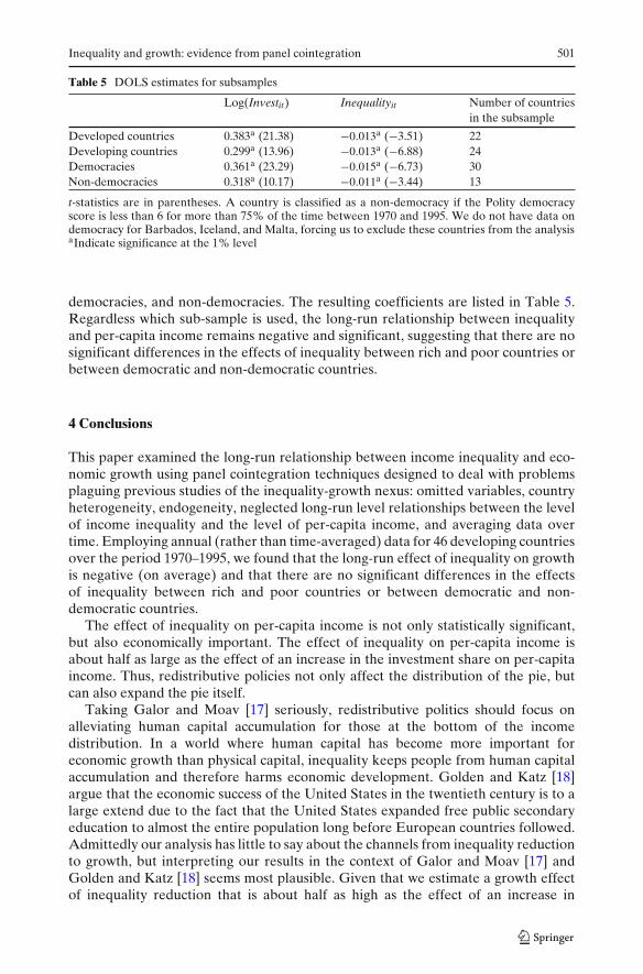
Developed countries 0.383a (21.38) −0.013a (−3.51) 22Developing countries 0.299a (13.96) −0.013a (−6.88) 24Democracies 0.361a (23.29) −0.015a (−6.73) 30Non-democracies 0.318a (10.17) −0.011a (−3.44) 13

t-statistics are in parentheses. A country is classified as a non-democracy if the Polity democracyscore is less than 6 for more than 75% of the time between 1970 and 1995. We do not have data ondemocracy for Barbados, Iceland, and Malta, forcing us to exclude these countries from the analysisaIndicate significance at the 1% level

democracies, and non-democracies. The resulting coefficients are listed in Table 5.Regardless which sub-sample is used, the long-run relationship between inequalityand per-capita income remains negative and significant, suggesting that there are nosignificant differences in the effects of inequality between rich and poor countries orbetween democratic and non-democratic countries.

4 Conclusions

This paper examined the long-run relationship between income inequality and eco-nomic growth using panel cointegration techniques designed to deal with problemsplaguing previous studies of the inequality-growth nexus: omitted variables, countryheterogeneity, endogeneity, neglected long-run level relationships between the levelof income inequality and the level of per-capita income, and averaging data overtime. Employing annual (rather than time-averaged) data for 46 developing countriesover the period 1970–1995, we found that the long-run effect of inequality on growthis negative (on average) and that there are no significant differences in the effectsof inequality between rich and poor countries or between democratic and non-democratic countries.

The effect of inequality on per-capita income is not only statistically significant,but also economically important. The effect of inequality on per-capita income isabout half as large as the effect of an increase in the investment share on per-capitaincome. Thus, redistributive policies not only affect the distribution of the pie, butcan also expand the pie itself.

Taking Galor and Moav [17] seriously, redistributive politics should focus onalleviating human capital accumulation for those at the bottom of the incomedistribution. In a world where human capital has become more important foreconomic growth than physical capital, inequality keeps people from human capitalaccumulation and therefore harms economic development. Golden and Katz [18]argue that the economic success of the United States in the twentieth century is to alarge extend due to the fact that the United States expanded free public secondaryeducation to almost the entire population long before European countries followed.Admittedly our analysis has little to say about the channels from inequality reductionto growth, but interpreting our results in the context of Galor and Moav [17] andGolden and Katz [18] seems most plausible. Given that we estimate a growth effectof inequality reduction that is about half as high as the effect of an increase in


the investment share, the prospective payoffs of redistributive policies (througheducation) are huge.

Open Access This article is distributed under the terms of the Creative Commons AttributionNoncommercial License which permits any noncommercial use, distribution, and reproduction inany medium, provided the original author(s) and source are credited.

References

1. Alesina, A., Rodrik, D.: Distributive politics and economic growth. Q. J. Econ. 109, 465–490(1994)

2. Atkinson, A.B.: On the measurement of inequality. J. Econ. Theory 2, 244–263 (1970)3. Attanasio, O.P., Picci, L., Scorcu, A.E.: Saving, growth, and investment: a macroeconomic analy-

sis using a panel of countries. Rev. Econ. Stat. 82, 182–211 (2000)4. Banerjee, A.V., Duflo, E.: Inequality and growth: what can the data Say? J. Econ. Growth 8,

267–299 (2003)5. Barro, R.J.: Inequality and growth in a panel of countries. J. Econ. Growth 5, 5–32 (2000)6. Breitung, J.: A parametric approach to the estimation of cointegrating vectors in panel data.

Econom. Rev. 24, 151–173 (2005)7. Chambers, D., Krause, A.: Is the relationship between inequality and growth affected by physical

and human capital accumulation? J. Econ. Inequal. doi:10.1007/s10888-009-9111-x. (2010)8. Clarke, G.R.G.: More evidence on income distribution and growth. J. Dev. Econ. 47, 403–427

(1995)9. Davis, L.S.: Explaining the evidence on inequality and growth: informality and redistribution.

B.E.J. Macroecon. (Contributions) 7, Issue 1, Article 7. (2007)10. de la Croix, D., Doepke, M.: Inequality and growth: why differential fertility matters. Am. Econ.

Rev. 93, 1091–1113 (2003)11. Deininger, K., Squire, L.: New ways of looking at old issues: inequality and growth. J. Dev. Econ.

57, 259–287 (1998)12. Ericsson, N.R., Irons, J.S., Tryon, R.W.: Output and inflation in the long-run. J. Appl. Econ. 16,

241–253 (2001)13. Forbes, K.J.: A reassessment of the relationship between inequality and growth. Am. Econ. Rev.

90, 867–889 (2000)14. Frank, M.W.: Inequality and growth in the United States: evidence from a new state-level panel

of income inequality measures. Econ. Inq. 47, 55–68 (2009)15. Galbraith, J.K.: Global inequality and global macroeconomics. J. Policy Model. 29, 587–607

(2007)16. Galbraith, J.K.: Inequality, unemployment and growth: new measures for old controversies. J.

Econ. Inequal. 7, 189–206 (2009)17. Galor, O., Moav, O.: From physical to human capital accumulation: inequality and the process

of development. Rev. Econ. Stud. 71, 1001–1026 (2004)18. Golden, C., Katz, L.: The race between education and technology. Harvard University Press,

Cambridge (2008)19. Guest, R., Swift, R.: Fertility, income inequality, and labor productivity. Oxford Econ. Pap. 60,

597–618 (2008)20. Im, K.S., Pesaran, M.H., Shin, Y.: Testing for unit roots in heterogeneous panels. J. Econom. 115,

53–74 (2003)21. Johansen, S.: Statistical analysis of cointegrating vectors. J. Econ. Dyn. Control 12, 231–254

(1988)22. Johansen, S.: Modelling of cointegration in the vector autoregressive model. Econ. Model. 17,

359–373 (2000)23. Jones, C.: Time series tests of endogenous growth models. Q. J. Econ. 110, 495–525 (1995)24. Knowles, S.: Inequality and economic growth: the empirical relationship reconsidered in the light

of comparable data. J. Dev. Stud. 41, 135–159 (2005)25. Larsson, R., Lyhagen, J., Löthegren, M.: Likelihood-based cointegration tests in heterogeneous

panels. Econom. J. 4, 109–142 (2001)

http://dx.doi.org/10.1007/s10888-009-9111-x.


26. Levin, A., Lin, C.-F., Chu, C.-S.J.: Unit root test in panel data: asymptotic and finite-sampleproperties. J. Econom. 108, 1–24 (2002)

27. Lundberg, M., Squire, L.: The simultaneous evolution of growth and inequality. Econ. J. 113,326–344 (2003)

28. Mankiw, N.G., Romer, D., Weil, D.N.: A contribution to the empirics of economic growth. Q. J.Econ. 107, 407–437 (1992)

29. Nair-Reichert, U., Weinhold, D.: Causality tests for cross-country panels: a new look at FDI andeconomic growth in developing countries. Oxford Bull. Econ. Statist. 63, 153–171 (2001)

30. Panizza, U.: Income inequality and economic growth: evidence from American data. J. Econ.Growth 7, 25–41 (2002)

31. Pedroni, P.: Critical values for cointegration tests in heterogeneous panels with multiple regres-sors. Oxford Bull. Econ. Statist. 61, 653–670 (1999)

32. Pedroni, P.: Purchasing power parity tests in cointegrated panels. Rev. Econ. Stat. 83, 727–731(2001)

33. Pedroni, P.: Social capital, barriers to production and capital shares: implications for the im-portance of parameter heterogeneity from a nonstationary panel approach. J. Appl. Econ. 22,429–451 (2007)

34. Perotti, R.: Growth, income distribution, and democracy: what the data say. J. Econ. Growth 1,149–187 (1996)

35. Persson, T., Tabellini, G.: Is inequality harmful for growth? Am. Econ. Rev. 84, 600–621 (1994)36. Pesaran, M.H.: A simple panel unit root test in the presence of cross-section dependence. J. Appl.

Econometrics 22, 265–312 (2007)37. Pesaran, M.H., Smith, R.: Estimating long-run relationships from dynamic heterogeneous panels.

J. Econometrics 68, 79–113 (1995)38. Reinsel, G.C., Ahn, S.K.: Vector autoregressive models with unit roots and reduced rank struc-

ture: estimation, likelihood ratio test and forecasting. J. Time Anal. 13, 353–357 (1992)39. Voitchovsky, S.: Does the profile of income inequality matter for economic growth? J. Econ.

Growth 10, 273–296 (2005)40. Wan, W., Lu, M., Chen, Z.: The inequality–growth nexus in the short and long run: empirical

evidence from China. J. Comp. Econ. 34, 654–667 (2006)

Inequality and growth: evidence from panel cointegration

Documents

Transcript of Inequality and growth: evidence from panel cointegration