Income Inequality and Polarization

Polarization and Income Inequality

Matthew Sommerfeld George Mason University

Department of Public and International Affairs GOVT 511

Professor Daigle

2

Introduction

Much has been written, both in the mainstream media and in the academic

literature, on the increasing ideological differences between Republicans and

Democrats in Washington. Indeed, simply looking at a map of the country on

election night reveals an apparent divide in this country between ‘red states’ in the

Midwest and the South, and ‘blue states’ on each of the coasts. Likewise, the number

of battleground, ‘purple’ states has significantly diminished since the 1960s

(Abramowitz and Saunders, 2008), leaving fewer states in which presidential

candidates direct their attention during campaigns. Similarly, in congressional

elections, fewer and fewer districts are deemed ‘competitive’, as a higher proportion

of incumbents currently reside in ‘safe seats’ than in previous decades (Silver,

2012). Likewise, divisive rhetoric in the media has become the norm, as the non-‐

partisan voices of Walter Cronkite and Tom Brokow have given way to the likes of

Rachel Maddow and Bill O’Reilly, who cater to their loyal followers by demonizing

political opponents. Internet political news is perhaps even more vitriolic than

television, with hardened partisans resorting to hate speech, hiding behind the

anonymity that comment boards provide.

In what could be described as a culmination of the foregoing polarizing

forces, in combination with the financial crisis in 2008, two social movements have

arisen during the past four years: the Tea Party and the Occupy Wall Street

Movement. Although diverging considerably on the ideological spectrum, both

groups embody a populist zeal, fed up what they perceive to be a corrupt system

that has facilitated the growth of unprecedented income inequality. In wake of the

3

growth of these two groups, a lingering question remains: has growing economic

inequality encouraged extreme political views, exacerbating political polarization

within the electorate? A number of researchers have attempted to demonstrate

various causes to polarization, both at the elite and mass level, with relatively few

specifically examining economic inequality as the primary causal factor for the

decline of moderates in the general populace. This analysis explores polarization

within the electorate during the 2012 election in the United States, testing whether

an individual’s economic standing influences the extremeness of their partisanship.

Upon a quantitative data analysis, considerable support is found for following

hypothesis: Individuals in lower income quintiles have more extreme support for the

Democratic Party, while individuals in the upper income quintiles have more extreme

support for the Republican Party. While it should come as no surprise to many that a

correlation exists between income and party identification, this analysis expands on

this development, measuring whether the ‘shrinking political center’ can be

explained by the growing income disparity in the US, which has only worsened since

the financial crisis in 2008.

Polarization Literature

Various prognosticators fondly remember a time when leaders in

Washington would meet together in the backrooms of the Capitol for cigars and

brandy, hashing out differences on policy (Matthews, 2013). Conditions have

changed dramatically over the past three decades, with many describing the 113th

Congress not only as the most polarized, but potentially also the least productive in

history (Desilver, 2013). While the evidence regarding the polarization of politicians

4

in Washington is irrefutable (McCarty, Poole, and Rosenthal, 2006), significant

disagreement remains regarding the extent to which the general electorate has

become more polarized. Disagreements on the latter question tend to result from

the variances in methodology and the specific factors examined when researching

the election survey results. This section begins by outlining the evidence regarding

the polarization of Congress, delves into the causes of this elite-‐level polarization,

specifically examining the elite-‐driven vs. grassroots-‐led divide in the literature. In

other words, are individuals in the electorate simply taking cues from opinion leaders

Washington and in the media, or are members of Congress simply adhering to

constituent preferences when they refuse to compromise with the other side?

Polarized Congress – Empirical Evidence

The most sophisticated method of determining a member of Congress’

‘ideology score’, developed by political scientists McCarty, Poole, Rosenthal,

analyzes every roll call vote in Congress and places each member on an ‘ideal point.’

This method allows researchers to compare members across space and time,

accurately depicting historical trends regarding the ideological ‘space’ between the

two parties. Their system, called DW-‐NOMINATE, places members on a sliding scale,

ranging from the most conservative score of +1, to the most liberal, -‐1.

Unsurprisingly, after comparing the mean scores of the respective parties in each

Congress, they find that the 113th is the most polarized since the Civil War era

(Figure 1).

5

Figure 1:

*Graphic Obtained from: http://voteview.com/blog/?p=892

Respectively, there is less ideological ‘overlap’ among Democrats and Republicans,

as the most liberal Republican is now more conservative than the most conservative

Democrat. Likewise, the number of moderates (members with scores between 0.25

and -‐0.25) in congress has shrunk from about 40% (both chambers) in 1980 to just

6 percent of House members and 13 percent of Senators in the 112th Congress

(McCarty, Poole, Rosenthal, 2013) (Figures 2 and 3).

Figure 2:


6

Figure 3:


Likewise, Mann and Orstein describe how these polarizing trends have

impacted recent events in Washington in their 2012 book, It’s Even Worse Than It

Looks. They specifically examine recent policy clashes between the Republican-‐led

congress and the Obama Administration, arguing that the current political climate

has made bipartisan compromise nearly impossible, especially when you account

for parliamentary maneuvers that enable the minority party to obstruct the

majority’s legislative agenda. Nowhere is this more evident than the unprecedented

number of ‘filibusters’ employed by the Republican minority since 2008 (Downie,

2012). Prior to the era of polarization, filibusters were utilized more judiciously, as

members of the minority party would make the effort to employ ‘talking filibusters’,

standing on the floor of the senate and speaking out against a policy for hours on

end. However, in recent years, requiring 60 votes to ensure cloture and allow a bill

to proceed to a vote on the floor has become a new norm in the Senate, a feat made

much more difficult with the aforementioned levels of polarization between the two

parties.

7

The foregoing confirms what prognosticators have been saying for over a

decade now: Republicans and Democrats are more polarized than they were in the

past, when a divided government did not necessarily result in gridlock. Few agree,

however, in regards to the primary source of this polarization in Washington, which

is elaborated on in the subsequent section.

Sources of Polarization

Theoretically, the United States’ employment of a simple-‐plurality, single-‐

member-‐district electoral system should result in two relatively moderate parties,

with each moving towards the center in an attempt to attract that elusive ‘median

voter’ (Downs, 1957). However, as the aforementioned evidence illustrates,

Republicans and Democrats have grown further apart over the past four decades, in

an apparent attempt to ensure the support of extreme voters on either side of the

political aisle, rather than courting centrists. What explains this disregard for the

moderate, median voter in the American electorate? Generally, the disagreement

regarding the explanation for this development is divided into two camps: 1)

members of Congress are simply reflecting the preferences of their voters, who

themselves have become more polarized over the years; or 2) there is a deep

disconnect between extreme politicians in Washington and their constituents, who

for the most part, have remained relatively moderate with each election cycle.

One of the most common explanations for the polarization of Congress

attributes the blame to the partisan districting process, or as it is more commonly

referred to – gerrymandering. Adherents to the ‘gerrymander hypothesis’ point out

that the redistricting process is a partisan affair, with political actors employing

8

sophisticated methods to maximize seat allocation for their party. While it is

ascetically pleasing argument that fits nicely into the confines of a 500-‐word

opinion-‐piece, there are many flaws in attributing gerrymandering as the primary

cause for polarization. McCarty, Poole, and Rosenthal (2006) respond to this claim,

first emphasizing that the Senate, which is not subject to redistricting, has become

nearly as polarized as the House over the past 40 years. Similarly, presidential

elections have also become less competitive on a state-‐by-‐state basis, as the number

of swing-‐states (+/-‐ 5%) has decreased by half from 1960 to 2004 (Abramowitz and

Saunders, 2008). Moreover, if a party were to strategically draw partisan district

lines, it would emphasize the efficient allocation of voters over many seats, rather

than packing their voters into incumbents’ districts. In other words, when a party’s

seats are inefficiently allocated, every vote over the plurality is essentially ‘wasted’,

as it is actually more advantageous to ‘spread your voters around’, while ensuring

the seat is still ‘safe’ come the next election. However, the reality is that districts are

just as likely to become more ideologically homogenous during non-‐redistricting

years than just following a ‘partisan gerrymander’.

The explanation for this ‘natural gerrymander’ is outlined in Bishop’s (2009)

account, The Big Sort, in which he explains that voters have been sorting themselves

geographically into neighborhoods based on income levels, and correspondingly

into like-‐minded ideological camps as well. Likewise, Chen and Rodden (2013) find

evidence that supports the claim that Democrats are disadvantaged in House races

because of the inefficient allocation of their supporters into more urban districts,

where they often win more than 70 percent of the vote. This trend towards fewer

9

and fewer competitive seats is outlined in Nate Silver’s analysis following the 2012

election, in which he compares the number of ‘swing districts’ (+/-‐ 5% of the

national popular vote margin) in 1992 to 2012. Corresponding to the polarization

data, he finds that out of the 103 districts (24%) that were deemed competitive in

1992, only 35 remain (8%).

Figure 4:

*Graphic from: http://fivethirtyeight.blogs.nytimes.com/2012/12/27/as-‐swing-‐districts-‐dwindle-‐can-‐a-‐

divided-‐house-‐stand/

An additional institutional explanation centers on the primary process as the

primary factor for the increased extremism in Washington, as members of Congress

adhere to the whims of the median primary voter, rather than the median voter in

their district. While it is true that individuals who take part in the primary process

are generally more engaged than the average voter, and thus more partisan in their

views, the empirical evidence is mixed in regards to the effects of open and closed

primary systems (open primary systems allow unaffiliated voters to participate,

thus theoretically moderating the pool of participants). While Gerber and Morton

(1998) find evidence to support the claim that closed primaries produce more

10

extreme candidates than open systems, there has been significant pushback (Hassel,

2013) on this claim, with arguments pointing to inconsistent turnout in primaries,

regardless of the format (unaffiliated voters are more likely to be disengaged, and

thus less likely to participate in primaries). The reality of the primary process

appears to be that the fear members of Congress have of being ‘primaried’ is indeed

real, the link between the types of primaries and the extremeness of candidates is

weak, if present at all.

Perhaps the most compelling explanation as to how Congress has become so

polarized attributes the impact of the Southern realignment. Following the Civil

War, the Democratic Party largely dominated Southern politics, with deep-‐seated

resentment towards the Republican Party, which was blamed for failures during the

reconstruction efforts (Key, 1949). These trends continued for about 100 years, in

both congressional and presidential elections, despite the fact that the South was

largely made up of conservative voters who continued to support an increasingly

liberal Democratic Party. A major shift began to take form during the battle over

Civil Rights in the 1960s, culminating in the 1964 presidential election, which saw

Republican candidate Barry Goldwater carry the southern states of Alabama,

Louisiana, South Carolina, Mississippi, and Georgia (Poole, McCarty, and Rosenthal,

2006). For about 30 years, Southerners continued to support Republicans for

president, while splitting their ticket and voting Democratic in Congressional and

Senate elections. This trend began to change in the early 1990s, when Newt Gingrich

devised a strategy to attract socially conservative voters to support the Republican

candidates on a ‘straight ticket’ basis, resulting in the GOP winning a majority of the

11

seats in the House in 1994 for the first time in over 40 years. The polarizing effect

this created on the overall makeup of members of Congress can be attributed to the

replacement of moderate, Southern Democrats with conservative Republicans.

However, what cannot be explained by this ‘Southern Realignment’ hypothesis is the

simultaneous displacement of moderate Republicans in the Northeast by liberal

Democrats, further exacerbating polarization of congress.

The foregoing explanations for attribute the polarization of Congress to a

grassroots-‐led, ‘adhering to what constituents’ preferences are’ rationale. Indeed,

many have argued that, despite the increased polarization in Congress, the ideology

of politicians in Washington actually more closely resembles that of their

constituents than ever before (Poole, McCarty, Rosenthal). While a strong case could

be made that ideologues in Congress are simply adhering to voter preferences,

many researchers downplay this line of thinking (Fiorina, 2006), arguing that a

significant ‘disconnect’ exists between voters and the politicians who represent

them in Washington.

Converse’s 1964 study was the first attempt at measuring the proximity of

the preferences of voters with the politicians who represent them in Congress. His

primary finding posits that most voters are generally disengaged from the political

process, and that respondents express inconsistent belief systems and viewpoints,

depending simply on what comes to mind first. Thus, the political viewpoints

expressed by opinion leaders has little effect on the public at large, as most

individuals are more concerned about paying their bills or other aspects of life than

they are about politics. Zaller and Feldman’s (1992) study in which they probe

12

respondents regarding the rationale for the ideological attitudes expressed support

these findings. They find that various factors, such as the ‘accessibility’ of viewpoint

significantly influence how one thinks about an issue. Achen (1975) challenges these

assertions, however, claiming that individuals do indeed hold consistent ideological

belies. The issue, he posits, lies in the survey methods employed to capture these

beliefs, which are often flawed, resulting in the illusion of a disengaged electorate.

Recent research (Fiorina and Abrams, 2009) additionally downplays the

common characterization of a ‘polarized electorate’, arguing that the politicians who

reside in Congress are disconnected from the public at large, whose attitudes have

changes little in the past 40 years. Contrary to common media conjecture, Fiorina

argues that Americans generally regard themselves to be ‘moderates’ on a host of

issues, from taxes to abortion. He comes to these conclusions after analyzing

election returns from elections studies in more depth (variances in red and blue

states), pinpointing the ‘true viewpoints’ of the electorate. While he does

acknowledge some of the aforementioned institutional factors (Southern

Realignment, primary systems) that have contributed to the polarization of

candidates for office, he finds that the percentage of Americans who identify as

politically extreme to have remained relatively constant during the same time span

of congressional polarization. Moreover, he claims that the differences between

voters and red and blue states is often overstated in the media, as various issues

receive relatively high support regardless of the political color of the state.

Finally, Abramowitz and Saunders (2008) challenge many of the claims made

by Fiorina that downplay the level of polarization, finding various contradictions

13

and inconsistencies. In their analysis, they create a ‘polarization index’ to measure

how the electorate’s views have changed over the years. The crux of their argument

emphasizes the increased capability of voters to digest and articulate political news,

due in large part to increased levels of education in society and access to

information. As a result of this increased ‘ideological awareness’, voters have

become more extreme, and thus more polarized from individuals on the other side

of the aisle. These findings support Prior’s theory (2007) regarding the evolving

nature of the mass media and its impact on polarization in the US. He argues that the

polarization of the electorate can be attributed to changing media habits, made

possible by evolving technology over the past 60 years. When individuals merely

had network news or radio at their disposal, their views were moderated by the

objective reporting disseminated by these stations. As cable news, and eventually

Internet political news proliferated, only the genuinely interested (and more

partisan) remained attuned to politics of the day, resulting in the increased demand

for more partisan and extreme commentary in the media (those who were not

genuinely interested have opted for entertainment programming, an option that

was not available in the ‘pre-‐cable era’). While the polarizing effect on the latent

public may not be that pronounced, according to Prior, those who have maintained

interest in political news, despite other entertainment options, have become more

polarized over time. Coincidentally, the consumers of partisan political news are

also the individuals who happen to participate in the selection of candidates for

office, leaving the disengaged ‘moderates’ to choose between two extremes.

Polarization in American Politics: Unanswered Questions

14

While the literature regarding political polarization is indeed numerous and

expansive, various unexplored considerations remain. For instance, nearly all of the

research emphasizes the partisan attachment of voters: are they more or less likely to

vote Democrat or Republican? This is a rather unsophisticated method to measure

polarization, on account of the US political system only having two parties to choose

from. Presumably, even if the number of moderates has decreased over the years,

they would still be forced to choose between one of the two candidates, a Democrat

or a Republican. Although Abramowitz and Saunders (2008) do consider

extremeness of views in their index, they attribute political engagement as the

primary independent variable to explain the increase in polarization. However,

various turnout studies have found that those in lower income brackets are less

likely to vote in elections, yet McCarty, Poole, and Rosenthal (2006) find that income

disparity has a been significant factor in the polarization, and ostensibly

engagement of voters in the electorate. Prominent democratic theories regarding

income distribution hypothesize a direct and positive relationship between income

inequality and support for redistributive policies within the electorate (Meltzer and

Richard, 1981). If this is indeed the case, then one would expect a leftward tilt

regarding the economic policies in the US over the past few decades, a development

that has failed to materialize, which lends credence to opposing theories that posit

inequality actually breads more right-‐wing economic preferences among voters

(Kelly and Enns, 2010).

McCarty, Poole, and Rosenthal do attempt to reconcile the debate regarding

voter preferences and inequality, asserting that individuals who are inclined to

15

support Democratic policies towards greater redistribution are much less likely to

vote, in large part because of the influx of immigrants over the past 40 years, many

of which are ineligible non-‐citizens. However, their study is limited in that it merely

examines the correlation between income and partisan identification, without

measuring whether voters within those identifications have become more extreme

in their views as they have become more wealthy or poor.

This analysis attempts to bridge this gap between Abramowitz and Saunders’

methodology of measuring polarization, and McCarty, Poole, and Rosenthal’s

employment of income inequality as the primary independent variable that explains

one’s level of political polarization. While the quantitative tests conducted in the

subsequent sections does not measure whether polarization has increased over

time, as many of the studies cited have done, it does aim to provide evidence

regarding the source of polarization that exists within the electorate during the 2012

presidential and congressional elections.

Methods

The 2012 Time Series National Election Survey is utilized in order to

measure both the dependent variable (strength partisan attitudes) and the

independent variable (income). More specifically, the strength of one’s partisan

attitudes is captured in three different variables: 1) a five-‐category partisanship self-‐

placement scale, 2) feeling thermometers towards the Republican and Democratic

Parties, and 3) a five-‐category ideological self-‐placement scale. The traditional

seven-‐point scale of partisanship was recoded into five categories in order to

combine the ‘independent Democrat/Republican’ with the ‘weak

16

Democrat/Republican’. Each of these categories represents a weaker attachment to

the party than ‘strong Republican/Democrat’, and thus provides a logical

measurement for the purposes of this study. Likewise, the thermometer scales were

divided into five ordinal categories: cold, cool, neutral, warm, hot. The coding schema

for the second dependent variable, ideological self-‐placement, is also receded from a

7-‐point to a 5-‐point scale, collapsing the moderate three choices into a single

‘moderate’ category. Finally, a control variable, region, is additionally examined in

order to test for the ‘Southern Effect’ hypothesis: are Southerners more susceptible to

party attachment based on their income quintile?

The independent variable, income, is divided into quintiles. The rationale

behind this decision is based on common economic tendencies when examining

economic inequality: how is the total output of the country divided among the fifths of

the population? When reports mention income inequality, they typically refer to how

much the top 1%, 10% or 20% is taking compared to the rest of the population. The

decision to divide the income variable into quintiles, therefor, is more feasible than

attempting to compare the top one or ten percent of the population against each

other.

Following a brief analysis of the frequency distribution of the dependent and

independent variables, a cross-‐tabulation is conducted that reveals the strength of

the relationship between economic inequality and strength of partisanship. On

account of both variables falling into the ordinal category, a Chi-‐Square and Tau-‐b

measurement are tabulated to provide quantitative support for the claim being

made.

17

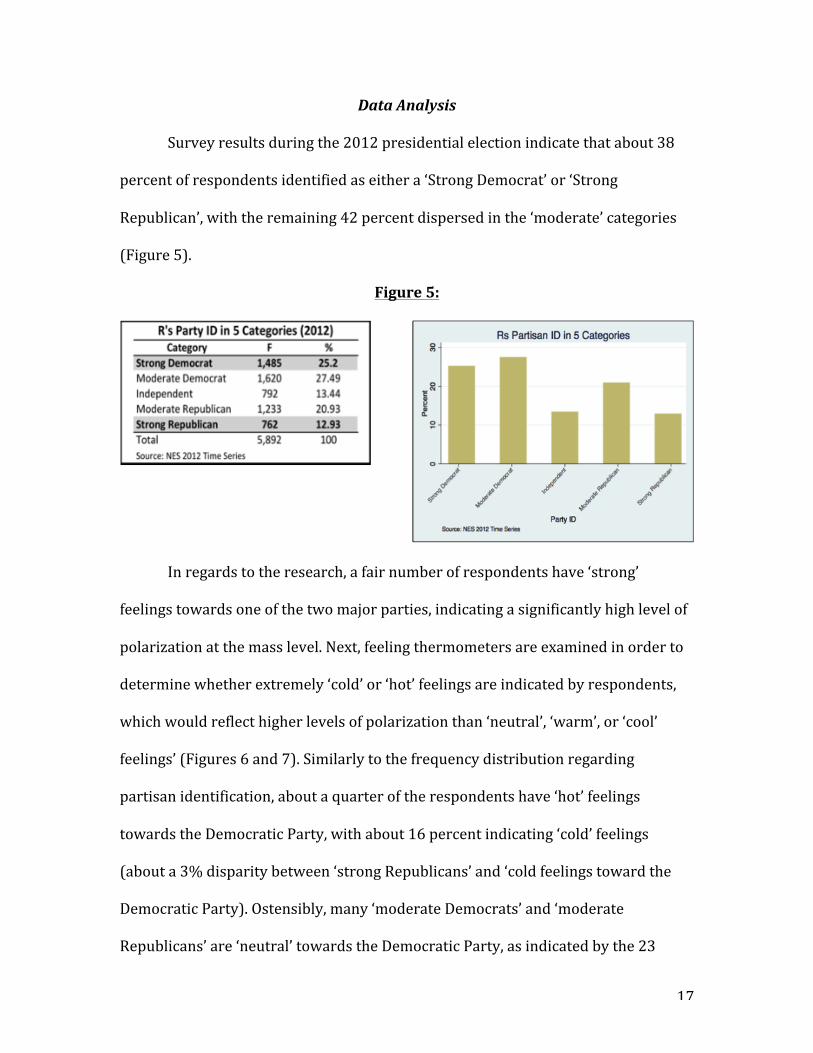
Data Analysis

Survey results during the 2012 presidential election indicate that about 38

percent of respondents identified as either a ‘Strong Democrat’ or ‘Strong

Republican’, with the remaining 42 percent dispersed in the ‘moderate’ categories

(Figure 5).

Figure 5:

In regards to the research, a fair number of respondents have ‘strong’

feelings towards one of the two major parties, indicating a significantly high level of

polarization at the mass level. Next, feeling thermometers are examined in order to

determine whether extremely ‘cold’ or ‘hot’ feelings are indicated by respondents,

which would reflect higher levels of polarization than ‘neutral’, ‘warm’, or ‘cool’

feelings’ (Figures 6 and 7). Similarly to the frequency distribution regarding

partisan identification, about a quarter of the respondents have ‘hot’ feelings

towards the Democratic Party, with about 16 percent indicating ‘cold’ feelings

(about a 3% disparity between ‘strong Republicans’ and ‘cold feelings toward the

Democratic Party). Ostensibly, many ‘moderate Democrats’ and ‘moderate

Republicans’ are ‘neutral’ towards the Democratic Party, as indicated by the 23

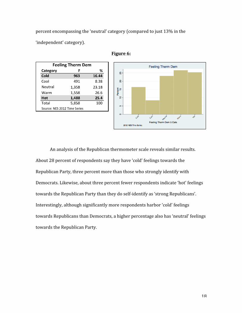
18

percent encompassing the ‘neutral’ category (compared to just 13% in the

‘independent’ category).

Figure 6:

An analysis of the Republican thermometer scale reveals similar results.

About 28 percent of respondents say they have ‘cold’ feelings towards the

Republican Party, three percent more than those who strongly identify with

Democrats. Likewise, about three percent fewer respondents indicate ‘hot’ feelings

towards the Republican Party than they do self-‐identify as ‘strong Republicans’.

Interestingly, although significantly more respondents harbor ‘cold’ feelings

towards Republicans than Democrats, a higher percentage also has ‘neutral’ feelings

towards the Republican Party.

19

Figure 7:

Both measures of the dependent variable, ‘polarization’, indicate that about a

38-‐40 percent of the electorate is polarized in the sense that they either identify

strongly with one of the two major parties or have extremely hot or cold feelings

towards one of the two major parties (or both). However, one must also consider

ideological feelings (Figure 8) in order to make the case that the electorate is indeed

more polarized. It is entirely possible that those identifying as ‘very liberal’ or ‘very

conservative’ simultaneously identify as ‘independents’, as they may feel alienated

by the two-‐party system that fails to adequately represent their ideological

preferences.

010

2030

Perc

ent

Cold Cool

Neutra

lWarm Hot

Feeling Therm Rep 5 Cats2012 NES Time Series

Feeling Therm Rep

20

Figure 8:

The traditional seven-‐point scale of ideological self-‐placement has been

recoded into five categories, collapsing the moderate three options into a single

category. Interestingly, far more respondents strong identify with one of the two

parties than as ‘very liberal’ or ‘very conservative’. Perhaps there is some

psychological dissonance at play, as respondents feel a moderate ideology is a more

‘socially acceptable’ response than admitting you harbor ‘extreme’ ideological

positions.

Finally, the primary task at hand: empirically measuring whether income

inequality correlates with a respondent placing oneself in one of the ‘polarized’

categories. Prior to delving into the cross-‐tabulation, an examination of the

frequency distribution of the income quintiles (Figure 9) is provided. Respondents

were broken up in to approximately equal categories, according to self-‐reported

income levels. The primary focus on this analysis emphasizes both the first ($0-‐

14,999) and fifth (more than$90,000) quintiles. The remaining quintiles encompass

anyone reporting income between $15,000 and $89,000 per year.

21

Figure 9:

The cross-‐tabulation (Figure 10) of income quintile and partisan

identification reveals a statistically significant relationship, albeit failing to be

completely linear. While the first quintile does represent the income bracket that is

most likely to identify as a ‘strong Democrat’, and least likely to identify as a ‘strong

Republican’, the gap between ‘moderate Democrat’ and ‘strong Democrat’ is small,

perhaps weakening the claim between individuals become more polarized as their

economic circumstances worsen. Likewise, counterintuitive findings in the fifth

quintile reveal that the wealthiest Americans are more likely to identify as a

‘moderate Republican’ than ‘strong Republican’, by quite a large margin (28.71% to

15.6%). In fact, the fifth quintile actually has a higher percentage of respondents

that identify as ‘strong’ or ‘moderate Democrat’, respectively, than ‘strong

Republican’. Despite these counterintuitive findings, a chi-‐square of 187.56 does

indicate a statistically significant relationship between income quintile and partisan

identification (p < 0.0001). Moreover, a Tau-‐B of 0.1174 indicates a moderately

weak, positive relationship. As one’s income increases, he or she is significantly

more likely to identify as a Republican or Strong Republican than a Independent,

moderate Democrat, or strong Democrat.

22

Figure 10:

The cross-‐tabulations regarding the feeling thermometers for the respective

parties and income distribution (Figures 11 and 12) largely support the previous

findings. The first quintile represents the category with the ‘hottest’ feelings

towards the Democratic Party, while the wealthiest quintile is most likely to rank

Democrats ‘cold’. However, once again, the 4th quintile is strikingly similar to the 5th

in this regard, as ‘cold’ feelings towards the Democrats seems to have a ‘threshold

effect’ occurring – once someone reaches a certain level of income, they become less

friendly towards Democrats, but not necessarily any more or less supportive than

the wealthiest individuals in the fifth quintile. In terms of statistical significance, a

Chi-‐square of 162.12 exceeds the critical value necessary for a 99 percent

probability of not making a Type I error. Moreover, a Tau-‐B of -‐0.1247 indicates a

moderate and negative relationship between the variables – higher feelings towards

the Democrats are more likely to be found in the lower quintiles (thus the inverse

relationship).

23

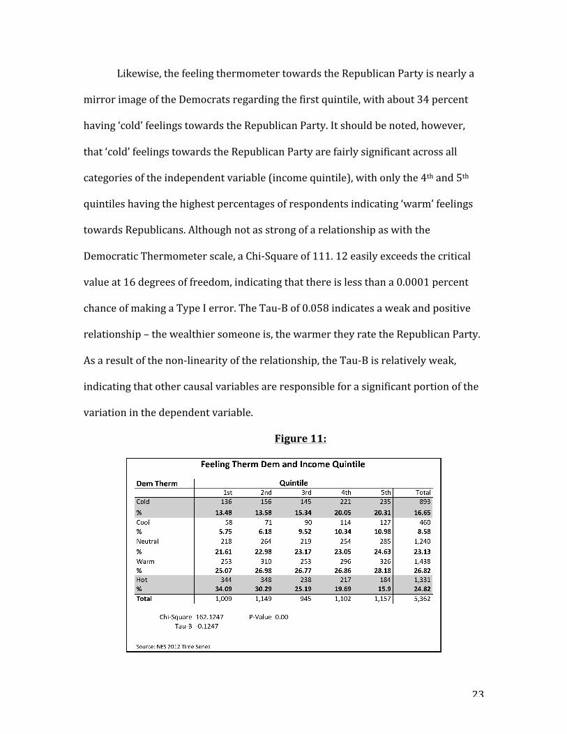
Likewise, the feeling thermometer towards the Republican Party is nearly a

mirror image of the Democrats regarding the first quintile, with about 34 percent

having ‘cold’ feelings towards the Republican Party. It should be noted, however,

that ‘cold’ feelings towards the Republican Party are fairly significant across all

categories of the independent variable (income quintile), with only the 4th and 5th

quintiles having the highest percentages of respondents indicating ‘warm’ feelings

towards Republicans. Although not as strong of a relationship as with the

Democratic Thermometer scale, a Chi-‐Square of 111. 12 easily exceeds the critical

value at 16 degrees of freedom, indicating that there is less than a 0.0001 percent

chance of making a Type I error. The Tau-‐B of 0.058 indicates a weak and positive

relationship – the wealthier someone is, the warmer they rate the Republican Party.

As a result of the non-‐linearity of the relationship, the Tau-‐B is relatively weak,

indicating that other causal variables are responsible for a significant portion of the

variation in the dependent variable.

Figure 11:

24

Figure 12:

The foregoing indicates that a significant relationship exists between one’s

income and partisanship. However, as the Tea Party and Occupy Wall Street

movements demonstrate, perhaps a significant portion of the electorate has become

more extreme ideologically, without actually becoming more ‘attached’ to one of the

two major parties (challenging political ‘the establishment’). A cross-‐tabulation

(Figure 13) is conducted in order to test ideology as the dependent variable across

categories of the independent variable, income quintile. Although the relationship is

statistically significant (chi-‐square value of 61.69), the Tau-‐B of 0.0375 indicates a

weak, positive relationship between ideology and income. Although those in the

lower income quintiles are more likely to identify as ‘very liberal’ or ‘liberal’ than

they are to identify as ‘very conservative’ or ‘conservative’, the differences across

the categories are non-‐linear and vary little from the ‘expected values’ on the right-‐

most column. Thus, although the Tau-‐B reveals a relationship, income as an

25

explanatory variable is responsible for a greater proportion of the variation in

partisan identification than it does in regards to ideological self-‐placement.

Figure 13:

A means comparison (Figures 14 and 15) is provided in order to

demonstrate variances across thermometer readings for the two parties across the

categories of the independent variable. Utilizing the original coding schema of the

thermometer readings (interval level), the mean scores indicated by respondents

from the various income quintiles an F-‐value of 36.59 for the Democratic

thermometer reveals statistic significance in the relationship at the 99 percent

confidence interval (4 df). The only two income quintiles in which the relationship

between the categories fails to reveal statistical significance is between the 1st and

2nd, and the 4th and 5th. On the other hand, the Republican thermometer reading

reveals much more counterintuitive findings. As one would expect, the lowest

income quintile ranks the Republican Party the lowest; however, the 4th quintile

26

represents the highest mean score (45.15), with the wealthiest quintile actually

ranking Republicans lower (42.13). Although the F-‐value of 10.36 reveals a

statistically significant relationship, differences across specific categories of income

indicate a lack of statistical significance, signifying that additional tests are required

in order to understand a larger portion of the variance regarding how one evaluates

the Republican Party.

Figure 14: Figure 15:

Finally, in order to test the ‘Southern Effect’ hypothesis, a cross-‐tabulation

analysis (Figures 16 and 17) is conducted in which Southerners are compared to

‘Non-‐Southerners’. A few differences between the following graphics are

noteworthy. First, Southerners in the first quintile are more likely to identify as

‘strong Democrats’, and are less likely to identify as ‘moderate Democrats’. This

provides some validity to the contention that South is more polarized than the other

regions of the country. However, wealthy Southerners are no more likely to identify

27

as ‘strong Republicans’ than are wealthy non-‐Southerners. Moreover, an analysis of

the total number of ‘moderates’ reveals only a three percent difference between

Southerners and non-‐Southerners. Although individuals in the lowest income

quintile do seem to have become more polarized in the South, based on the strength

of their attachment to the Democratic Party, the 5th quintile is actually more likely to

identify as a ‘moderate Republican’ than a ‘strong Republican’, as is the case with

non-‐Southerners.

Figure 16:

28

Figure 17:

Discussion

The data analysis reveals significant support for the hypothesis that voters

become more polarized as they move from middle income to the lower and upper

quintiles. This relationship is especially strong for Democrats, as both the cross-‐

tabulations (both partisan identification and ordinal thermometer readings) and the

ANOVA test reveal a linear relationship across the categories of the independent

variable. Individuals in the lowest income quintile not only harbor more extreme

feelings of positivity towards Democrats, but they also feel increasingly higher

amounts of animosity towards Republicans. Individuals on the higher ends of the

income ladder, on the other hand, seem more conflicted in regards to the strength of

the partisanship. The strongest feelings towards Republicans, regardless of the

variable being tested, are found most frequently in the 4th quintile, rather than the

5th, as predicted in the initial hypothesis. Although the wealthiest quintiles both

!"#$%$&'!"# $%& '(& )#* +#* ,-#./

0#(-%123 $4+ $!5 !5' !67 !76 8)8( )*+,- ).+/ )0+11 ))+0. )2+./ )3+119-&:(.#:23 $'+ $)) $44 !8+ $$$ !;485( 00+00 0,+2. )-+* )3+1 )1+/) )-+0.<%& !!8 !$$ 8' 86 66 +47( 2.+-- 21+,- 20+33 2)+2* -+*) 20+239-&:(.#:2= 77 !+' !)) !77 $)! 7!)( 2)+3- 2-+*2 ),+-2 )0+.) )/+*0 )2+,.0#(-%12= +7 6) 8$ !'7 !'5 )87( -+)0 *+21 20+)* 2/+03 21+/. 2)+--4$56% 64+ 748 58$ 685 75' ';75+

>*?@0AB.(: !')C)$ D@E./B: 4C44,.B@F 4C!!4!

0-B(G:H2IJ02$4!$2,?K:20:(?:"

7$859#:;<=>>#?5<@<A$;@7$859#:;#:B

C8D;5D%#

29

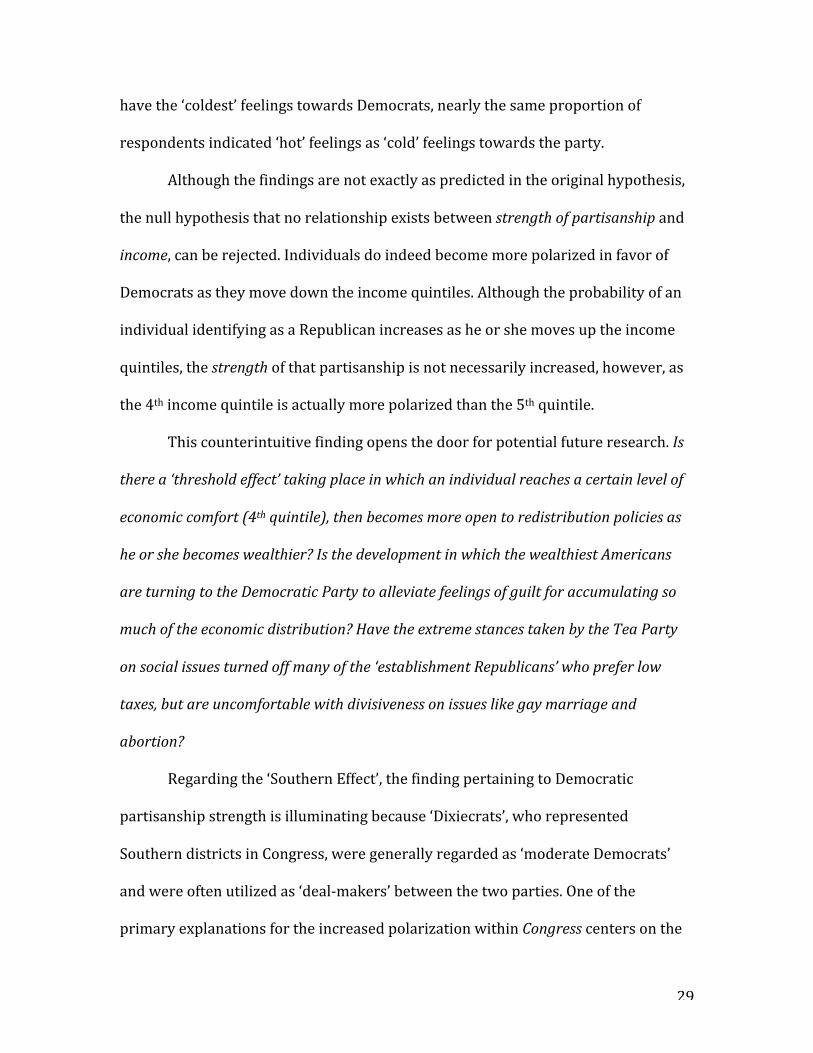
have the ‘coldest’ feelings towards Democrats, nearly the same proportion of

respondents indicated ‘hot’ feelings as ‘cold’ feelings towards the party.

Although the findings are not exactly as predicted in the original hypothesis,

the null hypothesis that no relationship exists between strength of partisanship and

income, can be rejected. Individuals do indeed become more polarized in favor of

Democrats as they move down the income quintiles. Although the probability of an

individual identifying as a Republican increases as he or she moves up the income

quintiles, the strength of that partisanship is not necessarily increased, however, as

the 4th income quintile is actually more polarized than the 5th quintile.

This counterintuitive finding opens the door for potential future research. Is

there a ‘threshold effect’ taking place in which an individual reaches a certain level of

economic comfort (4th quintile), then becomes more open to redistribution policies as

he or she becomes wealthier? Is the development in which the wealthiest Americans

are turning to the Democratic Party to alleviate feelings of guilt for accumulating so

much of the economic distribution? Have the extreme stances taken by the Tea Party

on social issues turned off many of the ‘establishment Republicans’ who prefer low

taxes, but are uncomfortable with divisiveness on issues like gay marriage and

abortion?

Regarding the ‘Southern Effect’, the finding pertaining to Democratic

partisanship strength is illuminating because ‘Dixiecrats’, who represented

Southern districts in Congress, were generally regarded as ‘moderate Democrats’

and were often utilized as ‘deal-‐makers’ between the two parties. One of the

primary explanations for the increased polarization within Congress centers on the

30

displacement of the Dixiecrats by extremely conservative Republicans in the South,

who are less likely to work across the aisle with Democrats. Despite the fact that a

higher proportion of individuals in the lowest income quintile in the South have

strong partisan attachment towards Democrats, their representation in Congress

has become much more conservative over the years.

Despite the relevant findings regarding a primary cause of polarization

within the electorate during the 2012 election, this analysis has a number of

limitations. A thorough analysis of polarization requires a comparison across time

and space, which this study fails to attempt. One would need to demonstrate

significant variance in income inequality over time in regards to polarization in

order to definitively attribute causation (McCarty, Poole, and Rosenthal, 2006).

Many of the analyses in the literature review portion of this analysis employ this

method, with significant disagreement as to whether increased polarization has

actually occurred among voters. This analysis operates under the assumption that

increased polarization has been occurring within the electorate and aims to uncover

the degree to which this polarization is caused by a factor that has demonstrably co-‐

varied with the polarization of Congress: income inequality.

Cross-‐state or cross-‐country analyses would further reveal noteworthy

findings regarding income inequality and polarization. Intuitively, one would

believe that the larger the middle-‐class of a society, the less adversarial the political

system is. Do states/countries with higher degrees of inequality also have more

polarized voters? Cross-‐national electoral systems may additionally provide

evidence as to the compounding factors of polarization. Various institutional

31

characteristics unique to the American political system have been discussed in

detail. Perhaps significant electoral reforms are the most ideal method of lessening

the polarization that plagues politics in Washington.

Limitations aside, this analysis examines interplay of two issues that are

seldom studied in conjunction: income inequality and polarization. Many discuss the

former on moral grounds, invoking emotive arguments to appeal to society to help

those who are less fortunate. While those arguments are relevant in their own right,

more pressing, practical issues present themselves to a society when a growing gap

persists between the ‘haves’ and ‘have nots’. The economic benefits of a thriving

middle class are well documented by politicians and economists a like; however,

perhaps the democratic ramifications of income disparity are even more pressing as

each passing conflict reflects the inability of the US political system to adequately

address the issues of the day.

32

Citations:

Abramowitz, Alan I; and Kyle L. Saunders (2008). “Is Polarization a Myth?” The Journal of Politics, Vol. 70, No. 2, April 2008, Pp. 542–555.

Achen, Christopher (1975). “Mass Political Attitudes and the Survey Response.” The

American Political Science Review. 69: 1218-‐31. The American National Election Studies (ANES; www.electionstudies.org). The

ANES 2012 Time Series Study [dataset]. Stanford University and the University of Michigan [producers].

Bishop, Bill (2009). The Big Sort: Why the Clustering of Like-‐Minded America is

Tearing Us Apart. Mariner Books. Chen, Jowei; and Jonathan Rodden (2013). “Unintentional Gerrymandering: Political

Geography and Electoral Bias in Legislatures.” Quarterly Journal of Political Science, 2013, 8: 239–269.

Converse, Philip E. 1964. ‘‘The Nature of Belief Systems in Mass Publics.’’ In Ideology

and Its Discontents, ed. David E. Apter, New York: The Free Press of Glencoe, 206–61.

Desilver, Drew (2013). “Current Congress is not the least productive in recent

history, but close.” The Pew Research Center. 4 Sept. 2013. Web. Nov. 15, 2013.

Downie, James (2013). “Republicans have only themselves to blame for Reid’s

‘nuclear option.’” The Washington Post. 21 Nov. 2013. Web. Nov. 30, 2013. Downs, Anthony (1957). An Economic Theory of Democracy. New York: Harper. Fironia, Morris P.; and Samuel J. Abrams (2009). Disconnect: The Breakdown of

Representation in American Politics. University of Oklahoma University Press. Gerber, Elisabeth R; and Rebecca B. Morton (1998). “Primary Election Systems and

Representation.” Oxford University Press. Hassell, Hans (2013). “The Non-‐existent Primary-‐Ideology Link, or Do Open

Primaries Actually Limit Party Influence in Primary Elections?” Presentation at the 2013 State Politics and Policy Conference, University of Iowa, Iowa City, Iowa.

Kelly, Nathan J.; and Peter K. Enns (2010). “Inequality and the Dynamics of Public

Opinion: The Self-‐Reinforcing Link Between Economic Inequality and Mass

33

Preferences.” American Journal of Political Science, Vol. 54, No. 4, October 2010, Pp. 855–870.

Key, V.O. (1949). Southern Politics in State and Nation. New York: A. A. Knopf. Mann, Thomas E.; and Norman J. Ornstein (2012). It’s Even Worse Than It Looks:

Howl the American Constitutional System Collided with the New Politics of Extremism. Basic Books.

Mathews, Chris (2013). “Tip and the Gipper.” Simon & Schuster; First Edition. McCarty, Poole, Rosenthal (2006). Polarized America: The Dance of Ideology and

Unequal Riches. Massachusetts Institute of Technology. McCarty, Poole, Rosenthal (2013). “An Update on Polarization through the 113th

Congress (Part II).” Voteview Blog. 9 Sept. 2013. Web. Nov. 20, 2013. Meltzer, Allan H. and Scott F. Richard (1981). “A rational theory of the size of

government.” The Journal of Political Economy, 89, 914–927. Prior, Markus (2007). Post-‐Broadcast Democracy: How Media Choice Increases

Inequality in Political Involvement and Polarizes Elections. Cambridge Studies in Public Opinion and Political Psychology.

Silver, Nate (2012). “As Swing Districts Dwindle, Can a Divided House Stand?” The

New York Times. 27 Dec. 2012. Nov. 15, 2013. Zaller, John; and Stanley Feldman (1992). “A Simple Theory of the Survey Response:

Answering Questions versus Revealing Preferences.” American Journal of Political Science, Vol. 36, No. 3. (Aug., 1992), pp. 579-‐616.

Income Inequality and Polarization

Documents

Transcript of Income Inequality and Polarization