Accounting for Differences in Income Inequality across Countries

www.liser.lu

WORKING PAPERS

Accounting for Differences

in Income Inequality across

Countries: Ireland and the

United Kingdom

Denisa SOLOGON1

Philippe VAN KERM1, 2

Jinjing LI3

Cathal O’DONOGHUE4

1 LISER, Luxembourg2 University of Luxembourg, Luxembourg3 University of Canberra, Australia4 The National University of Ireland, Ireland

n° 2018-01 January 2018

LISER Working Papers are intended to make research findings available and stimulate comments and discussion. They have been approved for circulation but are to be considered preliminary. They have not been edited and have not

been subject to any peer review.

The views expressed in this paper are those of the author(s) and do not necessarily reflect views of LISER. Errors and omissions are the sole responsibility of the author(s).

Accounting for Differences in Income Inequalityacross Countries: Ireland and the United Kingdom∗

Denisa M. Sologon†, Philippe Van Kerm‡, Jinjing Li§& Cathal O’Donoghue¶

4th January 2018

AbstractThis paper proposes a framework for studying international differences in the distribu-

tion of household income. Integrating micro-econometric and micro-simulation approachesin a decomposition analysis it quantifies the role of tax-benefit systems, employment andoccupational structures, labour prices and market returns, and demographic composition inaccounting for differences in income inequality across countries. Building upon EUROMOD(the European tax-benefit calculator) and its harmonized datasets, the model is portable andcan be implemented for any cross-country comparisons within the EU. An application to theUK and Ireland—two countries that have much in common while displaying different levels ofinequality—shows that differences in tax-benefit rules between the two countries account forroughly half of the observed difference in disposable household income inequality. Demographicdifferences play negligible roles. The Irish tax-benefit system is more redistributive thanUK’s due to a higher tax progressivity and higher average transfer rates. These are largelyattributable to policy parameter differences, but also to differences in pre-tax, pre-transferincome distributions.

Keyords: income inequality, decompositions, cross-national comparisons, microsimulation, tax andtransfer policy

JEL Codes: D31,H23,J21,J22,J31

∗This research is part of the SimDeco project (Tax-benefit systems, employment structures and cross-countrydifferences in income inequality in Europe: a micro-simulation approach) supported by the National Research Fund,Luxembourg (grant C13/SC/5937475). Emilia Toczydlowska and Carina Toussaint provided invaluable researchassistance. The results presented here use EUROMOD version G2.0+. EUROMOD is maintained, developed andmanaged by the Institute for Social and Economic Research (ISER) at the University of Essex, in collaborationwith national teams from the EU member states. We are indebted to the many people who have contributed tothe development of EUROMOD. The process of extending and updating EUROMOD is financially supported bythe European Union Programme for Employment and Social Innovation ‘Easi’ (2014-2020). The results and theirinterpretation are our responsibility. We are grateful for comments from Francesco Andreoli and Stephen Jenkinsand from participants of the International Microsimulation Association conferences 2015 and 2017, the “Inequalityin the Labour Market 2015” workshop , APPAM 2016, ECINEQ 2017, EALE 2017, and the SimDeco workshop2017 on “Understanding international differences in income inequality”.†Corresponding author: [email protected], Luxembourg Institute of Socio-Economic Research‡[email protected], Luxembourg Institute of Socio-Economic Research and University of Luxembourg§[email protected], University of Canberra¶[email protected], The National University of Ireland, Galway

1 Introduction

Trends in income inequality since the 1980s have been the subject of considerable attention;see for example the comprehensive review of thirty countries experiences in Nolan et al. (2014).Examinations of cross-national differences in inequality and, especially, of the driving forces behindthose differences are by comparison much less common (Förster and Tóth, 2015). Yet, variationsin income inequality levels across countries tend to be more striking than changes observed withinany rich country in recent years. For example, according to OECD (2011), the biggest increase inthe Gini coefficient of income between 1985 and 2008 among 22 OECD countries—a change of0.07 observed in Sweden and in New Zealand—is only half the difference of 0.13 observed betweenthe Gini coefficients for Denmark and the USA in 2008. Among EU countries, the Gini coefficientof income currently ranges from 0.24 in the Slovak Republic to 0.37 in Bulgaria, Romania orLithuania (Eurostat, 2017), a gap larger than any trends recently observed in the EU.

By proposing a generic framework for studying international differences in the distributionof household income and an analysis of the UK and Ireland, this paper makes a contributionto a literature that has been suprisingly small in recent years. Integrating micro-econometricand micro-simulation approaches in a decomposition analysis, the objective is to quantify thecontribution of four main potential drivers to inequality differences between countries: differencesin tax-benefit systems, differences in employment and occupational structures, differences in labourprices and market returns, and differences in demographic composition—four factors identified aspart of the grand drivers of inequality in Förster and Tóth (2015).

Even though Brandolini and Smeeding (2010, p.97) once remarked that “. . . attempts tomodel and understand causal factors and explanations for differences in level and trends in incomeinequality across nations is the ultimate challenge to which researchers on inequality shouldall aspire”, the overwhelming majority of recent research has focused on examination of thedeterminants of trends in inequality within countries rather than on the sources of cross-countrydifferences in the level of inequality; see for example Belfield et al. (2017); Biewen and Juhasz(2012); Brewer and Wren-Lewis (2016); Daly and Valletta (2006); Herault and Azpitarte (2016);Hyslop and Mare (2005); Jenkins et al. (2013); Larrimore (2014) to mention only recent studiesthat examined the distribution of household income.1 Although factors that drive changes ininequality may also explain why inequality differs across countries, countries differ considerablywith respect to their tax-benefit systems, labour market and social institutions, market structures,and demographic factors, and with respect to social norms and behaviours, culture and history,etc. (Alesina and Glaeser, 2005; Haveman et al., 2011). Direct examination of the drivers behindcross-national inequality difference remain indispensible.

A body of literature has used cross-country regressions to tease out the importance of variouseconomic and institutional variables on inequality. Aggregate indicators of inequality for a rangeof countries and years are regressed on macro-level economic, political or institutional variables aspotential explanatory factors. Notably, empirically testing the relationship between inequality andGDP—the Kuznets hypothesis—has been central to this literature. But inequality determinantsgo well beyond economic growth. The comprehensive review of recent studies exploiting cross-country regressions in Förster and Tóth (2015) however leads to the disappointing conclusionthat “inconclusiveness prevails for many possible drivers of inequality (...) which can often but

1An even larger body of literature has examined the trends in earnings and wage inequality (see, e.g., Atkinson,2007), while the distribution of wealth has recently received growing attention especially since Piketty (2013).

1

not always be traced back to different country samples, time periods, data and methodologicalspecifications” (p.1804).

Decomposition methods have been the main alternative to cross-country regressions. In theirsimplest form, inequality decomposition methods determine the contributions of a small numberof components—particular sources of income (Lerman and Yitzhaki, 1985; Shorrocks, 1982) orparticular partitions of the population (Shorrocks, 1980)—which add up to total inequality in acountry. This naturally leads to comparisons of the composition of inequality across countries orover time as a way to ‘explain’ inequality differences (see, e.g., Brewer and Wren-Lewis, 2016). Thisapproach is however limited to particular inequality measures and makes it difficult to examinemultiple factors simultaneously. More recently, flexible decomposition approaches have modelledthe full income distribution (rather than specific summary indices) and jointly examine severaldeterminants. Typically, the contribution of a number of factors to the differences in inequalityis assessed using (a sequence of) simulated counterfactual distributions of household disposableincomes that would prevail in each country (or time period), if these factors were common todifferent countries (or years).2 This is the approach we follow here. It should be clear that this isnot trying to generate the income distribution that would realistically be observed if one was toexogenously change the components of interest and then let households, policy-makers and theeconomy adjust to the change in the long run. Instead, the magnitude of the model’s response tothe simulated transformation is used to quantify the relative contribution of each of a number offactors of interest to the aggregate difference between two populations. While this has become apopular approach for examinations of changes in inequality, only very few studies have attemptedsuch a decomposition in a cross-country analysis.

The present paper builds upon the approach developed in Bourguignon et al.’s (2008) study ofthe determinants of inequality difference between Brazil and the USA. The procedure relies on aparametric representation of the link between the components of household income (individualearnings and unearned income) and household or individual socio-demographic characteristics,complemented by a non-parametric reweighting technique to account for demographic profiles.This approach extends the ubiquitous Oaxaca-Blinder and Juhn-Murphy-Pierce decompositions intwo ways: first it deals with the entire income distribution, not just mean earnings, and second itbuilds a parametric income-generation process based on a system of equations for multiple incomesources for the household, not just a parametric earnings process for individual wages.

While our “income generation model” bears resemblance with Bourguignon et al.’s (2008), ourimplementation differs in several dimensions. The most important difference is the treatment oftaxes and benefits. Unlike Bourguignon et al. (2008), we focus on household disposable income aftertaxes and transfers and explicitly study how much differences in tax-benefit systems across countriesaccount for inequality differences. This is critical not least because policy design and parameterscan be modified by government decisions, unlike demographic factors or labour market structureand returns. To obtain the most realistic contribution of taxes and benefits to household income,we incorporate tax-benefit rules by means of the pan-European tax-benefit micro-simulation engineEUROMOD (Sutherland and Figari, 2013). This allows us to represent accurately the relationshipbetween household characteristics, market incomes (from labour and capital) and taxes andbenefits. As we show in the comparison of the UK and Ireland, the tax-benefit policy differencesturn out to be the main force behind the higher income inequality observed in the UK. The secondmain development over Bourguignon et al.’s (2008) framework is the introduction of endogenous

2See Fortin et al. (2011) for a review of methods.

2

labour supply adjustments in the generation of simulated counterfactual distributions. While theapproach remains descriptive by nature, the apparatus offers sufficient sophistication to allowdetailed analysis of the way tax-benefit systems can interact with labour market structures, labourprices and returns to capital, and demographics in determining the distribution of householddisposable income.

Such microeconometric decomposition approaches are sometimes dismissed as being too difficultto construct to be of general practical use (Cowell and Fiorio, 2011). We address this concern bydeveloping a framework that is portable across all European countries. The model is constructed onthe basis of household survey data that are available in harmonized form in all EU countries. Usingcross-country comparable data, the income distribution model has a common specification for eachcountry so as to permit the simulation of counterfactual distributions holding components constantacross countries. Also, by exploiting EUROMOD, the heterogeneity of tax-benefit rules is easilyincorporated. This means that the model can be used to examine inequality differences across anypairs of European countries using a common analytic framework at a minimal development cost.

For the purpose of demonstrating the potential of the new framework, we undertake acomparison of Ireland and the UK. Ireland and UK have always formed a common travel areaand labour market, they share a language and border and their Welfare States have evolvedcontemporaneously, influenced by similar drivers and political philosophy principles. Neverthelessthere are also sufficient differences to call for examination of the factors that have resulted indifferent levels of inequality. We examine the year 2007, which is the latest year before the financialand economic crisis hit both countries. The Gini coefficient was 0.28 in Ireland—a relativelylow figure by international standards—while it had reached 0.32 in the UK. Our results showthat the direct effect of the differences in tax-benefit rules between the two countries accountsfor roughly half of the observed difference in income inequality. The Irish tax-benefit system ismore redistributive than the UK system due to a higher tax progressivity and more generousaverage transfer rates. These are largely attributable to differences in policy parameters, but alsoto differences in pre-tax, pre-transfer (market) income distributions.

The paper is organized as follows. Sections 2 and 3 present our methodology. Section 2describes our representation of the “income generation process”: we define the components ofhousehold income that we examine and we describe the parametric specifications to capture howthese income sources vary with observed and unobserved individual characteristics. Section 3proposes four generic “transformations” of income generation processes and shows how thesetransformations applied to estimates of income generation processes for different countries canbe used to account for cross-country inequality differences. Our illustrative application to theUK–Ireland contrast is presented in Section 4. Section 5 concludes.

2 A representation of the household disposable income genera-tion process

The core of the decomposition exercise is a representation of household incomes on the basis of (i)a set of basic observable characteristics (demographic characteristics (size, age and gender) andeducation level of adults), (ii) a vector of “parameters” describing how the receipt and level ofincome sources vary with household and individual characteristics, and (iii) a vector of household-specific ‘residuals’ linking predictions from model parameters to observed income sources. In

3

a basic unidimensional example—say for looking at individual earnings—this corresponds to aMincerian regression yh = xhβ + uh, and the three components would be (i) xh the householdcharacteristics, (ii) β the “parameter vector” and (iii) uh the household’s idiosyncratic residual.This is the set up used in Juhn et al. (1993) which we extend to a multivariate model. Each of thethree factors can drive inequality of incomes between households and account for cross-nationaldifferences in inequality. Differences in demographic and education characteristics reflect basic,observable population heterogeneity; parameter vectors capture how much differences in suchbasic characteristics lead to differences in (various sources of) income; residuals capture boththe magnitude of income differences between households with identical characteristics and thecorrelation between different sources of incomes (some are substitutes—benefits and replacementincome tend to substitute labour incomes—while others can be complementary—think of capitaland labour incomes).

A simple univariate regression model is a poor representation of total household incomes andrecent research has modelled the bigger complexity of the household income generation process.Building upon Bourguignon et al. (2008), we develop and estimate a detailed income generationprocess with hierarchically structured, multiple equation specifications for detailed sources ofincome.

We first detail in Section 2.1 the different components of income for which we estimate a specificparametric model. We then describe in Section 2.2 the details of those parametric specifications.

2.1 Household disposable income components

We examine five main constituents of total household disposable income yh, namely (gross) labourincomes, capital incomes, other non-benefit pre-tax incomes (e.g., private pensions, alimonies),public transfers and (minus) direct taxes:

yh = yLh + yKh + yOh + yBh − th. (1)

One can broadly think of the first three sources as returns to human capital, returns to physical orfinancial capital, and other private (or market) incomes. The last two reflect the direct interventionof the State through transfers and taxes.

Most of these five sources are themselves aggregates of smaller components of income—notablycontributions of individuals to overall household income—which we are going to model separatelyin order to have a parametric representation that is defined at a fine level of disaggregation.The details of our disaggregation are as follows. Labour income is the sum of employee andself-employment incomes of each household member:

yLh =nh∑i=1

I labhi(Iemphi yemphi + Isehiy

sehi

)(2)

where, in all expressions, ISj refers to a binary indicator equal to 1 if person (or household) jreceives any income from source S (and 0 otherwise) whereas ySj refers to the actual amount ofincome source S received. So I labhi = 1− (1−Iemphi )(1−Isehi ) identifes whether person hi receives anylabour income and Iemphi and Isehi identify whether she receives income from salaried employmentand from self-employment. (Although the use of binary indicators is not required at this stage,their use will become clear below.) Capital income is the sum of investment income and property

4

income received by each household member:

yKh =nh∑i=1

(Iinvhi y

invhi + Iprophi yprophi

).

The ‘other incomes’ component include private pension payments and a residual, catch-all measurethat aggregates all non-benefit individual incomes that are not included in labour and capitalincomes (mainly private transfers such as alimonies),

yOh =nh∑i=1

(Ipripenhi ypripenhi + Iotherhi yotherhi

).

The sum yLh +yKh +yOh is the total pre-transfer, pre-tax income of household h (or what we willalso call ‘market income’ of household h). We then add public transfers yBh and deduct taxes th toarrive at disposable income. Public transfers are composed of a range of individual replacementincomes (pension, survivor pension, disability, sickness and unemployment benefits), of household-level means-tested social assistance (including housing support) and of universal transfers towhich household h is eligible (including child support). For simplicity we will refer to three broadhousehold-level aggregates—public pensions, means-tested benefits and non-means-tested benefits:

yBh = ypensh + ymtbh + ynmtbh .

The fifth and final component is the level of direct taxes and social contributions paid byhousehold h. Direct taxes and social contributions are determined by the tax schedule in place asa function of the vector of gross incomes and household characteristics and composition:

th = taxh +nh∑i=1

sschi.

For reference, Table A–2 in Appendix A summarizes all separate income components included inour household income decomposition structure.

2.2 Parametric specifications

Now that we have identified the five main sources of household income and their components,we specify parametric relationships between observed household characteristics and each of thecomponents. In order to handle the mix of individual-level income sources and household-levelsources, we define the parametric relationship at the most disaggregate level described above. AsBourguignon et al. (2008) do, we give special treatment to labour income in order to take intoaccount the role of the occupational and industrial structure of employment in determining thelabour market returns to individual characteristics. We use reduced-form log-linear specificationsfor most pre-tax income components (expressing the probability of receipt and the level of incomeas separate equations). We then combine parametric specifications with a tax-benefit micro-simulation engine, EUROMOD, for the determination of taxes and benefits in order to representaccurately the role of tax-benefit parameters in the determination of disposable income. Thisleads to an overall strategy that combines ‘micro-econometric’ and ‘micro-simulation’ approaches.

5

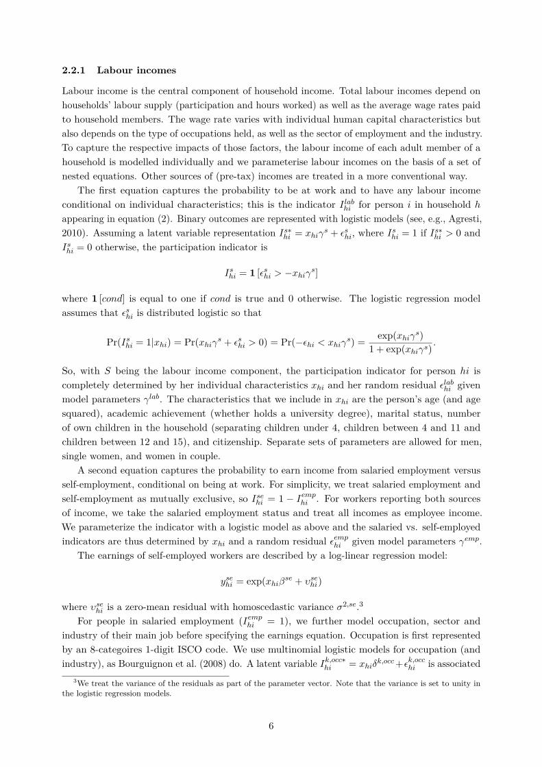
2.2.1 Labour incomes

Labour income is the central component of household income. Total labour incomes depend onhouseholds’ labour supply (participation and hours worked) as well as the average wage rates paidto household members. The wage rate varies with individual human capital characteristics butalso depends on the type of occupations held, as well as the sector of employment and the industry.To capture the respective impacts of those factors, the labour income of each adult member of ahousehold is modelled individually and we parameterise labour incomes on the basis of a set ofnested equations. Other sources of (pre-tax) incomes are treated in a more conventional way.

The first equation captures the probability to be at work and to have any labour incomeconditional on individual characteristics; this is the indicator I labhi for person i in household h

appearing in equation (2). Binary outcomes are represented with logistic models (see, e.g., Agresti,2010). Assuming a latent variable representation Is∗hi = xhiγ

s + εshi, where Ishi = 1 if Is∗hi > 0 andIshi = 0 otherwise, the participation indicator is

Ishi = 1 [εshi > −xhiγs]

where 1 [cond] is equal to one if cond is true and 0 otherwise. The logistic regression modelassumes that εshi is distributed logistic so that

Pr(Ishi = 1|xhi) = Pr(xhiγs + εshi > 0) = Pr(−εhi < xhiγs) = exp(xhiγs)

1 + exp(xhiγs).

So, with S being the labour income component, the participation indicator for person hi iscompletely determined by her individual characteristics xhi and her random residual εlabhi givenmodel parameters γlab. The characteristics that we include in xhi are the person’s age (and agesquared), academic achievement (whether holds a university degree), marital status, numberof own children in the household (separating children under 4, children between 4 and 11 andchildren between 12 and 15), and citizenship. Separate sets of parameters are allowed for men,single women, and women in couple.

A second equation captures the probability to earn income from salaried employment versusself-employment, conditional on being at work. For simplicity, we treat salaried employment andself-employment as mutually exclusive, so Isehi = 1 − Iemphi . For workers reporting both sourcesof income, we take the salaried employment status and treat all incomes as employee income.We parameterize the indicator with a logistic model as above and the salaried vs. self-employedindicators are thus determined by xhi and a random residual εemphi given model parameters γemp.

The earnings of self-employed workers are described by a log-linear regression model:

ysehi = exp(xhiβse + υsehi)

where υsehi is a zero-mean residual with homoscedastic variance σ2,se.3

For people in salaried employment (Iemphi = 1), we further model occupation, sector andindustry of their main job before specifying the earnings equation. Occupation is first representedby an 8-categoires 1-digit ISCO code. We use multinomial logistic models for occupation (andindustry), as Bourguignon et al. (2008) do. A latent variable Ik,occ∗hi = xhiδ

k,occ+εk,occhi is associated3We treat the variance of the residuals as part of the parameter vector. Note that the variance is set to unity in

the logistic regression models.

6

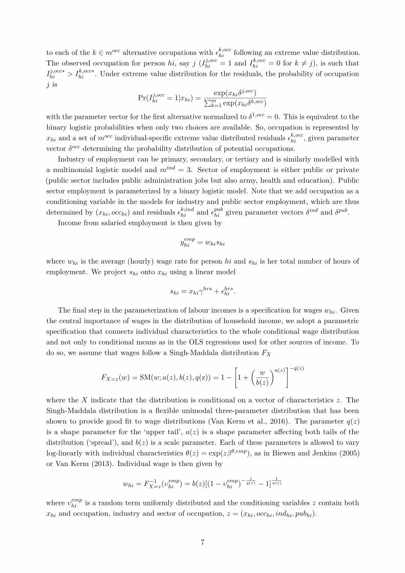
to each of the k ∈ mocc alternative occupations with εk,occhi following an extreme value distribution.The observed occupation for person hi, say j (Ij,occhi = 1 and Ik,occhi = 0 for k 6= j), is such thatIj,occ∗hi > Ik,occ∗hi . Under extreme value distribution for the residuals, the probability of occupationj is

Pr(Ij,occhi = 1|xhi) = exp(xhiδj,occ)∑mk=1 exp(xhiδk,occ)

with the parameter vector for the first alternative normalized to δ1,occ = 0. This is equivalent to thebinary logistic probabilities when only two choices are available. So, occupation is represented byxhi and a set of mocc individual-specific extreme value distributed residuals εk,occhi , given parametervector δocc determining the probability distribution of potential occupations.

Industry of employment can be primary, secondary, or tertiary and is similarly modelled witha multinomial logistic model and mind = 3. Sector of employment is either public or private(public sector includes public administration jobs but also army, health and education). Publicsector employment is parameterized by a binary logistic model. Note that we add occupation as aconditioning variable in the models for industry and public sector employment, which are thusdetermined by (xhi, occhi) and residuals εk;ind

hi and εpubhi given parameter vectors δind and δpub.Income from salaried employment is then given by

yemphi = whishi

where whi is the average (hourly) wage rate for person hi and shi is her total number of hours ofemployment. We project shi onto xhi using a linear model

shi = xhiγhrs + εhrshi .

The final step in the parameterization of labour incomes is a specification for wages whi. Giventhe central importance of wages in the distribution of household income, we adopt a parametricspecification that connects individual characteristics to the whole conditional wage distributionand not only to conditional means as in the OLS regressions used for other sources of income. Todo so, we assume that wages follow a Singh-Maddala distribution FX

FX=z(w) = SM(w; a(z), b(z), q(z)) = 1−[1 +

(w

b(z)

)a(z)]−q(z)

where the X indicate that the distribution is conditional on a vector of characteristics z. TheSingh-Maddala distribution is a flexible unimodal three-parameter distribution that has beenshown to provide good fit to wage distributions (Van Kerm et al., 2016). The parameter q(z)is a shape parameter for the ‘upper tail’, a(z) is a shape parameter affecting both tails of thedistribution (‘spread’), and b(z) is a scale parameter. Each of these parameters is allowed to varylog-linearly with individual characteristics θ(z) = exp(zβθ,emp), as in Biewen and Jenkins (2005)or Van Kerm (2013). Individual wage is then given by

whi = F−1X=z(υ

emphi ) = b(z)[(1− υemphi )−

1q(z) − 1]

1a(z)

where υemphi is a random term uniformly distributed and the conditioning variables z contain bothxhi and occupation, industry and sector of occupation, z = (xhi, occhi, indhi, pubhi).

7

The parameterisation of wages closes the model for labour incomes. To summarize: householdlabour income yLh is ultimately characterised by all adult members’ characteristics xhi andresidual heterogeneity terms (εlabhi , ε

emphi , εk,occhi , εk,indhi , εpubhi , ε

hrshi , υ

sehi , υ

emphi ) for i = 1, . . . , nh given the

model parameters (γlab, γemp, δocc, δind, δpub, (βse, σse), γhrs, (βa,emp, βb,emp, βq,emp)). Appendix Aprovides details of the model components in tabular format.

2.2.2 Other market incomes

We adopt much simpler parameterizations for all other market incomes that compose capitalincome (yKh ) and other pre-tax, pre-transfer incomes (yOh ). As for labour incomes, each aggregateis the sum of the contributions of individual members hi. For any of those four sources, say S, theprobability of receiving any income from the source S is modeled with a binary logistic regressiondescribed above, again conditioning on individual exogenous variables xhi: Ishi = 1 [εshi > −xhiγs].The amount received is log-linearly related to xhi: yShi = exp(xhiβS+υShi) with V ar(υShi) = σ2,S . Soboth capital incomes and other incomes are determined by all household members’ characteristicsxhi and two residual heterogeneity terms and two sets of parameters (γS , (βS , σS)).

2.2.3 Public transfers

The final two components of household income are the public transfers received and the incometax paid. Since many transfers and taxes are directly determined by the amount of all incomesreceived, they cannot reasonably be calculated and simulated independently. Instead, we derivetaxes and a range of benefits on the basis of a tax-benefit calculator that can estimate the amountof benefits received and income tax paid (or, at least, due) as a function of the income sources,household characteristics and a number of variables which may influence the benefit eligibilityand tax liabilities according to the rules in place.

Many such calculators exist for different countries, but for cross-country comparative analysis,it is important to rely on an engine that models taxes and benefits in a consistent way acrosscountries. For European countries, harmonized taxes and benefit calculations can be taken fromEUROMOD, a large-scale pan-European tax-benefit static micro-simulation engine (Sutherlandand Figari, 2013). This large-scale income calculator incorporates the tax-benefit schemes of themajority of European countries and allows computation of predicted household disposable income,on the basis of pre-tax, pre-benefit incomes, employment and other household characteristics. Italso makes it possible to implement ‘policy swaps’ in which particular tax or benefit policies fromone reference country or year are applied to other countries or time periods (see, e.g., Bargain,2012; Bargain and Callan, 2010; Levy et al., 2007). EUROMOD simulates direct taxes and a widerange of cash transfers to households: income and property taxes, social insurance contributions,family benefits, housing benefits, social assistance, and, where relevant other income-relatedbenefits (Figari et al., 2015).

Not all public transfers are evaluated by EUROMOD. Two main sources of public transfers arenot simulated (or are only partially simulated): contributory benefits and public pensions as wellas disability benefits which generally depend on past employment histories or other information(e.g., about the severity of a disability) that is usually not observed in household survey datathat input the tax-benefit simulator. For those components included in yBh , the benefits measuredat individual level are modelled like non-labour incomes with a logistic regression for receipt ofthe source and a log-linear specification for the amount received while benefits measured at the

8

household level are modelled similarly except that only one household level equation is specifiedfor each model and the exogenous characteristics xh are composed of household-level demographiccomposition and of the individual characteristics of the ‘household head’ (where household head isdefined as the person with the highest personal income or the eldest in the case of equal income).

The remaining components of yBh are calculated from EUROMOD on the basis of householdcharacteristics—typically universal transfers—and, for means-tested benefits, on the basis ofpre-tax household income.4

2.2.4 Taxes and social security contributions

Finally, we rely entirely on EUROMOD to calculate direct taxes and social security contributionsas a function of all income components and household characteristics. EUROMOD takes as inputthe household members’ ‘exogenous’ characteristics, as well as all income components previouslymodelled. It returns social security contributions and total taxes due by the household given thetax-benefit parameters in place in the country considered.5

2.3 Estimation of parameters

Following Bourguignon et al. (2008), each equation of the model—logistic, log-linear or Singh-Maddala—is estimated independently using standard estimators (OLS or maximum likelihood)to derive estimates of the model parameters. We do not attempt to model selectivity in theincome equations. The only exception is for the coefficients of the Singh-Maddala model for wages.The model is estimated for men and women separately. For women, we estimate a participation-corrected model as proposed in Van Kerm (2013). Given the size of the model, we do not attemptto estimate equations jointly or model correlations across equations parametrically. Of course,model parameters are not meant to capture causal relationships between the various ‘endogenous’variables yShi and IShi and the few ‘exogenous’ variables xhi. The parametric relationships arereduced-form projections that aim to describe the empirical associations between basic demographicvariables and various components of income.

3 Counterfactual distributions and the decomposition of cross-country inequality differences

The household income generation representation is now used to describe the overall householdincome distribution and to create counterfactual distributions. We are interested in studying thedistribution F of the random variable Y which represents household disposable income amongindividuals in the population. More specifically, we aim to study some summary index measure

4In effect some sources of benefits are of mixed type. Eligibility can be determined from household characteristics(and therefore modelled with a logistic regression) while the level of transfer is calculated by the tax-benefitparameters. Appendix B provides details on the sources and treatment of public transfers.

5A few additional variables that are not part of household income can influence household taxes and benefits(at least in some countries). These variables—for example mortgages, rents paid, and contributions for privatepensions — are also modelled to calculate liabilities. For instance, for those who are out of the labour market, wemodel the propensity of being unemployed and being formally retired. The exact status for those out of the labourmarket may have an impact on the final household disposable income via the tax and benefit system. Each of thesevariables is modelled as the ‘other income sources’ described above: the existence of such payment is according to alogit regression model, and the amount paid is based on a log-linear regression model. The values taken by thosevariables do not determine household income directly, but they are fed into the tax-benefit microsimulation engineto calculate taxes and benefits for household h. Appendix B describes those auxiliary variables.

9

θ(F )—say, the Gini coefficient—and to examine why this index differs from the index observed inanother country or another time period θ(G).

At this stage, it is convenient to think of our representation of the income generation processas a generic non-separable model

Y = m(X,Υ) (3)

where Y is income, X is a vector of ‘exogenous’ characteristics and Υ is a vector of unobservedheterogeneity (residual) terms (Matzkin, 2003; Rothe, 2010). The function m describes jointly therelationship between household characteristics and income and the heterogeneity in Y that is not‘explained’ by X. The derivative of m with respect to its first argument reflects variations in Yacross households that can be attributed to differences in observable household characteristicswhile the derivative of m with respect to its second argument reflects variations in Y acrosshouseholds of identical observable characteristics.

The parametric functional forms adopted for the different components of our income generationmodel imply a particular parametric shape for m, so

Y = mξ(X,Υ; ξ) (4)

where mξ represents the specific parametric structure adopted for the income generation model andξ is the vector of parameter values. Equation (4) has no ‘structural’ interpretation but it shouldbe viewed as a set of reduced form equations linking household characteristics and income—arelationship that may arise from an unknown, broader structural model—through earningsfunctions, equations for employment and occupational and industrial structure, equations fornon-labour income and replacement incomes and through tax-and-transfer rules. The distributionfunction F—and therefore any functional of interest θ(F )—depends on the (joint) distributionfunction of X and Υ in the population through mξ and ξ.

In this model, the distribution of income in two countries can differ because of differencesin the distribution of X, in the distribution of residual heterogeneity terms Υ and differences inm. To make progress, we assume that all countries can be represented by a common parametricmodel of the form mξ but that countries differ in the values taken by the parameters ξ. In orderto quantify the relative contributions of these factors, we define a number of ‘transformations’that, when applied to the model, allow us to capture how sensitive the income distribution isto specific dimensions of the model. The transformations are then calibrated to reflect actualdifferences across countries in the factors concerned and lead to a decomposition of cross-countrydifferences in income distributions into specific factors of interest.

3.1 Four transformations of the income generation process

We focus on four types of ‘transformations’ that will help us capture the relative contributions of fourbroad factors (or subsets thereof): (i) a demographic transformation, (ii) a labour market structuretransformation, (iii) a price-and-returns transformation and (iv) a tax-benefit transformation.These transformations follow from the construction of the income generation process, althoughthese are specific choices among many other possibilities offered by the model.

The demographic transformation involves modification of the distribution of the randomvariables X:

m(X̃(X),Υ; ξ)

10

which lead to a new, counterfactual distribution of outcome Y denoted F d. The impact of ademographic transformation, mξ(X̃(X),Υ; ξ)−mξ(X,Υ; ξ), on distribution functionals of interestθ is then given by ∆d

θ(F ) = θ(F d)− θ(F ). This measure is called a ‘partial distributional policyeffect’ in Rothe (2012), or simply a ‘policy effect’ in Firpo et al. (2009).

A labour market structure transformation works through the parameter vector ξ. The trans-formation involves modifying the parameters of the equations characterising the employmentprobabilities and hours worked (γlab, γemp, γhrs), and the occupational and industrial structure(δocc, δind, δpub),

mξ(X,Υ; l̃(ξ))

which, just like the demographic transformation, leads to a new counterfactual distribution ofoutcome Y denoted F l. The impact of the labour market structure transformationmξ(X,Υ; l̃(ξ))−mξ(X,Υ; ξ) on distribution functionals θ is given by ∆l

θ(F ) = θ(F l)− θ(F ).A price-and returns transformation again acts through the parameter vector ξ. The transforma-

tion involves changing the parameters of the equations characterising the level of earnings ((βse, σse),(βa,emp, βb,emp, βq,emp)) and all other pre-tax incomes ((βinv, σinv), (βprop, σprop), (βpripen, σpripen),(βother, σother)),

mξ(X,Υ; r̃(ξ))

and the impact on θ is denoted by ∆rθ(F ) = θ(F r)− θ(F ). Observe that this transformation is

analogous, albeit in a multiple equations setup, to the manipulation of the vector of coefficientsof Mincerian earnings regressions in order to capture ‘price’ effects (as distinct from ‘compo-sition effects) in traditional Oaxaca-Blinder decomposition exercises. It closely resembles thedecomposition of Juhn et al. (1993) in the way residual variances is accounted for.

The fourth and last form of transformation that we use is a tax-benefit transformation. Thetax-benefit transformation is a particular transformation of the parameter vector ξ which modifies(i) the regression parameters determining the level of public transfers received by households and(ii) the parameters of the EUROMOD tax-benefit calculator which evaluate the tax liabilities (andthe residual benefits, mostly universal benefits, which are determined directly by EUROMOD andnot modelled parametrically; see Appendix B for details):

mξ(X,Υ; t̃b(ξ)).

As above, we write the effect of a tax-benefit transformation on θ as ∆tbθ (F ) = θ(F tb)−θ(F ) where

F tb denotes the distribution function of household incomes after the tax benefit transformation isapplied to the income-generation model.

3.2 Cross-country comparisons

In an analysis of cross-country differences in income distributions, a natural way to use thetransformations just defined is to build the income generation model for countries A and B

separately and to calibrate transformations so as to ‘transplant’ components of the incomegeneration model across countries. For example, for the labour market structure transformationapplied to country A, l̃(ξ) is composed of the subset of parameters from ξA for the fixed parametersand of parameters taken from ξB for the transformed parameters which capture the characteristicsof the labour market structure in the income generation model. The transformed income generationprocess for country A thereby leads to a simulated distribution for country A as if it had a labour

11

market structure as country B and all other components of the model remained unchanged. Thedifference between the simulated and the observed distributions in country A (and inequalityfunctionals defined over them) provides a quantification of the contribution of labour marketstructure differences to the overall difference in income distribution between the two countries. Onceagain this procedure is fully analogous to standard Oaxaca-Blinder decompositions—swappingregression coefficients across earnings equations for alternative groups—although it is implementedin a multiple equations model.

The transplantation of country B parameters onto country A’s model is done similarly forthe price-and-returns transformation by swapping the relevant subset of parameters. Unlike thelabour market structure transformation, the price-and-returns transformation involves swappingvariance terms, σ2. This is achieved as in Juhn et al. (1993) by rescaling the residuals of countryA by the ratio

σSB

σSAfor each of the five components S that are affected by the transformation. This

procedure scales the distribution of residual terms while preserving the rank correlation of theresiduals across the different equations of the income generation model.

The calibration of the tax-benefit transformation combines both swapping model parametersas above (for the equations describing benefits) and using the EUROMOD tax-benefit calculatorto apply the tax and benefit rules and parameters of country B onto the market incomes andhousehold characteristics of country A. Such transplantation of tax-policy rules and parametersis most often done for analysis of trends in income distributions (see Bargain, 2012; Bargainand Callan, 2010; Herault and Azpitarte, 2016; Paulus and Tasseva, 2017), but it has also beenapplied to cross-country analysis (Levy et al., 2007).6 The underpinnings of transplantation oftax-and-transfer rules across countries are discussed in Dardanoni and Lambert (2002).

Finally, the demographic transformation involves modifying the distribution of populationcharacteristics of country A in such a way that it has the (joint) distribution of country B. Thedistribution of X is modified but the conditional distribution of Υ given X must not be affectedto remain as it is in A. As shown in DiNardo et al. (1996) and Barsky et al. (2002), this can beachieved semi-parametrically by reweighting. In evaluating F or θ(F ), population A householdsare reweighted by a factor

ω(X) = Pr(X|B)Pr(X|A) = Pr(B|X)

Pr(A|X)Pr(A)Pr(B) . (5)

The probabilities in (5) can be estimated by standard techniques for binary responses; see e.g.,Biewen and Juhasz (2012) for a recent application of this approach.

3.3 Decomposition

A decomposition procedure aims to (additively) decompose the total difference ∆θ(FA, FB) =θ(G)− θ(F ) into a number of factors that capture the contribution of different components of themodel:

∆θ(FA, FB) =K∑k=1

∆kθ(FA, FB).

6In an intertemporal context, studies usually attempt to disentangle the contribution of structural changes inpolicies from the mere uprating of policy parameters defined in nominal monetary units (Bargain, 2012; Figariet al., 2015). The issue is less relevant in the present context and we swap both structural differences and nominalparameters at once. For the conversion of nominal parameters across countries, all monetary units expressed indifferent currencies are converted on the basis of exchange rates in the year concerned.

12

A common way to build such a decomposition is to build a sequence of counterfactual distribu-tions by applying each of the four transformations one after the other from the original distribution,say FA, to the target distribution FB and to define the components of the decomposition as

∆kθ(FA, FB) = θ(FA,B(k))− θ(FA,B(k−1))

where FA,B(k) is a counterfactual distribution obtained by composing k transformations of theincome generation model for country A calibrated to the structure of country B (and we defineFA,B(0) = FA and FA,B(K) = FB). Note that the last factor K is a ‘residual’ (or ‘unexplained’)factor that is not modelled and transplanted explicitly but that collects all residual differencebetween the target distribution FB and the counterfactual distribution obtained after all froutransformations have been composed and applied to the income generation model for country A.7

The drawback of such a sequential decomposition is its path-dependence, the dependence on thesequence of composition of transformations in quantifying the contribution of each factor.8

To reduce issues of path-dependence we prefer to examine ‘direct effects’ to assess the impactof each factor from the same initial benchmark distribution : Dk

θ (FA, FB) = θ(F kA)− θ(FA) whereF kA is the counterfactual distribution obtained by applying one particular transformation k andavoid composing transformations. As Biewen and Juhasz (2012) argue, comparing ‘direct effects’is a natural way to compare the effects of alternative transformations. However the sum of directeffects does not add up to the overall inequality change. A decomposition can be expressed as

∆θ(FA, FB) = Ddθ(FA, FB) +Dl

θ(FA, FB) +Drθ(FA, FB) +Dtb

θ (FA, FB)+Iθ(FA, FB) +RΥ

θ (FA, FB)

where (i) the term Iθ(FA, FB) =(θ(F tb,r,l,dA )− θ(FA)

)−(∑

k∈{d,r,l,tb}Dkθ (FA, FB)

)is equal to

the difference between the combined effect of the four transformations composed and the sum ofdirect effects which captures all two-way and three-way interactions between the four componentsin the model (Biewen, 2014), and (ii) the residual difference RΥ

θ (FA, FB) = θ(FB)− θ(F tb,r,l,dA )captures factors that are not transplanted across countries by any of the transformations, namelythe distribution of residual heterogeneity terms Υ.

3.4 Incorporating labour supply responses

The optimal tax literature has long recognized the importance of accounting for labour supplyresponses to tax changes (Mirrlees, 1971) and recent analysis of tax-benefit policy changes

7Concretely, we would ascribe ∆1θ(FA, FB) ≡ ∆d

θ(FA, FB) = θ(F dA) − θ(FA) to the demographic dif-ferences between countries—F dA is the counterfactual distribution obtained after applying the demographictransformation to country A. The contribution of differences in labour market structure is ∆2

θ(FA, FB) ≡∆l|dθ (FA, FB) = θ(F l,dA ) − θ(F dA) where F l,dA is obtained by composing the demographic and labour market struc-

ture transformations, that is mξ(X̃(X),Υ; l̃(ξ)). Similarly, the contributions of prices-and-returns and of tax-benefits are respectively defined as ∆3

θ(FA, FB) ≡ ∆r|l,dθ (FA, FB) = θ(F r,l,dA ) − θ(F l,dA ) and ∆4

θ(FA, FB) ≡∆tb|r,l,dθ (FA, FB) = θ(F tb,r,l,dA ) − θ(F r,l,dA ) with composition of multiple transformations. The residual difference

∆5θ(FA, FB) ≡ ∆Υ

θ (FA, FB) = θ(FB) − θ(F tb,r,l,dA ) captures factors that are not transplanted across coun-tries by any of the transformations, namely the distribution of residual heterogeneity terms Υ. So, we have∆θ(FA, FB) =

[∆dθ(FA, FB) + ∆l|d

θ (FA, FB) + ∆r|l,dθ (FA, FB) + ∆tb|r,l,d

θ (FA, FB)]

+ ∆Υθ (FA, FB).

8Some authors have proposed to calculate the contribution of each factor in all possible sequence of introductionof factors and average across sequences (Chantreuil and Trannoy, 2013; Devicienti, 2010; Shorrocks, 2013). Thisapproach can however be computationally prohibitive for complex models and does not necessarily improve theeconomic interpretation of the estimated components.

13

incorporate analysis of labour supply responses to estimate the full effect of a reform (see, e.g.,Aaberge et al., 1995; Bargain, 2012). While the counterfactual distributions that we construct aremeant to quantify the contribution of various factors to inequality differences across countries in astatic perspective—we are not trying to describe accurately what would actually happen in countryA if, say, its labour market structure was to morph suddenly into the structure of B—we incorporatea structural labour supply model which evaluates employment probabilities (including part-timeemployment) by household members as a function of the household demographic characteristicsand disposable income where disposable income is itself a function of tax-benefit parameters,wages and non-labour incomes and individual characteristics. The labour supply model identifieshousehold labour supply elasticities that allow us to adjust employment probabilities as a result ofeither changes in tax-benefit parameters (after a tax-benefit transformation) or changes in marketincomes following from a price-and-return or labour market structure transformation.9

The labour supply response adjustment to a transformation of the parameters affects bothindividual employment I labhi and hours worked shi of all household members in the income generationmodel. Appendix C describes the labour supply model implemented in our empirical applicationand how predictions are incorporated in the representation of the income generation process.Comparing the decomposition results with and without allowing for labour supply adjustmentsto our cross-country transformations informs us of the potential importance of understandingbehavioural responses (at least in the short run). We isolate below the contribution of laboursupply responses by taking the difference between the counterfactual distribution when laboursupply responses are considered and the completely “static” counterfactual. The total effect of the“swap” is decomposed into a direct effect and indirect effect from the labour supply response.

4 Application to Ireland and the United Kingdom

We now provide an illustrative application of the methods to Ireland and the United Kingdom.The two countries share a common language and border and have much in common, historicallyand with respect to labour market and Welfare State policies which were influenced by similarpolitical philosophy principles. Nonetheless, the contemporaneous income distributions in the twocountries differ quite substantially. In 2007, the last year before the financial and economic crisishit both countries, the Gini coefficient was 0.28 in Ireland—a relatively low figure by internationalstandards—while it was 0.32 in the UK—among the highest EU figure. To put the gap inperspective, a difference of four Gini points corresponds to the increase in disposable incomeinequality reported by OECD (2011) for the USA between the mid-1980s and the late 2000’s—aperiod during which inequality is thought to have increased dramatically.

4.1 Data

We exploit two nationally representative household surveys: the European Union Statistics ofIncome and Living Conditions (EU-SILC) for Ireland and the Family Resources Survey (FRS) forthe United Kingdom. These surveys contain detailed information about household incomes aswell as a wide range of variables about the characteristics of households and their members. Theyhave been the key sources of official statistics about the distribution of income in both countries.

9By construction, the demographic transformation does not lead to any change in our household labour supplypredictions since it does not lead to any change in relevant individual or household-level variables.

14

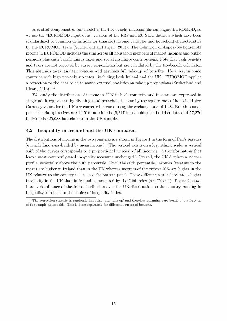
A central component of our model is the tax-benefit microsimulation engine EUROMOD, sowe use the “EUROMOD input data” versions of the FRS and EU-SILC datasets which have beenstandardized to common definitions for (market) income variables and household characteristicsby the EUROMOD team (Sutherland and Figari, 2013). The definition of disposable householdincome in EUROMOD includes the sum across all household members of market incomes and publicpensions plus cash benefit minus taxes and social insurance contributions. Note that cash benefitsand taxes are not reported by survey respondents but are calculated by the tax-benefit calculator.This assumes away any tax evasion and assumes full take-up of benefits. However, in somecountries with high non-take-up rates—including both Ireland and the UK—EUROMOD appliesa correction to the data so as to match external statistics on take-up proportions (Sutherland andFigari, 2013). 10

We study the distribution of income in 2007 in both countries and incomes are expressed in‘single adult equivalent’ by dividing total household income by the square root of household size.Currency values for the UK are converted in euros using the exchange rate of 1.484 British poundsper euro. Samples sizes are 12,516 individuals (5,247 households) in the Irish data and 57,276individuals (25,088 households) in the UK sample.

4.2 Inequality in Ireland and the UK compared

The distributions of income in the two countries are shown in Figure 1 in the form of Pen’s parades(quantile functions divided by mean income). (The vertical axis is on a logarithmic scale: a verticalshift of the curves corresponds to a proportional increase of all incomes—a transformation thatleaves most commonly-used inequality measures unchanged.) Overall, the UK displays a steeperprofile, especially above the 50th percentile. Until the 80th percentile, incomes (relative to themean) are higher in Ireland than in the UK whereas incomes of the richest 20% are higher in theUK relative to the country mean—see the bottom panel. These differences translate into a higherinequality in the UK than in Ireland as measured by the Gini index (see Table 1). Figure 2 showsLorenz dominance of the Irish distribution over the UK distribution so the country ranking ininequality is robust to the choice of inequality index.

10The correction consists in randomly imputing ‘non take-up’ and therefore assigning zero benefits to a fractionof the sample households. This is done separately for different sources of benefits.

15

0

.5

1

1.5

2

2.5

3

3.5

Qua

ntile

ove

r mea

n in

com

e (lo

g sc

ale)

10 20 30 40 50 60 70 80 90 100

United Kingdom

Ireland

-.15

-.1

-.05

0

.05

.1

.15

Rel

ativ

e di

ffere

nce

in n

orm

aliz

ed P

en p

arad

es

10 20 30 40 50 60 70 80 90 100

Figure 1: Distribution of equivalised household disposable income in Ireland and the UK: Normal-ized quantile functions (Pen’s parades) (top) and relative differences (IE/UK-1) (bottom)

16

0.2

.4.6

.81

Lore

nz o

rdin

ate

0 .2 .4 .6 .8 1Cumulative population share

United Kingdom Ireland

Figure 2: Lorenz curves for the United Kingdom and Ireland

Table 1: Equivalized household disposable income in the UK and Ireland, 2007 (monthly, in euros)

Mean Median Gini

UK 2341 2243 0.319Ireland 2541 2491 0.277

Table 2 shows differences across the two countries in a number of population charateristicsand labour market structures. The two countries have similar demographic profiles; with somenotable exceptions however. According to our samples, the population aged 25–64 is generallymore educated in Ireland than in the UK, and there are larger shares of people aged 65+ andsmaller shares of children aged 4+ in the UK than in Ireland. The share of people aged 16+at work is 6 percentage points higher in Ireland than in the UK but their distribution acrossoccupations are similar (we suspect that differences with respect to “professionals” and “associateprofessionals” reflect differences in data definitions). The distribution of workers across sectors ofactivity is however remarkably different: the share of workers in agriculture is almost four timeslarger in Ireland than in the UK, the share in industy is less than half, and the services sectoremploys 10 percentage points more people in Ireland. Public sector employment is also larger in

17

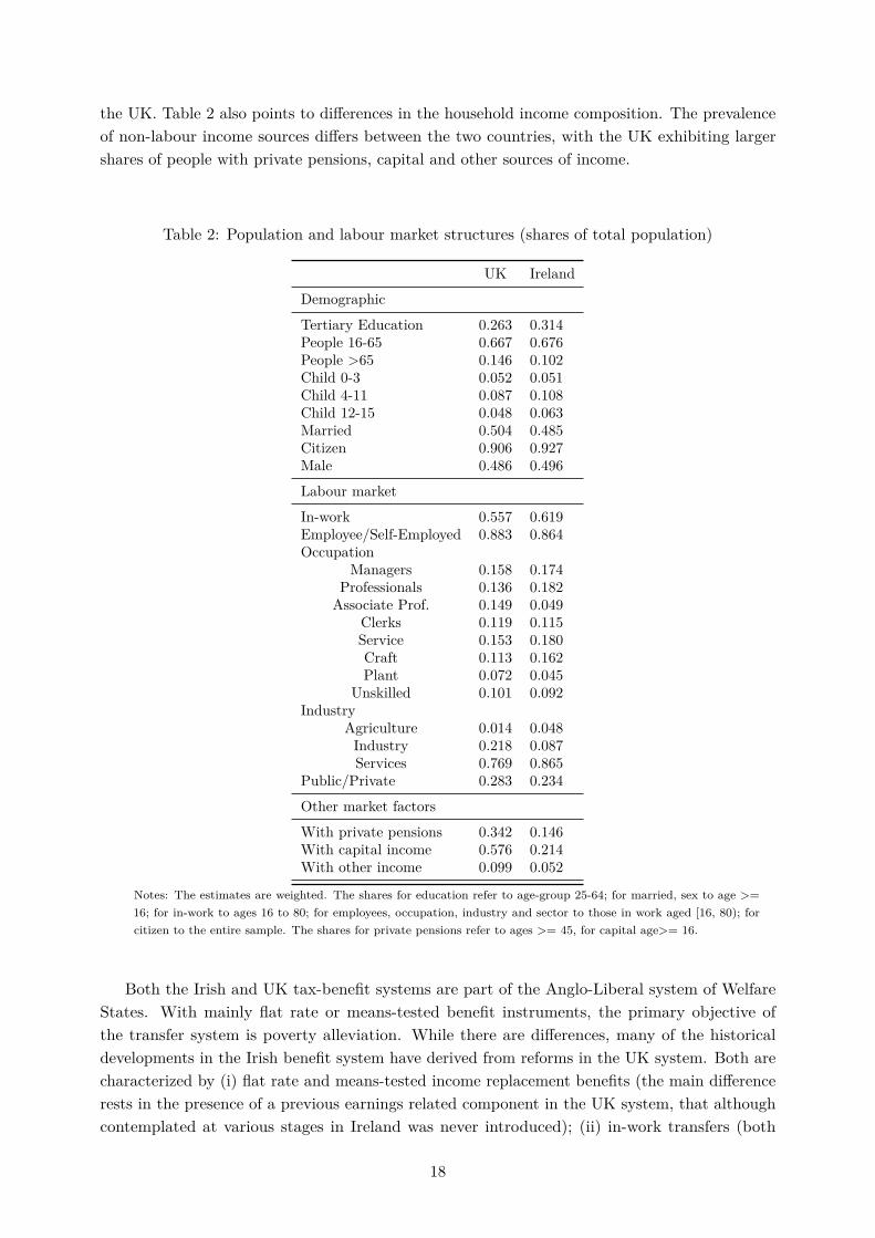
the UK. Table 2 also points to differences in the household income composition. The prevalenceof non-labour income sources differs between the two countries, with the UK exhibiting largershares of people with private pensions, capital and other sources of income.

Table 2: Population and labour market structures (shares of total population)

UK Ireland

Demographic

Tertiary Education 0.263 0.314People 16-65 0.667 0.676People >65 0.146 0.102Child 0-3 0.052 0.051Child 4-11 0.087 0.108Child 12-15 0.048 0.063Married 0.504 0.485Citizen 0.906 0.927Male 0.486 0.496

Labour market

In-work 0.557 0.619Employee/Self-Employed 0.883 0.864Occupation

Managers 0.158 0.174Professionals 0.136 0.182Associate Prof. 0.149 0.049

Clerks 0.119 0.115Service 0.153 0.180Craft 0.113 0.162Plant 0.072 0.045

Unskilled 0.101 0.092Industry

Agriculture 0.014 0.048Industry 0.218 0.087Services 0.769 0.865

Public/Private 0.283 0.234

Other market factors

With private pensions 0.342 0.146With capital income 0.576 0.214With other income 0.099 0.052

Notes: The estimates are weighted. The shares for education refer to age-group 25-64; for married, sex to age >=16; for in-work to ages 16 to 80; for employees, occupation, industry and sector to those in work aged [16, 80); forcitizen to the entire sample. The shares for private pensions refer to ages >= 45, for capital age>= 16.

Both the Irish and UK tax-benefit systems are part of the Anglo-Liberal system of WelfareStates. With mainly flat rate or means-tested benefit instruments, the primary objective ofthe transfer system is poverty alleviation. While there are differences, many of the historicaldevelopments in the Irish benefit system have derived from reforms in the UK system. Both arecharacterized by (i) flat rate and means-tested income replacement benefits (the main differencerests in the presence of a previous earnings related component in the UK system, that althoughcontemplated at various stages in Ireland was never introduced); (ii) in-work transfers (both

18

countries have transfers targeted at low-income families with children, where payments are madeonce a particular number of hours have been made; there is an additional child care component inthe UK system); (iii) flat rate universal child benefits; and (iv) housing benefits (coverage hasbeen lower historically in Ireland, but has been increasing).

Both countries have progressive income taxation systems and earnings-related social insurancecontributions that vary by employee and self-employed. There are however some notable differences.The Irish income taxation system is joint, while the UK system is an individualized system.

Table 3 documents the redistributive effects of the tax-benefit system in both countries. Notefirst that inequality in market income is more similar in the two countries than inequality ofdisposable income. The benefit schedule increases the difference in inequality between the twocountries by dropping inequality to a larger extent in Ireland compared with the UK, effect drivenby a higher degree of redistribution in Ireland. The benefit schedule is more regressive in theUK (more low incomes receive benefits), but the average benefit rate is also much lower. Thetax system increases further the percentage point difference in inequality between Ireland andthe UK. This is due to a more progressive and a more redistributive tax system in Ireland. Astaxes are progressive and benefits are regressive, the net schedule is equalizing in both countries.The Reynolds-Smolensky index of net redistributive effect shows the Irish tax-benefit system ismore redistributive than the UK system (Lambert, 2001). Whether these differences are due topolicy design or to differences in the market income distribution is revealed in the decompositionanalysis.

Table 3: Progressivity and redistribution of taxes and benefits on household equivalized disposableincome

UK Ireland Ratio: IRL/UK

Gini Gross Income 0.497 0.483 0.972Gini Gross Income (incl. benefits) 0.377 0.341 0.905Averate transfer rate 0.155 0.242 1.558Benefit Regressivity (K) 0.936 0.769 0.822Benefit Redistribution (RS) 0.120 0.142 1.183Gini (gross + benefits - income taxes) 0.332 0.289 0.871Averate tax rate 0.159 0.132 0.826Tax Progressivity (K) 0.242 0.354 1.460Tax Redistribution (RS) 0.045 0.053 1.156

Gini Disposable Income 0.319 0.277 0.869Net Redistributive Effect 0.178 0.206 1.157

Notes: K = Kakwani; RS = Reynolds-Smolensky.

4.3 Accounting for differences in income inequality

Preliminary inspection of the characteristics of the population and of the income distributionpoints towards a few explanatory factors of the difference in income inequality, mainly the tax-benefit system, but also differences in the industrial structure of the two countries and in thedistribution of non-income sources. Applying the counterfactual decomposition exercise quantifiesthe respective roles played by such factors.

19

4.3.1 Counterfactual distributions

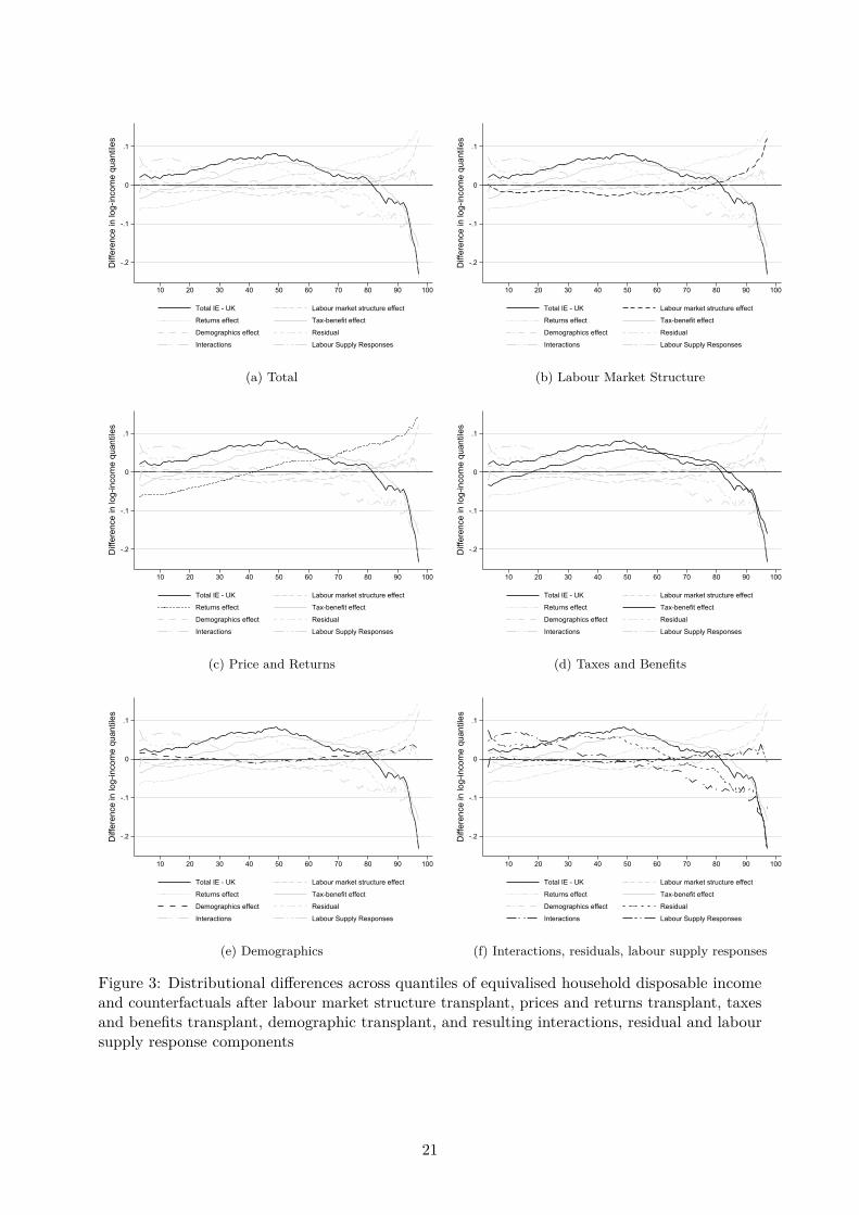
A decomposition of the differences between the mean-normalized quantile functions of the twodistributions of equivalised disposable income is displayed in Figure 3.11 Remember that mean-normalized quantiles are higher in Ireland than in the UK up to the 80th quantile beyond which thedifference turns negative; the observed difference is marked by dots on the plot. The counterfactualdifferences obtained by applying each of the four transformations defined in Section 3 onto the UKdata are shown in Figure 3. Figure 3(a) shows the total, observed difference; Figures 3(b,c,d,e)show how the ‘first order’, direct effect of applying each of the four transformations compares tothe total difference; Figure 3(f) highlights the residual and interaction terms and the impact oflabour supply responses.

11The fit of our simulation model is described in Appendix D. The whole set of model parameter estimates is notreported for the sake of brevity, but they are available on request.

20

-.2

-.1

0

.1

Diff

eren

ce in

log-

inco

me

quan

tiles

10 20 30 40 50 60 70 80 90 100

Total IE - UK Labour market structure effect

Returns effect Tax-benefit effect

Demographics effect Residual

Interactions Labour Supply Responses

(a) Total

-.2

-.1

0

.1

Diff

eren

ce in

log-

inco

me

quan

tiles

10 20 30 40 50 60 70 80 90 100





(b) Labour Market Structure

-.2

-.1

0

.1

Diff

eren

ce in

log-

inco

me

quan

tiles

10 20 30 40 50 60 70 80 90 100





(c) Price and Returns

-.2

-.1

0

.1

Diff

eren

ce in

log-

inco

me

quan

tiles

10 20 30 40 50 60 70 80 90 100





(d) Taxes and Benefits

-.2

-.1

0

.1

Diff

eren

ce in

log-

inco

me

quan

tiles

10 20 30 40 50 60 70 80 90 100





(e) Demographics

-.2

-.1

0

.1

Diff

eren

ce in

log-

inco

me

quan

tiles

10 20 30 40 50 60 70 80 90 100





(f) Interactions, residuals, labour supply responses

Figure 3: Distributional differences across quantiles of equivalised household disposable incomeand counterfactuals after labour market structure transplant, prices and returns transplant, taxesand benefits transplant, demographic transplant, and resulting interactions, residual and laboursupply response components

21

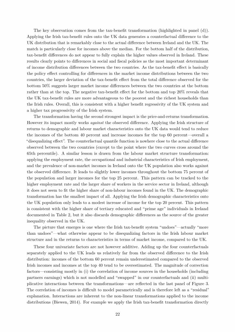
The key observation comes from the tax-benefit transformation (highlighted in panel (d)).Applying the Irish tax-benefit rules onto the UK data generates a counterfactual difference to theUK distribution that is remarkably close to the actual difference between Ireland and the UK. Thematch is particularly close for incomes above the median. For the bottom half of the distribution,tax-benefit differences do not appear to fully explain the higher values observed in Ireland. Theseresults clearly points to differences in social and fiscal policies as the most important determinantof income distribution differences between the two countries. As the tax-benefit effect is basicallythe policy effect controlling for differences in the market income distributions between the twocountries, the larger deviation of the tax-benefit effect from the total difference observed for thebottom 50% suggests larger market income differences between the two countries at the bottomrather than at the top. The negative tax-benefit effect for the bottom and top 20% reveals thatthe UK tax-benefit rules are more advantageous to the poorest and the richest households thanthe Irish rules. Overall, this is consistent with a higher benefit regressivity of the UK system anda higher tax progressivity of the Irish system.

The transformation having the second strongest impact is the price-and-returns transformation.However its impact mostly works against the observed difference. Applying the Irish structure ofreturns to demographic and labour market characteristics onto the UK data would tend to reducethe incomes of the bottom 40 percent and increase incomes for the top 60 percent—overall a“disequalizing effect”. The counterfactual quantile function is nowhere close to the actual differenceobserved between the two countries (except to the point where the two curves cross around the65th percentile). A similar lesson is drawn from the labour market structure transformation:applying the employment rate, the occupational and industrial characteristics of Irish employment,and the prevalence of non-market incomes in Ireland onto the UK population also works againstthe observed difference. It leads to slightly lower incomes throughout the bottom 75 percent ofthe population and larger incomes for the top 25 percent. This pattern can be tracked to thehigher employment rate and the larger share of workers in the service sector in Ireland, althoughit does not seem to fit the higher share of non-labour incomes found in the UK. The demographictransformation has the smallest impact of all. Applying the Irish demographic characteristics ontothe UK population only leads to a modest increase of income for the top 20 percent. This patternis consistent with the higher share of tertiary educated and “prime age” individuals in Irelanddocumented in Table 2, but it also discards demographic differences as the source of the greaterinequality observed in the UK.

The picture that emerges is one where the Irish tax-benefit system “undoes”—actually “morethan undoes”—what otherwise appear to be disequalizing factors in the Irish labour marketstructure and in the returns to characteristics in terms of market income, compared to the UK.

These four univariate factors are not however additive. Adding up the four counterfactualsseparately applied to the UK leads us relatively far from the observed difference to the Irishdistribution: incomes of the bottom 60 percent remain underestimated compared to the observedIrish incomes and incomes at the top 40 tend to be overestimated. The magnitude of correctionfactors—consisting mostly in (i) the correlation of income sources in the households (includingpartners earnings) which is not modelled and “swapped” in our counterfactuals and (ii) multi-plicative interactions between the transformations—are reflected in the last panel of Figure 3.The correlation of incomes is difficult to model parametrically and is therefore left as a “residual”explanation. Interactions are inherent to the non-linear transformations applied to the incomedistributions (Biewen, 2014). For example we apply the Irish tax-benefit transformation directly

22

on the UK distribution of market incomes and population structure. But if we had appliedthe tax-benefit transformation on a “modified” UK distribution reflecting the “disequalizing”adjustments due to the population structure or the different returns to characteristics, we canexpect that its impact would have been stronger than shown in Figure 3. These interactionsbeyond the “first order” effect of the transformations are bundled into the interaction term. As weshow below in the decomposition of Gini indices, the two factors—residual and interaction—seemto be of approximately equal sizes.

Panel (f) of Figure 3 also identifies the contribution of labour supply responses. Our trans-formations so far ignore the potential behavioural shifts. For instance, if the transplanted taxationsystem favours the mid-high income earners with lower taxes, disregarding the behavioural shiftmight underestimate the size of the high-income population as there is now a greater incentive fora worker with mid-high earning capacity to work. Additionally, the labour supply model capturesthe labour supply preference of the population, allowing us to swap the incentive structure of theeconomic system while retaining both the observed population characteristics and unobservedpreferences to some extent. The labour supply preference interacts with all other componentsas the hours of labour supply is a function of the population structure, tax benefit system, themarket composition and returns. Overall, the behavioural response, as an indirect factor, appearsto have a much smaller impact than the direct transformations.

4.3.2 Gini coefficients of disposable and market incomes and the net redistributiveimpact of taxes and transfers

We now move to examination of Gini indices. The first column of Table 4 presents decompositionresults for the difference in the Gini coefficients of disposable income—a 0.042 difference between0.319 in the UK and 0.277 in Ireland (rows 1–2). Rows 3–6 show the direct effects of applying eachof our four transformations onto the UK distribution: the difference between the Gini coefficientin the counterfactual distribution that would prevail in the UK if we transplant each factor inisolation from Ireland (assuming no labour supply responses) and the original distribution. Rows7-9 report indirect effects, namely the additional change once labour supply adjustments are takeninto account. Rows 10 and 11 capture respectively the interaction effects (the difference betweenthe sum of direct and indirect effects and the Gini observed when all four transformations arejointly applied) and the residual difference (that conflates all factors not explicitly modelled in theincome generation model, most notably the cross-equation correlation of unobserved heterogeneityterms). The direct effect of differences in the two tax-benefit systems (–0.015) is just under halfthe observed difference in disposable income inequality (–0.042). As was already apparent fromFigure 3, the cross-country difference in disposable income inequality is largely attributable todifferences in tax-benefit systems which counterbalance the disequalizing effect of the differencesin market composition and returns between Ireland and the UK. The effect of labour supplyresponses are relatively small.

The difference in gross income inequality between the two countries (column 2) is smaller thanin disposable income, yet inequality remains smaller in Ireland. Gross income includes only labourmarket income, private pensions, capital and “other” pre-tax incomes. Gross income inequalitywould be larger in the UK had the UK the market composition of Ireland but it would be smallerif the Irish returns to assets and human capital where transplanted in the UK (in this case anydifference in gross income inequality between the UK and Ireland would disappear). Again, the

23

contribution of demographic differences is comparatively small.12

Table 5 refines this picture by showing the contribution of more disaggregated transformations ofthe income distributions from our model. For the sake of brevity, we do not detail the constructionof all those sub-transformations but they should be self-explanatory from the table labels andnotes: they involve swapping only a subset of model parameters from ‘labour market structure’and ‘price and returns’ transformations across countries (either parameters reflecting the returns tosome specific characteristics or reflecting the relative prevalence of such characteristics). The effectof the labour market structure transformation is mostly driven by differences in the prevalenceof non-labour incomes in household portfolios. The price and returns transformation impact ondisposable income mostly arises from the parameters of the non-labour incomes equations again(concerning mostly capital incomes) while equations for labour income and private pensions aredriving the impact of the transformation on gross incomes.

12The small effect of the taxes and benefits transformation on gross income inequality is due to adjustments tominimum wages which are included in the taxes and benefit transformation.

24

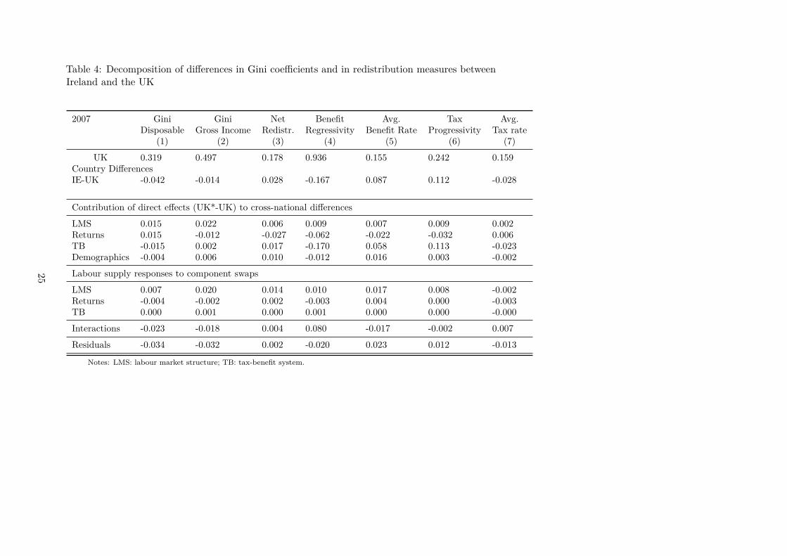
Table 4: Decomposition of differences in Gini coefficients and in redistribution measures betweenIreland and the UK

2007 Gini Gini Net Benefit Avg. Tax Avg.Disposable Gross Income Redistr. Regressivity Benefit Rate Progressivity Tax rate

(1) (2) (3) (4) (5) (6) (7)

UK 0.319 0.497 0.178 0.936 0.155 0.242 0.159Country DifferencesIE-UK -0.042 -0.014 0.028 -0.167 0.087 0.112 -0.028

Contribution of direct effects (UK*-UK) to cross-national differences

LMS 0.015 0.022 0.006 0.009 0.007 0.009 0.002Returns 0.015 -0.012 -0.027 -0.062 -0.022 -0.032 0.006TB -0.015 0.002 0.017 -0.170 0.058 0.113 -0.023Demographics -0.004 0.006 0.010 -0.012 0.016 0.003 -0.002

Labour supply responses to component swaps

LMS 0.007 0.020 0.014 0.010 0.017 0.008 -0.002Returns -0.004 -0.002 0.002 -0.003 0.004 0.000 -0.003TB 0.000 0.001 0.000 0.001 0.000 0.000 -0.000

Interactions -0.023 -0.018 0.004 0.080 -0.017 -0.002 0.007

Residuals -0.034 -0.032 0.002 -0.020 0.023 0.012 -0.013

Notes: LMS: labour market structure; TB: tax-benefit system.

25

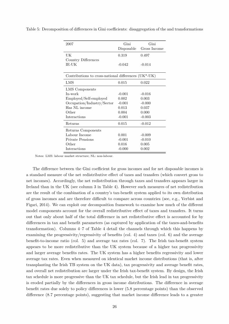
Table 5: Decomposition of differences in Gini coefficients: disaggregation of the and transformations

2007 Gini GiniDisposable Gross Income

UK 0.319 0.497Country DifferencesIE-UK -0.042 -0.014

Contributions to cross-national differences (UK*-UK)

LMS 0.015 0.022

LMS ComponentsIn-work -0.001 -0.016Employed/Self-employed 0.002 0.003Occupation/Industry/Sector -0.001 -0.000Has NL income 0.013 0.037Other 0.004 0.000Interactions -0.001 -0.003

Returns 0.015 -0.012

Returns ComponentsLabour Income 0.001 -0.009Private Pensions -0.001 -0.010Other 0.016 0.005Interactions -0.000 0.002

Notes: LMS: labour market structure; NL: non-labour.

The difference between the Gini coefficient for gross incomes and for net disposable incomes isa standard measure of the net redistributive effect of taxes and transfers (which convert gross tonet incomes). Accordingly, the net redistribution through taxes and transfers appears larger inIreland than in the UK (see column 3 in Table 4). However such measures of net redistributionare the result of the combination of a country’s tax-benefit system applied to its own distributionof gross incomes and are therefore difficult to compare across countries (see, e.g., Verbist andFigari, 2014). We can exploit our decomposition framework to examine how much of the differentmodel components account for the overall redistributive effect of taxes and transfers. It turnsout that only about half of the total difference in net redistributive effect is accounted for bydifferences in tax and benefit parameters (as captured by application of the taxes-and-benefitstransformation). Columns 4–7 of Table 4 detail the channels through which this happens byexamining the progressivity/regressivity of benefits (col. 4) and taxes (col. 6) and the averagebenefit-to-income ratio (col. 5) and average tax rates (col. 7). The Irish tax-benefit systemappears to be more redistributive than the UK system because of a higher tax progressivityand larger average benefits rates. The UK system has a higher benefits regressivity and loweraverage tax rates. Even when measured on identical market income distributions (that is, aftertransplanting the Irish TB system on the UK data), tax progressivity and average benefit rates,and overall net redistribution are larger under the Irish tax-benefit system. By design, the Irishtax schedule is more progressive than the UK tax schedule, but the Irish lead in tax progressivityis eroded partially by the differences in gross income distributions. The difference in averagebenefit rates due solely to policy differences is lower (5.8 percentage points) than the observeddifference (8.7 percentage points), suggesting that market income difference leads to a greater

26

difference in the average benefit rates between the two countries.

5 Concluding Remarks

This paper develops a methodological framework for exploring the drivers of cross-nationaldifferences in the distribution of household disposable income, focusing on the role of tax-benefitsystems, labour market structures, prices and returns, and demographic structures. Our frameworkdraws upon the Bourguignon et al. (2008) methodology by developing a household incomedistribution which incorporates a flexible parametric approach of modelling wage differentialsacross the entire distribution. We incorporate the complexity of tax-benefit rules through micro-simulation (EUROMOD) and integrate potential labour supply responses in the generation ofcounterfactual distributions. The result is an integrated framework that is portable across EUcountries for generating and simulating the distribution of household disposable income underalternative scenarios, thereby enabling the study of the various drivers of the cross-nationaldistributional differences in household disposable income. The framework proposed is descriptiveby nature, but the apparatus offers sufficient sophistication to allow detailed analysis of the way tax-benefit systems can interact with labour market structures, income structures and demographics indetermining the distribution of household disposable income and in explaining the cross-nationaldifferences in disposable income inequality. Compared to alternative decomposition approachessuch as Oaxaca-Blinder, and some variance decomposition techniques for inequality index, themethod can better capture the effect of policy through simulated counterfactuals instead of theobserved data which contains a mixture of policy and interaction effects. Additionally, this methodallows better control of the socio-economic characteristics including the entire market incomedistribution.

The paper illustrates use of the method through the analysis of two European neighbouringEnglish-speaking countries–the UK and Ireland–that share many similarities while displayingat the same time sufficient differences to merit understanding more clearly of the factors thathave resulted in different levels of inequality. We explored the drivers of distributional differencesbetween these countries in 2007, the latest year before the economic crisis in both countries.Whereas market income distribution is roughly 1.4 Gini point less unequal in Ireland than inthe UK, the difference in inequality in disposable income is almost three times larger (4.2 Ginipoints). Our decomposition analysis reveals that differences across countries are largely due topolicy parameter differences which more than offset otherwise disequalizing contributions of labourmarket structures and returns. Differences in demographic characteristics of the two populations(including differences in educational attainment) play a negligible role. Comparison of disposableand market incomes suggest that the Irish tax-benefit system is more redistributive than the UKsystem due to a higher tax progressivity and more generous average transfer rates. Market incomedistributional differences reinforce the net redistributive policy effect via both market compositionand demographic differences. The effect of the differences in market composition (mainly via theassignment of non-labour income sources and the occupational structure) and in demographicsstems primarily from the positive effect on both average transfer rates and tax progressivity. Ourmodel also allows labour supply behavioural shifts once each main component is swapped. Giventhe relatively inelastic labour supply for the general population, the behavioural impact for thewhole population income distribution is limited, with the static first round effect dominating theresults.

27

References

Aaberge, R., Dagsvik, J. K., and Strøm, S. (1995). Labor supply responses and welfare effects oftax reforms. Scandinavian Journal of Economics, pages 635–659.

Agresti, A. (2010). Analysis of Ordinal Categorical Data. Wiley Series in Probability and Statistics.Wiley.

Alesina, A. and Glaeser, E. (2005). Fighting Poverty in the U.S. and Europe: A World of Difference.Oxford University Press.

Atkinson, A. B. (2007). The distribution of earnings in OECD countries. International LabourReview, 146(1-2):41–60.

Bargain, O. (2012). Back to the future: decomposition analysis of distributive policies usingbehavioural simulations. International Tax and Public Finance, 19(5):708–731.

Bargain, O. and Callan, T. (2010). Analysing the effects of tax-benefit reforms on incomedistribution: a decomposition approach. Journal of Economic Inequality, 8(1):1–21.

Barsky, R., Bound, J., Charles, K., and Lupton, J. (2002). Accounting for the black-white wealthgap: A nonparametric approach. Journal of the American Statistical Association, 97:663–673.

Belfield, C., Blundell, R., Cribb, J., Hood, A., and Joyce, R. (2017). Two decades of incomeinequality in Britain: The role of wages, household earnings and redistribution. Economica,84(334):157–179.

Biewen, M. (2014). Additive decompositions and interaction effects. Applied Economics Letters,21(9):636–642.

Biewen, M. and Jenkins, S. P. (2005). A framework for the decomposition of poverty differences withan application to poverty differences between countries. Empirical Economics, 30(2):331–358.

Biewen, M. and Juhasz, A. (2012). Understanding rising income inequality in Germany, 1999/2000-2005/2006. Review of Income and Wealth, 58(4):622–647.

Bourguignon, F., Ferreira, F. H., and Leite, P. G. (2008). Beyond Oaxaca-Blinder: Accounting fordifferences in household income distributions. Journal of Economic Inequality, 6(2):117–148.

Brandolini, A. and Smeeding, T. (2010). Income inequality in richer and OECD countries.In Salverda, W., Nolan, B., and Smeeding, T., editors, The Oxford Handbook of EconomicInequality, pages 71–100. Oxford University Press.

Brewer, M. andWren-Lewis, L. (2016). Accounting for changes in income inequality: Decompositionanalyses for the UK, 1978–2008. Oxford Bulletin of Economics and Statistics, 78(3):289–322.

Chantreuil, F. and Trannoy, A. (2013). Inequality decomposition values: the trade-off betweenmarginality and efficiency. Journal of Economic Inequality, 11(1):83–98.

Colombino, U., Locatelli, M., Narazani, E., and O’Donoghue, C. (2010). Alternative basic incomemechanisms: An evaluation exercise with a microeconometric model. Basic Income Studies,5(1):1932–0183.

28

Cowell, F. and Fiorio, C. (2011). Inequality decompositions—a reconciliation. Journal of EconomicInequality, 9(4):509–528.

Creedy, J. and Duncan, A. (2002). Behavioural microsimulation with labour supply responses.Journal of Economic Surveys, 16(1):1–39.

Daly, M. C. and Valletta, R. G. (2006). Inequality and poverty in United States: The effects ofrising dispersion of men’s earnings and changing family behaviour. Economica, 73(289):75–98.

Dardanoni, V. and Lambert, P. J. (2002). Progressivity comparisons. Journal of Public Economics,86(1):99–122.

Devicienti, F. (2010). Shapley-value decompositions of changes in wage distributions: a note.Journal of Economic Inequality, 8(1):35–45.

DiNardo, J., Fortin, N. M., and Lemieux, T. (1996). Labor market institutions and the distributionof wages, 1973-1992: A semiparametric approach. Econometrica, 64(5):1001–1044.

Eurostat (2017). Gini coefficient of equivalised disposable income - EU-SILC survey. EuropeanCommission, http://ec.europa.eu/eurostat/web/products-datasets/-/tessi190 (accessed June 122017).

Figari, F., Paulus, A., and Sutherland, H. (2015). Microsimulation and policy analysis. InAtkinson, A. B. and Bourguignon, F., editors, Handbook of Income Distribution, volume 2B,chapter 24, pages 2141–2221. North-Holland, Oxford, UK.

Firpo, S., Fortin, N. M., and Lemieux, T. (2009). Unconditional quantile regressions. Econometrica,77(3):953–973.

Förster, M. and Tóth, I. G. (2015). Cross-country evidence of the multiple causes of inequalitychanges in the OECD area. In Atkinson, A. B. and Bourguignon, F., editors, Handbook ofIncome Distribution, volume 2B, chapter 19, pages 1729–1843. North Holland.

Fortin, N., Lemieux, T., and Firpo, S. (2011). Decomposition methods. In Ashenfelter, O. andCard, D., editors, Handbook of Labor Economics, volume 4A, pages 1–102. North-Holland,Amsterdam.

Haveman, R., Heinrich, C., and Smeeding, T. (2011). Policy Responses to the Recent PoorPerformance of the U.S. Labor Market. Journal of Policy Analysis and Management, 31(1):153–195.

Herault, N. and Azpitarte, F. (2016). Understanding changes in the distribution and redistributionof income: A unifying decomposition framework. Review of Income and Wealth, 62(2):266282.

Hyslop, D. R. and Mare, D. C. (2005). Understanding New Zealand’s Changing Income Distribution,1983 - 1998: A Semi-parametric Analysis. Economica, 72(287):469 – 495.

Jenkins, S., Brandolini, A., Micklewright, J., and Nolan, B., editors (2013). The Great Recessionand the Distribution of Household Income. Oxford University Press, Oxford, UK.

Juhn, C., Murphy, K. M., and Pierce, B. (1993). Wage inequality and the rise in returns to skill.Journal of Political Economy, 101(3):410–442.

29

Keane, C., Kelly, E., Callan, T., and Savage, M. (2012). Ireland 2007–2010. Euromod countryreport, EUROMOD, University of Essex.

Keane, M. and Moffitt, R. (1998). A structural model of multiple welfare program participationand labor supply. International Economic Review, pages 553–589.

Lambert, P. J. (2001). The Distribution and Redistribution of Income. Manchester UniversityPress, Manchester.

Larrimore, J. (2014). Accounting for United States household income inequality trends: Thechanging importance of household structure and male and female labor earnings inequality.Review of Income and Wealth, 60(4):683–701.

Lerman, R. I. and Yitzhaki, S. (1985). Income inequality effects by income. Review of Economicsand Statistics, 67(1):151–156.

Levy, H., Lietz, C., and Sutherland, H. (2007). Swapping policies: Alternative tax-benefit strategiesto support children in Austria, Spain and the UK. Journal of Social Policy, 36(4):625–647.

Matzkin, R. L. (2003). Nonparametric estimation of nonadditive random functions. Econometrica,71(5):1339–1375.

Mirrlees, J. A. (1971). An exploration in the theory of optimum income taxation. Review ofEconomic Studies, 38(2):175–208.

Nolan, B., Salverda, W., Checchi, D., Marx, I., McKnight, A., Tóth, I. G., and van de Werfhorst,H. G., editors (2014). Changing Inequalities and Societal Impacts in Rich Countries: ThirtyCountries’ Experiences. Oxford University Press.

OECD (2011). Divided We Stand: Why Inequality Keeps Rising. OECD, Paris.

Paulus, A. and Tasseva, I. (2017). Decomposition of changes in the EU income distribution in2007–2011. EUROMOD Working Paper EM 9/17, Institute for Social and Economic Research,University of Essex, UK.

Piketty, T. (2013). Capital in the Twenty-First Century. Harvard University Press.

Rothe, C. (2010). Nonparametric estimation of distributional policy effects. Journal of Economet-rics, 155(1):56–70.

Rothe, C. (2012). Partial distributional policy effects. Econometrica, 80(5):2269–2301.

Shorrocks, A. (1980). The class of additively decomposable inequality measures. Econometrica,48:613–625.

Shorrocks, A. F. (1982). Inequality decomposition by factor components. Econometrica, 50(1):193–211.

Shorrocks, A. F. (2013). Decomposition procedures for distributional analysis: a unified frameworkbased on the Shapley value. Journal of Economic Inequality, 11(1):99–126.

Sutherland, H. and Figari, F. (2013). EUROMOD: the European Union tax-benefit microsimulationmodel. International Journal of Microsimulation, 6(1):4–26.

30

Sutherland, H., Tumino, A., and Zantomio, F. (2012). United Kingdom 2006–2011. Euromodcountry report, EUROMOD, University of Essex.

Van Kerm, P. (2013). Generalized measures of wage differentials. Empirical Economics, 45(1):465–482.

Van Kerm, P., Choe, C., and Yu, S. (2016). Decomposing quantile wage gaps: a conditionallikelihood approach. Journal of the Royal Statistical Society (Series C), 65(4):507–527.

van Soest, A. (1995). Structural models of family labor supply: a discrete choice approach. Journalof Human Resources, 30(1):63–88.

van Soest, A., Das, M., and Gong, X. (2002). A structural labour supply model with flexiblepreferences. Journal of Econometrics, 107(1):345–374.

Verbist, G. and Figari, F. (2014). The redistributive effect and progressivity of taxes revisited: Aninternational comparison across the European Union. FinanzArchiv: Public Finance Analysis,70(3):405–429.

31

Appendices

A Summary of income generation process components

Tables A–2 and A–3 summarize the components of the income generation process. Table A–2 listsall income sources examined and identifies whether the source is an aggregate of sub-componentsor whether it is modelled directly, it identifies the type of model applied and the conditioningvariables, and it also identifies to what family of transformations the model corresponds to. TableA–3 describes the demographic and labour market variables in the same way.

32

Variable Definition Level Treatment TransformationModel Conditioningvari-ablesyh

total householddisposable income household aggregate – –

yLh gross labour income household aggregate – –

Iemphi ,yemphi

employee income(wage*hours) individual aggregate

Returns(wagerates) and/LM struc(hours)

– –

Isehi ,ysehi

self-employment income(receipt, amount) individual modelled Returns logit,

log-linear xhi

yKhcapital income(investment, property) household aggregate Returns –

Iinvh ,yinvh

investment income(receipt, amount) individual modelled Returns logit,log-linear xhi

Iproph ,yproph

property income(receipt, amount) individual modelled Returns logit,log-linear xhi

Ipripenh ,ypripenh

private pensions(receipt, amount) individual modelled Returns logit,log-linear xhi

yOh

other non-benefitincomes (receipt,amount)

individual aggregate,modelled Returns logit, log-linear xhi

yBh public transfers household aggregate TB – –

yreplhi

replacement income(pensions,unemployment)

individual aggregate TB – –

Iunemphi ,yunemphi

unemployment benefits(receipt, amount) individual aggregate,

modelled TB logit,log-linear,EUROMOD xhi

Ipenshi ,ypenshi

public (state, survival,occupational pensions)(receipt, amount)

individual aggregate,modelled TB logit,log-linear,

EUROMOD xhi

Idisabilityhi ,ydisabilityhi

disability (receipt andamount)sickness (receipt andamount)

individual aggregate,modelled TB

logit,log-linear,EUROMOD

xhi

Isicknesshi ,ysicknesshi

sickness (receipt,amount) individual modelled TB


xhi

Ihousingh ,yhousingh

housing benefits(receipt, amount) household modelled TB


xh

ysah social assistance household modelled TB EUROMOD xh

yoswh other social welfare household modelled TBlogit,log-linear,EUROMOD

xh

yfbh family benefits household modelled TB EUROMOD xh

ymbh maternity benefit household modelled TB logit,log-linear,EUROMOD xh

ycbh child benefit household modelled TB EUROMOD xh

thtaxes and socialsecurity contributions household aggregate,

modelled TB EUROMOD yLh , yKh ,yOh ,yBh ,xh

Table A–2: Definition of income components and summary modelling information33

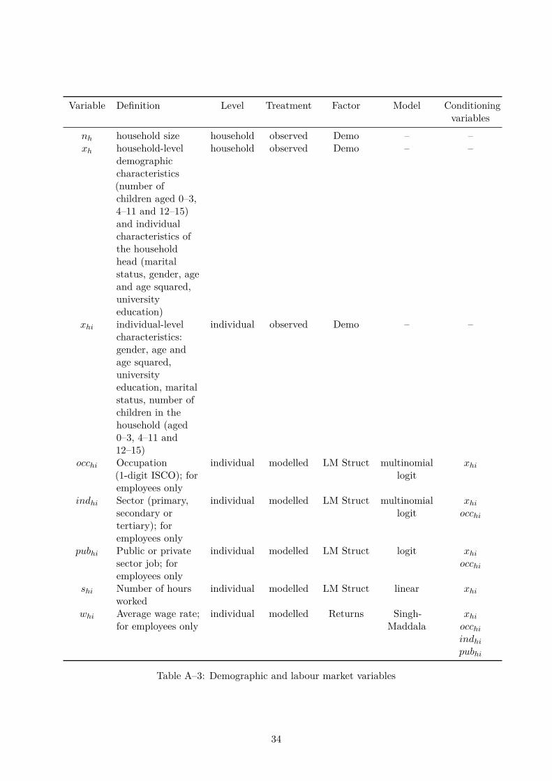
Variable Definition Level Treatment Factor Model Conditioningvariables

nh household size household observed Demo – –xh household-level

demographiccharacteristics(number ofchildren aged 0–3,4–11 and 12–15)and individualcharacteristics ofthe householdhead (maritalstatus, gender, ageand age squared,universityeducation)

household observed Demo – –

xhi individual-levelcharacteristics:gender, age andage squared,universityeducation, maritalstatus, number ofchildren in thehousehold (aged0–3, 4–11 and12–15)

individual observed Demo – –

occhi Occupation(1-digit ISCO); foremployees only

individual modelled LM Struct multinomiallogit

xhi

indhi Sector (primary,secondary ortertiary); foremployees only

individual modelled LM Struct multinomiallogit

xhiocchi

pubhi Public or privatesector job; foremployees only

individual modelled LM Struct logit xhiocchi

shi Number of hoursworked

individual modelled LM Struct linear xhi

whi Average wage rate;for employees only

individual modelled Returns Singh-Maddala

xhiocchiindhipubhi

Table A–3: Demographic and labour market variables

34

B The simulation of taxes and benefits in system swaps betweencountries using EUROMOD: detailed components and con-struction

EUROMOD calculates three main output groups of benefits (public pensions, means-tested benefitsand non means-tested benefits), taxes and social security contributions.

A challenge in swapping the tax-benefit rules between two countries is to standardize the twoinput datasets as to permit each system to be run on either input data. This implies that eachinput data needs to have the core variables required to run either system.

This process is made cumbersome by several factors. For one, not all benefits and taxes aresimulated in EUROMOD. EUROMOD simulates those instruments for which there are availabledata, whereas the rest are included from the data as input variable and are chosen as componentsof output variables. The EUROMOD country reports (Keane et al. (2012); Sutherland et al.(2012))discuss in detail which instruments are taken from the data and which are simulated orpartially simulated. Partially simulated instruments involve an eligibility condition that is basedon actual receipt plus other relevant conditions being satisfied. Our income generation modeldeals with non-simulated or partially simulated instruments as the other income componentsdiscussed above. We estimate parametric models for the presence of the income source and thelevel received. These variables serve as input variables in the tax-benefit simulator. EUROMOD“simulate” them as components of output variables.

Furthermore, each country system has specific rules. Some instruments could be (partially)simulated in one country, while used as input in the other. For example, state pension (basiccontributory) in the UK is directly included from the data because part of the eligibility informaitonis unavailable (e.g. contribution history or retirement date). In Ireland, the contributory statepension is partially simulated: the output variable depends on the value of the input variable(taken from the data) and a set of other eligibility conditions. So in both countries, the inputdata needs to indicate who gets the transfer and the level. For these two conditions, we estimateparametric models for the presence of the income source and the level. When swapping the twotax-benefit systems, the two distributions are swapped as well in the input data. In the case of thenon-contributory state pension in Ireland these steps are not required, as the transfer is simulated.

To start with, we mapped the instruments simulated in each system and their dependency onthe input data. We cross-checked the overlapping and non-overlapping input variables. (“Inputvariables” are variables present in the input data sets provided by the EUROMOD team.) Theresulting matrix can be summarized as follows:

Variables in input data needed for simulations Country tax-benefit system

W, Y, D A

Z, Y, D BD are overlapping variables that do not need parametric modelling (e.g. demographics) and Y

are overlapping variables that need modelling (e.g. employment, wage, occupation, contributoryunemployment benefit). For the overlapping variables that would be swapped parametrically (e.g.contributory unemployment benefit) we estimate parametric models for the presence of the incomesource and the level. These will allow swapping the two distributions between countries whenthe two tax-benefit systems are swapped. W and Z are non-overlapping variables that require

35

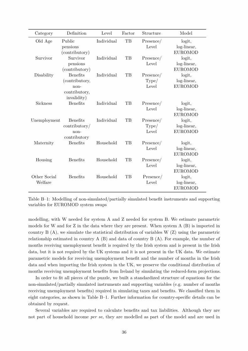
Category Definition Level Factor Structure Model

Old Age Publicpensions(contributory)

Individual TB Presence/Level

logit,log-linear,

EUROMODSurvivor Survivor

pensions(contributory)

Individual TB Presence/Level

logit,log-linear,

EUROMODDisability Benefits

(contributory,non-

contributory,invalidity)

Individual TB Presence/Type/Level

logit,log-linear,

EUROMOD

Sickness Benefits Individual TB Presence/Level

logit,log-linear,

EUROMODUnemployment Benefits

contributory/non-

contributory

Individual TB Presence/Type/Level

logit,log-linear,

EUROMOD

Maternity Benefits Household TB Presence/Level

logit,log-linear,

EUROMODHousing Benefits Household TB Presence/

Levellogit,

log-linear,EUROMOD

Other SocialWelfare

Benefits Household TB Presence/Level

logit,log-linear,

EUROMOD

Table B–1: Modelling of non-simulated/partially simulated benefit instruments and supportingvariables for EUROMOD system swaps

modelling, with W needed for system A and Z needed for system B. We estimate parametricmodels for W and for Z in the data where they are present. When system A (B) is imported incountry B (A), we simulate the statistical distribution of variables W (Z) using the parametricrelationship estimated in country A (B) and data of country B (A). For example, the number ofmonths receiving unemployment benefit is required by the Irish system and is present in the Irishdata, but it is not required by the UK systems and it is not present in the UK data. We estimateparametric models for receiving unemployment benefit and the number of months in the Irishdata and when importing the Irish system in the UK, we preserve the conditional distribution ofmonths receiving unemployment benefits from Ireland by simulating the reduced-form projections.

In order to fit all pieces of the puzzle, we built a standardized structure of equations for thenon-simulated/partially simulated instruments and supporting variables (e.g. number of monthsreceiving unemployment benefits) required in simulating taxes and benefits. We classified them ineight categories, as shown in Table B–1. Further information for country-specific details can beobtained by request.

Several variables are required to calculate benefits and tax liabilities. Although they arenot part of household income per se, they are modelled as part of the model and are used in

36

constructing counterfactual distributions by swapping their distributions depending on whichcomponent they belong to. Table B–2 describes the variables concerned.

Further information for country-specific details can be obtained upon request.

37

Variable Definition Level Factor Model Conditioningvariables

IsHomeOwnh Whetherhomeowner

household Market logit xhi, Ilabhi , I

emphi (demographics,

in work,employee)

Morth Whethermortgage

being paid andhow much

interest paid

household Market logit,log-linear

xhi, Ilabhi , I

emphi

(demographics, inwork, employee)

IsPubRenth Whetherbenefits frompublic rent


emphi


PaysRenth Whether itpays rent


emphi


Renth Value of rent household Market log-linear xhiIlabhi , I

emphi , IsPubRenth(demographics,

in work, employee,is renter)

Roomsh Number ofrooms

household Market log-linear xhi(demographics)

PPChi Voluntarycontributionsto private

pension plans

individual Market logit,log-linear

xhi(demographics)

ChChi Childcare cost household TB logit,log-linear

xh, Ilabhi , I

emphi

(demographics,employee, with

disability)Insurancehi Insurance

schemeindividual TB logit xhi, I

labhi , I

emphi

(demographics,labour marketcharacteristics)

Monthsw/em Months inwork/employed

individual TB logit/log-linear

xhi, Ilabhi , I

emphi

(demographics,labour marketcharacteristics)

Monthsub Monthsreceiving

unemploymentbenefits


xhi, Ilabhi , I

emphi

(demographics,labour marketexperience)

Monthsunem Months inunemployment


xhi, Ilabhi , I

emphi

(demographics,labour marketexperience)

Table B–2: Non-income components entering tax calculations

38

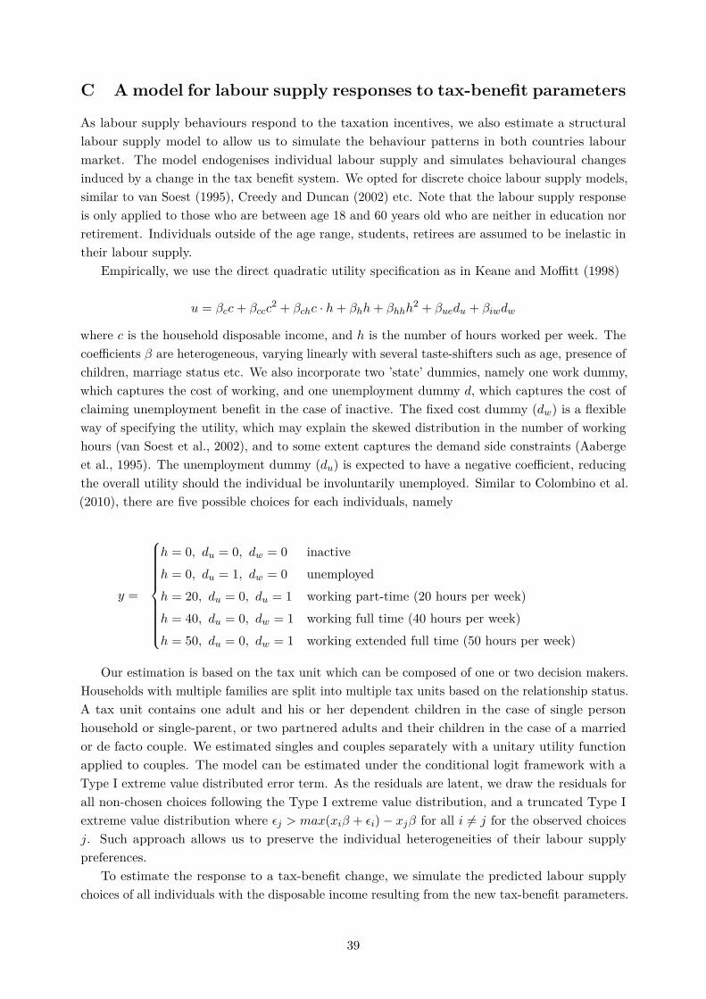
C Amodel for labour supply responses to tax-benefit parameters

As labour supply behaviours respond to the taxation incentives, we also estimate a structurallabour supply model to allow us to simulate the behaviour patterns in both countries labourmarket. The model endogenises individual labour supply and simulates behavioural changesinduced by a change in the tax benefit system. We opted for discrete choice labour supply models,similar to van Soest (1995), Creedy and Duncan (2002) etc. Note that the labour supply responseis only applied to those who are between age 18 and 60 years old who are neither in education norretirement. Individuals outside of the age range, students, retirees are assumed to be inelastic intheir labour supply.

Empirically, we use the direct quadratic utility specification as in Keane and Moffitt (1998)

u = βcc+ βccc2 + βchc · h+ βhh+ βhhh

2 + βuedu + βiwdw

where c is the household disposable income, and h is the number of hours worked per week. Thecoefficients β are heterogeneous, varying linearly with several taste-shifters such as age, presence ofchildren, marriage status etc. We also incorporate two ’state’ dummies, namely one work dummy,which captures the cost of working, and one unemployment dummy d, which captures the cost ofclaiming unemployment benefit in the case of inactive. The fixed cost dummy (dw) is a flexibleway of specifying the utility, which may explain the skewed distribution in the number of workinghours (van Soest et al., 2002), and to some extent captures the demand side constraints (Aabergeet al., 1995). The unemployment dummy (du) is expected to have a negative coefficient, reducingthe overall utility should the individual be involuntarily unemployed. Similar to Colombino et al.(2010), there are five possible choices for each individuals, namely

y =

h = 0, du = 0, dw = 0 inactiveh = 0, du = 1, dw = 0 unemployedh = 20, du = 0, du = 1 working part-time (20 hours per week)h = 40, du = 0, dw = 1 working full time (40 hours per week)h = 50, du = 0, dw = 1 working extended full time (50 hours per week)

Our estimation is based on the tax unit which can be composed of one or two decision makers.Households with multiple families are split into multiple tax units based on the relationship status.A tax unit contains one adult and his or her dependent children in the case of single personhousehold or single-parent, or two partnered adults and their children in the case of a marriedor de facto couple. We estimated singles and couples separately with a unitary utility functionapplied to couples. The model can be estimated under the conditional logit framework with aType I extreme value distributed error term. As the residuals are latent, we draw the residuals forall non-chosen choices following the Type I extreme value distribution, and a truncated Type Iextreme value distribution where εj > max(xiβ + εi)− xjβ for all i 6= j for the observed choicesj. Such approach allows us to preserve the individual heterogeneities of their labour supplypreferences.

To estimate the response to a tax-benefit change, we simulate the predicted labour supplychoices of all individuals with the disposable income resulting from the new tax-benefit parameters.

39

If the predicted outcome differs from the observed outcome under the original regime, we updatethe employment characteristics and the associated auxiliary variables, such as working hours shi,employment dummies and other characteristics in the income generation model (I labhi ), to matchthe predicted labour supply choice. The addition of the labour supply behavioural model altersthe sequence of the simulation compared with what was described in Section 2. Unemployment,non-participation, and working hours are now jointly simulated instead of sequentially determined.The logic for the rest of the simulation remains unchanged. The simulated disposable income isused for further analyses on the inequality.

40

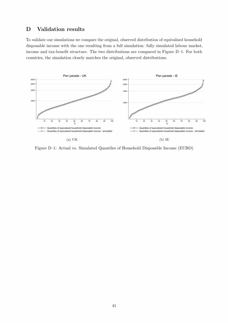
D Validation results

To validate our simulations we compare the original, observed distribution of equivalised householddisposable income with the one resulting from a full simulation: fully simulated labour market,income and tax-benefit structure. The two distributions are compared in Figure D–1. For bothcountries, the simulation closely matches the original, observed distributions.

2000

4000

6000

8000

10 20 30 40 50 60 70 80 90 100q

Quantiles of equivalized household disposable incomeQuantiles of equivalized household disposable income - simulated

Pen parade - UK

(a) UK

2000

4000

6000

8000

10 20 30 40 50 60 70 80 90 100q

Quantiles of equivalized household disposable incomeQuantiles of equivalized household disposable income - simulated

Pen parade - IE

(b) IE

Figure D–1: Actual vs. Simulated Quantiles of Household Disposable Income (EURO)

41

T +352 58 58 55-1F +352 58 58 55-700 www.liser.lu

11, Porte des SciencesCampus BelvalL-4366 Esch-sur-Alzette

Accounting for Differences in Income Inequality across Countries

Documents

Transcript of Accounting for Differences in Income Inequality across Countries