Regional Income Inequality and Economic Growth in China

JOURNAL OF COMPARATIVE ECONOMICS 22, 141–164 (1996)ARTICLE NO. 0015

Regional Income Inequality and Economic Growthin China1

JIAN CHEN

Kenyon College, Gambier, Ohio 43022

AND

BELTON M. FLEISHER

The Ohio State University, Columbus, Ohio 43210-1172

Received October 27, 1995; revised December 27, 1995

Chen, Jian, and Fleisher, Belton M.—Regional Income Inequality and EconomicGrowth in China

Using an augmented Solow growth model with cross section and panel data, wefind evidence of conditional convergence of per capita production across China’sprovinces from 1978 to 1993. Convergence is conditional on physical investmentshare, employment growth, human-capital investment, foreign direct investment, andcoastal location. We project that, in the near term, overall regional inequality asmeasured by the coefficient of variation is likely to decline modestly but that thecoast/noncoast income differential is likely to increase somewhat. We evaluate alterna-tive policies to reduce the coast–noncoast income differential and conclude focusingsolely on investment by rural collectives is insufficient. J. Comp. Econom., April1996, 22(2), pp. 141–164. Kenyon College, Gambier, Ohio 43022; The Ohio StateUniversity, Columbus, Ohio 43210-1172. q 1996 Academic Press, Inc.

Journal of Economic Literature Classification Numbers: 015, 053.

1. INTRODUCTION

Over the period from the beginning of economic reform, 1978, to 1993,average annual economic growth in China’s provinces ranged between 4.5

1 We acknowledge the valuable comments of Paul Evans, Pok-Sang Lam, Shuhe Li, WenLang Li, Yunhua Liu, Margaret Mary McConnell, John T. Sloan, Yangru Wu, and two anonymousreferees, and the assistance of Tong Lu, James McCown, and Qiang Zhang. We thank BruceReynolds for inviting us to present this paper at the April 1995 meetings of the Association ofAsian Studies in Washington, DC, from which we benefited greatly. We particularly thank onereferee whose suggestions made invaluable contributions to our revisions.

0147-5967/96 $18.00Copyright q 1996 by Academic Press, Inc.All rights of reproduction in any form reserved.

141

AID JCE 1352 / 6w06$$$$21 03-22-96 01:29:37 cea AP: Comp Econ

142 CHEN AND FLEISHER

and 11.7%. In this paper we adopt the framework of contemporary growthmodels to study the question of whether these disparate experiences representconvergence toward regional income equality. Our focus is on the dispersionand growth rates of provincial per capita production as measured by nationalincome and/or gross domestic product.2 The questions we ask are: (i) is therea tendency for relatively poor provinces to catch up to relatively rich onesover time; have the forces unleashed by the economic reforms that began inthe late 1970’s contributed to a widening or narrowing of regional incomegaps in China? (ii) What are the principal forces affecting provincial growthrates? (iii) Can we identify effects of variables favoring particular provinces,e.g., coastal location, foreign direct investment, that militate against conver-gence and in favor of persistent regional income and growth-rate gaps; isconvergence, if it can be identified, conditional or unconditional? (iv) Canwe use the estimated production-function parameters to suggest policies thatwill promote more rapid growth in China’s poorer provinces? The answersto these questions are important both because persistent or increasing incomeinequality may exacerbate feelings that economic reform in China has beenunfair, undermining social and political stability and the very foundations ofChina’s emergence as a major world economic power as well as for the lightthey may shed on the growth process itself.

Previous Research

The question of whether economic growth leads to increasing income in-equality has been discussed extensively. Simon Kuznets (1955) proposed

2 Full operational definitions of the variables used are contained in the Appendix. Where data areavailable, we have used variables that correspond to the standard national income accounting system,System of National Accounts or SNA, adopted by most market economies. However, over the entireperiod from 1952 to the present, for many important series used in this paper, data are available forall provinces only for variables corresponding to the System of Material Product Balances (MPS),the socialist national accounting system. Data are now available throughout the period through 1992for most MPS series and through 1993 from many SNA series.

We acknowledge that trends in the personal and regional disposable income distributions maybe better indexes of trends in economic well-being and may differ significantly from the regionaldistribution of production. Lyons (1991) presents data on the regional distribution of both con-sumption and production. Tsui (1991) notes that ‘‘. . . transfers [from the center] were notsignificant enough to reduce regional inequality in the long run’’ (p. 20). Moreover, the centralgovernment’s proportionate control over society’s resources has declined since the period coveredin Tsui’s 1991 paper. Between 1985 and 1993, central government revenues fell from 8.3% ofGDP to 5.3% (SSB, 1994, Tables 2 and 3. See also Kahn, 1995). An additional factor limitingthe central government’s willingness (if not its short-run ability) to maintain the traditional socialsafety net is a concern over inflation in the presence of as yet inadequate fiscal and monetarymacroeconomic controls (Chow, 1994, p. 143). See Khan et al. (1993) for a discussion of changesin the distribution of household incomes during the 1980’s. Tsui (1993) contains an analysis of thedistribution of alternative measures of economic well-being, including agricultural and industrialoutput, literacy rates, and infant-mortality rates.


143INEQUALITY AND GROWTH IN CHINA

that the relationship between income equality and the level of economicdevelopment is likely to be U-shaped, with increasing inequality during theinitial takeoff toward a modern economy giving way to more equality as acountry approaches the more advanced stages of industrialization. This hy-pothesis has been tested broadly and has been largely confirmed in studiesbased on both personal income and regional income distributions. JeffreyWilliamson’s (1965) widely cited study generally supports the Kuznets hy-pothesis for nonsocialist economies; moreover, he speculated that the leadingcommunist economies were unlikely to sacrifice much economic growth inorder to preserve or promote socialist ideals of income equality. A recentstudy by Harry T. Oshima (1992) of several Asian economies, not includingChina, reports that ‘‘. . . in most Asian countries, the peak in the trend [ofinequality] appears much earlier in the stage of development . . . than in theWest, . . . when the economy is still predominantly agricultural. The reason. . . is that Asia (with the exception of Japan) never went through the firstindustrial revolution of the 19th century.’’

We can see with data now available that in China during the Mao eravarious measures of income distribution fluctuated substantially. There is anextensive, earlier body of research on this period based on fragmentary datasources. A major theme in the earlier literature is the degree to which inter-provincial transfers tended to level the distribution of consumption relativeto production and to transfer investment funds away from coastal provincestoward the less-developed interior. In a detailed analysis of the pre-reformera, Nicholas Lardy (1978, 1980) focused on rural–urban, agricultural–indus-trial, and inter-provincial measures of production and income. On the basisof admittedly limited information, he found little or no evidence that incomeinequality had grown between the late 1940’s and mid-1970’s, despite anoverall trend of moderate economic growth. Lardy’s study was not withoutcritics, e.g., Audrey Donnithorne (1978), and a lively controversy emerged.This controversy and a number of other earlier analyses are summarized inimportant recent papers by Thomas P. Lyons (1991) and Kai Yuen Tsui(1991). The reader is referred to them for further information and citations.

In the first 7–9 years of reform in China, which are encompassed byLyons’s and Tsui’s papers, two aspects of the regional income distributionstand out: (i) a moderate decline in inequality following the inception ofreform and (ii) an increase in inequality when the early 1980’s are comparedwith the 1950’s. There is no consistent evidence of the Kuznets inverted U-shaped pattern. Lyons noted, ‘‘The notion that the post-Mao reforms arecausing increases in inequality finds little support in the data for 1978–87,insofar as relative dispersion of aggregate output is concerned’’ (1991, p. 476).The data indicate a decline in some measures of regional income inequality asreform progressed. Tsui (1991, p. 10) reports that ‘‘. . . [after the CulturalRevolution] the indices indicate that a phase of mildly declining regional



inequality has set in.’’ John Sloan (1994, p. 1) reports, ‘‘China’s rapid growthduring the 1980s was not associated with an increase in inter-provincialinequality . . . some measures indicate a statistically significant reduction of. . . inequality. . . . The most rapid growth was in what were middle incomeprovinces in 1981.’’

Jean C. Oi (1993) reports that rural–urban inequalities, one of the principalsources of regional inequality in China, have narrowed since the advent ofeconomic reform in the late 1970’s, because previously repressed agricultureand rural industry have been permitted to take advantage of benefits of freermarkets. In apparent contrast, Dali Yang and Houkai Wei (1995) have noteda widening income gap between coastal and interior provinces, particularlyin the 1990’s, despite efforts by the central government to stimulate thedevelopment of rural enterprises in the interior. These seemingly contradictoryfindings on the behavior of regional inequality since reform are due in partto different ways of dividing up the regions. The income gap between coastaland interior provinces may widen, for example, while the gap within thecoastal and noncoastal regions narrows. The impact on overall inter-provincialinequality could go in either direction. This ambiguity is implicit in Sloan’sreport, noted above, that middle-income provinces have narrowed the gapbetween themselves and high-income provinces, while widening the gap sepa-rating them from the poorest regions.

Outline of the Remainder of the Paper

We view our approach as complementary to those taken in Lyons’s andTsui’s papers. Their focus was primarily on trends and fluctuations of regionalinequality in the Mao and post-Mao eras and the central government’s rolein redistributing production, investment, and income from rich to poor prov-inces. Our interest lies mainly in the growth process during the post-Maoreform period and its impact on regional dispersion of per capita productionsince the late 1970’s. We draw on various published sources of provincialmacroeconomic data that are now available for the period from approximately1950 to 1993 (See State Statistical Bureau in the References and Hsueh etal., 1993). These data are extensions of data, first available in 1987, whichfacilitated a turning point in the study of Chinese regional inequality repre-sented by the papers of Lyons and Tsui.

In Section 2 we briefly discuss the regional (provincial) distribution of percapita production from 1952 to 1992. The remainder of the paper focuses onthe period for which GDP data are available, beginning roughly with theintroduction of economic reform, 1978–1993. In Section 3 we use an econo-metric model adapted from the Solow growth model (1956) to test for bothunconditional and conditional convergence of production per capita acrossprovinces. In testing for unconditional convergence, we attempt to answer



the question, is there a tendency for average production per capita to approachthe same level across all provinces. With conditional convergence we addressthe question, does provincial production per capita tend to converge to adifferent level in each province. That is, does each province converge to itsown unique equilibrium, and, if so, what are the variables on which theseequilibrium values of per capita production depend? By identifying variablesthat condition the convergence of provincial production we gain insight intothe forces that restrict movement toward regional income inequality. We testfor unconditional convergence using a cross section approach, and we adoptboth a cross section and panel approach to test hypotheses related to condi-tional convergence.

In the concluding section we summarize our econometric results by usingthem to suggest the future direction of regional inequality in China. We alsouse our results to simulate the impact of altering the levels of importantgrowth-determining variables, e.g., foreign-direct investment and domesticinvestment, to increase the rates of growth of laggard regions. We then suggesthow our econometric results and simulations may suggest policies to promoteregional growth where it has lagged behind the national average.

2. OVERVIEW OF THE PROVINCIAL DISTRIBUTIONOF PRODUCTION 1952–1993

In previous studies of China’s regional income distribution, researchers arenot in general agreement on two issues: (i) weighting the provincial summarystatistics by provincial population, and (ii) whether the city provinces ofBeijing and Tianjin should be combined with their adjacent province, Hebei,and Shanghai with its adjacent province, Jiangsu. Tsui based his analysis onpopulation-weighted provincial data, relying on the argument that these pro-vide a more accurate measure of income inequality among individual membersof the population. Lyons, on the other hand, shows that the use of populationweights does not provide an unambiguously clear picture of changes in thedegree of regional inequality (p. 474). Tsui also combines Beijing and Tianjinwith Hebei and Shanghai with Jiangsu. In this section, we present data forthe combined and noncombined samples, not weighted by provincial popula-tions, in Figs. 1 and 2, respectively. The population-weighted data providean almost identical picture.3

Figure 1 plots the data for the set of noncombined provinces, in whichBeijing, Tianjin, and Shanghai stand alone. It shows the coefficient of varia-

3 We have computed the coefficient of variation of provincial per capita real national incomeboth with and without provincial population weights. The results are quite similar in terms oftrend and turning points. The mean cv of the 25-province set is much lower, though, becauseper capita production in the three cities is much higher than the national average.



FIG. 1. Coefficient of variation: noncombined. Tibet and Hainan are excluded in the NI series.Jilin, Guangxi, Hainan, Qinghai, and Tibet are excluded from the GDP series. The noncombinedsample includes Beijing, Tianjin, and Shanghai as separate provinces.

tion (cv) of per capita national income, corrected for provincial price-levelchanges (RNI) over the period 1952–1992 and for per capita GDP (RGDP),also corrected for provincial price-level changes, over the period 1978–1993.4

4 Data gaps limited Tsui’s and Lyons’s research (1991) to 20–24 provinces. Fragmentary datafor provinces with gaps were used by both authors to show that their results appeared insensitiveto omissions of these provinces from their computations. We also find that our computations arenot materially affected by excluding the provinces they were forced to ignore.

NI corresponds to the measure of net material product (NMP) used by Tsui and Lyons in their1991 papers. SSB (1991), Hsueh (1993), and SSB (1995 and earlier years) contain data on annualchanges in NI at constant prices in index form. We use these indexes, as did Tsui and Lyons, toconstruct a RNI index with 1952 as the base year. As Lyons points (p. 473), this index does notsolve the problem of correcting cross section initial differences in NI for the interprovincial differencein price levels in any given year, only for their rates of growth. Consequently, the RNI series probablygives an inaccurate picture of the level of the cv of RNI. The main focus of our research, as ofprevious research, however, is on changes in relative production and economic well-being over time.Lyons uses NI instead of RNI as the basic measure of inequality because, he argues, nominal measuresare more likely to affect perceptions of inequality within China itself (p. 473). We do not find thisargument for emphasizing nominal over real measures of production and consumption persuasive.

The cv is probably the most widely used measure of interregional disparities; see Lyons, p.474 and footnote 8. It is not only a well-recognized statistic, but it is also a reasonably goodmeasure of inequality and satisfied the Pigou–Dalton Condition as defined in Sen (1973). Anadditional reason for using only the cv measure of inequality in our research is that it is directlyrelated to variance, and it is the variance of provincial growth rates that is explained by thegrowth regressions in Section 3. Tsui’s 1991 paper contains an analysis of alternative inequality



FIG. 2. Coefficient of variation: combined. In the combined sample, Beijing and Tianjin arecombined with Hebei and Shanghai with Jiangsu.

As discussed in the preceding section, the overall trend in the cv of RNI after1952 is evidently positive, despite the downward drift starting about 1980,and is similar to that reported by Tsui for 1952–1987. The negative overalltrend reported by Lyons is evidently attributable to his use of nominal nationalincome (NI) data. Our own calculations using a common, rather than province-specific, deflator also shows a very steep decline in the cv starting in the late1970’s, inducing a negative overall trend.5 See also, Sloan (1994) reportingon the cv of nominal per capita provincial GDP.

The downward trend in the cv of per capita production during the reformperiod is more pronounced in Fig. 1 than in Fig. 2. Indeed, the per capitaGDP series in Fig. 2, which plots data on the combined provinces, displaysa distinct uptick after 1990, which is visible, but less pronounced in thenoncombined series depicted in Fig. 1. The tendency for measures of regionalinequality to increase after 1990 is due to a widening of the gap betweencoastal and noncoastal provinces during this period. This can be inferred fromthe negative 1978–1993 trend of the cv of per capita GDP within the coastaland noncoastal groups, shown in both Figs. 1 and 2.

statistics, including the Gini coefficient, Theil entropy measure, and Atkinson index. (See alsoSloan, 1994.)

5 We are indebted to one of our referees for emphasizing the importance of allowing forregional differences in inflation. The cv based on a price index common to all provinces isequivalent to the cv of NI, since the common price index pt appears in both the numerator anddenominator of the expression for cv.



The Mao regime was apparently unsuccessful or unwilling, as suggestedby Williamson, in achieving a sustained reduction in regional inequality. Itappears, however, that market reforms may well have led to a modest nar-rowing of the overall variation in regional per capita income, at least through1990. In the remainder of this paper we analyze the nature of this reductionin depth and address the issue of whether the coast/noncoast gap threatensto overwhelm the tendency toward narrowing regional differentials that isobservable within the groups of coastal and noncoastal provinces.

3. FACTORS CONTRIBUTING TO REGIONAL ECONOMICGROWTH AND INEQUALITY

In this section we address the questions: (i) What are the forces influencingregional economic growth and inequality over time? (ii) Have variables lead-ing to economic progress since reform caused growth to be greater in prov-inces with highest initial income levels, leading to divergence from economicequality? For example, currently wealthy provinces, e.g., Shanghai and Guan-gdong, are also those offering better access to the transportation facilities thatfacilitate both exports and domestic sales. Being coastal provinces, they alsohave, through historical emigration patterns, the closest ties to overseas Chi-nese who have been the most important source of direct foreign investmentand business know-how. According to conventional wisdom these ties havecontributed significantly to these provinces’ recent phenomenal growth rates.

The conceptual framework we adopt to analyze the variables influencingprovincial growth rates is based on the Solow growth model (1956) augmentedto include human capital. We make use of Solow’s original assumption ofHicks-neutral technological change.6 Our maintained hypothesis is that all theprovinces experienced four major shocks that coincided with the Communistvictory in 1949, the Great Leap Forward, the Cultural Revolution, and theeconomic reforms that began around 1978.7

In our empirical work, we estimate both cross section and panel provincialgrowth equations. The cross section and panel growth equations take thegeneral forms, respectively,

gi Å g0 / g1ln(ski) / g2ln(shi) / g3ln(ni) / g4ln(yi,0) / F*Xi / 1i (1)

and

gi,t Å g0 / g1ln(ski,t01) / g2ln(shi,t0p) / g3ln(ni,t)

/ g4ln(yi,t01) / F*Xi,t / 1i,t, (2)

6 Except for the assumption of Hicks-neutral technological change, our approach is similar tothat of Mankiw et al. (1992), Barro (1992), and Barro and Sala-i-Martin (1991 and 1992).

7 Thus we assume that the objections to this approach raised by Quah (1993) do not apply.



where the variables denote

gi,t the annual growth rate of real production per capita from time t-1 to t;gi average annual growth rate of real production per capita from the begin-

ning to the end of the period;sk rate of accumulation in fixed assets as a proportion of production;sh rate of investment in human capital as a proportion of production, and

the subscript p is a time lag;n annual growth rate of employed labor force;y real production per capita;X a vector of variables hypothesized to increase per capita production, such

as technology growth and market reforms that may vary by province.

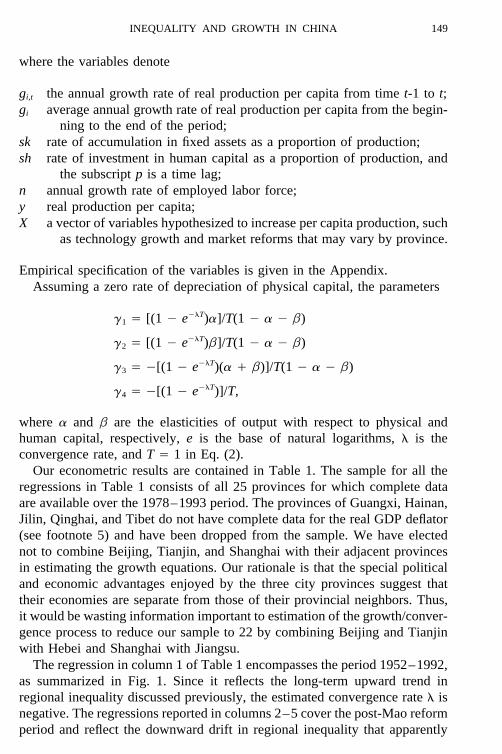
Empirical specification of the variables is given in the Appendix.Assuming a zero rate of depreciation of physical capital, the parameters

g1 Å [(1 0 e0lT)a]/T(1 0 a 0 b)

g2 Å [(1 0 e0lT)b]/T(1 0 a 0 b)

g3 Å 0[(1 0 e0lT)(a / b)]/T(1 0 a 0 b)

g4 Å 0[(1 0 e0lT)]/T,

where a and b are the elasticities of output with respect to physical andhuman capital, respectively, e is the base of natural logarithms, l is theconvergence rate, and T Å 1 in Eq. (2).

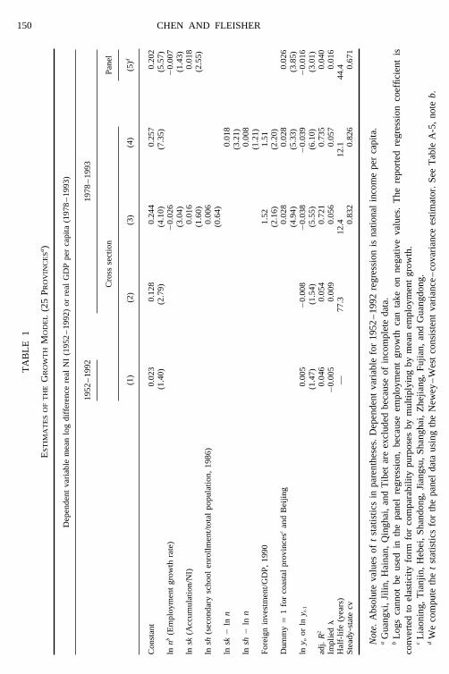
Our econometric results are contained in Table 1. The sample for all theregressions in Table 1 consists of all 25 provinces for which complete dataare available over the 1978–1993 period. The provinces of Guangxi, Hainan,Jilin, Qinghai, and Tibet do not have complete data for the real GDP deflator(see footnote 5) and have been dropped from the sample. We have electednot to combine Beijing, Tianjin, and Shanghai with their adjacent provincesin estimating the growth equations. Our rationale is that the special politicaland economic advantages enjoyed by the three city provinces suggest thattheir economies are separate from those of their provincial neighbors. Thus,it would be wasting information important to estimation of the growth/conver-gence process to reduce our sample to 22 by combining Beijing and Tianjinwith Hebei and Shanghai with Jiangsu.

The regression in column 1 of Table 1 encompasses the period 1952–1992,as summarized in Fig. 1. Since it reflects the long-term upward trend inregional inequality discussed previously, the estimated convergence rate l isnegative. The regressions reported in columns 2–5 cover the post-Mao reformperiod and reflect the downward drift in regional inequality that apparently


150 CHEN AND FLEISHERT

AB

LE

1

ES

TIM

AT

ES

OF

TH

EG

RO

WT

HM

OD

EL

(25

PR

OV

INC

ES

a )

Dep

ende

ntva

riab

lem

ean

log

diff

eren

cere

alN

I(1

952

–19

92)

orre

alG

DP

per

capi

ta(1

978

–19

93)

1952

–19

9219

78–

1993

Cro

ssse

ctio

nP

anel

(1)

(2)

(3)

(4)

(5)d

Con

stan

t0.

023

0.12

80.

244

0.25

70.

202

(1.4

0)(2

.79)

(4.1

0)(7

.35)

(5.5

7)ln

nb(E

mpl

oym

ent

grow

thra

te)

00.

026

00.

007

(3.0

4)(1

.43)

lnsk

(Acc

umul

atio

n/N

I)0.

016

0.01

8(1

.60)

(2.5

5)ln

sh(s

econ

dary

scho

olen

roll

men

t/to

tal

popu

lati

on,

1986

)0.

006

(0.6

4)ln

sk0

lnn

0.01

8(3

.21)

lnsh0

lnn

0.00

8(1

.21)

For

eign

inve

stm

ent/

GD

P,

1990

1.52

1.51

(2.1

6)(2

.20)

Dum

myÅ

1fo

rco

asta

lpr

ovin

cesc

and

Bei

jing

0.02

80.

028

0.02

6(4

.94)

(5.3

3)(3

.85)

lny o

orln

y t-1

0.00

50

0.00

80

0.03

80

0.03

90

0.01

6(1

.47)

(1.5

4)(5

.55)

(6.1

0)(3

.01)

adj.

R2

0.04

60.

054

0.72

10.

735

0.04

0Im

plie

dl

00.

005

0.00

90.

056

0.05

70.

016

Hal

f-li

fe(y

ears

)—

77.3

12.4

12.1

44.4

Ste

ady-

stat

ecv

0.83

20.

826

0.67

1

Not

e.A

bsol

ute

valu

esof

tst

atis

tics

inpa

rent

hese

s.D

epen

dent

vari

able

for

1952

–19

92re

gres

sion

isna

tion

alin

com

epe

rca

pita

.a

Gua

ngxi

,Ji

lin,

Hai

nan,

Qin

ghai

,an

dT

ibet

are

excl

uded

beca

use

ofin

com

plet

eda

ta.

bL

ogs

cann

otbe

used

inth

epa

nel

regr

essi

on,

beca

use

empl

oym

ent

grow

thca

nta

keon

nega

tive

valu

es.

The

repo

rted

regr

essi

onco

effi

cien

tis

conv

erte

dto

elas

tici

tyfo

rmfo

rco

mpa

rabi

lity

purp

oses

bym

ulti

plyi

ngby

mea

nem

ploy

men

tgr

owth

.c

Lia

onin

g,T

ianj

in,

Heb

ei,

Sha

ndon

g,Ji

angs

u,S

hang

hai,

Zhe

jian

g,F

ujia

n,an

dG

uang

dong

.d

We

com

pute

the

tst

atis

tics

for

the

pane

lda

taus

ing

the

New

ey–

Wes

tco

nsis

tent

vari

ance

–co

vari

ance

esti

mat

or.

See

Tab

leA

-5,

note

b.

AID JCE 1352 / 6w06$$1352 03-22-96 01:29:37 cea AP: Comp Econ


began with China’s transition to a market economy.8 This downward drift isreflected in the weak evidence of unconditional convergence shown in theregression of column 2. The implied unconditional convergence rate is only0.9% per year, indicating that it would take 77.3 years to eliminate half ofthe 1978 gap in provincial per capital GDP, assuming no disturbances to thegrowth process. Both casual evidence and formal research, e.g., Yang (1995),show that coastal provinces have experienced a disproportionate share ofChina’s post-reform economic growth, and the regressions reported in col-umns 3–5 clearly indicate that failure to take account of the difference be-tween coastal and noncoastal provincial growth rates leads to serious misspec-ification. They contain a dummy variable set equal to one for the coastalprovinces of Liaoning, Hebei, Tianjin, Shandong, Jiangsu, Shanghai, Zheji-ang, Fujian, and Guangdong, plus Beijing. The coefficient of the coastaldummy is highly significant and indicates that, on average, the coastal prov-inces experienced a 2.6–2.8 percentage point higher growth rate, almost halfagain as much as noncoastal provinces, over the 1978–1993 period.9

The regressions in columns 3 and 4 show the result of estimating the Solowgrowth model augmented to include investment in human capital, coastallocation, and advantages in obtaining direct foreign investment, measured bythe share of direct foreign investment realized in 1990 as a proportion ofprovincial GDP.10 It is hypothesized that foreign investment, originating infirms in major industrialized nations and often supplied by overseas Chinesein Hong Kong, Taiwan, and southeast Asia, embodies the latest in productionand management technology and is a source of technology transfer to theprovinces that receive it. The regression in column 4 reflects the restrictiong3 Å 0(g1 / g2). In column 3, the estimated coefficients all have the hypothe-sized signs, but the coefficient of the variable representing investment inhuman capital is statistically insignificant and that of investment in nonhumancapital is only marginally so.

In the regression in column 4, testing the restriction that g3 Å 0(g1 / g2),is perhaps questionable, because our human-capital investment variable isonly a proxy for the share of human-capital investment in GDP. However, ifthe variable we use is a constant multiple of the true variable, then theestimated coefficient of sh is unaffected by the measurement error. An F testindicates the null hypothesis that the restriction is valid cannot be rejected atany reasonable level of significance. The implied magnitudes of a and (a /b), the production elasticities of physical capital and physical-plus-human

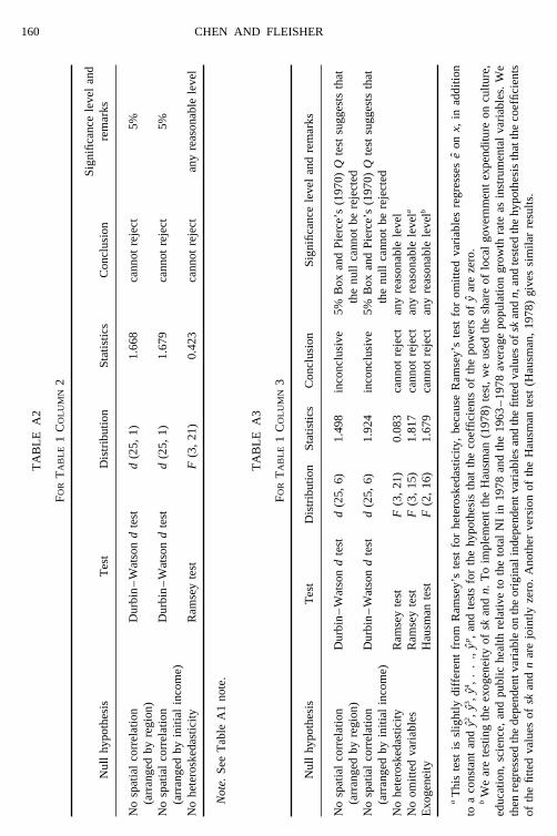
8 Standard diagnostic tests for the cross section regressions are contained in Tables A1–A4.9 The null hypothesis that the convergence rates for coastal and noncoastal provinces are equal

cannot be rejected.10 We chose 1990 because earlier years are plagued by missing data. We cannot use the log

of this variable, because it takes on a value of zero for a number of provinces.



capital, are 0.27 and 0.39, respectively. This implies that the productionelasticity of raw labor is 0.61. These estimates are consistent with thoseobtained in other research on the Chinese economy. See, for example, Chen,et al. (1988), Chow (1994), p. 204, and Fleisher et al. (1996).

The last column of Table 1 reports the results of estimating the growthregression on panel data for all 25 provinces over the period 1978–1993.11

The variables for investment in human capital and for foreign direct invest-ment could not be included in the panel regression because of missing data.12

Moreover, the existence of some negative values for the employment-growthvariable necessitates use of the arithmetic value rather than its log in theregression. The arithmetic specification of employment growth precludes im-posing the restriction that the production elasticity of labor plus that of physi-cal investment equal unity. Despite these omissions and modifications, theestimated regression coefficients of the panel regression are remarkably closeto those of the cross section regressions. For ease of comparison, the regres-sion coefficient of employment growth has been expressed as an elasticitycalculated at the mean of GDP growth and employment growth. There aretwo implied estimates for the production elasticities of both labor and capital.The coefficient of the employment-growth variable implies that the productionelasticity of labor is 0.70 and that of physical capital 0.30, maintaining thesame order of magnitude as implied in the constrained regression reported incolumn 4. However, the coefficient of sk implies that the production elasticityof physical capital is 0.53 and that of labor is 0.47. The estimated growthadvantage of the coastal provinces is almost identical in the panel regressionto that estimated with cross section data. The value of l is smaller than inthe cross section regressions, implying a half life to total convergence of 44.4years, compared to a little more than 12 years in the cross section estimates.13

11 Standard diagnostic tests for the panel regression are contained in Appendix Table A5. Wehave chosen not to assume a fixed effect represented in the regression by a dummy variable foreach province in order to focus attention on only one fixed effect, namely, the growth advantageof coastal over noncoastal provinces.

12 We experimented using a value of zero for all provinces with missing direct foreign invest-ment data. However, the estimated coefficient is ridiculously large, leading us to believe that wehad introduced a severe measurement error.

13 We have estimated the growth equations using the sample in which Beijing, Tianjin, andShanghai are combined with their adjacent provinces. In the specifications corresponding to thosein columns 4 and 5, the coefficient of lagged y in the cross section regression is somewhat largerbut in the panel regression about half as large as reported in 1, 00.0046 and 00.0081, withabsolute t statistics of 5.5 and 1.2, respectively. In the cross section regression, correspondingto column 4, the estimated coefficients of (ln sk 0ln n) and (ln sh 0ln n) are 0.021 and 0.017,respectively, and the coefficient of foreign direct investment is 0.92. The t statistics are 3.0, 1.8,and 1.3, respectively. The coefficient of the coastal dummy variable is 0.030 and highly signifi-cant. In the panel regression corresponding to column 5, the estimated coefficients of physicalinvestment, employment growth, and the coastal dummy are 0.022, 00.004 (at the sample mean



4. IMPLICATIONS AND CONCLUSIONS

The estimates reported in Table 1 provide evidence that China’s movementtoward a market economy has unleashed forces working toward convergence ofboth rates of growth and levels of provincial GDP per capita. However, there isstrong evidence that convergence is conditional on the variables included in theaugmented Solow growth model, particularly coastal location. In order to gain abetter understanding of the forces working against total unconditional convergenceto equal per capita GDP, we use the solution for the steady-state per capita GDPimplicit in Eq. (1) to derive implications for the course of provincial inequalityas economic development in China continues.14 We also derive implications forthe impact of hypothetical policies that would alter the magnitudes of the growth-determining variables specified in the equation.

The last row of Table 1 shows the coefficient of variation of provincialper capita GDP in the steady state. We compare these simulated steady-statecv’s with the actual cv of provincial per capita GDP in 1993, which was0.874. The steady-state cv based on the constrained cross section regressionreported in column 4 is 0.826, amounting to little more than 5% decline inthis measure of inequality. The cv’s of the coastal and noncoastal provinceswould, under this simulation, decline by 17 and 12%, respectively.15 Thismay be compared with an overall drop between 1978 and 1993 from 1.015to 0.874, or 14%. The steady-state cv forecast by the panel regression ofcolumn 5 is much lower, only 0.67, which is a 23% drop compared to 1993.Our inability to include the human-capital and direct foreign investment vari-ables and to use the log of employment growth in the panel regression leadsus to believe more in the implications of the constrained cross section esti-mates of column 4 than the panel estimates of column 5.

The relatively small remaining gap to total conditional convergence impliedby the cross section regression suggests that any additional movement toward

labor-force growth), and 0.029, respectively, with absolute t statistics of 2.8, 0.9, and 4.2,respectively. Despite these similarities, we choose to maintain the hypothesis that the correctsample to use includes Beijing, Tianjin, and Shanghai as separate provinces, because politicaland economic restrictions impose a special economic status on these regions. Because of theirunique circumstances, aggregation with their surrounding regions would be inappropriate.

14 To solve for the steady state, we assume that yt Å yt01 and that the current, or average,magnitudes of the right-hand variables will not change in the steady state. We consider the useof the steady state to be a heuristic device that enables us to simulate the effects of alternativepolicies that would modify rates of investment in physical and human capital, employmentgrowth, and foreign direct investment. Our assumption of the steady state amounts to using theproduction elasticities implied by the estimated parameters of the growth equations to measurethe impact of policies that would alter the variables mentioned in the preceding sentence.

15 Using the combined-province data set, the simulated steady-state cv for all provinces takentogether rises by 5%, while that of the coastal and noncoastal provinces would be 50% lowerand 5% higher, respectively.



TABLE 2

VARIABLE MEANS FOR COASTAL AND NONCOASTAL PROVINCES 1978–1993

Variable Coastal Noncoastal Ratio

y1978 763 yuan 301 yuan 2.53Employment growth 0.0243 0.0285 0.86sk 0.215 0.238 0.90sh 0.0159 0.0156 1.02Foreign investment/GDP 0.0052 0.0007 7.28

regional inequality will occur only when there is a change in the regionaldistribution of variables important in determining provincial growth rates.

The Coast–Noncoast Differential

One of the main sources of steady-state variation in provincial per capita GDPis the coast–noncoast differential. Between 1978 and 1993, the coast/noncoastratio of mean GDP per capita grew from 2.53, see Table 2, to 2.82, or 11%.Our steady-state simulated ratio is 2.87, implying a further widening coast–noncoast gap, albeit a small one, only 2% rather than a convergence towardequality.16 This implies that convergence is occurring within the coastal andnoncoastal groups, but not between them. As mentioned above, this is consistentwith the observations of Sloan (1994) and Yang and Wei (1996).

Aware of the political danger and perhaps also sensitive to the inequity offavoring coastal development over that of the interior, the central governmenthas in the past several years taken steps to promote the growth of enterprisesin the interior, focusing particular attention on steps to encourage investmentin rural enterprises.17 Presumably the focus on rural collectives is motivatedby two assumptions: (i) the payoff to investment in collectives and the con-comitant economic growth induced is greater than to investment in otherenterprise forms; (ii) rural unemployment, now approaching perhaps 150million (Yang and Wei, 1996), is a growing threat to social stability.

While a cursory evaluation of the data lends superficial support to thenotion that promoting investment in rural enterprises may well be the key toexpanding the interior relative to the coast, critical analysis suggests a less

16 Using the combined-province data, the steady-state coast/noncoast ratio would rise by 13%in equilibrium.

17 See Yang and Wei (1995) for references documenting the central government’s concernover the widening coast/interior gap and the measures taken to alleviate it through promotinginvestment in rural enterprise.



promising outcome. The appeal of investment in rural enterprise may arisefrom noticing that in 1993 the share of investment in fixed capital of ruralcollectives was over 17% of total fixed investment in the coastal provinces,but only 7% in the interior (SSB, 1995, p. 142). Indeed, in Jiangsu andZhejiang, rural collectives absorbed over 30% of total fixed investment (SSB,1995). Our empirical results provide a means of forecasting how effectivegovernment policies to accelerate rural collective investments are likely tobe in achieving the goal of coast–noncoast equality.

Table 2 reveals the perhaps surprising fact that over the period 1978–1993 the noncoastal provinces had a total investment/GDP ratio 10%higher than the coastal provinces.18 Thus it has not been lack of investmentper se that has caused the interior to experience lagging economic growth.It may well be that if only investment had been directed more toward ruralcollectives there would have been a greater payoff and more rapid eco-nomic expansion. Perhaps with this in mind, in 1992 and 1993 the People’sBank of China and the State Council took steps to authorize additionalcredit of up to 15 billion yuan per year continuing to the end of the decade(Brauchli, 1995). If this authorized credit was in fact translated into newcapital formation, there would be nearly a 50% increase in rural-coopera-tive fixed capital formation, compared to the 1993 level. Assuming suchan increase in investment, what would be the payoff in terms of economicgrowth? The econometric results reported in Table 1 suggest that a dou-bling of the share of fixed investment in GDP would lead to an approxi-mately 1 percentage point increase in economic growth. So, even if theproductivity of investing in rural collectives were twice as high as that forthe average investment project in China, it seems unlikely that the policiesdescribed above would be sufficient to eliminate the coast–noncoast gapof over 2 percentage points in the growth rate indicated by the coefficientof the coastal dummy in Table 1 (SSB, 1995).

Moreover, as Yang and Wei (1996) point out, China’s ongoing financialreforms have sharply restricted the ability and willingness of banks tocreate new loans in regions where default rates on old loans are unaccept-ably high, and that is the case in much of central and western China. Asa consequence, the announced policies have not been fully executed. Evenif they were, the frequency of nonperforming loans raises the questionwhether additional investment in noncoastal rural collectives in the pastwere likely to have been or in the near future are likely to be as productiveas on the coast. We conclude that a strategy focusing on fixed investment

18 Of course, this is not to say that the magnitude of investment is greater, given the muchlower GDP of the noncoastal provinces. However it is the relative ratio of investment to GDPthat determines relative growth rates.



TABLE 3

IMPACT ON STEADY-STATE COAST/NONCOAST GDP RATIO OF ASSIGNING

COASTAL MEAN VALUES TO NONCOASTAL PROVINCES

Steady-state gap with own means 2.87Effect on gap of changing

Employment growth 00.45sk 0.11sh 00.03Foreign investment/GDP 00.46

Summation of all effects 00.83

alone is unlikely to be a cost-effective means of narrowing the coast–noncoast income gap. A solution to this problem must lie in policiesaffecting other variables in the growth equation as well. We now proceedto examine them one at a time.

What, apart from assigning each noncoastal province a place by the sea,would contribute to narrowing the coast–noncoast gap? Table 2 reveals thatin addition to their inland disadvantage and modest physical-investment ratioadvantage, the noncoastal provinces are currently burdened with a laborgrowth rate that is nearly 20% greater than that of the coastal provinces, andthey have a only one-seventh the coast’s rate of foreign direct investment.There is only a minor gap in the school enrollment/population ratios of thetwo regions. One may conclude that central-government redistribution policieshave contributed not only to increasing the investment/GDP ratio, but alsoto equality of schooling/population ratio, thus contributing modestly to nar-rowing the coastal–noncoastal income gap. On the other hand, central andlocal government restrictions have surely severely restricted labor-force andgeneral population movements toward the high-income coast.

As Table 3 shows, the net outcome of assigning the noncoastal provincesthe employment-growth, investment/GDP ratio, and school enrollment/popu-lation ratio of the coastal provinces would be to lower the coast–noncoaststeady-state gap ratio from 2.87 to 2.50, about 15%. If the noncoastal prov-inces could obtain the same level of foreign direct investment as the coast,the gap ratio would fall another 0.46, over 15% farther, to 2.04, 20% lowerthan the ratio 2.53 that was obtained in 1978.19

What actual policies could the central government adopt to promote a more

19 Using the combined-province data, the result of assigning the noncoastal provinces thecoastal-province values of all these variables would reduce the coastal/noncoastal steady-stateper capita GDP ratio from 2.37 to 2.10, an 11% reduction, but leaving the ratio 35% higher thanthe 1973 ratio of 1.55.



substantial movement toward regional income equality? Is investment in ruralenterprises indeed the most productive use of additional capital formation inthe interior? What underlies the residual impact of coastal location on eco-nomic growth that is implicit in the rather large and highly significant coeffi-cient of the coastal dummy variables in the augmented growth equationsreported in columns 4 and 5 of Table 1? A careful answer to these questionsgoes far beyond the scope of this paper, but perhaps some speculation willsuggest fruitful avenues of future research.

Altering the future distribution of labor-force growth across regions isperhaps the most difficult economic and social problem facing China today.The likely hundreds of millions who would migrate to the coastal provinces,particularly to urban locations, if there were no legal restrictions would nodoubt raise per capita income in the interior as that in coastal locations woulddecline. However, such migration would, in the foreseeable future, overwhelmthe capacity of all types of infrastructure, particularly sanitation and transpor-tation facilities.

If we accept as given that allowing free migration of labor from the interiorto the coast is currently not a viable policy alternative, then a direct attackon the productivity of investment in the interior is the only remaining policyalternative. One useful step may be to further reduce centralized economiccontrol over existing enterprises, which some Chinese observers feel hasalready given local government incentives to create a better social and eco-nomic environment for local economies, led to better resource allocation, andthus contributed to regional equality (Institute of Economics, 1994). It seemsto us that much of the residual advantage of coastal location resides in itscurrent advantage in internal transportation and access to overseas transportand in the acquired business acumen embodied in its management personnel.For example, anecdotal evidence as well as some research supports the advan-tages of enterprise managers in Shanghai over the remainder of China.20

Migration of capital to the interior is already occurring along routes wheretransportation bottlenecks are least obstructive, such as the Yangtze valley.21

Thus emphasizing development of the interior infrastructure would not onlyraise the incentive for coastal businesses, including those funded by foreigninvestors, to expand to the interior but also would facilitate the transfer ofthe know-how that already exists on the coast to the interior and further helpto enhance noncoastal economic growth. In such an environment, we projectthat government encouragement and private investment incentives togethermay well achieve a significant movement toward regional income equalityin China.

20 See, for example, Fleisher et al. (1996).21 See, for example, Brauchli (1995).



AP

PE

ND

IX:

DA

TA

SO

UR

CE

SA

ND

VA

RIA

BL

ED

EF

INIT

ION

S

All

data

for

1952

–19

89ar

efr

omth

eS

SB

sour

ces

list

edin

the

refe

renc

esan

dfr

omH

sueh

etal

.(1

993)

,ex

cept

whe

reot

herw

ise

note

d.A

llth

ese

ries

are

upda

ted

afte

r19

89us

ing

data

cont

aine

din

vari

ous

issu

esof

SS

B,

Chi

naSt

atis

tica

lY

earb

ook.

Dat

aso

urce

sfo

rva

riab

les:

Var

iabl

eS

erie

sus

ed

Rea

lna

tion

alin

com

epe

rca

pita

Nat

iona

lIn

com

e,G

uom

insh

ouru

(Sys

tem

ofM

ater

ial

Bal

ance

s[M

PS

]);

Rea

lN

IIn

dice

sat

Com

para

ble

Pri

ces,

Shij

igu

omin

shou

ru;

Tot

alP

opul

atio

n,R

enko

ushu

y t(r

eal

GD

Ppe

rca

pita

).R

eal

Gro

ssD

omes

tic

Pro

duct

,G

uone

ish

engc

han

zong

zhi

(Sys

tem

ofN

atio

nal

Acc

ount

s[S

NA

]);

Rea

lG

DP

GD

Pis

cons

truc

ted

usin

gth

eIn

dice

sat

Com

para

ble

Pri

ces,

Shij

igu

onei

shen

chan

zong

zhi;

Tot

alP

opul

atio

n,R

enko

ushu

.sa

me

proc

edur

eas

for

real

nati

onal

inco

me.

n(e

mpl

oym

ent

grow

thra

te)*

Tot

alE

mpl

oyed

Lab

orF

orce

,Sh

ehui

laod

ongz

hezo

ngsh

u

sk(i

nves

tmen

t/na

tion

alin

com

e)T

otal

Acc

umul

atio

nof

Fix

edA

sset

s,G

udi

ngzi

chan

jile

izo

ng’e

;N

atio

nal

Inco

me,

Guo

min

shou

ru(M

PS

);In

vest

men

tba

sed

onS

NA

mea

sure

sis

unav

aila

ble

over

the

tim

epe

riod

cove

red.

sh(s

econ

dary

scho

olen

roll

men

t)S

choo

len

roll

men

t,R

uxue

rens

hu(C

hina

Stat

isti

cal

Yea

rboo

k,19

87,

pp.

692,

693)

;T

otal

Pop

ulat

ion,

Ren

kous

hu

For

eign

inve

stm

ent/

GD

PT

otal

Val

ueof

For

eign

Cap

ital

Uti

lize

d,Sh

iji

liyo

ngw

aizi

’e;

GD

P,

Guo

nei

shen

gcha

nzo

ngzh

i

Not

e.*I

nth

ecr

oss

sect

ion

regr

essi

ons,

empl

oym

ent

grow

this

the

aver

age

grow

thra

tefr

om19

78to

1993

;sk

ism

easu

red

asth

em

ean

inve

stm

ent

shar

e19

77–

1992

;sh

issc

hool

enro

llm

ent/

tota

lpo

pula

tion

in19

86.



TA

BL

EA

1

FO

RT

AB

LE

1C

OL

UM

N1

Sig

nifi

canc

ele

vel

and

Nul

lhy

poth

esis

Tes

tD

istr

ibut

ion

Sta

tist

ics

Con

clus

ion

rem

arks

No

spat

ial

corr

elat

ion

Dur

bin

–W

atso

nd

test

d(2

5,1)

1.93

2ca

nnot

reje

ct5%

(arr

ange

dby

regi

on)

No

spat

ial

corr

elat

ion

Dur

bin

–W

atso

nd

test

d(2

5,1)

2.09

8ca

nnot

reje

ct5%

(arr

ange

dby

init

ial

inco

me)

No

hete

rosk

edas

tici

tyR

amse

yte

sta

F(3

,21

)0.

246

cann

otre

ject

any

reas

onab

lele

vel

Not

e.W

edi

dno

tte

stfo

rom

itte

dva

riab

les

beca

use

we

only

wan

tto

obta

ina

roug

hid

eaof

unco

ndit

iona

lco

nver

genc

ehe

re(F

ora

sim

ilar

appr

oach

,se

e,am

ong

othe

rs,

Bar

roan

dS

ala-

i-M

arti

n,19

92).

aT

oim

plem

ent

Ram

sey’

s(1

969)

test

for

hete

rosk

edas

tici

ty,

cons

ider

the

foll

owin

gsi

mpl

ere

gres

sion

:yÅ

xb/

e,R

amse

ysu

gges

tsth

efo

llow

ing

test

proc

edur

e:1.

Reg

ress

yon

xan

dob

tain

yan

de,

whe

rey

and

ear

eth

efi

tted

valu

esof

yan

de,

resp

ecti

vely

.2.

Reg

ress

eon

aco

nsta

ntan

dy2 ,

y3 ,y4 ,

..

.,yp ,

and

test

for

the

hypo

thes

isth

atth

eco

effi

cien

tsof

the

pow

ers

ofy

are

zero

.R

amse

ypo

ints

out

that

pÅ

4ha

sbe

ensu

ffici

ent.

03-22-96 01:29:37 cea AP: Comp Econ

160 CHEN AND FLEISHERT

AB

LE

A2

FO

RT

AB

LE

1C

OL

UM

N2

Sig

nifi

canc

ele

vel

and

Nul

lhy

poth

esis

Tes

tD

istr

ibut

ion

Sta

tist

ics

Con

clus

ion

rem

arks

No

spat

ial

corr

elat

ion

Dur

bin

–W

atso

nd

test

d(2

5,1)

1.66

8ca

nnot

reje

ct5%

(arr

ange

dby

regi

on)

No

spat

ial

corr

elat

ion

Dur

bin

–W

atso

nd

test

d(2

5,1)

1.67

9ca

nnot

reje

ct5%

(arr

ange

dby

init

ial

inco

me)

No

hete

rosk

edas

tici

tyR

amse

yte

stF

(3,

21)

0.42

3ca

nnot

reje

ctan

yre

ason

able

leve

l

Not

e.S

eeT

able

A1

note

.

TA

BL

EA

3

FO

RT

AB

LE

1C

OL

UM

N3

Nul

lhy

poth

esis

Tes

tD

istr

ibut

ion

Sta

tist

ics

Con

clus

ion

Sig

nifi

canc

ele

vel

and

rem

arks

No

spat

ial

corr

elat

ion

Dur

bin

–W

atso

nd

test

d(2

5,6)

1.49

8in

conc

lusi

ve5%

Box

and

Pie

rce’

s(1

970)

Qte

stsu

gges

tsth

at(a

rran

ged

byre

gion

)th

enu

llca

nnot

bere

ject

edN

osp

atia

lco

rrel

atio

nD

urbi

n–

Wat

son

dte

std

(25,

6)1.

924

inco

nclu

sive

5%B

oxan

dP

ierc

e’s

(197

0)Q

test

sugg

ests

that

(arr

ange

dby

init

ial

inco

me)

the

null

cann

otbe

reje

cted

No

hete

rosk

edas

tici

tyR

amse

yte

stF

(3,

21)

0.08

3ca

nnot

reje

ctan

yre

ason

able

leve

lN

oom

itte

dva

riab

les

Ram

sey

test

F(3

,15

)1.

817

cann

otre

ject

any

reas

onab

lele

vela

Exo

gene

ity

Hau

sman

test

F(2

,16

)1.

679

cann

otre

ject

any

reas

onab

lele

velb

aT

his

test

issl

ight

lydi

ffer

ent

from

Ram

sey’

ste

stfo

rhe

tero

sked

asti

city

,be

caus

eR

amse

y’s

test

for

omit

ted

vari

able

sre

gres

ses

eon

x,in

addi

tion

toa

cons

tant

and

y2 ,y3 ,

y4 ,.

..,

yp ,an

dte

sts

for

the

hypo

thes

isth

atth

eco

effi

cien

tsof

the

pow

ers

ofy

are

zero

.b

We

are

test

ing

the

exog

enei

tyof

skan

dn.

To

impl

emen

tth

eH

ausm

an(1

978)

test

,w

eus

edth

esh

are

oflo

cal

gove

rnm

ent

expe

ndit

ure

oncu

ltur

e,ed

ucat

ion,

scie

nce,

and

publ

iche

alth

rela

tive

toth

eto

tal

NI

in19

78an

dth

e19

63–

1978

aver

age

popu

lati

ongr

owth

rate

asin

stru

men

tal

vari

able

s.W

eth

enre

gres

sed

the

depe

nden

tvar

iabl

eon

the

orig

inal

inde

pend

entv

aria

bles

and

the

fitt

edva

lues

ofsk

and

n,an

dte

sted

the

hypo

thes

isth

atth

eco

effi

cien

tsof

the

fitt

edva

lues

ofsk

and

nar

ejo

intl

yze

ro.

Ano

ther

vers

ion

ofth

eH

ausm

ante

st(H

ausm

an,

1978

)gi

ves

sim

ilar

resu

lts.

03-22-96 01:29:37 cea AP: Comp Econ


TA

BL

EA

4

FO

RT

AB

LE

1C

OL

UM

N4

Nul

lhy

poth

esis

Tes

tD

istr

ibut

ion

Sta

tist

ics

Con

clus

ion

Sig

nifi

canc

ele

vel

and

rem

arks

No

spat

ial

corr

elat

ion

Dur

bin

–W

atso

nd

test

d(2

5,5)

1.48

2in

conc

lusi

ve5%

Box

and

Pie

rce’

s(1

970)

Qte

stsu

gges

tsth

at(a

rran

ged

byre

gion

)th

enu

llca

nnot

bere

ject

ed.

No

spat

ial

corr

elat

ion

Dur

bin

–W

atso

nd

test

d(2

5,5)

1.88

6in

conc

lusi

ve5%

Box

and

Pie

rce’

s(1

970)

Qte

stsu

gges

tsth

at(a

rran

ged

byin

itia

lin

com

e)th

enu

llca

nnot

bere

ject

ed.

No

hete

rosk

edas

tici

tyR

amse

yte

stF

(3,

21)

0.08

4ca

nnot

reje

ctan

yre

ason

able

leve

l

No

omit

ted

vari

able

sR

amse

yte

stF

(3,

16)

1.59

2ca

nnot

reje

ctan

yre

ason

able

leve

l

Res

tric

tion

ofco

effi

cien

tsF

test

F(1

,18

)0.

068

cann

otre

ject

a

aT

his

test

sugg

ests

that

the

unre

stri

cted

regr

essi

onis

impr

oper

lysp

ecifi

ed.

Nev

erth

eles

s,w

ere

port

the

unre

stri

cted

resu

lts,

beca

use

the

empi

rica

lsp

ecifi

cati

onof

shdo

esno

tm

atch

the

theo

reti

cal

spec

ifica

tion

.



TA

BL

EA

5

FO

RT

AB

LE

1C

OL

UM

N5

Sig

nifi

canc

ele

vel

Nul

lhy

poth

esis

Tes

tD

istr

ibut

ion

Sta

tist

ics

Con

clus

ion

and

rem

arks

Uni

tro

otA

ugm

ente

dt

and

Fas

intÅ0

5.22

,0

4.10

,0

3.65

2,re

ject

a

Dic

key

–F

ulle

r(1

976)

and0

6.62

7fo

rg,

y 0,

sk,

Ful

ler

test

and

Dic

key

–an

dn,

resp

ecti

vely

,in

(AD

F)

Ful

ler

(198

1)A

DF

test

wit

hout

tim

etr

end;

FÅ

13.8

63,

10.6

17,

8.02

2,an

d22

.998

for

g,y 0

,sk

,an

dn,

resp

ecti

vely

,in

the

AD

Fte

stw

ith

tim

etr

end.

No

seri

alco

rrel

atio

nD

urbi

n–

Wat

son

d(3

75,

4)1.

631

reje

ct5%

dte

stN

oau

tore

gres

sive

Eng

le’s

(198

2)x

2(1

)9.

370

reje

ct1%

b

cond

itio

nal

LM

test

hete

rosk

edas

tici

ty(A

RC

H)

No

omit

ted

vari

able

sR

amse

yte

stF

(3,

367)

2.97

reje

ct5%

Exo

gene

ity

Hau

sman

test

F(2

,36

8)0.

272

cann

otre

ject

any

reas

onab

lele

velc

aT

hela

gus

edin

the

AD

Fte

stis

7,w

hich

isap

prox

imat

ely

equa

lto

the

num

ber

ofob

serv

atio

nsto

the

pow

erof

one-

thir

d,as

sugg

este

din

Sai

dan

dD

icke

y(1

980)

.b

Inth

epr

esen

ceof

AR

CH

,th

eO

LS

esti

mat

esar

est

ill

unbi

ased

and

cons

iste

nt,

but

the

esti

mat

esof

the

vari

ance

sar

ebi

ased

and

inco

nsis

tent

.T

oob

tain

aco

nsis

tent

esti

mat

orof

the

vari

ance

s,w

eus

eth

eN

ewey

–W

est

(198

7)co

nsis

tent

cova

rian

cees

tim

ator

wit

hla

gse

tat

the

valu

esu

gges

ted

byA

ndre

ws

(199

1).

cW

eus

edth

esh

are

oflo

cal

gove

rnm

ent

expe

ndit

ure

oncu

ltur

e,ed

ucat

ion,

scie

nce,

and

publ

iche

alth

rela

tive

toto

tal

NI

from

1974

to19

89an

dth

ean

nual

popu

lati

ongr

owth

rate

from

1963

to19

78as

inst

rum

enta

lva

riab

les

inth

eH

ausm

ante

st.

03-22-96 01:29:37 cea AP: Comp Econ


REFERENCESAndrews, D. W. K., ‘‘Heteroskedasticity and Autocorrelation Consistent Covariance Matrix

Estimation.’’ Econometrica 59, 3:817–858, May 1991.Barro, Robert J., ‘‘Economic Growth in a Cross Section of Countries.’’ Quart. J. Econom. 106,

2:407–443, May 1992.Barro, Robert J., and Sala-i-Martin, X., ‘‘Convergence across States and Regions.’’ Brookings

Papers Econ. Activity no. 1, 107–182, 1991.Barro, Robert J., and Sala-i-Martin, X., ‘‘Convergence.’’ J. Polit. Econom. 100, 2:223–251,

April 1992.Box, G., and Pierce, D., ‘‘Distribution of Residual Autocorrelation in Autoregressive moving

average time series models.’’ J. Amer. Statist. Assoc. 65, 332:1509–1526, 1970.Brauchli, Marcus W., ‘‘River of Dreams.’’ Wall Street J. Midwest Edition, LXXII, 42:1, Decem-

ber 13, 1995.Chen, Kuan, Wang, Hongchang, Zhen, Yuxin, Jefferson, Gary, and Rawski, Thomas, ‘‘Productiv-

ity Change in Chinese Industry.’’ J. Comp. Econom. 12, 4:570–91, 1988.Chow, Gregory C., Understanding the Chinese Economy. Singapore: World Scientific, 1994.Dickey, D. A., and Fuller, W. A., ‘‘Likelihood Ratio Statistics for Autoregressive Time Series

With a Unit Root.’’ Econometrica. 49, 4:1057–1072, June 1981.Donnithorne, Audrey, ‘‘China’s Cellular Economy: Some Economic Trends since the Cultural

Revolution.’’ China Quart. 52:605–619, 1972.Engle, Robert F., ‘‘Autoregressive Conditional Heteroskedasticity with Estimates of the Variance

of United Kingdom Inflation.’’ Econometrica 50:987–1007, 1982.Fleisher, Belton M., Dong, Keyong, and Liu, Yunhua, ‘‘Education, Enterprise Organization, and

Productivity in the Chinese Paper Industry.’’ Econom. Dev. Cult. Change 44, 3, April1996. (in press)

Fuller, W. A., Introduction to Statistical Time Series. New York: Wiley, 1976.Hausman, Jerry A., ‘‘Specification Tests for Econometrics.’’ Econometrica 46, 6:1251–1271,

November 1978.Hsueh, T., et al., China’s Provincial Statistics 1949–1989. Boulder, CO: Westview Press, 1993.Institute of Economics Nankai University and China and Regional Science Department, Univer-

sity of Pennsylvania, ‘‘Kong Jian Ping Deng Yu Zong Ti Jing Ji Xiao Lu (RegionalEquality and Total Economic Efficiency in China).’’ Jing Ji Yan Jiu (J. Econom. Res.)316:63–69, August 1994.

Kahn, Joseph, ‘‘As China Prospers, Its Tax Man Fumbles.’’ Wall Street J. Midwest Edition: A8,July 26, 1995.

Khan, Azizur Rahman, Griffin, Keith, Riskin, Carl, and Renwei, Zhao, ‘‘Sources of IncomeInequality in Post-Reform China.’’ China Econ. Rev. 4, 1:19–25, 1993.

Kuznets, Simon, ‘‘Economic Growth and Income Inequality.’’ Amer. Econom. Rev. 45:1–28,1955.

Lardy, Nicholas R., ‘‘Regional Growth and Income Distribution in China.’’ In Robert F. Dernb-erger, Ed., China’s Development Experience in Comparative Perspective. pp. 153–190.Cambridge, MA: Cambridge Univ. Press, 1980.

Lardy, Nicholas R., Economic Growth and Distribution in China. New York: Cambridge Univ.Press, 1978.

Lyons, Thomas P., ‘‘Interprovincial Disparities in China: Output and Consumption, 1952–1987.’’Econom. Dev. Cult. Change 39, 3:471–506, 1991.

Maddala, George S., Introduction to Econometrics. New York: Macmillan, 1992.Mankiw, N. Gregory, Romer, David, and Weil, David N., ‘‘A Contribution to the Empirics of

Economic Growth.’’ Quart. J. Econom. 107, 2:407–457, 1992.Newey, W., and West, K., ‘‘A Simple Positive Semi-Definite, Heteroskedasticity and Autocorre-

lation Consistent Covariance Matrix.’’ Econometrica 55, 3:703–708, May 1987.



Oi, Jean C., ‘‘Reform and Urban Bias in China.’’ J. Dev. Stud. 29, 4:129–148, July 1993.Oshima, Harry T., ‘‘Kuznets’ Curve and Asian Distribution Trends.’’ Hitotsubashi J. Econom.

33, 1:95–111, June 1992.Ramsey, J. B., ‘‘Test for specification errors in classical linear squares regression analysis.’’ J.

Royal Statist. Soc. Series B 31:350–371, 1969.Said, S. E., and Dickey, D. A., ‘‘Testing for Unit Root in ARMA Models of Unknown Order.’’

Biometrica 71:599–607, 1980.Sen, Amartya, On Economic Inequality. Oxford: Clarendon Press, 1973.Sloan, John, ‘‘Measures of Inter-Provincial Inequality in China During the Reform Period, 1981–

1990.’’ Paper presented to the Midwest Conference on Asian Affairs, September 1994.Department of Economics, University of Illinois, 1994.

Solow, Robert M., ‘‘A Contribution to the Theory of Economic Growth.’’ Quart. J. Econom.70, 3:65–94, Feb. 1956.

State Statistical Bureau (SSB), Quanguo gesheng zishiqu zhixiashi lishi tongji ziliao huibian1949–1989 (Compilation of provincial economic statistics). Beijing: Chinese StatisticsPress, 1991.

State Statistical Bureau (SSB), China Statistical Yearbook 1994 (and previous years). Beijing:Chinese Statistics Press, 1995 (and earlier).

Tsui, Kai Yuen, ‘‘China’s Regional Inequality, 1952–1985.’’ J. Comp. Econom. 15, 1:1–21,March 1991.

Tsui, Kai Yuen, ‘‘Decomposition of China’s Regional Inequalities.’’ J. Comp. Econom. 17,3:600–627, September 1993.

Williamson, Jeffrey G., ‘‘Regional Inequality in the Process of National Development.’’ Econom.Dev. Cult. Change 17, 4 pt. 2:3–84, July 1965.

Yang, Dali L., and Wei, Houkai, ‘‘Rural Enterprise Development and Regional Policy in China.’’Asian Perspective 35, 1, Spring 1996. (in press)


Regional Income Inequality and Economic Growth in China

Documents

Transcript of Regional Income Inequality and Economic Growth in China