Rising Inequality? Changes in the Distribution of Income and Consumption in the 1980s
Upload
khangminh22Category
view
0download
0
Illinois Wesleyan University
Digital Commons IWU Digital Commons IWU
Honors Projects Economics Department
1995
Income Inequality in Developing Countries Income Inequality in Developing Countries
Baindu Banya 95 Illinois Wesleyan University
Follow this and additional works at httpsdigitalcommonsiwueduecon_honproj
Part of the Economics Commons
Recommended Citation Banya 95 Baindu Income Inequality in Developing Countries (1995) Honors Projects 53 httpsdigitalcommonsiwueduecon_honproj53
This Article is protected by copyright andor related rights It has been brought to you by Digital Commons IWU with permission from the rights-holder(s) You are free to use this material in any way that is permitted by the copyright and related rights legislation that applies to your use For other uses you need to obtain permission from the rights-holder(s) directly unless additional rights are indicated by a Creative Commons license in the record and or on the work itself This material has been accepted for inclusion by faculty at Illinois Wesleyan University For more information please contact digitalcommonsiwuedu copyCopyright is owned by the author of this document
~AY 2
BAINDU BANYA
RESEARCH HONORS PROJECT
INCOME INEQUALITY IN DEVELOPING COUNTRIES
-~-~~~~~lt -
ABSTRACT
7 bull
Globally it is reported that the top 1 percent of income recipients receive about 15 percent of worldwide income and the top 5 percent receive 40 percent of all income Meanwhile the poorest 20 percent receive only 1 percent of the global income This paper attempts to unlock the significant factors that affect income inequality
In 1963 Simon Kuznets derived the inverted U hypothesis from which he inferred that through the course of development as per capita income increases initially income inequality will increase before it starts to improve Hence he inferred that the trend of income inequality through a countrys development takes the form of an inverted U However Kuznets inverted U is a development pattern and not a theory Therefore the inverted U pattern does not explain income inequality
In this study using data on 61 countries an inverted u pattern is found The labor surplus model supports that the share of labor in industry and high population growth rates explain the inverted U An explanation given by Arthur Lewis also supports that education explains the inverted U pattern Using empirical tests this paper addresses whether the share of labor high population growth rates and education determine the inverted U pattern that was also found using data in this study
bull
1
Introduction
Economic growth refers to a rise in national per capita income and product (peY)
However economic growth does not mean that there is improvement in mass living
standards It can be a result of increase of wealth for the rich while the poor have less or
no improvement in their living standards (Gillis 70) This uneven distribution of income
is referred to as income inequality There is much income inequality existing in
individual countries as well as globally Globally it is reported that the top 1 percent of
income recipients receive about 15 percent of worldwide income and the top 5 percent
receive 40 percent of all income Meanwhile the poorest 20 percent receive only 1
percent of the global income (Braun 49) In this paper I intend to unlock significant
factors that affect the level of income inequality in developing nations
There was much interest in income inequality in developing countries in the
1960s which diminished as these countries became faced with greater problems including
declining growth rates and the debt problem (Gillis 72) Today income inequality
remains an important issue because it concerns human welfare Measures of income
inequality give insights into the extent of poverty in countries and are guides for both
local and international organizations concerned about the improvement of living
standards of the very poor
bull
2
Theoretical Considerations and Hypothesis
Economic Growth and Income Inequality
KuznetsInverted U hypothesis
The foundation of most works on income inequality is provided by Simon Kuznets In
1963 Kuznets suggested that the relationship between economic growth and income
inequality takes the form of an inverted U In his study Kuznets used cross-section data
of 18 countries Using his data he derived the inverted U hypothesis from which he
inferred that through the course of development as PCY increases initially income
inequality worsens after which income inequality improves (Fields 61) Diagram 1
illustrates this inverted U pattern According to the pattern moving from low-income
economies ($0-500 World Bank (WB) 1988) to lower-middle economies ($500-2200
W B 1988) income inequality should increase Starting from about upper middleshy
income ($2200-6000 W B 1988) onwards income inequality should decrease (Poulson
150)
Kuznets inverted U is a development pattern and not a theory Chenery and
Syrquin define development patterns to be changes in the structure of the economy
associated with rising level of income (Chenery 4) The main difference between a
pattern and a theory is that a theory asserts causality and a pattern does not A theory
asserts that changes in one variable cause a change in another variable A pattern on the
other hand would show a relationship between variables but does not assert that a change
in one variable is the cause of a change in another variable Since every country develops
in a unique way patterns are often used in development economics because they provide
a basis for comparative analysis in order to make generalizations about the development
process of a single country (Chenery 3)
bull 3
Kuznets Inverted U Patternmiddot
~
Income Inequality shy
PCY
DIAGRAM 1
bull
4
Since Kuznets inverted U is a pattern it does not explain income inequality That
is rising PCY does not cause the inverted U trend Rather there is a relationship
between PCY and income inequality which is illustrated by the inverted U pattern Thus
the question becomes what factors affect the level of income inequality in a country The
rest of this paper attempts to disclose the explanatory variables of income inequality It is
found that two explanatory variables the shares of labor in industry and education
support the inverted U A third explanatory variable population growth rate is expected
to affect the level of income inequality at any stage of development
Effect of Increasing Share of Labor In The Industrial Sector
The migration oflabor from the agricultural (rural) sector to the industrial (urban) sector
plays an important role in the development of a country Often when industrialization
begins in a country the industries require a significant amount oflabor which must come
from the rural sector When labor migrates to the urban sector production in this sector
increases and the economy grows Moreover the urban sector has other benefits for
workers who migrate including access to services like public schools and health services
which enhance human capital and facilitate higher income As will be discussed below
this rural to urban migration also affects income inequality In this study the share of
labor in the industrial sector is used to account for the effect of rural to urban migration
on income inequality
The argument here is that initially the share of labor in the industrial sector would
be positively related to the level of income inequality and after some point in
development the share of labor in the industrial sector will be negatively related to the
level of income inequality Thus this argument is consistent with the inverted U pattern
The support for this argument is provided by the two-sector labor surplus model The
two sectors in this model are the agricultural and industrial sectors In this paper it is
bull
5
assumed that if wages are rising then income inequality is improving This is because
when workers earn higher wages they take away more income from the wealthy and
reduce wage differentials in the economy causing the level of income inequality to
decrease
The Two-Sector Labor Surplus Model
It is assumed that before development takes place a nation is primarily agrarian and that
surplus labor exists Because land is fixed in supply and the supply of agricultural labor
varies as labor increases initially agricultural output will increase until diminishing
returns set in Then additional labor will not increase output and the marginal
productivity of labor will be zero This situation indicates the existence of surplus labor
Since wage is a function of marginal productivity wages will be constant whenever
there is surplus labor In a country that is at its early stages of development this constant
wage is the subsistence wage (Gillis 54-59)
According to the two-sector model the start of industrialization marks the start of
development Industries need workers and given the initial surplus of labor in the
agricultural sector the industries attract workers from the agricultural sector by paying a
constant wage which is slightly higher than the subsistence wage The horizontal part of
the labor supply curve QR in diagram 2 represents the period when there is surplus labor
in agriculture and the constant wage paid in the industrial sector is Q
As long as there is surplus labor in the agricultural sector the labor surplus model
suggests that there will be rising income inequality in the economy as workers move to
the industrial sector This is because the increasing amount and low cost of labor in the
industrial sector raises output in that sector causing the owners of industries to realize
huge profits while wages cannot rise above point Q (diagram 2) until labor becomes a
scarce factor (Gillis 93) As illustrated in diagram 2 when there is surplus labor an
increase in demand for labor in the industrial sector from D1 to D2 does not force wages
bull 6
Supply ofLabor in the Industrial Sector Using the Labor Surplus Model
Wages
e ---- ------ - --------- shy
d ------------------ -- shy
~ 1----gt----gt----
D3
Labor
DIAGRAM 2
bull
7
to rise Thus although workers earn more than subsistence wage by moving to the
industrial sector which should decrease the overall level of income inequality the huge
profit of capitalists rises faster and dominates the level of income inequality so that
overall income inequality increases
When surplus labor ceases to exist in agriculture further increases in demand for
labor by industries will lead to higher wages in the industrial sector and at the same time
workers in the agricultural sector become better off since the supply of agricultural labor
is decreasing Thus there will be an improvement in the overall level of income
inequality The point at which labor becomes scarce is point R and marks the start of a
trend towards income equality The supply curve facing the industrial sector becomes
RS an upward sloping curve which indicates that labor is in scarce supply Those
remaining in agriculture are better off for the following reasons Workers in the
industrial sector are no longer producing their own food causing the demand for
agricultural products to increase and consequently the price of these products to be
higher Moreover the available land per worker in the agricultural sector is rising and
thus the marginal productivity of labor in the agricultural sector also rises Increasing
marginal productivity in the agricultural sector implies that wages in this sector are also
rising Thus to attract more workers from agriculture industries must offer even higher
wages than those existing in the agricultural sector (Gillis 53) Thus in diagram 2 an
increase in demand for labor in the industrial sector from D3 to D4 raises wages from d to
e which would mean a decrease in the overall level of income inequality
The initial worsening followed by an improvement in the level of income
inequality is consistent with Kuznets inverted U hypothesis That is the labor surplus
model supports the inverted U Because the labor surplus model is based on the
migration oflabor to the industrial sector it supports the argument that the share oflabor
in industry should first increase then decrease the level of income inequality
bull
8
The Effect of Population Growth Rates
It is stated that one reason why developing countries have high degrees of income
inequality at relatively high levels of industrialization is because of rapid population
growth in these countries (Dovring 91) Countries like South Korea and Taiwan that
have succeeded in improving income distribution adopted measures to control population
growth as one ofthe necessary tools (Frank 102) Moreover other studies have shown a
positive relationship between high population growth rates and income inequality
(Chenery et aI 17)
These observations support the argument that high population growth rates will
cause the level of income inequality to increase for any given level of PCY Given that a
country does not have perfect income equality at the start of its development process the
countrys inverted U curve will intersect the income inequality axis at a point other than
zero
The argument given here is that high population growth rates will shift the
countrys inverted U curve upward so that the curve intersects the income inequality axis
at a higher point than before indicating an increase in the level of income inequality for
any given PCY This argument is illustrated in diagram 3 Higher population growth
rates causes the curve to shift from A to B and the intercept of the curve to rise from 02
to 05 for example (measurement of income inequality is the gini coefficient - see
appendix 2) Thus at PCY of 300 the level of income inequality also rises from 04 to
06 Therefore population growth rates can be said to determine the intercept of the
inverted U An economy with a low population growth rate will have a lower intercept
than a country with high population growth rates That is the higher the intercept of the
inverted U curve of a country the higher the level of income inequality for any given
PCY
bull
9
Strong support for the argument that high population growth rates are positively
related to the level of income inequality is provided by the two-sector labor surplus
model and the theory of supply and demand As previously discussed the labor surplus
model suggests that a country first has a period of worsening income inequality followed
by a period of improvements in the level of income inequality During the period of
worsening income inequality there is surplus labor in the agricultural sector and income
inequality improves when labor becomes scarce Using the labor surplus model and the
theory of supply and demand it will be shown that high population growth rates are
positively related to the level of income inequality during the periods of abundant and
scarce supplies of labor
Diagram 4 shows the effect of rising population growth rates when there is
surplus labor in agriculture As discussed before BC indicates the period when income
inequality rises because the owners of industries are realizing huge profits due to the
growth of industries and low labor costs At point C income inequality will take a
downturn and further demand for labor by industries will cause wages to rise If the
population growth rate is not high then the supply curve of labor Sind should remain
BCD
However if the supply oflabor is increasing because of high population growth
rates then Sind will be ABCD The amount of surplus labor will become ABC which is
greater than BC that represents surplus labor when population growth rates are very low
Therefore when population growth rates are high it will take a longer time for the
economy to reach point C where all surplus labor is absorbed by industries and the
economy tends towards income equality Also labor costs will remain low for a longer
time causing the owners of industries to make greater profits than when population
growth rates are low This is because if population growth rates are relatively stable then
the time when labor becomes scarce comes sooner so that the owners of industries must
cut profits at an earlier stage to increase wages in order to hire more workers
10
Upward Shift of the Inverted U Curve
Income Inequality
d
b middot
800 PCY
DIAGRAM 3
-1 1
Lffect of High Population Growth Rates with Surplus Labor in the Economy
W~ges ages
D
A ~ __ __ __ _B+-- ----C
o o Labor
DIAGRAM 4
Effect ofHigh Population Growth Rates with Scarce Supply ofLabor in the Economy
Wages
81
Wl 82
~ I------~
W21--- _
Labor
DIAGRAMS
bull
12
In summary when surplus labor exists and a country finds itself along the upside of the
inverted U when its level of income inequality is rising high population growth rates
would further increase the level of income inequality for each PCY along this part of the
inverted U curve This is due to the widening of income differentials between industrial
owners and workers
If the country is at the stage when labor is in scarce supply then the supply curve
facing industries will be upward sloping Thus there will be improvements in the level
of income inequality because wages will increase whenever the demand for labor by
industries increases This is illustrated in diagram SA where S1 is the supply curve of
labor facing industries and an increase in their demand for labor from D1 to D2 raises
wages from a to b
An increase in the supply of labor at the stage of development when there is
scarcity of labor causes labor to be less scarce and reduces wages As shown in diagram
58 an increase in the supply of labor due to high population growth rates will cause the
supply curve to shift from Sl to S2 causing wages to fall from d to c Since falling
wages are linked with higher profits for industrial owners there would be an increase in
the level of income inequality Thus when labor is scarce and a country finds itself along
the downside of the inverted U high population growth rates will retard improvements in
the level of income inequality That is the level of income inequality will increase for
every PCY along the downside of the inverted U
Since it has been shown that high population growth rates shift both the upside
and downside of the inverted U curve upward it is clear that high population growth rates
shift the inverted U curve upward When this upward shift occurs the inverted U will
intercept the income inequality axis at a higher point implying that the level of income
inequality will rise for any given level ofPCY
bull
13
Effect of Education
Education is important because it allows people to contribute effectively towards the
growth of the economy Education also improves the level of income inequality by
eliminating skill differentials which reduce wage differentials This is because education
facilitates higher labor productivity which leads to higher labor income
The effect of education on income inequality is given by Lewis who focuses on
the differentials between skilled and unskilled labor As an economy grows industries
expand and they demand more skilled and unskilled labor But at the early stages of
development there will be a scarce amount of literate people to carry out for example
supervisory and administrative tasks Because of this scarcity of skilled workers
compared to the abundant supply of unskilled workers wage differentials between the
two groups of workers will widen Skilled workers will see increases in their wages
while the wages of unskilled workers may even fall if the supply of unskilled workers
increases (Lewis 180-181) The initial widening of wage differentials that results
between the two groups of workers causes a worsening of the level of income inequality
in the economy
However as the economy grows and educational facilities spread to a larger
proportion of the population in the long run skilled workers in the country will increase
causing the wages of skilled workers to fall (Lewis 180-181) Thus wage differentials
between the skilled and unskilled workers will reduce causing the level of income
inequality to improve The initial worsening followed by improvements in the level of
income inequality that is caused by the widening and then narrowing of wage
differentials is consistent with the inverted U pattern Thus it is argued here that
initially education is likely to be positively related before it becomes negatively related
to the level of income inequality
bull
14
More support for the fact that education affects the level of income inequality is
shown by the need for expansion of education systems worldwide and in the studies of
many economists Compulsory education is widely accepted as an important public
service and every country has some form of compulsory education (Eckstein 1992)
Eckstein and Zilcha show empirically that human capital affects the quality of labor and
that compulsory education will improve the distribution of income through generations
(Eckstein 1992) If education improves labor and causes higher wages then compulsory
education should improve the level of income inequality Also Chenery and Syrquin
found that education removes income away from the richest 20 and increases income of
the lowest 40 (Chenery 63) More interestingly where primary and secondary
schooling were found to be positively related to income shares obtained by individuals it
was also shown that primarily schooling significantly explained variations in income for
the lowest 40 and secondary education significantly explained those of the middle
40(Chenery et aI 17) This finding helps explain why emphasis is often placed at least
on compulsory primary schooling in many developing nations It can be said that the aim
is to improve the lot of the very poor
Hypotheses
The discussions above generate four hypotheses
I The inverted U exists supported by the fact that the labor surplus model
predicts the inverted U pattern
II The share of labor in industry is initially positively related then negatively related
to the level of income inequality
III Population growth rates are positively related to the level of income
inequality at any stage of development Higher population growth rates are
associated with higher income inequality
bull
15
IV It is likely that education is initially positively related before it becomes
negatively related to the level of income inequality
Research Design
Data on 61 countries mainly low-income and middle-income countries are used in this
study (see Appendix 1) The measure of income inequality used is the gini coefficient
This coefficient is calculated from a Lorenz curve that is constructed using data on
income distribution of a given country Appendix 2 gives an explanation of how gini
coefficients are calculated I created a program in Pascal to calculate this coefficient
based on the Lorenz curve the formula for the area of trapezoids and the formula for the
coefficient
Data on income distribution share of labor in industry and population growth
rates were obtained from the World Banks publication Social Indicators of Development
1991-92 Primary and secondary school enrollments are used as a measure of the
expansion of education and the data for these variables were also obtained from the
Social Indicators of Development Data for all variables are not given annually but for
periods of time This is possibly due to the fact that data on variables such as the income
distribution in a country are collected less frequently The periods for which data are
reported are 25-30 years ago 15-20 years ago and the most recent period
PCY Groups
When I plotted gini coefficients for the countries used in this study all the points were
crowded so that no pattern was observed When I tried to observe patterns using PCY
groups I found an inverted U pattern According to the inverted U pattern I found the
upside ofthe inverted U existed for countries with PCY up to $300 (dollar amounts are
bull
16
1990 current market prices in US dollars) There was no clear trend for countries with
PCY between $300 and $1000 but there was clear evidence of the downside ofthe
inverted U starting with countries with PCY about $1000 and higher Diagram 6
illustrates the inverted U pattern that I found using plotted graphs PCY Group I will
refer to countries with PCY less than or equal to $300 PCY Group II will refer to
countries with PCY between $300 and $1000 and PCY Group III will refer to countries
with PCY greater than $1000
Table 1 which shows regression results for the PCY groups identified above
verifies the inverted U pattern that was observed using plotted graphs The PCY2 term is
included since the inverted U pattern is quadratic According to Table 1 there is an initial
worsening of income inequality for PCY Group I judging from the positive significant
sign of the PCY variable The results for PCY Group II does not indicate any significant
pattern and confirms that a horizontal line best represents the trend of income inequality
for this PCY group For PCY Group III there is strong evidence of decreasing income
inequality which is indicated by the negative significant sign of the PCY variable Thus
the results shown in this table confirm that the inverted U pattern exists In Appendices
34 and 5 the regression lines for PCY Group I II and III drawn against the plotted data
for the PCY groups respectively are shown Put together the regression lines of the three
PCY groups also show the inverted U pattern I found using plotted graphs Later on we
will see whether the labor surplus model supports that this inverted U pattern exists
My findings using plotted graphs and regression models discussed above are good
findings since they posit that the phase of worsening income inequality ends earlier than
expected at PCY of about $300 and that the point at which income inequality starts it
downward trend also occurs earlier at PCY of about $1000 As previously mentioned
according to the inverted U pattern it is expected that income inequality worsens up to
PCY of about $2200 before it starts to improve
17
PCYGroups
Income In shyegua 1
inverted U pattern
PCYGroupll
middot300 1000 PCY
DIAGRAM 6middotshy -~ - -~-
Table 1 INVERTED U PATTERN
VARIABLES
PCY
PCYlt=300
(+)
+000262
300ltPCYlt= 1000
-000012
PCYgt1000
(-) -000003
-
PCY2 (-) -000001
+000000 (+) +000000
= significant at the 90 confidence level signs in parentheses are the hypothesized signs
bull
18
Models
To test the hypotheses in this paper several regression models are created and tested for
each PCY group On an aggregate level the regression results for all three PCY groups
will test the four hypotheses In these models Industry represents the share of labor in
industry PopRate represents population growth rates and Primary and Secondary
represent primary and secondary school enrollments respectively Table 2 clearly presents
the variables used in this study and their definitions OLS regressions were used to test
the models
For each PCY group Modell includes all the variables and tests all four
hypothesis Models 2 and 3 attempt to improve Modell The equation for Model 1 is
Gini = Constant + PCY + PCy2 + Industry + Industry2 + PopRate + Primary +
Primary2 + Secondary + Secondary2
[Equation 1]
Again the squared terms are included since the inverted U pattern is a quadratic curve
PopRate2 is not included in the equation above because PopRate is hypothesized to
always be positively related to the level of income inequality
According to the hypothesis for PCY Group I it is expected that in the regression
result for Modell the PCY term will be positive and significant This result will
confirm the upside of the inverted U Industry is expected to be positive and significant
to imply that during the early stages of development rural to urban migration causes the
economy to experience worsening levels of income inequality High population growth
rates should always worsen the level of income inequality and therefore a positive and
significant sign is expected for PopRate Primary and Secondary are also expected to be
positive and significant since a country at its early stage of development is likely to have
large wage differentials between the few literate people who receive high wages and the
masses of illiterate people who receive very low wages
bull 19
TABLE 2 DEFINITION OF VARIABLES
VARIABLES DEFINITIONS
PCY GNP per capita Estimates are for 1990 at current market prices in US dollars
INDUSTRY Labor force in mining manufacturing construction electricity water and gas as a percentage of the total labor force
POPRATE Population growth rate Annual growth rate calculated from mid year total and urban population
PRIMARY Primary school enrollmen t Gross enrollment of all ages at primary level as a percentage of school age children as defined by each country and reported to UNESCO
SECONDARY Secondary school enrollment Computed in the same manner as the primary school ratio
Source = Social Indicators of Development 1991 -92
bull
20
For PCY Group II the regression result for Modell will likely indicate nothing
significant as is implicated by the results presented in Table 1
For PCY Group III a negative significant sign is expected for the PCY variable to
confirm the downside of the inverted U Industry is also expected to be negative and
significant since countries in this group should have competitive labor markets so that
higher demands of labor increase wages PopRate is expected to be positive and
significant Primary and Secondary are expected to be negative and significant This is
because at the later stages of development there should be more literate people in the
labor force which should cause wage differentials to reduce and income inequality to
decrease
Results Conclusions and Policy Implications
Tables 3 4 and 5 show the regression models for PCY Group I II and III respectively
PCY Group I (The early stage of development)
Results
Table 3 shows the results for this group Modell which contains all the variables is a
good model judging from its R2 of 080 All the variables are significant except for
Primary and Primary 2 Secondary and Secondary2 have unexpected signs In Model 2
where the Secondary variables are excluded the R2 becomes 054 and only PopRate is
significant However the Primary variables have the expected signs Model 3 appears to
be the best model in which the Primary variables are excluded All the variables in this
model are significant and the model has an R2 of 080 However the Secondary
variables have the unexpected signs
bull
21
TABLE 3 GINI REGRESSIONS FOR PCY lt=300
VARIABLE MODEL 1 MODEL 2 MODEL 3
PCY (+ ) +000428
(+) +000110
(+ ) +000191
PCy2 ( shy )
-000001 ( shy )
-000002 ( - )
-000001
INDUSTRY (+ ) +015718
(+ ) +002127
(+ ) +008700
INDUSTRy2 ( shy )
-000786 ( shy )
-000092 ( shy )
-000414
POPORATE (+ ) +017821
(+) +007699
(+ ) +010363
PRIMARY (+ ) -000240
(+ ) +000247
PRIMARy2 ( shy )
+000000 ( - )
-000002
SECONDARY (+ ) -001823
(+ ) -001467
SECONDARy2 ( shy )
+000047 ( shy )
+000030
ADJUSTED R2
080 054 080
= significant at 90 confidence level (two-tail test) Signs in parentheses are the hypothesized signs
bull
22
Given that Model 3 is the best model it will be used to estimate the impact of
each variable on income inequality The equation for Model 3 is
Gini = -02636 + 0002PCY - 0000PCy2 + 0087Industry shy
0004Industry2 + 01 0363PopRate - 00 I5Secondary +
0000Secondary2
[Equation 2]
The positive sign and significance of the PCY variable in Model 3 confirm the
initial positive relationship between PCY and income inequality The positive and
significant sign of Industry is consistent with the labor surplus models prediction that at
the initial stages of development an increase of workers in the industrial sector worsens
the level of income inequality The result for PopRate supports that high population
growth rates are positively related to the upside ofthe inverted U This result is also
consistent with the explanation provided by the labor surplus model that high population
growth rates will increase the amount of surplus labor in this PCY group and worsen
income inequality The unexpected results for the Primary variables may be due to the
fact that this variable is not lagged The unexpected significant result for Secondary is an
important finding and can be explained as follows
At PCY less than $300 it is likely that secondary school enrollments are not
high However an increase in secondary school enrollments implies that there is likely
an increase in primary school enrollments Since at the early stage of development most
primary school graduates enter the labor force an increase in secondary school
enrollments also implies that more primary school graduates are entering the labor force
Therefore secondary school enrollment may be proxying for more people in the labor
force with primary school education who because of their primary school education
should be making higher wages More people making higher wages reduces wage
bull
23
differentials which improves income inequality This explanation is consistent with the
result obtained from the Secondary variable
Conclusions and Policy Implications
As explained in Appendix 2 where the method ofcalculating gini coefficient is
discussed the value of the gini coefficient lies between 1 and O The closer the
coefficient is to 0 the lower the level of income inequality The closer the gini coefficient
is to I the higher the level of income inequality From Equation 2 above it is deduced
that an increase ofPCY by $1 will cause the gini coefficient to rise by 0002 This means
that an increase ofPCY by $50 causes the gini coefficient to rise by a tenth (01) This
result is significant and posits that when a country begins its development process and
PCY increases the initial worsening of income inequality is inevitable Thus for
countries with PCY up to about $300 a worsening trend of income inequality can be
accepted as an initial phase that accompanies development
According to Equation 2 above a percentage increase of labor in industry (the
variable Industry) causes the gini coefficient to increase by 0087 Thus a 115
percentage increase of labor in the industrial sector causes the gini coefficient to rise by
about a tenth This result is also significant and implies that about a 9 percent increase of
labor in industry will cause the level of income inequality to be at the highest possible
level Therefore the results suggest that developing countries within PCY Group I
should not only concentrate on the developing the industrial sector but should
simultaneously concentrate on developing the agricultural sector That way they may be
able to reduce the amount of migrants from agriculture into industry
How much income inequality exists at the early stages of development depends
significantly on population growth rates The higher the population growth rate the
bull
24
higher is the level of income inequality at each PCY According to Equation 2 a 1
percentage increase in population growth rates causes the gini coefficient to rise by 0104
This implies that an increase of population growth rate by 096 percent (approximately 1
percent) causes the gini coefficient to rise by a tenth This result points out that it is
necessary for developing countries to adopt measures to control population growth rates
as early as possible in their development process By maintaining low population growth
rates and as according to the labor surplus model labor in the economy becomes a scarce
factor earlier and labor markets are competitive sooner Then also wages should
increase and income inequality should improve
If Secondary is accepted as a proxy for the amount of primary school graduates
entering the labor force then as calculated from Equation 2 a 667 increase of primary
school graduates entering the labor force (ie 667 increase in secondary school
enrollment) should decrease the gini coefficient by a tenth This is a significant and
encouraging result because it emphasizes the universal benefits of education even at the
early stages of development
PCY Group II (The intermediate stage of development)
Results
All the models created for this PCY group show no significant result as noted in Table 4
None of the variables are significant and the R2s for all the models are very low The
results confirm that the curve is a straight line for this PCY group
Conclusion
The results for PCY Group II does not allow one to make any generalizations applicable
to countries in this PCY group today Perhaps conditions in these countries are complex
and varied and therefore cannot be easily summarized
bull 25
TABLE 4 GINI REGRESSIONS FOR 300 lt PCY lt= 1000
VARIABLE MODEL 1 MODEL 2 MODEL 3
PCY 000004 000005 000008
PCy2 -000000 -000000 -000000
INDUSTRY -000842 -000720 -000836
INDUSTRy2 -000000 -000004 000002
POPRATE -002217 -002602 -000794
PRIMARY 001063 001068
PRIMARy2 -000006 -000006
SECONDARY 000171 000232
SECONDARy2 -000002 -000002
ADJUSTED Rl -007 005 002
bull 26
VARIABLES MODEL 1 MODEL 2 MODEL 3
PCY ( - )
-000002 ( - )
-000001 ( - )
-000002
PCy2 (+ ) +000000
(+ ) +000000
(+ ) +000000
INDUSTRY ( - )
-000460 ( - )
-001577 ( shy )
-000720
INDUSTRy2 (+ ) 000007
( + ) +000024
(+ ) 000012
PORPORATE (+ ) -001515
(+ ) +000806
(+ ) -001960
PRIMARY ( shy )
-001664 ( shy )
-005207
PRlMARy2 (+ ) +000008
(+ ) +000024
SECONDARY ( shy )
-000971 ( - )
-000866
SECONDARy2 (+ ) +000006
(+ ) +000005
ADJUSTED Rl 050 044
= SIGNIFICANT AT THE 90 CONFINDENCE LEVEL (TWO-TAIL TESr SIGNS IN PARENTEHESES ARE THE HYPOTHESIZED SIGNS
TABLE 5 GINI REGRESSIONS FOR PCY gt 1000
bull
27
PCY Group III (The industrialized stage of development)
Results
Only the education variables have significant coefficients in the models in Table 5 The
PCY variables in this table are not significant although they are in Table 1 This is
possibly because the explanatory variables in the regression equations for the models in
Table 5 (these explanatory variables are not included in the regression equation for Table
1) reduce the significance of the PCY variable The significant and expected coefficient
for Secondary in the models supports Lewis explanation that as an economy develops
education facilities become available to more people so that in the long run education has
a negative effect on the level of income inequality
Conclusion
Since countries in PCY Group III are well industrialized the increasing share of labor in
industry may have little impact on the level of income inequality Likewise population
growth rates which are relatively stable in these countries may have negligible effect on
the level of income inequality It is likely that there are other variables that may help
explain the downward trend of income inequality that is expected for industrialized
countries Often countries in the early stages of development experience political and
social instabilities conditions which improve as these countries develop Thus a measure
of political and social conditions may for instance be a crucial determinant of the
downward trend of income inequality It is also likely that the existence of certain
institutions in industrialized countries like unions that function to improve wages help
improve the level of income inequality in these countries Thus a measure of
unionization may also improve the results for this group Another variable that measures
bull
28
U This is because it is usual to find more advanced technological equipment and
facilities in industrialized countries and not in developing countries In summary the
share of labor in industry and population growth rates do not explain the downside of the
inverted U
General Conclusion
In this paper four hypothesis were generated and tested to confirm that the inverted U
exists and that the share of labor in industry population growth rates and education were
explanatory variables of income inequality Moreover the labor surplus model predicts
the inverted U pattern Although the inverted U pattern was found as presented in Table 1
where only PCY variables were used in the regression equation the explanatory variables
failed to show the inverted U pattern in its entirety The explanatory variables were able
to explain the upside of the inverted U as shown in Table 3 but the same explanatory
variables could not explain the downside of the inverted U as shown in Table 5
Thus this study also shows that the labor surplus model explains the upward trend
for countries with very low PCY and that high population growth rates worsen the level
of income inequality for these countries This study highlights that the labor surplus
model is incapable of explaining any other part of the inverted U especially the downside
of the inverted U
Suggestions For Future Research
Another explanation for the inverted U pattern can be given using labor market power as
follows At the early stages of development firms have monosony power and can force
the technological know-how in the various countries may also help explain the inverted
bull
29
wages to be low which signifies a period of worsening income inequality At the
intermediate stage of development more firms may exist which may cause the initial
monosony power of firms to reduce and at least prevent further worsening of income
inequality At the industrialized stage of development workers are likely to organize into
unions and counter the remaining monosony power of firms This should increase wages
and cause income inequality to improve This brief discussion suggests an important area
for future research Perhaps a better explanation of the inverted U pattern or an important
area to be considered along with the labor surplus model may be discovered
Another area for future research will be to separate the countries in PCY Group III
(countries that have PCY greater than $1000) into two categories the newly industrialized
and the well industrialized countries This may help control for the wide range of PCY in
PCY Group III and also the differences in institutions that exist in these countries
bull
30
WORK CITED
Ahluwalia Montek S 1976 Inequality Poverty and Development Journal of Development
Economics 3306-342
Braun Denny The Rich Get Richer The Rise ofIncome Inequality in the United States and the World
Chicago Nelson-Hall Publishers 1991
Chenery Hollis Ahluwalia S Montek C L G Bell John H Duloy Richard Jolly Redistribution
with ~rowth London Oxford University Press 1975
Chenery Hollis amp Moises Syrquin Patterns of Development 1950-1970 Published for the World Bank
by Oxford University Press 1975
Dovring Folke Inequality New York Praeger Publishers 1991
Eckstein Zvi amp Zilcha Itzhak 1992 The effects of compulsory schooling on growth
income distribution and welfare Journal of Public Economics 543339-359
Fields Gary F Poverty Inequality and Development London Cambridge University Press 1980
Gillis Malcom Economics of Development New York WW Norton amp Company 1992
Lewis W Arthur Theory of Economic Growth New York Harper Row 1970
Poulson Barry W Economic Development Minneapolis West Publishing Company 1994
APPENDIX 1shy
bull
~Cgt -ntneG time gini pey PopPate indu~ primary r
3an~1lade 25-30 030 7000 26 48 31
ncilet 25-30 036 9000 23 119 74
Paki~tan 25-30 034- 11000 26 183 40
Pak~tan 15-20 0294 130 31 172 12
Banglade 15-20 0316 130 25 54 73 Thailand 25-30 039 14000 31 52 78
0ri Lanka 25-30 041 16000 25 139 93
India 15-20 037 17000 23 129 79
Tanzania 15middot20 038 17000 28 38 53 Phiflipine 25-30 045 18000 31 158 113
Indonesia 15-20 038 21000 24 117 86
Uganda 15-20 036 22000 26 39 44 Sierra Le 15middot20 040 22000 2 132 39
Kenya 15-20 049 23000 37 62 95 0ri Lanka 15-20 032 29000 16 142 77 Mauritius 25-30 040 31000 24 254 72
Egypt 15-20 038 32000 2 184 71
Columbia 2~30 O~6 32000 3 214 84 Phillipine 15-20 043 34000 26 161 107 Botswana 15-20 050 35000 38 84 72
Bolivia 15-20 046 36000 25 199 85 0uriname 25-30 029 39000 27 215 120
Costa Ric 25-30 045 40000 32 192 106 Liberia 15-20 055 41000 3 94 62 Mexico 25-30 049 46000 33 219 92 Ecuador 15-20 059 54000 3 202 104
Zambia 15-20 050 55000 3 92 97
Columbia 15-20 047 55000 21 234 118 Guatemal 15-20 046 57000 28 17 61
Nicaragu 15-20 052 63000 3 156 82
Spain 25-30 035 70000 1 345 115
Tunisia 15-20 034 71000 21 311 97 Mauritius 15-20 043 71000 15 245 107
Libya 25-30 024 81000 39 209 78
Malaysia 15-20 045 82000 23 166 91 Argentina 25-30 038 87000 15 342 101
Japan 25-30 037 90000 11 32 100 Costa Ric 15-20 045 95000 25 216 107
Peru 15-20 052middot 100000 27 18 113
bull
Fiji 15-20 038 03000 i 9 160 115
Brazil 15-20 051 1070gt 24shy 243 88
Venezuel 25-30 048 113000 34 237 94
Israel 25-30 030 130000 35 354 95 Barbados 15-20 032 152000 04 233 103
Portugal 15-20 038 154000 38 347 113 Netherlan 25-30 039 156000 14 407 104
Trinidad 15-20 041 172000 09 372 99
Finland 25-30 042 175000 03 354 92 rmiddotJnrway 25-30 032 184000 08 368 97
France 25-30 046 203000 09 39 134
Denmark 25-30 035 205000 08 369 98 Venezuel 15-20 045 238000 36 267 97
Canada 25-30 030 262000 18 325 105
Ireland 15-20 029 265000 17 324 103 Sweden 25-30 036 276000 09 428 95
Spain 15-20 034 278000 1 374 111 I~rael 15-20 028 389000 23 337 97
rrance 15-20 036 600000 05 373 109
Germany 15-20 033 667000 -04 476 103 Sweden 15-20 027 832000 04 365 101
Australia Recent 034 1668000 16 344 106
bull APPENDIX 2
Calculatin2 Gjni Coefficjents
To convert the figures of an income distribution data into a measure of
income inequality can be done by constructing a Lorenz curve for each
country from which the Gini coefficientconcentration ratio(a measure of
inequality) is calculated The Lorenz curve shows the total percentage of
total income accounted for by any cumulative percentage of recipients
The shape of this curve indicates the degree of income inequality in the
income distribution(Gillis 1992 74) To illustrate how a Lorenz curve is
derived consider the following data for Brazil in 1983
poorest 20 of households receive 24 of total income
second quintile receive 57
third quintile receive 107
fourth quintile receive 186
richest 20 receive 626
From these data it can be observed that Brazil has a high degree of
inequality if 626 of its total income goes to the richest 20 of total
households Also a total of 100 of households receive 100 of total
income To construct a Lorenz curve first the cumulative income share
accruing to any given percentage of households is calculated Thus for the
data above we get the following calculations
poorest 20 receive 24 of total income
poorest 40 receive 24 + 57 = 81 of total income
poorest 60 receive 81 + 107 = 188 of total income
poorest 80 receive 188 + 186 = 374 of total income
100 of households receive 100 of total income
bull
The Lorenz curve is a graph plotted from the data above with the
horizontal axis measuring the cumulative percentage of recipient units and
the vertical axis measunng the cumulative share of total income
Diagram2 below shows the Lorenz curve obtained from the data above
J
J~
t
1
I
l
~ 1 IA I
I
~ [J I
J 1
Diagram2
(Bolnick 1987 61-62)
The diagonal line is a 45-degree line The closer the curve is to this line
the lesser is income inequality The closer it is to the right hand borders
the greater is income inequality(Gillis 1992 74)
To calculate the Gini coefficient let A be the area between the Lorenz
curve and the diagonal line and let B be the area under the Lorenz curve
as show in Figure 2 The formula to calculate the Gini coefficient is given
as
bull
A(A + B) A + B will always be 05 because the box in which the Lorenz
curve is drawn is a unit square especially seen if all percentages are taken
as decimal units eg 20 as 02 Therefore the area of the square becomes
lxl = 10 and half the area of the square (A + B) is 05(Bolnick 1987 62)
Area B can be calculated geometrically using formulas for calculating areas
of rectangles triangles and trapezoids The area of B was calculated
geometrically to be 0233 Since A + B = 05 A = 05 - 0233 = 0267 The
Gini Coefficient AlA + B) = 026705 = 0534 The closer the Gini
coefficient is to 0 the lesser is income inequality and the closer it is to 1
the greater is income inequality
I created a program in Pascal that calculates gini coefficients based
on the Lorenz curve the formula for the area of trapezoids and the
formula for the gini coefficient
bull bull
045
03
bull
APPENDIX 3
REGRESSION LINE DRAWN AGAINST PLOTTED DATA FOR pey GROUP I
05--------------------------------bull
04
035 bull
bull bull
bull bull
bull
bull bulli~t=-+~=
bull
bull
025l-------r------r--r-------------_r-----r---------------------------r-----------J 7000 13000 16000 18000 22000
bull bull
bull bull bull
APPENDIX 4
REGRESSION LINE DRAWN AGAINST PLOTTED DATA FOR pey GROUP II
bull
06-------------------------------------
055 bull
bull bullbullbull 05 bull bull bullbullA45
bull 04 bull
035 bull
bull 03
bull
025
bull
O 2--L--------------------------------------------r----------------------r----------------------------------------r---r---l
31000 34000 39000 46000 55000 70000 81000 90000
bull bull
APPENDIX 5
REGRESSION LINE DRAWN AGAINST PLOTTED DATA FOR pey GROUP III
bull
0S5------------------------------
05 bull
bull045 bull
bull ~ 04
bull~ 035 bull
03
bull bull 025
02
01 f0-+-0-0--2-0-r-0-0--3-000--40-0-0--S-OO-0--610010--700-0--8-00-0--9---1000
PCY
bull
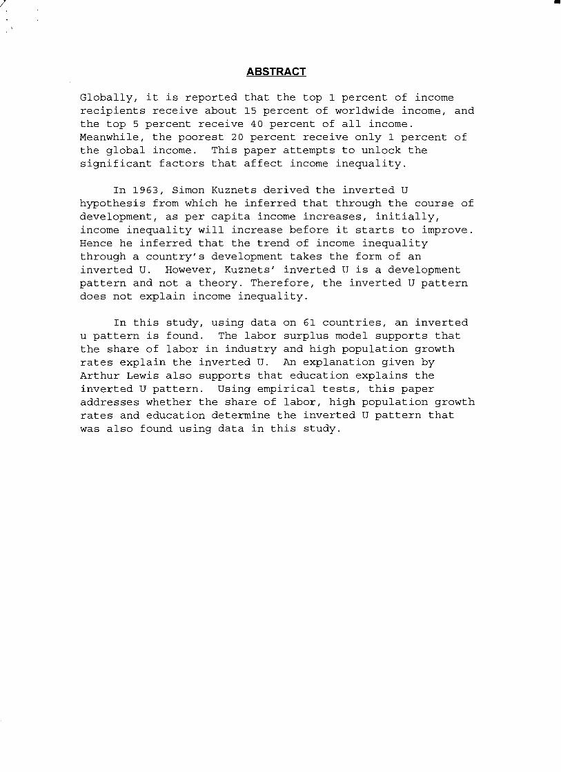

bull
1
Introduction
Economic growth refers to a rise in national per capita income and product (peY)
However economic growth does not mean that there is improvement in mass living
standards It can be a result of increase of wealth for the rich while the poor have less or
no improvement in their living standards (Gillis 70) This uneven distribution of income
is referred to as income inequality There is much income inequality existing in
individual countries as well as globally Globally it is reported that the top 1 percent of
income recipients receive about 15 percent of worldwide income and the top 5 percent
receive 40 percent of all income Meanwhile the poorest 20 percent receive only 1
percent of the global income (Braun 49) In this paper I intend to unlock significant
factors that affect the level of income inequality in developing nations
There was much interest in income inequality in developing countries in the
1960s which diminished as these countries became faced with greater problems including
declining growth rates and the debt problem (Gillis 72) Today income inequality
remains an important issue because it concerns human welfare Measures of income
inequality give insights into the extent of poverty in countries and are guides for both
local and international organizations concerned about the improvement of living
standards of the very poor
bull
2
Theoretical Considerations and Hypothesis
Economic Growth and Income Inequality
KuznetsInverted U hypothesis
The foundation of most works on income inequality is provided by Simon Kuznets In
1963 Kuznets suggested that the relationship between economic growth and income
inequality takes the form of an inverted U In his study Kuznets used cross-section data
of 18 countries Using his data he derived the inverted U hypothesis from which he
inferred that through the course of development as PCY increases initially income
inequality worsens after which income inequality improves (Fields 61) Diagram 1
illustrates this inverted U pattern According to the pattern moving from low-income
economies ($0-500 World Bank (WB) 1988) to lower-middle economies ($500-2200
W B 1988) income inequality should increase Starting from about upper middleshy
income ($2200-6000 W B 1988) onwards income inequality should decrease (Poulson
150)
Kuznets inverted U is a development pattern and not a theory Chenery and
Syrquin define development patterns to be changes in the structure of the economy
associated with rising level of income (Chenery 4) The main difference between a
pattern and a theory is that a theory asserts causality and a pattern does not A theory
asserts that changes in one variable cause a change in another variable A pattern on the
other hand would show a relationship between variables but does not assert that a change
in one variable is the cause of a change in another variable Since every country develops
in a unique way patterns are often used in development economics because they provide
a basis for comparative analysis in order to make generalizations about the development
process of a single country (Chenery 3)
bull 3
Kuznets Inverted U Patternmiddot
~
Income Inequality shy
PCY
DIAGRAM 1
bull
4
Since Kuznets inverted U is a pattern it does not explain income inequality That
is rising PCY does not cause the inverted U trend Rather there is a relationship
between PCY and income inequality which is illustrated by the inverted U pattern Thus
the question becomes what factors affect the level of income inequality in a country The
rest of this paper attempts to disclose the explanatory variables of income inequality It is
found that two explanatory variables the shares of labor in industry and education
support the inverted U A third explanatory variable population growth rate is expected
to affect the level of income inequality at any stage of development
Effect of Increasing Share of Labor In The Industrial Sector
The migration oflabor from the agricultural (rural) sector to the industrial (urban) sector
plays an important role in the development of a country Often when industrialization
begins in a country the industries require a significant amount oflabor which must come
from the rural sector When labor migrates to the urban sector production in this sector
increases and the economy grows Moreover the urban sector has other benefits for
workers who migrate including access to services like public schools and health services
which enhance human capital and facilitate higher income As will be discussed below
this rural to urban migration also affects income inequality In this study the share of
labor in the industrial sector is used to account for the effect of rural to urban migration
on income inequality
The argument here is that initially the share of labor in the industrial sector would
be positively related to the level of income inequality and after some point in
development the share of labor in the industrial sector will be negatively related to the
level of income inequality Thus this argument is consistent with the inverted U pattern
The support for this argument is provided by the two-sector labor surplus model The
two sectors in this model are the agricultural and industrial sectors In this paper it is
bull
5
assumed that if wages are rising then income inequality is improving This is because
when workers earn higher wages they take away more income from the wealthy and
reduce wage differentials in the economy causing the level of income inequality to
decrease
The Two-Sector Labor Surplus Model
It is assumed that before development takes place a nation is primarily agrarian and that
surplus labor exists Because land is fixed in supply and the supply of agricultural labor
varies as labor increases initially agricultural output will increase until diminishing
returns set in Then additional labor will not increase output and the marginal
productivity of labor will be zero This situation indicates the existence of surplus labor
Since wage is a function of marginal productivity wages will be constant whenever
there is surplus labor In a country that is at its early stages of development this constant
wage is the subsistence wage (Gillis 54-59)
According to the two-sector model the start of industrialization marks the start of
development Industries need workers and given the initial surplus of labor in the
agricultural sector the industries attract workers from the agricultural sector by paying a
constant wage which is slightly higher than the subsistence wage The horizontal part of
the labor supply curve QR in diagram 2 represents the period when there is surplus labor
in agriculture and the constant wage paid in the industrial sector is Q
As long as there is surplus labor in the agricultural sector the labor surplus model
suggests that there will be rising income inequality in the economy as workers move to
the industrial sector This is because the increasing amount and low cost of labor in the
industrial sector raises output in that sector causing the owners of industries to realize
huge profits while wages cannot rise above point Q (diagram 2) until labor becomes a
scarce factor (Gillis 93) As illustrated in diagram 2 when there is surplus labor an
increase in demand for labor in the industrial sector from D1 to D2 does not force wages
bull 6
Supply ofLabor in the Industrial Sector Using the Labor Surplus Model
Wages
e ---- ------ - --------- shy
d ------------------ -- shy
~ 1----gt----gt----
D3
Labor
DIAGRAM 2
bull
7
to rise Thus although workers earn more than subsistence wage by moving to the
industrial sector which should decrease the overall level of income inequality the huge
profit of capitalists rises faster and dominates the level of income inequality so that
overall income inequality increases
When surplus labor ceases to exist in agriculture further increases in demand for
labor by industries will lead to higher wages in the industrial sector and at the same time
workers in the agricultural sector become better off since the supply of agricultural labor
is decreasing Thus there will be an improvement in the overall level of income
inequality The point at which labor becomes scarce is point R and marks the start of a
trend towards income equality The supply curve facing the industrial sector becomes
RS an upward sloping curve which indicates that labor is in scarce supply Those
remaining in agriculture are better off for the following reasons Workers in the
industrial sector are no longer producing their own food causing the demand for
agricultural products to increase and consequently the price of these products to be
higher Moreover the available land per worker in the agricultural sector is rising and
thus the marginal productivity of labor in the agricultural sector also rises Increasing
marginal productivity in the agricultural sector implies that wages in this sector are also
rising Thus to attract more workers from agriculture industries must offer even higher
wages than those existing in the agricultural sector (Gillis 53) Thus in diagram 2 an
increase in demand for labor in the industrial sector from D3 to D4 raises wages from d to
e which would mean a decrease in the overall level of income inequality
The initial worsening followed by an improvement in the level of income
inequality is consistent with Kuznets inverted U hypothesis That is the labor surplus
model supports the inverted U Because the labor surplus model is based on the
migration oflabor to the industrial sector it supports the argument that the share oflabor
in industry should first increase then decrease the level of income inequality
bull
8
The Effect of Population Growth Rates
It is stated that one reason why developing countries have high degrees of income
inequality at relatively high levels of industrialization is because of rapid population
growth in these countries (Dovring 91) Countries like South Korea and Taiwan that
have succeeded in improving income distribution adopted measures to control population
growth as one ofthe necessary tools (Frank 102) Moreover other studies have shown a
positive relationship between high population growth rates and income inequality
(Chenery et aI 17)
These observations support the argument that high population growth rates will
cause the level of income inequality to increase for any given level of PCY Given that a
country does not have perfect income equality at the start of its development process the
countrys inverted U curve will intersect the income inequality axis at a point other than
zero
The argument given here is that high population growth rates will shift the
countrys inverted U curve upward so that the curve intersects the income inequality axis
at a higher point than before indicating an increase in the level of income inequality for
any given PCY This argument is illustrated in diagram 3 Higher population growth
rates causes the curve to shift from A to B and the intercept of the curve to rise from 02
to 05 for example (measurement of income inequality is the gini coefficient - see
appendix 2) Thus at PCY of 300 the level of income inequality also rises from 04 to
06 Therefore population growth rates can be said to determine the intercept of the
inverted U An economy with a low population growth rate will have a lower intercept
than a country with high population growth rates That is the higher the intercept of the
inverted U curve of a country the higher the level of income inequality for any given
PCY
bull
9
Strong support for the argument that high population growth rates are positively
related to the level of income inequality is provided by the two-sector labor surplus
model and the theory of supply and demand As previously discussed the labor surplus
model suggests that a country first has a period of worsening income inequality followed
by a period of improvements in the level of income inequality During the period of
worsening income inequality there is surplus labor in the agricultural sector and income
inequality improves when labor becomes scarce Using the labor surplus model and the
theory of supply and demand it will be shown that high population growth rates are
positively related to the level of income inequality during the periods of abundant and
scarce supplies of labor
Diagram 4 shows the effect of rising population growth rates when there is
surplus labor in agriculture As discussed before BC indicates the period when income
inequality rises because the owners of industries are realizing huge profits due to the
growth of industries and low labor costs At point C income inequality will take a
downturn and further demand for labor by industries will cause wages to rise If the
population growth rate is not high then the supply curve of labor Sind should remain
BCD
However if the supply oflabor is increasing because of high population growth
rates then Sind will be ABCD The amount of surplus labor will become ABC which is
greater than BC that represents surplus labor when population growth rates are very low
Therefore when population growth rates are high it will take a longer time for the
economy to reach point C where all surplus labor is absorbed by industries and the
economy tends towards income equality Also labor costs will remain low for a longer
time causing the owners of industries to make greater profits than when population
growth rates are low This is because if population growth rates are relatively stable then
the time when labor becomes scarce comes sooner so that the owners of industries must
cut profits at an earlier stage to increase wages in order to hire more workers
10
Upward Shift of the Inverted U Curve
Income Inequality
d
b middot
800 PCY
DIAGRAM 3
-1 1
Lffect of High Population Growth Rates with Surplus Labor in the Economy
W~ges ages
D
A ~ __ __ __ _B+-- ----C
o o Labor
DIAGRAM 4
Effect ofHigh Population Growth Rates with Scarce Supply ofLabor in the Economy
Wages
81
Wl 82
~ I------~
W21--- _
Labor
DIAGRAMS
bull
12
In summary when surplus labor exists and a country finds itself along the upside of the
inverted U when its level of income inequality is rising high population growth rates
would further increase the level of income inequality for each PCY along this part of the
inverted U curve This is due to the widening of income differentials between industrial
owners and workers
If the country is at the stage when labor is in scarce supply then the supply curve
facing industries will be upward sloping Thus there will be improvements in the level
of income inequality because wages will increase whenever the demand for labor by
industries increases This is illustrated in diagram SA where S1 is the supply curve of
labor facing industries and an increase in their demand for labor from D1 to D2 raises
wages from a to b
An increase in the supply of labor at the stage of development when there is
scarcity of labor causes labor to be less scarce and reduces wages As shown in diagram
58 an increase in the supply of labor due to high population growth rates will cause the
supply curve to shift from Sl to S2 causing wages to fall from d to c Since falling
wages are linked with higher profits for industrial owners there would be an increase in
the level of income inequality Thus when labor is scarce and a country finds itself along
the downside of the inverted U high population growth rates will retard improvements in
the level of income inequality That is the level of income inequality will increase for
every PCY along the downside of the inverted U
Since it has been shown that high population growth rates shift both the upside
and downside of the inverted U curve upward it is clear that high population growth rates
shift the inverted U curve upward When this upward shift occurs the inverted U will
intercept the income inequality axis at a higher point implying that the level of income
inequality will rise for any given level ofPCY
bull
13
Effect of Education
Education is important because it allows people to contribute effectively towards the
growth of the economy Education also improves the level of income inequality by
eliminating skill differentials which reduce wage differentials This is because education
facilitates higher labor productivity which leads to higher labor income
The effect of education on income inequality is given by Lewis who focuses on
the differentials between skilled and unskilled labor As an economy grows industries
expand and they demand more skilled and unskilled labor But at the early stages of
development there will be a scarce amount of literate people to carry out for example
supervisory and administrative tasks Because of this scarcity of skilled workers
compared to the abundant supply of unskilled workers wage differentials between the
two groups of workers will widen Skilled workers will see increases in their wages
while the wages of unskilled workers may even fall if the supply of unskilled workers
increases (Lewis 180-181) The initial widening of wage differentials that results
between the two groups of workers causes a worsening of the level of income inequality
in the economy
However as the economy grows and educational facilities spread to a larger
proportion of the population in the long run skilled workers in the country will increase
causing the wages of skilled workers to fall (Lewis 180-181) Thus wage differentials
between the skilled and unskilled workers will reduce causing the level of income
inequality to improve The initial worsening followed by improvements in the level of
income inequality that is caused by the widening and then narrowing of wage
differentials is consistent with the inverted U pattern Thus it is argued here that
initially education is likely to be positively related before it becomes negatively related
to the level of income inequality
bull
14
More support for the fact that education affects the level of income inequality is
shown by the need for expansion of education systems worldwide and in the studies of
many economists Compulsory education is widely accepted as an important public
service and every country has some form of compulsory education (Eckstein 1992)
Eckstein and Zilcha show empirically that human capital affects the quality of labor and
that compulsory education will improve the distribution of income through generations
(Eckstein 1992) If education improves labor and causes higher wages then compulsory
education should improve the level of income inequality Also Chenery and Syrquin
found that education removes income away from the richest 20 and increases income of
the lowest 40 (Chenery 63) More interestingly where primary and secondary
schooling were found to be positively related to income shares obtained by individuals it
was also shown that primarily schooling significantly explained variations in income for
the lowest 40 and secondary education significantly explained those of the middle
40(Chenery et aI 17) This finding helps explain why emphasis is often placed at least
on compulsory primary schooling in many developing nations It can be said that the aim
is to improve the lot of the very poor
Hypotheses
The discussions above generate four hypotheses
I The inverted U exists supported by the fact that the labor surplus model
predicts the inverted U pattern
II The share of labor in industry is initially positively related then negatively related
to the level of income inequality
III Population growth rates are positively related to the level of income
inequality at any stage of development Higher population growth rates are
associated with higher income inequality
bull
15
IV It is likely that education is initially positively related before it becomes
negatively related to the level of income inequality
Research Design
Data on 61 countries mainly low-income and middle-income countries are used in this
study (see Appendix 1) The measure of income inequality used is the gini coefficient
This coefficient is calculated from a Lorenz curve that is constructed using data on
income distribution of a given country Appendix 2 gives an explanation of how gini
coefficients are calculated I created a program in Pascal to calculate this coefficient
based on the Lorenz curve the formula for the area of trapezoids and the formula for the
coefficient
Data on income distribution share of labor in industry and population growth
rates were obtained from the World Banks publication Social Indicators of Development
1991-92 Primary and secondary school enrollments are used as a measure of the
expansion of education and the data for these variables were also obtained from the
Social Indicators of Development Data for all variables are not given annually but for
periods of time This is possibly due to the fact that data on variables such as the income
distribution in a country are collected less frequently The periods for which data are
reported are 25-30 years ago 15-20 years ago and the most recent period
PCY Groups
When I plotted gini coefficients for the countries used in this study all the points were
crowded so that no pattern was observed When I tried to observe patterns using PCY
groups I found an inverted U pattern According to the inverted U pattern I found the
upside ofthe inverted U existed for countries with PCY up to $300 (dollar amounts are
bull
16
1990 current market prices in US dollars) There was no clear trend for countries with
PCY between $300 and $1000 but there was clear evidence of the downside ofthe
inverted U starting with countries with PCY about $1000 and higher Diagram 6
illustrates the inverted U pattern that I found using plotted graphs PCY Group I will
refer to countries with PCY less than or equal to $300 PCY Group II will refer to
countries with PCY between $300 and $1000 and PCY Group III will refer to countries
with PCY greater than $1000
Table 1 which shows regression results for the PCY groups identified above
verifies the inverted U pattern that was observed using plotted graphs The PCY2 term is
included since the inverted U pattern is quadratic According to Table 1 there is an initial
worsening of income inequality for PCY Group I judging from the positive significant
sign of the PCY variable The results for PCY Group II does not indicate any significant
pattern and confirms that a horizontal line best represents the trend of income inequality
for this PCY group For PCY Group III there is strong evidence of decreasing income
inequality which is indicated by the negative significant sign of the PCY variable Thus
the results shown in this table confirm that the inverted U pattern exists In Appendices
34 and 5 the regression lines for PCY Group I II and III drawn against the plotted data
for the PCY groups respectively are shown Put together the regression lines of the three
PCY groups also show the inverted U pattern I found using plotted graphs Later on we
will see whether the labor surplus model supports that this inverted U pattern exists
My findings using plotted graphs and regression models discussed above are good
findings since they posit that the phase of worsening income inequality ends earlier than
expected at PCY of about $300 and that the point at which income inequality starts it
downward trend also occurs earlier at PCY of about $1000 As previously mentioned
according to the inverted U pattern it is expected that income inequality worsens up to
PCY of about $2200 before it starts to improve
17
PCYGroups
Income In shyegua 1
inverted U pattern
PCYGroupll
middot300 1000 PCY
DIAGRAM 6middotshy -~ - -~-
Table 1 INVERTED U PATTERN
VARIABLES
PCY
PCYlt=300
(+)
+000262
300ltPCYlt= 1000
-000012
PCYgt1000
(-) -000003
-
PCY2 (-) -000001
+000000 (+) +000000
= significant at the 90 confidence level signs in parentheses are the hypothesized signs
bull
18
Models
To test the hypotheses in this paper several regression models are created and tested for
each PCY group On an aggregate level the regression results for all three PCY groups
will test the four hypotheses In these models Industry represents the share of labor in
industry PopRate represents population growth rates and Primary and Secondary
represent primary and secondary school enrollments respectively Table 2 clearly presents
the variables used in this study and their definitions OLS regressions were used to test
the models
For each PCY group Modell includes all the variables and tests all four
hypothesis Models 2 and 3 attempt to improve Modell The equation for Model 1 is
Gini = Constant + PCY + PCy2 + Industry + Industry2 + PopRate + Primary +
Primary2 + Secondary + Secondary2
[Equation 1]
Again the squared terms are included since the inverted U pattern is a quadratic curve
PopRate2 is not included in the equation above because PopRate is hypothesized to
always be positively related to the level of income inequality
According to the hypothesis for PCY Group I it is expected that in the regression
result for Modell the PCY term will be positive and significant This result will
confirm the upside of the inverted U Industry is expected to be positive and significant
to imply that during the early stages of development rural to urban migration causes the
economy to experience worsening levels of income inequality High population growth
rates should always worsen the level of income inequality and therefore a positive and
significant sign is expected for PopRate Primary and Secondary are also expected to be
positive and significant since a country at its early stage of development is likely to have
large wage differentials between the few literate people who receive high wages and the
masses of illiterate people who receive very low wages
bull 19
TABLE 2 DEFINITION OF VARIABLES
VARIABLES DEFINITIONS
PCY GNP per capita Estimates are for 1990 at current market prices in US dollars
INDUSTRY Labor force in mining manufacturing construction electricity water and gas as a percentage of the total labor force
POPRATE Population growth rate Annual growth rate calculated from mid year total and urban population
PRIMARY Primary school enrollmen t Gross enrollment of all ages at primary level as a percentage of school age children as defined by each country and reported to UNESCO
SECONDARY Secondary school enrollment Computed in the same manner as the primary school ratio
Source = Social Indicators of Development 1991 -92
bull
20
For PCY Group II the regression result for Modell will likely indicate nothing
significant as is implicated by the results presented in Table 1
For PCY Group III a negative significant sign is expected for the PCY variable to
confirm the downside of the inverted U Industry is also expected to be negative and
significant since countries in this group should have competitive labor markets so that
higher demands of labor increase wages PopRate is expected to be positive and
significant Primary and Secondary are expected to be negative and significant This is
because at the later stages of development there should be more literate people in the
labor force which should cause wage differentials to reduce and income inequality to
decrease
Results Conclusions and Policy Implications
Tables 3 4 and 5 show the regression models for PCY Group I II and III respectively
PCY Group I (The early stage of development)
Results
Table 3 shows the results for this group Modell which contains all the variables is a
good model judging from its R2 of 080 All the variables are significant except for
Primary and Primary 2 Secondary and Secondary2 have unexpected signs In Model 2
where the Secondary variables are excluded the R2 becomes 054 and only PopRate is
significant However the Primary variables have the expected signs Model 3 appears to
be the best model in which the Primary variables are excluded All the variables in this
model are significant and the model has an R2 of 080 However the Secondary
variables have the unexpected signs
bull
21
TABLE 3 GINI REGRESSIONS FOR PCY lt=300
VARIABLE MODEL 1 MODEL 2 MODEL 3
PCY (+ ) +000428
(+) +000110
(+ ) +000191
PCy2 ( shy )
-000001 ( shy )
-000002 ( - )
-000001
INDUSTRY (+ ) +015718
(+ ) +002127
(+ ) +008700
INDUSTRy2 ( shy )
-000786 ( shy )
-000092 ( shy )
-000414
POPORATE (+ ) +017821
(+) +007699
(+ ) +010363
PRIMARY (+ ) -000240
(+ ) +000247
PRIMARy2 ( shy )
+000000 ( - )
-000002
SECONDARY (+ ) -001823
(+ ) -001467
SECONDARy2 ( shy )
+000047 ( shy )
+000030
ADJUSTED R2
080 054 080
= significant at 90 confidence level (two-tail test) Signs in parentheses are the hypothesized signs
bull
22
Given that Model 3 is the best model it will be used to estimate the impact of
each variable on income inequality The equation for Model 3 is
Gini = -02636 + 0002PCY - 0000PCy2 + 0087Industry shy
0004Industry2 + 01 0363PopRate - 00 I5Secondary +
0000Secondary2
[Equation 2]
The positive sign and significance of the PCY variable in Model 3 confirm the
initial positive relationship between PCY and income inequality The positive and
significant sign of Industry is consistent with the labor surplus models prediction that at
the initial stages of development an increase of workers in the industrial sector worsens
the level of income inequality The result for PopRate supports that high population
growth rates are positively related to the upside ofthe inverted U This result is also
consistent with the explanation provided by the labor surplus model that high population
growth rates will increase the amount of surplus labor in this PCY group and worsen
income inequality The unexpected results for the Primary variables may be due to the
fact that this variable is not lagged The unexpected significant result for Secondary is an
important finding and can be explained as follows
At PCY less than $300 it is likely that secondary school enrollments are not
high However an increase in secondary school enrollments implies that there is likely
an increase in primary school enrollments Since at the early stage of development most
primary school graduates enter the labor force an increase in secondary school
enrollments also implies that more primary school graduates are entering the labor force
Therefore secondary school enrollment may be proxying for more people in the labor
force with primary school education who because of their primary school education
should be making higher wages More people making higher wages reduces wage
bull
23
differentials which improves income inequality This explanation is consistent with the
result obtained from the Secondary variable
Conclusions and Policy Implications
As explained in Appendix 2 where the method ofcalculating gini coefficient is
discussed the value of the gini coefficient lies between 1 and O The closer the
coefficient is to 0 the lower the level of income inequality The closer the gini coefficient
is to I the higher the level of income inequality From Equation 2 above it is deduced
that an increase ofPCY by $1 will cause the gini coefficient to rise by 0002 This means
that an increase ofPCY by $50 causes the gini coefficient to rise by a tenth (01) This
result is significant and posits that when a country begins its development process and
PCY increases the initial worsening of income inequality is inevitable Thus for
countries with PCY up to about $300 a worsening trend of income inequality can be
accepted as an initial phase that accompanies development
According to Equation 2 above a percentage increase of labor in industry (the
variable Industry) causes the gini coefficient to increase by 0087 Thus a 115
percentage increase of labor in the industrial sector causes the gini coefficient to rise by
about a tenth This result is also significant and implies that about a 9 percent increase of
labor in industry will cause the level of income inequality to be at the highest possible
level Therefore the results suggest that developing countries within PCY Group I
should not only concentrate on the developing the industrial sector but should
simultaneously concentrate on developing the agricultural sector That way they may be
able to reduce the amount of migrants from agriculture into industry
How much income inequality exists at the early stages of development depends
significantly on population growth rates The higher the population growth rate the
bull
24
higher is the level of income inequality at each PCY According to Equation 2 a 1
percentage increase in population growth rates causes the gini coefficient to rise by 0104
This implies that an increase of population growth rate by 096 percent (approximately 1
percent) causes the gini coefficient to rise by a tenth This result points out that it is
necessary for developing countries to adopt measures to control population growth rates
as early as possible in their development process By maintaining low population growth
rates and as according to the labor surplus model labor in the economy becomes a scarce
factor earlier and labor markets are competitive sooner Then also wages should
increase and income inequality should improve
If Secondary is accepted as a proxy for the amount of primary school graduates
entering the labor force then as calculated from Equation 2 a 667 increase of primary
school graduates entering the labor force (ie 667 increase in secondary school
enrollment) should decrease the gini coefficient by a tenth This is a significant and
encouraging result because it emphasizes the universal benefits of education even at the
early stages of development
PCY Group II (The intermediate stage of development)
Results
All the models created for this PCY group show no significant result as noted in Table 4
None of the variables are significant and the R2s for all the models are very low The
results confirm that the curve is a straight line for this PCY group
Conclusion
The results for PCY Group II does not allow one to make any generalizations applicable
to countries in this PCY group today Perhaps conditions in these countries are complex
and varied and therefore cannot be easily summarized
bull 25
TABLE 4 GINI REGRESSIONS FOR 300 lt PCY lt= 1000
VARIABLE MODEL 1 MODEL 2 MODEL 3
PCY 000004 000005 000008
PCy2 -000000 -000000 -000000
INDUSTRY -000842 -000720 -000836
INDUSTRy2 -000000 -000004 000002
POPRATE -002217 -002602 -000794
PRIMARY 001063 001068
PRIMARy2 -000006 -000006
SECONDARY 000171 000232
SECONDARy2 -000002 -000002
ADJUSTED Rl -007 005 002
bull 26
VARIABLES MODEL 1 MODEL 2 MODEL 3
PCY ( - )
-000002 ( - )
-000001 ( - )
-000002
PCy2 (+ ) +000000
(+ ) +000000
(+ ) +000000
INDUSTRY ( - )
-000460 ( - )
-001577 ( shy )
-000720
INDUSTRy2 (+ ) 000007
( + ) +000024
(+ ) 000012
PORPORATE (+ ) -001515
(+ ) +000806
(+ ) -001960
PRIMARY ( shy )
-001664 ( shy )
-005207
PRlMARy2 (+ ) +000008
(+ ) +000024
SECONDARY ( shy )
-000971 ( - )
-000866
SECONDARy2 (+ ) +000006
(+ ) +000005
ADJUSTED Rl 050 044
= SIGNIFICANT AT THE 90 CONFINDENCE LEVEL (TWO-TAIL TESr SIGNS IN PARENTEHESES ARE THE HYPOTHESIZED SIGNS
TABLE 5 GINI REGRESSIONS FOR PCY gt 1000
bull
27
PCY Group III (The industrialized stage of development)
Results
Only the education variables have significant coefficients in the models in Table 5 The
PCY variables in this table are not significant although they are in Table 1 This is
possibly because the explanatory variables in the regression equations for the models in
Table 5 (these explanatory variables are not included in the regression equation for Table
1) reduce the significance of the PCY variable The significant and expected coefficient
for Secondary in the models supports Lewis explanation that as an economy develops
education facilities become available to more people so that in the long run education has
a negative effect on the level of income inequality
Conclusion
Since countries in PCY Group III are well industrialized the increasing share of labor in
industry may have little impact on the level of income inequality Likewise population
growth rates which are relatively stable in these countries may have negligible effect on
the level of income inequality It is likely that there are other variables that may help
explain the downward trend of income inequality that is expected for industrialized
countries Often countries in the early stages of development experience political and
social instabilities conditions which improve as these countries develop Thus a measure
of political and social conditions may for instance be a crucial determinant of the
downward trend of income inequality It is also likely that the existence of certain
institutions in industrialized countries like unions that function to improve wages help
improve the level of income inequality in these countries Thus a measure of
unionization may also improve the results for this group Another variable that measures
bull
28
U This is because it is usual to find more advanced technological equipment and
facilities in industrialized countries and not in developing countries In summary the
share of labor in industry and population growth rates do not explain the downside of the
inverted U
General Conclusion
In this paper four hypothesis were generated and tested to confirm that the inverted U
exists and that the share of labor in industry population growth rates and education were
explanatory variables of income inequality Moreover the labor surplus model predicts
the inverted U pattern Although the inverted U pattern was found as presented in Table 1
where only PCY variables were used in the regression equation the explanatory variables
failed to show the inverted U pattern in its entirety The explanatory variables were able
to explain the upside of the inverted U as shown in Table 3 but the same explanatory
variables could not explain the downside of the inverted U as shown in Table 5
Thus this study also shows that the labor surplus model explains the upward trend
for countries with very low PCY and that high population growth rates worsen the level
of income inequality for these countries This study highlights that the labor surplus
model is incapable of explaining any other part of the inverted U especially the downside
of the inverted U
Suggestions For Future Research
Another explanation for the inverted U pattern can be given using labor market power as
follows At the early stages of development firms have monosony power and can force
the technological know-how in the various countries may also help explain the inverted
bull
29
wages to be low which signifies a period of worsening income inequality At the
intermediate stage of development more firms may exist which may cause the initial
monosony power of firms to reduce and at least prevent further worsening of income
inequality At the industrialized stage of development workers are likely to organize into
unions and counter the remaining monosony power of firms This should increase wages
and cause income inequality to improve This brief discussion suggests an important area
for future research Perhaps a better explanation of the inverted U pattern or an important
area to be considered along with the labor surplus model may be discovered
Another area for future research will be to separate the countries in PCY Group III
(countries that have PCY greater than $1000) into two categories the newly industrialized
and the well industrialized countries This may help control for the wide range of PCY in
PCY Group III and also the differences in institutions that exist in these countries
bull
30
WORK CITED
Ahluwalia Montek S 1976 Inequality Poverty and Development Journal of Development
Economics 3306-342
Braun Denny The Rich Get Richer The Rise ofIncome Inequality in the United States and the World
Chicago Nelson-Hall Publishers 1991
Chenery Hollis Ahluwalia S Montek C L G Bell John H Duloy Richard Jolly Redistribution
with ~rowth London Oxford University Press 1975
Chenery Hollis amp Moises Syrquin Patterns of Development 1950-1970 Published for the World Bank
by Oxford University Press 1975
Dovring Folke Inequality New York Praeger Publishers 1991
Eckstein Zvi amp Zilcha Itzhak 1992 The effects of compulsory schooling on growth
income distribution and welfare Journal of Public Economics 543339-359
Fields Gary F Poverty Inequality and Development London Cambridge University Press 1980
Gillis Malcom Economics of Development New York WW Norton amp Company 1992
Lewis W Arthur Theory of Economic Growth New York Harper Row 1970
Poulson Barry W Economic Development Minneapolis West Publishing Company 1994
APPENDIX 1shy
bull
~Cgt -ntneG time gini pey PopPate indu~ primary r
3an~1lade 25-30 030 7000 26 48 31
ncilet 25-30 036 9000 23 119 74
Paki~tan 25-30 034- 11000 26 183 40
Pak~tan 15-20 0294 130 31 172 12
Banglade 15-20 0316 130 25 54 73 Thailand 25-30 039 14000 31 52 78
0ri Lanka 25-30 041 16000 25 139 93
India 15-20 037 17000 23 129 79
Tanzania 15middot20 038 17000 28 38 53 Phiflipine 25-30 045 18000 31 158 113
Indonesia 15-20 038 21000 24 117 86
Uganda 15-20 036 22000 26 39 44 Sierra Le 15middot20 040 22000 2 132 39
Kenya 15-20 049 23000 37 62 95 0ri Lanka 15-20 032 29000 16 142 77 Mauritius 25-30 040 31000 24 254 72
Egypt 15-20 038 32000 2 184 71
Columbia 2~30 O~6 32000 3 214 84 Phillipine 15-20 043 34000 26 161 107 Botswana 15-20 050 35000 38 84 72
Bolivia 15-20 046 36000 25 199 85 0uriname 25-30 029 39000 27 215 120
Costa Ric 25-30 045 40000 32 192 106 Liberia 15-20 055 41000 3 94 62 Mexico 25-30 049 46000 33 219 92 Ecuador 15-20 059 54000 3 202 104
Zambia 15-20 050 55000 3 92 97
Columbia 15-20 047 55000 21 234 118 Guatemal 15-20 046 57000 28 17 61
Nicaragu 15-20 052 63000 3 156 82
Spain 25-30 035 70000 1 345 115
Tunisia 15-20 034 71000 21 311 97 Mauritius 15-20 043 71000 15 245 107
Libya 25-30 024 81000 39 209 78
Malaysia 15-20 045 82000 23 166 91 Argentina 25-30 038 87000 15 342 101
Japan 25-30 037 90000 11 32 100 Costa Ric 15-20 045 95000 25 216 107
Peru 15-20 052middot 100000 27 18 113
bull
Fiji 15-20 038 03000 i 9 160 115
Brazil 15-20 051 1070gt 24shy 243 88
Venezuel 25-30 048 113000 34 237 94
Israel 25-30 030 130000 35 354 95 Barbados 15-20 032 152000 04 233 103
Portugal 15-20 038 154000 38 347 113 Netherlan 25-30 039 156000 14 407 104
Trinidad 15-20 041 172000 09 372 99
Finland 25-30 042 175000 03 354 92 rmiddotJnrway 25-30 032 184000 08 368 97
France 25-30 046 203000 09 39 134
Denmark 25-30 035 205000 08 369 98 Venezuel 15-20 045 238000 36 267 97
Canada 25-30 030 262000 18 325 105
Ireland 15-20 029 265000 17 324 103 Sweden 25-30 036 276000 09 428 95
Spain 15-20 034 278000 1 374 111 I~rael 15-20 028 389000 23 337 97
rrance 15-20 036 600000 05 373 109
Germany 15-20 033 667000 -04 476 103 Sweden 15-20 027 832000 04 365 101
Australia Recent 034 1668000 16 344 106
bull APPENDIX 2
Calculatin2 Gjni Coefficjents
To convert the figures of an income distribution data into a measure of
income inequality can be done by constructing a Lorenz curve for each
country from which the Gini coefficientconcentration ratio(a measure of
inequality) is calculated The Lorenz curve shows the total percentage of
total income accounted for by any cumulative percentage of recipients
The shape of this curve indicates the degree of income inequality in the
income distribution(Gillis 1992 74) To illustrate how a Lorenz curve is
derived consider the following data for Brazil in 1983
poorest 20 of households receive 24 of total income
second quintile receive 57
third quintile receive 107
fourth quintile receive 186
richest 20 receive 626
From these data it can be observed that Brazil has a high degree of
inequality if 626 of its total income goes to the richest 20 of total
households Also a total of 100 of households receive 100 of total
income To construct a Lorenz curve first the cumulative income share
accruing to any given percentage of households is calculated Thus for the
data above we get the following calculations
poorest 20 receive 24 of total income
poorest 40 receive 24 + 57 = 81 of total income
poorest 60 receive 81 + 107 = 188 of total income
poorest 80 receive 188 + 186 = 374 of total income
100 of households receive 100 of total income
bull
The Lorenz curve is a graph plotted from the data above with the
horizontal axis measuring the cumulative percentage of recipient units and
the vertical axis measunng the cumulative share of total income
Diagram2 below shows the Lorenz curve obtained from the data above
J
J~
t
1
I
l
~ 1 IA I
I
~ [J I
J 1
Diagram2
(Bolnick 1987 61-62)
The diagonal line is a 45-degree line The closer the curve is to this line
the lesser is income inequality The closer it is to the right hand borders
the greater is income inequality(Gillis 1992 74)
To calculate the Gini coefficient let A be the area between the Lorenz
curve and the diagonal line and let B be the area under the Lorenz curve
as show in Figure 2 The formula to calculate the Gini coefficient is given
as
bull
A(A + B) A + B will always be 05 because the box in which the Lorenz
curve is drawn is a unit square especially seen if all percentages are taken
as decimal units eg 20 as 02 Therefore the area of the square becomes
lxl = 10 and half the area of the square (A + B) is 05(Bolnick 1987 62)
Area B can be calculated geometrically using formulas for calculating areas
of rectangles triangles and trapezoids The area of B was calculated
geometrically to be 0233 Since A + B = 05 A = 05 - 0233 = 0267 The
Gini Coefficient AlA + B) = 026705 = 0534 The closer the Gini
coefficient is to 0 the lesser is income inequality and the closer it is to 1
the greater is income inequality
I created a program in Pascal that calculates gini coefficients based
on the Lorenz curve the formula for the area of trapezoids and the
formula for the gini coefficient
bull bull
045
03
bull
APPENDIX 3
REGRESSION LINE DRAWN AGAINST PLOTTED DATA FOR pey GROUP I
05--------------------------------bull
04
035 bull
bull bull
bull bull
bull
bull bulli~t=-+~=
bull
bull
025l-------r------r--r-------------_r-----r---------------------------r-----------J 7000 13000 16000 18000 22000
bull bull
bull bull bull
APPENDIX 4
REGRESSION LINE DRAWN AGAINST PLOTTED DATA FOR pey GROUP II
bull
06-------------------------------------
055 bull
bull bullbullbull 05 bull bull bullbullA45
bull 04 bull
035 bull
bull 03
bull
025
bull
O 2--L--------------------------------------------r----------------------r----------------------------------------r---r---l
31000 34000 39000 46000 55000 70000 81000 90000
bull bull
APPENDIX 5
REGRESSION LINE DRAWN AGAINST PLOTTED DATA FOR pey GROUP III
bull
0S5------------------------------
05 bull
bull045 bull
bull ~ 04
bull~ 035 bull
03
bull bull 025
02
01 f0-+-0-0--2-0-r-0-0--3-000--40-0-0--S-OO-0--610010--700-0--8-00-0--9---1000
PCY
bull
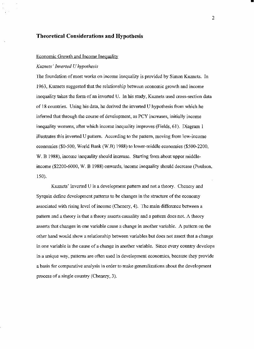
bull
2
Theoretical Considerations and Hypothesis
Economic Growth and Income Inequality
KuznetsInverted U hypothesis
The foundation of most works on income inequality is provided by Simon Kuznets In
1963 Kuznets suggested that the relationship between economic growth and income
inequality takes the form of an inverted U In his study Kuznets used cross-section data
of 18 countries Using his data he derived the inverted U hypothesis from which he
inferred that through the course of development as PCY increases initially income
inequality worsens after which income inequality improves (Fields 61) Diagram 1
illustrates this inverted U pattern According to the pattern moving from low-income
economies ($0-500 World Bank (WB) 1988) to lower-middle economies ($500-2200
W B 1988) income inequality should increase Starting from about upper middleshy
income ($2200-6000 W B 1988) onwards income inequality should decrease (Poulson
150)
Kuznets inverted U is a development pattern and not a theory Chenery and
Syrquin define development patterns to be changes in the structure of the economy
associated with rising level of income (Chenery 4) The main difference between a
pattern and a theory is that a theory asserts causality and a pattern does not A theory
asserts that changes in one variable cause a change in another variable A pattern on the
other hand would show a relationship between variables but does not assert that a change
in one variable is the cause of a change in another variable Since every country develops
in a unique way patterns are often used in development economics because they provide
a basis for comparative analysis in order to make generalizations about the development
process of a single country (Chenery 3)
bull 3
Kuznets Inverted U Patternmiddot
~
Income Inequality shy
PCY
DIAGRAM 1
bull
4
Since Kuznets inverted U is a pattern it does not explain income inequality That
is rising PCY does not cause the inverted U trend Rather there is a relationship
between PCY and income inequality which is illustrated by the inverted U pattern Thus
the question becomes what factors affect the level of income inequality in a country The
rest of this paper attempts to disclose the explanatory variables of income inequality It is
found that two explanatory variables the shares of labor in industry and education
support the inverted U A third explanatory variable population growth rate is expected
to affect the level of income inequality at any stage of development
Effect of Increasing Share of Labor In The Industrial Sector
The migration oflabor from the agricultural (rural) sector to the industrial (urban) sector
plays an important role in the development of a country Often when industrialization
begins in a country the industries require a significant amount oflabor which must come
from the rural sector When labor migrates to the urban sector production in this sector
increases and the economy grows Moreover the urban sector has other benefits for
workers who migrate including access to services like public schools and health services
which enhance human capital and facilitate higher income As will be discussed below
this rural to urban migration also affects income inequality In this study the share of
labor in the industrial sector is used to account for the effect of rural to urban migration
on income inequality
The argument here is that initially the share of labor in the industrial sector would
be positively related to the level of income inequality and after some point in
development the share of labor in the industrial sector will be negatively related to the
level of income inequality Thus this argument is consistent with the inverted U pattern
The support for this argument is provided by the two-sector labor surplus model The
two sectors in this model are the agricultural and industrial sectors In this paper it is
bull
5
assumed that if wages are rising then income inequality is improving This is because
when workers earn higher wages they take away more income from the wealthy and
reduce wage differentials in the economy causing the level of income inequality to
decrease
The Two-Sector Labor Surplus Model
It is assumed that before development takes place a nation is primarily agrarian and that
surplus labor exists Because land is fixed in supply and the supply of agricultural labor
varies as labor increases initially agricultural output will increase until diminishing
returns set in Then additional labor will not increase output and the marginal
productivity of labor will be zero This situation indicates the existence of surplus labor
Since wage is a function of marginal productivity wages will be constant whenever
there is surplus labor In a country that is at its early stages of development this constant
wage is the subsistence wage (Gillis 54-59)
According to the two-sector model the start of industrialization marks the start of
development Industries need workers and given the initial surplus of labor in the
agricultural sector the industries attract workers from the agricultural sector by paying a
constant wage which is slightly higher than the subsistence wage The horizontal part of
the labor supply curve QR in diagram 2 represents the period when there is surplus labor
in agriculture and the constant wage paid in the industrial sector is Q
As long as there is surplus labor in the agricultural sector the labor surplus model
suggests that there will be rising income inequality in the economy as workers move to
the industrial sector This is because the increasing amount and low cost of labor in the
industrial sector raises output in that sector causing the owners of industries to realize
huge profits while wages cannot rise above point Q (diagram 2) until labor becomes a
scarce factor (Gillis 93) As illustrated in diagram 2 when there is surplus labor an
increase in demand for labor in the industrial sector from D1 to D2 does not force wages
bull 6
Supply ofLabor in the Industrial Sector Using the Labor Surplus Model
Wages
e ---- ------ - --------- shy
d ------------------ -- shy
~ 1----gt----gt----
D3
Labor
DIAGRAM 2
bull
7
to rise Thus although workers earn more than subsistence wage by moving to the
industrial sector which should decrease the overall level of income inequality the huge
profit of capitalists rises faster and dominates the level of income inequality so that
overall income inequality increases
When surplus labor ceases to exist in agriculture further increases in demand for
labor by industries will lead to higher wages in the industrial sector and at the same time
workers in the agricultural sector become better off since the supply of agricultural labor
is decreasing Thus there will be an improvement in the overall level of income
inequality The point at which labor becomes scarce is point R and marks the start of a
trend towards income equality The supply curve facing the industrial sector becomes
RS an upward sloping curve which indicates that labor is in scarce supply Those
remaining in agriculture are better off for the following reasons Workers in the
industrial sector are no longer producing their own food causing the demand for
agricultural products to increase and consequently the price of these products to be
higher Moreover the available land per worker in the agricultural sector is rising and
thus the marginal productivity of labor in the agricultural sector also rises Increasing
marginal productivity in the agricultural sector implies that wages in this sector are also
rising Thus to attract more workers from agriculture industries must offer even higher
wages than those existing in the agricultural sector (Gillis 53) Thus in diagram 2 an
increase in demand for labor in the industrial sector from D3 to D4 raises wages from d to
e which would mean a decrease in the overall level of income inequality
The initial worsening followed by an improvement in the level of income
inequality is consistent with Kuznets inverted U hypothesis That is the labor surplus
model supports the inverted U Because the labor surplus model is based on the
migration oflabor to the industrial sector it supports the argument that the share oflabor
in industry should first increase then decrease the level of income inequality
bull
8
The Effect of Population Growth Rates
It is stated that one reason why developing countries have high degrees of income
inequality at relatively high levels of industrialization is because of rapid population
growth in these countries (Dovring 91) Countries like South Korea and Taiwan that
have succeeded in improving income distribution adopted measures to control population
growth as one ofthe necessary tools (Frank 102) Moreover other studies have shown a
positive relationship between high population growth rates and income inequality
(Chenery et aI 17)
These observations support the argument that high population growth rates will
cause the level of income inequality to increase for any given level of PCY Given that a
country does not have perfect income equality at the start of its development process the
countrys inverted U curve will intersect the income inequality axis at a point other than
zero
The argument given here is that high population growth rates will shift the
countrys inverted U curve upward so that the curve intersects the income inequality axis
at a higher point than before indicating an increase in the level of income inequality for
any given PCY This argument is illustrated in diagram 3 Higher population growth
rates causes the curve to shift from A to B and the intercept of the curve to rise from 02
to 05 for example (measurement of income inequality is the gini coefficient - see
appendix 2) Thus at PCY of 300 the level of income inequality also rises from 04 to
06 Therefore population growth rates can be said to determine the intercept of the
inverted U An economy with a low population growth rate will have a lower intercept
than a country with high population growth rates That is the higher the intercept of the
inverted U curve of a country the higher the level of income inequality for any given
PCY
bull
9
Strong support for the argument that high population growth rates are positively
related to the level of income inequality is provided by the two-sector labor surplus
model and the theory of supply and demand As previously discussed the labor surplus
model suggests that a country first has a period of worsening income inequality followed
by a period of improvements in the level of income inequality During the period of
worsening income inequality there is surplus labor in the agricultural sector and income
inequality improves when labor becomes scarce Using the labor surplus model and the
theory of supply and demand it will be shown that high population growth rates are
positively related to the level of income inequality during the periods of abundant and
scarce supplies of labor
Diagram 4 shows the effect of rising population growth rates when there is
surplus labor in agriculture As discussed before BC indicates the period when income
inequality rises because the owners of industries are realizing huge profits due to the
growth of industries and low labor costs At point C income inequality will take a
downturn and further demand for labor by industries will cause wages to rise If the
population growth rate is not high then the supply curve of labor Sind should remain
BCD
However if the supply oflabor is increasing because of high population growth
rates then Sind will be ABCD The amount of surplus labor will become ABC which is
greater than BC that represents surplus labor when population growth rates are very low
Therefore when population growth rates are high it will take a longer time for the
economy to reach point C where all surplus labor is absorbed by industries and the
economy tends towards income equality Also labor costs will remain low for a longer
time causing the owners of industries to make greater profits than when population
growth rates are low This is because if population growth rates are relatively stable then
the time when labor becomes scarce comes sooner so that the owners of industries must
cut profits at an earlier stage to increase wages in order to hire more workers
10
Upward Shift of the Inverted U Curve
Income Inequality
d
b middot
800 PCY
DIAGRAM 3
-1 1
Lffect of High Population Growth Rates with Surplus Labor in the Economy
W~ges ages
D
A ~ __ __ __ _B+-- ----C
o o Labor
DIAGRAM 4
Effect ofHigh Population Growth Rates with Scarce Supply ofLabor in the Economy
Wages
81
Wl 82
~ I------~
W21--- _
Labor
DIAGRAMS
bull
12
In summary when surplus labor exists and a country finds itself along the upside of the
inverted U when its level of income inequality is rising high population growth rates
would further increase the level of income inequality for each PCY along this part of the
inverted U curve This is due to the widening of income differentials between industrial
owners and workers
If the country is at the stage when labor is in scarce supply then the supply curve
facing industries will be upward sloping Thus there will be improvements in the level
of income inequality because wages will increase whenever the demand for labor by
industries increases This is illustrated in diagram SA where S1 is the supply curve of
labor facing industries and an increase in their demand for labor from D1 to D2 raises
wages from a to b
An increase in the supply of labor at the stage of development when there is
scarcity of labor causes labor to be less scarce and reduces wages As shown in diagram
58 an increase in the supply of labor due to high population growth rates will cause the
supply curve to shift from Sl to S2 causing wages to fall from d to c Since falling
wages are linked with higher profits for industrial owners there would be an increase in
the level of income inequality Thus when labor is scarce and a country finds itself along
the downside of the inverted U high population growth rates will retard improvements in
the level of income inequality That is the level of income inequality will increase for
every PCY along the downside of the inverted U
Since it has been shown that high population growth rates shift both the upside
and downside of the inverted U curve upward it is clear that high population growth rates
shift the inverted U curve upward When this upward shift occurs the inverted U will
intercept the income inequality axis at a higher point implying that the level of income
inequality will rise for any given level ofPCY
bull
13
Effect of Education
Education is important because it allows people to contribute effectively towards the
growth of the economy Education also improves the level of income inequality by
eliminating skill differentials which reduce wage differentials This is because education
facilitates higher labor productivity which leads to higher labor income
The effect of education on income inequality is given by Lewis who focuses on
the differentials between skilled and unskilled labor As an economy grows industries
expand and they demand more skilled and unskilled labor But at the early stages of
development there will be a scarce amount of literate people to carry out for example
supervisory and administrative tasks Because of this scarcity of skilled workers
compared to the abundant supply of unskilled workers wage differentials between the
two groups of workers will widen Skilled workers will see increases in their wages
while the wages of unskilled workers may even fall if the supply of unskilled workers
increases (Lewis 180-181) The initial widening of wage differentials that results
between the two groups of workers causes a worsening of the level of income inequality
in the economy
However as the economy grows and educational facilities spread to a larger
proportion of the population in the long run skilled workers in the country will increase
causing the wages of skilled workers to fall (Lewis 180-181) Thus wage differentials
between the skilled and unskilled workers will reduce causing the level of income
inequality to improve The initial worsening followed by improvements in the level of
income inequality that is caused by the widening and then narrowing of wage
differentials is consistent with the inverted U pattern Thus it is argued here that
initially education is likely to be positively related before it becomes negatively related
to the level of income inequality
bull
14
More support for the fact that education affects the level of income inequality is
shown by the need for expansion of education systems worldwide and in the studies of
many economists Compulsory education is widely accepted as an important public
service and every country has some form of compulsory education (Eckstein 1992)
Eckstein and Zilcha show empirically that human capital affects the quality of labor and
that compulsory education will improve the distribution of income through generations
(Eckstein 1992) If education improves labor and causes higher wages then compulsory
education should improve the level of income inequality Also Chenery and Syrquin
found that education removes income away from the richest 20 and increases income of
the lowest 40 (Chenery 63) More interestingly where primary and secondary
schooling were found to be positively related to income shares obtained by individuals it
was also shown that primarily schooling significantly explained variations in income for
the lowest 40 and secondary education significantly explained those of the middle
40(Chenery et aI 17) This finding helps explain why emphasis is often placed at least
on compulsory primary schooling in many developing nations It can be said that the aim
is to improve the lot of the very poor
Hypotheses
The discussions above generate four hypotheses
I The inverted U exists supported by the fact that the labor surplus model
predicts the inverted U pattern
II The share of labor in industry is initially positively related then negatively related
to the level of income inequality
III Population growth rates are positively related to the level of income
inequality at any stage of development Higher population growth rates are
associated with higher income inequality
bull
15
IV It is likely that education is initially positively related before it becomes
negatively related to the level of income inequality
Research Design
Data on 61 countries mainly low-income and middle-income countries are used in this
study (see Appendix 1) The measure of income inequality used is the gini coefficient
This coefficient is calculated from a Lorenz curve that is constructed using data on
income distribution of a given country Appendix 2 gives an explanation of how gini
coefficients are calculated I created a program in Pascal to calculate this coefficient
based on the Lorenz curve the formula for the area of trapezoids and the formula for the
coefficient
Data on income distribution share of labor in industry and population growth
rates were obtained from the World Banks publication Social Indicators of Development
1991-92 Primary and secondary school enrollments are used as a measure of the
expansion of education and the data for these variables were also obtained from the
Social Indicators of Development Data for all variables are not given annually but for
periods of time This is possibly due to the fact that data on variables such as the income
distribution in a country are collected less frequently The periods for which data are
reported are 25-30 years ago 15-20 years ago and the most recent period
PCY Groups
When I plotted gini coefficients for the countries used in this study all the points were
crowded so that no pattern was observed When I tried to observe patterns using PCY
groups I found an inverted U pattern According to the inverted U pattern I found the
upside ofthe inverted U existed for countries with PCY up to $300 (dollar amounts are
bull
16
1990 current market prices in US dollars) There was no clear trend for countries with
PCY between $300 and $1000 but there was clear evidence of the downside ofthe
inverted U starting with countries with PCY about $1000 and higher Diagram 6
illustrates the inverted U pattern that I found using plotted graphs PCY Group I will
refer to countries with PCY less than or equal to $300 PCY Group II will refer to
countries with PCY between $300 and $1000 and PCY Group III will refer to countries
with PCY greater than $1000
Table 1 which shows regression results for the PCY groups identified above
verifies the inverted U pattern that was observed using plotted graphs The PCY2 term is
included since the inverted U pattern is quadratic According to Table 1 there is an initial
worsening of income inequality for PCY Group I judging from the positive significant
sign of the PCY variable The results for PCY Group II does not indicate any significant
pattern and confirms that a horizontal line best represents the trend of income inequality
for this PCY group For PCY Group III there is strong evidence of decreasing income
inequality which is indicated by the negative significant sign of the PCY variable Thus
the results shown in this table confirm that the inverted U pattern exists In Appendices
34 and 5 the regression lines for PCY Group I II and III drawn against the plotted data
for the PCY groups respectively are shown Put together the regression lines of the three
PCY groups also show the inverted U pattern I found using plotted graphs Later on we
will see whether the labor surplus model supports that this inverted U pattern exists
My findings using plotted graphs and regression models discussed above are good
findings since they posit that the phase of worsening income inequality ends earlier than
expected at PCY of about $300 and that the point at which income inequality starts it
downward trend also occurs earlier at PCY of about $1000 As previously mentioned
according to the inverted U pattern it is expected that income inequality worsens up to
PCY of about $2200 before it starts to improve
17
PCYGroups
Income In shyegua 1
inverted U pattern
PCYGroupll
middot300 1000 PCY
DIAGRAM 6middotshy -~ - -~-
Table 1 INVERTED U PATTERN
VARIABLES
PCY
PCYlt=300
(+)
+000262
300ltPCYlt= 1000
-000012
PCYgt1000
(-) -000003
-
PCY2 (-) -000001
+000000 (+) +000000
= significant at the 90 confidence level signs in parentheses are the hypothesized signs
bull
18
Models
To test the hypotheses in this paper several regression models are created and tested for
each PCY group On an aggregate level the regression results for all three PCY groups
will test the four hypotheses In these models Industry represents the share of labor in
industry PopRate represents population growth rates and Primary and Secondary
represent primary and secondary school enrollments respectively Table 2 clearly presents
the variables used in this study and their definitions OLS regressions were used to test
the models
For each PCY group Modell includes all the variables and tests all four
hypothesis Models 2 and 3 attempt to improve Modell The equation for Model 1 is
Gini = Constant + PCY + PCy2 + Industry + Industry2 + PopRate + Primary +
Primary2 + Secondary + Secondary2
[Equation 1]
Again the squared terms are included since the inverted U pattern is a quadratic curve
PopRate2 is not included in the equation above because PopRate is hypothesized to
always be positively related to the level of income inequality
According to the hypothesis for PCY Group I it is expected that in the regression
result for Modell the PCY term will be positive and significant This result will
confirm the upside of the inverted U Industry is expected to be positive and significant
to imply that during the early stages of development rural to urban migration causes the
economy to experience worsening levels of income inequality High population growth
rates should always worsen the level of income inequality and therefore a positive and
significant sign is expected for PopRate Primary and Secondary are also expected to be
positive and significant since a country at its early stage of development is likely to have
large wage differentials between the few literate people who receive high wages and the
masses of illiterate people who receive very low wages
bull 19
TABLE 2 DEFINITION OF VARIABLES
VARIABLES DEFINITIONS
PCY GNP per capita Estimates are for 1990 at current market prices in US dollars
INDUSTRY Labor force in mining manufacturing construction electricity water and gas as a percentage of the total labor force
POPRATE Population growth rate Annual growth rate calculated from mid year total and urban population
PRIMARY Primary school enrollmen t Gross enrollment of all ages at primary level as a percentage of school age children as defined by each country and reported to UNESCO
SECONDARY Secondary school enrollment Computed in the same manner as the primary school ratio
Source = Social Indicators of Development 1991 -92
bull
20
For PCY Group II the regression result for Modell will likely indicate nothing
significant as is implicated by the results presented in Table 1
For PCY Group III a negative significant sign is expected for the PCY variable to
confirm the downside of the inverted U Industry is also expected to be negative and
significant since countries in this group should have competitive labor markets so that
higher demands of labor increase wages PopRate is expected to be positive and
significant Primary and Secondary are expected to be negative and significant This is
because at the later stages of development there should be more literate people in the
labor force which should cause wage differentials to reduce and income inequality to
decrease
Results Conclusions and Policy Implications
Tables 3 4 and 5 show the regression models for PCY Group I II and III respectively
PCY Group I (The early stage of development)
Results
Table 3 shows the results for this group Modell which contains all the variables is a
good model judging from its R2 of 080 All the variables are significant except for
Primary and Primary 2 Secondary and Secondary2 have unexpected signs In Model 2
where the Secondary variables are excluded the R2 becomes 054 and only PopRate is
significant However the Primary variables have the expected signs Model 3 appears to
be the best model in which the Primary variables are excluded All the variables in this
model are significant and the model has an R2 of 080 However the Secondary
variables have the unexpected signs
bull
21
TABLE 3 GINI REGRESSIONS FOR PCY lt=300
VARIABLE MODEL 1 MODEL 2 MODEL 3
PCY (+ ) +000428
(+) +000110
(+ ) +000191
PCy2 ( shy )
-000001 ( shy )
-000002 ( - )
-000001
INDUSTRY (+ ) +015718
(+ ) +002127
(+ ) +008700
INDUSTRy2 ( shy )
-000786 ( shy )
-000092 ( shy )
-000414
POPORATE (+ ) +017821
(+) +007699
(+ ) +010363
PRIMARY (+ ) -000240
(+ ) +000247
PRIMARy2 ( shy )
+000000 ( - )
-000002
SECONDARY (+ ) -001823
(+ ) -001467
SECONDARy2 ( shy )
+000047 ( shy )
+000030
ADJUSTED R2
080 054 080
= significant at 90 confidence level (two-tail test) Signs in parentheses are the hypothesized signs
bull
22
Given that Model 3 is the best model it will be used to estimate the impact of
each variable on income inequality The equation for Model 3 is
Gini = -02636 + 0002PCY - 0000PCy2 + 0087Industry shy
0004Industry2 + 01 0363PopRate - 00 I5Secondary +
0000Secondary2
[Equation 2]
The positive sign and significance of the PCY variable in Model 3 confirm the
initial positive relationship between PCY and income inequality The positive and
significant sign of Industry is consistent with the labor surplus models prediction that at
the initial stages of development an increase of workers in the industrial sector worsens
the level of income inequality The result for PopRate supports that high population
growth rates are positively related to the upside ofthe inverted U This result is also
consistent with the explanation provided by the labor surplus model that high population
growth rates will increase the amount of surplus labor in this PCY group and worsen
income inequality The unexpected results for the Primary variables may be due to the
fact that this variable is not lagged The unexpected significant result for Secondary is an
important finding and can be explained as follows
At PCY less than $300 it is likely that secondary school enrollments are not
high However an increase in secondary school enrollments implies that there is likely
an increase in primary school enrollments Since at the early stage of development most
primary school graduates enter the labor force an increase in secondary school
enrollments also implies that more primary school graduates are entering the labor force
Therefore secondary school enrollment may be proxying for more people in the labor
force with primary school education who because of their primary school education
should be making higher wages More people making higher wages reduces wage
bull
23
differentials which improves income inequality This explanation is consistent with the
result obtained from the Secondary variable
Conclusions and Policy Implications
As explained in Appendix 2 where the method ofcalculating gini coefficient is
discussed the value of the gini coefficient lies between 1 and O The closer the
coefficient is to 0 the lower the level of income inequality The closer the gini coefficient
is to I the higher the level of income inequality From Equation 2 above it is deduced
that an increase ofPCY by $1 will cause the gini coefficient to rise by 0002 This means
that an increase ofPCY by $50 causes the gini coefficient to rise by a tenth (01) This
result is significant and posits that when a country begins its development process and
PCY increases the initial worsening of income inequality is inevitable Thus for
countries with PCY up to about $300 a worsening trend of income inequality can be
accepted as an initial phase that accompanies development
According to Equation 2 above a percentage increase of labor in industry (the
variable Industry) causes the gini coefficient to increase by 0087 Thus a 115
percentage increase of labor in the industrial sector causes the gini coefficient to rise by
about a tenth This result is also significant and implies that about a 9 percent increase of
labor in industry will cause the level of income inequality to be at the highest possible
level Therefore the results suggest that developing countries within PCY Group I
should not only concentrate on the developing the industrial sector but should
simultaneously concentrate on developing the agricultural sector That way they may be
able to reduce the amount of migrants from agriculture into industry
How much income inequality exists at the early stages of development depends
significantly on population growth rates The higher the population growth rate the
bull
24
higher is the level of income inequality at each PCY According to Equation 2 a 1
percentage increase in population growth rates causes the gini coefficient to rise by 0104
This implies that an increase of population growth rate by 096 percent (approximately 1
percent) causes the gini coefficient to rise by a tenth This result points out that it is
necessary for developing countries to adopt measures to control population growth rates
as early as possible in their development process By maintaining low population growth
rates and as according to the labor surplus model labor in the economy becomes a scarce
factor earlier and labor markets are competitive sooner Then also wages should
increase and income inequality should improve
If Secondary is accepted as a proxy for the amount of primary school graduates
entering the labor force then as calculated from Equation 2 a 667 increase of primary
school graduates entering the labor force (ie 667 increase in secondary school
enrollment) should decrease the gini coefficient by a tenth This is a significant and
encouraging result because it emphasizes the universal benefits of education even at the
early stages of development
PCY Group II (The intermediate stage of development)
Results
All the models created for this PCY group show no significant result as noted in Table 4
None of the variables are significant and the R2s for all the models are very low The
results confirm that the curve is a straight line for this PCY group
Conclusion
The results for PCY Group II does not allow one to make any generalizations applicable
to countries in this PCY group today Perhaps conditions in these countries are complex
and varied and therefore cannot be easily summarized
bull 25
TABLE 4 GINI REGRESSIONS FOR 300 lt PCY lt= 1000
VARIABLE MODEL 1 MODEL 2 MODEL 3
PCY 000004 000005 000008
PCy2 -000000 -000000 -000000
INDUSTRY -000842 -000720 -000836
INDUSTRy2 -000000 -000004 000002
POPRATE -002217 -002602 -000794
PRIMARY 001063 001068
PRIMARy2 -000006 -000006
SECONDARY 000171 000232
SECONDARy2 -000002 -000002
ADJUSTED Rl -007 005 002
bull 26
VARIABLES MODEL 1 MODEL 2 MODEL 3
PCY ( - )
-000002 ( - )
-000001 ( - )
-000002
PCy2 (+ ) +000000
(+ ) +000000
(+ ) +000000
INDUSTRY ( - )
-000460 ( - )
-001577 ( shy )
-000720
INDUSTRy2 (+ ) 000007
( + ) +000024
(+ ) 000012
PORPORATE (+ ) -001515
(+ ) +000806
(+ ) -001960
PRIMARY ( shy )
-001664 ( shy )
-005207
PRlMARy2 (+ ) +000008
(+ ) +000024
SECONDARY ( shy )
-000971 ( - )
-000866
SECONDARy2 (+ ) +000006
(+ ) +000005
ADJUSTED Rl 050 044
= SIGNIFICANT AT THE 90 CONFINDENCE LEVEL (TWO-TAIL TESr SIGNS IN PARENTEHESES ARE THE HYPOTHESIZED SIGNS
TABLE 5 GINI REGRESSIONS FOR PCY gt 1000
bull
27
PCY Group III (The industrialized stage of development)
Results
Only the education variables have significant coefficients in the models in Table 5 The
PCY variables in this table are not significant although they are in Table 1 This is
possibly because the explanatory variables in the regression equations for the models in
Table 5 (these explanatory variables are not included in the regression equation for Table
1) reduce the significance of the PCY variable The significant and expected coefficient
for Secondary in the models supports Lewis explanation that as an economy develops
education facilities become available to more people so that in the long run education has
a negative effect on the level of income inequality
Conclusion
Since countries in PCY Group III are well industrialized the increasing share of labor in
industry may have little impact on the level of income inequality Likewise population
growth rates which are relatively stable in these countries may have negligible effect on
the level of income inequality It is likely that there are other variables that may help
explain the downward trend of income inequality that is expected for industrialized
countries Often countries in the early stages of development experience political and
social instabilities conditions which improve as these countries develop Thus a measure
of political and social conditions may for instance be a crucial determinant of the
downward trend of income inequality It is also likely that the existence of certain
institutions in industrialized countries like unions that function to improve wages help
improve the level of income inequality in these countries Thus a measure of
unionization may also improve the results for this group Another variable that measures
bull
28
U This is because it is usual to find more advanced technological equipment and
facilities in industrialized countries and not in developing countries In summary the
share of labor in industry and population growth rates do not explain the downside of the
inverted U
General Conclusion
In this paper four hypothesis were generated and tested to confirm that the inverted U
exists and that the share of labor in industry population growth rates and education were
explanatory variables of income inequality Moreover the labor surplus model predicts
the inverted U pattern Although the inverted U pattern was found as presented in Table 1
where only PCY variables were used in the regression equation the explanatory variables
failed to show the inverted U pattern in its entirety The explanatory variables were able
to explain the upside of the inverted U as shown in Table 3 but the same explanatory
variables could not explain the downside of the inverted U as shown in Table 5
Thus this study also shows that the labor surplus model explains the upward trend
for countries with very low PCY and that high population growth rates worsen the level
of income inequality for these countries This study highlights that the labor surplus
model is incapable of explaining any other part of the inverted U especially the downside
of the inverted U
Suggestions For Future Research
Another explanation for the inverted U pattern can be given using labor market power as
follows At the early stages of development firms have monosony power and can force
the technological know-how in the various countries may also help explain the inverted
bull
29
wages to be low which signifies a period of worsening income inequality At the
intermediate stage of development more firms may exist which may cause the initial
monosony power of firms to reduce and at least prevent further worsening of income
inequality At the industrialized stage of development workers are likely to organize into
unions and counter the remaining monosony power of firms This should increase wages
and cause income inequality to improve This brief discussion suggests an important area
for future research Perhaps a better explanation of the inverted U pattern or an important
area to be considered along with the labor surplus model may be discovered
Another area for future research will be to separate the countries in PCY Group III
(countries that have PCY greater than $1000) into two categories the newly industrialized
and the well industrialized countries This may help control for the wide range of PCY in
PCY Group III and also the differences in institutions that exist in these countries
bull
30
WORK CITED
Ahluwalia Montek S 1976 Inequality Poverty and Development Journal of Development
Economics 3306-342
Braun Denny The Rich Get Richer The Rise ofIncome Inequality in the United States and the World
Chicago Nelson-Hall Publishers 1991
Chenery Hollis Ahluwalia S Montek C L G Bell John H Duloy Richard Jolly Redistribution
with ~rowth London Oxford University Press 1975
Chenery Hollis amp Moises Syrquin Patterns of Development 1950-1970 Published for the World Bank
by Oxford University Press 1975
Dovring Folke Inequality New York Praeger Publishers 1991
Eckstein Zvi amp Zilcha Itzhak 1992 The effects of compulsory schooling on growth
income distribution and welfare Journal of Public Economics 543339-359
Fields Gary F Poverty Inequality and Development London Cambridge University Press 1980
Gillis Malcom Economics of Development New York WW Norton amp Company 1992
Lewis W Arthur Theory of Economic Growth New York Harper Row 1970
Poulson Barry W Economic Development Minneapolis West Publishing Company 1994
APPENDIX 1shy
bull
~Cgt -ntneG time gini pey PopPate indu~ primary r
3an~1lade 25-30 030 7000 26 48 31
ncilet 25-30 036 9000 23 119 74
Paki~tan 25-30 034- 11000 26 183 40
Pak~tan 15-20 0294 130 31 172 12
Banglade 15-20 0316 130 25 54 73 Thailand 25-30 039 14000 31 52 78
0ri Lanka 25-30 041 16000 25 139 93
India 15-20 037 17000 23 129 79
Tanzania 15middot20 038 17000 28 38 53 Phiflipine 25-30 045 18000 31 158 113
Indonesia 15-20 038 21000 24 117 86
Uganda 15-20 036 22000 26 39 44 Sierra Le 15middot20 040 22000 2 132 39
Kenya 15-20 049 23000 37 62 95 0ri Lanka 15-20 032 29000 16 142 77 Mauritius 25-30 040 31000 24 254 72
Egypt 15-20 038 32000 2 184 71
Columbia 2~30 O~6 32000 3 214 84 Phillipine 15-20 043 34000 26 161 107 Botswana 15-20 050 35000 38 84 72
Bolivia 15-20 046 36000 25 199 85 0uriname 25-30 029 39000 27 215 120
Costa Ric 25-30 045 40000 32 192 106 Liberia 15-20 055 41000 3 94 62 Mexico 25-30 049 46000 33 219 92 Ecuador 15-20 059 54000 3 202 104
Zambia 15-20 050 55000 3 92 97
Columbia 15-20 047 55000 21 234 118 Guatemal 15-20 046 57000 28 17 61
Nicaragu 15-20 052 63000 3 156 82
Spain 25-30 035 70000 1 345 115
Tunisia 15-20 034 71000 21 311 97 Mauritius 15-20 043 71000 15 245 107
Libya 25-30 024 81000 39 209 78
Malaysia 15-20 045 82000 23 166 91 Argentina 25-30 038 87000 15 342 101
Japan 25-30 037 90000 11 32 100 Costa Ric 15-20 045 95000 25 216 107
Peru 15-20 052middot 100000 27 18 113
bull
Fiji 15-20 038 03000 i 9 160 115
Brazil 15-20 051 1070gt 24shy 243 88
Venezuel 25-30 048 113000 34 237 94
Israel 25-30 030 130000 35 354 95 Barbados 15-20 032 152000 04 233 103
Portugal 15-20 038 154000 38 347 113 Netherlan 25-30 039 156000 14 407 104
Trinidad 15-20 041 172000 09 372 99
Finland 25-30 042 175000 03 354 92 rmiddotJnrway 25-30 032 184000 08 368 97
France 25-30 046 203000 09 39 134
Denmark 25-30 035 205000 08 369 98 Venezuel 15-20 045 238000 36 267 97
Canada 25-30 030 262000 18 325 105
Ireland 15-20 029 265000 17 324 103 Sweden 25-30 036 276000 09 428 95
Spain 15-20 034 278000 1 374 111 I~rael 15-20 028 389000 23 337 97
rrance 15-20 036 600000 05 373 109
Germany 15-20 033 667000 -04 476 103 Sweden 15-20 027 832000 04 365 101
Australia Recent 034 1668000 16 344 106
bull APPENDIX 2
Calculatin2 Gjni Coefficjents
To convert the figures of an income distribution data into a measure of
income inequality can be done by constructing a Lorenz curve for each
country from which the Gini coefficientconcentration ratio(a measure of
inequality) is calculated The Lorenz curve shows the total percentage of
total income accounted for by any cumulative percentage of recipients
The shape of this curve indicates the degree of income inequality in the
income distribution(Gillis 1992 74) To illustrate how a Lorenz curve is
derived consider the following data for Brazil in 1983
poorest 20 of households receive 24 of total income
second quintile receive 57
third quintile receive 107
fourth quintile receive 186
richest 20 receive 626
From these data it can be observed that Brazil has a high degree of
inequality if 626 of its total income goes to the richest 20 of total
households Also a total of 100 of households receive 100 of total
income To construct a Lorenz curve first the cumulative income share
accruing to any given percentage of households is calculated Thus for the
data above we get the following calculations
poorest 20 receive 24 of total income
poorest 40 receive 24 + 57 = 81 of total income
poorest 60 receive 81 + 107 = 188 of total income
poorest 80 receive 188 + 186 = 374 of total income
100 of households receive 100 of total income
bull
The Lorenz curve is a graph plotted from the data above with the
horizontal axis measuring the cumulative percentage of recipient units and
the vertical axis measunng the cumulative share of total income
Diagram2 below shows the Lorenz curve obtained from the data above
J
J~
t
1
I
l
~ 1 IA I
I
~ [J I
J 1
Diagram2
(Bolnick 1987 61-62)
The diagonal line is a 45-degree line The closer the curve is to this line
the lesser is income inequality The closer it is to the right hand borders
the greater is income inequality(Gillis 1992 74)
To calculate the Gini coefficient let A be the area between the Lorenz
curve and the diagonal line and let B be the area under the Lorenz curve
as show in Figure 2 The formula to calculate the Gini coefficient is given
as
bull
A(A + B) A + B will always be 05 because the box in which the Lorenz
curve is drawn is a unit square especially seen if all percentages are taken
as decimal units eg 20 as 02 Therefore the area of the square becomes
lxl = 10 and half the area of the square (A + B) is 05(Bolnick 1987 62)
Area B can be calculated geometrically using formulas for calculating areas
of rectangles triangles and trapezoids The area of B was calculated
geometrically to be 0233 Since A + B = 05 A = 05 - 0233 = 0267 The
Gini Coefficient AlA + B) = 026705 = 0534 The closer the Gini
coefficient is to 0 the lesser is income inequality and the closer it is to 1
the greater is income inequality
I created a program in Pascal that calculates gini coefficients based
on the Lorenz curve the formula for the area of trapezoids and the
formula for the gini coefficient
bull bull
045
03
bull
APPENDIX 3
REGRESSION LINE DRAWN AGAINST PLOTTED DATA FOR pey GROUP I
05--------------------------------bull
04
035 bull
bull bull
bull bull
bull
bull bulli~t=-+~=
bull
bull
025l-------r------r--r-------------_r-----r---------------------------r-----------J 7000 13000 16000 18000 22000
bull bull
bull bull bull
APPENDIX 4
REGRESSION LINE DRAWN AGAINST PLOTTED DATA FOR pey GROUP II
bull
06-------------------------------------
055 bull
bull bullbullbull 05 bull bull bullbullA45
bull 04 bull
035 bull
bull 03
bull
025
bull
O 2--L--------------------------------------------r----------------------r----------------------------------------r---r---l
31000 34000 39000 46000 55000 70000 81000 90000
bull bull
APPENDIX 5
REGRESSION LINE DRAWN AGAINST PLOTTED DATA FOR pey GROUP III
bull
0S5------------------------------
05 bull
bull045 bull
bull ~ 04
bull~ 035 bull
03
bull bull 025
02
01 f0-+-0-0--2-0-r-0-0--3-000--40-0-0--S-OO-0--610010--700-0--8-00-0--9---1000
PCY
bull

bull
4
Since Kuznets inverted U is a pattern it does not explain income inequality That
is rising PCY does not cause the inverted U trend Rather there is a relationship
between PCY and income inequality which is illustrated by the inverted U pattern Thus
the question becomes what factors affect the level of income inequality in a country The
rest of this paper attempts to disclose the explanatory variables of income inequality It is
found that two explanatory variables the shares of labor in industry and education
support the inverted U A third explanatory variable population growth rate is expected
to affect the level of income inequality at any stage of development
Effect of Increasing Share of Labor In The Industrial Sector
The migration oflabor from the agricultural (rural) sector to the industrial (urban) sector
plays an important role in the development of a country Often when industrialization
begins in a country the industries require a significant amount oflabor which must come
from the rural sector When labor migrates to the urban sector production in this sector
increases and the economy grows Moreover the urban sector has other benefits for
workers who migrate including access to services like public schools and health services
which enhance human capital and facilitate higher income As will be discussed below
this rural to urban migration also affects income inequality In this study the share of
labor in the industrial sector is used to account for the effect of rural to urban migration
on income inequality
The argument here is that initially the share of labor in the industrial sector would
be positively related to the level of income inequality and after some point in
development the share of labor in the industrial sector will be negatively related to the
level of income inequality Thus this argument is consistent with the inverted U pattern
The support for this argument is provided by the two-sector labor surplus model The
two sectors in this model are the agricultural and industrial sectors In this paper it is
bull
5
assumed that if wages are rising then income inequality is improving This is because
when workers earn higher wages they take away more income from the wealthy and
reduce wage differentials in the economy causing the level of income inequality to
decrease
The Two-Sector Labor Surplus Model
It is assumed that before development takes place a nation is primarily agrarian and that
surplus labor exists Because land is fixed in supply and the supply of agricultural labor
varies as labor increases initially agricultural output will increase until diminishing
returns set in Then additional labor will not increase output and the marginal
productivity of labor will be zero This situation indicates the existence of surplus labor
Since wage is a function of marginal productivity wages will be constant whenever
there is surplus labor In a country that is at its early stages of development this constant
wage is the subsistence wage (Gillis 54-59)
According to the two-sector model the start of industrialization marks the start of
development Industries need workers and given the initial surplus of labor in the
agricultural sector the industries attract workers from the agricultural sector by paying a
constant wage which is slightly higher than the subsistence wage The horizontal part of
the labor supply curve QR in diagram 2 represents the period when there is surplus labor
in agriculture and the constant wage paid in the industrial sector is Q
As long as there is surplus labor in the agricultural sector the labor surplus model
suggests that there will be rising income inequality in the economy as workers move to
the industrial sector This is because the increasing amount and low cost of labor in the
industrial sector raises output in that sector causing the owners of industries to realize
huge profits while wages cannot rise above point Q (diagram 2) until labor becomes a
scarce factor (Gillis 93) As illustrated in diagram 2 when there is surplus labor an
increase in demand for labor in the industrial sector from D1 to D2 does not force wages
bull 6
Supply ofLabor in the Industrial Sector Using the Labor Surplus Model
Wages
e ---- ------ - --------- shy
d ------------------ -- shy
~ 1----gt----gt----
D3
Labor
DIAGRAM 2
bull
7
to rise Thus although workers earn more than subsistence wage by moving to the
industrial sector which should decrease the overall level of income inequality the huge
profit of capitalists rises faster and dominates the level of income inequality so that
overall income inequality increases
When surplus labor ceases to exist in agriculture further increases in demand for
labor by industries will lead to higher wages in the industrial sector and at the same time
workers in the agricultural sector become better off since the supply of agricultural labor
is decreasing Thus there will be an improvement in the overall level of income
inequality The point at which labor becomes scarce is point R and marks the start of a
trend towards income equality The supply curve facing the industrial sector becomes
RS an upward sloping curve which indicates that labor is in scarce supply Those
remaining in agriculture are better off for the following reasons Workers in the
industrial sector are no longer producing their own food causing the demand for
agricultural products to increase and consequently the price of these products to be
higher Moreover the available land per worker in the agricultural sector is rising and
thus the marginal productivity of labor in the agricultural sector also rises Increasing
marginal productivity in the agricultural sector implies that wages in this sector are also
rising Thus to attract more workers from agriculture industries must offer even higher
wages than those existing in the agricultural sector (Gillis 53) Thus in diagram 2 an
increase in demand for labor in the industrial sector from D3 to D4 raises wages from d to
e which would mean a decrease in the overall level of income inequality
The initial worsening followed by an improvement in the level of income
inequality is consistent with Kuznets inverted U hypothesis That is the labor surplus
model supports the inverted U Because the labor surplus model is based on the
migration oflabor to the industrial sector it supports the argument that the share oflabor
in industry should first increase then decrease the level of income inequality
bull
8
The Effect of Population Growth Rates
It is stated that one reason why developing countries have high degrees of income
inequality at relatively high levels of industrialization is because of rapid population
growth in these countries (Dovring 91) Countries like South Korea and Taiwan that
have succeeded in improving income distribution adopted measures to control population
growth as one ofthe necessary tools (Frank 102) Moreover other studies have shown a
positive relationship between high population growth rates and income inequality
(Chenery et aI 17)
These observations support the argument that high population growth rates will
cause the level of income inequality to increase for any given level of PCY Given that a
country does not have perfect income equality at the start of its development process the
countrys inverted U curve will intersect the income inequality axis at a point other than
zero
The argument given here is that high population growth rates will shift the
countrys inverted U curve upward so that the curve intersects the income inequality axis
at a higher point than before indicating an increase in the level of income inequality for
any given PCY This argument is illustrated in diagram 3 Higher population growth
rates causes the curve to shift from A to B and the intercept of the curve to rise from 02
to 05 for example (measurement of income inequality is the gini coefficient - see
appendix 2) Thus at PCY of 300 the level of income inequality also rises from 04 to
06 Therefore population growth rates can be said to determine the intercept of the
inverted U An economy with a low population growth rate will have a lower intercept
than a country with high population growth rates That is the higher the intercept of the
inverted U curve of a country the higher the level of income inequality for any given
PCY
bull
9
Strong support for the argument that high population growth rates are positively
related to the level of income inequality is provided by the two-sector labor surplus
model and the theory of supply and demand As previously discussed the labor surplus
model suggests that a country first has a period of worsening income inequality followed
by a period of improvements in the level of income inequality During the period of
worsening income inequality there is surplus labor in the agricultural sector and income
inequality improves when labor becomes scarce Using the labor surplus model and the
theory of supply and demand it will be shown that high population growth rates are
positively related to the level of income inequality during the periods of abundant and
scarce supplies of labor
Diagram 4 shows the effect of rising population growth rates when there is
surplus labor in agriculture As discussed before BC indicates the period when income
inequality rises because the owners of industries are realizing huge profits due to the
growth of industries and low labor costs At point C income inequality will take a
downturn and further demand for labor by industries will cause wages to rise If the
population growth rate is not high then the supply curve of labor Sind should remain
BCD
However if the supply oflabor is increasing because of high population growth
rates then Sind will be ABCD The amount of surplus labor will become ABC which is
greater than BC that represents surplus labor when population growth rates are very low
Therefore when population growth rates are high it will take a longer time for the
economy to reach point C where all surplus labor is absorbed by industries and the
economy tends towards income equality Also labor costs will remain low for a longer
time causing the owners of industries to make greater profits than when population
growth rates are low This is because if population growth rates are relatively stable then
the time when labor becomes scarce comes sooner so that the owners of industries must
cut profits at an earlier stage to increase wages in order to hire more workers
10
Upward Shift of the Inverted U Curve
Income Inequality
d
b middot
800 PCY
DIAGRAM 3
-1 1
Lffect of High Population Growth Rates with Surplus Labor in the Economy
W~ges ages
D
A ~ __ __ __ _B+-- ----C
o o Labor
DIAGRAM 4
Effect ofHigh Population Growth Rates with Scarce Supply ofLabor in the Economy
Wages
81
Wl 82
~ I------~
W21--- _
Labor
DIAGRAMS
bull
12
In summary when surplus labor exists and a country finds itself along the upside of the
inverted U when its level of income inequality is rising high population growth rates
would further increase the level of income inequality for each PCY along this part of the
inverted U curve This is due to the widening of income differentials between industrial
owners and workers
If the country is at the stage when labor is in scarce supply then the supply curve
facing industries will be upward sloping Thus there will be improvements in the level
of income inequality because wages will increase whenever the demand for labor by
industries increases This is illustrated in diagram SA where S1 is the supply curve of
labor facing industries and an increase in their demand for labor from D1 to D2 raises
wages from a to b
An increase in the supply of labor at the stage of development when there is
scarcity of labor causes labor to be less scarce and reduces wages As shown in diagram
58 an increase in the supply of labor due to high population growth rates will cause the
supply curve to shift from Sl to S2 causing wages to fall from d to c Since falling
wages are linked with higher profits for industrial owners there would be an increase in
the level of income inequality Thus when labor is scarce and a country finds itself along
the downside of the inverted U high population growth rates will retard improvements in
the level of income inequality That is the level of income inequality will increase for
every PCY along the downside of the inverted U
Since it has been shown that high population growth rates shift both the upside
and downside of the inverted U curve upward it is clear that high population growth rates
shift the inverted U curve upward When this upward shift occurs the inverted U will
intercept the income inequality axis at a higher point implying that the level of income
inequality will rise for any given level ofPCY
bull
13
Effect of Education
Education is important because it allows people to contribute effectively towards the
growth of the economy Education also improves the level of income inequality by
eliminating skill differentials which reduce wage differentials This is because education
facilitates higher labor productivity which leads to higher labor income
The effect of education on income inequality is given by Lewis who focuses on
the differentials between skilled and unskilled labor As an economy grows industries
expand and they demand more skilled and unskilled labor But at the early stages of
development there will be a scarce amount of literate people to carry out for example
supervisory and administrative tasks Because of this scarcity of skilled workers
compared to the abundant supply of unskilled workers wage differentials between the
two groups of workers will widen Skilled workers will see increases in their wages
while the wages of unskilled workers may even fall if the supply of unskilled workers
increases (Lewis 180-181) The initial widening of wage differentials that results
between the two groups of workers causes a worsening of the level of income inequality
in the economy
However as the economy grows and educational facilities spread to a larger
proportion of the population in the long run skilled workers in the country will increase
causing the wages of skilled workers to fall (Lewis 180-181) Thus wage differentials
between the skilled and unskilled workers will reduce causing the level of income
inequality to improve The initial worsening followed by improvements in the level of
income inequality that is caused by the widening and then narrowing of wage
differentials is consistent with the inverted U pattern Thus it is argued here that
initially education is likely to be positively related before it becomes negatively related
to the level of income inequality
bull
14
More support for the fact that education affects the level of income inequality is
shown by the need for expansion of education systems worldwide and in the studies of
many economists Compulsory education is widely accepted as an important public
service and every country has some form of compulsory education (Eckstein 1992)
Eckstein and Zilcha show empirically that human capital affects the quality of labor and
that compulsory education will improve the distribution of income through generations
(Eckstein 1992) If education improves labor and causes higher wages then compulsory
education should improve the level of income inequality Also Chenery and Syrquin
found that education removes income away from the richest 20 and increases income of
the lowest 40 (Chenery 63) More interestingly where primary and secondary
schooling were found to be positively related to income shares obtained by individuals it
was also shown that primarily schooling significantly explained variations in income for
the lowest 40 and secondary education significantly explained those of the middle
40(Chenery et aI 17) This finding helps explain why emphasis is often placed at least
on compulsory primary schooling in many developing nations It can be said that the aim
is to improve the lot of the very poor
Hypotheses
The discussions above generate four hypotheses
I The inverted U exists supported by the fact that the labor surplus model
predicts the inverted U pattern
II The share of labor in industry is initially positively related then negatively related
to the level of income inequality
III Population growth rates are positively related to the level of income
inequality at any stage of development Higher population growth rates are
associated with higher income inequality
bull
15
IV It is likely that education is initially positively related before it becomes
negatively related to the level of income inequality
Research Design
Data on 61 countries mainly low-income and middle-income countries are used in this
study (see Appendix 1) The measure of income inequality used is the gini coefficient
This coefficient is calculated from a Lorenz curve that is constructed using data on
income distribution of a given country Appendix 2 gives an explanation of how gini
coefficients are calculated I created a program in Pascal to calculate this coefficient
based on the Lorenz curve the formula for the area of trapezoids and the formula for the
coefficient
Data on income distribution share of labor in industry and population growth
rates were obtained from the World Banks publication Social Indicators of Development
1991-92 Primary and secondary school enrollments are used as a measure of the
expansion of education and the data for these variables were also obtained from the
Social Indicators of Development Data for all variables are not given annually but for
periods of time This is possibly due to the fact that data on variables such as the income
distribution in a country are collected less frequently The periods for which data are
reported are 25-30 years ago 15-20 years ago and the most recent period
PCY Groups
When I plotted gini coefficients for the countries used in this study all the points were
crowded so that no pattern was observed When I tried to observe patterns using PCY
groups I found an inverted U pattern According to the inverted U pattern I found the
upside ofthe inverted U existed for countries with PCY up to $300 (dollar amounts are
bull
16
1990 current market prices in US dollars) There was no clear trend for countries with
PCY between $300 and $1000 but there was clear evidence of the downside ofthe
inverted U starting with countries with PCY about $1000 and higher Diagram 6
illustrates the inverted U pattern that I found using plotted graphs PCY Group I will
refer to countries with PCY less than or equal to $300 PCY Group II will refer to
countries with PCY between $300 and $1000 and PCY Group III will refer to countries
with PCY greater than $1000
Table 1 which shows regression results for the PCY groups identified above
verifies the inverted U pattern that was observed using plotted graphs The PCY2 term is
included since the inverted U pattern is quadratic According to Table 1 there is an initial
worsening of income inequality for PCY Group I judging from the positive significant
sign of the PCY variable The results for PCY Group II does not indicate any significant
pattern and confirms that a horizontal line best represents the trend of income inequality
for this PCY group For PCY Group III there is strong evidence of decreasing income
inequality which is indicated by the negative significant sign of the PCY variable Thus
the results shown in this table confirm that the inverted U pattern exists In Appendices
34 and 5 the regression lines for PCY Group I II and III drawn against the plotted data
for the PCY groups respectively are shown Put together the regression lines of the three
PCY groups also show the inverted U pattern I found using plotted graphs Later on we
will see whether the labor surplus model supports that this inverted U pattern exists
My findings using plotted graphs and regression models discussed above are good
findings since they posit that the phase of worsening income inequality ends earlier than
expected at PCY of about $300 and that the point at which income inequality starts it
downward trend also occurs earlier at PCY of about $1000 As previously mentioned
according to the inverted U pattern it is expected that income inequality worsens up to
PCY of about $2200 before it starts to improve
17
PCYGroups
Income In shyegua 1
inverted U pattern
PCYGroupll
middot300 1000 PCY
DIAGRAM 6middotshy -~ - -~-
Table 1 INVERTED U PATTERN
VARIABLES
PCY
PCYlt=300
(+)
+000262
300ltPCYlt= 1000
-000012
PCYgt1000
(-) -000003
-
PCY2 (-) -000001
+000000 (+) +000000
= significant at the 90 confidence level signs in parentheses are the hypothesized signs
bull
18
Models
To test the hypotheses in this paper several regression models are created and tested for
each PCY group On an aggregate level the regression results for all three PCY groups
will test the four hypotheses In these models Industry represents the share of labor in
industry PopRate represents population growth rates and Primary and Secondary
represent primary and secondary school enrollments respectively Table 2 clearly presents
the variables used in this study and their definitions OLS regressions were used to test
the models
For each PCY group Modell includes all the variables and tests all four
hypothesis Models 2 and 3 attempt to improve Modell The equation for Model 1 is
Gini = Constant + PCY + PCy2 + Industry + Industry2 + PopRate + Primary +
Primary2 + Secondary + Secondary2
[Equation 1]
Again the squared terms are included since the inverted U pattern is a quadratic curve
PopRate2 is not included in the equation above because PopRate is hypothesized to
always be positively related to the level of income inequality
According to the hypothesis for PCY Group I it is expected that in the regression
result for Modell the PCY term will be positive and significant This result will
confirm the upside of the inverted U Industry is expected to be positive and significant
to imply that during the early stages of development rural to urban migration causes the
economy to experience worsening levels of income inequality High population growth
rates should always worsen the level of income inequality and therefore a positive and
significant sign is expected for PopRate Primary and Secondary are also expected to be
positive and significant since a country at its early stage of development is likely to have
large wage differentials between the few literate people who receive high wages and the
masses of illiterate people who receive very low wages
bull 19
TABLE 2 DEFINITION OF VARIABLES
VARIABLES DEFINITIONS
PCY GNP per capita Estimates are for 1990 at current market prices in US dollars
INDUSTRY Labor force in mining manufacturing construction electricity water and gas as a percentage of the total labor force
POPRATE Population growth rate Annual growth rate calculated from mid year total and urban population
PRIMARY Primary school enrollmen t Gross enrollment of all ages at primary level as a percentage of school age children as defined by each country and reported to UNESCO
SECONDARY Secondary school enrollment Computed in the same manner as the primary school ratio
Source = Social Indicators of Development 1991 -92
bull
20
For PCY Group II the regression result for Modell will likely indicate nothing
significant as is implicated by the results presented in Table 1
For PCY Group III a negative significant sign is expected for the PCY variable to
confirm the downside of the inverted U Industry is also expected to be negative and
significant since countries in this group should have competitive labor markets so that
higher demands of labor increase wages PopRate is expected to be positive and
significant Primary and Secondary are expected to be negative and significant This is
because at the later stages of development there should be more literate people in the
labor force which should cause wage differentials to reduce and income inequality to
decrease
Results Conclusions and Policy Implications
Tables 3 4 and 5 show the regression models for PCY Group I II and III respectively
PCY Group I (The early stage of development)
Results
Table 3 shows the results for this group Modell which contains all the variables is a
good model judging from its R2 of 080 All the variables are significant except for
Primary and Primary 2 Secondary and Secondary2 have unexpected signs In Model 2
where the Secondary variables are excluded the R2 becomes 054 and only PopRate is
significant However the Primary variables have the expected signs Model 3 appears to
be the best model in which the Primary variables are excluded All the variables in this
model are significant and the model has an R2 of 080 However the Secondary
variables have the unexpected signs
bull
21
TABLE 3 GINI REGRESSIONS FOR PCY lt=300
VARIABLE MODEL 1 MODEL 2 MODEL 3
PCY (+ ) +000428
(+) +000110
(+ ) +000191
PCy2 ( shy )
-000001 ( shy )
-000002 ( - )
-000001
INDUSTRY (+ ) +015718
(+ ) +002127
(+ ) +008700
INDUSTRy2 ( shy )
-000786 ( shy )
-000092 ( shy )
-000414
POPORATE (+ ) +017821
(+) +007699
(+ ) +010363
PRIMARY (+ ) -000240
(+ ) +000247
PRIMARy2 ( shy )
+000000 ( - )
-000002
SECONDARY (+ ) -001823
(+ ) -001467
SECONDARy2 ( shy )
+000047 ( shy )
+000030
ADJUSTED R2
080 054 080
= significant at 90 confidence level (two-tail test) Signs in parentheses are the hypothesized signs
bull
22
Given that Model 3 is the best model it will be used to estimate the impact of
each variable on income inequality The equation for Model 3 is
Gini = -02636 + 0002PCY - 0000PCy2 + 0087Industry shy
0004Industry2 + 01 0363PopRate - 00 I5Secondary +
0000Secondary2
[Equation 2]
The positive sign and significance of the PCY variable in Model 3 confirm the
initial positive relationship between PCY and income inequality The positive and
significant sign of Industry is consistent with the labor surplus models prediction that at
the initial stages of development an increase of workers in the industrial sector worsens
the level of income inequality The result for PopRate supports that high population
growth rates are positively related to the upside ofthe inverted U This result is also
consistent with the explanation provided by the labor surplus model that high population
growth rates will increase the amount of surplus labor in this PCY group and worsen
income inequality The unexpected results for the Primary variables may be due to the
fact that this variable is not lagged The unexpected significant result for Secondary is an
important finding and can be explained as follows
At PCY less than $300 it is likely that secondary school enrollments are not
high However an increase in secondary school enrollments implies that there is likely
an increase in primary school enrollments Since at the early stage of development most
primary school graduates enter the labor force an increase in secondary school
enrollments also implies that more primary school graduates are entering the labor force
Therefore secondary school enrollment may be proxying for more people in the labor
force with primary school education who because of their primary school education
should be making higher wages More people making higher wages reduces wage
bull
23
differentials which improves income inequality This explanation is consistent with the
result obtained from the Secondary variable
Conclusions and Policy Implications
As explained in Appendix 2 where the method ofcalculating gini coefficient is
discussed the value of the gini coefficient lies between 1 and O The closer the
coefficient is to 0 the lower the level of income inequality The closer the gini coefficient
is to I the higher the level of income inequality From Equation 2 above it is deduced
that an increase ofPCY by $1 will cause the gini coefficient to rise by 0002 This means
that an increase ofPCY by $50 causes the gini coefficient to rise by a tenth (01) This
result is significant and posits that when a country begins its development process and
PCY increases the initial worsening of income inequality is inevitable Thus for
countries with PCY up to about $300 a worsening trend of income inequality can be
accepted as an initial phase that accompanies development
According to Equation 2 above a percentage increase of labor in industry (the
variable Industry) causes the gini coefficient to increase by 0087 Thus a 115
percentage increase of labor in the industrial sector causes the gini coefficient to rise by
about a tenth This result is also significant and implies that about a 9 percent increase of
labor in industry will cause the level of income inequality to be at the highest possible
level Therefore the results suggest that developing countries within PCY Group I
should not only concentrate on the developing the industrial sector but should
simultaneously concentrate on developing the agricultural sector That way they may be
able to reduce the amount of migrants from agriculture into industry
How much income inequality exists at the early stages of development depends
significantly on population growth rates The higher the population growth rate the
bull
24
higher is the level of income inequality at each PCY According to Equation 2 a 1
percentage increase in population growth rates causes the gini coefficient to rise by 0104
This implies that an increase of population growth rate by 096 percent (approximately 1
percent) causes the gini coefficient to rise by a tenth This result points out that it is
necessary for developing countries to adopt measures to control population growth rates
as early as possible in their development process By maintaining low population growth
rates and as according to the labor surplus model labor in the economy becomes a scarce
factor earlier and labor markets are competitive sooner Then also wages should
increase and income inequality should improve
If Secondary is accepted as a proxy for the amount of primary school graduates
entering the labor force then as calculated from Equation 2 a 667 increase of primary
school graduates entering the labor force (ie 667 increase in secondary school
enrollment) should decrease the gini coefficient by a tenth This is a significant and
encouraging result because it emphasizes the universal benefits of education even at the
early stages of development
PCY Group II (The intermediate stage of development)
Results
All the models created for this PCY group show no significant result as noted in Table 4
None of the variables are significant and the R2s for all the models are very low The
results confirm that the curve is a straight line for this PCY group
Conclusion
The results for PCY Group II does not allow one to make any generalizations applicable
to countries in this PCY group today Perhaps conditions in these countries are complex
and varied and therefore cannot be easily summarized
bull 25
TABLE 4 GINI REGRESSIONS FOR 300 lt PCY lt= 1000
VARIABLE MODEL 1 MODEL 2 MODEL 3
PCY 000004 000005 000008
PCy2 -000000 -000000 -000000
INDUSTRY -000842 -000720 -000836
INDUSTRy2 -000000 -000004 000002
POPRATE -002217 -002602 -000794
PRIMARY 001063 001068
PRIMARy2 -000006 -000006
SECONDARY 000171 000232
SECONDARy2 -000002 -000002
ADJUSTED Rl -007 005 002
bull 26
VARIABLES MODEL 1 MODEL 2 MODEL 3
PCY ( - )
-000002 ( - )
-000001 ( - )
-000002
PCy2 (+ ) +000000
(+ ) +000000
(+ ) +000000
INDUSTRY ( - )
-000460 ( - )
-001577 ( shy )
-000720
INDUSTRy2 (+ ) 000007
( + ) +000024
(+ ) 000012
PORPORATE (+ ) -001515
(+ ) +000806
(+ ) -001960
PRIMARY ( shy )
-001664 ( shy )
-005207
PRlMARy2 (+ ) +000008
(+ ) +000024
SECONDARY ( shy )
-000971 ( - )
-000866
SECONDARy2 (+ ) +000006
(+ ) +000005
ADJUSTED Rl 050 044
= SIGNIFICANT AT THE 90 CONFINDENCE LEVEL (TWO-TAIL TESr SIGNS IN PARENTEHESES ARE THE HYPOTHESIZED SIGNS
TABLE 5 GINI REGRESSIONS FOR PCY gt 1000
bull
27
PCY Group III (The industrialized stage of development)
Results
Only the education variables have significant coefficients in the models in Table 5 The
PCY variables in this table are not significant although they are in Table 1 This is
possibly because the explanatory variables in the regression equations for the models in
Table 5 (these explanatory variables are not included in the regression equation for Table
1) reduce the significance of the PCY variable The significant and expected coefficient
for Secondary in the models supports Lewis explanation that as an economy develops
education facilities become available to more people so that in the long run education has
a negative effect on the level of income inequality
Conclusion
Since countries in PCY Group III are well industrialized the increasing share of labor in
industry may have little impact on the level of income inequality Likewise population
growth rates which are relatively stable in these countries may have negligible effect on
the level of income inequality It is likely that there are other variables that may help
explain the downward trend of income inequality that is expected for industrialized
countries Often countries in the early stages of development experience political and
social instabilities conditions which improve as these countries develop Thus a measure
of political and social conditions may for instance be a crucial determinant of the
downward trend of income inequality It is also likely that the existence of certain
institutions in industrialized countries like unions that function to improve wages help
improve the level of income inequality in these countries Thus a measure of
unionization may also improve the results for this group Another variable that measures
bull
28
U This is because it is usual to find more advanced technological equipment and
facilities in industrialized countries and not in developing countries In summary the
share of labor in industry and population growth rates do not explain the downside of the
inverted U
General Conclusion
In this paper four hypothesis were generated and tested to confirm that the inverted U
exists and that the share of labor in industry population growth rates and education were
explanatory variables of income inequality Moreover the labor surplus model predicts
the inverted U pattern Although the inverted U pattern was found as presented in Table 1
where only PCY variables were used in the regression equation the explanatory variables
failed to show the inverted U pattern in its entirety The explanatory variables were able
to explain the upside of the inverted U as shown in Table 3 but the same explanatory
variables could not explain the downside of the inverted U as shown in Table 5
Thus this study also shows that the labor surplus model explains the upward trend
for countries with very low PCY and that high population growth rates worsen the level
of income inequality for these countries This study highlights that the labor surplus
model is incapable of explaining any other part of the inverted U especially the downside
of the inverted U
Suggestions For Future Research
Another explanation for the inverted U pattern can be given using labor market power as
follows At the early stages of development firms have monosony power and can force
the technological know-how in the various countries may also help explain the inverted
bull
29
wages to be low which signifies a period of worsening income inequality At the
intermediate stage of development more firms may exist which may cause the initial
monosony power of firms to reduce and at least prevent further worsening of income
inequality At the industrialized stage of development workers are likely to organize into
unions and counter the remaining monosony power of firms This should increase wages
and cause income inequality to improve This brief discussion suggests an important area
for future research Perhaps a better explanation of the inverted U pattern or an important
area to be considered along with the labor surplus model may be discovered
Another area for future research will be to separate the countries in PCY Group III
(countries that have PCY greater than $1000) into two categories the newly industrialized
and the well industrialized countries This may help control for the wide range of PCY in
PCY Group III and also the differences in institutions that exist in these countries
bull
30
WORK CITED
Ahluwalia Montek S 1976 Inequality Poverty and Development Journal of Development
Economics 3306-342
Braun Denny The Rich Get Richer The Rise ofIncome Inequality in the United States and the World
Chicago Nelson-Hall Publishers 1991
Chenery Hollis Ahluwalia S Montek C L G Bell John H Duloy Richard Jolly Redistribution
with ~rowth London Oxford University Press 1975
Chenery Hollis amp Moises Syrquin Patterns of Development 1950-1970 Published for the World Bank
by Oxford University Press 1975
Dovring Folke Inequality New York Praeger Publishers 1991
Eckstein Zvi amp Zilcha Itzhak 1992 The effects of compulsory schooling on growth
income distribution and welfare Journal of Public Economics 543339-359
Fields Gary F Poverty Inequality and Development London Cambridge University Press 1980
Gillis Malcom Economics of Development New York WW Norton amp Company 1992
Lewis W Arthur Theory of Economic Growth New York Harper Row 1970
Poulson Barry W Economic Development Minneapolis West Publishing Company 1994
APPENDIX 1shy
bull
~Cgt -ntneG time gini pey PopPate indu~ primary r
3an~1lade 25-30 030 7000 26 48 31
ncilet 25-30 036 9000 23 119 74
Paki~tan 25-30 034- 11000 26 183 40
Pak~tan 15-20 0294 130 31 172 12
Banglade 15-20 0316 130 25 54 73 Thailand 25-30 039 14000 31 52 78
0ri Lanka 25-30 041 16000 25 139 93
India 15-20 037 17000 23 129 79
Tanzania 15middot20 038 17000 28 38 53 Phiflipine 25-30 045 18000 31 158 113
Indonesia 15-20 038 21000 24 117 86
Uganda 15-20 036 22000 26 39 44 Sierra Le 15middot20 040 22000 2 132 39
Kenya 15-20 049 23000 37 62 95 0ri Lanka 15-20 032 29000 16 142 77 Mauritius 25-30 040 31000 24 254 72
Egypt 15-20 038 32000 2 184 71
Columbia 2~30 O~6 32000 3 214 84 Phillipine 15-20 043 34000 26 161 107 Botswana 15-20 050 35000 38 84 72
Bolivia 15-20 046 36000 25 199 85 0uriname 25-30 029 39000 27 215 120
Costa Ric 25-30 045 40000 32 192 106 Liberia 15-20 055 41000 3 94 62 Mexico 25-30 049 46000 33 219 92 Ecuador 15-20 059 54000 3 202 104
Zambia 15-20 050 55000 3 92 97
Columbia 15-20 047 55000 21 234 118 Guatemal 15-20 046 57000 28 17 61
Nicaragu 15-20 052 63000 3 156 82
Spain 25-30 035 70000 1 345 115
Tunisia 15-20 034 71000 21 311 97 Mauritius 15-20 043 71000 15 245 107
Libya 25-30 024 81000 39 209 78
Malaysia 15-20 045 82000 23 166 91 Argentina 25-30 038 87000 15 342 101
Japan 25-30 037 90000 11 32 100 Costa Ric 15-20 045 95000 25 216 107
Peru 15-20 052middot 100000 27 18 113
bull
Fiji 15-20 038 03000 i 9 160 115
Brazil 15-20 051 1070gt 24shy 243 88
Venezuel 25-30 048 113000 34 237 94
Israel 25-30 030 130000 35 354 95 Barbados 15-20 032 152000 04 233 103
Portugal 15-20 038 154000 38 347 113 Netherlan 25-30 039 156000 14 407 104
Trinidad 15-20 041 172000 09 372 99
Finland 25-30 042 175000 03 354 92 rmiddotJnrway 25-30 032 184000 08 368 97
France 25-30 046 203000 09 39 134
Denmark 25-30 035 205000 08 369 98 Venezuel 15-20 045 238000 36 267 97
Canada 25-30 030 262000 18 325 105
Ireland 15-20 029 265000 17 324 103 Sweden 25-30 036 276000 09 428 95
Spain 15-20 034 278000 1 374 111 I~rael 15-20 028 389000 23 337 97
rrance 15-20 036 600000 05 373 109
Germany 15-20 033 667000 -04 476 103 Sweden 15-20 027 832000 04 365 101
Australia Recent 034 1668000 16 344 106
bull APPENDIX 2
Calculatin2 Gjni Coefficjents
To convert the figures of an income distribution data into a measure of
income inequality can be done by constructing a Lorenz curve for each
country from which the Gini coefficientconcentration ratio(a measure of
inequality) is calculated The Lorenz curve shows the total percentage of
total income accounted for by any cumulative percentage of recipients
The shape of this curve indicates the degree of income inequality in the
income distribution(Gillis 1992 74) To illustrate how a Lorenz curve is
derived consider the following data for Brazil in 1983
poorest 20 of households receive 24 of total income
second quintile receive 57
third quintile receive 107
fourth quintile receive 186
richest 20 receive 626
From these data it can be observed that Brazil has a high degree of
inequality if 626 of its total income goes to the richest 20 of total
households Also a total of 100 of households receive 100 of total
income To construct a Lorenz curve first the cumulative income share
accruing to any given percentage of households is calculated Thus for the
data above we get the following calculations
poorest 20 receive 24 of total income
poorest 40 receive 24 + 57 = 81 of total income
poorest 60 receive 81 + 107 = 188 of total income
poorest 80 receive 188 + 186 = 374 of total income
100 of households receive 100 of total income
bull
The Lorenz curve is a graph plotted from the data above with the
horizontal axis measuring the cumulative percentage of recipient units and
the vertical axis measunng the cumulative share of total income
Diagram2 below shows the Lorenz curve obtained from the data above
J
J~
t
1
I
l
~ 1 IA I
I
~ [J I
J 1
Diagram2
(Bolnick 1987 61-62)
The diagonal line is a 45-degree line The closer the curve is to this line
the lesser is income inequality The closer it is to the right hand borders
the greater is income inequality(Gillis 1992 74)
To calculate the Gini coefficient let A be the area between the Lorenz
curve and the diagonal line and let B be the area under the Lorenz curve
as show in Figure 2 The formula to calculate the Gini coefficient is given
as
bull
A(A + B) A + B will always be 05 because the box in which the Lorenz
curve is drawn is a unit square especially seen if all percentages are taken
as decimal units eg 20 as 02 Therefore the area of the square becomes
lxl = 10 and half the area of the square (A + B) is 05(Bolnick 1987 62)
Area B can be calculated geometrically using formulas for calculating areas
of rectangles triangles and trapezoids The area of B was calculated
geometrically to be 0233 Since A + B = 05 A = 05 - 0233 = 0267 The
Gini Coefficient AlA + B) = 026705 = 0534 The closer the Gini
coefficient is to 0 the lesser is income inequality and the closer it is to 1
the greater is income inequality
I created a program in Pascal that calculates gini coefficients based
on the Lorenz curve the formula for the area of trapezoids and the
formula for the gini coefficient
bull bull
045
03
bull
APPENDIX 3
REGRESSION LINE DRAWN AGAINST PLOTTED DATA FOR pey GROUP I
05--------------------------------bull
04
035 bull
bull bull
bull bull
bull
bull bulli~t=-+~=
bull
bull
025l-------r------r--r-------------_r-----r---------------------------r-----------J 7000 13000 16000 18000 22000
bull bull
bull bull bull
APPENDIX 4
REGRESSION LINE DRAWN AGAINST PLOTTED DATA FOR pey GROUP II
bull
06-------------------------------------
055 bull
bull bullbullbull 05 bull bull bullbullA45
bull 04 bull
035 bull
bull 03
bull
025
bull
O 2--L--------------------------------------------r----------------------r----------------------------------------r---r---l
31000 34000 39000 46000 55000 70000 81000 90000
bull bull
APPENDIX 5
REGRESSION LINE DRAWN AGAINST PLOTTED DATA FOR pey GROUP III
bull
0S5------------------------------
05 bull
bull045 bull
bull ~ 04
bull~ 035 bull
03
bull bull 025
02
01 f0-+-0-0--2-0-r-0-0--3-000--40-0-0--S-OO-0--610010--700-0--8-00-0--9---1000
PCY
bull
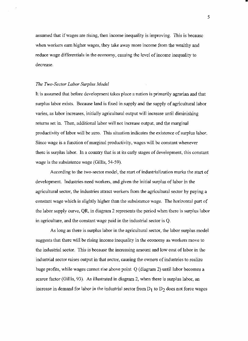
bull
5
assumed that if wages are rising then income inequality is improving This is because
when workers earn higher wages they take away more income from the wealthy and
reduce wage differentials in the economy causing the level of income inequality to
decrease
The Two-Sector Labor Surplus Model
It is assumed that before development takes place a nation is primarily agrarian and that
surplus labor exists Because land is fixed in supply and the supply of agricultural labor
varies as labor increases initially agricultural output will increase until diminishing
returns set in Then additional labor will not increase output and the marginal
productivity of labor will be zero This situation indicates the existence of surplus labor
Since wage is a function of marginal productivity wages will be constant whenever
there is surplus labor In a country that is at its early stages of development this constant
wage is the subsistence wage (Gillis 54-59)
According to the two-sector model the start of industrialization marks the start of
development Industries need workers and given the initial surplus of labor in the
agricultural sector the industries attract workers from the agricultural sector by paying a
constant wage which is slightly higher than the subsistence wage The horizontal part of
the labor supply curve QR in diagram 2 represents the period when there is surplus labor
in agriculture and the constant wage paid in the industrial sector is Q
As long as there is surplus labor in the agricultural sector the labor surplus model
suggests that there will be rising income inequality in the economy as workers move to
the industrial sector This is because the increasing amount and low cost of labor in the
industrial sector raises output in that sector causing the owners of industries to realize
huge profits while wages cannot rise above point Q (diagram 2) until labor becomes a
scarce factor (Gillis 93) As illustrated in diagram 2 when there is surplus labor an
increase in demand for labor in the industrial sector from D1 to D2 does not force wages
bull 6
Supply ofLabor in the Industrial Sector Using the Labor Surplus Model
Wages
e ---- ------ - --------- shy
d ------------------ -- shy
~ 1----gt----gt----
D3
Labor
DIAGRAM 2
bull
7
to rise Thus although workers earn more than subsistence wage by moving to the
industrial sector which should decrease the overall level of income inequality the huge
profit of capitalists rises faster and dominates the level of income inequality so that
overall income inequality increases
When surplus labor ceases to exist in agriculture further increases in demand for
labor by industries will lead to higher wages in the industrial sector and at the same time
workers in the agricultural sector become better off since the supply of agricultural labor
is decreasing Thus there will be an improvement in the overall level of income
inequality The point at which labor becomes scarce is point R and marks the start of a
trend towards income equality The supply curve facing the industrial sector becomes
RS an upward sloping curve which indicates that labor is in scarce supply Those
remaining in agriculture are better off for the following reasons Workers in the
industrial sector are no longer producing their own food causing the demand for
agricultural products to increase and consequently the price of these products to be
higher Moreover the available land per worker in the agricultural sector is rising and
thus the marginal productivity of labor in the agricultural sector also rises Increasing
marginal productivity in the agricultural sector implies that wages in this sector are also
rising Thus to attract more workers from agriculture industries must offer even higher
wages than those existing in the agricultural sector (Gillis 53) Thus in diagram 2 an
increase in demand for labor in the industrial sector from D3 to D4 raises wages from d to
e which would mean a decrease in the overall level of income inequality
The initial worsening followed by an improvement in the level of income
inequality is consistent with Kuznets inverted U hypothesis That is the labor surplus
model supports the inverted U Because the labor surplus model is based on the
migration oflabor to the industrial sector it supports the argument that the share oflabor
in industry should first increase then decrease the level of income inequality
bull
8
The Effect of Population Growth Rates
It is stated that one reason why developing countries have high degrees of income
inequality at relatively high levels of industrialization is because of rapid population
growth in these countries (Dovring 91) Countries like South Korea and Taiwan that
have succeeded in improving income distribution adopted measures to control population
growth as one ofthe necessary tools (Frank 102) Moreover other studies have shown a
positive relationship between high population growth rates and income inequality
(Chenery et aI 17)
These observations support the argument that high population growth rates will
cause the level of income inequality to increase for any given level of PCY Given that a
country does not have perfect income equality at the start of its development process the
countrys inverted U curve will intersect the income inequality axis at a point other than
zero
The argument given here is that high population growth rates will shift the
countrys inverted U curve upward so that the curve intersects the income inequality axis
at a higher point than before indicating an increase in the level of income inequality for
any given PCY This argument is illustrated in diagram 3 Higher population growth
rates causes the curve to shift from A to B and the intercept of the curve to rise from 02
to 05 for example (measurement of income inequality is the gini coefficient - see
appendix 2) Thus at PCY of 300 the level of income inequality also rises from 04 to
06 Therefore population growth rates can be said to determine the intercept of the
inverted U An economy with a low population growth rate will have a lower intercept
than a country with high population growth rates That is the higher the intercept of the
inverted U curve of a country the higher the level of income inequality for any given
PCY
bull
9
Strong support for the argument that high population growth rates are positively
related to the level of income inequality is provided by the two-sector labor surplus
model and the theory of supply and demand As previously discussed the labor surplus
model suggests that a country first has a period of worsening income inequality followed
by a period of improvements in the level of income inequality During the period of
worsening income inequality there is surplus labor in the agricultural sector and income
inequality improves when labor becomes scarce Using the labor surplus model and the
theory of supply and demand it will be shown that high population growth rates are
positively related to the level of income inequality during the periods of abundant and
scarce supplies of labor
Diagram 4 shows the effect of rising population growth rates when there is
surplus labor in agriculture As discussed before BC indicates the period when income
inequality rises because the owners of industries are realizing huge profits due to the
growth of industries and low labor costs At point C income inequality will take a
downturn and further demand for labor by industries will cause wages to rise If the
population growth rate is not high then the supply curve of labor Sind should remain
BCD
However if the supply oflabor is increasing because of high population growth
rates then Sind will be ABCD The amount of surplus labor will become ABC which is
greater than BC that represents surplus labor when population growth rates are very low
Therefore when population growth rates are high it will take a longer time for the
economy to reach point C where all surplus labor is absorbed by industries and the
economy tends towards income equality Also labor costs will remain low for a longer
time causing the owners of industries to make greater profits than when population
growth rates are low This is because if population growth rates are relatively stable then
the time when labor becomes scarce comes sooner so that the owners of industries must
cut profits at an earlier stage to increase wages in order to hire more workers
10
Upward Shift of the Inverted U Curve
Income Inequality
d
b middot
800 PCY
DIAGRAM 3
-1 1
Lffect of High Population Growth Rates with Surplus Labor in the Economy
W~ges ages
D
A ~ __ __ __ _B+-- ----C
o o Labor
DIAGRAM 4
Effect ofHigh Population Growth Rates with Scarce Supply ofLabor in the Economy
Wages
81
Wl 82
~ I------~
W21--- _
Labor
DIAGRAMS
bull
12
In summary when surplus labor exists and a country finds itself along the upside of the
inverted U when its level of income inequality is rising high population growth rates
would further increase the level of income inequality for each PCY along this part of the
inverted U curve This is due to the widening of income differentials between industrial
owners and workers
If the country is at the stage when labor is in scarce supply then the supply curve
facing industries will be upward sloping Thus there will be improvements in the level
of income inequality because wages will increase whenever the demand for labor by
industries increases This is illustrated in diagram SA where S1 is the supply curve of
labor facing industries and an increase in their demand for labor from D1 to D2 raises
wages from a to b
An increase in the supply of labor at the stage of development when there is
scarcity of labor causes labor to be less scarce and reduces wages As shown in diagram
58 an increase in the supply of labor due to high population growth rates will cause the
supply curve to shift from Sl to S2 causing wages to fall from d to c Since falling
wages are linked with higher profits for industrial owners there would be an increase in
the level of income inequality Thus when labor is scarce and a country finds itself along
the downside of the inverted U high population growth rates will retard improvements in
the level of income inequality That is the level of income inequality will increase for
every PCY along the downside of the inverted U
Since it has been shown that high population growth rates shift both the upside
and downside of the inverted U curve upward it is clear that high population growth rates
shift the inverted U curve upward When this upward shift occurs the inverted U will
intercept the income inequality axis at a higher point implying that the level of income
inequality will rise for any given level ofPCY
bull
13
Effect of Education
Education is important because it allows people to contribute effectively towards the
growth of the economy Education also improves the level of income inequality by
eliminating skill differentials which reduce wage differentials This is because education
facilitates higher labor productivity which leads to higher labor income
The effect of education on income inequality is given by Lewis who focuses on
the differentials between skilled and unskilled labor As an economy grows industries
expand and they demand more skilled and unskilled labor But at the early stages of
development there will be a scarce amount of literate people to carry out for example
supervisory and administrative tasks Because of this scarcity of skilled workers
compared to the abundant supply of unskilled workers wage differentials between the
two groups of workers will widen Skilled workers will see increases in their wages
while the wages of unskilled workers may even fall if the supply of unskilled workers
increases (Lewis 180-181) The initial widening of wage differentials that results
between the two groups of workers causes a worsening of the level of income inequality
in the economy
However as the economy grows and educational facilities spread to a larger
proportion of the population in the long run skilled workers in the country will increase
causing the wages of skilled workers to fall (Lewis 180-181) Thus wage differentials
between the skilled and unskilled workers will reduce causing the level of income
inequality to improve The initial worsening followed by improvements in the level of
income inequality that is caused by the widening and then narrowing of wage
differentials is consistent with the inverted U pattern Thus it is argued here that
initially education is likely to be positively related before it becomes negatively related
to the level of income inequality
bull
14
More support for the fact that education affects the level of income inequality is
shown by the need for expansion of education systems worldwide and in the studies of
many economists Compulsory education is widely accepted as an important public
service and every country has some form of compulsory education (Eckstein 1992)
Eckstein and Zilcha show empirically that human capital affects the quality of labor and
that compulsory education will improve the distribution of income through generations
(Eckstein 1992) If education improves labor and causes higher wages then compulsory
education should improve the level of income inequality Also Chenery and Syrquin
found that education removes income away from the richest 20 and increases income of
the lowest 40 (Chenery 63) More interestingly where primary and secondary
schooling were found to be positively related to income shares obtained by individuals it
was also shown that primarily schooling significantly explained variations in income for
the lowest 40 and secondary education significantly explained those of the middle
40(Chenery et aI 17) This finding helps explain why emphasis is often placed at least
on compulsory primary schooling in many developing nations It can be said that the aim
is to improve the lot of the very poor
Hypotheses
The discussions above generate four hypotheses
I The inverted U exists supported by the fact that the labor surplus model
predicts the inverted U pattern
II The share of labor in industry is initially positively related then negatively related
to the level of income inequality
III Population growth rates are positively related to the level of income
inequality at any stage of development Higher population growth rates are
associated with higher income inequality
bull
15
IV It is likely that education is initially positively related before it becomes
negatively related to the level of income inequality
Research Design
Data on 61 countries mainly low-income and middle-income countries are used in this
study (see Appendix 1) The measure of income inequality used is the gini coefficient
This coefficient is calculated from a Lorenz curve that is constructed using data on
income distribution of a given country Appendix 2 gives an explanation of how gini
coefficients are calculated I created a program in Pascal to calculate this coefficient
based on the Lorenz curve the formula for the area of trapezoids and the formula for the
coefficient
Data on income distribution share of labor in industry and population growth
rates were obtained from the World Banks publication Social Indicators of Development
1991-92 Primary and secondary school enrollments are used as a measure of the
expansion of education and the data for these variables were also obtained from the
Social Indicators of Development Data for all variables are not given annually but for
periods of time This is possibly due to the fact that data on variables such as the income
distribution in a country are collected less frequently The periods for which data are
reported are 25-30 years ago 15-20 years ago and the most recent period
PCY Groups
When I plotted gini coefficients for the countries used in this study all the points were
crowded so that no pattern was observed When I tried to observe patterns using PCY
groups I found an inverted U pattern According to the inverted U pattern I found the
upside ofthe inverted U existed for countries with PCY up to $300 (dollar amounts are
bull
16
1990 current market prices in US dollars) There was no clear trend for countries with
PCY between $300 and $1000 but there was clear evidence of the downside ofthe
inverted U starting with countries with PCY about $1000 and higher Diagram 6
illustrates the inverted U pattern that I found using plotted graphs PCY Group I will
refer to countries with PCY less than or equal to $300 PCY Group II will refer to
countries with PCY between $300 and $1000 and PCY Group III will refer to countries
with PCY greater than $1000
Table 1 which shows regression results for the PCY groups identified above
verifies the inverted U pattern that was observed using plotted graphs The PCY2 term is
included since the inverted U pattern is quadratic According to Table 1 there is an initial
worsening of income inequality for PCY Group I judging from the positive significant
sign of the PCY variable The results for PCY Group II does not indicate any significant
pattern and confirms that a horizontal line best represents the trend of income inequality
for this PCY group For PCY Group III there is strong evidence of decreasing income
inequality which is indicated by the negative significant sign of the PCY variable Thus
the results shown in this table confirm that the inverted U pattern exists In Appendices
34 and 5 the regression lines for PCY Group I II and III drawn against the plotted data
for the PCY groups respectively are shown Put together the regression lines of the three
PCY groups also show the inverted U pattern I found using plotted graphs Later on we
will see whether the labor surplus model supports that this inverted U pattern exists
My findings using plotted graphs and regression models discussed above are good
findings since they posit that the phase of worsening income inequality ends earlier than
expected at PCY of about $300 and that the point at which income inequality starts it
downward trend also occurs earlier at PCY of about $1000 As previously mentioned
according to the inverted U pattern it is expected that income inequality worsens up to
PCY of about $2200 before it starts to improve
17
PCYGroups
Income In shyegua 1
inverted U pattern
PCYGroupll
middot300 1000 PCY
DIAGRAM 6middotshy -~ - -~-
Table 1 INVERTED U PATTERN
VARIABLES
PCY
PCYlt=300
(+)
+000262
300ltPCYlt= 1000
-000012
PCYgt1000
(-) -000003
-
PCY2 (-) -000001
+000000 (+) +000000
= significant at the 90 confidence level signs in parentheses are the hypothesized signs
bull
18
Models
To test the hypotheses in this paper several regression models are created and tested for
each PCY group On an aggregate level the regression results for all three PCY groups
will test the four hypotheses In these models Industry represents the share of labor in
industry PopRate represents population growth rates and Primary and Secondary
represent primary and secondary school enrollments respectively Table 2 clearly presents
the variables used in this study and their definitions OLS regressions were used to test
the models
For each PCY group Modell includes all the variables and tests all four
hypothesis Models 2 and 3 attempt to improve Modell The equation for Model 1 is
Gini = Constant + PCY + PCy2 + Industry + Industry2 + PopRate + Primary +
Primary2 + Secondary + Secondary2
[Equation 1]
Again the squared terms are included since the inverted U pattern is a quadratic curve
PopRate2 is not included in the equation above because PopRate is hypothesized to
always be positively related to the level of income inequality
According to the hypothesis for PCY Group I it is expected that in the regression
result for Modell the PCY term will be positive and significant This result will
confirm the upside of the inverted U Industry is expected to be positive and significant
to imply that during the early stages of development rural to urban migration causes the
economy to experience worsening levels of income inequality High population growth
rates should always worsen the level of income inequality and therefore a positive and
significant sign is expected for PopRate Primary and Secondary are also expected to be
positive and significant since a country at its early stage of development is likely to have
large wage differentials between the few literate people who receive high wages and the
masses of illiterate people who receive very low wages
bull 19
TABLE 2 DEFINITION OF VARIABLES
VARIABLES DEFINITIONS
PCY GNP per capita Estimates are for 1990 at current market prices in US dollars
INDUSTRY Labor force in mining manufacturing construction electricity water and gas as a percentage of the total labor force
POPRATE Population growth rate Annual growth rate calculated from mid year total and urban population
PRIMARY Primary school enrollmen t Gross enrollment of all ages at primary level as a percentage of school age children as defined by each country and reported to UNESCO
SECONDARY Secondary school enrollment Computed in the same manner as the primary school ratio
Source = Social Indicators of Development 1991 -92
bull
20
For PCY Group II the regression result for Modell will likely indicate nothing
significant as is implicated by the results presented in Table 1
For PCY Group III a negative significant sign is expected for the PCY variable to
confirm the downside of the inverted U Industry is also expected to be negative and
significant since countries in this group should have competitive labor markets so that
higher demands of labor increase wages PopRate is expected to be positive and
significant Primary and Secondary are expected to be negative and significant This is
because at the later stages of development there should be more literate people in the
labor force which should cause wage differentials to reduce and income inequality to
decrease
Results Conclusions and Policy Implications
Tables 3 4 and 5 show the regression models for PCY Group I II and III respectively
PCY Group I (The early stage of development)
Results
Table 3 shows the results for this group Modell which contains all the variables is a
good model judging from its R2 of 080 All the variables are significant except for
Primary and Primary 2 Secondary and Secondary2 have unexpected signs In Model 2
where the Secondary variables are excluded the R2 becomes 054 and only PopRate is
significant However the Primary variables have the expected signs Model 3 appears to
be the best model in which the Primary variables are excluded All the variables in this
model are significant and the model has an R2 of 080 However the Secondary
variables have the unexpected signs
bull
21
TABLE 3 GINI REGRESSIONS FOR PCY lt=300
VARIABLE MODEL 1 MODEL 2 MODEL 3
PCY (+ ) +000428
(+) +000110
(+ ) +000191
PCy2 ( shy )
-000001 ( shy )
-000002 ( - )
-000001
INDUSTRY (+ ) +015718
(+ ) +002127
(+ ) +008700
INDUSTRy2 ( shy )
-000786 ( shy )
-000092 ( shy )
-000414
POPORATE (+ ) +017821
(+) +007699
(+ ) +010363
PRIMARY (+ ) -000240
(+ ) +000247
PRIMARy2 ( shy )
+000000 ( - )
-000002
SECONDARY (+ ) -001823
(+ ) -001467
SECONDARy2 ( shy )
+000047 ( shy )
+000030
ADJUSTED R2
080 054 080
= significant at 90 confidence level (two-tail test) Signs in parentheses are the hypothesized signs
bull
22
Given that Model 3 is the best model it will be used to estimate the impact of
each variable on income inequality The equation for Model 3 is
Gini = -02636 + 0002PCY - 0000PCy2 + 0087Industry shy
0004Industry2 + 01 0363PopRate - 00 I5Secondary +
0000Secondary2
[Equation 2]
The positive sign and significance of the PCY variable in Model 3 confirm the
initial positive relationship between PCY and income inequality The positive and
significant sign of Industry is consistent with the labor surplus models prediction that at
the initial stages of development an increase of workers in the industrial sector worsens
the level of income inequality The result for PopRate supports that high population
growth rates are positively related to the upside ofthe inverted U This result is also
consistent with the explanation provided by the labor surplus model that high population
growth rates will increase the amount of surplus labor in this PCY group and worsen
income inequality The unexpected results for the Primary variables may be due to the
fact that this variable is not lagged The unexpected significant result for Secondary is an
important finding and can be explained as follows
At PCY less than $300 it is likely that secondary school enrollments are not
high However an increase in secondary school enrollments implies that there is likely
an increase in primary school enrollments Since at the early stage of development most
primary school graduates enter the labor force an increase in secondary school
enrollments also implies that more primary school graduates are entering the labor force
Therefore secondary school enrollment may be proxying for more people in the labor
force with primary school education who because of their primary school education
should be making higher wages More people making higher wages reduces wage
bull
23
differentials which improves income inequality This explanation is consistent with the
result obtained from the Secondary variable
Conclusions and Policy Implications
As explained in Appendix 2 where the method ofcalculating gini coefficient is
discussed the value of the gini coefficient lies between 1 and O The closer the
coefficient is to 0 the lower the level of income inequality The closer the gini coefficient
is to I the higher the level of income inequality From Equation 2 above it is deduced
that an increase ofPCY by $1 will cause the gini coefficient to rise by 0002 This means
that an increase ofPCY by $50 causes the gini coefficient to rise by a tenth (01) This
result is significant and posits that when a country begins its development process and
PCY increases the initial worsening of income inequality is inevitable Thus for
countries with PCY up to about $300 a worsening trend of income inequality can be
accepted as an initial phase that accompanies development
According to Equation 2 above a percentage increase of labor in industry (the
variable Industry) causes the gini coefficient to increase by 0087 Thus a 115
percentage increase of labor in the industrial sector causes the gini coefficient to rise by
about a tenth This result is also significant and implies that about a 9 percent increase of
labor in industry will cause the level of income inequality to be at the highest possible
level Therefore the results suggest that developing countries within PCY Group I
should not only concentrate on the developing the industrial sector but should
simultaneously concentrate on developing the agricultural sector That way they may be
able to reduce the amount of migrants from agriculture into industry
How much income inequality exists at the early stages of development depends
significantly on population growth rates The higher the population growth rate the
bull
24
higher is the level of income inequality at each PCY According to Equation 2 a 1
percentage increase in population growth rates causes the gini coefficient to rise by 0104
This implies that an increase of population growth rate by 096 percent (approximately 1
percent) causes the gini coefficient to rise by a tenth This result points out that it is
necessary for developing countries to adopt measures to control population growth rates
as early as possible in their development process By maintaining low population growth
rates and as according to the labor surplus model labor in the economy becomes a scarce
factor earlier and labor markets are competitive sooner Then also wages should
increase and income inequality should improve
If Secondary is accepted as a proxy for the amount of primary school graduates
entering the labor force then as calculated from Equation 2 a 667 increase of primary
school graduates entering the labor force (ie 667 increase in secondary school
enrollment) should decrease the gini coefficient by a tenth This is a significant and
encouraging result because it emphasizes the universal benefits of education even at the
early stages of development
PCY Group II (The intermediate stage of development)
Results
All the models created for this PCY group show no significant result as noted in Table 4
None of the variables are significant and the R2s for all the models are very low The
results confirm that the curve is a straight line for this PCY group
Conclusion
The results for PCY Group II does not allow one to make any generalizations applicable
to countries in this PCY group today Perhaps conditions in these countries are complex
and varied and therefore cannot be easily summarized
bull 25
TABLE 4 GINI REGRESSIONS FOR 300 lt PCY lt= 1000
VARIABLE MODEL 1 MODEL 2 MODEL 3
PCY 000004 000005 000008
PCy2 -000000 -000000 -000000
INDUSTRY -000842 -000720 -000836
INDUSTRy2 -000000 -000004 000002
POPRATE -002217 -002602 -000794
PRIMARY 001063 001068
PRIMARy2 -000006 -000006
SECONDARY 000171 000232
SECONDARy2 -000002 -000002
ADJUSTED Rl -007 005 002
bull 26
VARIABLES MODEL 1 MODEL 2 MODEL 3
PCY ( - )
-000002 ( - )
-000001 ( - )
-000002
PCy2 (+ ) +000000
(+ ) +000000
(+ ) +000000
INDUSTRY ( - )
-000460 ( - )
-001577 ( shy )
-000720
INDUSTRy2 (+ ) 000007
( + ) +000024
(+ ) 000012
PORPORATE (+ ) -001515
(+ ) +000806
(+ ) -001960
PRIMARY ( shy )
-001664 ( shy )
-005207
PRlMARy2 (+ ) +000008
(+ ) +000024
SECONDARY ( shy )
-000971 ( - )
-000866
SECONDARy2 (+ ) +000006
(+ ) +000005
ADJUSTED Rl 050 044
= SIGNIFICANT AT THE 90 CONFINDENCE LEVEL (TWO-TAIL TESr SIGNS IN PARENTEHESES ARE THE HYPOTHESIZED SIGNS
TABLE 5 GINI REGRESSIONS FOR PCY gt 1000
bull
27
PCY Group III (The industrialized stage of development)
Results
Only the education variables have significant coefficients in the models in Table 5 The
PCY variables in this table are not significant although they are in Table 1 This is
possibly because the explanatory variables in the regression equations for the models in
Table 5 (these explanatory variables are not included in the regression equation for Table
1) reduce the significance of the PCY variable The significant and expected coefficient
for Secondary in the models supports Lewis explanation that as an economy develops
education facilities become available to more people so that in the long run education has
a negative effect on the level of income inequality
Conclusion
Since countries in PCY Group III are well industrialized the increasing share of labor in
industry may have little impact on the level of income inequality Likewise population
growth rates which are relatively stable in these countries may have negligible effect on
the level of income inequality It is likely that there are other variables that may help
explain the downward trend of income inequality that is expected for industrialized
countries Often countries in the early stages of development experience political and
social instabilities conditions which improve as these countries develop Thus a measure
of political and social conditions may for instance be a crucial determinant of the
downward trend of income inequality It is also likely that the existence of certain
institutions in industrialized countries like unions that function to improve wages help
improve the level of income inequality in these countries Thus a measure of
unionization may also improve the results for this group Another variable that measures
bull
28
U This is because it is usual to find more advanced technological equipment and
facilities in industrialized countries and not in developing countries In summary the
share of labor in industry and population growth rates do not explain the downside of the
inverted U
General Conclusion
In this paper four hypothesis were generated and tested to confirm that the inverted U
exists and that the share of labor in industry population growth rates and education were
explanatory variables of income inequality Moreover the labor surplus model predicts
the inverted U pattern Although the inverted U pattern was found as presented in Table 1
where only PCY variables were used in the regression equation the explanatory variables
failed to show the inverted U pattern in its entirety The explanatory variables were able
to explain the upside of the inverted U as shown in Table 3 but the same explanatory
variables could not explain the downside of the inverted U as shown in Table 5
Thus this study also shows that the labor surplus model explains the upward trend
for countries with very low PCY and that high population growth rates worsen the level
of income inequality for these countries This study highlights that the labor surplus
model is incapable of explaining any other part of the inverted U especially the downside
of the inverted U
Suggestions For Future Research
Another explanation for the inverted U pattern can be given using labor market power as
follows At the early stages of development firms have monosony power and can force
the technological know-how in the various countries may also help explain the inverted
bull
29
wages to be low which signifies a period of worsening income inequality At the
intermediate stage of development more firms may exist which may cause the initial
monosony power of firms to reduce and at least prevent further worsening of income
inequality At the industrialized stage of development workers are likely to organize into
unions and counter the remaining monosony power of firms This should increase wages
and cause income inequality to improve This brief discussion suggests an important area
for future research Perhaps a better explanation of the inverted U pattern or an important
area to be considered along with the labor surplus model may be discovered
Another area for future research will be to separate the countries in PCY Group III
(countries that have PCY greater than $1000) into two categories the newly industrialized
and the well industrialized countries This may help control for the wide range of PCY in
PCY Group III and also the differences in institutions that exist in these countries
bull
30
WORK CITED
Ahluwalia Montek S 1976 Inequality Poverty and Development Journal of Development
Economics 3306-342
Braun Denny The Rich Get Richer The Rise ofIncome Inequality in the United States and the World
Chicago Nelson-Hall Publishers 1991
Chenery Hollis Ahluwalia S Montek C L G Bell John H Duloy Richard Jolly Redistribution
with ~rowth London Oxford University Press 1975
Chenery Hollis amp Moises Syrquin Patterns of Development 1950-1970 Published for the World Bank
by Oxford University Press 1975
Dovring Folke Inequality New York Praeger Publishers 1991
Eckstein Zvi amp Zilcha Itzhak 1992 The effects of compulsory schooling on growth
income distribution and welfare Journal of Public Economics 543339-359
Fields Gary F Poverty Inequality and Development London Cambridge University Press 1980
Gillis Malcom Economics of Development New York WW Norton amp Company 1992
Lewis W Arthur Theory of Economic Growth New York Harper Row 1970
Poulson Barry W Economic Development Minneapolis West Publishing Company 1994
APPENDIX 1shy
bull
~Cgt -ntneG time gini pey PopPate indu~ primary r
3an~1lade 25-30 030 7000 26 48 31
ncilet 25-30 036 9000 23 119 74
Paki~tan 25-30 034- 11000 26 183 40
Pak~tan 15-20 0294 130 31 172 12
Banglade 15-20 0316 130 25 54 73 Thailand 25-30 039 14000 31 52 78
0ri Lanka 25-30 041 16000 25 139 93
India 15-20 037 17000 23 129 79
Tanzania 15middot20 038 17000 28 38 53 Phiflipine 25-30 045 18000 31 158 113
Indonesia 15-20 038 21000 24 117 86
Uganda 15-20 036 22000 26 39 44 Sierra Le 15middot20 040 22000 2 132 39
Kenya 15-20 049 23000 37 62 95 0ri Lanka 15-20 032 29000 16 142 77 Mauritius 25-30 040 31000 24 254 72
Egypt 15-20 038 32000 2 184 71
Columbia 2~30 O~6 32000 3 214 84 Phillipine 15-20 043 34000 26 161 107 Botswana 15-20 050 35000 38 84 72
Bolivia 15-20 046 36000 25 199 85 0uriname 25-30 029 39000 27 215 120
Costa Ric 25-30 045 40000 32 192 106 Liberia 15-20 055 41000 3 94 62 Mexico 25-30 049 46000 33 219 92 Ecuador 15-20 059 54000 3 202 104
Zambia 15-20 050 55000 3 92 97
Columbia 15-20 047 55000 21 234 118 Guatemal 15-20 046 57000 28 17 61
Nicaragu 15-20 052 63000 3 156 82
Spain 25-30 035 70000 1 345 115
Tunisia 15-20 034 71000 21 311 97 Mauritius 15-20 043 71000 15 245 107
Libya 25-30 024 81000 39 209 78
Malaysia 15-20 045 82000 23 166 91 Argentina 25-30 038 87000 15 342 101
Japan 25-30 037 90000 11 32 100 Costa Ric 15-20 045 95000 25 216 107
Peru 15-20 052middot 100000 27 18 113
bull
Fiji 15-20 038 03000 i 9 160 115
Brazil 15-20 051 1070gt 24shy 243 88
Venezuel 25-30 048 113000 34 237 94
Israel 25-30 030 130000 35 354 95 Barbados 15-20 032 152000 04 233 103
Portugal 15-20 038 154000 38 347 113 Netherlan 25-30 039 156000 14 407 104
Trinidad 15-20 041 172000 09 372 99
Finland 25-30 042 175000 03 354 92 rmiddotJnrway 25-30 032 184000 08 368 97
France 25-30 046 203000 09 39 134
Denmark 25-30 035 205000 08 369 98 Venezuel 15-20 045 238000 36 267 97
Canada 25-30 030 262000 18 325 105
Ireland 15-20 029 265000 17 324 103 Sweden 25-30 036 276000 09 428 95
Spain 15-20 034 278000 1 374 111 I~rael 15-20 028 389000 23 337 97
rrance 15-20 036 600000 05 373 109
Germany 15-20 033 667000 -04 476 103 Sweden 15-20 027 832000 04 365 101
Australia Recent 034 1668000 16 344 106
bull APPENDIX 2
Calculatin2 Gjni Coefficjents
To convert the figures of an income distribution data into a measure of
income inequality can be done by constructing a Lorenz curve for each
country from which the Gini coefficientconcentration ratio(a measure of
inequality) is calculated The Lorenz curve shows the total percentage of
total income accounted for by any cumulative percentage of recipients
The shape of this curve indicates the degree of income inequality in the
income distribution(Gillis 1992 74) To illustrate how a Lorenz curve is
derived consider the following data for Brazil in 1983
poorest 20 of households receive 24 of total income
second quintile receive 57
third quintile receive 107
fourth quintile receive 186
richest 20 receive 626
From these data it can be observed that Brazil has a high degree of
inequality if 626 of its total income goes to the richest 20 of total
households Also a total of 100 of households receive 100 of total
income To construct a Lorenz curve first the cumulative income share
accruing to any given percentage of households is calculated Thus for the
data above we get the following calculations
poorest 20 receive 24 of total income
poorest 40 receive 24 + 57 = 81 of total income
poorest 60 receive 81 + 107 = 188 of total income
poorest 80 receive 188 + 186 = 374 of total income
100 of households receive 100 of total income
bull
The Lorenz curve is a graph plotted from the data above with the
horizontal axis measuring the cumulative percentage of recipient units and
the vertical axis measunng the cumulative share of total income
Diagram2 below shows the Lorenz curve obtained from the data above
J
J~
t
1
I
l
~ 1 IA I
I
~ [J I
J 1
Diagram2
(Bolnick 1987 61-62)
The diagonal line is a 45-degree line The closer the curve is to this line
the lesser is income inequality The closer it is to the right hand borders
the greater is income inequality(Gillis 1992 74)
To calculate the Gini coefficient let A be the area between the Lorenz
curve and the diagonal line and let B be the area under the Lorenz curve
as show in Figure 2 The formula to calculate the Gini coefficient is given
as
bull
A(A + B) A + B will always be 05 because the box in which the Lorenz
curve is drawn is a unit square especially seen if all percentages are taken
as decimal units eg 20 as 02 Therefore the area of the square becomes
lxl = 10 and half the area of the square (A + B) is 05(Bolnick 1987 62)
Area B can be calculated geometrically using formulas for calculating areas
of rectangles triangles and trapezoids The area of B was calculated
geometrically to be 0233 Since A + B = 05 A = 05 - 0233 = 0267 The
Gini Coefficient AlA + B) = 026705 = 0534 The closer the Gini
coefficient is to 0 the lesser is income inequality and the closer it is to 1
the greater is income inequality
I created a program in Pascal that calculates gini coefficients based
on the Lorenz curve the formula for the area of trapezoids and the
formula for the gini coefficient
bull bull
045
03
bull
APPENDIX 3
REGRESSION LINE DRAWN AGAINST PLOTTED DATA FOR pey GROUP I
05--------------------------------bull
04
035 bull
bull bull
bull bull
bull
bull bulli~t=-+~=
bull
bull
025l-------r------r--r-------------_r-----r---------------------------r-----------J 7000 13000 16000 18000 22000
bull bull
bull bull bull
APPENDIX 4
REGRESSION LINE DRAWN AGAINST PLOTTED DATA FOR pey GROUP II
bull
06-------------------------------------
055 bull
bull bullbullbull 05 bull bull bullbullA45
bull 04 bull
035 bull
bull 03
bull
025
bull
O 2--L--------------------------------------------r----------------------r----------------------------------------r---r---l
31000 34000 39000 46000 55000 70000 81000 90000
bull bull
APPENDIX 5
REGRESSION LINE DRAWN AGAINST PLOTTED DATA FOR pey GROUP III
bull
0S5------------------------------
05 bull
bull045 bull
bull ~ 04
bull~ 035 bull
03
bull bull 025
02
01 f0-+-0-0--2-0-r-0-0--3-000--40-0-0--S-OO-0--610010--700-0--8-00-0--9---1000
PCY
bull

bull
7
to rise Thus although workers earn more than subsistence wage by moving to the
industrial sector which should decrease the overall level of income inequality the huge
profit of capitalists rises faster and dominates the level of income inequality so that
overall income inequality increases
When surplus labor ceases to exist in agriculture further increases in demand for
labor by industries will lead to higher wages in the industrial sector and at the same time
workers in the agricultural sector become better off since the supply of agricultural labor
is decreasing Thus there will be an improvement in the overall level of income
inequality The point at which labor becomes scarce is point R and marks the start of a
trend towards income equality The supply curve facing the industrial sector becomes
RS an upward sloping curve which indicates that labor is in scarce supply Those
remaining in agriculture are better off for the following reasons Workers in the
industrial sector are no longer producing their own food causing the demand for
agricultural products to increase and consequently the price of these products to be
higher Moreover the available land per worker in the agricultural sector is rising and
thus the marginal productivity of labor in the agricultural sector also rises Increasing
marginal productivity in the agricultural sector implies that wages in this sector are also
rising Thus to attract more workers from agriculture industries must offer even higher
wages than those existing in the agricultural sector (Gillis 53) Thus in diagram 2 an
increase in demand for labor in the industrial sector from D3 to D4 raises wages from d to
e which would mean a decrease in the overall level of income inequality
The initial worsening followed by an improvement in the level of income
inequality is consistent with Kuznets inverted U hypothesis That is the labor surplus
model supports the inverted U Because the labor surplus model is based on the
migration oflabor to the industrial sector it supports the argument that the share oflabor
in industry should first increase then decrease the level of income inequality
bull
8
The Effect of Population Growth Rates
It is stated that one reason why developing countries have high degrees of income
inequality at relatively high levels of industrialization is because of rapid population
growth in these countries (Dovring 91) Countries like South Korea and Taiwan that
have succeeded in improving income distribution adopted measures to control population
growth as one ofthe necessary tools (Frank 102) Moreover other studies have shown a
positive relationship between high population growth rates and income inequality
(Chenery et aI 17)
These observations support the argument that high population growth rates will
cause the level of income inequality to increase for any given level of PCY Given that a
country does not have perfect income equality at the start of its development process the
countrys inverted U curve will intersect the income inequality axis at a point other than
zero
The argument given here is that high population growth rates will shift the
countrys inverted U curve upward so that the curve intersects the income inequality axis
at a higher point than before indicating an increase in the level of income inequality for
any given PCY This argument is illustrated in diagram 3 Higher population growth
rates causes the curve to shift from A to B and the intercept of the curve to rise from 02
to 05 for example (measurement of income inequality is the gini coefficient - see
appendix 2) Thus at PCY of 300 the level of income inequality also rises from 04 to
06 Therefore population growth rates can be said to determine the intercept of the
inverted U An economy with a low population growth rate will have a lower intercept
than a country with high population growth rates That is the higher the intercept of the
inverted U curve of a country the higher the level of income inequality for any given
PCY
bull
9
Strong support for the argument that high population growth rates are positively
related to the level of income inequality is provided by the two-sector labor surplus
model and the theory of supply and demand As previously discussed the labor surplus
model suggests that a country first has a period of worsening income inequality followed
by a period of improvements in the level of income inequality During the period of
worsening income inequality there is surplus labor in the agricultural sector and income
inequality improves when labor becomes scarce Using the labor surplus model and the
theory of supply and demand it will be shown that high population growth rates are
positively related to the level of income inequality during the periods of abundant and
scarce supplies of labor
Diagram 4 shows the effect of rising population growth rates when there is
surplus labor in agriculture As discussed before BC indicates the period when income
inequality rises because the owners of industries are realizing huge profits due to the
growth of industries and low labor costs At point C income inequality will take a
downturn and further demand for labor by industries will cause wages to rise If the
population growth rate is not high then the supply curve of labor Sind should remain
BCD
However if the supply oflabor is increasing because of high population growth
rates then Sind will be ABCD The amount of surplus labor will become ABC which is
greater than BC that represents surplus labor when population growth rates are very low
Therefore when population growth rates are high it will take a longer time for the
economy to reach point C where all surplus labor is absorbed by industries and the
economy tends towards income equality Also labor costs will remain low for a longer
time causing the owners of industries to make greater profits than when population
growth rates are low This is because if population growth rates are relatively stable then
the time when labor becomes scarce comes sooner so that the owners of industries must
cut profits at an earlier stage to increase wages in order to hire more workers
10
Upward Shift of the Inverted U Curve
Income Inequality
d
b middot
800 PCY
DIAGRAM 3
-1 1
Lffect of High Population Growth Rates with Surplus Labor in the Economy
W~ges ages
D
A ~ __ __ __ _B+-- ----C
o o Labor
DIAGRAM 4
Effect ofHigh Population Growth Rates with Scarce Supply ofLabor in the Economy
Wages
81
Wl 82
~ I------~
W21--- _
Labor
DIAGRAMS
bull
12
In summary when surplus labor exists and a country finds itself along the upside of the
inverted U when its level of income inequality is rising high population growth rates
would further increase the level of income inequality for each PCY along this part of the
inverted U curve This is due to the widening of income differentials between industrial
owners and workers
If the country is at the stage when labor is in scarce supply then the supply curve
facing industries will be upward sloping Thus there will be improvements in the level
of income inequality because wages will increase whenever the demand for labor by
industries increases This is illustrated in diagram SA where S1 is the supply curve of
labor facing industries and an increase in their demand for labor from D1 to D2 raises
wages from a to b
An increase in the supply of labor at the stage of development when there is
scarcity of labor causes labor to be less scarce and reduces wages As shown in diagram
58 an increase in the supply of labor due to high population growth rates will cause the
supply curve to shift from Sl to S2 causing wages to fall from d to c Since falling
wages are linked with higher profits for industrial owners there would be an increase in
the level of income inequality Thus when labor is scarce and a country finds itself along
the downside of the inverted U high population growth rates will retard improvements in
the level of income inequality That is the level of income inequality will increase for
every PCY along the downside of the inverted U
Since it has been shown that high population growth rates shift both the upside
and downside of the inverted U curve upward it is clear that high population growth rates
shift the inverted U curve upward When this upward shift occurs the inverted U will
intercept the income inequality axis at a higher point implying that the level of income
inequality will rise for any given level ofPCY
bull
13
Effect of Education
Education is important because it allows people to contribute effectively towards the
growth of the economy Education also improves the level of income inequality by
eliminating skill differentials which reduce wage differentials This is because education
facilitates higher labor productivity which leads to higher labor income
The effect of education on income inequality is given by Lewis who focuses on
the differentials between skilled and unskilled labor As an economy grows industries
expand and they demand more skilled and unskilled labor But at the early stages of
development there will be a scarce amount of literate people to carry out for example
supervisory and administrative tasks Because of this scarcity of skilled workers
compared to the abundant supply of unskilled workers wage differentials between the
two groups of workers will widen Skilled workers will see increases in their wages
while the wages of unskilled workers may even fall if the supply of unskilled workers
increases (Lewis 180-181) The initial widening of wage differentials that results
between the two groups of workers causes a worsening of the level of income inequality
in the economy
However as the economy grows and educational facilities spread to a larger
proportion of the population in the long run skilled workers in the country will increase
causing the wages of skilled workers to fall (Lewis 180-181) Thus wage differentials
between the skilled and unskilled workers will reduce causing the level of income
inequality to improve The initial worsening followed by improvements in the level of
income inequality that is caused by the widening and then narrowing of wage
differentials is consistent with the inverted U pattern Thus it is argued here that
initially education is likely to be positively related before it becomes negatively related
to the level of income inequality
bull
14
More support for the fact that education affects the level of income inequality is
shown by the need for expansion of education systems worldwide and in the studies of
many economists Compulsory education is widely accepted as an important public
service and every country has some form of compulsory education (Eckstein 1992)
Eckstein and Zilcha show empirically that human capital affects the quality of labor and
that compulsory education will improve the distribution of income through generations
(Eckstein 1992) If education improves labor and causes higher wages then compulsory
education should improve the level of income inequality Also Chenery and Syrquin
found that education removes income away from the richest 20 and increases income of
the lowest 40 (Chenery 63) More interestingly where primary and secondary
schooling were found to be positively related to income shares obtained by individuals it
was also shown that primarily schooling significantly explained variations in income for
the lowest 40 and secondary education significantly explained those of the middle
40(Chenery et aI 17) This finding helps explain why emphasis is often placed at least
on compulsory primary schooling in many developing nations It can be said that the aim
is to improve the lot of the very poor
Hypotheses
The discussions above generate four hypotheses
I The inverted U exists supported by the fact that the labor surplus model
predicts the inverted U pattern
II The share of labor in industry is initially positively related then negatively related
to the level of income inequality
III Population growth rates are positively related to the level of income
inequality at any stage of development Higher population growth rates are
associated with higher income inequality
bull
15
IV It is likely that education is initially positively related before it becomes
negatively related to the level of income inequality
Research Design
Data on 61 countries mainly low-income and middle-income countries are used in this
study (see Appendix 1) The measure of income inequality used is the gini coefficient
This coefficient is calculated from a Lorenz curve that is constructed using data on
income distribution of a given country Appendix 2 gives an explanation of how gini
coefficients are calculated I created a program in Pascal to calculate this coefficient
based on the Lorenz curve the formula for the area of trapezoids and the formula for the
coefficient
Data on income distribution share of labor in industry and population growth
rates were obtained from the World Banks publication Social Indicators of Development
1991-92 Primary and secondary school enrollments are used as a measure of the
expansion of education and the data for these variables were also obtained from the
Social Indicators of Development Data for all variables are not given annually but for
periods of time This is possibly due to the fact that data on variables such as the income
distribution in a country are collected less frequently The periods for which data are
reported are 25-30 years ago 15-20 years ago and the most recent period
PCY Groups
When I plotted gini coefficients for the countries used in this study all the points were
crowded so that no pattern was observed When I tried to observe patterns using PCY
groups I found an inverted U pattern According to the inverted U pattern I found the
upside ofthe inverted U existed for countries with PCY up to $300 (dollar amounts are
bull
16
1990 current market prices in US dollars) There was no clear trend for countries with
PCY between $300 and $1000 but there was clear evidence of the downside ofthe
inverted U starting with countries with PCY about $1000 and higher Diagram 6
illustrates the inverted U pattern that I found using plotted graphs PCY Group I will
refer to countries with PCY less than or equal to $300 PCY Group II will refer to
countries with PCY between $300 and $1000 and PCY Group III will refer to countries
with PCY greater than $1000
Table 1 which shows regression results for the PCY groups identified above
verifies the inverted U pattern that was observed using plotted graphs The PCY2 term is
included since the inverted U pattern is quadratic According to Table 1 there is an initial
worsening of income inequality for PCY Group I judging from the positive significant
sign of the PCY variable The results for PCY Group II does not indicate any significant
pattern and confirms that a horizontal line best represents the trend of income inequality
for this PCY group For PCY Group III there is strong evidence of decreasing income
inequality which is indicated by the negative significant sign of the PCY variable Thus
the results shown in this table confirm that the inverted U pattern exists In Appendices
34 and 5 the regression lines for PCY Group I II and III drawn against the plotted data
for the PCY groups respectively are shown Put together the regression lines of the three
PCY groups also show the inverted U pattern I found using plotted graphs Later on we
will see whether the labor surplus model supports that this inverted U pattern exists
My findings using plotted graphs and regression models discussed above are good
findings since they posit that the phase of worsening income inequality ends earlier than
expected at PCY of about $300 and that the point at which income inequality starts it
downward trend also occurs earlier at PCY of about $1000 As previously mentioned
according to the inverted U pattern it is expected that income inequality worsens up to
PCY of about $2200 before it starts to improve
17
PCYGroups
Income In shyegua 1
inverted U pattern
PCYGroupll
middot300 1000 PCY
DIAGRAM 6middotshy -~ - -~-
Table 1 INVERTED U PATTERN
VARIABLES
PCY
PCYlt=300
(+)
+000262
300ltPCYlt= 1000
-000012
PCYgt1000
(-) -000003
-
PCY2 (-) -000001
+000000 (+) +000000
= significant at the 90 confidence level signs in parentheses are the hypothesized signs
bull
18
Models
To test the hypotheses in this paper several regression models are created and tested for
each PCY group On an aggregate level the regression results for all three PCY groups
will test the four hypotheses In these models Industry represents the share of labor in
industry PopRate represents population growth rates and Primary and Secondary
represent primary and secondary school enrollments respectively Table 2 clearly presents
the variables used in this study and their definitions OLS regressions were used to test
the models
For each PCY group Modell includes all the variables and tests all four
hypothesis Models 2 and 3 attempt to improve Modell The equation for Model 1 is
Gini = Constant + PCY + PCy2 + Industry + Industry2 + PopRate + Primary +
Primary2 + Secondary + Secondary2
[Equation 1]
Again the squared terms are included since the inverted U pattern is a quadratic curve
PopRate2 is not included in the equation above because PopRate is hypothesized to
always be positively related to the level of income inequality
According to the hypothesis for PCY Group I it is expected that in the regression
result for Modell the PCY term will be positive and significant This result will
confirm the upside of the inverted U Industry is expected to be positive and significant
to imply that during the early stages of development rural to urban migration causes the
economy to experience worsening levels of income inequality High population growth
rates should always worsen the level of income inequality and therefore a positive and
significant sign is expected for PopRate Primary and Secondary are also expected to be
positive and significant since a country at its early stage of development is likely to have
large wage differentials between the few literate people who receive high wages and the
masses of illiterate people who receive very low wages
bull 19
TABLE 2 DEFINITION OF VARIABLES
VARIABLES DEFINITIONS
PCY GNP per capita Estimates are for 1990 at current market prices in US dollars
INDUSTRY Labor force in mining manufacturing construction electricity water and gas as a percentage of the total labor force
POPRATE Population growth rate Annual growth rate calculated from mid year total and urban population
PRIMARY Primary school enrollmen t Gross enrollment of all ages at primary level as a percentage of school age children as defined by each country and reported to UNESCO
SECONDARY Secondary school enrollment Computed in the same manner as the primary school ratio
Source = Social Indicators of Development 1991 -92
bull
20
For PCY Group II the regression result for Modell will likely indicate nothing
significant as is implicated by the results presented in Table 1
For PCY Group III a negative significant sign is expected for the PCY variable to
confirm the downside of the inverted U Industry is also expected to be negative and
significant since countries in this group should have competitive labor markets so that
higher demands of labor increase wages PopRate is expected to be positive and
significant Primary and Secondary are expected to be negative and significant This is
because at the later stages of development there should be more literate people in the
labor force which should cause wage differentials to reduce and income inequality to
decrease
Results Conclusions and Policy Implications
Tables 3 4 and 5 show the regression models for PCY Group I II and III respectively
PCY Group I (The early stage of development)
Results
Table 3 shows the results for this group Modell which contains all the variables is a
good model judging from its R2 of 080 All the variables are significant except for
Primary and Primary 2 Secondary and Secondary2 have unexpected signs In Model 2
where the Secondary variables are excluded the R2 becomes 054 and only PopRate is
significant However the Primary variables have the expected signs Model 3 appears to
be the best model in which the Primary variables are excluded All the variables in this
model are significant and the model has an R2 of 080 However the Secondary
variables have the unexpected signs
bull
21
TABLE 3 GINI REGRESSIONS FOR PCY lt=300
VARIABLE MODEL 1 MODEL 2 MODEL 3
PCY (+ ) +000428
(+) +000110
(+ ) +000191
PCy2 ( shy )
-000001 ( shy )
-000002 ( - )
-000001
INDUSTRY (+ ) +015718
(+ ) +002127
(+ ) +008700
INDUSTRy2 ( shy )
-000786 ( shy )
-000092 ( shy )
-000414
POPORATE (+ ) +017821
(+) +007699
(+ ) +010363
PRIMARY (+ ) -000240
(+ ) +000247
PRIMARy2 ( shy )
+000000 ( - )
-000002
SECONDARY (+ ) -001823
(+ ) -001467
SECONDARy2 ( shy )
+000047 ( shy )
+000030
ADJUSTED R2
080 054 080
= significant at 90 confidence level (two-tail test) Signs in parentheses are the hypothesized signs
bull
22
Given that Model 3 is the best model it will be used to estimate the impact of
each variable on income inequality The equation for Model 3 is
Gini = -02636 + 0002PCY - 0000PCy2 + 0087Industry shy
0004Industry2 + 01 0363PopRate - 00 I5Secondary +
0000Secondary2
[Equation 2]
The positive sign and significance of the PCY variable in Model 3 confirm the
initial positive relationship between PCY and income inequality The positive and
significant sign of Industry is consistent with the labor surplus models prediction that at
the initial stages of development an increase of workers in the industrial sector worsens
the level of income inequality The result for PopRate supports that high population
growth rates are positively related to the upside ofthe inverted U This result is also
consistent with the explanation provided by the labor surplus model that high population
growth rates will increase the amount of surplus labor in this PCY group and worsen
income inequality The unexpected results for the Primary variables may be due to the
fact that this variable is not lagged The unexpected significant result for Secondary is an
important finding and can be explained as follows
At PCY less than $300 it is likely that secondary school enrollments are not
high However an increase in secondary school enrollments implies that there is likely
an increase in primary school enrollments Since at the early stage of development most
primary school graduates enter the labor force an increase in secondary school
enrollments also implies that more primary school graduates are entering the labor force
Therefore secondary school enrollment may be proxying for more people in the labor
force with primary school education who because of their primary school education
should be making higher wages More people making higher wages reduces wage
bull
23
differentials which improves income inequality This explanation is consistent with the
result obtained from the Secondary variable
Conclusions and Policy Implications
As explained in Appendix 2 where the method ofcalculating gini coefficient is
discussed the value of the gini coefficient lies between 1 and O The closer the
coefficient is to 0 the lower the level of income inequality The closer the gini coefficient
is to I the higher the level of income inequality From Equation 2 above it is deduced
that an increase ofPCY by $1 will cause the gini coefficient to rise by 0002 This means
that an increase ofPCY by $50 causes the gini coefficient to rise by a tenth (01) This
result is significant and posits that when a country begins its development process and
PCY increases the initial worsening of income inequality is inevitable Thus for
countries with PCY up to about $300 a worsening trend of income inequality can be
accepted as an initial phase that accompanies development
According to Equation 2 above a percentage increase of labor in industry (the
variable Industry) causes the gini coefficient to increase by 0087 Thus a 115
percentage increase of labor in the industrial sector causes the gini coefficient to rise by
about a tenth This result is also significant and implies that about a 9 percent increase of
labor in industry will cause the level of income inequality to be at the highest possible
level Therefore the results suggest that developing countries within PCY Group I
should not only concentrate on the developing the industrial sector but should
simultaneously concentrate on developing the agricultural sector That way they may be
able to reduce the amount of migrants from agriculture into industry
How much income inequality exists at the early stages of development depends
significantly on population growth rates The higher the population growth rate the
bull
24
higher is the level of income inequality at each PCY According to Equation 2 a 1
percentage increase in population growth rates causes the gini coefficient to rise by 0104
This implies that an increase of population growth rate by 096 percent (approximately 1
percent) causes the gini coefficient to rise by a tenth This result points out that it is
necessary for developing countries to adopt measures to control population growth rates
as early as possible in their development process By maintaining low population growth
rates and as according to the labor surplus model labor in the economy becomes a scarce
factor earlier and labor markets are competitive sooner Then also wages should
increase and income inequality should improve
If Secondary is accepted as a proxy for the amount of primary school graduates
entering the labor force then as calculated from Equation 2 a 667 increase of primary
school graduates entering the labor force (ie 667 increase in secondary school
enrollment) should decrease the gini coefficient by a tenth This is a significant and
encouraging result because it emphasizes the universal benefits of education even at the
early stages of development
PCY Group II (The intermediate stage of development)
Results
All the models created for this PCY group show no significant result as noted in Table 4
None of the variables are significant and the R2s for all the models are very low The
results confirm that the curve is a straight line for this PCY group
Conclusion
The results for PCY Group II does not allow one to make any generalizations applicable
to countries in this PCY group today Perhaps conditions in these countries are complex
and varied and therefore cannot be easily summarized
bull 25
TABLE 4 GINI REGRESSIONS FOR 300 lt PCY lt= 1000
VARIABLE MODEL 1 MODEL 2 MODEL 3
PCY 000004 000005 000008
PCy2 -000000 -000000 -000000
INDUSTRY -000842 -000720 -000836
INDUSTRy2 -000000 -000004 000002
POPRATE -002217 -002602 -000794
PRIMARY 001063 001068
PRIMARy2 -000006 -000006
SECONDARY 000171 000232
SECONDARy2 -000002 -000002
ADJUSTED Rl -007 005 002
bull 26
VARIABLES MODEL 1 MODEL 2 MODEL 3
PCY ( - )
-000002 ( - )
-000001 ( - )
-000002
PCy2 (+ ) +000000
(+ ) +000000
(+ ) +000000
INDUSTRY ( - )
-000460 ( - )
-001577 ( shy )
-000720
INDUSTRy2 (+ ) 000007
( + ) +000024
(+ ) 000012
PORPORATE (+ ) -001515
(+ ) +000806
(+ ) -001960
PRIMARY ( shy )
-001664 ( shy )
-005207
PRlMARy2 (+ ) +000008
(+ ) +000024
SECONDARY ( shy )
-000971 ( - )
-000866
SECONDARy2 (+ ) +000006
(+ ) +000005
ADJUSTED Rl 050 044
= SIGNIFICANT AT THE 90 CONFINDENCE LEVEL (TWO-TAIL TESr SIGNS IN PARENTEHESES ARE THE HYPOTHESIZED SIGNS
TABLE 5 GINI REGRESSIONS FOR PCY gt 1000
bull
27
PCY Group III (The industrialized stage of development)
Results
Only the education variables have significant coefficients in the models in Table 5 The
PCY variables in this table are not significant although they are in Table 1 This is
possibly because the explanatory variables in the regression equations for the models in
Table 5 (these explanatory variables are not included in the regression equation for Table
1) reduce the significance of the PCY variable The significant and expected coefficient
for Secondary in the models supports Lewis explanation that as an economy develops
education facilities become available to more people so that in the long run education has
a negative effect on the level of income inequality
Conclusion
Since countries in PCY Group III are well industrialized the increasing share of labor in
industry may have little impact on the level of income inequality Likewise population
growth rates which are relatively stable in these countries may have negligible effect on
the level of income inequality It is likely that there are other variables that may help
explain the downward trend of income inequality that is expected for industrialized
countries Often countries in the early stages of development experience political and
social instabilities conditions which improve as these countries develop Thus a measure
of political and social conditions may for instance be a crucial determinant of the
downward trend of income inequality It is also likely that the existence of certain
institutions in industrialized countries like unions that function to improve wages help
improve the level of income inequality in these countries Thus a measure of
unionization may also improve the results for this group Another variable that measures
bull
28
U This is because it is usual to find more advanced technological equipment and
facilities in industrialized countries and not in developing countries In summary the
share of labor in industry and population growth rates do not explain the downside of the
inverted U
General Conclusion
In this paper four hypothesis were generated and tested to confirm that the inverted U
exists and that the share of labor in industry population growth rates and education were
explanatory variables of income inequality Moreover the labor surplus model predicts
the inverted U pattern Although the inverted U pattern was found as presented in Table 1
where only PCY variables were used in the regression equation the explanatory variables
failed to show the inverted U pattern in its entirety The explanatory variables were able
to explain the upside of the inverted U as shown in Table 3 but the same explanatory
variables could not explain the downside of the inverted U as shown in Table 5
Thus this study also shows that the labor surplus model explains the upward trend
for countries with very low PCY and that high population growth rates worsen the level
of income inequality for these countries This study highlights that the labor surplus
model is incapable of explaining any other part of the inverted U especially the downside
of the inverted U
Suggestions For Future Research
Another explanation for the inverted U pattern can be given using labor market power as
follows At the early stages of development firms have monosony power and can force
the technological know-how in the various countries may also help explain the inverted
bull
29
wages to be low which signifies a period of worsening income inequality At the
intermediate stage of development more firms may exist which may cause the initial
monosony power of firms to reduce and at least prevent further worsening of income
inequality At the industrialized stage of development workers are likely to organize into
unions and counter the remaining monosony power of firms This should increase wages
and cause income inequality to improve This brief discussion suggests an important area
for future research Perhaps a better explanation of the inverted U pattern or an important
area to be considered along with the labor surplus model may be discovered
Another area for future research will be to separate the countries in PCY Group III
(countries that have PCY greater than $1000) into two categories the newly industrialized
and the well industrialized countries This may help control for the wide range of PCY in
PCY Group III and also the differences in institutions that exist in these countries
bull
30
WORK CITED
Ahluwalia Montek S 1976 Inequality Poverty and Development Journal of Development
Economics 3306-342
Braun Denny The Rich Get Richer The Rise ofIncome Inequality in the United States and the World
Chicago Nelson-Hall Publishers 1991
Chenery Hollis Ahluwalia S Montek C L G Bell John H Duloy Richard Jolly Redistribution
with ~rowth London Oxford University Press 1975
Chenery Hollis amp Moises Syrquin Patterns of Development 1950-1970 Published for the World Bank
by Oxford University Press 1975
Dovring Folke Inequality New York Praeger Publishers 1991
Eckstein Zvi amp Zilcha Itzhak 1992 The effects of compulsory schooling on growth
income distribution and welfare Journal of Public Economics 543339-359
Fields Gary F Poverty Inequality and Development London Cambridge University Press 1980
Gillis Malcom Economics of Development New York WW Norton amp Company 1992
Lewis W Arthur Theory of Economic Growth New York Harper Row 1970
Poulson Barry W Economic Development Minneapolis West Publishing Company 1994
APPENDIX 1shy
bull
~Cgt -ntneG time gini pey PopPate indu~ primary r
3an~1lade 25-30 030 7000 26 48 31
ncilet 25-30 036 9000 23 119 74
Paki~tan 25-30 034- 11000 26 183 40
Pak~tan 15-20 0294 130 31 172 12
Banglade 15-20 0316 130 25 54 73 Thailand 25-30 039 14000 31 52 78
0ri Lanka 25-30 041 16000 25 139 93
India 15-20 037 17000 23 129 79
Tanzania 15middot20 038 17000 28 38 53 Phiflipine 25-30 045 18000 31 158 113
Indonesia 15-20 038 21000 24 117 86
Uganda 15-20 036 22000 26 39 44 Sierra Le 15middot20 040 22000 2 132 39
Kenya 15-20 049 23000 37 62 95 0ri Lanka 15-20 032 29000 16 142 77 Mauritius 25-30 040 31000 24 254 72
Egypt 15-20 038 32000 2 184 71
Columbia 2~30 O~6 32000 3 214 84 Phillipine 15-20 043 34000 26 161 107 Botswana 15-20 050 35000 38 84 72
Bolivia 15-20 046 36000 25 199 85 0uriname 25-30 029 39000 27 215 120
Costa Ric 25-30 045 40000 32 192 106 Liberia 15-20 055 41000 3 94 62 Mexico 25-30 049 46000 33 219 92 Ecuador 15-20 059 54000 3 202 104
Zambia 15-20 050 55000 3 92 97
Columbia 15-20 047 55000 21 234 118 Guatemal 15-20 046 57000 28 17 61
Nicaragu 15-20 052 63000 3 156 82
Spain 25-30 035 70000 1 345 115
Tunisia 15-20 034 71000 21 311 97 Mauritius 15-20 043 71000 15 245 107
Libya 25-30 024 81000 39 209 78
Malaysia 15-20 045 82000 23 166 91 Argentina 25-30 038 87000 15 342 101
Japan 25-30 037 90000 11 32 100 Costa Ric 15-20 045 95000 25 216 107
Peru 15-20 052middot 100000 27 18 113
bull
Fiji 15-20 038 03000 i 9 160 115
Brazil 15-20 051 1070gt 24shy 243 88
Venezuel 25-30 048 113000 34 237 94
Israel 25-30 030 130000 35 354 95 Barbados 15-20 032 152000 04 233 103
Portugal 15-20 038 154000 38 347 113 Netherlan 25-30 039 156000 14 407 104
Trinidad 15-20 041 172000 09 372 99
Finland 25-30 042 175000 03 354 92 rmiddotJnrway 25-30 032 184000 08 368 97
France 25-30 046 203000 09 39 134
Denmark 25-30 035 205000 08 369 98 Venezuel 15-20 045 238000 36 267 97
Canada 25-30 030 262000 18 325 105
Ireland 15-20 029 265000 17 324 103 Sweden 25-30 036 276000 09 428 95
Spain 15-20 034 278000 1 374 111 I~rael 15-20 028 389000 23 337 97
rrance 15-20 036 600000 05 373 109
Germany 15-20 033 667000 -04 476 103 Sweden 15-20 027 832000 04 365 101
Australia Recent 034 1668000 16 344 106
bull APPENDIX 2
Calculatin2 Gjni Coefficjents
To convert the figures of an income distribution data into a measure of
income inequality can be done by constructing a Lorenz curve for each
country from which the Gini coefficientconcentration ratio(a measure of
inequality) is calculated The Lorenz curve shows the total percentage of
total income accounted for by any cumulative percentage of recipients
The shape of this curve indicates the degree of income inequality in the
income distribution(Gillis 1992 74) To illustrate how a Lorenz curve is
derived consider the following data for Brazil in 1983
poorest 20 of households receive 24 of total income
second quintile receive 57
third quintile receive 107
fourth quintile receive 186
richest 20 receive 626
From these data it can be observed that Brazil has a high degree of
inequality if 626 of its total income goes to the richest 20 of total
households Also a total of 100 of households receive 100 of total
income To construct a Lorenz curve first the cumulative income share
accruing to any given percentage of households is calculated Thus for the
data above we get the following calculations
poorest 20 receive 24 of total income
poorest 40 receive 24 + 57 = 81 of total income
poorest 60 receive 81 + 107 = 188 of total income
poorest 80 receive 188 + 186 = 374 of total income
100 of households receive 100 of total income
bull
The Lorenz curve is a graph plotted from the data above with the
horizontal axis measuring the cumulative percentage of recipient units and
the vertical axis measunng the cumulative share of total income
Diagram2 below shows the Lorenz curve obtained from the data above
J
J~
t
1
I
l
~ 1 IA I
I
~ [J I
J 1
Diagram2
(Bolnick 1987 61-62)
The diagonal line is a 45-degree line The closer the curve is to this line
the lesser is income inequality The closer it is to the right hand borders
the greater is income inequality(Gillis 1992 74)
To calculate the Gini coefficient let A be the area between the Lorenz
curve and the diagonal line and let B be the area under the Lorenz curve
as show in Figure 2 The formula to calculate the Gini coefficient is given
as
bull
A(A + B) A + B will always be 05 because the box in which the Lorenz
curve is drawn is a unit square especially seen if all percentages are taken
as decimal units eg 20 as 02 Therefore the area of the square becomes
lxl = 10 and half the area of the square (A + B) is 05(Bolnick 1987 62)
Area B can be calculated geometrically using formulas for calculating areas
of rectangles triangles and trapezoids The area of B was calculated
geometrically to be 0233 Since A + B = 05 A = 05 - 0233 = 0267 The
Gini Coefficient AlA + B) = 026705 = 0534 The closer the Gini
coefficient is to 0 the lesser is income inequality and the closer it is to 1
the greater is income inequality
I created a program in Pascal that calculates gini coefficients based
on the Lorenz curve the formula for the area of trapezoids and the
formula for the gini coefficient
bull bull
045
03
bull
APPENDIX 3
REGRESSION LINE DRAWN AGAINST PLOTTED DATA FOR pey GROUP I
05--------------------------------bull
04
035 bull
bull bull
bull bull
bull
bull bulli~t=-+~=
bull
bull
025l-------r------r--r-------------_r-----r---------------------------r-----------J 7000 13000 16000 18000 22000
bull bull
bull bull bull
APPENDIX 4
REGRESSION LINE DRAWN AGAINST PLOTTED DATA FOR pey GROUP II
bull
06-------------------------------------
055 bull
bull bullbullbull 05 bull bull bullbullA45
bull 04 bull
035 bull
bull 03
bull
025
bull
O 2--L--------------------------------------------r----------------------r----------------------------------------r---r---l
31000 34000 39000 46000 55000 70000 81000 90000
bull bull
APPENDIX 5
REGRESSION LINE DRAWN AGAINST PLOTTED DATA FOR pey GROUP III
bull
0S5------------------------------
05 bull
bull045 bull
bull ~ 04
bull~ 035 bull
03
bull bull 025
02
01 f0-+-0-0--2-0-r-0-0--3-000--40-0-0--S-OO-0--610010--700-0--8-00-0--9---1000
PCY
bull
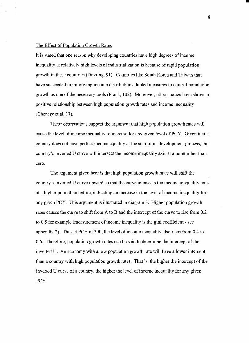
bull
9
Strong support for the argument that high population growth rates are positively
related to the level of income inequality is provided by the two-sector labor surplus
model and the theory of supply and demand As previously discussed the labor surplus
model suggests that a country first has a period of worsening income inequality followed
by a period of improvements in the level of income inequality During the period of
worsening income inequality there is surplus labor in the agricultural sector and income
inequality improves when labor becomes scarce Using the labor surplus model and the
theory of supply and demand it will be shown that high population growth rates are
positively related to the level of income inequality during the periods of abundant and
scarce supplies of labor
Diagram 4 shows the effect of rising population growth rates when there is
surplus labor in agriculture As discussed before BC indicates the period when income
inequality rises because the owners of industries are realizing huge profits due to the
growth of industries and low labor costs At point C income inequality will take a
downturn and further demand for labor by industries will cause wages to rise If the
population growth rate is not high then the supply curve of labor Sind should remain
BCD
However if the supply oflabor is increasing because of high population growth
rates then Sind will be ABCD The amount of surplus labor will become ABC which is
greater than BC that represents surplus labor when population growth rates are very low
Therefore when population growth rates are high it will take a longer time for the
economy to reach point C where all surplus labor is absorbed by industries and the
economy tends towards income equality Also labor costs will remain low for a longer
time causing the owners of industries to make greater profits than when population
growth rates are low This is because if population growth rates are relatively stable then
the time when labor becomes scarce comes sooner so that the owners of industries must
cut profits at an earlier stage to increase wages in order to hire more workers
10
Upward Shift of the Inverted U Curve
Income Inequality
d
b middot
800 PCY
DIAGRAM 3
-1 1
Lffect of High Population Growth Rates with Surplus Labor in the Economy
W~ges ages
D
A ~ __ __ __ _B+-- ----C
o o Labor
DIAGRAM 4
Effect ofHigh Population Growth Rates with Scarce Supply ofLabor in the Economy
Wages
81
Wl 82
~ I------~
W21--- _
Labor
DIAGRAMS
bull
12
In summary when surplus labor exists and a country finds itself along the upside of the
inverted U when its level of income inequality is rising high population growth rates
would further increase the level of income inequality for each PCY along this part of the
inverted U curve This is due to the widening of income differentials between industrial
owners and workers
If the country is at the stage when labor is in scarce supply then the supply curve
facing industries will be upward sloping Thus there will be improvements in the level
of income inequality because wages will increase whenever the demand for labor by
industries increases This is illustrated in diagram SA where S1 is the supply curve of
labor facing industries and an increase in their demand for labor from D1 to D2 raises
wages from a to b
An increase in the supply of labor at the stage of development when there is
scarcity of labor causes labor to be less scarce and reduces wages As shown in diagram
58 an increase in the supply of labor due to high population growth rates will cause the
supply curve to shift from Sl to S2 causing wages to fall from d to c Since falling
wages are linked with higher profits for industrial owners there would be an increase in
the level of income inequality Thus when labor is scarce and a country finds itself along
the downside of the inverted U high population growth rates will retard improvements in
the level of income inequality That is the level of income inequality will increase for
every PCY along the downside of the inverted U
Since it has been shown that high population growth rates shift both the upside
and downside of the inverted U curve upward it is clear that high population growth rates
shift the inverted U curve upward When this upward shift occurs the inverted U will
intercept the income inequality axis at a higher point implying that the level of income
inequality will rise for any given level ofPCY
bull
13
Effect of Education
Education is important because it allows people to contribute effectively towards the
growth of the economy Education also improves the level of income inequality by
eliminating skill differentials which reduce wage differentials This is because education
facilitates higher labor productivity which leads to higher labor income
The effect of education on income inequality is given by Lewis who focuses on
the differentials between skilled and unskilled labor As an economy grows industries
expand and they demand more skilled and unskilled labor But at the early stages of
development there will be a scarce amount of literate people to carry out for example
supervisory and administrative tasks Because of this scarcity of skilled workers
compared to the abundant supply of unskilled workers wage differentials between the
two groups of workers will widen Skilled workers will see increases in their wages
while the wages of unskilled workers may even fall if the supply of unskilled workers
increases (Lewis 180-181) The initial widening of wage differentials that results
between the two groups of workers causes a worsening of the level of income inequality
in the economy
However as the economy grows and educational facilities spread to a larger
proportion of the population in the long run skilled workers in the country will increase
causing the wages of skilled workers to fall (Lewis 180-181) Thus wage differentials
between the skilled and unskilled workers will reduce causing the level of income
inequality to improve The initial worsening followed by improvements in the level of
income inequality that is caused by the widening and then narrowing of wage
differentials is consistent with the inverted U pattern Thus it is argued here that
initially education is likely to be positively related before it becomes negatively related
to the level of income inequality
bull
14
More support for the fact that education affects the level of income inequality is
shown by the need for expansion of education systems worldwide and in the studies of
many economists Compulsory education is widely accepted as an important public
service and every country has some form of compulsory education (Eckstein 1992)
Eckstein and Zilcha show empirically that human capital affects the quality of labor and
that compulsory education will improve the distribution of income through generations
(Eckstein 1992) If education improves labor and causes higher wages then compulsory
education should improve the level of income inequality Also Chenery and Syrquin
found that education removes income away from the richest 20 and increases income of
the lowest 40 (Chenery 63) More interestingly where primary and secondary
schooling were found to be positively related to income shares obtained by individuals it
was also shown that primarily schooling significantly explained variations in income for
the lowest 40 and secondary education significantly explained those of the middle
40(Chenery et aI 17) This finding helps explain why emphasis is often placed at least
on compulsory primary schooling in many developing nations It can be said that the aim
is to improve the lot of the very poor
Hypotheses
The discussions above generate four hypotheses
I The inverted U exists supported by the fact that the labor surplus model
predicts the inverted U pattern
II The share of labor in industry is initially positively related then negatively related
to the level of income inequality
III Population growth rates are positively related to the level of income
inequality at any stage of development Higher population growth rates are
associated with higher income inequality
bull
15
IV It is likely that education is initially positively related before it becomes
negatively related to the level of income inequality
Research Design
Data on 61 countries mainly low-income and middle-income countries are used in this
study (see Appendix 1) The measure of income inequality used is the gini coefficient
This coefficient is calculated from a Lorenz curve that is constructed using data on
income distribution of a given country Appendix 2 gives an explanation of how gini
coefficients are calculated I created a program in Pascal to calculate this coefficient
based on the Lorenz curve the formula for the area of trapezoids and the formula for the
coefficient
Data on income distribution share of labor in industry and population growth
rates were obtained from the World Banks publication Social Indicators of Development
1991-92 Primary and secondary school enrollments are used as a measure of the
expansion of education and the data for these variables were also obtained from the
Social Indicators of Development Data for all variables are not given annually but for
periods of time This is possibly due to the fact that data on variables such as the income
distribution in a country are collected less frequently The periods for which data are
reported are 25-30 years ago 15-20 years ago and the most recent period
PCY Groups
When I plotted gini coefficients for the countries used in this study all the points were
crowded so that no pattern was observed When I tried to observe patterns using PCY
groups I found an inverted U pattern According to the inverted U pattern I found the
upside ofthe inverted U existed for countries with PCY up to $300 (dollar amounts are
bull
16
1990 current market prices in US dollars) There was no clear trend for countries with
PCY between $300 and $1000 but there was clear evidence of the downside ofthe
inverted U starting with countries with PCY about $1000 and higher Diagram 6
illustrates the inverted U pattern that I found using plotted graphs PCY Group I will
refer to countries with PCY less than or equal to $300 PCY Group II will refer to
countries with PCY between $300 and $1000 and PCY Group III will refer to countries
with PCY greater than $1000
Table 1 which shows regression results for the PCY groups identified above
verifies the inverted U pattern that was observed using plotted graphs The PCY2 term is
included since the inverted U pattern is quadratic According to Table 1 there is an initial
worsening of income inequality for PCY Group I judging from the positive significant
sign of the PCY variable The results for PCY Group II does not indicate any significant
pattern and confirms that a horizontal line best represents the trend of income inequality
for this PCY group For PCY Group III there is strong evidence of decreasing income
inequality which is indicated by the negative significant sign of the PCY variable Thus
the results shown in this table confirm that the inverted U pattern exists In Appendices
34 and 5 the regression lines for PCY Group I II and III drawn against the plotted data
for the PCY groups respectively are shown Put together the regression lines of the three
PCY groups also show the inverted U pattern I found using plotted graphs Later on we
will see whether the labor surplus model supports that this inverted U pattern exists
My findings using plotted graphs and regression models discussed above are good
findings since they posit that the phase of worsening income inequality ends earlier than
expected at PCY of about $300 and that the point at which income inequality starts it
downward trend also occurs earlier at PCY of about $1000 As previously mentioned
according to the inverted U pattern it is expected that income inequality worsens up to
PCY of about $2200 before it starts to improve
17
PCYGroups
Income In shyegua 1
inverted U pattern
PCYGroupll
middot300 1000 PCY
DIAGRAM 6middotshy -~ - -~-
Table 1 INVERTED U PATTERN
VARIABLES
PCY
PCYlt=300
(+)
+000262
300ltPCYlt= 1000
-000012
PCYgt1000
(-) -000003
-
PCY2 (-) -000001
+000000 (+) +000000
= significant at the 90 confidence level signs in parentheses are the hypothesized signs
bull
18
Models
To test the hypotheses in this paper several regression models are created and tested for
each PCY group On an aggregate level the regression results for all three PCY groups
will test the four hypotheses In these models Industry represents the share of labor in
industry PopRate represents population growth rates and Primary and Secondary
represent primary and secondary school enrollments respectively Table 2 clearly presents
the variables used in this study and their definitions OLS regressions were used to test
the models
For each PCY group Modell includes all the variables and tests all four
hypothesis Models 2 and 3 attempt to improve Modell The equation for Model 1 is
Gini = Constant + PCY + PCy2 + Industry + Industry2 + PopRate + Primary +
Primary2 + Secondary + Secondary2
[Equation 1]
Again the squared terms are included since the inverted U pattern is a quadratic curve
PopRate2 is not included in the equation above because PopRate is hypothesized to
always be positively related to the level of income inequality
According to the hypothesis for PCY Group I it is expected that in the regression
result for Modell the PCY term will be positive and significant This result will
confirm the upside of the inverted U Industry is expected to be positive and significant
to imply that during the early stages of development rural to urban migration causes the
economy to experience worsening levels of income inequality High population growth
rates should always worsen the level of income inequality and therefore a positive and
significant sign is expected for PopRate Primary and Secondary are also expected to be
positive and significant since a country at its early stage of development is likely to have
large wage differentials between the few literate people who receive high wages and the
masses of illiterate people who receive very low wages
bull 19
TABLE 2 DEFINITION OF VARIABLES
VARIABLES DEFINITIONS
PCY GNP per capita Estimates are for 1990 at current market prices in US dollars
INDUSTRY Labor force in mining manufacturing construction electricity water and gas as a percentage of the total labor force
POPRATE Population growth rate Annual growth rate calculated from mid year total and urban population
PRIMARY Primary school enrollmen t Gross enrollment of all ages at primary level as a percentage of school age children as defined by each country and reported to UNESCO
SECONDARY Secondary school enrollment Computed in the same manner as the primary school ratio
Source = Social Indicators of Development 1991 -92
bull
20
For PCY Group II the regression result for Modell will likely indicate nothing
significant as is implicated by the results presented in Table 1
For PCY Group III a negative significant sign is expected for the PCY variable to
confirm the downside of the inverted U Industry is also expected to be negative and
significant since countries in this group should have competitive labor markets so that
higher demands of labor increase wages PopRate is expected to be positive and
significant Primary and Secondary are expected to be negative and significant This is
because at the later stages of development there should be more literate people in the
labor force which should cause wage differentials to reduce and income inequality to
decrease
Results Conclusions and Policy Implications
Tables 3 4 and 5 show the regression models for PCY Group I II and III respectively
PCY Group I (The early stage of development)
Results
Table 3 shows the results for this group Modell which contains all the variables is a
good model judging from its R2 of 080 All the variables are significant except for
Primary and Primary 2 Secondary and Secondary2 have unexpected signs In Model 2
where the Secondary variables are excluded the R2 becomes 054 and only PopRate is
significant However the Primary variables have the expected signs Model 3 appears to
be the best model in which the Primary variables are excluded All the variables in this
model are significant and the model has an R2 of 080 However the Secondary
variables have the unexpected signs
bull
21
TABLE 3 GINI REGRESSIONS FOR PCY lt=300
VARIABLE MODEL 1 MODEL 2 MODEL 3
PCY (+ ) +000428
(+) +000110
(+ ) +000191
PCy2 ( shy )
-000001 ( shy )
-000002 ( - )
-000001
INDUSTRY (+ ) +015718
(+ ) +002127
(+ ) +008700
INDUSTRy2 ( shy )
-000786 ( shy )
-000092 ( shy )
-000414
POPORATE (+ ) +017821
(+) +007699
(+ ) +010363
PRIMARY (+ ) -000240
(+ ) +000247
PRIMARy2 ( shy )
+000000 ( - )
-000002
SECONDARY (+ ) -001823
(+ ) -001467
SECONDARy2 ( shy )
+000047 ( shy )
+000030
ADJUSTED R2
080 054 080
= significant at 90 confidence level (two-tail test) Signs in parentheses are the hypothesized signs
bull
22
Given that Model 3 is the best model it will be used to estimate the impact of
each variable on income inequality The equation for Model 3 is
Gini = -02636 + 0002PCY - 0000PCy2 + 0087Industry shy
0004Industry2 + 01 0363PopRate - 00 I5Secondary +
0000Secondary2
[Equation 2]
The positive sign and significance of the PCY variable in Model 3 confirm the
initial positive relationship between PCY and income inequality The positive and
significant sign of Industry is consistent with the labor surplus models prediction that at
the initial stages of development an increase of workers in the industrial sector worsens
the level of income inequality The result for PopRate supports that high population
growth rates are positively related to the upside ofthe inverted U This result is also
consistent with the explanation provided by the labor surplus model that high population
growth rates will increase the amount of surplus labor in this PCY group and worsen
income inequality The unexpected results for the Primary variables may be due to the
fact that this variable is not lagged The unexpected significant result for Secondary is an
important finding and can be explained as follows
At PCY less than $300 it is likely that secondary school enrollments are not
high However an increase in secondary school enrollments implies that there is likely
an increase in primary school enrollments Since at the early stage of development most
primary school graduates enter the labor force an increase in secondary school
enrollments also implies that more primary school graduates are entering the labor force
Therefore secondary school enrollment may be proxying for more people in the labor
force with primary school education who because of their primary school education
should be making higher wages More people making higher wages reduces wage
bull
23
differentials which improves income inequality This explanation is consistent with the
result obtained from the Secondary variable
Conclusions and Policy Implications
As explained in Appendix 2 where the method ofcalculating gini coefficient is
discussed the value of the gini coefficient lies between 1 and O The closer the
coefficient is to 0 the lower the level of income inequality The closer the gini coefficient
is to I the higher the level of income inequality From Equation 2 above it is deduced
that an increase ofPCY by $1 will cause the gini coefficient to rise by 0002 This means
that an increase ofPCY by $50 causes the gini coefficient to rise by a tenth (01) This
result is significant and posits that when a country begins its development process and
PCY increases the initial worsening of income inequality is inevitable Thus for
countries with PCY up to about $300 a worsening trend of income inequality can be
accepted as an initial phase that accompanies development
According to Equation 2 above a percentage increase of labor in industry (the
variable Industry) causes the gini coefficient to increase by 0087 Thus a 115
percentage increase of labor in the industrial sector causes the gini coefficient to rise by
about a tenth This result is also significant and implies that about a 9 percent increase of
labor in industry will cause the level of income inequality to be at the highest possible
level Therefore the results suggest that developing countries within PCY Group I
should not only concentrate on the developing the industrial sector but should
simultaneously concentrate on developing the agricultural sector That way they may be
able to reduce the amount of migrants from agriculture into industry
How much income inequality exists at the early stages of development depends
significantly on population growth rates The higher the population growth rate the
bull
24
higher is the level of income inequality at each PCY According to Equation 2 a 1
percentage increase in population growth rates causes the gini coefficient to rise by 0104
This implies that an increase of population growth rate by 096 percent (approximately 1
percent) causes the gini coefficient to rise by a tenth This result points out that it is
necessary for developing countries to adopt measures to control population growth rates
as early as possible in their development process By maintaining low population growth
rates and as according to the labor surplus model labor in the economy becomes a scarce
factor earlier and labor markets are competitive sooner Then also wages should
increase and income inequality should improve
If Secondary is accepted as a proxy for the amount of primary school graduates
entering the labor force then as calculated from Equation 2 a 667 increase of primary
school graduates entering the labor force (ie 667 increase in secondary school
enrollment) should decrease the gini coefficient by a tenth This is a significant and
encouraging result because it emphasizes the universal benefits of education even at the
early stages of development
PCY Group II (The intermediate stage of development)
Results
All the models created for this PCY group show no significant result as noted in Table 4
None of the variables are significant and the R2s for all the models are very low The
results confirm that the curve is a straight line for this PCY group
Conclusion
The results for PCY Group II does not allow one to make any generalizations applicable
to countries in this PCY group today Perhaps conditions in these countries are complex
and varied and therefore cannot be easily summarized
bull 25
TABLE 4 GINI REGRESSIONS FOR 300 lt PCY lt= 1000
VARIABLE MODEL 1 MODEL 2 MODEL 3
PCY 000004 000005 000008
PCy2 -000000 -000000 -000000
INDUSTRY -000842 -000720 -000836
INDUSTRy2 -000000 -000004 000002
POPRATE -002217 -002602 -000794
PRIMARY 001063 001068
PRIMARy2 -000006 -000006
SECONDARY 000171 000232
SECONDARy2 -000002 -000002
ADJUSTED Rl -007 005 002
bull 26
VARIABLES MODEL 1 MODEL 2 MODEL 3
PCY ( - )
-000002 ( - )
-000001 ( - )
-000002
PCy2 (+ ) +000000
(+ ) +000000
(+ ) +000000
INDUSTRY ( - )
-000460 ( - )
-001577 ( shy )
-000720
INDUSTRy2 (+ ) 000007
( + ) +000024
(+ ) 000012
PORPORATE (+ ) -001515
(+ ) +000806
(+ ) -001960
PRIMARY ( shy )
-001664 ( shy )
-005207
PRlMARy2 (+ ) +000008
(+ ) +000024
SECONDARY ( shy )
-000971 ( - )
-000866
SECONDARy2 (+ ) +000006
(+ ) +000005
ADJUSTED Rl 050 044
= SIGNIFICANT AT THE 90 CONFINDENCE LEVEL (TWO-TAIL TESr SIGNS IN PARENTEHESES ARE THE HYPOTHESIZED SIGNS
TABLE 5 GINI REGRESSIONS FOR PCY gt 1000
bull
27
PCY Group III (The industrialized stage of development)
Results
Only the education variables have significant coefficients in the models in Table 5 The
PCY variables in this table are not significant although they are in Table 1 This is
possibly because the explanatory variables in the regression equations for the models in
Table 5 (these explanatory variables are not included in the regression equation for Table
1) reduce the significance of the PCY variable The significant and expected coefficient
for Secondary in the models supports Lewis explanation that as an economy develops
education facilities become available to more people so that in the long run education has
a negative effect on the level of income inequality
Conclusion
Since countries in PCY Group III are well industrialized the increasing share of labor in
industry may have little impact on the level of income inequality Likewise population
growth rates which are relatively stable in these countries may have negligible effect on
the level of income inequality It is likely that there are other variables that may help
explain the downward trend of income inequality that is expected for industrialized
countries Often countries in the early stages of development experience political and
social instabilities conditions which improve as these countries develop Thus a measure
of political and social conditions may for instance be a crucial determinant of the
downward trend of income inequality It is also likely that the existence of certain
institutions in industrialized countries like unions that function to improve wages help
improve the level of income inequality in these countries Thus a measure of
unionization may also improve the results for this group Another variable that measures
bull
28
U This is because it is usual to find more advanced technological equipment and
facilities in industrialized countries and not in developing countries In summary the
share of labor in industry and population growth rates do not explain the downside of the
inverted U
General Conclusion
In this paper four hypothesis were generated and tested to confirm that the inverted U
exists and that the share of labor in industry population growth rates and education were
explanatory variables of income inequality Moreover the labor surplus model predicts
the inverted U pattern Although the inverted U pattern was found as presented in Table 1
where only PCY variables were used in the regression equation the explanatory variables
failed to show the inverted U pattern in its entirety The explanatory variables were able
to explain the upside of the inverted U as shown in Table 3 but the same explanatory
variables could not explain the downside of the inverted U as shown in Table 5
Thus this study also shows that the labor surplus model explains the upward trend
for countries with very low PCY and that high population growth rates worsen the level
of income inequality for these countries This study highlights that the labor surplus
model is incapable of explaining any other part of the inverted U especially the downside
of the inverted U
Suggestions For Future Research
Another explanation for the inverted U pattern can be given using labor market power as
follows At the early stages of development firms have monosony power and can force
the technological know-how in the various countries may also help explain the inverted
bull
29
wages to be low which signifies a period of worsening income inequality At the
intermediate stage of development more firms may exist which may cause the initial
monosony power of firms to reduce and at least prevent further worsening of income
inequality At the industrialized stage of development workers are likely to organize into
unions and counter the remaining monosony power of firms This should increase wages
and cause income inequality to improve This brief discussion suggests an important area
for future research Perhaps a better explanation of the inverted U pattern or an important
area to be considered along with the labor surplus model may be discovered
Another area for future research will be to separate the countries in PCY Group III
(countries that have PCY greater than $1000) into two categories the newly industrialized
and the well industrialized countries This may help control for the wide range of PCY in
PCY Group III and also the differences in institutions that exist in these countries
bull
30
WORK CITED
Ahluwalia Montek S 1976 Inequality Poverty and Development Journal of Development
Economics 3306-342
Braun Denny The Rich Get Richer The Rise ofIncome Inequality in the United States and the World
Chicago Nelson-Hall Publishers 1991
Chenery Hollis Ahluwalia S Montek C L G Bell John H Duloy Richard Jolly Redistribution
with ~rowth London Oxford University Press 1975
Chenery Hollis amp Moises Syrquin Patterns of Development 1950-1970 Published for the World Bank
by Oxford University Press 1975
Dovring Folke Inequality New York Praeger Publishers 1991
Eckstein Zvi amp Zilcha Itzhak 1992 The effects of compulsory schooling on growth
income distribution and welfare Journal of Public Economics 543339-359
Fields Gary F Poverty Inequality and Development London Cambridge University Press 1980
Gillis Malcom Economics of Development New York WW Norton amp Company 1992
Lewis W Arthur Theory of Economic Growth New York Harper Row 1970
Poulson Barry W Economic Development Minneapolis West Publishing Company 1994
APPENDIX 1shy
bull
~Cgt -ntneG time gini pey PopPate indu~ primary r
3an~1lade 25-30 030 7000 26 48 31
ncilet 25-30 036 9000 23 119 74
Paki~tan 25-30 034- 11000 26 183 40
Pak~tan 15-20 0294 130 31 172 12
Banglade 15-20 0316 130 25 54 73 Thailand 25-30 039 14000 31 52 78
0ri Lanka 25-30 041 16000 25 139 93
India 15-20 037 17000 23 129 79
Tanzania 15middot20 038 17000 28 38 53 Phiflipine 25-30 045 18000 31 158 113
Indonesia 15-20 038 21000 24 117 86
Uganda 15-20 036 22000 26 39 44 Sierra Le 15middot20 040 22000 2 132 39
Kenya 15-20 049 23000 37 62 95 0ri Lanka 15-20 032 29000 16 142 77 Mauritius 25-30 040 31000 24 254 72
Egypt 15-20 038 32000 2 184 71
Columbia 2~30 O~6 32000 3 214 84 Phillipine 15-20 043 34000 26 161 107 Botswana 15-20 050 35000 38 84 72
Bolivia 15-20 046 36000 25 199 85 0uriname 25-30 029 39000 27 215 120
Costa Ric 25-30 045 40000 32 192 106 Liberia 15-20 055 41000 3 94 62 Mexico 25-30 049 46000 33 219 92 Ecuador 15-20 059 54000 3 202 104
Zambia 15-20 050 55000 3 92 97
Columbia 15-20 047 55000 21 234 118 Guatemal 15-20 046 57000 28 17 61
Nicaragu 15-20 052 63000 3 156 82
Spain 25-30 035 70000 1 345 115
Tunisia 15-20 034 71000 21 311 97 Mauritius 15-20 043 71000 15 245 107
Libya 25-30 024 81000 39 209 78
Malaysia 15-20 045 82000 23 166 91 Argentina 25-30 038 87000 15 342 101
Japan 25-30 037 90000 11 32 100 Costa Ric 15-20 045 95000 25 216 107
Peru 15-20 052middot 100000 27 18 113
bull
Fiji 15-20 038 03000 i 9 160 115
Brazil 15-20 051 1070gt 24shy 243 88
Venezuel 25-30 048 113000 34 237 94
Israel 25-30 030 130000 35 354 95 Barbados 15-20 032 152000 04 233 103
Portugal 15-20 038 154000 38 347 113 Netherlan 25-30 039 156000 14 407 104
Trinidad 15-20 041 172000 09 372 99
Finland 25-30 042 175000 03 354 92 rmiddotJnrway 25-30 032 184000 08 368 97
France 25-30 046 203000 09 39 134
Denmark 25-30 035 205000 08 369 98 Venezuel 15-20 045 238000 36 267 97
Canada 25-30 030 262000 18 325 105
Ireland 15-20 029 265000 17 324 103 Sweden 25-30 036 276000 09 428 95
Spain 15-20 034 278000 1 374 111 I~rael 15-20 028 389000 23 337 97
rrance 15-20 036 600000 05 373 109
Germany 15-20 033 667000 -04 476 103 Sweden 15-20 027 832000 04 365 101
Australia Recent 034 1668000 16 344 106
bull APPENDIX 2
Calculatin2 Gjni Coefficjents
To convert the figures of an income distribution data into a measure of
income inequality can be done by constructing a Lorenz curve for each
country from which the Gini coefficientconcentration ratio(a measure of
inequality) is calculated The Lorenz curve shows the total percentage of
total income accounted for by any cumulative percentage of recipients
The shape of this curve indicates the degree of income inequality in the
income distribution(Gillis 1992 74) To illustrate how a Lorenz curve is
derived consider the following data for Brazil in 1983
poorest 20 of households receive 24 of total income
second quintile receive 57
third quintile receive 107
fourth quintile receive 186
richest 20 receive 626
From these data it can be observed that Brazil has a high degree of
inequality if 626 of its total income goes to the richest 20 of total
households Also a total of 100 of households receive 100 of total
income To construct a Lorenz curve first the cumulative income share
accruing to any given percentage of households is calculated Thus for the
data above we get the following calculations
poorest 20 receive 24 of total income
poorest 40 receive 24 + 57 = 81 of total income
poorest 60 receive 81 + 107 = 188 of total income
poorest 80 receive 188 + 186 = 374 of total income
100 of households receive 100 of total income
bull
The Lorenz curve is a graph plotted from the data above with the
horizontal axis measuring the cumulative percentage of recipient units and
the vertical axis measunng the cumulative share of total income
Diagram2 below shows the Lorenz curve obtained from the data above
J
J~
t
1
I
l
~ 1 IA I
I
~ [J I
J 1
Diagram2
(Bolnick 1987 61-62)
The diagonal line is a 45-degree line The closer the curve is to this line
the lesser is income inequality The closer it is to the right hand borders
the greater is income inequality(Gillis 1992 74)
To calculate the Gini coefficient let A be the area between the Lorenz
curve and the diagonal line and let B be the area under the Lorenz curve
as show in Figure 2 The formula to calculate the Gini coefficient is given
as
bull
A(A + B) A + B will always be 05 because the box in which the Lorenz
curve is drawn is a unit square especially seen if all percentages are taken
as decimal units eg 20 as 02 Therefore the area of the square becomes
lxl = 10 and half the area of the square (A + B) is 05(Bolnick 1987 62)
Area B can be calculated geometrically using formulas for calculating areas
of rectangles triangles and trapezoids The area of B was calculated
geometrically to be 0233 Since A + B = 05 A = 05 - 0233 = 0267 The
Gini Coefficient AlA + B) = 026705 = 0534 The closer the Gini
coefficient is to 0 the lesser is income inequality and the closer it is to 1
the greater is income inequality
I created a program in Pascal that calculates gini coefficients based
on the Lorenz curve the formula for the area of trapezoids and the
formula for the gini coefficient
bull bull
045
03
bull
APPENDIX 3
REGRESSION LINE DRAWN AGAINST PLOTTED DATA FOR pey GROUP I
05--------------------------------bull
04
035 bull
bull bull
bull bull
bull
bull bulli~t=-+~=
bull
bull
025l-------r------r--r-------------_r-----r---------------------------r-----------J 7000 13000 16000 18000 22000
bull bull
bull bull bull
APPENDIX 4
REGRESSION LINE DRAWN AGAINST PLOTTED DATA FOR pey GROUP II
bull
06-------------------------------------
055 bull
bull bullbullbull 05 bull bull bullbullA45
bull 04 bull
035 bull
bull 03
bull
025
bull
O 2--L--------------------------------------------r----------------------r----------------------------------------r---r---l
31000 34000 39000 46000 55000 70000 81000 90000
bull bull
APPENDIX 5
REGRESSION LINE DRAWN AGAINST PLOTTED DATA FOR pey GROUP III
bull
0S5------------------------------
05 bull
bull045 bull
bull ~ 04
bull~ 035 bull
03
bull bull 025
02
01 f0-+-0-0--2-0-r-0-0--3-000--40-0-0--S-OO-0--610010--700-0--8-00-0--9---1000
PCY
bull

bull
16
1990 current market prices in US dollars) There was no clear trend for countries with
PCY between $300 and $1000 but there was clear evidence of the downside ofthe
inverted U starting with countries with PCY about $1000 and higher Diagram 6
illustrates the inverted U pattern that I found using plotted graphs PCY Group I will
refer to countries with PCY less than or equal to $300 PCY Group II will refer to
countries with PCY between $300 and $1000 and PCY Group III will refer to countries
with PCY greater than $1000
Table 1 which shows regression results for the PCY groups identified above
verifies the inverted U pattern that was observed using plotted graphs The PCY2 term is
included since the inverted U pattern is quadratic According to Table 1 there is an initial
worsening of income inequality for PCY Group I judging from the positive significant
sign of the PCY variable The results for PCY Group II does not indicate any significant
pattern and confirms that a horizontal line best represents the trend of income inequality
for this PCY group For PCY Group III there is strong evidence of decreasing income
inequality which is indicated by the negative significant sign of the PCY variable Thus
the results shown in this table confirm that the inverted U pattern exists In Appendices
34 and 5 the regression lines for PCY Group I II and III drawn against the plotted data
for the PCY groups respectively are shown Put together the regression lines of the three
PCY groups also show the inverted U pattern I found using plotted graphs Later on we
will see whether the labor surplus model supports that this inverted U pattern exists
My findings using plotted graphs and regression models discussed above are good
findings since they posit that the phase of worsening income inequality ends earlier than
expected at PCY of about $300 and that the point at which income inequality starts it
downward trend also occurs earlier at PCY of about $1000 As previously mentioned
according to the inverted U pattern it is expected that income inequality worsens up to
PCY of about $2200 before it starts to improve
17
PCYGroups
Income In shyegua 1
inverted U pattern
PCYGroupll
middot300 1000 PCY
DIAGRAM 6middotshy -~ - -~-
Table 1 INVERTED U PATTERN
VARIABLES
PCY
PCYlt=300
(+)
+000262
300ltPCYlt= 1000
-000012
PCYgt1000
(-) -000003
-
PCY2 (-) -000001
+000000 (+) +000000
= significant at the 90 confidence level signs in parentheses are the hypothesized signs
bull
18
Models
To test the hypotheses in this paper several regression models are created and tested for
each PCY group On an aggregate level the regression results for all three PCY groups
will test the four hypotheses In these models Industry represents the share of labor in
industry PopRate represents population growth rates and Primary and Secondary
represent primary and secondary school enrollments respectively Table 2 clearly presents
the variables used in this study and their definitions OLS regressions were used to test
the models
For each PCY group Modell includes all the variables and tests all four
hypothesis Models 2 and 3 attempt to improve Modell The equation for Model 1 is
Gini = Constant + PCY + PCy2 + Industry + Industry2 + PopRate + Primary +
Primary2 + Secondary + Secondary2
[Equation 1]
Again the squared terms are included since the inverted U pattern is a quadratic curve
PopRate2 is not included in the equation above because PopRate is hypothesized to
always be positively related to the level of income inequality
According to the hypothesis for PCY Group I it is expected that in the regression
result for Modell the PCY term will be positive and significant This result will
confirm the upside of the inverted U Industry is expected to be positive and significant
to imply that during the early stages of development rural to urban migration causes the
economy to experience worsening levels of income inequality High population growth
rates should always worsen the level of income inequality and therefore a positive and
significant sign is expected for PopRate Primary and Secondary are also expected to be
positive and significant since a country at its early stage of development is likely to have
large wage differentials between the few literate people who receive high wages and the
masses of illiterate people who receive very low wages
bull 19
TABLE 2 DEFINITION OF VARIABLES
VARIABLES DEFINITIONS
PCY GNP per capita Estimates are for 1990 at current market prices in US dollars
INDUSTRY Labor force in mining manufacturing construction electricity water and gas as a percentage of the total labor force
POPRATE Population growth rate Annual growth rate calculated from mid year total and urban population
PRIMARY Primary school enrollmen t Gross enrollment of all ages at primary level as a percentage of school age children as defined by each country and reported to UNESCO
SECONDARY Secondary school enrollment Computed in the same manner as the primary school ratio
Source = Social Indicators of Development 1991 -92
bull
20
For PCY Group II the regression result for Modell will likely indicate nothing
significant as is implicated by the results presented in Table 1
For PCY Group III a negative significant sign is expected for the PCY variable to
confirm the downside of the inverted U Industry is also expected to be negative and
significant since countries in this group should have competitive labor markets so that
higher demands of labor increase wages PopRate is expected to be positive and
significant Primary and Secondary are expected to be negative and significant This is
because at the later stages of development there should be more literate people in the
labor force which should cause wage differentials to reduce and income inequality to
decrease
Results Conclusions and Policy Implications
Tables 3 4 and 5 show the regression models for PCY Group I II and III respectively
PCY Group I (The early stage of development)
Results
Table 3 shows the results for this group Modell which contains all the variables is a
good model judging from its R2 of 080 All the variables are significant except for
Primary and Primary 2 Secondary and Secondary2 have unexpected signs In Model 2
where the Secondary variables are excluded the R2 becomes 054 and only PopRate is
significant However the Primary variables have the expected signs Model 3 appears to
be the best model in which the Primary variables are excluded All the variables in this
model are significant and the model has an R2 of 080 However the Secondary
variables have the unexpected signs
bull
21
TABLE 3 GINI REGRESSIONS FOR PCY lt=300
VARIABLE MODEL 1 MODEL 2 MODEL 3
PCY (+ ) +000428
(+) +000110
(+ ) +000191
PCy2 ( shy )
-000001 ( shy )
-000002 ( - )
-000001
INDUSTRY (+ ) +015718
(+ ) +002127
(+ ) +008700
INDUSTRy2 ( shy )
-000786 ( shy )
-000092 ( shy )
-000414
POPORATE (+ ) +017821
(+) +007699
(+ ) +010363
PRIMARY (+ ) -000240
(+ ) +000247
PRIMARy2 ( shy )
+000000 ( - )
-000002
SECONDARY (+ ) -001823
(+ ) -001467
SECONDARy2 ( shy )
+000047 ( shy )
+000030
ADJUSTED R2
080 054 080
= significant at 90 confidence level (two-tail test) Signs in parentheses are the hypothesized signs
bull
22
Given that Model 3 is the best model it will be used to estimate the impact of
each variable on income inequality The equation for Model 3 is
Gini = -02636 + 0002PCY - 0000PCy2 + 0087Industry shy
0004Industry2 + 01 0363PopRate - 00 I5Secondary +
0000Secondary2
[Equation 2]
The positive sign and significance of the PCY variable in Model 3 confirm the
initial positive relationship between PCY and income inequality The positive and
significant sign of Industry is consistent with the labor surplus models prediction that at
the initial stages of development an increase of workers in the industrial sector worsens
the level of income inequality The result for PopRate supports that high population
growth rates are positively related to the upside ofthe inverted U This result is also
consistent with the explanation provided by the labor surplus model that high population
growth rates will increase the amount of surplus labor in this PCY group and worsen
income inequality The unexpected results for the Primary variables may be due to the
fact that this variable is not lagged The unexpected significant result for Secondary is an
important finding and can be explained as follows
At PCY less than $300 it is likely that secondary school enrollments are not
high However an increase in secondary school enrollments implies that there is likely
an increase in primary school enrollments Since at the early stage of development most
primary school graduates enter the labor force an increase in secondary school
enrollments also implies that more primary school graduates are entering the labor force
Therefore secondary school enrollment may be proxying for more people in the labor
force with primary school education who because of their primary school education
should be making higher wages More people making higher wages reduces wage
bull
23
differentials which improves income inequality This explanation is consistent with the
result obtained from the Secondary variable
Conclusions and Policy Implications
As explained in Appendix 2 where the method ofcalculating gini coefficient is
discussed the value of the gini coefficient lies between 1 and O The closer the
coefficient is to 0 the lower the level of income inequality The closer the gini coefficient
is to I the higher the level of income inequality From Equation 2 above it is deduced
that an increase ofPCY by $1 will cause the gini coefficient to rise by 0002 This means
that an increase ofPCY by $50 causes the gini coefficient to rise by a tenth (01) This
result is significant and posits that when a country begins its development process and
PCY increases the initial worsening of income inequality is inevitable Thus for
countries with PCY up to about $300 a worsening trend of income inequality can be
accepted as an initial phase that accompanies development
According to Equation 2 above a percentage increase of labor in industry (the
variable Industry) causes the gini coefficient to increase by 0087 Thus a 115
percentage increase of labor in the industrial sector causes the gini coefficient to rise by
about a tenth This result is also significant and implies that about a 9 percent increase of
labor in industry will cause the level of income inequality to be at the highest possible
level Therefore the results suggest that developing countries within PCY Group I
should not only concentrate on the developing the industrial sector but should
simultaneously concentrate on developing the agricultural sector That way they may be
able to reduce the amount of migrants from agriculture into industry
How much income inequality exists at the early stages of development depends
significantly on population growth rates The higher the population growth rate the
bull
24
higher is the level of income inequality at each PCY According to Equation 2 a 1
percentage increase in population growth rates causes the gini coefficient to rise by 0104
This implies that an increase of population growth rate by 096 percent (approximately 1
percent) causes the gini coefficient to rise by a tenth This result points out that it is
necessary for developing countries to adopt measures to control population growth rates
as early as possible in their development process By maintaining low population growth
rates and as according to the labor surplus model labor in the economy becomes a scarce
factor earlier and labor markets are competitive sooner Then also wages should
increase and income inequality should improve
If Secondary is accepted as a proxy for the amount of primary school graduates
entering the labor force then as calculated from Equation 2 a 667 increase of primary
school graduates entering the labor force (ie 667 increase in secondary school
enrollment) should decrease the gini coefficient by a tenth This is a significant and
encouraging result because it emphasizes the universal benefits of education even at the
early stages of development
PCY Group II (The intermediate stage of development)
Results
All the models created for this PCY group show no significant result as noted in Table 4
None of the variables are significant and the R2s for all the models are very low The
results confirm that the curve is a straight line for this PCY group
Conclusion
The results for PCY Group II does not allow one to make any generalizations applicable
to countries in this PCY group today Perhaps conditions in these countries are complex
and varied and therefore cannot be easily summarized
bull 25
TABLE 4 GINI REGRESSIONS FOR 300 lt PCY lt= 1000
VARIABLE MODEL 1 MODEL 2 MODEL 3
PCY 000004 000005 000008
PCy2 -000000 -000000 -000000
INDUSTRY -000842 -000720 -000836
INDUSTRy2 -000000 -000004 000002
POPRATE -002217 -002602 -000794
PRIMARY 001063 001068
PRIMARy2 -000006 -000006
SECONDARY 000171 000232
SECONDARy2 -000002 -000002
ADJUSTED Rl -007 005 002
bull 26
VARIABLES MODEL 1 MODEL 2 MODEL 3
PCY ( - )
-000002 ( - )
-000001 ( - )
-000002
PCy2 (+ ) +000000
(+ ) +000000
(+ ) +000000
INDUSTRY ( - )
-000460 ( - )
-001577 ( shy )
-000720
INDUSTRy2 (+ ) 000007
( + ) +000024
(+ ) 000012
PORPORATE (+ ) -001515
(+ ) +000806
(+ ) -001960
PRIMARY ( shy )
-001664 ( shy )
-005207
PRlMARy2 (+ ) +000008
(+ ) +000024
SECONDARY ( shy )
-000971 ( - )
-000866
SECONDARy2 (+ ) +000006
(+ ) +000005
ADJUSTED Rl 050 044
= SIGNIFICANT AT THE 90 CONFINDENCE LEVEL (TWO-TAIL TESr SIGNS IN PARENTEHESES ARE THE HYPOTHESIZED SIGNS
TABLE 5 GINI REGRESSIONS FOR PCY gt 1000
bull
27
PCY Group III (The industrialized stage of development)
Results
Only the education variables have significant coefficients in the models in Table 5 The
PCY variables in this table are not significant although they are in Table 1 This is
possibly because the explanatory variables in the regression equations for the models in
Table 5 (these explanatory variables are not included in the regression equation for Table
1) reduce the significance of the PCY variable The significant and expected coefficient
for Secondary in the models supports Lewis explanation that as an economy develops
education facilities become available to more people so that in the long run education has
a negative effect on the level of income inequality
Conclusion
Since countries in PCY Group III are well industrialized the increasing share of labor in
industry may have little impact on the level of income inequality Likewise population
growth rates which are relatively stable in these countries may have negligible effect on
the level of income inequality It is likely that there are other variables that may help
explain the downward trend of income inequality that is expected for industrialized
countries Often countries in the early stages of development experience political and
social instabilities conditions which improve as these countries develop Thus a measure
of political and social conditions may for instance be a crucial determinant of the
downward trend of income inequality It is also likely that the existence of certain
institutions in industrialized countries like unions that function to improve wages help
improve the level of income inequality in these countries Thus a measure of
unionization may also improve the results for this group Another variable that measures
bull
28
U This is because it is usual to find more advanced technological equipment and
facilities in industrialized countries and not in developing countries In summary the
share of labor in industry and population growth rates do not explain the downside of the
inverted U
General Conclusion
In this paper four hypothesis were generated and tested to confirm that the inverted U
exists and that the share of labor in industry population growth rates and education were
explanatory variables of income inequality Moreover the labor surplus model predicts
the inverted U pattern Although the inverted U pattern was found as presented in Table 1
where only PCY variables were used in the regression equation the explanatory variables
failed to show the inverted U pattern in its entirety The explanatory variables were able
to explain the upside of the inverted U as shown in Table 3 but the same explanatory
variables could not explain the downside of the inverted U as shown in Table 5
Thus this study also shows that the labor surplus model explains the upward trend
for countries with very low PCY and that high population growth rates worsen the level
of income inequality for these countries This study highlights that the labor surplus
model is incapable of explaining any other part of the inverted U especially the downside
of the inverted U
Suggestions For Future Research
Another explanation for the inverted U pattern can be given using labor market power as
follows At the early stages of development firms have monosony power and can force
the technological know-how in the various countries may also help explain the inverted
bull
29
wages to be low which signifies a period of worsening income inequality At the
intermediate stage of development more firms may exist which may cause the initial
monosony power of firms to reduce and at least prevent further worsening of income
inequality At the industrialized stage of development workers are likely to organize into
unions and counter the remaining monosony power of firms This should increase wages
and cause income inequality to improve This brief discussion suggests an important area
for future research Perhaps a better explanation of the inverted U pattern or an important
area to be considered along with the labor surplus model may be discovered
Another area for future research will be to separate the countries in PCY Group III
(countries that have PCY greater than $1000) into two categories the newly industrialized
and the well industrialized countries This may help control for the wide range of PCY in
PCY Group III and also the differences in institutions that exist in these countries
bull
30
WORK CITED
Ahluwalia Montek S 1976 Inequality Poverty and Development Journal of Development
Economics 3306-342
Braun Denny The Rich Get Richer The Rise ofIncome Inequality in the United States and the World
Chicago Nelson-Hall Publishers 1991
Chenery Hollis Ahluwalia S Montek C L G Bell John H Duloy Richard Jolly Redistribution
with ~rowth London Oxford University Press 1975
Chenery Hollis amp Moises Syrquin Patterns of Development 1950-1970 Published for the World Bank
by Oxford University Press 1975
Dovring Folke Inequality New York Praeger Publishers 1991
Eckstein Zvi amp Zilcha Itzhak 1992 The effects of compulsory schooling on growth
income distribution and welfare Journal of Public Economics 543339-359
Fields Gary F Poverty Inequality and Development London Cambridge University Press 1980
Gillis Malcom Economics of Development New York WW Norton amp Company 1992
Lewis W Arthur Theory of Economic Growth New York Harper Row 1970
Poulson Barry W Economic Development Minneapolis West Publishing Company 1994
APPENDIX 1shy
bull
~Cgt -ntneG time gini pey PopPate indu~ primary r
3an~1lade 25-30 030 7000 26 48 31
ncilet 25-30 036 9000 23 119 74
Paki~tan 25-30 034- 11000 26 183 40
Pak~tan 15-20 0294 130 31 172 12
Banglade 15-20 0316 130 25 54 73 Thailand 25-30 039 14000 31 52 78
0ri Lanka 25-30 041 16000 25 139 93
India 15-20 037 17000 23 129 79
Tanzania 15middot20 038 17000 28 38 53 Phiflipine 25-30 045 18000 31 158 113
Indonesia 15-20 038 21000 24 117 86
Uganda 15-20 036 22000 26 39 44 Sierra Le 15middot20 040 22000 2 132 39
Kenya 15-20 049 23000 37 62 95 0ri Lanka 15-20 032 29000 16 142 77 Mauritius 25-30 040 31000 24 254 72
Egypt 15-20 038 32000 2 184 71
Columbia 2~30 O~6 32000 3 214 84 Phillipine 15-20 043 34000 26 161 107 Botswana 15-20 050 35000 38 84 72
Bolivia 15-20 046 36000 25 199 85 0uriname 25-30 029 39000 27 215 120
Costa Ric 25-30 045 40000 32 192 106 Liberia 15-20 055 41000 3 94 62 Mexico 25-30 049 46000 33 219 92 Ecuador 15-20 059 54000 3 202 104
Zambia 15-20 050 55000 3 92 97
Columbia 15-20 047 55000 21 234 118 Guatemal 15-20 046 57000 28 17 61
Nicaragu 15-20 052 63000 3 156 82
Spain 25-30 035 70000 1 345 115
Tunisia 15-20 034 71000 21 311 97 Mauritius 15-20 043 71000 15 245 107
Libya 25-30 024 81000 39 209 78
Malaysia 15-20 045 82000 23 166 91 Argentina 25-30 038 87000 15 342 101
Japan 25-30 037 90000 11 32 100 Costa Ric 15-20 045 95000 25 216 107
Peru 15-20 052middot 100000 27 18 113
bull
Fiji 15-20 038 03000 i 9 160 115
Brazil 15-20 051 1070gt 24shy 243 88
Venezuel 25-30 048 113000 34 237 94
Israel 25-30 030 130000 35 354 95 Barbados 15-20 032 152000 04 233 103
Portugal 15-20 038 154000 38 347 113 Netherlan 25-30 039 156000 14 407 104
Trinidad 15-20 041 172000 09 372 99
Finland 25-30 042 175000 03 354 92 rmiddotJnrway 25-30 032 184000 08 368 97
France 25-30 046 203000 09 39 134
Denmark 25-30 035 205000 08 369 98 Venezuel 15-20 045 238000 36 267 97
Canada 25-30 030 262000 18 325 105
Ireland 15-20 029 265000 17 324 103 Sweden 25-30 036 276000 09 428 95
Spain 15-20 034 278000 1 374 111 I~rael 15-20 028 389000 23 337 97
rrance 15-20 036 600000 05 373 109
Germany 15-20 033 667000 -04 476 103 Sweden 15-20 027 832000 04 365 101
Australia Recent 034 1668000 16 344 106
bull APPENDIX 2
Calculatin2 Gjni Coefficjents
To convert the figures of an income distribution data into a measure of
income inequality can be done by constructing a Lorenz curve for each
country from which the Gini coefficientconcentration ratio(a measure of
inequality) is calculated The Lorenz curve shows the total percentage of
total income accounted for by any cumulative percentage of recipients
The shape of this curve indicates the degree of income inequality in the
income distribution(Gillis 1992 74) To illustrate how a Lorenz curve is
derived consider the following data for Brazil in 1983
poorest 20 of households receive 24 of total income
second quintile receive 57
third quintile receive 107
fourth quintile receive 186
richest 20 receive 626
From these data it can be observed that Brazil has a high degree of
inequality if 626 of its total income goes to the richest 20 of total
households Also a total of 100 of households receive 100 of total
income To construct a Lorenz curve first the cumulative income share
accruing to any given percentage of households is calculated Thus for the
data above we get the following calculations
poorest 20 receive 24 of total income
poorest 40 receive 24 + 57 = 81 of total income
poorest 60 receive 81 + 107 = 188 of total income
poorest 80 receive 188 + 186 = 374 of total income
100 of households receive 100 of total income
bull
The Lorenz curve is a graph plotted from the data above with the
horizontal axis measuring the cumulative percentage of recipient units and
the vertical axis measunng the cumulative share of total income
Diagram2 below shows the Lorenz curve obtained from the data above
J
J~
t
1
I
l
~ 1 IA I
I
~ [J I
J 1
Diagram2
(Bolnick 1987 61-62)
The diagonal line is a 45-degree line The closer the curve is to this line
the lesser is income inequality The closer it is to the right hand borders
the greater is income inequality(Gillis 1992 74)
To calculate the Gini coefficient let A be the area between the Lorenz
curve and the diagonal line and let B be the area under the Lorenz curve
as show in Figure 2 The formula to calculate the Gini coefficient is given
as
bull
A(A + B) A + B will always be 05 because the box in which the Lorenz
curve is drawn is a unit square especially seen if all percentages are taken
as decimal units eg 20 as 02 Therefore the area of the square becomes
lxl = 10 and half the area of the square (A + B) is 05(Bolnick 1987 62)
Area B can be calculated geometrically using formulas for calculating areas
of rectangles triangles and trapezoids The area of B was calculated
geometrically to be 0233 Since A + B = 05 A = 05 - 0233 = 0267 The
Gini Coefficient AlA + B) = 026705 = 0534 The closer the Gini
coefficient is to 0 the lesser is income inequality and the closer it is to 1
the greater is income inequality
I created a program in Pascal that calculates gini coefficients based
on the Lorenz curve the formula for the area of trapezoids and the
formula for the gini coefficient
bull bull
045
03
bull
APPENDIX 3
REGRESSION LINE DRAWN AGAINST PLOTTED DATA FOR pey GROUP I
05--------------------------------bull
04
035 bull
bull bull
bull bull
bull
bull bulli~t=-+~=
bull
bull
025l-------r------r--r-------------_r-----r---------------------------r-----------J 7000 13000 16000 18000 22000
bull bull
bull bull bull
APPENDIX 4
REGRESSION LINE DRAWN AGAINST PLOTTED DATA FOR pey GROUP II
bull
06-------------------------------------
055 bull
bull bullbullbull 05 bull bull bullbullA45
bull 04 bull
035 bull
bull 03
bull
025
bull
O 2--L--------------------------------------------r----------------------r----------------------------------------r---r---l
31000 34000 39000 46000 55000 70000 81000 90000
bull bull
APPENDIX 5
REGRESSION LINE DRAWN AGAINST PLOTTED DATA FOR pey GROUP III
bull
0S5------------------------------
05 bull
bull045 bull
bull ~ 04
bull~ 035 bull
03
bull bull 025
02
01 f0-+-0-0--2-0-r-0-0--3-000--40-0-0--S-OO-0--610010--700-0--8-00-0--9---1000
PCY
bull
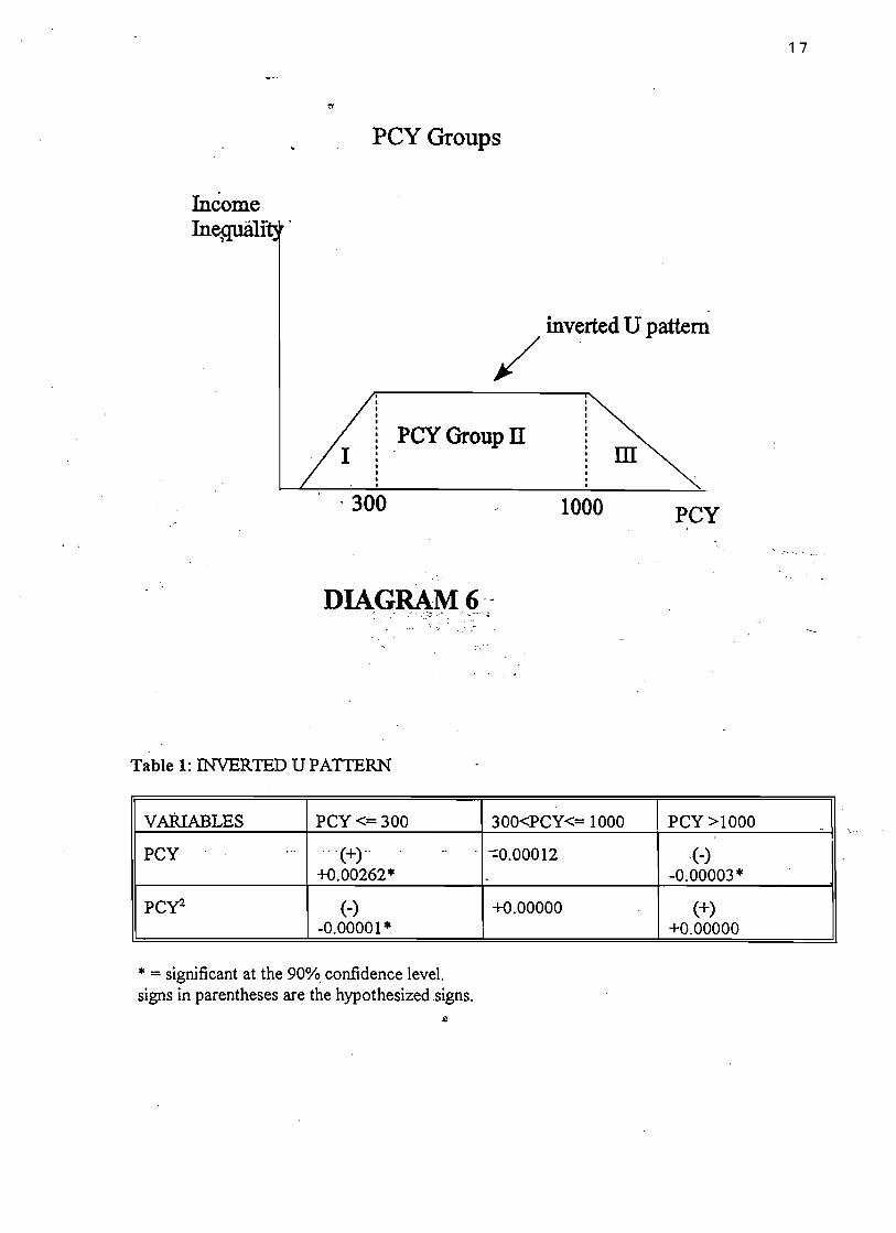

bull
18
Models
To test the hypotheses in this paper several regression models are created and tested for
each PCY group On an aggregate level the regression results for all three PCY groups
will test the four hypotheses In these models Industry represents the share of labor in
industry PopRate represents population growth rates and Primary and Secondary
represent primary and secondary school enrollments respectively Table 2 clearly presents
the variables used in this study and their definitions OLS regressions were used to test
the models
For each PCY group Modell includes all the variables and tests all four
hypothesis Models 2 and 3 attempt to improve Modell The equation for Model 1 is
Gini = Constant + PCY + PCy2 + Industry + Industry2 + PopRate + Primary +
Primary2 + Secondary + Secondary2
[Equation 1]
Again the squared terms are included since the inverted U pattern is a quadratic curve
PopRate2 is not included in the equation above because PopRate is hypothesized to
always be positively related to the level of income inequality
According to the hypothesis for PCY Group I it is expected that in the regression
result for Modell the PCY term will be positive and significant This result will
confirm the upside of the inverted U Industry is expected to be positive and significant
to imply that during the early stages of development rural to urban migration causes the
economy to experience worsening levels of income inequality High population growth
rates should always worsen the level of income inequality and therefore a positive and
significant sign is expected for PopRate Primary and Secondary are also expected to be
positive and significant since a country at its early stage of development is likely to have
large wage differentials between the few literate people who receive high wages and the
masses of illiterate people who receive very low wages
bull 19
TABLE 2 DEFINITION OF VARIABLES
VARIABLES DEFINITIONS
PCY GNP per capita Estimates are for 1990 at current market prices in US dollars
INDUSTRY Labor force in mining manufacturing construction electricity water and gas as a percentage of the total labor force
POPRATE Population growth rate Annual growth rate calculated from mid year total and urban population
PRIMARY Primary school enrollmen t Gross enrollment of all ages at primary level as a percentage of school age children as defined by each country and reported to UNESCO
SECONDARY Secondary school enrollment Computed in the same manner as the primary school ratio
Source = Social Indicators of Development 1991 -92
bull
20
For PCY Group II the regression result for Modell will likely indicate nothing
significant as is implicated by the results presented in Table 1
For PCY Group III a negative significant sign is expected for the PCY variable to
confirm the downside of the inverted U Industry is also expected to be negative and
significant since countries in this group should have competitive labor markets so that
higher demands of labor increase wages PopRate is expected to be positive and
significant Primary and Secondary are expected to be negative and significant This is
because at the later stages of development there should be more literate people in the
labor force which should cause wage differentials to reduce and income inequality to
decrease
Results Conclusions and Policy Implications
Tables 3 4 and 5 show the regression models for PCY Group I II and III respectively
PCY Group I (The early stage of development)
Results
Table 3 shows the results for this group Modell which contains all the variables is a
good model judging from its R2 of 080 All the variables are significant except for
Primary and Primary 2 Secondary and Secondary2 have unexpected signs In Model 2
where the Secondary variables are excluded the R2 becomes 054 and only PopRate is
significant However the Primary variables have the expected signs Model 3 appears to
be the best model in which the Primary variables are excluded All the variables in this
model are significant and the model has an R2 of 080 However the Secondary
variables have the unexpected signs
bull
21
TABLE 3 GINI REGRESSIONS FOR PCY lt=300
VARIABLE MODEL 1 MODEL 2 MODEL 3
PCY (+ ) +000428
(+) +000110
(+ ) +000191
PCy2 ( shy )
-000001 ( shy )
-000002 ( - )
-000001
INDUSTRY (+ ) +015718
(+ ) +002127
(+ ) +008700
INDUSTRy2 ( shy )
-000786 ( shy )
-000092 ( shy )
-000414
POPORATE (+ ) +017821
(+) +007699
(+ ) +010363
PRIMARY (+ ) -000240
(+ ) +000247
PRIMARy2 ( shy )
+000000 ( - )
-000002
SECONDARY (+ ) -001823
(+ ) -001467
SECONDARy2 ( shy )
+000047 ( shy )
+000030
ADJUSTED R2
080 054 080
= significant at 90 confidence level (two-tail test) Signs in parentheses are the hypothesized signs
bull
22
Given that Model 3 is the best model it will be used to estimate the impact of
each variable on income inequality The equation for Model 3 is
Gini = -02636 + 0002PCY - 0000PCy2 + 0087Industry shy
0004Industry2 + 01 0363PopRate - 00 I5Secondary +
0000Secondary2
[Equation 2]
The positive sign and significance of the PCY variable in Model 3 confirm the
initial positive relationship between PCY and income inequality The positive and
significant sign of Industry is consistent with the labor surplus models prediction that at
the initial stages of development an increase of workers in the industrial sector worsens
the level of income inequality The result for PopRate supports that high population
growth rates are positively related to the upside ofthe inverted U This result is also
consistent with the explanation provided by the labor surplus model that high population
growth rates will increase the amount of surplus labor in this PCY group and worsen
income inequality The unexpected results for the Primary variables may be due to the
fact that this variable is not lagged The unexpected significant result for Secondary is an
important finding and can be explained as follows
At PCY less than $300 it is likely that secondary school enrollments are not
high However an increase in secondary school enrollments implies that there is likely
an increase in primary school enrollments Since at the early stage of development most
primary school graduates enter the labor force an increase in secondary school
enrollments also implies that more primary school graduates are entering the labor force
Therefore secondary school enrollment may be proxying for more people in the labor
force with primary school education who because of their primary school education
should be making higher wages More people making higher wages reduces wage
bull
23
differentials which improves income inequality This explanation is consistent with the
result obtained from the Secondary variable
Conclusions and Policy Implications
As explained in Appendix 2 where the method ofcalculating gini coefficient is
discussed the value of the gini coefficient lies between 1 and O The closer the
coefficient is to 0 the lower the level of income inequality The closer the gini coefficient
is to I the higher the level of income inequality From Equation 2 above it is deduced
that an increase ofPCY by $1 will cause the gini coefficient to rise by 0002 This means
that an increase ofPCY by $50 causes the gini coefficient to rise by a tenth (01) This
result is significant and posits that when a country begins its development process and
PCY increases the initial worsening of income inequality is inevitable Thus for
countries with PCY up to about $300 a worsening trend of income inequality can be
accepted as an initial phase that accompanies development
According to Equation 2 above a percentage increase of labor in industry (the
variable Industry) causes the gini coefficient to increase by 0087 Thus a 115
percentage increase of labor in the industrial sector causes the gini coefficient to rise by
about a tenth This result is also significant and implies that about a 9 percent increase of
labor in industry will cause the level of income inequality to be at the highest possible
level Therefore the results suggest that developing countries within PCY Group I
should not only concentrate on the developing the industrial sector but should
simultaneously concentrate on developing the agricultural sector That way they may be
able to reduce the amount of migrants from agriculture into industry
How much income inequality exists at the early stages of development depends
significantly on population growth rates The higher the population growth rate the
bull
24
higher is the level of income inequality at each PCY According to Equation 2 a 1
percentage increase in population growth rates causes the gini coefficient to rise by 0104
This implies that an increase of population growth rate by 096 percent (approximately 1
percent) causes the gini coefficient to rise by a tenth This result points out that it is
necessary for developing countries to adopt measures to control population growth rates
as early as possible in their development process By maintaining low population growth
rates and as according to the labor surplus model labor in the economy becomes a scarce
factor earlier and labor markets are competitive sooner Then also wages should
increase and income inequality should improve
If Secondary is accepted as a proxy for the amount of primary school graduates
entering the labor force then as calculated from Equation 2 a 667 increase of primary
school graduates entering the labor force (ie 667 increase in secondary school
enrollment) should decrease the gini coefficient by a tenth This is a significant and
encouraging result because it emphasizes the universal benefits of education even at the
early stages of development
PCY Group II (The intermediate stage of development)
Results
All the models created for this PCY group show no significant result as noted in Table 4
None of the variables are significant and the R2s for all the models are very low The
results confirm that the curve is a straight line for this PCY group
Conclusion
The results for PCY Group II does not allow one to make any generalizations applicable
to countries in this PCY group today Perhaps conditions in these countries are complex
and varied and therefore cannot be easily summarized
bull 25
TABLE 4 GINI REGRESSIONS FOR 300 lt PCY lt= 1000
VARIABLE MODEL 1 MODEL 2 MODEL 3
PCY 000004 000005 000008
PCy2 -000000 -000000 -000000
INDUSTRY -000842 -000720 -000836
INDUSTRy2 -000000 -000004 000002
POPRATE -002217 -002602 -000794
PRIMARY 001063 001068
PRIMARy2 -000006 -000006
SECONDARY 000171 000232
SECONDARy2 -000002 -000002
ADJUSTED Rl -007 005 002
bull 26
VARIABLES MODEL 1 MODEL 2 MODEL 3
PCY ( - )
-000002 ( - )
-000001 ( - )
-000002
PCy2 (+ ) +000000
(+ ) +000000
(+ ) +000000
INDUSTRY ( - )
-000460 ( - )
-001577 ( shy )
-000720
INDUSTRy2 (+ ) 000007
( + ) +000024
(+ ) 000012
PORPORATE (+ ) -001515
(+ ) +000806
(+ ) -001960
PRIMARY ( shy )
-001664 ( shy )
-005207
PRlMARy2 (+ ) +000008
(+ ) +000024
SECONDARY ( shy )
-000971 ( - )
-000866
SECONDARy2 (+ ) +000006
(+ ) +000005
ADJUSTED Rl 050 044
= SIGNIFICANT AT THE 90 CONFINDENCE LEVEL (TWO-TAIL TESr SIGNS IN PARENTEHESES ARE THE HYPOTHESIZED SIGNS
TABLE 5 GINI REGRESSIONS FOR PCY gt 1000
bull
27
PCY Group III (The industrialized stage of development)
Results
Only the education variables have significant coefficients in the models in Table 5 The
PCY variables in this table are not significant although they are in Table 1 This is
possibly because the explanatory variables in the regression equations for the models in
Table 5 (these explanatory variables are not included in the regression equation for Table
1) reduce the significance of the PCY variable The significant and expected coefficient
for Secondary in the models supports Lewis explanation that as an economy develops
education facilities become available to more people so that in the long run education has
a negative effect on the level of income inequality
Conclusion
Since countries in PCY Group III are well industrialized the increasing share of labor in
industry may have little impact on the level of income inequality Likewise population
growth rates which are relatively stable in these countries may have negligible effect on
the level of income inequality It is likely that there are other variables that may help
explain the downward trend of income inequality that is expected for industrialized
countries Often countries in the early stages of development experience political and
social instabilities conditions which improve as these countries develop Thus a measure
of political and social conditions may for instance be a crucial determinant of the
downward trend of income inequality It is also likely that the existence of certain
institutions in industrialized countries like unions that function to improve wages help
improve the level of income inequality in these countries Thus a measure of
unionization may also improve the results for this group Another variable that measures
bull
28
U This is because it is usual to find more advanced technological equipment and
facilities in industrialized countries and not in developing countries In summary the
share of labor in industry and population growth rates do not explain the downside of the
inverted U
General Conclusion
In this paper four hypothesis were generated and tested to confirm that the inverted U
exists and that the share of labor in industry population growth rates and education were
explanatory variables of income inequality Moreover the labor surplus model predicts
the inverted U pattern Although the inverted U pattern was found as presented in Table 1
where only PCY variables were used in the regression equation the explanatory variables
failed to show the inverted U pattern in its entirety The explanatory variables were able
to explain the upside of the inverted U as shown in Table 3 but the same explanatory
variables could not explain the downside of the inverted U as shown in Table 5
Thus this study also shows that the labor surplus model explains the upward trend
for countries with very low PCY and that high population growth rates worsen the level
of income inequality for these countries This study highlights that the labor surplus
model is incapable of explaining any other part of the inverted U especially the downside
of the inverted U
Suggestions For Future Research
Another explanation for the inverted U pattern can be given using labor market power as
follows At the early stages of development firms have monosony power and can force
the technological know-how in the various countries may also help explain the inverted
bull
29
wages to be low which signifies a period of worsening income inequality At the
intermediate stage of development more firms may exist which may cause the initial
monosony power of firms to reduce and at least prevent further worsening of income
inequality At the industrialized stage of development workers are likely to organize into
unions and counter the remaining monosony power of firms This should increase wages
and cause income inequality to improve This brief discussion suggests an important area
for future research Perhaps a better explanation of the inverted U pattern or an important
area to be considered along with the labor surplus model may be discovered
Another area for future research will be to separate the countries in PCY Group III
(countries that have PCY greater than $1000) into two categories the newly industrialized
and the well industrialized countries This may help control for the wide range of PCY in
PCY Group III and also the differences in institutions that exist in these countries
bull
30
WORK CITED
Ahluwalia Montek S 1976 Inequality Poverty and Development Journal of Development
Economics 3306-342
Braun Denny The Rich Get Richer The Rise ofIncome Inequality in the United States and the World
Chicago Nelson-Hall Publishers 1991
Chenery Hollis Ahluwalia S Montek C L G Bell John H Duloy Richard Jolly Redistribution
with ~rowth London Oxford University Press 1975
Chenery Hollis amp Moises Syrquin Patterns of Development 1950-1970 Published for the World Bank
by Oxford University Press 1975
Dovring Folke Inequality New York Praeger Publishers 1991
Eckstein Zvi amp Zilcha Itzhak 1992 The effects of compulsory schooling on growth
income distribution and welfare Journal of Public Economics 543339-359
Fields Gary F Poverty Inequality and Development London Cambridge University Press 1980
Gillis Malcom Economics of Development New York WW Norton amp Company 1992
Lewis W Arthur Theory of Economic Growth New York Harper Row 1970
Poulson Barry W Economic Development Minneapolis West Publishing Company 1994
APPENDIX 1shy
bull
~Cgt -ntneG time gini pey PopPate indu~ primary r
3an~1lade 25-30 030 7000 26 48 31
ncilet 25-30 036 9000 23 119 74
Paki~tan 25-30 034- 11000 26 183 40
Pak~tan 15-20 0294 130 31 172 12
Banglade 15-20 0316 130 25 54 73 Thailand 25-30 039 14000 31 52 78
0ri Lanka 25-30 041 16000 25 139 93
India 15-20 037 17000 23 129 79
Tanzania 15middot20 038 17000 28 38 53 Phiflipine 25-30 045 18000 31 158 113
Indonesia 15-20 038 21000 24 117 86
Uganda 15-20 036 22000 26 39 44 Sierra Le 15middot20 040 22000 2 132 39
Kenya 15-20 049 23000 37 62 95 0ri Lanka 15-20 032 29000 16 142 77 Mauritius 25-30 040 31000 24 254 72
Egypt 15-20 038 32000 2 184 71
Columbia 2~30 O~6 32000 3 214 84 Phillipine 15-20 043 34000 26 161 107 Botswana 15-20 050 35000 38 84 72
Bolivia 15-20 046 36000 25 199 85 0uriname 25-30 029 39000 27 215 120
Costa Ric 25-30 045 40000 32 192 106 Liberia 15-20 055 41000 3 94 62 Mexico 25-30 049 46000 33 219 92 Ecuador 15-20 059 54000 3 202 104
Zambia 15-20 050 55000 3 92 97
Columbia 15-20 047 55000 21 234 118 Guatemal 15-20 046 57000 28 17 61
Nicaragu 15-20 052 63000 3 156 82
Spain 25-30 035 70000 1 345 115
Tunisia 15-20 034 71000 21 311 97 Mauritius 15-20 043 71000 15 245 107
Libya 25-30 024 81000 39 209 78
Malaysia 15-20 045 82000 23 166 91 Argentina 25-30 038 87000 15 342 101
Japan 25-30 037 90000 11 32 100 Costa Ric 15-20 045 95000 25 216 107
Peru 15-20 052middot 100000 27 18 113
bull
Fiji 15-20 038 03000 i 9 160 115
Brazil 15-20 051 1070gt 24shy 243 88
Venezuel 25-30 048 113000 34 237 94
Israel 25-30 030 130000 35 354 95 Barbados 15-20 032 152000 04 233 103
Portugal 15-20 038 154000 38 347 113 Netherlan 25-30 039 156000 14 407 104
Trinidad 15-20 041 172000 09 372 99
Finland 25-30 042 175000 03 354 92 rmiddotJnrway 25-30 032 184000 08 368 97
France 25-30 046 203000 09 39 134
Denmark 25-30 035 205000 08 369 98 Venezuel 15-20 045 238000 36 267 97
Canada 25-30 030 262000 18 325 105
Ireland 15-20 029 265000 17 324 103 Sweden 25-30 036 276000 09 428 95
Spain 15-20 034 278000 1 374 111 I~rael 15-20 028 389000 23 337 97
rrance 15-20 036 600000 05 373 109
Germany 15-20 033 667000 -04 476 103 Sweden 15-20 027 832000 04 365 101
Australia Recent 034 1668000 16 344 106
bull APPENDIX 2
Calculatin2 Gjni Coefficjents
To convert the figures of an income distribution data into a measure of
income inequality can be done by constructing a Lorenz curve for each
country from which the Gini coefficientconcentration ratio(a measure of
inequality) is calculated The Lorenz curve shows the total percentage of
total income accounted for by any cumulative percentage of recipients
The shape of this curve indicates the degree of income inequality in the
income distribution(Gillis 1992 74) To illustrate how a Lorenz curve is
derived consider the following data for Brazil in 1983
poorest 20 of households receive 24 of total income
second quintile receive 57
third quintile receive 107
fourth quintile receive 186
richest 20 receive 626
From these data it can be observed that Brazil has a high degree of
inequality if 626 of its total income goes to the richest 20 of total
households Also a total of 100 of households receive 100 of total
income To construct a Lorenz curve first the cumulative income share
accruing to any given percentage of households is calculated Thus for the
data above we get the following calculations
poorest 20 receive 24 of total income
poorest 40 receive 24 + 57 = 81 of total income
poorest 60 receive 81 + 107 = 188 of total income
poorest 80 receive 188 + 186 = 374 of total income
100 of households receive 100 of total income
bull
The Lorenz curve is a graph plotted from the data above with the
horizontal axis measuring the cumulative percentage of recipient units and
the vertical axis measunng the cumulative share of total income
Diagram2 below shows the Lorenz curve obtained from the data above
J
J~
t
1
I
l
~ 1 IA I
I
~ [J I
J 1
Diagram2
(Bolnick 1987 61-62)
The diagonal line is a 45-degree line The closer the curve is to this line
the lesser is income inequality The closer it is to the right hand borders
the greater is income inequality(Gillis 1992 74)
To calculate the Gini coefficient let A be the area between the Lorenz
curve and the diagonal line and let B be the area under the Lorenz curve
as show in Figure 2 The formula to calculate the Gini coefficient is given
as
bull
A(A + B) A + B will always be 05 because the box in which the Lorenz
curve is drawn is a unit square especially seen if all percentages are taken
as decimal units eg 20 as 02 Therefore the area of the square becomes
lxl = 10 and half the area of the square (A + B) is 05(Bolnick 1987 62)
Area B can be calculated geometrically using formulas for calculating areas
of rectangles triangles and trapezoids The area of B was calculated
geometrically to be 0233 Since A + B = 05 A = 05 - 0233 = 0267 The
Gini Coefficient AlA + B) = 026705 = 0534 The closer the Gini
coefficient is to 0 the lesser is income inequality and the closer it is to 1
the greater is income inequality
I created a program in Pascal that calculates gini coefficients based
on the Lorenz curve the formula for the area of trapezoids and the
formula for the gini coefficient
bull bull
045
03
bull
APPENDIX 3
REGRESSION LINE DRAWN AGAINST PLOTTED DATA FOR pey GROUP I
05--------------------------------bull
04
035 bull
bull bull
bull bull
bull
bull bulli~t=-+~=
bull
bull
025l-------r------r--r-------------_r-----r---------------------------r-----------J 7000 13000 16000 18000 22000
bull bull
bull bull bull
APPENDIX 4
REGRESSION LINE DRAWN AGAINST PLOTTED DATA FOR pey GROUP II
bull
06-------------------------------------
055 bull
bull bullbullbull 05 bull bull bullbullA45
bull 04 bull
035 bull
bull 03
bull
025
bull
O 2--L--------------------------------------------r----------------------r----------------------------------------r---r---l
31000 34000 39000 46000 55000 70000 81000 90000
bull bull
APPENDIX 5
REGRESSION LINE DRAWN AGAINST PLOTTED DATA FOR pey GROUP III
bull
0S5------------------------------
05 bull
bull045 bull
bull ~ 04
bull~ 035 bull
03
bull bull 025
02
01 f0-+-0-0--2-0-r-0-0--3-000--40-0-0--S-OO-0--610010--700-0--8-00-0--9---1000
PCY
bull

bull
21
TABLE 3 GINI REGRESSIONS FOR PCY lt=300
VARIABLE MODEL 1 MODEL 2 MODEL 3
PCY (+ ) +000428
(+) +000110
(+ ) +000191
PCy2 ( shy )
-000001 ( shy )
-000002 ( - )
-000001
INDUSTRY (+ ) +015718
(+ ) +002127
(+ ) +008700
INDUSTRy2 ( shy )
-000786 ( shy )
-000092 ( shy )
-000414
POPORATE (+ ) +017821
(+) +007699
(+ ) +010363
PRIMARY (+ ) -000240
(+ ) +000247
PRIMARy2 ( shy )
+000000 ( - )
-000002
SECONDARY (+ ) -001823
(+ ) -001467
SECONDARy2 ( shy )
+000047 ( shy )
+000030
ADJUSTED R2
080 054 080
= significant at 90 confidence level (two-tail test) Signs in parentheses are the hypothesized signs
bull
22
Given that Model 3 is the best model it will be used to estimate the impact of
each variable on income inequality The equation for Model 3 is
Gini = -02636 + 0002PCY - 0000PCy2 + 0087Industry shy
0004Industry2 + 01 0363PopRate - 00 I5Secondary +
0000Secondary2
[Equation 2]
The positive sign and significance of the PCY variable in Model 3 confirm the
initial positive relationship between PCY and income inequality The positive and
significant sign of Industry is consistent with the labor surplus models prediction that at
the initial stages of development an increase of workers in the industrial sector worsens
the level of income inequality The result for PopRate supports that high population
growth rates are positively related to the upside ofthe inverted U This result is also
consistent with the explanation provided by the labor surplus model that high population
growth rates will increase the amount of surplus labor in this PCY group and worsen
income inequality The unexpected results for the Primary variables may be due to the
fact that this variable is not lagged The unexpected significant result for Secondary is an
important finding and can be explained as follows
At PCY less than $300 it is likely that secondary school enrollments are not
high However an increase in secondary school enrollments implies that there is likely
an increase in primary school enrollments Since at the early stage of development most
primary school graduates enter the labor force an increase in secondary school
enrollments also implies that more primary school graduates are entering the labor force
Therefore secondary school enrollment may be proxying for more people in the labor
force with primary school education who because of their primary school education
should be making higher wages More people making higher wages reduces wage
bull
23
differentials which improves income inequality This explanation is consistent with the
result obtained from the Secondary variable
Conclusions and Policy Implications
As explained in Appendix 2 where the method ofcalculating gini coefficient is
discussed the value of the gini coefficient lies between 1 and O The closer the
coefficient is to 0 the lower the level of income inequality The closer the gini coefficient
is to I the higher the level of income inequality From Equation 2 above it is deduced
that an increase ofPCY by $1 will cause the gini coefficient to rise by 0002 This means
that an increase ofPCY by $50 causes the gini coefficient to rise by a tenth (01) This
result is significant and posits that when a country begins its development process and
PCY increases the initial worsening of income inequality is inevitable Thus for
countries with PCY up to about $300 a worsening trend of income inequality can be
accepted as an initial phase that accompanies development
According to Equation 2 above a percentage increase of labor in industry (the
variable Industry) causes the gini coefficient to increase by 0087 Thus a 115
percentage increase of labor in the industrial sector causes the gini coefficient to rise by
about a tenth This result is also significant and implies that about a 9 percent increase of
labor in industry will cause the level of income inequality to be at the highest possible
level Therefore the results suggest that developing countries within PCY Group I
should not only concentrate on the developing the industrial sector but should
simultaneously concentrate on developing the agricultural sector That way they may be
able to reduce the amount of migrants from agriculture into industry
How much income inequality exists at the early stages of development depends
significantly on population growth rates The higher the population growth rate the
bull
24
higher is the level of income inequality at each PCY According to Equation 2 a 1
percentage increase in population growth rates causes the gini coefficient to rise by 0104
This implies that an increase of population growth rate by 096 percent (approximately 1
percent) causes the gini coefficient to rise by a tenth This result points out that it is
necessary for developing countries to adopt measures to control population growth rates
as early as possible in their development process By maintaining low population growth
rates and as according to the labor surplus model labor in the economy becomes a scarce
factor earlier and labor markets are competitive sooner Then also wages should
increase and income inequality should improve
If Secondary is accepted as a proxy for the amount of primary school graduates
entering the labor force then as calculated from Equation 2 a 667 increase of primary
school graduates entering the labor force (ie 667 increase in secondary school
enrollment) should decrease the gini coefficient by a tenth This is a significant and
encouraging result because it emphasizes the universal benefits of education even at the
early stages of development
PCY Group II (The intermediate stage of development)
Results
All the models created for this PCY group show no significant result as noted in Table 4
None of the variables are significant and the R2s for all the models are very low The
results confirm that the curve is a straight line for this PCY group
Conclusion
The results for PCY Group II does not allow one to make any generalizations applicable
to countries in this PCY group today Perhaps conditions in these countries are complex
and varied and therefore cannot be easily summarized
bull 25
TABLE 4 GINI REGRESSIONS FOR 300 lt PCY lt= 1000
VARIABLE MODEL 1 MODEL 2 MODEL 3
PCY 000004 000005 000008
PCy2 -000000 -000000 -000000
INDUSTRY -000842 -000720 -000836
INDUSTRy2 -000000 -000004 000002
POPRATE -002217 -002602 -000794
PRIMARY 001063 001068
PRIMARy2 -000006 -000006
SECONDARY 000171 000232
SECONDARy2 -000002 -000002
ADJUSTED Rl -007 005 002
bull 26
VARIABLES MODEL 1 MODEL 2 MODEL 3
PCY ( - )
-000002 ( - )
-000001 ( - )
-000002
PCy2 (+ ) +000000
(+ ) +000000
(+ ) +000000
INDUSTRY ( - )
-000460 ( - )
-001577 ( shy )
-000720
INDUSTRy2 (+ ) 000007
( + ) +000024
(+ ) 000012
PORPORATE (+ ) -001515
(+ ) +000806
(+ ) -001960
PRIMARY ( shy )
-001664 ( shy )
-005207
PRlMARy2 (+ ) +000008
(+ ) +000024
SECONDARY ( shy )
-000971 ( - )
-000866
SECONDARy2 (+ ) +000006
(+ ) +000005
ADJUSTED Rl 050 044
= SIGNIFICANT AT THE 90 CONFINDENCE LEVEL (TWO-TAIL TESr SIGNS IN PARENTEHESES ARE THE HYPOTHESIZED SIGNS
TABLE 5 GINI REGRESSIONS FOR PCY gt 1000
bull
27
PCY Group III (The industrialized stage of development)
Results
Only the education variables have significant coefficients in the models in Table 5 The
PCY variables in this table are not significant although they are in Table 1 This is
possibly because the explanatory variables in the regression equations for the models in
Table 5 (these explanatory variables are not included in the regression equation for Table
1) reduce the significance of the PCY variable The significant and expected coefficient
for Secondary in the models supports Lewis explanation that as an economy develops
education facilities become available to more people so that in the long run education has
a negative effect on the level of income inequality
Conclusion
Since countries in PCY Group III are well industrialized the increasing share of labor in
industry may have little impact on the level of income inequality Likewise population
growth rates which are relatively stable in these countries may have negligible effect on
the level of income inequality It is likely that there are other variables that may help
explain the downward trend of income inequality that is expected for industrialized
countries Often countries in the early stages of development experience political and
social instabilities conditions which improve as these countries develop Thus a measure
of political and social conditions may for instance be a crucial determinant of the
downward trend of income inequality It is also likely that the existence of certain
institutions in industrialized countries like unions that function to improve wages help
improve the level of income inequality in these countries Thus a measure of
unionization may also improve the results for this group Another variable that measures
bull
28
U This is because it is usual to find more advanced technological equipment and
facilities in industrialized countries and not in developing countries In summary the
share of labor in industry and population growth rates do not explain the downside of the
inverted U
General Conclusion
In this paper four hypothesis were generated and tested to confirm that the inverted U
exists and that the share of labor in industry population growth rates and education were
explanatory variables of income inequality Moreover the labor surplus model predicts
the inverted U pattern Although the inverted U pattern was found as presented in Table 1
where only PCY variables were used in the regression equation the explanatory variables
failed to show the inverted U pattern in its entirety The explanatory variables were able
to explain the upside of the inverted U as shown in Table 3 but the same explanatory
variables could not explain the downside of the inverted U as shown in Table 5
Thus this study also shows that the labor surplus model explains the upward trend
for countries with very low PCY and that high population growth rates worsen the level
of income inequality for these countries This study highlights that the labor surplus
model is incapable of explaining any other part of the inverted U especially the downside
of the inverted U
Suggestions For Future Research
Another explanation for the inverted U pattern can be given using labor market power as
follows At the early stages of development firms have monosony power and can force
the technological know-how in the various countries may also help explain the inverted
bull
29
wages to be low which signifies a period of worsening income inequality At the
intermediate stage of development more firms may exist which may cause the initial
monosony power of firms to reduce and at least prevent further worsening of income
inequality At the industrialized stage of development workers are likely to organize into
unions and counter the remaining monosony power of firms This should increase wages
and cause income inequality to improve This brief discussion suggests an important area
for future research Perhaps a better explanation of the inverted U pattern or an important
area to be considered along with the labor surplus model may be discovered
Another area for future research will be to separate the countries in PCY Group III
(countries that have PCY greater than $1000) into two categories the newly industrialized
and the well industrialized countries This may help control for the wide range of PCY in
PCY Group III and also the differences in institutions that exist in these countries
bull
30
WORK CITED
Ahluwalia Montek S 1976 Inequality Poverty and Development Journal of Development
Economics 3306-342
Braun Denny The Rich Get Richer The Rise ofIncome Inequality in the United States and the World
Chicago Nelson-Hall Publishers 1991
Chenery Hollis Ahluwalia S Montek C L G Bell John H Duloy Richard Jolly Redistribution
with ~rowth London Oxford University Press 1975
Chenery Hollis amp Moises Syrquin Patterns of Development 1950-1970 Published for the World Bank
by Oxford University Press 1975
Dovring Folke Inequality New York Praeger Publishers 1991
Eckstein Zvi amp Zilcha Itzhak 1992 The effects of compulsory schooling on growth
income distribution and welfare Journal of Public Economics 543339-359
Fields Gary F Poverty Inequality and Development London Cambridge University Press 1980
Gillis Malcom Economics of Development New York WW Norton amp Company 1992
Lewis W Arthur Theory of Economic Growth New York Harper Row 1970
Poulson Barry W Economic Development Minneapolis West Publishing Company 1994
APPENDIX 1shy
bull
~Cgt -ntneG time gini pey PopPate indu~ primary r
3an~1lade 25-30 030 7000 26 48 31
ncilet 25-30 036 9000 23 119 74
Paki~tan 25-30 034- 11000 26 183 40
Pak~tan 15-20 0294 130 31 172 12
Banglade 15-20 0316 130 25 54 73 Thailand 25-30 039 14000 31 52 78
0ri Lanka 25-30 041 16000 25 139 93
India 15-20 037 17000 23 129 79
Tanzania 15middot20 038 17000 28 38 53 Phiflipine 25-30 045 18000 31 158 113
Indonesia 15-20 038 21000 24 117 86
Uganda 15-20 036 22000 26 39 44 Sierra Le 15middot20 040 22000 2 132 39
Kenya 15-20 049 23000 37 62 95 0ri Lanka 15-20 032 29000 16 142 77 Mauritius 25-30 040 31000 24 254 72
Egypt 15-20 038 32000 2 184 71
Columbia 2~30 O~6 32000 3 214 84 Phillipine 15-20 043 34000 26 161 107 Botswana 15-20 050 35000 38 84 72
Bolivia 15-20 046 36000 25 199 85 0uriname 25-30 029 39000 27 215 120
Costa Ric 25-30 045 40000 32 192 106 Liberia 15-20 055 41000 3 94 62 Mexico 25-30 049 46000 33 219 92 Ecuador 15-20 059 54000 3 202 104
Zambia 15-20 050 55000 3 92 97
Columbia 15-20 047 55000 21 234 118 Guatemal 15-20 046 57000 28 17 61
Nicaragu 15-20 052 63000 3 156 82
Spain 25-30 035 70000 1 345 115
Tunisia 15-20 034 71000 21 311 97 Mauritius 15-20 043 71000 15 245 107
Libya 25-30 024 81000 39 209 78
Malaysia 15-20 045 82000 23 166 91 Argentina 25-30 038 87000 15 342 101
Japan 25-30 037 90000 11 32 100 Costa Ric 15-20 045 95000 25 216 107
Peru 15-20 052middot 100000 27 18 113
bull
Fiji 15-20 038 03000 i 9 160 115
Brazil 15-20 051 1070gt 24shy 243 88
Venezuel 25-30 048 113000 34 237 94
Israel 25-30 030 130000 35 354 95 Barbados 15-20 032 152000 04 233 103
Portugal 15-20 038 154000 38 347 113 Netherlan 25-30 039 156000 14 407 104
Trinidad 15-20 041 172000 09 372 99
Finland 25-30 042 175000 03 354 92 rmiddotJnrway 25-30 032 184000 08 368 97
France 25-30 046 203000 09 39 134
Denmark 25-30 035 205000 08 369 98 Venezuel 15-20 045 238000 36 267 97
Canada 25-30 030 262000 18 325 105
Ireland 15-20 029 265000 17 324 103 Sweden 25-30 036 276000 09 428 95
Spain 15-20 034 278000 1 374 111 I~rael 15-20 028 389000 23 337 97
rrance 15-20 036 600000 05 373 109
Germany 15-20 033 667000 -04 476 103 Sweden 15-20 027 832000 04 365 101
Australia Recent 034 1668000 16 344 106
bull APPENDIX 2
Calculatin2 Gjni Coefficjents
To convert the figures of an income distribution data into a measure of
income inequality can be done by constructing a Lorenz curve for each
country from which the Gini coefficientconcentration ratio(a measure of
inequality) is calculated The Lorenz curve shows the total percentage of
total income accounted for by any cumulative percentage of recipients
The shape of this curve indicates the degree of income inequality in the
income distribution(Gillis 1992 74) To illustrate how a Lorenz curve is
derived consider the following data for Brazil in 1983
poorest 20 of households receive 24 of total income
second quintile receive 57
third quintile receive 107
fourth quintile receive 186
richest 20 receive 626
From these data it can be observed that Brazil has a high degree of
inequality if 626 of its total income goes to the richest 20 of total
households Also a total of 100 of households receive 100 of total
income To construct a Lorenz curve first the cumulative income share
accruing to any given percentage of households is calculated Thus for the
data above we get the following calculations
poorest 20 receive 24 of total income
poorest 40 receive 24 + 57 = 81 of total income
poorest 60 receive 81 + 107 = 188 of total income
poorest 80 receive 188 + 186 = 374 of total income
100 of households receive 100 of total income
bull
The Lorenz curve is a graph plotted from the data above with the
horizontal axis measuring the cumulative percentage of recipient units and
the vertical axis measunng the cumulative share of total income
Diagram2 below shows the Lorenz curve obtained from the data above
J
J~
t
1
I
l
~ 1 IA I
I
~ [J I
J 1
Diagram2
(Bolnick 1987 61-62)
The diagonal line is a 45-degree line The closer the curve is to this line
the lesser is income inequality The closer it is to the right hand borders
the greater is income inequality(Gillis 1992 74)
To calculate the Gini coefficient let A be the area between the Lorenz
curve and the diagonal line and let B be the area under the Lorenz curve
as show in Figure 2 The formula to calculate the Gini coefficient is given
as
bull
A(A + B) A + B will always be 05 because the box in which the Lorenz
curve is drawn is a unit square especially seen if all percentages are taken
as decimal units eg 20 as 02 Therefore the area of the square becomes
lxl = 10 and half the area of the square (A + B) is 05(Bolnick 1987 62)
Area B can be calculated geometrically using formulas for calculating areas
of rectangles triangles and trapezoids The area of B was calculated
geometrically to be 0233 Since A + B = 05 A = 05 - 0233 = 0267 The
Gini Coefficient AlA + B) = 026705 = 0534 The closer the Gini
coefficient is to 0 the lesser is income inequality and the closer it is to 1
the greater is income inequality
I created a program in Pascal that calculates gini coefficients based
on the Lorenz curve the formula for the area of trapezoids and the
formula for the gini coefficient
bull bull
045
03
bull
APPENDIX 3
REGRESSION LINE DRAWN AGAINST PLOTTED DATA FOR pey GROUP I
05--------------------------------bull
04
035 bull
bull bull
bull bull
bull
bull bulli~t=-+~=
bull
bull
025l-------r------r--r-------------_r-----r---------------------------r-----------J 7000 13000 16000 18000 22000
bull bull
bull bull bull
APPENDIX 4
REGRESSION LINE DRAWN AGAINST PLOTTED DATA FOR pey GROUP II
bull
06-------------------------------------
055 bull
bull bullbullbull 05 bull bull bullbullA45
bull 04 bull
035 bull
bull 03
bull
025
bull
O 2--L--------------------------------------------r----------------------r----------------------------------------r---r---l
31000 34000 39000 46000 55000 70000 81000 90000
bull bull
APPENDIX 5
REGRESSION LINE DRAWN AGAINST PLOTTED DATA FOR pey GROUP III
bull
0S5------------------------------
05 bull
bull045 bull
bull ~ 04
bull~ 035 bull
03
bull bull 025
02
01 f0-+-0-0--2-0-r-0-0--3-000--40-0-0--S-OO-0--610010--700-0--8-00-0--9---1000
PCY
bull
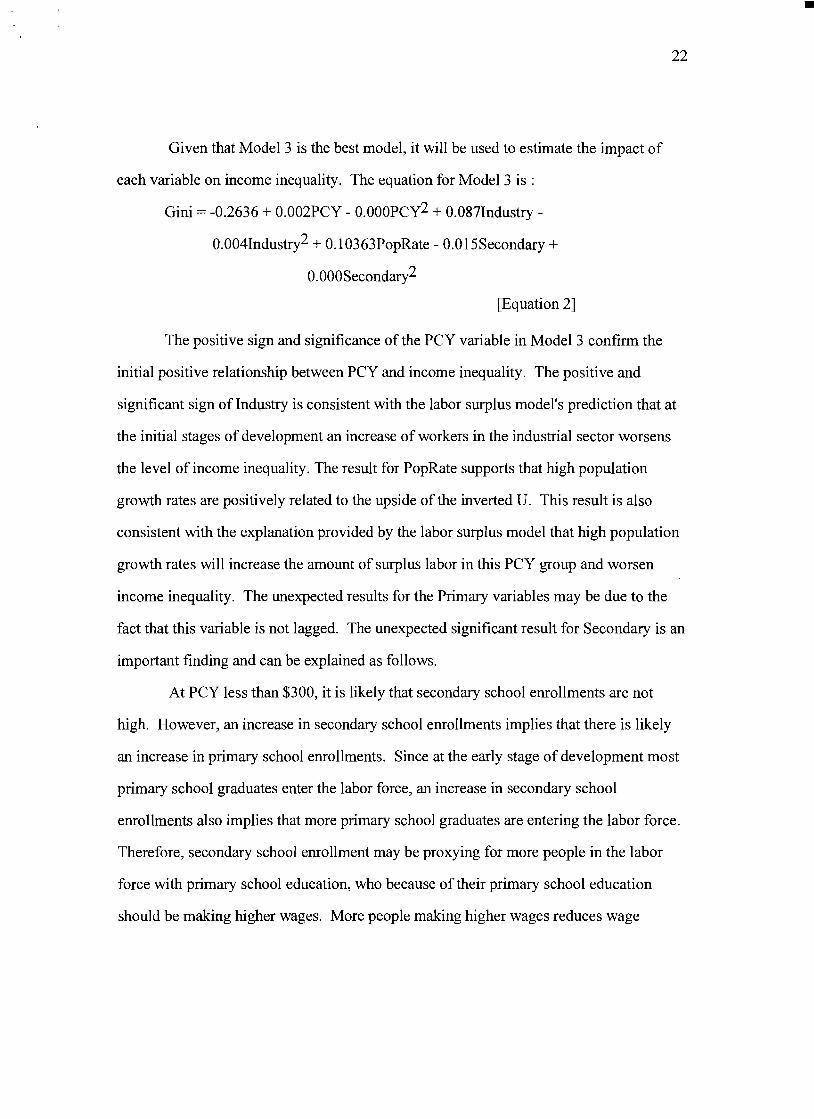
bull
22
Given that Model 3 is the best model it will be used to estimate the impact of
each variable on income inequality The equation for Model 3 is
Gini = -02636 + 0002PCY - 0000PCy2 + 0087Industry shy
0004Industry2 + 01 0363PopRate - 00 I5Secondary +
0000Secondary2
[Equation 2]
The positive sign and significance of the PCY variable in Model 3 confirm the
initial positive relationship between PCY and income inequality The positive and
significant sign of Industry is consistent with the labor surplus models prediction that at
the initial stages of development an increase of workers in the industrial sector worsens
the level of income inequality The result for PopRate supports that high population
growth rates are positively related to the upside ofthe inverted U This result is also
consistent with the explanation provided by the labor surplus model that high population
growth rates will increase the amount of surplus labor in this PCY group and worsen
income inequality The unexpected results for the Primary variables may be due to the
fact that this variable is not lagged The unexpected significant result for Secondary is an
important finding and can be explained as follows
At PCY less than $300 it is likely that secondary school enrollments are not
high However an increase in secondary school enrollments implies that there is likely
an increase in primary school enrollments Since at the early stage of development most
primary school graduates enter the labor force an increase in secondary school
enrollments also implies that more primary school graduates are entering the labor force
Therefore secondary school enrollment may be proxying for more people in the labor
force with primary school education who because of their primary school education
should be making higher wages More people making higher wages reduces wage
bull
23
differentials which improves income inequality This explanation is consistent with the
result obtained from the Secondary variable
Conclusions and Policy Implications
As explained in Appendix 2 where the method ofcalculating gini coefficient is
discussed the value of the gini coefficient lies between 1 and O The closer the
coefficient is to 0 the lower the level of income inequality The closer the gini coefficient
is to I the higher the level of income inequality From Equation 2 above it is deduced
that an increase ofPCY by $1 will cause the gini coefficient to rise by 0002 This means
that an increase ofPCY by $50 causes the gini coefficient to rise by a tenth (01) This
result is significant and posits that when a country begins its development process and
PCY increases the initial worsening of income inequality is inevitable Thus for
countries with PCY up to about $300 a worsening trend of income inequality can be
accepted as an initial phase that accompanies development
According to Equation 2 above a percentage increase of labor in industry (the
variable Industry) causes the gini coefficient to increase by 0087 Thus a 115
percentage increase of labor in the industrial sector causes the gini coefficient to rise by
about a tenth This result is also significant and implies that about a 9 percent increase of
labor in industry will cause the level of income inequality to be at the highest possible
level Therefore the results suggest that developing countries within PCY Group I
should not only concentrate on the developing the industrial sector but should
simultaneously concentrate on developing the agricultural sector That way they may be
able to reduce the amount of migrants from agriculture into industry
How much income inequality exists at the early stages of development depends
significantly on population growth rates The higher the population growth rate the
bull
24
higher is the level of income inequality at each PCY According to Equation 2 a 1
percentage increase in population growth rates causes the gini coefficient to rise by 0104
This implies that an increase of population growth rate by 096 percent (approximately 1
percent) causes the gini coefficient to rise by a tenth This result points out that it is
necessary for developing countries to adopt measures to control population growth rates
as early as possible in their development process By maintaining low population growth
rates and as according to the labor surplus model labor in the economy becomes a scarce
factor earlier and labor markets are competitive sooner Then also wages should
increase and income inequality should improve
If Secondary is accepted as a proxy for the amount of primary school graduates
entering the labor force then as calculated from Equation 2 a 667 increase of primary
school graduates entering the labor force (ie 667 increase in secondary school
enrollment) should decrease the gini coefficient by a tenth This is a significant and
encouraging result because it emphasizes the universal benefits of education even at the
early stages of development
PCY Group II (The intermediate stage of development)
Results
All the models created for this PCY group show no significant result as noted in Table 4
None of the variables are significant and the R2s for all the models are very low The
results confirm that the curve is a straight line for this PCY group
Conclusion
The results for PCY Group II does not allow one to make any generalizations applicable
to countries in this PCY group today Perhaps conditions in these countries are complex
and varied and therefore cannot be easily summarized
bull 25
TABLE 4 GINI REGRESSIONS FOR 300 lt PCY lt= 1000
VARIABLE MODEL 1 MODEL 2 MODEL 3
PCY 000004 000005 000008
PCy2 -000000 -000000 -000000
INDUSTRY -000842 -000720 -000836
INDUSTRy2 -000000 -000004 000002
POPRATE -002217 -002602 -000794
PRIMARY 001063 001068
PRIMARy2 -000006 -000006
SECONDARY 000171 000232
SECONDARy2 -000002 -000002
ADJUSTED Rl -007 005 002
bull 26
VARIABLES MODEL 1 MODEL 2 MODEL 3
PCY ( - )
-000002 ( - )
-000001 ( - )
-000002
PCy2 (+ ) +000000
(+ ) +000000
(+ ) +000000
INDUSTRY ( - )
-000460 ( - )
-001577 ( shy )
-000720
INDUSTRy2 (+ ) 000007
( + ) +000024
(+ ) 000012
PORPORATE (+ ) -001515
(+ ) +000806
(+ ) -001960
PRIMARY ( shy )
-001664 ( shy )
-005207
PRlMARy2 (+ ) +000008
(+ ) +000024
SECONDARY ( shy )
-000971 ( - )
-000866
SECONDARy2 (+ ) +000006
(+ ) +000005
ADJUSTED Rl 050 044
= SIGNIFICANT AT THE 90 CONFINDENCE LEVEL (TWO-TAIL TESr SIGNS IN PARENTEHESES ARE THE HYPOTHESIZED SIGNS
TABLE 5 GINI REGRESSIONS FOR PCY gt 1000
bull
27
PCY Group III (The industrialized stage of development)
Results
Only the education variables have significant coefficients in the models in Table 5 The
PCY variables in this table are not significant although they are in Table 1 This is
possibly because the explanatory variables in the regression equations for the models in
Table 5 (these explanatory variables are not included in the regression equation for Table
1) reduce the significance of the PCY variable The significant and expected coefficient
for Secondary in the models supports Lewis explanation that as an economy develops
education facilities become available to more people so that in the long run education has
a negative effect on the level of income inequality
Conclusion
Since countries in PCY Group III are well industrialized the increasing share of labor in
industry may have little impact on the level of income inequality Likewise population
growth rates which are relatively stable in these countries may have negligible effect on
the level of income inequality It is likely that there are other variables that may help
explain the downward trend of income inequality that is expected for industrialized
countries Often countries in the early stages of development experience political and
social instabilities conditions which improve as these countries develop Thus a measure
of political and social conditions may for instance be a crucial determinant of the
downward trend of income inequality It is also likely that the existence of certain
institutions in industrialized countries like unions that function to improve wages help
improve the level of income inequality in these countries Thus a measure of
unionization may also improve the results for this group Another variable that measures
bull
28
U This is because it is usual to find more advanced technological equipment and
facilities in industrialized countries and not in developing countries In summary the
share of labor in industry and population growth rates do not explain the downside of the
inverted U
General Conclusion
In this paper four hypothesis were generated and tested to confirm that the inverted U
exists and that the share of labor in industry population growth rates and education were
explanatory variables of income inequality Moreover the labor surplus model predicts
the inverted U pattern Although the inverted U pattern was found as presented in Table 1
where only PCY variables were used in the regression equation the explanatory variables
failed to show the inverted U pattern in its entirety The explanatory variables were able
to explain the upside of the inverted U as shown in Table 3 but the same explanatory
variables could not explain the downside of the inverted U as shown in Table 5
Thus this study also shows that the labor surplus model explains the upward trend
for countries with very low PCY and that high population growth rates worsen the level
of income inequality for these countries This study highlights that the labor surplus
model is incapable of explaining any other part of the inverted U especially the downside
of the inverted U
Suggestions For Future Research
Another explanation for the inverted U pattern can be given using labor market power as
follows At the early stages of development firms have monosony power and can force
the technological know-how in the various countries may also help explain the inverted
bull
29
wages to be low which signifies a period of worsening income inequality At the
intermediate stage of development more firms may exist which may cause the initial
monosony power of firms to reduce and at least prevent further worsening of income
inequality At the industrialized stage of development workers are likely to organize into
unions and counter the remaining monosony power of firms This should increase wages
and cause income inequality to improve This brief discussion suggests an important area
for future research Perhaps a better explanation of the inverted U pattern or an important
area to be considered along with the labor surplus model may be discovered
Another area for future research will be to separate the countries in PCY Group III
(countries that have PCY greater than $1000) into two categories the newly industrialized
and the well industrialized countries This may help control for the wide range of PCY in
PCY Group III and also the differences in institutions that exist in these countries
bull
30
WORK CITED
Ahluwalia Montek S 1976 Inequality Poverty and Development Journal of Development
Economics 3306-342
Braun Denny The Rich Get Richer The Rise ofIncome Inequality in the United States and the World
Chicago Nelson-Hall Publishers 1991
Chenery Hollis Ahluwalia S Montek C L G Bell John H Duloy Richard Jolly Redistribution
with ~rowth London Oxford University Press 1975
Chenery Hollis amp Moises Syrquin Patterns of Development 1950-1970 Published for the World Bank
by Oxford University Press 1975
Dovring Folke Inequality New York Praeger Publishers 1991
Eckstein Zvi amp Zilcha Itzhak 1992 The effects of compulsory schooling on growth
income distribution and welfare Journal of Public Economics 543339-359
Fields Gary F Poverty Inequality and Development London Cambridge University Press 1980
Gillis Malcom Economics of Development New York WW Norton amp Company 1992
Lewis W Arthur Theory of Economic Growth New York Harper Row 1970
Poulson Barry W Economic Development Minneapolis West Publishing Company 1994
APPENDIX 1shy
bull
~Cgt -ntneG time gini pey PopPate indu~ primary r
3an~1lade 25-30 030 7000 26 48 31
ncilet 25-30 036 9000 23 119 74
Paki~tan 25-30 034- 11000 26 183 40
Pak~tan 15-20 0294 130 31 172 12
Banglade 15-20 0316 130 25 54 73 Thailand 25-30 039 14000 31 52 78
0ri Lanka 25-30 041 16000 25 139 93
India 15-20 037 17000 23 129 79
Tanzania 15middot20 038 17000 28 38 53 Phiflipine 25-30 045 18000 31 158 113
Indonesia 15-20 038 21000 24 117 86
Uganda 15-20 036 22000 26 39 44 Sierra Le 15middot20 040 22000 2 132 39
Kenya 15-20 049 23000 37 62 95 0ri Lanka 15-20 032 29000 16 142 77 Mauritius 25-30 040 31000 24 254 72
Egypt 15-20 038 32000 2 184 71
Columbia 2~30 O~6 32000 3 214 84 Phillipine 15-20 043 34000 26 161 107 Botswana 15-20 050 35000 38 84 72
Bolivia 15-20 046 36000 25 199 85 0uriname 25-30 029 39000 27 215 120
Costa Ric 25-30 045 40000 32 192 106 Liberia 15-20 055 41000 3 94 62 Mexico 25-30 049 46000 33 219 92 Ecuador 15-20 059 54000 3 202 104
Zambia 15-20 050 55000 3 92 97
Columbia 15-20 047 55000 21 234 118 Guatemal 15-20 046 57000 28 17 61
Nicaragu 15-20 052 63000 3 156 82
Spain 25-30 035 70000 1 345 115
Tunisia 15-20 034 71000 21 311 97 Mauritius 15-20 043 71000 15 245 107
Libya 25-30 024 81000 39 209 78
Malaysia 15-20 045 82000 23 166 91 Argentina 25-30 038 87000 15 342 101
Japan 25-30 037 90000 11 32 100 Costa Ric 15-20 045 95000 25 216 107
Peru 15-20 052middot 100000 27 18 113
bull
Fiji 15-20 038 03000 i 9 160 115
Brazil 15-20 051 1070gt 24shy 243 88
Venezuel 25-30 048 113000 34 237 94
Israel 25-30 030 130000 35 354 95 Barbados 15-20 032 152000 04 233 103
Portugal 15-20 038 154000 38 347 113 Netherlan 25-30 039 156000 14 407 104
Trinidad 15-20 041 172000 09 372 99
Finland 25-30 042 175000 03 354 92 rmiddotJnrway 25-30 032 184000 08 368 97
France 25-30 046 203000 09 39 134
Denmark 25-30 035 205000 08 369 98 Venezuel 15-20 045 238000 36 267 97
Canada 25-30 030 262000 18 325 105
Ireland 15-20 029 265000 17 324 103 Sweden 25-30 036 276000 09 428 95
Spain 15-20 034 278000 1 374 111 I~rael 15-20 028 389000 23 337 97
rrance 15-20 036 600000 05 373 109
Germany 15-20 033 667000 -04 476 103 Sweden 15-20 027 832000 04 365 101
Australia Recent 034 1668000 16 344 106
bull APPENDIX 2
Calculatin2 Gjni Coefficjents
To convert the figures of an income distribution data into a measure of
income inequality can be done by constructing a Lorenz curve for each
country from which the Gini coefficientconcentration ratio(a measure of
inequality) is calculated The Lorenz curve shows the total percentage of
total income accounted for by any cumulative percentage of recipients
The shape of this curve indicates the degree of income inequality in the
income distribution(Gillis 1992 74) To illustrate how a Lorenz curve is
derived consider the following data for Brazil in 1983
poorest 20 of households receive 24 of total income
second quintile receive 57
third quintile receive 107
fourth quintile receive 186
richest 20 receive 626
From these data it can be observed that Brazil has a high degree of
inequality if 626 of its total income goes to the richest 20 of total
households Also a total of 100 of households receive 100 of total
income To construct a Lorenz curve first the cumulative income share
accruing to any given percentage of households is calculated Thus for the
data above we get the following calculations
poorest 20 receive 24 of total income
poorest 40 receive 24 + 57 = 81 of total income
poorest 60 receive 81 + 107 = 188 of total income
poorest 80 receive 188 + 186 = 374 of total income
100 of households receive 100 of total income
bull
The Lorenz curve is a graph plotted from the data above with the
horizontal axis measuring the cumulative percentage of recipient units and
the vertical axis measunng the cumulative share of total income
Diagram2 below shows the Lorenz curve obtained from the data above
J
J~
t
1
I
l
~ 1 IA I
I
~ [J I
J 1
Diagram2
(Bolnick 1987 61-62)
The diagonal line is a 45-degree line The closer the curve is to this line
the lesser is income inequality The closer it is to the right hand borders
the greater is income inequality(Gillis 1992 74)
To calculate the Gini coefficient let A be the area between the Lorenz
curve and the diagonal line and let B be the area under the Lorenz curve
as show in Figure 2 The formula to calculate the Gini coefficient is given
as
bull
A(A + B) A + B will always be 05 because the box in which the Lorenz
curve is drawn is a unit square especially seen if all percentages are taken
as decimal units eg 20 as 02 Therefore the area of the square becomes
lxl = 10 and half the area of the square (A + B) is 05(Bolnick 1987 62)
Area B can be calculated geometrically using formulas for calculating areas
of rectangles triangles and trapezoids The area of B was calculated
geometrically to be 0233 Since A + B = 05 A = 05 - 0233 = 0267 The
Gini Coefficient AlA + B) = 026705 = 0534 The closer the Gini
coefficient is to 0 the lesser is income inequality and the closer it is to 1
the greater is income inequality
I created a program in Pascal that calculates gini coefficients based
on the Lorenz curve the formula for the area of trapezoids and the
formula for the gini coefficient
bull bull
045
03
bull
APPENDIX 3
REGRESSION LINE DRAWN AGAINST PLOTTED DATA FOR pey GROUP I
05--------------------------------bull
04
035 bull
bull bull
bull bull
bull
bull bulli~t=-+~=
bull
bull
025l-------r------r--r-------------_r-----r---------------------------r-----------J 7000 13000 16000 18000 22000
bull bull
bull bull bull
APPENDIX 4
REGRESSION LINE DRAWN AGAINST PLOTTED DATA FOR pey GROUP II
bull
06-------------------------------------
055 bull
bull bullbullbull 05 bull bull bullbullA45
bull 04 bull
035 bull
bull 03
bull
025
bull
O 2--L--------------------------------------------r----------------------r----------------------------------------r---r---l
31000 34000 39000 46000 55000 70000 81000 90000
bull bull
APPENDIX 5
REGRESSION LINE DRAWN AGAINST PLOTTED DATA FOR pey GROUP III
bull
0S5------------------------------
05 bull
bull045 bull
bull ~ 04
bull~ 035 bull
03
bull bull 025
02
01 f0-+-0-0--2-0-r-0-0--3-000--40-0-0--S-OO-0--610010--700-0--8-00-0--9---1000
PCY
bull
bull
23
differentials which improves income inequality This explanation is consistent with the
result obtained from the Secondary variable
Conclusions and Policy Implications
As explained in Appendix 2 where the method ofcalculating gini coefficient is
discussed the value of the gini coefficient lies between 1 and O The closer the
coefficient is to 0 the lower the level of income inequality The closer the gini coefficient
is to I the higher the level of income inequality From Equation 2 above it is deduced
that an increase ofPCY by $1 will cause the gini coefficient to rise by 0002 This means
that an increase ofPCY by $50 causes the gini coefficient to rise by a tenth (01) This
result is significant and posits that when a country begins its development process and
PCY increases the initial worsening of income inequality is inevitable Thus for
countries with PCY up to about $300 a worsening trend of income inequality can be
accepted as an initial phase that accompanies development
According to Equation 2 above a percentage increase of labor in industry (the
variable Industry) causes the gini coefficient to increase by 0087 Thus a 115
percentage increase of labor in the industrial sector causes the gini coefficient to rise by
about a tenth This result is also significant and implies that about a 9 percent increase of
labor in industry will cause the level of income inequality to be at the highest possible
level Therefore the results suggest that developing countries within PCY Group I
should not only concentrate on the developing the industrial sector but should
simultaneously concentrate on developing the agricultural sector That way they may be
able to reduce the amount of migrants from agriculture into industry
How much income inequality exists at the early stages of development depends
significantly on population growth rates The higher the population growth rate the
bull
24
higher is the level of income inequality at each PCY According to Equation 2 a 1
percentage increase in population growth rates causes the gini coefficient to rise by 0104
This implies that an increase of population growth rate by 096 percent (approximately 1
percent) causes the gini coefficient to rise by a tenth This result points out that it is
necessary for developing countries to adopt measures to control population growth rates
as early as possible in their development process By maintaining low population growth
rates and as according to the labor surplus model labor in the economy becomes a scarce
factor earlier and labor markets are competitive sooner Then also wages should
increase and income inequality should improve
If Secondary is accepted as a proxy for the amount of primary school graduates
entering the labor force then as calculated from Equation 2 a 667 increase of primary
school graduates entering the labor force (ie 667 increase in secondary school
enrollment) should decrease the gini coefficient by a tenth This is a significant and
encouraging result because it emphasizes the universal benefits of education even at the
early stages of development
PCY Group II (The intermediate stage of development)
Results
All the models created for this PCY group show no significant result as noted in Table 4
None of the variables are significant and the R2s for all the models are very low The
results confirm that the curve is a straight line for this PCY group
Conclusion
The results for PCY Group II does not allow one to make any generalizations applicable
to countries in this PCY group today Perhaps conditions in these countries are complex
and varied and therefore cannot be easily summarized
bull 25
TABLE 4 GINI REGRESSIONS FOR 300 lt PCY lt= 1000
VARIABLE MODEL 1 MODEL 2 MODEL 3
PCY 000004 000005 000008
PCy2 -000000 -000000 -000000
INDUSTRY -000842 -000720 -000836
INDUSTRy2 -000000 -000004 000002
POPRATE -002217 -002602 -000794
PRIMARY 001063 001068
PRIMARy2 -000006 -000006
SECONDARY 000171 000232
SECONDARy2 -000002 -000002
ADJUSTED Rl -007 005 002
bull 26
VARIABLES MODEL 1 MODEL 2 MODEL 3
PCY ( - )
-000002 ( - )
-000001 ( - )
-000002
PCy2 (+ ) +000000
(+ ) +000000
(+ ) +000000
INDUSTRY ( - )
-000460 ( - )
-001577 ( shy )
-000720
INDUSTRy2 (+ ) 000007
( + ) +000024
(+ ) 000012
PORPORATE (+ ) -001515
(+ ) +000806
(+ ) -001960
PRIMARY ( shy )
-001664 ( shy )
-005207
PRlMARy2 (+ ) +000008
(+ ) +000024
SECONDARY ( shy )
-000971 ( - )
-000866
SECONDARy2 (+ ) +000006
(+ ) +000005
ADJUSTED Rl 050 044
= SIGNIFICANT AT THE 90 CONFINDENCE LEVEL (TWO-TAIL TESr SIGNS IN PARENTEHESES ARE THE HYPOTHESIZED SIGNS
TABLE 5 GINI REGRESSIONS FOR PCY gt 1000
bull
27
PCY Group III (The industrialized stage of development)
Results
Only the education variables have significant coefficients in the models in Table 5 The
PCY variables in this table are not significant although they are in Table 1 This is
possibly because the explanatory variables in the regression equations for the models in
Table 5 (these explanatory variables are not included in the regression equation for Table
1) reduce the significance of the PCY variable The significant and expected coefficient
for Secondary in the models supports Lewis explanation that as an economy develops
education facilities become available to more people so that in the long run education has
a negative effect on the level of income inequality
Conclusion
Since countries in PCY Group III are well industrialized the increasing share of labor in
industry may have little impact on the level of income inequality Likewise population
growth rates which are relatively stable in these countries may have negligible effect on
the level of income inequality It is likely that there are other variables that may help
explain the downward trend of income inequality that is expected for industrialized
countries Often countries in the early stages of development experience political and
social instabilities conditions which improve as these countries develop Thus a measure
of political and social conditions may for instance be a crucial determinant of the
downward trend of income inequality It is also likely that the existence of certain
institutions in industrialized countries like unions that function to improve wages help
improve the level of income inequality in these countries Thus a measure of
unionization may also improve the results for this group Another variable that measures
bull
28
U This is because it is usual to find more advanced technological equipment and
facilities in industrialized countries and not in developing countries In summary the
share of labor in industry and population growth rates do not explain the downside of the
inverted U
General Conclusion
In this paper four hypothesis were generated and tested to confirm that the inverted U
exists and that the share of labor in industry population growth rates and education were
explanatory variables of income inequality Moreover the labor surplus model predicts
the inverted U pattern Although the inverted U pattern was found as presented in Table 1
where only PCY variables were used in the regression equation the explanatory variables
failed to show the inverted U pattern in its entirety The explanatory variables were able
to explain the upside of the inverted U as shown in Table 3 but the same explanatory
variables could not explain the downside of the inverted U as shown in Table 5
Thus this study also shows that the labor surplus model explains the upward trend
for countries with very low PCY and that high population growth rates worsen the level
of income inequality for these countries This study highlights that the labor surplus
model is incapable of explaining any other part of the inverted U especially the downside
of the inverted U
Suggestions For Future Research
Another explanation for the inverted U pattern can be given using labor market power as
follows At the early stages of development firms have monosony power and can force
the technological know-how in the various countries may also help explain the inverted
bull
29
wages to be low which signifies a period of worsening income inequality At the
intermediate stage of development more firms may exist which may cause the initial
monosony power of firms to reduce and at least prevent further worsening of income
inequality At the industrialized stage of development workers are likely to organize into
unions and counter the remaining monosony power of firms This should increase wages
and cause income inequality to improve This brief discussion suggests an important area
for future research Perhaps a better explanation of the inverted U pattern or an important
area to be considered along with the labor surplus model may be discovered
Another area for future research will be to separate the countries in PCY Group III
(countries that have PCY greater than $1000) into two categories the newly industrialized
and the well industrialized countries This may help control for the wide range of PCY in
PCY Group III and also the differences in institutions that exist in these countries
bull
30
WORK CITED
Ahluwalia Montek S 1976 Inequality Poverty and Development Journal of Development
Economics 3306-342
Braun Denny The Rich Get Richer The Rise ofIncome Inequality in the United States and the World
Chicago Nelson-Hall Publishers 1991
Chenery Hollis Ahluwalia S Montek C L G Bell John H Duloy Richard Jolly Redistribution
with ~rowth London Oxford University Press 1975
Chenery Hollis amp Moises Syrquin Patterns of Development 1950-1970 Published for the World Bank
by Oxford University Press 1975
Dovring Folke Inequality New York Praeger Publishers 1991
Eckstein Zvi amp Zilcha Itzhak 1992 The effects of compulsory schooling on growth
income distribution and welfare Journal of Public Economics 543339-359
Fields Gary F Poverty Inequality and Development London Cambridge University Press 1980
Gillis Malcom Economics of Development New York WW Norton amp Company 1992
Lewis W Arthur Theory of Economic Growth New York Harper Row 1970
Poulson Barry W Economic Development Minneapolis West Publishing Company 1994
APPENDIX 1shy
bull
~Cgt -ntneG time gini pey PopPate indu~ primary r
3an~1lade 25-30 030 7000 26 48 31
ncilet 25-30 036 9000 23 119 74
Paki~tan 25-30 034- 11000 26 183 40
Pak~tan 15-20 0294 130 31 172 12
Banglade 15-20 0316 130 25 54 73 Thailand 25-30 039 14000 31 52 78
0ri Lanka 25-30 041 16000 25 139 93
India 15-20 037 17000 23 129 79
Tanzania 15middot20 038 17000 28 38 53 Phiflipine 25-30 045 18000 31 158 113
Indonesia 15-20 038 21000 24 117 86
Uganda 15-20 036 22000 26 39 44 Sierra Le 15middot20 040 22000 2 132 39
Kenya 15-20 049 23000 37 62 95 0ri Lanka 15-20 032 29000 16 142 77 Mauritius 25-30 040 31000 24 254 72
Egypt 15-20 038 32000 2 184 71
Columbia 2~30 O~6 32000 3 214 84 Phillipine 15-20 043 34000 26 161 107 Botswana 15-20 050 35000 38 84 72
Bolivia 15-20 046 36000 25 199 85 0uriname 25-30 029 39000 27 215 120
Costa Ric 25-30 045 40000 32 192 106 Liberia 15-20 055 41000 3 94 62 Mexico 25-30 049 46000 33 219 92 Ecuador 15-20 059 54000 3 202 104
Zambia 15-20 050 55000 3 92 97
Columbia 15-20 047 55000 21 234 118 Guatemal 15-20 046 57000 28 17 61
Nicaragu 15-20 052 63000 3 156 82
Spain 25-30 035 70000 1 345 115
Tunisia 15-20 034 71000 21 311 97 Mauritius 15-20 043 71000 15 245 107
Libya 25-30 024 81000 39 209 78
Malaysia 15-20 045 82000 23 166 91 Argentina 25-30 038 87000 15 342 101
Japan 25-30 037 90000 11 32 100 Costa Ric 15-20 045 95000 25 216 107
Peru 15-20 052middot 100000 27 18 113
bull
Fiji 15-20 038 03000 i 9 160 115
Brazil 15-20 051 1070gt 24shy 243 88
Venezuel 25-30 048 113000 34 237 94
Israel 25-30 030 130000 35 354 95 Barbados 15-20 032 152000 04 233 103
Portugal 15-20 038 154000 38 347 113 Netherlan 25-30 039 156000 14 407 104
Trinidad 15-20 041 172000 09 372 99
Finland 25-30 042 175000 03 354 92 rmiddotJnrway 25-30 032 184000 08 368 97
France 25-30 046 203000 09 39 134
Denmark 25-30 035 205000 08 369 98 Venezuel 15-20 045 238000 36 267 97
Canada 25-30 030 262000 18 325 105
Ireland 15-20 029 265000 17 324 103 Sweden 25-30 036 276000 09 428 95
Spain 15-20 034 278000 1 374 111 I~rael 15-20 028 389000 23 337 97
rrance 15-20 036 600000 05 373 109
Germany 15-20 033 667000 -04 476 103 Sweden 15-20 027 832000 04 365 101
Australia Recent 034 1668000 16 344 106
bull APPENDIX 2
Calculatin2 Gjni Coefficjents
To convert the figures of an income distribution data into a measure of
income inequality can be done by constructing a Lorenz curve for each
country from which the Gini coefficientconcentration ratio(a measure of
inequality) is calculated The Lorenz curve shows the total percentage of
total income accounted for by any cumulative percentage of recipients
The shape of this curve indicates the degree of income inequality in the
income distribution(Gillis 1992 74) To illustrate how a Lorenz curve is
derived consider the following data for Brazil in 1983
poorest 20 of households receive 24 of total income
second quintile receive 57
third quintile receive 107
fourth quintile receive 186
richest 20 receive 626
From these data it can be observed that Brazil has a high degree of
inequality if 626 of its total income goes to the richest 20 of total
households Also a total of 100 of households receive 100 of total
income To construct a Lorenz curve first the cumulative income share
accruing to any given percentage of households is calculated Thus for the
data above we get the following calculations
poorest 20 receive 24 of total income
poorest 40 receive 24 + 57 = 81 of total income
poorest 60 receive 81 + 107 = 188 of total income
poorest 80 receive 188 + 186 = 374 of total income
100 of households receive 100 of total income
bull
The Lorenz curve is a graph plotted from the data above with the
horizontal axis measuring the cumulative percentage of recipient units and
the vertical axis measunng the cumulative share of total income
Diagram2 below shows the Lorenz curve obtained from the data above
J
J~
t
1
I
l
~ 1 IA I
I
~ [J I
J 1
Diagram2
(Bolnick 1987 61-62)
The diagonal line is a 45-degree line The closer the curve is to this line
the lesser is income inequality The closer it is to the right hand borders
the greater is income inequality(Gillis 1992 74)
To calculate the Gini coefficient let A be the area between the Lorenz
curve and the diagonal line and let B be the area under the Lorenz curve
as show in Figure 2 The formula to calculate the Gini coefficient is given
as
bull
A(A + B) A + B will always be 05 because the box in which the Lorenz
curve is drawn is a unit square especially seen if all percentages are taken
as decimal units eg 20 as 02 Therefore the area of the square becomes
lxl = 10 and half the area of the square (A + B) is 05(Bolnick 1987 62)
Area B can be calculated geometrically using formulas for calculating areas
of rectangles triangles and trapezoids The area of B was calculated
geometrically to be 0233 Since A + B = 05 A = 05 - 0233 = 0267 The
Gini Coefficient AlA + B) = 026705 = 0534 The closer the Gini
coefficient is to 0 the lesser is income inequality and the closer it is to 1
the greater is income inequality
I created a program in Pascal that calculates gini coefficients based
on the Lorenz curve the formula for the area of trapezoids and the
formula for the gini coefficient
bull bull
045
03
bull
APPENDIX 3
REGRESSION LINE DRAWN AGAINST PLOTTED DATA FOR pey GROUP I
05--------------------------------bull
04
035 bull
bull bull
bull bull
bull
bull bulli~t=-+~=
bull
bull
025l-------r------r--r-------------_r-----r---------------------------r-----------J 7000 13000 16000 18000 22000
bull bull
bull bull bull
APPENDIX 4
REGRESSION LINE DRAWN AGAINST PLOTTED DATA FOR pey GROUP II
bull
06-------------------------------------
055 bull
bull bullbullbull 05 bull bull bullbullA45
bull 04 bull
035 bull
bull 03
bull
025
bull
O 2--L--------------------------------------------r----------------------r----------------------------------------r---r---l
31000 34000 39000 46000 55000 70000 81000 90000
bull bull
APPENDIX 5
REGRESSION LINE DRAWN AGAINST PLOTTED DATA FOR pey GROUP III
bull
0S5------------------------------
05 bull
bull045 bull
bull ~ 04
bull~ 035 bull
03
bull bull 025
02
01 f0-+-0-0--2-0-r-0-0--3-000--40-0-0--S-OO-0--610010--700-0--8-00-0--9---1000
PCY
bull

bull
24
higher is the level of income inequality at each PCY According to Equation 2 a 1
percentage increase in population growth rates causes the gini coefficient to rise by 0104
This implies that an increase of population growth rate by 096 percent (approximately 1
percent) causes the gini coefficient to rise by a tenth This result points out that it is
necessary for developing countries to adopt measures to control population growth rates
as early as possible in their development process By maintaining low population growth
rates and as according to the labor surplus model labor in the economy becomes a scarce
factor earlier and labor markets are competitive sooner Then also wages should
increase and income inequality should improve
If Secondary is accepted as a proxy for the amount of primary school graduates
entering the labor force then as calculated from Equation 2 a 667 increase of primary
school graduates entering the labor force (ie 667 increase in secondary school
enrollment) should decrease the gini coefficient by a tenth This is a significant and
encouraging result because it emphasizes the universal benefits of education even at the
early stages of development
PCY Group II (The intermediate stage of development)
Results
All the models created for this PCY group show no significant result as noted in Table 4
None of the variables are significant and the R2s for all the models are very low The
results confirm that the curve is a straight line for this PCY group
Conclusion
The results for PCY Group II does not allow one to make any generalizations applicable
to countries in this PCY group today Perhaps conditions in these countries are complex
and varied and therefore cannot be easily summarized
bull 25
TABLE 4 GINI REGRESSIONS FOR 300 lt PCY lt= 1000
VARIABLE MODEL 1 MODEL 2 MODEL 3
PCY 000004 000005 000008
PCy2 -000000 -000000 -000000
INDUSTRY -000842 -000720 -000836
INDUSTRy2 -000000 -000004 000002
POPRATE -002217 -002602 -000794
PRIMARY 001063 001068
PRIMARy2 -000006 -000006
SECONDARY 000171 000232
SECONDARy2 -000002 -000002
ADJUSTED Rl -007 005 002
bull 26
VARIABLES MODEL 1 MODEL 2 MODEL 3
PCY ( - )
-000002 ( - )
-000001 ( - )
-000002
PCy2 (+ ) +000000
(+ ) +000000
(+ ) +000000
INDUSTRY ( - )
-000460 ( - )
-001577 ( shy )
-000720
INDUSTRy2 (+ ) 000007
( + ) +000024
(+ ) 000012
PORPORATE (+ ) -001515
(+ ) +000806
(+ ) -001960
PRIMARY ( shy )
-001664 ( shy )
-005207
PRlMARy2 (+ ) +000008
(+ ) +000024
SECONDARY ( shy )
-000971 ( - )
-000866
SECONDARy2 (+ ) +000006
(+ ) +000005
ADJUSTED Rl 050 044
= SIGNIFICANT AT THE 90 CONFINDENCE LEVEL (TWO-TAIL TESr SIGNS IN PARENTEHESES ARE THE HYPOTHESIZED SIGNS
TABLE 5 GINI REGRESSIONS FOR PCY gt 1000
bull
27
PCY Group III (The industrialized stage of development)
Results
Only the education variables have significant coefficients in the models in Table 5 The
PCY variables in this table are not significant although they are in Table 1 This is
possibly because the explanatory variables in the regression equations for the models in
Table 5 (these explanatory variables are not included in the regression equation for Table
1) reduce the significance of the PCY variable The significant and expected coefficient
for Secondary in the models supports Lewis explanation that as an economy develops
education facilities become available to more people so that in the long run education has
a negative effect on the level of income inequality
Conclusion
Since countries in PCY Group III are well industrialized the increasing share of labor in
industry may have little impact on the level of income inequality Likewise population
growth rates which are relatively stable in these countries may have negligible effect on
the level of income inequality It is likely that there are other variables that may help
explain the downward trend of income inequality that is expected for industrialized
countries Often countries in the early stages of development experience political and
social instabilities conditions which improve as these countries develop Thus a measure
of political and social conditions may for instance be a crucial determinant of the
downward trend of income inequality It is also likely that the existence of certain
institutions in industrialized countries like unions that function to improve wages help
improve the level of income inequality in these countries Thus a measure of
unionization may also improve the results for this group Another variable that measures
bull
28
U This is because it is usual to find more advanced technological equipment and
facilities in industrialized countries and not in developing countries In summary the
share of labor in industry and population growth rates do not explain the downside of the
inverted U
General Conclusion
In this paper four hypothesis were generated and tested to confirm that the inverted U
exists and that the share of labor in industry population growth rates and education were
explanatory variables of income inequality Moreover the labor surplus model predicts
the inverted U pattern Although the inverted U pattern was found as presented in Table 1
where only PCY variables were used in the regression equation the explanatory variables
failed to show the inverted U pattern in its entirety The explanatory variables were able
to explain the upside of the inverted U as shown in Table 3 but the same explanatory
variables could not explain the downside of the inverted U as shown in Table 5
Thus this study also shows that the labor surplus model explains the upward trend
for countries with very low PCY and that high population growth rates worsen the level
of income inequality for these countries This study highlights that the labor surplus
model is incapable of explaining any other part of the inverted U especially the downside
of the inverted U
Suggestions For Future Research
Another explanation for the inverted U pattern can be given using labor market power as
follows At the early stages of development firms have monosony power and can force
the technological know-how in the various countries may also help explain the inverted
bull
29
wages to be low which signifies a period of worsening income inequality At the
intermediate stage of development more firms may exist which may cause the initial
monosony power of firms to reduce and at least prevent further worsening of income
inequality At the industrialized stage of development workers are likely to organize into
unions and counter the remaining monosony power of firms This should increase wages
and cause income inequality to improve This brief discussion suggests an important area
for future research Perhaps a better explanation of the inverted U pattern or an important
area to be considered along with the labor surplus model may be discovered
Another area for future research will be to separate the countries in PCY Group III
(countries that have PCY greater than $1000) into two categories the newly industrialized
and the well industrialized countries This may help control for the wide range of PCY in
PCY Group III and also the differences in institutions that exist in these countries
bull
30
WORK CITED
Ahluwalia Montek S 1976 Inequality Poverty and Development Journal of Development
Economics 3306-342
Braun Denny The Rich Get Richer The Rise ofIncome Inequality in the United States and the World
Chicago Nelson-Hall Publishers 1991
Chenery Hollis Ahluwalia S Montek C L G Bell John H Duloy Richard Jolly Redistribution
with ~rowth London Oxford University Press 1975
Chenery Hollis amp Moises Syrquin Patterns of Development 1950-1970 Published for the World Bank
by Oxford University Press 1975
Dovring Folke Inequality New York Praeger Publishers 1991
Eckstein Zvi amp Zilcha Itzhak 1992 The effects of compulsory schooling on growth
income distribution and welfare Journal of Public Economics 543339-359
Fields Gary F Poverty Inequality and Development London Cambridge University Press 1980
Gillis Malcom Economics of Development New York WW Norton amp Company 1992
Lewis W Arthur Theory of Economic Growth New York Harper Row 1970
Poulson Barry W Economic Development Minneapolis West Publishing Company 1994
APPENDIX 1shy
bull
~Cgt -ntneG time gini pey PopPate indu~ primary r
3an~1lade 25-30 030 7000 26 48 31
ncilet 25-30 036 9000 23 119 74
Paki~tan 25-30 034- 11000 26 183 40
Pak~tan 15-20 0294 130 31 172 12
Banglade 15-20 0316 130 25 54 73 Thailand 25-30 039 14000 31 52 78
0ri Lanka 25-30 041 16000 25 139 93
India 15-20 037 17000 23 129 79
Tanzania 15middot20 038 17000 28 38 53 Phiflipine 25-30 045 18000 31 158 113
Indonesia 15-20 038 21000 24 117 86
Uganda 15-20 036 22000 26 39 44 Sierra Le 15middot20 040 22000 2 132 39
Kenya 15-20 049 23000 37 62 95 0ri Lanka 15-20 032 29000 16 142 77 Mauritius 25-30 040 31000 24 254 72
Egypt 15-20 038 32000 2 184 71
Columbia 2~30 O~6 32000 3 214 84 Phillipine 15-20 043 34000 26 161 107 Botswana 15-20 050 35000 38 84 72
Bolivia 15-20 046 36000 25 199 85 0uriname 25-30 029 39000 27 215 120
Costa Ric 25-30 045 40000 32 192 106 Liberia 15-20 055 41000 3 94 62 Mexico 25-30 049 46000 33 219 92 Ecuador 15-20 059 54000 3 202 104
Zambia 15-20 050 55000 3 92 97
Columbia 15-20 047 55000 21 234 118 Guatemal 15-20 046 57000 28 17 61
Nicaragu 15-20 052 63000 3 156 82
Spain 25-30 035 70000 1 345 115
Tunisia 15-20 034 71000 21 311 97 Mauritius 15-20 043 71000 15 245 107
Libya 25-30 024 81000 39 209 78
Malaysia 15-20 045 82000 23 166 91 Argentina 25-30 038 87000 15 342 101
Japan 25-30 037 90000 11 32 100 Costa Ric 15-20 045 95000 25 216 107
Peru 15-20 052middot 100000 27 18 113
bull
Fiji 15-20 038 03000 i 9 160 115
Brazil 15-20 051 1070gt 24shy 243 88
Venezuel 25-30 048 113000 34 237 94
Israel 25-30 030 130000 35 354 95 Barbados 15-20 032 152000 04 233 103
Portugal 15-20 038 154000 38 347 113 Netherlan 25-30 039 156000 14 407 104
Trinidad 15-20 041 172000 09 372 99
Finland 25-30 042 175000 03 354 92 rmiddotJnrway 25-30 032 184000 08 368 97
France 25-30 046 203000 09 39 134
Denmark 25-30 035 205000 08 369 98 Venezuel 15-20 045 238000 36 267 97
Canada 25-30 030 262000 18 325 105
Ireland 15-20 029 265000 17 324 103 Sweden 25-30 036 276000 09 428 95
Spain 15-20 034 278000 1 374 111 I~rael 15-20 028 389000 23 337 97
rrance 15-20 036 600000 05 373 109
Germany 15-20 033 667000 -04 476 103 Sweden 15-20 027 832000 04 365 101
Australia Recent 034 1668000 16 344 106
bull APPENDIX 2
Calculatin2 Gjni Coefficjents
To convert the figures of an income distribution data into a measure of
income inequality can be done by constructing a Lorenz curve for each
country from which the Gini coefficientconcentration ratio(a measure of
inequality) is calculated The Lorenz curve shows the total percentage of
total income accounted for by any cumulative percentage of recipients
The shape of this curve indicates the degree of income inequality in the
income distribution(Gillis 1992 74) To illustrate how a Lorenz curve is
derived consider the following data for Brazil in 1983
poorest 20 of households receive 24 of total income
second quintile receive 57
third quintile receive 107
fourth quintile receive 186
richest 20 receive 626
From these data it can be observed that Brazil has a high degree of
inequality if 626 of its total income goes to the richest 20 of total
households Also a total of 100 of households receive 100 of total
income To construct a Lorenz curve first the cumulative income share
accruing to any given percentage of households is calculated Thus for the
data above we get the following calculations
poorest 20 receive 24 of total income
poorest 40 receive 24 + 57 = 81 of total income
poorest 60 receive 81 + 107 = 188 of total income
poorest 80 receive 188 + 186 = 374 of total income
100 of households receive 100 of total income
bull
The Lorenz curve is a graph plotted from the data above with the
horizontal axis measuring the cumulative percentage of recipient units and
the vertical axis measunng the cumulative share of total income
Diagram2 below shows the Lorenz curve obtained from the data above
J
J~
t
1
I
l
~ 1 IA I
I
~ [J I
J 1
Diagram2
(Bolnick 1987 61-62)
The diagonal line is a 45-degree line The closer the curve is to this line
the lesser is income inequality The closer it is to the right hand borders
the greater is income inequality(Gillis 1992 74)
To calculate the Gini coefficient let A be the area between the Lorenz
curve and the diagonal line and let B be the area under the Lorenz curve
as show in Figure 2 The formula to calculate the Gini coefficient is given
as
bull
A(A + B) A + B will always be 05 because the box in which the Lorenz
curve is drawn is a unit square especially seen if all percentages are taken
as decimal units eg 20 as 02 Therefore the area of the square becomes
lxl = 10 and half the area of the square (A + B) is 05(Bolnick 1987 62)
Area B can be calculated geometrically using formulas for calculating areas
of rectangles triangles and trapezoids The area of B was calculated
geometrically to be 0233 Since A + B = 05 A = 05 - 0233 = 0267 The
Gini Coefficient AlA + B) = 026705 = 0534 The closer the Gini
coefficient is to 0 the lesser is income inequality and the closer it is to 1
the greater is income inequality
I created a program in Pascal that calculates gini coefficients based
on the Lorenz curve the formula for the area of trapezoids and the
formula for the gini coefficient
bull bull
045
03
bull
APPENDIX 3
REGRESSION LINE DRAWN AGAINST PLOTTED DATA FOR pey GROUP I
05--------------------------------bull
04
035 bull
bull bull
bull bull
bull
bull bulli~t=-+~=
bull
bull
025l-------r------r--r-------------_r-----r---------------------------r-----------J 7000 13000 16000 18000 22000
bull bull
bull bull bull
APPENDIX 4
REGRESSION LINE DRAWN AGAINST PLOTTED DATA FOR pey GROUP II
bull
06-------------------------------------
055 bull
bull bullbullbull 05 bull bull bullbullA45
bull 04 bull
035 bull
bull 03
bull
025
bull
O 2--L--------------------------------------------r----------------------r----------------------------------------r---r---l
31000 34000 39000 46000 55000 70000 81000 90000
bull bull
APPENDIX 5
REGRESSION LINE DRAWN AGAINST PLOTTED DATA FOR pey GROUP III
bull
0S5------------------------------
05 bull
bull045 bull
bull ~ 04
bull~ 035 bull
03
bull bull 025
02
01 f0-+-0-0--2-0-r-0-0--3-000--40-0-0--S-OO-0--610010--700-0--8-00-0--9---1000
PCY
bull
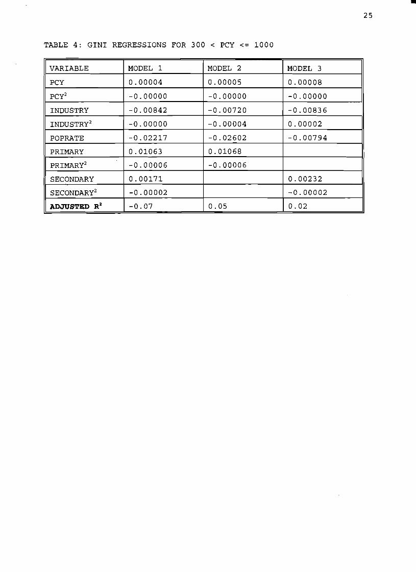

bull
27
PCY Group III (The industrialized stage of development)
Results
Only the education variables have significant coefficients in the models in Table 5 The
PCY variables in this table are not significant although they are in Table 1 This is
possibly because the explanatory variables in the regression equations for the models in
Table 5 (these explanatory variables are not included in the regression equation for Table
1) reduce the significance of the PCY variable The significant and expected coefficient
for Secondary in the models supports Lewis explanation that as an economy develops
education facilities become available to more people so that in the long run education has
a negative effect on the level of income inequality
Conclusion
Since countries in PCY Group III are well industrialized the increasing share of labor in
industry may have little impact on the level of income inequality Likewise population
growth rates which are relatively stable in these countries may have negligible effect on
the level of income inequality It is likely that there are other variables that may help
explain the downward trend of income inequality that is expected for industrialized
countries Often countries in the early stages of development experience political and
social instabilities conditions which improve as these countries develop Thus a measure
of political and social conditions may for instance be a crucial determinant of the
downward trend of income inequality It is also likely that the existence of certain
institutions in industrialized countries like unions that function to improve wages help
improve the level of income inequality in these countries Thus a measure of
unionization may also improve the results for this group Another variable that measures
bull
28
U This is because it is usual to find more advanced technological equipment and
facilities in industrialized countries and not in developing countries In summary the
share of labor in industry and population growth rates do not explain the downside of the
inverted U
General Conclusion
In this paper four hypothesis were generated and tested to confirm that the inverted U
exists and that the share of labor in industry population growth rates and education were
explanatory variables of income inequality Moreover the labor surplus model predicts
the inverted U pattern Although the inverted U pattern was found as presented in Table 1
where only PCY variables were used in the regression equation the explanatory variables
failed to show the inverted U pattern in its entirety The explanatory variables were able
to explain the upside of the inverted U as shown in Table 3 but the same explanatory
variables could not explain the downside of the inverted U as shown in Table 5
Thus this study also shows that the labor surplus model explains the upward trend
for countries with very low PCY and that high population growth rates worsen the level
of income inequality for these countries This study highlights that the labor surplus
model is incapable of explaining any other part of the inverted U especially the downside
of the inverted U
Suggestions For Future Research
Another explanation for the inverted U pattern can be given using labor market power as
follows At the early stages of development firms have monosony power and can force
the technological know-how in the various countries may also help explain the inverted
bull
29
wages to be low which signifies a period of worsening income inequality At the
intermediate stage of development more firms may exist which may cause the initial
monosony power of firms to reduce and at least prevent further worsening of income
inequality At the industrialized stage of development workers are likely to organize into
unions and counter the remaining monosony power of firms This should increase wages
and cause income inequality to improve This brief discussion suggests an important area
for future research Perhaps a better explanation of the inverted U pattern or an important
area to be considered along with the labor surplus model may be discovered
Another area for future research will be to separate the countries in PCY Group III
(countries that have PCY greater than $1000) into two categories the newly industrialized
and the well industrialized countries This may help control for the wide range of PCY in
PCY Group III and also the differences in institutions that exist in these countries
bull
30
WORK CITED
Ahluwalia Montek S 1976 Inequality Poverty and Development Journal of Development
Economics 3306-342
Braun Denny The Rich Get Richer The Rise ofIncome Inequality in the United States and the World
Chicago Nelson-Hall Publishers 1991
Chenery Hollis Ahluwalia S Montek C L G Bell John H Duloy Richard Jolly Redistribution
with ~rowth London Oxford University Press 1975
Chenery Hollis amp Moises Syrquin Patterns of Development 1950-1970 Published for the World Bank
by Oxford University Press 1975
Dovring Folke Inequality New York Praeger Publishers 1991
Eckstein Zvi amp Zilcha Itzhak 1992 The effects of compulsory schooling on growth
income distribution and welfare Journal of Public Economics 543339-359
Fields Gary F Poverty Inequality and Development London Cambridge University Press 1980
Gillis Malcom Economics of Development New York WW Norton amp Company 1992
Lewis W Arthur Theory of Economic Growth New York Harper Row 1970
Poulson Barry W Economic Development Minneapolis West Publishing Company 1994
APPENDIX 1shy
bull
~Cgt -ntneG time gini pey PopPate indu~ primary r
3an~1lade 25-30 030 7000 26 48 31
ncilet 25-30 036 9000 23 119 74
Paki~tan 25-30 034- 11000 26 183 40
Pak~tan 15-20 0294 130 31 172 12
Banglade 15-20 0316 130 25 54 73 Thailand 25-30 039 14000 31 52 78
0ri Lanka 25-30 041 16000 25 139 93
India 15-20 037 17000 23 129 79
Tanzania 15middot20 038 17000 28 38 53 Phiflipine 25-30 045 18000 31 158 113
Indonesia 15-20 038 21000 24 117 86
Uganda 15-20 036 22000 26 39 44 Sierra Le 15middot20 040 22000 2 132 39
Kenya 15-20 049 23000 37 62 95 0ri Lanka 15-20 032 29000 16 142 77 Mauritius 25-30 040 31000 24 254 72
Egypt 15-20 038 32000 2 184 71
Columbia 2~30 O~6 32000 3 214 84 Phillipine 15-20 043 34000 26 161 107 Botswana 15-20 050 35000 38 84 72
Bolivia 15-20 046 36000 25 199 85 0uriname 25-30 029 39000 27 215 120
Costa Ric 25-30 045 40000 32 192 106 Liberia 15-20 055 41000 3 94 62 Mexico 25-30 049 46000 33 219 92 Ecuador 15-20 059 54000 3 202 104
Zambia 15-20 050 55000 3 92 97
Columbia 15-20 047 55000 21 234 118 Guatemal 15-20 046 57000 28 17 61
Nicaragu 15-20 052 63000 3 156 82
Spain 25-30 035 70000 1 345 115
Tunisia 15-20 034 71000 21 311 97 Mauritius 15-20 043 71000 15 245 107
Libya 25-30 024 81000 39 209 78
Malaysia 15-20 045 82000 23 166 91 Argentina 25-30 038 87000 15 342 101
Japan 25-30 037 90000 11 32 100 Costa Ric 15-20 045 95000 25 216 107
Peru 15-20 052middot 100000 27 18 113
bull
Fiji 15-20 038 03000 i 9 160 115
Brazil 15-20 051 1070gt 24shy 243 88
Venezuel 25-30 048 113000 34 237 94
Israel 25-30 030 130000 35 354 95 Barbados 15-20 032 152000 04 233 103
Portugal 15-20 038 154000 38 347 113 Netherlan 25-30 039 156000 14 407 104
Trinidad 15-20 041 172000 09 372 99
Finland 25-30 042 175000 03 354 92 rmiddotJnrway 25-30 032 184000 08 368 97
France 25-30 046 203000 09 39 134
Denmark 25-30 035 205000 08 369 98 Venezuel 15-20 045 238000 36 267 97
Canada 25-30 030 262000 18 325 105
Ireland 15-20 029 265000 17 324 103 Sweden 25-30 036 276000 09 428 95
Spain 15-20 034 278000 1 374 111 I~rael 15-20 028 389000 23 337 97
rrance 15-20 036 600000 05 373 109
Germany 15-20 033 667000 -04 476 103 Sweden 15-20 027 832000 04 365 101
Australia Recent 034 1668000 16 344 106
bull APPENDIX 2
Calculatin2 Gjni Coefficjents
To convert the figures of an income distribution data into a measure of
income inequality can be done by constructing a Lorenz curve for each
country from which the Gini coefficientconcentration ratio(a measure of
inequality) is calculated The Lorenz curve shows the total percentage of
total income accounted for by any cumulative percentage of recipients
The shape of this curve indicates the degree of income inequality in the
income distribution(Gillis 1992 74) To illustrate how a Lorenz curve is
derived consider the following data for Brazil in 1983
poorest 20 of households receive 24 of total income
second quintile receive 57
third quintile receive 107
fourth quintile receive 186
richest 20 receive 626
From these data it can be observed that Brazil has a high degree of
inequality if 626 of its total income goes to the richest 20 of total
households Also a total of 100 of households receive 100 of total
income To construct a Lorenz curve first the cumulative income share
accruing to any given percentage of households is calculated Thus for the
data above we get the following calculations
poorest 20 receive 24 of total income
poorest 40 receive 24 + 57 = 81 of total income
poorest 60 receive 81 + 107 = 188 of total income
poorest 80 receive 188 + 186 = 374 of total income
100 of households receive 100 of total income
bull
The Lorenz curve is a graph plotted from the data above with the
horizontal axis measuring the cumulative percentage of recipient units and
the vertical axis measunng the cumulative share of total income
Diagram2 below shows the Lorenz curve obtained from the data above
J
J~
t
1
I
l
~ 1 IA I
I
~ [J I
J 1
Diagram2
(Bolnick 1987 61-62)
The diagonal line is a 45-degree line The closer the curve is to this line
the lesser is income inequality The closer it is to the right hand borders
the greater is income inequality(Gillis 1992 74)
To calculate the Gini coefficient let A be the area between the Lorenz
curve and the diagonal line and let B be the area under the Lorenz curve
as show in Figure 2 The formula to calculate the Gini coefficient is given
as
bull
A(A + B) A + B will always be 05 because the box in which the Lorenz
curve is drawn is a unit square especially seen if all percentages are taken
as decimal units eg 20 as 02 Therefore the area of the square becomes
lxl = 10 and half the area of the square (A + B) is 05(Bolnick 1987 62)
Area B can be calculated geometrically using formulas for calculating areas
of rectangles triangles and trapezoids The area of B was calculated
geometrically to be 0233 Since A + B = 05 A = 05 - 0233 = 0267 The
Gini Coefficient AlA + B) = 026705 = 0534 The closer the Gini
coefficient is to 0 the lesser is income inequality and the closer it is to 1
the greater is income inequality
I created a program in Pascal that calculates gini coefficients based
on the Lorenz curve the formula for the area of trapezoids and the
formula for the gini coefficient
bull bull
045
03
bull
APPENDIX 3
REGRESSION LINE DRAWN AGAINST PLOTTED DATA FOR pey GROUP I
05--------------------------------bull
04
035 bull
bull bull
bull bull
bull
bull bulli~t=-+~=
bull
bull
025l-------r------r--r-------------_r-----r---------------------------r-----------J 7000 13000 16000 18000 22000
bull bull
bull bull bull
APPENDIX 4
REGRESSION LINE DRAWN AGAINST PLOTTED DATA FOR pey GROUP II
bull
06-------------------------------------
055 bull
bull bullbullbull 05 bull bull bullbullA45
bull 04 bull
035 bull
bull 03
bull
025
bull
O 2--L--------------------------------------------r----------------------r----------------------------------------r---r---l
31000 34000 39000 46000 55000 70000 81000 90000
bull bull
APPENDIX 5
REGRESSION LINE DRAWN AGAINST PLOTTED DATA FOR pey GROUP III
bull
0S5------------------------------
05 bull
bull045 bull
bull ~ 04
bull~ 035 bull
03
bull bull 025
02
01 f0-+-0-0--2-0-r-0-0--3-000--40-0-0--S-OO-0--610010--700-0--8-00-0--9---1000
PCY
bull
bull
29
wages to be low which signifies a period of worsening income inequality At the
intermediate stage of development more firms may exist which may cause the initial
monosony power of firms to reduce and at least prevent further worsening of income
inequality At the industrialized stage of development workers are likely to organize into
unions and counter the remaining monosony power of firms This should increase wages
and cause income inequality to improve This brief discussion suggests an important area
for future research Perhaps a better explanation of the inverted U pattern or an important
area to be considered along with the labor surplus model may be discovered
Another area for future research will be to separate the countries in PCY Group III
(countries that have PCY greater than $1000) into two categories the newly industrialized
and the well industrialized countries This may help control for the wide range of PCY in
PCY Group III and also the differences in institutions that exist in these countries
bull
30
WORK CITED
Ahluwalia Montek S 1976 Inequality Poverty and Development Journal of Development
Economics 3306-342
Braun Denny The Rich Get Richer The Rise ofIncome Inequality in the United States and the World
Chicago Nelson-Hall Publishers 1991
Chenery Hollis Ahluwalia S Montek C L G Bell John H Duloy Richard Jolly Redistribution
with ~rowth London Oxford University Press 1975
Chenery Hollis amp Moises Syrquin Patterns of Development 1950-1970 Published for the World Bank
by Oxford University Press 1975
Dovring Folke Inequality New York Praeger Publishers 1991
Eckstein Zvi amp Zilcha Itzhak 1992 The effects of compulsory schooling on growth
income distribution and welfare Journal of Public Economics 543339-359
Fields Gary F Poverty Inequality and Development London Cambridge University Press 1980
Gillis Malcom Economics of Development New York WW Norton amp Company 1992
Lewis W Arthur Theory of Economic Growth New York Harper Row 1970
Poulson Barry W Economic Development Minneapolis West Publishing Company 1994
APPENDIX 1shy
bull
~Cgt -ntneG time gini pey PopPate indu~ primary r
3an~1lade 25-30 030 7000 26 48 31
ncilet 25-30 036 9000 23 119 74
Paki~tan 25-30 034- 11000 26 183 40
Pak~tan 15-20 0294 130 31 172 12
Banglade 15-20 0316 130 25 54 73 Thailand 25-30 039 14000 31 52 78
0ri Lanka 25-30 041 16000 25 139 93
India 15-20 037 17000 23 129 79
Tanzania 15middot20 038 17000 28 38 53 Phiflipine 25-30 045 18000 31 158 113
Indonesia 15-20 038 21000 24 117 86
Uganda 15-20 036 22000 26 39 44 Sierra Le 15middot20 040 22000 2 132 39
Kenya 15-20 049 23000 37 62 95 0ri Lanka 15-20 032 29000 16 142 77 Mauritius 25-30 040 31000 24 254 72
Egypt 15-20 038 32000 2 184 71
Columbia 2~30 O~6 32000 3 214 84 Phillipine 15-20 043 34000 26 161 107 Botswana 15-20 050 35000 38 84 72
Bolivia 15-20 046 36000 25 199 85 0uriname 25-30 029 39000 27 215 120
Costa Ric 25-30 045 40000 32 192 106 Liberia 15-20 055 41000 3 94 62 Mexico 25-30 049 46000 33 219 92 Ecuador 15-20 059 54000 3 202 104
Zambia 15-20 050 55000 3 92 97
Columbia 15-20 047 55000 21 234 118 Guatemal 15-20 046 57000 28 17 61
Nicaragu 15-20 052 63000 3 156 82
Spain 25-30 035 70000 1 345 115
Tunisia 15-20 034 71000 21 311 97 Mauritius 15-20 043 71000 15 245 107
Libya 25-30 024 81000 39 209 78
Malaysia 15-20 045 82000 23 166 91 Argentina 25-30 038 87000 15 342 101
Japan 25-30 037 90000 11 32 100 Costa Ric 15-20 045 95000 25 216 107
Peru 15-20 052middot 100000 27 18 113
bull
Fiji 15-20 038 03000 i 9 160 115
Brazil 15-20 051 1070gt 24shy 243 88
Venezuel 25-30 048 113000 34 237 94
Israel 25-30 030 130000 35 354 95 Barbados 15-20 032 152000 04 233 103
Portugal 15-20 038 154000 38 347 113 Netherlan 25-30 039 156000 14 407 104
Trinidad 15-20 041 172000 09 372 99
Finland 25-30 042 175000 03 354 92 rmiddotJnrway 25-30 032 184000 08 368 97
France 25-30 046 203000 09 39 134
Denmark 25-30 035 205000 08 369 98 Venezuel 15-20 045 238000 36 267 97
Canada 25-30 030 262000 18 325 105
Ireland 15-20 029 265000 17 324 103 Sweden 25-30 036 276000 09 428 95
Spain 15-20 034 278000 1 374 111 I~rael 15-20 028 389000 23 337 97
rrance 15-20 036 600000 05 373 109
Germany 15-20 033 667000 -04 476 103 Sweden 15-20 027 832000 04 365 101
Australia Recent 034 1668000 16 344 106
bull APPENDIX 2
Calculatin2 Gjni Coefficjents
To convert the figures of an income distribution data into a measure of
income inequality can be done by constructing a Lorenz curve for each
country from which the Gini coefficientconcentration ratio(a measure of
inequality) is calculated The Lorenz curve shows the total percentage of
total income accounted for by any cumulative percentage of recipients
The shape of this curve indicates the degree of income inequality in the
income distribution(Gillis 1992 74) To illustrate how a Lorenz curve is
derived consider the following data for Brazil in 1983
poorest 20 of households receive 24 of total income
second quintile receive 57
third quintile receive 107
fourth quintile receive 186
richest 20 receive 626
From these data it can be observed that Brazil has a high degree of
inequality if 626 of its total income goes to the richest 20 of total
households Also a total of 100 of households receive 100 of total
income To construct a Lorenz curve first the cumulative income share
accruing to any given percentage of households is calculated Thus for the
data above we get the following calculations
poorest 20 receive 24 of total income
poorest 40 receive 24 + 57 = 81 of total income
poorest 60 receive 81 + 107 = 188 of total income
poorest 80 receive 188 + 186 = 374 of total income
100 of households receive 100 of total income
bull
The Lorenz curve is a graph plotted from the data above with the
horizontal axis measuring the cumulative percentage of recipient units and
the vertical axis measunng the cumulative share of total income
Diagram2 below shows the Lorenz curve obtained from the data above
J
J~
t
1
I
l
~ 1 IA I
I
~ [J I
J 1
Diagram2
(Bolnick 1987 61-62)
The diagonal line is a 45-degree line The closer the curve is to this line
the lesser is income inequality The closer it is to the right hand borders
the greater is income inequality(Gillis 1992 74)
To calculate the Gini coefficient let A be the area between the Lorenz
curve and the diagonal line and let B be the area under the Lorenz curve
as show in Figure 2 The formula to calculate the Gini coefficient is given
as
bull
A(A + B) A + B will always be 05 because the box in which the Lorenz
curve is drawn is a unit square especially seen if all percentages are taken
as decimal units eg 20 as 02 Therefore the area of the square becomes
lxl = 10 and half the area of the square (A + B) is 05(Bolnick 1987 62)
Area B can be calculated geometrically using formulas for calculating areas
of rectangles triangles and trapezoids The area of B was calculated
geometrically to be 0233 Since A + B = 05 A = 05 - 0233 = 0267 The
Gini Coefficient AlA + B) = 026705 = 0534 The closer the Gini
coefficient is to 0 the lesser is income inequality and the closer it is to 1
the greater is income inequality
I created a program in Pascal that calculates gini coefficients based
on the Lorenz curve the formula for the area of trapezoids and the
formula for the gini coefficient
bull bull
045
03
bull
APPENDIX 3
REGRESSION LINE DRAWN AGAINST PLOTTED DATA FOR pey GROUP I
05--------------------------------bull
04
035 bull
bull bull
bull bull
bull
bull bulli~t=-+~=
bull
bull
025l-------r------r--r-------------_r-----r---------------------------r-----------J 7000 13000 16000 18000 22000
bull bull
bull bull bull
APPENDIX 4
REGRESSION LINE DRAWN AGAINST PLOTTED DATA FOR pey GROUP II
bull
06-------------------------------------
055 bull
bull bullbullbull 05 bull bull bullbullA45
bull 04 bull
035 bull
bull 03
bull
025
bull
O 2--L--------------------------------------------r----------------------r----------------------------------------r---r---l
31000 34000 39000 46000 55000 70000 81000 90000
bull bull
APPENDIX 5
REGRESSION LINE DRAWN AGAINST PLOTTED DATA FOR pey GROUP III
bull
0S5------------------------------
05 bull
bull045 bull
bull ~ 04
bull~ 035 bull
03
bull bull 025
02
01 f0-+-0-0--2-0-r-0-0--3-000--40-0-0--S-OO-0--610010--700-0--8-00-0--9---1000
PCY
bull

bull
30
WORK CITED
Ahluwalia Montek S 1976 Inequality Poverty and Development Journal of Development
Economics 3306-342
Braun Denny The Rich Get Richer The Rise ofIncome Inequality in the United States and the World
Chicago Nelson-Hall Publishers 1991
Chenery Hollis Ahluwalia S Montek C L G Bell John H Duloy Richard Jolly Redistribution
with ~rowth London Oxford University Press 1975
Chenery Hollis amp Moises Syrquin Patterns of Development 1950-1970 Published for the World Bank
by Oxford University Press 1975
Dovring Folke Inequality New York Praeger Publishers 1991
Eckstein Zvi amp Zilcha Itzhak 1992 The effects of compulsory schooling on growth
income distribution and welfare Journal of Public Economics 543339-359
Fields Gary F Poverty Inequality and Development London Cambridge University Press 1980
Gillis Malcom Economics of Development New York WW Norton amp Company 1992
Lewis W Arthur Theory of Economic Growth New York Harper Row 1970
Poulson Barry W Economic Development Minneapolis West Publishing Company 1994
APPENDIX 1shy
bull
~Cgt -ntneG time gini pey PopPate indu~ primary r
3an~1lade 25-30 030 7000 26 48 31
ncilet 25-30 036 9000 23 119 74
Paki~tan 25-30 034- 11000 26 183 40
Pak~tan 15-20 0294 130 31 172 12
Banglade 15-20 0316 130 25 54 73 Thailand 25-30 039 14000 31 52 78
0ri Lanka 25-30 041 16000 25 139 93
India 15-20 037 17000 23 129 79
Tanzania 15middot20 038 17000 28 38 53 Phiflipine 25-30 045 18000 31 158 113
Indonesia 15-20 038 21000 24 117 86
Uganda 15-20 036 22000 26 39 44 Sierra Le 15middot20 040 22000 2 132 39
Kenya 15-20 049 23000 37 62 95 0ri Lanka 15-20 032 29000 16 142 77 Mauritius 25-30 040 31000 24 254 72
Egypt 15-20 038 32000 2 184 71
Columbia 2~30 O~6 32000 3 214 84 Phillipine 15-20 043 34000 26 161 107 Botswana 15-20 050 35000 38 84 72
Bolivia 15-20 046 36000 25 199 85 0uriname 25-30 029 39000 27 215 120
Costa Ric 25-30 045 40000 32 192 106 Liberia 15-20 055 41000 3 94 62 Mexico 25-30 049 46000 33 219 92 Ecuador 15-20 059 54000 3 202 104
Zambia 15-20 050 55000 3 92 97
Columbia 15-20 047 55000 21 234 118 Guatemal 15-20 046 57000 28 17 61
Nicaragu 15-20 052 63000 3 156 82
Spain 25-30 035 70000 1 345 115
Tunisia 15-20 034 71000 21 311 97 Mauritius 15-20 043 71000 15 245 107
Libya 25-30 024 81000 39 209 78
Malaysia 15-20 045 82000 23 166 91 Argentina 25-30 038 87000 15 342 101
Japan 25-30 037 90000 11 32 100 Costa Ric 15-20 045 95000 25 216 107
Peru 15-20 052middot 100000 27 18 113
bull
Fiji 15-20 038 03000 i 9 160 115
Brazil 15-20 051 1070gt 24shy 243 88
Venezuel 25-30 048 113000 34 237 94
Israel 25-30 030 130000 35 354 95 Barbados 15-20 032 152000 04 233 103
Portugal 15-20 038 154000 38 347 113 Netherlan 25-30 039 156000 14 407 104
Trinidad 15-20 041 172000 09 372 99
Finland 25-30 042 175000 03 354 92 rmiddotJnrway 25-30 032 184000 08 368 97
France 25-30 046 203000 09 39 134
Denmark 25-30 035 205000 08 369 98 Venezuel 15-20 045 238000 36 267 97
Canada 25-30 030 262000 18 325 105
Ireland 15-20 029 265000 17 324 103 Sweden 25-30 036 276000 09 428 95
Spain 15-20 034 278000 1 374 111 I~rael 15-20 028 389000 23 337 97
rrance 15-20 036 600000 05 373 109
Germany 15-20 033 667000 -04 476 103 Sweden 15-20 027 832000 04 365 101
Australia Recent 034 1668000 16 344 106
bull APPENDIX 2
Calculatin2 Gjni Coefficjents
To convert the figures of an income distribution data into a measure of
income inequality can be done by constructing a Lorenz curve for each
country from which the Gini coefficientconcentration ratio(a measure of
inequality) is calculated The Lorenz curve shows the total percentage of
total income accounted for by any cumulative percentage of recipients
The shape of this curve indicates the degree of income inequality in the
income distribution(Gillis 1992 74) To illustrate how a Lorenz curve is
derived consider the following data for Brazil in 1983
poorest 20 of households receive 24 of total income
second quintile receive 57
third quintile receive 107
fourth quintile receive 186
richest 20 receive 626
From these data it can be observed that Brazil has a high degree of
inequality if 626 of its total income goes to the richest 20 of total
households Also a total of 100 of households receive 100 of total
income To construct a Lorenz curve first the cumulative income share
accruing to any given percentage of households is calculated Thus for the
data above we get the following calculations
poorest 20 receive 24 of total income
poorest 40 receive 24 + 57 = 81 of total income
poorest 60 receive 81 + 107 = 188 of total income
poorest 80 receive 188 + 186 = 374 of total income
100 of households receive 100 of total income
bull
The Lorenz curve is a graph plotted from the data above with the
horizontal axis measuring the cumulative percentage of recipient units and
the vertical axis measunng the cumulative share of total income
Diagram2 below shows the Lorenz curve obtained from the data above
J
J~
t
1
I
l
~ 1 IA I
I
~ [J I
J 1
Diagram2
(Bolnick 1987 61-62)
The diagonal line is a 45-degree line The closer the curve is to this line
the lesser is income inequality The closer it is to the right hand borders
the greater is income inequality(Gillis 1992 74)
To calculate the Gini coefficient let A be the area between the Lorenz
curve and the diagonal line and let B be the area under the Lorenz curve
as show in Figure 2 The formula to calculate the Gini coefficient is given
as
bull
A(A + B) A + B will always be 05 because the box in which the Lorenz
curve is drawn is a unit square especially seen if all percentages are taken
as decimal units eg 20 as 02 Therefore the area of the square becomes
lxl = 10 and half the area of the square (A + B) is 05(Bolnick 1987 62)
Area B can be calculated geometrically using formulas for calculating areas
of rectangles triangles and trapezoids The area of B was calculated
geometrically to be 0233 Since A + B = 05 A = 05 - 0233 = 0267 The
Gini Coefficient AlA + B) = 026705 = 0534 The closer the Gini
coefficient is to 0 the lesser is income inequality and the closer it is to 1
the greater is income inequality
I created a program in Pascal that calculates gini coefficients based
on the Lorenz curve the formula for the area of trapezoids and the
formula for the gini coefficient
bull bull
045
03
bull
APPENDIX 3
REGRESSION LINE DRAWN AGAINST PLOTTED DATA FOR pey GROUP I
05--------------------------------bull
04
035 bull
bull bull
bull bull
bull
bull bulli~t=-+~=
bull
bull
025l-------r------r--r-------------_r-----r---------------------------r-----------J 7000 13000 16000 18000 22000
bull bull
bull bull bull
APPENDIX 4
REGRESSION LINE DRAWN AGAINST PLOTTED DATA FOR pey GROUP II
bull
06-------------------------------------
055 bull
bull bullbullbull 05 bull bull bullbullA45
bull 04 bull
035 bull
bull 03
bull
025
bull
O 2--L--------------------------------------------r----------------------r----------------------------------------r---r---l
31000 34000 39000 46000 55000 70000 81000 90000
bull bull
APPENDIX 5
REGRESSION LINE DRAWN AGAINST PLOTTED DATA FOR pey GROUP III
bull
0S5------------------------------
05 bull
bull045 bull
bull ~ 04
bull~ 035 bull
03
bull bull 025
02
01 f0-+-0-0--2-0-r-0-0--3-000--40-0-0--S-OO-0--610010--700-0--8-00-0--9---1000
PCY
bull
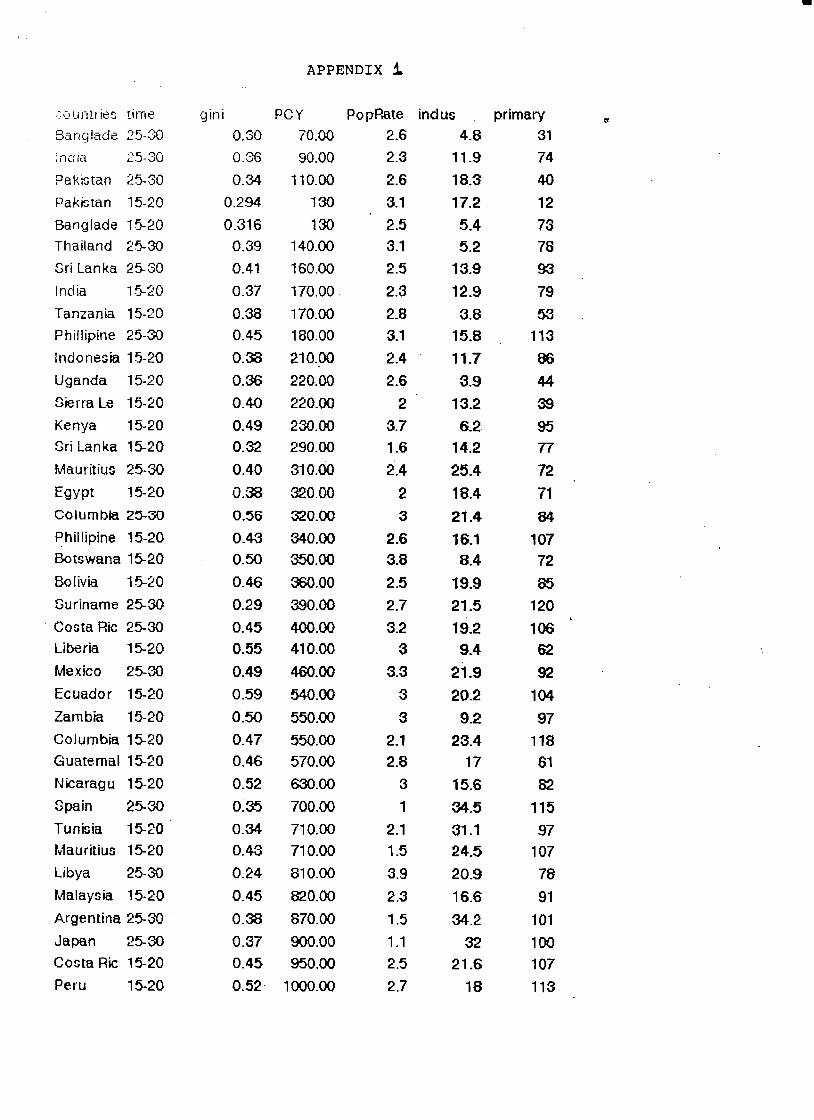
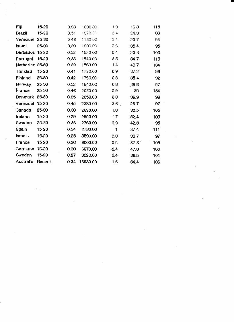
bull
Fiji 15-20 038 03000 i 9 160 115
Brazil 15-20 051 1070gt 24shy 243 88
Venezuel 25-30 048 113000 34 237 94
Israel 25-30 030 130000 35 354 95 Barbados 15-20 032 152000 04 233 103
Portugal 15-20 038 154000 38 347 113 Netherlan 25-30 039 156000 14 407 104
Trinidad 15-20 041 172000 09 372 99
Finland 25-30 042 175000 03 354 92 rmiddotJnrway 25-30 032 184000 08 368 97
France 25-30 046 203000 09 39 134
Denmark 25-30 035 205000 08 369 98 Venezuel 15-20 045 238000 36 267 97
Canada 25-30 030 262000 18 325 105
Ireland 15-20 029 265000 17 324 103 Sweden 25-30 036 276000 09 428 95
Spain 15-20 034 278000 1 374 111 I~rael 15-20 028 389000 23 337 97
rrance 15-20 036 600000 05 373 109
Germany 15-20 033 667000 -04 476 103 Sweden 15-20 027 832000 04 365 101
Australia Recent 034 1668000 16 344 106
bull APPENDIX 2
Calculatin2 Gjni Coefficjents
To convert the figures of an income distribution data into a measure of
income inequality can be done by constructing a Lorenz curve for each
country from which the Gini coefficientconcentration ratio(a measure of
inequality) is calculated The Lorenz curve shows the total percentage of
total income accounted for by any cumulative percentage of recipients
The shape of this curve indicates the degree of income inequality in the
income distribution(Gillis 1992 74) To illustrate how a Lorenz curve is
derived consider the following data for Brazil in 1983
poorest 20 of households receive 24 of total income
second quintile receive 57
third quintile receive 107
fourth quintile receive 186
richest 20 receive 626
From these data it can be observed that Brazil has a high degree of
inequality if 626 of its total income goes to the richest 20 of total
households Also a total of 100 of households receive 100 of total
income To construct a Lorenz curve first the cumulative income share
accruing to any given percentage of households is calculated Thus for the
data above we get the following calculations
poorest 20 receive 24 of total income
poorest 40 receive 24 + 57 = 81 of total income
poorest 60 receive 81 + 107 = 188 of total income
poorest 80 receive 188 + 186 = 374 of total income
100 of households receive 100 of total income
bull
The Lorenz curve is a graph plotted from the data above with the
horizontal axis measuring the cumulative percentage of recipient units and
the vertical axis measunng the cumulative share of total income
Diagram2 below shows the Lorenz curve obtained from the data above
J
J~
t
1
I
l
~ 1 IA I
I
~ [J I
J 1
Diagram2
(Bolnick 1987 61-62)
The diagonal line is a 45-degree line The closer the curve is to this line
the lesser is income inequality The closer it is to the right hand borders
the greater is income inequality(Gillis 1992 74)
To calculate the Gini coefficient let A be the area between the Lorenz
curve and the diagonal line and let B be the area under the Lorenz curve
as show in Figure 2 The formula to calculate the Gini coefficient is given
as
bull
A(A + B) A + B will always be 05 because the box in which the Lorenz
curve is drawn is a unit square especially seen if all percentages are taken
as decimal units eg 20 as 02 Therefore the area of the square becomes
lxl = 10 and half the area of the square (A + B) is 05(Bolnick 1987 62)
Area B can be calculated geometrically using formulas for calculating areas
of rectangles triangles and trapezoids The area of B was calculated
geometrically to be 0233 Since A + B = 05 A = 05 - 0233 = 0267 The
Gini Coefficient AlA + B) = 026705 = 0534 The closer the Gini
coefficient is to 0 the lesser is income inequality and the closer it is to 1
the greater is income inequality
I created a program in Pascal that calculates gini coefficients based
on the Lorenz curve the formula for the area of trapezoids and the
formula for the gini coefficient
bull bull
045
03
bull
APPENDIX 3
REGRESSION LINE DRAWN AGAINST PLOTTED DATA FOR pey GROUP I
05--------------------------------bull
04
035 bull
bull bull
bull bull
bull
bull bulli~t=-+~=
bull
bull
025l-------r------r--r-------------_r-----r---------------------------r-----------J 7000 13000 16000 18000 22000
bull bull
bull bull bull
APPENDIX 4
REGRESSION LINE DRAWN AGAINST PLOTTED DATA FOR pey GROUP II
bull
06-------------------------------------
055 bull
bull bullbullbull 05 bull bull bullbullA45
bull 04 bull
035 bull
bull 03
bull
025
bull
O 2--L--------------------------------------------r----------------------r----------------------------------------r---r---l
31000 34000 39000 46000 55000 70000 81000 90000
bull bull
APPENDIX 5
REGRESSION LINE DRAWN AGAINST PLOTTED DATA FOR pey GROUP III
bull
0S5------------------------------
05 bull
bull045 bull
bull ~ 04
bull~ 035 bull
03
bull bull 025
02
01 f0-+-0-0--2-0-r-0-0--3-000--40-0-0--S-OO-0--610010--700-0--8-00-0--9---1000
PCY
bull
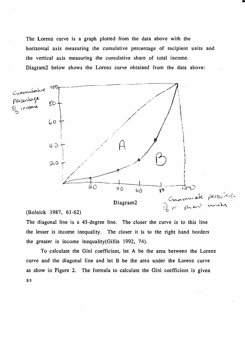
bull
A(A + B) A + B will always be 05 because the box in which the Lorenz
curve is drawn is a unit square especially seen if all percentages are taken
as decimal units eg 20 as 02 Therefore the area of the square becomes
lxl = 10 and half the area of the square (A + B) is 05(Bolnick 1987 62)
Area B can be calculated geometrically using formulas for calculating areas
of rectangles triangles and trapezoids The area of B was calculated
geometrically to be 0233 Since A + B = 05 A = 05 - 0233 = 0267 The
Gini Coefficient AlA + B) = 026705 = 0534 The closer the Gini
coefficient is to 0 the lesser is income inequality and the closer it is to 1
the greater is income inequality
I created a program in Pascal that calculates gini coefficients based
on the Lorenz curve the formula for the area of trapezoids and the
formula for the gini coefficient
bull bull
045
03
bull
APPENDIX 3
REGRESSION LINE DRAWN AGAINST PLOTTED DATA FOR pey GROUP I
05--------------------------------bull
04
035 bull
bull bull
bull bull
bull
bull bulli~t=-+~=
bull
bull
025l-------r------r--r-------------_r-----r---------------------------r-----------J 7000 13000 16000 18000 22000
bull bull
bull bull bull
APPENDIX 4
REGRESSION LINE DRAWN AGAINST PLOTTED DATA FOR pey GROUP II
bull
06-------------------------------------
055 bull
bull bullbullbull 05 bull bull bullbullA45
bull 04 bull
035 bull
bull 03
bull
025
bull
O 2--L--------------------------------------------r----------------------r----------------------------------------r---r---l
31000 34000 39000 46000 55000 70000 81000 90000
bull bull
APPENDIX 5
REGRESSION LINE DRAWN AGAINST PLOTTED DATA FOR pey GROUP III
bull
0S5------------------------------
05 bull
bull045 bull
bull ~ 04
bull~ 035 bull
03
bull bull 025
02
01 f0-+-0-0--2-0-r-0-0--3-000--40-0-0--S-OO-0--610010--700-0--8-00-0--9---1000
PCY
bull

bull bull
APPENDIX 5
REGRESSION LINE DRAWN AGAINST PLOTTED DATA FOR pey GROUP III
bull
0S5------------------------------
05 bull
bull045 bull
bull ~ 04
bull~ 035 bull
03
bull bull 025
02
01 f0-+-0-0--2-0-r-0-0--3-000--40-0-0--S-OO-0--610010--700-0--8-00-0--9---1000
PCY
bull
Copyright © 2022 FDOKUMEN