Income Inequality Impact on Crime in Indonesia :Static and Dynamic Analysis During 2007-2011

Davy Hendri1

IAIN Imam Bonjol Padang

Fajri Muharja2

Andalas University

Abstract

Indonesia experienced a tremendous surge in crime over the last few years. I tries to explain the evolution of this crime to determine the main economy cause. I use regression analysis with panel data set of 33 provinces in Indonesia in the range of 2007 to 2011. The primary crime categories studied are several kind of property crime and aggregate violent crime. The incidence rates of these crimes are regressed against the gini coefficient and an array of other explanatory variables. First, I describe the relationship between inequality and crime with a pooled ordinary least squares (OLS) model. Secondly a fixed effects model is used to control for possible omitted variable problem in simple OLS regressions. Finally, I employ a generalized method of moments (GMM) model in order to address the issues of criminal dynamics and endogeneity of regressors.

My results confirm that every kind of crime in Indonesia have some similarity and difference also in its explanatory variables. Inequality and urbanization (fraction of population live in urban area) is criminogenic factor for almost all kind of crime. Government policy also has a direct impact on the variation of crime. In this model, 2008 set as dummy, there is oil subsidy reduction policy, resulting in enhancing every type of crime rates. Household headed by female its likely push violent that lead to increasing homicide rate. For robbery, which usually related for young’s (male) deliquency behaviour, school participation play important reducing factor (protective effect). I also find another interesting fact that gini's relation on crime rate takes an U-shape. It means after reach a given treshold value, impact of the worsening income distribution on crimerate is decreasing. It’s works in every kind of crime with various threshold of gini.

Keywords: crime, income distribution, povertyJEL Classification: D63, O15, I32

1 Ph.D student at Economics Department, Indonesia University

2 Ph.D student at Economics Department, Indonesia University

1

1. Introduction

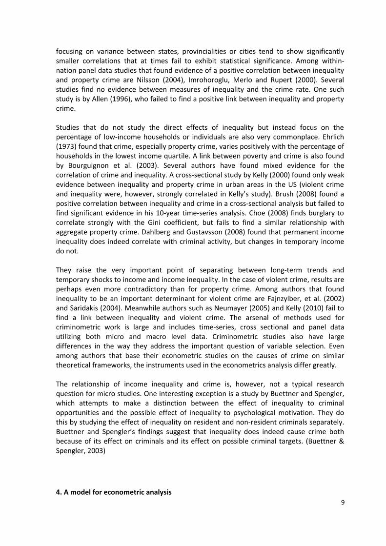
There are two important phenomena in the course of development of Indonesia is interesting to observe in recent times. First, the exciting news from the economy. The nation is experiencing steady economic growth and shows an ascending trend. If in 2009, economic growth of 4.5 % then in 2010 and 2011, respectively, increased to 6,0 % and 6,3 %. Second, the sad news from the social side. High economic growth was not enjoyed by all the people according to their proportions. Gini index of income inequality as a proxy, crawling slowly but surely over the years. In 2005 the Gini index is merely 0,34 , rose to 0.37 in 2009 and then to 0,41 in 2011. In other areas, the crime rate is also increasingly rising. The number of crimes in the year 2012, to be exact until November 2012, reaching 316.500 cases. Risk population who experience crime around 136 people this year. So, every 91 seconds a crime occurred in Indonesia in 20123 (Criminal Police Headquarters, 2012).

3 The first indicator is the total incidence of crime (C) that occur and are reported to or recorded by the police in one year. Meanwhile, residents of the affected criminalist risk is the ratio between the total incidence of crime per 100,000 population (C / population) * 100,000. Meanwhile the timing of crime ratio of the number of seconds in a year to total incidence of crime (3600 * 365 * 24 / C). More details see Crime Statistics, BPS

2

Sumber : Data diolah dari Statistik Kriminalitas, BPS

Fig 1. National Crime rate and Gini Index 2005-2011

It is undeniable that both records counterproductive. This is certainly an interesting phenomenon. Straightforward question arises, whether economic growth is synonymous with inequality and criminality ?. If the answer is yes, this is certainly a paradox. Sociologists and economists then started emphasizing their alleged link between income inequality and crime4. Examples of sociological studies conducted by Hagan and Petersen (1995 ), Kennedy et al . (1998 ) and Daly et al . ( 2001). Hagan and Petersen (1995 ) argues that the frustration felt by low-income individuals when perceiving welfare of others, a phenomenon known as the feeling of relative deprivation, may be the source of the positive effect of inequality on crime. They also claim that poverty produces social disorganization, which then lowers the informal control over individuals who are poor, and therefore lead to increased crime. Kennedy et al . (1998 ) postulated that the growing gap between rich and poor segments of society undermine social cohesion or social capital and the decline of social capital increases the incidence of crime and violence using firearms. Economic studies also found a positive relationship between income inequality and crime.

This article is a study of the empirical relationship of economic inequality and property crime in Indonesia. Economic theory suggests that there is a positive relationship between income inequality and crime. Inequality can be a source for criminal opportunities while at the same time representing poor opportunities for legal income for some individuals. The empirical portion of my thesis uses provincial level data from Indonesia spanning the years from 2007 to 2011. The primary crime categories studied are aggregate property crime, aggregate violent crime, motor theft, robbery and homicide. The incidence rates of these crimes are regressed against the Gini coefficient and an array of other explanatory variables. I will examine the crime rates using three different models. First, I describe the relationship between inequality and crime with a pooled ordinary least squares (OLS) model. Secondly a fixed effects model is used to control for possible omitted variable problem in simple OLS regressions. Finally, I employ a generalized method of moments (GMM) model in order to address the issues of criminal dynamics and endogeneity of regressors.

My results do not confirm a universal correlation between inequality and crime. Furthermore, I find strong evidence the importance of fraction of urbanization (percentage of people living in urban area) in strengthen the correlation between the gini coefficient and theft crimes and other property crimes such as robbery. For violent crimes

4 Various different theories of criminality presented from the viewpoint of different sciences. Criminology as a field of science devoted to learning the cause arises, motive and perpetrators of the crime, also has a different approach. As a specific science, criminology has a more complete theory of the causes of crime

3

the urbanization proves not to contribute. The regression results for the other determinants of crime are mostly in line with previous research. Property crime in Indonesia is positively correlated with gini, urbanization and to some degree the population density. The relationship between education and property crime rates is more complex as the general education index shows a positive correlation with crime in some specification. However the number of youth lacking higher education seems to be a good predictor of crime rates.

The structure of this article is the following. In chapter 2, I present a discussion on the economic theory of criminal decisions. Chapter 3, offers a brief summary of previous research on the topic of inequality and crime. In chapter 4, I introduce the models used in the econometric portion of the thesis and discuss the variables used in the regressions in-depth. These models are put into use in chapter 5, where I present the data and the results from the regressions. Finally, chapter 6, offers some concluding remarks on my work and findings.

2. Theoretical framework

I will next present a summary of the theoretical discussion concerning the determination of crime. Chapter 2.1 will first present the typical economic approach to the question of criminal behavior. A more detailed analysis of how the relationship between inequality and crime works in the various theoretical frameworks is offered in chapter 2.2. Chapters 2.3-2.4 summarize two key issues relevant to understanding the relationship of inequality and crime: heterogeneity of crimes and the dynamic nature of crime.

2.1. Economic theory of crime

The starting point of modern economic study of crime is often seen in the pioneering seminal article by Becker (1968). Becker’s rational choice theory stated that the decision of an individual to commit crime based on several assumptions underlying the choice of an individual to commit a crime are :1. Individuals are assumed to allocate the time available only for two types of activities,

namely the job utilities definite legal and non-legal (crimes) that utilities would not have been in a period of time (uncertainty model).

2. Individuals then maximize utility by selecting one of the two types of activities earlier. Risk-neutral individuals will rationally decide to commit a crime if the expectation of utility of doing non-legal activity (expected utiliy, cEU ) is greater than the utility hopes of doing legal activity (expected utiliy, lEU )

.............(1)c lEU EU>

3. So people choose to do evil or not be based on the analysis of profit and loss (cost-benefit analysis in monetary units).

4

4. If someone committed a crime then he could be caught with probability p and could not be caught with probability (1-p). So the expected utility of crime

Expected utility from doing crime cEU will depend on the expected benefits (l) of committing a crime in monetary units corresponding market value of the goods obtained (ie stolen) from individual victims with a certain level of wealth. While the cost (c) is physical effort and cost. Meanwhile f is due to the cost of getting caught, such as fines, costs opportuniy during incarceration, decreased life satisfaction selaam in prison and so on. Meanwhile p is also a proxy of the degree of risk averse individual (individual degree of risk aversion) to commit a crime. Crime is a very risky job while the outcome is uncertain.

For example, this model predicts that the expected utility of committing a crime would decrease if the probability of getting caught and the cost greater.

2.2. Inequality and crime

Although the positive relationship between economic inequality and crime is a common assumption among economists and criminologists alike, there are several versions of the description of this relationship. In this chapter we will discuss the exact manners in which inequality is expected to have an effect on criminal behavior. We can distinguish three distinct motifs offered for the relationship: opportunities for crime, opportunities for legal income and psychological motivation.

Criminal opportunities are expected to increase as well off individuals are placed in proximity with poorer individuals. Criminal behavior may, depending on the model used, be further escalated by lower opportunities for labor income for those at the lower end of the income spectrum. As the opportunity cost of crime is labor income, it is commonly argued that an increase in legal income opportunities makes the time spent incarcerated and out of the job market more costly (see for example Lochner & Moretti, 2004). For different models that deal with the relationship between the level of crime and the distribution of income, see for example Chiu and Madden (1998), Benoit and Osbourne (1995) or Sala-i-Martin (1995). All of the models mentioned predict criminal behavior to increase as the income distribution becomes more unequal.

A skewed income distribution might also be a sign of low income mobility and poor future prospects for skilled poor individuals. The relevance of long term income prospects is also

5

(1 ) ( , ) ( , ).........(2)cEU p U l c pU l f c= − + −

( , ) ( , ) 0........(3)cEUU l c U l f c

p

∂ = − + − <∂

'( , ) 0..................(4)cEUpU l f c

f

∂ = − − <∂

discussed by Bourguignon, who sees that “absence of income and social upward mobility [...] may be as important as relative poverty at a given point of time to explain criminality at the bottom of the income scale.” (Bourguignon, 1999). The stunted opportunity could also act as a catalyst for a sense of relative deprivation. Relative deprivation is one of the leading explanations for the psychological relationship between inequality and crime.

While economists such as Kelly acknowledge the potentially large psychological effect of inequality on crime, economists generally focus more on the economic motivations altered by inequality (Kelly 2000). Trying to fit the assumptions made by theories such as social disorganization theory or strain theory into an economic framework is not always straightforward. In part, this could be done through changes in an attribute that describes an agent’s tendency for crime. Changes in social pressure or one of the many environmental factors could be simplified by altering just one variable: change in the threshold for crime. In Becker’s framework this could mean variation in the psychological income/loss attributed to committing offenses. Bourguignon et al. use a similar parameter called ‘honesty’ to capture differences in attitudes (Bourguignon, et al., 2003). For practical reasons authors such as Becker worked under the assumption that these preferences differ between individuals but are stable between periods.

2.3. Heterogeneity of different crime types

Intuition alone tells us that one type of crime differs greatly from another one in many characteristics. Crimes are heterogenous in the inherent risk and reward, expertise required, psychological costs and many other aspects. Aggregating different types of crimes thus means losing a lot of information in the process. According to Entorf and Spengler (2002)”Aggregate crime rates are almost meaningless. They give a murder the same weight as the theft of bicycle, so that the variation of property crimes dominates the time series fluctuation of overall crime rates”. On the basis of her empirical work, Edmark also finds that trying to explain aggregate crimes is very fruitless in comparison to examining individual crimes (Edmark, 2003).

A classical way to classify crimes is to separate crimes against property and crimes against the person. Eide (1994) makes a distinction between “expressive” crimes such as rape or arson and “instrumental” crimes - namely non-violent property crimes - and a wide spectrum of crimes with a degree of each element. Rational behavior models are typically seen as having more explanatory power for instrumental crimes than expressive ones. Many crimes also require a very specific skill set. In studying these type of crimes we might take into account theories of differential association, where information on criminal techniques is passed on from one individual to the other. On the other hand, crimes such as tax evasion are available to anyone willing to break the moral code and risk punishment. Parallel qualities can be seen in exaggerated insurance reports and many other non-violent “victimless” crimes.

The psychological cost element of crime was discussed before. In these aspects individuals as well as crimes may be very heterogeneous. Property crimes that require the threat or use of violence can be expected to come at a great psychological cost to most individuals. Likewise, social stigma and reputational costs might vary according to crime type. Among

6

property crimes, one might imagine different attitudes towards crimes against a single person versus crimes against a large entity such as a large corporation or the state. Indeed justification may act as a motivation in offenses where the criminal takes back from an employer or an insurance company that they feel has gained from them in the past. Different types of crimes are typically committed by different people.

In Benoit and Osbournes framework crime rates of different crimes vary in their elasticities to income distribution. The elasticity is determined by the relative incomes of the individuals who tend to commit a crime of a particular type. Their model predicts that certain crimes that the rich people are sensitive to could be rare in an unequal society while the same circumstances might lead to a high crime rate in poor on poor –crime. (Beinoit & Osborne, 1995). Finally, not all crimes are reported to the police with the same likelihood, nor are they as likely to be solved. Virén mentions shoplifting as an interesting example: shoplifting is reported mainly in cases where the criminal is caught red handed. Thus the clear up rate for shoplifting is close to a hundred percent (Virén, 2000). We must also take into account the possibility that crimes differ in the way they are investigated and treated in the criminal justice system.

2.4. Dynamics of crime

There are strong grounds to assume that crime in previous periods influence the current period for both individuals and communities. The beginning of this chapter will deal with arguments that suggest individuals to be path dependent on their choices regarding crime. After this I’ll discuss criminal inertia on a community level. An empirical test on the effect on dynamics is conducted in chapter 5.5

Any model that has individuals comparing the costs and benefits of crime predicts a high rate of repeat offenses. If preferences are stable and economic conditions are similar before and after incarceration, previous offenders are expected to return to crime. Sala-i-Martin offers the counter argument that criminals might find the reality of prison life harder than previously thought, thus leading to an increase in the perceived penalty after an individual has been incarcerated (Sala-i-Martin, 1995). However, if human capital is accumulated at the workplace, people who devote their time to crime instead of work will suffer a severe handicap at the labor market (Flinn, 1986). At the same time their acumen in property crime can possibly lower their risk of getting caught as well as increase the potential gains from crime. The payoff gap between legal work and crime might thus widen with every criminal act.

Eide quotes a study by Wilson and Hernnstein (1985) that highlights the fact that the majority of career criminals have first started with crime at a very early age (Eide, 1994). This result might be explained by personal characteristics, path dependency or both.

7

Williams and Sickles use an earnings function where individual social capital stock includes aspects such as reputation and social networks (Williams & Sickels, 2008). An individual thathas a low capital stock in these terms (a known criminal) has less to lose from further acts of crime. Reputation and social networks are of course advantageous to even individuals whose earnings do not directly depend on them. As Garoupa puts it, criminal life has high exit barriers (Garoupa, 2003).

It is another question altogether whether criminal activity in a community will cause more criminal activity in subsequent periods. If more crime is to be expected, the community might react in a number of ways that deter crime. First, individuals might invest more in personal protection (Demombynes & Özler, 2005). Second, the community might introduce harsher punishment for criminals. A third possible response would be to allocate more resources to law enforcement. It is also critical to note that many socioeconomical factors and crime are jointly endogenous with a very high probability. High crime areas could arguably deter both business and affluent, high-skill individuals. The links between, for example, crime and unemployment and crime and education are likely to work in both ways.

3. Summary of previous research

Econometric studies on crime - often grouped under the name of criminometric studies – are found in abundance. The focus point of existing research varies, and it is easy to find a large number of papers that focus on, for instance, deterrence variables, income opportunities or sociological factors. This chapter includes a summary of those studies that directly address the relationship between inequality and crime. The range of methods employed in related studies is discussed at the end of the chapter. For a general overview of previous criminometric work not limited to only inequality and crime, see Eide (1994) or Soares (2004).

Existing studies on the relationship between inequality and crime generally focus on estimating the magnitude of the relationship while sidestepping the issue of verifying the underlying theory. This is understandable, as the relationship has important policy implication regardless of which theoretical framework is the most appropriate. Furthermore we need to note that statistically determining the relative importance of psychological, social and economic motivations for crime is a very hard task. One testable implication of many sociological theories is that they suggest that poor on poor crime is also very highly positively correlated with inequality. Such test would, however, require the use of micro level data.

The clearest statistical correlation between inequality and crime has been found in studies that use countries as the level of aggregation (see for example Fajnzylber, et al., 2002; Soares, 2004). In fact, Soares (2004) found income inequality to be the single most important variable to explain between differing crime rates between countries. Studies

8

focusing on variance between states, provincialities or cities tend to show significantly smaller correlations that at times fail to exhibit statistical significance. Among within-nation panel data studies that found evidence of a positive correlation between inequality and property crime are Nilsson (2004), Imrohoroglu, Merlo and Rupert (2000). Several studies find no evidence between measures of inequality and the crime rate. One such study is by Allen (1996), who failed to find a positive link between inequality and property crime.

Studies that do not study the direct effects of inequality but instead focus on the percentage of low-income households or individuals are also very commonplace. Ehrlich (1973) found that crime, especially property crime, varies positively with the percentage of households in the lowest income quartile. A link between poverty and crime is also found by Bourguignon et al. (2003). Several authors have found mixed evidence for the correlation of crime and inequality. A cross-sectional study by Kelly (2000) found only weak evidence between inequality and property crime in urban areas in the US (violent crime and inequality were, however, strongly correlated in Kelly’s study). Brush (2008) found a positive correlation between inequality and crime in a cross-sectional analysis but failed to find significant evidence in his 10-year time-series analysis. Choe (2008) finds burglary to correlate strongly with the Gini coefficient, but fails to find a similar relationship with aggregate property crime. Dahlberg and Gustavsson (2008) found that permanent income inequality does indeed correlate with criminal activity, but changes in temporary income do not.

They raise the very important point of separating between long-term trends and temporary shocks to income and income inequality. In the case of violent crime, results are perhaps even more contradictory than for property crime. Among authors that found inequality to be an important determinant for violent crime are Fajnzylber, et al. (2002) and Saridakis (2004). Meanwhile authors such as Neumayer (2005) and Kelly (2010) fail to find a link between inequality and violent crime. The arsenal of methods used for criminometric work is large and includes time-series, cross sectional and panel data utilizing both micro and macro level data. Criminometric studies also have large differences in the way they address the important question of variable selection. Even among authors that base their econometric studies on the causes of crime on similar theoretical frameworks, the instruments used in the econometrics analysis differ greatly.

The relationship of income inequality and crime is, however, not a typical research question for micro studies. One interesting exception is a study by Buettner and Spengler, which attempts to make a distinction between the effect of inequality to criminal opportunities and the possible effect of inequality to psychological motivation. They do this by studying the effect of inequality on resident and non-resident criminals separately. Buettner and Spengler’s findings suggest that inequality does indeed cause crime both because of its effect on criminals and its effect on possible criminal targets. (Buettner & Spengler, 2003)

4. A model for econometric analysis9

The primary purpose of this study is to estimate the causal relationship between income building a model of crime determination. Some variables are discussed are ultimately omitted from the model specification or only represented by weak instruments. One such topic is the deterrence effect, which has been a central focus of criminometrics in general, is but given very little weight in this study. The relevant variables discussed next are put to test in chapter 5, where the empirical results are reviewed.

In chapter 5, I will present the results of three sets of regressions for a number of crime categories. First, I study the effects of inequality on crime using an OLS model. The modelwill include an array of explanatory variables and a yearly dummy tγ to control for national trends in crime. Year 2008 used as a dummy due to on May 28, 2008 the government adopted a policy of partially lifted fuel subsidies (fuel price hike). Fuel subsidy removal policy is compensated for by the division BLT since June to December 2008. For that to see the net effect of the negative impact of rising fuel prices and the positive effect of BLT to the welfare of society and ultimately the crime rate then in 2008 selected as a dummy year. It is well to confirm the results of research Cameron (2011)5 that examined the impact of mistargeting BLT, the destruction of social capital and rising crime

To be able to properly isolate the effect of income inequality we must take into account the control variables as a vector kitX in equation (1). Equation (1) assumes all nine control variables are employed. The resulting model can be stated as:

1 22

n

it t it kit itk

C G Xγ β β ε=

= + + +∑ ..........................................(1)

The second model I use is a fixed effects panel data model. To amend (1) with unit specific fixed effects, we assume that the error term itε may be divided into unobserved area specific fixed effects iα and observation specific errors itω .

it i itε α ω= + .................................................................(2)

Crime is thus expected to be partly caused by unobserved qualities in each unit - in this case provinciality.

1 22

n

it i t it kit itk

C G Xα γ β β ω=

= + + + +∑ ...............................................(3)

The fixed effects approach lets us work around the possibility that the model would otherwise suffer from omitted variable bias. It is possible that the gini coefficient and other regressors are correlated with certain important differences in the provincialities that also

5 This paper focuses on the potential social consequences arising from misallocation of resources in close knit communities. She found that the mistargeting of a cash transfer program in Indonesia is significantly associated with increases in crime and declines in social capital within communities.

10

play a part in determining the crime rate. A key assumption for such between-area differences is that they be time-invariant. Prime examples of differences that do not change over time include geographical considerations, such as proximity to national borders and neighboring provincialities. Effects that are very time-invariant, but not strictly fixed, include popular tourist attractions, the presence of particular industries, certain demographic variables etc.

Measurement error is a well known problem with criminometric work that also motivates the use of a fixed effect model. Crime underreporting is likely to be vast and to correlate with factors such as education, urbanization rate and inequality. The part of underreporting that is not correlated with the regressors, but constant on a per provinciality basis (systematic error), will be captured by the fixed effects model. Equation (3) describes criminal determination as assumed by the fixed effects model. With the exception of separating the provinciality specific term iα from the error term, equation (3) is identical to

1 2 1 33

n

it it it kit itk

C G C Xβ β β ε−=

∆ = ∆ + ∆ + ∆ + ∆∑ ............................(4)

In the fourth set of regressions we take into account the possibility that crime is serially correlated. This assumes a correlation between itC and 1itC − . The model applied is an Arellano-Bond Dynamic Panel GMM estimator. We amend (1) with the lagged crime term and take first differences of all the regressors. Unobserved fixed effects no longer enter the equation as they are by assumption constant between periods.

4.1. Data and Varibles

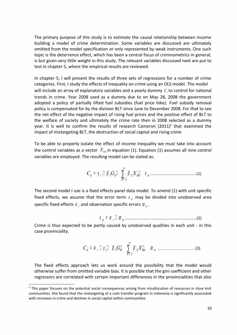
The data set I use is a balanced panel series that covers the 33 Indonesia provincialities. The panel consists of annual figures from 2007 to 2011. In total this makes for 135 observations.

Variable | Obs Mean Std. Dev. Min Max-------------+-------------------------------------------------------- crate | 165 186.9152 110.0117 13 557 propercrate | 127 30.20089 63.8661 .3571429 509.6154 mototheft | 128 22.31567 51.56902 .1111111 421.9231 robbery | 131 7.537151 12.97751 .0444444 87.69231 homicide | 132 1.103826 1.297432 .0222222 8.529411-------------+-------------------------------------------------------- gini | 165 .3438485 .0389873 .26 .46 ginisq | 165 .1197426 .0273709 .0676 .2116 jkpp | 165 198.6303 159.6806 36 662 lrgpc | 165 15.70295 .5697687 14.70583 17.58329 mys | 165 8.419576 .8925207 6.66 11.22-------------+-------------------------------------------------------- p0 | 165 15.32606 8.275156 3.48 40.78 tpt | 165 7.053455 2.824817 2.32 15.75 urban | 165 40.55848 17.76328 14.56067 100

11

Tabel 1 : Statistic Descriptive of Data

hh_female | 165 3.489488 1.211448 1.712164 8.173773 clear | 132 52.48152 19.95271 6.28 109.41-------------+-------------------------------------------------------- laki15_24 | 165 8.47332 1.344547 .5712942 10.21161 gdp_gr | 132 .2404262 .2587852 -1.574227 .9327309 APS2 | 165 14.92958 6.209737 7.07 44.03 t2008 | 165 .2 .4012177 0 1

Indonesia police authorities published crime statistics in a total of 14 major property crime categories. In part these subcategories are more detailed representation of the criminal act; for example theft from motor vehicles as a subcategory of total theft. Some categories are divided into two or three subcategories according to the severity of the act, such as theft, severe theft and petty theft. Several subcategories have been included only towards the end of the observation period and are thus not available for time series analysis. Large fluctuations within subcategories led to dismissing them from detailed analysis, as the stability of these classifications comes into question.

This paper uses a Gini coefficient for disposable income as a measure of income inequality. The per provinciality income Gini coefficients are available from 2007 to 2011. During this timeframe the national Gini as well as the mean Gini coefficient have drifted upwards, as seen in Figure 3. The mean Gini coefficient among the Indonesia provincialities was 0.29, with a standard deviation of 0.31. The average Gini coefficient of 0. 44 in DKI Jakarta income distribution the most unequal of all the provincialities in Indonesia. The lowest average Gini coefficient, 0.24, is found in Bali.

4.2. Bivariate correlations

The simple two variable correlations are presented in Table 2. There are many interesting fact if looking at correlation between several variables. As an example, if estimation include all range (0.26 – 0.46) of data, gini index will have negative correlation signs with all kind of crimes, as opposite to the theory.

| crate proper~e mototh~t robbery homicide gini ginisq-------------+--------------------------------------------------------------- crate | 1.0000 propercrate | 0.2079 1.0000 mototheft | 0.2097 0.9962 1.0000 robbery | 0.1731 0.9386 0.9048 1.0000 homicide | 0.1911 0.6218 0.5780 0.7419 1.0000 gini | -0.0324 -0.1000 -0.0880 -0.1329 -0.1779 1.0000 ginisq | -0.0270 -0.1012 -0.0886 -0.1352 -0.1798 0.9975 1.0000 jkpp | 0.0351 0.1682 0.1577 0.2049 0.1444 0.0074 0.0092 lrgpc | -0.0432 0.0471 0.0396 0.0534 0.1476 -0.1134 -0.1110 mys | 0.2722 0.1736 0.1890 0.1046 0.0428 -0.0491 -0.0464 p0 | -0.1708 -0.1994 -0.2083 -0.1407 -0.0499 0.1645 0.1639 tpt | 0.0530 -0.0830 -0.0583 -0.1630 -0.1843 -0.0714 -0.0745 urban | 0.2176 0.2429 0.2728 0.1183 -0.0932 0.0834 0.0866 hh_female | -0.0332 -0.0129 0.0010 -0.0502 -0.1246 -0.0041 -0.0067

12

Tabel 2 : Bivariate Correlation

clear | -0.0634 -0.0306 -0.0138 -0.0758 -0.0825 -0.2011 -0.1990 laki15_24 | -0.0579 -0.1825 -0.1855 -0.1608 -0.1268 -0.1063 -0.0957 gdp_gr | 0.1784 0.0627 0.0636 0.0564 0.0559 0.2387 0.2397 APS2 | -0.1038 -0.0267 -0.0111 -0.0888 -0.0771 -0.0370 -0.0385 t2008 | -0.0505 -0.1076 -0.1056 -0.0988 -0.0405 -0.3068 -0.3029

| jkpp lrgpc mys p0 tpt urban hh_fem~e-------------+--------------------------------------------------------------- jkpp | 1.0000 lrgpc | 0.0287 1.0000 mys | 0.1358 0.0166 1.0000 p0 | -0.0998 -0.1329 -0.3631 1.0000 tpt | 0.0614 0.0328 0.4762 -0.1535 1.0000 urban | 0.0748 0.0170 0.6511 -0.5282 0.4460 1.0000 hh_female | 0.0023 0.0651 0.0633 -0.0257 0.0278 0.2198 1.0000 clear | -0.0126 -0.0312 -0.0942 -0.2435 0.0450 0.1282 0.1624 laki15_24 | 0.0109 0.0780 0.0747 0.0612 0.2103 -0.1306 -0.1756 gdp_gr | 0.0162 0.0078 -0.0712 -0.2147 -0.0905 0.1341 0.1601 APS2 | -0.0047 0.0028 0.0165 0.0926 -0.0527 -0.0040 0.2271 t2008 | -0.0066 0.0043 -0.0643 0.0540 0.0587 0.0003 -0.1277

| clear laki1~24 gdp_gr APS2 t2008-------------+--------------------------------------------- clear | 1.0000 laki15_24 | -0.0583 1.0000 gdp_gr | 0.0229 -0.1057 1.0000 APS2 | -0.1359 -0.1213 0.0216 1.0000 t2008 | 0.1502 -0.0124 -0.2349 -0.0154 1.0000

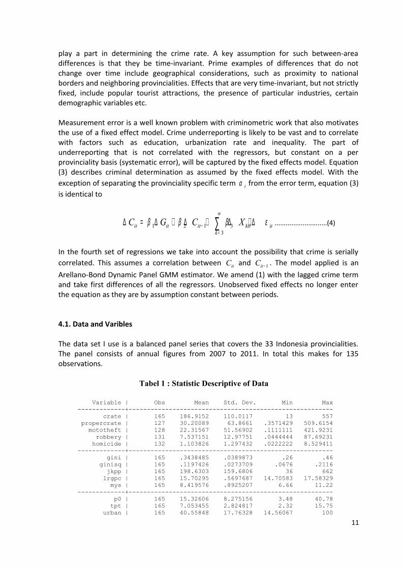
There are many explanation for this fact. What can be happening is that the marginal effect of gini is being taken up by one or more of the other variables. But, interestingly when we drop the value of gini index if higher than 0.33 , the signs become relevan to theory.

drop if gini>=0.33

pwcorr gini crate homicide mototheft robbery

| gini crate homicide mototh~t robbery-------------+--------------------------------------------- gini | 1.0000 crate | 0.1087 1.0000 homicide | 0.1451 0.3012 1.0000 mototheft | 0.1686 0.1886 0.6226 1.0000 robbery | 0.1879 0.1729 0.6867 0.9686 1.0000

The unexpected signs of education index (mys), house hold headed female and poverty rate may be explained with a very high correlation with other explanatory variables. For example, the effect of high population density might overshadow the effect of poverty as large cities seem to have a smaller poverty rate yet a higher crime rate. The more refined models used in chapters 5.3-5.5 show that these results are no robust. The relationship between the crime rate and the regressors is easily misrepresented by choosing the wrong model.The remaining figures are gathered by Statistics Indonesia.

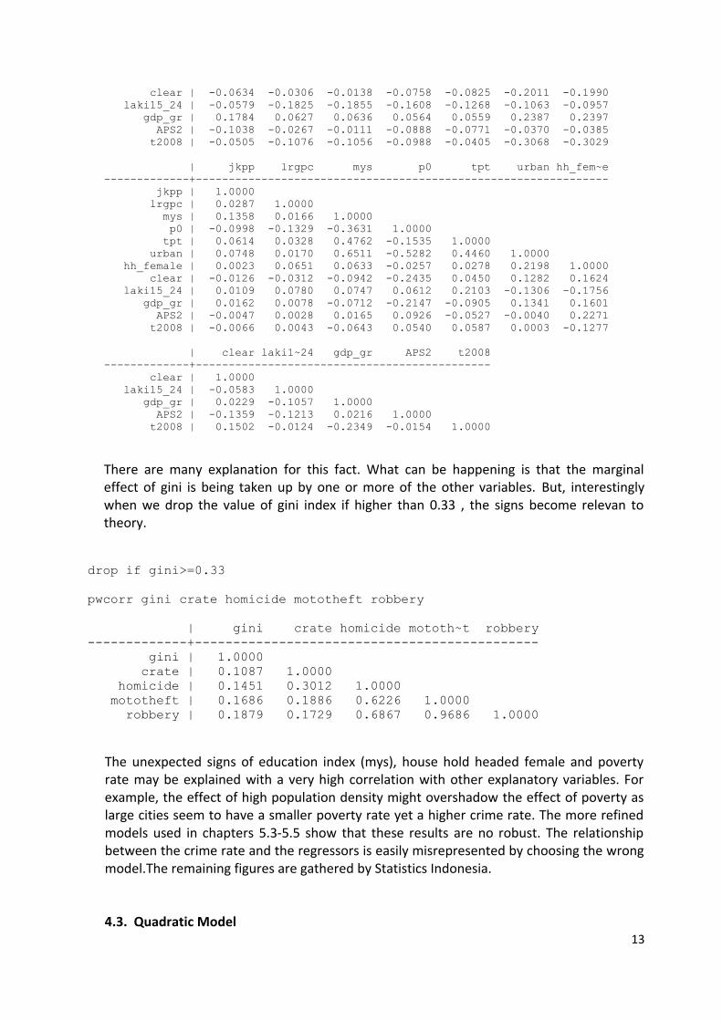
4.3. Quadratic Model13

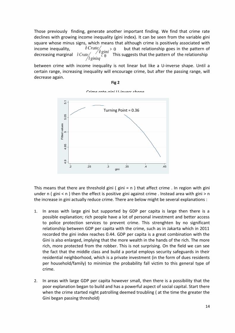
Those previously finding, generate another important finding. We find that crime rate declines with growing income inequality (gini index). It can be seen from the variable gini square whose minus signs, which means that although crime is positively associated with income inequality, but that relationship goes in the pattern of decreasing marginal . This suggests that the pattern of the relationship

between crime with income inequality is not linear but like a U-inverse shape. Until a certain range, increasing inequality will encourage crime, but after the passing range, will decrease again.

4.9

4.9

55

5.0

55

.1F

itte

d v

alu

es

.2 .25 .3 .35 .4 .45gini

This means that there are threshold gini ( gini = n ) that affect crime . In region with gini under n ( gini < n ) then the effect is positive gini against crime . Instead area with gini > n the increase in gini actually reduce crime. There are below might be several explanations :

1. In areas with large gini but supported by GDP per capita is large then there is a possible explanation; rich people have a lot of personal investment and better access to police protection services to prevent crime. This strenghten by no significant relationship between GDP per capita with the crime, such as in Jakarta which in 2011 recorded the gini index reaches 0.44. GDP per capita is a great combination with the Gini is also enlarged, implying that the more wealth in the hands of the rich. The more rich, more protected from the robber. This is not surprising. On the field we can see the fact that the middle class and build a portal employs security safeguards in their residential neighborhood, which is a private investment (in the form of dues residents per household/family) to minimize the probability fall victim to this general type of crime.

2. In areas with large GDP per capita however small, then there is a possibility that the poor explanation began to build and has a powerful aspect of social capital. Start there when the crime started night patrolling deemed troubling ( at the time the greater the Gini began passing threshold)

14

Fig 2

Crime rate-gini U-invers shape

Turning Point = 0.36

0Crategini

∂ >∂0Crate

ginisq∂ <∂

However, the possible role of social capital and public spending (households) to obtain appropriate protection from crime threats above hypothesis remains to be tested by the availability of data related to it.

4.3. Variables

4.3.1. Dependent variable

The dependent variable itC represents the number of crimes in a provinciality, as reported to police, divided by 100.000 inhabitants. This approach to measuring crime, while being a standard one, is by no means perfect. Perhaps the largest source of error in reported crime statistics stems from crime underreporting, which need not be homogenous between areas, periods or crime types.

The regressions use a Gini coefficient of disposable income, itG , as a measure of inequality. Although the use of Gini coefficient is the most common choice of practitioners to measure inequality, alternative instruments are also found in the empirical literature. To name just one such example, Ehrlich (1973) discusses using mean income versus median income, but due to statistical considerations chooses to use the percentage of families below one half of the median income in his model. The Gini coefficient nevertheless has very strong theoretical appeal. In total 13 out of 15 studies presented by Soares chose to use it as a primary measure of inequality (Soares, 2004).

The theoretical framework of criminal activity predicts individuals to respond to the deterrent of getting caught and punished. As the deterrence variables are very significant from a policy point of view, testing their effect on criminal behavior has been a central focus of Becker and many subsequent scholars. Criminals are often found to be risk-lovers in the sense that a rise in the probability of punishment has a more drastic effect on crime than increasing the severity of punishment (see for example Virén, 2000; Becker, 1968). In a timeseries study covering Finnish counties for the years 1951-1955, Virén found a substantial effect of both the clear-up rate and the severity of punishment.

4.3.1. Deterrence variable

The use of deterrence variables such as the clear-up rate (percentage of crimes solved) as explanatory variables for crime is a very common approach in empirical studies. The variables mentioned do, however, pose several serious caveats. First, none of these variables can be assumed to be exogenous. The severity of punishment, the allocation of

15

police resource and the level of private protection are all influenced by the rate of crime. Eide (1994) adds another insight by assuming that a society that chooses to assign unusually severe punishments to a certain type of crime might simultaneously signal its members that this particular act is exceptionally detrimental to the community. The level of sanctions might thus be a partial cause, not just the outcome, of societal norms.

The clear-up rate (also called clearance rate), on the other hand, is already by definition subject to the number of crimes in an area. If police resources are fixed in the short term, an increase in the number of crimes will lead to a drop in the clear-up rate. Past clearance rate is a very typical proxy for the likelihood of punishment. In reality, the link between actual clearance rate and individuals perception of the risk of getting caught could be influenced by factors such as visible police presence and media activity. Eide (1994) refers to studies in which people have been noticed to overestimate the average risk while underestimating their own risk of apprehension. Meanwhile Eide (1999) also finds that inmates’ perception of risk of imprisonment corresponds closely to the actual rate.

Provincialities might be heterogeneous in the types of crimes committed and the implications for clear-up rate cannot be dismissed. Different crimes have differing clear-up rates and the overrepresentation of certain crimes might bias the general clear-up rate. In the case of shoplifting, for example, the clear up rate seems high because shoplifting is reported practically only in cases when the perpetrator is caught in the act. The clear-up rates for this particular crime are thus exaggerated by the data. (Virén, 2000) The problem is avoided altogether by using a per-crime clear-up rate instead of a measure calculated from aggregate figures. This is a more fine-grained approach in the sense that a per-crime clearance rate is expected to reflect not only police resources and the effectiveness of their use, but also the focal point of police work.

The downside of this approach is a much larger volatility for the clearance rate of the more marginal crime categories. The clear-up rates are treated on a per-crime basis. Precise data for conviction rates and the severity of punishments in Indonesia is not available on a provincial level. The clear-up rate thus serves as the sole deterrence variable in all of the regressions. This is a limitation for my empirical work if we assume that conviction rates and the severity of punishment differ between provincialities.

4.3.2. Control variable

In the regressions I will employ the following socio-demographic control variables: the houdehold headed by female, the proportion of young men in a population and the education index. While these factors are mainly seen as socioeconomical ones, Bourguignon (1999) suggests that many of them may be closely related to labor market conditions.

Household headed by female rate has been found correlate very well with the crime rate (see for example Entorf and Spengler, 2002; Nilsson, 2004). The theoretical link between

16

houdehold headed by female rates and crime is not entirely clear. Levitt and Lochner (2001) name the quality of parenting as a key social factor determining crime. This would imply that broken families show up on crime rates with a sizable lag but it does not explain the more short-term effects that have been found empirically. Eide (1994) suggests that family problems and delinquency caused by same factors, such as poverty. I use the houdehold headed by female rate per 1000 inhabitants as an explanatory variable in all of the regressions.

It is a well documented fact that a large share of crimes is committed by males of the age of 14-24 (see for example Entorf & Spengler, 2002). The explanations to why young men seem to be more prone to criminal acts are numerous. For one, young men have lower possibilities for legal income since their accumulated human capital is low (Lochner, 2004). If norm formation is assumed to be slow, then the norms of a person at a young age could differ from his or her norms at a later point in time. There is typically very little variation between different areas in the percentage of young males in the population. Their effect is nevertheless tested in the following regressions by the proportion of young males in a population.

Education is expected to affect criminal behavior in various ways. Schooling may affect earnings, the time available for crime as well as preferences. The relationship between education and measured crime on a macro level may also be affected by issues such as crime underreporting and the general moral in an area. The correlation between education and crime is expected to be negative through most of these channels. As education is linked with earnings potential, the theory expects the likelihood of offending to go down with an individual’s educational level. In a micro level study by Lochner, crime was found to be “primarily a problem among young uneducated men” (Lochner, 1999). Similar results are found by Lochner and Moretti (2004). It has however also been suggested that individual skills might in some cases increase the rewards for crime and even the likelihood of offenses.

A study by Levitt and Lochner suggest that males with high scores on mechanical information tests have an increased probability of committing crimes (Levitt & Lochner, 2001). Another effect of education on crime is the time-availability argument, according to which youth busy with schoolwork simply have less time for criminal activity. Jacob and Lefgren (2003) use teacher training days as an instrument for school attendance. They find evidence that property crimes are significantly larger in areas where youth have more days off school. Jacob and Lefgren acknowledge that their results only imply short-term effects, but as Lochner and Moretti (2004) argue, the probability of committing crime could largely be state dependent and thus determined by past behavior. If this assumption is correct, allocating more time to school work could have long-lasting effects on crime reduction.

Machin et al. (2011) argue that education increases risk-aversity. If this is the case, then decreased risk taking is one explanation for the decreased likelihood that well educated individuals have for committing crimes. Education can likewise increase patience and thus make an agent less prone to short-sighted decisions such as participation in crime. Finally, schooling may directly alter preferences and make an individual more hesitant to breaking

17

the law (Lochner & Moretti, 2004). Usher (1997) calls this the ‘civilization effect’ of education.

Although the reasons to expect education to reduce crime are numerous, the relationship between education and crime on a macro level is not as straightforward. Ehrlich found a positive and significant relationship between the level of education and criminal activity. He lists several theories that might explain this relationship, among them the possibility that higher average levels of education may be associated with less underreporting of crime. (Ehrlich, 1975, p. 333). Lochner also found a positive, although statistically insignificant, correlation between the rates for crimes such as forgery and counterfeiting, fraud, and embezzlement and average education levels. (Lochner, 2004). Lochners results might be explained by increasing returns to white collar crimes with skill level, as discussed above. In the regressions that follow I use an educational index as a measure of the average educational attainment and school participation for 15-17 years old population.

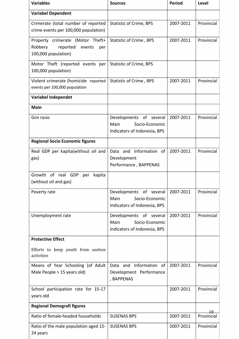
Table 3 : Data sources for main variables

18

19

Variables Sources Period Level

Variabel Dependent

Crimerate (total number of reported crime events per 100,000 population)

Statistic of Crime, BPS 2007-2011 Provincial

Property crimerate (Motor Theft+ Robbery reported events per 100,000 population)

Statistic of Crime , BPS 2007-2011 Provincial

Motor Theft (reported events per 100,000 population)

Statistic of Crime, BPS

Violent crimerate (homicide reported events per 100,000 population

Statistic of Crime , BPS 2007-2011 Provincial

Variabel Independet

Main

Gini rasio Developments of several Main Socio-Economic Indicators of Indonesia, BPS

2007-2011 Provincial

Regional Socio Economic figures

Real GDP per kapita(without oil and gas)

Data and Information of Development Performance , BAPPENAS

2007-2011 Provincial

Growth of real GDP per kapita (without oil and gas)

Poverty rate Developments of several Main Socio-Economic Indicators of Indonesia, BPS

2007-2011 Provincial

Unemployment rate Developments of several Main Socio-Economic Indicators of Indonesia, BPS

2007-2011 Provincial

Protective Effect

Efforts to keep youth from useless activities

Means of Year Schooling (of Adult Male People > 15 years old)

Data and Information of Development Performance , BAPPENAS

2007-2011 Provincial

School participation rate for 15-17 years old

2007-2011 Provincial

Regional Demografi figures

Ratio of female-headed households SUSENAS BPS 2007-2011 Provincial

Ratio of the male population aged 15-24 years

SUSENAS BPS 2007-2011 Provincial

5. Empirical Results

This chapter contains empirical estimations of the effect between crime and inequality. The other explanatory variables used in the regressions were discussed in chapter 4. Chapter 5.1 offers a multivariate regression (OLS). A more complete model in chapter 5.2 will also take into account fixed effects between provincialities and periods. The fixed effects regression offers the best estimate for the effect that changes in inequality and other variables are expected to have on crime. The fixed effect regression is also conducted with various secondary instrument variables to ensure robustness. Chapter 5.3. will introduce dynamics to test for the persistence of criminal activity within a community. The dynamics will be incorporated through the use of an Arellano-Bond GMM model.

The OLS regression, fixed effects model and the GMM estimator are all techniques widely employed by criminometricians working with similar datasets. Although the methods differ significantly, the most robust findings will be present with all three models. We will see that in the case of the Gini coefficient and in particular theft crimes, all three methods yield similar results. However we are not able to draw definite conclusions about several of the control variables in cases where different models give differing results. This is the case with the percentage of young males, historical crime clear-up rate and the percentage of low income households.

5.1. Pooled OLS regression

In order to isolate the effect of inequality, we will next continue with a multivariate ordinary least squares (OLS) regression. National trends in crime are controlled for by yearly dummies in all the regressions, but omitted from the summary tables. The OLS approach assumes that all variance between municipalities that might affect crime rate is represented in the explanatory variables and that the error term is uncorrelated with crime rate. The assumptions of the OLS model are generally seen as too strict for similar scenarios. The possibility of omitted variable bias is treated in the next chapter with the fixed effects model. The regression results for six different crime classifications are summarized in Table 5.3.

----------------------------------------------------------------------------------------- (1) (2) (3) (4) (5) homicide mototheft robbery propercrate crate -----------------------------------------------------------------------------------------

gini 6.443 119.0 164.6 333.3 -3868.5 (0.17) (0.08) (0.43) (0.17) (-1.16)

20

Tabel 5.3 : (Pooled/Common Effect) OLS Regression Model Results

ginisq -21.38 -617.4 -370.5 -1063.2 4914.0 (-0.39) (-0.28) (-0.69) (-0.39) (1.04)

jkpp 0.00131* 0.0588** 0.0195*** 0.0775** -0.00163 (1.92) (2.18) (2.92) (2.33) (-0.03)

lrgpc 0.294 0.929 0.227 1.711 -14.76 (1.51) (0.12) (0.12) (0.18) (-0.89)

mys 0.300 1.633 0.782 2.427 40.86*** (1.67) (0.22) (0.45) (0.27) (2.66)

p0 0.00931 0.353 0.107 0.421 0.533 (0.50) (0.48) (0.59) (0.46) (0.34)

tpt -0.0913* -4.673** -1.506*** -6.166** -5.316 (-1.76) (-2.29) (-2.98) (-2.44) (-1.20)

urban -0.00573 1.265*** 0.231** 1.479*** 0.482 (-0.55) (3.01) (2.25) (2.84) (0.54)

hh_female -0.170* -4.964 -1.302 -6.413 -3.808 (-1.67) (-1.21) (-1.31) (-1.26) (-0.44)

clear -0.00428 -0.159 -0.0794 -0.251 -0.416 (-0.71) (-0.66) (-1.33) (-0.84) (-0.80)

laki15_24 -0.160* -4.610 -1.128 -5.692 -2.693 (-1.96) (-1.43) (-1.41) (-1.43) (-0.38)

gdp_gr 0.631 4.548 2.457 7.049 94.69** (1.37) (0.24) (0.54) (0.30) (2.39)

APS2 -0.0235 -0.356 -0.293 -0.631 -2.350 (-1.30) (-0.50) (-1.66) (-0.72) (-1.52)

t2008 -0.278 -19.56 -4.581 -24.58 -6.960 (-0.92) (-1.63) (-1.55) (-1.65) (-0.27)

_cons -2.769 63.95 3.855 53.24 898.0 (-0.35) (0.20) (0.05) (0.14) (1.32) -----------------------------------------------------------------------------------------N 132 128 131 127 132 adj. R-sq 0.112 0.127 0.151 0.131 0.084 -----------------------------------------------------------------------------------------t statistics in parentheses* p<0.1 , ** p<0.05 , *** p<0.01

5.2. Fixed Effect

Next we will use a fixed effect model to control for area specific differences. Controlling for fixed effects lets us work around the possibility that the regressors included in the model are not the only factors explaining differences in crime rates. In effect this approach assumes that there is a fixed amount of crime in each municipality that is caused by area specific characteristics not captured by the explanatory variables. A key assumption of the model is of course, that the area specific characteristics are stable between periods. The fixed effects approach is widely used by practitioners who work with similar data sets (see for example Levitt & Lochner, 2001; Nilsson, 2004). Results of the fixed effect regression are summarized in Table 5.2.

----------------------------------------------------------------------------------------- (1) (2) (3) (4) (5)

21

Tabel 5.2. : Hasil Regressi Model Fixed-Effect

homicide mototheft robbery propercrate crate

gini 82.26* 6679.9*** 1248.5** 8102.6*** 2681.9 (1.71) (3.14) (2.34) (3.05) (1.08)

ginisq -114.5* -9392.4*** -1727.4** -11341.8*** -4171.7 (-1.74) (-3.21) (-2.37) (-3.10) (-1.22)

jkpp 0.000966 0.0834*** 0.0203* 0.103*** -0.0155 (1.34) (2.70) (2.54) (2.69) (-0.42)

lrgpc -0.0179 -2.529 -1.229 -3.483 -16.27 (-0.08) (-0.26) (-0.49) (-0.28) (-1.40)

mys 0.278 2.042 -2.334 -0.775 -29.73 (0.34) (0.06) (-0.26) (-0.02) (-0.71)

p0 -0.0518 -15.58** -3.025* -18.71** 4.209 (-0.35) (-2.43) (-1.84) (-2.33) (0.55)

tpt -0.618*** -13.96 -3.896* -17.57 8.013 (-3.07) (-1.60) (-1.74) (-1.61) (0.77)

urban 0.0528* 4.527*** 0.964*** 5.534*** 1.093 (1.83) (3.65) (3.01) (3.56) (0.73)

hh_female 0.561** 17.09 2.457 20.77 -22.41* (2.31) (1.61) (0.91) (1.55) (-1.78)

clear -0.00121 0.0172 0.0111 0.0142 -0.418 (-0.15) (0.05) (0.13) (0.03) (-1.03)

laki15_24 -0.0800 -7.195* -1.304 -8.529 2.827 (-0.93) (-1.95) (-1.37) (-1.85) (0.64)

gdp_gr 0.291 -3.479 0.857 -4.416 12.03 (0.61) (-0.17) (0.16) (-0.17) (0.49)

APS2 -0.135 -7.440 -2.759** -10.08 0.395 (-1.13) (-1.45) (-2.08) (-1.57) (0.06)

t2008 1.034** 47.43** 9.135* 57.98** -52.36** (2.21) (2.35) (1.76) (2.28) (-2.16)

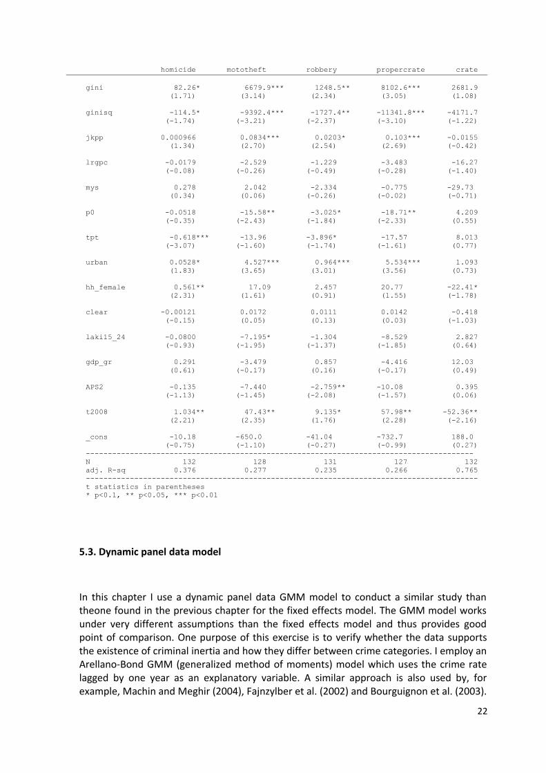
_cons -10.18 -650.0 -41.04 -732.7 188.0 (-0.75) (-1.10) (-0.27) (-0.99) (0.27) ----------------------------------------------------------------------------------------N 132 128 131 127 132 adj. R-sq 0.376 0.277 0.235 0.266 0.765 -----------------------------------------------------------------------------------------t statistics in parentheses* p<0.1, ** p<0.05, *** p<0.01

5.3. Dynamic panel data model

In this chapter I use a dynamic panel data GMM model to conduct a similar study than theone found in the previous chapter for the fixed effects model. The GMM model works under very different assumptions than the fixed effects model and thus provides good point of comparison. One purpose of this exercise is to verify whether the data supports the existence of criminal inertia and how they differ between crime categories. I employ an Arellano-Bond GMM (generalized method of moments) model which uses the crime rate lagged by one year as an explanatory variable. A similar approach is also used by, for example, Machin and Meghir (2004), Fajnzylber et al. (2002) and Bourguignon et al. (2003).

22

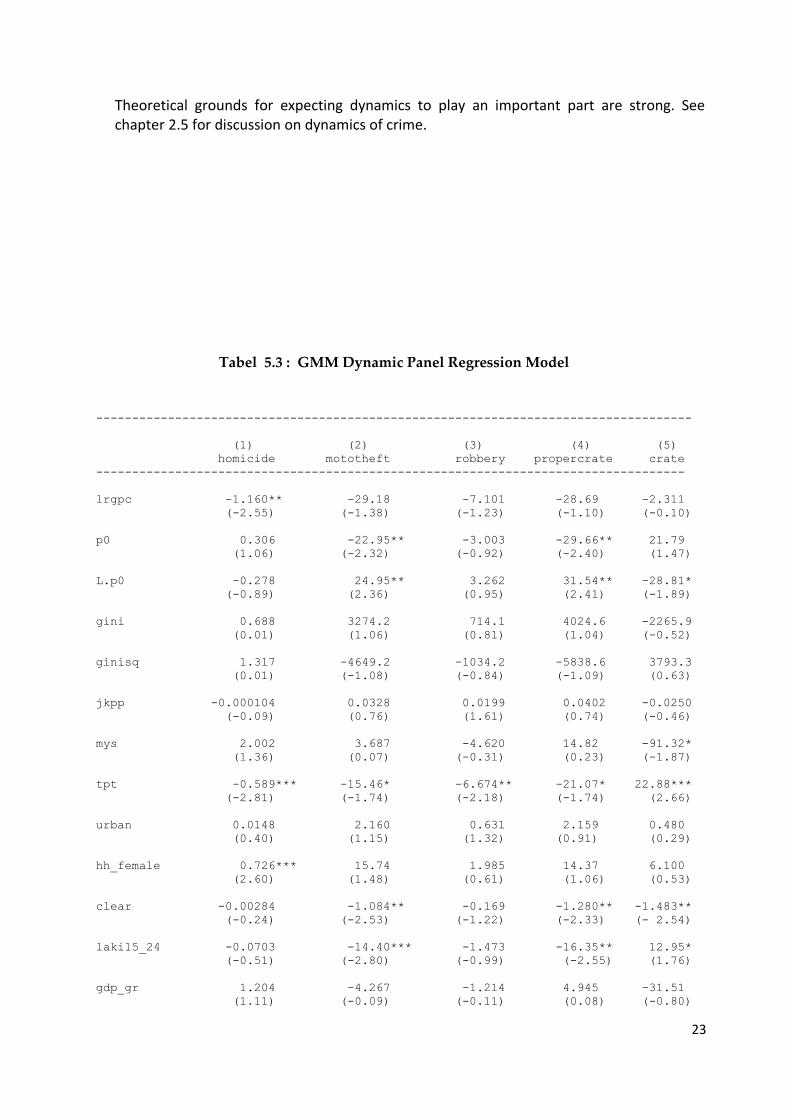
Theoretical grounds for expecting dynamics to play an important part are strong. See chapter 2.5 for discussion on dynamics of crime.

-----------------------------------------------------------------------------------

(1) (2) (3) (4) (5) homicide mototheft robbery propercrate crate ----------------------------------------------------------------------------------

lrgpc -1.160** -29.18 -7.101 -28.69 -2.311 (-2.55) (-1.38) (-1.23) (-1.10) (-0.10)

p0 0.306 -22.95** -3.003 -29.66** 21.79 (1.06) (-2.32) (-0.92) (-2.40) (1.47)

L.p0 -0.278 24.95** 3.262 31.54** -28.81* (-0.89) (2.36) (0.95) (2.41) (-1.89)

gini 0.688 3274.2 714.1 4024.6 -2265.9 (0.01) (1.06) (0.81) (1.04) (-0.52)

ginisq 1.317 -4649.2 -1034.2 -5838.6 3793.3 (0.01) (-1.08) (-0.84) (-1.09) (0.63)

jkpp -0.000104 0.0328 0.0199 0.0402 -0.0250 (-0.09) (0.76) (1.61) (0.74) (-0.46)

mys 2.002 3.687 -4.620 14.82 -91.32* (1.36) (0.07) (-0.31) (0.23) (-1.87)

tpt -0.589*** -15.46* -6.674** -21.07* 22.88*** (-2.81) (-1.74) (-2.18) (-1.74) (2.66)

urban 0.0148 2.160 0.631 2.159 0.480 (0.40) (1.15) (1.32) (0.91) (0.29) hh_female 0.726*** 15.74 1.985 14.37 6.100 (2.60) (1.48) (0.61) (1.06) (0.53)

clear -0.00284 -1.084** -0.169 -1.280** -1.483** (-0.24) (-2.53) (-1.22) (-2.33) (- 2.54)

laki15_24 -0.0703 -14.40*** -1.473 -16.35** 12.95* (-0.51) (-2.80) (-0.99) (-2.55) (1.76)

gdp_gr 1.204 -4.267 -1.214 4.945 -31.51 (1.11) (-0.09) (-0.11) (0.08) (-0.80)

23

Tabel 5.3 : GMM Dynamic Panel Regression Model

APS2 0.0214 0.852 -0.843 -0.608 2.115 (0.17) (0.16) (-0.62) (-0.09) (0.27)

Lagged Dep Var 0.74* -0.219 -1.028 -0.590 0.671*** (1.84) (-0.21) (-0.80) (-0.50) (3.06) _cons 1.648 -59.65 76.41 -178.0 1084.4 (0.08) (-0.08) (0.35) (-0.19) (1.11) -----------------------------------------------------------------------------------N 99 94 97 93 132 adj. R-sq -----------------------------------------------------------------------------------t statistics in parentheses* p<0.1, ** p<0.05, *** p<0.01

The Arellano-Bond GMM estimator is designed for panels with few periods but a large number of units (small T, large N), such as this one. The model can also be used to address to endogeneity of explanatory variables. For example Kelly (2000) sees police activity as potentially endogenous. The same assumption could be made about most of the explanatory variables applied in this study. The regressions are run under the assumption that gini index, socio-economic and the demographic variables are exogenous, while the income related variables (gdp per capita) are predetermined, but not strictly endogenous. Poverty rate and lagged poverty rate were first tested as an endogenously determined variable.

The result also show that in the long-run previously (lagged for one year) poverty rate positively impact on all kind of property crime. The regression results in Table 5.3. reveal that violent crime (homicide) and aggregate crimes exhibit significant criminal inertia. Surprisingly, dynamics seem to play as opposite way in more skill-intensive crime categories such as robbery and mototheft. Robbery (doing young) is also often seen as a crime motivated by peer influence rather than economic motives.

Similar comparisons have also been made by other authors. Fajnzylber et al. (2002), find that homicides are more subject to criminal inertia than robberies - as does Choe (2008). Bourguignon (1999) finds the exact opposite to hold true. Choe’s study compares different US states while the other two studies mentioned examine between-country differences. The relative complexity of the GMM model makes it sensitive to the assumptions made by the econometrician employing it. But, the hypothesis that the full GMM specification used is suffering from too many instruments may be rejected.

6. Conclusions.

I tested the empirical relationship between income inequality, as measured by the Gini coefficient, and crime rates in Indonesia provincialities. The analysis was made for a data set spanning 33 provincialities and 5 years from 2007 to 2011. The models most suitable

24

for this type of work seem to be a fixed effects model and a generalized method of moments (GMM) model. Using area specific fixed effects is a good way to avoid omitted variable bias that is likely to plague simple OLS regressions. Introducing fixed effects changes the correlation coefficients drastically and reduces the apparent correlation between the Gini coefficient and crime rates. The fixed effects model fails to find a statistically significant relationship between the Gini coefficient and crime rates with the exception of theft crimes.

The GMM method takes into account dynamics and endogeneity of regressors. Both issues seem to be highly relevant when studying crime rates. If criminal activity does indeed persist over periods, it is possible that the coefficients in static models are underestimated. Criminal inertia suggests that a change in any of the coefficients would continue to have an effect for several periods. The time-span of static models might thus prove to be too short to properly represent reality. These issues may be reflected in the trend witnessed in more recent studies of favoring the GMM model. As is the case in existing literature, findings between my different specifications are somewhat contradictory. The key question of correlation between inequality and crime was found to be positive but not statistically significant for all kinds of crimes. For homicide in general, the evidence is more weaker as the fixed effects model does not find a statistically significant relationship.

The GMM results suggest that robbery crimes be the ones most directly affected by clearance rate. The direct effect of this variables seem to be somewhat lower, but persist longer due to the highly dynamic nature of crime. The very high multiplier effect for mototheft, robbery and aggregate crimes suggest that in the long term, these kind of crime rates are the ones that are most subject to shocks to more productive police and judicial system. For violent crimes the clearance rate was found to be irrelevant in determining crime rates.

The relationship between education and crime is complex in light of theoretical consideration as well as the results of my empirical work. The general education index was found to be negatively correlated with some crimes but positively correlated with, for instance, violent crime. One explanation for this is a possible correlation between education of victims and the underreporting rate of crimes. The ratio of noneducated youth was however a clearly positively correlated predictor of crime rates.

On the basis of my empirical work, clear distinctions may be made between different types of crimes. My findings suggest that crimes such as homicide are largely driven by other factors than theft and robbery. In the Indonesia setting over 60 per cent of reported property crimes are accounted by for theft crimes. Fluctuations in the general property crime rates thus reflect in large part changes in the number of thefts - mainly petty theft. My findings suggest that future examination of the topic should be made on a percrime basis rather than investigating property crimes as a whole.

25

7. Bibliography

Agnew, R., 1984. Goal achievement and delinquency. Sociology & Social Research, Vol 68, no. 4, pp. 435-451.

Allen, R., 1996. Socioeconomic conditions and property crime: a comprehensive review and test of the professional literature. The American Journal of Economics and Sociology, 55(3), pp. 293-308.

Becker, G., 1968. Crime and Punishment: An Economic Approach.:Journal of Political Economy, University of Chicago Press, vol. 76.

Beinoit, J.-P. & Osborne, M., 1995. Crime, Punishment and Social Expenditure. Journal of Institutional and Theoretical Economics, pp. 326-347.

Bourguignon, F., 1999. Crime, Violence, and Inequitable Development.:Annual Bank Conference on Development Economics, edited by B. Pelskovic and J. Stiglitz, WashingtonDC: The World Bank.

Bourguignon, F., Nuñez, J. & Sanchez, F., 2003. What part of the income distribution doesmatter for explaining crime? The case of Columbia,. DELTA Working Papers 2003-04, DELTA (Ecole normale supérieure).

Britt, C., 1997. Reconsidering the Unemployment and Crime Relationship: Variation by Age Group and Historical Period. Journal of Quantitative Criminology, 13(4), pp. 405-426.

Brush, J., 2008. Does income inequality lead to more crime? A comparison of cross-sectional and time-series analyses of United States counties. Elsevier Economics Letters, 96(2), pp. 264-268.

Buettner, T. & Spengler, H., 2003. Local Determinants of Crime: Ditinguishing Between Resident and Non-resident Offenders. s.l.:Darmstadt Discussion Papers in Economics 37307,

Darmstadt Technical University, Department of Business Administration, Economics and Law, Institute of Economics (VWL).

Burton, V., Cullen, F., Evans, D. & Dunaway, G., 1994. Reconsidering strain theory: Operationalization, rival theories, and adult criminality. Journal of Quantitative Criminology, 10(3), pp. 213-239.

Bushway, S. & Reuter, P., 2008. Economists' Contribution to the Study of Crime and the Criminal Justice System. Crime & Justice, Volume 37, pp. 389-452.

Cameron, Lisa and Manisha Shah, (2011), Mistargeting of Cash Transfers, Social Capital Destruction, and Crime in Indonesia, Monash University

26

Carr-Hill, R. & Stern, N., 1973. An econometric model of the supply and control of recorded offences in England and Wales. Journal of public economics,, 2(4), pp. 289-318.

Chiu, H. & Madden, P., 1998. Burglary and income inequality. Journal of Public Economics , Volume 69, pp. 123-141.

Choe, C. & Chisholm, J., 2008. Income Variables and the Measures of Gains from Crime. Oxford Economic Papers, 57(1), pp. 112-119.

Choe, J., 2008. Income inequality and crime in the United States. Elsevier Economic Letters, 101(1), pp. 31-33.

Cohen, L. & Felson, M., 1979. Social Change and Crime Rate Trends: A Routine Activity Approach. American Sociological Review, 44(4), pp. 588-608.

Cooter, R., 1997. Law From Order: Economic Development and the Jurisprudence of Social Norms. s.l.:The Selected Works of Robert Cooter.

Dahlberg, M. & Gustavsson, M., 2008. Inequality and Crime: Separating the Effects of Permanent and Transitory Income. Oxford Bulletin of Economics and Statistics, 70(2), p. 129–153.

Demombynes, G. & Özler, B., 2005. Crime and local inequality in South Africa. Journal ofDevelopment Economics, Elsevier, 76(2), pp. 265-292.

Edmark, K., 2003. The Effects of Unemployment on Property Crime: Evidence from a Period. Working Paper Series 2003:Uppsala University, Department of Economic, Volume 14.

Ehrlich, I., 1973. Participation in Illegitimate Activities: A Theoretical and Empirical Investigation. Journal of Political Economy, 81(3), pp. 521-565.

Eide, E., 1994. Economics of crime : deterrence and the rational offender.:North Holland.

Eide, E., 1999. Economics of criminal behavior. Encyclopedia of Law and Economics, Volume 5.

Entorf, H. & Spengler, H., 2002. Crime in Europe: causes and consequences.:Springer.

Esteban, J.-M. & Ray, D., 1994. On the Measurement of Polarization. Econometrica, Econometric Society, 62(4), pp. 819-51.

Fajnzylber, P., Lederman, D. & Loayza, N., 2002. Inequality and Violent Crime. Journal of Law and Economics, 45(1), pp. 1-39.

Flinn, C., 1986. Dynamic Models of Criminal Careers. In: Criminal Careers and "Career Criminals". Washington, DC: National Academy Press.

27

Garoupa, N., 2003. Behavioral Economic Analysis of Crime: A Critical Review. European Journal of Law and Economics, 15(1), pp. 5-15.

Glaeser, E. & Sacerdote, B., 1999. Why Is There More Crime in Cities?. Journal of Political Economy, 107(6), pp. 225-258.

Hirschi, T., 1986. On the compatibility of rational choice and social control theories of crime. In: The Reasoning Criminal: Rational Choice Perspectives on Offending. New York: Springer- Verlag, pp. 105-117.

Imrohoglu, A., Merlo, A. & Rupert, P., 2000. On the Political Economy of Income Redistribution and Crime. International Economic Review, 41(1), pp. 1-25.

Jacob, B. & Lefgren, L., 2003. Are Idle Hands the Devil's Workshop? Incapacitation, Concentration and Juvenile Crime. American Economic Review, American Economic Association, 93(5), pp. 1560-1577.

Kelly, M., 2000. Inequality and Crime. The Review of Economics and Statistics, 82(4), pp. 530-539.

Kubrin, C. & Weitzer, R., 2003. New Diretions in Social Disorganization Theory. Journal of Researh in Crime and Delinquency, 40(4), pp. 374-402.

Levitt, S., 1997. Using electoral cycles in police hiring to estimate the effect of police on crime. The American Economic Review, 87(3), pp. 270-290.

Levitt, S. & Lochner, L., 2001. The Determinants of Juvenile Crime.:University of Chicago Press.

Lochner, L., 1999. Education, Work, and Crime: Theory and Evidence.:Rochester Center for Economic Research Working Paper No. 465.

Lochner, L., 2004. Education, work, and crime: a human capital approach. International Economic Review, Volume 45, pp. 811-43.

Lochner, L. & Moretti, E., 2004. The Effect of Education on Crime: Evidence from Prison

Inmates, Arrests, and Self-Reports. American Economic Review, American Economic Association, 94(1), pp. 155-189.

Machin, S. & Meghir, C., 2004. Crime and Economic Incentives. The Journal of Human Resources, 39(4), pp. 958-979.

Machin, S., Olivier, M. & Vujic, S., 2011. The Crime Reducing Effect of Education. The Economics Journal, 121(552), pp. 463-484.

28

Merton, R., 1938. Social structure and anomie. American Sociological Review 3, pp. 672-682.

Nagin, D. & Paternoster, R., 1993. Enduring Individual Differences and Rational Choice Theories of Crime. Law & Society Review, 27(3), pp. 467-496.

Neumayer, E., 2005. Inequality and Violent Crime: Evidence from Data on Robbery and Violent Theft. Journal of Peace Research, 42(1), pp. 101-112.

Nilsson, A., 2004. Income inequality and crime: The case of Sweden:Working Paper Series 2004:6, IFAU - Institute for Labour Market Policy Evaluation.

Paternoster, R., 1989. Decisions to Participate in and Desist from Four Types of Common Delinquency: Deterrence and the Rational Choice Perspective. Law & Society Review, 23(1),pp. 7-40.

Sah, R. K., 1991. Social Osmosis and Patterns of Crime. Journal of Political Economy, 99(6), pp. 1272-1295.

Sala-i-Martin, 1995. Transfers, social safety nets and economic growth. Economics Working Papers 139, Department of Economics and Business, Universitat Pompeu Fabra.

Sampson, R. & Wilson, W., 1995. Toward a Theory of Race, Crime, and Urban Inequality. In: J. H. a. R. D. Peterson, ed. In Crime and Inequality. Stanford, CA: Stanford University Press, pp. 37-56.

Saridakis, G., 2004. Violent crime in the United States of America: a time-series analysis between 1960–2000. European Journal of Law and Economics, Volume 18, pp. 203-221.

Shover, N. & Honaker, D., 2009. The Socially Bounded Decision Making of Persistent Property Offenders. The Howard Journal of Criminal Justice, Volume 31, p. 276–293.

Siegel, L., 2003. Criminology.:Thomson Learning, Canada.

Soares, R., 2004. Development, crime, and punishment: Accounting for the international differences in crime rates. Journal of Development Economics, Elsevier, 73(1), pp. 155-184.

Usher, D., 1997. Education as Deterrent to Crime. Canadian Journal of Economics, 30(2), pp. 367-384.

Virén, M., 2000. Modelling crime and punishment: Discussion Papers 244, Government Institute for Economic Research Indonesia (VATT).

Wahlroos, B., 1981. On Indonesia Property Criminality: An Empirical Analysis of the Postwar Era Using an Erlich Model. The Scandinavian Journal of Economics, 83(4), pp. 553-562.

29

Williams, J. & Sickels, R., 2008. Turning from crime: A dynamic perspective. Journal of Econometrics, 145(1), pp. 158-173.

Witte, A. D. & Witt, R., 2001. Crime Causation: Economic Theories. In: Encyclopedia of Crime and Justice. :Macmillan Reference USA.

30