Immigration and Crime:A Microeconometric Study

By

Georgios Papadopoulos

A thesis submitted for the degree of

Doctor of Philosophy

Department of Economics

University of Essex

February 2011

...στην oικoγενεια µoυ

Acknowledgements

My greatest gratitude goes to my supervisor Joao Santos Silva for his excellent guid-

ance, enthusiastic support and constant attention during all stages of my PhD studies.

It has been an honour to work next to him and learn from him.

I am also grateful to Tim Hatton; not only did he help me to get started at the

initial stages of the PhD, but he also provided essential advice throughout. I would

like to thank my internal examiner, Marco Francesconi, and my external examiner,

Peter Moffat for their comments and suggestions increased the quality of this thesis.

Morever, many thanks to the academic staff of the Department of Economics and in

particular, Alison Booth, Ken Burdett, Holger Breinlich, Gianluigi Vernasca and the

Chair of my Supervisory Board Meetings George Symeonidis for the helpful comments

and suggestions. Participants in the Research Strategy Seminar in the Department

of Economics also provided many intuitive comments and suggestions and I am very

thankful for that.

Many thanks to my good friends and colleagues Marina Fernadez Salgado and Michail

Veliziotis for their multidimensional support and to all research students at the Uni-

versity of Essex that offered great ideas and insightful discussions.

I would also like to acknowledge the precious help of all the administrative team of the

Department of Economics throughout my graduate studies.

I would like to thank Rainer Winkelmann for kindly providing the data used in the

first chapter.

I would especially like to thank my girfriend Zelda Brutti, who lovingly provided price-

less help at the last stages of this thesis. Her help and support has considerably

increased the quality of this thesis, but most importantly, the quality of my whole life.

Moreover, I would like to express my gratitude to all my friends that I have met at

the University of Essex during these years, and especially to Elizabeth Mantzati, Tom

Ieuan Martin, Dafni Papoutsaki, Tina Rampino and Theodoros Theodoridis.

Last but not least, I would like to thank my whole family in Greece and Germany and

my best friends Zahos Alexandridis, Alexis Larchanidis and Fotis Papadopoulos for

their unconditional support throughout bad and good periods of my life.

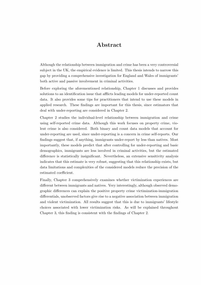
Abstract

Although the relationship between immigration and crime has been a very controversial

subject in the UK, the empirical evidence is limited. This thesis intends to narrow this

gap by providing a comprehensive investigation for England and Wales of immigrants’

both active and passive involvement in criminal activities.

Before exploring the aforementioned relationship, Chapter 1 discusses and provides

solutions to an identification issue that afflicts leading models for under-reported count

data. It also provides some tips for practitioners that intend to use these models in

applied research. These findings are important for this thesis, since estimators that

deal with under-reporting are considered in Chapter 2.

Chapter 2 studies the individual-level relationship between immigration and crime

using self-reported crime data. Although this work focuses on property crime, vio-

lent crime is also considered. Both binary and count data models that account for

under-reporting are used, since under-reporting is a concern in crime self-reports. Our

findings suggest that, if anything, immigrants under-report by less than natives. Most

importantly, these models predict that after controlling for under-reporting and basic

demographics, immigrants are less involved in criminal activities, but the estimated

difference is statistically insignificant. Nevertheless, an extensive sensitivity analysis

indicates that this estimate is very robust, suggesting that this relationship exists, but

data limitations and complexities of the considered models reduce the precision of the

estimated coefficient.

Finally, Chapter 3 comprehensively examines whether victimization experiences are

different between immigrants and natives. Very interestingly, although observed demo-

graphic differences can explain the positive property crime victimization-immigration

differentials, unobserved factors give rise to a negative association between immigration

and violent victimization. All results suggest that this is due to immigrants’ lifestyle

choices associated with lower victimization risks. As will be explained throughout

Chapter 3, this finding is consistent with the findings of Chapter 2.

Contents

Introduction 1

1 The Poisson-Logit Model: Identification Issues and Extensions 11

1.1 Introduction . . . . . . . . . . . . . . . . . . . . . . . . . . . . . . . . . . . . 11

1.2 The Poisson Logistic Regression Model . . . . . . . . . . . . . . . . . . . . . 15

1.3 Extensions - The Negative Binomial Logit Case . . . . . . . . . . . . . . . . 20

1.4 Identification Issues in the Poisson-Logit model . . . . . . . . . . . . . . . . 23

1.5 Possible Solutions to the Identification Problem . . . . . . . . . . . . . . . . 24

1.5.1 Sign Restrictions on the Reporting Process . . . . . . . . . . . . . . . 25

1.5.2 Exclusion Restrictions on the Reporting Process . . . . . . . . . . . . 26

1.5.3 Exclusion Restrictions on the Count Process . . . . . . . . . . . . . . 27

1.5.4 Specifying the Count Generating Process, as Negative Binomial 1 . . 27

1.5.5 Specifying the Reporting Probability as a Probit or CLogLog . . . . . 28

1.6 Discussion . . . . . . . . . . . . . . . . . . . . . . . . . . . . . . . . . . . . . 29

1.7 Other Related Models . . . . . . . . . . . . . . . . . . . . . . . . . . . . . . 32

1.8 An Illustration using Data on Labour Mobility . . . . . . . . . . . . . . . . . 34

1.8.1 Same Regressors in both Processes . . . . . . . . . . . . . . . . . . . 35

1.8.2 Exclusion Restrictions on Logit . . . . . . . . . . . . . . . . . . . . . 37

1.8.3 Exclusion Restrictions on Count Process . . . . . . . . . . . . . . . . 38

1.8.3.1 Excluding a very Insignificant Variable from the Count Process 38

1.8.3.2 Excluding Dummies from the Count Process with Large Ef-

fect on Logit Process . . . . . . . . . . . . . . . . . . . . . . 39

1.8.4 Specifying the Reporting Process as a Probit . . . . . . . . . . . . . . 39

1.9 Conclusion . . . . . . . . . . . . . . . . . . . . . . . . . . . . . . . . . . . . . 40

Tables . . . . . . . . . . . . . . . . . . . . . . . . . . . . . . . . . . . . . . . . . . 42

2 The Relationship between Immigration Status and Criminal Behaviour 48

2.1 Introduction . . . . . . . . . . . . . . . . . . . . . . . . . . . . . . . . . . . . 48

2.2 An Economic Model of Property Crime . . . . . . . . . . . . . . . . . . . . . 53

iv

v

2.2.1 Immigration and Crime . . . . . . . . . . . . . . . . . . . . . . . . . 60

2.3 Immigration and Crime. A Review of Research . . . . . . . . . . . . . . . . 62

2.3.1 Empirical Evidence by Economists . . . . . . . . . . . . . . . . . . . 63

2.3.2 Empirical Evidence by other Scholars . . . . . . . . . . . . . . . . . . 65

2.4 The OCJS. Some Methodological Issues . . . . . . . . . . . . . . . . . . . . . 68

2.5 Econometric Models . . . . . . . . . . . . . . . . . . . . . . . . . . . . . . . 71

2.5.1 Binary Choice Models . . . . . . . . . . . . . . . . . . . . . . . . . . 73

2.5.2 Count Data Models . . . . . . . . . . . . . . . . . . . . . . . . . . . . 77

2.6 Data Set and Discussion of Variables . . . . . . . . . . . . . . . . . . . . . . 79

2.7 Main Results . . . . . . . . . . . . . . . . . . . . . . . . . . . . . . . . . . . 85

2.7.1 Preliminary Results . . . . . . . . . . . . . . . . . . . . . . . . . . . . 86

2.7.2 Probit Model that allows for Misclassification . . . . . . . . . . . . . 87

2.7.2.1 Constant Misclassification . . . . . . . . . . . . . . . . . . . 87

2.7.2.2 Allowing Misclassification of 1 as 0 to depend on Regressors 89

2.8 Robustness Checks . . . . . . . . . . . . . . . . . . . . . . . . . . . . . . . . 95

2.8.1 Count Data Models . . . . . . . . . . . . . . . . . . . . . . . . . . . . 95

2.8.2 Violent Crime . . . . . . . . . . . . . . . . . . . . . . . . . . . . . . . 99

2.8.3 Weighted versus Unweighted Regressions of Property Crime . . . . . 100

2.8.4 Are the Results Driven by the Exclusion Restriction of the “Truthful-

ness” Dummy? . . . . . . . . . . . . . . . . . . . . . . . . . . . . . . 101

2.9 Decomposition of Immigrants by Ethnicity and Regions . . . . . . . . . . . . 104

2.9.1 Interaction between Immigration and Ethnicity . . . . . . . . . . . . 104

2.9.2 Interaction between Immigration and Region . . . . . . . . . . . . . . 106

2.10 Discussion . . . . . . . . . . . . . . . . . . . . . . . . . . . . . . . . . . . . . 107

2.11 Conclusion . . . . . . . . . . . . . . . . . . . . . . . . . . . . . . . . . . . . . 109

Figures & Tables . . . . . . . . . . . . . . . . . . . . . . . . . . . . . . . . . . . . 111

Appendix A. Zero-Inflated Misprobit . . . . . . . . . . . . . . . . . . . . . . . . . 127

A1. Constant Misclassification Results . . . . . . . . . . . . . . . . . . . . . 128

A2. Covariate-Dependent Under-reporting Results . . . . . . . . . . . . . . . 128

Appendix B. NB1-Logit, GenNB-Logit, and ZI-NB2-Logit . . . . . . . . . . . . . 134

Appendix C. More Robustness Checks . . . . . . . . . . . . . . . . . . . . . . . . 137

C1. Dropping Very Recent Immigrants . . . . . . . . . . . . . . . . . . . . . 137

C2. Dropping Very Young Individuals . . . . . . . . . . . . . . . . . . . . . . 137

C3. Without Criminal Damage . . . . . . . . . . . . . . . . . . . . . . . . . 138

vi

3 The Relationship between Immigration Status and Victimization 140

3.1 Introduction . . . . . . . . . . . . . . . . . . . . . . . . . . . . . . . . . . . . 140

3.2 Theoretical Perspectives on Victimization . . . . . . . . . . . . . . . . . . . 144

3.2.1 The Immigration-Victimization Link . . . . . . . . . . . . . . . . . . 149

3.3 BCS, Dependent Variables and Descriptive Statistics . . . . . . . . . . . . . 152

3.3.1 The British Crime Survey and Dependent Variables . . . . . . . . . . 153

3.3.2 Description of the Data . . . . . . . . . . . . . . . . . . . . . . . . . . 156

3.4 Risk of Household Crime . . . . . . . . . . . . . . . . . . . . . . . . . . . . . 159

3.4.1 Inside Burglary . . . . . . . . . . . . . . . . . . . . . . . . . . . . . . 160

3.4.2 Outside Burglary . . . . . . . . . . . . . . . . . . . . . . . . . . . . . 161

3.4.3 Remaining Household Crime Groups . . . . . . . . . . . . . . . . . . 163

3.5 Risk of Personal Victimization . . . . . . . . . . . . . . . . . . . . . . . . . . 165

3.5.1 Risk of Personal Theft . . . . . . . . . . . . . . . . . . . . . . . . . . 166

3.5.2 Risk of Violence . . . . . . . . . . . . . . . . . . . . . . . . . . . . . . 168

3.5.2.1 Domestic Crime . . . . . . . . . . . . . . . . . . . . . . . . 171

3.5.2.2 Crime by Acquaintances . . . . . . . . . . . . . . . . . . . . 172

3.5.2.3 Crime by Strangers . . . . . . . . . . . . . . . . . . . . . . . 173

3.6 Sensitivity Analysis . . . . . . . . . . . . . . . . . . . . . . . . . . . . . . . . 175

3.6.1 Controlling for Correlated Errors . . . . . . . . . . . . . . . . . . . . 175

3.6.2 Examining Differences in Reporting Behaviour . . . . . . . . . . . . . 177

3.6.2.1 Use of the Self-Completions on Domestic Violence . . . . . 178

3.6.2.2 The Presence of Others during the Face-to-Face Interview . 181

3.6.3 Controlling for Racially Motivated Crime . . . . . . . . . . . . . . . . 184

3.6.4 Network Effects and Assimilation Patterns for Violent Crime . . . . 186

3.7 Further Topics . . . . . . . . . . . . . . . . . . . . . . . . . . . . . . . . . . . 189

3.7.1 Decomposition of Immigrants by Ethnicity and Location . . . . . . . 189

3.7.2 Seriousness of Crime . . . . . . . . . . . . . . . . . . . . . . . . . . . 191

3.8 Count Data Models . . . . . . . . . . . . . . . . . . . . . . . . . . . . . . . . 193

3.9 Conclusion . . . . . . . . . . . . . . . . . . . . . . . . . . . . . . . . . . . . . 200

Tables . . . . . . . . . . . . . . . . . . . . . . . . . . . . . . . . . . . . . . . . . . 205

Appendix. A Hurdle-Poisson Model for Censored Counts . . . . . . . . . . . . . . 227

References 230

List of Figures

2.1 Immigration Rates and Crime Rates through time . . . . . . . . . . . . . . . 111

2.2 Crime Indexes through time: Recorded crime Vs BCS . . . . . . . . . . . . . 111

2.3 MisProbit: Interpretation as Misclassification . . . . . . . . . . . . . . . . . 112

2.4 MisProbit: Interpretation as Zero-One-Inflation . . . . . . . . . . . . . . . . 112

2.5 Zero-Inflation MisProbit . . . . . . . . . . . . . . . . . . . . . . . . . . . . . 131

2.6 Zero-Inflation Poisson-Logit . . . . . . . . . . . . . . . . . . . . . . . . . . . 131

vii

List of Tables

1.1 Modelling Reporting Probability as a Logit: Same Regressors in both Processes 42

1.2 Modelling Reporting Probability as a Logit: Exclusion Restrictions in Logit

Process . . . . . . . . . . . . . . . . . . . . . . . . . . . . . . . . . . . . . . . 43

1.3 Modelling Reporting Probability as a Logit: Excluding an Insignificant Dummy

from Count Process . . . . . . . . . . . . . . . . . . . . . . . . . . . . . . . . 44

1.4 Modelling Reporting Probability as a Logit: Excluding Important Dummies

from the Count Process . . . . . . . . . . . . . . . . . . . . . . . . . . . . . . 45

1.5 Modelling Reporting Probability as a Probit: Same Regressors in both Processes 46

1.6 Modelling Reporting Probability as a Probit: Excluding Important Dummies

from the Count Process . . . . . . . . . . . . . . . . . . . . . . . . . . . . . . 47

2.1 Perceptions of Natives towards Immigrants: Immigrants make country’s crime

problems worse or better - ESS 2002 . . . . . . . . . . . . . . . . . . . . . . . 113

2.2 Perceptions of Natives towards Immigrants: Immigrants increase crime rates

- ISS 1995 Vs ISS 2003 . . . . . . . . . . . . . . . . . . . . . . . . . . . . . . 113

2.3 Ordered Probit. Determinants of Natives Attitudes - ISS . . . . . . . . . . . 113

2.4 Tabulation of OCJS Respondents by Sample Type . . . . . . . . . . . . . . . 114

2.5 Tabulation of the Number of Property Crimes . . . . . . . . . . . . . . . . . 115

2.6 Descriptive Statistics from the OCJS . . . . . . . . . . . . . . . . . . . . . . 116

2.7 Probit Estimates for all Crime Categories . . . . . . . . . . . . . . . . . . . . 117

2.8 Negative Binomial Estimates for all Crime Categories . . . . . . . . . . . . . 117

2.9 Probit Estimates for Property Crime . . . . . . . . . . . . . . . . . . . . . . 118

2.10 Negative Binomial Estimates for Property Crime . . . . . . . . . . . . . . . 118

2.11 MisProbit Estimates for Property Crime: Constant Misclassification . . . . . 119

2.12 MisProbit Estimates for Property Crime: Covariate-Dependent Misclassifica-

tion of 1 as 0 . . . . . . . . . . . . . . . . . . . . . . . . . . . . . . . . . . . 120

2.13 NB2 - NB2-Logit - ZI-NB2-Logit Estimates for Property Crime . . . . . . . 121

2.14 MisProbit: Weighted Property Crime Vs Weighted Violent Crime Vs Un-

weighted Property Crime . . . . . . . . . . . . . . . . . . . . . . . . . . . . . 122

viii

ix

2.15 MisProbit: Truthfulness Vs No Exclusion Vs Other Present, for Property Crime123

2.16 MisProbit: Truthfulness Vs No Exclusion Vs Other Present, for Violent Crime124

2.17 NB2-Logit: Truthfulness Vs Other Present for Property Crime . . . . . . . . 125

2.18 MisProbit: Interaction Terms . . . . . . . . . . . . . . . . . . . . . . . . . . 126

2.19 MisProbit Vs ZI-MisProbit: Constant Misclassification . . . . . . . . . . . . 132

2.20 MisProbit Vs ZI-MisProbit: Covariate-Dependent Misclassification . . . . . 133

2.21 More Robustness Checks . . . . . . . . . . . . . . . . . . . . . . . . . . . . . 139

3.1 BCS Crime Codes . . . . . . . . . . . . . . . . . . . . . . . . . . . . . . . . . 205

3.2 Count Data Tabulations for each Crime Group . . . . . . . . . . . . . . . . . 207

3.3 Descriptive Statistics . . . . . . . . . . . . . . . . . . . . . . . . . . . . . . . 208

3.4 The Risk of Inside Burlglury plus Attempts . . . . . . . . . . . . . . . . . . 211

3.5 The Risk of Outside Burlglury plus Attempts . . . . . . . . . . . . . . . . . 211

3.6 The Risk of Personal Theft . . . . . . . . . . . . . . . . . . . . . . . . . . . . 212

3.7 The Risk of Violent Victimization - Without Ethnic Group Dummies . . . . 213

3.8 The Risk of Violent Victimization Including Ethnic Group Dummies . . . . 213

3.9 The Risk of Domestic Violence . . . . . . . . . . . . . . . . . . . . . . . . . . 214

3.10 The Risk of Victimization suffered by Acqaintances . . . . . . . . . . . . . . 215

3.11 The Risk of Victimization suffered by Strangers . . . . . . . . . . . . . . . . 215

3.12 A Trivariate Probit Model for Violent Victimization . . . . . . . . . . . . . . 216

3.13 Comparison Between Face-to-Face and Self-Reported Domestic Violence . . . 217

3.14 The Presence of the Partner . . . . . . . . . . . . . . . . . . . . . . . . . . . 218

3.15 Tabulation between Racially Motivated Crime by Relationship Type . . . . . 219

3.16 Mean Comparison between Racially Motivated Crime by Relationship Type 219

3.17 Probit Models before and after controlling for Racial Crime . . . . . . . . . . 219

3.18 Network Effect and Assimilation Patterns . . . . . . . . . . . . . . . . . . . 220

3.19 Decomposition by Ethnic Group . . . . . . . . . . . . . . . . . . . . . . . . . 221

3.20 Decomposition by Location . . . . . . . . . . . . . . . . . . . . . . . . . . . 221

3.21 The effect of being an Immigrant on perceived Seriousness . . . . . . . . . . 222

3.22 Distribution of Violent Crime . . . . . . . . . . . . . . . . . . . . . . . . . . 223

3.23 Poisson, Negative Binomial 2 and Censored Poisson . . . . . . . . . . . . . . 224

3.24 Quantiles for Counts . . . . . . . . . . . . . . . . . . . . . . . . . . . . . . . 225

3.25 Hurdle-Poisson for Censored Counts . . . . . . . . . . . . . . . . . . . . . . . 226

Introduction

The phenomenon of international migration has been a subject of controversy for politicians,

policy makers, and the general public in all countries that sustained large inflows of immi-

gration.1 Consequently, academic communities have devoted a considerably large amount of

research to understand the actual impact of migration on many different aspects of both the

host countries and countries of origin. These include the effects of immigration on different

dimensions of the labour market (Borjas, 1994, 1999a, 2003) and the welfare state of the

host countries (Borjas and Trejo, 1991, and Borjas, 1999b), the impact of brain drain in the

countries of origin (Mountford 1997, and Beine, Docquier and Rapoport, 2001, 2008) and

the relationship between ethnic diversity and economic performance and growth (Alesina

and La Ferrara, 2005), to mention only a few.

Following this debate, scholars have also devoted a lot of research to understand the rea-

sons behind the heterogeneity in individual beliefs towards migration movements by studying

the economic and noneconomic determinants of people being anti or pro-immigration (see,

for example, Mayda, 2006, O’Rourke and Sinnott, 2006, and Facchini and Mayda, 2009).

A particular aspect of immigration where we expect to observe a high proportion of anti-

immigration protesters is the relationship between immigration and crime. Indeed, at least

for the UK where this thesis focuses on, using data from two important social surveys (look

at the introduction of Chapter 1) we can observe that a large fraction of population believes

that immigration and crime are linked positively.

However, very interestingly, a high proportion of the researchers’ community in social

sciences does not share the same view, particularly when it comes to the empirical evidence.

1Before getting into the main stage of this introduction, it is important to note that each chapter of thisthesis is independent and therefore provides its own comprehensive introduction and conclusion.

1

2

Actually most research about the immigration situation in the US indicates that there is a

negative association, but results from Europe suggest that there is a positive or no associa-

tion between immigration and crime (see, Section 2.3). Nevertheless, we need to stress that

compared to other aspects of immigration, such as the ones described in the previous para-

graphs, the available evidence is rather inconclusive. It is also important to note that the

crime-immigration association has been generally overlooked by economists as the majority

of the empirical evidence comes from criminological or sociological research.

Most importantly, although this subject is of major interest in political and public debates

in the UK, there is lack of empirical evidence. Therefore, this thesis intends to narrow this

gap by providing a micro-investigation of immigrants’ involvement in criminal activities both

as offenders and victims in the UK. It will be made clear to the reader that looking at both

the offending behaviour and the victimization experiences of immigrants will provide a more

satisfactory picture of the immigration-crime relationship and the rationale behind it.

As this thesis focuses on the micro-immigration-crime link, microeconomic and microe-

conometric tools will be used throughout. However, in this work we particularly focus on

the econometric techniques and specifications that are used as an attempt to overcome data

or other methodological limitations. Actually, it could be said that this work is in a sense

two-dimensional, as there are two major themes that stand out independently. The first

one is the empirical research questions itself, while the second one is the microeconometric

methodology, specification, and theory developed to answer the research questions.

Actually, this thesis starts in an unusual way as the first chapter does not investigate

the main research question, but it is a small theoretical econometric investigation of some

estimators for count data that are used in the second chapter. However, it would be more

proper to briefly explain the subject of the first chapter once we understand the limitations

of the data and estimators used in the second chapter, which investigates the relationship

between immigration status and criminal behaviour in England and Wales.

In this chapter most attention is paid to property crime, although violent crime is also

considered. The chapter starts by developing a simple theoretical model of property crime

through which the individual link between immigration and property crime is discussed. The

model depicts several channels that may lead to higher (because of labour outcomes) or lower

3

(because of deterrent or risk factors) involvement of immigrants in illegitimate activities,

in comparison to natives. Therefore, as opposed to the public sentiment in the UK that

immigrants are more criminal than natives, the theoretical analysis is not able to predict the

direction of the relationship in object. As a consequence, an empirical analysis is required

to establish this link. Nevertheless, a major limitation is that true crime is unobserved and

therefore, data on criminal activity are really difficult to obtain. Although police records

on criminal activity do exist, they do not give any information about immigration status of

offenders. Even if this information was available, this type of data would not be appropriate

for my study as there is evidence that two thirds of the crime remains unrecorded, but most

importantly (for reasons explained in Section 2.4) immigrant population is over-represented

in official criminal records. Moreover, prison data would be even more misleading, as people

in prison can be considered as a highly selected sample that does not represent the general

population.

Thus, the most appropriate strategy would be to use data of survey self-reported crime.1

For this purpose the Offending, Crime, and Justice Survey (OCJS) of 2003 is used, a rep-

resentative national survey of (computer-based) self-reported crime. Although the survey

design is developed so as to obtain the most reliable responses possible (see, Section 2.4),

under-reporting is still a major concern. Therefore, conventional econometric models that

ignore this type of measurement error provide inconsistent estimates of the determinants

of the actual crime, especially if respondents’ reporting behaviour depends on respondents’

characteristics. As the dependent crime variable is observed in count form, both count data

models, the Poisson-Logit and Negative Binomial-Logit (NB-Logit), and binary choice mod-

els, the Misclassification Probit model (MisProbit), that are developed to take into account

under-reporting are considered. These are two-index parametric models which, using only

observed crime self reports, give information for the determinants of both the true criminal

activity and the reporting behaviour. However, identification of the count data models con-

sidered in this chapter is afflicted by a subtle problem and further assumptions are required

in order to identify the parameters of interest.

1Another idea would be to conduct an appropriate controlled experiment for criminal actions, whereparticipants would form a representative part of the general population. This is left for future research.

4

Therefore, in Chapter 1, which is an extended version of the paper by Papadopoulos and

Santos Silva (2008), we provide a thorough investigation of the conditions under which the

Poisson-Logit and two popular generalizations of this model (the NB2-Logit and the NB1-

Logit) are identified. Although these models are described in the well known monographs

for count data by Cameron and Trivedi (1998) and Winkelmann (2008), this identification

problem has not been recognized by any work prior to the present thesis. As mentioned in

the previous paragraph, the Poisson-Logit is a double index model where by only observing

the reported counts we want to draw inference for both the determinants of total counts

(modeled as if they follow the Poisson distribution) and the probability of a count to be

successful (modeled as a Logit). In the self-reported crime context, total counts correspond

to the number of actual but unobserved crimes and the probability of a successful count

corresponds to the probability of reporting a committed crime.

In this chapter we show that without appropriate restrictions, taking either the form of

at least one sign restriction on the Logit part, or at least one exclusion restriction on the

Poisson part, it is not possible to identify the parameters of the Poisson-Logit model, as two

identical “global” maxima exist. However, these restrictions must be “strong”. In the sign

restriction context this means that the sign of at least one coefficient must be determined

by well established theoretical results and that the estimated coefficient which we want to

impose the restriction on must be statistically significant. In the exclusion restriction context

this means that the excluded variables from the Poisson part must have a significant effect

on the Logit part and no effect on the Poisson part. Also note that exclusion restrictions on

the Logit part can be helpful towards identifying only those coefficients of the Poisson part

which are set to zero in the Logit part.

This study also reveals that the same identification problem is present in NB2-Logit.

However, even without the aforementioned type of restrictions, a “weak” form of identifica-

tion is achieved when the NB1-Logit specification is adopted. Here we use the term “weak”

as identification of the conditional mean is achieved solely because of an extra parametric

assumption on the form of the conditional variance of the dependent variable. Therefore,

identification of the mean is highly dependent on the specification of the variance, which

has negative consequences in terms of robustness of the estimator. Finally, this identifica-

5

tion failure does not extend to models where a different conditional distribution function for

binary data is used for the reporting process, such as the Probit.

Although identification of the Poisson-Logit and the NB2-Logit is achieved when we im-

pose exclusion restrictions on the count process, it is high likely that another local maximum

exists. Actually the likelihood value of the local maximum will be very close to the like-

lihood value of the global one if the exclusion restrictions are not “strong”, and therefore,

identification will be more difficult. As a result, practitioners that intend to use the above

models must perform a thorough search for alternative maxima before accepting the first

achieved maximum as the global one. Thus, some tips are also provided that can be used to

help the practitioner find the global maximum. All theoretical results are supported by an

empirical illustration with data on labour mobility.

Back to Chapter 2, due to the small number of positives, a fact that affects the robustness

of the count data models, it has been considered as more appropriate to base the main results

on the binary choice models and use count data models for sensitivity analyses only. The

results of the MisProbit model indicate that respondents considerably under-report their

criminal activity. They also suggest that under-reporting is not constant, but it rather

depends on respondents’ characteristics. However, if anything, immigrants tend to under-

report by less than natives. These results are strengthened by the count data models which

also indicate that, the probability to report a committed crime depends on respondents’

characteristics and also, being an immigrant increases the probability to report a committed

crime. Nevertheless, although the interpretation of the coefficients in the Logit part of

the count data models is clear, it is important to note that we must be cautious with the

interpretation of the coefficients in the under-reporting equation of the MisProbit model,

as exactly the same model can be obtained under a zero-inflation framework. According

to the zero-inflation specification a fraction of people consists of genuine noncriminals who

regardless of their observed characteristics never commit and consequently never report any

crimes. Therefore, the MisProbit model is not able to distinguish between zero-inflation and

under-reporting. Moreover, this means that only a part of the population participates in the

binary model to either commit crimes or not and the estimates of the crime equation must

be interpreted as if we exclude genuine noncriminals.

6

The MisProbit model reveals that, after controlling for under-reporting (zero-inflation)

and for basic demographic characteristics, the probability of committing a property crime is

lower for immigrants, but the difference is statistically insignificant. This finding is supported

by estimation of count data models as well, as being an immigrant (insignificantly) decreases

the mean number of actual crimes. Furthermore, violent crime results are in line with

the findings of property crime, as the immigrant-crime association is also negative but not

statistically significant. A further series of robustness checks (for example, different exclusion

restrictions, weighted versus unweighted estimation, and some types of restrictions in the

sample) indicates that, although statistically insignificant, the immigration-crime estimated

differential is very robust. This suggests that this relationship exists, but data limitations and

complexities of the models considered in this chapter reduce the precision of the estimated

coefficient.

In the next step, recognising that immigrants’ choice of location is not random, we de-

compose immigrants by region of residence. This exercise interestingly reveals that different

regions attract immigrants of different criminal behaviour, or that immigrants adapt differ-

ently across regions. According to these results, London is the place with the least criminal

immigrants, but South of England is the place with the most crime-prone immigrants. We

further allow for the fact that immigrant population is highly heterogeneous by decomposing

immigrants by ethnic background. The results of this exercise indicate that immigrants of

different ethnic groups exhibit different criminal behaviour. Particularly, black immigrants

are less involved in criminal activities than their native counterparts, even though this is

also the group that faces the most unfavorable labour outcomes. However, this analysis is

restricted by the limited variation between the (small) number of individuals in each partic-

ular group and the small number of positives in the dependent variable. For this reason the

analysis is kept very descriptive in the sense that we do not investigate the forces behind

the underlined estimated relationships. Further research considering a much larger sample

could be useful. However, at the moment the OCJS is the only available survey for England

and Wales.

Finally, it is also important to stress that this chapter does not use “validation” data,

that is data that correspond to respondents’ true criminal behaviour. Although the results

7

are relatively robust across several specification and models, both binary and count data

models that take into account under-reporting are based on similar assumptions and there-

fore, to some extent it is expected that they would provide similar results. Hence, we cannot

say with certainty that these models “work” and whether they provide results that reflect

the true criminal activity. Thus, it would be important for future research to find relatively

similar situations where both the under-reported number and the actual number of inci-

dents is observed. As a potential example we could consider the investigation of individual

determinant’s of students absenteeism, where we observe both survey data on self-reported

absenteeism and official school records of absences. Thus, if the models used in this chapter

“work”, we would expect that the estimates from the models that use the under-reported

data but control for under-reporting to be similar to the estimates of the model that uses

the actual number of absences. Of course, availability of such data is questionable.1

In Chapter 3, we study the “other side of the coin”; that is, the relationship between

immigration status and victimization in England and Wales. Although investigation of this

relationship is very important to understand the whole immigration-crime picture, it has

been totally neglected by the researchers’ community. For this purpose, we use data from

the 2007/08 sweep of the British Crime Survey, a representative victimization survey where

respondents were asked in face-to-face interviews about their victimization experiences in

household and personal crime. As will be made clear from the results of this chapter, the

investigation of this relationship provides many interesting insights for both the criminal

behaviour and the reporting behaviour of immigrants.

In the empirical analysis we look at both instrumental and violent crime, but we partic-

ularly focus on the latter.2 This is because, compared to instrumental victimization, violent

victimization is a much more complex process since it is highly dependent on interactions

and interrelations between both potential offenders and potential victims prior to the inci-

dent. Therefore, as opposed to instrumental crime, (unobserved from the author) potential

1Another potential application could consider victimization data from the British Crime Survey. Peopletend to report for some reasons only one third of the suffered crimes to the police. However, for eachvictimization incident we know whether the victim reported it to the police. Thus, we know the (under-reported) number of incidents reported to the police and the actual number of incidents.

2Instrumental crime can be defined as any criminal action where the offender targets victim’s property,whereas in violent crime the offender’s target is to hurt the victim itself. This is actually very important forthe understanding of the forces behind the empirical results.

8

victim’s personal behaviour is a very strong determinant of violent crime.

Regarding the empirical results, we first find that the probability of being a victim of a

burglary or a personal theft is higher for immigrants, which as expected however, can be well

explained by the fact that immigrants exhibit some demographic characteristics associated

with higher victimization relative to natives. Contrary to the above, we interestingly find

that conditional on basic demographic characteristics, immigrants face a lower risk of violent

victimization compared to natives.1 Thus, because of some unobserved characteristics such

as unobserved behavioural factors, immigrants encounter a lower risk of violent victimization

although they face the same risk of instrumental crime. For instance, a possible story, which

is examined throughout the chapter, is that immigrants follow different lifestyle choices

associated with lower victimization risks.

However, violent crime is composed of three very different crime types with respect to the

relationship between offenders and victims. We actually have information about whether a

violent crime was committed by a stranger, or an acquaintance, or a family member. Very

interestingly, breaking down violence into these three groups, we find that the immigration-

violence estimated differential is driven by the lower crime immigrants suffer by acquaintances

and by family members relative to natives, as there is no association for crime by strangers.

This is not consistent with the previous hypothesis though, because if immigrants followed

the aforementioned lifestyle choices we would expect a lower probability of victimization by

strangers as well. The next sections are devoted to examining this pattern.

Firstly, we examine whether immigrants are less willing to report crime committed by

familiar people relative to natives due to some cultural factors, but they do not mind report-

ing crime by strangers. Using data on self-reported domestic victimization (which data are

proved to be less under-reported) and the information on whether there was someone else

present during the face-to-face interview (which might have affected the reporting behaviour

of respondents), we show that immigrants do not under-report domestic crime by more than

natives. Therefore, we do not expect that they under-report crime by acquaintances either.

In the next step we investigate whether the unexpected pattern could be explained by

1Controlling for many other observed characteristics associated with the risk of victimization does notalter the result. Actually, the effect of immigration on violent victimization is remarkably robust.

9

the fact that immigrant are more likely to suffer racially motivated crime (RMC) relative to

natives, a crime that does not depend (or at least in depends much less compared to other

types of violence) on interactions and interrelations between the victim and the offender.

Using the information about whether the victim perceived a violent action as being racially

motivated, we show that if immigrants did not face RMC, they would also face a significantly

lower risk of victimization by strangers.

Finally, we examine whether immigrants’ lower risk of victimization by acquaintances

or family members could be because more recent immigrants have a smaller number of

acquaintances (network effect) or smaller households. First of all, we find that even the

most recent immigrants have larger households than natives of the same age. Moreover, as

information about the number of acquaintances is not available, we examine the “network

effect” hypothesis by assuming that immigrants start with small networks when they enter

the country which are being broadened over time. Therefore, we attempted to capture this

effect by exploiting the information about duration of time that immigrants have spent

in the host country. However, based on the results, we argue that although assimilation

patterns exist (for all violent crime types), the contribution of the “network effect” should

be relatively weak.

Therefore, all evidence of this study suggests that indeed, immigrants face a lower risk

of violent victimization because they follow lifestyles associated with a lower exposure to

criminal activities. This result is consistent with the findings of Chapter 2. For instance,

individuals that exhibit a relatively lower involvement in violent crime activities are directly

less exposed on violent victimization. Another plausible story is again related to the results

of the second chapter but from the offenders’ point of view. That is, if we assume that

people primarily socialize with people of the same background and if we also accept that

immigrants are slightly less likely to commit violent crimes, holding everything else constant,

we would expect a negative relationship between being an immigrant and the probability to

suffer a violent crime by acquaintances or family members, but a much lower difference for

crime by strangers (see, subsection 3.2.1 for a numerical example).

In the rest of the chapter, based on criminological theories of repeated victimization, the

total number of victimization incidents is used to investigate whether the effect of being an

10

immigrant on the probability of victimization is different from the effect of being an immigrant

on the number of victimization incidents. To investigate this issue we use several count data

models that allow for the effect of the independent variables to be different at different parts

of the outcome variable’s distribution, such as hurdle models for counts (Mullahy, 1986) and

the quantile estimator for counts (Machado and Santos Silva, 2005). However, the results

show that patterns of repeated victimization are generally the same between immigrants

and natives and that if differential repeated victimization between immigrants and natives

exists, this is only for individuals that suffer large numbers of victimization incidents.

The count data models used in this section seem very promising towards analysing the de-

terminants of victimization incidents. Although some interesting relationships are revealed,

our analysis was restricted by the fact that the number of positives is relatively too small.

Therefore, it would be interesting to re-investigate the issue once we pool several sweeps of

the BCS.

In a nutshell, this thesis provides interesting contributions to both the empirical relation-

ship between immigration and crime, and to some econometric issues surrounding models

for counts and models developed to take into account under-reporting. Moreover, this study

opens several fields for future research, which are going to further enrich the understanding

of the empirical questions and the econometric issues analysed in this thesis.

Chapter 1

The Poisson-Logit Model:

Identification Issues and Extensions

1.1 Introduction

In applied work, researchers are in many occasions forced to use variables which are measured

with error, sometimes due to the data collection methods or because of the special nature

of some variables. Under-reporting or, under-recording can be listed as a particular type of

measurement error, where the observed size of the variable of interest is only a subset of its

actual size. For example, this problem is present in surveys, where people are reluctant to

reveal the true size of a particular activity, or, in cases where the recording mechanism is

unable to record the total amount of actual events.1

Specifically, this paper is concerned with the problem of under-reporting/under-recording

in count data models.2 This is a well known problem in the statistics and econometrics liter-

ature3 and well described in the two monographs of Cameron and Trivedi (1998) and Winkel-

1See, for example, Feinstein (1991), who discusses the tax evasion problem, Alessie, Gradus and Me-lenberg (1990), who explore the consequences of not observing small expenditures in consumer expendituresurveys and propose solutions (using a “count amount” model - see, also Van Praag and Vermeulen, 1993),and MacDonald (2002), who discusses the so-called “dark figure” of recorded crime.

2This first Chapter is essentially a much more extensive version of the paper “Identification Issues inModels for Underreported Counts”, (2008) co-written with Professor Joao Santos Silva. Therefore, thisChapter shares many common features with the aforementioned paper.

3Studies on this problem can be traced back to early works by statisticians such as Leslie and Davis(1939) and Moran (1951) who discuss the problem of estimating the number of total animals in a given areahaving information only on the trapped animals, by using the assumption that the underlined populationof animals decreases as more of them are trapped (and given that there is no reproduction). More recentworks include, Olkin, Petkau and Zidek (1981), who develop some estimators to estimate the true number

11

12

mann (2008).1 Although some theory has been developed to deal with this problem, empirical

research on this topic is still limited. It needs to be stressed that under-reporting/under-

recording is a concept beyond its literal meaning. It includes every situation where the

amount of observed, reported events is only a subset of the total number of unobserved, ac-

tual events. There are many examples in empirical applications where the above idea can be

put into effect. For instance, in a crime survey, respondents may not be willing to reveal the

actual number of the crimes they have committed (see, Papadopoulos, 2011b). Moreover, in

an application of workers’ absenteeism, it may be the case that some absences in a workplace

will not be recorded if the monitoring mechanism is weak (see, Mukhopadhyay and Trivedi,

1995). In a different context, a researcher interested in labour mobility may wish to model

(unobserved) job offers during a fixed period of time, having only data on (observed) job

changes. Since the number of job changes is only a subset of job offers, this situation can be

included in the broad concept of under-reported/under-recorded counts (see, Winkelmann

and Zimmermann, 1993).

We need to note that the concept of “under-reporting” is conceptually different from

“under-recording”. In under-reporting, the individual who is responsible for an action is

the one that determines the decision whether to report this particular action. For instance,

in a crime survey, whether someone reports a crime that he/she has committed, depends

on his/her own characteristics. Contrary to that, what determines whether a crime com-

mitted by an individual is recorded or not, may be totally irrelevant to the offender’s char-

acteristics. In this particular example, this will depend for example on police effectiveness

or on laws severity. As will be made clear later in this paper, this is important for the

identification of the model presented in the following section that intends to correct for

under-reporting/under-recording. Nevertheless, from now on we will be referring to this

measurement error problem as under-reporting for ease of exposition.

of trials (and discuss their stability), given that successful trials are independent random binomial variables,Feinstein (1989, 1990) who explores the problem of compliance and detection, Solow (1993), who discusses theproblem of incomplete records of counts of some historic events and estimates the “inclusion” probabilityunder the assumption that this probability monotonically increases over time, and Yannaros (1993) whodiscusses under-reporting in the context of reported/recorded to police crime and estimates a lower boundfor the probability of reporting and consequently an upper bound for the number of the true number ofcrimes, to mention only a few.

1Furthermore, a model accounting for under-reporting is implemented in a popular software for econo-metrics (see, Econometric Software, Inc., 2007).

13

The special nature of count data (non-negative integers) has concerned econometricians

throughout the last decades.1 The benchmark model for count data is the Poisson regression

model, an important property of which is that its density falls within the Linear Exponential

Family (LEF).2 As Gourieroux, Monford and Trognon (1984a) show, if a density belongs to

the LEF, consistency of the Maximum Likelihood Estimator (MLE) only requires correct

specification of the conditional mean. Thus, the Poisson MLE is a very robust estimator

since it is consistent even when the true density (true data generating process) is not Poisson,

given correct specification of the mean.3 The Poisson MLE that permits misspecification of

higher moments is known as Poisson Pseudo-MLE (see, also, Cameron and Trivedi, 1998,

and Winkelmann, 2008).

A limitation of the Poisson model is the assumption of equi-dispersion, which (in a

regression framework) means that the conditional mean equals the conditional variance. If

the data in hand are over-dispersed (under-dispersed), meaning that the variance is higher

(lower) than the mean, conventional Poisson MLE standard errors, obtained from estimating

the variance matrix n−1I−1 (where I is the information matrix), will be under-estimated

(over-estimated) resulting in inflated (deflated) asymptotic t-statistics and thus, in incorrect

inference (see, Cameron and Trivedi, 1986). This is not very restrictive though, since as

Gourieroux, Monford and Trognon (1984a) showed, we can still obtain valid inference by

estimating the variance matrix as n−1I−1JI−1 (where J is the variance of the score vector).4

This results in the Pseudo-ML standard errors, which are simply known as robust standard

errors. If the variance is higher than the mean, an alternative is to use a different distribution

that allows for over-dispersion, such as the Negative Binomial family of distributions (NB).

The NB2 and NB1 are the most popular models in the literature.5 Although the NB models

1Milestone works dealing with methods appropriate for count data are, among others, Jorgenson (1961),Gourieroux, Monford and Trognon (1984a,b), Hausman, Hall and Griliches (1984), and Cameron and Trivedi(1986).

2A density function with mean λ belongs to the LEF if it can be written as f(y, λ) = eA(λ)+B(y)+C(λ)y.Thus, the Poisson model belongs to the LEF with A(λ) = −λ, B(y) = − ln (y!) and C(λ) = ln (λ).

3Very briefly, this important property comes from the fact that the first order condition (Score Funcion)of any LEF can be written as (∂C(λ)/∂λ)[y − λ] (see, for example, Winkelmann, 2008) and therefore, ifE(y) = λ the expected score converges to the observed score, since the MLE sets the observed score to zero.

4This simple modification of the variance-covariance matrix is similar to the modification required incontinuous data under heteroskedasticity (see, White, 1982).

5These models allow for over-dispersion, as we will describe in detail later, by introducing an unobservedgamma distributed parameter with mean equal to one and variance equal to a parameter αi. The NB2 modelwith mean λi is obtained if αi is the same for every individual (homoskedastic), while the NB1 follows if αi

14

can lead to efficiency gains in the presence of over-dispersed data compared to Poisson MLE

(since they exploit information of the second moment), they do not belong to the LEF and

hence, they are less robust in the sense that both the conditional mean and variance must

be correctly specified (see, Cameron and Trivedi, 1998).1

However, although quite robust, the conventional Poisson model becomes inappropriate

under some other types of misspecification, under-reporting of the count outcome being one

of them.2 Consequently, when under-reporting is evident, a conventional regression model for

count data will be misspecified and the estimation procedure will generally yield inconsistent

estimates. On this direction, models that take into account this source of misspecification

have been developed. In the next section, such a regression model will be presented. This

model is named Poisson-Logit (Poisson-Logistic Regression Model) since it is a double index

model based on the mixture of a Poisson with a Logit. True counts are generated by a Poisson

process and a different process, modeled as a Logit, determines whether an actual event is

reported. This is the simplest and the most popular among all other models developed for

this purpose. As will be made clear later, its simplicity can be attributed to the assumption

of independence between the count and the reporting process. Two natural extensions of the

Poison-Logit model are also presented, the Negative Binomial 2-Logit (NB2-Logit) and the

Negative Binomial 1-Logit (NB1-Logit). As in the simple NB regression model, NB-Logit is

used to take into account gamma distributed unobserved individual heterogeneity.3

is a function of the regressors such that αi = δ/λi (heteroskedastic).1However, note that the NB2 belongs to the LEF only if α is known (fixed), which is not true in practice.2For a detailed analysis on sources of misspecification, see Winkelmann (2008), page 102.3In the literature of econometrics and statistics there are a few studies that deal with under-reporting.

These are the following: a NB2-Probit model is developed by Feinstein (1989) under the name of “Detec-tion Controlled Random Poisson”. In this study he discusses the problem that inspectors of nuclear plantssometimes fail to detect a number of violations, so that the detected violations are only a number of the trueviolations. This concept can be naturally applied in any situation that involves compliance and inspection(see, also, Feinstein, 1990). A Poisson-Probit model is applied in transportation research by Kumara andChin (2005) who want to identify the determinants of actual road accident given the recorded ones. Winkel-mann (1998) presents a model where the strong assumption of independence between the two underlinedprocesses is relaxed. This is succeeded by allowing unobservables from both processes to be correlated. Forconvenience, the reporting process is developed as a Probit. Pararai, Famoye and Lee (2006), use the Gener-alized Poisson distribution instead of the Poisson, a model that is appropriate in the presence of both over andunder-dispersion. Li, Trivedi and Guo (2003) on the other hand, develop a structural Generalized NegativeBinomial mixture of Poisson regression, suitable for both under and over-reporting. Winkelamann (1996)adopts a Bayesian approach, where he can estimate the parameters of the model by simulating their jointposterior distribution using the Marcov chain-Monte Carlo simulation method, although each parameter’smarginal posterior distribution is analytically intractable. On the other hand, Fader and Hardy (2000) areable to derive analytic expressions for the marginal posteriors of interest, by using a Beta Binomial-NegativeBinomial Distribution model, however, not in a regression but in a univariate framework. Van Praag and

15

Although very useful as an idea, identification of the Poisson-Logit model is problematic,

in the sense that even under the strong parametric assumptions required for setting up the

model, two identical “global” maxima exist and therefore, identification of the parameters of

interest is not possible. However, as will be made clear later, identification of the parameters

of the Poisson-Logit model can be achieved under further assumptions, which take the form

of either sign restrictions or exclusion restrictions. Moreover, it will be shown that exactly the

same identification issues arise in the NB2-Logit. Contrary to this, another parameterization

of the Negative Binomial distribution gives rise to the NB1-Logit model, whose structure

makes identification easier. Finally, all the analysis implies that the identification problems

affecting the Poisson-Logit cannot be extended to a model where the Probit specification is

used instead of the Logit.

The rest of this paper is organized as follows: in Section 1.2 the Poisson-Logit model is

presented. Section 1.3 generalizes this model to allow for gamma specific unobserved individ-

ual heterogeneity, giving rise to the Negative Binomial family of models. Section 1.4 discusses

the identification issues of the presented frameworks. In Section 1.5 some possible solutions

to these identification issues are discussed. A general discussion on the aforementioned anal-

ysis follows in Section 1.6. Section 1.7 briefly discusses other models that are used in different

contexts but either their conditional mean is specified as the Poisson-Logit’s one or they face

similar identification problems. Section 1.8 uses an empirical application to labour mobility,

adopted by Winkelmann and Zimmermann (1993), to illustrate the theoretical results of this

study. Finally, Section 1.9 consists of concluding remarks.

1.2 The Poisson Logistic Regression Model

In this section we present the Poisson-Logit model, introduced in Winkelmann and Zim-

mermann (1993), but also discussed in Mukhopadhyay and Trivedi (1995). To begin with,

consider the data generating process (DGP) where true events are generated by a Pois-

Vermeulen (1993) develop a “count-amount” model based on a different approach, utilizing the extra in-formation that an event is recorded only if it exceeds a threshold value. Finally, Cohen (1960) discussesa situation of Poisson distributed counts where a proportion of ones are recorded as zeroes. For example,when an inspector examines an item he/she may conclude that it is perfect even if there is one small defect,while he/she records correctly items with two or more defects. However, he recognizes that this situation isunrealistic.

16

son process, but whether each event is reported is determined by a Bernoulli process, a

mechanism known in the literature as binomial thinning.1 According to this procedure, for

individual i, the total amount of events is considered as the sum of a sequence of Bernoulli

trials, where for every particular event there is a constant probability of “success” equal to

p. If an event turns to be successful, it is consequently reported, whereas if unsuccessful,

with probability 1 − p, it remains unreported. As a consequence, the observed counts are

only a subset of the true counts. In a regression framework, the estimates of a conven-

tional Poisson model which aims to identify the parameters of the true events will most

probably be inconsistent, since these estimates are based on the reported events rather than

the true events (see, Winkelmann, 2008). However, a more appropriate compound Poisson

distribution, combining the poisson process with the reporting process can be developed.2

It should be mentioned that throughout the analysis a regression framework is assumed,

in which the object of interest is the distribution of the true (unobserved) events for individual

i, y∗i , conditional on a set of regressors xi = (x1i, x2i). Vector x1i is assumed to affect the

Poisson process while vector x2i affects the reporting process. These two sets of regressors

may be identical, disjoint or overlapping.3

To start with, assume that y∗i , conditional on the set of covariates x1i, follows the Poisson

distribution. Therefore, the conditional probability of the random variable to be equal to a

realization y∗i is given by,

Pr(Y ∗i = y∗i |x1i) = e−λiλy∗ii /y

∗i !,

λi = E[y∗i |x1i] = ex′1iβ,

(1.1)

where λi is both the Poisson conditional mean and variance, a result known as “equi-

dispersion”. As it is very common in econometrics literature, λi is assumed to depend

1The “binomial thinning” process is introduced in count data regression models for time series. See, forexample, Steutel and Van Harn (1979), and McKenzie (1985). In this paper, the binomial thinning operatorwill be modeled as a Logit.

2For a detailed discussion of compound and mixture distributions refer to Johnson, Kemp, Kotz (2005).3According to note 5, in cases that we deal with under-reporting, x1i and x2i will generally be identical,

unless there are good reasons to advocate an exclusion restriction either from the reporting or the countprocess. However, if our research project deals with under-recording, x1i and x2i will generally be disjointor overlapping, but not identical. As will be seen later, this is important for the identification of the modelspresented in this paper.

17

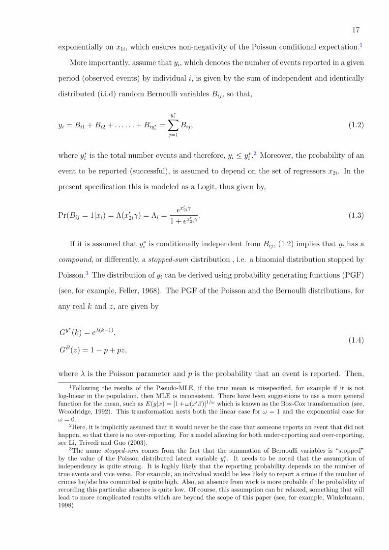
exponentially on x1i, which ensures non-negativity of the Poisson conditional expectation.1

More importantly, assume that yi, which denotes the number of events reported in a given

period (observed events) by individual i, is given by the sum of independent and identically

distributed (i.i.d) random Bernoulli variables Bij, so that,

yi = Bi1 +Bi2 + . . . . . .+Biy∗i=

y∗i∑j=1

Bij, (1.2)

where y∗i is the total number events and therefore, yi ≤ y∗i .2 Moreover, the probability of an

event to be reported (successful), is assumed to depend on the set of regressors x2i. In the

present specification this is modeled as a Logit, thus given by,

Pr(Bij = 1|xi) = Λ(x′2iγ) = Λi =ex′2iγ

1 + ex′2iγ. (1.3)

If it is assumed that y∗i is conditionally independent from Bij, (1.2) implies that yi has a

compound, or differently, a stopped-sum distribution , i.e. a binomial distribution stopped by

Poisson.3 The distribution of yi can be derived using probability generating functions (PGF)

(see, for example, Feller, 1968). The PGF of the Poisson and the Bernoulli distributions, for

any real k and z, are given by

Gy∗(k) = eλ(k−1),

GB(z) = 1− p+ pz,

(1.4)

where λ is the Poisson parameter and p is the probability that an event is reported. Then,

1Following the results of the Pseudo-MLE, if the true mean is misspecified, for example if it is notlog-linear in the population, then MLE is inconsistent. There have been suggestions to use a more generalfunction for the mean, such as E(y|x) = [1 +ω(x′β)]1/ω which is known as the Box-Cox transformation (see,Wooldridge, 1992). This transformation nests both the linear case for ω = 1 and the exponential case forω = 0.

2Here, it is implicitly assumed that it would never be the case that someone reports an event that did nothappen, so that there is no over-reporting. For a model allowing for both under-reporting and over-reporting,see Li, Trivedi and Guo (2003).

3The name stopped-sum comes from the fact that the summation of Bernoulli variables is “stopped”by the value of the Poisson distributed latent variable y∗i . It needs to be noted that the assumption ofindependency is quite strong. It is highly likely that the reporting probability depends on the number oftrue events and vice versa. For example, an individual would be less likely to report a crime if the number ofcrimes he/she has committed is quite high. Also, an absence from work is more probable if the probability ofrecording this particular absence is quite low. Of course, this assumption can be relaxed, something that willlead to more complicated results which are beyond the scope of this paper (see, for example, Winkelmann,1998)

18

it can be shown that the compound PGF of y, under independence of y∗i from Bij, is given

by,

Gy(k(z)) = Gy∗(GB(z)) = eλ(GB(z)−1) = eλ(−p+pz) = eλp(z−1) = eµ(z−1). (1.5)

Thus, the distribution of y is also Poisson with mean and variance equal to µ = λp.1 In the

regression framework, λi = ex′1iβ and pi = Λi. The resulting conditional probability of yi,

and the conditional mean are given by,

Pr(Yi = yi|xi) = e−µiµyii /yi!,

µi = E[yi|xi] = λiΛi,

(1.6)

respectively. This model is named Poisson-Logit for obvious reasons. Parameters β and γ

(henceforth denoted as θ = (β, γ) ) can be estimated by the method of Maximum Likelihood,

as we can easily specify the likelihood function from (1.6). The resulting log-likelihood

function is given by,

`(θ) = ln L (θ) =n∑i=1

(− µi + yi log µi − ln (yi!)

). (1.7)

Estimation of θ follows by maximization of (1.7) using numerical algorithms, such as the

Newton-Raphson, as the first order conditions (FOCs) for optimality are non-linear.2 Hence,

according to this framework, by only observing the reported events, we are able to estimate

the impact of x1i and x2i on the true events and on the probability for each event to be

1This result can be traced even further back than Feller (1968) to the early works in statistics by Neyman(1939) and Catcheside (1948). Neyman explains that in a given area, if the number of eggs laid by a fly perplant follow the Poisson distribution with λ, and if these masses of eggs hatch independently with probabilityof survival p, then the survived flies also follow the Poisson distribution with µ = λp. Similarly, Catcheside,in an example adjusted to genetics, says that if a given dosage of radiation causes breakages to chromosomes(where the number of total unobserved breakages per cell follow the Poisson distribution), and if there is aconstant probability, 1− p, for a break chromosome to heal , then the observed breakages follow the Poissondistribution with parameter µ = λp.

2The Score and Hessian of the Poisson-Logit model are given by, s(θ) = ∂`(θ)∂θ =

n∑i=1

(yi − µi)[

x′i1x′i2(1−Λi)

]and H(θ) = ∂2`(θ)

∂θ∂θ′ =n∑i=1

−µi[

xi1x′i1 xi1x

′i2(1−Λi)

xi1x′i2(1−Λi) xi2x

′i2

[(1−Λi)

2+yi−µiµi

Λi(1−Λi)] ], respectively. The lower right block

of the second matrix is negative if yi < λi(2Λi − 1) and therefore, H(θ) is not always negative definite.Consequently, `(θ) is not globally concave which may lead to multimodality. This feature and its consequenceswill be discussed later.

19

reported, respectively.

We notice that the Poisson-Logit probability distribution is the same as the one of the

traditional Poisson model, with a modified conditional mean. Therefore, as the density of

the traditional Poisson model belongs to the LEF (see, Gourieroux, Monfort, and Trognon,

1984), so does the density of the Poisson-Logit model with µ in place of λ. Therefore, using

the result of the Pseudo-MLE, consistent estimation of θ only requires correct specification

of the conditional mean. That is, the true DGP need not be Poisson-Logit but the true mean

must be given as µi = λiΛi. However, in cases of misspecified distributional assumptions,

estimates of higher moments will be inconsistent. Therefore, valid inference still requires

that the conditional variance is correctly specified (equal to µi in the case of Poisson-Logit).

Particularly, as it is the case for the conventional Poisson model, it can be shown that

if V ar(yi|xi) > E(yi|xi), the Poisson-Logit MLE standard errors will be underestimated

yielding false inference for the parameters of interest. In these cases, statistical inference

must be based on Pseudo-ML standard errors which consistently estimate the variance of θ as

explained in the introduction. Therefore, as long as we are confident about the specification

of µi, the Pseudo-ML is a consistent estimator for both θ, and the variance of θ.

It is clear that the above compound model is applicable not only in cases of under-

reporting, but whenever the observed number of events is a subset of the actual number.

Thus, as mentioned in the introduction, “under-reporting” can be considered as a broader

concept. For example, Winkelmann and Zimmermann (1993) analyze job offers, which can

be considered as the true DGP in labour mobility models, by merely observing the number of

job changes (see also, Section 1.7). In this sense, using the Poisson-Logit, that imposes more

structure to the model, they are able to estimate the impact of employee’s characteristics on

both the number of outside job offers they receive and the probability of accepting an outside

job offer. As another example consider firms’ innovative activity. As Wang, Cockburn, and

Putermam (1998) discuss, economists usually use the number of patents as an indicator of

a firm’s inventive activity since inventive activity is not directly observed. However, having

only data on the count of patents, the Poisson-Logit model enables the researcher to draw

inference for the probability of an invention to be patented and the determinants of the true

inventive activity.

20

1.3 Extensions - The Negative Binomial Logit Case

A basic property of the Poisson-Logit model is that µi is both the conditional mean and

variance of the dependent variable. This result often makes the Poisson distribution less ap-

propriate in fitting “real” data, since many empirical applications reveal that over-dispersion

exists. In the presence of over-dispersion, although the Poisson MLE complemented by ro-

bust standard errors is totally appropriate, given that the conditional mean is correctly

specified, researchers tend to use models more suitable for over-dispersed data, the most

popular being the Negative Binomial family of models (NB). One way to obtain the NB

model is by combining a Poisson distribution with an independent gamma distributed error

term (see, for example, Cameron and Trivedi, 1986). This error term can be regarded as

an unobserved individual heterogeneity, for instance, because of omitted regressors from the

mean specification.

To this end, suppose that there is an unobservable individual effect, υi = eεi , which is

gamma distributed with E(υi) = 1 and V ar(υi) = αi. Moreover, assume that y∗i conditional

on x1i and υi is Poisson distributed with mean λieεi . Thus, conditional on x1i only, the

distribution of y∗i is Poisson-Gamma with conditional probability,

Pr(Y ∗i = y∗i |x1i) =

∫e−λiυi(λiυi)

y∗i

y∗i !g (υi, 1/αi) dυi ≡ Eυ

[Pr(Y ∗i = y∗i |x1i, υi)

], (1.8)

where g(.) is the gamma density function with parameter 1/αi. Averaging out (1.8) leads to

the NB distribution1 with mean, λi and variance,

ωi = λi + αiλ2i . (1.9)

Therefore, this formulation allows for over-dispersion since αi > 0, implies that, ωi > λi.2

Now, similarly to the previous section, assume that yi has a stopped-sum distribution as

given in (1.2), however, in this case this sum is stopped by the value of y∗i , which follows

1For a proof, see, Cameron and Trivedi (1998), p101.2The mean of the NB can be obtained by using the Law of Iterated Expectations as E(y|x) =

Eυ [E(y|x, υ)] = Eυ[λυ] = λ. The variance is obtained by using the Law of Total Variance, as V ar(y|x) =Eυ [V ar(y|x, υ)] + V arυ [E(y|x, υ)] = Eυ[λυ] + V arυ[λυ] = λ + αλ2. For further details about the Nega-tive Binomial models refer to Hausman, Hall and Griliches (1984), Cameron and Trivedi (1986, 1998), andWinkelmann (2008).

21

the NB rather than the Poisson distribution. Again, the probability of an actual event to be

reported, conditional also on this error term, is given by Λi. The distribution of yi can be

similarly derived using a compound PGF, resulting from compounding a NB PGF together

with a Bernoulli PGF. Following Anscombe (1950), the NB PGF for y∗, with mean equal to

λ and variance equal to λ(1 + αλ), is given by,

Gy∗(k) = (1 + αλ− αλk)−α−1

. (1.10)

Therefore, the compound PGF for yi is the following:

Gy(k(z)) = Gy∗(GB(z)) = (1 + αλ− αλGB(z))−α−1

= (1 + αλ− αλ(1− p+ pz))−α−1

= (1 + αλp− αλpz)−α−1

= (1 + αµ− αµz)−α−1

.

(1.11)

Thus, the distribution of y is NB with mean µ and variance µ(1 + αµ). According to the

regression framework, similarly to the procedure followed for the simple NB model, the

distribution of yi conditional on xi only, is NB with mean equal to µi and variance given by,

ωi = µi + αiµ2i . (1.12)

As it is clear from (1.12), the NB-Logit converges to the Poisson-Logit model as αi approaches

zero, since consequently, ωi converges to µi.1

The NB2 is the most used and cited model among the NB family. It is obtained if it

is assumed that the variance of the error term, αi, is constant (homoscedastic), so that

the variance of yi is ωi = µi + αµ2i , which is quadratic on µi. The conditional probability

of the NB2-Logit follows the conditional probability of the simple NB2 model, with mean

1A formal proof that shows how the NB probability function converges to Poisson as α → 0, can befound in Wineklmann (2008), p23.

22

parameter µi = λiΛi in place of λi, such that,

Pr(Yi = yi|xi, α) =Γ(yi + α−1)

Γ(yi + 1)Γ(α−1)

(α−1

α−1 + µi

)α−1 (µi

α−1 + µi

)yi

=Γ(yi + α−1)

Γ(yi + 1)Γ(α−1)(1 + αµi)

−(α−1+yi)(αµi)yi .

(1.13)

We can estimate θ and the additional “overdispersion” parameter α by Maximum Likelihood,

specifying first the log likelihoods from (1.13), which is,

ln L (α, β, γ) =n∑i=1

(ln

(Γ(yi + α−1)

Γ(yi + 1)Γ(α−1)

)−(α−1+yi) ln(1+αµi)+yi(lnµi+lnα).

)(1.14)

Another model of this family that is extensively used in empirical works is the NB1. The

NB1 is obtained if we consider that αi is not constant but instead, it is a function of the

regressors (heteroscedastic) according to the following relationship, αi = δ/λi. Substituting

this relationship into (1.12) we obtain the variance of the NB1-Logit,

ωi = µi + δλiΛ2i . (1.15)

Thus, this different parameterization leads to a variance form which is no more quadratic

on µi, but rather, linear with respect to λi and quadratic with respect to Λi. Given (1.15)

the probability distribution of the NB1-Logit model is given by,

Pr(Yi = yi|xi, δ) =Γ(yi + δ−1λi)

Γ(yi + 1)Γ(δ−1λi)

(δ−1λi

δ−1λi + µi

)δ−1λi ( µiδ−1λi + µi

)yi

=Γ(yi + δ−1λi)

Γ(yi + 1)Γ(δ−1λi)(1 + δΛi)

−(δ−1λi+yi)(δΛi)yi .

(1.16)

The log likelihood of NB1-Logit is therefore given by,

ln L (α, β, γ) =n∑i=1

(ln

(Γ(yi + δ−1λi)

Γ(yi + 1)Γ(δ−1λi)

)− (δ−1λi + yi) ln (1 + δΛi) + yi(ln δ + ln Λi)

).

(1.17)

23

From (1.17) it is clear that the parameters of the NB1-Logit model do not always appear

together, as opposed to both Poisson-Logit and NB2-Logit where the regressors of both

the count and reporting processes affect the log likelihood function only through µi. The

interesting implication of this feature will be discussed in Section 1.5. Similar to the NB2-

Logit, maximum likelihood can be performed to estimate the values of β, γ and δ that

maximize the likelihood of having obtained the observed data.1

We need to stress, however, that although these two models may lead in efficiency gains

in the presence of over-dispersion, they do not belong to the LEF.2 Thus, the robustness

properties of the Pseudo-MLE do not hold in this case. For consistency of the NB-Logit

models it is required that the true DGP is NB-Logit, so that the individual unobserved

heterogeneity is gamma distributed with variance equal to α and δ/λi for NB2-Logit and

NB1-Logit, respectively. Therefore, by using the NB-Logit models instead of the Poisson-

Logit we trade-off robustness for a possible gain in efficiency.

1.4 Identification Issues in the Poisson-Logit model

Even though the Poisson regression model is very robust, the Poisson-Logit is a double-index

model where identification of θ is problematic. As will be made clear in this section, apart

from all the aforementioned assumptions in the set up of the model, further parametric

assumptions are needed in order for the parameters β and γ to be identifiable. This iden-

tification problem stems from the fact that the Poisson-Logit mean is given as the product

of the Poisson mean (exponential) and the Logit function. Consider the following simple

manipulation of µi:

µi ≡ ex′1iβ

ex′2iγ

1 + ex′2iγ

= ex′1iβ+x

′2iγ

1

1 + ex′2iγ

= ex′1iβ+x

′2iγ

e−x′2iγ

1 + e−x′2iγ≡ µ∗i , (1.18)

1Studies that explore the NB1-Logit and NB2-Logit models are limited. However, a detailed descriptionof the NB2-Logit model together with its FOCs and its Information Matrix can be found in Mukhopadhyayand Trivedi (1995), and Cameron and Trivedi (1998). In addition, a conditional probability function similarto the NB1-Logit is obtained by Van Praag and Vermeulen (1993).

2The NB2-Logit belongs to the LEF only for given α. Nevertheless, in practice α is subject to estimationas there is no a priori information about its value.

24

where we notice that the conditional mean can be written in two different ways as µi = λiΛi

and µ∗i = λiex′2iγ(1 − Λi), where µi ≡ µ∗i . This simple, yet important, result has critical

consequences for the identification of the Poisson-Logit model.

First, recall that the Poisson-Logit MLE aims to determine the values of θ that maximize

the value of the likelihood function. From (1.7) we can see that these parameters enter the log

likelihood function only through µi, which appears in the log likelihood only as a whole (the

Poisson mean is not separated from the Logit at any point). Therefore, identification of β and

γ will depend only on µi. Now assume that there is µi that maximizes the likelihood function.

However, since µi ≡ µ∗i , µ∗i also maximizes the same likelihood function. This means that,

µi is observationally equivalent to µ∗i , unless appropriate restrictions are imposed on θ.1

Particularly, as will be made clearer in the next paragraphs, unless at least one exclusion

restriction is imposed on β, (1.18) implies that there are two Poisson-Logit regression models

with conditional means µi and µ∗i , that lead to the same likelihood value.

To fix ideas, consider first the case where the same regressors appear in both processes,

so that xi = x1i = x2i. According to this assumption, (1.18) gives,

µi ≡ ex′iβ

ex′iγ

1 + ex′iγ

= ex′i(β+γ)

e−x′iγ

1 + e−x′iγ

= ex′iβ∗ ex

′iγ∗

1 + ex′iγ∗ ≡ µ∗i (1.19)

Therefore, there are always two observationally equivalent models and identification fails.

The parameters θ and θ∗ of the two models are related to each other in the following manner:

if the parameters of the first model are given by β for the Poisson and γ for the Logit part,

then the parameters of the second model are given by β∗ = β+γ and γ∗ = −γ, respectively.

In Section 1.7, we illustrate this result using a real data set.

1.5 Possible Solutions to the Identification Problem

In this section, we firstly present the conditions under which the Poisson-Logit model is

identified. One possible identification strategy is to use sign restrictions on the Logit process,

henceforth called “reporting process”, which is helpful whenever prior information of the sign

1By “observational equivalence” we mean that there are two different linearly dependent sets of param-eters, for example, θ = (β, γ) and θ∗ = (β∗, γ∗), that maximize the value of the likelihood function.

25

of at least one parameter of the reporting process exists. Moreover, exclusion restrictions on

the reporting or the count process can be used. This requires that we have initial information

for at least one parameter of β or γ to be zero, meaning that a regressor that belongs to

the reporting process has no effect on the reporting process, or the opposite.1 Following

another direction, we consider small departures from the Poisson-Logit model by assuming a

different distribution for the count process, or a different model for the reporting process, or

any combination of the two. We will also show that it is possible to identify θ by imposing

a different structure on the density function. In this section only the theoretical results are

presented. Discussion of these findings and empirical illustrations follow in subsections 1.6

and 1.8, respectively.

1.5.1 Sign Restrictions on the Reporting Process

A first way to identify θ is by imposing at least one sign restrictions on the reporting

process. It must be stressed that this option is valid only if established theoretical results

clearly suggest the direction of the impact of an independent variable on the reporting

process. For instance, consider the example of labour mobility adopted by Winkelmann and

Zimmermann (1993), where job offers follow the Poisson distribution and the probability

to accept an offer is given as a Logit. Now suppose that a hypothetical “well” established

theory for labour mobility suggests that more “firm specific” human capital accumulation

(FS-HCA) by employees increases wage in the current job but not the wage offered by outside

firms. Therefore, more FS-HCA increases the wages differential between the current job and

potential outside job offers. Consequently, following this theory, an increase in FS-HCA will

have a negative effect in the probability of a worker to accept a job offer, therefore, resulting

in a negative coefficient in the Logit part.2

Since without exclusion restrictions two observationally equivalent models always exist

with θ = (β, γ) and, θ∗ = (β + γ,−γ), the effect of this variable will be positive in the one

1If the model was not afflicted by this identification problem, it would be natural to assume that theindividual characteristics affecting the count process are the same with the individual characteristics deter-mining the reporting process. For example, assume that the decision to commit a crime depends on thegender, age and race. However, the probability of reporting this crime would be naturally affected by thesame features. Therefore, it is a quite strong assumption to a priori restrict a coefficient to zero. Theremust always be rational reasons behind our choices.

2Winkelmann (2008) in section 9.7 presents a brief review on theories developed for labour mobility.

26

model but negative in the second. Hence, identification is achieved since we reject the model

in which the coefficient appears with the wrong sign. Finally, notice that sign restrictions

on the count process are not appropriate as β and β∗ = β + γ can be of the same sign, so

that the effect of a variable can possibly be of the same direction in both models.

1.5.2 Exclusion Restrictions on the Reporting Process

As mentioned at the beginning of this section, imposing exclusion restrictions can help

identifying θ. However, it is easy to show that if exclusion restrictions are placed only on the

Logit part, by restricting some elements of γ to zero, only the elements of β corresponding

to the zeros in γ are identified.

Consider the case where we a priori know that at least one regressor belongs only to the

count process. Differently, this can be considered as restricting the corresponding elements

of γ to zero. When exclusion restrictions are placed on γ, vector x2i can be considered as

a subset of x1i, so that in vector x1i there is at least one variable that does not appear in

x2i. Assume that this set of regressors is denoted by wi. Thus, since vector x1i consists of

vector x2i plus vector wi, the exclusion restrictions on the Logit part could be thought of as

having added another set of regressors wi in the Poisson part, changing the Poisson-Logit

mean into µi = ex′2iβ+w

′iηΛi, where η consists of the parameters corresponding to the zeros

in γ. Now, following the same reasoning as in (1.18) and (1.19) we have that,

µi ≡ ex′2iβ+w

′iη

ex′2iγ

1 + ex′2iγ

= ex′2i(β+γ)+w

′iη

e−x′2iγ

1 + e−x′2iγ

= ex′2iβ∗+w′iη

∗ ex′2iγ∗

1 + ex′2iγ∗ ≡ µ∗i . (1.20)

Therefore, even in this case two observationally equivalent models exist where β∗ = β + γ

and, γ∗ = −γ, but η∗ = η. It is clear that β and γ remain unidentified, since two different

set of these parameters will lead to exactly the same likelihood value. In spite of this, all

the elements included in η are identified, as η is identical in both µi and µ∗i . Hence, unless

we are interested only in η, this kind of restrictions seems inappropriate.

27

1.5.3 Exclusion Restrictions on the Count Process

Now assume that exclusion restrictions are placed in the Poisson part, by setting some

parameters of β to zero. Consequently, x2i consists of x1i plus a set of regressors that

corresponds to the excluded variables of the Poisson part. Let us denote this vector by

qi. Therefore, the probability of reporting an event is now given by Λ(ex′1iγ+q

′iϕ), where ϕ

contains the parameters in the reporting process corresponding to the restricted to zero

parameters of β. Accordingly, we have:

µi ≡ ex′1iβ

ex′1iγ+q

′iϕ

1 + ex′1iγ+q

′iϕ

= ex′1i(β+γ)+q

′iϕ

e−x′1iγ−q′iϕ

1 + e−x′1iγ−q′iϕ

6= ex′1iβ∗ ex

′1iγ∗+q′iϕ

∗

1 + ex′1iγ∗+q′iϕ

∗ ≡ µ∗i , (1.21)

where β∗ = β + γ, γ∗ = −γ, and ϕ∗ = −ϕ. As we notice from (1.21), the two models µi and

µ∗i are not observationally equivalent in this case, since the vector qi appears in the Poisson

mean of µi but not in µ∗i , and identification for the whole model is achieved.

1.5.4 Specifying the Count Generating Process, as Negative Bi-

nomial 1

As mentioned before, models for count data that use the Negative Binomial distribution

have been very popular as they allow for over-dispersion through the extra parameter α (or

δ, in NB1 case). As presented in Section 1.3, allowing for gamma distributed unobserved

heterogeneity in the Poisson-Logit model gives rise to the NB-Logit family of models. There,

the two basic generalizations of the Poisson-Logit model were presented, the NB2-Logit and

the NB1-Logit.

Concerning the NB2-Logit model, it is clear from (1.14) that its log likelihood depends

on the regressors only through µi, as it is the case in the Poisson-Logit model. This is

because of the homoscedastic form of the variance of the gamma distributed error term α.

As a consequence, identification of the NB2-Logit model requires exactly the same conditions

established for the Poisson-Logit model.

On the other hand, according to the NB1-Logit model, the variance of the error term

is heteroscedastic of the form δ/λi. This is incorporated into the log likelihood function

28

(1.17), where it now depends on x1i through λi, and on x2i through Λi, separately. Thus,

in a sense, the likelihood function of the NB1-Logit model can distinguish the count process

from the reporting process, and consequently, β from γ. As a result, adopting the NB1

distribution, identification becomes possible even when both parts of the model contain the

same regressors.

Nevertheless, it is very important to stress that NB1-Logit model is not a LEF and

therefore, it is not robust in misspecifications of moments higher than the conditional mean.

Therefore, since NB1-Logit MLE achieves identification of the mean by assuming a particular

form of hetersoskedasticity of the error term, and consequently, by imposing a different

structure on ωi, the estimates of θ will be inconsistent if the variance form is misspecified.

1.5.5 Specifying the Reporting Probability as a Probit or CLogLog

Another very popular model that deals with binary choice problems is the Probit model,

which exhibits nearly the same properties as the Logit model (see, Maddala, 1983). Never-

theless, assume that the correct specification for reporting a particular event is given by a

Probit model instead of a Logit. According to the Probit model, Pr(Bij = 1|xi) = Φ(x′2iγ),

where Φ(.) is the standard normal cumulative distribution function (CDF).

Given this assumption, the Poisson-Logit changes into the Poisson-Probit model with

mean equal to µi = λiΦ(x′2iγ). As opposed to the Logit, the functional form of the Probit

model cannot give rise to the identification problem described in Section 1.4, even when

the regressors are the same in both parts of the model. This is obvious, since now µi =

ex′iβΦ(x′iγ) 6= ex

′i(β+γ)Φ(−x′iγ). Therefore, when the probability of reporting an event is

given by a Probit, identification of the whole model is achieved.

Although less popular, the complementary log-log model (CLogLog) has also been used

in the literature. Contrary to the Probit or Logit, this model assumes a non-symmetric

CDF that is derived from the extreme value distribution. Therefore, according to this model

Pr(Bij = 1|xi) = 1 − exp(−ex′iγ). As CLogLog relaxes the assumption of symmetry, it

becomes more appropriate in cases where the observed average probability of the outcome

is close to one or close to zero. Therefore, if there are good reasons to believe that the

probability of reporting a true event is very close to one or very close to zero, a researcher

29

could advocate that a Poisson-CLogLog model is more appropriate and use the CLogLog

CDF instead of the symmetric Logit. As it is the case for the Poisson-Probit, µi = ex′iβ(1−

exp(−ex′iγ)) 6= ex′i(β+γ)(1− exp(−e−x′iγ)) and this model is identified.

1.6 Discussion

The theoretical results developed in this paper suggest that identification of the Poisson-

Logit, and the NB2-Logit models is problematic, in the sense that without further parametric

assumptions two identical “global” maxima exist. However, identification is achieved if true

events follow the NB1 distribution, or if the reporting process is specified as a Probit model.

In this section, further implications of the above results will be discussed. Moreover, some

tips for researchers who intend to use the above models will be described.

As explained in subsection 1.5.1, a first way to achieve identification is by sign restrictions

on the reporting process. We need to stress that this type of restriction becomes more

appropriate the more certain we are about the theoretical result that determines the sign of

the “restricted” coefficient. For instance, in the example of subsection 1.5.1, if information of

the FS-HCA was publicly available, it could increase the wage of outside offers as well, making

the change in wages differential uncertain. Moreover in practice, given correct specification of

the conditional mean,1 the effect of the “restricted” variable should be statistically significant.

In fact, the more significant the effect, the more certain we are about the appeared sign in

the two models. Finally, in many cases the “restricted variable” is not directly observed and

therefore, the researcher is forced to use proxy variables. In the previous example, FS-HCA

is not observed in practice but it can be approximated by “job experience”. However, it is

ambiguous whether general “job experience” captures the true effect of FS-HCA.

More interestingly, the results of subsection 1.5.3 showed that when exclusion restrictions

are imposed on the count process, identification of the whole model is achieved, since there

cannot be two linearly dependent sets of parameters that lead to the same likelihood value.

However, even in this case, it is clear from (1.21) that the identification problem is exactly

1By correct specification we mean that not only should the true mean be given by λiΛi but also thatboth processes include all the required information. That is, we do not include irrelevant variables, and wedo not omit variables that must be included.

30

restored when ϕ = 0, or when the regressors excluded from the Poisson part, qi, are perfectly

collinear with the remaining elements of this vector, x1i. Hence, the closer we move towards

the one of these two conditions, the smaller the effect of the exclusion restriction, and the

more difficult the identification becomes. Practically, we find that if the exclusion restriction

is very “weak”, meaning that the excluded from the count process variable has a very small

effect on the reporting process, another local maximum probably exists with likelihood value

very close to the global one and estimated parameters very close to θ∗ = (β + γ,−γ). If

a second maximum does exist, the estimation process, using zeros or conventional Poisson

estimates for starting values in the count process, will always converge either towards the

global or the local maximum. If a researcher performing the Poisson-Logit or the NB2-Logit

MLE in real data is unaware of these problems, he/she may be puzzled estimating parameters

with unexpected signs or implausible values. Section 1.7 will present a very comprehensive

example of this situation.

Thus, although an appropriate restriction guarantees identification of θ, it is not guaran-

teed that the global maximum has been found. Therefore, estimation of the above models

must be always accompanied by a thorough search for alternative maxima. A very useful way

of searching for other candidate maxima is the following: firstly, a regression is performed

using randomly chosen values for the coefficients of the reporting process and conventional

Poisson or NB2 estimates for the coefficients of the count process. This helps the estimation

to be smoother, avoiding possible numerical errors in the optimization procedure. Unless

more problems exist, the model will converge on log likelihood value ln L , corresponding to

estimates θ = (β, γ). According to the theoretical results, the other maximum will be close

to θ∗ = (β + γ,−γ). Hence, the estimated values of θ∗ can be used as starting values for a

second regression. If the second maximum exists, it will be found by this second regression,

with log likelihood value ln L ∗ and θ∗ ≈ θ∗. Consequently, if we find both maxima, we will

accept the set of parameters that maximize the likelihood of obtaining the observed data.

It would also be useful to note that sometimes, different numerical algorithms work better

in different models or different data, in the sense that they perform with lower number of

numerical errors and achieve convergence more easily.1 Therefore, in case a numerical algo-

1Some popular algorithms available in econometric packages are: the Newton-Raphson which uses an-

31

rithm does not perform well, before coming to the decision that there is something wrong

with our model, it would be very practical to run the same model with alternative numerical

optimizers.

In footnote 2 of page 14, we mentioned that the likelihood function of the Poisson-Logit

model is not always globally concave which might lead to multimodality. Therefore, not

always can we be certain that only two maxima exist. In practice, there might be cases where

more than two maxima exist. The method described above could not succeed in reaching

a, supposedly, third local maximum. One way to reach a potential third maximum would

be to use random starting values for all the parameters and to experiment with different

numerical algorithms. If this is repeated many times, it is highly likely that the regression

procedure will converge in every candidate maximum.

Of course a researcher, using over-dispersed data could assume that the observed data

are generated by a NB1-Logit model and avoid using sign or exclusion restrictions. However,

the NB1-Logit MLE is less robust than the Poisson-Logit MLE, since it does not fall within

the LEF. Therefore, consistency of the estimated parameters requires not only correct spec-

ification of µi, but also that the data are truly generated by a NB1-Logit process. Most

importantly, as mentioned in Section 1.5.3, identification is achieved by assuming a specific

form of heteroskedasticity for αi. Therefore, the estimates will be inconsistent if the variance

form is misspecified.

As explained in subsection 1.5.5, the Poisson-Probit model is identified even when x1i =

x2i. In spite of this, since the shape of the standard normal pdf is very similar to the logistic

probability function, it is quite possible that still multiple maxima exist, whose likelihood

values are very close to each other. The procedures described above can assist the researcher

to check for alternative maxima as ex′iβΦ(x′iγ) ' ex

′iβΛ(x′iγ/s) ' ex

′i(β+γ/s)Φ(−x′iγ), where

s is a scaling parameter (≈ 31/2/π, see, Maddala, 1983) used in order for the Probit and

Logit parameters to be approximately the same. Finally, the Poisson-CLogLog model is also

identified even when x1i = x2i. However, the empirical results (which are not presented in

alytic second derivatives and performs very well if the likelihood function is globally concave. The Bernt-Hall-Hall-Hausman (BHHH) which uses only first derivatives (outer product of the score), which results inlower computational intensity, and the Broyden-Fletcher-Goldfarb-Shanno (BFGS) which is a refinement ofDavidon-Fletcher-Powell (DFP) and also uses first order derivatives. For details, see Chapter 10, in Cameronand Trivedi (2005).

32

Section 1.8 but are available on request) show that again a second maximum exists with

likelihood value very close to the global one and estimates very close to θ∗. This might

be, because conditional on vector xi the distribution of the Logit model is similar to the

distribution of the CLogLog model.

1.7 Other Related Models

Now that the conditions under which identification of the Poisson-Logit model (and small

departures from it) are understood, it would be important to briefly discuss other models

that are used in different contexts but either their conditional mean is specified as the

Poisson-Logit’s one or they face similar identification problems.

To begin with, it would be interesting to briefly discuss the connection between the

Poisson-Logit model and the popular Zero-Inflation Poisson model (ZI-Poisson) as intro-

duced by Mullahy (1986) and Lambert (1992). Although the interpretation of the Poisson-

Logit for under-reporting can be very different from the interpretation of ZI models, the

conditional mean in both models is specified as µi = λiΛi, where in Poisson-Logit, Λi is the

conditional probability of reporting an actual event, while in the ZI-Poisson model it denotes

the conditional probability of having no Zero-Inflation.1 However, the ZI-Poisson model is

not afflicted by the identification problem discussed above because it imposes more structure

in the log likelihood function (see, Lambert, 1992). Actually, the extra structure imposed on

the likelihood function has as a result that it depends separately on λi and Λi and thus, we

can still identify the parameters β and γ without extra restrictions. Nonetheless, this type of

ZI models does not belong to the LEF and therefore, they are very sensitive to distributional

misspecfications.2

Instead, Staub and Winkelmann (2010) propose the less parametric Poisson Quasi-

1According to the ZI models there are two different sources of zeroes. As a comprehensive example,consider the question “how many times you go fishing per month”. A proportion of people will reply “zerotimes” regardless of their characteristics x, because they actually never go fishing (perhaps because they donot like it at all, or because there is not a lake, river, or sea around the area they reside so that they canuse it for fishing - these are called “structural zeros”). The rest of them, who fish sometimes, will say either“zero” (incidental zeroes) or “n times” depending on whether they actually went fishing during the givenperiod. However, it is important to note that the ZI-Poisson model can be also interpreted as a model oftotal under-reporting. That is, everybody that under-reports, reports exactly zero counts.

2Particularly, even if the mean is correctly specified, the ZI-Poisson MLE is not consistent if the DGP isgiven by a distribution different from the ZI-Poisson.

33

Likelihood (PQL) estimator that estimates the same conditional mean without making any

assumptions on the exact distribution of the counts, resulting in a model that is formally

identical to the Poisson-Logit. Thus, they use the results of the Pseudo-ML to advocate that

consistency of this estimator only requires correct specification of the mean. As it is clear,

identification of this model requires exactly the same assumptions needed for identification

of the Poisson-Logit, which will be discussed in the next section.

It is also important to stress that this identification problem is not limited to count data

models. Actually, it arises in any model where the conditional mean is specified as the

product of an exponential function and a Logit, and there is not extra structure imposed

by the researcher on the estimation procedure. Mullahy (1998), for example, motivated by

the earlier work of Duan at al (1983), introduces a two-part model for non negative data

(calling it Modified two-part model (M2PM)) that is applicable in both count and continuous

data. According to this model, conditional on x, the probability to observe a positive value,

Pr(y > 0|x), is given by a Logit, and once a non-zero outcome is observed, the expected value

of the observed amount, E(y|x, y > 0), is given as an exponential function that also depends

on x. The conditional expectation is thus given by µi = E(y|x) = Pr(y > 0|x)E(y|x, y >

0) = Λiλi, which is the same as the conditional mean of the Poisson-Logit model. This model

can be put into effect in applications that include a quite frequent zero “corner solution”,

such as the amount money spent on medical care, or expenditures in unhealthy products

such as alcohol.

According to this model, the effect of x on the probability of observing a positive outcome

is allowed to be different from the effect of x on the total amount, conditional on having

observed a positive outcome (see, also Pohlmeier and Ulrich, 1995). Mullahy proposes two

estimation procedures: 1) the two-steps estimation (M2PM-2), where in the first step a

Logit is used to model Pr(y > 0|x) and in the second step E(y|x, y > 0) = ex′iβ is estimated

by nonlinear least squares (NLLS), and 2) the one-step estimation (M2PM-1), where µi =

E(y|x) = Λiλi is directly estimated using NLLS, minimizing the objective function∑n

i=1(yi−

µi)2. It is clear that in the M2PM-1, the sum of square residuals depends on θ only through

µi and thus, the same identification problem arises. However, in M2PM-2, by estimating

β and γ separately, more structure is imposed on the model and therefore, θ is identified

34

without further restrictions.

Finally, a similar identification issue arises in a model for binary choice data that al-

lows for missclassification probabilities developed by Hausman, Abrevaya, and Scott-Morton

(1998). According to this model, Pr(y∗i = 1|xi) = Φ(x′iβ), where y∗ refers to the true

but unobserved outcome, and Φ(.) denotes the Probit CDF. The true outcome, however,

is subject to missclassification, where the missclassification probabilities are given by a0 =

Pr(yi = 0|y∗i = 1) and a1 = Pr(yi = 1|y∗i = 0), where y refers to the observed outcome. In

the context of misreporting, the misclassification of one as zero takes the interpretation of

under-reporting, while the misclassification of zero as one takes the interpretation of over-

reporting. It can be easily shown that the probability to observe an outcome is given by

Pr(yi = 1|xi) = a1 + (1 − a0 − a1)Φ(x′iβ). Estimation is straightforward by ML using nu-

merical optimizers. Hausman, Abrevaya, and Scott-Morton (1998) show that the model is

not globally identified since, a1 + (1 − a0 − a1)Φ(x′iβ) = a1 + (1 − a0 − a1)Φ(−x′iβ) where

a0 = 1 − a1 and a1 = 1 − a0. Thus, there are two observationally equivalent models with

parameters (a0, a1, β) and (a0, a1,−β). Identification is achieved by imposing the “mono-

tonicity” condition, which states that a0 + a1 < 1. According to this, we are able to rule out

the “wrong” maximum, since a0 + a1 < 1 implies that a0 + a1 > 1. If this condition fails,

the misclassification probabilities are too large, and therefore, the data are most probably

too noisy to provide reasonable results.

1.8 An Illustration using Data on Labour Mobility

This section provides some examples that illustrate the theoretical results of this study. This

illustration, should by no means be considered as an empirical application aiming to identify

the determinants of labour mobility. It should be regarded instead as an example showing

readers a practical application of the theoretical results discussed above.

This illustration uses the same data used by Winkelmann (2008) in an empirical applica-

tion to labour mobility, in Chapter 9 of his monograph.1 The original data set comes from

the German Socio-Economic Panel (GSOEP) which is provided by the Deutsches Institut

1The data used throughout the empirical illustration have been kindly provided by Rainer Winkelmanand are from the public use version of the German Socio-Economic Panel Study.

35

fur Wirtschaftsforschung.1 This subsample considers 1,962 males between 25 and 50 years

old in 1974. The dependent variable is the number of Direct Job Changes, thus, it is a pure

count variable. The set of independent variables includes, Education∗10−1, Experience∗10−1,

Experience2 ∗ 10−2, Union Membership, German, Qualified White Collar, Ordinary White

Collar, Qualified Blue Collar (excluded group being ordinary blue collar) and Single. These

are the variables that Winkelmann also uses in his aforementioned work. For descriptive

statistics and details about the data and the variables used in this empirical application

refer to Winkelmann (2008).

Moreover, the model used in this illustration is also adopted by Winkelmann and Zim-

mermann (1993). As briefly described in Section 1.2, this model intends to identify the

determinants of job offers and the probability to accept an offer by merely observing ac-

cepted job offers. That is, workers receive (unobserved) job offers, assumed to be distributed

as Poisson, NB2 or NB1 variables. For every job offer a decision is taken whether to accept or

reject it. If a job is accepted (successful event) it is consequently reported, where decision of

acceptance is modeled as a Logit or a Probit. Therefore, given that the process of receiving

(a number of) job offers is independent from the process of accepting or rejecting them, then

(observed) job changes follow a stopped sum distribution given by (1.2). Consequently yi

follows the Poisson-Logit, or any other of the generalizations considered in this paper, de-

pending on the assumptions we make on the distribution of true events and the probability

of acceptance.

All the theoretical results obtained in the previous sections are being tested in the re-

mainder of this section.

1.8.1 Same Regressors in both Processes

This subsection examines the case where both the count process (offers) and the reporting

process (probability to accept an offer) are assumed to be affected by the same vector of

regressors xi. In this example, we can see in practice the identification failure described

earlier. The results are given in Table 1.1. The reporting probability process, modeled as a

Logit is reported in the upper part of this table, whereas the count process is reported at

1See, Wagner, Burkhauser and Behringer (1993) for more information.

36

the lower part. Robust standard errors are presented in parentheses. Results of using the

Probit specification to model the reporting process are presented in subsection 1.7.4.

The identification failure is obvious. For the Poisson-Logit and NB2-Logit, two identical

“global” maxima exist (same log-likelihood value). Therefore, there are two observation-

ally equivalent models with very different parameterizations of the conditional mean. Very

clearly, it can be checked that if the estimated coefficients of the one model are given by

θ = (β, γ), the estimates of the other model are given by θ∗ = (β + γ,−γ). Thus, as far as

the Logit part is concerned, we see that the coefficients of the two equivalent models have

the same values but opposite signs. Regarding the count process, any βj(2), which is the

estimated coefficient of regressor j in model (2), is given by βj(1), the estimated coefficient

of the same regressor in the count process of model (1), plus γj(1), the estimated coefficient

of the same regressor in the Logit part of model (1), and vice versa.1

The NB2-Logit results are presented in columns (3) and (4). We notice that exactly the

same situation occurs for this model, confirming the theoretical results of subection 1.5.4.

Moreover, it is also clear that NB2-Logit fits the data better than the Poisson-Logit model,

given by the better log likelihood value of the NB2-Logit. This may be the result of including

the extra parameter α to account for gamma distributed unobserved heterogeneity.

The most interesting results appear in model (5), where the NB1-Logit estimated coef-

ficients are reported. This column establishes the theoretical argument of subection 1.5.3,

that if a NB1 distribution is used instead of the Poisson or the NB2 one, the identification

problem vanishes. Here, only one maximum seems to exist (at least one could be found

after many repeated regressions and different methods), with coefficients approaching the

coefficients of the first and third column (apart from the Experience2 ∗ 10−2 case). Also, it is

worth noting that the NB1 model exhibits the highest log likelihood value, which situation

holds in all results presented in the following subsections. Nevertheless, these differences are

quite small in magnitude.

Moreover, it was argued in Section 1.5 that an appropriate sign restriction solves the iden-

tification problem. For example, in subsection 1.5.1 we explained that a hypothetical theory

1Therefore, for example, the education coefficient at the count process of column 1 (2), which is 1.962(-0.976), is given by the education coefficient of the count process of column 2 (1), -0.976 (1.962), plus theeducation coefficient of the Logit process of column 2 (1), which is 2.938 (-2.938).

37

of labour mobility suggests that as experience increases, the probability to accept an external

job offer should decrease, so that the coefficient in the Logit process is expected to be nega-

tive. However, as can be seen from model (2), both Experience∗10−1 and Experience2 ∗ 10−2

are positive which means that the probability to accept a job offer increases at an increasing

rate. Hence, according to the “established” theoretical results we should reject model (2) and

accept model (1). However, notice that these coefficients are not statistically different from

zero and therefore, this sign restriction becomes less appropriate in this particular example.

Of course, this is just an illustration where µi is probably misspecified. In real empirical

applications, this kind of decisions must be based on well established theoretical results and

well specified models.

1.8.2 Exclusion Restrictions on Logit

It has been established in subsection 1.5.2, that the model can be only partially identified

by restricting at least one coefficient of the Logit part to zero, since only the elements of β

corresponding to the zeros in γ can be identified. This situation is depicted in Table 1.2,

where the constant, along with the coefficients of other five dummies in the Logit process

are restricted to zero.1

Table 1.2 supports all theoretical results given in subsection 1.5.2. Once more, it is

very interesting that two observationally equivalent models exist with θ =((β, η), γ

)and

θ∗ =((β + γ, η),−γ

). Thus, the parameters in the count process that correspond to the

excluded variables in the Logit part, η, are identified as they are the same in both models.

Concerning the remaining coefficients in which no exclusion restrictions have been imposed,

we notice that two different but linearly dependent sets of estimates maximize the log like-

lihood function. Therefore, β and γ remain unidentified.

Finally, according to the results of NB1-Logit, the model is identified since only one max-

imum seems to exist. However, in this case, it cannot be said as before that the coefficients

of NB1-Logit are in accordance with the first or the second model.

1It should be noted that in this example we follow the specification followed in Winkelmann and Zim-mermann (1993). The results of specification (2) and (4) are the results presented in Table 1.2 (overlappingcase) in Winkelmann and Zimmermann (1993). However as opposed to their study, here we use robust(Pseudo-ML) standard errors.

38

1.8.3 Exclusion Restrictions on Count Process

We have seen in subsection 1.5.3 that one way to identify all elements of θ is to restrict

at least one coefficient of the count process to zero. However, it is still possible that local

maxima exist. In the few next pages two different cases are presented. In the first one, the

variable excluded from the count process has a very small effect on probability of accepting

a job offer, so that it is a “weak” exclusion. On the other hand, the second case shows the

situation where a “strong” exclusion restriction is imposed, in the sense that the excluded

variables’ impact on the probability of acceptance is large.

1.8.3.1 Excluding a very Insignificant Variable from the Count Process

It has been argued in subsection 1.5.2, that by excluding a variable from the count process

identification is achieved, yielding estimates θ = (β, γ). However, if all elements of ϕ ap-

proach zero, a second maximum will possibly exist with estimates θ∗ = (β∗, γ∗) very close

to θ∗ = (β + γ,−γ). Suppose now, that the correct specification of the mean is given by

including the Ordinary White Collar variable to the already existed regressors of subsection

1.8.1. Furthermore, assume that this variable belongs only to the reporting process so as it

can be excluded from the count process. Moreover, note that Ordinary White Collar has a

very small effect on the acceptance decision.

The results, presented in Table 1.3, are a good illustration of the situation explained

before. When Ordinary White Collar is excluded from the count process, two maxima still

exist with log likelihood values very close to each other. Moreover, it is remarkable how close

the estimates of the second maximum are to θ∗ = (β + γ,−γ). However, as the estimated

parameters that maximize the likelihood of having obtained the observed data are obtained

by model (1), the second model should be rejected. The results for NB2-Logit reinforce these

findings. Finally, it is interesting that the maximum of the NB1-Logit model gives estimates

with values closer to the ones of the accepted model.

39

1.8.3.2 Excluding Dummies from the Count Process with Large Effect on Logit

Process

Contrary to the previous case, the example in this subsection shows how the identification

problem is suppressed when the excluded variables have large coefficients in the Logit process.

Here we examine the effect of excluding the dummies Unionist and German. Although there

are reasons to believe that these regressors should have been included in the count process, in

this illustration we assume that they belong only to the Logit part. The results are presented

in Table 1.4.

According to the findings of the Poisson-Logit, being a Unionist, or German significantly

decreases the probability of accepting a job offer. In contrast, although larger in magnitude,

these dummies are very imprecisely estimated in the NB2-Logit. In both cases, however, we

can see that although a second maximum exists, its log likelihood value is much smaller than

the one of the global maximum. Thus, according to these results we accept the maxima of

models (1) and (3). Recall that this is the model that we accept when we exclude Ordinary

White Collar from the count process. Furthermore, for both Poisson-Logit and NB2-Logit,

the estimates of the second maximum, θ∗ = (β∗, γ∗), are far away from θ∗ = (β + γ,−γ).

Finally, the estimates of the NB1-Logit model are more similar to the estimates of the

accepted models. Thus, it is important for the researcher to perform a thorough search of

alternative maxima, as local maxima may still exist.

1.8.4 Specifying the Reporting Process as a Probit

In this section we illustrate the results of assuming the probability of accepting a job offer to

be given by a Probit. As noted in subsection 1.5.5, we are able to identify all elements of θ

in both the Poisson-Probit and NB2-Probit models, even when x1i = x2i. However, it is still

possible that at least a second maximum exists with likelihood value close to the ones from

the Poisson-Logit model. This situation is depicted in Table 1.5, where the same regressors

as in subsection 1.8.1 are considered.

First of all, from Table 1.5, we can see that still at least two maxima exist. Basically, for

this particular specification of the mean, several maxima exist in the neighborhood of the

40

maximum of models (2) and (4). Nevertheless identification is achieved, since the maxima

in models (1) and (3) have the largest log likelihood values. It can also be seen that the

difference between the log likelihood values of the two models is very small. Furthermore, a

quite interesting result from Table 1.5 is that the estimated coefficients of the local maximum

cannot be associated to θ∗ = (β+ γ,−γ).1 Finally, NB1-Probit still fits the data better than

the NB2-Probit.

The findings in this table suggest that we should accept models (1) and (3) which are

similar to the models (2) and (4) from Table 1.1. Nonetheless, it would be more appropriate

to compare the Poisson-Probit and NB-Probit models with their corresponding Logit models

when we use a specification that guarantees identification of the Poisson-Logit or NB2-Logit

models. We consider, for example, the estimates when we exclude the dummies Unionist

and German from the count process when the reporting process is modeled as a Probit, and

compare them with the results from Table 1.4, where the same exclusion restrictions are

considered in Poisson-Logit and NB-Logit models. Table 1.6 shows that only one maximum

for each model seems to exist. In this case, we can see that the estimates of the Poisson-

Probit and NB2-Probit MLE are similar to the ones of the accepted models (1) and (3) of

their Logit counterparts from Table 1.4. Moreover, the NB1-Probit results are quite close

to the results of the NB1-Logit. However, this by no means should be considered as an

indicator that the aforementioned models provide similar results under similar conditions.

Further research must be done to shed light on the properties of the count data models that

specify the reporting process as a Probit.

1.9 Conclusion

This paper investigates the conditions under which the Poisson-Logit and other simple mod-

ified models for under-reported count data are identified. The theoretical results reveal that

it is impossible to identify the parameters of the Poisson-Logit model, unless further para-

1Results of considering different specifications (in terms of regressors used) for the mean of the Poisson-Probit and NB2-Probit models (however, with the same data), showed that in all cases that local maxima

exist, their coefficients have no relationship with θ∗ = (β + γ,−γ) even after taking into account that thecoefficients of the Probit model can be approximated by rescaled Logit coefficients (look at last paragraphof Section 1.6).

41

metric assumptions are imposed. A first way to identify this model is to assume that at

least one regressor does not affect either the reporting or the count process. Although par-

tial identification is achieved when exclusion restrictions are imposed only on the reporting

process, the whole model is identified whenever we exclude at least one variable from the

count process. However, these variables must not have a zero coefficient in the Logit part

and neither can they be perfectly collinear with the remaining regressors of this vector. If

such a regressor is not available, sign restrictions on at least one parameter of the reporting

process can be used. This restriction must be based on rational choice, for example, by

considering established economic theories.

Two basic extensions of the Poisson-Logit model that take into account possible over-

dispersion have also been presented. As this study shows, in order to identify the NB2-Logit

model we require exactly the same conditions established for the Poisson-Logit. On the other

hand, identification of the NB1-Logit model seems easier, since the different specification of

the variance disentangles the effect of the regressors on the mean of the count process and

on the probability of reporting. However, in this case identification of µi is achieved by

assuming a different parametric specification for ωi. This has obvious consequences for the

robustness of the NB1-Logit MLE. Finally, it has been noted that the identification problems

of the Poisson-Logit and NB2-Logit do not extend to models where Pr(Bij = 1|xi) is not of

the Logit form, like in a Poisson-Probit model.

Nevertheless, although under further parametric assumptions identification is achieved,

it is still possible that multiple maxima exist. Therefore, an estimation of the above models

must be accompanied by a thorough search for alternative maxima. Otherwise, we are not

able to know whether a global or a local maximum has been found. For this reason, in

Section 1.6 few methods assisting a practitioner that uses the above models to find alterna-

tive maxima have been proposed. Finally, an empirical application to labour mobility has

illustrated all the theoretical results of this paper.

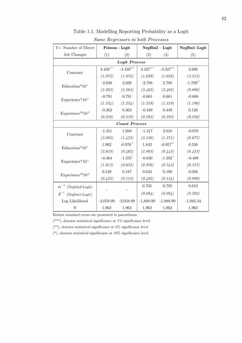
42

Table 1.1. Modelling Reporting Probability as a Logit

Same Regressors in both Processes

Y= Number of Direct

Job Changes

Poisson - Logit

(1) (2)

NegBin2 – Logit

(3) (4)

NegBin1–Logit

(5)

Logit Process

3.439*** -3.439*** 3.327*** -3.327*** 2.696 Constant

(1.075) (1.075) (1.059) (1.059) (3.515)

-2.938 2.938 -2.798 2.798 -1.709** Education*10-1

(2.263) (2.263) (2.462) (2.462) (0.806)

-0.791 0.791 -0.661 0.661 -0.686 Experience*10-1

(1.254) (1.254) (1.319) (1.319) (1.196)

-0.362 0.362 -0.449 0.449 0.126 Experience2*10-2

(0.538) (0.538) (0.593) (0.593) (0.256)

Count Process

-1.451 1.988 -1.317 2.010 -0.078 Constant

(2.005) (1.455) (2.120) (1.571) (0.677)

1.962 -0.976** 1.842 -0.957** 0.538 Education*10-1

(2.610) (0.462) (2.803) (0.445) (0.453)

-0.464 -1.255* -0.630 -1.292* -0.489 Experience*10-1

(1.013) (0.655) (0.976) (0.743) (0.337)

0.549 0.187 0.643 0.196 0.056 Experience2*10-2

(0.455) (0.123) (0.495) (0.134) (0.099)

0.705 0.705 0.610 1α−

(Negbin2-Logit)

1δ−

(Negbin1-Logit) - -

(0.084) (0.084) (0.502)

Log Likelihood -2,058.99 -2,058.99 -1,888.99 -1,888.99 -1,882.34

N 1,962 1,962 1,962 1,962 1,962

Robust standard errors are presented in parentheses.

(***), denotes statistical significance at 1% significance level

(**), denotes statistical significance at 5% significance level

(*), denotes statistical significance at 10% significance level

43

Table 1.2. Modelling Reporting Probability as a Logit

Exclusion Restrictions in Logit Process

Y= Number of Direct

Job Changes

Poisson – Logit

(1) (2)

NegBin2 – Logit

(3) (4)

NegBin1 – Logit

(5)

Logit Process

-3.619 3.619 -3.784 3.784 -0.701*** Education*10-1

(2.261) (2.261) (2.986) (2.986) (0.169)

5.715 -5.715 5.981 -5.981 -0.173 Experience*10-1

(4.458) (4.458) (5.490) (5.490) (0.280)

-3.102 3.102 -3.240 3.240 0.031 Experience2*10-2

(2.483) (2.483) (3.036) (3.036) (0.083)

Count Process

0.823 0.823*** 0.929*** 0.929*** 0.825*** Constant

(0.265) (0.265) (0.313) (0.313) (0.243)

3.291 -0.328* 3.429 -0.354 0.984*** Education*10-1

(2.317) (0.198) (3.049) (0.233) (0.416)

-6.380 -0.665*** -6.704 -0.723 -0.527 Experience*10-1

(4.472) (0.197) (5.503) (0.170) (0.392)

3.172 0.070 3.323 0.082 0.069 Experience2*10-2

(2.501) (0.067) (3.054) (0.056) (0.118)

-0.292 -0.292*** -0.308*** -0.308*** -0.272*** Unionist

(0.094) (0.094) (0.082) (0.082) (0.079)

-0.397*** -0.397*** -0.422*** -0.422*** -0.342*** German

(0.130) (0.130) (0.097) (0.097) (0.104)

0.069 0.069 0.036 0.036 -0.020 Qualified White Collar

(0.196) (0.196) (0.174) (0.174) (0.165)

0.179 0.179 0.184 0.184 0.188 Ordinary White Collar

(0.193) (0.193) (0.229) (0.229) (0.174)

0.133 0.133 0.114 0.114 0.066 Qualified Blue Collar

(0.117) (0.117) (0.112) (0.112) (0.106)

0.735 0.735 0.200 1α−

(Negbin2-Logit)

1δ−

(Negbin1-Logit) - -

(0.066) (0.066) (0.082)

Log Likelihood -2,039.40 -2,039.40 -1,875.95 -1,875.95 -1,869.62

N 1,962 1,962 1,962 1,962 1,962

Robust standard errors are presented in parentheses.

(***), denotes statistical significance at 1% significance level

(**), denotes statistical significance at 5% significance level

(*), denotes statistical significance at 10% significance level

44

Table 1.3. Modelling Reporting Probability as a Logit

Excluding an Insignificant Dummy (“Ordinary White Collar”) from Count Process

Y= Number of Direct

Job Changes

Poisson – Logit

(1) (2)

NegBin2 – Logit

(3) (4)

NegBin1–Logit

(5)

Logit Process

3.420*** -3.415*** 3.313*** -3.271*** 2.638 Constant

(1.048) (1.088) (1.024) (1.031) (3.641)

-2.877 2.951 -2.751 2.729 -1.695*** Education*10-1

(2.316) (2.357) (2.423) (2.485) (0.830)

-0.813 0.722 -0.680 0.602 -0.688 Experience*10-1

(1.257) (1.411) (1.313) (1.443) (1.229)

-0.352 0.388 -0.442 0.466 0.128 Experience2*10-2

(0.547) (0.610) (0.592) (0.880) (0.262)

0.082 0.231 0.094 0.287 0.104 Ordinary White Collar

(0.204) (1.073) (0.194) (0.880) (0.312)

Count Process

-1.395 1.966 -1.273 2.030 -0.067 Constant

(2.047) (1.496) (2.090) (1.658) (0.724)

1.887 -0.973** 1.783 -0.963** 0.539 Education*10-1

(2.683) (0.470) (2.770) (0.456) (0.455)

-0.460 -1.236* -0.628 -1.293 -0.484 Experience*10-1

(0.983) (0.686) (0.953) (0.796) (0.345)

0.543 0.183 0.639 0.192 0.054 Experience2*10-2

(0.456) (0.130) (0.490) (0.143) (0.101)

0.706 0.705 0.601 1α−

(Negbin2-Logit)

1δ−

(Negbin1-Logit) - -

(0.084) (0.084) (0.522)

Log Likelihood -2,058.87 -2,058.90 -1,888.89 -1,888.91 -1,882.29

N 1,962 1,962 1,962 1,962 1,962

Robust standard errors are presented in parentheses.

(***), denotes statistical significance at 1% significance level

(**), denotes statistical significance at 5% significance level

(*), denotes statistical significance at 10% significance level

45

Table 1.4. Modelling Reporting Probability as a Logit

Excluding “Unionist” and “German” from the Count Process

Y= Number of Direct

Job Changes

Poisson – Logit

(1) (2)

NegBin2 – Logit

(3) (4)

NegBin1-Logit

(5)

Logit Process

3.897*** -6.547*** 4.007** -4.269*** 6.317 Constant

(0.756) (2.196) (1.671) (0.798) (4.850)

-2.234 2.681*** -1.193 -0.879* -1.562** Education*10-1

(1.788) (0.933) (3.577) (0.490) (0.603)

-0.298 1.323 -1.005 -0.209 -1.251 Experience*10-1

(1.337) (1.137) (2.929) (0.480) (1.133)

-0.421 -0.150 -0.221 0.038 0.138 Experience2*10-2

(0.594) (0.257) (0.677) (0.134) (0.252)

-0.461** -0.315*** -0.557 -0.300*** -0.820** Unionist

(0.202) (0.107) (0.350) (0.092) (0.361)

-0.764** -0.351*** -0.955 -0.333*** -2.312 German

(0.375) (0.133) (0.762) (0.117) (3.429)

Count Process

-1.015 6.652*** -0.324 4.901*** -0.328 Constant

(1.413) (2.255) (2.296) (0.701) (0.352)

1.403 -2.404*** 0.542 0.722** 0.448 Education*10-1

(1.839) (0.776) (2.686) (0.433) (0.447)

-0.978 -1.994* -0.870* -0.579 -0.537*** Experience*10-1

(0.800) (1.103) (0.480) (0.422) (0.197)

0.567 0.269 0.475 0.077 0.107* Experience2*10-2

(0.517) (0.229) (0.338) (0.122) (0.064)

0.754 0.004 0.888 1α−

(Negbin2-Logit)

1δ−

(Negbin1-Logit) - -

(0.090) (0.000) (0.263)

Log Likelihood -2,027.18 -2,045.04 -1,868.97 -1,870.95 -1,864.02

N 1,962 1,962 1,962 1,962 1,962

Robust standard errors are presented in parentheses.

(***), denotes statistical significance at 1% significance level

(**), denotes statistical significance at 5% significance level

(*), denotes statistical significance at 10% significance level

46

Table 1.5. Modelling Reporting Probability as a Probit

Same Regressors in both Processes

Y= Number of Direct

Job Changes

Poisson - Probit

(1) (2)

NegBin2 – Probit

(3) (4)

NegBin1-Probit

(5)

Probit Process

-2.134*** -2.403 -2.059*** -1.353 0.544 Constant

(0.660) (3.717) (0.617) (1.610) (9.165)

1.820 -0.590 1.707 -0.398 -0.733 Education*10-1

(1.540) (0.469) (1.574) (0.380) (1.877)

0.513 -0.978 0.440 -1.354 -0.229 Experience*10-1

(0.823) (0.748) (0.873) (1.208) (1.333)

0.226 0.020 0.276 0.018 0.046 Experience2*10-2

(0.337) (0.053) (0.356) (0.035) (0.237)

Count Process

1.992** 4.378 2.039 2.200 0.496 Constant

(0.660) (9.693) (1.681) (2.722) (6.266)

-0.977* 2.228 -0.962** 1.053 0.537 Education*10-1

(1.540) (3.996) (0.443) (1.643) (0.733)

-1.279 2.684 -1.328 2.355 -0.536 Experience*10-1

(0.823) (1.863) (0.863) (0.592) (0.550)

0.194 0.394 0.202 0.811 0.059 Experience2*10-2

(0.337) (0.832) (0.157) (1.527) (0.116)

0.705 0.703 0.360 1α−

(Negbin2-Probit)

1δ−

(Negbin1-Probit) - -

(0.084) (0.084) (2.379)

Log Likelihood -2,058.88 -2,060.21 -1,888.91 -1,889.61 -1,882.69

N 1,962 1,962 1,962 1,962 1,962

Robust standard errors are presented in parentheses.

(***), denotes statistical significance at 1% significance level

(**), denotes statistical significance at 5% significance level

(*), denotes statistical significance at 10% significance level

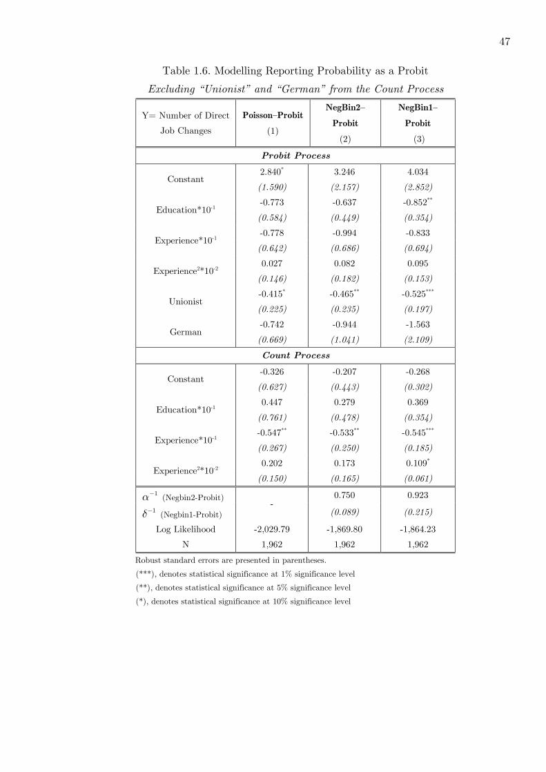
47

Table 1.6. Modelling Reporting Probability as a Probit

Excluding “Unionist” and “German” from the Count Process

Y= Number of Direct

Job Changes

Poisson–Probit

(1)

NegBin2–

Probit

(2)

NegBin1–

Probit

(3)

Probit Process

2.840* 3.246 4.034 Constant

(1.590) (2.157) (2.852)

-0.773 -0.637 -0.852** Education*10-1

(0.584) (0.449) (0.354)

-0.778 -0.994 -0.833 Experience*10-1

(0.642) (0.686) (0.694)

0.027 0.082 0.095 Experience2*10-2

(0.146) (0.182) (0.153)

-0.415* -0.465** -0.525*** Unionist

(0.225) (0.235) (0.197)

-0.742 -0.944 -1.563 German

(0.669) (1.041) (2.109)

Count Process

-0.326 -0.207 -0.268 Constant

(0.627) (0.443) (0.302)

0.447 0.279 0.369 Education*10-1

(0.761) (0.478) (0.354)

-0.547** -0.533** -0.545*** Experience*10-1

(0.267) (0.250) (0.185)

0.202 0.173 0.109* Experience2*10-2

(0.150) (0.165) (0.061)

0.750 0.923 1α−

(Negbin2-Probit)

1δ−

(Negbin1-Probit) -

(0.089) (0.215)

Log Likelihood -2,029.79 -1,869.80 -1,864.23

N 1,962 1,962 1,962

Robust standard errors are presented in parentheses.

(***), denotes statistical significance at 1% significance level

(**), denotes statistical significance at 5% significance level

(*), denotes statistical significance at 10% significance level

Chapter 2

The Relationship between

Immigration Status and Criminal

Behaviour

2.1 Introduction

Academic debates on the relationship between immigration and crime date back at late 1800s

and early 1990s (see, for example, Hart, 1986, Hourwich, 1912, and Taft, 1933), following

large inflows of European and Canadian citizens into the United States. It seems that the

native born population of countries that sustained heavy migration inflows always developed

hostile feelings against foreigners. This can be attributed to the fact that natives always

feared that immigrants could take away their jobs and deteriorate several problems of the host

countries, including crime. Although the bulk of the media in the host countries supported

and even strengthened this hostile feelings against immigrants, researchers’ community often

concluded the opposite. Many found evidence that immigrants seem to commit fewer crimes

than natives, even though they usually encounter unfavorable circumstances, such as blocked

opportunities, or acculturation problems (Tonry, 1997, Hagan and Palloni, 1998, and Mears,

2001).

The present study attempts to investigate the relationship between immigration and

48

49

crime in England and Wales.1 In spite of the fact that the immigration-crime link is such

a controversial subject, it is generally overlooked by the research community compared to

other aspects of crime. To my knowledge, apart from the very recent study by Bell, Machin

and Fasani (2010), there is not any other study that investigates whether such a relationship

exists in the UK.2

As figure 2.1 demonstrates, England and Wales have recently experienced a steady in-

crease in immigration stock relative to the total population. It is notable that, as explained

by Hatton and Tani (2005), immigration net flows were responsible for about one half of the

population growth during the 90’s. Moreover, Hatton (2005) explains that after reaching

the minimum between 1993 and 1995, immigrant net flows increased until 2000, reaching the

figure of 100,000 individuals per year. After 2000, the proportion of immigrants increased

even more, because of the large inflow of around 560,000 Eastern European workers between

2004 and 2006.3

Following this increase in foreign population, immigration in the UK became a very

controversial subject, and one of the “hottest” topics in political agenda. During the last

two decades natives have developed negative beliefs against their immigrant counterparts,

with regard to labour market outcomes, cultural issues, and crime. This hostile tendency

is quite clear if we look at the UK sample of two very important attitudes surveys, the

European Social Survey (ESS) of 2002, and the International Social Survey Programmes

(ISSP) of 1995 and 2003, where questions related to immigration and crime were included.

According to the ESS (see, Table 2.1) there is a clear tendency towards the perception

that immigrants have worsened UK’s crime rates. Even more interesting findings come from

the ISSPs (Table 2.2). Although in ISSP of 1995 only 26% of the respondents believe that

immigrants increase crime rates (agree and strongly agree), this figure increases to around

40% in 2003. These findings coincide with the increase in population of immigrants. It is

1Scotland and Northern Ireland are excluded from the survey used to investigate this research questionbecause of their separate criminal and justice system, which generates incomparable crime statistics.

2However, there is a crucial difference between the present study and the study of Bell, Machin andFasani (2010); that is, the present study looks at this relationship from a micro perspective, examiningwhether immigrants are more prone to criminal activities than natives, whereas their study focuses on theeffect of two waves of large inflows of immigrants on crime rates.

3This evidence comes from the Worker Registration Scheme and National Insurance Number applications(see, Gilpin at al, 2006, Blanchflower at al, 2007, and Lemos and Portes, 2008).

50

quite interesting that natives developed negative beliefs about immigrants despite the fact

that crime rates (at least for total crime) started falling after 1995 (see, figure 2.1 and 2.2.

Also see, Smith, 2006, and Kershaw and al, 2008, p.2). To reinforce these findings, the

results of an ordered Probit regression model are presented in Table 2.3, where a simple

dummy for year 2003 aims to capture the evolution in natives’ attitudes, once we have

pooled the data from ISSP 1995 and ISSP 2003. This is done because we recognize that the

sample in 1995 might differ in many aspects from the sample in 2003. It is clear that even

after controlling for some basic characteristics correlated with respondents’ attitudes, such

as education, party affiliation, income, gender, and age, moving from 1995 to 2003 strongly

increased the sentiment that immigrants increase crime rates.1

But which are the theoretical reasons that link immigration with crime? There are two

distinct effects of immigration on crime. The first one, that I call the “aggregate” effect or

macro effect, states that immigration inflows are related to economy’s crime rates as they: 1)

can affect aggregate outcomes of the domestic economy, such as wages and unemployment,

and 2) may impose cultural conflicts and social disorganization according to criminological

theories (see, for example, Martinez and Lee, 2000). The second one, which I call the

“individual” or micro effect, is the direct effect. This states that immigrants are more or

less crime-prone than natives for reasons that are described in detail in the next section.

This paper attempts to shed light on the direct relationship by investigating the question:

Are immigrants more or less involved in criminal activities than natives and why? It should

be also stressed that this work focuses on property crime, which can be better explained

by economic theory, as opposed to violent crime, which is better explained by psychological

factors rather than material needs. Therefore, psychological theories developed basically by

criminologists, rather than economic theory, would stand better to explain violent crime.2

In the next section a simple economic model of crime is presented to investigate the direct

1The base group for the variable “party” is “left-wing”. For “education” the base group is “high educa-tion”. The marginal effects on the “year 2003” dummy, which are not presented here but are available fromthe author upon request, show that the probability of responding with “agree that immigrants increasedcrime rates” increased by 7.3 percentage points from 1995 to 2003, and the probability of responding with“strongly agree. . . ” by 5.9 percentage points. These differences, calculated using the ‘nlcom’ command inStatar, are statistically significant at 1% significance level. Note that the standard errors are calculatedusing the delta method.

2However, as the explanatory variables used to the empirical analysis may also determine the decisionto commit violent crimes, the results of a violent crime model are presented in subsections 2.8.2-2.8.4

51

immigration-crime relationship.

For the purposes of the empirical analysis individual level crime data are needed. A

first choice would be to use recorded by police crime and compare the crime records of

immigrants to those of natives. However, data on recorded crime in England and Wales

are very poor in terms of information provided, and therefore, are inappropriate for an

individual empirical investigation. Most importantly, these data provide no information on

the immigration status of criminals. In Section 2.4, other shortcomings of this kind of data

are explained. In another direction, self-reports on crime can be used, a practice that is

very common among criminologists and sociologists (see, Junger-Tas and Marchall, 1999).

Therefore, in the present study the Offending, Crime and Justice Survey (OCJS) of 2003 is

used, a nationally representative survey that asks people in England and Wales about their

experiences and attitudes towards criminal activities (Hamlyn at al, 2003).1 Not only does

this kind of surveys reveal to some extent unreported/unrecorded to the police crime, but

it also provides a rich set of respondents’ attributes which enables the investigation of the

determinants of criminal behaviour.

Of course, to identify these relationships it is required that respondents truthfully reveal

their criminal activity. Nevertheless, reliability of self-reports on crime is a major concern as

many individuals may be reluctant to provide sincere answers to questions related to such

sensitive activities. Therefore, under-reporting is a major concern, although nowadays many

techniques are used to improve the reliability and validity of these data (Thornberry and

Krohn, 2000). From the econometric point of view, estimators that ignore under-reporting

are inconsistent (see, for example, Hausman, Abrevaya and Scott-Morton, 1998, for binary

outcome models, and Winkelmann and Zimmermann, 1993, for count data models). There-

fore, it is highly possible that they provide misleading estimates for the coefficients of inter-

ests. This problem becomes even more salient if differences in respondents’ characteristics

are associated with different reporting behaviour (so that under-reporting is not random),

and more importantly, if immigrants’ reporting behaviour differs from natives’ one. Never-

theless, more appropriate econometric models incorporating this problem can be developed

1The OCJS data used in this Chapter are sponsored by the Home Office and provided by the UK DataArchive.

52

and applied. Given that these models are correctly specified, they consistently estimate the

determinants of true crime by using only data of self-reported crime. Section 2.5 presents in

detail the issue of econometric modeling.

Initially, we treat immigrants as a homogeneous group of people. However, this may not

be proper for plenty of reasons. For example, immigrants of different ethnic backgrounds

might be very different from each other. Furthermore, location of immigrants is not ran-

domly assigned, but it is a rather complicated process that depends on many factors. For

example, if immigrants try to match their abilities with the opportunities that each area pro-

vides, more crime-prone immigrants would decide to reside in areas that offer more criminal

opportunities. Or, as the location of immigrants also depends on central decisions, it might

be that different kind of immigrants are located in areas characterized by different socioe-

conomic features. For example, following the 1999 Immigration and Asylum Act, asylum

seekers were located by the National Asylum Support Service in specific areas, London being

excluded (see, Bell, Machin and Fasani, 2010). Given the facts above, the estimated effect

of immigrant status on criminal behaviour might be misleading and therefore, the effect of

immigration on crime is also investigated once we decompose immigrants by ethic group and

location.

The remainder of this paper is organized as follows. Section 2.2 puts the individual

decision to commit property crimes in a simple economic framework of individual supply of

crime. Utilizing this simple economic model, it also investigates the individual relationship

between immigration and property crime. In Section 2.3 a very brief review of studies on this

topic is presented. In Section 2.4 some methodological issues of self-reports are discussed.

Section 2.5 offers a presentation of the econometric models that are more appropriate in the

presence of under-reporting. Section 2.6 discusses the data and the variables and offers some

basic descriptive statistics. The main results follow in Section 2.7. In Section 2.8 robustness

of these results is checked. Section 2.9 investigates whether the immigrant-native property

crime differentials depend on ethnic status or the regions they reside. Finally, discussion of

the empirical results follows in Section 2.10, and Section 2.11 concludes.

53

2.2 An Economic Model of Property Crime

As discussed in the introduction, this study investigates whether immigrants are different

from natives with regard to their behaviour towards criminal activities, and particularly

towards property crime. Therefore, in this section the individual relationship between im-

migration and property crime is examined. We start with a general examination of a simple

model of property crime. In the next subsection we examine how immigration status is as-

sociated with this model, and consequently what this model predicts about criminal activity

of immigrants compared to natives.

Generally, the economic theory of crime is based on the idea of the rational individual

who chooses how to allocate his/her time between legitimate and illegitimate activities so

as to maximize his/her personal expected utility. As there is a probability of apprehension,

the final outcome of the criminal act is uncertain.

Becker (1968) has offered the first prominent paper to incorporate economic theory on

the analysis of criminal behaviour. However, in this early work illegal and legal activities

were considered as mutually exclusive. A few years later, Ehrlich (1973), in a cornerstone

work, relaxed this assumption so as individuals are utility maximizers who allocate their time

between crime and work. In another vital work, Block and Heineke (1975) criticize the two

previous works on the grounds that they treat crime and punishment outcomes as if they can

be always represented by their pecuniary equivalents. Using a more general, multiattributed

utility function, they show that the results of Becker’s and Ehrlich’s works hold only under

very special conditions, and that determining the supply of property crime is a harder task

that needs further assumptions.1 From then on, many other economic theoretical models

have been developed2 and tested using micro or macro data.3 It needs to be stressed that

in general, property crime fits better in the economic models of crime, since violent crimes

can be considered as non market activities that are primarily motivated by hate or passion

1The utility function is given as consisting of three attributes, U(L, T,W ), (where L and T are, time spenton legal and illegal activities respectively, and W represents wealth), rather than a wealth only function.

2Cameron (1988) and Eide (1999) are good surveys on this topic. Freeman (1999) is also an excellentsurvey that discusses many aspects surrounding the economic theory of crime from both a theoretical andan empirical perspective.

3See, for example, Sjoquist (1973), Woplin (1978), Witte (1980), Myers (1983), Reilly and Witt (1996),Cornwell and Trumbull (1994), and Kelly (2000), to mention only a few.

54

(Ehrlich, 1973).1

Economic models of crime have been extended beyond the classical theory of crime de-

terrence, particularizing in examining relationships such as investment in human capital and

crime (Lochner, 2004, Lochner and Moretti, 2004), inequality and crime (Chiu, Madden,

1998), the effect of economic incentives on crime (Machin and Meghir, 2004), crime and

unemployment (Burdett, Lagos and Wright, 2003), crime and social interactions (Glaeser,

Sacerdote and Scheinkman, 1996), etc. Nevertheless, there is no theoretical framework that

investigates the relationship between immigration and crime. For this reason, the follow-

ing subsection presents a simple model that incorporates immigration with the purpose of

demonstrating why immigrants might exhibit different criminal behaviour than natives.

To make it as simple as possible, the following model is a one period model under un-

certainty that borrows features from Ehrlich (1973), and Lochner and Moretti, (2001). This

model is by no means a complete investigation of criminal behaviour, but it illustrates quite

well why someone would expect differences in participation rates of illegitimate activities

between immigrants and natives.

Consider a rational individual who, after receiving the initial endowment z, optimally

decides how to allocate his/her total time available, τ , between criminal activity, τi, and

work, τ`. We assume that leisure time, where the individual consumes all his/her outcomes,

is constant and therefore does not affect the results of the model.2 Although in general z can

represent other individual characteristics such as, age, gender, parental features, respondent’s

location features, etc., in this model z is an indicator variable that determines immigration

status. In turn, z is assumed to affect most of the parameters of this model.

Uncertainty is incorporated in the model because of two reasons. First, there is a prob-

ability of apprehension, π(τi, z), in case the individual is involved in criminal activities.

Second, legal outcomes are also not certain because there is a probability of unemployment,

µ(z), which is assumed to be given exogenously at the beginning of the period.

If the individual is employed in the legal sector, he/she receives wage w(τ`, z). This legal

1However, as will be clear later, some factors determining property crimes, such as probability of appre-hension, severity of punishment and risk aversion, are directly associated with violent crime as well.

2Without loss of generality, τ can be considered as the time available for allocation between the legaland illegal activities after extracting leisure time from total available time.

55

wage depends positively on τ`, such that dw(τ`, z)/dτ` > 0, and d2w(τ`, z)/dτ2` < 0. The

latter can be assumed to be negative as productivity and efficiency may decrease as more

time is spent on work. On the other hand, if unemployed he/she receives an unemployment

benefit D(τ`), which is the same for immigrants and natives, but depends linearly on τ`, so

that dD(τ`)/dτ` > 0 and dD2(τ`)/dτ2` = 0. Thus, this benefit is acquired only as long as the

individual spends time on legal sector, such as time on looking for a new job (which time

must be then reported) and increases with τ`. Also it is assumed that w(τ`, z) > D(τ`) and

dw(τ`, z)/dτ` > dD(τ`)/dτ` , where w is the minimum wage rate.1

Apart from legal opportunities, the individual also faces illegal opportunities, given by

k(τi, z), which consists of financial and psychological (mental) outcomes measured in their

pecuniary equivalent.2 Apart from financial and psychological gains, k(τi, z) also includes

some costs (measured in their pecuniary value) associated with a crime, such as bad reputa-

tion, compunction, regrets, uneasiness, etc. The costs of trial, conviction and punishment,

are not included in these costs but, as will be shown shortly, they will be introduced as

distinct components of the utility function. Similarly to the legal wage, “criminal wage” also

depends continuously on τi, with dk(τi, z)/dτi > 0, and d2k(τi, z)/dτ2i < 0. Thus, when the

individual enters the market he/she considers a continuous set of illegal opportunities. We

assume that illegal opportunities that pay high pecuniary returns require considerable time

in the illegal sector and that they also involve higher psychological costs.3

There are two states of nature, the good State A, where someone is employed with

probability 1 − µ(z), and the bad State B, where someone is unemployed with probability

µ(z). The corresponding returns from legal and illegal actions in the good and the bad states

1Otherwise, there could exist cases where it would be optimal for the individual to remain unemployed,so that the probability of being unemployed would be endogenous, and the model would have been morecomplicated.

2By pecuniary equivalent we mean the amount of money that someone is willing to pay in order to getthis gain or to avoid a cost.

3Therefore, regardless of psychological costs, someone who pursuits high returns to illegal actions caneither commit many crimes, or one high value crime which requires much time spent in the illegal sec-tor though. This can be the case, as this type of property crimes requires much time for organization,preparation, etc.

56

respectively are the following,

ya = w(τ`, z) + k(τi, z),

yb = D(τ`) + k(τi, z),

(2.1)

where ya is associated with State A, and yb with State B. Therefore, the expected utility

once consuming ya, yb, (without considering potential punishment) is given by,

(1− µ(z))u(ya) + µ(z)u(yb) (2.2)

with u′(y) = ∂u(y)/∂y > 0, and u′′(y) = ∂2u(y)/∂y2 < 0, where = (a, b).

Moreover, crime is a risky action. Thus, if someone is involved in criminal activities

he/she faces a probability of arrest, π(τi, z), as described before. We assume that this

probability increases with time spent on illegal sector, so that dπ(τi, z)/dτi > 0, but the

sing of the second derivative is uncertain.1 Here we assume that if arrested, conviction, and

thus, punishment is certain. Nothing is lost from this simplification since it can be shown

that it does not affect the implications of the model. Conviction occurs at the end of the

period, where the individual receives a punishment P (τi, z), pecuniary or not pecuniary such

as imprisonment, with dP (τi, z)/dτi > 0 and dP (τi, z)/dτi > 0.2 According to the above, the

present value of the expected future punishment is given by,

Π(τi, z) = ρ(z)π(τi, z)P (τi, z) (2.3)

where ρ(z) discounts punishment since it occurs at the end of the period. For simplic-

ity, expected punishment is measured in utility terms as in Lochner and Moretti, (2001).3

1It could be negative, since self-protection improves as people spend more time in criminal activities.On the other hand, it could be positive as well, as more time in the illegal sector allows the law enforcementto acquire more evidence against the criminal, which increases the probability of apprehension

2Any kind of punishment, as in the cases on Becker (1968) and Ehrlich (1973), is measured in its monetaryequivalent. Here it is assumed that the more serious the crime the stricter the punishment becomes.

3That this future potential punishment is measured in utility terms has as implication that punishmentis separable from (2.2). Otherwise, this future punishment should have been incorporated in the utilityfunction in the same manner as in (2.2). In that case, there should have been four mutually exclusivestates, for employed and not arrested, unemployed and not arrested, employed and arrested, and unem-ployed and arrested, as described in Ehrlich (1973). This would result in four mutually exclusive utilityoutcomes, each associated with the probability of the state of nature to be observed and the total expectedutility would have been, U(τi) = (1− π(τi)) (1 − µ)u (w(τ`) + k(τi)) + (1− π(τi))µ · u (k(τi)) + π(τi)(1 −

57

Henceforth, z is omitted from the equations for brevity.

Given all the above, the total expected utility received by both legal and illegal activity

from both states is the following,

U(τi, τ`) = (1− µ)u (ya) + µu (yb)− ρ π(τi)P (τi). (2.4)

Thus, the problem of the individual is to allocate his/her available time between legal and

illegal activities in order to maximize (2.4) subject to the time constraints,

τ = τi + τ`, and, τi ≥ 0, τ` ≥ 0. (2.5)

Substituting τ` = τ − τi, and (2.1) into (2.4), the problem simplifies into an optimization

problem with one variable. The Kunh-Tucker first order condition for τi is given by,

dU (τi)

dτiτi = 0,

dU (τi)

dτi≤ 0, τi ≥ 0. (2.6)

The interior solution of spending some time in illegal activities is dU(τi)/dτi = 0,

⇒(

(1− µ)u′(ya) + µu′(yb)

)dk

dτi−(

(1− µ)u′(ya)dw

dτ`+ µu′(yb)

dD

dτ`

)= ρ

(dπ

dτiP (τi) +

dP (τi)

dτiπ(τi)

), (2.7)

so that the marginal utility from criminal activities minus the marginal utility from legal

activities must be equal to the marginal punishment.1 The sufficient condition for a strict

µ)u (w(τ`) + k(τi)− ρP (τi)) + π(τi)µ · u (k(τi)− ρP (τi)) rather than the simpler function (2.4).1The LFS of the FOC could also be written as, (1− µ)u′(ya)

(dkdτi− dw

dτ`

)+ µ u′(yb)

(dkdτi− dD

dτ`

), so that

the marginal utility from the good and the bad state must be equal to the marginal punishment. Here,dw(τ`)/dτ` and dD(τ`)/dτ` can be considered as the opportunity costs of crime of not spending the extratime dτi on the legal sector.

58

global maximum is given by,

∆ = (1− µ)

[u′′(ya)

(dk

dτi− dw

dτ`

)2

+ u′(ya)

(d2k

dτ 2i+d2w

dτ 2`

)]

+ µ

[u′′(yb)

(dk

dτi− dD

dτ`

)2

+ u′(yb)d2k

dτ 2i

]− ρ

(d2π

dτ 2iP + 2

dπ

dτi

dP

dτi+ π

d2P

dτ 2i

)< 0. (2.8)

Since the term on the right hand side of (2.7) is weakly positive, and given that (2.8)

holds, it is required that the marginal utility from criminal activities is at least as high as the

marginal utility from the legal sector. This is because crime is a risky action that involves

losses in the case of a potential future punishment. Thus, the term on the right hand side

can be considered as the extra marginal compensation required for crimes to be committed.

Note also that if dkdτi

< dwdτ`

, so that the marginal return from crime is lower than the marginal

legal return, it is highly unlikely that (2.7) holds. However, it could still hold in cases where

the unemployment rate is very high, the unemployment benefits are very small, and the

marginal legal return is only a bit larger than the marginal illegal return.

As the criminal wage rate is in general quite small in comparison to the legal wage

rate for most property crimes, and if we consider that for most people the criminal wage

further decreases by the psychological costs associated with a crime, the corner solution

where someone allocates all his/her time in legal actions is highly possible.1 Moreover,

property crimes that pay a quite high financial return are also very rare, as according to

our assumptions, crimes that pay high returns require plenty of time which in turn increases

the risk of apprehension and the severity of punishment.2 Also, crimes that pay a high

return involve much higher psychological costs than psychological gains for most people, so

that k(τi) is not large enough. Finally, we must also consider that many individuals do not

exhibit strong criminal ability which might decrease k(τi) (if less able criminals target in

criminal activities that pay low returns) or increase π(τi). All the above are possible reasons

to explain why crime is such a rare event.3 On the other hand, the individual will specialise

1For most people, property crimes would include more psychological costs because of regret, bad repu-tation, etc, rather than psychological gains because of possible satisfaction.

2Think for example bank robberies, or car thefts. Although the crimes itself may not need so much time,we can assume that they need a lot of preparation, which is also measured in τ i.

3In my sample, the proportion of people who have have admitted committing at least one property crimeduring last year is just 5%.

59

in the illegal sector (τ` = 0), if and only if, the marginal legal utility plus the marginal cost of

punishment is smaller than the marginal utility from illegitimate activities, which is highly

unlikely for most people.

A main point of (2.7) is that, starting from an equilibrium where the individual spends

some time on the illegal sector, the better the opportunities in legal sector, expressed as

higher dw(τ`)/dτ`, the higher the opportunity cost of crime is. Therefore, holding everything

else constant, the participation in illegal activities will decrease. The same is true if there

is an exogenous increase in D(τ`). This change will increase the marginal legal utility, and

therefore it is less likely that (2.7) is satisfied. The opposite holds for the marginal return

to crime. As it becomes higher compared to the marginal return to legal activities, the

individual is better off if he/she allocates more time to criminal activities than before.

Another important result is that, starting from an interior solution for crime, the effect of

an increase in unemployment rate is positive, as somebody would expect. The comparative

static analysis shows that dτ ∗i /dµ = −(u′(yb)(

dkdτi− dD

dτ`)− u′(ya)( dkdτi −

dwdτ`

))/∆, which is

positive iff,

u′(yb)

(dk

dτi− dD

dτ`

)− u′(ya)

(dk

dτi− dw

dτ`

)> 0. (2.9)

Now, as dDdτ`

< dwdτ`

, we know that ( dkdτi− dD

dτ`) > ( dk

dτi− dw

dτ`). But, moreover, as w(τ`) > D(τ`)

we have that ya > yb, and since the individual is risk averse (u′′(y) < 0), which implies that

u(.) is strictly concave, we know that u′(yb) > u′(ya). Thus, the first term of the LHS of

(2.9) is always higher than the second term and (2.9) always holds.

The effect of all the components of the potential punishment is also the expected one.

For example, following an exogenous increase in the probability of punishment, the marginal

return to criminal activities must also go up to compensate this increase in potential pun-

ishment. Otherwise the individual would decrease τi. The same will be the effect if there is

an exogenous increase in the severity of punishment.1

1Note that in my model, the deterrent effect of a 1 percent increase in π is equal to the deterrent effectof a 1 percent increase in P . This is because of the simplification that punishment is measured in utilityterms, which means that all individuals are risk neutral with respect to punishment, although they are riskaverse with respect to legal or illegal wages. If the punishment was incorporated in the utility functions ofa risk averse individual, as described in note 3 of page 52, it can be shown, as in Ehrlich (1973), that an 1percent increase in P has a larger effect than an 1 percent increase in π.

60

Finally, risk attitudes, which can be expressed through the discount factor or the cur-

vature of the utility curves, are quite important. As someone becomes less risk averse or

more impatient, he/she discounts future potential punishment more heavily (lower ρ). In

this way, the marginal return from crime must be higher for a more risk averse or a more

patient individual, since he/she puts much weight on the consequences of a possible future

apprehension. Moreover, as y goes up, u′(.) decreases by more for a more risk averse indi-

vidual (as his/her utility function is more “curvy”), which consequently decreases the left

hand side of (2.7), resulting in a higher extra compensation required for the more risk averse

person to participate in the illegal sector.

2.2.1 Immigration and Crime

What could this simple model tell us about immigrants’ behaviour towards crime? Since

z determines whether someone is an immigrant or a native, immigration status affects the

first order condition (2.7) through many channels. Although immigrants do not form a

homogeneous group of people, as individuals of very different ethnic backgrounds are included

in this group, they exhibit some common features that distinguish them from natives. As is

explained below, some of these features are positively related to crime and some negatively,

so that link between being an immigrant and criminal behaviour is not obvious.

First of all, since immigrants generally face lower legal opportunities, meaning that they

have on average lower dw(τ`)/dτ`, or higher µ (see, for example, Algan at al, 2010), we would

expect a positive link. For instance, they hold lower quality jobs and a lower chance of

getting accepted in higher status jobs. This might be for instance because of discrimination,

limitations in human capital or in language proficiency, etc. According to this, they may find

opportunities in illegal sectors more attractive. Regarding criminal opportunities, it is not

clear whether immigrants face a higher or a lower dk(τi)/dτi. It is therefore not appropriate

to associate immigration with crime using the return to criminal activities.

On the other hand, there are a few reasons which would indicate a negative associa-

tion between being an immigrant and criminal behaviour. Some evidence by criminologist

shows that the criminal justice system and law enforcement are biased in various stages

against ethnic minorities (see, for example, Smith, 1997, Feilzer and Hood, 2004). This

61

implies that immigrants may face more severe punishments compared to natives. Moreover,

highly deprived areas are generally associated with both higher concentration of immigrant

population and higher concentration of police force. This increases the risk of apprehension.

Finally, immigrants also face deportation which is a punishment specific to them. This could

be considered as a large disincentive to commit crimes (Butcher and Piehl, 2007). Thus,

according to the above, we would expect that the average immigrant faces both higher π(τi)

and P (τi).

In another direction, discount factors and risk attitudes may also be different for immi-

grants. It could be said that immigrants are willing to take more risks, since migration is in

general a risky action with quite uncertain outcomes (see, for example, Jaeger at al, 2010).

On the other hand, there is empirical evidence that immigrants are more risk averse than

the native population (see, for example, Bonin at al, 2009). A considerable number of im-

migrants leave their families back at their countries of origin. Even though they have taken

the risk to migrate away from their countries, they target on a better life for them and their

families. In addition, they would like to feel socially equal to natives by presenting a highly

responsible and credible behaviour. They may not be willing to take highly risky actions

which can cost them their presence in the host country. In addition, a large proportion of

immigrants come from poor countries. Since they have already faced quite harsh conditions,

it could be assumed that they are more resilient not only in financial difficulties but also in

psychological and physical severities.

Furthermore, discount factors and risk behaviour are strongly associated with cultural

factors. Therefore, coming from different cultures, risk attitudes and discount factors may

have been shaped quite differently. Cultural differences are also important for the percep-

tions towards the moral dimension of crime. Thus, psychological costs, also incorporated in

dk(τi)/dτi, may be very different between immigrants and natives.

Finally note that, the model does not explicitly include variables for demographic fac-

tors such as age, gender, or location features, that are found to be associated with crime.

Therefore, there could be also some indirect effects of immigration on crime if immigrants

are different from natives with respect to these demographic features.1 Thus, taking all the

1All the discussion above concerns the individual supply of property crime that economic theory predicts.

62

above discussion into consideration, the individual relationship between immigration and

property crime cannot be determined by this theory, and can only be established by an

empirical analysis, using a well specified model and appropriate data.

2.3 Immigration and Crime. A Review of Research

Although other indicators of crime, such as education, inequality, labour opportunities, etc.,

have been well studied by economists, the empirical research of the immigration-crime nexus

is limited. However, the literature by criminology and sociology scholars is much more

extended, both theoretically and empirically. Traditionally, these studies are developed in

countries which have experienced large inflows of migrants. For instance, the US with the

inflow of Latino and Afro-Caribbean population, Germany with immigrants from Turkey

and the former Yugoslavia, Netherlands with Turkish and Moroccans, etc.

The results of various researchers are often contradictory. This is natural, mainly be-

cause the empirical results by each researcher are subject to the composition of immigrant

population in each destination country, the circumstances that immigrants encounter in dif-

ferent countries, the differences in the data sets they use, and last but not least, the different

statistical tools and strategies each researcher follows. Thus, we cannot identify globally

what is the effect of immigration on crime by looking only at one country, or one approach,

but we need to look at the broader picture.

The literature review is presented in two subsections. In the first one the results found

by economists are presented, whereas the second one briefly presents the results found by

sociologists and criminologists. A basic difference between studies by criminologists and

sociologists and studies by economists is the theoretical hypothesis. The first group bases

its theory on disorganization and culture conflicts whereas economists associate immigrants

In another direction, long before economists, criminologists developed some ideas on the immigration-crimenexus. Starting with eccentric ideas that immigrants commit more crimes just because they are a group ofinferior individuals (see, Armstrong, 1935, and, Sellin, 1938), they switched to more rational theories basedon psychological patterns. One of the earliest theories is based on the so-called “strain” theory, presented byMerton (1938), which states that immigrants present adverse behaviour due to accumulative pressure, as forexample, because of discrimination, racism and unequal social and financial opportunities. Other theoriessuggest that there might be deviant behaviour by both immigrants and natives because of cultural conflicts.Thus, contrary to economic theory, criminologist’s theories stand better for violent crime. For an excellentsurvey on these theories the reader may refer to Martinez and Lee (2000).

63

with crime through the economic models of crime. The second main difference stems from

the fact that economists traditionally use more analytical statistical and mathematical tools

than the other group. Thus, in general the studies by economists use more sophisticated

and in many cases, more appropriate statistical models.1

Before presenting details of the empirical findings, in a nutshell, the available literature

seemingly agrees on the following: both macro and micro-analysis in the US indicates that

there is a negative association between immigration and crime. Regarding Europe, crimi-

nologists find that immigrants are over-represented in official records, but less involved in

criminal activities according to crime self-reports. Finally, the empirical work by economists

in Europe suggests either a positive link (mostly for property crime) or no link.

2.3.1 Empirical Evidence by Economists

To begin with, as mentioned in the introduction, to my knowledge there is only one study

concerning the UK. Bell, Machin and Fasani (2010) examine how two separate large waves

of immigrants affected crime rates. These waves are, the late 1990s wave of asylum seekers

and the large inflow from the “A8” Eastern European countries since May 2004. What they

find is that the first wave is associated with higher property crime, even after controlling

for endogenous location using fixed effects and instrumental variables.2 However, they find

that the A8 wave did not affect property crime.3 Moreover, their results indicate that

there is no effect for violent crime. They argue that this finding is consistent with a simple

economic model of crime, as asylum seekers face much lower legal opportunities realtive to

A8 immigrants and natives, and therefore, illegal activities seem more attractive to them.

As far as I know, the first attempt by economists to investigate the immigration-crime

relationship is that of Bucher and Piehl (1998a). Using data from the Uniform Crime Re-

ports and Current Population Surveys, they first look at the aggregate effects of immigration

on crime in the US, during the 80s. Although they find that there is a positive relationship

1This review does not intend to criticize or judge the methods and specifications of different researchers,but instead, it is purely descriptive.

2As asylum seekers where located by the National Asylum Support Service, they were mostly locatedin unpopular areas with a large amount of vacant houses. Thus, they instrument for endogenous locationdecisions by the number of dispersal accommodation in each local area.

3In this case they control for endogenous location by using the availability of flights to A8 countries asan exogenous variation for immigrants choices of location.

64

between crime rates and the fraction of recent (within one year) immigrants, this association

fades out once they include controls both correlated with the location choice of immigrants

and crime rates. Actually, the effect of immigration becomes negative but statistically in-

significant. Using fixed effect analysis, they find that there is no association (negative but

insignificant) between flows of immigrants and crime rates, or flows of immigrants and growth

in crime rates (one year changes). Their results are strengthened by the use of self reports

from the National Longitudinal Survey of Youth of 1980. What they find is that in all cases

immigrants report considerably less crime (statistically significant at 5% in most cases), a

relationship that is more clear once they control for other individual characteristics associ-

ated with crime. Immigrants are also less involved in arrests and convictions. Nevertheless,

they do not use any strategy to control for any possible under-reporting, a major concern in

self-reports.

Bianchi, Buonanno and Pinotti (2007), study the same research question but for Italy,

by using police administrative records for Italian provinces. Using a panel data set from

1990 to 2003, they find a positive relationship between the size of immigrant population

and most categories of crime rates, even after controlling not only for other determinants

correlated with the factors that determine both crime and the location choice of immigrants,

but also for province and year dummies. However, they recognize that even after controlling

for these factors, there can still be some time varying unobserved factors correlated with

both immigration and crime (for example, a economic crisis in a specific area would reduce

the cost of living, which would in turn attract immigration population, but at the same time,

also increase crime rates). Moreover, there is the concern of reverse causality, since crime

rates in an area could affect the location choice of immigrants. Therefore, they employ a

two-stage least square approach, using changes over time of immigrant population in the

rest of Europe as an instrument for changes of immigrant population in Italy. Arguing that

this is not a “weak” instrument, they find that there is no relationship between immigration

and most categories of crime. However, there still exists a positive association for murders,

robberies and thefts.

Finally, in another direction Bucher and Piehl (1998b, 2007), use institutionalization rates

as a proxy for incarceration rates. Using the 5% Public Use Microsamples of the US census

65

in 1980, 1990, and 2000, they find that the probability of an immigrant being incarcerated is

much lower, even after controlling for educational attainment and ethnic status. They also

find that this difference has increased over the last three decades, as more recent immigrants

have the lowest incarceration rates. They attribute this to two reasons. First, they argue

that this improvement is due to the stricter legislation for immigrants, since recent laws

have broadened the crimes for which an immigrant is deported. They find that although

deportation itself does not drive the results (meaning that the share of immigrants is not

lower in prisons just because they get deported), it acts as a deterrent effect specific to

immigration population. Second, they show evidence that the recent migration process to

the US selects individuals who are either less crime-prone, or more responsive to deterrent

effects.

2.3.2 Empirical Evidence by other Scholars

As opposed to economists, criminologists and sociologists have paid more attention to this

relationship. Here, I will try to briefly describe the results of the most important works in

each country.

The majority of immigration-crime studies come from the US and focuses on violent

crime.1 Most of evidence from the US shows that although the public opinion keeps as-

sociating immigrants with crime, immigration is not associated with higher crime, and in

many cases it is associated with lower crime. Hagan and Palloni (1998), perform an empir-

ical analysis using a sample of 34 Standard Metropolitan Statistical Areas of the US. By

regressing logged arrests on the proportion of immigrants in the population, they find no

association between immigration and both property and violent crime. Reid at al. (2005),

combining 2000 US Census data and 2000 Uniform Crime Report (UCR), explore how the

immigrant population affects crime rates across a sample of metropolitan areas. They find

that, after controlling for demographic and economic conditions, immigration does not af-

fect violent and nonviolent crime. Lee, Martinez and Rosefend (2007), examine whether

1A more detailed review can be found in Hagan and Paloni (1998), and Martinez and Lee (2004). Formost recent evidence refer to Stowell (2007). Also, each individual study described in the subsection providessome related literature. For example see, Ousey and Kubrin (2009), Stowell at al (2009), and Wadsworth(2010). Stawell at al (2009), also provide a table that presents important information for the main studiesin the US (Table 1, p.895).

66

immigration increased homicide in the three border cities of Miami, El Paso, and San Diego,

using 3,345 homicide occurrences happened between 1985 and 1995. Poisson regression re-

sults indicate that there is no relationship, or, even a negative relationship between the

percentage of new immigrants and homicide levels. Stowell (2007), in the same direction

examines the crime-immigration nexus for three US cities, Alexandria, Houston and Miami.

Using neighborhood-level data from 2000, he also finds no direct evidence between the pro-

portion of recent (less than ten years) immigrants in the population and violent crime levels.

However, he finds a negative association for Miami.

Even more recently, there was a quite large amount of publications on this subject for

the US.1 Most of those studies also show that if there is an association, this is negative.

Very briefly, Ousey and Kubrin (2009), using fixed effects for 159 US cities (with more than

100,000 residents) for the three time periods 1980, 1990 and 2000, find that the proportion

of recent immigrants decreases violent crime. Wadsworth (2010), in a similar manner, uses

a fixed effect model for 459 cities (with more than 50,000 residents), between 1990 and 2000.

Both robbery and homicide rates are examined. The results of this study suggest that the

proportion of foreign born population and the proportion of new immigrants decreased crime

rates within this time period. Stowell at al (2009) use a panel over the period 1994-2004

for 103 metropolitan areas (with more than 500,000 residents). Their results indicate that

there is a negative association between changes in immigration concentration and changes

in crime rates. This effect is particularly stronger for robberies.

The “Homicide Studies” journal published an issue on 2009 that solely focuses on aspects

between immigration and homicides and other crime types. Graif and Sampson (2009), in a

neighborhood study of Chicago, using a “weighting” estimator that assigns different weights

for points of different proximity to each data point, find that higher concentration of for-

eign born population is either negatively or not associated with homicide. Feldmeyer and

Steffebsmeier (2009), using homicide arrest data from California, find that the proportion of

recent (entered USA between 1990 and 2000) immigrants does not affect the mean number

of overall homicides, but it does affect negatively the mean of homicides against white and

black people. Velez (2010), by allowing the effect of immigration to be different between ad-

1For all studies described in this paragraph, crime data are collected from the Uniform Crime Reports.

67

vantaged and disadvantaged neighborhoods of Chicago (by using an interaction term), finds

that an increase of recent immigrants decreases the number of homicides in disadvantaged

areas but has no effect in the more advantaged ones. In another study for Chicago, Chavez

and Griffiths (2009), argue that growing immigrant population was unrelated to homicide

patterns. Polczynski at al (2009), look at arrest rates for different types of crime in Orange

County, Florida, and show that arrest rates are generally lower for foreign born individuals.

Moreover, their results suggest that concentration of immigration is not associated with the

number of arrests. Finally, the studies of Akins, Rumbaut, and Stansfield (2009), and Stow-

ell and Martinez (2009), focus on the area of Miami. The former suggests that for the area of

Austin, Miami, where the immigration population increased by around 580 percent, there is

no association between migration and homicides. In the latter, they find that neighborhoods

with higher number of Latino immigrants exhibit lower levels of homicide.

In Germany the studies of immigration-crime link are based on official criminal statistics,

since in official records from police or courts there is a categorization of people as foreigners or

not. Using police and court data Albrecht (1987) finds that foreign population’s involvement

in criminal activities is higher than that of Germans. However, this relationship disappears

once controls for socio-economic conditions and demographic differences are accounted for.

The same positive relationship is also found in Albrecht (1997). However, in this second

study the higher involvement of immigrants in crime persists, even after controlling for the

above factors. Finally, Chapin (1997), using basic statistic analysis finds that changes in

foreign population increase the growth of crime levels.

Evidence from official statistics of Switzerland also suggests that immigrants are less

law-abiding. For example, Killias (1997) using police and conviction statistics finds that,

although in the 70s immigrants displayed similar crime rates with natives, after the 80s

immigrants were over-represented in crime statistical tables. However, he expressed many

concerns about the reliability of official crime statistics. Contrary to that, using self-reported

data from more than 3,000 adolescents and employing basic statistics, Vazsonyi and Killias

(2001), find that first generation adolescent immigrants display slightly lower crime rates

than native Swiss adolescents. This result coincides with other works in Switzerland that

have used self-reported crime data. They also find that second-generation immigrants are

68

more crime-prone than natives, a result that it is common in literature.

In Netherlands, Junger-Tas (1997), finds that Moroccans and Antilleans are overrepre-

sented in official criminal statistics. Contrary to that, he also presents a review of self-report

studies in Netherlands which suggest that the above groups, and other groups of ethnic mi-

norities, are less involved in crime. Concerning France, Tournier (1997), finds that although

immigrants are over-represented in prison statistics and statistics of criminal suspects, a

large fraction of their crimes concerns violations of immigration law regulation. Thus, when

he controls for this fact the difference between foreigners’ and natives’ involvement in crime

is considerably lower. In a study for Sweden, Martens (1997), finds that the fraction of

immigrants who have been suspected for crimes is clearly higher than the fraction of native

population. A difference still exists even after immigrant-native differences are accounted

for, although it becomes noticeably smaller. He also finds that first-generation immigrants

display higher crime rates than second-generation immigrants, a result that contradicts with

findings in other countries. Finally, Yeager (1997) presents a cross-country review of immi-

gration and criminality. According to this review, immigrants are not as highly involved in

crime as natives in Canada and Australia. Criminal records form France, Sweden, Nether-

lands and Germany indicate that immigrants are over-represented in various criminal aspects.

He also briefly describes the results of crime self-reports for Switzerland, Netherlands and

Germany, which suggest that immigrants are less involved in crime than natives citizens.

2.4 The OCJS. Some Methodological Issues

The basic target of the present study is to identify whether immigrants are more or less

crime-prone than natives, even after controlling for the fact that immigrants might exhibit

some differences in basic demographic characteristics associated with higher or lower crime.

For this purpose the Offending Crime and Justice Survey (OCJS) of 2003 is used, a nationally

representative survey which asks people in England and Wales about their experiences as

offenders and their attitudes towards criminal activities.1 Although a few earlier offending

1Although three subsequent OCJSs exist (2004, 2005, 2006), they are particularized in adolescent delin-quency (people from 10 to 25 years old). Thus, they are not appropriate for the purposes of my researchquestion.

69

surveys in the UK exist, this is the largest one and the most sophisticated in terms of design

and construction.1 This section discusses some features, advantages and limitations of the

OCJS, and self-report studies in general.

A basic target of the OJCS is to provide an accurate measure of the prevalence of offending

in the general population, as opposed to studies of already convicted criminals, and to

investigate the factors related to committing crimes (Hamlyn, and Hales 2003).2 However,

this is a hard task if we consider a few limitations of the OCJS.

To begin with, validity and reliability of the responses is a concern, since questions try

to elicit information in a very sensitive part of personal activities such as crime. Particu-

larly, a response error is expected that most probably takes the form of under-reporting if

respondents conceal some aspects of true crime activities. However, it is important to stress

that computer-based interviews are used as opposed to face-to-face interviews, a method

that is found to increase the reliability of responses (see, for example, Turner at al, 1998,

and Newman at al, 2002).3 As will be explained in Section 2.5, a conventional regression

model that does not take into acount under-reporting would result in inconsistent estimated

coefficients for the true crime, as it is developed to estimate the coefficients of the observed,

reported crime. More importantly, if for any reasons immigrants under-report by more than

natives, the estimated effect of being an immigrant on crime will be downward biased.

Another concern stems from the fact that some individuals selected by the survey’s

conductors denied participation in the survey. In spite of the fact that response rates of

the OCJS are very close to response rates of other population surveys,4 such as the Labour

Force Survey or the British Crime Survey (BCS) (see, Sharp and Budd, 2005), estimates of

prevalence of crime will be downward biased in case non-respondents commit more crimes

(see, Farrington at al., 1990).5 In addition, if the effect of being an immigrant on criminal

1For a review of other self-report studies the reader can refer to Farrington (2003), Thornberry andKrohn (2000), and Junget-Tas and Marsall (1999).

2For surveys of convicted criminals see, Budd at al. (2005).3Actually, the OCJS aimed to get the highest level of reliability possible by using well trained interviewers,

appropriately designed questionnaires and feasibility studies.4The response rate for the core sample and youth-boost sample is around 74%. For the nonwhite-boost

sample the response rate is around 50% which is common in surveys that include nonwhite boosts. Dependingon the assumptions used to provide the response rate estimates, Hamlyn at al (2003) provide un upper andlower limit on the response rate estimates. For the core and youth-boost sample these are 78.5% and 73%and for nonwhite-boost, 60% and 45% respectively, a figure that matches closely the figures of 2001 census.

5Although the weights used in empirical analysis take into account non-respondents (see, Hamlyn and

70

behaviour is different between respondents and non-respondents, the coefficient measuring

the difference between immigrants and natives propensity to crime will be biased. Moreover,

this survey does not capture individuals currently in institutions who would most probably

commit more crimes than the general population if they were free. The consequences are

similar to the previous point.

Despite these limitations, relying on self-reports constitutes the most suitable method to

identify predictors of criminal behaviour. As Thornberry and Krohn (2000) point out, the

best way to identify factors of criminal behaviour would be to observe the actual behaviour

of potential criminals, self reports being the nearest proxy to actual criminal behaviour. The

OCJS also provides important information on a wide range of characteristics of potential

criminals as opposed to victimization surveys and official statistics. Actually, self-reports

is the most commonly used technique in criminology research to discuss causes of crime

(see, Hagan, 1993, and Junger-Tas and Marshall, 1999). Moreover, it would be misleading

to attempt to identify the determinants of criminal behaviour by comparing convicted and

non-convicted individuals, since there is quite a large number of individuals that have com-

mitted crimes but are not convicted. Similar logic applies to comparisons between arrested

immigrants and natives.

As we saw in the previous section, some criminologists prefer to use data of recorded

crime. There are two main pitfalls in using official recorded crime by the police. First of all,

these statistics are very poor in terms of information provided. Concerning official statistics

in England and Wales, they offer no information concerning immigration status. Therefore,

they are inappropriate for native-immigrant crime comparisons. Furthermore, even if the

same information was available, it is widely accepted that many crimes are not reported

to the police, and many reported crimes are not even recorded because of inside-police

operational reasons (for example, some reported crimes are not considered serious enough

to be recorded). This is the so-called “dark-figure” of crime, for which a vast literature

exists (see, for example, MacDonald, 2001, 2002).1 Moreover, there is some evidence by

Maxwell, 2003, and Budd, Sharp and Mayhew, 2005), they do not control for possible higher crime ofnon-respondents.

1For example, using data from the BCS of 2007/08 we find that around 60% of crimes were not reportedto the police.

71

criminologist that the criminal justice system and law enforcement are biased in various

stages against ethnic minorities, mostly against black individuals (see, for example, Smith,

1997, Feilzer and Hood, 2004). Perhaps, immigrants are also more “visible” to the police

because of over-policing in target areas where ethnic minorities are concentrated, increasing

the likelihood of immigrants to be arrested (Sharp and Budd, 2005). Therefore, official

statistics would overestimate immigrants’ crime if immigrants face a higher probability of

arrest for the same crimes, or, if police officers disproportionately record crimes that are

supposedly committed by immigrants.

On the other hand, although victimization surveys, such as the BCS for England and

Wales, provide the most precise estimates of the actual crime, they do not provide any

information about criminals’ characteristics. However, if we accept that the BCS reveals the

figure of crime that is the closest to the true one, we could compare official and OCJS’ crime

figures to BCS’ one in order to evaluate their precision in measuring crime. Kershaw and

Walker (2008), suggest that recorded crime is only 42% of the total crime in England and

Wales. Concerning the OCJS, Budd, Sharp and Mayhew (2005), suggest that the figure of

violent crime is quite close to that of BCS, but the count of property crime is quite lower

than in BCS. This would suggest that there is under-reporting in property crime. However,

these figures must be treated with caution since there are fundamental design differences

between these two sources, and therefore, they do not provide comparable crime figures (see,

Budd, Sharp and Mayhew, 2005).

2.5 Econometric Models

As will be described in the next section, the dependent variable is observed in count form

(number of crimes committed during the twelve months prior to the interview). Therefore,

count data models (number of crimes) or binary choice models (crime or not) are more

appropriate than simple linear models. Nevertheless, as will be better explained in the next

section, the very large number of zeros in the property crime variable, resulting in very low

variation in the dependent variable, will make estimation of count data models quite harsh,

mainly when estimators to allow for under-reporting are used. Alternatively, a safer choice

72

would be to use the binary information, whether or not someone has committed a crime last

year although these models do not use all available information. Therefore, a compromise

would be to base my empirical results on binary choice models, while count data estimation

models can be used for robustness check analysis.

As explained in detail before, under-reporting is the main concern in this data set.1 Tra-

ditional nonlinear estimators for binary and count data are inconsistent if under-reporting,

or more generally, response error in the outcome variable is present (Hausman, Abrevaya

and Scott-Morton, 1998, Cameron and Trivedi, 1998 (p.313), and Winkelmann, 2008).2 The

problem is even more salient if under-reporting depends on individual characteristics which

is most probably the case with self-reports in crime. On this direction, parametric models

that take into account misreporting (both under and over-reporting for binary choice mod-

els, but only under-reporting in count data models) will be used. Another concern is the

large number of zeros (95%) in the dependent variables. This has obvious consequences for

the precision of the estimates in both binary and count data models. Adding the fact that

estimation of models that account for under-reporting is quite demanding, to achieve precise

estimates quite rich samples are required.

Moreover, as explained in the previous section, there is also a potential sample selection

problem, since it is likely that people who refused participation in the survey are more

prone to crime. However, models that correct for sample selection problems, such as the

Heckit procedure (see, Heckman 1976, 1979), would require information of non respondents,

which is not available. Therefore, this problem is ignored in the analysis, hoping that non

respondents exhibit the same criminal behaviour, or at least that the crime differentials

between immigrant and natives respondents follow the same pattern with crime differentials

between immigrant and native respondents. In the following subsections models that control

for misclassification, or, under-reporting are described.

1Although we could assume that someone would never report a crime if he/she has not committed one,we could not rule out that over-reporting may be present as well. This could be attributed to the fact that theOJCS is a retrospective study and measurement error in both directions could be possible. Although over-reporting is most possible unintentional, so that it is random, under-reporting is most probably intentional.

2Note that, as it is well known, random response error in linear models does not affect consistency. Theonly consequence of the presence of this error is the increase of the error variance which leads to less preciseestimates. However, in our case, estimation of linear models is inappropriate as we deal with count data.Moreover, the error component because of under-reporting is most probably not random but it depends onrespondents’ attributes, which leads to endogeneity.

73

2.5.1 Binary Choice Models

In this section the model of Hausman, Abrevaya and Scott-Morton (1996, 1998) is presented,

a parametric model that takes into account both probabilities of under-reporting (misclas-

sification of a true one as zero) and over-reporting (misclassification of a true zero as one).

Throughout the present study I refer to this model as MisProbit (Misclassification-Probit).

The model comes naturally from a latent variable specification. To simplify things,

assume that in a given period of time, an individual would commit a crime (or a number

of crimes) if the total utility from committing this crime is higher than the utility obtained

from not committing it. So, let u∗i be the (unobserved) utility obtained if committing the

crime(s) minus the utility if not committing it (them). We specify u∗i to depend linearly on

the vector of characteristics xi such that,

u∗i = x′iβ + εi, (2.10)

where εi is a random i.i.d error. Thus, the individual commits at least one crime according

to the following,

y∗i =

1 if u∗i > 0

0 if u∗i ≤ 0(2.11)

where y∗ is a dummy for the true but unobserved crime. Given (2.10) and (2.11), conditional

on xi, the probability of committing a crime is given by,

Pr(y∗i = 1|xi) = Pr(u∗i > 0|xi) = Pr(εi > −x′iβ|xi) = F (x′iβ) (2.12)

where F (x′iβ) is assumed to have a known functional form such as the standard normal, if

εi ∼ N (0, 1).

Let us now define yi to be a dummy for the reported and therefore, observed crime.

Suppose that the reported crime does not coincide with the actual crime since there is mis-

reporting (in this context defined as misclassification). The probabilities of misclassification

74

are defined as follows,

a1 = Pr(yi = 1|y∗i = 0),

a0 = Pr(yi = 0|y∗i = 1),

(2.13)

where a1 is the probability of reporting a crime, conditional on committing no crime (over-

reporting) and a0 is the probability of reporting no crime, conditional on committing crimes

(under-reporting). Notice that according to this specification the misclassification probabil-

ities do not depend on xi but only on y∗i .

It is easy to derive the conditional probabilities of the observed crime, incorporating the

probabilities of misclassification. The response tree in figure 2.3 is a very clear way to do

that. It is clear that these probabilities are given by,

Pr(yi = 1|xi) = (1− F (x′iβ)) a1 + F (x′iβ)(1− a0)

= a1 + (1− a0 − a1)F (x′iβ),

(2.14)

Pr(yi = 0|xi) = (1− F (x′iβ)) (1− a1) + F (x′iβ)a0

= 1− a1 − (1− a0 − a1)F (x′iβ),

(2.15)

and therefore the expected value E(yi|xi) is also given by (2.14). We can estimate, a0,

a1, and, β, using the method of Maximum Likelihood (MLE) once we have specified the

log-likelihood function as,

ln L (β, a0, a1) =n∑i=1

(yi ln [Pr(yi = 1|xi)] + (1− yi) ln [Pr(yi = 0|xi)]

). (2.16)

Given correct specification of the model, meaning that the specified model of constant mis-

classification is the correct model under the true data generating process (DGP), maximiza-

tion of (2.16) using numerical optimizers, such as the Newton-Raphson, yields consistent

estimates for the coefficients of true crime, the probability of under-reporting, and the prob-

75

ability of over-reporting.1

We notice that a0 is only designed to capture total under-reporting as opposed to partial

under-reporting. That is, the probability of under-reporting will ignore the cases where indi-

viduals report just a portion of the total number of crimes they have committed. However,

as will be explained later in this section, models that use the count form of the dependent

variable are able to estimate the probability of any committed crime to be reported, given

that this probability is constant for each individual.

Hausman, Abrevaya and Scott-Morton (1998) show that the model is not globally iden-

tified since for symmetric F (.), a1 + (1− a0− a1)F (x′iβ) = a1 + (1− a0− a1)F (−x′iβ) where

a0 = 1 − a1 and a1 = 1 − a0. Thus, there are two observationally equivalent models with

parameters (a0, a1, β) and (a0, a1,−β). Identification is achieved by imposing the “mono-

tonicity” condition, which states that a0 + a1 < 1. According to this, we are able to rule out

the “wrong” maximum, since a0 + a1 < 1 implies that a0 + a1 > 1. If this condition fails,

the misclassification probabilities are too large, and therefore, the data are most probably

too noisy to obtain reasonable results.

As the assumption of constant misclassification is not realistic in many applications,

including the present study, it can be easily relaxed if we model a0 and a1 to be functions

of covariates, so that, a0 = F (z′iγ), and a1 = F (w′iδ), where F can be the cumulative

distribution of a binary model, such as a Probit or a Logit. Vectors x, z, w can be the same,

disjoint or overlapping. No further assumptions are required to identify this model. There

are some papers in the literature that have utilized this estimator (see, for example, Leece,

2000, Artis at al, 2002, Caudil and Mixon, 2005, and Falaris, 2007). Nevertheless, none of

them allows the probabilities of misclassification to depend on covariates.2

1Hausman, Abrevaya and Scott-Morton (1996) explain why estimating a simple nonlinear binary model,under the presence of misclassification, leads to inconsistency even when misclassification is constant. In-tuitively, the MLE of a simple binary model that ignores misclassification will set the score (FOC) to zero,although if misclassification exists the expected score of the ML is not zero, which leads to inconsistency. So,if constant misclassification is a problem, the likelihood function that must be maximized is (2.16). Noticehowever, that identification of the model comes from the nonlinear specification of the log likelihood function.This has negative consequences on the robustness of this model. For this reason, Hausman, Abrevaya andScott-Morton (1996, 1998) also propose a semi-parametric estimation.

2It is interesting that this estimator is very similar to the Detection Controlled Estimator, presentedin Feinstein (1989). In that paper Feinstein explains that sometimes inspectors fail to detect a violation.However, they never detect a violation if there is not one. Therefore, in the simplest form, when theprobability of detection and the probability of violations are independent, he derives the same log-likelihoodfunction as (2.14), if we set a1 to zero. However, in his estimator, a0 depends on regressors. This concept can

76

Although this is quite an easy model to implement in econometric software, in practice

estimation is quite difficult, particularly when the misclassification probabilities are allowed

to depend on variables, and when the data are quite noisy with very low variation partic-

ularly in the dependent variable. Always, exclusion restrictions could help the estimation

procedure. Moreover, as Hausman, Abrevaya and Scott-Morton at al (1996) stress, it is quite

difficult to get precise estimates and imprecision will increase the higher the misclassification

becomes. They note that this is partly because the corrected for misclassification Informa-

tion Matrix is not block diagonal. Simple binary models ignore this fact and consequently,

underestimate the true standard errors. Thus, it could be said that the MisProbit MLE

corresponds to the true precision, given correct specification of the model. According to

this, in cases where misclassification is very high, as it may be the case for crime self-reports,

quite rich samples are needed in order to obtain precise estimates.

So far, we have regarded zeros coming from two different sources; misclassification of 1 as

0, and zeros from the traditionally binary choice model. Nonetheless, zero-inflation can be

incorporated into this model if we think of zeroes coming from a third source. That is, there

are some individuals who, regardless of the conditioning set xi, never commit any crimes

(and consequently they do not report any). We will call these individuals “genuinely non

criminals”. If we do not incorporate this zero-inflation probability separately, the estimated

probability a0 cannot distinguish under-reporting from zero-inflation.1 This is clear if we

examine figure 2.4, where a0 and a1 are expressed as probabilities of zero-inflation and

one-inflation respectively. Following this tree we notice that the conditional probabilities of

observing 1 and 0 are exactly as in (2.14) and (2.15). However, in this case the interpretation

of a0 and a1 is very different. Although, probability of one-inflation is unrealistic, zero-

inflation is quite possible.2 Nevertheless, it is possible to separate under-reporting from

be naturally applied in any situation that involves compliance and inspection, as for example, tax evasion(Feinstein, 1991).

1This idea of adding in a probability of inflation can be traced back to Gaudry and Dagenais (1979)where they developed an estimator for multinomial choice models, calling this the “dogit” model. Gaudry(1980) and Swait and Ben-Akiva (1987), apply this model for individual choices between a set of differenttransportation modes. They explain that given a set of choices, an individual is either captive to one choiceregardless of his/her characteristics (inflation probability) or free to choose from the full set of choices(traditional multinomial choice model). In this models there is inflation probability for each category,whereas in the model presented here there is only zero-inflation probability, making this model more similarto zero-inflation models for count data as described in Mullahy (1986) and Lambert (1992).

2One-inflation could be interpreted as follows: there are some individuals who, regardless of xi, always

77

zero-inflation by incorporating zero-inflation separately in the likelihood function. This

model is presented in Appendix A.1

2.5.2 Count Data Models

The models presented here are based on the Poisson Logistic Regression model of Winkel-

mann and Zimmermann (1993), also presented in Mukhopadhyay and Trivedi (1995).2 This

model is a particular case of a Poisson stopped-sum distribution where the i.i.d random vari-

ables to be summed follow the Bernoulli distribution with constant probability of success p.

According to this specification, the observed number of counts is given as,

y = b1 + b2 + . . . . . .+ by∗ , (2.17)

where y∗ is a latent variable of the true counts that follows the Poisson distribution with mean

and variance equal to λ.3 A basic assumption of any stopped-sum distribution, is that y∗

and bi are conditionally independent.4 Under this independency condition it is easy to show

(for example, using probability generating functions as in, Feller, 1968) that the observed

counts, y, also follow the Poisson distribution with parameter µ = pλ (see, for example,

Papadopoulos, 2011a). It is clear that y ≤ y∗, and it is said that the observed counts are

“under-reported”. We must underline that this specification assumes no over-reporting.5

The above concept can be extended in a multiple regression framework, where the prob-

ability of success and the true Poisson process are allowed to depend on covariates. In the

Poisson-Logit model, the true counts follow the Poisson distribution with,

Pr(Y ∗i = y∗i |xi) = e−λiλy∗ii /y

∗i !,

λi = E[y∗i |xi] = ex′iβ,

(2.18)

commit crimes in the specified time period and they are always willing to report that they have committedthem.

1However, note that this model is identified only because its nonlinear functional form.2Here, only a brief discussion of these models is presented. For a more detailed analysis the reader may

refer to Winkelmann, 2008, Cameron and Trivedi, 1998, and Papadopoulos, 2011a.3The name stopped-sum comes from the fact that the summation of Bernoulli variables is stopped by the

value of the Poisson distributed latent variable y∗.4This assumption is relaxed in Winkelmann (1998).5At least we need that over-reporting is not correlated with the regressors, so that it is totally random.

78

and the probability of success is given as a Logit, so that,

Pr(bij = 1|zi) = Λ(z′iγ) = Λi =ez′iγ

1 + ez′iγ. (2.19)

Consequently, it can be shown that the observed counts also follow the Poisson distribution

(see, Papadopoulos, 2011a) with conditional probability distribution and expectation,

Pr(Yi = yi|xi, zi) = e−µiµyii /yi!,

µi = E[yi|xi, zi] = λiΛi,

(2.20)

respectively. The log-likelihood function is given by,

ln L (β, γ) =n∑i=1

(− µi + yi lnµi − ln (yi!)

). (2.21)

Papadopoulos and Santos Silva (2008), show that identification of all the parameters of this

model requires at least one exclusion restriction in the Poisson process, or at least one sign

restriction on a parameter of the Logit part (see also, subsection 2.8.1). This means that we

know with certainty that either at least one of the elements of β is zero, or the sign of at

least one element of γ (see, Papadopoulos, 2011a, for a detailed discussion).

Despite the fact that consistency of the Poisson-Logit estimator only requires that µi =

E[yi|x1i], as this model belongs to the Linear Exponential Family (see, Papadopoulos, 2011a),

we can extend this model to account for possible over-dispersion, relaxing the strong assump-

tion that both the conditional mean and variance of yi are equal to µi. This approach is

quite popular as in many empirical applications it is high likely that E(yi|xi) < V ar(yi|xi).

The standard way to do this is by adding an unobservable individual effect υi = eεi which

will account for extra unobserved heterogeneity. Now, conditionally on xi and υi, yi has a

Poisson distribution with parameter µiυi. Under the usual assumption that υi has a gamma

distribution with unit mean and variance αi, the distribution of yi conditional on xi only,

after integrating out the unobservable individual effect, is negative-binomial with mean µi

and variance ωi = µi +αiµ2i . If the variance of υi is constant (homoscedastic), we obtain the

Negative Binomial 2-Logit (NB2-Logit) with variance, ωi = µi + αµ2i .

79

The log-likelihood of the NB2-Logit is the following,

ln L (α, β, γ) =n∑i=1

(ln

(Γ(yi + α−1)

Γ(yi + 1)Γ(α−1)

)−(α−1+yi) ln(1+αµi)+yi(lnµi+lnα).

)(2.22)

Maximization of (2.22) will yield consistent estimates for (α, β, γ), given correct specification

of the model, that is, the true DGP is NB2-Logit.1 As Papadopoulos and Santos Silva (2008)

show, the conditions required for identification of this model are exactly the same as the one’s

required for the Poisson-Logit model (for more details see, Section 2.8.1, or Papadopoulos

2011a). To provide evidence against equi-dispersion a Lagrange-multiplier (Score) test can

be performed since Poisson-Logit and NB2-Logit are nested, as can be shown that NB2-

Logit reduces to the Poisson-Logit when α goes to zero (see, Cameron and Trivedi, 1998,

or Winkelmann 2008 for a formal proof).2 Other possible NB-Logit models considering a

different functional form for the variance are presented in Appendix B. Finally, we need

to stress that similarly to the models for binary choice, models for count data with under-

reporting incorporated can also be generalized to take into account zero-inflation. These

models are also presented in Appendix B.

2.6 Data Set and Discussion of Variables

Before describing the details of the data set, it must be stressed that some effort has been

made to keep the sample size as large as possible. The reason behind this is twofold. First,

the econometric methods used in the empirical analysis are very demanding, as explained in

the previous section. Secondly, the variation of the dependent variable is very low, as 95% of

respondents reported no property crime. Therefore, larger samples will assist on estimating

the coefficients of interest more precisely.

To achieve the highest sample size possible, I exploit the sophisticated design of the

1Correct specification of the mean is not enough for consistency as the NB2-Logit is an LEF only for fixedvalue of α. However, since α is subject to estimation, practically NB2-Logit is not an LFE and therefore,misspecification of higher than the mean moments will lead to inconsistency. Therefore, we actually need toassume the much stronger assumption that the data are generated by a NB2-Logit distribution.

2Note that both the likelihood-ratio and the Wald tests are not valid for testing the null that α = 0.This is because these statistics have a limiting χ2 distribution only in the interior of all possible values of α.However, under the null, α is on the boundary since it can only be positive. However, the Score test is valideven if we want to test α on the boundary. For details, see, Wooldridge (2010).

80

OCJS that makes use of “boost” samples. There are three independent samples in the

OJCS; the core sample (10-65 year olds, 58%), the youth-boost sample (10-25 year olds,

27%), and the nonwhite-boost sample (non-white individuals, 10-65 years old, 15%).1 Each

sample is accompanied by its (sampling) weighting variable, which must be used to restore

the representative of each sample. I increase the sample size by around 5,000 individuals by

adding these three samples together. However, to re-establish representativeness, a weighting

variable that combines the three separate weights is used.2 A tabulation by sample type

follows in Table 2.4. Thus, the resulting data set I use in my empirical investigation consists

of 11,658 individuals, 5,604 males and 6,054 females, between 10 and 65 years old.3

Concerning the dependent variable, as explained before, this paper focuses on property

crime which consists of: thefts and attempted vehicle thefts, thefts and attempted thefts

of parts from inside or outside vehicles, domestic and commercial robbery, domestic and

commercial burglary, thefts from person, thefts from work, thefts from school, thefts from

shops, other thefts, and criminal damage of cars or other objects. The information on

property crime can be either used to construct a dichotomous variable which takes the value

one if someone has committed a property crime during the year prior to the interview,

or a count variable measuring the number of property crimes during the same specified

period. The latter will be used for robustness analysis only, as the large number of zeroes

complicates the estimation of count data models.4 The observed distribution of the property

1Criminal behaviour of people between 10 and 25 years old is the primary interest of the OJCS. Thesubsequent OJCSs of 2004, 2005 and 2006 include only 10-25 years old individuals. Some of them areincluded in all OJCSs constituting a panel. The percentages in the parentheses of Table 2.4 denote thefraction of people of each sub-sample to the total sample size. This is the total sample size I use in myanalysis and not the initial total sample size of the unrefined OJCS.

2This weighting variable was kindly provided by the Home Office. A detailed analysis of the constructionof the combined weighting variable is given in the Appendix F of Hamlyn and Hales (2003).

3We need to note that by using individuals from 10 to 65 years old, we include students, retirees andpeople not in the labour force such as house keepers. Therefore, there is a departure from the economicmodel of crime which is designed for people in the labour force. However, these groups could somehow fitin the model as we can think that students are looking at their future legal opportunities, housekeepers areconsidering the household income, and retirees receive a legal stream of pensions. Anyhow, in the empiricalanalysis we try to formulate and estimate the behaviour towards property crime for the whole population.This was inevitable, as limiting the sample only to individuals in the labour force reduces the sample size ata point where obtaining sensible results seems impossible (at least for the models with under-reporting andmisclassification).

4Alternatively, one could use the variable “ever committed a property crime” which increases the per-centage of positives to around 30%. However, this is not an appropriate variable to use because of tworeasons. Firstly, the possibility of response error would be much higher if we considered the whole lifespanof an individual, since this is a retrospective survey. Secondly, some crimes that immigrants report arecommitted long before the decision of an immigrant to immigrate in the host country.

81

crime variable is given in Table 2.5. We observe that 94% is concentrated in 0 crimes, 5.5%

is concentrated between 1 and 14 crimes, and the rest 0.5% is spread from 15 up to 225

crimes. Using the sampling weights, we find that the unconditional mean is 0.34 crimes

per person, whereas the unconditional variance is 34.32. Therefore, the raw data suggest

that there is over-dispersion, which indicates that Negative Binomial models may provide a

better fit to the data. Moreover, notice that the sample size differs between the count and

the binary form of the variable. This is because some respondents who reported a crime were

reluctant to report the number of crimes they committed. Consequently, these observations

are recorded as missing cases, leading in further reduction in the variation of the dependent

variable.

Information about violent crime is also available.1 Although violent crime is not the main

subject of this paper, a few empirical results of violent crime are presented in subsection 2.8.2.

Moreover, it would be possible to separate crime in more types (such as burglary, robbery,

criminal damage, vehicle thefts, other thefts, etc). The large number of zeros, however, does

not allow to use these crime types separately.

Although many respondents’ characteristics are available, only controls for basic demo-

graphic characteristics, such as age, gender, regions and ethnic background are considered

in the empirical investigation. This followed strategy is attributed mainly to two reasons.

Firstly, the main target of this study is to identify whether immigrants’ criminal behaviour

(mainly for property crime) would be different from natives’ one if immigrants and natives

shared the same basic demographic characteristics. Of course, it would be interesting to

explore the behaviour of the impact of immigration on criminal behaviour once other con-

trols such as education, working status, parental characteristics, marital status, risk factors,

etc, are included. However, most of these variables are derived from questions that involve

only people older than 17 years old, which results in reducing the sample by around 2,500

individuals. Moreover, some other variables, such as risk factors, contain many missing cases

which would reduce the sample size even more.2 Thus, the reduction in the sample size is

1Violent crime consists of: assaults with and without injuries, and commercial and personal robberies.Notice that both property and violent crime include robberies. However, also note that only 9 individualsreported a robbery.

2Some of the independent variables include many missing values, ranging from 180 to 424 cases. Droppingall these missing cases would result in losing around 1,300 extra cases. Instead, dummy variables, which take

82

the second reason why these controls are not used. Actually, the empirical investigation

showed that when the estimators that control for misreporting are used, the variation of

the reduced sample does not allow identification of the parameters of interest.1 Instead, an

“open” discussion will try to identify the factors that result in potential estimated crime

differentials between immigrants and natives.

Proceeding now to the independent variables, it would be proper to first discuss the main

regressor, a dummy that indicates whether someone is an immigrant or a native. While it is

common in empirical studies to define an immigrant as the person who is not born in the host

country, a question for country of birth is not available in the questionnaire. The question

used to construct immigration status is the following: “Can I just check how long have you

lived in the United Kingdom?” Respondents that replied with “All my life” are considered

as natives. Otherwise, they are classified as immigrants.2 A limitation of this construction is

that there can be some natives who had left UK but returned after a certain period of time.

These people may have categorized themselves as living in the UK less than their whole life,

therefore as “immigrants”, although they should be considered as natives, particularly if the

period of staying outside the UK was very small. People born in the UK but lived most

of their life in another country would exhibit very common characteristics with immigrants.

Thus, it would not be very unreasonable to place them in the same group with actual

immigrants. Nevertheless, I would not expect this number to be large enough, as according

to the core sample, the weighted percentage of people who did not live in the UK their whole

life is 9.2%, which is quite close to the percentage of immigrants in the UK from other sources

in 2003.3 Although in the initial core sample only 729 immigrants appear, I have increased

their number to around 2,000, by exploiting the youth-boost and most importantly the

the value one if the associated variable has a missing value could be constructed and used together with the“parent” variable. However, the use of these variables seemed impossible, since in most cases the variationbetween the regressand and these “missing” variables is very low.

1Actually, to achieve convergence we had to impose many exclusion restrictions from both processes,which led to bad misspecification of the models, since some of the excluded variables actually belong to thetwo processes. Thus, using these models would not be enough to shed light on the question of interest, andpossibly it would result in misleading conclusions.

2Respondents had to choose among the following alternatives: 1) Less than 12 months, 2) More than 12months but less than 2 years, 3) More than 2 years but less than 5 years, 4) more than 5 years but less than10 years, 5) 10 years or more but not the whole life, and 6) All of his/her life.

3For instance, according to the OECD estimates, the proportion of foreign born population in the totalpopulation in the UK was 8.8% in 2003 and 9.3% in 2004.

83

nonwhite-boost. This has been done mostly to increase precision of “immigrant” estimates.

To restore representativeness, as described shortly before, a combined weighting variable of

the weights of the three distinct data sets is used.

In the remainder of this section a description of the other covariates that are used in

the regression analysis is presented. These variables involve very basic characteristics of

the population, such as age, gender, and region of residence. Descriptive statistics of the

independent and the dependent variables can be found in Table 2.6.

It is well known in criminologists’ research that age is closely linked to criminal be-

haviour (see, for example, Farrington, 1986). Most evidence suggests that crime peaks in

the teenage years and then falls steadily. Therefore, higher powers for the “age” variable

should be also used. Gender is another very significant determinant of crime as men’s crime

rates are universally much higher than women’s ones (see, for example, Steffensmeier and

Allan, 1996). Thus, a dummy distinguishing men from women is used. Finally, controlling

for the region where the respondent lives seems to be quite important to capture regional

unobserved characteristics associated with crime (see, for example, Glaeser and Sacerdote,

1999), such as high poverty rates, or high unemployment rates. Moreover, different areas

may be associated with higher returns to illegal acts, or, lower probabilities of arrest. Using

the standard regional variable, ten regional dummies have been constructed. Nonetheless,

the very demanding econometric models require the grouping of regions into four groups.

These are North (North, York, North West), Midlands (East, West, and Wales), and South

(East Anglia, South East and South West). London will be the baseline group.

In a second specification also ethnic background is added. Criminologists have devoted

much research on how different ethnic groups relate to different criminal behaviour (see,

for example, Torny, 1997). Most of them find that individuals from ethnic minorities are

disproportionately represented in official crime records.1 However, using self-reports the

opposite is found (see, for example, Sharp and Budd, 2005). The reasoning behind any

possible link between different ethnic groups and crime shares many arguments similar to

the link between immigration and crime. Since a higher fraction of immigrants come from

ethnic minorities compared to the native population, we would expect that inserting dummies

1It must be stressed that ethnic minorities are most of the times defined as non-white individuals.

84

for ethnic groups would have a strong effect on the impact of immigration status on crime.1

Five dummies for ethnic groups are constructed. White or not, Black or not, Asian or not,

Mixed or not, and Other Ethnicity or not. As the proportion of people of other ethnicity is

very low, Other Ethnicity is grouped together with Asians. This does not seem inappropriate

as around 50% of people from other ethnic groups are Chinese.

Finally, I would like to devote a few lines to two “special” variables which will be also

used in the next sections. As described in Section 2.5 identification of count data models

requires at least one exclusion restriction on crime process, or a sign restriction on the re-

porting process. Although, as we will see at the next sections, there is no available a priori

information on any sign of the parameters in the reporting process, we can use some informa-

tion in the data set to impose an exclusion restriction on the crime process by constructing

a variable assumed to belong to the reporting process only. Note that, as was also described

in Section 2.5, the binary choice models are identified even without any exclusion restriction.

However, this extra information will be also used in binary choice models in order for the

analysis to be consistent across all models, and because it can also facilitate the estimation

procedure. However, as will be made clear in the subsection 2.8.4 the exclusion restriction

does not drive the binary models results. In the next two paragraphs two available options

are described.

Firstly, respondents have been asked whether they replied to the questions concerning

crime truthfully. Thus, a dummy variable of truthfulness can be generated. As will be

explained also later, it is reasonable to assume that this variable belongs only to the reporting

process, because can be considered as a characteristic that shapes the reporting behaviour.

Therefore, since this variable appears only in the reporting process, we technically have an

exclusion restriction on the crime process. This will help to distinguish the probability to

report a crime from the probability to commit a crime, even though reliability of responses

on this question is also doubtful.2

Secondly, although interviewers tried to provide a private environment while conducting

the interviews, in 32% of the cases (3,768 cases) there was someone else present during

1In the core sample, the fraction of immigrants to the total population of ethnic minorities is about 61%.2It is noteworthy that 93% of the respondents replied that they truthfully answered all questions con-

cerning crime.

85

the interview, mostly in the cases of young individuals. Even though crime questions in the

OCJS are self-completed in a computer (as opposed to face-to-face interviews), and although

it was stressed by the interviewers that nobody should disturb the interviewee during the self-

completion part, it is still possible that presence of someone else could affect the reporting

behaviour of the respondents. Therefore, a dummy is constructed that takes the value 1 if

someone else was present. Since there are 409 missing cases, I have also constructed a dummy

that takes the value one for these missing cases. Moreover, in the cases where someone else

was actually present during the self-completion part, there is the extra information whether

this other person actually looked at the screen (15% of the 3,768 cases). Thus, a dummy

variable is generated to capture the fact that the reporting behaviour might have been more

affected in the cases where someone else looked at the answers. More discussion of these

variables will follow in subsections 2.7.2 and 2.8.4.

2.7 Main Results

As discussed in Section 2.5, the main results follow from the binary choice variable, whether

or not someone has committed a crime last year, whereas the extra information from counts

is used for robustness checks.1 In this section, first the results of conventional models for

binary and count data are presented. The main findings of the binary models that allow for

misclassification probabilities follow in subsection 2.7.2. It must be stressed that throughout

the empirical analysis the appropriate sampling weights to restore representativeness of the

sample are used. This is mainly because there are different sampling probabilities for young

people (youth-boost) and ethnic minorities (ethnic-boost).2

1All the empirical analysis of this study is implemented in Statar and TSPr econometrics software.2It must be stressed that in a stratified sample, which is the case in the current sample because of

different sampling probabilities for youth boost and ethnic boost groups relative to the core sample, ifthe conditional expectation is correctly specifies, the unweighted MLE is still consistent and more efficientthan the weighted MLE (see, for example, Wooldridge, 2010). However, since weighted and unweightedregressions yield different estimates across different models, it is more appropriate to use the samplingweights. However, as will be discussed in subsection 2.8.3, the unweighted results of the covariate-dependentProbit with misclassification are very similar to the weighted ones.

86

2.7.1 Preliminary Results

To acquire a first idea of the impact of being an immigrant on crime, conventional Probit

results of regressing the crime variables on immigration status only are presented in Table

2.7.1 Even though this work focuses on property crime, in this table also results for all

the different categories of crime are presented in order for the reader to obtain a more

general idea. Assuming that there is no misreporting, this table clearly shows that being an

immigrant does decrease the probability of committing crimes for all categories. Table 2.8

portrays the results for the count form of these variables, using a Negative Binomial 2 model

(NB2). Not only are immigrants less likely to commit crimes but they also commit fewer

crimes. This is evident in these results, since taking into account the number of reported

crimes, immigration coefficient becomes even more statistically significant in all but drugs

related offences. As mentioned in the previous section, there are 54 extra missing cases in

the count form of property crime variable. However, this is not much of a concern since the

Probit results hardly change even when these missing cases are dropped.

As these models are nonlinear, interpretation requires the calculation of marginal effects.

Focusing on property crime, we find that being an immigrant reduces the probability of

committing a property offence in last year by 1.81 percentage points (from 5.68% to 3.87%),

a relative change of 46.78%. Regarding the NB2 model, this preliminary estimation says

that, without taking into account differences in demographic factors, an immigrant yearly

commits 0.160 crimes on average whereas a native commits 0.366 crimes, a difference of

0.206 crimes (a percentage increase of 128.75%).

Nonetheless, it would be more interesting to see whether immigrants exhibit different

criminal behaviour than otherwise comparable, in terms of basic demographic characteristics,

native-born individuals. Thus, in Tables 2.9 and 2.10 we look at this difference, once we

have controlled for fundamental demographical features such as gender, age and region of

residence in specification 1, and also for ethnicity in specifications 2 and 3. Although the

sign maintains, the statistical significance fades away in both binary and count models.2

1Although, Complementary Log-Log (CLogLog) models might be more appropriate when there are somany zeroes, as it assumes an asymmetric cumulative function, the empirical results showed that nothing wasgained by using this model, in terms of better fit or any differences in the estimates. Moreover, specificationtests were not of support of using an asymmetric binary model such as the CLogLog.

2Although insignificant, it would be interesting to evaluate the magnitude of these coefficients once we

87

Specifications 2 and 3 show that the coefficient on immigration dummy becomes even smaller

and less significant once we control for ethnicity. This is expected, since immigrants are

relatively more nonwhite than natives (see, Table 2.6) and, as the results show (without

controlling for under-reporting), white individuals are more crime-prone. However, in the

NB2 model the immigration status coefficient does not lose so much of its magnitude. Finally,

from specification 3 in both Tables 2.9 and 2.10 we can see that Asians & Others, and in a

lesser degree Blacks, are less prone to crime than otherwise comparable Whites.1

The above results are just a first indicator of the crime picture as we can hardly draw

inference for the actual crime relying on the reporting crime, unless there is no under-

reporting. According to these results we are only confident to say that for some reasons

immigrants report less crime than natives, but this difference fades away once we control

for some basic characteristic. However, someone would argue that this difference exists

because immigrants may under-report criminal activities by more than natives. If this is the

case, immigrants may still commit more crimes than natives but at the same time under-

report by more, resulting in this negative coefficient. This can also be argued for the case

of white individuals if the groups of ethnic minorities are reluctant to report truthfully.

Nevertheless, more appropriate (yet, parametric) models that control for this possibility,

resulting in estimated coefficients corresponding to the actual crime, are presented in the

following subsection.

2.7.2 Probit Model that allows for Misclassification

2.7.2.1 Constant Misclassification

In this subsection the results of the MisProbit model are presented. As discussed in Section

2.5.1, this is a parametric model that takes into account both under-reporting (misclassifica-

have constructed a “representative” individual. Thus, what would be the difference in the probability ofcommitting a property crime between a native and an immigrant, who are both 25 years old, males, and livein London? According to this model this is -1.95 percentage points but statistically insignificant, a relativeeffect of 26.37%. The NB2 model says that being an immigrant, holding all other characteristics constant,reduces the expected number of crime by 0.12, which is statistically insignificant as well.

1Note that the variable ‘age’ and its quadratic do not provide a very good fit. To obtain the patternof the impact of age on property crime we need to include up to the fourth power of age. Following this,immigration dummy’s effect becomes slightly more significant. Here, we present only the quadratic term inorder to be in line with the specifications we use in the models that control for misreporting.

88

tion of one as zero) and over-reporting (misclassification of zero as one). This model captures

the actual probability of committing a crime, but it will be misspecified if probabilities of

misclassification do depend on covariates. Although it may be sensible for over-reporting to

be considered as constant, since we can assume that people may over-report randomly, it

cannot be the case for under-reporting. It is highly possible that the same characteristics

affect both the probability of committing a crime and the probability of reporting it. The

assumption of constant misclassification will be relaxed in the next subsection.

Table 2.11 presents the results of MisProbit in three specifications, as in the previous

subsection. There are a few important findings that deserve some discussion. To start with,

we notice that in the 1st specification, being an immigrant still decreases the probability of

committing a crime. However, this coefficient is even less significant than the conventional

Probit. We can also see that this coefficient turns positive once we control for ethnicity but

it is always very statistically insignificant.

It is also very important to stress the estimated value of misclassification of one as zero,

which is around 81% and statistically significant at any level of significance. This seems very

large, as this estimate indicates that 81% of people have committed crimes but have reported

none of them. However, as emphasized in the previous section, we must be cautious with the

interpretation of this probability as this model cannot distinguish the probability of under-

reporting from the probability of never committing a crime and therefore never reporting

one (zero-inflation). Nevertheless, nothing can be said about the importance of each, unless

we model it somehow into the likelihood function.1 In any way, the interpretation of the

coefficients does not change, which still capture true crime given that misclassification is

constant. Concerning the probability of misclassification of zero as one, it has a clear-cut

interpretation as probability of over-reporting, since interpretation as one-inflation seems

unreasonable.2 Moreover, the estimated value of this probability of 0.012 is also expected,

1Such a model together with results is presented in Appendix A. Although it seems that identification ofthis model requires the same conditions as the simple MisProbit, it does not behave very well in estimationterms and consequently its results are questionable. This may be a consequence of the very noisy (crimeself-reported) data used in this paper. Future research using less noisy data and larger/richer samples couldreveal more interesting things about the behaviour of this model. Also, further theoretical investigation ofthis model could reveal interesting outcomes. Also, the parametric assumptions of this model may be toostrong to give reasonable estimates.

2In this context, one-inflation would mean that: given the set of covariates xi some people always commitand always report that they have committed crimes independent of these xi.

89

as we would not expect that people would report crimes that they did not commit. However,

we cannot ignore it since it is very statistically significant.

Moreover, as was also discussed in Section 2.5.1, although the sample size is fairly large,

the estimates are very imprecise perhaps because of the noisy nature of crime self-reports.1

The only coefficients that preserve some of their significance are the coefficients on gender

and ethnicity. We also notice that although less imprecise, the coefficients are quite larger

in size. Furthermore, the average conditional probability of committing a crime calculated

as Pr(yi = 1) =∑n

i=1 Φ(x′iβ)/n, is now around 29%. This is much higher than the predicted

average probability of the simple Probit model, which is calculated to be 6%. More discussion

on this finding will follow in the next subsection.

It can be also noticed that the maximum of the MisProbit model corresponds to a log

likelihood value that is only slightly larger than the log likelihood of the conventional Probit,

even though two extra statistically significant parameters are added into the model. This

can be attributed to the fact that the estimated coefficients of the MisProbit model are less

precise in comparison to Probit.

2.7.2.2 Allowing Misclassification of 1 as 0 to depend on Regressors

As opposed to the previous subsection, this subsection presents the results of a MisProbit

model in which misclassification of true ones as zeroes (under-reporting) is allowed to depend

on regressors, whereas misclassification of true zeroes as ones (over-reporting) is assumed to

be constant.2 Since the same individual is responsible for both actions of committing and

reporting a crime, logically both processes are functions of the same variables.3 However,

1Note also, that if misreporting exists, the standard Probit model overestimates the asymptotic t-statistics. As Hausman, Abrevaya and Scott-Morton (1998) point out, the higher the misclassificationprobabilities, the more difficult it is to obtain a good fit. However, the estimated variance will correspondto the true precision, given of course that misclassification is constant.

2Treating over-reporting as constant helps identifying all the parameters of interest. Although constantover-reporting is a sensible assumption to make, there might still be cases where this probability dependson the regressors. Nevertheless, the estimation analysis showed that identifying all coefficients of a fullyspecified model (a model that includes the same regressors in both probabilities of misclassification) seemedimpossible. The estimation analysis also showed that it is feasible to identify all parameters of a model wherethere are extra exclusion restrictions from the reporting process (these results are available upon request).However, this practice would result in a mispecified model, since many variables that actually belong to thereporting process are excluded.

3For instance, age affects both the probability to commit a crime, as younger people commit more crimesin general, and the probability to report a crime, as younger individuals would be less willing to reveal theirtrue criminal behaviour. Similar arguments hold for the other independent variables.

90

as mentioned in Section 2.5, exclusion restrictions would assist the estimation procedure,

even though this model is identified even without any exclusions (see, Hausman, Abrevaya

and Scott-Morton, 1998). To be consistent with the NB2-Logit model which is used as a

robustness check (see, subsection 2.8.1), an exclusion restriction on the crime process is used,

as this is crucial for the identification of the NB2-Logit.1 The exclusion must be “strong”, in

the sense that the variable which is excluded from the crime process must have a significant

effect on the reporting process. Otherwise, inserting variables that have no effect on the

reporting part, and at the same time are correlated with the rest of the variables in this

part, could result in undesirable outcomes. As described in the previous section, some

information in the data set can be used to construct two variables that are assumed to affect

only the reporting process.

A first choice would be to use the information whether someone else was present during

the self-completion part. There is evidence, at least for face-to-face interviews (see, for ex-

ample, Aquilino, 1993) that someone else’s presence during responding to sensitive questions

affects the reporting behaviour. However, since the questions about crime were (computer-

based) self-completed, which is a much more private environment, the effect of this dummy

could be much smaller than in face-to-face interviews. Indeed, as the results show (see,

subsection 2.8.4), this turns to be a “weak” restriction.

In another direction, the variable “truthfulness” can be exploited, a dummy that takes

the value one if people said that responded in all questions concerning crime truthfully. This

variable is used only in the reporting process, as it makes sense to assume that whether or

not someone has truthfully reported his/her actual criminal activity at the time of the survey

could not affect the action of committing a crime before the survey took place. If any empir-

ical relationship exists, this would be because “truthfulness” is correlated with unobserved

characteristics correlated with crime, or because there is a reverse causality of committed

crimes on “truthfulness”.2 The problem is that it is also not correct to assume that “truthful-

1Note that exclusion restrictions on the reporting process does not solve the identification problem (see,Papadopoulos and Santos Silva, 2008)

2For example, the probability to answer “I was truthful” would be higher for people who commit morecrimes but report fewer, if this was a way to hide misreporting. Or, it might be that, it is less possible forpeople who commit no crimes to say that they are not truthful, as there is no reason for them to lie. In bothcases we would expect a negative relationship between reported crime and “truthfulness”. In fact, a weightedProbit regression of “trufulness” on number of reported property crimes, showed that this is actually the

91

ness” actually affects the reporting behaviour, unless the reported “truthfulness” coincides

with the actual behavioural characteristic of how truthful someone is. However, what we

assume here is that being “truthful” while answering questions about crime is a feature that

“shapes” some behavioural attributes, which in turn affects the reporting behaviour. In

any way, as will be discussed also later, the results show that “truthfulness” actually has

a very significant effect on the reporting process but no effect on the crime process, once

“truthfulness” is included in both processes.1

According to all the above, the main results of this section are based on the specification

where “truthfulness” affects only the reporting process. In the robustness check section

it will be shown that this exclusion restriction does not drive the results. Some results of

using “other’s presence” as an exclusion restriction are also presented in the robustness check

section. There, we will also see that the inclusion of this dummy has some undesirable effects

on the estimation of the model. As we discussed in the previous section a dummy “someone

looked at the screen during the self completion part” can be also constructed. The results

also show that this information is unrelated to the probability of not reporting committed

crimes.2

The results of this model are depicted in Table 2.12. The estimated coefficients of the

crime process are reported in the upper part of this table, whereas the coefficients of the

“reporting” process are presented in the lower part. Before discussing the effect of the

immigration dummy, I would like to mention some main features of the findings of this

model. First of all, the log likelihood corresponding to the global maximum is considerably

improved comparing to the previous model. Since the covariate-dependent MisProbit model

nests the MisProbit with constant misclassification (when all coefficients but the constant

of the “reporting process” are zero), we can construct a likelihood ratio test to test whether

misclassifying one as zero is constant. Since the likelihood ratio statistics is around 49 for all

three specifications, there is strong evidence against the null hypothesis that misclassification

case.1This is true for both binary choice, and count data models. If “truthfulness” is included only in the

crime process, it has a small but statistically significant effect.2This dummy has no effect either using it as an interaction term (so that conditional on the presence of

someone else there is no effect of some of them looking at the screen), or using it alone without controllingfor the cases where someone was present but did not look at the screen.

92

of one as zero is constant.1

According to this models, the predicted average probability of committing a property

crime during the last period, calculated as∑n

i=1 Φ(x′iβ)/n, is around 29%, which is in line

with the result of the previous subsection.2 However, notice that if we accept the interpreta-

tion of misclassification of 1 as 0 as zero-inflation, this is actually the predicted probability

of committing a crime only for those that participate in the binary choice model. Moreover,

the average probability of misclassifying an one as zero, calculated now as∑n

i=1 Φ(z′iγ)/n,

is now 10 percentage points lower than the estimate of the Probit model with constant mis-

classification. Finally, notice that the coefficient of over-reporting is again around 1.3% and

statistically significant at 1%.

Concerning the main objective of this research work, this table shows that even after con-

trolling for any potential difference in the reporting behaviour of immigrants, the coefficient

on immigration status is still negative and fairly larger than before. In the 1st specification

this coefficient doubles in size, comparing to the previous model, and becomes statistically

significant at 10% significance level. However, after controlling for ethnicity, although still

negative and fairly large, it becomes insignificant. Finally, from all three specifications we

can say that being the “representative” individual and immigrant, reduces the probability of

committing a property crime by around 6 percentage points, before controlling for ethnicity,

and around 4 percentage points, after controlling for ethnicity.3

The reason why immigration status coefficient becomes larger in magnitude can be at-

tributed to the fact that native-born individuals in fact under-report by more than immi-

grants, and not the opposite. However, as mentioned before, the coefficients on the reporting

behaviour can also take a zero-inflation interpretation. Therefore, the negative coefficient

might also mean that a smaller proportion of immigrants belong to the group of genuine

1A Wald test that all coefficients of the “reporting” process but the constant are zero gives similar results.2Note that, although the estimates of the BCS are not directly comparable to the ones from the OCJS,

we have estimated that the probability of suffering a crime in 2008 was around 0.235. Notice finally, thatin BCS commercial crimes and crimes against children are not included. Also note that crime rates wereslightly higher in 2003 according to both recorded to the police crime and the BCS (see, Kershaw at al,2008).

3The predicted probabilities to commit a crime for the “representative” individual are 4.27%, and 9.87%,for an immigrant and a native, respectively. This corresponds to the marginal effect of 5.6 percentagepoints, and relative effect of 131.14%. After controlling for ethnicity the above figures become ≈ 6%, 10%,4 percentage points and 66.7%, respectively.

93

non-criminals. These two interpretations contradict each other but we cannot say which

effect is larger. If the “reporting” process was measuring only under-reporting, it would be

easier to analyze what would be the direction of the change in crime process coefficients once

we control for the corresponding characteristics in the “reporting” process. Thus, if immi-

grants under-report by less, this would result in the coefficient of crime process to become

more negative. However, the effects of changing the portion of zero-inflation on the crime

process coefficients are not clear. According to this interpretation, a positive coefficient for

immigration status would just mean that fewer immigrants comparing to natives participate

in the binary choice decision of committing crimes or not. Thus, it does not give information

about how the remaining individuals, who may or may not commit crimes, behave. In any

case, we must say that the total effect of controlling for under-reporting on the coefficients of

the crime process is not easy to predict, since this will depend on all inter-correlations of the

variables across the two processes and all variables within a process. However, notice that

the coefficient of immigration status on the reporting process is statistically insignificant in

all specifications.

It would be also interesting to briefly discuss the effects of the other explanatory variables.

To begin with, it is notable that being a white individual still increases the probability of

committing a crime. However, this effect is only significant at 10% significance level. From

the 3rd specification, we notice that black individuals’ coefficient is negative and significant

at 10%, in contrast to the previous model where it was very insignificant. On the other

hand, the coefficient on “Asian & Others” dummy is still negative but now insignificant.

Concerning gender, the sign on “male” dummy is still the expected one since males

commit more crimes than females. Males’ coefficient is still significant at 1% significance

level, even though the sign in the reporting process is negative and significant at 10%. This

negative sign indicates that females are more reluctant to report their criminal activities

truthfully, perhaps because of “embarrassment” effects.1 However, this may also indicate

that it is more likely for a female to belong to the genuine non criminal group of people,

which is also reasonable.

The results of the regional dummies are also interesting. First of all, including these

1It is relatively less acceptable by the society if a woman commits a crime.

94

dummies in the reporting process, we control for area-specific unobserved characteristics

that may affect the decision to misclassify. We see that people who do not live in London

commit more crime. Comparing to the previous models, the magnitude and significance of

these three coefficients increase. Nevertheless, only people living in North England seem to

commit significantly more crime (but just in 10%). This change may be attributed to the

significant effect that this dummy has on the reporting process.

Furthermore, we can see that both “age” and “age squared” have a significant effect in

both processes. Concerning the crime process, the negative sign on age and the positive sign

on age squared variables indicate that crime falls with age but in a decreasing rate. A quick

calculation using the coefficients in Table 2.12 show that the minimum is reached at about

42 years of age. We must notice that these results do not coincide with the theoretical views

of the effect of age on crime, where crime increases with age during the adolescence years and

then steadily falls. Although for conventional Probit this shape is captured once a quartic

on age is included, for covariate-depended MisProbit, including higher powers of age does

not provide a better fit.1 The coefficients of age and age2 variables in the reporting process

are also negative and positive respectively. This also predicts that people under-report by

less as they are getting older at a decreasing rate (or that they are increasingly likely to

switch to the category of potential criminals).

Special attention must be finally paid to the effect of the “truthfulness” dummy. As

mentioned before, this dummy belongs only to the reporting process.2 Table 2.12 shows

that this dummy has the largest coefficient among all the regressors in the reporting part.

It is also statistically significant at 1% significance level. This coefficient can be interpreted

in two contradictory ways. Respondents who replied that they answer all crime questions

truthfully are honest people who, regardless the other observed characteristics, never commit

and never report crimes. On the other hand, this coefficient may also indicate that “truthful”

1Regressions that include up to the 5th power of “age” have been performed. Including more powers,results in no convergence of the optimization procedure.

2The estimation results, when “truthfulness” is also included in both processes of the covariate-dependentMisProbit model, show that this dummy has no effect in the crime process. The rest of the estimates arevirtually unchanged. Thus, these results also support the theoretical assumption that “truthfulness” shouldnot be included in the crime process. However, even if there was an effect, this would be misleading since asignificant effect would just capture unobserved characteristics that are both correlated with crime and howtruthful someone is.

95

respondents are people that under-report by more than “non truthful” respondents, so that

they commit more crime than what they actually report.

2.8 Robustness Checks

2.8.1 Count Data Models

In this section we examine whether the results of modified count data models that take

into account under-reporting coincide with the main findings of the MisProbit. Of course

these two models are not directly comparable, since the count data models use the extra

information of the number of property crimes. Nevertheless, similar estimates between the

count and the binary models used in the present study, mostly with respect to the reporting

process, would strengthen the reliability of the results of the main analysis. As described

in Section 2.6, the unconditional variance of the dependent variable is much larger than the

unconditional mean. This is a first rough but strong indicator against the equi-dispersion

assumption of the Poisson distribution that the mean equals the variance. Therefore the

NB2 distribution, that allows for over-dispersion by using an extra parameter that accounts

for extra unobserved heterogeneity, may provide a better fit to the data. Table 2.13 portrays

the results of three NB2 models. The 1st column reproduces the results of the simple NB2

model for the sake of comparisons. The 2nd model, which is the NB2-Logit, controls for

under-reporting, while the 3rd one also incorporates Zero-Inflation.1

Regarding the NB2-Logit model, Papadopoulos and Santos Silva (2008) showed that

unless exclusion restrictions are imposed on the count part, there are two linearly dependent

sets of parameters that correspond to the same maximum likelihood value. Consequently,

the model is unidentified since it cannot be said which set of estimated parameters is the

“correct” one. Although sign restrictions in the reporting part is a possible solution, here

there is not any a priori information to suggest the sign of any of the parameters of the

reporting process. Therefore, in line with the binary choice models, to identify all the

parameters of the model the “truthfulness” dummy is used in the reporting process only. In

1The formulation, the density, and the log likelihood function of the ZI-NB2-Logit is presented in Ap-pendix B.

96

subsection 2.8.4 we will show the consequences of excluding the dummy “other present” from

the crime process. However, we must be very cautious since, although the model is globally

identified, there can still exist more than one maxima. Therefore, a thorough analysis must

be performed to find all possible maxima.1 Also notice that this model does not control for

over-reporting, differing in this aspect from binary choice models. However, the covariate-

dependent MisProbit gives very similar results even when the probability of over-reporting is

assumed to be zero.2 It is also important to stress that the structure of this model provides

more information about the data generating process than the binary choice model. The

binary models only provide information about reporting or not crimes, regardless of how

many crimes someone has committed. This model on the other hand, provides estimates for

the probability of any given committed crime to be reported.3

The regression analysis showed that the global maximum of the NB2-Logit is the one

depicted in Table 2.13.4 The upper part of this table presents the coefficients of the crime, or

differently, count process. The lower part presents the coefficients of the reporting process,

which is the probability of reporting a committed crime. First of all, the very large value of

α must be noticed, which is statistical significant in any significance level.5 Therefore, there

is evidence that the data are over-dispersed even after conditioning on the set of regressors.

Concerning the immigration status coefficient in the crime process, we can see that

even after controlling for under-reporting, it is negative and even larger in value than the

conventional NB2 model. This is the consequence of immigrants’ coefficient in the reporting

process being positive. That is, being an immigrant increases the probability of reporting a

given crime and therefore decreases the conditional expectation of crime by more than the

1Some tips on several possible ways to find the best maximum are described in Papadopoulos and SantosSilva (2008). In the present analysis, the regression analysis showed that several local maxima exist.

2These results are available upon request. This similarity of the coefficients across the two models wasexpected, since the probability of over-reporting is too small to affect the parameters of the other processes.

3Although this probability is allowed to differ across individuals, it is assumed to be constant for allcommitted crimes by individual i regardless of the number of committed crimes he/she has committed.

4The estimation analysis showed that another maximum exists with log likelihood value of 2,315.80. Thismaximum corresponds to coefficients very different from the global maximum. These results are availablefrom the author upon request. As shown in Papadopoulos and Santos Silva (2008), there is a relationshipbetween the coefficients of the two models. A brief description of this relationship follows in subsection 2.8.4.Although the log likelihood value of this local maximum is close to the log likelihood value of the globalmaximum, the difference is sufficient to permit identification of the “correct” maximum depicted in Table2.13. This is because the excluded variable “truthfulness” has a strong significant effect on the reportingprocess. In subsection 2.8.4 we show what are the consequences of a “weak” exclusion restriction.

5The log likelihood of the corresponding global Poisson-Logit maximum is -9,132.31.

97

conventional NB2 model. This finding is consistent with the binary models. In addition, in

line with the binary models, the coefficient of immigration dummy is insignificant in both

processes. I would like to mention that in NB2-Logit, contrary to the covariate-dependent

MisProbit, the immigration status coefficient does not depend on whether or not we control

for ethnicity. This is the reason why only the model that controls for ethnicity is presented

in this subsection. Finally, the marginal effect of our “representative” individual says that

being an immigrant decreases the expected number of crimes by around 0.19 crimes (this

difference was 0.11 for the simple NB2 model).1

As far as the rest of the coefficients in the crime process is concerned, their direction is

in accordance with the coefficients of the MisProbit model. However, we must stress that

the NB2-Logit models the conditional mean of crime events, whereas the MisProbit models

the conditional probability of committing a crime. Therefore, it is always possible that a

few differences exist across binary and count data models, even if both models are correctly

specified.2

As far as the reporting process is concerned, this model predicts that the average condi-

tional probability of reporting a committed crime is 43%. However, we need to distinguish

this probability from the probability of under-reporting in the binary models. The MisProbit

estimates the probability of reporting zero crimes given that some crimes have been com-

mitted (or the probability of never committing and consequently never reporting crimes),

whereas the NB2-Logit model estimates the probability of someone reporting a commit-

ted crime, regardless of the number of crimes he/she has committed (see also footnote 78).

Therefore, this model is in a sense more structural, since it also captures cases where people

under-report but still report some of their crimes. On the other hand, the binary model

ignores this kind of under-reporting since it can capture only reporting zero crimes. We can

see that most of the coefficients of the Logit (reporting) part in the NB2-Logit have opposite

signs to the ones of the under-reporting (zero-inflation) part of the MisProbit model. This

1The expected number of committed crimes by the “representative” individual are, 0.1771, and 0.3628,for an immigrant and a native, respectively. This corresponds to the marginal effect of 0.19 crimes, and therelative effect of 104.9%.

2For example, here the coefficient of “white” dummy is insignificant but it was significant at 10% signifi-cance level in the MisProbit model. This might mean that although white people are more likely to commita property crime, they do not commit more crimes than nonwhite individuals, so that taking into accountthe extra information of the counts reduces the white-nonwhite crime differential.

98

is expected, since here we measure probability of reporting a committed crime, whereas in

MisProbit we were measuring probability of not reporting crimes.1

In the 3rd column, the results of the ZI-NB2-Logit model are presented. According to this

model, some people never report crimes just because they never commit crimes, or because

they do not report any of the committed crimes. Therefore, the zero-inflation probability,

in line with the MisProbit, gives the proportion of people that totally under-report or the

proportion of genuine non-criminals. The rest of the individuals may or may not commit

crimes, but their responses are still subject to under-reporting. In this sense, we assume that

not everyone is a potential criminal, so that not everyone participates in the choice whether or

not to commit crimes. In other words, the Logit part of this model measures the probability

of reporting a committed crime once we partial out people that always under-report with

zero, or people that never commit and consequently never report crimes.

Since identification of this model requires the same conditions as in NB2-Logit, the

exclusion restriction of “truthfulness” from the crime process is also followed. To model the

zero-inflation process I make use of the same variables I use to model the crime process.

The coefficients of the ZI-NB2-Logit model that correspond to the global maximum are

presented in the last column of Table 2.13.2 An interesting finding of this model is that the

conditional predicted probability of zero-inflation is around 62%. This is very close to what

the covariate-dependent MisProbit predicted. There, the same probability was calculated to

be around 71%.

This model also predicts that, even after controlling for zero-inflation, the probability

of reporting a committed crime is 37.6%, which is even lower than in NB2-Logit model.

According to this model, once we control for zero-inflation and under-reporting, immigrants’

coefficient decreases even more. However, it is still statistically insignificant as the preci-

sion of the estimate decreases. We can also notice that in ZI-NB2-Logit, males’ coefficient

1However, I would like to repeat that in MisProbit we could not separate zero-inflation from under-reporting, and therefore exact comparison between the coefficients of the two models would not be appropri-ate. Anyhow, the only striking difference is that the NB2-Logit model predicts that being a male decreasesthe probability of reporting a given crime, while in the MisProbit being a male decrease the probability ofreporting no crimes, either because of misclassification or because of never committing and consequentlynever reporting crimes.

2As was the case for NB2-Logit, the estimation analysis shows that, again, another maximum exists withlog likelihood value of 2,261.28. These results are available from the author upon request.

99

becomes insignificant. More interestingly, the coefficient of “white” dummy turns negative.

This is perhaps because of the negative and statistically significant coefficient of this variable

on the zero-inflation process, which may mean that the probability of white individuals to

always under-report with zero is smaller than non-white persons. Finally, we notice that

people who live in South and in North commit more crimes than people who live in London

(significant at 5% and 1% respectively).

Since the “zero-inflation” process of the ZI-NB2-Logit has the same interpretation as

the “misclassification of one as zero” process of the covariate-dependent MisProbit, it would

be interesting to compare the corresponding coefficients of the two models. We notice that

apart from the coefficients on “age” variables, all other coefficients follow the same direction.

Furthermore, it can be observed that there are a few differences in the statistical significance

of some coefficients. Finally, the coefficients of the “reporting a committed crime” process

are relatively similar across the two NB2 models.

2.8.2 Violent Crime

In this subsection we briefly investigate what is the relationship between immigration and vi-

olent crime. Although violent crime is more impulsive, some of the reasons used in Section 2.2

can be also applied here to hypothesize a link between being an immigrant and committing

violent crimes. For example, according to Merton’s (1938) “strain theory” immigrants may

become violent due to accumulation pressure because of discrimination, or racist behaviour

against them by native population. On the other hand, a credible behaviour associated with

“no crime” would be a good path of integration in the host country. Furthermore, risk atti-

tudes and deterrent effects, which are very important in explaining the decision to commit

both property and violent crimes, might be different between immigrants and natives. Other

reasons that act in the one or the other direction can be thought of. Therefore, as was the

case with property crime, empirical investigation can offer more insights on this link.

The results, presented in Table 2.14, are obtained using the MisProbit model. The same

specification as the 2nd specification of Table 2.12 is used. In the 1st column the results

of property crime are reproduced, whereas in the 2nd column the violent crime results are

depicted. It is striking how close the results between the two models are, since apart from

100

the coefficients of the regional dummies, all other coefficients are very similar.1 We can see

that the same basic demographical characteristics are good predictors of both violent crime

as well as property crime. Also, we can see that the probability of committing a violent

crime but not reporting it is lower than for property crime. Finally, separating ethnicity in

three groups as before, I find that now Asians & Others is the least crime-prone group.

Concerning the effect of the immigration dummy, it is again negative but slightly less

significant. Hence, immigrants are slightly more law-abiding than natives for both crime

types. This might be because immigrants are more risk averse, or because they are more

responsive to deterrent effects.

2.8.3 Weighted versus Unweighted Regressions of Property Crime

As mentioned at the beginning of Section 2.7, throughout the empirical research the ap-

propriate weights to restore representativeness of the sample are used. However, if the

conditional expectation is correctly specified, both weighted and unweighted estimators are

consistent, but the unweighted one is also more efficient (see, Wooldridge, 2010). Thus, if

the estimated parameters of the unweighted model are very close to the parameters of the

model that uses weights, there is some support of correct specification of the model.

According to my results, the weighted estimates are very different from the unweighted

estimates in the constant-misclassification MisProbit model.2 It is noteworthy, however, that

the coefficient values of the weighted estimates of the covariate-dependent MisProbit are very

close to the unweighted ones (see, last column of Table 2.14). Moreover, it is evident that

the coefficients of the unweighted regression are more precisely estimated. The only notable

difference is that in the unweighted estimation the effect of immigration is higher, in terms of

1The tetrachoric correlation coefficient (see, Edwards and Edwards, 1984) is 0.5760, so that it is notthe case that the results are too close just because the same people who committed property crimes alsocommitted violent crimes. In addition, notice that although both crimes include robberies, this type ofcrime accounts only for a very small proportion of the total number of property or violent crimes (1.2% forproperty crime and 1.1% for violence.

2Although the differences in the coefficients between conventional weighted Probit and unweighted Pro-bit are smaller than the differences between weighted constant-misclassification MisProbit and unweightedconstant-misclassification MisProbit, this cannot be an argument that the conventional Probit model is abetter specified model than the MisProbit. This is because Probit is designed to capture reported crimebut MisProbit intends to capture actual crime. What these results might indicate, is that a Probit model isprobably a correct specification for reported crime, but constant-misclassification MisProbit is a misspecifiedmodel for actual crime.

101

magnitude, and statistically significant at 5%. This might be the case because the unweighted

estimator is more efficient, so that the immigration coefficient in the weighted estimation

is less precisely estimated. Furthermore, as we have included an ethnic-boost data set,

immigrant population is over-represented in my sample. Thus, using weights has as a result

to down-weigh the immigration sample, which may induce differences in immigration status

coefficient. Note also that among all variables used in these models the immigration dummy

is the variable with the most zeroes. Hence, down-weighing (over-weighing) a variable with a

low variation could result in higher differences between weighted and unweighted regressions,

than down-weighing (over-weighing) a variable with higher variation. For instance, we can

see that although the use of the weighting variable down-weighs young people (as we use a

youth-boost), the differences of the age variable coefficients are marginal. Finally, notice that

the biggest differences are observed in the coefficients of the variables that are insignificant

when we use weights, such as the coefficients of the regional dummies.

2.8.4 Are the Results Driven by the Exclusion Restriction of the

“Truthfulness” Dummy?

In this subsection I briefly intent to show that the main results are not driven by the use of the

exclusion restriction “truthfulness”. Indeed, the covariate-dependent MisProbit gives quite

similar results even without any exclusion restrictions. Moreover, we briefly examine the

consequences of using the dummy “other present” as an exclusion restriction, which seems

to be a rather weak restriction for property crime but a “strong” restriction for violent crime.

On the other hand, exclusion restrictions are necessary to identify both the NB2-Logit and

the ZI-NB2-Logit models. Therefore, also the results of using “other present” as a dummy

in count data models are discussed. It needs to be stressed that when the dummy “other

present” is used, as was explained in Section 2.6, a dummy for its missing cases must be also

included.

First of all, the results of the covariate-dependent MisProbit are discussed, which are

given in Table 2.15 for property crime and Table 2.16 for violent crime. The 1st specification

of Table 2.15 and Table 2.16 reproduces the 1st (for property crime) and 2nd (for violent

102

crime) specifications of Table 2.14 respectively, where the variable “truthfulness” is used.

For both property and violent crime we can clearly see that the coefficients of the 2nd

specification, where there is no exclusion restriction, are fairly similar to the coefficients of

the 1st specification. Concerning the coefficient of main interest, we can see that for both

property and violent crimes, the probability for an immigrant to commit a crime slightly

increases, but it is still negative and similar in terms of significance. Thus, according to

these results, the use of “truthfulness” does not affect the main results of the model.

In specification 3 of Table 2.15, we look at the consequences of excluding “other present”

from the property crime process. It seems that this dummy has no effect on the reporting

process of property crime, therefore, the restriction is very “weak”. We can see that inclusion

of “other present” actually results in much less precise estimates for most of the parameters.1

Thus, not only has this dummy no effect on the probability to under-report, but its inter-

action with the other variables in the reporting process also worsens the general behaviour

of the model.2 Consequently, the effect of immigration status dummy, which is the case for

most variables, decreases in both magnitude and significance. However, it still retains its

sign. On the other hand, it occurs that “other present” has a significant positive effect (at

1% significance level) on the reporting behaviour of violent crime (it increases the probability

of misclassification of one as zero). Contrary to property crime, it is noteworthy that all

the estimates of this specification are very close to both the 1st and 2nd specifications of

Table 2.16, in terms of both precision and magnitude. Again, the magnitude of immigrants’

coefficient slightly decreases but so does the standard error, leaving significance almost unaf-

fected. Thus, all together, there is some evidence that the results of the covariate-dependent

MisProbit are robust in relation to the exclusion restriction, as long as this is a “strong”

restriction.

Regarding count data models, in Table 2.17 I present results of including “other present”

in the reporting process of NB2-Logit model to test whether the results of count data models

are also robust in relation to the exclusion restriction.3 The 1st column reproduces the results

1Note that, if the variable for the missing cases of “other present” is not included, the precision of theestimates increases, although it is still worse than the other two specifications.

2If we include “other present” in the crime process as well, regardless of whether we include dummiesfor the missing cases, we obtain much more precise estimates which are fairly close to the 2nd specification.

3Results of ZI-NB2-Logit, which are also available from the author on request, are very similar.

103

of the 2nd column of Table 2.13 for the sake of comparisons. As can be seen from the 2nd

column, “other present” has again no effect on the probability of reporting a committed

property crime. However, in this case we must be very careful as another maximum very close

(in terms of the log likelihood value) to the global maximum exists that corresponds to very

different parameter estimates. This is presented in the 3rd column. As Papadopoulos and

Santos Silva (2008) show, it appears that there is a close relationship between the parameters

of the two maxima. Given that θ = (β, γ) is the set of true parameters of the model, where

β corresponds to the vector of parameters of true crime and γ to the vector of parameters of

the probability to report a committed crime, if the exclusion restriction is “weak”, another

maximum very close to the true one exists with parameter values θ ' (−β, β + γ). The

stronger the exclusion, as for example the case for “truthfulness”, the easier it is to distinguish

the correct maximum and the higher the deviation of θ from (−β, β + γ) becomes.1 Despite

the identification problem of this model, given that we accept that the correct maximum is

the one in column 2, it is clear that the estimated parameters are very similar whether we

use “truthfulness” or “other present” as an exclusion restriction. Once more, the coefficient

on immigration status slightly reduces in magnitude but it gains in precision, resulting in a

slightly higher p-value.

Note finally, that the dummy “someone else looking at the screen during the self comple-

tion part” has no effect neither in binary nor count data models for property crime, regardless

whether we use it alone, or when we use two dummies, “other present but did not look” and

“other present but looked”. However, both dummies have an equal, statistically significant

(at 5%) impact on violent crime.

Thus, according to the analysis of this subsection, the results from both binary and count

data models are not driven by the exclusion restriction of “truthfulness”.

To sum up, all the results of this section strengthen the relationship found in the main

results of subsection 2.7.2.2. That is, immigrants’ involvement in criminal activities is lower

than natives’ one. More robustness checks presented in Appendix C also agree with this

1Actually, there are cases where the model identifies as global maximum the “wrong” maximum, wherethe parameters of the reporting process have the opposite from the expected sign. However, from the author’sexperience, this happens only in cases where the exclusion is very “weak”.

104

finding. Thus, although the main results indicate that this relationship is statistically in-

significant, this section (and the results of Appendix C) suggest that it is very robust.

2.9 Decomposition of Immigrants by Ethnicity and Re-

gions

Throughout the empirical analysis, a negative relationship between property crime and being

an immigrant has been observed, other things being equal. However, we have treated immi-

grants as a homogeneous group of people which is not realistic. Therefore, in this subsection

I decompose immigrants by ethnic groups and by region (by using interaction terms), to

investigate whether different groups of immigrants are different with regard to their criminal

behaviour. These results are presented in Table 2.18 where the covariate-dependent MisPro-

bit is used in all cases. Although this table presents only the estimates of the crime process,

the interaction terms are also inserted in the reporting process. Thus, as in all models so

far, there is only one exclusion restriction with the form of including “truthfulness” only in

the reporting part. Note that all the coefficients of the interaction terms in the reporting

process are statistically insignificant. All results are available from the author upon request.

Finally, I would like to stress that this subsection is used to illustrate the results of the

aforementioned decomposition, letting discussion be a part of the next section.

2.9.1 Interaction between Immigration and Ethnicity

It is a fact that immigrant population in England and Wales is very heterogeneous, as far as

the ethnicity is concerned. For example, there are black immigrants coming from Caribbean

or African countries, Asians from both the south and the east parts of Asia, and white

population from both Europe and the “old” Commonwealth of Nations, such as Australia

or Canada. Naturally, immigrants from different countries of origin have grown up with

different principles, in different socioeconomic conditions, so that they differ a great deal in

many aspects, both between each other and with respect to the native population. Thus,

their criminal behaviour may differ as well. Moreover, following the same reasoning, we might

105

also expect that foreigners who belong to an ethnic group, for instance Asians, will exhibit

different behaviour than natives of the same ethnic group, as the latter are better adapted

in the British lifestyle. In this subsection I intend to investigate the above concepts by

decomposing immigrants in four groups, which are, ‘White immigrants’, ‘Black immigrants’,

‘Asian & Other immigrants’, and ‘Mixed immigrants’.1

First of all, comparing each group with the whole native population (regardless the

ethnicity of natives), we find that the probability to commit a crime is considerably smaller

for black immigrants (significant at 1%).2 Moreover, ‘Asians & Other’ immigrants also

commit less crime than natives, but it is significant only at 20% significance level. Finally,

the coefficients of the other two groups are also negative but very insignificant. From the

above, it seems that there are differences in the criminal behaviour among the immigrant

groups. However, the only statistically significant difference is between black immigrants

and white immigrants (at 10%).

Next, we investigate whether there are differences in criminal activity between each group

of immigrants and their native counterparts. For this purpose, three interaction terms are

used, and the results are presented in the 1st specification of Table 2.18.a. From this table it

seems that black immigrants commit less crime than black natives. Moreover, according to

these results there is no difference in crime between the other three immigrant groups and

their native counterparts. Although the interaction term “black & immigrant” is statistical

insignificant, redefining the dummies by disaggregating the population in eight groups (see,

Table 2.18.b) we find that black immigrants commit significantly (at 5% significance level)

less crime than black natives. We also find that this is the least crime-prone group. They

commit significantly less crime than all other groups but ‘Asians & Others’ and ‘Mixed’

immigrants. This is quite interesting since the involvement of black natives in criminal

activities is not different than the involvement of all other groups. We can conclude that,

due to some unobservable characteristics, black immigrants are less crime-prone than black,

1It would be better if there was a disaggregation of immigrant population in more groups, since, forexample, black immigrants from Caribbean would be different from black immigrants from Africa. The dataset actually includes a derived variable that separates immigrants in 15 groups. However, the use of thisvariable would be impossible, because there is not enough variation between these groups and the dependentvariable to identify the parameters of interest.

2These results are also not presented but they are available upon request.

106

white, and mixed natives.

Finally, note that interaction terms between immigration status and ethnic groups for

violent crime show that the effect of being an immigrant on violent crime does not differ

among the different ethnicities.

2.9.2 Interaction between Immigration and Region

As mentioned in the introduction, location of immigrants is not randomly assigned. Differ-

ent locations may attract different types of immigrants, or, immigrants located in different

places may face different conditions, which in turn may affect their criminal activity. In this

subsection interaction terms between regional dummies and immigration status are used.

The results are shown in the 2nd specification of Table 2.18.a.

From this table there are two things that merit some discussion. Firstly, we can notice

that immigrants located in London are much less involved in criminal activities than na-

tives located in London (since this is what the coefficient of the dummy “immigrant” now

captures). This difference is significant at 1% level of significance. Also, we notice that

immigrants who live in South England commit considerably more crime than immigrants of

London. This relationship is much clearer in Table 2.18.c, where we redefine the popula-

tion in eight groups according to the immigration status and the region of residence. It is

clear that immigrants of London are the least crime-prone group. Apart from immigrants

located in North and Midlands, they commit considerably less crime than all other groups.

On the other hand, it is also interesting that immigrant population located in South is the

most crime-prone category. However, they do not commit significantly more crime than

the native population of Southern regions. Finally, we find that although immigrants from

Midlands and North commit less crime than their native counterparts, these differences are

statistically insignificant.

Finally, as it is the case for ethnic background, interaction terms between immigration

status and regional dummies are very insignificant in the case of violent crime.

107

2.10 Discussion

In Sections 2.7 and 2.8 I presented and evaluated the results of different models that control

for under-reporting. Particularly, the results of the covariate-dependent MisProbit showed

that if immigrants exhibited the same basic demographic characteristics with natives, there

would be a negative association between actual criminal behaviour and immigration status.

Even though the estimated difference is statistically insignificant, all the results in the sen-

sitivity analysis section (and in Appendix C) suggest that it is actually quite robust. Most

importantly, the results of the unweighted MisProbit signified that if we were able to obtain

a larger sample, the estimated negative association would be much more precise. Therefore,

altogether the robustness of the association indicates that this relationship probably exists,

but the nature of the models and data do not allow precise estimation.

In Section 2.2 some channels through which there can be a positive or a negative relation-

ship between property crime and immigration were discussed. However, it was concluded

that even if these channels are “active”, the final outcome is uncertain as they operate in

opposite directions. How can the estimated difference can be explained by the theoretical

framework? A possible story is the following. It is a fact that immigrants are located in

more deprived areas and confront blocked opportunities, perhaps because of human capital

limitations (for instance, in terms of language efficiency), because employers tend to prefer

natives, or due to other reasons (see, Algan at al, 2010). There are also, to some extent,

cultural conflicts, and difficulties of adjustment. However, at the same time immigrants may

be more risk averse and discount future less heavily. They might also be more responsive to

the deterrent effects of potential punishment (Bucher and Piehl, 2007). In addition, not only

do immigrants face a higher probability of apprehension, but they are also confronted with

the threat of deportation. Finally, coming from poorer countries, they are satisfied even with

much lower economic outcomes than natives. Therefore, if we accept that some of the factors

associated with more crime actually exist, we must also accept that the factors associated

with lower crime work in the opposite direction over-balancing the situation. Therefore, if

immigrants did not encounter the problems associated with more crime, they would be even

less prone to crime compared to natives.

108

The use of interaction terms have provided some interesting insights. Although as a

whole immigrants are insignificantly less involved in criminal activities, immigrants located

in London are considerably less likely to participate in illegal activities than natives of

London (but also natives of all other regions). It might be that immigrants integrate in

London more easily than in other locations. Furthermore, concentration of immigrants in

specific areas might create strong social controls that discourage criminal activities. In

addition, as immigrants are more responsive to deterrent factors, strict policing in London

would discourage criminal activities of immigrants by more than natives. The sure thing is

that there are many unobserved cultural differences between immigrants and natives with

respect to criminal behaviour. Finally, it could be that immigrants with different criminal

propensities are located in areas other than London by central agencies, such as the National

Asylum Support Service. For example, asylum seekers, which is the group that according

to their economic outcomes would find illegal sectors the most attractive, were located in

unpopular areas outside London (see, Bell, Machin and Fasani, 2010).

But why are immigrants located in South more crime-prone than most of the other

groups? This may indicate that immigrants in these areas encounter problems of adaptation

in the English society, or that the socioeconomic conditions they face are less favorable

than those of other regions. They may also present adverse behaviour due to accumulative

pressure, for example, because of discrimination, racism by natives, or cultural conflicts.

Additionally, it might be the case that South England pulls the most crime-prone groups

of immigrants, perhaps because there are criminal opportunities that suit them better than

other groups of immigrants. It must be stressed though, that in spite of the fact that

immigrants in South are more crime-prone than immigrants in London, their involvement in

crime is not statistically different from the involvement of natives in South.

Finally, we have found evidence that the group of black immigrants is significantly less

involved in criminal activities than both black natives and white natives. This is very

interesting if we consider that black immigrants, particular those emigrating from Africa,

exhibit the most unfavorable socioeconomic conditions (see, for example, Algan at al, 2010,

and Dustmann and Theodoropoulos, 2010). Therefore, unobserved cultural and deterrent

factors may have a stronger effect for this group.

109

2.11 Conclusion

This study investigated the individual relationship between immigration and property crime

in England and Wales. Although there is a public sentiment that immigrants are more

involved in criminal activities, both the theoretical and the empirical results of this paper

lead to different conclusions.

A simple economic model of crime that incorporates immigration has been developed in

Section 2.2. Both this model and other theories developed by sociologists and criminologists

illustrated that, even though there are reasons to believe that immigration can be associated

with crime, the sign of this association is not clear. Therefore, in order to investigate the

empirical relationship between immigration and property crime, the Offending, Crime, and

Justice Survey of 2003 was employed, a representative national survey of self-reported crime.

Models that account for under-reporting were developed and used, as this is the major

concern in crime self-reports. First of all, the empirical analysis showed that under-reporting

exists. Moreover, we showed that under-reporting is not constant, but it rather depends

on respondents’ characteristics. However, if anything, immigrants tend to under-report

by less than natives. Nevertheless, it was explained that the coefficients of the reporting

process of the covariate-dependent MisProbit model must be treated with caution, since

the reporting process can be also interpreted in a zero-inflation framework. The models

indicated that reporting zero crimes because of total under-reporting or because of zero-

inflation, conditional on the set of covariates, is around 70%.

Concerning the crime process, the results of the covariate-dependent MisProbit model

suggested that, taking into account under-reporting or zero-inflation, the predicted probabil-

ity to commit a property crime is about 29%, much higher than what the conventional Probit

model predicts (about 6%). Most importantly, according to the findings of the covariate-

dependent MisProbit, there is a negative but not statistically significant association between

immigration and crime, which is, however, significant at 10% significance level if we do not

control for ethnicity.

It is important to also stress that all robustness checks reinforce the above relationship

and suggest that although insignificant, this relationship exists. For example, the estimated

110

difference is much more precise (significant at 5%) if we do not use sampling weights that

downweigh the immigrant population. Moreover, exploiting the extra information of the

count form of the property crime variable, and using a NB2-Logit framework, we get to

the same conclusion. Natives commit more crimes than immigrants, but this difference is

statistically insignificant. The effects of the other covariates on crime are also robust across

the binary and the count data models. Moreover, our findings also suggest that immigrants

are slightly less involved in violent criminal activities as well. Finally, it is quite important

that the results of the models used in empirical analysis are not driven by the assumption

that “truthfulness” affects only the reporting process.

Finally, the use of interaction terms offered some interesting insights. Immigrants lo-

cated in London are considerably less involved in property crime activities than natives.

Contrary to that, immigrants in South are more crime-prone than immigrants in London,

but not more crime-prone than natives in South (although South immigrants’ effect on the

probability to commit a crime is higher than all other groups but statistically insignificant).

Thus, it might be that either different socio-economic conditions that immigrants encounter

in different locations and their interactions with the native population may affect their crim-

inal behaviour, or that different areas attract different types of immigrants. Finally, the

decomposition of immigrants by ethnic group showed that black immigrants display a con-

siderably lower probabilities of committing a property crime than black natives and white

natives, despite the fact that they are the least favored group with regard to their economic

outcomes. However, notice that the analysis of interaction terms is limited by the small

sample size of each separate group and the low variation in the dependent variables. Further

investigation is required to establish whether the effect of being an immigrant on criminal

behaviour differs with respect to immigrants’ demographic characteristics.

111

Figure 2.1. Immigration Rates and Crime Rates through time∇

6

6.5

7

7.5

8

8.5

9

9.5

10

10.5

11

Imm

igra

tion R

ate

/ C

rim

e R

ate

1995

1996

1997

1998

1999

2000

2001

2002

2003

2004

2005

2006

2007

2008

Year

Immigration Rate Crime Rate

The Immigration rate statistics are provided by the OECD Stat. Extracts

The Recorded Crime rate statistics are constructed using data from the Home Office – Research Development Statistics.

Figure 2.2. Crime Indexes through time: Recorded crime Vs BCS◊

∇ This graph is constructed without adjustments for the change in recording of crime method happened in April 1998 and the

introduction of the National Crime Recording Standard (NCRS) across England and Wales in April 2002. Both changes had the

effect of increasing the number of crimes recorded by the police and thus, numbers of recorded crimes are not comparable with

previous years. Therefore, the positive tendency for recorded crime between 1998 and 2003 can be considered as a result of these

changes, and not as a true increase in crime rates. In figure 2, where the crime data are adjusted for the change in 1998 but not for

the introduction of NCRS, it is clear that there is a negative trend up to 2002. The British Crime Survey also coincides with this

negative growth rate for crime. It needs to be stressed that criminologists consider the BCS as more reliable than recorded by police

crime, since many crimes are not reported to the police, and some reported crimes are not recorded. ◊ This figure is taken by the independent review of Smith (2006), carried out for the Home Office, page 2.

112

Figure 2.3. MisProbit: Interpretation as Misclassification

Figure 2.4. MisProbit: Interpretation as Zero-One-Inflation

0a

0

β′−1 ( )i

F x

1

01 a−

0

β′( )i

F x

1

1a

11 a−

0

1 β′−1 ( )i

F x

1

0 11 a a− −

0

β′( )i

F x

0a

1a

113

Table 2.1 ESS 2002 Table 2.2. ISSP 1995(n=996) / 2003(n=834)

Source: ESS(2002), ISSP(2003)

Table 2.3. Ordered Probit. Determinants of Natives’ Attitudes

Immigrants Increase Crime

Rates Coefficients

Robust Standard

Errors

ISS 2003 0.372*** (0.054)

Male 0.267*** (0.055)

Age 0.008*** (0.002)

Income -0.013** (0.006)

Center 0.049 (0.076)

Right 0.368*** (0.067)

No party 0.225*** (0.079)

Low Education 0.599*** (0.073)

Middle Education 0.390*** (0.066)

N 1,635

Log-Likelihood -2,247.69

Robust standard errors are presented in parentheses.

(***), denotes statistical significance at 1% significance level

(**), denotes statistical significance at 5% significance level

Immigrants make country’s

crime problems worse or better %

Crime problems made worse 8.3

1 5.8

2 13.5

3 16.5

4 16.9

5 30.8

6 4.0

7 2.2

8 1.3

9 0.3

Crime problems made better 0.3

Total 100

Immigrants increase crime

rates 1995 2003

Agree strongly 7.8 13.6

Agree 18.2 26.3

Neither agree nor disagree 34.9 32.6

Disagree 31.7 24.5

Disagree strongly 7.3 3.1

Total 100 100

114

Table 2.4. Tabulation of OCJS Respondents by Sample Type

Sample Type Total Immigrants Natives

N % N % N %

Core 10-65 6,771 58.08 729 36.25 6,042 62.63

Boost 10-25 3,098 26.57 186 9.25 2,912 30.19

Ethnic Boost 1,789 15.35 1096 54.50 693 7.18

Total 11,658 100.00 2,011 100.00 9.647 100.00

115

Table 2.5. Tabulation of Number of Property Crimes

Frequency Percent Cum.

0 10,927 94.17 94.17

1 251 2.16 96.33

2 123 1.06 97.39

3 67 0.58 97.97

4 40 0.34 98.31

5 48 0.41 98.72

6 29 0.25 98.97

7 6 0.05 99.03

8 11 0.09 99.12

9 5 0.04 99.16

10 12 0.1 99.27

11 14 0.12 99.39

12 9 0.08 99.47

13 4 0.03 99.5

14 1 0.01 99.51

15 3 0.03 99.53

16 1 0.01 99.54

17 1 0.01 99.55

18 1 0.01 99.56

19 4 0.03 99.59

20 8 0.07 99.66

21 1 0.01 99.67

22 3 0.03 99.7

23 3 0.03 99.72

24 1 0.01 99.73

25 2 0.02 99.75

27 1 0.01 99.76

28 1 0.01 99.77

30 4 0.03 99.8

33 1 0.01 99.81

34 1 0.01 99.82

35 4 0.03 99.85

36 1 0.01 99.86

40 2 0.02 99.88

41 1 0.01 99.89

50 1 0.01 99.9

54 1 0.01 99.91

55 1 0.01 99.91

56 1 0.01 99.92

57 1 0.01 99.93

60 1 0.01 99.94

73 1 0.01 99.95

100 2 0.02 99.97

113 1 0.01 99.97

168 1 0.01 99.98

194 1 0.01 99.99

225 1 0.01 100

Total 11,604 100

116

Table 2.6. Descriptive Statistics

Variables N Mean Weighted Mean Min Max

All Nat. Imm. All Nat. Imm.

Crime Variables

Any Property Crime last year 11,658 9,647 2,011 0.063 0.055 0.057 0.039 0 1

Any Violent Crime last year 11,667 9,641 2,026 0.072 0.054 0.056 0.036 0 1

Number of Property Crime

last year 11,604 9,598 2,006 0.371

0.342

(5.858)◊

0.366

(6.011)

0.160

(2.218) 0 225∅

Independent Variables

Immigrant 2,069 0.174 0.119∇ 0 1

Native 9,853 0.826 0.881

Age 11,922 9,853 2,069 32.549 36.738

(17.473)

36.554

(17.146)

38.098

(19.017) 10 66

Male 5,755 4,748 1,007 0.483 0.497 0.496 0.505 0 1

Female 6,167 5,105 1,062 0.517 0.503 0.504 0.495

White 9,284 8,702 582 0.779 0.909 0.956 0.553 0 1

Black 743 291 452 0.062 0.023 0.010 0.120 0 1

Asian 1,116 496 620 0.094 0.045 0.022 0.214 0 1

Other 350 91 259 0.029 0.012 0.003 0.073 0 1

Mixed 429 273 156 0.036 0.012 0.008 0.039 0 1

North 3,249 2,898 351 0.273 0.274 0.288 0.175. 0 1

Midlands 2,822 2,480 342 0.237 0.235 0.246 0.150 0 1

South 3,856 3,352 504 0.323 0.351 0.358 0.298 0 1

London 1,992 1,122 870 0.167 0.139 0.107 0.376 0 1

Truthfulness 11,118 9,271 1,847 0.933 0.942 0.946 0.915 0 1

Other Present 3,768 3,171 597 0.327 0.285 0.288 0.263 0 1

◊ Weighted standard deviations in paretheses. ∅ The max for immigrants is 60 property crimes, while the max for natives is 225 property crimes. ∇ Notice that the weighted mean for the core sample only is 0.091 which is very close to the percentage of

immigrants in the UK from other sources. The weighted mean presented here is calculated from the combining

sample (core & youth boost & ethnic minorities boost). Although the weights are used to restore

representativeness of the sample, these weights are designed to restore representativeness with respect to age

and race composition (and also with respect to non respondents). Therefore, it is not surprising to notice a 2.8

percentage points difference.

117

Table 2.7. Probit Estimates for all Crime Categories

Any … in last year Coefficient Robust St.Error Log - Likelihood N

Property Offence -0.184** (0.089) -2,467.26 11,658

Violent Offence -0.209*** (0.082) -2,440.57 11,667

Drugs related Offence -0.091 (0.144) -680.19 11,866

Vehicle Theft -0.137 (0.255) -358.43 11,873

Criminal Damage -0.468*** (0.134) -693.62 11,858

Burglary -0.485** (0.210) -131.93 11,870

Robbery -0.231 (0.277) -31.87 11,897

Other Theft -0.149 (0.091) -2188.28 11,713

Assault -0.210*** (0.082) -2438.79 11,676

Robust standard errors are presented in parentheses.

(***), denotes statistical significance at 1% significance level

(**), denotes statistical significance at 5% significance level

Table 2.8. Negative Binomial Estimates for all Crime Categories

Number of ….. in last

year Coefficient

Robust

St.Error Alpha

Log -

Likelihood N

Property Offences -0.825** (0.351) 57.46*** -2,400.98 11,604

Violent Offences -1.062*** (0.236) 50.02*** -2,397.71 11,640

Drugs Offences -0.144 (0.645) 406.34*** -675.27 11,862

Vehicle Thefts -1.792** (0.722) 542.04*** -289.88 11,869

Criminal Damages -2.451*** (0.494) 182.86*** -571.78 11,856

Burglaries -3.035*** (0.932) 2,123.43*** -115.21 11,869

Robberies -2.373** (1.105) 7,695.16*** -25.65 11,897

Other Thefts -0.664* (0.366) 64.41*** -2,157.15 11,695

Assaults -1.060*** (0.237) 50.05*** -2,393.85 11,649

Robust standard errors are presented in parentheses.

(***), denotes statistical significance at 1% significance level

(**), denotes statistical significance at 5% significance level

(*), denotes statistical significance at 10% significance level

118 Table 2.9. Probit Estimates

Probit (1) (2) (3)

Coefficient Robust

S.E Coefficient

Robust

S.E Coefficient

Robust

S.E

Probability of Committing a Property Offence in Last Year

Constant -1.204*** (0.127) -1.454*** (0.143) -1.134*** (0.129)

Immigrant -0.127 (0.102) -0.025 (0.111) -0.014 (0.109)

Age -.0178** (0.007) -0.018*** (0.007) -0.018** (0.007)

Age2 0.0001 (0.0001) 0.0001 (0.0001) 0.0001 (0.0001)

Male 0.362*** (0.049) 0.362*** (0.049) 0.364*** (0.049)

White 0.331*** (0.077)

Black -0.201* (0.119)

Asian & Other -0.501*** (0.101)

Mixed -0.016 (0.115)

Region South 0.089 (0.082) 0.028 (0.082) 0.034 (0.083)

Region Midlands 0.061 (0.084) 0.007 (0.085) 0.012 (0.086)

Region North 0.066 (0.086) 0.009 (0.085) 0.015 (0.086)

Sample Size 11,658 11,658 11,658

Log Likelihood -1,452.88 -1,447.94 -1,445.82

Predicted.Prob.Crime 0.064 0.061 0.062

Table 2.10. Negative Binomial 2 Estimates

NegBin2 (1) (2) (3)

Coefficient R.S.E Coefficient R.S.E Coefficient R.S.E

Expected number of Property Offences in Last Year

Constant -1.299*** (0.505) -1.897*** (0.529) -1.065*** (0.484)

Immigrant -0.441 (0.356) -0.309 (0.352) -0.232 (0.353)

Age 0.001 (0.031) 0.002 (0.030) 0.003 (0.030)

Age2 -0.001* (0.0004) -0.001* (0.0004) -0.001* (0.0004)

Male 0.669** (0.278) 0.672** (0.275) 0.663** (0.276)

White 0.788*** (0.268)

Black -0.736** (0.328)

Asian & Other -1.337*** (0.366)

Mixed 0.112 (0.435)

Region South 0.504* (0.284) 0.305 (0.279) 0.244 (0.283)

Region Midlands 0.593** (0.272) 0.441 (0.269) 0.370 (0.274)

Region North 1.256** (0.501) 1.065** (0.507) 1.008** (0.503)

Sample Size 11,604 11,604 11,604

Log Likelihood -2,346.791 -2,344.4531 -2,342.7878

Alpha 47.06*** 46.66*** 46.33***

Predicted.Num.Crimes 0.407 0.388 0.388

Robust standard errors are presented in parentheses.

(***), denotes statistical significance at 1% significance level

(**), denotes statistical significance at 5% significance level

(*), denotes statistical significance at 10% significance level

119

Table 2.11. MisProbit Estimates for Property Crime: Constant Misclassification

Mis.Probit (1) (2) (3)

Coefficient Robust

S.E Coefficient

Robust

S.E Coefficient

Robust

S.E

Probability of Committing a Property Offence in Last Year

Constant 0.395 (0.954) -0.226 (0.701) 0.678 (1.016)

Immigrant -0.217 (0.278) 0.055 (0.334) 0.091 (0.379)

Age -0.056 (0.045) -0.060 (0.046) -0.064 (0.051)

Age2 0.000 (0.000) 0.000 (0.000) 0.000 (0.000)

Male 0.914** (0.379) 0.926*** (0.379) 0.997** (0.443)

White 0.826** (0.405)

Black -0.511 (0.362)

Asian and Other -1.341* (0.714)

Mixed -0.064 (0.344)

Region South 0.291 (0.283) 0.147 (0.250) 0.199 (0.297)

Region Midlands 0.156 (0.241) 0.024 (0.225) 0.063 (0.257)

Region North 0.230 (0.264) 0.109 (0.250) 0.164 (0.297)

Prob of Misclassification of One as Zero (Under-reporting or Zero-Inflation)

Constant 0.813*** (0.070) 0.811*** (0.066) 0.819*** (0.060)

Prob of Misclassification of Zero as One (Over-reporting)

Constant 0.013*** (0.005) 0.012*** (0.005) 0.013*** (0.005)

Sample Size 11,658 11,658 11,658

Log Likelihood -1,452.05 -1,446.92 -1,444.77

Predicted.Prob.Crime 0.295 0.280 0.295

Robust standard errors are presented in parentheses.

(***), denotes statistical significance at 1% significance level

(**), denotes statistical significance at 5% significance level

(*), denotes statistical significance at 10% significance level

120

Table 2.12. MisProbit Property Crime: Covariate-Dependent Misclassification of 1 as 0

Mis.Probit (1) (2) (3)

Coefficient R.S.E Coefficient R.S.E Coefficient R.S.E

Probability of Committing a Property Offence in Last Year

Constant 2.597*** (0.895) 2.335*** (0.896) 2.833*** (0.926)

Immigrant -0.431* (0.251) -0.254 (0.273) -0.277 (0.275)

Age -0.248*** (0.045) -0.259*** (0.046) -0.255*** (0.047)

Age2 0.003*** (0.001) 0.003*** (0.001) 0.003*** (0.001)

Male 0.439*** (0.156) 0.440*** (0.156) 0.429*** (0.156)

White 0.542* (0.293)

Black -0.559* (0.323)

Asian and Other -0.638 (0.430)

Mixed 0.004 (0.391)

Region South 0.300 (0.219) 0.273 (0.231) 0.272 (0.227)

Region Midlands 0.151 (0.209) 0.124 (0.228) 0.124 (0.223)

Region North 0.501* (0.282) 0.496 (0.318) 0.498 (0.317)

Prob of Misclassification of One as Zero (Under-reporting or Zero-Inflation)

Constant 2.196*** (0.522) 2.267*** (0.507) 2.072*** (0.516)

Immigrant -0.391 (0.371) -0.410 (0.346) -0.437 (0.359)

Age -0.205** (0.081) -0.195*** (0.074) -0.193*** (0.074)

Age2 0.003** (0.001) 0.003*** (0.001) 0.003*** (0.001)

Male -0.260* (0.144) -0.277* (0.142) -0.285*** (0.142)

White -0.198 (0.224)

Black -0.264 (0.447)

Asian and Other 0.467 (0.327)

Mixed 0.104 (0.281)

Region South 0.201 (0.228) 0.262 (0.224) 0.252 (0.221)

Region Midlands 0.151 (0.215) 0.224 (0.215) 0.211 (0.212)

Region North 0.432** (0.211) 0.490** (0.212) 0.480** (0.207)

Truthfulness 0.876*** (0.319) 0.868*** (0.256) 0.854*** (0.255)

Prob of Misclassification of Zero as One (Over-reporting) +

Constant -2.244*** (0.292) -2.234*** (0.204) -2.256*** (0.210)

Sample Size 11,658 11,658 11,658

Log Likelihood -1,427.97 -1,422.05 -1,419.99

Predicted.Prob.Crime 0.285 0.292 0.295

Predicted.Prob.Under 0.681 0.709 0.709

Robust standard errors are presented in parentheses.

(***), denotes statistical significance at 1% significance level

(**), denotes statistical significance at 5% significance level

(*), denotes statistical significance at 10% significance level

+ Which corresponds to probability of misclassification of zero as one of Φ(-2.234)=0.0127

121

Table 2.13. Negative Binomial 2 Models

NB2 NB2-Logit ZI-NB2-Logit

Coefficient R.S.E Coefficient R.S.E Coefficient R.S.E

Expected number of Property Offences in Last Year

Constant -1.897*** (0.529) 8.633** (3.671) 10.950** (5.288)

Immigrant -0.309 (0.352) -0.617 (0.636) -0.757 (0.721)

Age 0.002 (0.030) -0.677*** (0.224) - 0.711** (0.308)

Age2 -0.001* (0.000) 0.009*** (0.003) 0.010** (0.005)

Male 0.672** (0.275) 1.457*** (0.443) 0.657 (0.498)

White 0.788*** (0.268) 0.196 (0.611) -0.939 (0.706)

Region South 0.305 (0.279) 1.024 (0.696) 1.504** (0.694)

Region Midlands 0.441 (0.269) 0.247 (0.561) 0.501 (0.682)

Region North 1.065 ** (0.507) 1.676** (0.662) 2.733*** (0.949)

Probability of Reporting a Committed Crime

Constant -12.253*** (3.510) -13.285*** (4.520)

Immigrant 0.451 (1.043) 0.130 (0.869)

Age 1.008*** (0.206) 1.058*** (0.230)

Age2 -0.015*** (0.003) -0.015*** (0.004)

Male -1.333* (0.687) -0.406 (0.625)

White 0.638 (1.062) 1.053 (0.994)

Region South -1.508 (0.937) -1.890** (0.771)

Region Midlands 0.255 (0.954) -0.480 (0.878)

Region North -1.628 (1.027) -2.800*** (1.010)

Truthfulness -1.237*** (0.475) -1.963*** (0.468)

Probability of Zero-Inflation

Constant -1.212 (1.133)

Immigrant -0.533 (0.549)

Age 0.138** (0.060)

Age2 -0.001 (0.001)

Male -0.960*** (0.259)

White -1.634*** (0.387)

Region South 0.490 (0.480)

Region Midlands 0.136 (0.561)

Region North 0.820* (0.479)

Sample Size 11,604 11,604 11,604

Log Likelihood -2,344.45 -2,313.99 -2,258.49

alpha 46.66*** 41.64*** 15.474***

Pred.Pr. of Reporting 0.430 0.376

Pred.Pr. of ZI 0.617

Robust standard errors are presented in parentheses.

(***), denotes statistical significance at 1% significance level

(**), denotes statistical significance at 5% significance level

(*), denotes statistical significance at 10% significance level

122

Table 2.14. Weighted Property Crime versus Weighted Violent Crime versus

Unweighted Property Crime

Mis.Probit Weighted Property

Crime

Weighted Violent

Crime

Unweighted Property

Crime

Coefficient Robust

S.E Coefficient

Robust

S.E Coefficient

Robust

S.E

Probability of Committing an Offence in Last Year

Constant 2.335*** (0.896) 2.778** (0.925) 2.576*** (0.569)

Immigrant -0.254 (0.273) -0.241 (0.341) -0.493** (0.210)

Age -0.259*** (0.046) -0.315*** (0.056) -0.270*** (0.035)

Age2 0.003*** (0.001) 0.004*** (0.001) 0.004*** (0.001)

Male 0.440*** (0.156) 0.428*** (0.102) 0.464*** (0.125)

White 0.542* (0.293) 0.447*** (0.172) 0.487** (0.189)

Region South 0.273 (0.231) -0.063 (0.241) 0.050 (0.162)

Region Midlands 0.124 (0.228) -0.085 (0.242) -0.032 (0.177)

Region North 0.496 (0.318) -0.140 (0.246) 0.103 (0.201)

Prob of Misclassification of One as Zero (Under-reporting or Zero-Inflation)

Constant 2.267*** (0.507) 6.174*** (1.250) 2.509*** (0.526)

Immigrant -0.410 (0.346) -0.553 (0.416) -0.209 (0.262)

Age -0.195*** (0.074) -0.646*** (0.154) -0.261*** (0.066)

Age2 0.003*** (0.001) 0.012*** (0.003) 0.004*** (0.001)

Male -0.277* (0.142) -0.229 (0.149) -0.179 (0.130)

White -0.198 (0.224) -0.057 (0.264) -0.074 (0.211)

Region South 0.262 (0.224) -0.237 (0.310) 0.151 (0.178)

Region Midlands 0.224 (0.215) -0.063 (0.309) 0.222 (0.184)

Region North 0.490** (0.212) -0.256 (0.316) 0.299 (0.192)

Truthfulness 0.868*** (0.256) 0.876*** (0.253) 1.181*** (0.197)

Prob of Misclassification of Zero as One (Over-reporting)

Constant -2.234*** (0.204) -2.081*** (0.088) -2.175*** (0.121)

Sample Size 11,658 11,667 11,658

Log Likelihood -1,422.05 -1,303.74 -2,441.32

Predicted.Prob.Crime 0.292 0.223 0.260

Predicted.Prob.Under 0.709 0.514 0.650

Robust standard errors are presented in parentheses.

(***), denotes statistical significance at 1% significance level

(**), denotes statistical significance at 5% significance level

(*), denotes statistical significance at 10% significance level

123

Table 2.15. Truthfulness versus No Exclusion versus Other Present, for Property Crime

Mis.Probit

(1)

Property Crime

(Truthfulness)

(2)

Property Crime

(No Exclusion)

(3)

Property Crime

(Other Present)

Coefficient Rob. S.E Coefficient Rob. S.E Coefficient Rob. S.E

Probability of Committing an Offence in Last Year

Constant 2.335*** (0.896) 2.298 (1.558) 0.985 (5.056)

Immigrant -0.254 (0.273) -0.232 (0.276) -0.143 (0.528)

Age -0.259*** (0.046) -0.242*** (0.083) -0.170 (0.285)

Age2 0.003*** (0.001) 0.003*** (0.001) 0.002 (0.004)

Male 0.440*** (0.156) 0.401*** (0.149) 0.382*** (0.122)

White 0.542* (0.293) 0.369 (0.297) 0.369* (0.219)

Region South 0.273 (0.231) 0.175 (0.247) 0.085 (0.456)

Region Midlands 0.124 (0.228) 0.066 (0.203) 0.022 (0.212)

Region North 0.496 (0.318) 0.379 (0.297) 0.369 (0.219)

Prob of Misclassification of One as Zero (Under-reporting or Zero-Inflation)

Constant 2.267*** (0.507) 3.070*** (0.715) 2.906** (1.179)

Immigrant -0.410 (0.346) -0.343 (0.305) -0.387 (0.399)

Age -0.195*** (0.074) -0.192* (0.107) -0.244 (0.367)

Age2 0.003*** (0.001) 0.003** (0.001) 0.004 (0.005)

Male -0.277* (0.142) -0.239 (0.169) -0.168 (0.394)

White -0.198 (0.224) -0.239 (0.240) -0.103 (0.760)

Region South 0.262 (0.224) 0.200 (0.194) 0.188 (0.558)

Region Midlands 0.224 (0.215) 0.126 (0.208) 0.086 (0.355)

Region North 0.490** (0.212) 0.438** (0.181) 0.475* (0.266)

Truthfulness 0.868*** (0.256)

Other Present 0.294 (0.505)

Prob of Misclassification of Zero as One (Over-reporting)

Constant -2.234*** (0.204) -2.552*** (0.709) -2.941 (2.019)

Log Likelihood -1,422.05 -1,432.94 -1,430.67

Predicted.Prob.Crime 0.292 0.291 0.170

Predicted.Prob.Under 0.709 0.684 0.475

Robust standard errors are presented in parentheses.

(***), denotes statistical significance at 1% significance level

(**), denotes statistical significance at 5% significance level

(*), denotes statistical significance at 10% significance level

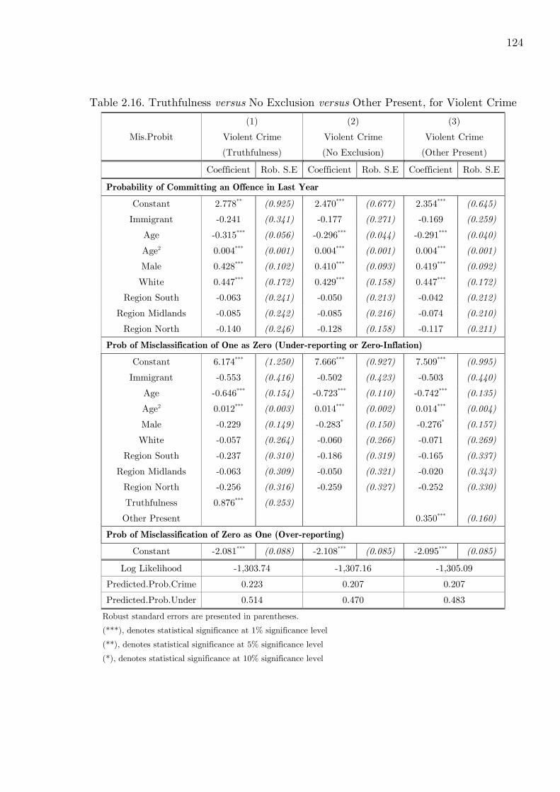
124

Table 2.16. Truthfulness versus No Exclusion versus Other Present, for Violent Crime

Mis.Probit

(1)

Violent Crime

(Truthfulness)

(2)

Violent Crime

(No Exclusion)

(3)

Violent Crime

(Other Present)

Coefficient Rob. S.E Coefficient Rob. S.E Coefficient Rob. S.E

Probability of Committing an Offence in Last Year

Constant 2.778** (0.925) 2.470*** (0.677) 2.354*** (0.645)

Immigrant -0.241 (0.341) -0.177 (0.271) -0.169 (0.259)

Age -0.315*** (0.056) -0.296*** (0.044) -0.291*** (0.040)

Age2 0.004*** (0.001) 0.004*** (0.001) 0.004*** (0.001)

Male 0.428*** (0.102) 0.410*** (0.093) 0.419*** (0.092)

White 0.447*** (0.172) 0.429*** (0.158) 0.447*** (0.172)

Region South -0.063 (0.241) -0.050 (0.213) -0.042 (0.212)

Region Midlands -0.085 (0.242) -0.085 (0.216) -0.074 (0.210)

Region North -0.140 (0.246) -0.128 (0.158) -0.117 (0.211)

Prob of Misclassification of One as Zero (Under-reporting or Zero-Inflation)

Constant 6.174*** (1.250) 7.666*** (0.927) 7.509*** (0.995)

Immigrant -0.553 (0.416) -0.502 (0.423) -0.503 (0.440)

Age -0.646*** (0.154) -0.723*** (0.110) -0.742*** (0.135)

Age2 0.012*** (0.003) 0.014*** (0.002) 0.014*** (0.004)

Male -0.229 (0.149) -0.283* (0.150) -0.276* (0.157)

White -0.057 (0.264) -0.060 (0.266) -0.071 (0.269)

Region South -0.237 (0.310) -0.186 (0.319) -0.165 (0.337)

Region Midlands -0.063 (0.309) -0.050 (0.321) -0.020 (0.343)

Region North -0.256 (0.316) -0.259 (0.327) -0.252 (0.330)

Truthfulness 0.876*** (0.253)

Other Present 0.350*** (0.160)

Prob of Misclassification of Zero as One (Over-reporting)

Constant -2.081*** (0.088) -2.108*** (0.085) -2.095*** (0.085)

Log Likelihood -1,303.74 -1,307.16 -1,305.09

Predicted.Prob.Crime 0.223 0.207 0.207

Predicted.Prob.Under 0.514 0.470 0.483

Robust standard errors are presented in parentheses.

(***), denotes statistical significance at 1% significance level

(**), denotes statistical significance at 5% significance level

(*), denotes statistical significance at 10% significance level

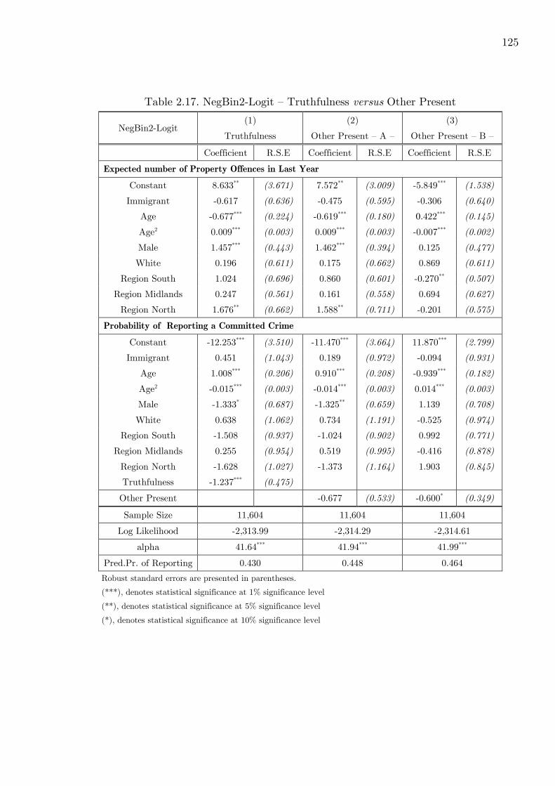
125

Table 2.17. NegBin2-Logit – Truthfulness versus Other Present

NegBin2-Logit (1)

Truthfulness

(2)

Other Present – A –

(3)

Other Present – B –

Coefficient R.S.E Coefficient R.S.E Coefficient R.S.E

Expected number of Property Offences in Last Year

Constant 8.633** (3.671) 7.572** (3.009) -5.849*** (1.538)

Immigrant -0.617 (0.636) -0.475 (0.595) -0.306 (0.640)

Age -0.677*** (0.224) -0.619*** (0.180) 0.422*** (0.145)

Age2 0.009*** (0.003) 0.009*** (0.003) -0.007*** (0.002)

Male 1.457*** (0.443) 1.462*** (0.394) 0.125 (0.477)

White 0.196 (0.611) 0.175 (0.662) 0.869 (0.611)

Region South 1.024 (0.696) 0.860 (0.601) -0.270** (0.507)

Region Midlands 0.247 (0.561) 0.161 (0.558) 0.694 (0.627)

Region North 1.676** (0.662) 1.588** (0.711) -0.201 (0.575)

Probability of Reporting a Committed Crime

Constant -12.253*** (3.510) -11.470*** (3.664) 11.870*** (2.799)

Immigrant 0.451 (1.043) 0.189 (0.972) -0.094 (0.931)

Age 1.008*** (0.206) 0.910*** (0.208) -0.939*** (0.182)

Age2 -0.015*** (0.003) -0.014*** (0.003) 0.014*** (0.003)

Male -1.333* (0.687) -1.325** (0.659) 1.139 (0.708)

White 0.638 (1.062) 0.734 (1.191) -0.525 (0.974)

Region South -1.508 (0.937) -1.024 (0.902) 0.992 (0.771)

Region Midlands 0.255 (0.954) 0.519 (0.995) -0.416 (0.878)

Region North -1.628 (1.027) -1.373 (1.164) 1.903 (0.845)

Truthfulness -1.237*** (0.475)

Other Present -0.677 (0.533) -0.600* (0.349)

Sample Size 11,604 11,604 11,604

Log Likelihood -2,313.99 -2,314.29 -2,314.61

alpha 41.64*** 41.94*** 41.99***

Pred.Pr. of Reporting 0.430 0.448 0.464

Robust standard errors are presented in parentheses.

(***), denotes statistical significance at 1% significance level

(**), denotes statistical significance at 5% significance level

(*), denotes statistical significance at 10% significance level

126 Table 2.18.a Interaction Terms

Covariate Dependent MisProbit (1)

Ethnicity

(2)

Regions

Coef R.S.E Coef R.S.E

Constant 2.777*** (0.898) 1.997** (0.838)

Immigrant -0.196 (0.287) -0.917*** (0.352)

Age -0.252*** (0.046) -0.248*** (0.036)

Age2 0.003*** (0.001) 0.003*** (0.001)

Male 0.428*** (0.158) 0.521*** (0.140)

White 0.571 (0.372)

Black 0.013 (0.367)

Asian and Other -0.617 (0.457)

Mixed 0.372 (0.541)

Region South 0.275 (0.237) 0.009 (0.217)

Region Midlands 0.139 (0.228) -0.051 (0.226)

Region North 0.489 (0.316) 0.301 (0.289)

Immigrant*Black -0.934 (0.583)

Immigr*Asian&Other 0.054 (0.730)

Immigrant*Mixed -0.615 (0.919)

Immigrant*South 1.483*** (0.570)

Immigrant*Midlands 0.690 (0.556)

Immigrant*North 0.240 (0.539)

Sample Size 11,658 11,658

Log Likelihood -1,418.40 -1,413.96

Predicted.Prob.Crime 0.297 0.243

Table 2.18.b. Interaction Terms (Specification (1) Cont) ⊕ Table 2.18.c. Interaction Terms (Specification (2) Cont)

Robust standard errors are presented in parentheses.

(***), denotes statistical significance at 1% significance level

(**), denotes statistical significance at 5% significance level

(*), denotes statistical significance at 10% significance level

⊕ This model is exactly the same with the one presented in Table 7.7, apart from the way we define the variables associated with the

interaction terms. Thus, all the other coefficients are exactly the same with specification (1) of Table 7.7 and therefore, not presented

here. The same holds for the second specification

Covariate Dependent MisProbit (2)

Regions

Immigrant*London

Immigrant*South 1.492*** (0.484)

Immigrant*Midlands 0.639 (0.504)

Immigrant*North 0.541 (0.459)

Native*London 0.917*** (0.352)

Native*South 0.927*** (0.308)

Native*Midlands 0.867*** (0.320)

Native*North 0.541*** (0.459)

Covariate Dependent

MisProbit

(1)

Ethnicity

Immigrant*Black

Immigrant*Asian&Other 0.359 (0.709)

Immigrant*Mixed 0.678 (0.780)

Immigrant*White 0.921* (0.475)

Native*Black 1.131** (0.522)

Native*Asian&Other 0.501 (0.585)

Native*Mixed 1.490** (0.669)

Native*White 1.117*** (0.404)

127

Appendix A. Zero-Inflated MisProbit

As mentioned in Section 2.5, it would be a good idea to incorporate a zero inflation proba-

bility in the MisProbit model in an attempt to separate under-reporting from zero-inflation.

In other words this model will attempt to separate potential criminals from genuine non

criminals. In this Appendix, this model together with some empirical results are presented.

To this end, assume that there is a fraction of people, ξ, that never commit and consequently

never report a crime. The remaining fraction of individuals, 1− ξ, follow the binary choice

model with misclassification. The corresponding response tree is presented in figure 2.5. The

conditional probabilities for the reported crime now become,

Pr(yi = 1|xi) = (1− ξ) [(1− F (x′iβ)) a1 + F (x′iβ)(1− a0)]

Pr(yi = 0|xi) = ξ + (1− ξ) [(1− F (x′iβ)) (1− a1) + F (x′iβ)a0]

(A.1)

Then, we specify the log-likelihood function as in (2.14) and we find the values of ξ, a0, a1,

and β that maximize it. In case the probability of zero inflation is given by a Logit model,

such as ξi = eq′iu/(1 + eq

′iu), the log-likelihood takes the following form,

lnL(β, u, a0, a1) =n∑i=1

− ln(1 + eq′iu) + yi ln [(1− F (x′iβ))a1 + F (x′iβ)(1− a0)]

+ (1− yi) ln[eq′iu + (1− F (x′iβ))(1− a1) + F (x′iβ)a0].

(A.2)

Estimation of this model seems difficult if probabilities of misclassification and zero-inflation

are all covariate-dependent, since with one data set we try to estimate four distinct processes.

Instead, given quite large samples, estimation could be feasible if for example, zero-inflation

probability is allowed to depend on regressors but one of the misclassification probabilities

is considered as constant. In any way, estimation of these models is a hard task, particularly

when noisy data such as crime data are used.

The estimation analysis has shown that, although identifiable theoretically, misclassi-

fication and zero-inflation probabilities cannot be estimated if they are all considered as

constants.The zero-inflation parameter remains unidentified even when under-reporting de-

pends on covariates. However, if zero-inflation depends on regressors, both the ZI-MisProbit

128

model with constant misclassification and the covariate dependent ZI-MisProbit model be-

have better. First, the case of constant misclassification is presented, followed by the covari-

ate dependent ZI-MisProbit.

Constant Misclassification

Although under-reporting seems to be covariate dependent, here the results of a model

of constant under-reporting is presented. Naturally, zero-inflation should depend on the

same vector of regressors. Here, truthfulness, which is assumed to affect the zero-inflation

probability, is used to facilitate the optimization procedure. However, an extra exclusion

was required (here in the form of not including age squared in the reporting process), even

though there was no specific reason for this. Otherwise, misclassification probabilities were

forced to be negative, and therefore, not helping the separation of zero-inflation from under-

reporting. This is also the reason why this model was not presented in the main results

analysis, as its behaviour was not trustworthy, perhaps because of the combination of noisy

data and complicated models. Nevertheless, a few results which will be presented in this

Appendix indicate that this model “works”, as it can potentially separate zero-inflation from

under-reporting.

These results are presented in Table 2.19. In the first column results of the MisProbit

model with constant misclassification are presented, whereas the ZI-MisProbit results are

presented in column 2. It is very interesting that, after controlling for zero-inflation, the

probability of under-reporting is predicted to be 0.48, almost 33 percentage points lower

than the model in column 1. The predicted probability of zero-inflation is 39.3%. Thus, this

model says that almost 40% of people (about 3,680 individuals) never commit crimes and

consequently they do not report any, and from the rest of them, 48% report no crimes even

though they have committed at least one.1 Furthermore, we can notice that all coefficient of

the zero-inflation process are statistically insignificant. We finally see that both the predicted

probability of committing a crime and the probability of over-reporting is almost the same

across the two models.

1Apart from the case where age squared was included in both processes, all other specifications showthat given the set of controls, zero-inflation probability is around 40% and probability of under-reporting isaround 35%.

129

Covariate-Dependent Under-reporting

As we have seen from the main results, the mix of under-reporting and zero-inflation is

covariate-dependent. In the previous part only zero-inflation was allowed to depend on

covariates. In this part we will have a look at the model where both processes are covariate-

dependent. Misclassifying a zero as one will still be considered as constant. Before proceeding

to the results, we must stress that with one data set we try to identify the parameters of

three different processes. In addition to that, we must be cautious not to misspecify the

model by excluding variables that must be included. For example, in the previous model I

did not include age squared in the zero-inflation process without a special reason. Therefore,

this model is too demanding to produce reliable estimates with such noisy data. However,

some results are presented in Table 2.20, which show that this model also “works”.

Once more, the first column replicates the second specification of Table 2.12. First of all,

we notice that all parameters of this model are identified. It can be said that, this is a “better

specified” model, since there is only one exclusion restriction from both the zero-inflation

and crime processes. This role, as before, is played by the dummy “truthfulness”. On the

other hand, as mentioned before, this is a too complicated model relative to the quality of

data and trustworthiness is a question here.

Unfortunately, the results of this model do not coincide with ZI-MisProbit with constant

misclassification. In this model, we see that the predicted probability of crime is around 51%,

which says that from potential criminals (since we have separated the genuine non criminals)

almost half of them commit at least one property crime. Moreover, we can also notice that

the predicted probability of zero-inflation is around 8%, which is much smaller than the

predictions of the previous model. Nonetheless, there is one common finding across these

two. In both models, apart from truthfulness which seems to be significant in the current

model, the independent variables do not seem to affect the probability of being genuine

non-criminal. However, the values of their corresponding coefficients differ considerably. For

some of these variables even the direction of the effect is the opposite one.

Comparing the first column with the second, there are a few things that merit some

discussion. Although we would expect the predicted probability to be lower, the ZI-MisProbit

130

gives almost the same probability of under-reporting and an extra zero-inflation probability

of 8%. Thus, this model, at least for the data of this study, does not seem to separate

zero-inflation from under-reporting. Regarding the immigrant coefficient, in contrast with

column 1, the ZI-MisProbit model says that being an immigrant increases the probability of

crime, but the coefficient is statistically insignificant. Although the rest of the coefficients in

the crime process follow the same direction as the coefficients of the first column, they are

very different in terms of magnitude. The rest of the coefficients of the two processes are not

discussed further since this model is just presented to show that if there are good reasons to

believe that the generating data process follows a ZI-MisProbit model, given a richer data

set, there might be gains from using it.

131 Figure 2.5. Zero Inflation MisProbit

Figure 2.6. Zero-Inflation – Poisson-Logit

µ−=(0) if e

0

ξ

1 ξ−

0

µµ

−

=e

( )!

i iy

i

i

f yy

≥ 1

0a

0

β′−1 ( )i

F x

1

01 a−

0

β′( )i

F x

1

1a

11 a−

ξ−1

ξ

0

132 Table 2.19. MisProbit Vs ZI-MisProbit. Constant Misclassification

MisProbit ZI-MisProbit

Coefficient Robust S.E Coefficient Robust S.E

Constant -0.226 (0.701) 0.671 (0.977)

Immigrant 0.055 (0.334) 0.095 (0.439)

Age -0.060 (0.046) -0.126** (0.057)

Age2 0.000 (0.000) 0.001* (0.000)

Male 0.926*** (0.379) 0.546*** (0.212)

White 0.826** (0.405) 0.719* (0.388)

Region South 0.147 (0.250) 0.484 (0.493)

Region Midlands 0.024 (0.225) 0.489 (0.453)

Region North 0.109 (0.250) 0.627 (0.505)

Prob of Misclassification of One as Zero (Under-reporting)

Constant 0.811*** (0.066) 0.480* (0.288)

Prob of Misclassification of Zero as One (Over-reporting)

Constant 0.012*** (0.005) 0.014** (0.006)

Prob of Zero-Inflation

Constant 2.509 (6.468)

Immigrant 0.136 (0.977)

Age -0.075 (0.053)

Male -0.448 (0.383)

White -0.073 (0.668)

Region South 1.013 (1.364)

Region Midlands 1.283 (1.179)

Region North 1.359 (1.216)

Truthfulness 3.668 (4.989)

Sample Size 11,658 11,658

Log Likelihood -1,446.92 -1,429.16

Predicted.Prob.Crime 0.280 0.269

Predicted Prob. of ZI 0.393

Robust standard errors are presented in parentheses.

(***), denotes statistical significance at 1% significance level

(**), denotes statistical significance at 5% significance level

(*), denotes statistical significance at 10% significance level

133 Table 2.20. MisProbit Vs ZI-MisProbit. Covariate-Dependent Misclassification

(1) (2)

Coefficient R.S.E Coefficient R.S.E

Prob of Property Offence in Last Year

Constant 2.335*** (0.896) 5.959 (3.660)

Immigrant -0.254 (0.273) 0.756 (0.748)

Age -0.259*** (0.046) -0.386* (0.203)

Age2 0.003*** (0.0006) 0.003* (0.002)

Male 0.440*** (0.156) 1.225 (0.828)

White 0.542* (0.293) 1.380* (0.787)

Region South 0.273 (0.231) 1.650 (1.585)

Region Midlands 0.124 (0.228) 1.973 (1.902)

Region North 0.496 (0.318) 1.951 (1.642)

Prob of Misclassification of One as Zero (Under-reporting)

Constant 2.267*** (0.507) -1.068** (0.505)

Immigrant -0.410 (0.346) 0.061 (0.185)

Age -0.195*** (0.074) 0.165*** (0.039)

Age2 0.003*** (0.001) -0.003*** (0.001)

Male -0.277* (0.142) -0.306*** (0.085)

White -0.198 (0.224) -0.394*** (0.140)

Region South 0.262 (0.224) 0.132 (0.144)

Region Midlands 0.224 (0.215) 0.305** (0.144)

Region North 0.490** (0.212) 0.208 (0.155)

Truthfulness 0.868*** (0.256) 0.623*** (0.138)

Prob of Zero-Inflation

Constant -44.141 (68.415)

Immigrant 0.271 (0.847)

Age 8.640 (12.355)

Age2 -0.406 (0.533)

Male -0.557 (0.498)

White 0.354 (0.718)

Region South -0.394 (0.632)

Region Midlands -0.754 (0.849)

Region North -0.503 (0.948)

Prob of Misclassification of Zero as One (Over-reporting)

Constant -2.234*** (0.204) -2.140*** (0.083)

Log Likelihood -1,422.05 -1,415.86

Predicted.Prob.Crime 0.292 0.509

Predicted.Prob.Under 0.709 0.719

Predicted.Prob.Inflation 0.076

Robust standard errors are presented in parentheses.

(***), denotes statistical significance at 1% significance level

(**), denotes statistical significance at 5% significance level

(*), denotes statistical significance at 10% significance level

134

Appendix B. NB1-Logit, Generalized-NB-Logit, ZI-Poisson-

Logit, and ZI-NB2-Logit

In subsection 2.5.2 we discussed that identification of the NB2-Logit model requires exactly

the same conditions established for the Poisson-Logit model (exclusion restriction on count

process or sign restrictions on reporting process). A model that is identified even without

the restrictions described above is the Negative Binomial 1-Logit (NB1-Logit), which is

obtained if we assume that αi depends on regressors in the following manner, αi = θ/λi (see,

Papadopoulos, 2011a, and Papadopoulos and Santos Silva, 2008). According to this form

of variance of εi, the variance of yi changes to ωi = µi + θλiΛ2i . It should be noted that

identification of the conditional mean is easier only because we impose more structure on

the variance. Hence, if the variance form of αi is misspecified, the estimates of θ will be in

general inconsistent.

Instead of assuming the form of the variance, we can specify a generalization of it as

ωi = µi + θλ2−ci Λ2i , where c is an extra parameter to be estimated. In case c = 0, a NB2-

Logit is obtained, whereas in case c = 1, a NB1-Logit is obtained. Therefore, identification

becomes “weaker” as c gets closer to 0. According to this general parameterization of the

variance the following log-likelihood arises,

lnL(θ, c, β, γ) =n∑i=1

ln(Γ(yi + θ−1λci)/Γ(yi + 1)Γ(θ−1λci)

)−

(θ−1λci + yi) ln(1 + θλ1−ci Λi) + yi(lnλ1−ci + ln Λi + ln θ) (B.1)

Similarly to the models for binary choice, models for count data with under-reporting can

also be generalized to take into account zero-inflation. First, the Zero-Inflation-Poisson-Logit

(ZIP-Logit) specification is presented. A construction of a response tree similar to (5.2) is

helpful to derive the conditional probabilities of interest. As before, there is a fraction of

people, ξ, that never commit and consequently never report crimes. The remaining fraction

of individuals, (1 − ξ) , can either commit or not commit crimes, but their responses are

subject to under-reporting, meaning that they follow the Poisson-Logit model. Therefore,

zeroes come from zero-inflation, or, from the Poisson-Logit mixture distribution. That is,

135

zeroes because of under-reporting, or zeroes because of the choice not to commit crimes.

The response tree is presented in figure 2.6 (page 122). In this case, ξ cannot distinguish

between zeroes because of never committing crimes (zero inflation) and always reporting

zeroes (total under-reporting), which was the case in the binary choice model.

In this tree, e−µi , is the probability of zero from the Poisson-Logit model, and µi = λiΛi.

According to this model, the conditional probabilities of zero and positives are the following,

Pr(yi = 0|xi) = ξ + (1− ξ)e−µi ,

Pr(yi > 0|xi) = (1− ξ)e−µiµyiiyi!

.(B.2)

The mean of this model is given by νi = (1− ξ)µi and variance ωi = (1− ξ)(1 + ξµi)µi, so

that there is overdispersion. If ξ is a constant, the log-likelihood is given by,

lnL(u, β, γ) =∑y=0

ln(ξ + (1− ξ)e−µi

)+∑y>0

ln

((1− ξ)e

−µiµyiiyi!

). (B.3)

However, ξ can also depend on covariates, so that we try to model what are the characteristics

that lead people never committing crimes or always reporting no crimes. If ξ is a Logit, with

ξi = eq′iu/(1 + eq

′iu), then we can write the log-likelihood function of the ZIP-Logit as,

lnL(u, β, γ) = −n∑i=1

ln(

1 + eq′iu)

+∑y=0

(eq′iu + e−µi

)+∑y>0

(−µi + yi lnµi − ln(yi!)) .

(B.4)

Identification of this model requires the same assumptions established for the Poisson-Logit,

so that exclusion restrictions in the Poisson part, or sign restrictions on the Logit part are

required.

Reformulation as a Zero-Inflation-NB2-Logit (ZI-NB2-Logit) model is straightforward.

The probability of an observed zero outcome from the NB2-Logit is now given by (1+αµi)α−1

,

136

and if ξ is a Logit, the resulting log-likelihood is given as,

lnL(θ, u, β, γ) = −n∑i=1

ln(

1 + eq′iu)

+∑y=0

ln(eq′iu + (1 + αµi)

α−1)

+

∑y>0

ln(Γ(yi + α−1)/Γ(yi + 1)Γ(α−1)

)−

(α−1 + yi) ln(1 + αµi) + yi(lnµi + lnα).

(B.5)

The mean of the ZI-NB2-Logit is given by νi = (1 − ξ)µi as before, and the variance is

given by ωi = (1− ξ)(1 + ξµi + θµi)µi. Again, identification of this model requires the same

conditions established for the Poisson-Logit and the NB2-Logit models.

137

Appendix C. More Robustness Checks

In this Appendix we consider three extra robustness checks. All results of the these three

exercises are presented in Table 2.21. The first specification of this table gives the results of

the second specification of Table 2.12 for the sake of comparisons. Note that the covariate-

dependent MisProbit is used to obtain all the estimates presented in this Appendix. However,

Table 2.21 presents only the results of the crime part. The estimates of the reporting part

are available from the author on request.

Dropping Very Recent Immigrants

As a first exercise we drop from the sample immigrants who have reported that have been in

the country for less than 12 months. This serves two purposes. Firstly, the OCJS does not

record crimes that happened outside the UK. Since the crime questions concern individuals’

criminal behaviour during the 12 months prior to the day of the interview, there might be

some cases of very recent immigrants who have committed crimes outside the UK which are

not recorded. Thus, the immigration coefficient would be downward biased if we overlooked

those cases. However, at the same time, some of the most recent immigrants may have

committed crimes in their source countries and mistakenly recorded them as happened in

the UK. Nevertheless, we would not like to include these reported crimes in our sample either

as we are only interested in the criminal behaviour of immigrants in the host country, since

their countries of origin may exhibit very different characteristics associated with property

crime, such as different economic opportunities and deterrent factors. Therefore, by dropping

immigrants that have been in the UK for less than a year we avoid these two ambiguous

scenarios. From specification 2 of Table 2.12 we notice that when we drop these 117 cases,

the coefficient on migration status slightly increases in magnitude but it is still statistically

insignificant.

Dropping very Young Individuals

The analysis so far has included people from 10 to 66 years old. In this exercise we are

looking at the consequence of dropping very young individuals, as responses of children

138

might be less reliable. However, notice that dropping even very young individuals, since we

include a youth-boost (3,185 individuals) we lose many observations which are essential for

the behavior of the model. The results are presented in four specifications. Specification

3 excludes respondents younger than 11 years old, specification 4 also excludes 12 year

olds, specification 5 also excludes 13 year olds and specification 6 also excludes 14 year

olds. First notice that the immigration coefficient becomes more negative if we drop ten

year olds and keeps increasing in magnitude as we drop individuals of 11, 12, and 13 years

of age and it actually becomes significant at 10% in specification 5. However, notice that

although the remaining individuals might provide more reliable information, the precision

of all estimates substantially decreases in specifications 4 to 6. Although not presented in

the table, the precision of the coefficients of the under-reporting (zero-inflation) part also

decreases considerably. This is because, as explained throughout this study, given the low

variation of the dependent variable, the noisy nature of self-reports and the complexities of

the MisProbit MLE, the sample size is very important. Thus, dropping 1,443 individuals

in specification 6 results in very harmful consequences for the behavior of the model. Also

notice that if we drop 14 years old individuals, which reduces the sample size by 1,785

observations, results in no convergence of the estimation procedure.

Without Criminal Damage

Even though criminal damage is also a crime against the property, it entails only psycholog-

ical gains to the offenders and therefore, it is not very clear whether it is proper to include

it in the property crime variable. This is because as it is the case for violent crime, criminal

damage cannot be well explained by the economic model of crime. First, excluding criminal

damage (1.51% positives) reduces the probability of observing a property crime from 5.47%

to 4.91%. The results in specification 5 and 6, where in specification 6 we have no exclusion

restriction, show that the immigration-property crime differential slightly reduces in magni-

tude but it still retains its sign. Notice however, that increasing the number of zeroes also

results in less precise estimates for all estimates, as in the previous exercise.

139

Table 2.21. More Robustness Checks

Mis.Probit

Property

Crime

(1)

Property

Crime

(2)

> 1 year

Immigrants

(3)

Age>10

(4)

Age > 11

(5)

Age>12

(6)

Age>13

(7)

No

Criminal

Damage

(8)

No Cr.Damage

No

Truthfulness

2.335*** 2.220** 1.872** 1.816* 1.462 1.362 1.912* 2.363 Constant

(0.896) (0.881) (0.812) (1.049) (1.217) (1.118) (1.005) (1.666)

-0.254 -0.301 -0.325 -0.524 -0.668* -0.713 -0.162 -0.201 Immigrant

(0.273) (0.287) (0.286) (0.403) (0.374) (0.466) (0.278) (0.306)

-0.259*** -0.249*** -0.241*** -0.225*** -0.190** -0.187** -0.254*** -0.254*** Age

(0.046) (0.044) (0.045) (0.065) (0.091) (0.084) (0.052) (0.076)

0.003*** 0.003*** 0.003*** 0.003*** 0.002* 0.002* 0.003*** 0.003*** Age2

(0.001) (0.001) (0.001) (0.001) (0.001) (0.001) (0.001) (0.001)

0.440*** 0.463*** 0.434*** 0.339 0.209 0.176 0.531*** 0.458*** Male

(0.156) (0.160) (0.169) (0.281) (0.338) (0.309) (0.160) (0.170)

0.542* 0.439* 0.566** 0.553 0.449 0.545 0.609* 0.375* White

(0.293) (0.259) (0.283) (0.409) (0.493) (0.645) (0.329) (0.381)

0.273 0.228 0.382 0.552 0.798 0.892 0.315 0.245 Region

South (0.231) (0.218) (0.257) (0.466) (0.788) (0.844) (0.257) (0.284)

0.124 0.096 0.208 0.292 0.337 0.348 0.211 0.160 Region

Midlands (0.228) (0.218) (0.242) (0.344) (0.529) (0.588) (0.247) (0.235)

0.496 0.416 0.564 1.008 1.393 1.345* 0.526 0.462 Region

North (0.318) (0.289) (0.350) (0.710) (0.958) (0.869) (0.351) (0.432)

Sample

Size 11,658 11,541 11,365 10,997 10,620 10,215 11,658 11,658

Log

Likelihood -1,422.05 -1,413.88 -1,392.28 -1,358.77 -1,322.63 -1,265.83 -1,321.94 -1,329.40

Predicted.

Prob.Crime 0.292 0.272 0.249 0.313 0.355 0.357 0.250 0.302

Predicted.

Prob.Under 0.709 0.678 0.657 0.753 0.791 0.798 0.664 0.715

Robust standard errors are presented in parentheses.

(***), denotes statistical significance at 1% significance level

(**), denotes statistical significance at 5% significance level

(*), denotes statistical significance at 10% significance level

Chapter 3

The Relationship between

Immigration Status and Victimization

3.1 Introduction

The link between immigration and crime is well discussed among scholar and non-scholar

communities. Nevertheless, most of the discussions by non-scholars concern immigrants’

involvement into criminal activities as offenders. This one-dimensional treatment has led to

the sentiment that immigrants are more involved in illegal actions. This is in most cases

in contradiction with scholars’ findings (mostly by criminologists and sociologists) which

suggest the opposite.1 For instance, Papadopoulos’ (2010b) findings, in a study for England

and Wales, suggest that immigrants’ participation in criminal activities as offenders (both

in property and violent crimes) is slightly lower than natives’ one as opposed to the public

sentiment.2

Since scholars have also focused on the immigration-crime link from the offending point

of view, they have overlooked the other important side of the coin which concerns the en-

gagement of immigrants in crime as victims. To my knowledge there are no comprehensive

studies that concentrate on this relationship,3 as most studies focus on the determinants

1For a review of the literature for the involvement of immigrants as offenders refer to Papadopoulos(2010b).

2These results are obtained using the Offending, Crime and Justice Survey of 2003 and appropriateestimators to correct for possible under-reporting of self-reported crime.

3To the author’s knowledge, the only finding on this link for the UK comes from Machin, Bell and Fasani(2010) study, who find that immigrants are less likely to be victimized using British Crime Survey data from

140

141

of victimization in general (see, for example, Miethe, Stafford and Long, 1987, Smith and

Jarjoura, 1989, Kennedy and Forde, 1990, Mustaine and Tewksbury, 1998, Wiles, Simmons

and Pease, 2003, Tseloni, Wittebrood, Farrell and Pease, 2004, and Tseloni, 2006). More

relevant studies look at the experiences of ethnic minority groups without distinguishing

between native and immigrant populations (see, for instance, Clancy at al, 2001, Jansson,

2006) and some of them are criminological studies that focus on a very specific aspect of vic-

timization experiences by ethnic minorities, namely, racially motivated crime, or differently,

“hate” crime (see, Gabbidon and Greene 2009, Spalek, 2008, and Kalunta-Crumpton, 2010).

This study, therefore, intends to fill this gap by investigating the victimization differences

between immigrants and natives in England and Wales.1 Looking into victimization would

complete the crime picture and possibly provide many interesting insights for immigrants’

behaviour towards criminal activities. Moreover, this study would shed some light on the

social integration of immigrants into the society. As a result, the findings of this work could

be a useful tool for policy makers.

The first aim of the present study is to comprehensively examine whether immigrants are

more or less at risk of becoming victims of crime and whether differences would still exist

if immigrants shared the same demographical characteristics with the native population. In

a second step we try to identify the reasons that lead to higher or lower victimization of

immigrants. For the purposes of the above analysis we use the 2007-08 sweep of the British

Crime Survey (BCS), a representative victimization survey where respondents were asked

in face-to-face interviews about their victimization experiences in household and personal

crime.2 We need to note that the nature of the victimization incident is very different across

different crime categories, such as property crime (burglaries, vehicle thefts, other thefts,

criminal damage) and personal crime (personal thefts, violence). Therefore, the immigration-

victimization link will be examined separately for the different crime categories, but more

attention will be paid to violent crime.

2004 to 2008. However, the victimization part concerns only a very small part of their paper, so that theygive only a very narrow picture of the immigration-victimization link.

1This study examines the victimization experiences of immigrants and natives only in England andWales, as Northern Ireland and Scotland are excluded from the British Crime Survey because of theirdistinct criminal justice system.

2The BCS data used in this study are sponsored by the Home Office and provided by the UK DataArchive.

142

Although the present study is mainly empirical, and to some extent methodological, some

theory developed by criminologists and sociologists will still be presented in the next sec-

tion, that formalizes the theoretical expected link between immigration and victimization.

This theory is based on potential victims’ lifestyle-exposure (Hindelang, Gottfredson, and

Garofalo, 1978) and routine activities (Cohen and Felson, 1979) which shape their so-called

criminal opportunity structure. In the present study these theories are adjusted to incorpo-

rate simple notions from the seminal economic models of crime by Becker (1968) and Ehrlich

(1973).

According to the above theories there are many channels, at least for instrumental crime1

both against the household and against the person, through which immigration and victim-

ization are linked either positively or negatively. For instance, immigrants would be more

victimized as they are disproportionately located in deprived areas where crime rates are

much higher. On the other hand, immigrants are less attractive as targets since they usually

possess fewer properties, or relatively less valuable objects. Therefore, the theory cannot

provide a clear-cut relationship between immigration and pecuniary crime; this is rather an

empirical question. As our data provide a lot of information on attributes that are associated

with instrumental crime, we are able to acquire a better understanding of the reasons why

we (do not) observe differential risks of victimization between immigrants and natives.2

The case of violent crimes is less obvious, as violence refers to expressive actions where

the offender intends to hurt the person and not to acquire his/her property. In violent crime,

contrary to property crimes, inter-relations and interactions between potential offenders and

potential victims are important. Thus, personal behaviour is a much stronger predictor of

violent victimization compared to instrumental victimization. Although the above theories

are still valid (given some conceptual modifications), it is difficult to identify the theoretical

channels through which immigrants become more or less likely to be victimized, as most

determinants of the violent victimization incident are unobserved factors determined by the

1By instrumental I mean pecuniary, or differently, a crime that the intention of the offender is to acquirevictim’s property and not to hurt the person itself.

2For example, even if it is the case in the raw data that immigrants face the same risk of becomingvictims of burglaries, we know that immigrants would actually face a lower risk of burglary victimization ifthey were located in natives’ residents, as immigrants are located in relatively more deprived areas wherethe crime rates are higher.

143

potential victim and his/her relationship and interactions with potential offenders. For in-

stance, some people would be less likely to suffer a violent crime if they followed particular

lifestyles associated with lower crime. However, since most aspects of this lifestyle are un-

observed, only speculations can be done to explain the factors that have generated this

differential risk of victimization among different groups of individuals.

Nevertheless, there is one channel that is very clear. Holding all other factors associated

with victimization constant, immigrants would still be at higher risk of violent victimization

than natives because of racially motivated crime. To what extent can racially motivated

crime explain differences in the victimization patterns between immigrants and natives?

This is also an interesting issue that will be examined. Moreover, violent crime consists

of three distinct types of very different nature, namely crime suffered by strangers, crime

suffered by acquaintances and crime suffered by family members (or ex-family members,

such as ex-partners). As will be seen later, modeling these three crime types separately will

provide some very interesting insights on the immigration-victimization nexus.

Another important point is that, since the questionnaire of the BCS involves some ques-

tions that try to elicit very sensitive information, misreporting is a concern. For instance,

there is evidence that respondents tend to under-report domestic violence perhaps because

of fear of reprisal, or because they want to protect the offender (Walby and Allen, 2004,

and Felson at al, 2006). If immigrants’ reporting behaviour differs from natives’ one then,

the coefficient representing the difference in domestic victimization between immigrants and

natives will be biased. However, in Section 3.6, by utilizing two different strategies we show

that immigrants do not under-report by more than natives.

Once the above relationships are established using a thorough examination of sensitivity

tests, some equally interesting topics will be examined. For example, exploiting the number

of victimization incidents we will be able to develop a better understanding of the victim-

ization experiences of immigrants. Is the use of count data models going to change the

picture obtained by the binary choice models? If yes, count data models have something to

say about differential repeated victimization experiences between immigrants and natives.

As will be clear later, conventional count data models, such as the Poisson or the Negative

Binomial regression models, are inadequate to explain the underlying relationship between

144

immigration and victimization due to limitations of the data set, such as the presence of

a few extreme cases where respondents reported a very high number of victimization inci-

dents, or, the very large number of zeroes. Therefore, models that take into account these

limitations are used.

Other interesting topics that will be investigated involve whether the ethnic composition

or the location of immigrants matters, whether there are assimilation patterns in the immi-

grants’ victimization experiences and whether immigrant victims perceive their victimization

experiences as more serious than otherwise comparable natives.

We need to note that there will be no separate section for the econometric models used

throughout this study. Instead, if the econometric models used in each section deserve a

formal presentation or at least some clarifications or discussions, they will be given at the

beginning of each corresponding section.

The rest of this study is organized as follows. In the next section a brief exposition

of a victimization theory together with a short discussion of the link between immigration

and crime is presented. Section 3.3 is devoted to explaining some technical parts of the

BCS and the construction of the dependent variables. Additionally, a description of the

data used in the empirical analysis and some descriptive statistics are presented. In Section

3.4 a basic analysis for household crime follows, where we investigate whether immigrants

are less or more likely to be victims of household crimes, focusing on inside and outside

burglaries. Section 3.5 examines the experiences of personal crime. Although some results

on personal theft are also presented, this section puts more weight on violent victimization.

Section 3.6 provides a thorough sensitivity analysis with regard to the results of the previous

section. Section 3.7 delivers a few results of interaction terms and perceived seriousness of

victimization incidents. A comprehensive analysis of count data models follows in Section

3.8. Finally, Section 3.9 consists of concluding remarks.

3.2 Theoretical Perspectives on Victimization

Before discussing the theoretical concepts of victimization it is worth noting that although

this study also presents results on inside and outside burglaries and on personal thefts, most

145

of the attention is paid to violent victimization. The results for the other crime types, such

as vehicle crime, criminal damage and household thefts will be briefly discussed but not

presented in detail. Moreover, as these crime types are of a very different nature, we need

to emphasize that to some extent the theoretical concepts apply differently to the different

crime groups.

When it comes to the offender-victim relationship it is natural to argue that in many

cases full responsibility falls onto the offender (although victims could still be unintentionally

responsible). For instance, think of a young girl whose purse gets stolen in a station of

London’s Underground. This is not always the case though. Even early theories (see,

for example, Von Hentig, 1940 and Wolfgang, 1958) admit that there are cases in which

offenders do not bare full responsibility, but the crime is a function of the underlying offender-

victim relationship evolving prior to the victimization incidence. Crimes are considered as

interactive acts that depend upon the actions of both parts. Thus, these theories rule out

the factor of “randomness” in victimization incidents.1 For instance, precipitation theory,

first discussed by Wolfgang (1958), argues that to some extent it is the victims’ provocative

behaviour that initiates subsequent crimes against them (see, Schultz, 1968, and Curtis,

1974). Clearly, the above theories seem more appropriate to describe violent crimes where

for instance, the victim using gestures or offensive language initiates an assault. Or, we could

think of a case of domestic crime where the interaction of family members is very important.

However, the theories that have attracted most both theoretical and empirical research

are based on the concepts of lifestyle-exposure (Hindelang, Gottfredson, and Garofalo, 1978)

and routine activities (Cohen, and Felson, 1979). Earlier concepts, such as the importance

of offender-victim relationship are integrated into these more recent ones. We need to note

that although each of these theories was initially developed for different purposes, they

are closely related and the present study treats them as a single comprehensive theoreti-

cal framework (see, Meier and Miethe, 1993, for an elaborate exposition of these theories).

According to them, routine activities and particular lifestyles of potential victims shape a

criminal opportunity structure which consists of four distinct risk factors that are associ-

1By “random” victimization incidents I mean situations where, there is no prior relationship between theoffender and the victim and the victimization incident does not depend on the interaction between offendersand victims.

146

ated with victimization. These factors are: proximity, exposure, attractiveness and capable

guardianship. Proximity and exposure create the criminal opportunity structure, whereas

attractiveness and ability of effective guardianship determine the criminals’ choice of victims

(Miethe and Meier, 1990).

Proximity is defined as the physical distance between locations that potential targets

tend to spend most of their time in and locations where potential offenders mostly act.

For instance, living in highly deprived areas, where the crime rates are high, increases the

probability to be victimized, as it increases the probability of contacting potential offenders.

This concept becomes less relevant as the mobility of the target increases, since the task of

identifying the distance between offenders and victims becomes more difficult. Therefore,

although the concept of proximity is very clear for household crimes, it loses some trans-

parency once we deal with personal crime. However, it is still important as most victims

tend to socialize in areas close to their residences.1

Exposure refers to the physical visibility or availability of potential victims. The meaning

of this concept changes substantially between different types of crime. For personal violence,

exposure can be conceptualized as the general routine activities or lifestyles of potential

victims, associated with higher or lower likelihood of victimization. For instance, people

that mostly stay at home and do not socialize in bars or pubs tend to be less likely to

suffer a violent crime. Here, general lifestyle also includes relationships and interactions of

potential offenders with potential targets. Thus, this concept also incorporates the earlier

theories of precipitation. For household crime, this risk factor takes a very different meaning.

For instance, for inside or outside burglaries exposure may refer to the location of the house

(such as main road or cul-de-sac), or the amount of properties someone possesses. For vehicle

crime just a high number of cars owned by an individual can be considered as an indicator

of high exposure.

Target attractiveness is defined as the material (for acquisitive crimes) or symbolic (for

violent crimes) desirability (value) of targets to potential offenders. The notion of attractive-

1According to the victim forms of the 2007/08 BCS around 20% of all personal victimization incidentshappened inside or immediately outside victims’ residence. From the rest of them, 6% occurred in workplace,18% at pub/bar/club, 35% in other public or commercial location and 22% elsewhere. Moreover, it is veryinteresting that for the incidents that did not happen inside or outside residence, 40% of them took placewithin 15 minutes from victim’s residence.

147

ness is again very different across acquisitive and violent crimes. For instance, in household

crime of acquisitive nature, the appearance of the house, or the information of offenders

for valuable objects inside the house increases attractiveness. For personal thefts, the gen-

eral appearance can indicate a level of attractiveness. On the other hand, violence is an

expressive crime, as offenders target to hurting the victim itself without being interested in

victim’s valuable possessions.1 Just the ethnicity of a potential victim can be considered as

highly attractive attribute for an extremist. In other cases attractiveness develops through

interactions and interrelations among people. For example, a member of a gang finds as an

attractive target a member of another gang (with regard to the symbolic utility that the

offender gains if he/she commits the crime). Or, two persons with a history of previous

arguments find one another more attractive to a potential offence.

Finally, physical or social guardianship is the effectiveness of objects (physical guardian-

ship) or people (social guardianship) in preventing crime from occurring. For personal crimes,

guardianship is the ability of the person, or the ability of people around him/her, to protect

him/her. Having a weapon in apparent place, or guards, is a type of physical guardianship.

Also demographic features as height, weight, age, appearance, could indicate an ability of

protection. Physical guardianship for dwellings and vehicles could be for example security

measures, neighbourhood watching program, etc. On the other hand social measures could

be number of hours house left unoccupied, number of household members (more members

indicates that the house is left unoccupied less hours per day, which decreases the likelihood

to be burglarized), knowledge on what to do in case someone breaks into the house, etc.

The basic economic theory of crime is closely related to the above sociological views.

A two-stage model which borrows simple notions from the early economic models of crime

by Becker (1968) and Ehrlich (1973) could be formulated to describe the victim-offender

relationship. According to these early models of crime, individuals use a rational cost-benefit

analysis where they weigh the expected costs and benefits in utility terms and subsequently

decide how much time to allocate in legal and criminal activities in order to maximize their

net expected utility. Since crime involves uncertainty, because of potential apprehension

1We need to note that for robberies there is a violent act together with the theft. However, as theprimary target of the offender is instrumental I consider robbery as personal theft.

148

and consequent future punishment, the notion of risk aversion is very important. At the

same time, uncertainty and risk aversion are also very important from the potential victims’

point of view, as the actions of potential victims could not perfectly determine the criminal

activity against them.1

Although in reality the situation is much more complicated, a simple model could be for-

mulated as follows: in the first period the (rational) potential victims, given the level of risk

aversion and the initial values of attractiveness, exposure, proximity and capable guardianship

(as these are determined by their exogenous socio-economic and demographic attributes),

consider a set of different strategies and the possible consequent actions of potential offenders

for each different strategy. Consequently, they re-evaluate their position by determining to

some extent the optimal levels of attractiveness, exposure, proximity and capable guardian-

ship in order to maximize the net benefits. For instance, people that are highly afraid of

potential offenses (such as older people), which could translate into very high risk aversion,

would decide to exhibit very low exposure, for example, by staying mostly at home and

avoiding going out at night, or to increase guardianship by taking higher physical measures

of protection. On the other hand, people that value enjoyment by much more than safety

(such as younger people), which could be related to lower risk aversion, would disregard many

potential dangers and exhibit high exposure and attractiveness for the sake of amusement.

In the second stage, once the opportunity criminal structure is set by the determination

of proximity, exposure, attractiveness and guardianship, potential criminals come into play.

Each of the four risk factors can be translated into costs and benefits for the offender.

For instance, a highly attractive person or household would result in higher utility for the

offender, a well protected house increases the uncertainty of success of the criminal action and

therefore increases costs, a household of high exposure decreases uncertainty and therefore,

decreases costs, and so on. Consequently, potential criminals, comparing their legal and

illegal opportunities and taking into account their criminal ability and risks they are willing

to take, decide whether to commit crimes and consequently which targets to hit in order

to maximize their expected utility. Of course, the whole procedure is more complicated

since potential victims cannot perfectly observe the actual risks of victimization for each

1For instance, a burglary cannot be avoided with certainty even if the potential victim is very cautious.

149

strategy they follow, and in a similar manner in the second period the four risk factors

are not perfectly observed by the potential criminal. Moreover, this model also ignores the

possibility that potential victims can at the same time be potential offenders. Nevertheless,

this simple form together with the socio-criminological views could give some predictions on

the immigrant-victimization relationship.

We need to emphasize that all ascribed or acquired attributes, such as age, gender and

race, or education, income, family and employment conditions, respectively, are associated

with victimization likelihood through their effects on the described risk factors. For example,

males generally prefer to socialize more frequently in dangerous places and they exhibit a

more aggressive behaviour relatively to females. Therefore, they would decide to be more

exposed to criminal activities, which makes them more likely to become victims of violence.

However, the situation is very different for domestic crime. Males within a family are vic-

timized to a lesser degree because they exhibit higher guardianship. Moreover, the effect of

some other attributes is ambiguous as they affect victimization risk through two or more

risk factors. For instance, more affluent households are associated with both higher or lower

risk of a burglary, since high household income may indicate a better protected house (more

capable guardianship) or a very attractive target (since there are many valuable objects both

in the house and outside the house).

3.2.1 The Immigration-Victimization Link

Immigration status (at least for the purposes of the empirical analysis) can be considered

as an attribute ascribed to an individual.1 Although immigrant population is rather het-

erogeneous, immigrants share some common characteristics. In Table 3.3 some descriptive

statistics from the BCS 2007-08, by immigration status, can be found. From this table it

is clear that immigrants are relatively younger, more from ethnic minorities and relatively

more married. It is also clear that they are more unemployed and there is evidence that

they are on average poorer and face lower legal opportunities relative to natives (see, for

example, Algan at al, 2010). Given all the above characteristics, and assuming that labour

outcomes enter the problem exogenously, immigrants evaluate their initial levels of attrac-

1Thus, we consider immigrants’ behaviour after the decision to migrate.

150

tiveness, exposure, proximity and guardianship, as all these exogenous attributes are to some

extent associated with these four risk factors.1 Consequently, they reevaluate their position

by following strategies that minimize the victimization risks for each crime group given all

the aforementioned constraints.

For instance, location, and consequently proximity, is constrained by the labour outcomes

of immigrants. As we can see from the descriptive statistics immigrants are disproportion-

ately located in deprived inner city areas, mostly of London. This could be the consequence

of the following reason. As immigrants face unfavorable labour outcomes they can only

afford to reside in areas where the rents are relatively low. It happens that these areas are

relatively more deprived with high crime rates and therefore, of higher proximity. Neverthe-

less, given the above constraint, immigrants reduce the risk of both personal and household

victimization by choosing to reside (within these areas of high proximity) in locations with

high concentration of the same ethnic group. This develops a type of natural protection, or

provides a higher insurance against risk of victimization by increasing social guardianship.

At the same time, household physical guardianship is also constrained by their labour out-

comes, as they could not afford means of high protection. Residing in the aforementioned

areas performs as a natural social guardianship that intends to balance the lower physical

guardianship.

Moreover, as immigrants disproportionately belong to ethnic minority groups they are

in higher danger of racially motivated violence, since they are relatively more attractive

to extremist groups. Therefore, they might choose to balance this unfavorable position by

choosing routine activities and lifestyle exposure associated with lower victimization (and

therefore, by reducing exposure). In addition, a proportion of immigrants might feel alienated

and react in this perceived hostile environment by following strategies that reduces the risk

of victimization. Finally, immigrants could naturally exhibit different exposure, because of

cultural differences that are associated with different lifestyles.

As mentioned in the introduction, violence consists of three crime types of very different

nature, namely crime by strangers, crime by acquaintances, and domestic crime. Theoretical

1For example, younger people prefer to have a social life associated with higher exposure. Married peopleon the contrary follow lifestyles associated with lower exposure.

151

predictions on the association between immigration status and domestic crime or crime

by acquaintances can be given by immigrants’ relative participation in the illegal sector

as offenders. For instance, according to the “homogamy” principle immigrants tend to

socialize with other immigrants of the same ethnic group and therefore, a large proportion

of immigrants’ acquaintances or family members are immigrants as well. If we accept that

immigrants, according to Papadopoulos (2010b), are slightly less likely to commit violent

crimes, holding everything else constant, we would expect a negative relationship between

being an immigrant and violent crime suffered by acquaintances or family members.1

However, a negative relationship could be also observed because of “network effects”, a

concept closely related to exposure. For instance, crime suffered by acquaintances could be

lower for more recent immigrants due to the fact that more recent immigrants know fewer

people. Therefore, the “pool” of acquaintances is larger for natives or earlier immigrants.

According to this, we could expect that as time spent in the host country increases, immi-

grants enlarge their group of acquaintances, and therefore, to some extent they assimilate

to natives’ risk of victimization by acquaintances.

As it is clear from the discussion of this section, the unobserved interactions and inter-

relations among people are relevant for violent crime, but not for household burglaries and

personal thefts. Household burglaries more or less depend on observed household charac-

teristics. The fact that the household reference person is an immigrant should not affect

the risk of victimization, given that we are able to control for all household characteristics

associated with burglary victimization.2 The only unobserved (by the author) characteristic

that might be important to describe instrumental victimization risks is the size of potential

victims’ possessions (apart from the number of vehicles which is observed).3 Fortunately, the

BCS provides a rich set of household characteristics directly associated with lifestyle-exposure

1As an example, consider the following simple calculation. Assume that the probability to commit a crimeis 6% and 10% for an immigrant and a native respectively. Also, assume that 5% of natives’ acquaintancesare immigrants, but 60% of immigrants’ acquaintances are immigrants. According to these assumptions,holding everything else constant, the probability for an immigrant to suffer a crime by an acquaintance is6% × 0.60 + 10% × 0.40 = 7.6%, but this figure is 9.8% for natives, so that the difference is 2.2 percentagepoints.

2Unless criminals seek places that are inhabited by immigrants or criminals have information about theimmigration status of residents and tend to prefer targeting these places. However, for a household crime itis the instrument that is much more important than the person who owns it or resides in it.

3This can be considered as more important for properties outside the dwelling as they are directlyobserved by potential criminals, as opposed to interior properties.

152

and routine activities, such as hours home left unoccupied, being in a neighbourhood watch-

ing program, house condition, type, location, etc (see, next section). he situation of personal

thefts is a bit more complicated due to the fact that it entails personal contact and thus,

the potential criminal can directly observe the potential victim. However, as for burglaries,

personal theft is in a sense more “random” in the sense that personal behavior is not an

important predictor of the action.

Nevertheless, for violent crime, the risk of victimization highly depends on the unobserved

strategies associated with particular lifestyle-exposure and routine activities that immigrants

set in order to reduce the victimization costs. As described above, lifestyle-exposure and

routine activities might be very different between immigrant and native groups and therefore,

the theory cannot provide a clear-cut relationship. This should instead be established by

the empirical analysis. Hopefully, the empirical analysis would also provide many insights

on the reasons behind the observed immigrants-natives violent victimization differentials.

In addition, we need to recognize that immigrant population is highly heterogeneous and

the different groups of immigrants (for example, according with their ethnic background, or

the time spent in the UK) might be associated with different unobserved victimization-prone

factors. This subject will be examined in Section 3.7. Finally, for some reasons explained in

Section 3.8, repeated victimization may be different between immigrants and natives. Count

data models will provide insights on this relationship.

3.3 BCS, Dependent Variables and Descriptive Statis-

tics

In the first subsection of Section 3.3 a brief description of the British Crime Survey together

with some important issues concerning the construction of the dependent variables is pre-

sented. A description of the data together with some descriptive statistics follow in the

second subsection.

153

3.3.1 The British Crime Survey and Dependent Variables

The British Crime Survey 2007-08 (BCS), carried out by the Home Office, is a representative

(primarily) victimization survey where respondents in England and Wales were asked in

face-to-face interviews about their victimization experiences in both household and personal

crime. As will be described later, the BCS also includes computer-based self-completed

interviews for the more sensitive crimes. such as domestic violence and sexually motivated

offences. Moreover, it does not interview people from Scotland and Northern Ireland as

they now conduct separate surveys. The reference period for all interviews refers to the

victimization incidents during the last 12 months prior to the date of the interview. It is

one of the largest social surveys in England and Wales as it interviews approximately 47,000

respondents per year.

This survey is ideal to identify determinants of victimization since, together with in-

formation on victimization experiences, a large set of demographic characteristics together

with information on household and personal characteristics associated with victimization are

available. Note that, since the BCS interviews only private households, it does not cover

commercial victimization, frauds and victimless crime, crime against children, crime against

people currently in institutions, and murders (for details of the BCS refer to Bolling, Grant,

and Donovan, 2008, I).

For the purposes of this study, information from three separate files of the BCS 2007-

08 was combined using the unique identifier variable from the three data sets. These files

are: 1) the Main BCS data set, where information for all respondents and their households

regardless of their victimization experiences is included, 2) the Victimization Form data set,

in which details of each crime reported by victims are given, and 3) the Self Completion

data set of domestic violence, where all people between 16-59 years old, by participating

in computer-based self-reported interviews, provided information on their experiences of

domestic violence.1

These three data sets were constructed by using a complicated procedure whose main

steps are briefly described as follows: interviewees, after giving some information on de-

1There is evidence that respondents under-report by less in computer-based self-reports (see, for example,Turner at al, 1998). Therefore, as mentioned in the introduction, the purpose of using this information is tocheck whether immigrants under-report violent crime by more or less than natives.

154

mographic and other individual and household characteristics, were asked a list of screener

questions about whether they suffered any type of victimization incidents during the last 12

months (against them or against their household). In case the respondent reported a suf-

fered crime, a victim form was given for each crime suffered. The victim forms assigned to

each individual were limited to six. Each victimization form contained detailed information

on the crime incident. This information was next used by trained coders to assign either

a valid or an invalid victimization code.1 The cases in which the conductor was uncertain

about the offence code to be assigned were sent to Home Office to be crosschecked by Home

Office experts. There, a finalized code was assigned. If a particular crime in a given victim

form was described as a “series” crime, where a series crime is defined as “the same thing,

done under the same circumstances and probably by the same people”, the number of the

incidents was recorded. The classification of crime codes is depicted in Table 3.1.

It is important to note that some incidents included a sequence of crime events which

might have been of different nature. For instance, we could imagine a case where a stranger

broke into a house to steal valuables but during the act of burglary the victim tried to

prevent the incident resulting in suffering an assault with serious wounding. Eventually, the

offender also burned the house. This incident (which is of course extreme and not very likely

to have happened) involves three separate crimes but it will be recorded as arson because

arson takes priority over burglaries and serious wounding. In similar cases the final coding

depends on the seriousness of the incident. For details on the coding and which crimes take

priority over other ones refer to Bolling, Grant and Donovan (2008, II).

The dependent variables used in this study were created from the offence code variable

given in the Victim Forms data set (see, Table 3.1). As the question of interest in this

study is to identify whether immigrants are more or less likely to be victims of criminal

activity (and in extension whether immigrants are more frequently victimized than natives)

a grouping of the individual codes was required. Otherwise there was not enough variation

in the dependent variable to give precise and robust estimates for the coefficients of the

1The incidents are given invalid codes if the offence was a duplicate, if the offender was described asmentally ill, if the offender was a police member on duty, and if incidents that initially were given a victimform decided to be coded as no crimes after a scrutinized examination. Note that incidents outside Englandand Wales were given a valid code.

155

models. Seven main groups were constructed according to the nature of each crime code (as

judged by the author being of the same nature), five of them for household crime and two

for personal crime. For household crime these are: Inside Burglaries (codes 51-53), Outside

Burglaries (codes 50, 57, 58), Vehicle Thefts (codes 60-64, 71, 72), Household Thefts (codes

55, 56, 65-67, 73)1 and Vandalism (codes 80-86).2 Regarding personal crime, these are:

Personal Theft (codes 41-45) and Personal Violence (11-13, 21).3

For all constructed variables I use both the binary information, which is used in the

first part of the empirical analysis (Sections 3.4-3.7), and the count form (number of crimes

suffered), which is used in the second part (Section 3.8). For each crime group, the binary

dependent variable is just a dummy that takes the value one if the individual reported

a victimization of that crime group in at least one victim form and zero otherwise. The

count variables are created by using the “series” information from the victim forms. For

example, if an assault with wounding was considered as a “series” crime, the number of

assaults forms the count variable. Moreover, if the same individual suffered another assault,

for instance without injury, the number of assaults from this victim form, as indicated by

the “series” information, are added to the previous count.4 Finally, note that it is possible

two victimization forms to be assigned by the conductor for two very similar crimes, which

even belong to the same code, if some characteristics of the first (series of) incident(s) are

considered by the coders to be different from the second (series of) incident(s).5

As mentioned in the introduction, the personal violence variable is the mix of three crimes

1Separation between inside, outside and other thefts was also considered.2A separation between home vandalism and vehicle vandalism was considered to be interesting.3For details on the crimes that each individual code included refer to the Offence Coding Coders Manual

in Bolling, Grant, and Donovan (2008, II).4We need to note that the main data provides derived crime variables which are used by the Home Office

to calculate prevalence and incidence rates. However, for each crime code in these variables a cap of fivecrimes is imposed. Therefore, the total count for a crime group, say violent crime, will be the sum of crimesfrom each victimization form that fall within this crime group, where the number of crimes in each victimform is censored in five crimes. Thus, the resulting count variable will be the sum of up to six censored atfive crimes. According to this, it is not proper to use a simple right censored at 30 crimes count data modelbut a model that allows for censoring at 5 crimes for each victimization form someone gets. This of coursewill result in a very complicated situation. Moreover, these derived variables do not include cases where thecoder was uncertain what code to assign.

5For instance, consider a case where a victim suffered 15 assaults without injury (1st victimization form)and 5 assaults again without injury (2nd victimization form). The difference between these two series ofcrimes is that, for instance, the first series of assaults were committed by an acquaintance whereas the secondseries by a partner. Therefore, although these two crimes at the end take the same code (number 13), twodifferent victimization forms are assigned. To construct the count of assault without injury for this individualwe need to sum the count from the 1st victimization form and the count from the 2nd victimization form.

156

of very different nature. Crime suffered by strangers, crime suffered by acquaintances and

domestic crime. Since these three crimes are different in many dimensions it is more proper

to treat them as three separate crime categories. Fortunately, this information is also given

in the Victim Forms data set and three separate dummies or count variables can be created.1

This will be well discussed in Section 3.5.

However, another question is raised. Is it appropriate to treat these three types as being

independent from each other (and therefore, model them as three independent equations)?

For instance, when we consider crime by acquaintances, is it appropriate to consider an

individual who suffered a domestic crime but not a crime by acquaintances as being the

same with an individual who did not suffer crimes at all? It might be more proper to

take into account the fact that people who suffered a violent crime of one type may share

common unobserved characteristics with people that suffered a violent crime of another type.

Allowing for these unobserved factors to be correlated might result in efficiency gains. This

will be further discussed in Section 3.6.

Finally, for each (series of) crime event(s) the information whether it is (they are) per-

ceived as a racially motivated crime, together with the reason why it is (they are) perceived

as such, is available. Therefore, (perceived) racially motivated crime can be controlled for.

3.3.2 Description of the Data

To begin with, although in the empirical analysis I focus on burglaries, personal thefts and

violent crime, the distribution of the count form of all dependent variables is presented in

Table 3.2. However, the full distribution of the violent crime variables is presented separately

in Table 3.22. There are two main issues that deserve a brief discussion. Firstly, the number

of zeroes is very large for most of the variables. Thus, for some variables it is hard to obtain

precise estimates because of the low variation in the dependent variable, particularly for count

data models which are not very robust when the presence of zeroes is very high. Secondly,

there are few cases of victims that reported extreme number of crimes. For instance, in

variable Personal Theft there is only one person above ten crimes, who actually reported

1The ‘do’ files (Statar format) for the creation of dependent variables from the Victim Forms data setare available from the author upon request.

157

97 crimes, or, for Inside Burglary there are eight people that reported between 70 and 100

crimes. In this table for ease of exposition we cap the crime count at ten plus more. Count

data models are very sensitive to these cases, particularly when the positive counts are too

few to identify the parameters assumed to affect the conditional mean, and when the extreme

cases are very dispersed from the less extreme cases. Someone would think of dropping these

cases because they could be considered as highly unreliable. However, this practice would

result in sample selection issues. Therefore, as will be discussed in Section 3.8, we also

use several modified count data models that are both (in a sense) more robust under these

cases and more appropriate to explain the observed distribution of victimization incidents.

Finally, it is also clear that the dispersion of most variables is very high. Therefore, the

Negative Binomial distribution that allows for over-dispersion may be more appropriate to

fit the observed data.

Moreover, descriptive statistics of the dependent and independent variables are presented

in Table 3.3. The mean for native and immigrant groups for all variables is also given in order

to have a first indication on the victimization differences between immigrants and natives.

In addition, we will be able to observe the aspects in which immigrants differ from natives

with regard to their observed characteristics. It must be noted that, the immigration status

variable is created as a dummy that takes the value 1 if the respondent or the house reference

person is not born in the UK. Moreover, the information of how many years the respondent

lives in the UK can be exploited to examine assimilation patterns of the immigration-native

victimization differentials. This will be examined in Section 3.6.

A first look at the raw data shows that there are victimization differences between immi-

grant and native groups, although they are very small in most cases. Regarding acquisitive

crime, both household and personal, we can see that the probability and the mean victimiza-

tion are higher for immigrants, apart from Outside Burglary (and Outside Thefts or Other

Thefts).1 Moreover, Home Criminal Damage is slightly lower but Vehicle Criminal Damage

is slightly higher for immigrants. Concerning Violent Crime, which is the crime group most

discussed in this study, we can see that immigrants are less victimized. However, the picture

1Here I do not discuss statistical significance of the differences as these descriptive statistics are usedjust as a first indication.

158

is different if we break violence into the categories discussed before, as immigrants are much

less victimized by acquaintances and family members, but slightly more by strangers.

In addition, in Table 3.3 the independent variables which will be used in the main anal-

ysis are also presented. Again, the mean for both immigrants and natives is given. Note

that the means for the respondent’s and the household reference person’s characteristic are

separately given. This is because the appropriate variables in personal crime are the personal

characteristics, but in household crime it is the household characteristics. The main observed

differences between immigrants and natives is that immigrants are younger (which can be

considered mainly as a measure of exposure) and that they are relatively more concentrated

in London, urban and inner city areas, but most importantly that they reside in relatively

more deprived areas (which can be thought as proximity measures).1 Thus, a first question in

the main analysis would be: what would be the immigrant-native differences in the likelihood

to suffer a crime if immigrants displayed the same basic demographic characteristics?

Moreover, immigrants are more married, more of nonwhite ethnic groups, more renters

and they reside relatively more in flats (mainly exposure measures). They also live fewer

years at their current home or area (which is a measure of social guardianship) and finally,

they possess fewer cars (measure of exposure). There are no strong differences in income

and education. Hence, another question would be: if there still are differences, can they be

explained by the remaining observed individual and household characteristics?

Finally, notice that for some of the independent variables there are many missing cases.

Dropping all these cases would result in losing too much information. Therefore, a dummy

is created for each variable that contains a considerable number of missing cases that takes

the value one if the particular variable displays a missing value and zero otherwise. Thus,

1The Deprivation Index is the “Multiple Deprivation Index of England and Wales” for 2007, constructedas a weighted mixture of the individual deprivation indices (Income deprivation, Employment deprivation,Health deprivation and disability, Education, skills and training deprivation, Barriers to housing and services,Living environment deprivation, and Crime deprivation index) provided by the Department of Communitiesand Local Governments for England and Welsh Assembly Government for Welsh. Very briefly, this index,that takes integer values from 1 to 10, provides a measure of multiple deprivation at the Lower SuperOutput Areas (LSOAs) level by considering some indicators of deprivation. These values indicate the decileof deprivation in which someone scores. For example, if someone scores at the 7th decile, only 30% of thepopulation resides in more deprived areas. Each respondent, depending on the small level area that he/sheresides, is matched by the Home Office with the corresponding decile of this variable. For more informationon these indices refer to Noble at al (2008). In the empirical analysis I include this variable as an 1 - 10integer index that measures the effect of scoring at a one decile higher on the probability of victimization.

159

these dummies intend to absorb the effects of the missing cases of each characteristic on the

dependent variables.

In a summary of this subsection, we saw that immigrants suffer in general slightly more

property crime and personal theft (apart from outside thefts and home criminal damage) but

less violent crime than natives, although they live in more deprived inner city neighbourhoods

where violent crime is much higher. However this picture changes if we distinguish crime

by strangers from crime by acquaintances and family members. More on these relationships

will be discussed in the next two sections.

3.4 Risk of Household Crime

In this section simple Probit results for household crime are presented.1 As discussed in the

previous section household crime was separated in five mutually exclusive groups. However,

here mainly the results of Inside Burglaries plus Attempts and Outside Burglaries plus At-

tempts are presented. The results of the other variables are briefly discussed in the second

subsection. Full results are available from the author on request. The regressors believed to

affect the conditional expectation of the dependent variables are assumed to be the same for

both crime groups.2

In the results that follow four specifications of the conditional mean are presented. In

specification 1 the effect of the household reference person (hrp) being an immigrant on the

likelihood of victimization is considered without taking into account that immigrants differ

from natives in many dimensions. In specification 2 some important proximity measures

are controlled for. In specification 3 some important characteristics of the hrp are also

included, which are thought in literature to be associated mostly with the risk factor of

exposure. Finally, in specification 4 some extra important household characteristics that are

theoretically associated with exposure, attractiveness and guardianship are used.

1All the empirical results in this study are obtained using Statar and TSPr econometrics software.2Thus, we assume that the factors that affect the criminal opportunity structure through their effects

on the four risk factors are generally the same for the two crime variables.

160

3.4.1 Inside Burglary

Before discussing the results we need to note that 81% of the Inside Burglaries plus At-

tempts incidents the victim did not know the offender, whereas only 10% of the cases

happened because of preexisted personal relationship/history between the victim and the

offender. Therefore, although there are a few cases where interrelations and interaction be-

tween victim-offender matter, inside burglary can be considered in a high degree as “random”

where criminals solely target the property without interest in the household composition

and without intentions to victimize household members. Thus, we can assume that offend-

ers target specific dwellings not because of the composition of the residents, but because

these specific dwellings exhibit characteristics associated with higher risk of inside burglary

victimization. Moreover, notice that most of the times, criminals’ information about inte-

rior properties is limited, so that the value of the interior properties would not be a large

factor for the risk of victimization. Instead, attractiveness is approximated by the external

household characteristics.

According to the above, we would expect that if a relationship between immigration and

inside burglaries exists, it is not because criminals prefer targeting immigrants’ properties,

but because immigrants’ household characteristics are associated with more or less victim-

ization, as discussed in Section 3.2. These characteristics refer to both direct household

characteristics such as location and external condition, and indirect characteristics associ-

ated with the four risk factors, such as household reference person’s age, marital status, or

how many hours the house is left unoccupied. Therefore, we would expect that this associa-

tion would fade out if we were able to control for the characteristics that make immigrants’

properties subject to higher or lower victimization.

The Probit results are presented in Table 3.4. First of all, we can see that the likelihood

of victimization increases if the hrp is an immigrant. The marginal effect is 0.74 percentage

points (which is statistically significant at 1% significance level) which is fairly large in

magnitude if we bear in mind that the probability to suffer an inside burglary is 2.99% for

immigrants and 2.25% for natives, a relative effect of 33%. Note that the result is almost

identical if we control for respondent’s immigration status rather than hrp’s immigration

161

status. This was expected because according to the “homogamy” principle it is highly

possible that if the respondent is an immigrant the hrp is also an immigrant.1

Hence, dwellings in which the hrp is an immigrant are disproportionately victimized.

However, a major part of this difference can be explained by the fact that immigrant dispro-

portionately reside in urban areas where the deprivation index is much higher, two factors

that are highly associated with the risk of inside burglary.2 Moreover, from specification 3

it is clear that the rest of the difference is explained by hrp’s basic characteristics indirectly

associated with exposure, attractiveness, and capable guardianship. The association even be-

comes negative if we include the extra controls of the fourth specification. It is important

to note that, as the research question mainly concerns the immigration-native victimization

differentials, discussion of the effects of the other variables will not be given in the main text

but as a note for each different crime group.3

3.4.2 Outside Burglary

Outside Burglaries plus Attempts (burglaries of non-connected domestic garage/outhouse)

are considered separately due to the following two reasons. Firstly, as immigrants dispropor-

tionately reside in flats or maisonettes, they probably possess fewer outside properties, such

as non-connected to the main house garages, outhouses, storehouses and conservatories.4

Therefore, controlling for other characteristics, the risk of outside burglary is expected to

still be lower for immigrants. Unfortunately, information of outside properties is not given in

the BCS. Secondly, outside properties can be considered as “safer” targets because of lower

1The tetrachoric correlation coefficient (see, Edwards and Edwards, 1984) is 0.9841.2The marginal effect decreases to 0.29 percentage points and it is statistically insignificant.3We can see that if the hrp is older, married, employed and owner, the victimization risk falls. However,

the gender of the hrp does not affect risk of victimization. For the rest of the coefficients in specification 4 wehave the following relationships: as the perceived condition of the house increases, risk of victimization alsoincreases. Also, condition of the dwelling relative to the other dwellings in the neighbourhood is importantas both better and worse condition houses are of higher risk of victimization. Moreover, detached houses,and properties located on main or the side of the road are associated with more crime. Number of adults inthe house and hours that the house is left unoccupied have no effect. On the other hand, if the respondentis a lone parent the risk of victimization increases. The longer the respondent resides in the same housethe lower the likelihood of an inside burglary. In addition, if the property is in a neighbourhood WatchingProgram the risk of victimization decreases (significant at 10%). The joint effect of income dummies, havingless than 10,000 pounds of annual income as the reference group, is significant at 1% with 50+ group beingthe only group associated with more crime than the base group (significant at 10%). Finally, educationdummies are jointly significant at 10%, with more crime for higher educated people.

4We need to stress that theft of outside properties and car thefts are not included in outside burglariesbut they are treated separately.

162

physical and social guardianship. Using the Victim Forms data set we can see that in 96%

of the cases the criminal was a stranger1 and that in 99% of the cases the incident could

not be attributed to previous personal history or relationship. Hence, the same argument in

favor of “randomness” used for Inside Burglaries plus Attempts holds here as well. Finally,

notice that for this crime category we observe very few positives (99% of zeroes).

The results are depicted in Table 3.5. In spite of the fact that the variation of the

dependent variable is very low, Table 3.5 shows that the immigration coefficient is very

robust across all specifications. We see that the likelihood of victimization is lower for

immigrant households and statistically significant at 5% regardless of the control variables.

To evaluate the magnitude of this difference marginal effects are calculated. For example, for

specification 2, evaluated for a household that is located in an average deprived area, in the

inner city of an urban area in London, the probability of an Outside Burglary plus Attempt

is around 0.3 percentage points lower for households in which the hrp is an immigrant, with

a relative effect of around 60%.

Thus, even though immigrants live in relatively more deprived areas, they face a much

lower probability of victimization. This may be attributed, as mentioned before, to the

fact that immigrants possess fewer domestic outside properties. Unfortunately, there is no

information on non-connected domestic outside properties and therefore, we are not able to

test the above argument. However, a zero-inflation (ZI) count data model could be relevant

in this case (see, Mullahy, 1986, and Lambert, 1992). According to the ZI model some

households will never experience an outside burglary just because they do not own any

outside properties. It is interesting that, in accordance with this previous argument, ZI

models for counts show that the immigration status coefficient is positive in the inflation

equation and significant at least at 10% significance level in most specifications. A zero-

inflated Probit model was also employed, whose log-likelihood function resembles the log-

likelihood of the MisProbit model presented in Papadopoulos (2010b) if the one inflation

probability is constraint to be equal to 0. Although the behaviour of this model in terms of

estimation was not trustworthy, its results also indicate that the proportion of immigrants

1Of course, this might be because in most of outside burglaries it is highly likely that the victim had nocontact with the offender, and therefore, could not be able to evaluate whether he/she knew the offender.

163

in the zero inflation category is more than the proportion of natives and significant at 5%

level of significance. All results are available from the author on request.

Moreover, we could think that earlier immigrants are better settled and therefore, their

outside properties would be more similar to natives’ ones. Thus, we expect to observe a

lower risk of outside burglaries for earlier immigrant with an assimilation pattern as the

number of years in the country increases. Unfortunately, Number of Years in the Country is

not provided for the hrp, but we could approximate it with respondent’s Number of Years

in the Country since, as in the previous section, using the variable Immigrant instead of

Hrp Immigrant the results were identical. The results, which are presented in the first two

rows of the second part of Table 3.5, are quite supportive of the above argument.1 We

can see that when we include the linear trend for the number of years of an immigrant in

the host country, more recent immigrants are associated with a much lower probability of

victimization (even lower than before) and that this probability converges to natives’ one as

years in the country increase (although the marginal effects show that it takes more than 40

years for immigrants to assimilate to natives’ probability of outside burglary victimization).

Note that the “assimilation” coefficient is insignificant in specifications 1 and 2 because we

do not control for age, as immigrants that are more years in the country are relatively older,

and older people are associated with lower victimization risks. Once we control for age, the

coefficient of immigration dummy increases in magnitude and the “assimilation” coefficient

becomes significant at 5% significance level. Finally, we need to note that most regressors

have an insignificant effect on the probability to suffer an outside burglary.2

3.4.3 Remaining Household Crime Groups

In this subsection the main results of the association between immigration and the risk of vic-

timization for Vehicle Thefts, Household Thefts and Criminal Damage are briefly discussed.

1Here, only the coefficients of interest are presented. Full results are available upon request.2For the coefficients in specification 4 we have the following relationships: only relative condition affects

victimization, as the better the condition relatively to other houses, the higher the risk of victimization. Thereis no effect for worse condition. The dummies for the type of the house have no joint effect. Being located ina main road increases the risk of victimization but being in a side road does not affect it. Number of Adultshas no effect as well. On the contrary, as for inside burglary, lone parents’ households experience higherrisk. Moreover, there is no effect for, Hours Unoccupied, Years at Home and Years in Area, neighbourhoodWatching Program and income dummies. Finally, education is jointly significant at 1%, with more crime formore educated people (more than a-levels).

164

The results are not presented but are available from the author on request.

To begin with, contrary to burglaries, Vehicle Thefts are much more often, as the prob-

ability of victimization in the raw data is 6.53%. Therefore, the estimates obtained for this

crime group are much more precise. Once more, we expect that holding everything else

constant, immigrants would experience a lower risk of vehicle thefts just because they own

fewer vehicles. However, as opposed to outside burglary, in this case we have information

on both the number of cars a household owns and on ownership of motorbikes and bicycles.

The results show that immigrants face a higher risk of vehicle thefts (statistically significant

at 1%) even though they own fewer vehicles, if we do not control for demographic disad-

vantages of immigrants. Thus, the coefficient of the effect of immigration status on vehicle

crime increases once we control for this fact by including the natural logarithm of vehicles

as a regressor and considering only the population that possesses vehicles.1 However, as

expected, if basic demographic differences between immigrants and natives are controlled

for, the difference in the likelihood of victimization fades out.

Household Thefts consists of Inside Thefts (0.25% positives), Outside Thefts (2.62% pos-

itives), Other Household Thefts that do not fall within these two categories (1.76% positives)

and Attempted Thefts (0.16% positives).2 The results indicate that immigrants do not ex-

perience a higher risk of being victims of Household Thefts even thought they have some

demographic disadvantages (the coefficient is 0.002 and very insignificant). Therefore, as we

1The reason why we include the number of vehicles in the natural logarithm form is the following: firstly,it is important to note that any binary choice model could be thought of as a censored at 1 crime count datamodel. For example, in the Poisson case, the probability of the zero outcome is e−λ and the probability of apositive is 1− e−λ where λ is the Poisson conditional mean. Thus, the structure of the conditional mean ofthe binary model should be consistent with the structure of the conditional mean of a count data model. Asit is very common in count data models, in order to ensure nonnegativity we consider the mean to be givenby λi = ex

′iβ . Moreover, it is natural to assume that the risk of suffering a vehicle crime is proportional

to the number of vehicles someone possesses (in the same way we model cases where different individualsare exposed on the outcome y for a different time interval), since the number of vehicles can be consideredas a direct measure of exposure. Thus, if N is the number of vehicles someone possesses, the mean in thisparticular case is given by λi

N = ex′iβ ⇒ λi = N · ex′iβ . Therefore, the number of vehicles should be included

in the regression framework as the ln of N , so that λi = ex′iβ+lnN . From the last expression it is clear that we

cannot include the households with zero vehicles. Intuitively, considering only the population that possessesvehicles, we directly control for the zero-inflation probability which is the probability of not suffering vehiclecrimes just because of no possession of any vehicles (No exposure).

2The differences between a burglary and a household theft are explained in detail in Bolling, Grant, andDonovan (2008). Very briefly, inside thefts consist of the cases where there was a theft by a person whowas in the house with the consent of households members. Outside thefts consists of thefts of propertiesoutside the house without any sign of outside burglary. Other household thefts include all other categoriesof household thefts excluding personal thefts.

165

control for demographic differences the coefficient becomes negative and significant at 5%.

It has to be stressed that these results are driven by Outside Thefts, as it is the variable

with the most positives. If we break household thefts in the three categories we observe the

following: for Inside Thefts immigrant coefficient is always positive but insignificant in all

specifications. For Outside Thefts it is negative but insignificant in specifications similar to

1 and 2 of Tables 3.4 and 3.5, but negative and significant at 10% if we include further con-

trols. Finally, for Other Thefts it is positive and insignificant in specification 1, but negative

and insignificant in specifications 2, 3 and 4. Thus, immigrants face a lower probability of

Household Thefts probably because they do not own many outside properties, or because

they are more capable of protecting and monitoring their outside properties.

Finally, the nature of Criminal Damage is very different, since vandalism is an expres-

sive crime, as opposed to the other crimes discussed above which can be considered as

acquisitive crimes. Criminal Damage includes Home Criminal Damage (2.48% positives),

Vehicle Criminal Damage (5.37% positives), Other Criminal Damage (0.11% positives) and

Arson (0.001% positives). The empirical analysis shows that, as for Household Thefts, al-

though immigrants stay in disadvantageous areas, they experience the same risk of vandalism.

Therefore, the coefficient of immigration status becomes negative and significant at 5% in

specifications 3 and 4 (but not significant in specification 2). Further analysis shows that the

previous effect is driven by the effect of immigration on Home Criminal Damage, as there is

no relationship for Vehicle Criminal Damage (as it was the case for Vehicle Theft).

3.5 Risk of Personal Victimization

In this section the results of personal victimization are presented. First of all, personal

victimization differs from household victimization in one essential element; it entails personal

contact with the victim. Therefore, personal characteristics of the victim might directly

affect the criminal action. The implications of this crucial difference on the immigration-

victimization relationship can be quite important. This is mostly because, as potential

offenders directly observe potential victims, they are able to approximately determine the

ethnic background of the potential victim. Thus, the fact that someone is an immigrant

166

might have an effect on the victimization probability even after controlling for a large set

of observed individual characteristics, if there are still immigrants’ characteristics associated

with personal victimization that are observed by potential offenders but unobservered in the

data. For instance, immigrants may appear as more vulnerable and therefore, they could be

considered as an easier and safer target.

In addition, there is also a crucial difference between the two main personal crime types,

Personal Theft and Personal Violence, which indicates that they should be treated sepa-

rately. Personal theft is an instrumental type of crime whereas violent crime is an expressive

type. Therefore, contrary to personal theft, as discussed in Section 3.2, a violent action

in most cases requires personal interaction between the potential victim and the potential

offender. This should not be translated as prior history in the victim-offender relationship,

as there can still be interactions that generate a violent act even for individuals that were

unknown to each other prior to the incident, such as brawls or arguments in pubs and bars.

According to this, there might even be cases where the victim is at the same time an of-

fender, which is unlikely for personal theft. On the other hand, personal theft is mainly

“random”.1 The potential offender observes the potential victim and once a set of infor-

mation is obtained, an evaluation of the expected utility follows. If the expected gains are

higher that the expected costs the individual commits the crime.2 In the first subsection

the risk of personal theft is examined, whereas the analysis for violent crime follows in the

second subsection.

3.5.1 Risk of Personal Theft

First of all, it is important to note that in the present study robberies are considered as

personal thefts although they entail violence. I examine robbery in this category rather than

in violent crimes because primary target of the offender is to acquire victim’s valuables and

not just to hurt the victim. Personal Thefts (1.59% positives) consists of Robberies plus

Attempts (0.42% positives), Snatch Thefts from the Person (0.15% positives), Other Thefts

1Although the victim might sometimes consider himself/herself as responsible for the action (in thesample 6% of victims of personal theft considered themselves as responsible for the action), the responsibilityis unintentional.

2For a formal model on the decision to commit property crimes see, Papadopoulos (2010b).

167

from the Person (0.73% positives), and Other Attempted Personal Thefts (1.39% positives).

As described before, although personal theft can be considered mainly as “random”, personal

observed by the offender characteristics are still important for the final outcome as personal

theft entails personal contact. An indicator for the “randomness” of personal theft is that,

94% of personal thefts were committed by strangers, 98.8% thefts did not happen because

of prior history/relationship between the offender and the victim and from the cases where

the victim consider himself/herself as responsible for the action (6% of the incidents) there

is no incident where the victim provoked the offender.

Table 3.6 presents the results in four specifications. In the first specification the effect of

being an immigrant on the risk of a personal theft is examined, without taking into account

that immigrants differ from natives in some important characteristics. Predicted probabil-

ities and marginal effects are also presented. Specification 1 shows that the probability of

victimization is much higher for immigrants (61.2% higher). As shown in specification 2,

this difference cannot be totally explained by immigrant-native differences in some important

demographic characteristics (the relative effect of 34.9% is still very high).1 Thus, even after

controlling for the fact that immigrants are relatively younger and less white and that they

disproportionately reside in deprived urban areas could not explain the difference in the risk

of victimization.2 However, the third specification reveals that immigrants are more likely

to become victims of personal theft because they disproportionately reside in London, which

is, according to the estimates, the place with the highest risk of personal theft. However,

the coefficient still preserves its sign. If we consider that the variation of the dependent

variable is very low (although the sample is quite large) we cannot ignore this relationship.

From specification 4 we can see that even after controlling for other important characteristics

associated with the risk of victimization, the coefficient still preserves its magnitude.

Hence, there are still some unobservables, specific to immigrants, that increase their risk

of victimization. For instance, they might be considered by potential offenders as more

vulnerable targets of lower risk.3 Or, immigrants might follow some lifestyle activities as-

1The marginal effects are calculated for a white male, between the age of 36 and 45, who stays in anurban area where the deprivation index takes the average value.

2It seems that ‘ethic group’ matters for personal theft. Black individuals experience a higher risk, whileAsians, Chinese and Others experience a lower risk.

3As an example, offenders might think that immigrants are not familiar with the criminal justice system,

168

sociated with higher crime, such as staying out relatively more than natives at the streets

of crowed disadvantageous neighbourhoods where the risk of a theft is higher. However, we

should finally stress that if no controls for ethnic group are included in specifications 3 and

4, the immigration coefficient goes very close to zero (0.003 with a p-value of 0.959). This is

because immigrants are disproportionately from the Asian, Chinese & Other ethnic group,

which faces much lower risk of victimization in the 3rd and 4th specifications. However, in

the second specification, not adding ethnic dummies even increases the significance of the

estimated immigration status coefficient (the value of the coefficient is 0.110 with a p-value

of 0.024).1

3.5.2 Risk of Violence

Violent Crime (2.54% positives) includes Assaults with Serious Wounding (0.21% positives),

Assaults with Other Wounding (0.55% positives), Common Assaults (1.6% positives), and

Attempted Assaults (0.32% positives).2 We need to stress that violent crimes with sexual

motive and robberies are not included in this group. As discussed before, violence is an

expressive type of crime where interrelations and interactions between potential victims and

potential offenders are vital. As an indicator of this, the Victim Forms data set shows that

in 23.03% of the victimization incidents the victim knew the offender casually, and in 34.44%

he/she knew the offender very well. Moreover, in 27.34% of the cases the incident happened

because of previous history/relationship between the victim and the offender. Finally, in

6.31% of the cases (81 incidents) the respondent considers himself/herself as being responsible

for the action, while in the 65.43% of these 81 incidents there was provocation by the victim,

and consequently, that to some extent they do not know how to proceed after a personal theft against themtakes place. This directly decreases the risk of apprehension for the offenders and thus, uncertainty.

1For the last specification, the effects of the variables whose estimates are not presented in the table arethe following: education dummies are jointly significant at 1% (having no qualification as the baseline group),with more than a-levels people being the most victimized group. Income dummies are jointly significant aswell, but the relationship is not very clear. People of the lowest income category (10,000 or less) face higherrisk than the 10,000-20,000 income category. The group from 20,000-40,000 face lower risk but the effect isinsignificant, while the group 40,000-50,000 experience more risk but the effect is again insignificant. Finally,the group 50,000 more experience higher risk but still insignificant. For the dummies of employment status(where employed people is the baseline dummy) and marital status (with married people being the baselinedummy), employed and married people face the lowest victimization risk. Finally, owners experience lowerrisk relative to renters.

2You can notice that adding up the 4 violent crime groups together you obtain a probability of victimiza-tion equal to 0.0268 which is higher than the probability to suffer a violent crime (0.0254). This is becauseit is possible that a person suffers more than one type of crimes.

169

which means that probably the victim initiated the action. As explained in Section 3.2

and in the introduction of this section, unobserved (in the data) characteristics associated

with routine activities and lifestyle-exposure could be important on explaining remaining

differentials in the immigration-victimization relationship.

The results for this crime category are presented in Table 3.7. Specification 1 shows

that, without controls, immigrants face a lower risk of victimization but the difference is

statistically insignificant. However, the marginal effect is significant at 10%.1 As it is clear

from specification 2, victimization decreases considerably with age, and since immigrants are

relatively younger, controlling for age (using dummies) results in increasing the magnitude of

the immigration status coefficient. Therefore, if immigrants faced the native age distribution

they would experience a much lower risk of violence. The marginal effect shows that being an

immigrant decreases the probability of a violent incident from 3.61% to 2.48%, a difference of

1.13 percentage points. According to the estimates of specification 3, the risk of victimization

remains relatively the same, with marginal difference to be 1 percentage point, or around

43% lower for immigrants. Note that, this effect increases in magnitude if we do not include

regional dummies. This is very interesting, because London is the place the residents of

which go through the lowest risk of violent victimization, as opposed to personal theft, where

London was the place with the highest risk of victimization. Finally, it is quite important

that the effect of immigration preserves its magnitude even when we use some other observed

characteristics associated with risks of violence.2

Furthermore, in Table 3.8 we present the results of the same specifications once we

include dummies for ethnic background. As expected, inclusion of ethnic dummies affects

the immigration status coefficient (which becomes more significant in specification 1, but

1The standard errors of the marginal effects are calculated using the delta method (command ‘nlcom’ inStatar).

2The effect for the rest of the controls in specification 4 is the following: the education dummies (wherebaseline group is no qualification) are not jointly significant. However, it seems that the risk of victimizationincreases with higher education. Being married lowers the risk while being single has the highest risk.Unemployed individuals have higher risk than employed ones, while inactive individuals endure the samerisk. Regarding income dummies effects (where the base is less than 10,000 pounds), all groups suffer lowerviolence than the poorest group, however, the statistical significance decreases as income increases. Finallythe risk increases for lone parents and bigger households. Also note that the marginal effects are evaluatedfor the following representative individual: a male, between 35-44 years old, residing in an average deprivedurban area in the East of England, who has a-levels qualifications, and also he is married, employed, ownsthe place he lives and finally belongs to a family with 2 household members.

170

less significant in specifications 2-4), since immigrants are disproportionately from ethnic

minority groups. This can be also seen by the marginal effects.1 Concerning the effect of the

ethnic dummies, although it seems that Asians and to a smaller extent Blacks experience a

lower risk of victimization relative to Whites, their joint effect is insignificant. Even in the

last specification where both the effect of Asians and Blacks relative to Whites is significant

at 5%, the Wald test fails to reject the null (the p-value from the Wald test is 0.123).2

Therefore, it seems that immigrants experience a lower risk of violent victimization be-

cause of some unobserved characteristics specific with this group. A general explanation for

this could be that immigrants set strategies that correspond to unobserved differences in

routine activities or lifestyle-exposure associated with lower criminal activity. For instance,

immigrants may avoid socializing in places where there is a high risk of violence, such as

pubs or clubs.3 Or, as (according to Papadopoulos, 2010b) immigrants are less violent,

they directly demonstrate a lower exposure in violent crime, since violence is strongly as-

sociated with the criminal behaviour of both potential victims and potential offenders. As

evidence of this, we can see that according to the BCS Victim Forms immigrant victims

exhibit a less provocative behaviour than native victims.4 Moreover, a part of the estimated

difference could be explained by the following hypothesis, also consistent with the results of

Papadopoulos (2010b) and closely related to the one above. If we accept that immigrants

socialize mostly with other immigrants, and if we also assume that immigrants socialize with

1The marginal effects are calculated for the same individual as before, plus the extra characteristic thathe is white.

2In addition, we need to mention that there are two variables derived from the questions, “how often haveyou visited a pub in the last month” and “how often have you visited a club in the last month”, which areasked by the conductors to be used as a proxy for exposure. However, this information can be considered asa poor measure of exposure if we are not able to control for day-life activities and other activities associatedwith more or less exposure. Thus, this regressor is measured with error for representing a lifestyle-exposure,which attenuates the immigration coefficient since there is a strong and statistically significant associationbetween being and immigrants and going to pubs and clubs (being an immigrant decreases the probabilityof going to clubs or bars by around 18 percentage points, a relative effect of around 53%). Nevertheless, thecoefficient of immigration status is still significant at 5% in specifications 2, 3 and 4. The only case thatimmigration coefficient turns insignificant is when both controls for going to the pub/club and ethnicity areused.

3According to the BCS data 35% of all immigrants, but 53% of all natives, have been to a pub or a barduring the month prior to the interview.

4From the 980 victimization incidents where the victim finds himself/herself as responsible for the inci-dent, we observe that only 6.32% of immigrant victims provoked the offender, but 8.93% of native victimsprovoked the offender. Note that here I include all types of crime. If we consider violent crime only, thesefigures change to 50% for immigrants and 65.79% for natives, but note that there are only 4 violent crimeincidents where an immigrant considered himself/herself as responsible for the incident.

171

the same number of people as natives do, the probability of violent victimization would be

lower for immigrants just because immigrants are less violent.

However, as discussed in the introduction and in Section 3.3 this result may be misleading

as violent crime is composed of three different types: Domestic Crime, Crime by Acquain-

tances, and Crime by Strangers. In the next subsections we investigate the immigration-

victimization relationship once violence is decomposed into the three distinct crime types.

3.5.2.1 Domestic Crime

In the present study, Domestic Crime refers to inter-family antisocial behaviour. This also

involves violence from ex family members such as ex partners. Note that the variation of this

variable is very low, as only 0.51% of the respondents reported that they had experienced

domestic violence.

The Probit results are presented in Table 3.9 in four specifications.1 The coefficient of

the marital status dummies are also presented as they seem very important in explaining

variations in domestic crime. We can see that the likelihood of an immigrant being a victim

of domestic violence is much lower in all specifications. Being an immigrant almost halves

the probability of domestic violence.2 Someone would argue that this is driven by the

fact that some immigrants, particularly younger or more recent ones, leave their families

back as they intend to work a few years and return back. However, from the distribution

of the number of household members across families we can see that (even more recent)

immigrants have actually more members in their families, even if we control for differences

in age distribution.3 Hence, it seems that families that consist of immigrants, perhaps

because of cultural differences, exhibit family values associated with lower domestic crime.

1Ethnic dummies are not used for domestic crime, as they do not affect the probability of domestic crimeeven when we do not control for immigration.

2The marginal effects are evaluated for a female, between 36-45 years old, with all other characteristicsthe same as in the previous subsection.

3Actually, a Poisson regression of the number of household members on immigration dummy and alinear trend for the number of years in the country, and controlling for differences in immigrant-native agedistribution (including a cubic on age), shows that being a very recent immigrant (who just entered thecountry) increases the mean number of family members from 2.28 to 2.39, a difference that is statisticallysignificant at 1%. Moreover, being an extra year in the country adds 0.002 members in a family, which isalso significant, but only at 5%. As expected, if we do not control for ‘age’, being an immigrant increasesthe size family by almost one person, but being an extra year in the country decreases the family size by0.028 members. Both differences are very statistically significant.

172

However, it might also be the case that due to cultural differences immigrants might be less

willing than natives to report inter-family violence.1 This issue will be examined in the next

section.

From Table 3.9 we can also see that men are less victimized than women as expected.

In addition, it is noteworthy that divorced and separated individuals face the highest risk of

victimization. Thus, women get victimized by ex partners during the 12 months prior to the

interview, or victimized individuals tend to move forward incidents that happened long time

ago, or married people for some reasons tend to under-report disproportionately. Finally, it

is worth mentioning that the deprivation index is not associated with higher crime once we

control for marital status.2

3.5.2.2 Crime by Acquaintances

Crime by Acquaintances refers to crime suffered by people who are familiar to the victim, but

not family members. Only one percent of respondents suffered a crime by familiar people. As

for domestic crime, prior history is also important for this type of crime. As an indication, in

around 30% of Crime by Acquaintances prior history was responsible for the incidence and

in 55% out of the 36 cases where victims consider themselves as responsible for the incident,3

the victim provoked the offender.

The results, depicted in Table 3.10, are striking. From specification 2 we can see that

natives are more than 100 percent more likely to suffer a crime by acquaintances, once

we control for some basic demographics.4 The immigration status coefficient preserves its

significance and magnitude even under a rich set of controls for observed characteristics. In

specification 4, where we also include controls for ethnic status (as now ethnicity dummies

have a joint significant at 5% effect), immigration coefficient loses some of its significance

1If immigrant families are in a sense more “traditional” or more patriarchal, fear of reprisal could behigher for them, resulting in higher under-reporting.

2With regard to the effects of the other variables we have the following relationships: education dummieshave no joint effect. Income dummies are jointly significant with poorest people being the group associatedwith the highest risk of victimization. Lone parent has a positive and significant effect even after controllingfor marital status and number of household members. However, bigger households are not associated withhigher or lower victimizations. The effect of regional dummies is significant at 5%, London being the regionwith the lowest risk of domestic victimization.

3The victim believed that he/she is responsible for the incident in 36 out of 507 cases (7.1%).4The marginal effects are calculated for a person between 36-45 years old, and rest of characteristics the

same as the individual in Violent Crime results.

173

and magnitude (as now being an immigrant decreases the probability of victimization by

around 60%) as anticipated, but it is still significant at 10%, which is still important given

the very few zeroes in the dependent variable (even though the data set is quite large).

This result is consistent with the findings of Papadopoulos (2010b). According to the

“homogamy” principle, acquaintances of one ethnic group consist in a high proportion of

people from the same ethnic group. Therefore, we expect that in a high proportion, immi-

grants’ (natives’) acquaintances are immigrants (natives) as well. Since immigrants are less

prone to violent crime as offenders, we expect that immigrants would be less likely to suffer

crimes by acquaintances relatively to natives. Moreover, if immigrants are less anti-social,

following a less “criminal” behaviour, they would not initiate arguments and fights, but at

the same time they would avoid socializing with “dangerous” people, or avoid being in places

where they know that there is a person with whom a prior history existed. On the other

hand, it could also be that immigrants are less likely to suffer a crime by acquaintances just

because they have smaller networks of acquaintances (“network effects”), a feature directly

associated with exposure. If this is true, we expect that assimilation patterns would exist,

assuming that immigrants increase their networks of acquaintances as they stay longer in

the country. This hypothesis will be examined in the next section. Finally, as for domestic

crime, we cannot exclude the possibility that immigrants might be less willing than natives

to report crimes that suffered by friends and other familiar individuals.1

3.5.2.3 Crime by Strangers

Crime by Strangers involves brawls in pubs and bars (31% of the cases), arguments and

fights on the streets or in public transportation means, and so forth. In the data, 1.09%

of respondents went through a victimization incident by a stranger. Although this crime

can be considered as more “random” than crime by acquaintances and domestic crime,

interactions between offenders and victims are still important. For instance, it is not very

likely that someone will be attacked in the street without any reason, unless the primary

1The effects of the variables whose coefficients are not presented in Table 3.10 are as follows: regionaldummies affect victimization significantly, London being the place with lowest victimization. Risk alsoincreases for bigger households. The effect of income is significant as well, and the risk of victimizationbecomes smaller as income increases. On the other hand, education is jointly insignificant. Finally marriedpeople and owners face a lower risk of victimization by acquaintances.

174

target is to acquire victim’s property which is, however, recorded as a robbery (or attempted

robbery if offender’s effort fails). According to our data, only in 17 out of 529 incidents the

victim considered himself/herself as responsible for the action (2.26%), 9 of which the victim

provoked the offender (52.94%).1

The results for this crime category are presented in Table 3.11. Contrary to the other

two types of crime, immigrants are equally likely to suffer a crime by a stranger, even af-

ter controlling for disadvantageous characteristics of immigrants. Thus, the results of Total

Violence were driven by Domestic Crime and Crime by Acquaintances. This is in contrast

with the “anti-criminal” social behaviour of immigrants discussed in the previous subsection.

We would expect to observe a similar pattern between being an immigrant and Crime by

Strangers, and being an immigrant and Crime by Acquaintances, if immigrants do avoid crim-

inal actions in general. The difference could be lower, since it is more likely that strangers

are not immigrants themselves, and natives exhibit slightly more violent behaviour (accord-

ing to Papadopoulos, 2010b).2 Moreover, it would be lower because a few cases could be

totally “random” (not depending on social interactions), so that the unobserved immigrants’

behaviour associated with lower victimization would make no difference in these “random”

cases. But still, we should have observed a negative, even insignificant, relationship.

Thus, this finding raises some important questions. Why do we observe a significant neg-

ative immigrant-victimization association for Domestic Crime and Crime by Acquaintances,

but no association for Crime by Strangers? How can this difference be explained? Is it

because immigrants under-report domestic crime and crime by acquaintances? Or, is the

“randomness” of Crime by Strangers enough to close the gap in the probability of victimiza-

tion between immigrants and natives? Nevertheless, there is another possible reason which

1Note also, that 222 of the crimes by strangers (41.9%) happened because the offender was under theinfluence of alcohol or drugs and 98% because of an attack by young people, teenagers or mindless vandalism.

2Following the simple calculation in subsection 3.2.1, assume again that the probability of committinga crime is 6% for an immigrant and 10% for a native. However, now assume that there is 10% probabilityfor a native to interact with a stranger immigrant (which is about the proportion of immigrants in the UK)but there is 25% probability for an immigrant to interact with a stranger immigrant (since it is still morelikely that an immigrant will interact with strangers from the same ethnic background due to concentrationof immigrants in specific areas.) Thus, according to this simple example, holding everything else constant,the probability for an immigrant to be recipient of a crime by stranger is 6%× 0.25 + 10%× 0.75 = 9%, but6%×0.10+10%×0.90 = 9.6% for immigrants, a difference of 0.6 percentage points. However, this differencefor crime by acquaintances was 2.2 percentage points.

175

is not considered yet. Holding everything else constant, immigrants are more likely to be

victims of racially motivated crime compared to natives. This is because racially motivated

crime is highly associated with ethnic minorities, and immigrants are disproportionately

from ethnic minorities. Finally, could the “network effect” hypothesis explain some of this

difference? These issues are examined in the next section.

3.6 Sensitivity Analysis

In this section a series of robustness checks in relation to the results found in the previous

section for violent crime are presented. Initially, we compare the results of violent crime,

found on the previous section, with a Trivariate Probit model that controls for the possibility

of correlated unobserved factors across the three crime variables, Domestic Crime, Crime

by Acquaintances, and Crime by Strangers. Next, we attempt to shed light on the reasons

why we observed a significant difference on the immigrant-native victimization association

for crime by acquaintances and domestic crime, but no difference for crime by strangers.

Following two different approaches we will claim that this is not due to under-reporting

of victimization incidents by immigrants. Moreover, we intend to show whether racially

motivated crime can explain some of the observed differences between crime by strangers

and crime by familiar people. Finally, we examine whether some of this difference can be

explained by “network effects”, by looking at assimilation patterns.

We need to stress that henceforth, we will be controlling only for the following basic

demographic characteristics: Gender, Age, Deprivation Index, Regions, Urban and Inner

City. Thus, all the following results look at the differences in the likelihood of victimization

between natives and immigrants, if these two groups exhibited the same basic demographic

characteristics.

3.6.1 Controlling for Correlated Errors

As mentioned in the end of subsection 3.3.1 it might not be appropriate to treat the three

violent categories as independent from each other. It would be more proper to take into

account the fact that people who suffered a violent crime of one group may share common

176

unobserved characteristics with people that suffered a violent crime of another group. Thus,

there might be individual unobservable factors common to the three crime groups that make

some individuals more inclined to victimization than others. Accordingly, we could use a

model that allows for correlated errors across the three crime groups, similar to the Seemingly

Unrelated Regression framework (see, Parks, 1967). This can be done by using a Trivariate

Probit model which might result in efficiency gains as it exploits the information that some

sets of unobserved characteristics appear in all equations (see, Greene, 2008, for a formal

representation of Bivariate and Multivariate Probit models).

A complexity here is that, although there are algorithms to evaluate univariate and

bivariate normal integrals, these algorithms cannot evaluate M -variate normal integrals (see,

Greene, 2008). On this direction, a simulation-based integration has been developed (see,

Cappellari and Jenkins, 2003). Therefore, for the purposes of this analysis a simulated

maximum likelihood three-equation Probit estimator that uses the Geweke-Hajivassiliou-

Keane smooth recursive simulator is used (see, Terracol, 2002).1 Obtaining estimates by

using this estimator is time demanding and therefore, the number of draws selected is quite

important. According to Cappellari and Jenkins (2003) this estimator is consistent when

the number of draws and the sample size go to infinite. However, they find that a number

of draws close to the square root of the sample size is a reasonable number to use. In my

case, it is found that the estimated coefficients change very little if the number of draws is

larger than 200.2 The results in Table 3.12 are obtained using 300 draws. The results of this

model are presented in Table 3.12.

We can see that the estimates of this model, both for the immigration coefficient and

the coefficients of the other regressors, are very similar to the estimates when we treated

the three crime group as independent. The only change is that the estimated coefficient of

immigration status in the domestic equation loses a little of its magnitude. However, since

this coefficient is more precisely estimated, its statistical significance remains the same.

It is also very interesting that we estimate a significant at 1% significance level positive

1To obtain these estimates the ‘tribrobit’ command in econometrics software Statar, written by AntoineTerracol (2002) was used. A similar Statar command that is generalized to account for a larger number ofequations is written by Cappellari and Jenkins (2003).

2Only changes after the second decimal points of the estimates were observed. However, the estimatedcorrelations between the error terms seem more sensitive to the number of draws selected.

177

correlation of the errors between Domestic Crime and Crime by Acquaintances, and between

Crime by Acquaintances and Crime by Strangers, but no correlation between Domestic Crime

and Crime by Strangers. This implies that there are common unobserved characteristics

between victims of domestic and by acquaintances crime and different common unobserved

factors between people that suffered crime by acquaintances and people that suffered crime

by strangers. Moreover, we can see that the likelihood ratio test rejects the hypothesis that

the three equations are independent.

However, as the estimated coefficients are very similar between the single equation Pro-

bits and multivariate Probits, and since this is a highly time consuming estimator, we keep

presenting the results of the conventional Probit models. Alternatively, the estimated corre-

lations of the errors suggest that (the much simpler in terms of time and numerical intensity)

bivariate Probits between the two crime pairs could be used. However, even these results

are very close to the ones obtained by conventional Probit models.1

3.6.2 Examining Differences in Reporting Behaviour

As discussed above, a reason why we observe a different pattern in the immigrant-native

victimization differentials between crime suffered by strangers and crime suffered by familiar

people might be that immigrants under-report by more than natives crime experiences by

familiar people. Thus, the question is: is it that immigrants do not hesitate to report crimes

suffered by strangers (and thus, observing no differences in the risk of victimization between

the two groups) but hesitate to report crimes by acquaintances and (ex) family members? To

explain the differences in the victimization patterns between crime groups we must be able

to exclude the possibility of differential under-reporting between immigrants and natives. In

the next two subsections, following two different strategies, we show that immigrants do not

under-report, at least by more than natives. Firstly, we use self-reports on domestic violence

and secondly, we exploit the available information on whether the partner was present during

the face-to-face interviews. Both of them will provide important insights on differences on

immigrants-natives reporting differentials.2

1These results are available from the author upon request.2A third approach that uses two parametric models which are more appropriate under the presence of

under-reporting was also followed for both binary and count data models. The binary model, which is based

178

3.6.2.1 Use of the Self-Completions on Domestic Violence

As mentioned in the introduction there is evidence that respondents under-report domestic

crime (see, for example, Walby and Allen, 2004). Self-completions, as opposed to face-to-face

interviews, are used as a technique to elicit more reliable responses to sensitive questions

(see, Turner at al, 1998). For this purpose, people from 16 to 59 years of age were asked

to self-complete a computer-based questionnaire for domestic crime. Therefore, a dummy

Self-Completed Domestic Crime was constructed which takes the value one if the individual

revealed (in the computer-based questionnaire) that he/she suffered a crime by any family

member and zero otherwise. This variable consists of assaults and serious threats. Note that

sexual abuse is not used. Regarding under-reporting the results are striking. Only 0.51%

of the respondents reported a domestic crime in face-to-face, but 3.64% in self-completion

interviews.1

Thus, given that under-reporting is much lower in self-completions for both immigrants

and natives, if in face-to-face interviews immigrants under-report by more than natives, we

would expect to observe a quite smaller immigrant-native victimization differential for Self-

Completed Domestic Crime than for Face-to-Face Domestic Crime, as immigrants would

now report more freely.

There is a small complication that does not allow us to directly use conventional Probit

models though. This is because some individuals did not participate in the self-completion

procedure, probably because they refused participation. Is this because the most victimized

individuals are more reluctant to participate, or just because some people did not want to

participate for unrelated to crime reasons, such as being older, language difficulties, and so

forth? In addition, there is an extra complication. Some people who accepted participation,

on Hausman, Abrevaya and Scott-Morton (1998), is the model presented in Papadopoulos (2010b) under thename of MisProbit apart from the difference that the probability of over-reporting in the present study is setto zero. Note that this binary model shares the same likelihood function with the Detection Control Estimatorof Feinstein (1990). References for the count data models include Papadopoulos (2010a), Papadopoulos andSantos Silva (2008), Winkelmann and Zimmermann (1993), Mukhopadhyay and Trivedi (1995), Cameronand Trivedi (1998) and Winkelmann (2008). The results of these models show that if anything, immigrantsunder-report by less than natives. However, these results were very unreliable, probably because of both thevery low variation in the dependent variable and the noisy nature of victimization data. Thus, they are notpresented in this study but they are available upon request.

1However, we must be cautious with this difference between self-reports and face-to-face interviews,as the questionnaires between these two different types of interviews and the whole procedure followed toconstruct the two data sets are very different (for details refer to, Bolling, Grant, and Donovan, 2008)

179

for some reasons asked for the help of the interviewer to complete this questionnaire. These

people did not answer the crime questions of the self-completed questionnaire.

First of all, comparing immigrants and natives’ participation rates we find that the

probability of an immigrant to participate in the self-completion procedure is much lower

than natives’ one. 5.58% of natives between 16-59 years old did not participate compared

to 13.98% of immigrants. Moreover, from people that accepted participation 13.06% of

natives did not complete the relevant crime questions while the 21.46% of immigrants did

not complete them. Thus, altogether, 32.44% of immigrants did not complete the self-

questionnaire compared to 17.91% of natives. Therefore, if people that did not participate

are the ones that are victimized the most, and given that respondents report more truthfully

in self-reports, then the coefficient measuring the immigrant-native Self-Completed Domestic

Crime differential would be downward biased.

Therefore, Sample Selection Probit models would be more appropriate if sample selection

problem exists (see, Heckman, 1979). In this subsection I use the estimator proposed by Van

de Ven and Van Praag (1981), which is a maximum likelihood modified Probit model that

provides consistent and asymptotically efficient estimates if sample selection exists. Two

different specifications for the Sample Selection Probit are considered. In the first one, we

treat people that accepted participation, but did not answer the crime questions (because

they asked from the interviewer to complete the supposedly self-completed questionnaire),

as being the same with the ones that did not participate at all, and we use a sample selection

model including in crime equation only people who self-completed crime questions. In the

second one, we exclude people that initially rejected participation and we keep only the sam-

ple of people that accepted participation. In this model the selection process includes only

individuals who accepted participation, whereas in the first case it includes all individuals

between 16-59 years old. Using these models we can actually test whether sample selection

is a problem. If there is no evidence of sample selection, we can use simple Probit models

for the sample of completers only.

The results are depicted in Table 3.13.1 As can be seen from this table four separate

1According to the results of the previous section, marital status dummies are very important factors ofdomestic violence. However, the results of these models, which are not presented here but are available onrequest, are very similar even when we include these dummies.

180

specifications are used. In the first specification we present the simple Probit estimates of

face-to-face interviews for all respondents between 16-59 years old for the sake of compar-

isons. In the second specification a model that does not correct for sample selection for the

sample of the individuals that contributed to the self-completions only is given. Finally,

in specifications 3 and 4 we present the results of the two Sample Selection Probit models

discussed above. First of all, we note that the censoring of the sample to individuals between

16 and 59 years of age alone does not bias our results. This can be seen by specification 1,

which will be the reference model for comparisons. Note also that the sample in specification

4 is different from the sample in specification 1 even though both models include all respon-

dents between 16 and 59 years old. This is because there are some people whose answers on

self-reported crime questions were recorded, for unspecified reasons, as missing cases.

It is well known that the sample selection models are better behaved if at least one exclu-

sion restriction is imposed on the crime equation. Otherwise there is severe multicollinearity

and identification is obtained only due to nonlinearity of the functional form. For this rea-

sons in model 4 we use No Qualification and Other Present as two dummies that belong

to the selection equation only. Other Present is a dummy variable that takes the value one

if someone else was present during the face-to-face interview. Here we assume that others’

presence and low education might have affected the selection process but not the crime pro-

cess. The presence of someone else during the interview might have affected the selection

process as the respondent might feel some kind of pressure from the other members. For

instance, in an extreme case, the husband could have prohibited respondent from complet-

ing the self-report questionnaire. In another direction, the presence of others might indicate

that respondents needed help during the interviews and therefore, they did not answer the

relevant crime questions. No Qualification could be a proxy for not participation, because

of difficulties in using the computer.1 In specification 3 a more appropriate variable is used.

Once they accepted self-completion, respondents replied to the question whether they have

language difficulties, which is a major factor for asking help to complete the questions but

not a factor for reporting domestic crimes. However, this variable cannot be used in model

1Note that the No Qualification dummy has no effect on the crime equation once we include it in theselection process. Actually, none of the variables used as “instruments” have a significant effect in the“victimization” process once they are included in the “selection” process.

181

4 as answers on this question are conditional on accepting participation.

Table 3.13 gives some very interesting findings. First of all, we can see that the probability

of an immigrant to take part and subsequently, answer the crime questions is much lower.

Moreover, it is also clear that the variables used only in the selection equation have strong

negative effects in the likelihood of selection. We also notice that the immigration status

coefficient is still negative and very significant.1 Nevertheless, most importantly, there is

no support of sample selection, as suggested by the estimated correlation coefficients which

are not statistically significant different from zero. Moreover, notice that the estimated

coefficients are very similar between the sample selection models and the simple Probit model

of specification 2. Therefore, in accordance with the above, the results of specification 2 can

be used.

From the results in specification 2 we can see that the coefficient of immigration status is

slightly smaller than in face-to-face interviews. Using the representative individual used in

the previous section for domestic violence we find that, the probability of an immigrant to

suffer a domestic crime is 2.36%, while the same probability for their native counterparts is

3.92%. Thus, the estimated difference is 1.55 percentage points or a decrease of around 66%,

which is lower than the relative effect in face-to-face interviews. However, the difference in the

estimated victimization-immigration gap between face-to-face and self-completed interviews

is too small to be interpreted as more under-reporting by immigrants. We might observe this

difference just because of the different nature of the self-completion questions or, because of

differences in the sample size.2

3.6.2.2 The Presence of Others during the Face-to-Face Interview

Presence of other family members during the (mainly face-to-face) interview process may af-

fect the reporting behaviour of the respondents (see, for example, Conti and Pudney, 2008),

1Note that more positives help to obtain more precise estimates, but lower sample reduces precision.2Note that when we run a Probit model in face-to-face interviews holding only the sample from specifi-

cation 2, the immigration coefficient becomes insignificant. However, it is high likely that this is because ofthe very low variation of the domestic crime variable combined with the relatively smaller sample. Moreover,regarding the effects of the other variables on the crime equations from models 2 to 4 we have: risk decreaseswith age and London is the least risky place. Concerning the selection equation in specifications 3 and 4 weobserve that the probability of selection decreases as age increases. Full results are available from the authoron request.

182

and it may actually result in under-reporting if the questions refer to very sensitive informa-

tion (see, Acquilino, 1993). Particularly, we would expect that the presence of respondent’s

partner, mainly if the respondent is a female, would reduce the reporting of domestic crime.

This might be because of respondent’s fear of reprisal if the partner is also the offender, or

because the respondent does not want to reveal to partner a crime that suffered by other

family member, such as parents. As a first indicator, the data show that the probability to

report a domestic crime is only 0.19% if the partner is present but 0.57% if the partner is

not present, an increase of 200%.

Thus, using this information we could say something about the reporting behaviour

of immigrants relative to the reporting behaviour of natives. On this direction, we could

examine whether the effect of being an immigrant on the risk of victimization in the cases

where the partner is present is different from this effect in the cases where the partner is not

present. According to this, if immigrants under-report by more than natives, the estimated

gap will be larger in the cases where partner is present (more negative). This could be

formulated using the Probit model below,

E(yi|xi) = Φ(β0 + β1Immigrant+ β2Par.Present+ β3Immgrant× Par.Present), (3.1)

where yi, as before, is the binary variable that takes the value one if a person is victimized by

a family member and zero otherwise. The coefficient of the interaction term β3 is the one of

interest. Holding everything else constant, if immigrants under-report by more than natives,

we expect this coefficient to be negative. Of course, here we also assume that immigrants’

reporting behaviour does not differ from natives’ one under no presence of the partner.

Most importantly, this strategy requires that Partner’s Presence is assigned randomly,

so that people whose partner was present are not different from people whose partner was

not present. However, this is not the case. Probit results show that people whose partner

was present are relatively more males, less educated, more married, less employed, and stay

relatively more in more deprived and urban areas. Also, age has an inverse U-shaped effect

on the probability of the partner being present. Therefore, a more appropriate strategy

would be to examine the differences in reporting behaviour between immigrants and natives

183

once we control for these characteristics. If β3 is still negative, there is evidence of more

under-reporting by immigrants relative to natives.

The main results are presented in Table 3.14.A in three specifications (without controls,

after controlling for age, gender, and area dummies, and after controlling for the previous

set of variables plus dummy variables for marital, education, and employment status). Table

3.14.B shows the predictions of these models for the representative individual used in the

previous section for domestic crime. The results are very interesting. We can see that in

specification 1, β3 (the estimate of β3) is actually positive and statistically significant, which

indicates that if one group under-reports it is the one of natives. Although this estimated

coefficient becomes insignificant once we use the previously discussed regressors, it is still

positive and preserves some of its magnitude. Particularly, the predictions show that this

difference exists due to the following: a) immigrants whose partners are present actually

report (insignificantly) more that immigrants whose partners are not present (but the same

in specifications 1 and 2), but b) natives whose partners are present report (insignificantly)

less than natives whose partners are not present (but significantly less in specifications 1 and

2).1 Thus, this might indicate that immigrants’ reporting behaviour does not alter in the

presence of their partners but natives’ one does.

For the above result to take the interpretation of under-reporting by natives we conduct

two further exercises. Firstly, we examine the reporting behaviour in self-completions, where

the presence of the partner should have a much smaller effect both because respondents

under-report relatively less in self-completions and because there were clear instructions by

the interview conductor that the partner was not allowed to disrupt the interviewee by any

means (for instance, not allowed to look at the computer’s screen). The results which are

again shown in Table 3.14.A and Table 3.14.B are quite interesting. From specifications

1 and 2 we can see that both immigrants and natives report significantly less crime when

partner is present than in the cases when partner is not present. However, this is due to

differences in observed characteristics between people whose partner is present and people

whose partner is not present, as in specification 3 it is clear that the reporting behaviour of

1Differently, immigrants without the presence of their partner report significantly less than nativeswithout the presence of their partner, but immigrants with the presence of their partner report insignificantlymore than natives with the presence of their partner.

184

both immigrants and natives does not change under the presence of their partner.

Secondly, although the presence of the partner may affect the reporting behaviour in

domestic crime, it should not affect the reporting behaviour for crimes suffered by acquain-

tances (or, it should affect it by much less). Indeed, the results in the lower parts of Tables

3.14.A and 3.14.B are very similar to the results of self-completions. Specification 3 shows

that the probability of both immigrants and natives to report a crime by an acquaintance is

exactly the same with and without the presence of their partner. In other words, being an

an immigrant decreases the probability to suffer a crime by acquaintances by 0.4 percentage

points regardless of the presence of the partner.

Overall, from both strategies used we can conclude that, there is no evidence that immi-

grants under-report by more than natives and perhaps, immigrants report more accurately

than natives. Thus, there is also no reason to believe that immigrants would under-report

by more than natives crime suffered by acquaintances either. Therefore, the different pat-

tern in the immigrant-native differences in the probability of victimization between crime

by strangers and crime by familiar people cannot be attributed to under-reporting. In the

contrary, if we observed the true victimization incidents the differences in the probability to

suffer a crime could be even larger. Thus, there should be other reasons to explain the above

pattern. This is examined in the following two subsections.

3.6.3 Controlling for Racially Motivated Crime

Racially motivated crime (RMC) has been the subject of many monographs, such as Gab-

bidon and Greene (2009), Spalek (2008) and Kalunta-Crumpton (2010) to mention only a

few. Traditionally associated with ethnic minorities, RMC refers to “hate crime” against

individuals of different ethnic group. As opposed to violent crime in general, RMC does not

require interactions or interrelations between the potential victims and potential offenders.

Offenders, most probably extremists of one race, violently abuse people of a different race,

colour, or religion, without any pre-existent argument and in most cases without any pro-

voking action by the victim. A 43% of immigrant population in the BCS data consists of

nonwhite individuals as opposed to only 2.5% for natives.

185

Of course, a basic complexity in empirical studies of RMC is that it is very difficult to

find appropriate data. Moreover, as RMC is traditionally associated with ethnic minorities,

occasionally, researchers ignore that white people can also be victims of RMC.

In the present study I deal with RMC as follows. For each victimization incident a

question is asked about whether the victims think that the incident was racially motivated.

As the question is asked to every victim, we control for RMC against white people as well.

However, the problem is that I observe perceived RMC rather than actual RMC. Therefore,

we need to take into account that, as RMC is traditionally associated with minority groups,

ethnic minorities could be more likely to consider a violent crime as being of race motive

compared to whites, even if the crime is of the same nature. Nevertheless, in this study

I assume that victims’ perceived RMC coincides with actual RMC. In the data only 37

victims of violent crime out of 1,190 victims perceived an incident suffered as RMC (3.11%).

From these 37 victims 17 were immigrants (around 17% of immigrant victims) and 20 where

natives (which is only the 1.83% of native victims).

Thus, I can identify all cases of racially motivated incidents and control for them by

replacing their values with zeroes.1 First of all, from Table 3.15, we can see that apart

from one case, RMCs were committed by strangers, which is consistent with the argument

that pre-existed history and interrelations are not needed for this crime to take place. In

Table 3.16, as a first indicator, a simple mean comparison is presented before and after

controlling for RMC. We can see that the immigrant-native difference in the probability to

suffer a violent Crime by a Stranger alters sign. However, it is still far from the differences

in Domestic Crime and Crime by Acquaintances.

In the next stage we look at the relationship between Immigrant and Crime by Strangers

once we control for RMC and for basic demographic characteristics. This is examined in

Table 3.17. In the first specification the results for Crime by Strangers without controlling

for RMC are given. The second specification presents the estimates for Crime by Strangers

once we replace the cases of RMC with zeroes. Finally, specifications 3 and 4 present the

results of Crime by Acquaintances and Domestic Crime for the sake of comparisons. From

specification 2 we can see that if RMC did not exist and if immigrants faced the same area,

1I have also tried dropping the RMC from the sample. The results are almost identical.

186

gender and age distribution, they would be less victimized by strangers, a difference that is

statistically significant at 10%. The marginal effects, using the representative individual of

subsection 3.5.2.2, show that after controlling for RMC, being an immigrant does reduce the

probability of Crime by Strangers by 0.49 percentage points (which is significant at 5%), a

relative decrease of around 37%, whereas there is no change in the estimated probability of

crime if we do not control for RMC.

Thus, we can see that controlling for these very few cases of RMC is enough for changing

the picture for crime suffered by strangers. However, comparisons with specifications 3 and

4 show that controlling for RMC is not enough to explain the estimated differences between

the three crime types. As we can see from specification 2 and 3 the relative effects are much

larger for Crime by Acquaintances and Domestic Crime. Thus, although RMC is able to

explain some of the unexpected difference in the estimated immigrant-native victimization

differentials by relationship status, some unobserved reasons remain.

3.6.4 Network Effects and Assimilation Patterns for Violent Crime

As discussed in subsection 3.5.2.2 a reason why immigrants are less likely than natives

to suffer a Crime by Acquaintances could just be that immigrants are also more likely,

particularly the most recent ones, to have a smaller network of acquaintances. However, this

cannot be the case for domestic crime because, as we saw in subsection 3.5.2.1, immigrants’

households consists of more members (even for the most recent immigrants). Unfortunately,

the BCS does not provide any information on the number of acquaintances the respondent

has. Nevertheless, in this subsection, I examine the “network effect” hypothesis by assuming

that immigrants expand their networks of acquaintances as they stay longer in the country.

Therefore, a linear trend that measures the number of years of an immigrant in the country

is used, once I control for immigration status and basic demographic characteristics. If the

aforementioned hypothesis holds, we expect the linear trend to have a positive significant

effect.

At a first glance, the results which are presented in Table 3.18 provide some support on

the above hypothesis. We can see from specification 1 that the linear trend has a positive

and significant at 10% effect. Thus, more recent immigrants are much less victimized than

187

natives, but immigrants’ victimization probability converges to natives’ one as time spent

in the host country increases, perhaps because of network effects. However, we can also see

that this assimilation is very slow as it takes around 70 years for immigrants to reach natives’

victimization probability. Moreover, the results in specification 3, where I use four assimila-

tion dummies, also show that more recent immigrants are less victimized by acquaintances.

However, they also indicate that time spent in the country does not affect the victimization

probability linearly but a quadratic trend would be more appropriate. This is evident in

specification 2 as well, where a quadratic term is also included. It is clear that starting with

a very large difference, the victimization differential between immigrants and natives closes

but it never becomes zero. The gap reaches its minimum at around 30 years in the country

and then starts increasing.

If the effect of the trend was purely due to networks effects, we would expect it to have a

linear effect. Therefore, we must be cautious with the interpretation of these results as there

might be some other unobserved factors involved that give rise to the observed relationship.

From specification 4 we can see that there is a linear assimilation trend for Domestic Crime as

well, even though, as we saw before, immigrants’ families are larger.1 Moreover, specification

5 indicates that a weak quadratic assimilation pattern exists for Crime by Strangers too,

even though networks should make no difference in crime by strangers.

Given the evidence from all crime types, it seems that if networks effects exist in Crime

by Acquaintances, they are quite weak. According to these results the following story could

be more appropriate. More recent immigrants, perhaps because they consider themselves

more vulnerable, set strategies associated with lower victimization. As time spent in the

country increases, immigrants assimilate in natives’ lifestyle, or increase their networks of

familiar people, resulting in a smaller victimization difference for all crime types. However,

for earlier immigrants, the picture looks different for Crime by Acquaintances and Crime by

Strangers. Earlier immigrants seem to suffer fewer violent incidents even though we control

for differences in the age distribution.2 Hence, earlier immigrants, due to some unobserved

1The quadratic trend does not fit well in domestic crime.2It is essential to control for Age because earlier immigrants are older and therefore, they have a lower

victimization probability. Moreover, it is important to stress that controlling for Age by including a quadraticor a cubic term instead of dummies makes no difference in the assimilation patterns found for domestic andcrime by acquaintances (but slightly weakens the assimilation relationship for crime by strangers). Therefore,

188

factors (perhaps cultural), follow social lifestyles associated with lower victimization than

natives with the same basic demographic characteristics.

Summing up, immigrants face a lower probability of violent victimization and we have

argued that this might be because immigrants follow social lifestyles associated with lower

victimization. However, further analysis showed that this difference exists only for crime by

familiar people, as immigrants face the same victimization probability for crime by strangers

if we do not control for racially motivated crime. This should be considered as unexpected if

immigrants follow a lifestyle that draws them away from crime activities, given that violent

crime depends a lot on interactions between potential victims and potential offenders. How-

ever, we provided evidence that this difference is not because of more under-reporting by

immigrants. Moreover, some of this difference can be explained by racially motivated crime,

and perhaps in a small degree by “network effects”. In addition, we should not ignore that

crime by strangers is more “random”. Finally, the fact that the proportion of immigrants in

the “strangers group” is probably smaller than the proportion of immigrants in the “family

and acquaintances group”, as natives account for the 90.5% of the population (at least in

the BCS data of 2007-08), could be another reason to explain the aforementioned difference,

given that as found by Papadopoulos (2010b), immigrants are slightly less violent as offender

than natives.

An interesting question emerging from our analysis is the following: if immigrants set

the aforementioned lifestyle strategies, why do we still observe the positive (although in-

significant) association for personal thefts? First of all, as has been stressed throughout this

paper, personal behaviour is a highly more important determinant for violent crime than for

personal thefts. This is closely related to the “randomness” that I have discussed through-

out this study. Therefore, the aforementioned lifestyles of immigrants would have a much

stronger effect on violent crime than on personal thefts, which has as a result to overbalance

the positive victimization-immigration association because of higher proximity for violent

crime, but not for personal thefts. In a cost-benefit setting, the above can be explained by

the fact that it is much more costly (in the sense that it needs much higher effort) to reduce

we can argue that it is not the case that we observe the negative relationship for earlier immigrants becausewe were not able to capture the age distribution properly.

189

the uncertainty of suffering a personal theft than to reduce the uncertainty of suffering a

violent crime.

3.7 Further Topics

3.7.1 Decomposition of Immigrants by Ethnicity and Location

So far, we have ignored the fact that there is a great deal of ethnic heterogeneity in im-

migrant population. It might be that, due to cultural differences, immigrants of different

ethnic background may follow different social lifestyles associated with different risks of vi-

olent victimization. Moreover, location of immigrants is not randomly assigned. Different

locations may attract different types of immigrants, or immigrants located in different places

may face different conditions, which in turn may affect the strategies they set with regard

to their social lifestyle-exposure and routine activities.

We first look at the former by including interaction terms between immigration status and

ethnic background. The results are presented in Table 3.19 for all violent crime categories.

Note that, although only the coefficients of interest are included, we use the specification

where we control for gender, age dummies, and location characteristics (as in the third spec-

ification of Tables 3.7 and 3.8). Regarding Total Violence, we find that the results shown

in Table 3.8 (where immigration status has a negative significant at 5% effect on violent

victimization) is primarily driven by the differences in victimization experiences between

White immigrant-native counterparts, and Chinese & Other immigrant-native counterparts,

as there are no differences between the other three ethnic group of immigrant-native coun-

terparts.1 Moreover, only Asian natives suffer lower violence than White natives.

The picture is different if we decompose violent crime by relationship status. It is im-

portant to stress that for Domestic Crime and Crime by Strangers we only use interactions

between White and Immigrant because, otherwise, the variation was not enough to esti-

1Comparing a white immigrant with a white native, who are both males, between 26 and 35 years of ageand live in average deprived urban areas of East England, we find that being an immigrant decreases theprobability of violent victimization by 1.09 percentage points (from 0.0534 to 0.0425, a significant differenceat 10% significance level). Moreover, regarding the ‘Chinese & Other’ ethnic group we find the for the samerepresentative individual, Chinese and Other immigrants’ victimization probability is -0.067 percentagepoints lower than Chinese and Other natives (from 0.0238 to 0.0908, a significant difference at 5%).

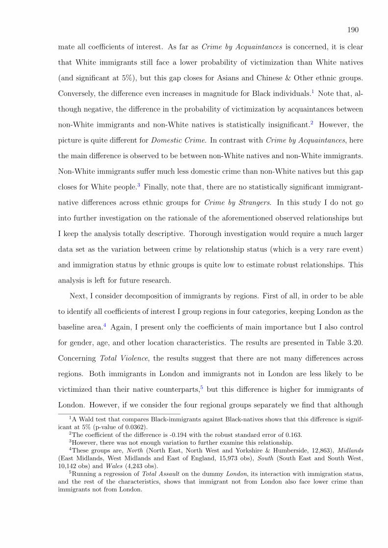
190

mate all coefficients of interest. As far as Crime by Acquaintances is concerned, it is clear

that White immigrants still face a lower probability of victimization than White natives

(and significant at 5%), but this gap closes for Asians and Chinese & Other ethnic groups.

Conversely, the difference even increases in magnitude for Black individuals.1 Note that, al-

though negative, the difference in the probability of victimization by acquaintances between

non-White immigrants and non-White natives is statistically insignificant.2 However, the

picture is quite different for Domestic Crime. In contrast with Crime by Acquaintances, here

the main difference is observed to be between non-White natives and non-White immigrants.

Non-White immigrants suffer much less domestic crime than non-White natives but this gap

closes for White people.3 Finally, note that, there are no statistically significant immigrant-

native differences across ethnic groups for Crime by Strangers. In this study I do not go

into further investigation on the rationale of the aforementioned observed relationships but

I keep the analysis totally descriptive. Thorough investigation would require a much larger

data set as the variation between crime by relationship status (which is a very rare event)

and immigration status by ethnic groups is quite low to estimate robust relationships. This

analysis is left for future research.

Next, I consider decomposition of immigrants by regions. First of all, in order to be able

to identify all coefficients of interest I group regions in four categories, keeping London as the

baseline area.4 Again, I present only the coefficients of main importance but I also control

for gender, age, and other location characteristics. The results are presented in Table 3.20.

Concerning Total Violence, the results suggest that there are not many differences across

regions. Both immigrants in London and immigrants not in London are less likely to be

victimized than their native counterparts,5 but this difference is higher for immigrants of

London. However, if we consider the four regional groups separately we find that although

1A Wald test that compares Black-immigrants against Black-natives shows that this difference is signif-icant at 5% (p-value of 0.0362).

2The coefficient of the difference is -0.194 with the robust standard error of 0.163.3However, there was not enough variation to further examine this relationship.4These groups are, North (North East, North West and Yorkshire & Humberside, 12,863), Midlands

(East Midlands, West Midlands and East of England, 15,973 obs), South (South East and South West,10,142 obs) and Wales (4,243 obs).

5Running a regression of Total Assault on the dummy London, its interaction with immigration status,and the rest of the characteristics, shows that immigrant not from London also face lower crime thanimmigrants not from London.

191

the sign on the immigration-victimization relationship is still negative it turns insignificant.

The only area for which the difference is still significant is Midlands.1 Almost the same

relationships hold for Crime by Acquaintances, with the only difference that now, the dif-

ference between immigrants and natives of London is higher in magnitude and that the

difference is also significant for the regional group South. For Domestic Crime, the results

are very insignificant probably because of the low variation between the dependent variables

and the interaction terms. However, we still find that immigrants not in London are less

likely to be victims of domestic crime than natives not in London.2 Moreover, it is found

that immigrants of Midlands suffer less domestic crime than natives of Midlands.3 Finally,

no statistical relationships are found for Crime by Strangers, even if we control for racially

motivated crime.4

3.7.2 Seriousness of Crime

So far, we have found that if immigrants exhibited the same basic demographic characteristics

with natives, they would face a lower probability of violent victimization but a similar

probability of property victimization. However, we have not made any reference on the

seriousness of crimes they have suffered. In this subsection I exploit information from the

Victim Forms, where all victims were able to rank the “seriousness” of the crimes they

suffered in a scale from 1 (not serious) to 20 (very serious). Since each victim could take up

to six victim forms, I averaged the “seriousness” score for each victim and then I created

1This is the case perhaps because it is the region with the highest number of observations. A Wald testof the difference gives a p-value of 0.0348. For South, the Wald test gives a p-value of 0.115.

2A regression of Domestic Crime on the dummy London, its interaction with immigration status, andthe rest of the characteristics, shows that immigrant not from London face lower crime than natives notfrom London with a coefficient of -0.240 which is statistically significant at 5%.

3The Wald test gives a p-value of 0.03.4Finally, note that further exercises using interactions (which results are not presented here but are

available on request) show that the highest differences between immigrants and natives exist for, residentsof the most deprived areas (although the effect of the interaction term is statistically insignificant), peoplewho rent, people who are less educated, and single individuals (but only for domestic crime). Moreover,there are no interaction effects between gender and immigration status, apart from crime by strangers (oncewe control for racially motivated crime) for which we find that immigrant males suffer less crime thannative male (significant at 5%), but this difference closes for females. In general, it seems that the highestdifferences exist for the most vulnerable groups of immigrants. Perhaps immigrants who believe that theyare in weak positions (lower guardianship or higher proximity) are more in fear of a potential crime againstthem and therefore, decide to balance their position by exhibiting lower exposure. As the findings indicate,the result is to suffer lower crime than their native counterparts, perhaps because the effect of lower exposureoverbalances the effect of higher proximity and lower guardianship. This subject is left for future research.

192

an ordinal variable that takes value ‘1’ if victims believed that the “seriousness” of the

crimes experienced is between 1 and 5 (Not Serious), ‘2’ if it is between 6 and 10 (Relatively

Serious), ‘3’ if it is between 11 and 15 (Serious) and ‘4’ if is between 16 and 20 (Very

Serious).1

It is clear that since this is a measure of perceived “seriousness”, the coefficient of immi-

gration status would be upward biased if for some reasons immigrants tend to score incidents

of the same actual seriousness as being more serious. The results for total crime are pre-

sented on Table 3.21. Specification 1 uses no controls, while in specification 2, in line with

previous regressions, we control for basic demographics and in specification 3 we include

further controls that might be associated with perceived seriousness. What we find is that,

regardless the controls we use (look at specifications 1 to 3), immigrants strongly believe

that crimes they suffer are much more serious than what natives believe. As we mentioned

before, this might not indicate that immigrants are recipients of more serious crimes if they,

for some unobserved reasons, tend to overvalue the seriousness relatively to natives. Using

the cutoff estimates and the estimated coefficients from specification 2, this model predicts

that being an immigrant victim:2 1) decreases the probability for an experienced crime to

be considered as Not Serious (1-5) by 8.3 percentage points, a relative effect of 11%, but

2) increases the probability for a crime to be considered as Relatively Serious (6-10) by 5.3

percentage points, a relative increase of 26%, 3) increases the probability for a crime to be

considered as Serious (11-15) by 2.3 percentage points, but with a relative effect of 56% and

finally, 4) increases the probability for a crime to be considered as Very Serious (16-20) by

0.7 percentage points, which account for an even higher relative effect of 89%. Note that all

these differences are statistically significant at 1%.

Moreover, specification 4 shows that the immigration status dummy has no effect if we

control for ethnic background (but it is still significant at 5% if we include the ethnicity

dummies on specification 3). However, specification 5, where we interact immigration status

1Note that from the 11,208 victims, 66% believed that the victimization incidents they experienced areof seriousness from 1 to 5, 25% from 6 to 10, 7% from 11 to 15 and only 2% from 16 to 20. Moreover, notethat creating an ordinal variable with 8 categories gives very similar results.

2For these predictions we use the representative individual who is a male between 25 and 35 years old,and live in an average deprived urban area in the East of England. The estimated probabilities, differencesand relative effect, are calculated with the “nlcom” command in Statar.

193

with ethnicity dummies, provides further interesting insights. Although White immigrants

do not perceive crimes they suffer as more serious than their native counterparts, non-

White immigrants do. Actually, a regression where we only interact immigration status

with ethnic group White shows that being a non-White immigrant significantly increases

the probability to perceive a crime as more serious relative to a non-White native.1 In

more detail, specification 5 shows that apart from White and Mixed ethnic groups, Black,

Asian and Chinese & Other immigrants value their crime experiences as more serious than

their native counterparts, although the estimated difference is statistically significant (at

5% significance level) only for the group of Asians. Finally, further analysis where we look

at household crime, personal theft and violence separately shows that the above negative

relationship holds for each crime category, but it is a bit less significant for personal crime.2

3.8 Count Data Models

All previous analysis concerned the conditional probability of victimization and provided

some very robust results regarding the difference in the probability of victimization between

immigrants and natives across the different crime types. However, the count nature of the

victimization variable was totally neglected. Considering the count form of the crime vari-

ables and utilizing several count data models could provide some further insights on the

determinants of victimization in general, and particularly, on the immigration-victimization

relationship. For instance, even though immigrants face a lower probability of violent vic-

timization, the implications of our analysis would be very different if, as will be discussed

further below, immigrants experience a higher number of crime incidents than natives.

Count data are directly related to the problem of repeated victimization, as someone is

said to be a “repeated” victim if he/she has suffered more than one incident of the same

crime type within the reference period.3 Together with the causes of a single crime incident,

1The coefficient is 0.292 with a robust standard error of 0.082.2It is actually significant at 10% for violence, but insignificant for personal theft. However, notice that

we only have 1,186 cases of violence and 745 cases of personal theft. Full results are available from theauthor on request.

3In general criminologists distinguish between the term “repeated victim” and the term “multiple victim”(see, for example, Hope at al, 2001). A person is a multiple victim if he/she suffered more than one typeof crimes in the reference period, regardless of the number of crimes of the same crime type. For instance,a person experiences in the last 12 months both an inside burglary and an assault. However, other studies

194

the understanding of the channels through which repeated victimization occurs has also

received a lot of attention by criminologists, in an attempt to find alternative effective

policies for crime reduction which would in turn allow policy makers to efficiently allocate

scarce resources in the areas where people or households face the greatest risks (see, Sparks,

1981, Farrell, 1992, Farrell, Phillips and Pease, 1995, and Osborn at al, 1996). This is

important, as crime is found to be concentrated among a small group of people and areas

(see, Spelman, 1995, Ellingworth, Farrell and Pease, 1995) and because prior victimization

is found to be a very strong predictor of future victimization (Hindelang, Gottfredson and

Garofalo, 1978, Ellingworth at al, 1997, and Wittebrood and Nieuwbeerta, 2000). Several

researchers have attempted to understand the process of repeated victimization by using

count data models (see, for example, Nelson, 1980, Tseloni and Pease, 2003, 2004).

There are a couple of reasons to expect that the process of having suffered a single

incident is to some extent different from the process of repeated victimization. According to

this, we implicitly allow for the effects of the characteristics associated with victimization to

differ between the probability of a single incident and the number of incidents conditional

on victimization. First of all, criminologists have made some effort towards understanding

whether there is some kind of dependence among crimes suffered by the same individuals

or, it is just that the characteristics associated with higher risks responsible for a first crime

incident persist over time resulting in further actions against them. Event-dependence among

sequences of crimes against the same individuals could be possible if a first crime initiates

a positive or a negative “contagious” process. For example, a positive “contagion” (mostly

for household crimes) could be the consequence of some kind of transmission of information

amongst offenders concerning the vulnerability or attractiveness of some targets. Differently,

a positive “contagion” for violent victimization could exist if following the victimization

incident, victims choose to revenge or retaliate, which in turn would expose the victim to

further violence. On the other hand, negative “contagion” would be the result of reevaluation

of strategies following an incident, which would make victims, for instance, to increase their

guardianship or reduce their exposure. However, we need to stress that these dynamics cannot

do not distinguish between these two terms (see, Farrell, 1992). In the present study, the victim is said tobe “repeated” if he/she suffered more than one crime (depending on the crime type I consider) within thereference period of 12 months prior to the interview.

195

be identified in the absence of panel data, which is the case in the present study. This is

because, firstly, we are not able to observe when the first action occurred, and secondly

because the cross-section models used in this study assume independency of the incidents.1

Secondly, the effect of the regressors could be different between the two processes (vic-

timization or not, and the number of incidents conditional on victimization), if there is

unobserved heterogeneity within the same variables which is associated with differential

victimization across the two processes. As an example, consider the relationship between

gender and violence. As males exhibit a much higher exposure, the victimization probability

is much higher for them. However, the picture could be different if we consider only victims,

as females might be victimized more frequently, perhaps because of domestic violence. A

similar story can be considered for immigrants. Given that immigrants are generally more

vulnerable (lower risk for offenders) they decide to set strategies associated with lower ex-

posure on crime. As a result, according to the findings of the previous sections, immigrants

are on average less likely to be victims of violence. However, if we consider the popula-

tion of the victims only, it might be the case that here we have either the immigrants that

failed to successfully set the low exposure strategies, or groups of immigrants whose cultural

characteristics are associated with higher exposure relative to the groups of less victimized

immigrants. According to this, immigrant victims could be equally or even more victimized

than native victims. Therefore, if the above were true, we would expect that the coefficient

in the count data models to be less negative than in binary models, as the number of the

incidents is also taken into account.

In this study I consider Poisson and Negative Binomial 2 models, as the latter also

takes into account over-dispersion (by allowing for an unobserved gamma distributed error)

which, as described before, is evident in my victimization data.2 However, the nature of

victimization data gives rise to two issues that require special attention. Firstly, as crime

1We need to note that although the Negative Binomial distribution is consistent with a count generationprocess with positive “contagion”, in the absence of panel data we cannot distinguish between “contagion”and “heterogeneity” among different groups. For interesting details on the genesis and other aspects ofthe Negative Binomial distribution the reader may refer to Johnson, Kemp and Kotz (2005), Cameron andTrivedi (1998), and Winkelmann (2008).

2It is well known that the Poisson distribution assumes equi-dispersion meaning that the first two mo-ments are equal to each other. For more details on count data models refer to Winkelmann (2008) andCameron and Trivedi (1998).

196

is a rare event (at least if we want to consider the different crime types separately), the

number of zeroes is very large. Moreover, the (very few) positives are quite dispersed for

most of the crime categories. This has harmful consequences on the robustness of the count

data estimators. Secondly, there are few cases of victims that reported extreme number of

crimes.1 Count data models are very sensitive to these cases, particularly when the positive

counts are too few to identify the parameters of the variables assumed to affect the mean.

I deal with the second issue using two different approaches. Firstly, I censor the crime

variable at different points of the violent crime distribution and then I use a Poisson model

with a modified likelihood function that takes into account the censoring in the dependent

variable (for details in censored count data, see, Terza, 1985, and Brannas, 1992). Not only

does this strategy tests for the robustness of the estimates of the conventional count data

models, but it also adds some robustness to the estimator.2

Furthermore, I use the “Quantile Estimator for counts” developed by Machado and San-

tos Silva (2005) and successfully used by Winkelmann (2006), Booth and Kee (2006), and

Miranda (2008). Usual quantile estimators are developed for continuous data (see, Koenker

and Bassett, 1978) and are not available for counts, or other discrete choice variables. How-

ever, very briefly, Machado and Santos Silva (2005) suggest a method that overcome this

problem by adding a uniformly distributed noise to the count outcome (a method called “jit-

tering”), which artificially generates the required smoothness of a continuous variable. Then,

quantile estimation proceeds by using standard quantile techniques. Moreover, they propose

averaging out the uniformly distributed noise by considering m jittering samples which in-

creases efficiency of the estimator.3 Utilization of this estimator serves two purposes. Firstly,

the quantiles are insensitive to the extreme cases, and secondly, we can estimate the effect

of the regressors on different parts of the distribution (which might be different according

to the repeated victimization theories). However, as the number of zeroes in my dependent

1The maximum they could report in each victim form was 97 crimes. Therefore, in the extreme, someonecould report 582 crimes.

2On the other hand, the results of censored count count data models are at same time less “robust”because the results of the Poisson Pseudo Maximum Likelihood (see, Gourieroux, Monfort, and Trognon,1984) do not hold. Thus, the censored model would be misspesified, if the remaining counts above theconsidered cut-off point do not follow the poisson distribution. In the contrary, the Poisson distribution onlyrequires correct specification of the conditional mean, with valid inference given by the Pseudo MaximumLikelihood standard errors, or differently, Eicker-White robust standard errors.

3For details on this estimator refer to Machado and Santos Silva (2005).

197

variables is very high, it is more reasonable to look at the effects of the variables on very

high quantiles.

Alternatively, a model that would be also consistent with the story of differential repeated

victimization could be a hurdle (two-part) model, where the “hurdle” is set at no crimes.

According to this model (see, Mullahy, 1986), zeroes or positives (without distinction on the

number of incidents) are generated by a distribution appropriate for binary choice models. If

the realization is positive, the hurdle is crossed, and positives are generated by a truncated

at zero (see, Grogger and Carson, 1991, and Gurmu, 1991) distribution for counts, such

as the truncated at zero Poisson or the truncated at zero Negative Binomial distribution.1

Hence, this model explicitly allows to separately model the binary outcome (victimized or

not) from the positives (number of incidents given victimization, or differently, repeated

victimization).2 Therefore, we can directly observe whether the independent variables have

different effects below and above the hurdle (thus, at different parts of the distribution).

Again, the very low number of positives and the extreme reports by some individuals will

constraint my analysis. Nevertheless, as an alternative and in line with the Censored-Poisson

model, I develop a two-part model for censored counts. Details on the probability and

likelihood functions of this modified Hurdle-Censored Poisson model are presented in the

Appendix.

In this study I only present results on violent victimization, which was the centre of

attention in the main analysis. Furthermore, because of the aforementioned large number

of zeroes, the estimation analysis is not so reliable if we further decompose violent crime by

relationship type, particularly when I use the Hurdle-Censored Poisson estimator. Thus, I

mainly present results on total violent victimization and I refer to results of the separate

groups when necessary.3 Before presenting the count data results, the complete distribution

together with the three unconditional moments of the violent crime variables are presented

1Count hurdle models (together with some modified count hurdle models) are very successfully used inhealth economic literature (see, for example Pohlmeier, Ulrish, 1995, and Gurmu, 1997), or other contexts(see, for example, Gurmu and Trivedi, 1996, Arulampalam, Booth 1997, Santos Silva and Covas 2000, andHelstrom, 2006).

2By taking into account the different data generating process below the hurdle and above the hurdle, weexplicitly take into account the exceptional nature of zeroes. Moreover, the hurdle model accounts for bothover-dispersion and under-dispersion.

3All results that are not present here are available from the author upon request.

198

in Table 3.22. It is clear that Total Violence is a rare event as only 3.54% of respondents

reported at least on violent incidence. It is also clear that incidents of violence are highly

dispersed and skewed to the right, a feature driven by Domestic Crime and Crime by Ac-

quaintances, as Crime by Strangers is generally concentrated on the first 10 counts.

The results of the count models are presented in Tables 3.23, 3.24 and 3.25. The second

and the third specifications of Table 3.23 depict the results of the conventional Poisson and

Negative Binomial 2 (NB2) regression models, whereas specification 1 gives simple Logit

results for the sake of comparisons. The rest of the specifications present the Censored-

Poisson model, where we censor the dependent variable at 5, 10, 15, 20 and 25 crimes. Table

3.24 displays the estimates resulting from the Quantile estimator for counts, where we look

at the effect of the variables at the 25th, 50th, 70th, 80th, 90th, 95th, 99th, 99.9th, and

99.99th percentiles of the distribution. We explore unusually high quantiles because, as I

mentioned earlier, it is important to explore the impact of the regressors on the very right

end of the distribution. It is also important to note that my results are obtained using

100 jittered samples. Finally, Table 3.25 shows the results from a simple Hurdle-Poisson

model and the results from the modified Hurdle-Censored Poisson model, where I censor at

5 and 10 crimes.1 Specifically, the first column gives the probability of crossing the hurdle

for which the Poisson distribution is also used,2 the second specification shows the Zero-

Truncated results without censoring and the rest of the specifications provide the findings

of the Zero-Truncated Censored models.

To begin with, apart from the coefficient on Urban and the fact that regional dum-

mies have a smaller effect (relative to London) in NB2, the results of Poisson and NB2 are

fairly similar. According to the NB2 model, there is quite strong evidence in favor of over-

dispersion.3 However, it is important to stress that although the Poisson regression model

assumes equi-dispersion (conditional mean equal to conditional variance), which implies that

1The estimation procedure was numerically unstable when censoring at higher than 10 crimes was con-sidered. This is probably because of the small number of observations above the hurdle (1,190 observations).Therefore, the results of censoring the variable at a higher value are not presented here.

2These estimates are closely comparable to Logit ones. Actually, the Logit probability function can bealso obtained from considering only the zero probability from the Geometric version of the Negative Binomialdistribution for count data (see, Mullahy, 1986).

3In this table, ‘alpha’ is the estimated variance of the gamma distributed unobserved effect. Accordingto the NB2 model the conditional variance of the dependent variable is given by ω = λ + αλ2. As theestimated ‘alpha’ is around 40 and statistically significant, the variance is much higher than the mean.

199

the variance-covariance matrix is misspecified under the presence of over-dispersion, it is ab-

solutely valid even in the cases of very over-dispersed data. This is because, as the results

of the pseudo-maximum likelihood show (see, Gourieroux, Monfort and Trognon, 1984), the

Poisson Maximum Likelihood Estimator consistently estimates the conditional mean and

valid inference for the variance matrix of the estimator is obtained by using robust (Eicker-

White) standard errors.1

Comparing the binary information with the conventional count data models several in-

teresting points emerge that need some discussion. Firstly, we can see that although the

Immigrant coefficient is still negative, it is now insignificant. However, this should not be

interpreted as higher repeated victimization of immigrants without further investigation.

Indeed, the Censored-Poisson models, regardless of the cut-off point of censoring, show that

the effect of immigration is still very significant and not much different in magnitude than

when we use the binary information only. This suggests that the long right tail of the ob-

served distribution affects the precision of the effect of Immigrant on Total Violence. The

results of the Quantile estimator and the Hurdle-Censored Poisson model are relatively in

line with the aforementioned analysis. Regarding the Quantile Estimator results, although

the immigration dummy has no effect on the first quartile and the median, as expected due

to the small number of positives, its effect is negative and significant along the right part of

the distribution. It is also clear that the effect starts diminishing when considering very high

quantiles. Finally, from Table 3.25, the zero-truncated but uncensored Poisson assigns a pos-

itive but very imprecisely estimated coefficient to the immigration dummy which, however,

turns negative in Zero-Truncated Censored models if we censor at 10 crimes. Overall, these

results indicate that the very few observations at the end of the observed distribution reduce

the influence of the immigration dummy. This suggests that if a differential repeated vic-

timization between immigrants and natives exist relatively to the risk of victimization from

the binary choice model, this is only for individuals that suffer a large number of incidents.

Unfortunately, the sample size does not permit further investigation and safer conclusions.

The most striking result is that although being a male increases the probability of suffer-

1However, note that if the true data are truly generated by a Negative Binomial distribution, PoissonPseudo Maximum Likelihood is less efficient.

200

ing a crime, it actually decreases the mean number of crimes. The Hurdle-Poisson models

present this picture clearly. Conditional on being victimized, being a male significantly

decreases the number of incidents. The effect is smaller for the Zero-Truncated Censored

models but still very significant. Further investigation shows that this result is primarily

driven by the relationship between gender and Domestic Crime. Nevertheless, a negative

relationship holds for Crime by Acquaintances too, although it is less significant, but not for

Crime by Strangers. Thus, there is some evidence that although males are more exposed on

the incident of violence, females are more repeatedly victimized. This is probably because

some women are captured in “unhealthy” relationships that bring them in situations of a

constant high risk of victimization.

Finaly, it is also interesting that although the effect of Urban is positive but insignificant

in the binary models, it turns negative in the count models. From the Quantile regressions

we can observe that the effect of Urban is the highest between the 90th and the 95th per-

centiles and then decreases turning negative after the 99th percentile. Similar conclusions are

obtained from examining the Hurdle-Censored Poisson model. Further analysis shows that

this result is driven by the impact of being in an urban area on Crime by Strangers.1 Even

though people in urban areas face a significantly higher risk of victimization by strangers,

repeated victimization by strangers is higher in rural areas if we only victimized individu-

als. This indicates that in rural areas there is a higher concentration of Crime by Strangers

among the same individuals compared to urban areas. This is an interesting finding, but

further research is required to identify the reasons behind this relationship.2

3.9 Conclusion

This study presented a comprehensive analysis of the relationship between immigration

status and victimization in England and Wales using the 2007/08 sweep of the British Crime

Survey.

1Being in urban areas significantly increases the victimization risk, where the estimated coefficient ofUrban in the Logit model is 0.358 with a p-value of 0.005. However, in the Zero-Truncated Poisson thisestimate is negative (-0.647) with a p-value of 0.014.

2Further investigation of these models with regard to the effects of the other variables can result in manyinteresting implications. However, as this paper concentrates on the victimization-immigration relationshipthis analysis is skipped here, but it is subject to future research.

201

Initially, we presented some evidence on the immigration-victimization relationship for

Inside and Outside Burglaries. Immigrants’ households are more at risk of Inside Burglaries

but this is mostly explained by the fact that immigrants reside relatively more than na-

tives in urban and more deprived areas where the incident of an Inside Burglary is highly

more likely. On the other hand, a negative relationship was found between immigrants’

households and the incident of Outside Burglaries. We argued that this is probably because

immigrants possess a smaller amount of properties that are subject to Outside Burglaries

such as, outhouses, garages, etc. This argument was supported with results on assimilation

patterns (earlier immigrants are better settled and therefore, possess more outside properties

than more recent immigrants) and zero-inflation count models (which show that a higher

proportion of immigrants belong to the zero inflation category, meaning that immigrants are

in lower risk just because they own fewer outside properties).

Furthermore, we showed evidence on Personal Thefts, a crime that is of a very different

nature since, although instrumental as well, it entails personal contact. The results indicated

that immigrants are in higher risk of Personal Thefts, but most of this positive association

can be attributed to the fact that they disproportionately reside in the areas of London where

the incident of a Personal Theft is much more probable than any other region in England

and Wales.

Next we presented a series of evidence for Violent Crime, in which this work focuses on.

Violent Crime, as opposed to the aforementioned categories, is an expressive type of crime

where interrelations and interactions between the potential victims and potential offenders

are vital. According to this, personal behaviour is a much stronger predictor for violent vic-

timization than for Personal Thefts and Household Crime. Even after controlling for a rich

set of characteristics associated with violent victimization, the empirical analysis indicated

that immigrants are still at lower risk of violence. A possible explanation, which relies on

the theoretical views of this paper, is that immigrants set strategies (that determine their

lifestyle-exposure and routine activities) that are associated with a lower risk of violent vic-

timization. Nevertheless, a closer examination indicated that the negative association is due

to the lower risk of victimization by Acquaintances and lower risk of Domestic Crime, since

the regression results showed that there is not any association between being an immigrant

202

and crime suffered by Strangers. This result is, at a first glance, not in line with the hypoth-

esis mentioned above, since if immigrants follow a particular lifestyle associated with lower

exposure and therefore, lower crime, we expected to observe a negative association for crime

by strangers as well. Thus, the next section attempted to shed light on the differences in the

estimated immigration-victimization associations across the three (by relationship status)

Violent Crime types.

Firstly, we examined the reporting behaviour of respondents towards Domestic Crime,

as there is evidence that respondents tend to under-report domestic crime in face-to-face

interviews. Thus, if immigrants tend to under-report crime suffered by (ex) family mem-

bers, the observed immigration-victimization association will be downward biased. However,

both strategies that we followed showed no evidence that immigrants under-report Domestic

Crime by more than natives, and therefore, there is no reason to believe that they would

under-report crime by Acquaintances either. Particularly, in the first strategy we used data

on computer-based self-reported crime, as there is evidence that people respond much more

truthfully in computer-based than in face-to-face interviews. The results from computer-

based interviews are in line with the results from face-to-face interviews, that is, immigrants

are significantly less likely to be victims of domestic violence. In the second strategy, we

explored the information on whether respondents’ partners were present during the face-

to-face interviews, as people may under-report domestic crime by more in the presence of

their partner. After a thorough analysis, also comparing with results in crime by acquain-

tances and computer-based self-reports of domestic crime, we concluded that if one group

under-reports, this is the group of natives.

In the second step, the differences in immigration-victimization patterns among Violent

Crime types were attempted to be explained by “racially motivated crime” and “network

effects”. Interestingly, we showed that if we control for (the only 37 cases - 20 for natives and

17 for immigrants - of perceived) racially motivated crime, which is a much more “random”

crime highly associated with ethnic minorities, the risk of suffering a Violent Crime by

Strangers becomes negative and significant at 10%, but not of the magnitude observed

for crime by familiar people and (ex) family members. Next, using the “network effect”

hypothesis, meaning that immigrants increase the number of acquaintances as time in the

203

country increases, we tested whether the lower risk of victimization by Acquaintances that

immigrants face is just because of the fact that the groups of acquaintances are relatively

smaller for more recent immigrants. Therefore, connecting that to assimilation patterns, we

showed that more recent immigrants are actually in lower risk of victimization than earlier

ones. However, showing some further evidence, we argued that the observed assimilation link

was most probably driven by other unobserved assimilation features. If “network effects”

exist, they are relatively weak, and by no means could they explain the observed differences

across violence crime types.

Finally, we considered further reasons that might explain the rest of the difference.

Firstly, crime by strangers is in a sense more “random” than crime by familiar people,

meaning that personal behaviours, and thus social lifestyles, have a smaller effect on the

victimization outcome. Moreover, looking at the behaviour of immigrants as offenders can

provide some interesting insights. For example, according to the “homogamy” principle,

a high proportion of immigrants’ (natives’) acquaintances and family members are immi-

grants (natives) as well. But according to Papadopoulos (2010b), immigrants are (slightly)

less likely to commit violent crimes, and therefore, we expect that, everything else constant,

the risk of victimization by Acquaintances and Domestic Crime would be higher for natives.

Finally, violent behaviour is a direct measure of exposure, and therefore, since immigrants

exhibit a less violent behaviour, they are also of lower risk of violent victimization. However,

this effect is incorporated into the aforementioned general lifestyle activities of immigrants.

Next, we briefly discussed the seriousness of the crimes that victims face. We actually

found that although immigrants are less likely to be victims of violent activity, they consider

the crimes they suffer as more serious than the crimes natives suffer. Of course, if for

any reasons, immigrants tend to perceive crime of the same actual seriousness as more

serious, all results of this section are biased upwards. Moreover, a very brief analysis of

decomposition of immigrants by ethnic status and location did not reveal any important

relationships. However, a much closer examination is required, perhaps using even larger

data sets (by pooling several sweeps from the British Crime Survey), since in the present

study the variation between the crime variables and the different immigrant groups was too

small to obtain robust results.

204

After establishing the above relationship for the probability of victimization we consid-

ered count data models, exploiting the count nature of the Violent Crime variable. Count

data analysis is important because it is directly connected with the concept of repeated vic-

timization. As explained in detail in Section 3.8, some characteristics, such as gender, could

have a different effect on the probability of suffering a crime and on the number of crimes

suffered given victimization. Thus, the implications of our analysis would be very different

if immigrants were disproportionately victims of repeated crimes. Several models were con-

sidered (Poisson, NB2, Censored Poisson, Quantile Estimator for counts, Hurdle-Censored

Poisson) to explore the association between the number of violent victimization incidents

and immigration. Initially, conventional Poisson and NB2 models showed that once we take

the count information into account, immigrant coefficient loses much of its significance and

magnitude. However, this should not be interpreted as differential repeated victimization

by immigrants, as the Censored(-Hurdle) Poisson, and the “Quantile for counts” estimator

showed that this result was driven by the very end of violent crime distribution. This means

that if differential repeated victimization between immigrants and natives exists, it does only

among highly victimized individuals. Therefore, according to these results, the effect of be-

ing an immigrant on victimization is relatively similar in both, the probability of suffering a

crime and the number of crimes suffered. However, data limitations (very few and dispersed

positives) did not allow us to examine the above relationships by relationship status.

Nevertheless, the use of the count information together with appropriate count data

models is very promising and it can provide many interesting insights not only about the

relationship between immigration and victimization but also about the determinants of vic-

timization is general. For instance, we showed evidence that the victimization probability is

higher for males because of their higher exposure, but once considering the victimized indi-

viduals only, females are victimized much more frequently perhaps due to repeated domestic

violence. Further analysis is subject to future research, perhaps considering pooling several

sweeps from the British Crime Survey in order to increase the sample size, and consequently,

the robustness of the estimated relationships.

205

Table 3.1. BCS Crime Codes1

1 This table is taken by the BCS 2008-09 User Guide pages 19 and 20.

206

Table 3.1. Continued

207

Table 3.2. Count Data Tabulations for each Crime Group

Acquisitive Crime

Total Inside Burglary

Outside Burglary

Vehicle Theft

Inside Theft

Outside Theft

Other Theft

N % N % N % N % N % N % N % 0 40,738 86.87 45,805 97.68 46,421 98.99 43,832 93.47 46,774 99.75 45,663 97.38 46,068 98.24 1 4,646 9.91 921 1.96 407 0.87 2,496 5.32 86 0.18 1,001 2.13 742 1.58 2 950 2.03 97 0.21 43 0.09 398 0.85 18 0.04 148 0.32 55 0.12 3 296 0.63 26 0.06 15 0.03 99 0.21 4 0.01 41 0.09 16 0.03 4 120 0.26 12 0.03 1 0.00 35 0.07 4 0.01 19 0.04 6 0.01 5 47 0.1 8 0.02 0 0.00 19 0.04 0 0.00 5 0.01 3 0.01 6 29 0.06 4 0.01 2 0.00 1 0.00 3 0.01 4 0.01 1 0.00 7 17 0.04 3 0.01 1 0.00 5 0.01 1 0.00 3 0.01 0 0.00 8 8 0.02 2 0.00 0 0.00 1 0.00 0 0.00 1 0.00 1 0.00 9 5 0.01 1 0.00 0 0.00 9 0.00 1 0.00 0 0.00 0 0.00

10+ 37 0.08 14 0.01 3 0.00 6 0.01 2 0.00 8 0.02 1 0.00

Criminal Damage Personal Theft Total

(+ Other, Arson) Home Vehicle Total Mugging Theft

N % N % N % N % N % N % 0 43,331 92.40 45,733 97.5 44,421 94.73 46,292 99.00 46,630 99.00 46,549 99.30 1 2,418 5.16 776 1.65 1,776 3.79 554 1.18 228 0.49 333 0.71 2 603 1.29 190 0.41 409 0.87 33 0.07 23 0.05 10 0.02 3 264 0.56 79 0.17 161 0.34 4 0.01 2 0.00 1 0.00 4 105 0.22 33 0.07 48 0.10 2 0.00 3 0.01 0 0.00 5 46 0.10 12 0.03 32 0.07 3 0.01 4 0.01 0 0.00 6 41 0.09 24 0.05 18 0.04 3 0.01 2 0.00 0 0.00 7 9 0.02 2 0.00 3 0.01 1 0.00 0 0.00 0 0.00 8 6 0.01 4 0.01 2 0.00 0 0.00 0 0.00 0 0.00 9 8 0.02 1 0.00 1 0.00 0 0.00 0 0.00 0 0.00

10+ 62 0.01 39 0.08 22 0.05 1 0.00 1 0.00 0 0.00

208

Table 3.3. Descriptive Statistics

Variables Mean Min Max Mis All Native Immigrant

Personal Crime Variables

Violence by Strangers (Binary) 0.011 0.011 0.013 0 1

Violence by Strangers (Count) 0.015 (0.20)

0.015 (0.20)

0.018 (0.20)

0 11

Violence by Acquaintances (Binary) 0.010 0.011 0.006 0 1

Violence by Acquaintances (Count) 0.027 (0.93)

0.027 (0.85)

0.034 (1.47)

0 97

Domestic Violence (Binary) 0.005 0.005 0.003 0 1

Domestic Violence (Count) 0.026 (1.30)

0.028 (1.37)

0.007 (0.17)

0 194

Mugging (Binary) 0.006 0.005 0.008

Mugging (Count) 0.009 (0.46)

0.009 (0.48)

0.010 (0.12)

0 97

Other Personal Theft (Binary) 0.007 0.007 0.011

Other Personal Theft (Count) 0.008 (0.09)

0.007 (0.09)

0.012 (0.112)

0 3

Household Crime Variables

Inside Burglary (Binary) 0.023 0.023 0.030 0 1

Inside Burglary (Count) 0.046 (1.20)

0.044 (1.17)

0.060 (1.48)

0 100

Outside Burglary (Binary) 0.010 0.010 0.007 0 1

Outside Burglary (Count) 0.014 (0.47)

0.015 (0.50)

0.010 (0.15)

0 97

Vehicle Theft (Binary) 0.065 0.064 0.076 0 1

Vehicle Theft (Count) 0.085 (0.40)

0.083 (0.40)

0.099 (0.41)

0 20

Inside, Outside, & Other Thefts (Binary)

0.047 0.047 0.046 0 1

Inside, Outside, & Other Thefts (Count)

0.073 (1.10)

0.074 (1.12)

0.068 (0.94)

0 98

Home Criminal Damage (Binary) 0.025 0.025 0.022 0 1

Home Criminal Damage (Count) 0.075 (1.72)

0.077 (1.74)

0.057 (1.48)

0 97

Vehicle Criminal Damage (Binary) 0.053 0.052 0.055 0 1

Vehicle Criminal Damage (Count) 0.092 (1.03)

0.090 (0.96)

0.106 (1.53)

0 97

Respondent’s Characteristics

Immigrant 0.095 0 1

Age 50.45 (18.58)

51.01 (18.64)

45.17 (17.16)

16 101 66

Gender (female) Male 0.454 0.455 0.444 0 1

Marital Status

Married Cohabiting Single Widowed Divorced Separated

0.476 0.088 0.204 0.115 0.087 0.030

0.470 0.089 0.204 0.119 0.090 0.027

0.527 0.074 0.209 0.071 0.067 0.054

0 0 0 0 0 0

1 1 1 1 1 1

20

209

Table 3.3. Continued

Variables Mean Min Max Mis

All Native Immigrant

Employment Status

Employed Unemployed Inactive Student Inactive Retired Inactive Other

0.562 0.017 0.002 0.281 0.117

0.558 0.016 0.002 0.292 0.112

0.605 0.023 0.004 0.176 0.157

0 0 0 0 0

1 1 1 1 1

64

Education

None O-level / gcse A-lavel /Apprent. Degree /Diploma Other

0.283 0.199 0.170 0.304 0.043

0.287 0.208 0.176 0.289 0.040

0.250 0.112 0.113 0.449 0.076

0 0 0 0 0

1 1 1 1 1

81

Ethnic Group

White Black Asian Chinese / Other Mixed

0.933 0.018 0.031 0.012 0.006

0.976 0.006 0.010 0.004 0.004

0.528 0.133 0.233 0.086 0.019

0 0 0 0 0

1 1 1 1 1

7

Hhd Ref Person’s Characteristics

Immigrant 0.095 0 1

Age 52.60 (17.13)

53.18 (17.10)

47.08 (16.44)

16 101 105

Gender (female) Male 0.624 0.624 0.622 0 1

Marital Status

Married Cohabiting Single Widowed Divorced Separated

0.513 0.090 0.150 0.118 0.095 0.033

0.511 0.092 0.147 0.123 0.097 0.030

0.538 0.070 0.181 0.074 0.076 0.061

0 0 0 0 0 0

1 1 1 1 1 1

23

Employment Status

Employed Unemployed Inactive Student Inactive Retired Inactive Other

0.610 0.011 0.009 0.280 0.089

0.603 0.011 0.007 0.291 0.087

0.675 0.016 0.029 0.177 0.102

0 0 0 0 0

1 1 1 1 1

65

Hhd Caracteristics Tenure Type (Renters)

Owners 0.702 0.719 0.543 0 1 127

Condition (Bad) Indifferent Good Very Good

0.219 0.416 0.332

0.213 0.417 0.339

0.284 0.405 0.264

0 0 0

1 1 1

2746

Relative Condition (Same)

Better Worse

0.085 0.062

0.085 0.062

0.077 0.070

0 0

1 1

3059

Accommodation Type

Detached Semi Detached Terrace Flat/ Maisonette Other

0.265 0.332 0.280 0.119 0.005

0.273 0.339 0.277 0.107 0.005

0.179 0.265 0.316 0.237 0.003

0 0 0 0

1 1 1 1

2549

Location (Other) Main Road Side Road

0.142 0.536

0.142 0.535

0.139 0.548

0 0

1 1

Number of Adults 1.898 (1.898)

1.881 (0.809)

2.061 (0.984)

1 10

Lone Parent 0.051 0.051 0.054 0 1 107

210

Table 3.3. Continued

Variables Mean Min Max Mis

All Native Immigrant

Hours Away 4.587 4.577 4.682 1 6

(index) 127

Years Home 4.902 4.996 4.015 1 7

(index) 4

Years Area 5.475 5.588 4.401 1 7

(index) 1

Neighbor Watching Program 0.272 0.275 0.242 0 1 10743

Income

under £10,000 £10,000-£19,999 £20,000-£29,999 £30,000-£39,999 £40,000-£49,999 £50,000 or more nothing

0.202 0.224 0.175 0.135 0.095 0.153 0.016

0.201 0.227 0.177 0.136 0.096 0.150 0.014

0.205 0.199 0.157 0.133 0.089 0.187 0.030

0 0 0 0 0 0 0

1 1 1 1 1 1 1

10026

Number of Cars 1.265 (0.924)

1.284 (0.925)

1.091 (0.894)

0 4(+)

Motorcycle 0.067 0.070 0.039 0 1

Bicycle 0.444 0.452 0.370 0 1

Area Characteristics

Regions

North East North West Yorkshire East Midlands West Midlands East of England London South East South West Wales

0.066 0.118 0.091 0.111 0.100 0.130 0.077 0.111 0.106 0.091

0.070 0.122 0.095 0.114 0.101 0.129 0.055 0.110 0.109 0.096

0.026 0.076 0.060 0.088 0.091 0.133 0.290 0.123 0.076 0.038

0 0 0 0 0 0 0 0 0 0

1 1 1 1 1 1 1 1 1 1

Urban 0.744 0.730 0.880 0 1

Inner City 0.079 0.069 0.167 0 1

Deprived 5.232 (2.824)

5.161 (2.80)

5.911 (2.93)

1 10

10th percentile 0.109 0.110 0.096 20th 0.108 0.110 0.083 30th 0.115 0.118 0.084 40th 0.110 0.113 0.080 50th 0.098 0.100 0.073 60th 0.104 0.104 0.107 70th 0.098 0.097 0.105 80th 0.090 0.088 0.115 90th 0.088 0.084 0.126 100th percentile 0.082 0.077 0.126

Standard deviations are presented in parentheses.

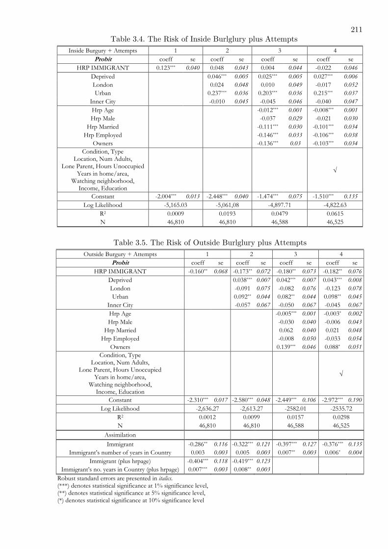
211

Table 3.4. The Risk of Inside Burlglury plus Attempts

Inside Burgury + Attempts 1 2 3 4

Probit coeff se coeff se coeff se coeff se

HRP IMMIGRANT 0.123*** 0.040 0.048 0.043 0.004 0.044 -0.022 0.046

Deprived 0.046*** 0.005 0.025*** 0.005 0.027*** 0.006

London 0.024 0.048 0.010 0.049 -0.017 0.052

Urban 0.237*** 0.036 0.203*** 0.036 0.215*** 0.037

Inner City -0.010 0.045 -0.045 0.046 -0.040 0.047

Hrp Age -0.012*** 0.001 -0.008*** 0.001

Hrp Male -0.037 0.029 -0.021 0.030

Hrp Married -0.111*** 0.030 -0.101*** 0.034

Hrp Employed -0.146*** 0.033 -0.106*** 0.038

Owners -0.136*** 0.03 -0.103*** 0.034

Condition, Type Location, Num Adults,

Lone Parent, Hours Unoccupied Years in home/area,

Watching neighborhood, Income, Education

√

Constant -2.004*** 0.013 -2.448*** 0.040 -1.474*** 0.075 -1.510*** 0.135

Log Likelihood -5,165.03 -5,061,08 -4,897.71 -4,822.63

R2 0.0009 0.0193 0.0479 0.0615

N 46,810 46,810 46,588 46,525

Table 3.5. The Risk of Outside Burlglury plus Attempts

Outside Burgury + Attempts 1 2 3 4

Probit coeff se coeff se coeff se coeff se

HRP IMMIGRANT -0.160** 0.068 -0.173** 0.072 -0.180** 0.073 -0.182** 0.076

Deprived 0.038*** 0.007 0.042*** 0.007 0.043*** 0.008

London -0.091 0.075 -0.082 0.076 -0.123 0.078

Urban 0.092** 0.044 0.082** 0.044 0.098** 0.045

Inner City -0.057 0.067 -0.050 0.067 -0.045 0.067

Hrp Age -0.005*** 0.001 -0.003* 0.002

Hrp Male -0.030 0.040 -0.006 0.043

Hrp Married 0.062 0.040 0.021 0.048

Hrp Employed -0.008 0.050 -0.033 0.054

Owners 0.139*** 0.046 0.088* 0.051

Condition, Type Location, Num Adults,

Lone Parent, Hours Unoccupied Years in home/area,

Watching neighborhood, Income, Education

√

Constant -2.310*** 0.017 -2.580*** 0.048 -2.449*** 0.106 -2.972*** 0.190

Log Likelihood -2,636.27 -2,613.27 -2582.01 -2535.72

R2 0.0012 0.0099 0.0157 0.0298

N 46,810 46,810 46,588 46,525

Assimilation

Immigrant -0.286** 0.116 -0.322*** 0.121 -0.397*** 0.127 -0.376*** 0.135

Immigrant’s number of years in Country 0.003 0.003 0.005 0.003 0.007** 0.003 0.006* 0.004

Immigrant (plus hrpage) -0.404*** 0.118 -0.419*** 0.123

Immigrant’s no. years in Country (plus hrpage) 0.007*** 0.003 0.008** 0.003

Robust standard errors are presented in italics. (***) denotes statistical significance at 1% significance level, (**) denotes statistical significance at 5% significance level, (*) denotes statistical significance at 10% significance level

212

Table 3.6. The Risk of Personal Theft

Personal Theft (Incl. Attempts)

1 2 3 4

Probit coeff se coeff se coeff se coeff se

Immigrant 0.190*** 0.047 0.113* 0.059 0.036 0.060 0.030 0.060

Male -0.082** 0.032 -0.082** 0.033 -0.076** 0.035

Age 26 – 35 -0.339*** 0.053 -0.341*** 0.054 -0.211*** 0.059

Age 36 – 45 -0.472*** 0.054 -0.476*** 0.055 -0285*** 0.065

Age 45 – 56 -0.470*** 0.057 -0.474*** 0.058 -0.273*** 0.069

Age 56 – plus -0.479*** 0.046 -0.477*** 0.046 -0.196*** 0.073

Black 0.186* 0.097 0.064 0.099 0.012 0.100

Asian & Other -0.117 0.083 -0.159* 0.084 -0.163* 0.087

Mixed -0.142 0.202 -0.217 0.202 -0.389* 0.228

Deprived 0.022*** 0.007 0.031*** 0.007 0.027*** 0.008

Urban 0.138*** 0.043 0.076* 0.045 0.073 0.045

Inner City 0.191*** 0.052 0.129** 0.053 0.111** 0.054

North East -0.441*** 0.083 -0.402*** 0.085

North West -0.373*** 0.068 -0.319*** 0.069

Yorkshire -0.364*** 0.073 -0.292*** 0.074 East Midlands -0.361*** 0.070 -0.304*** 0.071

West Midlands -0.322*** 0.069 -0.259*** 0.070

East of England -0.311*** 0.067 -0.259*** 0.069

South East -0.156** 0.065 -0.118* 0.066

South West -0.391*** 0.074 -0.334*** 0.075

Wales -0.504*** 0.083 -0.440*** 0.084

Education, Marital, Employment, Tenure,

Income √

Constant -2.254*** 0.017 -2.083*** 0.062 -1.760*** 0.082 -2.062*** 0.117

Log Likelihood -3,198.49 -3,090.00 -3577.29 -2,974.69

R2 0.0024 0.0362 0.0467 0.0662

N 46,827 46,820 46,820 46,567 Pr(Y=1|Immigrant=1) 0.0195 0.0116 0.0093 0.0040 Pr(Y=1|Immigrant=0) 0.0121 0.0086 0.0084 0.0036

Diff (se)

0.0074*** (0.0021)

0.0030* (0.0018)

0.0009 (0.0015)

0.0003 (0.0007)

Ratio 1.612 1.355 1.104 1.094

Robust standard errors are presented in italics. (***) denotes statistical significance at 1% significance level, (**) denotes statistical significance at 5% significance level, (*) denotes statistical significance at 10% significance level.

213

Table 3.7. The Risk of Violent Victimization

Total Assault (Incl. Attempts) 1 2 3 4

Probit coeff se coeff se coeff se coeff se

Immigrant -0.068 0.044 -0.165*** 0.046 -0.157*** 0.049 -0.151*** 0.051

Male 0.179*** 0.026 0.185*** 0.026 0.240*** 0.029

Age 20 – 24 -0.195*** 0.056 -0.216*** 0.057 -0.200*** 0.063

Age 25 – 34 -0.426*** 0.049 -0.432*** 0.049 -0.354*** 0.061

Age 35 – 44 -0.671*** 0.049 -0.663*** 0.049 -0.542*** 0.064

Age 45 – 54 -0.824*** 0.053 -0.813*** 0.053 -0.659*** 0.070

Age 55 – 64 -1.119*** 0.059 -1.107*** 0.06 -0.924*** 0.079

Age 65 – 74 -1.361*** 0.074 -1.353*** 0.075 -1.139*** 0.098

Age 75 – plus -1.897*** 0.138 -1.889*** 0.139 -1.757*** 0.168

Deprived 0.025*** 0.005 0.010* 0.006

Urban 0.059*** 0.034 0.066* 0.035

Inner City 0.023 0.048 0.010 0.049

Regions √ √ Education, Marital,

Employment, Tenure, Income, Lone Parent, Hhd members

√

Constant -1.948*** 0.013 -1.306*** 0.043 -1.654*** 0.078 -1.861*** 0.127

Log Likelihood -5,536.52 -4,989.29 -4,959.87 -4,777.29

R2 0.0002 0.1002 0.1055 0.1275

N 46,827 46,827 46,827 46,532

Pr(Y=1|Immigrant=1) 0.0219 0.0248 0.0228 0.0265 Pr(Y=1|Immigrant=0) 0.0258 0.0361 0.0327 0.0372

Diff -0.0038* (0.0023)

-0.0113*** (0.0028)

-0.0100*** (0.0029)

-0.0107*** (0.0036)

Ratio 0.8512 0.6872 0.6971 0.7121

Table 3.8. The Risk of Violent Victimization – Including Ethnic Group Dummies

Total Assault (Incl. Attempts) 1 2 3 4

Probit coeff se coeff se coeff se coeff se

Immigrant -0.093* 0.054 -0.114** 0.053 -0.103** 0.055 -0.093* 0.057

Black 0.005 0.102 -0.130 0.105 -0.149 0.108 -0.216** 0.110

Asian 0.053 0.081 -0.156** 0.080 -0.174** 0.081 -0.170** 0.087

Chinese or Other 0.108 0.115 -0.022 0.123 -0.033 0.124 -0.037 0.126

Mixed 0.242* 0.139 -0.020 0.145 -0.035 0.146 -0.116 0.153

Log Likelihood -5,534.43 -4,980.17 -4,950.12 -4,769.33

R2 0.0006 0.1006 0.1061 0.1283

N 46,820 46,818 46,818 46,526

Pr(Y=1|Immigrant=1) 0.0205 0.0281 0.0262 0.0304

Pr(Y=1|Immigrant=0) 0.0256 0.0363 0.0331 0.0373

Diff -0.0051* (0.0023)

-0.0082*** (0.0035)

-0.0069** (0.0034)

-0.0070* (0.0041)

Ratio 0.8015 0.7740 0.7919 0.8132

Robust standard errors are presented in italics. (***) denotes statistical significance at 1% significance level, (**) denotes statistical significance at 5% significance level, (*) denotes statistical significance at 10% significance level.

214

Table 3.9. The Risk of Domestic Violence

Domestic (Incl. Attempts)

1 2 3 4

Probit coeff se coeff se coeff se coeff se

Immigrant -0.177* 0.091 -0.248** 0.100 -0.219** 0.107 -0.207* 0.112

Male -0.438*** 0.056 -0.419*** 0.057 -0.337*** 0.061

Age 26 – 35 0.123* 0.069 0.167** 0.074 0.114 0.081

Age 36 – 45 -0.131* 0.073 -0.121 0.082 -0.138 0.09

Age 45 – 56 -0.346*** 0.087 -0.335*** 0.104 -0.283** 0.115

Age 56 – plus -0.794*** 0.090 -0.682*** 0.115 -0.646*** 0.14

Deprived 0.027*** 0.010 0.017 0.010 -0.003 0.011

Urban -0.005 0.060 -0.015 0.062 0.003 0.063

Inner City 0.086 0.085 0.090 0.087 0.065 0.089

Regions √ √ √ Cohabiting 0.129 0.097 0.136 0.098

Single 0.363*** 0.073 0.238*** 0.084

Widowed -0.093 0.195 -0.204 0.194

Divorced 0.621*** 0.084 0.450*** 0.096

Separated 0.882*** 0.092 0.711*** 0.106

Education, Employment, Tenure, Income,

Lone Parent, Hhd members √

Constant -2.556*** 0.023 -2.668*** 0.150 -2.954*** 0.166 -2.673*** 0.226

Log Likelihood -1,492.38 -1,345.71 -1,283.47 -1,232.80

R2 0.0014 0.0996 0.1412 0.1684

N 46,827 46,827 46,811 46,532

Pr(Y=1|Immigrant=1) Pr(Y=1|Immigrant=0)

Diff (se) ratio

0.0031 0.0053 -0.0022** (0.001) 0.593

0.0041 0.0084 -0.0042** (0.002) 0.494

0.0017 0.0034 -0.0017**

(0.001) 0.505

0.0011 0.0022 -0.0011*

(0.001) 0.511

Robust standard errors are presented in italics. (***) denotes statistical significance at 1% significance level, (**) denotes statistical significance at 5% significance level, (*) denotes statistical significance at 10% significance level.

215

Table 3.10. The Risk of Victimization suffered by Acqaintances

By Acquaintances (Incl. Attempts)

1 2 3 4

Probit coeff se coeff se coeff se coeff se

Immigrant -0.209*** 0.070 -0.299*** 0.078 -0.274*** 0.081 -0.165* 0.087

Male 0.198*** 0.037 0.219*** 0.040 0.222*** 0.041

Age 26 – 35 -0.384*** 0.050 -0.225*** 0.056 -0.224*** 0.056

Age 36 – 45 -0.589*** 0.053 -0.391*** 0.064 -0.398*** 0.064

Age 45 – 56 -0.722*** 0.061 -0.484*** 0.077 -0.494*** 0.077

Age 56 – plus -1.18*** 0.064 -0.896*** 0.095 -0.91*** 0.096

Deprived 0.031*** 0.008 0.011 0.008 0.013 0.008

Urban -0.022 0.047 -0.012 0.049 -0.005 0.049

Inner City 0.009 0.068 -0.003 0.069 -0.003 0.070

Regions √ √ √

Education, Marital, Employment, Tenure, Income, Lone Parent, Hhd members

√ √

Black -0.193 0.162

Asian -0.582*** 0.184

Other -0.188 0.200

Mixed -0.056 0.189

Constant -2.300*** 0.018 -2.121*** 0.105 -2.348*** 0.161 -2.332*** 0.163

Log Likelihood -2,675.70 -2,392.23 -2,297.46 -2,289.76

R2 0.0019 0.1076 0.1301 0.1330

N 46,827 46,827 46,532 46,526

Pr(Y=1|Immigrant=1) 0.0060 0.0049 0.0032 0.0046

Pr(Y=1|Immigrant=0) 0.0107 0.0112 0.0072 0.0074

Diff -0.0047*** (0.0013)

-0.0063***

(0.0016) -0.0039*** (0.0013)

-0.0028** (0.0014)

Ratio 0.564 0.438 0.451 0.625

Table 3.11. The Risk of Victimization suffered by Strangers

By Strangers (plus Attempts) 1 2 3 4

Probit coeff se coeff se coeff se coeff se

Immigrant 0.084 0.053 0.010 0.056 -0.004 0.059 -0.009 0.061

Male 0.441*** 0.038 0.444*** 0.038 0.411*** 0.041

Age 26 – 35 -0.341*** 0.05 -0.339*** 0.051 -0.279*** 0.057

Age 36 – 45 -0.518*** 0.052 -0.506*** 0.052 -0.402*** 0.062

Age 45 – 56 -0.672*** 0.06 -0.658*** 0.061 -0.543*** 0.074

Age 56 – plus -1.029*** 0.058 -1.012*** 0.058 -0.795*** 0.088

Deprived 0.011 0.007 0.015* 0.008

Urban 0.138*** 0.048 0.136*** 0.049

Inner City -0.015 0.066 -0.007 0.067

Regions √ √

Other regressors (as for by acquaintance crime)

√

Constant -2.304*** 0.018 -2.013*** 0.041 -2.223*** 0.094 -2.565*** 0.154

Log Likelihood -2,806.62 -2,534.25 -2,525.73 -2,456.38

R2 0.0004 0.0974 0.1005 0.1127

Robust standard errors are presented in italics. (***) denotes statistical significance at 1% significance level, (**) denotes statistical significance at 5% significance level, (*) denotes statistical significance at 10% significance level.

216

Table 3.12. A Trivariate Probit Model for Violent Victimization

Trivariate Probit (300 draws)

1st Equation Domestic

2nd Equation By Acquaintances

3rd Equation By Strangers

coeff se coeff se coeff se

Immigrant -0.213** 0.089 -0.298*** 0.077 -0.013 0.059

Male -0.433*** 0.054 0.195*** 0.037 0.445*** 0.038

Age 26 – 35 0.118* 0.068 -0.382*** 0.050 -0.338*** 0.051

Age 36 – 45 -0.142** 0.072 -0.586*** 0.053 -0.504*** 0.052

Age 45 – 56 -0.324*** 0.081 -0.724*** 0.061 -0.665*** 0.061

Age 56 – plus -0.805*** 0.091 -1.178*** 0.063 -1.008*** 0.058

Deprived 0.027*** 0.010 0.030*** 0.008 0.011 0.007

Urban 0.002 0.060 -0.023 0.047 0.140*** 0.048

Inner City 0.086 0.084 0.004 0.068 -0.010 0.066

North East 0.230 0.152 0.271*** 0.101 0.088 0.093

North West 0.255* 0.135 0.107 0.097 0.019 0.083

Yorkshire 0.421*** 0.133 0.177* 0.099 -0.023 0.090

East Midlands 0.455*** 0.131 0.166** 0.098 0.112 0.082

West Midlands 0.344*** 0.134 0.237** 0.096 0.021 0.085

East of England 0.211* 0.136 0.086 0.099 0.027 0.083

South East 0.306** 0.136 0.206** 0.099 0.051 0.085

South West 0.404*** 0.136 0.069 0.104 0.046 0.087

Wales 0.391*** 0.139 0.183* 0.103 0.033 0.091

Constant -2.660*** 0.144 -2.118*** 0.105 -2.231*** 0.094

Log Likelihood -6,254.93

N 46,827

Rho between 1st & 2nd 0.153*** 0.058 LR test for Rho12=Rho13=Rho23=0

Rho between 1nd & 3rd 0.013 0.059 chi2(3)=17.48

Rho between 2nd & 3rd 0.142*** 0.046 Prob>chi2=0.0006

Robust standard errors are presented in italics. (***) denotes statistical significance at 1% significance level, (**) denotes statistical significance at 5% significance level, (*) denotes statistical significance at 10% significance level.

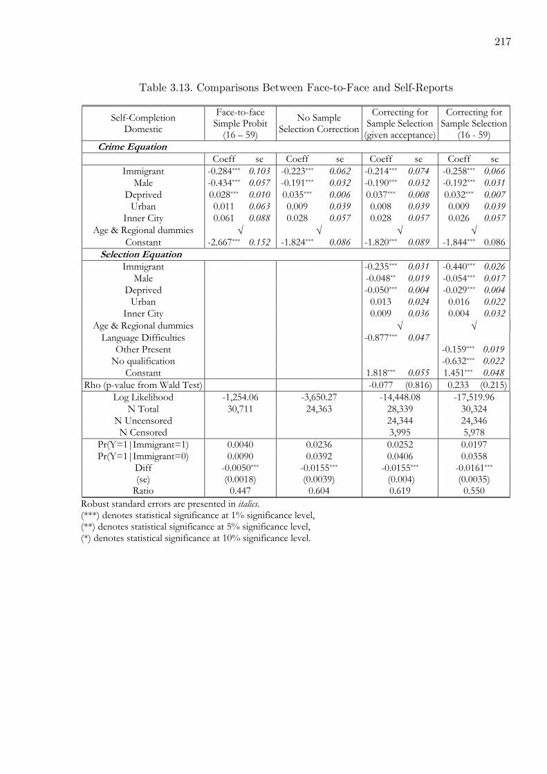
217

Table 3.13. Comparisons Between Face-to-Face and Self-Reports

Self-Completion Domestic

Face-to-face Simple Probit (16 – 59)

No Sample Selection Correction

Correcting for Sample Selection (given acceptance)

Correcting for Sample Selection (16 - 59)

Crime Equation

Coeff se Coeff se Coeff se Coeff se

Immigrant -0.284*** 0.103 -0.223*** 0.062 -0.214*** 0.074 -0.258*** 0.066

Male -0.434*** 0.057 -0.191*** 0.032 -0.190*** 0.032 -0.192*** 0.031

Deprived 0.028*** 0.010 0.035*** 0.006 0.037*** 0.008 0.032*** 0.007

Urban 0.011 0.063 0.009 0.039 0.008 0.039 0.009 0.039

Inner City 0.061 0.088 0.028 0.057 0.028 0.057 0.026 0.057

Age & Regional dummies √ √ √ √ Constant -2.667*** 0.152 -1.824*** 0.086 -1.820*** 0.089 -1.844*** 0.086

Selection Equation

Immigrant -0.235*** 0.031 -0.440*** 0.026

Male -0.048** 0.019 -0.054*** 0.017

Deprived -0.050*** 0.004 -0.029*** 0.004

Urban 0.013 0.024 0.016 0.022

Inner City 0.009 0.036 0.004 0.032

Age & Regional dummies √ √ Language Difficulties -0.877*** 0.047

Other Present -0.159*** 0.019

No qualification -0.632*** 0.022

Constant 1.818*** 0.055 1.451*** 0.048

Rho (p-value from Wald Test) -0.077 (0.816) 0.233 (0.215)

Log Likelihood -1,254.06 -3,650.27 -14,448.08 -17,519.96

N Total 30,711 24,363 28,339 30,324

N Uncensored 24,344 24,346

N Censored 3,995 5,978

Pr(Y=1|Immigrant=1) 0.0040 0.0236 0.0252 0.0197 Pr(Y=1|Immigrant=0) 0.0090 0.0392 0.0406 0.0358

Diff (se)

-0.0050*** (0.0018)

-0.0155*** (0.0039)

-0.0155*** (0.004)

-0.0161*** (0.0035)

Ratio 0.447 0.604 0.619 0.550

Robust standard errors are presented in italics. (***) denotes statistical significance at 1% significance level, (**) denotes statistical significance at 5% significance level, (*) denotes statistical significance at 10% significance level.

218

Table 3.14.A. The Presence of the Partner – Probit Estimates⊕

Coeff se Coeff se Coeff se

Domestic Face-to-face 1 2 3

Immigrant -0.227** 0.102 -0.281** 0.110 -0.275** 0.119 Partner Present -0.408*** 0.093 -0.314*** 0.100 -0.125 0.113

Immigrant & Partner Present 0.446** 0.235 0.335 0.254 0.377 0.256

Domestic Self-completion 1 2 3

Immigrant -0.187*** 0.062 -0.209*** 0.066 -0.186*** 0.070 Partner Present -0.157*** 0.054 -0.118** 0.056 0.067 0.061

Immigrant & Partner Present 0.006 0.183 -0.067 0.186 -0.023 0.190

Acquaintance 1 2 3

Immigrant -0.204*** 0.075 -0.285*** 0.083 -0.249*** 0.084 Partner Present -0.237*** 0.058 -0.131** 0.062 0.005 0.068

Immigrant & Partner Present 0.007 0.213 -0.049 0.226 -0.021 0.226

Robust standard errors are presented in italics. (***) denotes statistical significance at 1% significance level, (**) denotes statistical significance at 5% significance level, (*) denotes statistical significance at 10% significance level.

Table 3.14.B. The Presence of the Partner – Predictions

PREDICTIONS Pr(y=1) Difference

(s.e) Ratio

Pr(y=1) Difference

(s.e) Ratio

Pr(y=1) Difference

(s.e) Ratio

Domestic Face-to-face 1 2 3

Immigrant & Partner Present 0.0034 0.0004 (0.0022)

0.0089 0.0005 0.0069 0.0036 (0.0043)

Immigrant & NO Partner Present 0.0031 1.119 0.0084 1.060 0.0033 2.075

Native & Partner Present 0.0017 -0.0043*** (0.0006)

0.0077 -0.0097*** (0.0029)

0.0052 -0.0022 (0.0019)

Native & NO Partner Present 0.0060 0.291 0.0174 0.440 0.0074 0.702

Domestic Self-completion 1 2 3

Immigrant & Partner Present Immigrant & NO Partner Present

Native & Partner Present Native & NO Partner Present

Acquaintance 1 2 3

Immigrant & Partner Present 0.0034 -0.0033 (0.0024)

0.0032 -0.0022 (0.0023)

0.0033 -0.0002 (0.0022)

Immigrant & NO Partner Present 0.0067 0.513 0.0054 0.588 0.0035 0.953

Native & Partner Present 0.0061 -0.0055*** (0.0011)

0.0083 -0.0035*** (0.1185)

0.0073 0.0001 (0.0014)

Native & NO Partner Present 0.0116 0.524 0.0118 0.704 0.0072 1.014

⊕ Specification 2 also includes age, gender, and area dummies. Specification 3 further includes marital, education, and employment status dummies.

219

Table 3.15. Tabulation of Racially Motivated Crime by Relationship Type

Racially Motivated Crime No Yes

Domestic 237 (99.58%) 1 (0.42%) By Acquaintances 481 (100.0%) 0 (0.00%) By Strangers 472 (92.73%) 37 (7.27%) Immigrants 42 (71.19%) 17 (28.81%) Natives 430 (95.56%) 20 (4.44%)

Table 3.16. Mean Comparison of Racially Motivated Crime by Relationship Type

Mean Comparisons Immigrants Natives Diff Ratio

Crime by Strangers

Without controlling for RMC 0.0132 0.0106 0.0026 1.244

After controlling for RMC 0.0094 0.0102 -0.0007 0.930

Acquaintances 0.0060 0.0107 -0.0047 0.564***

Domestic 0.0031 0.0053 -0.0022 0.593*

Table 3.17. Probit Models before and after controlling for Racially Motivated Crime

Strangers (No Control for RMC)

Strangers (Control for RMC)

Acquaintances Domestic

Probit Coeff se Coeff se Coeff se Coeff se

Immigrant -0.004 0.059 -0.122* 0.067 -0.299*** 0.078 -0.248** 0.100

Male 0.444*** 0.038 0.438*** 0.039 0.198*** 0.037 -0.438*** 0.056

Age 26 – 35 -0.339*** 0.051 -0.341*** 0.052 -0.384*** 0.05 0.123* 0.069

Age 36 – 45 -0.506*** 0.052 -0.531*** 0.054 -0.589*** 0.053 -0.131* 0.073

Age 45 – 56 -0.658*** 0.061 -0.641*** 0.062 -0.722*** 0.061 -0.346*** 0.087

Age 56 – plus -1.012*** 0.058 -1.013*** 0.06 -1.180*** 0.064 -0.794*** 0.09

Deprived 0.011 0.007 0.005 0.007 0.031*** 0.008 0.027*** 0.01

Urban 0.138*** 0.048 0.141*** 0.049 -0.022 0.047 -0.005 0.06

Inner City -0.015 0.066 -0.013 0.069 0.009 0.068 0.086 0.085

Regions◊ √ √ √ √ Constant -2.223*** 0.094 -2.176*** 0.095 -2.121*** 0.105 -2.668*** 0.150

Log Likelihood -2,525.73 -2,375.9717 -2,392.23 -1,345.71

R2 0.1005 0.0997 0.1076 0.0996

N 46,827 46,827 46,827 46,827 Pr(Y=1|Immigrant=1) Pr(Y=1|Immigrant=0)

Diff (se) Ratio

0.0189 0.0191 -0.0002 (0.0027) 0.990

0.0129 0.0175 -0.0046** (0.0023) 0.736

0.0049 0.0112 -0.0063***

(0.0016) 0.438

0.0041 0.0084 -0.0042** (0.0020) 0.494

Robust standard errors are presented in italics. (***) denotes statistical significance at 1% significance level, (**) denotes statistical significance at 5% significance level, (*) denotes statistical significance at 10% significance level.

◊ Regions’ effect is jointly insignificant for crime by strangers.

220

Table 3.18. Network Effects and Assimilation Patterns

Linear Trend (Acquaintnaces)

(1)

Quadratic Trend (Acquaintances)

(2)

Dummies (Acquaintances)

(3)

Linear Trend (Domestic) (4)

Quadratic Trend (Strangers NO RMC) (5)

Probit Coeff se Coeff se Coeff se Coeff se Coeff se

Immigrant -0.405*** 0.106 -0.646*** 0.165 -0.587*** 0.157 -0.342** 0.151

Number of Years in Country 0.006* 0.004 0.038** 0.017 0.015*** 0.005 0.029* 0.015

Number of Years in Country2 -0.0006* 0.0004 -0.0006** 0.0003

Immigrant 1 – 10 -0.388*** 0.114

Immigrant 11 - 20 -0.315* 0.169

Immigrant 21 - 40 -0.089 0.136

Immigrant 41 more -0.255 0.228

Male 0.198*** 0.037 0.199*** 0.037 0.199*** 0.037 -0.439*** 0.055 0.439*** 0.039

Age 26 – 35 -0.385*** 0.050 -0.387*** 0.050 -0.386*** 0.050 0.124* 0.069 -0.343*** 0.052

Age 36 – 45 -0.594*** 0.053 -0.598*** 0.053 -0.595*** 0.053 -0.142* 0.073 -0.537*** 0.055

Age 45 – 56 -0.730*** 0.061 -0.732*** 0.061 -0.730*** 0.061 -0.371*** 0.087 -0.647*** 0.062

Age 56 – plus -1.191*** 0.065 -1.184*** 0.064 -1.184*** 0.064 -0.833*** 0.092 -1.011*** 0.060

Deprived 0.031*** 0.007 0.031*** 0.007 0.031*** 0.007 0.027*** 0.010 0.005 0.007

Urban -0.022 0.047 -0.022 0.047 -0.021 0.047 -0.005 0.060 0.142*** 0.049

Regions √ √ √ √ √

Constant -2.116*** 0.105 -2.121*** 0.105 -2.119*** 0.105 -2.649*** 0.149 -2.179*** 0.096

Log Likelihood -2,391.29 -2,389.52 -2,391.16 -1,341.63 -2,373.892

R2 0.1079 0.1086 0.1079 0.1022 0.1004

N 46,808 46,808 46,808 46,808 46,771

Marginal Effects∇∇∇∇

1)Pr(Y=1|Immigrant=0) 0.0190 0.0190 0.0189 0.0170 0.0173

2)Pr(Y=1|Immigrant=1) 0.0066 0.0033 0.0034 0.0071

Difference (at 0 years) 2 - 1 -0.0124*** 0.0028 -0.0157*** 0.0030 -0.0136*** 0.0033 -0.0103*** 0.0033

Difference (after 10 years) -0.0112*** 0.0026 -0.0109*** 0.0027 -0.0117*** 0.0031 -0.0040 0.0027

Difference (after 20 years) -0.0098*** 0.0025 -0.0055 0.0038 -0.0088*** 0.0030 0.0008 0.0041

Difference (after 30 years) -0.0082*** 0.0028 -0.0029 0.0045 -0.0047 0.0034 0.0013 0.0049

Difference (after 40 years) -0.0064* 0.0035 -0.0051 0.0050 0.0012 0.0052 -0.0029 0.0044

Difference (after 50 years) -0.0043 0.0049 -0.0104 0.0063 0.0092 0.0090 -0.0092** 0.0045

Difference (after 60 years) -0.0019 0.0068 -0.0154*** 0.0056 0.0201 0.0152 -0.0142*** 0.0039

Difference (after 70 years) 0.0009 0.0093 -0.0181*** 0.0037 0.0344 0.0240 -0.0166*** 0.0030

Diff. Immigrant 1 – 10 -0.0121*** 0.0029

Diff. Immigrant 11 - 20 -0.0105** 0.0043

Diff. Immigrant 21 - 40 -0.0038 0.0053

Diff. Immigrant 41 more -0.0091 0.0062

Robust standard errors are presented in italics. (***) denotes statistical significance at 1% significance level, (**) denotes statistical significance at 5% significance level, (*) denotes statistical significance at 10% significance level.

∇ The marginal effects for crime by acquaintances and crime by strangers are calculated for a male, 26 to 35 years old, in an average deprived and urban area in East of England. Note that the average ‘number of years in the country’ for an immigrant is 26 years. For domestic crime the marginal effects are calculation for a person with characteristics as before, but female.

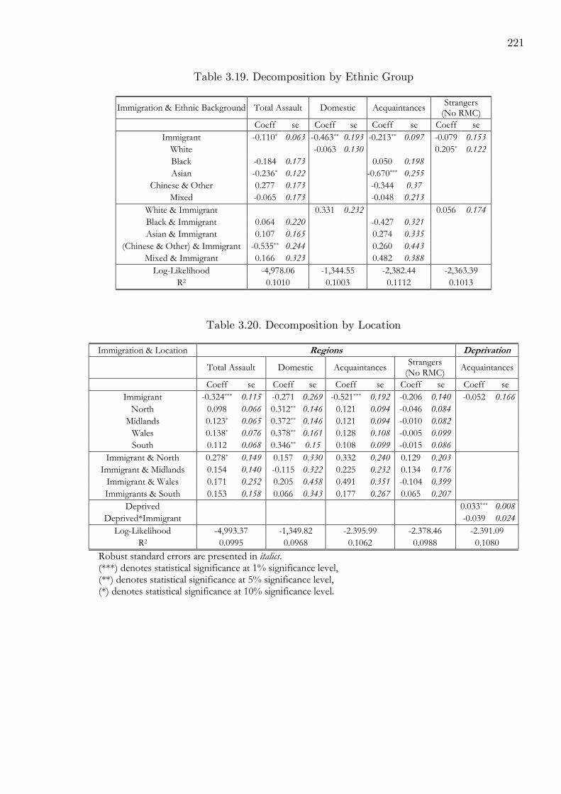
221

Table 3.19. Decomposition by Ethnic Group

Immigration & Ethnic Background Total Assault Domestic Acquaintances Strangers (No RMC)

Coeff se Coeff se Coeff se Coeff se

Immigrant -0.110* 0.063 -0.463** 0.193 -0.213** 0.097 -0.079 0.153

White -0.063 0.130 0.205* 0.122

Black -0.184 0.173 0.050 0.198

Asian -0.236* 0.122 -0.670*** 0.255

Chinese & Other 0.277 0.173 -0.344 0.37

Mixed -0.065 0.173 -0.048 0.213

White & Immigrant 0.331 0.232 0.056 0.174

Black & Immigrant 0.064 0.220 -0.427 0.321

Asian & Immigrant 0.107 0.165 0.274 0.335

(Chinese & Other) & Immigrant -0.535** 0.244 0.260 0.443

Mixed & Immigrant 0.166 0.323 0.482 0.388

Log-Likelihood -4,978.06 -1,344.55 -2,382.44 -2,363.39

R2 0.1010 0.1003 0.1112 0.1013

Table 3.20. Decomposition by Location

Immigration & Location Regions Deprivation

Total Assault Domestic Acquaintances Strangers (No RMC)

Acquaintances

Coeff se Coeff se Coeff se Coeff se Coeff se

Immigrant -0.324*** 0.115 -0.271 0.269 -0.521*** 0.192 -0.206 0.140 -0.052 0.166

North 0.098 0.066 0.312** 0.146 0.121 0.094 -0.046 0.084

Midlands 0.123* 0.065 0.372** 0.146 0.121 0.094 -0.010 0.082

Wales 0.138* 0.076 0.378** 0.161 0.128 0.108 -0.005 0.099

South 0.112 0.068 0.346** 0.15 0.108 0.099 -0.015 0.086

Immigrant & North 0.278* 0.149 0.157 0.330 0.332 0.240 0.129 0.203

Immigrant & Midlands 0.154 0.140 -0.115 0.322 0.225 0.232 0.134 0.176

Immigrant & Wales 0.171 0.252 0.205 0.458 0.491 0.351 -0.104 0.399

Immigrants & South 0.153 0.158 0.066 0.343 0.177 0.267 0.065 0.207

Deprived 0.033*** 0.008

Deprived*Immigrant -0.039 0.024

Log-Likelihood -4,993.37 -1,349.82 -2.395.99 -2.378.46 -2.391.09

R2 0.0995 0.0968 0.1062 0.0988 0.1080

Robust standard errors are presented in italics. (***) denotes statistical significance at 1% significance level, (**) denotes statistical significance at 5% significance level, (*) denotes statistical significance at 10% significance level.

222

Table 3.21. The effect of being an Immigrant on perceived Seriousness

Seriousness 1 2 3 4 5

Ordinal Probit Coeff se Coeff se Coeff se Coeff se Coeff se

Immigrant 0.270*** 0.037 0.243*** 0.039 0.281*** 0.040 0.063 0.043 0.003 0.051

Black 0.515*** 0.085 0.396*** 0.138 Asian 0.481*** 0.063 0.371*** 0.096 Other 0.255** 0.105 0.109 0.172 Mixed -0.123 0.132 -0.099 0.145

Immigrant & Black 0.231 0.175 Immigrant & Asian 0.224* 0.128 Immigrant & Other 0.278 0.218 Immigrant & Mixed -0.075 0.341

Age dummies, Male, Deprived, Urban, Inner City, Regions

√ √ √ √

Marital, Education, Employment, Income, Tenure

√

Cutpoint 1 0.443 0.013 0.655 0.063 0.340 0.090 0.689 0.063 0.675 0.064 Cutpoint 2 1.404 0.018 1.629 0.064 1.330 0.091 1.669 0.064 1.656 0.065 Cutpoint 3 2.131 0.029 2.365 0.069 2.082 0.095 2.414 0.069 2.402 0.07

Log Likelihood -9,774.44 -9,675.22 -9,495.70 -9,626.40 -9,623.63 N 11,208 11,208 11,148 11,205 11,205

Robust standard errors are presented in italics. (***) denotes statistical significance at 1% significance level, (**) denotes statistical significance at 5% significance level, (*) denotes statistical significance at 10% significance level.

223

Table 3.22. Distribution of Violent Crime

Total Violence

Violence Zero

Truncated Domestic

Domestic Zero

Truncated

By Acquaintance

Acquaintance Zero

Truncated By Stranger

By Stranger Zero

Truncated

Observations 46827 1190 46827 238 46827 481 46827 509

Mean 0.0692 2.7218 0.0264 5.2017 0.0274 2.6632 0.0153 1.4106

Std. Deviation 1.613 9.759 1.3048 17.589 0.9262 8.7547 0.1956 1.2464

Variance 2.6018 95.239 1.7026 309.37 0.8578 76.645 0.0382 1.5535

Skewness 71.044 11.803 103.48 7.4549 85.974 9.0086 26.721 4.7561

Percentiles 75% 0 2 0 3 0 2 0 1

90% 0 4 0 6 0 3 0 2

95% 0 6 0 12 0 5 0 3

99% 1 40 0 97 1 50 1 8

N % % N % % N % % N % %

0 45,637 97.46 - 46,589 99.49 - 46,346 98.97 - 46,318 98.91 -

1 842 1.8 70.76 126 0.27 52.94 349 0.75 72.56 412 0.88 80.94

2 164 0.35 13.78 42 0.09 17.65 67 0.14 13.93 60 0.13 11.79

3 64 0.14 5.38 22 0.05 9.24 24 0.05 4.99 15 0.03 2.95

4 29 0.06 2.44 12 0.03 5.04 7 0.01 1.46 4 0.01 0.79

5 21 0.04 1.76 7 0.01 2.94 10 0.02 2.08 6 0.01 1.18

6 23 0.05 1.93 7 0.01 2.94 6 0.01 1.25 6 0.01 1.18

7 2 0.00 0.17 1 0.00 0.42 1 0.00 0.21 0 0.00 0.00

8 5 0.01 0.42 2 0.00 0.84 1 0.00 0.21 1 0.00 0.20

9 1 0.00 0.08 0 0.00 0.00 1 0.00 0.21 0 0.00 0.00

10 13 0.03 1.09 6 0.01 2.52 3 0.01 0.62 4 0.01 0.79

11 1 0.00 0.08 0 0.00 0.00 0 0.00 0.00 0 0.00 0.00

12 2 0.00 0.17 2 0.00 0.84 1 0.00 0.21 1 0.00 0.20

13 1 0.00 0.08 0 0.00 0.00 0 0.00 0.00 0 0.00 0.00

15 1 0.00 0.08 1 0.00 0.42 0 0.00 0.00 0 0.00 0.00

20 6 0.01 0.5 2 0.00 0.84 4 0.01 0.83 0 0.00 0.00

24 1 0.00 0.08 1 0.00 0.42 0 0.00 0.00 0 0.00 0.00

25 0 0.00 0.00 0 0.00 0.00 1 0.00 0.21 0 0.00 0.00

26 1 0.00 0.08 0 0.00 0.00 0 0.00 0.00 0 0.00 0.00

40 2 0.00 0.17 1 0.00 0.42 1 0.00 0.21 0 0.00 0.00

48 1 0.00 0.08 1 0.00 0.42 0 0.00 0.00 0 0.00 0.00

50 1 0.00 0.08 0 0.00 0.00 1 0.00 0.21 0 0.00 0.00

60 1 0.00 0.08 0 0.00 0.00 1 0.00 0.21 0 0.00 0.00

75 1 0.00 0.08 1 0.00 0.42 0 0.00 0.00 0 0.00 0.00

97 5 0.01 0.42 2 0.00 0.84 3 0.01 0.62 0 0.00 0.00

100 1 0.00 0.08 1 0.00 0.42 0 0.00 0.00 0 0.00 0.00

194 1 0.00 0.08 1 0.00 0.42 0 0.00 0.00 0 0.00 0.00

224

Table 3.23. Poisson, Negative Binomial 2, Censored Poisson

Logit Poisson NegBin2 Censored Poisson

5 10 15 20 25

Immigrant -0.371*** -0.240 -0.360 -0.359*** -0.365** -0.381** -0.388** -0.383** 0.113 0.427 0.283 0.134 0.149 0.162 0.177 0.194

Male 0.440*** -0.382** -0.314** 0.236*** 0.167 0.106 0.055 0.023 0.060 0.183 0.136 0.070 0.082 0.090 0.099 0.106

Age 26 – 35 -0.638*** -0.549** -0.631*** -0.660*** -0.648*** -0.653*** -0.669*** -0.670*** 0.078 0.237 0.171 0.093 0.109 0.119 0.129 0.136

Age 36 – 45 -1.185*** -0.672** -0.795*** -1.108*** -1.096*** -1.079*** -1.062*** -1.032*** 0.085 0.283 0.207 0.101 0.117 0.131 0.147 0.157

Age 45 – 56 -1.605*** -1.702*** -1.773*** -1.709*** -1.772*** -1.802*** -1.829*** -1.829*** 0.103 0.356 0.217 0.118 0.133 0.145 0.159 0.172

Age 56 – plus -2.810*** -3.244*** -3.285*** -2.976*** -3.024*** -3.037*** -3.060*** -3.062*** 0.112 0.229 0.217 0.128 0.152 0.172 0.191 0.206

Deprived 0.054*** 0.042 0.048* 0.067*** 0.071*** 0.071*** 0.070*** 0.071*** 0.012 0.037 0.028 0.015 0.017 0.019 0.021 0.023

Urban 0.127 -0.170 -0.365* 0.009 -0.013 -0.037 -0.056 -0.052 0.079 0.302 0.217 0.093 0.110 0.124 0.139 0.148

Inner City 0.034 -0.022 0.126 0.035 0.057 0.060 0.072 0.047 0.106 0.211 0.177 0.127 0.149 0.160 0.174 0.177

North East 0.530*** 0.456 0.306 0.333* 0.361* 0.385* 0.412* 0.412* 0.163 0.280 0.244 0.187 0.209 0.221 0.236 0.238

North West 0.265* 0.270 0.205 0.264 0.267 0.260 0.257 0.255 0.153 0.230 0.212 0.177 0.189 0.191 0.192 0.194

Yorkshire 0.394** 0.746*** 0.468** 0.520*** 0.595*** 0.638*** 0.673*** 0.688*** 0.157 0.272 0.239 0.182 0.199 0.209 0.220 0.224

East Midlands 0.535*** 0.858*** 0.666*** 0.550*** 0.579*** 0.607*** 0.636*** 0.667*** 0.151 0.322 0.250 0.176 0.190 0.196 0.204 0.212

West Midlands 0.447*** 1.054*** 0.888*** 0.569*** 0.696*** 0.781*** 0.840*** 0.866*** 0.152 0.303 0.273 0.176 0.193 0.203 0.212 0.219

East of England 0.230 0.882** 0.664** 0.239 0.337* 0.394** 0.449** 0.465** 0.155 0.424 0.337 0.181 0.202 0.211 0.223 0.227

South East 0.396** 0.730** 0.927** 0.469*** 0.482*** 0.509*** 0.527*** 0.545*** 0.156 0.356 0.377 0.177 0.190 0.197 0.204 0.212

South West 0.342* 0.764** 0.702** 0.351* 0.464*** 0.530*** 0.590** 0.644** 0.160 0.347 0.355 0.188 0.213 0.227 0.243 0.257

Wales 0.456*** 1.549*** 1.178*** 0.498*** 0.605*** 0.701*** 0.791*** 0.876*** 0.162 0.477 0.357 0.191 0.220 0.241 0.264 0.284

Constant -3.342*** -2.277*** -1.980*** -2.801*** -2.714*** -2.659*** -2.605*** -2.600*** 0.165 0.467 0.355 0.195 0.221 0.240 0.262 0.275

N 46,827 46,827 46,827 46,827 46,827 46,827 46,827 46,827

Alpha 40.06*** Log-Likelihood -4,989.07 -15,242.52 -6,839.61 -7,879.36 -8,967.57 -9,554.84 -10,103.04 -10,511.68

Robust standard errors are presented in italics. (***) denotes statistical significance at 1% significance level, (**) denotes statistical significance at 5% significance level, (*) denotes statistical significance at 10% significance level

225

Table 3.24. Quantiles for Counts

Quantiles 0.025 0.500 0.700 0.800 0.900 0.950 0.990 0.999 0.9999

Immigrant -0.038 -0.319 -0.422** -0.440*** -0.498*** -0.599*** -0.393** -0.609* -0.321 0.061 0.981 0.199 0.152 0.141 0.188 0.206 0.326 0.251

Male 0.054* 0.235*** 0.423*** 0.449*** 0.532*** 0.548*** 0.285** -0.206 -0.514*** 0.030 0.052 0.063 0.063 0.081 0.106 0.121 0.209 0.157

Age 26 – 35 -0.083*** -0.371*** -0.580*** -0.594*** -0.807*** -2.158*** -0.782*** -0.733* 0.121 0.035 0.065 0.079 0.079 0.130 0.242 0.225 0.419 0.155

Age 36 – 45 -0.129*** -0.721*** -1.080*** -1.134*** -1.363*** -3.067*** -1.112*** -0.604 0.075 0.044 0.193 0.098 0.090 0.136 0.127 0.216 0.465 0.255

Age 46 – 55 -0.187 -0.947*** -1.537*** -1.600*** -1.827*** -3.517*** -1.703*** -1.916*** -1.192*** 0.164 0.138 0.152 0.180 0.155 0.133 0.242 0.360 0.227

Age 56 – plus -0.229*** -1.519 -2.714 -2.790*** -3.129*** -4.749*** -6.346*** -2.775*** -2.272*** 0.069 4.427 5.025 0.294 0.458 0.152 0.223 0.285 0.142

Deprived 0.002 0.029*** 0.055*** 0.053*** 0.062*** 0.088*** 0.080*** 0.081*** 0.073*** 0.005 0.011 0.013 0.013 0.015 0.020 0.026 0.044 0.025

Urban 0.001 0.023 0.128 0.113 0.163* 0.182 -0.007 -0.208 -1.165*** 0.032 0.073 0.117 0.086 0.096 0.116 0.149 0.203 0.149

Inner City -0.014 0.024 -0.058 -0.004 0.040 0.024 0.150 0.152 0.269 0.063 0.097 0.119 0.115 0.141 0.180 0.261 0.344 0.209

North East 0.044 0.387* 0.466 0.493** 0.576*** 0.642** 0.071 -0.299 -0.127 0.074 0.216 0.335 0.197 0.209 0.264 0.259 0.357 0.227

North West -0.025 0.224 0.200 0.259 0.308* 0.382 0.237 -0.129 -0.059 0.080 0.212 0.329 0.185 0.183 0.249 0.259 0.262 0.223

Yorkshire 0.012 0.269 0.334 0.374* 0.426** 0.568** 0.327 -0.008 0.037 0.073 0.227 0.362 0.193 0.194 0.266 0.267 0.338 0.211

East Midlands -0.018 0.273 0.478 0.515*** 0.620*** 0.737*** 0.612* 0.260 0.799*** 0.097 0.229 0.332 0.184 0.188 0.251 0.329 0.309 0.211

West Midlands 0.025 0.230 0.346 0.379** 0.488*** 0.627** 0.578* 0.601 1.824*** 0.077 0.223 0.334 0.190 0.188 0.251 0.294 0.393 0.194

East of England -0.011 0.048 0.177 0.229 0.258 0.373 0.167 0.253 1.582*** 0.073 1.104 0.335 0.189 0.188 0.245 0.271 0.335 0.250

South East 0.013 0.256 0.384 0.412** 0.469** 0.659** 0.397 0.610 2.225*** 0.107 0.341 0.328 0.189 0.189 0.260 0.290 0.516 0.328

South West -0.107 0.163 0.242 0.284 0.368* 0.499* 0.273 0.209 2.475*** 7.310 0.402 0.381 0.205 0.194 0.263 0.272 0.459 0.271

Wales 0.049 0.340 0.393 0.396** 0.480** 0.725*** 0.295 1.236*** 2.153*** 0.066 0.224 0.354 0.199 0.203 0.275 0.275 0.615 0.281

Constant -0.512*** -2.313*** -3.479*** -3.449*** -3.430*** -1.974*** 0.225 2.624*** 3.463*** 0.074 0.216 0.338 0.195 0.195 0.327 0.329 0.410 0.302

N 46,827 46,827 46,827 46,827 46,827 46,827 46,827 46,827 46,827

Standard errors are presented in italics. (***) denotes statistical significance at 1% significance level, (**) denotes statistical significance at 5% significance level, (*) denotes statistical significance at 10% significance level

226

Table 3.25. Hurdle Poisson for Censored Counts

Hurdle Zero Trunc Poisson

Zero Truncated Censored Poisson

5 10

Immigrant -0.360*** 0.047 0.002 -0.026 0.110 0.512 0.189 0.205

Male 0.430*** -1.106*** -0.400*** -0.446*** 0.058 0.243 0.098 0.114

Age 26 – 35 -0.616*** 0.018 -0.175 -0.128 0.076 0.290 0.130 0.145

Age 36 – 45 -1.153*** 0.498 -0.022 0.005 0.083 0.348 0.130 0.147

Age 45 – 56 -1.566*** -0.275 -0.491*** -0.547*** 0.101 0.551 0.179 0.219

Age 56 – plus -2.765*** -0.778* -0.693*** -0.652*** 0.111 0.410 0.221 0.282

Deprived 0.052*** -0.032 0.033 0.033 0.012 0.048 0.021 0.024

Urban 0.123 -0.362 -0.268** -0.269** 0.078 0.326 0.126 0.145

Inner City 0.032 -0.077 0.029 0.062 0.103 0.274 0.179 0.196

North East 0.530*** -0.035 -0.504 -0.345 0.159 0.441 0.323 0.365

North West 0.259* -0.023 0.024 0.026 0.149 0.317 0.263 0.276

Yorkshire 0.388** 0.513 0.238 0.327 0.153 0.352 0.254 0.275

East Midlands 0.523*** 0.673 0.080 0.127 0.147 0.419 0.258 0.275

West Midlands 0.437*** 0.954*** 0.303 0.480* 0.149 0.369 0.250 0.265

East of England 0.224 0.985* 0.012 0.207 0.152 0.546 0.278 0.301

South East 0.388** 0.556 0.153 0.157 0.156 0.512 0.259 0.278

South West 0.333** 0.577 0.007 0.210 0.157 0.450 0.283 0.308

Wales 0.446*** 1.426*** 0.089 0.267 0.158 0.478 0.273 0.301

Constant -3.365*** 1.018** 0.360 0.473 0.161 0.513 0.288 0.315

N 46,827 1,190 1,190 1,190 Log-Likelihood -4,988.90 -4,361.55 -1,326.98 -1,751.82

Robust standard errors are presented in italics. (***) denotes statistical significance at 1% significance level, (**) denotes statistical significance at 5% significance level, (*) denotes statistical significance at 10% significance level

227

Appendix: A Hurdle-Poisson Model for Censored Counts

This model combines results from hurdle models and censored models for counts as pre-

sented by Mullahy (1986) and Terza (1985), respectively. The hurdle part of the model

recognizes that the binary outcome (zeroes or positives) is generated by a probability dis-

tribution appropriate for binary models, while the counts are generated by a truncated at

zero distribution appropriate for count data. However, this model is modified to take into

account that once the hurdle is crossed the probability function that has support only over

the positive counts is censored at C. According to this, the probability of a zero, the prob-

ability of a positive but uncensored integer, and the probability of a censored outcome are

given by,

Pr(y = 0) = f1(0),

Pr(y = k|0 < y < C) = (1− f1(0))

(f2(y)

1− f2(0)

),

Pr(y ≥ C) = 1− f1(0)− (1− f1(0))

(f2(1)− f2(2)− f2(3) . . . f2(C − 1)

1− f2(0)

),

where 1− f2(0) is used as a normalization to account for the zero truncation. In the present

study we assume that both f1(.) and f2(.) are Poisson distributed. In a regression framework,

conditional on a set of characteristics x which is assumed to be common in both processes,

f1(.) and f2(.) follow the Poisson distribution with λ1 = ex′iβ and λ2 = ex

′iγ. The likelihood

function is given by,

L(β, γ) =n∏i=1

f1(0)(y=0) ×[(

1− f1(0)

1− f2(0)

)f2(y)

](0<y<C)

×[1− f1(0)−

(1− f1(0)

1− f2(0)

)(f2(1) + f2(2) + f3(3) + . . . f2(C − 1))

]y≥C

228

=n∏i=1

(e−λ1)(y=0) ×[(

1− e−λ11− e−λ2

)e−λ2λyi2yi!

](0<y<C)

×[1− e−λ1 −

(1− e−λ11− e−λ2

)[e−λ2

(λ2 +

λ222

+λ323!

+ . . . +λC−12

(C − 1)!

)]]y≥C,

which collapses to the standard Censored Poisson model if λ1 = λ2. Now, once we mul-

tiply and divide the second term by eλ1 , the log likelihood is the following:

lnL =n∑i=1

(y = 0)(−λ1) + (0 < y < C)[ln (1− e−λ1)− ln (eλ2 − 1)− ln (yi!) + yi lnλ2

]+ (y ≥ C) ln

[(1− e−λ1)−

(1− e−λ1eλ2 − 1

)(λ2 +

λ222

+λ323!

+ . . . +λC−12

(C − 1)!

)],

which can be further simplified as,

lnL =n∑i=1

(y = 0)(−λ1) + (y > 0) ln (1− e−λ1) + (0 < y < C)[− ln (eλ2 − 1)− ln (yi!) + yi lnλ2

]+ (y ≥ C) ln

[1−

(1

eλ2 − 1

)(λ2 +

λ222

+λ323!

+ . . . +λC−12

(C − 1)!

)].

From the last expression it is clear that the log likelihood function is separable. This simplifies

the estimation procedure as we can separately maximize the likelihood part of the binary

outcome, using all observations, and the likelihood part of the zero truncated censored

counts using only the positive counts. Turning the last term into a fraction with common

denominator, and separating it into two logs we can finally rewrite the likelihood function

as,

229

lnL =n∑i=1

(y = 0)(−λ1) + (y > 0) ln (1− e−λ1)

− (y > 0) ln (eλ2 − 1) + (0 < y < C) [− ln (yi!) + yi lnλ2]

+ (y ≥ C) ln

[eλ2 − 1− λ2 −

λ222− λ32

3!− . . . − λC−12

(C − 1)!

].

Maximum likelihood estimation follows using numerical algorithms, such as the Newton-

Raphson.

230

References

Akins, S., R. G. Rumbaut, and Richard Stansfield (2009), “Immigration, EconomicDisadvantage, and Homicide: A Community-level Analysis of Austin, Texas”, HomicideStudies, 13, 307-314.

Albrecht, H. (1987), “Foreign Minorities and the Criminal Justice System in The FederalRepublic of Germany”, The Howard Journal of Criminal Justice, 26, 272-286.

Albrecht, H. (1997), “Ethnic Minorities, Crime, and Criminal Justice in Germany”, inMichael Torny (ed): Ethnicity, Crime, and Immigration. Comparative and Cross-NationalPerspective - Crime and Justice: A Review of Research, 21, 31-93. University of ChicagoPress.

Alessie, R., R. Gradus, and B. Melenberg (1990), “The Problem of not ObservingSmall Expenditures in a Consumer Expenditure Survey”, Journal of Applied Econometrics,5, 151-166.

Alesina, A., and E. La Ferrara (2005), “Ethnic Diversity and Economic Performance”,Journal of Economic Literature, 43, 762-800.

Algan, Y., C. Dustmann, A. Glitz, and Alan Manning (2010), “The EconomicSituation of First and Second-Generation Immigrants in France, Germany and the UnitedKingdom”, The Economic Journal, 120, F4-F30.

Anscombe, F.G. (1950), “Sampling Theory of the Negative Binomial and LogarithmicSeries Distributions” Biometrica, 37, 358-382.

Aquilino, W. S. (1993), “Effects of Spouse Presence During the Interview on SurveyResponses Concerning Marriage”, Public Opinion Quarterly, 57, 358 - 376.

Armstrong, C. P. (1935), “Some Mental and Social Inadequates”, The Journal of Abnor-mal and Social Psychology, 30, 371-383.

Artis, M., M. Ayuso, and M. Guillen (2002), “Detection of Automobile Insurance Fraudwith Discrete Choice Models and Misclassified Claims”, Journal of Risk and Insurance,69, 325-340.

Arulampalam, W., and A. L. Booth (1997), “Who Gets over the Training Hurdle?A Study of the Training Experiences of Young Men and Women in Britain”, Journal ofPopulation Economics, 10, 197-217.

Becker, G. S. (1968), “Crime and Punishment: An Economic Approach”, Journal ofPolitical Economy, 76, 169-217.

Beine, M., F.Docquier, and H. Rapoport (2001), “Brain Drain and Economic Growth:Theory and Evidence”, Journal of Development Economics, 64, 275-289.

Beine, M., F.Docquier, and H. Rapoport (2008), “Brain Drain and Human CapitalFormation in Developing Countries”, The Economic Journal, 118, 631-652.

Bell, B., S. Machin, and F. Fasani (2010), “Crime and Immigration: Evidence fromLarge Immigration Waves,” LSE, CEP Discussion Paper No 984.

231

Bianchi, M., P. Buonanno, and P. Pinotti (2008), “Do Immigrants Cause Crime?”,Paris School of Economics, Working Parer, No. 2008 - 05.

Blanchflower, D. G., J. Saleheen, and C. Shadforth (2007), “The Impact of theRecent Migration from Eastern Europe on the UK Economy”, IZA Discussion Paper, No.2615.

Block, M. K., and J. M. Heineke (1975), “A Labor Theoretic Analysis of the CriminalChoice”, American Economic Review, 65, 314-325.

Bolling, K., C. Grant, and J. Donovan (2008), 2007-08 British Crime Survey (Englandand Wales), Technical Report I-II, Home Office.

Bonin, H., A. Constant, K. Tatsiramos, and K. F. Zimmermann (2009), “Native-Migrant Differences in Risk Attitudes”, Applied Economics Letters, 16, 1581-1586.

Booth. A. L., and H. J. Kee (2006), “Intergenerational Transmission of Fertility Patternsin Britain”, IZA Discussion Paper No. 2437.

Borjas, G. J. (1994), “The Economics of Immigration”, Journal of Economic Literature,32, 1667-1717.

Borjas, G. J. (1999a), “The Economic Analysis of Immigration”, in: Ashenfelter O. andD. Card (ed.) Handbook of Labor Economics, 3(28), 1697-1760. Elsevier.

Borjas, G. J. (1999b), “Immigration and Welfare Magnets”, Journal of Labor Economics,17, 607-637.

Borjas, G. J. and S. T. Trejo (1991), “Immigrants Participation in the Welfare System”,Industrial and Labor Relations Review, 44, 195-211.

Brannas K. (1992), “Limited Dependent Poisson Regression”, Journal of the Royal Sta-tistical Society, Series D (The Statistician), 41, 413-423.

Bucher, F. K., and A. M. Piehl (1998a), “Cross-City Evidence on the Relationshipbetween Immigration and Crime”, Journal of Policy Analysis and Management, 17, 457-493.

Bucher, F. K., and A. M. Piehl (1998b), “Recent Immigrants: Unexpected Implicationsfor Crime and Incarceration”, Industrial and Labor Relations Review, 51, 654-679.

Bucher, F. K., and A. M. Piehl (2007), “Why are Immigrant’ Incarceration Rates soLow? Evidence on Selective Immigration, Deterrence, and Deportation”, NBER WorkingPaper, No. 13229.

Budd, T., C. Sharp, and P. Mayhew (2005), “Offending in England and Wales: FirstResults from the 2003 Crime and Justice Survey”, Home Office Resealrch Study 275.

Budd, T., P. Collier, B. Mhlanga, C. Sharp, and G. Weir (2005), “Levels of Self-report Offending and Drug Use Among Offenders: Findings from the Criminality Surveys”,Home Office Online Report 18/05.

Burdett K., R. Lagos, and R. Wright (2003), “Crime, Inequality, and Unemployment”,American Economic Review, 93, 1764-1777.

232

Cameron, A. C., and P.K. Trivedi (1986), “Econometric Models Based on Count Data:Comparisons and Applications of Some Estimators”, Journal of Applied Econometrics, 1,29-53.

Cameron, A. C., and P.K. Trivedi (1998), Regression Analysis of Count Data, NewYork, Cambridge University Press.

Cameron, A. C., and P.K. Trivedi (2005), Microeconometrics. Methods and Applica-tions, New York, Cambridge University Press.

Cameron, S. (1988), “The Economics of Crime Deterrence”, Kyklos, 41, 301-323.

Cappellari L., and S. T. Jenkins (2003), “Multivariate Probit Regression using Simu-lated Maximum Likelihood”, The Stata Journal, 3, 278-294.

Catcheside, D. G. (1948), “Genetic Effect of Radiation” Advances in Genetics, 2, 271-358.

Caudill, S. B., and F. G. Mixon (2005), “Practitioners’ Corner. Analysing MisleadingDiscrete Responses: A Logit Model Based on Misclassified Data”, Oxford Bulletin ofEconomics and Statistics, 67, 105-113.

Chapin, W. D. (1997), “Auslnder Raus? The Empirical Relationship between Immigrationand Crime in Germany”, Social Science Quarterly, 78, 543-557.

Chavez J. M, and E. Griffiths (2009), “Neighborhood Dynamics of Urban Violence:Understanding the Immigration Connection”, Homicide Studies, 13, 261-273.

Chiu, W. H., and P. Madden (1998), “Burglary and income inequality”, Journal ofPublic Economics, 69, 123-141.

Clancy. A., M. Hough, R. Aust, and C. Kershaw (2001), “Crime, Policing andJustice: the Experience of Ethnic Minorities Findings from the 2000 British Crime Survey”,Home Office Research Study 223.

Cohen, A. C. (1960), “Estimating the Parameters of a Modified Poisson Distribution”,Journal of the American Statistical Association, 55, 139-143.

Cohen, L. E. and M. Felson (1979), “Social Change and Crime Rate Trends: A RoutineActivity Approach”, American Sociological Review, 44, 588-608.

Conti, G., and S. Pudney (2008), “If you’re Happy and you know it, clap your Hands!Survey Design and the Analysis of Satisfaction”, ISER Working Paper Series, No. 2008-39.

Cornwell, C., and W. N. Trumbull (1994), “Estimating the Economic Model of Crimewith Panel Data”, Review of Economics and Statistics, 76, 360-366.

Curtis, A. L. (1974), “Victim Precipitation and Violent Crime ”, Social Problems, 21,594-605.

Duan N., W. G. Manning, C. N. Morris, and J. P. Newhouse (1983), “A Comparisonof Alternative Models for Demand for Medical Care”, Journal of Business and EconomicsStatistics, 1, 115-126.

233

Dustman, C., F. Fabbri, I. Preston and J. Wadworth (1997), “The Distributionof Discrimination in Immigrant Earnings - Evidence from Britain 1974-93”, Institute forFiscal Studies, Working Paper no.97/19.

Dustman, C., F. Fabbri, I. Preston and J. Wadworth (2003), “The Local LabourMarket Effects of Immigration in the UK”, Home Office Online Report 06/03.

Dustman, C., F. Fabbri and I. Preston (2005), “The Impact of Immigration on theBritish Labour Market”, Economic Journal, 113, F324-F341.

Dustman, C., and Nikolaos Theodoropoulos (2010), “Ethnic Minority Immigrantsand their Children in Britain”, Oxford Economic Papers, 62, 209-233.

Econometric Software (2007), LIMDEP 9.0, New York, Plainview.

Edwards, J. H. and A. W. F. Edwards (1984), “Approximating the Tetrachoric Cor-relation Coefficient”, Biometrics, 40, 563.

Ehrlich, I. (1973), “Participation in Illegitimate Activities: A Theoretical and EmpiricalInvestigation”, Journal of Political Economy, 81, 521-565.

Ehrlich, I. (1975), “On the Relation Between Education and Crime”, in F. T. Juster (ed):Education, Income, and Human Behavior, 313-338, NBER.

Eide, E. (2000), “Economics of Criminal Behavior”, Encyclopedia of Law and Economics,345-389, 8100.

Ellingworth, D., G. Farrel, and K. Pease (1995), “A Victim Is a Victim. Is a Victim?Chronic Victimization in Four Sweeps of the British Crime Survey”, British Journal ofCriminology, 35, 360-365.

Ellingworth, D., T. Hope, D. R. Osborn, A. Trickett and K. Pease (1997), “PriorVictimization and Crime Risk”, International Journal of Risk, Security, and Crime Pre-vention, 2, 201-214.

Facchini, G., and A. M. Mayda (2009), “Does the Welfare State Affect IndividualAttitudes toward Immigrants? Evidence across Countries”, Review of Economics andStatistics, 91, 295-314.

Fader, P. S., and B. G. S. Hardie (2000), “A Note on Modelling Underreported PoissonCounts”, Journal of Applied Statistics, 27, 953-964.

Falaris E. M. (2007), “Misclassification of the Dependent Variable in Binary Choice Mod-els: Evidence from Five Latin American Countries”, Department of Economics, Universityof Delaware, Working Paper No. 2007-05.

Farrell, G. (1992), “Multiple Victimization: Its Extent and Significance”, InternationalReview of Victimology, 2, 85-102.

Farrell, G., C. Phillips, and K. Pease (1995), “Like Taking Candy. Why Does RepeatVictimization Occur?” British Journal of Criminology, 35, 384-399.

234

Farrington, D. P., B. Gallagher, B. Morley, L. St. Ledger, and D. J. West(1990), “Minimizing Attrition in Longitudinal Research: Methods of Tracing and SecuringCooperation in a 24-year Follow-up Study”, in D. Magnusson, and L. Bergman (ed): DataQuality in Longitudinal Research, 122-147, Cambridge: Cambridge University Press.

Farrington, D. P. (1986), “Age and Crime”, Crime and Justice, 7, 189-250.

Farrington, D. P. (2003), “What Has Been Learned from Self-Reports About CriminalCareers and the Causes of Offending?”, Report to the Home Office.

Feilzer, M., and R. Hood (2004), “Differences or Discrimination: Minority Ethnic YoungPeople in the Youth Justice System”, London: Youth Justice Board.

Feinstein, J. S. (1989), “The Safety Regulation of U.S. Nuclear Power Plants: ViolationsInspections, and Abnormal Occurrences”, Journal of Political Economy, 97, 115-154.

Feinstein, J. S. (1990), “Detection Controlled Estimation”, Journal of Law and Economics,33, 233-276.

Feinstein, J. S. (1991), “An Econometric Analysis of Income Tax Evasion and Its Detec-tion”, RAND Journal of Economics, 22, 14-35.

Feldmeyer, B., and D. Steffensmeier (2009), “Immigration Effects on Homicide Offend-ing for Total and Race/Ethnicity-Disaggregated Populations (White, Black, and Latino),Homicide Studies, 13, 211-226.

Feller, W. (1968), An Introduction to Probability Theory and Its Applications, Volume 1,Edition 3, New York, John Wiley.

Felson, B. R., S. F. Messner, A. W. Hosking, and G. Deane (2006), “Reasons forReporting and not Reporting Domestic Violence to the Police”, Criminology, 40, 617-648.

Freeman, R. B. (1999), “Economics of Crime”, Handbook in Economics, 52, 3529-3571.

Gabbidon, L., and H. T. Greene (2009), Race and Crime, 2nd Ed., SAGE Publications,Inc.

Gaudry, M. J. I. (1980), “Dogit and Logit Models of Travel Mode Choice in Montreal”,Canadian Journal of Economics, 13, 268-279.

Gaudry, M. J. I., and M. Dagenais (1979), “The Dogit Model”, Transportation Re-search, 13B, 105-111.

Gilpin, N., M. Henty, S. Lemos, J. Portes, and C. Bullen (2006): “The Impact ofFree Movement of Workers from Central and Eastern Europe on the UK Labour Market”,Department for Work and Pensions, Working Paper No. 29.

Glaeser, E. L., and B. Sacerdote (1999), “Why is There More Crime in Cities?”, Journalof Political Economy, 107, S225-S258.

Glaeser, E. L., B. Sacerdote, and J. A. Scheinkman (1996), “Crime and SocialInteractions”, Quarterly Journal of Economics, 111, 507-548.

Gourieroux, C., A. Monfort, and A. Trognon (1984a), “Pseudo Maximum LikelihoodMethods: Theory”, Econometrica, 52, 681-700.

235

Gourieroux, C., A. Monfort, and A. Trognon (1984b), “Pseudo Maximum LikelihoodMethods: Applications to Poisson Models”, Econometrica, 52, 701-720.

Graif, C., and R. J. Sampson (2009), “Spatial Heterogeneity in the Effects of Immigra-tion and Diversity on Neighborhood Homicide Rates”, Homicide Studies, 13, 242-260.

Greene, H. W. (2008), Econometric Analysis, 6th Ed., New Jersey, Prentice Hall, PearsonEducation International.

Grogger, J. T., and R. T. Carson (1991), “Models for Truncated Counts”, Journal ofApplied Econometrics, 6, 225-238.

Gurmu, S. (1991), “Tests for Detecting Overdispersion in the Positive Poisson RegressionModel”, Journal of Business and Economic Statistics, 9, 215-222.

Gurmu, S. (1997), “Semi-Parametric Estimation of Hurdle Regression Models With anApplication to Medicaid Utilization”, Journal of Applied Econometrics, 12, 225-242.

Gurmu S., and P. K. Trivedi (1996), “Excess Zeros in Count Models for RecreationalTrips”, Journal of Business and Economic Statistics, 14, 469-477.

Hagan, F. E. (1993), Research Methods in Criminal Justice and Criminology, 3rd Edition,New York: Macmillan.

Hagan, J., and A. Palloni (1998), “Immigration and crime in the United States”, inJ.P. Smith and B. Edmonston (ed): The immigration debate, edited by. Washington, D.C.National Academy Press.

Hall, B., and C. Cummins (2005), TSP 5.0 Reference Manual, TSP International.

Hall, B., and C. Cummins (2006), TSP User’s Guide, TSP International.

Hamlyn, B., C. Maxwell, J. Hales, C. Tait (2003), 2003 Crime & Justice Survey(England and Wales), Technical Report, Home Office.

Hart, H. H. (1896), “Immigration and Crime”, The American Journal of Sociology, 2,369-377.

Hatton, T. J. (2005), “Explaining Trends in UK Immigration”, Journal of PopulationEconomics, 18, 719-740.

Hatton, T. J., and M. Tani (2005), “Immigration and Inter-regional Mobility in the UK,1982-2000”, Economic Journal, 115, F342-F358.

Hausman, J.A., B.H. Hall, and Z. Griliches (1984), “Econometric Models for CountData with an Application to the Patents-R and D Relationship”, Econometrica, 52, 909-938.

Hausman, J. A., J. Abrevaya, and F. M. Scott-Morton (1996), “Misclassification ofthe Dependent Variable in a Discrete-Response Setting”, mimeo.

Hausman, J. A., J. Abrevaya, and F. M. Scott-Morton (1998), “Misclassificationof the Dependent Variable in a Discrete-Response Setting”, Journal of Econometrics, 87,239-269.

236

Heckman, J. J. (1976), “The Common Structure of Statistical Models of Truncation, Sam-ple Selection and Limited Dependent Variables and a Simple Estimator for Such Models”,Annals of Economic and Social Measurement, 5, 475-492.

Heckman, J. J. (1979), “Sample Selection Bias as a Specification Error”, Econometrica,47, 153-161.

Hellstrom, J. (2005), “A Bivariate Count Data Model for Household Tourism Demand”,Journal of Applied Econometrics, 21, 213-226.

Hindelang, M., M. Gottfredson, and J. Garofalo (1978), Victims of Personal Crime:An Empirical Foundation for the Theory of Personal Victimization, Cambridge, MA:Ballinger.

Hope, T., J. Bryan, A. Trickett, and D. R. Osborne (2001), “The Phenomena ofMultiple Victimization: The relationship between Personal and Property Crime Risk”,British Journal of Criminology, 595-617.

Hourwich, I. A. (1912), “Immigration and Crime”, American Journal of Sociology, 17,478-490.

Jaeger, D. A., T. Dohmen, A. Falk, D. Huffman, U. Sunde, and H. Bonin(2010), “Direct Evidence on Risk Attitudes and Migration”, The Review of Economicsand Statistics, 92, 684-689.

Jansson, K. (2006), “Black and Minority Ethnic Groups’ Experiences and Perceptions ofCrime, Racially Motivated Crime and the Police: Findings from the 2004/05 British CrimeSurvey”, Home Office Online Report 25/06.

Johnson, N. L., A. W. Kemp, and S. Kotz (2005), Univariate Discrete Distributions,3rd ed., New Jersey, John Wiley & Sons.

Jorgenson, D. W. (1961), “Multiple Regression Analysis of a Poisson Process”, Journalof the American Statistical Association, 56, 235-245.

Junger-Tas, J. (1997), “Ethnic Minorities and Criminal Justice in the Netherlands”, inMichael Torny (ed): Ethnicity, Crime, and Immigration. Comparative and Cross-NationalPerspectives - Crime and Justice: A Review of Research, 21, 257-307. University of ChicagoPress.

Junger-Tas, J., and I. H. Marshall (1999), “The Self-Report Methodology in CrimeResearch”, Crime & Justice, 291-367.

Kalunta-Crumpton, A. (2010), Race, Crime and Criminal Justice: International Per-spectives, edited by Anita Kalunta-Crumpton, Palgrave Macmillan, New York.

Kelly, M. (2000), “Inequality and Crime”, Review of Economics and Statistics, 82, 530-539.

Kennedy, W. L., and D. R. Forde (1990), “Routine Activities and Crime: An Analysisof Victimization in Canada”, Criminology, 28, 137-152.

Kershaw, C., S. Nicholas and A. Walker (2008), “Crime in England and Wales2007/08”, Home Office Statistical Bulletin, 07/08.

237

Killias, M. (1997), “Immigrants, Crime, and Criminal Justice in Switzerland”, in MichaelTorny (ed): Ethnicity, Crime, and Immigration. Comparative and Cross-National Per-spectives - Crime and Justice: A Review of Research, 21, 375-405. University of ChicagoPress.

Koenker, R., and G. Bassett (1978), “Regression Quantiles”, Econometrica, 46, 33-50.

Kumara, S. S. P. and H. C. Chin (2005), “Application of Poisson Underreporting Modelto Examine Crash Frequences at Signalized Three-Legged Intersections”, TransportationResearch Record, 1908, 46-50.

Lambert, D. (1992), “Zero-Inflated Poisson Regression, with an Application to Defects inManufacturing”, Technometrics, 34, 1-14.

Lee, M. T., R. Martinez, and R. Rosenfeld (2001), “Does Immigration Increase Homi-cide? Negative Evidence From Three Border Cities”, The Sociological Quarterly, 42, 559-580.

Leece, D. (2000), “Household Choice of Fixed Versus Floating Rate Debt: A BinomialProbit Model with Correction for Classification Error”, Oxford Bulletin of Economics andStatistics, 62, 61-82.

Lemos, S., and J. Portes (2008), “New Labour? The Impact of Migration from Centraland Eastern European Countries on the UK Labour Market”, IZA Discussion Papers

Leslie, P. H., and D. H. S. Davis (1939), “An Attempt to Determine the AbsoluteNumber of Rats on a Given Area”, Journal of Animal Ecology, 8, 94-113.

Li, T., P.K. Trivedi, and J. Guo (2003), “Modeling Response Bias in Count: A Struc-tural Approach with an Application to the National Crime Victimization Survey Data”,Sociological Methods & Research, 31, 514-544.

Lochner, L. (2004), “Education, Work, and Crime: A Human Capital Approach”, Inter-national Economic Review, 45, 811-843.

Lochner, L., and E. Moretti (2001), “The Effect of Education on Crime: Evidence fromPrison Inmates, Arrests, and Self-Reports”, NBER Working Paper No. 8605.

Lochner, L., and E. Moretti (2004), “The Effect of Education on Crime: Evidence fromPrison Inmates, Arrests, and Self-Reports”, American Economic Review, 94, 155-189.

MacDonald Z. (2001), “Revisiting the Dark Figure. A Microeconometric Analysis of theUnder-reporting of Property Crime and its Implications,” The British Journal of Crimi-nology, 41, 127-149.

MacDonald Z. (2002), “Official Crime Statistics: Their Use and Interpretation”, TheEconomic Journal, 112, 85-106.

Machado, J. A. F., and J. M. C. Santos Silva (2005), “Quantiles for Counts”, Journalof the American Statistical Association, 100, 1226-1237.

Machin, S., and C. Meghir (2004), “Crime and Economic Incentives”, Journal of HumanResources, 39, 958-979.

238

Maddala, G. S. (1983), Limited-Dependent and Qualitative Variables in Econometrics,Cambridge University Press: Cambridge.

Martens, P. L. (1997), “Immigrants, Crime, and Criminal Justice in Sweden, in MichaelTorny (ed): Ethnicity, Crime, and Immigration. Comparative and Cross-National Per-spectives - Crime and Justice: A Review of Research, 21, 183-256. University of ChicagoPress.

Martinez R., and M. T. Lee (2000), “On Immigration and Crime”, Criminal Justice,US Department of Justice, Office of Justice Programs, 1, 486-524.

Mayda, A. M. (2006), “Who Is Against Immigration? A Cross-Country Investigation ofIndividual Attitudes toward Immigrants”, Review of Economics and Statistics, 88, 510-530.

McCullagh, P., and J.A. Nelder (1983), Generalised Linear Models, Chapman and Hall,London.

McKenzie, E. (1985), “Some ARMA Models for Dependent Sequences of Poisson Counts”,Advances in Applied Probability, 18, 679-705.

McBride, D., and C. B. McCoy (1993), “The Drugs-Crime Relationship: An AnalyticalFramework”, The Prison Journal, 73, 257-278.

Mears, D. P. (2001), “The Immigration-Crime Nexus: Towards an Analytic Framework forAssessing and Guiding Theory, Research and Policy”, Sociological Perspectives, 44, 1-19.

Meier, R. F. and T. D. Miethe (1993), “Understanding Theories of Criminal Victim-ization”, Crime and Justice, 17, 459-499.

Merton, R. K. (1938), “Social Structure and Anomie”, American Sociological Review, 3,672-682.

Miethe, D. T., M. Stafford, and J. S. Long (1987), “Social Differentiation in CriminalVictimization: A test of Routine Activities/Lifestyle Theories”, American SociologicalReview, 52, 184-194.

Miranda, A. (2008), “Planned Fertility and Family Background: A Quantile Regressionfor Counts Analysis”, Journal of Population Economics, 21, 67-81.

Moran, P. A. P. (1951), “A Mathematical Theory of Animal Trapping”, Biometrika, 38,307-311.

Mountford, A. (1997), “Can a Brain Drain be Good for Growth in the Source Economy?”,Journal of Development Economics, 287-303.

Myers, S. L. (1983), “Estimating the Economic Model of Crime: Employment versusPunishment Effects”, Quarterly Journal of Economics, 98, 157-166.

Mukhopadhyay, K., and P.K. Trivedi (1995), “Regression Models for Under-recordedCount Data,” Paper presented at the Econometric Society 7th World Congress, Tokyo.

Mullahy, J. (1986), “Specification and Testing of Some Modified Count Data Models”,Journal of Econometrics, 33, 341-365.

239

Mullahy, J. (1998), “Much Ado about Two: Reconsidering Retransformation and theTwo-Part Model in Health Econometrics”, Journal of Health Economics, 17, 247-281.

Mustaine, E. E., and R. Tewksbury (1998), “Predicting Risks of Larceny Theft Vic-timization: A Routine Activity Analysis using Refined Lifestyle Measures”, Criminology,36, 829-858.

Nelson, J. F. (1980), “Multiple Victimization in American Cities: A Statistical Analysisof Rare Events”, American Journal of Sociology, 85, 870-91.

Newman, J. C., D. C. D. Jarlais, C. F. Turner, J. Gribble, P. Cooley, and D.Paone (2002), “The Differential Effects of Face-to-Face and Computer Interview Modes”,American Journal of Public Health, 92, 294-297.

Neyman, J. (1939), “On a Class of “Contagious” Distributions Applicable in Entomologyand Bacteriology”, Annals of Mathematical Statistics, 10, 35-47.

Noble, M., D. McLennan, K. Wilkinson, A. Whitworth, H. Barnes, and C.Dibben (2008), “The English Indices of Deprivation 2007”, Communities and Local Gov-ernment: London, Crown Copyright.

O’Rourke K. H., and R. Sinnott (2006), “The determinants of individual attitudestowards immigration”, European Journal of Political Economy, 22, 838-861.

Olkin, I., A. J. Petkau, and J. V. Zidek (1981), “A comparison of N Estimators forthe Binomial Distribution”, Journal of the American Statistical Association, 76, 637-662.

Osborn, R. D., D. Ellingworth, T. Hope., and A. Trickett (1996), “Are RepeatedlyVictimized Households Different?”, Journal of Quantitative Criminology, 12, 223-245.

Ousey, G. G., and C. E. Hubrin (2009), “Exploring the Connection between Immigrationand VIolent Crime Rates in U.S Cities, 1980-2000”, Social Problems, 56, 447-473.

Papadopoulos, G. (2011a), “The Poisson-Logit Model: Identification Issues and Exten-sions”, First chapter of PhD Thesis, Department of Economics, University of Essex.

Papadopoulos, G. (2011b), “The Relationship between Immigration Status and CriminalBehaviour: Evidence from the Offending, Crime, and Justice Survey”, Second chapter ofPhD Thesis, Department of Economics, University of Essex.

Papadopoulos, G. and J.M.C. Santos Silva (2008), “Identification Issues in Models forUnderreported Counts”, Department of Economics, University of Essex, Discussion PaperSeries, No. 657.

Pararai M., F. Famoye, and C. Lee (2006), “Generalized Poisson regression model forunderreported counts”, Advances and Applications in Statistics, 6, 305-322.

Parks, R. (1967), “Efficient Estimation of a System of Regression Equations when Distur-bances are both Serially and Contemporaneously Correlated”, The Journal of the AmericanStatistical Association, 62, 500-509.

Pohlmeier, W. and V. Ulrich (1995), “An Econometric Model of the Two-part Deci-sionmaking Process in the Demand for Health Care”, Journal of Human Resources, 30,339-361.

240

Polczynski O. C., M. K. Laurikkala, L. Huff-Corzine, and J. Corzine (2009), “Im-migration and Violent Crime: Citizenship Status and Social Disorganization”, HomicideStudies, 13, 227-241.

Polvi, N., T. Looman, C. Humphries, and K. Pease (1991), “The Time Course ofRepeat Burglary Victimization”, British Journal of Criminology, 31, 411-414.

Raphael, S., and R. Winter-Ebmer (2001), “Identifying the Effect of Unemploymenton Crime”, Journal of Law and Economics, 44, 259-283.

Reid, L.W., H.E. Weiss, R.M. Adelman, and, C. Jaret (2005), “The Immigration-Crime Relationship: Evidence across US metropolitan areas”, Social Science Research, 34,757-780.

Reilly, B., and R. Witt (1996), “Crime, Deterrence and Unemployment in England andWales: An Empirical Analysis”, Bulletin of Economic Research, 48, 137-159.

Santos Silva, J. M. C., and F. Covas (2000), “A Modified Hurdle Model for CompletedFertility”, Journal of Population Economics, 13, 173-188.

Schultz, L. (1968), “The Victim-offender Relationship ”, Crime and Delinquency, 4, 135-141.

Sellin, T. (1938), “Culture Conflict and Crime”. New York: Social Science ResearchCouncil.

Sharp, C., and T. Budd (2005), “Minority Ethnic Groups and Crime: Findings fromthe Offending, Crime and Justice Survey 2003”, 2nd Edition, Home Office Online Report33/05.

Sjoquist, D. L. (1973), “Property Crime and Economic Behavior: Some Empirical Re-sults”, American Economic Review, 63, 439-446.

Smith, A. (2006), “Crime Statistics: An Independent Review”, Carried out for the Secre-tary of State for the Home Department.

Smith, A. D. and G. R. Jarjoura (1989), “Household Characteristics, NeighborhoodComposition and Victimization Risk”, Social Forces, 68, 621-640.

Smith, D. J. (1997), “Ethnic Origins, Crime, and Criminal Justice in England and Wales”,in Michael Torny (ed): Ethnicity, Crime, and Immigration. Comparative and Cross-National Perspectives - Crime and Justice: A Review of Research, 21, 101-182. Universityof Chicago Press.

Solow, A. R. (1993), “Estimating Record Inclusion Probability”, American Statistician,47, 206-209.

Spalek, B. (2008), Ethnicity and Crime: A Reader, Edited by Basia Spalek in SandraWalklate (ed): Readings in Criminology and Criminal Justice Series, Open UniversityPress, England.

Sparks, R. F. (1981), “Multiple Victimization: Evidence, Theory, and Future Research”,The Journal of Criminal Law & Criminology, 72, 762-778.

241

Spelman, W. (1995), “Once Bitten, Then What? Cross-sectional and Time-course Expla-nations of Repeat Victimization”, British Journal of Criminology, 35, 366-383.

Staub, E. K. and R. Winkelmann (2010), “Quasi-likelihood Estimation of Zero-inflatedCount Models”, SOI Working Paper No.0908, Department of Economics, University ofZurich.

Steffensmeier, D., and E. Allan (1996), “Gender and Crime: Toward a Gendered Theoryof Female Offending”, Annual Review of Sociology, 22, 459-487.

Steutel, F. W. and K. van Harn (1979), “Discrete Analogous of Self-Decomposabilityand Stability”, Annals of Probability, 7, 893-899.

Stowell, I. J. (2007), Immigration and Crime: The Effects of Immigration on CriminalBehavior, LFB Scholarly Publishing LLC, New York

Stowell, I. J., and R. Martinez (2009), “Incorporating Ethnic-Specific Measures ofImmigration in the Study of Lethal Violence”, Homicide Studies, 13, 315-324.

Stowell, I. J., S. F. Messner, K. F. McGeever, L. E. Raffalovich (2009), “Immigra-tion and the Recent Violent Crime Drop in the United States: A Pooled, Cross-SectionalTime-Series Analysis of Metropolitan Areas”, Criminology, 47, 889-928.

Swait, J., and M. Ben-Akiva (1987), “Empirical Test of a Constrained Choice DiscreteModel: Mode Choice in Sao Paulo. Brazil”, Transportation Research, 21B, 103-115.

Taft, R. D. (1987), “Does Immigration Increase Crime?”, Social Forces, 12, 69-77.

Terracol, A. (2002), “Triprobit and the GHK Simulator: A Short Note”, mimeo.

Terza, V. J (1985), “A Tobit-type Estimator for the Censored Poisson Regression Model”,Economics Letters, 18, 361-365.

Thornberry, T. P., and M. D. Krohl (2000), “The Self-Report Method for MeasuringDelinquency and Crime”, Criminal Justice, 4, 33-83.

Tonry, M. (1997), “Ethnicity, Crime, and Immigration”, in Michael Torny (ed): Ethnic-ity, Crime, and Immigration. Comparative and Cross-National Perspectives - Crime andJustice: A Review of Research, 21, 1-29. University of Chicago Press.

Tournier, P. (1997), “Nationality, Crime, and Criminal ustice in France”, in Michael Torny(ed): Ethnicity, Crime, and Immigration. Comparative and Cross-National Perspectives -Crime and Justice: A Review of Research, 21, 523-5. University of Chicago Press.

Tseloni, A. (2006), “Multilevel Modelling of the Number of Property Crimes: Householdand Area Effects”, Journal of Royal Statistical Society. Series A (Statistics in Society),169, 205-233.

Tseloni, A., and K. Pease (2003), “Repeat Personal Victimization. ‘Boosts’ or ‘Flags’?”,British Journal of Criminology, 43 196-212.

Tseloni, A., and K. Pease (2004), “Repeat Personal Victimization. Random Effects,Event Dependence and Unexplained Heterogeneity”, British Journal of Criminology, 44,931-945.

242

Tseloni, A., K. Wittebrood, G. Farrel, and K. Pease (2004), “Burglary Victimizationin England and Wales, the United Stated and the Netherlands: A Cross-National Compar-ative Test of Routine Activities and Lifestyle Theories”, British Journal of Criminology,44, 66-91.

Turner, C. F., L. Ku, S. M. Rogers, L. D. Lindberg, J. H. Pleck, and F. L.Sonenstein (1998), “Adolescent Sexual Behavior, Drug Use, and Violence: IncreasedReporting with Computer Survey Technology”, Science, 280, 867-873.

Van De Ven, W., and B. Van Praag (1981), “The Demand for Deductibles in PrivateHealth Insurance. A Probit Model with Sample Selection”, Journal of Econometrics, 17,229-252.

Van Praag, B. M. S, and E. M Vermeulen (1993), “A Count-Amount Model withEndogenous Recording of Observations”, Journal of Applied Econometrics, 8, 383-395.

Vazsonyi, A. T., and M. Killias (2001), “Immigration and Crime among Youth inSwitzerland”, Criminal Justice and Behavior, 28, 329-366.

von Hentig, H. (1940), “Remarks on the Interaction of Perpetrator and Victim ”, Journalof Criminal Law and Criminology, 31, 303-309.

Velez, M. B. (2009) “Contextualizing the Immigration Crime Effect: An Analysis ofHomicide in Chicago Neighborhoods”, Homicide Studies, 13, 325-335.

Wadswarth, T. (2010), “Is Immigration Responsible for the Crime Drop? An Assessmentof the Influence of Immigration on Changes in Violent Crime Between 1990 and 2000”,Social Science Quarterly, 91, 531-553.

Wagner, G.G., R.V. Burkhauser, and F. Behringer (1993), “The English LanguagePublic Use File of the German Socio-Economic Panel”, Journal of Human Resources, 28,429-433.

Walby S., and J. Allen (2004), “Domestic Violence, Sexual Assault and Stalking: Find-ings from the British Crime Survey”, Home Office Research Study 276.

Wang, P., I. M. Cockburn and M. L. Puterman (1998), “Analysis of Patent Data: AMixed-Poisson-Regression-Model Approach”, Journal of Business & Economic Statistics,16, 27-41.

Wiles, P., J. Simmons, and K. Pease (2003), “Crime Victimization: Its Extent andCommunication”, Journal of Royal Statistical Society. Series A (Statistics in Society),166, 247-252.

White, H. (1982), “Maximum Likelihood Estimation of Misspecified Models”, Economet-rica, 50, 1-25.

White, H. R., and D. M. Gorman (2000), “Dynamics of the Drug-Crime Relationship”,Criminal Justice, US Department of Justice, Office of Justice Programs, 1, 151-218.

Winkelmann, R. (1996), “Markov Chain Monte Carlo Analysis of Underreported CountData with an Application to Worker Absenteeism”, Empirical Economics, 21, 575-587.

Winkelmann, R. (1998), “Count Data Models with Selectivity”, Econometric Reviews,17, 339-359.

243

Winkelmann, R. (2006), “Reforming Health Care: Evidence from Quantile Regressionsfor Counts”, Journal of Health Economics, 25, 131-145.

Winkelmann, R. (2008), Econometric Analysis of Count Data, 5th ed., Berlin, Springer-Verlag.

Winkelmann, R., and K.F. Zimmermann (1993), “Poisson Logistic Regression”, De-partment of Economics, University of Munich, Working Paper No. 93-18.

Witte, A. D. (1980), “Estimating the Economic Model of Crime with Individual Data”,Quarterly Journal of Economics, 94, 57-84.

Wittebrood, K., and P. Nieubeerta (2000), “Criminal Victimization during One’s LifeCourse: The Effects of Previous Victimization and Patterns on Routine Activities”, Jour-nal of Research in Crime and Delinquency, 37, 91-122.

Wooldridge, J. M. (1992), “Some Alternatives to the Box-Cox Regression Model”, Inter-national Economic Review, 33, 935-955.

Wooldridge, J. M. (2010), Econometric Analysis of Cross Section and Panel Data, 2nd

Cambridge, MIT Press.

Wolfgang, M. (1958), Patterns in Criminal Homicide, University of Pennsylvania Press;Philadelphia.

Woplin, K. (1978), “An Economic Analysis of Crime and Punishment in England andWales, 1894-1967”, Journal of Political Economy, 86, 815-840.

Yannaros, N. (1993), “Analyzing Incomplete Count Data”, The Statistician, 42, 181-187.

Yeager, M. G. (1997), “Immigrants and criminality: A review”, Criminal Justice Ab-stracts, 29, 143-171.