Guns, Privacy, and crime

Guns, Privacy, and Crime∗

Alessandro Acquisti† and Catherine Tucker‡

January 2, 2011

Abstract

Anecdotal evidence suggests that online information about potential victims is be-ing exploited to plan and conduct offline crimes. For instance, Twitter feeds, Facebookstatus updates, and online foreclosure listings have been linked to alleged changes inburglars’ behavior. We investigate the effect of the online publication of personal infor-mation of handgun carry permits holders on criminals’ propensity to commit crimes.In December 2008, a Memphis, TN newspaper published a searchable online databaseof names, zip codes, and ages of Tennessee handgun carry permit holders. We usedetailed crime and handgun carry permit data for Memphis to estimate the impact ofpublicity about the database on different types of crime. We find that crimes morelikely to be affected by knowledge of gun ownership - such as burglaries - increasedmore significantly, after the database was publicized, in zip codes with fewer gun per-mits, and decreased in those with more gun permits. We find no comparable effect forcrimes that are usually not premeditated, like assaults or shootings, or in nearby areasand comparable cities that were not covered by the published database. Our findingsprovide suggestive evidence of criminals’ usage of online tools for offline crimes.

∗The authors wish to thank Ralph Gross, Sajit Kunnumkal, Pratik Parikh, and Ganesh Raj for excel-lent research assistance; Michael Erskine and the staff of the Commercial Appeal for their collaboration;Colin Drane for providing and discussing www.spotcrime.com data; Alfred Blumstein, Daniel Nagin, LamarPierce, Mel Stephens, K.B. Turner, Hal Varian, and participants in workshops at Harvard University, GeorgeWashington University, and Katholieke Universiteit Leuven for insightful comments.†Heinz College, Carnegie Mellon University, Pittsburgh, PA; [email protected].‡MIT Sloan School of Business, MIT, Cambridge, MA; [email protected].

1

1 Introduction

A small but growing body of anecdotal evidence is emerging, suggesting that online informa-

tion about potential victims is being exploited to plan and conduct offline crimes. Twitter

feeds,1 Facebook status updates,2 and online foreclosure listings,3 have, allegedly, been used

to target vacant dwellings and precisely time burglaries based on the victims’ schedules and

locations. Websites such as www.icanstalku.com and www.pleaserobme.com have alerted

users of online social networks of the offline dangers of online oversharing. For instance,

photos captured with most smart-phone cameras contain geolocation meta-data that reveals

the exact location where each photo was taken; once uploaded to - say - a Twitter feed, they

may be used to infer whether the uploader is currently away from home. So far, evidence

for such Internet-driven crimes is merely episodic and hardly significant: for instance, the

alleged Facebook “burglary ring” prying on victims through their status updates4 turned

out to be an isolated case of two individuals accused of “burglarizing the house of [a] Face-

book ‘friend’ after she posted a message [that] she would be out at a concert that night.”5

However, according to a British insurance company’s recent study, 12 per cent of surveyed

former criminals claimed to have “used social networking sites to do their research” before

committing a crime.6 In this manuscript, we exploit a natural experiment which took place

in Memphis, Tennessee between 2008 and 2009 to investigate the likelihood that traditional,

offline crimes can be significantly affected by information that criminals may find online.

In December 2008, the Commercial Appeal (a newspaper in Memphis, Tennessee) made

available on its website a searchable database of names, addresses, and ages of all Tennessee

handgun carry permit holders.7 Two months after its publication, after a shooting incident

near a Memphis shopping mall, the database came under public scrutiny. The National Rifle

Association (NRA)’s Institute for Legislative Action, alerted of its content, orchestrated a

campaign against the newspaper, drawing even more publicity to its database. The Commer-

cial Appeal was flooded “with calls and e-mails demanding the database be removed on the

1“‘Bling ring’ on trial for Hollywood celebrity burglaries,” The Observer, Paul Harris, January 17, 2010.2“Hoover Police officers arrest Facebook burglary suspects,” NBC13, Shannon Delcambre, July 31, 2009;

“Burglars said to have picked houses based on Facebook updates,” New York Times Bits blog, Nick Bilton,September 12, 2010.

3“Homes in tax foreclosure property listings attract crime,” Real Estate Pro Articles, John Cutts, January11, 2010.

4“NH burglary ring found victims on Facebook,” FoxNews.com, September 10, 2010.5“Second in ‘Facebook burglary’ case arrested,” NewsAndTribune.com, Matt Thacker, September 27,

2010.6“Burglars using Twitter and Facebook to ‘case the joint’,” The Telegraph, Harry Wallop, July 20, 2010.7At the time of writing, the database is still accessible at http://www.commercialappeal.com/data/gunpermits/.

2

grounds that it [was] an invasion of privacy.”8 The NRA argued that the newspaper’s deci-

sion to publish the list of permit holders had put law-abiding gun owners at risk. A lobbyist

for the NRA said, “[W]hat they’ve done is give criminals a lighted pathway to [burglarize]

the homes of gun owners.”9 Using the words of the late Charlton Heston, the NRA claimed

that the risks extended to non-permit-holders: “[T]he essence of Right-to-Carry is that in a

world where wolves cannot distinguish between lions and lambs, the whole flock is safer.”10

The Tennessee newspaper that released the data responded by rhetorically asking, in an

editorial, whether criminals checking the permit-to-carry list before picking a target “would

[be] likely [to] choose a house where they know the owner could be carrying a gun, or would

they more likely steer away from that house to avoid a possible confrontation?”11 Invoking

the First Amendment of the US Constitution, the Commercial Appeal noted that the pub-

lication of the database had drawn attention to who, in the community, carries “concealed

weapons.”12

Did the online publication of gun permit holders’ information deter, or increase, certain

types of crimes? Or did it simply displace crime from one area to another? We investigate

this question using detailed crime and handgun carry permit data for Memphis and nearby

areas, from before and after the newspaper’s publication of the permits. We evaluate how

incidences of different kinds of crime changed before and after the database was published

and publicized, as a function of the number of guns in a zip code. Our analysis suggests a

post-publicization relative decrease - both in absolute and in percentage terms - in the types

of crimes likely to be affected by knowledge of the data publicized (in particular, burglaries)

in zip codes with higher numbers of gun permits, relative to zip codes with median numbers

of permits, and a post-publicization relative increase in zip codes with fewer gun permits.

We model the relationship between gun permits and crimes using both continuous and

non-parametric specifications, and we test numerous variations of our primary specification.

Across all specifications, in order to control for the spatial dependency that may exists for

crimes across zip codes, we use cross-sectional averages (for each time period) of the moment

conditions and rely on asymptotics in the time dimension to yield consistent estimators for

8‘Tennessee bills focus on gun owners,’ The Commercial Appeal, Richard Locker, February 13, 2009.9‘Armed and dangerous: Dozens with violent histories received handgun carry permits,’ The Commercial

Appeal, Marc Perrusquia, March 12, 2009.10NRA News Release, February 10, 2009, at http://www.nraila.org/News/Read/NewsReleases.aspx?id=12123,

accessed on May 21, 2010.11‘Inside the Newsroom: Case for gun-permit listings trumps emotional opposition,’ The Commercial

Appeal, Chris Peck, February 15, 2009.12Under Tennessee law, handgun carry permits do not actually require citizens to conceal their firearms.

The Commercial Appeal was probably implying that many permit holders carry their handguns concealed.

3

the spatial covariance structure, as suggested in Driscoll and Kraay (1998). We test our

hypotheses using absolute counts of permits and crimes, and then normalizing dependent

and independent variables by the number of dwellings in a zip code. We test both OLS and

negative binomial specifications, to account for our use of count data. We test log-normalized

versions of our model, to account for the fact that, while the number of crimes may change

more dramatically in zip codes with more guns, the percentage changes in crimes may not

differ across zip codes with different numbers of guns. Our main results are consistent across

all specifications. Furthermore, to control for the complex patterns of crime raises and

falls across zip codes, we add zip code-specific cubic time fixed effects; our results remain

consistent also under this specification.

In order to exclude alternative explanations for the relationship we observed, we ran

multiple robustness checks. We find no significant changes for the types of crimes that are

usually not premeditated, such as assaults or shootings. We find no comparable changes

in border counties in states neighboring Memphis that were not covered in the published

database (such as DeSoto County, MS, and West Memphis, AR), or in similar southern

metropolitan cities (such as Jackson, MS, and St Louis, MO). We also find no strong evidence

of a link between the number of burglaries and the number of issued permits that were

too new to be included in the online database, and that therefore were not visible to the

newspaper’s readers.

Our finding that the publicization of gun permit records was linked to localized changes

in the number of crimes provides suggestive evidence of criminals’ usage of online tools for

offline crimes. It also carries direct implications for a heated political debate. In the United

States, some of the strongest regulatory protections of privacy are those afforded to gun

owners and dealers.13 As the Electronic Privacy Information Center (EPIC)’s page on “Gun

Owners Privacy” notes, “[w]hile it is possible for a person to legally purchase a firearm on

the secondary market without revealing personal information, it is not possible for the same

individual to open a U.S. bank account without providing personally identifying information,

including name, address, date of birth, and often social security number, which is retained

indefinitely for later verification purposes.”14 Due to this particular controversy over the

gun permit database, four bills were filed in the state of Tennessee to protect the identities

of gun-carry permit holders, and to make it a crime for anyone to publish their names.15 At

the time of writing, 19 states allow gun permit information to be made public, and 21 states

13See, for instance, Bureau of Alcohol, Tobacco, and Firearms v. City of Chicago.14At http://epic.org/privacy/firearms/, accessed on May 21, 2010.15‘Tennessee bills focus on gun owners,’ The Commercial Appeal, Richard Locker, February 13, 2009.

4

keep that information confidential.16 As noted by EPIC, “[g]un ownership organizations [...]

argue that the release of information about licensed concealed handgun holders may create a

larger illegal secondary market for gun resale, which in turn would create a more dangerous

society.”17 Our results suggest that, despite activism on the part of gun owners against the

publication of such databases, it may actually be gun permit holders who benefited from

publicization, relative to people who do not hold gun permits, or relative to people living in

areas with a lower number, or density, of gun permits. Furthermore, we found no evidence

that publishing the identities of gun permit holders led to an increase in crimes aimed at

stealing their weapons, relative to other forms of theft or burglaries.

Our findings link two different streams of academic literature.

First, they contribute to the economics and criminology literature on the role of guns in

either preventing or spurring crime (and, in particular, burglaries: Kopel (2001); Cook and

Ludwig (2003)). This literature has been marked by conflicting results. Lott and Mustard

(1997), and then Lott (2000), found a relationship between a reduction in violent crime and

a concealed weapons law. As Ayres and Donohue (2003) noted, Lott and Mustard’s work

triggered “an unusually large set of academic responses, with talented scholars lining up

on both sides of the debate.” The theoretical underpinnings of a “more guns, less crime”

argument rely on a deterrence effect, whereas unobservable precautions by ordinary citizens

(such as carrying concealed weapons) should make criminals more cautious about engaging

in crime. The counterarguments focus on the possibility that “shall-issue” laws (under which

the authority granting permits to carry concealed guns has no discretion in the awarding of

said permits) may increase both the number of criminals carrying weapons, and the speed at

which they decide to use them on potential victims (Ayres and Donohue, 2003). Furthermore,

the presence of guns may escalate otherwise resolvable conflicts, and also may increase the

likelihood that guns may fall into the hands of criminals. Lott and Mustard (1997)’s results

have since been disputed in research by Black and Nagin (1998), Ayres and Donohue (2003),

and Levitt (2004), who found little evidence to support the hypothesis that right-to-carry

laws reduce violent crime. Duggan (2001), using gun magazine subscription rates as a proxy

for gun ownership, found that an increase in gun ownership was associated with an increase in

homicides. On the other hand, Bronars and Lott (1998) presented evidence of a displacement

effect of crime in counties bordering states that enacted shall-issue, concealed-carry licensing

laws.

16‘Gun Database Ignites Debate in Tennessee,’ The Associated Press, March 1, 2009.17At http://epic.org/privacy/firearms/, accessed on May 21, 2010.

5

This debate has remained contentious. In 2004, a report by the Committee on Law and

Justice of the National Academy of Science concluded that, despite the wealth of research in

the area, “no credible evidence [was found] that the passage of right-to-carry laws decreases

or increases violent crime” (see Wellford et al. (2005), which also contains an overview of the

literature). The committee also concluded that “the data available on these questions are too

weak to support unambiguous conclusions or strong policy statements.” Our contribution

to this literature consists in estimating the impact of information about the location and

numbers of gun permit holders being made publicly available. The informational shock

represented by the publication and publicization of gun permit holders’ data allows us to

address one of the challenges faced by previous studies, which have argued that changes in gun

ownership rates deter criminals, but have not been able to specify the mechanism by which

criminals themselves were aware of the changing gun rates that the researchers study. Our

study focuses on the very events of publication and publicization of gun permit ownership,

so we directly study one mechanism for potential offenders to be aware of gun ownership

rates, and therefore for guns to affect crime. Criminals may infer from the published data

the probability of encountering armed resistance when committing certain crimes in a given

location; this, in turn, should influence their propensity to commit the crime in that location.

In this respect, our manuscript is also related to the economics literature on crime and

criminals’ decision making (Becker, 1968).

Second, our manuscript is related to the literature and debate over the boundaries and

connections between privacy and security, and, specifically, the stream of research on the

so-called economics of privacy (Stigler, 1980; Posner, 1981). Real or alleged trade-offs be-

tween privacy and security have been highlighted in disciplines as diverse as computer science

(Demchak and Fenstermacher, 2004), law (Harris, 2006), and public policy (Kleiman, 2002).

This debate has often intersected with the discussion of the private costs (in terms of loss of

confidentiality) versus the public benefits of the dissemination of governmental data (Dun-

can et al., 1993). Some argue that privacy and security are part of a “zero-sum game.”18

According to this view, for certain crimes to be prevented (for instance, acts of terrorism), it

is necessary to monitor individuals’ activities closely. On the opposite side, it is argued that

a society does not have to “accept less of one to get more of the other [..] Security affects

privacy only when it is based on identity.”19 Frequently, in this debate, personal privacy is

18Ed Giorgio, an NSA security consultant, as quoted in a New Yorker’s article in January 2008:http://www.newyorker.com/reporting/2008/01/21/080121fa fact wright?currentPage=all.

19‘Security vs. Privacy,’ Schneier on Security, Bruce Schneier, January 29, 2008,http://www.schneier.com/blog/archives/2008/01/security vs pri.html.

6

contrasted to collective security. For instance, the personal (i.e. private) benefit an individ-

ual enjoys when her privacy is protected may come at the collective (i.e. societal) cost of less

security: Consider, as an example, the case of public databases of convicted sex offenders.20

However, nuanced trade-offs also arise in the context of personal privacy and personal secu-

rity: When an individual’s personal data is intruded upon (for instance, her bank account

balance is exposed), that individual may become more vulnerable to crime, because crimi-

nals gain information that can motivate or direct an attack. In other situations, the opposite

may happen: criminals may use personal data to choose which potential victims to avoid.

Other times, the very lack of data may favor, or damage, the individual. The debate gets, if

anything, thornier when – instead of trading off privacy for security – a more ethereal call for

“transparency” pits against each other the privacy rights of the individual and the collective,

societal right to know. Consider, for instance, databases with information about salaries of

public officials,21 or databases listing personal finances of congressional members,22 or the

above-mentioned case of databases of sex offenders.

Our results bear witness to the nuances of this debate. When personal data listing

gun permit holders’ names and locations are made public, potential criminals might be

deterred from initiating criminal acts against gun permit holders, knowing beforehand that

a person is likely to be armed (the argument the Commercial Appeal invoked in defending

its decision to publish the TN permits database). On the other hand, criminals may also

use that information to identify individuals to steal guns from (the argument adopted by

the NRA to attack that decision), or, more indirectly, to target individuals whose personal

information did not appear in the database (and who were therefore less likely to own,

and be ready to use, a gun).23 In a seminal article, Posner (1981) argued that privacy, in

an economics sense, should be interpreted as the concealment of personal information, and

that such concealment, even when intended to protect the subject, “is surely an inefficient

method of insurance; rather than spread costs widely, it shifts them from one small group to

another.” In the scenario we investigate, however, a related but different dynamic seems to

be occurring: It is the revelation of personal information (the identity and location of permit

holders) that may affect how costs (various types of crimes) are spread, and the individual

may suffer or benefit even if (or precisely because) her identity has not been revealed.

20See, for instance, http://www.nsopr.gov/.21See, for instance, http://db.lsj.com/community/dc/som/index.php.22See, for instance, http://www.opensecrets.org/pfds/index.php.23In Section 3, we discuss how a growing body of anecdotal evidence suggests that criminals - and, in

particular, burglars - have started using the Internet and online social media tools to target potential victims.

7

In short, the Commercial Appeal controversy highlights issues arising from the interaction

of First and Second Amendments, as well as the challenges raised by databases of personal

information already available under old information technologies,24 but now “too” available

(Varian, 1996) in our Internet age.

2 Institutional Details and Data

2.1 The Publishing of Tennessee’s Handgun Carry Permit Database

In October of 1996, the Tennessee Department of Safety began issuing “shall-issue” handgun

carry permits pursuant to Public Chapter 905. Prior to this change, handgun carry permits

were issued by local sheriff’s offices. Since then, the Department of Safety has issued more

than 339,000 handgun carry permits.

Under Tennessee law, handgun carry permits do not require citizens to conceal their

firearms. In fact, the number of permits does not represent the total number of guns owned

by Tennesseeans, since no permit is necessary to purchase or hold an handgun at home,

and also because not every permit holder can be presumed to own a gun. Furthermore, the

identities of those obtaining such permits are not considered confidential information: The

Tennessee Department of Safety (TDS) makes the list available to anyone who wants it for

a very reasonable charge.25

The Commercial Appeal – Memphis’s highest-circulation daily newspaper – obtained

the handgun data from the TDS to include it in its online ‘Data Center.’ In conversations

with staff of the Commercial Appeal, we established that the publication of the gun permits

database was not endogenous: it was not motivated by any particular or novel crime trend

in the Memphis area. Rather, the Data Center was created by the newspaper in a bid

to establish itself as a data provider and data clearinghouse for the Memphis area, as the

Internet had been threatening their previous print subscription business model. It contains

numerous databases, including ones for missing IRS refund checks, nursing home reports,

health and safety scores of local restaurants and school test scores. However, the database

that has received the most attention is the listing of all residents in Tennessee who have a

handgun carry permit.

The database was first made available online on December 12, 2008.26 The newspaper did

24Handgun carry permit information was public in TN even before the Commercial Appeal published thepermit holders’ list on its website.

25We obtained the list ourselves and paid $80, including postage. However, it did take some weeks of‘phone tag’ to identify the correct person from whom to get the list.

26This was not the first time a Tennessee newspaper had published the database, but it was the firsttime that the database stayed up. In 2007, the Nashville Tennessean had published the handgun per-

8

edit the TDS’s publicly available list: it removed street addresses and birth dates to lessen

the chance that somebody might use information on the list for identity theft. The primary

pieces of information available to website users once the database came under public scrutiny

were, therefore, the first names and last names of gun permit holders, and the 5-digit zip

code for their address.27 The fact that the geographical information available was presented

at the zip code level motivates our use of zip codes as the primary unit of analysis.

Although the information was made available to online readers of the Commercial Appeal

in mid-December 2008, the database only started receiving attention around February 10,

2009. Its traffic increased sharply after a reader linked the database in an online comment

to the February 9, 2009 report of a shooting at a Memphis shopping center.28 Web-searchers

wanted to find out whether the shooter had a gun permit - and soon, the database itself be-

came the story. The database page was inundated with comments, often, but not exclusively,

critical of its content. The Tennessee Firearms Association and other pro-gun organizations

orchestrated a campaign where the Commercial Appeal executives were sent as many as 600

e-mails a day, along with dozens of phone calls at home, at work and on their cell phones.

Soon, stories about the Commercial Appeal database started appearing in local, then na-

tional news sources. By March, Fox News, CBS News, and The New York Times had all

run stories about the Commercial Appeal database. According to the statistics we have

received from the newspaper, after receiving an average of only 5 pageviews per day since its

December 2008 inception, the database suddenly attracted 589,697 page views in February

2009 and 250,520 page views in March; after that, the number of pages viewed settled to

40,000 per month. By December 2009, the database had received more than a million page

views.29

2.2 Data

In order to estimate whether and how the number of crimes changed in the Memphis area

after the Commercial Appeal’s publication of the gun permits list, we used two sources of

data: 1) the gun database itself, and 2) crime statistics.

mit database on its website, before shutting the information down within hours of making it public: seehttp://news.tennesseeanytime.org/node/958.

27The other pieces of information consisted of the holder’s year of birth, the date when their permit wasissued, and the date when the permit would expire.

28‘Attorney: Accused shooter in Cordova parking-lot killing regretful,’ The Commercial Appeal, HankDudding, February 9, 2009.

29We mined data from Alexa.com’s AWIS service in order to estimate the number of users visiting theentire Commercial Appeal website between December 2008 and May 2009. These estimates confirm a spikein traffic in February, corresponding to the initial publicity the database received (February 10, 2009), andfollowing the Commercial Appeal op-ed about the controversy (February 16, 2009).

9

2.2.1 Gun Database

We used original data obtained by the Commercial Appeal in December 2008 from the

Tennessee Department of Safety to measure the actual number of gun permit holders in

each zip code. This database held information on permits that were issued up to July 2008.

We then obtained a second, updated database of gun permit holders from the Tennessee

Department of Safety, which covers the period until December 2009. In the time period we

study, it appears that the newspaper requested new data twice, once around February 19th,

2009, and once around May 1st, 2009. We exploit as a robustness check the fact that, due

to these lags, the displayed number of gun permits on the webpage did not always reflect

the true extent of gun permits in a zip code.

Although the database contains information on guns in all Tennessee zip codes, we focused

our analysis on Memphis zip codes, because the newspaper that published the database

was targeted at Memphis-area readers, and consequently much of the publicity around the

database focused on that city. Figure 1 shows the relative distribution of gun permits across

zip codes at the time the database was publicized. More than 80 percent of zip codes had at

least one permit. In communications with the authors, the Commercial Appeal confirmed

that it believes the data to be as accurate as government data can be. Naturally, the database

cannot provide any information on whether the gun permit holder continues to own a gun or

not at his or her home address, or indeed whether they ever did. However, and importantly,

our research focuses on the fact that holding a gun permit creates the impression that the

person in question currently owns, and may regularly carry, a gun. Furthermore, we focus

on permitted guns only, meaning that we ignore any potential effects of black-market guns.

As pointed out by Jacobs and Potter (1995), black-market guns are often linked to the

commission of crimes.

However, not only is the actual spatial correlation between propensity to own a gun and

issuance of right-to-carry permits likely to be positive; more importantly, because the actual

distribution of gun ownership across zip codes could not be precisely estimated by criminals

before the publication of the database, individuals perusing the database would infer the

likely distribution of gun ownership from the distribution of gun permits. In other words,

lacking a reliable prior, potential criminals’ expected spatial correlation between guns and

gun permits is likely to be high; our results focus, precisely, on the deterrent effects of such

an exogenous information shock about gun permits and gun ownership where no reliable

information about either gun ownership or gun permits previously existed.

10

s

Figure 1: Distribution of Gun Permits

Distribution of Gun Permits by Zip Codes at the Time the Database Was Publicized.

2.2.2 Crime Data

We gathered daily data on Memphis criminal activity from the website http://spotcrime.com/.

As described by Smillie (2010), SpotCrime was set up to help home-owners map areas of high

crime. We focused on weekly reports of crimes starting from October 28, 2008 through May

21, 2009, which formed a 30-week window around the publicization of the database. These

data are largely based on information released electronically by police departments,30 but

are sometimes augmented by media reports. (Since the role of the media could be viewed as

somewhat endogenous, we test, below, the robustness of our results to the exclusion of these

press-reported crimes.31) Figure 2 shows the relative distribution of total crimes summed

across weeks in our data. The distribution is skewed, but more than 70% of zip codes ex-

perienced at least one of the types of crime we investigate (assaults, burglaries, robberies,

shootings, and thefts) during the period of observation (the correlation between zip codes

with zero permits and zip codes with zero crimes is low: 0.1942).

Typically, police blotters report crimes on the basis of intersections or redacted street

addresses, for example, ‘Shooting 20XX Brooks Rd’ or ‘Shooting, North Hollywood and

Hunter.’ Therefore, we queried Google Maps API in order to match each crime record’s

redacted location to a specific zip code, in order to get a zip code identifier which could be

associated with the zip code presentation of the hand gun permit information used by the

30We requested crime records from the Memphis Police Department in order to verify SpotCrime data,but the MPD refused to participate in this study.

31We interviewed the founder and owner of SpotCrime, who verified that he believed that the informationwas representative and accurate. Our analysis of Memphis data contained in the spotcrime.com databasesuggests that the overwhelming majority of those crimes come, in fact, from police blotters.

11

Figure 2: Distribution of Crimes

Distribution of Total Crimes Across Zip Codes.

Commercial Appeal.32

2.3 Initial Analysis

Table 1 presents an overview of the data in our possession. We analyzed data for 54 Memphis

zip codes, as identified by the Census (including rural areas and densely populated zip

codes), and 30 weeks. These were all zip codes that lay in or within 20km of the Memphis

metropolitan statistical area, but within Tennessee state lines. The weeks spanned the period

from October 28, 2008 through May 21, 2009 (15 weeks before the publicity surrounding the

database and 15 weeks after). According to TDS data, four percent of Memphis residents

own handgun permits. On a per-dwelling basis this translates to one gun permit for every

three dwellings (as identified by the 2000 Census, “dwellings” include large multi-family

housing blocks).

Figure 3 shows mean trends, over time, for different types of crimes in the period from

October 2008 to May 2009. In each sub-figure, vertical bars indicate the time of publication

(December 12th, 2008) and the time (February 10th, 2009) when publicity increased aware-

ness of the database. The values on the y axis are the weekly averages, by zip code, of the

total number of various crimes across three types of zip codes: Those lying in the top third

of the distribution of the number of gun permits, those in the middle third, and those in the

bottom third. In Figure 6 in the Appendix, we repeat the exercise, but the values on the y

axis are the mean logarithms of the total number of various crimes in each week.33

32When Google Maps API returned two zip codes for a given address (which may be the case when thestart and end of a block lie in two different zip codes), we repeated the analysis presented below using thealternative zip code. Our results did not change.

33Unless otherwise specified, in all tables, figures, and discussions that follow, the term ‘guns’ concisely

12

The top left quadrant of Figure 3 combines different types of crime. In general, zip codes

with higher numbers of gun permits also have higher numbers of crimes, including burglaries

(Cook and Ludwig (2003) also find that residential burglary rates are correlated with gun

prevalence). However, the figure also suggests an upward trend in crimes across all zip codes

in December, spiking around Christmas, followed by a downward trend in January. After the

publicity around the database started intensifying in early February (solid vertical line), the

downward trend seems to intensify. The reduction seems particularly dramatic for certain

types of crimes - such as burglaries - and in zip codes with more gun permits. By late

February, an overall upward trend emerges. Note that the values reported in the Figure are

weekly means per single zip code: in reality, even across the bottom zip codes, more than 8

burglaries per week would take place before the publicization of the database.

We advise caution against reading too much into absolute numbers such as the ones

presented in these figures. From the perspective of our analysis, what matters is whether the

trends in zip codes with more gun permits differ more from the trends in zip codes with lower

numbers of gun permits after the publicization of the database, than they differed before.

By inspecting the figures, it is hard to establish whether specific crimes did experience a

steeper decline in higher-gun-permit zip codes following the February 2009 events. Our

econometric analysis below can help us compare relative trends while controlling for factors

such as seasonal trends common across zip codes, as well as the size and population of a given

zip code. Controlling for those factors, in turn, helps us determine the statistical significance

of the variations in crimes that Figure 3 seems to suggest.

3 Theoretical background

Did the publication and publicization of the gun permit database give burglars a “lighted

pathway” to the homes of gun owners, as Chris Cox, executive director of the lobbying arm

of the NRA, put it, or did it make criminals less likely to target households they knew to be

protected by weapons, as the Commercial Appeal argued? Or, perhaps, did the publication

and publicization of the database have no effect on crime?

Consider a potential offender who is contemplating engaging in a crime. The offender

may rationally choose whether to commit crimes by trading off the expected benefits of

doing so and the probability, and cost, of being apprehended and punished (Becker, 1968).

In fact, criminals may make strategic use of information about the likelihood of successfully

completing the criminal offense (Ayres and Levitt, 1998; Vollaard and Ours, 2010). A sim-

refers to the number of handgun carry permits issued and displayed, at a given time and for a given zip code,on the Commercial Appeal database.

13

Table 1: Summary Statistics for Memphis Sample (by Week and Zip Code)(1)

Mean Std Dev Min Max ObservationsNo. Assault 3.94 6.57 0 35 1620No. Burglary 4.24 7.13 0 50 1620No. Robbery 1.15 2.34 0 17 1620No. Shooting 0.080 0.41 0 6 1620No. Theft 3.12 4.91 0 30 1620Gun stolen 0.029 0.24 0 3 1620Jewelry stolen 0.12 0.49 0 5 1620Computer stolen 0.39 1.10 0 8 1620Currency stolen 0.19 0.69 0 7 1620Outside stolen 0.044 0.29 0 4 1620Lowvalue stolen 0.080 0.46 0 10 1620Guns 654.6 579.2 0 2637 1620Guns per Dwelling 0.39 0.34 0 1.97 1620Bottom Third gun permits zipcode: Number of Guns 89.0 82.3 0 330 540Middle Third gun permits zipcode: Number of Guns 536.8 142.9 273 898 540Top Third gun permits zipcode: Number of Guns 1338.0 422.2 744 2637 540Post-Publication 0.77 0.42 0 1 1620Post-Publicity 0.53 0.50 0 1 1620Undisplayed Guns 61.9 83.6 0 453 1620Dwellings 1768.6 900.5 193 4971 1620Observations 1620

ilar account would be posited by the routine activity theory of crime of Cohen and Felson

(1979), according to which variations in crime rates over space are affected by the perceived

availability of “suitable targets” and the absence of “capable guardians.” The expected

punishment may not act as deterrent if the offender had a short time horizon (McCrary

and Lee (2009) find only a 2 percent decline in the probability of offense when a juvenile

offender becomes of legal age - which represents an increase of roughly 230 percent in the

expected period of detention). In our case, however, the exogenous shock represented by

the Commercial Appeal’s publication of the gun permits database offered information with

immediate relevance to offenders: The likelihood that a potential victim in a certain location

might protect herself with a gun is analogous to a probability of “immediate” punishment for

the attempted crime. Both the economics and the sociology literature on crime, therefore,

would predict a link between the publication and publicization of the database, and localized

changes in crime patterns in the Memphis area.

The opposing argument - suggesting that the publication and publicization of the database

could not produce any discernible effect on crime - would, instead, rely on one or more of

the following claims: Maybe criminals did not know about the database; or, they were

not interested enough to check it; or, they did check it, but did not find a way to extract

useful information from it, were not sophisticated enough to use it, or simply did not find

its information sufficiently compelling to affect their established crime patterns. Each of

14

Figure 3: Variation of Mean Weekly Crimes by Gun Permits.

these alternative explanations, however, seems unlikely in the case of the Commercial Ap-

peal database. First, burglars are known to carefully select their targets (Cromwell et al.,

1991) (for instance, burglaries planned on information retrieved from obituaries are recurrent

phenomena across the United States).34 Second, scholars have found that participants in

criminal activities comprise both unsophisticated offenders (unlikely to make strategic use of

the available information) and elite, professional criminals (Clarke and Felson, 1993). While

the former are the vast majority, the latter are more likely to use information for tactic

and strategic planning (Miethe and McCorkle, 1998), and even to recruit less sophisticated

colleagues to direct them towards targets.35 Third, as noted in the Introduction, a grow-

ing body of anecdotal evidence suggests that criminals - and in particular burglars - have

started using the Internet and online social media to plan their crimes: from Twitter feeds

to Facebook status updates and online foreclosure listings. Fourth, the Commercial Appeal

is Memphis’s highest-circulation daily newspaper, and the database controversy attracted

significant attention both nationally and locally. The Commercial Appeal confirmed to us

that the gun permit database received more than half a million page views in February 2009,

34See “‘Funeral Day Burglar’ found guilty in Mo.“, The Associated Press, May 9, 2008; or: “Should TerryLee Alexander, the ‘Obituary Burglar,’ Be Given a Second Chance?, The Seattle Weekly, Caleb Hannan,November 6, 2009.

35For the specific case of burglaries, see, for instance, “‘Fence’ in burglary receives sentence,” The TimesHerald, Carl Hessler Jr., March 28, 2010.

15

Figure 4: The Commercial Appeal Gun Permits DatabaseLeft quadrant: The search interface. Right quadrant: An example of results following a query for all

permits in zip code 38104 (last names have been obscured by the authors). Note the total count of permitholders near the bottom.

immediately following the shopping mall incident; the ostensibly rising popularity among

potential criminals of Internet tools suggests a high likelihood that, among the hundreds of

thousands of visitors to the database over those days, there were also potential offenders

motivated by more than simple curiosity. Fifth, the search interface for the Commercial

Appeal database is very intuitive: It allows a visitor to search for an individual’s name (and

find whether he or she has a permit), as well as to obtain a count of all gun permit holders

in a given zip code (with a list of their names); this makes it fast and simple for any visitor

to estimate the number of permit holders across zip codes (see Figure 4).36 Furthermore,

several sites can be used to precisely map the boundaries of a zip code.37

Research in economics and criminology suggests that burglars, in particular, are likely to

engage in advance planning before attempting a crime. A majority of felons interviewed on

the impact of target victims’ firearms on burglars’ behavior agreed that a reason burglars

avoid houses when people are at home is the fear of being shot (Wright and Rossi, 1986).

The availability of guns increases the likelihood that a victim will defend herself against

assault, especially in the case of so-called “hot” burglaries of occupied dwellings (Kopel,

36To our knowledge, even if the database attracted considerable attention in February 2009, the interfacedepicted in Figure 4 remained the only way - aside from requesting the original data from the TDS - to getinformation about the prevalence of gun permits across Memphis zip codes.

37For Memphis, see for instance http://www.city-data.com/zipmaps/Memphis-Tennessee.html.

16

2001).38 When burglars lack the knowledge of which households are armed, households that

hold gun permits for self-defense may generate positive externalities for households that do

not (Kopel, 2001). On the other hand, the NRA’s argument that publishing information

about gun (permit) owners may put the latter at risk is not without merit. Burglars value

guns highly, as “items that are easy to carry, easily concealed, and have a high ‘pound for

pound value’ ” (Cook and Ludwig, 2003, p. 78). Estimates of the actual frequency of gun

use in self-defense against burglaries, however, vary significantly across studies (Cook and

Ludwig, 2003); and the issue of whether available empirical evidence links guns to a net

increase or decrease in burglaries is still hotly debated (see Kopel (2001), Cook and Ludwig

(2003), and Kopel’s commentary to Cook and Ludwig (2003)). To address this issue, Cook

and Ludwig (2003) used the proportion of suicides that involved firearms as a proxy for local

gun ownership prevalence. They found no support for a net deterrence effect of guns on

burglaries; however, in absence of an exogenous shock such as the publication of gun permit

owners’ information, the precision of Cook and Ludwig (2003)’s results was reduced by the

difficulty of establishing causal relationships between burglaries and guns.

In short, both Becker (1968)’s and Cohen and Felson (1979)’s theories of crime, and

the specifics surrounding the Commercial Appeal database publicization, suggest an high

likelihood that potential offenders in the Memphis area became aware of the database and

had reasons to peruse it. The streams of economics and criminology literature that focus

on burglars, furthermore, suggest that said offenders would be more likely to focus on the

uncertainty of being confronted by gun holders, than on the possibility of stealing a gun from

a household which held it. This is because the Commercial Appeal published zip codes, but

expunged the actual street addresses, of gun permit holders, making it costlier (albeit by no

means impossible) to identify specific houses holding guns. In other words, the publication

of the database did not readily offer all the information to easily target specific households,

but provided a simple way to infer which zip codes, having a larger number of carry-gun

permits, might also be rich in gun-holding households. This information may have been used

by potential offenders either to avoid areas with higher concentration of gun permits, or to

target areas with low numbers of permits, or both.

Therefore, we would expect to detect an impact of the publicization of the database

on crime trends, because - lacking a reliable prior about actual gun ownership - potential

criminals’ may have taken the distribution of gun permits as a proxy foro the distribution of

38Our crime data for Memphis area does not distinguish between burglaries to occupied or unoccupiedhomes, and therefore does not allow us to control for hot burglaries.

17

actual gun ownership. Specifically, we would expect to detect an impact of the publicization

of the database on crime trends measured at the zip code level, as this was the information

available to potential criminals who perused the Commercial Appeal database. Furthermore,

and unlike the impact of shall-issue concealed gun permit laws (which increase the overall

uncertainty about who may or may not be carrying a gun in public across an entire state),

we would expect a more significant effect of the permits database publication for crimes

likely to be premeditated and/or associated with households (such as thefts and burglaries),

compared to non-premeditated crimes (such as assaults) or crimes not confined to households

(such as shootings). Finally, while we would expect this effect to be statistically significant,

we would also hypothesize it to be associated with the activities of elite, professional burglars

(rather than the majority of amateur criminals), and therefore circumscribed to a minority

portion of thefts and burglaries.

4 Results

We estimated a panel fixed-effects specification to establish whether the publication of the

gun permit database had an impact on crimes in the Memphis area. As noted above,

visitors to the database could straightforwardly infer not just whether a given individual

held a permit, but also the total count of individuals holding permits in a given zip code.

Hence, in our initial analysis, we use the absolute number of guns permits in a zip code.

Before moving on, we alert the reader that the results for our absolute counts model remain

robust when we examine a per-dwelling specification, which focuses on normalized crime

trends, and a logged specification, which measures the percentage changes in crimes across

zip codes (see Section 5).

We model Crimes in week t in zip code z, such that:

Crimeszt = α1Guns

zt + β1Postpublicityt ×Gunsz

t + γz + δt + εz (1)

Since crimes rise and fall repeatedly in complex patterns across zip codes, γ - a series of

fixed effects at the zip code level - captures characteristics of a zip code which may affect the

number of crimes but are likely to remain constant during our period of observation (such as

number of residents, racial composition, income distribution, stock of guns, and so forth);39

while δt - a series of fixed effects for each week - captures time-specific trends in crime that

are constant across Memphis zip codes.

39On the effects of neighborhood on crime propensity, see Kling et al. (2005).

18

Gunszt represents the number of gun permits displayed in the Commercial Appeal database

for a given zip code z in week t (the number of permits displayed in the database changed,

albeit very slightly, over time: old permits expired and were removed, while new permits were

added to the database. We exploit this variation in our panel fixed-effects specification.).

Postpublicityt is an indicator variable representing weeks from February 10, 2009 onward,

when the publicity surrounding the database first started (= 1), or from before February

10, 2009 (= 0). The inclusion of the week fixed effects means that we omit the collinear

main effect of Postpublicityt. Our key variable of interest is Postpublicityt ×Gunszt , which

captures how crimes differed in the period after the database was publicized for zip codes as

a function of their number of gun permits. We use weekly data for the period from October

28, 2008 to May 21, 2009. Our panel is balanced since it covers the 15 weeks before the

publicity surrounding the database and 15 weeks after.

We estimate this specification using ordinary least squares (we present other specifications

further below). Standard errors are clustered at the zip code level, in accordance with the

simulation results presented by Bertrand et al. (2004). Furthermore, we use the approach

presented in Driscoll and Kraay (1998) to consistently estimate standard errors taking into

account the spatial dependency across zip codes. Driscoll and Kraay (1998)’s approach avoids

estimating the spatial covariances by distance bands in latitudes and longitudes by using

cross-sectional averages (for each time period) of the moment conditions, and by relying on

asymptotics in the time dimension to yield an estimator for the spatial covariance structure.

Table 2 presents the results of our basic model. Column (1) presents the results of the

specification that examines the correlation between publicity surrounding the database and

all types of crime. The fact that Postpublicityt ×Gunszt is negative suggests that zip codes

with more gun permits were more likely, after the database was publicized, to experience a

drop in overall crime. However, the result is only marginally significant. Column (2) reports

the results for burglaries. We find a significant drop in the number of burglaries, after the

database was publicized, in zip codes with more gun permit holders. This suggests that,

even though handgun permits are primarily for the use of guns outside the home, potential

criminals may still use the issuance of a permit as an indicator of the presence of a gun within

a home. For every 1,000 more gun permits in a zip code than the average zip code, there were

1.62 fewer burglaries per week in the mid-February 2009 through May 2009 period. Column

(3) reports the results for assaults. The estimates suggest that there was no appreciable

effect on assaults. Column (4) reports the results for robberies. Ayres and Donohue (2003)

19

Table 2: Results for Memphis: Continuous specification(1) (2) (3) (4) (5) (6)

No. All No. Burglary No. Assault No. Robbery No. Shooting No. TheftPost-Publicity*Guns -0.00269∗∗∗ -0.00162∗∗ 0.000132 -0.000281 -0.00000669 -0.000910∗∗∗

(0.000879) (0.000642) (0.000264) (0.000176) (0.0000372) (0.000182)

Guns 0.00661 0.00378 -0.00152 0.00169 -0.000126 0.00279∗

(0.00586) (0.00376) (0.00177) (0.00102) (0.000165) (0.00153)

Zipcode Fixed Effects Yes Yes Yes Yes Yes Yes

Week Fixed Effects Yes Yes Yes Yes Yes YesObservations 1620 1620 1620 1620 1620 1620Log-Likelihood

Standard errors adjusted for spatial correlation clustered at zip code level.* p < 0.10, ** p < 0.05, *** p < 0.01Dependent variable is weekly observations of different crimes in the Memphis area.

argue that concealed-carry permits should be associated with a drop in robberies.40 The sign

is indeed negative, but we are not able to estimate such an effect precisely. This could be

because criminals who commit robberies find it difficult to connect a person in a database to

the set of people who may be present in a store or bank at any one time. Column (5) reports

results for shootings. Again, we see no significant effect of publicization. Last, column (6)

reports the correlation between publicization in areas with many gun permits and thefts.

As for burglaries, there appears to be a negative and significant correlation. Because the

majority of these thefts were car thefts, this result suggests that car thieves were less likely

to target zip codes where more people had handgun carry permits.

The results in Table 2 suggest that zip codes with more gun permits experienced a

larger decrease in burglaries relative to zip codes with fewer gun permits. However, they do

not tell us whether this relative effect was primarily driven by crime going down in areas

with more gun permits, or by crime increasing in areas with fewer gun permits. This is

important, as it is this distinction that illuminates whether publicization led to a relative

deterrence of crimes or merely a relative displacement. The 2004 NAS Committee’s Report

found that intensive, localized crime prevention initiatives in high gun density areas did not

seem to generate crime displacement to other areas (Wellford et al., 2005). Guerette and

Bowers (2009) analyzed a plethora of evaluations of situationally-focused crime-prevention

projects, and found that negative displacement was observed in 26 percent of cases (diffusion

of benefits was observed in 27 percent of cases). To investigate this question, we estimate

Equation (2) - a non-parametric version of Equation (1) in which we separate and consider

three types of zip codes.

40TN law does not require permit holders to conceal their arms. However, permit holders may still carrytheir weapons concealed.

20

Crimeszt = α1TopGuns

zt + α2BottomGuns

zt + β1Postpublicityt × TopGunsz

t + (2)

β2Postpublicityt ×BottomGunszt + γz + δt + εz

We define a zip code to be a top-gun-permit zip code if it lies in the top third of the

distribution of number of gun permits in the gun database. We define a zip code to be a

bottom-gun-permit zip code if it lies in the bottom third of the distribution for the number of

gun permits. This means that the results associated with Equation (2) should be interpreted

relatively to the middle tier of gun permit holding. Note that the difference in the number

of gun permit holders in each zip code during our period of observation was quite dramatic.

On average, zip codes in the bottom third had a mean of 71 gun permits, in the middle third

they had a mean of 533 gun permits, and in the top third they had a mean of 1330 gun

permits. Again, we determine top, middle and bottom gun permit zip codes by the absolute

number of gun permits in a zip code.

Our key variables of interest are Postpublicityt×TopGunszt and Postpublicityt×BottomGunsz

t ,

which capture how crimes differed in the period after the database was publicized for zip

codes in the top and bottom third of gun permit distribution. Again, the signs and coef-

ficients of Postpublicityt × TopGunszt and Postpublicityt × BottomGunsz

t should be inter-

preted relative to the changes in the middle third of zip codes in terms of gun permits. So,

for instance, when the overall seasonal trend suggests a rise in crime across all zip codes,

a negative sign for Postpublicityt × TopGunszt would imply that crimes in zip codes with

larger numbers of guns decreased, or increased less dramatically, after the publication of the

database, relative to the corresponding change in the number of crimes in zip codes in the

middle tier of gun permit holding.

Table 3 reports the results for this specification. They confirm that for zip codes with

many gun permits, burglaries and thefts decreased relatively to median gun permits zip

codes, but burglaries and (to a lesser extent) robberies increased. That is, burglars may

have been deterred from burglarizing houses in higher-gun-permit zip codes, their crimes

being displaced to zip codes with fewer guns. Relative to zip codes with the middle number

of permits, zip codes with the highest concentration of permits experienced roughly 1.7 fewer

burglaries per week/per zip code in the 15 weeks following the publicization of the database,

and those with the lowest concentration experienced on average 1.5 more burglaries. Given

that, on average, there were 9.7 burglaries per week in each of the top zip codes, our results

21

Table 3: Results for Memphis: Non-Parametric Specification(1) (2) (3) (4) (5) (6)

No. All No. Burglary No. Assault No. Robbery No. Shooting No. TheftPost-Publicity*Top Third Guns -2.974∗∗∗ -1.719∗∗∗ -0.185 -0.0111 -0.0259 -1.033∗∗∗

(0.714) (0.594) (0.288) (0.223) (0.0544) (0.367)

Post-Publicity*Bottom Third Guns 2.052 1.548∗∗∗ -0.370 0.470∗∗ -0.0185 0.422(1.290) (0.564) (0.306) (0.184) (0.0420) (0.412)




imply an 18% relative decrease of burglaries in those zip codes. This finding supports the

hypothesis of a relatively small but significant group of burglars following the publication of

the database and being affected by it. Once more, however, we stress that our results should

be considered in relative terms: in absolute terms, as Figure 3 suggests, overall crimes fell

in both top and middle zip codes, and remained more or less stable in bottom zip. However,

the usage of zip code and week fixed effects allows us to at least partially disentangle the

effect of time and spatial trends from that of the publicization of the database.

Note that the results for the non-parametric specification are more precisely estimated

than those for the continuous specification. A similar trend can also be observed for the

additional specifications we present in the rest of the paper. This may reflect that the

assumption of a linear-functional form leads to worse predictions, and is compatible with

the hypothesis that potential offenders merely roughly evaluated the permit count difference

across zip codes, rather than precisely sorting in a linear manner the number of permits in

each zip code.

The results in Table 3 are not yet conclusive: the negative sign associated with the

Postpublicityt× TopGunszt coefficient could represent an actual decrease, or merely smaller

increases, of burglaries and robberies, relative to the trends in the zip codes with a median

number of gun permits. Furthermore, we do not know about the trends in the middle zip

codes. Therefore, we cannot yet distinguish between the relative potency of possible deter-

rence and displacement effects. In order to further disentangle this issue, we estimated a

simpler specification of Equation (2). Equation (3), below, represents a two-period compar-

ison without fixed effects, 15 weeks before and 15 weeks after the database was publicized.

The interaction terms, similarly to Equation (2), non-parametrically evaluate how the num-

ber of crimes for zip code z varies with the relative number of gun permits in that zip

code:

22

Table 4: Results for Memphis: Before and After Comparison(1) (2) (3) (4) (5) (6)

Total All Total Burglary Total Assault Total Robbery Total Shooting Total TheftPost-Publicity*Top Third Guns -44.61∗ -25.78∗ -2.778 -0.167 -0.389 -15.50∗

(25.11) (15.34) (7.672) (5.175) (0.748) (8.688)

Post-Publicity*Bottom Third Guns 30.78∗∗ 23.22∗∗∗ -5.556 7.056 -0.278 6.333(14.15) (7.869) (6.333) (4.236) (0.585) (4.619)

Post-Publicity -33.56∗∗ -25.39∗∗∗ 7.222 -7.944∗ 0.278 -7.722∗

(13.98) (7.578) (6.053) (4.174) (0.579) (4.394)

Bottom Third Guns -201.2∗∗∗ -73.89∗∗∗ -56.67∗∗∗ -21.00∗∗∗ -1.389∗∗∗ -48.22∗∗∗

(61.49) (21.85) (20.82) (7.562) (0.391) (14.24)

Top Third Guns 148.0 64.67 30.39 10.44 0.500 42.00∗

(102.9) (40.35) (32.03) (11.57) (0.833) (23.17)

Constant 227.1∗∗∗ 80.83∗∗∗ 66.28∗∗∗ 23.89∗∗∗ 1.500∗∗∗ 54.61∗∗∗

(59.16) (21.34) (19.84) (7.322) (0.383) (13.60)Observations 108 108 108 108 108 108Log-Likelihood -738.4 -629.0 -627.3 -496.3 -235.9 -579.3

Standard errors clustered by zip code. * p < 0.10, ** p < 0.05, *** p < 0.01Dependent variable is observations of crimes in the Memphis area, pre- and post-publicization of database.

Crimeszt = α1TopGuns

zt + α2BottomGuns

zt + β1Postpublicityt × TopGunsz

t + (3)

β2Postpublicityt ×BottomGunszt + β3Postpublicityt + εz

Since we use only two data periods, spanning October 28, 2008 to May 21, 2009, Postpublicityt

is again the indicator variable representing the weeks following February 10, 2009, when the

publicity surrounding the database first started (= 1), or the weeks before February 10, 2009

(= 0). Once again, this implies that the signs and coefficients of Postpublicityt×TopGunszt

and Postpublicityt×BottomGunszt should be interpreted relative to the changes in the bot-

tom third of zip codes. However, the exclusion of the week fixed effects means that we no

longer need to omit the main effect of Postpublicityt, which now captures the impact of

publicization on the zip codes with the middle number of gun permits. Table 4 reports the

results of this specification.

The coefficient for Postpublicityt shows that, in zip codes in the middle third of the

distribution of gun permits, burglaries significantly decreased in the overall period following

the publicization of the database. Interestingly, it appears that in this simple comparison,

the displacement effect is measured more precisely than the deterrence effect.

We then explored what kinds of burglaries were affected most by the publicization of

the database. In around 70% of burglaries, SpotCrime detailed what was stolen. We used

these data to split out five categories of stolen items: guns, jewelry, cash, computers, items

that were most likely to be stolen from the exterior of the property (predominantly tools

and window air conditioners), and items that were stolen but had little value (dog food,

23

Table 5: Results for Memphis: Crimes Involving Guns(1) (2) (3) (4) (5) (6) (7)

Gun stolen Television stolen Jewelry stolen Computer stolen Currency stolen Outside stolen Lowvalue stolenPost-Publicity*Top Third Guns -0.0296 -0.852∗∗∗ -0.159∗∗∗ -0.463∗∗ -0.126 -0.0667∗ -0.0296

(0.0340) (0.222) (0.0402) (0.185) (0.0867) (0.0346) (0.0519)

Post-Publicity*Bottom Third Guns 0.0407∗ 0.404∗∗∗ 0.167∗∗∗ 0.526∗∗∗ 0.252∗∗∗ 0.0296 0.115∗∗

(0.0204) (0.113) (0.0356) (0.116) (0.0569) (0.0356) (0.0435)

Zipcode Fixed Effects Yes Yes Yes Yes Yes Yes Yes

Week Fixed Effects Yes Yes Yes Yes Yes Yes YesObservations 1620 1620 1620 1620 1620 1620 1620Log-Likelihood

(1) (2) (3) (4) (5) (6) (7)Gun stolen Television stolen Jewelry stolen Computer stolen Currency stolen Outside stolen Lowvalue stolen

Post-Publicity*Guns -0.0000235 -0.000711∗∗ -0.000202∗∗∗ -0.000427∗∗ -0.000237∗∗∗ -0.00000284 -0.0000755(0.0000220) (0.000306) (0.0000684) (0.000210) (0.0000844) (0.0000228) (0.0000471)

Guns -0.0000393 0.00178 0.000774∗ 0.000806 0.000845∗∗ -0.000251 0.000124(0.0000827) (0.00173) (0.000432) (0.00112) (0.000338) (0.000162) (0.000295)

Zipcode Fixed Effects Yes Yes Yes Yes Yes Yes Yes

Week Fixed Effects Yes Yes Yes Yes Yes Yes YesObservations 1620 1620 1620 1620 1620 1620 1620Log-Likelihood


cigarettes, lottery tickets, hair accessories, or drinks). Table 5 reports the results (again, for

both the non-parametric and the continuous specifications). They suggest that burglaries

involving jewelry, currency, televisions, and computers appeared to experience the largest

effect from publication. There was less or no effect for low-value and external goods. This

makes sense, because these are more likely to be crimes of opportunity, rather than crimes

that are premeditated in a manner such that the burglar would examine a database in

advance. Furthermore, we find that the effect of the publicization of the database on gun

theft was similar to other categories. This is of interest, because one of the main concerns of

gun rights protestors (and, indeed, one of the arguments in support of gun owners’ privacy)

was that the publication of the database would make it easier for burglars to steal their guns.

This should have been reflected in an increase in guns stolen during burglaries in zip codes

with more gun permits. However, we do not find such an effect, perhaps because many of

the guns stolen were rifles, and rifle owners did not need to apply for a handgun permit.

5 Robustness

We ran a battery of tests to verify the robustness of our results to different specifications of

the model, as well as to investigate further the mechanisms underlying our results.

A concern may stem from the fact that our main specification is couched in absolute

numbers both for the dependent variable (crimes) and the explanatory variable of interest

24

(gun permits). As noted, this specification reflects the most probable behavior of potential

offenders. Mining the database for actionable information, offenders would have searched

either for specific names of gun permit holders, or - more easily, and more likely - for all

gun permit holders in a given zip code. The output to a query of the latter type would

have been a list of such holders, which provides the total number of permits in a given zip

code. However, this specification could be biased by trends in zip codes with particularly

many permits. The specification may inaccurately report as significant changes which, in

percentage terms, are not significant, and may ignore the fact that, with some extra effort,

would-be offenders could have ‘normalized’ the total number of permits per zip code by its

population. We ran five additional specifications to rule out these possibilities.

First, we examined whether our results held if we used a logged dependent variable. This

is a useful robustness check: it studies the effect of policy shifts on the percentage change

in crime, rather than the absolute number of crimes. Even if potential offenders used an

absolute count of permits, we should expect the effect of the law to have an impact not just

on the level but on the percentage of crimes.41 One issue with using a logged specification,

however, is that - as noted in Section 2.2.2 and Figure 2 - many of our dependent variables

have a value of zero (close to 30 percent of zip codes did not experience any of the crimes we

investigate in this study). Dropping zero-crime observations would not be a desirable option:

Bartley and Cohen (1998) have shown that results previously reported in the literature on

the impact of guns on crimes were biased by the exclusion of counties with zero-crime rates

from regressions. To keep all zip codes and avoid this bias - which would naturally arise in

any log-distribution where the log of zero is not defined - we transpose all observations by

adding 1 to each week/zip code observation. Since we are interested in the relative direction

of coefficients, this would not bias our results. Table 6 reports our results. The results for the

deterrence and displacement effects are similar to what we have reported above. (Table A-1

in the Appendix presents the results of the logged dependent variable specification without

such ‘plus-one’ transformation. The results are directionally consistent with those presented

in this section, albeit not significant.)

Second, Table 7 reports our results for a negative binomial specification that reflects our

use of count data (Plassmann and Tideman, 2001). The estimates for the displacement effect

in the non-parametric specification and for the interaction between number of permits and

publicization in the continuous specification are consistent with those reported previously.

41Our main specifications already included zip code fixed effects, and therefore took into account stockof crimes and gun permits by zip code. A log-type specification of our model, however, tests directly fordifferences in the percentage changes in crime across different zip codes.

25

Table 6: Results for Memphis: Logged Dependent Variable(1) (2) (3) (4) (5) (6)

No. All No. Burglary No. Assault No. Robbery No. Shooting No. TheftPost-Publicity*Top Third Guns -0.0602∗ -0.107∗∗∗ -0.0163 -0.0223 -0.00285 -0.0606

(0.0356) (0.0365) (0.0381) (0.0572) (0.0233) (0.0606)

Post-Publicity*Bottom Third Guns 0.119∗∗ 0.181∗∗ -0.0292 0.0907 0.00185 0.109∗∗

(0.0578) (0.0715) (0.0475) (0.0608) (0.0194) (0.0489)



(1) (2) (3) (4) (5) (6)No. All No. Burglary No. Assault No. Robbery No. Shooting No. Theft

Post-Publicity*Guns -0.000144∗∗∗ -0.000171∗∗∗ -0.00000926 -0.0000589∗ -0.00000127 -0.000119∗∗∗

(0.0000289) (0.0000401) (0.0000343) (0.0000344) (0.0000194) (0.0000325)

Guns 0.000617∗∗ 0.000624∗∗ 0.000131 0.000335 -0.0000751 0.000405∗∗

(0.000292) (0.000265) (0.000310) (0.000253) (0.0000913) (0.000191)



Standard errors adjusted for spatial correlation clustered at zip code level.* p < 0.10, ** p < 0.05, *** p < 0.01Dependent variable is logged (plus one) weekly observations of different crimes in the Memphis area.

We employed a negative binomial specification because a likelihood ratio test of the natural

log of the over-dispersion coefficient, α, strongly rejected the hypothesis that it is zero (for

example, χ = 202.08 for column (1)). Over-dispersion in our dependent variable implies

that the negative binomial distribution fits our data better than a simple poisson. Note,

however, that our distribution of crimes displays not only over-dispersion but also - as noted

above - a concentration of zeros. As discussed by Winkelmann (2003), the negative binomial

distribution can address either a concentration of zeros or over-dispersion for the dependent

variable, but attempting to use its functional form assumptions to address both often leads

to imprecision and lack of convergence. This explains why a specification that does not use

a ‘plus-one’ transformation (see in Table A-2 in the Appendix) is not precisely estimated.42

Third, we looked at the relationship between per-dwelling crimes and per-dwelling gun

permit holding. We normalize crimes and permits using dwellings, rather than population,

because our results focus on property crimes. Table 8 reports the results. The results are

consistent with our general findings, especially in the case of the displacement effect in the

non-parametric specification and the negative and significant interaction in the continuous

42As noted in Section 2.2.1 and shown by Figure 1, slightly more than 15 percent of all zip codes alsorecorded no gun permits. This would not affect the specification represented by Equation (2), since thebottom third of zip codes includes those without permits. However, we also tested Equation (1) again,focusing only on zip codes with at least one permit. The results - available on request from the authors -remain robust to these specifications, albeit less precise (after removal of zip codes without gun permits, theinteraction Postpublicityt × TopGunsz

t is still negative and significant at the 10% level).

26

Table 7: Results for Memphis: Negative Binomial Regression(1) (2) (3) (4) (5) (6)

No. All No. Burglary No. Assault No. Robbery No. Shooting No. TheftPost-Publicity*Top Third Guns -0.0843 -0.0779 -0.0466 0.0474 -0.0233 -0.102

(0.0591) (0.0680) (0.0763) (0.107) (0.0433) (0.0910)

Post-Publicity*Bottom Third Guns 0.0804 0.206∗∗ -0.0258 0.175∗ -0.0167 0.0710(0.0556) (0.0936) (0.0854) (0.101) (0.0341) (0.0810)

Top Third Guns -2.227∗∗∗ -1.589∗∗∗ -1.040∗∗∗ -0.418∗∗∗ -0.146∗∗∗ -1.140∗∗∗

(0.0263) (0.0436) (0.0439) (0.0460) (0.0172) (0.0380)


(0.0273) (0.0286) (0.0391) (0.0479) (0.0217) (0.0411)


Week Fixed Effects Yes Yes Yes Yes Yes YesObservations 1620 1620 1620 1620 1620 1620Log-Likelihood -3491.8 -2893.5 -2845.7 -2373.4 -1718.0 -2891.8


Post-Publicity*Guns -0.000188∗∗ -0.000205∗∗ -0.0000370 -0.0000981 -0.00000440 -0.000181(0.0000791) (0.0000837) (0.0000934) (0.000113) (0.0000357) (0.000148)

Guns 0.000733 0.000825∗ -0.0000643 0.000935 -0.000138 0.000676(0.000592) (0.000487) (0.000644) (0.000782) (0.000227) (0.000966)



Standard errors adjusted for spatial correlation clustered at zip code level.* p < 0.10, ** p < 0.05, *** p < 0.01Dependent variable is weekly observations of different crimes (plus one) in the Memphis area.

specification. Echoing earlier robustness checks, it appears that, relative to the middle zip

codes, the displacement effect is more precisely estimated than the deterrence effect.

Fourth, we reran the basic specification described by Equation (1) multiple times, omit-

ting one zip code and then one week in each run, in order to investigate whether a specific

zip code or week drove our results. The results suggest that our findings are robust and

not driven by outliers. The standard deviation on Postpublicityt × Gunszt when we omit

different weeks is 0.00016; when we omit different zip codes, it is 0.00012. Figure A-2, in

the Appendix, displays box-plots for coefficients and their t-values. It reassures us that our

results do not change substantially and do remain significant when omitting specific weeks

or zip codes.

Fifth, we tested a specification that focuses only on zip codes with fewer than 200 resi-

dents. The results can be found in the Appendix (Table A-3) and are, again, consistent with

the results presented here.

Overall, our nonparametric specifications tend to be more precisely estimated than the

continuous ones, and the specifications with absolute and logged variables seem to be more

precisely estimated than specifications based on per-dwelling values; all this is compatible

with the observation that potential offenders had access to aggregate, absolute data.

27

Table 8: Results for Memphis: Crimes per Dwelling as a Function of Guns per Dwelling(1) (2) (3) (4) (5) (6)

No. All No. Burglary No. Assault No. Robbery No. Shooting No. TheftPost-Publicity*Top Third Guns per Dwelling -0.000383 0.000123 -0.000491∗∗ 0.000254∗∗ 0.0000149 -0.000283

(0.000447) (0.000220) (0.000227) (0.000120) (0.0000337) (0.000255)

Post-Publicity*Bottom Third Guns per Dwelling 0.00197∗ 0.00157∗∗∗ -0.000598∗ 0.000357∗∗ -0.00000310 0.000650∗∗

(0.00101) (0.000433) (0.000333) (0.000135) (0.0000256) (0.000282)




Post-Publicity*Guns per Dwelling -0.00173∗∗ -0.00131∗∗ 0.000490 -0.000285 0.00000568 -0.000626∗∗∗

(0.000671) (0.000546) (0.000633) (0.000179) (0.0000305) (0.000193)

Guns per Dwelling 0.00290 0.00540 -0.00424 0.00204 -0.0000100 -0.000297(0.00471) (0.00374) (0.00474) (0.00125) (0.000193) (0.00189)




As noted above, crimes rise and fall repeatedly in complex patterns across zip codes.

While our original specification already included zip and week specific fixed effects, we tested

a version with zip code-specific cubic time fixed effects, which more closely captures the

changes in crime rates over time. This, however, comes at a cost: we can present only

results for the continuous specification, since the combination of a non-parametric model,

together with time trends fixed effects and spatial correlation, creates nonsymmetric variance

matrix. For the continuous specification (Table A-4 in the Appendix), we do find that, even

after controlling for possible time trends across zip codes, there is a significant negative

relation between permits and overall crimes, which supports our main findings (burglaries

are not significant likely due to multi-collinearity and the fact that we may be overfitting

the model).

One assumption in our regressions is that the effective “publication date” was really

the date of publicization: The date associated with the publicity in the local press about

the availability of the database. However, the data were made available without fanfare two

months earlier, and could have already been used by potential offenders. To check robustness

to this earlier publication date, we reran our basic specification including interactions for

the actual publication date. Table 9 reports the results. The point estimates suggests that

the effect was both larger and more significant for all crimes, and only significant for certain

crimes, in the post-publicization period compared to the post-publication period. This seems

28

Table 9: Results for Memphis: Publication Relative to Publicization(1) (2) (3) (4) (5) (6)

No. All No. Burglary No. Assault No. Robbery No. Shooting No. TheftPost-Publication*Top Third Guns -1.506∗∗ -1.580∗ -0.659∗∗ -0.130 0.0417 0.821

(0.704) (0.839) (0.322) (0.299) (0.0356) (0.504)

Post-Publication*Bottom Third Guns 2.110∗ 1.186∗∗∗ -0.179 0.244 0.0843∗∗ 0.775(1.250) (0.283) (0.292) (0.211) (0.0382) (0.591)

Post-Publicity*Top Third Guns -3.677∗∗∗ -2.456∗∗∗ -0.493 -0.0718 -0.00648 -0.650(0.705) (0.367) (0.352) (0.324) (0.0580) (0.406)

Post-Publicity*Bottom Third Guns 3.037∗∗ 2.101∗∗∗ -0.454 0.584∗∗∗ 0.0208 0.784(1.341) (0.524) (0.344) (0.195) (0.0423) (0.469)




Post-Publicity*Guns -0.00308∗∗∗ -0.00196∗∗∗ 0.0000777 -0.000341∗∗ -0.0000159 -0.000840∗∗∗

(0.000670) (0.000418) (0.000286) (0.000148) (0.0000378) (0.000209)

Post-Publication*Guns -0.00116∗∗ -0.00100∗∗ -0.000164 -0.000178∗ -0.0000274 0.000207(0.000497) (0.000402) (0.000194) (0.000105) (0.0000167) (0.000143)

Guns 0.00601 0.00327 -0.00160 0.00160∗ -0.000140 0.00289∗

(0.00520) (0.00323) (0.00177) (0.000925) (0.000161) (0.00163)




to confirm that the effect of the publication of the database was sharply increased by the

publicity surrounding it. In other words, as noted above, our results can be taken to reflect

the combined effect of the publication and the publicization of the database, rather than

only the effect of publication.

We also checked that the results were not influenced by the nature of the crime data we

used. The SpotCrime website used both police blotter and press reports. A danger exists that

press reports may be influenced by the very policy that we study. For example, newspapers

keen to emphasize the benefits of free speech may have been less keen to report crimes that

could have resulted from the publication of the database. To check for such bias, we reran

our regressions using only the crimes that came from the Memphis police blotter. Table A-5,

in the Appendix, report the results for both non-parametric and continuous specifications,

which are reassuringly similar to those in Tables 3 and 2.

Finally, we found that our results are also robust to a different specification in which

we estimate a monthly rather than a weekly panel model, suggesting that any potential

29

variations in the blotter’s daily reporting patterns is not driving our results.43

5.1 Falsification Checks

The previous section presented evidence suggesting that our results are robust to multiple

specifications and alternative definitions of the variables. However, there is still the concern

that unobserved heterogeneity may drive the findings, providing an alternative explanation

of why burglaries in high-gun areas fell after the publicization of the database and rose in

low-gun areas. To rule out this possibility we conducted two sets of falsification tests. The

first set looked at actually registered guns that, because of time delays, were not reported

in the database. The second set looked at whether similar time trends in crimes could be

observed within comparable communities which were not covered by the publication of the

database.

As a first falsification check, we checked whether a correlation could be found between

the gun permits that were displayed by the Commercial Appeal database over time, and

gun permits that had recently been approved but were not yet included in the database

published online, and therefore could not motivate the actions of potential offenders who

consulted the database. Table 10 presents the results of this robustness check. In the non-

parametric specification, the interaction terms between zip codes and number of undisplayed

gun permits are, as we would hypothesize, not significant. In the continuous specification, the

interaction between undisplayed gun permits and post-publicity is positive and significant

(although, in terms of economic significance, it is smaller than the effect of interest, because

there was only one-tenth as many undisplayed guns as displayed guns). This may be because

the new guns (that were too new to be displayed) in the database were obtained in response

to an increase in burglaries in that zip code. Overall, these results do not suggest a strong

linkage between guns that had not yet been added to the database and crimes: Table 10

suggests that crimes were more strongly linked to publicized guns.

We then tested whether comparable cities in neighboring states (Jackson, MS and St

Louis, MO) had a similar pattern of crime. Jackson and St Louis are reasonably similar to

Memphis in terms of population size and crime rates. Crime data available for these cities

from SpotCrime are also based on a similar feeds mechanism (from electronic police blotters)

as the one we used for our Memphis specifications.44 However, Mississippi and Missouri do

not publish gun records, so we had to predict how many gun permits each zip code had using

43Results for this specification are available on request from the authors.44The SpotCrime data experienced a data-processing issue when mining data from the police blotters for

both St Louis and Jackson in November 2008. We drop the problematic weeks from our data.

30

Table 10: Results for Memphis: Falsification Check Specification(1) (2) (3) (4) (5) (6)

No. All No. Burglary No. Assault No. Robbery No. Shooting No. TheftPost-Publicity*Top Third Undisplayed Guns 1.637 0.838 -0.210 0.440∗ -0.0121 0.581

(1.395) (0.651) (0.388) (0.245) (0.0276) (0.402)

Post-Publicity*Bottom Third Undisplayed Guns 0.188 0.421 -0.102 0.189 0.119∗∗ -0.439(1.268) (0.627) (0.392) (0.180) (0.0520) (0.268)

Post-Publicity*Top Third Guns -3.764∗∗ -2.084∗∗ -0.0929 -0.207 -0.00587 -1.374∗∗∗

(1.489) (0.869) (0.457) (0.334) (0.0537) (0.433)

Post-Publicity*Bottom Third Guns 2.157 1.407 -0.337 0.416 -0.0914 0.763(1.962) (0.854) (0.518) (0.253) (0.0639) (0.502)




Post-Publicity*Undisplayed Guns 0.0471∗ 0.0378∗∗∗ -0.00276 0.00514 0.0000921 0.00683(0.0269) (0.0136) (0.00577) (0.00518) (0.000991) (0.00652)

Post-Publicity*Guns -0.0107∗ -0.00809∗∗∗ 0.000802 -0.00116 -0.000000952 -0.00226(0.00560) (0.00286) (0.00113) (0.00109) (0.000211) (0.00137)

Guns 0.0549 0.0440∗ -0.0137 0.00726 -0.00103 0.0184(0.0521) (0.0260) (0.00865) (0.00949) (0.00179) (0.0130)

Undisplayed Guns 0.00105 0.00241 -0.00993∗ 0.000434 -0.00105 0.00919(0.0259) (0.0135) (0.00496) (0.00455) (0.000931) (0.00625)




demographic data. Following Glaeser and Glendon (1998), who examined the correlates of

gun ownership using national survey data, we used the 2000 Census data information on

each zip code’s land area and demographic measures, and we used political donations data

from the website OpenSecrets.org, projecting the number of gun permits in these other states

based on the actual gun permit information that is available in Tennessee. Table 11 presents

the results of this prediction exercise. The r-squared, at 0.89, is relatively high, suggesting

that we are able to predict the number of guns using these data relatively well.

One disadvantage of not having gun data, and having to predict gun permit numbers

from external data, is that we are less able to predict changes in the time trend of gun

registrations. Therefore, for these falsification checks, we focus on a simple ‘two-period’

model before and after the change in policy. Since this is a two-period model, Table 4 should

be used as a comparison. The results of the falsification checks for St Louis and for Jackson

are presented in Tables 12 and 13 respectively. They suggest that, unlike Memphis, neither

St Louis nor Jackson exhibited a significant larger decrease in burglaries (or in all other

crimes) in gun-permit-heavy zip codes in the period following February 10, 2009. These

31

Table 11: First Stage Results for Predicting Guns(1)

No. GunsRepublican Donations (000) -0.685∗∗∗ (0.0683)Democrat Donations (000) 0.727∗∗∗ (0.0722)Land Area 0.0335 (0.0793)Water Area 17.81∗∗∗ (1.667)Pop 18 years and over: Total 0.182∗∗∗ (0.0146)Pop 25 years and over: Total -0.217∗∗∗ (0.0155)Households: Total 0.282∗∗∗ (0.0174)Total Pop: Total -0.451∗∗∗ (0.0219)Households: 2-or-more-person household; Married-couple family 0.888∗∗∗ (0.0391)Total Pop: Native; Born in state of residence -0.0983∗∗∗ (0.00640)Workers 16 years and over: Private vehicle occupancy; Car; truck; or van -0.141∗∗∗ (0.0110)Total Pop: Urban; Inside urbanized areas 0.0530∗∗∗ (0.00235)Total Pop: Rural 0.138∗∗∗ (0.00376)Total Pop: Rural; Farm -1.691∗∗∗ (0.0656)Total Pop: White alone 0.192∗∗∗ (0.0130)Total Pop: Black or African American alone 0.234∗∗∗ (0.0129)Households: Median household income in 1999 0.000609∗∗∗ (0.000110)Civilian veterans 18 years and over: Total 0.410∗∗∗ (0.0184)Total Pop: Male 0.406∗∗∗ (0.0269)Pop 25 years and over: Male; High school graduate (includes equivalency) -0.868∗∗∗ (0.0367)Pop 25 years and over: Female; Bachelor’s degree -0.316∗∗∗ (0.0355)Pop 25 years and over: Female; High school graduate (includes equivalency) -0.0292 (0.0323)Pop 25 years and over: Male; Bachelor’s degree -0.933∗∗∗ (0.0503)Pop 18 years and over: Male; 18 to 64 years; In Armed Forces -1.967∗∗∗ (0.0628)o.Pop 18 years and over: Female; 65 years and over; In Armed Forces 0 (.)postpublicity 133.9∗∗∗ (5.322)Constant -78.37∗∗∗ (10.47)Observations 6156R-Squared 0.889Adjusted R-Squared 0.889Log-Likelihood -41587.6

Standard errors adjusted for spatial correlation clustered at zip code level.* p < 0.10, ** p < 0.05, *** p < 0.01Dependent variable is weekly number of guns in a zip code.

coefficients remain similarly not significant when estimated on a per-dwelling basis (such

results are available from the authors on request).

Finally, we looked at two Memphis suburbs that actually lie in a different state, and

for which crime data was available: DeSoto County (in Mississippi) and West Memphis (in

Arkansas). We employed the same approach described above, first estimating the number

of gun permits by zip codes, and then estimating the relationship between crimes and (pre-

dicted) gun permits before and after February 10, 2010. Because of the scarcity of crimes

in DeSoto County and West Memphis compared to Memphis, TN, our analysis aggregates

the two suburbs. Even so, there are so few crimes that the results should only be considered

suggestive, rather than conclusive. Furthermore, the crime data for these border counties

is based on media reports rather than official police records. This is less than ideal, but it

should provide some form of robustness check, providing there is no reason to think that

there would be different time trends in official versus media-reported crimes. The results

are presented Table A-6 in the Appendix. The table suggests that DeSoto County and West

Memphis did not exhibit a significant fall in burglaries. There would appear to be a signifi-

cant fall in thefts and shootings - but given that there were only one instance of a shooting

and ten instances of a theft in our data, these results should be considered with extreme

caution.

32

Table 12: Results for St Louis(1) (2) (3) (4) (5) (6)

Total All Total Burglary Total Assault Total Robbery Total Shooting Total TheftPost-Publicity*Top Third Guns -26.40 -3.468 -8.149∗ -1.894 -0.0851 -12.81

(17.72) (3.123) (4.791) (1.772) (0.0909) (8.461)

Post-Publicity*Bottom Third Guns -11.38 -1.362 -4.979 -1.149 7.56e-17 -3.894(20.01) (3.495) (5.186) (1.833) (0.0680) (10.12)

Post-Publicity 43.11∗∗∗ 6.638∗∗∗ 12.36∗∗∗ 3.766∗∗∗ 0.0213 20.32∗∗∗

(14.22) (2.351) (3.865) (1.271) (0.0569) (7.152)

Bottom Third Guns -8.915 -1.979 -1.851 -0.660 -1.09e-16 -4.426(13.95) (2.711) (3.020) (1.397) (0.0422) (7.424)

Top Third Guns -21.94∗ -4.021∗ -4.298 -2.043∗ 0.0638 -11.64∗

(12.53) (2.366) (2.689) (1.136) (0.0694) (6.851)

Constant 32.81∗∗∗ 5.596∗∗∗ 6.532∗∗∗ 2.915∗∗∗ 0.0426 17.72∗∗∗


(1) (2) (3) (4) (5) (6)Total All Total Burglary Total Assault Total Robbery Total Shooting Total Theft

Post-Publicity*Guns -0.0207 -0.00323 -0.00499 -0.00143 -0.0000639 -0.0110(0.0239) (0.00436) (0.00573) (0.00227) (0.0000614) (0.0122)

Post-Publicity 44.69∗∗ 7.252∗∗ 11.30∗∗ 3.800∗∗ 0.0260 22.30∗∗

(18.44) (3.358) (4.417) (1.750) (0.0473) (9.372)

Guns -0.0157 -0.00256 -0.00311 -0.00160 0.0000303 -0.00849(0.0169) (0.00308) (0.00405) (0.00161) (0.0000434) (0.00860)

Constant 29.58∗∗ 4.742∗∗ 5.878∗∗ 2.732∗∗ 0.0503 16.17∗∗∗


Standard errors clustered by zip code. * p < 0.10, ** p < 0.05, *** p < 0.01Dependent variable is pre- and post-publicization of database observations of different crimes in the St Louis, MO area.

33

Table 13: Results for Jackson(1) (2) (3) (4) (5) (6)

Total All Total Burglary Total Assault Total Robbery Total Shooting Total TheftPost-Publicity*Top Third Guns -43.10 -26.17 -3.467 -1.967 -0.367 -11.13

(36.49) (24.98) (2.635) (2.809) (0.258) (6.971)

Post-Publicity*Bottom Third Guns -51.24∗ -31.83 -3.522 -3.067 -0.356 -12.47∗

(29.16) (19.43) (2.446) (1.953) (0.263) (6.301)

Post-Publicity 67.80∗∗ 43.67∗∗ 4.467∗ 4.067∗∗ 0.467∗ 15.13∗∗

(27.95) (18.51) (2.392) (1.890) (0.238) (6.069)

Bottom Third Guns -37.72∗ -25.67∗ -1.267 -2.100 -0.400∗∗ -8.289∗

(19.54) (13.20) (0.901) (1.273) (0.165) (4.564)

Top Third Guns -33.57 -22.83 -0.600 -2.300∗ -0.400∗∗ -7.433(22.53) (14.97) (1.247) (1.278) (0.165) (5.491)

Constant 45.67∗∗ 30.33∗∗ 1.600∗ 2.600∗∗ 0.400∗∗ 10.73∗∗



Post-Publicity*Guns 0.0209 0.0146 0.000810 0.00227 0.0000715 0.00315(0.0410) (0.0274) (0.00242) (0.00254) (0.000313) (0.00907)

Post-Publicity 25.21 16.57 1.662 1.263 0.198 5.509(26.44) (17.66) (1.557) (1.639) (0.202) (5.845)

Guns 0.0120 0.00775 0.00116 0.000204 0.0000161 0.00285(0.0290) (0.0194) (0.00171) (0.00180) (0.000222) (0.00641)

Constant 18.22 11.79 0.557 1.121 0.134 4.619(17.49) (11.68) (1.030) (1.084) (0.134) (3.866)

Observations 86 86 86 86 86 86Log-Likelihood -513.5 -478.8 -269.9 -274.3 -94.29 -383.7

Standard errors clustered by zip code. * p < 0.10, ** p < 0.05, *** p < 0.01Dependent variable is pre- and post-publicization of database observations of different crimes in the Jackson, MS area.

5.2 Time Trends in Gun Ownership

Last, we considered the potential endogeneity of gun permits to crimes. Memphis resi-

dents may have reacted to the publication of the database (and the discovery of the number

of their neighbors owning a permit) by applying for gun permits and/or purchasing guns;

this, in turn, may have affected the number of crimes, especially if residents in zip codes

with higher density of gun permits (as reported in the database) were more likely to apply

for new permits. Even so, we can rule out that any such endogeneity biased our results.

First, we must consider that there exists a rather significant lag between the decision to

apply for a permit and the time when a permit is issued. That lag is due to the fre-

quency and schedule of the course that any TN aspiring permit holder must undertake (see,

e.g., http://www.rattlesnakeridge.org/Handgunpermitinfo.html), and the time that

the DMV requires to process the application (around 6 weeks45). In other words, 1) Any

effect of the permits database publication on new permits would not have taken place for at

least 7 weeks from the time of the publication; 2) Furthermore, since the newspaper updated

the online permit database only twice (around February 19, 2009 and around May 1, 2009),

45See, for instance, http://www.lesjones.com/posts/000191.shtml.

34

Table 14: New Gun Permits(1) (2) (3) (4) (5) (6)

8 Week Lag 12 Week Lag 16 Week Lag 20 Week Lag m16 mPost-Publicity* 8 Week Lagged Guns 0.0000955 -0.00243

(0.000109) (0.0258)

Post-Publicity* 10 Week Lagged Guns 0.000188 -0.0123(0.000114) (0.0359)

Post-Publicity* 12 Week Lagged Guns 0.000348∗∗∗ -0.0228(0.000117) (0.0216)

Post-Publicity* 14 Week Lagged Guns 0.000152 0.0640∗

(0.000122) (0.0361)

Post-Publicity* 16 Week Lagged Guns 0.000295∗∗ -0.0259(0.000113) (0.0299)

8 Week Lagged Guns 0.00440∗∗∗ 0.00511(0.000440) (0.0255)

10 Week Lagged Guns 0.00563∗∗∗ 0.0155(0.000839) (0.0355)

12 Week Lagged Guns 0.00622∗∗∗ 0.0263(0.00185) (0.0211)

14 Week Lagged Guns -0.00333 -0.0567∗∗

(0.00436) (0.0218)

16 Week Lagged Guns 0.000394 0.0334∗

(0.00375) (0.0190)



Standard errors adjusted for spatial correlation clustered at zip code level.* p < 0.10, ** p < 0.05, *** p < 0.01Dependent variable is the weekly number of new gun permits in Memphis, by zip code. Explanatory variable is the lagged stock of gun permits

(with various different lags) in that week, by zip code.

any published evidence of newer gun permits would have only affected the very final weeks

of the period we considered.

In any case, we tested whether the number of guns in a given zip code was correlated with

a larger number of newly issued permits following the publication of the database, with lags

of 8, 10, 12, 14, and 16 weeks. The results are presented in Table 14, and suggest a positive

but insignificant relation (for three out of five possible lags) between the number of newly

issued permits and the number of permits at the time of publication. The few significant

effects disappear when we consider the permits issued with various lags from publication:

See Column (6).

This makes sense. The gun rights debate is so polarized that, arguably, most Memphis

residents already fell into two opposite categories at the time of the database publication:

“Wants and has guns” or “Does not want and does not have guns.” Only a few ‘marginal’

individuals, in the middle between those positions, would have been moved to apply for

a permit they did not hold before by the publicity surrounding the Commercial Appeal

database.

35

6 Discussion

While a growing body of anecdotes suggests that online information is being exploited by

potential criminals to plan and conduct offline crimes, the evidence for such Internet-driven

crimes has been, so far, merely episodic and hardly significant. In this manuscript, we offer

some evidence of a specific a mechanism by which criminals may have became aware, and

taken advantage of, online information about potential victims. Furthermore, due to an

exogenous information shock (the gun permits database publication and its subsequent pub-

licization) we can establish a firmer causal relationship between crimes (and, in particular,

burglaries) and guns than what had been possible so far in the literature. Our results suggest

that potential offenders (and in particular, burglars) in the Memphis area did pay attention

to the publication of the gun permits database. Specifically, we found evidence of a larger

decrease in burglaries in zip codes with higher levels of permit issuances and their displace-

ment to zip codes with lower number of gun permits. Relative to zip codes with the middle

number of permits, zip codes with the highest concentration of permits experienced roughly

1.7 fewer burglaries per week in the 15 weeks following the publicization of the database,

and those with the lowest concentration experienced on average 1.5 more burglaries.

With 19 states allowing gun permit holders information to be made public, 21 states

keeping that information confidential, and four bills criminalizing the publication of gun

owners’ names filed in Tennessee after the Commercial Appeal controversy, the privacy of

gun owners is a topic as hotly debated as the actual impact of guns on crimes. In principle,

the publication of the names of gun permit holders might have produced a host of different

outcomes, thus fueling both sides of the debate on the privacy and security trade-offs of

gun holders’ privacy. Opposing yet equally reasonable theoretical arguments could be put

forward, to suggest that the availability of this information could carry both positive and

negative consequences for permit holders, non-holders, and their respective neighbors. In

practice, in the Memphis case, revealing identities and zip codes of gun permit holders

seemed to lead to a decrease in violent crimes in the areas more likely to host them, and

a relative increase in areas with fewer guns. However, despite activism on the part of gun

owners against the publication of such databases, we found no evidence that publishing the

identities of gun permit holders led to an increase in crimes aimed at stealing their weapons,

relative to other forms of theft or burglaries. If anything, the loss of privacy seemed to carry

a positive, but short-lived, externality for both those whose identities were published on the

database, and for some of those living near them.

It is appropriate to point at a number of limitations to qualify our current results. First

36

of all, it is worth noting that the changes in crime we detected came as a result of the

publicization of the database. This implies two things. First, our results do not distinguish

between the effect of information about gun permit holders per se, and the combined effect of

that information and its publicization. Second, they suggest that information alone may not

be sufficient to influence criminal behavior: The decrease in crime was much more significant

after its publicization. As we wrote in the Introduction, Varian (1996) once wrote that public

information becomes “too” public under new information technologies that lower the cost

of access. Our results suggest that, even in presence of such lowered costs, catalytic events

are needed to raise the public’s awareness of those data. Furthermore, seasonality (as well

as countless other factors) may have affected the general crime trends in the Memphis area.

Second, and more pertinently to our analysis, we should stress that our econometric

approach was aimed at teasing out differential patterns in the number of crimes across zip

codes with different numbers of guns. Therefore, it should not be concluded, based only on

these data, that an overall increase in gun permits will correspond to overall net decreases

in crime, since - in an arms-race dynamic - even zip codes with an absolutely high number

of permits may still be perceived as less dangerous by criminals, relative to zip codes with

even higher numbers of permits.

Third, it is open to debate whether a privacy cost had to be actually paid for the decrease

in crimes following the publicization of the database. On the one hand, one may conjecture

that an anonymous publication of gun permits statistics - such as the number of permits in

a given zip code - may have achieved similar results, without invading individual holders’

privacy. On the other hand, part of the appeal of the database, and the reason why it drew

significant traffic, was arguably the fact that it included individual permit holders’ names.

Fourth, the kind of crime data that we have access to does not contain information about

the specifics of the crime. Therefore, we cannot distinguish between, say, burglaries where

many things were stolen and burglaries where little was stolen.

Finally, the location where the gun permits publication occurred has several state-specific

features that may make the findings non-generalizable. Unlike in most states, in Tennessee

there is no requirement to conceal a weapon. This, in theory, should mute the effects that

we study, and may explain why we observe a reduction in burglaries but not in person-to-

person crimes. Tennessee, and Memphis in particular, also have many gun permits (as high

as one gun permit for every three Memphis dwellings). It is not clear whether criminals

could be deterred by publicly available information on gun permits if there were fewer gun

permit holders. The Commercial Appeal redacted street address information, making their

37

information available at the zip code level. It is not clear whether the pattern of a zip-code-

wide reduction in crimes would hold if gun permit street addresses were also available.

On the one hand, a gun permit holder in Memphis may have felt violated even if the

publication of the database led to a statistical decrease of certain crimes in her zip code. On

the other hand, members of the Memphis community may still invoke a right to know who

and how many, among them, are carrying arms, independently of the positive or negative

effects on certain types of crime associated with the publication of that information. Our

findings, however, provide new evidence for this debate, and bear witness to the power that

the revelation of personal information can have on complex societal dynamics.

38

References

Ayres, I. and J. Donohue (2003). Shooting down the ‘more guns, less crime’ hypothesis.Stanford Law Review 51 (4), 1193–1310.

Ayres, I. and S. Levitt (1998). Measuring positive externalities from unobservable victimprecaution: An empirical analysis of lojack. Quarterly Journal of Economics 113 (1),43–77.

Bartley, W. and M. Cohen (1998). The effect of concealed weapons laws: An extreme boundanalysis. Economic Inquiry 36 (2), 258–265.

Becker, G. S. (1968). Crime and punishment: An economic approach. Journal of PoliticalEconomy 76, 169.

Bertrand, M., E. Duflo, and S. Mullainathan (2004). How much should we trust differences-in-differences estimates? The Quarterly Journal of Economics 119 (1), 249–275.

Black, D. and D. Nagin (1998). Do Right-to-Carry Laws Deter Violent Crime? The Journalof Legal Studies 27 (1), 209–219.

Bronars, S. and J. Lott (1998). Criminal deterrence, geographic spillovers, and the right tocarry concealed handguns. The American Economic Review 88 (2), 475–479.

Clarke, R. and M. Felson (1993). Routine activity and rational choice. Transaction Publish-ers.

Cohen, L. and M. Felson (1979). Social change and crime rate trends: A routine activityapproach. American sociological review , 588–608.

Cook, P. and J. Ludwig (2003). Guns and burglary. In P. Cook and J. Ludwig (Eds.),Evaluating gun policy: Effects on crime and violence, pp. 74–106. Brookings InstitutionPress.

Cromwell, P., J. Olson, and D. Avary (1991). Breaking and Entering: An EthnographicAnalysis of Burglary. Sage Publications.

Demchak, C. and K. Fenstermacher (2004). Balancing security and privacy in the 21stcentury. In Lecture notes in computer science, Volume 3073, pp. 322–330. Springer.

Driscoll, J. and A. Kraay (1998). Consistent covariance matrix estimation with spatiallydependent panel data. Review of Economics and Statistics 80 (4), 549–560.

Duggan, M. (2001). More guns, more crime. Journal of Political Economy 109 (5), 1086–1114.

Duncan, G., T. Jabine, and V. De Wolf (1993). Private lives and public policies: Confiden-tiality and accessibility of government statistics. National Academy Press.

39

Glaeser, E. L. and S. Glendon (1998). Who owns guns? criminals, victims, and the cultureof violence. The American Economic Review 88 (2), 458–462.

Guerette, R. and K. Bowers (2009). Assessing the extent of crime displacement and diffusionof benefits: A review of situational crime prevention evaluations. Criminology 47 (4), 1331–1368.

Harris, E. (2006). Personal data privacy tradeoffs and how a Swedish church lady, Austrianpublic radio employees, and transatlantic air carriers show that Europe does not have theanswers. American University International Law Review 22, 745.

Jacobs, J. B. and K. A. Potter (1995). Keeping guns out of the “wrong” hands: The Bradylaw and the limits of regulation. The Journal of Criminal Law and Criminology (1973-) 86 (1), 93–120.

Kleiman, M. (2002). The false ID problem. Journal of Policy Analysis and Manage-ment 21 (2), 283–286.

Kling, J., J. Ludwig, and L. Katz (2005). Neighborhood effects on crime for female and maleyouth: Evidence from a randomized housing voucher experiment. Quarterly Journal ofEconomics 120 (1), 87–130.

Kopel, D. (2001). Lawyers, guns, and burglars. Arizona Law Review 43, 345.

Levitt, S. D. (2004). Understanding why crime fell in the 1990s: Four factors that explainthe decline and six that do not. Journal of Economic Perspectives 18 (1), 163–190.

Lott, J. (2000). More guns, less crime: understanding crime and gun-control laws. Universityof Chicago Press.

Lott, J. and D. B. Mustard (1997). Crime, deterrence, and right-to-carry concealed handguns.Journal of Legal Studies 26 (1), 1–68.

McCrary, J. and D. Lee (2009). The deterrence effect of prison: Dynamic theory and evi-dence. Unpublished manuscript, UC Berkeley.

Miethe, T. and R. McCorkle (1998). Crime Profiles The Anatomy of Dangerous Persons,Places, and Situations. Roxbury.

Plassmann, F. and T. Tideman (2001). Does the right to carry concealed handguns detercountable crimes? Only a count analysis can say. The Journal of Law and Economics 44.

Posner, R. (1981). The economics of privacy. The American Economic Review 71 (2), 405–409.

Smillie, D. (2010, March 29). Data-mapping crimes. Forbes .

40

Table A-1: Results for Memphis: Logged Dependent Variable(1) (2) (3) (4) (5) (6)

No. All No. Burglary No. Assault No. Robbery No. Shooting No. TheftPost-Publicity*Top Third Guns -0.0760 0.0125 -0.103 0.0131 -0.187 -0.139

(0.0507) (0.0573) (0.0655) (0.109) (0.309) (0.0881)

Post-Publicity*Bottom Third Guns 0.0583 -0.00826 -0.0157 0.0247 -0.0956 0.0789(0.0698) (0.181) (0.0905) (0.125) (0.365) (0.174)




Post-Publicity*Guns -0.000118 -0.000103 -0.0000336 0.0000185 0.000536 -0.000188∗∗

(0.0000880) (0.000119) (0.000107) (0.000136) (0.000670) (0.0000791)

Guns 0.000689 0.00150∗∗ -0.000526 0.000507 -0.00545 0.000570(0.000608) (0.000676) (0.000723) (0.000743) (0.00602) (0.000664)



Standard errors adjusted for spatial correlation clustered at zip code level.* p < 0.10, ** p < 0.05, *** p < 0.01Dependent variable is logged weekly observations of different crimes in the Memphis area. These results should be compared to Table 6, where

the dependent variable is transformed by adding one to account for the over-dispersion of zeroes.

Stigler, G. (1980). An introduction to privacy in economics and politics. The Journal ofLegal Studies 9 (4), 623–644.

Varian, H. (1996). Economic aspects of personal privacy. In Privacy and Self-Regulation inthe Information Age. NTIA.

Vollaard, B. and V. Ours (2010). Does regulation of built-in security reduce crime? Evi-dence from a natural experiment. Unpublished manuscript, Tilburg University, Center forEconomic Research.

Wellford, C., J. Pepper, and C. Petrie (2005). Firearms and violence: A critical review.National Academy Press.

Winkelmann, R. (2003). Econometric analysis of count data (4. ed ed.). Berlin: Springer.

Wright, J. and P. Rossi (1986). Armed and considered dangerous: A survey of felons andtheir firearms. Aldine de Gruyter.

41

Table A-2: Results for Memphis: Negative Binomial Regression(1) (2) (3) (4) (5) (6)

No. All No. Burglary No. Assault No. Robbery No. Shooting No. TheftPost-Publicity*Top Third Guns -0.0860 -0.0589 -0.0617 0.0881 0.00764 -0.0818

(0.0649) (0.0804) (0.0982) (0.175) (0.376) (0.127)

Post-Publicity*Bottom Third Guns 0.0477 0.0111 0.0343 0.000000817 0.0364 0.00962(0.0651) (0.259) (0.153) (0.197) (0.775) (0.160)

Top Third Guns -17.60∗∗∗ -18.52∗∗∗ -17.23∗∗∗ -16.21∗∗∗ -17.15∗∗∗ -19.45∗∗∗

(1.010) (1.015) (1.013) (1.014) (1.118) (1.012)


(0.0297) (0.0319) (0.0502) (0.0816) (1.055) (0.0532)




Post-Publicity*Guns -0.000217∗∗ -0.000239∗ -0.0000935 0.000000758 0.00235 -0.000213(0.0000869) (0.000144) (0.000146) (0.000294) (0.00153) (0.000179)

Guns 0.000955 0.00159 0.000112 0.00151 -0.0242∗∗ 0.000997(0.000589) (0.000993) (0.000991) (0.00202) (0.0116) (0.00119)



Standard errors adjusted for spatial correlation clustered at zip code level.* p < 0.10, ** p < 0.05, *** p < 0.01Dependent variable is weekly observations of different crimes in the Memphis area. These results should be compared to Table 7, where the

dependent variable is transformed by adding one to account for the over-dispersion of zeroes.

Table A-3: Results for Memphis: Zip codes with < 200 population(1) (2) (3) (4) (5) (6)

No. All No. Burglary No. Assault No. Robbery No. Shooting No. TheftPost-Publicity*Top Third Guns -2.974∗∗∗ -1.719∗∗∗ -0.185 -0.0111 -0.0259 -1.033∗∗∗

(0.714) (0.594) (0.288) (0.223) (0.0544) (0.367)

Post-Publicity*Bottom Third Guns 1.980 1.512∗∗∗ -0.334 0.444∗∗ -0.0185 0.377(1.280) (0.561) (0.299) (0.182) (0.0424) (0.414)




Post-Publicity*Guns -0.00252∗∗∗ -0.00150∗∗ 0.0000607 -0.000236 0.00000110 -0.000844∗∗∗

(0.000872) (0.000630) (0.000293) (0.000189) (0.0000390) (0.000183)

Post-Publicity 10.49∗∗∗ 2.960 5.805∗∗∗ -0.127 0.176∗ 1.673∗

(3.219) (1.932) (1.068) (0.588) (0.0901) (0.975)

Guns 0.00704 0.00406 -0.00141 0.00181 -0.000213 0.00279∗

(0.00576) (0.00356) (0.00192) (0.00109) (0.000171) (0.00165)




42

Table A-4: Results for Memphis: Zip code cubic time fixed effects(1) (2) (3) (4) (5) (6)

No. All No. Burglary No. Assault No. Robbery No. Shooting No. TheftPost-Publicity*Guns -0.00218∗∗∗ -0.000741 -0.000193 -0.0000955 -0.0000183 -0.00113∗∗∗

(0.000613) (0.000481) (0.000242) (0.0000828) (0.0000149) (0.000186)

Guns -0.00532 -0.00346∗∗∗ -0.00264 0.000225 -0.000326∗∗∗ 0.000876(0.00357) (0.00113) (0.00164) (0.000525) (0.000102) (0.00135)

d zip 1 timetrend -0.0958∗∗ -0.0283 -0.0141 -0.0146∗∗∗ 0.00121∗∗∗ -0.0399∗∗∗

(0.0431) (0.0196) (0.0117) (0.00417) (0.000408) (0.0126)

d zip 1 timetrend2 -0.000141 0.0000108 -0.00000738 -0.0000548∗∗ 0.0000105∗∗∗ -0.0000999(0.000213) (0.0000984) (0.0000581) (0.0000217) (0.00000293) (0.0000625)

d zip 2 timetrend -0.0713∗∗ -0.0187 -0.0177∗∗∗ -0.00824∗∗ 0.00127∗ -0.0279∗∗∗

(0.0281) (0.0132) (0.00530) (0.00398) (0.000651) (0.00847)

d zip 2 timetrend2 -0.000176 -0.00000600 -0.0000563∗ -0.0000239 0.00000714∗∗ -0.0000965∗∗

(0.000135) (0.0000641) (0.0000290) (0.0000197) (0.00000333) (0.0000373)

d zip 3 timetrend -0.0734∗∗∗ -0.0197 -0.0201∗∗∗ -0.00821∗∗ 0.00126∗ -0.0267∗∗∗

(0.0264) (0.0122) (0.00504) (0.00348) (0.000671) (0.00792)

d zip 3 timetrend2 -0.000201 -0.0000164 -0.0000685∗∗ -0.0000265 0.00000697∗∗ -0.0000965∗∗∗

(0.000125) (0.0000576) (0.0000271) (0.0000179) (0.00000341) (0.0000347)

d zip 4 timetrend -0.0661∗∗∗ -0.0162 -0.0194∗∗∗ -0.00791∗∗ 0.00133∗ -0.0240∗∗∗

(0.0243) (0.0119) (0.00454) (0.00387) (0.000782) (0.00683)

d zip 4 timetrend2 -0.000202∗ -0.0000144 -0.0000731∗∗∗ -0.0000236 0.00000644∗ -0.0000969∗∗∗

(0.000113) (0.0000550) (0.0000240) (0.0000189) (0.00000375) (0.0000291)

d zip 5 timetrend -0.0897∗ -0.0268 -0.0199∗∗ -0.00848 0.00104∗∗ -0.0355∗∗

(0.0471) (0.0202) (0.00835) (0.00617) (0.000411) (0.0171)

d zip 5 timetrend2 -0.0000718 0.0000387 -0.0000269 -0.0000265 0.0000101∗∗∗ -0.0000671(0.000221) (0.0000917) (0.0000442) (0.0000267) (0.00000289) (0.0000752)

d zip 6 timetrend 0.0166 -0.00392 -0.0109 -0.0131∗∗ 0.00126∗∗∗ 0.0432∗∗

(0.0408) (0.0145) (0.0114) (0.00611) (0.000464) (0.0198)

d zip 6 timetrend2 0.000263 0.000132∗ -0.00000521 -0.0000392 0.00000951∗∗∗ 0.000166∗

(0.000198) (0.0000688) (0.0000565) (0.0000314) (0.00000300) (0.0000903)

d zip 7 timetrend -0.0346 -0.00530 -0.00342 -0.00511 0.00126∗ -0.0220∗∗∗

(0.0255) (0.0104) (0.00832) (0.00314) (0.000633) (0.00780)

d zip 7 timetrend2 0.00000617 0.0000765 -0.00000468 -0.00000447 0.00000733∗∗ -0.0000685∗

(0.000125) (0.0000525) (0.0000392) (0.0000174) (0.00000331) (0.0000403)

d zip 8 timetrend -0.0684∗∗ -0.0172 -0.0196∗∗∗ -0.00798∗∗ 0.00128∗ -0.0249∗∗∗

(0.0259) (0.0121) (0.00576) (0.00389) (0.000742) (0.00718)

d zip 8 timetrend2 -0.000198 -0.0000135 -0.0000707∗∗ -0.0000236 0.00000650∗ -0.0000966∗∗∗

(0.000121) (0.0000573) (0.0000293) (0.0000191) (0.00000362) (0.0000309)

d zip 9 timetrend -0.0519∗ -0.00665 -0.0147∗∗∗ -0.00715∗∗ 0.00124∗ -0.0246∗∗∗

(0.0276) (0.0136) (0.00534) (0.00351) (0.000664) (0.00829)

d zip 9 timetrend2 -0.000103 0.0000430 -0.0000470 -0.0000215 0.00000681∗∗ -0.0000847∗∗

(0.000134) (0.0000657) (0.0000291) (0.0000185) (0.00000336) (0.0000368)

d zip 10 timetrend -0.0621∗∗∗ -0.0157 -0.0171∗∗∗ -0.00780∗∗ 0.00132 -0.0228∗∗∗

(0.0229) (0.0116) (0.00453) (0.00384) (0.000823) (0.00651)

d zip 10 timetrend2 -0.000200∗ -0.0000196 -0.0000656∗∗∗ -0.0000234 0.00000601 -0.0000971∗∗∗

(0.000104) (0.0000525) (0.0000233) (0.0000187) (0.00000387) (0.0000274)

d zip 11 timetrend -0.0627∗∗∗ -0.0159 -0.0171∗∗∗ -0.00783∗∗ 0.00132 -0.0232∗∗∗

(0.0232) (0.0117) (0.00457) (0.00385) (0.000808) (0.00660)

d zip 11 timetrend2 -0.000197∗ -0.0000181 -0.0000645∗∗∗ -0.0000235 0.00000614 -0.0000971∗∗∗

(0.000106) (0.0000533) (0.0000237) (0.0000187) (0.00000383) (0.0000279)

d zip 12 timetrend -0.0633∗∗∗ -0.0162 -0.0173∗∗∗ -0.00783∗∗ 0.00130 -0.0233∗∗∗

(0.0234) (0.0117) (0.00459) (0.00385) (0.000798) (0.00663)

d zip 12 timetrend2 -0.000197∗ -0.0000181 -0.0000645∗∗∗ -0.0000235 0.00000613 -0.0000969∗∗∗

(0.000107) (0.0000538) (0.0000240) (0.0000187) (0.00000379) (0.0000280)

d zip 13 timetrend -0.0629∗∗∗ -0.0160 -0.0172∗∗∗ -0.00782∗∗ 0.00131 -0.0231∗∗∗

(0.0231) (0.0117) (0.00453) (0.00384) (0.000813) (0.00658)

d zip 13 timetrend2 -0.000200∗ -0.0000197 -0.0000656∗∗∗ -0.0000234 0.00000600 -0.0000970∗∗∗

(0.000106) (0.0000531) (0.0000234) (0.0000187) (0.00000384) (0.0000277)

d zip 14 timetrend -0.0621∗∗∗ -0.0157 -0.0171∗∗∗ -0.00780∗∗ 0.00133 -0.0229∗∗∗

(0.0230) (0.0116) (0.00454) (0.00384) (0.000822) (0.00651)

d zip 14 timetrend2 -0.000199∗ -0.0000193 -0.0000653∗∗∗ -0.0000235 0.00000604 -0.0000971∗∗∗

(0.000105) (0.0000526) (0.0000234) (0.0000187) (0.00000387) (0.0000274)

d zip 15 timetrend -0.0631∗∗∗ -0.0146 -0.0167∗∗∗ -0.00793∗∗ 0.00132∗ -0.0252∗∗∗

(0.0221) (0.0110) (0.00486) (0.00388) (0.000778) (0.00667)

d zip 15 timetrend2 -0.000192∗ -0.00000914 -0.0000624∗∗ -0.0000236 0.00000644∗ -0.000103∗∗∗

(0.000104) (0.0000526) (0.0000254) (0.0000189) (0.00000374) (0.0000277)

d zip 16 timetrend -0.0935∗∗ -0.0243 -0.0229∗∗ -0.0108∗ 0.00215 -0.0376∗∗∗

(0.0436) (0.0179) (0.0100) (0.00544) (0.00150) (0.0136)

d zip 16 timetrend2 -0.000176 0.00000839 -0.0000603 -0.0000324 0.0000106∗ -0.000102(0.000212) (0.0000856) (0.0000525) (0.0000263) (0.00000571) (0.0000626)

d zip 17 timetrend -0.0536∗ -0.0177 -0.00810 -0.00794∗∗ 0.00132∗ -0.0211∗∗∗

(0.0270) (0.0122) (0.00702) (0.00388) (0.000780) (0.00716)

d zip 17 timetrend2 -0.000138 -0.0000174 -0.0000265 -0.0000236 0.00000640∗ -0.0000766∗∗

(0.000123) (0.0000577) (0.0000330) (0.0000190) (0.00000375) (0.0000329)

d zip 18 timetrend -0.0611∗∗ -0.0148 -0.0143∗∗∗ -0.00564 0.00128∗ -0.0275∗∗∗

(0.0252) (0.0133) (0.00536) (0.00358) (0.000669) (0.00726)

d zip 18 timetrend2 -0.000149 0.000000802 -0.0000444 -0.00000790 0.00000712∗∗ -0.000105∗∗∗

(0.000120) (0.0000647) (0.0000294) (0.0000178) (0.00000341) (0.0000308)

d zip 19 timetrend -0.0732∗∗∗ -0.0172 -0.0246∗∗∗ -0.00818∗∗ 0.00453∗∗ -0.0277∗∗∗

(0.0265) (0.0130) (0.00759) (0.00396) (0.00176) (0.00741)

d zip 19 timetrend2 -0.000196 0.00000117 -0.0000911∗∗ -0.0000238 0.0000191∗∗∗ -0.000101∗∗∗

(0.000126) (0.0000617) (0.0000382) (0.0000195) (0.00000698) (0.0000337)

d zip 20 timetrend -0.0641∗∗∗ -0.0163 -0.0172∗∗∗ -0.00791∗∗ 0.00132∗ -0.0240∗∗∗

(0.0240) (0.0119) (0.00470) (0.00387) (0.000774) (0.00686)

d zip 20 timetrend2 -0.000191∗ -0.0000145 -0.0000621∗∗ -0.0000236 0.00000643∗ -0.0000969∗∗∗

(0.000111) (0.0000552) (0.0000249) (0.0000189) (0.00000372) (0.0000293)

d zip 21 timetrend -0.0734∗∗ -0.0227 -0.0172∗∗∗ -0.00814∗∗ 0.00127∗ -0.0267∗∗∗

(0.0278) (0.0139) (0.00506) (0.00395) (0.000704) (0.00926)

d zip 21 timetrend2 -0.000211 -0.0000335 -0.0000596∗∗ -0.0000237 0.00000677∗ -0.000101∗∗

(0.000132) (0.0000673) (0.0000274) (0.0000194) (0.00000351) (0.0000389)

d zip 22 timetrend -0.0653∗∗∗ -0.0162 -0.0172∗∗∗ -0.00786∗∗ 0.00131 -0.0253∗∗∗

(0.0229) (0.0117) (0.00457) (0.00386) (0.000801) (0.00657)

d zip 22 timetrend2 -0.000207∗ -0.0000183 -0.0000647∗∗∗ -0.0000235 0.00000611 -0.000107∗∗∗

(0.000104) (0.0000539) (0.0000238) (0.0000188) (0.00000380) (0.0000271)

d zip 23 timetrend -0.0675∗∗∗ -0.0185 -0.0172∗∗∗ -0.00787∗∗ 0.00132 -0.0254∗∗∗

(0.0234) (0.0124) (0.00461) (0.00386) (0.000794) (0.00658)

d zip 23 timetrend2 -0.000215∗∗ -0.0000275 -0.0000633∗∗ -0.0000236 0.00000628 -0.000106∗∗∗

(0.000107) (0.0000570) (0.0000242) (0.0000188) (0.00000379) (0.0000273)

d zip 24 timetrend -0.0619∗∗ -0.0150 -0.0172∗∗∗ -0.00783∗∗ 0.00131 -0.0232∗∗∗

(0.0232) (0.0117) (0.00459) (0.00385) (0.000801) (0.00661)

d zip 24 timetrend2 -0.000188∗ -0.00000928 -0.0000644∗∗∗ -0.0000235 0.00000615 -0.0000970∗∗∗

(0.000107) (0.0000538) (0.0000239) (0.0000187) (0.00000380) (0.0000280)

d zip 25 timetrend 0.0756∗∗ -0.00189 0.0359 -0.0138 0.00176 0.0536∗∗

(0.0349) (0.0203) (0.0288) (0.0144) (0.00145) (0.0260)

d zip 25 timetrend2 0.000778∗∗∗ 0.0000571 0.000326∗∗ -0.0000688 0.00000632 0.000458∗∗∗

(0.000176) (0.0000979) (0.000147) (0.0000660) (0.00000593) (0.000126)

d zip 26 timetrend 0.304∗∗∗ 0.0280 0.0764∗∗ -0.0257 0.000356 0.225∗∗∗

(0.106) (0.0534) (0.0340) (0.0209) (0.00455) (0.0633)

d zip 26 timetrend2 0.00150∗∗∗ 0.000148 0.000339∗∗ -0.0000511 0.00000829 0.00105∗∗∗

(0.000464) (0.000276) (0.000143) (0.000101) (0.0000243) (0.000264)

d zip 27 timetrend -0.0234 -0.00713 -0.00252 0.0104 -0.00169 -0.0225(0.0351) (0.0324) (0.0199) (0.0140) (0.00240) (0.0244)

d zip 27 timetrend2 -0.000126 0.00000801 -0.00000368 0.0000397 -0.00000567 -0.000164(0.000149) (0.000133) (0.0000860) (0.0000682) (0.0000104) (0.000104)

d zip 28 timetrend 0.0255 0.0571 -0.0407 0.0345∗∗ 0.00148 -0.0268(0.0555) (0.0382) (0.0369) (0.0150) (0.00941) (0.0328)

d zip 28 timetrend2 -0.00000368 0.000226 -0.000156 0.0000514 0.0000179 -0.000144(0.000284) (0.000181) (0.000186) (0.0000748) (0.0000402) (0.000159)

d zip 29 timetrend 0.243∗∗∗ 0.166∗∗∗ -0.0154 0.0281 -0.00338 0.0670∗

(0.0725) (0.0338) (0.0406) (0.0257) (0.00576) (0.0354)

d zip 29 timetrend2 0.00125∗∗∗ 0.000657∗∗∗ 0.000179 0.000127 -0.0000242 0.000310∗

(0.000349) (0.000157) (0.000203) (0.000114) (0.0000256) (0.000161)

d zip 30 timetrend 0.296∗∗∗ 0.223∗∗∗ 0.0365 0.0222 0.00190 0.0120(0.0620) (0.0382) (0.0281) (0.0265) (0.00443) (0.0232)

d zip 30 timetrend2 0.00133∗∗∗ 0.00105∗∗∗ 0.000216 0.0000757 0.0000186 -0.0000257(0.000265) (0.000164) (0.000143) (0.000112) (0.0000201) (0.0000969)

d zip 31 timetrend 0.244∗∗ 0.0564 0.162∗∗∗ 0.0659∗∗ -0.00589 -0.0342(0.101) (0.0436) (0.0538) (0.0306) (0.00420) (0.0311)

d zip 31 timetrend2 0.00143∗∗∗ 0.000356∗∗ 0.000847∗∗∗ 0.000387∗∗ -0.0000165 -0.000140(0.000497) (0.000175) (0.000253) (0.000159) (0.0000231) (0.000162)

d zip 32 timetrend 0.126 0.209∗∗∗ -0.0736∗∗ 0.00685 0.00101 -0.0179(0.0955) (0.0487) (0.0332) (0.0251) (0.00304) (0.0593)

d zip 32 timetrend2 0.000692 0.000868∗∗∗ -0.000179 0.0000607 -0.00000224 -0.0000550(0.000478) (0.000237) (0.000157) (0.000125) (0.0000155) (0.000280)

d zip 33 timetrend 0.0680 0.0396 -0.0124 0.0221 -0.00705 0.0257(0.0595) (0.0420) (0.0324) (0.0136) (0.0101) (0.0272)

d zip 33 timetrend2 0.000480∗ 0.000276 0.0000417 0.0000980 -0.0000276 0.0000912(0.000281) (0.000212) (0.000133) (0.0000633) (0.0000427) (0.000114)

d zip 34 timetrend 0.0625 0.116∗ -0.0776∗ -0.00657 0.0127∗∗∗ 0.0178(0.101) (0.0599) (0.0449) (0.0327) (0.00469) (0.0405)

d zip 34 timetrend2 0.000275 0.000557∗ -0.000361 -0.0000197 0.0000507∗∗∗ 0.0000480(0.000509) (0.000292) (0.000230) (0.000142) (0.0000185) (0.000191)

d zip 35 timetrend 0.319∗∗∗ 0.177∗∗∗ 0.0478 0.0447∗∗∗ 0.00120∗ 0.0483(0.106) (0.0401) (0.0367) (0.0150) (0.000602) (0.0552)

d zip 35 timetrend2 0.00129∗∗ 0.000705∗∗∗ 0.000210 0.000165∗ 0.00000732∗∗ 0.000200(0.000508) (0.000211) (0.000184) (0.0000828) (0.00000322) (0.000239)

d zip 36 timetrend 0.332∗∗ 0.267∗∗∗ -0.0583∗∗ 0.0321∗∗ 0.00882 0.0822∗∗

(0.136) (0.0976) (0.0271) (0.0159) (0.00846) (0.0396)

d zip 36 timetrend2 0.00175∗∗∗ 0.00117∗∗ -0.0000491 0.000127 0.0000351 0.000462∗∗∗

(0.000613) (0.000487) (0.000145) (0.0000774) (0.0000344) (0.000165)

d zip 37 timetrend 0.200∗∗∗ 0.212∗∗∗ 0.0128 -0.0212∗∗ 0.00122∗∗ -0.00485(0.0670) (0.0370) (0.0206) (0.00849) (0.000545) (0.0290)

d zip 37 timetrend2 0.000897∗∗∗ 0.000868∗∗∗ 0.000166 -0.0000816∗∗ 0.00000815∗∗ -0.0000629(0.000311) (0.000161) (0.000102) (0.0000393) (0.00000312) (0.000141)

d zip 38 timetrend 0.306∗∗∗ 0.145∗∗∗ 0.118∗∗∗ 0.126∗∗∗ -0.00810 -0.0754(0.110) (0.0503) (0.0426) (0.0420) (0.00642) (0.0508)

d zip 38 timetrend2 0.00127∗∗ 0.000587∗∗ 0.000641∗∗∗ 0.000527∗∗∗ -0.0000326 -0.000449∗

(0.000508) (0.000240) (0.000206) (0.000177) (0.0000297) (0.000243)

d zip 39 timetrend 0.0746 0.119∗∗∗ -0.0186 0.0159∗∗ 0.00321 -0.0449(0.0782) (0.0250) (0.0255) (0.00770) (0.00254) (0.0429)

d zip 39 timetrend2 0.000341 0.000541∗∗∗ -0.0000880 0.0000793∗∗ 0.0000271 -0.000219(0.000358) (0.000115) (0.000111) (0.0000367) (0.0000164) (0.000191)

d zip 40 timetrend 0.0251 0.0586∗∗∗ -0.00448 -0.0110 0.00125∗ -0.0193(0.0247) (0.0186) (0.00953) (0.00837) (0.000652) (0.0203)

d zip 40 timetrend2 0.000198 0.000276∗∗∗ -0.00000554 -0.0000252 0.00000689∗∗ -0.0000546(0.000119) (0.0000811) (0.0000475) (0.0000416) (0.00000331) (0.000104)

d zip 41 timetrend 0.235∗ 0.115∗∗ -0.0548∗ 0.107∗∗∗ 0.00824∗∗ 0.0600(0.119) (0.0459) (0.0304) (0.0393) (0.00324) (0.0408)

d zip 41 timetrend2 0.000949∗ 0.000421∗ -0.000168 0.000384∗∗ 0.0000308∗∗ 0.000282(0.000495) (0.000214) (0.000148) (0.000163) (0.0000130) (0.000198)

d zip 42 timetrend -0.0927∗∗ -0.0194 -0.00689 -0.0129∗∗∗ -0.000822 -0.0527∗∗

(0.0418) (0.0180) (0.00927) (0.00475) (0.00175) (0.0245)

d zip 42 timetrend2 -0.0000936 0.0000280 0.0000115 -0.0000403 -0.00000144 -0.0000915(0.000208) (0.0000849) (0.0000443) (0.0000253) (0.00000900) (0.000129)

d zip 43 timetrend 0.00121 0.0146 -0.0123 -0.00623 0.00633∗ -0.00115(0.0489) (0.0253) (0.0259) (0.00922) (0.00323) (0.0160)

d zip 43 timetrend2 0.000111 0.0000535 0.0000531 -0.0000253 0.0000261∗ 0.00000401(0.000231) (0.000125) (0.000126) (0.0000467) (0.0000131) (0.0000723)

d zip 44 timetrend 0.477∗∗∗ 0.216∗∗∗ 0.149∗∗∗ 0.0865∗∗∗ 0.0282∗∗∗ -0.00226(0.0901) (0.0793) (0.0304) (0.0281) (0.00677) (0.0384)

d zip 44 timetrend2 0.00188∗∗∗ 0.000742∗∗ 0.000729∗∗∗ 0.000368∗∗∗ 0.000135∗∗∗ -0.0000968(0.000427) (0.000343) (0.000157) (0.000114) (0.0000311) (0.000186)

d zip 45 timetrend 0.550∗∗∗ 0.264∗∗∗ 0.0928∗∗ 0.0559∗∗∗ 0.0108∗∗ 0.126∗∗∗

(0.0822) (0.0827) (0.0430) (0.0162) (0.00511) (0.0337)

d zip 45 timetrend2 0.00234∗∗∗ 0.000981∗∗∗ 0.000547∗∗ 0.000288∗∗∗ 0.0000576∗∗ 0.000472∗∗∗

(0.000379) (0.000328) (0.000215) (0.000101) (0.0000271) (0.000171)

d zip 46 timetrend -0.0404 -0.0157 -0.0121∗∗∗ 0.000487 0.00132 -0.0144∗∗

(0.0246) (0.0116) (0.00452) (0.00580) (0.000825) (0.00561)

d zip 46 timetrend2 -0.0000853 -0.0000196 -0.0000404∗ 0.0000219 0.00000601 -0.0000531∗

(0.000111) (0.0000525) (0.0000220) (0.0000265) (0.00000388) (0.0000269)

d zip 47 timetrend -0.0477∗ -0.0164 -0.0132∗∗∗ -0.000362 0.00132 -0.0191∗∗

(0.0250) (0.0106) (0.00473) (0.00567) (0.000825) (0.00845)

d zip 47 timetrend2 -0.000129 -0.0000239 -0.0000559∗∗ 0.0000125 0.00000601 -0.0000681(0.000115) (0.0000483) (0.0000244) (0.0000251) (0.00000388) (0.0000409)

d zip 48 timetrend -0.0308 0.0182 -0.0183 -0.0232∗∗∗ 0.00124∗∗ -0.00875(0.0277) (0.0118) (0.0129) (0.00648) (0.000548) (0.0148)

d zip 48 timetrend2 -0.0000426 0.000163∗∗ -0.0000904 -0.000122∗∗∗ 0.00000805∗∗ -0.00000117(0.000129) (0.0000609) (0.0000596) (0.0000300) (0.00000310) (0.0000799)

d zip 49 timetrend -0.0319 0.0778∗ -0.0600∗∗∗ 0.00442 0.00108∗∗ -0.0551(0.0619) (0.0389) (0.0197) (0.0194) (0.000432) (0.0422)

d zip 49 timetrend2 0.0000422 0.000455∗∗ -0.000228∗∗ 0.0000117 0.00000834∗∗∗ -0.000205(0.000289) (0.000211) (0.0000925) (0.0000920) (0.00000277) (0.000195)

d zip 50 timetrend -0.0803∗ -0.0262 -0.0189∗∗ 0.00274 0.00528∗∗ -0.0432∗∗∗

(0.0464) (0.0196) (0.00885) (0.00836) (0.00219) (0.0153)

d zip 50 timetrend2 -0.0000824 0.00000716 -0.0000190 0.0000256 0.0000252∗∗∗ -0.000121(0.000226) (0.0000945) (0.0000477) (0.0000400) (0.00000894) (0.0000729)

d zip 51 timetrend -0.0826∗∗ -0.0266∗ -0.0203∗∗ -0.00644∗ 0.00120∗∗ -0.0305∗∗

(0.0345) (0.0148) (0.00820) (0.00368) (0.000484) (0.0114)

d zip 51 timetrend2 -0.000153 -0.0000159 -0.0000487 -0.00000698 0.00000857∗∗∗ -0.0000901∗

(0.000165) (0.0000689) (0.0000451) (0.0000196) (0.00000295) (0.0000502)

d zip 52 timetrend -0.0707∗∗ -0.0175 -0.0177∗∗∗ -0.00831∗∗ 0.00129∗∗ -0.0286∗∗∗

(0.0292) (0.0135) (0.00595) (0.00400) (0.000618) (0.00883)

d zip 52 timetrend2 -0.000145 0.0000168 -0.0000491 -0.0000241 0.00000772∗∗ -0.0000962∗∗

(0.000142) (0.0000662) (0.0000339) (0.0000199) (0.00000330) (0.0000394)

d zip 53 timetrend -0.00987 0.000382 0.00924 -0.00423 0.0211∗∗ -0.0364∗∗∗

(0.0207) (0.0162) (0.0133) (0.00594) (0.00908) (0.0126)

d zip 53 timetrend2 0.0000506 0.0000266 0.0000874 0.0000241 0.0000989∗∗ -0.000186∗∗∗

(0.000110) (0.0000804) (0.0000645) (0.0000342) (0.0000379) (0.0000554)

d zip 54 timetrend -0.0621∗∗∗ -0.0157 -0.0171∗∗∗ -0.00780∗∗ 0.00132 -0.0228∗∗∗

(0.0229) (0.0116) (0.00452) (0.00384) (0.000825) (0.00650)

d zip 54 timetrend2 -0.000200∗ -0.0000196 -0.0000656∗∗∗ -0.0000234 0.00000601 -0.0000971∗∗∗

(0.000104) (0.0000525) (0.0000232) (0.0000186) (0.00000388) (0.0000273)




43

Table A-5: Results for Memphis: Blotter Crimes(1) (2) (3) (4) (5) (6)

No. All No. Burglary No. Assault No. Robbery No. Shooting No. TheftPost-Publicity*Top Third Guns -2.804∗∗∗ -1.644∗∗∗ -0.193 0.0370 0.0333∗ -1.037∗∗∗

(0.687) (0.598) (0.299) (0.226) (0.0168) (0.376)

Post-Publicity*Bottom Third Guns 2.226∗ 1.567∗∗∗ -0.370 0.563∗∗∗ 0.0333 0.433(1.285) (0.554) (0.310) (0.175) (0.0210) (0.415)




Post-Publicity*Guns -0.00272∗∗∗ -0.00158∗∗ 0.000115 -0.000297 0.00000621 -0.000964∗∗∗

(0.000871) (0.000629) (0.000288) (0.000184) (0.00000870) (0.000183)

Guns 0.00712 0.00369 -0.00144 0.00170 -0.0000327 0.00320∗∗

(0.00586) (0.00365) (0.00183) (0.00111) (0.0000511) (0.00153)




Table A-6: Results for Border Counties(1) (2) (3) (4) (5) (6)

Total All Total Burglary Total Assault Total Robbery Total Shooting Total TheftPost-Publicity*Top Third Guns -0.726∗ -0.0902 -0.162 -0.105 -0.0526 -0.316

(0.393) (0.174) (0.235) (0.0734) (0.0534) (0.233)

Post-Publicity*Bottom Third Guns -0.357 -0.143 -0.214 -9.88e-17 5.34e-18 5.69e-16∗∗∗

(0.226) (0.0974) (0.215) (1.30e-16) (4.39e-17) (1.92e-16)

Post-Publicity 0.357 0.143 0.214 4.65e-17 -1.86e-17 -5.25e-16∗

(0.226) (0.0974) (0.215) (1.44e-16) (6.80e-17) (2.94e-16)

Bottom Third Guns -0.0714 -0.0714 1.86e-17 1.35e-16∗∗∗ 5.02e-17 -7.51e-16∗∗∗

(0.0717) (0.0717) (.) (3.93e-17) (.) (1.36e-16)

Top Third Guns 0.823∗∗ 0.0865 0.105 0.158∗ 0.0526 0.421(0.401) (0.137) (0.0734) (0.0872) (0.0534) (0.272)

Constant 0.0714 0.0714 4.16e-17 -8.33e-17∗∗∗ -3.64e-17 5.13e-16∗∗∗

(0.0717) (0.0717) (.) (2.22e-25) (2.78e-17) (7.85e-17)Observations 88 88 88 88 88 88Log-Likelihood -120.1 -33.25 -39.60 17.35 74.52 -71.93


Post-Publicity*Guns -0.000487∗∗∗ -0.0000547 -0.0000808 -0.0000649 -0.0000502∗∗ -0.000237∗∗

(0.000178) (0.0000707) (0.0000782) (0.0000411) (0.0000202) (0.000104)

Post-Publicity 0.258 0.0953 0.146 -0.00258 0.0108 0.00898(0.230) (0.0917) (0.101) (0.0532) (0.0261) (0.134)

Guns 0.000653∗∗∗ 0.000125∗∗ 0.0000753 0.0000689∗∗ 0.0000502∗∗∗ 0.000333∗∗∗

(0.000126) (0.0000500) (0.0000553) (0.0000290) (0.0000143) (0.0000732)

Constant -0.0271 0.00722 -0.00490 0.0221 -0.0108 -0.0407(0.158) (0.0629) (0.0695) (0.0365) (0.0179) (0.0920)

Observations 88 88 88 88 88 88Log-Likelihood -112.3 -31.29 -40.06 16.58 79.21 -64.78

Standard errors clustered by zip code. * p < 0.10, ** p < 0.05, *** p < 0.01Dependent variable is pre- and post-publicization of database observations of different crimes in the border counties area.

44

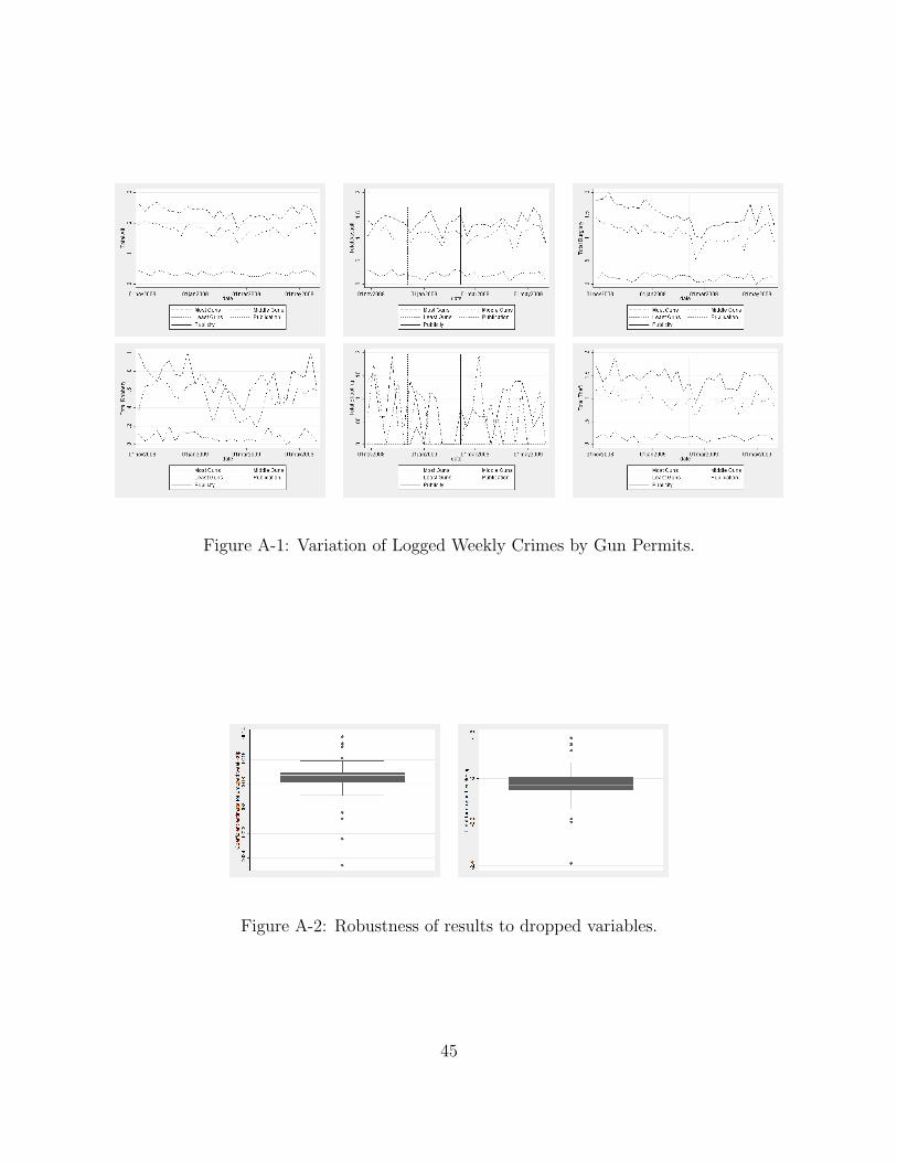
Figure A-1: Variation of Logged Weekly Crimes by Gun Permits.

Figure A-2: Robustness of results to dropped variables.

45

Guns, Privacy, and crime

Documents

Transcript of Guns, Privacy, and crime