Since 1994 Inter-University Consortium

Connecting Universities, the Labour Market and Professionals

S t b 2011

ALMALAUREA WORKING PAPERS no. 29

AlmaLaurea Working Papers – ISSN 2239-9453

September 2011

Religious Schooling, Secular Schooling, and Household Income Inequality in Israel

by

Ayal Kimhi, Moran SandelThe Hebrew Universityy

This paper can be downloaded at:

AlmaLaurea Working Papers seriesg phttp://www.almalaurea.it/universita/pubblicazioni/wp

REsearch Papers in Economics (RePEC)

Also available at:

The AlmaLaurea working paper series is designed to make available to a wide readership selectedworks by AlmaLaurea staff or by outside, generally available in English or Italian. The series focuses on thestudy of the relationship between educational systems, society and economy, the quality of educationalprocess, the demand and supply of education, the human capital accumulation, the structure and working ofthe labour markets, the assessment of educational policies.Comments on this series are welcome and should be sent to pubblicazioni@almalaurea.it.

AlmaLaurea is a public consortium of Italian universities which, with the support of the Ministry ofEducation, meets the information needs of graduates, universities and the business community. AlmaLaureahas been set up in 1994 following an initiative of the Statistical Observatory of the University of Bologna. Itsupplies reliable and timely data on the effectiveness and efficiency of the higher education system tomember universities’ governing bodies, assessment units and committees responsible for teaching activitiesand career guidance.

AlmaLaurea:

facilitates and improves the hiring of young graduates in the labour markets both at the national andinternational level;

simplifies companies' search for personnel reducing the gap between the demand for and supply of simplifies companies search for personnel, reducing the gap between the demand for and supply of qualified labour (www.almalaurea.it/en/aziende/);

makes available online more than 1.5 million curricula (in Italian and English) of graduates, including those with a pluriannual work experience (www.almalaurea.it/en/);

ensures the optimization of human resources utilization through a steady updating of data on the careers of students holding a degree (www.almalaurea.it/en/lau/).

Each year AlmaLaurea plans two main conferences (www.almalaurea.it/en/informa/news) in which the results of the annual surveys on Graduates’ Employment Conditions and Graduates’ Profile are presented.

___________________________________________________________________________________________

AlmaLaurea Inter-University Consortium | viale Masini 36 | 40126 Bologna (Italy)Website: www.almalaurea.it | E-mail: pubblicazioni@almalaurea.it

___________________________________________________________________________________________

The opinions expressed in the papers issued in this series do not necessarily reflect the position of AlmaLaurea

© AlmaLaurea 2011Applications for permission to reproduce or translate all or part of this material should be made to:AlmaLaurea Inter-University Consortiumemail: pubblicazioni@almalaurea.it | fax +39 051 6088988 | phone +39 051 6088919

1

International Conference on “Human Capital and Employment in the European and Mediterranean Area”

Bologna, 10-11 March 2011

Religious Schooling, Secular Schooling, and Household Income Inequality in Israel∗

by

Ayal Kimhi♦, Moran Sandel♠

Abstract The important role of education in the process of economic development is well known. Less known is the effect of education on inequality. This is an important issue, since economic policies that promote growth often lead to higher income inequality. A policy that promotes growth and at the same time reduces inequality would be preferred. The question is whether promoting education is such a policy. In this paper, the determinants of income inequality in Israel are analyzed using regression-based inequality decomposition techniques, focusing on the role of years of schooling and type of education. In particular, we differentiate between general schooling and ultra-orthodox schooling, following the common belief that ultra-orthodox schooling is not as valuable as general schooling for labor market outcomes. Indeed, we find that years of general schooling of the household head have a positive effect on per-capita household income, while the effect of years of ultra-orthodox schooling is negative. Years of general schooling are positively correlated with income, while years of ultra-orthodox schooling are negatively correlated with income. This implies that a policy that closes the schooling gaps in the secular sector is equalizing, while a policy that closes the schooling gaps in the ultra-orthodox sector is disequalizing. In addition, a uniform percentage increase in years of general schooling reduces per-capita income inequality, while a similar increase in ultra-orthodox years of schooling increases inequality. These results are robust to the type of regression used (OLS versus Gini regression), the use of equivalence scales, and do not change qualitatively even when we allow all regression coefficients to be different in the ultra-orthodox subsample. We conclude that policies directed at general schooling can potentially promote development and reduce inequality at the same time. However, when policy makers consider public funding of ultra-orthodox schools, they should take into account the adverse effects of this type of schooling on income inequality. In particular, we suggest that such funding will be conditioned on aligning the curriculum with the requirements of modern labor markets.

∗ This research was supported by a grant from the National Insurance Institute, the Center for Agricultural Economic Research, and the Taub Center for Social Policy Studies in Israel. The views expressed herein are those of the authors and do not necessarily reflect the views of these institutions. ♦ Associate Professor at the Department of Agricultural Economics and Management, The Robert H. Smith Faculty of Agriculture, Food and Environment, The Hebrew University of Jerusalem, Director of Research at the Center for Agricultural Economic Research, and Deputy Director at the Taub Center for Social Policy Studies in Israel. e-mail: kimhi@agri.huji.ac.il ♠ Graduate student at the Department of Agricultural Economics and Management, The Robert H. Smith Faculty of Agriculture, Food and Environment, The Hebrew University of Jerusalem.

2

1. Introduction Education is one of the keys to success in the labor market. Years of schooling are often used as a quantitative measure of education. However, types of schools may differ substantially in their quality. In Israel, an on-going policy debate exists with regard to government funding of ultra-orthodox schools that emphasize religious studies rather than topics that are associated with success in the labor market, such as math, sciences and English. It is often claimed that this is one of the reasons for the fact that many ultra-orthodox families are trapped in poverty (Gottlieb, 2007). Income inequality in Israel is one of the highest among Western countries (Ben David, 2009; OECD, 2009). Evidence from other countries suggests that education is a key determinant of income inequality (Cholezas and Tsakloglou, 2007), although the empirical evidence is still mixed. For example, Park (1996) found that a higher level of educational attainment of the labor force has an equalizing effect on the distribution of income in a cross section of 59 countries. On the other hand, Rodríguez-Pose and Tselios (2009) found that the relationship between a good human capital endowment and income inequality is positive in the regions of the European Union. For Israel, it was found, using regression-based inequality decomposition techniques (Kimhi, 2009), that reducing inequality in years of schooling as well as increasing the average years of schooling could reduce income inequality. In this paper, we examine whether this result is independent of the type of schooling. Specifically, we try to replicate the earlier results while differentiating between ultra-orthodox schooling and general schooling. We find that as opposed to general schooling, years of ultra-orthodox schooling increase income inequality. This result is robust to a variety of model and data specifications, including the type of regression used, adult equivalence scales, and sampling weights. In the next section we describe the regression-based inequality decomposition techniques. We also describe the Gini regression that is used as an alternative to OLS, and the method that we use to derive marginal effects of explanatory variables on inequality. The following section describes the data used in the empirical analysis. Then we move to the empirical results. The final section concludes with a discussion and some policy implications. 2. Methodology The regression-based inequality decomposition techniques are directly derived from inequality decomposition by income sources. Hence, we will start by presenting this latter technique.

Decomposition by income sources Shorrocks (1982) was the first to offer a unified approach to inequality decomposition by income sources. Earlier, Fei et al. (1978) and Pyatt et al. (1980), among others, offered a decomposition of the Gini index of inequality by income sources, but this happens to be a special case of Shorrocks' (1982) approach. Specifically, Shorrocks (1982) suggested focusing on inequality measures that can be written as a weighted sum of incomes: (1) I(y) = Σiai(y)yi, where ai are the weights, yi is the income of household i, and y is the vector of household incomes. This class of inequality measures includes as special cases the Gini index as well as the family of Generalized Entropy indices. If income is observed as the sum of incomes from k different sources, yi=Σkyi

k, the inequality measure (1) can be written as the sum of source-specific components Sk: (2) I(y) = Σiai(y)Σkyi

k = Σk[Σiai(y)yik] ≡ ΣkSk.

Dividing (2) by (1), one implicitly obtains the "proportional contribution" of income source k to overall inequality as:

3

(3) sk = Σiai(y)yi

k/Σiai(y)yi, so that Σksk=1. Shorrocks (1982) noted that the decomposition procedure (3) yields an infinite number of potential decomposition rules for each inequality index, because in principle, the weights ai(y) can be chosen in numerous ways, so that the proportional contribution assigned to any income source can be made to take any value between minus and plus infinity. Still, the Gini-based inequality decomposition rule remains the most popular in the empirical literature, in part because of the popularity of the Gini index as an inequality measure, and, perhaps more importantly, because it offers an intuitive interpretation of the decomposition result. Specifically, the Gini decomposition rule can be obtained by using ai(y)=2(i-(n+1)/2)/(μn2), where i is the index of observation after sorting the observations from lowest to highest income, n is the number of observations and μ is mean income. It has been shown, in this case, that the decomposition results can be expressed as Sk= αkRkGk, where αk is the share of income from source k in total income, Rk is the "Gini correlation" between yk and y, and Gk is the Gini index of yk (e.g., Lerman and Yitzhaki 1985). In essence, a mean-preserving increase in inequality in an income source that is positively correlated with total income will increase the Gini index of total income, holding other income sources fixed.

Decomposition by income determinants Morduch and Sicular (2002) and Fields (2003) extended the technique of inequality decomposition by income sources (3) to regression-based inequality decomposition by determinants of income. They suggested expressing household income (or log-income) as y=Xβ+ε, where X is a (nxk) matrix of explanatory variables (including a constant), β is a (kx1) vector of coefficients, and ε is a (nx1) vector of random error terms. Given a vector of consistently estimated coefficients b, income can be expressed as a sum of predicted income and a prediction error as: (4) y = Xb+e. Substituting (4) into (1) and dividing by (1), the share of inequality attributed to explanatory variable m is obtained as sm = bmΣiai(y)xi

m/Σiai(y)yi.1 Wan (2004) showed that this method can also be applied to nonlinear income-generating equations.

Gini regression Olkin and Yitzhaki (1992) suggested the Gini regression as an alternative to OLS. Its main advantages are that (a) no linear connection is assumed between the dependent variable and the explanatory variables; and (b) it puts lower weights on outliers. The implication of (a) is that the Gini regression coefficients are implied partial derivatives of the dependent variable, and in this sense they are comparable in nature to OLS coefficients. To demonstrate (b), note that the estimated coefficient of the slope in the Gini regression is in fact an instrumental variable estimator where the rank of the observation in the distribution of the explanatory variable is used as the instrument (Olkin and Yitzhaki, 1992). Since the rank is less sensitive to outliers than the value of the explanatory variable itself, the estimator is less sensitive than the OLS estimator. Alternatively, it

1 Morduch and Sicular (2002) suggested a simple procedure to compute standard errors of sm, but the procedure turns out to be incorrect. They claimed that since the components are linear in the regression coefficients, i.e. sm=bmΣiai(y)xi

m/I(y), standard errors can be computed as σ(sm)= σ(bm)Σiai(y)xim/I(y). This ignores the fact that

Σiai(y)xim/I(y) is itself a random variable that is not independent of bm (through the dependence of bm on y). Hence the

true standard errors cannot be computed in such a simple way (which, in fact, results in t-statistics that are identical to those of the regression coefficients). As suggested by Cowell and Fiorio (2009), bootstrapping is used to obtain standard errors in the empirical application below.

4

can be shown that OLS coefficients are weighted average of slopes between each observation and the sample mean. The sensitivity of the OLS coefficients to outliers result from the weights, which are proportional to the square of the distances of observations from the sample mean. The Gini regression coefficients, on the other hand, are weighted sums of the slopes between all adjacent observations, where the weights are proportional to the distance between the observations (Olkin and Yitzhaki, 1992). Schechtman and Yitzhaki (2007) extended the Gini regression to the case of a multiple regression, which is used in this research.

Marginal effects Several authors suggested, in the context of inequality decomposition by income sources, that a more interesting result is the effect on inequality of a uniform percentage increase in income from a certain source, holding income from other sources fixed. These "marginal effects" are more informative than the proportional contributions to inequality sk when one wants to know whether a particular income source is equalizing or disequalizing (Podder, 1993; Podder and Chatterjee, 2002). Lerman and Yitzhaki (1985) showed that the elasticity of the Gini index with respect a uniform percentage change in yk is sk-αk. This brings us back to the intuitive observation made by Shorrocks (1983), that comparing sk and αk is useful for knowing whether the kth income source is equalizing or disequalizing. The Lerman and Yitzhaki (1985) formula can be adapted to the case of regression-based inequality decomposition. Using the regression coefficients, it is possible to compute the “income shares” of the explanatory variables as αm = bmΣixi

m/Σiyi, and evaluate the marginal effect on the Gini index of inequality of a uniform increase in an explanatory variable m by computing sm-αm.

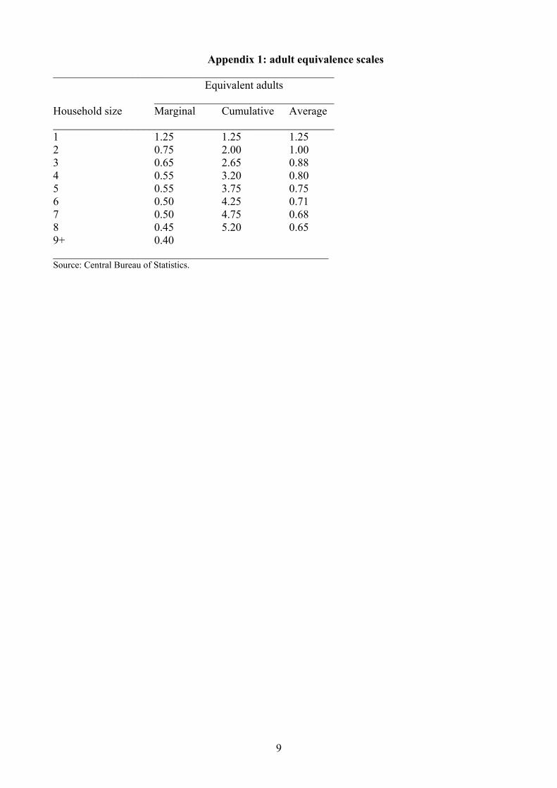
3. Data The data for this research were taken from the 2006 Income Survey in Israel. In addition to a detailed account of household income, the survey collected personal information, such as age and schooling, about all household members over 15 years of age, as well as the demographic structure of the household, i.e. the number of household members in different age groups. The data set included 14,582 households, representing all Israeli households except for Kibbutzim and Collective Moshavim, where household income is not easy to define, and Bedouins living outside of recognized localities. The household head is defined as the household member with the largest number of hours worked per week. Several personal characteristics, religion for example, are available only for the household head. The income measure we use is gross (before tax) household income from all sources, including wages and salaries, self-employment income, profits, capital income (rents, profits, dividends), and public and private transfers. Mean per-capita income in the sample was NIS 3,682 per month. In addition to per-capita income, we also analyze income per equivalent adult. The number of equivalent adults is increasing with household size, but the marginal increase is decreasing (appendix 1). Mean income per equivalent adult was NIS 3,915 per month. Note that Wodon and Yitzhaki (2005) raised some concern about the use of equivalence scales in inequality analysis. Nevertheless, our aim is to examine the robustness of our inequality analysis to the use of equivalence scales. Variables used to explain household income include several household head characteristics: gender, marital status, religion, origin, age, and schooling. Gender is represented by a dummy variable for female-headed households. Marital status is represented by a dummy variable for unmarried (or separated) heads of household. Religion is represented by a dummy variable for non-Jewish heads of household. Origin is represented by a dummy variable for heads of household whose father was not born in Israel. Age and schooling are measured in years. We differentiate between ultra-orthodox schooling and other types of schooling, using an indicator that the last type of school the household head attended was a yeshiva. We also add this indicator as an explanatory variable, and

5

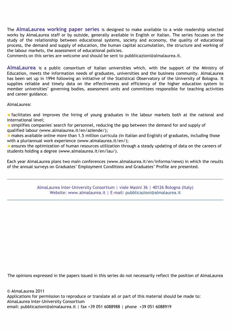
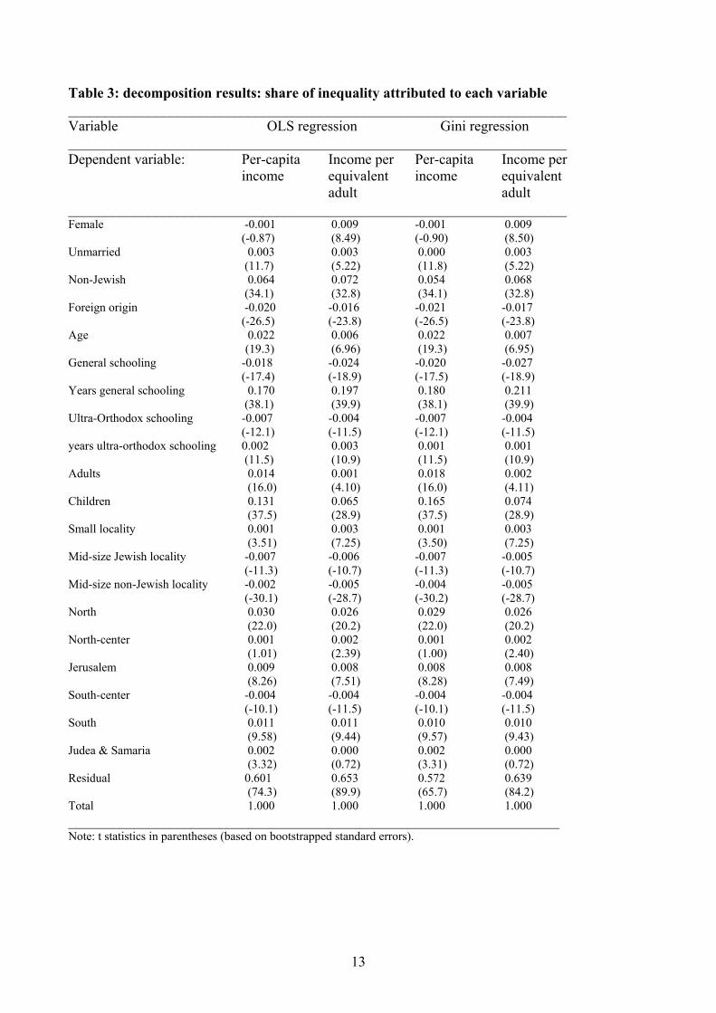
another indicator variable is used to distinguish those with positive years of general schooling from those with no schooling. Additional explanatory variables include the demographic structure of the household, type of locality and geographic location. The demographic structure of the household is represented by two variables: number of adults (age 18+) and number of children (up to age 17). Type of locality is represented by three dummy variables: for small localities (up to 2,000 residents), mid-size localities (up to 200,000 residents) with a Jewish majority, and mid-size localities with a non-Jewish majority. The excluded category includes localities with more than 200,000 residents. Geographic location is represented by six regional dummies: north, center-north, Jerusalem, center-south, south, Judea and Samaria. The excluded category is the center region. A map of the regions can be found in appendix 2. The means of explanatory variables are shown in table 1. Note that the means of years of schooling are for the whole sample; the mean of years of ultra-orthodox schooling among the ultra-orthodox is of course much higher. 4. Empirical analysis and results The estimation results of the income-generating equations are presented in table 2. We compare OLS regressions with Gini regressions, and compare two dependent variables, income per capita and income per equivalent adult. Most of the estimated marginal effects on income are robust, at least in terms of signs and significance, across the four specifications. This relates to the negative marginal effects associated with female-heads households, non-Jewish households, households with a foreign origin, households outside of the central region, and households in mid-size Jewish localities, as well as to the positive marginal effects associated with age, years of general schooling, and with households in small localities.2 There are some exceptions of differences between the results of income per capita and income per equivalent adult, in the case of variables that are most sensitive to the demographic structure of the household. The most striking example is the number of adults, which has negative marginal effects on income per-capita but positive marginal effects on income per equivalent adult. The number of children has negative marginal effects always, but they are smaller in magnitude in the case of income per equivalent adult. The marginal effects on income associated with unmarried household heads are positive in the case of income per-capita and negative in the case of income per equivalent adult.3 The most notable difference between the OLS results and those of the Gini regressions is with respect to the marginal effects on income of ultra-orthodox years of schooling, which are always negative, but are much smaller in magnitude and insignificant in the Gini regressions. These differences implies that attention should be given to the sensitivity of the results when one of these variables is at the focus of the analysis. In our case, this applies especially to years of schooling. The negative coefficient means, at least when it is statistically significant, that more schooling leads to a lower standard of living for ultra-orthodox households, probably because this specific type of schooling does not enhance labor market qualifications but rather encourage the engagement in non-remunerative religious activities. Moving forward to the inequality decomposition results (table 3), we observe that the explanatory variables explain roughly 40% of income inequality. The difference between the OLS and the Gini regression results are negligible. There are a few differences between the decomposition results of income per capita and income per equivalent adult. The most notable one is the inequality contribution of the Female dummy, which is not statistically significant in the case of income per capita, and significantly positive in the case of income per equivalent adult. The positive

2 Age squared turned out negative in the OLS regression, as expected, but it was eliminated because the Gini regression cannot accommodate both a variable and its square. 3 Evidently, virtually all unmarried household heads have no other adult in the household. This implies multicollinearity between number of adults and the unmarried dummy, and this could explain, at least in part, the opposite signs of their coefficients. The two variables are jointly significant, however, and removing the unmarried dummy did not change the coefficient of adults meaningfully.

6

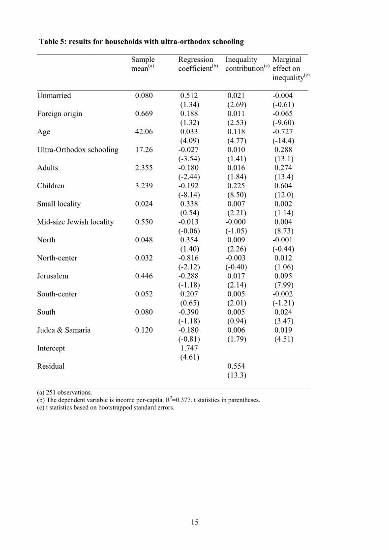
contribution of this variable implies that eliminating the differences between male- and female-headed households is likely to reduce income inequality. Similar conclusions can be drawn with regard to family size: eliminating the variability in the number of children, for example, can reduce per-capita income inequality quite substantially. This interpretation of the signs and magnitudes of the inequality contributions should be used with caution: it is not easy to generalize it to dummy variables that are part of a set of dummies (such as location), or to continuous variables that are interacted with dummy indicators (such as years of schooling). Table 4 includes the marginal effects of explanatory variables on inequality. Marginal effects are the changes in inequality that result from a uniform 1% increase in the value of each explanatory variable. The marginal effects are statistically significant, and are mostly consistent across the four specifications. The exceptions are those same variables for which regression coefficients vary across the specifications. In particular, the marginal effects on inequality of the number of adults are positive in the case of income per capita and negative in the case of income per equivalent adult. The opposite is true with respect to the marginal effects on inequality of being unmarried. The marginal effect of the number of children is always positive, but quantitatively smaller in the case of income per equivalent adult. A uniform fertility reduction is, therefore, a natural candidate for an equalizing policy target. The marginal effects of female-headed households, non-Jewish households and heads of household of foreign origin are all positive, indicating that an increase in the share of these population sub-groups is likely to increase income inequality. The marginal effects of small localities and mid-size non-Jewish localities are also negative, while the marginal effects of mid-size Jewish localities are positive. The marginal effects of all the out-of-center regional dummies are positive, while age has a negative marginal effect on inequality. Another policy-sensitive variable is schooling. Years of general schooling have an equalizing marginal effect, with an elasticity that is the largest in magnitude among all explanatory variables. Years of ultra-orthodox schooling, on the other hand, have positive marginal effects on income inequality. Recall, though, that the marginal effects of this variable on income (table 2) were not always significant, and sensitive to the type of regression used. At least, it is quite obvious that a uniform percentage increase in years of ultra-orthodox schooling does not reduce income inequality, while a similar increase in years of general schooling does. The fact that only less than 2% of the sample households have ultra-orthodox schooling (table 1) raises the question of whether it is legitimate to assume that the regression coefficients, other than the coefficient of schooling, are the same for these and other types of households. To examine this issue, we have estimated the OLS per-capita income generation equation for the subset of households with positive years of ultra-orthodox schooling, and repeated the decomposition analysis using the estimated coefficients. Evidently, we could not use the complete set of explanatory variables as we did for the whole sample. There were no ultra-orthodox households in the non-Jewish population or in non-Jewish localities, and there was only one among the female-headed households. The irrelevant explanatory variables were therefore removed from the model, as was the variable indicating years of general schooling. The remaining variables were used to derive the decomposition results in table 5. The estimated regression coefficients are in the second column, and they are naturally different than the coefficients estimated using the whole sample (table 2). Although most of the signs remained the same, the magnitudes and significance differed. The most noticeable differences are in the coefficients of the regional dummies, type of locality, unmarried, foreign origin, and number of children. This reflects the fact that the distributions of these variables in the ultra-orthodox subsample are different than in the complete sample (compare the means in tables 1 and 5). Interestingly, the negative coefficient of years of ultra-orthodox schooling remains qualitatively similar, and even becomes more statistically significant. As a result, the marginal effect of

7

schooling on inequality among ultra-orthodox households remains positive (fourth column), meaning that ultra-orthodox schooling is disequalizing.4

5. Discussion In this paper we have illustrated the use of regression-based inequality decomposition techniques to evaluate the impact of public policy on income inequality. Using Israel as a case study, we focused on the role of years of schooling and type of education, which are sensitive to government budget allocations. In particular, we differentiated between general schooling and ultra-orthodox schooling, following the common belief that ultra-orthodox schooling is not as valuable as general schooling for labor market outcomes. We found that years of general schooling of the household head have a positive effect on per-capita household income, while the effect of years of ultra-orthodox schooling is negative (but not always statistically significant). These differences carry over to different effects of schooling on inequality: a uniform percentage increase in years of general schooling reduces per-capita income inequality, while a similar increase in ultra-orthodox years of schooling increases inequality. These results are robust to the type of regression used (OLS versus Gini regression), the use of equivalence scales, and do not change qualitatively even when we allow all regression coefficients to be different in the ultra-orthodox subsample. We conclude that when policy makers consider the public funding of ultra-orthodox schools, they should take into account the adverse effects of this type of schooling on income inequality. In particular, we suggest that such funding will be conditioned on aligning the curriculum with the requirements of modern labor markets.

4 The marginal effects in tables 4 and 5 are not comparable in magnitude, because those in table 5 measure the impact on inequality among ultra-orthodox households only.

8

References Ben-David, Dan (2009). A Comprehensive Program for Reducing Inequality and Poverty and Increasing Economic Growth in Israel. Taub Center for Social Policy Studies in Israel, Jerusalem, (http://www.taubcenter.org.il/files/E2009_Government_Report.pdf). Cholezas, Ioannis, and Panos Tsakloglou (2007). Earnings Inequality in Europe: Structure and Patterns of Inter-Temporal Changes. IZA Discussion Paper No. 2636. Cowell, Frank A., and Carlo V. Fiorio (2009). Inequality Decomposition – A Reconciliation. LSE STRICERD Research Paper No. DARP 100. Fei, John C.H., Gustav Ranis and Shirley W.Y Kuo (1978). "Growth and the Family Distribution of Income by Factor Components." Quarterly Journal of Economics 92: 17-53. Fields, Gary (2003). "Accounting for Income Inequality and Its Change: A New Method, with Application to the Distribution of Earnings in the United States." Research in Labor Economics 22: 1-38. Gottlieb, Daniel (2007). Poverty and Labor Market Behavior in the Ultra-Orthodox Population in Israel. Policy Research Paper No. 4, The Van Leer Jerusalem Institute. Kimhi, Ayal (2009). "Male Income, Female Income, and Household Income Inequality in Israel: A Decomposition Analysis." Journal of Income Distribution 18: 34-48. Lerman, Robert I., and Shlomo Yitzhaki (1985). “Income Inequality Effects by Income Source: A New Approach and Applications to the United States.” Review of Economics and Statistics 67: 151-156. Morduch, Jonathan, and Terry Sicular (2002). “Rethinking Inequality Decomposition, with Evidence from Rural China.” The Economic Journal 112: 93-106. OECD (2009). OECD Economic Surveys: Israel. Olkin, Ingram, and Shlomo Yitzhaki. "Gini Regression Analysis". International Statistical Review 60 (1992): 185-196. Park, Kang H. (1996). "Educational Expansion and Educational Inequality on Income Distribution." Economics of Education Review 15: 51-58. Podder, Nripesh (1993). "The Disaggregation of the Gini Coefficient by Factor Components and its Applications to Australia." Review of Income and Wealth 39: 51-61. Podder, Nripesh, and Srikanta Chatterjee (2002). "Sharing the National Cake in Post Reform New Zealand: Income Inequality Trends in Terms of Income Sources." Journal of Public Economics 86: 1-27. Pyatt, Graham, Chau-nan Chen, and John Fei (1980). "The Distribution of Income by Factor Components." Quarterly Journal of Economics 94: 451-474. Rodríguez-Pose, Andrés, and Vassilis Tselios (2009). "Education and Income Inequality in the Regions of the European Union." Journal of Regional Science 49: 411-437. Schechtman, Edna, and Shlomo Yitzhaki (2007). Gini's Multiple Regression. Unpublished manuscript. Electronic paper is available at: http://ssrn.com/abstract=720641. Shorrocks, Anthony F. (1982). “Inequality Decomposition by Factor Components.” Econometrica 50: 193-211. Shorrocks, Anthony F. (1983). “The Impact of Income Components on the Distribution of Family Incomes.” Quarterly Journal of Economics 98: 311-326. Wan, Guanghua (2004). “Accounting for Income Inequality in Rural China: A Regression-Based Approach.” Journal of Comparative Economics 32: 348-363. Wodon, Quentin T., and Shlomo Yitzhaki (2005). Inequality and Social Welfare when Using Equivalence Scales. Available at SSRN: http://ssrn.com/abstract=874704.

9

Appendix 1: adult equivalence scales __________________________________________________ Equivalent adults ________________________________ Household size Marginal Cumulative Average __________________________________________________ 1 1.25 1.25 1.25 2 0.75 2.00 1.00 3 0.65 2.65 0.88 4 0.55 3.20 0.80 5 0.55 3.75 0.75 6 0.50 4.25 0.71 7 0.50 4.75 0.68 8 0.45 5.20 0.65 9+ 0.40 _________________________________________________ Source: Central Bureau of Statistics.

10

Appendix 2: map of regions

Note: the southern region is trimmed from below. Source: Central Bureau of Statistics, and authors' definition of regions.

11

Table 1: explanatory variables __________________________________________________

Variable Mean __________________________________________________

Female 0.363 Unmarried 0.372 Non-Jewish 0.134 Foreign origin 0.741 Age 47.651 General schooling 0.959 Years general schooling 12.618 Ultra-Orthodox schooling 0.017 Years ultra-orthodox schooling 0.302 Adults 2.227 Children 1.099 Small locality 0.053 Mid-size Jewish locality 0.564 Mid-size non-Jewish locality 0.095 North 0.144 North-center 0.181 Jerusalem 0.106 South-center 0.102 South 0.134 Judea & Samaria 0.028

_________________________________________________

12

Table 2: regression results _____________________________________________________________________ Variable OLS regression Gini regression _____________________________________________________________________ Dependent variable Per-capita Income per Per-capita Income per income equivalent income equivalent adult adult _____________________________________________________________________ Female -0.770 -0.715 -0.768 -0.713 (-10.3) (-9.56) (-10.1) (-9.49) Unmarried 0.177 -0.334 0.013 -0.357 (2.34) (-4.60) (0.17) (-4.85) Non-Jewish -1.288 -1.580 -1.091 -1.491 (-9.25) (-11.5) (-7.53) (-10.5) Foreign origin -0.453 -0.423 -0.482 -0.467 (-3.01) (-2.81) (-3.16) (-3.07) Age 0.021 0.016 0.022 0.019 (9.06) (6.91) (8.65) (7.82) General schooling -1.475 -1.751 -1.603 -1.929 (-10.8) (-12.8) (-11.6) (-14.1) Years general schooling 0.269 0.282 0.284 0.302 (25.0) (25.8) (25.7) (26.9) Ultra-Orthodox schooling 1.158 0.840 1.189 0.648 (4.45) (3.14) (2.81) (1.66) Years ultra-orthodox schooling -0.021 -0.028 -0.006 -0.006 (-1.72) (-2.19) (-0.24) (-0.27) Adults -0.267 0.103 -0.333 0.123 (-11.2) (4.24) (-9.36) (3.62) Children -0.492 -0.366 -0.620 -0.415 (-25.1) (-19.9) (-27.0) (-16.2) Small locality 0.442 0.598 0.512 0.618 (2.57) (3.30) (2.98) (3.40) Mid-size Jewish locality -0.404 -0.331 -0.361 -0.311 (-4.64) (-3.82) (-4.15) (-3.58) Mid-size non-Jewish locality 0.059 0.141 0.112 0.162 (0.48) (1.10) (0.88) (1.24) North -1.139 -1.104 -1.141 -1.098 (-12.5) (-11.7) (-12.4) (-11.6) North-center -0.889 -0.828 -0.888 -0.828 (-8.55) (-7.95) (-8.55) (-7.94) Jerusalem -1.013 -1.027 -0.944 -1.007 (-8.03) (-8.27) (-7.44) (-8.04) South-center -0.473 -0.363 -0.437 -0.348 (-4.41) -3.10) (-4.07) (-2.96) South -1.112 -1.095 -1.059 -1.063 (-12.2) (-11.2) (-11.5) (-10.8) Judea & Samaria -1.168 -1.212 -1.089 -1.179 (-8.36) (-7.99) (-7.71) (-7.75) Intercept 3.395 3.141 (15.8) (15.1) R2 0.178 0.150 _____________________________________________________________________ Note: 14560 observations. t statistics in parentheses (based on bootstrapped standard errors in the Gini regressions).

13

Table 3: decomposition results: share of inequality attributed to each variable _____________________________________________________________________ Variable OLS regression Gini regression _____________________________________________________________________ Dependent variable: Per-capita Income per Per-capita Income per income equivalent income equivalent adult adult _____________________________________________________________________ Female -0.001 0.009 -0.001 0.009 (-0.87) (8.49) (-0.90) (8.50) Unmarried 0.003 0.003 0.000 0.003 (11.7) (5.22) (11.8) (5.22) Non-Jewish 0.064 0.072 0.054 0.068 (34.1) (32.8) (34.1) (32.8) Foreign origin -0.020 -0.016 -0.021 -0.017 (-26.5) (-23.8) (-26.5) (-23.8) Age 0.022 0.006 0.022 0.007 (19.3) (6.96) (19.3) (6.95) General schooling -0.018 -0.024 -0.020 -0.027 (-17.4) (-18.9) (-17.5) (-18.9) Years general schooling 0.170 0.197 0.180 0.211 (38.1) (39.9) (38.1) (39.9) Ultra-Orthodox schooling -0.007 -0.004 -0.007 -0.004 (-12.1) (-11.5) (-12.1) (-11.5) years ultra-orthodox schooling 0.002 0.003 0.001 0.001 (11.5) (10.9) (11.5) (10.9) Adults 0.014 0.001 0.018 0.002 (16.0) (4.10) (16.0) (4.11) Children 0.131 0.065 0.165 0.074 (37.5) (28.9) (37.5) (28.9) Small locality 0.001 0.003 0.001 0.003 (3.51) (7.25) (3.50) (7.25) Mid-size Jewish locality -0.007 -0.006 -0.007 -0.005 (-11.3) (-10.7) (-11.3) (-10.7) Mid-size non-Jewish locality -0.002 -0.005 -0.004 -0.005 (-30.1) (-28.7) (-30.2) (-28.7) North 0.030 0.026 0.029 0.026 (22.0) (20.2) (22.0) (20.2) North-center 0.001 0.002 0.001 0.002 (1.01) (2.39) (1.00) (2.40) Jerusalem 0.009 0.008 0.008 0.008 (8.26) (7.51) (8.28) (7.49) South-center -0.004 -0.004 -0.004 -0.004 (-10.1) (-11.5) (-10.1) (-11.5) South 0.011 0.011 0.010 0.010 (9.58) (9.44) (9.57) (9.43) Judea & Samaria 0.002 0.000 0.002 0.000 (3.32) (0.72) (3.31) (0.72) Residual 0.601 0.653 0.572 0.639 (74.3) (89.9) (65.7) (84.2) Total 1.000 1.000 1.000 1.000 ____________________________________________________________________ Note: t statistics in parentheses (based on bootstrapped standard errors).

14

Table 4: marginal effects on inequality (%) _____________________________________________________________________ Variable OLS regression Gini regression ______________________________________________________________________ Dependent variable: Per-capita Income per Per-capita Income per income equivalent income equivalent adult adult _____________________________________________________________________ Female 0.076 0.076 0.076 0.076 (59.3) (52.6) (59.3) (52.6) Unmarried -0.014 0.034 -0.001 0.036 (-46.6) (45.1) (-45.7) (45.0) Non-Jewish 0.110 0.125 0.093 0.118 (33.3) (41.3) (33.4) (41.2) Foreign origin 0.072 0.064 0.076 0.071 (85.4) (82.6) (85.4) (82.6) Age -0.257 -0.187 -0.259 -0.224 (-98.8) (-106) (-98.8) (-106) General schooling 0.362 0.399 0.393 0.439 (96.5) (99.4) (96.5) (99.4) Years general schooling -0.740 -0.699 -0.782 -0.748 (-109) (-98.7) (-109) (-98.7) Ultra-Orthodox schooling - 0.012 -0.008 -0.013 -0.006 (-14.5) (-14.4) (-14.6) (-14.4) Years ultra-orthodox schooling 0.004 0.005 0.001 0.001 (13.9) (14.0) (14.6) (14.3) Adults 0.173 -0.056 0.216 -0.067 (77.1) (-96.1) (77.1) (-96.1) Children 0.278 0.168 0.351 0.191 (49.9) (51.0) (49.9) (51.0) Small locality -0.005 -0.005 -0.006 -0.005 (-15.7) (-10.7) (-16.0) (-10.6) Mid-size Jewish locality 0.054 0.042 0.048 0.039 (71.4) (60.6) (71.4) (60.6) Mid-size non-Jewish locality -0.004 -0.008 -0.007 -0.010 (-28.6) (-36.1) (-28.3) (-36.1) North 0.076 0.068 0.076 0.067 (31.3) (43.9) (31.3) (43.9) North-center 0.045 0.041 0.045 0.041 (35.1) (39.6) (35.2) (39.6) Jerusalem 0.036 0.034 0.033 0.033 (26.6) (26.8) (26.6) (26.8) South-center 0.009 0.006 0.008 0.005 (16.8) (15.1) (16.7) (15.2) South 0.051 0.048 0.049 0.046 (32.0) (30.9) (32.0) (30.9) Judea & Samaria 0.012 0.010 0.011 0.010 (15.7) (13.3) (15.7) (13.3) _____________________________________________________________________ Notes: Marginal effect is the percentage change in the Gini coefficient as a result of a uniform 1% increase in the explanatory variable. t statistics in parentheses (based on bootstrapped standard errors).

15

Table 5: results for households with ultra-orthodox schooling _____________________________________________________________________ Sample Regression Inequality Marginal mean(a) coefficient(b) contribution(c) effect on inequality(c) _____________________________________________________________________ Unmarried 0.080 0.512 0.021 -0.004 (1.34) (2.69) (-0.61) Foreign origin 0.669 0.188 0.011 -0.065 (1.32) (2.53) (-9.60) Age 42.06 0.033 0.118 -0.727 (4.09) (4.77) (-14.4) Ultra-Orthodox schooling 17.26 -0.027 0.010 0.288 (-3.54) (1.41) (13.1) Adults 2.355 -0.180 0.016 0.274 (-2.44) (1.84) (13.4) Children 3.239 -0.192 0.225 0.604 (-8.14) (8.50) (12.0) Small locality 0.024 0.338 0.007 0.002 (0.54) (2.21) (1.14) Mid-size Jewish locality 0.550 -0.013 -0.000 0.004 (-0.06) (-1.05) (8.73) North 0.048 0.354 0.009 -0.001 (1.40) (2.26) (-0.44) North-center 0.032 -0.816 -0.003 0.012 (-2.12) (-0.40) (1.06) Jerusalem 0.446 -0.288 0.017 0.095 (-1.18) (2.14) (7.99) South-center 0.052 0.207 0.005 -0.002 (0.65) (2.01) (-1.21) South 0.080 -0.390 0.005 0.024 (-1.18) (0.94) (3.47) Judea & Samaria 0.120 -0.180 0.006 0.019 (-0.81) (1.79) (4.51) Intercept 1.747 (4.61) Residual 0.554 (13.3) _____________________________________________________________________ (a) 251 observations. (b) The dependent variable is income per-capita. R2=0.377. t statistics in parentheses. (c) t statistics based on bootstrapped standard errors.