1

World Income Inequality 1820-2000

Joerg Baten, Peter Foldvari, Bas van Leeuwen and Jan Luiten van Zanden

First and very preliminary draft

Correspondence: jvz@iisg.nl

1. Introduction

The aim of this paper is to present a new dataset of global inequality between 1820 and the present, based on the available historical evidence, and to tentatively analyse some of the results that emerge from these data. The importance of the subject hardly needs to be stressed: the enormous increase of inequality on a global scale is one of the most significant – and worrying - features of the development of the world economy in the past 200 years. For this reason, the subject has become one of the most discussed topics in the social sciences; in particular the debate on the measurement and interpretation of recent trends in global inequality – is it still increasing? and why or why not? – has attracted considerable attention (Deininger and Squire, 1996; Jones, 1997; Bourguignon and Morrison, 2002; Milanovic, 2007 for a review of the debate). Economic historians have also intensely discussed the long term trends in the world that lead to the growing income disparities between nations and changed patterns of inequality within nations, although often using other concepts (such as ‘the Great Divergence’). We argue, however, that we lack the historical data to really analyse these patterns of changing global inequality in detail. The one paper that has attempted to do this, Bourguignon and Morrison’s seminal AER 2002 article, is for the period before 1950 largely based on the assumption that income inequality within countries is unchanging. They extrapolate their estimates of income inequality in certain periods to cover much longer time periods, as a result of which, we think, changes in income inequality within countries are clearly underestimated. For large parts of the world the result is that estimates from the post 1914 or even the post 1945 period are used to infer income inequality in the 19th century, and that, in other words, inequality within countries is assumed to have remained constant. For Latin America and Africa B & M rely completely on 20th century data to estimate inequality in the 19th century; for Asia they have in total four historical estimates (in fact often very partial estimates): one for China in 1890, two for Indonesia and one for Japan. The dataset for Europe and North America is somewhat better, but also uses only part of the evidence available. For a large majority of the world’s population, and almost all people living in the ‘developing countries’, their estimates are based on almost no historical evidence, implying that we really cannot rely on their work to analyse the long term patterns of global inequality. Moreover, scholars interested in the question whether different levels of inequality may have affected the way in which countries participated in the Great Divergence, cannot use this dataset to analyse such a possible link, as it simply does not have sufficient historical observations to make such an analysis feasible.

2

For these reasons, we have set out to try to create a new dataset of global inequality focused on improving the estimates of inequality within countries through the use of the results of (old and) recent research on this topic, and through the application of a number of indirect ways of measuring (changes in) income inequality in the past. In reviewing their work, we saw no reasons to modify the other pillar of the Bourguignon and Morrison paper, the estimates by Maddison of inter-country inequality (although we used an updated version of his estimates, Maddison 2003); there has been some discussion about, in particular, his 19th century estimates, which have been criticised for a number of reasons, such as underestimating GDP per capita (or more in general, welfare levels) in China (and India, and Japan) at the beginning of the 19th century (Pomeranz 2001, but see Van Zanden 2002); for underestimating GDP per capita of the US during much of the 19th century (Ward and Devereux 2005); and more fundamentally, because of possible fundamental flaws in the methodology, which uses 1990 benchmark estimates of PPP-corrected GDP per capita, which are then extrapolated back in time using time series of GDP and population (Prados de la Escosura 2000). We think that for the 19th and 20th

century the Maddison framework is the best on offer, and probably catches the overall changes in inter-country inequality rather well. Perhaps Chinese income per capita at the beginning of the 19th century is underestimated somewhat and the decline sketched by Maddison is perhaps even larger than he envisaged; the relative position of the US versus the UK is still a matter of considerable debate (Broadberry 2003), but it is not clear that this will affect the overall pattern of global inequality very much – as a different assessment of the Chinese growth record would clearly do.1 We consider the within country estimates of income inequality to be the weaker part of the estimates of global inequality, where in view of ongoing research in this area, much more progress could be made, and we therefore concentrated on this part of the story.

How did we enlarge the dataset? Basically, in three ways: firstly, by incorporating new research done since the 1990s and collecting the results of older research overlooked by B & M. This, however, does not really solve the problem of the data gap between rich and poor – probably the gap even widens, as much more evidence is available and much more work has been done on Europe and the Americas than on Africa or large parts of Asia. Therefore, in order to get a more balanced set of estimates, we had to apply two alternative ways of estimating (changes in) income inequality suggested in the literature. The first one, which we particularly used for the 19th century (and for a few countries also to the interwar period), was to infer changes in income inequality from the development of the ratio between GDP per capita and wages of unskilled labourers . The idea, initially suggested by Jeffrey Williamson (1998, 2000), and recently tested by Leandro Prados de la Escosura (2008) is that if wages lag behind income per capita, inequality is probably increasing; conversely, if wages grow faster than GDP per capita, this may point to a decline in inequality. We tested this relationship for a set of countries for which we had independent estimates of inequality of income distribution, and found a small but (just) significant effect, which we used to extrapolate (or intrapolate) estimates of the Ginis of income distribution. The second ‘new’ approach that we applied is to use data on the distribution of heights of the population that can be derived from different sources to estimate the Gini of the income distribution. Again, for a subset of countries for which

1 At some point we hope to experiment with the alternative set of estimates produced by Prados de la Escosura 2000.

3

we have both independent Gini coefficients of income distribution and data on the distribution of heights, we could establish the link between the two measures of socio-economic disparities; the found relationship was then used to estimate income inequality for those countries and periods for which other data were lacking. This procedure has been developed by Baten (1999) and Moradi and Baten (2005), and has now been extended to a much broader sample of countries (all details below).Moreover, we identified a group of 30 countries – most of them relatively large, but spread more or less equally over the globe (with an inevitable over-representation of Western Europe, however) – for which we tried to get consistent estimates of income inequality for all the benchmark years, starting in 1820. These countries were: (in Europe) Belgium, Denmark, France, Germany, Italy, Netherlands, Norway, Poland, Portugal, Russia/USSR, Spain, Sweden, Czechoslovakia, UK; (in Asia) China, India, Indonesia, Japan, Thailand, Turkey; (in the Americas) Argentina, Brazil, Canada, Chile, Mexico, Peru, USA; (in Africa) Egypt, Ghana; and Australia. Together, these countries represent 70-80% of the world’s population (according to the Maddison estimates). We think this dataset is more or less representative of global trends, although it is handicapped by the underrepresentation of in particular Africa in it (and the overpresentation of Western Europe). In a second step, we considered all countries with 500,000 and more inhabitants. To this were added all countries, even those for which we have only a few – and sometimes only one – datapoint (Botswana in 1990, or Sudan in 1910, 1929, and 1970, for example).

2. Data2.1 Income inequality in post 1945 periodData on income inequality is relatively scattered. However, for the twentieth century two important sources may be distinguished that contain direct information on income inequality. First, there are the direct Gini-coefficients. One major source is the WIID (2008). These cover most of the period after 1950. However, these estimates are not completely consistent. As pointed out by François and Rojas-Romagosa (2005), three broad groups can be distinguished based on gross household income, net household income and expenditure data. These are not mutually exchangeable because the trend in these data is different (François and Rojas-Romagosa 2005). The major actor causing a different trend is income/expenditure smoothing: progressive taxation, extra earnings from by-employment, and the black economy all contribute to some kind of smoothing of expenditure and net income. In addition, the wealthy are expected to save a larger share of their income, and therefore the observed expenditures are far from being a linear function of income. Finally, François and Rojas-Romagosa (2005, 17) point out that expenditure measures are subject to bias caused by borrowing or lending. These factors are especially prevalent in the post World War II period when many countries expanded their income taxation. However, as suggested by Van Leeuwen and Foldvari (2008) for Indonesia, it seems that there is only a relative short transition phase when income taxes gain ground. This means that, after (and also before) a relatively short transition period after WWII, the trends in the net hh/expenditure Ginis and the gross household income gini are again similar. We test this hypothesis for a larger sample of countries in regressions, where we regress the gross household Gini prior to 1980 (and after 1980) on the net household income Gini, a trend, a cross effect of trend and net household income Gini.

4

Before 1980. xtreg grosshhincome nethhincome nethhincomet t doecd dsocialist dafrica dasia dlatinamerica daustralia d

northamerica if year<1981, rob fe

Fixed-effects (within) regression Number of obs = 82Group variable: countrynum~r Number of groups = 12

R-sq: within = 0.7298 Obs per group: min = 1 between = 0.9121 avg = 6.8 overall = 0.8775 max = 36

F(3,11) = 59.35corr(u_i, Xb) = 0.5026 Prob > F = 0.0000

(Std. Err. Adjusted for 12 clusters in countrynumber)

| Robustgrosshhinc~e | Coef. Std. Err. T P>|t| [95% Conf. Interval]-------------+---------------------------------------------------------------- nethhincome | .7876379 .1768145 4.45 0.001 .3984717 1.176804nethhincomet | .0021408 .0002889 7.41 0.000 .001505 .0027766 t | -.0729689 .0141431 -5.16 0.000 -.1040975 -.0418402 _cons | 9.420317 6.075219 1.55 0.149 -3.951149 22.79178-------------+---------------------------------------------------------------- sigma_u | 2.8443162 sigma_e | 1.0527019 rho | .87952345 (fraction of variance due to u_i)

After 1980. xtreg grosshhincome nethhincome nethhincomet t doecd dsocialist dafrica dasia dlatinamerica daustralia d> northamerica if year>1980, rob fe

Fixed-effects (within) regression Number of obs = 114Group variable: countrynum~r Number of groups = 23

R-sq: within = 0.4624 Obs per group: min = 1 between = 0.8302 avg = 5.0 overall = 0.7872 max = 17

F(3,22) = 11.34corr(u_i, Xb) = 0.6261 Prob > F = 0.0001

(Std. Err. adjusted for 23 clusters in countrynumber)------------------------------------------------------------------------------ | Robustgrosshhinc~e | Coef. Std. Err. t P>|t| [95% Conf. Interval]-------------+---------------------------------------------------------------- nethhincome | .3671768 .4023948 0.91 0.371 -.467339 1.201693nethhincomet | .0034468 .0069078 0.50 0.623 -.0108792 .0177728 t | -.0590284 .224085 -0.26 0.795 -.5237522 .4056954 _cons | 19.61811 11.80289 1.66 0.111 -4.859587 44.0958-------------+---------------------------------------------------------------- sigma_u | 2.771718 sigma_e | 1.6913547 rho | .728668 (fraction of variance due to u_i)------------------------------------------------------------------------------

In the period prior to 1980, the cross-sectional effect is significant and positive, implying that (combined with the coefficient of the net household Gini), that the net household Gini grows slower the gross household Gini. If we compare the same regression from the period after 1980, where we may reasonably assume that there is a linear relationship

5

between the gross and net household Gini, we indeed find none of the coefficients significant.

2.2 Direct estimates for pre 1945 period

Reworking the WIID dataset is a first step. A lot of new work has been done recently on the estimation of income inequality in the past that can also be included in the dataset. This consists of two things: direct Gini coefficients can be obtained from several other, mostly scattered publications. A good overview of a lot of the historical work is supplied by Lindert, Milanovic and Williamson (2007), and on the Global Income and Prices website at UCDavis (http://gpih.ucdavis.edu/Distribution.htm). New work has also been done (and old work has gone unnoticed), by Bertola et al. (2009) for parts of South America, Rossi et al. (2001) for Italy, Soltow and Van Zanden (1998) for the Netherlands.

A separate category of new work is related to income share estimates, in particular the project focused on estimating the historical development of the share of the richest 1 or 5 % in total income, inspired by the work of Piketty and Atkinson. Studies are available for Australia (1921-2003) (Atkinson and Leigh 2007a), Canada (1920-2000) (Saez and Veall 2005), France (1905-1998) (Piketty 2007), Germany (1925-1998) (Dell 2007), India (1922-1999) (Bannerjee and Piketty 2003), Indonesia (1920-2004) (Leigh and Van der Eng 2007), Ireland (1922-2000) (Nolan 2007), Japan (1886-2002) (Moriguchi and Saez 2006), Netherlands (1914-1999) (Salverda and Atkinson 2007), New Zealand (1921-2002) (Atkinson and Leigh 2005), Spain (1981-2002) (Alvaredo and Saez 2006), Sweden (1903-2004) (Roine and Waldenström 2006), Switzerland (1933-1996) (Dell, Piketty, and Saez 2007), UK (1908-2000) (Atkinson 2007b) and the USA (1913-2004) (Piketty and Saez 2006b).

One problem, however, is how to convert these income shares, which are nothing more than just one point on the Lorenz curve, into Ginis. The only way this can be done is by assuming a distribution. Two distributions are normally used: a log-normal, and a Pareto distribution (see Soltow 1998). We use the log-normal distribution in this paper. Lopez and Servén (2006) shows that the Lorenz-curve, under the assumption of log-normality, can be expressed as follows:

Where p denotes the poorest pth quantile of the population, and σ is the standard deviation of the log income and Φ(.) denotes the cumulative normal distribution.The Gini coefficient (G) can be expressed as:

1 12

2

G

In the end, it turned out that on average the difference between both methods was

limited. Van Leeuwen and Foldvari (2008, 16-17) claim that their level slightly differs. More interesting is the question if the movement over time of the estimated Gini is really independent of using a Pareto or lognormal distribution. As the Gini in both cases is estimated using only one point at the Lorenz curve (mostly of the upper quintiles), this is

6

actually the question as to whether the relative distribution of the upper quintiles versus the lower quintiles changes over time. Clearly, this is a bold assumption, but there is some evidence in its favor. First, Soltow (1998, 17) argues that at max the distribution of the top 33% richest person resembles a Pareto distribution while the log-normality assumption maywork fine otherwise. Hence, the suggestion is to use the lowest possible quintile to calculate the Gini coefficient using a log-normal distribution. Second, another way of looking at this issue is by the extraction ratio (Milanovic et al. 2007). This indicates how much of the above-subsistence income is extracted by the rich. Although it therefore does not say much about the distribution sec, it can be considered as an indication of the shape of the Lorenz curve. As indicated by Milanovic et al. (2007, Table 2 and Figure 4), with the exception of some very poor countries, this changes relatively little over time in the twentieth century. Consequently, the relative position of the upper and lower quintiles also does not change much over time meaning that using either a Pareto or lognormal distribution does not bias the change of the estimated Gini coefficients over time. Indeed, as most income shares are calculated for Western countries in the twentieth century, we may accept this assumption. Finally, and most importantly, empirical results seem to confirm this finding.

In this paper we will use the log-normal distribution given the situation that the log-normal is most widely used and is applicable both on higher and lower classes in society. Since this only provides a trend of inequality, we can use benchmark Ginis to bring the Gini estimates back in time using the income share estimates.

2.3 GDP divided by unskilled wages as a proxy Above two methods give us a reasonable complete picture of income distribution among countries in the twentieth century. Except for some direct estimates of income inequality available for a limited number of countries not much is known, however, for the earlier period. For earlier periods (and for countries with less abundant data) we therefore have to rely on proxies for income inequality. Several options exist, for example, the economic distance between the landed elite and landless labour or the ratio of average family income (y) to that of an unskilled rural labourer (w). Both methods draw heavily on the extraction rate (Lindert et al.). This ratio indicates what share of potential surplus can be taken from the poorer groups, hence increasing inequality. The basic equation used by Milanovic et al is:

* 1t t t

t

G s

where G* is the possible maximum Gini, ε is the share of higher class people (assumed constant), µ the mean income (per capita GDP) and s the unskilled income. When taking logarithm of both sides, this becomes:

*l n l n 1 l n l nt t t tG s If we assume that the expropriation of the incomes of lower classes by the elite is not complete we can have a more general form:

*l n l n 1 l n l nt t tG s

7

where β=γ=1 is the basic case, with the maximum income diversion. In our case, we used a LSDV regression model with GDP and wage premium as independent variables, i.e.

tiDywusyG ,lnlnln Where the dummies indicate year and country. The sources used for the real wage series were Williamson (1999a, 1999b, 2000), Mitchell (1998 a, b, c), Allen (2001), Mironov (2004), and Allen et al. (2005); the GDP estimates were again taken from Maddison. This results in a fit of 0.7.

2.4 The distribution of heights as a proxy

A completely independent method of looking at early inequality is by looking at the relation between inequality in heights and income inequality. For example Baten (1999, 2000, 2000a), Pradhan et al. 2003, Moradi and Baten (2005), Sunder (2003), Guntupalli and Baten (2006) have argued that the coefficient of variance of the height of individuals may be a proxy for income distribution. The idea is that growth takes place especially between age 0 and 5, that there are no genetic population differences in height. As wealthier people have better food and shelter and less illnesses, they tend to be taller. Hence, the variation of height at the present may be indicative of income distribution during the decade of birth.

Heights offer a good complement to conventional inequality indicators and constitute perhaps an even better indicator in some respect. If the distribution of food and medical goods in an economy becomes more unequal, heights should also become more unequal. Yet while a correlation with income does exist, this correlation is only partial. Some important inputs are not traded on markets but are provided as public goods, such as public health measures or food supplements for schoolchildren. Public goods lead to modest deviations between purchasing power-based and height-based inequality measures. Moreover, income totally neglects transfers within households. This is a major argument in favor of height-based inequality measures: heights are an outcome indicator, whereas real income represents an input to human utility. Deaton (2001) and Pradhan et al. (2003) have argued convincingly that measures of health inequality are important in their own right, not only in relation to income. Heights do capture important biological aspects of the standard of living (Komlos, 1985; Steckel, 1995), irrespective of the fact that some problems regarding the stature variable may exist.

Anthropometric methods are even more advantageous for studying developing countries of the 20th and the generally poorer countries of the 19th century. To date, the development of inequality within LDCs could not be sufficiently explored because reliable data were lacking. The well-known Deininger and Squire data set (1996), for example, provides only eight gini coefficients of income for Subsahran Africa for the period before 1980, labeled as “acceptable”. Atkinson and Brandolini (2001) convincingly pointed to serious flaws in the income inequality data collected by Deininger and Squire, arising from insufficient consistency across countries and over time. For those countries, height inequality measures can provide important additional insights. We do not claim that height is the only accurate measure of inequality, but argue

8

that it generates new insights on inequality while serving as a useful countercheck for other indicators, thereby leading to more meaningful results overall.The effects of inequality on heights are best understood by comparing the likely outcomes of a hypothetical situation, in which a population is exposed to two alternative allocations of ressources A and B after birth:

(A) All individuals receive the same quantity and quality of resources (nutritional and health inputs). This case refers to a situation of perfect equality.

(B) Available resources are allocated unequally (but independently of the genetic height potential of the individuals).

In the case of A, the height distribution should only reflect genetic factors. Despite perfect equality, we observe a biological variance of (normally distributed) heights in this case. Yet how does the height distribution respond to an increase in inequality (B)? The unequal allocation of nutritional, medical and shelter resources allows some individuals to gain and grow taller, while others lose and suffer from decreasing nutritional status. In comparison with the situation of perfect equality, the individual heights of the rich strata shift therefore to the right, the poor strata shift to the left. Thus rising inequality should lead to higher height inequality, although this effect is weakened by the fact that the genetic height variation accounts for the largest share of height variation. Even a bimodal height distribution could result if the resource endowment differed extremely between groups. In practice, since the biological variance continues to contribute a large share to the total variance, most height distributions are normally distributed or very close to normal, but with a much higher standard deviation than A (but see A’Hearn 2004, Jacobs, Katzur and /Tassenaar 2008 on late teenagers).

The standard deviation is not a satisfactory measure of inequality, since anthropologists argue that the biological variance increases with average height (Schmitt and Harrison 1988). The coefficient of variation (CV) takes this effect into account and is a consistent and robust estimate of inequality. For a country i and a five-year-age birth decade t, the CV is defined as:

(1) 100it

ititCV

Thus, the standard deviation is expressed as a percentage of the mean . Baten (1999, 2000a) compared height differences between social groups using the CV for early 19th century Bavaria, since an ideal data set was available for this region and time period, with nearly the entire male population measured at a homogeneous age and the economic status of all parents recorded. The measures turned out to be highly correlated. Therefore, high CVs sufficiently reflect social and occupational differences without relying on classifications. The CV of a totally equal society is yet unknown and can only be empirically approximated. For decomposing world health inequality, Pradhan et al. (2003) tried to standardise height inequality by assuming that the height distributions in OECD countries reflect the genetic growth potential of individuals only. However, this would mean that no nutritional and health inequality exists in OECD countries, which seems highly implausible. In Germany during the 1990s, for example, height differences between social groups were as large as two centimeters (Baten and Boehm 2009; Komlos

9

and Kriwy 2003). Even in egalitarian Scandinavia, some height inequality remains between regions (Sunder 2003).

Moradi and Baten (2005) have estimated the relationship between income inequality and height CV for 14 African countries and 29 five-year periods. They controlled for the differences in income definition and population coverage by including dummy variables. In addition, country fixed-effects were included (Table 1, model 1 and 3) which implies that their analysis focused mainly on intertemporal effects.

They found that height CV was significant and positively correlated with the gini coefficients of income (Table 1). An increase in the CV by one unit corresponded with a rise in the gini coefficient by 13.2 points in the fixed-effects specification. It is noteworthy that the relationship between the CV and the gini coefficient is not sensitive to country fixed-effects in general. In another regression without country fixed effects (2), they obtained a coefficient between nutritional and income inequality of 20.9. Both coefficients were very close to Baten and Fraunholz's (2004) estimate for Latin America, which reported a significant coefficient of 15.5 based on gini coefficients whose underlying data are of the highest possible quality. Additional robustness tests including weighting for sample quality confirmed the relationship. Moradi and Baten (2005) recommended the following formula for translating height CVS into income ginis:

(2) Giniit=-33.5+20.5*CVit

Table 1: Relationship between income (gini) and height inequality (CV)

Gini-coefficient of income (1) (2) (3) (4)

Constant-23.429(-0.80)

-65.912(-2.06)

19.235(0.23)

-33.557(-0.70)

CV13.182(1.72)

20.932(2.87)

8.988(0.42)

20.547(1.67)

Coverage of female population (in %)0.016(0.20)

0.024(0.13)

Age group 20-24 (1=yes, 0=no)-2.073(-0.85)

Age group 45-49 (1=yes, 0=no)-2.343(-0.60)

Gabon19.582(4.22)

21.167(3.01)

Country fixed-effects [p-value] [0.000] [0.387]

Fixed effects for population coverage and income definition [p-value]

[0.000] [0.000] [0.810] [0.026]

Fixed effects for primary source [p-value]

[0.000] [0.052]

Weighted by share of female population multiple country-periods

R²-adj. 0.812 0.521 0.324 0.436

N 78 78 29 29

10

Degrees of freedom 42 58 6 19

Source: Moradi and Baten (2005). Notes: Gini coefficients which were not based on a national coverage were excluded; t-values in circular parentheses. Number of countries: 14. The reference category represents a gini based on gross income, which covers the total population and persons as reference units. When dummies for countries and the source of gini are included, the reference category additionally represents Kenya and Bigsten (1986). The population coverage controlled for refers to households, economically active population, income recipients and taxpayers, with the income definitions referring to expenditure, net income and income not nearer specified. In cases where two DHS-surveys offer information on the same birth cohort, we took the average weighted by the female population they cover. The gini coefficients were derived from twelve primary sources listed in Deininger and Squire (1996). Coverage/Age: Additionally, we would have expected a negative coefficient for the percentage of the female population measured, correcting for the somewhat higher CV when based on more women. Obviously, however, the impact is almost zero. Similarly, age effects have the expected negative sign but do not introduce a significant bias.

Figure 1: Development of income and nutritional inequality in Kenya

60

62

64

66

68

70

72

46 50 55 60 64 67 69 71 74 76

Gin

i coe

ffici

ent

3,6

3,7

3,8

3,9

4,0

4,1

4,2

CV

Gini Coefficient CV

Source: Moradi and Baten (2005). Notes: The gini coefficients are from Bigsten (1985) with a national coverage but based on national accounts of income groups, although Deininger and Squire (1996) label them as being based on taxpayers. Bigsten (1985) admits that his estimation technique overestimates the gini coefficients by about 20 percentage points. Birth cohorts were averaged from Kenya II and Kenya III, weighted by the coverage of female population.

Moradi and Baten argued that an excellent case for comparing the development of both income and height-based inequality measures is Kenya, for which the estimates by Bigsten (1985) offer a consistent source with a sufficient number of data points (Figure1). The development of both inequality measures is nearly identical, except for the sudden fall of the gini coefficient in 1955 with which the CV does not correspond. It is actually not clear which of the two inequality measures describes the development better, but at least it seems that the CV’s movement is somewhat smoother and less volatile (the CV might moreover be less volatile due to some consumption smoothing, as people

11

reduce their savings in harder times to smooth their consumption). However, both the strong rise of inequality in Kenya during the early 1950s and the more gradual rise of the late 1960s are clearly visible in both series. Similarly, the decline in inequality thereafter is confirmed by both measures. Summing up, the development of CVs over time serves as a promising measure of inequality, even more so because in periods and countries in which other data on inequality are either non-existent or unreliable.

Taking the formula of Moradi and Baten (2005) and translating height CVs into income ginis, we compared the resulting gini coefficients with income based gini coefficients. Actually, most estimates between height CV and income gini have been performed for the period after 1950s when the budgets started to increase and a smaller part of that budget was allocated to food and shelter. This might bias the correlation between height CV and gini coefficient of income downwards because in many regions a lower portion of income was spend on food and shelter in the later period. Our main interest is the period prior to 1950, and especially the poorer countries. In that period budgets were relatively small, and the proportion spent on food and shelter high, so height CV and income ginis should be closer correlated than in the post-1950 period.

In sum, the relationship between gini coefficient of income and height CV seems quite well-established. Hence we collected all available data from hundreds of previously published articles (a list of references is available upon request), and benefited from scholars who provided us with their original height data sets. We excluded cases with very small numbers of height measurements, or if only one special group within a country was included. We took care that late teenage year / early twen samples, military truncation, gender, prison selectivity and other factors did not distort our samples. Finally, we calculated the height CV for each country and birth decade not covered by the income ginis and converted the CV with formula (2) into income gini equivalents.

3. Description of inequality: regions and countries

Table 2 gives a summary of the sources of the newly constructed dataset. The overall dataset consists of about 1000 estimates of gini coefficients of income inequality, spread over more than 130 countries. The greatest number of new estimates is produced by using the heights data, but because these often refer to relatively small countries, the total impact on the estimates of global inequality that will be presented is more limited. The other new sources of estimates – ‘new’ direct estimates of income inequality, and indirect estimates derived from the GDP/wage ratio – are used for the larger countries (on which we focused this part of the research). When more than one estimate for a country was available, we applied the following rules: a direct estimate of income inequality superseded all indirect estimates, which were in that case ignored; when we had two different indirect estimates, based on heights and on the GDP/wage ratio, we used more or less arbitrarily the unweighted average of the two, which happened in 54 cases (Col. 6 of Table 2). Changing this assumption does not have a big impact on the final results,

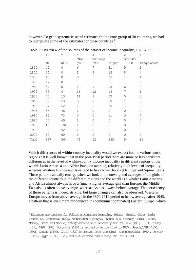
12

however. To get a systematic set of estimates for the core-group of 30 countries, we had to interpolate some of the estimates for those countries.2

Table 2: Overview of the sources of the dataset of income inequality, 1820-20001 2 3 4 5 6 7

All WIID‘New’ ginis

GDP/wage ratio Heights

Both 4&5 (50/50) Interpolations

1820 40 0 6 7 21 5 1

1850 40 0 1 9 18 8 4

1870 45 0 9 6 19 10 1

1890 47 0 7 6 21 11 2

1910 54 0 12 9 25 6 2

1929 55 0 16 12 19 7 1

1950 75 13 11 9 37 5 0

1960 89 53 3 2 30 1 0

1970 97 62 2 2 30 1 0

1975 53 48 1 0 4 0 0

1980 84 73 0 0 11 0 0

1985 70 69 1 0 0 0 0

1990 105 104 1 0 0 0 0

1995 93 92 1 0 0 0 0

2000 50 50 0 0 0 0 0

Total 997 564 71 62 235 54 11

Which differences of within-country inequality would we expect for the various world regions? It is well known that in the post-1950 period there are more or less persistent differences in the level of within-country income inequality in different regions of the world; Latin America and Africa have, on average, relatively high levels of inequality, whereas Western Europe and Asia tend to have lower levels (Deiniger and Squire 1998). These patterns actually emerge when we look at the unweighted averages of the ginis of the different countries in the different regions and the world as a whole: Latin America and Africa almost always have a (much) higher average gini than Europe; the Middle East also is often above average, whereas Asia is always below average. The persistency of these patterns is indeed striking, but large changes can also be observed: Western Europe moves from above average in the 1870-1910 period to below average after 1945, a pattern that is even more pronounced in (communist dominated) Eastern Europe, which

2 Estimates are complete for following countries: Argentina, Belgium, Brazil, China, Spain, France, UK, Indonesia, Italy, Netherlands, Portugal, Sweden, USA, Germany, India, Poland, Norway, Ghana and Mexico; interpolations were necessary for Thailand (1850, 1910), Turkey (1850, 1890, 1980), Australia (1820 is assumed to be identical to 1850), Russia/USSR (1850, 1890), Canada (1870), Chile (1820 is derived from Argentina), Czechoslovakia (1910), Denmark (1850), Egypt (1890, 1929, and 1820 derived from Turkey) and Peru (1910).

13

has by far the lowest ginis during the 1950-1990 period. The ‘egalitarian revolution’ of the 20th century is also apparent in North America/Australia, and can even be found in the (unweighted) global averages, which decline between 1929 and 1980 (by about 10%). In all regions we see an increase in inequality in the last decade of the 20th century; it is most striking in post communist Eastern Europe.

Table 3 Unweighted averages of the gini coefficients by region and period, 1820-2000

Western Europe

Eastern Europe Asia

Middle East Africa

Latin America

N.America/Australia World

Gini

1820 49,73 43,42 49,08 57,71 44,60 66,74 45,92 49,65

1850 46,16 43,86 43,08 51,73 52,42 47,42 44,54 46,04

1870 49,19 49,86 39,39 46,93 53,13 53,80 42,48 47,56

1890 44,35 38,22 38,97 43,10 42,41 48,37 44,37 42,45

1910 45,80 38,56 41,23 37,35 41,97 47,48 41,75 42,73

1929 44,26 37,11 41,28 40,58 47,65 51,75 43,51 44,12

1950 40,22 34,25 41,86 44,25 48,68 47,65 34,97 43,99

1960 40,71 31,32 40,21 50,02 48,75 49,18 34,43 43,68

1970 37,59 27,01 39,12 48,40 46,73 49,05 33,38 42,21

1980 35,84 28,84 39,87 40,68 46,23 46,69 35,68 40,50

1990 34,77 28,82 38,23 44,22 45,42 50,27 38,93 40,11

2000 38,98 37,63 42,28 47,32 47,49 51,60 43,81 43,03

Idem, as percentage of world average1820 100 87 99 116 90 134 92 100

1850 100 95 94 112 114 103 97 100

1870 103 105 83 99 112 113 89 100

1890 104 90 92 102 100 114 105 100

1910 107 90 96 87 98 111 98 100

1929 100 84 94 92 108 117 99 100

1950 91 78 95 101 111 108 79 100

1960 93 72 92 114 112 113 79 100

1970 89 64 93 115 111 116 79 100

1980 89 71 98 100 114 115 88 100

1990 87 72 95 110 113 125 97 100

2000 91 87 98 110 110 120 102 100

Sample size

1820 14 5 5 2 8 4 3 41

1850 14 7 6 2 3 4 3 39

1870 13 7 9 3 4 5 3 44

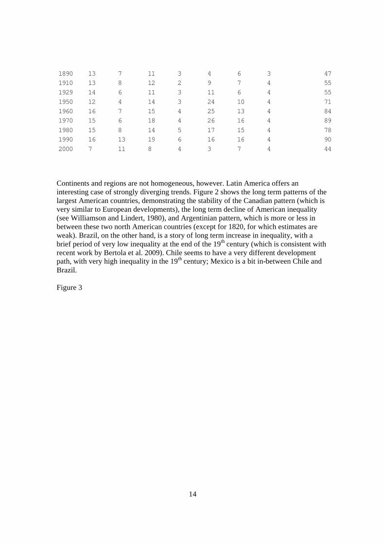
14

1890 13 7 11 3 4 6 3 47

1910 13 8 12 2 9 7 4 55

1929 14 6 11 3 11 6 4 55

1950 12 4 14 3 24 10 4 71

1960 16 7 15 4 25 13 4 84

1970 15 6 18 4 26 16 4 89

1980 15 8 14 5 17 15 4 78

1990 16 13 19 6 16 16 4 90

2000 7 11 8 4 3 7 4 44

Continents and regions are not homogeneous, however. Latin America offers an interesting case of strongly diverging trends. Figure 2 shows the long term patterns of the largest American countries, demonstrating the stability of the Canadian pattern (which is very similar to European developments), the long term decline of American inequality (see Williamson and Lindert, 1980), and Argentinian pattern, which is more or less in between these two north American countries (except for 1820, for which estimates are weak). Brazil, on the other hand, is a story of long term increase in inequality, with a brief period of very low inequality at the end of the 19th century (which is consistent with recent work by Bertola et al. 2009). Chile seems to have a very different development path, with very high inequality in the 19th century; Mexico is a bit in-between Chile and Brazil.

Figure 3

15

Gini's of income inequality for Americas, 1820-2000

0

10

20

30

40

50

60

70

80

90

1820 1850 1870 1890 1910 1929 1950 1960 1970 1980 1990 2000

BrazilchileMexicoargentinaUSACanada

A much more uniform picture emerges from looking at Western Europe, where all countries (with the possible exception of Spain, which has a relatively low level of inequality in the 19th century) share the same long term decline of the gini index (please note the different scale). We do not find much evidence for a Kuznets curve here, in the case of the UK perhaps because the first data point is in 1820, when the industrialization process is well underway. This does not explain the absence of Kuznets-like patterns in the rest of the region, however, because industrialization there started after 1820.

Figure 4

16

Ginis of income inequality in Western Europe, 1820-2000

0

10

20

30

40

50

60

70

1820 1850 1870 1890 1910 1929 1950 1960 1970 1980 1990 2000

SpainFranceUKItalyNetherlandsSwedenGermany

17

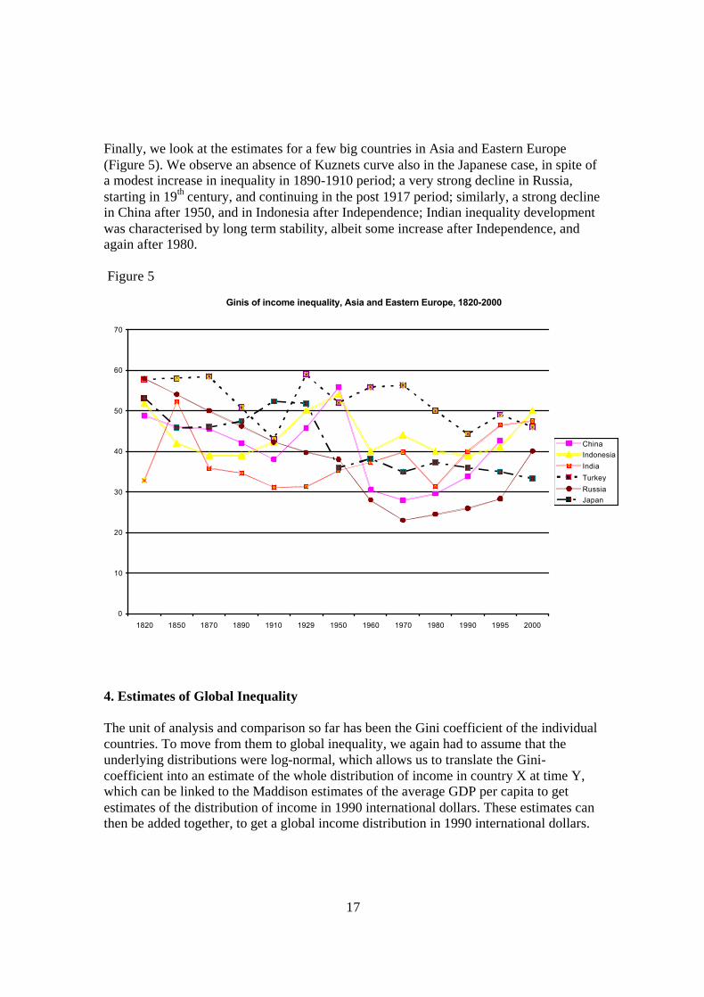
Finally, we look at the estimates for a few big countries in Asia and Eastern Europe (Figure 5). We observe an absence of Kuznets curve also in the Japanese case, in spite of a modest increase in inequality in 1890-1910 period; a very strong decline in Russia, starting in 19th century, and continuing in the post 1917 period; similarly, a strong decline in China after 1950, and in Indonesia after Independence; Indian inequality development was characterised by long term stability, albeit some increase after Independence, and again after 1980.

Figure 5

Ginis of income inequality, Asia and Eastern Europe, 1820-2000

0

10

20

30

40

50

60

70

1820 1850 1870 1890 1910 1929 1950 1960 1970 1980 1990 1995 2000

ChinaIndonesiaIndiaTurkeyRussiaJapan

4. Estimates of Global Inequality

The unit of analysis and comparison so far has been the Gini coefficient of the individual countries. To move from them to global inequality, we again had to assume that the underlying distributions were log-normal, which allows us to translate the Gini-coefficient into an estimate of the whole distribution of income in country X at time Y, which can be linked to the Maddison estimates of the average GDP per capita to get estimates of the distribution of income in 1990 international dollars. These estimates can then be added together, to get a global income distribution in 1990 international dollars.

18

What are the results of our estimates for the development of global inequality? Table 4 gives the most important results: the development of the gini of the global income distribution. It increases from .47 in 1820 to .62 in 1929 and .65 in 1950, after which its more or less stabilises at that (extremely high) level during the second half of the 20th

century. The table also demonstrates that we cover between 85 and 94 percent of global population, which is (we think) quite high; this percentage tends to increase somewhat during the period under study. On the basis of the Maddison dataset we estimate that the average income of this 85 to 94 share is only slightly higher than that of the world as a whole – but the average income of the uncovered rest is clearly lower than of the countries covered by this experiment (for example, in 1820, the average income of ‘the rest’ can be estimated to be about 500 dollars). We therefore more or less consistently underestimate inequality, but the bias does not change much over time. A comparison with Bourguignon and Morrison (2002) appears to point in the same direction: their Gini estimate of global inequality is during the 19th century consistently higher than ours, by an unchanging 3 points on the Gini scale (their estimates of global inequality increase from .50 in 1820 to .61 in 1910). The difference disappears however in 1929 (B&M: .62), and both sets of estimates are almost identical for the post 1945 period. The disappearance of the gap between these two sets of estimates is somewhat puzzling as B&M are supposedly always based on a total coverage of the global population, whereas we also after 1910 or 1945 still miss 5-15 percent of the global population, who are on average poorer than the average global citizen (that both sets of estimates for the rest are quite similar is not unexpected, of course, given the fact that we both use Maddison’s estimates of GDP per capita and the Worldbank’s estimates of income inequality). This bias in our results may also affect our estimates of the development of absolute poverty levels, which is probably also somewhat lower than in ‘reality’. Still they point to a rapid decline of absolute poverty during these two centuries, a process that however seems to come to a halt during the most recent period. The total number of poor people (below 1 dollar) was more or less stable between 1820 and 1929 (when economic growth was apparently strong enough to compensate for the growth of the total population), increased very rapidly between 1929 and 1950 (from 381 to 624 millions), fell rather rapidly after 1950 to its lowest point, 221 million, in 1980, but began to increase again after 1980 – in the fifteen years between 1980 and 1995 the total increase was almost 50%. This result is really different from that published by B&M, who estimated that the number of people living in extreme poverty remained more or less the same between 1960 and 1992.

19

Table 4. Global Ginis, and data on the coverage of our samples, 1820-1995

World GINIs

Population covered

Share of global population

Average income covered population*

Average income World* Ratio

Millions coverage/all

1820 0,47 921 0,88 689 667 1,03

1850 0,50 1034 0,88 804 791 1,02

1870 0,53 1086 0,85 921 873 1,05

1890 0,55 1266 0,86 1149 1133 1,01

1910 0,58 1518 0,87 1535 1465 1,05

1929 0,62 1791 0,87 1899 1784 1,06

1950 0,65 2298 0,91 2258 2113 1,07

1960 0,64 2789 0,92 2898 2775 1,04

1970 0,65 3474 0,94 3855 3736 1,03

1980 0,65 4023 0,91 4767 4521 1,05

1985 0,64 4081 0,85 5258 4763 1,10

1990 0,64 4946 0,94 5467 5162 1,06

1995 0,65 5087 0,90 5647 5452 1,04

in1990 international dollars

Table 5. Estimates of ‘real’ poverty: number of people earning less than 1 or 2 USD dollars per day (in 1990 international dollars, and in millions)

1 USD day 2 USD dayno persons

share of population covered

no persons

share of population covered

1820 363 0,39 669 0,73

1850 369 0,36 695 0,67

1870 367 0,34 717 0,66

1890 338 0,27 749 0,59

1910 334 0,22 763 0,50

1929 381 0,21 805 0,45

1950 624 0,27 1047 0,46

1960 437 0,16 1110 0,40

1970 375 0,11 1173 0,34

1975 319 0,10 1077 0,33

1980 221 0,05 953 0,22

1985 229 0,05 758 0,17

1990 246 0,05 831 0,16

1995 325 0,06 899 0,17

20

Another way to present these estimates is to chart the different global income distributions in one picture, shown below, which indicates both the increase in income levels, the growth of the population and the changes in its distribution (all in 1990 dollars). What is in particular striking, is the change in the structure of the income pyramid through time (see for similar analyses of the more recent period, see Milanovic 2002). Between 1820 and 1929 world income distribution is unimodal, but in the next few decades a different distribution emerges with two clearly separate ‘modes’ or peaks –this begins to show a bit in 1950, is more clearly in 1960, and becomes very significant in 1970 and 1980, when indeed a big gap between rich and poor appears. However, in the 1980s the two modes begin to merge, and in 1995 the distribution has become consistently unimodal again.

Figure 6 Global income distributions: number of people with certain level of income (in dollars of 1990), 1820-1995

0

200000

400000

600000

800000

1000000

1200000

1400000

1600000

1800000

10 100 1000 10000 100000

1990 1995

1980 1970

1960 1950

1929 1910

1890 1870

1850 1820

21

Another way of analysing these estimates is to make the distinction between within country and between countries inequality. Table 6 below presents the different ginis of within country and between country inequality. Unsurprisingly, the between country inequality is relatively low at the beginning of the period, and increases strongly with the growth of income disparities between countries. The within country inequality does not increase in the very long run (comparing 1995 with 1820), although in the 1950-1980 period there is a fall, followed by an increase in the final decades of the 20th century. It follows that the total increase in global inequality is the result of the increase in between country inequality.

Table 6 also shows the overlap factor; because of the statistical features of the Gini coefficient, the sum of the within country gini and the between country gini is larger than the global gini. The difference between them is the overlap factor, which is in essence nothing more than that share of the within group inequality of country A that overlaps with within group inequality of country B. This has led Milanovic (2002, 70) to claim that "the more important the overlapping component..... the less one's income depends on where she lives" . Between 1820 and 1970 the overlap factor does not increase at all, but it suddenly declines between 1970 and 1985 (a sign of growing polarization of the income pyramid we already noticed), followed by an even stronger increase between 1985 and 1995, indicating that the dual structure of the incomes pyramid has disappeared again.

Table 6. Within country and between countries inequality, 1820-19953

Within country inequality

Between country inequality Sum

Actual world gini

Overlap factor

1820 0,43 0,24 0,67 0,47 -0,19

1850 0,43 0,26 0,70 0,50 -0,19

1870 0,41 0,33 0,74 0,53 -0,21

1890 0,39 0,34 0,73 0,55 -0,19

1910 0,41 0,38 0,78 0,58 -0,20

1929 0,47 0,41 0,88 0,62 -0,26

1950 0,45 0,49 0,93 0,65 -0,28

1960 0,38 0,46 0,84 0,64 -0,20

1970 0,37 0,48 0,85 0,65 -0,20

1975 0,37 0,49 0,86 0,68 -0,18

1980 0,35 0,45 0,80 0,65 -0,16

1985 0,37 0,39 0,76 0,64 -0,12

3 Estimated in the following way: column 2 results from assuming that incomes levels of all countries are the same (and identical to the world average); column 3 is the result of assuming that the Ginis in all countries are the same at 0.01 (for mathematical reasons we cannot assume that the Gini is 0)

22

1990 0,39 0,47 0,86 0,64 -0,22

1995 0,43 0,52 0,95 0,65 -0,30

5 Inequality and economic growth: explaining the Great Divergence?

Does the level of income inequality during the 19th and early 20th century help to explain economic performance during the process of industrialization? Because we especially broaden the dataset available for studying 19th and early 20th century inequality, we focus on this question here. There is a large literature about inequality and growth, which already started with the works of Gerschenkron who argued that inequality did have positive effects during this period. He imagined positive effects of physical capital formation which might have been larger if the richer income groups were able to save more (assuming that the poorer strata saved close to nothing). On the other hand, the growth miracles of relatively egalitarian East Asian economies during the later 20th

century encouraged a more recent literature which found that inequality did have negative effects on growth (among many, Benabou 1996; Persson and Tabellini, 1994), or insignificant effects at least if country fixed effects are controlled for (again, in a large literature, Barro 2000; Forbes 2000)Our dependent variable is annual growth of GDP per capita for the 1820-50, 1850-1870, 1870-1890, 1890-1910, 1910-1950 periods. The periods are of different length, but by annualizing the growth rate, we obtain comparable units. We include all explanatory variables as levels at the beginning of periods, in order to measure “growth capabilities”. The gini coefficient is coded between 0 and 1, and is available for all 97 panel units, for which we could obtain growth data of the countries included, which are reported under Table 8. In contrast, the institutional variable “polity2” is only available for 78 cases. This variable is based on the coding of participation possibilities in many countries of the world, which has been classified in a systematic way by the POLITY IV project. We included this variable, as there is a big debate whether institutional quality matters for growth, and in particular, whether “princes” or other autocratic rulers can appropriate physical and financial capital from private owners (Glaeser et al. 2004, DeLong and Shleifer 1993, Baten and van Zanden 2008 on the early modern period). Initial GDP per capita could be an important factor, as it might proxy initial physical capital endowment (Barro 2000). Moreover, there might be convergence events, if the initially poor can adopt more advanced technologies from the richer technology leaders. Finally, we included a variable for initial population size, as it proxies jointly with GDP per capita the size of economies. Moreover, to a certain extent, it allows to control for Kremer-Boserup effects of large populations encouraging more inventions (as the pool of inventions might be larger, although the “pool” might of course not be defined by nation states).Average growth of the countries studied was 1.14 % per year, with a minimum of –0.65, a maximum of 3.07 percent annual growth, and a standard deviation of 0.757 (Table 7). Our compilation of gini coefficients varied between 0.247 and 0.741, with a standard deviation of 0.107.

23

Table 7: Descriptives of our growth regression variables

Variable | Obs Mean Std. Dev. Min Max-------------+-------------------------------------------------------- ygrpct | 97 1.144796 .7570685 -.6507819 3.068836 gini1 | 97 .4655103 .1065775 .247 .741 polity2 | 78 -.474359 6.076834 -10 10 lny | 97 7.345828 .633732 6.272877 8.578534 lnpop | 97 9.46843 1.465968 6.405229 12.92878

Table 8. Fixed effect regressions of GDP per capita growth 1820-50, 1850-1870, 1870-1890, 1890-1910, 1910-1950 (p-values reported in parentheses)

(1) (2) (3)gini1 -2.68* -3.87*** -3.20**

(0.075) (0.0095) (0.015)polity2 0.08*** 0.06**

(0.0041) (0.028)Lny -1.80*** -0.83***

(0.00070) (0.0049)Lnpop 0.99**

(0.024)Constant 6.77*** 9.29*** 2.63***

(0.0077) (0.00015) (0.000040)Observations 78 78 97Number of countries 22 22 25R-squared 0.31 0.24 0.08Countries included are ar, au, be, br, ca, cl, cn, co, de, dk, eg, es, fr, hr, id, ie, in, it, jp, ke, mx, nl, no, nz, ph, pl, ru, se, th, tr, uk, us

Table 9. Fixed effect regressions of GDP per capita growth 1820-50, 1850-1870, 1870-1890, 1890-1910, 1910-1950 (p-values reported in parentheses)

(1) (2) (3)extraction ratio -1.63* -2.05*** -3.20

(0.062) (0.001) (0.185)polity2 0.08*** 0.06*

(0.002) (0.064)Lny -2.19*** -1.25***

(0.001) (0.008)Lnpop 1.03***

(0.005)Constant 9.20** 12.05*** 1.54***

(0.016) (0.001) (0.000)Observations 76 76 94Number of countries 22 22 25R-squared 0.33 0.25 0.02

24

Countries included are ar, au, be, br, ca, cl, cn, co, de, dk, eg, es, fr, hr, id, ie, in, it, jp, ke, mx, nl, no, nz, ph, pl, ru, se, th, tr, uk, usNote: the extraction ratio is calculated under the assumption of 1% elite share

As a result, inequality mattered for 19th century growth – and the effect was negative and statistically significant across various specifications (Table 8). We get very similar results when we use the extraction ratio as defined by Lindert etal (2007) instead of the Gini-coefficient; again, inequality seems to be bad for long term growth (Table 9). Gerschenkron was wrong – inequality did not have positive effects via physical capital formation during this period. Was this effect also economically significant? Multiplying the coefficient of Model 2 with a standard deviation of inequality (.1065775*-3.87) informs us that annual growth was reduced by -0.412 percent. Is this large or small? The standard deviation of GDP growth in the period was only 0.757. Hence yes, inequality had an economically important effect on the differing growth experiences of the countries studied here.Other results are that democracy and the institutions which came with it were good for growth. The negative coefficient of initial GDP per capita suggests that we observe here conditional convergence (note, however, that fixed effects growth regressions are sometimes biased towards convergence). Although China, India, Indonesia and all those large, slowly growing countries are included, also the coefficient for log population size is positive. The effect of inequality is also relatively robust, if we move from the more inclusive model (1) to the less and least inclusive models. The R-square drops to 0.08 when inequality is the only explanatory variable, although it still has explanatory power. It is also robut, if extraction ratios are included instead of gini coefficients (Table 9).As caveats, we need to mention some of the variables which we could not measure for the 19th century for a sufficient number of countries and early periods yet. Among them are human capital, innovativeness, entrepreneurial spirit, openness and similar variables which might have a good potential to explain growth differences. Some of those might have been partially captured by the fixed effect, but it is definitely on the agenda to include them as expanatory variables.In spite of those caveats, it seems fair to conclude that inequality mattered strongly and negatively for the 19th and early 20th century growth history.

6. Conclusion

We have reconstructed a new dataset of estimates of the inequality of the income distribution for a large set of countries for benchmark years starting in 1820 and ending in 1995. This was, in comparison with the estimates produced by Bourguignon and Morrison (2002), based on the use of new (and old) historical studies of income inequality in different countries, on estimates based on the development of the ratio between wage and income, and on estimates based on heights inequality (or a combination of the latter two approaches). Moreover, these estimates have been used to reconstruct the evolution of global inequality between 1820 and 1995. The long term evolution of global inequality that emerges from this is not very dissimilar from the

25

results presented by B & M. Within country inequality did not change a lot in the very long run, although in many countries inequality tended to decline during the 20th century ‘egalitarian revolution’, but this was often followed by a rise of inequality after 1980. Between country inequality increased a lot and was the main cause behind the very strong increase in global inequality in these two centuries – but this process appears to have come to an end during the second half of the 20th century. Perhaps even more interesting were the changes in the structure of global inequality; it was an almost uniformly uni-modal distribution in the 19th century, because increasingly bi-modal during the 1950-1980 period, and ‘suddenly’ changed into a bi-modal distribution again between 1980 and 1995. We intend to analyse the underlying dynamics of these changes in more detail in the future.The main contribution of the paper is perhaps the enlargement of the database of 19th and early 20th century estimates of income inequality. We therefore also tried to establish –very tentatively – if there was a link between income inequality and economic performance during the ‘long’ 19th century. It appears that, after controlling for the influence of amongst other institutions, inequality had a negative impact on economic growth during this period, which, when it can shown to be robust, will be an important new result.

References

A’Hearn, B. (2004). A Restricted Maximum Likelihood Estimator for Truncated Height Samples. Economics and Human Biology 2, pp. 5-19

Aaberge (2005): Gini's Nuclear Family International Conference to Honor Two Eminent Social Scientists, Allen, Robert C. (2001).‘The Great Divergence in European Wages and Prices from the Middle Ages to the

First World War,’ Explorations in Economic History, Vol. 38, pp 411-447.Allen, Robert & Jean-Pascal Bassino & Debin Ma & Christine Moll-Murata & Jan Luiten van Zanden,

2007. ‘Wages, Prices, and Living Standards in China,1738-1925: in comparison with Europe, Japan, and India,’ Economics Series Working Papers 316, University of Oxford, Department of Economics.

Alvaredo, F. and Saez, E. (2006). ‘Income and wealth concentration in Spain in a Atkinson, A. B. (2007b). ‘Top incomes in the United Kingdom over the twentieth century.’ In Top Incomes

over the Twentieth Century: A Contrast Between Continental European and English Speaking Countries (ed. A. Atkinson and T. Piketty), pp.82-140. Oxford: Oxford University Press.

Atkinson, A. B. and Leigh, A. (2005). ‘The distribution of top incomes in New Zealand.’ Atkinson, A. B. and Leigh, A. (2007a). ‘The distribution of top incomes in Australia.’ Atkinson, A.B., & Brandolini, A. (2001). Promise and Pitfalls in the Use of ‘Secondary’ Data Sets: Income

Inequality in OECD Countries as a Case Study. Journal of Economic Literature, 39(3), 771-799.Australian National University CEPR Discussion Paper 503.

Banerjee, A. and T. Piketty (2005), “Top Indian Incomes, 1922-2000”, The World Bank Economic Review, 19, 1-20.

Barro, R. J. (2000), ‘Inequality and Growth in a Panel of Countries’, Journal of Economic Growth, vol. 5, no. 1, March 2000, pp. 5-32.

Bassino, J.P. (2006). Inequality in Japan (1892-1941): Physical Stature, Income, and Health. Economic and Human Biology 4, pp. 62-88.

Baten, J. (1999). Ernährung und wirtschaftliche Entwicklung in Bayern, 1730-1880. Stuttgart: Steiner.Baten, J. (2000). "Economic Development and the Distribution of Nutritional Resources in Bavaria, 1797-

1839," in Journal of Income Distribution 9, pp. 89-106

26

Baten, J. and U. Fraunholz (2004). Did Partial Globalization Increase Inequality? The Case of the Latin American Periphery, 1950-2000" with Uwe Fraunholz, CESifo Economic Studies 50-1 (2004), pp. 45-84.

Baten, J., and Böhm, A. (2009). “Trends of Children’s Height and Parental Unemployment: A Large-Scale Anthropometric Study on Eastern Germany, 1994-2006.”, German Economic Review(forthcoming).

Benabou, R. (1996), ‘Inequality and Growth’, in: B. S. Bernanke and J. J. Rotemberg (eds), NBER Macroeconomics Annual 1996, Cambridge, MA: MIT Press, pp. 11–74.

Bertola, Luis, Cecilia Castelnovo, Javier Rodriguez, Henry Willebald (2009). ‘Income distribution in the Latin American Southern Cone during the first globalization boom and beyond’ International Journal of Comparative Sociology (forthcoming)

Bigsten, A. (1985). Income Distribution and Growth in a Dual Economy. PhD thesis, Gothenburg University, Department of Economics.

Bourguignon, F., Morrisson, C.,(2002). Inequality among world citizens: 1890-1992, American Economic Review 92 (4), 727-744, September.

Broadberry, S. (2003) “Relative per capita Income Levels in the United Kingdom and the United States since 1870: Reconciling Time Series Projections and Direct Benchmark Estimates”, Journal of Economic History, 63 (2003): 852-863.

Deaton, A. (2001). Relative Deprivation, Inequality and Mortality. NBER Working Paper 8099.Deininger, K. and Squire, L. (1996), ‘A new dataset measuring income inequality’, The World Bank

Economic Review, 10, 565-591.Deininger, K. and Squire, L. (1998), ‘New Ways of Looking at Old Issues: Inequality and Growth’,

Journal of Development Economics, December 1998, 57(2), pp. 259 – 87Dell, F. (2007). ‘Top incomes in Germany throughout the twentieth century: 1891–1998.’ In Top Incomes

over the Twentieth Century: A Contrast Between Continental European and English Speaking Countries (ed. A. Atkinson and T. Piketty), pp.365-425. Oxford: Oxford University Press.

Dell, F., Piketty T. and Saez, E. (2007). ‘Income and wealth concentration in Switzerland over the 20th century.’ In Top Incomes over the Twentieth Century: A Contrast Between Continental European and English Speaking Countries (ed. A. Atkinson and T. Piketty), pp.472-500. Oxford: Oxford University Press.

DeLong, J. Bradford and Andrei Shleifer. 1993. “Princes and Merchants: City Growth before the Industrial Revolution.” Journal of Law and Economics 36(2): 671-702.

Forbes, K. J. (2000), ‘A Reassessment of the Relationship between Inequality and Growth’, American Economic Review, vol. 90-4, pp. 869-87.

François, J.F., and H. Rojas-Romagosa (2005), “The Construction and Interpretation of Combined Cross Section and Time-Series Inequality Datasets,” Worl d Bank Policy Research Working Paper 3748.

Glaeser, E.L., R. La Porta, F. Lopez-de-Silanes, A. Shleifer (2004). ‘Do Institutions Cause Growth?’Journal of Economic Growth 9-, 271-303.Global History of Prices and Wages, Utrecht - 19-21 August 2004

Guntupalli, A.M. and Baten, J. (2006). “The Development and Inequality of Heights in North, West and East India, 1915-44”, Explorations in Economic History 43, iss. 4, pp. 578-608.

Jacobs, J., Katzur, T., Tassenaar, V. (2008). On Estimators for Truncated Height Samples. Economics and Human Biology 6-1, pp. 43-56.

Jones, C.I., (1997). On the evolution of the world income distribution, Journal of Economic Perspectives 11 (3), 19-36, Summer.

Komlos, J. & Kriwy, P. (2003). The Biological Standard of Living in the Two Germanies. German Economic Review, 4(4), 459-73.

Komlos, J. (1985). Stature and Nutrition in the Habsburg Monarchy: The Standard of Living and Economic Development. American Historical Review, 90, 1149-1161.

Latham and H. Kawakatsu (eds.), Asia Pacific Dynamism 1500-2000 (London: Routledge): 13-45.Leigh, A., and P. van der Eng (2007), “Top Incomes in Indonesia, 1920-2004,” Australian National

University, Centre for Economic Policy Research, Discussion Paper no. 549.Lindert, P., Milanovic, B., and J. Williamson (2007), “Measuring Ancient Inequality,” NBER Working

Paper No. 13550.Lindert, Peter, Brank Milanovic, and Jeffrey G. Williamson (2007). Measuring Ancient Inequality NBER

Paper #13550

27

López, J.H., Servén, L., 2006. A normal relationship? Poverty, growth, and inequality.Macmillan Reference; New York : Stockton Press, 1998.

Maddison, A. (2001). The world economy: a millennial perspective. OECD, Paris.Maddison, A. (2003). The world economy: historical statistics. OECD, ParisMilanovic, B., (2002). True world income distribution, 1988 and 1993: First calculation based on

household surveys alone, Economic Journal 112 (476), 51-92, January.Milanovic, Branko (2007) World Apart. Measuring International and Global Inequality. Princeton.Mironov, B. (2004). Prices and Wages in St. Petersburg for Three Centuries (1703-2003). Towards a Mitchell, B. R. (2003a). International Historical Statistics: Africa, Asia and Oceania, 1750-2000

(Basingstoke and New York: Palgrave Macmillan, 4th edn. 2003.Mitchell, B.R. (1998). International historical statistics: the Americas, 1750-1993, London: Macmillan Mitchell, B.R. (1998b). International historical statistics: Africa, Asia & Oceania, 1750-1993, London:

Macmillan Reference; New York : Stockton Press, 1998. Mitchell, B.R. (1998c). International historical statistics: Europe, 1750-1993, London : Moradi, A. and Baten, J. (2005) “Inequality in Sub-Saharan Africa 1950-80: New Estimates and New

Results, ” World Development Volume 33-8 (2005), pp. 1233-1265.Moriguchi, C. and Saez, E. (2006). ‘The evolution of income concentration in Japan, 1885-2002: evidence

from income tax statistics,’ National Bureau of Economic Research Working Paper 12558, NBER, Cambridge, MA.

Nolan, B. (2007). ‘Long-term trends in top income shares in Ireland.’ In Top Incomes over the Twentieth Century: A Contrast Between Continental European and English Speaking Countries (ed. A. Atkinson and T. Piketty), pp.501-530. Oxford: Oxford University Press.

Persson, T. and Tabellini, G. (1994), ‘Is Inequality Harmful for Growth?’, American Economic Review, 84-3, pp. 600–21.

Piketty, T. (2007). ‘Income, wage and wealth inequality in France, 1901-1998.’ In Top Incomes over the Twentieth Century: A Contrast Between Continental European and English Speaking Countries (ed. A. Atkinson and T. Piketty), pp.43-81. Oxford: Oxford University Press.

Piketty, T. and Saez, E. (2006b). ‘Income inequality in the United States.’ Tables and Figures updated to 2004 in Excel format, http://emlab.berkeley.edu/users/saez/ (downloaded 6 December 2006).

Pomeranz, K. (2000). The Great Divergence. China, Europe and the Making of the Modern World Economy. Princeton U.P

Pradhan, M., Sahn, D.E., & Younger, S.D. (2003). Decomposing World Health Inequality. Journal of Health Economics, 22(2), 271-293.

Prados de la Escosura, L. (2008), ‘Inequality, Poverty and the Kuznets Curve in Spain, 1850-2000. European Review of Economic History 12, pp. 287-324

Prados de la Escosura, Leandro, (2000). "International Comparisons of Real Product, 1820-1990: An Alternative Data Set," Explorations in Economic History, vol. 37(1), pages 1-41, January.Reference; New York : Stockton Press.

Roine, J. and Waldenström, D. (2006). ‘Top incomes in Sweden over the twentieth century.’ Research Institute of Industrial Economics Working Paper 667, Stockholm, Sweden.

Rossi, N., G. Toniolo, G. Vecchi, “Is the Kuznets curve still alive ? Evidence from Italian household budgets, 1881-1961”, The journal of economic history, 4, 2001.

Saez, E. and Veall, M. (2005). ‘The evolution of high incomes in Northern America: lessons from Canadian evidence.’ American Economic Review, vol. 95(3), (June), pp. 831-849.

Salverda, W. and Atkinson, A. B. (2007). ‘Top incomes in the Netherlands over the twentieth century.’ In Top Incomes over the Twentieth Century: A Contrast Between Continental European and English Speaking Countries (ed. A. Atkinson and T. Piketty), pp.426-472. Oxford: Oxford University Press.

Schmitt, L.H. & Harrison, G.A. (1988). Patterns in the Within-Population Variability of Stature and Weight. Annals of Human Biology, 15(5), 353-364.

Soltow, L. (1998), “The Measures of Inequality”, in: L. Soltow and J.L. van Zanden (eds.), Income & Wealth Inequality in the Netherlands 16th-20th Century, Het Spinhuis: Amsterdam, 7-22.

Soltow, Lee and Jan Luiten van Zanden (1998) Income and Wealth Inequality in the Netherlands 1500-1990. Het Spinhuis Amsterdam

Steckel, R. (1995). Stature and the Standard of Living. Journal of Economic Literature, 33(4), 1903–1940.

28

Sunder, M. (2003). The Making of Giants in a Welfare State: The Norwegian Experience in the 20th Century. Economics & Human Biology, 1(2), 267-276.

Van Leeuwen, Bas and Péter Földvári, 'The Development of inequality and poverty in Ward, M. H., Devereux, J. (2005). Relative British and American Income Levels during the First Industrial

Revolution, Research in Economic History, 23, (2005), p. 255-292. Williamson Jeffrey G. (1998). “Globalization and the Labor Market: Using History to Inform Policy ” pp.

103-193 in P. Aghion and J. G. Williamson, eds.Growth, Inequality and Globalization. Cambridge UP.

Williamson, J. (1999c). Real Wages, Inequality, and Globalization in Latin America Before 1940. Revista de Historia Economica, 17 (special number), 101-142.

Williamson, J. (2000a). Globalization, Factor Prices and Living Standards in Asia Before 1940, in A.J.H. Williamson, J. (2000b). Real Wages and Factor Prices Around the Mediterranean 1500-1940,in S. Pamuk

and J.G. Williamson (eds.) The Mediterranean Response to Globalization Before 1950 (London: Routledge) : 45-75.

Williamson, J. G. and P. H. Lindert (1980), American Inequality: A Macroeconomic History. (New York: Academic Press).

Williamson, Jeffrey G. (2000) "Real Wages and Factor Prices Around the Mediterranean 1500-1940," Chp. 3 in S. Pamuk and J.G. Williamson (eds.) The Mediterranean Response to Globalization Before 1950 (London: Routledge 2000) : 45-75World Bank Policy Research Working Paper 3814.

World Income Inequality Database V2.0c May 2008 (http://www.wider.unu.edu/research/Database/en_GB/database/)Zanden, J.L. van (2002) 'Rich and Poor before the Industrial Revolution: a comparison between Java and

the Netherlands at the beginning of the 19th century', Explorations in Economic History 40, 1-23.