The Lahore Journal of Economics 12 : 1 (Summer 2007) pp. 1-34

Financial Development and Economic Growth: Evidence from a Heterogeneous Panel of High Income Countries

A.R. Kemal*, Abdul Qayyum** and Muhammad Nadim Hanif***

Abstract

This paper examines the empirical relationship between financial development and economic growth for high income countries. The study focuses on both indirect finance and direct finance, separately as well as jointly. Applying the methodology of Nair-Reichert and Weinhold (2001) for causality analysis in heterogeneous panel data, two sets of results are reported. First, the evidence regarding the relationship between financial development and economic growth from a contemporaneous non-dynamic fixed effects panel estimation is mixed. Negative and statistically significant estimates of the coefficient of the inflation and financial development interaction variable indicate that financial sector development may even be harmful to economic growth when inflation is rising. Second, in contrast with the recent evidence of Beck and Levine (2003), heterogeneous panel causality analysis applied on a refined model indicates that there is no definite evidence that finance spurs economic growth or growth spurs finance. Most of our findings are in line with the Lucas (1988) view that the importance of financial matters is over-stressed. The only exception is the case of activity in stock markets where our result supports the Robinson (1952) view that finance follows enterprise.

Introduction

The relationship between financial development and economic growth has always fascinated economists. As far back as 1873, Bagehot argued that the financial system played a critical role in igniting industrialization in England by facilitating the mobilization of capital for growth1. Schumpeter (1934) noted that banks actively spur innovation and

* Visiting Professor of Economics, Fatima Jinnah University, Rawalpindi. ** Registrar, Pakistan Institute of Development Economics (PIDE), Islamabad. *** State Bank of Pakistan, Karachi. 1 Hicks (1969) also came out with the similar conclusion.

A.R. Kemal, Abdul Qayyum and Muhammad Nadim Hanif 2

future growth by identifying and funding productive investments. McKinnon (1973) and Shaw (1973) brought the relationship between financial development and economic growth at the centre stage of research. Lucas (1988), however, dismisses finance as a major determinant of economic growth calling its role over-stressed by economists. Empirical evidence is also mixed as has been pointed out by Levine (1997, 2003) in extensive reviews of the literature.

In view of the conflicting evidence, Khan and Senhadji (2000) stress that the relationship between financial development and economic growth needs to be refined and appropriate estimation methods employed.

Both the theoretical and empirical literature suggest that increases in the rate of inflation can adversely affect financial market conditions (Khan, Senhadji, and Smith, 2003). A simple way to allow for such an effect is to write the coefficient of financial development as a function of inflation, and to consider both financial development and inflation separately as well as interactively while modeling the relation between financial development and economic growth.

Previous studies have been based either on time series data or on cross-sectional data. Whereas time series analysis is confined to an individual country, the cross-sectional studies have been criticized on the grounds of failure to control effectively for cross-country heterogeneity. No doubt some studies have used a panel GMM estimator to analyze the finance and growth relationship, but as pointed out by Kiviet (1995), panel data models that use instrumental variables estimation often lead to poor finite sample efficiency and bias. Considering the heterogeneous nature of the relationship between financial development and economic growth across countries, Nair-Reichert and Weinhold’s (2001) methodology of panel causality analysis has been used in this study.

The main objective of the present study is to investigate the causal relationship between financial development and economic growth by using panel data from 19 High Income Countries (HIC) for the period 1974-2001. The plan of the paper is as follows. The theoretical and empirical work relating to the relationship between financial development and economic growth is reviewed in the next section. The model used in the study and the methodology applied are outlined in section 3. The empirical results are provided in section 4. A summary of the conclusions and policy recommendations are given in the last section of the paper.

Financial Development and Economic Growth

3

2. Review of Literature

The literature on the finance-growth nexus may be grouped into four schools of thought.

i) Finance promotes growth: Banks act as an engine of economic growth as noted by Bagehot (1873), Schumpeter, (1934), Hicks (1969), McKinnon (1973), Shaw (1973), and some others.

ii) Finance hurts growth: As explained in Levine (2003), it is believed that banks have done more harm to the morality, tranquility, and even wealth of nations than they have done or ever will do good. Although financial institutions facilitate risk amelioration and the efficient allocation of resources, it may not boost growth because better finance means greater returns to saving and lower risk (which may result in lower savings) and resultantly lower growth.

iii) Finance follows growth: Robinson (1952) pointed out that the enterprise leads financial development. Economic growth creates a demand for financial arrangements and the financial sector responds automatically to these demands.

iv) Finance does not matter: According to Lucas (1988) the role of finance in economic growth has been overstressed.

As pointed out earlier, some studies (such as those of Levine, Loayza and Beck (2000) and Beck, Levine, and Loayza (2000)) have used a panel GMM estimator to analyze the finance and growth relationship to control for cross country heterogeneity, but it has often led to poor finite sample efficiency and bias. Some studies allow for intercept heterogeneity but Pesaran and Smith (1995) show that if slope coefficients are assumed to be constant, the traditional panel estimators may yield inconsistent estimates. Moreover, using a period average, i.e., collapsing each time series variable into a single observation, has been criticized because of the nonstationary nature of these data [See Van den Berg and Schmidt (1994) and Van den Berg (1997)].

The use of time-series-cross-section panel data estimation allows researchers to control for country-specific, time-invariant fixed effects, and includes dynamic, lagged dependent variables which are also helpful in controlling for omitted variable bias. But the traditional panel data fixed effects estimators (FEE) impose homogeneity assumptions on the coefficients of lagged dependent variables when, in fact, the dynamics are heterogeneous across the panel. Pesaran and Smith (1995) argue that this misspecification

A.R. Kemal, Abdul Qayyum and Muhammad Nadim Hanif 4

may lead to serious biases that cannot be remedied with instrumental variable estimation. The Mean Group Estimator of Pesaran and Smith (1995) is an unweighted average of the country specific coefficients and is particularly sensitive to outliers. A simple Random Coefficient (RC) estimator, on the other hand, calculates a variance weighted average, but it is not possible to estimate dynamic RC models. The Mixed Fixed Random (MFR) effects approach of Hsiao et al (1989) which has been utilized by Weinhold (1999), and Nair-Reichert and Weinhold (2001) falls somewhere in between the two extremes of FEE and MGE in terms of allowing for heterogeneity. This method imposes more structure on the coefficient values of the exogenous variables than the MGE. As compared to the FE estimator with a small T, the MFR coefficients approach produces a considerably less biased parameter estimate [Nair-Reichert and Weinhold (2001)]. Weinhold (1999) shows that the MFR coefficients model performs very well compared to instrumental variables (GMM), and it has other features well suited for the causality analysis in heterogeneous panel data sets.

Nausser and Kugler (1998) use the heterogeneous panel data approach for a limited number of OECD countries and after doing panel cointegration analysis, individual country causality analysis has been applied. Christopoulos and Tsionas (2003) use panel unit root tests and panel cointegration analysis to examine the relationship between financial development and economic growth in ten developing countries. But for causality analysis they use time-series tests to yield causality inferences within a panel context.

Chari, Jones and Manuelli (1996) argue that financial regulations and their interaction with inflation have substantial effects on growth. Choi, Smith, and Boyd (1996) argue that inflation reduces the real return to savings and makes the adverse selection problems in capital markets more severe inducing a high degree of credit rationing and a negative impact on financial development. In a monetary growth model, Huybens and Smith (1999) show that, at the steady state, higher rates of money creation reduce the real return on all assets and, under certain conditions, lead to a reduction in the volume of trading in equity markets. Boyd, Levine and Smith (2001) consider an alternative theory regarding the relationship between inflation and financial sector performance: governments combine high inflation with various restrictions on the financial sector to help fund expenditures. As a result, they have both poorly developed financial systems and high inflation. Barro (1997) finds that permanent increases in the rate of inflation have significant negative effects on long run real growth rates. Khan, Senhadji, and Smith (2003) assert that the real effects of inflation derive from the consequences of inflation for financial markets conditions.

Financial Development and Economic Growth

5

3. Model, Data, and Econometric Methodology

3.1 Model Specification

Following King and Levine (1993), the relationship between financial development and economic growth using the linear regression equation is given below:

G F Xα β γ= + + (3.1)

where is growth in real GDP per capita; G

F is the proxy for financial development; and

X is the set of conditioning information to control for other factors associated with economic growth.

For the heterogeneous panel data, the model may be specified as

it i i it i it itG F Xα β γ ε′= + + + (3.2)

where , and .

rs to the number of observations over time for country in the panel.

Parameter

Ni ,...,2,1= Tt ,...,2,1= i

N refers to the number of countries;

iT refe i

iα is the country specific intercept, or fixed effect paramet

The slope coefficient is also allowed to vary across countries to take into account the possible heterogeneity3 among the various countries in a panel.

er, which of course is also allowed to vary across individual countries2.

2 Country specific fixed effects heterogeneity is assumed on the basis of differences in technology. 3 Even though we have grouped countries according to their level of income, there may still be heterogeneity between the countries in the panel. There are different sources of such heterogeneity such as differences in population size, differences in political and economic institutions, differences in geography, and differences in culture.

A.R. Kemal, Abdul Qayyum and Muhammad Nadim Hanif 6

The other factors associated with economic growth (i.e. the variables in X ) include two types of variables: state as well as control variables. State variables are the initial stock of physical capital and the initial stock of human capital. The available data on physical capital seem unreliable (Barro and Sala-i-Martin, 2004). Following Barro and Sala-i-Martin (2004) we assume that for a given stock of human capital, a higher level of initial income reflects a greater stock of physical capital or larger quantity of natural resources. For the initial level of income we use real GDP per capita with a one year lag. Because of diminishing returns to reproducible factors, a richer economy tends to grow at slower rate. Therefore, the influence of the higher initial level of income on the growth rate of real GDP per capita in equa

ent ratio on the growth rate of real GDP per capita in equation (3.2) would be positive because

er capita GDP to be negative and the sign of the coefficient of the initial level of secondary school enrollment ratio to

atio (denoted by GCGR) as fiscal policy variable, and international trade openness (denoted by TRGR) as internat

will increase the complexity of contracts, raise the frequency of negotiations,

tion (3.2) would be negative.

There are some very interesting and path breaking models which shed light on the role of human capital in economic growth. One of the most prominent and influential contributions is that of Lucas (1988), which in turn is related to the previous work by Uzawa (1965). In the long run, sustained growth is linked with human capital. Human capital is a broader concept. We use educational attainment as a stock of human capital. The variable we use to proxy the educational attainment is the secondary school enrollment ratio. The influence of the higher (initial) secondary school enrollm

educational attainment affects productivity positively.

Previous empirical studies [for example Barro (1997), Barro and Sala-i-Martin (2004)] have shown that growth in real GDP per capita is negatively related to the initial level of GDP. So we also expect, in our study, the sign of the coefficient of initial level real p

be positive in equation (3.2).

Following the recent literature on the analysis of financial development and economic growth, the control variables we use are: inflation rate (denoted by INFL) as measure of macro economic instability, government consumption to GDP r

ional trade policy variable.

Temple (2000) asserts that inflation increases uncertainty. It will tend to introduce unwelcome noise into the workings of the markets, for instance raising relative price variability. Planning will become more difficult. Heyman and Leijonhufvus (1995) argue that high inflation rates

Financial Development and Economic Growth

7

and perhaps lead to certain contracts being avoided altogether. Planning horizons shorten, and firms avoid long run commitments. In this way, inflation tends to have negative effects on growth.

rnment consumption to GDP ratio on growth rate of real GDP per capita.

ogical progress and hence, permanently rises growth rates (Winter, 2004).

Accordingly (3.2) is written as

SE

TRGRGCGRINFLFGRGPC

The issue of the effect of government consumption is complicated. Government consumption is a component of aggregate demand, and if there is slack in production and prices and/or wages are sticky downward, it will have a positive effect on GDP according to Keynesian hypothesis. Moreover, the public sector may raise the productivity of the private sector by providing legal, defense, judiciary and police services, enforcing property rights, and correcting failures in the markets etc. On the other hand, government interventions generate disincentive effects caused by revenue raising and transfer activities. Taxes to meet the expenditures can result in serious resource misallocation. Additionally, potential inefficiencies caused by rent-seeking and principal-agent problems in the provision of government output may result in substantial negative impact on productivity. This can mitigate or even offset the potential positive effects of government consumption on economic growth and we may have a negative sign of the impact of gove

Overall, the trade to GDP ratio is a measure of the openness of a country to international trade. It is argued in the literature that the greater the openness the greater the competition or exposure to a larger set of ideas or technologies which increases the technol

itiitiitiitiiit ββββα

ititiiti RGPCS R εββ +++ −− 1655

+++′+= 4321 (3.3)

where itε are assumed to be idiosyncratic errors.

We first estimate the contemporaneous non-dynamic fixed effects panel model of economic growth by regressing the GRGPC on conditioning variables (INFL, GCGR; TRGR; SSER4; and initial RGPC) and we name it as the general model. Dropping the insignificant variables (if any) we will be left with a parsimonious basic model for economic 4 We use secondary school enrollment ratio with 5 year lag because people in secondary school at time will generally be entering the labour force in some latter time and will not be productive for 5 years or so.

t

A.R. Kemal, Abdul Qayyum and Muhammad Nadim Hanif 8

growth. To this basic model we add a proxy for financial development and have an intermediate model to see how financial development contributes to economic growth. In order to capture the impact of changes in the rate

ial market conditions, it is hypothesized that the of inflation on financfinancial development effect, i1β ′ , is a function of the inflation rate, i.e.;

INFL7 itiii 11 βββ + . By substituting it back into equation (3.3) we get:

INFLFRGPCSSER

=′

ititiitiiti

itiitiitiitiiit TRGRGCGRINFLFGRGPC

εβββββββα

++++++++= 4321 (3.4)

−− )*(71655

To analyze whether there is a causal relationship between economic growth and financial development we turn to the dynamic panel form of (3.4) in which GRGPC is modeled as a function only of lags of itself and of all other right hand side variables in (3.4). That is:

INFLFGRGPCGRGPC

β

This gives us the final model which includes the proxy for financial development and inflation, both individually as well as interactively.

itiitiitiiit ββγα

ititi

itiitiitiiti

INFLF

RGPCSSERTRGRGCGR

εββββ

+++++

−

−−−−

17

26651413

)*(

(3.4a)

++++= −−− 12111

To take care of the linear influences of the remaining right-hand side variables in (3.4a) on the candidate causal variable, we orthogonalize the candidate causal variable5 and thus our final model in dynamic form

GCG

INFLFGRGPC

βββγα ++++= −−−

3

12111

becomes:

ititi

itiitiitiit

INFLF

RGPCSSERTRGRR

εββββ

+++++

−

−−−−

17

2665141

)*(

(3.5)

All the variables in the model are assumed to be stationary.

i

itio

itiitiiitGRGPC

5 Our causal candidate variable is the proxy for financial development and we orthogonalize only this variable in order to ensure that the estimated coefficients are independent. We base our non-causality inference on estimated coefficient of the causal candidate variable to be zero.

Financial Development and Economic Growth

9

3.2 Data

One of the important issues pertaining to the analysis of the finance growth nexus is the selection of proxies to measure financial development and economic growth. For economic growth, following King and Levine (1993), we use real per capita GDP growth. We denote it by GRGPC6. Th FollowiDemirgindirectalso comproxy oof financial sector development which will be used in this study. These measures are discussed below.

i)

of banks and other financial intermediaries, divided by GDP,

the functioning of the financial system.

ii) vate sector credit (by deposit

money banks and other financial institutions) to GDP ratio (PCGR).

iii) (MCGR),

which equals the market value of listed shares divided by GDP.

iv) raded in the

stock market to GDP ratio (VTGR).

ere is no single accepted empirical definition of financial development. ng King and Levine (1993); Levine and Zervos (1998); and Beck, uc-Kunt, and Levine (2001) various indicators of size and activity of as well as direct finance proxy for financial sector development. We bine the size and activity measures of direct and indirect finance to

verall financial sector development. As a whole, we have six measures

The size of indirect finance: The size of the financial intermediaries is measured as currency plus demand and interest bearing liabilities

generally known as liquid liabilities to GDP ratio (LLGR). This is the broadest available indicator of financial intermediation. However, the size of the financial sector may not accurately measure

The activity of indirect finance: To measure the activity of financial intermediaries we consider the pri

The size of direct finance: As an indicator of the size of direct finance we use the stock market capitalization to GDP ratio

The activity of direct finance: As an indicator of the activity of direct finance we use the total value of the shares t

v) The size of the overall financial sector: Combining the two size measures we have an overall size measure of the financial sector. We call it the financial depth to GDP ratio, denoted by FDGR.

6 For a complete list of data, variables, and sources of data see Appendix A.

A.R. Kemal, Abdul Qayyum and Muhammad Nadim Hanif 10

vi) The activity of the overall financial sector: Combining the two activity measures we have an overall activity measure of the financial sector, i.e., the financial activity to GDP ratio (FAGR).

Stock variables are measured at the end of a period and the flow variables are def

ing timing and deflation. To address these problems, we deflate the end-of-year financial aggregates by end-of-year consum

llowing:

ined relative to a period. This presents a problem in the first type of measure, both in terms of correct

er price indices (CPIe) and deflate the GDP series by annual consumer price index (CPIa), following Demirguc-Kunt and Levine (2001). Then we compute the average of the real financial aggregate in year t , and

1−t and divide this average by real GDP measured in year t . The end-of-year CPI is either the value for December, or, where the December-CPI is not available, for the last quarter. The formula, for LLGR7, is the fo

⎥⎥⎦⎢

⎢⎣

⎟⎠

⎜⎝ − tatete CPICPICPI ,1,,

*5.0 (3.6)

In the case of the ratio of two flow variables measured in the same time, deflating is

⎤⎡⎟⎞

⎜⎛

+= − ttt GDPLLBLLBLLGR 1

not necessary.

We use a dataset of 19 HIC countries listed in the Appendix A. The countries have been selected from the overall list of High Income Countries

car

that data are available for at least 15 observations for both types of finance.

3.3 Methodology

for which World Bank publishes income classifi ation in its World Development Indicators8. The countries included e selected on two criteria: there is data both on indirect as well direct finance; and

For testing the stationarity of the variables we apply the Im, Pesaran and Shin (2002) panel unit root test for dynamic heterogeneous panels which is based on the average (across countries) of the (augmented) Dickey-Fuller statistics.

7 The same is also done for MCGR. 8 The World Development Indicators for 2002 have been used. The country classification is based on World Bank estimates of per capita GNI during 2000. Countries for which estimates of per capita GNI are US$ 9265 or more are classified as High Income Countries.

Financial Development and Economic Growth

11

3.3.1 Pane o Test

r the calculation of individual country unit root (augmented) Dickey-Fuller test-statistics denoted by . The process starts

by estimating the following (augmented) Dickey-Fuller regression:

l Unit R ot s

First we conside

iiTt~

it

ip

jjititiiiit yyty ερδα +∆+++=∆ ∑

=

riables to be included depends on the stationarity of the error term and here we will be using a step down procedure starting at a maximum lag of four.

IPS pan t test is

−−1

1 (3.7)

for each of the cross sectional units in the panel and estimating the value of the t-statistics and then averaging them. The decision on the number of lags of the dependent va

ρ

The null hypothesis for the el unit roo

0:0 =iH ρ for all i (3.8)

against the alternatives

0:1 <iH ρ , fo ,..,2 N , and 0=iρ , for NNi ,1 11 +=

iσ , iiTt are independently (but not

9>iT bart −~ statistic:

r ,1i = 1 N,...,2+ (3.9)

his f m alternative h ot esis allows for T or ulation of yp h i differing across groups. It allows for some (but not all) of the individual series to have unit roots under the alternative hypothesis. Essentially, the IPS test averages

estimating (3.7) for each the ADF individual unit root test statistics that are obtained from

i (allowing each series to have a different lag length, ip if necessary); that is:

∑=−N

iTNT tbart ~1~ =

iN (3.10)

i 1

which is referred to as the bart −~ statistic.

IPS shows that under the assumption that iit TtNi ,...,2,1,,...,2,1, ==ε in (3.7) are independently and identically distributed for all i and t with mean

2 ~zero and finite heterogeneous variances identically) distributed for and that the standardized

A.R. Kemal, Abdul Qayyum and Muhammad Nadim Hanif

12

N t~ − barNT − 1−

N ∑ =

N

i TitE

1)~(

=tbarZ

∑ =

− N

i TitVARN

1

1)~(

(3.11)

c ge ly.

growth. Otherwise, the order of integration of the series of interest does not support a move to cointegration analysis. On the basis of the evidence docume

3.3.2 Contemporaneous Fixed Effects Model Estimation

Assuming the slope coefficients to be homogeneous, we estimate the model in (3.4) using a fixed effects methodology in which the country specific fixed effects are wiped out and each variable is replaced by its deviation form cross-sectional means. On this transformed data the OLS

Weinhold (1999) and Nair-Reichert and Weinhold (2001) for causality

onver s to standard normal variate9 as N increases indefinite

When testing for panel unit roots at level we take both the unobserved effects and heterogeneous time trend as in equation (3.7). If in no case we reject the null hypothesis that every country has a unit root for the series in levels, we then test for a unit root in first differences.

If the proxy for economic growth and for financial development are of the same order of integration and none of the control variables is of a higher order than that of the dependent variable, we move towards testing for possible cointegration between financial development and economic

nted in Lee, Pesaran and Smith (1997) and in Canning and Pedroni (1999), we expect our dependent variable (growth in real GDP per capita) and the variables of interest to be stationary and therefore we may not have to apply panel cointegration analysis.

method is applied. However, for calculating the estimated t-values robust variance estimator proposed in Arellano (1987) is used to address the issue of possible heteroscedasticity.

3.3.3 Panel Causality Analysis for Dynamic Heterogeneous Panel Data Model

We examine the direction of causality between financial development and economic growth, and vice versa, using the methodology introduced by

9 IPS standardized their test statistics based on simulations of the mean and variance (with different values obtained depending on the lag length used in the ADF tests and the value of N). These simulated values are given in IPS (2002).

Financial Development and Economic Growth

13

analysis in heterogeneous panel data which is based upon the mixed fixed random (MFR) coefficients approach of Hsiao et al (1989).

air-Reichert and Weinhold (2001), we consider the model

ε+−12 (3.12)

Following N

ioitiitiiit xxyy ββγα +++= −− 21111 itit

where ijji ηββ += . iη is a random disturbance. Here

),(~2

jjji N βσββ . The variable oitx 11 − denotes the orthogonalized

candidate causal variable after the linear influences of the remaining right-hand side variables have been taken into account. Orthogonalization10 provides for the appropriate interpretation of the estimated variances by making sure that the coefficients are independent. Unobserved effects ( iα ) and the coefficient of the lagged dependent variable are fixed and country specific; and the coefficients on the exogenous explanatory variables are drawn from a random distribution with mean jβ and finite variance11.

The estimator and the corresponding standard error are discussed in Appendix B.

4. Results

4.1 Statistical properties of the data

Table-4.1A shows the summary statistics of various variables used in this study. The comparison of within and between-country standard deviation for all the variables shows that most of the variability in all the variables is between countries which shows the heterogeneity amongst the countries.

The pair-wise correlations matrix, presented in Table 4.1B, shows that the growth in real per capita GDP is positively related to openness measured by trade to GDP ratio and to all the indicators of financial development, except private credit to GDP ratio. The secondary school

10 For the purpose of orthogonalization of the lagged causal candidate variable, we regress the lagged causal candidate variable on the constant, lagged dependent variable and all other explanatory variables. We use errors of this regression as orthogonalized (lagged) causal candidate variable. 11 Weinhold (1999) explains why to model this particular combination of fixed individual specific coefficients on the lagged dependent variable and random coefficients on the lagged independent variables.

A.R. Kemal, Abdul Qayyum and Muhammad Nadim Hanif 14

enrollment to GDP ratio is negatively correlated with growth in real per capita GDP12 because it may not be a good proxy for education in a high income country; higher education may have a strong positive correlation with re

development and inflation interaction outweighs the positive contribution from financial development t

4.2 Im

evel, we consider both the unobserved effects and heterogeneous time trend as in equation (3.7). It can be argu

rowth rate of real GDP per capita to inflation, government consumption to GDP ratio, overall trade to GDP ratio, (initial)

al per capita GDP growth. Real GDP per capita growth is negatively related to the government consumption to GDP ratio and to the rate of inflation. Finally, the inflation rate is negatively correlated with all the measures of financial development. Interestingly, the correlation coefficients between inflation and financial development are higher compared to the correlation coefficients between financial development and economic growth, i.e. the negative contribution of financial

o real GDP per capita growth.

-Pesaran-Shin Panel Unit Root Test

Table-4.2 presents the results of the Im-Pesaran-Shin (2002) panel unit root (IPS PUR) test on all variables used in this study. All the variables are stationary at level except (initial) RGPC, GCGR, TRGR, INFL*PCGR, and FDGR. These variables are nonstationary and become stationary after first differencing 13.

While testing for panel unit roots at l

ed, particularly in the case of the growth rate of real GDP per capita and inflation, that there is no reason to include the heterogeneous time trend while testing for the unit root. However, it has been observed that the orders of integration of growth and inflation are insensitive to whether or not we include the heterogeneous time trend.

4.3 Contemporaneous Fixed Effects Model Estimation

In order to explore the relationship between financial development indicators and economic growth, we start with the estimation of the contemporaneous non-dynamic fixed effects panel estimation of the most general form which relates g

secondary school enrollment ratio and the (initial) level of per capita GDP14.

12 In Table-4.3.1 we can also see that SSER is found to be insignificant in contemporaneous non dynamic fixed effects panel estimation. 13 We will be using first differences of such variables in the panel causality analysis. 14 All the variables are in log form.

Financial Development and Economic Growth

15

4.3.1 Indirect Finance and Economic Growth

Inflation, government consumption to GDP ratio, overall trade to GDP ratio, and initial per capita income are the significant determinants of growth in per capita GDP in High Income Countries (see Table 4.3.1). These results show that all the four explanatory variables in the basic model have the appropriate sign. These results are consistent with standard growth theory. Inflation depresses growth due to its adverse implications for working markets. Government consumption affects growth negatively, because of well known inefficiencies associated with the larger size of the government. A negative significant coefficient of the initial level of per

ence growth theories. Overall the trade to GDP ratio has a positive effect on the growth rate of

of the financial sector become insignificant. However, the interaction term is negative and significant in the case of interaction with

on with the activity indicator of financial development. Thus in the HIC, we do not find any rela

n in the column under the intermediate model. Both the proxies of size and activity of the (direct) financial sector are significant irrespective of whethe

capita GDP is in accordance with the conditional converg

real GDP per capita.

By including proxies for financial development as regressors besides these four variables and re-estimating the simple contemporaneous non dynamic fixed effects panel regression, we find that the coefficient of the proxy for the size of the financial sector is insignificant, whereas the coefficient of the proxy for the activity of the financial sector is significant with a negative sign. When the interaction of finance with inflation is introduced, then the coefficients of the proxies of both the size and the activity

the size indictor and is insignificant in the case of interacti

tionship between financial development and economic growth when we have the interaction variable in the model. However, the economic growth returns of further financial development in the size of indirect finance declines with increased inflation.

4.3.2 Direct Financial Development and Economic Growth

Table-4.3.2 gives the results of the simple contemporaneous non-dynamic fixed effects panel estimation. By including proxies for direct finance as regressors in the basic model, the simple contemporaneous non-dynamic fixed effects panel regression has been re-estimated and the results are show

r the interaction variables are included or not. Interaction variables themselves are found to be insignificant. This shows that size and activity of direct finance has a strong positive relationship with economic growth for HICs.

A.R. Kemal, Abdul Qayyum and Muhammad Nadim Hanif 16

4.3.3 Overall Financial Development and Economic Growth

Table-4.3.3 gives the results of the simple contemporaneous non-The proxy of the size of the overall

financial sector is statistically significant irrespective of whether we take finance

ncially developed stage of the economy as its impact is greater than that which can be at the lesser (financially) developed stage of the e

above is based on the underlying m geneity of the relationships across countries in

the panel. Heterogeneity is restricted to the intercept but is not permitted e apply the Nair-Reiche t and Weinhold (2001)

panel causality method to our final model in the dynamic form in equation (3.5). I

th of one due to the

dynamic fixed effects panel estimation.

alone or as an interaction variable with inflation. However, the proxy of the activity of the overall financial sector is statistically insignificant, irrespective of whether we take finance alone or along with an interaction variable with inflation. The implications are clear: economic growth has a relationship with only the size of the overall financial sector and is independent of financial development expressed in terms of activities of the (overall) financial sector. The coefficient of the interaction variable is insignificant for both the size as well as activity of the overall financial sector.

It is also observed that the magnitude of the partial effect of inflation on growth rate of GDP per capita is larger in the final model as compared to the basic model. It shows that inflation may be a much more serious issue in the fina

conomy.

4.4 Panel Causality Analysis

The entire analysis of the contemporaneous non-dynamic fixed effects panel estimation presented assumption about the ho o

in the slope coefficients. W r

n this model, the coefficient on the lagged dependent variable is country specific and the coefficients on the other right hand side variables are allowed to have normal distribution. We choose a lag leng

large number of explanatory variables and relatively short time series for each country. The results are presented in Table 4.4 where we report the mean of the estimated coefficient, standard error of the mean of the estimated coefficient, and the variance estimate of the estimated coefficient on the causal variable.

For causality testing, we build confidence intervals around zero (here we will use the first element in the estimated vector 1

~θ which is ]1[1~θ

which is to be tested to be zero) to test for the mean of the estimated

Financial Development and Economic Growth

17

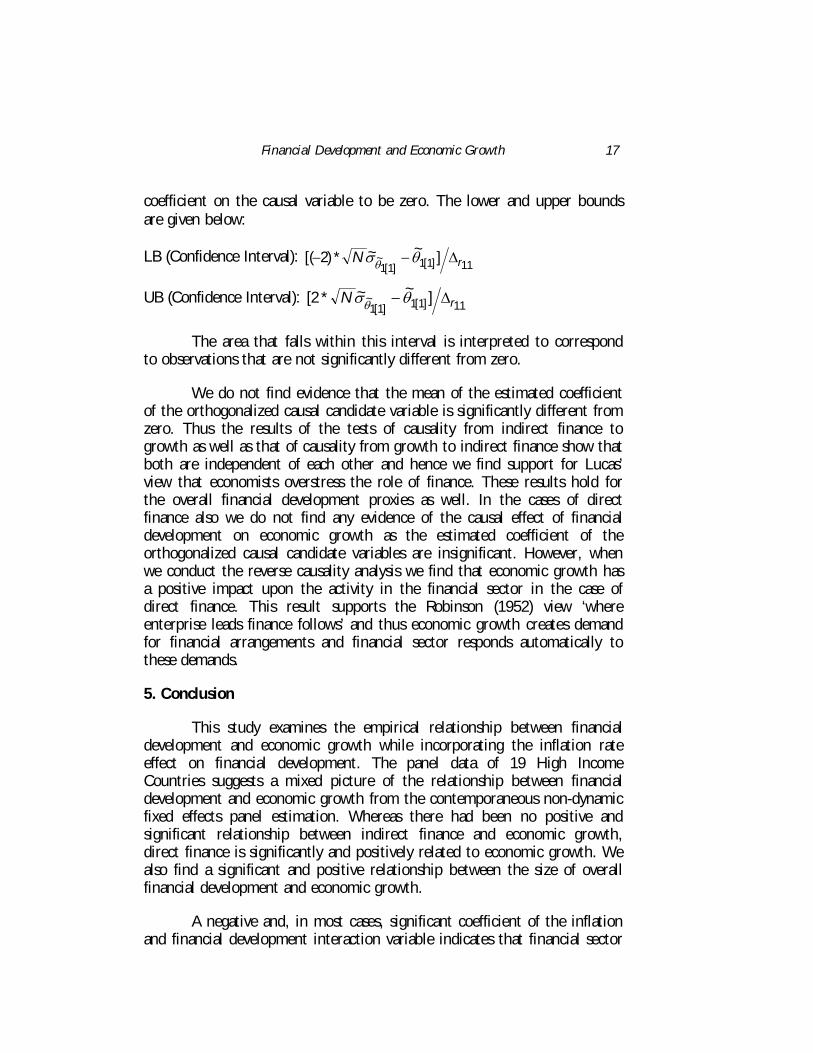
coefficient on the causal variable to be zero. The lower and upper bounds are given below:

LB (Confidence Interval): 11]1[1]1[1

~ ]~~*)2[( rN ∆−− θσθ

UB (Confidence 11]1[1]1[1

~ ]~~*2[ rN ∆−θσθ Interval):

The area that falls within this interval is interpreted to correspond to obse

the causal effect of financial development on economic growth as the estimated coefficient of the orthogo

This study examines the empirical relationship between financial develop

A negative and, in most cases, significant coefficient of the inflation and financial development interaction variable indicates that financial sector

rvations that are not significantly different from zero.

We do not find evidence that the mean of the estimated coefficient of the orthogonalized causal candidate variable is significantly different from zero. Thus the results of the tests of causality from indirect finance to growth as well as that of causality from growth to indirect finance show that both are independent of each other and hence we find support for Lucas’ view that economists overstress the role of finance. These results hold for the overall financial development proxies as well. In the cases of direct finance also we do not find any evidence of

nalized causal candidate variables are insignificant. However, when we conduct the reverse causality analysis we find that economic growth has a positive impact upon the activity in the financial sector in the case of direct finance. This result supports the Robinson (1952) view ‘where enterprise leads finance follows’ and thus economic growth creates demand for financial arrangements and financial sector responds automatically to these demands.

5. Conclusion

ment and economic growth while incorporating the inflation rate effect on financial development. The panel data of 19 High Income Countries suggests a mixed picture of the relationship between financial development and economic growth from the contemporaneous non-dynamic fixed effects panel estimation. Whereas there had been no positive and significant relationship between indirect finance and economic growth, direct finance is significantly and positively related to economic growth. We also find a significant and positive relationship between the size of overall financial development and economic growth.

A.R. Kemal, Abdul Qayyum and Muhammad Nadim Hanif 18

development is actually more harmful for economic growth when inflation is high, especially at a more developed stage of the financial system. In the cases where the interaction term is significant, the magnitude of the partial effect o

pment. Most of our findings are in line with the Lucas view on finance that the importance of financial matters is very badly over-stressed. The only exception is the case when we conduct the reverse causality analysis and find that economic growth has a positive impact upon activity in the financial sector in the case of direct finance. This result supports the Robinson (1952) view that where enterprise leads finance follows. Therefore it follows thus that economic growth creates a demand for financial arrangements and the financial sector responds automatically to these demands15.

We examined the empirical relationship between financial development and economic growth for a panel of high income countries. All of the countries in the sample had, during the time period under consideration, relatively developed and sophisticated financial markets, in which ‘marginal’ improvements in financial sector size and/or activity might have only modest effects on growth and thus might be the conclusion we reached above. Thus we would like to caution about generalizing these results on all countries, particularly low income countries. The causal relationship between financial development and economic growth may be different for low income countries than for high income countries.

f inflation on the growth rate of GDP per capita is found to be larger in the final model as compared to that in the basic model, i.e. inflation may be a much more serious issue in the financially developed stage of the economy as its impact is greater than that which can be at the lesser (financially) developed stage of the economy.

The use of the Nair-Reichert and Weinhold (2001) panel causality methodology for the dynamic heterogeneous panel and a refined model employed in this study show that there is no indication that financial development spurs economic growth or growth spurs financial develo

15 During the 1990’s, information technology revolution has changed the nature and speed of financial transaction which coupled with globalization of stock markets and banking structure has given new meanings to financial development. In the light of these comments of one of the anonymous referees we also did the whole above exercise for post 1990 sample. The results of Nair-Reichert and Weinhold panel causality analysis for post 1990 sample are reported in Table 4.4A of the Appendix A which are not much different from those reported for full period sample in Table 4.4. The detailed results on panel unit root analysis and contemporaneous fixed effects panel estimation are available from the corresponding author on request.

Financial Development and Economic Growth

19

Appendix A

Table-3.1: Countries Included in Study

Country Time Span and

Number of Observations

Country Time Span and

Number of Observations

From To From To

Australia 1979 2001 23 Luxembourg 1978 2001 24

Austria 1974 2001 28 Netherlands 1976 2000 25

Belgium 1974 2001 28 Norway 1976 2001 26

Canada 1976 2000 25 Portugal 1978 2001 24

Denmark 1980 2001 22 Singapore 1981 2001 21

Finland 1976 2001 26 Sweden 1974 1999 26

France 1974 2000 27 Switzerland 1976 2001 26

Greece 1974 2001 28 United Kingdom 1974 2001 28

Italy 1976 2001 26 United States 1978 2001 24

Japan 1974 2001 28 Total Observations 485

A.R. Kemal, Abdul Qayyum and Muhammad Nadim Hanif 20

Table-3.2: Data Description and Sources

Variable Data Description and Source

CPIa Annual Consumer Price Index from IFS (Line 64)

CPIe End-of-year CPI from IFS (Line 64M, or 64Q where 64M is not available)

GDP Gross Domestic Product from IFS (Line 99B)

LLB Liquid Liabilities from IFS (Line 55L or 35L, if 55L is not available)

MCP Market Capitalization from Global Financial Data Base

PCR Claims of Private Sector from IFS [Lines 22D.MZF, 22D.TZF, 22D.ZF, 42D.FZF, 42D.GZF, 42D.LZF, 42D.NZF, and 42D.SZF are included]

POP Population (Line 99Z)

VTD Value Traded from Global Financial Data Base

GCE Government Consumption Expenditures from IFS (Line 91F)

TRD Sum of Exports and Import (Line 90C+98C from IFS) of Goods and Services

GRGPC Annual percentage growth rate of GDP per capita based on constant local currency from WDI-2004. (Dependent Variable)

LLGR Liquid Liabilities to GDP ratio

PCGR Private sector credit to GDP ratio

MCGR Stock market capitalization to GDP ratio

VTGR Stock market total value traded to GDP ratio

FDGR (Overall) financial depth to GDP ratio

FAGR (Overall) financial activity to GDP ratio

INFL Inflation Rate Calculated from CPIa

GCGR Government Consumption Expenditures to GDP ratio

TRGR International Trade (sum of Exports and Import of Goods and Services) to GDP ratio

SSER Gross Secondary School Enrollment Ratio from UNESCO

RGPC GDP per capita based on purchasing power parity from WDI-2004

Financial Development and Economic Growth

21

Table-4.1A: Summary Statistics - Panel Data (yearly observations) of HIC

Variable Mean Std. Dev. Min. Max. Observations Overall 0.0219 0.0229 -0.0678 0.0945 485 Between 0.0396 19 GRGPC Within 0.0220 21, 28 Overall 0.8235 0.5272 0.3049 3.4231 485 Between 2.4992 19 LLGR Within 0.2177 21, 28 Overall 0.7998 0.3606 0.1985 2.2463 485 Between 1.5275 19 PCGR Within 0.2119 21, 28 Overall 0.5516 0.5513 0.0036 2.9530 485 Between 2.1076 19 MCGR Within 0.3796 21, 28 Overall 0.2962 0.5536 0.00001 6.6322 485 Between 1.5594 19 VTGR Within 0.4737 21, 28 Overall 1.3751 0.8889 0.4275 5.2424 485 Between 3.7766 19 FDGR Within 0.5193 21, 28 Overall 1.0960 0.7931 0.2205 7.9635 485 Between 2.6485 19 FAGR Within 0.6184 21, 28 Overall 5.50 4.85 -1.40 25.70 485 Between 14.69 19 INFL (%) Within 4.01 21, 28 Overall 0.1883 0.0431 0.0845 0.2944 485 Between 0.2043 19 GCGR Within 0.0177 21, 28 Overall 0.7761 0.5990 0.1592 3.3712 485 Between 3.0445 19 TRGR Within 0.1210 21, 28 Overall 90.08 18.11 37.18 148.25 485 Between 63.30 19

Initial SSER (%)

Within 13.64 21, 28

A.R. Kemal, Abdul Qayyum and Muhammad Nadim Hanif 22

Table-4.1B: Pair wise Correlations-Panel Data (485 Annual Observations of HIC)

GRGPC LLGR PCGR MCGR VTGR FDGR FAGR INFL GCGR TRGR SSER

GRGPC 1.0000

LLGR 0.1530 1.0000

PCGR -0.0151 0.4936 1.0000

MCGR 0.2673 0.3677 0.3909 1.0000

VTGR 0.1918 0.0665 0.3377 0.6585 1.0000

FDGR 0.2515 0.8403 0.5369 0.8131 0.4255 1.0000

FAGR 0.1045 0.3496 0.8288 0.6369 0.8066 0.5901 1.0000

INFL -0.1847 -0.2145 -0.3785 -0.4506 -0.4060 -0.3969 -0.4791 1.0000

GCGR -0.2672 -0.4201 -0.2543 -0.3185 -0.1536 -0.4487 -0.2510 -0.0188 1.0000

TRGR 0.2857 0.3376 0.2721 0.5976 0.2126 0.5597 0.2972 -0.2503 -0.3445 1.0000

SSER -0.1144 -0.1683 0.0839 0.0500 0.3104 -0.0762 0.2372 -0.4509 0.3710

-0.2372 1.0000

Financial Development and Economic Growth

23

Table-4.2: IPS PUR Test

Variable IPS-PUR test at Level

IPS-PUR test at First Difference

I(0)/I(1)

INFL -6.2101** I(0)@

GCGR -1.2399 -24.2779** I(1)@

TRGR -1.0099 -33.0263** I(1)@

SSER -2.0165** I(0)

RGPC 0.7392 -10.8977** I(1)@

GRGPC -8.3566** I(0)@

LLGR -2.4721** I(0)

PCGR -2.9472** I(0)

INFL.LLGR -6.0404** I(0)@

INFL.PCGR -1.1889 -12.0460** I(1)

MCGR -2.9005** I(0)@

VTGR -4.6956** I(0)@

INFL.MCGR -4.3908** I(0)@

INFL.VTGR -3.1746** I(0)@

FDGR -0.4946 -24.4457** I(1)

FAGR -2.0728** I(0)

INFL.FDGR -5.4697** I(0)@

INFL.FAGR -2.3877** I(0)@

*: Significant at 10% level where critical value is -1.28

**: Significant at 5% level where critical value is -1.64

@: Order of integration is insensitive to maximum lag selection for general to specific methodology between 4 (for which these results are presented) and 1 (results for maximum lag selected 3, 2, and 1 are not presented here).

A.R. Kemal, Abdul Qayyum and Muhammad Nadim Hanif 24

Table-4.3.1: Indirect Finance and Economic Growth

Contemporaneous “Fixed Effects” Panel Regressions: Dependent Variable= GRGPC: Heteroscedasticity Consistent t-statistics in parentheses

Intermediate Model

Final Model Variable

General Model

Basic Model

Size Activity Size Activity

INFL -0.3247 (-8.94**)

-0.3255 (-9.19**)

-0.3275 (-9.96**)

-0.3184 (-8.50**)

-0.3882 (-10.6**)

-0.3286 (-7.77**)

GCGR -0.0728 (-5.25**)

-0.0729 (-5.35**)

-0.0725 (-5.09**)

-0.0747 (-5.50**)

-0.0767 (-5.72**)

-0.0750 (-5.68**)

TRGR 0.0472 (3.30**)

0.0473 (3.25**)

0.0475 (3.30**)

0.0490 (3.50**)

0.0503 (3.94**)

0.0491 (3.55**)

SSER 0.0011 (0.15)

RGPC -0.0212 (-4.64**)

-0.0210 (-5.04**)

-0.0216 (-5.19**)

-0.0156 (-3.59**)

-0.0222 (-5.47**)

-0.0159 (-3.64**)

LLGR 0.0017 (0.25) 0.0971

(1.25)

PCGR -0.0121 (-2.80**)

-0.0108 (-1.50)

INFL.LLGR -0.1481 (-2.25**)

INFL.PCGR -0.0195 (-0.28)

NT 471 471 471 471 471 471

R2 0.2837 0.2837 0.2838 0.3014 0.2933 0.3016

**Significant at 5%;*Significant at 10%.

Financial Development and Economic Growth

25

Table-4.3.2: Direct Finance and Economic Growth

Contemporaneous “Fixed Effects” Panel Regressions: Dependent Variable= GRGPC: Heteroscedasticity Consistent t-statistics in parentheses

Intermediate Model

Final Model Variable

General Model

Basic Model

Size Activity Size Activity

INFL -0.3247 (-8.94**)

-0.3255 (-9.19**)

-0.2500 (-5.75**)

-0.2790 (-6.89**)

-0.3086 (-5.58**)

-0.3151 (-6.83**)

GCGR -0.0728 (-5.25**)

-0.0729 (-5.35**)

-0.0714 (-4.61**)

-0.0695 (-4.98**)

-0.0693 (-4.15**)

-0.0668 (-4.66**)

TRGR 0.0472 (3.30**)

0.0473 (3.25**)

0.0443 (2.99**)

0.0452 (3.01**)

0.0407 (2.65**)

0.0431 (2.75**)

SSER 0.0011 (0.15)

RGPC -0.0212 (-4.64**)

-0.0210 (-5.04**)

-0.0267 (-6.63**)

-0.0245 (-4.80**)

-0.0295 (-8.03**)

-0.0263 (-5.22**)

MCGR 0.0069 (4.34**) 0.0103

(3.59**)

VTGR 0.0021 (1.90*)

0.0033 (1.99**)

INFL.MCGR -0.0302 (-1.36)

INFL.VTGR -0.0104 (-1.01)

NT 471 471 471 471 471 471

R2 0.2837 0.2837 0.3070 0.2920 0.3127 0.2941

**Significant at 5%;*Significant at 10%.

A.R. Kemal, Abdul Qayyum and Muhammad Nadim Hanif 26

Table-4.3.3: Overall Finance and Economic Growth

Contemporaneous “Fixed Effects” Panel Regressions: Dependent Variable= GRGPC: Heteroscedasticity Consistent t-statistics in parentheses

Intermediate Model Final Model Variable General

Model Basic Model Size Activity Size Activity

INFL -0.3247 (-8.94**)

-0.3255 (-9.19**)

-0.3137 (-8.00**)

-0.3304 (-8.47**)

-0.3291 (-8.93**)

-0.3696 (-9.82**)

GCGR -0.0728 (-5.25**)

-0.0729 (-5.35**)

-0.0675 (-4.27**)

-0.0753 (-4.93**)

-0.0702 (-4.75**)

-0.0756 (-5.11**)

TRGR 0.0472 (3.30**)

0.0473 (3.25**)

0.0425 (2.89**)

0.0499 (3.20**)

0.0420 (3.17**)

0.0496 (3.34**)

SSER 0.0011 (0.15)

RGPC -0.0212 (-4.64**)

-0.0210 (-5.04**)

-0.0272 (-8.59**)

-0.0184 (-4.80**)

-0.0273 (-8.18**)

-0.0193 (-5.04**)

FDGR 0.0127 (2.34**) 0.0172

(2.62**)

FAGR -0.0042 (-1.02)

0.0004 (0.07)

INFL.FDGR -0.1260 (-1.88*)

INFL.FAGR -0.1029 (-1.67*)

NT 471 471 471 471 471 471

R2 0.2837 0.2837 0.2973 0.2867 0.3045 0.2929

**Significant at 5%;*Significant at 10%.

Financial Development and Economic Growth

27

Table-4.4: Reichert and Weinhold Panel Causality Analysis (Full Sample)

Causality Reverse Causality

Size Activity Size Activity

Indirect Finance

Estimated Coefficient

Standard Error

LB (Confidence Interval)

UB (Confidence Interval)

Est. Coefficient Variance

-0.0460

0.0194

-1.1651

2.0340

0.0112

-0.0246

0.0201

-2.4902

3.3034

0.0037

0.1185

0.1731

-2.4124

2.0611

0.4553

-0.1911

0.3684

-1.9209

2.1640

2.4722

Direct Finance

Estimated Coefficient

Standard Error

LB (Confidence Interval)

UB (Confidence Interval)

Est. Coefficient Variance

-0.0003

0.0028

-1.3145

1.3493

0.0003

0.0004

0.0012

-0.8474

0.7796

0.0002

-1.0713

0.8431

-1.9328

2.5923

10.5528

2.4375**

1.9222

-2.4661

1.8397

60.5836

Overall Finance

Estimated Coefficient

Standard Error

LB (Confidence Interval)

UB (Confidence Interval)

Est. Coefficient Variance

0.0496

0.0196

-2.1991

1.2086

0.0100

-0.0178

0.0092

-1.0345

1.6218

0.0037

0.1270

0.3432

-3.2416

2.9776

0.9259

-0.2003

0.4977

-1.5984

1.7532

6.7026

**Significant at 5%, *Significant at 10%.

A.R. Kemal, Abdul Qayyum and Muhammad Nadim Hanif 28

Table-4.4A: Reichert and Weinhold Panel Causality Analysis (Sample - post 1990)

Causality Reverse Causality

Size Activity Size Activity

Indirect Finance

Estimated Coefficient

Standard Error

LB (Confidence Interval)

UB (Confidence Interval)

Est. Coefficient Variance

0.2887

0.3609

-2.9885

2.4862

1.3210

-0.1565

0.2092

-1.2253

1.4553

0.0037

-0.3202

1.2714

-4.3260

4.5834

6.1905

-0.6105

0.9886

-4.0780

4.7050

3.8515

Direct Finance

Estimated Coefficient

Standard Error

LB (Confidence Interval)

UB (Confidence Interval)

Est. Coefficient Variance

0.1516

0.0691

-3.8963

2.3285

0.0374

0.0345

0.0164

-2.8346

1.7303

0.0039

1.5350**

2.1890

-1.6065

1.3673

164.7161

8.2387**

4.3030

-2.5638

1.6405

318.4377

Overall Finance

Estimated Coefficient

Standard Error

LB (Confidence Interval)

UB (Confidence Interval)

Est. Coefficient Variance

0.3190

0.1509

-4.3078

2.6264

0.1440

0.2554

0.1070

-2.3833

1.3589

0.2487

0.8985

1.1809

-1.5281

1.2828

53.6608

0.4887

1.4061

-1.6072

1.4839

62.8985

**Significant at 5%, *Significant at 10%.

Financial Development and Economic Growth

29

Appendix B

Let be the dependent variable; Y Z contains vector of 1s for the intercept, and the lagged dependent variables, i.e. those for which we have fixed coefficients; X has the orthogonalized causal candidate variable and other control variables, i.e. all other right hand side variables for which we have random coefficients. We denote the vector of all the right hand side variables (including unobserved effects) by W , i.e. it contains all the variables that are in Z and X . Let 2θ be a vector of fixed coefficients (which are f in number) and 1θ be vector of random coefficients (which are r in number). Let θ denote the vector of all fixed as well as random coefficients.

We estimate 1θ by

]ii Zφ

)ˆ

)(

[])([~

1111

1

11 NN −

1111 ii

iiiiiiii

iiii

ii

=== (3.13

11111

iiiii

N

ii

N

i

YZZZX

YXXZZZZXXX

−−−−

=

−−−−−−

′′′

−′′′′−′=

∑

∑∑∑

φφ

φφφφφθ)

which is the GLS estimate of 1θ under MFR coefficients assumption. Here

( +′∆= irii XXφ

ˆiσ iY

i

12

−Ti Iσ (3.14)

and is OLS estimate of error variance of individual regression of 2

∑ ′−−

upon W , i.e. errorWY iii += θ , and r∆ is the covariance matrix which sub-m rix for random coefficients from

iθ̂ iY iW

errorWY iii += θ and θ̂ is the average of such s for the individuals countries in the panel.

timate individual coefficients under MFR effects approach by

iθ̂

is at

==∆

Nˆˆˆˆ1 θθθθ (3.15)

where is the OLS estimate from individual regression of upon ,

i.e.

− iiiN 1

))((1

We es

A.R. Kemal, Abdul Qayyum and Muhammad Nadim Hanif 30

]~ˆ

ˆ

})(

{ˆ

1[]})({

11

11

2

111

21

θθ

σσ−

−−−

∆+′′′

−′∆+′′′−′

riiiiiii

ii

i

riiiiiiii

i

i

XZZZZX

XXXZZZZXXX (3.16)

(3.17)

ave

1[

~θ =

−

and

)}~

(){(~

12 iiiiiii XYZZZ θθ −′′=

We h

12( θσ ~~

and mean square error is

1~θ ]1[1

~θ

ititiitit XZYu 12 θθ −−=

∑∑ +−= )}*({)(~ rNfTu iitσ

11]1[1]1[1~ ]

~~*)2[( rN ∆−− θσθ

22

~ −and )(~)( ′= WWVar σθ from whi h

11]1[1]1[1~ ]

~~*2[ rN ∆−θσθ

c we can have standard errors ) of

the MFR effects estimates.

round zero16

(here we will use the first element in the vector which is ) for which

the lower and upper bounds are given below:

Lower Bound (Confidence Interval):

For causality testing, we have to build the confidence interval a

Upper Bound (Confidence Interval):

The area that falls within this interval is interpreted to correspond to observations that are not significantly different from zero17.

16 Theoretically speaking; for population parameter under the null hypothesis that ]1[1θ is zero. 17 For panel causality analysis, we use the SAS version of the program (which calculates the estimate of the coefficient of the causal variable, its standard error, the confidence interval and the estimate of the variance of the estimated random coefficient) developed by Diana Weinhold and available on her site linked with that of the London School of Economics, UK. This SAS program does not orthogonalize the candidate casual variable, however, we did it.

~~~

Financial Development and Economic Growth

31

References

Arellano M., 1987, Computing Robust Standard Errors for Within Group Estimators,” Oxford Bulletin of Economics and Statistics, 49, 431-434.

Bagehot, Walter, 1873, Lombard Street. Homewood, IL: Richard D. Irwin, 1962 Edition.

Barro, R. J., 1997, Determinants of Economic Growth: A Cross Country Empirical Study,” MIT Press, Massachusetts.

Barro, R. J. and X. Sala-i-Martin 2004, Economic Growth, Second Edition, MIT Press.

Beck, T, Demirguc-Kunt, Asli, and Levine, R., 2001, “Legal Theories of Financial Development,” Oxford Review of Economic Policy, Vol. 17, No. 4, 483-501.

Beck, T. and R. Levine, 2003, “Stock Markets, Banks and Growth: Panel Evidence”, Journal of Banking and Finance.

Beck, T., R. Levine and N. Loayza, 2000, “Finance and the Sources of Growth”, Journal of Financial Economics, 58: 261–300.

Boyd, John H., Ross Levine, and Bruce D. Smith, 2001, “The Impact of Inflation on Financial Sector Performance,” Journal of Monetary Economics, 47, 221-248.

Canning, D. and P. Pedroni, 1999, “Infrastructure and Long Run Economic Growth,” CAE Working Paper, No. 99-09, Connell University.

Chari, VV, Larry E. Jones and Rodolfo E. Manuelli, 1996, “Inflation, Growth and Financial Intermediation,” Federal Reserve Bank of St. Louis Review, May/June.

Choi, S., Bruce D. Smith, and John H. Boyd, 1996, “Inflation Financial Markets and Capital Formation,” Federal Reserve Bank of St. Louis Review, May/June.

Christopoulos, D. K. and E. G. Tsionas, 2004, “Financial Development and Economic Growth: Evidence from Panel Unit Root and Cointegration Tests”, Journal of Development Economics, 73, pp 55-74.

A.R. Kemal, Abdul Qayyum and Muhammad Nadim Hanif 32

De Gregorio, Jose and Federico Sturzenegger, 1994a, “Credit Markets and the Welfare Costs of Inflation,” NBER Working Paper 4873.

De Gregorio, Jose and Federico Sturzenegger, 1994b, “Financial Markets and Inflation under Imperfect Information,” IMF Working Paper 94/63.

Demirguc-Kunt, Asli and Ross Levine, 2001, “Financial Structure and Economic Growth: A Cross Country Comparison of Banks, Markets, and Developments,” Edited, MIT Press.

Heyman, D. and Leijonhufvus, A. 1995, High Inflation, Clarendon Press, Oxford.

Hicks, J., 1969, “A theory of economic history”, Oxford: Clarendon Press.

Hsiao, C., Mountain, D.C., Chan, M.W.L. and Tsui, K.Y., 1989, “Modeling Ontario Regional Electricity System Demand Using a Mixed Fixed Random Coefficients Approach,” Regional Science and Urban Economics, Vol. 19, pp. 565-87.

Huybens, Elisabeth & Smith, Bruce D., 1999, “Inflation Financial Markets, and Long Run Real Activity” Journal of Monetary Economics 43, 283-315.

Im, K. Pesaran, H. and Shin, Y., 2002, “Testing for Unit Roots in Heterogeneous Panels, A revised version of Im, Pesaran and Shin (1997), received though Email from Pesaran.

Kemal, A.R., 2000, “Financing Economic Development”, Presidential Address at the 16th AGM of PSDE, January, Islamabad.

Khan, Mohsin S. Abdelhak S. Senhadji and B.D. Smith, 2003, “Inflation and Financial Depth,” Improved version of IMF Working Paper WP/01/44, International Monetary Fund, Washington, Sent by Khan through email.

King, R. G. and R. Levine, 1993, “Finance and Growth: Schumpeter Might Be Right Quarterly Journal of Economics, August, 717-738.

Kiviet, Jan F., 1995, “On Bias, Inconsistency, and Efficiency of Various Estimators in Dynamic Panel Data Models,” Journal of Econometrics, Vol. 68.

Financial Development and Economic Growth

33

Lee, K., H. Pesaran and R. Smith, 1997, “Growth and Convergence in a Multi-Country Empirical Stochastic Solow Growth Model”, Journal of Applied Econometrics, 12, 357-92.

Levine, R., 1997, “Financial Development and Economic growth: Views and Agenda”, Journal of Economic Literature, Vol. XXXV, (June), pp. 688-726.

Levine, R., 2003, “Finance and Economic growth: Theory, Evidence and Mechanism,” An Unpublished Paper.

Levine, R. and S. Zervos, 1998, “Stock Markets, Banks, and Economic Growth,” American Economic Review, Vol. 88, June, 537-558.

Levine, R., Loayza, N. and Beck, T., 2000, “Financial Intermediation and Growth: Causality and Causes,” J. of Monetary Eco., 46, 31-77.

Lucas, Robert E., Jr., 1988, “On the Mechanics of Economic Development”, Journal Monetary Economics, July, 22(1), pp. 3-42.

McKinnon, Ronald I., 1973, “Money and capital in economic development”, Washington, DC: Brookings Institution.

Nair-Reichert U. and Weinhold, 2001, “Causality Tests for Cross-Country Panels: A New Look at FDI and Economic Growth in Developing Countries,” Oxford Bulletin of Economics and Statistics, 63, 2, pp. 153-171.

Neusser, Klaus and Kugler, Maurice, 1998, “Manufacturing Growth and Financial Development: Evidence from OECD Countries,” The Review of Economics and Statistics, 80, November, 638-646.

Pedroni, Peter, 1999, “Critical Values for Cointegration Tests in Heterogeneous Panels with Multiple Regressors,” Oxford Bulleting of Economics and Statistics, Vol. 61, pp. 653-670.

Pesaran, M.H. and R.P. Smith, 1995, “Estimating Long Run Relationships from Dynamic Hetrogenous Panels,” J. of Econometrics, 68, 79-113.

Robinson, Joan, 1952, “The Generalization of General Theory,” in The rate of interest, and other essays. London: Macmillan, pp.67-142.

A.R. Kemal, Abdul Qayyum and Muhammad Nadim Hanif 34

Schumpeter, Joseph A., 1934, Theorie der Wirtschaftlichen Entwickiung [The theory of economic development]. Leipzig: Dunker & Humblot, 1912; translated by Redvers Opie. Cambridge, MA: Harvard U. Press.

Shaw, E. S., 1973, “Financial Deepening in Economic Development,” Oxford University Press, New York.

Temple, Jonathon 2000, “Inflation and Growth: Stories Short and Tall,” Journal of Economic Surveys, Vol. 14, No. 4, pp. 395-432.

Uzawa, H. 1965, “Optimal Technical Change in an Aggregate Model of Economic Growth,” International Economic Review, 6, 18-31.

Van den Berg, Hendrick, 1997, “The Relationship Between International Trade and Economic Growth in Mexico,” North American Journal of Economic and Finance, Volume 11 (4), pp. 510-538.

Van den Berg, Hendrick and James R. Schmidt, 1994, “Foreign Trade and Economic Growth: Time Series Evidence from Latin America,” The Journal of International Trade and Economic Development, Volume 3 (3), pp. 249-268.

Weinhold, D., 1999, “A Dynamic Fixed Effects Model for Heterogeneous Panel Data,” London: London School of Economics. Mimeo.

Winter, L. Alan 2004, “Trade Liberalization and Economic Performance,” An Overview,” The Economic Journal, 114 (February), F4-F21

World Bank, 2004, “World Development Indicators 2004”, World Bank, Washington D.C.