Buckling Testing and Analysis of Honeycomb Sandwich Panel ...
Upload
independentCategory
view
1download
0
Analysis of Panel Data
Panel data models have become increasingly popular among applied re-searchers due to their heightened capacity for capturing the complexity ofhuman behavior as compared to cross-sectional or time-series data mod-els. As a consequence, more and richer panel data sets also have becomeincreasingly available. This second edition is a substantial revision of thehighly successful first edition of 1986. Recent advances in panel data re-search are presented in a rigorous and accessible manner and are carefullyintegrated with the older material. The thorough discussion of theory andthe judicious use of empirical examples will make this book useful to grad-uate students and advanced researchers in economics, business, sociology,political science, etc. Other specific revisions include the introduction ofBayes method and the notion of strict exogeneity with estimators presentedin a generalized method of moments framework to link the identificationof various models, intuitive explanations of semiparametric methods ofestimating discrete choice models and methods of pairwise trimming forthe estimation of panel sample selection models, etc.
Cheng Hsiao is Professor of Economics at the University of SouthernCalifornia. His first edition of Analysis of Panel Data (EconometricSociety Monograph 11, Cambridge University Press, 1986) has beenthe standard introduction for students to the subject in the economicsliterature. Professor Hsiao is also a coauthor of Econometric Models,Techniques, and Applications, Second Edition (Prentice Hall, 1996, withM. Intriligator and R. Bodkin), coeditor of Analysis of Panels and LimitedDependent Variable Models (Cambridge University Press, 1999, withK. Lahiri, L.F. Lee, and M.H. Pesaran), and coeditor of Nonlinear Stati-stical Inference (Cambridge University Press, 2001, with K. Morimuneand J.L. Powell). He is a Fellow of the Econometric Society and coeditorand Fellow of the Journal of Econometrics.

Analysis of Panel DataSecond Edition
C H E N G H S I A OUniversity of Southern California

Cambridge, New York, Melbourne, Madrid, Cape Town, Singapore, São Paulo
Cambridge University PressThe Edinburgh Building, Cambridge , United Kingdom
First published in print format
isbn-13 978-0-521-81855-1 hardback
isbn-13 978-0-521-52271-7 paperback
isbn-13 978-0-511-06140-0 eBook (NetLibrary)
© Cheng Hsiao 2003
2003
Information on this title: www.cambridge.org/9780521818551
This book is in copyright. Subject to statutory exception and to the provision ofrelevant collective licensing agreements, no reproduction of any part may take placewithout the written permission of Cambridge University Press.
isbn-10 0-511-06140-4 eBook (NetLibrary)
isbn-10 0-521-81855-9 hardback
isbn-10 0-521-52271-4 paperback
Cambridge University Press has no responsibility for the persistence or accuracy ofs for external or third-party internet websites referred to in this book, and does notguarantee that any content on such websites is, or will remain, accurate or appropriate.
Published in the United States of America by Cambridge University Press, New York
www.cambridge.org
-
-
-
-
-
-

Econometric Society Monographs No. 34
Editors:Andrew Chesher, University College LondonMatthew O. Jackson, California Institute of Technology
The Econometric Society is an international society for the advancement of economic theory inrelation to statistics and mathematics. The Econometric Society Monograph Series is designed topromote the publication of original research contributions of high quality in mathematicaleconomics and theoretical and applied econometrics.
Other titles in the series:
G. S. Maddala Limited-dependent and qualitative variables in econometrics, 0 521 33825 5Gerard Debreu Mathematical economics: Twenty papers of Gerard Debreu, 0 521 33561 2Jean-Michel Grandmont Money and value: A reconsideration of classical and neoclassical
monetary economics, 0 521 31364 3Franklin M. Fisher Disequilibrium foundations of equilibrium economics, 0 521 37856 7Andreu Mas-Colell The theory of general economic equilibrium: A differentiable approach,
0 521 26514 2, 0 521 38870 8Truman F. Bewley, Editor Advances in econometrics – Fifth World Congress (Volume I),
0 521 46726 8Truman F. Bewley, Editor Advances in econometrics – Fifth World Congress (Volume II),
0 521 46725 XHerve Moulin Axioms of cooperative decision making, 0 521 36055 2, 0 521 42458 5L. G. Godfrey Misspecification tests in econometrics: The Lagrange multiplier principle and
other approaches, 0 521 42459 3Tony Lancaster The econometric analysis of transition data, 0 521 43789 XAlvin E. Roth and Marilda A. Oliviera Sotomayor, Editors Two-sided matching: A study in
game-theoretic modeling and analysis, 0 521 43788 1Wolfgang Hardle, Applied nonparametric regression, 0 521 42950 1Jean-Jacques Laffont, Editor Advances in economic theory – Sixth World Congress (Volume I),
0 521 48459 6Jean-Jacques Laffont, Editor Advances in economic theory – Sixth World Congress (Volume II),
0 521 48460 XHalbert White Estimation, inference and specification, 0 521 25280 6, 0 521 57446 3Christopher Sims, Editor Advances in econometrics – Sixth World Congress (Volume I),
0 521 56610 XChristopher Sims, Editor Advances in econometrics – Sixth World Congress (Volume II),
0 521 56609 6Roger Guesnerie A contribution to the pure theory of taxation, 0 521 23689 4, 0 521 62956 XDavid M. Kreps and Kenneth F. Wallis, Editors Advances in economics and econometrics –
Seventh World Congress (Volume I), 0 521 58011 0, 0 521 58983 5David M. Kreps and Kenneth F. Wallis, Editors Advances in economics and econometrics –
Seventh World Congress (Volume II), 0 521 58012 9, 0 521 58982 7David M. Kreps and Kenneth F. Wallis, Editors Advances in economics and econometrics –
Seventh World Congress (Volume III), 0 521 58013 7, 0 521 58981 9Donald P. Jacobs, Ehud Kalai, and Morton I. Kamien, Editors Frontiers of research in economic
theory: The Nancy L. Schwartz Memorial Lectures, 1983–1997, 0 521 63222 6, 0 521 63538 1A. Colin Cameron and Pravin K. Trivedi, Regression analysis of count data, 0 521 63201 3,
0 521 63567 5Steinar Strøm, Editor Econometrics and economic theory in the 20th century: The Ragnar Frisch
Centennial Symposium, 0 521 63323 0, 0 521 63365 6Eric Ghysels, Norman R. Swanson, and Mark Watson, Editors Essays in econometrics: Collected
papers of Clive W. J. Granger (Volume I), 0 521 77496 9Eric Ghysels, Norman R. Swanson, and Mark Watson, Editors Essays in econometrics: Collected
papers of Clive W. J. Granger (Volume II), 0 521 79649 0

To my wife, Amy Mei-Yunand my children,
Irene ChiayunAllen ChenwenMichael ChenyeeWendy Chiawen

Contents
Preface to the Second Edition page xiiiPreface to the First Edition xv
Chapter 1. Introduction 11.1 Advantages of Panel Data 11.2 Issues Involved in Utilizing Panel Data 8
1.2.1 Heterogeneity Bias 81.2.2 Selectivity Bias 9
1.3 Outline of the Monograph 11
Chapter 2. Analysis of Covariance 142.1 Introduction 142.2 Analysis of Covariance 152.3 An Example 21
Chapter 3. Simple Regression with Variable Intercepts 273.1 Introduction 273.2 Fixed-Effects Models: Least-Squares Dummy-Variable
Approach 303.3 Random-Effects Models: Estimation of
Variance-Components Models 343.3.1 Covariance Estimation 353.3.2 Generalized-Least-Squares Estimation 353.3.3 Maximum Likelihood Estimation 39
3.4 Fixed Effects or Random Effects 413.4.1 An Example 413.4.2 Conditional Inference or Unconditional (Marginal)
Inference 433.4.2.a Mundlak’s Formulation 443.4.2.b Conditional and Unconditional Inferences in the
Presence or Absence of Correlation betweenIndividual Effects and Attributes 46

viii Contents
3.5 Tests for Misspecification 493.6 Models with Specific Variables and Both Individual- and
Time-Specific Effects 513.6.1 Estimation of Models with Individual-Specific
Variables 513.6.2 Estimation of Models with Both Individual and
Time Effects 533.7 Heteroscedasticity 553.8 Models with Serially Correlated Errors 573.9 Models with Arbitrary Error Structure – Chamberlain π
Approach 60Appendix 3A: Consistency and Asymptotic Normality of the
Minimum-Distance Estimator 65Appendix 3B: Characteristic Vectors and the Inverse of the
Variance–Covariance Matrix of aThree-Component Model 67
Chapter 4. Dynamic Models with Variable Intercepts 694.1 Introduction 694.2 The Covariance Estimator 714.3 Random-Effects Models 73
4.3.1 Bias in the OLS Estimator 734.3.2 Model Formulation 754.3.3 Estimation of Random-Effects Models 78
4.3.3.a Maximum Likelihood Estimator 784.3.3.b Generalized-Least-Squares Estimator 844.3.3.c Instrumental-Variable Estimator 854.3.3.d Generalized Method of Moments
Estimator 864.3.4 Testing Some Maintained Hypotheses on Initial
Conditions 904.3.5 Simulation Evidence 91
4.4 An Example 924.5 Fixed-Effects Models 95
4.5.1 Transformed Likelihood Approach 964.5.2 Minimum-Distance Estimator 984.5.3 Relations between the Likelihood-Based
Estimator and the Generalized Method ofMoments Estimator (GMM) 99
4.5.4 Random- versus Fixed-Effects Specification 1014.6 Estimation of Dynamic Models with Arbitary Correlations
in the Residuals 1034.7 Fixed-Effects Vector Autoregressive Models 105
4.7.1 Model Formulation 1054.7.2 Generalized Method of Moments (GMM) Estimation 107
Contents ix
4.7.3 (Transformed) Maximum Likelihood Estimator 1094.7.4 Minimum-Distance Estimator 109
Appendix 4A: Derivation of the Asymptotic Covariance Matrixof the Feasible MDE 111
Chapter 5. Simultaneous-Equations Models 1135.1 Introduction 1135.2 Joint Generalized-Least-Squares Estimation Technique 1165.3 Estimation of Structural Equations 119
5.3.1 Estimation of a Single Equation in the Structural Model 1195.3.2 Estimation of the Complete Structural System 124
5.4 Triangular System 1275.4.1 Identification 1275.4.2 Estimation 129
5.4.2.a Instrumental-Variable Method 1305.4.2.b Maximum-Likelihood Method 133
5.4.3 An Example 136Appendix 5A 138
Chapter 6. Variable-Coefficient Models 1416.1 Introduction 1416.2 Coefficients That Vary over Cross-Sectional Units 143
6.2.1 Fixed-Coefficient Model 1446.2.2 Random-Coefficient Model 144
6.2.2.a The Model 1446.2.2.b Estimation 1456.2.2.c Predicting Individual Coefficients 1476.2.2.d Testing for Coefficient Variation 1476.2.2.e Fixed or Random Coefficients 1496.2.2.f An Example 150
6.3 Coefficients That Vary over Time and Cross-Sectional Units 1516.3.1 The Model 1516.3.2 Fixed-Coefficient Model 1536.3.3 Random-Coefficient Model 153
6.4 Coefficients That Evolve over Time 1566.4.1 The Model 1566.4.2 Predicting �t by the Kalman Filter 1586.4.3 Maximum Likelihood Estimation 1616.4.4 Tests for Parameter Constancy 162
6.5 Coefficients That Are Functions of Other ExogenousVariables 163
6.6 A Mixed Fixed- and Random-Coefficients Model 1656.6.1 Model Formulation 1656.6.2 A Bayes Solution 1686.6.3 An Example 170

x Contents
6.6.4 Random or Fixed Parameters 1726.6.4.a An Example 1726.6.4.b Model Selection 173
6.7 Dynamic Random-Coefficient Models 1756.8 An Example – Liquidity Constraints and Firm Investment
Expenditure 180Appendix 6A: Combination of Two Normal Distributions 185
Chapter 7. Discrete Data 1887.1 Introduction 1887.2 Some Discrete-Response Models 1887.3 Parametric Approach to Static Models with Heterogeneity 193
7.3.1 Fixed-Effects Models 1947.3.1.a Maximum Likelihood Estimator 1947.3.1.b Conditions for the Existence of a Consistent
Estimator 1957.3.1.c Some Monte Carlo Evidence 198
7.3.2 Random-Effects Models 1997.4 Semiparametric Approach to Static Models 202
7.4.1 Maximum Score Estimator 2037.4.2 A Root-N Consistent Semiparametric Estimator 205
7.5 Dynamic Models 2067.5.1 The General Model 2067.5.2 Initial Conditions 2087.5.3 A Conditional Approach 2117.5.4 State Dependence versus Heterogeneity 2167.5.5 Two Examples 218
7.5.5.a Female Employment 2187.5.5.b Household Brand Choices 221
Chapter 8. Truncated and Censored Data 2258.1 Introduction 2258.2 An Example – Nonrandomly Missing Data 234
8.2.1 Introduction 2348.2.2 A Probability Model of Attrition and Selection Bias 2358.2.3 Attrition in the Gary Income-Maintenance Experiment 238
8.3 Tobit Models with Random Individual Effects 2408.4 Fixed-Effects Estimator 243
8.4.1 Pairwise Trimmed Least-Squares andLeast-Absolute-Deviation Estimators forTruncated and Censored Regressions 243
8.4.1.a Truncated Regression 2438.4.1.b Censored Regressions 249
8.4.2 A Semiparametric Two-Step Estimator for theEndogenously Determined Sample Selection Model 253

Contents xi
8.5 An Example: Housing Expenditure 2558.6 Dynamic Tobit Models 259
8.6.1 Dynamic Censored Models 2598.6.2 Dynamic Sample Selection Models 265
Chapter 9. Incomplete Panel Data 2689.1 Estimating Distributed Lags in Short Panels 268
9.1.1 Introduction 2689.1.2 Common Assumptions 2709.1.3 Identification Using Prior Structure of the Process
of the Exogenous Variable 2719.1.4 Identification Using Prior Structure of the Lag
Coefficients 2759.1.5 Estimation and Testing 277
9.2 Rotating or Randomly Missing Data 2799.3 Pseudopanels (or Repeated Cross-Sectional
Data) 2839.4 Pooling of a Single Cross-Sectional and a Single
Time-Series Data Set 2859.4.1 Introduction 2859.4.2 The Likelihood Approach to Pooling Cross-Sectional
and Time-Series Data 2879.4.3 An Example 288
Chapter 10. Miscellaneous Topics 29110.1 Simulation Methods 29110.2 Panels with Large N and T 29510.3 Unit-Root Tests 29810.4 Data with Multilevel Structures 30210.5 Errors of Measurement 30410.6 Modeling Cross-Sectional Dependence 309
Chapter 11. A Summary View 31111.1 Introduction 31111.2 Benefits and Limitations of Panel Data 311
11.2.1 Increasing Degrees of Freedom and Lesseningthe Problem of Multicollinearity 311
11.2.2 Identification and Discrimination betweenCompeting Hypotheses 312
11.2.3 Reducing Estimation Bias 31311.2.3.a Omitted-Variable Bias 31311.2.3.b Bias Induced by the Dynamic Structure
of a Model 31511.2.3.c Simultaneity Bias 31611.2.3.d Bias Induced by Measurement Errors 316

xii Contents
11.2.4 Providing Micro Foundations for Aggregate DataAnalysis 316
11.3 Efficiency of the Estimates 317
Notes 319References 331Author Index 353Subject Index 359

CHAPTER 1
Introduction
1.1 ADVANTAGES OF PANEL DATA
A longitudinal, or panel, data set is one that follows a given sample of individualsover time, and thus provides multiple observations on each individual in thesample. Panel data have become widely available in both the developed anddeveloping countries. For instance, in the U.S., two of the most prominent paneldata sets are the National Longitudinal Surveys of Labor Market Experience(NLS) and the University of Michigan’s Panel Study of Income Dynamics(PSID).
The NLS began in the mid-1960s. It contains five separate longitudinal databases covering distinct segments of the labor force: men whose ages were 45to 59 in 1966, young men 14 to 24 in 1966, women 30 to 44 in 1967, youngwomen 14 to 24 in 1968, and youth of both sexes 14 to 21 in 1979. In 1986, theNLS expanded to include surveys of the children born to women who partici-pated in the National Longitudinal Survey of Youth 1979. The list of variablessurveyed is running into the thousands, with the emphasis on the supply sideof the labor market. Table 1.1 summarizes the NLS survey groups, the sizes ofthe original samples, the span of years each group has been interviewed, andthe current interview status of each group (for detail, see NLS Handbook 2000,U.S. Department of Labor, Bureau of Labor Statistics).
The PSID began with collection of annual economic information from arepresentative national sample of about 6,000 families and 15,000 individualsin 1968 and has continued to the present. The data set contains over 5,000variables, including employment, income, and human-capital variables, as wellas information on housing, travel to work, and mobility. In addition to the NLSand PSID data sets there are several other panel data sets that are of interestto economists, and these have been cataloged and discussed by Borus (1981)and Juster (2000); also see Ashenfelter and Solon (1982) and Becketti et al.(1988).1
In Europe, various countries have their annual national or more frequentsurveys – the Netherlands Socio-Economic Panel (SEP), the German SocialEconomics Panel (GSOEP), the Luxembourg Social Economic Panel (PSELL),

Tabl
e1.
1.T
heN
LS:
Surv
eygr
oups
,sam
ple
size
s,in
terv
iew
year
s,an
dsu
rvey
stat
us
Age
Bir
thye
arO
rigi
nal
Initi
alye
ar/
Num
ber
Num
ber
atSu
rvey
grou
pco
hort
coho
rtsa
mpl
ela
test
year
ofsu
rvey
sla
stin
terv
iew
Stat
us
Old
erm
en45
–59
4/2/
07–4
/1/2
15,
020
1966
/199
013
2,09
21E
nded
Mat
ure
wom
en30
–44
4/2/
23–4
/1/3
75,
083
1967
/199
919
2,46
62C
ontin
uing
You
ngm
en14
–24
4/2/
42–4
/1/5
25,
225
1966
/198
112
3,39
8E
nded
You
ngw
omen
14–2
419
44–1
954
5,15
919
68/1
999
202,
9002
Con
tinui
ng
NL
SY79
14–2
119
57–1
964
12,6
863
1979
/199
818
8,39
9C
ontin
uing
NL
SY79
child
ren
birt
h–14
——
419
86/1
998
74,
924
Con
tinui
ngN
LSY
79yo
ung
adul
ts15
–22
——
419
94/1
998
32,
143
Con
tinui
ng
NL
SY97
12–1
619
80–1
984
8,98
419
97/1
999
38,
386
Con
tinui
ng
1In
terv
iew
sin
1990
wer
eal
soco
nduc
ted
with
2,20
6w
idow
sor
othe
rne
xt-o
f-ki
nof
dece
ased
resp
onde
nts.
2Pr
elim
inar
ynu
mbe
rs.
3A
fter
drop
ping
the
mili
tary
(in
1985
)an
dec
onom
ical
lydi
sadv
anta
ged
non-
Bla
ck,n
on-H
ispa
nic
over
sam
ples
(in
1991
),th
esa
mpl
eco
ntai
ns9,
964
resp
onde
nts
elig
ible
for
inte
rvie
w.
4T
hesi
zes
ofth
eN
LSY
79ch
ildre
nan
dyo
ung
adul
tsam
ples
are
depe
nden
ton
the
num
ber
ofch
ildre
nbo
rnto
fem
ale
NL
SY79
resp
onde
nts,
whi
chis
incr
easi
ngov
ertim
e.So
urce
:N
LS
Han
dboo
k,20
00,U
.S.D
epar
tmen
tof
Lab
or,B
urea
uof
Lab
orSt
atis
tics.

1.1 Advantages of Panel Data 3
the British Household Panel Survey (BHPS), etc. Starting in 1994, the NationalData Collection Units (NDUs) of the Statistical Office of the European Com-munities, “in response to the increasing demand in the European Union forcomparable information across the Member States on income, work and em-ployment, poverty and social exclusion, housing, health, and many other diversesocial indicators concerning living conditions of private households and per-sons” (Eurostat (1996)), have begun coordinating and linking existing nationalpanels with centrally designed standardized multipurpose annual longitudinalsurveys. For instance, the Manheim Innovation Panel (MIP) and the ManheimInnovation Panel – Service Sector (MIP-S) contain annual surveys of innova-tive activities (product innovations, expenditure on innovations, expenditureon R&D, factors hampering innovations, the stock of capital, wages, and skillstructures of employees, etc.) of German firms with at least five employees inmanufacturing and service sectors, started in 1993 and 1995, respectively. Thesurvey methodology is closely related to the recommendations on innovationsurveys manifested in the OSLO Manual of the OECD and Eurostat, therebyyielding international comparable data on innovation activities of German firms.The 1993 and 1997 surveys also become part of the European Community Inno-vation Surveys CIS I and CIS II (for detail, see Janz et al. (2001)). Similarly, theEuropean Community Household Panel (ECHP) is to represent the populationof the European Union (EU) at the household and individual levels. The ECHPcontains information on demographics, labor-force behavior, income, health,education and training, housing, migration, etc. The ECHP now covers 14 of the15 countries, the exception being Sweden (Peracchi (2000)). Detailed statisticsfrom the ECHP are published in Eurostat’s reference data base New Cronosin three domains, namely health, housing, and income and living conditions(ILC).2
Panel data have also become increasingly available in developing countries.In these countries, there may not have a long tradition of statistical collection.It is of special importance to obtain original survey data to answer many sig-nificant and important questions. The World Bank has sponsored and helpedto design many panel surveys. For instance, the Development Research Insti-tute of the Research Center for Rural Development of the State Council ofChina, in collaboration with the World Bank, undertook an annual survey of200 large Chinese township and village enterprises from 1984 to 1990 (Hsiaoet al. (1998)).
Panel data sets for economic research possess several major advantages overconventional cross-sectional or time-series data sets (e.g., Hsiao (1985a, 1995,2000)). Panel data usually give the researcher a large number of data points,increasing the degrees of freedom and reducing the collinearity among explana-tory variables – hence improving the efficiency of econometric estimates. Moreimportantly, longitudinal data allow a researcher to analyze a number of im-portant economic questions that cannot be addressed using cross-sectional ortime-series data sets. For instance, consider the following example taken fromBen-Porath (1973): Suppose that a cross-sectional sample of married women
4 Introduction
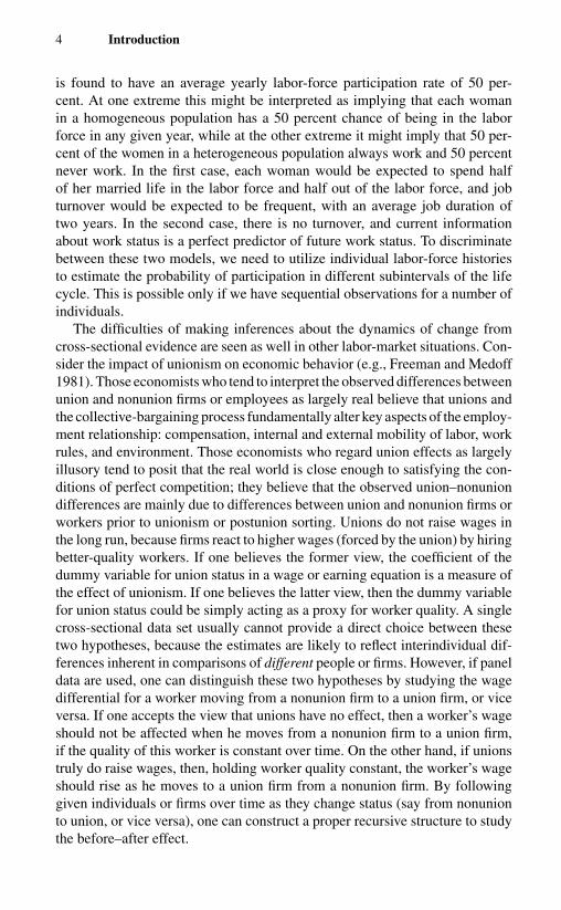
is found to have an average yearly labor-force participation rate of 50 per-cent. At one extreme this might be interpreted as implying that each womanin a homogeneous population has a 50 percent chance of being in the laborforce in any given year, while at the other extreme it might imply that 50 per-cent of the women in a heterogeneous population always work and 50 percentnever work. In the first case, each woman would be expected to spend halfof her married life in the labor force and half out of the labor force, and jobturnover would be expected to be frequent, with an average job duration oftwo years. In the second case, there is no turnover, and current informationabout work status is a perfect predictor of future work status. To discriminatebetween these two models, we need to utilize individual labor-force historiesto estimate the probability of participation in different subintervals of the lifecycle. This is possible only if we have sequential observations for a number ofindividuals.
The difficulties of making inferences about the dynamics of change fromcross-sectional evidence are seen as well in other labor-market situations. Con-sider the impact of unionism on economic behavior (e.g., Freeman and Medoff1981). Those economists who tend to interpret the observed differences betweenunion and nonunion firms or employees as largely real believe that unions andthe collective-bargaining process fundamentally alter key aspects of the employ-ment relationship: compensation, internal and external mobility of labor, workrules, and environment. Those economists who regard union effects as largelyillusory tend to posit that the real world is close enough to satisfying the con-ditions of perfect competition; they believe that the observed union–nonuniondifferences are mainly due to differences between union and nonunion firms orworkers prior to unionism or postunion sorting. Unions do not raise wages inthe long run, because firms react to higher wages (forced by the union) by hiringbetter-quality workers. If one believes the former view, the coefficient of thedummy variable for union status in a wage or earning equation is a measure ofthe effect of unionism. If one believes the latter view, then the dummy variablefor union status could be simply acting as a proxy for worker quality. A singlecross-sectional data set usually cannot provide a direct choice between thesetwo hypotheses, because the estimates are likely to reflect interindividual dif-ferences inherent in comparisons of different people or firms. However, if paneldata are used, one can distinguish these two hypotheses by studying the wagedifferential for a worker moving from a nonunion firm to a union firm, or viceversa. If one accepts the view that unions have no effect, then a worker’s wageshould not be affected when he moves from a nonunion firm to a union firm,if the quality of this worker is constant over time. On the other hand, if unionstruly do raise wages, then, holding worker quality constant, the worker’s wageshould rise as he moves to a union firm from a nonunion firm. By followinggiven individuals or firms over time as they change status (say from nonunionto union, or vice versa), one can construct a proper recursive structure to studythe before–after effect.
1.1 Advantages of Panel Data 5
Whereas microdynamic and macrodynamic effects typically cannot be es-timated using a cross-sectional data set, a single time-series data set usuallycannot provide precise estimates of dynamic coefficients either. For instance,consider the estimation of a distributed-lag model:
yt =h∑
τ=0
βτ xt−τ + ut , t = 1, . . . , T, (1.1.1)
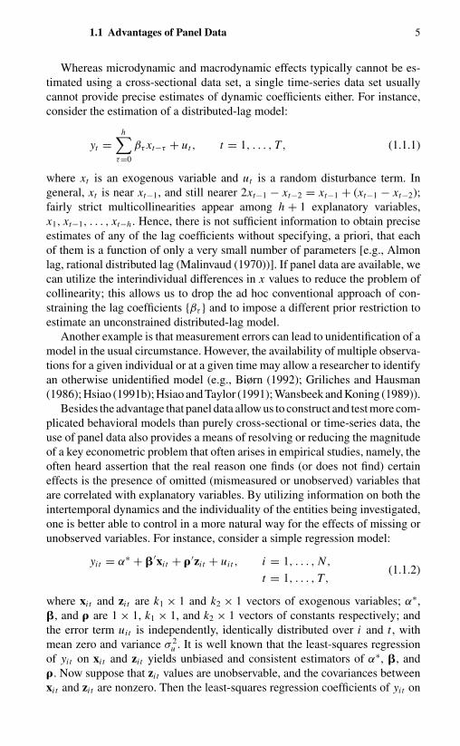
where xt is an exogenous variable and ut is a random disturbance term. Ingeneral, xt is near xt−1, and still nearer 2xt−1 − xt−2 = xt−1 + (xt−1 − xt−2);fairly strict multicollinearities appear among h + 1 explanatory variables,x1, xt−1, . . . , xt−h . Hence, there is not sufficient information to obtain preciseestimates of any of the lag coefficients without specifying, a priori, that eachof them is a function of only a very small number of parameters [e.g., Almonlag, rational distributed lag (Malinvaud (1970))]. If panel data are available, wecan utilize the interindividual differences in x values to reduce the problem ofcollinearity; this allows us to drop the ad hoc conventional approach of con-straining the lag coefficients {βτ } and to impose a different prior restriction toestimate an unconstrained distributed-lag model.
Another example is that measurement errors can lead to unidentification of amodel in the usual circumstance. However, the availability of multiple observa-tions for a given individual or at a given time may allow a researcher to identifyan otherwise unidentified model (e.g., Biørn (1992); Griliches and Hausman(1986); Hsiao (1991b); Hsiao and Taylor (1991); Wansbeek and Koning (1989)).
Besides the advantage that panel data allow us to construct and test more com-plicated behavioral models than purely cross-sectional or time-series data, theuse of panel data also provides a means of resolving or reducing the magnitudeof a key econometric problem that often arises in empirical studies, namely, theoften heard assertion that the real reason one finds (or does not find) certaineffects is the presence of omitted (mismeasured or unobserved) variables thatare correlated with explanatory variables. By utilizing information on both theintertemporal dynamics and the individuality of the entities being investigated,one is better able to control in a more natural way for the effects of missing orunobserved variables. For instance, consider a simple regression model:
yit = α∗ + �′xi t + �′zi t + uit , i = 1, . . . , N ,
t = 1, . . . , T,(1.1.2)
where xi t and zi t are k1 × 1 and k2 × 1 vectors of exogenous variables; α∗,�, and � are 1 × 1, k1 × 1, and k2 × 1 vectors of constants respectively; andthe error term uit is independently, identically distributed over i and t , withmean zero and variance σ 2
u . It is well known that the least-squares regressionof yit on xi t and zi t yields unbiased and consistent estimators of α∗, �, and�. Now suppose that zi t values are unobservable, and the covariances betweenxi t and zi t are nonzero. Then the least-squares regression coefficients of yit on

6 Introduction
xi t are biased. However, if repeated observations for a group of individuals areavailable, they may allow us to get rid of the effect of z. For example, if zi t = zi
for all t (i.e., z values stay constant through time for a given individual but varyacross individuals), we can take the first difference of individual observationsover time and obtain
yit − yi,t−1 = �′(xi t − xi,t−1) + (uit − ui,t−1), i = 1, . . . , N ,
t = 2, . . . , T .
(1.1.3)
Similarly, if zi t = zt for all i (i.e., z values stay constant across individuals at agiven time, but exhibit variation through time), we can take the deviation fromthe mean across individuals at a given time and obtain
yit − yt = �′(xi t − xt ) + (uit − ut ), i = 1, . . . , N ,
t = 1, . . . , T,(1.1.4)
where yt = (1/N )∑N
i=1 yit , xt = (1/N )∑N
i=1 xi t , and ut = (1/N )∑N
i=1 uit .Least-squares regression of (1.1.3) or (1.1.4) now provides unbiased and con-sistent estimates of �. Nevertheless if we have only a single cross-sectionaldata set (T = 1) for the former case (zi t = zi ), or a single time-series data set(N = 1) for the latter case (zi t = zt ), such transformations cannot be performed.We cannot get consistent estimates of � unless there exist instruments that arecorrelated with x but are uncorrelated with z and u.
MaCurdy’s (1981) work on the life-cycle labor supply of prime-age malesunder certainty is an example of this approach. Under certain simplifying as-sumptions, MaCurdy shows that a worker’s labor-supply function can be writtenas (1.1.2), where y is the logarithm of hours worked, x is the logarithm of thereal wage rate, and z is the logarithm of the worker’s (unobserved) marginalutility of initial wealth, which, as a summary measure of a worker’s lifetimewages and property income, is assumed to stay constant through time but to varyacross individuals (i.e., zit = zi ). Given the economic problem, not only is xit
correlated with zi , but every economic variable that could act as an instrumentfor xit (such as education) is also correlated with zi . Thus, in general, it is notpossible to estimate � consistently from a cross-sectional data set,3 but if paneldata are available, one can consistently estimate � by first-differencing (1.1.2).
The “conditional convergence” of the growth rate is another example (e.g.,Durlauf (2001); Temple (1999)). Given the role of transitional dynamics, it iswidely agreed that growth regressions should control for the steady state levelof income (e.g., Barro and Sala-i-Martin (1995); Mankiew, Romer, and Weil(1992)). Thus, a growth-rate regression model typically includes investmentratio, initial income, and measures of policy outcomes like school enrollmentand the black-market exchange-rate premium as regressors. However, an im-portant component, the initial level of a country’s technical efficiency, zi0, isomitted because this variable is unobserved. Since a country that is less efficient

1.1 Advantages of Panel Data 7
is also more likely to have lower investment rate or school enrollment, one caneasily imagine that zi0 is correlated with the regressors and the resulting cross-sectional parameter estimates are subject to omitted-variable bias. However,with panel data one can eliminate the influence of initial efficiency by takingthe first difference of individual country observations over time as in (1.1.3).
Panel data involve two dimensions: a cross-sectional dimension N , and atime-series dimension T . We would expect that the computation of panel dataestimators would be more complicated than the analysis of cross-section dataalone (where T = 1) or time series data alone (where N = 1). However, incertain cases the availability of panel data can actually simplify the computationand inference. For instance, consider a dynamic Tobit model of the form
y∗i t = γ y∗
i,t−1 + βxit + εi t (1.1.5)
where y∗ is unobservable, and what we observe is y, where yit = y∗i t if y∗
i t > 0and 0 otherwise. The conditional density of yit given yi,t−1 = 0 is much morecomplicated than the case if y∗
i,t−1 is known, because the joint density of(yit , yi,t−1) involves the integration of y∗
i,t−1 from −∞ to 0. Moreover, whenthere are a number of censored observations over time, the full implemen-tation of the maximum likelihood principle is almost impossible. However,with panel data, the estimation of γ and β can be simplified considerably bysimply focusing on the subset of data where yi,t−1 > 0, because the joint den-sity of f (yit , yi,t−1) can be written as the product of the conditional densityf (yi,t | yi,t−1) and the marginal density of yi,t−1. But if y∗
i,t−1 is observable,the conditional density of yit given yi,t−1 = y∗
i,t−1 is simply the density of εi t
(Arellano, Bover, and Labeager (1999)).Another example is the time-series analysis of nonstationary data. The large-
sample approximation of the distributions of the least-squares or maximum like-lihood estimators when T → ∞ are no longer normally distributed if the dataare nonstationary (e.g., Dickey and Fuller (1979, 1981); Phillips and Durlauf(1986)). Hence, the behavior of the usual test statistics will often have to beinferred through computer simulations. But if panel data are available, and ob-servations among cross-sectional units are independent, then one can invokethe central limit theorem across cross-sectional units to show that the limitingdistributions of many estimators remain asymptotically normal and the Wald-type test statistics are asymptotically chi-square distributed (e.g., Binder, Hsiao,and Pesaran (2000); Levin and Lin (1993); Pesaran, Shin, and Smith (1999),Phillips and Moon (1999, 2000); Quah (1994)).
Panel data also provide the possibility of generating more accurate predic-tions for individual outcomes than time-series data alone. If individual behaviorsare similar conditional on certain variables, panel data provide the possibilityof learning an individual’s behavior by observing the behavior of others, inaddition to the information on that individual’s behavior. Thus, a more accuratedescription of an individual’s behavior can be obtained by pooling the data

8 Introduction
(e.g., Hsiao and Mountain (1994); Hsiao and Tahmiscioglu (1997); Hsiao et al.(1989); Hsiao, Applebe, and Dineen (1993)).
1.2 ISSUES INVOLVED IN UTILIZINGPANEL DATA
1.2.1 Heterogeneity Bias
The oft-touted power of panel data derives from their theoretical ability to iso-late the effects of specific actions, treatments, or more general policies. Thistheoretical ability is based on the assumption that economic data are gener-ated from controlled experiments in which the outcomes are random variableswith a probability distribution that is a smooth function of the various vari-ables describing the conditions of the experiment. If the available data were infact generated from simple controlled experiments, standard statistical methodscould be applied. Unfortunately, most panel data come from the very compli-cated process of everyday economic life. In general, different individuals maybe subject to the influences of different factors. In explaining individual behav-ior, one may extend the list of factors ad infinitum. It is neither feasible nordesirable to include all the factors affecting the outcome of all individuals in amodel specification, since the purpose of modeling is not to mimic the realitybut is to capture the essential forces affecting the outcome. It is typical to leaveout those factors that are believed to have insignificant impacts or are peculiarto certain individuals.
However, when important factors peculiar to a given individual are left out,the typical assumption that economic variable y is generated by a parametricprobability distribution function P(y | �), where � is an m-dimensional realvector, identical for all individuals at all times, may not be a realistic one.Ignoring the individual or time-specific effects that exist among cross-sectionalor time-series units but are not captured by the included explanatory variablescan lead to parameter heterogeneity in the model specification. Ignoring suchheterogeneity could lead to inconsistent or meaningless estimates of interestingparameters. For example, consider a simple model postulated as
yit = α∗i + βi xi t + uit , i = 1, . . . , N ,
t = 1, . . . , T,(1.2.1)
where x is a scalar exogenous variable (k1 = 1) and uit is the error term withmean zero and constant variance σ 2
u . The parameters α∗i and βi may be differ-
ent for different cross-sectional units, although they stay constant over time.Following this assumption, a variety of sampling distributions may occur. Suchsampling distributions can seriously mislead the least-squares regression of yit
on xit when all N T observations are used to estimate the model:
yit = α∗ + βxit + uit , i = 1, . . . , N ,
t = 1, . . . , T .(1.2.2)
1.2 Issues Involved in Utilizing Panel Data 9
For instance, consider the situation that the data are generated as either in case1 or case 2.
Case 1: Heterogeneous intercepts (α∗i �= α∗
j ), homogeneous slope(βi = β j ). We use graphs to illustrate the likely biases due to theassumption that α∗
i �= α∗j and βi = β j . In these graphs, the broken-
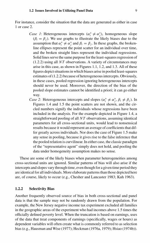
line ellipses represent the point scatter for an individual over time,and the broken straight lines represent the individual regressions.Solid lines serve the same purpose for the least-squares regression of(1.2.2) using all N T observations. A variety of circumstances mayarise in this case, as shown in Figures 1.1, 1.2, and 1.3. All of thesefigures depict situations in which biases arise in pooled least-squaresestimates of (1.2.2) because of heterogeneous intercepts. Obviously,in these cases, pooled regression ignoring heterogeneous interceptsshould never be used. Moreover, the direction of the bias of thepooled slope estimates cannot be identified a priori; it can go eitherway.
Case 2: Heterogeneous intercepts and slopes (α∗i �= α∗
j , βi �= β j ). InFigures 1.4 and 1.5 the point scatters are not shown, and the cir-cled numbers signify the individuals whose regressions have beenincluded in the analysis. For the example depicted in Figure 1.4, astraightforward pooling of all N T observations, assuming identicalparameters for all cross-sectional units, would lead to nonsensicalresults because it would represent an average of coefficients that dif-fer greatly across individuals. Nor does the case of Figure 1.5 makeany sense in pooling, because it gives rise to the false inference thatthe pooled relation is curvilinear. In either case, the classic paradigmof the “representative agent” simply does not hold, and pooling thedata under homogeneity assumption makes no sense.
These are some of the likely biases when parameter heterogeneities amongcross-sectional units are ignored. Similar patterns of bias will also arise if theintercepts and slopes vary through time, even though for a given time period theyare identical for all individuals. More elaborate patterns than those depicted hereare, of course, likely to occur (e.g., Chesher and Lancaster 1983; Kuh 1963).
1.2.2 Selectivity Bias
Another frequently observed source of bias in both cross-sectional and paneldata is that the sample may not be randomly drawn from the population. Forexample, the New Jersey negative income tax experiment excluded all familiesin the geographic areas of the experiment who had incomes above 1.5 times theofficially defined poverty level. When the truncation is based on earnings, usesof the data that treat components of earnings (specifically, wages or hours) asdependent variables will often create what is commonly referred to as selectionbias (e.g., Hausman and Wise (1977); Heckman (1976a, 1979); Hsiao (1974b)).

10 Introduction
Fig. 1.1 Fig. 1.2 Fig. 1.3
Fig. 1.4 Fig. 1.5
L
Fig. 1.6
For ease of exposition, we shall consider a cross-sectional example to getsome idea of how using a nonrandom sample may bias the least-squares esti-mates. We assume that in the population the relationship between earnings (y)and exogenous variables (x), including education, intelligence, and so forth, isof the form
yi = �′xi + ui , i = 1, . . . , N , (1.2.3)
where the disturbance term ui is independently distributed with mean zero andvariance σ 2
u . If the participants of an experiment are restricted to have earnings

1.3 Outline of the Monograph 11
less than L , the selection criterion for families considered for inclusion in theexperiment can be stated as follows:
yi = �′xi + ui ≤ L, included,
yi = �′xi + ui > L, excluded.(1.2.4)
For simplicity, we assume that the values of exogenous variables, except forthe education variable, are the same for each observation. In Figure 1.6, we letthe upward-sloping solid line indicate the “average” relation between educationand earnings and the dots represent the distribution of earnings around this meanfor selected values of education. All individuals with earnings above a givenlevel L , indicated by the horizontal line, would be eliminated from this experi-ment. In estimating the effect of education on earnings, we would observe onlythe points below the limit (circled) and thus would tend to underestimate the ef-fect of education using ordinary least squares.4 In other words, the sample selec-tion procedure introduces correlation between right-hand variables and the errorterm, which leads to a downward-biased regression line, as the dashed line inFigure 1.6 indicates.
These examples demonstrate that despite the advantages panel data maypossess, they are subject to their own potential experimental problems. It isonly by taking proper account of selectivity and heterogeneity biases in thepanel data that one can have confidence in the results obtained. The focus ofthis monograph will be on controlling for the effect of unobserved individualand/or time characteristics to draw proper inference about the characteristics ofthe population.
1.3 OUTLINE OF THE MONOGRAPH
Because the source of sample variation critically affects the formulation andestimation of many economic models, we shall first briefly review the clas-sic analysis of covariance procedures in Chapter 2. We shall then relax theassumption that the parameters that characterize all temporal cross-sectionalsample observations are identical and examine a number of specifications thatallow for differences in behavior across individuals as well as over time. Forinstance, a single-equation model with observations of y depending on a vectorof characteristics x can be written in the following form:
1. Slope coefficients are constant, and the intercept varies over individu-als:
yit = α∗i +
K∑k=1
βk xkit + uit , i = 1, . . . , N ,
(1.3.1)t = 1, . . . , T .

12 Introduction
2. Slope coefficients are constant, and the intercept varies over individu-als and time:
yit = α∗i t +
K∑k=1
βk xkit + uit , i = 1, . . . , N ,
(1.3.2)t = 1, . . . , T .
3. All coefficients vary over individuals:
yit = α∗i +
K∑k=1
βki xkit + uit , i = 1, . . . , N ,
(1.3.3)t = 1, . . . , T .
4. All coefficients vary over time and individuals:
yit = α∗i t +
K∑k=1
βki t xkit + uit , i = 1, . . . , N ,
(1.3.4)t = 1, . . . , T .
In each of these cases the model can be classified further, depending on whetherthe coefficients are assumed to be random or fixed.
Models with constant slopes and variable intercepts [such as (1.3.1) and(1.3.2)] are most widely used when analyzing panel data because they providesimple yet reasonably general alternatives to the assumption that parameterstake values common to all agents at all times. We shall consequently devotethe majority of this monograph to this type of model. Static models with vari-able intercepts will be discussed in Chapter 3, dynamic models in Chapter 4,simultaneous-equations models in Chapter 5, and discrete-data and sampleselection models in Chapters 7 and 8, respectively. Basic issues in variable-coefficient models for linear models [such as (1.3.3) and (1.3.4)] will be dis-cussed in Chapter 6. Chapter 9 discusses issues of incomplete panel models,such as estimating distributed-lag models in short panels, rotating samples,pooling of a series of independent cross sections (pseudopanels), and the pool-ing of data on a single cross section and a single time series. Miscellaneoustopics such as simulation methods, measurement errors, panels with large Nand large T , unit-root tests, cross-sectional dependence, and multilevel panelswill be discussed in Chapter 10. A summary view of the issues involved inutilizing panel data will be presented in Chapter 11.
The challenge of panel data analysis has been, and will continue to be, thebest way to formulate statistical models for inference motivated and shapedby substantive problems compatible with our understanding of the processesgenerating the data. The goal of this monograph is to summarize previous workin such a way as to provide the reader with the basic tools for analyzing and dra-wing inferences from panel data. Analyses of several important and advanced

1.3 Outline of the Monograph 13
topics, such as continuous time-duration models (e.g., Florens, Fougere, andMouchart (1996); Fougere and Kamionka (1996); Heckman and Singer (1984);Kiefer (1988); Lancaster (1990)), general nonlinear models (e.g., Abrevaya(1999); Amemiya (1983); Gourieroux and Jasiak (2000); Hsiao (1992c);Jorgenson and Stokes (1982); Lancaster (2001); Wooldridge (1999)),5 countdata (Cameron and Trevedi 1998), and econometric evaluation of social pro-grams (e.g., Angrist and Hahn (1999); Hahn (1998); Heckman (2001); Heckmanand Vytlacil (2001); Heckman, Ichimura, and Todd (1998); Hirano, Imbens, andRidder (2000); Imbens and Angrist (1994)), are beyond the scope of this mono-graph.
CHAPTER 2
Analysis of Covariance
2.1 INTRODUCTION1
Suppose we have sample observations of characteristics of N individuals over Ttime periods denoted by yit , xkit , i = 1, . . . , N , t = 1, . . . , T , k = 1, . . . , K .Conventionally, observations of y are assumed to be the random outcomes ofsome experiment with a probability distribution conditional on vectors of thecharacteristics x and a fixed number of parameters �, f (y | x, �). When paneldata are used, one of the ultimate goals is to use all available information tomake inferences on �. For instance, a simple model commonly postulated isthat y is a linear function of x. Yet to run a least-squares regression with allN T observations, we need to assume that the regression parameters take valuescommon to all cross-sectional units for all time periods. If this assumption isnot valid, as shown in Section 1.2, the pooled least-squares estimates may leadto false inferences. Thus, as a first step toward full exploitation of the data,we often test whether or not parameters characterizing the random outcomevariable y stay constant across all i and t .
A widely used procedure to identify the source of sample variation is theanalysis-of-covariance test. The name “analysis of variance” is often reservedfor a particular category of linear hypotheses that stipulate that the expectedvalue of a random variable y depends only on the class (defined by one or morefactors) to which the individual considered belongs, but excludes tests relatingto regressions. On the other hand, analysis-of-covariance models are of a mixedcharacter involving genuine exogenous variables, as do regression models, andat the same time allowing the true relation for each individual to depend onthe class to which the individual belongs, as do the usual analysis-of-variancemodels.
A linear model commonly used to assess the effects of both quantitative andqualitative factors is postulated as
yit = α∗i t + �′
i t xi t + uit , i = 1, . . . , N ,
t = 1, . . . , T,(2.1.1)
where α∗i t and �′
i t = (β1i t , β2i t , . . . , βK it ) are 1 × 1 and 1 × K vectors of

2.2 Analysis of Covariance 15
constants that vary across i and t , respectively, x′i t = (x1i t , . . . , xK it ) is a 1 × K
vector of exogenous variables, and uit is the error term. Two aspects of the esti-mated regression coefficients can be tested: first, the homogeneity of regressionslope coefficients; second, the homogeneity of regression intercept coefficients.The test procedure has three main steps:
1. Test whether or not slopes and intercepts simultaneously are homoge-neous among different individuals at different times.
2. Test whether or not the regression slopes collectively are the same.3. Test whether or not the regression intercepts are the same.
It is obvious that if the hypothesis of overall homogeneity (step 1) is ac-cepted, the testing procedure will go no further. However, should the overallhomogeneity hypothesis be rejected, the second step of the analysis is to decideif the regression slopes are the same. If this hypothesis of homogeneity is notrejected, one then proceeds to the third and final test to determine the equalityof regression intercepts. In principle, step 1 is separable from steps 2 and 3.2
Although this type of analysis can be performed on several dimensions,as described by Scheffe (1959) or Searle (1971), only one-way analysis ofcovariance has been widely used. Therefore, here we present only the proceduresfor performing one-way analysis of covariance.
2.2 ANALYSIS OF COVARIANCE
Model (2.1.1) only has descriptive value. It can neither be estimated nor beused to generate prediction, because the available degrees of freedom, N T ,is less than the number of parameters, N T (K + 1) + (number of parameterscharacterizing the distribution of uit ). A structure has to be imposed on (2.1.1)before any inference can be made. To start with, we assume that parameters areconstant over time, but can vary across individuals. Thus, we can postulate aseparate regression for each individual:
yit = α∗i + �′
i xi t + uit , i = 1, . . . , N ,
t = 1, . . . , T .(2.2.1)
Three types of restrictions can be imposed on (2.2.1). Namely:
H1: Regression slope coefficients are identical, and intercepts are not.That is,
yit = α∗i + �′xi t + uit . (2.2.2)
H2: Regression intercepts are the same, and slope coefficients are not.That is,
yit = α∗ + �′i xi t + uit . (2.2.3)
H3: Both slope and intercept coefficients are the same. That is,
yit = α∗ + �′xi t + uit . (2.2.4)

16 Analysis of Covariance
Because it is seldom meaningful to ask if the intercepts are the same when theslopes are unequal, we shall ignore the type of restrictions postulated by (2.2.3).We shall refer to (2.2.1) as the unrestricted model, (2.2.2) as the individual-meanor cell-mean corrected regression model, and (2.2.4) as the pooled regression.
Let
yi = 1
T
T∑t=1
yit , (2.2.5)
xi = 1
T
T∑t=1
xi t (2.2.6)
be the means of y and x, respectively, for the i th individual. The least-squaresestimates of �i and α∗
i in the unrestricted model (2.2.1) are given by3
�i = W −1xx,i Wxy,i , αi = yi − �′
i xi , i = 1, . . . , N , (2.2.7)
where
Wxx,i =T∑
t=1
(xi t − xi )(xi t − xi )′,
Wxy,i =T∑
t=1
(xi t − xi )(yit − yi ), (2.2.8)
Wyy,i =T∑
t=1
(yit − yi )2.
In the analysis-of-covariance terminology, equations (2.2.7) are called within-group estimates. The i th-group residual sum of squares is RSSi = Wyy,i −W ′
xy,i W−1xx,i Wxy,i . The unrestricted residual sum of squares is
S1 =N∑
i=1
RSSi . (2.2.9)
The least-squares regression of the individual-mean corrected model yieldsparameter estimates
�w = W −1xx Wxy,
(2.2.10)α∗
i = yi − �′w xi , i = 1, . . . , N ,
where
Wxx =N∑
i=1
Wxx,i and Wxy =N∑
i=1
Wxy,i .
Let Wyy = ∑Ni=1 Wyy,i ; the residual sum of squares of (2.2.2) is
S2 = Wyy − W ′xy W −1
xx Wxy . (2.2.11)

2.2 Analysis of Covariance 17
The least-squares regression of the pooled model (2.2.4) yields parameterestimates
� = T −1xx Txy, α∗ = y − �′x, (2.2.12)
where
Txx =N∑
i=1
T∑t=1
(xi t − x)(xi t − x)′,
Txy =N∑
i=1
T∑t=1
(xi t − x)(yit − y),
Tyy =N∑
i=1
T∑t=1
(yit − y)2,
y = 1
N T
N∑i=1
T∑t=1
yit , x = 1
N
N∑i=1
T∑t=1
xi t .
The (overall) residual sum of squares is
S3 = Tyy − T ′xy T −1
xx Txy . (2.2.13)
Under the assumption that the uit are independently normally distributedover i and t with mean zero and variance σ 2
u , F tests can be used to test therestrictions postulated by (2.2.2) and (2.2.4). In effect, (2.2.2) and (2.2.4) canbe viewed as (2.2.1) subject to various types of linear restrictions. For instance,the hypothesis of heterogeneous intercepts but homogeneous slopes [equation(2.2.2)] can be reformulated as (2.2.1) subject to (N − 1)K linear restrictions:
H1 : �1 = �2 = · · · = �N .
The hypothesis of common intercept and slope can be viewed as (2.2.1) subjectto (K + 1)(N − 1) linear restrictions:
H3 : α∗1 = α∗
2 = · · · = α∗N ,
�1 = �2 = · · · = �N .
Thus, application of the analysis-of-covariance test is equivalent to the ordi-nary hypothesis test based on sums of squared residuals from linear-regressionoutputs.
The unrestricted residual sum of squares S1 divided by σ 2u has a chi-square
distribution with N T − N (K + 1) degrees of freedom. The increment in theexplained sum of squares due to allowing for the parameters to vary acrossi is measured by (S3 − S1). Under H3, the restricted residual sum of squaresS3 divided by σ 2
u has a chi-square distribution with N T − (K + 1) degrees offreedom, and (S3 − S1)/σ 2
u has a chi-square distribution with (N − 1)(K + 1)degrees of freedom. Because (S3 − S1)/σ 2
u is independent of S1/σ2u , the F
18 Analysis of Covariance
statistic
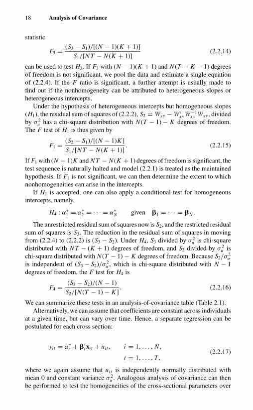
F3 = (S3 − S1)/[(N − 1)(K + 1)]
S1/[N T − N (K + 1)](2.2.14)
can be used to test H3. If F3 with (N − 1)(K + 1) and N (T − K − 1) degreesof freedom is not significant, we pool the data and estimate a single equationof (2.2.4). If the F ratio is significant, a further attempt is usually made tofind out if the nonhomogeneity can be attributed to heterogeneous slopes orheterogeneous intercepts.
Under the hypothesis of heterogeneous intercepts but homogeneous slopes(H1), the residual sum of squares of (2.2.2), S2 = Wyy − W ′
xy W −1xx Wxy , divided
by σ 2u has a chi-square distribution with N (T − 1) − K degrees of freedom.
The F test of H1 is thus given by
F1 = (S2 − S1)/[(N − 1)K ]
S1/[N T − N (K + 1)]. (2.2.15)
If F1 with (N − 1)K and N T − N (K + 1) degrees of freedom is significant, thetest sequence is naturally halted and model (2.2.1) is treated as the maintainedhypothesis. If F1 is not significant, we can then determine the extent to whichnonhomogeneities can arise in the intercepts.
If H1 is accepted, one can also apply a conditional test for homogeneousintercepts, namely,
H4 : α∗1 = α∗
2 = · · · = α∗N given �1 = · · · = �N .
The unrestricted residual sum of squares now is S2, and the restricted residualsum of squares is S3. The reduction in the residual sum of squares in movingfrom (2.2.4) to (2.2.2) is (S3 − S2). Under H4, S3 divided by σ 2
u is chi-squaredistributed with N T − (K + 1) degrees of freedom, and S2 divided by σ 2
u ischi-square distributed with N (T − 1) − K degrees of freedom. Because S2/σ
2u
is independent of (S3 − S2)/σ 2u , which is chi-square distributed with N − 1
degrees of freedom, the F test for H4 is
F4 = (S3 − S2)/(N − 1)
S2/[N (T − 1) − K ]. (2.2.16)
We can summarize these tests in an analysis-of-covariance table (Table 2.1).Alternatively, we can assume that coefficients are constant across individuals
at a given time, but can vary over time. Hence, a separate regression can bepostulated for each cross section:
yit = α∗t + �′
t xi t + uit , i = 1, . . . , N ,(2.2.17)
t = 1, . . . , T,
where we again assume that uit is independently normally distributed withmean 0 and constant variance σ 2
u . Analogous analysis of covariance can thenbe performed to test the homogeneities of the cross-sectional parameters over

Tabl
e2.
1.C
ovar
ianc
ete
sts
for
hom
ogen
eity
Sour
ceof
vari
atio
nR
esid
uals
umof
squa
res
Deg
rees
offr
eedo
mM
ean
squa
res
With
ingr
oup
with
hete
roge
neou
sin
terc
epta
ndsl
ope
S 1=
∑ N i=1
( Wyy
,i−
W′ xy,
iW−1 xx,
iWx
y,i
)N
(T−
K−
1)S 1
/N
(T−
K−
1)
Con
stan
tslo
pe:h
eter
ogen
eous
inte
rcep
tS 2
=W
yy−
W′ xyW
−1 xx
Wx
yN
(T−
1)−
KS 2
/[N
(T−
1)−
K]
Com
mon
inte
rcep
tand
slop
eS 3
=T
yy−
T′ xyT
−1 xx
T xy
NT
−(K
+1)
S 3/[N
T−
(K+
1)]
Not
atio
n:C
ells
orgr
oups
(or
indi
vidu
als)
i=
1,..
.,N
Obs
erva
tions
with
ince
llt=
1,..
.,T
Tota
lsam
ple
size
NT
With
in-c
ell(
grou
p)m
ean
y i,x i
Ove
rall
mea
ny,
xW
ithin
-gro
upco
vari
ance
Wyy
,i,
Wyx
,i,
Wx
x,i
Tota
lvar
iatio
nT
yy,
Tyx
,T x
x

20 Analysis of Covariance
time. For instance, we can test for overall homogeneity (H ′3 : α∗
1 = α∗2 = · · · =
α∗T , �1 = �2 = · · · = �T ) by using the F statistic
F ′3 = (S3 − S′
1)/[(T − 1)(K + 1)]
S′1/[N T − T (K + 1)]
(2.2.18)
with (T − 1)(K + 1) and N T − T (K + 1) degrees of freedom, where
S′1 =
T∑t=1
(Wyy,t − W ′
xy,t W−1xx,t Wxy,t
),
Wyy,t =N∑
i=1
(yit − yt )2, yt = 1
N
N∑i=1
yit ,
(2.2.19)
Wxx,t =N∑
i=1
(xi t − xt )(xi t − xt )′, xt = 1
N
N∑t=1
xi t ,
Wxy,t =N∑
i=1
(xi t − xt )(yit − yt ).
Similarly, we can test the hypothesis of heterogeneous intercepts, but homoge-neous slopes (H ′
1 : α∗1 �= α∗
2 �= · · · �= α∗T , �1 = �2 = · · · = �T ), by using the
F statistic
F ′1 = (S′
2 − S′1)/[(T − 1)K ]
S′1/[N T − T (K + 1)]
(2.2.20)
with (T − 1)K and N T − T (K + 1) degrees of freedom, where
S′2 =
T∑t=1
Wyy,t −(
T∑t=1
W ′xy,t
)(T∑
t=1
Wxx,t
)−1 (T∑
t=1
Wxy,t
),
(2.2.21)
or test the hypothesis of homogeneous intercepts conditional on homogeneousslopes �1 = �2 = · · · = �T (H ′
4) by using the F statistic
F ′4 = (S3 − S′
2)/(T − 1)
S′2/[T (N − 1) − K ]
(2.2.22)
with T − 1 and T (N − 1) − K degrees of freedom. In general, unless bothcross-section and time-series analyses of covariance indicate the acceptanceof homogeneity of regression coefficients, unconditional pooling (i.e., a singleleast-squares regression using all observations of cross-sectional units throughtime) may lead to serious bias.
Finally, it should be noted that the foregoing tests are not independent. Forexample, the uncomfortable possibility exists that according to F3 (or F ′
3),we might find homogeneous slopes and intercepts, and yet this finding couldbe compatible with opposite results according to F1(F ′
1) and F4(F ′4), because the
alternative or null hypotheses are somewhat different in the two cases. Worse
2.3 An Example 21
still, we might reject the hypothesis of overall homogeneity using the test ratioF3(F ′
3), but then find according to F1(F ′1) and F4(F ′
4) that we cannot reject thenull hypothesis, so that the existence of heterogeneity indicated by F3 (or F ′
3)cannot be traced. This outcome is quite proper at a formal statistical level,although at the less formal but important level of interpreting test statistics, itis an annoyance.
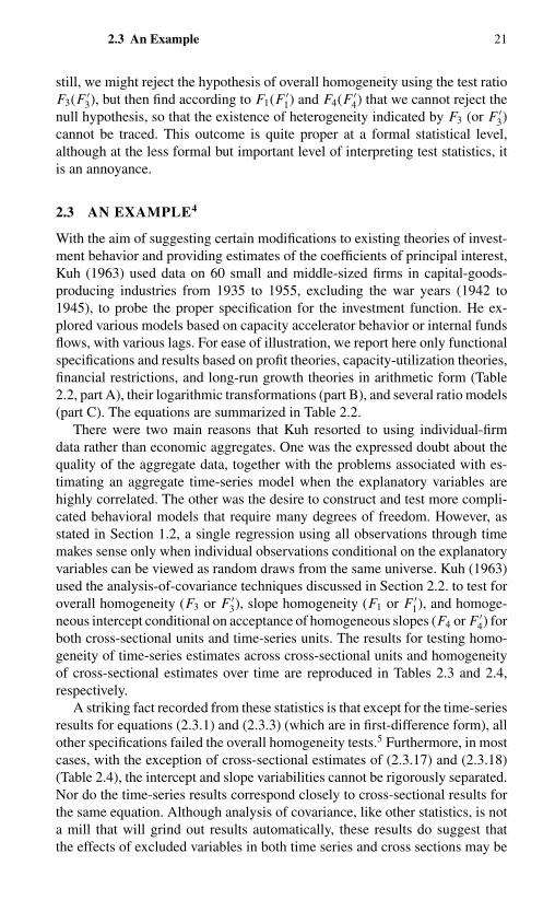
2.3 AN EXAMPLE4
With the aim of suggesting certain modifications to existing theories of invest-ment behavior and providing estimates of the coefficients of principal interest,Kuh (1963) used data on 60 small and middle-sized firms in capital-goods-producing industries from 1935 to 1955, excluding the war years (1942 to1945), to probe the proper specification for the investment function. He ex-plored various models based on capacity accelerator behavior or internal fundsflows, with various lags. For ease of illustration, we report here only functionalspecifications and results based on profit theories, capacity-utilization theories,financial restrictions, and long-run growth theories in arithmetic form (Table2.2, part A), their logarithmic transformations (part B), and several ratio models(part C). The equations are summarized in Table 2.2.
There were two main reasons that Kuh resorted to using individual-firmdata rather than economic aggregates. One was the expressed doubt about thequality of the aggregate data, together with the problems associated with es-timating an aggregate time-series model when the explanatory variables arehighly correlated. The other was the desire to construct and test more compli-cated behavioral models that require many degrees of freedom. However, asstated in Section 1.2, a single regression using all observations through timemakes sense only when individual observations conditional on the explanatoryvariables can be viewed as random draws from the same universe. Kuh (1963)used the analysis-of-covariance techniques discussed in Section 2.2. to test foroverall homogeneity (F3 or F ′
3), slope homogeneity (F1 or F ′1), and homoge-
neous intercept conditional on acceptance of homogeneous slopes (F4 or F ′4) for
both cross-sectional units and time-series units. The results for testing homo-geneity of time-series estimates across cross-sectional units and homogeneityof cross-sectional estimates over time are reproduced in Tables 2.3 and 2.4,respectively.
A striking fact recorded from these statistics is that except for the time-seriesresults for equations (2.3.1) and (2.3.3) (which are in first-difference form), allother specifications failed the overall homogeneity tests.5 Furthermore, in mostcases, with the exception of cross-sectional estimates of (2.3.17) and (2.3.18)(Table 2.4), the intercept and slope variabilities cannot be rigorously separated.Nor do the time-series results correspond closely to cross-sectional results forthe same equation. Although analysis of covariance, like other statistics, is nota mill that will grind out results automatically, these results do suggest thatthe effects of excluded variables in both time series and cross sections may be

22 Analysis of Covariance
Table 2.2. Investment equation forms estimated by Kuh (1963)
Part AIit = α0 + β1Ci + β2Kit + β3Sit (2.3.1)Iit = α0 + β1Ci + β2Kit + β4Pit (2.3.2)Iit = α0 + β1Ci + β2Kit + β3Sit + β4Pit (2.3.3)Iit = α0 + β1Ci + β2 Kit + β3 Sit (2.3.4)Iit = α0 + β1Ci + β2 Kit + β4 Pit (2.3.5)Iit = α0 + β1Ci + β2 Kit + β3 Sit + β4 Pit (2.3.6)Iit = α0 + β1Ci + β2 Kit + β3 Si,t−1 (2.3.7)Iit = α0 + β1Ci + β2 Kit + β4 Pi,t−1 (2.3.8)Iit = α0 + β1Ci + β2 Kit + β3 Si,t−1 + β4 Pi,t−1 (2.3.9)Iit = α0 + β1Ci + β2 Kit + β3[(Sit + Si,t−1) ÷ 2] (2.3.10)Iit = α0 + β1Ci + β2 Kit + β4[(Pit + Pi,t−1) ÷ 2] (2.3.11)Iit = α0 + β1Ci + β2 Kit + β3[(Sit + Si,t−1) ÷ 2] (2.3.12)
+ β4[(Pit + Pi,t−1) ÷ 2][(Iit + Ii,t−1) ÷ 2] = α0 + β1Ci + β2 Kit + β3[(Sit + Si,t−1) ÷ 2] (2.3.13)[(Iit + Ii,t−1) ÷ 2] = α0 + β1Ci + β2 Kit + β4[(Pit + Pi,t−1) ÷ 2] (2.3.14)[(Iit + Ii,t−1) ÷ 2] = α0 + β1Ci + β2 Kit + β3[(Sit + Si,t−1) ÷ 2] (2.3.15)
+ β4[(Pit + Pi,t−1) ÷ 2]
Part B log Iit = α0 + β1 log Ci + β2 log Kit + β3 log Sit (2.3.16)log Iit = α0 + β1 log Ci + β2 log Kit + β3 log Sit (2.3.17)log Iit = α0 + β1 log Ci + β2 log Kit + β3 log Si,t−1 (2.3.18)log Iit = α0 + β1 log Ci + β2 log[(Kit + Ki,t−1) ÷ 2] (2.3.19)
+ β3 log[(Sit + Si,t−1) ÷ 2]
Part CIit
Kit= α0 + β1
Pit
Kit+ β2
Si,t−1
Ci · Ki,t−1(2.3.20)
Iit
Kit= α0 + β1
Pit
Kit+ β2
Si,t−1
Ci · Ki,t−1+ β3
Sit
Ci · Kit(2.3.21)
Iit
Kit= α0 + β1
Pit + Pi,t−1
Kit · 2+ β2
Si,t−1
Ci · Ki,t−1(2.3.22)
Iit
Kit= α0 + β1
Pit + Pi,t−1
Kit · 2+ β2
Si,t−1
Ci · Ki,t−1+ β3
Sit
Ci · Kit(2.3.23)
Note: I = gross investment; C = capital-intensity index; K = capital stock; S = sales;P = gross retained profits.
very different. It would be quite careless not to explore the possible causes ofdiscrepancies that give rise to the systematic interrelationships between differentindividuals at different periods of time.6
Kuh explored the sources of estimation discrepancies through decompo-sition of the error variances, comparison of individual coefficient behavior,assessment of the statistical influence of various lag structures, and so forth. Heconcluded that sales seem to include critical time-correlated elements commonto a large number of firms and thus have a much greater capability of annihilatingsystematic, cyclical factors. In general, his results are more favorable to the ac-celeration sales model than to the internal-liquidity/profit hypothesis supported

Tabl
e2.
3.C
ovar
ianc
ete
sts
for
regr
essi
on-c
oeffi
cien
thom
ogen
eity
acro
sscr
oss-
sect
iona
luni
tsa
F3
over
allt
est
F1
slop
eho
mog
enei
tyF
4ce
llm
ean
sign
ifica
nce
Deg
rees
offr
eedo
mD
egre
esof
free
dom
Deg
rees
offr
eedo
m
Equ
atio
nN
umer
ator
Den
omin
ator
Act
ual
Fs
Num
erat
orD
enom
inat
orA
ctua
lF
sN
umer
ator
Den
omin
ator
Act
ual
Fs
(2.3
.1)
177
660
1.25
118
660
1.75
c57
660
0.12
(2.3
.2)
177
660
1.40
b11
866
01.
94c
5766
00.
11(2
.3.3
)23
660
01.
1317
760
01.
42b
5660
00.
10(2
.3.4
)17
784
02.
28c
118
840
1.58
c57
840
3.64
c
(2.3
.5)
177
840
2.34
c11
884
01.
75c
5784
03.
23c
(2.3
.6)
236
780
2.24
c17
778
01.
76c
5678
03.
57c
(2.3
.7)
177
720
2.46
c11
872
01.
95c
5772
03.
57c
(2.3
.8)
177
720
2.50
c11
872
01.
97c
5772
03.
31c
(2.3
.9)
236
660
2.49
c17
766
02.
11c
5666
03.
69c
(2.3
.10)
177
720
2.46
c11
872
01.
75c
5772
03.
66c
(2.3
.11)
177
720
2.60
c11
872
02.
14c
5772
03.
57c
(2.3
.12)
236
660
2.94
c17
766
02.
49c
5666
04.
18c
(2.3
.16)
177
720
1.92
c11
872
02.
59c
5772
00.
55(2
.3.1
7)17
784
04.
04c
118
840
2.70
c57
840
0.39
(2.3
.18)
177
720
5.45
c11
872
04.
20c
5772
06.
32c
(2.3
.19)
177
720
4.68
c11
872
03.
17c
5772
07.
36c
(2.3
.20)
177
720
3.64
c11
872
03.
14c
5772
03.
66c
(2.3
.21)
236
660
3.38
c17
766
02.
71c
5666
04.
07c
(2.3
.22)
177
600
3.11
c11
860
02.
72c
5760
03.
22c
(2.3
.23)
236
540
2.90
c17
754
02.
40c
5654
03.
60c
aC
ritic
alF
valu
esw
ere
obta
ined
from
A.M
.Moo
d,In
trod
ucti
onto
Stat
isti
cs,T
able
V,p
p.42
6–42
7.L
inea
rin
terp
olat
ion
was
empl
oyed
exce
ptfo
rde
gree
sof
free
dom
exce
edin
g12
0.T
hecr
itica
lF
valu
esin
ever
yca
seha
vebe
enre
cord
edfo
r12
0de
gree
sof
free
dom
for
each
deno
min
ator
sum
ofsq
uare
sev
enth
ough
the
actu
alde
gree
sof
free
dom
wer
eat
leas
tfou
rtim
esas
grea
t.T
heap
prox
imat
ion
erro
rin
this
case
isne
glig
ible
.bSi
gnifi
cant
atth
e5
perc
entl
evel
.c Si
gnifi
cant
atth
e1
perc
entl
evel
.So
urce
:K
uh(1
963,
pp.1
41–1
42).

Tabl
e2.
4.C
ovar
ianc
ete
sts
for
hom
ogen
eity
ofcr
oss-
sect
iona
lest
imat
esov
erti
mea
F′ 3
over
allt
est
F′ 1
slop
eho
mog
enei
tyF
′ 4ce
llm
ean
sign
ifica
nce
Deg
rees
offr
eedo
mD
egre
esof
free
dom
Deg
rees
offr
eedo
m
Equ
atio
nN
umer
ator
Den
omin
ator
Act
ual
Fs
Num
erat
orD
enom
inat
orA
ctua
lF
sN
umer
ator
Den
omin
ator
Act
ual
Fs
(2.3
.1)
5278
42.
45b
3978
42.
36b
1078
42.
89b
(2.3
.2)
5278
43.
04b
3978
42.
64b
1078
44.
97b
(2.3
.3)
6577
02.
55b
5277
02.
49b
977
03.
23b
(2.3
.4)
6495
22.
01b
4895
21.
97b
1395
22.
43b
(2.3
.5)
6495
22.
75b
4895
22.
45b
1395
23.
41b
(2.3
.6)
8093
51.
91b
6493
51.
82b
1293
52.
66b
(2.3
.7)
5684
02.
30b
4284
02.
11b
1184
03.
66b
(2.3
.8)
5684
02.
83b
4284
02.
75b
1184
03.
13b
(2.3
.9)
7082
52.
25b
5682
52.
13b
1082
53.
53b
(2.3
.10)
5684
01.
80b
4284
01.
80b
1184
01.
72d
(2.3
.11)
5684
02.
30b
4284
02.
30b
1184
01.
79d
(2.3
.12)
7082
51.
70b
5682
51.
74b
1082
51.
42

(2.3
.13)
5684
02.
08b
4284
02.
11b
1184
02.
21c
(2.3
.14)
5684
02.
66b
4284
02.
37b
1184
02.
87b
(2.3
.15)
7082
51.
81b
5682
51.
76b
1082
52.
35c
(2.3
.16)
5684
03.
67b
4284
02.
85b
1184
03.
10b
(2.3
.17)
6495
21.
51c
4895
21.
1413
952
0.80
(2.3
.18)
5684
02.
34b
4284
01.
0411
840
1.99
c
(2.3
.19)
5684
02.
29b
4284
02.
03b
1184
02.
05c
(2.3
.20)
4285
54.
13b
2885
55.
01b
1285
52.
47b
(2.3
.21)
5684
02.
88b
4284
03.
12b
1184
02.
56b
(2.3
.22)
4285
53.
80b
2885
54.
62b
1285
51.
61b
(2.3
.23)
5684
03.
51b
4284
04.
00b
1184
01.
71b
aC
ritic
alF
valu
esw
ere
obta
ined
from
A.M
.Moo
d,In
trod
ucti
onto
Stat
isti
cs,T
able
V,p
p.42
6–42
7.L
inea
rin
terp
olat
ion
was
empl
oyed
exce
ptfo
rde
gree
sof
free
dom
exce
edin
g12
0.T
hecr
itica
lF
valu
esin
ever
yca
seha
vebe
enre
cord
edfo
r12
0de
gree
sof
free
dom
for
each
deno
min
ator
sum
ofsq
uare
sev
enth
ough
the
actu
alde
gree
sof
free
dom
wer
eat
leas
tfou
rtim
esas
grea
t.T
heap
prox
imat
ion
erro
rin
this
case
isne
glig
ible
.bSi
gnifi
cant
atth
e1
perc
entl
evel
.c Si
gnifi
cant
atth
e5
perc
entl
evel
.dSi
gnifi
cant
atth
e10
perc
entl
evel
.So
urce
:K
uh(1
963,
pp.1
37–1
38).

26 Analysis of Covariance
by the results obtained using cross-sectional data (e.g., Meyer and Kuh (1957)).He found that the cash-flow effect is more important some time before the actualcapital outlays are made than it is in actually restricting the outlays during theexpenditure period. It appears more appropriate to view internal liquidity flowsas a critical part of the budgeting process that later is modified, primarily inlight of variations in levels of output and capacity utilization.
The policy implications of Kuh’s conclusions are clear. Other things beingequal, a small percentage increase in sales will have a greater effect on invest-ment than will a small percentage increase in internal funds. If the governmentseeks to stimulate investment and the objective is magnitude, not qualitativecomposition, it inexorably follows that the greatest investment effect will comefrom measures that increase demand rather than from measures that increaseinternal funds.7

CHAPTER 3
Simple Regression with Variable Intercepts
3.1 INTRODUCTION
When the overall homogeneity hypothesis is rejected by the panel data whilethe specification of a model appears proper, a simple way to take account ofthe heterogeneity across individuals and/or through time is to use the variable-intercept models (1.3.1) and (1.3.2). The basic assumption of such models isthat, conditional on the observed explanatory variables, the effects of all omit-ted (or excluded) variables are driven by three types of variables: individualtime-invariant, period individual-invariant, and individual time-varying.1 Theindividual time-invariant variables are variables that are the same for a givencross-sectional unit through time but that vary across cross-sectional units.Examples of these are attributes of individual-firm management, ability, sex,and socioeconomic-background variables. The period individual-invariant vari-ables are variables that are the same for all cross-sectional units at a given point intime but that vary through time. Examples of these variables are prices, interestrates, and widespread optimism or pessimism. The individual time-varyingvariables are variables that vary across cross-sectional units at a given point intime and also exhibit variations through time. Examples of these variables arefirm profits, sales, and capital stock. The variable-intercept models assume thatthe effects of the numerous omitted individual time-varying variables are eachindividually unimportant but are collectively significant, and possess the prop-erty of a random variable that is uncorrelated with (or independent of) all otherincluded and excluded variables. On the other hand, because the effects ofremaining omitted variables either stay constant through time for a given cross-sectional unit or are the same for all cross-sectional units at a given point in time,or a combination of both, they can be absorbed into the intercept term of a re-gression model as a means to allow explicitly for the individual and/or time het-erogeneity contained in the temporal cross-sectional data. Moreover, when theindividual- or time-specific effects are absorbed into the intercept term, there isno need to assume that those effects are uncorrelated with x, although sometimesthey are.

28 Simple Regression with Variable Intercepts
The variable-intercept models can provide a fairly useful specification forfitting regression models using panel data. For example, consider fitting a Cobb–Douglas production function
yit = µ + β1x1i t + · · · + βK xK it + vit , i = 1, . . . , N ,
t = 1, . . . , T,(3.1.1)
where y is the logarithm of output and x1, . . . , xK are the logarithms of theinputs. The classic procedure is to assume that the effects of omitted variablesare independent of x and are independently identically distributed. Thus, con-ditioning on x, all observations are random variations of a representative firm.However, (3.1.1) has often been criticized for ignoring variables reflecting man-agerial and other technical differences between firms or variables that reflectgeneral conditions affecting the productivity of all firms but that are fluctuatingover time (such as weather in agriculture production); see, e.g., Hoch (1962);Mundlak (1961); Nerlove (1965). Ideally, such firm- and time-effects variables,say Mi and Pt , should be explicitly introduced into (3.1.1). Thus, vit can bewritten as
vit = αMi + λPt + uit , (3.1.2)
with uit representing the effects of all remaining omitted variables. Unfortu-nately, there usually are no observations on Mi and Pt . It is impossible toestimate α and λ directly. A natural alternative would then be to consider theeffects of the products, αi = αMi and λt = λPt , which then leads to a variable-intercept model: (1.3.1) or (1.3.2).
Such a procedure was used by Hoch (1962) to estimate parameters of aCobb–Douglas production function based on annual data for 63 Minnesotafarms from 1946 to 1951. He treated output y as a function of labor x1, realestate x2, machinery x3, and feed, fertilizer, and related expenses, x4. However,because of the difficulties of measuring real-estate and machinery variables,he also tried an alternative specification that treated y as a function of x1,x4, a current-expenditures item x5, and fixed capital x6. Regression results forboth specifications rejected the overall homogeneity hypothesis at the 5 percentsignificance level. The least-squares estimates under three assumptions (αi =λt = 0; αi = 0, λt �= 0; and αi �= 0, λt �= 0) are summarized in Table 3.1.They exhibit an increase in the adjusted R2 from 0.75 to about 0.88 when αi
and λt are introduced.There are also some important changes in parameter estimates when we
move from the assumption of identical αi s to the assumption that both αi andλt differ from zero. There is a significant drop in the sum of the elasticities,mainly concentrated in the labor variable. If one interprets αi as the firm scaleeffect, then this indicates that efficiency increases with scale. As demonstrated inFigure 1.1, when the production hyperplane of larger firms lies above the averageproduction plane and the production plane of smaller firms below the average
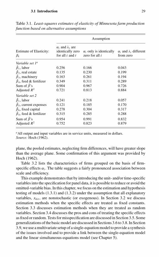
3.1 Introduction 29
Table 3.1. Least-squares estimates of elasticity of Minnesota farm productionfunction based on alternative assumptions
Assumption
αi and λt areEstimate of Elasticity: identically zero αi only is identically αi and λt differentβk for all i and t zero for all i from zero
Variable set 1a
β1, labor 0.256 0.166 0.043β2, real estate 0.135 0.230 0.199β3, machinery 0.163 0.261 0.194β4, feed & fertilizer 0.349 0.311 0.289Sum of β’s 0.904 0.967 0.726Adjusted R2 0.721 0.813 0.884
Variable set 2β1, labor 0.241 0.218 0.057β5, current expenses 0.121 0.185 0.170β6, fixed capital 0.278 0.304 0.317β4, feed & fertilizer 0.315 0.285 0.288
Sum of β’s 0.954 0.991 0.832Adjusted R2 0.752 0.823 0.879
aAll output and input variables are in service units, measured in dollars.Source: Hoch (1962).
plane, the pooled estimates, neglecting firm differences, will have greater slopethan the average plane. Some confirmation of this argument was provided byHoch (1962).
Table 3.2 lists the characteristics of firms grouped on the basis of firm-specific effects αi . The table suggests a fairly pronounced association betweenscale and efficiency.
This example demonstrates that by introducing the unit- and/or time-specificvariables into the specification for panel data, it is possible to reduce or avoid theomitted-variable bias. In this chapter, we focus on the estimation and hypothesistesting of models (1.3.1) and (1.3.2) under the assumption that all explanatoryvariables, xkit , are nonstochastic (or exogenous). In Section 3.2 we discussestimation methods when the specific effects are treated as fixed constants.Section 3.3 discusses estimation methods when they are treated as randomvariables. Section 3.4 discusses the pros and cons of treating the specific effectsas fixed or random. Tests for misspecification are discussed in Section 3.5. Somegeneralizations of the basic model are discussed in Sections 3.6 to 3.8. In Section3.9, we use a multivariate setup of a single-equation model to provide a synthesisof the issues involved and to provide a link between the single-equation modeland the linear simultaneous-equations model (see Chapter 5).
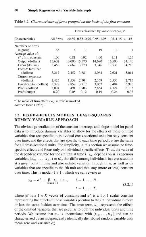
30 Simple Regression with Variable Intercepts
Table 3.2. Characteristics of firms grouped on the basis of the firm constant
Firms classified by value of exp(αi )a
Characteristics All firms <0.85 0.85–0.95 0.95–1.05 1.05–1.15 >1.15
Numbers of firmsin group 63 6 17 19 14 7
Average value of:eαi , firm constant 1.00 0.81 0.92 1.00 1.11 1.26Output (dollars) 15,602 10,000 15,570 14,690 16,500 24,140Labor (dollars) 3,468 2,662 3,570 3,346 3,538 4,280Feed & fertilizer
(dollars) 3,217 2,457 3,681 3,064 2,621 5,014Current expenses
(dollars) 2,425 1,538 2,704 2,359 2,533 2,715Fixed capital (dollars) 3,398 2,852 3,712 3,067 3,484 3,996Profit (dollars) 3,094 491 1,903 2,854 4,324 8,135Profit/output 0.20 0.05 0.12 0.19 0.26 0.33
aThe mean of firm effects, αi , is zero is invoked.Source: Hoch (1962).
3.2 FIXED-EFFECTS MODELS: LEAST-SQUARESDUMMY-VARIABLE APPROACH
The obvious generalization of the constant-intercept-and-slope model for paneldata is to introduce dummy variables to allow for the effects of those omittedvariables that are specific to individual cross-sectional units but stay constantover time, and the effects that are specific to each time period but are the samefor all cross-sectional units. For simplicity, in this section we assume no time-specific effects and focus only on individual-specific effects. Thus, the value ofthe dependent variable for the i th unit at time t , yit , depends on K exogenousvariables, (x1i t , . . . , xK it ) = x′
i t , that differ among individuals in a cross sectionat a given point in time and also exhibit variation through time, as well as onvariables that are specific to the i th unit and that stay (more or less) constantover time. This is model (1.3.1), which we can rewrite as
yit = α∗i + �′
1×Kxi t
K×1+ uit , i = 1, . . . , N ,
(3.2.1)t = 1, . . . , T,
where �′ is a 1 × K vector of constants and α∗i is a 1 × 1 scalar constant
representing the effects of those variables peculiar to the i th individual in moreor less the same fashion over time. The error term, uit , represents the effectsof the omitted variables that are peculiar to both the individual units and timeperiods. We assume that uit is uncorrelated with (xi1, . . . , xiT ) and can becharacterized by an independently identically distributed random variable withmean zero and variance σ 2
u .
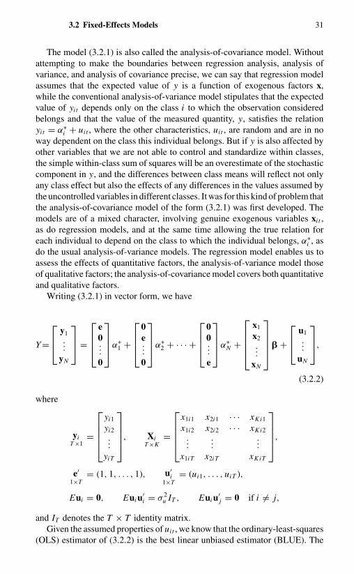
3.2 Fixed-Effects Models 31
The model (3.2.1) is also called the analysis-of-covariance model. Withoutattempting to make the boundaries between regression analysis, analysis ofvariance, and analysis of covariance precise, we can say that regression modelassumes that the expected value of y is a function of exogenous factors x,while the conventional analysis-of-variance model stipulates that the expectedvalue of yit depends only on the class i to which the observation consideredbelongs and that the value of the measured quantity, y, satisfies the relationyit = α∗
i + uit , where the other characteristics, uit , are random and are in noway dependent on the class this individual belongs. But if y is also affected byother variables that we are not able to control and standardize within classes,the simple within-class sum of squares will be an overestimate of the stochasticcomponent in y, and the differences between class means will reflect not onlyany class effect but also the effects of any differences in the values assumed bythe uncontrolled variables in different classes. It was for this kind of problem thatthe analysis-of-covariance model of the form (3.2.1) was first developed. Themodels are of a mixed character, involving genuine exogenous variables xi t ,as do regression models, and at the same time allowing the true relation foreach individual to depend on the class to which the individual belongs, α∗
i , asdo the usual analysis-of-variance models. The regression model enables us toassess the effects of quantitative factors, the analysis-of-variance model thoseof qualitative factors; the analysis-of-covariance model covers both quantitativeand qualitative factors.
Writing (3.2.1) in vector form, we have
Y=
y1...
yN
=
e0...0
α∗1 +
0e...0
α∗2 + · · · +
00...e
α∗N +
x1
x2...
xN
� +
u1...
uN
,
(3.2.2)
where
yiT ×1
=
yi1
yi2...
yiT
, XiT ×K
=
x1i1 x2i1 · · · xK i1
x1i2 x2i2 · · · xK i2...
......
x1iT x2iT xK iT
,
e′1×T
= (1, 1, . . . , 1), u′i
1×T= (ui1, . . . , uiT ),
Eui = 0, Eui u′i = σ 2
u IT , Eui u′j = 0 if i �= j,
and IT denotes the T × T identity matrix.Given the assumed properties of uit , we know that the ordinary-least-squares
(OLS) estimator of (3.2.2) is the best linear unbiased estimator (BLUE). The
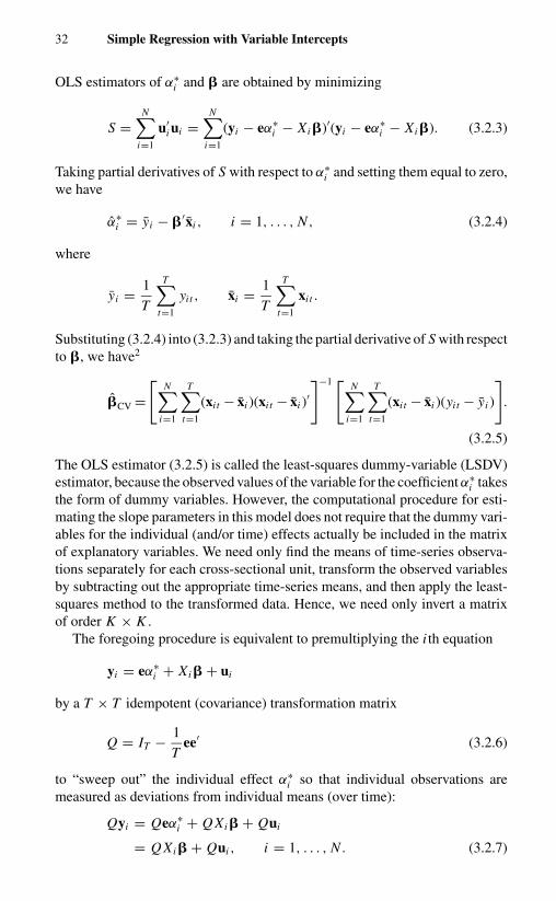
32 Simple Regression with Variable Intercepts
OLS estimators of α∗i and � are obtained by minimizing
S =N∑
i=1
u′i ui =
N∑i=1
(yi − eα∗i − Xi �)′(yi − eα∗
i − Xi �). (3.2.3)
Taking partial derivatives of S with respect to α∗i and setting them equal to zero,
we have
α∗i = yi − �′xi , i = 1, . . . , N , (3.2.4)
where
yi = 1
T
T∑t=1
yit , xi = 1
T
T∑t=1
xi t .
Substituting (3.2.4) into (3.2.3) and taking the partial derivative of S with respectto �, we have2
�CV =[
N∑i=1
T∑t=1
(xi t − xi )(xi t − xi )′]−1 [
N∑i=1
T∑t=1
(xi t − xi )(yit − yi )
].
(3.2.5)
The OLS estimator (3.2.5) is called the least-squares dummy-variable (LSDV)estimator, because the observed values of the variable for the coefficient α∗
i takesthe form of dummy variables. However, the computational procedure for esti-mating the slope parameters in this model does not require that the dummy vari-ables for the individual (and/or time) effects actually be included in the matrixof explanatory variables. We need only find the means of time-series observa-tions separately for each cross-sectional unit, transform the observed variablesby subtracting out the appropriate time-series means, and then apply the least-squares method to the transformed data. Hence, we need only invert a matrixof order K × K .
The foregoing procedure is equivalent to premultiplying the i th equation
yi = eα∗i + Xi � + ui
by a T × T idempotent (covariance) transformation matrix
Q = IT − 1
Tee′ (3.2.6)
to “sweep out” the individual effect α∗i so that individual observations are
measured as deviations from individual means (over time):
Qyi = Qeα∗i + Q Xi � + Qui
= Q Xi � + Qui , i = 1, . . . , N . (3.2.7)

3.2 Fixed-Effects Models 33
Applying the OLS procedure to (3.2.7), we have3
�CV =[
N∑i=1
X ′i Q Xi
]−1 [N∑
i=1
X ′i Qyi
], (3.2.8)
which is identically equal to (3.2.5). Because (3.2.2) is called the analysis-of-covariance model, the LSDV estimator of � is sometimes called the covarianceestimator. It is also called the within-group estimator, because only the variationwithin each group is utilized in forming this estimator.4
The covariance estimator βCV is unbiased. It is also consistent when eitherN or T or both tend to infinity. Its variance–covariance matrix is
Var(�CV) = σ 2u
[N∑
t=1
X ′i Q Xi
]−1
. (3.2.9)
However, the estimator for the intercept, (3.2.4), although unbiased, is consistentonly when T → ∞.
It should be noted that an alternative and equivalent formulation of (3.2.1)is to introduce a “mean intercept,” µ, so that
yit = µ + �′xi t + αi + uit . (3.2.10)
Because both µ and αi are fixed constants, without additional restriction, theyare not separately identifiable or estimable. One way to identify µ and αi is tointroduce the restriction
∑Ni=1 αi = 0. Then the individual effect αi represents
the deviation of the i th individual from the common mean µ.Equations (3.2.10) and (3.2.1) lead to the same least-squares estimator for �
[equation (3.2.5)]. This can easily be seen by noting that the BLUEs for µ, αi ,and � are obtained by minimizing
N∑i=1
u′i ui =
N∑i=1
T∑t=1
u2i t
subject to the restriction∑N
t=1 αi = 0. Utilizing the restriction∑N
t=1 αi = 0 insolving the marginal conditions, we have
µ = y − �′x, where y = 1
N T
N∑i=1
T∑t=1
yit ,
(3.2.11)
x = 1
N T
N∑i=1
T∑t=1
xi t ,
αi = yi − µ − �′xi . (3.2.12)
Substituting (3.2.11) and (3.2.12) into (3.2.10) and solving the marginal con-dition for �, we obtain (3.2.5).

34 Simple Regression with Variable Intercepts
3.3 RANDOM-EFFECTS MODELS: ESTIMATIONOF VARIANCE-COMPONENTS MODELS
In Section 3.2, we discussed the estimation of linear-regression models whenthe effects of omitted individual-specific variables (αi ) are treated as fixedconstants over time. In this section we treat the individual-specific effects, likeuit , as random variables.
It is a standard practice in the regression analysis to assume that the largenumber of factors that affect the value of the dependent variable, but that havenot been explicitly included as independent variables, can be appropriatelysummarized by a random disturbance. When numerous individual units areobserved over time, it is sometimes assumed that some of the omitted variableswill represent factors peculiar to both the individual units and time periods forwhich observations are obtained, whereas other variables will reflect individualdifferences that tend to affect the observations for a given individual in more orless the same fashion over time. Still other variables may reflect factors peculiarto specific time periods, but affecting individual units more or less equally. Thus,the residual, vit , is often assumed to consist of three components:5
vit = αi + λt + uit , (3.3.1)
where
Eαi = Eλt = Euit = 0, Eαiλt = Eαi uit = Eλt uit = 0,
Eαiα j ={
σ 2α if i = j,
0 if i �= j,
Eλtλs ={
σ 2λ if t = s,
0 if t �= s,
Euit u js ={
σ 2u if i = j, t = s,
0 otherwise,
(3.3.2)
and
Eαi x′i t = Eλt x′
i t = Euit x′i t = 0′.
The variance of yit conditional on xi t is, from (3.3.1) and (3.3.2), σ 2y =
σ 2α + σ 2
λ + σ 2u . The variances σ 2
α , σ 2λ , and σ 2
u are accordingly called variancecomponents; each is a variance in its own right and is a component of σ 2
y . There-fore, this kind of model is sometimes referred to as a variance-components (orerror-components) model.
For ease of exposition we assume λt = 0 for all t in this and the followingthree sections. That is, we concentrate on models of the form (3.2.10).
Rewriting (3.2.10) in vector form, we have
yiT ×1
= X iT ×(K+1)
�(K+1)×1
+ viT ×1
, i = 1, 2, . . . , N , (3.3.3)

3.3 Random-Effects Models 35
where X i = (e, Xi ), �′ = (µ, �′), v′i = (vi1, . . . , viT ), and vit = αi + uit . The
variance–covariance matrix of vi is
Evi v′i = σ 2
u IT + σ 2α ee′ = V . (3.3.4)
Its inverse is (see Graybill (1969); Nerlove (1971b); Wallace and Hussain(1969))
V −1 = 1
σ 2u
[IT − σ 2
α
σ 2u + T σ 2
α
ee′]. (3.3.5)
3.3.1 Covariance Estimation
The presence of αi produces a correlation among residuals of the same cross-sectional unit, though the residuals from different cross-sectional units are in-dependent. However, regardless of whether the αi s are treated as fixed or as ran-dom, the individual-specific effects for a given sample can be swept out by theidempotent (covariance) transformation matrix Q [equation (3.2.6)], becauseQe = 0, and hence Qvi = Qui . Thus, premultiplying (3.3.3) by Q, we have
Qyi = Qeµ + Q Xi � + Qeαi + Qui
= Q Xi � + Qui . (3.3.6)
Applying the least-squares method to (3.3.6), we obtain the covarianceestimator (CV) (3.2.8) of �. We estimate µ by µ = y − �
′CVx.
Whether αi are treated as fixed or random, the CV of � is unbiased andconsistent either N or T or both tend to infinity. However, whereas the CV isthe BLUE under the assumption that αi are fixed constants, it is not the BLUE infinite samples when αi are assumed random. The BLUE in the latter case is thegeneralized-least-squares (GLS) estimator.6 Moreover, if the explanatory vari-ables contain some time-invariant variables zi , their coefficients cannot be esti-mated by CV, because the covariance transformation eliminates zi from (3.3.6).
3.3.2 Generalized-Least-Squares Estimation
Because vit and vis both contain αi , the residuals of (3.3.3) are correlated. Toget efficient estimates of �′ = (µ, �′), we have to use the GLS method. Thenormal equations for the GLS estimators are[
N∑i=1
X ′i V
−1 X i
]�GLS =
N∑i=1
X ′i V
−1yi . (3.3.7)
Following Maddala (1971a), we write V −1 [equation (3.3.5)] as
V −1 = 1
σ 2u
[(IT − 1
Tee′
)+ ψ · 1
Tee′
]= 1
σ 2u
[Q + ψ · 1
Tee′
],
(3.3.8)

36 Simple Regression with Variable Intercepts
where
ψ = σ 2u
σ 2u + T σ 2
α
. (3.3.9)
Hence, (3.3.7) can conveniently be written as
[Wxx + ψ Bx x ]
[µ
�
]GLS
= Wx y + ψ Bx y, (3.3.10)
where
Tx x =N∑
i=1
X ′i X i , Tx y =
N∑i=1
X ′i yi ,
Bx x = 1
T
N∑i=1
(X ′i ee′ X i ), Bx y = 1
T
N∑i=1
(X ′i ee′yi ),
Wxx = Tx x − Bx x , Wx y = Tx y − Bx y .
The matrices Bx x and Bx y contain the sums of squares and sums of crossproducts between groups, Wxx and Wx y are the corresponding matrices withingroups, and Tx x and Tx y are the corresponding matrices for total variation.
Solving (3.3.10), we haveψ N T ψT
N∑i=1
x′i
ψTN∑
i=1
xi
N∑i=1
X ′i Q Xi + ψT
N∑i=1
xi x′i
[µ
�
]GLS
=
ψ N T y
N∑i=1
X ′i Qyi + ψT
N∑i=1
xi yi
. (3.3.11)
Using the formula of the partitioned inverse, we obtain
�GLS =[
1
T
N∑i=1
X ′i Q Xi + ψ
N∑i=1
(xi − x)(xi − x)′]−1
×[
1
T
N∑i=1
X ′i Qyi + ψ
N∑i=1
(xi − x)(yi − y)
](3.3.12)
= �b + (IK − )�CV,
µGLS = y − �′GLSx,
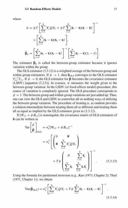
3.3 Random-Effects Models 37
where
= ψT
[N∑
i=1
X ′i Q Xi + ψT
N∑i=1
(xi − x)(xi − x)′]−1
×[
N∑i=1
(xi − x)(xi − x)′],
�b =[
N∑i=1
(xi − x)(xi − x)′]−1 [
N∑i=1
(xi − x)(yi − y)
].
The estimator �b is called the between-group estimator because it ignoresvariation within the group.
The GLS estimator (3.3.12) is a weighted average of the between-group andwithin-group estimators. If ψ → 1, then �GLS converges to the OLS estimatorT −1
x x Tx y . If ψ → 0, the GLS estimator for � becomes the covariance estimator(LSDV) [equation (3.2.5)]. In essence, ψ measures the weight given to thebetween-group variation. In the LSDV (or fixed-effects model) procedure, thissource of variation is completely ignored. The OLS procedure corresponds toψ = 1. The between-group and within-group variations are just added up. Thus,one can view the OLS and LSDV as somewhat all-or-nothing ways of utilizingthe between-group variation. The procedure of treating αi as random providesa solution intermediate between treating them all as different and treating themall as equal as implied by the GLS estimator given in (3.3.12).
If [Wxx + ψ Bx x ] is nonsingular, the covariance matrix of GLS estimators of� can be written as
Var
[µ
�
]GLS
= σ 2u [Wxx + ψ Bx x ]−1
= σ 2u
0 0′
0N∑
i=1
X ′i Q Xi
+ T ψ
N
N∑i=1
x′i
N∑i=1
xi
N∑i=1
xi x′i
−1
. (3.3.13)
Using the formula for partitioned inversion (e.g., Rao (1973, Chapter 2); Theil(1971, Chapter 1)), we obtain
Var(�GLS) = σ 2u
[N∑
i=1
X ′i Q Xi + T ψ
N∑i=1
(xi − x)(xi − x)′]−1
.
(3.3.14)
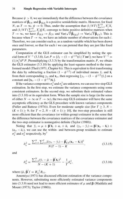
38 Simple Regression with Variable Intercepts
Because ψ > 0, we see immediately that the difference between the covariancematrices of �CV and �GLS is a positive semidefinite matrix. However, for fixedN , as T → ∞, ψ → 0. Thus, under the assumption that (1/N T )
∑Ni=1 X ′
i Xi
and (1/N T )∑N
i=1 X ′i Q Xi converge to finite positive definitive matrices when
T → ∞, we have βGLS → βCV and Var(√
T �GLS) → Var(√
T �CV). This isbecause when T → ∞, we have an infinite number of observations for each i .Therefore, we can consider each αi as a random variable which has been drawnonce and forever, so that for each i we can pretend that they are just like fixedparameters.
Computation of the GLS estimator can be simplified by noting the spe-cial form of V −1 (3.3.8). Let P = [IT − (1 − ψ1/2)(1/T )ee′]; we have V −1 =(1/σ 2
u )P ′ P . Premultiplying (3.3.3) by the transformation matrix P , we obtainthe GLS estimator (3.3.10) by applying the least-squares method to the trans-formed model (Theil (1971, Chapter 6)). This is equivalent to first transformingthe data by subtracting a fraction (1 − ψ1/2) of individual means yi and xi
from their corresponding yit and xi t , then regressing [yit − (1 − ψ1/2)yi ] on aconstant and [xi t − (1 − ψ1/2)xi ].
If the variance components σ 2u and σ 2
α are unknown, we can use two-step GLSestimation. In the first step, we estimate the variance components using someconsistent estimators. In the second step, we substitute their estimated valuesinto (3.3.10) or its equivalent form. When the sample size is large (in the senseof either N → ∞ or T → ∞), the two-step GLS estimator will have the sameasymptotic efficiency as the GLS procedure with known variance components(Fuller and Battese (1974)). Even for moderate sample size [for T ≥ 3, N −(K + 1) ≥ 9; for T = 2, N − (K + 1) ≥ 10], the two-step procedure is stillmore efficient than the covariance (or within-group) estimator in the sense thatthe difference between the covariance matrices of the covariance estimator andthe two-step estimator is nonnegative definite (Taylor (1980)).
Noting that yi = µ + �′xi + αi + ui and (yit − yi ) = �′(xi t − xi ) +(uit − ui ), we can use the within- and between-group residuals to estimateσ 2
u and σ 2α respectively, by7
σ 2u =
∑Ni=1
∑Tt=1[(yit − yi ) − �
′CV(xi t − xi )]2
N (T − 1) − K, (3.3.15)
and
σ 2α =
∑Ni=1(yi − µ − �
′xi )2
N − (K + 1)− 1
Tσ 2
u , (3.3.16)
where (µ, �′)′ = B−1
x x Bx y .Amemiya (1971) has discussed efficient estimation of the variance compo-
nents. However, substituting more efficiently estimated variance componentsinto (3.3.9) need not lead to more efficient estimates of µ and � (Maddala andMount (1973); Taylor (1980)).

3.3 Random-Effects Models 39
3.3.3 Maximum Likelihood Estimation
When αi and uit are random and normally distributed, the logarithm of thelikelihood function is
log L = − N T
2log 2π − N
2log |V |
− 1
2
N∑i=1
(yi − eµ − Xi �)′V −1(yi − eµ − Xi �)
= − N T
2log 2π − N (T − 1)
2log σ 2
u − N
2log
(σ 2
u + T σ 2α
)− 1
2σ 2u
N∑i=1
(yi − eµ − Xi �)′ Q(yi − eµ − Xi �)
− T
2(σ 2
u + T σ 2α
) N∑i=1
(yi − µ − �′xi )2, (3.3.17)
where the second equality follows from (3.3.8) and
|V | = σ 2(T −1)u
(σ 2
u + T σ 2α
). (3.3.18)
The maximum likelihood estimator (MLE) of (µ, �′, σ 2u , σ 2
α ) = �′is obtained
by solving the following first-order conditions simultaneously:
∂ log L
∂µ= T
σ 2u + T σ 2
α
N∑i=1
(yi − µ − x′i �) = 0, (3.3.19)
∂ log L
∂�= 1
σ 2u
[N∑
i=1
(yi − eµ − Xi �)′ Q Xi
− T σ 2u
σ 2u + T σ 2
α
N∑i=1
(yi − µ − x′i �)x′
i
]= 0, (3.3.20)
∂ log L
∂σ 2u
= − N (T − 1)
2σ 2u
− N
2(σ 2
u + T σ 2α
)+ 1
2σ 4u
N∑i=1
(yi − eµ − Xi �)′ Q(yi − eµ − Xi �)
+ T
2(σ 2
u + T σ 2α
)2
N∑i=1
(yi − µ − x′i �)2 = 0, (3.3.21)
∂ log L
∂σ 2α
= − N T
2(σ 2
u + T σ 2α
) + T 2
2(σ 2
u + T σ 2α
)2
N∑i=1
(yi − µ − x′i �)2 = 0.
(3.3.22)

40 Simple Regression with Variable Intercepts
Simultaneous solution of (3.3.19)–(3.3.22) is complicated. The Newton–Raphson iterative procedure can be used to solve for the MLE. The procedureuses an initial trial value ˆ�
(1)
of � to start the iteration by substituting it into theformula
ˆ�( j) = ˆ�
( j−1) −[∂2 log L
∂� ∂�′
]−1
�= ˆ�( j−1)
∂ log L
∂�
∣∣∣∣∣�= ˆ�
( j−1)
(3.3.23)
to obtain a revised estimate of �, ˆ�(2)
. The process is repeated until the j thiterative solution ˆ�
( j)
is close to the ( j − 1)th iterative solution ˆ�( j−1)
.Alternatively, we can use a sequential iterative procedure to obtain the MLE.
We note that from (3.3.19) and (3.3.20), we have
[µ
�
]=
[N∑
i=1
X ′i V
−1 X i
]−1 [N∑
i=1
X ′i V
−1yi
]
={
N∑i=1
[e′
X ′i
] [IT − σ 2
α
σ 2α + T σ 2
α
ee′]
(e, Xi )
}−1
×{
N∑i=1
[e′
X ′i
] [IT − σ 2
α
σ 2u + T σ 2
α
ee′]
yi
}. (3.3.24)
Substituting (3.3.22) into (3.3.21), we have
σ 2u = 1
N (T − 1)
N∑i=1
(yi − eµ − Xi �)′ Q(yi − eµ − Xi �). (3.3.25)
From (3.3.22), we have
σ 2α = 1
N
N∑i=1
(yi − µ − x′i �)2 − 1
Tσ 2
u . (3.3.26)
Thus, we can obtain the MLE by first substituting an initial trial value ofσ 2
α/(σ 2u + T σ 2
α ) into (3.3.24) to estimate µ and �′, and then estimate σ 2u by
(3.3.25) using the solution of (3.3.24). Substituting the solutions of (3.3.24)and (3.3.25) into (3.3.26), we obtain an estimate of σ 2
α . Then we repeat theprocess by substituting the new values of σ 2
u and σ 2α into (3.3.24) to obtain new
estimates of µ and �, and so on until the solution converges.
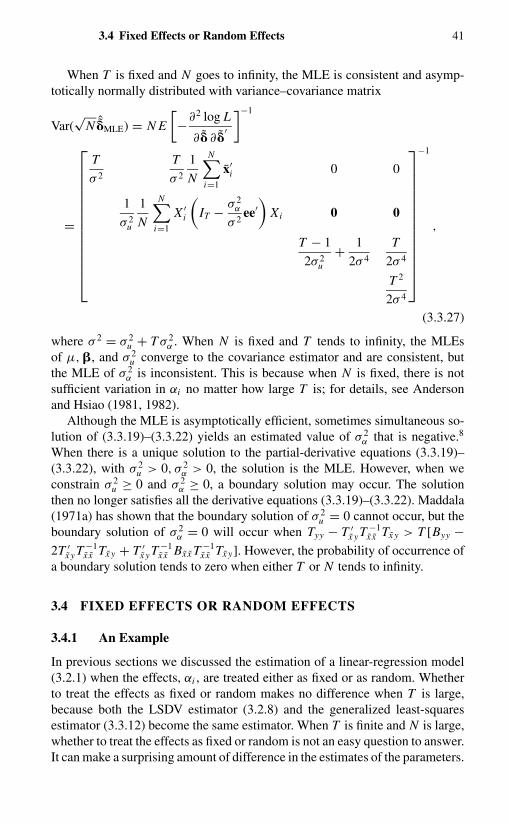
3.4 Fixed Effects or Random Effects 41
When T is fixed and N goes to infinity, the MLE is consistent and asymp-totically normally distributed with variance–covariance matrix
Var(√
N ˆ�MLE) = N E
[−∂2 log L
∂� ∂�′
]−1
=
T
σ 2
T
σ 2
1
N
N∑i=1
x′i 0 0
1
σ 2u
1
N
N∑i=1
X ′i
(IT − σ 2
α
σ 2ee′
)Xi 0 0
T − 1
2σ 2u
+ 1
2σ 4
T
2σ 4
T 2
2σ 4
−1
,
(3.3.27)
where σ 2 = σ 2u + T σ 2
α . When N is fixed and T tends to infinity, the MLEsof µ, �, and σ 2
u converge to the covariance estimator and are consistent, butthe MLE of σ 2
α is inconsistent. This is because when N is fixed, there is notsufficient variation in αi no matter how large T is; for details, see Andersonand Hsiao (1981, 1982).
Although the MLE is asymptotically efficient, sometimes simultaneous so-lution of (3.3.19)–(3.3.22) yields an estimated value of σ 2
α that is negative.8
When there is a unique solution to the partial-derivative equations (3.3.19)–(3.3.22), with σ 2
u > 0, σ 2α > 0, the solution is the MLE. However, when we
constrain σ 2u ≥ 0 and σ 2
α ≥ 0, a boundary solution may occur. The solutionthen no longer satisfies all the derivative equations (3.3.19)–(3.3.22). Maddala(1971a) has shown that the boundary solution of σ 2
u = 0 cannot occur, but theboundary solution of σ 2
α = 0 will occur when Tyy − T ′x y T −1
x x Tx y > T [Byy −2T ′
x y T −1x x Tx y + T ′
x y T −1x x Bx x T −1
x x Tx y]. However, the probability of occurrence ofa boundary solution tends to zero when either T or N tends to infinity.
3.4 FIXED EFFECTS OR RANDOM EFFECTS
3.4.1 An Example
In previous sections we discussed the estimation of a linear-regression model(3.2.1) when the effects, αi , are treated either as fixed or as random. Whetherto treat the effects as fixed or random makes no difference when T is large,because both the LSDV estimator (3.2.8) and the generalized least-squaresestimator (3.3.12) become the same estimator. When T is finite and N is large,whether to treat the effects as fixed or random is not an easy question to answer.It can make a surprising amount of difference in the estimates of the parameters.
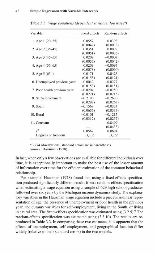
42 Simple Regression with Variable Intercepts
Table 3.3. Wage equations (dependent variable: log wagea)
Variable Fixed effects Random effects
1. Age 1 (20–35) 0.0557 0.0393(0.0042) (0.0033)
2. Age 2 (35–45) 0.0351 0.0092(0.0051) (0.0036)
3. Age 3 (45–55) 0.0209 −0.0007(0.0055) (0.0042)
4. Age 4 (55–65) 0.0209 −0.0097(0.0078) (0.0060)
5. Age 5 (65–) −0.0171 −0.0423(0.0155) (0.0121)
6. Unemployed previous year −0.0042 −0.0277(0.0153) (0.0151)
7. Poor health previous year −0.0204 −0.0250(0.0221) (0.0215)
8. Self-employment −0.2190 −0.2670(0.0297) (0.0263)
9. South −0.1569 −0.0324(0.0656) (0.0333)
10. Rural −0.0101 −0.1215(0.0317) (0.0237)
11. Constant — 0.8499— (0.0433)
s2 0.0567 0.0694Degrees of freedom 3,135 3,763
a3,774 observations; standard errors are in parentheses.Source: Hausman (1978).
In fact, when only a few observations are available for different individuals overtime, it is exceptionally important to make the best use of the lesser amountof information over time for the efficient estimation of the common behavioralrelationship.
For example, Hausman (1978) found that using a fixed-effects specifica-tion produced significantly different results from a random-effects specificationwhen estimating a wage equation using a sample of 629 high school graduatesfollowed over six years by the Michigan income dynamics study. The explana-tory variables in the Hausman wage equation include a piecewise-linear repre-sentation of age, the presence of unemployment or poor health in the previousyear, and dummy variables for self-employment, living in the South, or livingin a rural area. The fixed-effects specification was estimated using (3.2.5).9 Therandom-effects specification was estimated using (3.3.10). The results are re-produced in Table 3.3. In comparing these two estimates, it is apparent that theeffects of unemployment, self-employment, and geographical location differwidely (relative to their standard errors) in the two models.
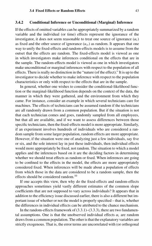
3.4 Fixed Effects or Random Effects 43
3.4.2 Conditional Inference or Unconditional (Marginal) Inference
If the effects of omitted variables can be appropriately summarized by a randomvariable and the individual (or time) effects represent the ignorance of theinvestigator, it does not seem reasonable to treat one source of ignorance (αi )as fixed and the other source of ignorance (uit ) as random. It appears that oneway to unify the fixed-effects and random-effects models is to assume from theoutset that the effects are random. The fixed-effects model is viewed as onein which investigators make inferences conditional on the effects that are inthe sample. The random-effects model is viewed as one in which investigatorsmake unconditional or marginal inferences with respect to the population of alleffects. There is really no distinction in the “nature (of the effect).” It is up to theinvestigator to decide whether to make inference with respect to the populationcharacteristics or only with respect to the effects that are in the sample.
In general, whether one wishes to consider the conditional-likelihood func-tion or the marginal-likelihood function depends on the context of the data, themanner in which they were gathered, and the environment from which theycame. For instance, consider an example in which several technicians care formachines. The effects of technicians can be assumed random if the techniciansare all randomly drawn from a common population. But if the situation is notthat each technician comes and goes, randomly sampled from all employees,but that all are available, and if we want to assess differences between thosespecific technicians, then the fixed-effects model is more appropriate. Similarly,if an experiment involves hundreds of individuals who are considered a ran-dom sample from some larger population, random effects are more appropriate.However, if the situation were one of analyzing just a few individuals, say fiveor six, and the sole interest lay in just these individuals, then individual effectswould more appropriately be fixed, not random. The situation to which a modelapplies and the inferences based on it are the deciding factors in determiningwhether we should treat effects as random or fixed. When inferences are goingto be confined to the effects in the model, the effects are more appropriatelyconsidered fixed. When inferences will be made about a population of effectsfrom which those in the data are considered to be a random sample, then theeffects should be considered random.10
If one accepts this view, then why do the fixed-effects and random-effectsapproaches sometimes yield vastly different estimates of the common slopecoefficients that are not supposed to vary across individuals? It appears that inaddition to the efficiency issue discussed earlier, there is also a different but im-portant issue of whether or not the model is properly specified – that is, whetherthe differences in individual effects can be attributed to the chance mechanism.
In the random-effects framework of (3.3.1)–(3.3.3), there are two fundamen-tal assumptions. One is that the unobserved individual effects αi are randomdraws from a common population. The other is that the explanatory variables arestrictly exogenous. That is, the error terms are uncorrelated with (or orthogonal
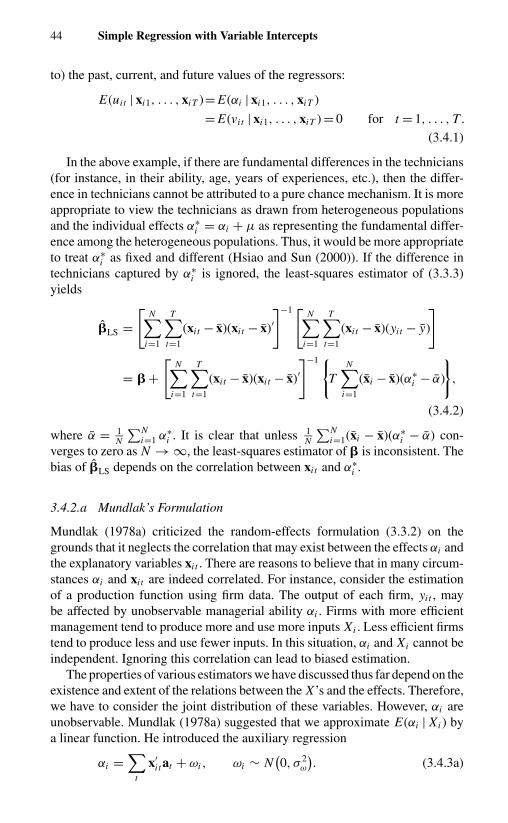
44 Simple Regression with Variable Intercepts
to) the past, current, and future values of the regressors:
E(uit | xi1, . . . , xiT )= E(αi | xi1, . . . , xiT )
= E(vit | xi1, . . . , xiT ) = 0 for t = 1, . . . , T .
(3.4.1)
In the above example, if there are fundamental differences in the technicians(for instance, in their ability, age, years of experiences, etc.), then the differ-ence in technicians cannot be attributed to a pure chance mechanism. It is moreappropriate to view the technicians as drawn from heterogeneous populationsand the individual effects α∗
i = αi + µ as representing the fundamental differ-ence among the heterogeneous populations. Thus, it would be more appropriateto treat α∗
i as fixed and different (Hsiao and Sun (2000)). If the difference intechnicians captured by α∗
i is ignored, the least-squares estimator of (3.3.3)yields
�LS =[
N∑i=1
T∑t=1
(xi t − x)(xi t − x)′]−1 [
N∑i=1
T∑t=1
(xi t − x)(yit − y)
]
= � +[
N∑i=1
T∑t=1
(xi t − x)(xi t − x)′]−1 {
TN∑
i=1
(xi − x)(α∗i − α)
},
(3.4.2)
where α = 1N
∑Ni=1 α∗
i . It is clear that unless 1N
∑Ni=1(xi − x)(α∗
i − α) con-verges to zero as N → ∞, the least-squares estimator of � is inconsistent. Thebias of �LS depends on the correlation between xi t and α∗
i .
3.4.2.a Mundlak’s Formulation
Mundlak (1978a) criticized the random-effects formulation (3.3.2) on thegrounds that it neglects the correlation that may exist between the effects αi andthe explanatory variables xi t . There are reasons to believe that in many circum-stances αi and xi t are indeed correlated. For instance, consider the estimationof a production function using firm data. The output of each firm, yit , maybe affected by unobservable managerial ability αi . Firms with more efficientmanagement tend to produce more and use more inputs Xi . Less efficient firmstend to produce less and use fewer inputs. In this situation, αi and Xi cannot beindependent. Ignoring this correlation can lead to biased estimation.
The properties of various estimators we have discussed thus far depend on theexistence and extent of the relations between the X ’s and the effects. Therefore,we have to consider the joint distribution of these variables. However, αi areunobservable. Mundlak (1978a) suggested that we approximate E(αi | Xi ) bya linear function. He introduced the auxiliary regression
αi =∑
t
x′i t at + ωi , ωi ∼ N
(0, σ 2
ω
). (3.4.3a)

3.4 Fixed Effects or Random Effects 45
A simple approximation to (3.4.3a) is to let
αi = x′i a + ωi , ωi ∼ N
(0, σ 2
ω
). (3.4.3b)
Clearly, a will be equal to zero (and σ 2ω = σ 2
α ) if (and only if) the explanatoryvariables are uncorrelated with the effects.
Substituting (3.4.3b) into (3.3.3), and stacking equations over t and i , wehave
y1
y2...
yN
=
X1
X2...
X N
� +
ex′
1ex′
2...
ex′N
a +
e0...0
ω1
+
0e...0
ω2 + · · · +
00...
eN
ωN +
u1
u2...
uN
, (3.4.4)
where, conditional on xi ,
E(ui + eωi ) = 0,
E(ui + eωi )(u j + eω j )′ =
{σ 2
u IT + σ 2ωee′ = V if i = j,
0 if i �= j,
V −1 = 1
σ 2u
[IT − σ 2
ω
σ 2u + T σ 2
ω
ee′].
Utilizing the expression for the inverse of a partitioned matrix (Theil (1971,Chapter 1)), we obtain the GLS of (µ, �′, a′) as
µ∗GLS = y − x′�b, (3.4.5)
�∗GLS = �CV, (3.4.6)
a∗GLS = �b − �CV. (3.4.7)
Thus, in the present framework, the BLUE of � is the covariance estima-tor of (3.2.1) or (3.2.10). It does not depend on knowledge of the variancecomponents. Therefore, Mundlak (1978a) maintained that the imaginary dif-ference between the fixed-effects and random-effects approaches is based onan incorrect specification. In fact, applying GLS to (3.2.10) yields a biasedestimator. This can be seen by noting that the GLS estimate of � for (3.3.3),that is, (3.3.10), can be viewed as the GLS estimate of (3.4.4) after imposingthe restriction a = 0. As shown in (3.3.12),
�GLS = �b + (IK − )�CV. (3.4.8)
If (3.4.4) is the correct specification, then E�b is equal to � + a, and E�CV = �,

46 Simple Regression with Variable Intercepts
so that
E�GLS = � + a. (3.4.9)
This is a biased estimator if a �= 0. However, when T tends to infinity,
tends to zero, and �GLS tends to �CV and is asymptotically unbiased. Butin the more relevant situation in which T is fixed and N tends to infinity,plimN→∞�GLS �= � in Mundlak’s formulation.
While it is important to recognize the possible correlation between the effectsand the explanatory variables, Mundlak’s claim (1978a) that there is only oneestimator and that efficiency is not a consideration in distinguishing betweenthe random-effects and fixed-effects approaches is perhaps a bit strong. In fact,in the dynamic, random-coefficient, and discrete-choice models to be discussedlater, one can show that the two approaches do not lead to the same estimatoreven when one allows for the correlation between αi and Xi . Moreover, in thelinear static model if a = 0, the efficient estimator is (3.3.12), not the covarianceestimator (3.2.8).
3.4.2.b Conditional and Unconditional Inferences in the Presence orAbsence of Correlation between Individual Effects and Attributes
To gain further intuition about the differences between models (3.3.3) and(3.4.4) within the conditional- and unconditional-inference frameworks, weconsider the following two experiments. Let a population be made up of acertain composition of red and black balls. The first experiment consists in Nindividuals, each picking a fixed number of balls randomly from this popula-tion to form his person-specific urn. Each individual then makes T independenttrials of drawing a ball from his specific urn and putting it back. The secondexperiment assumes that individuals have different preferences for the composi-tions of red and black balls for their specific urns and allows personal attributesto affect the compositions. Specifically, prior to making T independent trialswith replacement from their respective urns, individuals are allowed to take anynumber of balls from the population until their compositions reach the desiredproportions.
If one is interested in making inferences regarding an individual urn’s com-position of red and black balls, a fixed-effects model should be used, whetherthe sample comes from the first or the second experiment. On the other hand,if one is interested in the population composition, a marginal or unconditionalinference should be used. However, the marginal distributions are different forthese two cases. In the first experiment, differences in individual urns are out-comes of random sampling. The subscript i is purely a labeling device, with nosubstantive content. A conventional random-effects model assuming indepen-dence between αi and xi t would be appropriate. In the second experiment, thedifferences in individual urns reflect differences in personal attributes. A propermarginal inference has to allow for these nonrandom effects. It so happens that,

3.4 Fixed Effects or Random Effects 47
for the Mundlak’s formulation a marginal inference that properly allows for thecorrelation between individual effects (αi ) and the attributes (xi ) generating theprocess gives rise to the same estimator as when the individual effects are treatedas fixed. It is not that in making inferences about population characteristics weshould assume a fixed-effects model.
Formally, let uit and αi be independent normal processes that are mutu-ally independent. In the case of the first experiment, αi are independently dis-tributed and independent of individual attributes xi , so the distribution of αi
must be expressible as random sampling from a univariate distribution (Box andTiao (1968); Chamberlain (1980)). Thus, the conditional distribution of {(ui +eαi )′, αi | Xi } is identical with the marginal distribution of {(ui + eαi )′, αi },
ui1 + αi...
uiT + αi
. . . . . . . . .
αi
=
ui1 + αi
...uiT + αi Xi
. . . . . . . . .
αi
∼ N
[0. . .
0
],
σ 2u IT + σ 2
α ee′ ... σ 2α e
. . . . . . . . . . . .... . . . .
σ 2α e′ ... σ 2
α
. (3.4.10a)
In the second experiment, αi may be viewed as a random draw fromheterogeneous populations with mean a∗
i and variance σ 2ωi (Mundlak’s (1978a)
formulation may be viewed as a special case of this in which E(αi | Xi ) =a∗
i = a′xi , and σ 2ωi = σ 2
ω for all i). Then the conditional distribution of{(ui + eαi )′
... αi | Xi } isui1 + αi
...uiT + αi Xi
. . . . . . . . .
αi
∼ N
ea∗
i. . .
a∗i
,
σ 2u IT + σ 2
ωi ee′ ... σ 2ωi e
. . . . . . . . . . . .... . . . .
σ 2ωi e
′ ... σ 2ωi
.
(3.4.10b)
In both cases, the conditional density of ui + eαi , given αi , is11
(2πσ 2
u
)T/2exp
{− 1
2σ 2u
u′i ui
}. (3.4.11)
But the marginal density of ui + eαi , given Xi , are different [(3.4.10a) and(3.4.10b), respectively]. Under the independence assumption, {ui + eαi | Xi }has a common mean of zero for i = 1, . . . , N . Under the assumption that αi
and Xi are correlated or αi is a draw from a heterogeneous population, {ui +eαi | Xi } has a different mean ea∗
i for different i .

48 Simple Regression with Variable Intercepts
In the linear regression model, conditional on αi the Jacobian of transforma-tion from ui + eαi to yi is 1. Maximizing the conditional-likelihood functionof (y1 | α1, X1), . . . , (yN | αN , X N ), treating αi as unknown parameters, yieldsthe covariance (or within-group) estimators for both cases. Maximizing themarginal-likelihood function of (y1, . . . , yN | X1, . . . , X N ) yields the GLS es-timator (3.3.12) for (3.4.10a) if σ 2
u and σ 2α are known, and it happens to yield
the covariance estimator for (3.4.10b) in the linear case. In other words, thereis no loss of information using a conditional approach for the case of (3.4.10b).However, there is a loss in efficiency in maximizing the conditional-likelihoodfunction for the former case [i.e., (3.4.10a)] because of the loss of degreesof freedom in estimating additional unknown parameters (α1, . . . , αN ), whichleads to ignoring the information contained in the between-group variation.
The advantage of the unconditional inference is that the likelihood functionmay only depend on a finite number of parameters and hence can often leadto efficient inference. The disadvantage is that the correct specification of theconditional density of yi given Xi ,
f (yi | Xi ) =∫
f (yi | Xi , αi ) f (αi | Xi ) dαi , (3.4.12)
depends on the correct specification of f (αi | Xi ). A misspecified f (αi | Xi )can lead to a misspecified f (yi | Xi ). Maximizing the wrong f (yi | Xi ) can leadto biased and inconsistent estimators. The bias of the GLS estimator (3.3.12)in the case that αi ∼ N (a∗
i , σ 2ωi ) is not due to any fallacy of the unconditional
inference, but due to the misspecification of f (αi | Xi ).The advantage of the conditional inference is that there is no need to specify
f (αi | Xi ). Therefore, if the distribution of effects cannot be represented bya simple parametric functional form (say bimodal), or one is not sure of thecorrelation pattern between the effects and Xi , there may be an advantage inbasing one’s inference conditionally. In the situation that there are fundamentaldifferences between the effects (for instance, if there are fundamental differ-ences in the ability, years of experiences, etc., as in the previous of example oftechnicians), then it is more appropriate to treat the technicians’ effects as fixed.
The disadvantage of the conditional inference is that not only there is a loss ofefficiency due to the loss of degrees of freedom of estimating the effects, there isalso an issue of incidental parameters if T is finite (Neyman and Scott (1948)).A typical panel contains a large number of individuals observed over a shorttime period; the number of individual effects parameters (α∗
i ) increases withthe number of cross-sectional dimension, N . Because increase in N providesno information on a particular α∗
i apart from that already contained in yi , α∗i
cannot be consistently estimated with finite T . The condition that, in general,
E(uit | xi t ) = 0 (3.4.13)
is not informative about the common parameters � in the absence of any knowl-edge about α∗
i . If the estimation of the incidental parameters α∗i is not asymptoti-
cally independent of the estimation of the common parameters (called structural
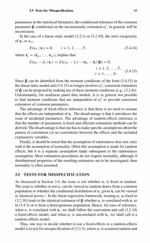
3.5 Tests for Misspecification 49
parameters in the statistical literature), the conditional inference of the commonparameter � conditional on the inconsistently estimated α∗
i , in general, will beinconsistent.
In the case of a linear static model (3.2.1) or (3.2.10), the strict exogeneityof xi t to uit ,
E(uit | xi ) = 0, t = 1, 2, . . . , T, (3.4.14)
where x′i = (x′
i1, . . . , x′iT ), implies that
E(uit − ui | xi ) = E[(yit − yi ) − (xi t − xi )′�] = 0,
t = 1, 2, . . . , T,(3.4.15)
i = 1, . . . , N .
Since � can be identified from the moment conditions of the form (3.4.15) inthe linear static model and (3.4.15) no longer involves α∗
i , consistent estimatorsof � can be proposed by making use of these moment conditions (e.g., (3.2.8)).Unfortunately, for nonlinear panel data models, it is in general not possibleto find moment conditions that are independent of α∗
i to provide consistentestimators of common parameters.
The advantage of fixed-effects inference is that there is no need to assumethat the effects are independent of xi . The disadvantage is that it introduces theissue of incidental parameters. The advantage of random-effects inference isthat the number of parameters is fixed and efficient estimation methods can bederived. The disadvantage is that one has to make specific assumptions about thepattern of correlation (or no correlation) between the effects and the includedexplanatory variables.
Finally, it should be noted that the assumption of randomness does not carrywith it the assumption of normality. Often this assumption is made for randomeffects, but it is a separate assumption made subsequent to the randomnessassumption. Most estimation procedures do not require normality, although ifdistributional properties of the resulting estimators are to be investigated, thennormality is often assumed.
3.5 TESTS FOR MISSPECIFICATION
As discussed in Section 3.4, the issue is not whether αi is fixed or random.The issue is whether or not αi can be viewed as random draws from a commonpopulation or whether the conditional distribution of αi given xi can be viewedas identical across i . In the linear-regression framework, treating αi as fixed in(3.2.10) leads to the identical estimator of � whether αi is correlated with xi asin (3.4.3) or is from a heterogeneous population. Hence, for ease of reference,when αi is correlated with xi , we shall follow the convention and call (3.2.10)a fixed-effects model, and when αi is uncorrelated with xi , we shall call it arandom-effects model.
Thus, one way to decide whether to use a fixed-effects or a random-effectsmodel is to test for misspecification of (3.3.3), where αi is assumed random and

50 Simple Regression with Variable Intercepts
uncorrelated with xi . Using Mundlak’s formulation, (3.4.3a) or (3.4.3b), thistest can be reduced to a test of
H0 : a = 0
against
H1 : a �= 0.
If the alternative hypothesis H1 holds, we use the fixed-effects model (3.2.1).If the null hypothesis H0 holds, we use the random-effects model (3.3.3). Theratio
F =
∑Ni=1(yi − X i �GLS)′V ∗−1(yi − X i �GLS)
−∑Ni=1(yi − X i �
∗GLS − ex′
i a∗GLS)′V ∗−1 · (yi − X i �
∗GLS − ex′
i a∗GLS)
K
(∑N
i=1(yi − X i �∗GLS − ex′
i a∗GLS)′V ∗−1(yi − X i �
∗GLS − ex′
i a∗GLS)
N T − (2K + 1)
)(3.5.1)
under H0 has a central F distribution with K and N T − (2K + 1) degreesof freedom, where V ∗−1 = (1/σ 2
u )[Q + ψ∗(1/T )ee′], ψ∗ = σ 2u /(σ 2
u + T σ 2ω).
Hence, (3.5.1) can be used to test H0 against H1.12
An alternative testing procedure suggested by Hausman (1978) notes thatunder H0 the GLS for (3.3.3) achieves the Cramer–Rao lower bounds, but underH1, the GLS is a biased estimator. In contrast, the CV of � is consistent underboth H0 and H1. Hence, the Hausman test basically asks if the CV and GLSestimates of � are significantly different.
To derive the asymptotic distribution of the differences of the two estimates,Hausman makes use of the following lemma:13
Lemma 3.5.1. Based on a sample of N observations, consider two estimates�0 and �1 that are both consistent and asymptotically normally distributed,with �0 attaining the asymptotic Cramer–Rao bound so that
√N (�0 − �) is
asymptotically normally distributed with variance–covariance matrix V0. Sup-pose
√N (�1 − �) is asymptotically normally distributed, with mean zero and
variance–covariance matrix V1. Let q = �1 − �0. Then the limiting distri-bution of
√N (�0 − �) and
√N q has zero covariance: C(�0, q) = 0, a zero
matrix.
From this lemma, it follows that Var(q) = Var(�1) − Var(�0). Thus,Hausman suggests using the statistic14
m = q′ Var(q)−1q, (3.5.2)
where q = �CV − �GLS, Var(q) = Var(�CV) − Var(�GLS), to test the nullhypothesis E(αi | Xi ) = 0 against the alternative E(αi | Xi ) �= 0. Under the
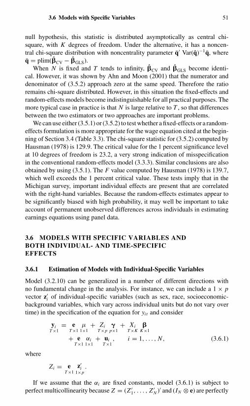
3.6 Models with Specific Variables 51
null hypothesis, this statistic is distributed asymptotically as central chi-square, with K degrees of freedom. Under the alternative, it has a noncen-tral chi-square distribution with noncentrality parameter q′ Var(q)−1q, whereq = plim(�CV − �GLS).
When N is fixed and T tends to infinity, �CV and �GLS become identi-cal. However, it was shown by Ahn and Moon (2001) that the numerator anddenominator of (3.5.2) approach zero at the same speed. Therefore the ratioremains chi-square distributed. However, in this situation the fixed-effects andrandom-effects models become indistinguishable for all practical purposes. Themore typical case in practice is that N is large relative to T , so that differencesbetween the two estimators or two approaches are important problems.
We can use either (3.5.1) or (3.5.2) to test whether a fixed-effects or a random-effects formulation is more appropriate for the wage equation cited at the begin-ning of Section 3.4 (Table 3.3). The chi-square statistic for (3.5.2) computed byHausman (1978) is 129.9. The critical value for the 1 percent significance levelat 10 degrees of freedom is 23.2, a very strong indication of misspecificationin the conventional random-effects model (3.3.3). Similar conclusions are alsoobtained by using (3.5.1). The F value computed by Hausman (1978) is 139.7,which well exceeds the 1 percent critical value. These tests imply that in theMichigan survey, important individual effects are present that are correlatedwith the right-hand variables. Because the random-effects estimates appear tobe significantly biased with high probability, it may well be important to takeaccount of permanent unobserved differences across individuals in estimatingearnings equations using panel data.
3.6 MODELS WITH SPECIFIC VARIABLES ANDBOTH INDIVIDUAL- AND TIME-SPECIFICEFFECTS
3.6.1 Estimation of Models with Individual-Specific Variables
Model (3.2.10) can be generalized in a number of different directions withno fundamental change in the analysis. For instance, we can include a 1 × pvector z′
i of individual-specific variables (such as sex, race, socioeconomic-background variables, which vary across individual units but do not vary overtime) in the specification of the equation for yit and consider
yiT ×1
= eT ×1
µ1×1
+ ZiT ×p
�p×1
+ XiT ×K
�K×1
+ eT ×1
αi1×1
+ uiT ×1
, i = 1, . . . , N , (3.6.1)
where
Zi = eT ×1
z′i
1×p.
If we assume that the αi are fixed constants, model (3.6.1) is subject toperfect multicollinearity because Z = (Z ′
1, . . . , Z ′N )′ and (IN ⊗ e) are perfectly

52 Simple Regression with Variable Intercepts
correlated.15 Hence, �, µ, and αi are not separately estimable. However, �may still be estimated by the covariance method (provided
∑Ni=1 X ′
i Q Xi is offull rank). Premultiplying (3.6.1) by the (covariance) transformation matrix Q[(3.2.6)], we sweep out Zi , eµ, and eαi from (3.6.1), so that
Qyi = Q Xi � + Qui , i = 1, . . . , N . (3.6.2)
Applying OLS to (3.6.2), we obtain the CV estimate of �, (3.2.8).When the αi are assumed random and uncorrelated with Xi and Zi , CV
uses the same method to estimate � (3.2.8). To estimate �, we note that theindividual mean over time satisfies
yi − x′i � = µ + z′
i � + αi + ui , i = 1, . . . , N . (3.6.3)
Treating (αi + ui ) as the error term and minimizing∑N
i=1(αi + ui )2, we obtain
� =[
N∑i=1
(zi − z)(zi − z)′]−1 {
N∑i=1
(zi − z)[(yi − y) − (xi − x)′�]
},
(3.6.4)
µ = y − x′� − z′�, (3.6.5)
where
z = 1
N
N∑i=1
zi , x = 1
N
N∑i=1
xi , y = 1
N
N∑i=1
yi .
Substituting the CV estimate of � into (3.6.4) and (3.6.5), we obtain estimatorsof � and µ. When N tends to infinity, this two-step procedure is consistent.When N is fixed and T tends to infinity, � can still be consistently estimated by(3.2.8). But � can no longer be consistently estimated, because when N is fixed,we have a limited amount of information on αi and zi . To see this, note thatthe OLS estimate of (3.6.3) after substituting plimT →∞ �CV = � converges to
�OLS = � +[
N∑i=1
(zi − z)(zi − z)′]−1 [
N∑i=1
(zi − z)(αi − α)
]
+[T
N∑i=1
(zi − z)(zi − z)′]−1 [
N∑i=1
T∑t=1
(zi − z)(uit − u)
],
(3.6.6)
where
u = 1
N T
N∑i=1
T∑t=1
uit , α = 1
N
N∑i=1
αi .
It is clear that
plimT →∞
1
N
N∑i=1
(zi − z)1
T
T∑t=1
(uit − u) = 0,

3.6 Models with Specific Variables 53
but (1/N )∑N
i=1(zi − z)(αi − α) is a random variable, with mean zero and co-variance σ 2
α [∑N
i=1(zi − z)(zi − z)′/N 2] �= 0 for finite N , so that the secondterm in (3.6.6) does not have zero plim.
When αi are random and uncorrelated with Xi and Zi , the CV is not theBLUE. The BLUE of (3.6.1) is the GLS estimator
µ
�
�
=
N T ψ N T ψ z′ N T ψ x′
N T ψ z T ψ
N∑i=1
zi z′i T ψ
N∑i=1
zi x′i
N T ψ x T ψ
N∑i=1
xi z′i
N∑i=1
X ′i Q Xi + ψT
N∑i=1
xi x′i
−1
×
N T ψ y
ψTN∑
i=1
zi yi
N∑i=1
X ′i Qyi + ψT
N∑i=1
xi yi
. (3.6.7)
If ψ in (3.6.7) is unknown, we can substitute a consistent estimate for it. WhenT is fixed, the GLS is more efficient than the CV. When T tends to infinity, theGLS estimator of � converges to the CV estimator; for details, see Lee (1978b).
One way to view (3.6.1) is that by explicitly incorporating time-invariantexplanatory variables zi we can eliminate or reduce the correlation betweenαi and xi t . However, if αi remains correlated with xi t or zi , the GLS will be abiased estimator. The CV will produce an unbiased estimate of �, but the OLSestimates of � andµ in (3.6.3) are inconsistent even when N tends to infinity ifαi
is correlated with zi .16 Thus, Hausman and Taylor (1981) suggested estimating� in (3.6.3) by two-stage least squares, using those elements of xi that areuncorrelated with αi as instruments for zi . A necessary condition to implementthis method is that the number of elements of xi that are uncorrelated with αi
must be greater than the number of elements of zi that are correlated with αi .
3.6.2 Estimation of Models with Both Individual and Time Effects
We can further generalize model (3.6.1) to include time-specific variables andeffects. Let
yit = µ + z′i
1×p�
p×1+ r′
t1×l
�l×1
+ x′i t
1×K�
K×1+ αi + λt + uit ,
i = 1, . . . , N ,(3.6.8)
t = 1, . . . , T,

54 Simple Regression with Variable Intercepts
where rt and λt denote l × 1 and 1 × 1 time-specific variables and effects.Stacking (3.6.8) over i and t , we have
YN T ×1
=
y1
y2...
yN
=
e Z1 R X1
e Z2 R X2...
......
...e Z N R X N
µ
�
�
�
+ (IN ⊗ e)� + (eN ⊗ IT )� +
u1
u2...
uN
, (3.6.9)
where � ′ = (α1, . . . , αN ), � ′ = (λ1. . . . , λT ), R′ = (r1, r2, . . . , rT ), eN is anN × 1 vector of ones, and ⊗ denotes the Kronecker product.
If � and � are treated as fixed constants, there is a multicollinearity problem,for the same reasons stated in Section 3.6.1. The coefficients �, �, �, �, and µ
cannot be separately estimated. The coefficient � can still be estimated by thecovariance method. Using the N T × N T (covariance) transformation matrix
Q = IN T − IN ⊗ 1
Tee′ − 1
NeN e′
N ⊗ IT + 1
N TJ, (3.6.10)
where J is an N T × N T matrix of ones, we can sweep out µ, zi , rt , αi , and λt
and estimate � by
�CV = [(X ′1, . . . , X ′
N )Q(X ′1, . . . , X ′
N )′]−1[(X ′1, . . . , X ′
N )QY ].
(3.6.11)
If αi and λt are random, we can still estimate � by the covariance method.To estimate µ, �, and �, we note that the individual-mean (over time) andtime-mean (over individuals) equations are of the form
yi − x′i � = µ∗
c + z′i � + αi + ui , i = 1, . . . , N , (3.6.12)
yt − x′t � = µ∗
T + r′t � + λt + ut , t = 1, . . . , T, (3.6.13)
where
µ∗c = µ + r′� + λ, (3.6.14)
µ∗T = µ + z′� + α, (3.6.15)
and
r = 1
T
T∑t=1
rt , z = 1
N
N∑i=1
zi , λ = 1
T
T∑t=1
λt , α = 1
N
N∑i=1
αi ,
yt = 1
N
N∑i=1
yit , xt = 1
N
N∑i=1
xi t , ut = 1
N
N∑i=1
uit .

3.7 Heteroscedasticity 55
Replacing � by �CV, we can estimate (µ∗c , �′) and (µ∗
T , �′) by applying OLSto (3.6.12) and (3.6.13) over i and t , respectively, if αi and λt are uncorrelatedwith zi , rt , and xi t . To estimate µ, we can substitute estimated values of �, �,and � into any of
µ = µ∗c − r′�, (3.6.16)
µ = µ∗T − z′�, (3.6.17)
µ = y − z′� − r′� − x′�, (3.6.18)
or apply the least-squares method to the combined equations (3.6.16)–(3.6.18).When both N and T go to infinity, µ is consistent.
If αi and λt are random and uncorrelated with zi , rt , and xi t , the BLUE is theGLS estimator. Assuming αi and λt satisfy (3.3.2), the N T × N T variance–covariance matrix of the error term, u + (IN ⊗ e)� + (eN ⊗ IT )�, is
V = σ 2u IN T + σ 2
α IN ⊗ ee′ + σ 2λ eN e′
N ⊗ IT . (3.6.19)
Its inverse (Henderson (1971); Nerlove (1971b); Wallace and Hussain (1969))(see Appendix 3B) is
V −1 = 1
σ 2u
[IN T − η1 IN ⊗ ee′ − η2eN e′N ⊗ IT + η3 J ], (3.6.20)
where
η1 = σ 2α
σ 2u + T σ 2
α
, η2 = σ 2λ
σ 2u + Nσ 2
λ
,
η3 = σ 2ασ 2
λ(σ 2
u + T σ 2α
)(σ 2
u + Nσ 2λ
) (2σ 2
u + T σ 2α + Nσ 2
λ
σ 2u + T σ 2
α + Nσ 2λ
).
When N → ∞, T → ∞, and the ratio N/T tends to a nonzero constant,Wallace and Hussain (1969) have shown that the GLS estimator converges to theCV estimator. It should also be noted that, contrary to the conventional linear-regression model without specific effects, the speed of convergence of �GLS to� is (N T )1/2, whereas the speed of convergence for µ is N 1/2. This is becausethe effect of a random component can be averaged out only in the direction ofthat random component. For details, see Kelejian and Stephan (1983).
For the discussion of the MLE of the two-way error components models,see Baltagi (1995) and Baltagi and Li (1992).
3.7 HETEROSCEDASTICITY
So far we have confined our discussion to the assumption that the variancesof the errors across individuals are identical. However, many panel studiesinvolve cross-sectional units of varying size. In an error-components setup,heteroscedasticity can arise because the variance σ 2
αi of αi varies with i
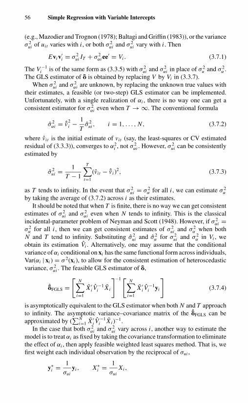
56 Simple Regression with Variable Intercepts
(e.g., Mazodier and Trognon (1978); Baltagi and Griffin (1983)), or the varianceσ 2
ui of uit varies with i , or both σ 2αi and σ 2
ui vary with i . Then
Evi v′i = σ 2
ui IT + σ 2αi ee′ = Vi . (3.7.1)
The V −1i is of the same form as (3.3.5) with σ 2
ui and σ 2αi in place of σ 2
u and σ 2α .
The GLS estimator of � is obtained by replacing V by Vi in (3.3.7).When σ 2
ui and σ 2αi are unknown, by replacing the unknown true values with
their estimates, a feasible (or two-step) GLS estimator can be implemented.Unfortunately, with a single realization of αi , there is no way one can get aconsistent estimator for σ 2
αi even when T → ∞. The conventional formula
σ 2αi = ˆv2
i − 1
Tσ 2
ui , i = 1, . . . , N , (3.7.2)
where vi t is the initial estimate of vit (say, the least-squares or CV estimatedresidual of (3.3.3)), converges to α2
i , not σ 2αi . However, σ 2
ui can be consistentlyestimated by
σ 2ui = 1
T − 1
T∑t=1
(vi t − ˆvi )2, (3.7.3)
as T tends to infinity. In the event that σ 2αi = σ 2
α for all i , we can estimate σ 2α
by taking the average of (3.7.2) across i as their estimates.It should be noted that when T is finite, there is no way we can get consistent
estimates of σ 2ui and σ 2
αi even when N tends to infinity. This is the classicalincidental-parameter problem of Neyman and Scott (1948). However, if σ 2
αi =σ 2
α for all i , then we can get consistent estimates of σ 2ui and σ 2
α when bothN and T tend to infinity. Substituting σ 2
ui and σ 2α for σ 2
ui and σ 2α in Vi , we
obtain its estimation Vi . Alternatively, one may assume that the conditionalvariance of αi conditional on xi has the same functional form across individuals,Var(αi | xi ) = σ 2(xi ), to allow for the consistent estimation of heteroscedasticvariance, σ 2
αi . The feasible GLS estimator of �,
�FGLS =[
N∑i=1
X ′i V
−1i X i
]−1 [N∑
i=1
X ′i V
−1i yi
](3.7.4)
is asymptotically equivalent to the GLS estimator when both N and T approachto infinity. The asymptotic variance–covariance matrix of the �FGLS can beapproximated by (
∑Ni=1 X ′
i V−1
i X i )−1.In the case that both σ 2
αi and σ 2ui vary across i , another way to estimate the
model is to treat αi as fixed by taking the covariance transformation to eliminatethe effect of αi , then apply feasible weighted least squares method. That is, wefirst weight each individual observation by the reciprocal of σui ,
y∗i = 1
σuiyi , X∗
i = 1
σuiXi ,

3.8 Models with Serially Correlated Errors 57
then apply the covariance estimator to the transformed data
�CV =[
N∑i=1
X∗′i Q X∗
i
]−1 [N∑
i=1
X∗′i Qy∗
i
]. (3.7.5)
3.8 MODELS WITH SERIALLY CORRELATEDERRORS
The fundamental assumption we made with regard to the variable-interceptmodel was that the error term is serially uncorrelated conditional on the indi-vidual effects αi . But there are cases in which the effects of unobserved variablesvary systematically over time, such as the effect of serially correlated omittedvariables or the effects of transitory variables whose effects last more than oneperiod. The existence of these variables is not well described by an error termthat is either constant or independently distributed over time periods. To pro-vide for a more general autocorrelation scheme, one can relax the restrictionthat uit are serially uncorrelated (e.g., Lillard and Weiss (1978, 1979??)).17
Anderson and Hsiao (1982) have considered the MLE of the model (3.3.3) withuit following a first-order autoregressive process,
uit = ρui,t−1 + εi t , (3.8.1)
where εi t are independently, identically distributed, with zero mean and varianceσ 2
ε . However, computation of the MLE is complicated. But if we know ρ, wecan transform the model into a standard variance-components model,
yit − ρyi,t−1 = µ(1 − ρ) + �′(xi t − ρxi,t−1) + (1 − ρ)αi + εi t .
(3.8.2)
Therefore, we can obtain an asymptotically efficient estimator of � by thefollowing multistep procedure:
Step 1. Eliminate the individual effect αi by subtracting the individualmean from (3.3.3). We have
yit − yi = �′(xi t − xi ) + (uit − ui ). (3.8.3)
Step 2. Use the least-squares residual of (3.8.3) to estimate the se-rial correlation coefficient ρ, or use the Durbin (1960) methodby regressing (yit − yi ) on (yi,t−1 − yi,−1), and (xi,t−1 − xi,−1),and treat the coefficient of (yi,t−1 − yi,−1) as the estimated value ofρ, where yi,−1 = (1/T )
∑Tt=1 yi,t−1 and xi,−1 = (1/T )
∑Tt=1 xi,t−1.
(For simplicity, we assume that yi0 and xi0 are observable.)

58 Simple Regression with Variable Intercepts
Step 3. Estimate σ 2ε and σ 2
α by
σ 2ε = 1
N T
N∑i=1
T∑t=1
{(yit − yi )
−(1 − ρ)µ − ρ(yi,t−1 − yi,−1)
−�′[(xi t − xi ) − (xi,t−1 − xi,−1)ρ]}2, (3.8.4)
and
σ 2α = 1
(1 − ρ)2· 1
N
N∑i=1
[yi − µ(1 − ρ) − ρ yi,−1 − �′(xi − xi,−1ρ)]2
− 1
Tσ 2
ε . (3.8.5)
Step 4. Substituting ρ, (3.8.4), and (3.8.5) for ρ, σ 2ε , and σ 2
α in thevariance–covariance matrix of εi t + (1 − ρ)αi , we estimate (3.8.2)by the GLS method.
The above multistep or feasible generalized least-squares procedure treatsthe initial ui1 as fixed constants. A more efficient, but computationally moreburdensome, feasible GLS is to treat initial ui1 as random variables with mean 0and variance σ 2
ε /(1 − ρ2) (e.g., Baltagi and Li (1991)). Premultiplying (3.3.3)by the T × T transformation matrix
R =
(1 − ρ2)1/2 0 0 · · · 0 0−ρ 1 0 · · · 0 00 −ρ 1 · · · 0 0
0 0 −ρ. . .
......
......
.... . . 1 0
0 0 0 · · · −ρ 1
transforms ui into serially uncorrelated homoscedastic error terms, but alsotransforms eT αi into (1 − ρ)�T αi , where
�T =[(
1 + ρ
1 − ρ
)1/2
, 1, . . . , 1
]′.
Therefore, the transformed error terms will have covariance matrix
V ∗ = σ 2ε IT + (1 − ρ)2σ 2
α�T �′T , (3.8.6)
with inverse
V ∗−1 = 1
σ 2ε
[IT − (1 − ρ)2σ 2
α
[T − (T − 1)ρ − ρ2]σ 2α + σ 2
ε
�T �′T
]. (3.8.7)
Substituting initial estimates of ρ, σ 2α , and σ 2
ε into (3.8.7), one can apply theGLS procedure using (3.8.7) to estimate �.

3.8 Models with Serially Correlated Errors 59
When T tends to infinity, the GLS estimator of � converges to the covarianceestimator of the transformed model (3.8.2). In other words, an asymptoticallyefficient estimator of � is obtained by finding a consistent estimate of ρ, trans-forming the model to eliminate the serial correlation, and then applying thecovariance method to the transformed model (3.8.2).
MaCurdy (1982) has considered a similar estimation procedure for (3.3.3)with a more general time-series process of uit . His procedure essentiallyinvolves eliminating αi by first-differencing and treating yit − yi,t−1 as thedependent variable. He then modeled the variance–covariance matrix ofui by using a standard Box–Jenkins (1970) procedure to model the least-squares predictor of uit − ui,t−1, and estimated the parameters by an efficientalgorithm.
Kiefer (1980) considered estimation of fixed-effects models of (3.2.1) witharbitrary intertemporal correlations for uit . When T is fixed, the individualeffects cannot be consistently estimated. He suggested that we first eliminatethe individual effects by transforming the model to the form (3.8.3) using thetransformation matrix Q = IT − (1/T )ee′. Then estimate the intertemporal co-variance matrix of Qui by
�∗ = 1
N
N∑i=1
[Q(yi − Xi �)][Q(yi − Xi �)]′, (3.8.8)
where � is any arbitrary consistent estimator of � (e.g., CV of �). Given anestimate of �∗, one can estimate � by the GLS method,
�∗ =
[N∑
i=1
X ′i Q�∗− Q Xi
]−1 [N∑
i=1
X ′i Q�∗− Qyi
], (3.8.9)
where �∗− is a generalized inverse of �∗, because �∗ has only rank T − 1.The asymptotic variance–covariance matrix of �
∗is
Var(�∗) =
[N∑
i=1
X ′i Q�∗− Q Xi
]−1
. (3.8.10)
Although any generalized inverse can be used for �∗, a particularly attractivechoice is
�∗− =[�∗−1
T −1 0
0′ 0
],
where �∗T −1 is the (T − 1) × (T − 1) full-rank submatrix of �∗ obtained by
deleting the last row and column from �∗. Using this generalized inverse simplyamounts to deleting the T th observation from the transformed observationsQyi and Q Xi , and then applying GLS to the remaining subsample. However,it should be noted that this is not the GLS estimator that would be used if thevariance–covariance matrix of ui were known.

60 Simple Regression with Variable Intercepts
3.9 MODELS WITH ARBITRARY ERRORSTRUCTURE – CHAMBERLAIN π APPROACH
The focus of this chapter is formulation and estimation of linear-regressionmodels when there exist time-invariant and/or individual-invariant omitted(latent) variables. In Sections 3.1–3.7 we have been assuming that the variance–covariance matrix of the error term possesses a known structure. In fact, whenN tends to infinity, the characteristics of short panels allow us to exploit the un-known structure of the error process. Chamberlain (1982, 1984) has proposed totreat each period as an equation in a multivariate setup to transform the problemsof estimating a single-equation model involving two dimensions (cross sectionsand time series) into a one-dimensional problem of estimating a T -variate re-gression model with cross-sectional data. This formulation avoids imposingrestrictions a priori on the variance–covariance matrix, so that serial correlationand certain forms of heteroscedasticity in the error process, which covers cer-tain kinds of random-coefficient models (see Chapter 6), can be incorporated.The multivariate setup also provides a link between the single-equation andsimultaneous-equations models (see Chapter 5). Moreover, the extended viewof the Chamberlain method can also be reinterpreted in terms of the generalizedmethod of moments (GMM) method to be discussed in Chapter 4 (Crepon andMairesse (1996)).
For simplicity, consider the following model:
yit = α∗i + �′xi t + uit , i = 1, . . . , N ,
(3.9.1)t = 1, . . . , T,
and
E(uit | xi1, . . . , xiT , α∗i ) = 0. (3.9.2)
When T is fixed and N tends to infinity, we can stack the T time-period ob-servations of the i th individual’s characteristics into a vector (y′
i , x′i ), where
y′i = (yi1, . . . , yiT ) and x′
i = (x′i1, . . . , x′
iT ) are 1 × T and 1 × K T vectors, re-spectively. We assume that (y′
i , x′i ) is an independent draw from a common
(unknown) multivariate distribution function with finite fourth-order momentsand with Exi x′
i = �xx positive definite. Then each individual observation vec-tor corresponds to a T -variate regression
yiT ×1
= eα∗i + (IT ⊗ �′)xi + ui , i = 1, . . . , N . (3.9.3)
To allow for the possible correlation between α∗i and xi , Chamberlain, fol-
lowing the idea of Mundlak (1978a), assumes that
E(α∗i | xi ) = µ +
T∑t=1
a′t xi t = µ + a′xi , (3.9.4)
where a′ = (a′1, . . . , a′
T ). While E(yi | xi , α∗i ) is assumed linear, it is possible

3.9 Models with Arbitrary Error Structure 61
to relax the assumption of E(α∗i | xi ) being linear for the linear model. In the
case in which E(α∗i | xi ) is not linear, Chamberlain (1984) replaces (3.9.4) by
E∗(α∗i | xi ) = µ + a′xi , (3.9.5)
where E∗(α∗i | xi ) refers to the (minimum-mean-squared-error) linear predictor
(or the projection) of α∗i onto xi . Then,18
E∗(yi | xi ) = E∗{E∗(yi | xi , α∗i ) | xi }
= E∗{eα∗i + (IT ⊗ �′)xi | xi }
= eµ + �xi , (3.9.6)
where
�T ×K T
= IT ⊗ �′ + ea′. (3.9.7)
Rewrite equations (3.9.3) and (3.9.6) as
yi = eµ + [IT ⊗ x′i ]� + i , i = 1, . . . , N , (3.9.8)
where i = yi − E∗(yi | xi ) and �′ = vec(�∗′)′ = [�′1, . . . , �′
T ] is a 1 × K T 2
vector with �′t denoting the t th row of �. Treating the coefficients of (3.9.8) as
if they were unconstrained, we regress (yi − y) on [IT ⊗ (xi − x∗)′] and obtainthe least-squares estimate of � as19
� ={
N∑i=1
[IT ⊗ (xi − x∗)][IT ⊗ (xi − x∗)′]
}−1
×{
N∑i=1
[IT ⊗ (xi − x∗)](yi − y)
}
= � +{
1
N
N∑i=1
[IT ⊗ (xi − x∗)][IT ⊗ (xi − x∗)′]
}−1
×{
1
N
N∑i=1
[IT ⊗ (xi − x∗)] i
}, (3.9.9)
where y = (1/N )∑N
i=1 yi and x∗ = (1/N )∑N
i=1 xi .By construction, E( i | xi ) = 0, and E( i ⊗ xi ) = 0. The law of large num-
bers implies that � is a consistent estimator of � when T is fixed and N tendsto infinity (Rao (1973, Chapter 2)). Moreover, because
plimN→∞
1
N
N∑i=1
(xi − x∗)(xi − x∗)′ = E[xi − Exi ][xi − Exi ]′
= �xx − (Ex)(Ex)′ = �xx ,

62 Simple Regression with Variable Intercepts
we have√
N (� − �) converging in distribution to (Rao (1973, Chapter 2))
[IT ⊗ �−1
xx
] { 1√N
N∑i=1
[IT ⊗ (xi − x∗)] i
}
= [IT ⊗ �−1
xx
] { 1√N
N∑i=1
[ i ⊗ (xi − x∗)]
}. (3.9.10)
So the central limit theorem implies that√
N (� − �) is asymptotically normallydistributed, with mean zero and variance–covariance matrix �, where20
� = E[(yi − eµ − �xi )(yi − eµ − �xi )
′
⊗ �−1xx (xi − Ex)(xi − Ex)′�−1
xx
]. (3.9.11)
A consistent estimator of � is readily available from the correspondingsample moments,
� = 1
N
N∑i=1
{[(yi − y) − �(xi − x∗)][(yi − y)
− �(xi − x∗)]′ ⊗ S−1xx (xi − x∗)(xi − x∗)′S−1
xx
},
(3.9.12)
where
Sxx = 1
N
N∑i=1
(xi − x∗)(xi − x∗)′.
Equation (3.9.7) implies that � is subject to restrictions. Let � = (�′, a′).We specify the restrictions on � [equation (3.9.7)] by the conditions that
� = f(�). (3.9.13)
We can impose these restrictions by using a minimum-distance estimator.Namely, choose � to minimize
[� − f(�)]′�−1[� − f(�)]. (3.9.14)
Under the assumptions that f possesses continuous second partial derivatives,and the matrix of first partial derivatives
F = ∂f∂�′ (3.9.15)
has full column rank in an open neighborhood containing the true parameter �,the minimum-distance estimator � of (3.9.14) is consistent, and
√N (� − �) is
asymptotically normally distributed, with mean zero and variance–covariancematrix
(F ′�−1 F)−1. (3.9.16)

3.9 Models with Arbitrary Error Structure 63
The quadratic form
N [� − f(�)]′�−1[� − f(�)] (3.9.17)
converges to a chi-square distribution with K T 2 − K (1 + T ) degrees offreedom.21
The advantage of the multivariate setup is that we need only to assumethat the T period observations of the characteristics of the i th individual areindependently distributed across cross-sectional units with finite fourth-ordermoments. We do not need to make specific assumptions about the error process.Nor do we need to assume that E(α∗
i | xi ) is linear.22 In the more restrictive casethat E(α∗
i | xi ) is indeed linear, [then the regression function is linear, that is,E(yi | xi ) = eµ + �xi ] and Var(yi | xi ) is uncorrelated with xi x′
i , (3.9.12) willconverge to
E[Var(yi | xi )] ⊗ �−1xx . (3.9.18)
If the conditional variance–covariance matrix is homoscedastic, so thatVar(yi | xi ) = � does not depend on xi , then (3.9.12) will converge to
� ⊗ �−1xx . (3.9.19)
The Chamberlain procedure of combining all T equations for a single indi-vidual into one system, obtaining the matrix of unconstrained linear-predictorcoefficients, and then imposing restrictions by using a minimum-distance es-timator also has a direct analog in the linear simultaneous-equations model,in which an efficient estimator is provided by applying a minimum-distanceprocedure to the reduced form (Malinvaud (1970, Chapter 19)). We demon-strate this by considering the standard simultaneous-equations model for thetime-series data,23
�yt + Bxt = ut , t = 1, . . . , T, (3.9.20)
and its reduced form
yt = �xt + vt , � = −�−1 B, vt = �−1ut , (3.9.21)
where �, B, and � are G × G, G × K , and G × K matrices of coefficients,yt and ut are G × 1 vectors of observed endogenous variables and unobserveddisturbances, respectively, and xt is a K × 1 vector of observed exogenous vari-ables. The ut are assumed to be serially independent, with bounded variancesand covariances.
In general, there are restrictions on � and B. We assume that the model(3.9.20) is identified by zero restrictions (e.g., Hsiao (1983)), so that the gthstructural equation is of the form
ygt = w′gt �g + vgt , (3.9.22)
where the components of wgt are the variables in yt and xt that appear inthe gth equation with unknown coefficients. Let �(�) and B(�) be parametric

64 Simple Regression with Variable Intercepts
representations of� and B that satisfy the zero restrictions and the normalizationrule, where �′ = (�′
1, . . . , �′G). Then � = f(�) = vec{[−�−1(�)B(�)]′}.
Let � be the least-squares estimate of �, and
� = 1
T
T∑t=1
[(yt − �xt )(yt − �xt )
′ ⊗ S∗−1x (xt x′
t )S∗−1x
], (3.9.23)
where S∗x = (1/T )
∑Tt=1 xt x′
t . The generalization of the Malinvaud (1970)minimum-distance estimator is to choose � to
min[� − f(�)]′�−1[� − f(�)]. (3.9.24)
Then we have√
T (� − �) being asymptotically normally distributed, with meanzero and variance–covariance matrix (F ′�−1 F)−1, where F = ∂f(�)/∂�′.
The formula for ∂�/∂�′ is given in Rothenberg (1973, p. 69):
F = ∂�
∂�′ = −(�−1 ⊗ IK )[�w x
(IG ⊗ �−1
xx
)]′, (3.9.25)
where �wx is block-diagonal: �w x = diag{E(w1t x′t ), . . . , E(wGt x′
t )} and�xx = E(xt x′
t ). So we have
(F ′�−1 F)−1 = {�w x [E(ut u′t ⊗ xt x′
t )]−1�′
w x }−1, (3.9.26)
If ut u′t is uncorrelated with xt x′
t , then (3.9.26) reduces to{�wx
[[E(ut u′
t )]−1 ⊗ �−1
xx
]�′
xw
}−1, (3.9.27)
which is the conventional asymptotic covariance matrix for the three-stage least-squares (3SLS) estimator (Zellner and Theil (1962)). If ut u′
t is correlated withxt x′
t , then the minimum-distance estimator of � is asymptotically equivalent tothe Chamberlain (1982) generalized 3SLS estimator,
�G3SLS = (Swx�−1S′
w x )−1(Sw x�−1sxy), (3.9.28)
where
Swx = diag
{1
T
T∑t=1
w1t x′t , . . . ,
1
T
T∑t=1
wGt x′t
},
� = 1
T
T∑t=1
{ut u′t ⊗ xt x′
t }, sxy = 1
T
T∑t=1
yt ⊗ xt ,
and
ut = �yt + Bxt ,
where � and B are any consistent estimators for � and B. When certain equa-tions are exactly identified, then just as in the conventional 3SLS case, applyingthe generalized 3SLS estimator to the system of equations, excluding the ex-actly identified equations, yields the same asymptotic covariance matrix as theestimator obtained by applying the generalized 3SLS estimator to the full setof G equations.24
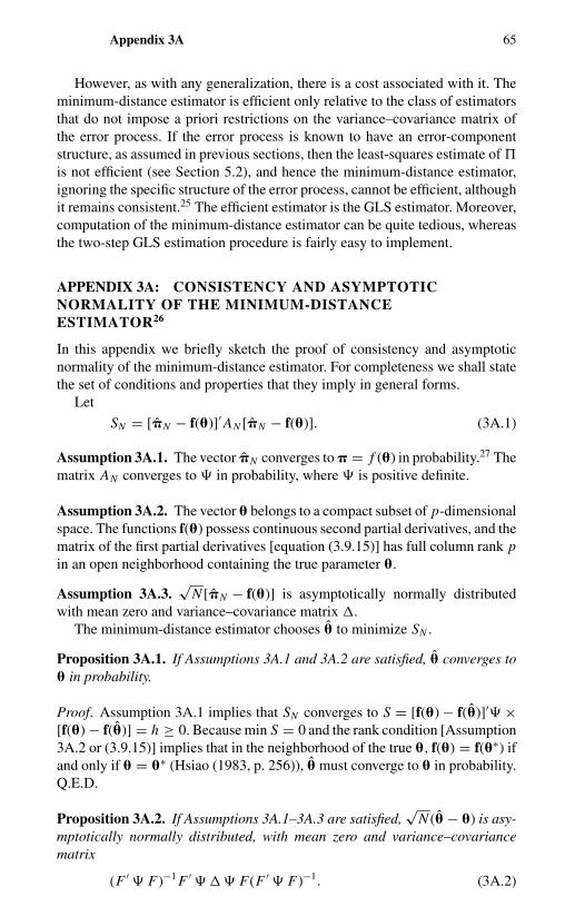
Appendix 3A 65
However, as with any generalization, there is a cost associated with it. Theminimum-distance estimator is efficient only relative to the class of estimatorsthat do not impose a priori restrictions on the variance–covariance matrix ofthe error process. If the error process is known to have an error-componentstructure, as assumed in previous sections, then the least-squares estimate of �
is not efficient (see Section 5.2), and hence the minimum-distance estimator,ignoring the specific structure of the error process, cannot be efficient, althoughit remains consistent.25 The efficient estimator is the GLS estimator. Moreover,computation of the minimum-distance estimator can be quite tedious, whereasthe two-step GLS estimation procedure is fairly easy to implement.
APPENDIX 3A: CONSISTENCY AND ASYMPTOTICNORMALITY OF THE MINIMUM-DISTANCEESTIMATOR26
In this appendix we briefly sketch the proof of consistency and asymptoticnormality of the minimum-distance estimator. For completeness we shall statethe set of conditions and properties that they imply in general forms.
Let
SN = [�N − f(�)]′ AN [�N − f(�)]. (3A.1)
Assumption 3A.1. The vector �N converges to � = f (�) in probability.27 Thematrix AN converges to � in probability, where � is positive definite.
Assumption 3A.2. The vector � belongs to a compact subset of p-dimensionalspace. The functions f(�) possess continuous second partial derivatives, and thematrix of the first partial derivatives [equation (3.9.15)] has full column rank pin an open neighborhood containing the true parameter �.
Assumption 3A.3.√
N [�N − f(�)] is asymptotically normally distributedwith mean zero and variance–covariance matrix .
The minimum-distance estimator chooses � to minimize SN .
Proposition 3A.1. If Assumptions 3A.1 and 3A.2 are satisfied, � converges to� in probability.
Proof. Assumption 3A.1 implies that SN converges to S = [f(�) − f(�)]′� ×[f(�) − f(�)] = h ≥ 0. Because min S = 0 and the rank condition [Assumption3A.2 or (3.9.15)] implies that in the neighborhood of the true �, f(�) = f(�∗) ifand only if � = �∗ (Hsiao (1983, p. 256)), � must converge to � in probability.Q.E.D.
Proposition 3A.2. If Assumptions 3A.1–3A.3 are satisfied,√
N (� − �) is asy-mptotically normally distributed, with mean zero and variance–covariancematrix
(F ′ � F)−1 F ′ � � F(F ′ � F)−1. (3A.2)
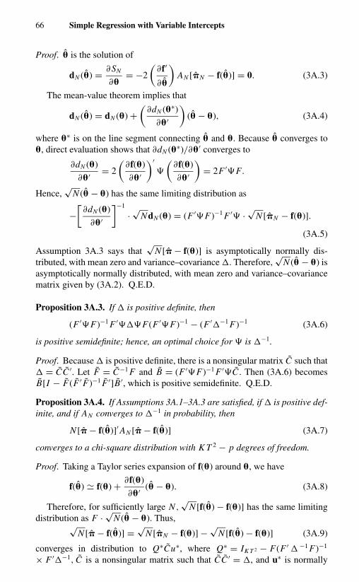
66 Simple Regression with Variable Intercepts
Proof. � is the solution of
dN (�) = ∂SN
∂�= −2
(∂f′
∂�
)AN [�N − f(�)] = 0. (3A.3)
The mean-value theorem implies that
dN (�) = dN (�) +(
∂dN (�∗)
∂�′
)(� − �), (3A.4)
where �∗ is on the line segment connecting � and �. Because � converges to�, direct evaluation shows that ∂dN (�∗)/∂�′ converges to
∂dN (�)
∂�′ = 2
(∂f(�)
∂�′
)′�
(∂f(�)
∂�′
)= 2F ′�F.
Hence,√
N (� − �) has the same limiting distribution as
−[∂dN (�)
∂�′
]−1
·√
NdN (�) = (F ′�F)−1 F ′� ·√
N [�N − f(�)].
(3A.5)
Assumption 3A.3 says that√
N [� − f(�)] is asymptotically normally dis-tributed, with mean zero and variance–covariance . Therefore,
√N (� − �) is
asymptotically normally distributed, with mean zero and variance–covariancematrix given by (3A.2). Q.E.D.
Proposition 3A.3. If is positive definite, then
(F ′�F)−1 F ′��F(F ′�F)−1 − (F ′−1 F)−1 (3A.6)
is positive semidefinite; hence, an optimal choice for � is −1.
Proof. Because is positive definite, there is a nonsingular matrix C such that = CC ′. Let F = C−1 F and B = (F ′�F)−1 F ′�C . Then (3A.6) becomesB[I − F(F ′ F)−1 F ′]B ′, which is positive semidefinite. Q.E.D.
Proposition 3A.4. If Assumptions 3A.1–3A.3 are satisfied, if is positive def-inite, and if AN converges to −1 in probability, then
N [� − f(�)]′ AN [� − f(�)] (3A.7)
converges to a chi-square distribution with K T 2 − p degrees of freedom.
Proof. Taking a Taylor series expansion of f(�) around �, we have
f(�) � f(�) + ∂f(�)
∂�′ (� − �). (3A.8)
Therefore, for sufficiently large N ,√
N [f(�) − f(�)] has the same limitingdistribution as F · √
N (� − �). Thus,√N [� − f(�)] =
√N [�N − f(�)] −
√N [f(�) − f(�)] (3A.9)
converges in distribution to Q∗Cu∗, where Q∗ = IK T 2 − F(F ′ −1 F)−1
× F ′−1, C is a nonsingular matrix such that CC ′ = , and u∗ is normally
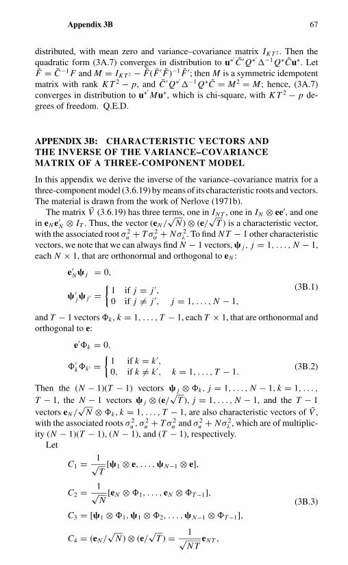
Appendix 3B 67
distributed, with mean zero and variance–covariance matrix IK T 2 . Then thequadratic form (3A.7) converges in distribution to u∗′
C ′ Q∗′−1 Q∗Cu∗. Let
F = C−1 F and M = IK T 2 − F(F ′ F)−1 F ′; then M is a symmetric idempotentmatrix with rank K T 2 − p, and C ′ Q∗′
−1 Q∗C = M2 = M ; hence, (3A.7)converges in distribution to u∗′
Mu∗, which is chi-square, with K T 2 − p de-grees of freedom. Q.E.D.
APPENDIX 3B: CHARACTERISTIC VECTORS ANDTHE INVERSE OF THE VARIANCE–COVARIANCEMATRIX OF A THREE-COMPONENT MODEL
In this appendix we derive the inverse of the variance–covariance matrix for athree-component model (3.6.19) by means of its characteristic roots and vectors.The material is drawn from the work of Nerlove (1971b).
The matrix V (3.6.19) has three terms, one in IN T , one in IN ⊗ ee′, and onein eN e′
N ⊗ IT . Thus, the vector (eN /√
N ) ⊗ (e/√
T ) is a characteristic vector,with the associated root σ 2
u + T σ 2α + Nσ 2
λ . To find N T − 1 other characteristicvectors, we note that we can always find N − 1 vectors, j , j = 1, . . . , N − 1,each N × 1, that are orthonormal and orthogonal to eN :
e′N j = 0,
′j j ′ =
{1 if j = j ′,0 if j �= j ′, j = 1, . . . , N − 1,
(3B.1)
and T − 1 vectors �k, k = 1, . . . , T − 1, each T × 1, that are orthonormal andorthogonal to e:
e′�k = 0,
�′k�k ′ =
{1 if k = k ′,0, if k �= k ′, k = 1, . . . , T − 1.
(3B.2)
Then the (N − 1)(T − 1) vectors j ⊗ �k, j = 1, . . . , N − 1, k = 1, . . . ,
T − 1, the N − 1 vectors j ⊗ (e/√
T ), j = 1, . . . , N − 1, and the T − 1vectors eN /
√N ⊗ �k, k = 1, . . . , T − 1, are also characteristic vectors of V ,
with the associated roots σ 2u , σ 2
u + T σ 2α and σ 2
u + Nσ 2λ , which are of multiplic-
ity (N − 1)(T − 1), (N − 1), and (T − 1), respectively.Let
C1 = 1√T
[1 ⊗ e, . . . , N−1 ⊗ e],
C2 = 1√N
[eN ⊗ �1, . . . , eN ⊗ �T −1],
C3 = [1 ⊗ �1, 1 ⊗ �2, . . . , N−1 ⊗ �T −1],
C4 = (eN /√
N ) ⊗ (e/√
T ) = 1√N T
eN T ,
(3B.3)
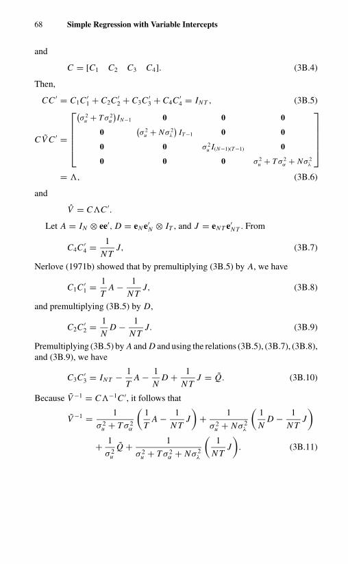
68 Simple Regression with Variable Intercepts
and
C = [C1 C2 C3 C4]. (3B.4)
Then,
CC ′ = C1C ′1 + C2C ′
2 + C3C ′3 + C4C ′
4 = IN T , (3B.5)
CV C ′ =
(σ 2
u + T σ 2α
)IN−1 0 0 0
0(σ 2
u + Nσ 2λ
)IT −1 0 0
0 0 σ 2u I(N−1)(T −1) 0
0 0 0 σ 2u + T σ 2
α + Nσ 2λ
= �, (3B.6)
and
V = C�C ′.
Let A = IN ⊗ ee′, D = eN e′N ⊗ IT , and J = eN T e′
N T . From
C4C ′4 = 1
N TJ, (3B.7)
Nerlove (1971b) showed that by premultiplying (3B.5) by A, we have
C1C ′1 = 1
TA − 1
N TJ, (3B.8)
and premultiplying (3B.5) by D,
C2C ′2 = 1
ND − 1
N TJ. (3B.9)
Premultiplying (3B.5) by A and D and using the relations (3B.5), (3B.7), (3B.8),and (3B.9), we have
C3C ′3 = IN T − 1
TA − 1
ND + 1
N TJ = Q. (3B.10)
Because V −1 = C�−1C ′, it follows that
V −1 = 1
σ 2u + T σ 2
α
(1
TA − 1
N TJ
)+ 1
σ 2u + Nσ 2
λ
(1
ND − 1
N TJ
)+ 1
σ 2u
Q + 1
σ 2u + T σ 2
α + Nσ 2λ
(1
N TJ
). (3B.11)
CHAPTER 4
Dynamic Models with Variable Intercepts
4.1 INTRODUCTION
In the last chapter we discussed the implications of treating the specific effectsas fixed or random and the associated estimation methods for the linear staticmodel
yit = �′xi t + α∗i + λt + uit , i = 1, . . . , N ,
t = 1, . . . , T,(4.1.1)
where xi t is a K × 1 vector of explanatory variables, including the constant term;� is a K × 1 vector of constants; α∗
i and λt are the (unobserved) individual-and time-specific effects, which are assumed to stay constant for given i overt and for given t over i , respectively; and uit represents the effects of thoseunobserved variables that vary over i and t . Very often we also wish to usepanel data to estimate behavioral relationships that are dynamic in character,namely, models containing lagged dependent variables such as1
yit = γ yi,t−1 + �′xi t + α∗i + λt + uit , i = 1, . . . , N ,
t = 1, . . . , T,(4.1.2)
where Euit = 0, and Euit u js = σ 2u if i = j and t = s, and Euit u js = 0 other-
wise. It turns out that in this circumstance the choice between a fixed-effectsformulation and a random-effects formulation has implications for estimationthat are of a different nature than those associated with the static model.
Roughly speaking, two issues have been raised in the literature regardingwhether the effects, α∗
i and λt , should be treated as random or as fixed for alinear static model, namely, the efficiency of the estimates and the independencebetween the effects and the regressors [i.e., the validity of the strict exogeneityassumption of the regressors (equation (3.4.1))]; (see, e.g., Maddala (1971a),Mundlak (1978a) and Chapter 3). When all the explanatory variables are ex-ogenous, the covariance estimator is the best linear unbiased estimator underthe fixed-effects assumption and a consistent and unbiased estimator under therandom-effects assumption, even though it is not efficient when T is fixed.

70 Dynamic Models with Variable Intercepts
However, when there exist omitted individual attributes that are correlated withthe included exogenous variables, the covariance estimator does not suffer frombias due to omission of these relevant individual attributes, because their ef-fects have been differenced out; but a generalized least-squares estimator forthe random-effects model under the assumption of independence between theeffects and explanatory variables will be biased. Furthermore, in a linear staticmodel, if the effects are correlated with the explanatory variables, a correctlyformulated random-effects model leads to the same covariance estimator (CV)as the fixed-effects model (Mundlak (1978a), also see Section 3.4). Thus, thefixed-effects model has assumed paramount importance in empirical studies(e.g., Ashenfelter (1978); Hausman (1978); Kiefer (1979)).
However, if lagged dependent variables also appear as explanatory variables,strict exogeneity of the regressors no longer holds. The maximum-likelihoodestimator (MLE) or the CV under the fixed-effects formulation is no longerconsistent in the typical situation in which a panel involves a large numberof individuals, but over only a short period of time. The initial values of adynamic process raise another problem. It turns out that with a random-effectsformulation, the interpretation of a model depends on the assumption of initialobservation. The consistency property of the MLE and the generalized least-squares estimator (GLS) also depends on this assumption and on the way inwhich the number of time-series observations (T ) and the number of cross-sectional units (N ) tend to infinity.
In Section 4.2, we show that the CV (or the least-squares dummy variable)estimator is inconsistent for a panel-dynamic model, whether the effects aretreated as fixed or random. Section 4.3 discusses the random-effects model.We discuss the implications of various formulation and methods of estimation.We show that the ordinary least-squares estimator is inconsistent but the MLE,the instrumental variable (IV), and the generalized method of moments (GMM)estimator are consistent. Procedures to test initial conditions are also discussed.In Section 4.4, we use Balestra and Nerlove’s model (1966) of demand for nat-ural gas to illustrate the consequences of various assumptions for the estimatedcoefficients.
Section 4.5 discusses the estimation of fixed-effects dynamic model. Weshow that although the conventional MLE and CV estimators are inconsistentwhen T is fixed and N tends to infinity, there exists a transformed likelihoodapproach that does not involve the incidental parameter and is consistent andefficient under proper formulation of initial conditions. We also discuss the IVand GMM estimators that do not need the formulation of initial conditions.Procedures to test fixed versus random effects are also suggested.
In Section 4.6, we relax the assumption on the specific serial-correlationstructure of the error term and propose a system approach to estimating dynamicmodels. Section 4.7 discusses the estimation of fixed effects vector autoregres-sive models. For ease of exposition, we assume that the time-specific effects λt
do not appear.

4.2 The Covariance Estimator 71
4.2 THE COVARIANCE ESTIMATOR
The CV estimator is consistent for the static model whether the effects are fixedor random. In this section we show that the CV (or LSDV) is inconsistent for adynamic panel data model with individual effects, whether the effects are fixedor random.
Consider2
yit = γ yi,t−1 + α∗i + uit , |γ | < 1, i = 1, . . . , N ,
t = 1, . . . , T,(4.2.1)
where for simplicity we let α∗i = αi + µ to avoid imposing the restriction that∑N
i=1 αi = 0. We also assume that yi0 are observable, Euit = 0, and Euit u js =σ 2
u if i = j and t = s, and Euit u js = 0 otherwise.Let yi = ∑T
t=1 yit/T, yi,−1 = ∑Tt=1 yi,t−1/T , and ui = ∑T
t=1 uit/T . TheLSDV estimators for α∗
i and γ are
α∗i = yi − γCV yi,−1, i = 1, . . . , N , (4.2.2)
γCV =∑N
i=1
∑Tt=1(yit − yi )(yi,t−1 − yi,−1)∑N
i=1
∑Tt=1(yi,t−1 − yi,−1)2
(4.2.3)
= γ +∑N
i=1
∑Tt=1(yi,t−1 − yi,−1)(uit − ui )/N T∑N
i=1
∑Tt=1(yi,t−1 − yi,−1)2/N T
.
The CV exists if the denominator of the second term of (4.2.3) is nonzero.It is consistent if the numerator of the second term of (4.2.3) converges to zero.
By continuous substitution, we have
yit = uit + γ ui,t−1 + · · · + γ t−1ui1 + 1 − γ t
1 − γα∗
i + γ t yi0. (4.2.4)
Summing yi,t−1 over t , we have
T∑t=1
yi,t−1 = 1 − γ T
1 − γyi0 + (T − 1) − T γ + γ T
(1 − γ )2α∗
i
+ 1 − γ T −1
1 − γui1 + 1 − γ T −2
1 − γui2 + · · · + ui,T −1. (4.2.5)
Because uit are uncorrelated with α∗i and are independently and identically
distributed, by a law of large numbers (Rao (1973)), and using (4.2.5), we can
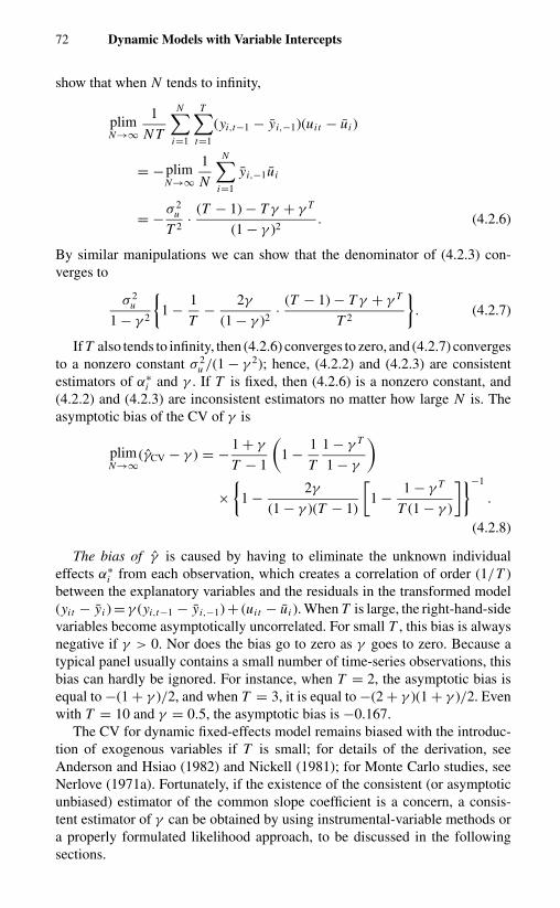
72 Dynamic Models with Variable Intercepts
show that when N tends to infinity,
plimN→∞
1
N T
N∑i=1
T∑t=1
(yi,t−1 − yi,−1)(uit − ui )
= −plimN→∞
1
N
N∑i=1
yi,−1ui
= −σ 2u
T 2· (T − 1) − T γ + γ T
(1 − γ )2. (4.2.6)
By similar manipulations we can show that the denominator of (4.2.3) con-verges to
σ 2u
1 − γ 2
{1 − 1
T− 2γ
(1 − γ )2· (T − 1) − T γ + γ T
T 2
}. (4.2.7)
If T also tends to infinity, then (4.2.6) converges to zero, and (4.2.7) convergesto a nonzero constant σ 2
u /(1 − γ 2); hence, (4.2.2) and (4.2.3) are consistentestimators of α∗
i and γ . If T is fixed, then (4.2.6) is a nonzero constant, and(4.2.2) and (4.2.3) are inconsistent estimators no matter how large N is. Theasymptotic bias of the CV of γ is
plimN→∞
(γCV − γ ) = − 1 + γ
T − 1
(1 − 1
T
1 − γ T
1 − γ
)×
{1 − 2γ
(1 − γ )(T − 1)
[1 − 1 − γ T
T (1 − γ )
]}−1
.
(4.2.8)
The bias of γ is caused by having to eliminate the unknown individualeffects α∗
i from each observation, which creates a correlation of order (1/T )between the explanatory variables and the residuals in the transformed model(yit − yi ) = γ (yi,t−1 − yi,−1) + (uit − ui ). When T is large, the right-hand-sidevariables become asymptotically uncorrelated. For small T , this bias is alwaysnegative if γ > 0. Nor does the bias go to zero as γ goes to zero. Because atypical panel usually contains a small number of time-series observations, thisbias can hardly be ignored. For instance, when T = 2, the asymptotic bias isequal to −(1 + γ )/2, and when T = 3, it is equal to −(2 + γ )(1 + γ )/2. Evenwith T = 10 and γ = 0.5, the asymptotic bias is −0.167.
The CV for dynamic fixed-effects model remains biased with the introduc-tion of exogenous variables if T is small; for details of the derivation, seeAnderson and Hsiao (1982) and Nickell (1981); for Monte Carlo studies, seeNerlove (1971a). Fortunately, if the existence of the consistent (or asymptoticunbiased) estimator of the common slope coefficient is a concern, a consis-tent estimator of γ can be obtained by using instrumental-variable methods ora properly formulated likelihood approach, to be discussed in the followingsections.

4.3 Random-Effects Models 73
4.3 RANDOM-EFFECTS MODELS
When the specific effects are treated as random, they can be considered to beeither correlated or not correlated with the explanatory variables. In the casein which the effects are correlated with the explanatory variables, ignoringthis correlation and simply using the covariance estimator no longer yields thedesirable properties as in the case of static regression models. Thus, a moreappealing approach here would be to take explicit account of the linear depen-dence between the effects and the exogenous variables by letting αi = a′xi + ωi
(Mundlak (1978a)) (see Section 3.4) and use a random-effects framework ofthe model
yi = yi,−1γ + Xi � + ex′i a + eωi + ui , (4.3.1)
where now E(xi tωi ) = 0, and E(xi t uit ) = 0. However, because xi is time-invariant and the (residual) individual effect ωi possesses the same propertyas αi when the assumption Eαi x′
i t = 0′ holds, the estimation of (4.3.1) is for-mally equivalent to the estimation of the model
yi = yi,−1γ + Xi � + ez′i � + eαi + ui , (4.3.2)
with Xi now denoting the T × K1 time-varying explanatory variables, z′i being
the 1 × K2 time-invariant explanatory variables including the intercept term,and Eαi = 0, Eαi z′
i = 0′, and Eαi x′i t = 0′. So, for ease of exposition, we
assume in this section that the effects are uncorrelated with the exogenousvariables.3
We first show that the ordinary-least-squares (OLS) estimator for dynamicerror-component models is biased. We then discuss how the assumption aboutthe initial observations affects interpretation of a model. Finally we discussestimation methods and their asymptotic properties under various assumptionsabout initial conditions and sampling schemes.
4.3.1 Bias in the OLS Estimator
In the static case in which all the explanatory variables are exogenous andare uncorrelated with the effects, we can ignore the error-component structureand apply the OLS method. The OLS estimator, although less efficient, is stillunbiased and consistent. But this is no longer true for dynamic error-componentmodels. The correlation between the lagged dependent variable and individual-specific effects would seriously bias the OLS estimator.
We use the following simple model to illustrate the extent of bias. Let
yit = γ yi,t−1 + αi + uit , |γ | < 1, i = 1, . . . , N ,
t = 1, . . . , T,(4.3.3)
where uit is independently, identically distributed over i and t . The OLS
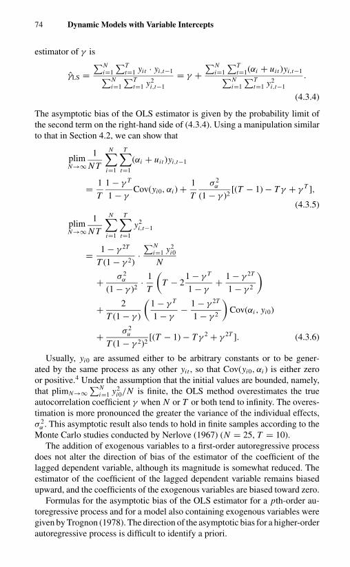
74 Dynamic Models with Variable Intercepts
estimator of γ is
γLS =∑N
i=1
∑Tt=1 yit · yi,t−1∑N
i=1
∑Tt=1 y2
i,t−1
= γ +∑N
i=1
∑Tt=1(αi + uit )yi,t−1∑N
i=1
∑Tt=1 y2
i,t−1
.
(4.3.4)
The asymptotic bias of the OLS estimator is given by the probability limit ofthe second term on the right-hand side of (4.3.4). Using a manipulation similarto that in Section 4.2, we can show that
plimN→∞
1
N T
N∑i=1
T∑t=1
(αi + uit )yi,t−1
= 1
T
1 − γ T
1 − γCov(yi0, αi ) + 1
T
σ 2α
(1 − γ )2[(T − 1) − T γ + γ T ],
(4.3.5)
plimN→∞
1
N T
N∑i=1
T∑t=1
y2i,t−1
= 1 − γ 2T
T (1 − γ 2)·∑N
i=1 y2i0
N
+ σ 2α
(1 − γ )2· 1
T
(T − 2
1 − γ T
1 − γ+ 1 − γ 2T
1 − γ 2
)+ 2
T (1 − γ )
(1 − γ T
1 − γ− 1 − γ 2T
1 − γ 2
)Cov(αi , yi0)
+ σ 2u
T (1 − γ 2)2[(T − 1) − T γ 2 + γ 2T ]. (4.3.6)
Usually, yi0 are assumed either to be arbitrary constants or to be gener-ated by the same process as any other yit , so that Cov(yi0, αi ) is either zeroor positive.4 Under the assumption that the initial values are bounded, namely,that plimN→∞
∑Ni=1 y2
i0/N is finite, the OLS method overestimates the trueautocorrelation coefficient γ when N or T or both tend to infinity. The overes-timation is more pronounced the greater the variance of the individual effects,σ 2
α . This asymptotic result also tends to hold in finite samples according to theMonte Carlo studies conducted by Nerlove (1967) (N = 25, T = 10).
The addition of exogenous variables to a first-order autoregressive processdoes not alter the direction of bias of the estimator of the coefficient of thelagged dependent variable, although its magnitude is somewhat reduced. Theestimator of the coefficient of the lagged dependent variable remains biasedupward, and the coefficients of the exogenous variables are biased toward zero.
Formulas for the asymptotic bias of the OLS estimator for a pth-order au-toregressive process and for a model also containing exogenous variables weregiven by Trognon (1978). The direction of the asymptotic bias for a higher-orderautoregressive process is difficult to identify a priori.

4.3 Random-Effects Models 75
4.3.2 Model Formulation
When T is fixed, the interpretation of a model depends on the assumption aboutthe behavior of the initial values yi0. The statistical properties of the maximumlikelihood and generalized least squares (GLS) estimation methods also dependon the assumption about yi0, but not those of the IV or the GMM methods.
Consider a model of the form5
yit = γ yi,t−1 + �′zi + �′xi t + vit , i = 1, . . . , N ,
t = 1, . . . , T,(4.3.7)
where |γ | < 1, vit = αi + uit ,
Eαi = Euit = 0,
Eαi z′i = 0′, Eαi x′
i t = 0′,
Eαi u jt = 0,
Eαiα j ={σ 2
α if i = j,0 otherwise,
Euit u js ={σ 2
u if i = j, t = s,
0 otherwise,
and where zi is a K2 × 1 vector of time-invariant exogenous variables such asthe constant term or an individual’s sex or race, xi t is a K1 × 1 vector of time-varying exogenous variables, γ is 1 × 1, and � and � are K2 × 1 and K1 × 1vectors of parameters, respectively. Equation (4.3.7) can also be written in theform
wit = γ wi,t−1 + �′zi + �′xi t + uit , (4.3.8)
yit = wit + ηi , (4.3.9)
where
αi = (1 − γ )ηi , Eηi = 0, Var(ηi ) = σ 2η = σ 2
α
/(1 − γ )2.
(4.3.10)
Algebraically, (4.3.7) is identical to (4.3.8) and (4.3.9). However, the inter-pretation of how yit is generated is not the same. Equation (4.3.7) implies thatapart from a common response to its own lagged value and the exogenous vari-ables, each individual process is also driven by the unobserved characteristicsαi ,which are different for different individuals. Equations (4.3.8) and (4.3.9) implythat the dynamic process {wit } is independent of the individual effect ηi . Condi-tional on the exogenous variables, individuals are driven by an identical stochas-tic process with independent (and different) shocks that are random draws froma common population [equation (4.3.8)]. It is the observed value of the latentvariable wit , yit , that is shifted by the individual time-invariant random variableηi [equation (4.3.9)]. This difference in means can be interpreted as a differencein individual endowments or a common measurement error for the i th process.

76 Dynamic Models with Variable Intercepts
If we observed wit , we could distinguish (4.3.7) from (4.3.8) and (4.3.9). Un-fortunately, wit are unobservable. However, knowledge of initial observationscan provide information to distinguish these two processes. Standard assump-tions about initial observations are either that they are fixed or that they arerandom. If (4.3.7) is viewed as the model, we have two fundamental cases:(I) yi0 fixed and (II) yi0 random. If (4.3.8) and (4.3.9) are viewed as the basicmodel, we have (III) wi0 fixed and (IV) wi0 random.
Case I: yi0 fixed. A cross-sectional unit may start at some arbitrary po-sition yi0 and gradually move toward a level (αi + �′zi )/(1 − γ ) +�′ ∑
j=0 xi,t− jγj . This level is determined jointly by the unobserv-
able effect (characteristic) αi , observable time-invariant character-istics zi , and time-varying variables xi t . The individual effect, αi ,is a random draw from a population with mean zero and varianceσ 2
α . This appears to be a reasonable model. But if the decision aboutwhen to start sampling is arbitrary and independent of the valuesof yi0, treating yi0 as fixed might be questionable because the as-sumption Eαi yi0 = 0 implies that the individual effects, αi , are notbrought into the model at time 0, but affect the process at time 1and later. If the process has been going on for some time, there isno particular reason to believe that yi0 should be viewed differentlythan yit .
Case II: yi0 random. We can assume that the initial observations arerandom, with a common mean µ0 and variance σ 2
y0. Namely, let
yi0 = µy0 + εi . (4.3.11)
A rationalization of this assumption is that we can treat yit as astate. We do not care how the initial state is reached, as long aswe know that it has a distribution with finite mean and variance.Or, alternatively, we can view εi as representing the effect of initialindividual endowments (after correction for the mean). Dependingon the assumption with regard to the correlation between yi0 andαi , we can divide this case into two subcases:Case IIa: yi0 independent of αi ; that is, Cov(εi , αi ) = 0. In this case
the impact of initial endowments gradually diminishes over timeand eventually vanishes. The model is somewhat like case I, inwhich the starting value and the effect αi are independent, exceptthat now the starting observable value is not a fixed constant buta random draw from a population with mean µy0 and varianceσ 2
y0.Case IIb: yi0 correlated with αi . We denote the covariance
between yi0 and αi by φσ 2y0. Then, as time goes on, the
impact of initial endowments (εi ) affects all future values of yit
through its correlation with αi and eventually reaches a level [φεi/

4.3 Random-Effects Models 77
(1 − γ )] = limt→∞ E[yit − �′zi/(1−γ ) − �′ ∑t−1j=0 xi,t− jγ
j | εi ].In the special case that φσ 2
y0 = σ 2α , namely, εi = αi , the indi-
vidual effect can be viewed as completely characterized by thedifferences in initial endowments. The eventual impact of thisinitial endowment equals [αi/(1 − γ )] = ηi .
Case III: wi0 fixed. Here the unobserved individual process {wit }has an arbitrary starting value. In this respect, this case is sim-ilar to case I. However, the observed cross-sectional units, yit ,are correlated with the individual effects ηi . That is, each of theobserved cross-sectional units may start at some arbitrary posi-tion yi0 and gradually move toward a level ηi + �′zi/(1 − γ ) +�′ ∑t−1
j=0 xi,t− jγj . Nevertheless, we allow for the possibility that
the starting period of the sample observations need not coincidewith the beginning of a stochastic process by letting the individualeffect ηi affect all sample observations, including yi0.
Case IV: wi0 random. Depending on whether or not the wi0 are viewedas having common mean, we have four subcases:Case IVa: wi0 random, with common mean µw and variance
σ 2u /(1 − γ 2).
Case IVb: wi0 random, with common mean µw and arbitrary vari-ance σ 2
w0.Case IVc: wi0 random, with mean θi0 and variance σ 2
u /(1 − γ 2).Case IVd: wi0 random, with mean θi0 and arbitrary variance σ 2
w0.
In each of these four subcases we allow correlation between yi0 and ηi . Inother words, ηi affects yit in all periods, including yi0. Cases IVa and IVb aresimilar to the state-space representation discussed in case IIa, in which the initialstates are random draws from a distribution with finite mean. Case IVa assumesthat the initial state has the same variance as the latter states. Case IVb allowsthe initial state to be nonstationary (with arbitrary variance). Cases IVc and IVdtake a different view in that they assume that the individual states are randomdraws from different populations with different means. A rationalization forthis can be seen through successive substitution of (4.3.8), yielding
wi0 = 1
1 − γ�′zi + �′
∞∑j=0
xi,− jγj + ui0 + γ ui,−1 + γ 2ui,−2 + · · · .
(4.3.12)
Because xi0, xi,−1, . . . are not observable, we can treat the combined cumulativeeffects of nonrandom variables for the i th individual as an unknown parameterand let
θi0 = 1
1 − γ�′zi + �′
∞∑j=0
xi,− jγj . (4.3.13)
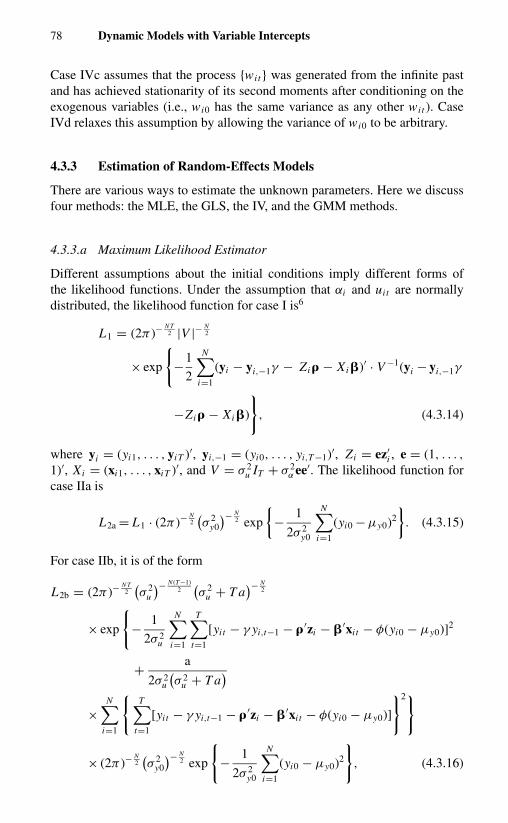
78 Dynamic Models with Variable Intercepts
Case IVc assumes that the process {wit } was generated from the infinite pastand has achieved stationarity of its second moments after conditioning on theexogenous variables (i.e., wi0 has the same variance as any other wit ). CaseIVd relaxes this assumption by allowing the variance of wi0 to be arbitrary.
4.3.3 Estimation of Random-Effects Models
There are various ways to estimate the unknown parameters. Here we discussfour methods: the MLE, the GLS, the IV, and the GMM methods.
4.3.3.a Maximum Likelihood Estimator
Different assumptions about the initial conditions imply different forms ofthe likelihood functions. Under the assumption that αi and uit are normallydistributed, the likelihood function for case I is6
L1 = (2π )−N T2 |V |− N
2
× exp
{−1
2
N∑i=1
(yi − yi,−1γ − Zi � − Xi �)′ · V −1(yi − yi,−1γ
−Zi � − Xi �)
}, (4.3.14)
where yi = (yi1, . . . , yiT )′, yi,−1 = (yi0, . . . , yi,T −1)′, Zi = ez′i , e = (1, . . . ,
1)′, Xi = (xi1, . . . , xiT )′, and V = σ 2u IT + σ 2
α ee′. The likelihood function forcase IIa is
L2a = L1 · (2π )−N2(σ 2
y0
)− N2 exp
{− 1
2σ 2y0
N∑i=1
(yi0 − µy0)2
}. (4.3.15)
For case IIb, it is of the form
L2b = (2π )−N T2(σ 2
u
)− N (T −1)2
(σ 2
u + T a)− N
2
× exp
{− 1
2σ 2u
N∑i=1
T∑t=1
[yit − γ yi,t−1 − �′zi − �′xi t − φ(yi0 − µy0)]2
+ a
2σ 2u
(σ 2
u + T a)
×N∑
i=1
{T∑
t=1
[yit − γ yi,t−1 − �′zi − �′xi t − φ(yi0 − µy0)]
}2}
× (2π )−N2(σ 2
y0
)− N2 exp
{− 1
2σ 2y0
N∑i=1
(yi0 − µy0)2
}, (4.3.16)

4.3 Random-Effects Models 79
where a = σ 2α − φ2σ 2
y0. The likelihood function for case III is
L3 = (2π )−N T2(σ 2
u
)− N T2
× exp
{− 1
2σ 2u
N∑i=1
T∑t=1
[(yit − yi0 + wi0) − γ (yi,t−1 − yi0 + wi0)
− �′zi − �′xi t ]2
}· (2π )−
N2(σ 2
η
)− N2
× exp
{− 1
2σ 2η
N∑i=1
(yi0 − wi0)2
}, (4.3.17)
and for case IVa it is
L4a = (2π )−N (T +1)
2 |�| − N2
× exp
{−1
2
N∑i=1
(yi0 − µw , yi1 − γ yi0 − �′zi − �′xi1, . . . ,
yiT − γ yi,T −1 − �′zi − �′xiT )
× �−1(yi0 − µw , . . . , yiT − γ yi,T −1 − �′zi − �′xiT )′}, (4.3.18)
where
�(T +1)×(T +1)
= σ 2u
1
1 − γ 20′
0 IT
+ σ 2α
1
1 − γe
(1
1 − γ, e′
),
|�| = σ 2Tu
1 − γ 2
(σ 2
u + T σ 2α + 1 + γ
1 − γσ 2
α
),
�−1 = 1
σ 2u
[[1 − γ 2 0′
0 IT
]
−(
σ 2u
σ 2α
+ T + 1 + γ
1 − γ
)−1[
1 + γ
e
](1 + γ, e′)
].
(4.3.19)
The likelihood function for case IVb, L4b, is of the form (4.3.18), except that �
is replaced by �, where � differs from � only in that the upper left element ofthe first term, 1/(1 − γ 2), is replaced by σ 2
w0/σ2u . The likelihood function for
case IVc, L4c, is similar to that for case IVa, except that the mean of yi0 in theexponential term is replaced by θi0. The likelihood function for case IVd, L4d,is of the form (4.3.16), with θi0, (1 − γ )σ 2
η /(σ 2η + σ 2
w0), and σ 2η + σ 2
w0 replacingµy0, φ, and σ 2
y0, respectively.Maximizing the likelihood function with respect to unknown parameters
yields the MLE. The consistency of the MLE depends on the initial conditions

80 Dynamic Models with Variable Intercepts
and on the way in which the numbers of time-series observations (T ) and ofcross-sectional units (N ) tend to infinity. For cases III and IVd, the MLEs do notexist. By letting yi0 equal wi0 or θi0, the exponential term of the second functionof their respective likelihood function becomes 1. If we let the variances σ 2
η orσ 2
η + σ 2w0 approach zero, the likelihood functions become unbounded. However,
we can still take partial derivatives of these likelihood functions and solve forthe first-order conditions. For simplicity of exposition, we shall refer to theseinterior solutions as the MLEs and examine their consistency properties in thesame way as in other cases in which the MLEs exist.
When N is fixed, a necessary condition for � being identifiable is that N ≥K2. Otherwise, the model is subject to strict multicollinearity. However, whenT tends to infinity, even with N greater than K2, the MLEs for � and σ 2
α remaininconsistent because of insufficient variation across individuals. On the otherhand, the MLEs of γ , �, and σ 2
u are consistent for all these different cases. WhenT becomes large, the weight of the initial observations becomes increasinglynegligible, and the MLEs for different cases all converge to the same covarianceestimator.
Table 4.1. Consistency properties of the MLEs for dynamic random-effectsmodelsa
N fixed, T fixed,Case T → ∞ N → ∞Case I: yi0 fixed γ, �, σ 2
u Consistent Consistent�, σ 2
α Inconsistent Consistent
Case II: yi0 randomIIa: yi0 independent of αi γ, �, σ 2
u Consistent Consistentµy0, �, σ 2
α , σ 2y0 Inconsistent Consistent
IIb: yi0 correlated γ, �, σ 2u Consistent Consistent
with αi µy0, �, σ 2α , σ 2
y0, φ Inconsistent Consistent
Case III: wi0 fixed γ, �, σ 2u Consistent Inconsistent
wi0, �, σ 2η Inconsistent Inconsistent
Case IV: wi0 randomIVa: mean µw
and variance γ, �, σ 2u Consistent Consistent
σ 2u /(1 − γ 2) µw , �, σ 2
η Inconsistent Consistent
IVb: mean µw γ, �, σ 2u Consistent Consistent
and variance σ 2w0 σ 2
w0, �, σ 2η , µw Inconsistent Consistent
IVc: mean θi0 γ, �, σ 2u Consistent Inconsistent
and variance σ 2u /(1 − γ 2) θi0, �, σ 2
η Inconsistent Inconsistent
IVd: mean θi0 γ, �, σ 2u Consistent Inconsistent
and variance σ 2w0 θi0, �2
η, σ2w0 Inconsistent Inconsistent
aIf an MLE does not exist, we replace it by the interior solution.Source: Anderson and Hsiao (1982).

4.3 Random-Effects Models 81
For cases IVc and IVd, where wi0 have means θi0, Bhargava and Sargan(1983) suggest predicting θi0 by all the observed xi t and zi as a way to getaround the incidental-parameters problem.7 If xi t is generated by a homoge-neous stochastic process
xi t = c +∞∑j=0
b j �i,t− j , (4.3.20)
where �i t is independently, identically distributed, then conditional on xi t andzi , we have
yi0 =T∑
t=1
�′0t xi t + �∗′zi + vi0, (4.3.21)
and
vi0 = εi0 + u∗i0 + ηi , i = 1, . . . , N . (4.3.22)
The coefficients �0t are identical across i (Hsiao, Pesaran, and Tahmiscioglu(2002)). The error term vi0 is the sum of three components: the predictionerror of θi0, εi0, the cumulative shocks before time zero, u∗
i0 = ui0 + γ ui,−1 +γ 2ui,−2 + · · · , and the individual effects ηi . The prediction error εi0 is indepen-dent of uit and ηi , with mean zero and variance σ 2
ε0. Depending on whether ornot the error process of wi0 conditional on the exogenous variables has achievedstationarity (i.e., whether or not the variance of wi0 is the same as any otherwit ), we have8 case IVc′,
Var(vi0) = σ 2ε0 + σ 2
u
1 − γ 2+ σ 2
α
(1 − γ )2,
(4.3.23)
Cov(vi0, vit ) = σ 2α
(1 − γ ), t = 1, . . . , T,
or case IVd′,
Var(vi0) = σ 2w0 and Cov(vi0, vit ) = σ 2
τ , t = 1, . . . , T .
(4.3.24)
Cases IVc′ and IVd′ transform cases IVc and IVd, in which the number ofparameters increases with the number of observations, into a situation in whichN independently distributed (T + 1)-component vectors depend only on a fixednumber of parameters. Therefore, the MLE is consistent when N → ∞.
The MLE is obtained by solving the first-order conditions of the likelihoodfunction with respect to unknown parameters. If there is a unique solution tothese partial-derivative equations with σ 2
α > 0, the solution is the MLE. How-ever, just as in the static case discussed in Section 3.3, a boundary solution withσ 2
α = 0 may occur for dynamic error-components models as well. Anderson andHsiao (1981) have derived the conditions under which the boundary solutionwill occur for various cases. Trognon (1978) has provided analytic explanationsbased on asymptotic approximations where the number of time periods tends

82 Dynamic Models with Variable Intercepts
to infinity. Nerlove (1967, 1971a) has conducted Monte Carlo experiments toexplore the properties of the MLE. These results show that the autocorrelationstructure of the exogenous variables is a criterion for the existence of boundarysolutions. In general, the more autocorrelated the exogenous variables or themore important the weight of the exogenous variables, the less likely it is thata boundary solution will occur.
The solution for the MLE is complicated. We can apply the Newton–Raphson iterative procedure or the sequential iterative procedure suggestedby Anderson and Hsiao (1982) to obtain a solution. Alternatively, because wehave a cross section of size N repeated successively in T time periods, wecan regard the problems of estimation (and testing) of (4.3.7) as akin to thosefor a simultaneous-equations system with T or T + 1 structural equations withN observations available on each of the equations. That is, the dynamic rela-tionship (4.3.7) in a given time period is written as an equation in a system ofsimultaneous equations,
�Y ′ + B X ′ + P Z ′ = U ′, (4.3.25)
where we now let9
YN×(T +1)
=
y10 y11 . . . y1T
y20 y21 . . . y2T...
......
yN0 yN1 . . . yN T
,
XN×T K1
=
x′
11 x′12 . . . x′
1T
x′21 x′
22 . . . x′2T
......
...x′
N1 x′N2 . . . x′
N T
,
ZN×K2
=
z′
1
z′2...
z′N
, i = 1 . . . , N ,
and U is the N × T matrix of the errors if the initial values yi0 are treatedas constants, and the N × (T + 1) matrix of errors if the initial values aretreated as stochastic. The structural-form coefficient matrix A = [� B P] isT × [(T + 1) + T K1 + K2] or (T + 1) × [(T + 1) + T K1 + K2], dependingon whether the initial values are treated as fixed or random. The earlier serialcovariance matrix [e.g., (3.3.4), (4.3.19), (4.3.23), or (4.3.24)] now becomes thevariance–covariance matrix of the errors on T or (T + 1) structural equations.We can then use the algorithm for solving the full-information maximum-likelihood estimator to obtain the MLE.
There are cross-equation linear restrictions on the structural-form coefficientmatrix, and restrictions on the variance–covariance matrix. For instances, in case
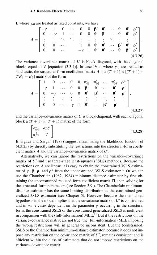
4.3 Random-Effects Models 83
I, where yi0 are treated as fixed constants, we have
A =
−γ 1 0 · · · 0 0 �′ 0′ · · · 0′ 0′ �′
0 −γ 1 · · · 0 0 0′ �′ · · · 0′ 0′ �′...
.... . .
. . ....
......
.... . .
......
...0 0 · · · 1 0 0′ 0′ · · · �′ 0′ �′
0 0 · · · −γ 1 0′ 0′ · · · 0′ �′ �′
.
(4.3.26)
The variance–covariance matrix of U is block-diagonal, with the diagonalblocks equal to V [equation (3.3.4)]. In case IVd′, where yi0 are treated asstochastic, the structural-form coefficient matrix A is a (T + 1) × [(T + 1) +T K1 + K2] matrix of the form
A =
1 0 · · · 0 0 �′
01 �′02 · · · �′
0T �∗′
−γ 1 · · · 0 0 �′ 0′ · · · 0′ �′
0 −γ · · · 0 0 0′ �′ · · · 0′ �′...
.... . .
......
......
. . ....
...0 0 · · · −γ 1 0′ · · · �′ �′
,
(4.3.27)
and the variance–covariance matrix of U is block-diagonal, with each diagonalblock a (T + 1) × (T + 1) matrix of the form[
σ 2w0 σ 2
τ e′
σ 2τ e V
]. (4.3.28)
Bhargava and Sargan (1983) suggest maximizing the likelihood function of(4.3.25) by directly substituting the restrictions into the structural-form coeffi-cient matrix A and the variance–covariance matrix of U ′.
Alternatively, we can ignore the restrictions on the variance–covariancematrix of U ′ and use three-stage least-squares (3SLS) methods. Because therestrictions on A are linear, it is easy to obtain the constrained 3SLS estima-tor of γ , �, �, and �∗ from the unconstrained 3SLS estimator.10 Or we canuse the Chamberlain (1982, 1984) minimum-distance estimator by first ob-taining the unconstrained reduced-form coefficient matrix �, then solving forthe structural-form parameters (see Section 3.9.). The Chamberlain minimum-distance estimator has the same limiting distribution as the constrained gen-eralized 3SLS estimator (see Chapter 5). However, because the maintainedhypothesis in the model implies that the covariance matrix of U ′ is constrainedand in some cases dependent on the parameter γ occurring in the structuralform, the constrained 3SLS or the constrained generalized 3SLS is inefficientin comparison with the (full-information) MLE.11 But if the restrictions on thevariance–covariance matrix are not true, the (full-information) MLE imposingthe wrong restrictions will in general be inconsistent. But the (constrained)3SLS or the Chamberlain minimum-distance estimator, because it does not im-pose any restriction on the covariance matrix of U ′, remains consistent and isefficient within the class of estimators that do not impose restrictions on thevariance–covariance matrix.
84 Dynamic Models with Variable Intercepts
4.3.3.b Generalized Least-Squares Estimator
We note that except for cases III, IVc, and IVd, the likelihood function onlydepends on a fixed number of parameters. Furthermore, conditional on � or σ 2
u ,σ 2
α , σ 2y0 and φ, the MLE is equivalent to the GLS estimator. For instance, under
case I, the covariance matrix of (yi1, . . . , yiT ) is the usual error-componentsform (3.3.4). Under cases IIa,b, and under cases IVa,b or cases IVc,d whenthe conditional mean of θi0 can be represented in the form of (4.3.21), thecovariance matrix V of vi = (vi0, vi1, . . . , viT ) is of similar form to (4.3.28).Therefore, a GLS estimator of �′ = (�′, �∗′, γ, �′, �′), can be applied:
�GLS =(
N∑i=1
X ′i V
−1 X i
)−1 (N∑
i=1
X ′i V
−1yi
), (4.3.29)
where y′i = (yi0, . . . , yiT ), and
X i =
x′i1 x′
i2 · · · x′iT z′
i 0 0′ 0
0′ · · · · · · · · · 0′ yi0 x′i1 z′
i...
... yi1 x′i2 z′
i...
......
......
0′ · · · · · · · · · 0′ yi,T −1 x′iT z′
i
.
The estimator is consistent and asymptotically normally distributed as N → ∞.Blundell and Smith (1991) suggest a conditional GLS procedure by condi-
tioning (yi1, . . . , yiT ) on vi0 = yi0 − E(yi0 | x′i , zi ):
yi = yi,−1γ + Zi � + Xi � + vi0 + v∗i , (4.3.30)
where v∗i = (v∗
i1, . . . , v∗iT )′, and is a T × 1 vector of constants with the values
depending on the correlation pattern between yi0 and αi . For case IIa, = 0,case IIb, = eT · φ. When the covariances between yi0 and (yi1, . . . , yiT ) arearbitrary, is a T × 1 vector of unrestricted constants. Application of the GLSto (4.3.30) is consistent as N → ∞.
When the covariance matrix of vi or v∗i is unknown, a feasible GLS estimator
can be applied. In the first step, we obtain some consistent estimates of thecovariance matrix from the estimated vi or v∗
i . For instance, we can use theIV estimator, to be discussed in Section 4.3.3.c, to obtain consistent estimatorsof γ and �, then substitute them into yit − γ yi,t−1 − �′xi t , and regress theresulting value on zi across individuals to obtain a consistent estimate of �.Substituting estimated γ , �, and � into (4.3.2), we obtain estimates of vit fort = 1, . . . , T . The estimates of vi0 can be obtained as the residuals of the cross-section regression of (4.3.21). The covariance matrix of vi can then be estimatedusing the procedures discussed in Chapter 3. The estimated v∗
i can also beobtained as the residuals of the cross-sectional regression of yi − yi,−1γ − Xi �on Zi and evi0. In the second step, we treat the estimated covariance matrix of

4.3 Random-Effects Models 85
vi or v∗i as if it were known, and apply the GLS to the system composed of
(4.3.2) and (4.3.21) or the conditional system (4.3.30).It should be noted that if Cov(yi0, αi ) �= 0, the GLS applied to the system
(4.3.2) is inconsistent when T is fixed and N → ∞. This is easily seen by notingthat conditional on yi0, the system is of the form (4.3.30). Applying GLS to(4.3.2) is therefore subject to omitted-variable bias. However, the asymptoticbias of the GLS of (4.3.2) is still smaller than that of the OLS or the withinestimator of (4.3.2) (Sevestre and Trognon (1982)). When T tends to infinity,GLS of (4.3.2) is again consistent because GLS converges to the within (orLSDV) estimator, which becomes consistent.
It should also be noted that contrary to the static case, the feasible GLS isasymptotically less efficient than the GLS knowing the true covariance matrix,because when a lagged dependent variable appears as one of the regressors,the estimation of slope coefficients is no longer asymptotically independent ofthe estimation of the parameters of the covariance matrix (Amemiya and Fuller(1967); Hsiao, Pesaran, and Tahmiscioglu (2002); or Appendix 4A).
4.3.3.c Instrumental-Variable Estimator
Because the likelihood functions under different initial conditions are differentwhen dealing with panels involving large numbers of individuals over a shortperiod of time, mistaken choices of initial conditions will yield estimators thatare not asymptotically equivalent to the correct one, and hence may not beconsistent. Sometimes we have little information to rely on in making a correctchoice about the initial conditions. A simple consistent estimator that is inde-pendent of the initial conditions is appealing in its own right and in additioncan be used to obtain initial values for the iterative process that yields the MLE.One estimation method consists of the following procedure.12
Step 1: Taking the first difference of (4.3.7), we obtain
yit − yi,t−1 = γ (yi,t−1 − yi,t−2) + �′(xi t − xi,t−1) + uit − ui,t−1,
for t = 2, . . . , T . (4.3.31)
Because yi,t−2 or (yi,t−2 − yi,t−3) are correlated with (yi,t−1 −yi,t−2) but are uncorrelated with (uit − ui,t−1) they can be usedas an instrument for (yi,t−1 − yi,t−2) and estimate γ and � by theinstrumental-variable method. Both(γiv
�iv
)=
[N∑
i=1
T∑t=3
×(
(yi,t−1 − yi,t−2)(yi,t−2 − yi,t−3) (yi,t−2 − yit−3)(xi t − xi,t−1)′
(xi t − xi,t−1)(yi,t−2 − yi,t−3) (xi t − xi,t−1)(xi t − xi,t−1)′
)]−1
×[
N∑i=1
T∑t=3
(yi,t−2 − yi,t−3
xi t − xi,t−1
)(yit − yi,t−1)
], (4.3.32)

86 Dynamic Models with Variable Intercepts
and(γiv
�iv
)=
[N∑
i=1
T∑t=2
(yi,t−2(yi,t−1 − yi,t−2) yi,t−2(xi t − xi,t−1)′
(xi t − xi,t−1)yi,t−2 (xi t − xi,t−1)(xi t − xi,t−1)′
)]−1
×[
N∑i=1
T∑t=2
(yi,t−2
xi t − xi,t−1
)(yi,t − yi,t−1)
](4.3.33)
are consistent. The estimator (4.3.33) has an advantage over (4.3.32)in that the minimum number of time periods required is two,whereas (4.3.33) requires T ≥ 3. In practice, if T ≥ 3, the choicebetween (4.3.33) and (4.3.32) depends on the correlations between(yi,t−1 − yi,t−2) and yi,t−2 or (yi,t−2 − yi,t−3). For a comparison ofasymptotic efficiencies of the instruments yi,t−2 or (yi,t−2 − yi,t−3),see Anderson and Hsiao (1981).
Step 2: Substitute the estimated � and γ into the equation
yi − γ yi,−1 − �′xi = �′zi + αi + ui , i = 1, . . . , N , (4.3.34)
where yi = ∑Tt=1 yit/T, yi,−1 = ∑T
t=1 yi,t−1/T , xi = ∑Tt=1 xi t/T ,
and ui = ∑Tt=1 uit/T . Estimate � by the OLS method.
Step 3: Estimate σ 2u and σ 2
α by
σ 2u =
∑Ni=1
∑Tt=2[(yit − yi,t−1) − γ (yi,t−1 − yi,t−2) − �
′(xi t − xi,t−1)]2
2N (T − 1),
(4.3.35)
σ 2α =
∑Ni=1(yi − γ yi,−1 − �′zi − �
′xi )2
N− 1
Tσ 2
u . (4.3.36)
The consistency of these estimators is independent of initial conditions. Theinstrumental-variable estimators of γ , �, and σ 2
u are consistent when N or Tor both tend to infinity. The estimators of � and σ 2
α are consistent only when Ngoes to infinity. They are inconsistent if N is fixed and T tends to infinity. Theinstrumental-variable method is simple to implement. But if we also wish to testthe maintained hypothesis on initial conditions in the random-effects model, itwould seem more appropriate to rely on maximum likelihood methods.
4.3.3.d Generalized Method of Moments Estimator
We note that yi,t−2 or (yi,t−2 − yi,t−3) is not the only instrument for(yi,t−1 − yi,t−2). In fact, it is noted by Amemiya and MaCurdy (1986),Arellano and Bond (1991), Breusch, Mizon, and Schmidt (1989), etc. that allyi,t−2− j , j = 0, 1, . . . , satisfy the conditions E[yi,t−2− j (yi,t−1 − yi,t−2)] �= 0and E[yi,t−2− j (uit − ui,t−1)] = 0. Therefore, they all are legitimate instru-ments for (yi,t−1 − yi,t−2). Letting = (1 − L) where L denotes the lag op-erator and qi t = (yi0, yi1, . . . , yi,t−2, x′
i )′, where x′
i = (x′i1, . . . , x′
iT ), we have
Eqi tuit = 0, t = 2, . . . , T . (4.3.37)

4.3 Random-Effects Models 87
Stacking the (T − 1) first-differenced equations of (4.3.31) in matrix form,we have
yi = yi,−1γ + Xi � + ui , i = 1, . . . , N , (4.3.38)
where yi , yi,−1, and ui are (T − 1) × 1 vectors of the form (yi2 − yi1, . . . ,
yiT − yi,T −1)′, (yi1 − yi0, . . . , yi,T −1 − yi,T −2)′, (ui2 − ui1, . . . , uiT − ui,T −1)′,respectively, and Xi is the (T − 1) × K matrix of (xi2 − xi1, . . . , xiT −xi,T −1)′. The T (T − 1)[K1 + 1
2 ] orthogonality (or moment) conditions of(4.3.37) can be represented as
EWiui = 0, (4.3.39)
where
Wi =
qi2 0 · · · 0
0 qi3 · · · 0...
.... . .
...
0 0 · · · qiT
(4.3.40)
is of dimension [T (T − 1)(K1 + 12 )] × (T − 1). The dimension of (4.3.40) in
general is much larger than K1 + 1. Thus, Arellano and Bond (1991) suggest ageneralized method of moments (GMM) estimator.
The standard method of moments estimator consists of solving the unknownparameter vector � by equating the theoretical moments with their empiricalcounterparts or estimates. For instance, suppose that m(y, x; �) denotes somepopulation moments of y and/or x (say the first and second moments), whichare functions of the unknown parameter vector � and are supposed to equalsome known constants, say zero. Let m(y, x; �) = 1
N
∑Ni=1 m(yi , xi ; �) be their
sample estimates based on N independent samples of (yi , xi ). Then the methodof moments estimator of � is �mm, such that
m(y, x; �) = m(y, x; �mm) = 0. (4.3.41)
For instance, the orthogonality conditions between Q Xi and Qui for thefixed-effects linear static model (3.2.2), E(X ′
i Qui ) = E[X ′i Q(yi − eα∗
i −Xi �)] = 0, lead to the LSDV estimator (3.2.8). In this sense, the method ofmoments estimator may be viewed as descendents of the IV method.
If the number of equations in (4.3.41) is equal to the dimension of �, it is ingeneral possible to solve for �mm uniquely. If the number of equations is greaterthan the dimension of �, (4.3.41) in general has no solution. It is then necessaryto minimize some norm (or distance measure) of m(y, x; �) − m(y, x; �), say
[m(y, x; �) − m(y, x; �)]′ A[m(y, x; �) − m(y, x; �)], (4.3.42)
where A is some positive definite matrix.

88 Dynamic Models with Variable Intercepts
The property of the estimator thus obtained depends on A. The optimalchoice of A turns out to be
A∗ = {E[m(y, x; �) − m(y, x; �)][m(y, x; �) − m(y, x; �)]′}−1
(4.3.43)
(Hansen (1982)). The GMM estimation of � is to choose �GMM such that itminimizes (4.3.42) when A = A∗.
The Arellano and Bond GMM estimator of � = (γ, �′)′ is obtained by min-imizing (
1
N
N∑i=1
u′i W ′
i
)�−1
(1
N
N∑i=1
Wiui
), (4.3.44)
where � = E[1/N 2 ∑Ni=1 Wiuiu′
i W ′i ]. Under the assumption that uit
is i.i.d. with mean zero and variance σ 2u , � can be approximated by
(σ 2u /N 2)
∑Ni=1 Wi AW ′
i , where
A(T −1)×(T −1)
=
2 −1 0 · · · 0
−1 2 −1 · · · 0
0. . .
. . .. . .
......
. . .. . . 2 −1
0 · · · 0 −1 2
. (4.3.45)
Thus, the Arellano–Bover GMM estimator takes the form
�GMM,AB =[
N∑i=1
(y′
i,−1
X ′i
)W ′
i
][N∑
i=1
Wi AW ′i
]−1[ N∑i=1
Wi (yi,−1, Xi )
]−1
×[
N∑i=1
(y′
i,−1
X ′i
)W ′
i
][N∑
i=1
Wi AW ′i
]−1[ N∑i=1
Wiyi
],
(4.3.46)
with asymptotic covariance matrix
Cov(�GMM,AB)
= �2u
[
N∑i=1
(y′
i,−1
X ′i
)W ′
i
][N∑
i=1
Wi AW ′i
]−1 [N∑
i=1
Wi (yi,−1, Xi )
]−1
.
(4.3.47)
In addition to the moment conditions (4.3.38), Arellano and Bover (1995)also note that Evi = 0, where vi = yi − yi,−1γ − x′
i � − �′zi .13 Therefore, ifinstruments qi exist (for instance, the constant 1 is a valid instrument) such that
E qi vi = 0, (4.3.48)

4.3 Random-Effects Models 89
then a more efficient GMM estimator can be derived by incorporating thisadditional moment condition.
Apart from the linear moment conditions (4.3.39) and (4.3.48), Ahn andSchmidt (1995) note that the homoscedasticity condition on E(v2
i t ) implies thefollowing T − 2 linear conditions:
E(yitui,t+1 − yi,t+1ui,t+2) = 0, t = 1, . . . , T − 2. (4.3.49)
Combining (4.3.39), (4.3.48), and (4.3.49), a more efficient GMM estimatorcan be derived by minimizing14(
1
N
N∑i=1
u+′i W +′
i
)�+−1
(1
N
N∑i=1
W +i u+
i
)(4.3.50)
with respect to �, where u+i = (u′
i , vi )′, �+ = E((1/N 2)∑N
i=1 W +i u+
i ×u+′
i W +′i ), and
W +′i =
(W ′
i W ∗′i 0
0′ 0′ q′i
),
where
W ∗i
(T −2)×(T −1)=
yi1 −yi2 0 0 · · · 0 00 yi2 −yi3 0 · · · 0 0...
.... . .
. . .. . .
......
0 0 · · · yi,T −3 −yi,T −2 0 0
0 0 . . . 0 yi,T −2 −yi,T −1 0
.
However, because the covariance matrix (4.3.49) depends on the unknown �,it is impractical to implement the GMM. A less efficient, but computationallyfeasible GMM estimation is to ignore the information that �+ also depends on� and simply replace � by its consistent estimator
�+ =(
1
N 2
N∑i=1
W +i u+
i u+′i W +′
i
)(4.3.51)
in the objective function (4.3.50) to derive a linear estimator of form (4.3.46),where u+
i is derived by using some simple consistent estimator of γ and �, saythe IV discussed in Section 4.3.3.c, into (4.3.38) and the vi equation.
In principle, one can improve the asymptotic efficiency of the GMM estima-tor by adding more moment conditions. For instance, Ahn and Schmidt (1995)note that in addition to the linear moment conditions of (4.3.39), (4.3.48),and (4.3.49), there exist (T − 1) nonlinear moment conditions of the formE((yi − γ yi,−1 − �′xi )uit ) = 0, t = 2, . . . , T , implied by the homoscedas-ticity conditions of Ev2
i t . Under the additional assumption that E(αi yi t ) is thesame for all t , this condition and condition (4.3.49) can be transformed into the(2T − 2) linear moment conditions
E[(yiT − γ yi,T −1 − �′xiT )yit ] = 0, t = 1, . . . , T − 1, (4.3.52)

90 Dynamic Models with Variable Intercepts
and
E[(yit − γ yi,t−1 − �′xi t )yit − (yi,t−1 − γ yi,t−2 − �′xi,t−1)yi,t−1] = 0,
t = 2, . . . , T . (4.3.53)
While theoretically it is possible to add additional moment conditions toimprove the asymptotic efficiency of GMM, it is doubtful how much efficiencygain one can achieve by using a huge number of moment conditions in a fi-nite sample. Moreover, if higher-moment conditions are used, the estimator canbe very sensitive to outlying observations. Through a simulation study, Ziliak(1997) has found that the downward bias in GMM is quite severe as the num-ber of moment conditions expands, outweighing the gains in efficiency. Thestrategy of exploiting all the moment conditions for estimation is actually notrecommended for panel data applications. For further discussions, see Judsonand Owen (1999), Kiviet (1995), and Wansbeek and Bekker (1996).
4.3.4 Testing Some Maintained Hypotheses on Initial Conditions
As discussed in Sections 4.3.2 and 4.3.3, the interpretation and consistencyproperty for the MLE and GLS of a random-effects model depend on the initialconditions. Unfortunately, in practice we have very little information on thecharacteristics of the initial observations. Because some of these hypotheses arenested, Bhargava and Sargan (1983) suggest relying on the likelihood principleto test them. For instance, when yi0 are exogenous (case I), we can test thevalidity of the error-components formulation by maximizing L1 with or withoutthe restrictions on the covariance matrix V . Let L∗
1 denote the maximum of logL1 subject to the restriction of model (4.3.7), and let L∗∗
1 denote the maximumof log L1 with V being an arbitrary positive definite matrix. Under the nullhypothesis, the resulting test statistic 2(L∗∗
1 − L∗1) is asymptotically chi-square
distributed, with [T (T + 1)/2 − 2] degrees of freedom.Similarly, we can test the validity of the error-components formulation under
the assumption that yi0 are endogenous. Let the maximum of the log likelihoodfunction under case IVa and case IVc′ be denoted by L∗
4a and L∗4c′ , respec-
tively. Let the maximum of the log likelihood function under case IVa or IVc′
without the restriction (4.3.19) or (4.3.23) [namely, the (T + 1) × (T + 1) co-variance matrix is arbitrary] be denoted by L∗∗
4a or L∗∗4c′ , respectively. Then,
under the null, 2(L∗∗4a − L∗
4a) and 2(L∗∗4c′ − L∗
4c′ ) are asymptotically chi-square,with [(T + 1)(T + 2)/2 − 2] and [(T + 1)(T + 2)/2 − 3] degrees of freedom,respectively.
To test the stationarity assumption, we denote the maximum of the loglikelihood function for case IVb and case IVd′ as L∗
4b and L∗4d′ , respectively.
Then 2(L∗4b − L∗
4a) and 2(L∗4d′ − L∗
4c′ ) are asymptotically chi-square, with onedegree of freedom. The statistics 2(L∗∗
4a − L∗4b) and 2(L∗∗
4c′ − L∗4d′ ) can also
be used to test the validity of case IVb and case IVd′, respectively. Theyare asymptotically chi-square distributed, with [(T + 1)(T + 2)/2 − 3] and[(T + 1)(T + 2)/2 − 4] degrees of freedom, respectively.
4.3 Random-Effects Models 91
We can also generalize Bhargava and Sargan’s principle to test the as-sumption that the initial observations have a common mean µw or have dif-ferent means θi0 under various assumptions about the error process. Thestatistics 2[L∗
4c′ − L∗4a], 2[L∗∗
4c′ − L∗∗4a ], and 2[L∗
4d′ − L∗4b] are asymptotically
chi-square distributed, with q, (q − 1), and (q − 1) degrees of freedom, respec-tively, where q is the number of unknown coefficients in (4.3.21). We can alsotest the combined assumption of a common mean and a variance-componentsformulation by using the statistic 2[L∗∗
4c′ − L∗4a] or 2[L∗∗
4c′ − L∗4b], which are
asymptotically chi-square distributed, with q + (T + 1)(T + 2)/2 − 3 andq + (T + 1)(T + 2)/2 − 4 degrees of freedom, respectively.
With regard to the test that yi0 are exogenous, unfortunately it is not pos-sible to compare L1 directly with the likelihood functions of various formsof case IV, because in the former case we are considering the density of(yi1, . . . , yiT ) assuming yi0 to be exogenous, whereas in the latter case it isthe joint density of (yi0, . . . , yiT ). However, we can write the joint likelihoodfunction of (4.3.7) and (4.3.21) under the restriction that vi0 are independentof ηi (or αi ) and have variance σ 2
ε0. Namely, we impose the restriction thatCov(vi0, vit ) = 0, t = 1, . . . , T , in the (T + 1) × (T + 1) variance–covariancematrix of (yi0, . . . , yiT ). We denote this likelihood function by L5. Let L∗∗
5 de-note the maximum of log L5 with unrestricted variance–covariance matrix for(vi0, . . . , viT ). Then we can test the exogeneity of yi0 using 2(L∗∗
4c′ − L∗∗5 ), which
is asymptotically chi-square with T degrees of freedom under the null.It is also possible to test the exogeneity of yi0 by constraining the error terms
to have a variance-components structure. Suppose the variance–covariance ma-trix of (vi1, . . . , viT ) is of the form V [equation (3.3.4)]. Let L∗
5 denote the maxi-mum of the log likelihood function L5 under this restriction. Let L∗
4d′ denote themaximum of the log likelihood function of (yi0, . . . , yiT ) under the restrictionthat Evi v′
i = V ∗, but allowing the variance of vi0 and the covariance betweenvi0 and vit , t = 1, . . . , T , to be arbitrary constants σ 2
w0 and σ 2τ . The statistic
2(L∗4d′ − L∗
5) is asymptotically chi-square with one degree of freedom if yi0
are exogenous. In practice, however, it may not even be necessary to calculateL∗
4d′ , because L∗4d′ ≥ L∗
4c′ , and if the null is rejected using 2(L∗4c′ − L∗
5) againstthe critical value of chi-square with one degree of freedom, then 2(L∗
4d′ − L∗∗5 )
must also reject the null.
4.3.5 Simulation Evidence
In order to investigate the performance of maximum likelihood estimators undervarious assumptions about the initial conditions, Bhargava and Sargan (1983)conducted Monte Carlo studies. Their true model was generated by
yit = 1 + 0.5yi,t−1 − 0.16zi + 0.35xit + αi + uit , i = 1, . . . , 100,
t = 1, . . . , 20,
(4.3.54)

92 Dynamic Models with Variable Intercepts
where αi and uit were independently normally distributed, with means zero andvariances 0.09 and 0.4225, respectively. The time-varying exogenous variablesxit were generated by
xit = 0.1t + φi xi,t−1 + ωi t , i = 1, . . . , 100,(4.3.55)
t = 1, . . . , 20,
with φi and ωi t independently normally distributed, with means zero and vari-ances 0.01 and 1, respectively. The time-invariant exogenous variables zi weregenerated by
zi = −0.2xi4 + ω∗i , i = 1, . . . , 100, (4.3.56)
and ω∗i were independently normally distributed, with mean zero and variance 1.
The z and the x were held fixed over the replications, and the first 10 observationswere discarded. Thus, the yi0 are in fact stochastic and are correlated withthe individual effects αi . Table 4.2 reproduces the results on the biases in theestimates for various models obtained in 50 replications.
In cases where the yi0 are treated as endogenous, the MLE performs ex-tremely well, and the biases in the parameters are almost negligible. But this isnot so for the MLE where yi0 are treated as exogenous. The magnitude of the biasis about one standard error. The boundary solution of σ 2
α = 0 occurs in a numberof replications for the error components formulation as well. The likelihood-ratio statistics also rejected the exogeneity of yi0 46 and 50 times, respectively,using the tests 2[L∗∗
4c′ − L∗∗5 ] and 2[L∗
4c′ − L∗5]. Under the endogeneity assump-
tion, the likelihood-ratio statistic 2(L∗∗4c′ − L∗
4c′ ) rejected the error-componentsformulation 4 times (out of 50), whereas under the exogeneity assumption, thestatistic 2(L∗∗
1 − L∗1) rejected the error-components formulation 7 times.15
4.4 AN EXAMPLE
We have discussed the properties of various estimators for dynamic models withindividual-specific effects. In this section we report results from the study ofdemand for natural gas conducted by Balestra and Nerlove (1966) to illustratethe specific issues involved in estimating dynamic models using observationsdrawn from a time series of cross sections.
Balestra and Nerlove (1966) assumed that the new demand for gas (inclusiveof demand due to the replacement of gas appliances and the demand due to netincreases in the stock of such appliances), G∗, was a linear function of therelative price of gas, P , and the total new requirements for all types of fuel, F∗.Let the depreciation rate for gas appliances be r , and assume that the rate ofutilization of the stock of appliances is constant; the new demand for gas andthe gas consumption at year t , Gt , follow the relation
G∗t = Gt − (1 − r )Gt−1. (4.4.1)
They also postulated a similar relation between the total new demand for all

Tabl
e4.
2.Si
mul
atio
nre
sult
sfo
rth
ebi
ases
ofth
eM
LE
sfo
rdy
nam
icra
ndom
-effe
cts
mod
els
y i0
exog
enou
s,un
rest
rict
edy i
0ex
ogen
ous,
erro
r-y i
0en
doge
nous
,unr
estr
icte
dy i
0en
doge
nous
,err
or-
Coe
ffici
ento
fco
vari
ance
mat
rix
com
pone
nts
form
ulat
ion
cova
rian
cem
atri
xco
mpo
nent
sfo
rmul
atio
n
Inte
rcep
t−0
.199
3−0
.115
6−0
.022
10.
0045
(0.1
42)a
(0.1
155)
(0.1
582)
(0.1
05)
z i0.
0203
0.01
080.
0007
−0.0
036
(0.0
365)
(0.0
354)
(0.0
398)
(0.0
392)
x it
0.00
280.
0044
0.00
460.
0044
(0.0
214)
(0.0
214)
(0.0
210)
(0.0
214)
y i,t
−10.
0674
0.03
770.
0072
−0.0
028
(0.0
463)
(0.0
355)
(0.0
507)
(0.0
312)
σ2 α
/ σ2 u
−0.0
499
0.00
11(0
.059
1)(0
.058
8)
aM
eans
ofth
ees
timat
edst
anda
rder
rors
inpa
rent
hese
s.So
urce
:Bha
rgav
aan
dSa
rgan
(198
3).
94 Dynamic Models with Variable Intercepts
types of fuel and the total fuel consumption F , with F approximated by a linearfunction of the total population N and per capita income I . Substituting theserelations into (4.4.1), they obtained
Gt = β0 + β1 Pt + β2Nt + β3 Nt−1
+ β4It + β5 It−1 + β6Gt−1 + vt , (4.4.2)
where Nt = Nt − Nt−1, It = It − It−1, and β6 = 1 − r .Balestra and Nerlove used annual U.S. data from 36 states over the period
1957–1962 to estimate the model (4.4.2) for residential and commercial demandfor natural gas. Because the average age of the stock of gas appliances duringthis period was relatively young, it was expected that the coefficient of thelagged gas-consumption variable, β6, would be less than 1, but not by much.The OLS estimates of (4.4.2) are reported in the second column of Table 4.3.The estimated coefficient of Gt−1 is 1.01. It is clearly incompatible with apriori theoretical expectations, as it implies a negative depreciation rate for gasappliances.
One possible explanation for the foregoing result is that when cross-sectionaland time-series data are combined in the estimation of (4.4.2), certain effectsspecific to the individual state may be present in the data. To account for sucheffects, dummy variables corresponding to the 36 different states were intro-duced into the model. The resulting dummy-variable estimates are shown in thethird column of Table 4.3. The estimated coefficient of the lagged endogenous
Table 4.3. Various estimates of the parameters of Balestra and Nerlove’sdemand-for-gas model (4.4.2) from the pooled sample, 1957–1962
Coefficient OLS LSDV GLS
β0 −3.650 — −4.091(3.316)a (11.544)
β1 −0.0451 −0.2026 −0.0879(0.0270) (0.0532) (0.0468)
β2 0.0174 −0.0135 −0.00122(0.0093) (0.0215) (0.0190)
β3 0.00111 0.0327 0.00360(0.00041) (0.0046) (0.00129)
β4 0.0183 0.0131 0.0170(0.0080) (0.0084) (0.0080)
β5 0.00326 0.0044 0.00354(0.00197) (0.0101) (0.00622)
β6 1.010 0.6799 0.9546(0.014) (0.0633) (0.0372)
aFigures in parentheses are standard errors for the corresponding coefficients.Source: Balestra and Nerlove (1966).

4.5 Fixed-Effects Models 95
variable is drastically reduced; in fact, it is reduced to such a low level that itimplies a depreciation rate of gas appliances of over 30 percent – again highlyimplausible.
Instead of assuming the regional effect to be fixed, they again estimated(4.4.2) by explicitly incorporating individual state-effects variables into theerror term, so that vit = αi + uit , where αi and uit are independent randomvariables. The two-step GLS estimates under the assumption that the initial ob-servations are fixed are shown in the fourth column of Table 4.3. The estimatedcoefficient of lagged consumption is 0.9546. The implied depreciation rate isapproximately 4.5 percent, which is in agreement with a priori expectation.
The foregoing results illustrate that by properly taking account of the unob-served heterogeneity in the panel data, Balestra and Nerlove were able to obtainresults that were reasonable on the basis of a priori theoretical considerationsthat they were not able to obtain through attempts to incorporate other variablesinto the equation by conventional procedures. Moreover, the least-squares andthe least-squares dummy-variables estimates of the coefficient of the laggedgas-consumption variable were 1.01 and 0.6799, respectively. In previous sec-tions we showed that for dynamic models with individual-specific effects, theleast-squares estimate of the coefficient of the lagged dependent variable isbiased upward and the least-squares dummy-variable estimate is biased down-ward if T is small. Their estimates are in agreement with these theoreticalresults.16
4.5 FIXED-EFFECTS MODELS
If individual effects are considered fixed and different across individuals, thenbecause of the strict multicollinearity between the effects and other time-invariant variables, there is no way one can disentangle the effects from thoseof other time-invariant variables. We shall therefore assume zi ≡ 0. When Ttends to infinity, even though lagged y does not satisfy the strict exogene-ity condition for the regressors, it does satisfy the weak exogeneity condi-tion E(uit | yi,t−1, yi,t−2, .; αi ) = 0; hence the least-squares regression of yit onlagged yi,t and xi t and the individual specific constant yields consistent estima-tor. In the case that T is fixed and N tends to infinity, the number of parametersin a fixed-effects specification increases with the number of cross-sectional ob-servations. This is the classical incidental-parameters problem (Neyman andScott (1948)). In a static model with strict exogeneity assumption, the presenceof individual specific constants does not affect the consistency of the CV orMLE estimator of the slope coefficients (see Chapter 3). However, the result nolonger holds if lagged dependent variables also appear as explanatory variables.The regularity conditions for the consistency of the MLE is violated. In fact, ifuit are normally distributed and yi0 are given constants, the MLE of (4.2.1) isthe CV of (4.2.2) and (4.2.3). The asymptotic bias is given by (4.2.8).
While the MLE is inconsistent, the IV estimator of (4.3.31) or the GMMestimator (4.3.42) remains consistent and asymptotically normally distributed

96 Dynamic Models with Variable Intercepts
with fixed α∗i . The transformed equation (4.3.38) does not involve the incidental
parameters α∗i . The orthogonality condition (4.3.39) remains valid.
In addition to the IV type estimator, a likelihood-based approach based on atransformed likelihood function can also yield a consistent and asymptoticallynormally distributed estimator.
4.5.1 Transformed Likelihood Approach
The first-difference equation (4.3.31) no longer contains the individual ef-fects α∗
i and is well defined for t = 2, 3, . . . , T, under the assumption thatthe initial observations yi0 and xi0 are available. But (4.3.31) is not defined foryi1 = (yi1 − yi0), because yi0 and xi0 are missing. However, by continu-ous substitution, we can write yi1 as
yi1 = ai1 +∞∑j=0
γ jui,1− j , (4.5.1)
where ai1 = �′ ∑∞j=0 xi,1− jγ
j . Since xi,1− j , j = 1, 2, . . . , are unavail-able, ai1 is unknown. Treating ai1 as a free parameter to be estimated will againintroduce the incidental-parameters problem. To get around this problem, theexpected value of ai1, conditional on the observables, has to be a function of afinite number of parameters of the form
E(ai1 | xi ) = c∗ + �′xi , i = 1, . . . , N , (4.5.2)
where � is a T K1 × 1 vector of constants, and xi is the T K1 × 1 vector(x′
i1, . . . , x′iT )′. Hsiao, Pesaran, and Tahmiscioglu (2002) have shown that
if xi t are generated by
xi t = �i + gt +∞∑j=0
b j �i,t− j ,
∞∑j=0
|b j | < ∞, (4.5.3)
where �i t are assumed to be i.i.d. with mean zero and constant covariance matrix,then (4.5.2) holds. The data-generating process of the exogenous variables xi t
(4.5.3) can allow fixed and different intercepts �i across i , or �i randomlydistributed with a common mean. However, if there exists a trend term in thedata generating process of xi t , then they must be identical across i .
Given (4.5.2), yi1 can be written as
yi1 = c∗ + �′xi + v∗i1, (4.5.4)
where v∗i1 = ∑∞
j=0 γ jui,1− j + [ai1 − E(ai1 | xi )]. By construction, E(v∗i1 |
xi ) = 0, E(v∗2i1 ) = σ 2
v∗ , E(v∗i1ui2) = −σ 2
u , and E(v∗i1uit ) = 0, for t =
3, 4, . . . , T . It follows that the covariance matrix of u∗i = (v∗
i1, u′i )
′ has

4.5 Fixed-Effects Models 97
the form
�∗ = σ 2u
h −1 0 · · · 0
−1 2 −1 · · · 0
0. . .
. . .. . .
......
. . .. . .
. . . −10 . . . 0 −1 2
= σ 2u �∗, (4.5.5)
where h = σ 2v∗/σ 2
u .Combining (4.3.31) and (4.5.4), we can write the likelihood function of
y∗i = (yi1, . . . , yiT ), i = 1, . . . , N , in the form
(2π )−N T2 |�∗|− N
2 exp
{−1
2
N∑i=1
u∗′i �∗−1u∗
i
}(4.5.6)
if u∗i is normally distributed, where
u∗i = [yi1 − c∗ − �′xi , yi2 − γyi1
−�′xi2, . . . , yiT − γyi,T −1 − �′xiT ]′.
The likelihood function again only depends on a fixed number of parametersand satisfies the standard regularity conditions, so that the MLE is consistentand asymptotically normally distributed as N → ∞.
Since |�∗| = 1 + T (h − 1) and
�∗−1 = [1 + T (h − 1)]−1
×
T T − 1 · · · 2 1
T − 1 (T − 1)h · · · 2h h...
......
...2 2h · · · 2[(T − 2)h − (T − 3)] (T − 2)h − (T − 3)1 h · · · (T − 2)h − (T − 3) (T − 1)h − (T − 2)
,
(4.5.7)
the logarithm of the likelihood function (4.5.6) is
log L = − N T
2log 2π − N T
2log σ 2
u − N
2log [1 + T (h − 1)]
− 1
2
N∑i=1
[(y∗i − Hi )′�∗−1(y∗
i − Hi )], (4.5.8)
where y∗i = (yi1, . . . , yiT )′, = (c∗, �′, γ, �′)′, and
Hi =
1 x′
i 0 0′
0 0′ yi1 x′i2
......
......
0 0′ yi,T −1 x′iT
.

98 Dynamic Models with Variable Intercepts
The MLE is obtained by solving the following equations simultaneously:
=(
N∑i=1
H ′i
ˆ�∗−1
Hi
)−1 (N∑
i=1
H ′i
ˆ�∗−1
y∗i
), (4.5.9)
σ 2u = 1
N T
N∑i=1
[(y∗i − Hi )′( ˆ�
∗)−1(y∗
i − Hi )], (4.5.10)
h = T − 1
T+ 1
σ 2u N T 2
N∑i=1
[(y∗i − Hi )′(JJ′)(y∗
i − Hi )],
(4.5.11)
where J′ = (T, T − 1, . . . , 2, 1). One way to obtain the MLE is to iterate among(4.5.9)–(4.5.11) conditionally on the early round estimates of the other parame-ters until the solution converges, or to use a Newton–Raphson iterative scheme(Hsiao, Pesaran, and Tahmiscioglu (2002)).
4.5.2 Minimum-Distance Estimator
Conditional on �∗, the MLE is the minimum-distance estimator (MDE) of theform
minN∑
i=1
u∗′i �∗−1u∗
i . (4.5.12)
In the case that �∗ is unknown, a two-step feasible MDE can be implemented.In the first step we obtain consistent estimators of σ 2
u and σ 2v∗. For instance,
we can regress (4.5.4) across i to obtain the least-squares residuals v∗i1, then
estimate
σ 2v∗ = 1
N − T K1 − 1
N∑i=1
v∗2i1 . (4.5.13)
Similarly, we can apply the IV to (4.3.31) and obtain the estimated residualsui t and
σ 2u = 1
N (T − 1)
N∑i=1
u′i A−1ui , (4.5.14)
where A is defined in (4.3.45).In the second step, we substitute estimated σ 2
u and σ 2v∗ into (4.5.5) and treat
them as if they were known, and use (4.5.9) to obtain the MDE of , MDE.The asymptotic covariance matrix of the MDE, Var(MDE), using the true
�∗ as the weighting matrix, is equal to (∑N
i=1 H ′i �
∗−1 Hi )−1. The asymptoticcovariance of the feasible MDE using a consistently estimated �∗, Var(FMDE),
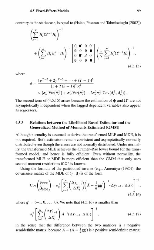
4.5 Fixed-Effects Models 99
contrary to the static case, is equal to (Hsiao, Pesaran and Tahmiscioglu (2002))(N∑
i=1
H ′i �
∗−1 Hi
)−1
+(
N∑i=1
H ′i �
∗−1 Hi
)−1
0 0′ 0 0′
0 0 0 00 0′ d 0′
0 0 0 0
(
1
N
N∑i=1
H ′i �
∗−1 Hi
)−1
,
(4.5.15)
where
d = [γ T −2 + 2γ T −3 + · · · + (T − 1)]2
[1 + T (h − 1)]2σ 4u
× (σ 4
u Var(σ 2
v∗) + σ 4
v∗Var(σ 2
u
) − 2σ 2u σ 2
v∗ Cov(σ 2
v∗ , σ2u
)).
The second term of (4.5.15) arises because the estimation of and �∗ are notasymptotically independent when the lagged dependent variables also appearas regressors.
4.5.3 Relations between the Likelihood-Based Estimator and theGeneralized Method of Moments Estimated (GMM)
Although normality is assumed to derive the transformed MLE and MDE, it isnot required. Both estimators remain consistent and asymptotically normallydistributed, even though the errors are not normally distributed. Under normal-ity, the transformed MLE achieves the Cramer–Rao lower bound for the trans-formed model, and hence is fully efficient. Even without normality, thetransformed MLE or MDE is more efficient than the GMM that only usessecond-moment restrictions if �∗ is known.
Using the formula of the partitioned inverse (e.g., Amemiya (1985)), thecovariance matrix of the MDE of (γ, �) is of the form
Cov
(γMDE
�MDE
)= σ 2
u
[N∑
i=1
(y′
i,−1
X ′i
)(A − 1
hgg′
)−1
(yi,−1, Xi )
]−1
,
(4.5.16)
where g′ = (−1, 0, . . . , 0). We note that (4.5.16) is smaller than
σ 2u
[N∑
i=1
(y′
i,−1
X ′i
)A−1(yi,−1, Xi )
]−1
, (4.5.17)
in the sense that the difference between the two matrices is a negativesemidefinite matrix, because A − ( A − 1
h gg′) is a positive semidefinite matrix.

100 Dynamic Models with Variable Intercepts
Furthermore,
N∑i=1
(y′
i,−1
X ′i
)A−1(yi,−1, Xi )
−[
N∑i=1
(y′
i,−1
X ′i
)W ′
i
](N∑
i=1
Wi AW ′i
)−1 [N∑
i=1
Wi (yi,−1, Xi )
]= D′[I − Q(Q′ Q)−1 Q]D, (4.5.18)
is a positive semidefinite matrix, where D = (D′1, . . . , D′
N )′, Q = (Q′1,
Q′2, . . . , Q′
N )′, Di = �′(yi,−1, Xi ), Qi = �−1Wi , and ��′ = A−1. There-fore, the asymptotic covariance matrix (4.3.47) of the GMM estimator (4.3.46)is greater than (4.5.17), which is greater than (4.5.16) in the sense that thedifference of the two covariance matrix is a positive semidefinite matrix.
When �∗ is unknown, the asymptotic covariance matrix of (4.3.46) remains(4.3.47). But the asymptotic covariance matrix of the feasible MDE is (4.5.15).Although the first term of (4.5.15) is smaller than (4.3.47), it is not clear thatwith the addition of the second term it will remain smaller. However, it is verylikely that it will, for several reasons. First, additional information due to theyi1 equation is utilized, which can be substantial (e.g., see Hahn (1999)).Second, the GMM method uses the (t − 1) instruments (yi0, . . . , yi,t−2)for the yit equation for t = 2, 3, . . . , T . The likelihood-based approachuses the t instruments (yi0, yi1, . . . , yi,t−1). Third, the likelihood approachuses the condition E(u∗
i ) = 0, and the GMM method uses the conditionE( 1
N
∑Ni=1 Wiui ) = 0. The grouping of observations in general will lead to a
loss of information.17
Hsiao, Pesaran, and Tahmiscioglu (2002) have conducted Monte Carlo stud-ies to compare the performance of the IV of (4.3.31), the GMM of (4.3.43), theMLE, and the MDE. They generate yit by
yit = αi + γ yi,t−1 + βxit + uit , (4.5.19)
where the error term uit is generated from two schemes. One is N (0, σ 2u ).
The other is the mean adjusted chi-square with two degrees of freedom. Theregressor xit is generated according to
xit = µi + gt + ξi t , (4.5.20)
where ξi t follows an autoregressive moving average process
ξi t − φξi,t−1 = εi t + θεi,t−1, (4.5.21)
and εi t ∼ N (0, σ 2ε ). The fixed effects µi and αi are generated from a variety of
schemes such as being correlated with xit or uncorrelated with xit but from amixture of different distributions. Table 4.4 gives a summary of the differentdesigns of the Monte Carlo study.
In generating yit and xit , both are assumed to start from zero. But the first50 observations are discarded. The bias and root mean square error (RMSE)

4.5 Fixed-Effects Models 101
Table 4.4. Monte Carlo design
Design number γ β φ θ g R2y σε
1 0.4 0.6 0.5 0.5 0.01 0.2 0.8002 0.4 0.6 0.9 0.5 0.01 0.2 0.7313 0.4 0.6 1 0.5 0.01 0.2 0.7114 0.4 0.6 0.5 0.5 0.01 0.4 1.3075 0.4 0.6 0.9 0.5 0.01 0.4 1.1946 0.4 0.6 1 0.5 0.01 0.4 1.1617 0.8 0.2 0.5 0.5 0.01 0.2 1.8758 0.8 0.2 0.9 0.5 0.01 0.2 1.3029 0.8 0.2 1 0.5 0.01 0.2 1.104
10 0.8 0.2 0.5 0.5 0.01 0.4 3.06211 0.8 0.2 0.9 0.5 0.01 0.4 2.12712 0.8 0.2 1 0.5 0.01 0.4 1.803
Source: Hsiao, Pesaran, and Tahmiscioglu (2002, Table 1).
of various estimators of γ and β when T = 5 and N = 50 based on 2500replications are reported in Tables 4.5 and 4.6 respectively. The results showthat the bias of the MLE of γ as a percentage of the true value is smaller than1 percent in most cases. The bias of the IV of γ can be significant for certaindata-generating processes. The MDE and GMM of γ also have substantialdownward biases in all designs. The bias of the GMM estimator of γ can beas large as 15 to 20 percent in many cases and is larger than the bias of theMDE. The MLE also has the smallest RMSE, followed by the MDE and thenthe GMM. The IV has the largest RMSE.
4.5.4 Random- versus Fixed-Effects Specification
When αi are random, the MLE of the transformed likelihood function (4.5.6) orthe MDE (4.5.12) remains consistent and asymptotically normally distributed.However, comparing the likelihood function of (4.3.25) with (4.5.6), it is ob-vious that first-differencing reduces the number of time-series observations byone per cross-sectional unit, and hence will not be as efficient as the MLE of(4.3.25) when αi are indeed random. However, if αi are fixed, then the MLE of(4.3.25) yields an inconsistent estimator.
The transformed MLE or MDE is consistent under a more general data-generating process of xi t than the MLE of (4.3.25) or the GLS (4.3.29). In orderfor the Bhargava–Sargan (1983) MLE of the random-effects model to be con-sistent, we shall have to assume that the xi t are generated from the same station-ary process with common means (equation (4.3.20)). Otherwise, E(yi0 | xi ) =ci + �′
i xi , where ci and �i vary across i , and we have the incidental-parametersproblem again. On the other hand, the transformed likelihood approach allowsxi t to have different means (or intercepts) (equation (4.5.3)). Therefore it ap-pears that if one is not sure about the assumption on the effects αi , or the

102 Dynamic Models with Variable Intercepts
Table 4.5. Bias of estimators (T = 5 and N = 50)
Bias
Design Coeff. IVE MDE MLE GMM
1 γ = 0.4 0.0076201 −0.050757 −0.000617 −0.069804β = 0.6 −0.001426 0.0120812 0.0023605 0.0161645
2 γ = 0.4 0.0220038 −0.052165 −0.004063 −0.072216β = 0.6 −0.007492 0.0232612 0.0027946 0.0321212
3 γ = 0.4 1.3986691 −0.054404 −0.003206 −0.075655β = 0.6 −0.386998 0.0257393 0.0002997 0.0365942
4 γ = 0.4 0.0040637 −0.026051 −0.001936 −0.03616β = 0.6 0.0004229 0.0066165 0.0019218 0.0087369
5 γ = 0.4 0.1253257 −0.023365 −0.000211 −0.033046β = 0.6 −0.031759 0.0113724 0.0016388 0.0155831
6 γ = 0.4 −0.310397 −0.028377 −0.00351 −0.040491β = 0.6 0.0640605 0.0146638 0.0022274 0.0209054
7 γ = 0.8 −0.629171 −0.108539 0.009826 −0.130115β = 0.2 −0.018477 0.0007923 0.0026593 0.0007962
8 γ = 0.8 −1.724137 −0.101727 0.0027668 −0.128013β = 0.2 0.0612431 0.0109865 −0.000011 0.013986
9 γ = 0.8 −0.755159 −0.102658 0.00624 −0.133843β = 0.2 −0.160613 0.0220208 0.0002624 0.0284606
10 γ = 0.8 0.1550445 −0.045889 0.001683 −0.05537β = 0.2 0.0096871 0.0000148 0.0007889 −0.000041
11 γ = 0.8 −0.141257 −0.038216 −0.000313 −0.050427β = 0.2 0.0207338 0.0048828 0.0007621 0.0063229
12 γ = 0.8 0.5458734 −0.039023 0.0005702 −0.053747β = 0.2 −0.069023 0.0079627 0.0003263 0.010902
Source: Hsiao, Pesaran, and Tahmiscioglu (2002, Table 2).
homogeneity assumption about the data-generating process for xi t , one shouldwork with the transformed likelihood function (4.5.6) or the MDE (4.5.12),despite the fact that one may lose efficiency under the ideal condition.
The use of the transformed likelihood approach also offers the possibilityof using a Hausman (1978) test for fixed- versus random-effects specification,or of testing the homogeneity and stationarity assumption about the xi t processunder the assumption that αi are random. Under the null of random effects andhomogeneity of the xi t process, the MLE of (4.3.25) is asymptotically efficient.The transformed MLE of (4.5.6) is consistent, but not efficient. On the otherhand, if αi are fixed or xi t is not generated by a homogeneous process butsatisfies (4.5.3), the transformed MLE of (4.5.6) is consistent, but the MLE of(4.3.25) is inconsistent. Therefore, a Hausman type test statistic (3.5.2) can beconstructed by using the difference between the two estimators.

4.6 Estimation of Dynamic Models 103
Table 4.6. Root mean square error (T = 5 and N = 50)
Root Mean Square Error
Design Coeff. IVE MDE MLE GMM
1 γ = 0.4 0.1861035 0.086524 0.0768626 0.1124465β = 0.6 0.1032755 0.0784007 0.0778179 0.0800119
2 γ = 0.4 0.5386099 0.0877669 0.0767981 0.11512β = 0.6 0.1514231 0.0855346 0.0838699 0.091124
3 γ = 0.4 51.487282 0.0889483 0.0787108 0.1177141β = 0.6 15.089928 0.0867431 0.0848715 0.0946891
4 γ = 0.4 0.1611908 0.0607957 0.0572515 0.0726422β = 0.6 0.0633505 0.0490314 0.0489283 0.0497323
5 γ = 0.4 2.3226456 0.0597076 0.0574316 0.0711803β = 0.6 0.6097378 0.0529131 0.0523433 0.0556706
6 γ = 0.4 14.473198 0.0620045 0.0571656 0.0767767β = 0.6 2.9170627 0.0562023 0.0550687 0.0607588
7 γ = 0.8 27.299614 0.1327602 0.116387 0.1654403β = 0.2 1.2424372 0.0331008 0.0340688 0.0332449
8 γ = 0.8 65.526156 0.1254994 0.1041461 0.1631983β = 0.2 3.2974597 0.043206 0.0435698 0.0450143
9 γ = 0.8 89.83669 0.1271169 0.104646 0.1706031β = 0.2 5.2252014 0.0535363 0.0523473 0.0582538
10 γ = 0.8 12.201019 0.074464 0.0715665 0.0884389β = 0.2 0.6729934 0.0203195 0.020523 0.0203621
11 γ = 0.8 17.408874 0.0661821 0.0642971 0.0822454β = 0.2 1.2541247 0.0268981 0.026975 0.02756742
12 γ = 0.8 26.439613 0.0674678 0.0645253 0.0852814β = 0.2 2.8278901 0.0323355 0.0323402 0.0338716
Source: Hsiao, Pesaran, and Tahmiscioglu (2002, Table 5).
4.6 ESTIMATION OF DYNAMIC MODELSWITH ARBITRARY CORRELATIONSIN THE RESIDUALS
In previous sections we discussed estimation of the dynamic model
yit = γ yi,t−1 + �′xi t + α∗i + uit , i = 1, . . . , N ,
(4.6.1)t = 1, . . . , T,
under the assumption that uit are serially uncorrelated, where we now againlet xi t stand for a K × 1 vector of time-varying exogenous variables. WhenT is fixed and N tends to infinity, we can relax the restrictions on the serialcorrelation structure of uit and still obtain efficient estimates of γ and �.
Taking the first difference of (4.6.1) to eliminate the individual effect α∗i ,
and stacking all equations for a single individual, we have a system of (T − 1)

104 Dynamic Models with Variable Intercepts
equations,
yi2 − yi1 = γ (yi1 − yi0) + �′(xi2 − xi1) + (ui2 − ui1),
yi3 − yi2 = γ (yi2 − yi1) + �′(xi3 − xi2) + (ui3 − ui2),...
yiT − yi,T −1 = γ (yi,T −1 − yi,T −2) + �′(xiT − xi,T −1)
+ (uiT − ui,T −1), i = 1, . . . , N , (4.6.2)
We complete the system (4.6.2) with the identities
yi0 = E∗(yi0 | xi1, . . . , xiT ) + [yi0 − E∗(yi0 | xi1, . . . , xiT )]
= a0 +T∑
t=1
�′0t xi t + εi0, (4.6.3)
and
yi1 = E∗(yi1 | xi1, . . . , xiT ) + [yi1 − E∗(yi1 | xi1, . . . , xiT )]
= a1 +T∑
t=1
�′1t xi t + εi1, i = 1, . . . , N , (4.6.4)
where E∗ denotes the projection operator. Because (4.6.3) and (4.6.4) are ex-actly identified equations, we can ignore them and apply the three-stage least-squares (3SLS) or generalized 3SLS (see Chapter 5) to the system (4.6.2) only.With regard to the cross-equation constraints in (4.6.2), one can either directlysubstitute them out or first obtain unknown nonzero coefficients of each equationignoring the cross-equation linear constraints, then impose the constraints anduse the constrained estimation formula [Theil (1971, p. 281, equation (8.5))].
Because the system (4.6.2) does not involve the individual effects α∗i , nor
does the estimation method rely on specific restrictions on the serial-correlationstructure of uit , the method is applicable whether α∗
i are treated as fixedor random or as being correlated with xi t . However, in order to implementsimultaneous-equations estimation methods to (4.6.2) without imposing restric-tions on the serial-correlation structure of uit , there must exist strictly exogenousvariables xi t such that
E(uit | xi1, . . . , xiT ) = 0. (4.6.5)
Otherwise, the coefficient γ and the serial correlations of uit cannot be disen-tangled (e.g., Binder, Hsiao, and Pesaran (2000)).

4.7 Fixed-Effects Vector Autoregressive Models 105
4.7 FIXED-EFFECTS VECTOR AUTOREGRESSIVEMODELS
4.7.1 Model Formulation
Vector autoregressive (VAR) models have become a widely used modelingtool in economics (e.g., Hsiao (1979a,b, 1982); Sims (1980)). To provide moreflexibility to the VAR modeling for panel data, it is common to assume that fixedindividual specific effects �∗
i are present for the panel VAR (PVAR) models(Holtz-Eakin, Newey, and Rosen (1988)):
�(L)yi t = yi t − �1yi,t−1 − · · · − �pyi,t−p = �∗i + �i t ,
i = 1, . . . , N , (4.7.1)t = 1, . . . , T,
where yi t is an m × 1 vector of observed random variables, �∗i is an m × 1
vector of individual specific constants that vary with i, �i t is an m × 1 vector ofrandom variables that is independently, identically distributed with mean zeroand covariance matrix �, and �(L) = Im − �1L − · · · − �p L p is a pth-orderpolynomial of the lag operator L , Lsyt = yt−s .
It is well known that time-series inference on VARs critically depends onwhether the underlying processes are (trend) stationary, or integrated, or coin-tegrated, and, if they are cointegrated, on the rank of cointegration18 (e.g., Sims,Stock, and Watson (1990); Phillips (1991); Johansen (1995); Pesaran, Shin, andSmith (2000)). To simplify the analysis, instead of considering (4.7.1) directly,we consider
�(L)(yi t − �i − �t) = �i t , (4.7.2)
where the roots of the determinant equation
|�(ρ)| = 0 (4.7.3)
either are equal to unity or fall outside the unit circle. Under the assumptionthat E�i t = 0, it follows that
E(yi t − �i − �t) = 0. (4.7.4)
To allow for the possibility of the presence of unit roots, we assume that
E(yi t − �i − �t)(yi t − �i − �t)′ = �t . (4.7.5)
Model (4.7.2)–(4.7.5) encompasses many well-known PVAR models as spe-cial cases. For instance:
Case 1: Stationary PVAR with fixed effects. Let � = 0m×1. If all rootsof (4.7.3) fall outside the unit circle, (4.7.2) becomes (4.7.1) with

106 Dynamic Models with Variable Intercepts
�∗i = −��i , and
� = −(
Im −p∑
j=1
� j
). (4.7.6)
Case 2: Trend-stationary PVAR with fixed effects. If all roots of (4.7.3)fall outside the unit circle and � �= 0, we have
�(L)yi t = ai0 + a1t + εi t , (4.7.7)
where ai0 = −��i + (� + �)�,
� = −� +p∑
j=1
j� j , (4.7.8)
and a1 = −��.Case 3: PVAR with unit roots (but noncointegrated).
�∗(L)yi t = −�∗� + �i t , (4.7.9)
where = (1 − L),
�∗(L) = Im −p−1∑j=1
�∗j L j , (4.7.10)
�∗j = −(Im − ∑ j
�=1 ��), j = 1, 2. . . . , p − 1, and �∗ = −(Im −∑p−1j=1 �∗
j ).Case 4: Cointegrated PVAR with fixed effects. If some roots of (4.7.3)
are equal to unity and rank(�) = r, 0 < r < m, then (4.7.2) may berewritten in the form of a panel vector error-corrections model
yi t = �∗i + (� + �)� + a1t + �yi,t−1 +
p−1∑j=1
� jyi,t− j + �i t ,
(4.7.11)
where � j = −∑ps= j+1 �s, j = 1, . . . , p − 1, and � can be decom-
posed as the product � = J� of two m × r matrices J and �, withrank r, and J ′
⊥β⊥ is of rank m − r , where J⊥ andβ⊥ are m × (m − r )matrices of full column rank such that J ′ J⊥ = 0 and �′�⊥ = 0 (Jo-hansen (1995)).
The reason for formulating the fixed-effects VAR model in terms of (4.7.2)–(4.7.5) rather than (4.7.1) is that it puts restrictions on the model interceptsand trend term so that the time-series properties of yi t remain the same in thepresence of unit roots and cointegration. For instance, when � = 0, whether theroots of (4.7.3) all fall outside the unit circle or one or more roots are equalto unity, yi t exhibit no trend growth. However, if �∗
i is unrestricted, then yi t
will exhibit differential trend growth if unit roots are present. If � �= 0, (4.7.2)ensures that the trend growth of yi t is linear whether the roots of (4.7.3) areall outside the unit circle or some or all are unity. But if the trend term isunrestricted, then yi t exhibit linear trends if the roots of (4.7.3) all fall outside

4.7 Fixed-Effects Vector Autoregressive Models 107
the unit circle and exhibit quadratic trends if one or more roots of (4.7.3) areequal to unity (e.g. Pesaran, Shin, and Smith (2000)).
When the time dimension of the panel is short, just as in the single-equationfixed-effects dynamic panel data model (Section 4.5), (4.7.2) raises the classicalincidental-parameters problem and the issue of modeling initial observations.For ease of exposition, we shall illustrate the estimation and inference by con-sidering p = 1, namely, the model
(I − �L)(yi t − �i − �t) = �i t , i = 1. . . . , N ,(4.7.12)
t = 1, . . . , T .
We also assume that yi0 are available.
4.7.2 GMM Estimation
Just as in the single-equation case, the individual effects �i can be eliminatedby first-differencing (4.7.12):
yi t − � = �(yi,t−1 − �) + �i t , t = 2, . . . , T . (4.7.13)
Thus, we have the orthogonality conditions
E{[(yi t − �) − �(yi,t−1 − �)]q′i t } = 0, t = 2, . . . , T,
(4.7.14)
where
qi t = (1, y′i0, . . . , y′
i,t−2)′. (4.7.15)
Stacking the (T − 1) (4.7.13) together yields
Si = Ri� + Ei , i = 1, 2, . . . , N , (4.7.16)
where
Si = (yi2, yi3, . . . , yiT )′, Ei = (�i2, . . . , �iT )′
Ri = (Si,−1, eT −1), Si,−1 = (yi1, . . . , yi,T −1)′, (4.7.17)
� = (�, a1), a1 = (Im − �)�,
and eT −1 denotes a (T − 1) × 1 vector of ones. Premultiplying (4.7.16) by the(MT/2 + 1)(T − 1) × (T − 1) block-diagonal instrumental variable matrix
Qi =
qi2 0 · · · 00 qis · · · 0...
.... . .
...0 0 · · · qiT
, (4.7.18)
one obtains
Qi Si = Qi Ri� + Qi Ei , (4.7.19)

108 Dynamic Models with Variable Intercepts
the transpose of which in vectorized form becomes19
(Qi ⊗ Im) vec(S′i ) = (Qi Ri ⊗ Im)�
+ (Qi ⊗ Im) vec(E ′i ), (4.7.20)
where λ = vec(�′), and vec(·) is the operator that transforms a matrix into avector by stacking the columns of the matrix one underneath the other. Thus,the GMM estimator of � can be obtained by minimizing (Binder, Hsiao, andPesaran (2000))[
N∑i=1
((Qi ⊗ Im) vec(S′i ) − (Qi Ri ⊗ Im)�)
]′
×[
N∑i=1
(Qi ⊗ Im)�(Qi ⊗ Im)′]−1
×[
N∑i=1
((Qi ⊗ Im) vec(S′i ) − (Qi Ri ⊗ Im)�)
], (4.7.21)
where
� =
2� −� 0 · · · 0−� 2� −� · · · 0
0 −� 2� · · · 0...
......
. . ....
0 0 0 · · · 2�
. (4.7.22)
The moment conditions relevant to the estimation of � are given by
E{[yi t − � − �(yi,t−1 − �)][yi t − � − �(yi,t−1 − �)]′
−2�} = 0, t = 2, 3, . . . , T . (4.7.23)
Also, in the trend-stationary case, upon estimation of a1, � may be obtained as
� = (Im − �)−1a1. (4.7.24)
The GMM estimator is consistent and asymptotically normally distributedas N → ∞ if all the roots of (4.7.3) fall outside the unit circle, but breaks downif some roots are equal to unity. To see this, note that a necessary condition forthe GMM estimator (4.7.21) to exist is that rank(N−1 ∑N
i=1 Qi Ri ) = m + 1 asN → ∞. In the case where � = Im , we have yi t = � + �i t and yi t = yi0 +�t + ∑t
�=1 �i�. Thus it follows that for t = 2, 3, . . . , T, j = 0, 1, . . . , t − 2,as N → ∞,
1
N
N∑i=1
yi,t−1y′i j → �(yi0 + � j)′, (4.7.25)
which is of rank one. In other words, when � = Im , the elements of qi t are notlegitimate instruments.

4.7 Fixed-Effects Vector Autoregressive Models 109
4.7.3 (Transformed) Maximum Likelihood Estimator
We note that, conditional on yi−1, (4.7.13) is well defined for t = 2, . . . , T .For yi1, from (4.7.12), we have
yi1 − � = −(I − �)(yi0 − �i ) + �i1. (4.7.26)
We note that by (4.7.4) and (4.7.5), E(yi1 − �) = −(I − �)E(yi0 − �i ) +E�i1 = 0 and E(yi1 − �)(yi1 − �)′ = −(I − �)�0(I − �)′ + � = �1.Therefore, the joint likelihood of y′
i = (y′i1, . . . , y′
iT ) is well defined anddoes not involve incidental parameters. Under the assumption that �i t is nor-mally distributed, the likelihood function is given by
N∑i=1
(2π )−N T2 |�∗|− 1
2 exp[− 1
2 (ri − Hi �)′�∗−1(ri − Hi �)], (4.7.27)
where
Hi = G ′i ⊗ Im,
Gi = (0, yi1 − �, . . . , yiT −1 − �),
� = vec(�),
and
�∗ =
�1 −� 0 · · · . . . 0 0−� 2� −� . . . 0 0
0 −� 2�. . . 0 0
......
. . .. . .
. . ....
0 0 · · · −� 2� −�
0 0 · · · 0 −� 2�
. (4.7.28)
Maximizing the logarithm of (4.7.27), �(�), with respect to �′ = (�′, �′, �′)′,where � denotes the unknown element of �∗, yields the (transformed) MLEthat is consistent and asymptotically normally distributed with asymptotic co-variance matrix given by −E
(∂2�(�)/∂� ∂�′)−1
as N → ∞, independent ofwhether yi t contains unit roots or is cointegrated.
4.7.4 Minimum-Distance Estimator
We note that conditional on �∗, the MLE of � and � is equivalent to the MDEthat minimizes
N∑i=1
(ri − Hi �)′�∗−1(ri − Hi �). (4.7.29)

110 Dynamic Models with Variable Intercepts
Furthermore, conditional on � and �∗, the MDE of � is given by
� =(
N∑i=1
H ′i �
∗−1 Hi
)−1 (N∑
i=1
H ′i �
∗−1ri
). (4.7.30)
Conditional on � and �∗, the MDE of � is equal to
� = (N P�∗−1 P ′)−1
[N∑
i=1
P�∗−1(yi − Li �)
], (4.7.31)
where
P = (Im, Im − �′, Im − �′, . . . , Im − �′), (4.7.32)
and
Li = K ′i ⊗ Im and Ki = (0, yi1, . . . , yi,T −1).
Conditional on �,
�1 = 1
N
N∑i=1
(yi1 − �)(yi1 − �)′, (4.7.33)
and conditional on �, �,
� = 1
N (T − 1)
N∑i=1
T∑t=2
[yi t − � − �(yi,t−1 − �)]
× [yi t − � − �(yi,t−1 − �)]′. (4.7.34)
We may iterate between (4.7.30) and (4.7.34) to obtained the feasible MDE,using
�(0) = 1
N T
N∑i=1
T∑t=1
yi t , (4.7.35)
and
�(0) =[
N∑i=1
T∑t=3
(yi t − �)(yi,t−2 − �)′]
×[
N∑i=1
T∑t=3
(yi,t−1 − �)(yi,t−2 − �)′]−1
(4.7.36)
to start the iteration.Conditional on �∗, the MDE of � and � is identical to the MLE. When
� = 0 (no trend term), conditional on �∗, the asymptotic covariance matrix of

Appendix 4A 111
the MLE or MDE of � is equal to[N∑
i=1
(Ki ⊗ Im)�∗−1(K ′i ⊗ Im)
]−1
. (4.7.37)
When �∗ is unknown, the asymptotic variance–covariance matrices of the MLEand MDE of � do not converge to (4.7.37), because when lagged dependentvariables appear as regressors, the estimation of � and �∗ is not asymptoticallyindependent. The asymptotic variance–covariance matrix of the feasible MDEis equal to the sum of (4.7.37) and a positive semidefinite matrix attributable tothe estimation error of �∗ (Hsiao, Pesaran, and Tahmiscioglu (2002)).
Both the MLE and MDE always exist, whether yi t contains unit roots ornot. The MLE and MDE are asymptotically normally distributed, independentof whether yi t is (trend) stationary, integrated, or cointegrated as N → ∞.Therefore, the conventional likelihood-ratio test statistic or Wald test statisticof the unit root or the rank of cointegration can be approximated by chi-squarestatistics. Moreover, the limited Monte Carlo studies conducted by Binder,Hsiao, and Pesaran (2000) show that both the MLE and MDE perform verywell in finite samples and dominate the conventional GMM, in particular, if theroots of (4.7.3) are near unity.
APPENDIX 4A: DERIVATION OF THEASYMPTOTIC COVARIANCE MATRIX OF THEFEASIBLE MDE
The estimation error of MDE is equal to
√N (MDE − ) =
(1
N
N∑i=1
H ′i
ˆ�∗−1
Hi
)−1(1√N
N∑i=1
H ′i
ˆ�∗−1
u∗i
).
(4A.1)
When N → ∞,
1
N
N∑i=1
H ′i
ˆ�∗−1
Hi → 1
N
N∑i=1
H ′i �
∗−1 Hi , (4A.2)
but
1√N
N∑i=1
H ′i
ˆ�∗−1
u∗i � 1√
N
N∑i=1
H ′i �
∗−1u∗i
+[
1
N
N∑i=1
H ′i
(∂
∂h�∗−1
)u∗
i
]·√
N ( h − h),
(4A.3)

112 Dynamic Models with Variable Intercepts
where the right-hand side follows from taking the Taylor series expansion ofˆ�
∗−1
around �∗−1. By (4.5.7),
∂
∂h�∗−1 = −T
[1 + T (h − 1)]2�∗−1 + 1
1 + T (h − 1)
×
0 0 . . . 0 00 T − 1 . . . 2 1...
......
...0 2 . . . 2T T − 20 1 . . . T − 2 T − 1
. (4A.4)
We have
1
N
N∑i=1
H ′i �
∗−1u∗i → 0,
1
N
N∑i=1
[1 x′
i 0′
0 0 Xi
]′· ∂
∂h�∗−1u∗
i → 0,
1
N
N∑i=1
y′i,−1
T − 1 . . . 1
......
2 · · · T − 21 · · · T − 1
u∗i → [γ T −2 + 2γ T −3 + · · · + (T − 1)]σ 2
u .
Since plim σ 2u = σ 2
u , and
√N (h − h) =
√N
[σ 2
v∗
σ 2u
− σ 2v∗
σ 2u
]=
√N
σ 2u
(σ 2
v∗ − σ 2v∗) − σ 2
v∗(σ 2
u − σ 2u
)σ 2
u σ 2u
,
it follows that the limiting distribution of the feasible MDE converges to√
N (MDE − )
→(
1
N
N∑i=1
H ′i �
∗−1 Hi
)−1
×{
1√N
N∑i=1
H ′i �
∗−1u∗i −
0010
[γ T −2 + 2γ T −3 + · · · + (T − 1)]
[1 + T (h − 1)]σ 2u
× [σ 2
u ·√
N(σ 2
v∗ − σ 2v∗) − σ 2
v∗ ·√
N(σ 2
u − σ 2u
)]},
(4A.5)
with the asymptotic covariance matrix equal to (4.5.15).

CHAPTER 5
Simultaneous-Equations Models
5.1 INTRODUCTION
In Chapters 3 and 4, we discussed the approach of decomposing the effectof a large number of factors that affect the dependent variables, but are notexplicitly included as explanatory variables, into effects specific to individualunits, to time periods, and to both individual units and time periods as a meansto take account of the heterogeneity in panel data in estimating single-equationmodels. However, the consistency or asymptotic efficiency of various estimatorsdiscussed in previous chapters depends on the validity of the single-equationmodel assumptions. If they are not true, this approach may solve one problem,but aggravate other problems.
For instance, consider the income-schooling model,
y = β0 + β1S + β2 A + u, (5.1.1)
where y is a measure of income, earnings, or wage rate, S is a measure ofschooling, and A is an unmeasured ability variable that is assumed to be posi-tively related to S. The coefficients β1 and β2 are assumed positive. Under theassumption that S and A are uncorrelated with u, the least-squares estimateof β1 that ignores A is biased upward. The standard left-out-variable formulagives the size of this bias as
E(β1,LS) = β1 + β2σAS
σ 2S
, (5.1.2)
where σ 2S is the variance of S, and σAS is the covariance between A and S.
If the omitted variable A is a purely “family” one,1 that is, if siblings haveexactly the same level of A, then estimating β1 from within-family data (i.e.,from differences between the brothers’ earnings and differences between thebrothers’ education) will eliminate this bias. But if ability, apart from having afamily component, also has an individual component, and this individual com-ponent is not independent of the schooling variable, the within-family estimatesare not necessarily less biased.

114 Simultaneous-Equations Models
Suppose
Ait = αi + ωi t , (5.1.3)
where i denotes the family, and t denotes members of the family. If ωi t isuncorrelated with Sit , the combination of (5.1.1) and (5.1.3) is basically of thesame form as (3.3.3). The expected value of the within (or LSDV) estimatoris unbiased. On the other hand, if the within-family covariance between A andS, σsω, is not equal to zero, the expected value of the within estimator is
E(β1,w ) = β1 + β2σS�
σ 2S|w
, (5.1.4)
where σ 2S|w is the within-family variance of S. The estimator remains biased.
Furthermore, if the reasons for the correlation between A and S are largelyindividual rather than familial, then going to within data will drastically reduceσ 2
S|w , with little change to σAS (or σSω), which would make this source of biaseven more serious.
Moreover, if S is also a function of A and other social–economic variables,(5.1.1) is only one behavioral equation in a simultaneous-equations model. Thenthe probability limit of the least-squares estimate, β1,LS, is no longer (5.1.2) butis of the form
plim β1,LS = β1 + β2σAS
σ 2S
+ σuS
σ 2S
, (5.1.5)
where σuS is the covariance between u and S. If, as argued by Griliches (1977,1979), schooling is the result, at least in part, of optimizing behavior by indi-viduals and their family, σuS could be negative. This opens the possibility thatthe least-squares estimates of the schooling coefficient may be biased down-ward rather than upward. Furthermore, if the reasons for σuS being negativeare again largely individual rather than familial, and the within-family covari-ance between A and S reduces σAS by roughly the same proportion as σ 2
S|wis to σ 2
S , there will be a significant decline in the β1,w relative to β1,LS. Thesize of this decline will be attributed to the importance of ability and “familybackground,” but in fact it reflects nothing more than the simultaneity problemsassociated with the schooling variable itself. In short, the simultaneity problemcould reverse the single-equation conclusions.
In this chapter we focus on estimating simultaneous-equations models froma time series of cross sections. Suppose the model is2
�yi t + Bxi t + � = vi t , i = 1, . . . , N ,(5.1.6)
t = 1, . . . , T,
where � and B are G × G and G × K matrices of coefficients; yi t is a G × 1vector of observed endogenous variables, xi t is a K × 1 vector of observedexogenous variables; � is the G × 1 vector of intercepts, vi t is a G × 1 vector

5.1 Introduction 115
of unobserved disturbances, with
vi t = �i + � t + ui t , (5.1.7)
where � i , � t , and ui t are each G × 1 random vectors that have zero means andare independent of one another, and
Exi t v′js = 0,
E� i �′j =
{�α = (
σ 2αg�
)if i = j,
0 if i �= j,(5.1.8)
E� t �′s =
{�λ = (
σ 2λg�
)if t = s,
0 if t �= s,
Eui t u′js =
{�u = (
σ 2ug�
)if i = j, and t = s,
0 otherwise.
Multiplying (5.1.6) by �−1, we have the reduced form
yi t = �∗ + �xi t + �i t , (5.1.9)
where �∗ = −�−1�, � = −�−1B, and �i t = �−1vi t . The reduced-form errorterm �i t again has an error-component structure3
�i t = �∗i + �∗
t + u∗i t , (5.1.10)
with
E�∗i = E�∗
t = Eu∗i t = 0, E�∗
i �∗′t = E�∗
i u∗′i t = E�∗
t u∗′i t = 0,
E�∗i �∗′
j ={�∗
α = (σ ∗2
αg�
)if i = j,
0 if i �= j,
E�∗t �∗′
s ={�∗
λ = (σ ∗2
λg�
)if t = s,
0 if t �= s,(5.1.11)
Eu∗i t u
∗′js =
{�∗
u = (σ ∗2
ug�
)if i = j and t = s,
0 otherwise.
If the G × G covariance matrices �α, �λ, and �u are unrestricted, thereare no restrictions on the variance–covariance matrix. The usual order and rankconditions are the necessary and sufficient conditions for identifying a particularequation in the system (e.g., Hsiao (1983)). If there are restrictions on �α, �λ,or �u , we can combine these covariance restrictions with the restrictions on thecoefficient matrices to identify a model and obtain efficient estimates of the pa-rameters. We shall first discuss estimation of the simultaneous-equations modelunder the assumption that there are no restrictions on the variance–covariancematrix, but the rank condition for identification holds. Estimation of reduced-form or stacked equations will be discussed in Section 5.2, and estimation ofthe structural form will be dealt with in Section 5.3. We then discuss the case inwhich there are restrictions on the variance–covariance matrix in Section 5.4.Because a widely used structure for longitudinal microdata is the triangular
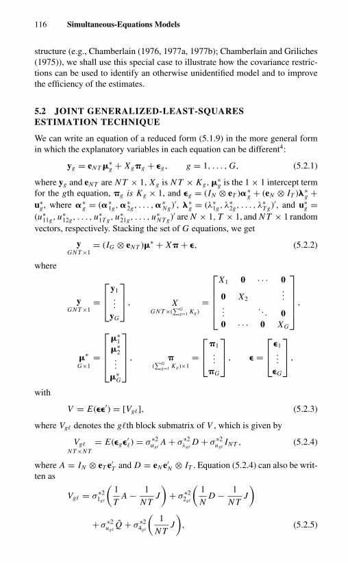
116 Simultaneous-Equations Models
structure (e.g., Chamberlain (1976, 1977a, 1977b); Chamberlain and Griliches(1975)), we shall use this special case to illustrate how the covariance restric-tions can be used to identify an otherwise unidentified model and to improvethe efficiency of the estimates.
5.2 JOINT GENERALIZED-LEAST-SQUARESESTIMATION TECHNIQUE
We can write an equation of a reduced form (5.1.9) in the more general formin which the explanatory variables in each equation can be different4:
yg = eN T �∗g + Xg�g + �g, g = 1, . . . , G, (5.2.1)
where yg and eN T are N T × 1, Xg is N T × Kg, �∗g is the 1 × 1 intercept term
for the gth equation, �g is Kg × 1, and �g = (IN ⊗ eT )�∗g + (eN ⊗ IT )�∗
g +u∗
g , where �∗g = (�∗
1g, �∗2g, . . . , �∗
Ng)′, �∗g = (λ∗
1g, λ∗2g, . . . , λ
∗T g)′, and u∗
g =(u∗
11g, u∗12g, . . . , u∗
1T g, u∗21g, . . . , u∗
N T g)′ are N × 1, T × 1, and N T × 1 randomvectors, respectively. Stacking the set of G equations, we get
yG N T ×1
= (IG ⊗ eN T )�∗ + X� + �, (5.2.2)
where
yG N T ×1
=
y1...
yG
, XG N T ×(
∑Gg=1 Kg)
=
X1 0 · · · 0
0 X2...
.... . . 0
0 · · · 0 XG
,
�∗G×1
=
�∗
1�∗
2...
�∗G
, �(∑G
g=1 Kg)×1=
�1...
�G
, � =
�1...
�G
,
with
V = E(��′) = [Vg�], (5.2.3)
where Vg� denotes the g�th block submatrix of V , which is given by
Vg�
N T ×N T= E(�g�′
�) = σ ∗2αg�
A + σ ∗2λg�
D + σ ∗2ug�
IN T , (5.2.4)
where A = IN ⊗ eT e′T and D = eN e′
N ⊗ IT . Equation (5.2.4) can also be writ-ten as
Vg� = σ ∗21g�
(1
TA − 1
N TJ
)+ σ ∗2
2g�
(1
ND − 1
N TJ
)+ σ ∗2
ug�Q + σ ∗2
4g�
(1
N TJ
), (5.2.5)

5.2 Joint Generalized-Least-Squares Estimation Technique 117
where J = eN T e′N T , Q = IN T − (1/T )A − (1/N )D + (1/N T )J , σ ∗2
1g�= σ ∗2
ug�+
T σ ∗2αg�
, σ ∗22g�
= σ ∗2ug�
+ Nσ ∗2λg�
, and σ ∗24g�
= σ ∗2ug�
+ T σ ∗2αg�
+ Nσ ∗2λg�
. It was shown in
Appendix 3B that σ ∗21g�
, σ ∗22g�
, σ ∗2ug�
, and σ ∗24g�
are the distinct characteristic roots ofVg� of multiplicity N − 1, T − 1, (N − 1)(T − 1), and 1, with C1, C2, C3, andC4 as the matrices of their corresponding characteristic vectors.
We can rewrite V as
V = V1 ⊗(
1
TA − 1
N TJ
)+ V2 ⊗
(1
ND − 1
N TJ
)+ �∗
u ⊗ Q + V4 ⊗(
1
N TJ
), (5.2.6)
where V1 = (σ ∗21g�
), V2 = (σ ∗22g�
), and V4 = (σ ∗24g�
) all of dimension G × G. Using
the fact that [(1/T )A − (1/N T )J ], [(1/N )D − (1/N T )J ], Q, and [(1/N T )J ]are symmetric idempotent matrices, mutually orthogonal, and sum to the iden-tity matrix IN T , we can write down the inverse of V explicitly as (Avery (1977);Baltagi (1980))5
V −1 = V −11 ⊗
(1
TA − 1
N TJ
)+ V −1
2 ⊗(
1
ND − 1
N TJ
)+ �∗−1
u ⊗ Q + V −14 ⊗
(1
N TJ
). (5.2.7)
The GLS estimators of �∗ and � are obtained by minimizing the distancefunction
[y − (IG ⊗ eN T )�∗ − X�]′V −1[y − (IG ⊗ eN T )�∗ − X�]. (5.2.8)
Taking partial derivatives of (5.2.8) with respect to �∗ and �, we obtain thefirst-order conditions
(IG ⊗ eN T )′V −1[y − (IG ⊗ eN T )�∗ − X�] = 0, (5.2.9)
−X ′V −1[y − (IG ⊗ eN T )�∗ − X�] = 0. (5.2.10)
Solving (5.2.9) and making use of the relations [(1/T )A − (1/N T )J ]eN T =0, [(1/N )D − (1/N T )J ]eN T = 0, QeN T = 0, and (1/N T )JeN T = eNT, wehave
�∗ =(
IG ⊗ 1
N Te′
N T
)(y − X�). (5.2.11)
Substituting (5.2.11) into (5.2.10), we have the GLS estimator of � as6
�GLS = [X ′V −1 X ]−1(X ′V −1y), (5.2.12)

118 Simultaneous-Equations Models
where
V −1 = V −11 ⊗
(1
TA − 1
N TJ
)+ V −1
2 ⊗(
1
ND − 1
N TJ
)+ �∗−1
u ⊗ Q. (5.2.13)
If E(�g�′�) = 0 for g �= � then V is block-diagonal, and equation (5.2.12) is
reduced to applying the GLS estimation method to each equation separately.If both N and T tend to infinity and N/T tends to a nonzero constant, thenlim V −1
1 = 0, lim V −12 = 0, and lim V −1
4 = 0. Equation (5.2.12) becomes theleast-squares dummy-variable (or fixed-effects) estimator for the seeminglyunrelated regression case,
plim �GLS = plimN→∞
T →∞
[1
NX ′(�∗−1
u ⊗ Q)X
]−1
×[
1
N TX ′(�∗−1
u ⊗ Q)y]. (5.2.14)
In the case of the standard reduced form, X1 = X2 = · · · = XG = X ,
�GLS =[
V −11 ⊗ X ′
(1
TA − 1
N TJ
)X
+ V −12 ⊗ X ′
(1
ND − 1
N TJ
)X + �∗−1
u ⊗ X ′ Q X
]−1
×{[
V −11 ⊗ X ′
(1
TA − 1
N TJ
)]y
+[
V −12 ⊗ X ′
(1
ND − 1
N TJ
)]y + [
�∗−1u ⊗ X ′ Q
]y}.
(5.2.15)
We know that in the conventional case when no restriction is imposed on thereduced-form coefficients vector �, estimating each equation by the least-squares method yields the best linear unbiased estimate. Equation (5.2.15)shows that in a seemingly unrelated regression model with error components,the fact that each equation has an identical set of explanatory variables is not asufficient condition for the GLS performed on the whole system to be equivalentto estimating each equation separately.
Intuitively, by stacking different equations together we shall gain efficiencyin the estimates, because knowing the residual of the �th equation helps in pre-dicting the gth equation when the covariance terms between different equationsare nonzero. For instance, if the residuals are normally distributed, E(�g | ��) =Cov(�g, ��)Var(��)−1�� �= 0. To adjust for this nonzero mean, it would be ap-propriate to regress yg − Cov(�g, ��)Var(��)−1�� on (eN T , Xg). Although ingeneral �� is unknown, asymptotically there is no difference if we replace it by

5.3 Estimation of Structural Equations 119
the least-squares residual, ��. However, if the explanatory variables in differentequations are identical, namely, Xg = X� = X , there is no gain in efficiency bybringing different equations together when the cross-equation covariances areunrestricted; because Cov(�g, ��) = σεg�
IN T , Var(��) = σε��IN T , and �� is or-
thogonal to (eN T , Xg) by construction, the variable σε�σ−1
��� can have no effect
on the estimate of (µg, �′g) when it is subtracted from yg . But the same cannot
be said for the error-components case, because Cov(�g, ��)Var(��)−1 is not pro-portional to an identity matrix. The weighted variable Cov(�g, ��)Var(��)−1��
is no longer orthogonal to (eN T , X ). Therefore, in the error-components caseit remains fruitful to exploit the covariances between different equations toimprove the accuracy of the estimates.
When V1, V2, and �∗u are unknown, we can replace them by their consistent
estimates. In Chapter 3, we discussed methods of estimating variance com-ponents. These techniques can be straightforwardly applied to the multiple-equations model as well (Avery (1977); Baltagi (1980)).
The model discussed earlier assumes the existence of both individual andtime effects. Suppose we believe that the covariances of some of the componentsare zero. The same procedure can be applied to the simpler model with someslight modifications. For example, if the covariance of the residuals betweenequations g and � is composed of only two components (an individual effectand overall effect), then σ 2
λg�= 0. Hence, σ ∗2
1g�= σ ∗2
4g�, and σ ∗2
2g�= σ ∗2
ug�. These
adjusted roots can be substituted into the appropriate positions in (5.2.6) and(5.2.7), with coefficient estimates following directly from (5.2.12).
5.3 ESTIMATION OF STRUCTURAL EQUATIONS
5.3.1 Estimation of a Single Equation in the Structural Model
As (5.2.12) shows, the generalized least-squares estimator of the slope coeffi-cients is invariant against centering the data around overall sample means; sofor ease of exposition we shall assume that there is an intercept term and that allsample observations are measured as deviations from their respective overallmeans and consider the gth structural equation as
ygN T ×1
= Yg�g + Xg�g + vg
= Wg�g + vg, g = 1, . . . , G, (5.3.1)
where Yg is an N T × (Gg − 1) matrix of N T observations of Gg − 1 includedjoint dependent variables, Xg is an N T × Kg matrix of N T observations of Kg
included exogenous variables, Wg = (Yg, Xg), and �g = (�′g, �′
g)′, The vg isan N T × 1 vector of error terms,
vg = (IN ⊗ eT )� g + (eN ⊗ IT )�g + ug, (5.3.2)
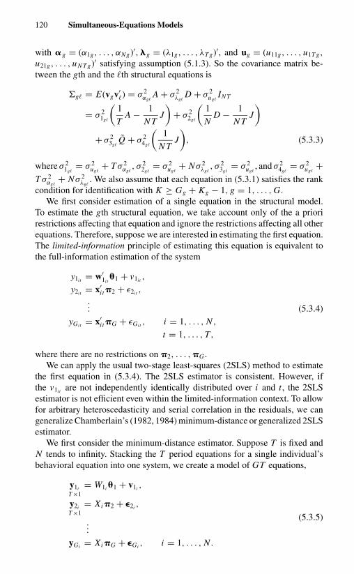
120 Simultaneous-Equations Models
with � g = (α1g, . . . , αNg)′, �g = (λ1g, . . . , λT g)′, and ug = (u11g, . . . , u1T g,
u21g, . . . , uN T g)′ satisfying assumption (5.1.3). So the covariance matrix be-tween the gth and the �th structural equations is
�g� = E(vgv′�) = σ 2
αg�A + σ 2
λg�D + σ 2
ug�IN T
= σ 21g�
(1
TA − 1
N TJ
)+ σ 2
2g�
(1
ND − 1
N TJ
)+ σ 2
3g�Q + σ 2
4g�
(1
N TJ
), (5.3.3)
where σ 21g�
= σ 2ug�
+ T σ 2αg�
, σ 22g�
= σ 2ug�
+ Nσ 2λg�
, σ 23g�
= σ 2ug�
, and σ 24g�
= σ 2ug�
+T σ 2
αg�+ Nσ 2
λg�. We also assume that each equation in (5.3.1) satisfies the rank
condition for identification with K ≥ Gg + Kg − 1, g = 1, . . . , G.We first consider estimation of a single equation in the structural model.
To estimate the gth structural equation, we take account only of the a priorirestrictions affecting that equation and ignore the restrictions affecting all otherequations. Therefore, suppose we are interested in estimating the first equation.The limited-information principle of estimating this equation is equivalent tothe full-information estimation of the system
y1i t = w′1i t
�1 + v1i t ,
y2i t = x′i t �2 + ε2i t ,
... (5.3.4)
yGit = x′i t �G + εGit , i = 1, . . . , N ,
t = 1, . . . , T,
where there are no restrictions on �2, . . . , �G .We can apply the usual two-stage least-squares (2SLS) method to estimate
the first equation in (5.3.4). The 2SLS estimator is consistent. However, ifthe v1i t are not independently identically distributed over i and t , the 2SLSestimator is not efficient even within the limited-information context. To allowfor arbitrary heteroscedasticity and serial correlation in the residuals, we cangeneralize Chamberlain’s (1982, 1984) minimum-distance or generalized 2SLSestimator.
We first consider the minimum-distance estimator. Suppose T is fixed andN tends to infinity. Stacking the T period equations for a single individual’sbehavioral equation into one system, we create a model of GT equations,
y1iT ×1
= W1i �1 + v1i ,
y2iT ×1
= Xi �2 + �2i ,
(5.3.5)...
yGi = Xi �G + �Gi , i = 1, . . . , N .

5.3 Estimation of Structural Equations 121
Let y′i = (y′
1i, . . . , y′
Gi). The reduced form of yi is
yi =
y1i
y2i
...yGi
= (IG ⊗ X i )� + �i , i = 1, . . . , N , (5.3.6)
where
X iT ×T K
=
x′
i1 0x′
i2. . .
0 x′iT
,
(5.3.7)� = vec(�′),
�GT ×K
= � ⊗ eT , and � = E(yi t | xi t ). (5.3.8)
The unconstrained least-squares regression of yi on (IG ⊗ X i ) yields a con-sistent estimate of �, ˆ�. If �i are independently distributed over i , then√
N ( ˆ� − �) is asymptotically normally distributed, with mean zero andvariance–covariance matrix
�GT K×GT K
= (IG ⊗ �−1
xx
)V(IG ⊗ �−1
xx
), (5.3.9)
where �xx = E X ′i X i = diag{E(xi1x′
i1), . . . , E(xiT x′iT )}, and V is a GTK ×
GTK matrix, with the g�th block a TK × TK matrix of the form
V g� = E
�gi1 ��i1 xi1x′
i1 �gi1 ��i2 xi1x′i2 · · · �gi1 ��iT xi1x′
iT�gi2 ��i1 xi2x′
i1 �gi2 ��i2 xi2 x′i2 · · · �gi2 ��iT x i2 x′
iT...
......
�giT ��i1 xiT x′i1 �giT ��i2 xiT x′
i2 · · · �giT ��iT xiT x′iT
.
(5.3.10)
One can obtain a consistent estimator of � by replacing the population mo-ments in � by the corresponding sample moments (e.g., Exi1x′
i1 is replaced by∑Ni=1 xi1x′
i1/N ).Let �′ = (�′
1, �′2, . . . , π
′G), and specify the restrictions on � by the condition
that � = f(�). Choose � to minimize the following distance function:
[ ˆ� − f(�)]′ ˆ�−1
[ ˆ� − f(�)]. (5.3.11)
Then√
N (� − �) is asymptotically normally distributed with mean zeroand variance–covariance matrix (F ′�−1 F)−1, where F = ∂ f/∂�′. Noting that� = � ⊗ eT , and evaluating the partitioned inverse, we obtain the asymptoticvariance–covariance matrix of
√N (�1 − �1) as{
�w1x�−111 �′
w1x
}−1, (5.3.12)
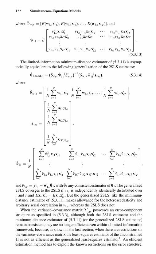
122 Simultaneous-Equations Models
where �w1x = [E(w1i1 x′i1), E(w1i2 x′
i2), . . . , E(w1iT x′iT )], and
�11 = E
v2
1i1xi1x′
i1 v1i1 v1i2 xi1x′i2 · · · v1i1 v1i1 xi1x′
iTv1i2 v1i1 xi2x′
i1 v21i2
xi2x′i2 · · · v1i2 v1iT xi2x′
iT...
......
v1iT v1i1 xiT x′i1 v1iT v1i2 xiT x′
i2 · · · v1iT v1iT xiT x′iT
.
(5.3.13)
The limited-information minimum-distance estimator of (5.3.11) is asymp-totically equivalent to the following generalization of the 2SLS estimator:
�1,G2SLS = (Sw1x�
−111 S′
w1x
)−1(Sw1x�
−111 sxy1
), (5.3.14)
where
Sw1x =[
1
N
N∑i=1
w1i1 x′i1,
1
N
N∑i=1
w1i2 x′i2, . . . ,
1
N
N∑i=1
w1iT x′iT
],
sxy1 =
1
N
N∑i=1
xi1 y1i1
1
N
N∑i=1
xi2 y1i2
...
1
N
N∑i=1
xiT y1iT
,
�11 = 1
N
N∑i=1
v21i1
xi1x′i1
N∑i=1
v1i1 v1i2 xi1x′i2 · · ·
N∑i=1
v1i1 v1iT xi1x′iT
......
...N∑
i=1
v1iT v1i1 xiT x′i1
N∑i=1
v1iT v1i2 x iT x i2 · · ·N∑
i=1
v1iT v1iT xiT x′iT
,
and v1iT = y1i t − w′1i t
�1, with �1 any consistent estimator of �1. The generalized2SLS coverges to the 2SLS if v1i t is independently identically distributed overi and t and Exi t x′
i t = Exisx′is . But the generalized 2SLS, like the minimum-
distance estimator of (5.3.11), makes allowance for the heteroscedasticity andarbitrary serial correlation in ν1i t , whereas the 2SLS does not.
When the variance–covariance matrix∑
gg possesses an error-componentstructure as specified in (5.3.3), although both the 2SLS estimator and theminimum-distance estimator of (5.3.11) (or the generalized 2SLS estimator)remain consistent, they are no longer efficient even within a limited-informationframework, because, as shown in the last section, when there are restrictions onthe variance–covariance matrix the least-squares estimator of the unconstrained� is not as efficient as the generalized least-squares estimator7. An efficientestimation method has to exploit the known restrictions on the error structure.

5.3 Estimation of Structural Equations 123
Baltagi (1981a) has suggested using the following error-component two-stageleast-squares (EC2SLS) method to obtain a more efficient estimator of theunknown parameters in the gth equation.
Transforming (5.3.1) by the eigenvectors of∑
gg, C ′1, C ′
2, and C ′3, we have8
y(h)g = Y (h)
g �g + X (h)g �g + v(h)
g = W (h)g �g + v(h)
g , (5.3.15)
where y(h)g = C ′
hyg, W (h)g = C ′
h Wg, v(h)g = C ′
hvg for h = 1, 2, 3, and C ′1, C ′
2,and C ′
3 are as defined in Appendix 3B. The transformed disturbance term v(h)g
is mutually orthogonal and has a covariance matrix proportional to an identitymatrix. We can therefore use X (h) = C ′
h X as the instruments and apply theAitken estimation procedure to the system of equationsX (1)′y(1)
g
X (2)′y(2)g
X (3)′y(3)g
=
X (1)′W (1)g
X (2)′W (2)g
X (3)′W (3)g
[�g
�g
]+
X (1)′v(1)g
X (2)′v(2)g
X (3)′v(3)g
. (5.3.16)
The resulting Aitken estimator of (�′g, �′
g) is
�g,EC2SLS ={
3∑h=1
[1
σ 2hgg
W (h)′g PX (h)W (h)
g
]}−1
(5.3.17){3∑
h=1
[1
σ 2hgg
W (h)′g PX (H )y(h)
g
]},
where PX (h) = X (h)(X (h)′ X (h))−1 X (h)′. It is a weighted combination of thebetween-groups, between-time-periods, and within-groups 2SLS estimators of(�′
g, �′g). The weights σ 2
hgg can be estimated by substituting the transformed2SLS residuals in the usual variance formula,
σ 2hgg = (
y(h)g − W (h)
g �(h)g,2SLS
)′(y(h)
g − W (h)g �
(h)g,2SLS
)/n(h), (5.3.18)
where �(h)g,2SLS = [W (h)′
g PX (h)W (h)g ]−1[W (h)′
g PX (h)y(h)g ], and n(1) = N − 1,
n(2) = T − 1, n(3) = (N − 1)(T − 1). If N → ∞, T → ∞, and N/T tendsto a nonzero constant, then the probability limit of the EC2SLS tends to the2SLS estimator based on the within-groups variation alone.
In the special case in which the source of correlation between some of theregressors and residuals comes from the unobserved time-invariant individ-ual effects alone, the correlations between them can be removed by removingthe time-invariant component from the corresponding variables. Thus, instru-ments for the correlated regressors can be chosen from “inside” the equation,as opposed to the conventional method of being chosen from “outside” theequation. Hausman and Taylor (1981) noted that for variables that are time-varying and are correlated with αig , transforming them into deviations fromtheir corresponding time means provides legitimate instruments, because theywill no longer be correlated with αig . For variables that are time-invariant, thetime means of those variables that are uncorrelated with αig can be used as

124 Simultaneous-Equations Models
instruments. Hence, a necessary condition for identification of all the param-eters within a single-equation framework is that the number of time-varyingvariables that are uncorrelated with αig be at least as great as the number oftime-invariant variables that are correlated with αig . They further showed thatwhen the variance-component structure of the disturbance term is taken ac-count of, the instrumental-variable estimator with instruments chosen this wayis efficient among the single-equation estimators.
5.3.2 Estimation of the Complete Structural System
The single-equation estimation method considered earlier ignores restrictionsin all equations in the structural system except the one being estimated. Ingeneral, we expect to get more efficient estimates if we consider the additionalinformation contained in the other equations. In this subsection we consider thefull-information estimation methods.
Let y = (y′1, . . . , y′
G)′, v = (v′1, . . . , v′
G)′,
W =
W1 0 · · · 00 W2 · · · 0...
......
0 0 · · · WG
, and � =
�1...
�G
.
We write the set of G structural equations as
y = W � + v. (5.3.19)
We can estimate the system (5.3.19) by the three-stage least-squares (3SLS)method. But just as in the limited-information case, the 3SLS estimator isefficient only if (v1i t , v2i t , . . . , vGit ) are independently identically distributedover i and t . To allow for arbitrary heteroscedasticity or serial correlation, wecan use the full-information minimum-distance estimator or the generalized3SLS estimator.
We first consider the minimum-distance estimator. When T is fixed andN tends to infinity, we can stack the T period equations for an individual’sbehavioral equation into a system to create a model of GT equations,
y1iT ×1
= W1i �1 + v1i ,
y2i = W2i �2 + v2i , (5.3.20)...
yGi = WGi �G + vGi , i = 1, . . . , N .
We obtain a minimum-distance estimator of � by choosing � to minimize[ ˆ� − f(�)]′ ˆ�
−1
[ ˆ� − f(�)], where ˆ� is the unconstrained least-squares estima-tor of regressing yi on (IG ⊗ X i ), and ˆ� is a consistent estimate of � [equa-tion (5.3.9)]. Noting that � = � ⊗ eT and vec(�′) = � = vec[−�−1 B]′ for allelements of � and B not known a priori, and making use of the formula ∂�/∂�′
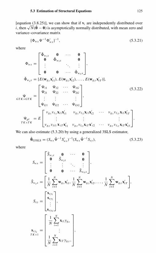
5.3 Estimation of Structural Equations 125
[equation (3.8.25)], we can show that if vi are independently distributed overi , then
√N (� − �) is asymptotically normally distributed, with mean zero and
variance–covariance matrix
{�wx�−1�′
wx }−1, (5.3.21)
where
�wx =
�w1x 0 · · · 0
0 �w2x 0...
. . ....
0 0 · · · �wG x
,
�wg x = [E(wgi1 x′i1), E(wgi2 x′
i2), . . . , E(wgiT x′iT )],
(5.3.22)
�GT K×GT K
=
�11 �12 · · · �1G
�21 �22 · · · �2G...
......
�G1 �G2 · · · �GG
,
�g�
T K×T K= E
vgi1 v�i1 xi1x′i1 vgi1 v�i2 xi1x′
i2 · · · vgi1 v�iT xi1x′iT
......
...vgiT v�i1 x iT x′
i1 vgiT v�i2 xiT x′i2 · · · vgiT v�iT xiT x′
iT
.
We can also estimate (5.3.20) by using a generalized 3SLS estimator,
�G3SLS = (Swx�−1S′
w x )−1(Sw x�−1Sxy), (5.3.23)
where
Swx =
Sw1x 0 · · · 0
0 Sw2x 0...
.... . .
...0 0 · · · SwG x
,
Swg x =[
1
N
N∑i=1
wgi1 x′i1,
1
N
N∑i=1
wgi2 x′i2, . . . ,
1
N
N∑i=1
wgiT x′iT
],
Sxy =
sxy1
sxy2
...sxyG
,
sxyg
T K×1
=
1
N
N∑i=1
xi1 ygi1
...
1
N
N∑i=1
xiT ygiT ,
,
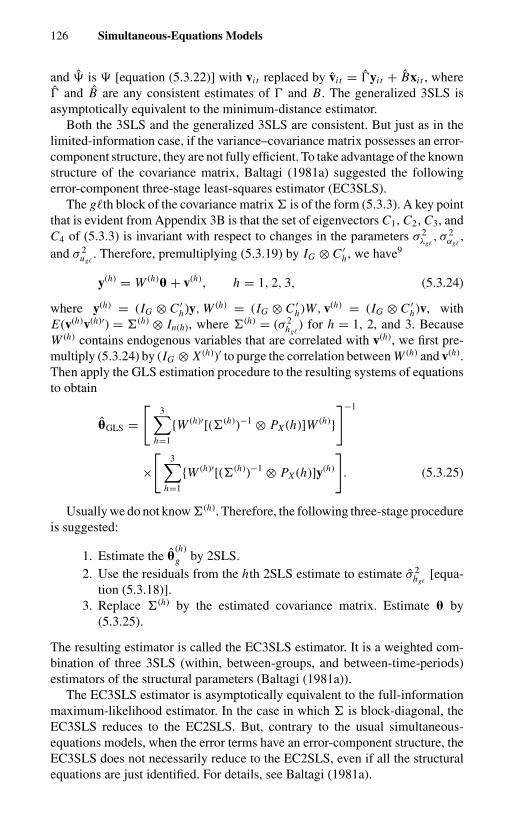
126 Simultaneous-Equations Models
and � is � [equation (5.3.22)] with vi t replaced by vi t = �yi t + Bxi t , where� and B are any consistent estimates of � and B. The generalized 3SLS isasymptotically equivalent to the minimum-distance estimator.
Both the 3SLS and the generalized 3SLS are consistent. But just as in thelimited-information case, if the variance–covariance matrix possesses an error-component structure, they are not fully efficient. To take advantage of the knownstructure of the covariance matrix, Baltagi (1981a) suggested the followingerror-component three-stage least-squares estimator (EC3SLS).
The g�th block of the covariance matrix � is of the form (5.3.3). A key pointthat is evident from Appendix 3B is that the set of eigenvectors C1, C2, C3, andC4 of (5.3.3) is invariant with respect to changes in the parameters σ 2
λg�, σ 2
αg�,
and σ 2ug�
. Therefore, premultiplying (5.3.19) by IG ⊗ C ′h , we have9
y(h) = W (h)� + v(h), h = 1, 2, 3, (5.3.24)
where y(h) = (IG ⊗ C ′h)y, W (h) = (IG ⊗ C ′
h)W, v(h) = (IG ⊗ C ′h)v, with
E(v(h)v(h)′) = �(h) ⊗ In(h), where �(h) = (σ 2hg�
) for h = 1, 2, and 3. BecauseW (h) contains endogenous variables that are correlated with v(h), we first pre-multiply (5.3.24) by (IG ⊗ X (h))′ to purge the correlation between W (h) and v(h).Then apply the GLS estimation procedure to the resulting systems of equationsto obtain
�GLS =[
3∑h=1
{W (h)′[(�(h))−1 ⊗ PX (h)]W (h)}]−1
×[
3∑h=1
{W (h)′[(�(h))−1 ⊗ PX (h)]y(h)
]. (5.3.25)
Usually we do not know �(h). Therefore, the following three-stage procedureis suggested:
1. Estimate the �(h)g by 2SLS.
2. Use the residuals from the hth 2SLS estimate to estimate σ 2hg�
[equa-tion (5.3.18)].
3. Replace �(h) by the estimated covariance matrix. Estimate � by(5.3.25).
The resulting estimator is called the EC3SLS estimator. It is a weighted com-bination of three 3SLS (within, between-groups, and between-time-periods)estimators of the structural parameters (Baltagi (1981a)).
The EC3SLS estimator is asymptotically equivalent to the full-informationmaximum-likelihood estimator. In the case in which � is block-diagonal, theEC3SLS reduces to the EC2SLS. But, contrary to the usual simultaneous-equations models, when the error terms have an error-component structure, theEC3SLS does not necessarily reduce to the EC2SLS, even if all the structuralequations are just identified. For details, see Baltagi (1981a).

5.4 Triangular System 127
5.4 TRIANGULAR SYSTEM
The model discussed earlier assumes that residuals of different equations ina multiequation model have an unrestricted variance-component structure.Under this assumption, the panel data only improve the precision of the es-timates by providing a large number of sample observations. It does not offeradditional opportunities that are not standard. However, quite often the residualcorrelations may simply be due to one or two common omitted or unobserv-able variables (Chamberlain (1976, 1977a, 1977b); Chamberlain and Griliches(1975); Goldberger (1972); Zellner (1970). For instance, in the estimation of in-come and schooling relations or individual-firm production and factor-demandrelations, it is sometimes postulated that the biases in different equations arecaused by a common left-out “ability” or “managerial-differences” variable.When panel data are used, this common omitted variable is again assumed tohave a within- and between-group structure. The combination of this factor-analytic structure with error-components formulations puts restrictions on theresidual covariance matrix that can be used to identify an otherwise unidenti-fied model and improve the efficiency of the estimates. Because a widely usedstructure for longitudinal microdata is the triangular structure, and because itsconnection with the general simultaneous-equations model in which the resid-uals have a factor-analytic structure holds in general, in this section we focuson the triangular structure to illustrate how such information can be used toidentify and estimate a model.
5.4.1 Identification
A convenient way to model correlations across equations, as well as the corre-lation of a given individual at different times (or different members of a group),is to use latent variables to connect the residuals. Let ygit denote the value ofthe variable yg for the i th individual (or group) at time t (or tth member). Wecan assume that
vgit = dghit + ugit , (5.4.1)
where the ug are uncorrelated across equations and across i and t . The corre-lations across equations are all generated by the common omitted variable h,which is assumed to have a variance-component structure:
hit = αi + ωi t , (5.4.2)
where αi is invariant over t but is independently identically distributed across i(groups), with mean zero and variance σ 2
α , and ωi t is independently identicallydistributed across i and t , with mean zero and variance σ 2
ω and is uncorrelatedwith αi .
An example of the model with Γ lower-triangular and v of the form (5.4.1)is (Chamberlain (1977a, 1977b); Chamberlain and Griliches (1975); Griliches
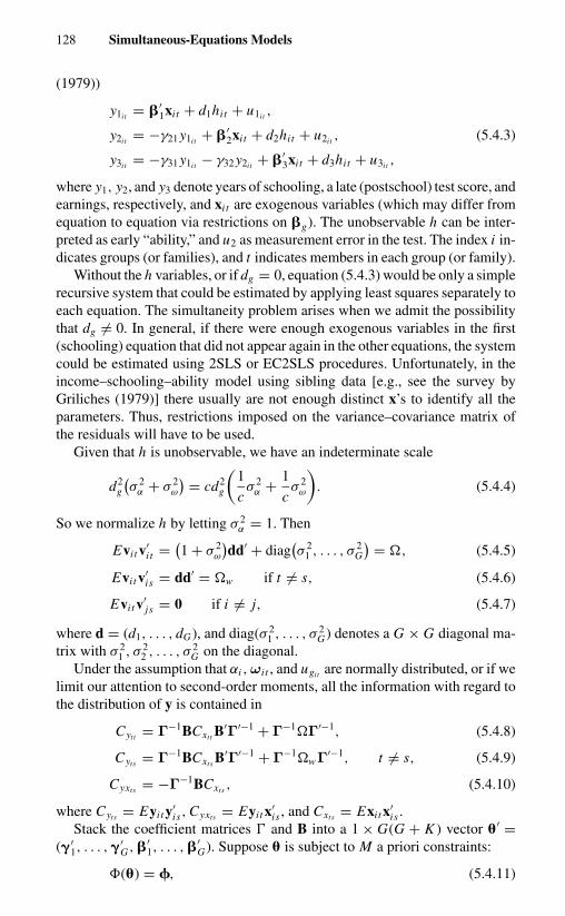
128 Simultaneous-Equations Models
(1979))
y1i t = �′1xi t + d1hit + u1i t ,
y2i t = −γ21 y1i t + �′2xi t + d2hit + u2i t , (5.4.3)
y3i t = −γ31 y1i t − γ32 y2i t + �′3xi t + d3hit + u3i t ,
where y1, y2, and y3 denote years of schooling, a late (postschool) test score, andearnings, respectively, and xi t are exogenous variables (which may differ fromequation to equation via restrictions on �g). The unobservable h can be inter-preted as early “ability,” and u2 as measurement error in the test. The index i in-dicates groups (or families), and t indicates members in each group (or family).
Without the h variables, or if dg = 0, equation (5.4.3) would be only a simplerecursive system that could be estimated by applying least squares separately toeach equation. The simultaneity problem arises when we admit the possibilitythat dg �= 0. In general, if there were enough exogenous variables in the first(schooling) equation that did not appear again in the other equations, the systemcould be estimated using 2SLS or EC2SLS procedures. Unfortunately, in theincome–schooling–ability model using sibling data [e.g., see the survey byGriliches (1979)] there usually are not enough distinct x’s to identify all theparameters. Thus, restrictions imposed on the variance–covariance matrix ofthe residuals will have to be used.
Given that h is unobservable, we have an indeterminate scale
d2g
(σ 2
α + σ 2ω
) = cd2g
(1
cσ 2
α + 1
cσ 2
ω
). (5.4.4)
So we normalize h by letting σ 2α = 1. Then
Evi t v′i t = (
1 + σ 2ω
)dd′ + diag
(σ 2
1 , . . . , σ 2G
) = �, (5.4.5)
Evi t v′is = dd′ = �w if t �= s, (5.4.6)
Evi t v′js = 0 if i �= j, (5.4.7)
where d = (d1, . . . , dG), and diag(σ 21 , . . . , σ 2
G) denotes a G × G diagonal ma-trix with σ 2
1 , σ 22 , . . . , σ 2
G on the diagonal.Under the assumption that αi ,ωi t , and ugit are normally distributed, or if we
limit our attention to second-order moments, all the information with regard tothe distribution of y is contained in
Cytt = Γ−1BCxtt B′Γ′−1 + Γ−1�Γ′−1, (5.4.8)
Cyts = Γ−1BCxts B′Γ′−1 + Γ−1�wΓ′−1, t �= s, (5.4.9)
Cyxts = −Γ−1BCxts , (5.4.10)
where Cyts = Eyi t y′is, Cyxts = Eyi t x′
is , and Cxts = Exi t x′is .
Stack the coefficient matrices � and B into a 1 × G(G + K ) vector �′ =(�′
1, . . . , �′G, �′
1, . . . , �′G). Suppose � is subject to M a priori constraints:
�(�) = �, (5.4.11)
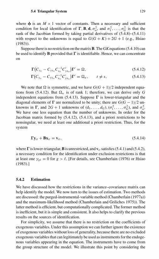
5.4 Triangular System 129
where � is an M × 1 vector of constants. Then a necessary and sufficientcondition for local identification of Γ, B, d, σ 2
ω, and σ 21 , . . . , σ 2
G is that therank of the Jacobian formed by taking partial derivatives of (5.4.8)–(5.4.11)with respect to the unknowns is equal to G(G + K ) + 2G + 1 (e.g., Hsiao(1983)).
Suppose there is no restriction on the matrix B. The GK equations (5.4.10) canbe used to identify B provided that Γ is identifiable. Hence, we can concentrateon
Γ(Cytt − Cyxtt C
−1xtt
C ′yxtt
)Γ′ = �, (5.4.12)
Γ(Cyts − Cyxts C
−1xts
C ′yxts
)Γ′ = �w , t �= s, (5.4.13)
We note that � is symmetric, and we have G(G + 1)/2 independent equa-tions from (5.4.12). But �w is of rank 1; therefore, we can derive only Gindependent equations from (5.4.13). Suppose Γ is lower-triangular and thediagonal elements of Γ are normalized to be unity; there are G(G − 1)/2 un-knowns in Γ, and 2G + 1 unknowns of (d1, . . . , dG), (σ 2
1 , . . . , σ 2G), and σ 2
ω.We have one less equation than the number of unknowns. In order for theJacobian matrix formed by (5.4.12), (5.4.13), and a priori restrictions to benonsingular, we need at least one additional a priori restriction. Thus, for thesystem
Γyi t + Bxi t = vi t , (5.4.14)
whereΓ is lower-triangular, B is unrestricted, and vi t satisfies (5.4.1) and (5.4.2),a necessary condition for the identification under exclusion restrictions is thatat least one γg� = 0 for g > �. [For details, see Chamberlain (1976) or Hsiao(1983).]
5.4.2 Estimation
We have discussed how the restrictions in the variance–covariance matrix canhelp identify the model. We now turn to the issues of estimation. Two methodsare discussed: the purged-instrumental-variable method (Chamberlain (1977a))and the maximum-likelihood method (Chamberlain and Griliches 1975)). Thelatter method is efficient, but computationally complicated. The former methodis inefficient, but it is simple and consistent. It also helps to clarify the previousresults on the sources of identification.
For simplicity, we assume that there is no restriction on the coefficients ofexogenous variables. Under this assumption we can further ignore the existenceof exogenous variables without loss of generality, because there are no excludedexogenous variables that can legitimately be used as instruments for the endoge-nous variables appearing in the equation. The instruments have to come fromthe group structure of the model. We illustrate this point by considering the

130 Simultaneous-Equations Models
following triangular system:
y1i t = + v1i t ,
y2i t = γ21 y1i t + v2i t ,...
yGit = γG1 y1i t + · · · + γG,G−1 yG−1i t + vGit ,
(5.4.15)
where vgit satisfy (5.4.1) and (5.4.2). We assume one additional γ�k = 0 forsome � and k, � > k, for identification.
The reduced form of (5.4.15) is
ygit = aghit + εgit , g = 1, . . . , G, (5.4.16)
where
a =
a1
a2
a3...
aG
=
d1
d2 + γ21d1
d3 + γ31d1 + γ32(d2 + γ21d1)...
, (5.4.17)
�i t =
ε1i t
ε2i t
ε3i t
...εgit
...
=
u1i t
u2i t + γ21u1i t
u3i t + γ31u1i t + γ32(u2i t + γ21u1i t )...
ugit +g−1∑k=1
γ ∗gkukit
...
, (5.4.18)
where γ ∗gk = γgk + ∑g−1
i=k+1 γgiγ∗ik if g > 1 and k + 1 < g, and γ ∗
gk = γgk ifk + 1 = g.
5.4.2.a Instrumental-Variable Method
The trick of the purged instrumental-variable (IV) method is to leave h in theresidual and construct instruments that are uncorrelated with h. Before goingto the general formula, we use several simple examples to show where theinstruments come from.
Consider the case that G = 3. Suppose γ21 = γ31 = 0. Using y1 as a proxyfor h in the y3 equation, we have
y3i t = γ32 y2i t + d3
d1y1i t + u3i t − d3
d1u1i t . (5.4.19)
If T ≥ 2 then y1is , s �= t , is a legitimate instrument for y1i t , because it is uncorre-lated with u3i t − (d3/d1)u1i t but it is correlated with y1i t provided that d1σ
2α �= 0.
Therefore, we can use (y2i t, y1is ) as instruments to estimate (5.4.19).

5.4 Triangular System 131
Next, suppose that only γ32 = 0. The reduced form of the model becomesy1
y2
y3
=d1
d2 + γ21d1
d3 + γ31d1
hit +u1i t
u2i t + γ21u1i t
u3i t + γ31u1i t
=
a1
a2
a3
hit +ε1i t
ε2i t
ε3i t
. (5.4.20)
In this case, the construction of valid instruments is more complicated. It re-quires two stages. The first stage is to use y1 as a proxy for h in the reduced-formequation for y2:
y2i t = a2
a1y1i t + ε2i t − a2
a1ε1i t . (5.4.21)
Equation (5.4.21) can be estimated by using y1is , s �= t , as an instrument fory1i t , provided that d1σ
2α �= 0. Then form the residual, thereby purging y2 of its
dependence on h:
z2i t = y2i t − a2
a1y1i t = ε2i t − a2
a1ε1i t . (5.4.22)
The second stage is to use z2 as an instrument for y1 in the structural equationy3:
y3i t = γ31 y1i t + d3hit + u3i t . (5.4.23)
The variable z2 is an appropriate IV because it is uncorrelated with h and u3, butit is correlated with y1, provided d2σ
21 �= 0. (If d2 = 0, then z2 = y2 − γ21 y1 =
u2. It is no longer correlated with y1.) Therefore, we require that h appeardirectly in the y2 equation and that y1 not be proportional to h – otherwise wecould never separate the effects of y1 and h.
In order to identify the y2 equation
y2i t = γ21 y1i t + d2hit + u2i t , (5.4.24)
we can interchange the reduced-form y2 and y3 equations and repeat the twostages. With γ21 and γ31 identified, in the third stage we form the residuals
v2i t = y2i t − γ21 y1i t = d2hit + u2i t , (5.4.25)v3i t = y3i t − γ31 y1i t = d3hit + u3i t .
Then use y1 as a proxy for h:
v2i t = d2
d1y1i t + u2i t − d2
d1u1i t ,
(5.4.26)
v3i t = d3
d1y1i t + u3i t − d3
d1u1i t .
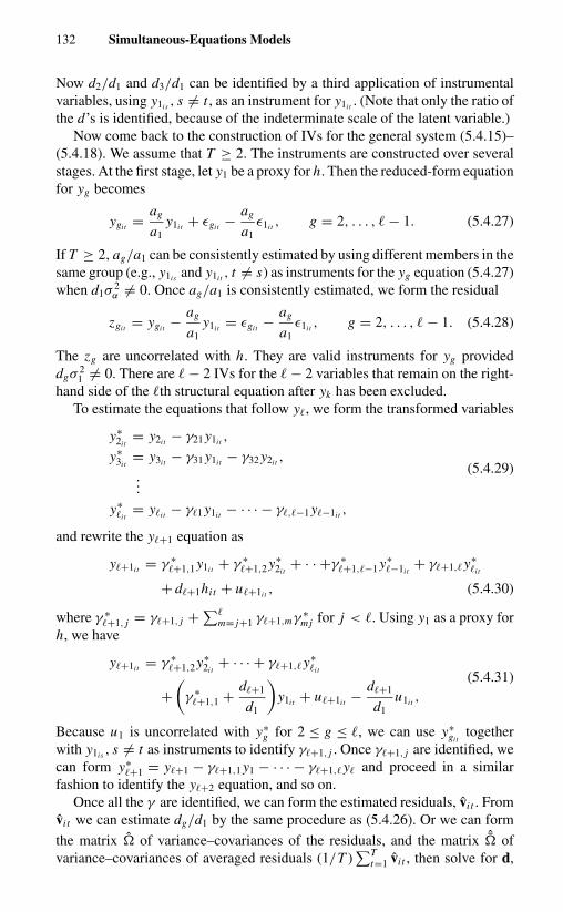
132 Simultaneous-Equations Models
Now d2/d1 and d3/d1 can be identified by a third application of instrumentalvariables, using y1is , s �= t , as an instrument for y1i t . (Note that only the ratio ofthe d’s is identified, because of the indeterminate scale of the latent variable.)
Now come back to the construction of IVs for the general system (5.4.15)–(5.4.18). We assume that T ≥ 2. The instruments are constructed over severalstages. At the first stage, let y1 be a proxy for h. Then the reduced-form equationfor yg becomes
ygit = ag
a1y1i t + εgit − ag
a1ε1i t , g = 2, . . . , � − 1. (5.4.27)
If T ≥ 2, ag/a1 can be consistently estimated by using different members in thesame group (e.g., y1is and y1i t , t �= s) as instruments for the yg equation (5.4.27)when d1σ
2α �= 0. Once ag/a1 is consistently estimated, we form the residual
zgit = ygit − ag
a1y1i t = εgit − ag
a1ε1i t , g = 2, . . . , � − 1. (5.4.28)
The zg are uncorrelated with h. They are valid instruments for yg provideddgσ
21 �= 0. There are � − 2 IVs for the � − 2 variables that remain on the right-
hand side of the �th structural equation after yk has been excluded.To estimate the equations that follow y�, we form the transformed variables
y∗2i t
= y2i t − γ21 y1i t ,
y∗3i t
= y3i t − γ31 y1i t − γ32 y2i t , (5.4.29)...
y∗�i t
= y�i t − γ�1 y1i t − · · · − γ�,�−1 y�−1i t ,
and rewrite the y�+1 equation as
y�+1i t = γ ∗�+1,1 y1i t + γ ∗
�+1,2 y∗2i t
+ · · +γ ∗�+1,�−1 y∗
�−1i t+ γ�+1,�y∗
�i t
+ d�+1hit + u�+1i t , (5.4.30)
where γ ∗�+1, j = γ�+1, j + ∑�
m= j+1 γ�+1,mγ ∗mj for j < �. Using y1 as a proxy for
h, we have
y�+1i t = γ ∗�+1,2 y∗
2i t+ · · · + γ�+1,�y∗
�i t(5.4.31)
+(
γ ∗�+1,1 + d�+1
d1
)y1i t + u�+1i t − d�+1
d1u1i t ,
Because u1 is uncorrelated with y∗g for 2 ≤ g ≤ �, we can use y∗
gittogether
with y1is , s �= t as instruments to identify γ�+1, j . Once γ�+1, j are identified, wecan form y∗
�+1 = y�+1 − γ�+1,1 y1 − · · · − γ�+1,�y� and proceed in a similarfashion to identify the y�+2 equation, and so on.
Once all the γ are identified, we can form the estimated residuals, vi t . Fromvi t we can estimate dg/d1 by the same procedure as (5.4.26). Or we can form
the matrix � of variance–covariances of the residuals, and the matrix ˆ� ofvariance–covariances of averaged residuals (1/T )
∑Tt=1 vi t , then solve for d,

5.4 Triangular System 133
(σ 21 , . . . , σ 2
G), and σ 2ω from the relations
� = (1 + σ 2
ω
)dd′ + diag
(σ 2
1 , . . . , σ 2G
), (5.4.32)
ˆ� = (1 + σ 2
ω
)dd′ + 1
Tdiag
(σ 2
1 , . . . , σ 2G
). (5.4.33)
The purged IV estimator is consistent. It also will often indicate quickly ifa new model is identified. For instance to see the necessity of having at leastone more γg� = 0 for g > � to identify the foregoing system, we can check ifthe instruments formed by the foregoing procedure satisfy the required rankcondition. Consider the example where G = 3 and all γg� �= 0 for g > �. Inorder to follow the strategy of allowing h to remain in the residual, in the thirdequation we need IVs for y1 and y2 that are uncorrelated with h. As indicatedearlier, we can purge y2 of its dependence on h by forming z2 = y2 − (a2/a1)y1.A similar procedure can be applied to y1. We use y2 as a proxy for h, with y2is
as an IV for y2i t . Then form the residual z1 = y1 − (a1/a2)y2. Again z1 isuncorrelated with h and u3. But z1 = −(a1/a2)z2, and so an attempt to use bothz2 and z1 as IVs fails to meet the rank condition.
5.4.2.b Maximum-Likelihood Method
Although the purged IV method is simple to use, it is likely to be inefficient,because the correlations between the endogenous variables and the purged IVswill probably be small. Also, the restriction that (5.4.6) is of rank 1 is notbeing utilized. To obtain efficient estimates of the unknown parameters, it isnecessary to estimate the covariance matrices simultaneously with the equationcoefficients. Under the normality assumptions for αi , ωi t and uit , we can obtainefficient estimates of (5.4.15) by maximizing the log likelihood function
log L = − N
2log |V |
− 1
2
N∑i=1
(y′1i , y′
2i , . . . , y′Gi )V
−1(y′1i , . . . , y′
Gi )′, (5.4.34)
where
ygiT ×1
= (ygi1 , . . . , ygiT )′, g = 1, . . . , G,
VGT ×GT
= � ⊗ IT + aa′ ⊗ eT e′T , (5.4.35)
�G×G
= E(�i t �′i t ) + σ 2
ωaa′.
Using the relations10
V −1 = �−1 ⊗ IT − cc′ ⊗ eT e′T , (5.4.36)
|V | = |�|T |1 − T c′�c|−1, (5.4.37)

134 Simultaneous-Equations Models
we can simplify the log likelihood function as11
log L = − N T
2log |�| + N
2log(1 − T c′�c)
− N T
2tr(�−1 R) + N T 2
2c′ Rc, (5.4.38)
where c is a G × 1 vector proportional to �−1a, R is the matrix of the sumsof the squares and cross-products of the residuals divided by N T , and R is thematrix of sums of squares and cross-products of the averaged residuals (overt for i) divided by N . In other words, we simplify the log likelihood function(5.4.34) by reparameterizing it in terms of c and �.
Taking partial derivatives of (5.4.38), we obtain the first-order conditions12
∂ log L
∂�−1= N T
2� + N T
2
1
(1 − T c′�c)�cc′� − N T
2R = 0,
(5.4.39)∂ log L
∂c= − N T
1 − T c′�c�c + N T 2 Rc = 0. (5.4.40)
Postmultiplying (5.4.39) by c and regrouping the terms, we have
�c = 1 − T c′�c1 − (T − 1)c′�c
Rc. (5.4.41)
Combining (5.4.40) and (5.4.41), we obtain[R − 1
T [1 − (T − 1)c′�c]R
]c = 0. (5.4.42)
Hence, the MLE of c is a characteristic vector corresponding to a root of
|R − λR| = 0. (5.4.43)
The determinate equation (5.4.43) has G roots. To find which root to use,substitute (5.4.39) and (5.4.40) into (5.4.38):
log L = − N T
2log |�| + N
2log(1 − T c′�c)
− N T
2(G + T tr c′ Rc) + N T 2
2tr(c′ Rc)
= − N T
2log |�| + N
2log(1 − T c′�c) − N T G
2. (5.4.44)
Let the G characteristic vectors corresponding to the G roots of (5.4.43)be denoted as c1(= c), c2, . . . , cG . These characteristic vectors are determinedonly up to a scalar. Choose the normalization c∗′
g Rc∗g = 1, g = 1, . . . , G, where
c∗g = (c′
g Rcg)−1/2cg . Let C∗ = [c∗1, . . . , c∗
G]; then C∗′ RC∗ = IG . From (5.4.39)
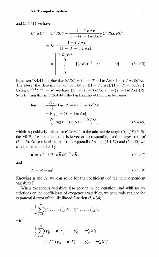
5.4 Triangular System 135
and (5.4.41) we have
C∗′�C∗ = C∗′ RC∗ − 1 − T c′�c[1 − (T − 1)c′�c]2
C∗′ Rcc′ RC∗
= IG − 1 − T c′�c[1 − (T − 1)c′�c]2
×
(c′ Rc)1/2
0...0
[(c′ Rc)1/2 0 · · · 0]. (5.4.45)
Equation (5.4.41) implies that (c′ Rc) = {[1 − (T − 1)c′�c]/[1 − T c′�c]}c′�c.Therefore, the determinant of (5.4.45) is {[1 − T c′�c]/[1 − (T − 1)c′�c]}.Using C∗′−1C∗−1 = R, we have |�| = {[1 − T c′�c]/[1 − (T − 1)c′�c]}|R|.Substituting this into (5.4.44), the log likelihood function becomes
log L = − N T
2{log |R| + log(1 − T c′�c)
− log[1 − (T − 1)c′�c]}+ N
2log[1 − T c′�c] − N T G
2, (5.4.46)
which is positively related to c′�c within the admissible range (0, 1/T ).13 Sothe MLE of c is the characteristic vector corresponding to the largest root of(5.4.43). Once c is obtained, from Appendix 5A and (5.4.39) and (5.4.40) wecan estimate a and � by
a′ = T (1 + T 2c′ Rc)−1/2c′ R, (5.4.47)
and
� = R − aa′. (5.4.48)
Knowing a and �, we can solve for the coefficients of the joint dependentvariables �.
When exogenous variables also appear in the equation, and with no re-strictions on the coefficients of exogenous variables, we need only replace theexponential term of the likelihood function (5.4.34),
−1
2
N∑i=1
(y′1i , . . . , y′
Gi )V−1(y′
1i , . . . , y′Gi )
′,
with
−1
2
N∑i=1
(y′1i − �′
1 X ′i , . . . , y′
Gi − �′G X ′
i )
× V −1(y′1i − �′
1 X ′i , . . . , y′
Gi − �′G X ′
i )′.

136 Simultaneous-Equations Models
The MLEs of c, a, and � remain the solutions of (5.4.43), (5.4.47), and (5.4.48).From knowledge of � and a we can solve for � and σ 2
ω. The MLE of � condi-tional on V is the GLS of �. Knowing � and �, we can solve for B = −��.
Thus, Chamberlain and Griliches (1975) suggested the following iterativealgorithm to solve for the MLE. Starting from the least-squares reduced-formestimates, we can form consistent estimates of R and R. Then estimate c bymaximizing14
c′ Rcc′ Rc
. (5.4.49)
Once c is obtained, we solve for a and � by (5.4.47) and (5.4.48). After obtaining� and a, the MLE of the reduced-form parameters is just the generalized least-squares estimate. With these estimated reduced-form coefficients, one can formnew estimates of R and R and continue the iteration until the solution converges.The structural-form parameters are then solved from the convergent reduced-form parameters.
5.4.3 An Example
Chamberlain and Griliches (1975) used the Gorseline (1932) data of the highestgrade of schooling attained (y1), the logarithm of the occupational (Duncan’sSES) standing (y2), and the logarithm of 1927 income (y3) for 156 pairs of broth-ers from Indiana (U.S.) to fit a model of the type (5.4.1)–(5.4.3). Specifically,they let
y1i t = �′1xi t + d1hit + u1i t ,
y2i t = γ21 y1i t + �′2xi t + d2hit + u2i t , (5.4.50)
y3i t = γ31 y1i t + �′3xi t + d3hit + u3i t .
The set X contains a constant, age, and age squared, with age squared appearingonly in the income equation.
The reduced form of (5.4.50) is
yi t = �xi t + ahit + �i t , (5.4.51)
where
Π =�′
1γ21�′
1 + �′2
γ31�′1 + �′
3
,
a =d1
d2 + γ21d1
d3 + γ31d1
, (5.4.52)
�i t =u1i t
u2i t + γ21u1i t
u3i t + γ31u1i t
.

5.4 Triangular System 137
Therefore,
E�i t �′i t =
σ 2u1 γ21σ
2u1 γ31σ
2u1
σ 2u2 + γ 2
21σ2u1 γ21γ31σ
2u1
σ 2u3 + γ 2
31σ2u1
, (5.4.53)
and
� =σ11 σ12 σ13
σ22 σ23
σ33
= E(�i t �′i t ) + σ 2
ωaa′. (5.4.54)
We show that knowing a and � identifies the structural coefficients of thejoint dependent variables as follows: For a given value of σ 2
ω, we can solve for
σ 2u1 = σ11 − σ 2
ωa21, (5.4.55)
γ21 = σ12 − σ 2ωa1a2
σ 2u1
, (5.4.56)
γ31 = σ13 − σ 2ωa1a3
σ 2u1
. (5.4.57)
Equating
γ21γ31 = σ23 − σ 2ωa2a3
σ 2u1
(5.4.58)
with the product of (5.4.56) and (5.4.57), and making use of (5.4.55), we have
σ 2ω = σ12σ13 − σ11σ23
σ12a1a3 + σ13a1a2 − σ11a2a3 − σ23a21
. (5.4.59)
The problem then becomes one of estimating a and �. Table 5.1 presentsthe MLE of Chamberlain and Griliches (1975) for the coefficients of schoolingand (unobservable) ability variables with σ 2
α normalized to equal 1. Their least-squares estimates ignore the familial information, and the covariance estimatesin which each brother’s characteristics (his income, occupation, schooling, andage) are measured around his own family’s mean are also presented in Table 5.1.
The covariance estimate of the coefficient-of-schooling variable in theincome equation is smaller than the least-squares estimate. However, thesimultaneous-equations model estimate of the coefficient for the ability variableis negative in the schooling equation. As discussed in Section 5.1, if schoolingand ability are negatively correlated, the single-equation within-family estimateof the schooling coefficient could be less than the least-squares estimate (here0.080 versus 0.082). To attribute this decline to “ability” or “family background”is erroneous. In fact, when schooling and ability were treated symmetrically, thecoefficient-of-schooling variable (0.088) became greater than the least-squaresestimate 0.082.

138 Simultaneous-Equations Models
Table 5.1. Parameter estimates and their standard errors for the income–occupation–schooling model
Method
Least-squares CovarianceCoefficients of the structural equations estimate estimate MLE
Schooling in the:Income equation 0.082 0.080 0.088
(0.010)a (0.011) (0.009)
Occupation equation 0.104 0.135 0.107(0.010) (0.015) (0.010)
“Ability” in the:Income equation 0.416
(0.038)
Occupation equation 0.214(0.046)
Schooling equation −0.092(0.178)
aStandard errors in parentheses.Source: Chamberlain and Griliches (1975, p. 429).
APPENDIX 5A
Let
V = � ⊗ IT + aa′ ⊗ eT e′T . (5A.1)
Because � is positive definite and aa′ is positive semidefinite, there exists aG × G nonsingular matrix F such that (Anderson (1958, p. 341))
F ′�F = IG and F ′aa′F =
ψ1 0
0. . .
0 0
,
where ψ1 is the root of
|aa′ − λ�| = 0. (5A.2)
Next, choose a T × T orthogonal matrix E , with the first column of E beingthe vector (1/
√T )eT . Then
E ′E = IT and E ′eT e′T E =
[T 0′
0 0
]. (5A.3)

Appendix 5A 139
Now F ⊗ E can be used to diagonalize V ,
(F ⊗ E)′V (F ⊗ E) = IGT +[ψ1 0′
0 0
]G×G
⊗[
T 0′
0 0
]T ×T
, (5A.4)
and factor V −1,
V −1 = �−1 ⊗ IT − F ′
ψ1
1 + T ψ10′
0 0
G×G
F ⊗ eT e′T
= �−1 ⊗ IT − cc′ ⊗ eT e′T , (5A.5)
where c′ = [ψ1/(1 + T ψ1)]1/2f ′1, and f1 is the first column of F .
The determinant of V can be obtained from (5A.4):
|V | = |�|T · (1 + T ψ1). (5A.6)
This can be expressed in terms of c and � by noting that
c′�c = ψ1
1 + T ψ1. (5A.7)
Thus, we have
1 − T c′�c = 1
1 + T ψ1, (5A.8)
and
|V | = |�|T · |1 − T c′�c|−1. (5A.9)
From V · V −1 = IGT it is implied that
−�cc′ + aa′�−1 − T aa′cc′ = 0. (5A.10)
Premultiplying (5A.10) by c′, we obtain
a = c′a[c′�c + (c′a)2]
�c. (5A.11)
Also, from f ′1a = ψ1/2 and a proportional to c1 [equation (5A.11)], and
hence f1, we have
a = ψ1/2
f ′1f1
f1 = 1
(1 + T ψ1)1/2(c′c)c. (5A.12)
Premultiplying (5.4.40) by c′, we obtain
c′ Rc = c′�cT (1 − T c′�c)
= 1
Tψ1. (5A.13)
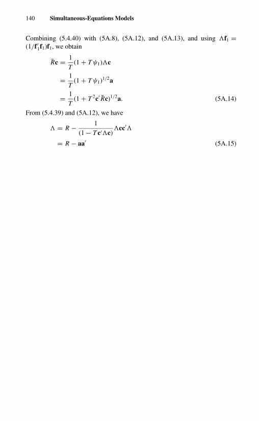
140 Simultaneous-Equations Models
Combining (5.4.40) with (5A.8), (5A.12), and (5A.13), and using �f1 =(1/f ′
1f1)f1, we obtain
Rc = 1
T(1 + T ψ1)�c
= 1
T(1 + T ψ1)1/2a
= 1
T(1 + T 2c′ Rc)1/2a. (5A.14)
From (5.4.39) and (5A.12), we have
� = R − 1
(1 − T c′�c)�cc′�
= R − aa′ (5A.15)

CHAPTER 6
Variable-Coefficient Models
6.1 INTRODUCTION
So far we have confined our discussion to models in which the effects of omit-ted variables are either individual-specific or time-specific or both. But thereare cases in which there are changing economic structures or different so-cioeconomic and demographic background factors that imply that the responseparameters may be varying over time and/or may be different for different cross-sectional units. For example, in Chapter 2 we reported a study (Kuh (1963)) oninvestment expenditures of 60 small and middle-sized firms in capital-goods-producing industries from 1935 to 1955, excluding the war years (1942–1945).In a majority of the cases Kuh investigated, the hypothesis of common inter-cept and slope coefficients for all firms, as well as that of variable intercept butcommon slope, was rejected (Tables 2.3 and 2.4). Similar results were found bySwamy (1970), who used the annual data on 11 U.S. corporations from 1935to 1954 to fit the Grunfeld (1958) investment functions. His preliminary test ofa variable intercept but common coefficients for the value of a firm’s outstand-ing shares at the beginning of the year and its beginning-of-year capital stockyielded an F value of 14.4521. That is well above the 5 percent value of an Fdistribution with 27 and 187 degrees of freedom.1
When data do not support the hypothesis of coefficients being the same, yetthe specification of the relationships among variables appears proper or it is notfeasible to include additional conditional variables, then it would seem reason-able to allow variations in parameters across cross-sectional units and/or overtime as a means to take account of the interindividual and/or interperiod het-erogeneity. A single-equation model in its most general form can be written as
yit =K∑
k=1
βki t xkit + uit , i = 1, . . . , N ,(6.1.1)
t = 1, . . . , T,
where, in contrast to previous chapters, we no longer treat the intercept dif-ferently than other explanatory variables and let x1i t = 1. However, if all thecoefficients are treated as fixed and different for different cross-sectional units

142 Variable-Coefficient Models
in different time periods, there are N K T parameters with only N T observa-tions. Obviously, there is no way we can obtain any meaningful estimates ofβki t . We are thus led to search for an approach that allows the coefficients ofinterest to differ, but provides some method of modeling the cross-sectionalunits as a group rather than individually.
One possibility would be to introduce dummy variables into the model thatwould indicate differences in the coefficients across individual units and/orover time, that is, to develop an approach similar to the least-squares dummy-variable approach. In the case in which only cross-sectional differences arepresent, this approach is equivalent to postulating a separate regression foreach cross-sectional unit,2
yit = �′i xi t + uit , i = 1, . . . , N ,
(6.1.2)t = 1, . . . , T,
where �i and xi t are K × 1 vectors of parameters and explanatory variables.Alternatively, each regression coefficient can be viewed as a random variable
with a probability distribution (e.g., Hurwicz (1950); Klein (1953); Theil andMennes (1959); Zellner (1966)). The random-coefficient specification reducesthe number of parameters to be estimated substantially, while still allowing thecoefficients to differ from unit to unit and/or from time to time. Depending on thetype of assumption about the parameter variation, it can be further classified intoone of two categories: stationary and nonstationary random-coefficient models.
Stationary random-coefficient models regard the coefficients as having con-stant means and variance–covariances. Namely, the K × 1 vector of parameters�i t is specified as
�i t = � + �i t , i = 1, . . . , N ,(6.1.3)
t = 1, . . . , T,
where � is a K × 1 vector of constants, and �i t is a K × 1 vector of stationaryrandom variables with zero means and constant variance–covariances. For thistype of model we are interested in (1) estimating the mean coefficient vector �,(2) predicting each individual component �i t , (3) estimating the dispersion ofthe individual-parameter vector, and (4) testing the hypothesis that the variancesof �i t are zero.
The nonstationary random-coefficient models do not regard the coefficientvector as having constant mean or variance. Changes in coefficients from oneobservation to the next can be the result of the realization of a nonstationarystochastic process or can be a function of exogenous variables. In this case weare interested in (1) estimating the parameters characterizing the time-evolvingprocess, (2) estimating the initial value and the history of parameter realizations,(3) predicting the future evolutions, and (4) testing the hypothesis of randomvariation.
Because of the computational complexities, variable-coefficient models havenot gained as wide acceptance in empirical work as has the variable-interceptmodel. However, that does not mean that there is less need for taking account

6.2 Coefficients That Vary over Cross-Sectional Units 143
of parameter heterogeneity in pooling the data. For instance, take the empiricalstudies of economic growth as an example, the per capita output growth ratesare assumed to depend over a common horizon on two sets of variables. Oneset of variables consists of the initial per capita output and the savings andpopulation growth rates, variables that are suggested by the Solow growthmodel. The second set of variables consists of control variables that correspondto whatever additional determinants of growth a researcher wishes to examine(e.g., Durlauf (2001); Durlauf and Quah (1999)). However, there is nothingin growth theory which would lead one to think that the marginal effect of achange in high school enrollment percentages on the per capita growth of theU.S. should be the same as the effect on a country in SubSaharan Africa. In fact,any parsimonious regression will necessarily leave out many factors that fromthe perspective of economic theory would be likely to affect the parameters ofthe included variables (e.g., Canova (1999); Durlauf and Johnson (1995)).
In this chapter we shall survey some of the popular single-equation varying-coefficient models. We shall first discuss the single-equation model with ex-ogenous explanatory variables, then discuss models involving lagged dependentvariables (e.g., Hsiao and Mountain (1994); Hsiao and Tahmiscioglu (1997);Hsiao, Pesaran, and Tahmiscioglu (1999); Liu and Tiao (1980) Nicholls andQuinn (1982); and Swamy (1974)). We shall not discuss simultaneous-equationsmodels with random coefficients (e.g., see Chow (1983); Kelejian (1977); andRaj and Ullah (1981)). Further discussion of the subject of this chapter can alsobe found in Amemiya (1983), Chow (1983), Judge et al. (1980), and Raj andUllah (1981).
In Section 6.2, we discuss models with coefficients varying over individuals,and in Section 6.3, we discuss models with coefficients varying over individ-uals and time. Section 6.4 concerns models with time-evolving coefficients.Models with coefficients that are functions of other exogenous variables willbe discussed in Section 6.5. Section 6.6 proposes a mixed fixed- and random-coefficient model as a unifying framework for various approaches to controllingunobserved heterogeneity. Section 6.7 discusses issues of dynamic models.Section 6.8 provides an analysis of liquidity constraints and firm investmentexpenditure.
6.2 COEFFICIENTS THAT VARY OVERCROSS-SECTIONAL UNITS
When regression coefficients are viewed as invariant over time, but varyingfrom one unit to another, we can write the model as
yit =K∑
k=1
βki xkit + uit
(6.2.1)=
K∑k=1
(βk + αki )xkit + uit , i = 1, . . . , N ,
t = 1, . . . , T,

144 Variable-Coefficient Models
where � = (β1, . . . , βK )′ can be viewed as the common-mean-coefficientvector, and � i = (α1i , . . . , αK i )′ as the individual deviation from the commonmean �. If individual observations are heterogeneous or the performance ofindividual units from the data base is of interest, then � i are treated as fixedconstants. If conditional on xkit , individual units can be viewed as random drawsfrom a common population or the population characteristics are of interest, thenαki are generally treated as random variables having zero means and constantvariances and covariances.
6.2.1 Fixed-Coefficient Model
When �i are treated as fixed and different constants, we can stack the N Tobservations in the form of the Zellner (1962) seemingly unrelated regressionmodel
y1
y2...
yN
=
X1 0
X2
. . .0 X N
�1
�2...
�N
+
u1
u2...
uN
, (6.2.2)
where yi and ui are T × 1 vectors (yi1, . . . , yiT )′ and (ui1, . . . , uiT )′, and Xi
is the T × K matrix of the time-series observations of the i th individual’sexplanatory variables with the t th row equal to x′
i t . If the covariances betweendifferent cross-sectional units are not zero (Eui u′
j �= 0), the GLS estimator of(�′
1, . . . , �′N ) is more efficient than the single-equation estimator of �i for each
cross-sectional unit. If Xi are identical for all i or Eui u′i = σ 2
i I and Eui u′j = 0
for i �= j , the GLS estimator for (�′1, . . . , �′
N ) is the same as applying leastsquares separately to the time-series observations of each cross-sectional unit.
6.2.2 Random-Coefficient Model
6.2.2.a The Model
When �i = � + � i are treated as random, with common mean �, Swamy(1970) assumed that3
E� i = 0,
E� i �′j
K×K
={ if i = j,0 if i �= j,
Exi t �′j = 0, E� i u′
j = 0,
Eui u′j =
{σ 2
i IT if i = j,0 if i �= j.
(6.2.3)

6.2 Coefficients That Vary over Cross-Sectional Units 145
Stacking all N T observations, we have
y = X � + X� + u, (6.2.4)
where
yN T ×1
= (y′1, . . . , y′
N )′,
XN T ×K
=
X1
X2...
X N
, XN T ×N K
=
X1 0
X2
. . .0 X N
= diag(X1, . . . , X N ),
u = (u′1, . . . , u′
N )′, and � = (� ′1, . . . , � ′
N )′. The covariance matrix for the com-posite disturbance term X� + u is block-diagonal, with the i th diagonal blockgiven by
�i = XiX ′i + σ 2
i IT . (6.2.5)
6.2.2.b Estimation
Under Swamy’s assumption, the simple regression of y on X will yield an un-biased and consistent estimator of � if (1/N T )X ′ X converges to a nonzeroconstant matrix. But the estimator is inefficient, and the usual least-squaresformula for computing the variance–covariance matrix of the estimator is in-correct, often leading to misleading statistical inferences. Moreover, when thepattern of parameter variation is of interest in its own right, an estimator ig-noring parameter variation is incapable of shedding light on this aspect of theeconomic process.
The best linear unbiased estimator of � for (6.2.4) is the GLS estimator4
ˆ�GLS =(
N∑i=1
X ′i�
−1i Xi
)−1 (N∑
i=1
X ′i�
−1i yi
)
=N∑
i=1
Wi �i , (6.2.6)
where
Wi ={
N∑i=1
[ + σ 2
i (X ′i Xi )
−1]−1
}−1 [ + σ 2
i (X ′i Xi )
−1]−1
,
and
�i = (X ′i Xi )
−1 X ′i yi .
The last expression of (6.2.6) shows that the GLS estimator is a matrix-weighted average of the least-squares estimator for each cross-sectional unit,

146 Variable-Coefficient Models
with the weights inversely proportional to their covariance matrices. It alsoshows that the GLS estimator requires only a matrix inversion of order K , andso it is not much more complicated to compute than the simple least-squaresestimator.
The covariance matrix for the GLS estimator is
Var( ˆ�GLS) =(
N∑i=1
X ′i�
−1i Xi
)−1
={
N∑i=1
[ + σ 2
i (X ′i Xi )
−1]−1
}−1
. (6.2.7)
Swamy proposed using the least-squares estimators �i = (X ′i Xi )−1 X ′
i yi andtheir residuals ui = yi − Xi �i to obtain5 unbiased estimators of σ 2
i and ,
σ 2i = u′
i ui
T − K
= 1
T − Ky′
i [I − Xi (X ′i Xi )
−1 X ′i ]yi , (6.2.8)
= 1
N − 1
N∑i=1
(�i − N−1
N∑i=1
�i
)(�i − N−1
N∑i=1
�i
)′
− 1
N
N∑i=1
σ 2i (X ′
i Xi )−1. (6.2.9)
Again, just as in the error-component model, the estimator (6.2.9) is not nec-essarily nonnegative definite. In this situation, Swamy [see also Judge et al.(1980)] has suggested replacing (6.2.9) by
= 1
N − 1
N∑i=1
(�i − N−1
N∑i=1
�i
)(�i − N−1
N∑i=1
�i
)′. (6.2.10)
This estimator, although not unbiased, is nonnegative definite and is consistentwhen T tends to infinity. Alternatively, we can use the Bayes mode estimatorsuggested by Lindley and Smith (1972) and Smith (1973),
∗ = {R + (N − 1)}(N + ρ − K − 2)
, (6.2.11)
where R and ρ are prior parameters, assuming that −1 has a Wishart distribu-tion with ρ degrees of freedom and matrix R. For instance, we may let R =
and ρ = 2 as in Hsiao, Pesaran, and Tahmiscioglu (2002).Swamy proved that substituting σ 2
i and for σ 2i and in (6.2.6) yields an
asymptotically normal and efficient estimator of �. The speed of convergenceof the GLS estimator is N 1/2. This can be seen by noting that the inverse of the
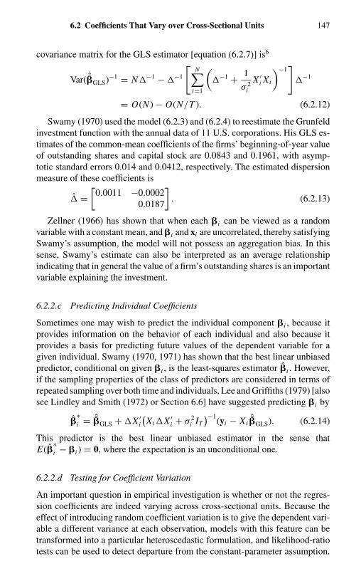
6.2 Coefficients That Vary over Cross-Sectional Units 147
covariance matrix for the GLS estimator [equation (6.2.7)] is6
Var( ˆ�GLS)−1 = N−1 − −1
[N∑
i=1
(−1 + 1
σ 2i
X ′i Xi
)−1]
−1
= O(N ) − O(N/T ). (6.2.12)
Swamy (1970) used the model (6.2.3) and (6.2.4) to reestimate the Grunfeldinvestment function with the annual data of 11 U.S. corporations. His GLS es-timates of the common-mean coefficients of the firms’ beginning-of-year valueof outstanding shares and capital stock are 0.0843 and 0.1961, with asymp-totic standard errors 0.014 and 0.0412, respectively. The estimated dispersionmeasure of these coefficients is
=[
0.0011 −0.00020.0187
]. (6.2.13)
Zellner (1966) has shown that when each �i can be viewed as a randomvariable with a constant mean, and �i and xi are uncorrelated, thereby satisfyingSwamy’s assumption, the model will not possess an aggregation bias. In thissense, Swamy’s estimate can also be interpreted as an average relationshipindicating that in general the value of a firm’s outstanding shares is an importantvariable explaining the investment.
6.2.2.c Predicting Individual Coefficients
Sometimes one may wish to predict the individual component �i , because itprovides information on the behavior of each individual and also because itprovides a basis for predicting future values of the dependent variable for agiven individual. Swamy (1970, 1971) has shown that the best linear unbiasedpredictor, conditional on given �i , is the least-squares estimator �i . However,if the sampling properties of the class of predictors are considered in terms ofrepeated sampling over both time and individuals, Lee and Griffiths (1979) [alsosee Lindley and Smith (1972) or Section 6.6] have suggested predicting �i by
�∗i = ˆ�GLS + X ′
i
(XiX ′
i + σ 2i IT
)−1(yi − Xi
ˆ�GLS). (6.2.14)
This predictor is the best linear unbiased estimator in the sense thatE(�
∗i − �i ) = 0, where the expectation is an unconditional one.
6.2.2.d Testing for Coefficient Variation
An important question in empirical investigation is whether or not the regres-sion coefficients are indeed varying across cross-sectional units. Because theeffect of introducing random coefficient variation is to give the dependent vari-able a different variance at each observation, models with this feature can betransformed into a particular heteroscedastic formulation, and likelihood-ratiotests can be used to detect departure from the constant-parameter assumption.

148 Variable-Coefficient Models
However, computation of the likelihood-ratio test statistic can be complicated.To avoid the iterative calculations necessary to obtain maximum likelihood es-timates of the parameters in the full model, Breusch and Pagan (1979) haveproposed a Lagrange-multiplier test for heteroscedasticity. Their test has thesame asymptotic properties as the likelihood-ratio test in standard situations,but it is computationally much simpler. It can be computed simply by repeatedlyapplying least-squares regressions.
Dividing the individual-mean-over-time equation by σ−1i , we have
1
σiyi = 1
σix′
i � + ωi , i = 1, . . . , N , (6.2.15)
where
ωi = 1
σix′
i � i + 1
σiui .
When the assumption (6.2.3) holds, (6.2.15) is a model with heteroscedas-tic variances, Var(ωi ) = (1/T ) + (1/σ 2
i )x′ixi , i = 1, . . . , N . Under the null
hypothesis that = 0, (6.2.15) has homoscedastic variances, Var(ωi ) = 1/T,
i = 1, . . . , N . Thus, we can generalize Breusch and Pagan’s (1979) test ofheteroscedasticity to test for random-coefficient variation here.
Following the procedures of Rao (1973, pp. 418–419) we can show that thetransformed Lagrange-multiplier statistic7 for testing the null hypothesis leadsto computing one-half the predicted sum of squares in a regression of
(T ω2
i − 1) = 1
σ 2i
[K∑
k=1
K∑k ′=1
x ki x k ′iσ2αkk′
]+ εi , i = 1, . . . , N ,
(6.2.16)
where σ 2αkk′ = E(αkiαk ′i ).8 Because ωi and σ 2
i usually are unknown, we canreplace them by their estimated values ωi and σ 2
i , where ωi is the least-squaresresidual of (6.2.15) and σ 2
i is given by (6.2.8). When both N and T tend toinfinity, the transformed Lagrange-multiplier statistic has the same limitingdistribution as chi-square with [K (K + 1)]/2 degrees of freedom under thenull hypothesis of = 0.
Breusch and Pagan’s (1979) Lagrange-multiplier test can be put into theframework of the White (1980) information-matrix test. Chesher (1984) hasshown that the many variants of varying parameters of the same general typeof model under consideration can be tested using the statistic
DN (�N ) = 1
N
N∑i=1
T∑t=1
∂2 log f (yit | xi t , �N )
∂� ∂�′
+ 1
N
N∑i=1
[T∑
t=1
∂ log f (yit | xi t , θN )
∂�
][T∑
t=1
∂ log f (yit | xi t ; �N )
∂�′
],
(6.2.17)

6.2 Coefficients That Vary over Cross-Sectional Units 149
where f (yit | xi t , �) denotes the conditional density of yit given xi t and � underthe null of no parameter variation, and �N denotes the maximum likelihoodestimator of �. The elements of
√N DN (�N ) are asymptotically jointly normal
with mean zero and the covariance matrix given by White (1980) and simplifiedby Chesher (1983) and Lancaster (1984).
Alternatively, because � i is fixed for given i , we can test for random variationindirectly by testing whether or not the fixed-coefficient vectors �i are all equal.That is, we form the null hypothesis
H0 : �1 = �2 = · · · = �N = �.
If different cross-sectional units have the same variance, σ 2i = σ 2, i =
1, . . . , N , the conventional analysis-of-covariance test for homogeneity dis-cussed in Chapter 2 (F3) can be applied. If σ 2
i are assumed different, as postu-lated by Swamy (1970, 1971), we can apply the modified test statistic
F∗3 =
N∑i=1
(�i − ˆ�∗)′ X ′
i Xi (�i − ˆ�∗)
σ 2i
, (6.2.18)
where
ˆ�∗ =
[N∑
i=1
1
σ 2i
X ′i Xi
]−1 [N∑
i=1
1
σ 2i
X ′i yi
].
Under H0, (6.2.18) is asymptotically chi-square-distributed, with K (N − 1)degrees of freedom, as T tends to infinity and N is fixed.
6.2.2.e Fixed or Random Coefficients
The question whether �i should be assumed fixed and different or random anddifferent depends on whether �i can be viewed as coming from a heterogeneouspopulation or as random draws from a common population, and on whether weare making inferences conditional on the individual characteristics or makingunconditional inferences on the population characteristics. If �i are heteroge-neous or we are making inferences conditional on the individual characteristics,the fixed-coefficient model should be used. If �i can be viewed as random drawsfrom a common population and inference is on the population characteristics,the random-coefficient model should be used. However, extending his work onthe variable-intercept model, Mundlak (1978b) has raised the issue of whetheror not the variable coefficients are correlated with the explanatory variables. Ifthey are, the assumptions of the Swamy random-coefficient model are unrea-sonable, and the GLS estimator of the mean coefficient vector will be biased. Tocorrect this bias, Mundlak (1978b) suggested that the inferences of f (yi | Xi , �)be viewed as
∫f (yi | Xi , �, � i ) f (� i | Xi ) d� i , where f (yi | Xi , �, � i ) denotes
the conditional density of yi given Xi , �, and � i , and f (� i | Xi ) denotes theconditional density of � i given Xi , which provides auxiliary equations for thecoefficient vector � i as a function of the i th individual’s observed explanatory

150 Variable-Coefficient Models
variables. Because this framework can be viewed as a special case of a random-coefficient model with the coefficients being functions of other explanatoryvariables, we shall maintain the assumption that the random coefficients arenot correlated with the explanatory variables, and we shall discuss estimationof the random coefficients that are functions of other explanatory variables inSection 6.5.
6.2.2.f An Example
To illustrate the specific issues involved in estimating a behavioral equationusing temporal cross-sectional observations when the data do not support thehypothesis that the coefficients are the same for all cross-sectional units, wereport a study conducted by Barth, Kraft, and Kraft (1979). They used quarterlyobservations on output prices, wages, materials prices, inventories, and salesfor 17 manufacturing industries for the period from 1959 (I) to 1971 (II) toestimate a price equation for the U.S. manufacturing sector. Assuming het-eroscedastic disturbance, but common intercept and slope coefficients acrossindustries, and using the two-step Aitken estimator, they obtained
y = 0.0005 + 0.2853x2 + 0.0068x3 + 0.0024x4,(0.0003) (0.0304) (0.005) (0.0017)
(6.2.19)
where yt is the quarterly change in output price, x2 is labor costs, x3 is mate-rials input prices, and x4 is a proxy variable for demand, constructed from theratio of finished inventory to sales. The standard errors of the estimates are inparentheses.
The findings (6.2.19) are somewhat unsettling. The contribution of materialsinput costs is extremely small, less than 1 percent. Furthermore, the proxyvariable has the wrong sign. As the inventory-to-sales ratio increases, one wouldexpect the resulting inventory buildup to exert a downward pressure on prices.
There are many reasons that (6.2.19) can go wrong. For instance, pricingbehavior across industries is likely to vary, because input combinations aredifferent, labor markets are not homogeneous, and demand may be more elasticor inelastic in one industry than another. In fact, a modified one-way analysis-of-covariance test for the common intercept and slope coefficients,
H0 : �1 = �2 = · · · = �N , N = 17,
using the statistic (6.2.18), has a value of 449.28. That is well above thechi-square critical value of 92.841 for the 1 percent significance level with64 ((N − 1)K ) degrees of freedom.
The rejection of the hypothesis of homogeneous price behavior across indus-tries suggests a need to modify the model to allow for heterogeneous behavioracross industries. However, previous studies have found that output prices areaffected mainly by unit labor and materials input costs, and only secondarily,if at all, by demand factors. Thus, to account for heterogeneous behavior, onecan assume that the relationships among variables are proper, but the coefficientsare different across industries. But if these coefficients are treated as fixed and

6.3 Coefficients That Vary over Time and Cross-Sectional Units 151
different, this will imply a complicated aggregation problem for the price be-havior of the U.S. manufacturing sector (e.g., Theil (1954)). On the other hand,if the coefficients are treated as random, with common means, there is no aggre-gation bias (Zellner (1966)). The random-coefficient formulation will providea microeconomic foundation for aggregation, as well as permit the aggregate-price equation to capture more fully the disaggregated industry behavior.
Therefore, Barth, Kraft, and Kraft (1979) used the Swamy random-coefficient formulation, (6.2.3) and (6.2.4), to reestimate the price equation.Their new estimates, with standard errors in parentheses, are
y = −0.0006 + 0.3093x2 + 0.2687x3 − 0.0082x4.(0.0005) (0.0432) (0.0577) (0.0101)
(6.2.20)
The estimated dispersion of these coefficients is
β1 β2 β3 β4
=
0.0000 −0.0002 0.0000 −0.0001
0.0020 0.0003 0.0081
0.0320 0.0030
0.0014
. (6.2.21)
The results of the Swamy random-coefficient formulation appear more plausiblethan the previous aggregate price specification [equation (6.2.19), which ignoresvariation across industries] from several points of view: (1) both labor costs andmaterials costs are now dominant in determining output prices; (2) the proxyvariable for demand has the correct sign, although it plays only a small andinsignificant role in the determination of manufacturing prices; (3) productivity,as captured in the intercept term, appears to be increasing.
This example suggests that one must be careful about drawing conclusionson the basis of aggregate data or pooled estimates that do not allow for individualheterogeneity. Such estimates can be misleading with regard to both the size ofcoefficients and the significance of variables.
6.3 COEFFICIENTS THAT VARY OVER TIMEAND CROSS-SECTIONAL UNITS
6.3.1 The Model
Just as in the variable-intercept models, it is possible to assume that the coeffi-cient of the explanatory variable has a component specific to an individual unitand a component specific to a given time period such that
yit =K∑
k=1
(βk + αki + λkt )xkit + uit , i = 1, . . . , N ,(6.3.1)
t = 1, . . . , T .
Stacking all N T observations, we can rewrite (6.3.1) as
y = X � + X� + X¯
� + u, (6.3.2)
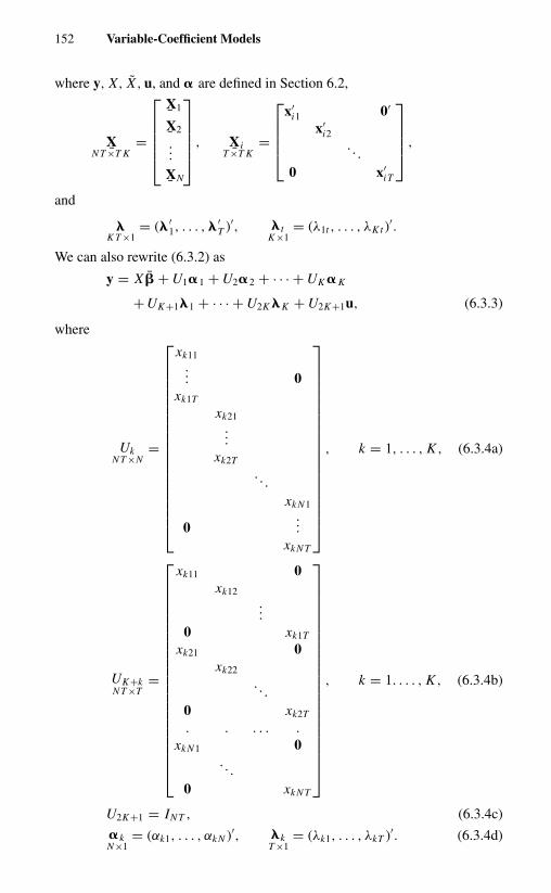
152 Variable-Coefficient Models
where y, X, X , u, and � are defined in Section 6.2,
X¯N T ×T K
=
X1¯X2
...XN¯
, Xi¯T ×T K=
x′
i1 0′
x′i2
. . .0 x′
iT
,
and
�K T ×1
= (� ′1, . . . , � ′
T )′, � tK×1
= (λ1t , . . . , λK t )′.
We can also rewrite (6.3.2) as
y = X � + U1�1 + U2�2 + · · · + UK � K
+ UK+1�1 + · · · + U2K �K + U2K+1u, (6.3.3)
where
UkN T ×N
=
xk11... 0
xk1T
xk21...
xk2T
. . .xk N1
0...
xk N T
, k = 1, . . . , K , (6.3.4a)
UK+kN T ×T
=
xk11 0xk12
...0 xk1T
xk21 0xk22
. . .0 xk2T
. . . . . .
xk N1 0. . .
0 xk N T
, k = 1. . . . , K , (6.3.4b)
U2K+1 = IN T , (6.3.4c)
� kN×1
= (αk1, . . . , αk N )′, �kT ×1
= (λk1, . . . , λkT )′. (6.3.4d)

6.3 Coefficients That Vary over Time and Cross-Sectional Units 153
When � k and �k as well as � are considered fixed, it is a fixed-effects model;when � k and �k are considered random, with � fixed, equation (6.3.3) cor-responds to the mixed analysis-of-variance model (Hartley and Rao (1967),Miller (1977)). Thus, model (6.3.1) and its special case (6.2.1) fall within thegeneral analysis-of-variance framework.
6.3.2 Fixed-Coefficient Model
When � k and �k are treated as fixed, as mentioned earlier, (6.3.1) can beviewed as a fixed-effects analysis-of-variance model. However, the matrix ofexplanatory variables is N T × (T + N + 1)K , but its rank is only (T + N −1)K ; so we must impose 2K independent linear restrictions on the coefficients� k and �k for estimation of �, � , and �. A natural way of imposing theconstraints in this case is to let9
N∑i=1
αik = 0, (6.3.5)
andT∑
t=1
λkt = 0, k = 1, . . . , K . (6.3.6)
Then the best linear unbiased estimators (BLUEs) of �, � , and � are the solu-tions of
min(y − X � − X� − X¯
�)′(y − X � − X� − X¯
�) (6.3.7)
subject to (6.3.5) and (6.3.6).
6.3.3 Random-Coefficient Model
When � i and � t are treated as random, Hsiao (1974a, 1975) assumes that
E� i �′j
K×K
={ if i = j,0 if i �= j,
(6.3.8)E� t �
′s
K×K
={� if t = s,0 if t �= s,
E� i �′t = 0, E� i x′
i t = 0, E� t x′i t = 0,
and
Eui u′j =
{σ 2
u IT if i = j,
0 if i �= j.
Then the composite error term,
v = X� + X¯
� + u, (6.3.9)

154 Variable-Coefficient Models
has a variance–covariance matrix
� = Evv′ =
X1X ′
1 0X2X ′
2. . .
0 X N X ′N
+
D(X1�X ′
1) D(X1�X ′2) · · · D(X1�X ′
N )
D(X2�X ′1) D(X2�X ′
2) . . . D(X2�X ′N )
......
. . ....
D(X N �X ′1) D(X N �X ′
2) · · · D(X N �X ′N )
+ σ 2u IN T ,
(6.3.10)
where
D(Xi�X ′j )
T ×T
=
x′
i1�x j1 0x′
i2�x j2
. . .0 x′
iT �x jT
.
We can estimate � by the least-squares method, but as discussed inSection 6.2.2.b, it is not efficient. Moreover, the associated sampling theoryis misleading.
If � is known, the BLUE of � is the GLS estimator,
ˆ�GLS = (X ′�−1 X )−1(X ′�−1y). (6.3.11)
The variance–covariance matrix of the GLS estimator is
Var( ˆ�GLS) = (X ′�−1 X )−1. (6.3.12)
Without knowledge of �, we can estimate � and � simultaneously by themaximum likelihood method. However, because of the computational difficulty,a natural alternative is to first estimate �, then substitute the estimated � in(6.3.11).
When and � are diagonal, it is easy to see from (6.3.3) that � is a linearcombination of known matrices with unknown weights. So the problem of es-timating the unknown covariance matrix is actually the problem of estimatingthe variance components. Statistical methods developed for estimating the vari-ance (and covariance) components can be applied here (e.g., Anderson (1969,1970); Rao (1970, 1972)). In this section we shall describe only a method dueto Hildreth and Houck (1968).10
Consider the time-series equation for the i th individual,
yi = Xi (� + � i ) + Xi¯� + ui . (6.3.13)
We can treat � i as if it is a vector of constants. Then (6.3.13) is a lin-ear model with heteroscedastic variance. The variance of the error term

6.3 Coefficients That Vary over Time and Cross-Sectional Units 155
rit = ∑Kk=1 λkt xkit + uit is
θi t = E[r2
i t
] =K∑
k=1
σ 2λk x2
ki t + σ 2u . (6.3.14)
Let �i = (θi1, . . . , θiT )′; then
�i = Xi �2λ, (6.3.15)
where Xi is Xi with each of its elements squared, and �2λ = (σ 2
λ1 +σ 2
u , σ 2λ2, . . . , σ
2λK )′.
An estimate of ri can be obtained as the least-squares residual, ri =yi − Xi �i = Mi yi , where �i = (X ′
i Xi )−1 X ′i yi and Mi = IT − Xi (X ′
i Xi )−1 X ′i .
Squaring each element of ri and denoting it by ri , we have
E(˙ri ) = Mi �i = Fi �2λ, (6.3.16)
where Mi is Mi with each of its elements squared, and Fi = Mi X i .Repeating the foregoing process for all i gives
E(˙r) = F�2λ, (6.3.17)
where ˙r = (˙r1, . . . , ˙rN )′, and F = (F ′1, . . . , F ′
N )′. Application of least squaresto (6.3.17) yields a consistent estimator of σ2
λ,
�2λ = (F ′F)−1 F ′ ˙r. (6.3.18)
Similarly, we can apply the same procedure with respect to each time periodto yield a consistent estimator of �2
α = (σ 2α1
+ σ 2u , σ 2
α2, . . . , σ 2
αK)′. To obtain
separate estimates of σ 2u , σ 2
α1, and σ 2
λ1, we note that E(x′
i t � i + uit )(x′i t � t +
uit ) = σ 2u . So, letting si t denote the residual obtained by applying least squares
separately to each time period, we can consistently estimate σ 2u by
σ 2u = 1
N T
N∑i=1
T∑t=1
ri t si t . (6.3.19)
Subtracting (6.3.19) from an estimated σ 2α1
+ σ 2u and σ 2
λ1+ σ 2
u , we obtain con-sistent estimates of σ 2
α1, and σ 2
λ1, respectively.
Substituting consistently estimated values of �2α , �2
λ, and σ 2u into (6.3.11),
one can show that when N and T both tend to infinity and N/T tends to anonzero constant, the two-stage Aitken estimator is asymptotically as efficientas if one knew the true �. Also, Kelejian and Stephan (1983) have pointed outthat, contrary to the conventional regression model, the speed of convergenceof ˆ�GLS here is not (N T )1/2, but max(N 1/2, T 1/2).
If one is interested in predicting the random components associated with anindividual, Lee and Griffiths (1979) have shown that the predictor
� = (IN ⊗ )X ′�−1(y − X ˆ�GLS) (6.3.20)
is the BLUE.
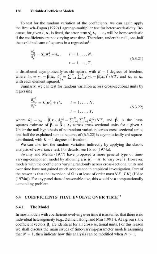
156 Variable-Coefficient Models
To test for the random variation of the coefficients, we can again applythe Breusch–Pagan (1979) Lagrange-multiplier test for heteroscedasticity. Be-cause, for given i , � i is fixed, the error term x′
i t � t + uit will be homoscedasticif the coefficients are not varying over time. Therefore, under the null, one-halfthe explained sum of squares in a regression11
u2i t
σ 2u
= x′i t �
2λ + εi t , i = 1, . . . , N ,
(6.3.21)t = 1, . . . , T,
is distributed asymptotically as chi-square, with K − 1 degrees of freedom,where ui t = yit − �′
i xi t , σ2u = ∑N
i=1
∑Tt=1(yit − �′
i xi t )2/N T , and xi t is xi t
with each element squared.12
Similarly, we can test for random variation across cross-sectional units byregressing
u∗2i t
σ ∗2u
= x′i t �
2α + ε∗
i t , i = 1, . . . , N ,(6.3.22)
t = 1, . . . , T,
where u∗i t = yit − �
′t xi t , σ
∗2u = ∑N
t=1
∑Tt=1 u∗2
i t /N T , and �t is the least-squares estimate of �t = � + � t across cross-sectional units for a given t .Under the null hypothesis of no random variation across cross-sectional units,one-half the explained sum of squares of (6.3.22) is asymptotically chi-square-distributed, with K − 1 degrees of freedom.
We can also test the random variation indirectly by applying the classicanalysis-of-covariance test. For details, see Hsiao (1974a).
Swamy and Mehta (1977) have proposed a more general type of time-varying-component model by allowing E� t �
′t = �t to vary over t . However,
models with the coefficients varying randomly across cross-sectional units andover time have not gained much acceptance in empirical investigation. Part ofthe reason is that the inversion of � is at least of order max(N K , T K ) (Hsiao(1974a)). For any panel data of reasonable size, this would be a computationallydemanding problem.
6.4 COEFFICIENTS THAT EVOLVE OVER TIME13
6.4.1 The Model
In most models with coefficients evolving over time it is assumed that there is noindividual heterogeneity (e.g., Zellner, Hong, and Min (1991)). At a given t , thecoefficient vectors �t are identical for all cross-sectional units. For this reasonwe shall discuss the main issues of time-varying-parameter models assumingthat N = 1, then indicate how this analysis can be modified when N > 1.

6.4 Coefficients That Evolve over Time 157
As shown by Chow (1983, Chapter 10), a wide variety of time-varying-parameter models can be put in the general form
yt = �′t xt + ut , (6.4.1)
and
�t = H�t−1 + �t , t = 1, . . . , T, (6.4.2)
where xt is a K × 1 vector of exogenous variables, ut is independent normalwith mean zero and variance σ 2
u , �t is a K -variant independent normal randomvariable with mean zero and covariance matrix �, and � and u are indepen-dent. For instance, when H = IK , it is the random-walk model of Cooley andPrescott (1976). When H = IK and � = 0, this model is reduced to the standardregression model.
The Rosenberg (1972, 1973) return-to-normality model can also be put in thisform. The model corresponds to replacing �t and �t−1 in (6.4.2) by (�t − �)and (�t−1 − �) and restricting the absolute value of the characteristic roots ofH to less than 1. Although this somewhat changes the formulation, if we define�∗
t = �t − � and �t = �, the return-to-normality model can be rewritten as
yt = (x′t , x′
t )
[�t
�∗t
]+ ut ,
(6.4.3)[�t
�∗t
]=
[I 00 H
][�t−1
�∗t−1
]+
[0�t
],
which is a special case of (6.4.1) and (6.4.2).Similarly, we can allow �t to be stationary, with constant mean � (Pagan
(1980)). Suppose
yt = x′t � + x′
t �∗t + ut ,
(6.4.4)�∗
t = �t − � = A−1(L)�t ,
where A(L) is a ratio of polynomials of orders p and q in the lag operatorL (L�t = �t−1), and � is independent normal, so that �∗
t follows an autoregres-sive moving-average (ARMA) (p, q) process. Because an ARMA of order pand q can be written as a first-order autoregressive process, this model can againbe put in the form of (6.4.1) and (6.4.2). For example,
�∗t = B1�∗
t−1 + B2�∗t−2 + �t + B3�t−1 (6.4.5)
can be written as
�∗t =
�∗t
�∗t−1
�t
=B1 B2 B3
I 0 00 0 0
�∗
t−1
�∗t−2
�t−1
+�t
0�t
= H �∗t−1 + �t .
(6.4.6)

158 Variable-Coefficient Models
Thus, we can write Pagan’s model in the form
yt = (x′t , x′
t )
[�t
�∗t
]+ ut , (6.4.4a)
where x ′t = (x′
t , 0′, 0′). Equation (6.4.4a) is then formally equivalent to (6.4.3).The Kalman filter (Kalman (1960)) provides a basis for computing the max-
imum likelihood estimators and predicting the evolution of the time path of �t
for this type of model. In this section we first consider the problem of estimating�t using informationIs , up to the time s, assuming that σ 2
u , �, and H are known.We denote the conditional expectation of �t , given Is , as E(�t | Is) = �t |s . Theevaluation of �t |s is called filtering when t = s; it is called smoothing whens > t ; it is called prediction when s < t . We then study the problem of estimat-ing σ 2
u , �, and H by the method of maximum likelihood. Finally, we considerthe problem of testing for constancy of the parameters.
6.4.2 Predicting �t by the Kalman Filter
Denote (y1, . . . , yt ) by Yt . By definition, the conditional mean of �t , givenYt , is
�t |t = E(�t | yt , Yt−1)
= E(�t | Yt−1) + Lt [yt − E(yt | Yt−1)]
= �t |t−1 + Lt [yt − x′t �t |t−1], (6.4.7)
where yt − E(yt | Yt−1) denotes the additional information of yt not containedin Yt−1, and Lt denotes the adjustment of �t |t−1 due to this additional infor-mation. If Lt is known, (6.4.7) can be used to update our estimate �t |t−1 toform �t |t .
To derive Lt , we know from our assumption on �t and ut that, conditional onxt , yt and �t are jointly normally distributed. The normal-distribution theory(Anderson (1958, Chapter 2)) states that, conditional on Yt−1 (and Xt ), themean of �t , given yt , is E(�t | Yt−1) + Cov(�t , yt | Yt−1) Var(yt | Yt−1)−1[yt −E(yt | Yt−1)]. Therefore,
Lt = [E(�t − �t |t−1)(yt − yt |t−1)] Var(yt | Yt−1)−1, (6.4.8)
where yt |t−1 = E(yt | Yt−1) = x′t �t |t−1. Denoting the covariance matrix
Cov(�t | Yt−1) = E(�t − �t |t−1)(�t − �t |t−1)′ by �t |t−1, we have
E(�t − �t |t−1)(yt − yt |t−1)
= E{(�t − �t |t−1)[(�t − �t |t−1)′xt + ut ]} = �t |t−1xt , (6.4.9)
and
Var(yt | Yt−1) = E[x′t (�t − �t |t−1) + ut ][(�t − �t |t−1)′xt + ut ]
= x′t�t |t−1xt + σ 2
u . (6.4.10)
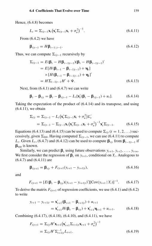
6.4 Coefficients That Evolve over Time 159
Hence, (6.4.8) becomes
Lt = �t |t−1xt(x′
t�t |t−1xt + σ 2u
)−1. (6.4.11)
From (6.4.2) we have
�t |t−1 = H�t−1 | t−1. (6.4.12)
Thus, we can compute �t |t−1 recursively by
�t |t−1 = E(�t − H�t−1|t−1)(�t − H�t−1|t−1)′
= E[H (�t−1 − �t−1|t−1) + �t ]
× [H (�t−1 − �t−1|t−1) + �t ]′
= H�t−1|t−1 H ′ + �. (6.4.13)
Next, from (6.4.1) and (6.4.7) we can write
�t − �t |t = �t − �t |t−1 − Lt [x′t (�t − �t |t−1) + ut ]. (6.4.14)
Taking the expectation of the product of (6.4.14) and its transpose, and using(6.4.11), we obtain
�t |t = �t |t−1 − Lt(x′
t�t |t−1xt + σ 2u
)L ′
t
= �t |t−1 − �t |t−1xt(x′
t�t |t−1xt + σ 2u
)−1x′
t�t |t−1. (6.4.15)
Equations (6.4.13) and (6.4.15) can be used to compute �t |t (t = 1, 2, . . .) suc-cessively, given �0|0. Having computed �t |t−1, we can use (6.4.11) to computeLt . Given Lt , (6.4.7) and (6.4.12) can be used to compute �t |t from �t−1|t−1 if�0|0 is known.
Similarly, we can predict �t using future observations yt+1, yt+2, . . . , yt+n .We first consider the regression of �t on yt+1, conditional on Yt . Analogous to(6.4.7) and (6.4.11) are
�t |t+1 = �t |t + Ft |t+1(yt+1 − yt+1|t ), (6.4.16)
and
Ft |t+1 = [E(�t − �t |t )(yt+1 − yt+1|t )′][Cov(yt+1 | Yt )]−1. (6.4.17)
To derive the matrix Ft |t+1 of regression coefficients, we use (6.4.1) and (6.4.2)to write
yt+1 − yt+1|t = x′t+1(�t+1 − �t+1|t ) + ut+1
= x′t+1 H (�t − �t |t ) + x′
t+1�t+1 + ut+1. (6.4.18)
Combining (6.4.17), (6.4.18), (6.4.10), and (6.4.11), we have
Ft |t+1 = �t |t H ′xt+1(x′
t+1�t+1|t xt+1 + σ 2u
)−1
= �t |t H ′�−1t+1|t Lt+1. (6.4.19)

160 Variable-Coefficient Models
Therefore, from (6.4.19) and (6.4.14), we can rewrite (6.4.16) as
�t |t+1 = �t |t + �t |t H ′�−1t+1|t (�t+1|t+1 − �t+1|t ). (6.4.20)
Equation (6.4.20) can be generalized to predict �t using future observationsyt+1, . . . , yt+n:
�t |t+n = �t |t+n−1 + F∗t (�t+1|t+n − �t+1|t+n−1), (6.4.21)
where F∗t = �t |t H ′�−1
t+1|t . The proof of this is given by Chow (1983,Chapter 10).
When H , �, and σ 2u are known, (6.4.7) and (6.4.21) trace out the time path of
�t and provide the minimum-mean-squared-error forecast of the future valuesof the dependent variable, given the initial values �0|0 and �0|0. To obtain theinitial values of �0|0 and �0|0, Sant (1977) suggested using the generalizedleast-squares method on the first K observations of yt and xt . Noting that
�t = H�t−1 + �t
= H 2�t−2 + �t + H�t−1
= H t− j � j + �t + H�t−1 + · · · + H t− j−1� j , (6.4.22)
and assuming that H−1 exists, we can also write yk in the form
yk = x′k�k + uk
= x′k[H−K+k�K − H−K+k�K − · · · − H−1�k+1] + uk .
Thus, (y1, . . . , yK ) can be written asy1
y2...
yK
=
x′
1 H−K+1
x′2 H−K+2
...x′
K
�K +
u1
u2...
uK
−
x′
1 H−1 x′1 H−2 . . . x′
1 H−K+1
0′ x′2 H−1 . . . x′
2 H−K+2
. . ....
x′K−1 H−1
0′
�2�3...
�K
. (6.4.23)
Applying GLS to (6.4.23) gives
�K |K = σ 2u {[H ′−K+1x1, H ′−K+2x2, . . . , xK ]
× [IK + AK (IK−1 ⊗ P)A′K ]−1[H−K+1x1, . . . , xK ]′}−1,
(6.4.24)

6.4 Coefficients That Evolve over Time 161
and
�K |K = 1
σ 2u
�K |K [H ′−K+1x1, H ′−K+2x2, . . . , xK ]
× [IK + AK (IK−1 ⊗ P)A′K ]−1
y1...
yK
, (6.4.25)
where P = σ−2u �, and AK is the coefficient matrix of (�2, . . . , �K )′ in (6.4.23).
The initial estimators, �K |K and �K |K , are functions of σ 2u , �, and H .
6.4.3 Maximum Likelihood Estimation
When H , �, and σ 2u are unknown, (6.4.7) opens the way for maximum likeli-
hood estimation without the need for repeated inversions of covariance matricesof large dimensions. To form the likelihood function, we note that
yt − yt |t = x′t (�t − �t |t−1) + ut = yt − x ′
t �t |t−1 (6.4.26)
is normal and serially uncorrelated. Hence, the joint density of (y1, . . . , yT )can be written as the product of the conditional density of (yK+1, . . . , yT |y1, . . . , yK ) and the marginal density of (y1, . . . , yK ). The log likelihood func-tion of (yK+1, . . . , yT ), given (y1, . . . , yK ), is
log L = −T − K
2log 2π − 1
2
T∑t=K+1
log(x′
t�t |t−1xt + σ 2u
)− 1
2
T∑t=K+1
(yt − x′t �t |t−1)2
x′t�t |t−1xt + σ 2
u
. (6.4.27)
The first K observations are used to compute �K |K and �K |K [equations (6.4.24)and (6.4.25)] as functions of σ 2
u , �, and H . Hence, the data �t |t−1 and �t |t−1
(t = K + 1, . . . , T ) required to evaluate log L are functions of σ 2u , �, and H ,
as given by (6.4.13), (6.4.15), (6.4.12), and (6.4.11). To find the maximum of(6.4.27), numerical methods will have to be used.
When we estimate the model (6.4.1) and (6.4.2) using panel data, all thederivations in Section 6.4.2 remain valid if we replace yt , xt , ut , and σ 2
u by theN × 1 vector yt = (y1t , . . . , yNt )′, the N × K matrix Xt = (x1t , . . . , xN T )′, theN × 1 vector ut = (u1t , . . . , uNt )′, and σ 2
u IN in appropriate places. The MLEcan be carried out in the same way as outlined in this section, except that thelikelihood function (6.4.27) is replaced by
log L = const − 1
2
∑t
log∣∣X ′
t�t |t−1 Xt + σ 2u IN
∣∣− 1
2
∑t
(yt − Xt �t |t−1)′
× (Xt�t |t−1 X ′
t + σ 2u IN
)−1(yt − Xt �t |t−1). (6.4.27′)

162 Variable-Coefficient Models
However, we no longer need to use the first K period observations to start theiteration. If N > K , we need to use only the first-period cross-sectional data toobtain �1|1 and �1|1. Additional details with regard to the computation can befound in Harvey (1978) and Harvey and Phillips (1982).
6.4.4 Tests for Parameter Constancy
A simple alternative to the null hypothesis of constancy of regression coeffi-cients over time is
�t = �t−1 + �t , (6.4.28)
where �t is assumed independently normally distributed, with mean zero anda diagonal covariance matrix �. Regarding �0 as fixed, we have
�t = �0 +t∑
s=1
�s . (6.4.29)
Thus, the regression model becomes
yt = x′t �t + ut = x′
t �0 + ut + x′t
(t∑
s=1
�s
)= x′
t �0 + u∗t , (6.4.30)
where u∗t = ut + x′
t (∑t
s=1�s) has variance
Eu∗2t = σ 2
u + tx′t�xt . (6.4.31)
For � = diag{ψkk}, (6.4.31) becomes
Eu∗2t = σ 2
u + tK∑
k=1
x2ktψkk, t = 1. . . . , T . (6.4.32)
The null hypothesis states that � = 0. Hence, the Breusch–Pagan(1979) Lagrange-multiplier test applied here is to regress u2
t /σ2u on
t(1, x22t , . . . , x2
K t ), t = 1, . . . , T , where ut is the least-squares residual ut =yt − �
′xt , � = (
∑Tt=1 xt x′
t )−1(
∑Tt=1 xt yt ), and σ 2
u = ∑Tt=1 u2
t /T . Under thenull hypothesis, one-half the explained sum of squares of this regression isasymptotically chi-square-distributed, with K degrees of freedom.14
When panel data are available, it is possible to test for parameter constancyindirectly using the classic analysis-of-covariance test. By the assumption thatthe parameter vector �t is constant over cross-sectional units in the sampleperiod, an indirect test is to postulate the null hypothesis
H0 : �1 = �2 = · · · = �T = �.
If the disturbances of the regression model yit = �′t xi t + uit are independently
normally distributed over i and t , then the test statistic F ′3 from Chapter 2 has

6.5 Coefficients That Are Functions of Other Exogenous Variables 163
an F distribution with (T − 1)K and N (T − K ) degrees of freedom under thenull.
If the null hypothesis is rejected, we can use the information that under mildregularity conditions plimN→∞�t = �t , t = 1, . . . , T , to investigate the natureof variation in the parameters over time. We can apply the Box–Jenkins (1970)method on �t to identify a suitable stochastic process with which to model theparameter variation.
6.5 COEFFICIENTS THAT ARE FUNCTIONS OFOTHER EXOGENOUS VARIABLES
Sometimes, instead of assuming that parameters are random draws from a com-mon distribution, an investigation of possible dependence of �i t on characteris-tics of the individuals or time is of considerable interest (e.g., Amemiya (1978b);Hendricks, Koenker, and Poirier (1979); Singh et al. (1976); Swamy and Tinsley(1977); Wachter (1970)). A general formulation of stochastic-parameter modelswith systematic components can be expressed within the context of the linearmodel. Suppose that
yi = Xi1�1 + Xi2�2i + ui , i = 1, . . . , N , (6.5.1)
and
�2i = Zi � + �2i (6.5.2)
where Xi1 and Xi2 denote the T × K1 and T × K2 matrices of the time-seriesobservations of the first K1 and last K2 (= K − K1) exogenous variables forthe i th individual, �1 is a K1 × 1 vector of fixed constants, �2i is a K2 × 1vector that varies according to (6.5.2), Zi and � are a K2 × M matrix of knownconstants and a M × 1 vector of unknown constants, respectively, and ui and �2i
are T × 1 and K2 × 1 vectors of unobservable random variables. For example,in Wachter (1970), yi is a vector of time-series observations on the logarithmof the relative wage rate in the i th industry. Xi1 contains the logarithms of suchvariables as the relative value added in the i th industry and the change in theconsumer price, Xi2 consists of a single vector of time-series observations onthe logarithm of unemployment, and Zi contains the degree of concentrationand the degree of unionization in the i th industry.
For simplicity, we assume that ui and �2i are uncorrelated with each otherand have zero means. The variance–covariance matrices of ui and �2i are givenby
Eui u′j = σi j IT , (6.5.3)
and
E�2i �′2 j =
{� if i = j,0 if i �= j.
(6.5.4)

164 Variable-Coefficient Models
Let � = (σi j ). We can write the variance–covariance matrices of u =(u′
1, . . . , u′N )′ and �2 = (�′
21, . . . , �′2N )′ as
Euu′ = � ⊗ IT , (6.5.5)
and
E�2�′2 =
� 0. . .
0 �
= �. (6.5.6)
Combining (6.5.1) and (6.5.2), we have
y = X1�1 + W� + X2�2 + u, (6.5.7)
where
yN T ×1
= (y′1, . . . , y′
N )′,
X1N T ×K1
= (X ′11, . . . , X ′
N1)′,
WN T ×M
= (Z ′1 X ′
12, Z ′2 X ′
22, . . . , Z ′N X ′
N2)′,
X2N T ×N K2
=
X12 0
X22
. . .0 X N2
,
and
�2N K2×1
= (�′21, . . . , �′
2N )′.
The BLUE of �1 and � of (6.5.7) is the GLS estimator[�1�
]GLS
={[
X ′1
W ′
][� ⊗ IT + X2�X ′
2]−1(X1, W )
}−1
×{[
X ′1
W ′
][� ⊗ IT + X2�X ′
2]−1y}
. (6.5.8)
If � is diagonal, the variance–covariance matrix of the stochastic term of(6.5.7) is block-diagonal, with the i th diagonal block equal to
�i = Xi2�X ′i2 + σi i IT . (6.5.9)
The GLS estimator (6.5.8) can be simplified as[�1�
]GLS
=[
N∑i=1
[X ′
i1
Z ′i X ′
i2
]�−1
i (Xi1, X2i Zi )
]−1
×[
N∑i=1
[X ′
i1
Z ′i X ′
i2
]�−1
i yi
]. (6.5.10)

6.6 A Mixed Fixed- and Random-Coefficients Model 165
Amemiya (1978b) suggested estimating � and σi j as follows. Let
y1...
yN
=
X11...
X N1
�1 +
X12
0...0
�21 +
0
X22...0
�22
+ · · · +
0...
X N2
�2N +
u1...
uN
. (6.5.11)
Apply the least-squares method to (6.5.11). Denote the resulting estimates by�1 and �2i , i = 1, . . . , N . Then σi j can be estimated by
σi j = 1
T(yi − Xi1�1 − Xi2�2i )
′(y j − X j1�1 − X j2�2 j ), (6.5.12)
and � can be estimated by
� =(
N∑i=1
Z ′i Zi
)−1 (N∑
i=1
Z ′i �2i
). (6.5.13)
We then estimate � by
� = 1
N
N∑i=1
(�2i − Zi �)(�2i − Zi �)′. (6.5.14)
Once consistent estimates of σi j and � are obtained (as both N and T ap-proach infinity), we can substitute them into (6.5.8). The resulting two-stageAitken estimator of (�′
1, �′) is consistent and asymptotically normally dis-tributed under general conditions. A test of the hypothesis that � = 0 can beperformed in the usual regression framework using
Var(�GLS) = [W ′�−1W − W ′�−1 X1(X ′1�
−1 X1)−1 X ′1�
−1W ]−1,
(6.5.15)
where
� = X2�X ′2 + � ⊗ IT .
6.6 A MIXED FIXED- ANDRANDOM-COEFFICIENTS MODEL
6.6.1 Model Formulation
Many of the previously discussed models can be treated as special cases of ageneral mixed fixed- and random-coefficients model. For ease of exposition,we shall assume that only time-invariant cross-sectional heterogeneity exists.

166 Variable-Coefficient Models
Suppose that each cross-sectional unit is postulated to be different, so that
yit =K∑
k=1
βki xkit +m∑
�=1
γ�i w�i t + uit , i = 1, . . . , N ,(6.6.1)
t = 1, . . . , T,
where xi t and wi t are each a K × 1 and an m × 1 vector of explanatory vari-ables that are independent of the error of the equation, uit . Stacking the N Tobservations together, we have
y = X� + W � + u, (6.6.2)
where
XN T ×N K
=
X1 0 . . . 00 X2 . . . 0...
. . ....
0 X N
,
WN T ×Nm
=
W1 0 . . . 00 W2 . . . 0...
. . ....
0 WN
,
uN T ×1
= (u′1, . . . , u′
N ),
�N K×1
= (�′1, . . . , �′
N )′ and �Nm×1
= (�′1, . . . , �′
N )′.
Equation (6.6.1), just like (6.2.2), assumes a different behavioral-equation rela-tion for each cross-sectional unit. In this situation, the only advantage of poolingis to put the model (6.6.2) in Zellner’s (1962) seemingly unrelated regressionframework to obtain efficiency of the estimates of the individual behavioralequation.
The motivation of a mixed fixed- and random-coefficients model is thatwhile there may be fundamental differences among cross-sectional units, byconditioning on these individual specific effects one may still be able to drawinferences on certain population characteristics through the imposition of a pri-ori constraints on the coefficients of xi t and wi t . We assume that there exist twokinds of restrictions, stochastic and fixed (e.g., Hsiao (1991a); Hsiao, Appelbe,and Dineen (1993)), in the following form:
A.6.6.1. The coefficients of xi t are assumed to be subject to stochastic restric-tions of the form
� = A1� + �, (6.6.3)
where A1 is an N K × L matrix with known elements, � is an L × 1vector of constants, and � is assumed to be (normally distributed)
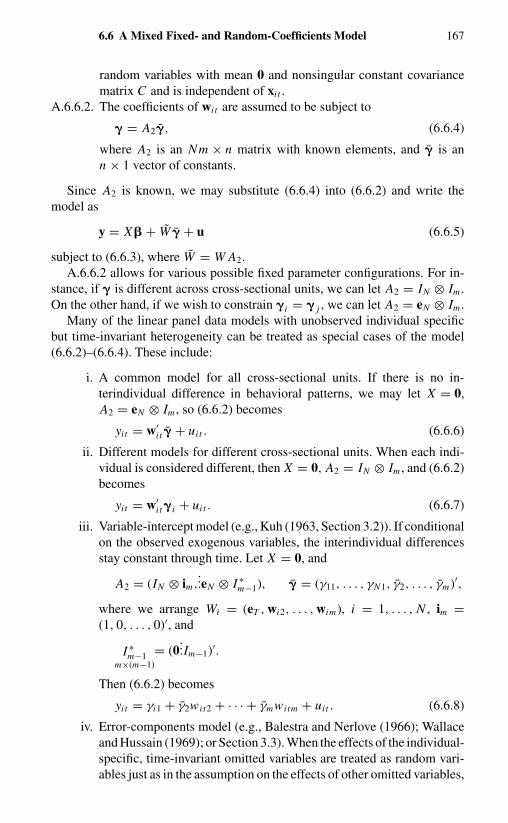
6.6 A Mixed Fixed- and Random-Coefficients Model 167
random variables with mean 0 and nonsingular constant covariancematrix C and is independent of xi t .
A.6.6.2. The coefficients of wi t are assumed to be subject to
� = A2�, (6.6.4)
where A2 is an Nm × n matrix with known elements, and � is ann × 1 vector of constants.
Since A2 is known, we may substitute (6.6.4) into (6.6.2) and write themodel as
y = X� + W � + u (6.6.5)
subject to (6.6.3), where W = W A2.A.6.6.2 allows for various possible fixed parameter configurations. For in-
stance, if � is different across cross-sectional units, we can let A2 = IN ⊗ Im .On the other hand, if we wish to constrain �i = � j , we can let A2 = eN ⊗ Im .
Many of the linear panel data models with unobserved individual specificbut time-invariant heterogeneity can be treated as special cases of the model(6.6.2)–(6.6.4). These include:
i. A common model for all cross-sectional units. If there is no in-terindividual difference in behavioral patterns, we may let X = 0,A2 = eN ⊗ Im , so (6.6.2) becomes
yit = w′i t � + uit . (6.6.6)
ii. Different models for different cross-sectional units. When each indi-vidual is considered different, then X = 0, A2 = IN ⊗ Im , and (6.6.2)becomes
yit = w′i t �i + uit . (6.6.7)
iii. Variable-intercept model (e.g., Kuh (1963, Section 3.2)). If conditionalon the observed exogenous variables, the interindividual differencesstay constant through time. Let X = 0, and
A2 = (IN ⊗ im,...eN ⊗ I ∗
m−1), � = (γ11, . . . , γN1, γ2, . . . , γm)′,
where we arrange Wi = (eT , wi2, . . . , wim), i = 1, . . . , N , im =(1, 0, . . . , 0)′, and
I ∗m−1
m×(m−1)
= (0...Im−1)′.
Then (6.6.2) becomes
yit = γi1 + γ2wit2 + · · · + γmwitm + uit . (6.6.8)
iv. Error-components model (e.g., Balestra and Nerlove (1966); Wallaceand Hussain (1969); or Section 3.3). When the effects of the individual-specific, time-invariant omitted variables are treated as random vari-ables just as in the assumption on the effects of other omitted variables,

168 Variable-Coefficient Models
we can let Xi = eT , � ′ = (α1, . . . , αN ), A1 = eN , C = σ 2α IN , β be an
unknown constant, and wi t not contain an intercept term. Then (6.4.2)becomes
yit = β + �′wi t + αi + uit . (6.6.9)
v. Random-coefficients model (Swamy (1970), or Section 6.2.2). LetZ = 0, A1 = eN ⊗ IK , and C = IN ⊗ . Then we have model (6.2.4).
6.6.2 A Bayes Solution
The formulation of (6.6.5) subject to (6.6.3) can be viewed from a Bayesianperspective, as there exists an informative prior on � (6.6.3), but not on �. In theclassical sampling approach, inferences are made typically by assuming thatthe probability law f (y, �) generating the observations y is known, but not thevector of constant parameters �. Estimators �(y) of the parameters � are chosenas functions of y so that their sampling distributions, in repeated experiments,are, in some sense, concentrated as closely as possible about the true valuesof �. In the Bayesian approach, a different line is taken. First, all quantities,including the parameters, are considered random variables. Second, all proba-bility statements are conditional, so that in making a probability statement it isnecessary to refer to the conditioning event as well as the event whose prob-ability is being discussed. Therefore, as part of the model, a prior distributionp(�) of the parameter � is introduced. The prior distribution is supposed to ex-press a state of knowledge (or ignorance) about � before the data are obtained.Given the probability model f (y; �), the prior distribution, and the data y, theprobability distribution of � is revised to p(� | y), which is called the posteriordistribution of �, according to Bayes’ theorem (e.g., Kaufman (1977),Intriligator, Bodkin, and Hsiao (1996)):15
P(� | y) ∝ p(�) f (y | �), (6.6.10)
where the sign “∝” denotes “is proportional to,” with the factor of proportion-ality being a normalizing constant.
Under the assumption that
A.6.6.3. u ∼ N (0, �),
we may write the model (6.6.5) as follows:
A.1. Conditional on X, W , �, and �,
y ∼ N (X� + W �, �). (6.6.11)
A.2. The prior distributions of � and � are independent:
P(�, �) = P(�) · P(�). (6.6.12)
A.3. P(�) ∼ N (A1�, C).

6.6 A Mixed Fixed- and Random-Coefficients Model 169
A.4. There is no information about � and �; therefore P(�) and P(�) areindependent and
P(�) ∝ constant,
P(�) ∝ constant.
Conditional on � and C , repeatedly applying the formulas in Appendix 6Ayields (Hsiao, Appelbe, and Dineen (1993)):
i. The posterior distribution of � and � given y is
N
((β∗
�∗
), D1
), (6.6.13)
where
D1 =[(
A′1 X ′
W ′
)(� + XC X ′)−1(X A1, W )
]−1
, (6.6.14)
and(�
∗
�∗
)= D1
[A′
1 X ′
W ′
](� + XC X ′)−1y. (6.6.15)
ii. The posterior distribution of � given � and y is N (�∗, D2), where
D2 = {X ′[�−1 − �−1W (W ′�−1W )−1W ′�−1]X + C−1}−1,
(6.6.16)
�∗ = D2{X ′[�−1 − �−1W (W ′�−1W )−1W ′�−1]y + C−1 A1�}.(6.6.17)
iii. The (unconditional) posterior distribution of � is N (�∗∗, D3), where
D3 = {X ′[�−1 − �−1W (W ′�−1W )−1W ′�−1]X + C−1
− C−1 A1(A′1C−1 A1)−1 A′
1C−1}−1, (6.6.18)
�∗∗ = D3{X ′[�−1 − �−1W (W ′�−1W )−1W ′�−1]y}= D2{X ′[�−1 − �−1W (W ′�−1W )−1W ′�−1]X � + C−1 A1�
∗},(6.6.19)
where � is the GLS estimate of (6.6.5),
� = {X ′[�−1 − �−1W (W ′�−1W )−1W ′�−1]X}−1
× {X ′[�−1 − �−1W (W ′�−1W )−1W ′�−1]y}. (6.6.20)
Given a quadratic loss function of the error of the estimation, a Bayes pointestimate is the posterior mean. The posterior mean of � and � (6.6.15) is theGLS estimator of the model (6.6.5) after substituting the restriction (6.6.3),
y = X A1� + W � + v, (6.6.21)
where v = X� + u. However, the posterior mean of � is not the GLS estimator

170 Variable-Coefficient Models
of (6.6.5). It is the weighted average between the GLS estimator of � and theoverall mean � (6.6.17) or �
∗(6.6.19) with the weights proportional to the in-
verse of the precision of respective estimates. The reason is that although both(6.2.2) and (6.6.5) allow the coefficients to be different across cross-sectionalunits, (6.6.3) has imposed the additional prior information that � are randomlydistributed with mean A1�. For (6.2.2), the best linear predictor for an individ-ual outcome is to substitute the best linear unbiased estimator of the individualcoefficients into the individual equation. For model of (6.6.5) and (6.6.3), be-cause the expected �i is the same across i and the actual difference can beattributed to a chance outcome, additional information about �i may be ob-tained by examining the behavior of others, hence (6.6.17) or (6.6.19).
In the special case of the error-components model (6.6.9), X = IN ⊗ eT .Under the assumption that wi t contains an intercept term (i.e., β = 0) and uit
is i.i.d., the Bayes estimator ((6.6.15)) of � is simply the GLS estimator of(6.6.21) �∗. The Bayes estimator of αi (6.6.17) is
α∗∗i =
(T σ 2
α
T σ 2α + σ 2
u
)ˆvi , (6.6.22)
where ˆvi = 1T
∑Tτ=1 vi t and vi t = yit − �∗wi t . Substituting �∗, and α∗∗
i for theunknown �, and αi in (6.6.9), Wansbeek and Kapteyn (1978) and Taub (1979)show that
yi,T +S = �∗′wi,t+s + α∗∗
i (6.6.23)
is the best linear unbiased predictor (BLUP) for the i th individual s periodsahead.16
6.6.3 An Example
In a classical framework, it makes no sense to predict the independently drawnrandom variable �i (or � i ). However, in panel data, we actually operate withtwo dimensions – a cross-sectional dimension and a time-series dimension.Even though �i is an independently distributed random variable across i , oncea particular �i is drawn, it stays constant over time. Therefore, it makes senseto predict �i . The classical predictor of �i is the generalized least-squaresestimator of the model (6.6.5). The Bayes predictor (6.6.19) is the weightedaverage between the generalized least-squares estimator of � for the model(6.6.5) and the overall mean A1� if � is known, or A1�
∗if � is unknown,
with the weights proportional to the inverse of the precisions of respectiveestimates. The Bayes estimator of the individual coefficients, �i , “shrinks” theGLS estimator of �i toward the grand mean � or �
∗. The reason for doing so
stems from DeFinetti’s (1964) exchangeability assumption. When there are notenough time-series observations to allow for precise estimation of individual�i (namely, T is small), additional information about �i may be obtained by
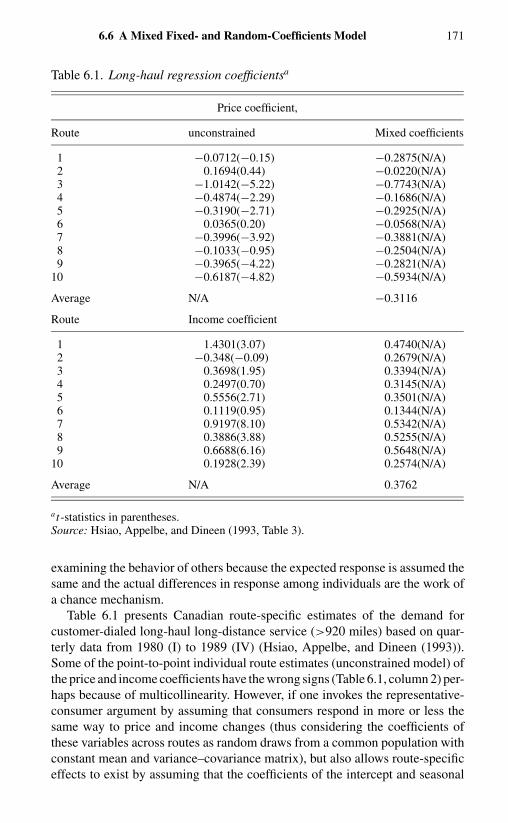
6.6 A Mixed Fixed- and Random-Coefficients Model 171
Table 6.1. Long-haul regression coefficientsa
Price coefficient,
Route unconstrained Mixed coefficients
1 −0.0712(−0.15) −0.2875(N/A)2 0.1694(0.44) −0.0220(N/A)3 −1.0142(−5.22) −0.7743(N/A)4 −0.4874(−2.29) −0.1686(N/A)5 −0.3190(−2.71) −0.2925(N/A)6 0.0365(0.20) −0.0568(N/A)7 −0.3996(−3.92) −0.3881(N/A)8 −0.1033(−0.95) −0.2504(N/A)9 −0.3965(−4.22) −0.2821(N/A)
10 −0.6187(−4.82) −0.5934(N/A)
Average N/A −0.3116
Route Income coefficient
1 1.4301(3.07) 0.4740(N/A)2 −0.348(−0.09) 0.2679(N/A)3 0.3698(1.95) 0.3394(N/A)4 0.2497(0.70) 0.3145(N/A)5 0.5556(2.71) 0.3501(N/A)6 0.1119(0.95) 0.1344(N/A)7 0.9197(8.10) 0.5342(N/A)8 0.3886(3.88) 0.5255(N/A)9 0.6688(6.16) 0.5648(N/A)
10 0.1928(2.39) 0.2574(N/A)
Average N/A 0.3762
at-statistics in parentheses.Source: Hsiao, Appelbe, and Dineen (1993, Table 3).
examining the behavior of others because the expected response is assumed thesame and the actual differences in response among individuals are the work ofa chance mechanism.
Table 6.1 presents Canadian route-specific estimates of the demand forcustomer-dialed long-haul long-distance service (>920 miles) based on quar-terly data from 1980 (I) to 1989 (IV) (Hsiao, Appelbe, and Dineen (1993)).Some of the point-to-point individual route estimates (unconstrained model) ofthe price and income coefficients have the wrong signs (Table 6.1, column 2) per-haps because of multicollinearity. However, if one invokes the representative-consumer argument by assuming that consumers respond in more or less thesame way to price and income changes (thus considering the coefficients ofthese variables across routes as random draws from a common population withconstant mean and variance–covariance matrix), but also allows route-specificeffects to exist by assuming that the coefficients of the intercept and seasonal

172 Variable-Coefficient Models
dummies are fixed and different for different routes, then all the estimatedroute-specific price and income coefficients have the correct signs (Table 6.1,column 3).
6.6.4 Random or Fixed Parameters
6.6.4.a An Example
When homogeneity is rejected by the data, whether to treat unobserved hetero-geneity as fixed or random has paramount importance in panel data modeling.For instance, in a study of Ontario, Canada regional electricity demand, Hsiaoet al. (1989) estimate a model of the form
yit = γi yi,t−1 + �′i di t + �′
i xi t + uit , (6.6.24)
where yit denotes the logarithm of monthly kilowatt-hour or kilowatt demandfor region i at time t , di t denotes 12 monthly dummies, and xi t denotes theclimatic factor and the logarithm of income, own price, and price of its closesubstitutes, all measured in real terms. Four different specifications are consid-ered:
1. The coefficients �′i = (γi , �′
i , �′i ) are fixed and different for different
regions.2. The coefficients �i = �′ = (γ, �′, �′) for all i .3. The coefficients vectors �i are randomly distributed with common
mean � and covariance matrix .4. The coefficients �i are randomly distributed with common mean �
and covariance matrix 11, and the coefficients γi and �i are fixed anddifferent for different i .
Monthly data for Hamilton, Kitchener–Waterloo, London, Ottawa, St.Catherines, Sudbury, Thunder Bay, Toronto, and Windsor from January 1967 toDecember 1982 are used to estimate these four different specifications. Com-parisons of the one-period-ahead root-mean-square prediction error√√√√ T + f∑
t=T +1
(yit − yi t )2/ f
from January 1983 to December 1986 are summarized in Tables 6.2 and 6.3.As one can see from these tables, the simple pooling (model 2) and random-coefficients (model 3) formulations on average yield less precise prediction forregional demand. The mixed fixed- and random-coefficient model (model 4)performs the best. It is interesting to note that combining information acrossregions together with a proper account of region-specific factors is capable ofyielding better predictions for regional demand than the approach of simplyusing region-specific data (model 1).

6.6 A Mixed Fixed- and Random-Coefficients Model 173
Table 6.2. Root-mean-square prediction error of log kilowatt-hours(one-period-ahead forecast)
Root Mean Square Error
Region- RandomMunicipality specific Pooled coefficients Mixed
Hamilton 0.0865 0.0535 0.0825 0.0830Kitchener–Waterloo 0.0406 0.0382 0.0409 0.0395London 0.0466 0.0494 0.0467 0.0464Ottawa 0.0697 0.0523 0.0669 0.0680St. Catharines 0.0796 0.0724 0.0680 0.0802Sudbury 0.0454 0.0857 0.0454 0.0460Thunder Bay 0.0468 0.0615 0.0477 0.0473Toronto 0.0362 0.0497 0.0631 0.0359Windsor 0.0506 0.0650 0.0501 0.0438Unweighted average 0.0558 0.0586 0.0568 0.0545Weighted averagea 0.0499 0.0525 0.0628 0.0487
aThe weight is kilowatt-hours of demand in the municipality in June 1985.Source: Hsiao et al. (1989, p. 584).
6.6.4.b Model Selection
The above example demonstrates that the way in which individual heterogeneityis taken into account makes a difference in the accuracy of inference. The variousestimation methods discussed so far presuppose that we know which coefficients
Table 6.3. Root-mean-square prediction error of log kilowatts (one-period-ahead forecast)
Root Mean Square Error
Regional RandomMunicipality specific Pooled coefficients Mixed
Hamilton 0.0783 0.0474 0.0893 0.0768Kitchener–Waterloo 0.0873 0.0440 0.0843 0.0803London 0.0588 0.0747 0.0639 0.0586Ottawa 0.0824 0.0648 0.0846 0.0768St. Catharines 0.0531 0.0547 0.0511 0.0534Sudbury 0.0607 0.0943 0.0608 0.0614Thunder Bay 0.0524 0.0597 0.0521 0.0530Toronto 0.0429 0.0628 0.0609 0.0421Windsor 0.0550 0.0868 0.0595 0.0543Unweighted average 0.0634 0.0655 0.0674 0.0619Weighted averagea 0.0558 0.0623 0.0673 0.0540
aThe weight is kilowatt-hours of demand in the municipality in June 1985.Source: Hsiao et al. (1989, p. 584).
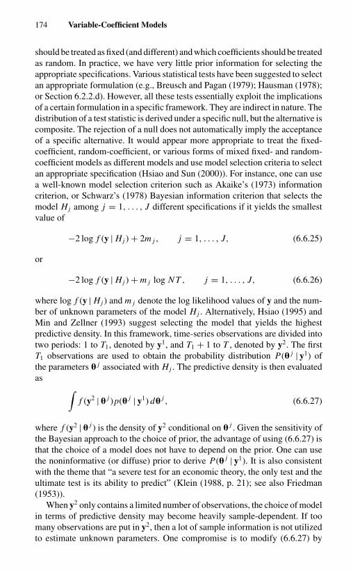
174 Variable-Coefficient Models
should be treated as fixed (and different) and which coefficients should be treatedas random. In practice, we have very little prior information for selecting theappropriate specifications. Various statistical tests have been suggested to selectan appropriate formulation (e.g., Breusch and Pagan (1979); Hausman (1978);or Section 6.2.2.d). However, all these tests essentially exploit the implicationsof a certain formulation in a specific framework. They are indirect in nature. Thedistribution of a test statistic is derived under a specific null, but the alternative iscomposite. The rejection of a null does not automatically imply the acceptanceof a specific alternative. It would appear more appropriate to treat the fixed-coefficient, random-coefficient, or various forms of mixed fixed- and random-coefficient models as different models and use model selection criteria to selectan appropriate specification (Hsiao and Sun (2000)). For instance, one can usea well-known model selection criterion such as Akaike’s (1973) informationcriterion, or Schwarz’s (1978) Bayesian information criterion that selects themodel Hj among j = 1, . . . , J different specifications if it yields the smallestvalue of
−2 log f (y | Hj ) + 2m j , j = 1, . . . , J, (6.6.25)
or
−2 log f (y | Hj ) + m j log N T , j = 1, . . . , J, (6.6.26)
where log f (y | Hj ) and m j denote the log likelihood values of y and the num-ber of unknown parameters of the model Hj . Alternatively, Hsiao (1995) andMin and Zellner (1993) suggest selecting the model that yields the highestpredictive density. In this framework, time-series observations are divided intotwo periods: 1 to T1, denoted by y1, and T1 + 1 to T , denoted by y2. The firstT1 observations are used to obtain the probability distribution P(� j | y1) ofthe parameters � j associated with Hj . The predictive density is then evaluatedas ∫
f (y2 | � j )p(� j | y1) d� j , (6.6.27)
where f (y2 | � j ) is the density of y2 conditional on � j . Given the sensitivity ofthe Bayesian approach to the choice of prior, the advantage of using (6.6.27) isthat the choice of a model does not have to depend on the prior. One can usethe noninformative (or diffuse) prior to derive P(� j | y1). It is also consistentwith the theme that “a severe test for an economic theory, the only test and theultimate test is its ability to predict” (Klein (1988, p. 21); see also Friedman(1953)).
When y2 only contains a limited number of observations, the choice of modelin terms of predictive density may become heavily sample-dependent. If toomany observations are put in y2, then a lot of sample information is not utilizedto estimate unknown parameters. One compromise is to modify (6.6.27) by

6.7 Dynamic Random-Coefficient Models 175
recursively updating the estimates,∫f (yT | � j , yT −1)P(� j | yT −1) d� j
×∫
f (yT −1 | � j , yT −2)P(� j | yT −2) d� j · · ·
×∫
f (yT1+1 | � j , y1)P(� j | y1) d� j , (6.6.28)
where P(� j | yT ) denotes the posterior distribution of � given observationsfrom 1 to T . While the formula may look formidable, it turns out that the Bayesupdating formula is fairly straightforward to compute. For instance, considerthe model (6.6.5). Let � = (�, �), �t , and Vt denote the posterior mean andvariance of � based on the first t observations. Then
�t = Vt−1(Q′
t�−1yt + V −1
t−1�t−1), (6.6.29)
Vt = (Q′
t�−1 Qt + V −1
t−1
)−1, t = T1 + 1, . . . , T, (6.6.30)
and
P(yt+1 | yt ) =∫
P(yt+1 | �, yt )P(� | yt ) d�
∼ N (Qt+1�t , � + Qt+1Vt Q′t+1), (6.6.31)
where y′t = (y1t , y2t , . . . , yNt ), Qt = (x′
t , w′t ), xt = (x1t , . . . , xNt ), wt =
(w1t , . . . , wNt ), � = Eut u′t , and u′
t = (u1t , . . . , uNt ) (Hsiao, Appelbe, andDineen (1993)).
Hsiao and Sun (2000) have conducted limited Monte Carlo studies to evaluatethe performance of these model selection criteria in selecting the random-,fixed-, and mixed random–fixed-coefficient specification. They all appear tohave very good performance in selecting the correct specification.
6.7 DYNAMIC RANDOM-COEFFICIENT MODELS
For ease of exposition and without loss of the essentials, instead of consideringgeneralizing (6.6.5) to the dynamic model, in this section we consider thegeneralization of the random-coefficient model (6.2.1) to the dynamic modelof the form17
yit = γi yi,t−1 + β ′i xi t + uit , |γi | < 1, i = 1, . . . , N ,
(6.7.1)t = 1, . . . , T,
where xi t is a k × 1 vector of exogenous variables, and the error term uit isassumed to be independently, identically distributed over t with mean zeroand variance σ 2
uiand is independent across i . The coefficients �i = (γi , �′
i )′ are
assumed to be independently distributed across i with mean � = (γ , �′)′ and

176 Variable-Coefficient Models
covariance matrix . Let
�i = � + � i , (6.7.2)
where � i = (αi1, � ′i2). We have
E� i = 0, E� i �′j =
{ if i = j,
0 otherwise,(6.7.3)
and18
E� i x′j t = 0. (6.7.4)
Stacking the T time-series observations of the i th individuals in matrix formyields
yiT ×1
= Qi �i + ui , i = 1, . . . , N , (6.7.5)
where yi = (yi1, . . . , yi t )′, Qi = (yi,−1, Xi ), yi,−1 = (yi0, . . . , yi,T −1)′, Xi =
(xi1, . . . , xi t )′, ui = (ui1, . . . , ui t )
′, and for ease of exposition we assume thatyi0 are observable.19
We note that because yi,t−1 depends on γi , we have E Qi �′i �= 0, i.e., the
independence between the explanatory variables and � i (equation (6.2.3)) isviolated. Substituting �i = � + � i into (6.7.5) yields
yi = Qi � + vi , i = 1, . . . , N , (6.7.6)
where
vi = Qi � i + ui . (6.7.7)
Since
yi,t−1 =∞∑j=0
(γ + αi1) j x′i,t− j−1(� + � i2) +
∞∑j=0
(γ + αi1) j ui,t− j−1,
(6.7.8)
it follows that E(vi | Qi ) �= 0. Therefore, contrary to the static case, the least-squares estimator of the common mean, �, is inconsistent.
Equations (6.7.7) and (6.7.8) also demonstrate that the covariance matrix Vof vi is not easily derivable. Thus, the procedure of premultiplying (6.7.6) byV −1/2 to transform the model into one with serially uncorrelated error is notimplementable. Neither does the instrumental-variable method appear imple-mentable, because the instruments that are uncorrelated with vi are most likelyuncorrelated with Qi as well.
Pesaran and Smith (1995) have noted that as T → ∞, the least-squaresregression of yi on Qi yields a consistent estimator �i of �i . They suggestfinding a mean group estimator of � by taking the average of �i across i ,
ˆ� = 1
N
N∑i=1
�i . (6.7.9)

6.7 Dynamic Random-Coefficient Models 177
The mean group estimator (6.7.9) is consistent and asymptotically normallydistributed so long as
√N/T → 0 as both N and T → ∞ (Hsiao, Pesaran,
and Tahmiscioglu (1999)).Panels with large T are the exception in economics. Nevertheless, under
the assumption that yi0 are fixed and known and � i and uit are independentlynormally distributed, we can implement the Bayes estimator of � conditional onσ 2
i and using the formula (6.6.19), just as in the mixed-model case discussedin Section 6.6. The Bayes estimator condition on and σ 2
i is equal to
ˆ�B ={
N∑i=1
[σ 2
i (Q′i Qi )
−1 + ]−1
}−1 N∑i=1
[σ 2
i (Q′i Qi )
−1 + ]−1
�i ,
(6.7.10)
which is a weighted average of the least-squares estimator of individual unitswith the weights being inversely proportional to individual variances. WhenT → ∞, N → ∞, and
√N/T 3/2 → 0, the Bayes estimator is asymptoti-
cally equivalent to the mean group estimator (6.7.9) (Hsiao, Pesaran, andTahmiscioglu (1999)).
In practice, the variance components, σ 2i and , are rarely known, so the
Bayes estimator (6.7.10) is rarely calculable. One approach is to substitutethe consistently estimated σ 2
i and , say (6.2.8) and (6.2.9), into the formula(6.7.10), and treat them as if they were known. For ease of reference, we shallcall (6.7.10) with known σ 2
i and the infeasible Bayes estimator. We shall callthe estimator obtained by replacing σ 2
i and in (6.7.10) with their consistentestimates, say (6.2.8) and (6.2.9), the empirical Bayes estimator.
The other approach is to follow Lindley and Smith (1972) and assume thatthe prior distributions of σ 2
i and are independent and are distributed as
P(−1, σ 2
1 , . . . , σ 2N
) = W (−1 | (ρR)−1, ρ)N∏
i=1
σ−1i , (6.7.11)
where W represents the Wishart distribution with scale matrix (ρR) and degreesof freedom ρ (e.g., Anderson (1958)). Incorporating this prior into the model(6.7.1)–(6.7.2), we can obtain the marginal posterior densities of the parametersof interest by integrating out σ 2
i and from the joint posterior density. However,the required integrations do not yield closed-form solutions. Hsiao, Pesaran, andTahmiscioglu (1999) have suggested using Gibbs sampler to calculate marginaldensities.
The Gibbs sampler is an iterative Markov-chain Monte Carlo method whichonly requires the knowledge of the full conditional densities of the parametervector (e.g., Gelfand and Smith (1990)). Starting from some arbitrary initialvalues, say (�(0)
1 , �(0)2 , . . . , �(0)
k ), for a parameter vector � = (�1, . . . , �k), itsamples alternatively from the conditional density of each component of theparameter vector, conditional on the values of other components sampled in the
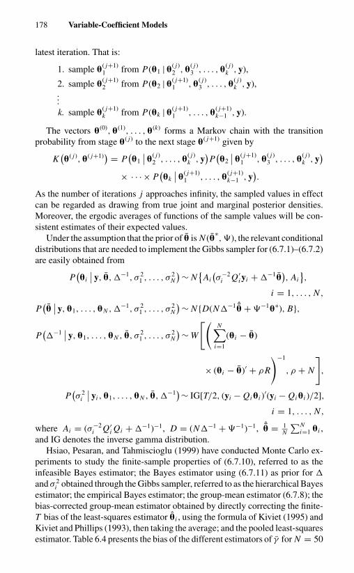
178 Variable-Coefficient Models
latest iteration. That is:
1. sample �( j+1)1 from P(�1 | �
( j)2 , �
( j)3 , . . . , �
( j)k , y),
2. sample �( j+1)2 from P(�2 | �
( j+1)1 , �
( j)3 , . . . , �
( j)k , y),
...k. sample �
( j+1)k from P(�k | �
( j+1)1 , . . . , �
( j+1)k−1 , y).
The vectors �(0), �(1), . . . , �(k) forms a Markov chain with the transitionprobability from stage �( j) to the next stage �( j+1) given by
K(�( j), �( j+1)) = P
(�1
∣∣ �( j)2 , . . . , �
( j)k , y
)P(�2
∣∣ �( j+1)1 , �
( j)3 , . . . , �
( j)k , y
)× · · · × P
(�k
∣∣ �( j+1)1 , . . . , �
( j+1)k−1 , y
).
As the number of iterations j approaches infinity, the sampled values in effectcan be regarded as drawing from true joint and marginal posterior densities.Moreover, the ergodic averages of functions of the sample values will be con-sistent estimates of their expected values.
Under the assumption that the prior of � is N (�∗, �), the relevant conditional
distributions that are needed to implement the Gibbs sampler for (6.7.1)–(6.7.2)are easily obtained from
P(�i
∣∣ y, �, −1, σ 21 , . . . , σ 2
N
)∼ N{
Ai(σ−2
i Q′i yi + −1�
), Ai
},
i = 1, . . . , N ,
P(�∣∣ y, �1, . . . , �N , −1, σ 2
1 , . . . , σ 2N
)∼ N {D(N−1 ˆ� + �−1�∗), B},
P(−1
∣∣ y, �1, . . . , �N , �, σ 21 , . . . , σ 2
N
)∼ W
[(N∑
i=1
(�i − �)
× (�i − �)′ + ρR
)−1
, ρ + N
],
P(σ 2
i
∣∣ yi , �1, . . . , �N , �, −1)∼ IG[T/2, (yi − Qi �i )
′(yi − Qi �i )/2],
i = 1, . . . , N ,
where Ai = (σ−2i Q′
i Qi + −1)−1, D = (N−1 + �−1)−1, ˆ� = 1N
∑Ni=1 �i ,
and IG denotes the inverse gamma distribution.Hsiao, Pesaran, and Tahmiscioglu (1999) have conducted Monte Carlo ex-
periments to study the finite-sample properties of (6.7.10), referred to as theinfeasible Bayes estimator; the Bayes estimator using (6.7.11) as prior for
and σ 2i obtained through the Gibbs sampler, referred to as the hierarchical Bayes
estimator; the empirical Bayes estimator; the group-mean estimator (6.7.8); thebias-corrected group-mean estimator obtained by directly correcting the finite-T bias of the least-squares estimator �i , using the formula of Kiviet (1995) andKiviet and Phillips (1993), then taking the average; and the pooled least-squaresestimator. Table 6.4 presents the bias of the different estimators of γ for N = 50

Tabl
e6.
4.B
ias
ofth
esh
ort-
run
coef
ficie
ntγ
Bia
s
Bia
s-co
rrec
ted
Infe
asib
leE
mpi
rica
lH
iera
rchi
cal
Tγ
Pool
edO
LS
Mea
ngr
oup
mea
ngr
oup
Bay
esB
ayes
Bay
es
51
0.3
0.36
859
−0.2
3613
−0.1
4068
0.05
120
−0.1
2054
−0.0
2500
20.
30.
4111
6−0
.235
64−0
.140
070.
0474
0−0
.111
51−0
.015
003
0.6
1.28
029
−0.1
7924
−0.1
0969
0.05
751
−0.0
2874
0.02
884
40.
61.
2949
0−0
.183
39−0
.108
300.
0687
9−0
.007
040.
0646
55
0.3
0.06
347
−0.2
6087
−0.1
5550
0.01
016
−0.1
8724
−0.1
0068
60.
30.
0835
2−0
.260
39−0
.154
860.
0114
1−0
.180
73−0
.095
447
0.6
0.54
756
−0.2
8781
−0.1
7283
0.05
441
−0.1
2731
−0.0
2997
80.
60.
5760
6−0
.281
98−0
.169
350.
0625
8−0
.103
66−0
.010
12
209
0.3
0.44
268
−0.0
7174
−0.0
1365
0.00
340
−0.0
0238
0.00
621
100.
30.
4900
6−0
.069
10−0
.012
300.
0049
8−0
.001
060.
0069
411
0.35
0.25
755
−0.0
6847
−0.0
1209
−0.0
0172
−0.0
1004
−0.0
0011
120.
350.
2586
9−0
.066
44−0
.011
89−0
.002
29−0
.008
420.
0011
613
0.3
0.07
199
−0.0
7966
−0.0
1508
−0.0
0054
−0.0
1637
−0.0
0494
140.
30.
0934
2−0
.076
59−0
.012
820.
0024
4−0
.012
62−0
.001
0715
0.55
0.26
997
−0.0
9700
−0.0
2224
−0.0
0062
−0.0
1630
0.00
011
160.
550.
2986
3−0
.094
48−0
.021
74−0
.000
53−0
.013
520.
0019
8
Sour
ce:
Hsi
ao,P
esar
an,a
ndTa
hmis
ciog
lu(1
999)
.

180 Variable-Coefficient Models
and T = 5 or 20. The infeasible Bayes estimator performs very well. It hassmall bias even for T = 5. For T = 5, its bias falls within the range of 3 to 17percent. For T = 20, the bias is at most about 2 percent. The hierarchical Bayesestimator also performs well,20 followed by the empirical Bayes estimator whenT is small; but the latter improves quickly as T increases. The empirical Bayesestimator gives very good results even for T = 5 in some cases, but the biasalso appears to be quite large in certain other cases. As T gets larger its biasdecreases considerably. The mean-group and the bias-corrected mean-group es-timator both have large bias when T is small, with the bias-corrected estimatorperforming slightly better. However, the performance of both improves as T in-creases, and both are still much better than the least-squares estimator. The least-squares estimator yields significant bias, and its bias persists as T increases.
The Bayes estimator is derived under the assumption that the initial observa-tions yi0 are fixed constants. As discussed in Chapter 4 or Anderson and Hsiao(1981, 1982), this assumption is clearly unjustifiable for a panel with finite T .However, contrary to the sampling approach, where the correct modeling of ini-tial observations is quite important, Bayesian approach appears to perform fairlywell in the estimation of the mean coefficients for dynamic random-coefficientmodels even the initial observations are treated as fixed constants. The MonteCarlo study also cautions against the practice of justifying the use of certainestimators on the basis of their asymptotic properties. Both the mean-group andthe corrected mean-group estimator perform poorly in panels with very smallT . The hierarchical Bayes estimator appears preferable to the other consistentestimators unless the time dimension of the panel is sufficiently large.
6.8 AN EXAMPLE --- LIQUIDITY CONSTRAINTSAND FIRM INVESTMENT EXPENDITURE
The effects of financial constraints on company investment have been subjectto intensive debate by economists. At one extreme, Jorgenson (1971) claimsthat “the evidence clearly favors the Modigliani–Miller theory [Modiglianiand Miller (1958), Miller and Modigliani (1961)]. Internal liquidity is not animportant determinant of the investment, given the level of output and externalfunds.” At the other extreme, Stiglitz and Weiss (1981) argue that becauseof imperfections in the capital markets, costs of internal and external fundsgenerally will diverge, and internal and external funds generally will not beperfect substitutes for each other. Fazzari, Hubbard, and Petersen (1988), Bondand Meghir (1994), etc. tested for the importance of internal finance by studyingthe effects of cash flow across different groups of companies – identified, e.g.,according to company retention practices. If the null hypothesis of a perfectcapital market is correct, then no difference should be found in the coefficientof the cash-flow variable across groups. However, these authors find that thecash-flow coefficient is large for companies with low dividend payout rates.
However, there is no sound theoretical basis for assuming that only low-dividend-payout companies are subject to financial constraints. The findingthat larger companies have larger cash-flow coefficients is inconsistent with
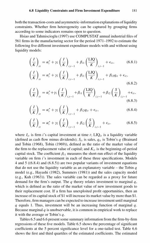
6.8 Liquidity Constraints and Firm Investment Expenditure 181
both the transaction-costs and asymmetric-information explanations of liquidityconstraints. Whether firm heterogeneity can be captured by grouping firmsaccording to some indicators remains open to question.
Hsiao and Tahmiscioglu (1997) use COMPUSTAT annual industrial files of561 firms in the manufacturing sector for the period 1971–1992 to estimate thefollowing five different investment expenditure models with and without usingliquidity models:(
I
K
)i t
= α∗i + γi
(I
K
)i,t−1
+ βi1
(LIQ
K
)i,t−1
+ εi t , (6.8.1)
(I
K
)i t
= α∗i + γi
(I
K
)i,t−1
+ βi1
(LIQ
K
)i,t−1
+ βi2qit + εi t ,
(6.8.2)(I
K
)i t
= α∗i +γi
(I
K
)i,t−1
+βi1
(LIQ
K
)i,t−1
+βi2
(S
K
)i,t−1
+εi t ,
(6.8.3)(I
K
)i t
= α∗i + γi
(I
K
)i,t−1
+ βi2qit + εi t , (6.8.4)
(I
K
)i t
= α∗i + γi
(I
K
)i,t−1
+ βi2
(S
K
)i,t−1
+ εi t . (6.8.5)
where Iit is firm i’s capital investment at time t ; LIQi t is a liquidity variable(defined as cash flow minus dividends); Sit is sales, qit is Tobin’s q (Brainardand Tobin (1968), Tobin (1969)), defined as the ratio of the market value ofthe firm to the replacement value of capital; and Kit is the beginning-of-periodcapital stock. The coefficient βi1 measures the short-run effect of the liquidityvariable on firm i’s investment in each of these three specifications. Models4 and 5 ((6.8.4) and (6.8.5)) are two popular variants of investment equationsthat do not use the liquidity variable as an explanatory variable – the Tobin qmodel (e.g., Hayashi (1982), Summers (1981)) and the sales capacity model(e.g., Kuh (1963)). The sales variable can be regarded as a proxy for futuredemand for the firm’s output. The q theory relates investment to marginal q,which is defined as the ratio of the market value of new investment goods totheir replacement cost. If a firm has unexploited profit opportunities, then anincrease of its capital stock of $1 will increase its market value by more than $1.Therefore, firm managers can be expected to increase investment until marginalq equals 1. Thus, investment will be an increasing function of marginal q.Because marginal q is unobservable, it is common in empirical work to replaceit with the average or Tobin’s q.
Tables 6.5 and 6.6 present some summary information from the firm-by-firmregressions of these five models. Table 6.5 shows the percentage of significantcoefficients at the 5 percent significance level for a one-tailed test. Table 6.6shows the first and third quartiles of the estimated coefficients. The estimated
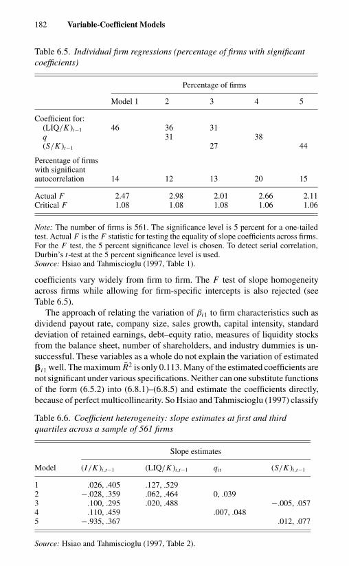
182 Variable-Coefficient Models
Table 6.5. Individual firm regressions (percentage of firms with significantcoefficients)
Percentage of firms
Model 1 2 3 4 5
Coefficient for:(LIQ/K )t−1 46 36 31q 31 38(S/K )t−1 27 44
Percentage of firmswith significantautocorrelation 14 12 13 20 15
Actual F 2.47 2.98 2.01 2.66 2.11Critical F 1.08 1.08 1.08 1.06 1.06
Note: The number of firms is 561. The significance level is 5 percent for a one-tailedtest. Actual F is the F statistic for testing the equality of slope coefficients across firms.For the F test, the 5 percent significance level is chosen. To detect serial correlation,Durbin’s t-test at the 5 percent significance level is used.Source: Hsiao and Tahmiscioglu (1997, Table 1).
coefficients vary widely from firm to firm. The F test of slope homogeneityacross firms while allowing for firm-specific intercepts is also rejected (seeTable 6.5).
The approach of relating the variation of βi1 to firm characteristics such asdividend payout rate, company size, sales growth, capital intensity, standarddeviation of retained earnings, debt–equity ratio, measures of liquidity stocksfrom the balance sheet, number of shareholders, and industry dummies is un-successful. These variables as a whole do not explain the variation of estimated�i1 well. The maximum R2 is only 0.113. Many of the estimated coefficients arenot significant under various specifications. Neither can one substitute functionsof the form (6.5.2) into (6.8.1)–(6.8.5) and estimate the coefficients directly,because of perfect multicollinearity. So Hsiao and Tahmiscioglu (1997) classify
Table 6.6. Coefficient heterogeneity: slope estimates at first and thirdquartiles across a sample of 561 firms
Slope estimates
Model (I/K )i,t−1 (LIQ/K )i,t−1 qit (S/K )i,t−1
1 .026, .405 .127, .5292 −.028, .359 .062, .464 0, .0393 .100, .295 .020, .488 −.005, .0574 .110, .459 .007, .0485 −.935, .367 .012, .077
Source: Hsiao and Tahmiscioglu (1997, Table 2).

6.8 Liquidity Constraints and Firm Investment Expenditure 183
Table 6.7. Variable intercept estimation of models for less- and more-capital-intensive firms
Variable intercept estimate
Variable Less-capital-intensive firms More-capital-intensive firms
(I/K )i,t−1 .265 .198 .248 .392 .363 .364(.011) (.012) (.011) (.022) (.023) (.022)
(LIQ/K )i,t−1 .161 .110 .119 .308 .253 .278(.007) (.007) (.007) (.024) (.027) (.025)
(S/K )i,t−1 .023 .025(.001) (.006)
qit .011 .009(.0006) (.002)
Actual F 2.04 1.84 2.22 2.50 2.19 2.10Critical F 1.09 1.07 1.07 1.20 1.17 1.17Numerator d.f. 834 1,251 1,251 170 255 255Denominator d.f. 6,592 6,174 6,174 1,368 1,282 1,282Number of firms 418 418 418 86 86 86
Note: The dependent variable is (I/K )i t . Less-capital-intensive firms are those with min-imum (K/S) between 0.15 and 0.55 over the sample period. For more-capital-intensivefirms, the minimum (K/S) is greater than 0.55. The regressions include company-specific intercepts. Actual F is the F statistic for testing the homogeneity of slopecoefficients. For the F test, a 5 percent significance level is chosen. The estimationperiod is 1974–1992. Standard errors are in parentheses.Source: Hsiao and Tahmiscioglu (1997, Table 5).
firms into reasonably homogeneous groups using the capital intensity ratio of0.55 as a cutoff point. Capital intensity is defined as the minimum value of theratio of capital stock to sales over the sample period. It is the most statisticallysignificant and most stable variable under different specifications.
Table 6.7 presents the variable intercept estimates for the groups of less- andmore-capital-intensive firms. The liquidity variable is highly significant in allthree variants of the liquidity model. There are also significant differences inthe coefficients of the liquidity variable across the two groups. However, Table6.7 also shows that the null hypothesis of the equality of slope coefficientsconditioning on the firm-specific effects is strongly rejected for all specificationsfor both groups. In other words, using the capital intensity ratio of 0.55 as acutoff point, there is still substantial heterogeneity within the groups.
Since neither does there appear to be a set of explanatory variables thatadequately explains the variation of βi1, nor can homogeneity be achieved byclassifying firms into groups, one is left with either treating �i as fixed anddifferent or treating �i as random draws from a common distribution. Withinthe random-effects framework, individual differences are viewed as randomdraws from a population with constant mean and variance. Therefore, it isappropriate to pool the data and try to draw some generalization about thepopulation. On the other hand, if individual differences reflect fundamentalheterogeneity or if individual response coefficients depend on the values of

184 Variable-Coefficient Models
Table 6.8. Estimation of mixed fixed- and random-coefficient models for less-and more-capital-intensive firms
Estimate
Variable Less-capital-intensive firms More-capital-intensive firms
(I/K )i,t−1 .230 .183 .121 .321 .302 .236(.018) (.017) (.019) (.036) (.037) (.041)
(LIQ/K )i,t−1 .306 .252 .239 .488 .449 .416(.021) (.023) (.027) (.065) (.067) (.079)
(S/K )i,t−1 .024 .038(.003) (.015)
qit .019 .022(.003) (.008)
Number of firms 418 418 418 86 86 86
Note: The dependent variable is (I/K )i t . The regressions include fixed firm-specificeffects. The estimation period is 1974–1992. Standard errors are in parentheses.Source: Hsiao and Tahmiscioglu (1997, Table 7).
the included explanatory variables, estimation of the model parameters basedon the conventional random-effects formulation can be misleading. To avoidthis bias, heterogeneity among individuals must be treated as fixed. In otherwords, one must investigate investment behavior firm by firm, and there is noadvantage in pooling. Without pooling, the shortage of degrees of freedomand multicollinearity can render the resulting estimates meaningless and makedrawing general conclusions difficult.
Table 6.8 presents the estimates of the mixed fixed- and random-coefficientmodel of the form (6.6.24) by assuming that, conditional on company-specificeffects, the remaining slope coefficients are randomly distributed around a cer-tain mean within the less- and the more-capital-intensive groups. To evaluatethe appropriateness of these specifications, Table 6.9 presents the comparisonof the recursive predictive density of the mixed fixed- and random-coefficientsmodel and the fixed-coefficient model, assuming that each company has dif-ferent coefficients for the three variants of the liquidity model, by dividingthe sample into pre- and post-1989 periods. The numbers reported in the tableare the logarithms of (6.6.28). The results indicate that the mixed fixed- andrandom-coefficient model is favored over the fixed-coefficient model for bothgroups. Similar comparison between the liquidity model, Tobin’s q, and salesaccelerator models also favor liquidity as an important explanatory variable.
Table 6.8 shows that the estimated liquidity coefficients are highly significantand there are significant differences between different classes of companies.The mean coefficient of the liquidity variable turns out to be 60–80 percentlarger for the more-capital-intensive group than for the less-capital-intensivegroup. The implied long-run relationships between the liquidity variable andthe fixed investment variable are also statistically significant. For instance,
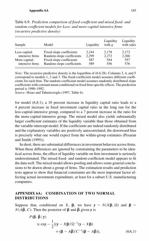
Appendix 6A 185
Table 6.9. Prediction comparison of fixed-coefficient and mixed fixed- andrandom-coefficient models for Less- and more-capital-intensive firms(recursive predictive density)
Liquidity LiquiditySample Model Liquidity with q with sales
Less-capital- Fixed-slope coefficients 2,244 2,178 2,172intensive firms Random-slope coefficients 2,299 2,272 2,266
More-capital- Fixed-slope coefficients 587 544 557intensive firms Random-slope coefficients 589 556 576
Note: The recursive predictive density is the logarithm of (6.6.28). Columns 3, 4, and 5correspond to models 1, 2 and 3. The fixed-coefficient model assumes different coeffi-cients for each firm. The random-coefficient model assumes randomly distributed slopecoefficients with constant mean conditional on fixed firm-specific effects. The predictionperiod is 1990–1992.Source: Hsiao and Tahmiscioglu (1997, Table 6).
for model (6.8.1), a 10 percent increase in liquidity capital ratio leads to a4 percent increase in fixed investment capital ratio in the long run for theless-capital-intensive group, compared to a 7 percent increase in the ratio forthe more-capital-intensive group. The mixed model also yields substantiallylarger coefficient estimates of the liquidity variable than those obtained fromthe variable-intercept model. If the coefficients are indeed randomly distributedand the explanatory variables are positively autocorrelated, the downward biasis precisely what one would expect from the within-group estimates (Pesaranand Smith (1995)).
In short, there are substantial differences in investment behavior across firms.When these differences are ignored by constraining the parameters to be iden-tical across firms, the effect of liquidity variable on firm investment is seriouslyunderestimated. The mixed fixed- and random-coefficient model appears to fitthe data well. The mixed model allows pooling and allows some general conclu-sions to be drawn about a group of firms. The estimation results and predictiontests appear to show that financial constraints are the most important factor af-fecting actual investment expenditure, at least for a subset U.S. manufacturingcompanies.
APPENDIX 6A: COMBINATION OF TWO NORMALDISTRIBUTIONS
Suppose that, conditional on X , �, we have y ∼ N (X�, �) and � ∼N (A�, C). Then the posterior of � and � given y is
P(�, � | y)
∝ exp − 1
2{(y − X�)′�−1(y − X�)
+ (� − A�)′C−1(� − A�)}, (6A.1)

186 Variable-Coefficient Models
where ∝ denotes proportionality. Using the identities (e.g., Rao (1973, p. 33 )
(D + B F B ′)−1 = D−1 − D−1 B(B ′ D−1 B + F−1)−1 B ′ D−1, (6A.2)
and
(D + F)−1 = D−1 − D−1(D−1 + F−1)−1 D−1, (6A.3)
we can complete the squares of
(� − A�)′C−1(� − A�) + (y − X�)′�−1(y − X�)
= �′C−1� + �′A′C−1 A� − 2�′C−1 A�
+ y′�−1y + �′ X ′�−1 X� − 2�′ X ′�−1y. (6A.4)
Let
Q1 = [� − (X ′�−1 X + C−1)−1(X�−1y + C−1 A�)]′
× (C−1 + X ′�−1 X )[� − (X ′�−1 X + C−1)−1
× (X ′�−1y + C−1 A�)]. (6A.5)
Then
�′C−1� + �′ X ′�−1 X� − 2�′C−1 A� − 2�′ X ′�−1y
= Q1 − (X ′�−1y + C−1 A�)′(X ′�−1 X + C−1)−1
× (X ′�−1y + C−1 A�).
(6A.6)
Substituting (6A.6) into (6A.4) yields
Q1 + y′[�−1 − �−1 X (X ′�−1 X + C−1)−1 X ′�−1]y
+ �′A′[C−1 − C−1(X ′�−1 X + C−1)−1C−1]A�
− 2�′A′C−1(X ′�−1 X + C−1)−1 X ′�−1y
= Q1 + y′(XC X ′ + �)−1y + �′A′ X ′(XC X ′ + �)−1 X A�
− 2�′A′ X ′(XC X ′ + �)−1y
= Q1 + Q2 + Q3, (6A.7)
where
Q2 = {� − [A′ X ′(XC X ′ + �)−1 X A]−1[A′ X ′(XC X ′ + �)−1 y]}′× [A′ X ′(XC X ′ + �)−1 X A]{� − [A′ X ′(XC X ′ + �)−1 X A]−1
× [A′ X ′(XC X ′ + �)−1y]}, (6A.8)
Q3 = y′{(XC X ′ + �)−1
− (XC X ′ + �)−1 X A[A′ X (XC X ′ + �)−1 X A]−1
× A′ X ′(XC X ′ + �)−1} y. (6A.9)
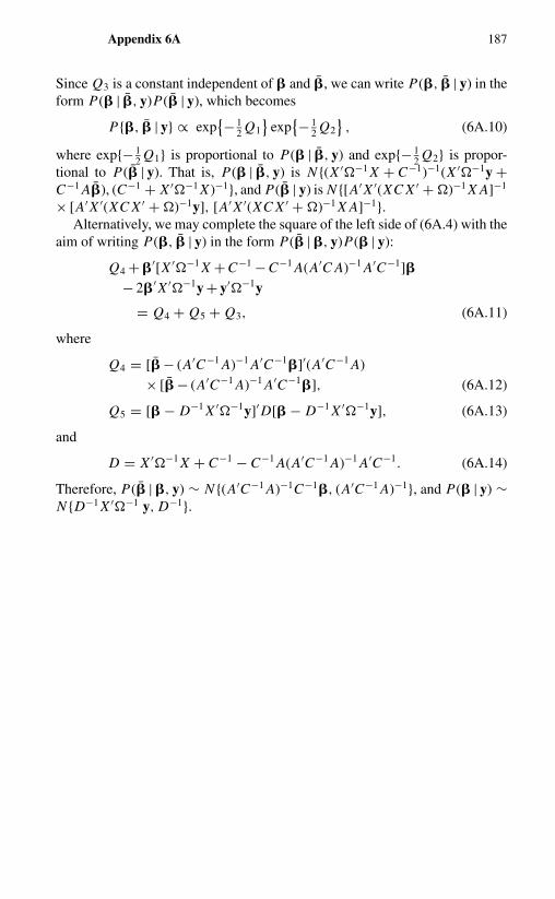
Appendix 6A 187
Since Q3 is a constant independent of � and �, we can write P(�, � | y) in theform P(� | �, y)P(� | y), which becomes
P{�, � | y} ∝ exp{− 1
2 Q1}
exp{− 1
2 Q2}, (6A.10)
where exp{− 12 Q1} is proportional to P(� | �, y) and exp{− 1
2 Q2} is propor-tional to P(� | y). That is, P(� | �, y) is N {(X ′�−1 X + C−1)−1(X ′�−1y +C−1 A�), (C−1 + X ′�−1 X )−1}, and P(� | y) is N {[A′ X ′(XC X ′ + �)−1 X A]−1
× [A′ X ′(XC X ′ + �)−1y], [A′ X ′(XC X ′ + �)−1 X A]−1}.Alternatively, we may complete the square of the left side of (6A.4) with the
aim of writing P(�, � | y) in the form P(� | �, y)P(� | y):
Q4 + �′[X ′�−1 X + C−1 − C−1 A(A′C A)−1 A′C−1]�
− 2�′ X ′�−1y + y′�−1y
= Q4 + Q5 + Q3, (6A.11)
where
Q4 = [� − (A′C−1 A)−1 A′C−1�]′(A′C−1 A)
× [� − (A′C−1 A)−1 A′C−1�], (6A.12)
Q5 = [� − D−1 X ′�−1y]′ D[� − D−1 X ′�−1y], (6A.13)
and
D = X ′�−1 X + C−1 − C−1 A(A′C−1 A)−1 A′C−1. (6A.14)
Therefore, P(� | �, y) ∼ N {(A′C−1 A)−1C−1�, (A′C−1 A)−1}, and P(� | y) ∼N {D−1 X ′�−1 y, D−1}.
CHAPTER 7
Discrete Data
7.1 INTRODUCTION
In this chapter, we consider situations in which an analyst has at his disposala random sample of N individuals, having recorded histories indicating thepresence or absence of an event in each of T equally spaced discrete timeperiods. Statistical models in which the endogenous random variables takeonly discrete values are known as discrete, categorical, qualitative-choice, orquantal-response models. The literature, both applied and theoretical, on thissubject is vast. Amemiya (1981), Maddala (1983), and McFadden (1976, 1984)have provided excellent surveys. Thus, the focus of this chapter will be onlyon controlling for unobserved characteristics of individual units to avoid spec-ification bias. Many important and more advanced topics are omitted, suchas continuous-time and duration-dependence models (Chamberlain (1978b);Flinn and Heckman (1982); Heckman and Borjas (1980); Heckman and Singer(1982); Lancaster (1990); Nickell (1979); Singer and Spilerman (1976)).
7.2 SOME DISCRETE-RESPONSE MODELS
In this section, we briefly review some widely used discrete-response models.We first consider the case in which the dependent variable y can assume onlytwo values, which for convenience and without any loss of generality will be thevalue 1 if an event occurs and 0 if it does not. Examples of this include purchasesof durables in a given year, participation in the labor force, the decision to entercollege, and the decision to marry.
The discrete outcome of y can be viewed as the observed counterpart of alatent continuous random variable crossing a threshold. Suppose that the con-tinuous latent random variable, y∗, is a linear function of a vector of explanatoryvariables, x,
y∗ = �′x + v, (7.2.1)
where the error term v is independent of x with mean zero. Suppose, instead of

7.2 Some Discrete-Response Models 189
observing y∗, we observe y, where
y ={
1 if y∗ > 0,
0 if y∗ ≤ 0.(7.2.2)
Then the expected value of yi is the probability that the event will occur,
E(y | x) = 1 · Pr(v > −�′x) + 0 · Pr(v ≤ −�′x)
= Pr(v > −�′x)
= Pr(y = 1 | x). (7.2.3)
When the probability law for generating v follows a two-point distribution(1 − �′x) and (−�′x), with probabilities �′x and (1 − �′x), respectively, wehave the linear-probability model
y = �′x + v, (7.2.4)
with Ev = �′x(1 − �′x) + (1 − �′x)(−�′x) = 0. When the probability den-sity function of v is a standard normal density function, (1/
√2π )
× exp(−v2/2) = φ(v), we have the probit model,
Pr(y = 1 | x) =∫ ∞
−�′xφ(v) dv
=∫ �′x
−∞φ(v) dv = �(�′x). (7.2.5)
When the probability density function is a standard logistic,
exp(v)
(1 + exp(v))2= [(1 + exp(v))(1 + exp(−v))]−1,
we have the logit model
Pr(y = 1 | x) =∫ ∞
−�′x
exp(v)
(1 + exp(v))2dvi = exp(�′x)
1 + exp(�′x). (7.2.6)
Let F(�′x) = E(yi | x). Then the three commonly used parametric modelsfor the binary choice may be summarized with a single index w as follows:
Linear-probability model,
F(w) = w . (7.2.7)
Probit model,
F(w) =∫ w
−∞
1√2π
e− u2
2 du = �(w). (7.2.8)
Logit model,
F(w) = ew
1 + ew. (7.2.9)

190 Discrete Data
The linear-probability model is a special case of the linear regression modelwith heteroscadastic variance, �′x(1 − �′x). It can be estimated by leastsquares or weighted least squares (Goldberger (1964)). But it has an obvi-ous defect in that �′x is not constrained to lie between 0 and 1 as a probabilityshould, whereas in the probit and logit models it is.
The probability functions used for the probit and logit models are the standardnormal distribution and the logistic distribution, respectively. We use cumulativestandard normal because in the dichotomy case there is no way to identify thevariance of a normal density. The logit probability density function is symmetricaround 0 and has a variance of π2/3. Because they are distribution functions,the probit and logit models are bounded between 0 and 1.
The cumulative normal distribution and the logistic distribution are veryclose to each other; the logistic distribution has sightly heavier tails (Cox(1970)). Moreover, the cumulative normal distribution � is reasonably wellapproximated by a linear function for the range of probabilities between 0.3and 0.7. Amemiya (1981) has suggested an approximate conversion rule forthe coefficients of these models. Let the coefficients for the linear-probability,probit, and logit models be denoted as �LP, �Φ, �L , respectively. Then
�L � 1.6�Φ,
�LP � 0.4�Φ except for the constant term, (7.2.10)
and
�LP � 0.4�Φ + 0.5 for the constant term.
For a random sample of N individuals, (yi , xi ), i = 1, . . . , N , the likelihoodfunction for these three models can be written in general form as
L =N∏
i=1
F(�′xi )yi [1 − F(�′xi )]
1−yi . (7.2.11)
Differentiating the logarithm of the likelihood function yields the vector of firstderivatives and the matrix of second-order derivatives as
∂ log L
∂�=
N∑i=1
yi − F(�′xi )
F(�′xi )[1 − F(�′xi )]F ′(�′xi )xi , (7.2.12)
and
∂2 log L
∂�∂�′ ={
−N∑
i=1
[yi
F2(�′xi )+ 1 − yi
[1 − F(�′xi )]2
][F ′(�′xi )]
2
+N∑
i=1
[yi − F(�′xi )
F(�′xi )[1 − F(�′xi )]
]F ′′(�′xi )
}xi x′
i ,
(7.2.13)
where F ′(�′xi ) and F ′′(�′xi ) denote the first and second derivatives of F(�′xi )with respect to �′xi . If the likelihood function (7.2.11) is concave, as in the
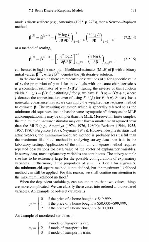
7.2 Some Discrete-Response Models 191
models discussed here (e.g., Amemiya (1985, p. 273)), then a Newton–Raphsonmethod,
�( j) = �
( j−1) −(
∂2 log L
∂� ∂�′
)−1
�=�( j−1)
(∂ log L
∂�
)�=�
( j−1), (7.2.14)
or a method of scoring,
�( j) = �
( j−1) −[
E∂2 log L
∂� ∂�′
]−1
�=�( j−1)
(∂ log L
∂�
)�=�
( j−1), (7.2.15)
can be used to find the maximum likelihood estimator (MLE) of � with arbitraryinitial values �
(0), where �
( j)denotes the j th iterative solution.
In the case in which there are repeated observations of y for a specific valueof x, the proportion of y = 1 for individuals with the same characteristic xis a consistent estimator of p = F(�′x). Taking the inverse of this functionyields F−1(p) = �′x. Substituting p for p, we have F−1( p) = �′x + ζ , whereζ denotes the approximation error of using F−1( p) for F−1(p). Since ζ has anonscalar covariance matrix, we can apply the weighted least-squares methodto estimate �. The resulting estimator, which is generally referred to as theminimum-chi-square estimator, has the same asymptotic efficiency as the MLEand computationally may be simpler than the MLE. Moreover, in finite samples,the minimum-chi-square estimator may even have a smaller mean squared errorthan the MLE (e.g., Amemiya (1974, 1976, 1980b); Berkson (1944, 1955,1957, 1980); Ferguson (1958); Neyman (1949)). However, despite its statisticalattractiveness, the minimum-chi-square method is probably less useful thanthe maximum likelihood method in analyzing survey data than it is in thelaboratory setting. Application of the minimum-chi-square method requiresrepeated observations for each value of the vector of explanatory variables.In survey data, most explanatory variables are continuous. The survey samplesize has to be extremely large for the possible configurations of explanatoryvariables. Furthermore, if the proportion of y = 1 is 0 or 1 for a given x,the minimum-chi-square method is not defined, but the maximum likelihoodmethod can still be applied. For this reason, we shall confine our attention tothe maximum likelihood method.1
When the dependent variable yi can assume more than two values, thingsare more complicated. We can classify these cases into ordered and unorderedvariables. An example of ordered variables is
yi =
0 if the price of a home bought < $49,999,
1 if the price of a home bought is $50,000−$99,999,
2 if the price of a home bought > $100,000.
An example of unordered variables is
yi =
1 if mode of transport is car,2 if mode of transport is bus,3 if mode of transport is train.
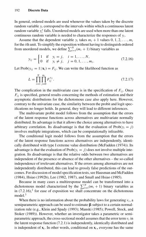
192 Discrete Data
In general, ordered models are used whenever the values taken by the discreterandom variable yi correspond to the intervals within which a continuous latentrandom variable y∗
i falls. Unordered models are used when more than one latentcontinuous random variable is needed to characterize the responses of yi .
Assume that the dependent variable yi takes mi + 1 values 0, 1, 2, . . . , mi
for the i th unit. To simplify the exposition without having to distinguish orderedfrom unordered models, we define
∑Ni=1(mi + 1) binary variables as
yi j ={
1 if yi = j, i = 1, . . . , N ,
0 if yi �= j, j = 0, 1, . . . , mi .(7.2.16)
Let Prob(yi j = 1 | xi ) = Fi j . We can write the likelihood function as
L =N∏
i=1
mi∏j=0
Fyi j
i j . (7.2.17)
The complication in the multivariate case is in the specification of Fi j . OnceFi j is specified, general results concerning the methods of estimation and theirasymptotic distributions for the dichotomous case also apply here. However,contrary to the univariate case, the similarity between the probit and logit spec-ifications no longer holds. In general, they will lead to different inferences.
The multivariate probit model follows from the assumption that the errorsof the latent response functions across alternatives are multivariate normallydistributed. Its advantage is that it allows the choice among alternatives to havearbitrary correlation. Its disadvantage is that the evaluation of Prob(yi = j)involves multiple integrations, which can be computationally infeasible.
The conditional logit model follows from the assumption that the errorsof the latent response functions across alternatives are independently, identi-cally distributed with type I extreme value distribution (McFadden (1974)). Itsadvantage is that the evaluation of Prob(yi = j) does not involve multiple inte-gration. Its disadvantage is that the relative odds between two alternatives areindependent of the presence or absence of the other alternatives – the so-calledindependence of irrelevant alternatives. If the errors among alternatives are notindependently distributed, this can lead to grossly false predictions of the out-comes. For discussion of model specification tests, see Hausman and McFadden(1984), Hsiao (1992b), Lee (1982, 1987), and Small and Hsiao (1985).
Because in many cases a multiresponse model can be transformed into adichotomous model characterized by the
∑Ni=1(mi + 1) binary variables as
in (7.2.16),2 for ease of exposition we shall concentrate on the dichotomousmodel.3
When there is no information about the probability laws for generating vi , asemiparametric approach can be used to estimate � subject to a certain normal-ization rule (e.g., Klein and Spady (1993); Manski (1985); Powell, Stock, andStoker (1989)). However, whether an investigator takes a parametric or semi-parametric approach, the cross-sectional model assumes that the error term vi inthe latent response function (7.2.1) is independently, identically distributed andis independent of xi . In other words, conditional on xi , everyone has the same

7.3 Parametric Approach to Static Models with Heterogeneity 193
probability that an event will occur. It does not allow the possibility that theaverage behavior given x can be different from individual probabilities, that is,that it does not allow Pr(yi = 1 | x) �= Pr(y j = 1 | x). The availability of paneldata provides the possibility of distinguishing average behavior from individualbehavior by decomposing the error term vit into
vit = αi + λt + uit , (7.2.18)
where αi and λt denote the effects of omitted individual-specific andtime-specific variables, respectively. In this chapter we shall demonstrate themisspecifications that can arise because of failure to control for unobservedcharacteristics of the individuals in panel data, and discuss possible remedies.
7.3 PARAMETRIC APPROACH TO STATICMODELS WITH HETEROGENEITY
Statistical models developed for analyzing cross-sectional data essentially ig-nore individual differences and treat the aggregate of the individual effectand the omitted-variable effect as a pure chance event. However, as stated inChapter 1, a discovery of a group of married women having an average yearlylabor participation rate of 50 percent could lead to diametrically opposite infer-ences. At one extreme, each woman in a homogeneous population could havea 50 percent chance of being in the labor force in any given year, whereas at theother extreme 50 percent of women in a heterogeneous population might alwayswork and 50 percent never work. Either explanation is consistent with the givencross-sectional data. To discriminate among the many possible explanations, weneed information on individual labor-force histories in different subintervals ofthe life cycle. Panel data, through their information on intertemporal dynamicsof individual entities, provide the possibility of separating a model of individualbehavior from a model of the average behavior of a group of individuals.
For simplicity, we shall assume that the heterogeneity across cross-sectionalunits is time-invariant,4 and these individual-specific effects are captured bydecomposing the error term vit in (7.2.1) as αi + uit . When the αi are treatedas fixed, Var(vit | αi ) = Var(uit ) = σ 2
u . When they are treated as random, weassume that Eαi = Euit = Eαi uit = 0 and Var(vit ) = σ 2
u + σ 2α . However, as
discussed earlier, when the dependent variables are binary, the scale factor isnot identifiable. Thus, for ease of exposition, we normalize the variance σ 2
u ofu to be equal to 1 for the specifications discussed in the rest of this chapter.
The existence of such unobserved permanent components allows individualswho are homogeneous in their observed characteristics to be heterogeneous intheir response probabilities F(�′xi t +αi ). For example, heterogeneity will im-ply that the sequential-participation behavior of a woman, F(�′x+αi ), withina group of observationally identical women differs systematically from F(�′x)or the average behavior of the group,
∫F(�′x + α) d H (α | x), where H (α | x)
gives the population probability (or empirical distribution) for α conditionalon x.5 In this section, we discuss statistical inference of the common parame-ters � based on a parametric specification of F(·).

194 Discrete Data
7.3.1 Fixed-Effects Models
7.3.1.a Maximum Likelihood Estimator
If the individual-specific effect, αi , is assumed to be fixed,6 then both αi and �are unknown parameters to be estimated for the model Prob(yit = 1 | xi t , αi ) =F(�′xi t +αi ). When T tends to infinity, the MLE is consistent. However, T isusually small for panel data. There are only a limited number of observations toestimate αi . Thus, we have the familiar incidental-parameter problem (Neymanand Scott (1948)). Any estimation of the αi is meaningless if we intend to judgethe estimators by their large-sample properties. We shall therefore concentrateon estimation of the common parameters, �.
Unfortunately, contrary to the linear-regression case where the individualeffects αi can be eliminated by taking a linear transformation such as the firstdifference, in general no simple transformation exists to eliminate the incidentalparameters from a nonlinear model. The MLEs for αi and � are not independentof each other for the discrete-choice models. When T is fixed, the inconsistencyof αi is transmitted into the MLE for �. Hence, even if N tends to infinity, theMLE of � remains inconsistent.
We demonstrate the inconsistency of the MLE for � by considering a logitmodel. The log likelihood function for this model is
log L = −N∑
i=1
T∑t=1
log[1 + exp(�′xi t +αi )] +N∑
i=1
T∑t=1
yit (�′xi t +αi ).
(7.3.1)
For ease of illustration, we consider the special case of T = 2 and one ex-planatory variable, with xi1 = 0 and xi2 = 1. Then the first-derivative equationsare
∂ log L
∂β=
N∑i=1
2∑t=1
[− eβxit+αi
1 + eβxit+αi+ yit
]xit
=N∑
i=1
[− eβ+αi
1 + eβ+αi+ yi2
]= 0, (7.3.2)
∂ log L
∂αi=
2∑t=1
[− eβxit+αi
1 + eβxit+αi+ yit
]= 0. (7.3.3)
Solving (7.3.3), we have
αi =
∞ if yi1 + yi2 = 2,
−∞ if yi1 + yi2 = 0,
−β
2if yi1 + yi2 = 1.
(7.3.4)
Inserting (7.3.4) into (7.3.2), and letting n1 denote the number of individuals

7.3 Parametric Approach to Static Models with Heterogeneity 195
with yi1 + yi2 = 1 and n2 the number of individuals with yi1 + yi2 = 2, wehave7
N∑i=1
eβ+αi
1 + eβ+αi= n1
eβ/2
1 + eβ/2+ n2 =
N∑i=1
yi2. (7.3.5)
Therefore,
β = 2
{log
(N∑
i=1
yi2 − n2
)− log
(n1 + n2 −
N∑i=1
yi2
)}. (7.3.6)
By a law of large numbers (Rao (1973, Chapter 2)),
plimN→∞
1
N
(N∑
i=1
yi2 − n2
)= 1
N
N∑i=1
Prob(yi1 = 0, yi2 = 1 | β, αi )
= 1
N
N∑i=1
eβ+αi
(1 + eαi )(1 + eβ+αi ), (7.3.7)
plimN→∞
1
N
(n1 + n2 −
N∑i=1
yi2
)= 1
N
N∑i=1
Prob(yi1 = 1, yi2 = 0 | β, αi )
= 1
N
N∑i=1
eαi
(1 + eαi )(1 + eβ+αi ). (7.3.8)
Substituting αi = − β
2 into (7.3.7) and (7.3.8), we obtain
plimN→∞
β = 2β, (7.3.9)
which is not consistent.
7.3.1.b Conditions for the Existence of a Consistent Estimator
Neyman and Scott (1948) suggested a general principle to find a consistentestimator for the (structural) parameter � in the presence of the incidentalparameters αi .8 Their idea is to find K functions
�N j (y1, . . . , yN | �), j = 1, . . . , K , (7.3.10)
that are independent of the incidental parameters αi and have the propertythat when � are the true values, �N j (y1, . . . , yN | �) converges to zero inprobability as N tends to infinity. Then an estimator � derived by solving�N j (y1, . . . , yN | �) = 0 is consistent under suitable regularity conditions. Forinstance, β∗ = ( 1
2 )β for the foregoing example of a fixed-effect logit model(7.3.1)–(7.3.3) is such an estimator.
In the case of a linear-probability model, either taking first differences overtime or taking differences with respect to the individual mean eliminates the

196 Discrete Data
individual-specific effect. The least-squares regression of the differenced equa-tions yields a consistent estimator for � when N tends to infinity.
But in the general nonlinear models, simple functions for � are not alwayseasy to find. For instance, in general we do not know the probability limit of theMLE of a fixed-effects logit model. However, if a minimum sufficient statisticτi for the incidental parameter αi exists and is not dependent on the structuralparameter �, then the conditional density,
f ∗(yi | �, τi ) = f (yi | �, αi )
g(τi | �, αi )for g(τi | �, αi ) > 0, (7.3.11)
no longer depends on αi .9 Andersen (1970, 1973) has shown that maximizingthe conditional density of y1, . . . , yN given τ1, . . . , τN ,
N∏i=1
f ∗ (yi | �, τi
), (7.3.12)
yields the first-order conditions �N j (y1, . . . , yN | �, τ1, τ2, . . . τN ) = 0 for j =1, . . . , K . Solving for these functions will give a consistent estimator of thecommon (structural) parameter � under mild regularity conditions.10
To illustrate the conditional maximum likelihood method, we use the logitmodel as an example. The joint probability of yi is
Prob(yi ) =exp
{αi
∑Tt=1 yit + �′ ∑T
t=1 xi t yi t
}∏T
t=1[1 + exp(�′xi t + αi )]. (7.3.13)
It is clear that∑T
t=1 yit is a minimum sufficient statistic for αi . The conditionalprobability for yi , given
∑Tt=1 yit , is
Prob
(yi
∣∣∣∣ T∑t=1
yit
)=
exp[�′ ∑T
t=1 xi t yi t
]∑
Di j ∈Biexp
{�′ ∑T
t=1 xi t di j t
} , (7.3.14)
where Bi = {Di j = (di j1, . . . , di jT ) | di jt = 0 or 1 and∑T
t=1 di jt = ∑Tt=1 yit =
s, j = 1, 2, . . . , T !s!(T −s)! } is the set of all possible distinct sequences (di j1,
di j2, . . . di jT ) satisfying∑T
t=1 di jt = ∑Tt=1 yit = s. There are T + 1 distinct
alternative sets corresponding to∑T
t=1 yit = 0, 1, . . . , T . Groups for which∑Tt=1 yit = 0 or T contribute zero to the likelihood function, because the cor-
responding conditional probability in this case is equal to 1 (with αi = −∞ or∞). So only T − 1 alternative sets are relevant. The alternative sets for groupswith
∑Tt=1 yit = s have ( T
s ) elements, corresponding to the distinct sequencesof T trials with s successes.
Equation (7.3.14) is in a conditional logit form (McFadden (1974)), withthe alternative sets (Bi ) varying across observations i . It does not depend onthe incidental parameters αi . Therefore, the conditional maximum likelihoodestimator of � can be obtained by using standard maximum likelihood logitprograms, and it is consistent under mild conditions. For example, with T = 2,

7.3 Parametric Approach to Static Models with Heterogeneity 197
the only case of interest is yi1 + yi2 = 1. The two possibilities are ωi = 1, if(yi1, yi2) = (0, 1), and ωi = 0, if (yi1, yi2) = (1, 0).
The conditional probability of wi = 1 given yi1 + yi2 = 1 is
Prob(ωi = 1 | yi1 + yi2 = 1) = Prob(ωi = 1)
Prob(ωi = 1) + Prob(ωi = 0)
= exp[�′(xi2 − xi1)]
1 + exp[�′(xi2 − xi1)]
= F[�′(xi2 − xi1)]. (7.3.15)
Equation (7.3.15) is in the form of a binary logit function in which the twooutcomes are (0, 1) and (1, 0), with explanatory variables (xi2 − xi1). The con-ditional log likelihood function is
log L∗ =∑i∈B1
{ωi log F[�′(xi2 − xi1)]
+ (1 − ωi ) log(1 − F[�′(xi2 − xi1)])}, (7.3.16)
where B1 = {i | yi1 + yi2 = 1}.Although B1 is a random set of indices, Chamberlain (1980) has shown
that the inverse of the information matrix based on the conditional-likelihoodfunction provides an asymptotic covariance matrix for the conditional MLE of� as N tends to infinity. This can be made more explicit by defining di = 1if yi1 + yi2 = 1, and di = 0 otherwise, for the foregoing case in which T = 2.Then we have
JB1= ∂2 log L∗
∂� ∂�′ = −N∑
i=1
di F[�′(xi2 − xi1)]
×{1 − F[�′(xi2 − xi1)]}(xi2 − xi1) · (xi2 − xi1)′. (7.3.17)
The information matrix is
J = E(JB1)
= −N∑
i=1
Pi F[�′(xi2 − xi1)]
× {1 − F[�′(xi2 − xi1)]}(xi2 − xi1) · (xi2 − xi1)′,(7.3.18)
where Pi = E(di | αi ) = F(�′xi1 + αi )[1 − F(�′xi2 + αi )] + [1 − F(�′xi1 +αi )]F(�′xi2 + αi ). Because di are independent, with Edi = Pi , and both F andthe variance of di are uniformly bounded, by a strong law of large numbers wehave
1
NJB1
− 1
NJ → 0 almost surely as N → ∞
ifN∑
i=1
1
i2mi m′
i < ∞, (7.3.19)

198 Discrete Data
where mi replaces each element of (xi2 − xi1) with its square. The conditionfor convergence clearly holds if xi t is uniformly bounded.
For the case of T > 2, there is no loss of generality in choosing the sequenceDi1 = (di11, . . . , di1T ),
∑Tt=1 di1t = ∑T
t=1 yit = s, 1 ≤ s ≤ T − 1, as the nor-malizing factor. Hence we may rewrite the conditional probability (7.3.14) as
Prob
(yi |
T∑t=1
yit
)=
exp{
�′{∑Tt=1 xi t (yit − di1t )
}}1 + ∑
Di j ∈(Bi −Di1) exp{
�′ ∑Tt=1 xi t (di jt − di1t )
} .
(7.3.20)
Then the conditional log-likelihood function takes the form
log L∗ =∑i∈C
{�′
T∑t=1
xi t (yit − di1t )
− log
1 +∑
Di j ∈(Bi −Di1)
exp
{�′
T∑t=1
xi t (di jt − di1t )
},
(7.3.21)
where C = {i | ∑Tt=1 yit �= T,
∑Tt=1 yit �= 0}.
Although we can find simple transformations of linear-probability and logitmodels that will satisfy the Neyman–Scott principle, we cannot find simplefunctions for the parameters of interest that are independent of the nuisance pa-rameters αi for probit models. That is, there does not appear to exist a consistentestimator of � for the fixed-effects probit models.
7.3.1.c Some Monte Carlo Evidence
Given that there exists a consistent estimator of � for the fixed-effects logitmodel, but not for the fixed-effects probit model, and that in the binary casethe probit and logit models yield similar results, it appears that a case can bemade for favoring the logit specification because of the existence of a consistentestimator for the structural parameter �. However, in the multivariate case, logitand probit models yield very different results. In this situation it will be usefulto know the magnitude of the bias if the data actually call for a fixed-effectsprobit specification.
Heckman (1981b) conducted a limited set of Monte Carlo experiments to getsome idea of the order of bias of the MLE for the fixed-effects probit models.His data were generated by the model
y∗i t = βxit + αi + uit , i = 1, 2, . . . , N , t = 1, . . . , T,
(7.3.22)

7.3 Parametric Approach to Static Models with Heterogeneity 199
Table 7.1. Average values of β for thefixed-effects probit model
β
σ 2α β = 1 β = −0.1 β = −1
3 0.90 −0.10 −0.941 0.91 −0.09 −0.950.5 0.93 −0.10 −0.96
Source: Heckman (1981b, Table 4.1).
and
yit ={
1 if y∗i t ≥ 0,
0 otherwise.
The exogenous variable xit was generated by a Nerlove (1971a) process,
xit = 0.1t + 0.5xi,t−1 + εi t , (7.3.23)
where εi t is a uniform random variable having mean zero and range −1/2 to1/2. The variance σ 2
u was set at 1. The scale of the variation of the fixed effect,σ 2
α , is changed for different experiments. In each experiment, 25 samples of100 individuals (N = 100) were selected for eight periods (T = 8).
The results of Heckman’s experiment with the fixed-effects MLE of probitmodels are presented in Table 7.1. For β = −0.1, the fixed-effects estimatordoes well. The estimated value comes very close to the true value. For β = −1or β = 1, the estimator does not perform as well, but the bias is never morethan 10 percent and is always toward zero. Also, as the scale of the variation inthe fixed-effects decreases, so does the bias.11
7.3.2 Random-Effects Models
When the individual specific effects αi are treated as random, we may stilluse the fixed effects estimators to estimate the structural parameters �. Theasymptotic properties of the fixed effects estimators of � remain unchanged.However, if αi are random, but are treated as fixed, the consequence, at its best,is a loss of efficiency in estimating �, but it could be worse, namely, the resultingfixed-effects estimators may be inconsistent, as discussed in Section 7.3.1.
When αi are independent of xi and are a random sample from a univariatedistribution G, indexed by a finite number of parameters �, the log likelihoodfunction becomes
log L =N∑
i=1
log∫ T∏
t=1
F(�′xi t + α)yit [1 − F(�′xi t + α)]1−yit dG(α | �),
(7.3.24)

200 Discrete Data
where F(·) is the distribution of the error term conditional on both xi and αi .Equation (7.3.24) replaces the probability function for y conditional on α by aprobability function that is marginal on α. It is a function of a finite number ofparameters (�′, �′). Thus, maximizing (7.3.24), under weak regularity condi-tions, will give consistent estimators for � and � as N tends to infinity.
If αi is correlated with xi t , maximizing (7.3.24) will not eliminate theomitted-variable bias. To allow for dependence between α and x, we mustspecify a distribution G(α | x) for α conditional on x, and consider the marginallog likelihood function
log L =N∑
i=1
log∫ T∏
t=1
F(�′xi t + α)yit
× [1 − F(�′xi t + α)]1−yit dG(α | x). (7.3.24′)
A convenient specification suggested by Chamberlain (1980, 1984) is to as-sume that αi = ∑T
t=1 a′t xi t + ηi = a′xi + ηi , where a′ = (a′
1, . . . a′T ), x′
i =(x′
i1, . . . , x′iT ), and ηi is the residual. However, there is a very important dif-
ference in this step compared with the linear case. In the linear case it was notrestrictive to decompose αi into its linear projection on xi and an orthogonalresidual. Now we are assuming that the regression function E(αi | xi ) is actu-ally linear, that ηi is independent of xi , and that ηi has a specific probabilitydistribution.
Given these assumptions, the log likelihood function under our random-effects specification is
log L =N∑
i=1
log∫ T∏
t=1
F(�′xi t + a′xi + η)yit
× [1 − F(�′xi t + a′xi + η)]1−yit dG∗ (η) ,
(7.3.25)
where G∗ is a univariate distribution function for η. For example, if F is astandard normal distribution function and we choose G∗ to be the distributionfunction of a normal random variable with mean 0 and variance σ 2
η , then ourspecification gives a multivariate probit model:
yit = 1 if �′xi t + a′xi + ηi + uit > 0, (7.3.26)
where ui + eηi is independent normal, with mean 0 and variance–covariancematrix IT + σ 2
η ee′.The difference between (7.3.25) and (7.3.24) is only in the inclusion of the
term a′xi to capture the dependence between the incidental parameters αi andxi . Therefore, the essential characteristics with regard to estimation of (7.3.24)and (7.3.25) are the same. So we shall discuss only the procedure to estimatethe more general model (7.3.25).
Maximizing (7.3.25) involves integration of T dimensions, which can becomputationally cumbersome. An alternative approach, which simplifies the
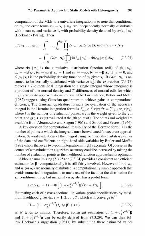
7.3 Parametric Approach to Static Models with Heterogeneity 201
computation of the MLE to a univariate integration is to note that conditionalon αi , the error terms vit = αi + uit are independently normally distributedwith mean αi and variance 1, with probability density denoted by φ (vit | αi )(Heckman (1981a)). Then
Pr(yi1, . . . yiT ) =∫ bi1
ci1
. . .
∫ biT
ciT
T∏t=1
φ(vit | αi )G(αi | xi ) dαi dvi1 · · · dviT
=∫ ∞
−∞G(αi | xi )
T∏t=1
[�(bit | αi ) − �(cit | αi )] dαi , (7.3.27)
where �(· | αi ) is the cumulative distribution function (cdf) of φ(· | αi ),cit = −�′xi t , bit = ∞ if yit = 1 and cit = −∞, bit = −�′xi t if yit = 0, andG(αi | xi ) is the probability density function of αi given xi . If G(αi | xi ) is as-sumed to be normally distributed with variance σ 2
α , the expression (7.3.27)reduces a T -dimensional integration to a single integral whose integrand isa product of one normal density and T differences of normal cdfs for whichhighly accurate approximations are available. For instance, Butler and Moffit(1982) suggest using Gaussian quadrature to achieve gains in computationalefficiency. The Gaussian quadrature formula for evaluation of the necessaryintegral is the Hermite integration formula
∫ ∞−∞ e−z2
g(z) dz = ∑lj=1 w j g(z j ),
where l is the number of evaluation points, w j is the weight given to the j thpoint, and g(z j ) is g(z) evaluated at the j th point of z. The points and weights areavailable from Abramowitz and Stegun (1965) and Stroud and Secrest (1966).
A key question for computational feasibility of the Hermite formula is thenumber of points at which the integrand must be evaluated for accurate approxi-mation. Several evaluations of the integral using four periods of arbitrary valuesof the data and coefficients on right-hand-side variables by Butler and Moffitt(1982) show that even two-point integration is highly accurate. Of course, in thecontext of a maximization algorithm, accuracy could be increased by raising thenumber of evaluation points as the likelihood function approaches its optimum.
Although maximizing (7.3.25) or (7.3.24) provides a consistent and efficientestimator for �, computationally it is still fairly involved. However, if both uit
and ηi (or αi ) are normally distributed, a computationally simple approach thatavoids numerical integration is to make use of the fact that the distribution foryit conditional on xi but marginal on αi also has a probit form:
Prob(yit = 1) = �[(
1 + σ 2η
)−1/2(�′xi t + a′xi )
]. (7.3.28)
Estimating each of t cross-sectional univariate probit specifications by maxi-mum likelihood gives �t , t = 1, 2, . . . , T , which will converge to12
� = (1 + σ 2
η
)−1/2(IT ⊗ �′ + ea′) (7.3.29)
as N tends to infinity. Therefore, consistent estimators of (1 + σ 2η )−1/2�
and (1 + σ 2η )−1/2a can be easily derived from (7.3.29). We can then fol-
low Heckman’s suggestion (1981a) by substituting these estimated values

202 Discrete Data
into (7.3.25) and optimizing the functions with respect to σ 2η conditional on
(1 + σ 2η )−1/2� and (1 + σ 2
η )−1/2a.A more efficient estimator that also avoids numerical integration is to impose
the restriction (7.3.29) by � = vec(Π′) = f(�), where �′ = (�′, a′, σ 2η ), and
use a minimum-distance estimator (see Section 3.9), just as in the linear case.Chamberlain (1984) suggests that we choose � to minimize13
[� − f(�)]′�−1[� − f(�)], (7.3.30)
where � is a consistent estimator of
� = J−1J−1, (7.3.31)
where
J =
J1 0 · · · 00 J2...
. . .0 JT
,
Jt = E
{φ2
i t
�i t (1 − �i t )xi x′
i
},
= E[�i ⊗ xi x′i ],
and where the t, s element of the T × T matrix �i is ψi t = cit cis , with
cit = yit − �i t
�i t (1 − �i t )φi t , t = 1, . . . , T .
The standard normal distribution function �i t and the standard normal densityfunction φi t are evaluated at �′xi . We can obtain a consistent estimator of � byreplacing expectations by sample means and using � in place of �.
7.4 SEMIPARAMETRIC APPROACHTO STATIC MODELS
The parametric approach to estimating discrete choice models suffers from twodrawbacks: (1) Conditional on x, the probability law of generating (uit , αi ) isknown a priori, or conditional on x and αi , the probability law of uit is knowna priori. (2) When αi are fixed, it appears that apart from the logit and linearprobability models, there does not exist a simple transformation that can getrid of the incidental parameters. The semiparametric approach not only avoidsassuming a specific distribution of uit , but also allows consistent estimation of� up to a scale, whether αi is treated as fixed or random.
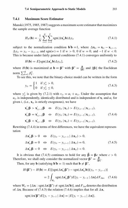
7.4 Semiparametric Approach to Static Models 203
7.4.1 Maximum Score Estimator
Manski (1975, 1985, 1987) suggests a maximum score estimator that maximizesthe sample average function
HN (b) = 1
N
N∑i=1
T∑t=2
sgn(x′i t b)yit (7.4.1)
subject to the normalization condition b′b =1, where xi t = xi t − xi,t−1,
yit = yit − yi,t−1, and sgn(w) = 1 if w > 0, 0 if w = 0, and −1 if w < 0.This is because under fairly general conditions (7.4.1) converges uniformly to
H (b) = E[sgn(x′i t b)yit ], (7.4.2)
where H (b) is maximized at b = �∗ with �∗ = �‖�‖ and ‖�‖ the Euclidean
norm∑K
k=1 β2k .
To see this, we note that the binary-choice model can be written in the form
yit ={
1 if y∗i t > 0,
0 if y∗i t ≤ 0,
(7.4.3)
where y∗i t is given by (7.2.1) with vit = αi + uit . Under the assumption that
uit is independently, identically distributed and is independent of xi and αi forgiven i , (i.e., xi t is strictly exogenous), we have
x′i t � > x′
i,t−1� ⇔ E(yit | xi t ) > E(yi,t−1 | xi,t−1),
x′i t � = x′
i,t−1� ⇔ E(yit | xi t ) = E(yi,t−1 | xi,t−1), (7.4.4)
x′i t � < x′
i,t−1� ⇔ E(yit | xi t ) < E(yi,t−1 | xi,t−1).
Rewriting (7.4.4) in terms of first differences, we have the equivalent represen-tation
x′i t � > 0 ⇔ E(yit − yi,t−1 | xi t ) > 0,
x′i t � = 0 ⇔ E(yit − yi,t−1 | xi t ) = 0, (7.4.5)
x′i t � < 0 ⇔ E(yit − yi,t−1 | xi t ) < 0.
It is obvious that (7.4.5) continues to hold for any � = �c where c > 0.Therefore, we shall only consider the normalized vector �∗ = �
‖�‖ .Then, for any b (satisfying b′b = 1) such that b �= �∗,
H (�∗) − H (b) = E{[sgn(x′i t �
∗) − sgn(x′i t b)](yit − yi,t−1)}
= 2∫
Wb
sgn(x′i t �
∗)E[yt − yt−1 | x] d Fx, (7.4.6)
where Wb = [x : sgn(x′�∗) �= sgn(x′b)], and Fx denotes the distributionof x. Because of (7.4.5) the relation (7.4.6) implies that for all x,
sgn(x′�∗)E[yt − yt−1 | x] = |E[yt − yt−1 | x]|.
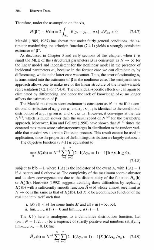
204 Discrete Data
Therefore, under the assumption on the x′s,
H (�∗) − H (b) = 2∫
Wb
|E[yt − yt−1 | x] | d Fx > 0. (7.4.7)
Manski (1985, 1987) has shown that under fairly general conditions, the es-timator maximizing the criterion function (7.4.1) yields a strongly consistentestimator of �∗.
As discussed in Chapter 3 and early sections of this chapter, when T issmall the MLE of the (structural) parameters � is consistent as N → ∞ forthe linear model and inconsistent for the nonlinear model in the presence ofincidental parameters αi , because in the former case we can eliminate αi bydifferencing, while in the latter case we cannot. Thus, the error of estimating αi
is transmitted into the estimator of � in the nonlinear case. The semiparametricapproach allows one to make use of the linear structure of the latent-variablerepresentation (7.2.1) or (7.4.4). The individual-specific effects αi can again beeliminated by differencing, and hence the lack of knowledge of αi no longeraffects the estimation of �.
The Manski maximum score estimator is consistent as N → ∞ if the con-ditional distribution of uit given αi and xi t , xi,t−1 is identical to the conditionaldistribution of ui,t−1 given αi and xi t , xi,t−1. However, it converges at the rateN 1/3, which is much slower than the usual speed of N 1/2 for the parametricapproach. Moreover, Kim and Pollard (1990) have shown that N 1/3 times thecentered maximum score estimator converges in distribution to the random vari-able that maximizes a certain Gaussian process. This result cannot be used inapplication, since the properties of the limiting distribution are largely unknown.
The objective function (7.4.1) is equivalent to
maxb
H∗N (b) = N−1
N∑i=1
T∑t=2
[2 · 1(yit = 1) − 1]1(x′i t b ≥ 0),
(7.4.8)
subject to b′b =1, where 1(A) is the indicator of the event A, with 1(A) = 1if A occurs and 0 otherwise. The complexity of the maximum score estimatorand its slow convergence are due to the discontinuity of the function HN (b)or H∗
N (b). Horowitz (1992) suggests avoiding these difficulties by replacingH∗
N (b) with a sufficiently smooth function H N (b) whose almost sure limit asN → ∞ is the same as that of H∗
N (b). Let K (·) be a continuous function of thereal line into itself such that
i. |K (v)| < M for some finite M and all v in (−∞, ∞),ii. limv→−∞ K (v) = 0 and limv→∞ K (v) = 1.
The K (·) here is analogous to a cumulative distribution function. Let{σN : N = 1, 2, . . .} be a sequence of strictly positive real numbers satisfyinglimN→∞ σN = 0. Define
H N (b) = N−1N∑
i=1
T∑t=2
[2 · 1(yit = 1) − 1]K (b′xi t/σN ). (7.4.9)
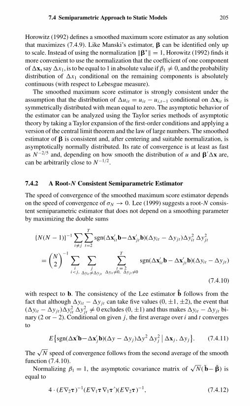
7.4 Semiparametric Approach to Static Models 205
Horowitz (1992) defines a smoothed maximum score estimator as any solutionthat maximizes (7.4.9). Like Manski’s estimator, � can be identified only upto scale. Instead of using the normalization ‖�∗‖ = 1, Horowitz (1992) finds itmore convenient to use the normalization that the coefficient of one componentof x, say x1, is to be equal to 1 in absolute value if β1 �= 0, and the probabilitydistribution of x1 conditional on the remaining components is absolutelycontinuous (with respect to Lebesgue measure).
The smoothed maximum score estimator is strongly consistent under theassumption that the distribution of uit = uit − ui,t−1 conditional on xi t issymmetrically distributed with mean equal to zero. The asymptotic behavior ofthe estimator can be analyzed using the Taylor series methods of asymptotictheory by taking a Taylor expansion of the first-order conditions and applying aversion of the central limit theorem and the law of large numbers. The smoothedestimator of � is consistent and, after centering and suitable normalization, isasymptotically normally distributed. Its rate of convergence is at least as fastas N−2/5 and, depending on how smooth the distribution of u and �′x are,can be arbitrarily close to N−1/2.
7.4.2 A Root-N Consistent Semiparametric Estimator
The speed of convergence of the smoothed maximum score estimator dependson the speed of convergence of σN → 0. Lee (1999) suggests a root-N consis-tent semiparametric estimator that does not depend on a smoothing parameterby maximizing the double sums
{N (N − 1)}−1∑i �= j
T∑t=2
sgn(x′i t b−x′
j t b)(yit − y jt )y2i t y2
j t
=(
N2
)−1 ∑i
i< j,
∑j
yit �=y jt
T∑t = 2
yit �=0, y jt �=0
sgn(x′i t b − x′
j t b)(yit − y jt )
(7.4.10)
with respect to b. The consistency of the Lee estimator b follows from thefact that although yit − y jt can take five values (0, ±1, ±2), the event that(yit − y jt )y2
i t y2j t �= 0 excludes (0, ±1) and thus makes yit − y jt bi-
nary (2 or − 2). Conditional on given j, the first average over i and t convergesto
E{sgn(x′b−x′
j b)(y − y j )y2 y2j
∣∣x j , y j}. (7.4.11)
The√
N speed of convergence follows from the second average of the smoothfunction (7.4.10).
Normalizing β1 = 1, the asymptotic covariance matrix of√
N ( b− �) isequal to
4 · (E∇2 )−1(E∇1 ∇1 ′)(E∇2 )−1, (7.4.12)

206 Discrete Data
where � = (β2, . . . , βK )′, b is its estimator,
τ (y j , x j , b) ≡ Ei | j{sgn(x′
i b − x′j b)(yi − y j )y2
i y2j
},
i �= j,
with Ei | j denoting the conditional expectation of (yi , x′i ) conditional on
(y j , x′j ), and ∇1 and ∇2 denote the first- and second-order derivative
matrices of τ (y j , x j , b) with respect to b.The parametric approach requires the specification of the distribution of u.
If the distribution of u is misspecified, the MLE of � is inconsistent. The semi-parametric approach does not require the specification of the distribution of uand permits its distribution to depend on x in an unknown way (heteroscedas-ticity of unknown form). It is consistent up to a scale, whether the unobservedindividual effects are treated as fixed or correlated with x. However, the step ofdifferencing xi t eliminates time-invariant variables from the estimation. Lee’s(1999) root-N consistent estimator takes the additional differencing across in-dividuals, xi − x j , and further reduces the dimension of estimable parame-ters by eliminating “period individual-invariant” variables (e.g., time dummiesand macroeconomic shocks common to all individuals) from the specification.Moreover, the requirement that uit and ui,t−1 be identically distributed condi-tional on (xi t , xi t−1, αi ) does not allow the presence of the lagged dependentvariables in xi t . Neither can a semiparametric approach be used to generate thepredicted probability conditional on x as in the parametric approach. All it canestimate is the relative effects of the explanatory variables.
7.5 DYNAMIC MODELS
7.5.1 The General Model
The static models discussed in the previous sections assume that the probabilityof moving (or staying) in or out of a state is independent of the occurrence ornonoccurrence of the event in the past. However, in a variety of contexts, suchas in the study of the incidence of accidents (Bates and Neyman (1951)), brandloyalty (Chintagunta, Kyriazidou, and Perktold (2001)), labor-force participa-tion (Heckman and Willis (1977); Hyslop (1999)), and unemployment (Layton(1978)), it is often noted that individuals who have experienced an event inthe past are more likely to experience the event in the future than individualswho have not. In other words, the conditional probability that an individual willexperience the event in the future is a function of past experience.
To analyze the intertemporal relationships among discrete variables,Heckman (1978a, 1981b) proposed a general framework in terms of a latent-continuous-random-variable crossing the threshold. He let the continuousrandom variable y∗
i t be a function of xi t and past occurrence of the event:
y∗i t = �′xi t +
t−1∑l=1
γl yi,t−l + φ
t−1∑s=1
s∏l=1
yi,t−l + vit ,
i = 1, . . . , N , t = 1, . . . , T, (7.5.1)

7.5 Dynamic Models 207
and
yit ={
1 if y∗i t > 0,
0 if y∗i t ≤ 0.
(7.5.2)
The error term vit is assumed to be independent of xi t and is independentlydistributed over i , with a general intertemporal variance–covariance matrixEvi v′
i = �. The coefficient γl measures the effect of experience of the event lperiods ago on current values of y∗
i t . The coefficient φ measures the effect ofthe cumulative recent spell of experience in the state, for those still in the state,on the current value of y∗
i t .Specifications (7.5.1) and (7.5.2) accommodate a wide variety of stochastic
models that appear in the literature. For example, let xi t = 1, and let vit beindependently identically distributed. If γl = 0, l = 2, . . . , T − 1, and φ = 0,equations (7.5.1) and (7.5.2) generate a time-homogenous first-order Markovprocess. If γl = 0, l = 1, . . . , T − 1, and φ �= 0, a renewal process is generated.If γl = 0, l = 1, . . . , T − 1, and φ = 0, a simple Bernoulli model results. Ifone allows vit to follow an autoregressive moving-average scheme, but keepsthe assumption that γl = 0, l = 1, . . . , T − 1, and φ = 0, the Coleman (1964)latent Markov model emerges.
As said before, repeated observations of a given group of individuals overtime permit us to construct a model in which individuals may differ in theirpropensity to experience the event. Such heterogeneity is allowed by decom-posing the error term vit as
vit = αi + uit , i = 1, . . . , N , t = 1, . . . , T, (7.5.3)
where uit is independently distributed over i with arbitrary serial correlation,and αi is individual-specific and can be treated as a fixed constant or as random.Thus, for example, if the previous assumptions on the Markov process
γl = 0, l = 2, . . . , T − 1, and φ = 0
hold, but vit follows a “components-of-variance” scheme (7.5.3), then acompound first-order Markov process, closely related to previous work onthe mover–stayer model (Goodman (1961); Singer and Spilerman (1976)), isgenerated.
Specifications (7.5.1)–(7.5.3) allow for three sources of persistence (aftercontrolling for the observed explanatory variables x). Persistence can be theresult of serial correlation in the error term uit , or the result of “unobservedheterogeneity” αi , or the result of true state dependence through the term γ yi,t−l
or φ∑t−l
s=1
∏sl=1 yi,t−l . Distinguishing the sources of persistence is important
because a policy that temporarily increases the probability that y = 1 will havedifferent implications about future probabilities of experiencing an event.
When the conditional probability of an individual staying in a state is afunction of past experience, two new issues arise. One is how to treat the ini-tial observations. The second is how to distinguish true state dependence fromspurious state dependence in which the past value appears in the specificationmerely as a proxy for the unobserved individual effects. The first issue is crucial
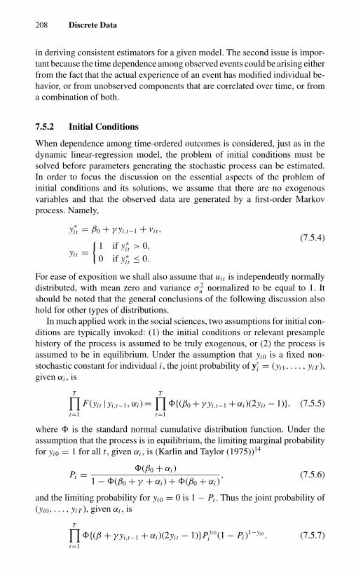
208 Discrete Data
in deriving consistent estimators for a given model. The second issue is impor-tant because the time dependence among observed events could be arising eitherfrom the fact that the actual experience of an event has modified individual be-havior, or from unobserved components that are correlated over time, or froma combination of both.
7.5.2 Initial Conditions
When dependence among time-ordered outcomes is considered, just as in thedynamic linear-regression model, the problem of initial conditions must besolved before parameters generating the stochastic process can be estimated.In order to focus the discussion on the essential aspects of the problem ofinitial conditions and its solutions, we assume that there are no exogenousvariables and that the observed data are generated by a first-order Markovprocess. Namely,
y∗i t = β0 + γ yi,t−1 + vit ,
(7.5.4)
yit ={
1 if y∗i t > 0,
0 if y∗i t ≤ 0.
For ease of exposition we shall also assume that uit is independently normallydistributed, with mean zero and variance σ 2
u normalized to be equal to 1. Itshould be noted that the general conclusions of the following discussion alsohold for other types of distributions.
In much applied work in the social sciences, two assumptions for initial con-ditions are typically invoked: (1) the initial conditions or relevant presamplehistory of the process is assumed to be truly exogenous, or (2) the process isassumed to be in equilibrium. Under the assumption that yi0 is a fixed non-stochastic constant for individual i , the joint probability of y′
i = (yi1, . . . , yiT ),given αi , is
T∏t=1
F(yit | yi,t−1, αi ) =T∏
t=1
�{(β0 + γ yi,t−1 + αi )(2yit − 1)}, (7.5.5)
where � is the standard normal cumulative distribution function. Under theassumption that the process is in equilibrium, the limiting marginal probabilityfor yi0 = 1 for all t , given αi , is (Karlin and Taylor (1975))14
Pi = �(β0 + αi )
1 − �(β0 + γ + αi ) + �(β0 + αi ), (7.5.6)
and the limiting probability for yi0 = 0 is 1 − Pi . Thus the joint probability of(yi0, . . . , yiT ), given αi , is
T∏t=1
�{(β + γ yi,t−1 + αi )(2yit − 1)}P yi0i (1 − Pi )
1−yi0 . (7.5.7)

7.5 Dynamic Models 209
If αi is random, with distribution G(α), the likelihood function for therandom-effects model under the first assumption is
L =N∏
i=1
∫ T∏t=1
�{(β0 + γ yi,t−1 + α)(2yit − 1)} dG(α). (7.5.8)
The likelihood function under the second assumption is
L =N∏
i=1
∫ T∏t=1
�{(β0 + γ yi,t−1 + α)(2yit − 1)}
× P yi0i (1 − Pi )
1−yi0 dG(α). (7.5.9)
The likelihood functions (7.5.8) and (7.5.9) under both sets of assumptionsabout initial conditions are in closed form. When αi is treated as random,the MLEs for β0, γ, and σ 2
α are consistent if N tends to infinity or if bothN and T tend to infinity. When αi is treated as a fixed constant (7.5.5), theMLEs for β0, γ, and αi are consistent only when T tends to infinity. If Tis finite, the MLE is biased. Moreover, the limited results from Monte Carloexperiments suggest that, contrary to the static case, the bias is significant(Heckman (1981b)).
However, the assumption that initial conditions are fixed constants may bejustifiable only if the disturbances that generate the process are serially indepen-dent and if a genuinely new process is fortuitously observed at the beginning ofthe sample. If the process has been in operation prior to the time it is sampled,or if the disturbances of the model are serially dependent as in the presenceof individual-specific random effects, the initial conditions are not exogenous.The assumption that the process is in equilibrium also raises problems in manyapplications, especially when time-varying exogenous variables are driving thestochastic process.
Suppose that the analyst does not have access to the process from thebeginning; then the initial state for individual i , yi0, cannot be assumed fixed.The initial state is determined by the process generating the panel sample. Thesample likelihood function for the fixed-effects model is
L =N∏
i=1
T∏t=1
�{(β0 + γ yi,t−1 + αi )(2yit − 1)} f (yi0 | αi ), (7.5.10)
and the sample likelihood function for the random-effects model is
L =N∏
i=1
∫ ∞
−∞
T∏t=1
�{(β0 + γ yi,t−1 + α)(2yit − 1)} f (yi0 | α) dG(α),
(7.5.11)
where f (yi0 | α) denotes the marginal probability of yi0 given αi . Thus, unlessT is very large, maximizing (7.5.5) or (7.5.8) yields inconsistent estimates.15
Because yi0 is a function of unobserved past values, besides the fact that themarginal distribution of f (yi0 | α) is not easy to derive, maximizing (7.5.10) or
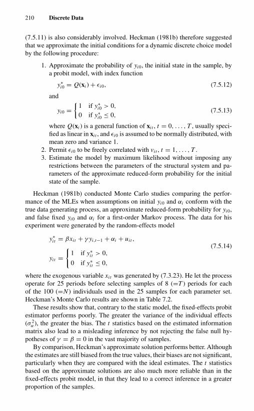
210 Discrete Data
(7.5.11) is also considerably involved. Heckman (1981b) therefore suggestedthat we approximate the initial conditions for a dynamic discrete choice modelby the following procedure:
1. Approximate the probability of yi0, the initial state in the sample, bya probit model, with index function
y∗i0 = Q(xi ) + εi0, (7.5.12)
and
yi0 ={
1 if y∗i0 > 0,
0 if y∗i0 ≤ 0,
(7.5.13)
where Q(xi ) is a general function of xi t , t = 0, . . . , T , usually speci-fied as linear in xi t , and εi0 is assumed to be normally distributed, withmean zero and variance 1.
2. Permit εi0 to be freely correlated with vit , t = 1, . . . , T .3. Estimate the model by maximum likelihood without imposing any
restrictions between the parameters of the structural system and pa-rameters of the approximate reduced-form probability for the initialstate of the sample.
Heckman (1981b) conducted Monte Carlo studies comparing the perfor-mance of the MLEs when assumptions on initial yi0 and αi conform with thetrue data generating process, an approximate reduced-form probability for yi0,and false fixed yi0 and αi for a first-order Markov process. The data for hisexperiment were generated by the random-effects model
y∗i t = βxit + γ yi,t−1 + αi + uit ,
(7.5.14)
yit ={
1 if y∗i t > 0,
0 if y∗i t ≤ 0,
where the exogenous variable xit was generated by (7.3.23). He let the processoperate for 25 periods before selecting samples of 8 (=T ) periods for eachof the 100 (=N ) individuals used in the 25 samples for each parameter set.Heckman’s Monte Carlo results are shown in Table 7.2.
These results show that, contrary to the static model, the fixed-effects probitestimator performs poorly. The greater the variance of the individual effects(σ 2
α ), the greater the bias. The t statistics based on the estimated informationmatrix also lead to a misleading inference by not rejecting the false null hy-potheses of γ = β = 0 in the vast majority of samples.
By comparison, Heckman’s approximate solution performs better. Althoughthe estimates are still biased from the true values, their biases are not significant,particularly when they are compared with the ideal estimates. The t statisticsbased on the approximate solutions are also much more reliable than in thefixed-effects probit model, in that they lead to a correct inference in a greaterproportion of the samples.

7.5 Dynamic Models 211
Table 7.2. Monte Carlo results for first-order Markov process
σ 2α = 3 σ 2
α = 1
γ β = −0.1 β = 1 β = 0 β = −0.1 β = 1 β = 0
Values of γ and β for the random-effects estimator with known initial conditionsa
0.5 γ n.a.c 0.57 n.a.c
β n.a.c 0.94 —d
0.1 γ 0.13 0.12 0.14β −0.11 1.10 —
Values of γ and β for the approximate random-effects estimationa
0.5 γ 0.63 0.60 0.70 n.a.c 0.54 0.62β −0.131 0.91 — n.a.c 0.93 —
0.1 γ 0.14 0.13 0.17 0.11 0.11 0.13β −0.12 0.92 — −0.12 0.95 —
Values of γ and β for the fixed-effects estimatorb
0.5 γ 0.14 0.19 0.03 n.a.c 0.27 0.17β −0.07 1.21 — n.a.c 1.17 —
0.1 γ −0.34 −0.21 −0.04 −0.28 −0.15 −0.01β −0.06 1.14 — −0.08 1.12 —
a N = 100; T = 3.b N = 100; T = 8.cData not available because the model was not estimated.d Not estimated.Source: Heckman (1981b, Table 4.2).
Heckman’s Monte Carlo results also point to a disquieting feature. Namely,the MLE produces a biased estimator even under ideal conditions with acorrectly specified likelihood function. Because a panel with 100 observationsof three periods is not uncommon, this finding deserves serious consideration.
7.5.3 A Conditional Approach
The likelihood approach cannot yield a consistent estimator when T is fixedand N tends to infinity if the individual effects are fixed. If the individual effectsare random and independent of x, the consistency of the MLE depends on thecorrect formulation of the probability distributions of the effects and initial ob-servations. A semiparametric approach cannot be implemented for a dynamicmodel, because the strict exogeneity condition of explanatory variables is vio-lated with the presence of lagged dependent variables as explanatory variables.When that condition is violated, E(uit | xi t , xi,t−1, yi,t−1, yi,t−2) �= 0. In otherwords, the one-to-one correspondence relation of the form (7.4.4) is violated.

212 Discrete Data
Hence, the Manski (1985) maximum score estimator cannot be implemented.Neither can the (unrestricted) conditional approach be implemented. Considerthe case of T = 2. The basic idea of the conditional approach is to consider theprobability of yi2 = 1 or 0 conditional on explanatory variables in both periodsand conditonal on yi1 �= yi2. If the explanatory variables of Prob(yi2 = 1) in-clude yi1, then the conditional probability is either 1 or 0 according as yi1 = 0or 1, and hence provides no information about γ and �.
However, in the case that T ≥ 3 and xi t follows a certain special pat-tern, Honore and Kyriazidou (2000a) show that it is possible to generalize theconditional-probability approach to consistently estimate the unknown param-eters for the logit model or to generalize the maximum score approach with-out the need of formulating the distribution of αi or the probability distributionof the initial observations for certain types of discrete choice models. However,the estimators converge to the true values at the speed considerably slowerthan the usual
√N rate.
Consider the model (7.5.4) with the assumption that uit is logistically dis-tributed. Then the model of (yi0, . . . yiT ) is of the form
P(yi0 = 1 | αi ) = P0(αi ), (7.5.15)
P(yit = 1 | αi , yi0, . . . , yi,t−1) = exp(γ yi,t−1 + αi )
1 + exp(γ yi,t−1 + αi )
for t = 1, 2, . . . , T . (7.5.16)
When T ≥ 3, Chamberlain (1993) shows that the inference on γ can be madeindependent of αi by using a conditional approach.
For ease of exposition, we shall assume that T = 3. Consider the events
A = {yi0, yi1 = 0, yi2 = 1, yi3},B = {yi0, yi1 = 1, yi2 = 0, yi3},
where yi0 and yi3 can be either 1 or 0. Then
P(A) = P0(αi )yi0 [1 − P0(αi )]
1−yi0 · 1
1 + exp(γ yi0 + αi )
× exp(αi )
1 + exp(αi )· exp[(γ + αi )yi3]
1 + exp(γ + αi ), (7.5.17)
and
P(B) = P0(αi )yi0 [1 − P0(αi )]
1−yi0 · exp(γ yi0 + αi )
1 + exp(γ yi0 + αi )
× 1
1 + exp(γ + αi )· exp(αi yi3)
1 + exp(αi ). (7.5.18)

7.5 Dynamic Models 213
Hence,
P(A | A ∪ B) = P(A | yi0, yi1 + yi2 = 1, yi3)
= exp(γ yi3)
exp(γ yi3) + exp(γ yi0)
= 1
1 + exp[γ (yi0 − yi3)], (7.5.19)
and
P(B | A ∪ B) = P(B | yi0, yi1 + yi2 = 1, yi3)
= 1 − P(A | A ∪ B)
= exp[γ (yi0 − yi3)]
1 + exp[γ (yi0 − yi3)]. (7.5.20)
Equations (7.5.19) and (7.5.20) are in the binary logit form and do not dependon αi . Let di = 1 if A occurs and 0 if B occurs. The conditional log likelihood
log L =N∑
i=1
1(yi1 + yi2 = 1)
× {yi1[γ (yi0 − yi3)] − log[1 + exp γ (yi0 − yi3)]} (7.5.21)
is in the conditional logit form. Maximizing (7.5.21) yields a√
N -consistentestimator of γ , where 1(A) = 1 if A occurs and 0 otherwise.
When exogenous variables xi t also appear as explanatory variables in thelatent response function
y∗i t = �′xi t + γ yi,t−1 + αi + uit , (7.5.22)
we may write
P(yi0 = 1 | xi , αi ) = P0(xi , αi ), (7.5.23)
P(yit = 1 | xi , αi , yi0, . . . , yi,t−1) = exp(x′i t � + γ yi,t−1 + αi )
1 + exp(x′i t � + γ yi,t−1 + αi )
,
t = 1, . . . , T . (7.5.24)
In general, P(A | xi , αi , A ∪ B) will depend on αi . However, if xi2 = xi3,Honore and Kyriazidou (2000a), using the same conditioning method, showthat
P(A | xi , αi , A ∪ B, xi2 = xi3)
= 1
1 + exp[(xi1 − xi2)′� + γ (yi0 − yi3)], (7.5.25)
which does not depend on αi . If xi t is continuous, it may be rare that xi2 = xi3.

214 Discrete Data
Honore and Kyriazidou (2000a) propose estimating β and γ by maximizing
N∑i=1
1(yi1 + yi2 = 1)K
(xi2 − xi3
σN
)log
{exp[(xi1 − xi2)′b + γ (yi0 − yi3)]yi1
1 + exp[(xi1 − xi2)′b + γ (yi0 − yi3)]
}(7.5.26)
with respect to b and γ (over some compact set) if P(xi2 = xi3) > 0. Here K (·)is a kernel density function which gives appropriate weight to observation i ,while σN is a bandwidth which shrinks to zero as N tends to infinity at a speedthat is also a function of the dimension of x. The asymptotic theory will requirethat K (·) be chosen so that a number of regularity conditions are satisfied, suchas |K (·)| < M for some constant M , K (v) → 0 as |v| → ∞, and
∫K (v) dv = 1.
For instance, K (v) is often taken to be the standard normal density function,and σN = cN−1/5 for some constant c when there is only one regressor. Theeffect of the factor K ((xi2 − xi3)/σN ) is to give more weight to observationsfor which xi2 is close to xi3. Their estimator is consistent and asymptoticallynormal, although their rate of convergence is only
√Nσ k
N , which is considerablyslower than
√N , where k is the dimension of xi t .
The conditional approach works for the logit model, but it does not seemapplicable for general nonlinear models. However, if the nonlinearity can beput in the single-index form F(a) with the transformation function F being astrictly increasing distribution function, then Manski’s (1987) maximum scoreestimator for the static case can be generalized to the case where the laggeddependent variable is included in the explanatory variable set by considering
P(A | xi , αi , xi2 = xi3)
= P0(xi , αi )yi0 [1 − P0(xi , αi )]
1−yi0
× [1 − F(x′i1� + γ yi0 + αi )] × F(x′
i2� + αi )
× [1 − F(x′i2� + γ + αi )]
1−yi3 × F(x′i2� + γ + αi )
yi3 , (7.5.27)
and
P(B | xi , αi , xi2 = xi3)
= P0(xi , αi )yi0 [1 − P0(xi , αi )]
1−yi0
× F(x′i1� + γ yi0 + αi ) × [1 − F(x′
i2� + γ + αi )]
× [1 − F(x′i2� + αi )]
1−yi3 × F(x′i2� + αi )
yi3. (7.5.28)
If yi3 = 0, then
P(A | xi , αi , xi2 = xi3)
P(B | xi , αi , xi2 = xi3)
= 1 − F(x′i1� + γ yi0 + αi )
1 − F(x′i2� + αi )
× F(x′i2� + αi )
F(x′i1� + γ yi0 + αi )
= 1 − F(x′i1� + γ yi0 + αi )
1 − F(x′i2� + γ yi3 + αi )
× F(x′i2� + γ yi3 + αi )
F(x′i1� + γ yi0 + αi )
, (7.5.29)
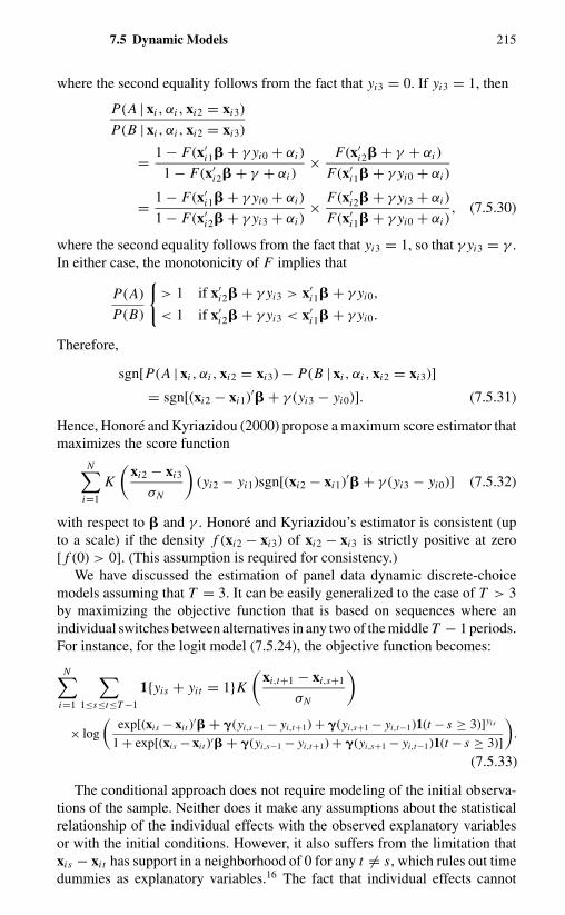
7.5 Dynamic Models 215
where the second equality follows from the fact that yi3 = 0. If yi3 = 1, then
P(A | xi , αi , xi2 = xi3)
P(B | xi , αi , xi2 = xi3)
= 1 − F(x′i1� + γ yi0 + αi )
1 − F(x′i2� + γ + αi )
× F(x′i2� + γ + αi )
F(x′i1� + γ yi0 + αi )
= 1 − F(x′i1� + γ yi0 + αi )
1 − F(x′i2� + γ yi3 + αi )
× F(x′i2� + γ yi3 + αi )
F(x′i1� + γ yi0 + αi )
, (7.5.30)
where the second equality follows from the fact that yi3 = 1, so that γ yi3 = γ .In either case, the monotonicity of F implies that
P(A)
P(B)
{> 1 if x′
i2� + γ yi3 > x′i1� + γ yi0,
< 1 if x′i2� + γ yi3 < x′
i1� + γ yi0.
Therefore,
sgn[P(A | xi , αi , xi2 = xi3) − P(B | xi , αi , xi2 = xi3)]
= sgn[(xi2 − xi1)′� + γ (yi3 − yi0)]. (7.5.31)
Hence, Honore and Kyriazidou (2000) propose a maximum score estimator thatmaximizes the score function
N∑i=1
K
(xi2 − xi3
σN
)(yi2 − yi1)sgn[(xi2 − xi1)′� + γ (yi3 − yi0)] (7.5.32)
with respect to � and γ . Honore and Kyriazidou’s estimator is consistent (upto a scale) if the density f (xi2 − xi3) of xi2 − xi3 is strictly positive at zero[ f (0) > 0]. (This assumption is required for consistency.)
We have discussed the estimation of panel data dynamic discrete-choicemodels assuming that T = 3. It can be easily generalized to the case of T > 3by maximizing the objective function that is based on sequences where anindividual switches between alternatives in any two of the middle T − 1 periods.For instance, for the logit model (7.5.24), the objective function becomes:
N∑i=1
∑1≤s≤t≤T −1
1{yis + yit = 1}K
(xi,t+1 − xi,s+1
σN
)× log
(exp[(xis − xi t )′� + �(yi,s−1 − yi,t+1) + �(yi,s+1 − yi,t−1)1(t − s ≥ 3)]yis
1 + exp[(xis − xi t )′� + �(yi,s−1 − yi,t+1) + �(yi,s+1 − yi,t−1)1(t − s ≥ 3)]
).
(7.5.33)
The conditional approach does not require modeling of the initial observa-tions of the sample. Neither does it make any assumptions about the statisticalrelationship of the individual effects with the observed explanatory variablesor with the initial conditions. However, it also suffers from the limitation thatxis − xi t has support in a neighborhood of 0 for any t �= s, which rules out timedummies as explanatory variables.16 The fact that individual effects cannot

216 Discrete Data
be estimated also means that it is not possible to make predictions or computeelasticities for individual agents at specified values of the explanatory variables.
7.5.4 State Dependence versus Heterogeneity
There are two diametrically opposite explanations for the often observed empir-ical regularity with which individuals who have experienced an event in the pastare more likely to experience that event in the future. One explanation is thatas a consequence of experiencing an event, preferences, prices, or constraintsrelevant to future choices are altered. A second explanation is that individualsmay differ in certain unmeasured variables that influence their probability ofexperiencing the event but are not influenced by the experience of the event. Ifthese variables are correlated over time and are not properly controlled, previousexperience may appear to be a determinant of future experience solely becauseit is a proxy for such temporally persistent unobservables. Heckman (1978a,1981a, 1981c) has termed the former case true state dependence and the lattercase spurious state dependence, because in the former case, past experience hasa genuine behavioral effect in the sense that an otherwise identical individualwho has not experienced the event will behave differently in the future than anindividual who has experienced the event. In the latter case, previous experienceappears to be a determinant of future experience solely because it is a proxy fortemporally persistent unobservables that determine choices.
The problem of distinguishing between true and spurious state dependenceis of considerable substantive interest. To demonstrate this, let us considersome work in the theory of unemployment. Phelps (1972) argued that currentunemployment has a real and lasting effect on the probability of future unem-ployment. Hence, short-term economic policies that alleviate unemploymenttend to lower aggregate unemployment rates in the long run by preventingthe loss of work-enhancing market experience. On the other hand, Cripps andTarling (1974) maintained the opposite view in their analysis of the incidenceand duration of unemployment. They assumed that individuals differ in theirpropensity to experience unemployment and in their unemployment durationtimes and that those differences cannot be fully accounted for by measuredvariables. They further assumed that the actual experience of having been un-employed or the duration of past unemployment does not affect future incidenceor duration. Hence, in their model, short-term economic policies have no effecton long-term unemployment.
Because the unobserved individual effects αi persist over time, ignoring theseeffects of unmeasured variables (heterogeneity) creates serially correlated resid-uals. This suggests that we cannot use the conditional probability, given pastoccurrence not equal to the marginal probability alone [Prob(yit | yi,t−s, xi t ) �=Prob(yit | xi t )], to test for true state dependence against spurious state depen-dence, because this inequality may be a result of past information on y yieldinginformation on the unobserved specific effects. A proper test for dependenceshould control for the unobserved individual-specific effects.

7.5 Dynamic Models 217
When, conditional on the individual effects αi , the error term uit is seriallyuncorrelated, a test for state dependence can be easily implemented by control-ling the individual effects and testing for the conditional probability equal tothe marginal probability,17
Prob(yit | yi,t−s, xi t , αi ) = Prob(yit | xi t , αi ). (7.5.34)
If the conditional distribution G(α | x) of αi given xi is known, a morepowerful test is to use an unconditional approach. Thus, one may test truestate dependence versus spurious state dependence by testing the significanceof the MLE of γ of the log likelihood
N∑i=1
log∫ T∏
t=1
{F(x′i t � + γ yi,t−1 + αi )
yit [1 − F(x′i t � + γ yi,t−1 + αi )]
1−yit
× P0(xi , α)yi0 [1 − P(xi , α)]1−yi0}G(α | xi ) dα. (7.5.35)
When, conditional on the individual effects αi , the error term uit remainsserially correlated, the problem becomes more complicated. The conditionalprobability Prob(yit | yi,t−l , αi ) might fail to be equal to the marginal probabil-ity Prob(yit | αi ) because of past yit containing information on uit . A test forstate dependence cannot simply rely on the multinomial distribution of the se-quence (yi1, . . . , yiT ). The general framework (7.5.1) and (7.5.2) proposed byHeckman (1978a, 1981a, 1981b) accommodates very general sorts of hetero-geneity and structural dependence. It permits an analyst to combine models andtest among competing specifications within a unified framework. However, thecomputations of maximum likelihood methods for the general models are quiteinvolved. It would be useful to rely on simple methods to explore data beforeemploying the computationally cumbersome maximum likelihood method fora specific model.
Chamberlain (1978b) suggested a simple method to distinguish true statedependence from spurious state dependence. He noted that just as in the contin-uous models, a key distinction between state dependence and serial correlationis whether or not there is a dynamic response to an intervention. This distinctioncan be made clear by examining (7.5.1). If γ = 0, a change in x has its full effectimmediately, whereas if γ �= 0, one has a distributed-lag response to a changein x. The lag structure relating y to x is not related to the serial correlation in u. Ifx is increased in period t and then returned to its former level, the probability ofyi,t+1 is not affected if γ = 0, because by assumption the distribution of uit wasnot affected. If γ �= 0, then the one-period shift in x will have lasting effects. Anintervention that affects the probability of y in period t will continue to affectthe probability of y in period t + 1, even though the intervention was presentedonly in period t . In contrast, an interpretation of serial correlation is that theshocks (u) tend to persist for more than one period and that yit is informativeonly in helping to infer uit and hence to predict uit . Therefore, a test that shouldnot be very sensitive to functional form is to simply include lagged xs withoutlagged y. After conditioning on the individual-specific effect αi , there may be

218 Discrete Data
two outcomes. If there is no state dependence, then
Prob(yit = 1 | xi t , xi,t−1, . . . , αi ) = Prob(yit = 1 | xi t , αi ), (7.5.36)
and if there is state dependence, then
Prob(yit = 1 | xi t , xi,t−1, . . . , αi ) �= Prob(yit = 1 | xi t , αi ). (7.5.37)
While the combination of (7.5.34), (7.5.36), and (7.5.37) provides a simpleform to distinguish pure heterogeneity, state dependence, and serial correlation,we cannot make further distinctions with regard to different forms of statedependence, heterogeneity, and serial correlation. Models (7.5.1) and (7.5.2)will have to be used to further narrow down possible specifications.
7.5.5 Two Examples
The control of heterogeneity plays a crucial role in distinguishing true statedependence from spurious state dependence. Neglecting heterogeneity and theissue of initial observations can also seriously bias the coefficient estimates. Itis important in estimating dynamic models that the heterogeneity in the samplebe treated correctly. To demonstrate this, we use the female-employment mod-els estimated by Heckman (1981c) and household brand choices estimated byChintagunta, Kyriazidou, and Perktold (2001) as examples.
7.5.5.a Female Employment
Heckman (1981c) used the first three-year sample of women aged 45–59 in1968 from the Michigan Panel Survey of Income Dynamics to study marriedwomen’s employment decisions. A woman is defined to be a market participantif she works for money any time in the sample year. The set of explanatoryvariables is as follows: the woman’s education; family income, excluding thewife’s earnings; number of children younger than six; number of children athome; unemployment rate in the county in which the woman resides; the wageof unskilled labor in the county (a measure of the availability of substitutes fora woman’s time in the home); the national unemployment rate for prime-agemales (a measure of aggregate labor-market tightness); and two types of priorwork experience: within-sample and presample. The effect of previous workexperience is broken into two components, because it is likely that presampleexperience exerts a weaker measured effect on current participation decisionsthan more recent experience. Furthermore, because the data on presample workexperience are based on a retrospective question and therefore are likely to bemeasured with error, Heckman replaces them with predicted values based on aset of regressors.
Heckman fitted the data with various multivariate probit models of theform (7.5.1) and (7.5.2) to investigate whether or not work experience raisesthe probability that a woman will work in the future (by raising her wagerates) and to investigate the importance of controlling for heterogeneity in
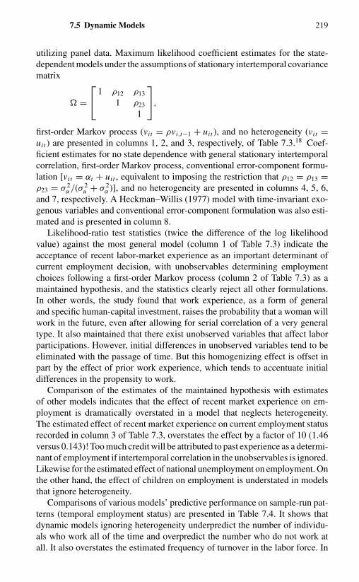
7.5 Dynamic Models 219
utilizing panel data. Maximum likelihood coefficient estimates for the state-dependent models under the assumptions of stationary intertemporal covariancematrix
� =1 ρ12 ρ13
1 ρ23
1
,
first-order Markov process (vit = ρvi,t−1 + uit ), and no heterogeneity (vit =uit ) are presented in columns 1, 2, and 3, respectively, of Table 7.3.18 Coef-ficient estimates for no state dependence with general stationary intertemporalcorrelation, first-order Markov process, conventional error-component formu-lation [vit = αi + uit , equivalent to imposing the restriction that ρ12 = ρ13 =ρ23 = σ 2
α/(σ 2u + σ 2
α )], and no heterogeneity are presented in columns 4, 5, 6,and 7, respectively. A Heckman–Willis (1977) model with time-invariant exo-genous variables and conventional error-component formulation was also esti-mated and is presented in column 8.
Likelihood-ratio test statistics (twice the difference of the log likelihoodvalue) against the most general model (column 1 of Table 7.3) indicate theacceptance of recent labor-market experience as an important determinant ofcurrent employment decision, with unobservables determining employmentchoices following a first-order Markov process (column 2 of Table 7.3) as amaintained hypothesis, and the statistics clearly reject all other formulations.In other words, the study found that work experience, as a form of generaland specific human-capital investment, raises the probability that a woman willwork in the future, even after allowing for serial correlation of a very generaltype. It also maintained that there exist unobserved variables that affect laborparticipations. However, initial differences in unobserved variables tend to beeliminated with the passage of time. But this homogenizing effect is offset inpart by the effect of prior work experience, which tends to accentuate initialdifferences in the propensity to work.
Comparison of the estimates of the maintained hypothesis with estimatesof other models indicates that the effect of recent market experience on em-ployment is dramatically overstated in a model that neglects heterogeneity.The estimated effect of recent market experience on current employment statusrecorded in column 3 of Table 7.3, overstates the effect by a factor of 10 (1.46versus 0.143)! Too much credit will be attributed to past experience as a determi-nant of employment if intertemporal correlation in the unobservables is ignored.Likewise for the estimated effect of national unemployment on employment. Onthe other hand, the effect of children on employment is understated in modelsthat ignore heterogeneity.
Comparisons of various models’ predictive performance on sample-run pat-terns (temporal employment status) are presented in Table 7.4. It shows thatdynamic models ignoring heterogeneity underpredict the number of individu-als who work all of the time and overpredict the number who do not work atall. It also overstates the estimated frequency of turnover in the labor force. In
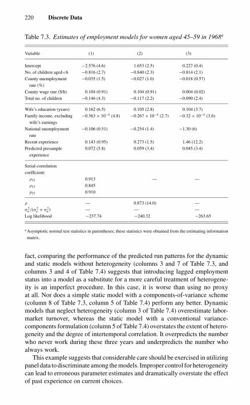
220 Discrete Data
Table 7.3. Estimates of employment models for women aged 45–59 in 1968a
Variable (1) (2) (3)
Intercept −2.576 (4.6) 1.653 (2.5) 0.227 (0.4)
No. of children aged<6 −0.816 (2.7) −0.840 (2.3) −0.814 (2.1)
County unemployment −0.035 (1.5) −0.027 (1.0) −0.018 (0.57)
rate (%)
County wage rate ($/h) 0.104 (0.91) 0.104 (0.91) 0.004 (0.02)
Total no. of children −0.146 (4.3) −0.117 (2.2) −0.090 (2.4)
Wife’s education (years) 0.162 (6.5) 0.105 (2.8) 0.104 (3.7)
Family income, excluding −0.363 × 10⁻⁴ (4.8) −0.267 × 10⁻⁴ (2.7) −0.32 × 10⁻⁴ (3.6)
wife’s earnings
National unemployment −0.106 (0.51) −0.254 (1.4) −1.30 (6)
rate
Recent experience 0.143 (0.95) 0.273 (1.5) 1.46 (12.2)
Predicted presample 0.072 (5.8) 0.059 (3.4) 0.045 (3.4)
experience
Serial-correlation
coefficient:
ρ12 0.913 — —
ρ13 0.845
ρ23 0.910
ρ — 0.873 (14.0) —
σ 2α /(σ 2
u + σ 2α ) — — —
Log likelihood −237.74 −240.32 −263.65
aAsymptotic normal test statistics in parentheses; these statistics were obtained from the estimating information
matrix.
fact, comparing the performance of the predicted run patterns for the dynamicand static models without heterogeneity (columns 3 and 7 of Table 7.3, andcolumns 3 and 4 of Table 7.4) suggests that introducing lagged employmentstatus into a model as a substitute for a more careful treatment of heterogene-ity is an imperfect procedure. In this case, it is worse than using no proxyat all. Nor does a simple static model with a components-of-variance scheme(column 8 of Table 7.3, column 5 of Table 7.4) perform any better. Dynamicmodels that neglect heterogeneity (column 3 of Table 7.4) overestimate labor-market turnover, whereas the static model with a conventional variance-components formulation (column 5 of Table 7.4) overstates the extent of hetero-geneity and the degree of intertemporal correlation. It overpredicts the numberwho never work during these three years and underpredicts the number whoalways work.
This example suggests that considerable care should be exercised in utilizingpanel data to discriminate among the models. Improper control for heterogeneitycan lead to erroneous parameter estimates and dramatically overstate the effectof past experience on current choices.

7.5 Dynamic Models 221
Table 7.3. (cont.)
(4) (5) (6) (7) (8)
−2.367 (6.4) −2.011 (3.4) −2.37 (5.5) −3.53 (4.6) −1.5 (0)
−0.742 (2.6) −0.793 (2.1) −0.70 (2.0) −1.42 (2.3) −0.69 (1.2)
−0.030 (1.5) −0.027 (1.2) −0.03 (1.6) −0.059 (1.3) 0.046 (11)
0.090 (0.93) 0.139 (1.5) 0.13 (1.4) 0.27 (1.1) 0.105 (0.68)
−0.124 (4.9) −0.116 (2.2) −0.161 (4.9) −0.203 (3.9) −0.160 (6.1)
0.152 (7.3) 0.095 (2.5) 0.077 (3) 0.196 (4.8) 0.105 (3.3)
−0.312 × 10⁻⁴ (5.2) −0.207 × 10⁻⁴ (2.3) −0.2 × 10⁻⁴ (2.6) −0.65 × 10⁻⁴ (5.1) −0.385 × 10⁻⁴ (20)
−0.003 (0.38) −0.021 (0.26) 0.02 (3) 1.03 (0.14) −0.71 (0)
—b — — — —
0.062 (0.38) 0.062 (3.5) 0.091 (7.0) 0.101 (5.4) 0.095 (11.0)
0.917 — — — —
0.873 — — — —
0.946 — — — —
— −0.942 (50) — — —
— — 0.92 (4.5) — 0.941 (4.1)
−239.81 −243.11 −244.7 −367.3 −242.37
bNot estimated.
Source: Heckman (1981c, Table 3.2).
7.5.5.b Household Brand Choices
Chintagunta, Kyriazidou, and Perktold (2001) use the A.C. Nielson data onyogurt purchases in Sioux Falls, South Dakota between September 17, 1986and August 1, 1988 to study yogurt brand loyalty. They focus on the 6 oz pack-ages of the two dominant yogurt brands, Yoplait and Nordica, for the analysis.These brands account for 18.4 and 19.5 percent of yogurt purchases by weight.Only data for households that have at least two consecutive purchases of eitherone of the two brands are considered. This leaves 737 households and 5,618purchase occasions, out of which 2,718 are for Yoplait and the remaining 2,900for Nordica. The panel is unbalanced.19 The minimum number of purchaseoccasions per household is 2, and the maximum is 305. The mean number ofpurchases is 9.5, and the median is 5.
The model they estimate is given by
Prob(yit = 1 | xi t , yi0, . . . , yi,t−1, αi ) = exp(x′i t � + γ yi,t−1 + αi )
1 + exp(x′i t � + γ yi,t−1 + αi )
,
(7.5.38)

222 Discrete Data
Table 7.4. Comparisons of employment models using run data: Women aged45–59 in 1968
(1) (2) (3) (4) (5)
Number Probit model Numberpredicted from that ignores predictedstate-dependent Probit model heterogeneity and frommodel with that ignores recent-sample Heckman–heterogeneity heterogeneity state dependence Willis model
Run Actual (column 2 of (column 3 of (column 7 of (column 8 ofpattern number Table 7.3) Table 7.3) Table 7.3) Table 7.3)
0,0,0 96 94.2 145.3 36.1 139.50,0,1 5 17.6 38.5 20.5 4.10,1,0 4 1.8 1.9 20.2 4.11,0,0 8 2.6 0.35 20.6 4.11,1,0 5 1.4 0.02 21.2 3.61,0,1 2 2.4 1.38 21.1 3.60,1,1 2 16.4 8.51 21.7 3.61,1,1 76 61.5 2.05 36.6 34.9
χ2 c — 48.5 4,419 221.8 66.3
aData for 1971, 1972, and 1973, three years following the sample data, were used toestimate the model.
b0 corresponds to not working; 1 corresponds to working; thus, 1,1,0 corresponds to awoman who worked the first two years of the sample and did not work in the final year.
cThis is the standard chi-square statistic for goodness of fit. The higher the value of thestatistic, the worse the fit.
Source: Heckman (1981c).
where yit = 1 if household i chooses Yoplait in period t and yit = 0 ifhousehold i chooses Nordica. The exogenous variables in xi t are the differ-ence in the natural logarithm of the price (coefficient denoted by βP ) and thedifferences in the dummy variables for the two brands that describe whetherthe brand was displayed in the store and featured in an advertisement that week(coefficients denoted by βD and βF respectively). Among the many models theyestimated, Table 7.5 presents the results of:
1. The pooled logit model with the lagged choice treated as exogenous,assuming there are no individual-specific effects (PLL).
2. The Chamberlain (1982) conditional logit approach with the laggedchoice treated as exogenous (CLL).
3. The pooled logit approach with normally distributed random effectswith mean µ and variance σ 2
α , with the initial choice treated as exoge-nous (PLLHET).
4. The pooled logit approach with normally distributed random effectsand the initial probability of choosing 1 given (xi , αi ) assumed at the

7.5 Dynamic Models 223
Table 7.5. Estimates of brand choices using various approaches(standard errors in parentheses)
Model βp βd β f γ µα σα
CLL −3.347 0.828 0.924 −0.068(0.399) (0.278) (0.141) (0.140)
PLL −3.049 0.853 1.392 3.458 −0.333(0.249) (0.174) (0.091) (0.084) (0.102)
PLLHET −3.821 1.031 1.456 2.126 0.198 1.677(0.313) (0.217) (0.113) (0.114) (0.150) (0.086)
PLLHETE −4.053 0.803 1.401 1.598 0.046 1.770(0.274) (0.178) (0.115) (0.115) (0.133) (0.102)
HK05 −3.477 0.261 0.782 1.223(0.679) (0.470) (0.267) (0.352)
HK10 −3.128 0.248 0.759 1.198(0.658) (0.365) (0.228) (0.317)
HK30 −2.644 0.289 0.724 1.192(0.782) (0.315) (0.195) (0.291)
PLLHET-Sa −3.419 1.095 1.291 1.550 0.681 1.161(0.326) (0.239) (0.119) (0.117) (0.156) (0.081)
aThe PLLHET estimates after excluding those households that are completelyloyal to one brand.
Source: Chintagunta, Kyriazidou, and Perktold (2001, Table 3).
steady state, which is approximated by
F(x′i � + αi )
1 − F(x′i � + γ + αi ) + F(x′
i � + αi ), (7.5.39)
where F(a) = exp(a)/(1 + exp(a)) and xi denotes the individual time-series mean of xi t (PLLHETE).
5. The Honore–Kyriazidou (2000) approach where σN = c · N−1/5 withc = 0.5 (HK05), 1.0 (HK10), and 3.0 (HK30).
Table 7.5 reveals that almost all procedures yield statistically significant co-efficients with the expected signs. An increase in the price of a brand reducesthe probability of choosing the brand, and the presence of a store display or ofa feature advertisement for a brand makes purchase of that brand more likely.Also, apart from CLL, all methods produce positive and statistically significantestimates for γ , i.e., a previous purchase of a brand increases the probabilityof purchasing the same brand in the next period. The lagged choice is foundto have a large positive effect in brand choice for pooled methods assuming noheterogeneity: The PLL estimate of γ is 3.5. However, introducing heterogene-ity lowers it substantially to 2.1 (PLLHET). The estimate of γ further drops to1.598 (PLLHETE) when the initial observations are treated as endogenous, anddrops to about 1.2 using the Honore–Kyriazidou estimator. Nevertheless, theresults do indicate that after controlling for the effects of αi , a previous purchaseof a brand increases the probability of purchasing the same brand in the next

224 Discrete Data
period, although their effect is substaintially reduced from the case of assumingno heterogeneity. There is also an indication of substantial heterogeneity inthe sample. All methods that estimate random effects give high values for thestandard deviation of the household effects, σα , about 1.7, bearing in mind thatσu is normalized to 1 only.
In general, the size of the estimated parameters varies considerably acrossestimation methods. There is also some sensitivity in the HK point estimates ofall coefficients with respect to the bandwidth choice. To investigate this issuefurther and identify situations where the different methods are most reliable inproducing point estimates, Chintagunta, Kyriazidou, and Perktold (2001) fur-ther conducted Monte Carlo studies. Their results indicate that the conditionallikelihood procedures are the most robust in estimating the coefficients on theexogenous variables. However, the coefficient on the lagged dependent vari-able is significantly underestimated. The pooled procedures are quite sensitiveto model misspecification, often yielding large biases for key economic pa-rameters. The estimator proposed by Honore and Kyriazidou (2000a) performsquite satisfactory despite a loss of precision because their method de facto onlyuses substantially smaller number of observations than other methods, due tothe use of the weighting scheme K ((xi t − xis)/σN ).

CHAPTER 8
Truncated and Censored Data
8.1 INTRODUCTION
In economics, the ranges of dependent variables are often constrained in someway. For instance, in his pioneering work on household expenditure on durablegoods, Tobin (1958) used a regression model that specifically took account of thefact that the expenditure (the dependent variable of his regression model) cannotbe negative. Tobin called this type of model the model of limited dependentvariables. It and its various generalization are known as Tobit models because oftheir similarities to probit models.1 In statistics they are known as truncated orcensored regression models. The model is called truncated if the observationsoutside a specific range are totally lost, and is called censored if we can at leastobserve some of the explanatory variables.
Consider a latent response function,
y∗ = �′x + u, (8.1.1)
where x is a K × 1 vector of exogenous variables and u is the error term thatis independently, identically distributed (i.i.d.) with mean 0 and variance σ 2
u .Without loss of generality, suppose that the observed y are related to y∗ by
y ={
y∗ if y∗ > 0,
0 if y∗ ≤ 0.(8.1.2)
Models of the form (8.1.1) and (8.1.2) are called censored regression modelsbecause the data consist of those points of the form (y∗
i , xi ) if y∗i > 0 and (0, xi )
if y∗i ≤ 0 for i = 1, . . . , N . The truncated data only consist of points of the form
(y∗i , xi ) where y∗
i > 0.The conditional expectation of y given x for truncated data is equal to
E(y | y > 0) = E(y∗ | y∗ > 0) = x′� + E(u | u > −x′�). (8.1.3)
The conditional expectation of y given x for censored data is equal to
E(y | x) = Prob(y = 0) · 0 + Prob(y > 0 | x) · E(y | y > 0, x)
= Prob(u ≤ −x′�) · 0 + Prob(u > −x′�)E(y∗ | x; u > −x′�)
= Prob(u > −x′�)[x′� + E(u | u > −x′�)]. (8.1.4)

226 Truncated and Censored Data
If u is independently normally distributed with mean 0 and variance σ 2u , then
Prob(u > −x′�) = 1 − �
(−x′�σu
)= �
(x′�σu
), (8.1.5)
and
E(u | u > −x′�) = σu ·φ
(x′�σu
)�
(x′�σu
) , (8.1.6)
where φ(·) and �(·) are standard normal density and cumulative (or integrated)normal, respectively. Equations (8.1.3) and (8.1.4) show that truncation or cen-soring of the dependent variables introduces dependence between the error termand the regressors for the model
y = x′� + ε, (8.1.7)
where the error
ε = ν + E(y | x) − x′�. (8.1.8)
Although ν = y − E(y | x) has E(ν | x) = 0, we have E(ε | x) �= 0. Therefore,the least-squares estimator of (8.1.7) is biased and inconsistent.
For a sample of N independent individuals, the likelihood function of thetruncated data is equal to
L1 =∏
1
[Prob(yi > 0 | xi )]−1 f (yi ), (8.1.9)
where f (·) denotes the density of y∗i (or ui ), and
∏1 means the product over
those i for which yi > 0. The likelihood function of the censored data is equal to
L2 ={∏
0
Prob(yi = 0 | xi ) ·∏
1
Prob(yi > 0 | xi )
}
×{∏
1
[Prob(yi > 0 | xi )]−1 f (yi )
}
=∏
0
Prob(yi = 0 | xi )∏
1
f (yi ), (8.1.10)
where∏
0 means the product over those i for which y∗i ≤ 0. In the case that
ui is independently normally distributed with mean 0 and variance σ 2u , we
have f (yi ) = (2π )−12 σ−1
u exp{−(1/2σ 2u )(yi − x′
i �)2} and Prob(yi = 0 | xi ) =�(−x′
i �/σu) = 1 − �(x′i �/σu).
Maximizing (8.1.9) or (8.1.10) with respect to �′ = (�′, σ 2u ) yields the
maximum likelihood estimator (MLE). The MLE, �, is consistent and isasymptotically normally distributed. The asymptotic covariance matrix ofthe MLE, asy cov[
√N (� − �)], is equal to the inverse of the informa-
tion matrix, [−E(1/N )∂2 log L j/∂� ∂�′]−1, which may be approximated by

8.1 Introduction 227
[−(1/N )∂2 log L j/∂� ∂�′ | �=�]−1, j = 1, 2. However, the MLE is highly non-linear. A Newton–Raphson iterative scheme may have to be used to obtain theMLE. Alternatively, if u is normally distributed, Heckman (1976a) suggests thefollowing two-step estimator:
1. Maximize the first factor in braces in the likelihood function (8.1.10)by probit MLE with respect to � = (1/σu)�, yielding �.
2. Substitute � for � into the truncated model
yi = E(yi | xi ; yi > 0) + ηi
= x′i � + σu
φ(x′i �)
�(x′i �)
+ ηi for those i such that yi > 0,
(8.1.11)
where E(ηi | xi ) = 0, Var(ηi | xi ) = σ 2u [1 − (x′
i �)λi − λ2i ], and λi =
φ(x′i �)/�(x′
i �). Regress yi on xi and φ(x′i �)/�(x′
i �) by least squares,using only the positive observations of yi .
The Heckman two-step estimator is consistent. The formula for computingthe asymptotic variance–covariance matrix of Heckman’s estimator is given byAmemiya (1978b). But the Heckman two-step estimator is not as efficient asthe MLE.
Both the MLE of (8.1.10) and the Heckman two-step estimator (8.1.11) areconsistent only if u is independently normally distributed with constant vari-ance. Of course, the idea of the MLE and the Heckman two-step estimatorcan still be implemented with proper modification if the identically distributeddensity function of u is correctly specified. A lot of times an investigator doesnot have the knowledge of the density function of u, or u is not identicallydistributed. Under the assumption that it is symmetrically distributed around 0,Powell (1986) proves that applying the least-squares method to the symmetri-cally censored or truncated data yields a consistent estimator which is robust tothe assumption of the probability density function of u and heteroscedasticityof the unknown form.
The problem of censoring or truncation is that conditional on x, y is nolonger symmetrically distributed around x′� even though u is symmetricallydistributed around zero. Data points for which ui ≤ −x′
i � are either censoredor omitted. However, we can restore symmetry by censoring or throwing awayobservations with ui ≥ x′
i � or yi ≥ 2x′i �, as shown in Figure 8.1, so that the
remaining observations fall between (0, 2x′�). Because of the symmetry ofu, the corresponding dependent variables are again symmetrically distributedabout x′� (Hsiao (1976)).
To make this approach more explicit, consider first the case in which thedependent variable is truncated at zero. In such a truncated sample, data pointsfor which ui ≤ −x′
i � are omitted. But if data points with ui ≥ x′i � are also
excluded from the sample, then any remaining observations would have er-ror terms lying within the interval (−x′
i �, x′i �). (Any observations for which
x′i � ≤ 0 are automatically deleted.) Because of the symmetry of the distribution

228 Truncated and Censored Data
y*
Density of y*
β′x 2β′x 0
Fig. 8.1 Density of y∗ censored or truncated at 0.
of u, the residuals for the symmetrically truncated sample will also be symmet-rically distributed about zero. The corresponding dependent variable would takevalues between zero and 2x′
i � as shown in the region AOB of Figure 8.2. In otherwords, points b and c in Figure 8.2 are thrown away (point a is not observed).
Definition of the symmetrically trimmed estimator for a censored sam-ple is similarly motivated. The error terms of the censored regression modelare of the form u∗
i = max{ui , −x′i �} (i.e., point a in Figure 8.2 is moved
to the corresponding circle point a′). Symmetric censoring would replace u∗i
with min{u∗i , x′
i �} whenever x′i � > 0, and would delete the observation other-
wise. In other words, the dependent variable yi = max{0, y∗i } is replaced with
min{yi , 2x′i �} as the points a,b,c in Figure 8.2 have been moved to the corre-
sponding circle points (a′, b′, c′).Applying the least-squares principle to the symmetrically trimmed truncated
data is equivalent to requiring the observations falling in the region AOB tosatisfy the following first-order condition:
1
N
N∑i=1
1(yi < 2�′xi )(yi − �′xi )xi = 0, (8.1.12)
in the limit, where 1(A) denotes the indicator function of the event A, whichtakes the value 1 if A occurs and 0 otherwise. Applying the least-squares princi-ple to the symmetrically censored data is equivalent to requiring the observationsin the region AOB and the boundary OA and OB (the circle points in Figure 8.2)to satisfy the first-order condition,
1
N
N∑i=1
1(�′xi > 0)(min{yi , 2�′xi } − �′xi )xi = 0, (8.1.13)

8.1 Introduction 229
in the limit. Therefore, Powell (1986) proposes the symmetrically trimmedleast-squares estimator as the � that minimizes
RN (�) =N∑
i=1
{yi − max
(12 yi , x′
i �)}2
(8.1.14)
for the truncated data, and
SN (�) =N∑
i=1
{yi − max
(12 yi , �′xi
)}2
+N∑
i=1
1(yi > 2x′�){(
12 yi
)2 − [max(0, x′i �)]2
}(8.1.15)
for the censored data. The motivation for RN (�) is that if y > 2�′x, it willhave zero weight in the first-order condition (8.1.12) for the truncated sample.The motivation for SN (�) is that observations greater than 2�′xi if �′x > 0 andall observations corresponding to x′� < 0 will have zero weight in the first-order condition (8.1.13) for the censored sample. Powell (1986) shows that thesymmetrically trimmed least-squares estimator is consistent and asymptoticallynormally distributed as N → ∞.
The exogenously determined limited-dependent-variable models can be gen-eralized to consider a variety of endogenously determined sample selectionissues. For instance, in Gronau (1976) and Heckman’s (1976a) female-labor-supply model the hours worked are observed only for those women who decideto participate in the labor force. In other words, instead of being exogenouslygiven, the truncating or censoring value is endogenously and stochastically
O x
βx
B
A
βx2
* , yy
b
c
a
a'
b'
c'
Fig. 8.2 Distribution of y and y∗ under symmetric trimming.
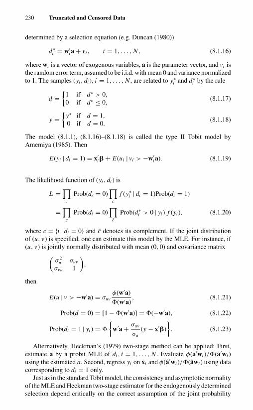
230 Truncated and Censored Data
determined by a selection equation (e.g. Duncan (1980))
d∗i = w′
i a + vi , i = 1, . . . , N , (8.1.16)
where wi is a vector of exogenous variables, a is the parameter vector, and vi isthe random error term, assumed to be i.i.d. with mean 0 and variance normalizedto 1. The samples (yi , di ), i = 1, . . . , N , are related to y∗
i and d∗i by the rule
d ={
1 if d∗ > 0,
0 if d∗ ≤ 0,(8.1.17)
y ={
y∗ if d = 1,
0 if d = 0.(8.1.18)
The model (8.1.1), (8.1.16)–(8.1.18) is called the type II Tobit model byAmemiya (1985). Then
E(yi | di = 1) = x′i � + E(ui | vi > −w′
i a). (8.1.19)
The likelihood function of (yi , di ) is
L =∏
c
Prob(di = 0)∏
c
f (y∗i | di = 1)Prob(di = 1)
=∏
c
Prob(di = 0)∏
c
Prob(d∗i > 0 | yi ) f (yi ), (8.1.20)
where c = {i | di = 0} and c denotes its complement. If the joint distributionof (u, v) is specified, one can estimate this model by the MLE. For instance, if(u, v) is jointly normally distributed with mean (0, 0) and covariance matrix(
σ 2u σuv
σvu 1
),
then
E(u | v > −w′a) = σuvφ(w′a)
�(w′a), (8.1.21)
Prob(d = 0) = [1 − �(w′a)] = �(−w′a), (8.1.22)
Prob(di = 1 | yi ) = �
{w′a + σuv
σu(y − x′�)
}. (8.1.23)
Alternatively, Heckman’s (1979) two-stage method can be applied: First,estimate a by a probit MLE of di , i = 1, . . . , N . Evaluate φ(a′wi )/�(a′wi )using the estimated a. Second, regress yi on xi and φ(a′wi )/�(awi ) using datacorresponding to di = 1 only.
Just as in the standard Tobit model, the consistency and asymptotic normalityof the MLE and Heckman two-stage estimator for the endogenously determinedselection depend critically on the correct assumption of the joint probability
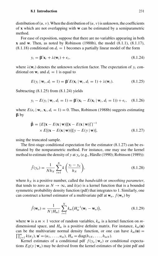
8.1 Introduction 231
distribution of (u, v). When the distribution of (u, v) is unknown, the coefficientsof x which are not overlapping with w can be estimated by a semiparametricmethod.
For ease of exposition, suppose that there are no variables appearing in bothx and w. Then, as noted by Robinson (1988b), the model (8.1.1), (8.1.17),(8.1.18) conditional on di = 1 becomes a partially linear model of the form
yi = �′xi + λ(wi ) + εi , (8.1.24)
where λ(wi ) denotes the unknown selection factor. The expectation of yi con-ditional on wi and di = 1 is equal to
E(yi | wi , di = 1) = �′E(xi | wi , di = 1) + λ(wi ). (8.1.25)
Subtracting (8.1.25) from (8.1.24) yields
yi − E(yi | wi , di = 1) = �′(xi − E(xi | wi , di = 1)) + εi , (8.1.26)
where E(εi | wi , xi , di = 1) = 0. Thus, Robinson (1988b) suggests estimating� by
� = {E[x − E(x | w)][x − E(x | w)]′}−1
× E[(x − E(x | w))][y − E(y | w)], (8.1.27)
using the truncated sample.The first-stage conditional expectation for the estimator (8.1.27) can be es-
timated by the nonparametric method. For instance, one may use the kernelmethod to estimate the density of y at ya (e.g., Hardle (1990); Robinson (1989)):
f (ya) = 1
NhN
N∑i=1
k
(yi − ya
hN
), (8.1.28)
where hN is a positive number, called the bandwidth or smoothing parameter,that tends to zero as N → ∞, and k(u) is a kernel function that is a boundedsymmetric probability density function (pdf) that integrates to 1. Similarly, onecan construct a kernel estimator of a multivariate pdf at wa, f (wa) by
f (wa) = 1
N |Hm |N∑
i=1
km(H−1
m (wi − wa)), (8.1.29)
where w is a m × 1 vector of random variables, km is a kernel function on m-dimensional space, and Hm is a positive definite matrix. For instance, km(u)can be the multivariate normal density function, or one can have km(u) =∏m
j=1 k(u j ), u′ = (u1, . . . , um), Hm = diag(h1N , . . . , hm N ).Kernel estimates of a conditional pdf f (ya | wa) or conditional expecta-
tions Eg(y | wa) may be derived from the kernel estimates of the joint pdf and

232 Truncated and Censored Data
marginal pdf. Thus, the conditional pdf may be estimated by
f (ya | wa) = f (ya, wa)
f (wa), (8.1.30)
and the conditional expectation by
Eg(y | wa) = 1
N |Hm |N∑
i=1
g(yi )km(H−1
m (wi −wa))/
f (wa). (8.1.31)
Robinson’s (1988b) approach does not allow the identification of the pa-rameters of variables that appear both in the regression equation (x) and inthe selection equation (w). When there are variables appearing in both x andw, Newey (1999) suggests a two-step series method of estimating � providedthat the selection correction term of (8.1.25), λ(wi , di = 1), is a function of thesingle index w′
i a:
λ(w, d = 1) = E[u | v(w′a), d = 1]. (8.1.32)
The first step of Newey’s method uses the distribution-free methods discussedin Chapter 7 and in Klein and Spady (1993) to estimate a. The second stepconsists of a linear regression of di yi on di xi and the approximations of λ(wi ).Newey suggests approximating λ(wi ) by either a polynomial function of (w′
i a)or a spline function PK
N (w′a) = (P1K (w′a), P2K (w′a), . . . , PK K (w′a))′ with theproperty that for large K , a linear combination of PK
N (w′a) can approximatean unknown function of λ(w′a) well. Newey (1999) shows that the two-stepseries estimation of � is consistent and asymptotically normally distributedwhen N → ∞, K → ∞, and
√N K −s−t+1 → 0, where s ≥ 5, and where
K 7/N → 0 if P KN (w′a) is a power series or m ≥ t − 1, s ≥ 3, and K 4/N → 0
if P K (w′a) is a spline of degree m in (w′a).2
If the selection factor λ(wi ) is a function of a single index w′i a, and the com-
ponents of wi are not a subset of xi , then instead of subtracting (8.1.26) from(8.1.25) to eliminate the unknown selection factor λ(wi ), Ahn and Powell (1993)note that for those individuals with w′
i a = w′j a, one has λ(w′
i a) = λ(w′j a).
Thus, conditional on w′i a = w′
j a, di = 1, d j = 1,
(yi − y j ) = (xi − x j )′� + (εi − ε j ), (8.1.33)
where the error term (ε j − ε j ) is symmetrically distributed around zero. Theyshow that ifλ is a sufficiently “smooth” function and a is a consistent estimator ofa, observations for which the difference (wi − w j )′a is close to zero should haveλ(x′
i a) − λ(w′j a) � 0. Therefore, Powell (2001) proposes a two-step procedure.
In the first step, consistent semiparametric estimates of the coefficients of theselection equation are obtained. The result is used to obtain estimates of thesingle index (x′
i a) variables characterizing the selectivity bias in the equationof interest. The second step of the approach estimates the parameters of theinterest by a weighted least-squares (or instrumental) variables regression of
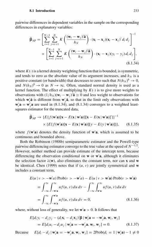
8.1 Introduction 233
pairwise differences in dependent variables in the sample on the correspondingdifferences in explanatory variables:
�AP =[
N−1∑i=1
N∑j=i+1
K
((wi − w j )′a
hN
)· (xi − x j )(xi − x j )
′ di d j
]−1
×[
N−1∑i=1
N∑j=i+1
K
((wi − w j )′a
hN
)· (xi − x j )(yi − y j ) di d j
],
(8.1.34)
where K (·) is a kernel density weighting function that is bounded, is symmetric,and tends to zero as the absolute value of its argument increases, and hN is apositive constant (or bandwidth) that decreases to zero such that N (hN )6 → 0,and N (hN )8 → 0 as N → ∞. Often, standard normal density is used as akernel function. The effect of multiplying by K (·) is to give more weights toobservations with (1/hN )(wi − w j )′a � 0 and less weight to observations forwhich w′
i a is different from w′j a, so that in the limit only observations with
w′i a = w′
j a are used in (8.1.34), and (8.1.34) converges to a weighted least-squares estimator for the truncated data,
�AP → {E{ f (w′a)[x − E(x | w′a)][x − E(x | w′a)]′}}−1
× {E{ f (w′a)[x − E(x | w′a)][y − E(y | w′a)]}}, (8.1.35)
where f (w′a) denotes the density function of w′a, which is assumed to becontinuous and bounded above.
Both the Robinson (1988b) semiparametric estimator and the Powell-typepairwise differencing estimator converge to the true value at the speed of N−1/2.However, neither method can provide estimate of the intercept term, becausedifferencing the observation conditional on w or w′a, although it eliminatesthe selection factor λ(w), also eliminates the constant term, nor can x and wbe identical. Chen (1999) notes that if (u, v) are jointly symmetrical and wincludes a constant term,
E(u | v > −w′a) Prob(v > −w′a) − E(u | v > w′a) Prob(v > w′a)
=∫ ∞
−∞
∫ ∞
−w′au f (u, v) du dv −
∫ ∞
−∞
∫ ∞
w′au f (u, v) du dv
=∫ ∞
−∞
∫ w′a
−w′au f (u, v) du dv = 0, (8.1.36)
where, without loss of generality, we let w′a > 0. It follows that
E[di yi − d j y j − (di xi − d j x j )′� | w′
i a = −w′j a, wi , w j ]
= E[di ui − d j u j | w′i a = −w′
j a, wi , w j ] = 0. (8.1.37)
Because E[di − d j | w′i a = −w′
j a, wi , w j ] = 2Prob(di = 1 | w′i a) − 1 �= 0

234 Truncated and Censored Data
and the conditioning is on w′i a = −w′
j a, not on w′i a = w′
j a, the moment condi-tion (8.1.37) allows the identification of the intercept and the slope parameterswithout the need to impose the exclusion restriction that at least one componentof x is excluded from w. Therefore, Chen (1999) suggests a
√N -consistent
instrumental variable estimator for the intercept and the slope parameters as
�c =[
N−1∑i=1
N∑j=i+1
K
((wi + w j )′a
hN
)(di xi − d j x j )(zi − z j )
′]−1
×[
N−1∑i=1
N∑j=i+1
K
((wi + w j )′a
hN
)(zi − z j )
′(di yi − d j y j )
],
(8.1.38)
where zi are the instruments for di xi . In the case when y are unobservable, but thecorresponding x are observable, the natural instrument will be E(d | w′a)x. Anefficient method for estimating binary-choice models that contain an interceptterm, suggested by Chen (2000), can be used to obtain the first-stage estimateof a.
8.2 AN EXAMPLE --- NONRANDOMLYMISSING DATA
8.2.1 Introduction
Attrition is a problem in any panel survey. For instance, by 1981, all four of thenational longitudinal surveys started in the 1960s had lost at least one-fourth oftheir original samples. In the Gary income maintenance project, 206 of the sam-ple of 585 Black, male-headed households, or 35.2 percent, did not completethe experiment. In Section 9.2 we shall discuss procedures to handle randomlymissing data. However, the major problem in econometrics is not simply miss-ing data, but the possibility that they are missing for a variety of self-selectionreasons. For instance, in a social experiment such as the New Jersey or Garynegative-income-tax experiments, some individuals may decide that keeping thedetailed records that the experiments require is not worth the payment. Also,some may move or may be inducted into the military. In some experiments,persons with large earnings receive no experimental-treatment benefit and thusdrop out of the experiment altogether. This attrition may negate the randomiza-tion in the initial experiment design. If the probability of attrition is correlatedwith experimental response, then traditional statistical techniques will lead tobiased and inconsistent estimates of the experimental effect. In this sectionwe show how models of limited dependent variables [e.g., see the surveys ofAmemiya (1984); Heckman (1976a); and Maddala (1983)] can provide both thetheory and the computational techniques for analyzing nonrandomly missingdata (Griliches, Hall, and Hausman (1978); Hausman and Wise (1979)).3

8.2 An Example – Nonrandomly Missing Data 235
8.2.2 A Probability Model of Attrition and Selection Bias
Suppose that the structural model is
yit = �′xi t + vit , i = 1, . . . , N ,
t = 1, . . . , T, (8.2.1)
where the error term vit is assumed to follow a conventional error-componentsformulation vit = αi + uit . For ease of exposition, we assume that T = 2.
If attrition occurs in the second period, a common practice is to discardthose observations for which yi2 is missing. But suppose that the probabilityof observing yi2 varies with its value, as well as the values of other variables;then the probability of observing yi2 will depend on vi2. Least squares of (8.2.1)based on observed y will lead to biased estimates of the underlying structuralparameters and the experimental response.
To formalize the argument, let the indicator variable di = 1 if yi2 is observedin period 2, and di = 0 if yi2 is not observed; in other words, attrition occurs.Suppose that yi2 is observed (di = 1) if the latent variable
d∗i = γ yi2 + �′xi2 + �′wi + ε∗
i ≥ 0, (8.2.2)
where wi is a vector of variables that do not enter the conditional expectation ofy but affect the probability of observing y; � and � are vectors of parameters;and (vi , ε
∗i ) are jointly normally distributed. Substituting for yi2 leads to the
reduced-form specification
d∗i = (γ �′ + �′)xi2 + �′wi + γ vi2 + ε∗
i
= �′xi2 + �′wi + εi
= a′ Ri + εi , (8.2.3)
where εi = γ vi2 + ε∗i , Ri = (x′
i2, w′i )
′, and a′ = (�′, �′). We further assumethat vit are also normally distributed, and we normalize the variance σ 2
ε of εi
to 1. Then the probabilities of retention and attrition are probit functions given,respectively, by
Prob(di = 1) = �(a′ Ri ),(8.2.4)
Prob(di = 0) = 1 − �(a′ Ri ),
where �(·) is the standard normal distribution function.Suppose we estimate the model (8.2.1) using only complete observations.
The conditional expectation of yi2, given that it is observed, is
E(yi2 | xi2, wi , di = 1) = �′xi2 + E(vi2 | xi2, wi , di = 1). (8.2.5)
From vi2 = σ2εεi + ηi , where σ2ε is the covariance between vi2 and εi , and ηi

236 Truncated and Censored Data
is independent of εi (Anderson (1958, Chapter 2)), we have
E(vi2 | wi , di = 1) = σ2ε E(εi | wi , di = 1)
= σ2ε
�(a′ Ri )
∫ ∞
−a′ Ri
ε · 1√2π
e−ε2/2 dε
= σ2ε
φ(a′ Ri )
�(a′ Ri ), (8.2.6)
where φ(·) denotes the standard normal density function. The last equality of(8.2.6) follows from the fact that the derivative of the standard normal densityfunction φ(ε) with respect to ε is −εφ(ε). Therefore,
E(yi2 | xi2, wi , di = 1) = �′xi2 + σ2ε
φ(a′ Ri )
�(a′ Ri ). (8.2.7)
Thus, estimating (8.2.1) using complete observations will lead to biased andinconsistent estimates of � unless σ2ε = 0. To correct for selection bias, onecan use either Heckman’s two-stage method (1979) (see Section 8.1) or themaximum likelihood method.
When di = 1, the joint density of di = 1, yi1, and yi2 is given by
f (di = 1, yi1, yi2) = Prob(di = 1 | yi1, yi2) f (yi1, yi2)
= Prob(di = 1 | yi2) f (yi1, yi2)
= �
a′ Ri +
(σ2ε
σ 2u + σ 2
α
)(yi2 − �′xi2)[
1 − σ 22ε
σ 2u + σ 2
α
]1/2
× [
2πσ 2u
(σ 2
u + 2σ 2α
)]−1/2
× exp
{− 1
2σ 2u
[2∑
t=1
(yit − �′xi t )2 − σ 2
α
σ 2u + 2σ 2
α
×(
2∑t=1
(yit − �′xi t )
)2 ]},
(8.2.8)
where the first factor follows from the fact that the conditional density off (εi | vi2) is normal, with mean [σ2ε/(σ 2
u + σ 2α )]vi2 and variance 1 − σ 2
2ε/(σ 2u +
σ 2α ). When di = 0, yi2 is not observed and must be integrated out. In this in-
stance, the joint density of di = 0 and yi1 is given by
f (di = 0, yi1) = Prob(di = 0 | yi1) f (yi1)
=
1 − �
a′ Ri + σ1ε
σ 2u + σ 2
α(yi1 − �′xi1)[
1 − σ 21ε
σ 2u + σ 2
α
]1/2
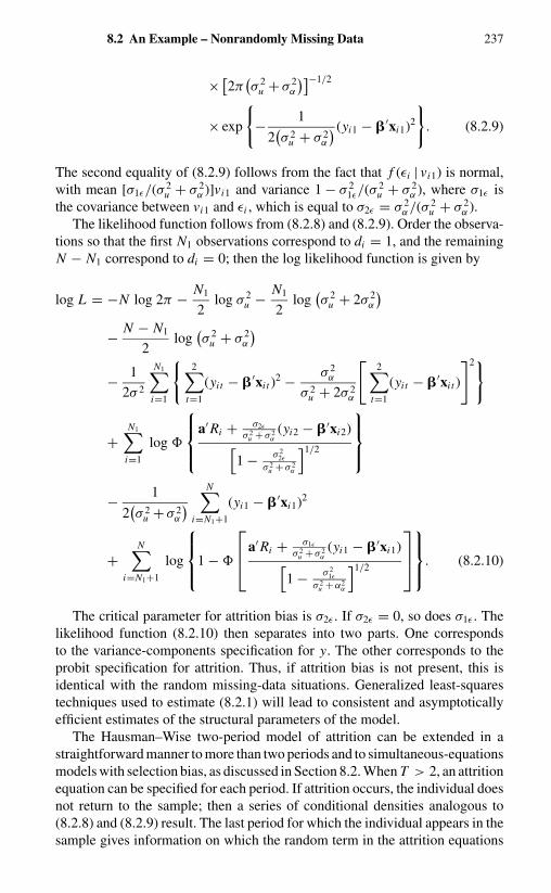
8.2 An Example – Nonrandomly Missing Data 237
× [2π
(σ 2
u + σ 2α
)]−1/2
× exp
{− 1
2(σ 2
u + σ 2α
) (yi1 − �′xi1)2
}. (8.2.9)
The second equality of (8.2.9) follows from the fact that f (εi | vi1) is normal,with mean [σ1ε/(σ 2
u + σ 2α )]vi1 and variance 1 − σ 2
1ε/(σ 2u + σ 2
α ), where σ1ε isthe covariance between vi1 and εi , which is equal to σ2ε = σ 2
α/(σ 2u + σ 2
α ).The likelihood function follows from (8.2.8) and (8.2.9). Order the observa-
tions so that the first N1 observations correspond to di = 1, and the remainingN − N1 correspond to di = 0; then the log likelihood function is given by
log L = −N log 2π − N1
2log σ 2
u − N1
2log
(σ 2
u + 2σ 2α
)− N − N1
2log
(σ 2
u + σ 2α
)− 1
2σ 2
N1∑i=1
{2∑
t=1
(yit − �′xi t )2 − σ 2
α
σ 2u + 2σ 2
α
[2∑
t=1
(yit − �′xi t )
]2}
+N1∑
i=1
log �
a′ Ri + σ2ε
σ 2u + σ 2
α(yi2 − �′xi2)[
1 − σ 22ε
σ 2u + σ 2
α
]1/2
− 1
2(σ 2
u + σ 2α
) N∑i=N1+1
(yi1 − �′xi1)2
+N∑
i=N1+1
log
1 − �
a′ Ri + σ1ε
σ 2u + σ 2
α(yi1 − �′xi1)[
1 − σ 21ε
σ 2u + α2
α
]1/2
. (8.2.10)
The critical parameter for attrition bias is σ2ε . If σ2ε = 0, so does σ1ε . Thelikelihood function (8.2.10) then separates into two parts. One correspondsto the variance-components specification for y. The other corresponds to theprobit specification for attrition. Thus, if attrition bias is not present, this isidentical with the random missing-data situations. Generalized least-squarestechniques used to estimate (8.2.1) will lead to consistent and asymptoticallyefficient estimates of the structural parameters of the model.
The Hausman–Wise two-period model of attrition can be extended in astraightforward manner to more than two periods and to simultaneous-equationsmodels with selection bias, as discussed in Section 8.2. When T > 2, an attritionequation can be specified for each period. If attrition occurs, the individual doesnot return to the sample; then a series of conditional densities analogous to(8.2.8) and (8.2.9) result. The last period for which the individual appears in thesample gives information on which the random term in the attrition equations

238 Truncated and Censored Data
is conditioned. For periods in which the individual remains in the sample, anequation like (8.2.8) is used to specify the joint probability of no attrition andthe observed values of the dependent variables.
In the case of simultaneous-equations models, all the attrition model does isto add an equation for the probability of observing an individual in the sample.Then the joint density of observing in-sample respondents becomes the productof the conditional probability of the observation being in the sample, given thejoint dependent variable y, and the marginal density of y. The joint density ofincomplete respondents becomes the product of the conditional probabilityof the observation being out of the sample, given the before-dropping-out valuesof y, and the marginal density of the previous periods’ y. The likelihood functionis simply the product of these two joint densities; see Griliches, Hall, andHausman (1978) for a three-equation model.
The employment of probability equations to specify the status of individualscan be very useful in analyzing the general problems of changing compositionsof the sample over time, in particular when changes are functions of individualcharacteristics. For instance, in addition to the problem of attrition in the nationallongitudinal surveys’ samples of young men, there is also the problem of sampleaccretion, that is, entrance into the labor force of the fraction of the sample origi-nally enrolled in school. The literature on switching regression models can beused as a basis for constructing behavioral models for analyzing the changingstatus of individuals over time.4
8.2.3 Attrition in the Gary Income-Maintenance Experiment
The Gary income-maintenance project focused on the effect of alternative setsof income-maintenance structures on work–leisure decisions. The basic projectdesign was to randomly divide individuals into two groups: controls and experi-mentals. The controls were not on an experimental-treatment plan, but receivednominal payments for completing periodic questionnaires. The experimentalswere randomly assigned to one of several income-maintenance plans. The ex-periment had four basic plans defined by an income guarantee and a tax rate.The two guarantee levels were $4,300 and $3,300 for a family of four and wereadjusted up for larger families and down for smaller families. The two marginaltax rates were 0.6 and 0.4. Retrospective information of individuals in the ex-periments was also surveyed for a preexperimental period (normally just priorto the beginning of the experimental period) so that the behavior of experimen-tals during the experiment could be compared with their own preexperimentalbehavior and also compared with that of the control group to obtain estimatesof the effects of treatment plans.
Two broad groups of families were studied in the Gary experiment: Blackfemale-headed households and black male-headed households. There was littleattrition among the first group, but the attrition among male-headed familieswas substantial. Of the sample of 334 experimentals used by Hausman and

8.2 An Example – Nonrandomly Missing Data 239
Wise (1979), the attrition rate was 31.1 percent. Among the 251 controls, 40.6percent failed to complete the experiment.
If attrition is random, as will be discussed in Section 9.2, it is not a majorproblem. What matters is that data are missing for a variety of self-selectionreasons. In this case it is easy to imagine that attrition is related to endogenousvariables. Beyond a breakeven point, experimentals receive no benefits from theexperimental treatment. The breakeven point occurs when the guarantee minustaxes paid on earnings (wage rate times hours worked) is zero. Individuals withhigh earnings receive no treatment payment and may be much like controlswith respect to their incentive to remain in the experiment. But because highearnings are caused in part by the unobserved random term of the structuralequation (8.2.1), attrition may well be related to it.
Hausman and Wise (1979) estimated structural models of earnings withand without correcting for attrition. The logarithm of earnings was regressedagainst time trend, education, experience, union membership, health status,and the logarithm of nonlabor family income. To control for the effects of thetreatment, they also used a dummy variable that was 1 if for that period thehousehold was under one of the four basic income-maintenance plans, and 0otherwise. Because hourly wages for experimentals and controls did not differ,the coefficient of this variable provided a reasonable indicator of the effect ofexperimental treatment on hours worked.
Because only three observations were available during the experiment, eachfor a one-month period, they concentrated on a two-period model: a periodfor the preexperiment average monthly earnings and a period for the averageearning of the three monthly observations of the experimental period. Theirgeneralized-least-squares estimates of the structural parameters that were notcorrected for attrition and the maximum likelihood estimates that incorporatedthe effects of attrition, (8.2.1) and (8.2.3), are presented in Table 8.1.
The attrition-bias parameter σ2ε/(σ 2u + σ 2
α ) was estimated to be −0.1089.This indicates a small but statistically significant correlation between earn-ings and the probability of attrition. The estimate of the experimental effectwas very close whether or not the attrition bias was corrected for. However,the experimental-effect coefficient did increase in magnitude from −0.079 to−0.082, an increase of 3.6 percent. Some of the other coefficients showed morepronounced changes. The effect of nonlabor family income on earnings (hencehours worked) decreased by 23 percent from the generalized-least-squares es-timates, and the effect of another year of education increased by 43 percent.These results demonstrate that attrition bias was a potentially important prob-lem in the Gary experiment. For other examples, see Ridder (1990), Nijmanand Verbeek (1992), and Verbeek and Nijman (1996).
The Hausman–Wise (HW) model assumes that the contemporaneous valuesaffect the probability of responding. Alternatively, the decision on whether torespond may be related to past experiences – if in the first period the effortin responding was high, an individual may be less inclined to respond in the
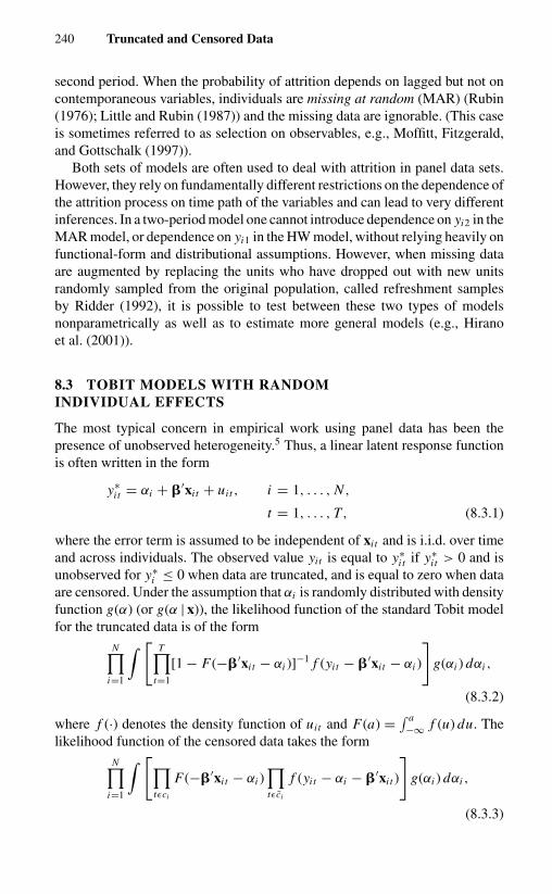
240 Truncated and Censored Data
second period. When the probability of attrition depends on lagged but not oncontemporaneous variables, individuals are missing at random (MAR) (Rubin(1976); Little and Rubin (1987)) and the missing data are ignorable. (This caseis sometimes referred to as selection on observables, e.g., Moffitt, Fitzgerald,and Gottschalk (1997)).
Both sets of models are often used to deal with attrition in panel data sets.However, they rely on fundamentally different restrictions on the dependence ofthe attrition process on time path of the variables and can lead to very differentinferences. In a two-period model one cannot introduce dependence on yi2 in theMAR model, or dependence on yi1 in the HW model, without relying heavily onfunctional-form and distributional assumptions. However, when missing dataare augmented by replacing the units who have dropped out with new unitsrandomly sampled from the original population, called refreshment samplesby Ridder (1992), it is possible to test between these two types of modelsnonparametrically as well as to estimate more general models (e.g., Hiranoet al. (2001)).
8.3 TOBIT MODELS WITH RANDOMINDIVIDUAL EFFECTS
The most typical concern in empirical work using panel data has been thepresence of unobserved heterogeneity.5 Thus, a linear latent response functionis often written in the form
y∗i t = αi + �′xi t + uit , i = 1, . . . , N ,
t = 1, . . . , T, (8.3.1)
where the error term is assumed to be independent of xi t and is i.i.d. over timeand across individuals. The observed value yit is equal to y∗
i t if y∗i t > 0 and is
unobserved for y∗i ≤ 0 when data are truncated, and is equal to zero when data
are censored. Under the assumption that αi is randomly distributed with densityfunction g(α) (or g(α | x)), the likelihood function of the standard Tobit modelfor the truncated data is of the form
N∏i=1
∫ [T∏
t=1
[1 − F(−�′xi t − αi )]−1 f (yit − �′xi t − αi )
]g(αi ) dαi ,
(8.3.2)
where f (·) denotes the density function of uit and F(a) = ∫ a−∞ f (u) du. The
likelihood function of the censored data takes the formN∏
i=1
∫ [∏tεci
F(−�′xi t − αi )∏tεci
f (yit − αi − �′xi t )
]g(αi ) dαi ,
(8.3.3)
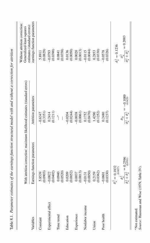
Tabl
e8.
1.Pa
ram
eter
esti
mat
esof
the
earn
ings
-fun
ctio
nst
ruct
ural
mod
elw
ith
and
wit
hout
aco
rrec
tion
for
attr
itio
n
With
attr
ition
corr
ectio
n:m
axim
umlik
elih
ood
estim
ates
(sta
ndar
der
rors
)
Var
iabl
esE
arni
ngs-
func
tion
para
met
ers
Attr
ition
para
met
ers
With
outa
ttriti
onco
rrec
tion:
Gen
eral
ized
-lea
st-s
quar
eses
timat
es(s
tand
ard
erro
rs):
earn
ings
-fun
ctio
npa
ram
eter
s
Con
stan
t5.
8539
−0.6
347
5.89
11(0
.090
3)(0
.335
1)(0
.082
9)
Exp
erim
enta
leff
ect
−0.0
822
0.24
14−0
.079
3(0
.040
2)(0
.121
1)(0
.039
0)
Tim
etr
end
0.09
40—
a0.
0841
(0.0
520)
—(0
.035
8)
Edu
catio
n0.
0209
−0.0
204
0.01
36(0
.005
2)(0
.024
4)(0
.005
0)
Exp
erie
nce
0.00
37−0
.003
80.
0020
(0.0
013)
(0.0
061)
(0.0
013)
Non
labo
rin
com
e−0
.013
10.
1752
−0.0
115
(0.0
050)
(0.0
470)
(0.0
044)
Uni
on0.
2159
1.42
900.
2853
(0.0
362)
(0.1
252)
(0.0
330)
Poor
heal
th−0
.060
10.
2480
−0.0
578
(0.0
330)
(0.1
237)
(0.0
326)
σ2 u
=0.
1832
(0.0
057)
σ2 u
=0.
1236
σ2 α
σ2 u+
σ2 α
=0.
2596
(0.0
391)
σ2ε
σ2 u+
σ2 α
=−0
.108
9(0
.042
9)
σ2 α
σ2 u+
σ2 α
=0.
2003
aN
otes
timat
ed.
Sour
ce:
Hau
sman
and
Wis
e(1
979,
Tabl
eIV
).
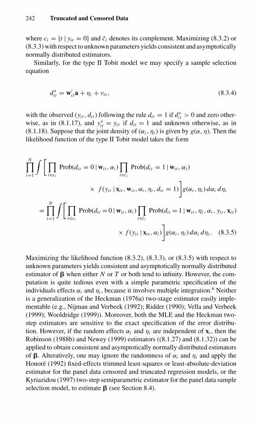
242 Truncated and Censored Data
where ci = {t | yit = 0} and ci denotes its complement. Maximizing (8.3.2) or(8.3.3) with respect to unknown parameters yields consistent and asymptoticallynormally distributed estimators.
Similarly, for the type II Tobit model we may specify a sample selectionequation
d∗i t = w′
i t a + ηi + νi t , (8.3.4)
with the observed (yit , dit ) following the rule dit = 1 if d∗i t > 0 and zero other-
wise, as in (8.1.17), and y∗i t = yit if dit = 1 and unknown otherwise, as in
(8.1.18). Suppose that the joint density of (αi , ηi ) is given by g(α, η). Then thelikelihood function of the type II Tobit model takes the form
N∏i=1
∫ [∏t∈ci
Prob(dit = 0 | wi t , αi )∏t∈ci
Prob(dit = 1 | wi t , αi )
× f (yit | xi t , wi t , αi , ηi , dit = 1)
]g(αi , ηi ) dαi dηi
=N∏
i=1
∫ [∏t∈ci
Prob(dit = 0 | wi t , αi )∏t∈ci
Prob(dit = 1 | wi t , ηi , αi , yit , xi t )
× f (yit | xi t , αi )
]g(αi , ηi ) dαi dηi . (8.3.5)
Maximizing the likelihood function (8.3.2), (8.3.3), or (8.3.5) with respect tounknown parameters yields consistent and asymptotically normally distributedestimator of � when either N or T or both tend to infinity. However, the com-putation is quite tedious even with a simple parametric specification of theindividuals effects αi and ηi , because it involves multiple integration.6 Neitheris a generalization of the Heckman (1976a) two-stage estimator easily imple-mentable (e.g., Nijman and Verbeek (1992); Ridder (1990); Vella and Verbeek(1999); Wooldridge (1999)). Moreover, both the MLE and the Heckman two-step estimators are sensitive to the exact specification of the error distribu-tion. However, if the random effects αi and ηi are independent of xi , then theRobinson (1988b) and Newey (1999) estimators ((8.1.27) and (8.1.32)) can beapplied to obtain consistent and asymptotically normally distributed estimatorsof �. Alteratively, one may ignore the randomness of αi and ηi and apply theHonore (1992) fixed-effects trimmed least-squares or least-absolute-deviationestimator for the panel data censored and truncated regression models, or theKyriazidou (1997) two-step semiparametric estimator for the panel data sampleselection model, to estimate � (see Section 8.4).

8.4 Fixed-Effects Estimator 243
8.4 FIXED-EFFECTS ESTIMATOR
8.4.1 Pairwise Trimmed Least-Squares andLeast-Absolute-Deviation Estimators forTruncated and Censored Regressions
When the effects are fixed and if T → ∞, the MLEs of �′ and αi are straightfor-ward to implement and are consistent. However, panel data often involve manyindividuals observed over few time periods, so that the MLE, in general, will beinconsistent as described in Chapter 7. In this section, we consider the pairwisetrimmed least-squares (LS) and least-absolute-deviation (LAD) estimators ofHonore (1992) for panel data censored and truncated regression models that areconsistent without the need to assume a parametric form for the disturbancesuit , nor homoscedasticity across individuals.
8.4.1.a Truncated Regression
We assume a model (8.3.1) and (8.1.2) except that now the individual effectsare assumed fixed. The disturbance uit is again assumed to be independentlydistributed over i and i.i.d. over t conditional on xi and αi .
We note that when data are truncated or censored, first-differencing doesnot eliminate the individual-specific effects from the specification. To see this,suppose that the data are truncated. Let
yit = E(yit | xi t , αi , yit > 0) + εi t , (8.4.1)
where
E(yit | xi t , αi , yit > 0) = αi + x′i t � + E(uit | uit > −αi − x′
i t �).
(8.4.2)
Since xi t �= xis , in general,
E(yit | xi t , αi , yit > 0) − E(yis | xis, αi , yis > 0)
= (xi t − xis)′� + E(uit | uit > −αi − x′i t �)
− E(uis | uis > −αi − x′is�). (8.4.3)
In other words,
(yit − yis) = (xi t − xis)′� + E(uit | uit > −αi − x′i t �)
− E(uis | uis > −αi − x′is�) + (εi t − εis). (8.4.4)
The truncation correction term, E(uit | uit > −αi − x′i t �), which is a function
of the individual specific effects αi , remains after first-differencing. However,we may eliminate the truncation correction term through first-differencing ifwe restrict our analysis to observations where yit > (xi t − xis)′� and yis >

244 Truncated and Censored Data
−(xi t − xis)′�. To see this, suppose that (xi t − xis)′� < 0. Then
E(yis | αi , xi t , xis, yis > −(xi t − xis)′�)
= αi + x′is� + E(uis | uis > −αi − x′
is� − (xi t − xis)′�). (8.4.5)
Since uit conditional on xi and αi is assumed to be i.i.d.,
E(uit | uit > −αi − x′i t �) = E(uis | uis > −αi − x′
i t �). (8.4.6)
Similarly, if (xi t − xis)′� > 0,
E(uit | uit > −αi − x′i t � + (xi t − xis)′�)
= E(uit | uit > −αi − x′is�)
= E(uis | uis > −αi − x′is�). (8.4.7)
Therefore, by confining our analysis to the truncated observations whereyit > (xi t − xis)′�, yis > −(xi t − xis)′�, yit > 0, yis > 0, we have
(yit − yis) = (xi t − xis)′� + (εi t − εis), (8.4.8)
which no longer involves the incidental parameters αi . Since E[(εi t − εis) |xi t , xis] = 0, applying least squares to (8.4.8) will yield a consistent estimatorof �.
The idea of restoring symmetry of the error terms of the pairwise differencingequation (yit − yis) by throwing away observations, where yit < (xi t − xis)′�and yis < −(xi t − xis)′� can be seen by considering the following graphs,assuming that T = 2. Suppose that the probability density function of uit isof the shape shown in Figure 8.3. Since ui1 and ui2 are i.i.d. conditional on(xi1, xi2, αi ), the probability density of y∗
i1 and y∗i2 conditional on (xi1, xi2, αi )
should have the same shape except for the location. The top and bottom graphs ofFigure 8.4 postulate the probability density of y∗
i1 and y∗i2 conditional on
(xi1, xi2, αi ), respectively, assuming that x′i � < 0, where xi = xi2 =
xi2 − xi1. The truncated data correspond to those sample points where y∗i t or
yit > 0. Because x′i1� �= x′
i2�, the probability density of yi1 is different fromthat of yi2. However, the probability density of y∗
i1 given y∗i1 > −x′
i � (or yi1
given yi1 > −x′i �) is identical to the probability density of y∗
i2 given y∗i2 > 0
(or yi2 given yi2 > 0) as shown in Figure 8.4. Similarly, if x′i � > 0, the proba-
bility density of y∗i1 given y∗
i1 > 0 (or yi1 given yi1 > 0) is identical to the proba-bility density of y∗
i2 given y∗i2 > x′
i � as shown in Figure 8.5.7 In other words,in a two-dimensional diagram of (y∗
i1, y∗i2) as in Figure 8.6 or 8.7, (y∗
i1, y∗i2)
conditional on (xi1, xi2, αi ) is symmetrically distributed around the 45-degreeline through (x′
i1� + αi , x′i2� + αi ), or equivalently, around the 45-degree line
through (x′i1�, x′
i2�) or (−x′i �, 0), e. g., the line L L ′. Since this is true for any
value of αi , the same statement is true for the distribution of (y∗i1, y∗
i2) conditionalon (xi1, xi2). When x′
i � < 0, the symmetry of the distribution of (y∗i1, y∗
i2)around L L ′ means that the probability that (y∗
i1, y∗i2) falls in the region A1 =
{(y∗i1, y∗
i2) : y∗i1 > −x′
i �, y∗i2 > y∗
i1 + x′i �} equals the probability that it
falls in the region B1 = {(y∗i1, y∗
i2) : y∗i1 > −x′
i �, 0 < y∗i2 < y∗
i1 + x′i �}

8.4 Fixed-Effects Estimator 245
uit0
f(uit)
Fig. 8.3 Probability density of uit .
(Figure 8.6). When x′i � > 0, the probability that (y∗
i1, y∗i2) falls in the
region A1 = {(y∗i1, y∗
i2) : y∗i1 > 0, y∗
i2 > y∗i1 + x′
i �} equals the probabilitythat it falls in the region B1 = {(y∗
i1, y∗i2) : y∗
i1 > 0, x′i � < y∗
i2 < y∗i1 +
x′i �} (Figure 8.7). That is, points in the regions A1 and B1 are not af-
fected by the truncation. On the other hand, points falling into the region(0 < y∗
i1 < −x′i �, y∗
i2 > 0) in Figure 8.6 (corresponding to points (yi1 <
−x′i �, yi2)) and (y∗
i1 > 0, 0 < y∗i2 < x′
i �) in Figure 8.7 (corresponding topoints (yi1, yi2 < x′
i �)) will have to be thrown away to restore symmetry.Let C = {i | yi1 > −x′
i �, yi2 > x′i �}; then (yi1 − x′
i1� − αi ) and(yi2 − x′
i2� − αi ) for i ∈ C are symmetrically distributed around zero. There-fore E[(yi2 − yi1) − (xi2 − xi1)′� | xi1, xi2, i ∈ C] = 0. In other words,
E[yi − x′i � | yi1 > −x′
i �, yi2 > x′i �]
= E[yi − x′i � | y∗
i1 > 0, y∗i1 > −x′
i �, y∗i2 > 0
y∗i2 > x′
i �] = 0, (8.4.9a)
and
E[(yi − x′i �)xi | yi1 > −x′
i �, yi2 > x′i �] = 0, (8.4.9b)
where yi = yi2 = yi2 − yi1. Therefore, Honore (1992) suggests thetrimmed LAD and LS estimators � and � that minimize the objective functions
QN (�) =N∑
i=1
[|yi − x′i �| 1{yi1 > −x′
i �, yi2 > x′i �}
+ |yi1| 1{yi1 ≥ −x′i �, yi2 < x′
i �}+ |yi2| 1{yi1 < −x′
i �, yi2 ≥ x′i �}]
=N∑
i=1
ψ(yi1, yi2, x′i �), (8.4.10)
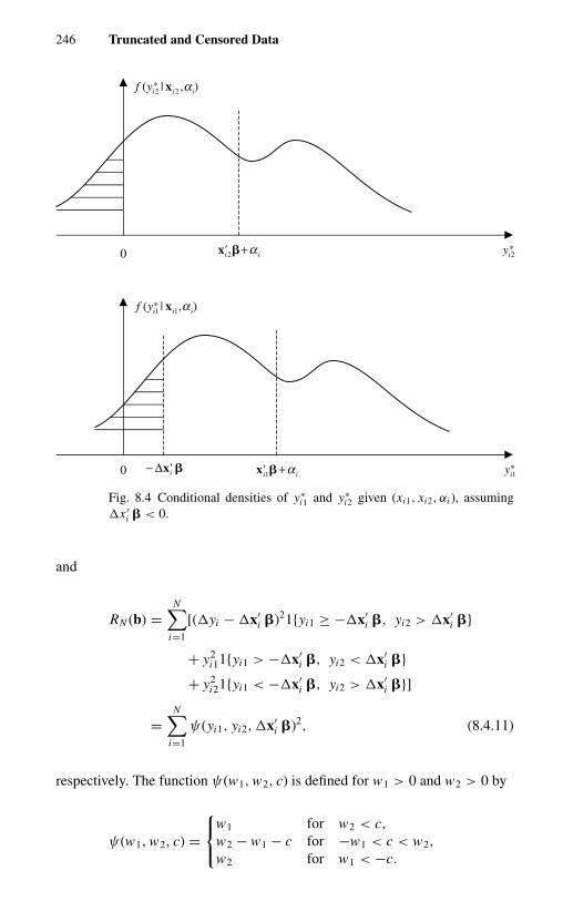
246 Truncated and Censored Data
0 iα+�xi'1�xi'∆−
),|*( 11 iiyf αix
*1iy
0 iα+�xi'2*2iy
),|*( 22 iiyf αix
Fig. 8.4 Conditional densities of y∗i1 and y∗
i2 given (xi1, xi2, αi ), assumingx ′
i � < 0.
and
RN (b) =N∑
i=1
[(yi − x′i �)21{yi1 ≥ −x′
i �, yi2 > x′i �}
+ y2i11{yi1 > −x′
i �, yi2 < x′i �}
+ y2i21{yi1 < −x′
i �, yi2 > x′i �}]
=N∑
i=1
ψ(yi1, yi2, x′i �)2, (8.4.11)
respectively. The function ψ(w1, w2, c) is defined for w1 > 0 and w2 > 0 by
ψ(w1, w2, c) =
w1 for w2 < c,w2 − w1 − c for −w1 < c < w2,
w2 for w1 < −c.

8.4 Fixed-Effects Estimator 247
0
0 iα+�xi1'
iα+�xi2'
*1iy
*2iy�x i'∆
),|*( 2 iiyf αi2x
),|*( 11 iiyf αix
Fig. 8.5 Conditional densities of y∗i1 and y∗
i2 given (xi1, xi2, αi ), assumingx ′
i � > 0.
The first-order conditions for (8.4.10) and (8.4.11) are the sample analoguesof
E{[P(yi1 > −x′i �, yi2 > yi1 + x′
i �)
− P(yi1 > −x′i �, x′
i � < yi2 < yi1 + x′i �)]x′
i } = 0′,(8.4.12)
and
E{(yi − x′i �) xi | (yi1 > −x′
i �, yi2 > yi1 + x′i �)
∪ (yi1 > −x′i �, x′
i � < yi2 < yi1 + x′i �)} = 0,
(8.4.13)
respectively. Honore (1992) proves that � and � are consistent and asymp-totically normally distributed if the density of u is strictly log-concave.The asymptotic covariance matrix of
√N (� − �) and
√N (� − �) may be

248 Truncated and Censored Data
yi1*
yi2*
(0, 0) (− ∆xi' �, 0)
L
L'
45°
A1
B1(xi1' �, xi2' �)
(x i1' � + αi, xi2' � + αi)
yi2* = yi1
* + ∆xi' �
A2
B2
Fig. 8.6 The distribution of (y∗i1, y∗
i2) assuming x′i β < 0.
A1 = {(y∗i1, y∗
i2) : y∗i1 > −x′
i �, y∗i2 > y∗
i1 + x′i �}, A2 = {(y∗
i1, y∗i2) :
y∗i1 ≤ −x′
i �, y∗i2 > 0},
B1 = {(y∗i1, y∗
i2) : y∗i1 > −x′
i �, 0 < y∗i2 < y∗
i1 + x′i �}, B2 = {(y∗
i1, y∗i2) :
y∗i1 > −x′
i �, y∗i2 ≤ 0}.
y i1*
yi2*
(0, 0)(− ∆xi' �, 0)
L
L'
45°
A1
B1
yi*2 = yi
*1 + ∆xi'�
A2
B2
(0, ∆xi' �)
Fig. 8.7 The distribution of (y∗i1, y∗
i2) assuming x′i � > 0.
A1 = {(y∗i1, y∗
i2) : y∗i1 > 0, y∗
i2 > y∗i1 + x′
i �}, A2 = {(y∗i1, y∗
i2) :y∗
i1 ≤ 0, y∗i2 > x′
i �},B1 = {(y∗
i1, y∗i2) : y∗
i1 > 0, x′i � < y∗
i2 < y∗i1 + x′
i �}, B2 = {(y∗i1, y∗
i2) :y∗
i1 > 0, y∗i2 ≤ x′
i �}.

8.4 Fixed-Effects Estimator 249
approximated by
Asy Cov(√
N (� − �)) = �−11 V1�
−11 , (8.4.14)
and
Asy Cov(√
N (� − �)) = �−12 V2�
−12 , (8.4.15)
where V1, V2, �1, and �2 may be approximated by
V 1 = 1
N
N∑i=1
1{−yi1 < x′i � < yi2}xi x′
i , (8.4.16)
V 2 = 1
N
N∑i=1
1{−yi1 < x′i � < yi2}(yi − x′
i �)2xi x′i ,
(8.4.17)
�( j,k)1 = 1
hN
[1
N
N∑i=1
(1{yi < xi (� + hN ik) < yi2}
− 1{−yi1 < xi (� + hN ik) < yi }) x( j)i
+ 1
N
N∑i=1
(−1{yi < x′i � < yi2}
+ 1{−yi1 < x′i � < yi }) x( j)
i
],
(8.4.18)
�( j,k)2 = 1
hN
[1
N
N∑i=1
1{−yi1 < x′i (� + hN ik) < yi2}
× (yi − x′i (� + hN ik)) x( j)
i
− 1
N
N∑i=1
1{−yi1 < x′i � < yi2}(yi − x′
i �) x( j)i
],
(8.4.19)
where �( j,k)� denotes the ( j, k)th element of �� for � = 1, 2, x( j)
i denotes thej th coordinate of xi , ik is a unit vector with 1 in its kth place, and hN decreasesto zero with the speed of N− 1
2 . The bandwidth factor hN appears in (8.4.18)and (8.4.19) because �� is a function of densities and conditional expectationsof y (Honore (1992)).
8.4.1.b Censored Regressions
When data are censored, observations {yit , xi t } are available for i =1, . . . , N , t = 1, . . . , T , where yit = max{0, y∗
i t }. In other words, yit can now

250 Truncated and Censored Data
be either 0 or a positive number, rather than just a positive number as in the caseof truncated data. Of course, we can throw away observations of (yit , xi t ) thatcorrespond to yit = 0 and treat the censored regression model as the truncatedregression model using the methods of Section 8.4.1.a. But this will lead to aloss of information.
In the case that data are censored, in addition to the relations (8.4.9a,b),the joint probability of yi1 ≤ −�′xi and yi2 > 0 is identical to the jointprobability of yi1 > −�′xi and yi2 = 0 when �′xi < 0, as shown inFigure 8.6, regions A2 and B2, respectively. When �′xi > 0, the joint prob-ability of yi1 = 0 and yi2 > �′xi is identical to the joint probability ofyi1 > 0 and yi2 ≤ �′xi , as shown in Figure 8.7. In other words, (y∗
i1, y∗i2)
conditional on (xi1, xi2, αi ) is symmetrically distributed around the 45-degreeline through (x′
i1� + αi , x′i2� + αi ) or equivalently around the 45-degree line
through (−x′i �, 0) – the line L L ′ in Figure 8.6 or 8.7. Since this is true for
any value of αi , the same statement is true for the distribution of (y∗i1, y∗
i2)conditional on (xi1, xi2). When x′
i � < 0, the symmetry of the distribu-tion of (y∗
i1, y∗i2) around L L ′ means that the probability that (y∗
i1, y∗i2) falls
in the region A1 = {(y∗i1, y∗
i2) : y∗i1 > −x′
i �, y∗i2 > y∗
i1 + x′i �} equals the
probability that it falls in the region B1 = {(y∗i1, y∗
i2) : y∗i1 > −x′
i �, 0 <
y∗i2 < y∗
i1 + x′i �}. Similarly, the probability that (y∗
i1, y∗i2) falls in the re-
gion A2 = {(y∗i1, y∗
i2) : y∗i1 < −x′
i �, y∗i2 > 0} equals the probability that
it falls in the region B2 = {(y∗i1, y∗
i2) : y∗i1 > −x′
i �, y∗i2 ≤ 0} as shown in
Figure 8.6. When x′i � > 0, the probability that (y∗
i1, y∗i2) falls in the re-
gion A1 = {(y∗i1, y∗
i2) : y∗i1 > 0, y∗
i2 > y∗i1 + x′
i �} equals the probability thatit falls in the region B1 = {(y∗
i1, y∗i2) : y∗
i1 > 0, x′i � < y∗
i2 < y∗i1 + x′
i �},and the probability that it falls in the region A2 = {(y∗
i1, y∗i2) : y∗
i1 ≤ 0, y∗i >
x′i �} equals the probability that it falls in the region B2 = {(y∗
i1, y∗i2) :
y∗i1 > 0, y∗
i2 ≤ x′i �}, as seen in Figure 8.7. Therefore, the probability of
(y∗i1, y∗
i2) conditional on (xi1, xi2) falling in A = (A1 ∪ A2) equals the prob-ability that it falls in B = (B1 ∪ B2). As neither of these probabilities is af-fected by censoring, the same is true in the censored sample. This impliesthat
E [(1{(yi1, yi2) ∈ A} − 1{(yi1, yi2) ∈ B}) xi ] = 0. (8.4.20)
In other words, to restore symmetry of censored observations around theirexpected values, observations corresponding to (yi1 = 0, yi2 < x′
i �) or(yi1 < −x′
i �, yi2 = 0) will have to be thrown away.By the same argument, conditional on (xi1, xi2), the expected vertical dis-
tance from a (yi1, yi2) in A to the boundary of A equals the expected horizontaldistance from a (yi1, yi2) in B to the boundary of B. For (yi1, yi2) in A1, thevertical distance to L L ′ is (yi − x′
i �). For (yi1, yi2) in B1, the horizontaldistance to L L ′ is yi1 − (yi2 − x′
i �) = −(yi − x′i �). For (yi1, yi2) in A2,
the vertical distance to the boundary of A2 is yi2 − max (0, x′i �). For (yi1, yi2)

8.4 Fixed-Effects Estimator 251
in B2, the horizontal distance is yi1− max(0, −x′i �). Therefore
E[(1{(yi1, yi2) ∈ A1}(yi − x′i �) + 1{(yi1, yi2) ∈ A2)}
× (yi2 − max(0, x′i �)) − 1{(yi1, yi2) ∈ B1}(yi − x′
i �)
− 1{yi1, yi2 ∈ B2}(yi1 − max(0, −x′i �)))xi ] = 0. (8.4.21)
The pairwise trimmed LAD and LS estimators, �∗
and �∗, for the estimation
of the censored regression model proposed by Honore (1992) are obtained byminimizing the objective functions
Q∗N (�) =
N∑i=1
[1 − 1{yi1 ≤ −x′i �, yi2 ≤ 0}]
× [1 − 1{yi2 ≤ x′i �, yi1 ≤ 0}]|yi − x′
i �|
=N∑
i=1
ψ∗(yi1, yi2, x′i �), (8.4.22)
R∗N (�) =
N∑i=1
{[max{yi2, x′i �} − max{yi1, −x′
i �} − x′i �)]2
− 2 × 1{yi1 < −x′i �}(yi1 + x′
i �)yi2
− 2 × 1{yi2 < x′i �}(yi2 − x′
i �)yi1}
=N∑
i=1
χ (yi1, yi2, x′i �), (8.4.23)
where
ψ∗(w1, w2, c)
={
0 for w1 ≤ max{0, −c} and w2 ≤ max(0, c),| w2 − w1 − c | otherwise,
and
χ(w1, w2, c) =
w2
1 − 2w1(w2 − c) for w2 ≤ c,
(w2 − w1 − c)2 for −w1 < c < w2,
w22 − 2w2(c + w1) for w1 ≤ −c.
The first-order conditions for (8.4.22) and (8.4.23) are the sample analogues of(8.4.20) and (8.4.21), respectively. For instance, when (yi1, yi2) ∈ (A1 ∪ B1),the corresponding terms in R∗
N become (yi − x′i �)2. When (yi1, yi2) ∈ A2,
the corresponding terms become y2i2 − 2 × 1{yi1 < −x′
i �}(yi1 + x′i �)yi2.
When (yi1, yi2) ∈ B2, the corresponding terms become y2i1 − 2 × 1{yi2 <
x′i �}(yi2 − x′
i �)yi1. The partial derivative of the first term with respect to �converges to E{[1{(yi1, yi2) ∈ A1}(yi − x′
i β) − 1{(yi1, yi2) ∈ B1}(yi −x′
i �)] xi }. The partial derivatives of the second and third terms with re-spect to � yield −2E[1{(yi1, yi2) ∈ A2}yi2 xi − 1{(yi1, yi2) ∈ B2}yi1 xi ].

252 Truncated and Censored Data
Because Q∗N (�) is piecewise linear and convex and R∗
N (�) is continuouslydifferentiable and convex and twice differentiable except at a finite number ofpoints, the censored pairwise trimmed LAD and LS estimators, �
∗and �
∗, are
computationally simpler than the truncated estimators � and �.Honore (1992) shows that �
∗and �
∗are consistent and asymptotically nor-
mally distributed. The asymptotic covariance matrix of√
N (�∗ − �) is equal
to
Asy Cov(√
N (�∗ − �)) = �−1
3 V3�−13 , (8.4.24)
and of√
N (�∗ − �) is equal to
Asy Cov(√
N (�∗ − �)) = �−1
4 V4�−14 , (8.4.25)
where V3, V4, �3, and �4 may be approximated by
V 3 = 1
N
N∑i=1
1{[x′i �
∗< yi , yi2 > max(0, x′
i �∗)]
∪ [yi < x′i �
∗, yi1 > max(0, −x′
i �∗)]} xi x′
i ,
(8.4.26)
V 4 = 1
N
N∑i=1
[y2
i21{x′i �
∗ ≤ −yi1} + y2i11{yi2 ≤ x′
i �∗}]
+ (yi − x′1 �
∗)21{−yi1 < x′
i �∗
< yi2}] xi x′i , (8.4.27)
�( j,k)3 = −1
hN
{1
N
N∑i=1
[1{yi2 > 0, yi2 > yi1 + x′i (�
∗ + hN ik)}
− 1{yi1 > 0, yi1 > yi2 − x′i (�
∗ + ωnik)}] x( j)i
− 1
N
N∑i=1
[1{yi2 > 0, yi2 > yi1 + x′i �
∗}
− 1{yi1 > 0, yi1 > yi2 − x′i �
∗}] x( j)i
},
(8.4.28)
and
�4 = 1
N
N∑i=1
1{−yi1 < x′i �
∗< yi2} xix′
i . (8.4.29)
Both the truncated and censored estimators are presented assuming thatT = 2. They can be easily modified to cover the case where T > 2. For instance,

8.4 Fixed-Effects Estimator 253
(8.4.23) can be modified to be the estimator
�∗ = arg min
N∑i=1
T∑t=2
χ (yi,t−1, yit , (xi t − xi t−1)′�), (8.4.30)
when T > 2.
8.4.2 A Semiparametric Two-Step Estimator for the EndogenouslyDetermined Sample Selection Model
In this subsection, we consider the estimation of the endogenously determinedsample selection model in which the sample selection rule is determined bythe binary-response model (8.3.4) and (8.1.17) for the linear regression model(8.3.1), where y∗
i t = yit if dit = 1 and y∗i t is unknown if dit = 0, as in (8.1.18).
We assume that both (8.3.1) and (8.3.4) contain unobserved fixed individual-specific effects αi and ηi that may be correlated with the observed explana-tory variables in an arbitrary way. Following the spirit of Heckman’s (1976a),two-step estimation procedure for the parametric model, Kyriazidou (1997)proposes a two-step semiparametric method for estimating the main regressionof interest, (8.3.1). In the first step, the unknown coefficients of the selec-tion equation (8.3.4), a, are consistently estimated by some semiparametricmethod. In the second step, these estimates are substituted into the equationof interest, (8.3.1), conditional on dit = 1, and estimate it by a weighted least-squares method. The fixed effect from the main equation is eliminated by tak-ing time differences on the observed yit . The selection effect is eliminatedby conditioning time-differencing of yit and yis on those observations wherew′
i t a � w′is a, because the magnitude of the selection effect is the same if the
effect of the observed variables determining selection remains the same overtime.
We note that without sample selectivity, that is, dit = 1 for all i and t , or ifuit and νi t are uncorrelated conditional on αi and xi t , then (8.3.1) and (8.1.18)correspond to the standard variable intercept model for panel data discussedin Chapter 3 with balanced panel or randomly missing data.8 If uit and νi t arecorrelated, sample selection will arise because E(uit | xi t , wi t , αi , dit = 1) �= 0.Let λ(·) denote the conditional expectation of u conditional on d = 1, x, w, α,and η; then (8.3.1) and (8.1.19) conditional on dit = 1 can be written as
yit = αi + �′xi t + λ(ηi + w′i t a) + εi t , (8.4.31)
where E(εi t | xi t , wi t , dit = 1) = 0.The form of the selection function λ(·) is derived from the joint distribution
of u and ν. For instance, if u and ν are bivariate normal, then we have the

254 Truncated and Censored Data
Heckman sample selection correction
λ(ηi + a′wi t ) = σuv
σv
φ(
ηi + w′i t a
σv
)�
(ηi + w′
i t aσv
) .
Therefore, in the presence of sample selection or attrition with short panels,regressing yit on xi t using only the observed information is invalidated by twoproblems – first, the presence of the unobserved effects αi , which introducesthe incidental-parameter problem, and second, the selection bias arising fromthe fact that
E(uit | xi t , wi t , dit = 1) = λ(ηi + w′i t a).
The presence of individual specific effects in (8.4.23) is easily obviated bytime-differencing those individuals that are observed for two time periods tand s, i.e., who have dit = dis = 1. However, the sample selectivity factorsare not eliminated by time-differencing. But conditional on given i , if (uit , vit )are stationary and w′
i t a = w′isa, then λ(ηi + wi t a) = λ(ηi + w′
isa). Then thedifference in (8.4.31) between t and s if both yit and yis are observable no longercontains the individual-specific effects αi or the selection factor λ(ηi + w′
i t a):
yits = yit − yis = (xi t − xis)′� + (εi t − εis) = x′i ts� + εi ts .
(8.4.32)
As shown by Ahn and Powell (1993), if λ is a sufficiently smooth function,and a is a consistent estimator of a, observations for which the difference(wi t − wis)′a is close to zero should have λi t − λis � 0. Therefore, Kyriazidou(1997) generalizes the pairwise difference concept of Ahn and Powell (1993)and propose to estimate the fixed-effects sample selection models in two steps:In the first step, estimate a by either Andersen (1970) and Chamberlain’s (1980)conditional maximum likelihood approach or Horowitz (1992) and Lee’s (1999)smoothed version of the Manski (1975) maximum score method discussed inChapter 7. In the second step, the estimated a is used to estimate � basedon pairs of observations for which dit = dis = 1 and for which (wi t − wis)′ais close to zero. This last requirement is operationalized by weighting eachpair of observations with a weight that depends inversely on the magnitudeof (wi t − wis)′a, so that pairs with larger differences in the selection effectsreceive less weight in the estimation. The Kyriazidou (1997) estimator takesthe form
�K ={
N∑i=1
1
Ti − 1
∑1≤s<t≤Ti
(xi t − xis)(xi t − xis)′K[
(wi t − wis)′ahN
]dit dis
}−1
×{
N∑i=1
1
Ti − 1
∑1≤s<t<Ti
(xi t − xis)(yi t − yis)′K[
(wi t − wis)′ahN
]dit dis
},
(8.4.33)

CHAPTER 8
Truncated and Censored Data
8.1 INTRODUCTION
In economics, the ranges of dependent variables are often constrained in someway. For instance, in his pioneering work on household expenditure on durablegoods, Tobin (1958) used a regression model that specifically took account of thefact that the expenditure (the dependent variable of his regression model) cannotbe negative. Tobin called this type of model the model of limited dependentvariables. It and its various generalization are known as Tobit models because oftheir similarities to probit models.1 In statistics they are known as truncated orcensored regression models. The model is called truncated if the observationsoutside a specific range are totally lost, and is called censored if we can at leastobserve some of the explanatory variables.
Consider a latent response function,
y∗ = �′x + u, (8.1.1)
where x is a K × 1 vector of exogenous variables and u is the error term thatis independently, identically distributed (i.i.d.) with mean 0 and variance σ 2
u .Without loss of generality, suppose that the observed y are related to y∗ by
y ={
y∗ if y∗ > 0,
0 if y∗ ≤ 0.(8.1.2)
Models of the form (8.1.1) and (8.1.2) are called censored regression modelsbecause the data consist of those points of the form (y∗
i , xi ) if y∗i > 0 and (0, xi )
if y∗i ≤ 0 for i = 1, . . . , N . The truncated data only consist of points of the form
(y∗i , xi ) where y∗
i > 0.The conditional expectation of y given x for truncated data is equal to
E(y | y > 0) = E(y∗ | y∗ > 0) = x′� + E(u | u > −x′�). (8.1.3)
The conditional expectation of y given x for censored data is equal to
E(y | x) = Prob(y = 0) · 0 + Prob(y > 0 | x) · E(y | y > 0, x)
= Prob(u ≤ −x′�) · 0 + Prob(u > −x′�)E(y∗ | x; u > −x′�)
= Prob(u > −x′�)[x′� + E(u | u > −x′�)]. (8.1.4)
256 Truncated and Censored Data
housing, costs of insuring the house, opportunity cost of housing equity (whichis set at 4 percent of the value of house minus the mortgage value), and mainte-nance cost, minus the increase of the value of the house. The explanatory vari-ables considered are the education level of the head of household (DOP), age ofthe head of the household (AGE), age squared (AGE2), marital status (DMAR),logarithm of monthly family income (LINC), its square (L2INC), monthlytotal family expenditure (EXP), logarithm of monthly total family expenditure(LEXP), its square (L2EXP), number of children (NCH), logarithm of constant-quality price of rental housing (LRP), logarithm of constant-quality price ofowner-occupied housing after tax (LOP), and LRP − LOP. The variables thatare excluded from the tenure choice equation (8.5.1) are DOP, LEXP, L2EXP,LRP, and LOP. The variables excluded from the budget share equations ((8.5.2)and (8.5.3)) are DOP, LINC, L2INC, EXP, NCH, and LRP − LOP.
The random-effects and fixed-effects models with and without selectionare estimated. However, since x includes LEXP and L2EXP and they couldbe endogenous, Charlier, Melenberg, and van Soest (2001) also estimate thismodel by the instrumental-variable (IV) method. For instance, the Kyriazidou(1997) weighted least-squares estimator is modified as
�K N ={
N∑i=1
∑1≤s<t≤Ti
(xi t − xis)(zi t − zis)′K[
(wi t − wis)′ahN
]dit dis
}−1
×{
N∑i=1
∑1≤s<t≤Ti
(zi t − zis)(yit − yis)K
[(wi t − wis)′a
hN
]dit dis
},
(8.5.4)
to take account of the potential endogeneity of LEXP and L2EXP, where zi t isa vector of instruments.
Tables 8.2 and 8.3 present the fixed-effects and random-effects estimationresults for the budget share equations without and with correction for selection,respectively. The Kyriazidou (1997) estimator is based on the first-stage logitestimation of the tenure choice equation (8.5.1). The random-effects estimatoris based on Newey’s (1989) series expansion method (Charlier, Melenberg,and van Soest (2000)). The differences among these formulations are quitesubstantial. For instance, the parameters related to AGE, AGE2, LEXP, L2EXP,and the prices are substantially different from their random-effects counterpartsbased on IV. They also lead to very different conclusions on the elasticities ofinterest. The price elasticities for the average renters and owners are about −0.5in the random-effects model, but are close to −1 for owners and −0.8 for rentersin the fixed-effects models.
The Hausman specification tests for endogeneity of LEXP and L2EXP areinconclusive. But a test for the presence of selectivity bias based on the dif-ference between the Kyriazidou IV and linear panel data estimates have teststatistics of 88.2 for owners and 23.7 for renters, which are significant at the5 percent level for the chi-square distribution with seven degrees of freedom.
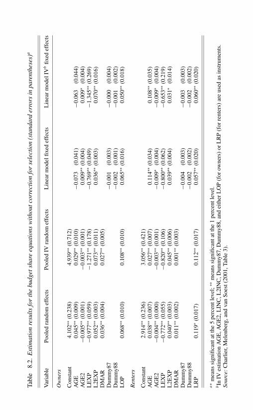
Tabl
e8.
2.E
stim
atio
nre
sult
sfo
rth
ebu
dget
shar
eeq
uati
ons
wit
hout
corr
ecti
onfo
rse
lect
ion
(sta
ndar
der
rors
inpa
rent
hese
s)a
Var
iabl
ePo
oled
rand
omef
fect
sPo
oled
IVra
ndom
effe
cts
Lin
ear
mod
elfix
edef
fect
sL
inea
rm
odel
IVb
fixed
effe
cts
Ow
ners
Con
stan
t4.
102∗∗
(0.2
38)
4.93
9∗∗(0
.712
)A
GE
0.04
5∗∗(0
.009
)0.
029∗∗
(0.0
10)
−0.0
73(0
.041
)−0
.063
(0.0
44)
AG
E2
−0.0
05∗∗
(0.0
01)
−0.0
03∗∗
(0.0
01)
0.00
9∗∗(0
.004
)0.
009∗
(0.0
04)
LE
XP
−0.9
77∗∗
(0.0
59)
−1.2
71∗∗
(0.1
78)
−0.7
69∗∗
(0.0
49)
−1.3
45∗∗
(0.2
69)
L2E
XP
0.05
2∗∗(0
.003
)0.
073∗∗
(0.0
11)
0.03
6∗∗(0
.003
)0.
070∗∗
(0.0
16)
DM
AR
0.03
6∗∗(0
.004
)0.
027∗∗
(0.0
05)
Dum
my8
7−0
.001
(0.0
03)
−0.0
00(0
.004
)D
umm
y88
−0.0
02(0
.001
)−0
.001
(0.0
02)
LO
P0.
068∗∗
(0.0
10)
0.10
8∗∗(0
.010
)0.
065∗∗
(0.0
16)
0.05
0∗∗(0
.018
)
Ren
ters
Con
stan
t2.
914∗∗
(0.2
36)
3.05
6∗∗(0
.421
)A
GE
0.03
8∗∗(0
.007
)0.
027∗∗
(0.0
07)
0.11
4∗∗(0
.034
)0.
108∗∗
(0.0
35)
AG
E2
−0.0
04∗∗
(0.0
00)
−0.0
03∗∗
(0.0
01)
−0.0
09∗
(0.0
04)
−0.0
09∗
(0.0
04)
LE
XP
−0.7
72∗∗
(0.0
55)
−0.8
20∗∗
(0.1
06)
−0.8
00∗∗
(0.0
62)
−0.6
53∗∗
(0.2
19)
L2E
XP
0.04
0∗∗(0
.003
)0.
045∗∗
(0.0
06)
0.03
9∗∗(0
.004
)0.
031∗
(0.0
14)
DM
AR
0.01
1∗∗(0
.002
)0.
001∗∗
(0.0
03)
Dum
my8
7−0
.004
(0.0
03)
−0.0
03(0
.003
)D
umm
y88
−0.0
02(0
.002
)−0
.002
(0.0
02)
LR
P0.
119∗
(0.0
17)
0.11
2∗∗(0
.017
)0.
057∗∗
(0.0
20)
0.06
0∗∗(0
.020
)
a∗
mea
nssi
gnifi
cant
atth
e5
perc
entl
evel
;∗∗m
eans
sign
ifica
ntat
the
1pe
rcen
tlev
el.
bIn
IVes
timat
ion
AG
E,A
GE
2,L
INC
,L2I
NC
,Dum
my8
7,D
umm
y88,
and
eith
erL
OP
(for
owne
rs)
orL
RP
(for
rent
ers)
are
used
asin
stru
men
ts.
Sour
ce:
Cha
rlie
r,M
elen
berg
,and
van
Soes
t(20
01,T
able
3).

Tabl
e8.
3.E
stim
atio
nre
sult
sfo
rth
ebu
dget
shar
eeq
uati
ons
usin
gpa
neld
ata
mod
els
taki
ngse
lect
ion
into
acco
unt
(sta
ndar
der
rors
inpa
rent
hese
s)a
Var
iabl
ePo
oled
rand
omef
fect
sbPo
oled
IVra
ndom
effe
ctsc
Kyr
iazi
dou
OL
Ses
timat
esK
yria
zido
uIV
des
timat
es
Ow
ners
Con
stan
t2.
595e
3.37
0e
AG
E−0
.040
∗∗(0
.013
)−0
.020
(0.0
15)
0.08
3(0
.083
)0.
359∗∗
(0.0
84)
AG
E2
0.00
4∗∗(0
.001
)0.
002
(0.0
01)
−0.0
08(0
.008
)−0
.033
∗∗(0
.009
)L
EX
P−0
.594
∗∗(0
.142
)−0
.821
(0.8
14)
−0.7
66∗∗
(0.1
02)
−0.8
01∗∗
(0.1
44)
L2E
XP
0.02
6∗∗(0
.008
)0.
042
(0.0
50)
0.03
6∗∗(0
.006
)0.
036∗∗
(0.0
08)
DM
AR
0.00
6(0
.007
)0.
012
(0.0
07)
LO
P0.
126∗∗
(0.0
12)
0.12
1∗∗(0
.011
)0.
006
(0.0
30)
0.00
1(0
.029
)D
umm
y87
−0.0
06(0
.007
)−0
.013
(0.0
07)
Dum
my8
8−0
.004
(0.0
04)
−0.0
08(0
.004
)
Ren
ters
Con
stan
t2.
679d
1.85
6d
AG
E−0
.037
∗∗(0
.012
)−0
.027
∗(0
.012
)0.
127∗
(0.0
51)
0.08
2(0
.080
)A
GE
20.
004∗∗
(0.0
01)
0.00
3∗(0
.001
)−0
.018
∗∗(0
.006
)−0
.014
(0.0
07)
LE
XP
−0.6
01∗∗
(0.0
91)
−0.4
17(0
.233
)−0
.882
∗∗(0
.087
)−0
.898
∗∗(0
.144
)L
2EX
P0.
027∗∗
(0.0
05)
0.01
6(0
.015
)0.
044∗∗
(0.0
05)
0.04
4∗∗(0
.009
)D
MA
R−0
.021
∗∗(0
.005
)−0
.019
∗∗(0
.005
)L
RP
0.10
5∗∗(0
.016
)0.
106∗∗
(0.0
16)
0.05
1(0
.028
)0.
024
(0.0
30)
Dum
my8
7−0
.024
∗∗(0
.007
)−0
.023
(0.0
13)
Dum
my8
8−0
.009
∗(0
.004
)−0
.012
(0.0
07)
a∗
mea
nssi
gnifi
cant
atth
e5
perc
entl
evel
;∗∗m
eans
sign
ifica
ntat
the
1pe
rcen
tlev
el.
bse
ries
appr
oxim
atio
nus
ing
sing
lein
dex
ML
prob
itin
estim
atin
gth
ese
lect
ion
equa
tion.
c IVus
ing
AG
E,A
GE
2,L
INC
,L2I
NC
,DM
AR
and
eith
erL
OP
(for
owne
rs)
orL
RP
(for
rent
ers)
asin
stru
men
ts.
dIn
IVes
timat
ion
AG
E,A
GE
2,L
INC
,L2I
NC
,Dum
my8
7,an
dD
umm
y88
are
used
asin
stru
men
ts.
e Est
imat
esin
clud
eth
ees
timat
efo
rth
eco
nsta
ntte
rmin
the
seri
esap
prox
imat
ion.
Sour
ce:
Cha
rlie
r,M
elen
berg
,and
van
Soes
t(20
01,T
able
4).
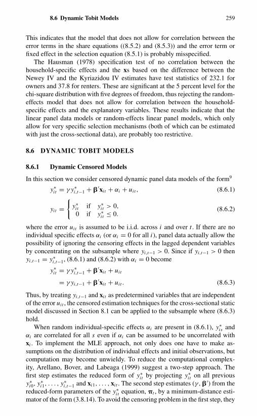
8.6 Dynamic Tobit Models 259
This indicates that the model that does not allow for correlation between theerror terms in the share equations ((8.5.2) and (8.5.3)) and the error term orfixed effect in the selection equation (8.5.1) is probably misspecified.
The Hausman (1978) specification test of no correlation between thehousehold-specific effects and the xs based on the difference between theNewey IV and the Kyriazidou IV estimates have test statistics of 232.1 forowners and 37.8 for renters. These are significant at the 5 percent level for thechi-square distribution with five degrees of freedom, thus rejecting the random-effects model that does not allow for correlation between the household-specific effects and the explanatory variables. These results indicate that thelinear panel data models or random-effects linear panel models, which onlyallow for very specific selection mechanisms (both of which can be estimatedwith just the cross-sectional data), are probably too restrictive.
8.6 DYNAMIC TOBIT MODELS
8.6.1 Dynamic Censored Models
In this section we consider censored dynamic panel data models of the form9
y∗i t = γ y∗
i,t−1 + �′xi t + αi + uit , (8.6.1)
yit ={
y∗i t if y∗
i t > 0,
0 if y∗i t ≤ 0.
(8.6.2)
where the error uit is assumed to be i.i.d. across i and over t . If there are noindividual specific effects αi (or αi = 0 for all i), panel data actually allow thepossibility of ignoring the censoring effects in the lagged dependent variablesby concentrating on the subsample where yi,t−1 > 0. Since if yi,t−1 > 0 thenyi,t−1 = y∗
i,t−1, (8.6.1) and (8.6.2) with αi = 0 become
y∗i t = γ y∗
i,t−1 + �′xi t + uit
= γ yi,t−1 + �′xi t + uit . (8.6.3)
Thus, by treating yi,t−1 and xi t as predetermined variables that are independentof the error uit , the censored estimation techniques for the cross-sectional staticmodel discussed in Section 8.1 can be applied to the subsample where (8.6.3)hold.
When random individual-specific effects αi are present in (8.6.1), y∗is and
αi are correlated for all s even if αi can be assumed to be uncorrelated withxi . To implement the MLE approach, not only does one have to make as-sumptions on the distribution of individual effects and initial observations, butcomputation may become unwieldy. To reduce the computational complex-ity, Arellano, Bover, and Labeaga (1999) suggest a two-step approach. Thefirst step estimates the reduced form of y∗
i t by projecting y∗i t on all previous
y∗i0, y∗
i1, . . . , y∗i,t−1 and xi1, . . . , xi t . The second step estimates (γ, �′) from the
reduced-form parameters of the y∗i t equation, �t , by a minimum-distance esti-
mator of the form (3.8.14). To avoid the censoring problem in the first step, they

260 Truncated and Censored Data
suggest that for the i th individual, only the string (yis, yi,s−1, . . . , yi0), whereyi0 > 0, . . . , yi,s−1 > 0 be used. However, in order to derive the estimates of�t , the conditional distribution of y∗
i t given y∗i0, . . . , y∗
i,t−1 will have to be as-sumed. Moreover, the reduced-form parameters �t are related to (γ, �′) in ahighly nonlinear way. Thus, the second-stage estimator is not easily derivable.Therefore, in this section we shall bypass the issue of fixed or random αi andonly discuss the trimmed estimator due to Honore (1993) and Hu (1999).
Consider the case where T = 2 and yi0 are available. In Figures 8.8 and 8.9,let the vertical axis measure the value of y∗
i2 − γ y∗i1 = y∗
i (γ ) and horizontalaxis measure y∗
i1. If ui1 and ui2 are i.i.d. conditional on (y∗i0, xi1, xi2, αi ), then
y∗i1 and y∗
i2 − γ y∗i1 = y∗
i2(γ ) are symmetrically distributed around the line (1),y∗
i2(γ ) = y∗i1 − γ y∗
i0 + �′xi2 (which is the 45-degree line through (γ y∗i0 +
�′xi1 + αi , �′xi2 + αi ) and (γ y∗i0 − �′xi2, 0)). However, censoring destroys
this symmetry. We only observe
yi1 = max(0, y∗i1)
= max(0, γ y∗i0 + �′xi1 + αi + ui1)
and yi2 = max(0, γ y∗i1 + �′xi2 + αi + ui2) or yi2(γ ) = max(−γ y∗
i1, y∗i2 −
γ y∗i1). That is, observations are censored from the left at the vertical axis, and for
any yi1 = y∗i1 > 0, yi2 = y∗
i2 > 0 implies y∗i2 − γ y∗
i1 > −γ y∗i1. In other words,
observations are also censored from below by yi2(γ ) = −γ yi1, which is line(2) in Figures 8.8 and 8.9. As shown in Figure 8.8, the observable range ofy∗
i1 and y∗i2 − γ y∗
i1 conditional on (xi1, xi2, y∗i0) are not symmetric around line
(1), which we have drawn with γ ≥ 0, γ y∗i0 − �′xi2 > 0. To restore symme-
try, we have to find the mirror images of these two borderlines – the verticalaxis and line (2) – around the centerline (1), and then symmetrically truncateobservations that fall outside these two new lines.
The mirror image of the vertical axis around line (1) is the horizontal liney∗
i2(γ ) = −γ y∗i0 + �′xi2, line (3) in Figure 8.8. The mirror image of line (2)
around line (1) has slope equal to the reciprocal of that of line (2), − 1γ
.Therefore, the mirror image of line (2) is the line y∗
i2(γ ) = − 1γ
y∗i1 + c that
passes through the intersection of line (1) and line (2). The intersection of line(1) and line (2) is given by ¯y∗
i2(γ ) = y∗i1 − (γ y∗
i0 − �′xi2) = −γ y∗i1. Solving
for (y∗i1,
¯y∗i2(γ )), we have y∗
i1 = 11+γ
(γ y∗i0 − �′xi2), ¯y∗
i2(γ ) = − γ
1+γ(γ y∗
i0 −�′xi2). Substituting y∗
i2(γ ) = ¯y∗i2(γ ) and y∗
i1 = y∗i1 into the equation y∗
i2(γ ) =− 1
γy∗
i1 + c, we have c = 1−γ
γ(γ y∗
i0 − �′xi2). Thus the mirror image ofline (2) is y∗
i2(γ ) = − 1γ
(y∗i1 − γ y∗
i0 + �′xi2) − (γ y∗i0 − �′xi2), line (4) in
Figure 8.8.In Figure 8.9 we show the construction of the symmetrical truncation region
for the case when γ y∗i0 − �′xi2 < 0. Since observations are truncated at the
vertical axis from the left and at line (2) from below, the mirror image ofthe vertical axis around line (1) is given by line (3). Therefore, if we truncateobservations at line (3) from below, then the remaining observations will besymmetrically distributed around line (1).

45°
A
B
)'
*(
*)
(*
~)1(
01
2i2x
�∆
−−
=i
ii
yy
yγ
γ *)
(*
~)2(
12
ii
yy
γγ
−=
i2x�
∆+
−=
'*
)(
*~
)3(0
2i
iy
yγ
γ
)'
**
()
(*
~)4(
01
12
ii
iy
yy
γγ
γ∆
+−
−=
−i2
*'
0iyγ−∆
+i2x
�
x�
**
)(
*~
12
2i
ii
yy
yγ
γ−
=
)0,'
*(
0i
iyα
γ+
+i1x
�)0,
'*
(0
i2x�
∆−
iyγ
iα+
i2x�
'
* 1iy
Fig.
8.8
γ>
0,γ
y∗ i0−
�′
x i2
>0.

yi1*
45°A
B
(0, −
γyi0*
+ �
'∆x i2
)
*)
(*~
)2(1
2i
iy
yγ
γ−
=
20
2'
*)
(*
~)3(
ii
iy
yx
�∆
+−
=γ
γ)'
*(
*)
(*
~)1(
20
12
ii
ii
yy
yx
�∆
−−
=γ
γ
**
)(
*~1
22
ii
iy
yy
γγ
−=
Fig.
8.9
γ>
0,γ
y∗ i0−
�′
x i2
>0.
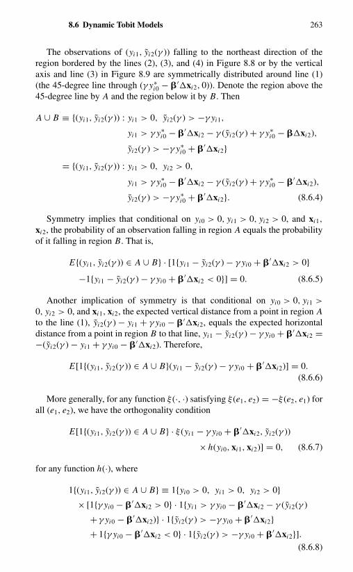
8.6 Dynamic Tobit Models 263
The observations of (yi1, yi2(γ )) falling to the northeast direction of theregion bordered by the lines (2), (3), and (4) in Figure 8.8 or by the verticalaxis and line (3) in Figure 8.9 are symmetrically distributed around line (1)(the 45-degree line through (γ y∗
i0 − �′xi2, 0)). Denote the region above the45-degree line by A and the region below it by B. Then
A ∪ B ≡ {(yi1, yi2(γ )) : yi1 > 0, yi2(γ ) > −γ yi1,
yi1 > γ y∗i0 − �′xi2 − γ (yi2(γ ) + γ y∗
i0 − �xi2),
yi2(γ ) > −γ y∗i0 + �′xi2}
= {(yi1, yi2(γ )) : yi1 > 0, yi2 > 0,
yi1 > γ y∗i0 − �′xi2 − γ (yi2(γ ) + γ y∗
i0 − �′xi2),
yi2(γ ) > −γ y∗i0 + �′xi2}. (8.6.4)
Symmetry implies that conditional on yi0 > 0, yi1 > 0, yi2 > 0, and xi1,
xi2, the probability of an observation falling in region A equals the probabilityof it falling in region B. That is,
E{(yi1, yi2(γ )) ∈ A ∪ B} · [1{yi1 − yi2(γ ) − γ yi0 + �′xi2 > 0}−1{yi1 − yi2(γ ) − γ yi0 + �′xi2 < 0}] = 0. (8.6.5)
Another implication of symmetry is that conditional on yi0 > 0, yi1 >
0, yi2 > 0, and xi1, xi2, the expected vertical distance from a point in region Ato the line (1), yi2(γ ) − yi1 + γ yi0 − �′xi2, equals the expected horizontaldistance from a point in region B to that line, yi1 − yi2(γ ) − γ yi0 + �′xi2 =−(yi2(γ ) − yi1 + γ yi0 − �′xi2). Therefore,
E[1{(yi1, yi2(γ )) ∈ A ∪ B}(yi1 − yi2(γ ) − γ yi0 + �′xi2)] = 0.
(8.6.6)
More generally, for any function ξ (·, ·) satisfying ξ (e1, e2) = −ξ (e2, e1) forall (e1, e2), we have the orthogonality condition
E[1{(yi1, yi2(γ )) ∈ A ∪ B} · ξ (yi1 − γ yi0 + �′xi2, yi2(γ ))
× h(yi0, xi1, xi2)] = 0, (8.6.7)
for any function h(·), where
1{(yi1, yi2(γ )) ∈ A ∪ B} ≡ 1{yi0 > 0, yi1 > 0, yi2 > 0}× [1{γ yi0 − �′xi2 > 0} · 1{yi1 > γ yi0 − �′xi2 − γ (yi2(γ )
+ γ yi0 − �′xi2)} · 1{yi2(γ ) > −γ yi0 + �′xi2}+ 1{γ yi0 − �′xi2 < 0} · 1{yi2(γ ) > −γ yi0 + �′xi2}].
(8.6.8)
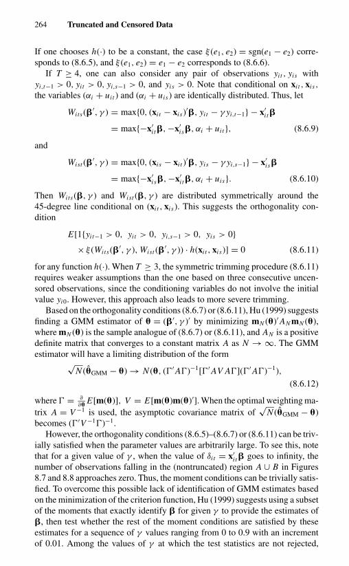
264 Truncated and Censored Data
If one chooses h(·) to be a constant, the case ξ (e1, e2) = sgn(e1 − e2) corre-sponds to (8.6.5), and ξ (e1, e2) = e1 − e2 corresponds to (8.6.6).
If T ≥ 4, one can also consider any pair of observations yit , yis withyi,t−1 > 0, yit > 0, yi,s−1 > 0, and yis > 0. Note that conditional on xi t , xis,
the variables (αi + uit ) and (αi + uis) are identically distributed. Thus, let
Wits(�′, γ ) = max{0, (xi t − xis)′�, yit − γ yi,t−1} − x′i t �
= max{−x′i t �, −x′
is�, αi + uit }, (8.6.9)
and
Wist (�′, γ ) = max{0, (xis − xi t )
′�, yis − γ yi,s−1} − x′is�
= max{−x′is�, −x′
i t �, αi + uis}. (8.6.10)
Then Wits(�, γ ) and Wist (�, γ ) are distributed symmetrically around the45-degree line conditional on (xi t , xis). This suggests the orthogonality con-dition
E[1{yit−1 > 0, yit > 0, yi,s−1 > 0, yis > 0}× ξ (Wits(�′, γ ), Wist (�
′, γ )) · h(xi t , xis)] = 0 (8.6.11)
for any function h(·). When T ≥ 3, the symmetric trimming procedure (8.6.11)requires weaker assumptions than the one based on three consecutive uncen-sored observations, since the conditioning variables do not involve the initialvalue yi0. However, this approach also leads to more severe trimming.
Based on the orthogonality conditions (8.6.7) or (8.6.11), Hu (1999) suggestsfinding a GMM estimator of � = (�′, γ )′ by minimizing mN (�)′ AN mN (�),where mN (�) is the sample analogue of (8.6.7) or (8.6.11), and AN is a positivedefinite matrix that converges to a constant matrix A as N → ∞. The GMMestimator will have a limiting distribution of the form
√N (�GMM − �) → N (�, (�′ A�)−1[�′ AV A�](�′ A�)−1),
(8.6.12)
where � = ∂∂�
E[m(�)], V = E[m(�)m(�)′]. When the optimal weighting ma-trix A = V −1 is used, the asymptotic covariance matrix of
√N (�GMM − �)
becomes (�′V −1�)−1.However, the orthogonality conditions (8.6.5)–(8.6.7) or (8.6.11) can be triv-
ially satisfied when the parameter values are arbitrarily large. To see this, notethat for a given value of γ , when the value of δi t = x′
i t � goes to infinity, thenumber of observations falling in the (nontruncated) region A ∪ B in Figures8.7 and 8.8 approaches zero. Thus, the moment conditions can be trivially satis-fied. To overcome this possible lack of identification of GMM estimates basedon the minimization of the criterion function, Hu (1999) suggests using a subsetof the moments that exactly identify � for given γ to provide the estimates of�, then test whether the rest of the moment conditions are satisfied by theseestimates for a sequence of γ values ranging from 0 to 0.9 with an incrementof 0.01. Among the values of γ at which the test statistics are not rejected,

8.6 Dynamic Tobit Models 265
Table 8.4. Estimates of AR(1) coefficients of log realannual earnings (in thousands)a
Linear GMM Nonlinear GMM with(assuming no censoring) correction for censoring
Black White Black White
0.379 0.399 0.210 0.380(0.030) (0.018) (0.129) (0.051)
aStandard errors in parenthesis.Source: Hu (1999).
the one which yields the smallest test statistic is chosen as the estimate of γ .Hu (1999) uses this estimation method to study earnings dynamics, usingmatched data from the Current Population Survey and Social Security Ad-ministration (CPS–SSA) Earnings Record for a sample of men who were bornin 1930–1939 and living in the South during the period of 1957–1973. The SSAearnings are top-coded at the maximum social security taxable level, namely,yit = min(y∗
i t , ct ), where ct is the social security maximum taxable earningslevel in period t . This censoring at the top can be easily translated into censor-ing at zero by considering yi t = ct − yit , then yi t = max(0, ct − y∗
i t ).Table 8.4 presents the estimates of the coefficient of the lagged log real annual
earnings coefficient of an AR(1) model based on a sample of 226 black and1883 white men with and without correction for censoring. When censoring isignored, the model is estimated by the linear GMM method. When censoring istaken into account, Hu uses an unbalanced panel of observations with positiveSSA earnings in three consecutive time periods. The estimated γ are verysimilar for black and white men when censoring is ignored. However, whencensoring is taken into account, the estimated autoregressive parameter γ ismuch higher for white men than for black men. The higher persistence of theearnings process for white men is consistent with the notion that white men hadjobs that had better security and were less vulnerable to economic fluctuationthan black men in the period 1957–1973.
8.6.2 Dynamic Sample Selection Models
When the selection rule is endogenously determined as given by (8.2.4) and y∗i t
is given by (8.6.1), with wi t and xi t being nonoverlapping vectors of strictlyexogenous explanatory variables (with possibly common elements), the modelunder consideration has the form10
yit = dit y∗i t , (8.6.13)
dit = 1{w′i t a + ηi + νi t }, i = 1, . . . , N ,
(8.6.14)t = 1, . . . , T,
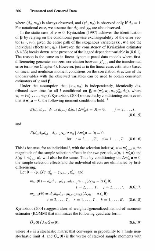
266 Truncated and Censored Data
where (dit , wi t ) is always observed, and (y∗i t , xi t ) is observed only if dit = 1.
For notational ease, we assume that di0 and yi0 are also observed.In the static case of γ = 0, Kyriazidou (1997) achieves the identification
of � by relying on the conditional pairwise exchangeability of the error vec-tor (uit , νi t ), given the entire path of the exogenous variables (xi , wi ) and theindividual effects (αi , ηi ). However, the consistency of Kyriazidou estimator(8.4.33) breaks down in the presence of the lagged dependent variable in (8.6.1).The reason is the same as in linear dynamic panel data models where first-differencing generates nonzero correlation between y∗
i,t−1 and the transformederror term (see Chapter 4). However, just as in the linear case, estimators basedon linear and nonlinear moment conditions on the correlation structure of theunobservables with the observed variables can be used to obtain consistentestimators of γ and �.
Under the assumption that {uit , νi t } is independently, identically dis-tributed over time for all i conditional on �i ≡ (w′
i , αi , ηi , y∗i0, di0), where
wi = (w′i1, . . . , wiT )′, Kyriazidou (2001) notes that by conditioning on the event
that w′i t a = 0, the following moment conditions hold:11
E(dit di,t−1 di,t−2 di,t− j uit | w′i t a = 0) = 0, j = 2, . . . , t,
(8.6.15)
and
E(disdit di,t−1di,t−2 xis uit | w′i t a = 0) = 0
for t = 2, . . . , T , s = 1, . . . , T . (8.6.16)
This is because, for an individual i , with the selection index w′i t a = w′
i,t−1a, themagnitude of the sample selection effects in the two periods, λ(ηi + w′
i t a) andλ(ηi + w′
i,t−1a), will also be the same. Thus by conditioning on w′i t a = 0,
the sample selection effects and the individual effects are eliminated by first-differencing.
Let � = (γ, �′)′, z′i t = (yi,t−1, x′
i t ), and
m1i t (�) = dit di,t−1di,t−2di,t− j yi,t− j (yit − z′i t �),
t = 2, . . . , T , j = 2, . . . , t, (8.6.17)
m2i t,k(�) = disdit di,t−1di,t−2xis,k(yit − z′i t �),
t = 2, . . . , T , s = 1, . . . , T , k = 1, . . . , K . (8.6.18)
Kyriazidou (2001) suggests a kernel-weighted generalized method-of-momentsestimator (KGMM) that minimizes the following quadratic form:
G N (�)′ AN G N (�), (8.6.19)
where AN is a stochastic matrix that converges in probability to a finite non-stochastic limit A, and G N (�) is the vector of stacked sample moments with
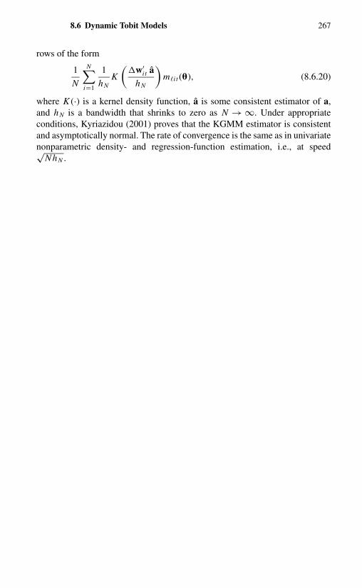
8.6 Dynamic Tobit Models 267
rows of the form
1
N
N∑i=1
1
hNK
(w′
i t ahN
)m�i t (�), (8.6.20)
where K (·) is a kernel density function, a is some consistent estimator of a,and hN is a bandwidth that shrinks to zero as N → ∞. Under appropriateconditions, Kyriazidou (2001) proves that the KGMM estimator is consistentand asymptotically normal. The rate of convergence is the same as in univariatenonparametric density- and regression-function estimation, i.e., at speed√
NhN .

CHAPTER 9
Incomplete Panel Data
Thus far our discussions have been concentrated on situations in which thesample of N cross-sectional units over T time periods is sufficient to identifya behavioral model. In this chapter we turn to the issues of incomplete paneldata. We first examine the problems of estimating dynamic models when thelength of time series is shorter than the maximum order of the lagged variablesincluded in the equation. We then discuss the issues when some individualsare dropped from the experiment or survey. We note that when individuals arefollowed over time, there is a high probability that this will occur. Since thesituations where individuals are missing for a variety of behavioral reasonshave been discussed in Chapter 8 in this chapter we only distinguish threesituations: (1) individuals are missing randomly or are being rotated; (2) a seriesof independent cross sections are observed over time; (3) only a single setof cross-sectional data is available in conjunction with the aggregate time-series observations. We briefly sketch how statistical methods developed foranalyzing complete panel data can be generalized to analyze incomplete paneldata.
9.1 ESTIMATING DISTRIBUTED LAGSIN SHORT PANELS1
9.1.1 Introduction
Because of technical, institutional, and psychological rigidities, often behavioris not adapted immediately to changes in the variables that condition it. In mostcases this adaptation is progressive. The progressive nature of adaptations inbehavior can be expressed in various ways. Depending on the rationale behindit, we can set up an autoregressive model, with the current value of y beinga function of lagged dependent variables and exogenous variables, or we canset up a distributed-lag model, with the current value of y being a functionof current and previous values of exogenous variables. Although usually alinear distributed-lag model can be expressed in an autoregressive form, andsimilarly, as a rule, any stable linear autoregressive model can be transformed
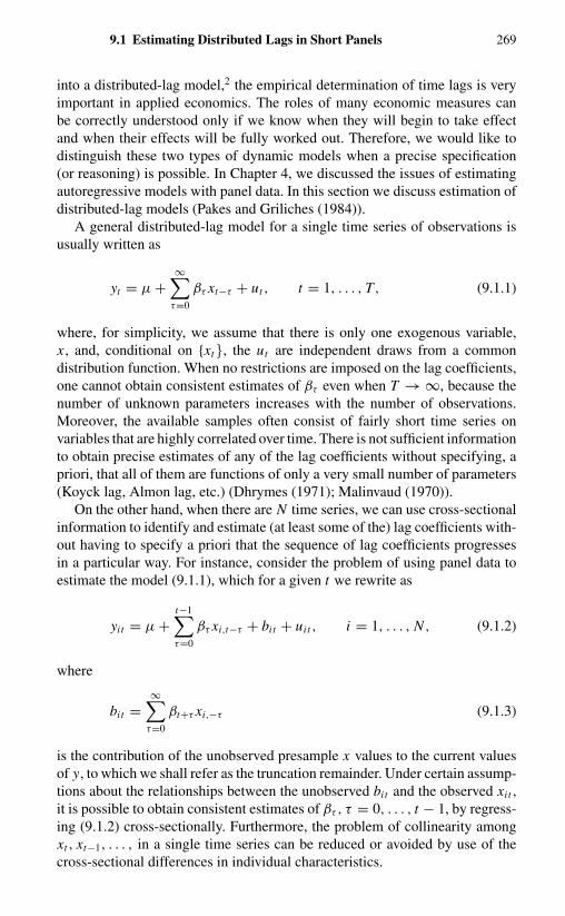
9.1 Estimating Distributed Lags in Short Panels 269
into a distributed-lag model,2 the empirical determination of time lags is veryimportant in applied economics. The roles of many economic measures canbe correctly understood only if we know when they will begin to take effectand when their effects will be fully worked out. Therefore, we would like todistinguish these two types of dynamic models when a precise specification(or reasoning) is possible. In Chapter 4, we discussed the issues of estimatingautoregressive models with panel data. In this section we discuss estimation ofdistributed-lag models (Pakes and Griliches (1984)).
A general distributed-lag model for a single time series of observations isusually written as
yt = µ +∞∑
τ=0
βτ xt−τ + ut , t = 1, . . . , T, (9.1.1)
where, for simplicity, we assume that there is only one exogenous variable,x , and, conditional on {xt}, the ut are independent draws from a commondistribution function. When no restrictions are imposed on the lag coefficients,one cannot obtain consistent estimates of βτ even when T → ∞, because thenumber of unknown parameters increases with the number of observations.Moreover, the available samples often consist of fairly short time series onvariables that are highly correlated over time. There is not sufficient informationto obtain precise estimates of any of the lag coefficients without specifying, apriori, that all of them are functions of only a very small number of parameters(Koyck lag, Almon lag, etc.) (Dhrymes (1971); Malinvaud (1970)).
On the other hand, when there are N time series, we can use cross-sectionalinformation to identify and estimate (at least some of the) lag coefficients with-out having to specify a priori that the sequence of lag coefficients progressesin a particular way. For instance, consider the problem of using panel data toestimate the model (9.1.1), which for a given t we rewrite as
yit = µ +t−1∑τ=0
βτ xi,t−τ + bit + uit , i = 1, . . . , N , (9.1.2)
where
bit =∞∑
τ=0
βt+τ xi,−τ (9.1.3)
is the contribution of the unobserved presample x values to the current valuesof y, to which we shall refer as the truncation remainder. Under certain assump-tions about the relationships between the unobserved bit and the observed xit ,it is possible to obtain consistent estimates of βτ , τ = 0, . . . , t − 1, by regress-ing (9.1.2) cross-sectionally. Furthermore, the problem of collinearity amongxt , xt−1, . . . , in a single time series can be reduced or avoided by use of thecross-sectional differences in individual characteristics.

270 Incomplete Panel Data
9.1.2 Common Assumptions
To see under what conditions the addition of a cross-sectional dimension canprovide information that cannot be obtained in a single time series, first we con-sider the case that the lag coefficients vary across individuals ({βiτ }∞τ=0 for i =1, . . . , N ). If there is no restriction on the distribution of these sequences overmembers of the population, then each time series contains information on only asingle sequence of coefficients. The problem of lack of information remains forpanel data. Second, even if the lag coefficients do not vary across individuals(βiτ = βτ for i = 1, . . . , N and τ = 0, 1, 2, . . .), the (often very significant)increase in sample size that accompanies the availability of panel data is entirelyan increase in cross-sectional dimension. Panel data sets, in fact, usually tracktheir observations over only a relatively short time interval. As a result, thecontributions of the unobserved presample x values to the current values of y(the truncation remainders bit ) are likely to be particularly important if we donot wish to impose the same type of restrictions on the lag coefficients as weoften do when a single time-series data set is used to estimate a distributed-lag model. Regression analysis, ignoring the unobserved truncation-remainderterm, will suffer from the usual omitted-variable bias.
Thus, in order to combine N time series to estimate a distributed-lag model,we have to impose restrictions on the distribution of lag coefficients acrosscross-sectional units and/or on the way the unobserved presample terms affectcurrent behavior. Pakes and Griliches (1984) considered a distributed-lag modelof the form
yit = α∗i +
∞∑τ=0
βiτ xi,t−τ + uit , i = 1, . . . , N ,
(9.1.4)t = 1, . . . , T,
where uit is independent of xis and is independently, identically distributed,with mean zero and variance σ 2
u . The coefficients of α∗i and βiτ are assumed to
satisfy the following assumptions.
Assumption 9.1.1. E(βiτ ) = βτ .
Assumption 9.1.2. Let β iτ = βiτ − βτ , ξi t = ∑∞τ=0 β iτ xi,t−τ , and �′
i =(ξi1, . . . , ξiT ); then E∗[�i | xi ] = 0.
Assumption 9.1.3. E∗(α∗i | xi ) = µ + a′xi .
Here E∗(Z1 | Z2) refers to the minimum-mean-squared-error linear predictor(or the projection) of Z1 onto Z2; xi denotes the vector of all observed xit . Weassume that there are � + 1 observations on x before the first observation ony, and the 1 × (� + 1 + T ) vector x′
i = [xi,−�, . . . , xiT ] is an independent drawfrom a common distribution with E(xi x′
i ) = �xx positive definite.3
A sufficient condition for Assumption 9.1.2 to hold is that differences in lagcoefficients across individuals are uncorrelated with the xi [i.e., βiτ is a random

9.1 Estimating Distributed Lags in Short Panels 271
variable defined in the sense of Swamy (1970), or see Chapter 6]. However,Assumption 9.1.3 does allow for individual-specific constant terms (the α∗
i ) tobe correlated with xi . The combination of Assumptions 9.1.1–9.1.3 is sufficientto allow us to identify the expected value of the lag-coefficient sequence {βτ }if both N and T tend to infinity.
If T is fixed, substituting Assumptions 9.1.1 and 9.1.2 into equation (9.1.4),we rewrite the distributed-lag model as
yit = α∗i +
t+�∑τ=0
βτ xi,t−τ + bit + ui t , i = 1, . . . , N ,(9.1.5)
t = 1, . . . , T,
where bit = ∑∞τ=�+1 βt+τ xi,−τ is the truncation remainder for individual i
in period t , and ui t = ξi t + uit is the amalgamated error term satisfyingE∗[ui | xi ] = 0. The unobserved truncation remainders are usually correlatedwith the included explanatory variables. Therefore, without additional restric-tions, we still cannot get consistent estimates of any of the lag coefficients βτ
by regressing yit on xi,t−τ , even when N → ∞.Because the values of the truncation remainders (bit ) are determined by the
lag coefficients and the presample x values, identification requires constraintseither on the lag coefficients or on the stochastic process generating these xvalues. Because there usually are many more degrees of freedom available inpanel data, this allows us to use prior restrictions of different kind than in theusual approach of constraining lag coefficients to identify truncation remainders(e.g., Dhrymes (1971)). In the next two subsections we illustrate how variousrestrictions can be used to identify the lag coefficients.
9.1.3 Identification Using Prior Structure of the Processof the Exogenous Variable
In this subsection we consider the identification of a distributed-lag model usinga kind of restriction different from that in the usual approach of constraining lagcoefficients. Our interest is focused on estimating at least some of the populationparameters βτ = E(βiτ ) for τ = 0, 1, . . . , without restricting βτ to be a functionof a small number of parameters. We consider a lag coefficient identified if itcan be calculated from the matrix of coefficients obtained from the projection ofyi onto xi , a T × (T + � + 1) matrix called �, where E∗(yi | xi ) = �∗ + �xi ,�∗ = (µ∗
1, . . . , µ∗T )′, and y′
i = (yi1, . . . , yiT ) is a 1 × T vector.Equation (9.1.5) makes it clear that each row of � will contain a combination
of the lag coefficients of interest and the coefficients from the projections ofthe two unobserved components, α∗
i and bit , on xi . Therefore, the problemis to separate out the lag coefficients from the coefficients defining these twoprojections.
Using equation (9.1.5), the projection of yi onto xi and α∗i is given by4
E∗(yi | xi , α∗i ) = [B + W ]xi + [e + c]α∗
i , (9.1.6)

272 Incomplete Panel Data
where B is the T × (T + � + 1) matrix of the lag coefficients
B =
β�+1 β� · · · β1 β0 0 0 · · · 0 0
β�+2 β�+1 · · · β2 β1 β0 0 · · · 0 0...
......
......
......
...
βT +�−1 βt+�−2 · · · βT +1 βT βT −1 βT −2 · · · β0 0
βT +� βT +�−1 · · · βT βT −1 βT −2 βT −3 · · · β1 β0
.
W and c are defined by the unconstrained projection of bi = (bi1, . . . , biT )′
onto xi and α∗i ,
E∗[bi | xi , α∗i ] = W xi + cα∗
i . (9.1.7)
Equation (9.1.6) and the fact that E∗{E∗(yi | xi , α∗i ) | xi } = E∗[yi | xi ] =
(e + c)µ + �xi imply that
� = B + [W + (e + c)a′], (9.1.8)
where a is defined by the unconstrained projection of α∗i onto xi , [E∗(α∗
i | xi ) =µ + a′xi ].
Clearly, if the T × (T + � + 1) matrix W is unrestricted, we cannot separateout the lag coefficients B and the effect of the truncation-remainder term fromthe matrix �. But given that ca′ is a matrix of rank 1, we may be able to identifysome elements of B if there are restrictions on W. Thus, in order to identifysome of the lag coefficients from �, we shall have to restrict W. W will berestricted if it is reasonable to assume that the stochastic process generating{xit }T
t=−∞ restricts the coefficients of xi in the projection of the presample xi,− j
values onto the in-sample xi and α∗i . The particular case analyzed by Pakes and
Griliches (1984) is given by the following assumption.5
Assumption 9.1.4. For q ≥ 1, E∗[xi,−�−q | xi , α∗i ] = cqα
∗i + ∑p
j=1 ρ(q)j ×
xi,−�+ j−1. That is, in the projection of the unseen presample x values onto xi
and α∗i , only [xi,−�, xi,−�+1, . . . , xi,−�+p−1] have nonzero coefficients.
If cq = 0, a sufficient condition for Assumption 9.1.4 to hold is that x isgenerated by a pth-order autoregressive process.6
Because each element of bi is just a different linear combination of the samepresample x values, the addition of Assumption 9.1.4 implies that
E∗[bit | xi , α∗i ] = ctα
∗i +
p∑j=1
wt, j−�−1xi, j−�−1, i = 1, . . . , N ,
t = 1, . . . , T,
(9.1.9)
where wt, j−�−1 = ∑∞q=1 βt+�+qρ
(q)j , j = 1, . . . , p, and ct = ∑∞
q=1 βt+l+qcq .This determines the vector c and the matrix W in (9.1.7). In particular, it impliesthat W can be partitioned into a T × (T + � − p + 1) matrix of zeros and a

9.1 Estimating Distributed Lags in Short Panels 273
T × p matrix of free coefficients,
W =[
...WT ×p
0T ×(T +�−p+1)...
]. (9.1.10)
Substituting (9.1.10) into (9.1.8) and taking partial derivatives of � withrespect to the leading (T + � − p + 1) lag coefficients, we can show thatthe resulting Jacobian matrix satisfies the rank condition for identification ofthese coefficients (e.g., Hsiao (1983, Theorem 5.1.2)). A simple way to checkthat the leading (T + � − p + 1) lag coefficients are indeed identified is toshow that consistent estimators for them exist. We note that by construction,cross-sectional regression of yi on xi yields consistent estimates of �. For thespecial case in which α∗
i = 0, the projections of each period’s value of y on allin-sample values of x are7
E∗(yi1 | xi ) = µ +p∑
j=1
φ1, j−�−1xi, j−�−1,
E∗(yi2 | xi ) = µ + β0x2 +p∑
j=1
φ2, j−�−1xi, j−�−1,
E∗(yi3 | xi ) = µ + β0x3 + β1x2 +p∑
j=1
φ3, j−�−1xi, j−�−1,
...
E∗(yiT | xi ) = µ + β0xT + · · · + βT +�−px p−�
+p∑
j=1
φT, j−�−1xi, j−�−1,
(9.1.11)
where φt, j−�−1 = βt+�+1− j + wt, j−�−1 for t = 1, . . . , T and j = 1, . . . , p, andfor simplicity we have let p = � + 2. The first p values of xi in each projec-tion have nonzero partial correlations with the truncation remainders (the bit ).Hence, their coefficients do not identify the parameters of the lag distribution.Only when (t + � − p + 1) > 0 are the leading coefficients in each equationin fact estimates of the leading lag coefficients. As t increases, we graduallyuncover the lag structure.
When cq �= 0, the finding of consistent estimators (hence identification)for the leading T + � − p + 1 lag coefficients is slightly more complicated.Substituting (9.1.9) into (9.1.7), we have
E∗(yit | xi , α∗i ) = (1 + ct )α
∗i +
t+�−p∑τ=0
βτ xi,t−τ
+p∑
j=1
φt, j−�−1xi, j−�−1, t = 1, . . . , T,
(9.1.12)
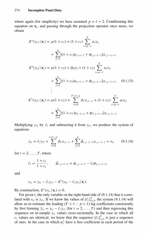
274 Incomplete Panel Data
where again (for simplicity) we have assumed p = � + 2. Conditioning thisequation on xi , and passing through the projection operator once more, weobtain
E∗(yi1 | xi ) = µ(1 + c1) + (1 + c1)T∑
t=p−�
at xit
+p∑
j=1
[(1 + c1)a j−�−1 + φ1, j−�−1]xi, j−�−1,
E∗(yi2 | xi ) = µ(1 + c2) + β0x2 + (1 + c2)T∑
t=p−�
at xit
+p∑
j=1
[(1 + c2)a j−�−1 + φ2, j−�−1]xi, j−�−1, (9.1.13)
...
E∗(yiT | xi ) = µ(1 + cT ) +T +�−p∑
τ=0
βτ xi,t−τ + (1 + cT )T∑
t=p−�
at xit
+p∑
j=1
[(1 + cT )a j−�−1 + φT, j−�−1]xi, j−�−1.
Multiplying yi1 by ct and subtracting it from yit , we produce the system ofequations
yit = ct yi1 +t+�−p∑τ=0
βτ xi,t−τ +p∑
j=1
φt, j−�−1xi, j−�−1 + νi t (9.1.14)
for t = 2, . . . , T , where
ct = 1 + ct
1 + c1, φt, j−�−1 = φt, j−�−1 − ctφ1, j−�−1,
and
νi t = yit − ct yi1 − E∗(yit − ct yi1| xi ).
By construction, E∗(νi t | xi ) = 0.For given t , the only variable on the right-hand side of (9.1.14) that is corre-
lated with νi t is yi1. If we know the values of {ct }Tt=2, the system (9.1.14) will
allow us to estimate the leading (T + � − p + 1) lag coefficients consistentlyby first forming yi t = yit − ct yi1 (for t = 2, . . . , T ) and then regressing thissequence on in-sample xit values cross-sectionally. In the case in which allct values are identical, we know that the sequence {ct }T
t=2 is just a sequenceof ones. In the case in which α∗
i have a free coefficient in each period of the

9.1 Estimating Distributed Lags in Short Panels 275
sample, we have unknown (1 + ct ). However, we can consistently estimate ct ,βτ , and φt, j by the instrumental-variable method, provided there is at least onexis that is excluded from the determinants of yit − ct yi1 and that is correlatedwith yi1. If T ≥ 3, then xi3, . . . , xiT are excluded from the equation determin-ing (yi2 − c2 yi1), and provided that not all of a3 to aT are zero, at least one ofthem will have the required correlation with yi1.
We have shown that under Assumptions 9.1.1–9.1.4, the use of panel dataallows us to identify the leading T + � − p + 1 lag coefficients without im-posing any restrictions on the sequence {βτ }∞τ=0. Of course, if T + � is smallrelative to p, we shall not be able to build up much information on the tail of thelag distribution. This simply reflects the fact that short panels, by their verynature, do not contain unconstrained information on that tail. However, theearly coefficients are often of significant interest in themselves. Moreover, theymay provide a basis for restricting the lag structure (to be a function of a smallnumber of parameters) in further work.
9.1.4 Identification Using Prior Structure of the Lag Coefficients
In many situations we may know that all βτ are positive. We may also knowthat the first few coefficients β0, β1, and β2 are the largest and that βτ decreaseswith increasing τ , at least after a certain value of τ . In this subsection weshow how the conventional approach of constraining the lag coefficients to bea function of a finite number of parameters can be used and generalized foridentification of a distributed-lag model in the panel data context. Therefore,we drop Assumption 9.1.4. Instead, we assume that we have prior knowledge ofthe structure of lag coefficients. The particular example we use here is the oneassumed by Pakes and Griliches (1984), where the sequence of lag coefficients,after the first few free lags, has an autoregressive structure. This restriction isformalized as follows:
Assumption 9.1.5.
βτ =
βτ for τ ≤ k1,
J∑j=1
δ jβτ− j otherwise,
where the roots of the characteristic equation 1 − ∑Jj=1 δ j L j = 0, say
λ−11 , . . . , λ−1
J , lie outside the unit circle.8 For simplicity, we assume thatk1 = � + 1, and that λ1, . . . , λJ are real and distinct.
Assumption 9.1.5 implies that βτ declines geometrically after the first k1
lags. Solving the J th-order difference equation
βτ − δ1βτ−1 − · · · − δJ βτ−J = 0, (9.1.15)

276 Incomplete Panel Data
we obtain the general solution (e.g., Box and Jenkins (1970, Chapter 3))
βτ =J∑
j=1
A jλτj , (9.1.16)
where A j are constants to be determined by the initial conditions of the differ-ence equation.
Substituting (9.1.16) into (9.1.5), we write the truncation-remainder termbit as
bit =∞∑
τ=�+1
(J∑
j=1
A jλt+τj
)xi,−τ
=J∑
j=1
λtj
(A j
∞∑τ=�+1
λτj xi,−τ
)
=J∑
j=1
λtj bi j , (9.1.17)
where bi j = A j∑∞
τ=�+1 λτj xi,−τ . That is, we can represent the truncation re-
mainder bit in terms of J unobserved initial conditions (bi1, . . . , bi J ). Thus,under Assumptions 9.1.1–9.1.3 and 9.1.5, the distributed-lag model becomesa system of T regressions with J + 1 freely correlated unobserved factors(α∗
i , bi1, . . . , bi J ) where the impact of last J of them decay geometrically overtime.
Because the conditions for identification of a model in which there are J + 1unobserved factors is a straightforward generalization from a model with twounobserved factors, we deal first with the case J = 1 and then point out theextensions required for J > 1.
When J = 1, it is the familiar case of a modified Koyck (or geometric) lagmodel. The truncation remainder becomes an unobserved factor that follows anexact first-order autoregression (i.e., bit = δbi,t−1). Substituting this result into(9.1.5), we have
yit = α∗i +
�+1∑τ=0
βτ xi,t−τ + β�+1
t+�∑τ=�+2
δτ−(�+1)xi,t−τ + δt−1bi + ui t ,
(9.1.18)
where bi = β�+1∑∞
τ=1 δτ xi,−τ−�.Recall from the discussion in Section 9.1.3 that to identify the lag param-
eters we require a set of restrictions on the projection matrix E∗(bi | xi ) =[W + ca′]xi [equation (9.1.7)]. The Koyck lag model implies that bit = δbi,t−1,which implies that E∗(bit | xi ) = δE∗(bi,t−1 | xi ); that is, wtr = δwt−1,r forr = 1, . . . , T + � + 1 and t = 2, . . . , T . It follows that the matrix � has theform
� = B∗ + �∗w∗′ + ea′, (9.1.19)
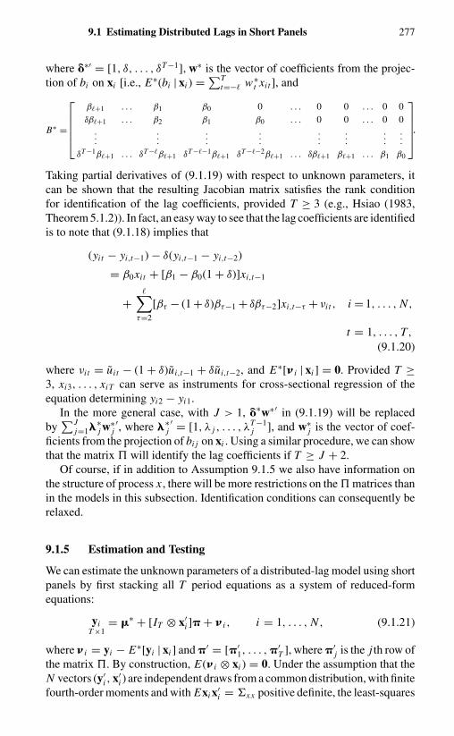
9.1 Estimating Distributed Lags in Short Panels 277
where �∗′ = [1, δ, . . . , δT −1], w∗ is the vector of coefficients from the projec-tion of bi on xi [i.e., E∗(bi | xi ) = ∑T
t=−� w∗t xi t ], and
B∗ =
β�+1 . . . β1 β0 0 . . . 0 0 . . . 0 0δβ�+1 . . . β2 β1 β0 . . . 0 0 . . . 0 0
......
......
......
......
δT −1β�+1 . . . δT −�β�+1 δT −�−1β�+1 δT −�−2β�+1 . . . δβ�+1 β�+1 . . . β1 β0
.
Taking partial derivatives of (9.1.19) with respect to unknown parameters, itcan be shown that the resulting Jacobian matrix satisfies the rank conditionfor identification of the lag coefficients, provided T ≥ 3 (e.g., Hsiao (1983,Theorem 5.1.2)). In fact, an easy way to see that the lag coefficients are identifiedis to note that (9.1.18) implies that
(yit − yi,t−1) − δ(yi,t−1 − yi,t−2)
= β0xit + [β1 − β0(1 + δ)]xi,t−1
+�∑
τ=2
[βτ − (1 + δ)βτ−1 + δβτ−2]xi,t−τ + νi t , i = 1, . . . , N ,
t = 1, . . . , T,
(9.1.20)
where νi t = ui t − (1 + δ)ui,t−1 + δui,t−2, and E∗[ i | xi ] = 0. Provided T ≥3, xi3, . . . , xiT can serve as instruments for cross-sectional regression of theequation determining yi2 − yi1.
In the more general case, with J > 1, �∗w∗′ in (9.1.19) will be replacedby
∑Jj=1�∗
j w∗j′, where �∗
j′ = [1, λ j , . . . , λ
T −1j ], and w∗
j is the vector of coef-ficients from the projection of bi j on xi . Using a similar procedure, we can showthat the matrix � will identify the lag coefficients if T ≥ J + 2.
Of course, if in addition to Assumption 9.1.5 we also have information onthe structure of process x , there will be more restrictions on the � matrices thanin the models in this subsection. Identification conditions can consequently berelaxed.
9.1.5 Estimation and Testing
We can estimate the unknown parameters of a distributed-lag model using shortpanels by first stacking all T period equations as a system of reduced-formequations:
yiT ×1
= �∗ + [IT ⊗ x′i ]� + i , i = 1, . . . , N , (9.1.21)
where i = yi − E∗[yi | xi ] and �′ = [�′1, . . . , �′
T ], where �′j is the j th row of
the matrix �. By construction, E( i ⊗ xi ) = 0. Under the assumption that theN vectors (y′
i , x′i ) are independent draws from a common distribution, with finite
fourth-order moments and with Exi x′i = �xx positive definite, the least-squares

278 Incomplete Panel Data
estimator � of � is consistent, and√
N (� − �) is asymptotically normallydistributed, with mean zero and variance–covariance matrix �, which is givenby (3.9.11).
The models of Sections 9.1.3 and 9.1.4 imply that � = f(�), where � isa vector of the model’s parameters of dimensions m ≤ (T + � + 1). We canimpose these restrictions by a minimum-distance estimator that chooses � tominimize
[� − f(�)]′�−1[� − f(�)], (9.1.22)
where � is a consistent estimator of (3.9.11). Under fairly general conditions,the estimator � is consistent, and
√N (� − �) is asymptotically normally dis-
tributed, with asymptotic variance–covariance matrix
(F ′�−1 F)−1, (9.1.23)
where F = ∂f(�)/∂�′. The identification condition ensures that F has rank m.The quadratic form
N [� − f(�)]′�−1[� − f(�)] (9.1.24)
is asymptotically chi-square-distributed with T (T + � + 1) − m degrees offreedom.
Equation (9.1.24) provides us with a test of the T (T + � + 1) − m con-straints f placed on �. To test nested restrictions, consider the null hypothesis� = g(�), where � is a k-dimensional vector (k ≤ m) of the parameters of therestricted model. Let h(�) = f[g(�)]; that is, h embodies the restrictions of theconstrained model. Then, under the null hypothesis,
N [� − h(�)]′�−1[� − h(�)] (9.1.25)
is asymptotically chi-square-distributed with T (T + � + 1) − k degrees of free-dom, where � minimizes (9.1.25). Hence, to test the null hypothesis, we canuse the statistic9
N [� − h(�)]′�−1[� − h(�)] − N [� − f(�)]′�−1[� − f(�)],
(9.1.26)
which is asymptotically chi-square-distributed, with m − k degrees of freedom.To illustrate the method of estimating unconstrained distributed-lag models
using panel data, Pakes and Griliches (1984) investigated empirically the issuesof how to construct the “stock of capital (G)” for analysis of rates of return.The basic assumption of their model is that there exists a stable relationshipbetween earnings (gross or net profits) (y) and past investments (x), and firmsor industries differ only in the level of the yield on their past investments, withthe time shapes of these yields being the same across firms and implicit in theassumed depreciation formula. Namely,
E∗[yit | Git , α∗i ] = α∗
i + γ Git , (9.1.27)
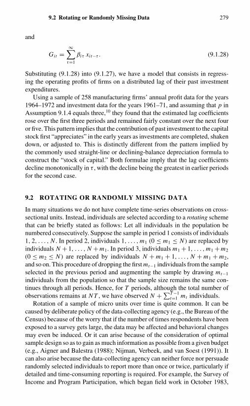
9.2 Rotating or Randomly Missing Data 279
and
Git =∞∑
τ=1
βiτ xit−τ . (9.1.28)
Substituting (9.1.28) into (9.1.27), we have a model that consists in regress-ing the operating profits of firms on a distributed lag of their past investmentexpenditures.
Using a sample of 258 manufacturing firms’ annual profit data for the years1964–1972 and investment data for the years 1961–71, and assuming that p inAssumption 9.1.4 equals three,10 they found that the estimated lag coefficientsrose over the first three periods and remained fairly constant over the next fouror five. This pattern implies that the contribution of past investment to the capitalstock first “appreciates” in the early years as investments are completed, shakendown, or adjusted to. This is distinctly different from the pattern implied bythe commonly used straight-line or declining-balance depreciation formula toconstruct the “stock of capital.” Both formulae imply that the lag coefficientsdecline monotonically in τ , with the decline being the greatest in earlier periodsfor the second case.
9.2 ROTATING OR RANDOMLY MISSING DATA
In many situations we do not have complete time-series observations on cross-sectional units. Instead, individuals are selected according to a rotating schemethat can be briefly stated as follows: Let all individuals in the population benumbered consecutively. Suppose the sample in period 1 consists of individuals1, 2, . . . , N . In period 2, individuals 1, . . . , m1 (0 ≤ m1 ≤ N ) are replaced byindividuals N + 1, . . . , N + m1. In period 3, individuals m1 + 1, . . . , m1 + m2
(0 ≤ m2 ≤ N ) are replaced by individuals N + m1 + 1, . . . , N + m1 + m2,and so on. This procedure of dropping the first mt−1 individuals from the sampleselected in the previous period and augmenting the sample by drawing mt−1
individuals from the population so that the sample size remains the same con-tinues through all periods. Hence, for T periods, although the total number ofobservations remains at N T , we have observed N + ∑T −1
t=1 mt individuals.Rotation of a sample of micro units over time is quite common. It can be
caused by deliberate policy of the data-collecting agency (e.g., the Bureau of theCensus) because of the worry that if the number of times respondents have beenexposed to a survey gets large, the data may be affected and behavioral changesmay even be induced. Or it can arise because of the consideration of optimalsample design so as to gain as much information as possible from a given budget(e.g., Aigner and Balestra (1988); Nijman, Verbeek, and van Soest (1991)). Itcan also arise because the data-collecting agency can neither force nor persuaderandomly selected individuals to report more than once or twice, particularly ifdetailed and time-consuming reporting is required. For example, the Survey ofIncome and Program Participation, which began field work in October 1983,

280 Incomplete Panel Data
has been designed as an ongoing series of national panels, each consisting ofabout 20,000 interviewed households and having a duration of 2.5 years. Everyfour months the Census Bureau will interview each individual of age 15 yearsor older in the panel. Information will be collected on a monthly basis for mostsources of money and nonmoney income, participation in various governmentaltransfer programs, labor-force status, and household composition.
Statistical methods developed for analyzing complete panel data can beextended in a straightforward manner to analyze rotating samples if rotation is bydesign (i.e., random dropping and addition of individuals) and if a model is staticand the error terms are assumed to be independently distributed across cross-sectional units. The likelihood function for the observed samples in this caseis simply the product of the N + ∑T −1
t=1 mt joint densities of (yit i , yi,ti +1, . . . ,
yiTi ),
L =N+∑T −1
t=1 mt∏i=1
f(yiti , . . . , yiTi
), (9.2.1)
where ti and Ti denote first and last periods during which the i th individual wasobserved. Apart from the minor modifications of ti for 1 and Ti for T , (9.2.1)is basically of the same form as the likelihood functions for the complete paneldata.
As an illustration, we consider a single-equation error-components model(Biørn (1981)). Let
yit = �′xi t + vit , (9.2.2)
where � and xi t are k × 1 vectors of parameters and explanatory variables,respectively, and
vit = αi + uit . (9.2.3)
The error terms αi and uit are independent of each other and are independentlydistributed, with zero means and constant variances σ 2
α and σ 2u , respectively.
For ease of exposition, we assume that αi and uit are uncorrelated with xi t .11
We also assume that in each period a fixed number of individuals are droppedfrom the sample and the same number of individuals from the population areadded back to the sample (namely, mt = m for all t). Thus, the total number ofindividuals observed is
H = (T − 1)m + N . (9.2.4)
Denote the number of times the i th individual is observed by qi ; then qi =Ti − ti + 1. Stacking the time-series observations for the i th individual in vectorform, we have
yi = Xi � + vi , (9.2.5)
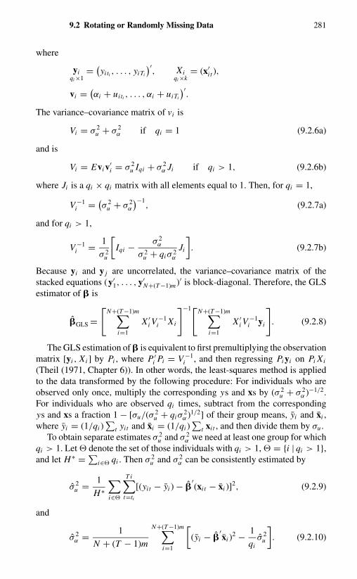
9.2 Rotating or Randomly Missing Data 281
where
yiqi ×1
= (yiti , . . . , yiTi
)′, Xi
qi ×k= (x′
i t ),
vi = (αi + uiti , . . . , αi + uiTi
)′.
The variance–covariance matrix of vi is
Vi = σ 2u + σ 2
α if qi = 1 (9.2.6a)
and is
Vi = Evi v′i = σ 2
u Iqi + σ 2α Ji if qi > 1, (9.2.6b)
where Ji is a qi × qi matrix with all elements equal to 1. Then, for qi = 1,
V −1i = (
σ 2u + σ 2
α
)−1, (9.2.7a)
and for qi > 1,
V −1i = 1
σ 2u
[Iqi − σ 2
α
σ 2u + qiσ 2
α
Ji
]. (9.2.7b)
Because yi and y j are uncorrelated, the variance–covariance matrix of thestacked equations (y′
1, . . . , y′N+(T −1)m)′ is block-diagonal. Therefore, the GLS
estimator of � is
�GLS =[
N+(T −1)m∑i=1
X ′i V
−1i Xi
]−1[N+(T −1)m∑i=1
X ′i V
−1i yi
]. (9.2.8)
The GLS estimation of � is equivalent to first premultiplying the observationmatrix [yi , Xi ] by Pi , where P ′
i Pi = V −1i , and then regressing Pi yi on Pi Xi
(Theil (1971, Chapter 6)). In other words, the least-squares method is appliedto the data transformed by the following procedure: For individuals who areobserved only once, multiply the corresponding ys and xs by (σ 2
u + σ 2α )−1/2.
For individuals who are observed qi times, subtract from the correspondingys and xs a fraction 1 − [σu/(σ 2
u + qiσ2α )1/2] of their group means, yi and xi ,
where yi = (1/qi )∑
t yi t and xi = (1/qi )∑
t xi t , and then divide them by σu .To obtain separate estimates σ 2
u and σ 2α we need at least one group for which
qi > 1. Let � denote the set of those individuals with qi > 1, � = {i | qi > 1},and let H∗ = ∑
i∈� qi . Then σ 2u and σ 2
α can be consistently estimated by
σ 2u = 1
H∗∑i∈�
T i∑t=ti
[(yit − yi ) − �′(xi t − xi )]
2, (9.2.9)
and
σ 2α = 1
N + (T − 1)m
N+(T −1)m∑i=1
[(yi − �
′xi )
2 − 1
qiσ 2
u
]. (9.2.10)

282 Incomplete Panel Data
Similarly, we can apply the MLE by maximizing the logarithm of the likelihoodfunction (9.2.1):
log L = − N T
2log 2π − 1
2
N+(T −1)m∑i=1
log |Vi |
− 1
2
N+(T −1)m∑i=1
(yi − Xi �)′V −1i (yi − Xi �)
= − N T
2log 2π − 1
2
[N+(T −1)m∑
i=1
(qi − 1)
]log σ 2
u
− 1
2
N+(T −1)m∑i=1
log(σ 2
u + qiσ2α
)− 1
2
N+(T −1)m∑i=1
(yi − Xi �)′V −1i (yi − Xi �). (9.2.11)
Conditioning on σ 2u and σ 2
α , the MLE is the GLS (9.2.8). Conditioning on �, theMLEs of σ 2
u and σ 2α are the simultaneous solutions of the following equations:
∂ log L
∂σ 2u
= − 1
2σ 2u
[N+(T −1)m∑
i=1
(qi − 1)
]
− 1
2
[N+(T −1)m∑
i=1
1
σ 2u + qiσ 2
α
]
+ 1
2σ 4u
N+(T −1)m∑i=1
(yi − Xi �)′ Qi (yi − Xi �)
+ 1
2
N+(T −1)m∑i=1
qi(σ 2
u + qiσ 2α
)2 (yi − x′i �) = 0, (9.2.12)
and
∂ log L
∂σ 2α
= −1
2
N+(T −1)m∑i=1
[qi
σ 2u + qiσ 2
α
− q2i(
σ 2u + qiσ 2
α
)2 (yi − x′i �)2
],
= 0, (9.2.13)
where Qi = Iqi − (1/qi )eqi e′qi , and eqi is a qi × 1 vector of ones. Unfortunately,
because qi are different for different i , (9.2.12) and (9.2.13) cannot be put in the

9.3 Pseudopanels (or Repeated Cross-Sectional Data) 283
simple form of (3.3.25) and (3.3.26). Numerical methods will have to be usedto obtain a solution. However, computation of the MLEs of �, σ 2
u , and σ 2α can
be simplified by switching iteratively between (9.2.8) and (9.2.12)–(9.2.13).This principle of modifying complete-panel-data estimation methods for
the incomplete-panel-data case can be extended straightforwardly to dynamicmodels and multiple-equation models. However, with dynamic models thereis a problem of initial conditions.12 Different assumptions about initial con-ditions will suggest different ways of incorporating new observations withthose already in the sample. It would appear a reasonable approximation inthis case is to modify the methods based on the assumption that initial ob-servations are correlated with individual effects and have stationary variances(Chapter 4, case IVc or IVc′). Alternatively, instrumental variable methods pro-posed for the analysis of dynamic models from repeated cross-section data (e.g.,Collado (1997); Moffit (1993)) can be implemented with proper modification.However, the assumption imposed on the model will have to be even morerestrictive.
When data are randomly missing, a common procedure is to focus on thesubset of individuals for which complete time-series observations are available.However, the subset of incompletely observed individuals also contains someinformation about unknown parameters. A more efficient and computationallysomewhat more complicated way is to treat randomly missing samples in thesame way as rotating samples. For instance, the likelihood function (9.2.1), withthe modification that ti = 1 for all i , can also be viewed as the likelihood functionfor this situation: In time period 1 there are N + ∑T −1
t=1 mt individuals; in period2, m1 of them randomly drop out, and so on, so that at the end of T periodsthere are only N individuals remaining in the sample. Thus, the procedure forobtaining the GLS or MLE for unknown parameters with all the observationsutilized is similar to the situation of rotating samples.
9.3 PSEUDOPANELS (OR REPEATEDCROSS-SECTIONAL DATA)
When repeated observations on the same individuals are not available, it is notpossible to control the effect of unobserved individual characteristics in a linearmodel of the form
yit = �′xi t + αi + uit (9.3.1)
if αi and xi t are correlated by the fixed-effects estimator discussed in Chapter 3.However, several authors have argued that with some additional assumptions� may be identified from a single cross section or a series of independentcross sections (e.g., Blundell, Browning, and Meghir (1994); Deaton (1985);Heckman and Robb (1985); Moffit (1993)).
Deaton (1985) suggests using a cohort approach to obtain consistent esti-mators of � of (9.3.1) if repeated cross-sections data are available. Cohorts

284 Incomplete Panel Data
are defined as groups of individuals sharing common observed characteristics,such as age, sex, education or socioeconomic background. Suppose that onecan divide the sample into C cohorts where all individuals within the cohorthave identical αc, c = 1, . . . , C . Then aggregation of all observations to cohortlevel results in
yct = x′ct � + αc + uct , c = 1, . . . , C,
(9.3.2)t = 1, . . . , T,
where yct and xct are the averages of all observed y′i ts and x′
i ts in cohort c attime period t . The resulting data set is a pseudopanel with repeated observationson C cohorts over T time periods. If xct are uncorrelated with uct , the withinestimator (3.2.8) can be applied to the pseudopanel
�w =(
C∑c=1
T∑t=1
(xct − xc)(xct − xc)′)−1( C∑
c=1
T∑t=1
(xct − xc)(yct − yc)
),
(9.3.3)
where xc = 1T
∑Tt=1 xct , and yc = 1
T
∑Tt=1 yct .
In the case that xi t contains the lagged dependent variables, then xct willintroduce the well-known measurement error problem because yit is supposedto depend on one’s own past value yi,t−1, not some averaged value. In the casethat the observed cohort means yct and xct are error-ridden, Deaton (1985)suggests estimating � by13
�D =(
1
CT
C∑c=1
T∑t=1
(xct − xc)(xct − xc)′ − �x
)−1
×(
1
CT
C∑c=1
T∑t=1
(xct − xc)(yct − y) − �
), (9.3.4)
where �x denotes the variance–covariance matrix of the measurement er-rors in xct , and � denotes the covariance of the measurement errors of yct
and xct .
Although the cohort approach offers a useful framework to make use ofindependent cross-sectional information, there are problems with some of itsfeatures. First, the assertion of intracohort homogeneity appears very strong,particularly in view of the fact that the cohort classification is often arbitrary.Second, grouping or aggregating individuals may result in the loss of infor-mation or the heteroscedasticity of the errors of the cohort equation (9.3.2).Third, the practice of establishing the large-sample properties of econometricestimators and test statistics by assuming that the number of cohorts, C , tendsto infinity is not satisfactory. There is often a physical limit beyond which one

9.4 Pooling of Cross-Sectional and Time-Series Data 285
cannot increase the number of cohorts. The off-cited example of date-of-birthcohorts is a case in point.
9.4 POOLING OF A SINGLE CROSS-SECTIONALAND A SINGLE TIME-SERIES DATA SET
9.4.1 Introduction
In this section we consider the problem of pooling when we have a single cross-sectional and a single time-series data set. Empirical studies based solely ontime-series data often result in very inaccurate parameter estimates because ofthe high collinearity among the explanatory variables. For instance, income andprice time series can be highly correlated. On the other hand, a cross-sectionaldata set may contain good information on household income, but not on price,because the same price is likely to be faced by all households. Thus, each dataset contains useful information on some of the variables, but not on all thevariables so as to allow accurate estimates of all the parameters of interest.A classic example of this is provided in a study (Stone (1954)) of aggregate-demand systems in which there was no cross-sectional variation in commodityprices and inadequate time-series variation in real incomes.
To overcome the problem of lack of information on interesting parame-ters from time-series or cross-sectional data alone, one frequently estimatessome parameters from cross-sectional data, then introduces these estimatesinto time-series regression to estimate other parameters of the model. For in-stance, Tobin (1950) calculated income elasticity from cross-sectional data,then multiplied it by the time-series income variable and subtracted the prod-uct from the annual time series of quantity demand to form a new dependentvariable. This new dependent-variable series was then regressed against thetime series of the price variable to obtain an estimate of the price elasticity ofdemand.
The purpose of pooling here, as in the cases analyzed earlier, is to get moreefficient estimates for the parameters that are of interest. In a time series, thenumber of observations is usually limited, and variables are highly correlated.Moreover, an aggregate data set or a single individual time-series data set doesnot contain information on microsociodemographic variables that affect eco-nomic behavior. Neither are cross-sectional data more structurally complete.Observations on individuals at one point in time are likely to be affected byprior observations. These raise two fundamental problems: One is that thesource of estimation bias in cross-sectional estimates may be different fromthat in time-series estimates. In fact, many people have questioned the suit-ability and comparability of estimates from different kinds of data (micro oraggregate, cross section or time series), e.g., Kuh (1959) and Kuh and Meyer(1957). The second is, if pooling is desirable, what is the optimal way to do it? Itturns out that both problems can be approached simultaneously in the framework
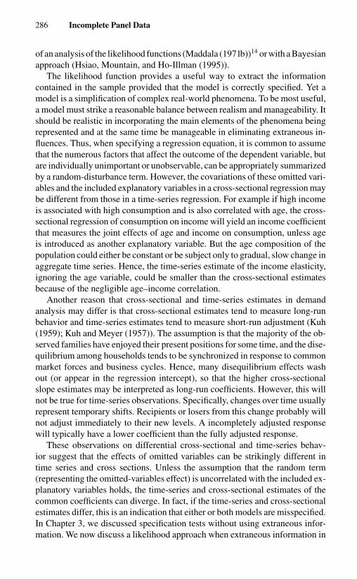
286 Incomplete Panel Data
of an analysis of the likelihood functions (Maddala (1971b))14 or with a Bayesianapproach (Hsiao, Mountain, and Ho-Illman (1995)).
The likelihood function provides a useful way to extract the informationcontained in the sample provided that the model is correctly specified. Yet amodel is a simplification of complex real-world phenomena. To be most useful,a model must strike a reasonable balance between realism and manageability. Itshould be realistic in incorporating the main elements of the phenomena beingrepresented and at the same time be manageable in eliminating extraneous in-fluences. Thus, when specifying a regression equation, it is common to assumethat the numerous factors that affect the outcome of the dependent variable, butare individually unimportant or unobservable, can be appropriately summarizedby a random-disturbance term. However, the covariations of these omitted vari-ables and the included explanatory variables in a cross-sectional regression maybe different from those in a time-series regression. For example if high incomeis associated with high consumption and is also correlated with age, the cross-sectional regression of consumption on income will yield an income coefficientthat measures the joint effects of age and income on consumption, unless ageis introduced as another explanatory variable. But the age composition of thepopulation could either be constant or be subject only to gradual, slow change inaggregate time series. Hence, the time-series estimate of the income elasticity,ignoring the age variable, could be smaller than the cross-sectional estimatesbecause of the negligible age–income correlation.
Another reason that cross-sectional and time-series estimates in demandanalysis may differ is that cross-sectional estimates tend to measure long-runbehavior and time-series estimates tend to measure short-run adjustment (Kuh(1959); Kuh and Meyer (1957)). The assumption is that the majority of the ob-served families have enjoyed their present positions for some time, and the dise-quilibrium among households tends to be synchronized in response to commonmarket forces and business cycles. Hence, many disequilibrium effects washout (or appear in the regression intercept), so that the higher cross-sectionalslope estimates may be interpreted as long-run coefficients. However, this willnot be true for time-series observations. Specifically, changes over time usuallyrepresent temporary shifts. Recipients or losers from this change probably willnot adjust immediately to their new levels. A incompletely adjusted responsewill typically have a lower coefficient than the fully adjusted response.
These observations on differential cross-sectional and time-series behav-ior suggest that the effects of omitted variables can be strikingly different intime series and cross sections. Unless the assumption that the random term(representing the omitted-variables effect) is uncorrelated with the included ex-planatory variables holds, the time-series and cross-sectional estimates of thecommon coefficients can diverge. In fact, if the time-series and cross-sectionalestimates differ, this is an indication that either or both models are misspecified.In Chapter 3, we discussed specification tests without using extraneous infor-mation. We now discuss a likelihood approach when extraneous information in

9.4 Pooling of Cross-Sectional and Time-Series Data 287
the form of cross-sectional data for the time-series model, or time-series datafor the cross-sectional model, is available.
9.4.2 The Likelihood Approach to Pooling Cross-Sectionaland Time-Series Data
Assume that we have a single cross-section consisting of N units and a timeseries extending over T time periods. Suppose that the cross-sectional model is
yc = Z1�1 + Z2�2 + uc, (9.4.1)
where yc is an N × 1 vector of observations on the dependent variable, Z1
and Z2 are N × K and N × L matrices of independent variables, and �1 and�2 are K × 1 and L × 1 vectors of parameters, respectively. The N × 1 errorterm uc is independently distributed, with variance–covariance matrix σ 2
u IN .The time-series model is
yT = X1�1 + X2�2 + vT , (9.4.2)
where yT is a T × 1 vector of observations on the dependent variable, X1 and X2
are T × K and T × M matrices of observations on the independent variables,�1 and �2 are K × 1 and M × 1 vectors of parameters, and vT is a T × 1 vectorof disturbances.15 For simplicity, we assume that vT is uncorrelated with uc andis serially uncorrelated, with variance–covariance matrix EvT v′
T = σ 2v IT .
The null hypothesis here is that �1 = �1. So with regard to the questionwhether or not to pool, we can use a likelihood-ratio test. Let L∗
1 and L∗2 de-
note the maxima of the log joint likelihood functions for (9.4.1) and (9.4.2)with and without the restriction that �1 = �1. Then, under the null hypothesis,2(L∗
2 − L∗1) is asymptotically chi-square-distributed, with K degrees of free-
dom. The only question is: What is the appropriate level of significance? If thecosts of mistakenly accepting the pooling hypothesis and rejecting the poolinghypothesis are the same, Maddala (1971b) suggested using something like a 25to 30 percent level of significance, rather than the conventional 5 percent, inour preliminary test of significance.
The specifications of the maximum likelihood estimates and their variance–covariances merely summarize the likelihood function in terms of the locationof its maximum and its curvature around the maximum. It is possible thatthe information that the likelihood function contains is not fully expressed bythese. When the compatibility of cross-sectional and time-series estimates isinvestigated, it is useful to plot the likelihood function extensively. For thispurpose, Maddala (1971b) suggested that one should also tabulate and plot therelative maximum likelihoods of each data set,
RM (δ1) =max
�L(�1, �)
max�1,�
L(�1, �), (9.4.3)

288 Incomplete Panel Data
where � represents the set of nuisance parameters, max� L(�1, �) denotes themaximum of L with respect to � given �1, and max�1,� L(�1, �) denotes themaximum of L with respect to both �1 and �. The plot of (9.4.3) summarizesalmost all the information contained in the data on �1. Hence, the shapes andlocations of the relative maximum likelihoods will reveal more informationabout the compatibility of the different bodies of data than a single test statisticcan.
If the hypothesis �1 = �1 is acceptable, then, as Chetty (1968), Durbin(1953), and Maddala (1971b) have suggested, we can stack (9.4.1) and (9.4.2)together as[
yc
yt
]=
[Z1
X1
]�1 +
[Z2
0
]�2 +
[0
X2
]�2 +
[uc
v T
]. (9.4.4)
It is clear that an efficient method of estimating of �1, �2, and �2 is to apply themaximum likelihood method to (9.4.4). An asymptotically equivalent procedureis to first apply least squares separately to (9.4.1) and (9.4.2) to obtain consistentestimates of σ 2
u and σ 2v , then substitute the estimated σ 2
u and σ 2v into the equation
1
σ uyc
1
σ vyT
=
1
σ uZ1
1
σ vX1
�1 + 1
σ uZ2
0
�2 +
0
1
σ vX2
�2 +
1
σ uuc
1
σ vvT
(9.4.5)
and apply the least-squares method to (9.4.5).The conventional procedure of substituting the cross-sectional estimates �1c
of �1 into the time-series model
yT − X1�1c = X2�2 + vT + X1(�1 − �1c), (9.4.6)
then regressing (yT − X1�1c) on X2, yields only conditional estimates of theparameters �2 – conditional on the estimates obtained from the cross-sectionaldata.16 However, there is also some information about �1 in the time-seriessample, and this should be utilized. Moreover, one should be careful in the use oftwo-step procedures. Proper evaluation of the asymptotic variance–covariancematrix of �2 should take account of the uncertainty (variance) in substituting�1c for �1. [For details, see Chetty (1968); Hsiao, Mountain, and Ho-Illman(1995); Jeong (1978); and Maddala (1971b).]
9.4.3 An Example
To illustrate application of the likelihood approach to pooling, Maddala (1971b)analyzed a simple econometric model relating to the demand for food in theUnited States. The model and the data were taken from Tobin (1950).
The cross-sectional demand equation is
y1i = δ0 + δ1z1i + δ2z2i + ui , i = 1, . . . , N , (9.4.7)
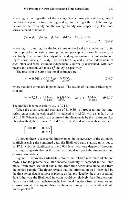
9.4 Pooling of Cross-Sectional and Time-Series Data 289
where y1i is the logarithm of the average food consumption of the group offamilies at a point in time, and z1i and z2i are the logarithms of the averageincome of the i th family and the average family size, respectively. The time-series demand function is
y2t = β0 + β1(x1t − β2x2t ) + β3(x2t − x2,t−1) + vt ,
t = 1, . . . , T, (9.4.8)
where y2t , x1t , and x2t are the logarithms of the food price index, per capitafood supply for domestic consumption, and per capita disposable income, re-spectively. The income elasticity of demand, δ1, was assumed common to bothregressions, namely, δ1 = β2. The error terms ui and vt were independent ofeach other and were assumed independently normally distributed, with zeromeans and constant variances σ 2
u and σ 2v , respectively.
The results of the cross-sectional estimates are
y1i = 0.569 + 0.5611z1i(0.0297)
+ 0.2540z2i(0.0367)
, (9.4.9)
where standard errors are in parentheses. The results of the time-series regres-sion are
y2t = 7.231 + 1.144x2t(0.0612)
− 0.1519(0.0906)
(x2t − x2,t−1) − 3.644x1t(0.4010)
. (9.4.10)
The implied income elasticity, δ1, is 0.314.When the cross-sectional estimate of δ1, 0.56, is introduced into the time-
series regression, the estimated β1 is reduced to −1.863, with a standard errorof 0.1358. When δ1 and β1 are estimated simultaneously by the maximum like-lihood method, the estimated δ1 and β1 are 0.5355 and −1.64, with a covariance[
0.00206 0.008270.04245
].
Although there is substantial improvement in the accuracy of the estimatedcoefficient using the combined data, the likelihood-ratio statistic turns out tobe 17.2, which is significant at the 0.001 level with one degree of freedom.It strongly suggests that in this case we should not pool the time-series andcross-sectional data.
Figure 9.1 reproduces Maddala’s plot of the relative maximum likelihoodRM (δ1) for the parameter δ1 (the income elasticity of demand) in the Tobinmodel from cross-sectional data alone, from time-series data alone, and fromthe pooled sample. The figure reveals that the information on δ1 provided bythe time-series data is almost as precise as that provided by the cross-sectionaldata (otherwise the likelihood function would be relatively flat). Furthermore,there is very little overlap between the likelihood functions from time-series andcross-sectional data. Again, this unambiguously suggests that the data shouldnot be pooled.17

290 Incomplete Panel Data
RM (δ1)Time series
RM (δ1)Pooled
data
RM (δ1) Cross-sectional data
1.0
0.8
0.6
0.4
0.2
0.25 0.30 0.35 0.40 0.45
δ1
0.50 0.55 0.60 0.65
Fig. 9.1 Relative likelihoods for the parameter δ1.Source: Maddala (1971b, Figure 1).
Given that the time-series data arise by aggregating some microeconomicprocess, there cannot possibly be a conflict between the time-series and cross-sectional inferences if individual differences conditional on explanatory vari-ables are viewed as chance outcomes. Thus, whenever the empirical resultsdiffer systematically between the two, as in the foregoing example, this is anindication that either or both models may be misspecified. The existence ofsupporting extraneous information in the form of cross-sectional or time-seriesdata provides an additional check on the appropriateness of a model specifica-tion that cannot be provided by a single cross-section or time-series data set,because there may be no internal evidence of this omitted-variable bias. How-ever, until a great deal is learned about the relation between cross-sectionaland time-series estimates, there appears to be no substitute for completeness ofinformation. Sequential observations on a number of individuals or panel dataare essential for a full understanding of the systematic interrelations at differentperiods of time.
CHAPTER 10
Miscellaneous Topics
In this chapter we briefly consider some miscellaneous topics. We shall firstconsider statistical inference using simulation methods (Section 10.1). We shallthen consider panels with both large N and large T (Section 10.2), leading to thediscussion of the specific issue of unit-root tests (Section 10.3). Section 10.4 willdiscuss panels with more than two dimensions. Section 10.5 considers issuesof measurement errors and indicates how one can take advantage of the panelstructure to identify and estimate an otherwise unidentified model. Finally, wediscuss proposals for relaxing the cross-section independence assumption apartfrom the specification of the individual-invariant time-varying factors.
10.1 SIMULATION METHODS
Panel data contain two dimensions – a cross-sectional dimension and a time di-mension. Models using panel data also often contain unobserved heterogeneityfactors. To transform a latent variable model involving missing data, randomcoefficients, heterogeneity, etc., into an observable model often requires theintegration of latent variables over multiple dimensions (e.g., Hsiao (1989,1991b, 1992c)). The resulting panel data model estimators can be quite dif-ficult to compute. Simulation methods have been suggested to get around thecomplex computational issues involving multiple integrations (e.g., Gourierouxand Monfort (1996); Hsiao and Wang (2000); Keane (1994); McFadden (1989);Pakes and Pollard (1989)).
The basic idea of the simulation approach is to rely on the law of large num-bers to obtain the approximation of the integrals through taking the averages ofrandom drawings from a known probability distribution function. For instance,consider the problem of computing the conditional density function f (yi | xi ; �)of yi given xi , or some conditional moments m(yi , xi ; �), say E(yi | xi ; �) orE(yi y′
i | xi ; �), where � is the vector of parameters characterizing these func-tions. In many cases, it is difficult to compute these functions because they donot have closed forms. However, if the conditional density or moments con-ditional on x and another vector �, namely f ∗(yi | xi , �; �) or m(y, x | �; �),have closed forms and the probability distribution P(�) of � is known, then

292 Miscellaneous Topics
from
f (yi | xi ; �) =∫
f ∗(yi | xi , �; �) dP(�), (10.1.1)
and
m(yi , xi ; �) =∫
m∗(yi , xi | �; �) dP(�), (10.1.2)
we may approximate (10.1.1) and (10.1.2) by
f H (yi | xi ; �) = 1
H
H∑h=1
f ∗(yi | xi , �ih ; �), (10.1.3)
and
mH (yi , xi ; �) = 1
H
H∑h=1
m∗(yi , xi | �ih ; �), (10.1.4)
where (�i1, . . . , �i H ) are H random draws from P(�).For example, consider the random-effects panel probit and Tobit models
defined by the latent response function
y∗i t = �′xi t + αi + uit , (10.1.5)
where αi and uit are assumed to be independently normally distributed withmean 0 and variance σ 2
α and 1, respectively, and are mutually independent. Theprobit model assumes that the observed yit takes the form
yit ={
1 if y∗i t > 0,
0 if y∗i t ≤ 0.
(10.1.6)
The Tobit model assumes that
yit ={
y∗i t if y∗
i t > 0,
0 if y∗i t ≤ 0.
(10.1.7)
We note that the density function of αi and uit can be expressed as transforma-tions of some standard distributions (here, standard normal), so that the densityfunction of y′
i = (yi1, . . . , yiT ) becomes an integral of a conditional functionover the range of these standard distributions:
f (yi | xi ; �) =∫
f ∗(yi | xi , η; �) dP(η) (10.1.8)
with p(η) ∼ N (0, 1). For instance, in the case of the probit model,
f ∗(yi | xi , η; �) =T∑
t=1
�(x′i t � + σαηi )
yit [1 − �(x′i t � + σαηi )]
1−yit ,
(10.1.9)

10.1 Simulation Methods 293
and in the case of the Tobit model,
f ∗(yi | xi , η; �) =∏t∈�1
φ(yit − x′i t � − σαηi )
×∏t∈�0
�(−x′i t � − σαηi ), (10.1.10)
where φ(·) and �(·) denote the standard normal density and integrated normal,respectively, and �1 = {t | yit > 0} and �0 = {t | yit = 0}. Because conditionalon xi t and each of the H random draws ηih, h = 1, . . . , H , of η from a standardnormal distribution, the conditional density function (10.1.9) or (10.1.10) iswell defined in terms of � and σ 2
α , the approximation of f (yi | xi ; �, σ 2α ) can
be obtained by taking their averages as in (10.1.3).More complicated forms of f (yi | xi ; �) can also be approximated by a rela-
tively simple simulator. For instance, if ui = (ui1, . . . , uiT )′ has a multivariatenormal distribution with mean 0 and covariance matrix �, we can let ui = ��∗
i ,where �∗
i is from a standard multivariate normal with mean 0 and covariancematrix IT , and � is a lower triangular matrix such that � = ��′. Thus, if uit
in the above example follows a first-order autoregressive process
uit = ρui,t−1 + εi t , |ρ| < 1, (10.1.11)
then we can rewrite (10.1.5) as
y∗i t = �′xi t + σαηi +
t∑τ=1
atτ η∗iτ , (10.1.12)
where η∗iτ , τ = 1, . . . , T are random draws from independent N (0, 1), and atτ
are the entries of the lower triangular matrix �. It turns out that here atτ =(1 − ρ2)−
12 ρ t−τ if t ≥ τ , and atτ = 0 if t < τ .
Using the approach described above, we can obtain an unbiased, differen-tiable and positive simulator of f (yi | xi ; �), � = (�′, σα, ρ)′, in the probit caseby considering the following drawings:
ηih is drawn from N (0,1);η∗
i1h is drawn from N (0, 1) restricted to
[−(�′xi1 + σαηih)/a11, ∞] if yi1 = 1
or
[−∞, −(�′xi1 + σαηih)/a11] if yi1 = 0;
η∗i2h is drawn from N (0, 1) restricted to
[−(�′xi2 + σαηih + a21η∗i1h)/a22, ∞] if yi2 = 1
and
[−∞, −(�′xi2 + σαηih + a21η∗i1h)/a22] if yi2 = 0;

294 Miscellaneous Topics
and so on. The simulator of f (yi | xi ; �) is
f H (yi | xi ; �) = 1
H
H∑h=1
T∏t=1
�
[(−1)1−yit
(�′xi t + σαηih +
t−1∑τ=1
atτ η∗iτh
)/att
],
(10.1.13)
where for t = 1, the sum over τ disappears.In the Tobit case, the same kind of method can be used. The only difference
is that the simulator of f (yi | xi ; �) becomes
f H (yi |xi ; �) = 1
H
H∑h=1
[∏t∈�1
1
attφ
([yit −
(�′xi t + σαηih +
t−1∑τ=1
atτ η∗iτh
)]/att
)
×∏t∈�0
�
[−(
�′xi t + σαηih +t−1∑τ=1
atτ η∗iτh
)/att
]]. (10.1.14)
The simulated maximum likelihood estimator (SMLE) is obtained frommaximizing the simulated log likelihood function. The simulated general-ized method-of-moments (SGMM) estimator is obtained from the simulated(4.3.37). The simulated least-squares (SLS) estimator is obtained if we letm(yi , xi ; �) = E(yi | xi ; �) and minimize
∑Ni=1[yi − E(yi | xi ; �)]2.
Although we need H → ∞ to obtain consistent simulators of f (yi | xi ; �)and m(yi , xi ; �), it is shown by McFadden (1989) that when a finite number Hof vectors (�i1, . . . , �i H ) are drawn by simple random sampling and indepen-dently for different i from the marginal density P(�), the simulation errors areindependent across observations; hence the variance introduced by simulationwill be controlled by the law of large numbers operating across observations,making it unnecessary to consistently estimate each theoretical m(yi , xi ; �) forthe consistency of the SGMM �SGMM as N → ∞.
The asymptotic covariance matrix of√
N (�SGMM − �) obtained by simulat-ing the moments in (4.3.37) that can be approximated by
(R′ AR)−1 R′ AG N H AR(R′ AR)−1, (10.1.15)
where
R = 1
N
N∑i=1
W ′i
∂mH (yi , xi ; �)
∂�′ ,
G N H = 1
N
N∑i=1
Wi
(� + 1
HH
)W ′
i , (10.1.16)
� = Cov(mi (yi , xi ; �)),
H = Cov[mH (yi , xi ; �) − m(yi , xi ; �)].
It is clear that as H → ∞, the SGMM has the same asymptotic efficiency asthe GMM. However, even with finite H , the relative efficiency of the SGMMis quite high. For instance, for the simple frequency simulator, H = �, one

10.2 Panels with Large N and T 295
draw per observation gives 50 percent of the asymptotic efficiency of the cor-responding GMM estimator, and nine draws per observation gives 90 percentrelative efficiency.
However, for the consistency of SMLE or SLS we shall need H → ∞ asN → ∞. With a finite H , the approximation error of the conditional densityor moments is of order H−1. This will lead to the asymptotic bias of O(1/H )(e.g., Gourieoux and Monfort (1996); Hsiao, Wang, and Wang (1997)). Never-theless, with a finite H it is still possible to propose an SLS estimator which isconsistent and asymptotically normally distributed as N → ∞ by noting thatfor the sequence of 2H random draws (�i1, . . . , �i H , �i,H+1, . . . , �i,2H ) foreach i , we have
E
[1
H
H∑h=1
m∗(yi , xi | �ih ; �)
]= E
[1
H
H∑h=1
m∗(yi , xi | �i,H+h ; �)
],
= m(yi , xi ; �), (10.1.17)
and
E
[yi − 1
H
H∑h=1
m∗(yi , xi | �ih ; �)
]′ [yi − 1
H
H∑h=1
m∗(yi , xi | �i,H+h ; �)
]= E [yi − m(yi , xi ; �)]′ [yi − m(yi , xi ; �)] , (10.1.18)
because of the independence between (�i1, . . . , �i H ) and (�i,H+1, . . . , �i,2H ).Then the SLS estimator that minimizes
N∑i=1
[yi − 1
H
H∑h=1
m∗(yi , xi | �ih ; �)
]′ [yi − 1
H
H∑h=1
m∗(yi , xi | �i,H+h ; �)
](10.1.19)
is consistent as N → ∞ even H is fixed (e.g., Gourieoux and Monfort (1996);Hsiao and Wang (2000)).
10.2 PANELS WITH LARGE N AND T
Most of this monograph has been concerned with panels with large N and smallT . However, some of the panel data sets, like the Penn–World tables, coverdifferent individuals, industries, and countries over long time periods. In somecases, the orders of magnitude of the cross section and time series are similar.These large-N , large-T panels call for the use of large-N and -T asymptoticsrather than just large-N asymptotics. Moreover, when T is large, there is a needto consider serial correlations more generally, including both short-memoryand persistent components. In some panel data sets like the Penn–World Table,the time-series components also have strongly evident nonstationarity. It turnsout that panel data in this case can sometimes offer additional insights into thedata-generating process than a single time series or a cross-section data set.

296 Miscellaneous Topics
In regressions with large-N, large-T panels most of the interesting test statis-tics and estimators inevitably depend on the treatment of the two indexes, Nand T, which tend to infinity together. Several approaches are possible. Theseare:
a. Sequential limits. A sequential approach is to fix one index, say N,and allow the other, say T, to pass to infinity, giving an intermediatelimit. Then, by letting N pass to infinity subsequently, a sequentiallimit theory is obtained.
b. Diagonal-path limits. This approach is to allow the two indexes, Nand T, to pass to infinity along a specific diagonal path in the two-dimensional array, say T = T (N ) as the index N → ∞.
c. Joint limits. A joint limit theory allows both indexes, N and T , topass to infinity simultaneously without placing specific diagonal pathrestrictions on the divergence, although it may still be necessary toexercise some control over the rate of expansion of the two indexes inorder to get definitive results.
In many applications, sequential limits are easy to derive and helpful inextracting quick asymptotics. However, sometimes sequential limits can givemisleading asymptotic results.1 A joint limit will give a more robust result thaneither a sequential limit or a diagonal-path limit, but will also be substantiallymore difficult to derive and will usually apply only under stronger conditions,such as the existence of higher moments, that will allow for uniformity in theconvergence arguments. Phillips and Moon (1999) have given a set of sufficientconditions that ensures that sequential limits are equivalent to joint limits.
In general, if an estimator is consistent in the fixed-T , large-N case, it willremain consistent if both N and T tend to infinity, irrespective of how theydo so. Moreover, even in the case that an estimator is inconsistent for fixed Tand large N , (say, the least-squares estimator for a dynamic random-coefficientmodel discussed in Chapter 6), it can become consistent if T also tends toinfinity. The probability limit of an estimator, in general, is identical no matterwhich limits one takes. However, the properly scaled limiting distribution maydepend on how the two indexes, N and T , tend to infinity (e.g., Levin and Lin(1993); Hahn and Kuersteiner (2000)).
For instance, consider the linear regression model
y = E(y | x) + v = βx + v . (10.2.1)
The least-squares estimator β of β gives the same interpretation irrespective ofwhether y and x are stationary or integrated of order 1 (i.e., the first differenceis stationary). In the case that y and x are bivariate normally distributed asN (0, �) with
� =(
�yy �yx
�xy �xx
), (10.2.2)

10.2 Panels with Large N and T 297
then plim β = �yx�−1xx . In a unit-root framework of the form(
yt
xt
)=
(yt−1
xt−1
)+
(uyt
uxt
), (10.2.3)
where the errors ut = (uyt , uxt )′ are stationary, then
plim β = �yx�−1xx , (10.2.4)
where �yx , �xx denote the long-run covariance between uyt and uxt and thelong-run variance of xt , defined by
� = limT →∞
E
[(1√T
T∑t=1
ut
)(1√T
T∑t=1
u′t
)]
=∞∑
�=−∞E(u0u′
�) =(
�yy �yx
�xy �xx
). (10.2.5)
When cross-sectional units have heterogeneous long-run covariance matri-ces �i for (yit , xit ), i = 1, . . . , N , with E�i = �, Phillips and Moon (1999)extend this concept of a long-run average relation among cross-sectional unitsfurther:
β = E(�yx,i )(E�xx,i )−1 = �yx�
−1xx . (10.2.6)
They show that the resulting least-squares estimator converges to (10.2.6) asN , T → ∞.
This generalized concept of average relation between cross-sectional unitscovers both the cointegrated case (Engle and Granger (1987)) in which β isa cointegrating coefficient in the sense that the particular linear combinationyt − βxt is stationary, and the correlated but noncointegrated case, which is notavailable for a single time-series. To see this point more clearly, suppose thatthe two nonstationary time-series variables have the following relation:
yt = ft + wt ,
xt = ft , (10.2.7)
with (wt
ft
)=
(wt−1
ft−1
)+
(uwt
u f t
), (10.2.8)
where uws is independent of u f t for all t and s and has nonzero long-runvariance. Then ft is a nonstationary common factor variable for y and x , anduw is a nonstationary idiosyncratic factor variable. Since wt is nonstationaryover time, it is apparent that there is no cointegrating relation between yt andxt . However, since the two nonstationary variables yt and xt share a commoncontributory nonstationary source in u f t , we may still expect to find evidence

298 Miscellaneous Topics
of long-run correlation between yt and xt , and this is what is measured by theregression coefficient β in (10.2.6).
Phillips and Moon (1999, 2000) show that for large-N and -T panels, theregression coefficient β converges to the long-run average relation so defined.However, if N is fixed, then as T → ∞, the least-squares estimator of β is anondegenerate random variable that is a functional of Brownian motion thatdoes not converge to β (Phillips and Durlauf (1986)). In other words, with asingle time series or a fixed number of time series, the regression coefficient β
will not converge to the long-run average relation defined by (10.2.6) if onlyT → ∞.
Therefore, if we define a spurious regression as one yielding nonzero β
for the two independent variables, then, contrary to the case of time-seriesregression of involving two linearly independent I (1) variables (Phillips andDurlauf (1986)), the issue of spurious regression will not arise for the panelestimates of N → ∞ (e.g., Kao (1999)).
10.3 UNIT-ROOT TESTS
Panels with large cross-sectional dimension and long time periods have alsobeen used by applied economists to examine the income-convergence hypoth-esis in growth theory (e.g. Bernard and Jones (1996)) and the purchasing-power parity hypothesis in exchange-rate determination (e.g., Frankel and Rose(1996)). While the time-series property of a variable is of significant interestto economists, the statistical properties of time-series estimators actually de-pend on whether the data are stationary or nonstationary.2 If the variables arestationary, the limiting distributions of most estimators will be approximatelynormal when T → ∞. Standard normal and chi-square tables can be used toconstruct confidence intervals or test hypotheses. If the data are nonstationary,or contain unit roots, standard estimators will have nonstandard distributionsas T → ∞. The conventional Wald test statistics cannot be approximated wellby t or chi-square distributions (e.g., Dickey and Fuller (1979, 1981); Phillipsand Durlauf (1986)). Computer simulations will have to be used to find the crit-ical values under the null. However, with panel data one can exploit informa-tion from cross-sectional dimensions to infer stationarity versus nonstationarityusing normal or t-distribution approximations by invoking central limit theo-rems across cross-sectional dimensions.
Since Quah (1994), many people have suggested panel unit-root test statisticswhen N and T are large (e.g., Binder, Hsiao, and Pesaran (2000); Choi (2002);Harris and Tzaralis (1999); Im, Pesaran, and Shin (1997); Levin and Lin (1993);Levin, Lin, and Chu (2002); Maddala and Wu (1999)). Here we shall onlydiscuss the tests of Levin and Lin (LL) (1993), Im, Pesaran, and Shin (IPS)(1997), and Maddala and Wu (MW) (1999).
Following Dickey and Fuller (1979, 1981), Levin and Lin (1993), and Levin,Lin and Chu (2002), consider a panel extension of the null hypothesis that each

10.3 Unit-Root Tests 299
individual time series in the panel contains a unit root against the alternativehypothesis that all individual series are stationary by considering the model
yit = αi + δi t + γi yi,t−1 +pi∑
�=1
φi�yi,t−� + εi t , i = 1, . . . , N ,
t = 1, . . . , T,
(10.3.1)
where εi t is assumed to be independently distributed across i and denotes thefirst-difference operator, 1 − L , with L being the lag operator that shifts the ob-servation by one period, Lyit = yi,t−1. If γi = 0, then yit contains a unit root. Ifγi < 0, then yit is stationary. Levin and Lin (1993) specify the null hypothesis as
H0 : γ1 = γ2 = · · · = γN = 0, (10.3.2)
and the alternative hypothesis as
H1 : γ1 = γ2 = · · · = γN = γ < 0. (10.3.3)
To test H0 against H1, Levin and Lin (1993) suggest first regressing yit andyi,t−1 on the remaining variables in (10.3.1) for each i , providing the residualsei t and vi,t−1, respectively. Then one estimates γ by running the regression ofthe following model:
ei t = γ vi,t−1 + εi t . (10.3.4)
To adjust for heteroscedasticity across i in (10.3.4), they suggest first using theleast-squares estimate γ of γ to compute the variance of ei t ,
σ 2ei = (T − pi − 1)−1
T∑t=pi +2
(ei t − γ vi,t−1)2, (10.3.5)
and then dividing (10.3.4) by σei for each i , to obtain the heteroscedasticity-adjusted model
ei t = γ vi,t−1 + εi t , (10.3.6)
where ei t = ei t/σei , vi,t−1 = vi,t−1/σei . The t statistic for testing γ = 0 is
tγ = γ
sdγ
, (10.3.7)
300 Miscellaneous Topics
where γ is the least-squares estimates of (10.3.6),
sdγ = σε
[N∑
i=1
T∑t=pi +2
v2i,t−1
]−1/2
σ 2ε = (N T )−1
N∑i=1
T∑t=pi +2
(ei t − γ vi,t−1)2,
p = 1
N
N∑i=1
pi , T = (T − p − 1).
Levin and Lin (1993) suggest adjusting (10.3.7) by
t∗ = tγ − N T SN T σ−2ε · sdγ · µT
σT, (10.3.8)
where
SN T = N−1N∑
i=1
ωyi
σei, (10.3.9)
and ω2yi is an estimate of the long-run variance of yi , say,
ω2yi = (T − 1)−1
T∑t=2
y2i t + 2
K∑j=1
WK ( j)
×(
(T − 1)−1T∑
t= j+2
yit yi,t− j
), (10.3.10)
where WK ( j) is the lag kernel to ensure the positivity of ω2yi ; for instance,
Newey and West (1987) suggest that
WK ( j) =1 − j
Tif j < K ,
0 if j ≥ K .
(10.3.11)
The µT and σT are mean and standard-deviation adjustment terms, which arecomputed by Monte Carlo simulation and tabulated in their paper. Levin andLin (1993) show that provided the augmented Dickey–Fuller (1981) lag order pincreases at some rate T p where 0 ≤ p ≤ 1/4, and the lag truncation parameterK increases at rate T q where 0 < q < 1, the panel test statistic tγ under thenull of γ = 0 converges to a standard normal distribution as T, N → ∞.
In the special case that αi = δi = φi� = 0, and εi t is i.i.d. with mean 0and variance σ 2
ε , Levin and Lin (1993) and Levin, Lin, and Chu (2002) showthat under the null of γ = 0, T
√N γ of the pooled least-squares estimator γ
converges to a normal distribution with mean 0 and variance 2, and the t statistic

10.3 Unit-Root Tests 301
of γ converges to a standard normal, as√
N/T → 0 while N , T → ∞ (i.e.,the time dimension can expand more slowly than the cross section).
Im, Pesaran, and Shin (1997) relax Levin and Lins’ strong assumptionof homogeneity for (10.3.1) under the alternative (i.e., allowing γi �= γ j ) bypostulating the alternative hypothesis as
H∗A : γi < 0 for at least one i. (10.3.12)
Thus, instead of pooling the data, Im, Pesaran, and Shin (1997) suggest takingthe average, τ , of separate unit-root tests for N individual cross-section units ofthe argument Dickey–Fuller (ADF) (Dickey and Fuller (1981)) t-ratios τi . Theyshow that τ converges to a normal distribution under the null with mean E(τ )and variance Var( ¯τN ) as T → ∞ and N → ∞. Since E(τi ) and Var(τi ) willvary as the lag length in the ADF regression varies, Im, Pesaran, and Shin (1997)tabulate E(τi ) and Var(τi ) for different lag lengths. They show in their MonteCarlos studies that their test is more powerful than Levin, Lin, and Chu’s (2001)test in certain cases.
Implicit in Im, Pesaran, and Shin’s (1997) test is the assumption that T is thesame for all cross-sectional units and that the same lag length is used for all theADF regressions for individual series. To relax these restrictions, Maddala andWu (1996) suggest using the Fisher (1932) Pλ test to combine the evidence fromseveral independent tests. The idea is as follows: Suppose there are N unit-roottests as in Im, Pesaran, and Shin (1997). Let Pi be the observed significance level(P value) for the i th test. Then (−2
∑Ni=1 log Pi ) has a chi-square distribution
with 2N degrees of freedom as Ti → ∞ (Rao (1952, p. 44)).The LL test is based on homogeneity of the autoregressive parameter (al-
though it allows heterogeneity in the error variances and the serial correlationstructure of the errors). Thus the test is based on pooled regressions. On theother hand, both the MW test and the IPS test are based on the heterogeneity ofthe autoregressive parameter under the alternative. The tests amount to a com-bination of different independent tests. The advantage of the MW test is thatit does not require a balanced panel, nor identical lag length in the individualADF regressions. In fact, it can be carried out for any unit-root test derived. Itis nonparametric. Whatever test statistic we use for testing for a unit root foreach individual unit, we can get the P-values, Pi . The disadvantage is that theP-values have to be derived by Monte Carlo simulation. On the other hand,the LL and the IPS tests are parametric. Although the use of the tγ and the τ
statistic involves the adjustment of the mean and variance, they are easy to usebecause ready tables are available from their papers. However, these tables arevalid only for the ADF test.
The panel unit-root tests have also been generalized to test for cointegration(Engle and Granger (1987)) by testing if the regression residual is stationaryor integrated of order 1 (e.g., Breitung and Mayer (1994); Kao and Chiang(2000); McCoskey and Kao (1998)). For a survey of panel unit-root tests andcointegration, see Banerjee (1999).

302 Miscellaneous Topics
10.4 DATA WITH MULTILEVEL STRUCTURES
We have illustrated panel data methodology by assuming the presence of indi-vidual and/or time effects only. However, panel data need not be restricted totwo dimensions. We can have a more complicated clustering or hierarchicalstructure. For example, Antweiler (2001), Baltagi, Song, and Jung (2001), andDavis (1999), following the methodology developed by Wansbeek and Kapteyn(1978, 1982), consider the multiway error-components model of the form
yi j�t = x′i j�t � + ui j�t , (10.4.1)
for i = 1, . . . , N , j = 1, . . . , Mi , � = 1, . . . , Li j , and t = 1, . . . , Ti j�. For ex-ample, the dependent variable yi j�t could denote the air pollution measured atstation � in city j of country i in time period t . This means that there are Ncountries, and each country i has Mi cities in which Li j observation stationsare located. At each station, air pollution is observed for Ti j� periods. Then xi j�t
denotes a vector of K explanatory variables, and the disturbance is assumed tohave a multiway error-components structure,
ui j�t = αi + λi j + νi j� + εi j�t , (10.4.2)
whereαi , λi j , νi j�, and εi j�t are assumed to be i.i.d. and are mutually independentwith mean zero and variances σ 2
α , σ 2λ , σ 2
ν , and σ 2ε , respectively.
In the case that the data are balanced, the variance–covariance matrix of uhas the form
� = σ 2α (IN ⊗ JM LT ) + σ 2
λ (IN M ⊗ JLT )
+ σ 2ν (IN M L ⊗ JT ) + σ 2
ε IL M N T , (10.4.3)
where Js is a square matrix of dimension s with all elements equal to 1. Rewriting(10.4.3) in the form representing the spectral decomposition � (e.g., as inAppendix 3B), we have
� = M LT σ 2α (IN ⊗ PM LT ) + LT σ 2
λ (IN M ⊗ PLT )
+ T σ 2ν (IN M L ⊗ PT ) + σ 2
ε IL M N T
= σ 2ε (IN M L ⊗ QT ) + σ 2
1 (IN M ⊗ QL ⊗ PT )
+ σ 22 (IN ⊗ QM ⊗ PLT ) + σ 2
3 (IN ⊗ PM LT ), (10.4.4)
where Ps ≡ 1s Js, Qs = Is − Ps , and
σ 21 = T σ 2
ν + σ 2ε , (10.4.5)
σ 22 = LT σ 2
λ + T σ 2ν + σ 2
ε , (10.4.6)
σ 23 = M LT σ 2
α + LT σ 2λ + T σ 2
ν + σ 2ε , (10.4.7)
σ 2ε being the characteristic roots of �. As each of the terms of (10.4.4) is

10.4 Data with Multilevel Structures 303
orthogonal to the others and they sum to IN M LT , it follows that
�−1/2 = σ−1ε (IN M L ⊗ QT ) + σ−1
1 (IN M ⊗ QL ⊗ PT )
+ σ−12 (IN ⊗ QM ⊗ PLT ) + σ−1
3 (IN ⊗ PM LT ). (10.4.8)
Expanding all the Q-matrices as the difference of I s and Ps, multiplying bothsides of the equation by σε , and collecting terms yield
σε�−1/2 = IN M LT −
(1 − σε
σ1
)(IN M L ⊗ PT )
−(
σε
σ1− σε
σ2
)(IN M ⊗ PLT )
−(
σε
σ2− σε
σ3
)(IN ⊗ PM LT ). (10.4.9)
The generalized least-squares (GLS) estimator of (10.4.1) is equivalent to theleast-squares estimator of
y∗i j�t = yi j�t −
(1 − σε
σ1
)yi j�. −
(σε
σ1− σε
σ2
)yi j .. −
(σε
σ2− σε
σ3
)yi...,
(10.4.10)
on
x∗i j�t = xi j�t −
(1 − σε
σ1
)xi j�. −
(σε
σ1− σε
σ2
)xi j .. −
(σε
σ2− σε
σ3
)xi...,
(10.4.11)
where yi j�.(xi j�.), yi j..(xi j..), and yi...(xi...) indicate group averages. The applica-tion of feasible GLS can be carried out by replacing the variances in (10.4.10)and (10.4.11) by their estimates obtained from the three groupwise betweenestimates and the within estimate of the innermost group.
The pattern exhibited in (10.4.10) and (10.4.11) is suggestive of solutions fora higher-order hierarchy with a balanced structure. If the hierarchical structureis unbalanced, the Kronecker-product operation can no longer be applied. Thisintroduces quite a bit of notational inconvenience into the algebra (e.g., Baltagi(1995, Chapter 9); Wansbeek and Kapteyn (1982)). Neither can the GLS es-timator be molded into a simple transformation to a least-squares estimator.However, an unbalanced panel is made up of N top-level groups, each contain-ing Mi second-level groups, the second-level groups containing the innermostLi j subgroups, which in turn contain Ti j� observations. The numbers of obser-vations in the higher-level groups are thus Ti j = ∑Li j
�=1 Ti j� and Ti = ∑Mij=1 Ti j ,
and the total number of observations is H = ∑Ni=1 Ti . The number of top-
level groups is N , the number of second-level groups is F = ∑Ni=1 Mi , and the

304 Miscellaneous Topics
number of bottom-level groups is G = ∑Ni=1
∑Mij=1 Li j . We can redefine the
J -matrices to be block-diagonal of size H × H , corresponding in structure tothe groups or subgroups they represent. They can be constructed explicitly byusing group membership matrices consisting of ones and zeros that uniquelyassign each of the H observations to one of the G (or F or N ) groups. Antweiler(2001) has derived the maximum likelihood estimator for panels with unbal-anced hierarchy.
When data constitute a multilevel hierarchical structure, the application ofa simple error-component estimation, although inefficient, remains consistentunder the assumption that the error component is independent of the regressors.However, the estimated standard errors of the slope coefficients are usuallybiased downward.
10.5 ERRORS OF MEASUREMENT
Thus far we have assumed that variables are observed without errors. Eco-nomic quantities, however, are frequently measured with errors, particularly iflongitudinal information is collected through one-time retrospective surveys,which are notoriously susceptible to recall errors. If variables are indeed sub-ject to measurement errors, exploiting panel data to control for the effects ofunobserved individual characteristics using standard differenced estimators (de-viations from means, etc.) may result in even more biased estimates than simpleleast-squares estimators using cross-sectional data alone.
Consider, for example, the following single-equation model (Solon (1985)):
yit = α∗i + βxit + uit , i = 1, . . . , N ,
(10.5.1)t = 1, . . . , T,
where uit is independently identically distributed, with mean zero and varianceσ 2
u , and Cov(xit , uis) = Cov(α∗i , uit ) = 0 for any t and s, but Cov(xit , α
∗i ) �= 0.
Suppose further that we observe not xit itself, but rather the error-ridden measure
x∗i t = xit + τi t , (10.5.2)
where Cov(xis, τi t ) = Cov(α∗i , τi t ) = Cov(uit , τis) = 0, and Var(τi t ) = σ 2
τ ,Cov(τi t , τi,t−1) = γτσ
2τ .
If we estimate (10.5.1) by OLS with cross-sectional data for period t , theestimator converges (as N → ∞) to
plimN→∞
βLS = β + Cov(xit , α∗i )
σ 2x + σ 2
τ
− βσ 2τ
σ 2x + σ 2
τ
, (10.5.3)
where σ 2x = Var(xit ). The inconsistency of the least-squares estimator involves
two terms: the first due to the failure to control for the individual effects α∗i ,
and the second due to measurement error.

10.5 Errors of Measurement 305
If we have panel data, say T = 2, we can alternatively first-difference thedata to eliminate the individual effects α∗
i ,
yit − yi,t−1 = β(x∗i t − x∗
i,t−1) + [(uit − βτi t ) − (ui,t−1 − βτi,t−1)],(10.5.4)
and then apply least squares. The probability limit of the differenced estimatoras N → ∞ becomes
plimN→∞
βd = β
[1 − 2(1 − γτ )σ 2
τ
Var(x∗i t − x∗
i,t−1)
]
= β − βσ 2τ
[(1 − γx )/(1 − γτ )]σ 2x + σ 2
τ
, (10.5.5)
where γx is the first-order serial-correlation coefficient of xit . The estimator βd
eliminates the first source of inconsistency, but may aggravate the second. Ifγx > γτ , the inconsistency due to measurement error is larger for βd than forβLS. This occurs because if the serial correlation of the measurement error is lessthan that of the true x (as seems often likely to be the case), first-differencingincreases the noise-to-signal ratio for the measured explanatory variable.
The standard treatment for the errors-in-variables models requires extrane-ous information in the form of either additional data (replication and/or in-strumental variables) or additional assumptions to identify the parameters ofinterest (e.g., Aigner et al. (1984)). With panel data, we can use a different trans-formation of the data to induce different and deducible changes in the biasesin the estimated parameters that can then be used to identify the importanceof measurement errors and recover the “true” parameters (Ashenfelter, Deaton,and Solon (1984); Griliches and Hausman (1986)). For instance, if the mea-surement error τi t is i.i.d. across i and t , and x is serially correlated,3 then inthe foregoing example we can use x∗
i,t−2 or (x∗i,t−2 − x∗
i,t−3) as instruments for(x∗
i t − x∗i,t−1) as long as T > 3. Thus, even though T may be finite, the resulting
IV estimator is consistent when N tends to infinity.Alternatively, we can obtain consistent estimates through a comparison of
magnitudes of the bias arrived at by subjecting a model to different transfor-mations (Griliches and Hausman (1986)). For instance, if we use a covariancetransformation to eliminate the contributions of unobserved individual compo-nents, we have
(yit − yi ) = β(x∗i t − x∗
i ) + [(uit − ui ) − β(τi t − τi )], (10.5.6)
where yi , x∗i , ui , and τi are individual time means of respective variables. The
LS regression of (10.5.6) converges to
plimN→∞
βw = β
[1 − T − 1
T
σ 2τ
Var(x∗i t − x∗
i )
]. (10.5.7)
306 Miscellaneous Topics
Then consistent estimators of β and σ 2τ can be found from (10.5.5) and (10.5.7),
β =[
2βw
Var(x∗i t − x∗
i,t−1)− (T − 1)βd
T Var(x∗i t − x∗
i )
]
×[
2
Var(x∗i t − x∗
i,t−1)− T − 1
T Var(x∗i t − x∗
i )
]−1
, (10.5.8)
σ 2τ = β − βd
β· Var(x∗
i t − x∗i,t−1)
2. (10.5.9)
In general, if the measurement errors are known to possess certain structures,consistent estimators may be available from a method-of-moments and/or froman IV approach by utilizing the panel structure of the data. Moreover, the first-difference and the within estimators are not the only ones that will give us animplicit estimate of the bias. In fact, there are T/2 such independent estimates.For a six-period cross section with τi t independently identically distributed, wecan compute estimates of β and σ 2
τ from y6 − y1, y5 − y2, and y4 − y3 usingthe relationships
plimN→∞
β61 = β − 2βσ 2τ /Var(x∗
i6 − x∗i1),
plimN→∞
β52 = β − 2βσ 2τ /Var(x∗
i5 − x∗i2), (10.5.10)
plimN→∞
β43 = β − 2βσ 2τ /Var(x∗
i4 − x∗i3).
Thus, there are alternative consistent estimators. This fact can be exploitedto test the assumptions with regard to measurement errors, which provide therationale for the validity of the instruments, by investigating whether or not thealternative estimates of β are mutually coherent (e.g., Griliches and Hausman(1986)). The moment conditions (10.5.5), (10.5.7), and (10.5.10) can also becombined to obtain efficient estimates of β and σ 2
τ by the use of Chamberlain’sπ method (Section 3.9) or a generalized method-of-moments estimator.
For instance, transforming y and x by the transformation matrix Ps such thatPseT = 0 eliminates the individual effects from the model (10.5.1). Regressingthe transformed y on transformed x yields an estimator that is a function ofβ, σ 2
x , στ , and the serial correlations of x and τ . Wansbeek and Koning (1989)have provided a general formula for the estimators that are based on varioustransformation of the data. Letting
Y ∗ = eN T µ + X∗� + v∗, (10.5.11)
where Y ∗ = (y∗′1 , . . . , y∗′
T )′, y∗t = (y1t , . . . , yNt )′, X∗ = (x∗′
1 , . . . , x∗′T )′, x∗
t =(x1t , . . . , xNt )′, v∗ = (v∗′
1 , . . . , v∗′T )′, v∗
t = (v1t , . . . , vNt )′ and vit = (α∗i − µ) +
uit . Then
bs = [X∗′(Qs ⊗ IN )X∗]−1[X∗′(Qs ⊗ IN )Y ∗]
= � + [X∗′(Qs ⊗ IN )X∗]−1[X∗′(Qs ⊗ IN )(u∗ − ∗�)],(10.5.12)
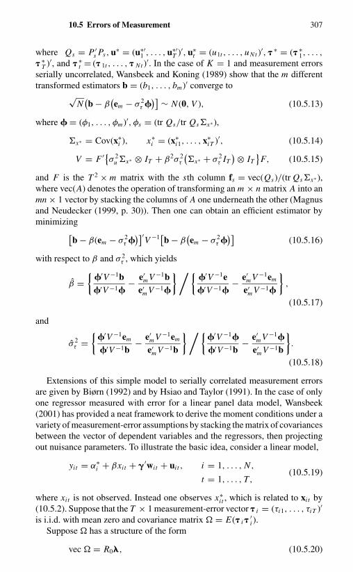
10.5 Errors of Measurement 307
where Qs = P ′s Ps, u∗ = (u∗′
1 , . . . , u∗′T )′, u∗
t = (u1t , . . . , uNt )′, ∗ = ( ∗1, . . . ,
∗T )′, and ∗
t = ( 1t , . . . , Nt )′. In the case of K = 1 and measurement errorsserially uncorrelated, Wansbeek and Koning (1989) show that the m differenttransformed estimators b = (b1, . . . , bm)′ converge to
√N(b − β
(em − σ 2
τ �)] ∼ N (0, V ), (10.5.13)
where � = (φ1, . . . , φm)′, φs = (tr Qs/tr Qs�x∗ ),
�x∗ = Cov(x∗i ), x∗
i = (x∗i1, . . . , x∗
iT )′, (10.5.14)
V = F ′{σ 2u �x∗ ⊗ IT + β2σ 2
τ
(�x∗ + σ 2
τ IT) ⊗ IT
}F, (10.5.15)
and F is the T 2 × m matrix with the sth column fs = vec(Qs)/(tr Qs�x∗ ),where vec(A) denotes the operation of transforming an m × n matrix A into anmn × 1 vector by stacking the columns of A one underneath the other (Magnusand Neudecker (1999, p. 30)). Then one can obtain an efficient estimator byminimizing[
b − β(em − σ 2τ �
)]′V −1
[b − β
(em − σ 2
τ �)]
(10.5.16)
with respect to β and σ 2τ , which yields
β ={
�′V −1b�′V −1�
− e′m V −1b
e′m V −1�
}/{�′V −1e�′V −1�
− e′m V −1em
e′m V −1�
},
(10.5.17)
and
σ 2τ =
{�′V −1em
�′V −1b− e′
m V −1em
e′m V −1b
}/{�′V −1�
�′V −1b− e′
m V −1�
e′m V −1b
}.
(10.5.18)
Extensions of this simple model to serially correlated measurement errorsare given by Biørn (1992) and by Hsiao and Taylor (1991). In the case of onlyone regressor measured with error for a linear panel data model, Wansbeek(2001) has provided a neat framework to derive the moment conditions under avariety of measurement-error assumptions by stacking the matrix of covariancesbetween the vector of dependent variables and the regressors, then projectingout nuisance parameters. To illustrate the basic idea, consider a linear model,
yit = α∗i + βxit + �′wi t + ui t , i = 1, . . . , N ,
(10.5.19)t = 1, . . . , T,
where xit is not observed. Instead one observes x∗i t , which is related to xi t by
(10.5.2). Suppose that the T × 1 measurement-error vector i = (τi1, . . . , τiT )′
is i.i.d. with mean zero and covariance matrix � = E( i ′i ).
Suppose � has a structure of the form
vec � = R0�, (10.5.20)

308 Miscellaneous Topics
where vec denotes the operation that stacks the rows of a matrix one afteranother in column-vector form, R is a matrix of order T 2 × m with knownelements, and � is an m × 1 vector of unknown constants. Using the covariancetransformation matrix Q = IT − 1
T eT e′T to eliminate the individual effects α∗
iyields
Qyi = Qxiβ + QWi � + Qui , (10.5.21)
Qx∗i = Qxi + Q i , (10.5.22)
where xi = (xi1, . . . , xiT )′, Wi = (w′i t ). Let
R ≡ (IT ⊗ Q)R0. (10.5.23)
From (10.5.2), we have
E( i ⊗ Q i ) = (IT ⊗ Q)E( i ⊗ i )
= (IT ⊗ Q)R0�
= R�. (10.5.24)
It follows that
E(x∗i ⊗ Qxi ) = E(x∗
i ⊗ Qx∗i ) − E[(xi + i ) ⊗ Q i ]
= E(x∗i ⊗ Qx∗
i ) − R�. (10.5.25)
Therefore,
E(x∗i ⊗ Qyi ) = E(x∗
i ⊗ Qx∗i )β + E(x∗
i ⊗ QWi )� − R�β.
(10.5.26)
Equation (10.5.26) contains the nuisance parameter �. To eliminate it, mul-tiplying by MR = IT 2 − R(R′ R)−1 R′ on both sides of (10.5.26), we have theorthogonality conditions
MR E{x∗i ⊗ Q(yi − x∗
i β − Wi �)} = 0. (10.5.27)
Combining (10.5.27) with the moment conditions E(W ′i Qui ) = 0, we have the
moment conditions for the measurement error model (10.5.19):
E M(di − Ci �) = 0, (10.5.28)
where
M =[
Mr 00 IK
], di =
[x∗
i ⊗ IT
W ′i
],
Ci =[
x∗i ⊗ IT
W ′i
]Q(x∗
i , Wi ), �′ = (β, �′).
A GMM estimator is obtained by minimizing
1
N
[N∑
i=1
M(di − Ci �)
]′AN
[N∑
i=1
M(di − Ci �)
]. (10.5.29)

10.6 Modeling Cross-Sectional Dependence 309
An optimal GMM estimator is to let
A−1N = 1
N
N∑i=1
(di − Ci �)(di − Ci �)′, (10.5.30)
where � is some consistent estimator of � such as
� =[(
N∑i=1
C ′i
)M
(N∑
i=1
Ci
)]−1 [(N∑
i=1
Ci
)′M
(N∑
i=1
di
)].
(10.5.31)
In the case when τi t is i.i.d. across i and over t , � is diagonal with equal di-agonal elements. Then m = 1 and R0= vec IT , R = (IT ⊗ Q) vec IT = vec Q,R′ R = tr Q = T − 1, and MR = IT 2 − 1
T −1 (vec Q) (vec Q)′. When � is diag-onal with distinct diagonal elements, m = T and R0 = it i′t ⊗ it , where it is thet th unit vector of order T . When τi t is a first-order moving average process andT = 4,
� =
a c 0 0c b c 00 c b c0 0 c a
;
then
R0 =1 0 0 0 0 0 0 0 0 0 0 0 0 0 0 1
0 0 0 0 0 1 0 0 0 0 1 0 0 0 0 00 1 0 0 1 0 1 0 0 1 0 1 0 0 1 0
,
and � = (a, b, c)′.Further variations on the covariance structure of the regressor x or the dis-
turbance term uit in a linear framework can also be put in this framework. Fordetail, see Wansbeek (2001).
The measurement errors for nonlinear models are much more difficult tohandle (e.g., Hsiao (1992c)). For dynamic models with measurement errors, seeWansbeek and Kapteyn (1982). For binary-choice models with measurementerrors, see Kao and Schnell (1987a, 1987b) and Hsiao (1991b).
10.6 MODELING CROSS-SECTIONALDEPENDENCE
Most panel studies assume that apart from the possible presence of individual-invariant but period-varying time-specific effects, the effects of omitted vari-ables are independently distributed across cross-sectional units. However, ofteneconomic theory predicts that agents take actions that lead to interdependenceamong themselves. For example, the prediction that risk-averse agents will makeinsurance contracts allowing them to smooth idiosyncratic shocks implies de-pendence in consumption across individuals. Kelejian and Prucha (2001) and

310 Miscellaneous Topics
Pinkse (2000) have suggested tests of cross-sectional dependence based onthe spatial correlation analogue of the Durbin–Watson and Box–Pierce testsfor time-series correlations; but unfortunately, contrary to the time-series datain which the time label gives a natural ordering and structure, general formsof dependence for cross-sectional dimension are difficult to formulate. There-fore, econometricians have relied on strong parametric assumptions to modelcross-sectional dependence.
Often, cross-sectional dependence is modeled in terms of some distancemeasure between cross-section units, and a spatial analogue of an autoregres-sive moving-average model is used (e.g., Anselin and Griffith (1988); Case(1991)). For example, Conley (1999) suggests using the notion of economicdistance to model proximity between two economic agents. The joint distri-bution of random variables at a set of points is assumed to be a function ofthe “economic distances” between them. In particular, the population of indi-viduals may be assumed to reside in a low-dimensional Euclidean space, sayR2, with each individual i located at a point si . The sample then consists ofrealizations of agents’ random variables at a collection of locations {si } insidea sample region. If two agents’ locations si and s j are close, then yit and y js
may be highly correlated. As the distance between si and s j grows large, yit
and y js approach independence. The joint distribution of random variables at aset of points is assumed to be invariant to a shift in location and is a function ofthe economic distances between them. Under this assumption, the dependenceamong cross-sectional data can be estimated using methods analogous to time-series procedures either parametrically or nonparametrically (e.g., Hall, Fisher,and Hoffman (1992); Priestley (1982); Newey and West (1987)).
While the approach of defining cross-sectional dependence in terms of eco-nomic distance allows for more complicated dependences than models withtime-specific (or group-specific) effects, it also requires that the econometri-cians have information regarding this distance. In certain urban, environmental,development, growth, and other areas of economics, this information may beavailable. For instance, in the investigation of people’s willingness to pay forlocal public goods, the relevant economic distance may be the time and mon-etary cost of traveling between points to use these goods. Alternatively if theamenity is air quality, then local weather conditions might constitute the majorunobservable. Other examples include studies of risk sharing in rural develop-ing economies where the primary shocks to individuals may be weather-related.If so, measures of weather correlation on farms of two individuals could be theproxy for the economic distance between them.

CHAPTER 11
A Summary View
11.1 INTRODUCTION
The preceding chapters have presented a wide variety of analytical tools devel-oped by econometricians for estimating behavioral equations using panel data.In choosing the proper method for exploiting the richness and unique propertiesof panel data it is helpful to keep several factors in mind. First, what advantagesdo panel data offer us in investigating economic issues over data sets consistingof a single cross section or time series? Second, what are the limitations of paneldata and the econometric methods that have been proposed for analyzing suchdata? Third, when using panel data, how can we increase the efficiency of pa-rameter estimates? Fourth, the usefulness of panel data in providing particularanswers to certain issues depends on the compatibility between the assumptionsunderlying the statistical inference procedures and the data-generating process.
11.2 BENEFITS AND LIMITATIONSOF PANEL DATA
The use of panel data provides major benefits for econometric estimation in atleast four areas: (1) increasing degrees of freedom and reducing problems of datamulticollinearity, (2) identifying economic models and discriminating betweencompeting economic hypotheses, (3) eliminating or reducing estimation bias,and (4) providing micro foundations for aggregate data analysis. However, thespecial features of panel data can often create new and difficult econometricproblems, particularly in nonlinear models.
11.2.1 Increasing Degrees of Freedom and Lessening the Problemof Multicollinearity
The shortage of degrees of freedom and severe multicollinearity in time-seriesdata often frustrate economists who wish to determine the individual influenceof each explanatory variable. This problem arises because the information pro-vided by the sample is not rich enough to meet the information requirements

312 A Summary View
of the model as specified. Given this situation, one must either augment thesample information or reduce the information requirements of the model (as byimposing prior restrictions on the parameters). Panel data, because they offermany more degrees of freedom and information on individual attributes, canreduce the gap between the information requirements of a model and the in-formation provided by the data (Section 1.1 or Fujiki, Hsiao, and Shen (2002);Hsiao, Mountain, and Ho-Illman (1995)).
11.2.2 Identification and Discrimination betweenCompeting Hypotheses
In economics, as in other branches of the social and behavioral sciences, oftenthere are competing theories. Examples of these include the effect of collectivebargaining on wages, the appropriate short-term policy to alleviate unemploy-ment (Chapters 1, 7 and 8), the effects of schooling on earnings (Chapter 5), andthe question of causal ordering. Economists on opposite sides of these issuesgenerally have very different views on the operation of the economy and theinfluence of institutions on economic performance. Some economists believeunions indeed raise wages or that advertising truly generates greater sales. Ad-herents of the opposite view tend to regard the effects more as epiphenomenathan as substantive forces and believe that observed differences are mainly dueto sorting of workers or firms by characteristics (e.g., Allison (2000)).
Aggregate time-series data are not particularly useful for discriminating be-tween hypotheses that depend on microeconomic attributes. Nor will a singleindividual time-series data set provide information on the effects of differentsociodemographic factors. Cross-sectional data, while containing variations inmicroeconomic and demographic variables, cannot be used to model dynamicsor causal ordering. The estimated coefficients from a single cross section aremore likely to reflect interindividual or interfirm differences than intraindividualor intrafirm dynamics, unless data on variables controlling for these differencesare available and are explicitly included in the chosen specification. For ex-ample, if information on worker quality is not available, a cross-sectionallyestimated coefficient for union status in a wage equation may reflect either theeffect of trade unions or differences in worker quality. Similarly, the findingthat there exists a negative relationship between measures of self-esteem anddelinquent behavior in a cross-sectional data set (Jang and Thornberry (1998))cannot answer the question: Does delinquency lead to low self-esteem, or doeslow self-esteem lead to delinquency?
Panel data, by providing sequential observations for a number of individuals,often allow us to distinguish interindividual differences from intraindividualdifferences and to construct a proper recursive structure for studying the issuein question through a before-and-after effect (e.g., Hsiao (1979a, 1979b, 1982)).For instance, in the foregoing example, even if information on worker quality isnot available, if a worker’s ability stays constant or changes only slowly, thewithin correlation between the union-status dummy and the worker-quality

11.2 Benefits and Limitations of Panel Data 313
variable is likely to be negligible. Thus, worker quality can be controlled throughthe use of within estimates. The resulting coefficient for the union-status dummythen will provide a measure of the effect of unionism (Chapters 3 and 4).
Moreover, proper recognition of the additional sources of variation can alsoprovide very useful information for discriminating individual behavior fromaverage behavior or for identifying an otherwise unidentified model. For ex-ample, in the income–schooling model, the availability of family groupingscan provide an additional set of cross-sibling covariances via a set of commonomitted variables. These additional restrictions can be combined with the con-ventional slope restrictions to identify what would otherwise be unidentifiedstructure parameters (Section 5.4).
Furthermore, addition of the cross-sectional dimension to the time-seriesdimension provides a distinct possibility of identifying the pattern of serial cor-relations in the residuals and of identifying the lag adjustment patterns when theconditioning variables are changed, without having to impose prior parametricspecifications (Sections 3.9 and 9.1) or identifying a model subject to measure-ment errors (Section 10.5).
11.2.3 Reducing Estimation Bias
A fundamental statistical problem facing every econometrician is the specifi-cation problem. By that we mean the selection of variables to be included ina behavioral relationship as well as the manner in which these variables arerelated to the variables that affect the outcome but appear in the equation onlythrough the error term. If the effects of the omitted variables are correlated withthe included explanatory variables, and if these correlations are not explicitlyallowed for, the resulting estimates will be biased. In order to minimize thebias, it is helpful to distinguish four types of correlations between the includedvariables and the error term. The first type is due to the correlation betweenthe included exogenous variables and those variables that should be includedin the equation but are not, either because of a specification error or becauseof unavailability of data. The second type is due to the dynamic structure ofthe model and the persistence of the shocks that give rise to the correlationbetween lagged dependent variables and the error term. The third type is due tothe simultaneity of the model, which gives rise to the correlation between thejointly dependent variables and the error terms. The fourth type is due to mea-surement errors in the explanatory variables. Knowing the different sources ofcorrelations provides important information for devising consistent estimators.It also helps one avoid the possibility of eliminating one source of bias whileaggravating another (e.g., Section 5.1).
11.2.3.a Omitted-Variable Bias
Empirical results are often criticized on the grounds that the researcher has notexplicitly recognized the effects of omitted variables that are correlated with

314 A Summary View
the included explanatory variables (in the union example, the omitted variable,worker quality, can be correlated with the included variable, union status). If theeffects of these omitted variables stay constant for a given individual throughtime or are the same for all individuals in a given time period, the omitted-variable bias can be eliminated by one of the following three methods whenpanel data are available: (1) differencing the sample observations to eliminatethe individual-specific and/or time-specific effects; (2) using dummy variablesto capture the effects of individual-invariant and/or time-invariant variables; or(3) postulating a conditional distribution of unobserved effects, given observedexogenous variables.
For linear-regression models, any of these three methods can be used toeliminate the bias created by the omitted invariant variables (Chapter 3). Fur-thermore, both the dummy-variable (fixed-effects) approach and the random-effects approach of specifying a conditional distribution of the effects, giventhe observed exogenous variables, lead to the same covariance estimator of theslope coefficient if the component of the error term that varies across individu-als and over time is i.i.d. (Section 3.4). Under other assumptions, although thecovariance estimator for the slope coefficient may not be efficient, it remainsunbiased and consistent. As a result, the fixed-effects approach has assumedparamount importance in empirical studies.
Unfortunately, the results for the linear model are really very special and gen-erally are not applicable for nonlinear models. In nonlinear models, the fixed-effect and the random-effects approaches yield different estimators. Moreover,contrary to the linear case, in general, the Neyman–Scott principle of separatingthe estimation of the common coefficients from the estimation of the specificeffects is not applicable. If the number of unknown specific effects increases atthe same rate as the sample size, attempts to estimate the specific effects willcreate the incidental-parameter problem. Hence, the fixed-effects approach maynot yield consistent estimates of the common coefficients (Chapters 7 and 8).For general nonlinear model with fixed effects there does not appear to exista generally applicable analytical framework to obtain consistent estimators ofthe parameters that are common across individuals and over time (structural pa-rameters). To devise consistent estimators of the structural parameters one hasto exploit the specific structure of a nonlinear model. The three most commonlyused approaches are: (i) the conditional approach, which conditions on the mini-mum sufficient statistics of the effects, (ii) the semiparametric approach, whichexploits the latent linear structure of a model, and (iii) reparameterization of themodel so that the information matrix of the reparametrized individual effects areuncorrelated with the reparameterized structural parameters (Lancaster (2001)).But none of these approaches is generally applicable for general nonlinear mod-els. Whether they will yield consistent estimators has to be considered case bycase.
On the other hand, the random-effects approach replaces the probabilitydistribution of the dependent variables conditional on the specific effects andthe exogenous variables by a probability distribution function that is conditional

11.2 Benefits and Limitations of Panel Data 315
on the explanatory variables only. Because the probability function of the effectsin general depends only on a finite number of parameters, there is no longeran incidental-parameter problem. However, between the linear and nonlinearmodels there is a very important difference. In linear models, we do not haveto make specific assumptions. We need only to decompose the specific effectsinto two components: their projections on observed exogenous variables andorthogonal residuals (Section 3.9). In nonlinear models, we often have to assumethat the conditional mean of the specific effects on observed exogenous variablesis actually linear and that the distribution of the effects, given explanatoryvariables, can be specified parametrically (e.g., Chapters 7 and 8). These arerestrictive assumptions, and there would be a payoff to relaxing them.
11.2.3.b Bias Induced by the Dynamic Structure of a Model
It is useful to distinguish between two sources of bias: One is ignoring thetime-persistent errors that are correlated with the lagged dependent variables;the other is the incorrect modeling of initial observations (Chapter 4 andSection 7.5). The issue of correlation between the residuals and lagged de-pendent variables is not affected by the size of the time-series observations, T ,whereas the initial-value problem arises only when there is no specific informa-tion to model the initial observation and T is small. When T is large, the weightof the initial observation in the likelihood function becomes negligible, and it isappropriate to ignore this issue. When T is small and the model and the data aresuch that it is appropriate to treat the initial observation as random, the correctprocedure for eliminating the bias induced by the correlation between the initialobservation and the residual depends on the pattern of serial dependence of theerror term.
If the model is linear and the time-persistent error is the sum of two compo-nents, one being individually time-invariant and the other being independentlydistributed, then the individual time-invariant effects can be eliminated by dif-ferencing successive observations of an individual. We can then use laggeddependent variables (of sufficiently high order) as instruments for the trans-formed model to circumvent the issues of both the initial observation and theserial dependence of the residual (Sections 4.3 and 4.5).
If the error terms have arbitrary patterns of serial correlations, as long as theassumption of independence across individual attributes holds, we can stackall T period observations for a given individual’s behavioral equation as Tequations in a given model and condition the initial observation on all theobserved exogenous variables. Consistent estimates of the coefficients and theserial covariance matrix can then be obtained by using simultaneous-equationsestimation methods in the same way that one would if there were only cross-sectional data for a simultaneous-equations model (Sections 4.3 and 4.6).
For the nonlinear case, specific distributional assumptions about the initialvalue and the error process must be made (Sections 7.5 and 8.3). Often, giventhe nature of the model, estimation of the coefficients of a model and estimation
316 A Summary View
of the parameters characterizing the error process cannot be separated. To obtainconsistent estimates, the error process must be correctly specified or specified ina general form that encompasses the underlying process, and computationallycomplicated maximum likelihood estimators may have to be used. However,identification of the error process is a nontrivial job. A sequence of likelihood-ratio tests to narrow down the possible specifications cannot be performedwithout first obtaining maximum likelihood estimates of unknown parametersunder various assumptions about the error process (e.g., Section 7.5).
11.2.3.c Simultaneity Bias
The standard approach to eliminate simultaneity bias is to use instrumentalvariables to purge the correlations between the joint dependent variables andthe error terms. If the cross-equation correlations in the errors are unrestricted,then, just as in the case of conventional cross-sectional or time-series data, weuse exogenous variables that are excluded from the equation as instruments forthe jointly dependent variables that appear in the equation. If the cross-equationcorrelations are due to common omitted invariant variables, then, in addition tothe excluded exogenous variables, we can also use included variables purgedof these invariant effects as instruments (Sections 5.3 and 5.4).
11.2.3.d Bias Induced by Measurement Errors
Measurement errors in the explanatory variables create correlations betweenthe regressors and the errors of the equation. If variables are subject to mea-surement errors, the common practice of differencing out individual effectseliminates one source of bias but creates another source, which may result ineven more biased estimates than simple least-squares estimators. However, dif-ferent transformation of the data can induce different and deducible changes inthe parameters, which can be used to determine the importance of measurementerrors and obtain consistent estimators of parameters of interest (Section 10.5).
11.2.4 Providing Micro Foundations for Aggregate Data Analysis
Aggregate data analysis often invokes the “representative agent” assumption.However, if micro units are heterogeneous, not only the time series propertiesof aggregate data can be very different from those of disaggregate data (e.g.,Granger (1980); Lewbel (1992, 1994); Pesaran (1999)), policy evaluation basedon aggregate data can be grossly misleading. Furthermore, the prediction ofaggregate outcomes using aggregate data can be less accurate than the predictionbased on micro-equations (e.g., Hsiao, Shen, and Fujiki (2002)). The variablecoefficient models discussed in Chapter 6 is an attempt to make inference aboutthe population taking account of the heterogeneity among micro units.

11.3 Efficiency of the Estimates 317
11.3 EFFICIENCY OF THE ESTIMATES
Because panel data usually contain a large number of observations, it mightappear that the problem of efficiency is not as important a consideration as isconsistency, but that is not necessarily the case. Assuming that the model iscorrectly specified, our example in Section 6.2 demonstrates that although theleast-squares estimates ignoring the random-coefficient assumptions should beconsistent, in practice they yield implausible results, as opposed to the efficientGLS estimates, which take account of the random nature of the cross-sectionalunits.
Intimately related to the problem of efficient use of the data is the issueof fixed-effects or random-effects inference. If the unobserved heterogeneitycan be viewed as random draws from a common population, then it is moreappropriate to postulate a random-effects model. If the unobserved heterogene-ity is correlated with explanatory variables or comes from a heterogeneouspopulation, then it is more appropriate to postulate a fixed-effects model. Thefixed-effects formulation makes inference conditional on the specific effects;hence it has the advantage of not requiring one to postulate the distribution ofthe effects or (in particular, if it is complicated) the correlation pattern betweenthe effects and included explanatory variables. However, there is also a loss ofefficiency in conditional inference because of the loss of degrees of freedom inestimating the specific effects (Section 3.4; Chapters 7 and 8). Furthermore, asdiscussed earlier, if the model is not linear and the specific effects vary with thedimension in which the number of observations is increased, the fixed-effectsinferences can create incidental-parameter problems that are likely to bias theestimates of the parameters that are common across individuals and throughtime (Chapters 4 and 7).
The random-effects inference, on the other hand, requires a distributionalassumption with regard to the effects. If the model is nonlinear, the assump-tion needs to be very specific, and often the complicated maximum-likelihoodmethod has to be used to obtain consistent estimates (Chapter 7). If the modelis linear and (conditional on the explanatory variables) individual observationscan be viewed as random draws from a common population, then the assumptioncan be in the general form of independently distributed effects, with commonmean and finite variance–covariance matrix. The generalized-least-squares es-timator is fairly simple to implement, provided we know the correlation patternof the remaining residuals, and is asymptotically efficient. In the case in whichT is fixed and the number of cross-sectional units, N , tends to infinity and theindividual characteristics are independently distributed across cross-sectionalunits, we can also use the general approach of stacking an individual’s behav-ioral equation over time periods as T equations in a given model and applyinga minimum-distance procedure over cross-sectional observations to estimatecommon parameters. This procedure allows arbitrary serial correlation and cer-tain forms of heteroscedasticity and yields consistent and efficient estimateswhen the error structure is unknown. Moreover, because the T-equation (serial)

318 A Summary View
variance–covariance matrix can be consistently estimated without imposing aspecific serial-dependence pattern, it also allows us to test the specific assump-tions on the distribution of the error term (e.g., error-components formulation)(Chapters 3–6).
Although a panel contains both cross-sectional and time-series dimensions,most often it contains only a few observations in one dimension (usually thetime dimension) and a great many observations in another dimension (usuallythe cross-sectional dimension). In order to obtain consistent estimates of theunknown parameters, we need the sample to increase in the dimension thatyields information on the relevant parameters (Chapters 4, 7, 8; Sections9.2–9.4). Thus, it is important to distinguish whether the panel tends to infinityin N or in T or in both N and T . On the basis of this information, one can thendetermine which parameters can, and which parameters cannot, be consistentlyestimated from a given panel data. The majority of this monograph focuseson the panels with large N and small T . Recently; panels with large N and Thave gained more attentions (Sections 10.2 and 10.3). However, assumptionssuch as the individual specific effects stay constant over time may no longerappear as reasonable approximations to the reality when T becomes large. Morerealistic assumptions consistent with the data generating process will have tobe postulated.
Finally, it should be noted that although panel data offer many advantages,they are not panacea. The power of panel data analysis depends critically onthe compatibility of the assumptions of statistical tools with the data generatingprocess. Otherwise, misleading inference will follow.

Notes
Chapter 1
1 For examples of marketing data, see Beckwith (1972); for biomedical data, seeSheiner, Rosenberg, and Melmon (1972); for a financial-market data base, seeDielman, Nantell, and Wright (1980).
2 Potential users interested in the ECHP can access and download the detailed doc-umentation of the ECHP users’ database (ECHP UDP) from the ECHP website:http://forum.europa.eu.int/irc/dsis/echpane/info/data/information.html.
3 This assumes that there are no other variables, such as consumption, that can actas a proxy for zi . Most North American data sets do not contain information onconsumption.
4 For a formal treatment of this, see Chapter 8.5 Many issues discussed in Chapters 7 and 8 apply to general nonlinear models as
well.
Chapter 2
1 This chapter is largely based on the work of Kuh (1963).2 Note that even if the homogeneity hypothesis is rejected, some useful information
can be found in pooling the data, as long as the source of sample variability can beidentified. For details, see later chapters.
3 We assume that T > K + 1. For details of this, see Section 3.2.4 See Johnston (1972, Chapter 6) for an illustration of the computation of analysis of
covariance.5 If the firm differences stay constant over time, heterogeneity among firms can be ab-
sorbed into the intercept term. Because intercepts are eliminated by first-differencing,the first-difference model (such as (2.3.1) or (2.3.3)) will be more likely to displayhomogeneous responses.
6 For further discussion of this issue, see Section 9.4 and Mairesse (1990).7 For further discussion of investment expenditure behavior, see Chapter 6 or Hsiao
and Tahmiscioglu (1997).

320 Notes to pp. 27–47
Chapter 3
1 These three different sorts of variations apply, of course, to both included and ex-cluded variables. Throughout this monograph we shall mostly concentrate on rela-tions between excluded individual time-invariant variables and included variables.
2 Although the notations are different, (3.2.5) is identical with (2.2.10).3 Equation (3.2.7) can be viewed as a linear-regression model with singular-
disturbance covariance matrix σ 2u Q. A generalization of Aitken’s theorem leads
to the generalized least-squares estimator
�CV =[
N∑i=1
X ′i Q ′ Q− Q Xi
]−1 [N∑
i=1
X ′i Q ′ Q− Qyi
]
=[
N∑i=1
X ′i Q Xi
]−1 [N∑
i=1
X ′t Qyi
],
where Q− is the generalized inverse of Q satisfying the conditions Q Q− Q = Q(Theil (1971, Sections 6.6, 6.7)).
4 Because the slope coefficients are assumed the same for all i and t , for simplicity weshall not distinguish the individual mean corrected estimator and the within-groupestimator as we did in Chapter 2. We shall simply refer to (3.2.8) or its equivalentas the within-group estimator.
5 Note that we follow the formulation of (3.2.10) in treating αi and λt as deviationsfrom the population mean. For ease of exposition we also restrict our attention tothe homoscedastic variances of αi and λt . For the heteroscedasticity generalizationof the error-component model, see Section 3.7 or Mazodier and Trognon (1978) andWansbeek and Kapteyn (1982). For a test of individual heteroscedasticity, see Hollyand Gardiol (2000).
6 For details, see Section 3.3.2.7 Equation (3.3.16) may yield a negative estimate of σ 2
α . For additional discussion onthis issue, see Section 3.3.3.
8 The negative variance-components problem also arises in the two-step GLS method.As one can see from (3.3.15) and (3.3.16), there is no guarantee that (3.3.16) nec-essarily yields a positive estimate of σ 2
α . A practical guide in this situation is toreplace a negative estimated variance component by its boundary value, zero. SeeBaltagi (1981b) and Maddala and Mount (1973) for Monte Carlo studies of thedesirable results of using this procedure in terms of the mean squared error of the es-timate. For additional discussion of the MLE of random-effects model, see Breusch(1987).
9 We note that the fixed-effects estimator, although not efficient, is consistent underthe random-effects formulation (Section 3.3.1).
10 In this respect, if N becomes large, one would not be interested in the specific effectof each individual but rather in the characteristics of the population. A random-effectsframework would be more appropriate.
11 If (Y (1)′, Y (2)′)′ is normally distributed with mean (�(1)′, �(2)′)′ and variance–covariance matrix[
�11 �12
�21 �22
],
Notes to pp. 47–65 321
the conditional distribution of Y (1) given Y (2) = y(2) is normal, with mean �(1) +�12�
−122 (y(2) − �(2)) and covariance matrix�11 − �12�
−122 �21 (e.g., Anderson (1958,
Section 2.5)).12 When ψ∗ is unknown, we replace it with an estimated value and treat (3.5.1) as
having an approximate F distribution.13 For proof, see Hausman (1978) or Rao (1973, p. 317).14 Strictly speaking, Hausman’s test is a test of
∑t x′
i t at = 0 versus∑
t x′i t at �= 0. It is
obvious that at = 0 implies that∑
t x′i t at = 0, but not necessarily the reverse. For a
discussion of the general relationship between Hausman’s specification testing andconventional testing procedures, see Holly (1982).
15 We use ⊗ to denote the Kronecker product of two matrices (Theil (1971, Chapter 7)).Suppose that A = (ai j ) is an m × n matrix and B is a p × q matrix; A ⊗ B is definedas an mp × nq matrix
a11 B a12 B . . . a1n B...
......
am1 B am2 B . . . amn B
.
16 This is because Q sweeps out αi from (3.6.1).17 See Li and Hsiao (1998) for a test of whether the serial correlation in the error is
caused by an individual-specific, time-invariant component or by the inertia in theshock, and Hong and Kao (2000) for testing for serial correlation of unknown form.
18 If E(α∗i | xi ) is linear, E∗(yi | xi ) = E(yi | xi ).
19 Of course, we can obtain the least-squares estimate of � by imposing the restrictionthat all T equations have identical intercepts µ. But this only complicates the alge-braic equation of the least-squares estimate without a corresponding gain in insight.
20 For details, see White (1980) or Chamberlain (1982).21 For proof, see Appendix 3A, Chamberlain (1982), Chiang (1956), or Malinvaud
(1970).22 If E(α∗
i | xi ) �= E∗(α∗i | xi ), then there will be heteroscedasticity, because the residual
will contain E(α∗i | xi ) − E∗(α∗
i | xi ).23 For fitting model (3.9.20) to panel data, see Chapter 5.24 This follows from examining the partitioned inverse of (3.9.25).25 If �∗ is another estimator of � with asymptotic variance–covariance matrix �∗, then
the minimum-distance estimator of � obtained by choosing �∗
to minimize [�∗ −f(�)]′�∗−1[�∗ − f(�)] has asymptotic variance–covariance matrix (F ′�∗−1 F)−1.Suppose � − �∗ is positive semidefinite; then F ′�∗−1 F − F ′�−1 F = F ′(�∗−1 −�−1)F is positive semidefinite. Thus, the efficiency of the minimum-distance esti-mator depends crucially on the efficiency of the (unconstrained) estimator of �.
26 For a comprehensive discussion of the Chamberlain π approach and the generalizedmethod of moments (GMM) method, see Crepon and Mairesse (1996).
27 In fact, a stronger result can be established for the proposition that � converges to� almost surely. In this monograph we do not attempt to distinguish the concept ofconvergence in probability and convergence almost surely (Rao (1973, Section 2.c)),because the stronger result requires a lot more rigor in assumptions and derivationswithout much gain in intuition.

322 Notes to pp. 69–82
Chapter 4
1 We defer the discussion of estimating distributed-lag models to Chapter 9.2 The assumption that |γ | < 1 is made to establish the (weak) stationarity of an au-
toregressive process (Anderson (1971, Chapters 5, 7)). A stochastic process {ξt } isstationary if its probability structure does not change with time. A stochastic processis weakly stationary if its mean Eξt = m is a constant, independent of its time, andif the covariance of any two variables, E(ξt − Eξt )(ξs − Eξs) = σξ (t − s), dependsonly on their distance apart in time. The statistical properties of a least-squares es-timator for the dynamic model depend on whether or not |γ | < 1 when T → ∞(Anderson (1959)). When T is fixed and N → ∞, it is not necessary to assume that|γ | < 1 to establish the asymptotic normality of the least-squares estimator (Anderson(1978), Goodrich and Caines (1979)). We keep this conventional assumption forsimplicity of exposition and also because it allows us to provide a unified approachtoward various assumptions about the initial conditions discussed in Section 4.3.
3 This does not mean that we have resolved the issue of whether or not the effects arecorrelated with the exogenous variables. It only means that for estimation purposeswe can let αi stand for ωi and treat (4.3.1) as a special case of (4.3.2).
4 For details, see Section 4.3.2 or Sevestre and Trognon (1982).5 The presence of the term �′xi t shows that the process {yit } is not generally stationary.
But the statistical properties of the process {yit } vary fundamentally when T → ∞according to whether or not {yit } converges to a stationary process when the sequenceof xi t is identically zero. As stated in footnote 2, we shall always adopt the firstposition by letting |γ | < 1.
6 V is the same as (3.3.4).7 Bhargava and Sargan (1983) get around the issue of incidental parameters associated
with the initial value yi0 by projecting yi0 on xi under the assumption that αi and xi areuncorrelated. Chamberlain (1984) and Mundlak (1978a) assume that the effects αi
are correlated with xi and get around the issue of incidental parameters by projectingαi on xi . In either case if N is not much larger than K T , the resulting estimator willhave better finite sample properties if yi0 or αi is projected on xi rather than xi .
8 Strictly speaking, from (4.3.21), the nonstationary analogue of case IVd would implythat
Var(vi0) = σ 2ω0 + σ 2
α
(1 − γ )2,
and
Cov(vi0, vit ) = σ 2α
1 − γ, t = 1, . . . , T .
However, given the existence of the prediction-error term εi0, it is not possible todistinguish this case from case IVc′ based on the information of yi0 alone. So weshall follow Bhargava and Sargan (1983) in treating case IVd′ as the nonstationaryanalogue of case IVd.
9 Previously we combined the intercept term and the time-varying exogenous variablesinto the vector xi t because the property of the MLE for the constant is the same asthat of the MLE for the coefficients of time-varying exogenous variables. Now wehave incorporated the constant term as an element in the time-invariant variable zi
to avoid having the constant term appearing more than once in (4.3.21).

Notes to pp. 83–117 323
10 For the formula of the constrained estimator, see Theil (1971, p. 285, equation (8.5)).11 See Chapter 5.12 See Section 3.5 for another approach.13 Note that we let zi = 0 for ease of exposition. When zi is present, the first-differencing
step of (4.3.38) eliminates zi from the specification; hence the moment conditions(4.3.39) remain valid. However, for Evi = 0 to hold requires the assumption ofstationarity in the mean (Blundell and Bond (1998)).
14 For ease of notation, we again assume that zi = 0.15 Bhargava and Sargan (1983) did not report the significance level of their tests. Pre-
sumably they used the conventional 5 percent significance level.16 We do not know the value of the GLS estimates when the initial observations are
treated as endogenous. My conjecture is that it is likely to be close to the two-stepGLS estimates with fixed initial observations. As mentioned in Section 4.3, Sevestreand Trognon (1982) have shown that even the initial values are correlated with theeffects; the asymptotic bias of the two-step GLS estimator under the assumptionof fixed initial observations is still smaller than the OLS or the within estimator.Moreover, if Bhargava and Sargan’s simulation result is any indication, the order ofbias due to the wrong assumption about initial observations when T is greater than 10is about one standard error or less. Here, the standard error of the lagged dependentvariable for the two-step GLS estimates with fixed initial values is only 0.037.
17 For additional discussions on the contribution of initial observations, see Blundelland Bond (1998) and Hahn (1999).
18 We say that yt is stationary if Eyt = �, E[(yt − �)(yt−s − �)′] = E[(yt+q −�)(yt+q−s − �)′]. We say that yt is integrated of order d, I (d), if (1 − L)d yt isstationary, I (0). If yt ∼ I (d) but �′yt ∼ I (d − c), say d = 1, c = 1, then yt is coin-tegrated of order c. The maximum number of linearly independent vectors � is calledthe rank of cointegration. For any m × 1 I (d) process, the cointegration rank canvary between 0 and m − 1 (e.g., Engle and Granger (1987), Intriligator, Bodkin, andHsiao (1996)).
19 Vec(ABC) = (C ′ ⊗ A) vec(B); see Magnus and Neudecker (1999).
Chapter 5
1 Namely, the family effect Ai has the same meaning as αi in Chapters 3–4.2 The asymptotic property of a fixed-effects linear simultaneous-equations model is
the same as the single-equation fixed-effects linear static model (see Chapter 3). TheMLE of � i is consistent only when T tends to infinity. The MLE of � t is consistentonly when N tends to infinity. However, just as in the linear static model, the MLEsof Γ and B do not depend on the MLEs of � i and � t . They are consistent wheneither N or T or both tend to infinity (Schmidt (1984)).
3 Note that the meaning of these asterisks has been changed from what it was inprevious chapters.
4 By allowing X to be different, the discussion of estimation of reduced-form equationscan proceed in the more general format of seemingly unrelated regression models(Avery (1977); Baltagi (1980)).
5 One can check that (5.2.7) is indeed the inverse of (5.2.6) by repeatedly using the for-mulas for the Kronecker products: (B + C) ⊗ A = B ⊗ A + C ⊗ A, (A ⊗ B)(C ⊗D) = AC ⊗ B D, provided the products exist (Theil (1971, Section 7.2)).

324 Notes to pp. 117–144
6 If only the first M out of G equations have nonzero intercepts, we estimate the firstM intercepts by {[IM , (V M M
4 )−1V M(G−M)4 ] ⊗ (1/N T )e′
N T }(y − X�) and estimate �by [X ′V ∗−1 X ]−1[X ′V ∗−1y], where IM is the M-rowed identity matrix, V M M
4 andV M(G−M)
4 are the corresponding M × M and M × (G − M) partitioned matrices of
V −14 =
[V M M
4 V M(G−M)4
V (G−M)M4 V (G−M)(G−M)
4
],
and
V ∗−1 = V −1
+[
0 0
0 V (G−M)(G−M)4 − V (G−M)M
4
(V M M
4
)−1V M(G−M)
4
]⊗ 1
N TJ.
For details, see Prucha (1983).7 See Chapter 3, footnote 22.8 As indicated earlier, we have assumed here that all variables are measured as de-
viations from their respective overall means. There is no loss of generality in thisformulation, because the interceptµg is estimated by µg = (1/N T )e′
N T (yg − Wg�g).Because C ′
heN T = 0 for h = 1, 2, 3, the only terms pertinent to our discussion areCh for h = 1, 2, 3.
9 Again, we ignore C4 = eN T /√
N T because we have assumed that there is an inter-cept for each equation and because C ′
heN T = 0 for h = 1, 2, 3.10 For the derivations of (5.4.36) and (5.4.37), see Appendix 5A.11 From V · V −1 = IGT we have −�cc′ − T aa′cc′ + aa′�−1 = 0. Premultiplying this
equation by c′, we obtain (b1 + T b22)c′ = b2a′�−1, where b1 = c′�c and b2 = c′a.
In Appendix 5A we give the values of b1 and b2 explicitly in terms of the eigenvalueof |aa′ − λ�| = 0.
12 We make use of the formula ∂ log |�|/∂�−1 = −�′ and ∂(c′�c)/∂�−1 = −�cc′�(Theil (1971, pp. 32–33)).
13 See Appendix 5A, equation (5A.7), in which ψ1 is positive.14 Finding the largest root of (5.4.43) is equivalent to maximizing (5.4.49). If we nor-
malize c′ Rc = 1, then to find the maximum of (5.4.49) we can use Lagrangianmultipliers and maximize c′ Rc + λ(1 − c′ Rc). Taking partial derivatives with re-spect to c gives (R − λR)c = 0. Premultiplying by c′, we have c′ Rc = λ. Thus, themaximum of (5.4.49) is the largest root of |R − λR| = 0, and c is the characteristicvector corresponding to the largest root.
Chapter 6
1 See Mehta, Narasimhan, and Swamy (1978) for another example to show that us-ing error-components formulation to allow for heterogeneity does not always yieldeconomically meaningful results.
2 Alternatively, we can postulate a separate regression for each time period, so yit =�′
t xi t + uit .3 See Chamberlain (1992) for an extension of the Mundlak–Chamberlain approach
of conditioning the individual effects on the conditioning variables to models withindividual-specific slopes that may be correlated with conditioning variables. An

Notes to pp. 144–170 325
instrumental-variable estimator is proposed within a finite-dimensional method-of-moments framework.
4 Repeatedly using the formula (A + B DB ′)−1 = A−1 − A−1 B(B ′ A−1 B + D−1)−1
B ′ A−1 (Rao (1973, Chapter 1)), we have
X ′i�
−1i Xi = X ′
i
[σ 2
i I + XiX ′i
]−1Xi
= X ′i
{1
σ 2i
IT − 1
σ 2i
Xi
[X ′
i Xi + σ 2i −1
]−1X ′
i
}Xi
= 1
σ 2i
[X ′
i Xi − X ′i Xi
{(X ′
i Xi )−1 − (X ′
i Xi )−1
×[
(X ′i Xi )
−1 + 1
σ 2i
]−1
(X ′i Xi )
−1
}X ′
i Xi
]= [
+ σ 2i (X ′
i Xi )−1
]−1.
5 Equation (6.2.9) follows from the relation that �i = �i + (X ′i Xi )−1 X ′
i ui andE(�i − �)(�i − �)′ = + σ 2
i (X ′i Xi )−1.
6 We use the notation O(N ) to denote that the sequence N−1aN is bounded (Theil(1971, p. 358)).
7 We call this a transformed Lagrange-multiplier test because it is derived by maxi-mizing the log likelihood function of yi/σi rather than maximizing the log likelihoodfunction of yit/σi t .
8 Let
(T ω2
i − 1) = 1
σ 2i
[K∑
i=1
K∑i ′=1
xki xk′i σ2αkk′
]
be the least-squares predicted value of (T ω2i − 1); then the predicted sum of squares is
N∑i=1
(T ω2
i − 1)2
.
9 We did not impose similar restrictions in Section 6.2.1 because we did not separate� from � i .
10 It has been shown (Hsiao (1975)) that the Hildreth–Houck estimator is the minimum-norm quadratic unbiased estimator of Rao (1970).
11 Let (yit − y) be the deviation of the sample mean, and let ( yit − y) be its least-squaresprediction. Then the explained sum of squares is
∑( yit − y)2.
12 Note here that the first term x1i t = 1. So the null hypothesis is (σ 2λ2, . . . , σ
2λK ) =
(0, . . . , 0).13 This section is largely drawn from the work of Chow (1983, Chapter 10).14 Note that under the alternative, u∗
t is serially correlated. Hence, the Breusch–Pagantest may not be powerful against the alternative.
15 According to Bayes’ theorem, the probability of B given A, written as P(B | A),equals P(B | A) = P(A | B)P(B)/P(A), which is proportional to P(A | B)P(B).
16 When uit is serially correlated, see Baltagi and Li (1992). For the asymptotic meansquared error when the coefficients and error-component parameters are estimated,see Baille and Baltagi (1999).
326 Notes to pp. 175–194
17 We are only concerned with the estimation of the short-run adjustment coefficient γ .For discussion of estimating the long-run coefficient, see Pesaran and Smith (1995),Pesaran and Zhao (1999), Pesaran, Shin, and Smith (1999), and Phillips and Moon(1999, 2000).
18 The strict exogeneity condition (6.7.4) on xi t is crucial in the identification of adynamic random-coefficients model. Chamberlain (1993) has given an example ofthe lack of identification of γ in a model of the form
yit = γ yi,t−1 + βi xit + αi + uit ,
where xit takes either 0 or 1. Since E(αi | xi , yi,−1) is unrestricted, the only momentsthat are relevant for the identification of γ are
E(yit − γyi,t−1
∣∣ xt−1i , yt−2
i
)= E(βixit
∣∣ xt−1i , yt−2
i
), t = 2, . . . , T,
where xti = (xi1, . . . , xi t ), yt
i = (yi0, . . . , yit ). Let wti = (xt
i , yti ), the above expression
is equivalent to the following two conditions:
E(yit − γyi,t−1
∣∣ wt−2i , xi,t−1 = 0
)= E
(βi
∣∣ wt−2i , xi,t−1 = 0
)P(xit = 1
∣∣ xt−2i , xi,t−1 = 0
),
and
E(yit − γyi,t−1
∣∣ xt−2i , xi,t−1 = 1
)= −E
(βi
∣∣ wt−2i , xi,t−1 = 1
)P(xit = 0
∣∣ wt−2i , xi,t−1 = 1
)If E(βi | wt−2
i , xi,t−1 = 0) and E(βi | wt−2i , xi,t−1 = 1) are unrestricted and T is fixed,
the autoregressive parameter γ cannot be identified from the above two equations.19 We assume that T (>3) is large enough to identify γ and β. For an example of lack
of identification when T = 3 and yit is binary, see Chamberlain (1993) or Arellanoand Honore (2001); see also Chapter 7.
20 The values �−1 = 0, ρ = 2, and R equal to the Swamy estimate of are used toimplement the hierarchical Bayes estimator.
Chapter 7
1 For a survey of the minimum-chi-square method, see Hsiao (1985b).2 The variable yi0 is sometimes omitted from the specification because it is deter-
mined by yi0 = 1 − ∑mj=1 yi j . For instance, a dichotomous model is often simply
characterized by a single binary variable yi , i = 1, . . . , N .3 It should be noted that in generalizing the results of the binary case to the multire-
sponse case, we should allow for the fact that although yi j and yi ′ j are independentfor i �= i ′, yi j and yi j ′ are not, because Cov(yi j , yi j ′ ) = −Fi j Fi j ′ .
4 For a random-coefficient formulation of probit models, see Hausman and Wise(1978).
5 Note that, in general, because F(�′x + α) is nonlinear,∫
F(�′x + α) d H (α | x) �=F[�′x + E(α | x)].
6 Note that for notational ease, we now use only αi instead of both αi and α∗i . Readers
should bear in mind that whenever αi are treated as fixed, they are not viewed as thedeviation from the common mean µ; rather, they are viewed as the sum of µ and theindividual deviation. On the other hand, when αi are treated as random, we assumethat Eαi = 0.

Notes to pp. 195–217 327
7 The number of individuals with yi1 + yi2 = 0 is N − n1 + n2.8 We call � the structural parameter because the value of � characterizes the structure
of the complete sequence of random variables. It is the same for all i and t . We callαi an incidental parameter to emphasize that the value of αi may change when ichanges.
9 Suppose that the observed random variables y have a certain joint distribution func-tion that belongs to a specific family J of distribution functions. The statistic S(y)(a function of the observed sample values y) is called a sufficient statistic if theconditional expectation of any other statistic H (y), given S(y), is independent ofJ . A statistic S∗(y) is called a minimum sufficient statistic if it is function ofevery sufficient statistic S(y) for J . For additional discussion, see Zacks (1971,Chapter 2).
10 When uit are independently normally distributed, the LSDV estimator of � for thelinear static model is the conditional MLE (Cornwell and Schmidt (1984)).
11 Similar results also hold for the MLE of the fixed-effects logit model. Wright andDouglas (1976), who used Monte Carlo methods to investigate the performance of theMLE, found that when T = 20, the MLE is virtually unbiased, and its distributionis well described by a limiting normal distribution, with the variance–covariancematrix based on the inverse of the estimated-information matrix.
12 In the case in which αi are uncorrelated with xi , we have a = 0 and σ 2η = σ 2
α .13 � is the asymptotic variance–covariance matrix of � when no restrictions are im-
posed on the variance–covariance matrix of the T × 1 normal random variableui + eηi . We can relax the serial-independence assumption on uit and allow Eui u′
i
to be arbitrary except for scale normalization. In this circumstance, � = diag{(σ 2u1 +
σ 2η )−1/2, . . . , (σ 2
uT + σ 2η )−1/2}[IT ⊗ �′ + ea′].
14 The transition-probability matrix of our homogeneous two-state Markov chain is
P =[
1 − �(β0 + αi ) �(β0 + αi )
1 − �(β0 + γ + ai ) �(β0 + γ + αi )
].
By mathematical induction, the n-step transition matrix is
Pn = 1
1 − �(β0 + γ + αi ) + �(β0 + αi )
×
[1 − �(β0 + γ + αi ) �(β0 + αi )1 − �(β0 + γ + αi ) �(β0 + αi )
]+ [�(β0 + γ + αi ) − �(β0 + αi )]
n
×[
�(β0 + αi ) −�(β0 + αi )−[1 − �(β0 + γ + αi )] 1 − �(β0 + γ + αi )
].
15 This can be easily seen by noting that the expectation of the first-derivative vectorof (7.5.5) or (7.5.8) with respect to the structural parameters does not vanish at thetrue parameter value when the expectations are evaluated under (7.5.10) or (7.5.11).
16 See Arellano and Carrasco (2000) for a GMM approach to estimate the dynamicrandom-effects probit model.
17 Let Pit = Prob(yit | xi t , αi ) and P∗i t = Prob(yit | yi,t−�, xi t , αi ). Let P i t and P∗
i t
be the MLEs obtained by maximizing L = ∏i
∏t P yit
i t (1 − Pit )1−yit and L∗ =∏i
∏t P∗yit
i t (1 − P∗i t )
1−yit with respect to unknown parameters, respectively. A

328 Notes to pp. 217–269
likelihood-ratio test statistic for the null hypothesis (7.5.34) is −2 log[L(P i t )/L(P∗
i t )]. When conditional on xi t and � i , there are repeated observations; we canalso use the Pesaran chi-square goodness-of-fit statistic to test (7.5.34). For details,see Bishop, Fienberg, and Holland (1975, Chapter 7). However, in the finite-T case,the testing procedure cannot be implemented, since the αi s are unknown and cannotbe consistently estimated.
18 A nonstationary model was also estimated by Heckman (1981c). But because the datadid not reject stationarity, we shall treat the model as having stationary covariance.
19 One can modify the estimator (7.5.33) by replacing T with Ti .
Chapter 81 See Amemiya (1985) and Maddala (1983) for extensive discussions of various types
of Tobit models.2 For instance, a spline of degree m in (w′a) with L evenly spaced knots on [−1, 1]
can be based on
PkK = (w′a)k−1 (1 ≤ k ≤ m + 1)
={[
w′a + 1 − 2(k − m − 1)
L + 1
]+
}m
, m + 2 ≤ k ≤ m + 1 + L ≡ K ,
where b+ ≡ 1(b > 0) · b.3 Another example is the analysis of event histories in which responses are at unequally
spaced points in time (e.g., Heckman and Singer (1984); Lancaster (1990)). Somepeople choose to model event histories in discrete time using sequences of binaryindicators. Then the subject becomes very much like the discrete panel data analysisdiscussed in Chapter 7.
4 See Quandt (1982) for a survey of switching regression models.5 In this chapter we only consider the case involving the presence of individual-specific
effects. For some generalization to the estimation of a random-coefficient sampleselection model, see Chen (1999).
6 A potentially computationally attractive alternative is to simulate the integrals; seeGourieroux and Monfort (1996), Keane (1994), Richard (1996), or Section 10.3.
7 I owe this exposition to the suggestion of J.L. Powell.8 Linear panel data with randomly missing data will be discussed in Section 9.2.9 See Honore (1993) for a discussion of the model y∗
i t = γ yi,t−1 + �′xi t + αi + uit .10 The assumption that xi t and wi t do not coincide rules out the censored regression
model as a special case of (8.6.13) and (8.6.14).11 Kyriazidou (2001) shows that these moment conditions also hold if d∗
i t = φdi,t−1 +w′
i t a + ηi + νi t .
Chapter 91 The material in this section is adapted from Pakes and Griliches (1984) with permis-
sion.2 We must point out that the errors are also transformed when we go from one form
to the other (e.g., Malinvaud (1970, Chapter 15)).

Notes to pp. 270–305 329
3 Note that assuming that there exist � + 1 observations on x before the first observationon y is not restrictive. If xit does not exist before time period 0, we can always let� = −1. If � has to be fixed, we can throw away the first � + 1 observations of y.
4 Note that we allow the projection of presample xi,−τ on in-sample xi and α∗i to
depend freely on the α∗i by permitting each element of the vector c to be different.
5 One can use various model-selection criteria to determine p (e.g., Amemiya 1980a).6 We note that cq = 0 implies that α∗
i is uncorrelated with presample xi .7 The coefficient of (9.1.11) is another way of writing � (9.1.8).8 The condition for the roots of the characteristics equation to lie outside the unit
circle is to ensure that �τ declines geometrically as τ → ∞ (e.g., Anderson (1971,Chapter 5)), so that the truncation remainder term will stay finite for any reasonableassumption on the x sequence.
9 See Neyman (1949) or Hsiao (1985b).10 Thus, they assume that this year’s investment does not affect this year’s profits and
that there are two presample observations (� = 1) on investment.11 If αi are correlated with xi t , we can eliminate the linear dependence between αi and
xi t by assuming αi = ∑t a′
t xi t + εi . For details, see Chapter 3 or Mundlak (1978a).12 For details, see Chapters 4 and 6.13 See Verbeek (1992) for the discussion of the case when (1/Nc)
∑i∈c αi = αct de-
pends on t , and Collado (1997), Girma (2000), and Moffit (1993) for the analysisof a dynamic cohort model by treating sample averages as error-ridden observationson typical individuals, with a GMM method, and with a two-stage least-squaresapproach, respectively.
14 See Chetty (1968) for a Bayesian approach.15 If the cross-sectional data consist of all individuals in the population, then in the
year in which cross-sectional observations are collected, the sum across individualobservations of a variable should be equal to the corresponding aggregate time-seriesvariable. Because in most cases cross-sectional samples consist of a small portionof the population, we shall ignore this relation and assume that the variables areunrelated.
16 In the Bayesian framework this is analogous to making inferences based on the con-ditional distribution of �2, f (�2 | �1 = �1c), whereas it is the marginal distributionof �2 that should be used whenever �1 is not known with certainty. For details seeChetty (1968).
17 It should be noted that the foregoing results are based on the assumption that both ui
and vt are independently normally distributed. In practice, careful diagnostic checksshould be performed before exploring the pooling issue, using the likelihood-ratiotest or relative maximum likelihoods. In fact, Izan (1980) redid the analysis byallowing vt to follow a first-order autoregressive process. The likelihood-ratio testafter allowing for autocorrelation resulted in accepting the pooling hypothesis.
Chapter 10
1 See Phillips and Moon (2000) for an example.2 For an introductory discussion, see Intriligator, Bodkin, and Hsiao (1996).3 The following results remain fundamentally unchanged when τi t contains an indi-
vidual time-invariant component and an independently identically distributed com-ponent.
References
Abramowitz, M., and J. Stegun (1965). Handbook of Mathematical Functions withFormulas, Graphs and Mathematical Tables. New York: Dover.
Abrevaya, J. (1999). “Leapfrog Estimation of a Fixed-Effects Model with UnknownTransformation of the Dependent Variable,” Journal of Econometrics, 93, 203–228.
(2000). “Rank Estimation of a Generalized Fixed-Effects Regression Model,” Journalof Econometrics, 95, 1–24.
Ahn, H., and J.L. Powell (1993). “Semiparametric Estimation of Censored SelectionModels with a Nonparametric Selection Mechanism,” Journal of Econometrics,58, 3–30.
Ahn, S.C., and H.R. Moon (2001). “On Large-N and Large-T Properties of Panel DataEstimators and the Hausman Test.” Mimeo, University of Southern California.
Ahn, S.C., and P. Schmidt (1995). “Efficient Estimation of Models for Dynamic PanelData,” Journal of Econometrics, 68, 5–27.
Aigner, D.J., and P. Balestra (1988). “Optimal Experimental Design for Error Compo-nents Models,” Econometrica, 56, 955–972.
Aigner, D.J., C. Hsiao, A. Kapteyn, and T. Wansbeek (1984). “Latent Variable Modelsin Econometrics,” in Handbook of Econometrics, vol. II, edited by Z. Griliches andM. Intriligator, pp. 1322–1393. Amsterdam: North-Holland.
Akaike, H. (1973). “Information Theory and an Extension of the Maximum LikelihoodPrinciple,” in Proceedings of the 2nd International Symposium on InformationTheory, edited by B.N. Petrov and F. Csaki, pp. 267–281. Budapest: AkademiaiKiado.
Allison, P. (2000). “Inferring Causal Order from Panel Data,” paper presented at the 9thInternational Conference on Panel Data, Geneva, Switzerland.
Amemiya, T. (1971). “The Estimation of the Variance in a Variance-Component Model,”International Economic Review, 12, 1–13.
(1974). “Bivariate Probit Analysis: Minimum Chi-Square Methods,” Journal of theAmerican Statistical Association, 69, 940–944.
(1976). “The Maximum Likelihood, the Minimum Chi-Square and the NonlinearWeighted Least Squares Estimator in the General Qualitative Response Model,”Journal of the American Statistical Association, 71, 347–351.
(1978a). “The Estimation of a Simultaneous Equation Generalized Probit Model,”Econometrica, 46, 1193–1205.

332 References
(1978b). “A Note on a Random Coefficients Model,” International Economic Review,19, 793–796.
(1980a). “Selection of Regressors,” International Economic Review, 21, 331–354.(1980b). “The n−2-Order Mean Squared Errors of the Maximum Likelihood and the
Minimum Logit Chi-Square Estimator,” Annals of Statistics, 8, 488–505.(1981). “Qualitative Response Models: A Survey,” Journal of Economic Literature,
19, 1483–1536.(1983). “Nonlinear Regression Models,” in Handbook of Econometrics, vol. I, edited
by Z. Griliches and M. Intriligator, pp. 333–89. Amsterdam: North-Holland.(1984). “Tobit Models: A Survey,” Journal of Econometrics, 24, 3–62.(1985).Advanced Theory of Econometrics.Cambridge,MA: Harvard University Press.
Amemiya, T., and W.A. Fuller (1967). “A Comparative Study of Alternative Estimatorsin a Distributed-Lag Model,” Econometrica, 35, 509–529.
Amemiya, T., and T.E. MaCurdy (1986). “Instrumental Variable Estimation of an ErrorComponents Model,” Econometrica, 54, 869–880.
Andersen, E.B. (1970). “Asymptotic Properties of Conditional Maximum LikelihoodEstimators,” Journal of the Royal Statistical Society, Series B, 32, 283–301.
(1973). Conditional Inference and Models for Measuring. Kobenhavn: Mental-hygiejnish Farlag.
Anderson, T.W. (1958). An Introduction to Multivariate Analysis. New York: Wiley.(1959). “On Asymptotic Distributions of Estimates of Parameters of Stochastic Dif-
ference Equations,” Annals of Mathematical Statistics, 30, 676–687.(1969). “Statistical Inference for Covariance Matrices with Linear Structure,” in
Multivariate Analysis, vol. 2, edited by P.R. Krishnaiah, pp. 55–66. New York:Academic Press.
(1970). “Estimation of Covariance Matrices Which Are Linear Combinations orWhose Inverses Are Linear Combinations of Given Matrices,” in Essays in Prob-ability and Statistics, edited by R.C. Bose, pp. 1–24. Chapel Hill: University ofNorth Carolina Press.
(1971). The Statistical Analysis of Time Series. New York: Wiley.(1978). “Repeated Measurements on Autoregressive Processes,” Journal of the Amer-
ican Statistical Association, 73, 371–378.Anderson, T.W., and C. Hsiao (1981). “Estimation of Dynamic Models with Error Com-
ponents,” Journal of the American Statistical Association, 76, 598–606.(1982). “Formulation and Estimation of Dynamic Models Using Panel Data,”Journal
of Econometrics, 18, 47–82.Angrist, J.D., and J. Hahn (1999). “When to Control for Covariates? Panel-
Asymptotic Results for Estimates of Treatment Effects,” NBER Technical WorkingPaper 241.
Anselin, L., and D.A. Griffith (1988). “Do Spatial Effects Really Matter in RegressionAnalysis?” Papers of the Regional Science Association, 65, 11–34.
Antweiler, W. (2001). “Nested Random Effects Estimation in Unbalanced Panel Data,”Journal of Econometrics, 101, 295–313.
Arellano, M., and S. Bond (1991). “Some Tests of Specification for Panel Data: MonteCarlo Evidence and an Application to Employment Equations,” Review of EconomicStudies, 58, 277–297.
Arellano, M., and O. Bover (1995). “Another Look at the Instrumental Variable Estima-tion of Error-Components Models,” Journal of Econometrics, 68, 29–51.
Arellano, M., O. Bover, and J. Labeaga (1999). “Autoregressive Models with SampleSelectivity for Panel Data,” in Analysis of Panels and Limited Dependent Variable

References 333
Models, edited by C. Hsiao, K. Lahiri, L.F. Lee and M.H. Pesaran, pp. 23–48.Cambridge: Cambridge University Press.
Arellano, M., and R. Carrasco (2000). “Binary Choice Panel Data Models with Prede-termined Variables,” Journal of Econometrics, (forthcoming).
Arellano, M., and B. Honore (2001). “Panel Models: Some Recent Development,” inHandbook of Econometrics, vol. 5, edited by J. Heckman and E. Leamer, Amster-dam: North Holland (forthcoming).
Ashenfelter, O. (1978). “Estimating the Effect of Training Programs on Earnings,” Re-view of Economics and Statistics, 60, 47–57.
Ashenfelter, O., A. Deaton, and G. Solon (1984). “Does It Make Sense to Collect PanelData in Developing Countries?” Mimeo. World Bank.
Ashenfelter, O., and G. Solon (1982). “Longitudinal Labor Market Data – Sources, Usesand Limitations,” in What’s Happening to American Labor Force and ProductivityMeasurements? pp. 109–126. Proceedings of a June 17, 1982, conference spon-sored by the National Council on Employment Policy, W.E. Upjohn Institute forEmployment Research.
Avery, R.B. (1977). “Error Components and Seemingly Unrelated Regressions,” Econo-metrica, 45, 199–209.
Baille, R.T., and B.H. Baltagi (1999). “Prediction from the Regression Model with One-Way Error Components,” in Analysis of Panels and Limited Dependent VariableModels, edited by C. Hsiao, K. Lahiri, L.F. Lee, and M.H. Pesaran, pp. 255–267.Cambridge: Cambridge University Press.
Balestra, P., and M. Nerlove (1966). “Pooling Cross-Section and Time Series Data inthe Estimation of a Dynamic Model: The Demand for Natural Gas,” Econometrica,34, 585–612.
Baltagi, B.H. (1980). “On Seemingly Unrelated Regressions with Error Components,”Econometrica, 48, 1547–1551.
(1981a). “Simultaneous Equations with Error Components,” Journal of Econometrics,17, 189–200.
(1981b). “Pooling: An Experimental Study of Alternative Testing and EstimationProcedures in a Two-Way Error Components Model.” Journal of Econometrics,17, 21–49.
(1995). Econometric Analysis of Panel Data. New York: Wiley.Baltagi, B.H., and J.M. Griffin (1983). “Gasoline Demand in the OECD: An Application
of Pooling and Testing Procedures,” European Economic Review, 22, 117–137.Baltagi, B.H., and Q. Li (1991). “A Transformation That Will Circumvent the Problem
of Autocorrelation in an Error Component Model,” Journal of Econometrics, 48,385–393.
(1992). “A Monotonic Property for Iterative GLS in the Two-Way Random EffectsModel,” Journal of Econometrics, 53, 45–51.
Baltagi, B.H., S. Song, and B. Jung (2001). “The Unbalanced Nested Error ComponentRegression Model,” Journal of Econometrics, 101, 357–381.
Banerjee, A. (1999). “Panel Data Unit Roots and Cointegration: An Overview,” OxfordBulletin of Economics and Statistics, 61, 607–630.
Barro, R., and X. Sala-i-Martin (1995). Economic Growth. New York: McGraw-Hill.Barth, J., A. Kraft, and J. Kraft (1979). “A Temporal Cross-Section Approach to the
Price Equation,” Journal of Econometrics, 11, 335–351.Bates, G., and J. Neyman (1951). “Contributions to the Theory of Accident Proneness.
II: True of False Contagion,” University of California Publications in Statistics,215–253.

334 References
Becketti, S., W. Gould, L. Lillard, and F. Welch (1988). “The Panel Study of IncomeDynamics after Fourteen Years: An Evaluation,” Journal of Labor Economics, 6,472–492.
Beckwith, N. (1972). “Multivariate Analysis of Sales Response of Competing Brandsto Advertising,” Journal of Marketing Research, 9, 168–176.
Ben-Porath, Y. (1973). “Labor Force Participation Rates and the Supply of Labor,”Journal of Political Economy, 81, 697–704.
Berkson, J. (1944). “Application of the Logistic Function to Bio-assay,” Journal of theAmerican Statistical Association, 39, 357–365.
(1955). “Maximum Likelihood and Minimum χ2 Estimates of the Logistic Function,”Journal of the American Statistical Association, 50, 130–162.
(1957). “Tables for Use in Estimating the Normal Distribution Function by NormitAnalysis,” Biometrika, 44, 411–435.
(1980). “Minimum Chi-Square, Not Maximum Likelihood!” Annals of Statistics, 8,457–487.
Bernard, A., and C. Jones (1996). “Productivity Across Industries and Countries: TimeSeries Theory and Evidence,” Review of Economics and Statistics, 78, 135–146.
Bhargava, A., and J.D. Sargan (1983). “Estimating Dynamic Random Effects Modelsfrom Panel Data Covering Short Time Periods,” Econometrica, 51, 1635–1659.
Binder, M., C. Hsiao, and M.H. Pesaran (2000). “Estimation and Inference in ShortPanel Vector Autoregression with Unit Roots and Cointegration.” Mimeo, Cam-bridge University.
Biørn, E. (1981). “Estimating Economic Relations from Incomplete Cross-Section/TimeSeries Data,” Journal of Econometrics, 16, 221–236.
(1992). “Econometrics of Panel Data with Measurement Errors,” in Econometricsof Panel Data: Theory and Applications, edited by L. Matyas and P. Sevestre,pp. 152–195. Kluwer.
Bishop, Y.M.M., S.E. Fienberg, and P.W. Holland (1975). Discrete Multivariate Analy-sis, Theory and Practice. Cambridge, MA: MIT Press.
Blanchard, P. (1996). “Software Review,” in The Econometrics of Panel Data, 2ndedition, edited by L. Matyas and P. Sevestre, pp. 879–913. Dordrecht: KluwerAcademic.
Blundell, R., and S. Bond (1998). “Initial Conditions and Moment Restrictions in Dy-namic Panel Data Models,” Journal of Econometrics, 87, 115–143.
Blundell, R., M. Browning, and C. Meghir (1994). “Consumer Demand and the LifeCycle Allocation of Household Expenditure,” Review of Economic Studies, 61,57–80.
Blundell, R., and R.J. Smith (1991). “Conditions Initiales et Estimation Efficace dans lesModeles Dynamiques sur Donnees de Panel,” Annals d’Economies et de Statistique,20–21, 109–124.
Bond, S., and C. Meghir (1994). “Dynamic Investment Models and the Firm’s FinancialPolicy,” Review of Economic Studies, 61, 197–222.
Borus, M.E. (1981). “An Inventory of Longitudinal Data Sets of Interest to Economists.”Mimeo. Ohio State University.
Box, G.E.P., and G.M. Jenkins (1970). Time Series Analysis: Forecasting and Control.San Francisco: Holden-Day.
Box, G.E.P., and G.C. Tiao (1968). “Bayesian Estimation of Means for the RandomEffects Model,” Journal of the American Statistical Association, 63, 174–181.
(1973). Bayesian Inference in Statistical Analysis. Reading, MA: Addison-Wesley.

References 335
Brainard, W.C., and J. Tobin (1968). “Pitfalls in Financial Model Building,” AmericanEconomic Review, 58, 99–122.
Breitung, J., and W. Mayer (1994). “Testing for Unit Roots in Panel Data: AreWages on Different Bargaining Levels Cointegrated,” Applied Economics, 26, 353–361.
Breusch, T.S. (1987). “Maximum Likelihood Estimation of Random Effects Models,”Journal of Econometrics, 36, 383–389.
Breusch, T.S., G.E. Mizon, and P. Schmidt (1989). “Efficient Estimation Using PanelData,” Econometrica, 51, 695–700.
Breusch, T.S., and A.R. Pagan (1979). “A Simple Test for Heteroscedasticity andRandom Coefficient Variation,” Econometrica, 47, 1287–1294.
Butler, J.S., and R. Moffitt (1982). “A Computationally Efficient Quadrature Procedurefor the One Factor Multinominal Probit Model,” Econometrica, 50, 761–764.
Cameron, A.C., and P.K. Trevedi (1998). Regression Analysis of Count Data. Cambridge:Cambridge University Press.
Canova, F. (1999). “Testing for Convergence Clubs in Income Per Capita: A PredictiveDensity Approach,” Mimeo, Universitat Pompeu Fabra.
Case, A.C. (1991). “Spatial Patterns in Household Demand,” Econometrica, 59, 953–965.
Chamberlain, G. (1976). “Identification in Variance Components Models,” DiscussionPaper No. 486. Harvard Institute of Economic Research.
(1977a). “Education, Income, and Ability Revisited,” in Latent Variables in Socio-Economic Models, edited by D.J. Aigner and A.S. Goldberger, pp. 143–161. Am-sterdam: North-Holland.
(1977b). “An Instrumental Variable Interpretation of Identification in Variance-Components and MIMIC Models,” in Kinometrics: Determinents of Social–Economic Success Within and Between Families, edited by P. Taubman, pp. 235–254. Amsterdam: North-Holland.
(1978a). “Omitted Variable Bias in Panel Data: Estimating the Returns to Schooling,”Annales de l’INSEE 30-1, 49–82.
(1978b). “On the Use of Panel Data,” paper presented at the Social Science ResearchCouncil Conference on Life-Cycle Aspects of Employment and the Labor Market,Mt. Kisco, N.Y.
(1980). “Analysis of Covariance with Qualitative Data,” Review of Economic Studies,47, 225–238.
(1982). “Multivariate Regression Models for Panel Data,” Journal of Econometrics,18, 5–46.
(1984). “Panel Data,” in Handbook of Econometrics, vol. II, edited by Z. Grilichesand M. Intriligator, pp. 1247–1318. Amsterdam: North-Holland.
(1992). “Efficiency Bounds for Semiparametric Regression,” Econometrica, 60, 567–596.
(1993). “Feedback in Panel Data Models,” Mimeo. Department of Economics,Harvard University.
Chamberlain, G., and Z. Griliches (1975). “Unobservables with a Variance-ComponentsStructure: Ability, Schooling and the Economic Success of Brothers,” InternationalEconomic Review, 16, 422–450.
Charlier, E., B. Melenberg, and A. van Soest (2000). “Estimation of a Censored Re-gression Panel Data Model Using Conditional Moment Restrictions Efficiently,”Journal of Econometrics, 95, 25–56.

336 References
(2001). “An Analysis of Housing Expenditure Using Semiparametric Models andPanel Data,” Journal of Econometrics, 101, 71–108.
Chen, S. (1999). “Distribution-Free Estimation of the Random Coefficient DummyEndogenous Variable Model,” Journal of Econometrics, 91, 171–199.
(2000). “Efficient Estimation of Binary Choice Models under Symmetry,” Journal ofEconometrics, 96, 183–199.
Chesher, A.D. (1983). “The Information Matrix Test: Simplified Calculation via a ScoreTest Interpretation,” Economics Letters, 13, 45–48.
(1984). “Testing for Neglected Heterogenity,” Econometrica, 52, 865–872.Chesher, A.D., and T. Lancaster (1983). “The Estimation of Models of Labor Market
Behavior,” Review of Economic Studies, 50, 609–624.Chetty, V.K. (1968). “Pooling of Time Series and Cross-Section Data,” Econometrica,
36, 279–290.Chiang, C.L. (1956). “On Regular Best Asymptotically Normal Estimates,” Annals of
Mathematical Statistics, 27, 336–351.Chintagunta, P., E. Kyriazidou, and J. Perktold (2001). “Panel Data Analysis of House-
hold Brand Choices,” Journal of Econometrics, 103, 111–153.Choi, In, (2002) “Instrumental Variable Estimation of a Nearly Nonstationary, Hetero-
geneous Error Components Model,” Journal of Econometrics, 109, 1–32.Chow, G.C. (1983). Econometrics. New York: McGraw-Hill.Coleman, J.S. (1964). Models of Change and Response Uncertainty. Englewood Cliffs,
NJ: Prentice-Hall.Collado, M.D. (1997). “Estimating Dynamic Models from Time Series of Independent
Cross-Sections,” Journal of Econometrics, 82, 37–62.Conley, T.G. (1999). “GMM Estimation with Cross-sectional Dependence,” Journal of
Econometrics, 92, 1–45.Cooley, T.F., and E.C. Prescott (1976). “Estimation in the Presence of Stochastic Pa-
rameter Variation,” Econometrica, 44, 167–84.Cornwell, C., and P. Schmidt (1984). “Panel Data with Cross-Sectional Variation in
Slopes as Well as Intercepts,” Mimeo. Michigan State University.Cox, D.R. (1957). “Note on Grouping,” Journal of the American Statistical Association,
52, 543–547.(1962). “Further Results on Tests of Separate Families of Hypotheses,” Journal of the
Royal Statistical Society, Series B, 24, 406–424.(1970). Analysis of Binary Data. London: Methuen.
Crepon, B., and J. Mairesse (1996). “The Chamberlain Approach,” in The Econometricsof Panel Data: A Handbook of the Theory with Applications, edited by L. Matyasand P. Sevestre, pp. 323–391. Dordrecht: Kluwer Academic.
Cripps, T., and R. Tarling (1974). “An Analysis of the Duration of Male Unemploymentin Great Britain, 1932–1973,” Economic Journal, 84, 289–316.
Davis, P. (1999). “Estimating Multi-way Error Components Models with UnbalancedData Structures,” Mimeo. MIT Sloan School.
Deaton, A. (1985). “Panel Data from Time Series of Cross-Sections,” Journal of Econo-metrics, 30, 109–126.
DeFinetti, B. (1964). “Foresight: Its Logical Laws, Its Subjective Sources,” in Studies inSubjective Probability, edited by H.E. Kyburg, Jr., and H.E. Smokler, pp. 93–158.New York: Wiley.
Dhrymes, P. (1971). Distributed Lags: Problems of Estimation and Formulation. SanFrancisco: Holden-Day.
Dickey, D.A., and W.A. Fuller (1979). “Distribution of the Estimators for Autoregressive

References 337
Time Series with a Unit Root,” Journal of the American Statistical Association, 74,427–431.
(1981). “Likelihood Ratio Statistics for Autoregressive Time Series with a Unit Root,”Econometrica, 49, 1057–1072.
Dielman, T., T. Nantell, and R. Wright (1980). “Price Effects of Stock Repurchasing: ARandom Coefficient Regression Approach,” Journal of Financial and QuantitativeAnalysis, 15, 175–189.
Duncan, G.M. (1980). “Formulation and Statistical Analysis of the Mixed Continuous/Discrete Dependent Variable Model in Classical Production Theory,” Economet-rica, 48, 839–852.
Durbin, J. (1953). “A Note on Regression When There Is Extraneous Information aboutOne of the Coefficients,” Journal of the American Statistical Association, 48, 799–808.
(1960). “Estimation of Parameters in Time-Series Regression Models,” Journal of theRoyal Statistical Society, Series B, 22, 139–153.
Durlauf, S.N. (2001). “Manifesto for Growth Econometrics,” Journal of Econometrics(forthcoming).
Durlauf, S.N., and P. Johnson (1995). “Multiple Regimes and Cross-Country GrowthBehavior,” Journal of Applied Econometrics, 10, 365–384.
Durlauf, S., and D. Quah (1999). “The New Empirics of Economic Growth,” in Hand-book of Macroeconomics, edited by J. Taylor and M. Woodford. Amsterdam: North-Holland.
Eicker, F. (1963). “Asymptotic Normality and Consistency of the Least Squares Esti-mators for Families of Linear Regression,” Annals of Mathematical Statistics, 34,447–456.
Engle, R.F., and C.W.J. Granger (1987). “Cointegration and Error Correction: Repre-sentation, Estimation, and Testing,” Econometica, 55, 251–276.
Eurostat (1996). European Community Household Panel (ECHP). Office for OfficialPublications of the European Communities, Luxembourg.
Fazzari, S.M., R.G. Hubbard, and B.C. Petersen (1988). “Financing Constraints andCorporate Investment,” Brookings Papers on Economic Activity, 1, 141–195.
Ferguson, T.S. (1958). “A Method of Generating Best Asymptotically Normal Estimateswith Application to the Estimation of Bacterial Densities,” Annals of MathematicalStatistics, 29, 1046–162.
Fisher, R.A. (1932). Statistical Methods for Research Workers, 4th edition. Edinburgh:Oliver and Boyd.
Flinn, C., and J. Heckman (1982). “New Methods for Analyzing Structural Models ofLabour Force Dynamics,” Journal of Econometrics, 8, 115–168.
Florens, J.P., D. Fougere, and M. Mouchart (1996). “Duration Models,” in The Eco-nometrics of Panel Data, 2nd edition, edited by L. Matyas and P. Sevestre, pp.491–536. Dordrecht: Kluwer Academic.
Fougere, D., and T. Kamionka (1996). “Individual Labour Market Transitions,” in TheEconometrics of Panel Data: A Handbook of the Theory with Applications, 2ndedition, edited by L. Matyas and P. Sevestre, pp. 771–809. Dordrecht: KluwerAcademic.
Frankel, J.A., and A.K. Rose (1996). “A Panel Project on Purchasing Power Parity: MeanRevesion Between and Within Countries,” Journal of International Economics, 40,209–244.
Freeman, R.B., and J.L. Medoff (1981). “The Impact of Collective Bargaining: Illusionor Reality?” Mimeo. Harvard University.

338 References
Friedman, M. (1953). Essays in Positive Economics. Chicago: University of ChicagoPress.
Fujiki, H., C. Hsiao, and Y. Shen (2002). “Is There a Stable Money Demand FunctionUnder the Low Interest Rate Policy? – A Panel Data Analysis,” Monetary andEconomic Studies, Bank of Japan (forthcoming).
Fuller, W.A., and G.E. Battese (1974). “Estimation of Linear Models with Cross-ErrorStructure,” Journal of Econometrics, 2, 67–78.
Gelfand, A.E., and A.F.M. Smith (1990). “Sampling-Based Approaches to CalculatingMarginal Densities,” Journal of the American Statistical Association, 85, 398–409.
Girma, S. (2000). “A Quasi-differencing Approach to Dynamic Modelling from a TimeSeries Independent Cross-Sections,” Journal of Econometrics, 98, 365–383.
Goldberger, A.S. (1964). Econometric Theory. New York: Wiley.(1972). “Maximum Likelihood Estimation of Regressions Containing Unobservable
Independent Variables,” International Economic Review, 13, 1–15.Goodman, L.A. (1961). “Statistical Methods for the Mover–Stayer Model,” Journal of
the American Statistical Association, 56, 841–68.Goodrich, R.L., and P.E. Caines (1979). “Linear System Identification from Nonsta-
tionary Cross-Sectional Data,” IEEE Transactions on Automatic Control, AC-24,403–11.
Gorseline, D.E. (1932). The Effect of Schooling upon Income. Bloomington: IndianaUniversity Press.
Gourieroux, C., and J. Jasiak (2000). “Nonlinear Panel Data Models with DynamicHeterogenity,” in Panel Data Econometrics, edited by J. Krishnakumar andE. Ronchetti, pp. 127–148. Amsterdam: North-Holland.
Gourieroux, C., and A. Monfort (1996). Simulation-Based Econometric Methods.Oxford: Oxford University Press.
Graybill, F.A. (1969). Introduction to Matrices with Applications in Statistics. Belmont,CA: Wadsworth.
Granger, C.W.J. (1980). “Long Memory Relationships and the Aggregation of DynamicModels,” Journal of Econometrics, 14, 227–238.
Griliches, Z. (1957). “Specification Bias in Estimates of Production Functions,” Journalof Farm Economics, 39, 8–20.
(1977). “Estimating the Returns to Schooling: Some Econometric Problems,” Econo-metrica, 45, 1–22.
(1979). “Sibling Models and Data in Economics: Beginning of a Survey,” Journal ofPolitical Economy 87 (Supplement 2), S37–S64.
Griliches, Z., B. Hall, and J.A. Hausman (1978). “Missing Data and Self-selection inLarge Panels,” Annales de l’INSEE 30-1, 137–176.
Griliches, Z., and J.A. Hausman (1986). “Errors-in-Variables in Panel Data,” Journal ofEconometrics, 31, 93–118.
Gronau, R. (1976). “The Allocation of Time of Israeli Women,” Journal of PoliticalEconomy, 84, 4, Part II.
Grunfeld, Y. (1958). “The Determinants of Corporate Investment.” Unpublished PhDthesis. University of Chicago.
Hahn, J. (1998). “On the Role of the Propensity Score in Efficient SemiparametricEstimation of Average Treatment Effects,” Econometrica, 66, 315–331.
(1999). “How Informative is the Initial Condition in a Dynamic Panel Model withFixed Effects?” Journal of Econometrics, 93, 309–326.
References 339
Hahn, J., and G. Kuersteiner (2000). “Asymptotically Unbiased Inference for a DynamicPanel Model with Fixed Effects When Both N and T are Large.” Mimeo.
Hall, P., N.I. Fisher, and B. Hoffman (1992). “On the Nonparametric Estimation ofCovariance Functions.” Working Paper. Australian National University.
Hansen, B. (1982). “Efficient Estimation and Testing of Cointegrating Vectors in thePresence of Deterministic Trends,” Journal of Econometrics, 53, 87–121.
Hardle, W. (1990). Applied Nonparametric Regression. Cambridge: Cambridge Univer-sity Press.
Harris, R.D.F., and E. Tzaralis (1999). “Inference for Unit Roots in Dynamic PanelsWhere the Time Dimension is Fixed,” Journal of Econometrics, 91, 201–226.
Hartley, H.O., and J.N.K. Rao (1967). “Maximum Likelihood Estimation for theMixed Analysis of Variance Model,” Biometrika, 54, 93–108.
Harvey, A.C., (1978). “The Estimation of Time-Varying Parameters from Panel Data,”Annales de l’INSEE, 30-1, 203–206.
Harvey, A.C., and G.D.A. Phillips (1982). “The Estimation of Regression Models withTime-Varying Parameters,” in Games, Economic Dynamics, and Time Series Anal-ysis, edited by M. Deistler, E. Furst, and G.S. Schwodiauer, pp. 306–321.Cambridge, MA: Physica-Verlag.
Hausman, J.A. (1978). “Specification Tests in Econometrics,” Econometrica, 46, 1251–1371.
Hausman, J.A., and D. McFadden (1984). “Specification Tests for the Multinomial LogitModels,” Econometrica, 52, 1219–1240.
Hausman, J.A., and W.E. Taylor (1981). “Panel Data and Unobservable IndividualEffects,” Econometrica, 49, 1377–1398.
Hausman, J.A., and D. Wise (1977). “Social Experimentation, Truncated Distributions,and Efficient Estimation,” Econometrica, 45, 919–938.
(1978). “A Conditional Probit Model for Qualitative Choice: Discrete DecisionsRecognizing Interdependence and Heterogeneous Preferences,” Econometrica, 46,403–426.
(1979). “Attrition Bias in Experimental and Panel Data: The Gary Income Mainte-nance Experiment,” Econometrica, 47, 455–473.
Hayashi, F. (1982). “Tobin’s Marginal q and Average q: A Neoclassical Interpretation,”Econometrica, 50, 213–224.
Heckman, J.J. (1976a). “The Common Structure of Statistical Models of Truncation,Sample Selection, and Limited Dependent Variables and a Simple Estimator forSuch Models,” Annals of Economic and Social Measurement, 5, 475–492.
(1976b). “Simultaneous Equations Models with Continuous and Discrete EndogenousVariables and Structural Shifts,” in Studies in Nonlinear Estimation, edited byS.M. Goldfeld and R.E. Quandt, pp. 235–272. Cambridge, MA: Ballinger.
(1978a). “Simple Statistical Models for Discrete Panel Data Developed and Appliedto Test the Hypothesis of True State Dependence against the Hypothesis of SpuriousState Dependence,” Annales e l’INSEE, 30-1, 227–269.
(1978b). “Dummy Endogenous Variables in a Simultaneous Equation System,”Econometrica, 46, 931–959.
(1979). “Sample Selection Bias as a Specification Error,” Econometrica, 47, 153–161.
(1981a). “Statistical Models for Discrete Panel Data,” in Structural Analysis ofDiscrete Data with Econometric Applications, edited by C.F. Manski andD. McFadden, pp. 114–178. Cambridge, MA: MIT Press.
340 References
(1981b). “The Incidental Parameters Problem and the Problem of Initial Conditionsin Estimating a Discrete Time–Discrete Data Stochastic Process,” in StructuralAnalysis of Discrete Data with Econometric Applications, edited by C.F. Manskiand D. McFadden, pp. 179–195. Cambridge, MA: MIT Press.
(1981c). “Heterogeneity and State Dependence,” in Studies in Labor Markets, editedby S. Rosen, pp. 91–139. University of Chicago Press.
(2001). “Econometric Evaluation of Social Programs,” in Handbook of Econometrics,vol. 5. Amsterdam: North-Holland (forthcoming).
Heckman, J.J., and G. Borjas (1980). “Does Unemployment Cause Future Unemploy-ment? Definitions, Questions and Answers from a Continuous Time Model ofHeterogeneity and State Dependence,” Economica, 47, 247–283.
Heckman, J.J., H. Ichimura, and P. Todd (1998). “Matching as an Econometric Evalua-tions Estimator,” Review of Economic Studies, 65, 261–294.
Heckman, J.J., and R. Robb (1985). “Alternative Methods for Evaluating the Im-pact of Interventions,” in Longitudinal Analysis of Labor Market Data, edited byJ. Heckman and B. Singer. New York: Cambridge University Press.
Heckman, J.J., and B. Singer (1982). “The Identification Problem in EconometricModels for Duration Data,” in Advances in Econometrics, edited by W.Hildenbrand, pp. 39–77. Cambridge: Cambridge University Press.
(1984). “Econometric Duration Analysis,” Journal of Econometrics, 24, 63–132.Heckman, J.J., and E.J. Vytlacil (2001). “Local Instrumental Variables,” in Nonlinear
Statistical Inference, edited by C. Hsiao, K. Morimune, and J.L Powell. New York:Cambridge University Press.
Heckman, J.J., and R. Willis (1977). “A Beta-Logistic Model for the Analysis of Sequen-tial Labor Force Participation by Married Women,” Journal of Political Economy,85, 27–58.
Henderson, C.R., Jr. (1971). “Comment on ‘The Use of Error Components Models inCombining Cross-Section with Time Series Data’,” Econometrica, 39, 397–401.
Hendricks, W., R. Koenker, and D.J. Poirier (1979). “Residential Demand for Electricity:An Econometric Approach,” Journal of Econometrics, 9, 33–57.
Hildreth, C., and J.P. Houck (1968). “Some Estimators for a Linear Model with RandomCoefficients,” Journal of the American Statistical Association, 63, 584–595.
Hirano, K., G.W. Imbens, and G. Ridder (2000). “Efficient Estimation of AverageTreatment Effects Using the Estimated Propensity Score,” Mimeo, University ofCalifornia, Los Angeles.
Hirano, K., G.W. Imbens, and G. Ridder, and D.B. Rubin (2001). “Combining PanelData Sets with Attrition and Refreshment Samples,” Econometrica, 69, 1645–1660.
Hoch, I. (1962). “Estimation of Production Function Parameters Combining Time-Seriesand Cross-Section Data,” Econometrica, 30, 34–53.
Holly, A. (1982). “A Remark on Hausman’s Specification Test,” Econometrica, 50,749–759.
Holly, A., and L. Gardiol (2000). “A Score Test for Individual Heteroscedasticity ina One-Way Error Components Model,” in Panel Data Econometrics, edited byJ. Krishnakumar and E. Ronchetti, pp. 199–211. Amsterdam: North-Holland.
Holtz-Eakin, D., W. Newey, and H.S. Rosen (1988). “Estimating Vector Autoregressionswith Panel Data,” Econometrica, 56, 1371–1395.
Hong, Y., and C. Kao (2000). “Wavelet-Based Testing for Serial Correlation of UnknownForm in Panel Models,” Mimeo, Cornell University.

References 341
Honore, B.E. (1992). “Trimmed LAD and Least Squares Estimation of Truncated andCensored Regression Models with Fixed Effects,” Econometrica, 60, 533–567.
(1993). “Orthogonality Conditions for Tobit Models with Fixed Effects and LaggedDependent Variables,” Journal of Econometrics, 59, 35–61.
Honore, B.E., and E. Kyriazidou (2000a). “Panel Data Discrete Choice Models withLagged Dependent Variables,” Econometrica, 68, 839–874.
(2000b). “Estimation of Tobit-Type Models with Individual Specific Effects,” Econo-metrics Review, 19.
Honore, B.E., and J.L. Powell (1994). “Pairwise Difference Estimators of Censored andTruncated Regression Models,” Journal of Econometrics, 64, 241–278.
Horowitz, J.L. (1992). “A Smoothed Maximum Score Estimator for the Binary ResponseModel,” Econometrica, 60, 505–531.
(1996). “Semiparametric Estimation of a Regression Model with an Unknown Trans-formation of the Dependent Variable,” Econometrica, 64, 103–137.
Hsiao, C. (1974a). “Statistical Inference for a Model with Both Random Cross-Sectionaland Time Effects,” International Economic Review, 15, 12–30.
(1974b). “The Estimation of Labor Supply of Low Income Workers – Some Econo-metric Considerations,” Working Paper 970-1. The Urban Institute, Washington,D.C.
(1975). “Some Estimation Methods for a Random Coefficients Model,” Econometrica,43, 305–25.
(1976). “Regression Analysis with Limited Dependent Variable,” 1P-186. IBER andCRMS, University of California, Berkeley.
(1979a). “Causality Tests in Econometrics,” Journal of Economic Dynamics andControl, 1, 321–346.
(1979b). “Autoregressive Modelling of Canadian Money and Income Data,” Journalof the American Statistical Association, 74, 553–560.
(1982). “Autoregressive Modelling and Causal Ordering of Economic Variables,”Journal of Economic Dynamics and Control, 4, 243–259.
(1983). “Identification,” in Handbook of Econometrics, vol. I, edited by Z. Grilichesand M. Intriligator, pp. 223–283. Amsterdam: North-Holland.
(1985a). “Benefits and Limitations of Panel Data,” Econometric Reviews, 4, 121–174.(1985b). “Minimum Chi-Square,” in the Encyclopedia of Statistical Science, vol. 5,
edited by S. Kotz and N. Johnson, pp. 518–522. New York: Wiley.(1989). “Consistent Estimation for Some Nonlinear Errors-in-Variables Models,”
Journal of Econometrics, 41, 159–185.(1991a). “A Mixed Fixed and Random Coefficients Framework for Pooling Cross-
Section and Time Series Data,” paper presented at the Third Conference onTelecommunication Demand Analysis with Dynamic Regulation, Hilton Head,S.C., in New Development in Quantitative Economics, edited by J.W. Lee and S.Y.Zhang. Beijing: Chinese Academy of Social Science.
(1991b). “Identification and Estimation of Latent Binary Choice Models Using PanelData,” Review of Economic Studies, 58, 717–731.
(1992a). “Random Coefficients Models,” in The Econometrics of Panel Data, editedby L. Matyas and P. Sevestres, Kluwer: 1st edition, pp. 223–241; 2nd edition (1996),pp. 410–428.
(1992b). “Logit and Probit Models,” in The Econometrics of Panel Data, edited byL. Matyas and P. Sevestre, pp. 223–241. Dordrecht: Kluwer Academic.
342 References
(1992c). “Nonlinear Latent Variables Models,” in Econometrics of Panel Data, editedby L. Matyas and P. Sevestre, pp. 242–261. Kluwer.
(1995). “Panel Analysis for Metric Data,” in Handbook of Statistical Modellingin the Social and Behavioral Sciences, edited by G. Arminger, C.C. Clogg, andM.Z. Sobel, pp. 361–400. Plenum.
(2000). “Economic Panel Data Methodology,” in International Encyclopedia of theSocial and Behavioral Sciences, edited by N.J. Snelser and P.B. Bates. Oxford:Elsevier (forthcoming).
Hsiao, C., T.W. Appelbe, and C.R. Dineen (1993). “A General Framework for PanelData Analysis – with an Application to Canadian Customer Dialed Long DistanceService,” Journal of Econometrics, 59, 63–86.
Hsiao, C., K. Lahiri, L.F. Lee, and M.H. Pesaran (1999). Analysis of Panel Data andLimited Dependent Variable Models. Cambridge: Cambridge University Press.
Hsiao, C., and D.C. Mountain (1994). “A Framework for Regional Modeling and ImpactAnalysis – An Analysis of the Demand for Electricity by Large Municipalities inOntario, Canada,” Journal of Regional Science, 34, 361–385.
Hsiao, C., D.C. Mountain, and K.F. Ho-Illman (1995). “Bayesian Integration of End-UseMetering and Conditional Demand Analysis,” Journal of Business and EconomicStatistics, 13, 315–326.
Hsiao, C., D.C. Mountain, K.Y. Tsui, and M.W. Luke Chan (1989). “Modeling OntarioRegional Electricity System Demand Using a Mixed Fixed and Random Coeffi-cients Approach,” Regional Science and Urban Economics, 19, 567–587.
Hsiao, C., K. Morimune, and J.L. Powell (2001). Nonlinear Statistical Inference. NewYork: Cambridge University Press.
Hsiao, C., M.H. Pesaran, and A.K. Tahmiscioglu (1999). “Bayes Estimation of Short-Run Coefficients in Dynamic Panel Data Models,” in Analysis of Panels and LimitedDependent Variables Models, edited by C. Hsiao, L.F. Lee, K. Lahiri, and M.H.Pesaran, pp. 268–296. Cambridge: Cambridge University Press.
Hsiao, C., M.H. Pesaran, and A.K. Tahmiscioglu (2002). “Maximum Likelihood Estima-tion of Fixed Effects Dynamic Panel Data Models Covering Short Time Periods,”Journal of Econometrics, 109, 107–150.
Hsiao, C., and B.H. Sun (2000). “To Pool or Not to Pool Panel Data,” in Panel DataEconometrics: Future Directions, Papers in Honor of Professor Pietro Balestra,edited by J. Krishnakumar and E. Ronchetti. Amsterdam: North Holland.
Hsiao, C., and A.K. Tahmiscioglu (1997). “A Panel Analysis of Liquidity Constraints andFirm Investment,” Journal of the American Statistical Association, 92, 455–465.
Hsiao, C., and G. Taylor (1991). “Some Remarks on Measurement Errors and the Iden-tification of Panel Data Models,” Statistica Neerlandica, 45, 187–194.
Hsiao, C., and K.Q. Wang (2000). “Estimation of Structural Nonlinear Errors-in-Variables Models by Simulated Least Squares Method,” International EconomicReview, 41, 523–542.
Hsiao, C., L.Q. Wang, and K.Q. Wang (1997). “Estimation of Nonlinear Errors-in-Variables Models – An Approximate Solution,” Statistical Papers, 38, 1–28.
Hsiao, C., Y. Shen, and H. Fujiki (2002). “Aggregate vs. Disaggregate Data Analysis –A Paradox in the Estimation of Money Demand Function of Japan Under the LowInterest Rate Policy,” Mimeo, University of Southern California.
Hsiao, C., J. Nugent, I. Perrigne, and J. Qiu (1998). “Shares versus Residual ClaimantContracts: The Case of Chinese TVEs,” Journal of Comparative Economics, 26,317–337.

References 343
Hu, L. (1999). “Estimating a Censored Dynamic Panel Data Model with an Applicationto Earnings Dynamics,” Mimeo. Department of Economics, Princeton University.
Hurwicz, L. (1950). “Systems with Nonadditive Disturbances,” in Statistical Inferencein Dynamic Economic Models, edited by T.C. Koopmans, pp. 330–372. New York:Wiley.
Hyslop, D. (1999). “State Dependence, Serial Correlation and Heterogeneity in Intertem-poral Labor Force Participation of Married Women,” Econometrica, 52, 363–389.
Im, K.S., M.H. Pesaran, and Y. Shin (1997). “Testing for Unit Roots in HeterogeneousPanels,” Mimeo. University of Cambridge.
Imbens, G.W., and J.D. Angrist (1994). “Identification and Estimation of Local AverageTreatment Effects,” Econometrica, 62, 467–475.
Intriligator, M.D., R.G. Bodkin, and C. Hsiao (1996). Econometric Models, Techniques,and Applications. Upper Saddle River, NJ: Prentice-Hall.
Izan, H.Y. (1980). “To Pool or not to Pool? A Reexamination of Tobin’s Food DemandProblem,” Journal of Econometrics, 13, 391–402.
Jang, S.J., and T.P. Thornberry (1998). “Self Esteem, Delinquent Peers, and Delinquency:A Test of Self-Enhancement Thesis,” American Sociological Review, 63, 586–598.
Janz, N., G. Ebling, S. Gottshalk, and H. Niggemann (2001). “The Mannheim InnovationPanels (MIP and MIP-S) of the Centre for European Economic Research (ZEW),Schmollers Jahrbuch, 121, 123–129.
Jeong, K.J. (1978). “Estimating and Testing a Linear Model When an Extraneous Infor-mation Exists,” International Economic Review, 19, 541–543.
Johansen, S. (1995). Likelihood Based Inference on Cointegration in the Vector Autore-gressive Model. Oxford: Oxford University Press.
Johnston, J. (1972). Econometric Methods, 2nd edition. New York: McGraw-Hill.Jorgenson, D.W. (1971). “Econometric Studies of Investment Behavior: A Survey,”
Journal of Economic Literature, 9, 1111–1147.Jorgenson, D.W., and T.M. Stokes (1982). “Nonlinear Three Stage Least Squares Pooling
of Time Series and Cross Section Data.” Discussion Paper No. 952. Harvard Insti-tute of Economic Research.
Judge, G., W.E. Griffiths, R. Hill, and T. Lee (1980). The Theory and Practice of Econo-metrics. New York: Wiley.
Judson, R.A., and A.L. Owen (1999). “Estimating Dynamic Panel Data Models: A Guidefor Macroeconomists,” Economic Letters, 65, 9–15.
Juster, T. (2000). “Economics/Micro Data,” in International Encyclopedia of SocialSciences (forthcoming).
Kalman, R.E. (1960) “A New Approach to Linear Filtering and Prediction Problems,”Transactions of the ASME, Series D, Journal of Basic Engineering, 82, 35–45.
Kao, C. (1999). “Spurious Regression and Residual-Based Tests for Cointegration inPanel Data,” Journal of Econometrics, 90, 1–44.
Kao, C., and M.H. Chiang (2000). “On the Estimation and Inference of a CointegratedRegression in Panel Data,” Advances in Econometrics, 15, 179–222.
Kao, C., and J.F. Schnell (1987a). “Errors in Variables in Panel Data with BinaryDependent Variable,” Economic Letters, 24, 45–49.
(1987b). “Errors-in-Variables in a Random Effects Probit Model for Panel Data,”Economic Letters, 24, 339–342.
Karlin, S., and H. Taylor (1975). A First Course in Stochastic Processes, 2nd edition.New York: Academic Press.

344 References
Kaufman, G.M. (1977). “Posterior Inference for Structural Parameters Using CrossSection and Time Series Data,” in Studies in Bayesian Econometrics and Statistics,in Honor of L. J. Savage, vol. 2, edited by S. Fienberg and A. Zellner, pp. 73–94.Amsterdam: North-Holland.
Keane, M.P. (1994). “A Computationally Practical Simulation Estimator for Panel Data,”Econometrica, 62, 95–116.
Kelejian, H.H. (1977). “Random Parameters in Simultaneous Equation Framework:Identification and Estimation,” Econometrica, 42, 517–527.
Kelejian, H.H., and I.R. Prucha (2001). “On the Asymptotic Distribution of the MoranI Test Statistic with Application,” Journal of Econometrics, 104, 219–257.
Kelejian, H.H., and S.W. Stephan (1983). “Inference in Random Coefficient Panel DataModels: A Correction and Clarification of the Literature,” International EconomicReview, 24, 249–254.
Kiefer, N.M. (1979). “Population Heterogeneity and Inference from Panel Data on theEffects of Vocational Education,” Journal of Political Economy, 87 (pt. 2), S213–S226.
(1980). “Estimation of Fixed Effects Models for Time Series of Cross-Sections withArbitrary Intertemporal Covariance, Journal of Econometrics, 14, 195–202.
(1988). “Economic Duration Data and Hazard Functions,” Journal of Economic Lit-erature, 26, 646–679.
Kim, J., and D. Pollard (1990). “Cube Root Asymptotics,” Annals of Statistics, 18,191–219.
Kiviet, J.F. (1995). “On Bias, Inconsistency, and Efficiency in Various Estimators ofDynamic Panel Data Models,” Journal of Econometrics, 68, 53–78.
Kiviet, J.F., and G.D.A. Phillips (1993). “Alternative Bias Approximation with LaggedDependent Variables,” Econometric Theory, 9, 62–80.
Klein, L.R. (1953). A Textbook of Econometrics. Evanston, IL.: Row Peterson.(1988). “The Statistical Approach to Economics,” Journal of Econometrics, 37, 7–26.
Klein, R., and R. Spady (1993). “An Efficient Semiparametric Estimator for BinaryResponse Models,” Econometrica, 61:2, 387–342.
Krishnakumar, J., and E. Ronchetti (2000). Panel Data Econometrics: Future Directions,Papers in Honor of Professor Pietro Balestra. Amsterdam: North Holland.
Kuh, E. (1959). “The Validity of Cross Sectionally Estimated Behavior Equations inTime Series Applications,” Econometrica 27, 197–214.
(1963). Capital Stock Growth: A Micro-Econometric Approach. Amsterdam: North-Holland.
Kuh, E., and J.R. Meyer (1957). “How Extraneous Are Extraneous Estimates?” Reviewof Economics and Statistics, 39, 380–393.
Kyriazidou, E. (1997). “Estimation of a Panel Data Sample Selection Model,” Econo-metrica, 65, 1335–1364.
(2001). “Estimation of Dynamic Panel Data Sample Selection Models,” Review ofEconomic Studies, 68, 543–572.
Lancaster, T. (1984). “The Covariance Matrix of the Information Matrix Test,” Econo-metrica, 52, 1051–1053.
(1990). The Econometric Analysis of Transition Data. New York: Cambridge Uni-versity Press.
(2001). “Some Econometrics of Scarring,” in Nonlinear Statistical Inference, editedby C. Hsiao, K. Morimune, and J.L. Powell, pp. 393–402. New York: CambridgeUniversity Press.
References 345
Layton, L. (1978). “Unemployment over the Work History.” PhD dissertation. Depart-ment of Economics, Columbia University.
Lewbel, A. (1992). “Aggregation with Log-Linear Models,” Review of EconomicStudies, 59, 635–642.
(1994). “Aggregation and Simple Dynamics,” American Economic Review, 84, 905–918.
Lee, L.F. (1978a). “Unionism and Wage Rates: A Simultaneous Equations Model withQualitative and Limited Dependent Variables,” International Economic Review,19, 415–434.
(1978b). “On the Issues of Fixed Effects vs. Random Effects Econometric Modelswith Panel Data,” Discussion Paper 78–101. University of Minnesota.
(1979). “Efficient Estimation of Dynamic Error Components Models with PanelData,” Discussion Paper No. 79–118. Center for Economic Research, University ofMinnesota.
(1982). “Specification Error in Multinominal Logit Models: Analysis of the OmittedVariable Bias,” Journal of Econometrics, 20, 197–209.
(1987). “Nonparametric Testing of Discrete Panel Data Models,” Journal of Econo-metrics, 34, 147–178.
Lee, L.F., and W.E. Griffiths (1979). “The Prior Likelihood and Best Linear UnbiasedPrediction in Stochastic Coefficient Linear Models,” Working Papers in Economet-rics and Applied Statistics, No. 1. University of New England.
Lee, M.J. (1999). “A Root-N Consistent Semiparametric Estimator for Related EffectsBinary Response Panel Data,” Econometrica, 67, 427–433.
Levin, A., and C. Lin (1993). “Unit Root Tests in Panel Data: Asymptotic and FiniteSample Properties,” Mimeo, University of California, San Diego.
Levin, A., C. Lin, and J. Chu (2002). “Unit Root Tests in Panel Data: Asymptotic andFinite-Sample Properties,” Journal of Econometrics, 108, 1–24.
Li, Q., and C. Hsiao (1998). “Testing Serial Correlation in Semi-parametric Panel DataModels,” Journal of Econometrics, 87, 207–237.
Lillard, L.A., and Y. Weiss (1979). “Components of Variation in Panel Earnings Data:American Scientists 1960–1970,” Econometrica, 47, 437–54.
Lillard, L.A., and R. Willis (1978). “Dynamic Aspects of Earnings Mobility,” Econo-metrica, 46, 985–1012.
Lindley, D.V., and A.F.M. Smith (1972). “Bayes Estimates for the Linear Model,” andDiscussion, Journal of the Royal Statistical Society, Series B, 34, 1–41.
Little, R.J.A., and D.B. Rubin (1987). Statistical Analysis with Missing Data. New York:Wiley.
Liu, L.M., and G.C. Tiao (1980). “Random Coefficient First-Order AutoregressiveModels,” Journal of Econometrics, 13, 305–25.
MaCurdy, T.E. (1981). “An Empirical Model of Labor Supply in a Life Cycle Setting,”Journal of Political Economy, 89, 1059–85.
(1982). “The Use of Time Series Processes to Model the Error Structure of Earningsin a Longitudinal Data Analysis,” Journal of Econometrics, 18, 83–114.
Maddala, G.S. (1971a). “The Use of Variance Components Models in Pooling CrossSection and Time Series Data,” Econometrica, 39, 341–58.
(1971b). “The Likelihood Approach to Pooling Cross-Section and Time Series Data,”Econometrica, 39, 939–53.
(1983). Limited Dependent and Qualitative Variables in Econometrics. Cambridge:Cambridge University Press.

346 References
Maddala, G.S., and T.D. Mount (1973). “A Comparative Study of Alternative Estimatorsfor Variance Components Models Used in Econometric Applications,” Journal ofthe American Statistical Association, 68, 324–8.
Maddala, G.S., and S. Wu (1999). “A Comparative Study of Unit Root Tests with PanelData and a New Simple Test,” Oxford Bulletin of Economics and Statistics, 61,631–652.
Magnus, J.R., and H. Neudecker (1999). Matrix Differential Calculus with Applicationsin Statistics and Econometrics, revised edition. New York: Wiley.
Mairesse, J. (1990). “Time-Series and Cross-sectional Estimates on Panel Data: Why areThey Different and Why Should They Be Equal?” in Panel Data and Labor MarketStudies, edited by J. Hartog, G. Ridder, and J. Theeuwes, pp. 81–95. Amsterdam:North-Holland.
Malinvaud, E. (1970). Statistical Methods of Econometrics, 2nd edition. Amsterdam:North-Holland.
Mankiew, N.G., D. Romer, and D. Weil (1992). “A Contribution to the Empirics ofEconomic Growth,” Quarterly Journal of Economics, 107, 407–437.
Manski, C.F. (1975). “Maximum Score Estimation of the Stochastic Utility Model ofChoice,” Journal of Econometrics, 3, 205–228.
(1985). “Semiparametric Analysis of Discrete Response: Asymptotic Propertiesof the Maximum Score Estimator,” Journal of Econometrics, 27, 313–333.
(1987). “Semiparametric Analysis of Random Effects Linear Models from BinaryPanel Data,” Econometrica, 55, 357–362.
Matyas, L., and P. Sevestre (1996). “The Econometrics of Panel Data: A Handbook ofthe Theory with Applications,” 2nd edition. Dordrecht: Kluwer Academic.
Mazodier, P., and A. Trognon (1978). “Heteroscedasticity and Stratification in ErrorComponents Models,” Annales de l’INSEE, 30-1, 451–482.
McCoskey, S., and C. Kao (1998). “A Residual-Based Test of the Null of Cointegrationin Panel Data,” Econometric Reviews, 17, 57–84.
McFadden, D. (1974). “Conditional Logit Analysis of Qualitative Choice Behavior,”in Frontiers in Econometrics, edited by P. Zarembka, pp. 105–142. New York:Academic Press.
(1976). “Quantal Choice Analysis: A Survey,” Annals of Economic and Social Mea-surement, 5, 363–390.
(1984). “Econometric Analysis of Qualitative Response Models,” in Handbook ofEconometrics, vol. II, edited by Z. Griliches and M. D. Intriligator, pp. 1395–1457.Amsterdam: North-Holland.
(1989). “A Method of Simulated Moments for Estimation of Discrete ResponseModels without Numerical Integration,” Econometrica, 57, 995–1026.
Mehta, J.S., G.V.L. Narasimham, and P.A.V.B. Swamy (1978). “Estimation of a DynamicDemand Function for Gasoline with Different Schemes of Parameter Variation,”Journal of Econometrics, 7, 263–279.
Meyer, J.R., and E. Kuh (1957). The Investment Decision: An Empirical Study.Cambridge, MA: Harvard University Press.
Miller, J.J. (1977). “Asymptotic Properties of Maximum Likelihood Estimates inthe Mixed Model of the Analysis of Variance,” Annals of Statistics, 5,746–62.
Miller, M.H., and F. Modigliani (1961). “Dividend Policy, Growth and the Valuation ofShares,” Journal of Business, 34, 411–433.

References 347
Min, C.K., and A. Zellner (1993). “Bayesian and Non-Bayesian Methods for CombiningModels and Forecasts with Applications to Forecasting International Growth Rate,”Journal of Econometrics, 56, 89–118.
Modigliani, F., and M.H. Miller (1958). “The Cost of Capital, Corporation Finance, andthe Theory of Investment,” American Economic Review, 48, 261–297.
Moffitt, R. (1993). “Identification and Estimation of Dynamic Models with a Time Seriesof Repeated Cross-Sections,” Journal of Econometrics, 59, 99–123.
Moffitt, R., J. Fitzgerald, and P. Gottschalk (1997). “Sample Selection in Panel Data:The Role of Selection on Observables,” Mimeo, Johns Hopkins University.
Mundlak, Y. (1961). “Empirical Production Function Free of Management Bias,” Journalof Farm Economics, 43, 44–56.
(1978a). “On the Pooling of Time Series and Cross Section Data,” Econometrica 46,69–85.
(1978b). “Models with Variable Coefficients: Integration and Extension,” Annales del’INSEE 30-1, 483–509.
Nerlove, M. (1965). Estimation and Identification of Cobb–Douglas Production Func-tions. Chicago: Rand McNally.
(1967). “Experimental Evidence on the Estimation of Dynamic Economic Relationsfrom a Time Series of Cross Sections,” Economic Studies Quarterly, 18, 42–74.
(1971a). “Further Evidence on the Estimation of Dynamic Economic Relations froma Time Series of Cross Sections,” Econometrica, 39, 359–82.
(1971b). “A Note on Error Components Models,” Econometrica, 39, 383–96.(2000). “An Essay on the History of Panel Data Econometrics,” paper presented at
2000 Panel Data Conference in Geneva.Newey, W. (1999). “Two Step Series Estimation of Sample Selection Models,” Mimeo,
MIT.Newey, W., and K. West (1987). “A Simple Positive Semi-Definite, Heteroscedasticity
and Autocorrelation Consistent Covariance Matrix,” Econometrica, 50, 703–708.Neyman, J. (1949). “Contribution to the Theory of the χ2 Test,” in Proceedings of the
First Berkeley Symposium on Mathematical Statistics and Probabilities, edited byJ. Neyman, pp. 230–270. Berkeley: University of California Press.
Neyman, J., and E.L. Scott (1948). “Consistent Estimates Based on Partially ConsistentObservations,” Econometrica, 16, 1–32.
Nicholls, D.F., and B.G. Quinn (1982). Random Coefficient Autoregressive Models: AnIntroduction. Berlin: Springer-Verlag.
Nickell, S. (1979). “Estimating the Probability of Leaving Unemployment,” Economet-rica, 47, 1249–1266.
(1981). “Biases in Dynamic Models with Fixed Effects,” Econometrica, 49, 1399–1416.
Nijman, T.H.E., and M. Verbeek (1992). “Nonresponse in Panel Data: The Impact on Es-timates of a Life Cycle Consumption Function,” Journal of Applied Econometrics,7, 243–257.
Nijman, T.H.E., M. Verbeek, and A. van Soest (1991). “The Efficiency of Rotating PanelDesigns in an Analysis of Variance Model,” Journal of Econometrics, 49, 373–399.
Pakes, A., and Z. Griliches (1984). “Estimating Distributed Lags in Short Panels withan Application to the Specification of Depreciation Patterns and Capital StockConstructs,” Review of Economic Studies, 51, 243–62.
Pakes, A., and D. Pollard (1989). “Simulation and the Asymptotics of OptimizationEstimators,” Econometrica, 57, 1027–1057.
348 References
Pagan, A. (1980). “Some Identification and Estimation Results for Regression Modelswith Stochastically Varying Coefficients,” Journal of Econometrics, 13, 341–364.
Peracchi, F. (2000). “The European Community Household Panel: A Review,” paperpresented at the Panel Data Conference in Geneva.
Pesaran, M.H. (1999). “On Aggregation of Linear Dynamic Models,” Mimeo, Universityof Southern California and University of Cambridge.
Pesaran, M.H., Y. Shin, and R.J. Smith (1999). “Pooled Mean Group Estimation ofDynamic Heterogeneous Panels,” Journal of the American Statistical Association,94, 621–634.
Pesaran, M.H., Y. Shin, and R.J. Smith (2000). “Structural Analysis of Vector ErrorCorrection Models with Exogenous I (1) Varibles,” Journal of Econometrics, 97,293–343.
Pesaran, M.H., and R. Smith (1995). “Estimation of Long-Run Relationships fromDynamic Heterogeneous Panels,” Journal of Econometrics, 68, 79–114.
Pesaran, M.H., and Z. Zhao (1999). “Bias Reduction in Estimating Long-Run Rela-tionships from Dynamic Heterogeneous Panels,” in Analysis of Panels and LimitedDependent Variables, edited by C. Hsiao, K. Lahiri, L.F. Lee, and M.H. Pesaran,pp. 297–322. Cambridge: Cambridge University Press.
Phelps, E. (1972). Inflation Policy and Unemployment Theory: The Cost Benefit Ap-proach to Monetary Planning. London: Macmillan.
Phillips, P.C.B. (1991). “Optimal Inference in Cointegrated Systems,” Econometrica,59, 283–306.
Phillips, P.C.B., and S.N. Durlauf (1986). “Multiple Time Series Regression with Inte-grated Processes,” Review of Economic Studies, 53, 473–495.
Phillips, P.C.B., and H.R. Moon (1999). “Linear Regression Limit Theory for Nonsta-tionary Panel Data,” Econometrica, 67, 1057–1111.
(2000). “Nonstationary Panel Data Analysis: An Overview of Some Recent Devel-opments,” Econometrics Review, 19, 263–286.
Pinkse, J. (2000). “Asymptotic Properties of Moran and Related Tests and Testing forSpatial Correlation in Probit Models,” Mimeo, University of British Columbia.
Powell, J.L. (1986). “Symmetrically Trimmed Least Squares Estimation for TobitModels,” Econometrica, 54, 1435–1460.
Powell, J.L. (2001). “Semiparametric Estimation of Censored Selection Models,” inNonlinear Statistical Inference, edited by C. Hsiao, K. Morimune, and J.L. Powell,New York: Cambridge University Press, 165–196.
Powell, J.L., J.H. Stock, and T. Stoker (1989). “Semiparametric Estimation of IndexCoefficients,” Econometrica, 57, 1403–1430.
Priestley, M.B. (1982). Spectral Analysis and Time Series, vols. I and II. New York:Academic Press.
Prucha, I.R. (1983). “Maximum Likelihood and Instrumental Variable Estimation inSimultaneous Equation Systems with Error Components,” Working Paper No.83–6. Department of Economics, University of Maryland.
Quah, D. (1994). “Exploiting Cross-Section Variations for Unit Root Inference inDynamic Data,” Economic Letters, 44, 9–19.
Quandt, R.E. (1982). “Econometric Disequilibrium Models,” Econometric Reviews, 1,1–64.
Raj, B., and A. Ullah (1981). Econometrics, A Varying Coefficient Approach. London:Croom Helm.
References 349
Rao, C.R. (1952). Advanced Statistical Methods in Biometric Research. New York:Wiley.
(1970). “Estimation of Heteroscedastic Variances in Linear Models,” Journal of theAmerican Statistical Association, 65, 161–172.
(1972). “Estimation of Variance and Covariance Components in Linear Models,”Journal of the American Statistical Association, 67, 112–115.
(1973). Linear Statistical Inference and Its Applications, 2nd edition. New York:Wiley.
Richard, J.F. (1996). “Simulation Techniques,” in The Econometrics of Panel Data,2nd edition, edited by L. Matyas and P. Sevestre, pp. 613–638. Dordrecht: KluwerAcademic.
Ridder, G. (1990). “Attrition in Multi-wave Panel Data,” in Panel Data and LaborMarket Studies, edited by J. Hartog, G. Ridder, and J. Theeuwes. Amsterdam:North-Holland.
(1992). “An Empirical Evaluation of Some Models for Non-random Attrition in PanelData,” Structural Change and Economic Dynamics, 3, 337–335.
Robinson, P.M. (1988a). “Semiparametric Econometrics: A Survey,” Journal of AppliedEconometrics, 3, 35–51.
(1988b). “Root-N -Consistent Semiparametric Regression,” Econometrica, 56, 931–954.
(1989). “Notes on Nonparametric and Semiparametric Estimation,” Mimeo. LondonSchool of Economics.
Rosenberg, B. (1972). “The Estimation of Stationary Stochastic Regression ParametersReexamined,” Journal of the American Statistical Association, 67, 650–654.
(1973). “The Analysis of a Cross-Section of Time Series by Stochastically ConvergentParameter Regression,” Annals of Economic and Social Measurement, 2, 39–428.
Rothenberg, T.J. (1973). Efficient Estimation with a Priori Information. New Haven:Yale University Press.
Rubin, D.B. (1976). “Inference and Missing Data,” Biometrica, 63, 581–592.Sant, D. (1977). “Generalized Least Squares Applied to Time-Varying Parameter
Models,” Annals of Economic and Social Measurement, 6, 301–14.Scheffe, H. (1959). The Analysis of Variance. New York: Wiley.Schmidt, P. (1984). “Simultaneous Equation Models with Fixed Effects,” Mimeo.
Michigan State University.Schwarz, G. (1978). “Estimating the Dimension of a Model,” Annals of Statistics, 6,
461–464.Searle, S.R. (1971). Linear Models. New York: Wiley.Sevestre, P., and A. Trognon (1982). “A Note on Autoregressive Error Component
Models.” #8204. Ecole Nationale de la Statistique et de l’Administration Econo-mique et Unite de Recherche.
Sheiner, L., B. Rosenberg, and K. Melmon (1972). “Modeling of Individual Pharmacoki-netics for Computer-Aided Drug Dosage,” Computers and Biomedical Research,5, 441–459.
Sims, C. (1980). “Macroeconomics and Reality,” Econometrica, 48, 1–48.Sims, C., J.H. Stock, and M.W. Watson (1990). “Inference in Linear Time Series Models
with Some Unit Roots,” Econometrica, 58(1), 113–144.

350 References
Singer, B., and S. Spilerman (1974). “Social Mobility Models for HeterogeneousPopulations,” in Sociological Methodology 1973–1974, edited by H.L. Costner,pp. 356–401. San Francisco: Jossey-Bass.
(1976). “Some Methodological Issues in the Analysis of Longitudinal Surveys,”Annals of Economic and Social Measurement, 5, 447–474.
Singh, B., A.L. Nagar, N.K. Choudhry, and B. Raj (1976). “On the Estimation of Struc-tural Changes: A Generalization of the Random Coefficients Regression Model,”International Economic Review, 17, 340–361.
Small, K., and C. Hsiao (1985). “Multinominal Logit Specification Tests,” InternationalEconomic Review, 26, 619–627.
Solon, G. (1985). “Comment on ‘Benefits and Limitations of Data’ by C. Hsiao,” Econo-metric Reviews, 4, 183–186.
Smith, A.F.M. (1973). “A General Bayesian Linear Model,” Journal of the RoyalStatistical Society, B, 35, 67–75.
Stiglitz, J.E., and A. Weiss (1981), “Credit Rationing in Markets with Imperfect Infor-mation,” American Economic Review, 71, 393–410.
Stone, R. (1954). The Measurement of Consumers’ Expenditure and Behavior in theUnited Kingdom, 1920–1938. Cambridge: Cambridge University Press.
Stroud, A.H., and D. Secrest (1966). Gaussian Quadrature Formulas. Englewood, NJ:Prentice Hall.
Summers, L.H. (1981). “Taxation and Corporate Investment: A q-theory Approach,”Brookings Papers on Economic Activity, 1, 67–127.
Swamy, P.A.V.B. (1970). “Efficient Inference in a Random Coefficient RegressionModel,” Econometrica, 38, 311–323.
(1971). Statistical Inference in Random Coefficient Regression Models. Berlin:Springer-Verlag.
(1974). “Linear Models with Random Coefficients,” in Frontiers in Econometrics,edited by P. Zarembka, pp. 143–168. New York: Academic Press.
Swamy, P.A.V.B., and J.S. Mehta (1973). “Bayesian Analysis of Error ComponentsRegression Models,” Journal of the American Statistical Association, 68, 648–658.
(1977). “Estimation of Linear Models with Time and Cross-Sectionally Varying Co-efficients,” Journal of the American Statistical Association, 72, 890–898.
Swamy, P.A.V.B., and P.A. Tinsley (1977). “Linear Prediction and Estimation Method forRegression Models with Stationary Stochastic Coefficients.” Special Studies PaperNo. 78. Federal Reserve Board Division of Research and Statistics, Washington,DC.
Taub, A.J. (1979). “Prediction in the Context of the Variance-Components Model,”Journal of Econometrics, 10, 103–107.
Taylor, W.E. (1980). “Small Sample Consideration in Estimation from Panel Data,”Journal of Econometrics, 13, 203–223.
Temple, J. (1999). “The New Growth Evidence,” Journal of Economic Literature, (1999),37(1), 112–156.
Theil, H. (1954). Linear Aggregation of Economic Relations. Amsterdam: North-Holland.
(1971). Principles of Econometrics. New York: Wiley.Theil, H., and L.B.M. Mennes (1959). “Conception Stochastique de Coefficients
Multiplicateurs dans l’Adjustment Lineaire des Series Temporelles,” Publicationsde l’Institut de Statistique de l’Universite de Paris, 8, 211–227.

References 351
Tobin, J. (1950). “A Statistical Demand Function for Food in the U.S.A.,” Journal of theRoyal Statistical Society, Series A, 113, 113–141.
(1958). “Estimation of Relationships for Limited Dependent Variables,” Economet-rica, 26, 24–36.
(1969). “A General Equilibrium Approach to Monetary Policy,” Journal of Money,Credit and Banking, 1, 15–29.
Trognon, A. (1978). “Miscellaneous Asymptotic Properties of Ordinary Least Squaresand Maximum Likelihood Estimators in Dynamic Error Components Models,”Annales de L’INSEE, 30-1, 631–657.
(2000). “Panel Data Econometrics: A Successful Past and a Promising Future,” paperpresented at the 2000 Panel Data Conference in Geneva.
Quah, D. (1994). “Exploiting Cross-Section Variations for Unit Root Inference inDynamic Data,” Economic Letters, 44, 9–19.
Vella, F., and M. Verbeek (1999). “Two-Step Estimation of Panel Data Models withCensored Endogenous Variables and Selection Bias,” Journal of Econometrics, 90,239–264.
Verbeek, M. (1992). “The Design of Panel Surveys and the Treatment of MissingObservations.” PhD Dissertation. Tilburg University.
Verbeek, M., and TH.E. Nijman (1996). “Incomplete Panels and Selection Bias,” inthe Econometrics of Panel Data, 2nd edition, edited by L. Matyas and P. Sevester.Dordercht: Kluwer Academic.
Wachter, M.L. (1970). “Relative Wage Equations for U.S. Manufacturing Industries1947–1967,” Review of Economics and Statistics, 52, 405–10.
Wallace, T.D., and A. Hussain (1969). “The Use of Error Components Models in Com-bining Cross-Section with Time Series Data,” Econometrica, 37, 55–72.
Wansbeek, T.J. (2001). “GMM Estimation in Panel Data Models with MeasurementError,” Journal of Econometrics, 104, 259–268.
Wansbeek, T.J., and P.A. Bekker (1996). “On IV, GMM and ML in a Dynamic PanelData Model,” Economic Letters, 51, 145–152.
Wansbeek, T.J., and A. Kapteyn (1978). “The Separation of Individual Variation andSystematic Change in the Analysis of Panel Data,” Annales de I’INSEE, 30-31,659–680.
(1982). “A Class of Decompositions of the Variance–Covariance Matrix of a Gener-alized Error Components Model,” Econometrica, 50, 713–24.
Wansbeek, T.J., and R.H. Koning (1989). “Measurement Error and Panel Data,” StatisticaNeerlandica, 45, 85–92.
White, H. (1980). “A Heteroscedasticity-Consistent Covariance Matrix Estimator and aDirect Test for Heteroscedasticity,” Econometrica, 48, 817–838.
(1982). “Maximum Likelihood Estimation of Misspecified Models,” Econometrica,50, 1–25.
Wooldridge, J.M. (1999). “Distribution-Free Estimation of Some Nonlinear Panel DataModels,” Journal of Econometrics, 90, 77–98.
Wright, B.D., and G. Douglas (1976). “Better Procedures for Sample-Free Item Analy-sis,” Research Memorandum 20. Statistical Laboratory, Department of Education,University of Chicago.
Zacks, S. (1971). The Theory of Statistical Inference. New York: Wiley.Zellner, A. (1962). “An Efficient Method of Estimating Seemingly Unrelated Regres-
sions and Tests for Aggregation Bias,” Journal of the American Statistical Associ-ation, 57, 348–368.

352 References
(1966). “On the Aggregation Problem: A New Approach to a Troublesome Prob-lem,” in Economic Models, Estimation and Risk Programming: Essays in Honorof Gerhard Tintner, edited by K. Fox, pp. 365–374. Berlin: Spinger-Verlag.
(1970). “Estimation of Regression Relationships Containing Unobservable Vari-ables,” International Economic Review, 11, 441–454.
Zellner, A., C. Hong, and C.K. Min (1991). “Forecasting Turning Points in InternationalOutput Growth Rates Using Bayesian Exponentially Weighted Autoregression,Time Varying Parameter and Pooling Techniques,” Journal of Econometrics, 49,275–304.
Zellner, A., and H. Theil (1962). “Three Stage Least Squares: Simultaneous Estimationof Simultaneous Equations,” Econometrica, 30, 54–78.
Ziliak, J.P. (1997). “Efficient Estimation with Panel Data When Instruments Are Prede-termined: An Empirical Comparison of Moment-Condition Estimators,” Journalof Business and Economic Statistics, 15, 419–431.
Copyright © 2022 FDOKUMEN