DATA ANALYSISFor Management and

Marketing Research Project Report

SPSS 13.0

By:

Assoc Prof Dr Amran AwangFaculty of Business Management

UiTM PerlisJan-May 2007

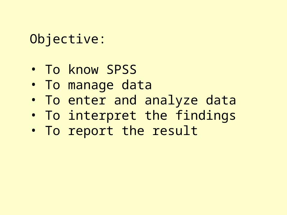
Objective:

• To know SPSS• To manage data• To enter and analyze data• To interpret the findings• To report the result

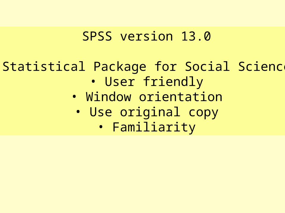
SPSS version 13.0

Statistical Package for Social Science• User friendly

• Window orientation• Use original copy

• Familiarity

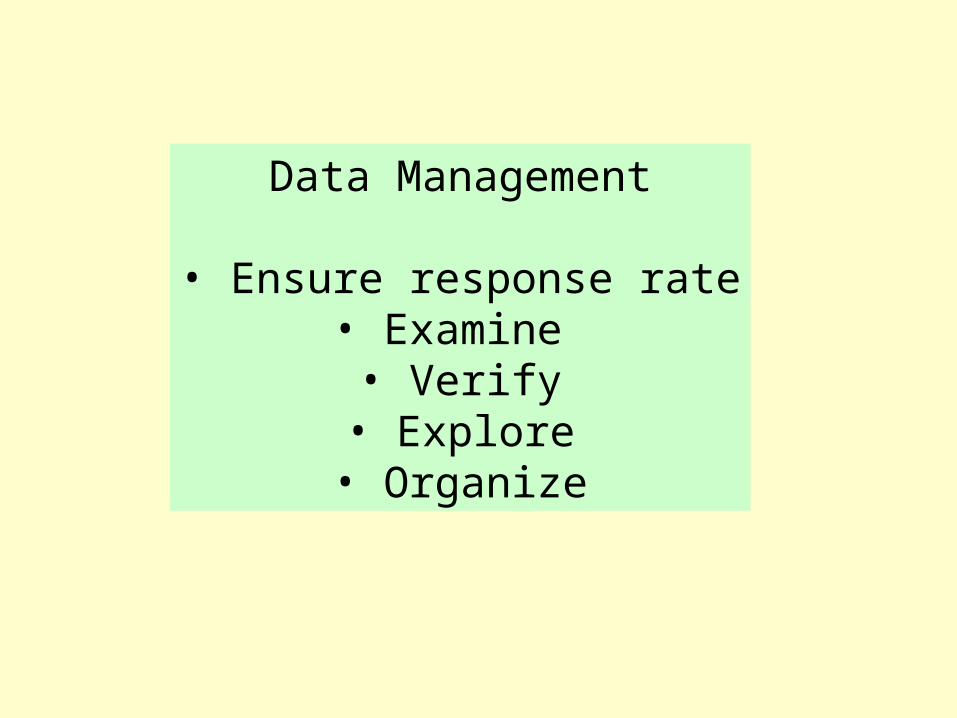
Data Management

• Ensure response rate• Examine • Verify• Explore• Organize

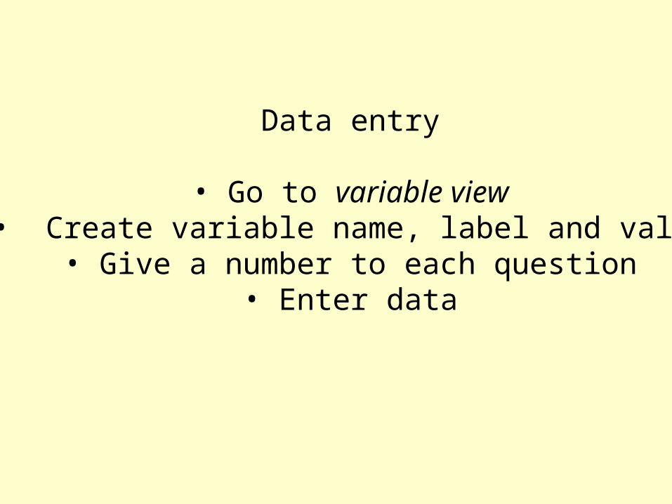
Data entry

• Go to variable view• Create variable name, label and value

• Give a number to each question• Enter data

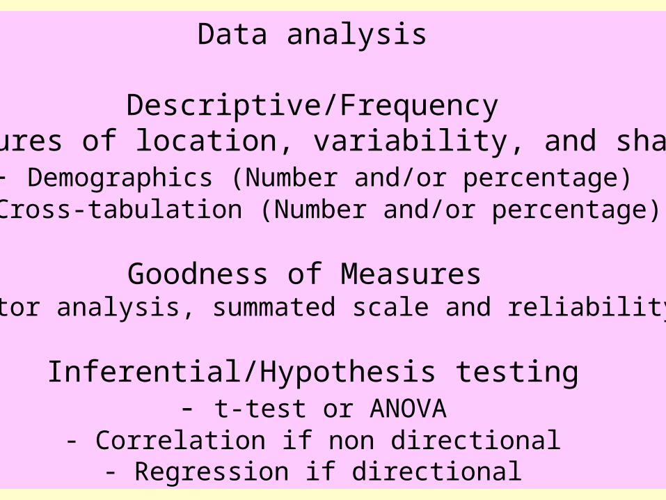
Data analysis

Descriptive/Frequency(Measures of location, variability, and shape)

- Demographics (Number and/or percentage)- Cross-tabulation (Number and/or percentage)

Goodness of Measures (Factor analysis, summated scale and reliability)

Inferential/Hypothesis testing- t-test or ANOVA

- Correlation if non directional- Regression if directional

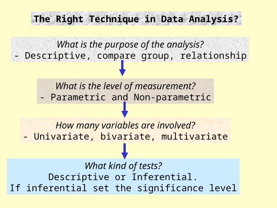
The Right Technique in Data Analysis?

What is the purpose of the analysis?- Descriptive, compare group, relationship

What is the level of measurement?- Parametric and Non-parametric

How many variables are involved?- Univariate, bivariate, multivariate

What kind of tests?Descriptive or Inferential.

If inferential set the significance level

Descriptive Analysis

Purpose: To describe the distribution of the demographic variable

Frequencies distribution – if 1 ordinal or nominalCross-tabulation – if 2 ordinal or nominalMeans – if 1 interval or ratio Means of subgroup – if 1 interval or ratio by subgroup

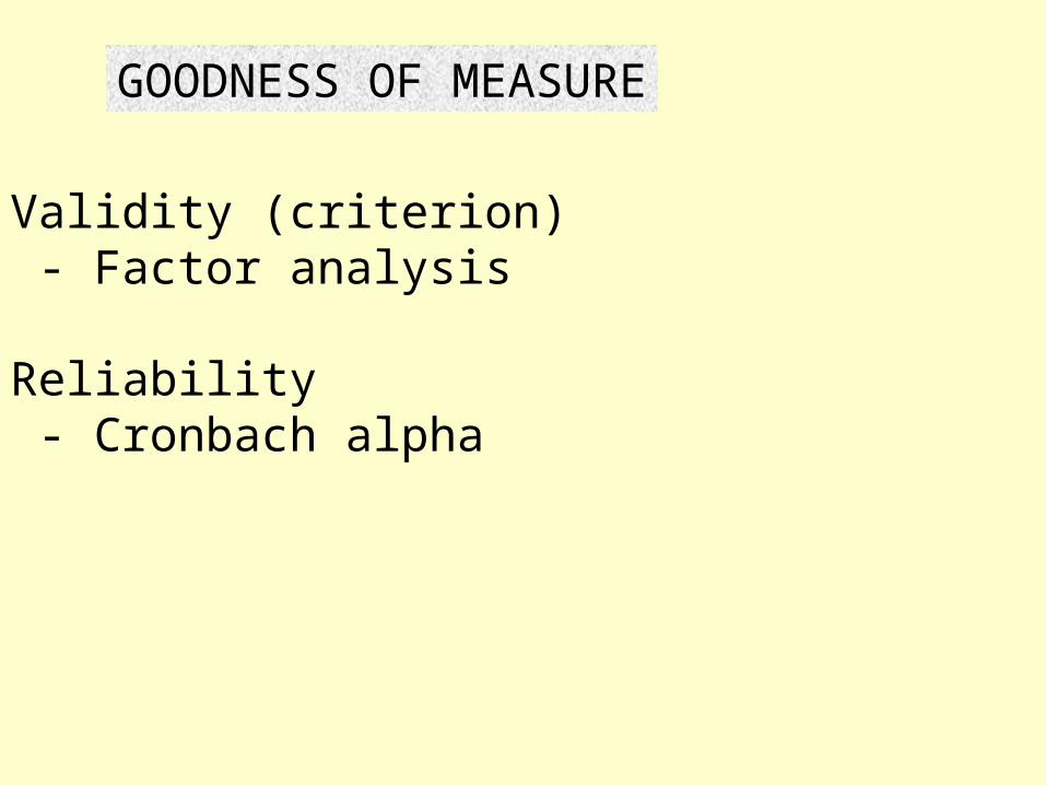
GOODNESS OF MEASURE

Validity (criterion) - Factor analysis

Reliability - Cronbach alpha

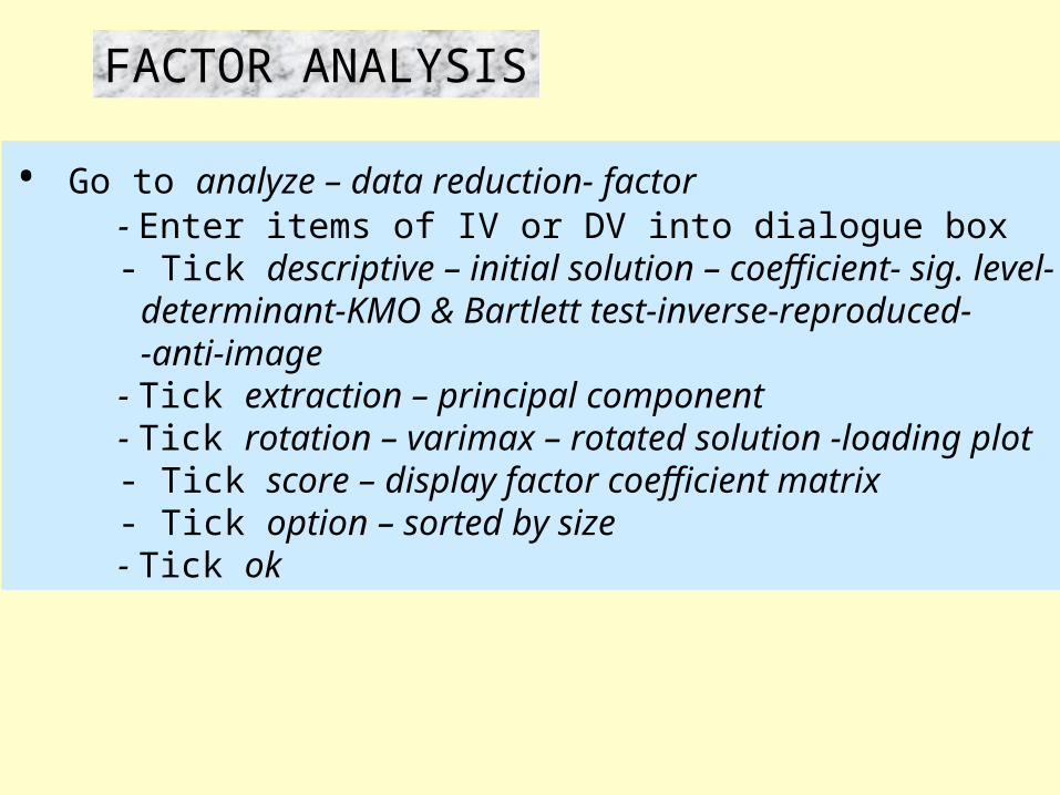
FACTOR ANALYSIS

• Go to analyze – data reduction- factor- Enter items of IV or DV into dialogue box- Tick descriptive – initial solution – coefficient- sig. level-

determinant-KMO & Bartlett test-inverse-reproduced- -anti-image

- Tick extraction – principal component- Tick rotation – varimax – rotated solution -loading plot - Tick score – display factor coefficient matrix- Tick option – sorted by size- Tick ok

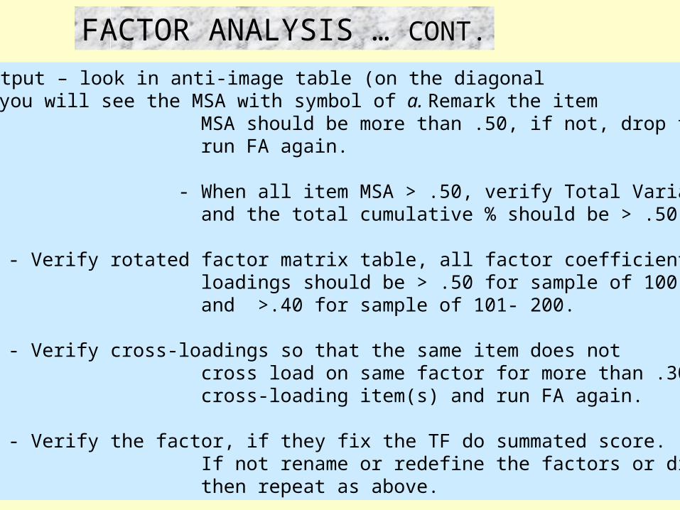
• Verify the output – look in anti-image table (on the diagonal you will see the MSA with symbol of a. Remark the item MSA should be more than .50, if not, drop the item and run FA again.

- When all item MSA > .50, verify Total Variance Explained and the total cumulative % should be > .50.

- Verify rotated factor matrix table, all factor coefficient or loadings should be > .50 for sample of 100 or less, and >.40 for sample of 101- 200.

- Verify cross-loadings so that the same item does not cross load on same factor for more than .30. Drop the cross-loading item(s) and run FA again.

- Verify the factor, if they fix the TF do summated score. If not rename or redefine the factors or dimensions and then repeat as above.

FACTOR ANALYSIS … CONT.

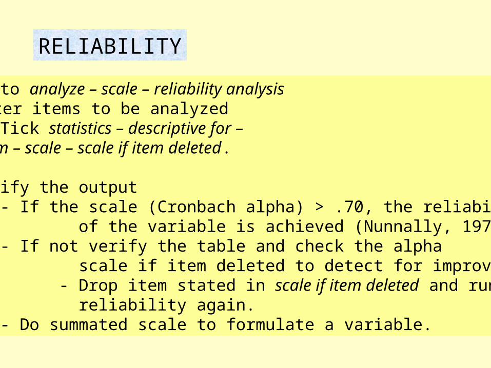
RELIABILITY• Go to analyze – scale – reliability analysis - Enter items to be analyzed - Tick statistics – descriptive for – item – scale – scale if item deleted.

• Verify the output- If the scale (Cronbach alpha) > .70, the reliability

of the variable is achieved (Nunnally, 1978)- If not verify the table and check the alpha

scale if item deleted to detect for improvement. - Drop item stated in scale if item deleted and run reliability again.

- Do summated scale to formulate a variable.

FACTOR ANALYSIS VS. RELIABILITY

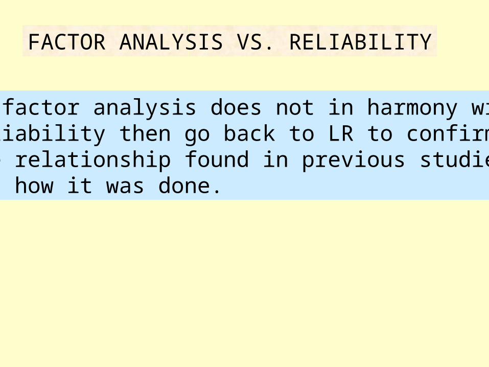
If factor analysis does not in harmony withreliability then go back to LR to confirmthe relationship found in previous studiesand how it was done.

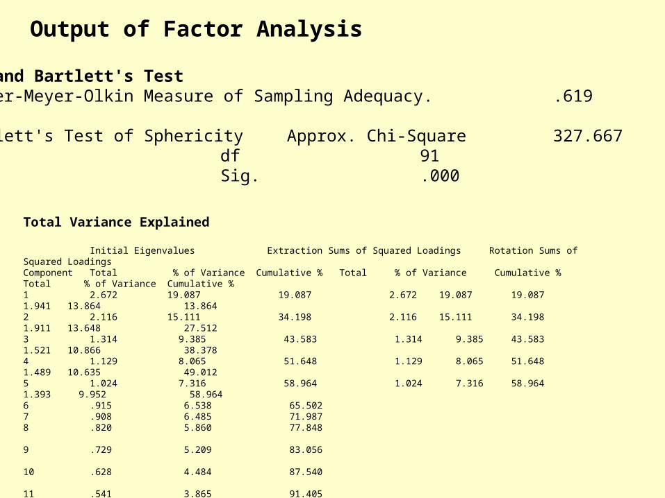
KMO and Bartlett's TestKaiser-Meyer-Olkin Measure of Sampling Adequacy. .619

Bartlett's Test of Sphericity Approx. Chi-Square 327.667 df 91 Sig. .000

Total Variance Explained

Initial Eigenvalues Extraction Sums of Squared Loadings Rotation Sums of Squared Loadings Component Total % of Variance Cumulative % Total % of Variance Cumulative % Total % of Variance Cumulative %1 2.672 19.087 19.087 2.672 19.087 19.087 1.941 13.864 13.864 2 2.116 15.111 34.198 2.116 15.111 34.198 1.911 13.648 27.512 3 1.314 9.385 43.583 1.314 9.385 43.583 1.521 10.866 38.378 4 1.129 8.065 51.648 1.129 8.065 51.648 1.489 10.635 49.012 5 1.024 7.316 58.964 1.024 7.316 58.964 1.393 9.952 58.9646 .915 6.538 65.5027 .908 6.485 71.9878 .820 5.860 77.848

9 .729 5.209 83.056

10 .628 4.484 87.540

11 .541 3.865 91.405

12 .471 3.365 94.771

13 .403 2.876 97.647

14 .329 2.353 100.000

Extraction Method: Principal Component Analysis.

Output of Factor Analysis

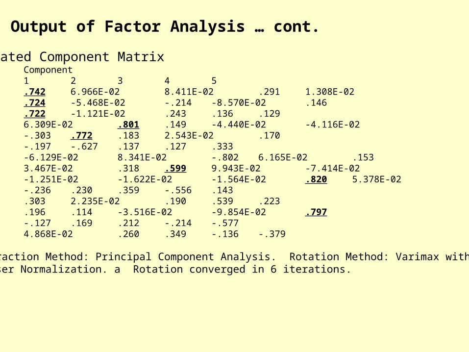
Rotated Component Matrix Component 1 2 3 4 5 BO12 .742 6.966E-02 8.411E-02 .291 1.308E-02 BO7 .724 -5.468E-02 -.214 -8.570E-02 .146 BO6 .722 -1.121E-02 .243 .136 .129 BO8 6.309E-02 .801 .149 -4.440E-02 -4.116E-02 BO14 -.303 .772 .183 2.543E-02 .170 BO13 -.197 -.627 .137 .127 .333 BO11 -6.129E-02 8.341E-02 -.802 6.165E-02 .153 BO4 3.467E-02 .318 .599 9.943E-02 -7.414E-02 BO9 -1.251E-02 -1.622E-02 -1.564E-02 .820 5.378E-02 BO1 -.236 .230 .359 -.556 .143 BO2 .303 2.235E-02 .190 .539 .223 BO3 .196 .114 -3.516E-02 -9.854E-02 .797 BO10 -.127 .169 .212 -.214 -.577 BO5 4.868E-02 .260 .349 -.136 -.379

Extraction Method: Principal Component Analysis. Rotation Method: Varimax with Kaiser Normalization. a Rotation converged in 6 iterations.

Output of Factor Analysis … cont.

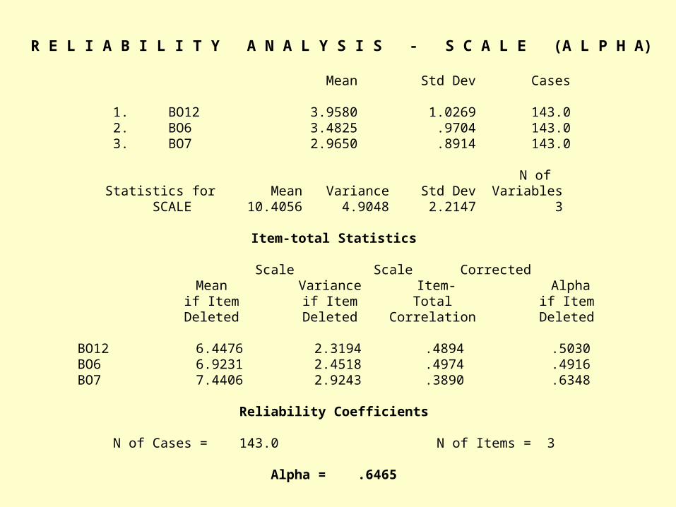
R E L I A B I L I T Y A N A L Y S I S - S C A L E (A L P H A)

Mean Std Dev Cases

1. BO12 3.9580 1.0269 143.0 2. BO6 3.4825 .9704 143.0 3. BO7 2.9650 .8914 143.0

N ofStatistics for Mean Variance Std Dev Variables SCALE 10.4056 4.9048 2.2147 3

Item-total Statistics

Scale Scale Corrected Mean Variance Item- Alpha if Item if Item Total if Item Deleted Deleted Correlation Deleted

BO12 6.4476 2.3194 .4894 .5030BO6 6.9231 2.4518 .4974 .4916BO7 7.4406 2.9243 .3890 .6348

Reliability Coefficients

N of Cases = 143.0 N of Items = 3

Alpha = .6465

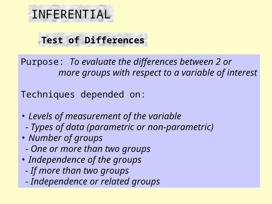
Test of Differences

Purpose: To evaluate the differences between 2 or more groups with respect to a variable of interest

Techniques depended on:

• Levels of measurement of the variable - Types of data (parametric or non-parametric)• Number of groups - One or more than two groups• Independence of the groups - If more than two groups - Independence or related groups

INFERENTIAL

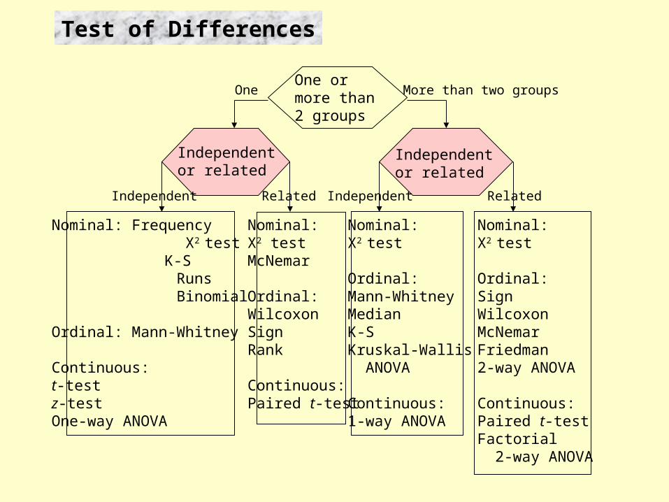
Test of Differences

One ormore than2 groups

Independentor related

One More than two groups

Independentor related

Independent Related

Nominal: Frequency Χ2 test K-S Runs Binomial

Ordinal: Mann-Whitney

Continuous:t-testz-test One-way ANOVA

Nominal:Χ2 testMcNemar

Ordinal:WilcoxonSignRank

Continuous:Paired t-test

Nominal:Χ2 test

Ordinal:Mann-WhitneyMedianK-SKruskal-Wallis ANOVA

Continuous:1-way ANOVA

Independent Related

Nominal:Χ2 test

Ordinal:SignWilcoxonMcNemarFriedman2-way ANOVA

Continuous:Paired t-testFactorial 2-way ANOVA

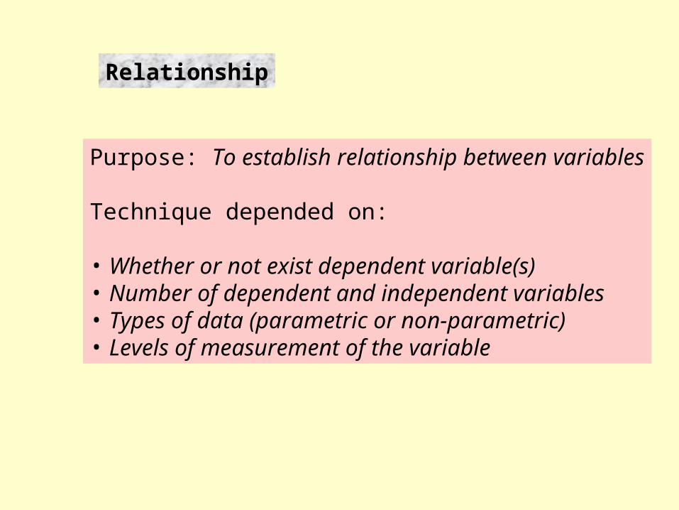
Relationship

Purpose: To establish relationship between variables

Technique depended on:

• Whether or not exist dependent variable(s) • Number of dependent and independent variables• Types of data (parametric or non-parametric)• Levels of measurement of the variable

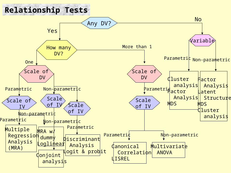
Relationship Tests

One

Scale of DV

Parametric

Scale of IV

Parametric

Multiple Regression Analysis (MRA)

Non-parametric

MRA w/ dummyLoglinear

Scaleof IV

Non-parametric

Conjoint analysis

Non-parametric

Scaleof IV

Parametric

Discriminant AnalysisLogit & probit

Scale of DV

More than 1

Scaleof IV

Parametric

Parametric Non-parametric

Canonical CorrelationLISREL

Multivariate ANOVA

Any DV?Yes

No

Variable

Cluster analysisFactor AnalysisMDS

Factor AnalysisLatent StructureMDSCluster analysis

Parametric Non-parametric

How manyDV?

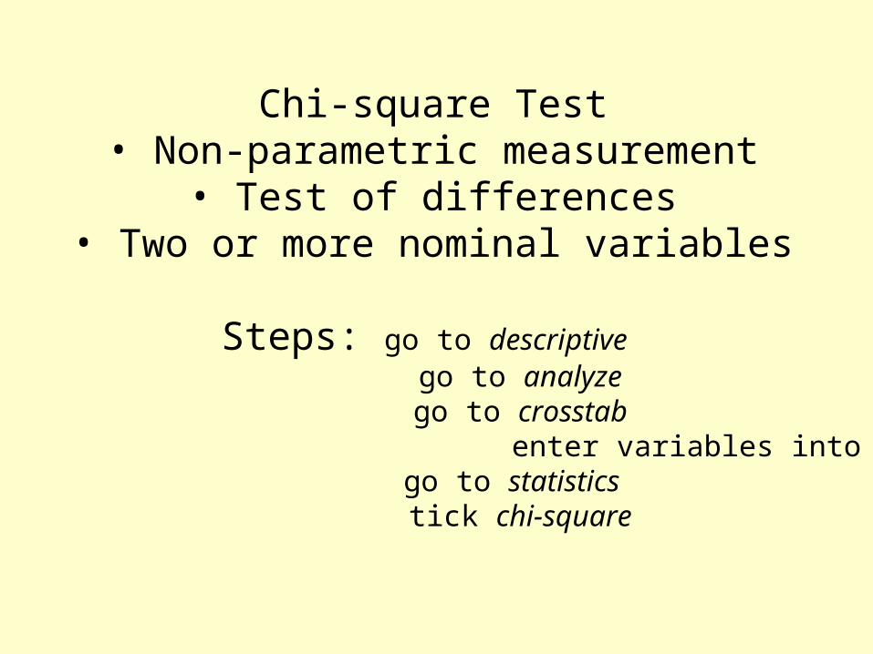
Chi-square Test• Non-parametric measurement

• Test of differences• Two or more nominal variables

Steps: go to descriptive go to analyze go to crosstab

enter variables into row and column go to statistics tick chi-square

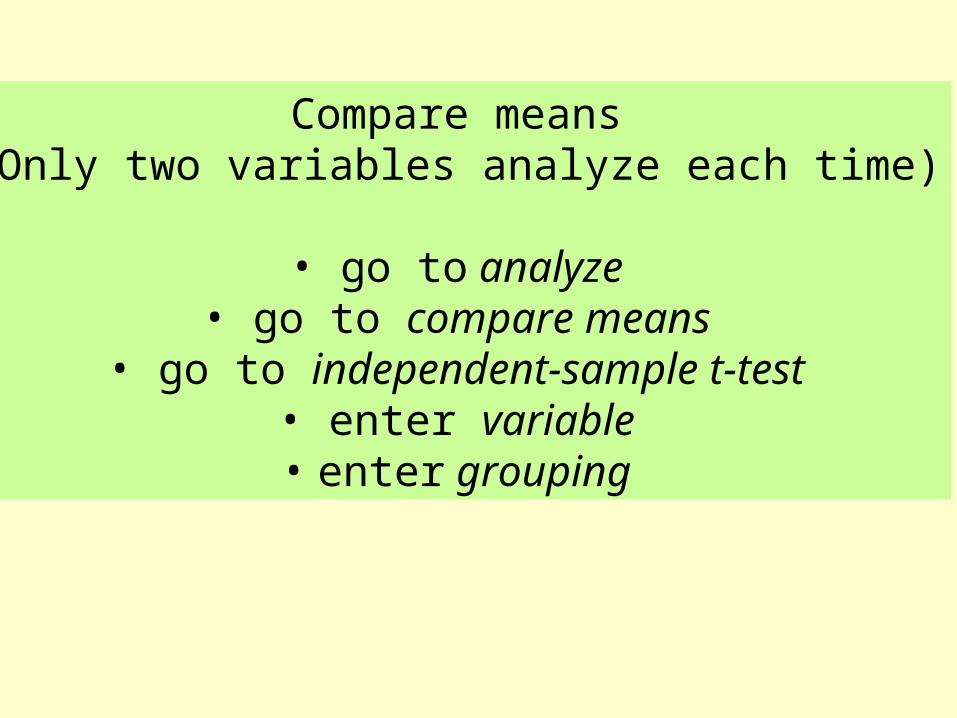
Compare means(Only two variables analyze each time)

• go to analyze• go to compare means

• go to independent-sample t-test• enter variable• enter grouping

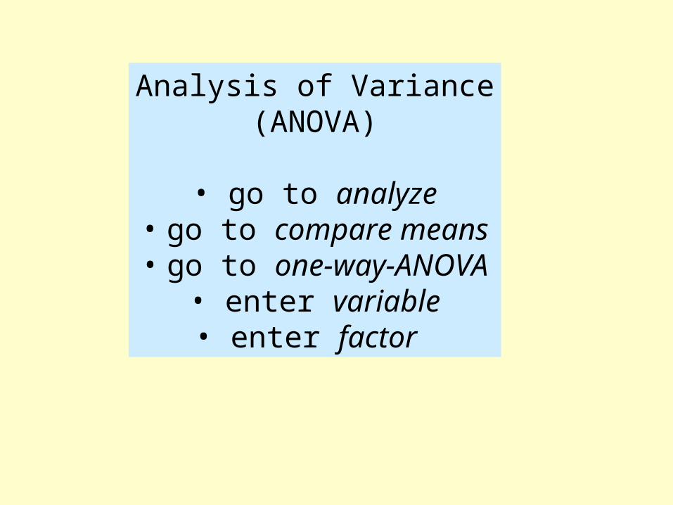
Analysis of Variance(ANOVA)

• go to analyze• go to compare means• go to one-way-ANOVA

• enter variable• enter factor

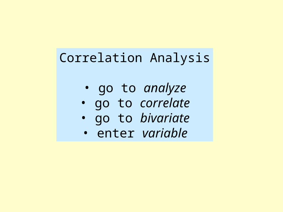
Correlation Analysis

• go to analyze• go to correlate• go to bivariate• enter variable

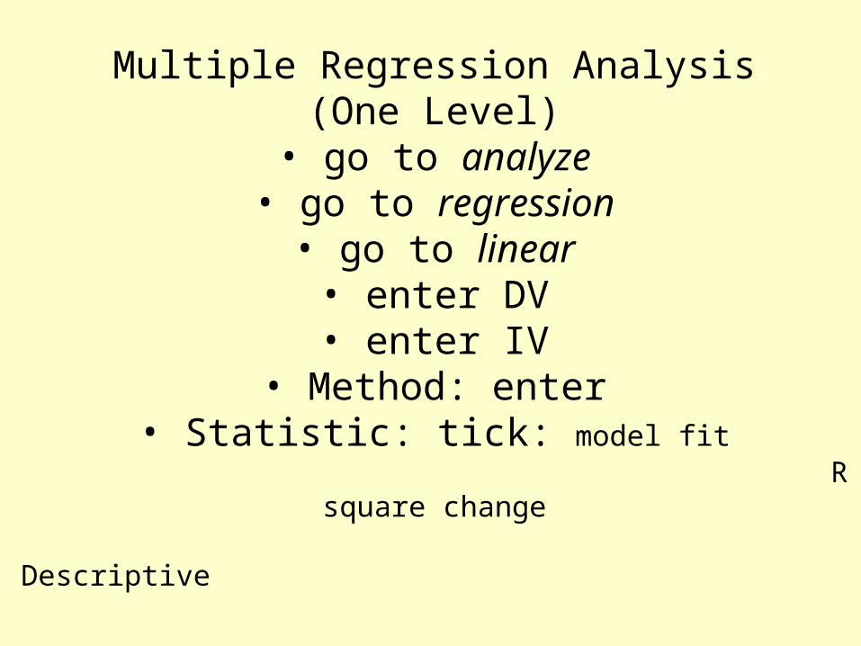
Multiple Regression Analysis(One Level)

• go to analyze• go to regression• go to linear• enter DV• enter IV

• Method: enter• Statistic: tick: model fit

R square change

Descriptive

Collinearity diagnostic

Durbin Watson Plot

Scatterplot

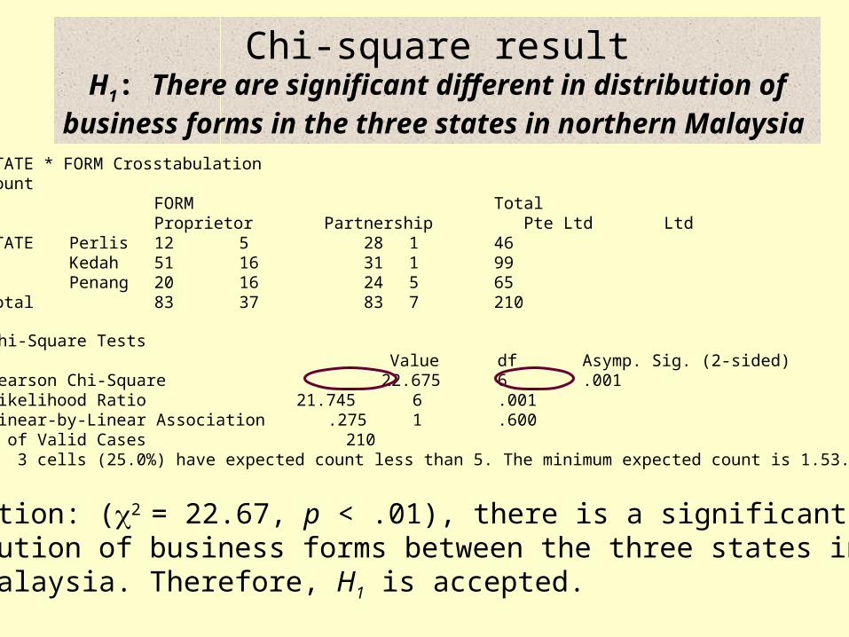
Chi-square resultH1: There are significant different in distribution of

business forms in the three states in northern Malaysia STATE * FORM CrosstabulationCount FORM Total Proprietor Partnership Pte Ltd Ltd STATE Perlis 12 5 28 1 46 Kedah 51 16 31 1 99 Penang 20 16 24 5 65 Total 83 37 83 7 210

Chi-Square Tests Value df Asymp. Sig. (2-sided) Pearson Chi-Square 22.675 6 .001 Likelihood Ratio 21.745 6 .001 Linear-by-Linear Association .275 1 .600 N of Valid Cases 210 a 3 cells (25.0%) have expected count less than 5. The minimum expected count is 1.53.

Interpretation: (2 = 22.67, p < .01), there is a significant different in distribution of business forms between the three states in northern Malaysia. Therefore, H1 is accepted.

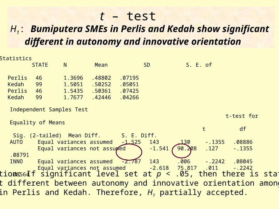
Group Statistics STATE N Mean SD S. E. of Mean AUTO Perlis 46 1.3696 .48802 .07195 Kedah 99 1.5051 .50252 .05051 INNO Perlis 46 1.5435 .50361 .07425 Kedah 99 1.7677 .42446 .04266

Independent Samples Test t-test for Equality of Means t df Sig. (2-tailed) Mean Diff. S. E. Diff.AUTO Equal variances assumed -1.525 143 .130 -.1355 .08886 Equal variances not assumed -1.541 90.208 .127 -.1355.08791 INNO Equal variances assumed -2.787 143 .006 -.2242 .08045 Equal variances not assumed -2.618 75.817 .011 -.2242.08564

t – testH1: Bumiputera SMEs in Perlis and Kedah show significant different in autonomy and innovative orientation

Interpretation: If significant level set at p < .05, then there is statistical significant different between autonomy and innovative orientation amongBumi SMEs in Perlis and Kedah. Therefore, H1 partially accepted.

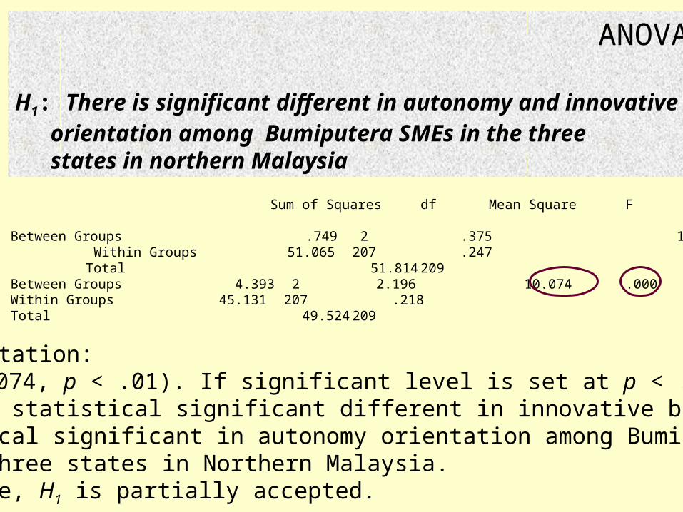
ANOVA

H1: There is significant different in autonomy and innovative orientation among Bumiputera SMEs in the three states in northern Malaysia

Sum of Squares df Mean Square F Sig.

AUTO Between Groups .749 2 .375 1.519 .221 Within Groups 51.065 207 .247 Total 51.814209 INNO Between Groups 4.393 2 2.196 10.074 .000 Within Groups 45.131 207 .218 Total 49.524209

Interpretation:(F = 10.074, p < .01). If significant level is set at p < .05, thenthere is statistical significant different in innovative but not statistical significant in autonomy orientation among Bumi SMEs in the three states in Northern Malaysia. Therefore, H1 is partially accepted.

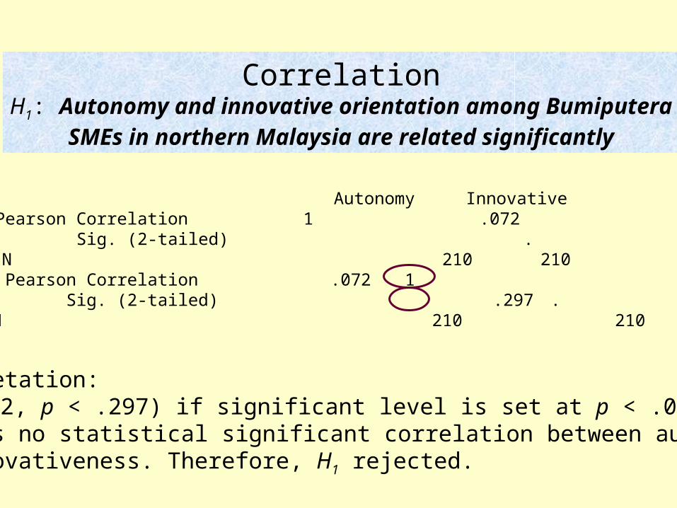
CorrelationH1: Autonomy and innovative orientation among Bumiputera

SMEs in northern Malaysia are related significantlyCorrelations Autonomy Innovative Autonomy Pearson Correlation 1 .072 Sig. (2-tailed) . .297 N 210 210 Innovative Pearson Correlation .072 1 Sig. (2-tailed) .297 . N 210 210

Interpretation:(r = .072, p < .297) if significant level is set at p < .05, thenthere is no statistical significant correlation between autonomyand innovativeness. Therefore, H1 rejected.

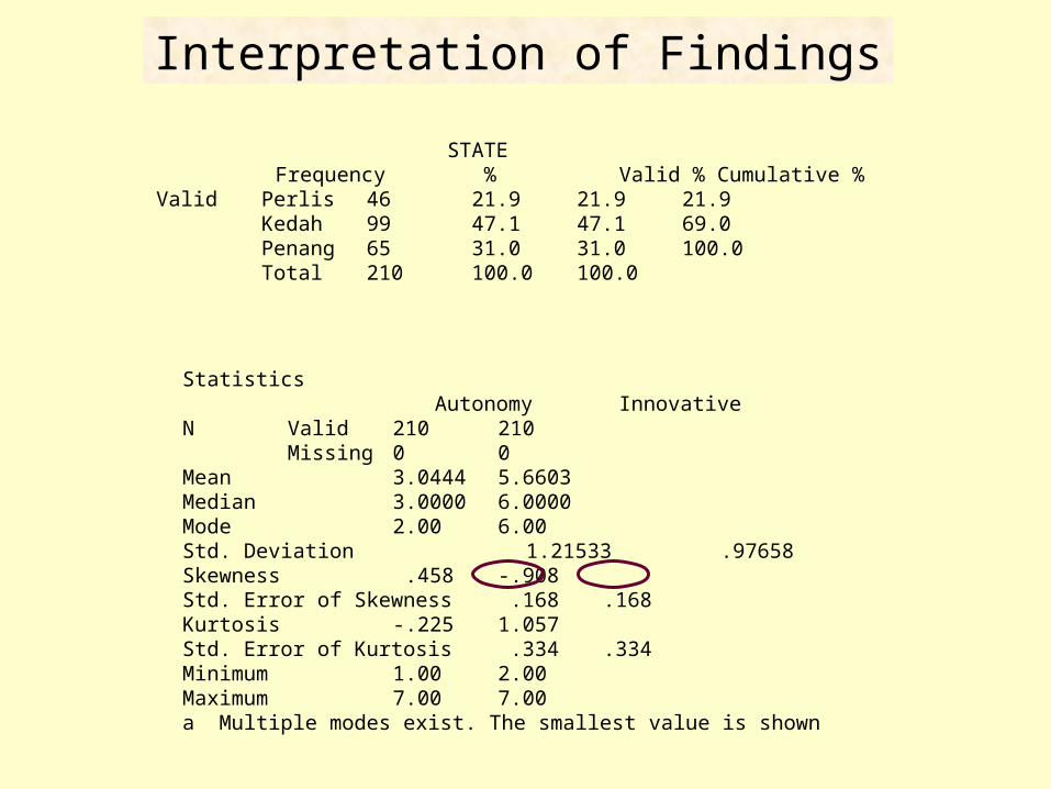
Interpretation of Findings

Statistics Autonomy Innovative N Valid 210 210 Missing 0 0 Mean 3.0444 5.6603 Median 3.0000 6.0000 Mode 2.00 6.00 Std. Deviation 1.21533 .97658 Skewness .458 -.908 Std. Error of Skewness .168 .168 Kurtosis -.225 1.057 Std. Error of Kurtosis .334 .334 Minimum 1.00 2.00 Maximum 7.00 7.00 a Multiple modes exist. The smallest value is shown

STATE Frequency % Valid % Cumulative %

Valid Perlis 46 21.9 21.9 21.9 Kedah 99 47.1 47.1 69.0 Penang 65 31.0 31.0 100.0 Total 210 100.0 100.0

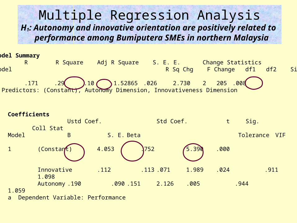
Multiple Regression AnalysisH1: Autonomy and innovative orientation are positively related to

performance among Bumiputera SMEs in northern Malaysia

Model Summary R R Square Adj R Square S. E. E. Change Statistics Model R Sq Chg F Change df1 df2 Sig. F Chg

1 .171 .29 .10 1.52865 .026 2.730 2 205 .008 a Predictors: (Constant), Autonomy Dimension, Innovativeness Dimension

Coefficients Ustd Coef. Std Coef. t Sig. Coll Stat Model B S. E. Beta Tolerance VIF

1 (Constant) 4.053 .752 5.390 .000

Innovative .112 .113 .071 1.989 .024 .911

1.098 Autonomy .190 .090 .151 2.126 .005 .9441.059 a Dependent Variable: Performance

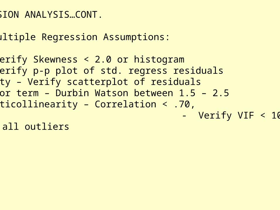
MULTIPLE REGRESSION ANALYSIS…CONT.

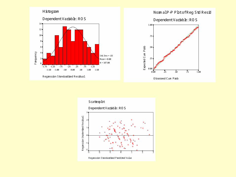
Consider Some Multiple Regression Assumptions:

1. Normality – Verify Skewness < 2.0 or histogram2. Linearity – Verify p-p plot of std. regress residuals3. Homocedasticity – Verify scatterplot of residuals4. Free from error term – Durbin Watson between 1.5 – 2.55. Free from multicollinearity – Correlation < .70, - Verify VIF < 10, Tol < .106. Get rid of all outliers

Norm al P-P Plot of Reg Std ResidDependent Variable: RO S

O bserved Cum Prob

1.00.75.50.250.00

Expecte

d Cu

m Prob

1.00

.75

.50

.25

0.00

ScatterplotDependent Variable: RO S

Regression Standardized Predicted Value

3210-1-2-3

Regressio

n Studentized Residu

al

3

2

1

0

-1

-2

Regression Standardized Residual

1.501.25

1.00.75

.50.25

0.00-.25

-.50-.75

-1.00-1.25

-1.50-1.75

HistogramDependent Variable: RO S

Frequency

14

12

10

8

6

4

2

0

Std. Dev = .83 Mean = 0.00N = 107.00

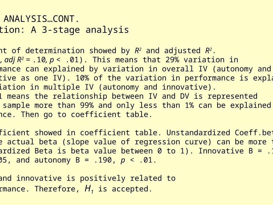
REGRESSION ANALYSIS…CONT.Interpretation: A 3-stage analysis

1. Coefficient of determination showed by R2 and adjusted R2. (R2 = .29, adj R2 = .10, p < .01). This means that 29% variation in performance can explained by variation in overall IV (autonomy and innovative as one IV). 10% of the variation in performance is explained by variation in multiple IV (autonomy and innovative). p < .01 means the relationship between IV and DV is represented by the sample more than 99% and only less than 1% can be explained by chance. Then go to coefficient table.

2. Beta coefficient showed in coefficient table. Unstandardized Coeff.beta is the actual beta (slope value of regression curve) can be more than 1. Standardized Beta is beta value between 0 to 1). Innovative B = .112, p < .05, and autonomy B = .190, p < .01.

3. Autonomy and innovative is positively related to performance. Therefore, H1 is accepted.

THANK YOU ALLNow analyze your own data