Anomaly detection technique for sequential data

HAL Id: tel-01548382https://tel.archives-ouvertes.fr/tel-01548382

Submitted on 27 Jun 2017

HAL is a multi-disciplinary open accessarchive for the deposit and dissemination of sci-entific research documents, whether they are pub-lished or not. The documents may come fromteaching and research institutions in France orabroad, or from public or private research centers.

L’archive ouverte pluridisciplinaire HAL, estdestinée au dépôt et à la diffusion de documentsscientifiques de niveau recherche, publiés ou non,émanant des établissements d’enseignement et derecherche français ou étrangers, des laboratoirespublics ou privés.

Anomaly detection technique for sequential dataMuriel Pellissier

To cite this version:Muriel Pellissier. Anomaly detection technique for sequential data. Data Structures and Algorithms[cs.DS]. Université de Grenoble, 2013. English. �NNT : 2013GRENM078�. �tel-01548382�

https://tel.archives-ouvertes.fr/tel-01548382

https://hal.archives-ouvertes.fr

Université Joseph Fourier / Université Pierre Mendès France / Université Stendhal / Université de Savoie / Grenoble INP

THÈSEPour obtenir le grade de

DOCTEUR DE L’UNIVERSITÉ DE GRENOBLE

préparée dans le cadre d’une cotutelle entre l’Université de Grenoble et le Centre Commun de Recherche de la Commission Européenne

Spécialité : Mathématiques, sciences et technologies de l’information, informatique

Arrêté ministériel : le 6 janvier 2005 -7 août 2006

Présentée par

Muriel Pellissier

Thèse dirigée par Herve Martincodirigée par Evangelos Kotsakis

préparée au sein des Laboratoires du Centre Commun de Recherche de la Commission Européenne

dans les Écoles Doctorales Mathématiques, sciences et technologies de l’information, informatique

Technique de détection d'anomalies utilisant des données séquentielles

Thèse soutenue publiquement le « 15 Octobre 2013 »,devant le jury composé de :

Mr, Hervé, MARTIN Université de Grenoble, Directeur

Mr, Evangelos, KOTSAKIS JRC – European Commission, Ispra (Italie), CoDirecteur

Mr Eric, GAUSSIER Universite de Grenoble Président

Mr, Jean-Marc, PETIT INSA, Lyon, Examinateur

Mme, Bénédicte, BUCHER IGN, Saint Mande, Rapporteur

Mr, Bruno, DEFUDE Telecom Sud Paris, Evry, Rapporteur

2

Muriel Pellissier

Contents

List of figures ................................................................................................................................................. 4

Acknowledgments ......................................................................................................................................... 5

Abstract ......................................................................................................................................................... 6

Résumé ......................................................................................................................................................... 7

Introduction ...................................................................................................................................... 9

1. Context ............................................................................................................................................... 9

2. Anomalies ......................................................................................................................................... 11

3. Data .................................................................................................................................................. 11

4. Anomaly detection techniques applied to maritime security .......................................................... 11

5. Our problem ..................................................................................................................................... 17

Literature review ............................................................................................................................. 20

I. Graph-based anomaly detection ............................................................................................. 20

1. Graph-Based Anomaly Detection ................................................................................................................ 21

2. Detecting Anomalies in Cargo Shipments Using Graph Properties ............................................................. 25

3. Anomaly detection in data represented as graph ....................................................................................... 28

4. Graph-Based Anomaly Detection Applied to Homeland Security Cargo Screening .................................... 35

II. Sequence mining ..................................................................................................................... 37

1. The sequence-based anomaly detection techniques .................................................................................. 38

a. Window-based techniques ............................................................................................................ 38

b. Markovian techniques ................................................................................................................... 40

2. The contiguous subsequence-based anomaly detection techniques .......................................................... 42

3. The pattern frequency-based anomaly detection techniques .................................................................... 43

III. String distance ......................................................................................................................... 46

1. Hamming distance ....................................................................................................................................... 46

2. Levenshtein distance ................................................................................................................................... 46

3. Damerau-Levenshtein distance ................................................................................................................... 47

4. The string edit distance with Moves ............................................................................................................ 47

5. Needleman-Wunsch algorithm.................................................................................................................... 47

3

Muriel Pellissier

6. Tichy distance .............................................................................................................................................. 48

7. String distance conclusion ........................................................................................................................... 48

Our anomaly detection approach ..................................................................................................... 50

I. Method ................................................................................................................................................... 50

II. Common sequences / subsequences ..................................................................................................... 53

III. Distance: anomaly degree ...................................................................................................................... 57

1. Structure Distance ....................................................................................................................................... 58

2. Port names distance .................................................................................................................................... 58

3. Anomaly degree........................................................................................................................................... 60

4. Example ....................................................................................................................................................... 65

Experiments .................................................................................................................................... 67

I. Container itinerary data .......................................................................................................... 67

II. Experimental data ................................................................................................................... 68

1. Graph-based anomaly detection technique .................................................................................................. 68

2. Our anomaly detection technique ................................................................................................................ 72

III. Real world data ....................................................................................................................... 75

1. Graph-based anomaly detection technique .................................................................................................. 75

2. Our anomaly detection technique ................................................................................................................ 75

IV. Discussion ................................................................................................................................ 80

Conclusion ....................................................................................................................................... 82

Conclusion (French).......................................................................................................................... 84

References ....................................................................................................................................... 86

Appendices ...................................................................................................................................... 89

1. Joint Research Centre – European Commission ............................................................................................ 89

2. ConTraffic: Maritime Container Traffic Anomaly Detection, A. Varfis, E. Kotsakis, A. Tsois, M. Sjachyn, A.

Donati, E. Camossi, P. Villa, T. Dimitrova and M. Pellissier – In Proceedings of the First International

Workshop on Maritime Anomaly Detection (MAD 2011), p. 13 – 14 – June 2011 ....................................... 90

3. Anomaly detection in large dataset containing container itineraries – Poster – LIG PhD Students’ Day, June

2012 ............................................................................................................................................................... 92

4. Mining irregularities in Maritime container itineraries, M. Pellissier, E. Kotsakis and H. Martin – EDBT/ICDT

Workshop, March 2013 ................................................................................................................................. 93

5. Anomaly detection for the security of cargo shipments, M. Pellissier, E. Kotsakis and H. Martin – IFGIS

Conference, May 2013 ................................................................................................................................ 106

4

Muriel Pellissier

List of figures

Figure 1: Picture of containers at the port of Genoa in Italy

Figure 2: Itinerary from Singapore to Rotterdam passing through Chiwan

Figure 3: Graph representation of the itinerary Singapore, Rotterdam, Chiwan

Figure 4: Example of a best substructure

Figure 5: Example of modification type of anomalies

Figure 6: Example of insertion type of anomalies

Figure 7: Example of deletion type of anomalies

Figure 8: Example of normative pattern shapes [34]

Figure 9: An itinerary and all his possible subsequences

Figure 10: Common subsequences algorithm

Figure 11: Two itineraries: a given itinerary (X1,X2,X3,X4) and a common itinerary (X1,*,X4)


Figure 13: Anomaly detection algorithm

Figure 14: Percentages of transshipments in real world data

Figure 15: Graph representation of the itinerary from port 1 to port 3 passing through port 2

Figure 16: Best substructures

Figure 17: Another graph representation of the itinerary port 1 to port 3 passing through port 2

Figure 18: Graph representation limitation

Figure 19: Anomalous itineraries using experimental data

Figure 20: Results obtained with different maximum anomaly degree values

Figure 21: Graph representing the anomalies depending on the maximum anomaly degree threshold

Figure 22: Results with different minimum frequency values

Figure 23: Anomalous itineraries using real world data


Figure 25: Graph representing the anomalies depending on the minimum frequency threshold


5

Muriel Pellissier

Acknowledgments

I would like to express my gratitude to my two supervisors, Herve Martin and Evangelos Kotsakis, for all

the help and the time they gave me during the three years of my thesis.

I would like to thank also all my colleagues from the Contraffic team for all their help and the nice time I

spent with them, and specially Elena Camossi that advised me and helped me a lot during all my PhD

research.

I would like to thank all the people from the laboratory LIG, as well as from the Joint Research Centre, that

helped me and gave me all the resources to succeed in my PhD research.

Finally, I thank all my family and friends for all their support and help.

6

Muriel Pellissier

Abstract

Nowadays, huge quantities of data can be easily accessible, but all these data are not useful if we do not

know how to process them efficiently and how to extract easily relevant information from a large quantity

of data. The anomaly detection techniques are used in many domains in order to help to process the data

in an automated way. The anomaly detection techniques depend on the application domain, on the type

of data, and on the type of anomaly.

For this study we are interested only in sequential data. A sequence is an ordered list of items, also called

events. Identifying irregularities in sequential data is essential for many application domains like DNA

sequences, system calls, user commands, banking transactions etc.

This thesis presents a new approach for identifying and analyzing irregularities in sequential data. This

anomaly detection technique can detect anomalies in sequential data where the order of the items in the

sequences is important. Moreover, our technique does not consider only the order of the events, but also

the position of the events within the sequences. The sequences are spotted as anomalous if a sequence

is quasi-identical to a usual behavior which means if the sequence is slightly different from a frequent

(common) sequence. The differences between two sequences are based on the order of the events and

their position in the sequence.

In this thesis we applied this technique to the maritime surveillance, but this technique can be used by

any other domains that use sequential data. For the maritime surveillance, some automated tools are

needed in order to facilitate the targeting of suspicious containers that is performed by the customs.

Indeed, nowadays 90% of the world trade is transported by containers and only 1-2% of the containers

can be physically checked because of the high financial cost and the high human resources needed to

control a container. As the number of containers travelling every day all around the world is really

important, it is necessary to control the containers in order to avoid illegal activities like fraud, quota-

related, illegal products, hidden activities, drug smuggling or arm smuggling. For the maritime domain, we

can use this technique to identify suspicious containers by comparing the container trips from the data

set with itineraries that are known to be normal (common). A container trip, also called itinerary, is an

ordered list of actions that are done on containers at specific geographical positions. The different actions

are: loading, transshipment, and discharging. For each action that is done on a container, we know the

container ID and its geographical position (port ID).

This technique is divided into two parts. The first part is to detect the common (most frequent) sequences

of the data set. The second part is to identify those sequences that are slightly different from the common

sequences using a distance-based method in order to classify a given sequence as normal or suspicious.

The distance is calculated using a method that combines quantitative and qualitative differences between

two sequences.

7

Muriel Pellissier

We will present in this thesis the context and the existing anomaly detection techniques. Then, we will

present our anomaly detection technique and the results obtained by testing this technique with

experimental data and with real world data.

Résumé

De nos jours, beaucoup de données peuvent être facilement accessibles. Mais toutes ces données ne sont

pas utiles si nous ne savons pas les traiter efficacement et si nous ne savons pas extraire facilement les

informations pertinentes à partir d’une grande quantité de données. Les techniques de détection

d’anomalies sont utilisées par de nombreux domaines afin de traiter automatiquement les données. Les

techniques de détection d’anomalies dépendent du domaine d’application, des données utilisées ainsi

que du type d’anomalie à détecter.

Pour cette étude nous nous intéressons seulement aux données séquentielles. Une séquence est une liste

ordonnée d’objets. Pour de nombreux domaines, il est important de pouvoir identifier les irrégularités

contenues dans des données séquentielles comme par exemple les séquences ADN, les commandes

d’utilisateur, les transactions bancaires etc.

Cette thèse présente une nouvelle approche qui identifie et analyse les irrégularités de données

séquentielles. Cette technique de détection d’anomalies peut détecter les anomalies de données

séquentielles dont l’ordre des objets dans les séquences est important ainsi que la position des objets

dans les séquences. Les séquences sont définies comme anormales si une séquence est presque identique

à une séquence qui est fréquente (normale). Les séquences anormales sont donc les séquences qui

diffèrent légèrement des séquences qui sont fréquentes dans la base de données.

Dans cette thèse nous avons appliqué cette technique à la surveillance maritime, mais cette technique

peut être utilisée pour tous les domaines utilisant des données séquentielles. Pour notre application, la

surveillance maritime, nous avons utilisé cette technique afin d’identifier les conteneurs suspects. En

effet, de nos jours 90% du commerce mondial est transporté par conteneurs maritimes mais seulement 1

à 2% des conteneurs peuvent être physiquement contrôlés. Ce faible pourcentage est dû à un coût

financier très élevé et au besoin trop important de ressources humaines pour le contrôle physique des

conteneurs. De plus, le nombre de conteneurs voyageant par jours dans le monde ne cesse d’augmenter,

il est donc nécessaire de développer des outils automatiques afin d’orienter le contrôle fait par les

douanes afin d’éviter les activités illégales comme les fraudes, les quotas, les produits illégaux, ainsi que

les trafics d’armes et de drogues. Pour identifier les conteneurs suspects nous comparons les trajets des

conteneurs de notre base de données avec les trajets des conteneurs dits normaux. Les trajets normaux

sont les trajets qui sont fréquents dans notre base de données.

Notre technique est divisée en deux parties. La première partie consiste à détecter les séquences qui sont

fréquentes dans la base de données. La seconde partie identifie les séquences de la base de données qui

8

Muriel Pellissier

diffèrent légèrement des séquences qui sont fréquentes. Afin de définir une séquence comme normale

ou anormale, nous calculons une distance entre une séquence qui est fréquente et une séquence aléatoire

de la base de données. La distance est calculée avec une méthode qui utilise les différences qualitative et

quantitative entre deux séquences.

Nous allons présenter dans cette thèse, tout d’abord, le contexte de recherche et les techniques de

détection d’anomalies qui existent. Puis nous présenterons notre technique de détection d’anomalies et

les résultats obtenus avec notre technique utilisant des données expérimentales et des données réelles

de conteneurs.

9

Muriel Pellissier

Introduction

1. Context

Maritime surveillance includes many different fields. Oceans, seas, and coasts are precious resources used

for different kind of activities like transport, tourism, fishing, mineral extraction, wind farms.

It is important to control the human exploitation of natural resources for environmental concerns. The

human activities are controlled in order to preserve the fragile balance of the maritime ecosystem. For

example, it is important to regulate and control fishing in order to preserve the fish species. It is also

important to control that industrial cargos do not discharge illegal substances into the sea, or to control

the pollution made by the ships, cargos, ferries etc…

Another concern linked with the maritime domain is the security. The security in maritime domain

includes many different aspects. One security matter is to control the transport of people and the

migration of people around the world by sea in order to avoid terrorism activities, to control the refugees,

or to control the spread of diseases. Every year, more than 400 million passengers embark and disembark

in European ports. Another security matter is to control the routes of cargo, ship, sail, private boat etc. in

order to avoid collisions, in the middle of the sea or close to the shore, between them or with smaller sea

users. Another really important and difficult security task is to predict, to inform, and to protect the sea

users against the piracy in order to reduce the cargo attacks. It is also really important to control the

containers that travel all around the world transporting goods.

As we have seen the maritime surveillance is a large domain with many applications. For this work, we

will focus on maritime container surveillance. The standardized steel shipping container was invited by

the shipping owner Malcom McLean in 1956. A container is a standardized steel box used for the safe,

efficient, and secure transport of materials, products, and goods. The containers travel all around the

world by container ship, freight trains, or semi-trailer truck. A container can have free different sized

defined by the ISO 6346 norm, norm established in 1967. The length of a container can vary from 20 feet

(6.10 m), 30 feet (9.15 m) or 40 feet (12.20 m), and the height can be 8 feet (2.44 m) or 9 feet 6 inches

(2.9m). The container capacity is expressed in twenty-foot equivalent units (TEU), an equivalent unit is

equal to the standard container capacity which is 20 feet * 8 feet (6.10m * 2.44m). The containers can be

from different types: standard container, refrigerated container for perishable goods, container with

tanks for liquid, ventilated container, container with open top, collapsible container etc. There are

approximately seventeen million containers of all types and sizes in the world. In 2007, the cost of a

standard container (20 feet – 8 feet) was 1 400 euros for a use of 15 years. In 2012, the French company

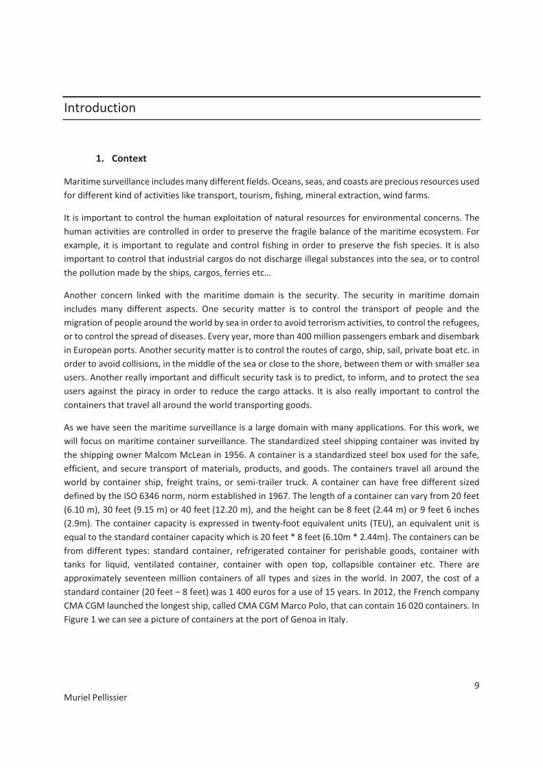
CMA CGM launched the longest ship, called CMA CGM Marco Polo, that can contain 16 020 containers. In

Figure 1 we can see a picture of containers at the port of Genoa in Italy.

10

Muriel Pellissier

Figure 1: Picture of containers at the port of Genoa in Italy

Most of the goods are transported by maritime containers all around the world and the number of

containers travelling every day keeps increasing. Nowadays, more than 90% of all world trade is

transported by maritime cargo containers moving from port to port. For example, 5/6 thousands of

containers arrive every day only in the port of Rotterdam in Netherlands. It is necessary to control the

container activities in order to detect threats like illegal activities, terrorism, miss-declaration, fraud,

quota-related, illegal products, hidden activities, or drug and arm smuggling. For example, a case of drug

smuggling was released in the press in 2000 [1]. The US Customs stopped a container containing marijuana

in the port of Everglades in Florida. The ship containing the container arrived from Kingston in Jamaica

and had for destination the port St John in Antigua. The container was manifested as “commercial cleaning

solvents”, some financial information was removed from the itinerary information and an extra port was

visited during the shipment. Another known example is an arm shipment going to El Salvador passing by

the port of Portland in the USA [2]. The content of the containers was hidden and the original port of

departure was removed from the itinerary information. As the cost and the human resources needed to

physically check a container are really high, only 1-2% of the containers can be physically controlled by

the customs. From statistics, around 10% of the containers are risky containers. As only few containers

can be checked and as the percentage of suspicious containers is not that high, it is not worth doing some

random physical checks on containers. As long as the number of containers travelling every day in the

world is so important, it is necessary to improve the targeting of suspicious containers in order to inspect

only the containers that are of high risk. In order to facilitate the targeting of anomalous containers, some

tools are needed to facilitate the targeting performed by the customs. Therefore, the maritime anomaly

detection field is more and more studied.

11

Muriel Pellissier

2. Anomalies

There exist many definitions on what the maritime anomalies are. In order to understand what an

anomaly is we need to define what a normal behavior is. Several definitions can be found for the normal

behaviors. For example, the normal behaviors are defined as the predictable events, as the events that

are recurrent, as the events that repeat in a predictable manner, or as the events that are frequent. The

anomalies are defined as the non-normal behaviors, as the unusual behaviors, as unexpected behaviors,

as the non-predictable events, as the infrequent events, as the extreme values, or as the events that

deviate from the routine. A general definition of the maritime anomaly detection could be to find unusual

behaviors using maritime information in order to improve the security of the citizens. For our application,

we define the anomalies as unexpected events, and as behaviors that are quasi-identical to normal

behaviors. It means that the suspicious containers behave as close as possible as normal containers.

3. Data

The maritime data can be of many different forms. We will list here some of them: vessel containers,

shipping company, cargo owner, route of a container (departure port, transshipment ports and arrival

port), image controls, time of the travel of a container, geographical position of a ship, speed of a ship,

weight of a container, Automatic Identification System (AIS) which is an automatic tracking system used

on ships in order to locate them. The AIS information gives different kind of information: a unique

identification of the ship, the ship position, the ship course, and the ship speed. The ship position is the

geographical position of the ship on the ocean. The ship course is the angle (in degrees) between the

actual path of the ship and a fixed reference object (usually north). This information is provided by AIS

equipment in the ship that communicates by electronically exchanges with the AIS Base stations. As the

equipment is inside the ship, the interruption of the signal could be of several causes. It could be because

of bad reception of the signal in areas that are not well covered, because of technical problems or due to

volunteer purposes in order to hide the ship information at least for a while.

4. Anomaly detection techniques applied to maritime security

The problem with maritime container surveillance is that many factors can influence the routes taken by

a container ship. A change in the itinerary can be justified by the global economic conditions, by cultural

factors, by political factors, or even by environmental factors. For example, a ship itinerary is conditioned

by political factor as embargo, an American ship cannot go in a Cuban port otherwise it is a violation of

the embargo imposed by the US on Cuba. Or a ship may deviate from his original route because of the

weather condition, like hurricane, iceberg, tide, or natural phenomena. A ship may change his route

depending on the fluctuating price of the oil a different market could be attracting. For example, if the

price of oil goes down enough, it makes the price of Brazilian bananas attractive to the French market,

and in consequence the bananas coming from other places will decrease. A ship may react also to the

crisis: a transporter could change the type of cargo to reduce the expenses, and/or the itinerary in order

to reduce the travel expenses. A ship might also change his route for “bad” purposes in order to avoid the

quotas legislation, to avoid taxes, to transport illegal products etc.

12

Muriel Pellissier

The purpose of the maritime anomaly detection is to sift through large quantities of data and spot the

data that are worthy of interest. The data worthy of interest are the anomalous data. As we have

described previously the data worthy of interest for the maritime security are data that have unusual,

infrequent, or suspicious behaviors. First, the idea is to find the normal behaviors. The normal behaviors

are the recurring events, also seen as the frequent events. Once the normal behaviors are defined, we

can spot the events that are suspicious which means the events that are different from the normal ones.

Martineau et al. [3] summarize some current studies on maritime anomaly detection that we will describe

in this paragraph.

Many techniques, before using the data, merge the data from different sources, different types, different

formats, or different precisions. The fusion of the data is used to reduce the volume of the data and to

improve the quality data in order to have the most accurate data as possible. As some data may provide

incomplete or uncertain information, by merging several data together these incomplete data can be

improved. For example, in order to detect the exact geographical position of a ship on the ocean several

types of data given the position of the ship can be used and merge together: the radar contacts, the

reconnaissance aircraft or aerial vehicles, and the Automatic Identification System (AIS). The radar

contacts give information with an elliptic error, they are limited in range, and they can miss small vessels.

The position given by the reconnaissance aircraft or aerial vehicles can be imprecise and they cannot cover

everywhere. And the AIS emissions are limited to certain areas, they may be interrupted, and only vessels

over 300 tons are equipped with transmitter. As all of these data are imprecise or can have some errors,

with the fusion of all these data it is possible to obtain the geographical position of the ship as close as

possible to the real position. We will not explain more details about the fusion process of data as it is a

full topic by itself. Moreover, we do not have different types of data available for our application so we

cannot merge data.

Many techniques use the Automatic Identification System (AIS) data in order to discover suspicious

(unusual) behaviors. We will describe some of them on the following paragraph. As explained previously,

the AIS data contain different information: the unique identification of the ship, the ship position

(geographical information), the ship course (orientation of the route of the ship), and the ship speed. We

will list several techniques using the AIS data in order to spot anomalous containers. These techniques

group ships together depending on their behaviors. All these techniques use different technologies to

learn the normal model and/or to detect the anomalies.

· Rhodes et al. 2005 propose maritime situation awareness technique [4]. This technique detects

the normal behaviors and learns continuously the models in order to detect deviation from the

normality. The anomalous (unusual) activities are detected using vessel data (speed, position,

etc.). In maritime surveillance the normality of an event can differ depending on the context like

the class of vessel, the weather conditions, the tide, the season, the time of day etc. The

continuously learning is used to continuously complete the set of rules in order to cover all cases.

Thus, a new event can be added to the normal event list or spotted as anomalous. They use a

modified version of the Fuzzy ARTMAP neural network classifier developed by Grossberg [5,6].

The ARTMAP algorithm is a learning algorithm that clusters features into categories using an

unsupervised approach. It also maps and labels the clusters using a supervised algorithm. A

13

Muriel Pellissier

threshold specified by the user, called vigilance, is used as the level of generality/specificity for

the clusters. With a high level of vigilance, the clusters will be more specific. An input pattern and

a pattern from the clusters are compared. If the match between two patterns (input pattern and

cluster pattern) satisfies the vigilance threshold, the input pattern is putted into the cluster. If the

match does not satisfy the threshold, the threshold is raised in order to learn correctly the training

example. The modified version of the ARTMAP algorithm uses the discovery of sub-space which

provides an effective feature for discernment between targets.

This technique does not need to have an operator supervising the process, except for an initial

bootstrapping phase. Then, the system is capable to discover normal and anomalous events and

is able to adapt to changing situation as it is continuously learning. This technique can benefit

from the operator knowledge as they can respond to the alerts defining an alert as suspicious or

as not suspicious. The model is then updated with the new status of the alert using the operator

knowledge. This technique can detect normal behaviors or anomalies only as continuous events.

If a normal behavior is formed by un-continuous events, which means that if the normal events

have an unusual order, this technique will not be able to detect them as it does not take into

account sequences or sets of events as behaviors.

· Garagic et al. 2009 propose an improved version of the previous technique developed by Rhodes

et al. [4] in order to detect anomalies [7]. They define the normal behavior as activity that occurs

frequently and anomaly as a rare activity that is different from the normal activity. The method

described previously [4] uses uniform probability inside a category. This technique [7] replaces

the fuzzy ARTMAP algorithm by a multidimensional probability density component. The

probability density function is calculated using the Expected Maximization (EM) algorithm [8] to

minimize the Killback-Leibler information metric [9]. The novel adaptive mixture-based neural

network classifier algorithm is used to determine the highest probability to assign to a category.

Then, a random input is compared to a specific category using the Mahalanobis distance (distance

based on correlations). If the distance is too high, the input will be defined as anomaly. If the input

is not an anomaly, a new category will be created. The probability density of this new category is

calculated as described previously.

This technique is a powerful tool for real world applications in maritime domain awareness. The

speed and the performance of the learning algorithm make it suitable for a real-time application.

Thanks to the learning algorithm this technique can adapt to changing situations. The robustness

of the overall system could be improved and as the previous method, the importance of the data

order should be reduced.

· De Vries et al. 2008 developed a technique to characterize the vessel behaviors using a semi-

automatic ontology [10]. This method uses a Hidden Markov Model (HMM) to characterize the

trajectory of ships using the AIS tracks. Then, the models are clustered to form classes of ships.

All the ships of a class share the same behavior. This technique is not an anomaly detection

technique, but as the vessels are classified into several groups where the behavior is supposed to

be normal, it is possible to spot the vessels that do not behave as the behavior of the different

groups.

14

Muriel Pellissier

This technique shows that the combination of machine learning and ontology engineering works

well and that there are interesting possibilities to explore. This technique opens the combination

between these two different fields but more experimental evaluations are required. This

technique can be used in the maritime domain and also in other domains, like domains related to

moving objects, such as cars or planes. But the technique needs to have good information

available on the domain used by the technique in order to cluster the entire data set. The Hidden

Markov Model is a well-known method to model data, for this application, another model could

be found in order to model the data in a faster way.

· De Vries et al. 2009 proposed another technique to model the ship trajectories using an

unsupervised method [11]. In order to model the trajectories of the ships this technique uses the

vessel tracks – AIS data. The Douglas-Peucker algorithm is used to compress the vessel tracks. The

Douglas-Peucker algorithm, also called Ramer-Douglas-Peucker algorithm, is used to reduce the

number of points in a curve by approximating a series of points. The simplified curve is composed

by a subset of the points that defined the original curve. The vessel tracks are then split into

segments. Different classes are created using the Affinity Propagation clustering. The Affinity

Propagation algorithm is an algorithm that identifies exemplars among data points and forms

clusters of data points around the exemplars. The exemplars are data points that represent

several data points. The algorithm consider all the data as potential exemplars and exchange

messages between the data points until a good set of exemplars is found in order to create the

clusters [12]. Using the vessel track of a ship, they can predict its future position by using the class

that is the closest to the vessel track. The anomalies can be detected by comparing the predicted

position and the actual position of the vessels.

This technique is an unsupervised approach that models the ship trajectories in clusters, it can

predict a ship trajectory thanks to the clusters, and it can detect anomalous ship track by

comparing the prediction to the actual position of the vessels. This technique does not take into

consideration for the model of the trajectory the type of the ship, even though the behaviors of

the ships depend on the type of the ship.

· Ma et al. 2009 propose a technique to spot the hidden behaviors [13]. The speed, the orientation,

and the position of the ships are used to classify the ships into different clusters defining the

normal behaviors. The classification is done using a Hierarchical Dirichlet process clustering. The

Hierarchical Dirichlet process (HDP) is a nonparametric Bayesian approach that clusters grouped

data. Each group of data is modeled with a mixture. Components can be shared across groups

which allow dependencies across groups. Once the ships are clustered in several groups, each

trajectory is then compared to the normal behaviors and detected as anomaly if the likelihood of

occurrence is below the anomaly threshold.

This technique can detect anomalies on ship behaviors depending on the trajectory of the ships.

Some results are given using parking lot data set [14]. Using a large data set require a large amount

of space to store the similarity matrix and a high computational cost to compute the similarities

of all the pairs of trajectories. For example, it is difficult to calculate the eigenvectors on a huge

matrix.

15

Muriel Pellissier

· Quanz et al. describe an anomaly detection technique for maritime security using cargo equipped

with sensing and communication abilities [15]. The shipment routes form a network of sensor

nodes. They define the anomaly (outlier) as an observation that deviates from the historical

patterns. The algorithms automatically learn the normal behaviors as rules. Groups are created

containing information sharing the same conditions. The anomaly detection is done on groups of

nodes and individual nodes. This technique provides also a real-time system that learns

continuously. They use three different algorithms for the anomaly detection. The first algorithm

is an Online One-Class Support Vector Machine (OOCSVM) which estimates the support of the

training data distribution. The OOCSVM tests each training instance with the current model. If the

instance is not classified, the current model is updated. The second algorithm is an online real-

valued Artificial Immune System (AIS) which compares random data with the training data in order

to discover the anomalous data. A distance between a given data and a training data is calculated.

If the distance is above a specified threshold the data is deleted because it is considered as similar

to the training data. If the distance is below the threshold the data is kept as anomalous. The third

algorithm is a simple threshold approach where the maximum value and the minimum value for

each feature in the training data are stored. The data are tested and spotted as anomalous if the

value exceeds the training stored values.

This technique improves the transportation chain security thanks to an anomaly detection based

on sensor data. Some experimentations on data have demonstrated the effectiveness and

feasibility of this approach. Although, this technique cannot relate the detection of anomalies on

individual objects (an object that affects individual objects) and the detection of anomalies on

group of objects (an event that affects the entire group of objects) as the two anomaly detection

parts are not combined. The use of this technique is a bit complicated because many parameters

have to be set as each algorithm has their own parameters.

Other techniques use the fusion of data, which means that they use many different kinds of data at the

same time in order to have a better picture. For these techniques, the first step is the data fusion. As

explained before, the fusion of the data process use data from different sources and combine them

together in order to improve the quality of the data. Even if these techniques have the same aim as our,

they are really different from our anomaly detection technique, by consequence, we will present only

briefly some techniques applied to the maritime surveillance using the fusion of different kinds of data.

The following techniques, as the ones we previously explained, cluster ships together depending on their

behaviors.

· The SeeCoast system [16] uses video data, radar detections, and Automatic Identification System

(AIS) data. This technique fuses all these different data in order to generate the tracks for vessels

approaching the port or the vessels already in ports. The system is able to detect, classify, and

track the vessels thanks to the video processing.

· The SCANMARIS project is used to detect anomalous vessels [17]. This method learns the normal

behaviors (Learning Engine) and then extracts automatically the anomalous vessels (Rule Engine).

This technique fuses different types of data: coastal radar, Automatic Identification System (AIS),

16

Muriel Pellissier

online databases, etc. The fusion of the data helps to add information to each vessel that is

detected like name, flag, type, operator, owner, tonnage characteristics, etc.

· The project SECurity system to protect people, goods, and facilities located in a critical MARitime

area (SECMAR) was developed by Thales Underwater Systems [18]. The system can detect

automatically the threatening targets using different types of data, like, underwater sonar

surveillance, above water radar surveillance, electro optic data, Automatic Identification System

(AIS) data, and information provided by the ports. This technique is used for detecting potential

terrorist threats by the sea, using data from the sea surface or under water data.

· Carley et al. 2009 use network analysis in order to detect anomalies for the maritime domain [19].

They use Automatic Identification System (AIS) tracks, boarding reports, port information, and

land data. This technique can detect different types of anomaly, for example, it can identify

suspicion on ship owners, crews, passengers, ports, and locations.

The two following techniques do not cluster the ships as the previous techniques which were based on

the ship behaviors. But they partition the oceans/seas by regions. Once they have modeled the behaviors

of the ships by areas, they can detect the abnormal behaviors depending on the behavior of a ship within

a specific area.

· The Learning and Prediction for Enhanced Readiness (LEPER) is a project sponsored by the Office

of Naval Research (ONR) [20]. This method predicts the position of vessels using Hidden Markov

Model prediction. The trajectories of ships are decomposed into sequences using a military grid

reference system. The Hidden Markov Model is used to calculate the probabilities between grid

locations using the sequences of ship trajectories. A vessel is anomalous if the distance between

the prediction and the actual position of the vessel is above a predefined threshold.

The project LEPER is a toolkit of components that can model normal behaviors and detect

anomalous behaviors, it can recommend actions against the threats, and detect strategy changes.

It has been tested on maritime data and all the anomalies were detected. More applications could

be done using multi-modal data and multi-grid scales.

· Janeja et al. 2004 present a study using the characterization of regions surrounding the locations

of interest in order to detect anomalous trajectories [21]. The areas are partitioned into regions

using Voronoi diagrams. The Voronoi diagrams are used to divide space into regions. A Voronoi

region contains every point whose distance to that region is less or equal to any other region.

Each region is defined with a specific vector representing the normal trajectory for this region.

Several regions can be grouped together if they have similar behaviors. The vector of the new

region is the average of all the vectors of all the regions used to create this new region. The

anomalies are detected using the combination of the path of a ship depending on the region.

This technique detects trajectory anomalies by characterizing the behaviors by regions. More

criteria could be added using different weights in order to define different levels of importance of

certain situations which will describe more accurately the behaviors in the different regions.

17

Muriel Pellissier

5. Our problem

The problematic that we have is to develop an anomaly detection technique that detects suspicious

containers using only few information about the container route. Many anomaly detection techniques for

maritime surveillance already exist and can really efficiently target suspicious behaviors. But most of these

techniques need a lot of information about the container route, the ship geographical position, knowledge

on the data etc. There is a need for the customs to detect suspicious containers using only the most basic

information. And it is important that a person that does not have any knowledge on maritime shipment

is able to use the anomaly detection technique. This anomaly detection technique is not a real time

application which means that the aim is not to use real time data but to use historical data. The anomalies

detected with historical data are information used by the customs to understand better their data, or a

situation, to help them to analyze the data, or to make statistics on the data etc. We define the suspicious

containers as containers behaving as close as possible as normal containers in a way that they do not

attract the attention of the customs. It means that the suspicious containers behave quasi-identically as

the normal containers. Thus, we are looking for containers that have a behavior slightly different from the

frequent behaviors.

As we have said the main, and important, difference between the techniques described previously and

our problem is the available data. We have access to a broad data set of container itineraries but we do

not have access to various kinds of data. For example, we do not have the AIS information for each ship,

thus, we do not know all the geographical positions of a ship during his whole travel. But we do have

information about the container events. When a container enters a port an event is created and some

information is available. An event defines what happened to a particular container using the container

identification number of the container at a particular date at a particular location. The different events

that can happen to a container is: departure, transshipment or arrival. For example, the container that

has the identification number 5016 leaves from the port of Rotterdam the 24th of January 2010. Some

events also mention the vessel name involved. The available data are container events from

heterogeneous, publically available sources. The integration of the collected data into a coherent data set

requires significant semi-automatic transformations and cleaning that deals mostly with non-standard

text strings defining geographic locations and container event types. The resulting dataset is stored in a

data warehouse which facilitates the analysis processes by using appropriate data structures and indexes.

The data set contains information in the form of container events. Currently the dataset contains more

than 900 million events and about more than 12 million containers. With the container event information

we can easily form the container itineraries. A container itinerary is the travel of a specific container (using

the container identification number) from his departure port to his arrival port, passing potentially

through transshipment port(s). The Figure 2 is an example of an itinerary with one transshipment port:

the container leaves from Singapore, goes to Chiwan and ends its trip in Rotterdam.

18

Muriel Pellissier

Figure 2: Itinerary from Singapore to Rotterdam passing through Chiwan

All the techniques that we have described previously share the same goal which is the maritime

surveillance. They also share the same principle: they detect common behaviors using maritime data

available, and then they detect the abnormal behaviors using the common ones. Our approach has also

the same principle and the same application. We want to detect anomalies in maritime containers data

thanks to a comparison between the normal container behaviors and random ones.

We developed an anomaly detection technique for maritime surveillance but our technique can be used

for other application too. The maritime data used are container itineraries which can be seen as ordered

sequences of events. The events are ports and an itinerary is composed by the departure port, followed

by the transshipment ports (if there is any transshipment port) and ending with the arrival port. Thus, this

technique can be used for any domain that uses sequences. A sequence is an order list of events as the

itineraries. This technique detects anomalous sequences based on the order of the events and the position

of these events within the sequences. The anomalous sequences are sequences that are close to normal

sequences but with some small changes. The normal sequences are the sequences that are common in

the data set. With this technique we compare a normal sequence with a random one in order to detect

that sequence as normal or as anomalous. The anomalous sequences are sequences that are similar to

normal sequences but not exactly identical. For example, if we have a normal sequence “a b c d e” we are

interested to detect the sequences that are almost identical to that sequence. Anomalous sequences

could be of different types:

· “a b d e”: where one event has been removed from the original sequence

· “a b f d e”: where one event has been replaced by another event from the original sequence

· “a b c d e f”: where one event has been added from the original sequence

· “ a c b d e”: where two events has been inverted from the original sequence

Anomalous sequences are only the sequences that contain few modifications from the normal sequence.

If the differences between the normal sequence and a random one are too important the random

sequence will not be spotted as anomalous compared to that normal sequence. For example, the

sequence “a d e c b” is too different from the normal sequence “a b c d e” to be spotted as anomalous.

Even if the two sequences have the same events within the sequences, both sequences are really different

because almost all the events have a different position with the sequences. Thus, we cannot say anything

about that random sequence based on that normal sequence.

Our anomaly detection approach is divided into two steps. First, we will find the normal sequences (for

our application the normal sequences are normal container itineraries). In order to detect the normal

19

Muriel Pellissier

sequences we will use an unsupervised approach, which means that we will use the whole data set (the

normal and abnormal sequences). We use the regular expressions in order to detect the common

sequences. Then, we compare random sequences from the data set with the common ones in order to

define them as normal or abnormal. In order to compare a common sequence and a random one, we

calculate a distance between them two. Depending on the value of the distance, the random sequence

will be defined as normal or anomalous.

In the following chapter, we will describe some existing techniques applied to the maritime domain using

graphs, some sequence mining techniques and some string distances. Then, we will explained in details

our approach and give some experiments using experimental data and real-world data.

20

Muriel Pellissier

Literature Review

In this section, we will first present some graph-based anomaly detection techniques that can be used

with maritime data. As we have seen previously, our data can be seen as sequences of events that happen

to maritime containers. Therefore, we will describe some sequence mining techniques. And as our

technique calculate the distance between two sequences; we will explain the main distance functions.

I. Graph-based anomaly detection

As we have seen previously, most of the anomaly detection techniques applied to maritime domain are

different from our approach because they use different maritime data. Some anomaly detection

approaches that are used in maritime domain and could also be used with our data are the graph-based

anomaly detection techniques. For example, using our data, an itinerary could be represented with a

graph.

A graph is a representation of a set of objects where some of them are connected by links. A link connects

two objects. The objects are called vertices/nodes and the connections are called links/edges. The edges

can be directed. A directed edge connects two vertices together in one way only. For example, the edge

a to b is directed. Or the edge between two vertices can be undirected. An undirected edge links two

vertices in both ways. For example, the edge a to b and the edge b to a are the same. For example, a graph

represents the route taken by a car. The car starts from Milan and stops in Grenoble. The graph

representing this information will be directed as there is a link only from Milan to Grenoble, the link

Grenoble to Milan should not exist. At the opposite, if the car goes from Milan to Grenoble and then come

back to Milan, the graph will be undirected as both directions exist. A sub graph is a part of the whole

graph, it is also called substructure. A graph can be composed by several sub graphs.

Knowing the definition of a graph, we can easily represent our data set with graphs. The whole data set

will be a graph that contains many sub graphs. Each sub graph will represent one itinerary. In Figure 3 we

can see an example of a sub graph representing an itinerary going from the port of Singapore to the port

of Chiwan passing through the port of Rotterdam.

21

Muriel Pellissier

Figure 3: Graph representation of the itinerary Singapore, Rotterdam, Chiwan

We will now describe several graph-based anomaly detection techniques.

1. Graph-Based Anomaly Detection

Noble et al. described two techniques to detect the anomalies in data that are represented with a graph

[22].

The challenge of the anomaly detection research is to define what an anomaly is. For this study, they

describe an anomaly as a surprising or an unusual pattern.

· Anomalous substructure detection:

The first technique is a general technique that uses the whole graph to detect the abnormal

substructures contained in the graph. The anomalies are defined as unusual events, which means

that the abnormal events are infrequent patterns. But it is not enough to detect only the

infrequent substructures in order to detect the anomalous substructures of a graph as the large

substructures occur only rarely. For example, the structure of the whole graph is present only

once. Thus, if the whole graph is seen as a substructure, it will be detected as an anomaly as it

occurs only once. In order to detect the unusual substructures they use the Subdue system [23].

The Subdue system is a graph-based data mining project that detects the repetitive patterns. As

we have seen before, an anomaly is an unusual event and it can be also defined as the opposite

of a common event. The repetitive patterns occur frequently in a graph and the anomalies occur

infrequently. In that case, Subdue will not detect the repetitive patterns but their opposites. The

Subdue system creates a list of substructures. It starts by creating one substructure for each

vertex of the graph. The substructures are extended by adding another vertex and its

22

Muriel Pellissier

corresponding link to the previous substructures. Every substructure is extended with the same

process. Once all the substructures are created, the best substructures are detecting using the

Minimum Description Length (MDL) heuristic [24]. The MDL is used for compressing the data using

the regularities of the data set. The Description Length of a substructure is the lowest number of

bits that is needed to encode it. The best substructure is the one that minimize the equation (1):

Where G is the entire graph, S is a substructure of G, DL(G/S) is the Description Length of the

graph G after compressing it using the substructure S, and DL(S) is the Description Length of the

substructure S.

The Figure 4 is an example of a graph composed by five sub graphs. The structure that can

compress the most the graph is the best structure that connects the node A to the node B.

Figure 4: Example of a best substructure

The measure F(S,G) estimates how well a substructure compresses a graph. The amount of

compression is linked to the substructure size and its number of instances. Large substructures

are expected to occur only rarely, and small substructures are less likely to be rare. Thus, the aim

is to discover small rare substructures. The frequent substructures, also called best substructures,

have low values of F(S,G). For detecting the anomalies of a graph, the infrequent substructures

are important. Unlike the frequent substructures that have a low value of F(S,G), the infrequent

23

Muriel Pellissier

substructures have a high value of F(S,G). In order to avoid the problems of the entire graph and

of the single vertex that will have high values of the equation (1), and knowing that the

compression of a graph depends on the size of the substructure, they do not use directly the

formula (1) but the derived equation (2):

Where Size(S) is the number of vertices contains in the substructure S, and Instances(S,G) is the

number of times that S is present in the graph G.

F’(S,G) is an approximation of the inverse of F(S,G). Therefore, S will be defined as an anomaly if

F’(S,G) has a low value.

· Anomalous sub graph detection:

The second anomaly detection technique developed by Noble et al. partitions the graph into

distinct substructures and it determines how anomalous is a sub graph compared to the other

ones. As for the previous method, the anomalous substructures are seen as the opposite of the

common substructures. Subdue is also used for this technique to detect the best substructures

by running several iterations on one graph. On each iteration, Subdue discovers the best

substructures using the Minimum Description Length (MDL) heuristic [24]. Then, the graph is

compressed using the best substructures found by Subdue, which means that a best substructure

is replaced by a single vertex in the entire graph. The next iterations will use the compressed graph

in order to detect the new best substructures. The substructures that can compress the best the

graph will be discovered at the first iterations. For example, after many iterations, Subdue will

find as best substructures, substructures that occur only few times as all the more common

patterns have already been detected. Thus, this technique needs to take into account when the

best substructure is obtained (the number of the iteration i) and how much the substructure can

compress the graph. The anomalous sub graphs tend to experience less compression than the

other sub graphs as they contain few common patterns. The anomalous sub graphs are found

using the principle that a sub graph that contains many common substructures is less likely to be

anomalous than a sub graph that have only few common substructures. An anomalous sub graph

is detected with a high value of the equation (3):

Where n is the number of iterations and DLi(G) is the description length of the sub graph after the

ith iterations. The fraction is the percentage of the sub graph that is compressed

at the ith iteration. All the sub graphs begin with A = 1, the value of A decreases depending on the

portions of the sub graph that are compressed during the iterations.

24

Muriel Pellissier

· Experimentations:

They tested these two techniques using the 1999 KDD Cup network intrusion dataset [25]. The

data are connection records which are labeled as normal or as one of the thirty seven different

attack types. Each record contains forty one characteristics that describe the connection, like

duration, protocol type, number of bytes etc. They created samples of data containing a certain

number of records from the data set. Most of the records of each sample are normal (96 – 96%

are normal records) and each sample contains only one type of attack. The assumption of these

unsupervised anomaly detection techniques is that the anomalous events are rare. Consequently,

these techniques would have worked very poorly if the samples were containing many attack

records. They tested these techniques with three different samples, varying the percentage of

attacks and the overall number of records. The first sample contains 50 records and 1 attack. The

second one contains 50 records and 2 attacks. The third sample contains 100 records and 2

attacks. Each sample was converted into a graph. The anomalous substructures are substructures

containing 2 or 3 vertices in order to avoid having a high computing time. They tested the three

different samples with all the different types of attack.

Using the first technique, the anomalous substructure detection technique, they limit the value

of to maximum 6 as they are interested only in the most anomalous substructures. The

maximum value is an arbitrary value, for this test the maximum value is set to 6 which is a

convenient value for this data set. The results were good for the sample containing 50 records

and one attack, only two types of attack worked poorly. The results for the sample containing 50

records and two attacks were poorer than the first sample. The attacks are not considered as

anomalous as they are 4% of all the records. As for the first sample, the same two types of attack

had poor results. The results for the sample containing 100 records and 2 attacks were the best,

slightly better than the first sample. As for the two other samples, the same two types of attack

had poor results.

Using the second technique, the anomalous sub graph detection technique, the results were

similar. The two same types of attack had poor results. The sample with 50 records and 2 attacks

did not have good results. The sample with 50 records and 1 attack had reasonably good results

and the sample with 100 records and 2 attacks had the best results.

These two graph-based anomaly detection techniques can spot the anomalies based on the facts that an

anomaly is the opposite of a normal event. The first technique examines the whole graph and detects

anomalous substructures contained in the graph. The second technique partitions the graph in sub graphs

and determines how anomalous each sub graph is compared to the other sub graphs. These two

techniques improve their results when the amount of available data increases. In order to have good

results the anomalies has to be really rare, which means that the number of anomalies has to be really

low compared to the normal data. As we have seen with the experimentations, we can see a difference

in the results when the anomalies are 2% of the whole data and when only 4% of the data are anomalous.

25

Muriel Pellissier

2. Detecting Anomalies in Cargo Shipments Using Graph Properties

Another anomaly detection technique using graphs is described by Eberle et al [26]. This technique uses

the variations of graph properties to detect structural anomalies in graphs. The aim of this technique is to

detect anomalies in structural data like cargo shipments data. They defined a graph anomaly as a change

in the structure and as a structural inconsistency. The anomalous structures are structures that are

different from the expected ones. As the anomaly reflects an event that wants to be hidden, the structure

of an anomaly should be similar to the normal structure of the graph but with some small differences. A

structural change could be of three different types: insertion, deletion, or modification. A substructure

could be added to the original structure, which means that a substructure of one or more edges and

vertices is added to the normal structure. Or a substructure could be removed from the original structure,

which means that a substructure of one or more edges and vertices is removed from the normal structure.

Or a substructure could be moved, a substructure of one or more edges and vertices is at a different place

in the normal structure and in the anomalous one. They applied this technique to real world data using

cargo shipments data. The shipments are represented with graphs; they can be expected or anomalous.

As defined previously the anomalous shipments are the graphs that are different from the expected ones.

They considered that the structural differences between graphs are determined by quantitative

measures. Thus, in order to detect the structural anomalies they use five different graph properties.

· Average shortest path length L:

In order to calculate the length of the shortest path between two connected vertices they use the

Floyd-Warshall all-pairs algorithm [27]. An adjacency matrix is created to determine the shortest

path length between two connected nodes. Once all the shortest lengths between all the

connected pair of nodes are calculated, they calculate the average length. The average length is

the sum of all the shortest lengths divided but the number of connected vertices. The value of the

average length will change if one shortest length between two vertices changes.

· Density D:

They define the density using the density definition for the social networks [28]. In a social

network, some entities are connected to other entities and an interruption of a relation between

two entities can affect the social network. In a same way, an anomaly can perturb the structural

relation between a set of data. The density D of a graph reflects how compact the graph is. The

density D is obtained by dividing the number of edges E of the graph by the maximum possible

number of edges (4):

Where E is the number of edges of the graph, V is the number of vertices of the graph, and V2 is

the maximum possible number of edges between V vertices.

The density value will change if a vertex or/and an edge is added or removed from the graph.

· Connectedness C:

26

Muriel Pellissier

They used a definition described by Broder et al. [29] that says that a set of vertices of a graph is

defined as strong-connected if for any vertices a and b of the set, there is a path from a to b in

the graph. Therefore, they calculate the connectedness of a graph using the set of vertices P that

contains all pairs (a,b), where there exist a path from a to b in the graph. The connectedness C is

the number of vertices of the set P divided by the number of possible pairs (V*V) (5):

The value of the connectedness will change if the number of edges changes. It means that if some

connections between vertices (connected directly or indirectly) are added or removed the

connectedness of the graph will change.

· Eigenvalues λ and ν:

This property uses, as the shortest path length, an adjacency matrix α. The element αij = αji = 1 if

there is an edge between i and j, otherwise αij = 0. The eigenvalue is the number λ and the

eigenvector is the vector ν that satisfy the equation (6):

There is one eigenvalue for each vertex. As observed by Chung et al. [30], most of the eigenvalues

are close to zero. Thus, the average of the eigenvalues is not useful information, only the

maximum eigenvalue λmax is used.

· Graph clustering coefficient CC:

The graph clustering coefficient is defined by Boykin et a. [31] as the average of the clustering

coefficients of each vertex (7):

Where V’ is the number of vertices of degree greater than 1, E is the number of edges, and k is

the degree.


They analyzed the effectiveness of this technique with synthetic data and cargo shipment data.

They created synthetic random graphs and they inserted randomly anomalies in the structure of

the graphs using some rules. The size of the graph containing the anomalies and the size of the

graph without anomalies are the same in order to be easily compared. The connections can

change but the number of vertices is identical. The density is also kept which means that the

number of connections is relatively identical. The computational complexity of some of the

measures increases as the number of connections increase. They use a ratio of approximately 4

edges for every 3 vertices. The size of the anomalies (number of vertices and number of edges)

influences the result. Thus, the anomalies inserted are proportional to the size of the graph. For

27

Muriel Pellissier

example, if the graph is small, the structure of the anomaly will also be small. They tested the

graph properties with different types of changes (anomalies). As we have described previously,

the structural changes could be of three different types: insertion, deletion, or modification. As

explained before an anomaly is a structure that is close to a normal one. The inserted anomalies

have a structure similar to the normal structure but not perfect. Consequently, the structure of

an anomalous graph and a non-anomalous graph are kept as similar as possible and the anomaly

structure has the same connection strategy than the rest of the associated graph.

They created six different graph sizes to test this technique containing 35 vertices, 100 vertices,

400 vertices, 100 vertices, 2000 vertices, and a dense graph of 100 vertices and 1000 edges. The

results shown with this experimentation are that certain properties can detect certain types of

anomalies. If the anomaly is an insertion of a substructure, the density and the connectedness are

useful to detect the anomaly. If a substructure has been removed from the graph, the eigenvalue

is used to detect the anomaly. If a substructure has been moved, the clustering coefficient and

the average shortest path length can detect the anomaly.

They tested this technique with real world data. The data used are the cargo shipments of the

imported items from foreign countries into the US. They created several graphs using the cargo

shipments data. They used 50 shipments per graph (about 1100 vertices). They introduced real

anomalies representing illegal cargo. The first anomaly is drug smuggling: some containers

containing marijuana were discovered in the port of Florida [1]. Some financial information was

removed and an extra port was traversed during the shipment. The second anomaly is an arms

shipment on the way to El Salvador passing by Portland [2]. The content of the containers was

hidden and the original port of departure was removed. For both cases, this technique had

detected the anomalies thanks to the density, the connectedness, and the clustering coefficient

properties.

As proved with the experimentations, this technique is able to detect if there is an anomaly within a graph

using the graph properties. It is important to keep in mind while using this technique that the

computational complexity increases with the number of connections. In order to have good results, the

anomaly has to be small compared to the size of the graph and the structure of the graph containing an

anomaly has to be as close as possible as the graph without anomalies. This technique detects if there is

an anomaly within a graph, the next step will be to detect what is the anomalous substructure. In order

to detect where the anomaly is within the graph, they proposed to partition the graph into smaller sub

graphs [32], [33]. Every sub graph is checked to know if it contains an anomalous graph using the different

properties. The anomalous sub graphs are divided into smaller sub graphs until the anomalous structure

is found.

28

Muriel Pellissier

3. Anomaly detection in data represented as graphs

Eberle et al. developed another technique to detect anomalies within a graph [34]. The purpose of this

anomaly detection technique is to detect anomalous data, like fraud, using data that can be represented

as a graph. It means that the data can be represented using vertices and edges. They have developed a

tool called Graph Based Anomaly Detection (GBAD) that detects anomalies in structured data. This

technique is an unsupervised approach which means that it does not required knowledge on the data.

The data does not have to be labeled and the system does not have to be trained for using this technique.

They defined the anomalies as hidden information, which means that the activities look as real as possible

to hide as much as possible the illicit behavior in order not to be caught easily. Thus, the anomalies have

to be close to the frequent patterns. An anomaly is an unexpected relationship between entities, where

the relationship is close to non-anomalous behaviors. Using the graph representation of the data, an

anomaly is a small deviation of the normal structure. The anomalies are of three different types:

modification, insertion, and deletion. The anomalies can be identifiable within a graph by small

modifications, insertions, or deletions of the graph structure. The modifications of a structure of a graph

are the modifications of a vertex and/or an edge of the normal structure. The insertions are the additions

of a vertex and/or an edge to the normal structure. And the deletions are the absence of a vertex and/or

an edge.

They have developed three different algorithms to detect the three different types of anomalies

(modification, insertion, and deletion) in order to detect the anomalous structures within a graph. Each

algorithm can detect one type of anomalies. The three different algorithms use the Minimum Description

Length (MDL) approach to first discover the common patterns. Then, the three algorithms have three

different approaches to detect the anomalies depending on the type of the anomaly.

In order to use this technique they assumed that the data is regular. The anomalies are only a small

percentage of the whole structure. For example, less than 10% of the structure of the graph is changed in

an anomalous structure in order to have anomalous structures that are close to the normal ones. The

normal structures, also defined as expected structures, are connected structures as they are not

interested to detect anomalies across disconnected structures. The normal structures have to be well

presented in the graph in order to distinguish easily the anomalous ones. It means that there are enough

samples of the normal structures within a graph to classify clearly the normal ones and the anomalous

ones.

We will describe now the three different algorithms used for this technique and then the

experimentations done on synthetic data and on real world cargo data.

· The first algorithm is the Graph-Based Anomaly detection – Minimum Description Length

algorithm (GBAD – MDL):

The GBAD-MDL algorithm uses the Subdue system [23] to detect the best substructure of the

graph. As we explained previously for the “anomalous substructure detection” approach [22], the

Subdue system is a graph-based data mining project that detects the repetitive patterns within a

graph. In order to detect the repetitive patterns, the Subdue system uses the Minimum

29

Muriel Pellissier

Description Length (MDL) approach [24] that discovers the best substructures of a graph G. The

best substructure is the structure that can compress the most the data using the regularity of the

data. Noble et al. [23] defined the best substructure as the structure that minimizes the

Description Length of G (equation 8).

Where G is the entire graph, S is a substructure of G, DL(G/S) is the Description Length of the

graph G after compressing it using the substructure S, and DL(S) is the Description Length of the

substructure S.

Once a best substructure has been found, this algorithm examines all the patterns that are

structurally similar with some relational deviations. The interesting instances are the structures

that are close to the best substructure but do not match exactly the best substructure. The level

of change between the best substructure and the patterns examined should be small in order to

consider only the structures that are the closest to the best substructure. Using a parameter called

“cost of transformation”, they calculate how close the instances are to the best substructure. The

value “1.0” is added every time a change is needed to obtain the substructure from an instance.

A change can be on a vertex or on an edge. As they are looking for hidden information, the

anomalous structure should be really close to the normal structure and they should occur rarely

within the graph. Thus, they do not have any interest in structures that are too different, which

means that the cost of transformation has to be less than a threshold defined by the user. And

the frequency of the anomalous structure should be low. Therefore, the potential anomalous

structures will be the ones that minimize the product “cost of transformation * frequency”. This

algorithm detects the modification anomaly type.

The Figure 5 is an example of a modification anomaly within a graph composed by five sub graphs.

The sub graph composed by the nodes A, B and C is detected as the best structure. The sub graph

composed by the nodes A, D and C is the anomalous structure as it is close enough to the best

structure and it is present only once in the graph.

30

Muriel Pellissier

Figure 5: Example of modification type of anomalies

· The second algorithm is the Probabilistic algorithm (GBAD – P):

This algorithm also uses the Minimum Description Length (MDL) approach to detect the best

substructure. Instead of looking at the changes of a structure, like the previous algorithm, this

algorithm examines the probability of all the extensions of the best substructure. An extension of a

structure is the original structure with an edge and a vertex added to it. The extensions with the lowest

occurrences (lowest probabilities) are the more anomalous ones. This algorithm detects the insertion

anomaly type.

The Figure 6 is an example of an insertion anomaly within a graph composed by five sub graphs. The

sub graph composed by the nodes A, B and C is detected as the best structure. The sub graph

composed by the nodes A, B, C and D is the anomalous structure as it is close enough to the best

structure and it is present only once in the graph.

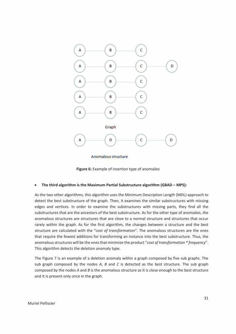
31

Muriel Pellissier

Figure 6: Example of insertion type of anomalies

· The third algorithm is the Maximum Partial Substructure algorithm (GBAD – MPS):

As the two other algorithms, this algorithm uses the Minimum Description Length (MDL) approach to

detect the best substructure of the graph. Then, it examines the similar substructures with missing

edges and vertices. In order to examine the substructures with missing parts, they find all the

substructures that are the ancestors of the best substructure. As for the other type of anomalies, the

anomalous structures are structures that are close to a normal structure and structures that occur

rarely within the graph. As for the first algorithm, the changes between a structure and the best

structure are calculated with the “cost of transformation“. The anomalous structures are the ones

that require the fewest additions for transforming an instance into the best substructure. Thus, the

anomalous structures will be the ones that minimize the product “cost of transformation * frequency”.

This algorithm detects the deletion anomaly type.

The Figure 7 is an example of a deletion anomaly within a graph composed by five sub graphs. The

sub graph composed by the nodes A, B and C is detected as the best structure. The sub graph

composed by the nodes A and B is the anomalous structure as it is close enough to the best structure

and it is present only once in the graph.

32

Muriel Pellissier

Figure 7: Example of deletion type of anomalies


They tested this technique with synthetic data and with real world data. The real world data used

for the experimentations are cargo shipment data. For both cases, the anomalies are slight

deviations from the normal structures, and the anomalies cannot be as common as the normal

structures.

For the synthetic data, they created randomly several graphs of various sizes. For each of these

graphs they created 30 graphs containing random modifications, insertions, and deletions. The

insertions are structures with added vertices and/or edges compare to the normal one. The

modifications are structures with modified vertices and/or edges. And the deletions are structures

with deleted vertices and/or edges. The anomalous structures are slight deviations from the

normal structures with a low frequency. They tested this technique with several sizes of graphs,

several sizes of common structures, several sizes of anomalies, and different anomalous

thresholds. For each test, they calculated the percentage of complete anomalous structures

discovered. They also calculated the percentage of part of anomalous structures discovered, it

means that only some vertices or edges were discovered but not the whole anomalous structure.

And they calculated the percentage of false positive anomalies. False positive anomalies are

structures that were not injected as anomalous in the graph. In order to calculate these

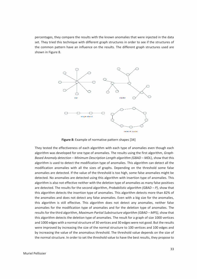
33

Muriel Pellissier

percentages, they compare the results with the known anomalies that were injected in the data

set. They tried this technique with different graph structures in order to see if the structures of

the common pattern have an influence on the results. The different graph structures used are

shown in Figure 8.

Figure 8: Example of normative pattern shapes [34]

They tested the effectiveness of each algorithm with each type of anomalies even though each

algorithm was developed for one type of anomalies. The results using the first algorithm, Graph-

Based Anomaly detection – Minimum Description Length algorithm (GBAD – MDL), show that this

algorithm is used to detect the modification type of anomalies. This algorithm can detect all the

modification anomalies with all the sizes of graphs. Depending on the threshold some false

anomalies are detected. If the value of the threshold is too high, some false anomalies might be

detected. No anomalies are detected using this algorithm with insertion type of anomalies. This

algorithm is also not effective neither with the deletion type of anomalies as many false positives

are detected. The results for the second algorithm, Probabilistic algorithm (GBAD – P), show that

this algorithm detects the insertion type of anomalies. This algorithm detects more than 82% of

the anomalies and does not detect any false anomalies. Even with a big size for the anomalies,

this algorithm is still effective. This algorithm does not detect any anomalies, neither false

anomalies for the modification type of anomalies and for the deletion type of anomalies. The

results for the third algorithm, Maximum Partial Substructure algorithm (GBAD – MPS), show that

this algorithm detects the deletion type of anomalies. The result for a graph of size 1000 vertices

and 1000 edges with a normal structure of 30 vertices and 30 edges were not good. But the results

were improved by increasing the size of the normal structure to 100 vertices and 100 edges and

by increasing the value of the anomalous threshold. The threshold value depends on the size of

the normal structure. In order to set the threshold value to have the best results, they propose to

34

Muriel Pellissier

have a first run to detect the normal structure size. The maximum size of the anomalies is

determined thanks to the size of the normal structure. As we have explained previously the

normal structure and the anomalous one are close, around 10% of the structure can change

between a normal and an anomalous structure. This algorithm does not have good results with

the modification type of anomalies. The algorithm does not detect any anomalies but detects

many false positives. The algorithm does not detect anything with the insertion type of anomalies.

They tested these three algorithms using the different structures of graph seen previously. All the

results are identical except for the star pattern.

They also tried this technique with real world data. The data are cargo shipments obtained from

the United States Customs and Border Protection (CBP) [35]. These data are the information

about the imports into the US by maritime containers. They created graphs that represent cargo

information. They first tested this technique with small random changes (modifications, deletions,

or insertions) on random shipping entries. These data are not as regular as the synthetic data, but

the three algorithms found successfully all the inserted anomalies without any false positive

anomalies been detected. Then, they tried this technique with real world scenarios. They tested

it with a drug smuggling case. A ton of marijuana was discovered in a port in Florida [19]. Some

financial information was hidden, and the shipment went to an extra port during the shipment.

The algorithm GBAD – MDL did not detect any anomalies, which is normal as no modification

anomalies were present. The algorithm GBAD – P detected the insertion of the extra port as an

insertion anomaly. And the algorithm GBAD – MPS found the missing financial information as a

deletion anomaly. They also tested this technique with a simulation of a real world anomaly. In

order to avoid quotas, embargoes, or prohibitions some information, like the port of origin, can

be changed. They changed the country of origin of one of the shipments. The algorithm GBAD –

MDL could detect the anomaly as it is a modification anomaly.

This anomaly detection technique is used to detect anomalies in data that can be represented with graphs.

The anomalies are defined as small deviations from a common structure. This technique detects three

different graph anomalies: modifications, insertions, and deletions. They proved the effectiveness of this

technique by testing this approach with synthetic data and with real world cargo data. As the anomalies

are not known in advance, in order to detect all anomalies of all the different types of anomalies of a data

set, it is needed to run the three different algorithms on the whole data set. Each algorithm has a different

threshold that the user has to set. Therefore, it is needed for each algorithm to run it several times with

different threshold values in order to obtain the best results. But as the anomalies are not known it is

difficult to evaluate what should be the best value for the different thresholds.

35

Muriel Pellissier

4. Graph-Based Anomaly Detection Applied to Homeland Security Cargo Screening

Eberle et al. proposed an improved technique of the graph-based anomaly detection technique presented

previously [36]. Knowing that many containers travel every day all around the world, strategic decisions

should be made to decide which cargo should be inspected carefully. For example, between 11 and 15

million of containers arrive into the United States every year. The aim of this technique is to be able to

improve the ability to target suspicious cargos in order to protect ports from illegal or dangerous goods

that could enter in a country. This technique can detect anomalous behaviors using cargo data. The cargo

data are shipping manifests. In order to detect the anomalous activities, they use the relationships

between the cargo data. The cargo data are represented with graphs which are analyzed in order to detect

the common patterns and the deviations of these patterns. This technique is an unsupervised approach.

An unsupervised approach is an approach that does not need to know what the normal behaviors are or

to train the data before using the technique. As the previous graph-based anomaly detection technique

[34], this technique detects three types of anomalies: modifications, insertions, and deletions thanks to

three different algorithms. For the previous technique, the three algorithms were implemented into the

Graph Based Anomaly Detection (GBAD) system based on the Subdue system. The Subdue system is a

graph-based knowledge discovery system [23] that detects the best structure in a graph using the

Minimum Description Length (MDL) heuristic.

One of the issues of the previous anomaly detection technique is the size of the cargo shipment

information. A graph that represents 500 shipments could result in tens of thousands of nodes and

vertices. Another issue is to detect if two structures are identical (also called graph isomorphism). In order

to facilitate the comparison between two structures they use the technique GASTON developed by Nijssen

et al. [37]. The GASTON technique uses a canonical approach to detect the frequent substructures of a

graph. This approach converts the graph into a string canonical form and performs a canonical-string

based graph match. The GASTON approach is an Apriori approach. All the embeddings of a graph are

stored in memory. The frequency of a structure is the number of different graphs in the embedding list of

that structure. The processing time using the GASTON technique is significantly improved compared to

the MDL approach used in the previous technique. They implemented the three GBAD algorithms into the

GASTON framework, which is called GBAD – FSM.


They tested this improved technique with ten different graphs having 550 to 281600 transactions. The

graph of 550 transactions contains 550 sub graphs. Each shipment is a disconnected sub graph. The

running time goes from 9.21 seconds (for the graph containing 550 transactions) to 2499.32 seconds (for

the graph containing 281600 transactions). The running time of the Minimum Description Length

algorithm (MDL) is linear. The running time of the Probabilistic algorithm (P) and the Maximum Partial

Substructure algorithm (MPS) is exponential after 140800 transactions. Thus, to have a good running time

using this technique, the number of shipments should be less than 140800. The P algorithm detects the

insertion type of anomalies. The MPS algorithm discovers the deletions. And the MDL algorithm detects

the modification type of anomalies. Only the MPS algorithm reported false anomalies.

36

Muriel Pellissier

They tested this technique with real world data [38]. Counterfeit boxes of laundry detergent were found

because of anomalies in the shipment details. The standard weight information of the container is

normally in pounds using a decimal point. In that anomalous container the weight was in kilograms using

a comma. They tested this anomaly using 550 shipment transactions. The graph was composed with 3840

vertices and 3584 edges. All the transactions were using as unit pounds and decimal point. One

transaction used kilograms and comma. The anomaly was detected by the MDL algorithm.

This technique uses a frequent sub graph mining approach to detect anomalies in cargo shipments data

that can be represented with graphs. This technique is efficient to detect the anomalies of a data set and

the running time has been improved compared to the previous technique using the Minimum Description

Length (MDL). This technique has good results with large graphs, but it is less efficient with very large

graphs (graphs containing more than 140800 transactions).

In this section, we have presented several graph-based anomaly detection techniques that can be used

with structural data as maritime data. For these techniques, the data are represented with graph

representations and the anomalies are structural anomalies. The anomalies are small structural changes

that could be of three different types: deletion, modification or substitution of a part of the structure. The

anomalies are detected by analyzing the properties of the graph or the structures (or substructures) of

the graph. Some techniques use the whole graph in order to detect the anomalous substructures. Some

other techniques partition the graph into several substructures and then compare all the substructures.

These graph-based anomaly detection techniques are efficient techniques that detect structural

anomalies based on the graph representation of the data. These techniques have good results with data

that contains only few anomalies within the whole dataset and where the normal structures are well

represented within the dataset. The normal structures have to be well represented within the dataset in

order to be able to detect easily the best substructures of the graph representing the whole dataset. As

explained previously, the anomalies are detected by comparing structures to the best substructures.

Indeed, if the normal structures are not well represented within the dataset, the best substructures will

be difficult to be detected and by consequences, the anomalies will be more difficult to be spotted

efficiently. Another limitation applied to these techniques is the size of the dataset. As the algorithms

involving graphs have a time complexity really high, the time of a graph-based anomaly detection

technique could be really important using a large dataset. While testing these techniques with our

sequential data, we have seen another important limitation using these techniques. The limitation is

linked with the graph representation of the data. We have realized that beside the fact that these

techniques are efficient only for dataset where the normal structures are well represented and where the

number of anomalies is low, it is not easy to find the efficient graph representation of the data in order to

use the graph-based anomaly detection techniques efficiently. For example, using our maritime dataset

where the order of the data and the position of the data is important, we could not find an appropriate

graph representation that could keep both information and detect efficiently the structural anomalies.

In the next paragraph, we will present the sequence mining techniques.

37

Muriel Pellissier

II. Sequence mining

As the nature of the data and the nature of the anomalies can differ depending on the domain, one

anomaly detection technique might be efficient for one domain but not efficient for another one.

Therefore many different anomaly detection techniques exist depending on the problem that needs to be

solved. Even if the algorithms are different, the principle of the anomaly detection techniques is often the

same. The idea is to detect in a given data set the patterns that are different from the normal behaviors.

The patterns that deviate from the normal ones are the anomalies.

The sequence mining techniques detect the anomalies in sequential data. A sequence is an ordered list of

events, also called symbols. A sequence is also called a string. A sequence can be finite like “1,2,3” or

infinite “1,2,3,…”. For this study we are interested only in finite sequences. The events are data using a

limited alphabet. For example, a text document can be seen as a sequence of words, and a gene as a

sequence of nucleic acids. A subsequence/substring is a part of a longer sequence/string where some

symbols are deleted from the original sequence and the order of the remaining symbols is kept. For

example, the subsequence “a b e” is part of the longer sequence “a b c d e”.

As sequences are ordered list of events, we can easily see a connection between our data and the notion

of sequence defined previously. The available data are container events. When a container enters a port,

an event is created given some information. The available information for each event is the identification

number of the container, the name of the port and what happened to the container at that specific

moment (departure, transshipment, or arrival). With this data we can easily create the itinerary of a

container. The itinerary tells the route of the container from its departure to its arrival. An itinerary is an

ordered list of events, where the events are ports. Thus, we can see our data set of itineraries as a data

set of sequences, where an itinerary is a sequence.

Different domains detect anomalies in sequences. For example, detecting anomalies in sequential data

can be used for biology in order to detect anomalies in DNA sequences [39], [40]. The alphabet

corresponds to the nucleic acid bases or amino acid bases. In that case the sequences are long and the

normal structures known. The idea is to spot the anomalous sequences within a long sequence knowing

the normal structures in order to detect mutations of DNA sequences or diseases. Another example is

detecting anomalies in system calls [41], [42], [43], [44]. The alphabet is made with all the possible system

calls or user commands. The anomalies are anomalous program behaviors that can be caused by virus or

an unauthorized user that wants to enter the computer system. For example, studying the sequences of

system calls you can detect an attack on a user session. Anomalous banking transactions, purchases can

also be identified using sequence anomaly detection techniques [45]. The sequences are the transactions.

The alphabet corresponds to all the actions possible for the users. The anomalies are irregular or abnormal

behaviors of customers.

Chandola et al. present a survey on anomaly detection technique for sequences that does not depend on

the application domain [46]. They give an overview of the existing research on anomaly detection in

38

Muriel Pellissier

sequences. They identify three different categories for the anomaly detection research using sequences.

The first category is the “sequence-based anomaly detection” that uses training data to create a model of

the data. Then, the test data set is compared to the model in order to detect the anomalies. For example,

the detection of illegal user sessions on a computer can be done using the past normal user sessions as

training data. The past user sessions are sequences of system calls or commands. A new user session (test

sequence) is compared to the past sequences (training sequences) in order to be defined as anomalous

or normal. The

second category is the “contiguous subsequence-based anomaly detection” where the anomalies are

subsequences of longer sequences. Each subsequence of a long sequence is compared to the other

subsequences of the same long sequence. The subsequences that are significantly different from the other

ones are anomalous. For example, it is possible to detect if a user’s account was hacked at some point

during a given day. The user’s day activity is a long sequence. The long sequence is tested in order to

detect anomalous subsequences.

The third category is the “pattern frequency-based anomaly detection” where the anomalies are detected

using the number of occurrences of the test patterns. A test pattern is anomalous if its frequency in a test

sequence is significantly different from its frequency in a sequence known to be a normal sequence. For

example, a particular sequence of commands made by a user can be detected as anomalous or as normal

depending on its frequency. The frequency of this sequence is compared to the expected frequency. The

sequence of commands is the query pattern made by the user, the frequency of that query pattern for a

given day is compared with the frequency of that query pattern in the past. For example, the sequence

“login, password, login, password” is normal if it occurs occasionally in a user’s daily profile, but it is

anomalous if it occurs frequently as it could correspond to an attempt to enter an unauthorized user’s

computer by trying several passwords.

1. The sequence-based anomaly detection techniques

The first group represents the sequence-based anomaly detection techniques. The anomalies are

detected thanks to the training data. The training data are sequences that are known to be normal. The

other sequences, called test sequences, are compared to the training data in order to be defined as normal

or as anomalous. Several techniques are part of this group.

a. Window-based techniques

The window-based techniques separate a sequence in fixed-length subsequences that are also called

windows. An anomaly score is calculated for each subsequences/windows. The anomaly score of the

whole sequence is obtained with the different anomaly scores of all the subsequences. These techniques

help to localize the cause of the anomaly within a sequence using the subsequences. It means that if a

sequence is detected as anomalous we can find with the subsequences which part of the sequence is

anomalous.

In order to define a sequence as anomalous, we need to extract the k-length subsequences of all the

sequences of the training data set. The frequency of each k-length sequence is calculated and defined as

the normal frequency. The second step is to extract k-length subsequences from a test sequence. A

39

Muriel Pellissier

likelihood score is assigned to each subsequence. The likelihood score is the frequency of the subsequence

in the training data set. A threshold is used to define a subsequence as anomalous or normal. A

subsequence is defined as anomalous if the likelihood value, which is the frequency, is below the threshold

and the subsequence is normal if the likelihood is above the threshold. The anomaly score of a test

sequence is proportional to the number of anomalous subsequence in the test sequence. The anomaly

score of the test sequence is the length of anomalous subsequences divided by the length of the whole

sequence. This technique is used for example for detecting intrusion in operating system call [47], [41],

[42], [44], [48], [49], [50], [51], [52], [53].

Several techniques exist based on the window-based approach. The different techniques differ on how

they assign the anomaly score to the windows and how they calculate the anomaly score of the whole

sequence. Some techniques are based on the frequency of the windows, some on the similarities between

two windows, or on labels (normal or anomalous) given to the windows.

Forrest et al. [42] described a technique to calculate the anomaly score of a subsequence using pairs of

symbols. Every pair (a,b)i is defined as normal if the symbol b occurs at the ith position after the symbol a

at least once in the subsequences of the training data set. The pairs of the test subsequences are

compared with the pairs of the training sequences. If a pair of a test subsequence does not exist in the

pairs found in the training sequences it will be defined as an anomalous pair. The anomaly score of a

subsequence is the number of anomalous pairs divided by the total number of possible pairs. For a k-

length subsequence, the number of possible pairs is k(k-1)/2.

Other techniques use the Hamming distance between two subsequences to obtain the anomaly score of

a subsequence [41], [53], [54], [49], [51], [52], [55]. The hamming distance between two sequences is the

number of symbols that are different between those two sequences. The anomaly score of a subsequence

of the test sequence is the hamming distance between that subsequence and the closest subsequence of

the training data set.

The similarity between two sequences can also be used for calculating the anomaly score between two

windows [44], [48], [56]. The similarity between a test subsequence and a training subsequence is

calculated. If two symbols from two different subsequences are identical at the location l, the value of the

similarity will be one, otherwise, the value is zero. If the previous symbols are also identical the similarity

value of the previous symbols will be added to the current similarity value. Therefore, if several symbols

are identical in a row the similarity value will be much higher than if only two symbols are identical. Thus,

the similarity is calculated using the continuity of the matching symbols, which means that the similarity

value will increase when several symbols will consecutively match. The anomaly score of a subsequence

is the inverse of the maximum similarity between a subsequence of the test data set and a subsequence

of the training data set.

Other techniques assign a label (anomalous or normal) to the subsequences in order to define a sequence

as anomalous or normal. The windows from the training sequences are labeled as normal subsequences.

Then, each subsequence from the test sequences is compared to the normal subsequences. If a

subsequence from the test sequences is not present in the normal subsequence list, the subsequence is

40

Muriel Pellissier

labeled as anomalous. In order to calculate the anomaly score of a test sequence, an anomaly score is

given to each subsequence of the test sequence. The anomaly score of a subsequence is zero is the

subsequence is normal and one if the subsequence is anomalous.

Once the anomaly score of each subsequence of a sequence is calculated we need to calculate the

anomaly score of the whole sequence. One sequence can be composed by several subsequences. All the

previous techniques focus on how to calculate the anomaly score of subsequences; other techniques

focus more on how to calculate an overall anomaly score for the whole sequence. Hofmeyr et al. [41]

proposed two different methods to calculate the anomaly score of the whole sequence. The first method

defines the overall anomaly score as the sum of all the anomaly scores of all the subsequences of a

sequence divided by the length of the sequence. The second method defines the overall anomaly score

as the number of the subsequences of the test sequence that are defined as anomalous.

Ghosh et al. [52] proposed another technique to calculate the overall anomaly score. Every subsequence

of a sequence is checked. If the subsequence is anomalous, the value one is added to the overall anomaly

score. If the subsequence is normal, the value one is subtracted to the overall anomaly score (the overall

score values cannot be negative, the minimum overall score is zero). If the overall anomaly score goes

above a threshold, the sequence will be targeted as anomalous.

The windows-based techniques are supervised techniques. Thus, in order to use these techniques you

need to have two data sets, one data set of data known as normal data and one data set of data that

needs to be tested. The windows-based techniques are able to localize the anomaly within a long

sequence thanks to the subsequences. But the results depend a lot on the length of the subsequences

used for the analysis. If the length is very small, most of the subsequences will have a high probability. If

the length is very large, most of the subsequences will have a low probability. In both cases, it will be

difficult to detect efficiently the anomalous subsequences. Thus, it is challenging to set the length value

in order to have the more accurate results. Plus, all the subsequences of the training data set and their

frequencies need to be stored which might require a large memory for big data set.

b. Markovian techniques

As the windows-based techniques, the Markovian techniques use the training data set (known as normal

data) and the test data set. First, an approximation of the normal sequences is created thanks to the

training sequences. This approximation is the model of the normal distribution. Then, a likelihood value is

computed for a test sequence based on the normal distribution.

The Markovian techniques use the “short memory property of sequences” [57], which is an order Markov

condition. The order Markov chain property uses the memory of the events which means that the past

symbols are used to predict the future symbol. A Markov chain of order m with m finite, also called Markov

chain with memory m, is a process satisfying the property (9):

41

Muriel Pellissier

X is a sequence of length l and Xn the symbol of X at the location n.

It exist several variants of the Markovian techniques. For example, the fixed Markovian techniques use a

fixed memory k to estimate the conditional probability of a symbol of the test sequence. The fixed memory

k is the length of the subsequence that is used to calculate the probability of a symbol.

The conditional probability of a given symbol ti is:

With f(ti,ti-1,..ti-k) the frequency of the subsequence “ti,ti-1,..ti-k” and f(ti-1,..ti-k) the frequency of the

subsequence “ti-1,..ti-k”. Both subsequences are obtained from the training sequences.

The probability of a symbol ti of a sequence depends on the previous k symbols.

Ye [58] proposed a technique for the special case where k = 1. For this technique the conditional

probability of the symbol ti depends only on the previous symbol. The probability is:

A variation of these techniques is to use a variable length conditional probability of a symbol and not a

fixed length probability as described previously. Using the frequency of a k fixed length subsequence may

not be sufficient to calculate the conditional probability of a symbol. For example, if the subsequence

“abcd” occurs once in all the training sequences and is followed by the symbol “e”. The fixed conditional

probability using k = 4 is Pr(e|abcd), which will be 1 as “e” is always after “abcd”. But as “abcd” occurs

only once in the training sequences the conditional probability does not give us reliable information. Using

a variable length to calculate the conditional probability it is possible to use a subsequence that has a

frequency higher than a certain threshold. For example, we do not calculate the conditional probability

with k = 4, Pr(e|abcd), but the conditional probability with k = 2, Pr(e|cd), as the subsequence “cd” occurs

often in the training sequences. Two models Probabilistic Suffix Trees [57] and Interpolated Markov

Models can be used to compute the variable length conditional probability of a symbol. For example, Sun

et al. [39] proposed a technique using the Probabilistic Suffix Trees (PTSs). A PTS is a tree that represents

the Markov chain using suffix trees as index structure. Each edge of the tree is a symbol. A subsequence

is obtained in each node using the path from the root of the tree to the node. Each node has the frequency

and conditional probability information. The PTS is created with the training sequences and contains only

the subsequences that have a frequency or a conditional probability above a specified threshold. A

likelihood measure is then calculated for a test sequence using the conditional probabilities.

Other techniques using the Markovian approach do not use only the immediate and contiguous k previous

symbols (with k a fixed-length or variable lengths), but they use a sparse history. It means that for these

techniques the history is not necessarily immediate to the symbol ti, or even contiguous. Using the

previous example, Pr(e|abcd), with these techniques the conditional probability could be Pr(e|aXcX)

where X is a wild card which means that X could be any symbol of the alphabet. For example, Eskin et al.

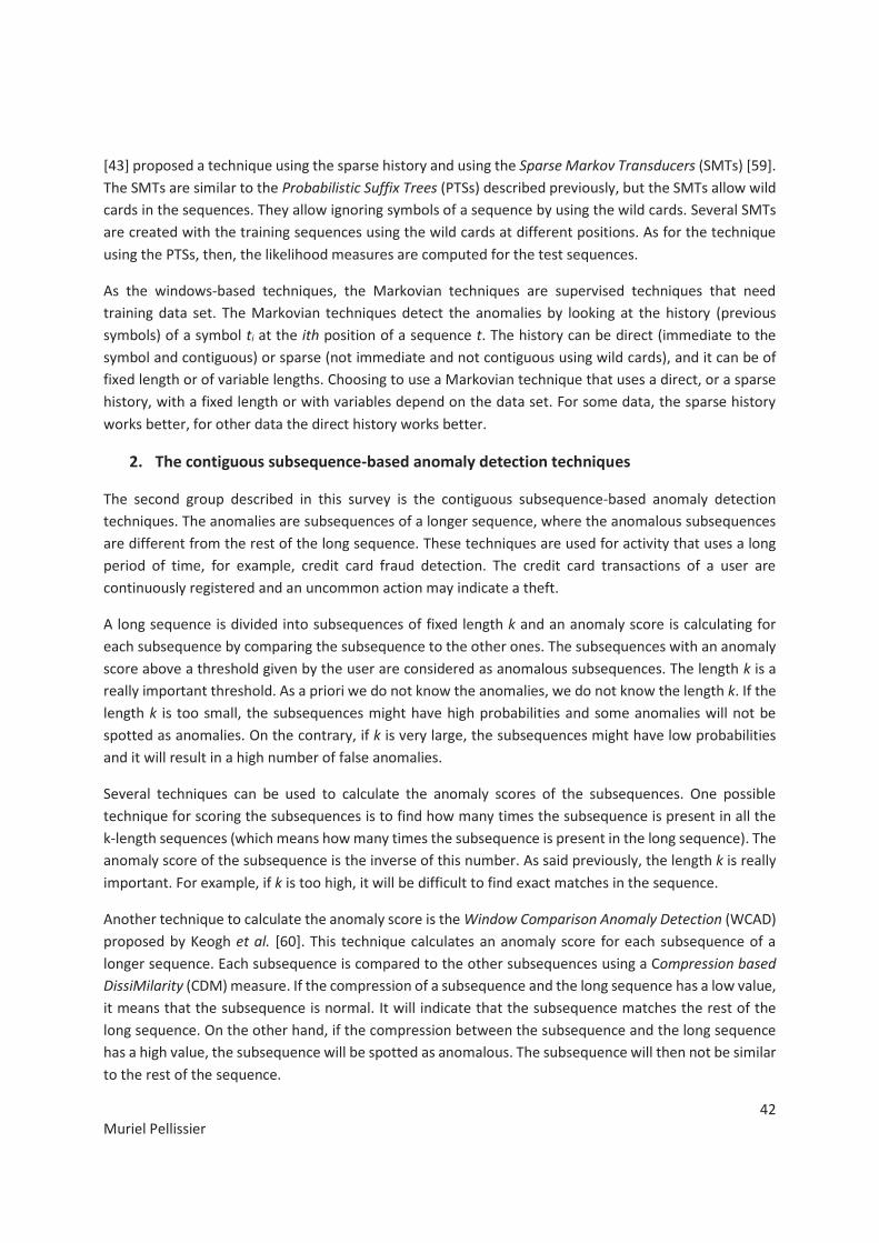
42

Muriel Pellissier

[43] proposed a technique using the sparse history and using the Sparse Markov Transducers (SMTs) [59].

The SMTs are similar to the Probabilistic Suffix Trees (PTSs) described previously, but the SMTs allow wild

cards in the sequences. They allow ignoring symbols of a sequence by using the wild cards. Several SMTs

are created with the training sequences using the wild cards at different positions. As for the technique

using the PTSs, then, the likelihood measures are computed for the test sequences.

As the windows-based techniques, the Markovian techniques are supervised techniques that need

training data set. The Markovian techniques detect the anomalies by looking at the history (previous

symbols) of a symbol ti at the ith position of a sequence t. The history can be direct (immediate to the

symbol and contiguous) or sparse (not immediate and not contiguous using wild cards), and it can be of

fixed length or of variable lengths. Choosing to use a Markovian technique that uses a direct, or a sparse

history, with a fixed length or with variables depend on the data set. For some data, the sparse history

works better, for other data the direct history works better.

2. The contiguous subsequence-based anomaly detection techniques

The second group described in this survey is the contiguous subsequence-based anomaly detection

techniques. The anomalies are subsequences of a longer sequence, where the anomalous subsequences

are different from the rest of the long sequence. These techniques are used for activity that uses a long

period of time, for example, credit card fraud detection. The credit card transactions of a user are

continuously registered and an uncommon action may indicate a theft.

A long sequence is divided into subsequences of fixed length k and an anomaly score is calculating for

each subsequence by comparing the subsequence to the other ones. The subsequences with an anomaly

score above a threshold given by the user are considered as anomalous subsequences. The length k is a

really important threshold. As a priori we do not know the anomalies, we do not know the length k. If the

length k is too small, the subsequences might have high probabilities and some anomalies will not be

spotted as anomalies. On the contrary, if k is very large, the subsequences might have low probabilities

and it will result in a high number of false anomalies.

Several techniques can be used to calculate the anomaly scores of the subsequences. One possible

technique for scoring the subsequences is to find how many times the subsequence is present in all the

k-length sequences (which means how many times the subsequence is present in the long sequence). The

anomaly score of the subsequence is the inverse of this number. As said previously, the length k is really

important. For example, if k is too high, it will be difficult to find exact matches in the sequence.

Another technique to calculate the anomaly score is the Window Comparison Anomaly Detection (WCAD)

proposed by Keogh et al. [60]. This technique calculates an anomaly score for each subsequence of a

longer sequence. Each subsequence is compared to the other subsequences using a Compression based

DissiMilarity (CDM) measure. If the compression of a subsequence and the long sequence has a low value,

it means that the subsequence is normal. It will indicate that the subsequence matches the rest of the

long sequence. On the other hand, if the compression between the subsequence and the long sequence

has a high value, the subsequence will be spotted as anomalous. The subsequence will then not be similar

to the rest of the sequence.

43

Muriel Pellissier

Other techniques prune the subsequences in order to reduce the execution time as the standard

techniques need O(l2) comparisons of subsequences, where l is the length of the long sequence.

Considering that most of the subsequences tend to be normal, the subsequences that do not have an

anomaly score high enough will be pruned [61], [62], [63], [64].

Chakrabarti et al. [45] proposed another technique using different length for the subsequences. As the

anomalies are not known we can imagine that the anomalous subsequences might have different lengths

k, therefore, a single value of the length might not be adapted. This technique is limited to small data set,

or small alphabet. The sequence is divided into varying length subsequences. The difference lengths of

the different subsequences are calculated in order to minimize the number of bits needed to encode each

subsequence. In order to encode the subsequences they use the Shannon’s Source Coding Theorem. The

subsequences that need the highest number of bits are defined as anomalous.

These techniques can detect anomalous subsequences of a longer sequence by comparing all the

subsequences of a sequence to each other. If a subsequence is different from the rest of the sequence it

will be defined as anomalous. The length of the subsequences k is really important. As the anomalies are

not known it might be difficult to set the k value to the best value. For example, if the length k is too small,

many subsequences might appears many times within the sequence. Thus, the subsequences will have

high probabilities and some anomalies might be missed. On the contrary, if k is very large, many

subsequences will be rare and their probability will be low. Many false anomalies might be detected.

3. The pattern frequency-based anomaly detection techniques

The third group is the pattern frequency-based anomaly detection techniques. The anomalies are patterns

of longer sequences that are detected using the frequencies of the patterns. The frequency of a pattern

of a long sequence is calculated as the number of times that the pattern is present in the long sequence.

In order to detect the anomalous pattern, the frequency of a pattern of a sequence from the test data set

is compared with its expected frequency obtained in the training data set. If the frequency of the pattern

in the test sequence and the frequency of the pattern in the training sequences are significantly different

the pattern will be classified as anomalous.

The basic pattern frequency-based technique calculates the anomaly score of a pattern as the absolute

difference between the frequency of that pattern in a test sequence and the average of the frequencies

of that pattern in the training sequences. The frequency of the pattern that occurs in the test sequence is

normalized with the length of the test sequence. The average frequency obtains with the training

sequences is calculated as the sum of each the normalized frequency of the pattern in each training

sequence divided by the number of training sequences. The normalized frequency is the frequency of a

pattern divided by the length of the long sequence.

The problem with this method is that only the exact matching patterns in the test sequence and in the

training sequences will be taken into account while calculating the anomaly score. If we are interested in

a long pattern, it might be more difficult to find exactly the same pattern in the training sequences. For

example, if we have the pattern “abd” in a test sequence and the training sequence “abcd”, with this

method the pattern “abd” will not be detected in the training sequence. However depending on the

44

Muriel Pellissier

application it could be really important to consider also the cases where some symbols are inserted into

the pattern. Some techniques, based on the previous one, are developed using subsequences in order to

take into consideration also the subsequences that are close to the pattern but not exactly identical.

Keogh et al. [65] proposed a technique using subsequences of the pattern. They count how many times a

subsequence of the pattern occurs in a sequence. They determinate the largest length l of the

subsequences, such that every subsequence of length l of the pattern occurs at least once in the training

sequences.

Gwadera et al [66] proposed another technique using subsequences of the pattern. For this technique,

they count how many times the pattern occurs as a noncontiguous subsequence in a sequence. They

divide the sequence in different windows of a fixed length, where the length is bigger than the length of

the pattern. The pattern is considered present in a sequence if there is at last one window where the

pattern is found as a subsequence of one of the windows. They determine how many windows of the

sequence contain the pattern as a subsequence. The anomaly score of the pattern is the absolute

difference between the number of windows containing the pattern in the sequence and the average

number of windows containing the pattern in the training sequences. They also proposed another similar

technique where not only the pattern can be detected as a noncontiguous subsequence but also where

the order of the symbols in the pattern is not important [67]. As the previous method, they use fixed

length windows and they count the number of windows that contain all the symbols of the pattern

independently of the order of the symbols.

These techniques use pattern of a longer sequence and the frequency of that pattern within the sequence

and within the training sequences in order to define the pattern as anomalous or normal. As the previous

technique, the abnormality of a pattern is based on the repetition of that pattern within a sequence. The

pattern can be seen as contiguous subsequence, as noncontiguous subsequence, and also as unordered

subsequence of symbols.

In this section, we have presented several sequence mining techniques divided in three different

categories. The first category contains the sequence mining techniques that compare the test data with

the training data in order to detect anomalies. These techniques are supervised approaches, which means

that you need training data known as normal data in order to use these techniques. The techniques

described in this category divide a test sequence in several subsequences and then compare the

subsequences with the subsequences of the training data. In order to compare two subsequences, these

techniques calculate anomaly scores for each subsequences based on the frequencies of the

subsequences, or the distance between two subsequences etc. As the anomalies are not known in

advance, it might be difficult to set properly the length of the subsequences. If the length is too small, the

subsequences will have high probabilities and it will end up in a high number of false negatives. At the

contrary, if the length is too large, the subsequences will have low probabilities and it will end up in a high

number of false positives.

The second category groups the sequence mining techniques that detect as anomalies subsequences of a

longer sequence that are different from the rest of the sequence. For these techniques the anomalies are

45

Muriel Pellissier

part of a long sequence, and they are defined as anomalous because they do not match the rest of the

long sequence. In order to compare two subsequences, these techniques calculate anomaly scores for

each subsequences based on the frequencies of the subsequences, or the distance between two

subsequences or the compression of sequence etc. As for the first group, the most important is to set

properly the length of the subsequence. As before, if the length of the subsequence is too small, the

technique might detect false negatives and if the length is too large, the technique might detect false

positives.

The third category is the sequence mining techniques that use the frequency in order to detect a pattern

of a longer sequence as anomalous. At the difference with the other techniques described before, these

techniques query only on a pattern, it does not detect anomalies within a sequence but detect if the

pattern is anomalous or not. These techniques are supervised techniques and they need training data as

the first group. They calculate the anomaly score of the pattern based on the frequency of the pattern in

the training dataset and the frequency of the pattern in the test dataset. As for the two other groups, if

the length of the pattern is too long it will be difficult to find exact match in the training dataset. These

techniques have a high computational complexity which limits the multiple queries.

All these sequence mining techniques detect anomalies within a sequence by comparing the order of the

elements within two sequences or two parts of a sequence. But these techniques do not take into account

while comparing the sequences the position of the elements within the sequences. However, depending

on the application, the position of the elements within a sequence could be really importance as it could

actually give an extra information.

Other techniques could be used for sequence mining as the regular expressions. A regular expression is a

sequence of characters that form a search pattern. The regular expressions are used for pattern/string

matching or to detect similar pattern. The regular expressions are used in different applications like

highlighting systems, internet search engines, network analysis, network security, network intrusion

detection, they are also used for biology in order to align sequences, or for text processing as for example

for translation of different languages. The sequence mining techniques uses subsequences and compare

them with other subsequences (from a longer sequence, from a training dataset or from a test dataset).

It is possible to use a regular expression in order to detect all the subsequences that are similar to a

subsequence. The subsequence used as a regular expression is the search pattern. It is also possible with

the regular expressions to detect subsequences that are not exactly similar using the wildcards. As a

wildcard could be any event of the alphabet, it is easy to detect all the subsequences of a dataset that

differ from the search pattern from only one event using a wildcard.

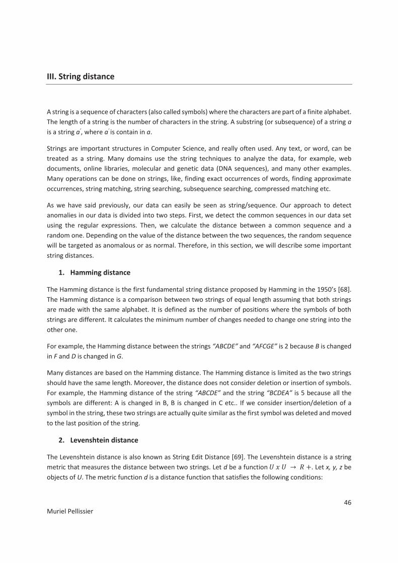
46

Muriel Pellissier

III. String distance

A string is a sequence of characters (also called symbols) where the characters are part of a finite alphabet.

The length of a string is the number of characters in the string. A substring (or subsequence) of a string a

is a string a’, where a’ is contain in a.

Strings are important structures in Computer Science, and really often used. Any text, or word, can be

treated as a string. Many domains use the string techniques to analyze the data, for example, web

documents, online libraries, molecular and genetic data (DNA sequences), and many other examples.

Many operations can be done on strings, like, finding exact occurrences of words, finding approximate

occurrences, string matching, string searching, subsequence searching, compressed matching etc.

As we have said previously, our data can easily be seen as string/sequence. Our approach to detect

anomalies in our data is divided into two steps. First, we detect the common sequences in our data set

using the regular expressions. Then, we calculate the distance between a common sequence and a

random one. Depending on the value of the distance between the two sequences, the random sequence

will be targeted as anomalous or as normal. Therefore, in this section, we will describe some important

string distances.

1. Hamming distance

The Hamming distance is the first fundamental string distance proposed by Hamming in the 1950’s [68].

The Hamming distance is a comparison between two strings of equal length assuming that both strings

are made with the same alphabet. It is defined as the number of positions where the symbols of both

strings are different. It calculates the minimum number of changes needed to change one string into the

other one.

For example, the Hamming distance between the strings “ABCDE” and “AFCGE” is 2 because B is changed

in F and D is changed in G.

Many distances are based on the Hamming distance. The Hamming distance is limited as the two strings

should have the same length. Moreover, the distance does not consider deletion or insertion of symbols.

For example, the Hamming distance of the string “ABCDE” and the string “BCDEA” is 5 because all the

symbols are different: A is changed in B, B is changed in C etc.. If we consider insertion/deletion of a

symbol in the string, these two strings are actually quite similar as the first symbol was deleted and moved

to the last position of the string.

2. Levenshtein distance

The Levenshtein distance is also known as String Edit Distance [69]. The Levenshtein distance is a string

metric that measures the distance between two strings. Let d be a function . Let x, y, z be

objects of U. The metric function d is a distance function that satisfies the following conditions:

47

Muriel Pellissier

1. Non-negativity:

2. Equality :

3. Symmetry :

Triangle inequality :

The Levenshtein distance is a metric distance that calculates the distance between two strings. The two

strings can have different lengths. The Levenshtein distance between two strings is defined as the

minimum number of insertions, deletions, or substitutions of a single character needed to transform one

string into the other one. For example, the Levenshtein distance between the strings “ABCD” and “AEC”

is 2. There is one substitution of the character B into E and one deletion of the character D.

3. Damerau-Levenshtein distance

The Damerau-Levenshtein distance measures the difference between two strings. The two strings can be

of different length. This distance is based on the Levenshtein distance. It is defined as the minimum

number of operations needed to change one string into the other one. As for the Levenshtein distance,

the operations allowed are the insertion, the deletion, the substitution of a single character. This distance

allows also the transposition of two adjacent characters.

For example, the Damerau-Levenshtein distance between the strings “ADB” and “ABCD” is 2. The

characters D and B are inverted from the string “ADB” into “ABD” and the character C is added between

B and D (“ADB” -> “ABD” -> “ABCD”).

4. The string edit distance with Moves

The string edit distance with Moves is also a distance using substrings [70]. The string edit distance with

Moves is a distance based on the Levenshtein distance (String Edit Distance). As we have seen previously,

the Levenshtein distance between two strings a and b is the minimum number of insertions, deletions, or

substitutions of a character to obtain the string b from the string a. The string edit distance with Moves

uses the insertion, deletion, and substitution of a character, as the Levenshtein distance, and it uses in

additional the move of substrings (blocks) in order to transform one string into the other one. A move of

a substring means that a substring of the string a is also present in b but at a different position.

5. Needleman-Wunsch algorithm

The Needleman-Wunsch algorithm is used to compare two sequences X and Y. It uses the alignment of

the symbols between the two sequences to calculate a score S(X,Y). The score between two sequences is

the addition of all the scores of each pair of symbol of the sequences. A sequence can contain wild cards,

the score is then calculated using a linear gap value. The value of the score for each pair of symbol is given

by a similarity matrix. Let F[i,j] be the similarity matrix with i the length of the sequence X and j the length

of the sequence Y. Let d be the linear gap penalty.

For example, the sequence X is “A-CD-G” and the sequence Y is “ABCDEF”. If the linear gap penalty is d =

1 and the similarity matrix is F[4,6]:

48

Muriel Pellissier

The score S(X,Y) is

.

6. Tichy distance

The Tichy distance is a distance using substrings [71]. The Tichy distance uses the substrings of a string

(also called blocks) in order to describe another string. The Tichy distance between a string a and a string

b is the minimum number of substrings of b that can be found in the string a. The Tichy distance is used

to measure the similarity between two strings. For example, the Tichy distance of the strings a =

“ABCDEFG” and b = “ABHEFJG” is 3. The substrings “AB”, “EF”, and “G” of the string b are also substrings

of the string a.

7. String distance conclusion

All these different string techniques calculate the distance between two strings that are made from the

same alphabet by comparing the symbols of the two strings. Some techniques can compare two strings

of different length; some compare only the strings that have the same length. Some techniques use the

insertions, deletions, or substitutions of a single symbol within a sequence, some techniques use the

transposition of two adjacent symbols, some techniques use the insertion of a substring into a string etc.

We presented in this chapter the existing techniques that are linked with our research. We detailed first

some graph-based anomaly detection that can be used with maritime data. The data are represented with

graphs. The anomalies are structural anomalies. The anomalies are detected by using the graph properties

or by analyzing the graph structure depending on the technique. Then, we presented some sequence

mining techniques grouped in three categories. Some techniques use training data in order to detect

anomalies in the test data set by comparing the test data with the training data. Some techniques detect

subsequences of a sequence as anomalous by detecting the subsequences of a sequence that are different

from the rest of the sequence. And some techniques use the frequency of subsequences in order to detect

the anomalies. Finally, we gave the definitions of some fundamental string distances. The string distances

calculate the distance between two strings based on character changes.

All these techniques compare the order of the symbols between the two strings but do not take into

account the actual position of the symbols in the sequence. In our case the position is really important.

The position of an event in the sequence will give some information about that event. For example, the

itinerary that has for departure port: Singapore, for transshipment port: Chiwan and for arrival port:

49

Muriel Pellissier

Rotterdam is seen as the sequence: “Singapore Chiwan Rotterdam”. For our application, the position gives

the information about the type of event. An event can be of three different types: departure,

transshipment, or arrival. The port that is at the first position in the sequence is the port of departure.

The last port of the sequence is the arrival port. And all the ports in between the first and the last one are

transshipment ports. Thus, when we compare two sequences, we need to compare the symbols of two

different strings but we also need to take into account the actual position of every symbol in the strings.

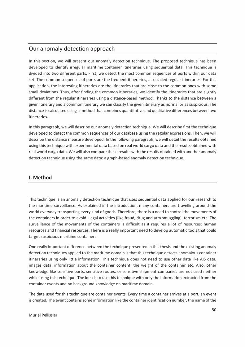
50

Muriel Pellissier

Our anomaly detection approach

In this section, we will present our anomaly detection technique. The proposed technique has been

developed to identify irregular maritime container itineraries using sequential data. This technique is

divided into two different parts. First, we detect the most common sequences of ports within our data

set. The common sequences of ports are the frequent itineraries, also called regular itineraries. For this

application, the interesting itineraries are the itineraries that are close to the common ones with some

small deviations. Thus, after finding the common itineraries, we identify the itineraries that are slightly

different from the regular itineraries using a distance-based method. Thanks to the distance between a

given itinerary and a common itinerary we can classify the given itinerary as normal or as suspicious. The

distance is calculated using a method that combines quantitative and qualitative differences between two

itineraries.

In this paragraph, we will describe our anomaly detection technique. We will describe first the technique

developed to detect the common sequences of our database using the regular expressions. Then, we will

describe the distance measure developed. In the following paragraph, we will detail the results obtained

using this technique with experimental data based on real world cargo data and the results obtained with

real world cargo data. We will also compare these results with the results obtained with another anomaly

detection technique using the same data: a graph-based anomaly detection technique.

I. Method

This technique is an anomaly detection technique that uses sequential data applied for our research to

the maritime surveillance. As explained in the introduction, many containers are travelling around the

world everyday transporting every kind of goods. Therefore, there is a need to control the movements of

the containers in order to avoid illegal activities (like fraud, drug and arm smuggling), terrorism etc. The

surveillance of the movements of the containers is difficult as it requires a lot of resources: human

resources and financial resources. There is a really important need to develop automatic tools that could

target suspicious maritime containers.

One really important difference between the technique presented in this thesis and the existing anomaly

detection techniques applied to the maritime domain is that this technique detects anomalous container

itineraries using only little information. This technique does not need to use other data like AIS data,

images data, information about the container content, the weight of the container etc. Also, other

knowledge like sensitive ports, sensitive routes, or sensitive shipment companies are not used neither

while using this technique. The idea is to use this technique with only the information extracted from the

container events and no background knowledge on maritime domain.

The data used for this technique are container events. Every time a container arrives at a port, an event

is created. The event contains some information like the container identification number, the name of the

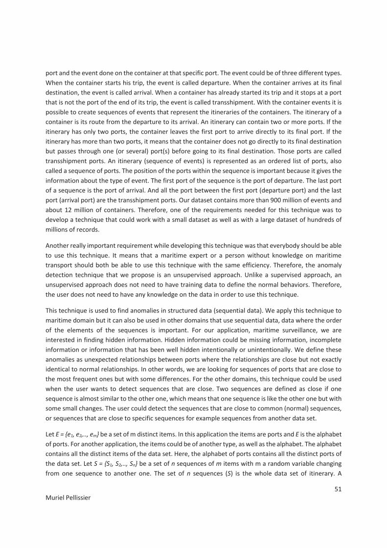
51

Muriel Pellissier

port and the event done on the container at that specific port. The event could be of three different types.

When the container starts his trip, the event is called departure. When the container arrives at its final

destination, the event is called arrival. When a container has already started its trip and it stops at a port

that is not the port of the end of its trip, the event is called transshipment. With the container events it is

possible to create sequences of events that represent the itineraries of the containers. The itinerary of a

container is its route from the departure to its arrival. An itinerary can contain two or more ports. If the

itinerary has only two ports, the container leaves the first port to arrive directly to its final port. If the

itinerary has more than two ports, it means that the container does not go directly to its final destination

but passes through one (or several) port(s) before going to its final destination. Those ports are called

transshipment ports. An itinerary (sequence of events) is represented as an ordered list of ports, also

called a sequence of ports. The position of the ports within the sequence is important because it gives the

information about the type of event. The first port of the sequence is the port of departure. The last port

of a sequence is the port of arrival. And all the port between the first port (departure port) and the last

port (arrival port) are the transshipment ports. Our dataset contains more than 900 million of events and

about 12 million of containers. Therefore, one of the requirements needed for this technique was to

develop a technique that could work with a small dataset as well as with a large dataset of hundreds of

millions of records.

Another really important requirement while developing this technique was that everybody should be able

to use this technique. It means that a maritime expert or a person without knowledge on maritime

transport should both be able to use this technique with the same efficiency. Therefore, the anomaly

detection technique that we propose is an unsupervised approach. Unlike a supervised approach, an

unsupervised approach does not need to have training data to define the normal behaviors. Therefore,

the user does not need to have any knowledge on the data in order to use this technique.

This technique is used to find anomalies in structured data (sequential data). We apply this technique to

maritime domain but it can also be used in other domains that use sequential data, data where the order

of the elements of the sequences is important. For our application, maritime surveillance, we are

interested in finding hidden information. Hidden information could be missing information, incomplete

information or information that has been well hidden intentionally or unintentionally. We define these

anomalies as unexpected relationships between ports where the relationships are close but not exactly

identical to normal relationships. In other words, we are looking for sequences of ports that are close to

the most frequent ones but with some differences. For the other domains, this technique could be used

when the user wants to detect sequences that are close. Two sequences are defined as close if one

sequence is almost similar to the other one, which means that one sequence is like the other one but with

some small changes. The user could detect the sequences that are close to common (normal) sequences,

or sequences that are close to specific sequences for example sequences from another data set.

Let E = {e1, e2,.., em} be a set of m distinct items. In this application the items are ports and E is the alphabet

of ports. For another application, the items could be of another type, as well as the alphabet. The alphabet

contains all the distinct items of the data set. Here, the alphabet of ports contains all the distinct ports of

the data set. Let S = {S1, S2,.., Sn} be a set of n sequences of m items with m a random variable changing

from one sequence to another one. The set of n sequences (S) is the whole data set of itinerary. A

52

Muriel Pellissier

subsequence of the sequence Sy is Sy’ = {ea, *, eb, *} where the symbol “ * ” corresponds to an unknown

item. As for this application the items are ports, the symbol “ * ” could represent any port of the port

alphabet E. The unknown items, represented by the symbol “ * ”, are also called wild cards. A subsequence

is defined as a part of the whole itinerary. It means that a subsequence is not the full itinerary from the

departure to the arrival but only a part of that itinerary.

This anomaly detection technique is divided into two steps:

1) First, we detect the sequences or subsequences that are common in our data set. We use the

regular expression methods in order to detect the common itineraries using all the available data

(normal data and anomalous data).

2) Then, we compare a given sequence with the common sequences/subsequences and we calculate

an anomaly degree with a distance technique. Depending on the anomaly degree value, we

classify the given sequence as normal or anomalous.

With this technique we can identify the anomalies and present their details to the user. The user can have

some controls on the results with several thresholds in order to adapt better the results to his needs. The

first threshold is to select the common itineraries. With a high threshold the user can select only the main

itineraries and with a lower threshold the user can select more common itineraries that are less frequent

than the main ones. The second threshold is the maximum anomaly degree threshold which is the level

defining an itinerary as normal or anomalous. Moreover, the first part of this technique could also be used

alone as it can detect common routes or frequent couple of ports. This information can be useful for the

maritime surveillance.

53

Muriel Pellissier

II. Common sequences / subsequences

The first step of this method is to detect the common itineraries. Thus, we need to detect the common

sequences (itineraries) of our data set. In order to find the common sequences, we need to compare all

the sequences of the data set and to calculate their frequency. Depending on their frequencies, they will

be targeted as frequent itineraries. The position of the ports within a sequence is important because we

know the event associated to a port with the position of that port in the sequence. For example, the first

port is related to the departure event, the last one is the arrival event and the ones in between are the

transshipment events. Thus, it is not enough to look only at frequent patterns within the data set. The

position within the sequence has to be taken into account too. For example, we have the itinerary where

a container leaves from Singapore to go to Rotterdam passing through Chiwan (Singapore – Chiwan –

Rotterdam) and the itinerary from Chiwan to Rotterdam arriving in Copenhagen (Chiwan – Rotterdam –

Copenhagen). The pattern “Chiwan – Rotterdam” in these two itineraries cannot be considered as the

same as for the first itinerary Chiwan is a port of transshipment and for the second itinerary Chiwan is the

port of departure.

We are also interested in finding common subsequences. A subsequence is a part of a sequence (part of

an itinerary) and not the whole sequence (itinerary). We use wild cards in order to create the

subsequences. A wild card can substitute any data of our alphabet. For this application, the alphabet is a

list of ports. Thus, a wild card can be any port of our alphabet. One wild card represents any port of the

alphabet but it corresponds to only one port. As said previously, the position of the ports in the sequences

is important, therefore, one wild card can be used only for one unknown port at a time. If several ports

are unknown in a sequence, we will use one wild card for each unknown port in order to maintain the

position of the ports in the sequences.

The frequencies of the whole sequences are directly obtained by counting how many times each sequence

appears in the data set. The frequencies of the subsequences are more difficult to calculate. As we do not

have any knowledge on the data, for example, we do not know the interesting sequences or the

interesting subsequences. Therefore, we need to create all the possible subsequences and we need to

calculate how many times each subsequence appears in the data set. In order to create the subsequences

we chose to use the wild cards. By replacing a port (or several ports) by a wild card (or several wild cards)

into a sequence of the data set we create a subsequence of that sequence. If an itinerary has only two

ports we will not create a subsequence. The subsequence of an itinerary of two ports will be composed

by only one port and a wild card. We are not interested in single port but only in relations between ports.

For every itinerary of more than two ports, we will create a subsequence of that itinerary by replacing

only one port by a wild card. For one itinerary we can create several subsequences by replacing every port

by a wild card at a time. The number of subsequences created depends on how many ports an itinerary

has. For example, we can create four subsequences with an itinerary that has four ports. The Figure 9

shows an example of an itinerary from port X1 to port X3 passing through X2 and all the possible

subsequences of this itinerary. In the subsequences, the character “ * ” is a wild card and it can correspond

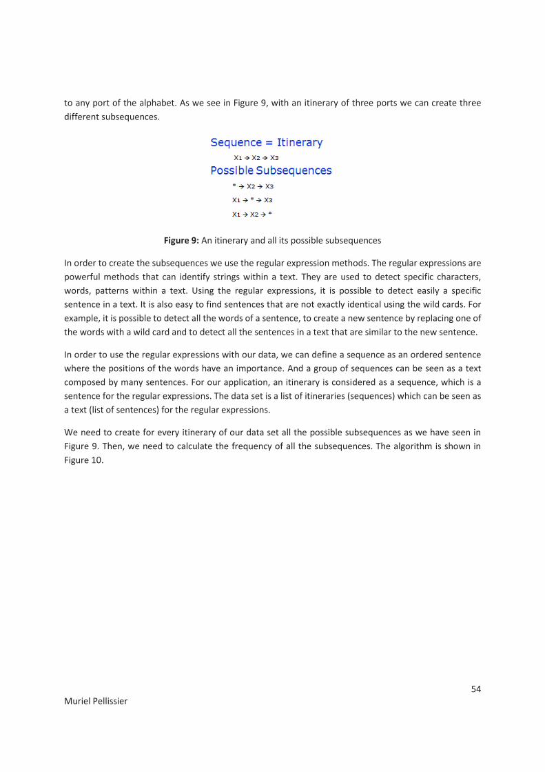
54

Muriel Pellissier

to any port of the alphabet. As we see in Figure 9, with an itinerary of three ports we can create three

different subsequences.

Figure 9: An itinerary and all its possible subsequences

In order to create the subsequences we use the regular expression methods. The regular expressions are

powerful methods that can identify strings within a text. They are used to detect specific characters,

words, patterns within a text. Using the regular expressions, it is possible to detect easily a specific

sentence in a text. It is also easy to find sentences that are not exactly identical using the wild cards. For

example, it is possible to detect all the words of a sentence, to create a new sentence by replacing one of

the words with a wild card and to detect all the sentences in a text that are similar to the new sentence.

In order to use the regular expressions with our data, we can define a sequence as an ordered sentence

where the positions of the words have an importance. And a group of sequences can be seen as a text

composed by many sentences. For our application, an itinerary is considered as a sequence, which is a

sentence for the regular expressions. The data set is a list of itineraries (sequences) which can be seen as

a text (list of sentences) for the regular expressions.

We need to create for every itinerary of our data set all the possible subsequences as we have seen in

Figure 9. Then, we need to calculate the frequency of all the subsequences. The algorithm is shown in

Figure 10.

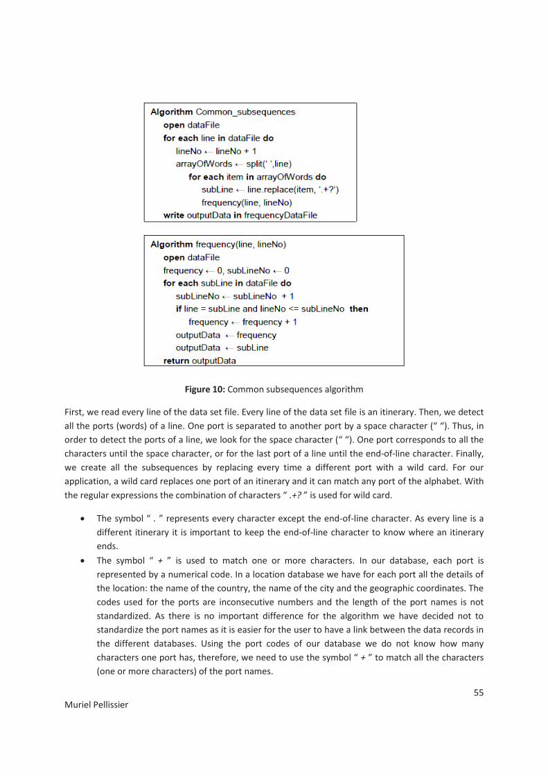
55

Muriel Pellissier

Figure 10: Common subsequences algorithm

First, we read every line of the data set file. Every line of the data set file is an itinerary. Then, we detect

all the ports (words) of a line. One port is separated to another port by a space character (“ “). Thus, in

order to detect the ports of a line, we look for the space character (“ “). One port corresponds to all the

characters until the space character, or for the last port of a line until the end-of-line character. Finally,

we create all the subsequences by replacing every time a different port with a wild card. For our

application, a wild card replaces one port of an itinerary and it can match any port of the alphabet. With

the regular expressions the combination of characters “ .+? ” is used for wild card.

· The symbol “ . ” represents every character except the end-of-line character. As every line is a

different itinerary it is important to keep the end-of-line character to know where an itinerary

ends.

· The symbol “ + ” is used to match one or more characters. In our database, each port is

represented by a numerical code. In a location database we have for each port all the details of

the location: the name of the country, the name of the city and the geographic coordinates. The

codes used for the ports are inconsecutive numbers and the length of the port names is not

standardized. As there is no important difference for the algorithm we have decided not to

standardize the port names as it is easier for the user to have a link between the data records in

the different databases. Using the port codes of our database we do not know how many

characters one port has, therefore, we need to use the symbol “ + ” to match all the characters

(one or more characters) of the port names.

56

Muriel Pellissier

· But as all the characters except the end-of-line character will match “ .+ ” we need to limit it. If

we do not limit it all the characters until the end-of-line character will always be a match. In order

to control the comparison we use the symbol “ ? ” which makes the operation lazy. This means

that every time we compare two characters the character after the characters “ .+? ” is also

checked. As soon as the character after “ .+? ” is found in the line the following characters will not

match “ .+? ” anymore.

Then, we count how often the subsequences are present in the data set. With a minimum frequency

threshold we can select which lines (itineraries) are frequent enough in the data set to be considered as

common itineraries.

This algorithm has a time complexity of O(n3), but as we use finite sequences and the sequences contain

only few objects (maximum 5), the time complexity is reduced to O(n2).

With this first part we are able to detect the common itineraries (or part of itineraries) of the data set.

The second part of this technique is used to detect the suspicious itineraries by comparing common

itineraries with unknown itineraries.

57

Muriel Pellissier

III. Distance: anomaly degree

The purpose of our anomaly detection technique is to detect anomalous itineraries and to be able to spot

the anomalies within the anomalous itineraries. We identify the anomalous itineraries by comparing a

given itinerary with the common ones. We calculate an anomaly degree between a given itinerary and a

common one. Depending on the value of the anomaly degree we will classify the given itinerary as normal

or abnormal (anomalous). The anomaly degree is calculated with a distance technique based on

quantitative and qualitative differences between two itineraries.

Let Sdata be a given sequence of the data set S containing all the itineraries of our database. Let Snor be a

common sequence or subsequence discovered with the regular expression methods as described in the

previously section. And let dist(Sdata,Snor) be the distance between two sequences: a given sequence Sdata

and a common one Snor. For example, in Figure 11, we compare two itineraries. One itinerary is a given

itinerary from the port X1 to the port X4 passing through the ports X2 and X3. The second itinerary is a

common itinerary from the port X1 to the port X4 with a wild card as transshipment port.


We define the distance dist(Sdata,Snor) as the number of actual changes divided by the maximum number

of possible changes between two sequences: Sdata (given itinerary) and Snor (common itinerary). We

calculate the distance using two criterions: the structure of the itinerary and the name of the ports. The

structure corresponds to the number of events of an itinerary. The port names are the actual ports visited

during an itinerary (the actual name of the ports) and their associated type. The type of a port could be

of three different types: departure port, transshipment port or arrival port. As shown in Figure 11, the

structure is the part above the black horizontal line and the port names is the part below the black

58

Muriel Pellissier

horizontal line. In the following paragraphs, we will explain how we calculate the distance between two

itineraries.

1. Structure distance

To calculate the structure distance we use the events of the itineraries. The three possible events are the

departure, the arrival, and the transshipment. For the structure distance, we calculate the actual changes

between the two itineraries and the maximum number of possible changes between the two itineraries.

· The actual changes are calculated with the absolute difference between the number of events of

a given sequence Sdata and the number of events of a common sequence Snor. A sequence (also

called itinerary) is an ordered list of ports. By consequence, the number of events can be easily

obtained with the length of the sequence. Therefore, in order to calculate the difference between

the numbers of events between the two sequences, we calculate the absolute difference between

the length of the given sequence Sdata and the length of the common sequence Snor (12):

· The maximum number of possible changes between the two sequences is the maximum number

of events between Sdata and Snor (13):

Then, we calculate the second part of the distance: the port names distance.

2. Port names distance

We also need to take into account the names of the ports and the events linked to the ports. In order to

calculate the distance we will attribute values to the ports of the two sequences. A port can be present in

the two sequences in three different ways:

1) A port is identical in both sequences Sdata and Snor. It means that the name of the port and the

event related to it are similar in both itineraries. For example, in Figure 12, the port X1 is for both

itineraries the port of departure.

2) A port of Sdata is also present in Snor but the port has not the same event in both itineraries. For

example, in Figure 12, the port X4 is the port of transshipment in the given itinerary Sdata and it is the port

of arrival in the common itinerary Snor.

3) A port of Sdata is not present in Snor or the opposite. For example, in Figure 12, the port X2 is

present only in the given itinerary Sdata, same for the port X3.

59

Muriel Pellissier


As said previously, the event related to the port is linked in our data (container itineraries) to the position

of the port in the sequence. The first port is the port of departure, the last port is the port of arrival, and

the ports in between are the ports of transshipment.

· In order to calculate the actual changes of the port names distance, we compare the ports of the

two sequences and we attribute a value to each port of the two itineraries. We will describe in

the following paragraph how we attribute values to each port of the sequences using the fact that

a port can be present in a sequence in three different manners as said previously.

1) The first case is if a port is identical in both itineraries we attribute the value 0 to the

port. Two ports are identical in two different itineraries if they have the same name and if they

have the same related event in both itineraries. For example, the port X1 is the port of arrival of

both itineraries. We know the event related to the port depending on the position of the port in

the sequence. As the sequence is an ordered list of port, the first port is the port of departure,

the last port is the port of arrival, and the ports in between are the ports of transshipment. Thus,

we look at the positions of the ports in the sequences in order to compare the ports between two

sequences. But as two itineraries might not have the same number of ports it is not

straightforward to compare the position of two ports. In order to compare the positions of a port

we compare the two itineraries starting from the beginning of the itineraries (starting from the

left) and also starting from the end of the itineraries (starting from the right). If the names of the

ports and the positions of the ports are similar in one of these two comparisons, the two ports

will be considered as having the same position and we will attribute the value 0 to the ports.

For example, if we consider the common itinerary X3 X5 * and the given itinerary X10 X3

X5 X6. If we compare them only from the beginning, they will have an anomaly degree really high

60

Muriel Pellissier

as none of the ports have the same position as in the other itinerary. But if we compare the two

itineraries from the end, they appear to be really similar.

2) The second case is if a port is present in both itineraries but with a different event, we

attribute the value 1. In order to compare the event, as for the first case, we compare the position

of the port in the two sequences. We compare the sequences starting from the beginning (left)

and from the end (right).

3) The last case is if a port is present in only one of the two itineraries, we attribute the

value 2 to the port.

4) We need to add the case when the common itinerary contains a wild card “ * ”. As we

have seen before, the character “ * ” implies that it can be any port of the port alphabet. We have

decided not put any weight on the unknown port “ * ” and that we will not consider it as the same

port as any other port. It means that when we compare a port with the wildcard, the two ports

will be consider as different while we attribute the values to the ports.

Then, we add all the values attributed to each port of the two itineraries in order to obtain

the value for the actual changes for the port names distance (14):

· The maximum number of changes that we can have with the port names is the number of distinct

ports between the two itineraries. We do not consider the port “ * ” as one of the distinct port

for the maximum number of changes. As we have seen we can attribute to a port the value 0, 1

or 2. As the maximum value attributed to a port is 2, if two itineraries are completely different,

the maximum possible value will be the number of all the distinct ports multiplied by 2. Therefore,

the number of maximum changes is the number of distinct ports multiplied by 2 (15).

Once we have calculated the structure distance and the port names distance, we can calculate the

anomaly degree.

3. Anomaly degree

The anomaly degree is defined as the sum of the actual changes in the structure and in the port names

divided by the sum of the maximum possible changes for the structure and for the port names (16).

The maximum anomaly degree threshold can be defined by the user. Depending on the threshold the

itinerary Sdata will be classify as normal or abnormal. If the anomaly degree is lower than the threshold,

the itinerary will be detected as anomalous. If the anomaly degree is higher than the threshold, the

itinerary will be defined as normal.

61

Muriel Pellissier

But in order to limit the number of false suspicious itineraries detected, we define two thresholds: the

minimum anomaly degree threshold and the maximum anomaly degree threshold. An itinerary will be

defined as anomalous if the value of its anomaly degree is included between the minimum anomaly

degree threshold and the maximum anomaly threshold. We set the minimum anomaly degree threshold

to 0.23 and the maximum anomaly degree threshold to 0.43. The user can change these values as needed.

· Minimum anomaly degree threshold:

We know that if an itinerary is common because of several itineraries, the common itinerary will

contain the wild card character “ * ”. Therefore, when we compare one of these several itineraries

with the common one, the anomaly degree value as defined previously will not be 0. For example,

we have in our data set the itineraries “a b c”, “a b d”, “a b e”, “a b f”, “a b g” and “h j k”. The

itinerary “a b *” will be a common itinerary. If we compare “a b c” with the common itinerary “a

b *”, even if “a b c” is actually included in “a b *”, the anomaly degree will be 0.2222.

Calculation of the anomaly degree between “a b c” and “a b *”:

1) Structure distance: As both itineraries have the same number of events (3 events) and

the actual changes value is the difference between the numbers of events of the two

itineraries, the actual changes value is 0. The maximum changes value is the

maximum number of events between the two itineraries. In this example, both

itineraries have the same number of events, by consequence, the maximum changes

value is 3.

2) Name ports: The ports “a” and the port “b” take the value 0 as “a” and “b” in both

itineraries have the same event. The port “a” is the port of departure, and the port

“b” is the port of transshipment. The port “c” takes the value 2, as the port “c” is not

present in the common itinerary. The port “*” does not take any value. The maximum

changes value is the number of distinct ports multiplied by 2. Here, the value is: 3 * 2

= 6.

3) Anomaly degree value: The anomaly degree value is the actual changes value in the

structures plus the total value attributed to ports divided by the addition of the

maximum changes values of the structure and of the ports names. Thus, in this

example the anomaly degree value is: 0 + 2 / 3 + 6 = 2/9 = 0.22.

Therefore, we will define a minimum anomaly degree equal to 0.23 in order to avoid considering

similar itinerary as anomalous. The itineraries that have an anomaly degree inferior to the

minimum degree will not be targeted as anomalous itineraries.

· Maximum anomaly degree threshold:

We also define a maximum anomaly degree threshold but the user can change this value in case

he wants to have a larger or smaller selection of anomalous itineraries. In order to define this

62

Muriel Pellissier

value we calculated the anomaly degree of different itineraries. We used suspicious itineraries

and normal itineraries.

Calculation of the anomaly degree between “1 3 4” and “1 3”:

The itinerary “1 3” is suspicious compared to the common itinerary “1 3 4” because one port is

missing, the arrival port has changed.

1) Structure distance: actual changes: 1 and maximum changes: 3

2) Name ports: ports value: 2 and maximum changes: 3*2

3) Anomaly degree value: 1 + 2 / 3 + 6 = 3/9 = 0.33

Calculation of the anomaly degree between “1 3 4” and “1 3 6”:

The itinerary “1 3 6” is suspicious compared to the common itinerary “1 3 4” because the port of

arrival has changed.


2) Name ports: ports value: 2 + 2 and maximum changes: 4*2


Calculation of the anomaly degree between “3 7 4 * 6” and “3 5 7 6”:

Depending on the needs of the user, the itinerary “3 5 7 6” could be targeted as suspicious

compared to the common itinerary “3 7 4 * 6”. Some transshipment ports have been removed

from the common itinerary but another transshipment port was added to the given itinerary.


2) Name ports: ports value: 2 + 2 + 1 and maximum changes: 5*2


Calculation of the anomaly degree between “3 5 *” and “10 3 5 6”:

The itinerary “10 3 5 6” is suspicious compared to the common itinerary “3 5 *” as the port of

departure changed and was added to the common itinerary.


2) Name ports: ports value: 2 + 2 and maximum changes: 4*2


Calculation of the anomaly degree between “1 3 *” and “1 5 6 3”:

The itinerary “1 5 6 3” can not be detected as suspicious compared to the common itinerary “1

3 *”, even if they have two ports in common.




Calculation of the anomaly degree between “1 * 4” and “1 2 3”:

The itinerary “1 2 3” can not be detected as suspicious compared to the common itinerary “1

* 4”.

63

Muriel Pellissier




With these different examples, we see that the maximum value of the anomaly degree used to

consider an itinerary as suspicious is 0.42. Thus, we set the maximum anomaly degree value to

0.43. If we use an anomaly degree level superior to 0.43, we might detect more suspicious

itineraries than we should. If we use an anomaly degree level inferior to 0.43, we might miss some

suspicious itineraries.

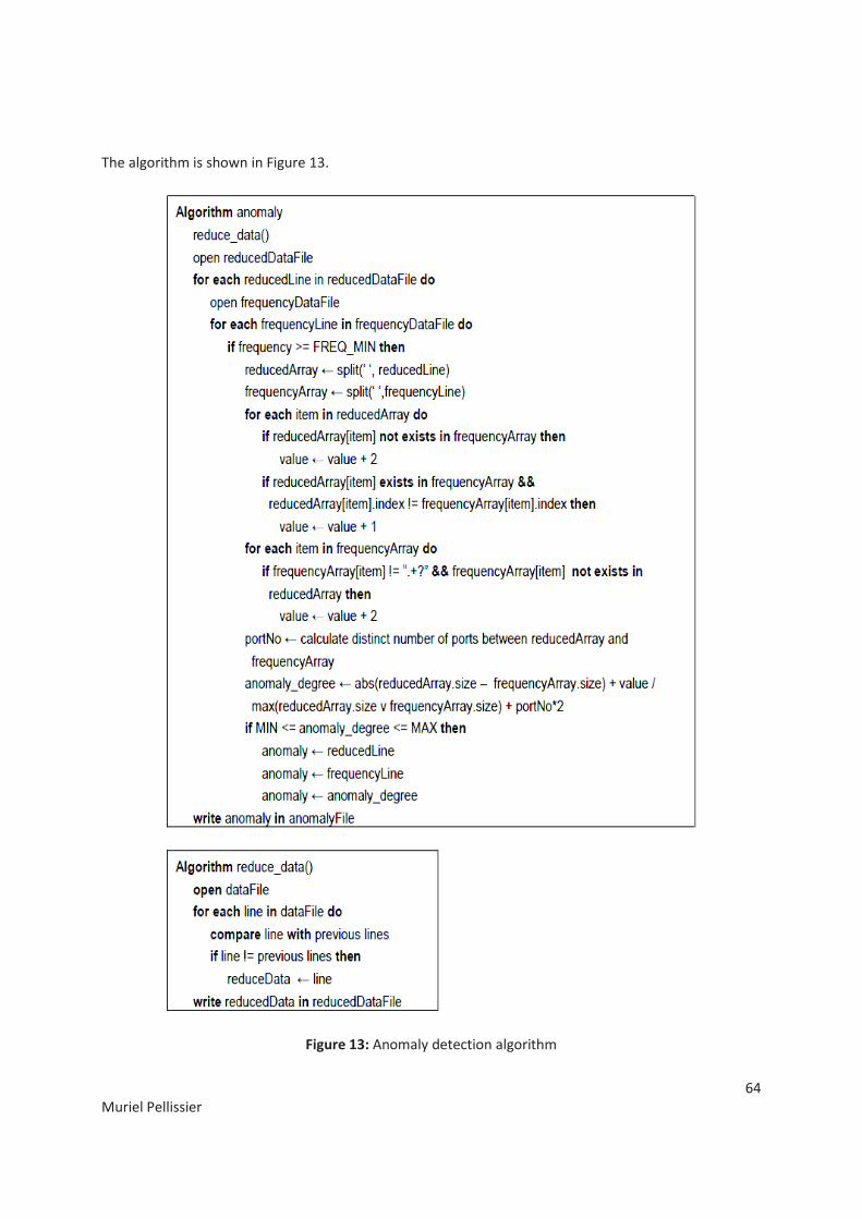
64

Muriel Pellissier

The algorithm is shown in Figure 13.

Figure 13: Anomaly detection algorithm

65

Muriel Pellissier

First, we reduce the data file. The data file contains all the itineraries of our data set. In consequence, the

same itinerary might be present several times. In order to avoid comparing several times a common

itinerary with the same itinerary, we create a new file where each itinerary is present only once. This new

file is the reducedDataFile. Every line of the reducedDataFile is an itinerary.

We read every line of the frequencyDataFile that we have created previously with the common

subsequences algorithm described in Figure 10. The file contains the frequency of every sequence of the

data set and every subsequence created.

A sequence/subsequence is considered to be a common itinerary it its frequency is superior to the

minimum frequency threshold. If the itinerary is a common itinerary we compare the two lines. The first

line is a given itinerary. The second line is the common sequence/subsequence found with the common

subsequences algorithm described in Figure 10.

Then, we attribute values to each port. The port has the value 0 if the port is in the other itinerary and at

the same position or if the port is “ * ”. The port has the value 1 if the port is in the other itinerary but at

a different position. And we attribute the value 2 to the port if the port is not present in the other itinerary.

Using the values attributed to the port, we calculate the anomaly degree between the two itineraries.

If the anomaly degree is between the minimum anomaly degree threshold and the maximum anomaly

degree threshold, then we put in an array the given itinerary, the common itinerary and the anomaly

degree value. We write all the anomalies found in a text file: anomalyFile.

This algorithm has a time complexity of O(n4), but as we use finite sequences and the sequences contain

only few objects (maximum 5), the time complexity is reduced to O(n2).

With this second part of this technique, we are able to target unknown itineraries as suspicious or as

normal by comparing them with common itineraries.

4. Example

As an example, we will calculate the anomaly degree of the two itineraries of the Figure 11:

1) First, we calculate the values of the actual changes and of the possible changes for the structure

distance. The actual changes value is the absolute difference between the number of events of

the given itinerary and the number of events of the common itinerary. The given itinerary has 4

events. The common itinerary has 3 events. Thus, the absolute difference is:

The maximum changes for the structure distance is the maximum number of events between the

two itineraries. Here, the maximum number of events is for the given itinerary that has 4 events.

2) Then, we calculate the values for the name ports distance. We compare each port of one itinerary

with the ports of the other itinerary. We attribute values to each port of the two sequences. We

compare the first port of the given itinerary (X1) with the first port of the common itinerary (X1).

Both are identical, thus we attribute the value 0 to the port X1. We compare the second port of

the given itinerary (X2) with the second port of the common itinerary (“ * ”). As the ports are

66

Muriel Pellissier

different, we also compare the two itineraries from the end, thus, we compare X2 with the port

X1 (both at the third position on the sequences starting from the end). In both cases, the ports

are different, and the port X2”is not present in the common itinerary. Therefore, we attribute the

value 2 to the port X2. We compare the port X3 with X4 (comparison starting from the beginning

of the sequences) and with “ * ” (comparison starting from the end of the sequences). In both

cases, the ports are different and the port X3 is not present in the common itinerary. Thus, we

attribute the value 2 to the port X3. Finally, we compare the last port of the given itinerary (X4)

with the last port of the common itinerary (X4). Both are identical so we attribute the value 0 to

the port X4. The sum of all the values of each port is:

Between the two itineraries we have 4 distinct ports (X1, X2, X3 and X4).

3) Finally we calculate the anomaly degree which is the sum of the actual changes of the structure

distance and of the name ports divided by the maximum changes of both distances.

If the user defines a maximum anomaly degree threshold higher than the distance, the itinerary will be

detected as anomalous. If we set the value of the maximum anomaly degree threshold to 0.43, as

explained previously, this itinerary that has an anomaly degree equal to 0.42 will be detected as

anomalous. The given itinerary might be seen as an anomalous itinerary as the normal behavior is to have

only one transshipment port but in this example the given itinerary Sdata has two transshipment ports.

We presented in this chapter our anomaly detection technique. This technique can detect anomalies in

sequential data were the order of the items in the sequence is important, as well as, the position of the

items in the sequence. This technique is divided in two parts. The first part detects the common sequences

from the data set using the regular expressions. The second part calculates the distance between a given

sequence of the data set and a sequence known as common. The distance is based on qualitative and

quantitative differences between two sequences.

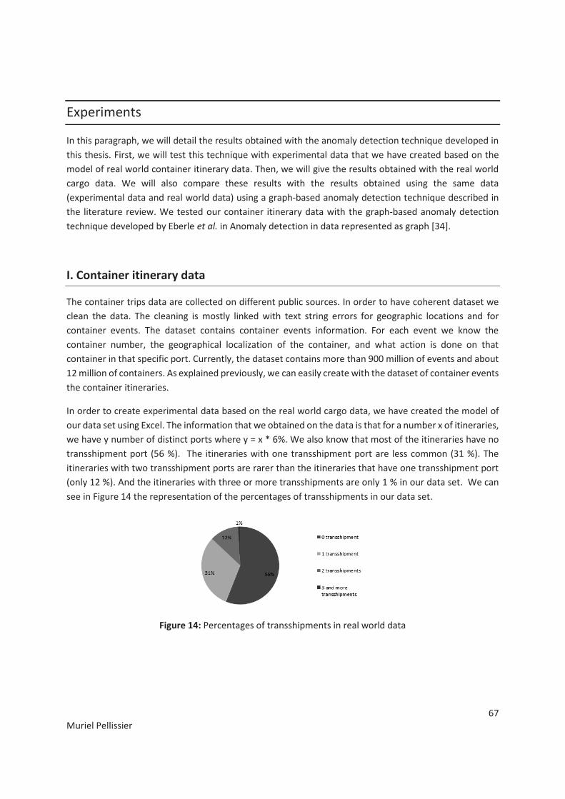
67

Muriel Pellissier

Experiments

In this paragraph, we will detail the results obtained with the anomaly detection technique developed in

this thesis. First, we will test this technique with experimental data that we have created based on the

model of real world container itinerary data. Then, we will give the results obtained with the real world

cargo data. We will also compare these results with the results obtained using the same data

(experimental data and real world data) using a graph-based anomaly detection technique described in

the literature review. We tested our container itinerary data with the graph-based anomaly detection

technique developed by Eberle et al. in Anomaly detection in data represented as graph [34].

I. Container itinerary data

The container trips data are collected on different public sources. In order to have coherent dataset we

clean the data. The cleaning is mostly linked with text string errors for geographic locations and for

container events. The dataset contains container events information. For each event we know the

container number, the geographical localization of the container, and what action is done on that

container in that specific port. Currently, the dataset contains more than 900 million of events and about

12 million of containers. As explained previously, we can easily create with the dataset of container events

the container itineraries.

In order to create experimental data based on the real world cargo data, we have created the model of

our data set using Excel. The information that we obtained on the data is that for a number x of itineraries,

we have y number of distinct ports where y = x * 6%. We also know that most of the itineraries have no

transshipment port (56 %). The itineraries with one transshipment port are less common (31 %). The

itineraries with two transshipment ports are rarer than the itineraries that have one transshipment port

(only 12 %). And the itineraries with three or more transshipments are only 1 % in our data set. We can

see in Figure 14 the representation of the percentages of transshipments in our data set.

Figure 14: Percentages of transshipments in real world data

68

Muriel Pellissier

II. Experimental data

We have created some experimental data based on the model made on real world data in order to test

the anomaly detection technique developed in this thesis. The model used for this experimental data is

the model detailed in the previous paragraph.

In order to test this technique with a small amount of data before testing it with our large data set, we

created experimental data with 210 itineraries.

1) Knowing that there is a link between the number of itineraries and the number of ports: y = x *

6%, with x the number of itineraries and y the number of ports. For 210 itineraries, we have twelve

distinct ports.

2) Based on the results detailed previously, we divided 160 itineraries as follow: 60 % of the

itineraries have zero transshipment port, 30 % have one transshipment port, and 10 % have two

transshipment ports. Thus, for 160 itineraries, we have 96 itineraries with zero transshipment

port, 48 itineraries with one transshipment port, and 16 itineraries with two transshipments

ports.

3) We created randomly the 160 itineraries. We added four different itineraries ten times in order

to be considered as frequent itineraries. And we added ten itineraries that are suspicious.

1. Graph-based anomaly detection technique

We described in details in the Literature review the graph-based anomaly detection technique developed

by Eberle et al. [34]. We will give here just a small description of this technique. This technique uses an

unsupervised approach and does not need to have training data. They detect the anomalies by analyzing

the relationships between the data using a graph-based representation. A graph represents a cargo and

all its information (contents, departure port, arrival port, transshipment ports, shipment company

information, vessel number etc.). By analyzing the graphs it is possible to detect the normal behaviors and

the deviations of those normal behaviors. Eberle et al. defines three types of graph-based anomalies:

modifications, insertions, and deletions [34]. This technique detects the best substructure(s) of the graphs

[23] using a Minimum Description Length (MDL) heuristic [24]. The detection of anomalies is performed

utilizing three different algorithms (one algorithm for each type of anomaly) by finding the patterns that

are close to the best substructure(s) [34].

· First, we tried this technique by representing the itineraries with a graph representation close to

the one they used for their experiments. We created for each itinerary of the experimental data

a sub graph on the model of the Figure 15. The Figure 15 represents the sub graph of the itinerary

leaving from port 1, arrival to port 3, and passing through the transshipment port 2.

69

Muriel Pellissier

Figure 15: Graph representation of the itinerary from port 1 to port 3 passing through port 2

Using the experimental data described previously, the software created one graph composed by

210 sub graphs. The graph contained 1303 vertices and 1094 edges. With this technique, we have

to execute the three different algorithms separately in order to detect the three different kinds

of anomalies: modifications, insertions, and deletions.

No anomalies were found with the Graph-Based Anomaly Detection - Minimum Description

length algorithm (GBAD – MDL). This algorithm detects the modification type of anomalies. Three

substructures were found as best substructures. The first best substructure was the structure

containing: Itinerary, Departure port and Arrival port. The second best substructure was:

Itinerary, Departure port, Arrival port and Transshipment port. The third best substructure was

Itinerary and Departure port.

No anomalies were found using the second algorithm: Probabilistic algorithm (GBAD – P). This

algorithm detects the deletion type of anomalies. No best structures were found neither using

this algorithm.

No anomalies were found using the third algorithm: Maximum Partial Substructure algorithm

(GBAD – MPS). This algorithm detects the insertion type of anomalies. Many best substructures

were found (45 best substructures).

No anomalies were found with this technique using the graph representation of itineraries shown

in Figure 15. We thought that the bad results could be explained by the representation we used

to represent our data. As this technique detects the best substructures of the graph, and then

thank to these best substructures this technique detects the anomalous structures, we can think

that our representation is not efficient for this technique. Indeed, as a sub graph represents an

itinerary, all of the sub graphs contain the vertex named “Itinerary”, as well as the vertices named

“Departure port” and “Arrival port”. And as 30% of the itineraries have one transshipment port,

30% of the sub graphs have also the vertex named “Transshipment port”. Therefore, even if an

itinerary is common it might not be as common as the substructures containing the vertices

“Itinerary”, “Departure port”, “Arrival port” and even “Transshipment port”. Thus, we could think

70

Muriel Pellissier

that the only best substructures that this technique will detect are the substructures shown in

Figure 16 and by consequence this technique will not be able to detect any anomalous itineraries.

Figure 16: Best substructures

As the results were not good using the previous graph representation, we tried to use this technique with

another graph representation of the itineraries.

· We tried to represent the itineraries with another graph representation. The Figure 17 represents

the sub graph of the same itinerary seen in Figure 15. The container leaves from port 1, arrival to

port 3, and passing through the transshipment port 2.

Figure 17: Another graph representation of the itinerary port 1 to port 3 passing through port 2

Using the same experimental data but with a different graph representation, the software created

one graph composed by 210 sub graphs. The graph contained 547 vertices and 338 edges. As for

the first try, we need to execute the three different algorithms in order to detect all the anomalies.

Three best substructures were detected with the GBAD – MDL algorithm. Two of the three

substructures detected were common itineraries that we added to the experimental data. The

algorithm detected one anomalous sub graph. The anomalous sub graph detected was an

anomalous itinerary that we added to the data.

Three best substructures were detected with the GBAD – MPS algorithm. The best substructures

detected with the GBAD – MPS were the same best substructures detected with the GBAD – MDL

algorithm. One sub graph was spotted as anomalous. The anomalous sub graph was not the same

sub graph that was detected by the GBAD – MDL algorithm. But this anomalous sub graph was

also part of the anomalous itineraries added to the data.

More substructures were detected as best substructures with the GBAD – P. Twenty substructures

were detected as best substructures, but no anomalies detected.

71

Muriel Pellissier

The results are a bit better using this graph representation of the itinerary but this technique does

not detect all the anomalous itineraries inserted in the data. Two common itineraries were

detected out of 4 common itineraries inserted in the data. And two anomalous itineraries were

detected out of ten anomalous itineraries inserted in the data.

Moreover, we can see that this graph representation does not work for our data as it does not

keep the position information. As we see with the Figure 18, if we have the itinerary from port 1

to port 3 passing by the port 2 as transshipment port, and the itinerary from port 2, to port 3

finishing in port 1. This technique will detect the substructure from port 2 to port 3 as best

substructure. But with that substructure we can see that the position information is not kept, and

for our application, the information of the port will not be taken into account while finding the

best substructures and by consequence the anomalies. Trying to apply this technique with our

data, we understood the importance of the graph representation of the data. The graph

representation could be, depending on the dataset, an important limitation of this technique.

Figure 18: Graph representation limitation

This graph-based anomaly detection technique does not give good results using our data. As they tested

this technique with cargo information and they had good results, we can think that the main difference

between our application and their application is the difference on the data. They created graphs that

contained more information than we had with our data. For example, they had information about the trip

and the container as us. They had also financial information, date of arrival, information about the cargo,

information on the vessel, information about the importer, information about the shipper. It is really

difficult to use this technique with our dataset that contains really little information because we could not

find a good graph representation. As this technique is based on the best substructures found with the

technique, if the graph representation is not good enough, the technique will have difficulties to detect

the best substructures and by consequence the technique will not detect efficiently the anomalies.

Best substructure

72

Muriel Pellissier

2. Our anomaly detection technique

We tested our anomaly detection technique with the same experimental data detailed previously.

For this experiment, we set the minimum frequency threshold to 5.40, the maximum anomaly degree

threshold to 0.43, and the minimum anomaly degree threshold to 0.23.

The maximum anomaly degree threshold value and the minimum anomaly threshold value were

explained in the previous section.

The minimum frequency threshold value was calculated with the frequencyDataFile created with the

common subsequences algorithm (Figure 10). The average frequency was calculated with the frequency

of all the itineraries. Another frequency value is calculated as the average of the frequency values of the

itineraries that have a frequency value above the first frequency average. The second frequency value is

the value used for the minimum frequency threshold.

The results obtained with this technique using the data set of 210 itineraries described previously are 31

itineraries that are detected as suspicious. The suspicious itineraries detected represent 15 % of the whole

data set. We have inserted 10 anomalous itineraries. All the anomalous itineraries that we have inserted

in the data set were detected as anomalous. With this technique, if an itinerary is really close to a common

itinerary it will be targeted as suspicious. Therefore, we can explain that this technique detected other

itineraries as suspicious because other suspicious itineraries might have been created while creating

randomly the data set. As we have created all the itineraries with only 12 different ports (using the same

percentage as in our real world data set), we might expect to create some itineraries that could be similar

enough to be detected by our technique as suspicious.

The results are written in a text file as we can see in Figure 19. Every anomalous itinerary uses three lines

on the text file. The first line is the anomalous itinerary, the second line is the common itineraries, and

the third line is the anomaly degree values.

Figure 19: Anomalous itineraries using experimental data

As shown in Figure 19, the first anomalous itinerary detected in this example is the itinerary going from

port 1 to port 8 passing through port 9. It is considered anomalous because of three different common

itineraries. The first common itinerary used to define this itinerary as abnormal is the itinerary going from

any port to port 8 passing through port 6 and 9. As the departure port of the common itinerary is a wild

card it can be any port, we consider the port of departure to be the port 1. We can see in that case that

73

Muriel Pellissier

the two itineraries are close but one transshipment port has been removed to the common itinerary. We

have the same conclusion when we compare this itinerary with the two others common itineraries, one

port of transshipment is missing.

We have tested our technique with the same experimental data using different values for the maximum

anomaly degree threshold. The Figure 20 gives the results obtained with 3 different values of the

maximum anomaly degree. The execution time does not change with different threshold values. The

program takes few minutes to execute (less than 5 minutes).

Minimum frequency 5,4 5,4 5,4

Minimum anomaly degree 0,23 0,23 0,23

Maximum anomaly degree 0,49 0,43 0,4

Anomalous itineraries 42 31 21

Percentage of the whole data set 20,00% 15,00% 10,00%

Anomalous itineraries inserted detected 10 (100%) 10 (100%) 8 (80%)

Figure 20: Results obtained with different maximum anomaly degree values

We tested our technique with an anomaly degree level that we increased. With the maximum anomaly

degree value equal to 0.49, we detected 42 suspicious itineraries. The suspicious itineraries detected

represent 20% of the whole data set. We have detected all the suspicious itineraries that we have inserted

in the data set. We detected 11 suspicious itineraries more than with the maximum anomaly degree equal

to 0.43. As expected, we can see that if you increase the level of the anomaly degree we will detect more

itineraries targeted as suspicious.

Then, we tested the technique with a lower anomaly degree level. With the maximum anomaly degree

value set to 0.40, we detected 21 anomalous itineraries, which is 10 % of the whole data set. But two

suspicious itineraries that we have inserted were not detected as suspicious. As expected if we lower the

anomaly degree level, we will detect less suspicious itineraries but we might detect as normal some

itineraries that are actually suspicious. The graph Figure 21 represents the anomalies detected depending

on the maximum anomaly level.

74

Muriel Pellissier


The results obtained with the experimental data were as expected. When the different thresholds are set

with the values that are the best adapted to the data, we obtained good results. Now that we validated

our technique with experimental data, we will test this technique with real world cargo data.

75

Muriel Pellissier

III. Real world data

We also tested the technique described in this thesis and the graph-based technique with real world data.

The data set has 135798 itineraries and 22831 distinct itineraries.

1. Graph-based anomaly detection technique

We tried to use the graph-based anomaly detection technique with the 135798 itineraries of our data set.

The first step of this graph-based anomaly detection technique is to create the graph and then by

executing the three different algorithms to detect the best substructures of the graph and the anomalies.

With this large data set, the software could not create the graph. The software can create five different

types of graph: directed, spring, radial, circular, large spring. But with this large data set, none of the

graphs could be created. As all the algorithms involving graphs have a time complexity that is really high,

it makes difficult to work with a large dataset with graphs. We had for all of them error messages like out

of memory, or error reading image. By consequence, we could not try the different algorithms on our data

set.

Even if we could not test the graph-based anomaly detection technique, we do not think it would have

been possible to have good results. As we have seen with the experimental data, we could not find a good

graph representation of our data that could work well for the graph-based anomaly detection techniques.

2. Our anomaly detection technique

We tested our technique with our real world cargo data. The minimum frequency calculated with the

average frequency of all the itineraries as described for the experimental data is for the real world data

60. As for the experimental data, the maximum anomaly degree is 0.43 and the minimum anomaly degree

is 0.23. Though, in order to compare the results, we tested this technique with different threshold values.

We tried our technique with different minimum frequency values, with different maximum anomaly

degree values and with different minimum anomaly degree values. We can see the results in Figure 22.

We do not give the execution time, as for the experimental data, the execution time is similar for all the

tests and really fast considering the amount of data (less than 10 minutes).

Minimum frequency 60 60 60 40 80 60

Minimum anomaly degree 0,23 0,23 0,23 0,23 0,23 0

Maximum anomaly degree 0,4 0,43 0,49 0,43 0,43 0,43

Anomalous itineraries 11965 11992 13065 14270 10199 15886

Percentage of the whole data set 8,80% 8,80% 9,60% 10,50% 7,50% 11,70%

Percentage of the distinct itineraries

52,40% 52,50% 57,20% 62,50% 44,70% 69,60%

Figure 22: Results with different threshold values

76

Muriel Pellissier

As expected, if we increase the maximum anomaly degree level, we will detect more anomalous

itineraries. We can see the results in the first three columns of the Figure 22. We tested with a maximum

anomaly degree equal to 0.40, 0.43, and 0.49.

If we decrease the minimum frequency value, we will detect more anomalous itineraries. We can see the

results in the column 3, 4, and 5 of the Figure 22. We tested with a minimum frequency value equal to 40,

60, and 80.

We also tried with a minimum anomaly degree equal to 0. We can see from the Figure 22 that we detect

many itineraries as anomalous with a minimum anomaly degree set to 0.

Even if we can see differences between the results depending on the thresholds, the results obtained are

not really good as we detect around 50% of the distinct itineraries as anomalous. The percentages of

anomalous itineraries detected with this technique are really higher for the real world data than for the

experimental data. Having a look at the itineraries that are detected as anomalous we can see that many

itineraries are detected as anomalous because they are inverted. We can see some examples in the Figure

23. The Figure 23 is a part of the output file we obtained. It represents a list of anomalous itineraries and

their anomaly degree values. The first itinerary is the itinerary detected as anomalous by this technique.

The second itinerary (itineraries) is (are) the common itinerary (itineraries) which is (are) compared to the

first itinerary. And the third line is the anomaly degree value (s).


For example, the itinerary “19 82” is spotted as anomalous while comparing it with the common itinerary

“82 19 *”. We can see that these two itineraries have similar ports, but that the order of the ports is

inverted between the two itineraries. Here, is the detail for the anomaly degree calculated for these two

itineraries:


2) Name ports: ports value: 1 and maximum changes: 2*2


Thus, the anomaly degree is included between the minimum anomaly degree that we have set to 0.23

and the maximum anomaly degree that we have set to 0.43. We do not think that this kind of itineraries

is relevant for our anomaly detection technique. Thus, we decide to remove the inverted itineraries from

our results. In order to remove these itineraries, we remove from the anomalous itineraries file, all the

77

Muriel Pellissier

itineraries where two consecutive ports are present in the first itinerary and also present in the second as

consecutive ports but where the order is inverted from the first itinerary.

Often, one itinerary is spotted as anomalous because of several common itineraries. If one of the common

itineraries does not contain inverted consecutive ports then we do not remove the given itinerary from

the anomalous data set. For example, the itinerary “148 277 70” is targeted as suspicious because of four

different common itineraries: “277 70”, “* 277 148”, “70 277 *”, and “148 277”. The anomaly degree

values are for the four itineraries 0.33. If the itinerary was targeted as anomalous only because of the

itinerary “70 277 *”, we will remove it, but as the itinerary is targeted as anomalous because of other

itineraries we keep this itinerary in the data set of anomalous itineraries.

Thus, we remove all the itineraries that have inverted consecutive ports from all the results obtained with

the real world data. We can see in Figure 24 that this time we obtain results as expected.

Minimum frequency 60 60 60 40 80 60

Minimum anomaly degree 0,23 0,23 0,23 0,23 0,23 0

Maximum anomaly degree 0,4 0,43 0,49 0,43 0,43 0,43




52,40% 52,50% 57,20% 62,50% 44,70% 69,60%

After reduction




12,54% 12,67% 20,29% 18,65% 9,18% 54,35%

Figure 24: Results after reduction with different threshold values

We can also see the influences of the different thresholds and the importance to set well the threshold

values in order to have the best results. As said before, the number of anomalous itineraries detected

decreases when the minimum frequency value increases as we can see in Figure 25.

78

Muriel Pellissier

Figure 25: Graph representing the anomalies depending on the minimum frequency threshold

The number of anomalous itineraries detected increases when the maximum anomaly degree threshold

increases as we can see in Figure 26.


The number of anomalous itineraries detected can increase a lot when the minimum anomaly degree

decreases.

For a minimum frequency set to 60, a minimum anomaly degree to 0.23 and a maximum anomaly degree

to 0.43, we obtained with the real world data set 12.7 % of the distinct itineraries as anomalous.

We know that around 10% of the containers travelling in the world are risky containers. Thus, we can say

that the percentage of anomalous itineraries detected with this anomaly detection technique is close

enough to the real percentage to be considered as satisfactory result. We cannot verify all the itineraries

found as anomalous as we do not have any knowledge on which itineraries are actually suspicious in our

data set. Nevertheless, with the results obtained with the experimental data and the real world cargo data

we can say that the results are good and as expected.

79

Muriel Pellissier

In this chapter, we have detailed the results obtained with our anomaly detection technique applied to

experimental data and with real world cargo data. We also tested with the same data, experimental data

and real world cargo data, to detect the anomalies using a graph-based anomaly detection technique. The

results obtained with the graph-based anomaly detection technique are not really satisfactory. As we

explained before, we were confronted to several problems while using a graph-based anomaly detection

technique. First, the algorithms that involve graphs have a high time complexity which makes the graph-

based techniques difficult to use when dealing with large data set. We also faced another problem linked

with the graph representation of the data. While testing a graph-based anomaly detection technique with

our data, we realized that it was really difficult to find a good graph representation of our data. As our

data does not contain many information, it was difficult for the graph technique to detect the best

substructures, and as result, to detect the anomalies. The only graph representation that we could find

could not take into account the position of the elements within a structure.

At the contrary, the results obtained with our anomaly detection technique are for both data set

satisfactory and as expected. Our anomaly detection technique detects anomalous sequences by

comparing random sequences with common sequences. The anomalous sequences are sequences that

are similar to common sequences but with small changes. The changes are based on the order of the

events of the two sequences and on the position of the events within the sequences. This technique can

be used for any application that uses sequential data where the order and the position of the events

within a sequence is important. Moreover this technique could be used with small and big data set.

80

Muriel Pellissier

IV. Discussion

We will now discuss how we could improve this technique. This technique can detect anomalous

sequences using a data set of sequences. We define a sequence as anomalous when a sequence is close

to a common sequence but not exactly identical. We have seen that depending on which kind of anomalies

the user is looking for, the user can set different thresholds: the minimum frequency threshold, the

minimum anomaly degree threshold and the maximum anomaly threshold. For our application, world

cargo data we set the thresholds as follow: the minimum frequency to 60 (this value is obtained with the

frequencies of the data), the minimum anomaly degree to 0.23 and the maximum anomaly degree to

0.43.

In order to reduce the number of anomalies detected and to improve this technique, we could add

external information. External information is information that is not extracted directly from the data set.

External information could be added by the user, combined with the data from the data set, and used by

this technique to select more precisely the anomalies. This information could be taken into account by

adding different weights to the items while calculating the distance between two sequences.

For example, for the maritime surveillance, the customs have some information like for example some

ports are known to be more sensitive than other ports, or some areas are sensitive or even some shipping

companies.

We do not have this information, but if we had we could add it while calculating the anomaly degree

between two itineraries. We could add this information by putting more weight on the sensitive ports

instead of putting weight on the ports only by comparing the ports from the given itinerary with the ports

of the common itinerary.

Same idea with the transshipment company, we do know for each trip the transshipment company, but

as we do not have any information on the company we do not use this information while calculating the

anomaly degree. If we knew which companies should have more surveillance, we could add weight to all

the itineraries that are used by these companies.

Future research aims at enriching the existing information with spatio-temporal data in order to identify

unnecessary delays in the movements of the maritime containers. For example, if we know how long a

container takes to travel from one port to another, or how long a container stays at a port, or the time for

the whole itinerary from the departure port to the arrival port, we can use this information in order to

detect other types of anomalies based on delays.

Environmental information could be considered while calculating the distance between two sequences.

For example, the weather can influence the routes taken by the cargo. The route could be changed

because of natural disasters.

81

Muriel Pellissier

Economical information could also affect the cargo routes. For example, the fluctuations of the oil price

can have an influence on the cost of transportation, thus, it can influence the itinerary taken by the cargo.

82

Muriel Pellissier

Conclusion

The aim of the research of this thesis was to develop a technique that could detect automatically

anomalous containers from a large data set of container trips using only little information on the container

itineraries. This technique was developed for the maritime surveillance in order to detect suspicious

containers by comparing container itineraries but it can also be applied to any other domain that uses

sequential data. In order to elaborate this technique we were interested in several fields. We looked at

the existing techniques developed for the maritime surveillance, the graph-based anomalies detection

techniques, and the sequence mining techniques. We also looked at the existing string distances.

The techniques developed for the maritime security are quite different from our approach as the

techniques need a lot of information about the containers, the routes, the cargo etc. The existing

techniques fuse different types of maritime information provided by different sources in order to detect

suspicious behaviors. For our application, the idea was to detect suspicious behaviors with only little

information about the container itineraries and no other information.

The sequence mining techniques can detect anomalous subsequences by comparing the subsequences of

a sequence with the other subsequences of the same sequence. Or they can detect anomalous sequences

by comparing items of different sequences. The anomalous subsequences are detected with differences

between sequences or subsequences. The differences are based on the order of the items within the

sequences. But the position of the items in the sequences is not taken into account. For our application,

we had to compare the items of two sequences based on the order of the items and their position.

The graph-based anomaly detection techniques are techniques that detect structural anomalies. These

techniques represent the data with graphs and then compare the structures of the graphs in order to

detect the anomalies. Some of these techniques are even applied to the maritime security. Though, we

tested some graph-based anomaly detection techniques with our data and the results were not

satisfactory. These techniques use a lot of information in order to create structures that are big enough

in order to be able to compare them. If the structures of the graphs are not important enough or regular

enough it is difficult to compare them. With our data, that contains little information, the structures

created were really small and it is difficult to obtain good results based on comparison of small structures.

Our anomaly detection technique for sequential data can be applied to small and large data set of

sequences. The anomalous sequences are defined as sequences that are close to common sequences but

not exactly identical. An anomalous sequence is like a common sequence with some small changes. In

order to detect a sequence as anomalous, this technique compares two sequences. One of the two

sequences is a given sequence from the data set. The other sequence could be a frequent sequence

detected from the data set, or a sequence from another data set given by the user depending on his needs.

The changes between two sequences are calculated based on the order of the items in the sequences like

for the sequence mining techniques. But the changes are not calculated only based on the order of the

items but also based on the position of the items in the sequences.

83

Muriel Pellissier

This technique is divided into two different steps. First, the technique detects the frequent sequences of

the data set with the regular expression methods. This part can be used alone in order to detect efficiently

the frequent sequences of a data set. The second part of this technique is to compare the sequences from

the data set with the sequences that were detected as common (frequent) with the first part of the

technique. In order to compare two sequences, this technique calculates an anomaly degree between two

sequences based on a distance measure. The distance between two sequences is calculated based on the

qualitative and quantitative differences between two sequences. Depending on the anomaly degree

value, the given sequence will be targeted as normal or as suspicious.

We tested this technique with experimental data and with real world cargo data. For both data sets, we

obtained satisfactory results.

This technique could be further improved by taking into account external information. External

information means information that is not extracted from the data set containing the sequences, but

information that comes from external sources. External information could be added to this technique by

adding different weights to the items while calculating the distance between two sequences. For example,

for the maritime surveillance, we could add some information about the sensitive ports, sensitive areas,

sensitive shipping companies etc.

84

Muriel Pellissier

Conclusion

L’objectif de cette thèse était de développer une technique pour détecter automatiquement des

conteneurs suspects à partir d’une large base de données d’itinéraires de conteneurs utilisant seulement

peu d’informations sur les itinéraires des conteneurs. Cette technique a été développée pour la

surveillance maritime afin de détecter les conteneurs suspects en comparant les itinéraires de conteneurs

mais cette technique peut être utilise par tous les domaines qui utilises des données séquentielles. Afin

de développer cette technique, nous nous sommes intéressés à plusieurs domaines. Nous avons étudié

les techniques existantes appliquées à la surveillance maritime, les techniques de détection d’anomalies

utilisant les graphs, et les techniques de traitement de séquence. Nous avons aussi regardé les distances

calculées à partir de séquences.

Les techniques développées pour la sécurité maritime sont assez différentes de notre approche. En effet,

ces techniques utilisent beaucoup d’informations différentes afin de détecter les comportements

suspects comme par exemple informations sur les conteneurs, sur les routes, ou sur les cargos. Les

techniques existantes regroupent différents types de données maritimes qui proviennent de différentes

sources.

Les techniques de traitement de séquence peuvent détecter des parties de séquence comme anormales

en comparant différentes parties d’une même séquence, ou bien elles peuvent détecter des séquences

comme anormales en comparant les objets de différentes séquences. Les séquences sont détectées

comme anormales en fonction des différences qu’il y a entre plusieurs séquences ou plusieurs parties de

séquence. Les différences sont obtenues en fonction de l’ordre des objets dans les séquences. Cependant,

la position des objets dans les séquences n’est pas prise en compte. Pour notre application, nous avons

besoin de comparer les objets de deux séquences en fonction de l’ordre des objets ainsi que de leur

position dans la séquence.

Les techniques de détection d’anomalies utilisant les graphs sont des techniques qui détectent les

anomalies utilisant la structure des graphs. Ces techniques représentent les données avec des graphs et

comparent les structures des graphs afin de détecter les anomalies. Certaines de ces techniques sont

même appliquées au domaine maritime. Cependant, nous avons teste ces techniques avec nos données

et les résultats n’ont pas été satisfaisants. Ces techniques utilisent beaucoup d’informations afin d’avoir

des structures qui soient suffisamment importantes pour pouvoir être comparées. Si les structures des

graphs ne sont pas assez importantes ou régulières, il est difficile de pouvoir les comparer. Avec nos

données, qui ne contiennent que peu d’informations, les structures crées étaient trop petites pour

pouvoir obtenir de bons résultats en comparant les structures.

Notre technique de détection d’anomalies peut être utilisée avec peu de données ainsi qu’avec une large

base de données. Une séquence est définie comme étant anormale si la séquence est presque identique

à une séquence qui est fréquente dans la base de données. Ce qui veut dire que la séquence est comme

la séquence qui est fréquente avec quelques changements. Afin de définir une séquence de la base de

85

Muriel Pellissier

données comme anormale, cette technique compare deux séquences. Une des deux séquences est une

séquence aléatoire de la base de données. L’autre séquence peut être en fonction du besoin de

l’utilisateur ou bien une séquence détectée comme fréquente dans la base de données, ou bien une

séquence d’une autre base de données. Les différences entre deux séquences sont calculées en tenant

compte de l’ordre des objets des séquences, ainsi que la position des objets dans les séquences.

Cette technique est divisée en deux parties. Premièrement, cette technique détecte les séquences qui

sont fréquentes dans la base de données utilisant les expressions régulières. Cette partie peut être utilisée

seule afin de détecter efficacement les séquences qui sont fréquentes dans la base de données. Ensuite,

cette technique compare les séquences de la base de données avec les séquences qui ont été détectées

comme fréquentes par la première partie de cette technique. Afin de comparer deux séquences, cette

technique calcule un degré d’anomalie entre deux séquences. Le degré d’anomalie est calcule grâce à une

mesure de distance qui est calculée sur les différences qualitatives et quantitatives entre deux séquences.

En fonction de la valeur du degré d’anomalie, la séquence sera définie comme normale ou anormale.

Nous avons testé notre technique avec des données expérimentales, ainsi qu’avec des données réelles de

conteneurs. Nous avons obtenu des résultats satisfaisants avec les données expérimentales, ainsi qu’avec

les données réelles.

Cette technique pourrait être approfondie en ajoutant d’autres informations qui ne peuvent être obtenue

directement en étudiant la base de données. Par exemple, des informations provenant d’une autre source

pourrait être ajoutées aux informations extraites de la base de données. Ces informations pourraient être

ajoutées à cette technique en donnant différents poids aux différents objets lorsque nous calculons la

distance entre deux séquences. Par exemple, pour la sécurité maritime, nous pourrions ajouter des

informations concernant les ports à risques, les régions à risques, les compagnies de transport à risques

etc.

86

Muriel Pellissier

References

[1] U.S. Customs Service “1,754 Pounds of Marijuana Seized in Cargo Container at Port Everglades”, 2000 (http://www.cbp.gov/hot-new/pressrel/2000/1106-01.htm)

[2] Mae Dey Newsletter “Customs Seizes Weapons”, 23(4), 2003 [3] E. Martineau, J. Roy, and Defence Research and Development Canada Valcartier, “Maritime Anomaly

Detection: Domain Introduction and Review of Selected Literature”, 2011 [4] B.J. Rhodes, N.A. Bomberger, M. Seibert, and A.M. Waxman, “Maritime Situation Monitoring and

Awareness Using Learning Mechanisms”, IEEE MILCOM 2005 Military Communications Conference, 2005

[5] G.A. Carpenter, S. Grossberg, and J.H. Reynolds, “ARTMAP: Supervised real-time learning and classification of nonstationary data by a selforganizingneural network”, Neural Networks, 4(5), pp. 565–588, 1991

[6] G.A. Carpenter, S. Grossberg, N. Markuzon, J.H. Reynolds, and D.B. Rosen, “Fuzzy ARTMAP: A neural network architecture for incremental supervised learning of analog multidimensional maps”, IEEE Transactions on Neural Networks, 3(5), pp. 698–713, 1992

[7] D. Garagic, B.J. Rhodes, N.A. Bomberger, and M. Zandipour, “Adaptive Mixture-Based Neural Network Approach for Higher-Level Fusion and Automated Behavior Monitoring”, NATO Workshop on Data Fusion and Anomaly Detection for Maritime Situational Awareness (NATO MSA 2009), NATO Undersea Research Centre (NURC), 2009

[8] D. M. Titterington, “Recursive parameter estimation using incomplete data,” Journal of Royal Statistical.Society: Series B, vol. 46, pp. 257-267, 1984

[9] G. McLachlan and D. Peel, “Finite Mixture Models”, New York John Wiley and Sons, 2000 [10] G. de Vries, V. Malaisé, M. van Someren, P. Adriaans, and G. Schreiber, “Semi-Automatic Ontology

Extension in the Maritime Domain”, The 20th Belgian-Netherlands Conference on Artificial Intelligence (BNAIC 2008), University of Twente, 2008

[11] G. de Vries, and M. van Someren, “Unsupervised Ship Trajectory Modeling and Prediction Using Compression and Clustering”, Proceedings of the 18th Annual Belgian-Dutch Conference on Machine Learning, pp. 7-12, 2009

[12] B.J. Frey, and D. Dueck, “Clustering by Passing Messages Between data Points”, www.sciencemag.org, vol. 315, pp. 972-977, 2007

[13] K.T. Ma, G.W. Ng, X. Wang, and W.E.L. Grimson, “Anomaly detection for Maritime Security”, NATO Workshop on Data Fusion and Anomaly Detection for Maritime Situational Awareness (NATO MSA 2009), NATO Undersea Research Centre (NURC), 2009

[14] X. Wang, K.T. Ma, W.E.L. Grimson, “Trajectory Analysis and Semantic Region Modeling Using A Nonparametric Bayesian Model”, CVPR, 2008

[15] B. Quanz, H. Fei, J. Huan, J. Evans, V. Frost, G. Minden, D. Deavours, L. Searl, D. DePardo, M. Kuehnhausen, D. Fokum, M. Zeets, A. Oguna, “Anomaly Detection with Sensor Data for Distributed Security”, ICCCN '09 Proceedings of the 2009 Proceedings of 18th International Conference on Computer Communications and Networks, pp. 1-6, 2009

[16] M. Seibert, B.J. Rhodes, N.A. Bomberger, P.O. Beane, J.J. Sroka, W. Kogel, W. Kreamer, C. Stauffer, L. Kirschner, E. Chalom, M. Bosse, and R. Tillson, “SeeCoast port surveillance”, Proceedings of SPIE, 6204(2), 2006

[17] M. Morel, J.P. George, F. Jangal, A. Napoli, M.A. Giraud, M. Botalla, and A. Littaye, “SCANMARIS Project – Detection of Abnormal Vessel Behaviours”, NATO Workshop on Data Fusion and Anomaly Detection for Maritime Situational Awareness (NATOMSA 2009), NATO Undersea Research Centre (NURC), 2009

[18] M. Géhant, V. Roy, J.P. Marmorat, and M. Bordier, “A Behaviour Analysis Prototype for Application to Maritime Security”, NATO Workshop on Data Fusion and Anomaly Detection for Maritime Situational Awareness (NATO MSA 2009), NATO Undersea Research Centre (NURC), 2009

[19] K.M. Carley, G.B. Davis, and J. Olson, “Dynamic Network Analysis for the Detection of Anomalies to Support Maritime Analysis”, Workshop on Detection of Anomalous Behaviors in Maritime Environments, Carnegie Mellon University, 2009

[20] C. Griffin, “Learning and Prediction for Enhanced Readiness: An ONR Office 31 Program”, Presentation to TTCP MAR AG-8, 2009

[21] V.P. Janeja, V. Atluri, and N.R. Adam, “Detecting Anomalous Geospatial Trajectories through Spatial Characterization and Spatio-Semantic Associations”, Proceedings of the 2004 annual conference on digital government research, 2004

[22] C. C. Noble and D. J. Cook, “Graph-Based Anomaly Detection”, 9th ACM SIGKDD International Conference on Knowledge Discovery and Data Mining, ACM, 2003

[23] D.J. Cook and L.B. Holder, “Graph-Based Data Mining”, IEEE Intelligent Systems, 15(2), pp. 32-41, 2000

[24] J. Rissanen, “Stochastic Complexity in Statistical Inquiry” World Scientific Publishing Company, 1989 [25] http://kdd.ics.uci.edu/databases/kddcup99/kddcup99.html [26] W. Eberle and L. Holder, “Detecting Anomalies in Cargo Shipments Using Graph Properties”, Journal

Intelligent Data Analysis, 11(6), pp. 663-689, 2007

87

Muriel Pellissier

[27] T.H. Cormen, C.E. Leiserson, R.l. Rivest, and C. Stein, “Introduction to Algorithms”, McGraw Hill, 2nd Edition. pp. 629-634, 2001

[28] J. Scott, “Social Network Analysis: A Handbook”, SAGE Publications, 2nd Edition, pp. 72-78, 2000 [29] A. Broder, R. Kumar, F. Maghoul, P. Raghavan, S. Rajagopalan, R. Stata, A. Tomkins, and J. Wiener

, “Graph Structure in the Web”, Proceedings of the 9th international World Wide Web conference on Computer networks : the international journal of computer and telecommunications netowrking, 33(1-6), pp. 309-320, 2000

[30] F. Chung, L. Lu, V. Vu, “Eigenvalues of Random Power Law Graphs, annals of combinatorics 7, pp. 21-33, 2003

[31] P. Boykin and V. Roychowdhury, “Leveraging Social Networks to Fight Spam”, IEEE Computer, 38(4), pp. 61-67, 2005

[32] K. Hogstedt, D. Kimelman, V.T. Rajan, T. Roth, M. Wegman, “Graph Cutting Algorithms for Distributed Applications Partitioning”, ACM SIGMETRICS, 28(4), pp. 27-29, 2001

[33] K. Lang, “Finding good nearly balanced cuts in power law graphs”, Technical Report, Yahoo! Inc., 2004

[34] W. Eberle and L. Holder, “Anomaly detection in data represented as graphs”, Journal Intelligent Data Analysis, 11(6), pp. 663-689, 2007

[35] U.S. Customs and Border Protection (CBP) - http://www.cbp.gov/ [36] W. Eberle, L. Holder, and B. Massengill, "Graph-Based Anomaly Detection Applied to Homeland

Security Cargo Screening", International Conference of the Florida Artificial Intelligence Research Society (FLAIRS), 2012

[37] S. Nijssen and J. Kok, “A quickstart in Frequent Structure Mining Can Make a Difference”, International Conference on Knowledge Discovery and Data Mining, SIKDD, pp. 647-652, 2004

[38] E. Lacitis, “Ports sleuths on the trail of counterfeit goods”, The Wasghinton Post, 2011 [39] P. Sun, S. Chawla, and B. Arunasalam, “Mining for Outliers in Sequential Databases”, Proc. SIAM

Int’l Conf. Data Mining, 2006 [40] D. Gusfield, “Algorithms on Strings, Trees, and Sequences: Computer Science and Computational

Biology”, Cambridge Univ, Press, 1997 [41] S.A. Hofmeyr, S. Forrest, and A. Somayaji, “Intrusion Detection Using Sequences of System Calls”, J.

Computer Security, 6(3), pp. 151-180, citeseer.ist.psu.edu/hofmeyr98intrusion.html, 1998 [42] S. Forrest, S.A. Hofmeyr, A. Somayaji, and T.A. Longstaff, “A Sense of Self for Unix Processes”, Proc.

IEEE Symp. Security and Privacy (ISRSP ’96), pp. 120-128, citeseer.ist.psu.edu/forrest96sense.html, 1996

[43] E. Eskin, W. Lee, and S. Stolfo, “Modeling System Call for Intrusion Detection Using Dynamic Window Sizes”, Proc. DARPA Information Survivability Conf. and Exposition (DISCEX), citeseer.ist.psu.edu/portnoy01intrusion.html, 2001

[44] T. Lane and C.E. Brodley, “Temporal Sequence Learning and Data Reduction for Anomaly Detection”, ACM Trans. Information Systems and Security, 2( 3), pp. 295-331, 1999

[45] S. Chakrabarti, S. Sarawagi, and B. Dom, “Mining Surprising Patterns Using Temporal Description Length”, Proc. 24th Int’l Conf. Very Large Data Bases, pp. 606-617, 1998

[46] V. Chandola, A. Banerjee and V. Kumar, “Anomaly Detection for Discrete Sequences: A Survey”, IEEE Trans. on Knowledge and Data Engineering, pp. 823-839, 2012

[47] S. Forrest, C. Warrender, and B. Pearlmutter, “Detecting Intrusions Using System Calls: Alternate Data Models”, Proc. IEEE Symp. Security and Privacy (ISRSP), pp. 133-145, 1999

[48] T. Lane and C.E. Brodley, “Sequence Matching and Learning in Anomaly Detection for Computer Security”, Proc. AI Approaches to Fraud Detection and Risk Management, Fawcett, Haimowitz, Provost, and Stolfo, eds., pp. 43-49, 1997

[49] D. Endler, “Intrusion Detection: Applying Machine Learning to Solaris Audit Data”, Proc. 14th Ann. Computer Security Applications Conf., pp. 268-279, 1998

[50] H. Debar, M. Dacier, M. Nassehi, and A. Wespi, “Fixed vs. Variable-Length Patterns for Detecting Suspicious Process Behavior”, Proc. Fifth European Symp. Research in Computer Security, pp. 1-15, 1998

[51] A.K. Ghosh, A. Schwartzbard, and M. Schatz, “Using Program Behavior Profiles for Intrusion Detection”, Proc. SANS Third Conf. and Workshop Intrusion Detection and Response, citeseer.ist.psu.edu/ghosh99learning.html, 1999

[52] A. Ghosh, A. Schwartzbard, and M. Schatz, “Learning Program Behavior Profiles for Intrusion Detection”, Proc. First USENIX Workshop Intrusion Detection and Network Monitoring, pp. 51-62, 1999

[53] J.B.D. Cabrera, L. Lewis, and R.K. Mehra, “Detection and Classification of Intrusions and Faults Using Sequences of System Calls”, SIGMOD Record, 30(4), pp. 25-34, 2001

[54] A.P. Kosoresow and S.A. Hofmeyr, “Intrusion Detection via System Call Traces”, IEEE Software, 14(5), pp. 35-42, 1997

[55] D. Dasgupta and F. Nino, “A Comparison of Negative and Positive Selection Algorithms in Novel Pattern Detection”, Proc. IEEE Int’l Conf. Systems, Man, and Cybernetics, 1, pp. 125-130, 2000

[56] T. Lane and C.E. Brodley, “An Application of Machine Learning to Anomaly Detection”, Proc. 20th Nat’l Information Systems Security Conf., pp. 366-380, 1997

88

Muriel Pellissier

[57] D. Ron, Y. Singer, and N. Tishby, “The Power of Amnesia: Learning Probabilistic Automata with Variable Memory Length”, Machine Learning, 25(2/3), pp. 117-149, 1996

[58] N. Ye, “A Markov Chain Model of Temporal Behavior for Anomaly Detection”, Proc. Fifth Ann. IEEE Information Assurance Workshop, 2004

[59] E. Eskin, W.N. Grundy, and Y. Singer, “Protein Family Classification Using Sparse Markov Transgucers”, Proc. Int Conf, Intelligent Systems for Molecular Biology (ISMB’ 08), pp. 134-145, 2000

[60] E. Keogh, S. Lonardi, and C.A. Ratanamahatana, “Towards Parameter-Free Data Mining”, Proc. 10th ACM SIGKDD Int’l Conf. Knowledge Discovery and Data Mining, pp. 206-215, 2004

[61] A. Ghoting, S. Parthasarathy, and M.E. Otey, “Fast Mining of Distance-Based Outliers in High-Dimensional Datasets”, Proc. SIAM Data Mining Conf., 2006

[62] E. Keogh, J. Lin, and A. Fu, “Hot SAX: Efficiently Finding the Most Unusual Time Series Subsequence”, Proc. Fifth IEEE Int’l Conf. Data Mining, pp. 226-233, 2005

[63] J. Lin, E. Keogh, A. Fu, and H.V. Herle, “Approximations to Magic: Finding Unusual Medical Time Series”, Proc. 18th IEEE Symp. Computer-Based Medical Systems, pp. 329-334, 2005

[64] L. Wei, E. Keogh, and X. Xi, “Saxually Explicit Images: Finding Unusual Shapes”, Proc. Sixth Int’l Conf. Data Mining, pp. 711-720, 2006

[65] E. Keogh, S. Lonardi, and B.Y.C. Chiu, “Finding Surprising Patterns in a Time Series Database in Linear Time and Space”, Proc. Eighth ACM SIGKDD Int’l Conf. Knowledge Discovery and Data Mining, pp. 550-556, 2002

[66] R. Gwadera, M. Atallah, and W. Szpankowski, “Reliable Detection of Episodes in Event Sequences”, Knowledge and Information Systems, 7(4), pp. 415-437, 2005

[67] R.Gwadera, M. Atallah, and W.Szpankowski, “Detection of Significant Sets of Episodes in Event Sequences”, Proc. Fourth IEEE Int Conf. Data Mining, pp. 3-10, 2004

[68] R. W. Hamming, “Coding and Information Theory”, Prentice-Hall, 1980 [69] V. I. Levenshtein, “Binary codes capable of correcting deletions, insertions and reversals”, Soviet

Physics Doklady, 10(8), pp. 707–710, 1966 [70] G. Cormode and S. Muthukrishnan, “The string edit distance matching problem with moves”,

Proceedings of the 13th Annual Symposium on Discrete Algorithms, pp. 667–676, 2002 [71] W. F. Tichy, “The string-to-string correction problem with block moves”, ACM Transactions on

Computer Systems, 2(4), pp. 309–321, 1984

89

Muriel Pellissier

Appendices

1. Joint Research Centre – European Commission

I did my thesis with the Laboratory of Informatics (LIG) of the University of Joseph Fourier of Grenoble in

France and with the Joint Research Centre (JRC) of the European Commission. My PhD research was part

of the Maritime affairs Unit which is part of the Institute for the Protection and Security of the Citizen

(IPSC) of the Joint Research Centre.

The European Union is divided into five institutions : the European Parliament, the Council of the

European Union, the European Commission, the European Court of Justice and the European Court of

Auditors.

The Joint Research Centre (JRC) is a Directorate-General of the European Commission. The mission of the

Joint Research Centre is to provide customer-driven scientific and technical support for the conception,

development, implementation and monitoring of European Union policies. The JRC is a reference center

of science and technology for the European Union. The scientific institutes of the JRC are located at five

different sites in Europe: Geel (BE), Ispra (IT), Karlsruhe (DE), Petten (NL) and Seville(ES).

The JRC has seven different scientific institutes. The Institutes are:

· Institute for Reference Materials and Measurements (IRMM)

· Institute for Transuranium Elements (ITU)

· Institute for Energy and Transport (IET)

· Institute for the Protection and Security of the Citizen (IPSC)

· Institute for Environment and Sustainability (IES)

· Institute for Health and Consumer Protection (IHCP)

· Institute for Prospective Technological Studies (IPTS)

The Institute for the Protection and Security of the Citizen (IPSC) is one of the institutes of the JRC located

in Ispra in Italy. The institute provides scientific and technological support to European Union policies in

many different areas like the stability and security, crisis management, maritime and fisheries policies and

the protection of critical infrastructures. The IPSC institute provides European policy makers with scientific

and technology advice on issues that are relevant to safety, security and stability within and outside the

European Union.

One of the fields of the IPSC institute is the maritime surveillance. The institute provides support in

maritime surveillance like piracy prediction, monitoring fisheries, transport safety (maritime, air and rail

traffic accident reporting), and containers monitoring (risk analysis for containers cargo).

90

Muriel Pellissier

2. ConTraffic: Maritime Container Traffic Anomaly Detection, A. Varfis, E. Kotsakis, A. Tsois, M. Sjachyn,

A. Donati, E. Camossi, P. Villa, T. Dimitrova and M. Pellissier – In Proceedings of the First International

Workshop on Maritime Anomaly Detection (MAD 2011), p. 13 – 14, June 2011

91

Muriel Pellissier

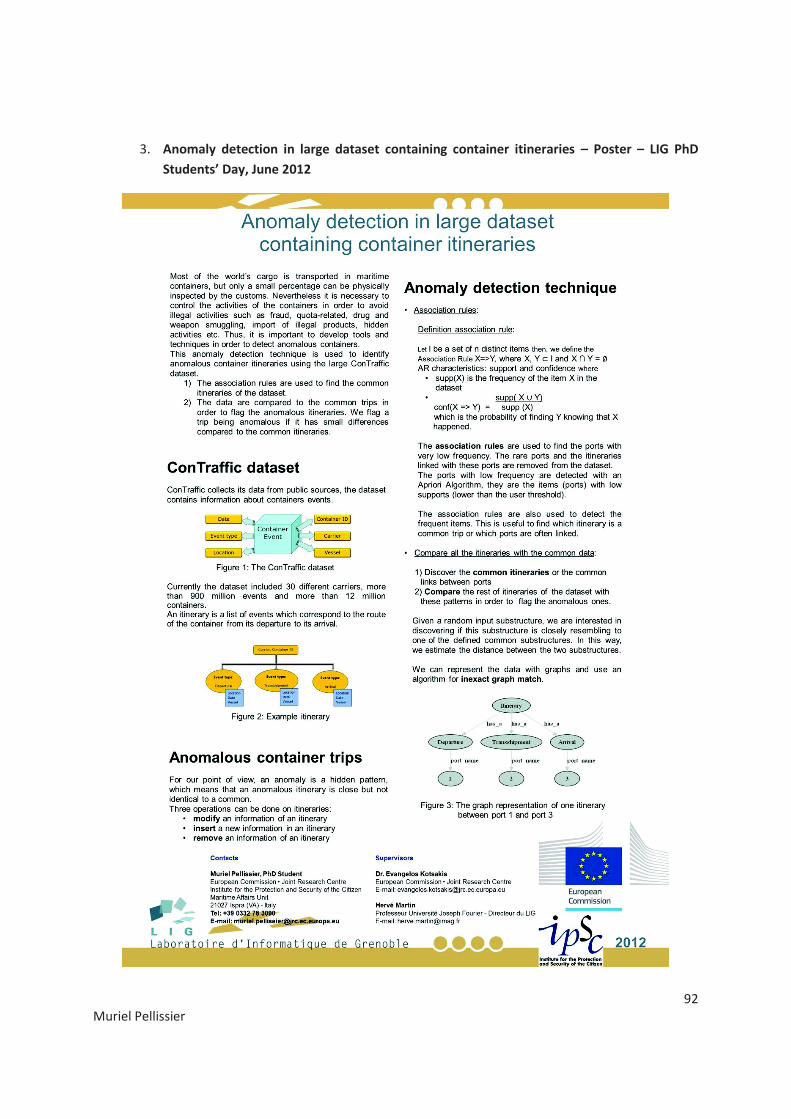
92

Muriel Pellissier

3. Anomaly detection in large dataset containing container itineraries – Poster – LIG PhD

Students’ Day, June 2012

93

Muriel Pellissier

4. Mining irregularities in Maritime container itineraries, M. Pellissier, E. Kotsakis and H.

Martin – EDBT/ICDT Workshop, March 2013

Mining irregularities in maritime container itineraries Muriel Pellissier

European Commission, Joint research Centre Institute for the Protection and Security of the Citizen

Ispra, Italy +390332783090

[email protected]

Supervised by

Hervé Martin

University Joseph Fourier Laboratory of Informatics

Grenoble, France +33476514859

[email protected]

Evangelos Kotsakis European Commission, Joint research Centre

Institute for the Protection and Security of the Citizen Ispra, Italy

+390332786103

[email protected]

ABSTRACT

Identifying irregularities in sequential data is essential for many application domains. This paper discusses unusual

events and how such events could be identified in sequential data. The type of sequential data used in this study holds

location-based and time-based information. The irregularities are managed by establishing a weighted relationship

between consecutive terms of the sequence. The sequences are spotted as irregular if a sequence is quasi-identical to

a usual behavior which means if it is slightly different from a frequent behavior.

This paper proposes a new approach for identifying and analyzing such irregularities in sequential data. The data used

to validate the method represent cargo shipments. This work is part of a PhD research, now in the 3rd year. The

proposed technique has been developed to identify irregular maritime container itineraries. The technique consists of

two main parts. The first part is to establish the most frequent sequences of ports (regular itineraries). The second part

identifies those itineraries that are slightly different to the regular itineraries using a distance-based method in order

to classify a given itinerary as normal or suspicious. The distance is calculated using a method that combines

quantitative and qualitative differences of the itineraries.

Permission to make digital or hard copies of part or all of this work for personal or classroom use is granted without fee

provided that copies are not made or distributed for profit or commercial advantage and that copies bear this notice and the full

citation on the first page. Copyrights for components of this work owned by others than ACM must be honored. Abstracting with

credit is permitted. To copy otherwise, to republish, to post on servers or to redistribute to lists, requires prior specific

permission and/or a fee.

EDBT/ICDT '13, March 18-22 2013, Genoa, Italy

Copyright 2013 ACM 978-1-4503-1599-9/13/03…$15.00.

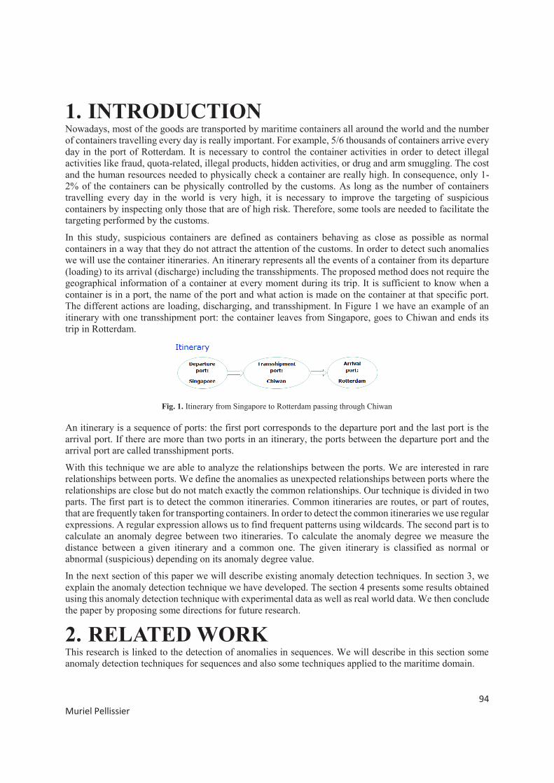
94

Muriel Pellissier

1. INTRODUCTION Nowadays, most of the goods are transported by maritime containers all around the world and the number

of containers travelling every day is really important. For example, 5/6 thousands of containers arrive every

day in the port of Rotterdam. It is necessary to control the container activities in order to detect illegal

activities like fraud, quota-related, illegal products, hidden activities, or drug and arm smuggling. The cost

and the human resources needed to physically check a container are really high. In consequence, only 1-

2% of the containers can be physically controlled by the customs. As long as the number of containers

travelling every day in the world is very high, it is necessary to improve the targeting of suspicious

containers by inspecting only those that are of high risk. Therefore, some tools are needed to facilitate the

targeting performed by the customs.

In this study, suspicious containers are defined as containers behaving as close as possible as normal

containers in a way that they do not attract the attention of the customs. In order to detect such anomalies

we will use the container itineraries. An itinerary represents all the events of a container from its departure

(loading) to its arrival (discharge) including the transshipments. The proposed method does not require the

geographical information of a container at every moment during its trip. It is sufficient to know when a

container is in a port, the name of the port and what action is made on the container at that specific port.

The different actions are loading, discharging, and transshipment. In Figure 1 we have an example of an

itinerary with one transshipment port: the container leaves from Singapore, goes to Chiwan and ends its

trip in Rotterdam.

Fig. 1. Itinerary from Singapore to Rotterdam passing through Chiwan

An itinerary is a sequence of ports: the first port corresponds to the departure port and the last port is the

arrival port. If there are more than two ports in an itinerary, the ports between the departure port and the

arrival port are called transshipment ports.

With this technique we are able to analyze the relationships between the ports. We are interested in rare

relationships between ports. We define the anomalies as unexpected relationships between ports where the

relationships are close but do not match exactly the common relationships. Our technique is divided in two

parts. The first part is to detect the common itineraries. Common itineraries are routes, or part of routes,

that are frequently taken for transporting containers. In order to detect the common itineraries we use regular

expressions. A regular expression allows us to find frequent patterns using wildcards. The second part is to

calculate an anomaly degree between two itineraries. To calculate the anomaly degree we measure the

distance between a given itinerary and a common one. The given itinerary is classified as normal or

abnormal (suspicious) depending on its anomaly degree value.

In the next section of this paper we will describe existing anomaly detection techniques. In section 3, we

explain the anomaly detection technique we have developed. The section 4 presents some results obtained

using this anomaly detection technique with experimental data as well as real world data. We then conclude

the paper by proposing some directions for future research.

2. RELATED WORK This research is linked to the detection of anomalies in sequences. We will describe in this section some

anomaly detection techniques for sequences and also some techniques applied to the maritime domain.

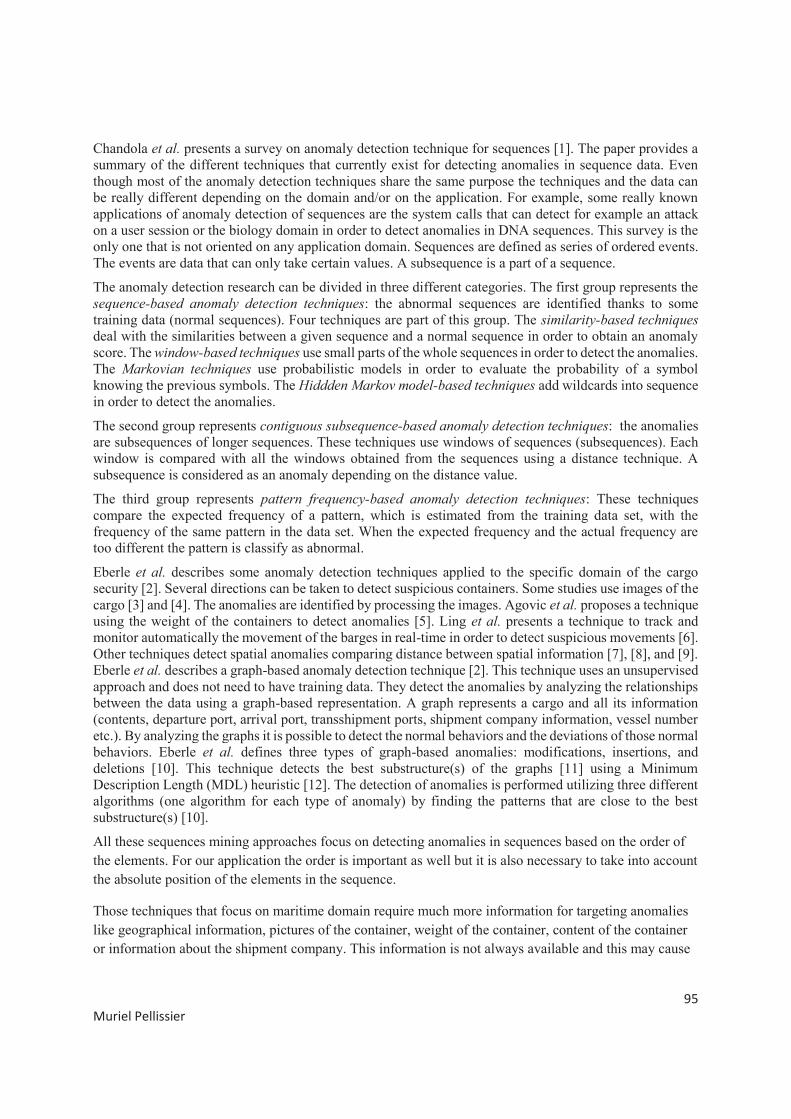
95

Muriel Pellissier

Chandola et al. presents a survey on anomaly detection technique for sequences [1]. The paper provides a

summary of the different techniques that currently exist for detecting anomalies in sequence data. Even

though most of the anomaly detection techniques share the same purpose the techniques and the data can

be really different depending on the domain and/or on the application. For example, some really known

applications of anomaly detection of sequences are the system calls that can detect for example an attack

on a user session or the biology domain in order to detect anomalies in DNA sequences. This survey is the

only one that is not oriented on any application domain. Sequences are defined as series of ordered events.

The events are data that can only take certain values. A subsequence is a part of a sequence.

The anomaly detection research can be divided in three different categories. The first group represents the

sequence-based anomaly detection techniques: the abnormal sequences are identified thanks to some

training data (normal sequences). Four techniques are part of this group. The similarity-based techniques

deal with the similarities between a given sequence and a normal sequence in order to obtain an anomaly

score. The window-based techniques use small parts of the whole sequences in order to detect the anomalies.

The Markovian techniques use probabilistic models in order to evaluate the probability of a symbol

knowing the previous symbols. The Hiddden Markov model-based techniques add wildcards into sequence

in order to detect the anomalies.

The second group represents contiguous subsequence-based anomaly detection techniques: the anomalies

are subsequences of longer sequences. These techniques use windows of sequences (subsequences). Each

window is compared with all the windows obtained from the sequences using a distance technique. A

subsequence is considered as an anomaly depending on the distance value.

The third group represents pattern frequency-based anomaly detection techniques: These techniques

compare the expected frequency of a pattern, which is estimated from the training data set, with the

frequency of the same pattern in the data set. When the expected frequency and the actual frequency are

too different the pattern is classify as abnormal.

Eberle et al. describes some anomaly detection techniques applied to the specific domain of the cargo

security [2]. Several directions can be taken to detect suspicious containers. Some studies use images of the

cargo [3] and [4]. The anomalies are identified by processing the images. Agovic et al. proposes a technique

using the weight of the containers to detect anomalies [5]. Ling et al. presents a technique to track and

monitor automatically the movement of the barges in real-time in order to detect suspicious movements [6].

Other techniques detect spatial anomalies comparing distance between spatial information [7], [8], and [9].

Eberle et al. describes a graph-based anomaly detection technique [2]. This technique uses an unsupervised

approach and does not need to have training data. They detect the anomalies by analyzing the relationships

between the data using a graph-based representation. A graph represents a cargo and all its information

(contents, departure port, arrival port, transshipment ports, shipment company information, vessel number

etc.). By analyzing the graphs it is possible to detect the normal behaviors and the deviations of those normal

behaviors. Eberle et al. defines three types of graph-based anomalies: modifications, insertions, and

deletions [10]. This technique detects the best substructure(s) of the graphs [11] using a Minimum

Description Length (MDL) heuristic [12]. The detection of anomalies is performed utilizing three different

algorithms (one algorithm for each type of anomaly) by finding the patterns that are close to the best

substructure(s) [10].

All these sequences mining approaches focus on detecting anomalies in sequences based on the order of

the elements. For our application the order is important as well but it is also necessary to take into account

the absolute position of the elements in the sequence.

Those techniques that focus on maritime domain require much more information for targeting anomalies

like geographical information, pictures of the container, weight of the container, content of the container

or information about the shipment company. This information is not always available and this may cause

96

Muriel Pellissier

certain problems when applying such techniques. The advantage of using our approach is that it requires

much less information about the shipments and it can be easily applied.

In the next section we will explain the different steps of the anomaly detection technique that we propose.

3. ANOMALY DETECTION TECHNIQUE The proposed anomaly detection technique uses an unsupervised approach. Unlike a supervised approach,

an unsupervised approach does not need to have training data to define the normal behavior. The user does

not need to have any knowledge on the data to use this technique. This technique is used to find anomalies

in structured data. We apply this technique to the maritime domain but it can also be used in other domains

as well. For our application, maritime surveillance, we are interested in finding hidden information. Hidden

information could be missing information, incomplete information or information that has been well hidden

intentionally or unintentionally. We define these anomalies as unexpected relationships between ports

where the relationships are close but not exactly identical to normal relationships. In other words we are

looking for sequences of ports that are close to the most frequent ones but with some differences. A

sequence of ports is called an itinerary.

Let E = {e1, e2,.., em} be a set of m distinct items. In this application the items are ports. Let S = {S1, S2,..,

Sn} be a set of n sequences of m items with m a random variable changing from one sequence to another

one. A subsequence of the sequence Sy is Sy’ = {ea, *, eb, *} with * unknown items (wildcard). A

subsequence is a part of an itinerary.


1) We detect sequences or subsequences that are common in our data set. We use a regular expression

technique in order to detect the common itineraries using all the data (normal and abnormal).

2) We compare a given sequence with the common sequences/subsequences and we calculate an

anomaly degree with a distance technique. Using the anomaly degree we can classify the given

sequence as normal or abnormal.






defining an itinerary as normal or abnormal. Moreover, the first part of this technique could also be used



3.1 Common sequences/subsequences To detect the common sequences (itineraries) we need to compare all the sequences of the data set and to

calculate their frequency. We are also interested in finding common subsequences. A subsequence is a part

of a sequence and not the whole sequence. We use wildcard in order to define the subsequences. The

wildcard can substitute any port.

The frequency is directly obtained by counting how many times each sequence appears in the data set. The

frequency of a subsequence is more difficult to calculate. In the following section we will discuss how to

calculate the frequency of a subsequence. As we do not have any knowledge about the data set, we do not

know the interesting subsequences. We need to create all the possible subsequences and to calculate how

many times they appear in the data set. In order to create the subsequences we need to add wildcards to the

sequences. If an itinerary has only two ports we will not create a subsequence. The subsequence of an

itinerary of two ports will be composed by only a port and a wildcard. We are not interested in single port

97

Muriel Pellissier

but only in relations between ports. For every itinerary of more than two ports, we will create a subsequence

of that itinerary by replacing only one port by a wildcard. For one itinerary we can create several

subsequences by replacing every port by a wildcard at a time. The number of subsequences created depends

on how many ports an itinerary has. For example, we can create four subsequences with an itinerary that

has four ports. Figure 2 shows an example of an itinerary from port X1 to port X3 passing through X2 and

all the possible subsequences of this itinerary. In the subsequences, the character “ * ” is a wildcard and it

can correspond to any port. As we see in Figure 2, with this itinerary we can create three different

subsequences.

Fig. 2. An itinerary and all his possible subsequences

The regular expression is a powerful method to identify strings in a text. It is used to detect specific

characters, words, patterns within a text. With regular expressions it is possible to detect easily a specific

sentence in a text. It is also easy to find sentences that are not exactly identical using wildcards. For example

it is possible to detect all the words of a sentence, to create a new sentence by replacing one of the words

with a wildcard and to detect all the sentences in a text that are similar to the new sentence.

A sequence can be seen as an ordered sentence where the positions of the words have an importance. A

group of sequences can be seen as a text composed by many sentences. For our application, an itinerary is

considered as a sequence which can be a sentence for the regular expression. The data set is a list of

itineraries which can be seen as a text (list of sequences) for the regular expression.

We need to create for every itinerary of our data set all the possible subsequences as we have seen in Figure

2. Then, we need to calculate the frequency of all the subsequences. The algorithm is shown in Figure 3.

Fig. 3. Common subsequences algorithm

1) We read every line of the data set file. Every line of the file is an itinerary.

98

Muriel Pellissier

2) We detect all the ports (words) of a line. All the ports are separated to each other by a space

character (‘ ‘).

3) We create subsequences by replacing every time a different port with a wildcard. With regular

expression the combination of characters “.+?” is used for wildcard.

4) We count how often the subsequences are present in the data set. With a minimum frequency

threshold we can select which lines (itineraries) are frequent enough in the data set to be considered

as common itineraries.

In our database each port is represented by a code. In a location database we have for each port all the

details of the location: the name of the country, the name of the city and the geographic coordinates. The

codes used for the ports are inconsecutive numbers and the length of the port names is not standardized. As

there is no important difference for the algorithm we have decided not to change the port names as it is

easier for the user to have a link between the data records in the different databases.

A wildcard “*” replace a port in an itinerary and it can match any port. With regular expression the wildcard

is the symbol “.+?”. The symbol “.” represents every character except the new-line character. As every line

is a different itinerary it is important to keep the new-line character to know where an itinerary ends. The

“+” is used to match one or more characters. But as all the characters except the new-line character will

match “.+” we need to limit it. If we do not limit it all the characters until the new-line character will always

be a match. In order to control the comparison we use the symbol “?” which makes the operation lazy. This

means that every time we compare two characters the character after “.+?” is also checked. As soon as the

character after “.+?” is found in the other line the characters following will not match “.+?” anymore.

With this first part we are able to detect the common itineraries and we need with the second part to detect

the suspicious itineraries.

3.2 Anomaly degree

The purpose of our technique is to detect anomalous itineraries and to spot the anomalies. We identify the

anomalies by comparing a given itinerary with the common ones. We calculate an anomaly degree between

a given itinerary and a common one. Depending on the value of the anomaly degree we will classify the

given itinerary as normal or abnormal. The anomaly degree is calculated with a distance technique.

Let Sdata be a given sequence of the data set S. Snor be a common sequence or subsequence discovered with

the regular expression technique as described previously. And dist(Sdata,Snor) is the distance between two

sequences: a given sequence Sdata and a common one Snor. For example, in Figure 4, we have two itineraries.

One itinerary is a given itinerary from X1 to X4 passing through X2 and X3. The second itinerary is a

common itinerary X1 to X4 with a wildcard for the transshipment port.

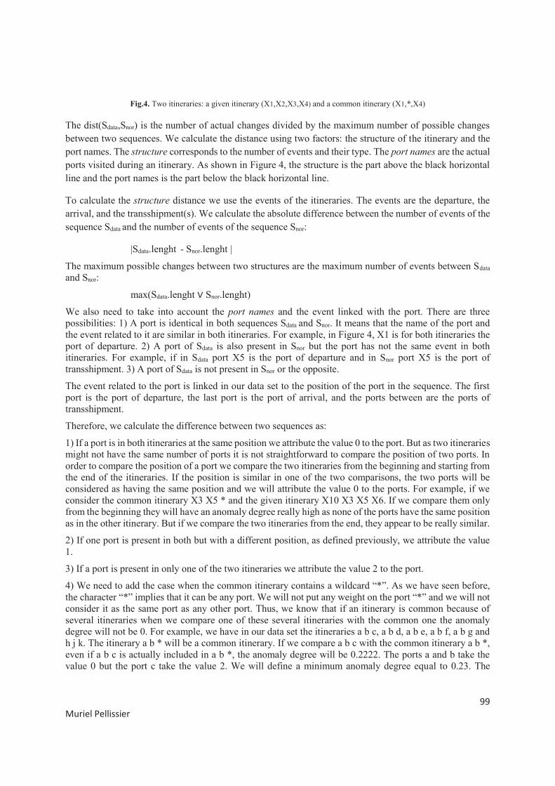
99

Muriel Pellissier

Fig.4. Two itineraries: a given itinerary (X1,X2,X3,X4) and a common itinerary (X1,*,X4)

The dist(Sdata,Snor) is the number of actual changes divided by the maximum number of possible changes

between two sequences. We calculate the distance using two factors: the structure of the itinerary and the

port names. The structure corresponds to the number of events and their type. The port names are the actual

ports visited during an itinerary. As shown in Figure 4, the structure is the part above the black horizontal

line and the port names is the part below the black horizontal line.

To calculate the structure distance we use the events of the itineraries. The events are the departure, the

arrival, and the transshipment(s). We calculate the absolute difference between the number of events of the

sequence Sdata and the number of events of the sequence Snor:

|Sdata.lenght - Snor.lenght |

The maximum possible changes between two structures are the maximum number of events between Sdata

and Snor:

max(Sdata.lenght Snor.lenght)

We also need to take into account the port names and the event linked with the port. There are three

possibilities: 1) A port is identical in both sequences Sdata and Snor. It means that the name of the port and

the event related to it are similar in both itineraries. For example, in Figure 4, X1 is for both itineraries the

port of departure. 2) A port of Sdata is also present in Snor but the port has not the same event in both

itineraries. For example, if in Sdata port X5 is the port of departure and in Snor port X5 is the port of

transshipment. 3) A port of Sdata is not present in Snor or the opposite.

The event related to the port is linked in our data set to the position of the port in the sequence. The first

port is the port of departure, the last port is the port of arrival, and the ports between are the ports of

transshipment.

Therefore, we calculate the difference between two sequences as:

1) If a port is in both itineraries at the same position we attribute the value 0 to the port. But as two itineraries

might not have the same number of ports it is not straightforward to compare the position of two ports. In

order to compare the position of a port we compare the two itineraries from the beginning and starting from

the end of the itineraries. If the position is similar in one of the two comparisons, the two ports will be

considered as having the same position and we will attribute the value 0 to the ports. For example, if we

consider the common itinerary X3 X5 * and the given itinerary X10 X3 X5 X6. If we compare them only

from the beginning they will have an anomaly degree really high as none of the ports have the same position

as in the other itinerary. But if we compare the two itineraries from the end, they appear to be really similar.

2) If one port is present in both but with a different position, as defined previously, we attribute the value

1.

3) If a port is present in only one of the two itineraries we attribute the value 2 to the port.

4) We need to add the case when the common itinerary contains a wildcard “*”. As we have seen before,

the character “*” implies that it can be any port. We will not put any weight on the port “*” and we will not

consider it as the same port as any other port. Thus, we know that if an itinerary is common because of

several itineraries when we compare one of these several itineraries with the common one the anomaly

degree will not be 0. For example, we have in our data set the itineraries a b c, a b d, a b e, a b f, a b g and

h j k. The itinerary a b * will be a common itinerary. If we compare a b c with the common itinerary a b *,

even if a b c is actually included in a b *, the anomaly degree will be 0.2222. The ports a and b take the

value 0 but the port c take the value 2. We will define a minimum anomaly degree equal to 0.23. The

100

Muriel Pellissier

itineraries that have an anomaly degree inferior to the minimum degree will not appear as abnormal

itineraries.

The maximum number of changes that we can have with the port names is the number of distinct ports

between the two itineraries. We do not consider the port “*” as one of the distinct port for the maximum

number of changes. As we have seen we can attribute to a port the value 0, 1 or 2. The maximum value

attributed to a port is 2 so if two itineraries are completely different, the maximum possible value will be

the number of all the distinct ports multiplied by 2. Thus, the number of maximum changes is the number

of distinct ports multiplied by 2.

The anomaly degree is:

dist(Sdata,Snor) = |Sdata.lenght - Snor.lenght | + Ʃport_value(0,1,2) .

max(Sdata.lenght Snor.lenght) + (num_of_distinct_port)*2

A maximum anomaly degree threshold is defined by the user. Depending on the threshold the itinerary Sdata

will be classify as normal or abnormal. If the anomaly degree is lower than the threshold the itinerary will

be detected as anomalous.

101

Muriel Pellissier


Fig. 5. Anomaly algorithm

1) We reduce the data file. The data file contains all the itineraries of our data set. In consequence, the


itinerary with the same itinerary we create a new file where each itinerary is present only once. This

new file is the reducedDataFile.

2) We read every line of the reducedDataFile.

3) We read every line of the frequencyDataFile that we have created previously with the common

subsequences algorithm described in Figure 3. The file contains the frequency of every

sequence/subsequence.

4) A sequence/subsequence is considered to be a common itinerary it its frequency is superior to the

minimum frequency threshold. If the itinerary is a common itinerary we compare the two lines. The

first line is a given itinerary. The second line is the sequence/subsequence found with the common


We attribute values to the ports. The value 0: if a port is in the other itinerary and at the same position

or if a port is “*”. The value 1: if a port is in the other itinerary but at a different position. And the

value 2: if a port is not present in the other itinerary.

5) We calculate the anomaly degree between the two itineraries.

102

Muriel Pellissier

6) If the anomaly degree is between the minimum anomaly degree threshold and the maximum anomaly


degree value.

7) We write all the anomalies found in a text file: anomalyFile.

For example, if we compare the two itineraries of Figure 4:

· Structure: actual changes: |4-3| (4 events Sdata and 3 events Snor) and maximum changes: 4

· Name ports: actual changes: 4 (X1 compared with X1 = 0, X2 compared with * or X1 = 2, X3

compared with * or X4 = 2, X4 compared with X4 = 0) and maximum changes: 4*2 (4 different

ports: X1, X2, X3. X4)

· Anomaly degree: dist(Sdata,Snor) = (1+4) / (4+4*2) = 0.41


detected as anomalous. The normal behavior is to have only one transshipment port but the itinerary Sdata

has two transshipment ports.

4. EXPERIMENT We collect our data on container trips on different public sources. In order to have coherent dataset we clean

the data. The cleaning is mostly linked with text string errors for geographic locations and container events.

The dataset contains container events information. For each event we know the container number, the

geographical localization of the container, and what action is done on that container in that specific port.

Currently, the dataset contains more than 900 million of events and about 12 million of containers. As our

data contains anomalies, first we tried this technique with some experimental data created based on the real

world data. Once the results with experimental data are satisfied we tried this technique with the real world

data.

4.1 Experimental data

We have created some experimental data set based on real world data. With some tests done on our data set

we know that for a number x of itineraries, we have y number of ports with y = x * 6%. We also know as

shown in Figure 6 that most of the itineraries have no transshipment port.

Fig. 6. Percentage of transshipments in real world data

We created experimental data with 200 itineraries. 60 % of the itineraries have zero transshipment, 30 %

have one transshipment, and 10 % have two transshipments. We use twelve distinct ports. With a random

function we create the itineraries. We add four different itineraries ten times in order to be considered as

frequent itineraries. We add ten suspicious itineraries.

For this experimentation, the minimum frequency will be 5.40, the maximum anomaly degree will be 0.49,

and the minimum anomaly degree is 0.23. The minimum frequency value is calculated with the

frequencyDataFile of the common subsequences algorithm. The average frequency is calculated with the

103

Muriel Pellissier

frequency of all the itineraries. Another frequency is calculated with the itineraries that have a frequency

above the frequency average. The second frequency value is the value used for the minimum frequency

threshold.

With this technique from a data set of 210 itineraries we detect 42 itineraries (20%) that could be anomalous.

All the anomalous itineraries inserted are detected as anomalous, other suspicious itineraries created

randomly are also detected.


on the text file. The first line is the anomalous itinerary, the second line is the common itineraries, and the

third line is the anomaly degree values.

Fig. 7. Anomalous itineraries using experimental data

As shown in Figure 7, the first anomalous itinerary detected in this example is the itinerary going from port

1 to port 8 passing through port 9. It is considered anomalous because of three different common itineraries.

The first common itinerary used to define this itinerary as abnormal is the itinerary going from any port to

port 8 passing through port 6 and 9. As the departure port of the common itinerary is a wildcard it can be

any port, we consider the port of departure to be the port 1. We can see in that case that the two itineraries

are close but one transshipment port has been removed to the common itinerary. We have the same

conclusion when we compare this itinerary with the two others common itineraries, one port of

transshipment is missing.

4.2 Real world data We tested this technique with real world data as well. The data set have 135798 itineraries but 22831 distinct

itineraries. The minimum frequency calculated with the frequency of the itineraries as described previously

is 60. As for the experimental data the maximum anomaly degree is 0.49 and the minimum anomaly degree

is 0.23.

We tested this technique with three different minimum frequency thresholds: 30, 50, and 60. 60 is the value

obtained as described previously with the frequency of the itineraries.

Fig. 8. Results with different minimum frequency values

104

Muriel Pellissier

As shown in Figure 8, the number of anomalous itineraries detected increases when the minimum frequency

value decreases. If the minimum frequency threshold is too low, a lot of itineraries will be spotted as

anomalous itineraries.

With the minimum frequency adapted (here 60) we detect 4773 anomalous itineraries. It is 3.5 % of the

whole dataset and 20.9 % of the distinct itineraries. Some examples of anomalous itineraries are shown in

Figure 9.

Fig. 9. Anomalous itineraries using real world data

As we can see in Figure 9, the method is able to identify suspicious itineraries thanks to changes between

a common itinerary and a given one. The changes that are detected are deletion, insertion, and replacement

of ports. For example, the itinerary “175 277 955” is tagged as anomalous. The common itinerary is “0 175

277”. The departure port and the arrival port are different. The departure port information was probably

removed from the itinerary in order to hide the origin of the container.

5. CONCLUSION This paper describes an anomaly detection technique for sequential data representing maritime container

itineraries. The method is performed into two steps. First, we detect the common sequences. Then, we

calculate the distance between a given itinerary and a common one.

We tested this technique with experimental data based on real world data as well as with real world data.

The results are very promising and indicate that this method is efficient in identifying suspicious/irregular

itineraries.

This technique could be further improved if it is enriched with customs based knowledge. For example,

knowing sensitive area, sensitive port, or which combination of ports could be potentially used for

transporting suspicious containers will facilitate the user in spotting the irregular itineraries much

successfully. Other information could be added like weather information, for example, routes could be

changed because of natural disasters.

Future research aims at enriching the existing information with spatio-temporal data in order to identify

unnecessary delays in the movements of the maritime containers. For example, if we know how long a

container takes to travel from one port to another, we can use this information in order to detect other types

of anomalies based on delays.

105

Muriel Pellissier

6. REFERENCES [1] V. Chandola, A. Banerjee and V. Kumar, “Anomaly Detection for Discrete Sequences: A Survey”, IEEE Trans. on Knowledge

and Data Engineering, pp. 823-839, 2012

[2] W. Eberle, L. Holder and B. Massengill, "Graph-Based Anomaly Detection Applied to Homeland Security Cargo Screening," International Conference of the Florida Artificial Intelligence Research Society (FLAIRS), 2012

[3] B. Cardoso “Standalone Multiple Anomaly Recognition Technique – SMART” http://www.sbir.gov/sbirsearch/detail/137676

[4] R.E. Swaney and E.R. Gianoulis “Cargo X-Ray Image Anomaly Detection using Intelligent Agents - FORELL”

http://www.sbir.gov/sbirsearch/detail/168550

[5] A. Agovic, A. Banerjee, A.R Ganguly, V. Protopopescu “Anomaly detection using manifold embedding and its applications in transportation corridors”, Intelligent Data Analysis, 13(3), pp. 435-455, 2009

[6] Y. Ling, M. Jin, M.R Hilliard and J.M Usher, “A study of real-time identification and monitoring of barge-carried hazardous commodities”, 17th International Conference on Geoinformatics, pp. 1-4, 2009

[7] P. Sun and S. Chawla, “On local spatial outliers”, Fourth IEEE International Conference on Data Mining, pp. 209-216, 2004

[8] C. Lu, D. Chen and Y. Kou, “Detecting spatial outliers with multiple attributes”, Fifth IEEE International Conference on Tools with Artificial Intelligence, pp. 122, 2008

[9] Y. Kou, C. Lu and D. Chen, “Spatial weighted outlier detection”, Proceedings of the Sixth SIAM International Conference on Data Mining, Bethesda, MD, USA, 2006



[12] J. Rissanen, “Stochastic Complexity in Statistical Inquiry”, World Scientific Publishing Company, 1989

106

Muriel Pellissier

5. Anomaly detection for the security of cargo shipments, M. Pellissier, E. Kotsakis and H.

Martin – IFGIS Conference, May 2013

Anomaly detection for the security of cargo shipments

Muriel Pellissier1, Evangelos Kotsakis1, Hervé Martin2

1 European Commission, Joint research Centre, Institute for the Protection and Security of the Citizen, Ispra, Italy

{muriel.pellissier, evangelos.kotsakis}@jrc.ec.europa.eu 2 University Joseph Fourier, Laborarory of Informatics, Grenoble, France

[email protected]

Abstract. Detecting anomalies in maritime domain is nowadays essential as the number of goods transported by

maritime containers keeps increasing. An anomaly can be described in several ways depending on the application

domain. For cargo shipment an anomaly can be defined as an unexpected relationship between ports.

This paper describes a new approach for detecting the anomalies in sequential data used to describe cargo

shipments. The technique is divided in two steps. First, we find the normal itineraries with a regular expression

technique. Then, we compare a given itinerary with a normal one using a distance-based method in order to classify

the given itinerary as normal or suspicious. The first results of this method are very promising and it can be further

improved when integrated with time-based information. This paper presents both the methodology and some results

obtained using real world data representing container movements.

Keywords: anomaly detection, maritime security, sequence, regular expression, distance

1 Introduction

Nowadays, most of the goods are transported by maritime containers all around the world and the number

of containers travelling every day is really important. For example, around 15 million containers arrive into

ports every year only in the US. It is necessary to control the container movements in order to detect illegal

activities like fraud, quota-related, illegal products, hidden activities, or drug and arm smuggling. But only

1-2% of the containers can be physically controlled by the customs because the cost and the human

resources needed to check a container are really high. As the number of containers travelling every day in

the world increases, it is necessary to improve the targeting in a way that it reduces as much as possible the

physical check on random containers. Performing physical checks only on those containers that seems to

be suspicious will improve both targeting and efficiency. Therefore, some computational tools are needed

to help the customs to focus their attention on suspicious containers.

In this study, suspicious containers are defined as containers behaving as close as possible as normal

containers in order not to attract the attention of the customs. In order to detect such anomalies we will use

the container itineraries. An itinerary represents all the events of a container from its departure (loading) to

its arrival (discharge) including the transshipments. The proposed method does not require the geographical

information of a container at every moment during its trip. It is sufficient to know when a container is in a

port, the name of the port and what action is made on the container at that specific port. The different actions

are loading, discharging, and transshipment. In Figure 1 we have an example of an itinerary with one

transshipment port: the container leaves from Singapore, goes to Chiwan and ends its trip in Rotterdam.

107

Muriel Pellissier

Fig. 2. Itinerary from Singapore to Rotterdam passing through Chiwan

An itinerary is a sequence of ports: the first port corresponds to the departure port and the last port is the

arrival port. If there are more than two ports in an itinerary, the ports between the departure port and the

arrival port are called transshipment ports.

With this technique we are able to analyze the relationships between the ports. We are interested in rare

relationships between ports. We define the anomalies as unexpected relationships between ports where the

relationships are close but do not match exactly the common relationships. Our technique is divided in two

parts. The first part is to detect the common itineraries. Common itineraries are itineraries, or part of

itineraries, that are frequently used in the transport of the containers. We detect the common itineraries

using regular expressions. A regular expression allows us to find frequent patterns using wildcards. The

second part is to calculate an anomaly degree between two itineraries. To calculate the anomaly degree we

measure the distance between a given itinerary and a common one. The given itinerary is classified as

normal or abnormal (suspicious) depending on its anomaly degree value.

In the next section of this paper we will describe existing anomaly detection techniques. In section 3, we

explain the anomaly detection technique we have developed. The section 4 presents some testing of this

anomaly detection technique and their corresponding results. We then conclude the paper by proposing

some directions for future research.

2 Related work

This research is linked to the detection of anomalies in sequences. We will describe in this section some

anomaly detection techniques for sequences and also some techniques applied to the maritime domain.

Chandola et al. presents a survey on anomaly detection technique for sequences [1]. The paper provides a

summary of the different techniques that currently exist for detecting anomalies in sequence data. Even

though most of the anomaly detection techniques share the same purpose the techniques and the data can

be really different depending on the domain and/or on the application. For example, some really known

applications of anomaly detection of sequences are the system calls that can detect for example an attack

on a user session or the biology domain in order to detect anomalies in DNA sequences. This survey is the

only one that is not oriented on any application domain. Sequences are defined as series of ordered events.

The events are data that can only take certain values. A subsequence is a part of a sequence.

The anomaly detection research can be divided in three different categories. The first group represents the

sequence-based anomaly detection techniques: the abnormal sequences are identified thanks to some

training data (normal sequences). Four techniques are part of this group. The similarity-based techniques

deal with the similarities between a given sequence and a normal sequence in order to obtain an anomaly

score. The window-based techniques use small parts of the whole sequences in order to detect the anomalies.

The Markovian techniques use probabilistic models in order to evaluate the probability of a symbol

108

Muriel Pellissier

knowing the previous symbols. The Hiddden Markov model-based techniques add wildcards into sequence

in order to detect the anomalies.

The second group represents contiguous subsequence-based anomaly detection techniques: the anomalies

are subsequences of longer sequences. These techniques use windows of sequences (subsequences). Each

window is compared with all the windows obtained from the sequences using a distance technique. A

subsequence is considered as an anomaly depending on the distance value.

The third group represents pattern frequency-based anomaly detection techniques: These techniques

compare the expected frequency of a pattern, which is estimated from the training data set, with the

frequency of the same pattern in the data set. When the expected frequency and the actual frequency are

too different the pattern is classify as abnormal.

Eberle et al. describes some anomaly detection techniques applied to the specific domain of the cargo

security [2]. Several directions can be taken to detect suspicious containers. Some studies use images of the

cargo [3] and [4]. The anomalies are identified by processing the images. Agovic et al. proposes a technique

using the weight of the containers to detect anomalies [5]. Ling et al. presents a technique to track and

monitor automatically the movement of the barges in real-time in order to detect suspicious movements [6].

Other techniques detect spatial anomalies comparing distance between spatial information [7], [8], and [9].

Eberle et al. describes a graph-based anomaly detection technique [2]. This technique uses an unsupervised

approach and does not need to have training data. They detect the anomalies by analyzing the relationships

between the data using a graph-based representation. A graph represents a cargo and all its information

(contents, departure port, arrival port, transshipment ports, shipment company information, vessel number

etc.). By analyzing the graphs it is possible to detect the normal behaviors and the deviations of those normal

behaviors. Eberle et al. defines three types of graph-based anomalies: modifications, insertions, and

deletions [10]. This technique detects the best substructure(s) of the graphs [11] using a Minimum

Description Length (MDL) heuristic [12]. The detection of anomalies is performed utilizing three different

algorithms (one algorithm for each type of anomaly) by finding the patterns that are close to the best

substructure(s) [10].

All these sequences mining approaches focus on detecting anomalies in sequences. For the sequence mining

approaches the order of the elements is important. For our application the order is important but the absolute

position of the elements in the sequence is equally important.

Those techniques that focus on the maritime domain require much more information for targeting anomalies

like geographical information, pictures of the container, weight of the container, content of the container or

information about the shipment company. This information is not always available and this may cause

certain problems when applying such techniques. The advantage of using our approach is that it requires

much less information about the shipments and it can be easily applied.

In the next section we will explain the different steps of the anomaly detection technique that we propose.

109

Muriel Pellissier

3 Anomaly detection technique

The proposed anomaly detection technique uses an unsupervised approach. Therefore this approach does

not need to have training data to define the normal data. The user does not need to have any knowledge on

the data to use this technique. This technique is used to find anomalies in structured data. We apply this

technique to the maritime domain but it can also be used in other domains as well. For our application,

maritime surveillance, we are interested in finding hidden information. Hidden information could be

missing information, incomplete information or information that has been well hidden intentionally or

unintentionally. We define these anomalies as unexpected relationships between ports where the

relationships are close but not exactly identical to normal relationships. In other words we are looking for

sequences of ports that are close to the most frequent ones but with some differences. A sequence of ports

is called an itinerary.

Let E = {e1, e2,.., em} be a set of m distinct items. In this application the items are ports. Let S = {S1, S2,..,

Sn} be a set of n sequences of m items with m a random variable changing from one sequence to another

one. A subsequence of the sequence Sy is Sy’ = {ea, *, eb, *} with * unknown items (wildcard). A

subsequence is a part of an itinerary.


1. We detect sequences or subsequences that are common in our data set. We use a regular expression

technique in order to detect the common itineraries using all the data (normal and abnormal).

2. We compare a given sequence with the common sequences/subsequences and we calculate an anomaly

degree with a distance technique. Using the anomaly degree we can classify the given sequence as normal

or abnormal.






defining an itinerary as normal or abnormal. Moreover, the first part of this technique could also be used



3.1 Common sequences/subsequences

To detect the common sequences (itineraries) we need to compare all the sequences of the data set and to

calculate their frequency. We are also interested in finding common subsequences. A subsequence is a part

of a sequence and not the whole sequence. We use wildcard in order to define the subsequences. The

wildcard can substitute any port.

The frequency is directly obtained by counting how many times each sequence appears in the data set. The

frequency of a subsequence is more difficult to calculate. In the following section we will discuss how to

calculate the frequency of a subsequence. As we do not have any knowledge about the data set, we do not

know the interesting subsequences. We need to create all the possible subsequences and to calculate how

many times they appear in the data set. In order to create the subsequences we need to add wildcards to the

sequences. If an itinerary has only two ports we will not create a subsequence. The subsequence of an

110

Muriel Pellissier

itinerary of two ports will be composed by only a port and a wildcard. We are not interested in single port

but only in relations between ports. For every itinerary of more than two ports, we will create a subsequence

of that itinerary by replacing only one port by a wildcard. For one itinerary we can create several

subsequences by replacing every port by a wildcard at a time. The number of subsequences created depends

on how many ports an itinerary has. For example, we can create four subsequences with an itinerary that

has four ports. Figure 2 shows an example of an itinerary from port X1 to port X3 passing through X2 and

all the possible subsequences of this itinerary. In the subsequences, the character “ * ” is a wildcard and it

can correspond to any port. As we see in Figure 2, with this itinerary we can create three different

subsequences.

Fig. 3. An itinerary and all his possible subsequences

The regular expression is a powerful method to identify strings in a text. It is used to detect specific

characters, words, patterns within a text. With regular expressions it is possible to detect easily a specific

sentence in a text. It is also easy to find sentences that are not exactly identical using wildcards. For example

it is possible to detect all the words of a sentence, to create a new sentence by replacing one of the words

with a wildcard and to detect all the sentences in a text that are similar to the new sentence.

A sequence can be seen as an ordered sentence where the positions of the words have an importance. A

group of sequences can be seen as a text composed by many sentences. For our application, an itinerary is

considered as a sequence which can be a sentence for the regular expression. The data set is a list of

itineraries which can be seen as a text (list of sequences) for the regular expression.

We need to create for every itinerary of our data set all the possible subsequences as we have seen in Figure

2. Then, we need to calculate the frequency of all the subsequences. The algorithm is shown in Figure 3.

111

Muriel Pellissier

Fig. 4. Common subsequences algorithm

1) We read every line of the data set file. Every line of the file is an itinerary.

2) We detect all the ports (words) of a line. All the ports are separated to each other by a space character

(‘ ‘).

3) We create subsequences by replacing every time a different port with a wildcard. With regular

expression the combination of characters “.+?” is used for wildcard.

4) We count how often the subsequences are present in the data set. With a minimum frequency

threshold we can select which lines (itineraries) are frequent enough in the data set to be considered

as common itineraries.

In our database each port is represented by a code. In a location database we have for each port all the

details of the location: the name of the country, the name of the city and the geographic coordinates. The

codes used for the ports are inconsecutive numbers and the length of the port names is not standardized.

As there is no important difference for the algorithm we have decided not to change the port names as it is

easier for the user to have a link between the data records in the different databases.

A wildcard “*” replace a port in an itinerary and it can match any port. With regular expression the

wildcard is the symbol “.+?”. The symbol “.” represents every character except the new-line character. As

every line is a different itinerary it is important to keep the new-line character to know where an itinerary

ends. The “+” is used to match one or more characters. But as all the characters except the new-line

character will match “.+” we need to limit it. If we do not limit it all the characters until the new-line

character will always be a match. In order to control the comparison we use the symbol “?” which makes

the operation lazy. This means that every time we compare two characters the character after “.+?” is also

checked. As soon as the character after “.+?” is found in the other line the characters following will not

match “.+?” anymore.

With this first part we are able to detect the common itineraries and we need with the second part to detect

the suspicious itineraries.

112

Muriel Pellissier

3.2 Anomaly degree

The purpose of our technique is to detect anomalous itineraries and to spot the anomalies. We identify the

anomalies by comparing a given itinerary with the common ones. We calculate an anomaly degree between

an itinerary and a common one. Depending on the value of the anomaly degree we will classify the given

itinerary as normal or abnormal. The anomaly degree is calculated with a distance technique.

Let Sdata be a given sequence of the data set S. Snor be a common sequence or subsequence discovered with

the regular expression technique as described previously. And dist(Sdata,Snor) is the distance between two

sequences: a given sequence Sdata and a common one Snor. For example, in Figure 4, we have two itineraries.

One itinerary is a given itinerary from X1 to X4 passing through X2 and X3. The second itinerary is a common

itinerary X1 to X4 with a wildcard for the transshipment port.

Fig. 5. Two itineraries: a given itinerary (X1,X2,X3,X4) and a common itinerary (X1,*,X4)

The dist(Sdata,Snor) is the number of actual changes divided by the maximum number of possible changes

between two sequences. We calculate the distance using two factors: the structure of the itinerary and the

port names. The structure corresponds to the number of events and their type. The port names are the actual

ports visited during an itinerary. As shown in Figure 4, the structure is the part above the black horizontal

line and the port names is the part below the black horizontal line.

To calculate the structure distance we use the events of the itineraries. The events are the departure, the

arrival, and the transshipment(s). We calculate the absolute difference between the number of events of the

sequence Sdata and the number of events of the sequence Snor:

|Sdata.lenght - Snor.lenght |

The maximum possible changes between two structures are the maximum number of events between Sdata

and Snor:

max(Sdata.lenght Snor.lenght)

We also need to take into account the port names and the event linked with the port. There are three

possibilities: 1) A port is identical in both sequences Sdata and Snor. It means that the name of the port and

the event related to it are similar in both itineraries. For example, in Figure 4, X1 is for both itineraries the

port of departure. 2) A port of Sdata is also present in Snor but the port has not the same event in both

113

Muriel Pellissier

itineraries. For example, if in Sdata port X5 is the port of departure and in Snor port X5 is the port of

transshipment. 3) A port of Sdata is not present in Snor or the opposite.

The event related to the port is linked in our data set to the position of the port in the sequence. The first

port is the port of departure, the last port is the port of arrival, and the ports between are the ports of

transshipment.

Therefore, we calculate the difference between two sequences as:

1) If a port is in both itineraries at the same position we attribute the value 0 to the port. But as two itineraries

might not have the same number of ports it is not straightforward to compare the position of two ports. In

order to compare the position of a port we compare the two itineraries from the beginning and starting from

the end of the itineraries. If the position is similar in one of the two comparisons, the two ports will be

considered as having the same position and we will attribute the value 0 to the ports. For example, if we

consider the common itinerary X3 X5 * and the given itinerary X10 X3 X5 X6. If we compare them only

from the beginning they will have an anomaly degree really high as none of the ports have the same position

as in the other itinerary. But if we compare the two itineraries from the end, they appear to be really similar.

2) If one port is present in both but with a different position, as defined previously, we attribute the value

1.

3) If a port is present in only one of the two itineraries we attribute the value 2 to the port.

4) We need to add the case when the common itinerary contains a wildcard “*”. As we have seen before,

the character “*” implies that it can be any port. We will not put any weight on the port “*” and we will not

consider it as the same port as any other port. Thus, we know that if an itinerary is common because of

several itineraries when we compare one of these several itineraries with the common one the anomaly

degree will not be 0. For example, we have in our data set the itineraries a b c, a b d, a b e, a b f, a b g and

h j k. The itinerary a b * will be a common itinerary. If we compare a b c with the common itinerary a b *,

even if a b c is actually included in a b *, the anomaly degree will be 0.2222. The ports a and b take the

value 0 but the port c take the value 2. We will define a minimum anomaly degree equal to 0.23. The

itineraries that have an anomaly degree inferior to the minimum degree will not appear as abnormal

itineraries.

The maximum number of changes that we can have with the port names is the number of distinct ports

between the two itineraries. We do not consider the port “*” as one of the distinct port for the maximum

number of changes. As we have seen we can attribute to a port the value 0, 1 or 2. The maximum value

attributed to a port is 2 so if two itineraries are completely different, the maximum possible value will be

the number of all the distinct ports multiplied by 2. Thus, the number of maximum changes is the number

of distinct ports multiplied by 2.

The anomaly degree is:

dist(Sdata,Snor) = |Sdata.lenght - Snor.lenght | + Ʃport_value(0,1,2) .

max(Sdata.lenght Snor.lenght) + (num_of_distinct_port)*2

114

Muriel Pellissier

A maximum anomaly degree threshold is defined by the user. Depending on the threshold the itinerary Sdata

will be classify as normal or abnormal. If the anomaly degree is lower than the threshold the itinerary will

be detected as anomalous.


Fig. 6. Anomaly algorithm

1) We reduce the data file. The data file contains all the itineraries of our data set. In consequence, the


itinerary with the same itinerary we create a new file where each itinerary is present only once. This

new file is the reducedDataFile.

2) We read every line of the reducedDataFile.

3) We read every line of the frequencyDataFile that we have created previously with the common

subsequences algorithm described in Figure 3. The file contains the frequency of every

sequence/subsequence.

115

Muriel Pellissier

4) A sequence/subsequence is considered to be a common itinerary it its frequency is superior to the

minimum frequency threshold. If the itinerary is a common itinerary we compare the two lines. The

first line is a given itinerary. The second line is the sequence/subsequence found with the common


We attribute values to the ports. The value 0 if a port is in the other itinerary and at the same position

or if a port is “*”. The value 1 if a port is in the other itinerary but at a different position. And the

value 2 if a port is not present in the other itinerary.

5) We calculate the anomaly degree between the two itineraries.

6) If the anomaly degree is between the minimum anomaly degree threshold and the maximum anomaly


degree value.

7) We write all the anomalies found in a text file: anomalyFile.

For example, if we compare the two itineraries of Figure 4:

· Structure: actual changes: |4-3| (4 events Sdata and 3 events Snor) and maximum changes: 4

· Name ports: actual changes: 4 (X1 compared with X1 = 0, X2 compared with * or X1 = 2, X3 compared

with * or X4 = 2, X4 compared with X4 = 0) and maximum changes: 4*2 (4 different ports: X1, X2, X3.

X4)

· Anomaly degree: dist(Sdata,Snor) = (1+4) / (4+4*2) = 0.41


detected as anomalous. The normal behavior is to have only one transshipment port but the itinerary Sdata

has two transshipment ports.

4 Experiment

We collect our data on container trips on different public sources. In order to have coherent dataset we clean

the data. The cleaning is mostly linked with text string errors for geographic locations and container events.

The dataset contains container events information. For each event we know the container number, the

geographical localization of the container, and what action is done on that container in that specific port.

Currently, the dataset contains more than 900 million of events and about 12 million of containers. As our

data contains anomalies, first we tried this technique with some experimental data created based on the real

world data. Once the results with experimental data are satisfied we tried this technique with the real world

data.

4.1 Experimental data

We have created some experimental data set based on real world data. With some tests done on our data set

we know that for a number x of itineraries, we have y number of ports with y = x * 6%. We also know as

shown in Figure 6 that most of the itineraries have no transshipment port.

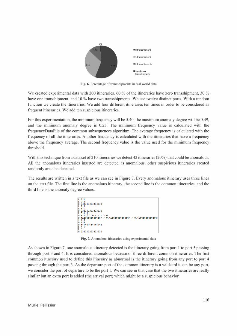
116

Muriel Pellissier

Fig. 6. Percentage of transshipments in real world data

We created experimental data with 200 itineraries. 60 % of the itineraries have zero transshipment, 30 %

have one transshipment, and 10 % have two transshipments. We use twelve distinct ports. With a random

function we create the itineraries. We add four different itineraries ten times in order to be considered as

frequent itineraries. We add ten suspicious itineraries.

For this experimentation, the minimum frequency will be 5.40, the maximum anomaly degree will be 0.49,

and the minimum anomaly degree is 0.23. The minimum frequency value is calculated with the

frequencyDataFile of the common subsequences algorithm. The average frequency is calculated with the

frequency of all the itineraries. Another frequency is calculated with the itineraries that have a frequency

above the frequency average. The second frequency value is the value used for the minimum frequency

threshold.

With this technique from a data set of 210 itineraries we detect 42 itineraries (20%) that could be anomalous.

All the anomalous itineraries inserted are detected as anomalous, other suspicious itineraries created

randomly are also detected.


on the text file. The first line is the anomalous itinerary, the second line is the common itineraries, and the

third line is the anomaly degree values.

Fig. 7. Anomalous itineraries using experimental data

As shown in Figure 7, one anomalous itinerary detected is the itinerary going from port 1 to port 5 passing

through port 3 and 4. It is considered anomalous because of three different common itineraries. The first

common itinerary used to define this itinerary as abnormal is the itinerary going from any port to port 4

passing through the port 3. As the departure port of the common itinerary is a wildcard it can be any port,

we consider the port of departure to be the port 1. We can see in that case that the two itineraries are really

similar but an extra port is added (the arrival port) which might be a suspicious behavior.

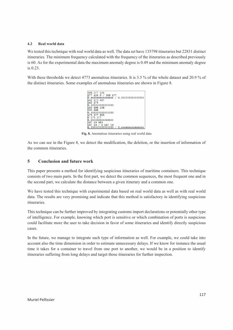
117

Muriel Pellissier

4.2 Real world data

We tested this technique with real world data as well. The data set have 135798 itineraries but 22831 distinct

itineraries. The minimum frequency calculated with the frequency of the itineraries as described previously

is 60. As for the experimental data the maximum anomaly degree is 0.49 and the minimum anomaly degree

is 0.23.

With these thresholds we detect 4773 anomalous itineraries. It is 3.5 % of the whole dataset and 20.9 % of

the distinct itineraries. Some examples of anomalous itineraries are shown in Figure 8.

Fig. 8. Anomalous itineraries using real world data

As we can see in the Figure 8, we detect the modification, the deletion, or the insertion of information of

the common itineraries.

5 Conclusion and future work

This paper presents a method for identifying suspicious itineraries of maritime containers. This technique

consists of two main parts. In the first part, we detect the common sequences, the most frequent one and in

the second part, we calculate the distance between a given itinerary and a common one.

We have tested this technique with experimental data based on real world data as well as with real world

data. The results are very promising and indicate that this method is satisfactory in identifying suspicious

itineraries.

This technique can be further improved by integrating customs import declarations or potentially other type

of intelligence. For example, knowing which port is sensitive or which combination of ports is suspicious

could facilitate more the user to take decision in favor of some itineraries and identify directly suspicious

cases.

In the future, we manage to integrate such type of information as well. For example, we could take into

account also the time dimension in order to estimate unnecessary delays. If we know for instance the usual

time it takes for a container to travel from one port to another, we would be in a position to identify

itineraries suffering from long delays and target those itineraries for further inspection.

118

Muriel Pellissier

References

[1] V. Chandola, A. Banerjee and V. Kumar, “Anomaly Detection for Discrete Sequences: A Survey”, IEEE Trans. on Knowledge and Data Engineering, pp. 823-839, 2012

[2] W. Eberle, L. Holder and B. Massengill, "Graph-Based Anomaly Detection Applied to Homeland Security Cargo Screening," International Conference of the Florida Artificial Intelligence Research Society (FLAIRS), 2012

[3] B. Cardoso “Standalone Multiple Anomaly Recognition Technique – SMART” http://www.sbir.gov/sbirsearch/detail/137676

[4] R.E. Swaney and E.R. Gianoulis “Cargo X-Ray Image Anomaly Detection using Intelligent Agents - FORELL” http://www.sbir.gov/sbirsearch/detail/168550

[5] A. Agovic, A. Banerjee, A.R Ganguly, V. Protopopescu “Anomaly detection using manifold embedding and its applications in transportation corridors”, Intelligent Data Analysis, 13(3), pp. 435-455, 2009

[6] Y. Ling, M. Jin, M.R Hilliard and J.M Usher, “A study of real-time identification and monitoring of barge-carried hazardous commodities”, 17th International Conference on Geoinformatics, pp. 1-4, 2009

[7] P. Sun and S. Chawla, “On local spatial outliers”, Fourth IEEE International Conference on Data Mining, pp. 209-216, 2004

[8] C. Lu, D. Chen and Y. Kou, “Detecting spatial outliers with multiple attributes”, Fifth IEEE International Conference on Tools with Artificial Intelligence, pp. 122, 2008

[9] Y. Kou, C. Lu and D. Chen, “Spatial weighted outlier detection”, Proceedings of the Sixth SIAM International Conference on Data Mining, Bethesda, MD, USA, 2006



[12] J. Rissanen, “Stochastic Complexity in Statistical Inquiry”, World Scientific Publishing Company, 1989

Anomaly detection technique for sequential data

Documents

Transcript of Anomaly detection technique for sequential data