arX

iv:h

ep-t

h/00

0214

3v3

30

May

200

1

IPM/P-2000/009

hep-th/0002143

Axial Anomaly in Noncommutative QED on R4

Farhad Ardalana and Neda Sadooghib

Institute for Studies in Theoretical Physics and Mathematics (IPM)

School of Physics, P.O. Box 19395-5531, Tehran-Iran

and

Department of Physics, Sharif University of Technology

P.O. Box 11365-9161, Tehran-Iran

Abstract

The axial anomaly of the noncommutative U(1) gauge theory is calculated by a

number of methods and compared with the commutative one. It is found to be given

by the corresponding Chern class.

PACS No.: 11.15.Bt, 11.10.Gh, 11.25.Db

Keywords: Noncommutative Field Theory, Ward Identity, Axial Anomaly

aElectronic address: ardalan@theory.ipm.ac.ir

bElectronic address: sadooghi@theory.ipm.ac.ir

1. Introduction

Quantum field theory on noncommutative spaces1,2 has been studied intensively in the last few

months: In Ref.3 certain properties of the perturbative dynamics of scalar fields were studied,

it was shown that noncommutativity can lead to unfamiliar ultraviolet (UV) and the infrared

(IR) behaviour of theories. In Refs.4,5 gauge theories were studied in the pure gauge theory

whereas in Refs.6,7,8,9,10 matter fields were introduced and detailed perturbative analysis of the

UV and IR behaviour of noncommutative gauge theory were carried out to one loop. Due to the

form of vertices in noncommutative gauge theory, certain phase factors appear in the Feynman

integrals in loop diagrams. Depending on whether these phases contain the loop momenta or

not, one speaks of nonplanar or planar diagrams, respectively. While the Feynman integrals of

planar diagrams in noncommutative gauge theory are exactly the same as in the commutative

case, within a constant factor, the nonplanar diagrams lead to important, rather unconventional

effects in the short- and long-distance behaviour of the theory.

In this paper we study the Ward identities and calculate the U(1)-anomaly in noncommutative

(NC)-U(1) gauge theory. Ward identities and anomalies are important for the renormalizability

of the NC-gauge theories. Recent studies have shown that noncommutative QED shares many

properties of the ordinary commutative non-Abelian gauge theories4,5. As for certain gauge

groups and their representations the anomaly cancels, it is an interesting question to know

under what condition the anomaly cancels in NC-QED.

The study of the anomalies in noncommutative gauge theories is also intersesting in connection

with the UV/IR mixing. As is well-known the U(1) anomaly is the result of a finite shift

of integration variables in the ultraviolet (linearly) divergent Feynman integrals for triangle

diagrams11. On the other hand the calculation of the commutative U(1)-anomaly in lattice

gauge theory shows that a very similar shift of integration variables in the lattice regulated

Feynman integrals for the triangle diagrams leads to a surface integral including an infrared

1

singularity at the origin of the first Brillouine zone12. There are other evidences which prove

that in commutative gauge theory the axial anomaly seems to have its origin both in the high

(UV) as well as in the low energy (IR) regime13. It is therefore important to study the axial

anomaly in detail in order to find its origin in noncommutative gauge theories. Anomalies arising

from nonplanar integrals, where UV/IR mixing seems to appear, are studied in a second paper14

separately.

In this paper, we have studied the axial anomaly arising from the planar diagrams of NC-

U(1) gauge theory with fermions in the fundamental representation in D = 2, 4 dimensions. The

organization of the paper is as follows. In Section 2 we introduce the noncommutative QED

on RD. After listing of Feynman rules of interest, gauge invariance of this theory is checked

in a simple example of fermion-antifermion annihilation into two gauge bosons at the tree level

(Section 3). As in the commutative non-Abelian gauge theories gauge invariance is guaranteed,

by considering not only the diagrams of the commutative QED but also a diagram containing

the three-photon vertex.

In Section 4, we then calculate the axial anomaly using the method of point splitting for

two- and four-dimensional NC-QED. Comparing to the commutative QED case, an additional

diagram has to be considered to produce the non-linear term in the field strength tensor of

NC-QED. Besides, from the start a non-trivial integration over noncommutative space-time

coordinates must be performed in order to guarantee the ⋆-gauge invariance of the result.

In the commutative field theory, the axial anomaly can also be interpreted as a result of

the non-invariance of the integration measure of the fermionic fields under local axial gauge

transformation. In noncommutative gauge theory, it is therefore interesting to check whether

the usual path integral method of Fujikawa15 goes through. From the technical point of view

the difference between this calculation and the standard one is that here, a ⋆-gauge covariant

regularization leads to a ⋆-gauge covariant expression for the anomaly and as in the method of

2

point-splitting gauge invariance can only be guaranteed after averaging over the densities. This

has serious consequences for topological properties of the anomaly. Here, the result for the axial

anomaly seems to be the same as in the commutative QED with the replacement of the ordinary

product of functions in the coordinate space with the ⋆-product. This replacement, however, is

not a priori. As for the case of instantons in the noncommutative space an a priori modification

of the usual product with the ⋆-product of function does not work16. It is therefore important

to carry out the calculation explicitly in NC-U(1) gauge theory.

We then turn to the triangle diagrams which, reproducing the previous result after inclusion

of higher loop corrections. As it turns out the triangle diagarms are all planar. This means that

the corresponding Feynman integrals differ from the usual commutative triangle integrals in an

overall phase factor, which only depends on the external loop momenta. These planar phase can

be brought out of the integrals and the rest of the calculation is just the standard calculation

of the anomaly in the commutative QED.c The expression for the axial anomaly turns out to

be ⋆-gauge invariant only after an integration over noncommutative space-time coordinates,

which then gives the Chern class. This calculation which yields a naively predictable result is

performed here explicitly in order to make a connection to another interesting method, where by

using the current algebra of NC-QED, a separation between a ”formal” part and a potentially

”anomalous” part of the divergence of the vertex function can be made, which is necessary in

the calculation of the axial anomaly for other noncommutative gauge theories, e.g. NC-U (N)14.

Here, as a by product, the current algebra of NC-U(1) gauge theory is presented. The non-trivial

expressions for the equal-time commutation relations of two-currents contain the novel effect of

being the difference of these currents at different space-time points, which cannot be obtained

from the Abelian or even non-Abelian commutative equal-time commutation relations by just

replacing the ordinary product with the ⋆-product. Section 5 is devoted to discussions.

cIn Ref.14 we study the effects of nonplanar diagrams on global U(1) anomaly.

3

2. Noncommutative Gauge Theory (NCGT)

In the noncommutative geometry formulation, geometric spaces are described by a C⋆-algebra,

which is in general not commutative. The familiar product of functions is therefore replaced

with the ⋆-product, which is characteristic for the noncommutative geometry and is given by:

f (x) ⋆ g (x) ≡ eiθµν

2

∂∂ξµ

∂∂ζν f (x+ ξ) g (x+ ζ)

∣

∣

∣

∣

ξ=ζ=0, (2.1)

where θµν is a real constant antisymmetric background, and reflects the noncommutativity of

the coordinates of RD2:

[xµ, xν ] = iθµν , (2.2)

The usual algebra of functions in RD is therefore modified to a noncommutative associative

algebra such that f ⋆ g = fg+ 12 iθ

µν∂µf∂νg+O(

θ2)

, with coefficients of each power being local

differential expressions bilinear in f and g. The ⋆-product satisfies the identity:

+∞∫

−∞

dDx f (x) ⋆ g (x) =

+∞∫

−∞

dDx g (x) ⋆ f (x) =

+∞∫

−∞

dDx f (x) g (x) , (2.3)

where the product on the last expression on the right hand side (r.h.s) of this equation is the

usual product of both functions f (x) and g (x). The associativity leads further to:

+∞∫

−∞

dDx (f1 ⋆ f2 ⋆ f3) (x) =

+∞∫

−∞

dDx (f3 ⋆ f1 ⋆ f2) (x) =

+∞∫

−∞

dDx (f2 ⋆ f3 ⋆ f1) (x) . (2.4)

Classical Action

The noncommutative Yang-Mills action is introduced in Refs.4,5, and the coupling of the U(1)

gauge fields with the matter fields is discussed in6,7. The noncommutative U(1) gauge connection

is given by1,5:

Dµ = ∂µ + ig[Aµ, ]⋆, (2.5)

where [f1, f2]⋆ is the Moyal bracket defined by:

[f1, f2]⋆ = f1 ⋆ f2 − f2 ⋆ f1. (2.6)

4

This leads to the definition of the field strength tensor

[Dµ,Dν ]⋆ = igFµν (x),

with

Fµν (x) ≡ ∂µAν (x) − ∂νAµ (x) + ig[Aµ (x) , Aν (x) ]⋆. (2.7)

The pure noncommutative U(1) gauge action is then given by:

SG[Aµ] = −1

4

∫

dDx Fµν (x) ⋆ Fµν (x) . (2.8)

Under an arbitrary local gauge transformation the gauge field Aµ (x) transforms as6,7:

Aµ (x) → A′µ (x) = U (x) ⋆ Aµ (x) ⋆ U−1 (x) +

i

g[∂µU (x) ] ⋆ U−1 (x) , (2.9)

where

U (x) ≡(

eigα(x))

⋆= 1 + igα (x) −

g2

2!α (x) ⋆ α (x) + O

(

α3⋆

)

. (2.10)

The subscript ⋆ denotes ⋆-multiplication in the products. Similarly U−1 (x) ≡(

e−igα(x))

⋆, which

can be shown to be the inverse of the U (x), i.e. U (x)⋆U−1 (x) = 1. Furthermore, the covariant

derivative transforms as:

Dµ → U (x) ⋆ Dµ ⋆ U−1 (x) . (2.11)

For infinitesimal gauge transformation parameter α (x) the transformation law for the gauge

field and the field strength tensor is given by2:

A′µ (x) = Aµ (x) − ∂µα (x) + ig[α (x) , Aµ (x)]⋆. (2.12a)

F ′µν (x) = Fµν (x) + ig[α (x) , Fµν (x)]⋆. (2.12b)

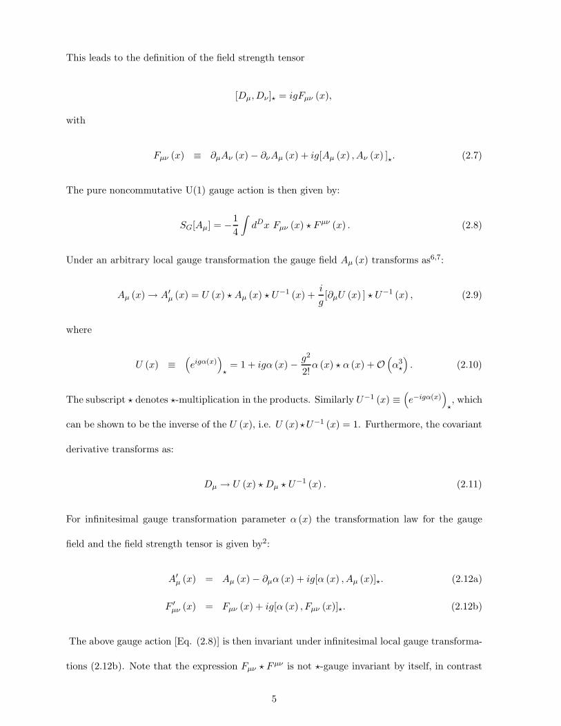
The above gauge action [Eq. (2.8)] is then invariant under infinitesimal local gauge transforma-

tions (2.12b). Note that the expression Fµν ⋆ Fµν is not ⋆-gauge invariant by itself, in contrast

5

to the local trace of the corresponding term in non-Abelian commutative gauge theories. The

⋆-gauge invariance of the gauge action (2.8) under gauge transformation (2.9) is only guaranteed

after the integration of this expression over the noncommutative space-time coordinates x.

The matter fields are similarly introduced6:

SF [ψ,ψ] =

∫

dDx

[

iψ (x) γµ ⋆ Dµψ (x) −mψ (x) ⋆ ψ (x)

]

, (2.13)

where the covariant derivative is defined by:

Dµψ (x) ≡ ∂µψ (x) + igAµ (x) ⋆ ψ (x) . (2.14)

The action (2.13) is invariant under the local gauge transformations of the gauge fields (2.9) and

the local gauge transformations of the matter fields:

ψ (x) → ψ′ (x) = U (x) ⋆ ψ (x) , ψ (x) → ψ′(x) = ψ (x) ⋆ U−1 (x) . (2.15)

Hence for infinitesimal local gauge transformations we have:

ψ′(x) ≈ ψ (x) − igψ (x) ⋆ α (x) and ψ′ (x) ≈ ψ (x) + igα (x) ⋆ ψ (x) . (2.16)

The total action in the noncommutative U(1) gauge theory therefore reads:

Stot.[Aµ, ψ, ψ] = −1

4

∫

dDx Fµν (x) ⋆ Fµν (x) +

∫

dDx ψ (x) ⋆ (iD/ −m)ψ (x) . (2.17)

3. Feynman Rules and Ward-Identity of NC-QED

Here, in analogy to commutative non-Abelian gauge theories, gauge fixing is necessary and leads

to noncommutative Faddeev-Popov-ghosts. The Feynman rules for gauge fields, matter fields

and ghosts are given in Ref.7. We will list here only the rules we will need in this paper:

The fermion and photon propagators do not change in NC-QED. For the fermion-propagator

we have:

pS (p) =

i

p/ −m, (3.1a)

6

whereas the photon propagator in Feynman gauge reads:

kµ νDµν (k) =

−igµνk2

. (3.1b)

The vertex of two fermions and one gauge field is given by:

k1, µ

p1 p2

Vµ (p1, p2; k1) = ig (2π)4 δ4 (p1 + p2 + k1) γµ exp

(

−iθησ2

pη1pσ2

)

. (3.1c)

The last term in the definition of field strength tensor containing the Moyal bracket, leads to

three- and four-gauge vertices in the NC-QED. The three-photon vertex is:

k1, µ1

k2, µ2 k3, µ3

Wµ1µ2µ3(k1, k2, k3) = −2g (2π)4 δ4 (k1 + k2 + k3) sin

(

iθησ2kη1k

σ2

)

×

[

gµ1µ2(k1 − k2)µ3

+ gµ1µ3(k3 − k1)µ2

+ gµ3µ2(k2 − k3)µ1

]

. (3.1d)

In analogy to the non-Abelian field theory all vertices involve the same coupling constant.

Check of the Ward-Identity in a simple case

To see a parallel between NC-QED and commutative non-Abelian gauge theory we study the

Ward identity at tree level. In this and the rest of the paper we follow Refs. 18,19 closely. As

in the commutative gauge theory the amplitude of gauge boson production is expected to obey

the Ward identity:

kµ

= 0. (3.2)

Let us check this identity in the simple case of the lowest order diagrams contributing to

fermion-antifermion annihilation into a pair of photons. In order g2 there are three diagrams,

7

shown in Fig. [1]. The first two diagrams are similar to QED diagrams. They sum to:

iMµνa+bǫ

∗µ (k1) ǫ

∗ν (k2) = (ig)2 v (p+) e−

iθησ

2pηpσ

+

[

γµi

p/ − k/2 −mγνe−

iθησ

2(p+p+)ηkσ

2

+γνi

k/2 − p/+ −mγµe+

iθησ

2(p+p+)ηkσ

2

]

u (p) ǫ∗µ (k1) ǫ∗ν (k2) . (3.3)

Here Mµνa+b denotes the contribution of both diagrams [1a] and [1b]; ǫ (ki)’s are photon polar-

ization vectors. For physical polarization they satisfy kµi ǫµ (ki) = 0. Note that the exponential

functions containing the noncommutativity parameter θησ are obtained by making use of the

definition of the usual vertex from the Eq. (3.1c).

To check the Ward identity we replace ǫ∗ν (k2) in the Eq. (3.3) by k2ν . This leads to:

iMµνa+bǫ

∗µ (k1) k2ν = (ig)2 v (p+) e−

iθησ

2pηpσ

+

[

γµi

p/ − k/2 −mk/2 e

−iθησ

2(p+p+)ηkσ

2

+k/2

i

k/2 − p/+ −mγµe+

iθησ

2(p+p+)ηkσ

2

]

u (p) ǫ∗µ (k1) . (3.4)

Then use of equations of motion leads to:

iMµνa+bǫ

∗µ (k1) k2ν = 2g2v (p+) γµu (p) ǫ∗µ (k1) e

−iθησ

2pηpσ

+ sin

(

θησ2

(p+ p+)η kσ2

)

. (3.5)

Notice that the above sine-function, which contains the parameter θησ, replaces the structure

constant fabc in the non-Abelian gauge theory.

The contribution of the diagram [1c], which in the non-Abelian commutative case is needed

to satisfy the Ward identity (3.2), is given by:

iMµνc ǫ∗µ (k1) ǫ

∗ν (k2) = +2ig2e−

iθησ

2pηpσ

+ sin

(

θησ2

(p+ p+)η kσ2

)

v (p+) γρu (p)

(

−i

k23

)

×

[

gµν (k2 − k1)ρ + gνρ (k3 − k2)

µ + gµρ (k1 − k3)ν

]

ǫ∗µ (k1) ǫ∗ν (k2) , (3.6)

where k3 = −k1 − k2 due to energy-momentum conservation. Replacing ǫν (k2) with k2ν and

using the momentum conservation the expression in the brackets reads:

k2ν

[

gµν (k2 − k1)ρ + gνρ (k3 − k2)

µ + gµρ (k1 − k3)ν

]

=

= k23gµρ − k3µk3ρ − k2

1gµρ + k1µk1ρ. (3.7)

8

Taking the gauge boson with momentum k1 to be on-shell and with transverse polarization, we

have k21 = 0 d as well as kµ1 ǫµ (k1) = 0. Then the third and the fourth terms on the r.h.s of the

above equation vanish. Furthermore, the term k3µk3ρ vanishes when it is contracted with the

fermion current. In the remaining term, the factor k23 cancels the photon propagator, and we

are left with

iMµνc ǫ∗µ (k1) k2ν = −2g2v (p+) γµu (p) ǫ∗µ (k1) e

−iθησ

2pηpσ

+ sin

(

θησ2

(p+ p+)η kσ2

)

, (3.8)

thus cancelling (3.5). The equality of the coupling constant in the fermion-photon and three-

photon vertices guarantees the validity of the Ward identity as in the commutative non-Abelian

gauge theories.

4. U(1)-Anomaly in NC-QED

Point-Splitting Method

i) U(1)-Anomaly in Two Dimensions

Before we take up the four dimensional anomaly, let us calculate the anomaly for two dimensional

NC-QED, with matter fields Lagrangian:

L = iψ (x) ⋆ γµDµψ (x) , (4.1)

which leads to the equation of motion

γµ∂µψ (x) = −igγµAµ (x) ⋆ ψ (x) , and ∂µψ (x) γµ = igψ (x) ⋆ Aµ (x) γµ. (4.2)

dContrast this with the dispersion relation of Ref.10. That dispersion relation is a consequence of the adjoint

representation of matter fields.

9

The anomaly to calculate is that of the axial vector current:e

Jµ(5) (x) ≡ iψ (x) γµγ5 ⋆ ψ (x) . (4.3)

This product of local operators is singular. The current is regularized by placing the two fermion

fields at different ”lattice” points separated by a distance ǫ:

Jµ(5) ≡ iψ (x) γµγ5 ⋆ ψ (x) −→ iψ (x+ ǫ/2) γµγ5 ⋆ ψ (x− ǫ/2) ,

which is not, however, invariant under local gauge transformations defined in the Eq. (2.15).

To make it ⋆-gauge invariant, introduce the link variable U (y, x):

U (y, x) ≡ exp

[

− ig

y∫

x

dzµAµ (z)

]

, (4.4)

which transforms under the local gauge transformation as:

U ′ (y, x) = U (y) ⋆ U (y, x) ⋆ U−1 (x) , (4.5)

where U (x) is the unitary matrix defined in the Eq. (2.10) and U (x) ⋆ U−1 (x) = 1. The axial

vector current in its point splitted, ⋆-gauge invariant version is then given by:

Jµ(5) (x) = limǫ→0

{

ψ (x+ ǫ/2) γµγ5 ⋆ U (x+ ǫ/2, x− ǫ/2) ⋆ ψ (x− ǫ/2)

}

. (4.6)

Keeping terms up to the first order in ǫ in U (y+, y−) for y± = x± ǫ/2 we get:

U (x+ ǫ/2, x − ǫ/2) = 1 − igǫνAν (x) + O(

ǫ2)

, (4.7)

and

∂µU (x+ ǫ/2, x − ǫ/2) = −igǫν∂µAν (x) + O(

ǫ2)

. (4.8)

eAs we have shown in Ref.14 U(1) gauge theory with fundamental matter field coupling has three different cur-

rents, which all, expressing the same global symmetry of the noncommutative action, lead to the same classically

conserved charge. Here we intend to work only with one of these currents.

10

Then we use the equations of motion (4.2) and the expression (4.8) in the Eq. (4.6) to obtain:

∂µJµ(5) (x) = lim

ǫ→0ψ (x+ ǫ/2) γµγ5 ⋆

[

ig{Aµ (x+ ǫ/2) −Aµ (x− ǫ/2)}

+g2ǫν {Aµ (x+ ǫ/2) ⋆ Aν (x) −Aν (x) ⋆ Aµ (x− ǫ/2)} − igǫν∂µAν (x)

]

⋆ ψ (x− ǫ/2) .

(4.9)

Note that in the standard derivation of the axial anomaly for two-dimensional commutative

QED the first two terms on the last line of the above equation cancel due to the commutativity

of the ordinary product. Here, exactly this term leads to the additional term [Aµ, Aν ]⋆ in the

definition of field strength tensor in NC-QED [see Eq. (2.7)].

Expanding the expression on the r.h.s. of Eq. (4.9) and keeping the terms of order ǫν , the

divergence of the axial current reads:

∂µJµ(5) (x) = lim

ǫ→0

[

− ig ǫν ψ (x+ ǫ/2) γµγ5 ⋆ Fµν (x) ⋆ ψ (x− ǫ/2)

]

, (4.10)

where Fµν (x) is defined in the Eq. (2.7). Let us take the expectation value of the above

equation in the presence of a fixed background gauge field. To obtain a ⋆-gauge invariant result,

we take the integral over two dimensonal space-time coordinates of this equation. Only after

this integration one can make use of Eq. (2.4) to find:

+∞∫

−∞

d2x

⟨

∂µJµ(5) (x)

⟩

= limǫ→0

[

− ig ǫν+∞∫

−∞

d2x Fµν (x) ⋆

⟨

ψ (x− ǫ/2) γµγ5 ⋆ ψ (x+ ǫ/2)

⟩]

= −ig

+∞∫

−∞

d2x Fµν (x) limǫ→0

ǫν⟨

ψ (x− ǫ/2) γµγ5 ⋆ ψ (x+ ǫ/2)

⟩

, (4.11)

where the ⋆-product between Fµν (x) and the rest of the expression is removed by using the Eq.

(2.3). In the momentum space the vacuum expectation value of the ⋆-product of ψ and ψ is

given by:

I ≡

⟨

ψ (y) γµγ5 ⋆ ψ (z)

⟩

=

⟨

+∞∫

−∞

d2p

(2π)2d2q

(2π)2ψ (p) γµγ5 ψ (q) e−ipy ⋆ e+iqz

⟩

.

11

Here y = x − ǫ2 and z = x+ ǫ

2 . In the zeroth order of perturbative expansionf the contraction

of fermion-antifermion leads to a term proportional to δ(2) (p− q)∆ (p), where ∆ (p) =ip/p2

is the

fermion propagator in massless case. The phase factor exp(

i2θησp

ηqσ)

, which appears in the

⋆-product of the exponential functions in the above expression vanishes due to the δ-function.

We arrive at:

I(0) = −

+∞∫

−∞

d2p

(2π)2Tr(

γαγµγ5) ipα e

ipǫ

p2= −Tr

(

γαγµγ5) ∂

∂ǫα

+∞∫

−∞

d2p

(2π)2eipǫ

p2

= −i

4πTr(

γαγµγ5) ∂

∂ǫαlogǫ2 = −

i

2πTr(

γαγµγ5) ǫαǫ2, (4.12)

and therefore:

I (ǫ) ≡

⟨

ψ (x− ǫ/2) γµγ5 ⋆ ψ (x+ ǫ/2)

⟩

= −i

2πTr(

γαγµγ5) ǫαǫ2

+ O (log ǫ) .

As we can see the contraction of the fermion-antifermion fields are singular for ǫ → 0. A finite

result can nevertheless be obtained after putting this result in the Eq. (4.11) and taking the

limit over ǫ→ 0:

+∞∫

−∞

d2x

⟨

∂µJµ(5) (x)

⟩

= −ig

+∞∫

−∞

d2x Fµν (x) limǫ→0

ǫν I (ǫ)

= −g

2πTr(

γαγµγ5)

+∞∫

−∞

Fµν (x) limǫ→0

ǫαǫν

ǫ2. (4.13)

Using equation:

limǫ→0

ǫαǫν

ǫ2=

1

Dδνα, (4.14)

in D = 2 dimensions, and the relation Tr(

γαγµγ5)

= 2εαµ, we obtain the axial anomaly in

two-dimensional massless NC-QED:

+∞∫

−∞

d2x 〈∂µJµ(5) (x) 〉 =

g

2πεµν

+∞∫

−∞

d2x Fµν (x) . (4.15)

fHigher order terms are less divergent and vanish after contracting with ǫν and taking the limit ǫ → 0.

12

At this stage two comments are in order: first the anomaly expression (4.15) is gauge invariant

because of the space and time integrals. Secondly, we have allowed for the noncommutativity of

space and time coordinates in two dimensions.

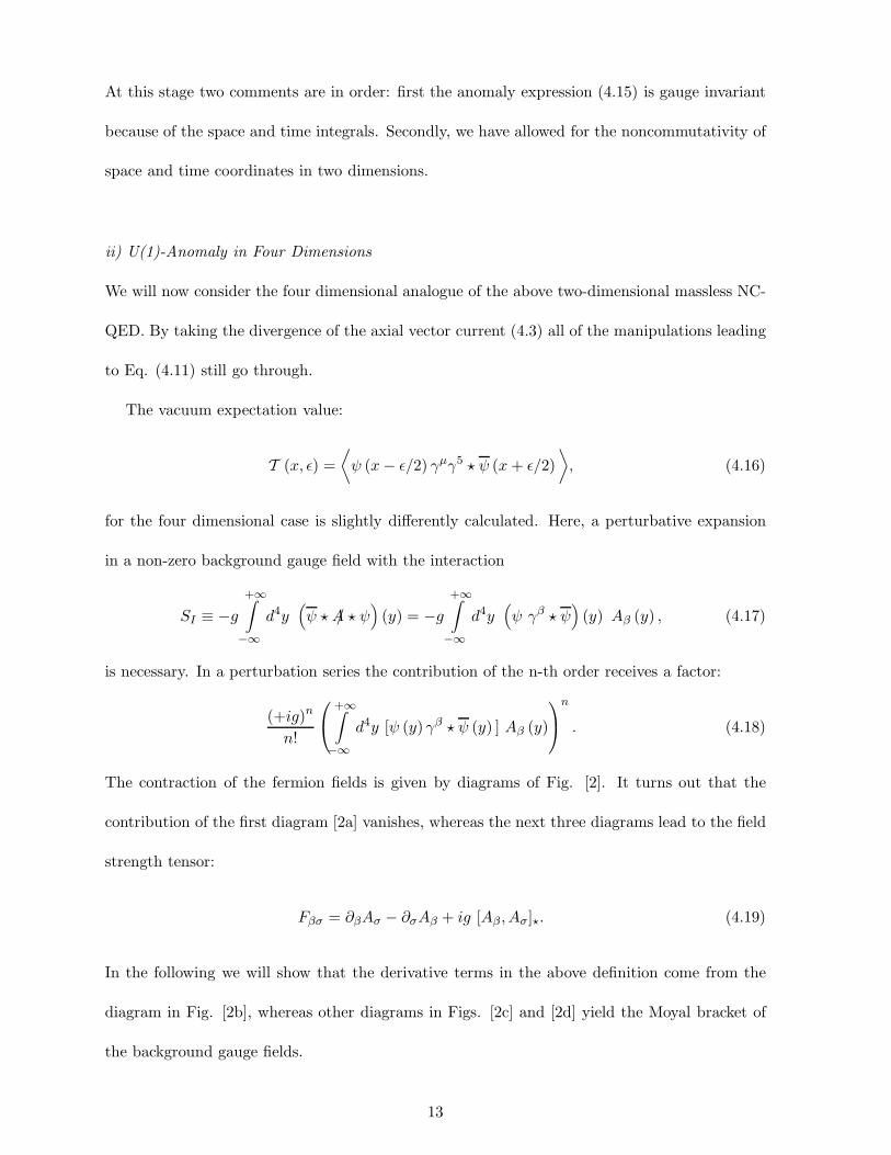
ii) U(1)-Anomaly in Four Dimensions

We will now consider the four dimensional analogue of the above two-dimensional massless NC-

QED. By taking the divergence of the axial vector current (4.3) all of the manipulations leading

to Eq. (4.11) still go through.

The vacuum expectation value:

T (x, ǫ) =

⟨

ψ (x− ǫ/2) γµγ5 ⋆ ψ (x+ ǫ/2)

⟩

, (4.16)

for the four dimensional case is slightly differently calculated. Here, a perturbative expansion

in a non-zero background gauge field with the interaction

SI ≡ −g

+∞∫

−∞

d4y(

ψ ⋆ A/ ⋆ ψ)

(y) = −g

+∞∫

−∞

d4y(

ψ γβ ⋆ ψ)

(y) Aβ (y) , (4.17)

is necessary. In a perturbation series the contribution of the n-th order receives a factor:

(+ig)n

n!

+∞∫

−∞

d4y [ψ (y) γβ ⋆ ψ (y) ] Aβ (y)

n

. (4.18)

The contraction of the fermion fields is given by diagrams of Fig. [2]. It turns out that the

contribution of the first diagram [2a] vanishes, whereas the next three diagrams lead to the field

strength tensor:

Fβσ = ∂βAσ − ∂σAβ + ig [Aβ , Aσ]⋆. (4.19)

In the following we will show that the derivative terms in the above definition come from the

diagram in Fig. [2b], whereas other diagrams in Figs. [2c] and [2d] yield the Moyal bracket of

the background gauge fields.

13

Let us begin the analysis with the zeroth order of perturbation theory. The integral appearing

from the contraction of the fermion-antifermion fields in the case n = 0 is highly divergent in the

limit ǫ→ 0, but gives zero when traced with γµγ5. This is the same result as in the commutative

four-dimensional massless QED.

The first perturbative correction of T (x, ǫ) is:

T1 (x, ǫ) = ig

+∞∫

−∞

d4p

(2π)4d4q

(2π)4d4ℓ

(2π)4∏

i=1,2

d4ℓi

(2π)4

⟨

ψ (p) γµγ5ψ (q) ψ (ℓ1) γβψ (ℓ2)

⟩

×

+∞∫

−∞

d4y1Aβ (ℓ) e−iℓy1(

e−iℓ1y1 ⋆ eiℓ2y1) (

e−ipx ⋆ eiqx)

ei(q+p)ǫ2 . (4.20)

Note that the product between the exponentials with x and the exponentials with y1 is the

ordinary product of functions. The definition of the ⋆-product in the momentum space leads to:

T1 (x, ǫ) = ig

+∞∫

−∞

d4p

(2π)4d4q

(2π)4d4ℓ

(2π)4∏

i=1,2

d4ℓi

(2π)4

⟨

ψ (p) γµγ5ψ (q) ψ (ℓ1) γβψ (ℓ2)

⟩

× (2π)4 δ4 (ℓ2 − ℓ1 − ℓ)Aβ (ℓ) ei(q−p)x ei(q+p)ǫ2 e

iθηκ

2 (pηqκ+ℓη1ℓκ2), (4.21)

where the integration over y1 is performed to yield the δ-function. Contraction of the fermions

removes the exponential function containing the noncommutativity parameter because of the

antisymmetry of θ. After a change of integration variables we get:

T1 (x, ǫ) = −ig

∫

d4s

(2π)4d4ℓ

(2π)4Tr

[

is/

s2γµγ5 i (s/ − ℓ/)

(s− ℓ)2γβ]

Aβ (ℓ) e−iℓx eisǫ. (4.22)

To evaluate the limit ǫ → 0, the integrand can be expanded for large external gauge field

momentum ℓ. We therefore obtain:

T1 (x, ǫ) = −igTr(

γαγµγ5γσγβ)

+∞∫

−∞

d4ℓ

(2π)4ℓσAβ (x) e−iℓx

+∞∫

−∞

d4s

(2π)4sαe

isǫ

s4,

= −ig εµαβσ

4π2(∂σAβ (x))

∂

∂ǫαlog

1

ǫ2

= −ig εµαβσ

4π2(∂βAσ (x) − ∂σAβ (x))

ǫαǫ2. (4.23)

Here, we have used Tr(

γ5γµγαγβγσ)

= −4iεµαβσ in four dimensions. Again a finite result can

be obtained by inserting this expression in the Eq. (4.11), now in four dimensions. In the first

14

order of perturbative expansion the contribution to the divergence of the axial vector current is

therefore given by:

[

+∞∫

−∞

d4x

⟨

∂µJµ(5) (x)

⟩]

for n = 1= −ig

+∞∫

−∞

d4x Fµν (x) limǫ→0

ǫν T1 (x, ǫ)

= −g2

4π2

(

limǫ→0

ǫαǫν

ǫ2

)

εµαβσ+∞∫

−∞

d4x [∂βAσ (x) − ∂σAβ (x) ] Fµν (x)

= −g2

16π2εµνβσ

+∞∫

−∞

d4x [∂βAσ (x) − ∂σAβ (x) ] Fµν (x) , (4.24)

where we have made use of the Eq. (4.14) for D = 4. In commutative QED the expression

in the square brackets on the last line of the above result is the Abelian field strength tensor

and the above result is the familiar result for the axial anomaly obtained in the point-splitting

method. However, it is only after considering the contribution of the next order of perturbation

theory, that the non-linear term in the definition of the field strength tensor in NC-QED can be

recovered.

The contribution of the second order perturbation theory to T (x, ǫ) can be obtained in a

similar way. The contraction of fermions yields two connected diagrams [Fig. [2c] and [2d]],

T2 (x, ǫ) = −ig2

2!

+∞∫

−∞

d4k

(2π)4d4ℓ

(2π)4d4s

(2π)4Aσ (k) Aβ (ℓ) e−i(ℓ+k)x eisǫ

×

{

Tr

[

s/ + k/

(s+ k)2γµγ5

s/ − ℓ/

(s− ℓ)2γβ

s/

s2γσ

]

e−iθηκ

2kηℓκ + [(ℓ, β) ↔ (k, σ)]

}

, (4.25)

where the first expression on the last line belongs to the diagram in Fig. [2c] and [(ℓ, β) ↔ (k, σ)]

denotes the contribution of diagram [2d]. Note that the effective phase e−iθηκ

2kηℓκ can be obtained

after performing all the ⋆-products appearing in this order and considering all the δ-functions

of the momenta, which arise after contractions of fermion-antifermion fields.

Next we have to evaluate the trace Tr[ (s/ + k/) γµγ5 (s/ − ℓ/) γβs/γσ] in the contribution of di-

agram [2c] and Tr[ (s/ + ℓ/) γµγ5 (s/ − k/) γσs/γβ ] in the contribution of diagram [2d]. It turns out

that the relevant contribution for the limit ǫ → 0 comes only from Tr (s/γµγ5s/γβs/γσ) in both

traces. Other terms lead to non-covariant expressions like [∂τAβ, Aσ ]⋆logǫ2, which vanish after

15

contracting with −igǫνFµν (x) and taking the limit ǫ→ 0.

For large k and ℓ the relevant contribution to the VEV T (x, ǫ), in second order of perturbation

theory in the limit ǫ→ 0 is given by:

T2 (x, ǫ) = −ig2

2!

[

+∞∫

−∞

d4k

(2π)4Aσ (k) e−ikx ⋆

∞∫

−∞

d4ℓ

(2π)4e−iℓxAβ (ℓ)

×

∫

d4s

(2π)4eisǫ

Tr (s/γµγ5s/γβs/γσ)

s6

]

+ [(ℓ, β) ↔ (k, σ)]

= −ig2

2!

[

Aσ (x) ⋆ Aβ (x)

∫

d4s

(2π)4eisǫ

Tr (s/γµγ5s/γβs/γσ)

s6

]

+ [β ↔ σ], (4.26)

where the definition of the ⋆-product is used on the first line to obtain Aσ ⋆Aβ . To evaluate the

traces we can make use of the relation:

Tr (γ5γργβγκγσγτγµ) = +4iεστµα(

δαµgβκ − δαβ gρκ + δακgρβ)

−4iερβκα(

δασ gτµ − δατ gσµ + δαµgστ)

, (4.27)

to obtain:

Tr (s/γµγ5s/γβs/γσ) = −4iεστµβ sτ s2.

The integration over s in the Eq. (4.24) can be performed in the same way as in Eq. (4.23),

giving:

T2 (x, ǫ) = +g2

4π2εµτβσ

[

Aβ (x) , Aσ (x)

]

⋆

ǫτǫ2. (4.28)

The contribution from the second order of perturbative expansion to the divergence of the axial

current is therefore given by:

[

+∞∫

−∞

d4x

⟨

∂µJµ(5) (x)

⟩]

for n = 2= −ig

+∞∫

−∞

d4x Fµν (x) limǫ→0

ǫν T2 (x, ǫ)

= −ig3

4π2

(

limǫ→0

ǫτ ǫν

ǫ2

)

εµτβσ+∞∫

−∞

d4x

[

Aβ (x) , Aσ (x)

]

⋆

Fµν (x) ,

= −ig3

16π2εµνβσ

+∞∫

−∞

d4x

[

Aβ (x) , Aσ (x)

]

⋆

Fµν (x) , (4.29)

16

where we have made use of the Eqs. (4.11) now in four dimensions, and (4.14). Adding the

result of the first order of expansion, Eq. (4.24), to this result gives the axial anomaly in

four-dimensional massless NC-QED:

+∞∫

−∞

d4x

⟨

∂µJµ(5) (x)

⟩

= −g2

16π2εµνβσ

+∞∫

−∞

d4x Fµν (x) ⋆ Fβσ (x) . (4.30)

Note that the integral over space-time coordinates plays the role of trace over group the indices

in the commutative non-Abelian gauge theories, and guarantees the ⋆-gauge invariance of the

result. Subsequently we will find the expression for the anomaly density in terms of Chern-

Pointryagin density, al beit a non gauge invariant equation.

The Fujikawa Method

In this method the axial anomaly is interpreted as a result of the non-invariance of the fermionic

measure of integration under infinitesimal local axial gauge transformations.

We begin the evaluation of the axial anomaly by studying the transformation properties of

the partition function of NC-QED,

Z =

∫

Dψ Dψ e−iSF [ψ,ψ], (4.31)

under local chiral gauge transformations:

ψ (x) → ψ′ (x) = U (5) (x) ⋆ ψ (x) , ψ (x) → ψ′(x) = ψ (x) ⋆ U (5) (x),

with

U (5) (x) =(

eiγ5α(x))

⋆. (4.32)

In the chiral limit and for vanishing background gauge field the fermionic action SF [ψ,ψ], Eq.

(2.13),

SF [ψ,ψ] ≡ i

∫

d4x ψ (x) γµ ⋆ ∂µψ (x) , (4.33)

17

transforms as,

SF → S′F = SF −

∫

d4x ψ (x) ⋆ ∂µα (x) γµγ5 ⋆ ψ (x) . (4.34)

From the definition of the ⋆-product we get:

∫

d4x ψ (x) ⋆ ∂µα (x) γµγ5 ⋆ ψ (x) = i

∫

d4x α (x) ⋆ ∂µJµ(5) (x) ,

where the axial current Jµ(5) is defined in the Eq. (4.3). The transformed fermionic action can

therefore be written as:

S′F [ψ′, ψ

′] = SF [ψ,ψ] − i

∫

d4x α (x) ⋆ ∂µJµ(5) (x) . (4.35)

Replacing this equation in the partition function of the fermion field yields,

Z ′ =

∫

Dψ′ Dψ′e−iS

′

F[ψ′,ψ

′

]

=

∫

Dψ′ Dψ′e−iSF [ψ,ψ] exp

{

−

∫

d4x α (x) ⋆ ∂µJµ(5) (x)

}

. (4.36)

Under a general local matrix transformation ψ (x) → U (x) ⋆ψ (x), with U (x) a unitary matrix,

the integration measure of the fermionic fields will transform with the inverse of the determinants

of the transform matrix19:

Dψ Dψ →(

Det U Det U)−1

Dψ Dψ,

where

Ux,y ≡ U (x) ⋆ δ4 (x− y) , Ux,y ≡ γ0U† (x) γ0 ⋆ δ

4 (x− y) . (4.37)

Notice that in the noncommutative field theory the δ4 (x− y)-function is definied as in the

commutativ case, i.e. by∫

g (x) ⋆ δ4 (x− y) d4x = g (y) for a test function g (x). For a local

chiral gauge transformation, replacing U (x) in the (4.37) by the unitary matrix U (5) (x) from

the Eq. (4.32), we obtain:

Ux,y = Ux,y. (4.38)

18

The transformation rule for the fermionic integration measure reads then:

Dψ Dψ → Dψ′ Dψ′= (Det Ux,y)

−2Dψ Dψ. (4.39)

From the Eq. (4.32) the fermionic fields transform as:

ψ (x) ≈ ψ (x) + iγ5ψ (x) ⋆ α (x) , ψ (x) ≈ ψ (x) + iγ5 α (x) ⋆ ψ (x) , (4.40)

and the fermionic integration measure tranforms as:

Dψ′ Dψ′

≈ (Det Ux,y)−2 Dψ Dψ

≈ exp

[

i

∫

d4x α (x) ⋆A (x)

]

Dψ Dψ. (4.41)

with

A (x) ≡ −2 Tr (γ5) δ4 (x− x) . (4.42)

In this expression the δ-function is infinite, whereas the trace over γ5 vanishes. To regularize it

in a ⋆-gauge covariant manner a differentiable operator f(

−Dµγ

µ⋆Dνγν

M2

)

, with Dµ introduced in

the Eq. (2.14), is inserted. Here, M is a large mass, which should be taken eventually to infinity.

The operator Dµ ⋆Dν transforms in the usual covariant manner: U (x)⋆Dµ ⋆Dν ⋆U−1 (x). This

operator should act first on δ4 (x− y) before taking the limit x → y. The regularized anomaly

function A (x) can therefore be given by:

A (x) = −2 Tr

{

γ5f

(

−Dµγµ ⋆ Dνγ

ν

M2

)}

⋆ δ4 (x− y) . (4.43)

The Fourier component of the above function f(

k2)

should satisfy the following conditions:

f(

k2 = 0)

= 1, f(

k2 → ∞)

= 0,

k2f ′(

k2)

= 0 for k2 = 0 and for k2 → ∞. (4.44)

Using

−Dµγµ ⋆ Dνγ

ν = −Dµ ⋆ Dµ −

g

2σµνF

µν (x) , (4.45)

19

where σµν ≡ i2 [γµ, γν ] and igFµν ≡ [Dµ,Dν ]⋆, and where the antisymmetry of σµν leads to

σµνDµ ⋆ Dν = 1

2σµν [Dµ,Dν ]⋆, we get:

A (x) = −2 limy→x

∫

dDk

(2π)DTr

[

γ5f

(

−Dµ ⋆ Dµ − g

2 σµνFµν (x)

M2

)

]

⋆ eik(x−y). (4.46)

Next a Taylor expansion on the regulator function f for large M can be performed to yield:

f

(

−Dµ ⋆ D

µ

M2+

g

2M2σµνF

µν (x)

)

=

+g2

2! × 4M4(σµνF

µν (x)) ⋆(

σξρFξρ (x)

)

f ′′(

−Dµ ⋆ Dµ

M2

)

+ O

(

1

M6

)

, (4.47)

The first two terms in the Taylor expansion vanish due to their traces with a γ5 matrix in A (x)

[Eq. (4.46)]. The only term which contributes is quadratic in Fµν . It turns out that only the

term with power 1/M4 leads to a mass independent expression which is just the expected axial

anomaly. Making use of the expression:

Tr (γ5σµν σξρ) = −4iεµνξρ,

the anomaly function A (x), Eq. (4.46), is then given by:

A (x) =ig2

M4εµνξρF

µν (x) ⋆ F ξρ (x) limy→x

∫

dDk

(2π)D

[

f ′′(

−Dµ ⋆ Dµ

M2

)]

⋆ eik(x−y). (4.48)

For vanishing background gauge field the above integration can be performed. Using

limx→y

f ′′(

−∂2µ

M2

)

⋆ eik(x−y) = f ′′(

k2

M2

)

, (4.49)

we obtain:

∫

dDk

(2π)Df ′′(

k2

M2

)

=M4

16π2.

The anomaly function thus reads:

A (x) =ig2

16π2εµνξρ F

µν (x) ⋆ F ξρ (x) . (4.50)

Under an infinitesimal local chiral gauge transformation the integration measure for the fermionic

fields behaves as [see Eq. (4.41)]:

Dψ′ Dψ′≈ exp

[

i

∫

d4x α (x) ⋆A (x)

]

Dψ Dψ,

20

with A (x) given in the Eq. (4.50). By making use of this transformation law the transformed

partition function Z ′ from the Eq. (4.36) can be completed to yield:

Z ′ =

∫

Dψ′ Dψ′e−iS

′

F[ψ′,ψ

′

]

=

∫

Dψ Dψ e−iSF [ψ,ψ] exp

{∫

d4x

[

α (x) ⋆(

iA (x) − ∂µJµ(5) (x)

)

]}

. (4.51)

The ⋆-product in the integration over x can be neglected. To derive the axial anomaly, we make

use of the invariance of the partition function under any infinitesimal change of variables. The

axial anomaly reads therefore:

< ∂µJµ(5) (x) >= −

g2

16π2εµνξρF

µν (x) ⋆ F ξρ (x) , (4.52)

which is only covariant under ⋆-gauge transformation though (4.51) is in fact gauge invariant.

This is due to the covariant regularization performed in the Eq. (4.43). Note that ⋆-gauge

invariance is guaranteed only by integrating the above result over x.

Triangle Anomaly

We will now present the direct calculation of the axial anomaly11 by calculating the triangle

diagrams. As a consequence of noncommutativity of QED, phases will appear in the Feynman

integrals corresponding to triangle diagrams. These phases will turn out to be independent of

the internal loop momentum, however. Hence no nonplanar triangle diagrams appear in this

case, as it was also originally suggested in Ref.7.

Let us begin the calculation with the three-point function of two vector and one axial vector

currents:

Γµλν (x, y, z) =

⟨

T(

Jµ(5) (x)Jλ (y) Jν (z))

⟩

. (4.53)

The axial vector current Jµ(5) is defined in the Eq. (4.3) and the vector current Jµ is given by:

Jµ (x) = ig ψ (x) γµ ⋆ ψ (x) . (4.54)

21

The operation between the currents in Eq. (4.53) is just the usual product of functions,

Γµλν (x, y, z) = −ig2

+∞∫

−∞

∏

i=1,2,3

d4pi

(2π)4∏

j=1,2,3

d4p′j

(2π)4ei(p1−p

′

1)xei(p2−p′

2)yei(p3−p′

3)z

⟨

ψ (p1) γµγ5ψ

(

p′1)

ψ (p2) γλψ(

p′2)

ψ (p3) γνψ(

p′3)

⟩

eiθησ

2

∑

j=1,2,3p

ηj p

′σj . (4.55)

There are two Feynman diagrams [Fig. [3]] contributing to this expression, with the result:

Γµλν (x, y, z) = −ig2

+∞∫

−∞

d4k2

(2π)4d4k3

(2π)4d4ℓ

(2π)4e−i(k2+k3)x eik2yeik3z

×

{

[

Tr

(

1

D (ℓ− k3)γµγ5 1

D (ℓ+ k2)γλ

1

D (ℓ)γν)

e+iθησ

2k

η2kσ3

]

+

[

(k2, λ) ↔ (k3, ν)

]

}

, (4.56)

where the first expression on the second line is the contribution of diagram [3a], whereas

[(k2, λ) ↔ (k3, ν)] denotes the contribution of diagram [3b]. Here D (ℓ) is the denominator

of the fermion propagator and is defined by D (ℓ) ≡ ℓ/−m. As we can see, the phases e±iθησ

2k

η2kσ3

corresponding to both triangle diagrams [3a] and [3b] are independent of the loop momentum

ℓ. Hence no nonplanar diagrams appear in this zeroth order of perturbative expansion.

i) Vector Ward Identity

To verify the vector Ward identities, we consider ∂λΓµλν , and use the identity

k/2 = D (ℓ+ k2) −D (ℓ) , (4.57a)

in the contribution of diagram [3a] and

k/2 = D (ℓ) −D (ℓ− k2) , (4.57b)

in the contribution of diagram [3b], to obtain

∂

∂yλΓµλν (x, y, z) = g2

+∞∫

−∞

d4k2

(2π)4d4k3

(2π)4dDℓ

(2π)De−i(k2+k3)x eik2y eik3z

×

{[

Tr

(

1

D (ℓ− k3)γµγ5 1

D (ℓ)γν)

− Tr

(

1

D (ℓ− k3)γµγ5 1

D (ℓ+ k2)γν)

]

e+iθησ

2k

η2kσ3

+

[

Tr

(

1

D (ℓ− k2)γµγ5 1

D (ℓ+ k3)γν)

− Tr

(

γµγ5 1

D (ℓ+ k3)γν

1

D (ℓ)

)

]

e−iθησ

2k

η2kσ3

}

.

(4.58)

22

The integrands on the second and third lines are linearly divergent in the limit D → 4. In the

usual commutative QED, where no phases appear, these integrals could be shown to cancel after

appropriate shifts of integration variables, which are justified by dimensional regularization. In

NC-QED, however, no cancellation takes place because of different phases in diagrams [3a] and

[3b]. After a shift ℓ→ ℓ+ k3 and ℓ→ ℓ+ k3 − k2 in the first and second integrands respectively,

we arrive at:

∂

∂yλΓµλν (x, y, z) = 2ig2

+∞∫

−∞

d4k2

(2π)4d4k3

(2π)4e−i(k2+k3)x eik2y eik3z sin

(

θησ2kη2k

σ3

)

×

+∞∫

−∞

dDℓ

(2π)D

[

Tr

(

1

D (ℓ)γµγ5 1

D (ℓ+ k3)γν)

− Tr

(

1

D (ℓ− k2)γµγ5 1

D (ℓ+ k3)γν)

]

.

(4.59)

Integration over the loop momentum ℓ vanishes due to the symmetry properties of the trace.

We therefore obtain:

∂

∂yλΓµλν (x, y, z) = 0. (4.60)

The triangle graphs make a contribution to the current in the presence of a gauge field Aν and

an axial gauge field A(5)µ :

〈Jλ (y) 〉 ≡1

2

∫

d4x d4z Γµλν (x, y, z)A(5)µ (x)Aν (z) . (4.61)

By making use of the Eq. (4.60) we therefore find the standard vector Ward identity in NC-QED:

〈∂λJλ (y) 〉 = 0. (4.62)

ii) Axial Vector Ward Identity

To evaluate the divergence of the axial vector current, we consider:

∂

∂xµΓµλν (x, y, z) = −g2

+∞∫

−∞

d4k2

(2π)4d4k3

(2π)4dDℓ

(2π)De−i(k2+k3)x eik2yeik3z

×

{

[

Tr

(

1

D (ℓ− k3)(k/2 + k/3) γ

5 1

D (ℓ+ k2)γλ

1

D (ℓ)γν)

e+iθησ

2k

η2kσ3

]

+

[

(k2, λ) ↔ (k3, ν)

]

}

. (4.63)

23

We follow the standard definition of γ5-matrix in D-dimensions (17, 18):

γ5 = iγ0γ1γ2γ3,

where γ5 anticommutes with γµ for µ = 0, 1, 2, 3 but commutes with γµ for other values of µ.

The loop momentum will have components in all dimensions, whereas the external momenta k2

and k3 are still defined only in four dimensions. Using the separation ℓ = ℓ|| + ℓ⊥, where ℓ|| has

nonzero components in dimensions 0, 1, 2, 3 and ℓ⊥ has nonzero components in the other D − 4

dimensions, and the identity:

(k/2 + k/3) γ5 = −γ5D (ℓ+ k2) −D (ℓ− k3) γ

5 − 2mγ5 + 2γ5ℓ/⊥, (4.64a)

in the first expression on the second line of Eq. (4.63), and

(k/2 + k/3) γ5 = −γ5D (ℓ+ k3) −D (ℓ− k2) γ

5 − 2mγ5 + 2γ5ℓ/⊥, (4.64b)

in the last expression on the second line of this equation, we obtain:

∂

∂xµΓµλν (x, y, z) =

+∞∫

−∞

d4k2

(2π)4d4k3

(2π)4e−i(k2+k3)x eik2y eik3z

×

[

2mg2T λν (m,k2, k3; θ) +Aλν (k2, k3; θ) +Rλν (m,k2, k3; θ)

]

, (4.65a)

where

T λν (m,k2, k3; θ) ≡

+∞∫

−∞

dDℓ

(2π)D

[

Tr

(

1

D (ℓ− k3)γ5 1

D (ℓ+ k2)γλ

1

D (ℓ)γν)

e+iθησ

2k

η2kσ3

]

+

[

(k2, λ) ↔ (k3, ν)

]

, (4.65b)

and

Aλν (k2, k3; θ) ≡

≡ −2g2

+∞∫

−∞

dDℓ

(2π)D

[

Tr

(

1

D (ℓ− k3)γ5ℓ/⊥

1

D (ℓ+ k2)γλ

1

D (ℓ)γν)

e+iθησ

2k

η2kσ3

]

+

[

(k2, λ) ↔ (k3, ν)

]

, (4.65c)

24

and

Rλν (m,k2, k3; θ) ≡ g2

+∞∫

−∞

dDℓ

(2π)D

[{

Tr

(

1

D (ℓ− k3)γ5γλ

1

D (ℓ)γν)

+Tr

(

γ5 1

D (ℓ+ k2)γλ

1

D (ℓ)γν)

}

e+iθησ

2k

η2kσ3

]

+

[

(k2, λ) ↔ (k3, ν)

]

. (4.65d)

Using the standard Feynman parametrization we obtain the following results for the above

functions. For T λν we get:

T λν (m,k2, k3; θ) =m

2π2ελναβk2αk3β cos

(

θησ2kη2k

σ3

)

×

1∫

0

dx

1−x∫

0

dy1

m2 − k22x (1 − x) − k2

3y (1 − y) − 2k2k3xy. (4.66)

Note that the contribution of this function to ∂µΓµλν (x, y, z) vanishes after taking the chiral

limit m→ 0 in the Eq. (4.65a).

For the anomalous function Aλν we have:

Aλν (k2, k3; θ) = −g2

2π2ελναβk2αk3β cos

(

θησ2kη2k

σ3

)

, (4.67)

which is independent of the fermion mass m and survives the chiral limit m → 0. This is the

anomalous contribution to ∂µΓµλν (x, y, z). For vanishing noncommutativity parameter θησ this

result is exactly the U(1)-anomaly in commutative QED.

For the rest term Rλν (m,k2, k3; θ), after performing a shift of integration variable ℓ, we

obtain:

Rλν (m,k2, k3; θ) = −2ig2 sin

(

θησ2kη2k

σ3

)

×

∞∫

−∞

dDℓ

(2π)D

[

Tr

(

1

D (ℓ)γλγ5 1

D (ℓ+ k3)γν)

− Tr

(

1

D (ℓ)γλγ5 1

D (ℓ− k2)γν)

]

. (4.68)

Here, a power counting shows that both integrals are linearly divergent in the limit D → 4. But

they vanish due to symmetry properties of the traces over the γ-matrices. We therefore have:

Rλν (m,k2, k3; θ) = 0. (4.69)

25

Inserting Eqs. (4.66)-(4.69) in Eq. (4.65a) and taking the chiral limit m→ 0 we get:

[

∂

∂xµΓµλν (x, y, z)

]

m→0

=

= −g2

2π2ελναβ

+∞∫

−∞

d4k2

(2π)4d4k3

(2π)4e−i(k2+k3)x eik2y eik3zk2αk3β cos

(

θησ2kη2k

σ3

)

. (4.70)

Thus the contribution of triangle diagrams to axial vector current in the presence of vector gauge

fields,

〈Jµ(5) (x) 〉 ≡1

2

∫

d4y d4z Γµλν (x, y, z) Aλ (y)Aν (z) , (4.71)

and Eq. (4.70) give,

⟨

∂µJµ(5) (x)

⟩

= −g2

4π2ελναβ∂λAν (x) ⋆ ∂αAβ (x) , (4.72)

for the divergence of the axial vector current. To obtain the result by the point-splitting method

[Eq. (4.52)]:

⟨

∂µJµ(5) (x)

⟩

= −g2

16π2ελναβFλν (x) ⋆ Fαβ (x) , (4.73)

we have to consider the contributions of all the diagrams shown in Figure [4]. Diagrams [4b]

and [4c] turn out to be planar, so that no new effects will occur. Note also that only integrating

over the variable x insures the ⋆-gauge invariance of the above result.

The Algebra of Currents and the Ward Identities

In what follows we will look anew at the Ward identities in NC-QED to show the analogy

between noncommutative U(1) gauge theory and commutative non-Abelian gauge theories. In

the previous section we have shown that as a consequence of the noncommutativity, phases will

appear in the Feynman integrals for the triangle diagrams. In the commutative non-Abelian

gauge theory these phases are replaced by traces over group generators19. A separation of these

traces in an antisymmetric and a symmetric part leads to a separation between a ”formal” part,

which is connected to the algebra of currents and involve the structure constants of the group,

26

and a ”potentially anomalous” parts in the divergences of Γµλν . The potentially anomalous part

in the vector Ward identity can be chosen to vanish and only the anomalous part of axial vector

Ward identity yields the usual axial anomaly.

In what follows we will show, that in NC-QED the same separation between the formal and the

anomalous part in vector- and axial vector Ward identities is possible. We will use dimensional

regularization to calculate the linearly divergent integrals appearing in the calculation. We

will show that the formal part of both vector and axial vector Ward identity vanish after this

regularization. Assuming gauge invariance, the anomalous part of the vector Ward identity can

be chosen to vanish, and the anomalous part of the axial vector Ward identity to contain the

anomaly.

i) Vector Ward Identity

The starting point here is the three-point function Γµλν (x, y, z) given in the Eq. (4.53). Using

the definition of the time-ordered product appearing on the r.h.s. of this equation and deriving

the resulting expression with respect to yλ, we obtain the separation:

∂λΓµλν (x, y, z) = [∂λΓ

µλν (x, y, z) ]formal + [∂λΓµλν (x, y, z) ]anomal, (4.74a)

where the formal part is given by:

[∂λΓµλν (x, y, z) ]formal ≡ δ

(

y0 − z0)

⟨

T

(

Jµ(5) (x)

[

J0 (y) , Jν (z)

])⟩

+δ(

y0 − x0)

⟨

T

([

J0 (y) , Jµ(5) (x)

]

Jν (z)

)⟩

, (4.74b)

and the potentially anomalous part by:

[∂λΓµλν (x, y, z) ]anomal ≡

⟨

T(

Jµ(5) (x)(

∂λJλ (y)

)

Jν (z))

⟩

. (4.74c)

Note that, the commutators above are the usual commutators of operators:

[f (x) , g (y)] ≡ f (x) g (y) − g (y) f (x) ,

27

and the ⋆-products appear only in the definition of the vector and the axial vector current.

Using the definition of the currents one obtains the following algebra of the vector and axial

vector currents,

[J0 (x) , Jλ (y) ]x0=y0= −

(

Jλ (x) − Jλ (y))

⋆ δ3 (x− y) , (4.75a)

[J0(5) (x) , Jλ(5) (y) ]x0=y0= −

(

Jλ (x) − Jλ (y))

⋆ δ3 (x− y) , (4.75b)

[J0 (x) , Jλ(5) (y) ]x0=y0= −

(

Jλ(5) (x) − Jλ(5) (y))

⋆ δ3 (x− y) , (4.75c)

[J0(5) (x) , Jλ (y) ]x0=y0= −

(

Jλ(5) (x) − Jλ(5) (y))

⋆ δ3 (x− y) . (4.75d)

It is possible to compare these relations with equal-time commutation relations of QCD. There

the structure constants fabc appear on the right-hand side of the commutation relations. In

NC-QED, however, these structure constants are replaced by 2i sin(

θησ

2 pηqσ)

where p and q are

the momenta of the first and second current in the commutation relation, respectively.

Using Eqs. (4.75a) and (4.75c), the formal part of ∂λΓµλν reads:

[

∂

∂yλΓµλν (x, y, z)

]

formal

= 2ig2

+∞∫

−∞

d4k2

(2π)4d4k3

(2π)4e−i(k2+k3)x eik2y eik3z sin

(

θησ2kη2k

σ3

)

×

+∞∫

−∞

dDℓ

(2π)D

[

Tr

(

1

D (ℓ)γµγ5 1

D (ℓ+ k3)γν)

− Tr

(

1

D (ℓ)γµγ5 1

D (ℓ+ k2 + k3)γν)

]

,

(4.76)

which, after a shift ℓ → ℓ− k2 in the second integral, is exactly the same as Eq. (4.59). These

integrals vanish due to the traces. We are therefore left with the potentially anomalous part of

∂λΓµλν (x, y, z), Eq. (4.74c), which if one assumes gauge invariance can be set to zero.

ii) Axial Vector Ward Identity

Considering the three-point function (4.53) and its derivative with respect to xµ, using the

definition of time-ordered product we have again:

∂µΓµλν (x, y, z) ≡ [∂µΓ

µλν (x, y, z) ]formal + [∂µΓµλν (x, y, z) ]anomal, (4.77a)

28

where the formal part is given by:

[∂µΓµλν (x, y, z) ]formal ≡ δ

(

x0 − y0)

⟨

T(

[J0(5) (x) , Jλ (y) ]Jν (z))

⟩

+δ(

x0 − z0)

⟨

T(

Jλ (y) [J0(5) (x) , Jν (z) ])

⟩

, (4.77b)

and the anomalous part by:

[∂µΓµλν (x, y, z) ]anomal ≡

⟨

T((

∂µJµ(5) (x)

)

Jλ (y)Jν (z))

⟩

. (4.77c)

The formal part can be evaluated using Eq. (4.75d). Going through the same manipulations

leading to the Eq. (4.76) we obtain exactly the same integrals given in the Eq. (4.68), which

vanish. We therefore have:

[∂µΓµλν (x, y, z) ]formal = 0, (4.78)

and are left with the anomalous part ∂µΓµλν , which we have already calculated, Eq. (4.70),

leading to the axial anomaly expression (4.73).

5. Conclusion

In this paper we have studied the Ward identities and calculated the axial anomaly in noncom-

mutative (NC)-QED on RD. We started from the NC-QED action, originally given in Refs.6,7.

As in the case of the commutative non-Abelian gauge theory, the Ward identity in the simple case

of fermion-antifermion annihilation into two gauge bosons is only satisfied, if the contribution of

the three-gauge vertex to this process is also considered. In this calculation, we have made use

of the usual dispersion relation, in contrast to Ref.10, where matter in adjoint representation is

used.

We then derived the U(1)-anomaly in NC-QED using several methods carried over from the

commutative field theory. First we studied the massless two-dimensional NC-QED. The axial

anomaly was obtained, in the method of point-splitting after an integration over noncomutative

29

space-time coordinates, which also preserved ⋆-gauge invariance of the axial anomaly. Similar

computation in four dimensions leads to the expected ⋆-gauge invariant result for the axial

anomaly.

In the Fujikawa method, performing a gauge covariant regularization, the anomaly in a gauge

covariant form was obtained. Then a detailed analysis of the triangle diagrams for the axial

vector current was carried out. The noncommutativity parameter θησ appeared in the phases

in the Feynman integrals for the triangle diagrams, but these phases were independent of the

internal loop momentum. Hence no nonplanar diagrams appear at this level and known methods

from commutative QED could be used to evaluate the vector and axial vector Ward identities

in NC-QED.

We have shown that in momentum space the resulting expression for the axial anomaly

differs from the corresponding commutative result by a factor cos(

θησ

2 kη1kσ2

)

. Here k1 and k2

are the momenta of the gauge fields interacting with both vector currents. For non-vanishing

parameter θησ, as in the commutative non-Abelian gauge theories, the anomalous contributions

from the triangle diagrams do not yield the full anomaly and higher order diagrams have to be

taken into account. These higher loop diagrams are also planar. This means that no UV/IR

mixing will appear also in the higher loop order. This is certainly the consequence of the

choice of the noncommutative U(1) current in the present paper. Further studies14 show that

in noncommutative U(1) gauge theory with fundamental matter field coupling, there are in fact

three different currents, which all, expressing the same global symmetry of the noncommutative

action, lead to the same classically conserved charge. Two of them lead to planar triangle

diagrams, whereas the third one includes planar as well as nonplanar diagrams, which have IR

singularities. We study the effect of nonplanar diagrams to the gauge and global anomalies

of noncommutative U(1) and U(N) gauge theories in a second paper14. For noncommutative

U(1) gauge theory, it will turn out that for certain choice of noncommutativity parameter a

30

finite global anomaly emerges from the nonplanar contributions to the triangle diagrams due to

UV/IR mixing.

Finally, here, a separation between the formal and the potentially anomalous part of the

divergence of the vertex function was performed. This is analogous to the separation between

the symmetric and antisymmetric part of traces over group generators in non-Abelian gauge

theories19. Using the algebra of the NC-QED currents the formal parts of vector and axial

vector were shown to vanish. Assuming gauge invariance of NC-QED the potentially anomalous

part of the vector Ward identity vanish leaving the axial vector current anomalous.

Acknowledgments

We would like to thank H. Arfaei for discussions and M. Hayakawa for a communication regarding

Feynman diagrams.

Note added: After this work (hep-th/0002143) other studies on the anomalies of non-Abelian

noncommutative gauge theories appeared20.

References

1. A. Connes, M. R. Douglas, and A. Schwarz, JHEP 9802:003 (1998).2. N. Seiberg, and E. Witten, JHEP 9909:032 (1999), hep-th/9908142.3. Sh. Minwalla, M. Van Raamsdonk, and N. Seiberg, JHEP 0001:028 (2000), hep-th/9912072.4. C. P. Martin, and D. Sanchez-Ruiz, Phys. Rev. Lett. 83 (1999) 476, hep-th/9903077.

M. M. Sheikh-Jabbari, JHEP 9906:015 (1999), hep-th/9903107.T. Krajewski and R. Wulkenhaar, Int. J. Mod. Phys. A15 (2000) 1011, hep-th/0003187.

5. I. Ya. Aref’eva and I.V. Volovich, in Karpacz 1999, New symmetries and integrable models (1999) 8, hep-th/9907114.

6. M. Hayakawa, Phys. Lett. B478 (2000) 394, hep-th/9912094.7. M. Hayakawa, hep-th/9912167.8. M. M. Sheikh-Jabbari, Phys. Rev. Lett. 84 (2000) 5265, hep-th/0001167.9. H. Grosse, T. Krajewski, and R. Wulkenhaar, hep-th/0001182.

10. A. Matusis, L. Susskind, and N. Toumbas, hep-th/0002075.11. S. L. Adler, Phys. Rev. 177 (1969) 2426; J. S. Bell, and R. Jackiw, Nuovo Cimento A60 (1969) 47.12. L. H. Karsten, and J. Smit, Nucl. Phys. B183 (1981) 103.

H. J. Rothe, and Neda Sadooghi, Phys. Rev. D58 (1998) 074502.13. Y. Frishman, A. Schwimmer, T. Banks, and S. Yankielowicz, Nucl. Phys. B177 (1981) 157.14. F. Ardalan, and N. Sadooghi, hep-th/0009233.15. K. Fujikawa, Phys. Rev. D21 (1980) 2848. Erratum-ibid. D22 (1980) 1499.

31

16. N. Nekrasov, and A. Schwarz, Commun. Math. Phys. 198 (1998) 689.17. G. ’t Hooft and M. Veltman, Nucl. Phys. B44 (1972) 189.18. M. E. Peskin, and D. V. Schroeder, An Introduction to Quantum Field Theory (Addison-Wesley, 1995).19. S. Weinberg, The Quantum Theory of Fields, Volume II (Cambridge University Press, 1996).20. J. M. Garcia-Bondia, and C. P. Martin, Phys. Lett. B479 (2000) 321, hep-th/0002171.

L. Bonora, M. Schnabl and A. Tomasiello, Phys. Lett. B485 (2000) 311, hep-th/0002210.E. F. Moreno and F. A. Schaposnik, JHEP 0003:032 (2000).

32

Figures

p+ p

k1, µ k2, ν

(1a)

+

p+ p

k1, µ k2, ν

(1b)

+

p+ p

k1, µ k2, ν

(1c)

k3, ρ

Figure 1: Lowest order diagrams contributing to fermion-antifermion annihilation into a pair of

gauge bosons.

y z

(2a)

+y z

⊗

(2b)

s

ℓ, β

+y z

(2c)

k, σ ℓ, β

s

⊗ ⊗

+y z

(2d)

k, σ ℓ, β

s

⊗ ⊗

Figure 2: Diagrams contributing to U(1)-anomaly in four dimensional massless NC-QED in the

method of point-splitting.

33

ℓJµ(5) (x)

Jν (z)

Jλ (y)

+ ℓJµ(5) (x)

Jν (z)

Jλ (y)

Figure 3: Triangle Diagrams for the anomaly in the axial vector current Jµ(5) (x) indicated by

the dashed line.

(4a) (4b) (4c)

+ +

Figure 4: (4a) Triangle diagram. (4b) and (4c) one-loop diagrams contributing to the anomaly

in an axial vector current indicated by the dashed line.

34