A Glimpse into the Evolutionary Journey of Podocytes in Culture
Upload
khangminh22Category
view
1download
0
A glimpse of noncommutative algebraic
geometry?
Hossein Abbaspour


0.1. INTRODUCTION AU COURS v
0.1. Introduction au cours
Le but de ce cours est de présenter le complexe de Hochschild commeinterface entre algèbre, topologie et géométrie. On commencera avec le com-plexe de Hochschild d’une algèbre associative unitaire, à partir duquel ondéfinira les homologies de Hochschild HH∗, cyclique HC∗ et périodiqueHP∗. On présentera également le complexe cyclique de Connes et un quasi-isomorphisme avec le (bi-complexe) cyclique. En suite on révisera les pro-priétés génériques des théories homologiques (produit de cap, cup, battageetc) ainsi que la structure de Gerstenhaber sur la cohomologie de Hochschild,et la suite exacte de Connes
· · · → HCk(A)→ HCk−2(A)→ HHk−1(A) · · ·
On conclura la première partie du cours avec des exemples et calculsde l’homologie de Hochschild pour les algèbres tensorielle, symétrique, en-veloppante et lisse. En particulier on démontrera le théorème de Hochschild-Kostant-Rosenberg qui exprime Ω∗(X) les formes différentielles sur une var-iété algébrique lisse X à l’aide de l’homologie de Hochschild de A = k[X]l’anneau des coordonnées de X
HH∗(A) ≃ Ω∗(X) = Λ∗(Γ(X,T ∗(X)) = Λ∗AΩ
1com(A)
Ici T ∗(X) est le fibré cotangent de X et T (X) le fibré tangent.Ce théorème est le point de départ de la géométrie (algébrique et différen-
tielle) non-commutative. Autrement dit, les classes caractéristiques (Chern,Atiyah, Todd,...) qui sont traditionnellement des éléments de la cohomolo-gie de de Rham, seront désormais des classes dans l’homologie de Hochschildd’une algèbre.
Nous avons également la version duale
(0.1) HH∗(A) ≃ χ(X) = Λ∗(Γ(X,T (X)) = Λ∗ADer(A)
où χ(X) est l’algèbre des champs de multi-vecteurs. Le défaut de préser-vation de la structure de Gerstenhaber par le dernier isomorphisme est unsujet très intéressant qu’on essayera d’aborder si le temps nous le permet.
Dans la deuxième partie du cours, on étendra la théorie de l’homologie etcohomologie de Hochschild aux algèbres associatives différentielles graduées.En particulier on vise à démontrer le remarquable théorème de (Chen, Jones)qui nous permet de calculer la cohomologie de singulière de LM =Map(S1,M)l’espace des lacets libres d’une variété simplement connexe M à l’aide de lacohomologie de Hochschild de C∗(M) l’algèbre des cochaînes de M i.e.
HH∗(C∗(M), C∗(M)) ≃ H∗(LM)
On discutera également la version cyclique/équivariante de cet énoncé due àJ. Jones, i.e.

vi
HC∗(C∗(M), C∗(M)) ≃ H∗
S1(LM)
où H∗S1(LM) est la cohomologie équivariante de LM par rapport à l’action
de S1 sur LM , donnée par la reparamétrisation des lacets.En fin, on envisage de donner la version définitive de l’homologie de
Hochschild i.e. à un objet simplicial on associe une théorie (co)homologiquesur les algèbres commutatives différentielles graduées qui ne dépend quede la réalisation géométrique de l’objet simplicial de départ. Par exemplequand l’objet simplicial est le cercle, la théorie obtenue est l’homologie deHochschild présentée auparavant. Cette théorie homologique nous permettrade calculer l’homologie des espaces d’applications comme Map(Σ,M) où Σest une surface et M est une variété, plus précisément
HHΣ∗ (C
∗(M)) ≃ H∗(Map(Σ,M))
Ici , HHΣ∗ est la théorie homologique associée à une surface (en tant
qu’un objet simplicial).

Contents
0.1. Introduction au cours v
Preface 1
Chapter 1. Hochschild and cyclic complex of associative algebras 31.1. Hochschild complex of unital associative 31.1.1. Normalized and redcued Hochschild complex 91.1.2. Hochschild homology as a derived functor 101.1.3. Relative Hochschild homology 111.1.4. Hochschild homology, Localization and flatness 121.2. Morita equivalence 191.2.1. Separable algebras 231.3. Hochschild homology and derivation 261.3.1. Hochschild homology and differentials forms 261.4. Hochschild complex of nonunital associative algerbas 271.4.1. Excision and Wodzicki’s theorem 301.5. Cyclic bicomplexes 331.5.1. Cyclic bicomplex CC∗∗(A): 331.5.2. Connes cyclic complex Cλ∗ 341.5.3. (d,B)- cyclic bicomplexes BC(A) and BC∗(A) 351.5.4. Connes’ exact sequence 391.5.5. De Rham differential and Connes’ operator 411.6. External product on Tor and Ext 451.6.1. External product on Tor 451.6.2. External product on Ext 481.6.3. Koszul complex and exterior product 491.6.4. Bar resolution and shuffle product 531.7. Smooth algebras and Hochschild-Kostant-Rosenberg theorem 571.8. Hochschild homology of tensor, symmetric and enveloping
algebras 621.8.1. Tensor algebra 621.8.2. Symmetric algebra 671.8.3. Enveloping algebra 711.9. Periodic and negative cyclic bicomplexes 741.10. Cohomologies 78Connecting map of Connes exact sequence 811.10.1. Cohomology-Homology pairing 81
vii

viii CONTENTS
1.11. Hochshcild cohomology, Hochsschild extension and smoothalgebras 83
Equivalences of Hochschild extensions 841.12. Hodge decomposition 881.13. Hochschild homology and cohomology of schemes 881.14. Derived category of coherent sheaves and Hochschild
cohomology 881.15. Hodge spectral sequence 881.16. HKR theorem and Todd class 88
Chapter 2. Hochschild Complex of differential modules 892.1. Hochschild Complex of differential bimodules 892.2. Hinich’s theorem and derived category of differential modules 932.3. Calabi-Yau DG algebras 982.3.1. Calabi-Yau algebras 992.3.2. Chains of Moore based loop space 1022.4. Derived Poincaré duality algebras 1072.5. Open Frobenius algebras 110
Chapter 3. Hochschild Homology and Simplicial objects(?) 1173.1. Simplicical and cosimplicial objects 1173.2. Categories and their classifying space 1173.3. Cup, cap, cross and shuffle product 1173.4. Loday Fonctor 1173.5. Higher Hochschild complex 1173.6. Burghelea-Fiedorowicz-Goodwille 1173.7. Chen-Jones Theorem 117
Chapter 4. Factorization algebras and Chiral homology 119
Appendix A. Higher order inverse limit 121Mittag-Leffler (ML) condition 122
Appendix B. A quick review of model categories and and derivedfunctors 125
Bibliography 133
Index 135

Preface
1


CHAPTER 1
Hochschild and cyclic complex of associative
algebras
1.1. Hochschild complex of unital associative
In this section we introduce the Hochschild complex of a unital associa-tive algebra over a commutative ring k. All tensor products are taken overk unless otherwise mentioned.
Let (A, ·) be a unital k-associative algebra. An A-bimodule M over A is ak-module on which A operates k-linearly on the right and left in a compatiblemanner i.e. , for all a, b ∈ M and m ∈ M we have a(mb) = (am)b. If A isunital, we suppose that 1 ∈ A acts by identity on both sides of M .
Let Aop denote the algebra whose underlying k-module is A and productis defined by a op b = ba. Then an A-bimodule M is a left A⊗Aop moduleby,
(a⊗ b)m = amb.
Remark 1.1.1. There is not much of a difference between right and leftAe-bimodue since the k-module isomorphism A ⊗ Aop → A ⊗ Aop givenby flipping the tensors elements, makes a left A ⊗ Aop-module into a rightA⊗Aop-module and vice versa.
The Hochschild chains of A with coefficient in M are the k-modulesCn(A,M) =M ⊗A⊗n with the differential
d =n∑
i=0
(−1)idi : Cn(A,M)→ Cn−1(A,M)
where:
(1.1) do(m[a1, a2 · · · , an]) = ma1[a1, · · · , an]
(1.2) di(m[a1, a2 · · · , an]) = m[a1, · · · , aiai+1, · · · , an], 1 ≤ i ≤ n− 1
(1.3) dn(m[a1, a2 · · · , an]) = anm[a1, a2 · · · , an−1]
It is easy to prove that didj = dj−1di for i < j therefore d2 = 0. TheHochschild homology is the graded k-module defined by
HHn(A,M) =ker(d : Cn(A,M)→ Cn−1(A,M))
Im(d : Cn+1(A,M)→ Cn(A,M)).
3

4 1. HOCHSCHILD AND CYCLIC COMPLEX OF ASSOCIATIVE ALGEBRAS
So far we have not used the unit of the algebra A, however the Hochschildhomology of a nonunital algebra is defined differently as you will in Section1.4.
For M = A, we obtain the Hochschild homology of A, denoted HH∗(A).We take one step further and write C∗(A) instead of C∗(A,A).
Remark 1.1.2. As obvious as it is, the HH∗(A,M) depends on theground ring k. For instance As we shall see below, for C as C-algebra,HH1(C) = 0 but HH1(C) 6= 0 if C is considered as Q-algebra (see Proposi-tion 1.1.6).
Some basic properties and examples. : The following can be easily provedby the reader.
(1) HH∗(A,M) is functorial with respect to M i.e. for a morphismof A-bimodules f : M → M ′ we have a naturallry induced mapf∗ : HH∗(A,M)→ HH∗(A,M
′).
(2) HH∗(A,M) is functorial with respect to A in the following sense:let g : A→ A′ be a morphism of k-algebras and M an A′-bimodule.Then one can trun M into an A-bimodule via g. Then g induces anatural k-module map g∗ : HH∗(A,M)→ HH∗(A
′,M ′).
(3) HH∗(A) and C∗(A) are functorial i.e. a k-algebra morphism f :A → A′ induces a natural maps of k-complexes f∗ : CC∗∗(A) →CC∗∗(A
′) and map of k-modules f∗ : HH∗(A)→ HH∗(A′).
(4) HH∗(A×A′,M ×M) ≃ HH(A,M)⊕HH∗(A
′,M ′).
(5) HH0(A) = A/[A,A]. In particular if A is commutative thenHH0(A) =A.
(6) HH0(k) = k and HHi(k) = 0 if i ≥ 1.
Exercise 1.1.3. Show that HH0(A,Ae) = A.
Action of the center. Let Z(A) be the center of A. The Z(A) operateson C∗(A,M) by
z.(m[a1, a2, · · · an]) = zm[a1, a2, · · · , an]).
The action commutes with the Hochschild differential, therefore Z(A) actson HH∗(A,M).
Proposition 1.1.4. For A commutative HH∗(A,A) is a left A-module
The following result is the first step toward the proof the Morita invari-ance of the the Hochschild homology. For a k-algebra A and an A-bimoduleM let Mr(M) be the space of r × r-matrices with entries in M . It is clearthat Mr(M) is a Mr(A)-bimodule.
Proposition 1.1.5. For all k-algebra A we have HH0(Mr(A),Mr(A)) ≃HH0(A,A) as k-module.

1.1. HOCHSCHILD COMPLEX OF UNITAL ASSOCIATIVE 5
Proof. We know that
HH0(Mr(A),Mr(A)) ≃Mr(A)
[Mr(A),Mr(A)]
and
HH0(A,A) =A
[A,A]
so we have to give a k-module isomorphism φ : Mr(A)[Mr(A),Mr(A)]
→ A[A,A] . The
composition of tr : Mr(A) → A and the projection A → A[A,A] passes to the
quotient Mr(A)[Mr(A),Mr(A)]
because
tr(AB −BA) =∑
i,j
aijbji −∑
i,j
bijaji =∑
i,j
(aijbji − bjiaij) ∈ [A,A].
So we have a well-defined map φ : Mr(A)[Mr(A),Mr(A)]
→ A[A,A] . It is obvious that
ker(φ) = 〈Eij(a), for i 6= j a ∈ A & diag(a11, · · · , arr), with
r∑
i=1
aii ∈ [A,A]〉
For i 6= j we have Eij(a) = [Eij(a), Ejj(1)] ∈ [Mr(A),Mr(A)]. So itremains to show that if
∑ri=1 aii ∈ [A,A] then diag(a11, · · · , arr) is in the
commutator [Mr(A),Mr(A)]:
diag(a11, · · · , arr) = E11(
r∑
i=1
aii) +
r∑
i=2
(Eii(aii)− E11(aii))(1.4)
Note that for i 6= 1, Eii(aii)−E11(aii) = [Ei1(aii), E1i(1)] ∈ [Mr(A),Mr(A)]and
E11([a, b]) = [E11(a), E11(b)] therefore E11([A,A]) ⊂ [Mr(A),Mr(A)]and this finishes the proof.
1.1.0.1. Commutative Kähler differential forms: For a commutative k-algebra A, we define Ω1
A|k to be the left A-module generated by the symbols
da, a ∈ A subject to the relations
d(µa+ λb) = µda+ λdb
and d(ab) = adb+ bda, for all a, b ∈ A and λ, µ ∈ A. In particular d(λ1) = 0for all λ ∈ k. Higher differential forms are defined by ΩnA|k := ΛnΩ1
A|k,
n > 0. For n = 0 we set Ω0A|k := A. By extending the Kähler differential to
ΩnA|k’s as a derivation we obtain a differential graded algebra (Ω∗A|k, d). The
cohomology of (Ω∗A|k, d) is denoted H∗
DR(A).
Proposition 1.1.6. For a commutative algebra A and all symmetricA-bimodule M , there is a canonical A-module isomorphism HH1(A,M) ≃M ⊗A Ω1
A|k.

6 1. HOCHSCHILD AND CYCLIC COMPLEX OF ASSOCIATIVE ALGEBRAS
Proof. Note that for all m,a, m[a] is a cycle, d(m[a]) = ma− am = 0,therefore
HH1(A,M) =M ⊗A
ma[b]−m[ab] + bm[a]| a, b, c ∈ A
The map φ : A⊗2 → Ω1A|k, φ(m[a]) = m ⊗ da induces a map φ :
HH1(A,M) → M ⊗A Ω1A|k because φ(ma[b] −m[ab] + bm[a]) = ma⊗ db −
m ⊗ d(ab) + bm ⊗ da = m ⊗ (adb − d(ab) + bda) = 0. The inverse of φ isinduced by ψ :M⊗AΩ
1A|k →M⊗A, ψ(m⊗da) = m[a] which is well-defined
because ψ(m⊗ (d(ab)− adb− bda)) = ψ(m⊗ d(ab)−ma⊗ db−mb⊗ da) =m[ab]−ma[b]− bm[a] = −dHoch(m[a, b]). Obviously φψ = ψφ = id.
Now we re-introduce Kähler differential forms as an universal object.This is a crucial step if we intend to the prove that the algebra of com-mutative differentials forms is isomorphic to Hochschild homology which isderived functor. For the rest of this sectionA is a commutative k-algebraand M , N · · · are symmetric A-bimodules.
Definition 1.1.7. A k-linear map D : A→M is said to be a derivationif for all a, b ∈ A, we have
D(ab) = (Da)b+ (Da)b.
The most classical example is given by A =M = C∞(Rn) and d(f) = f ′.One can replace M by Ω1(R∞) and take d = dDR is the De Rham differential.Another example is given by the polynomial algebra A = k[x1, · · · xn] in nvariable and polynomial differential forms M = Adx1 ⊕ · · · ⊕ Adxn. Here,dP =
∑i∂P∂xidxi for any polynomial P ∈ A.
For a commutative k-algebra A, the derivation d : A→ M is said to beuniversal if for any derivation δ : A→ N there is a A-linear map φ :M → Nsuch that δ = φ d.
Ad //
δ AAA
AAAA
A M
φN
A universal derivation is unique up to isomorphism of A-modules (exer-cise). Here we give two constructions for the universal derivation.
Construction 1. Let I be the kernel of the multiplication map µ : A ⊗A → A. We consider the quotient I/I2 with its the natural right and leftA-module structures. We first prove that they are the same or in other wordI/I2 is a symmetric A-bimodule. For α =
∑xi ⊗ yi ∈ I we can write
α =∑
xi(1⊗ yi − yi ⊗ 1) +∑
xiyi ⊗ 1 =∑
xi(1⊗ yi − yi ⊗ 1),
therefore I = 〈x⊗ 1− 1⊗ x|x ∈ A〉 as a left A-module. Since
a(x⊗ 1− 1⊗ x)− (x⊗ 1− 1⊗ x)a = (x⊗ 1− 1⊗ x)(a⊗ 1− 1⊗ a) ∈ I2,

1.1. HOCHSCHILD COMPLEX OF UNITAL ASSOCIATIVE 7
we conclude that the induced right and left A-module structures on I/I2
correspond. The derivation d : A→ I/I2 is given by dx = [x⊗ 1− 1⊗ x] ∈I/I2. If δ : A→ N is another derivation then φ : I/I2 → N is defined on agenerator x⊗ 1− 1⊗ x by φ(x⊗ 1− 1⊗ x) = δ(x).
Construction 2. The second construction is given by Kähler differentialsΩ1A|k and the derivation d : A → Ω1
A|k is the obvious map a 7→ da. For
any derivation δ : A → N , one defines φ(dx) = δ(x) and then extend itA-linearly to all of Ω1
A|k.
The following result will prove useful in Section 1.7.
Proposition 1.1.8. Let m be an ideal of A. Then there is a naturalisomorphism Ω1
Am|k ≃ (Ω1A|k)m of Am. Here, (Ω1
A|k)m := (Ω1A|k)⊗A Am.
Proof. It suffices to prove that (Ω1A|k)m provides us with a universal
derivation. Let d : Am → (ΩA|k)m be given by d(a/s) = da⊗1/s−ads⊗1/s2.
For any derivation δ : Am → N , we define the Am-linear maps φ : (Ω1A|k)m →
N by
φ(da ⊗1
s) =
δa
s.
Here δas = 1
s δa is defined using the Am-modules structure of N .
A simple computation shows that δ(1/s) = −δ(s)/s2, therefore
φ(d(a
s)) = φ(da ⊗
1
s− ads⊗
1
s2) =
δ(a)
s−aδs
s2= δ(
a
s),
proving that φ d = δ. By the same token, the natural isomorphism φ :(Ω1
A|k)m → Ω1Am|k is given by φ(d(a/s)) = da⊗1/s−ads⊗1/s2. Note that in
fact φ is determined by φ(da/s) = da⊗1/s, where da/s = (1/s) ·da ∈ Ω1Am|k.
Example 1.1.9. Let A = S(V ) the symmetric algebra of a k-module V .Since a derivation on S(V ) is determined by its on V we can easily checkthat d : S(V )→ S(V )⊗ V
(1.5) D(v1 · · · vn) =∑
i
v1 · · · vi · · · vn ⊗ vi
is a universal derivation. Therefore the S(V )-linear maps φ1 : Ω1S(V )|k →
S(V )⊗ V ,
(1.6) φ1 : d(v1 · · · vn) 7→∑
i
v1 · · · vi · · · vn ⊗ vi
and φ2 : S(V )⊗ V → Ω1S(V )|k
(1.7) φ2 : x⊗ v 7→ xdv.
where x ∈ S(V ) and v ∈ V . The isomorphism in any degree n, ΩnS(V )|k →
S(V ) ⊗ ΛnV , is given by xdv1 · · · dvn 7→ x ⊗ (v1 ∧ · · · ∧ vn) and x⊗ ∧(v1 ∧· · · ∧ vn) 7→ xdv1 · · · dvn.

8 1. HOCHSCHILD AND CYCLIC COMPLEX OF ASSOCIATIVE ALGEBRAS
Exercise 1.1.10. (1) Prove that dx = 0 ∈ Ω1R|Z iff x ∈ R is alge-
braic sur Z.(2) Let k be a field field . If K is a separable algebraic extension of k
then ΩnK|k = 0 for n ≥ 1.
One thinks of the symmetric algebras as the space of polynomial functionon a k
×n. Similarly the Kähler forms Ω∗S(V )|k are thought of the space of
polynomial differential form on k×n. In many interesting the the Dh Rham
cohomology of k×n is zero, for instance when k = R. It turns out that thesame is true for the polynomial differential forms. The mais point is thatthe homotopy given in the proof of the Poincaré lemma preserves the spaceof polynomial forms if Q ⊂ k.
Proposition 1.1.11. (Poincaré lemma ) Let V be a free k-module. If
Q ⊂ k then Ω∗S(V )|k is acyclic, that is H i≥1
DR (S(V )) = 0.
Proof. we prove that the identity map id : Ω∗S(V )|k → Ω∗
S(V )|k is homo-
toped to zero.Let xii∈I be a k-basis for V . Differential forms of degree k in S(V ) are
linear combination of the forms α = P (xα1 , · · · xαn)dxi1dxi2 · · · dxik . There-
fore it suffices to define the desired homotopy K : Ω∗S(V )|k → Ω∗−1
S(V )|k for
such forms and then extend it linearly to all of Ω∗S(V )|k. If k ≥, we set
K(α) =
k∑
j=1
[
∫ 1
0P (txα1 , · · · txαn)t
k−1dt](−1)jxijdxi1 · · ·ˆdxij · · · dxik .
Since Q ⊂ k, the integration preserves the space of polynomials with coeffi-cients in k, thus K is well-defined. Next we prove that
K(dα)− dK(α) = α,
which implies the statement. We have,
dK(α) =k∑
j=1
[
∫ 1
0(∂P
∂xijP (txα1 , · · · txαn)t
k + P (txα1 , · · · txαn)tk−1)dt]dxi1dxi2 · · · dxik
+k∑
j=1
∑
l 6=i′ms
∫ 1
0
∂P
∂xlP (txα1 , · · · txαn)t
k(−1)jxijdxldxi1 · · ·ˆdxij · · · dxik .

1.1. HOCHSCHILD COMPLEX OF UNITAL ASSOCIATIVE 9
and
K(dα) = K(∑
l 6=i′ms
∂P
∂xl(xα1 , · · · xαn)dxldxi1dxi2 · · · dxik)
=∑
l 6=i′ms
n∑
j=1
∫ 1
0
∂P
∂xl(txα1 , · · · txαn)t
k(−1)j+1xijdxldxi1 · · ·ˆdxij · · · dxik
+∑
l 6=i′ms
∫ 1
0
∂P
∂xl(txα1 , · · · txαn)t
kdxi1dxi2 · · · dxik .
Therefore,
(Kd+ dK)(α) =
k∑
j=0
[
∫ 1
0(∂P
∂xijP (txα1 , · · · txαn)t
k + P (txα1 , · · · txαn)tk−1)dt]dxi1dxi2 · · · dxik
+
∫ ∑
l 6=i′ms
∂P
∂xl(txα1 , · · · txαn)t
kdxi1dxi2 · · · dxik
=
k∑
j=0
[
∫ 1
0(∂P
∂xijP (txα1 , · · · txαn)t
kdt]dxi1dxi2 · · · dxik
+ (
∫ 1
0ktk−1P (txα1 , · · · txαn)dt)dxi1dxi2 · · · dxik
+
∫ 1
0
∑
l 6=i′ms
∂P
∂xl(txα1 , · · · txαn)t
kdxi1dxi2 · · · dxik
= (
∫ 1
0
d
dt(tkP (txα1 , · · · txαn))dxi1dxi2 · · · dxik
= P (xα1 , · · · xαn)dxi1dxi2 · · · dxik
1.1.1. Normalized and redcued Hochschild complex. For a unitalk-algebra A and an A-bimodule M , Let Dn ⊂ Cn(A,M) be the subcomplexgenerated by m[a0, · · · an] where ai = 1 for some i. As we shall prove laterthe (D∗, dHoch) is acyclic and therefore C∗(A,M)→ C∗(A,M)/D∗ is a qusi-isomoprhism. We denote C∗(A,M)/D∗ by C(A,M). In fact one can identifyCn(A,M) with M⊗A⊗n where A = A/k. Similary C∗(A) := C∗(A,A) is thereduced Hochschild complex of A. We will continue to denote the homologyof C∗(A,M) by H∗(A,M), as they are isomorphic.
Let k[0] be complex concentrated in degree zero where it is k. Then thereduced Hochschild complex is defined using the short exact sequence
0→ k[0]→ C∗(A)→ C∗(A)red → 0.

10 1. HOCHSCHILD AND CYCLIC COMPLEX OF ASSOCIATIVE ALGEBRAS
It follows from the long exact sequence associated to the short excat sequenceabove that HHn≥2(A) ≃ HHn(A,M) and that there is an exact sequence
0 // HH1(A) // HH1(A) // k // HH0(A) // HH0(A) // 0
for lower degrees.
1.1.2. Hochschild homology as a derived functor. It will provevery convenient to identify the Hochschild homology as a derived functor. Forinstance it will be particularly useful when we will be proving the localizationproperties of the Hochschild homology. To this end, we introduce the Barcomplex
B(A)n = A⊗(n+2)
whose elements are denoted∑a0[a1, a2, · · · an]an+1, if n > 0. For n = 0 the
elements are simply denoted∑a0 ⊗ a1.
The A-bimodule structure is simply given by
(a⊗ b).(a0[a1, a2, · · · an]an+1) = aa0[a1, a2, · · · an]an+1b
The differential dbar is as follows:
d(a0[a1, a2, · · · an]an+1)) = a0a1[a2, · · · an]an+1 − a0[a1a2, · · · an]an+1+
· · ·+ (−1)n+1a0[a1, a2, · · · an−1]anan+1
One can easily see that the differential commutes with the action of A⊗Aop.The relation dbar = dHoch − (−1)n+2dn+2 will play an important role later.
Proposition 1.1.12. If A is a k-projective (resp. flat) unital algebra,then (B(A)∗, dbar) is a projective (resp. flat) A-bimodule resolution of Avia the map ǫ0 : B(A)0 ⊂ B(A)∗ → A given by multiplication of A i.eǫ(a⊗ b) = ab.
Proof.
· · ·d --
B(A)2d --
sjj B(A)1
d --
smm B(A)0
ǫ**
smm A
s′mm
We first prove that the complex B(A)∗ is acyclic that is its homology isconcentrated in degree zero. The contracting homotopy is given by
s(a0[a1, · · · an]an+1) = 1[a0, a1, · · · an]an+1
For n = 0 , it reads s(a0 ⊗ a1) = 1[a0]a1. It can be easily checked
ds(a0[a1, · · · an]an+1) = d(1[a0, a1, · · · an]an+1)
= a0[a1, · · · an]an+1 − 1[a0a1, · · · an]an+1
+ · · ·+ (−1)n+11[a0, · · · an−1]anan+1
and
sd(a0[a1, · · · an]an+1) = 1[a0a1, · · · an]an+1 + · · ·+ (−1)n1[a0, · · · an−1]anan+1

1.1. HOCHSCHILD COMPLEX OF UNITAL ASSOCIATIVE 11
thus ds + sd = id which implies that Hn(B(A)∗) = 0 for n > 0. Next weshould prove that H0(B(A)) ≃ A. Note that
H0(B(A)) =A⊗A
Im(d)=
A⊗A
〈ab⊗ c− a⊗ bc|a, b, c ∈ A〉
Since ǫ(ab⊗c−a⊗bc) = 0, ǫ induces a map still denoted ǫ : H0(B(A)∗)→A. We introduce the inverse map s′(a) = 1⊗ b ∈ H0(B(A)∗). One can easilysee that s′ǫ(a ⊗ b) = 1 ⊗ ab which in the quotient H0(B(A)∗) is equal toa⊗ b.
Corollary 1.1.13. Let A be a k-projective or flat algebra, then for allA-bimodule M we have a k-module isomorphism
HH∗(A,M) ≃ TorAe
∗ (M,A) ≃ TorAe
∗ (A,M)
Proof. Using the A-bimodule structure, one turns M into a right Ae-module, i.e
m(x⊗ y) = ymx.
Therefore TorAe
∗ (A,M) = H∗(M ⊗Ae B(A)∗). It is a direct checked thatM ⊗Ae B(A)∗ ≃ C∗(A,M) as a k-complexe. Indeed the isomorphism φ :M ⊗Ae B(A)∗ → C∗(A,M) is given by
φ(m⊗ (a0[a1, · · · an]an+1) = an+1ma0[a1, · · · an].
which is Aebilinear because
φ(m⊗Ae (x⊗ y)(a0[a1, · · · an]an+1)) = φ(m⊗ (xa0[a1, · · · an]an+1y)
= an+1ymxa0[a1, · · · an].
and
φ(m(x⊗ y)⊗Ae a0[a1, · · · an]an+1) = φ(ymx⊗ (a0[a1, · · · an]an+1)
= an+1ymxa0[a1, · · · an].
Again by Remark 1.1.1 we can also write
TorAe
∗ (A,M) ≃ HH∗(A,M).
1.1.3. Relative Hochschild homology. Let I be a two sided idealof an associative k-algebra A. There is a natural way to define the relativeHochschild homology, by setting
Crel∗ (A, I) = Ker(C∗(A)→ C∗(A/I))
the kernel of the induced chain map by the natural projection A → A/I,and then
HHrel∗ (A, I) = H∗(C
rel∗ (A, I)).

12 1. HOCHSCHILD AND CYCLIC COMPLEX OF ASSOCIATIVE ALGEBRAS
Obviously HHrel∗ (A, I) differes from HH∗(A, I) in which I is considered
as an A-bimodule. The short exact sequence 0 → Crel∗ (A, I) → C∗(A) →C∗(A/I)→ 0 induces a long exact sequence
· · · // HHreln (A, I) // HHn(A) // HHn(A/I) // HHrel
n−1(A, I)// · · ·
1.1.4. Hochschild homology, Localization and flatness. This sec-tion contain a few results concering the behavior of Hochschild homologywith respect to localization. These results are very important if we wantto make the Hochschild complex and homology into a sheaf (see 1.13) overSpec(A). We start the section with recalling the definition of δ-functorson which the organization of some proofs relies. We refere the reader toCartan-Eilenberg [CE56] and Weibel [Wei94]
Definition 1.1.14. A homological δ-functor between two abelian cat-egories is a collection of functors Tn : A → B, n ≥ 0 with the natu-ral maps δn : Tn(C) → Tn−1(A) associated to each short exact sequence0→ A→ B → C → 0 making
· · · // Tn(A) // Tn(B) // Tn(C)δn // Tn−1(A) // · · ·
a long exact sequence. The naturality means that for any morphism of shortexact sequences
0 // A
g
// B
// C
f
// 0
0 // A′ // B′ // C ′ // 0
the diagram commutes
Tn(C)
Tn(f)
δn // Tn−1(A)
Tn(f)
Tn(C′)
δ′n // Tn−1(A′)
Among the well-known examples of δ-functor are the homology functoron the category of chain complexes, Tor and derived functors on abeliancategories.
Let S be a multiplicative subset of the centrer Z(A) \ 0 . The local-ization of an A-bimodule M is defined to be
MS =M ⊗(Z(A)⊗Z(A)) (Z(A)S ⊗ Z(A)S)
Here Z(A)S is the localization of Z(A) as a commutative ring. It is clearthat MS is an AS-bimodule.
Exercise 1.1.15. Prove that the localizations of A as an A-module andas an A-bimodule are isomorphic, more precisely
AS ≃ A⊗Z(A) Z(A)S .

1.1. HOCHSCHILD COMPLEX OF UNITAL ASSOCIATIVE 13
In fact they are isomorphic as A-bimodules.
Exercise 1.1.16. Prove that for S a multiplicative subset of a commu-tative algebra A, AS is an A-flat module .
Proposition 1.1.17. (J-L Brylinsky [Bry89]) For a unital k-algebra A,there is a natural isomorphism of δ-functors
HHn(A,M) ⊗Z(A) Z(A)S ≃ HHn(AS ,MS)
Proof. The functors Ψn(M) = HHn(A,M)⊗Z(A)Z(A)S and Ψ′n(M) =
HHn(As,MS) are δ-functors. Let us check these claims. If 0 → M →N → P → 0 is a short exact sequence, then 0 → MS → NS → PS →0 is exact since Z(A)S ⊗ Z(A)S is Z(A) ⊗ Z(A)-flat by Exercise 1.1.16.By Corollary 1.1.13 HH∗(A,−) is a δ-functor therefore Ψ′
n is a δ-functor.Similarly, M 7→ HHn(A,M) is δ-functor and tensoring with Z(A)S preservesthe exacts sequences as Z(A)S is Z(A)-flat. Note that the natural mapHH∗(A,M) → HH∗(AS ,MS) induces a natural transformation T = Tn,Tn : Ψn → Ψ′
n We claim that to prove the result, it suffices to prove it forn = 0, T0 is an isomorphism. We prove the claim first. For any Ae-moduleM there is a short exact sequence of 0 → R → F → M → 0 where F is afree Ae-module. Then we have a commutative diagram
Ψn(M)
Tn(M)
δn // Ψn−1(R)
Tn−1(R)
Ψ′n(M)
δ′n // Ψ′n−1(R)
Since F is free, from the long exact seqeunce we see that δn and δ′n areisomorphism, so if Tn−1(R) is an isomorphism for all Ae-module R thenTn(M) is an isomorphism for all Ae-moduleM . Therefore the claim is provedby an induction on n.
Now we claim to prove the statement for n = 0, it is sufficient to proveit for free Ae-modules. This follows from the fact that the any Ae-modulecan be inserted in an exact sequence F2 → F1 →M → 0. For instance, onecan take F1 to be the free Ae-module generated by all elements of M and F2
to be the free Ae-module generated by all relations. We have the followingcommutative diagram:
Ψ0(F2) //
T0(F2)
Ψ0(F1) //
T0(F1)
Ψ0(M)
T0(M)
// 0
Ψ′0(F2) // Ψ′
0(F1) // Ψ′0(M) // 0
The horizontal sequences in the diagram are exact since Φ0 and Ψ0 are exact,so if T0(F2) and T0(F1) are isomorphism then T0(M) is an isomorphism. Tocheck the statement for free Ae-module, it is enough to prove it for Ae. Using

14 1. HOCHSCHILD AND CYCLIC COMPLEX OF ASSOCIATIVE ALGEBRAS
Exercises 1.1.3 and 1.1.15, we have Ψ(Ae) = HH0(A,Ae) ⊗Z(A) Z(A)S ≃
A⊗Z(A) Z(A)S ≃ AS ≃ HH0(AS , AeS) ≃ HH0(AS , (A
e)S).
Corollary 1.1.18. For all commutative k-algebras A,
HH∗(A)S ≃ HH∗(AS).
Here HH∗(A) is the localization of HH∗(A) as an A-module i.e. HH∗(A)S =HH∗(A)⊗A AS.
For instance we have HH∗(AZ)⊗Q ≃ HH∗(AQ). We have another resulton the behavior of HH∗ with respect to flat base change which also impliesthe previous corollary.
Lemma 1.1.19. (Flat base change)Let A and B be two k-algebras witha given flat algebra homomorphism f : A → B, this means that A is a flatB-module via f .
(1) For all right B-module M and left A-module N we have
TorA(Mf , N) ≃ TorB(M,B ⊗A N)
Here the A-module Mf is B-module M turned into an A-module viaf .
(2) For all right Be-module M and left Be-module we have
TorAe
(M,N) ≃ TorBe
(M,Be ⊗Ae N)
Here the Ae-module Mf is Be-module M turned into an Ae-modulevia f ⊗ f .
Proof. Let P∗ ։ N be an A-projective resolution of N . Then,
TorA∗ (M,N) = H∗(M ⊗A P∗) = H∗(M ⊗B B ⊗A P∗).
Because B is A-flat, B⊗AP∗ ։ N⊗AP∗ is also a projective B-resolution,hence H∗(M ⊗B B⊗A P∗) ≃ TorA∗ (M,B⊗AN) . A similar argument provesthe second part.
Proposition 1.1.20. (Geller-Weibel [WG91]) Let f : A → B be a flatk-algebra map where A is k-projective. Then there is a k-module isomor-phism
HH∗(A)⊗A B ≃ HH∗(B,B ⊗A B)
Proof. Let P∗ ։ A be a projective Ae-resolution. Then,
HH∗(A)⊗A B ≃ TorAe
∗ (A,A) ⊗A B = H∗(P∗ ⊗Ae A)⊗A B.
Since B is A-flat the latter is isomorphic to
H∗(P∗ ⊗Ae A⊗A B) ≃ H∗(P∗ ⊗Ae B) ≃ TorAe
∗ (B,A)
On the other hand TorAe
∗ (B,A) ≃ TorBe
∗ (B,Be ⊗Be A) by Lemma 1.1.19.The obvious isomorphism Be ⊗Be A ≃ B ⊗A B finsihes the proof.

1.1. HOCHSCHILD COMPLEX OF UNITAL ASSOCIATIVE 15
As an application of the previous result, we give a second proof for Corol-lary 1.1.18. Since the natural map A→ AS is flat, we have
HH∗(A)⊗A AS ≃ HH∗(AS , AS ⊗A AS) ≃ HH∗(AS , AS).
Here we use the fact that AS ⊗A AS ≃ AS .There is another result on flat base change which will be particularly
useful later in Section 1.8.3. This allows us to identified Hochschild homologywith a derived functor in the category of A-module.
Proposition 1.1.21. Suppose that A = A⊕ k is an supplemented unitalk- algebra. Let I be the kernel of the multiplication A ⊗ Aop → A andδ : A → Ae = A ⊗ Aop be an algebra homomorphism making the followingdiagram commutative.
A
δ
ǫ // k
η
Ae µ
// A
where ǫ and η are respectively the augmentation and the unit.Let Aeδ be Ae considered as a right A-module via δ. Suppose that
(1) Aeδ is a flat A-module.
(2) ker µ = AeδA.
Then for any Ae-module M we have an isomorphism
TorA∗ (Mδ,k) ≃ TorAe
∗ (M,A) ≃ HH∗(A,M)
In TorAe
(M,A), A is consider as left Ae-module in the usual way. InTorA(M,k), k is considered as A-module via the augmentation ǫ : A → k.Similarly for Mδ, the A-modules structure by δ.
Proof. By applying Lemma 1.1.19 to the flat map δ : A→ Ae we have
TorA∗ (Mδ ,k) ≃ TorAe
∗ (M,Aeδ ⊗A k).
On the other hand, by tensoring the A-module short exact sequence 0 →A→ A→ k with the flat A-module Aeδ, we obtain an exact sequence
Aeδ ⊗A A→ Aeδ → Aeδ ⊗A k→ 0.
Hence
Aeδ ⊗A k ≃Aeδ
Im(Aeδ ⊗A A→ Ae)≃
AeδAeδA
≃Aeδkerµ
≃ A,
which implies the isomorphism in the statement.
We end this section with a useful characterization of flat modules due toDavid Lazard .In the rest of this section we suppose that R is a commutativering. The R-modules are symmetric (right and left) R-modules.
Proposition 1.1.22. Any flat module F over a commutative ring R isa direct limit (injective limit) of finite type free R-modules.

16 1. HOCHSCHILD AND CYCLIC COMPLEX OF ASSOCIATIVE ALGEBRAS
We need two basic commutative algebra facts for the proof.
Lemma 1.1.23. If P is a finitely presented R-module and F is a flatR-module, then for any R-module M there is a natural isomorphism
HomR(P,M)⊗R F ≃ HomR(P,M ⊗R F ).
Proof. There is a natural map ΨP : HomR(P,M)⊗RF → HomR(P,M⊗RF ) which we want to show that is an isomorphism. This map is an isomor-phism if P is finitely generated and free. In general, one can reduce finitelypresented case to the free case using a presentation Rn → Rm → P → 0 ofP and the flatness of F . We have a commutative diagram
Hom(Rn,M ⊗R F ) Hom(Rm,M ⊗R F )oo Hom(P,M ⊗R F )oo 0oo
Hom(Rn,M)⊗ F
ΨRn
OO
Hom(Rm,M)⊗ Foo
ΨRm
OO
Hom(P,M) ⊗ Foo
ΨP
OO
0oo
in which the horizontal lines are exact because Hom(−, F ), Hom(−,M) and−⊗F are left exact functors. Since ΨRn and ΨRm are isomorphisms thereforeΨP are.
Lemma 1.1.24. Let F be a flat R-module. For any finitely presented R-module P and R-module homomorphism φ : P → F there exists a finite typefree R-module L and R-module homorphisms u : P → L and v : L→ F suchthat φ = v u
Pφ //
u?
????
??? F
L
v
??
Proof. Using Lemma 1.1.23 for M = R, the map φ : P → F can bewritten as φ(x) =
∑nj=1 gj(x)mj where mj ∈ F and gj ∈ HomR(P,R). We
let L = R×n and define v : L→ F and u : P → L respectively by
v(x1, · · · , xn) =n∑
k=1
xjmj
and
u(x) = (g1(x), · · · , gn(x)).
Lemma 1.1.25. Any R-module F is a direct limit of finitely presentedR-modules.
Proof. Let RJ → RI → F → 0 be a presentation of F . Considerthe collection of finitely presented module M(I′,J ′) where I ′ ⊂ I and J ′ ⊂

1.1. HOCHSCHILD COMPLEX OF UNITAL ASSOCIATIVE 17
are finite subsets together with the induced maps u(I′,J ′) : RI′→ RI and
v(I′,J ′) : RJ ′→ RJ making the diagram
RJ // RI // F // 0
RJ′ //
v(I′,J′)
OO
RI′ //
u(I′,J′)
OO
M(I′,J ′)//
f(I′,J′)
OO
0
commutative. Indeed M(I′,J ′) and f(u,v) are determined by u and v. We
define a partial ordering on set of pairs α = (I ′, J ′) by
α1 = (I1, J1) ≤ α2 = (I2, J2)⇔ I1 ⊂ I2 & J1 ⊂ J2.
We can turn the collection of α = (I ′, J ′) into an inductive system by definingthe map φα1α2 : Mα1 → Mα2 to be the R-module homomorphism inducedby the maps RI1 → RI2 , RJ1 → RJ2 induced by the inclusions I1 ⊂ I2and J1 ⊂ J2. After passing to the inductive limit we obtain a commutativediagram
RJ // RI // F // 0
lim−→
RJ′ //
v
OO
lim−→
RI′ //
u
OO
lim−→
M(I′,J ′)//
f
OO
0
in which u and v are isomorphisms and horizontal lines are exact. Thereforef is an isomorphism.
Lemma 1.1.26. Consider F = lim−→Pα a direct limit of an inductive system
(Pα, φαβ)α∈I . Let f : I → I be a map such that f(α) > α for all α ∈ I.Suppose that for each α ∈ I there exists a set Lα together with maps uα :Pα → Lα and vα : Lα → Pα such that φf(α)α = vαuα.
(1.8) Pαφf(α)α //
uα AAA
AAAA
APf(α)
Lα
vα
<<yyyyyyyy
Let J be the poset whose underlying set is I together with the new ordering
α ≤ β in J ⇔ α = β or f(α) ≤ β in I.
Then the maps ψβα : Lα → Lβ is defined by
ψβα =
id if α = β
uβφβf(α)vα if f(α) ≤ β

18 1. HOCHSCHILD AND CYCLIC COMPLEX OF ASSOCIATIVE ALGEBRAS
Lαψβα //
vα
Lβ
Pf(α)ψβf(α)// Pβ
uβ
OO
turn Lα’s into an inductive system whose direct limit lim−→
Lα is isomorphicto F . The isomorphism η : lim
−→Lα → F is induced by the maps ηα : Lα → F
ηα := φf(α)vα.
Lαηα //
vα ""EEE
EEEE
EF
Pf(α)
φf(α)
==
Proof. Verifying that (Lα, ψβα) is an inductive system, is rather straight-forward and we leave to the reader. The surjectivity of Ψ is an immediateconsequence of the commutative diagram
Pαφα //
uα BBB
BBBB
BF
Lα
ηα
>>~~~~~~~~
,
ηαuα = φf(α)vαuα = φf(α)φf(α)α = φα.
Indeed this implies that η (lim−→
uα) = id. To prove the injectivity, suppose
that η(x) = η(y). Without loosing any generality we may suppose that x, yboth belong to the same Lα. So we have ηα(x) = ηα(y) in F = lim−→Pα, orequivalently
φf(α)vα(x) = φf(α)vα(y) in lim−→Pα
which means that there exists β ≥ f(α) such that
φβf(α)(vα(x)) = φβf(α)(vα(y)).
This leads us to the equality
ψβα(x) = uβφβf(α)(vα(x)) = uβφβf(α)(vα(y)) = ψβα(y)
which is to say that x = y ∈ lim−→
Lα.
Proof of Proposition 1.1.22: Given a flat R-module F , by Lemma 1.1.25 wecan write
F = lim−→α∈I
Pα
for finitely presented R-modules Pα with maps φα : Pα → F . We may assumethat I has no maximum, otherwise we replace I by N× I with lexicographicordering and we set Pn,α = Pα. For each α, using Lemma 1.1.24 there existfinitely presented free modules Lα and homomorphism v′α and uα such that

1.2. MORITA EQUIVALENCE 19
φα = v′αuα. Since Lα is of finite type and free, there exists β > α andv′′α : Lα → Eβ such that v′α = φβv
′′α (one only has to follow the image of
generators of Lα)
Pα
φβα
φα //
uα
BBB
BBBB
BF
Lα
v′α>>~~~~~~~~
v′′α
Pβ
φβ
LL
We have φβv′′αuα = v′αuα = φα = φβφβα. Therefore, since Pα is of finite
type, there exists γ ≥ β such that φγβv′′αuα = φγβφβα. We let f(α) = γ
and vα = φγβv′′α : Lα → F . In particular we have vαuα = φf(α)α. All the
assumptions of Lemma 1.1.26 are satisfied, thus F ≃ lim−→Lα
1.2. Morita equivalence
In this section we prove three important results which concern the in-variance of the Hochschild homology under Morita invariance. We startwith an elementary version. The usual trace map tr : Mr(M) → M ,tr([mij ] =
∑mii extends to a chain map .
Tr : C∗(Mr(A),Mr(M))→ C∗(A,M)
Tr(m[a, b, · · · x] =∑
i0,i1,···in
mi0i1 [ai1i2 , bi2i3 , · · · xini0 ]
called the generalized trace map
Proposition 1.2.1. Tr : C∗(Mr(A),Mr(M)) → C∗(A,M) is a chainmap.
Proof. For 0 < k < n, we have
dk(Tr(m[a1, a2, · · · an]) =∑
i0,i1,···in
mi0i1 [a1i1i2 , a
2i2i3 , · · · , a
kikik+1
ak+1ik+1ik+2
, · · · anini0 ]
=∑
i0,..ik,ik+2,..in
mi0i1 [a1i1i2 , a
2i2i3 , .., (a
kak+1)ikik+2, · · · anini0 ]
= Tr(di(m[a1, a2, · · · an]))
Similarly for i = 0, d0 Tr = Tr d0. For n = 0 this relies on the cyclicity oftrace.

20 1. HOCHSCHILD AND CYCLIC COMPLEX OF ASSOCIATIVE ALGEBRAS
dn Tr(m[a1, a2, · · · an]) =∑
i0,i1,···in
anini0mi0i1 [a1i1i2 , a
2i2i3 , · · · a
nin−1in ]
=∑
in,i1,···in−1
(anm)ini1 [a1i1i2 , a
2i2i3 , · · · a
nin−1in ]
An alternative proof of the previous proposition is to make the identifica-tion Mr(M) ≃M ⊗kMr(k). Under this identification, the generalized tracemap becomes Tr(mU0[a1U1, · · · anUn] = tr(U0U1 · · ·Un)m[a1, a2 · · · an]. Thisidentification leads us to a neater proof of the proposition.
Note that we have another natural map inc : C∗(A,M)→ C∗(Mr(A),Mr(M))induced by the inclusions of M → Mr(M) and A → Mr(A), given bym 7→ E11(m). It is clear that Tr inc = 1. Similarly we have the inclusionsMr(M)→Mr+1(M) which are compatible with the generalized trace map.
Exercise 1.2.2. prove that the following diagram commutes
Mr(M) inc //
Tr ##HHH
HHHH
HHMr+1(M)
Trzzttttttttt
M
Theorem 1.2.3. Let A be a unital k-algebra and M an A-bimodule.Then the generalized trace map induces an isomorphism
Tr : HH∗(Mr(A),Mr(M))→ HH∗(A,M)
whose inverse is inc∗ : HH∗(A,M)→ HH∗(Mr(A),Mr(M)).
Proof. As Tr inc = id, we only have to show that inc Tr is homotopicto the identity. The simplicail homotopy h =
∑ni=0 hi is given
hi(m[a1, a2 · · · , an]) =∑
j,k,m,...p,q
Ej1(mjk)[E11(a1km), E11(a
2mj) · · ·
· · ·E11(aipq), E1q(1), a
i+1, · · · an].
For instance h(m) =∑
jk Ej1(mjk)[E1k(1)] and
h(m[a]) =∑
jk
Ej1(mjk)[E1k(1), a] −∑
jk
Ej1(mjk)[E11(akl), E1l(1)]
To verify that h is simplicial homotopy, one has to check that
dihj = hj−1di, i < j
dihi = dihi−1, 0 < i ≤ n
dihj = hjdi−1, i > j + 1
d0h0 = id and dn+1hn = inc Tr

1.2. MORITA EQUIVALENCE 21
All these condition are proved quit easily. We check a few of them
d0h0(m[a1, · · · an]) = d0(∑
Ej1(mjk)[E1k(1), a1 · · · an])
=∑
Ejk(mjk)[a1, · · · an] = m[a1, · · · an]
dn+1hn(m[a1, · · · an]) =∑
Ej1(m0jk)[E11(a
1kn) · · ·E11(a
npq), E1q(1)]
=∑
E1q(1)Ej1(m0jk)[E11(a
1kn) · · ·E11(a
npq)]
=∑
E11(m0jk)[E11(a
1kn) · · ·E11(a
npj)]
= inc(Tr(m[a1, · · · an])).
For i > 0,
dihi(m[a1, · · · an]) =∑
j,k,m,...p,q
Ej1(mjk)[E11(a1km), E11(a
2mj) · · ·
· · ·E11(aipq)E1q(1), a
i+1, · · · an]
=∑
j,k,m,...p,q
Ej1(mjk)[E11(a1km), E11(a
2mj) · · ·
· · ·E11(ai−1lp ), E1q(a
ipq), a
i+1, · · · an]
and
dihi−1(m[a1, · · · an]) =∑
j,k,m,...p
Ej1(mjk)[E11(a1km), E11(a
2mj) · · ·
· · · , E11(ai−1lp ), E1p(1)a
i, ai+1, · · · an]
=∑
j,k,m,...p,q
Ej1(mjk)[E11(a1km), E11(a
2mj) · · ·
· · ·E11(ai−1lp ), E1q(a
ipq), a
i+1, · · · an],
therefore dihi = dihi−1.
Definition 1.2.4. Let R and S be two unital k-algebras. We shall saythat R and S are Morita equivalent if there is a R-S-bimodule P and a S-R-bimodule Q such that P ⊗S Q ≃ R as R-bimodule and Q ⊗R P ≃ S asS-bimodule.
Examples 1.2.5. (1) For a k-algbras A , Mr(A) and A are Moritaequivalence where P = Ar though of as 1 × r matrices (rows) andQ = Ar thought of as r× 1 matrices (columns). The isomorphismsP ⊗S Q → A and Q⊗R P → Mr(A) are given by matrix multipli-cation.

22 1. HOCHSCHILD AND CYCLIC COMPLEX OF ASSOCIATIVE ALGEBRAS
(2) Let R be a ring and e an idempotnent element of R (e2 = e). IfR = ReR then R and S = eRe are Morita equivalent. In thisexample P = Re and Q = eR
Exercise 1.2.6. Show that example (1) is a special case of example (2).
Theorem 1.2.7. Let S and R be two Morita equivalent k-algebras. Thenfor all R-bimodule we have a natural isomorphism
HH∗(R,M) ≃ HH∗(S,Q⊗RM ⊗ P )
Proof. First we prove that the isomorphisms
u : P ⊗S Q→ R
v : Q⊗R P → S
can be chosen such that
(1) qu(p⊗ q′) = v(q ⊗ p)q′,
(2) pv(q ⊗ p′) = u(p ⊗ q)p′. The proof is taken from [Bas68].
These conditions are sort of associativity conditions which are satisfied inExample 1.2.5 (1) becuase the isomorphisms are given by matrix multipli-cation. First we take care of condition (2). Consider the R − S-bimoduleisomorphisms
φ1 : P ⊗S Q⊗R Pu⊗idP−→ R⊗R P ≃ P
and
φ2 : P ⊗S Q⊗R PidP⊗v−→ P ⊗R R ≃ P.
provided by the definition of Morita equivalence.
Then φ2φ−11 ∈ AutR−S(P,P ). We observe that AutR−S(P,P )
≃→ AutR−R(R,R)
where the isomorphism is given by (ψ : P → P ) 7→ (ψ ⊗ idQ : P ⊗S Q →P ⊗S Q). As R is unital, AutR−R(R,R) ≃ R× ∩ Z(R). Here R× is the setof invertible elements. Therefore φ2φ
−11 corresponds to an invertible element
a ∈ Z(R), and to attain (2) it is sufficient to replace u by au. Now we showthat (1) follows from (2).
v(v(q ⊗ p)q′ ⊗ p′) = v(q ⊗ p)v(q′ ⊗ p′) right S-linearity of v
= v(q ⊗ pv(q′ ⊗ p′)) left S-linearity of v
= v(q ⊗ u(p ⊗ q′)p′) by (2)
= v(qu(p ⊗ q′)⊗ p′). S bilinearity (tesnor product over S
Therefore for all p′,
v((v(q ⊗ p)q′ − qu(p ⊗ q′))⊗ p′) = 0
Since v is an isomorphism, we have (v(q ⊗ p)q′ − qu(p ⊗ q′)) ⊗ p′ = 0 forall p′. For fix p, q and q′, let M be the right R-module generated by d =v(q ⊗ p)q′ − qu(p ⊗ q′). Then we have M ⊗R P = 0. On the other hand0 = M ⊗R P ⊗S Q = M ⊗R R = M , therefore M = 0 and d = 0 implying(1).

1.2. MORITA EQUIVALENCE 23
Now we come back to the proof of the theorem. We pick pi, qi and pj, qjsuch that u(
∑s1 pi ⊗ qi) = 1 and v(
∑t1 q
′j ⊗ p
′j) = 1. and define
Ψn :M ⊗R⊗n → (Q⊗RM ⊗R P )× S⊗n
and
Φn : (Q⊗RM ⊗R P )⊗ S⊗n →M ⊗R⊗n
as follows
Ψn(m[a1, · · · an]) =∑
1≤0,j1,··· ,jn≤s
qj0⊗m⊗pj1 [v(qj1⊗a1pj2), · · · , v(qjn⊗anpj0)],
Φn(q⊗m⊗p[b1, b2 · · · , bn)] =∑
u(p′k0⊗q)mu(p⊗q′k1)[u(p
′k1⊗b1q
′k2) · · · , u(p
′kn⊗bnq
′k0)].
It follows from the conditions (1) and (2) and our choice of pi, qi ,p′iand q′i that the Φn’s and Ψn’s are chain maps. It is a direct check thatΨnΦn = id. It turns out that ΦnΨn is homotopic to the identity. Indeed asimplical homotopy h =
∑ni=0(−1)
ihi : C∗(R,M)→ C∗+1(R,M) is given by
hi(m[a1, · · · an]) =∑
j0···ji,k0···ki
mu(pj0 ⊗ q′k0)[u(p
′k0 ⊗ qj0)a1u(pj1 ⊗ q
′k1), · · ·
· · · , u(p′ki−1⊗ qji−1)aiu(pji ⊗ q
′ki), u(p
′ki ⊗ qji), ai+1, · · · an]
and it verifies the identities
dihj = hj−1di, i < j
dihi = dihi−1, 0 < i ≤ n
dihj = hjdi−1, i > j + 1
d0h0 = id and dn+1hn = ΦnΨn
1.2.1. Separable algebras. This approach provides another general-ization of Theorem 1.2.3 which is different from the previous theorem. It israther simpler and also it allows us to compute the Hochschild homology oftriangular matrices.
Definition 1.2.8. A unital k-algebra is said to be separable over k ifthe multiplication S ⊗k S → S splits as a map of S-bimodule. Since S isunital, this is equivalent to the existence of an element e ∈ S ⊗ S such thatfor all s ∈ S, se = es.
The group algebra k[G] of a finite group G with invertible (in k) order.For this example e = 1
|G|
∑g∈G g ⊗ g
−1
The second important example is S = Mr(k) for which e =∑Ei1(1) ⊗
E1i(1).

24 1. HOCHSCHILD AND CYCLIC COMPLEX OF ASSOCIATIVE ALGEBRAS
Before moving to the next result, we introduce a variation of Hochschildcomplex over a noncommutative ground ring. For an S-algebra A, we define
CSn (A,M) =M ⊗S A⊗ · · · ⊗S A/(sm[a1, · · · , an] ∼ m[a1, · · · , ans])
The usual Hochschild differential is well-defined on CSn (A) because of theextra equivalence relation that has been added (since S in not central in A).Let us explain this point. In the tensor product over S, m[a1 · · · an−1, san] =m[a1 · · · an−1s, an] but
dn(m[a1, · · · , an−1, san]) = sanm[a1, · · · , an−1]
anddn(m[a1, · · · , an−1s, an]) = anm[a1, · · · , an−1s].
These two last terms of dHoch are equal only after adding the extra equiva-lence relation. We set
HHS∗ (A,M) := H∗(C
S(A,M)).
Similarly we define CS(A) := CS(A,A) and HHS∗ (A) := H∗(C
S(A)).
Theorem 1.2.9. For a k-algebra A with a k-separable subalgebra S, wehave a natural isomorphism
HHS∗ (A,M) = HH∗(A,M)
Proof. We have natural surjective map Φ : C∗(A,M) → CS∗ (A,M).Let Ψ∗ : CS∗ (A,M)→ C∗(A,M) be
Ψn(m[a1, . . . an]) =∑
j,k···
vpmuk[vka1ul, vla2uj , · · · , vqanup]
where e =∑ui ⊗ vi is provided by the definition of separability. Then
Φ Ψ = id and Ψ Φ is homotopic to the identity map via the simplicalhomotopy h =
∑ni=0(−1)
ihi : C∗(A,M)→ C∗+1(A,M) given by
hi(m[a1, . . . an]) =∑
j,k···
muk[vka1ul, vla2up, · · · , vqaiuj, vj , ai+1, · · · , an].
Corollary 1.2.10. Let A be a unital k-algebra and S a unital separablek-algebra. If S/[S, S] is k-flat then we have a natural isomorphism
HH∗(S ⊗k A) ≃ HH∗(A)⊗k
S
[S, S].
Proof. One can easily check that there is an isomorphism of complexesCS(S ⊗A) ≃ C∗(A) ⊗ S/[S, S]. Because S/[S, S] is k-flat, we have,
HHS∗ (S ⊗k A) ≃ HH∗(A)⊗k
S
[S, S]
On the other hand, by the previous theorem HH∗(S ⊗ A) ≃ HH∗(S ⊗k
A).

1.2. MORITA EQUIVALENCE 25
Remark 1.2.11. By applying the last corollary to the separable algebraS =Mr(k), and thanks to the identification Mr(A) =Mr(k)⊗A we obtaina second proof for Theorem 1.2.3.
The following result explains how to compute the Hochschild homologyof triangular matrices.
Theorem 1.2.12. Let A and A′ be unital k-algebras and M an (A −
A′)-bimodule. We set T :=
(a m0 a′
)|a ∈ A, a ∈ A′,m ∈ M. The
canonical projections from T to A and A′ induce an isomorphism HH∗(T ) ≃HH∗(A)⊕HH(A′).
Proof. Let S := kǫ ⊕ kǫ′ where ǫ =
(1 00 0
)and ǫ′ =
(0 00 1
).
One can easily check that S is separable and e = (ǫ ⊗ ǫ) ⊕ (ǫ′ ⊗ ǫ′) is anidempotent. We prove that natural projection induce an isomorphism ofcomplexes π : CS(T ) → C∗(A) ⊕ C∗(A
′). In fact we have an inclusion i :C∗(A)⊕C∗(A
′)→ CS∗ (T ) and it is clear that πi = idC∗(A)⊕C∗(A′). We prove
that i π = idCS∗ (T ). For x0 ⊗ · · · ⊗ xn ∈ C
S∗ (T ), where xi =
(ai mi
0 a′i
),
x0 ⊗ x1 · · · ⊗ xn = (ǫ
(a0 00 0
)+
(0 m0 a′0
), x1, · · · xn)
= (ǫ2(a0 00 0
), x1, · · · , xn) + (
(0 m0
0 a′0
)ǫ′2, x1 · · · , xn)
= (a0ǫ, x1, · · · , anǫ) + (
(0 m0
0 a′0
)ǫ′, ǫ′x1 · · · , xn)
= (a0ǫ, x1, · · · anǫ2) + (
(0 m0
0 a′0
)ǫ′, a′1ǫ
′, · · · , xn)
= (a0ǫ, x1, · · · an−1ǫ, anǫ) + (
(0 m0
0 a′0
)ǫ′, a′1ǫ
′2 · · · , xn)
= (a0ǫ, x1, · · · an−1ǫ, anǫ) + (
(0 m0
0 a′0
)ǫ′, a′1ǫ
′, a′2ǫ′, · · · , xn)
...
= (a0ǫ, x1, · · · an−1ǫ, anǫ) + (
(0 m0
0 a′0
)ǫ′, a′1ǫ
′, a′2ǫ′, · · · , a′nǫ
′)
...
= (a0ǫ, a1ǫ, · · · , an−2ǫ, an−1ǫ, anǫ) + (
(0 m0
0 a′0
)ǫ′, a′1ǫ
′, a′2ǫ′, · · · , a′nǫ
′)
= (a0ǫ, x1, · · · an−1ǫ, anǫ) + (a′0ǫ′, a′1ǫ
′, a′2ǫ′, · · · , a′nǫ
′)
= i.π(x0 ⊗ · · · ⊗ xn)
26 1. HOCHSCHILD AND CYCLIC COMPLEX OF ASSOCIATIVE ALGEBRAS
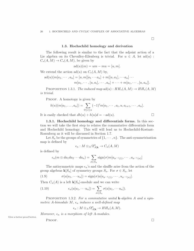
1.3. Hochschild homology and derivation
The following result is similar to the fact that the adjoint action of aLie algebra on its Chevalley-Eilenberg is trivial. For u ∈ A, let ad(u) :C∗(A,M)→ C∗(A,M), be given by
ad(u)(m) = um−mu = [u,m].
We extend the action ad(u) on C∗(A,M) by,
ad(u)(m[a1, · · · , an] = [u,m][a1 · · · an] +m[[u, a1], · · · an] · · ·
m[a1, · · · , [u, ai], · · · , an] + · · ·+m[a1, · · · , [u, an]].
Proposition 1.3.1. The induced map ad(u) : HH∗(A,M)→ HH∗(A,M)is trivial.
Proof. A homotopy is given by
h(u)(m[a1, . . . , an]) =∑
0≤i≤n
(−1)im[a1, · · · , ai, u, ai+1, · · · , an].
It is easily checked that dh(u) + h(u)d = −ad(u).
1.3.1. Hochschild homology and differentials forms. In this sec-tion we will take the first step to relates the commutative differentials formand Hochschild homology. This will will lead us to Hochschild-Kostant-Rosenberg as it will be discussed in Section 1.7.
Let Sn be the groups of symmetries of 1, · · · , n. The anti-symmetrisationmap is defined by
ǫn :M ⊗A ΩnA|k → Cn(A,M)
is defined by
ǫn(m⊗ da1da2 · · · dan) =∑
σ∈Sn
sign(σ)m[aσ−1(1), · · · , aσ−1(n)]
The antisymmetric maps ǫn’s and the shuffle arise from the action of thegroup algebras k[Sn] of symmetry groups Sn. For σ ∈ Sn, let
(1.9) σ(a[u1, · · · un]) = sign(σ)a[uσ−1(1), · · · , uσ−1(n)].
Then Cn(A) is a left k[Sn]-module and we can write
(1.10) ǫn(a[u1, · · · un]) =∑
σ∈Sn
σ(a[u1, · · · un]).
Proposition 1.3.2. For a commutative unital k-algebra A and a sym-metric A-bimodule M , ǫn induces a well-defined map
ǫn :M ⊗A ΩnA|k → HHn(A,M).
Moreover, ǫn is a morphism of left A-modules.Give a better proof better.
Proof.

1.4. HOCHSCHILD COMPLEX OF NONUNITAL ASSOCIATIVE ALGERBAS 27
We attempt to find an left inverse for ǫn. We define πn : Cn(A,M) →M ⊗A ΩnA|k by
πn(a0[a1, · · · , an]) = a0da1 · · · dan
Proposition 1.3.3. For any commutative k-algebra A and M any sym-metric bimodule A, πn induces a natural map
πn : HHn(A,M)→ ΩnA|k.
In the particular case of M = A, we obtain a map
πn : Cn(A)→M ⊗A ΩnA|k
which satisfies πn ǫn = n!idAΩnA|k
Proof. We prove that πndHoch = 0, therefore πn descends to HHn(A).Applying the definition of πn yields
πndHoch(m[a1, · · · an+1]) = ma0da1 · · · dan −md(a0a1) + · · ·+
(−1)imda0 · · · d(aiai+1)dai+2 · · · dan + · · ·
+ (−1)nmda0 · · · d(an−1dan).
So each termmaida0 · · · daidaidai+1 · · · dan appears twice with opposite signs,therefore πndHoch(m[a1, · · · an+1]) = 0.
The A-module structure of HH∗(A) is explained in Proposition 1.1.5 andit is clear that πn ia A-linear.
Corollary 1.3.4. If k ⊂ Q then for ant commutative k-algebra A,A⊗ ΩnA|k is a direct factor of HHn(A) as a left A-module.
1.4. Hochschild complex of nonunital associative algerbas
In this section we extend the definition of Hochschild homology to thenon-unital algebras. This will allow to consider the excision property ofHochschild homology and prove the Morita invariance for H-unital algebras.In particular we will be able to add the case r = ∞ to the statement ofTheorem 1.2.3. Note the M∞(A) = colimitrMr(A) is not unital even if A isunital. Most of the result of this section are due to Loday-Quillen [LQ84].
Let A be an arbitrary k-algebra, this mean not necessarily unital. Weset A+ = k⊕A be the unital algebra whose product is defined by
(µ, a)(λ, b) = (λµ, ab+ µb+ λa).
One defines the Hochschild homology of a nonunital algebra A to beHH∗(A) := coker(HH∗(k)→ HH∗(A+)), or in the other words the reducedHochschild homology of A+. For unital k-algebras, the new and old definitionof Hocshchild homology correspond, more precisely.
Proposition 1.4.1. For a unital k-algebra A, there is a natural isomor-phism HH∗(A) ≃ coker(HH∗(k)→ HH∗(A+)).

28 1. HOCHSCHILD AND CYCLIC COMPLEX OF ASSOCIATIVE ALGEBRAS
Proof. We have an algebra isomorphism A+ ≃ k×A given by (λ, a) 7→λ1A + a. Therefore HH∗(A+) ≃ HH∗(k) × HH∗(A) which implies thatHH∗(A) ≃ coker(HH∗(k)→ HH∗(A+)).
Since A+ is unital, we can use the normalized Hochschild complex toidentify the underlying complex of HH∗(A). We have that HH∗(A) =
H∗((A+ ⊗ A+⊗∗
)red) and ((A+ ⊗ A+⊗∗
)red)n = A⊗n+1 ⊕ A⊗n. Next weidentified the correspond differential on A⊗n+1 ⊕ A⊗n. On A⊗
n+1 the differ-
ential is the Hochschild differential. For A⊗n which should be thought of ask⊗An, we have
d(1[a1 · · · an]) = a1[a2, · · · , an]− 1[a1, · · · an] + 1[a1, a2a3, · · · ] + · · ·
+ (−1)(n−1)1[a1, · · · an] + (−1)an[a1, a2, · · · an].
Therefore the differential on ⊕n(A⊗(n+1) ⊕A⊗n) has the matricial form
(dHoch 1− tn0 −dbar
),
where tn−1 is the cyclic operator tn−1(a1[a2, · · · an] = (−1)(n−1)an[a1, · · · an−1].Now it is clear that HH∗(A) is the homology of the total complex of a bi-
complex d CC(2)∗∗ (A): .
...
...
oo
A⊗(n+1)
dHoch
A⊗(n+1)
−dbar
1−too
A⊗n
A⊗n
1−t
oo
...
...
1−too
A⊗2
dHoch
A⊗2
−dbar
1−too
A A1−t
oo
When there is no risk of confusion we will drop the index n in tn. Clearlywe have a short exact sequence of complexes
0 // C∗(A)inc. // CC
(2)∗∗ (A) // Cbar(A)[−1] // 0

1.4. HOCHSCHILD COMPLEX OF NONUNITAL ASSOCIATIVE ALGERBAS 29
Here C∗(A) is just the usual Hochschild complex of A whose definition doesnot require the existence of a unit. Its homology will be denoted HHnaive
∗ (A).The complex Cbar
∗ (A) is obtained from splicing B(A), the resolution of A,and A itself, and then a shift in degree by one. More explicitly Cbar
n (A) =A⊗n, n ≥ 0 and
dbar(a1⊗· · · an) = a1a2⊗· · ·⊗an−a1⊗a2a3⊗· · ·⊗an · · · (−1)(n−1)a1⊗a2⊗· · ·⊗an−1an
If A is unital, this complex is exact i.e. Hbar∗ (A) = 0 in all degrees. Just
like the proof of Proposition 1.1.12, the contracting homotopy is given bys(a1 ⊗ · · · an) = 1⊗ a1 ⊗ · · · an
Remark 1.4.2. If A is not unital, (Cbar∗ (A), dbar) is not necessarily an
exact complex. The last segment of the complex Cbar∗ (A), A⊗A→ A is not
generally onto. It is very easy to find such examples. We leave this as anexercise to the reader.
The short exact sequence (1.4) induces a long exact sequence relatingHH∗(A), HH
naive∗ (A) and Hbar
∗ (A) := H∗(Cbar∗ (A), dbar).
Proposition 1.4.3. For any k-algebra A (non-unitals included), thereis a long exact sequence
· · · // HHnaiven (A)
incl. // HHn(A) // Hbarn−1(A)
// HHnaiven−1 (A) · · ·
In particular, if Hbar∗ (A) = 0 then HHnaive
∗ (A) and HH∗(A) coincide.
For k-algebras A and a k-module V , let Cbar∗ (A,V ) := (Cbar
∗ (A) ⊗V, dbar ⊗ IdV ). Its homology is denoted Hbar
∗ (A,V ).
Definition 1.4.4. A k-algebra is said to be H-unital if Cbar∗ (A,V ) is an
exact complex for k-module V .
Exercise 1.4.5. If A is k-flat then Hbar∗ (A,k) = 0 implies that A is
H-unital.
A is said to have local units if for any finite set of ai ⊂ A there is aelement u ∈ A such that aiu = uai = 1 for all i. An interesting example ofsuch algebras is M∞(A) where A is a unital k-algebra.
Proposition 1.4.6. If A has local units then it is H-unital.
Proof. Let V be a k-algebra and z =∑
i1,···in+1ai1 ⊗ · · · ⊗ ain ⊗ vin+1
a cycle in Cbar∗ (A,V ). We chose u ∈ A such that for all i1, uai1 = ai1u = 1.
Following the proof of Proposition 1.1.12, z = dbar(∑
i1,···in+1u⊗ ai1 ⊗ · · · ⊗
ain) which prove that [z] = 0 ∈ Hbar∗ (A,V ).

30 1. HOCHSCHILD AND CYCLIC COMPLEX OF ASSOCIATIVE ALGEBRAS
1.4.1. Excision and Wodzicki’s theorem. Let I be an ideal in k-unital algebra A which is not required to be unital. We have a natural mapC∗(I)→ Crel(A, I). We shall say that I is excisive for Hochshild homology ifthis natural map induces an isomorphism HH∗(I) ≃ HH
rel(A, I). Similarly,one says that I is HHnaive
∗ -excisive (reps. Hbar∗ -excisive) if HHnaive
∗ (I) ≃HHnaive
∗ (A, I) (resp. Hbar∗ (I) ≃ Hbar
∗ (A, I)) is an isomorphism.For the rest of this section we suppose that the natural map A → A/I
is a split surjection. This implies that the short exact sequence 0 → I →A → A/I → 0 is split therefore for all k-module V , we have an injectionI ⊗ V → A⊗ V .
In this section we prove that I being H-untial is equivalent to I beingexcisive for all three cases mentioned above. This theorem is due M. Wodzicki[Wod89] but the proof is taken from [GG96].
Definition 1.4.7. A right I-module M is said to be H-unitary (withrespect to I) if for all k-module V , the complex (M ⊗ I⊗∗ ⊗ V, dbar ⊗ idV )is exact. Here dbar :M ⊗ I
⊗∗ →M ⊗ I⊗(∗−1) is defined by
dbar(m⊗ a1 ⊗ · · · an) = ma1 ⊗ a2 ⊗ · · · ⊗ an −m⊗ a1a2 ⊗ · · · ⊗ an
+ · · ·+ (−1)n+1m⊗ a1 ⊗ a2 · · · ⊗ an−1an.
Similarly one defines,
dHoch(m⊗ a1 ⊗ · · · an) = ma1 ⊗ a2 ⊗ · · · ⊗ an −m⊗ a1a2 ⊗ · · · ⊗ an
+ · · ·+ (−1)nm⊗ a1 ⊗ a2 · · · ⊗ an−1an
+ (−1)nanm⊗ a1 ⊗ a2 · · · ⊗ an−1.
For instance if I is H-unital then it is H-untiary.
Proposition 1.4.8. Let M be an I-bimodule. If M is H unitary thenthe maps indcued by inclusion
i : (M ⊗ I⊗∗ ⊗ V, dHoch ⊗ idV )→M ⊗A⊗∗ ⊗ V, dHoch ⊗ idV )
and
i : (M ⊗ I⊗∗ ⊗ V, dbar ⊗ idV )→M ⊗A⊗∗ ⊗ V, dbar ⊗ idV )
are quasi-isomorphisms.
Proof. Consider the filtration Fp,
Fp :M M ⊗AdHochoo · · · M ⊗A⊗pdHochoo M ⊗ I ⊗A⊗pdHochoo M ⊗ I ⊗ I ⊗A⊗pdHochoo
We have F0 ⊂ F1 · · · , F0⊗ V =M ⊗ I⊗∗⊗ V and F∞ ⊗ V =M ⊗A⊗∗⊗ V .To prove the statement it suffice to prove that for all p, Fp⊗ V → Fp+1⊗Vis a quasi-isomorphism. This is done by proving that the quotient Fp+1 ⊗V/Fp ⊗ V is exact. In fact one can verify that,
(Fp+1 ⊗ V
Fp ⊗ V, dHoch⊗idV ) ≃ (M⊗I∗−p−1⊗A/I⊗A⊗p⊗V, dbar⊗idA/I⊗idA⊗p⊗ idV )

1.4. HOCHSCHILD COMPLEX OF NONUNITAL ASSOCIATIVE ALGERBAS 31
as complexes. This is because many terms in the differential induced bydHoch on Fp+1⊗V/Fp⊗V vanishes. Some of them involve the multiplicationof elements of A/I and I which are zero since I is an ideal. There are alsosome terms coming from the part A⊗p, they vanish in the quotient by Fp⊗V .Since M is H-unitary the complex (M ⊗ I∗−p−1 ⊗ A/I ⊗ A⊗p ⊗ V, dbar ⊗idA/I⊗idA⊗p⊗idV ) is exact, for A/I⊗A⊗p⊗V instead of V in the definition.This finishes the proof of the first part. The proof of the second statementfor dbar is similar.
Proposition 1.4.9. If I is H-unital then the natural maps
π : (A/I ⊗A⊗∗ ⊗ V, dHoch ⊗ idV )→ A/I ⊗ (A/I)⊗∗ ⊗ V, dHoch ⊗ idV )
and
π : (A/I ⊗A⊗∗ ⊗ V, dbar ⊗ idV )→ A/I ⊗ (A/I)⊗∗ ⊗ V, dbar ⊗ idV )
induced by the natural projection, are quasi-isomorphisms.
Proof. The proof is similary to that of the previous proposition. Wetake the quotient filtration
Fp : A/I A/I ⊗A/IdHochoo · · · (A/I) ⊗ (A/I)⊗p
dHochoo A/I ⊗ (A/I)⊗p ⊗AdHochoo
A/I ⊗ (A/I)⊗p ⊗AdHochoo A/I ⊗ (A/I)⊗p ⊗A⊗2 · · ·
dHochoo
,
for which we have, F0 ⊗ V = (A/I) ⊗ A⊗∗ ⊗ V and F∞ ⊗ V = A/I ⊗(A/I)⊗∗⊗V . We prove the statement by proving that the natural projectionπp : (Fp ⊗ V, dHoch) → (Fp+1 ⊗ V, dHoch) is a quasi-isomorphism. In fact(ker(πp) ≃ (A/I)⊗ (A/I)p ⊗ I ⊗ I⊗∗−p−1⊗ V equipped with the differentialinduced by dHoch. In fact, one can easily see that
(ker(πp), dHoch) ≃ ((A/I)p ⊗ I ⊗ I⊗∗−p−1 ⊗ V, dbar ⊗ idV )
= ((A/I)p ⊗ I ⊗ I⊗∗−p−1 ⊗ V, id(A/I)p ⊗ dbar ⊗ idV ).
The latter is exact because I is H-unital.
Theorem 1.4.10. (M. Wodzicki)Let I be an ideal of a k-algebra. Thenthe following conditions are equivalent:
(1) I is H-unitary.(2) I is HHnaive
∗ -excisive.(3) I is Hbar
∗ -excisive.(4) I is HH∗-excisive.
Proof.

32 1. HOCHSCHILD AND CYCLIC COMPLEX OF ASSOCIATIVE ALGEBRAS
(1)⇒ (2): We have a commutative diagram
0
0
(I ⊗A⊗∗ ⊗ V, dHoch ⊗ idV ) //
Cnaive,rel∗ (A, I) ⊗ V, dHoch ⊗ idV )
(A⊗A⊗∗ ⊗ V, dHoch ⊗ idV )
id //
(A⊗A⊗∗ ⊗ V, dHoch ⊗ idV )
(A/I ⊗A⊗∗ ⊗ V, dHoch ⊗ idV )
π1 //
(A/I ⊗ (A/I)⊗n ⊗ V, dHoch ⊗ idV )
0 0
where the vertical sequence are exact. By Proposition 1.4.9, π1 is a quasi-isomorphism therefore
(I ⊗A⊗∗ ⊗ V, dHoch ⊗ idV )→ Cnaive,rel∗ (A, I) ⊗ V, dHoch ⊗ idV )
is a quasi-isomorphism. On the other hand, by Proposition 1.4.8,
(I ⊗ I⊗∗ ⊗ V, dHoch ⊗ idV )→ (I ⊗A⊗∗ ⊗ V, dHoch ⊗ idV )
is a quasi-isomorphism. Therefore
(I ⊗ I⊗∗ ⊗ V, dHoch ⊗ idV )→ (Cnaive,rel∗ (A, I) ⊗ V, dHoch ⊗ idV )
is a quasi-isomorphism, and HHnaive∗ (I) ≃ HHnaive,rel
∗ (A, I) are isomorphicvia the natural map.
(1) ⇒ (3) is similar to (1) ⇒ (2). It relies on the second statements inProposition 1.4.9 and Proposition 1.4.8.
(1)&(2)⇒ (3): It follows from the long exact sequence in Proposition 1.4.3.
(2) ⇒ (1): Let V be a k-module. We take A = I ⊕ V equipped withthe multiplication (u, v)(u′, v′) = (uu′, 0). Consier the natural projectionπ : (A ⊗ A⊗∗, dHoch) → ((A/I) ⊗ (A/I)⊗∗, dHoch). One can see easily that(I ⊗ I∗−1 ⊗ V, dbar ⊗ idV )⊕ (I ⊗ I⊗∗, dHoch) is a direct factor of ker(π). Byhypothesis H∗(ker(π)) ≃ H∗((I ⊗ I
⊗∗, dHoch)) therefore H∗(I∗−1 ⊗ V, dbar ⊗
idV ) = 0. This proves that I is H-unital.
(3)⇒ (1) is similar to (2)⇒ (1).
(4) ⇒ (1): For a k-module V , let A = I ⊕ V equipped with the product
(u, v)(u′, v′) = (uv, 0). For the map π : CC(2)∗∗ (A)→ CC
(2)∗∗ (A/I) induced by
the natural quotient map, we have that ker(π) = C(2)(I)⊕L for some factor
L. Since H∗(ker π) ≃ H∗(C(2)(I)) = HH∗(I) we conclude that H∗(L) = 0.

1.5. CYCLIC BICOMPLEXES 33
Note that (Cbar∗ (I, V )dbar⊗idV ) is a direct factor of L which is included in the
first column of CC(2)∗∗ (I) and the Hochschild differential on this subcomplex
is identical to the bar differential. Therefore Hbar∗ (I, V ) = 0.
1.5. Cyclic bicomplexes
In this section we introduce the cyclic bicomplex CC∗∗(A) of an arbitraryassociative A over a commutative ring k. The homology of the total complexof this bicomplex is the cyclic homology of A. The total complex of the cyclicbicomplex is quasi-isomorphic to some smaller complexes if Q ⊂ k or if A isunital. We have the quasi-isomorphisms
Tot(BC∗∗(A)) Tot(BC∗∗(A))oo Tot(CC∗∗(A)))if Q⊂k //if A unitaloo Cλ∗ (A)
1.5.1. Cyclic bicomplex CC∗∗(A): This complex is obtained by com-pleting the (two columns) bicomplex which defines the Hochschild homologyof a nonunital algebra. More precisely it is:
...
...
oo...
oo...
oo...
oo · · ·
A⊗(n+1)
dHoch
A⊗(n+1)
−dbar
1−too A⊗(n+1)
dHoch
Noo A⊗(n+1)
−dbar
1−too A⊗(n+1)
dHoch
Noo · · ·
A⊗n
A⊗n
1−t
oo A⊗n
N
oo A⊗n
1−t
oo A⊗n
N
oo · · ·
...
...
1−too
...
Noo
...
1−too
...
Noo · · ·
A⊗2
dHoch
A⊗2
−dbar
1−too A⊗2
dHoch
Noo A⊗2
−dbar
1−too A⊗2
dHoch
Noo · · ·
A A1−t
oo AN
oo A1−t
oo AN
oo · · ·
where Nn : A⊗(n+1) → A⊗(n+1) is N := 1 + tn + · · · + tnn. It is obvious that(1−t)N = 0. Note that we have already prove that dHoch(1−t) = (1−t)dbar
because the first two columns form the bicomplex whose total complex is theHochschild complex of a nonunital algebra. So it remains to prove that
Lemma 1.5.1. For an associative algebra A,
dHochNn = Nn−1dbar.

34 1. HOCHSCHILD AND CYCLIC COMPLEX OF ASSOCIATIVE ALGEBRAS
Proof. The proof is broken down in a few elementary steps. One caneasily check that d0tn = (−1)ndn and ditn = −tn−1di−1, for all n and 0 <i ≤ n. Let us check the first identity:
d0tn(a0[a1, · · · , an]) = (−1)nd0(an[a0, · · · an−1]) = (−1)nana0[a1, · · · an−1]
= (−1)ndn(a0[a1, · · · , an]).
As for the second identity,
ditn(a0[a1, · · · , an]) = (−1)nan[a0 · · · , ai−1ai, · · · an−1],
−tn−1di−1(a0[a1, · · · , an]) = −tn−1(a0[a1, · · · , ai−1ai, · · · an])
= (−1)nan[a0 · · · , ai−1ai, · · · an−1].
By using recursively these identities we obtain
ditj = (−1)jtjdi−j, if i ≥ j,
ditj = (−1)itid0tj−i, if 0 < i < j
andd0t
j = (−1)ndntj−1 = (−1)n+j−1tj−1dn−j+1.
Using all three identities, we have
dN = (n−1∑
i=0
(−1)idi)(n∑
j=0
tj) =∑
i,j
(−1)iditj =
∑
0≤j≤i≤n
(−1)iditj +
∑
0≤i<j≤n
(−1)iditj
=∑
0≤j≤i≤n−1
(−1)i(−1)jtjdi−j
+∑
0≤i<j≤n
(−1)n+1+i−jtj−1dn+1+i−j
A simple computation shows that the coefficient of (−1)kdk is∑
j≤n−k−1 tj+∑
n−k≤j−1≤n−1 tj−1 = N .
The cyclic homology of A is defined to beHCn(A) := Hn(Tot(CC∗∗(A)),
n ≥ 0. Note that Tot(CC∗∗(A))n = A⊕A⊗2 ⊕ · · ·A⊗(n+1)
Exercise 1.5.2. Show that HC0(A) = HH0(A).
1.5.2. Connes cyclic complex Cλ∗ . In the earlier years of (differential)noncommutative geometry Alain Connes [Con85] introduced another cycliccomplex and cyclic homology. This is done by considering the cyclicallyinvariant element of the Hochchild complex i.e.
Cλ∗ (A) =C∗(A)
Im(1− t)
Since dHoch(1 − t) = (1 − t)dbar ⊂ Im(1 − t), the Hochschild differen-tial induces a well-defined differential on Cλ(A). We define Hλ(A) :=H∗((C
λ(A), dHoch)).

1.5. CYCLIC BICOMPLEXES 35
There is natural complex map p : Tot(CC∗∗(A))n → Cλ∗ (A) given by thecomposition of projections
p : A⊕A⊗2 ⊕ · · ·A⊗(n+1) → A⊗(n+1) → A⊗(n+1)/ Im(1− t).
If that the lines of the bicomplex CC(A)∗ are acyclic then one of thenatural the spectral sequences of the complex TotCC(A)∗ collapses at E2
p,q
which is exactly Hλ∗ (A). This is the spectral sequence of the flitration on
Tot(CC∗∗(A))∗ induced by the truncating the bicomplex vertically. There-fore if the lines are acyclic the n HC∗(A) is isomorphic to Hλ
∗ (A).
Theorem 1.5.3. If Q ⊂ k then the natural map p∗ : HC∗(A)→ Hλ(A)is an isomorphism.
Proof. We prove that Q ⊂ k implies that the lines in CC∗∗(A) areacyclic. The homotopies are given by
A⊗(n+1)
h11 A
⊗(n+1)
h′11
1−tqqA⊗(n+1)
h11
NqqA⊗(n+1)
h′00
1−tqqA⊗(n+1) · · ·
Nqq
h := −1n+1
∑nk=1 kt
k,
h′ := 1n+1 id,
We prove that h′N + (1− t)h = id and Nh′ + h(1 − t) = id.
h′N + (1− t)h =1
n+ 1(1 + t · · ·+ tn)−
(1− t)
n+ 1(n∑
k=1
ktk)
=(1 + t · · ·+ tn)
n+ 1−
(t+ t2 · · ·+ tn − n · id)
n+ 1= id.
Nh′ + h(1 − t) =1 + t+ · · · tn
n+ 1−
1
n+ 1(n∑
k=1
ktk)(1− t)
=1 + t+ · · · tn
n+ 1−
(t+ t2 · · ·+ tn − n · id)
n+ 1add the spectral sequenceH∗(Z/(n + 1)Z,A) ⇒
HC∗(A)
1.5.3. (d,B)- cyclic bicomplexes BC(A) and BC∗(A). In this sec-tion we discuss the bicomplex CC∗∗(A) of a unital k-algebra A. In this casethe columns corresponding to the bar complex are exact and the followinglemma tell how to eliminate them from the bicomplex CC∗∗(A) and obtaina simpler bicomplex computing HC∗(A).
Lemma 1.5.4. Let (A∗ ⊕ A′∗, d) be a complex whose differential has the
matricial form d =
(α βγ δ
). Suppose that (A′
∗, δ) is an exact complex

36 1. HOCHSCHILD AND CYCLIC COMPLEX OF ASSOCIATIVE ALGEBRAS
with a contracting homotopy h : A′∗ → A′
∗+1, i.e
hδ + δh = [h, δ] = id.
Then (A∗, α−βhγ) is complex and the map ψ = (id,−hγ) : (A∗, α−βhγ)→(A∗ ⊕A
′∗, d) is a quasi-isomorphism.
Proof. Let first check that (α − βhγ)2 = 0. From d2 = 0 and δ2 = 0we get
α2 + βγ = 0 αβ + βδ = 0γα+ δγ = 0 γβ = 0
(α− βhγ)2 = α2 − αβhγ − βhγα+ βhγβhγ
= α2 + βδhγ + βhδγ = α2 + βγ = 0
Next we prove that the inclusion is a chain map. On one hand
(α βγ δ
)(id−hγ
)=
(α− βhγγ − δhγ
)
and on the other hand
(id−hγ
)(α− βγ
)=
(α− βγh
−hγα+ hγβhγ
)
−hγα+ hγβhγ = −hγα = hδγ = (id− δh)γ = γ − δhγ
which proves that i is a chain map. Since i is an inclusion, to prove that i is aquasi-isomorphism it is enought to prove that coker(ψ) is acyclic. In fact weprove that coker(ψ) is isomorphic to (A′, δ) as a complex. The isomorphismis given by φ : (x, y) 7→ y + hγ(x). Let us check that it is a chain map:
δφ(x, y) = δ(y + hγ(x)) = δ(y) + δhγ(x)
φ(d(x, y)) = φ(α(x) + β(y), γ(x) + δ(y))
= γ(x) + δ(y) + hγ(α(x) + β(y))
= γ(x) + δ(y) + hγα(x) = δ(y) + γ(x)− hδγ(x) = δ(y) + δhγ(x)
Its inverse if given by φ′(y) = (0, y) ∈ coker(ψ), for which φφ′ = id isobvious. As for φ′(φ(x, y)) = (0, y+hγ(x)) = (x, y)− (x,−hγ(x)), thereforeφ′(φ(x, y)) = (x, y) ∈ coker(ψ).
Now we apply the previous lemma to the cyclic bicomplex CC∗∗(A) of aunital algebra A. We can write
Tot(CC∗∗(A))n =⊕
q pair
CCp,q(A)⊕ ⊕
q odd
CCp,q(A)

1.5. CYCLIC BICOMPLEXES 37
and let
A =⊕
q pairCCp,q(A) A′ =⊕
q odd CCp,q(A)
α = dHoch, β = 1− t γ = N δ = −dbar,
and −s for contracting homotopy, where s is the contracting homotopy ofthe Bar complex as it was given in Proposition 1.1.12 (or Section 1.4). Sincethe odd columns correspond to the bar complex of A which is contractible,by the previous lemma Tot(CC∗∗(A)) is quasi isomorphic to BC(A) =(CC(A)∗,2q, dHoch + (1 − t)sN). This means that we can erase the the oddcolumns and replace the the total differential by dHoch− (1− t)sN . We shallcompute (1− t)sN :
B(a0[a1, · · · , an]) := (1− t)sN(a0[a1, · · · , an]) = (1− t)s(a0[a1, a2, · · · , an]
+ (−1)nan[a0, · · · , an−1] · · · + (−1)n2a1[a2, · · · , an, a0])
= (1− t)(∑
(−1)n(n−i+1)1[ai, · · · , an, a0, a1, · · · ai−1])
=∑
(−1)n(n−i+1)1[ai, · · · , an, a1, · · · ai−1]
−∑
(−1)n(n−i+1)+n+1ai−1[1, ai, · · · , an, , a0, a1, · · · ai−1]
=
n∑
i=0
(−1)ni1[ai, · · · , an, a0, a1, · · · ai−1]
+
n∑
i=0
(−1)n(n−i)ai−1[1, ai, · · · , an, a0, a1, · · · ai−1].

38 1. HOCHSCHILD AND CYCLIC COMPLEX OF ASSOCIATIVE ALGEBRAS
This is the non-normalized Connes operator which can be simplified as weshall see later.(1.11)
...
...
oo...
oo...
oo...
oo · · ·
A⊗(n+1)
dHoch
A⊗(n+1)
−dbar
1−too
s
II
A⊗(n+1)
dHoch
Noo
B
jjUUUUUUUUUUUUUUUUUUUUUUUUA⊗(n+1)
−dbar
1−too
s
II
A⊗(n+1)
dHoch
Noo
B
jjUUUUUUUUUUUUUUUUUUUUUUUU· · ·
A⊗n
A⊗n
1−too
s
HH
A⊗n
N
ooB
jjVVVVVVVVVVVVVVVVVVVVVVA⊗n
1−too
s
HH
A⊗n
N
ooB
jjVVVVVVVVVVVVVVVVVVVVVV· · ·
...
...
1−too ...
Noo
B
jjUUUUUUUUUUUUUUUUUUUUUUUUU ...
1−too ...
Noo
B
jjUUUUUUUUUUUUUUUUUUUUUUUUU· · ·
A⊗2
dHoch
A⊗2
−dbar
1−too
s
II
A⊗2
dHoch
Noo
B
jjUUUUUUUUUUUUUUUUUUUUUUUUUA⊗2
s
II
−dbar
1−too A⊗2
dHoch
Noo
B
jjUUUUUUUUUUUUUUUUUUUUUUUUU· · ·
A A1−too
s
HH
AN
ooB
jjVVVVVVVVVVVVVVVVVVVVVVVVVA
s
HH
1−too A
Noo
B
jjVVVVVVVVVVVVVVVVVVVVVVVVV· · ·
Therefore the cyclic homology HC∗(A) is the homology of the total complexthat can be organized in a half-first quadrant bicomplex
BC(A)∗ :=...
......
A⊗(n+1)
dHoch
A⊗n
dHoch
Boo A⊗(n−1)
dHoch
Boo A⊗(n−2)
dHoch
Boo A⊗(n−3) · · ·
Boo
A⊗n
dHoch
A⊗(n−1)
dHoch
Boo A⊗(n−2)
dHoch
Boo A⊗(n−3) · · ·
Boo
......
...
A⊗3
dHoch
A⊗2
dHoch
dHoch
Boo A
Boo
A⊗2
dHoch
AB
oo
A

1.5. CYCLIC BICOMPLEXES 39
The general term of this bicomplex for is given by
BC(A)p,q = A⊗A⊗(q−p),
if q ≥ p, otherwise it is zero. Therefore Tot(BC(A))n = ⊕2q≤nA⊗An−2q.As
we explained in Section 1.1.1, we can replace the Hochschild complex ofan algebra with a the normalized complex C∗(A) =
⊕nA ⊗ A⊗n. This
means that natural map C∗(A) → C∗(A) is quasi-isomorphism, thereforethe complex BC(A)∗ is isomorphic to
BC(A)∗ =:
......
...
A⊗A⊗n
dHoch
A⊗A⊗(n−1
dHoch
Boo A⊗A
⊗(n−2)
dHoch
Boo A⊗A
⊗(n−3)· · ·
dHoch
Boo
A⊗A⊗(n−1)
dHoch
A⊗A⊗(n−2)
dHoch
Boo A⊗A
⊗(n−3)
dHoch
Boo A⊗A
⊗(n−4)· · ·
Boo
......
...
A⊗A⊗2
dHoch
A⊗A
dHoch
dHoch
Boo A
Boo
A⊗A
dHoch
AB
oo
A
Here B is induced by B in (1.11) on C(A), it therefore reads
B(a0[a1, · · · , an]) =n∑
i=0
(−1)ni1[ai, · · · , an, a0, a1, · · · ai−1].
an it verifies B2 = 0. Since B is a chain map, it induces map B∗ : HH∗(A)→HH∗+1(A) of degree one which satifies B2 = 0.This is generally known asthe Connes operator. We precise that
BC(A)p,q = A⊗A⊗(q−p)
,
and Tot(BC(A))n = ⊕2q≤nA⊗An−2q
.
1.5.4. Connes’ exact sequence. We have a short exact sequence ofbicomplexes

40 1. HOCHSCHILD AND CYCLIC COMPLEX OF ASSOCIATIVE ALGEBRAS
(1.12) 0→ CC(2)∗∗ (A)
I→ CC∗∗(A))
S→ CC∗∗(A)[2, 0] → 0,
where CC∗∗(A)[2, 0] is CC∗∗(A) after a horizontal shift in degrees by 2. Thefirst map I is the obvious inclusion, S is just the natural projection whichsends the first two columns to zero. More precisely
(CC(A)[2, 0])pq = CCp−2,q(A),
therefore Hn(CC∗∗(A)[2, 0]) = HCn−2(A). The long exact sequence of theshort exact sequence (1.12) reads
(1.13)
· · ·HHn(A)I // HCn(A)
S // HCn−2(A)C // HHn−1(A) // HCn−1(A) · · ·
Here C : HCn−2(A) → HHn−1(A) is the connecting homomorphism, Icorrespond to the inclusion maps of Hochschild complex in cyclic complex.In the litterature S is called the periodicity map since it is related to therelated periodicity map in K-theory. It is an interesting exercise is tocompute the connecting map C in (1.13).
Exercise 1.5.5. Prove that the connecting map I : HC∗(A)→ HH∗+1(A)is induced by the chain map τ : Tot(CC∗+2(A)[2, 0]) → Tot(C∗+1(A))
τ(x0, · · · xn) = ((1− t)x0, 0)
where xi ∈ CCi(n−i)(A).
In the case of unital algebras there is an alternative way to compute theconnecting map. To this end we use the bicomplex BC∗(A) rather thanCC∗∗(A). The short exact sequence (1.12) corresponds to the short exactsequence
(1.14) 0 // C∗(A) // BC∗∗(A) // BC∗∗(A)[1, 1] // 0
where BCpq(A)[1, 1] = BCp−1,q−1(A). Here we think of C∗(A) as a bicom-plex consisting of only one column placed. Note that
Tot(BC(A)[1, 1])n = ⊕p+q=nBCp−1,q−1(A) = TotBC(A)n−2,
therefore Hn(BC∗∗(A)[1, 1]) = HCn−2(A). Therefore the long exact se-quence to associated (1.14) reads,
(1.15)
· · ·HHn(A)I // HCn(A)
S // HCn−2(A)C // HHn−1(A)
I // HCn−1(A) · · ·
In fact we can show that the connecting map C is defined at the chainlevel which is not generally true for connecting homorphisms. That’s we firstcompute at the homology level and then we notice that it is coming frommorphism of complexes.

1.5. CYCLIC BICOMPLEXES 41
Let x = (x0, x2, · · · , xn−2) be a cycle in Tot(CC∗∗(A)n−2 representing ahomology class, i.e.
0 = dTotx = (dHochx0 +Bx1, dHochx1 +Bx2, · · · , dHochxn−3 +Bxn−2).
Here xi is in the i-column of the bicomplex BC∗∗(A). Then y = (0, x0, · · · xn−2)is in the preimage of x. Then we should take
dToty = (Bx0, dHochx0+Bx1, · · · , dHochxn−3+Bxn−2) = (Bx0, 0, 0 · · · ) = I(Bx0).
We observe that Bpr0 : Tot(BC∗∗(A))→ C∗(A) given by the composite
(1.16) Tot(BC∗∗(A))pr0 // C∗(A)
B // C∗(A)
is chain map. Here pr0 is the projection (x0, x2, · · · , xn) 7→ x0. Therefore,
C([x]) = [Bpr0(x)] ∈ HH∗(A)
It follows from the identites B2 = [dHoch, B] = 0 that Bpr0 : Tot(BC∗∗(A))→C∗(A) is in fact a chain map and C = (Bpr0)∗ is the induced map in homol-ogy. As a result of this calculations we have,
Corollary 1.5.6. The chain map B : C∗(A) → C∗(A) factor throughthe cyclic complex i.e.
(1.17) C∗(A)
I ''NNNN
NNNN
NN
B // C∗(A)
Tot(BC∗∗(A))
Bpr0
88pppppppppp,
and similarly at the homology level B = CI where I : HH∗(A) → HC∗(A)is induced by inclusion the Hochschild complex of A as the first column inthe cyclic bicomplex of A.
1.5.5. De Rham differential and Connes’ operator. In this sec-tion A is a commutative k-algebra and Ω∗
A|k denotes the Kähler differentials
equipped with De Rham differential
dDR(a0da1 · · · dan) := da0da1 · · · dan.
In Section 1.3.1 we constructed the anti-symmetrisation map ǫn : ΩnA|k →
HHn(A). One naturally asks what is the image of dDR under ǫ.
Proposition 1.5.7. For a commutative k-algebra the following diagramcommutes:
(1.18) ΩnA|kdDR //
ǫn
Ωn+1A|k
ǫn+1
HHn(A)
B// HHn+1(A)

42 1. HOCHSCHILD AND CYCLIC COMPLEX OF ASSOCIATIVE ALGEBRAS
Proof.
B(ǫn(a0da1 · · · an) =n∑
i=0
∑
σ∈Sn
(−1)ni sign(σ)1[aσ−1(i), · · · aσ−1(n), a0, · · · aσ−1(i−1)]
and on the other hand
ǫn+1(dDR(a0da1 · · · an) =∑
τ∈Sn+1
1[aτ−1(0), · · · , aτ−1(n)].
There is bijection between Sn × Z/(n + 1)Z ↔ Sn+1, where Z/(n + 1)Zcorrespond to the cyclic subgroup o (n + 1) and Sn is the stablizer of anelement (here 0). This bijection is given by composing in Sn+1, (σ, z
i) 7→τ = ziσ where z is the obvious generator of Z/(n+1)Z. Now Bǫn = ǫn+1(dDRbecuase of this bijection and sign(τ) = sign(zi) sign(σ) = (−1)ni sign(σ).
Recall that in Section 1.3.1 we also introduced πn : HHn(A) → ΩnA|kwhich verifies
πnǫn = nId.
Proposition 1.5.8. For a commutative k-algebra A the diagram
HHn(A)B //
πn
HHn+1(A)
πn+1
ΩnA|k (n+1)dDR
// Ωn+1A|k
commutes.
Proof. Since πn dHoch = 0, it suffices to prove that the diagram
Cn(A)B //
πn
Cn+1(A)
πn+1
ΩnA|k (n+1)dDR
// Ωn+1A|k
commutes. We have,
πn+1B(a0[a1, · · · , an]) = πn+1(∑
(−1)ni1[ai, · · · an, a0, · · · ai]
=
n∑
i=0
(−1)nidai · · · danda0, · · · dai]
= (n+ 1)da0da1 · · · dan = (n+ 1)da0 · · · dan
= (n+ 1)dDR(a0da1 · · · dan) = (n+ 1)dDR(πn(a0[a1 · · · an])).

1.5. CYCLIC BICOMPLEXES 43
Corollary 1.5.9. If Q ⊂ k, the diagram,
HHn(A)B //
πnn!
HHn+1(A)
πn+1(n+1)!
ΩnA|k dDR
// Ωn+1A|k
Corollary 1.5.10. There is a natural map ǫcn : ΩnA|k/dΩn−1A|k → HCn(A)
which is induced by ǫn : ΩnA|k → Cn(A). If Q ⊂ k, this map is split-injective
and make the diagram below commutative.
· · · // Ωn−1A|k /dΩ
n−2A|k
dDR //
ǫcn−1
ΩnA|k//proj //
ǫn
ΩnA|k/dΩn−1A|k
0 //
ǫcn
Ωn−2A|k /dΩ
n−3A|k
//
ǫcn−1
· · ·
· · · // HCn−1(A)C // HHn(A)
I // HCn(A)S // HCn−2(A) // · · ·
The lowest sequence is Connes’ exact sequence.
Proof. We recall that the image anti-symmetrisation map ǫn : ΩnA|k →
Cn(A) is included in the cycles and therefore it induces a map ǫn : ΩnA|k →
HHn(A). We define ǫcn to be the composite
(1.19) ǫcn : ΩnA|kǫn→ HHn(A)
I→ HCn(A)
by ǫcn. Here I is the map induced by inclusion. All we have to do is toprove that ǫcn(dDR) = 0 , this is rather obvious because of the commutativediagram below.
Ωn−1A|k
dDR //
ǫcn−1
ǫn−1
ΩnA|kdDR //
ǫn
ǫcn
Ωn+1A|k
ǫn+1
HHn−1(A)
I &&NNNN
NNNN
NNN
B // HHn(A)B //
I &&NNNN
NNNN
NNN
HHn+1(A)
HCn(A)
C
88rrrrrrrrrrHCn+1(A)
C
77ooooooooooo
We have ǫcn(dDR) = IǫndDR = ICIǫn = 0 because of IC = 0, the ex-actness of Connes’ sequence. Therefore ǫcn descends to the quotient andinduces ΩnA|k/dΩ
n−1A|k→ HCn(A). The commutativity of the diagram in the
statement is clear from the diagram above and it is essentially due to thefactorisation B = CI.
If k ⊂ Q then a left inverse for ǫcn is induced by the composite
φn : Tot(CC∗ ∗ (A))npr0 // Cn(A)
πnn // ΩnA|k/dΩ
n−1A|k .

44 1. HOCHSCHILD AND CYCLIC COMPLEX OF ASSOCIATIVE ALGEBRAS
The reader should notice that pr0 is not a chain map but the composite passesto the homology HCn(A), more precisely we can show that φn dTot = 0 ∈ΩnA|k/dΩ
n−1A|k ,
φn dTot(x0, x1, · · · xn, xn+1) =πnnpr0(dHochx0 +Bx1, · · · , Bxn+1)
=πnn(dHochx0 +Bx1)
=1
n(πn(dHochx0) + πn(Bx1))
= dDRπn−1x1 = 0 ∈ ΩnA|k/dΩn−1A|k .
Above we used the fact πn dHoch = 0 which was proved in Section 1.3.1.Finally, we have
(πnn pr0) (I ǫn) =
πnn ǫn = id
which implies that φ is the left inverse of ǫcn or in other words ǫcn is split-injective.
We finish this section by introducing a double complex which prove usefulin computing the cyclic homology using the Hochschild-Kostant-Rosenberg.This bicomplex is called the truncated De Rham bicomplex D∗∗(A):
(1.20)
D∗∗(A) :=...
......
ΩnA|k
0
Ωn−1A|k
0
dDRoo Ωn−2A|k
0
dDRoo Ωn−3A|k · · ·
dDRoo
......
...
Ω2A|k
0
Ω1A|k
00
dDRoo Ω0A|k
dDRoo
Ω1A|k
0
Ω0A|k
dDRoo
Ω0A|k

1.6. EXTERNAL PRODUCT ON Tor AND Ext 45
It is quite clear that
Hn(Tot(D∗∗(A)) =ΩnA|k
dΩn−1A|k
⊕Hn−2DR (A)⊕Hn−4
DR (A) · · ·
where the last term in the sum above is either H0DR(A) orH1
DR(A) dependingon whether n is even or odd.
Note that ǫnn≥0 induces a map of bicomplexes ǫ : D∗∗(A)→ BC∗∗(A).
Similarly, If Q ⊂ k then ǫnn! n≥0 induced map of bicomplexes π : BC∗∗(A)→D∗∗(A) which is a left inverse of ǫ, i.e. π ǫ = idD(A), therefore:
Proposition 1.5.11. Let A be a commutative k-algebra. If Q ⊂ k andA then HCn(A) has
ΩnA|k
dΩn−1A|k
⊕Hn−2DR (A)⊕Hn−4
DR (A) · · ·
as a direct factor. The last term in the sum above is either H0DR(A) or
H1DR(A) depending on whether n is even or odd.
As we shall see in Section 1.7 in factHC∗(A) is isomorphic toH∗(Tot(D∗∗(A))when A is smooth.
1.6. External product on Tor and Ext
This section is dedicated to the algebra structures on Ext and Tor. Inparticular we aim at finding a chain level representation of such products inthe case of Hochschild homology.
1.6.1. External product on Tor. Let R1 and R2 be two k-algebrawhere k is a commutative ring. Let Mi and Ni be (left and right) Ri-modules, for i = 1, 2. The objective is to define a natural map
TorR1i (M1, N1)⊗ TorR2
i (M2, N2)→ ⊗TorR1⊗R2i (M1 ⊗M2, N1 ⊗N2)
For i = 1, 2, let P i∗ ։Mi be a Ri-projective resolution. Similarly supposethat P∗ ։ M1 ⊗ M2 is a R1 ⊗ R2-projective resolution. By the general
fact about projective resolutions one can lift the identity map M1 ⊗M2id→
M1 ⊗M2 to a chain map i : Tot(P 1∗ ⊗ P
2∗ )∗ → P∗, which is unique up to
homotopy,
Tot(P 1∗ ⊗ P
2∗ )∗
i //
P∗
M1 ⊗M2
// M1 ⊗M2
Consider the composite
Φ : Tot((P 1∗ ⊗R1 N1)⊗ (P 2
∗ ⊗R2 N2)) ≃Tot((P 1∗ ⊗ P
2∗ ))⊗R1⊗R2 (N1 ⊗N2))
i⊗id→ P∗ ⊗R1⊗R2 (N1 ⊗N2).

46 1. HOCHSCHILD AND CYCLIC COMPLEX OF ASSOCIATIVE ALGEBRAS
Then the external product is defined by precomposing the homological mapΦ∗ with the natural map
TorR1∗ (M1, N1)⊗ TorR2
i (M2, N2) = H∗(P1∗ ⊗R1 N1)⊗H∗(P
2∗ ⊗R2 N2))
→ H∗(Tot((P1∗ ⊗R1 N1)⊗ (P 2
∗ ⊗R2 N2)).
Recall that for two complexes C1∗ and C2
∗ there is a natural map H∗(C1∗ ) ⊗
H∗(C2∗ )→ H∗(C
1∗⊗C
2∗ ) which sends a generator [z1]⊗[z2] ∈ H∗(C
1∗ )⊗H∗(C
2∗ )
to [z1 ⊗ z2] ∈ H∗(C1∗ ⊗ C
2∗ ). Therefore the external product is given by the
composite
TorR1i (M1, N1)⊗ TorR2
i (M2, N2)→ Hi+j(Tot((P1∗ ⊗R1 N1)⊗ (P 2
∗ ⊗R2 N2))
Φ∗−→ Hi+j(P∗ ⊗R1⊗R2 (N1 ⊗N2))
= TorR1⊗R2i+j (M1 ⊗M2, N1 ⊗N2)
(1.21)
1.6.1.1. Special case: modules over a commutative k-algebra. If R1 =R2 = R is a commutative k-algebra, then a right R-module is naturally a leftR-module and vice-versa. In particular if M1 =M2 =M and N1 = N2 = Nare R-algebra then we have a composition of natural maps
(1.22) TorR⊗R∗ (M ⊗M,N ⊗N)(1)→ TorR⊗R∗ (M,N)
(2)→ TorR∗ (M,N).
The map (1) arises from the fact that M and N can be naturally endowedwith a R⊗R-module structure using the pullback of R-module structure viathe multiplication R ⊗ R → R. More explicitly (r1 ⊗ r2)m = r1r2m. Thisimplies that M ⊗M →M is map of R⊗R-modules (and algebras).
The map (1) is a consequence of the fact that R ⊗ R-module structureof M is the pullbck of R-module structure via the map R ⊗ R → R. So bypatching (1.21) [for M1 =M2 and N1 = N2] and (1.22), we get a product
(1.23) TorRi (M,N)⊗ TorRi (M,N)→ TorRi+j(M,N).
In the case of R = A ⊗ A⊗p and M = N = A, where A is a commutativek-projective (or flat) module, the external product provides us a pairing
(1.24) HHi(A)⊗Hj(A)→ HHi+j(A).
1.6.1.2. Special case: modules over a commutative ring. Suppose thatk = R1 = R2 = R is a commutative ring. So all the tensor products aretaken over R. Note that since R is commutative a right (resp. module) R-module is a left (resp. right) R-module and M⊗RN has a natural R-modulestructure, therefore Φ in above reads
Φ : Tot((P 1∗ ⊗R N1)⊗R (P 2
∗ ⊗R N2)) ≃Tot((P 1∗ ⊗R P
2∗ ))⊗R⊗RR (N1 ⊗R N2))
i⊗id→ P∗ ⊗R⊗RR (N1 ⊗R N2) ≃ P∗ ⊗R (N1 ⊗R N2).

1.6. EXTERNAL PRODUCT ON Tor AND Ext 47
and the external product reads
TorRi (M1, N1)⊗R TorRi (M2, N2)→ TorR⊗RRi+j (M1 ⊗RM2, N1 ⊗R N2)
≃ TorRi+j(M1 ⊗RM2, N1 ⊗R N2).
(1.25)
In the special case M1 = M2 = M and N1 = N2 = N of R-algebras, wehave also a natural map
TorR∗ (M ⊗RM,N ⊗R N)→ TorR∗ (M,N)
whose composition with the external product gives rise to a natural map
TorRi (M,N) ⊗R TorRi (M,N)→ TorRi+j(M,N).(1.26)
An interesting special case is when R = A⊗Aop and M = N = A whereA is commutative k-algebra. We obtain a product
(1.27) TorA⊗Aop
i (A,A) ⊗R TorA⊗Aop
i (A,A)→ TorA⊗Aop
i+j (A,A),
which gives rise to a product
(1.28) Hi(A,A)⊗A⊗Aop Hi(A,A)→ Hi+j(A,A),
if A is k-projective (or flat) module. The A⊗Aop-module structure ofH∗(A,A) is given by pulling back the (left) A-module structure using themultiplication map A⊗Aop → A(see Proposition 1.1.4 for the A-modulestructure) ).
Another special case of the above external product is when M = N =R/I where I is an ideal of R. Then the external product reads
TorRi (R/I,R/I) ⊗R TorRi (R/I,R/I)→ TorRi+j(R/I,R/I).(1.29)
This product will prove to be important in the proof of Hochschild-Kostant-Rosenberg in Section 1.7. In the next section, using the Koszul resolutionwe will find a chain level lift for this special case of external product.
We can recover the product (1.28) from (1.29) as follows. Let R =A⊗k A
op = A⊗k A and let I = kerµ
µ : A⊗k A→ A,
where µ is the surjective map given by the multiplication of A. So we haveR/I = A and the external product reads
(1.30) TorA⊗Ai (A,A) ⊗A⊗A TorA⊗Ai (A,A)→ TorA⊗Ai+j (A,A).
IfA is k-projective (or flat) then by Corollary 1.1.13 TorA⊗A∗ (A,A) ≃ HH∗(A,A),then external product provides us a (A⊗ A)-linear product on HH∗(A,A).This is identical to the product(1.28) and is also induced by (shupr) sincethe latter is A⊗Aop-bilinear.

48 1. HOCHSCHILD AND CYCLIC COMPLEX OF ASSOCIATIVE ALGEBRAS
In Section 1.6.4 we will show that this product has a chain level lift givenby the shuffle product. It turns out that the shuffle product is A⊗A-linearand it induces the external product (1.30).
1.6.2. External product on Ext. Now we turn our attention to theexternal product on the ExtR functor where R is an algebra over a commu-tative ring k. This can be done under some mild assumptions on R. Asbefore, for i = 1, 2, let P i∗ ։ Mi be a Ri-projective resolution. Similarlysuppose that P∗ ։M1⊗M2 is a R1⊗R2-projective resolution and considera chain map i : Tot(P 1
∗ ⊗ P2∗ )∗ → P∗ -lifting the identity map idM1⊗M2 . We
have the natural isomorphism
(1.31)Ψ : Tot(HomR1(P
1∗ , N1)⊗HomR2(P
2∗ , N2))→ HomR1⊗R2(Tot(P
1∗⊗P
2∗ ), N1⊗N2).
Now we need a map from HomR1⊗R2(Tot(P1∗⊗P
2∗ ), N1⊗N2)→ HomR1⊗R2(P,N1⊗
N2) which cannot be provided by i if it is not invertible up to homotopy. Infact i induces a map in the wrong direction
HomR1⊗R2(i,−) : HomR1⊗R2(P,N1⊗N2)→ HomR1⊗R2(Tot(P1∗⊗P
2∗ ), N1⊗N2)
So we need to add some assumptions ensuring that is map is at least homo-logically invertible, that is the map(1.32)i∗ : H∗(HomR1⊗R2(P,N1 ⊗N2))→ H∗(HomR1⊗R2(Tot(P
1∗ ⊗ P
2∗ ), N1 ⊗N2))
Lemma 1.6.1. If Ri are k-projective and Torkn(M1,M2) = 0, for n > 0,then i∗ is invertible. Consequently, there is natural product
(1.33) ExtR1i (M1, N1)⊗ ExtR2
j (M2, N2)→ ExtR1⊗R2i+j (M1 ⊗M2, N1 ⊗N2)
Proof. Note that Tot(P 1∗ ⊗ P 2
∗ ) is a complex of projective R1 ⊗ R2
because P i∗ are Ri are projective, for i = 1, 2. So we must show thatTot(P 1
∗ ⊗ P2∗ ) is also acyclic under the hypothesis of the lemma. Since Ri
is k-projective and P i∗ is Ri-projective complex, P i∗ is k-projective complex.Thus P 1
∗ and P 2∗ are respectively k-projective resolutions of M1 and M2 and
can be used to compute Tork∗ (M1,M2). Since Torkn>2(M1,M2) = 0 we con-clude that Hn>1(Tot(P
1∗ ⊗P
2∗ )) = 0. This means that Tot(P 1
∗ ⊗P2∗ ) is acyclic
therefore it is R1⊗R2-projective resolution and by the general fact in homo-logical algebra i is a homotopy equivalence. Now since i∗ is an isomorphism

1.6. EXTERNAL PRODUCT ON Tor AND Ext 49
in homology, we can consider the composite
H∗(Tot(HomR1(P1∗ , N1))⊗H
∗(HomR2(P2∗ , N2)))
H∗(Tot(HomR1(P
1∗ , N1)⊗HomR2(P
2∗ , N2)))
H∗(HomR1⊗R2(Tot(P
1∗ ⊗ P
2∗ ), N1 ⊗N2))
i−1∗
H∗(HomR1⊗R2(P,N1 ⊗N2))
which provides us the product (1.33)
1.6.3. Koszul complex and exterior product. Let R be commuta-tive ring and I an ideal. In section we construct an explicit resolution forR/I as a R-module such and find an explicit formula for external product(1.29). We start with a more general construction for R-modules.
Koszul complex. Let V be a R-module and x : V → R an element of thedual space HomR(V,R). Let K(x) := (Λ∗
RV, dx) wher dx : Λn+1R V → ΛnRV
is defined by
dx(v1 ∧ v2 · · · vn) =n∑
i=1
(−1)ix(vi)v1 ∧ · · · ∧ vi ∧ · · · vn
It is easily checked that d2x = 0 and we obtain a complex.
Definition 1.6.2. A sequence (x1, x2, · · · , xn) in R is said to be regularif for all 1 ≤ i ≤ n, multiplication by xi is an injective endomorphism of
RRx1+···+Rxi−1
. In particular multiplication by x1 in R is injective.
An ideal I of R is said to be regularly generated if it is generated by aregular sequence.
Among the interesting examples, in algebraic geometry at least, are themaximal ideal of k[x1, · · · , xm] where k is a algebraically closed field. For aregularly generated ideal I = Rx1 + · · · + Rxn, let V = R×n = R× · · · ×R︸ ︷︷ ︸
n
and x : R×n → R given by
x(r1, · · · , rn) = r1x1 + · · · rnxn.
Proposition 1.6.3. For an ideal I regularly generated by a sequence(x1, · · · , xn), th Koszul complex K(x) = K(x1, · · · , xn) = (Λ∗
RR×n, dx) is a
free resolution of R/I as a R-module.

50 1. HOCHSCHILD AND CYCLIC COMPLEX OF ASSOCIATIVE ALGEBRAS
Proof. We prove this by induction on n. For n = 1, we have a complexK(x1) := (Λ∗
RR, dx) which is concentrated in degree 0 and 1,
K(x1) : · · · −→ R×x1−→ R,
and the dx is the multiplication by x1 which is an injective map by the reg-ularity condition. Therefore Hn>0(K(x1)) = 0 and H0(K(x1)) = R/Rx1 =R/I, hence K(x) is acyclic and a resolution of R/I.
Now we prove that if the the statement is correct for n − 1 then it istrue for n. Suppose that I is an ideal generated by a regular sequence(x1, x, · · · , xn). It is clear that the ideal Rx1⊕· · ·⊕xn−1 is generated by theregular sequence (x1 · · · , xn−1). Let Kn−1 = K(x1, · · · xn−1). Consider thecomplexes R0 and R1 which are respectively concentrated in degree 0 and 1at which we have a copy of R. We have a map of complexes
(1.34) 0→ R0 → K(xn)→ R1 → 0;
given by
0 // 0 //
0 //
0 //
0
......
......
0 // 0 //
0 //
0 //
0
0 // 0 //
Rid //
×xn
R
// 0
0 // Rid // R // 0 // 0
Since all the involved R module are free we can take tensor the short exactsequence in (1.34) with K(n− 1) and obtain the short exact sequence
(1.35) 0→ R0 ⊗R K(n− 1)→ K(x1, · · · , xn)→ R1 ⊗R K(n− 1)→ 0,
hence a long exact seqeunce
· · · → Hk(Tot(R0⊗RK(n−1)))→ Hk(K(x1, · · · , xn))→ Hk(Tot(R1⊗RK(n−1)))→ · · · .
Note that
Tot(R0 ⊗R K(n− 1))k ≃ (R⊗R K(n− 1))k ≃ K(n− 1)k
and
Tot(R1 ⊗R K(n− 1))k ≃ (R⊗R K(n− 1))k−1 ≃ K(n− 1)k−1.
For k > 1 the exact sequence (1.35) reads
0→ Hk(K(n− 1))→ Hk(K(x1, · · · , xn))→ Hk−1(K(n− 1))→ 0,
and the induction hypothesis implies that Hk>1(K(x1, · · · , xn)) = 0.

1.6. EXTERNAL PRODUCT ON Tor AND Ext 51
For k = 1, 0 zero we have,
0→ H1(K(x1, · · · , xn))→ H0(K(n−1))conn. homo.→ H0(K(n−1))→ H0(K(x1, · · · , xn))→ 0
By induction H0(K(n − 1)) = RRx1⊕···Rxn−1
and an easy diagram chasing
shows that the connecting morphism is multiplication by xn, therefore
H1(K(x1, · · · , xn)) = Ker(R
Rx1 ⊕ · · · ⊕Rxn−1
×xn→R
Rx1 ⊕ · · · ⊕Rxn−1) = 0
and
H0(K(x1, · · · , xn)) = coker(R
Rx1 ⊕ · · · ⊕Rxn−1
×xn→R
Rx1 ⊕ · · · ⊕Rxn−1)
=R
Rx1 ⊕ · · · ⊕Rxn= R/I.
The resolution map K(x) ։ R/I is given at degree zero of K(x) = Rby the projection map R։ R/I.
We save a slightly more general construction K(x1 · · · , xn) which willprove useful later in Section 1.8.3.
Let V be a free k module on generators x1 · · · xn, and M a right S(V ) =k[x1, · · · xn] module. Then we define the complex K∗(V,M) := M ⊗ Λ∗Vwith
d(m⊗ (v1 ∧ · · · ∧ vn) =n∑
i=1
(−1)imvi ⊗ (v1 ∧ · · · vi · · · ∧ vn)
as the differential. There is an augmentation map ǫ : K0(V,M) = M ։
M/MIn there I is the ideal generated by x1, · · · , xn. In fact I is the kernelof the augmentation S(V )→ k.
Proposition 1.6.4. Let V = k〈x1 · · · , xn〉 be a free k-module and M aright S(V )-module. The augmentation map K∗(V,M) ։M/MI is a S(V )-module resolution if for all i,
(m ∈M & mxi ∈ Ii−1 ⇒ m ∈MIi−1.
Here Ii is the generator of k[x1 · · · , · · · xi] generated by x1, · · · , xi−1, orin other words the kernel of the augmentation ǫi : k[x1 · · · , · · · xi]→ k.
Proof. We only need to prove that K∗(V,M) is acyclic, and it willbe done by induction on k. Let Vi := k[x1, · · · , xi] and Ii as defined inthe statement. Consider the complexes C∗(i) := K∗(Vi,M). Note thatC∗>i(i) = 0. There is nothing to prove for k = 0. Suppose that the complexC∗(k − 1) is acyclic and we want to prove the C∗(k) is acyclic. It followsfrom the exactness of
· · ·Hj(C∗(k − 1))→ Hj(C∗(k))→ Hj(C∗(k)/C∗(k − 1))→ · · ·

52 1. HOCHSCHILD AND CYCLIC COMPLEX OF ASSOCIATIVE ALGEBRAS
that it suffices to prove that C∗(k)/C∗(k−1) is acyclic. We have a morphismof complexes
C∗(k − 1) : 0 // Ck−1(k − 1) //
Ck−2(k − 1) //
. . . C0(k − 1) //
MMIk−1
//
0
C∗(k)C∗(k−1) : 0
// Ck(k) // Ck−1(k)Ck−1(k−1)
// . . . C1(k)C1(k−1)
// MIkMIk−1
×xk // 0
The vertical arrow MMIk−1
→ MIkMIk−1
is given by multiplying by xk, which
is an isomorphism by hypothesis. The other vertical arrow are also givenby multiplication by xk but as element (generator) of the exterior algebrawhich are clearly isomorphism. As by hypothesis the top horizontal complexis acyclic, we conclude that the complex t C∗(k)/C∗(k−1) is acyclic as well.This finishes the proof.
Corollary 1.6.5. Let V be a free k-module. Then the complex S(V )⊗ΛV withe the differential
d(P ⊗ (v1 ∧ · · · ∧ vn) =n∑
i=1
(−1)iPvi ⊗ (v1 ∧ · · · vi · · · ∧ vn)
is acyclic. In particular the obvious augmentation ǫ : S(V )⊗ Λ∗V → k is aS(V )-module resolution of k. The S(V )-module structure of k is given viathe augmentation map S(V )→ k.
Proof. We apply Proposition 1.6.4 to M = S(V ). Note that we haveS(V )/S(V )I ≃ S(V )/I ≃ k.
We use the Koszul resolution to give a chain level description of theproducts (1.23) and (1.29). Note that the product is in fact obtained bylifting the products maps µ : R/I⊗R/I → R/I and µ : R/I⊗RR/I → R/Ito the projective resolution. Note that the second map is an isomorphism( orit can be thought of as the identity map). We have the following commutativediagrams
K(x)⊗K(x)
∧ // K(x)
R/I ⊗R/I
µ // R/I
and
K(x)⊗R K(x)
∧ // K(x)
R/I ⊗R R/I
µ // R/I

1.6. EXTERNAL PRODUCT ON Tor AND Ext 53
The wedge product is a chain map because dx is a derivation or the wedgeproduct on K(x). So the chain level representations of ( 1.22) and (1.29)respectively are
(K(x)⊗R R/I)⊗ (K(x)⊗R R/I)∧⊗µ−→ K(x)⊗R R/I.
and
(K(x)⊗R R/I)⊗R (K(x)⊗R R/I)∧⊗µ−→ K(x)⊗R R/I
After applying the isomorphismK(x)⊗RR/I ≃ Λ∗R×n⊗RR/I ≃ Λ∗((R/I)×n),the product (1.29) becomes the usual wedge product on Λ∗((R/I)×n). In factwe can say more, the (induced) differential on Λ∗R×n⊗RR/I is zero becausedx invovles multiplication in R and we are taking tensor product over R withR/I. More precisely we have an isomorphism of complexes
(K(x)⊗R R/I, dx ⊗ id) ≃ (Λ∗R/I((R/I)
×n), 0),
thereforeTorR∗ (R/I,R/I) = Λ∗
R/I((R/I)×n)
So we have proved:
Proposition 1.6.6. Let R be a commutative ring. If I is an ideal in Rgenerated by a regular sequence (x1, · · · , xn), the external product
TorR∗ (R/I,R/I) ⊗R TorR∗ (R/I,R/I)→ TorR∗ (R/I,R/I).
is given by the wedge product
Λ∗R/I((R/I)
×n)⊗R Λ∗R/I((R/I)
×n)→ Λ∗R/I((R/I)
×n).
Similarly,
Proposition 1.6.7. Let R be a commutative ring. If I is an ideal in Rgenerated by a regular sequence (x1, · · · , xn), the external product
TorR∗ (R/I,R/I) ⊗ TorR∗ (R/I,R/I)→ TorR∗ (R/I,R/I).
is given by the wedge product
Λ∗R/I((R/I)
×m)⊗ Λ∗R/I((R/I)
×m)→ Λ∗R/I((R/I)
×m).
1.6.4. Bar resolution and shuffle product. In this section we spe-cialize the external product (1.21) to the case R1 = A⊗Aop, R2 = A′⊗A′op,M1 = M2 = A and N1 = N2 = A′ where A and A′ are commutative k-projective (or flat). Our aims is the compute
TorA⊗Aop
∗ (A,A)⊗TorA′⊗A′op
∗ (A′, A′)→ Tor(A⊗A′)⊗(Aop⊗A′op
∗ (A⊗A′, A⊗A′)
or equivalently
(1.36) HH∗(A)⊗H∗(A′)→ HH∗(A⊗A
′).
In this case we have the bar resolutions B(A) ։ A, B(A′) ։ A′ andB(A⊗A′) ։ A⊗A′. So in order describe the external product explicitly one

54 1. HOCHSCHILD AND CYCLIC COMPLEX OF ASSOCIATIVE ALGEBRAS
has to lift the identity map A⊗A′ → A⊗A′ a chain map B(A)⊗B(A′)→B(A⊗A′), which is automatically unique up to homotopy. This chain mapis given by the so called shuffle product :
Sh : B(A)p ⊗B(A′)q → B(A⊗A′);
For x = a1[u1, · · · , up]a2 and y = b1[v1, · · · , vq]b2,
Sh(x, y) =∑
σ∈Shuffle(p,q)
sign(σ)(a1 ⊗ b1)[wσ−1(1), · · · , wσ−1(p+q)](a2 ⊗ b2)
where wi = ui ⊗ 1 ∈ A ⊗ A′ for 1 ≤ i ≤ p, wi = 1 ⊗ vi+p ∈ A ⊗ A′ for1 ≤ i ≤ q and
Shuffle(p, q) = σ ∈ Sp+q|σ(1) < σ(2) · · · σ(p) and σ(p+1) < · · · < σ(p+q)
which is the subgroup of the symmetry groups preserving the ordering of1, · · · , p and p+ 1, · · · , p+ q.
Exercise 1.6.8. Show that #Shuffle(p, q) =(p+qp
)
Proposition 1.6.9. For k-algebras A and A′,
Sh : B(A)p ⊗B(A′)q → B(A⊗A′)
is a chain map, that’s
dbar Sh(x, y) = Sh(dbarx, y) + (−1)p Sh(x, dbary)
Moreover, if A and A′ are k-projective then Sh is a homotopy eqivalence ofA⊗A′-bimodules.
Proof. While developing dbar Sh(x, y) = d(∑±(a1⊗b1)[wσ−1(1), · · · , wσ−1(p+q)](a2⊗
b2) we encounter four kinds of expression:
(1) (a1⊗b1)[wσ−1(1), · · · , wσ−1(i)wσ−1(i+1), · · · , wσ−1(p+q)](a2⊗b2) wherewσ−1(i) = uk ⊗ 1 and wσ−1(i+1) = uk+1 ⊗ 1 or wσ−1(i) = 1⊗ vk andwσ−1(i+1) = 1 ⊗ vk+1 for some k. These terms appear respectivelyin sh(dbarx, y) or sh(x, dbary) with identical sign.
(2) (a1⊗b1)[wσ−1(1), · · · , wσ−1(i)wσ−1(i+1), · · · , wσ−1(p+q)](a2⊗b2) wherewσ−1(i) = uk ⊗ 1 and wσ−1(i+1) = 1 ⊗ vl or wσ−1(i) = 1 ⊗ vl andwσ−1(i+1) = uk ⊗ 1. Each such term appears twice with oppositesigns and cancel each other out since uk ⊗ 1 and 1⊗ vl commute inA⊗ A′. The corresponding shuffles differ by a transposition there-fore have opposite signs.
(3) Terms like
(a1 ⊗ b1)wσ−1(1)[wσ−1(2), · · · , wσ−1(i)wσ−1(i+1), · · · , wσ−1(p+q)](a2 ⊗ b2)
or
(a1 ⊗ b1)[wσ−1(1), · · · , wσ−1(i)wσ−1(i+1), · · · , wσ−1(p+q−1)]wσ−1(p+q)(a2 ⊗ b2).
Such terms appears exactly once on both side of the identity.

1.6. EXTERNAL PRODUCT ON Tor AND Ext 55
As for the last part of the statement, it is clear that Sh preserves the A⊗A′-bimodule structure. The A⊗A′-bimodule structure of B(A)⊗B(A′) is givenby
(x1⊗y1)((a1[u1 · · · up]b1)⊗(a2[v1 · · · vq]b2)) = x1a1[u1 · · · up]b1⊗y1a2[v1 · · · vq]b2
and
(a1[u1 · · · up]b1)⊗(a2[v1 · · · vq]b2))(x2⊗y2) = a1[u1 · · · up]b1x2⊗a2[v1 · · · vq]b2y2
where xi, ai, ui ∈ A and yi, bi, vi ∈ A′.
Suppose that M (resp. M ′) is A (resp. A′)-bimodules considered as rightA ⊗ Aop-bimodule (A′ ⊗ A′op). By taking tensor products M and M ′ overA⊗Aop and A′ ⊗A′op we obtain,
(1.37) Cp(A,M) ⊗Cq(A′,M ′)→ Cp+q(A⊗A
′,M ⊗M ′)
which after the identifications M⊗A⊗AopB∗(A) = C∗(A,M) andM ′⊗A′⊗A′op
B∗(A′) = C∗(A′,M ′), reads
(1.38) Sh(x, y) =∑
σ∈Shuffle(p,q)
sign(σ)(m⊗m′)[wσ−1(1), · · · , wσ−1(p+q)].
Here x = m[u1, · · · , up], y = m′[v1, · · · , vq] and wi = ui ⊗ 1 ∈ A⊗A′ for1 ≤ i ≤ p, wi = 1⊗ vi+p ∈ A⊗A
′ for 1 ≤ i ≤ q. Refer to the general AWet EZ in the upcoming
simplicial sectionIn fact the shuffle map (1.37) is an special case of Eilenberg-Zeilber map.Its homotopy inverse known as the Alexandre-Whitney map is given by
Corollary 1.6.10. For k-projective (or flat) algebras A and A′,
Sh∗ : H∗(C∗(A,M)⊗ C∗(A′,M ′)) ≃ HH∗(A⊗A
′,M ⊗M ′)
is an isomorphism.
(1.39)
AW (m⊗m′)[u1⊗v1, · · · un⊗vn] =∑
1≤p≤n
up · · · unm[u1, · · · , up−1]⊗bv1 · · · vp−1[vp, · · · , vn]
Corollary 1.6.11. (Künneth Formula) Suppose that A and A are k-projective (or flat). If HH∗(A,M) or HH∗(A
′,M ′) is k-flat then there is anatural isomorphism
HH∗(A,M) ⊗HH∗(A′,M ′) ≃ HH∗(A⊗A
′,M ⊗M ′).
Proof. Because of k-flatness of HH∗(A,M) or HH∗(A′,M ′), we have
the isomorphism
HH∗(A,M)⊗HH∗(A′,M) ≃ H∗(C∗(A,M)⊗ C∗(A
′,M ′)),
which together with the previous corollary implies the desired isomorphism.
Specializing to the case M = A and M ′ = A′, we get the following result.

56 1. HOCHSCHILD AND CYCLIC COMPLEX OF ASSOCIATIVE ALGEBRAS
Corollary 1.6.12. (Künneth Formula) Suppose that A and A are k-projective (or flat). If HH∗(A) or HH∗(A
′) is k-flat then there is a naturalisomorphism
HH∗(A)⊗HH∗(A′) ≃ HH∗(A⊗A
′).
Now we specialize furthermore to the case A = A′ a commutative k-algebra. Since the multiplication A⊗A→ A is a map of algebras we have anatural map HH∗(A⊗A)→ HH∗(A). Combining this map with the shuffleisomorphism provides HH∗(A) with a product, called the shuffle product ,
Sh : HHi(A)⊗HHj(A)⊗HHi+j(A).
It is rather easy to write down this product at the chains level using theshuffle map. It is given by
(1.40) Sh(x, y) =∑
σ∈Shuffle(p,q)
sign(σ)ab[wσ−1(1), · · · , wσ−1(p+q)].
Here x = a[u1, · · · , up], y = b[v1, · · · , vq] and wi = ui for 1 ≤ i ≤ p,wi = vi−p ∈ A for p + 1 ≤ i ≤ p + q. It is clear that the shuffle product isA-linear (see Proposition 1.1.4 for the A-module structure) and we have aproduct
(1.41) HH∗(A)⊗A H∗(A)→ HH∗(A),
which induces the product (1.28) as well.
Proposition 1.6.13. If A is a commutative k-algebra then HH∗(A)equipped with the shuffle product (1.40) is a graded commutative algebra.
Proof. The commutativity is a consequence of the natural bijectiionShuffle(p, q) ↔ Shuffle(q, p). The bijection is given by multiplying in Snwith the fixed permutation which switches the two sequences (1, · · · , p) and(p+ 1, · · · , p+ q). This fixed permutation is of sign (−1)pq.
One naturally asks for the corresponding grading commutative producton the space differential forms Ω∗
A|k. This is naturally wedge product.
Proposition 1.6.14. For any commutative k-algebra A, we have a com-mutative diagram
ΩpA|k × ΩqA|kǫp×ǫq //
∧
HHp(A)×HHq(A)
Sh
Ωp+qA|k ǫp+q
// HHp+q
Proof. Consider two forms x = adu1 · · · ,∧up and y = bdv1 · · · dvq].We have
Sh(ǫp(x), ǫq(y)) =∑
σ′∈Shuffle( p,q),σ1∈Sp,σ2∈Sq
sign(σ′σ1σ2)ab[wσ′−1(1), · · · , wσ′−1(p+q)]

1.7. SMOOTH ALGEBRAS AND HOCHSCHILD-KOSTANT-ROSENBERG THEOREM57
where wi = uσ−11 (i) for 1 ≤ i ≤ p and wi = vσ−1
2 (i−q) for p + 1 ≤ i ≤ p + q.
On the other hand,
ǫp+q(abdu1 · · · dupdv1 · · · dvq) =∑
σ∈Sn
sign(σ)ab[wσ−1(1), · · · , wσ−1(p+q)].
The commutativity of the diagram follows from the fact the compositionmap Shuffle(p, q)×Sp×Sq → Sn is a bijection. Here Sp (resp. Sq) are consideras the subgroup of Sn fixing the element p + 1, · · · p + q (resp. 1, · · · p). Tosee that the composition map is a bijection, note that it is clearly injective,and since #(Shuffle(p, q) × Sp × Sq)) =
(p+qq
)p!q! = (p + q)! = #Sp+q, so it
is surjective as well.
Note that the wedge product and shuffle product are both A-linear, thus;
Corollary 1.6.15. For a commutative k-algebra, the diagram
ΩpA|k ⊗A ΩqA|kǫp×ǫq //
∧
HHp(A)⊗A HHq(A)
Sh
Ωp+qA|k ǫp+q
// HHp+q
commutes.
1.7. Smooth algebras and Hochschild-Kostant-Rosenbergtheorem
In this section we give a proof of the Hochschild-Kostant-Rosenberg(HKR) theorem for smooth algebra. There are various definitions for smoothalgebras. Here we have chosen a definition that leads us to the proof of theHKR theorem rather quickly. Another definition of smooth algebras is dis-cussed in Section 1.11.
The following definition is motivated by the observation that the normalbundle of the diagonal X → X ×X is isomorphic to the tangent bundle ofX if X is smooth variety (or manifold). So one can take the existence ofnormal bundle for the diagonal as a definition of smoothness. In trying toto find an algebraic equivalent of this dentition i.e for the case Spec(A) →Spec(A ⊗ A) = Spec(A) ×k Spec(A) one finds the regularity condition thelocal rings associated to the point on the diagonal sub-variety (See Theorem5.1 in [Har77])
Definition 1.7.1. A commutative projective k-algebra A is said to besmooth (over k) if for any maximal ideal m of A, I = kerµm the kernel ofµm : (A ⊗ A)µ−1(m) → Am is generated by a regular sequence(see Section1.6.3). Here µ : A⊗A→ A is the multiplication of A and µm is induced byµ.

58 1. HOCHSCHILD AND CYCLIC COMPLEX OF ASSOCIATIVE ALGEBRAS
Remark 1.7.2. Generally speaking, the pre-mage of a maximal ideal isnot a maximal ideal. However the pre-image of a prime ideal is a prime ideal.For instance the pre-image of the maximal ideal (0) in Q under the inclusionZ→ Q is not a maximal ideal in Z.
Lemma 1.7.3. For any maximal ideal m, there is a natural isomorphismof δ-functors
Tor(A⊗A)
µ−1(m)(Am,Mm) ≃ TorAm⊗Am(Am,Mm)
on the category of A-modules (thought of as symmetric bimodules), consideredas symmetric A-bimodules. For M = A, this is an isomorphism of algebraswhere the products are external product.
Proof. We have a commutative diagram
(A⊗A)µ−1(m)
µm &&LLLL
LLLL
LLAm ⊗Am
µzzuuuuuuuuuu
φoo
Am
where µ and µm are both induced by the multiplication µ : A⊗A→ and φis given by
φ(∑ ai
si⊗biti) =
∑ ai ⊗ bisi ⊗ ti
for ai, bi ∈ A and si, ti ∈ A \m.So for an A-module M , the (A⊗A)µ−1(m)-module and Am⊗Am-module
structure of Mm are both obtained by the pulling back theAm-module struc-ture which itself is induced by the A-module structure (Mm = M ⊗ AAm).µm and µ. Therefore we have the natural isomorphisms
Tor(A⊗A)
µ−1(m)∗ (Am,Mm)
φ∗ // TorAm⊗Am
∗ (Am,Mm)
TorAm
∗ (Am,Mm)
µ∗
55lllllllllllllll(µm)∗
iiSSSSSSSSSSSSSSSS
since Am-projective resolution can be used as (A⊗ A)µ−1(m)-projective andAm⊗Am-projective resolution to compute simultaneously all the three Tor’sin the diagram. The same arument shows that for A = M the externalproduct is preserved un the isomorphism above.
Remark 1.7.4. We remark that there is no reason for φ to be an iso-morphism.
Lemma 1.7.5. We have an isomorphims of algebras and Am -modules
Ω∗Am|k ≃ Λ∗
Am(I/I2)
Let J = ker µ : Am ⊗ Am → Am. In fact an isomorphism Λ∗Am
(J/J2) →
Λ∗Am
(I/I2) is induces by φ in Lemma 1.7.3.

1.7. SMOOTH ALGEBRAS AND HOCHSCHILD-KOSTANT-ROSENBERG THEOREM59
Proof. It suffices to prove that there is a universal derivation δ : Am →I/I2. First we have to define the Am-module structure. One can define aleft Am-module structure on I by
a
s(
∑xi ⊗ yi∑si ⊗ ti
) =∑ axi ⊗ yi
ssi ⊗ ti
where a, xi, yi ∈ A and s ∈ A\m and∑si⊗ti ∈ A⊗A\µ
−1(m). We can alsodefine an action from the right but as we shall see below the induced actionon the quotient I/I2 it is identical to the left action i.e. I/I2 is a symmetricAm-module. We first prove that I as a left Am-module is generated by the(1⊗y−y⊗1)
t where t ∈ A⊗A \ µ−1(m) because∑xi ⊗ yit
=∑ xi
1
(1⊗ yi − yi ⊗ 1)
t+
∑xiyi ⊗ 1
t.
On the other hand∑xi⊗yit ∈ ker µm implies that there is s ∈ A\m such that
s∑xiyi = 0, therefore (s⊗ 1)(
∑xiyi⊗ 1) = 0 ∈ A⊗A and s⊗ 1 /∈ µ−1(m).
This implies that∑xiyi⊗1t = 0 ∈ (A⊗A)µ−1(m). So in I/I2 we have
(1.42)
∑xi ⊗ yit
=∑ xi
1
(1⊗ yi − yi ⊗ 1)
t
Now looks the at difference of the left action and right action on generators:
D :=a
s(1⊗ y − y ⊗ 1∑
si ⊗ ti)− (
1⊗ y − y ⊗ 1∑si ⊗ ti
)a
s=a⊗ ys− ay ⊗ s− s⊗ ya+ sy ⊗ a∑
ssi ⊗ tis,
but
a⊗ ys− ay ⊗ s− s⊗ ya+ sy ⊗ a = (y ⊗ 1− 1⊗ y)(1⊗ a− a⊗ 1)(1⊗ s)
+ (s⊗ 1)(y ⊗ 1− 1⊗ y)(1⊗ a− a⊗ 1)
+ (y ⊗ 1− 1⊗ y)(as⊗ 1− 1⊗ as)
which implis that D ∈ I2. The derivation δ : Am → I/I2 is given byδ(xs ) =
1s (x ⊗ 1− 1 ⊗ x) = (x ⊗ 1− 1 ⊗ x)1s = x⊗1−1⊗x
s⊗1 = x⊗1−1⊗x1⊗s ∈ I/I2.
If δ1 : Am → M is another derivation with values in an Am-module M thenthe Am-module map ψ : I/I2 →M is characterized by
ψ(x⊗ 1− 1⊗ x∑
si ⊗ ti) = δ1(
x∑siti
).
Am
δ1 AAA
AAAA
A
δ // II2
ψ~~~~~~~
M
Note that since x⊗1−1⊗x∑si⊗ti
’s are generators, using (1.42) we extend Am-
linearly ψ to all of I/I2.

60 1. HOCHSCHILD AND CYCLIC COMPLEX OF ASSOCIATIVE ALGEBRAS
Lemma 1.7.6. Suppose that for a R-module map f :M → N , the naturalmap fm :Mm → Nm is an isomorphism for any maximal idea m in R. Thenf is an isomorphism
Proof. We prove that f is injective and surjective. Let x 6= 0 ∈ ker f .Choose a maximal ideal m such that Ann(x) ⊂ m ⊂ R. Then (the imageof) x ∈ Nm is nonzero, otherwise there would be s ∈ R \m such that sx = 0which implies the contradiction s ∈ Ann(x) ∩ (R \ m) = ∅. On the otherhand fm(x) = 0 since x ∈ ker contradicting the hypothesis. This proves thatker = 0.
Let y ∈ M \ Im(f). Consider the ideal Anncoker(y) = r ∈ R|ry ∈Im(f). Because y /∈ Im(f), the ideal Anncoker(y) is proper and there is amaximal ideal m such that Anncoker(y) ⊂ m. Just as above (the image of)∈ Mm is nonozero but y /∈ Im(fm), otherwise there would be a s ∈ R \ msuch that sy ∈ Im(f) contradicting the choice of m. So f is surjective.
Theorem 1.7.7. (Hochschild-Kostant-Rosenberg) For a smooth k-algebraA the anti-symmetrisation map
ǫ∗ : Ω∗A|k → HH∗(A)
is an isomorphism of both A-modules and graded commutative algebras. HereHH∗(A) is equipped with the shuffle product.
Proof. By Lemma (1.1.18) it suffices to prove that (ǫ∗)m is an isomor-phism for for any maximal ideal m.
We have the following sequence of algebra isomorphisms, one of which isLemma (1.7.8) below:
ψ∗ : Ω∗Am
Lemma (1.7.5)−→ Λ∗
Am(I/I2)
Lemma (1.7.8)−→ Λ∗
Am((R/I)×n)
Prop. (1.6.6)−→
TorR∗ (R/I,R/I)Lemma (1.7.3)−→ TorAm⊗Am(Am, Am)
Lemma (1.1.18)−→ HH∗(Am)
Here R = (A⊗A)µ−1(m), I = ker µm and n is the number of regular generatorsof I. So we have Am = R/I. In above all Tor’s are equipped with theexternal product. Since ψ∗ is a multiplicative isomorphism it is determinedby ψ1 which is (ǫ1)m. From Corollary 1.6.15 it follows that ψn = (ǫn)m forall n. Therefore for any maximal idea (ǫ∗)m is an isomorphism.
Lemma 1.7.8. Let I be an ideal in a commutative ring R which is gen-erated by a regular sequence (x1, x2, · · · , xn). Then there is a isomorphismof R/I modules
(R/I)×n → I/I2.

1.7. SMOOTH ALGEBRAS AND HOCHSCHILD-KOSTANT-ROSENBERG THEOREM61
Proof. The isomorphism is induced by the map φ : R× · · ·R︸ ︷︷ ︸n
→ I/I2
φ(r1, · · · rn) = r1x1 + · · · rnxn ∈ I/I2.
It is obvious that if all ri ∈ I then∑rixi ∈ I
2 and φ(r1, · · · , rn) = 0 ∈ I/I2.Thus φ : (R/I)×n → I/I2 is well-defined. It is surjective since I is generatedby (x1, · · · , xn). We have to prove that φ(r1, · · · rn) = 0 implies that
∑ri ∈ I
for all i. Suppose φ(r1, · · · , rn) = 0, therefore there exist aij ∈ R such that
(1.43) r1x1 + · · ·+ rnxn =∑
0≤i≤j≤n
aijxixj
From (1.43) we get
(rn−∑
i
ainxi)xn =∑
i,j 6=n
ai,jxixj− r1x1+ · · ·− rn−1xn−1 ∈ Rx1+ · · ·Rxn−1
Since the sequence (x1, · · · , xn) is regular, we have to have (rn−∑
i ai,nxi) ∈Rx1+· · ·Rxn−1 which implies that rn ∈ I. The identity (1.43) can be written
(1.44) r1x1 + · · ·+ rn−1xn−1 =∑
1≤i≤j≤n
bi,jxixj
with bnn = 0. Again (1.431) implies that
xn−1(rn−1−n−1∑
i=1
bi,n−1xi−bn−1,nxn) =∑
1≤i≤j≤n−2
bi,jxixj−r1x1 · · ·−rn−2xn−2 ∈ Rx1+· · ·Rxn−2,
because bnn = 0. Again by the regularity hypothesis we conclude that rn−1−∑n−1i=1 bi,n−1xi − bn−1,nxn ∈ Rx1 + · · · + Rxn−2. This implies that rn−2 ∈ I
and (1.44) can be rewritten
r1x1 + · · · + rn−2xn−2 =∑
1≤i≤j≤n
ci,jxixj
with cn−1,n = cn,n = 0. using the same argument as above we can provethat rn−2 ∈ I. So the statement is proves by a reversed induction. At k-thstage we are dealing with an equation of the form
r1x1 + · · ·+ rkxk =∑
1≤i≤j≤n
αi,jxixj
with αk+1,n = αk+2,n = · · · = αn,n = 0. The regularity hypothesis impliesthat rk ∈ I and the corresponding equation for k − 1. It is clear thatthe isomorphism induced by φ is R/I-linaer where R/I acts diagonally on(R/I)×n.

62 1. HOCHSCHILD AND CYCLIC COMPLEX OF ASSOCIATIVE ALGEBRAS
Corollary 1.7.9. Let A be a smooth k-algebra. If Q ⊂ k then we havean isomorphism
HCn(A) ≃ΩnA|k
dΩn−1A|k
⊕Hn−2DR (A) ⊕Hn−4
DR (A)⊕ . . .
Proof. Although ǫ∗ : Ω∗A|k → HH∗(A) cannot be lifted to the chains
level, its inverse over Q, πnn! : HHn(A)→ ΩnA|k → HH∗(A) is defined (Section
1.3.1) at the chains level
πnn!
: CCn(A)→ ΩnA|k,
and verifies πn+1
(n+1)!B = dDRπnn! (see the proof of Proposition 1.5.8). There-
fore (πnn! )’s induces a bicomplex (πnn! )n : (D∗∗(A), 0, dDR) → (CC∗∗(A), , B)which is a quasi-isomorphism once restricted to the vertical lines. More-over by Theorem 1.8.9 this bicomple map is a quasi-isomorphism once re-stricted to vertical lines. Therefore it induces an isomorphism between E2
term of the spectral sequences of the these bicomplex, thus an isomophismH∗(TotD∗∗(A)) ≃ HC∗(A). Since the vertical differential of D∗∗(A) is zero,after a simplee computation we get
Hn(TotD∗∗(A)) ≃ΩnA|k
dΩn−1A|k
⊕Hn−2DR (A) ⊕Hn−4
DR (A)⊕ . . . .
This finish the proof.
1.8. Hochschild homology of tensor, symmetric and envelopingalgebras
1.8.1. Tensor algebra. Let V be a k-module. Let A := TV = k⊕V ⊕V ⊗2 ⊕ · · · be the tensor algebra of A. Here we aim at computing HH∗(A).To this end we introduce the auxiliary complex Caux∗ (A) with, Cauxi≥2 (A) = 0,
Caux1 (A) = A ⊠ V and Caux0 (A) = A. The only nontrivial differential isd1(a ⊠ v) := av − va where av and va are the products of a ∈ A andv ∈ V ⊂ A in the tensor algebra A. Note that the obvious inclusion mapi : Caux∗ (A)→ C∗(A) is a chain map.
Proposition 1.8.1. The inclusion map i : Caux∗ (A)→ C∗(A) is a quasi-isomorphism.
Proof. We define a homotopy inverse φ∗ : C∗(A) → Caux∗ (A) for i bysetting φ0 = id : C0(A) → Caux0 (A), φ(Ck≥2(A)) = 0 and φ1 : C1(A) →Caux1 (A) given as follows:
φ1(a[(v1 ⊗ · · · ⊗ vn)]) =
n∑
i=1
vi+1 · · · vnav1 · · · vi−1 ⊠ vi, n>1
φ1(a[v]) = a⊠ v

1.8. HOCHSCHILD HOMOLOGY OF TENSOR, SYMMETRIC AND ENVELOPING ALGEBRAS63
In the expression defining φ1, vi are considered as the elements of the tensoralgebra TV and the multiplication vi+1 · · · vnav1 · · · vi−1 takes places in TV .
... //
...
//...
A⊗3
φ=0 // 0
// A⊗3
A⊗2
φ // A⊠ Vi //
A⊗2
A
φ=id // Ai=id // A
We have φ i = id. We prove that i φ is homotopic to idC∗(A). The
homotopy hn : Cn(A) → Cn+1(A) is constructed as follows: Let h0 = 0.For a fix n > 0, hn(a[a1, a2, · · · , an]) is defined recursively using the tensordegree of an by
hn(a0[a1, · · · , an−1, v]) = 0
hn(a0[a1, · · · , an−1, anv]) = hn(va0[a1, · · · , an]) + (−1)na0[a1, · · · , an, v]
where v ∈ V . Now we must prove that
dhn + hn−1d = idCn(A)− i φ, for n ≥ 1.(1.45)
The case n = 1 follows from dh1(a[v]) = 0, h0d(a[v]) = 0 and
i φ(a[v]) = i(a⊠ v) = a⊗ v
Now we prove that (1.45) is valid for n ≥ 2. This is done by induction onthe tensorial degree k of an in a0[a1, · · · , an]. For k = 1, i.e. an = v ∈ V , wehave
dhn(a0[a1, · · · , an−1, v]) = 0
hn−1(d(a0[a1, · · · , an−1, v])) = (−1)n−1hn−1(a0[a1, · · · , an−1v]) + (−1)nhn−1(va0[a1, · · · , an−1])
= (−1)n−1hn−1(va0[a1, · · · , an−1]) + (−1)n−1+n−1a0[a1, · · · , an−1, v]
+ (−1)nhn−1(va0[a1, · · · , an−1]) = a0[a1, · · · , an−1, v]
= (id− i φ)(a0[a1, · · · , an−1, v])
(1.46)
Now let us deal with the step k → k + 1: For an of tensorial degree k andusing the induction hypothesis for k − 1 we have
dhn(a0[a1, · · · , anv]) = d(hn(va0[a1, · · · , an]) + (−1)na0[a1, · · · , an, v])
= dhn((va0[a1, · · · , an]) + (−1)nd(a0[a1, · · · , an, v])
= −hn−1(d(va0[a1, · · · , an]) + va0[a1, · · · , an] + 0 + (−1)nd(a0[a1, · · · , an, v])

64 1. HOCHSCHILD AND CYCLIC COMPLEX OF ASSOCIATIVE ALGEBRAS
hn−1(d(a0[a1, · · · , anv]) = hn−1(
n−1∑
i=0
(−1)ia0[a1, · · · , aiai+1, · · · , anv] + (−1)nanva0[a1, · · · , an−1])
= hn−1(
n−1∑
i=0
(−1)iva0[a1, · · · , aiai+1, · · · , an]) +n−1∑
i=0
(−1)n−1+ia0[a1, · · · aiai+1, · · · , an, v]
+ (−1)nhn−1(anva0[a1, · · · , an−1])
= hn−1(d(va0[a1, · · · , an])) +n−1∑
i=0
(−1)n−1+ia0[a1, · · · , aiai+1, · · · , an, v].
Therefore,
(dhn + hn−1d)(a0[a1, · · · , anv]) = (−1)nd(a0[a1, · · · , an, v])
+
n−1∑
i=0
(−1)n−1+ia0[a1, · · · , aiai+1, · · · , an, v]
= a0[a1, · · · , an−1, anv]
= (id− i φ)([a1, · · · , an−1, anv])
Proposition 1.8.2. Let A = TV where V is k-module. We have
HH0(A) = ⊕n≥1(V⊗n)τn(1.47)
HH1(A) = k⊕⊕n≥1V ⊗n
Im(1− τn)(1.48)
HHi≥2(A) = 0.(1.49)
Here τn : V ⊗n → V ⊗n is given by τ(v1 ⊗ · · · vn) = vn ⊗ v1 · · · ⊗ vn−1.
Proof. By Proposition 1.8.1, HH∗(A) ≃ H∗(Caux∗ (A)). Now it is clear
that Hi≥2 = 0. For i = 0 and 2 we only have to compute the kerneland cokernel of d : Caux1 (A) → Caux0 (A). For that it suffices to note thatCaux1 (A) ≃ ⊕n≥1V
⊗n and Caux1 (A) ≃ ⊕n≥0V⊗n and the differential corre-
sponds to ⊕(1− τn).
In order to compute the cyclic homology of the tensor algebra A weshould compute transfer the Connes operator B to Caux∗ (A) using φ. Wedefine B1 : A→ A⊗ V to be
B1(v1 ⊗ v2 ⊗ · · · ⊗ vn) :=n∑
i=1
vi+1 ⊗ · · · ⊗ vn ⊗ v1 · · · vi−1 ⊠ vi
In fact for a = v1 ⊗ v2 ⊗ · · · ⊗ vn we can write
(1.50) B1(v1 ⊗ v2 ⊗ · · · ⊗ vn) = φ(1[(v1 ⊗ · · · ⊗ vn)]) = φ(1[a]).
We have B1d1(a⊠ v) = B1(v1 ⊗ · · · ⊗ vn ⊗ v − v1 ⊗ · · · ⊗ vn ⊗ v) = 0 and

1.8. HOCHSCHILD HOMOLOGY OF TENSOR, SYMMETRIC AND ENVELOPING ALGEBRAS65
d1B1(a) = d1B1(v1 ⊗ · · · ⊗ vn) = d1(n∑
i=1
vi+1 ⊗ · · · ⊗ vn ⊗ v1 ⊗ · · · ⊗ vi−1 ⊠ vi)
=
n∑
i=1
(vi+1 ⊗ · · · ⊗ vn ⊗ v1 ⊗ · · · ⊗ vi−1 ⊗ vi − vi ⊗ vi+1 ⊗ · · · ⊗ vn ⊗ v1 ⊗ · · · ⊗ vi−1)
= 0
therefore
(BCaux(A), d1, B1) :=
......
...
0
0
oo A⊗ Voo
d1
0
A⊗ V
d1d1
oo AB1
oo
A⊗ V
d1
AB1
oo
A
is a bicomplex. It turns out that φ induces a map of bicomplexes φ :(BC∗(A), dHoch, B)→ (Caux(A), d1, B1): For a = v1 ⊗ · · · ⊗ vn using (1.50)we have
φB(a) = φ(1⊗ a) = B1(a) = B1(φ(a)).
Also we have
d1φ(a[(v1 ⊗ · · · ⊗ vn−1 ⊗ vn)]) = d1(
n∑
i=1
vi+1 · · · vnav1 · · · vi−1 ⊠ vi)
=
n∑
i=1
(vi+1 · · · vnav1 · · · vi−1vi − vivi+1 · · · vnav1 · · · vi−1)
= av1v2 · · · vn − v1v2 · · · vna = a(v1 ⊗ · · · v ⊗ vn)− (v1 ⊗ · · · v ⊗ vn)a
= φdHoch(a[(v1 ⊗ · · · vn−1 ⊗ vn)])
Proposition 1.8.3. For the tensor algebra A = TV we have
HCn(A) ≃ HCn(k)⊕⊕m≥1Hn(· · ·V⊗m 1−τ→ V ⊗m N
→ V ⊗m 1−τ→ V ⊗m)
where N = 1 + τ + τ2 · · ·+ τn−1.
Proof. As we proved above φ : (BC∗∗(A), dHoch, B)→ (BCaux∗∗ (A), d1, B1)is morphism of bicomplexes which by Proposition 1.8.1 is an quasi-isomorphism

66 1. HOCHSCHILD AND CYCLIC COMPLEX OF ASSOCIATIVE ALGEBRAS
on vertical lines. Therefore φ induces an isomorphismHC∗(A) ≃ H∗(TotBCaux(A).
It is a direct check that Tot(BCaux∗∗ (A)) is the complex
(1.51) · · ·A⊗ V //d1 // AB1 // A⊗ V
d1 // A
Using the isomrophism A⊗V ≃ ⊕m≥1V⊗m, the complex (1.51) is isomorphic
to
⊕BC∗∗(k)⊕⊕m≥1(· · ·V⊗m 1−τ→ V ⊗m N
→ V ⊗m 1−τ→ V ⊗m)
In fact one can prove that
(1.52) Hn(Z/mZ, V ⊗m) ≃ Hn(· · · V⊗m 1−τ→ V ⊗m N
→ V ⊗m 1−τ→ V ⊗m)
Lemma 1.8.4. The complex
(1.53) · · ·1−t // k[Z/mZ]
N // k[Z/mZ]1−t // k[Z/mZ]
ǫ0 // k
is a free k[Z/mZ]-module resolution for k. Here ǫ(∑
i≥0 aiti) = a0 where t
is the generator of Z/mZ and N = 1 + t · · · tn−1
Proof. We prove the exactness at all degree of the complex. Supposethat (1 − t)(
∑i≥ ait
i) = 0. Then ai = ai+1 for all i hence a0 = a1 · · · = an
and∑
i aiti = a0(
∑n−1i=0 t
i) = a0N .Now suppose N(
∑aiti = 0. This implies that a0 + a1 · · · + an−1 = 0
thus a0 = −a1 − a2 · · · − an−1. Using this we obtain
a0 + a1t+ · · · + antn = −a1 − a2 · · · − an−1 + a1t+ a2t
2 · · · an−1tn−1
=− a1(1− t) · · · − an−1(1− tn−1)
which is divisible by 1− t.
Corollary 1.8.5. For all m ≥ 1,
Hn(· · ·V⊗m 1−τ→ V ⊗m N
→ V ⊗m 1−τ→ V ⊗m) ≃ Hn(Z/mZ, V ⊗m)
Proof. Following the definition of the group homology of Z/mZ withcoefficient V ⊗m and using the free resolution of k provided by the previouslemma we have,
H∗(Z/mZ, V ⊗m) ≃ H∗( · · ·1−t // k[Z/mZ]
N // k[Z/mZ]1−t // k[Z/mZ]
ǫ0 // k )⊗k[Z/mZ] V⊗m)
≃ H∗(· · · V⊗m 1−τ→ V ⊗m N
→ V ⊗m 1−τ→ V ⊗m)
If Q ⊂ k then one say more about H∗(Z/mZ, V ⊗m).
Proposition 1.8.6. If Q ⊂ k then Hi>0(Z/mZ, V ⊗m) = 0 and H0(Z/mZ, V ⊗m) ≃V .

1.8. HOCHSCHILD HOMOLOGY OF TENSOR, SYMMETRIC AND ENVELOPING ALGEBRAS67
Proof. If Q ⊂ k then the complex (1.53) is not only acyclic but alsocontractible.
. . . k[Z/mZ]N --
k[Z/mZ]h′
mm
1−t --k[Z/mZ]
N --
hmm k[Z/mZ]
h′mm
1−t --k[Z/mZ] ǫ
//
hmm k
h := −1n+1
∑nk=1 kt
k,
h′ := 1n+1 id,
We prove that h′N + (1− t)h = id and Nh′ + h(1 − t) = id.
h′N + (1− t)h =1
n+ 1(1 + t · · ·+ tn)−
(1− t)
n+ 1(n∑
k=1
ktk)
=(1 + t · · ·+ tn)
n+ 1−
(t+ t2 · · ·+ tn − n · id)
n+ 1= id.
Nh′ + h(1 − t) =1 + t+ · · · tn
n+ 1−
1
n+ 1(n∑
k=1
ktk)(1 − t)
=1 + t+ · · · tn
n+ 1−
(t+ t2 · · · + tn − n · id)
n+ 1= id
1.8.2. Symmetric algebra. Let V be a k-module. In this section wecompute the Hochschid homology of the symmetric algebra S(V ). We provethat if V a k-flat then
HHn(S(V )) ≃ ΩnS(V )|k
where Ω∗S(V )|k is the algebra of Kähler forms as defined in Section 1.1.0.1.
We first consider the case V a free k-module and define the Koszul complexK∗(V ) := S(V )⊗Λ∗V ⊗S(V ) with differential δ defined as follows. K∗(V )is naturally equipped with the product
(x⊗ u⊗ y)(x′ ⊗ v ⊗ y) = xx′ ⊗ uv ⊗ yy′.
We define δ(x ⊗ u ⊗ y) = xu ⊗ −x ⊗ uy, v ∈ V, x, y ∈ S(V ), and thenwe extend δ as a derivation to all of K∗(V ). One should think of K∗(V ) asa complex which graded using the degree of the Λ∗V component:
K∗(V ) : · · ·δ→ S(V )⊗ Λ2V ⊗ S(V )
δ→ S(V )⊗Λ1V ⊗ S(V )
δ→ S(V )⊗ S(V )
Here we identified the degree zero part of the Kozsul complex S(V ) ⊗k⊗ S(V ) with S(V )⊗ S(V ). It can be easily checked that
K∗(V ⊕W ) ≃ K∗(V )⊗K∗(W ).
If V = K〈X〉 is a free k- module on one generator then we can easily seethat the Kozsul complex is a resolution of S(V ). It is enough to splice the

68 1. HOCHSCHILD AND CYCLIC COMPLEX OF ASSOCIATIVE ALGEBRAS
Kozsul complex with the multiplication map µ : S(V ) ⊗ S(V ) → S(V ). Inother words the complex
0 // S(V )⊗ V ⊗ S(V )δ // S(V )⊗ S(V )
µ // S(V ) // 0
is acyclic and has S(V ) as it zeroth homology. First we must prove thatµδ = 0 which is not hard:
µ(δ(x⊗ v ⊗ y)) = µ(xv ⊗ y − x⊗ vy) = xvy − xvy = 0
In order to check the injectivity of δ we use the isomorphism S(V ) ≃k[X]. Then a typical element of S(V ) ⊗ V ⊗ S(V ) has an expression A =∑
i ani,miXni ⊗X ⊗Xmi where ani,mi
6= 0 for all i. If δA = 0 then we musthave
(1.54) ani,mi= −ani+1,mi−1
for all i. Choose i such ni is the maximum among. Then the identity above(1.54) implies that ani,mi
must be zero, a contradiction. Now we prove thatthe sequence is exact in the middle. Suppose that µ(
∑aiX
ni ⊗Xmi) = 0.Then for each fixed k we must have
∑mi+ni=k
ai = 0. For each i we canwrite
aiXni ⊗Xmi = ai(X
ni ⊗Xmi −Xni−1 ⊗Xmi+1) + ai(Xni−1 ⊗Xmi+1 −Xni−2 ⊗Xmi+2)+
· · ·+ ai(X ⊗Xmi+ni−1 − 1⊗Xmi+ni) + ai1⊗X
ni+mi
= aiδ(Xni−1 ⊗X ⊗Xmi) + aiδ(X
ni−2 ⊗X ⊗Xmi+1) + · · ·+
aiδ(1 ⊗X ⊗Xmi+ni−1) + ai(1⊗X
ni+mi)
which implies∑
mi+ni=k
aiXni ⊗Xmi ∈ Im(δ) +
∑
mi+ni=k
ai(1⊗Xni+mi) = Im(δ),
because∑
mi+ni=kaiX
ni+mi = 0. Therefore∑
i aiXni⊗Xmi =
∑k
∑mi+ni=k
aiXni⊗
Xmi ∈ Im(δ).
Proposition 1.8.7. Suppose that V is a finitely generated free k-module.The Kozsul complex K∗(V ) is a resolution of S(V ) as a S(V )-bimodule.
Proof. Above we proved the statement for a free k-module generated by
one generated K∗(W )µ։ S(V ) is resolution. In fact δ and µ are S(V )⊗S(V )
linear. The module structure of K∗(V ) is given by
(x⊗ y)(x′ ⊗ v ⊗ y′) := xx′ ⊗ v ⊗ yy′.
So K∗(V ) is resolution in the category of S(V ) ⊗ S(V )-modules. For ageneral finitely generated free k-module V = k〈X1〉 ⊕ · · ·k〈Xn〉 we haveK∗(V ) ≃ K∗(V1) ⊗ · · · ⊗ K∗(Vn) where Vi := k〈Xi〉 and S(V ) = ⊗iS(Vi).Since each K∗(Vi) is a resolution of S(Vi) therefore K(V )∗ is a resolution ofS(V ) as a S(V ) bimodule.
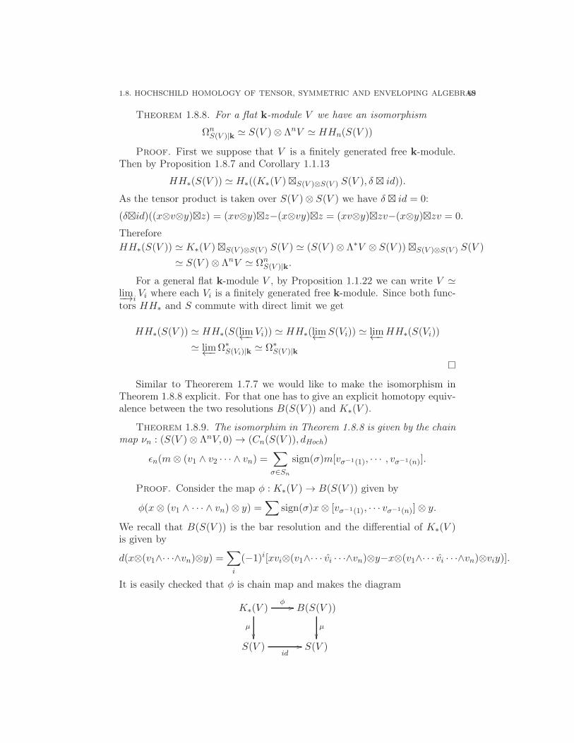
1.8. HOCHSCHILD HOMOLOGY OF TENSOR, SYMMETRIC AND ENVELOPING ALGEBRAS69
Theorem 1.8.8. For a flat k-module V we have an isomorphism
ΩnS(V )|k ≃ S(V )⊗ ΛnV ≃ HHn(S(V ))
Proof. First we suppose that V is a finitely generated free k-module.Then by Proposition 1.8.7 and Corollary 1.1.13
HH∗(S(V )) ≃ H∗((K∗(V )⊠S(V )⊗S(V ) S(V ), δ ⊠ id)).
As the tensor product is taken over S(V )⊗ S(V ) we have δ ⊠ id = 0:
(δ⊠id)((x⊗v⊗y)⊠z) = (xv⊗y)⊠z−(x⊗vy)⊠z = (xv⊗y)⊠zv−(x⊗y)⊠zv = 0.
Therefore
HH∗(S(V )) ≃ K∗(V )⊠S(V )⊗S(V ) S(V ) ≃ (S(V )⊗ Λ∗V ⊗ S(V ))⊠S(V )⊗S(V ) S(V )
≃ S(V )⊗ ΛnV ≃ ΩnS(V )|k.
For a general flat k-module V , by Proposition 1.1.22 we can write V ≃lim−→i
Vi where each Vi is a finitely generated free k-module. Since both func-tors HH∗ and S commute with direct limit we get
HH∗(S(V )) ≃ HH∗(S(lim←−Vi)) ≃ HH∗(lim←−
S(Vi)) ≃ lim←−
HH∗(S(Vi))
≃ lim←−Ω∗S(Vi)|k
≃ Ω∗S(V )|k
Similar to Theorerem 1.7.7 we would like to make the isomorphism inTheorem 1.8.8 explicit. For that one has to give an explicit homotopy equiv-alence between the two resolutions B(S(V )) and K∗(V ).
Theorem 1.8.9. The isomorphim in Theorem 1.8.8 is given by the chainmap νn : (S(V )⊗ ΛnV, 0)→ (Cn(S(V )), dHoch)
ǫn(m⊗ (v1 ∧ v2 · · · ∧ vn) =∑
σ∈Sn
sign(σ)m[vσ−1(1), · · · , vσ−1(n)].
Proof. Consider the map φ : K∗(V )→ B(S(V )) given by
φ(x⊗ (v1 ∧ · · · ∧ vn)⊗ y) =∑
sign(σ)x⊗ [vσ−1(1), · · · vσ−1(n)]⊗ y.
We recall that B(S(V )) is the bar resolution and the differential of K∗(V )is given by
d(x⊗(v1∧· · ·∧vn)⊗y) =∑
i
(−1)i[xvi⊗(v1∧· · · vi · · ·∧vn)⊗y−x⊗(v1∧· · · vi · · ·∧vn)⊗viy)].
It is easily checked that φ is chain map and makes the diagram
K∗(V )φ //
µ
B(S(V ))
µ
S(V )
id// S(V )

70 1. HOCHSCHILD AND CYCLIC COMPLEX OF ASSOCIATIVE ALGEBRAS
commutative therefore φ is homotopy equivaelenvce and it induces a quasi-morphism ν∗ := φ ⊗ id : K∗(V ) ⊗S(V )⊗S(V ) S(V ) → C(S(V ). A shortcomputation shows that this is precisely the anti-symmetrisation map asgiven in the statement.
Remark 1.8.10. An important remark to make is that the compos-ite of the chain map νn : S(V ) ⊗ Λ∗V → Cn(S(V )) and isomorphismΩnS(V )|k → S(V ) ⊗ ΛV given in Example 1.1.9 is a chain level lift of the
anti-symmetrisation map ǫn : ΩnS(V )|k → HHn(S(V )) (Section 1.3.1). It
is not true in general that the anti-symmetrisation maps ǫn : ΩnS(V )|k →
HHn(S(V )) is induced by a chain map.
The two previous theorems allow us to compute HH∗(S(V ), S(V )). Infact the these results are also valid for an arbitrary symmetric S(V )-bimodule.
Theorem 1.8.11. Let V be a flat k-module. For all symmetric S(V )-bimodule we have an isomorphism
M ⊗ Λ∗V ≃ HH∗(S(V ),M).
Moreover this is isormophism is induced by the chain map
ǫn(m⊗ (v1 ∧ v2 · · · ∧ vn) =∑
σ∈Sn
sign(σ)m[vσ−1(1), · · · , vσ−1(n)].
Proof. The proof is just like caseM = S(V ) in Theorem 1.8.8. SinceMis symmetric S(V )-bimodule the induced differential on M⊗S(V )⊗S(V )K∗(V )is zero. Therefore HH∗(S(V ),M) ≃ H∗(K∗(V )⊠S(V )⊗S(V ), δ ⊠ idM )) ≃M ⊗ Λ∗V .
As an important application of Theorem 1.8.9 we compute the cyclichomology of S(V ).
Corollary 1.8.12. Let V be a flat k-module. For A = S(V ) we havean isomorphism
HCn(A) ≃ΩnA|k
dΩn−1A|k
⊕Hn−2DR (A) ⊕Hn−4
DR (A)⊕ . . .
Proof. As it was explains in the previous remark the anti-symmetrisationis well-defined at the chain level therefore we have a bicomplex map (ǫn)n :(D∗∗(A), 0, dDR) → (CC∗∗(A), dHoch, B) where D∗∗(A) is the truncated DeRham bicomplex as defined in Section 1.5.5. Moreover by Theorem 1.8.9this bicomplex map is a quasi-isomorphism once restricted to vertical lines.Therefore it induces an isomorphism between E2-terms of the spectral se-quences of these bicomplexes, thus an isomophismH∗(Tot(D∗∗(A))) ≃ HC∗(A).On the other hand since the vertical differential of D∗∗(A) is zero we get,
Hn(TotD∗∗(A)) ≃ΩnA|k
dΩn−1A|k
⊕Hn−2DR (A) ⊕Hn−4
DR (A)⊕ . . . .

1.8. HOCHSCHILD HOMOLOGY OF TENSOR, SYMMETRIC AND ENVELOPING ALGEBRAS71
After combining this calculation with Proposition 1.1.11 we get :
Corollary 1.8.13. Let A = TV where V is a flat k-module. If Q ⊂ k
then,
HCn(A) ≃ΩnA|k
dΩn−1A|k
⊕HCn(k)
1.8.3. Enveloping algebra. All over this section g is a Lie algebraover k which is a free k-module. Let U(g) denote the universal envelopingalgebra of g. The aim of section is to compute HH∗(U(g),M). We beginby recalling the Chevalley-Eilenberg complex for Lie algebra g. Let M beg-module. This means that M that is a k-module and there is a morphismof Lie algebar g → Endk(M) where is the Lie bracket of Endk(M) is givenby the commutator:
m · g1 · g2 −m · g2 · g1 = m · [g1, g2]
In our convetion g acts on M from the right. The chains of degree n aredefined to Cn(g,M) :=M ⊗ Λng and the differential is given by
δ(m⊗ (g1 ∧ · · · ∧ gn)) =n∑
i=1
(−1)imgi ⊗ (g1 ∧ . . . gi · · · ∧ gn)
+∑
i<j
(−1)i+j−1m⊗ ([gi, gj ] ∧ . . . gi . . . gj . . . gn)
The main theorem of this section is the following.
Theorem 1.8.14. Let g be a Lie algebra over k. For all U(g)-bimoduleM we have an isomorphism
H∗(g,Mad) ≃ HH∗(U(g),M).
Here Mad is a g-Lie algebra module whose underlying k-module is M andthe action of g on m ∈ Mad is given by mg − gm, defined using the U(g)-bimodule structure of M . In fact the isomorphism is induced by the chainmap (the anti-symmetrisation map)
ǫn : Cn(g,Mad) =Mad ⊗ Λng→M ⊗ U(g)⊗n = Cn(U(g),M), n ≥ 0,
ǫn(m⊗ (g1 ∧ g2 · · · ∧ gn)) =∑
σ∈Sn
sign(σ)m[gσ−1(1), · · · , gσ−1(n)].

72 1. HOCHSCHILD AND CYCLIC COMPLEX OF ASSOCIATIVE ALGEBRAS
Our proof relies on the following construction. Let Ke∗(g) := U(g)⊗Λ∗
g
be the complex whose differential is
d(u⊗ (g1 ∧ · · · ∧ gn)) :=n∑
i=1
(−1)iugi ⊗ (g1 ∧ · · · gi · · · ∧ gn)
+∑
i<j
(−1)i+j+1u⊗ ([gi, gj ] ∧ g1 ∧ · · · gi · · · gj ∧ gn).
Verifying that d2 = 0 is a standard exercise. There is an obvious aug-mentation ǫ : Ke(U(g))→ k.
Lemma 1.8.15. The augmentation map ǫ : Ke∗(g) → k is a projective
U(g)-module resolution of k.
Proof. Since g is free over k, Λ∗g is also free over k. Therefore Ke
∗(g) isU(g)-free module thus projective. All we to have is to prove thatHk>0(K
e∗(g)) =
0. The enveloping algebra U(g) inherits a naturally induced filtration FpU(g)from the tensor algebra. This induces a flitration on Ke
∗(g) given by,
FpKen(g) := Fp−nU(g)⊗ Λ∗
g.
Note that ⊕ FpKe∗
Fp−1Ke∗
is canonically isomorphic to S(g)⊗Λ∗g. The induced
differential is∑n
i=1(−1)iugi ⊗ (g1 ∧ · · · gi · · · ∧ gn) since the second terms
vanish in the quotient. Therefore ⊕ FpKe∗
Fp−1Ke∗
is a Koszul complex (Section
1.6.3) and is acyclic by Corollary 1.6.5. We conclude that E1-term of thespectral sequence associated to the filtraion F∗K
e∗(g) is concentrated in E1
00therefore Ke
∗(g) is acyclic.
Corollary 1.8.16. Let g k- free Lie algebar. For all right g-module Mwe have an isomorphism
TorU(g)∗ (M,k) ≃ H∗(g,M).
Proof. Lemma 1.8.15 provides us a resolution of k as U(g)-module,therefore we can write
TorU(g)∗ (M,k) ≃ H∗((M ⊗U(g) K
e∗(U(g)), idM ⊗d)).
It is easily checked that the complex (M⊗U(g)Ke∗(U(g)), idM ⊗d) is precisely
the Chevalley-Eilenberg complex.
Proof of Theorem 1.8.14. The diagonal Lie homomorphism g→ g⊕g inducesan associative algebra homomorphism U(g)→ U(g⊕g) ≃ U(g)⊠U(g) whichis characterized by the property
(1.55) Dg = g ⊠ 1 + 1⊠ g, ∀g ∈ g ⊂ U(g).
For a general element x = g1 ⊗ · · · ⊗ gn ∈ U(g), Dx is computed usingthe fact that D is an algebra homomorphism and (1.55). We have also anantipodal map ∗ : U(g)→ U(g) which is induced by the isomorphism g→ g

1.8. HOCHSCHILD HOMOLOGY OF TENSOR, SYMMETRIC AND ENVELOPING ALGEBRAS73
given by g 7→ −g. The composition of D and id⊗∗ provides us a algebrahomomorphism
δ : U(g)→ U(g)e = U(g)⊠ U(g)op
which is characterized by δg = g ⊠ 1− 1⊠ g for all g ∈ g.We prove the if g is free over k, A = U(g) verifies the condition of
Proposition 1.1.21, therefore we obtain an isomorphism
TorU(g)∗ (Mδ ,k) ≃ Tor
U(g)e
∗ (M,U(g)) ≃ HH∗(U(g),M).
The proof of the first statement of the theorem is completed once we noticethat Mδ is precisely Mad and apply Corollary 1.8.16.
We recall that δ = D (id⊗∗) where ∗ is an isomorphism. So to provethe first condition, it suffices to prove that U(g)e is a flat U(g)-module usingthe homomorphism D. The diagonal map g → g ⊕ g is a monomorphismwith g as the cokernel. As g is free over k, by choosing a basis for U(g)and extending it to U(g ⊕ g) we see that D also is a monomorphism andU(g)⊠ U(g) ≃ U(g⊕ g) is free over U(g), hence flat.
As for the second condition, let∑
i ui⊠ vi ∈ J = ker µ ⊂ U(g)⊗U(g)op,that is
∑i uivi = 0. We can write∑
i
ui ⊠ vi =∑
(1⊠ vi)(ui ⊠−1⊠ ui) +∑
i
1⊠ uivi
=∑
(1⊠ vi)(ui ⊠ 1− 1⊠ ui)
which implies J is the left ideal in U(g)e generated by element of the formui ⊠ 1− 1⊠ ui with ui ∈ U(g). The following decomposition in U(g)e
uv ⊠ 1− 1⊠ uv = (u⊠ 1)(v ⊠ 1− 1⊠ v) + (1⊠ v)(u⊠ 1− 1⊠ u)
for u, v ∈ U(g) implies that in fact J is the left ideal generated by the imageof δ. This proves that the second condition is verified.
Now we take one step further and give an explicit chains level quasi-isomorphism. By Lemma 1.8.15, Ke
∗(g) ։ k is U(g)-module resolution, thusU(g)eδ ⊗U(g) K
e∗(g) ։ U(g)eδ ⊗U(g) k is a projective U(g)e-resolution. As
we saw in the proof of Proposition 1.1.21, U(g)eδ ⊗U(g) k ≃ U(g) as U(g)e-module. Therefore there should be a homotopy equivalence between thetwo projective resolutions, U(g)eδ ⊗U(g) K
e∗(g) and B(U(g), U(g)). In fact
any chain map φ∗ : U(g)eδ⊗U(g)Ke∗(g)→ B(U(g), U(g)) compatible with the
augmentations, is automatically a homotopy equivalence. It is easily checkedthat
φn((u⊠ v)⊗ (g1 ∧ g2 · · · ∧ gn)) =∑
σ∈Sn
sign(σ)u[gσ−1(1), · · · , gσ−1(n)]v
is a chain map and ǫn = idM ⊗U(g)e φn is the chain map given in the state-ment.

74 1. HOCHSCHILD AND CYCLIC COMPLEX OF ASSOCIATIVE ALGEBRAS
1.9. Periodic and negative cyclic bicomplexes
There are two variations of cyclic complex which play an important rolein algebraic K-theory, topology of mapping spaces and noncommutative al-gebraic geometry. For instance, some characteristic classes such as Bismut-Chern and Todd classes and some secondary classes such as holonomy consistof infinite sums so they do not belong to the cyclic complex but to negativeand periodic cyclic complexes. In this section A is an associative algebrawhich is not required A to be unital.The periodic bicomplex CCper∗∗ (A) isobtained by continuing the cyclic complex on left side i.e. for negative p.
· · ·...
...
oo ...
oo ...
oo ... · · ·
oo
· · ·A⊗(n+1)
dHoch
A⊗(n+1)
−dbar
1−too A⊗(n+1)
dHoch
Noo A⊗(n+1)
−dbar
1−too A⊗(n+1) · · ·
dHoch
Noo
· · ·A⊗n
A⊗n
1−t
oo A⊗n
N
oo A⊗n
1−t
oo A⊗n · · ·
N
oo
· · ·...
...
1−too
...
Noo
...
1−too
... · · ·
Noo
· · ·A⊗2
dHoch
A⊗2
−dbar
1−too A⊗2
dHoch
Noo A⊗2
−dbar
1−too A⊗2 · · ·
dHoch
Noo
· · ·A A1−t
oo AN
oo A1−t
oo A · · ·N
oo
−2 −1 0 +1 +2

1.9. PERIODIC AND NEGATIVE CYCLIC BICOMPLEXES 75
The negative cyclic bicomplex CC−∗∗(A) is the sub-bicomplex of the pe-
riodic bicomplex consisting of column number 1 or less.
· · ·...
...
oo ...
oo ...
oo
· · · A⊗(n+1)
dHoch
A⊗(n+1)
−dbar
1−too A⊗(n+1)
dHoch
Noo A⊗(n+1)
−dbar
1−too
· · · A⊗n
A⊗n
1−t
oo A⊗n
N
oo A⊗n
1−t
oo
· · ·...
...
1−too
...
Noo
...
Noo
· · · A⊗2
dHoch
A⊗2
−dbar
1−too A⊗2
dHoch
Noo A⊗2
−dbar
1−too
· · · A A1−t
oo AN
oo A1−t
oo
−2 −1 0 +1
Thus the cyclic complex is the quotient Cper∗∗ (A)/CC−∗∗(A) and we have a
short exact sequence of bicomplexes
(1.56) 0 // CC−∗∗(A)
Ineg,per// CCper∗∗ (A)Sper,cyc// CC∗∗(A)[2, 0] // 0.
Here Ineg,per is the inclusion map and Sper,cyc is the natural projection.Contrary to the case of cyclic homology, for the periodic and negative
cyclic homologies we have choice of the taking the total complex with respectto the direct product or sum. As we will explain in Remark 1.9.1 below thedirect sum total complex does not provide us an interesting theory. So wedefine periodic homology to be
HP∗(A) = H∗(TotΠCCper(A)),
where TotΠCCper(A)n =∏p+q=nCC
perpq (A). Similarly the negative cyclic
homology is defined by
HC−∗ (A) = H∗(Tot
ΠCC−(A)),
where TotΠCC−(A)n =∏p+q=nCC
−pq(A).
Remark 1.9.1. One naturally asks that why we don’t take the direct sumcomplex Tot⊕CCper∗∗ (A)n = ⊕p+q=nCC
perpq (A) instead of (TotΠCC−
∗∗(A)).Then answer is that If Q ⊂ k then H∗(Tot
⊕CCper∗∗ (A)) = 0, . Let d and d′

76 1. HOCHSCHILD AND CYCLIC COMPLEX OF ASSOCIATIVE ALGEBRAS
denote respectively the horizontal and vertical differential. It was explainedin the proof of Theorem 1.5.3, the horizontal lines of the periodic bicomplexesare exact. Let x = (x1, . . . , xk) be a cycle in Tot⊕CCper∗∗ (A) then we havedx0 = 0, since the horizontal are exact, there is y0 such that x0 = dy0. Wehave d(x1− d
′y0) = 0, again there is a y1 such that x1− d′y0 = dy1 therefore
x1 = d′y0 + dy1. We can continue this process and because of finitness ofthe length of the sequence we obtain a squence y = (y0, . . . , yn) such thatx = dtoty. Here dtot = d + d′ is differential of the total complex Tot⊕. Thesame argument shows that Tot⊕(CC−
∗∗(A)) is acyclic if Q ⊂ k. So the directsum does not provide us an interesting theory in many important cases.
Proposition 1.9.2. For any associative k-algebra A there is a naturallong exact sequence(1.57)
· · · // HC−n (A)
Ineg,per// HPn(A)Sper,cyc// HCn−2(A)
Ccyc,neg// HC−n−1(A)
// · · ·
Here Cneg,cyc denotes the connecting map.
Proof. The long exact sequence associated to the short exact sequence(1.56) (after taking the total complex).
Exercise 1.9.3. Prove that the connecting map Cneg,cyc is the mapinduced by the chain map Nneg,cyc : Tot(CC(A))∗ → Tot(CC−(A))∗−1,
Nneg,cyc(x0, · · · xn) = (· · · , 0, 0, Nx0, 0, 0) ∈ · · ·⊕CC−(−1)n(A)⊕CC
−0(n−1)(A)⊕CC
−1(n−2)(A)
where (x0, x1, · · · , xn−1, xn) ∈ CC0n(A) ⊕ CC1n(A) · · · ⊕ CC(n−1)1(A) ⊕CCn0.
It can be easily checked that the short exact (1.56) fits together with(1.12) into the commutative diagram
(1.58) 0 // CC−∗∗(A)
Ineg,per//
projneg,Hoch
CCper∗∗ (A)Sper,cyc//
projper,cyc
CC∗∗(A)[2, 0] //
id
0
0 // CC(2)∗∗ (A) // CC∗∗(A) // CC∗∗(A)[2, 0] // 0
Proposition 1.9.4. For any associative k-algebra there is a natural com-mutative diagram
· · · // HC−n (A)
Ineg,per//
projneg,Hoch
HPn(A)Sper,cyc//
projper,cyc
HCn−2(A)Ccyc,neg//
id
HC−n−1(A)
//
projneg,Hoch
· · ·
· · · // HHn(A)I // HCn(A)
S // HCn−2(A)C // HHn−1(A) // · · ·
where the lower long exact sequence is the exact sequence (1.13).

1.9. PERIODIC AND NEGATIVE CYCLIC BICOMPLEXES 77
Proposition 1.9.5. For any associative A, we have a natural short exactsequence
0→ lim←−
1HCn+2k+1(A)→ HPn(A)→ lim←−
HCn+2k(A)→ 0.
for all n.
Proof. We have that TotΠ(CCper∗∗ (A)) is the projective limit of theshifted complexes Tot(CC∗∗(A))[−2k] where the map π(k(k+1) : TotCC(A)[−2k−2] → Tot(CC∗∗(A))[−2k] is the natural projection. This projective systemclearly verifies the Mittag-Leffler condition. Now the statement follows fromLemma A.0.5.
Proposition 1.9.6. Let A be a k-smooth algebra. If Q ⊂ k then thereis an isormophism
HP0(A) ≃ H0DR(A)⊕H
2DR(A)⊕ · · ·
and
HP1(A) ≃ H1DR(A)⊕H
3DR(A)⊕ · · · .
Proof. We first prove that lim←−1HCn+2k+1(A) = 0. To this end we
identify the maps of the projective system HC∗+2k+1(A)k which are given
by the perdiocity maps S. By Corollary 1.7.9, HCn(A) ≃Ωn
A|k
dΩn−1A|k
⊕Hn−2DR (A)⊕
Hn−4DR (A) ⊕ . . . . By compraing with the bicomplex D∗∗(A) , (1.20), we
conclude that the periodicity map S : HCn+2(A) → HCn(A) correspondto
S :Ωn+2A|k
dΩnA|k⊕Hn
DR(A)⊕Hn−2DR (A)⊕· · · →
ΩnA|k
dΩn−1A|k
⊕Hn−2DR (A)⊕Hn−4
DR (A)⊕ . . .
given by S =
0 incl. 0 0 · · ·0 0 id 0 · · ·0 0 0 id · · ·...
......
...
. This implies that Im(S2) = Hn
DR(A)⊕
Hn−2DR (A)⊕Hn−4
DR (A) · · · , in particular Im(π(k+i)k) ≃ HnDR(A)⊕H
n−2DR (A)⊕
Hn−4DR (A) · · · for ≥ 4, and the projective system HC∗+2k+1(A)k verifies
the Mittag-leffler condition (See Appendix A). Thus lim←−1HCn+2k+1(A) = 0
by Proposition A.0.4, and by Proposition 1.9.5,
HPn(A) = lim←−HCn+2k(A).
Therefore,
HP0(A) = lim←−
HC2k(A) ≃ H0DR(A)⊕H
2DR(A) ⊕ · · · ,
HP1(A) ≃ lim←−
HC2k+1(A) ≃ H1DR(A)⊕H
3DR(A)⊕ · · · ..

78 1. HOCHSCHILD AND CYCLIC COMPLEX OF ASSOCIATIVE ALGEBRAS
1.10. Cohomologies
Let us start with a unital associative k-algebra A. We suppose that Ais k-projective1 and M is an A-bimodule. The Hochschild cohomology of Awith coefficients in M is naturally defined by
HHn(A,M) := ExtnAe(A,M) ≃ H∗(HomAe(B∗(A),M)).
Note that using the isomorphism HomAe(B∗(A),M) ≃ ⊕nHomAe(A ⊗A⊗n ⊗ A,M) ≃ ⊕nHomk(A
⊗n,M) and the differential of the complex isidentified to be
(dHochf)(a1, · · · , an+1) = a1f(a1, · · · , an+1) +n∑
i=0
(−1)if(a1 · · · , aiai+1, · · · , an+1)
+ (−1)n+1f(a1, · · · , an)an+1.
for f ∈ Homk(A⊗n,M).We define the Hochschild cochain complex to be
Cn(A,M) := Homk(A⊗n,M) and differential is given by (1.10). Notice
that the dual of Hochschild chains (Cn(A,A))∨) = Homk(A ⊗ A⊗n,k) ≃
Homk(A⊗n, A∨) = Cn(A,A∨) where A∨ = Homk(A,k) is the k-linear dual
of A. The A-bimodule structure of A∨ is given by (afb)(x) = f(bxa),for a, b ∈ A and f ∈ A∨. In fact we have an isomorphism of complexes(C∗(A,A))
∨, d∨Hoch) ≃ (C∗(A,A∨), dHoch) where d∨Hoch is the adjoint (or thedual) of the differential of Hochschild chains complex. So the dual theory(over k) of Hochschild homology is the Hochschild cohomology defined aboveand C∗(A) is by definition the cochain complex C∗(A,A∨).
Exercise 1.10.1. (1) Prove that H0(A,M) = m ∈ M |am =ma ∀ a ∈ A.
(2) Prove that H1(A,M) is isomorphic to the space of outter deriva-tions of A in M . We recall that an inner derivation in M is givenby adm(a) = ma− am.
Now one can lift the condition A being unital and dualize the bicomplexes
CC(2)∗∗ (A), CC∗∗(A), CC
−∗∗(A) and CCper∗∗ (A) in order to define respectively
the Hochschild cochain complex, cyclic cochain bicomplex, negative cycliccochain bicomplex and periodic cochain bicomplex of A.
Hochschild cochains bicomplex CC∗∗(2)(A) := Homk(CC
(2)∗∗ (A),k)
Cyclic cochains bicomplex CC∗∗(A) := Homk(CC∗∗(A),k)Negative cyclic cochains bicomplex CC∗∗
− (A) = Homk(CC−∗∗(A),k)
Periodic cochains bicomplex CC∗∗per(A) = Homk(CC
per∗∗ (A),k)
1Unlike Hochschild homology and TorAe
∗ , k-flatness do not suffice. Since the derivedfunctor Ext cannot be defined using flat resolutions.

1.10. COHOMOLOGIES 79
In the digram below A∨ = Homk(A,k) and by abuse of notation wecontinue the same notation for the duals of dHoch, dbar, N and t.
·... //
... //... //
... //... · · ·
· · ·A∨⊗(n+1)
dHoch
OO
1−t // A∨⊗(n+1)
−dbar
OO
N // A∨⊗(n+1)
dHoch
OO
N // A∨⊗(n+1)
−dbar
OO
1−t // A∨⊗(n+1) · · ·
dHoch
OO
· · ·A∨⊗n
OO
1−t // A∨⊗n
OO
N // A∨⊗n
OO
1−t // A∨⊗n
OO
N // A∨⊗n · · ·
OO
· · ·...
OO
1−t // ...
OO
N // ...
OO
1−t // ...
OO
N // ... · · ·
OO
· · ·A⊗2
dHoch
OO
1−t // A∨⊗2
−dbar
OO
N // A∨⊗2
dHoch
OO
1−t // A∨⊗2
−dbar
OO
N // A∨⊗2 · · ·
dHoch
OO
· · · A∨ 1−t //
dHoch
OO
A∨ N //
−dbar
OO
A∨ 1−t //
dHoch
OO
A∨ 1−t //
−dbar
OO
A∨ · · ·
dHoch
OO
−2 −1 0 +1 +2
In particular we have a short exact sequence of the bicomplexes
(1.59) 0 // CC∗∗(A)[2, 0] // CC∗∗per(A)
// CC∗∗− (A) // 0
Contrary to the case of chains, the cyclic cochain complex is subcomplex ofthe periodic cochain complex and the negative cochain complex is a quo-tient. In order to define the cohomologies one has to construct a cochaincomplex out of each of these bicomplexes. There are two ways to define thetotal complex of a bicomplex, using the direct sum Tot⊕ or direct productTotΠ. Note that TotΠ(C∗∗
per(A)) and TotΠC∗∗− (A) are respectively the dual
of Tot⊕(Cper∗∗ (A)) and Tot⊕(C−∗∗(A)) which by Remark 1.9.1 are both acyclic
if Q ⊂ k. So in order to have interesting theories we define:
HP ∗(A) := H∗(Tot⊕C∗∗per(A))
HC∗−(A) := H∗(Tot⊕C∗∗
per(A))HC∗(A) := H∗(Tot⊕C∗∗(A))
We recall that for a bicomplex C∗∗, Tot⊕Cn = ⊕p+q=nCpq. For the cyclic
cochain bicomplex the total complexes Tot⊕ and TotΠ coincide.Now that we have defined the cohomologies, one consider the long exact
sequence associated to the (1.59).

80 1. HOCHSCHILD AND CYCLIC COMPLEX OF ASSOCIATIVE ALGEBRAS
Proposition 1.10.2. For an associative algebra A, we have a naturallong exact sequence
· · · // HCn−2(A) // HPn(A) // HCn−(A) // HCn−1(A) // · · ·
By taking the dual of the short exact sequence (1.12), we get a shortexact seqeunce,
(1.60) 0→ CC∗∗(A)[2, 0] → CC∗∗(A)→ CC∗∗(2)(A)→ 0.
... //... //
... · · ·
A∨⊗(n+1)
dHoch
OO
N // A∨⊗(n+1)
−dbar
OO
1−t // A∨⊗(n+1) · · ·
dHoch
OO
A∨⊗n
OO
1−t // A∨⊗n
OO
N // A∨⊗n · · ·
OO
...
OO
1−t //...
OO
N //... · · ·
OO
A∨⊗2
dHoch
OO
1−t // A∨⊗2
−dbar
OO
N // A∨⊗2 · · ·
dHoch
OO
A∨ 1−t //
dHoch
OO
A∨ 1−t //
−dbar
OO
A∨ · · ·
dHoch
OO
0 +1 +2 · · ·
Proposition 1.10.3. (Cohomological Connes’ exact sequence) For anyassociative k-algebar A, we have a natural long exact sequence,(1.61)
· · ·HHn−1(A)C // HCn−2(A)
I // HCn(A) // HHn(A)C // HCn−1(A) · · ·
In the case of unital algebras, just like Section 1.5.3, we also have theoption of considering the bicomplex BC
∗(A) = (C
∗(A)[u], dHoch + uB)
The Connes operator on C∗(A), B : Cn+1(A,A∨) → Cn(A,A∨) is ob-
tatined by the homological Connes operator,
(1.62) (Bf)(a1, a2, · · · , an)(a0) =n∑
i=0
(−1)nif(ai, · · · , an, a0, · · · , ai−1)(1).
By abuse of notation we denote the cohomological Connes operator also byB. This is obtained by taking the transpose of the Connes operator onchains.

1.10. COHOMOLOGIES 81
Connecting map of Connes exact sequence. By taking the dual ofthe short exact (1.14) we obtain the short exact sequence
(1.63) 0 // BC∗∗(A)[1, 1] // BC
∗∗(A) // C∗(A) // 0
whose associated long exact sequence reads(1.64)
· · ·HHn(A)C // HCn−1(A)
S // HCn+1(A)I // HHn+1(A)
C // HCn(A) · · ·
where C is the connecting map. Note that I is induced by the dual of theinclusion maps C∗(A)→ Tot(C∗∗(A)).
Proposition 1.10.4. The connecting map C in the long exact sequence1.64 is given by the composite
(Bpr0)∨ : C∗(A)
B // C∗(A)pr0 // Tot(BC
∗∗(A))
which is the transpose of the composite (1.16).
Exercise 1.10.5. Prove that there is a complex isomorphism Tot(BC∗∗(A)) ≃
Homk[u](BC−∗∗(A),k[u]). Therefore the cyclic cohomology is the dual theory
of negative cyclic homology.
1.10.1. Cohomology-Homology pairing. There is a tautological pair-ing between the Hochschild chain and cochains
− ∩ − : C∗(A)⊗ C∗(A)→ k.
The pairing between a = a0[a1, · · · , an] ∈ Cn(A,A) and f ∈ Ck(A,A), n ≥ kis given by
(1.65) f ∩ a = f(a0, a1, · · · , an) ∈ k.
if k = n, otherwise it is defined to be zero. It is a chain map and it inducesa pairing at cohomology and homology level.
Similarly, there is a pairing for the cyclic complexes
− ∩ − : Tot(CC∗∗(A)) ⊗ Tot(CC∗∗(A))→ k
which for (f0, · · · fk) ∈ Tot(CC∗∗(A))k and (x0, · · · , xn) ∈ Tot(CC∗∗(A))nis given by
n∑
i=0
fi(xi)
if k = n, and zero otherwise. The same formula would make sense forperiod and negative complexes since the cochains of the period and negativecomplexes are finite sum. More precisely the pairing
− ∩ − :: Tot(CC∗∗per(A)) ⊗ Tot(CCper∗∗ (A))→ k

82 1. HOCHSCHILD AND CYCLIC COMPLEX OF ASSOCIATIVE ALGEBRAS
for (f0, · · · fn) ∈ Tot(CC∗∗(A))n and (x0, x1 · · · ) ∈ Tot(CC∗∗(A))n is givenby
n∑
i=0
fi(xi).
We have exactly the same pairing for the negative cyclic complexes.It is noteworthy to mention that obtained pairing
−∩ − : HH∗(A)⊗HH∗(A)→ k
−∩ − : HC∗(A)⊗HC∗(A)→ k
− ∩ − : HC∗−(A)⊗HC
−∗ (A)→ k
− ∩ − : HP ∗(A)⊗HP∗(A)→ k
are compatibles via the maps induced by the map involved in the short exactssequence (1.12),(1.60),(1.56) and (1.59).
Exercise 1.10.6. Prove that following diagrams are commutative thecommutative diagrams
(1.66) HCn(A)⊗HPn(A)1⊗Sneg,per //
S∨neg,per⊗1
HCn(A)⊗HCn(A)
−∩−
HPn(A)⊗HPn(A) −∩−
// k
(1.67) HPn(A)⊗HC−n (A)
I∨neg,per⊗1//
1⊗Ineg,per
HCn−(A)⊗HC−n (A)
−∩−
HPn(A)⊗HPn(A) −∩−
// k
(1.68) HCn−(A)⊗HCn−1(A)1⊗Ccyc,neg //
C∨neg,cyc⊗1
HCn−(A)⊗HC−n (A)
−∩−
HCn−1(A) ⊗HCn−1(A) −∩−
// k
(1.69) HHn(A)⊗HCn−1(A)1⊗C //
C∨neg,cyc⊗1
HHn(A)⊗HHn(A)
−∩−
HCn−1(A) ⊗HCn−1(A) −∩−
// k

1.11. HOCHSHCILD COHOMOLOGY, HOCHSSCHILD EXTENSION AND SMOOTH ALGEBRAS83
1.11. Hochshcild cohomology, Hochsschild extension and smoothalgebras
In this section we explain how the abelian extensions are controlled byHochschild cohomology. In fact this is how Hochschild (co)homology wasdiscovered by Gerhard Hochschild [Hoc45].
Let A be a k-algebra and M a k-module. A Hochschild extension of Aby M is a short exact sequence of k-algebras
0 // Mi // E
φ// A
suu // 0
which splits as k-modules and M2 = 0. In particular a Hochschild extensionis abelian. From now on we identify M with its image i(M) ⊂ A.
Proposition 1.11.1. A Hochschild extension of A by M gives rise to anA-bimodule structure on M .
Proof. The bimodule structure is given by
amb := s(a)ms(b)
for a, b ∈ A and m ∈ M . In the formula above the multiplication betweens(a), s(b) and m takes place in E.
We have φ(s(a)s(b)−s(ab)) = 0 since φ is an algebra morphism, therefores(a)s(b) − s(ab) ∈ ker φ = Im(M). Because M2 = 0, we have (s(a)s(b) −s(ab))m = 0 and m(s(a)s(b) − s(ab)) = 0 From these identities it followsthat
a(bm) = s(a)(bm) = s(a)s(b)m = s(ab)m = (ab)m,
and
(mb)a = (mb)s(a) = ms(b)s(a) = ms(ba) = m(ba),
thererfore the formula above endow M with an A-bimodule structure.Finally we check that the above A-bimodule structure is independent of
the section s. Let s′ be another section, then for a ∈ A, a = φs(a) = φs′(a)therefore s(a) − s′(a) ∈ ker φ = Im(i) = M . This implies that (s(a) −s′(a))m = 0, hence s(a)m = s′(a)m. Similarly we have ms(b) = ms′(b) forall m ∈M and b ∈ A.
Now let us determine the algebra structure of E which is from nowon identified with A ⊕ M as a k-module. The identification is given by(s+ i) : A⊕M → E. Let
f(a1a2) := s(a1)s(a2)− s(a1a2) ∈M.
Then product of (a1,m1) and (a2,m2) in E is
(a1,m1)(a2,m2) = s(a1)s(a2) + s(a1)m2 +m1s(a2) +m1m2
= s(a1a2) + f(a1, a2) + s(a1)m2 +m1s(a2)
= (a1a2, a1m2 +m1a2 + f(a1, a2))

84 1. HOCHSCHILD AND CYCLIC COMPLEX OF ASSOCIATIVE ALGEBRAS
Let us write down the associativity condition of the product in E:
[(a1,m1)(a2,m2)](a3,m3) = (a1a2a3,a1m2a3 +m1a2a3 + f(a1, a2)a3
+ a1a2m3 + f(a1a2, a3)
and
(a1,m1)[(a2,m2)(a3,m3)] = (a1a2a3,a1m2a3 +m1a2a3
+ a1a2m3 + a1f(a2, a3) + f(a1, a2a3).
So the associativity of the product of E implies.
f(a1, a2)a3 + f(a1a2, a3) = a1f(a2, a3) + f(a1, a2a3),
or in other f ∈ C2(A,M) is a Hochschild cocycle. The inverse is also true:
Proposition 1.11.2. Let E = A ⊕M as k-module where A is an as-sociative k-algebra. Then k-algebra structures of E for which M2 = 0, arein bijection with the Hochschild 2-cocyles in C2(A,M). More precisely, theexpression
(1.70) (a1,m1)(a2,m2) = (a1a2, a1m2 +m1a2 + f(a1, a2))
defines an associative product on E if and only if f ∈ C2(A,M) is a Hochschildcocycle. Any associative k-algebra structure with M2 = 0 is of the form(1.70)
In order to pass to Hochschilld cohomology we have to consider theequivalence classes of Hochschild extensions.
Equivalences of Hochschild extensions. Let A be k-algebra and Ma k-module. Two Hochschild extensions E and E′ of A by M are said to beequivalent is there is a k-algebra morphims f : E → E′ making the diagram
0 // M //
idM
Eφ //
Ψ
A //
idA
0
0 // M // E′ φ′ // A // 0
commutative.Note that A-bimodule structure by E and E′ on M might be different. If
s : A→ E and s′ : A→ E′ are the section the corresponding extensions, thenapriori there is no reason that s′(a)m = s(a)m. However since Ψs : A→ E′
is also a section for E′, then by the independency of the A-bimodule structureinduced by E′ onM of the section, we have Ψ(s(a)m) = Ψ(s(a))m = s′(a)m.
Definition 1.11.3. Let A be a k-algebra and M a A-bimodule. ByExt(A,M) we denote the equivalence classes of the Hochschild extension ofA by M whose induced A-bimodule structure is the given one.

1.11. HOCHSHCILD COHOMOLOGY, HOCHSSCHILD EXTENSION AND SMOOTH ALGEBRAS85
Proposition 1.11.4. Let A be a k-algebra. For all A-bimodule M thereis a bijection
HH2(A,M)←→ Ext(A,M).
Proof. The map was already given in Proposition 1.11.2,
f ∈ C2(A,M) 7→ A⊕fM
E = A⊕M
(a1,m1)(a2,m2) = (a1a2, a1m2 +m1a2 + f(a1, a2))
All we need to verify is that after passing to equivalences the bijection
holds. An equivalence Ψ : A⊕fM → A⊕f ′ M morphism has
[idA 0g idM
]
for its matricial form. By expanding the condition Ψ(a1,m1).Ψ(a2,m2) =Ψ(a1a2, a1m2 +m1a2 + f(a,a2)) we obtain
(a1,m1+g(a1))(a2,m2+g(a2)) = (a1a2, a1m2+m1a2+f(a1, a2)+g(a1a2)).
After computing the left hand side, the above identity becomes
(a1a2, a1(m2+g(a2))+(m1+g(a1))a2+f′(a1, a2)) = (a1a2, a1m2+m1a2+f(a1, a2)+g(a1a2)).
which implies
a1g(a2) + g(a1)a2 +m1 + f ′(a1, a2) = f(a1, a2) + g(a1a2).
The latter is equivalent to f − f ′ = dHochg. Conversely if f − f ′ = dHochg
then
[idA 0g idM
]is the desired equivalence between A⊕fM and A⊕f ′M .
We end this section by giving a second definition of smooth algebras. discuss how this is equiv-
alent to the previous def
Definition 1.11.5. A a commutative k-algebra R is said to be smooth
over k if for any k-split algebra extension 0→M → Eǫ→ T → 0 with M2=0
and any k-algebra morphism f : R → T , there is a k-algebra morphismg : R→ E such that ǫ g = f
R
f
g
~~~~~~~~
0 // M // Eǫ // T // 0
Smoothness behaves well with respect to base change.
Proposition 1.11.6. Let φ : k → k′ be a morphism of commutative
rings. If R is smooth over k then R⊗k k′ is smooth over l.
Proof. Consider the diagram of k′-algebras
R⊗k k′
f
0 // M // Eǫ // T // 0

86 1. HOCHSCHILD AND CYCLIC COMPLEX OF ASSOCIATIVE ALGEBRAS
where M2 = 0. This diagram can be considered as a diagram of k-algebraswhere the k-algebra structure are defined via φ. For instance k(r ⊗ k′) =rk ⊗ l = k ⊗ φ(k)k′. As R is k-smooth there there is a k- algebra mapg : R ⊗k k
′ → E making the diagram commutative. Define g1 : R ⊗k
k′ → E by g1(r ⊗ k′) = k′g(r ⊗ 1). It is easily checked that g1 is well-
defined and is k′ linear. This is the desired k′-morphism making the diagram
commutative.
Exercise 1.11.7. If R is smooth over S and S is smooth T then R.
Proposition 1.11.8. (Hochcschild-Whiethead) Let k be a field. Then Ris k-smooth if and only HH2(R,M) = 0 for all R-bimodule M .
Proof. Suppose that R is a smooth k-algebra and 0 → M → Eǫ→
R→ 0 be a Hochschild extension. Because of the smoothness of R, there isa k-algebra map g : R → E such that ǫ g = id. Therefore the extensionsplits as a k-algebra, thus it is trivial. This proves that HH2(R,M) = 0.
R
id
g
~~~~~~~~
0 // M // Eǫ // R // 0
Now suppose that HH2(M,R) = 0. For an extension 0 → M → Eǫ→
T → 0 with M2 = 0 and f : R→ T , let
D = (e, r) ∈ E ×R|ǫ(e) = f(r).
Now we have an extension 0 → M → Dǫ′→ R → 0 of k-algebras where ǫ′
is the natural projection. Since we are wokring over a field the extensionis split, therefore it is a Hochschild extension. Since HH2(R,M) = 0 thisextension ought to be trivial, providing us an k-algebra map h : R → D .
Then k-algebra map g : R→ Dpr1→ E given by g : pr1 h is the desired map
in the smoothness condition of R.
Proposition 1.11.9. If R is smooth over k-algebra then Ω1R|k is a pro-
jective R-module.
Proof. We prove that Ω1R|k satisfies the lifting property. Let f : M →
N be a surjective R-module map and h : Ω1R|k → N a R-module map.
Ω∗R|k
h
Mf // N //
As explained in Section 1.1.0.1 (Construction 1) there is an R-module iso-morphism t Ω1
R|k ≃ I/I2 where the ideal I is the kernel of the multiplication

1.11. HOCHSHCILD COHOMOLOGY, HOCHSSCHILD EXTENSION AND SMOOTH ALGEBRAS87
R⊗R→ R. Consider the Hochschild extension 0→ I/I2 → Re/I2 → R→ 0( these section R → Re/Ie is given by x 7→ x ⊗ 1). Since R is k-smooththis extension is trivial so there is a k-algebra isomorphism α : Re/I2 →R⋉ I/I2 ≃ R⋉ Ω∗
R|k.
Re
α
H
|||||||||||||||||||||
Re/I2 ≃ R⋉ I/I2
1×g
0 // 0× ker(f) // R⋉M
1×f // R⋉N // 0
Since R is smooth over k, Re is smooth over R (Proposition 1.11.6) henceover k (Exercise 1.11.7). Therefore there is a k-algebra map H : Re → R⋉Msuch that (1×f)H = (1×g)α. Note that H(I) ⊂ 0×M ⊂ R⋉M because(1×f)H(I) = (1×g)α(I) ⊂ (1×g)(I/I2) ⊂ 0⋉N . Using the same reasoning,H(I2) = 0. Thus H induces a R-linear mapH : I/I2 →M = 0⋉M ⊂ R⋉Mwhich is a lifting of 1× g.

88 1. HOCHSCHILD AND CYCLIC COMPLEX OF ASSOCIATIVE ALGEBRAS
1.12. Hodge decomposition
1.13. Hochschild homology and cohomology of schemes
1.14. Derived category of coherent sheaves and Hochschildcohomology
1.15. Hodge spectral sequence
1.16. HKR theorem and Todd class

CHAPTER 2
Hochschild Complex of differential modules
2.1. Hochschild Complex of differential bimodules
Throughout this chapter k is a field. Let A = k ⊕ A be an augmentedunital differential k-algebra with deg dA = +1, A = A/k or A is the kernelof the augmentation ǫ : A→ k.
A differential graded (A, d)-module, orA-module for short, is a k-complex(M,d) together with an (left) A-module structure · : A×M →M such that
dM (am) = dA(a).m+ (−1)|a|adM (m).Similarly for a (M,dM ) a graded differential (A, d)− bimodule, we have
dM (amb) = dA(a).m.b− (−1)|a|a.dM (m).b+ (−1)|a|+|m|a.m.dAb,
or equivalently, M is a (Ae := A⊗Aop, dA⊗1+1⊗dA) DG-module where Aop
is the algebra whose underlying graded vector space is A with the opposite
multiplication of A, i.e. aop· b = (−1)|a|.|b|b · a. The identity above implies
that the differential of M is of degree 1. From now on Mod(A) denotes thecategory of (lef or right) (differential) A-modules and Mod(Ae) denotes thecategory of differential A-bimodules. All modules considered in this articleare differential modules. We will also drop the indices from the differentialwhen there is no possibility of confusion.
We recall that the two-sided bar construction is given by B(A,A,A) :=A⊗ T (sA)⊗A equipped with the differential d = d0 + d1 where
d1(a[a1, · · · , an]b) = (−1)|a|aa1[a2, · · · , an]b+
n−1∑
i=1
(−1)ǫia[a1, · · · , aiai+1, . . . , an]b
−(−1)ǫna[a1, · · · , an−1]anb
(2.1)
and d0 is the internal differential for the tensor product complex A⊗T (sA)⊗A. Here ǫi = |a1| + · · · |ai| − i. The degree on B(A,A,A) is defined bydeg(a[a1, · · · , an]b) =
∑ni=1 |s(ai)| = |a| + |b| +
∑ni=1 |ai| − n, therefore
deg(d0 + d1) = +1. We recall that sA stands for the suspension of A,i.e. the shift in degree by −1.
We equip A and A⊗k A, or A⊗A for short, with the outer A-bimodulestructure that is a(b1⊗b2)c = (ab1)⊗(b2c). Similarly B(A,A,A) is equippedwith the outer A-bimodule structure. This is a free resolution of A as anA-bimodule which allows us to define Hochschild chains and cochains of A
89

90 2. HOCHSCHILD COMPLEX OF DIFFERENTIAL MODULES
with coefficients in M . Then (normalized) Hochschild chain complex withcoefficients in M is
(2.2) C∗(A,M) := M ⊗Ae B(A,A,A) =M ⊗ T (sA)
and comes equipped with a degree +1 differential D = d0 + d1. The internaldifferential is given by
d0(m[a1, · · · , an]) =n−1∑
i=1
(−1)ǫim[a1, · · · , dAai, . . . an]
− (−1)ǫndMm[a1, · · · , an],
(2.3)
and the external differential is
d1(m[a1, · · · , an]) = ma1[a2, · · · , an]+
n−1∑
i=1
(−1)ǫim[a1, · · · aiai+1 · · · an]
− (−1)ǫnanm[a1, · · · , an−1],
(2.4)
with ǫi = |a1|+· · · |ai|−i. Note that the degree ofm[a1, · · · , an] is∑n
i=1 |ai|−n+ |m|.
When M = A, by definition (CC∗(A),D = d0 + d1) := (C∗(A,A),D =d0+d1) is the Hochschild chain complex of A andHH∗(A,A) := kerD/ ImD)is the Hochschild homology of A.
Similarly we define the M -valued Hochschild cochain of A to be the dualcomplex
C∗(A,M) := HomAe(B(A,A,A),M) = Homk(T (sA),M).
For a homogenous cochain f ∈ Cn(A,M), the degree |f | is defined to bethe degree of the linear map f : (sA)⊗n → M . In the case of Hochschildcochains, the external differential of f ∈ Hom(sA⊗n,M) is
d1(f)(a1, · · · , an) = −(−1)(|a1|+1)|f |a1f(a2, · · · , an)+
−n∑
i=2
(−1)ǫif(a1, · · · , ai−1ai, · · · an) + (−1)ǫnf(a1, · · · , an−1)an,
(2.5)
where ǫi = |f | + |a1| + · · · + |ai−1| − i + 1. The internal differential off ∈ C∗(A,M) is
d0f(a1, · · · , an) = dMf(a1, · · · , an)−n∑
i=1
(−1)ǫif(a1, · · · dAai · · · , an).
(2.6)

2.1. HOCHSCHILD COMPLEX OF DIFFERENTIAL BIMODULES 91
Gerstenhaber bracket and cup product: WhenM = A, for x ∈ CCm(A,A)and y ∈ CCn(A,A) one defines the cup product x ∪ y ∈ CCm+n(A,A) andthe Gerstenhaber bracket [x, y] ∈ CCm+n−1(A,A) by
(2.7)
(x∪y)(a1, · · · , am+n) := (−1)|y|(∑
i≤m |ai|+1)x(a1, · · · , am)y(an+1, · · · , am+n),
and
(2.8) [x, y] := x y − (−1)(|x|+1)(|y|+1)y x,
where
(xy)(a1, · · · , am+n−1) =∑
(−1)(|y|+1)∑
(|ai|+1)x(a1, · · · , aj , y(aj+1, · · · , aj+m), · · · ).
Note that this is not an associative product. It turns out that the operations∪ and [−,−] are chain maps, hence they define two well-defined operationson HH∗(A,A). Moreover,
Theorem 2.1.1. (Gerstenhaber [Ger63]) (HH∗(A,A),∪, [−,−]) is aGerstenhaber algebra that is:
(1) ∪ is an associative and graded commutative product,
(2) [x, y ∪ z] = [x, y] ∪ z + (−1)(|x|−1)|y|y ∪ [x, z] (Leibniz rule),
(3) [x, y] = (−1)(|x|−1)(|y|−1)[y, x],
(4) [[x, y], z] = [x, [y, z]] − (−1)(|x|−1)(|y|−1)[y, [x, z]] (Jacobi identity).
In this article we show that under some kind of Poincaré duality conditionthis Gerstanhaber structure is part of a BV structure.
Definition 2.1.2. (Batalin-Vilkovisky algebra) A BV-algebra is a Ger-stenhaber algebra (A∗, ·, [−,−]) with a degree one operator ∆ : A∗ → A∗+1
whose deviation from being a derivation for the product · is the bracket[−,−], i.e.
[a, b] := (−1)|a|∆(ab)− (−1)|a|∆(a)b− a∆(b),
and ∆2 = 0.
It follows from ∆2 = 0 that ∆ is a derivation for the bracket. In fact theLeibniz identity for [−,−] is equivalent to the 7-term relation [Get94]
∆(abc) = ∆(ab)c+ (−1)|a|a∆(bc) + (−1)(|a|−1)|b|b∆(ac)
−∆(a)bc− (−1)|a|a∆(b)c− (−1)|a|+|b|ab∆c.(2.9)
Definition 2.1.2 is equivalent to the following one:
Definition 2.1.3. A BV-algebra is a graded commutative associativealgebra (A∗, ·) equipped with a degree one operator ∆ : A∗ → A∗+1 whichsatisfies the 7-term relation (2.9) and ∆2 = 0. It follows from the 7-term
relation that [a, b] := (−1)|a|∆(ab)− (−1)|a|∆(a)b−a∆(b) is a Gerstenhaberbracket for the graded commutative associative algebra (A∗, ·).

92 2. HOCHSCHILD COMPLEX OF DIFFERENTIAL MODULES
As we said before the Leibniz identity is equivalent to the 7-term identityand the Jacobi identity follows from ∆2 = 0 and the 7-term identity. We referthe reader interested in the homotopic aspects of BV-algebras to [DCV].
For M = A∨ := Homk(A,k), by definition (CC∗(A),D = d0 + d1) :=(CC∗(A,A∨), d0+d1) is the Hochschild cochain complex of A andHH∗(A) :=kerD/ ImD is the Hochschild cohomology of A. It is clear that CC∗(A) andHomk(CC∗(A), k) are isomorphic as k-complexes, therefore the Hochschildcohomology A is the dual theory of the Hochschild homology of A. TheHochschild homology and cohomology of an algebra have an extra featureand that is Connes operator B ([Con85]). On the chains we have
(2.10) B(a0[a1, a2 · · · , an]) =n+1∑
i=1
(−1)ǫi1[ai+1 · · · an, a0, · · · , ai]
and on the dual theory CC∗(A) = Homk(T (sA), A∨) = Hom(A⊗T (sA),k).
For φ ∈ CCn+1(A) = Hom(A⊗ (sA)⊗n+1,k)
(B∨φ)(a0[a1, a2 · · · , an]) = (−1)|φ|n+1∑
i=1
(−1)ǫiφ(1[ai+1 · · · an, a0, · · · , ai])
where ǫi = (|a0|+ . . . |ai−1| − i)(|ai|+ . . . |an| − n+ i− 1). In other words
B∨(φ) = (−1)|φ|φ B.
Note that
deg(B) = −1 and degB∨ = +1.
Warning: The degree k of a cycle x ∈ HHk(A,M), is not given by thenumber terms in a tensor product but by the total degree.
Remark 2.1.4. In this article we use normalized Hochschild chains andcochains. It turns out that they are quasi-isomorphic to the non-normalizedHochschild chains and cochains. The proof is the same as the one on page 46of [Lod92] for the algebras. One only has to modify the proof to the case ofsimplicial objects in the category of differential graded algebras. The proofof the Lemma 1.6.6 of [Lod92] works in this setting since the degeneracymaps commute with the internal differential of a simplicial differential gradedalgebra.
Chain and cochain pairings and noncommutative calculus. Here we bor-row some definitions and facts from noncommutative calculus [CST04].Roughly said, one should think of HH∗(A,A) and HH∗(A,A) respectivelyas multi-vector fields and differential forms, and of B as the de Rham differ-ential.

2.2. HINICH’S THEOREM AND DERIVED CATEGORY OF DIFFERENTIAL MODULES93
1. Contraction or cap product: The pairing between a0[a1, · · · , an] ∈Cn(A,A) and f ∈ Ck(A,A), n ≥ k is given by(2.11)
if (a0[a1, · · · , an]) = (−1)|f |(∑k
i=1(|ai|+1))a0f(a1, · · · , ak)[ak+1, · · · , an] ∈ Cn−k(A,A).
It is a chain map C∗(A,A) ⊗ C∗(A,A)→ C∗(A,A) and it induces a pairingat cohomology and homology level.
2. Lie derivative: The next operation is the infinitesimal Lie algebraaction of HH∗(A,A) on HH∗(A,A) and is given by Cartan’s formula
(2.12) Lf = [B, if ].
Note that the Gerstenhaber bracket on HH∗(A,A) becomes a (graded) Liebracket after a shift of degrees by one. This explains also the sign conventionbelow. The triple if , Lf and B form a calculus [CST04] that is,
Lf = [if , B](2.13)
i[f,g] = [Lf , ig](2.14)
if∪g = if ig(2.15)
L[f,g] = [Lf , Lg](2.16)
Lfg = [Lf , ig](2.17)
As HH∗(A,A) acts on HH∗(A) = HH∗(A,A) by contraction, it alsoacts on the dual theory i.e. HH∗(A) = HH∗(A,A∨). More explicitly,if (φ) ∈ C
n(A,A∨) is given by
(2.18)
if (φ)(a0[a1, · · · , an]) := (−1)|f |(|φ|+∑k
i=0(|ai|+1))φ(a0[f(a1, · · · , ak), ak+1, · · · , an])
where φ ∈ CCn−k(A,A∨) and f ∈ CCk(A,A), in other words
if (φ) := (−1)|f ||φ|φ if .
2.2. Hinich’s theorem and derived category of differentialmodules
Now we try to present the Hochschild (co)homology in a more concep-tual way i.e. as a derived functor on the category of A-bimodules. Wemust first introduce an appropriate class of objects which can approximateall A-bimodules. This is done properly using the concept of model categoryintroduced by Daniel Quillen [Qui67]. It is the right language for construct-ing homological invariant of homotopic categories. It will naturally lead usto the construction of derived categories as well.
The purpose of this section is to introduce a model category and derivedfunctors of DG-modules over a fixed differential graded k-algebra . Fromnow on we assume that k is a field. The main result is essentially due to

94 2. HOCHSCHILD COMPLEX OF DIFFERENTIAL MODULES
Hinich [Hin97] who introduced a model category structure for algebras overa vast class of operads.
Let C(k) be the category of (unbounded) complexes over k. For d ∈ Z
let Md ∈ C(k) be the complex
· · · → 0→ k = k→ 0→ 0 · · ·
concentrated in degree d and d+ 1.
Theorem 2.2.1. (V. Hinich) Let C be a category which admits finitelimits and arbitrary colimits and is endowed with two right and left adjointfunctors (#, F )
(2.19) # : C C(k) : F
such that for all A ∈ obj(A) the canonical map A → A∐F (Md) induces a
quasi-isomorphism A# → (A∐F (Md))
#. Then there is a model categorystructure on C where the three distinct classes of morphisms are:
(1) Weak equivalences W: f ∈Mor(C) is inW iff f# is quasi-isomorphism.
(2) Fibrations F : f ∈Mor(C) is in F if f# is (component-wise) sur-jective.
(3) Cofibrations C: f ∈ Mor(C) is a cofibration if it satisfies the LLPproperty with respect to all acyclic fibrations W ∩F .
As an application of Hinich’s theorem, one obtains a model categorystructure on the category Mod(A) of (left) differential graded modules overa differential graded algebra A. Here # is the forgetful functor and F isgiven by tensoring F (M) = A⊗k M .
Corollary 2.2.2. The category Mod(A) of DG A-modules is endowedwith a model category structure where
(i) weak equivalences are the quasi-isomorphisms.
(ii) fibrations are level-wise surjections. Therefore all objects are fibrant.
(iii) cofibrations are the maps have the left lifting property with respectto all acyclic fibrations.
In what follows we give a description of cofibrations and cofibrant objects.An excellent reference for this part is [FHT95].
Definition 2.2.3. An A-module P is called a semi-free extension of M ifP is a union of an increasing family of A-modules M = P (−1) ⊂ P (0) ⊂ · · ·where each P (k)/P (k − 1) is a free A-modules generated by cycles. Inparticular P is said to be a semi-free A-module if it is a semi-free extensionof the 0. A semi-free resolution of an A-module morphism f : M → N issemi-free extension P of M with a quasi-isomorphism P → N which extendsf .
In particular a semi-free resolution of an A-module M is a semi-freeresolution of the trivial map 0→M .

2.2. HINICH’S THEOREM AND DERIVED CATEGORY OF DIFFERENTIAL MODULES95
The notion of semi-free modules can be traced back to [GM74], and[Dri04] is another nice reference for the subject. A k-complex (M,d) is calledsemi-free, if it is semi-free as a differential k-module. Here k is equipped withthe trivial differential. In the case of a field k, every positively graded k-complex is semi-free. It is clear from the definition that a finitely generatedsemi-free A-module is obtained through a finite sequence of extensions ofsome free A-modules of the form A[n], n ∈ Z.
Lemma 2.2.4. Let M be an A-module with a filtration F0 ⊂ F1 ⊂ F2 · · ·such that F0 and all Fi+1/Fi are semifree A-module. Then M is semifree.
Proof. Since Fk/Fk−1 is semifree, it has a filtration · · ·P kl ⊂ P kl+1 · · ·
such that P kl /Pkl+1 is generated as an (A, d)-module by cycles. So one can
write Fk/Fk−1 = ⊕l(A⊗Z′k(l)) where Z ′
k(l) are free (graded) k-modules suchthat d(Zk(l)) ⊂ ⊕j≤lZk(j). Therefore there are free k-modules Zk(l) suchthat
Fk = Fk−1
⊕
l≥0
Z ′k(l)
and
d(Zk(l)) ⊂ Fk−1
⊕
j<l
A⊗ Zk(j).
In particular M is the free k-module generated by the union of all basiselements zα of Zk(l)’s. Now consider the filtration P0 ⊂ P1 · · · of freek-modules constructed inductively as follows: P0 is generates as k-moduleby the zα’ which are cycles, i.e. dzα = 0. Then Pk is generated by those zα’ssuch that dzα ∈ A · Pk−1. This is clearly a semifree resolution if we provethat M = ∪kPk. For that, we show by induction on degree that for all α, zαbelongs to some Pk. Suppose that zα ∈ Zk(l), then dzα ∈ ⊕A.Zi(j) wherei < k or i = k and j < l. By induction hypothesis all zβ’s in the sum dzαare in some Pmβ
. Therefore zα ∈ Pm where m = maxβmβ and this finishesthe proof.
Remark 2.2.5. If we had not assumed that k is a field but only a com-mutative ring then we could still put a model category on Mod(A) if A is acofibrant object ifn the model categsory of CH(k) of complexes over k. Inthe model category of CH(k) weak equivalences are the quasi-isomorphism,the fibration are level-wise surjective maps, and cofibrations are the mapswith left lifting property with respect to the acyclic fibrations.
Proposition 2.2.6. In the model category of A-modules, a maps f :M → N is a cofibration if and only if it is a retract of a semi-free extensionM → P . In particular an A-module M is cofibrant iff it is a retract of asemi-free A-module, in other words it is a direct summand of a semi-freeA-module.
Here is a list of properties of semi-free modules which allow us to definethe derived functions by means of semi-free resolutions.

96 2. HOCHSCHILD COMPLEX OF DIFFERENTIAL MODULES
Proposition 2.2.7. (i) Any morphism f : M → N of A-moduleshas a semi-free resolution. In particular every A-module has a semi-free resolution.
(ii) If P is a semi-free A-module then HomA(P,−) preserves the quasi-isomorphisms.
(iii) Let P and Q be semi-free A-modules and f : P → Q a quasi-isomorphism. Then
g ⊗ f :M ⊗A P → N ⊗A Q
is a quasi-isomorphism if g :M → N is a quasi-isomorphism.
(iv) Let P and Q be semi-free A-modules and f : P → Q a quasi-isomorphism. Then
HomR(g, f) : HomA(Q,M)→ HomA(P,N)
is a quasi-isomorphism if g :M → N is a quasi-isomorphism.
The second statement in the proposition above implies that a quasi-isomorphism f :M → N between semi-free A-modules is a homotopy equiv-alence i.e there is a map f ′ : N → M such that ff ′ − idN = [dN , h
′] andf ′f − idM = [dM , h] for some h :M → N and h′ : N →M . In fact part (iii)and (iv) follow easily from this observation.
The properties listed above imply that the functors −⊗AM and HomA(−,M)presevers enough weak equivalences, ensuring that the derived functors ⊗LAand RHomA(−,M) exist for all A-modules M .
Since we are interested in Hochschild and cyclic (co) homology, we switchto the category of DG bimodules. This category is the same as the categoryof DG Ae-modules. Therefore one can endow A-bimodules with a modelcategory structure and define the derived functors −⊗LM and RHom(−,M)by mean of fibrant-cofibrant replacements.
More precisely, for two A-bimodule M and N we have
TorAe
∗ (M,N) = H∗(P ⊗Ae N)
and
Ext∗Ae(M,N) = H∗(HomAe(P,N))
where P is cofibrant replacement for M .By Proposition 2.2.7 every Ae-module has a semi-free resolution for which
there is an explicit construction using the two-sided bar construction. For Pand N be respectively right and left A-module, let
(2.20) B(P,A,M) =⊕
k≥0
P ⊗ T (sA)⊗k ⊗M
equipped with the differential:if k = 0,
D(p[ ]m) = dp[ ]n+ (−1)|p|p[ ]dm

2.2. HINICH’S THEOREM AND DERIVED CATEGORY OF DIFFERENTIAL MODULES97
if k > 0
D(p[a1, · · · , ak]m) = d0(p[a1, · · · , ak]m) + d1(p[a1, · · · , ak]m))
= dp[a1, · · · , an]m+n−1∑
i=1
(−1)ǫip[a1, · · · , dai, . . . ak]m+ (−1)ǫk+1p[a1, · · · , ak]dm
+ (−1)|p|pa1[a2, · · · , ak]m+n−1∑
i=2
(−1)ǫip[a1, · · · , ai−1ai, . . . ak]m+ (−1)ǫkp[a1, · · · , ak−1]akm
whereǫi = |p|+ |a1|+ · · · |ai−1| − i− 1
Let P = A and ǫM : B(A,A,M)→M be defined by
(2.21) ǫM (a[a1, · · · , ak])m) =
0 if k ≥ 1
am if k = 0
It is clear that ǫM is a map of A-bimodules.
Lemma 2.2.8. In the category of left A-modules, ǫM : B(A,A,M)→Mis a semi-free resolution.
Proof. Let us first prove that this is a resolution. Let h : B(A,A,M)→B(A,A,M) be defined
(2.22) h(a[a1, a2, · · · ak]m) =
[a, a1, · · · ak]m, if k ≥ 1,
[a]m, if k = 0.
On can easily check that for [D,h] = id on ker ǫM , which impliesH∗(ker(ǫM )) =0. Since ǫM is surjective, ǫM is a quasi-isomorphism. Now we prove thatB(A,A,M) is a semifree A-module. Let Fk =
⊕i≤k A ⊗ T (sA)⊗i ⊗ M .
Since d1(Fk+1) ⊂ Fk), then Fk+1/Fk as a differential graded A is isomorphicto (A ⊗ (sA)⊗k ⊗M,d0) = (A, d) ⊗k ((sA)⊗k, d) ⊗ (M,d). The later is asemifree (A, d)-module since ((sA)⊗k, d) ⊗k (M,d) is a semifree k-modulevia the filtration
0 → ker(d⊗ 1 + 1⊗ d) → ((sA)⊗k, d)⊗k (M,d).
Therefore B(A,A,M) is semi-free by Lemma 2.2.4.
Corollary 2.2.9. The map ǫA : B(A,A) := B(A,A,k)→ k given by
ǫk(a[a1, a2 · · · an]) =
ǫ(a) if n = 0
0 otherwise
is a resolution. Here ǫ : A → k is the augmentation of A. In other wordsB(A,A) is acyclic.
Proof. In the previous lemma, let M = k be the differential A-modulewith trivial differential and the module structure a.k := ǫ(a)k

98 2. HOCHSCHILD COMPLEX OF DIFFERENTIAL MODULES
Lemma 2.2.10. In the category Mod(Ae), ǫA : B(A,A,A) → A is asemifree resolution.
Proof. The proof is similar to the previous lemma. First of all, it isobvious that this is a map of Ae-modules. Let Fk =
⊕i≤k A⊗T (sA)
⊗i⊗A.
Then Fk+1/Fk as a differential graded A is isomorphic to (A ⊗ (sA)⊗k ⊗A, d0) = (A, d) ⊗k ((sA)⊗k, d) ⊗ (A, d). The later is semi-free as Ae-modulesince ((sA)⊗k, d) is a semi-free k-module via the filtration ker d → (sA)⊗k.
Since the two-sided bar construction B(A,A,A) provides us with a semi-free resolution of A we have that
HH∗(A,M) = H∗(B(A,A,A) ⊗Ae M) = TorAe
∗ (A,M)
and
HH∗(A,M) = H∗(HomAe(B(A,A,A),M)) = Ext∗Ae(A,M).
In some special situations, for instance that of Calabi-Yau algebras, onecan choose smaller resolutions to compute Hochschild homology or cohomol-ogy.
The following will be useful.
Lemma 2.2.11. If H∗(A) is finite dimensional then for all finitely gener-ated semi-free A-bimodules P and Q, H∗(P ), H∗(Q) and H∗(HomAe(P,Q))are also finite dimensional.
Proof. Since A has finite dimensional cohomology, we see that H∗(A⊗Aop) is finite dimensional. Similarly P (or Q) has finite cohomological dimen-sion since it is obtained via a finite sequence of extensions of free bimodulesof the form (A ⊗ Aop)[n]. Note that since HomAe(A ⊗ Aop, A ⊗ Aop) ≃A ⊗ Aop, A ⊗ Aop is a free A bimodule of finite cohomological dimension,therefore HomAe(P,Q) is obtained through a finite sequence of extensionsof shifted free A-bimodules, proving that it has finite cohomological dimen-sion.
2.3. Calabi-Yau DG algebras
Throughout this section (A, d) is a differential graded algebra, and by anA-bimodule we mean a differential graded (A, d)-bimodule.
In this section we essentially explain how an isomorphism
(2.23) HH∗(A,A) ≃ HH∗(A,A)
(of HH∗(A,A)-modules) gives rise to a BV structure on HH∗(A,A) extend-ing its canonical Gerstenhaber structure. For Calabi-Yau DG algebra onedoes have such an isomorphism (2.23) and this is a special case of a moregeneral statement due to Van den Bergh [vdB98]. The main idea is due toV. Ginzburg [Gin] who proved that for a Calabi-Yau algebra A, HH∗(A,A)is a BV-algebra. However he works with ordinary algebras rather than DG

2.3. CALABI-YAU DG ALGEBRAS 99
algebras. But here we have adapted his result to the case of Calabi-Yau DGalgebras. For this purpose one has to work in the right derived category ofA-bimodules, and this is the derived category of perfect A-bimodules as itis formulated below. All this can be extended to the case of A∞ but forsimplicity we refrain from doing so.
2.3.1. Calabi-Yau algebras. We first give the definition of Calabi-Yau algebra which were introduced by Ginzburg in [Gin] for algebras withno differential and then generalized by Kontsevich-Soibelman [KS09] to thedifferential graded algebras.
Definition 2.3.1. (Kontsevich-Soibelman [KS09])
(1) An A-bimodule is perfect if it is quasi-isomorphic to a direct sum-mand of a finitely generated semifree A-bimodules.
(2) A is said to be homologically smooth if it is perfect as an A-bimodule.
Remark 2.3.2. In [KS09], the definition of perfectness uses the notionof extension [Kel94] and it is essentially the same as ours.
We define DG-projective A-modules to be the direct summands of semifreeA-modules. As a consequence, an A-bimodule is perfect iff it is quasi-isomorphic to a finitely generated DG-projective A-bimodule. We call thelatter a finitely generated DG-projective A-module resolution. This is ana-loguous to having a bounded projective resolution in the case of ordinarymodules (without differential). By Proposition 2.2.7, DG-projectives haveall the nice homotopy theoretic properties that one expects.
The content of the next lemma is that A! := RHomAe(A,Ae), calledthe derived dual of A, is also a perfect A-bimodule. Recall that for an A-bimodule M , RHomAe(−,M) is the right derived functor of HomAe(−,M)i.e. for an A-bimodule N , RHomAe(N,M) is the complex HomAe(P,M)where P is a DG-projective A-bimodule quasi-isomophic to N . In general,M ! = RHom∗
Ae(M,Ae) is different from the usual dual
M∨ = HomAe(M,Ae).
Lemma 2.3.3. [KS09] If A is homologically smooth then A! is a perfectA-bimodule.
Proof. Let P = P ։ A be a finitely generated DG-projective resolu-tion. Note that A! = RHomAe(A,Ae) is quasi-isomorphic to the complexHomAe(P,Ae). Each Pi being a direct summand of a semi-free module, sim-ilar to the proof of Lemma 2.2.11, one proves that the same is valid for eachHomAe(P,Ae). This proves the lemma.
We say that a DG algebra A is compact if the cohomology H∗(A) is finitedimensional.
Lemma 2.3.4. A compact homologically smooth DG algebra A has finitedimensional Hochschild cohomology HH∗(A,A).

100 2. HOCHSCHILD COMPLEX OF DIFFERENTIAL MODULES
Proof. By assumption A has finite dimensional cohomology and so doesAe = A⊗Aop. Now let P ։ A be a finitely generated DG-projective resolu-tion ofA-bimodules. We have a quasi-isomorphism of complexes CC∗(A,A) ≃RHomAe(A,A) ≃ HomAe(P,P ), which by Lemma 2.2.11 has finite dimen-sional cohomology.
Definition 2.3.5. (Ginzburg, Kontsevich-Soibelman [Gin],[KS09]) Ad-dimensional Calabi-Yau differential graded algebra is a homologically smoothDG-algebra endowed with an A-bimodule quasi-isomorphism
(2.24) ψ : A≃−→ A![d]
such that
(2.25) ψ! = ψ[d].
The main reason to call such algebras Calabi-Yau is that a tilting genera-tor E ∈ Db(Coh(X)) of the bounded derived category of coherent sheaves ona smooth algebraic variety X is a Calabi-Yau algebra iff X is a Calabi-Yau(see [Gin] Proposition 3.3.1 for more details).
There are many other examples provided by representation theory. Forinstance most of the three dimensional Calabi-Yau algebras are obtained asa quotient of the free associative algebras F = C〈x1, · · · xn〉 on n generators.An element Φ of Fcyc := F/[F,F ] is called a cyclic potential. One can defines
the partial derivatives ∂∂xi
: Fcyc → F in this setting. Many of 3-dimensional
Calabi-Yau algebras are obtained as a quotient U(F, φ) = F/ ∂Φ∂xi=0 i=0,···n
.
For instance for Φ(x, y, x) = xyz − yzx, we obtain U(F, φ) = C[x, y, z], thepolynomial algebra in 3 variables. The detail of this discussion is irrelevantto the context of this chapter which is the algebraic models of free loop space.We, therefore, refer the reader to [Gin] for further details.
Here A! = RHomAe(A,Ae) is called the dualizing the bi-module, which isalso a A-bimodule using outer multiplication. Condition (2.24) amounts tothe following.
Proposition 2.3.6. (Van den Bergh Isomorphism [vdB98]) Let A be aCalabi-Yau DG algebra of dimension d. Then for all A-bimodules A we have
(2.26) HHd−∗(A,N) ≃ HH∗(A,N).
Proof. We compute
HH∗(A,N) ≃ Ext∗Ae(A,N) ≃ H∗(RHomAe(A,N)) ≃ H∗(RHomAe(A,Ae)⊗LAe N))
≃ H∗(A! ⊗LAe N) ≃ H∗(A[−d]⊗LAe N) ≃ TorA
e
∗ (A,N) ≃ HHd−∗(A,N)
(2.27)
Note that the choice of the A-bimodule isomorphism ψ is important andit is characterized by the image of the unit π = ψ(1A) ∈ A
!. By definition,

2.3. CALABI-YAU DG ALGEBRAS 101
π is the volume of the Calabi-Yau algebra A. For a Calabi-Yau algebra Awith a volume π and N = A, we obtain an isomorphism
(2.28) D = Dπ : HHd−∗(A,A)→ HH∗(A,A).
One can use D to transfer the Connes operator B from HH∗(A,A) toHH∗(A,A),
∆ = ∆π := D B D−1
In the following lemmas A is a Calabi-Yau algebra with a fixed volumeπ and the associated operator ∆ .
Lemma 2.3.7. f ∈ HH∗(A,A) and a ∈ HH∗(A,A)
D(ifa) = f ∪Da.
Proof. To prove the lemma we use the derived description of Hochschild(co)homology, cap and cup product. Let (P, d) be a projective resolution ofA. Then HH∗(A,A) is computed by the complex (P ⊗Ae P, d), and similarlyHH∗(A,A) is computed by the complex (End(P ), ad(d) = [−, d]). HereEnd(P ) = ⊕r∈ZHomAe(P,P [r]). Then the cap product corresponds to thenatural pairing
(2.29) ev : (P ⊗Ae P )⊗k End(P )→ P ⊗Ae P
given by ev : (p1⊗p2)⊗f 7→ p1⊗f(p2). The quasi-isomorphism ψ : A→ A![d]yields a morphism φ : P → P∨. Let us explain this in detail.
Using the natural identification P∨⊗Ae P = End(P ), we have a commu-tative diagram
(2.30) End(P )⊗k (P ⊗Ae P )ev //
id⊗(φ⊗id)
P ⊗Ae P
φ⊗id
End(P )⊗k End(P )
composition // End(P ) = P∨ ⊗Ae P
After passing to (co)homology, φ ⊗ id becomes D, the composition inducesthe cup product and ev is the contraction (cap product), hence
D(ifa) = f ∪Da
which proves the lemma.
Lemma 2.3.8. For f, g ∈ HH∗(A,A) and a ∈ HH∗(A,A) we have
f, g · a = (−1)|f |B((f ∪ g)a)− f ·B(g · a) + (−1)(|f |+1)(|g|+1)g ·B(f · a)
+ (−1)|g|(f ∪ g) ·B(a).

102 2. HOCHSCHILD COMPLEX OF DIFFERENTIAL MODULES
Proof. We compute
i[f,g] = Lf ig − igLf
= ifBig −Bif ig − igBif − igifB
= ifBig − igBif −Bif∪g − igifB
(2.31)
Corollary 2.3.9. For all f, g ∈ HH∗(A,A) and a ∈ HH∗(A,A), wehave
[f, g] ∪D(a) = (−1)|f |∆(f ∪ g ∪Da)− f ∪∆(g ∪D(a))
+ (−1)(|f |+1)(|g|+1)g ∪∆(f ∪D(a)) − f ∪ g ∪DB(a).
Proof. After taking D of the identity in the previous lemma, we obtain
D(i[f,g]a) = (−1)|f |D(Bif∪ga)−D(ifBig(a)) + (−1)(|f |+1)(|g|+1)D(igBif (a))
+ (−1)|g|D(if igB(a))
By Lemma 2.3.7 and DB = ∆D, this reads
[f, g] ∪D(a) = (−1)|f |∆D(if∪ga)− f ∪∆D(ig(a)) + (−1)(|f |+1)(|g|+1)g ∪∆D(if (a))
− g ∪ f ∪DB(a).
Once again by Lemma 2.3.7 we get
[f, g] ∪D(a) = (−1)|f |∆(f ∪ g ∪Da)− f ∪∆(g ∪D(a))
+ (−1)(|f |+1)(|g|+1)g ∪∆(f ∪D(a)) + (−1)|g|f ∪ g ∪DB(a).
Theorem 2.3.10. For a Calabi-Yau algebra A with a volume π ∈ A!,(HH∗(A,A),∪,∆) is a BV-algebra i.e.
(2.32) [f, g] = (−1)|f |∆(f ∪ g)− (−1)|f |∆(f) ∪ g − f ∪∆(g).
Proof. In the statement of the previous lemma choose a ∈ HHd(A,A)such that D(a) = 1 ∈ HH0(A,A). The identity (2.42) will follow sinceB(a) = 0 for obvious degree reason.
2.3.2. Chains of Moore based loop space. Let us finish this sec-tion with some interesting examples of DG Calabi-Yau algebras. We willalso dicuss chains of the Moore based loop space. This example plays an im-portant role in symplectic geometry where it appears as the generator of aparticular type of Fukaya category called the wrapped Fukaya category (see[Abo11] for more details). One can then compute the Hochschild homol-ogy of wrapped Fukaya categories using Burghelea-Fiedorowicz-Goodwillietheorem. This theorem implies that the Hochschild homology of the Fukayacategory of a closed oriented manifold is isomorphic to the homology of thefree loop space of the manifold.

2.3. CALABI-YAU DG ALGEBRAS 103
We start with a more elementary example i.e. the Poincaré dualitygroups. Among the examples, we have the fundamental group of closedoriented aspherical manifolds. The closed oriented irreducible 3-manifoldsare aspherical, provide an interesting large class of examples.
Proposition 2.3.11. Let G be finitely generated oriented Poincaré du-ality group of dimension d. Then k[G] is a Calabi-Yau algebra of dimensiond, therefore HH∗(k[G],k[G]) is a BV algebra
Proof. First note that k[G] is only an ordinary algebra without grad-ing and differential. The hypothesis that G is a finitely generated orientedPoincaré duality group of dimension d means that Z has a bounded finiteprojective resolution P = Pd → · · ·P1 → P0 ։ Z as a k[G]-module, andHd(G,k[G]) ≃ Z as a k[G]. Here Z is a equipped with the trivial action andk[G] acts on Hd(G,k[G]) from via the coefficient module. In particular
(2.33) Extik[G](k,k[G]) ≃
k, i = d0, otherwise.
It is clear that Pd ⊗k k[G] → · · ·P1 ⊗k k[G] → P0 ⊗k k[G] ։ k[G] isa resolution of k[G] as k[G]-bimodule, proving that k[G] is homologicallysmooth. Moreover since k[G] is free over k, we have
k[G]! ≃ Homk[G]e(P ⊗k k[G],k[G]e) ≃ Homk[G]e(P ⊗k k[G],k[G]e)
≃ Homk[G](P,k[G]e) ≃ Homk[G](P,k[G]) ⊗k k[G] ≃ k[G][−d]
or k[G] ≃ k[G]![d] in the derived category of k[G]-bimodule. This provesthat the first condition in the definition of Calabi-Yau algebra is satisfied.Here [d] stands for the shift in degree by d, as before. In particular
Extik[G]e(k[G],k[G] ⊗k k[G]) ≃
k[G], i=d;0, otherwise.
Let us check the second condition. Let Qi = Pi ⊗k k[G]. Then Q∨ =Homk[G]e(Q,k[G]
e) = Homk[G](P,k[G]) ⊗k k[G]. Since G is an orientedPoincaré duality group, Homk[G](P,k[G]) is also a resolution of the triv-
ial k[G]-module Z ≃ Hd(G,k[G]), hence in the derived category of k[G]-bimodules one can take k[G]! = Q∨ and one has a quasi-isomorphism φ :k[G] → k[G]!. Since Q and Q∨ are semi-free(projective) replacements fork[G], there is a lift of φ to φ : Q→ Q∨.
Q
Q∨ = k[G]!
φ
φ
yyrrrrrrrrrr
φoo
k[G]id
// k[G]
By definition φ! = Homk[G]e(φ) : Homk[G]e(Q∨,k[G]e)→ Homk[G]e(Q,k[G]
e) =
Q∨. We have to show that φ! ≃ φ in the derived category. Since Q = P ⊗k

104 2. HOCHSCHILD COMPLEX OF DIFFERENTIAL MODULES
[G] ։ k[G] is a projective resolution of k[G]-modules and the group multipli-cation k[G]⊗k k[G]→ k[G] is surjective, there is map ψ : Q→ k[G]⊗k k[G]such that the diagram
Qψ
wwooooooooooooo
p
µ : k[G]⊗k k[G] // k[G]
commutes. The bottom arrow is the map induced by the group multiplica-tion. Consider the map
ρ : Homk[G]e(Q∨,k[G]e) = Homk[G]e(Homk[G]e(Q,k[G]
e),k[G]e)→ k[G]
given by the composition of the evaluation at ψ with the multiplicationin G i.e. ρ = µ evψ. There is also a natural inclusion incl. : Q →Homk[G]e(Q
∨,k[G]e) and ρincl. : Q→ k[G] is just the projection p. There-
fore ρ is also a projective resolution of k[G] and ρ : Q∨∨ = Homk[G]e(Q∨,k[G]e)→
k[G] is also a semifree resolution in the category of k[G]-bimodule. Thus wehave a commutative diagram
Qincl.≃ Q∨∨
p
Hom(φ)// Q∨ = k[G]!
φ
k[G]
id// k[G]
and by the uniquness of the lift identity map of we conclude that φ = φ! =Hom(φ) in the derived category. We refer to Brown’s book [Bro82] for moredetails on Poincaré duality groups.
Remark 2.3.12. In the case of G = π1(M) the fundamental group ofan aspherical manifold M , Vaintrob [Vai] has proved that the BV structureon HH∗+d(k[G],k[G]) ≃ HH∗(k[G],k[G]) corresponds to the Chas-SullivanBV structure on H∗(LM,k).
Let (X, ∗) be a finite CW complex with a basepoint and Poincaré duality.The Moore loop space of X ΩX = γ : [0, s]|γ(0) = γ(1) = ∗, s ∈ R>0is equipped with the standard concatenation which is strictly associative.Therefore the cubic chains C∗(ΩX) can be made into a strictly associativealgebra using the Eilenberg-Zilber map and the concatenation. The proof ofthe following result is sketched in [Gin], here we propose a different proof.
Proposition 2.3.13. For a Poincaré duality finite CW-complex X, C∗(ΩX)is homologically smooth.
Proof. The main idea of the proof is essentially taken from [FHT95].Let A = C∗(ΩX) be the cubic singular chains complex of the Moore loopspace. By composing the Eilenberg-Zilber and contcatenation maps C∗(ΩX)⊗

2.3. CALABI-YAU DG ALGEBRAS 105
C∗(ΩX)EZ−→ C∗(ΩX × ΩX)
concaten.−→ C∗(ΩX) one can define an associative
product on A . The product is often called the Pontryagin product. Onecould switch to the simplicial singular chain complex of ΩX but then onehas to work with A∞-algebras and A∞-bimodules and their derived category.All these work nicely [KS09, Mal] and the reader may wish to write downthe details in this setting.
Note that A has some additional structures. First of all, the composition
of Alexander-Withney and the diagonal maps C∗(ΩX)diagonal−→ C∗(ΩX ×
ΩX)A−W−→ C∗(ΩX) ⊗ C∗(ΩX) provides A with a coassociative coproduct,
which together with the Pontryagin product make C∗(ΩX) into a bialgebra.One can consider the inverse map on ΩX which makes the bialgebra C∗(ΩX)into a differential graded Hopf algebra up to homotopy. In order to get astrict differential graded Hopf algebra, one finds a topological group G whichis homotopy equivalent to ΩX (see [Kan56, HT10]). This can be done, andone can even find a simplicial topological group homotopy equivalent to ΩX.Therefore from now on, we assume that ΩX = G is a topological group andC∗(ΩX) is a differential graded Hopf algebra (A = C∗(ΩX), ·, δ, S) with thecoproduct δ and antipode map S.
First we prove that A has a finitely generated semifree resolution as an A-bimodule. The proof which is essentially taken from [FHT95] (Proposition5.3) relies on the cellular structure of X. Consider the path space E = γ :[0, s] → X|γ(s) = ∗. Using the concatenation of paths and loops, one candefine an action of ΩX on E, and thus C∗(E) becomes a C∗(ΩX))-module.Let G = ΩX → E → X be the path space fibration of X. We will constructa finitely generated semifree resolution of C∗(E) as an A-module which, sinceE is contractible, provides us with a finitely generated semifree resolutionof k ≃ C∗(E). Now by tensoring this resolution with A we obtain a finitelygenerated semifree resolution of A as A-bimodule. The semifree resolutionof C∗(E) is constructed as follows. Let X1 ⊂ X2 ⊂ · · · ⊂ Xm be the skeletaof X and Dn =
∐Dnα the disjoint union of n-cells and Σn =
∐Sn−1α .
Let Vn = H∗(Xn,Xn−1) be the free k-module on the basis vnα. Using thecellular structure of X we construct an A = C∗(G)-linear quasi-isomorphismφ : (V ⊗ A) → C∗(E) where V = ⊕nVn, inductively from the restrictionsφn = φ| ⊕i≤n Vi ⊗ A → C∗(En). The induction step n − 1 to n goes asfollows: Let f : (Dn,Σn)→ (Xn,Xn−1) be the characteristic map. Since the(homotopy) G-fibration E can be trivialized over Dn, one has a homotopyequivalence of pairs
Φ : (Dn,Σn)×G→ (En, En−1),

106 2. HOCHSCHILD COMPLEX OF DIFFERENTIAL MODULES
where Ei = E|Xn . We have a commutative diagram
(2.34) C∗(En)
q
C∗(Sn,Σn)⊗ C∗(G)
Φ∗EZ// C∗(En, En−1)
π∗
C∗(Sn,Σn)f∗
// C∗(Xn,Xn−1)
whose vertical arrows are quasi-isomorphisms. Here q is the standard pro-jection map and π is the fibration map. Since q is surjective there is anelement wnα ∈ C∗(En) such that q∗(w
αn) = Φ∗ EZ(v
αn ⊗ 1). Since vαn ⊗ 1
is a cycle we have that dwαn ∈ C∗(En−1). Because we have assumed thatmn−1 is a quasi-isomorphism, there is a cycle zαn−1 ∈ ⊕i≤n−1Vi ⊗ A suchthat φn−1(z
αn−1) = dwαn . First we extend the differential by d(vα ⊗ 1) = zα.
We extends φn−1 to φn by defining φn(vαn ⊗ 1) = wα. The fact that φn
is an quasi-isomorphism follows from an inductive argument and 5 Lemmaand the fact that on the quotient φn : Vn ⊗ C∗(G) → C∗(En, En−1) is aquasi-isomorphism.
Next, wet prove that A ≃ A! in the derived category of Ae-bimoduleswhich is a translation of Poincaré duality. Let Ad0 : A → Ae be definedby Ad0 = (A ⊗ S)δ. For an A-bimodule M let Ad∗0(M) be the A-modulewhose A-module structure is induced using pull-back by Ad0. By applyingthe result of Félix-Halperin-Thomas on the describing the chains of the basespace of a G-fiberation to the fibration G → EG → BG ≃ X, we get aquasi-isomorphism
C∗(X) ≃ B(k, A,k),
as coalgebras. Note that B(k, A,k) ≃ B(k, A,A) ⊗A B(A,A,k). ThePoincaré duality for X implies that there is a cycle z1 ∈ C∗(X) such thatcapping with z1
(2.35) − ∩ z1 : C∗(X)→ C∗−d(X),
is a quasi-isomorphism. The class z1 corresponds to a cycle z ∈ B(k, A,A)⊗AB(A,A,k) and the quasi-isomorphism (2.35) corresponds to the quasi-isomorphism
(2.36) evz,P : Homk(B(k, A,A), P ) → B(A,A,k) ⊗ P.
given by evz(f) =∑f(zi)z
′i, where f ∈ Homk(B(k, A,A),k) and z =
∑zi⊗
z′i.Let E = Ad∗0(A
e). Then we have the quasi-isomorphisms of Ae-modules(see [Mal] for more details),
A ≃ B(A,A,A) ≃ B(Ad∗(Ae), A,k) ≃ E ⊗A B(A,A,k),(2.37)

2.4. DERIVED POINCARÉ DUALITY ALGEBRAS 107
where Ae = A⊗A acts on the latter from the left and on the factor E. Onthe other hand
A! ≃ HomAe(B(A,A,A), Ae) ≃ HomAe(B(k, A,Ad∗(Ae)), Ae)
≃ HomA(B(k, A,A),HomAe(Ad∗0(Ae), Ae))
≃ HomA(B(k, A,A), Ad∗0(Ae)).
(2.38)
Therefore evz,E is a quasi-isomorphism of Ae-modules from A! and A[−d].
Corollary 2.3.14. For a closed oriented manifoldM , HH∗(C∗(ΩM), C∗(ΩM))is a BV-algebra.
Proof. Note that in the proof of Theorem 2.3.10 we don’t use the secondpart of the Calabi-Yau condition. We only use the derived equivalence A ≃A!.
Remark 2.3.15. Recently E. Malm [Mal] has proved that the Burghelea-Fiedorowicz-Goodwillie isomorphism ([BF86, Goo85])
HH∗(C∗(ΩM), C∗(ΩM)) ≃ HH∗(C∗(ΩM), C∗(ΩM))Burghelea-Fiedorowicz-Goodwillie
≃ H∗(LM).
is an isomorphism of BV-algebras where H∗(LM) is equipped with the Chas-Sullivan [CS] BV-structure.
2.4. Derived Poincaré duality algebras
In this section we essentially show how an isomorphism
HH∗(A,A) ≃ HH∗(A,A∨)
of HH∗(A,A)-modules gives rise to a BV structure on HH∗(A,A) whoseunderlying Gerstenhaber structure is the canonical one. The next lemmafollows from Lemma 2.3.8.
Lemma 2.4.1. For a, b ∈ HH∗(A,A) and φ ∈ HH∗(A,A∨) we have(2.39)
f, g·φ = (−1)|f |B∨((f∪g)φ)−f ·B∨(g·φ)+(−1)(|f |+1)(|g|+1)g·B∨(f ·φ)+(−1)|g|(f∪g)·B∨(φ).
Proof. To prove the identity, one evaluates the cochains in CC∗(A,A∨) =Homk(T (sA), A
∨) = Homk(A ⊗ T (sA),k) on both sides on a chain x =a0[a1, · · · , an] ∈ A⊗ T (sA). By (2.18) and Lemma 2.4.1, we have:

108 2. HOCHSCHILD COMPLEX OF DIFFERENTIAL MODULES
(f, g · φ)(x) = (if,gφ)(x) = (−1)|f,g|·|φ|φ(if,g(x))
= (−1)|f,g|·|φ|φ((−1)|f |B((f ∪ g) · x)− f · B(g · x) + (−1)(|f |+1)(|g|+1)g ·B(f · x)
+ (−1)|g|(f ∪ g) ·B(x)) = (−1)|f,g|·|φ|+|f |+|φ|B∨(φ)(if∪gx)− (−1)|f,g|·|φ|φ(ifB(igx))
(−1)|f,g|·|φ|+(|f |+1)(|g|+1)φ(igB(ifx)) + (−1)|f,g|.|φ|+|g|φ(if∪gB(x))
= (−1)|f,g|·|φ|+|f |+|φ|+(|φ|+1)|f∪g|if∪g(B∨(φ))(x)
− (−1)|f,g||φ|+|g|(|φ|+|f |+1)+|f |+|φ|+|f |·|φ|ig(B∨(ifφ))(x)
(−1)|f,g|·|φ|+(|f |+1)(|g|+1)+|f |(|φ|+|g|+1)+|g|+|φ|+|g|·|φ|if (B∨(igφ))(x)
+ (−1)|f,g|·|φ|+|g|+(|φ|+1)|f∪g|+|φ|if∪g(B∨φ)(x)
= (−1)|g|if∪g(B∨(φ))(x) + (−1)(|f |+1)(|g|+1)igB
∨(ifφ)(x)− ifB∨(igφ)(x)
+ (−1)|f |B∨((f ∪ g) · φ)(x).
This proves the statement.
Now let us suppose that we have an equivalence A ≃ A∨[d] in the derivedcategory of A-bimodules. This property provides us with an isomorphismD : HH∗(A,A∨) → HH∗+d(A,A) which allows us to transfer the Connesoperator on HH∗(A,A∨) to HH∗(A,A),
∆ := D B∨ D−1.
Lemma 2.4.2. Let A be a DGA algebra with an equivalence A ≃ A∨[d]in the derived category of A-bimodules. Then the induced isomorphism D :HH∗(A,A∨) → HH∗+d(A,A) is an isomorphism of HH∗(A,A)-modules,i.e. for all f ∈ HH∗(A,A) and φ ∈ HH∗(A,A∨) we have
(2.40) D(if (φ)) = f ∪D(φ)
Proof. The proof is identical to the proof of Lemma 2.3.7. One uses aresolution by semi-free modules in the category of A-bimodules and adaptsdiagram (2.30) to the case of CC∗(A,A∨), the dual theory of CC∗(A,A).
Corollary 2.4.3. Let A be a DGA algebra with an equivalence A ≃A∨[d] in the derived category of A-bimodules. Then for f, g ∈ HH∗(A,A)and φ ∈ HH∗(A,A∨) we have
f, g ∪D(φ) = (−1)|f |∆((f ∪ g) ·Dφ)− f ·∆(g ·Dφ) + (−1)(|f |+1)(|g|+1)g ·∆(f ·Dφ)
+ (−1)|g|(f ∪ g) ·DB∨(φ).
(2.41)
where D : HH∗(A,A∨) → HH∗(A,A) is the isomorphism induced by thederived equivalence.

2.4. DERIVED POINCARÉ DUALITY ALGEBRAS 109
Proof. This is a consequence of Lemma 2.4.1, the proof being similarto that of Corollary 2.3.9.
Definition 2.4.4. Let A be a differential graded algebra such that Ais equivalent to A∨[d] in the derived category of A-bimodules. This meansthat there is a quasi-isomorphism of A-bimodules ψ : P → A∨[d] where Pis a semi-free resolution of A. Then ψ is a cocycle in HomAe(P,A∨) forwhich − ∩ [ψ] : HH∗(A,A) → HH∗(A,A∨) is an isomorphism. Under thisassumption, A is said to be a derived Poincaré duality algebra (DPD forshort) of dimension d ∈ Z if B∨([ψ]) = 0.
Remark 2.4.5. For a cocycle ψ ∈ CCd(A,A∨), it is rather easy tocheck when −∩ [ψ] : HH∗(A,A)→ HH∗+d(A,A∨) is an isomorphism1: one
only has to check that − ∩ [φ] : H∗(A) → HH∗(A,A)∩[φ]→ H∗(A∨) is an
isomorphism (See [Men09], Proposition 11).
Two immediate consequences of the previous lemma are the followingtheorems.
Theorem 2.4.6. For a DPD algebra A, (HH∗(A,A),∪,∆) is a BV-algebra i.e.
(2.42) f, g = (−1)|f |∆(f ∪ g)− (−1)|f |∆(f) ∪ g − f ∪∆(g).
Proof. Suppose that the derived equivalence A∨[d] ≃ A is realized bya quasi-isomorphism ψ : P → A∨, where ǫ : P → A is a semi-free resolutionof A.
(2.43) Pψ // A∨
Pid // P
ψ
OO
ǫ
Pǫ // A
One can then use HomAe(P,A∨) to compute HH∗(A,A∨), and similarlyHomAe(P,A) or HomAe(P,P ) to compute the cohomology HH∗(A,A). LetD = (− ∩ [ψ])−1 : HH∗(A,A∨) → HH∗(A,A) be the isomorphism inducedby the derived equivalence.
Then the cohomology class represented by id ∈ HomAe(P,P ) corre-sponds to 1 ∈ HH∗(A,A) using ǫ∗ : HomAe(P,P ) → HomAe(P,A), andto ψ by the map
ψ∗ : HomAe(P,P )→ HomAe(P,A∨).
1Intuitively, one should think of HH∗(A,A) as the homology of the free loop space ofsome space, which includes a copy of the homology of the underlying space by the inclusionof constant loops. This condition means that one has to check that the restriction of thecap product to the constants loops corresponds to the Poincaré duality of the underlyingmanifold.

110 2. HOCHSCHILD COMPLEX OF DIFFERENTIAL MODULES
Therefore, D([ψ]) = 1 ∈ HH∗(A,A) where D = ǫ∗ ψ−1∗ . Now take φ = [ψ]
in the statement of Corollary 2.4.3.
A similar theorem can be proved under a slightly different assumption.
Theorem 2.4.7. (Menichi [Men09]) Let A be a differential graded alge-bra equipped with a quasi-isomorphism m : A→ A∨[d]. Then HH∗(A,A) hasa BV algebra structure extending its natural Gerstenhaber algebra structure.The BV operator is ∆ = DB∨D−1 where D : HH∗(A,A∨)→ HH∗(A,A) isthe isomorphism induced by m.
Proof. The proof is very similar to that of the previous theorem. Forsimplicity we take the two-sided bar resolution ǫ : B(A,A,A) → A, whereǫ : A ⊗ k ⊗ A ⊂ B(A,A,A) → A is given by the multiplication of A. Thenψ = mǫ : B(A,A,A)→ A∨ is a quasi-isomorphism. Let [ψ] ∈ HH∗(A,A∨)be the class represented by ψ, and D = (− ∩ [ψ])−1 : HH∗(A,A∨) →HH∗(A,A) be the inverse of the isomorphism induced by ψ. Similarly tothe proof of the previous theorem, we have D([ψ]) = 1 ∈ HH∗(A,A). Itonly remains to prove that DB∨([ψ]) = 0. For that we compute B∨([ψ]) =[B∨(ψ)]. Note that CC∗(A,A∨) = HomAe(B(A,A,A), A∨) ≃ Hom(A ⊗T (sA),k) = (A ⊗ T (sA))∨. The image of the Connes operator B : A ⊗T (sA)→ A⊗T (sA) is included in A⊗T (sA)+. Since ǫ|A⊗T (sA)+⊗A = 0, wehave m B = ψ ǫ B = 0.
2.5. Open Frobenius algebras
In this section we study the algebraic structure of the Hochschild coho-mology of an open Frobenius algebra. More precisely, we introduce a BValgebra structure on the Hochschild cohomology and homology of such alge-bras. In fact this structure is a consequence of the action of the Sullivan chorddiagrams on the Hochschild (co)homology of an open Frobenius algebra aswe’ll explain in the following section. But in this section we will present ex-plicitly all the operations and homotopies related to the BV structures. Themain theorems of this section hint that there should be a bi-BV structureof the Hochschild homology or cohomology of closed Frobenius algebras butwe won’t get into that. Let us just speculate that there should be a sort ofDrinfeld compatibility for the Gerstenhaber bracket and cobracket i.e. thecobracket is a Chevalley-Eilenberg cocycle with respect to the bracket. Theresults of this section are due to T. Tradler, M. Zeinalian and the author[ATZ].
All over this section, like the rest of the chapter, the signs are determinedby Koszul’s rule, we won’t give them explicitly. Readers interested in a moredetailed sign discussion are referred to [CG10] and [TZ06], and they willbe treated in [ATZ] as well.
Definition 2.5.1. (DG open Frobenius algebra). A differential gradedopen Frobenius k-algebra of degree m is a triple (A, ·, δ) such that:

2.5. OPEN FROBENIUS ALGEBRAS 111
(1) (A, ·) is a unital differential graded commutative associative algebrawhose product has degree −m,
(2) (A, δ) is differential graded cocommutative coassociative coalgebra,(3) δ : A → A ⊗ A is a right and left A-module map which using
(simplified) Sweedler’ notation reads∑
(x.y)
(x.y)′ ⊗ (xy)′′ =∑
(y)
x.y′ ⊗ y′′ =∑
(x)
(−1)m|x|x′ ⊗ x′′.y
Here we have simplified Sweedler’s notation for the coproduct ∆x =∑
i x′i⊗
x′′i , to ∆x =∑
(x) x′ ⊗ x′′ where (x) should be thought of as the index set
for i’s.
We recall that an ordinary (DG) Frobenius algebra, sometimes calledclosed Frobenius (DG) algebra, is a finite dimensional unital associative com-mutative differential graded algebra equipped with an nondegenerate innerproduct 〈−,−〉 which is invariant i.e
〈xy, z〉 = 〈x, yz〉.
In particular the inner product allows us to identify A with its dual A∨
(as A-modules, and even A-bimodules ) and define a coproduct on A by
A ≃ A∨ dual of product−→ (A⊗A)∨ ≃ A∨ ⊗A∨ ≃ A⊗A.
The coproduct is cocommutative and coassociative and satisfies condition(3) of the definition above, in other words a closed Frobenius algebra is alsoan open Frobenius algebra. Moreover, ǫ : A → k defined by η(x) = 〈x|1〉 isa counit (trace) (see the next section for the definition).
Exercise: Prove that an open Frobenius algebra with a counit is a closedFrobenius algeba, and in particular it is finite dimensional. Hint: To provethat it has finite dimension, prove that for all x, we have x =
∑(1) 1
′〈x|1′′〉
where δ1 =∑
(1) 1′⊗ 1′′ therefore A ⊂ Span(1)1
′ hence finite dimensional.
This explains why H∗(LM) the homology of the free space (and its algebramodels, Section 9) is generally not a closed Frobenius.
There are plenty of examples of closed Frobenius algebras, for instancethe cohomology and homology of a closed oriented manifold. This is a con-sequence of Poincaré duality. Over the rationals it is possible to lift thisFrobenius algebra structure to the cochains level. By a result of Lambrechtsand Stanley [LS08], there is a connected finite dimensional commutativeDG algebra A which is quasi-isomorphic to C∗(M) the cochains of a givenn-dimensional manifold M and is equipped with a bimodule isomorphismA → A∨ inducing the Poincaré dualité H∗(M) → H∗−n(M). For moreinteresting examples of open Frobenius algebras see Section 9.
HH∗(A,A∨) is already equipped with a BV operator namely the Connesoperator B∨, so we just need a product on HH∗(A,A∨) or equivalently acoproduct on the Hochshild chains. This is given by

112 2. HOCHSCHILD COMPLEX OF DIFFERENTIAL MODULES
(2.44)
θ(a0[a1, · · · , an]) =∑
(a0ai)
±((a0ai)′[a1, · · · , ai− 1])
⊗((a0ai)
′′[ai+1, · · · , an])
Then we can define the cup product of f, g ∈ CC∗(A,A∨) = Hom(A ⊗T (sA),k) by
(f ∪ g)(x) = µ(f ⊗ g)θ(x)
where µ : k⊗ k→ k is the multiplication. More explicitly
(f∪g)(a0[a1, · · · , an]) =∑
(a0ai)
±f((a0ai)′[a1, · · · , ai−1])g((a0ai)
′′[ai+1, · · · , an]).
Theorem 2.5.2. For an open Frobenius algebra A, (HH∗(A,A∨),∪, B∨)is a BV algebra.
Proof. To prove the theorem we show that (CC∗(A,A), θ, B) is a ho-motopy coBV coalgebra. It is a direct check that θ is co-associative. Weprove that it is co-commutative up to homotopy. The homotopy is given by
h(a0[a1, · · · , an]) :=∑
0≤i<j≤n
∑
(ai)
(a0[a1, · · · , ai−1, a′i, aj+1, · · · an])
⊗(a′′i [ai+1, · · · , aj ]).
(2.45)
For j = n, this expression reads∑
(ai)
(a0[a1, · · · , ai−1, a′i])
⊗(a′′i [ai+1, · · · , an]).
and for i = 0 is∑
(ai)
(a′0[aj+1, · · · , an])⊗
(a′′0[a1, · · · , aj ]).
It is a direct check that hd − (d ⊗ 1 + 1 ⊗ d)h = θ − τ θ where τ :CC∗(A)⊗CC∗(A)→ CC∗(A)⊗CC∗(A) is given by τ(α1⊗α2) = ±α2⊗α1.
To prove that the 7-term (coBV) relation holds, we use the Chas-Sullivan[CS] idea (see also [Tra08]) in the case of the free loop space adapted tothe combinatorial (simplicial) situation. First we identify the Gerstenhaberco-bracket explicitly. Let
S := h− τ h
Once proven S is, up to homotopy, the deviation of B from being a coderiva-tion for θ, the 7-term homotopy coBV relation is equivalent to the homotopyco-Leibniz identity for S.

2.5. OPEN FROBENIUS ALGEBRAS 113
Co-Leibniz identity: The idea of the proof is identical to Lemma 4.6 [CS].We prove that up to some homotopy we have
(2.46) (θ ⊗ id)S = (id ⊗ τ)(S ⊗ id)θ + (id⊗ S)θ
It is a direct check that
(id⊗ τ)(h⊗ id)θ + (id⊗ h)θ = (θ ⊗ id)h,
so to prove (2.46) we should prove that up to some homotopy
(2.47) (id⊗ τ)(τh⊗ id)θ + (id⊗ τh)θ = (θ ⊗ id)τh.
The homotopy is given by F : CC∗(A)→ (CC∗(A))⊗3
F (a0[a1, · · · , an]) =∑
i<j<k
∑
(ai),(ak)
(a0[a1, · · · ai−1, a′i, aj+1 . . . ak−1, a
′′k, al+1 · · · an])
⊗(a′′i [ai+1, · · · aj−1])
⊗a′k[ak+1, . . . , al].
The identity
(d⊗id⊗id+id⊗d⊗id+id⊗id⊗d)F = (id⊗τ)(τh⊗id)θ+(id⊗τh)θ−(θ⊗id)τh
can be checked directly and for that the diagrams in Figure ?? are veryhelpful. Note that in Figure ?? there are two diagrams which cancel eachother out.
Compatibility of B and S: The final step is to prove that S = θB± (B⊗id ± id ⊗ B)θ up to homotopy. To that end we prove that h is homotopicto (θB)2 − (B ⊗ id)θ and similarly τh ≃ (θB)1 − (id ⊗ B)θ where θB =(θB)1 + (θB)2, with
(θB)1(a0[a1, · · · , an]) =∑
i<j
∑
(aj)
(a′j [ai, · · · , aj−1])⊗
(a′′j [aj+1, · · · , an, a0 · · · , ai−1]).
and
(θB)2(a0[a1, · · · , an]) =∑
i<j
∑
ai
(a′i[aj , · · · , an, a0, a1 · · · , ai−1])⊗
(a′′i [ai+1, · · · , aj−1]).
It can be easily checked that
H(a0[a1, · · · , an]) =∑
0≤i<k<j
∑
(ai)
(1[ak+1, · · · an, a0, a1, · · · , ai−1, a′i, aj+1, · · · ak])
⊗(a′′i [ai+1, · · · , aj ]),
is a homotopy between h and (θB)2 − (B ⊗ id)θ. For j = n it reads∑
0≤i<k
∑
(ai)
(1[ak+1, · · · an, a0, a1, · · · , ai−1, a′i, a0, · · · ak])
⊗(a′′i [ai+1, · · · , an]).

114 2. HOCHSCHILD COMPLEX OF DIFFERENTIAL MODULES
While calculating dH we encounter a term which corresponds to a multi-plicative a′ia0, which relates to
(B ⊗ 1)θ(a0[a1, · · · , an]) =∑
(1[ak−1, · · · , ai−1, (a0ai)′, a1, · · · , ak])
⊗((a0ai)
′′[ai+1, · · · , an]).
Similarly one proves that τh ≃ (θB)1 − (id⊗B)θ.
There is a dual statement as follows.
Theorem 2.5.3. The Hochschild homology of an open Frobenius algebrais a BV algebra for which the BV operator is the Connes operator, and theproduct is given by
x · y =∑
(a0b0)
±(a0b0)′[a1, . . . , am, (a0b0)
′′, b1, . . . , bn]
=∑
a0)
±a′0[a1, . . . , am, a′′0b0, b1, . . . , bn]
=∑
b0
±a0b′0[a1, . . . , am, b
′′0, b1, . . . , bn]
(2.48)
for x = a0[a1, · · · , am] and y = b0[b1, · · · , bn] ∈ CC∗(A,A).
Note that the identities above hold because A is an open Frobenius al-gebra. The product defined above is strictly associative, but commutativeonly up to homotopy, and the homotopy being given by
H1(x, y) =∑
(a0b0)
±1[a1, · · · , an, (a0b0)′, b1, · · · , bm, (a0b0)
′′]
+n∑
i=1
∑
(a0b0)
±1[ai+1, · · · , an, (a0b0)′, b1, · · · , bm, (a0b0)
′′, a1, · · · , ai].
(2.49)
To prove that the 7-term relation holds, we adapt once again Chas-Sullivan’s[CS] idea to a simplicial situation. First we identify the Gerstenhaber bracketdirectly. Let
x y :=m∑
i=0
∑
(a0)
b0[b1, · · · bi, a′0, a1, · · · an, a
′′0, bi+1, · · · bm],(2.50)
and then define x, y := xy±yx. Next we prove that the bracket −,−is homotopic to the deviation of the BV operator from being a derivation.For that we decompose the Connes operator, our BV operator, in two pieces:
B1(x, y) :=
m∑
j=1
∑
(a0b0)
±1[bj+1, . . . bm, (a0b0)′, a1, . . . , an, (a0b0)
′′, b1, . . . , bj ],

2.5. OPEN FROBENIUS ALGEBRAS 115
B2(x, y) :=
m∑
j=1
∑
(a0b0)
±1[aj+1, . . . an, (a0b0)′, b1, . . . , bm, (a0b0)
′′, a1, . . . , aj ],
so that B = B1 +B2. Then x y is homotopic B1(x, y)− x.By. In fact thehomotopy is given by
H2(x, y) =∑
0≤j≤i≤m
∑
(a0)
1[bj+1, · · · , bi, (a0)′, a1, · · · an, (a0)
′′, bi+1, · · · , bm, b0, · · · bj ].
Similarly for y x and B2(x · y)−Bx · y. Therefore we have proved that onHH∗(A,A) the following identity holds:
x, y = B(x · y)−Bx · y ± x ·By.
Now proving the 7-term relation is equivalent to prove the Leibniz rule forthe bracket and the product, i.e.
x, y · z = x, y · z ± y · x, z.
It is a direct check that x (y · z) = (x y) · z+ y · (x z). On the other hand(y · z) x is homotopic to (y x) · z − y · (z x) using the homotopy
H3(x, y, z) =∑
a0[a1, . . . , ai, b′0, b1, . . . , bn, b
′′0, ai+1 . . . , aj , c
′0, c1, . . . , cm, c
′′0 , aj+1, . . . , ap].
Here z = c0[c1, . . . , cp]. This proves that the Leibniz rule holds up to homo-topy.
Remark 2.5.4. In [CG10] Chen and Gan prove that for an open Frobe-nius algebra A, the Hochschild homology of A seen as a coalgebra, is a BValgebra. They also prove that the reduced Hochschild homology is a BV andcoBV algebra. It is necessary to take the reduced Hochschild homology inorder to get the coBV structure.


CHAPTER 3
Hochschild Homology and Simplicial objects(?)
3.1. Simplicical and cosimplicial objects
3.2. Categories and their classifying space
3.3. Cup, cap, cross and shuffle product
3.4. Loday Fonctor
3.5. Higher Hochschild complex
3.6. Burghelea-Fiedorowicz-Goodwille
3.7. Chen-Jones Theorem
117


CHAPTER 4
Factorization algebras and Chiral homology
119


APPENDIX A
Higher order inverse limit
Let I be a partially ordered set. A I-system is collection of abeliangroups AI = (Ai)i∈I together with homomorphisms παβ : Aβ → Aα for allpairs β ≥ α subject to the coherency condition πβγπαβ = παγ .
To a projective system one can associate a cohomology theory whosen-cochains are
Cn(AI) := c = (cα0α1...αn)α0<···<αn |cα0α1...αn ∈ Aα0
and the differential δ : Cn(AI)→ Cn+1(AI) is defined by
δ(c)α0α1...αn+1 := πα0α1(cα1...αn) +n+1∑
i=1
(−1)icα0...αi...αn+1 .
It can be easily checked that δ2 = 0. We define the n-th inverse limit of AIto be n-th cohomology group,
lim←−
nAI := Hn(C∗(AI)).
As an example, we compute the zeroth inverse limit lim←−
0AI . A 0-cochain
c = (cα0α1)α0<α1 is a cocycle if and only it verifies the conditions πα0α1(cα1)−cα0 = 0. These are exactly the elements of standard direct limit lim
←−IAI ,
thereforelim←−
1AI = lim←−I
A.
Let us give an explicit a more description of lim←−
1AI for I = N = 0 <1 < . . . . Note that a cochain (aij)i<j is cocycle if and only if
aik = aij − πij(cjk)
for all i < j < k. By recursion we see that a cocycle (aij)i<j is indeeddetermined by the sequence (ai(i+1))i∈N . Similarly we see that (aij)i<j isco-exact if there is a sequence (ci)i such that ai(i+1) = πi(i+1)(ci+1) − ci.Putting these facts together we see that
(A.1) lim←−1AN = coker∆AN
where ∆AN: AN → AN is given by
∆((ai)i∈N) = (a0 − π01(a1), a1 − π12(a2), . . . )
It is clear from the definition of ∆ that
(A.2) lim←−0AN = ker∆AN
.
121

122 A. HIGHER ORDER INVERSE LIMIT
Remark A.0.1. There is a more conceptual way to introduce the func-tors lim
←−nIA and that is a the derived functor of (the standard) projective
limit lim←−
: I − ProjSys → Ab, where ProjSys and Ab are respectivelythe categories of I-projective systems and abelian groups. It turns out thatI−ProjSys is an abelian category with enough projectives which paves theway to define derived functors of the left exact functors.expand this remark
Proposition A.0.2. A short exact sequence of I-projective systems givesrise, in natural manner, to a long exact sequence
0 // lim←−AI// lim←−BI
// lim←−CI// lim←−
1AI // lim←−1BI // lim←−
1 CI // . . .
In particular such short exact sequence provide natural connecting morphismsδn : lim←−
nCI → lim←−
n+1AI , therefore lim←−
nn are δ-functors.
Proof. It is obvious from the construction that the level-wise shortexact sequences 0 → Ai → Bi → Ci → 0 gives rise, in a natural fashion, toa short exact sequence of complexes 0→ C∗(AI)→ C∗(BI)→ C∗(CI)→ 0whose associated long exact sequence in cohomology is the desired the longexact sequence.
Corollary A.0.3. For n ≥ 2, we have lim←−nAN ≃ 0.
Proof. For the map ∆ANdefined previously, δ′0(AN) = ker∆AN
andδ′1(AN) = coker∆AN
and δ′n≥2 = 0 defines a δ-functor. By (A.2) and (A.1)we have a have a natural isomorphism that Ψ0 : lim
←−AN ≃ δ′1 and Ψ1 :
lim←−
AN ≃ δ′1. We can complete Ψ0 and Ψ1 to a morphism of δ-functors bysetting Ψn≥0 = 0. Using the same argument as the one in Proposition 1.1.17one can prove that for all n, δ′n ≃ lim←−
n, proving the statement.
Mittag-Leffler (ML) condition. A projective system AI is said toverify Mittag-Leffler condition if for all i there exist α(i) such that for allk ≥ α(i), Im(πik : Ak → Ai) = Im(πiα(i) : Aα(i) → Ai). In other words, fora fixed i, the sequence of subgroups k 7→ Im(πik : Ak → Ai) ⊂ Ai eventuallybecomes constant. A projective system AI is said to be ML-trivial if for allk there is j(k) > k such that πj(k)k : Aj(k) → Ak is the trivial map.
From now on we suppose that that I = N = 0 < 1 < . . . .
Proposition A.0.4. If a projective system AN verifies the Mittag-Lefflercondition, then lim←−
1AI ≃ 0
Proof. We first prove the statement for the ML-trivial projective sys-tems. Suppose that AN is ML-trivial. For the seqeunce (bi)i∈N we setak = bk + ¯bk+1 · · ·+ ¯bj(k)−1 where j(k) is the one provided by the definitionof ML-triviality and bi = πki(bi). Because of the ML-triviality condition,the sequence (ak)k∈N is well-defined. From the definition of (ai) it is clearthat ∆((ai)i∈N, thus we have proved that ∆ is surjective and lim
←−1AN ≃ 0
(by (A.1)).

A. HIGHER ORDER INVERSE LIMIT 123
Now we consider a projective system AN verifying the Mittag-Lefflercondition. Let Bk be stable image of the homomorphisms πik : Ai → Ak,i.e. Bk = ∪i>k Im(πik). Then the quotient projective system (Ak/Bk)k∈N isML-trivial and the homomorphism πk(k+1) : Bk+1 → Bk is surjective for allk. The latter implies (using an inductive) that ∆BN
is surjective therefore
lim←−1Bk ≃ 0. On the other hand we have a short exact sequence of projective
systems
0→ (Bk)→ (Ak)→ (Ak/Bk)→ 0
whose associated long exact for lim←−n together with the fact that lim←−
1AN/BN ≃
lim←−
1BN ≃ 0 imply that lim←−
1AN ≃ 0.
Lemma A.0.5. Let · · ·Ck+1 → Ck → · · · → C0 be a projective system ofcomplexes. That is for each i degree we have a projective system of abeliangroups · · ·Ck+1
i → Cki → · · · → C0i where the homomorphism Ci+1 → Ci are
chain maps. Let C := lim←−Ck. If the system Ci verifies the Mittag-Leffler
condition then for each q ∈ N there is a short exact sequence
0→ lim←−1Hq+1(Ck)→ Hq(C)→ lim←−Hq(Ci)→ 0
Proof. Let Bi = B(Ci) = Im(d : Ci → Ci) and Zi = Z(Ci) = ker(d :Ci → Ci). Since the homomorphism Ci+1 → Ci are chain maps, we havethe induced homomorphism Bi+1 → Bi and Zi+1 → Zi and Bi and Ziform projective systems too.
The differential of Ci’s induces a differential on C which by abuse ofnotation is also denoted d and its image is denoted B := d(C). It is a directcheck that Z := ker d = lim←−Z
i therefore B[−1] ≃ C/Z. The short exactsequence
0 // Zi] // Cid // Bi[−1] // 0
induces the exact sequence
0 // Z // C // lim←−
Bi[−1] // lim←−
1Zi // lim←−
1Ci = 0
which gives rise to the exact sequence
(A.3) 0 // B[−1] ≃ C/Z // lim←−
Bi[−1] // lim←−
1Zi // 0
Since Ci verifies the ML condition, the projective system Bi also verifiesthe ML condition. Therefore the short exact sequence
(A.4) 0 // Bi // Zi // H(Ci) // 0
implies the (long) exact sequence
(A.5)
0 // lim←−
Bi // Z // lim←−
H(Ci) // 0 = lim←−
1B // lim←−
1Zi // lim←−
1H(Ci) // 0

124 A. HIGHER ORDER INVERSE LIMIT
therefore lim←−
1Zi ≃ lim←−
1H(Ci) and Z/ lim←−
Bi ≃ lim←−
H(Ci). We have a natu-
ral inclusion B → lim←−
Bi thus the short exact sequence
0→lim←−B
i
B→
Z
B→
Z
lim←−
Bi→ 0
which after the isommorphismlim←−Bi
B ≃ lim←−1Zi ≃ lim←−
1H(Ci) (using (A.3)
and Z/ lim←−
Bi ≃ lim←−
H(Ci it reads
(A.6) 0→ lim←−1H(Ck)→ H(C)→ lim←−H(Ci)→ 0

APPENDIX B
A quick review of model categories and and derived
functors
In order to present the Hochschild (co)homology in a more conceptualway i.e. as a derived functor on the category of differential A-bimodules, wemust first introduce an appropriate class of objects which can approximateall A-bimodules. This is done properly using the concept of model categoryintroduced by Daniel Quillen [Qui67]. It is also the right language for con-structing homological invariant of homotopic categories. It will naturallylead us to the construction of derived categories as well.
The classical references for this subject are Hovey’s book [Hov99] andDwyer-Spalinsky manuscript [DS95]. The reader who gets to know thenotion of model category for the first time, should not worry about the word“closed” which now has only a historical bearing. From now on we drop theword “closed” from closed model category.
Definition B.0.6. Let C be a category with three classes of morphismsC (cofibrations), F(fibrations) and W (weak equivalences) such that:(MC1) C is closed under finite limits and colimits.(MC2) Let f, g ∈ Mor(C) such that fg is defined. If any two among f, gand fg are in F , then the third one is in F .(MC3) Let f be a retract of g. If g ∈ C (resp. F or W), then f ∈ C (resp.F or W).(MC4) For a commutative diagram, as below, with i ∈ C and p ∈ F , themorphism f making the diagram commutative exists if
(1) i ∈ W (left lifting property (LLP) of fibrations f ∈ F with respectto acyclic cofibrations i ∈ W ∩ C).
(2) p ∈ W (right lifting property (RLP) of cofibrations i ∈ C withrespect to acyclic fibrations p ∈ W ∩F).
(B.1) A
i
// X
p
B
f>>
// Y
The reader should have noticed that we call the elements ofW∩C (resp.W ∩F) acyclic cofibrations (resp. fibrations).(MC5) Any morphism f : A→ B can be written as one of the following:
125

126B. A QUICK REVIEW OF MODEL CATEGORIES AND AND DERIVED FUNCTORS
(1) f = pi where p ∈ F and i ∈ C ∩W;
(2) f = pi where p ∈ F ∩W and i ∈ C.
In fact in a model category the lifting properties characterize the fibra-tions and cofibrations:
Proposition B.0.7. In a model category:
(i) The cofibrations are the morphisms which have the RLP with respectto acyclic fibrations.
(ii) The acyclic cofibrations are the morphisms which have the RLP withrespect to fibrations.
(iii) The fibrations are the morphisms which have the LLP with respectto acyclic cofibrations.
(iv) The acyclic fibrations in C are the maps which have the LLP withrespect to cofibrations.
It follows from (MC1) that a model category C has an initial object∅ and a terminal object ∗. Consequently, an object A ∈ Obj(C) is calledcofibrant if the morphism ∅ → A is a cofibration and is said to be fibrant ifthe morphism A→ ∗ is a fibration.Example 1: For any unital associative ring R, let CH(R) be the categoryof non-negatively graded chain complexes of R-modules. The following threeclasses of morphisms endow CH(R) with a model category structure:
(1) Weak equivalences W are the quasi-isomorphims i.e. maps of R-complexes f = fkk∈Z : Mkk≥0 → Nkk≥0 inducing an isomor-phism f∗ : H∗(M)→ H∗(N) in homology.
(2) Fibrations F : f is a fibration if it is (componentwise) surjective i.efor all k ≥ 0, fk :Mk → Nk is surjective.
(3) Cofibrations C: f = fk is a cofibration if for all k ≥ 0, fk :Mk → Nk is injective with a projective R-module as its cokernel.Here projective is the standard notion i.e. a direct summand of freeR-module.
Example 2: The category Top of topological spaces can be given the struc-ture of a model category by defining a map f : X → Y to be
(i) a weak equivalence if f is a homotopy equivalence;
(ii) a cofibration if f is a Hurewicz cofibration;
(iii) a fibration if f is a Hurewicz fibration.
We recall that an inclusion i : A → B of topological spaces is a Hurewiczcofibration if it has the homotopy extension property that is for all mapsf : B → X, any homotopy F : A × [0, 1] → X of f |A can be extended to a

B. A QUICK REVIEW OF MODEL CATEGORIES AND AND DERIVED FUNCTORS127
homotopy of f : B → X.
B ∪ (A× [0, 1])f∪F //
id×0∪(i×id)
X
B × [0, 1]
88qq
A Hurewicz fibration is a continuous map E → B which has the homo-topy lifting property with respect to all continuous maps X → B, whereX ∈ Top.Example 3: The category Top of topological spaces can be given the struc-ture of a model category by defining f : X → Y to be
(i) a weak equivalence when it is a weak homotopy equivalence.
(ii) a cofibration if it is a retract of a map X → Y ′ in which Y ′ isobtained from X by attaching cells,
(iii) a fibration if it is a Serre fibration.
We recall that a Serre fibration is a continuous map E → B which hasthe homotopy lifting property with respect to all continuous maps X → Bwhere X is a CW-complex (or equivalently cubes).
Cylinder, path objects and homotopy relation. After setting up the gen-eral framework, we define the notion of homotopy. A cylinder object forA ∈ obj(C) is an object A∧I ∈ obj(C) with a weak equivalence ∼: A∧I → Awhich factors the natural map idA ⊔ idA : A
∐A→ A:
idA ⊔ idA : A∐
Ai→ A ∧ I
∼→ A
Here A∐A ∈ obj(C) is the colimit, for which one has two structural
maps in0, in1 : A∐A. Let i0 = in0 i and i1 = in1 i. A cylinder object
A∧ I is said to be good if A∐A→ A∧ I is a cofibration. By (MC5), every
A ∈ obj(C) has a good cylinder objects.
Definition B.0.8. Two maps f, g : A→ B are said to be left homotopic
fl∼ g if there is a cylinder object A ∧ I and H : A ∧ I → B such that
f = H i0 and g = H i1. A left homotopy is said to be good if the cylinderobject A ∧ I is good. It turns out that every left homotopy relation can berealized by a good left homotopy. In addition one can prove that if A is afibrant object, then a left homotopy for f and g can be refined into a verygood one i.e A ∧ I → A is a fibration.
It is easy to prove the following:
Lemma B.0.9. If A is cofibrant, then left homotopyl∼ is an equivalence
relation on HomC(A,B).
Similary, we introduce the notion of path objects which will allow us todefine right homotopy relation. A path object for A ∈ obj(C) is an object

128B. A QUICK REVIEW OF MODEL CATEGORIES AND AND DERIVED FUNCTORS
AI ∈ obj(C) with a weak equivalence A∼→ AI and a morphism p : AI →
A×A which factors the diagonal map
(idA, idA) : A∼→ AI
p→ A×A
Let pr0, pr1 : A×A→ A be the structural projections. Define pi = prip.A path object AI is said to be good if AI → A×A is a fibration. By (MC5)every A ∈ obj(C) has a good path object.
Definition B.0.10. Two maps f, g : A→ B are said to be right homo-
topic fr∼ g if there is a path object BI and H : A→ BI such that f = p0H
and g = p1 H. A right homotopy is said to be good if the path object P I
is good. It turns out that every right homotopy relation can be refined intoa good one. In addition one can prove that if B is a cofibrant object then aright homotopy for f and g can be refined into a very good one i.e B → BI
is a cofibration.
Lemma B.0.11. If B is fibrant, then right homotopyr∼ is an equivalence
relation on HomC(A,B)
One can naturally asks the relationship between right and left homotopy.The following result answers this question.
Lemma B.0.12. Let f, g : A→ B be two morphisms in a model categoryC.
(1) If A is cofibrant then fl∼ g implies f
r∼ g
(2) If B is fibrant then fr∼ g implies f
l∼ g.
Cofibrant and Fibrant replacement and homotopy category. By applying(MC5) to the canonical morphism ∅ → A, there is a cofibrant object (not
unique) QA and an acyclic fibration p : QA∼→ A such that ∅ → QA
p→ A.
If A is cofibrant we can choose QA = A.
Lemma B.0.13. Given a morphism f : A→ B in C, there is a f : QA→QB such that the following diagram commutes:
(B.2) QA
pA
f // QA
pB
Af // B
The morphism f depends on f up to left and right homotopy, and is aweak equivalence if and only f is. Moreover, if B is fibrant then the right orleft homotopy class of f depends only on the left homotopy class of f .
Similarly one can introduce a fibrant replacement by applying (MC5)to the terminal morphism A → ∗ and obtain a fibrant object RA with anacyclic cofibration iA : A→ RA.

B. A QUICK REVIEW OF MODEL CATEGORIES AND AND DERIVED FUNCTORS129
Lemma B.0.14. Given a morphism f : A→ B in C, there is a f : RA→RB such that the following diagram commutes:
(B.3) A
iA
f // B
iB
RAf // RB
The morphism f depends on f up to left and right homotopy, and is aweak equivalence if and only f is. Moreover, if A is cofibrant then right orleft homotopy class of f depends only on the right homotopy class of f .
Remark B.0.15. For a cofibrant object A one RA is also cofibrant be-
cause the trivial morphism (∅ → RA) = (∅ → AiA→ RA) can be written as
the composition of two cofibrations, therefore is a cofibration. In particular,for any object A, RQA is fibrant and cofibrant. Similarly, QRA is a fibrantand cofibrant object.
Putting the last three lemmas together, one can make the following def-inition:
Lemma B.0.16. Suppose that f : A→ X is a map in C between objectsA and X which are both fibrant and cofibrant. Then f is a weak equivalenceif and only if f has a homotopy inverse, i.e., if and only if there exists amap g : X → A such that the composites gf and fg are homotopic to therespective identity maps.
Definition B.0.17. The homotopy category Ho(C) of a model categoryC has the same objects as C and the morphism set HomHo(C)(A,B) consistsof the (right or left) homotopy classes of the morphism HomC(RQA,RQB).Note that since RQA and RQB are fibrant and cofibrant, the left and righthomotopy relations are the same. There is a natural functor HC : C →Ho(C) which is the identity on the objects and sends a morphism f : A→ Bto the homotopy class of the morphism obtained in HomC(RQA,RQB) byapplying consecutively Lemma B.0.13 and Lemma B.0.14.
Localization functor. Here we give a brief conceptual description of thehomotopy category of a model category. This description relies only on theclass of weak equivalence morphisms and suggests that the weak equivalencesencodes most of the homotopic properties.
Let W be a subset of morphisms in a category C. A functor F : C→ D
is said to be a localization of C with respect to W if the elements of Ware sent to isomorphisms and if F is universal for this property i.e. if G :C→ D
′ is another localizing functor then G factors through F via a functorG′ : D→ D
′ for which G′F = G. It follows from lemma B.0.16 and a littlework that:
Theorem B.0.18. For a model category C, the natural functor HC :C→ Ho(C) is a localization of C with respect to the weak equivalences.

130B. A QUICK REVIEW OF MODEL CATEGORIES AND AND DERIVED FUNCTORS
spalinsDerived and total derived functors: In this section we introduce the no-
tions of left derived LF and right derived RF of a functor F : C → D ofmodel categories. In particular, we spell out the necessary conditions forthe existence of LF and RF which provide us a factorization of F via thehomotopy categories. All functors considered here are covariant, however seeRemark B.0.22.
Definition B.0.19. For a functor F : C → D on a model categoryC, we consider all pairs (G, s) where G : Ho(C) → D is a functor ands : GHC → F is a natural transformation. The left derived functor ofF is such a pair (LF, t) which is universal from left i.e. for another suchpair (G, s) there is a unique natural transformation t′ : G → LF such thatt(t′HC) : GHC → F is s.
Similarly one can define the right derived functor RF : Ho(C) → Dwhich provides a factorization of F and satisfies the usual universal propertyfrom the right. A right derived functor for F is a pair (RF, t) where RF :Ho(C)→ D and t is a natural transformation t : RFHC → D such that forany such pair (G, s) there is a unique natural transformation t′ : RF → Gsuch that t′HCt : F → GHC is s.
The reader can easily check that the derived functors of F are unique upto canonical equivalence.
The following result tells us when do derived functors exist.
Proposition B.0.20. (1) Suppose that F : C → D is a functorbetween two model categories which sends acyclic cofibration betweencofibrant objects to the isomorphims. Then (LF, t) the left derivedfunctor of F exists. Moreover for any cofibrant object X the maptx : LF (X)→ F (X) is an isomorphism.
(2) Suppose that F : C → D is a functor between two model cate-gories which sends acyclic fibrations between fibrant objects to iso-morphisms. Then (RF, t) the right derived functor of F exists.Moreover for all fibrant object X the map tx : RF (X) → F (X)is an isomorphism.
Definition B.0.21. Let F : C → D be a functor between two modelcategories. The total left derived functor LF : Ho(C) → Ho(D) is a leftderived functor of HDF : C→ Ho(D). Similarly one defines the total rightderived functor RF : C→ D to be the right derived functor of HDF : C→Ho(D).
Remark B.0.22. Till now we have defined and discussed the derivedfunctor for covariant functors. We can defined the derived functors for con-travariant functors as well, for that we have to only work with the oppositecategory of the source of the functor. A morphism A → B in the oppositecategory is a cofibration (resp. fibration, weak equivalence) if the correspond-ing morphism B → A is a fibration (resp. cofibration, weak equivalence).

B. A QUICK REVIEW OF MODEL CATEGORIES AND AND DERIVED FUNCTORS131
We finish this section with an example.
Example 4: Consider the model category CH(R) of Example B and let Mbe a fixed R-module. One defines the functor FM : CH(R)→ CH(Z) givenby FM (N∗) =M ⊗RN∗ where N∗ ∈ CH(R) is a complex of R-modules. Letus check that F = HCH(R)FM : CH(R) → CH(Z) satisfies the conditionsof Proposition B.0.20.
Note that in CH(R) every object is fibrant and a complex A∗ is cofibrantif for all k, Ak is a projective R-module. We have to show that an acycliccofibration f : A∗ → B∗ between cofibrant objects A and B is sent by F to anisomorphism. So for all k, we have a short exact sequence 0→ A∗ → B∗ →B∗/A∗ → 0 where for all k, Bk/Ak is also projective. Since f is a quasi-isomorphism the homology long exact sequence of this short exact sequencetells us that the complex B∗/A∗ is acyclic. The lemma below shows thatB∗/A∗ is in fact a projective complex. Therefore we have B∗ ≃ A∗⊕B∗/A∗.So FM (B∗) ≃ FM (A∗)⊕FM (B∗/A∗) ≃ FM (A∗)⊕
⊕k FM (Dk(Zk−1(B∗/A∗)).
It is a direct check that each FM (Dk(Zk−1(B∗/A∗)) is acyclic thereforeHCH(Z)(FM (B)) is isomorphic to HCH(Z)(FM (A)) in the homotopy cate-gory Ho(CH(Z)).
Lemma B.0.23. Let Ckk≥0 be an acyclic complex where each Ck isprojective R-module. Then Ckk≥0 is a projective complex i.e. any level-wise surjective chain complex map D∗ → E∗ can be lifted via any chaincomplex map C∗ → E∗.
Proof. Let us introduce a notation first. To any R-module X, one canassociate a complex D(X,n)kk≥0,
D(X,n)k =
0, if k 6= n, n− 1,
X, if k = n, n− 1,
where the only nontrivial differential is the identity map. It is easy to checkthat if X is a projective R-module then Dn(X) is a projective complex. Let
C(m)∗ be the complex
C(m)k =
Ck, if k ≥ m
Zk(C), if k = m− 1
0 otherwise
Here, Zk(C) denotes the space of cycles in Ck, and Bk(C) is the space of
boundary elements in Ck. The acyclicity condition implies that C(m)∗ /C
(m+1)∗ ≃
D(Zm−1(C),m). Note that Z0(C) = C0 is a projective R-module and
C∗ = C(1) = C(2) ⊕ D1(Z0(C)). Now D1(Z0(C)) is a projective complex
and C(2) also satisfies the assumption of the lemma and vanishes in de-gree zero. Therefore by applying the same argument one sees that C(2) =C(3)⊕D(Z1(C), 2). Continuing this process one obtains C∗ = D(Z0(C), 1)⊕

132B. A QUICK REVIEW OF MODEL CATEGORIES AND AND DERIVED FUNCTORS
D(Z1(C), 2) · · ·⊕D(Zk−1, k)⊕· · · where each factor is a projective complex,thus proving the statement.
We finish this example by computing the left derived functor. For anyR-module N let K(N, 0) be the chain complex concentrated in degree zerowhere there is a copy of N . Since every object is fibrant, a fibrant-cofibrantreplacement of K(N, 0) is simply a cofibrant replacement. A cofibrant re-placement P∗ ofK(N, 0) is exactly a projective resolution (in the usual sense)of N in the category of R-modules. Note that in CH(Z), all objects are fi-brant and cofibrant. In the homotopy category of CH(R), K(N, 0) and P areisomorphic because by definition HomHo(CH(R))(K(N, 0), P ) consists of thehomotopy classes of HomCH(R)(RQK(N, 0), RQP∗) = HomCH(R)(P∗, P∗)which contains the identity map. Therefore LF (K(N, 0)) ≃ LF (P∗) andLF (P∗) by Proposition B.0.20 and the definition of total derived functor isisomorphic to HCH(R)F (P∗) =M ⊗R P∗. In particular,
H∗(LF (K(N, 0)) = Tor∗R(N,M),
where Tor∗R is the usual TorR in homological algebra. We usually denotethe derived functor LF (N) = N ⊗LR M . Similarly one can prove that thecontravariant functor N∗ 7→ HomR(N∗,M) has a total right derived functor,denoted by RHomR(N∗,M) and
H∗(RHomR(K(N, 0),M)) ≃ Ext∗R(N,M),
is just the usual Ext functor (see Remark B.0.22).

Bibliography
[Abo11] Mohammed Abouzaid, A cotangent fibre generates the Fukaya category, Adv.Math. 228 (2011), no. 2, 894–939.
[ATZ] Hossein Abbaspour, Thomas Tradler, and Mahmoud Zeinalian, Homotopyabelian string bracket, In preparation.
[Bas68] Hyman Bass, Algebraic K-theory, W. A. Benjamin, Inc., New York-Amsterdam,1968.
[BF86] D. Burghelea and Z. Fiedorowicz, Cyclic homology and algebraic K-theory ofspaces. II, Topology 25 (1986), no. 3, 303–317.
[Bro82] Kenneth S. Brown, Cohomology of groups, Graduate Texts in Mathematics,vol. 87, Springer-Verlag, New York, 1982.
[Bry89] Jean-Luc Brylinski, Central localization in Hochschild homology, J. Pure Appl.Algebra 57 (1989), no. 1, 1–4.
[CE56] Henri Cartan and Samuel Eilenberg, Homological algebra, Princeton UniversityPress, Princeton, N. J., 1956. MR 0077480 (17,1040e)
[CG10] Xiaojun Chen and Wee Liang Gan, Batalin-Vilkovisky coalgebra of string topol-ogy, Pacific J. Math. 247 (2010), no. 1, 27–45.
[Con85] Alain Connes, Noncommutative differential geometry, Inst. Hautes Études Sci.Publ. Math. (1985), no. 62, 257–360.
[CS] Moira Chas and Dennis Sullivan, String topology, arxive math/9911159.[CST04] Joachim Cuntz, Georges Skandalis, and Boris Tsygan, Cyclic homology in
non-commutative geometry, Encyclopaedia of Mathematical Sciences, vol. 121,Springer-Verlag, Berlin, 2004, Operator Algebras and Non-commutative Geom-etry, II.
[DCV] Gabriel Drummond-Cole and Bruno Vallette, The minimal model for the batalin-vilkovisky operad, arxiv:1105.2008.
[Dri04] Vladimir Drinfeld, DG quotients of DG categories, J. Algebra 272 (2004), no. 2,643–691.
[DS95] W. G. Dwyer and J. Spaliński, Homotopy theories and model categories, Hand-book of algebraic topology, North-Holland, Amsterdam, 1995, pp. 73–126.
[FHT95] Yves Félix, Steve Halperin, and Jean-Claude Thomas, Differential graded alge-bras in topology, Handbook of algebraic topology, North-Holland, Amsterdam,1995, pp. 829–865.
[Ger63] Murray Gerstenhaber, The cohomology structure of an associative ring, Ann. ofMath. (2) 78 (1963), 267–288. MR 0161898 (28 #5102)
[Get94] E. Getzler, Two-dimensional topological gravity and equivariant cohomology,Comm. Math. Phys. 163 (1994), no. 3, 473–489.
[GG96] Jorge A. Guccione and Juan J. Guccione, The theorem of excision for Hochschildand cyclic homology, J. Pure Appl. Algebra 106 (1996), no. 1, 57–60.MR 1370842 (96m:16013)
[Gin] Victor Ginzburg, Calabi-Yau algebras, arXiv:math/0612139.[GM74] V. K. A. M. Gugenheim and J. Peter May, On the theory and applications of
differential torsion products, American Mathematical Society, Providence, R.I.,1974, Memoirs of the American Mathematical Society, No. 142.
133

134 BIBLIOGRAPHY
[Goo85] Thomas G. Goodwillie, Cyclic homology, derivations, and the free loop space,Topology 24 (1985), no. 2, 187–215.
[Har77] Robin Hartshorne, Algebraic geometry, Springer-Verlag, New York, 1977, Grad-uate Texts in Mathematics, No. 52.
[Hin97] Vladimir Hinich, Homological algebra of homotopy algebras, Comm. Algebra 25
(1997), no. 10, 3291–3323.[Hoc45] G. Hochschild, On the cohomology groups of an associative algebra, Ann. of
Math. (2) 46 (1945), 58–67.[Hov99] Mark Hovey, Model categories, Mathematical Surveys and Monographs, vol. 63,
American Mathematical Society, Providence, RI, 1999.[HT10] Kathryn Hess and Andrew Tonks, The loop group and the cobar construction,
Proc. Amer. Math. Soc. 138 (2010), no. 5, 1861–1876.[Kan56] Daniel M. Kan, Abstract homotopy. IV, Proc. Nat. Acad. Sci. U.S.A. 42 (1956),
542–544.[Kel94] Bernhard Keller, Deriving DG categories, Ann. Sci. École Norm. Sup. (4) 27
(1994), no. 1, 63–102.[KS09] M. Kontsevich and Y. Soibelman, Notes on A∞-algebras, A∞-categories and
non-commutative geometry, Homological mirror symmetry, Lecture Notes inPhys., vol. 757, Springer, Berlin, 2009, pp. 153–219.
[Lod92] Jean-Louis Loday, Cyclic homology, Grundlehren der Mathematischen Wis-senschaften [Fundamental Principles of Mathematical Sciences], vol. 301,Springer-Verlag, Berlin, 1992, Appendix E by María O. Ronco.
[LQ84] Jean-Louis Loday and Daniel Quillen, Cyclic homology and the Lie algebra ho-mology of matrices, Comment. Math. Helv. 59 (1984), no. 4, 569–591.
[LS08] Pascal Lambrechts and Don Stanley, Poincaré duality and commutative differ-ential graded algebras, Ann. Sci. Éc. Norm. Supér. (4) 41 (2008), no. 4, 495–509.
[Mal] Eric Malm, String topology and the based loop space, arXiv:1103.6198.[Men09] Luc Menichi, Batalin-Vilkovisky algebra structures on Hochschild cohomology,
Bull. Soc. Math. France 137 (2009), no. 2, 277–295.[Qui67] Daniel G. Quillen, Homotopical algebra, Lecture Notes in Mathematics, No. 43,
Springer-Verlag, Berlin, 1967.[Tra08] Thomas Tradler, The Batalin-Vilkovisky algebra on Hochschild cohomology in-
duced by infinity inner products, Ann. Inst. Fourier (Grenoble) 58 (2008), no. 7,2351–2379.
[TZ06] Thomas Tradler and Mahmoud Zeinalian, On the cyclic Deligne conjecture, J.Pure Appl. Algebra 204 (2006), no. 2, 280–299.
[Vai] Dimitry Vaintrob, The string topology BV-algebra, Hochschild cohomology andthe goldman bracket on surfaces, arxive math/0702859.
[vdB98] Michel van den Bergh, A relation between Hochschild homology and cohomologyfor Gorenstein rings, Proc. Amer. Math. Soc. 126 (1998), no. 5, 1345–1348.
[Wei94] Charles A. Weibel, An introduction to homological algebra, Cambridge Studies inAdvanced Mathematics, vol. 38, Cambridge University Press, Cambridge, 1994.MR 1269324 (95f:18001)
[WG91] Charles A. Weibel and Susan C. Geller, Étale descent for Hochschild and cyclichomology, Comment. Math. Helv. 66 (1991), no. 3, 368–388.
[Wod89] Mariusz Wodzicki, Excision in cyclic homology and in rational algebraic K-theory, Ann. of Math. (2) 129 (1989), no. 3, 591–639.

Index
BC(A), 37B, 39CC−
∗ ∗ (A), 75CC
per∗∗ (A), 74
CC∗∗(A), 33CC∗∗(A)[2, 0], 40
CC(2)∗∗ (A), 28
Cλ(A), 34Crel, 11C∗(A), 4C∗(A,A), 4Ccyc,neg, 76D∗∗(A), 44H-unital, 29H-unitary, 30HC−
∗ , 75HCn(A), 34HHn, 78HH∗(A), 4HH∗(A,M), 4HHrel
∗ (A, I), 11HP∗, 75Hλ(A), 34H∗
DR(A), 5Ineg,per, 76K(x), 49K(x1, · · · , xn), 49Ke
∗(g), 72K∗(V ), 67K∗(V,M), 51Mδ, 15Mf , 14Mr(M), 4S, 40Sn, 26Sper,cyc, 75, 76Sh(x, y), 54Z(A), 4, 12Ω∗
A,k, 5
Sh, 56Tor
U(g)∗ , 72
Tr, 19ad(u), 26A, 9Cbar
∗ (A), 29Cbar
∗ (A,V ), 29δ-functors, 12ǫcn, 43g, 71Hbar
∗ (A), 29HHnaive
∗ (A), 29πn, 27, 42C(A,M), 9C∗(A), 10Shuffle(p, q), 54U(g), 71lim←−
n, 121dx, 49projneg,Hoch, 76projper,cyc, 76tn, 28
Ineg,per , 75n-th inverse limit, 121Connes operator, 39
abelian extension, 83Acyclic, 10Algebra
Enveloping , 71Lie, 71
Algebraically closed field, 49Anti-symmetrisation map, 26, 70Associative algebras
nonunital, 27unital, 3
Bar complex, 10Bar homology, 29
135

136 INDEX
Bimodule, 3Brylinsky, 13
cap product, 81Center, 4Chevalley-Eilenberg complex, 71Cofibrant, 126Cofibrant replacement, 128Cofibration, 125Cohomology-Homology pairing, 81Connecting homomorphism, 40Connes operator, 38, 80Connes’ exact sequence, 39, 80Cyclic bicomplex, 33Cyclic operator, 28Cylinder object, 127
Derivation, 6Derived functor, 10, 11Direct limit, 15
Enveloping algebra, 71Equivalences of Hochschild extensions,
84Excision, 30Excisive, 30External product, 45, 47
commutative rings, 47External product on Ext, 48
Fibrant, 126Fibrant replacement, 128Fibration, 125Flat base change, 14, 15Flat map, 14Free resolution, 49
Geller, 14Generalized trace map, 19Group algebra, 26
Higher order Inverse limit, 121HKR, 57Hochcschild-Whiethead, 86Hochschild
complex, 3homology, 3
Hochschild cochain complex, 78Hochschild cohomology, 78Hochschild complex
Normalized, 9reduced, 9, 28
Hochschild complex overnoncommutative ring, 24
Hochschild extension, 83Hochschild homology
reduced, 9Hochschild-Kostant-Rosenberg theorem,
57Homotopy category, 128, 129Hurewicz cofibration, 127Hurewicz fibration, 127
IdealRegularly generated, 49
Injective limit, 15Internal derivation, 26Inverse limit, 121
of free modules, 15
Kähler, 5Kähler differential forms, 5, 6Künneth Formula, 56Koszul complex , 67Kozsul complex, 51Kozsul resolution, 68
Lazard, 15Left homotopic, 127Lie algebra, 71Lifting property
Left , 125Right, 125
Local units, 29Localization, 7, 12Localization functor, 129
Maximal ideal, 49Mittag-Leffler condition, 77, 122Mittag-Leffler trivial, 122ML-trivial, 122Model category, 125Morita equivalence, 19, 21Multiplicative subset, 12
NaiveHochschild complex, 29Hochschild homology, 29
Negative cyclic bicomplex, 75Negative cyclic homology, 75Nonunital, 27Normalized Hochschild complex, 9
Path object, 127Periodic bicomplex, 74Periodic homology, 75Periodicity map, 40Poincaré lemma , 8

INDEX 137
ProductShuffle, 56
RalativeHochschild homology, 11
Reduced Hochschild homology, 9Regular sequence, 49Regularly generated ideal, 49Right homotopic, 127
Separable algebras, 23Shuffle product, 54, 56Simplicial homotopy, 20smooth, 57Smooth algebra, 85Symmetric bimodule, 70
T otal left derived functor, 130Total derived functor, 130Trace
Generalized trace, 19Truncated De Rham bicomplex, 44
Weak equivalences, 125Weibel, 14Whiethead, 86Wodzicki’s theorem, 30
Copyright © 2022 FDOKUMEN