IBM SPSS Categories 28

IBM SPSS Categories 28

IBM

Note

Before using this information and the product it supports, read the information in “Notices” on page43.

Product Information

This edition applies to version 28, release 0, modification 0 of IBM® SPSS® Statistics and to all subsequent releases andmodifications until otherwise indicated in new editions.© Copyright International Business Machines Corporation .US Government Users Restricted Rights – Use, duplication or disclosure restricted by GSA ADP Schedule Contract withIBM Corp.

Contents

Chapter 1. Categories............................................................................................ 1Introduction to Optimal Scaling Procedures for Categorical Data............................................................. 1

What Is Optimal Scaling? ...................................................................................................................... 1Why Use Optimal Scaling? .....................................................................................................................1Optimal Scaling Level and Measurement Level .................................................................................... 1Which Procedure Is Best for Your Application? .................................................................................... 4Aspect Ratio in Optimal Scaling Charts .................................................................................................9

Categorical Regression (CATREG)............................................................................................................... 9Define Scale in Categorical Regression............................................................................................... 10Categorical Regression Discretization................................................................................................. 11Categorical Regression Missing Values............................................................................................... 11Categorical Regression Options...........................................................................................................11Categorical Regression Regularization................................................................................................ 12Categorical Regression Output............................................................................................................ 12Categorical Regression Save................................................................................................................13Categorical Regression Transformation Plots..................................................................................... 13CATREG Command Additional Features..............................................................................................14

Categorical Principal Components Analysis (CATPCA).............................................................................14Define Scale and Weight in CATPCA.................................................................................................... 15Categorical Principal Components Analysis Discretization.................................................................15Categorical Principal Components Analysis Missing Values...............................................................16Categorical Principal Components Analysis Options.......................................................................... 16Categorical Principal Components Analysis Output............................................................................18Categorical Principal Components Analysis Save............................................................................... 18Categorical Principal Components Analysis Object Plots................................................................... 18Categorical Principal Components Analysis Category Plots............................................................... 19Categorical Principal Components Analysis Loading Plots................................................................. 19Categorical Principal Components Analysis Bootstrap.......................................................................19CATPCA Command Additional Features.............................................................................................. 20

Nonlinear Canonical Correlation Analysis (OVERALS)..............................................................................20Define Range and Scale........................................................................................................................21Define Range........................................................................................................................................ 22Nonlinear Canonical Correlation Analysis Options..............................................................................22OVERALS Command Additional Features............................................................................................22

Correspondence Analysis.......................................................................................................................... 23Define Row Range in Correspondence Analysis.................................................................................. 24Define Column Range in Correspondence Analysis............................................................................ 24Correspondence Analysis Model..........................................................................................................25Correspondence Analysis Statistics.................................................................................................... 26Correspondence Analysis Plots........................................................................................................... 26CORRESPONDENCE Command Additional Features...........................................................................27

Multiple Correspondence Analysis............................................................................................................27Define Variable Weight in Multiple Correspondence Analysis............................................................ 28Multiple Correspondence Analysis Discretization...............................................................................28Multiple Correspondence Analysis Missing Values............................................................................. 28Multiple Correspondence Analysis Options.........................................................................................29Multiple Correspondence Analysis Output..........................................................................................30Multiple Correspondence Analysis Save..............................................................................................30Multiple Correspondence Analysis Object Plots................................................................................. 30Multiple Correspondence Analysis Variable Plots...............................................................................31MULTIPLE CORRESPONDENCE Command Additional Features.........................................................31

iii

Multidimensional Scaling (PROXSCAL)..................................................................................................... 31Proximities in Matrices across Columns ............................................................................................. 32Proximities in Columns ........................................................................................................................32Proximities in One Column .................................................................................................................. 33Create Proximities from Data .............................................................................................................. 33Create Measure from Data................................................................................................................... 33Define a Multidimensional Scaling Model............................................................................................34Multidimensional Scaling Restrictions.................................................................................................34Multidimensional Scaling Options....................................................................................................... 35Multidimensional Scaling Plots, Version 1...........................................................................................35Multidimensional Scaling Plots, Version 2...........................................................................................36Multidimensional Scaling Output.........................................................................................................36PROXSCAL Command Additional Features......................................................................................... 37

Multidimensional Unfolding (PREFSCAL)..................................................................................................37Define a Multidimensional Unfolding Model........................................................................................38Multidimensional Unfolding Restrictions.............................................................................................38Multidimensional Unfolding Options................................................................................................... 39Multidimensional Unfolding Plots........................................................................................................39Multidimensional Unfolding Output.....................................................................................................40PREFSCAL Command Additional Features.......................................................................................... 41

Notices................................................................................................................43Trademarks................................................................................................................................................ 44

Index.................................................................................................................. 45

iv

Chapter 1. Categories

The following categories features are included in SPSS Statistics Professional Edition or the Categoriesoption.

Introduction to Optimal Scaling Procedures for Categorical DataCategories procedures use optimal scaling to analyze data that are difficult or impossible for standardstatistical procedures to analyze. This chapter describes what each procedure does, the situationsin which each procedure is most appropriate, the relationships between the procedures, and therelationships of these procedures to their standard statistical counterparts.

Note: These procedures and their implementation in IBM SPSS Statistics were developed by the DataTheory Scaling System Group (DTSS), consisting of members of the departments of Education andPsychology, Faculty of Social and Behavioral Sciences, Leiden University.

What Is Optimal Scaling?The idea behind optimal scaling is to assign numerical quantifications to the categories of each variable,thus allowing standard procedures to be used to obtain a solution on the quantified variables.

The optimal scale values are assigned to categories of each variable based on the optimizing criterion ofthe procedure in use. Unlike the original labels of the nominal or ordinal variables in the analysis, thesescale values have metric properties.

In most Categories procedures, the optimal quantification for each scaled variable is obtained through aniterative method called alternating least squares in which, after the current quantifications are used tofind a solution, the quantifications are updated using that solution. The updated quantifications are thenused to find a new solution, which is used to update the quantifications, and so on, until some criterion isreached that signals the process to stop.

Why Use Optimal Scaling?Categorical data are often found in marketing research, survey research, and research in the social andbehavioral sciences. In fact, many researchers deal almost exclusively with categorical data.

While adaptations of most standard models exist specifically to analyze categorical data, they often donot perform well for datasets that feature:

• Too few observations• Too many variables• Too many values per variable

By quantifying categories, optimal scaling techniques avoid problems in these situations. Moreover, theyare useful even when specialized techniques are appropriate.

Rather than interpreting parameter estimates, the interpretation of optimal scaling output is often basedon graphical displays. Optimal scaling techniques offer excellent exploratory analyses, which complementother IBM SPSS Statistics models well. By narrowing the focus of your investigation, visualizing yourdata through optimal scaling can form the basis of an analysis that centers on interpretation of modelparameters.

Optimal Scaling Level and Measurement LevelThis can be a very confusing concept when you first use Categories procedures. When specifying the level,you specify not the level at which variables are measured but the level at which they are scaled. The ideais that the variables to be quantified may have nonlinear relations regardless of how they are measured.

For Categories purposes, there are three basic levels of measurement:

• The nominal level implies that a variable's values represent unordered categories. Examples ofvariables that might be nominal are region, zip code area, religious affiliation, and multiple choicecategories.

• The ordinal level implies that a variable's values represent ordered categories. Examples includeattitude scales representing degree of satisfaction or confidence and preference rating scores.

• The numerical level implies that a variable's values represent ordered categories with a meaningfulmetric so that distance comparisons between categories are appropriate. Examples include age in yearsand income in thousands of dollars.

For example, suppose that the variables region, job, and age are coded as shown in the following table.

Table 1. Coding scheme for region, job, and age

Region code Region value Job code Job value Age

1 North 1 intern 20

2 South 2 sales rep 22

3 East 3 manager 25

4 West 27

The values shown represent the categories of each variable. Region would be a nominal variable. Thereare four categories of region, with no intrinsic ordering. Values 1 through 4 simply represent the fourcategories; the coding scheme is completely arbitrary. Job, on the other hand, could be assumed tobe an ordinal variable. The original categories form a progression from intern to manager. Larger codesrepresent a job higher on the corporate ladder. However, only the order information is known--nothingcan be said about the distance between adjacent categories. In contrast, age could be assumed to be anumerical variable. In the case of age, the distances between the values are intrinsically meaningful. Thedistance between 20 and 22 is the same as the distance between 25 and 27, while the distance between22 and 25 is greater than either of these.

Selecting the Optimal Scaling LevelIt is important to understand that there are no intrinsic properties of a variable that automaticallypredefine what optimal scaling level you should specify for it. You can explore your data in any waythat makes sense and makes interpretation easier. By analyzing a numerical-level variable at the ordinallevel, for example, the use of a nonlinear transformation may allow a solution in fewer dimensions.

The following two examples illustrate how the "obvious" level of measurement might not be the bestoptimal scaling level. Suppose that a variable sorts objects into age groups. Although age can be scaled asa numerical variable, it may be true that for people younger than 25 safety has a positive relation with age,whereas for people older than 60 safety has a negative relation with age. In this case, it might be better totreat age as a nominal variable.

As another example, a variable that sorts persons by political preference appears to be essentiallynominal. However, if you order the parties from political left to political right, you might want thequantification of parties to respect this order by using an ordinal level of analysis.

Even though there are no predefined properties of a variable that make it exclusively one level or another,there are some general guidelines to help the novice user. With single-nominal quantification, you don'tusually know the order of the categories but you want the analysis to impose one. If the order of thecategories is known, you should try ordinal quantification. If the categories are unorderable, you might trymultiple-nominal quantification.

Transformation PlotsThe different levels at which each variable can be scaled impose different restrictions on thequantifications. Transformation plots illustrate the relationship between the quantifications and the

2 IBM SPSS Categories 28

original categories resulting from the selected optimal scaling level. For example, a linear transformationplot results when a variable is treated as numerical. Variables treated as ordinal result in a nondecreasingtransformation plot. Transformation plots for variables treated nominally that are U-shaped (or theinverse) display a quadratic relationship. Nominal variables could also yield transformation plots withoutapparent trends by changing the order of the categories completely. The following figure displays asample transformation plot.

Transformation plots are particularly suited to determining how well the selected optimal scaling levelperforms. If several categories receive similar quantifications, collapsing these categories into onecategory may be warranted. Alternatively, if a variable treated as nominal receives quantifications thatdisplay an increasing trend, an ordinal transformation may result in a similar fit. If that trend is linear,numerical treatment may be appropriate. However, if collapsing categories or changing scaling levels iswarranted, the analysis will not change significantly.

Category CodesSome care should be taken when coding categorical variables because some coding schemes may yieldunwanted output or incomplete analyses. Possible coding schemes for job are displayed in the followingtable.

Table 2. Alternative coding schemes for job

Category A B C D

intern 1 1 5 1

sales rep 2 2 6 5

manager 3 7 7 3

Some Categories procedures require that the range of every variable used be defined. Any value outsidethis range is treated as a missing value. The minimum category value is always 1. The maximum categoryvalue is supplied by the user. This value is not the number of categories for a variable—it is the largestcategory value. For example, in the table, scheme A has a maximum category value of 3 and scheme Bhas a maximum category value of 7, yet both schemes code the same three categories.

The variable range determines which categories will be omitted from the analysis. Any categories withcodes outside the defined range are omitted from the analysis. This is a simple method for omittingcategories but can result in unwanted analyses. An incorrectly defined maximum category can omit validcategories from the analysis. For example, for scheme B, defining the maximum category value to be 3indicates that job has categories coded from 1 to 3; the manager category is treated as missing. Becauseno category has actually been coded 3, the third category in the analysis contains no cases. If youwanted to omit all manager categories, this analysis would be appropriate. However, if managers are tobe included, the maximum category must be defined as 7, and missing values must be coded with valuesabove 7 or below 1.

For variables treated as nominal or ordinal, the range of the categories does not affect the results. Fornominal variables, only the label and not the value associated with that label is important. For ordinalvariables, the order of the categories is preserved in the quantifications; the category values themselvesare not important. All coding schemes resulting in the same category ordering will have identical results.For example, the first three schemes in the table are functionally equivalent if job is analyzed at an ordinallevel. The order of the categories is identical in these schemes. Scheme D, on the other hand, inverts thesecond and third categories and will yield different results than the other schemes.

Although many coding schemes for a variable are functionally equivalent, schemes with small differencesbetween codes are preferred because the codes have an impact on the amount of output produced bya procedure. All categories coded with values between 1 and the user-defined maximum are valid. Ifany of these categories are empty, the corresponding quantifications will be either system-missing or0, depending on the procedure. Although neither of these assignments affect the analyses, output isproduced for these categories. Thus, for scheme B, job has four categories that receive system-missingvalues. For scheme C, there are also four categories receiving system-missing indicators. In contrast, for

Chapter 1. Categories 3

scheme A there are no system-missing quantifications. Using consecutive integers as codes for variablestreated as nominal or ordinal results in much less output without affecting the results.

Coding schemes for variables treated as numerical are more restricted than the ordinal case. For thesevariables, the differences between consecutive categories are important. The following table displaysthree coding schemes for age.

Table 3. Alternative coding schemes for age

Category A B C

20 20 1 1

22 22 3 2

25 25 6 3

27 27 8 4

Any recoding of numerical variables must preserve the differences between the categories. Using theoriginal values is one method for ensuring preservation of differences. However, this can result in manycategories having system-missing indicators. For example, scheme A employs the original observedvalues. For all Categories procedures except for Correspondence Analysis, the maximum category valueis 27 and the minimum category value is set to 1. The first 19 categories are empty and receive system-missing indicators. The output can quickly become rather cumbersome if the maximum category is muchgreater than 1 and there are many empty categories between 1 and the maximum.

To reduce the amount of output, recoding can be done. However, in the numerical case, the AutomaticRecode facility should not be used. Coding to consecutive integers results in differences of 1 betweenall consecutive categories, and, as a result, all quantifications will be equally spaced. The metriccharacteristics deemed important when treating a variable as numerical are destroyed by recoding toconsecutive integers. For example, scheme C in the table corresponds to automatically recoding age. Thedifference between categories 22 and 25 has changed from three to one, and the quantifications willreflect the latter difference.

An alternative recoding scheme that preserves the differences between categories is to subtract thesmallest category value from every category and add 1 to each difference. Scheme B results from thistransformation. The smallest category value, 20, has been subtracted from each category, and 1 wasadded to each result. The transformed codes have a minimum of 1, and all differences are identical to theoriginal data. The maximum category value is now 8, and the zero quantifications before the first nonzeroquantification are all eliminated. Yet, the nonzero quantifications corresponding to each category resultingfrom scheme B are identical to the quantifications from scheme A.

Which Procedure Is Best for Your Application?The techniques embodied in four of these procedures (Correspondence Analysis, MultipleCorrespondence Analysis, Categorical Principal Components Analysis, and Nonlinear CanonicalCorrelation Analysis) fall into the general area of multivariate data analysis known as dimensionreduction. That is, relationships between variables are represented in a few dimensions—say two orthree—as often as possible. This enables you to describe structures or patterns in the relationships thatwould be too difficult to fathom in their original richness and complexity. In market research applications,these techniques can be a form of perceptual mapping. A major advantage of these procedures is thatthey accommodate data with different levels of optimal scaling.

Categorical Regression describes the relationship between a categorical response variable and acombination of categorical predictor variables. The influence of each predictor variable on the responsevariable is described by the corresponding regression weight. As in the other procedures, data can beanalyzed with different levels of optimal scaling.

Multidimensional Scaling and Multidimensional Unfolding describe relationships between objects in alow-dimensional space, using the proximities between the objects.

Following are brief guidelines for each of the procedures:


• Use Categorical Regression to predict the values of a categorical dependent variable from a combinationof categorical independent variables.

• Use Categorical Principal Components Analysis to account for patterns of variation in a single set ofvariables of mixed optimal scaling levels.

• Use Nonlinear Canonical Correlation Analysis to assess the extent to which two or more sets ofvariables of mixed optimal scaling levels are correlated.

• Use Correspondence Analysis to analyze two-way contingency tables or data that can be expressed as atwo-way table, such as brand preference or sociometric choice data.

• Use Multiple Correspondence Analysis to analyze a categorical multivariate data matrix when you arewilling to make no stronger assumption that all variables are analyzed at the nominal level.

• Use Multidimensional Scaling to analyze proximity data to find a least-squares representation of a singleset of objects in a low-dimensional space.

• Use Multidimensional Unfolding to analyze proximity data to find a least-squares representation of twosets of objects in a low-dimensional space.

Categorical RegressionThe use of Categorical Regression is most appropriate when the goal of your analysis is to predict adependent (response) variable from a set of independent (predictor) variables. As with all optimal scalingprocedures, scale values are assigned to each category of every variable such that these values areoptimal with respect to the regression. The solution of a categorical regression maximizes the squaredcorrelation between the transformed response and the weighted combination of transformed predictors.

Relation to other Categories procedures. Categorical regression with optimal scaling is comparable tooptimal scaling canonical correlation analysis with two sets, one of which contains only the dependentvariable. In the latter technique, similarity of sets is derived by comparing each set to an unknownvariable that lies somewhere between all of the sets. In categorical regression, similarity of thetransformed response and the linear combination of transformed predictors is assessed directly.

Relation to standard techniques. In standard linear regression, categorical variables can either berecoded as indicator variables or be treated in the same fashion as interval level variables. In the firstapproach, the model contains a separate intercept and slope for each combination of the levels of thecategorical variables. This results in a large number of parameters to interpret. In the second approach,only one parameter is estimated for each variable. However, the arbitrary nature of the category codingsmakes generalizations impossible.

If some of the variables are not continuous, alternative analyses are available. If the response iscontinuous and the predictors are categorical, analysis of variance is often employed. If the responseis categorical and the predictors are continuous, logistic regression or discriminant analysis may beappropriate. If the response and the predictors are both categorical, loglinear models are often used.

Regression with optimal scaling offers three scaling levels for each variable. Combinations of theselevels can account for a wide range of nonlinear relationships for which any single "standard" methodis ill-suited. Consequently, optimal scaling offers greater flexibility than the standard approaches withminimal added complexity.

In addition, nonlinear transformations of the predictors usually reduce the dependencies among thepredictors. If you compare the eigenvalues of the correlation matrix for the predictors with theeigenvalues of the correlation matrix for the optimally scaled predictors, the latter set will usually beless variable than the former. In other words, in categorical regression, optimal scaling makes the largereigenvalues of the predictor correlation matrix smaller and the smaller eigenvalues larger.

Categorical Principal Components AnalysisThe use of Categorical Principal Components Analysis is most appropriate when you want to account forpatterns of variation in a single set of variables of mixed optimal scaling levels. This technique attempts toreduce the dimensionality of a set of variables while accounting for as much of the variation as possible.Scale values are assigned to each category of every variable so that these values are optimal with respect


to the principal components solution. Objects in the analysis receive component scores based on thequantified data. Plots of the component scores reveal patterns among the objects in the analysis and canreveal unusual objects in the data. The solution of a categorical principal components analysis maximizesthe correlations of the object scores with each of the quantified variables for the number of components(dimensions) specified.

An important application of categorical principal components is to examine preference data, in whichrespondents rank or rate a number of items with respect to preference. In the usual IBM SPSS Statisticsdata configuration, rows are individuals, columns are measurements for the items, and the scores acrossrows are preference scores (on a 0 to 10 scale, for example), making the data row-conditional. Forpreference data, you may want to treat the individuals as variables. Using the Transpose procedure, youcan transpose the data. The raters become the variables, and all variables are declared ordinal. There isno objection to using more variables than objects in CATPCA.

Relation to other Categories procedures. If all variables are declared multiple nominal, categoricalprincipal components analysis produces an analysis equivalent to a multiple correspondence analysis runon the same variables. Thus, categorical principal components analysis can be seen as a type of multiplecorrespondence analysis in which some of the variables are declared ordinal or numerical.

Relation to standard techniques. If all variables are scaled on the numerical level, categorical principalcomponents analysis is equivalent to standard principal components analysis.

More generally, categorical principal components analysis is an alternative to computing the correlationsbetween non-numerical scales and analyzing them using a standard principal components or factor-analysis approach. Naive use of the usual Pearson correlation coefficient as a measure of association forordinal data can lead to nontrivial bias in estimation of the correlations.

Nonlinear Canonical Correlation AnalysisNonlinear Canonical Correlation Analysis is a very general procedure with many different applications.The goal of nonlinear canonical correlation analysis is to analyze the relationships between two or moresets of variables instead of between the variables themselves, as in principal components analysis.For example, you may have two sets of variables, where one set of variables might be demographicbackground items on a set of respondents and a second set might be responses to a set of attitude items.The scaling levels in the analysis can be any mix of nominal, ordinal, and numerical. Optimal scalingcanonical correlation analysis determines the similarity among the sets by simultaneously comparing thecanonical variables from each set to a compromise set of scores assigned to the objects.

Relation to other Categories procedures. If there are two or more sets of variables with only onevariable per set, optimal scaling canonical correlation analysis is equivalent to optimal scaling principalcomponents analysis. If all variables in a one-variable-per-set analysis are multiple nominal, optimalscaling canonical correlation analysis is equivalent to multiple correspondence analysis. If there are twosets of variables, one of which contains only one variable, optimal scaling canonical correlation analysis isequivalent to categorical regression with optimal scaling.

Relation to standard techniques. Standard canonical correlation analysis is a statistical technique thatfinds a linear combination of one set of variables and a linear combination of a second set of variables thatare maximally correlated. Given this set of linear combinations, canonical correlation analysis can findsubsequent independent sets of linear combinations, referred to as canonical variables, up to a maximumnumber equal to the number of variables in the smaller set.

If there are two sets of variables in the analysis and all variables are defined to be numerical, optimalscaling canonical correlation analysis is equivalent to a standard canonical correlation analysis. AlthoughIBM SPSS Statistics does not have a canonical correlation analysis procedure, many of the relevantstatistics can be obtained from multivariate analysis of variance.

Optimal scaling canonical correlation analysis has various other applications. If you have two sets ofvariables and one of the sets contains a nominal variable declared as single nominal, optimal scalingcanonical correlation analysis results can be interpreted in a similar fashion to regression analysis. If youconsider the variable to be multiple nominal, the optimal scaling analysis is an alternative to discriminantanalysis. Grouping the variables in more than two sets provides a variety of ways to analyze your data.


Correspondence AnalysisThe goal of correspondence analysis is to make biplots for correspondence tables. In a correspondencetable, the row and column variables are assumed to represent unordered categories; therefore, thenominal optimal scaling level is always used. Both variables are inspected for their nominal informationonly. That is, the only consideration is the fact that some objects are in the same category while others arenot. Nothing is assumed about the distance or order between categories of the same variable.

One specific use of correspondence analysis is the analysis of two-way contingency tables. If a table hasr active rows and c active columns, the number of dimensions in the correspondence analysis solution isthe minimum of r minus 1 or c minus 1, whichever is less. In other words, you could perfectly representthe row categories or the column categories of a contingency table in a space of dimensions. Practicallyspeaking, however, you would like to represent the row and column categories of a two-way table in alow-dimensional space, say two dimensions, for the reason that two-dimensional plots are more easilycomprehensible than multidimensional spatial representations.

When fewer than the maximum number of possible dimensions is used, the statistics produced in theanalysis describe how well the row and column categories are represented in the low-dimensionalrepresentation. Provided that the quality of representation of the two-dimensional solution is good, youcan examine plots of the row points and the column points to learn which categories of the row variableare similar, which categories of the column variable are similar, and which row and column categories aresimilar to each other.

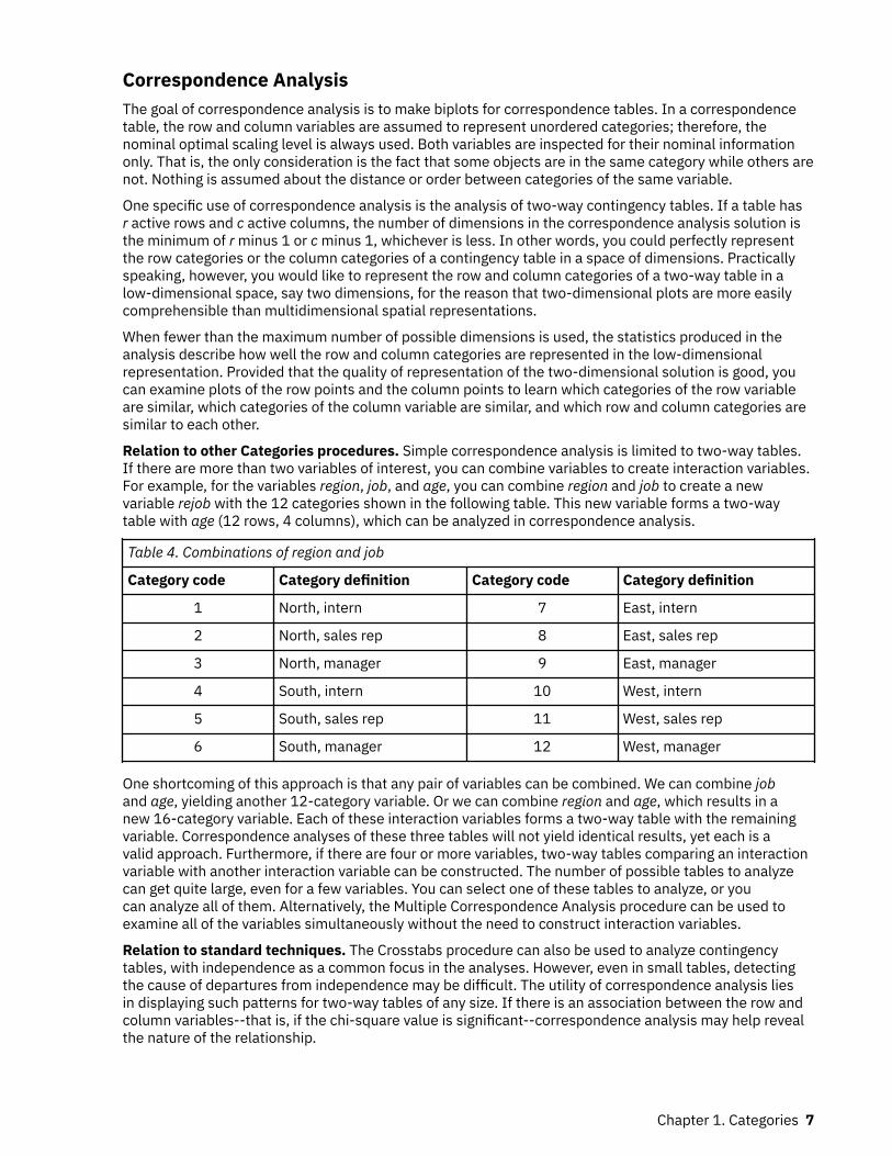
Relation to other Categories procedures. Simple correspondence analysis is limited to two-way tables.If there are more than two variables of interest, you can combine variables to create interaction variables.For example, for the variables region, job, and age, you can combine region and job to create a newvariable rejob with the 12 categories shown in the following table. This new variable forms a two-waytable with age (12 rows, 4 columns), which can be analyzed in correspondence analysis.

Table 4. Combinations of region and job

Category code Category definition Category code Category definition

1 North, intern 7 East, intern

2 North, sales rep 8 East, sales rep

3 North, manager 9 East, manager

4 South, intern 10 West, intern

5 South, sales rep 11 West, sales rep

6 South, manager 12 West, manager

One shortcoming of this approach is that any pair of variables can be combined. We can combine joband age, yielding another 12-category variable. Or we can combine region and age, which results in anew 16-category variable. Each of these interaction variables forms a two-way table with the remainingvariable. Correspondence analyses of these three tables will not yield identical results, yet each is avalid approach. Furthermore, if there are four or more variables, two-way tables comparing an interactionvariable with another interaction variable can be constructed. The number of possible tables to analyzecan get quite large, even for a few variables. You can select one of these tables to analyze, or youcan analyze all of them. Alternatively, the Multiple Correspondence Analysis procedure can be used toexamine all of the variables simultaneously without the need to construct interaction variables.

Relation to standard techniques. The Crosstabs procedure can also be used to analyze contingencytables, with independence as a common focus in the analyses. However, even in small tables, detectingthe cause of departures from independence may be difficult. The utility of correspondence analysis liesin displaying such patterns for two-way tables of any size. If there is an association between the row andcolumn variables--that is, if the chi-square value is significant--correspondence analysis may help revealthe nature of the relationship.


Multiple Correspondence AnalysisMultiple Correspondence Analysis tries to produce a solution in which objects within the same categoryare plotted close together and objects in different categories are plotted far apart. Each object is as closeas possible to the category points of categories that apply to the object. In this way, the categories dividethe objects into homogeneous subgroups. Variables are considered homogeneous when they classifyobjects in the same categories into the same subgroups.

For a one-dimensional solution, multiple correspondence analysis assigns optimal scale values (categoryquantifications) to each category of each variable in such a way that overall, on average, the categorieshave maximum spread. For a two-dimensional solution, multiple correspondence analysis finds a secondset of quantifications of the categories of each variable unrelated to the first set, attempting again tomaximize spread, and so on. Because categories of a variable receive as many scorings as there aredimensions, the variables in the analysis are assumed to be multiple nominal in optimal scaling level.

Multiple correspondence analysis also assigns scores to the objects in the analysis in such a way that thecategory quantifications are the averages, or centroids, of the object scores of objects in that category.

Relation to other Categories procedures. Multiple correspondence analysis is also known ashomogeneity analysis or dual scaling. It gives comparable, but not identical, results to correspondenceanalysis when there are only two variables. Correspondence analysis produces unique outputsummarizing the fit and quality of representation of the solution, including stability information. Thus,correspondence analysis is usually preferable to multiple correspondence analysis in the two-variablecase. Another difference between the two procedures is that the input to multiple correspondenceanalysis is a data matrix, where the rows are objects and the columns are variables, while the input tocorrespondence analysis can be the same data matrix, a general proximity matrix, or a joint contingencytable, which is an aggregated matrix in which both the rows and columns represent categories ofvariables. Multiple correspondence analysis can also be thought of as principal components analysisof data scaled at the multiple nominal level.

Relation to standard techniques. Multiple correspondence analysis can be thought of as the analysisof a multiway contingency table. Multiway contingency tables can also be analyzed with the Crosstabsprocedure, but Crosstabs gives separate summary statistics for each category of each control variable.With multiple correspondence analysis, it is often possible to summarize the relationship between all ofthe variables with a single two-dimensional plot. An advanced use of multiple correspondence analysis isto replace the original category values with the optimal scale values from the first dimension and performa secondary multivariate analysis. Since multiple correspondence analysis replaces category labels withnumerical scale values, many different procedures that require numerical data can be applied after themultiple correspondence analysis. For example, the Factor Analysis procedure produces a first principalcomponent that is equivalent to the first dimension of multiple correspondence analysis. The componentscores in the first dimension are equal to the object scores, and the squared component loadings areequal to the discrimination measures. The second multiple correspondence analysis dimension, however,is not equal to the second dimension of factor analysis.

Multidimensional ScalingThe use of Multidimensional Scaling is most appropriate when the goal of your analysis is to find thestructure in a set of distance measures between a single set of objects or cases. This is accomplished byassigning observations to specific locations in a conceptual low-dimensional space so that the distancesbetween points in the space match the given (dis)similarities as closely as possible. The result is aleast-squares representation of the objects in that low-dimensional space, which, in many cases, will helpyou further understand your data.

Relation to other Categories procedures. When you have multivariate data from which you createdistances and which you then analyze with multidimensional scaling, the results are similar to analyzingthe data using categorical principal components analysis with object principal normalization. This kind ofPCA is also known as principal coordinates analysis.

Relation to standard techniques. The Categories Multidimensional Scaling procedure (PROXSCAL) offersseveral improvements upon the scaling procedure available in the Statistics Base option (ALSCAL).PROXSCAL offers an accelerated algorithm for certain models and allows you to put restrictions on the


common space. Moreover, PROXSCAL attempts to minimize normalized raw stress rather than S-stress(also referred to as strain). The normalized raw stress is generally preferred because it is a measurebased on the distances, while the S-stress is based on the squared distances.

Multidimensional UnfoldingThe use of Multidimensional Unfolding is most appropriate when the goal of your analysis is to findthe structure in a set of distance measures between two sets of objects (referred to as the row andcolumn objects). This is accomplished by assigning observations to specific locations in a conceptuallow-dimensional space so that the distances between points in the space match the given (dis)similaritiesas closely as possible. The result is a least-squares representation of the row and column objects in thatlow-dimensional space, which, in many cases, will help you further understand your data.

Relation to other Categories procedures. If your data consist of distances between a single set ofobjects (a square, symmetrical matrix), use Multidimensional Scaling.

Relation to standard techniques. The Categories Multidimensional Unfolding procedure (PREFSCAL)offers several improvements upon the unfolding functionality available in the Statistics Base option(through ALSCAL). PREFSCAL allows you to put restrictions on the common space; moreover, PREFSCALattempts to minimize a penalized stress measure that helps it to avoid degenerate solutions (to whicholder algorithms are prone).

Aspect Ratio in Optimal Scaling ChartsAspect ratio in optimal scaling plots is isotropic. In a two-dimensional plot, the distance representing oneunit in dimension 1 is equal to the distance representing one unit in dimension 2. If you change the rangeof a dimension in a two-dimensional plot, the system changes the size of the other dimension to keep thephysical distances equal. Isotropic aspect ratio cannot be overridden for the optimal scaling procedures.

Categorical Regression (CATREG)Categorical regression quantifies categorical data by assigning numerical values to the categories,resulting in an optimal linear regression equation for the transformed variables. Categorical regressionis also known by the acronym CATREG, for categorical regression.

Standard linear regression analysis involves minimizing the sum of squared differences betweena response (dependent) variable and a weighted combination of predictor (independent) variables.Variables are typically quantitative, with (nominal) categorical data recoded to binary or contrastvariables. As a result, categorical variables serve to separate groups of cases, and the techniqueestimates separate sets of parameters for each group. The estimated coefficients reflect how changes inthe predictors affect the response. Prediction of the response is possible for any combination of predictorvalues.

An alternative approach involves regressing the response on the categorical predictor values themselves.Consequently, one coefficient is estimated for each variable. However, for categorical variables, thecategory values are arbitrary. Coding the categories in different ways yield different coefficients, makingcomparisons across analyses of the same variables difficult.

CATREG extends the standard approach by simultaneously scaling nominal, ordinal, and numericalvariables. The procedure quantifies categorical variables so that the quantifications reflect characteristicsof the original categories. The procedure treats quantified categorical variables in the same way asnumerical variables. Using nonlinear transformations allow variables to be analyzed at a variety of levelsto find the best-fitting model.

Example. Categorical regression could be used to describe how job satisfaction depends on job category,geographic region, and amount of travel. You might find that high levels of satisfaction correspond tomanagers and low travel. The resulting regression equation could be used to predict job satisfaction forany combination of the three independent variables.


Statistics and plots. Frequencies, regression coefficients, ANOVA table, iteration history, categoryquantifications, correlations between untransformed predictors, correlations between transformedpredictors, residual plots, and transformation plots.

Categorical Regression Data Considerations

Data. CATREG operates on category indicator variables. The category indicators should be positiveintegers. You can use the Discretization dialog box to convert fractional-value variables and stringvariables into positive integers.

Assumptions. Only one response variable is allowed, but the maximum number of predictor variables is200. The data must contain at least three valid cases, and the number of valid cases must exceed thenumber of predictor variables plus one.

Related procedures. CATREG is equivalent to categorical canonical correlation analysis with optimalscaling (OVERALS) with two sets, one of which contains only one variable. Scaling all variables at thenumerical level corresponds to standard multiple regression analysis.

To Obtain a Categorical Regression

1. From the menus choose:

Analyze > Regression > Optimal Scaling (CATREG)...2. Select the dependent variable and independent variable(s).3. Click OK.

Optionally, change the scaling level for each variable.

Define Scale in Categorical RegressionYou can set the optimal scaling level for the dependent and independent variables. By default, they arescaled as second-degree monotonic splines (ordinal) with two interior knots. Additionally, you can set theweight for analysis variables.

Optimal Scaling Level. You can also select the scaling level for quantifying each variable.

• Spline Ordinal. The order of the categories of the observed variable is preserved in the optimallyscaled variable. Category points will be on a straight line (vector) through the origin. The resultingtransformation is a smooth monotonic piecewise polynomial of the chosen degree. The pieces arespecified by the user-specified number and procedure-determined placement of the interior knots.

• Spline Nominal. The only information in the observed variable that is preserved in the optimally scaledvariable is the grouping of objects in categories. The order of the categories of the observed variableis not preserved. Category points will be on a straight line (vector) through the origin. The resultingtransformation is a smooth, possibly nonmonotonic, piecewise polynomial of the chosen degree. Thepieces are specified by the user-specified number and procedure-determined placement of the interiorknots.

• Ordinal. The order of the categories of the observed variable is preserved in the optimally scaledvariable. Category points will be on a straight line (vector) through the origin. The resultingtransformation fits better than the spline ordinal transformation but is less smooth.

• Nominal. The only information in the observed variable that is preserved in the optimally scaledvariable is the grouping of objects in categories. The order of the categories of the observed variableis not preserved. Category points will be on a straight line (vector) through the origin. The resultingtransformation fits better than the spline nominal transformation but is less smooth.

• Numeric. Categories are treated as ordered and equally spaced (interval level). The order of thecategories and the equal distances between category numbers of the observed variable are preservedin the optimally scaled variable. Category points will be on a straight line (vector) through the origin.When all variables are at the numeric level, the analysis is analogous to standard principal componentsanalysis.


Categorical Regression DiscretizationThe Discretization dialog box allows you to select a method of recoding your variables. Fractional-valuevariables are grouped into seven categories (or into the number of distinct values of the variable ifthis number is less than seven) with an approximately normal distribution unless otherwise specified.String variables are always converted into positive integers by assigning category indicators according toascending alphanumeric order. Discretization for string variables applies to these integers. Other variablesare left alone by default. The discretized variables are then used in the analysis.

Method. Choose between grouping, ranking, and multiplying.

• Grouping. Recode into a specified number of categories or recode by interval.• Ranking. The variable is discretized by ranking the cases.• Multiplying. The current values of the variable are standardized, multiplied by 10, rounded, and have a

constant added so that the lowest discretized value is 1.

Grouping. The following options are available when discretizing variables by grouping:

• Number of categories. Specify a number of categories and whether the values of the variable shouldfollow an approximately normal or uniform distribution across those categories.

• Equal intervals. Variables are recoded into categories defined by these equally sized intervals. Youmust specify the length of the intervals.

Categorical Regression Missing ValuesThe Missing Values dialog box allows you to choose the strategy for handling missing values in analysisvariables and supplementary variables.

Strategy. Choose to exclude objects with missing values (listwise deletion) or impute missing values(active treatment).

• Exclude objects with missing values on this variable. Objects with missing values on the selectedvariable are excluded from the analysis. This strategy is not available for supplementary variables.

• Impute missing values. Objects with missing values on the selected variable have those valuesimputed. You can choose the method of imputation. Select Mode to replace missing values with themost frequent category. When there are multiple modes, the one with the smallest category indicator isused. Select Extra category to replace missing values with the same quantification of an extra category.This implies that objects with a missing value on this variable are considered to belong to the same(extra) category.

Categorical Regression OptionsThe Options dialog box allows you to select the initial configuration style, specify iteration andconvergence criteria, select supplementary objects, and set the labeling of plots.

Supplementary Objects. This allows you to specify the objects that you want to treat as supplementary.Simply type the number of a supplementary object (or specify a range of cases) and click Add. You cannotweight supplementary objects (specified weights are ignored).

Initial Configuration. If no variables are treated as nominal, select the Numerical configuration. If atleast one variable is treated as nominal, select the Random configuration.

Alternatively, if at least one variable has an ordinal or spline ordinal scaling level, the usual model-fittingalgorithm can result in a suboptimal solution. Choosing Multiple systematic starts with all possible signpatterns to test will always find the optimal solution, but the necessary processing time rapidly increasesas the number of ordinal and spline ordinal variables in the dataset increase. You can reduce the numberof test patterns by specifying a percentage of loss of variance threshold, where the higher the threshold,the more sign patterns will be excluded. With this option, obtaining the optimal solution is not garantueed,but the chance of obtaining a suboptimal solution is diminished. Also, if the optimal solution is not found,the chance that the suboptimal solution is very different from the optimal solution is diminished. Whenmultiple systematic starts are requested, the signs of the regression coefficients for each start are written


to an external IBM SPSS Statistics data file or dataset in the current session. See the topic “CategoricalRegression Save” on page 13 for more information.

The results of a previous run with multiple systematic starts allows you to Use fixed signs for theregression coefficients. The signs (indicated by 1 and −1) need to be in a row of the specified dataset orfile. The integer-valued starting number is the case number of the row in this file that contains the signs tobe used.

Criteria. You can specify the maximum number of iterations that the regression may go through in itscomputations. You can also select a convergence criterion value. The regression stops iterating if thedifference in total fit between the last two iterations is less than the convergence value or if the maximumnumber of iterations is reached.

Label Plots By. Allows you to specify whether variables and value labels or variable names and values willbe used in the plots. You can also specify a maximum length for labels.

Categorical Regression RegularizationMethod. Regularization methods can improve the predictive error of the model by reducing the variabilityin the estimates of regression coefficient by shrinking the estimates toward 0. The Lasso and Elastic Netwill shrink some coefficient estimates to exactly 0, thus providing a form of variable selection. When aregularization method is requested, the regularized model and coefficients for each penalty coefficientvalue are written to an external IBM SPSS Statistics data file or dataset in the current session. See thetopic “Categorical Regression Save” on page 13 for more information.

• Ridge regression. Ridge regression shrinks coefficients by introducing a penalty term equal to the sumof squared coefficients times a penalty coefficient. This coefficient can range from 0 (no penalty) to 1;the procedure will search for the "best" value of the penalty if you specify a range and increment.

• Lasso. The Lasso's penalty term is based on the sum of absolute coefficients, and the specification ofa penalty coefficient is similar to that of Ridge regression; however, the Lasso is more computationallyintensive.

• Elastic net. The Elastic Net simply combines the Lasso and Ridge regression penalties, and will searchover the grid of values specified to find the "best" Lasso and Ridge regression penalty coefficients. Fora given pair of Lasso and Ridge regression penalties, the Elastic Net is not much more computationallyexpensive than the Lasso.

Display regularization plots. These are plots of the regression coefficients versus the regularizationpenalty. When searching a range of values for the "best" penalty coefficient, it provides a view of how theregression coefficients change over that range.

Elastic Net Plots. For the Elastic Net method, separate regularization plots are produced by values of theRidge regression penalty. All possible plots uses every value in the range determined by the minimumand maximum Ridge regression penalty values specified. For some Ridge penalties allows you to specifya subset of the values in the range determined by the minimum and maximum. Simply type the number ofa penalty value (or specify a range of values) and click Add.

Categorical Regression OutputThe Output dialog box allows you to select the statistics to display in the output.

Tables. Produces tables for:

• Multiple R. Includes R 2, adjusted R 2, and adjusted R 2 taking the optimal scaling into account.• ANOVA. This option includes regression and residual sums of squares, mean squares, and F. Two

ANOVA tables are displayed: one with degrees of freedom for the regression equal to the number ofpredictor variables and one with degrees of freedom for the regression taking the optimal scaling intoaccount.

• Coefficients. This option gives three tables: a Coefficients table that includes betas, standard error ofthe betas, t values, and significance; a Coefficients-Optimal Scaling table with the standard error ofthe betas taking the optimal scaling degrees of freedom into account; and a table with the zero-order,


part, and partial correlation, Pratt's relative importance measure for the transformed predictors, and thetolerance before and after transformation.

• Iteration history. For each iteration, including the starting values for the algorithm, the multiple R andregression error are shown. The increase in multiple R is listed starting from the first iteration.

• Correlations of original variables. A matrix showing the correlations between the untransformedvariables is displayed.

• Correlations of transformed variables. A matrix showing the correlations between the transformedvariables is displayed.

• Regularized models and coefficients. Displays penalty values, R-square, and the regressioncoefficients for each regularized model. If a resampling method is specified or if supplementary objects(test cases) are specified, it also displays the prediction error or test MSE.

Resampling. Resampling methods give you an estimate of the prediction error of the model.

• Crossvalidation. Crossvalidation divides the sample into a number of subsamples, or folds. Categoricalregression models are then generated, excluding the data from each subsample in turn. The first modelis based on all of the cases except those in the first sample fold, the second model is based on all ofthe cases except those in the second sample fold, and so on. For each model, the prediction error isestimated by applying the model to the subsample excluded in generating it.

• .632 Bootstrap. With the bootstrap, observations are drawn randomly from the data with replacement,repeating this process a number of times to obtain a number bootstrap samples. A model is fit for eachbootstrap sample. The prediction error for each model is estimated by applying the fitted model to thecases not in the bootstrap sample.

Category Quantifications. Tables showing the transformed values of the selected variables are displayed.

Descriptive Statistics. Tables showing the frequencies, missing values, and modes of the selectedvariables are displayed.

Categorical Regression SaveThe Save dialog box allows you to save predicted values, residuals, and transformed values to the activedataset and/or save discretized data, transformed values, regularized models and coefficients, and signsof regression coefficients to an external IBM SPSS Statistics data file or dataset in the current session.

• Datasets are available during the current session but are not available in subsequent sessions unlessyou explicitly save them as data files. Dataset names must adhere to variable naming rules.

• Filenames or dataset names must be different for each type of data saved.

Regularized models and coefficients are saved whenever a regularization method is selected on theRegularization dialog. By default, the procedure creates a new dataset with a unique name, but you can ofcourse specify a name of your own choosing or write to an external file.

Signs of regression coefficients are saved whenever multiple systematic starts are used as the initialconfiguration on the Options dialog. By default, the procedure creates a new dataset with a unique name,but you can of course specify a name of your own choosing or write to an external file.

Categorical Regression Transformation PlotsThe Plots dialog box allows you to specify the variables that will produce transformation and residualplots.

Transformation Plots. For each of these variables, the category quantifications are plotted againstthe original category values. Empty categories appear on the horizontal axis but do not affect thecomputations. These categories are identified by breaks in the line connecting the quantifications.

Residual Plots. For each of these variables, residuals (computed for the dependent variable predictedfrom all predictor variables except the predictor variable in question) are plotted against categoryindicators and the optimal category quantifications multiplied with beta against category indicators.


CATREG Command Additional FeaturesYou can customize your categorical regression if you paste your selections into a syntax window and editthe resulting CATREG command syntax. The command syntax language also allows you to:

• Specify rootnames for the transformed variables when saving them to the active dataset (with the SAVEsubcommand).

See the Command Syntax Reference for complete syntax information.

Categorical Principal Components Analysis (CATPCA)This procedure simultaneously quantifies categorical variables while reducing the dimensionality of thedata. Categorical principal components analysis is also known by the acronym CATPCA, for categoricalprincipal components analysis.

The goal of principal components analysis is to reduce an original set of variables into a smaller set ofuncorrelated components that represent most of the information found in the original variables. Thetechnique is most useful when a large number of variables prohibits effective interpretation of therelationships between objects (subjects and units). By reducing the dimensionality, you interpret a fewcomponents rather than a large number of variables.

Standard principal components analysis assumes linear relationships between numeric variables. On theother hand, the optimal-scaling approach allows variables to be scaled at different levels. Categoricalvariables are optimally quantified in the specified dimensionality. As a result, nonlinear relationshipsbetween variables can be modeled.

Example. Categorical principal components analysis could be used to graphically display the relationshipbetween job category, job division, region, amount of travel (high, medium, and low), and job satisfaction.You might find that two dimensions account for a large amount of variance. The first dimension mightseparate job category from region, whereas the second dimension might separate job division fromamount of travel. You also might find that high job satisfaction is related to a medium amount of travel.

Statistics and plots. Frequencies, missing values, optimal scaling level, mode, variance accounted for bycentroid coordinates, vector coordinates, total per variable and per dimension, component loadings forvector-quantified variables, category quantifications and coordinates, iteration history, correlations of thetransformed variables and eigenvalues of the correlation matrix, correlations of the original variables andeigenvalues of the correlation matrix, object scores, category plots, joint category plots, transformationplots, residual plots, projected centroid plots, object plots, biplots, triplots, and component loadingsplots.

Categorical Principal Components Analysis Data Considerations

Data. String variable values are always converted into positive integers by ascending alphanumeric order.User-defined missing values, system-missing values, and values less than 1 are considered missing; youcan recode or add a constant to variables with values less than 1 to make them nonmissing.

Assumptions. The data must contain at least three valid cases. The analysis is based on positive integerdata. The discretization option will automatically categorize a fractional-valued variable by grouping itsvalues into categories with a close to "normal" distribution and will automatically convert values of stringvariables into positive integers. You can specify other discretization schemes.

Related procedures. Scaling all variables at the numeric level corresponds to standard principalcomponents analysis. Alternate plotting features are available by using the transformed variables ina standard linear principal components analysis. If all variables have multiple nominal scaling levels,categorical principal components analysis is identical to multiple correspondence analysis. If sets ofvariables are of interest, categorical (nonlinear) canonical correlation analysis should be used.

To Obtain a Categorical Principal Components Analysis


Analyze > Dimension Reduction > Optimal Scaling...2. Select Some variable(s) not multiple nominal.


3. Select One set.4. Click Define.5. Select at least two analysis variables and specify the number of dimensions in the solution.6. Click OK.

You may optionally specify supplementary variables, which are fitted into the solution found, or labelingvariables for the plots.

Define Scale and Weight in CATPCAYou can set the optimal scaling level for analysis variables and supplementary variables. By default, theyare scaled as second-degree monotonic splines (ordinal) with two interior knots. Additionally, you can setthe weight for analysis variables.

Variable weight. You can choose to define a weight for each variable. The value specified must be apositive integer. The default value is 1.

Optimal Scaling Level. You can also select the scaling level to be used to quantify each variable.

• Spline ordinal. The order of the categories of the observed variable is preserved in the optimallyscaled variable. Category points will be on a straight line (vector) through the origin. The resultingtransformation is a smooth monotonic piecewise polynomial of the chosen degree. The pieces arespecified by the user-specified number and procedure-determined placement of the interior knots.

• Spline nominal. The only information in the observed variable that is preserved in the optimally scaledvariable is the grouping of objects in categories. The order of the categories of the observed variableis not preserved. Category points will be on a straight line (vector) through the origin. The resultingtransformation is a smooth, possibly nonmonotonic, piecewise polynomial of the chosen degree. Thepieces are specified by the user-specified number and procedure-determined placement of the interiorknots.

• Multiple nominal. The only information in the observed variable that is preserved in the optimallyscaled variable is the grouping of objects in categories. The order of the categories of the observedvariable is not preserved. Category points will be in the centroid of the objects in the particularcategories. Multiple indicates that different sets of quantifications are obtained for each dimension.

• Ordinal. The order of the categories of the observed variable is preserved in the optimally scaledvariable. Category points will be on a straight line (vector) through the origin. The resultingtransformation fits better than the spline ordinal transformation but is less smooth.

• Nominal. The only information in the observed variable that is preserved in the optimally scaledvariable is the grouping of objects in categories. The order of the categories of the observed variableis not preserved. Category points will be on a straight line (vector) through the origin. The resultingtransformation fits better than the spline nominal transformation but is less smooth.

• Numeric. Categories are treated as ordered and equally spaced (interval level). The order of thecategories and the equal distances between category numbers of the observed variable are preservedin the optimally scaled variable. Category points will be on a straight line (vector) through the origin.When all variables are at the numeric level, the analysis is analogous to standard principal componentsanalysis.

Categorical Principal Components Analysis DiscretizationThe Discretization dialog box allows you to select a method of recoding your variables. Fractional-valuedvariables are grouped into seven categories (or into the number of distinct values of the variable ifthis number is less than seven) with an approximately normal distribution, unless specified otherwise.String variables are always converted into positive integers by assigning category indicators according toascending alphanumeric order. Discretization for string variables applies to these integers. Other variablesare left alone by default. The discretized variables are then used in the analysis.


• Grouping. Recode into a specified number of categories or recode by interval.


• Ranking. The variable is discretized by ranking the cases.• Multiplying. The current values of the variable are standardized, multiplied by 10, rounded, and have a

constant added such that the lowest discretized value is 1.

Grouping. The following options are available when you are discretizing variables by grouping:



Categorical Principal Components Analysis Missing ValuesUse the Missing Values dialog box to choose the strategy for handling missing values in analysis variablesand supplementary variables.

Strategy. Choose to exclude missing values (passive treatment), impute missing values (activetreatment), or exclude objects with missing values (listwise deletion).

• Exclude missing values; for correlations impute after quantification. Objects with missing valueson the selected variable do not contribute to the analysis for this variable. If all variables are givenpassive treatment, then objects with missing values on all variables are treated as supplementary. Ifcorrelations are specified in the Output dialog box, then (after analysis) missing values are imputed withthe most frequent category, or mode, of the variable for the correlations of the original variables. For thecorrelations of the optimally scaled variables, you can choose the method of imputation.

– Mode. Replace missing values with the mode of the optimally scaled variable.– Extra category. Replace missing values with the quantification of an extra category. This setting

implies that objects with a missing value on this variable are considered to belong to the same (extra)category.

– Random category. Impute each missing value on a variable with the quantified value of a differentrandom category number based on the marginal frequencies of the categories of the variable.

• Impute missing values. Objects with missing values on the selected variable have those valuesimputed. You can choose the method of imputation.

– Mode. Replace missing values with the most frequent category. When there are multiple modes, theone with the smallest category indicator is used.

– Extra category. Replace missing values with the same quantification of an extra category. Thissetting implies that objects with a missing value on this variable are considered to belong to the same(extra) category.

– Random category. Replace each missing value on a variable with a different random categorynumber based on the marginal frequencies of the categories.


Categorical Principal Components Analysis OptionsThe Options dialog box provides controls to select the initial configuration, specify iteration andconvergence criteria, select a normalization method, choose the method for labeling plots, and specifysupplementary objects.

Supplementary Objects. Specify the case number of the object, or the first and last case numbers of arange of objects, that you want to make supplementary and then click Add. If an object is specified assupplementary, then case weights are ignored for that object.

Normalization Method. You can specify one of five options for normalizing the object scores and thevariables. Only one normalization method can be used in each analysis.

• Variable Principal. This option optimizes the association between variables. The coordinates of thevariables in the object space are the component loadings (correlations with principal components,


such as dimensions and object scores). This method is useful when you are primarily interested in thecorrelation between the variables.

• Object Principal. This option optimizes distances between objects. This method is useful when you areprimarily interested in differences or similarities between the objects.

• Symmetrical. Use this normalization option if you are primarily interested in the relation betweenobjects and variables.

• Independent. Use this normalization option if you want to examine distances between objects andcorrelations between variables separately.

• Custom. You can specify any real value in the closed interval [–1, 1]. A value of 1 is equal to the ObjectPrincipal method. A value of 0 is equal to the Symmetrical method. A value of –1 is equal to the VariablePrincipal method. By specifying a value greater than –1 and less than 1, you can spread the eigenvalueover both objects and variables. This method is useful for making a tailor-made biplot or triplot.

Criteria. You can specify the maximum number of iterations the procedure can go through in itscomputations. You can also select a convergence criterion value. The algorithm stops iterating if thedifference in total fit between the last two iterations is less than the convergence value or if the maximumnumber of iterations is reached.

Label Plots By. You can specify whether variables and value labels or variable names and values are usedin the plots. You can also specify a maximum length for labels.

Plot Dimensions. You can control the dimensions that are displayed in the output.

• Display all dimensions in the solution. All dimensions in the solution are displayed in a scatterplotmatrix.

• Restrict the number of dimensions. The displayed dimensions are restricted to plotted pairs. If yourestrict the dimensions, you must select the lowest and highest dimensions to be plotted. The lowestdimension can range from 1 to the number of dimensions in the solution minus 1 and is plottedagainst higher dimensions. The highest dimension value can range from 2 to the number of dimensionsin the solution and indicates the highest dimension to be used in plotting the dimension pairs. Thisspecification applies to all requested multidimensional plots.

Rotation. You can select a rotation method to obtain rotated results.

Note: These rotation methods are not available if you select Perform bootstrapping in the Bootstrapdialog.

• Varimax. An orthogonal rotation method that minimizes the number of variables that have high loadingson each component. It simplifies the interpretation of the components.

• Quartimax. A rotation method that minimizes the number of components that are needed to explaineach variable. It simplifies the interpretation of the observed variables.

• Equamax. A rotation method that is a combination of the Varimax method, which simplifies thecomponents, and the Quartimax method, which simplifies the variables. The number of variables thatload highly on a component and the number of components that are needed to explain a variable areminimized.

• Oblimin. A method for oblique (non-orthogonal) rotation. When delta equals 0, components are mostoblique. As delta becomes more negative, the components become less oblique. Positive values permitadditional component correlation. The value of Delta must be less than or equal to 0.8.

• Promax. An oblique (non-orthogonal) rotation, which allows components to be correlated. It can becalculated more quickly than a direct Oblimin rotation, so it is useful for large datasets. The amount ofcorrelation (obliqueness) that is allowed is controlled by the kappa parameter. The value of Kappa mustbe greater than or equal to 1 and less 10,000.

Configuration. You can read data from a file that contains the coordinates of a configuration. The firstvariable in the file contains the coordinates for the first dimension. The second variable contains thecoordinates for the second dimension, and so on.

• Initial. The configuration in the file that is specified is used as the starting point of the analysis.


• Fixed. The configuration in the file that is specified is used to fit in the variables. The variables that arefitted in must be selected as analysis variables, but because the configuration is fixed, they are treatedas supplementary variables (so they do not need to be selected as supplementary variables).

Categorical Principal Components Analysis OutputThe Output dialog box controls the display of results.

Object scores. Displays the object scores and has the following options:

• Include Categories Of. Displays the category indicators of the analysis variables selected.• Label Object Scores By. From the list of variables that are specified as labeling variables, you can select

one to label the objects.

Component loadings. Displays the component loadings for all variables that were not given multiplenominal scaling levels. You can sort the component loadings by size.

Iteration history. For each iteration, the variance accounted for, loss, and increase in variance accountedfor are shown.

Correlations of original variables. Shows the correlation matrix of the original variables and theeigenvalues of that matrix.

Correlations of transformed variables. Shows the correlation matrix of the transformed (optimallyscaled) variables and the eigenvalues of that matrix.

Variance accounted for. Displays the amount of variance accounted for by centroid coordinates, vectorcoordinates, and total (centroid and vector coordinates combined) per variable and per dimension.

Category Quantifications. Gives the category quantifications and coordinates for each dimension of thevariables that are selected.

Descriptive Statistics. Displays frequencies, number of missing values, and mode of the variables thatare selected.

Categorical Principal Components Analysis SaveThe controls in the Save dialog box save discretized data, object scores, transformed values, and otherresults to the active dataset, a new dataset in the current session, or an external file.


• Filenames or dataset names must be different for each type of data saved.• If you save object scores or transformed values to the active dataset, you can specify the number of

multiple nominal dimensions.• The options in the Bootstrap Confidence Ellipses group are only available if you select Perform

bootstrapping in the Bootstrap dialog.

Categorical Principal Components Analysis Object PlotsThe Object and Variable Plots dialog box allows you to specify the types of plots you want and thevariables for which plots will be produced.

Object points. A plot of the object points is displayed.

Objects and variables (biplot). The object points are plotted with your choice of the variablecoordinates--component loadings or variable centroids.

Objects, loadings, and centroids (triplot). The object points are plotted with the centroids of multiplenominal-scaling-level variables and the component loadings of other variables.

Biplot and Triplot Variables. You can choose to use all variables for the biplots and triplots or select asubset.


Label Objects. You can choose to have objects labeled with the categories of selected variables (you maychoose category indicator values or value labels in the Options dialog box) or with their case numbers.One plot is produced per variable if Variable is selected.

Categorical Principal Components Analysis Category PlotsThe Category Plots dialog box allows you to specify the types of plots you want and the variables forwhich plots will be produced.

Category Plots. For each variable selected, a plot of the centroid and vector coordinates is plotted.For variables with multiple nominal scaling levels, categories are in the centroids of the objects in theparticular categories. For all other scaling levels, categories are on a vector through the origin.

Joint Category Plots. This is a single plot of the centroid and vector coordinates of each selectedvariable.

Transformation Plots. Displays a plot of the optimal category quantifications versus the categoryindicators. You can specify the number of dimensions for variables with multiple nominal scaling levels;one plot will be generated for each dimension. You can also choose to display residual plots for eachvariable selected.

Project Centroids Of. You may choose a variable and project its centroids onto selected variables.Variables with multiple nominal scaling levels cannot be selected to project on. When this plot isrequested, a table with the coordinates of the projected centroids is also displayed.

Categorical Principal Components Analysis Loading PlotsThe Loading Plots dialog box controls the variables that are included in the plot, display of centroids in theloadings plot, and display of plots of variance accounted for.

Variance accounted for. For each dimension, displays a plot of variance accounted for.

Display component loadings. If selected, a plot of the component loadings is displayed.

Loading Variables. You can choose to use all variables for the component loadings plot or select a subset.

Include centroids. Variables with multiple nominal scaling levels do not have component loadings, butyou can choose to include the centroids of those variables in the plot. You can choose to use all multiplenominal variables or select a subset.

Categorical Principal Components Analysis BootstrapThe Bootstrap dialog specifies parameters for bootstrap analysis.

Perform bootstrapping. Performs bootstrap resampling.

• If plots of loadings, categories, or component scores are requested, extra plots are displayed. Theseplots display the points for the data sample and the bootstrap estimates. Transformation plots includeconfidence regions. A plot for the eigenvalues is also displayed.

• If a two-dimensional solution is specified, confidence ellipse plots for the eigenvalues, the componentloadings, the category points, and the object points are displayed.

• Bootstrap resampling is not available if you specify a rotation method in the Options dialog.

You can select Balanced or Unbalanced bootstrapping.

Number of samples. The number of bootstrap samples that are used to calculate the bootstrapestimates. The value must be a positive integer.

Confidence level. The confidence level of the bootstrap estimates, expressed as a percentage. The valuemust a be a positive number less than 100.

Matching Method. The two alternatives are Procrustes and Reflection.

Confidence Ellipses. Controls the threshold area for confidence ellipses in plots. For areas greater than (>operator) the specified value, the number of ellipses decreases as the threshold value increases.


• The settings in this group are only available if the number of dimensions that are specified on the maindialog is 2.

• Confidence ellipses for loading plots are available only if Display component loadings is selected in theLoading Plots dialog.

• Confidence ellipses for object plots are available only if Object points is selected in the Object andVariable Plots dialog.

• Confidence ellipses for category plots are available only if one or more variables are specified in theCategory Plots list in the Category Plots dialog.

Number of ellipse contour points. The number of plot points used to draw each confidence ellipse.Larger values produce smoother ellipses. The value must be a positive integer less than or equal to 100.

CATPCA Command Additional FeaturesYou can customize your categorical principal components analysis if you paste your selections into asyntax window and edit the resulting CATPCA command syntax. The command syntax language alsoallows you to:

• Specify rootnames for the transformed variables, object scores, and approximations when saving themto the active dataset (with the SAVE subcommand).

• Specify a maximum length for labels for each plot separately (with the PLOT subcommand).• Specify a separate variable list for residual plots (with the PLOT subcommand).


Nonlinear Canonical Correlation Analysis (OVERALS)Nonlinear canonical correlation analysis corresponds to categorical canonical correlation analysis withoptimal scaling. The purpose of this procedure is to determine how similar sets of categorical variablesare to one another. Nonlinear canonical correlation analysis is also known by the acronym OVERALS.

Standard canonical correlation analysis is an extension of multiple regression, where the second set doesnot contain a single response variable but instead contain multiple response variables. The goal is toexplain as much as possible of the variance in the relationships among two sets of numerical variablesin a low dimensional space. Initially, the variables in each set are linearly combined such that the linearcombinations have a maximal correlation. Given these combinations, subsequent linear combinations aredetermined that are uncorrelated with the previous combinations and that have the largest correlationpossible.

The optimal scaling approach expands the standard analysis in three crucial ways. First, OVERALS allowsmore than two sets of variables. Second, variables can be scaled as either nominal, ordinal, or numerical.As a result, nonlinear relationships between variables can be analyzed. Finally, instead of maximizingcorrelations between the variable sets, the sets are compared to an unknown compromise set that isdefined by the object scores.

Example. Categorical canonical correlation analysis with optimal scaling could be used to graphicallydisplay the relationship between one set of variables containing job category and years of education andanother set of variables containing region of residence and gender. You might find that years of educationand region of residence discriminate better than the remaining variables. You might also find that years ofeducation discriminates best on the first dimension.

Statistics and plots. Frequencies, centroids, iteration history, object scores, category quantifications,weights, component loadings, single and multiple fit, object scores plots, category coordinates plots,component loadings plots, category centroids plots, transformation plots.

Nonlinear Canonical Correlation Analysis Data Considerations

Data. Use integers to code categorical variables (nominal or ordinal scaling level). To minimize output, useconsecutive integers beginning with 1 to code each variable. Variables that are scaled at the numericallevel should not be recoded to consecutive integers. To minimize output, for each variable that is scaled


at the numerical level, subtract the smallest observed value from every value and add 1. Fractional valuesare truncated after the decimal.

Assumptions. Variables can be classified into two or more sets. Variables in the analysis are scaled asmultiple nominal, single nominal, ordinal, or numerical. The maximum number of dimensions that areused in the procedure depends on the optimal scaling level of the variables. If all variables are specifiedas ordinal, single nominal, or numerical, the maximum number of dimensions is the lesser of the followingtwo values: the number of observations minus 1 or the total number of variables. However, if only twosets of variables are defined, the maximum number of dimensions is the number of variables in thesmaller set. If some variables are multiple nominal, the maximum number of dimensions is the totalnumber of multiple nominal categories plus the number of nonmultiple nominal variables minus thenumber of multiple nominal variables. For example, if the analysis involves five variables, one of whichis multiple nominal with four categories, the maximum number of dimensions is (4 + 4 – 1), or 7. If youspecify a number that is greater than the maximum, the maximum value is used.

Related procedures. If each set contains one variable, nonlinear canonical correlation analysis isequivalent to principal components analysis with optimal scaling. If each of these variables is multiplenominal, the analysis corresponds to multiple correspondence analysis. If two sets of variables areinvolved, and one of the sets contains only one variable, the analysis is identical to categorical regressionwith optimal scaling.

To Obtain a Nonlinear Canonical Correlation Analysis


Analyze > Dimension Reduction > Optimal Scaling...2. Select either All variables multiple nominal or Some variable(s) not multiple nominal.3. Select Multiple sets.4. Click Define.5. Define at least two sets of variables. Select the variable(s) that you want to include in the first set. To

move to the next set, click Next, and select the variables that you want to include in the second set.You can add additional sets. Click Previous to return to the previously defined variable set.

6. Define the value range and measurement scale (optimal scaling level) for each selected variable.7. Click OK.8. Optionally:

• Select one or more variables to provide point labels for object scores plots. Each variable produces aseparate plot, with the points labeled by the values of that variable. You must define a range for each ofthese plot label variables. When you are using the dialog box, a single variable cannot be used both inthe analysis and as a labeling variable. If you want to label the object scores plot with a variable that isused in the analysis, use the Compute facility (available from the Transform menu) to create a copy ofthat variable. Use the new variable to label the plot. Alternatively, command syntax can be used.

• Specify the number of dimensions that you want in the solution. In general, choose as few dimensionsas needed to explain most of the variation. If the analysis involves more than two dimensions, three-dimensional plots of the first three dimensions are produced. Other dimensions can be displayed byediting the chart.

Define Range and ScaleYou must define a range for each variable. The maximum value that is specified must be an integer.Fractional data values are truncated in the analysis. A category value that is outside of the specifiedrange is ignored in the analysis. To minimize output, use the Automatic Recode facility (available fromthe Transform menu) to create consecutive categories beginning with 1 for variables that are treated asnominal or ordinal. Recoding to consecutive integers is not recommended for variables that are scaledat the numerical level. To minimize output for variables that are treated as numerical, for each variable,subtract the minimum value from every value and add 1.

You must also select the scaling to be used to quantify each variable.


• Ordinal. The order of the categories of the observed variable is preserved in the quantified variable.• Single nominal. In the quantified variable, objects in the same category receive the same score.• Multiple nominal. The quantifications can be different for each dimension.• Discrete numeric. Categories are treated as ordered and equally spaced. The differences between

category numbers and the order of the categories of the observed variable are preserved in thequantified variable.

Define RangeYou must define a range for each variable. The maximum value that is specified must be an integer.Fractional data values are truncated in the analysis. A category value that is outside of the specifiedrange is ignored in the analysis. To minimize output, use the Automatic Recode facility (available from theTransform menu) to create consecutive categories beginning with 1.

You must also define a range for each variable that is used to label the object scores plots. However,labels for categories with data values that are outside of the defined range for the variable do appear onthe plots.

Nonlinear Canonical Correlation Analysis OptionsThe Options dialog box allows you to select optional statistics and plots, save object scores asnew variables in the active dataset, specify iteration and convergence criteria, and specify an initialconfiguration for the analysis.

Display. Available statistics include marginal frequencies (counts), centroids, iteration history, weightsand component loadings, category quantifications, object scores, and single and multiple fit statistics.

• Centroids. Category quantifications, and the projected and the actual averages of the object scores forthe objects (cases) included in each set for those cases belonging to the same category of the variable.

• Weights and component loadings. The regression coefficients in each dimension for every quantifiedvariable in a set, where the object scores are regressed on the quantified variables, and the projectionof the quantified variable in the object space. Provides an indication of the contribution each variablemakes to the dimension within each set.

• Single and multiple fit. Measures of goodness of fit of the single- and multiple-category coordinates/category quantifications with respect to the objects.

• Category quantifications. Optimal scale values assigned to the categories of a variable.• Object scores. Optimal score assigned to an object (case) in a particular dimension.

Plot. You can produce plots of category coordinates, object scores, component loadings, categorycentroids, and transformations.

Save object scores. You can save the object scores as new variables in the active dataset. Object scoresare saved for the number of dimensions that are specified in the main dialog box.

Use random initial configuration. A random initial configuration should be used if some or all of thevariables are single nominal. If this option is not selected, a nested initial configuration is used.

Criteria. You can specify the maximum number of iterations that the nonlinear canonical correlationanalysis can go through in its computations. You can also select a convergence criterion value. Theanalysis stops iterating if the difference in total fit between the last two iterations is less than theconvergence value or if the maximum number of iterations is reached.

OVERALS Command Additional FeaturesYou can customize your nonlinear canonical correlation analysis if you paste your selections into a syntaxwindow and edit the resulting OVERALS command syntax. The command syntax language also allows youto:


• Specify the dimension pairs to be plotted, rather than plotting all extracted dimensions (using theNDIMkeyword on the PLOT subcommand).

• Specify the number of value label characters that are used to label points on the plots (with thePLOTsubcommand).

• Designate more than five variables as labeling variables for object scores plots (with thePLOTsubcommand).

• Select variables that are used in the analysis as labeling variables for the object scores plots (with thePLOT subcommand).

• Select variables to provide point labels for the quantification score plot (with the PLOT subcommand).• Specify the number of cases to be included in the analysis if you do not want to use all cases in the

active dataset (with the NOBSERVATIONS subcommand).• Specify rootnames for variables created by saving object scores (with the SAVE subcommand).• Specify the number of dimensions to be saved, rather than saving all extracted dimensions (with theSAVE subcommand).

• Write category quantifications to a matrix file (using the MATRIX subcommand).• Produce low-resolution plots that may be easier to read than the usual high-resolution plots (using theSET command).

• Produce centroid and transformation plots for specified variables only (with the PLOT subcommand).


Correspondence AnalysisOne of the goals of correspondence analysis is to describe the relationships between two nominalvariables in a correspondence table in a low-dimensional space, while simultaneously describing therelationships between the categories for each variable. For each variable, the distances between categorypoints in a plot reflect the relationships between the categories with similar categories plotted close toeach other. Projecting points for one variable on the vector from the origin to a category point for the othervariable describe the relationship between the variables.

An analysis of contingency tables often includes examining row and column profiles and testing forindependence via the chi-square statistic. However, the number of profiles can be quite large, and the chi-square test does not reveal the dependence structure. The Crosstabs procedure offers several measuresof association and tests of association but cannot graphically represent any relationships between thevariables.

Factor analysis is a standard technique for describing relationships between variables in a low-dimensional space. However, factor analysis requires interval data, and the number of observationsshould be five times the number of variables. Correspondence analysis, on the other hand, assumesnominal variables and can describe the relationships between categories of each variable, as well as therelationship between the variables. In addition, correspondence analysis can be used to analyze any tableof positive correspondence measures.

Example. Correspondence analysis could be used to graphically display the relationship between staffcategory and smoking habits. You might find that with regard to smoking, junior managers differ fromsecretaries, but secretaries do not differ from senior managers. You might also find that heavy smoking isassociated with junior managers, whereas light smoking is associated with secretaries.

Statistics and plots. Correspondence measures, row and column profiles, singular values, row andcolumn scores, inertia, mass, row and column score confidence statistics, singular value confidencestatistics, transformation plots, row point plots, column point plots, and biplots.

Correspondence Analysis Data Considerations

Data. Categorical variables to be analyzed are scaled nominally. For aggregated data or for acorrespondence measure other than frequencies, use a weighting variable with positive similarity values.Alternatively, for table data, use syntax to read the table.


Assumptions. The maximum number of dimensions used in the procedure depends on the number ofactive rows and column categories and the number of equality constraints. If no equality constraintsare used and all categories are active, the maximum dimensionality is one fewer than the number ofcategories for the variable with the fewest categories. For example, if one variable has five categories andthe other has four, the maximum number of dimensions is three. Supplementary categories are not active.For example, if one variable has five categories, two of which are supplementary, and the other variablehas four categories, the maximum number of dimensions is two. Treat all sets of categories that areconstrained to be equal as one category. For example, if a variable has five categories, three of which areconstrained to be equal, that variable should be treated as having three categories when determining themaximum dimensionality. Two of the categories are unconstrained, and the third category corresponds tothe three constrained categories. If you specify a number of dimensions greater than the maximum, themaximum value is used.

Related procedures. If more than two variables are involved, use multiple correspondence analysis. Ifthe variables should be scaled ordinally, use categorical principal components analysis.

To Obtain a Correspondence Analysis


Analyze > Dimension Reduction > Correspondence Analysis...2. Select a row variable.3. Select a column variable.4. Define the ranges for the variables.5. Click OK.

Define Row Range in Correspondence AnalysisYou must define a range for the row variable. The minimum and maximum values specified must beintegers. Fractional data values are truncated in the analysis. A category value that is outside of thespecified range is ignored in the analysis.

All categories are initially unconstrained and active. You can constrain row categories to equal other rowcategories, or you can define a row category as supplementary.

• Categories must be equal. Categories must have equal scores. Use equality constraints if the obtainedorder for the categories is undesirable or counterintuitive. The maximum number of row categories thatcan be constrained to be equal is the total number of active row categories minus 1. To impose differentequality constraints on sets of categories, use syntax. For example, use syntax to constrain categories 1and 2 to be equal and categories 3 and 4 to be equal.

• Category is supplemental. Supplementary categories do not influence the analysis but are representedin the space defined by the active categories. Supplementary categories play no role in definingthe dimensions. The maximum number of supplementary row categories is the total number of rowcategories minus 2.

Define Column Range in Correspondence AnalysisYou must define a range for the column variable. The minimum and maximum values specified mustbe integers. Fractional data values are truncated in the analysis. A category value that is outside of thespecified range is ignored in the analysis.

All categories are initially unconstrained and active. You can constrain column categories to equal othercolumn categories, or you can define a column category as supplementary.

• Categories must be equal. Categories must have equal scores. Use equality constraints if the obtainedorder for the categories is undesirable or counterintuitive. The maximum number of column categoriesthat can be constrained to be equal is the total number of active column categories minus 1. To imposedifferent equality constraints on sets of categories, use syntax. For example, use syntax to constraincategories 1 and 2 to be equal and categories 3 and 4 to be equal.


• Category is supplemental. Supplementary categories do not influence the analysis but are representedin the space defined by the active categories. Supplementary categories play no role in defining thedimensions. The maximum number of supplementary column categories is the total number of columncategories minus 2.

Correspondence Analysis ModelThe Model dialog box allows you to specify the number of dimensions, the distance measure, thestandardization method, and the normalization method.

Dimensions in solution. Specify the number of dimensions. In general, choose as few dimensions asneeded to explain most of the variation. The maximum number of dimensions depends on the numberof active categories used in the analysis and on the equality constraints. The maximum number ofdimensions is the smaller of:

• The number of active row categories minus the number of row categories constrained to be equal, plusthe number of constrained row category sets.

• The number of active column categories minus the number of column categories constrained to beequal, plus the number of constrained column category sets.

Distance Measure. You can select the measure of distance among the rows and columns of thecorrespondence table. Choose one of the following alternatives:

• Chi-square. Use a weighted profile distance, where the weight is the mass of the rows or columns. Thismeasure is required for standard correspondence analysis.

• Euclidean. Use the square root of the sum of squared differences between pairs of rows and pairs ofcolumns.

Standardization Method. Choose one of the following alternatives:

• Row and column means are removed. Both the rows and columns are centered. This method isrequired for standard correspondence analysis.

• Row means are removed. Only the rows are centered.• Column means are removed. Only the columns are centered.• Row totals are equalized and means are removed. Before centering the rows, the row margins are

equalized.• Column totals are equalized and means are removed. Before centering the columns, the column

margins are equalized.

Normalization Method. Choose one of the following alternatives:

• Symmetrical. For each dimension, the row scores are the weighted average of the column scoresdivided by the matching singular value, and the column scores are the weighted average of row scoresdivided by the matching singular value. Use this method if you want to examine the differences orsimilarities between the categories of the two variables.

• Principal. The distances between row points and column points are approximations of the distances inthe correspondence table according to the selected distance measure. Use this method if you want toexamine differences between categories of either or both variables instead of differences between thetwo variables.

• Row principal. The distances between row points are approximations of the distances in thecorrespondence table according to the selected distance measure. The row scores are the weightedaverage of the column scores. Use this method if you want to examine differences or similaritiesbetween categories of the row variable.

• Column principal. The distances between column points are approximations of the distances in thecorrespondence table according to the selected distance measure. The column scores are the weightedaverage of the row scores. Use this method if you want to examine differences or similarities betweencategories of the column variable.


• Custom. You must specify a value between –1 and 1. A value of –1 corresponds to column principal.A value of 1 corresponds to row principal. A value of 0 corresponds to symmetrical. All other valuesspread the inertia over both the row and column scores to varying degrees. This method is useful formaking tailor-made biplots.

Correspondence Analysis StatisticsThe Statistics dialog box allows you to specify the numerical output produced.

Correspondence table. A crosstabulation of the input variables with row and column marginal totals.

Overview of row points. For each row category, the scores, mass, inertia, contribution to the inertia of thedimension, and the contribution of the dimension to the inertia of the point.

Overview of column points. For each column category, the scores, mass, inertia, contribution to theinertia of the dimension, and the contribution of the dimension to the inertia of the point.

Row profiles. For each row category, the distribution across the categories of the column variable.

Column profiles. For each column category, the distribution across the categories of the row variable.

Permutations of the correspondence table. The correspondence table reorganized such that the rowsand columns are in increasing order according to the scores on the first dimension. Optionally, you canspecify the maximum dimension number for which permuted tables will be produced. A permuted tablefor each dimension from 1 to the number specified is produced.

Confidence Statistics for Row points. Includes standard deviation and correlations for allnonsupplementary row points.

Confidence Statistics for Column points. Includes standard deviation and correlations for allnonsupplementary column points.

Correspondence Analysis PlotsThe Plots dialog box allows you to specify which plots are produced.

Scatterplots. Produces a matrix of all pairwise plots of the dimensions. Available scatterplots include:

• Biplot. Produces a matrix of joint plots of the row and column points. If principal normalization isselected, the biplot is not available.

• Row points. Produces a matrix of plots of the row points.• Column points. Produces a matrix of plots of the column points.

Optionally, you can specify how many value label characters to use when labeling the points. This valuemust be a non-negative integer less than or equal to 20.

Line Plots. Produces a plot for every dimension of the selected variable. Available line plots include:

• Transformed row categories. Produces a plot of the original row category values against theircorresponding row scores.

• Transformed column categories. Produces a plot of the original column category values against theircorresponding column scores.

Optionally, you can specify how many value label characters to use when labeling the category axis. Thisvalue must be a non-negative integer less than or equal to 20.

Plot Dimensions. Allows you to control the dimensions displayed in the output.


• Restrict the number of dimensions. The displayed dimensions are restricted to plotted pairs. If yourestrict the dimensions, you must select the lowest and highest dimensions to be plotted. The lowestdimension can range from 1 to the number of dimensions in the solution minus 1, and is plottedagainst higher dimensions. The highest dimension value can range from 2 to the number of dimensions


in the solution, and indicates the highest dimension to be used in plotting the dimension pairs. Thisspecification applies to all requested multidimensional plots.

CORRESPONDENCE Command Additional FeaturesYou can customize your correspondence analysis if you paste your selections into a syntax window andedit the resulting CORRESPONDENCE command syntax. The command syntax language also allows you to:

• Specify table data as input instead of using casewise data (using the TABLE = ALL subcommand).• Specify the number of value-label characters used to label points for each type of scatterplot matrix or

biplot matrix (with the PLOT subcommand).• Specify the number of value-label characters used to label points for each type of line plot (with thePLOT subcommand).

• Write a matrix of row and column scores to a matrix data file (with the OUTFILE subcommand).• Write a matrix of confidence statistics (variances and covariances) for the singular values and the scores

to a matrix data file (with the OUTFILE subcommand).• Specify multiple sets of categories to be equal (with the EQUAL subcommand).


Multiple Correspondence AnalysisMultiple Correspondence Analysis quantifies nominal (categorical) data by assigning numerical values tothe cases (objects) and categories so that objects within the same category are close together and objectsin different categories are far apart. Each object is as close as possible to the category points of categoriesthat apply to the object. In this way, the categories divide the objects into homogeneous subgroups.Variables are considered homogeneous when they classify objects in the same categories into the samesubgroups.

Example. Multiple Correspondence Analysis could be used to graphically display the relationshipbetween job category, minority classification, and gender. You might find that minority classification andgender discriminate between people but that job category does not. You might also find that the Latinoand African-American categories are similar to each other.

Statistics and plots. Object scores, discrimination measures, iteration history, correlations of originaland transformed variables, category quantifications, descriptive statistics, object points plots, biplots,category plots, joint category plots, transformation plots, and discrimination measures plots.

Multiple Correspondence Analysis Data Considerations

Data. String variable values are always converted into positive integers by ascending alphanumeric order.User-defined missing values, system-missing values, and values less than 1 are considered missing; youcan recode or add a constant to variables with values less than 1 to make them nonmissing.

Assumptions. All variables have the multiple nominal scaling level. The data must contain at least threevalid cases. The analysis is based on positive integer data. The discretization option will automaticallycategorize a fractional-valued variable by grouping its values into categories with a close-to-normaldistribution and will automatically convert values of string variables into positive integers. You can specifyother discretization schemes.

Related procedures. For two variables, Multiple Correspondence Analysis is analogous toCorrespondence Analysis. If you believe that variables possess ordinal or numerical properties,Categorical Principal Components Analysis should be used. If sets of variables are of interest, NonlinearCanonical Correlation Analysis should be used.

To Obtain a Multiple Correspondence Analysis


Analyze > Dimension Reduction > Optimal Scaling...2. Select All variables multiple nominal.


3. Select One set.4. Click Define.5. Select at least two analysis variables and specify the number of dimensions in the solution.6. Click OK.

You may optionally specify supplementary variables, which are fitted into the solution found, or labelingvariables for the plots.

Define Variable Weight in Multiple Correspondence AnalysisYou can set the weight for analysis variables.

Variable weight. You can choose to define a weight for each variable. The value specified must be apositive integer. The default value is 1.

Multiple Correspondence Analysis DiscretizationThe Discretization dialog box allows you to select a method of recoding your variables. Fractional-valuedvariables are grouped into seven categories (or into the number of distinct values of the variable ifthis number is less than seven) with an approximately normal distribution unless otherwise specified.String variables are always converted into positive integers by assigning category indicators according toascending alphanumeric order. Discretization for string variables applies to these integers. Other variablesare left alone by default. The discretized variables are then used in the analysis.


• Grouping. Recode into a specified number of categories or recode by interval.• Ranking. The variable is discretized by ranking the cases.• Multiplying. The current values of the variable are standardized, multiplied by 10, rounded, and have a

constant added so that the lowest discretized value is 1.

Grouping. The following options are available when discretizing variables by grouping:



Multiple Correspondence Analysis Missing ValuesThe Missing Values dialog box allows you to choose the strategy for handling missing values in analysisvariables and supplementary variables.

Missing Value Strategy. Choose to exclude missing values (passive treatment), impute missing values(active treatment), or exclude objects with missing values (listwise deletion).

• Exclude missing values; for correlations impute after quantification. Objects with missing valueson the selected variable do not contribute to the analysis for this variable. If all variables are givenpassive treatment, then objects with missing values on all variables are treated as supplementary. Ifcorrelations are specified in the Output dialog box, then (after analysis) missing values are imputedwith the most frequent category, or mode, of the variable for the correlations of the original variables.For the correlations of the optimally scaled variables, you can choose the method of imputation. SelectMode to replace missing values with the mode of the optimally scaled variable. Select Extra categoryto replace missing values with the quantification of an extra category. This implies that objects with amissing value on this variable are considered to belong to the same (extra) category.

• Impute missing values. Objects with missing values on the selected variable have those valuesimputed. You can choose the method of imputation. Select Mode to replace missing values with themost frequent category. When there are multiple modes, the one with the smallest category indicator isused. Select Extra category to replace missing values with the same quantification of an extra category.


This implies that objects with a missing value on this variable are considered to belong to the same(extra) category.


Multiple Correspondence Analysis OptionsThe Options dialog box allows you to select the initial configuration, specify iteration and convergencecriteria, select a normalization method, choose the method for labeling plots, and specify supplementaryobjects.

Supplementary Objects. Specify the case number of the object (or the first and last case numbers ofa range of objects) that you want to make supplementary, and then click Add. Continue until you havespecified all of your supplementary objects. If an object is specified as supplementary, then case weightsare ignored for that object.

Normalization Method. You can specify one of five options for normalizing the object scores and thevariables. Only one normalization method can be used in a given analysis.

• Variable Principal. This option optimizes the association between variables. The coordinates of thevariables in the object space are the component loadings (correlations with principal components, suchas dimensions and object scores). This is useful when you are interested primarily in the correlationbetween the variables.

• Object Principal. This option optimizes distances between objects. This is useful when you areinterested primarily in differences or similarities between the objects.

• Symmetrical. Use this normalization option if you are interested primarily in the relation betweenobjects and variables.

• Independent. Use this normalization option if you want to examine distances between objects andcorrelations between variables separately.

• Custom. You can specify any real value in the closed interval [–1, 1]. A value of 1 is equal to the ObjectPrincipal method, a value of 0 is equal to the Symmetrical method, and a value of –1 is equal to theVariable Principal method. By specifying a value greater than –1 and less than 1, you can spread theeigenvalue over both objects and variables. This method is useful for making a tailor-made biplot ortriplot.

Criteria. You can specify the maximum number of iterations the procedure can go through in itscomputations. You can also select a convergence criterion value. The algorithm stops iterating if thedifference in total fit between the last two iterations is less than the convergence value or if the maximumnumber of iterations is reached.

Label Plots By. Allows you to specify whether variables and value labels or variable names and values willbe used in the plots. You can also specify a maximum length for labels.

Plot Dimensions. Allows you to control the dimensions displayed in the output.


• Restrict the number of dimensions. The displayed dimensions are restricted to plotted pairs. If yourestrict the dimensions, you must select the lowest and highest dimensions to be plotted. The lowestdimension can range from 1 to the number of dimensions in the solution minus 1 and is plottedagainst higher dimensions. The highest dimension value can range from 2 to the number of dimensionsin the solution and indicates the highest dimension to be used in plotting the dimension pairs. Thisspecification applies to all requested multidimensional plots.

Configuration. You can read data from a file containing the coordinates of a configuration. The firstvariable in the file should contain the coordinates for the first dimension, the second variable shouldcontain the coordinates for the second dimension, and so on.

• Initial. The configuration in the file specified will be used as the starting point of the analysis.


• Fixed. The configuration in the file specified will be used to fit in the variables. The variables that arefitted in must be selected as analysis variables, but, because the configuration is fixed, they are treatedas supplementary variables (so they do not need to be selected as supplementary variables).

Multiple Correspondence Analysis OutputThe Output dialog box allows you to produce tables for object scores, discrimination measures, iterationhistory, correlations of original and transformed variables, category quantifications for selected variables,and descriptive statistics for selected variables.

Object scores. Displays the object scores, including mass, inertia, and contributions, and has thefollowing options:

• Include Categories Of. Displays the category indicators of the analysis variables selected.• Label Object Scores By. From the list of variables specified as labeling variables, you can select one to

label the objects.

Discrimination measures. Displays the discrimination measures per variable and per dimension.

Iteration history. For each iteration, the variance accounted for, loss, and increase in variance accountedfor are shown.

Correlations of original variables. Shows the correlation matrix of the original variables and theeigenvalues of that matrix.

Correlations of transformed variables. Shows the correlation matrix of the transformed (optimallyscaled) variables and the eigenvalues of that matrix.

Category Quantifications and Contributions. Gives the category quantifications (coordinates), includingmass, inertia, and contributions, for each dimension of the variable(s) selected.

Note: the coordinates and contributions (including the mass and inertia) are displayed in separate layersof the pivot table output, with the coordinates shown by default. To display the contributions, activate(double-click) on the table and select Contributions from the Layer dropdown list.

Descriptive Statistics. Displays frequencies, number of missing values, and mode of the variable(s)selected.

Multiple Correspondence Analysis SaveThe Save dialog box allows you to save discretized data, object scores, and transformed values to anexternal IBM SPSS Statistics data file or dataset in the current session. You can also save transformedvalues and object scores to the active dataset.


• Filenames or dataset names must be different for each type of data saved.• If you save object scores or transformed values to the active dataset, you can specify the number of

multiple nominal dimensions.

Multiple Correspondence Analysis Object PlotsThe Object Plots dialog box allows you to specify the types of plots you want and the variables to beplotted

Object points. A plot of the object points is displayed.

Objects and centroids (biplot). The object points are plotted with the variable centroids.

Biplot Variables. You can choose to use all variables for the biplots or select a subset.

Label Objects. You can choose to have objects labeled with the categories of selected variables (you maychoose category indicator values or value labels in the Options dialog box) or with their case numbers.One plot is produced per variable if Variable is selected.


Multiple Correspondence Analysis Variable PlotsThe Variable Plots dialog box allows you to specify the types of plots you want and the variables to beplotted.

Category Plots. For each variable selected, a plot of the centroid coordinates is plotted. Categories are inthe centroids of the objects in the particular categories.

Joint Category Plots. This is a single plot of the centroid coordinates of each selected variable.

Transformation Plots. Displays a plot of the optimal category quantifications versus the categoryindicators. You can specify the number of dimensions; one plot will be generated for each dimension.You can also choose to display residual plots for each variable selected.

Discrimination Measures. Produces a single plot of the discrimination measures for the selectedvariables.

MULTIPLE CORRESPONDENCE Command Additional FeaturesYou can customize your Multiple Correspondence Analysis if you paste your selections into a syntaxwindow and edit the resulting MULTIPLE CORRESPONDENCE command syntax. The command syntaxlanguage also allows you to:

• Specify rootnames for the transformed variables, object scores, and approximations when saving themto the active dataset (with the SAVE subcommand).

• Specify a maximum length for labels for each plot separately (with the PLOT subcommand).• Specify a separate variable list for residual plots (with the PLOT subcommand).


Multidimensional Scaling (PROXSCAL)Multidimensional scaling attempts to find the structure in a set of proximity measures between objects.This process is accomplished by assigning observations to specific locations in a conceptual low-dimensional space such that the distances between points in the space match the given (dis)similaritiesas closely as possible. The result is a least-squares representation of the objects in that low-dimensionalspace, which, in many cases, will help you to further understand your data.

Example. Multidimensional scaling can be very useful in determining perceptual relationships. Forexample, when considering your product image, you can conduct a survey to obtain a dataset thatdescribes the perceived similarity (or proximity) of your product to those of your competitors. Usingthese proximities and independent variables (such as price), you can try to determine which variables areimportant to how people view these products, and you can adjust your image accordingly.

Statistics and plots. Iteration history, stress measures, stress decomposition, coordinates of thecommon space, object distances within the final configuration, individual space weights, individualspaces, transformed proximities, transformed independent variables, stress plots, common spacescatterplots, individual space weight scatterplots, individual spaces scatterplots, transformation plots,Shepard residual plots, and independent variables transformation plots.

Multidimensional Scaling Data Considerations

Data. Data can be supplied in the form of proximity matrices or variables that are converted into proximitymatrices. The matrices can be formatted in columns or across columns. The proximities can be treated onthe ratio, interval, ordinal, or spline scaling levels.

Assumptions. At least three variables must be specified. The number of dimensions cannot exceed thenumber of objects minus one. Dimensionality reduction is omitted if combined with multiple randomstarts. If only one source is specified, all models are equivalent to the identity model; therefore, theanalysis defaults to the identity model.

Related procedures. Scaling all variables at the numerical level corresponds to standardmultidimensional scaling analysis.


To Obtain a Multidimensional Scaling


Analyze > Scale > Multidimensional Scaling (PROXSCAL)...

This opens the Data Format dialog box.2. Specify the format of your data:

Data Format. Specify whether your data consist of proximity measures or you want to createproximities from the data.

Number of Sources. If your data are proximities, specify whether you have a single source or multiplesources of proximity measures.

One Source. If there is one source of proximities, specify whether your dataset is formatted with theproximities in a matrix across the columns or in a single column with two separate variables to identifythe row and column of each proximity.

• The proximities are in a matrix across columns. The proximity matrix is spread across a number ofcolumns equal to the number of objects. This leads to the Proximities in Matrices across Columnsdialog box.

• The proximities are in a single column. The proximity matrix is collapsed into a single column, orvariable. Two additional variables, identifying the row and column for each cell, are necessary. Thisleads to the Proximities in One Column dialog box.

Multiple Sources. If there are multiple sources of proximities, specify whether the dataset isformatted with the proximities in stacked matrices across columns, in multiple columns with onesource per column, or in a single column.

• The proximities are in stacked matrices across columns. The proximity matrices are spread acrossa number of columns equal to the number of objects and are stacked above one another acrossa number of rows equal to the number of objects times the number of sources. This leads to theProximities in Matrices across Columns dialog box.

• The proximities are in columns, one source per column. The proximity matrices are collapsed intomultiple columns, or variables. Two additional variables, identifying the row and column for eachcell, are necessary. This leads to the Proximities in Columns dialog box.

• The proximites are stacked in a single column. The proximity matrices are collapsed into a singlecolumn, or variable. Three additional variables, identifying the row, column, and source for each cell,are necessary. This leads to the Proximities in One Column dialog box.

3. Click Define.

Proximities in Matrices across ColumnsIf you select the proximities in matrices data model for either one source or multiple sources in the DataFormat dialog box, then do the following:

1. Select three or more proximities variables. (Be sure that the order of the variables in the list matchesthe order of the columns of the proximities.)

2. Optionally, select a number of weights variables equal to the number of proximities variables. (Be surethat the order of the weights matches the order of the proximities that they weight.)

3. Optionally, if there are multiple sources, select a sources variable. (The number of cases in eachproximities variable should equal the number of proximities variables times the number of sources.)

Additionally, you can define a model for the multidimensional scaling, place restrictions on the commonspace, set convergence criteria, specify the initial configuration to be used, and choose plots and output.

Proximities in ColumnsIf you select the multiple columns model for multiple sources in the Data Format dialog box, then do thefollowing:


1. Select two or more proximities variables. (Each variable is assumed to be a matrix of proximities from aseparate source.)

2. Select a rows variable to define the row locations for the proximities in each proximities variable.3. Select a columns variable to define the column locations for the proximities in each proximities

variable. (Cells of the proximity matrix that are not given a row/column designation are treated asmissing.)

4. Optionally, select a number of weights variables equal to the number of proximities variables.


Proximities in One ColumnIf you select the one column model for either one source or multiple sources in the Data Format dialogbox, then do the following:

1. Select a proximities variable. (t is assumed to be one or more matrices of proximities.)2. Select a rows variable to define the row locations for the proximities in the proximities variable.3. Select a columns variable to define the column locations for the proximities in the proximities variable.4. If there are multiple sources, select a sources variable. (For each source, cells of the proximity matrix

that are not given a row/column designation are treated as missing.)5. Optionally, select a weights variable.


Create Proximities from DataIf you choose to create proximities from the data in the Data Format dialog box, then do the following:

1. If you create distances between variables (see the Create Measure from Data dialog box), select atleast three variables. These variables will be used to create the proximity matrix (or matrices, if thereare multiple sources). If you create distances between cases, only one variable is needed.

2. If there are multiple sources, select a sources variable.3. Optionally, choose a measure for creating proximities.


Create Measure from DataMultidimensional scaling uses dissimilarity data to create a scaling solution. If your data are multivariatedata (values of measured variables), you must create dissimilarity data in order to compute amultidimensional scaling solution. You can specify the details of creating dissimilarity measures fromyour data.

Measure. Allows you to specify the dissimilarity measure for your analysis. Select one alternative fromthe Measure group corresponding to your type of data, and then select one of the measures from thedrop-down list corresponding to that type of measure. Available alternatives are:

• Interval. Euclidean distance, Squared Euclidean distance, Chebychev, Block, Minkowski, or Customized.• Counts. Chi-square measure or Phi-square measure.• Binary. Euclidean distance, Squared Euclidean distance, Size difference, Pattern difference, Variance, or

Lance and Williams.

Create Distance Matrix. Allows you to choose the unit of analysis. Alternatives are Between variables orBetween cases.


Transform Values. In certain cases, such as when variables are measured on very different scales,you want to standardize values before computing proximities (not applicable to binary data). Select astandardization method from the Standardize drop-down list (if no standardization is required, selectNone).

Define a Multidimensional Scaling ModelThe Model dialog box allows you to specify a scaling model, its minimum and maximum number ofdimensions, the structure of the proximity matrix, the transformation to use on the proximities, andwhether proximities are transformed within each source separately or unconditionally on the source.

Scaling Model. Choose from the following alternatives:

• Identity. All sources have the same configuration.• Weighted Euclidean. This model is an individual differences model. Each source has an individual

space in which every dimension of the common space is weighted differentially.• Generalized Euclidean. This model is an individual differences model. Each source has an individual

space that is equal to a rotation of the common space, followed by a differential weighting of thedimensions.

• Reduced rank. This model is a generalized Euclidean model for which you can specify the rank of theindividual space. You must specify a rank that is greater than or equal to 1 and less than the maximumnumber of dimensions.

Shape. Specify whether the proximities should be taken from the lower-triangular part or the upper-triangular part of the proximity matrix. You can specify that the full matrix be used, in which case theweighted sum of the upper-triangular part and the lower-triangular part will be analyzed. In any case, thecomplete matrix should be specified, including the diagonal, though only the specified parts will be used.

Proximities. Specify whether your proximity matrix contains measures of similarity or dissimilarity.

Proximity Transformations. Choose from the following alternatives:

• Ratio. The transformed proximities are proportional to the original proximities. This is allowed only forpositively valued proximities.

• Interval. The transformed proximities are proportional to the original proximities, plus an interceptterm. The intercept assures all transformed proximities to be positive.

• Ordinal. The transformed proximities have the same order as the original proximities. You specifywhether tied proximities should be kept tied or allowed to become untied.

• Spline. The transformed proximities are a smooth nondecreasing piecewise polynomial transformationof the original proximities. You specify the degree of the polynomial and the number of interior knots.

Apply Transformations. Specify whether only proximities within each source are compared with eachother or whether the comparisons are unconditional on the source.

Dimensions. By default, a solution is computed in two dimensions (Minimum = 2, Maximum = 2). Youchoose an integer minimum and maximum from 1 to the number of objects minus 1 (as long as theminimum is less than or equal to the maximum). The procedure computes a solution in the maximumdimensions and then reduces the dimensionality in steps until the lowest is reached.

Multidimensional Scaling RestrictionsThe Restrictions dialog box allows you to place restrictions on the common space.

Restrictions on Common Space. Specify the type of restriction you want.

• No restrictions. No restrictions are placed on the common space.• Some coordinates fixed. The first variable selected contains the coordinates of the objects on the first

dimension, the second variable corresponds to coordinates on the second dimension, and so on. Amissing value indicates that a coordinate on a dimension is free. The number of variables selected mustequal the maximum number of dimensions requested.


• Linear combination of independent variables. The common space is restricted to be a linearcombination of the variables selected.

Restriction Variables. Select the variables that define the restrictions on the common space. If youspecified a linear combination, you specify an interval, nominal, ordinal, or spline transformation for therestriction variables. In either case, the number of cases for each variable must equal the number ofobjects.

Multidimensional Scaling OptionsThe Options dialog box allows you to select the initial configuration style, specify iteration andconvergence criteria, and select standard or relaxed updates.

Initial Configuration. Choose one of the following alternatives:

• Simplex. Objects are placed at the same distance from each other in the maximum dimension. Oneiteration is taken to improve this high-dimensional configuration, followed by a dimension reductionoperation to obtain an initial configuration that has the maximum number of dimensions that youspecified in the Model dialog box.

• Torgerson. A classical scaling solution is used as the initial configuration.• Single random start. A configuration is chosen at random.• Multiple random starts. Several configurations are chosen at random, and the configuration with the

lowest normalized raw stress is used as the initial configuration.• Custom. You select variables that contain the coordinates of your own initial configuration. The number

of variables selected should equal the maximum number of dimensions specified, with the first variablecorresponding to coordinates on dimension 1, the second variable corresponding to coordinates ondimension 2, and so on. The number of cases in each variable should equal the number of objects.

Iteration Criteria. Specify the iteration criteria values.

• Stress convergence. The algorithm will stop iterating when the difference in consecutive normalizedraw stress values is less than the number that is specified here, which must lie between 0.0 and 1.0.

• Minimum stress. The algorithm will stop when the normalized raw stress falls below the number that isspecified here, which must lie between 0.0 and 1.0.

• Maximum iterations. The algorithm will perform the number of specified iterations, unless one of theabove criteria is satisfied first.

• Use relaxed updates. Relaxed updates will speed up the algorithm; these updates cannot be used withmodels other than the identity model or used with restrictions.

Multidimensional Scaling Plots, Version 1The Plots dialog box allows you to specify which plots will be produced. This topic describes the Plotsdialog box if you have the Proximities in Columns data format. For Individual space weights, Original vs.transformed proximities, and Transformed proximities vs. distances plots, you specify the sources forwhich the plots should be produced. The list of available sources is the list of proximities variables in themain dialog box.

Stress. A plot is produced of normalized raw stress versus dimensions. This plot is produced only if themaximum number of dimensions is larger than the minimum number of dimensions.

Common space. A scatterplot matrix of coordinates of the common space is displayed.

Individual spaces. For each source, the coordinates of the individual spaces are displayed in scatterplotmatrices. This is possible only if one of the individual differences models is specified in the Model dialogbox.

Individual space weights. A scatterplot is produced of the individual space weights. This is possible onlyif one of the individual differences models is specified in the Model dialog box. For the weighted Euclideanmodel, the weights are printed in plots, with one dimension on each axis. For the generalized Euclideanmodel, one plot is produced per dimension, indicating both rotation and weighting of that dimension. The


reduced rank model produces the same plot as the generalized Euclidean model but reduces the numberof dimensions for the individual spaces.

Original vs. transformed proximities. Plots are produced of the original proximities versus thetransformed proximities.

Transformed proximities vs. distances. The transformed proximities versus the distances are plotted.

Transformed independent variables. Transformation plots are produced for the independent variables.

Variable and dimension correlations. A plot of correlations between the independent variables and thedimensions of the common space is displayed.

Multidimensional Scaling Plots, Version 2The Plots dialog box allows you to specify which plots will be produced. This topic describes the Plotsdialog box if your data format is anything other than Proximities in Columns. For Individual spaceweights, Original vs. transformed proximities, and Transformed proximities vs. distances plots, youspecify the sources for which the plots should be produced. The source numbers entered must be valuesof the sources variable that is specified in the main dialog box and must range from 1 to the number ofsources.

Multidimensional Scaling OutputThe Output dialog box allows you to control the amount of displayed output and save some of it toseparate files.

Display. Select one or more of the following items for display:

• Common space coordinates. Displays the coordinates of the common space.• Individual space coordinates. The coordinates of the individual spaces are displayed only if the model

is not the identity model.• Individual space weights. Displays the individual space weights only if one of the individual differences

models is specified. Depending on the model, the space weights are decomposed in rotation weightsand dimension weights, which are also displayed.

• Distances. Displays the distances between the objects in the configuration.• Transformed proximities. Displays the transformed proximities between the objects in theconfiguration.

• Input data. Includes the original proximities and, if present, the data weights, the initial configuration,and the fixed coordinates of the independent variables.

• Stress for random starts. Displays the random number seed and normalized raw stress value of eachrandom start.

• Iteration history. Displays the history of iterations of the main algorithm.• Multiple stress measures. Displays different stress values. The table contains values for normalized

raw stress, Stress-I, Stress-II, S-Stress, Dispersion Accounted For (DAF), and Tucker's Coefficient ofCongruence.

• Stress decomposition. Displays an objects and sources decomposition of final normalized raw stress,including the average per object and the average per source.

• Transformed independent variables. If a linear combination restriction was selected, the transformedindependent variables and the corresponding regression weights are displayed.

• Variable and dimension correlations. If a linear combination restriction was selected, the correlationsbetween the independent variables and the dimensions of the common space are displayed.

Save to New File. You can save the common space coordinates, individual space weights, distances,transformed proximities, and transformed independent variables to separate IBM SPSS Statistics datafiles.


PROXSCAL Command Additional FeaturesYou can customize your multidimensional scaling of proximities analysis if you paste your selections intoa syntax window and edit the resulting PROXSCAL command syntax. The command syntax language alsoallows you to:

• Specify separate variable lists for transformations and residuals plots (with the PLOT subcommand).• Specify separate source lists for individual space weights, transformations, and residuals plots (with thePLOT subcommand).

• Specify a subset of the independent variables transformation plots to be displayed (with the PLOTsubcommand).


Multidimensional Unfolding (PREFSCAL)The Multidimensional Unfolding procedure attempts to find a common quantitative scale that allows youto visually examine the relationships between two sets of objects.

Examples. You have asked 21 individuals to rank 15 breakfast items in order of preference, 1 to 15. UsingMultidimensional Unfolding, you can determine that the individuals discriminate between breakfast itemsin two primary ways: between soft and hard breads, and between fattening and non-fattening items.

Alternatively, you have asked a group of drivers to rate 26 models of cars on 10 attributes on a 6-pointscale ranging from 1="not true at all" to 6="very true." Averaged over individuals, the values are taken assimilarities. Using Multidimensional Unfolding, you find clusterings of similar models and the attributeswith which they are most closely associated.

Statistics and plots. The Multidimensional Unfolding procedure can produce an iteration history, stressmeasures, stress decomposition, coordinates of the common space, object distances within the finalconfiguration, individual space weights, individual spaces, transformed proximities, stress plots, commonspace scatterplots, individual space weight scatterplots, individual spaces scatterplots, transformationplots, and Shepard residual plots.

Multidimensional Unfolding Data Considerations

Data. Data are supplied in the form of rectangular proximity matrices. Each column is considered aseparate column object. Each row of a proximity matrix is considered a separate row object. When thereare multiple sources of proximities, the matrices are stacked.

Assumptions. At least two variables must be specified. The number of dimensions in the solution may notexceed the number of objects minus one. If only one source is specified, all models are equivalent to theidentity model; therefore, the analysis defaults to the identity model.

To Obtain a Multidimensional Unfolding


Analyze > Scale > Multidimensional Unfolding (PREFSCAL)...2. Select two or more variables that identify the columns in the rectangular proximity matrix. Each

variable represents a separate column object.3. Optionally, select a number of weights variables equal to the number of column object variables. The

order of the weights variables should match the order of the column objects they weight.4. Optionally, select a rows variable. The values (or value labels) of this variable are used to label row

objects in the output.5. If there are multiple sources, optionally select a sources variable. The number of cases in the data file

should equal the number of row objects times the number of sources.

Additionally, you can define a model for the multidimensional unfolding, place restrictions on the commonspace, set convergence criteria, specify the initial configuration to be used, and choose plots and output.


Define a Multidimensional Unfolding ModelThe Model dialog box allows you to specify a scaling model, its minimum and maximum numberof dimensions, the structure of the proximity matrix, the transformation to use on the proximities,and whether proximities are transformed conditonal upon the row, conditional upon the source, orunconditionally on the source.

Scaling Model. Choose from the following alternatives:

• Identity. All sources have the same configuration.• Weighted Euclidean. This model is an individual differences model. Each source has an individual

space in which every dimension of the common space is weighted differentially.• Generalized Euclidean. This model is an individual differences model. Each source has an individual

space that is equal to a rotation of the common space, followed by a differential weighting of thedimensions.

Proximities. Specify whether your proximity matrix contains measures of similarity or dissimilarity.

Dimensions. By default, a solution is computed in two dimensions (Minimum = 2, Maximum = 2). Youcan choose an integer minimum and maximum from 1 to the number of objects minus 1 as long as theminimum is less than or equal to the maximum. The procedure computes a solution in the maximumdimensionality and then reduces the dimensionality in steps until the lowest is reached.

Proximity Transformations. Choose from the following alternatives:

• None. The proximities are not transformed. You can optionally select Include intercept, in which casethe proximities can be shifted by a constant term.

• Linear. The transformed proximities are proportional to the original proximities; that is, thetransformation function estimates a slope and the intercept is fixed at 0. This is also called a ratiotransformation. You can optionally select Include intercept, in which case the proximities can also beshifted by a constant term. This is also called an interval transformation.

• Spline. The transformed proximities are a smooth nondecreasing piecewise polynomial transformationof the original proximities. You can specify the degree of the polynomial and the number of interiorknots. You can optionally select Include intercept, in which case the proximities can also be shifted bya constant term.

• Smooth. The transformed proximities have the same order as the original proximities, including arestriction that takes the differences between subsequent values into account. The result is a "smoothordinal" transformation. You can specify whether tied proximities should be kept tied or allowed tobecome untied.

• Ordinal. The transformed proximities have the same order as the original proximities. You can specifywhether tied proximities should be kept tied or allowed to become untied.

Apply Transformations. Specify whether only proximities within each row are compared with eachother, or only proximities within each source are compared with each other, or the comparisons areunconditional on the row or source; that is, whether the transformations are performed per row, persource, or over all proximities at once.

Multidimensional Unfolding RestrictionsThe Restrictions dialog box allows you to place restrictions on the common space.

Restrictions on Common Space. You can choose to fix the coordinates of row and/or column objects inthe common space.

Row/Column Restriction Variables. Choose the file containing the restrictions and select the variablesthat define the restrictions on the common space. The first variable selected contains the coordinatesof the objects on the first dimension, the second variable corresponds to coordinates on the seconddimension, and so on. A missing value indicates that a coordinate on a dimension is free. The number ofvariables selected must equal the maximum number of dimensions requested. The number of cases foreach variable must equal the number of objects.


Multidimensional Unfolding OptionsThe Options dialog box allows you to select the initial configuration style, specify iteration andconvergence criteria, and set the penalty term for stress.

Initial Configuration. Choose one of the following alternatives:

• Classical. The rectangular proximity matrix is used to supplement the intra-blocks (values betweenrows and between columns) of the complete symmetrical MDS matrix. Once the complete matrix isformed, a classical scaling solution is used as the initial configuration. The intra-blocks can be filled viaimputation using the triangle inequality or Spearman distances.

• Ross-Cliff. The Ross-Cliff start uses the results of a singular value decomposition on the doublecentered and squared proximity matrix as the initial values for the row and column objects.

• Correspondence. The correspondence start uses the results of a correspondence analysis on thereversed data (similarities instead of dissimilarities), with symmetric normalization of row and columnscores.

• Centroids. The procedure starts by positioning the row objects in the configuration using an eigenvaluedecomposition. Then the column objects are positioned at the centroid of the specified choices. For thenumber of choices, specify a positive integer between 1 and the number of proximities variables.

• Multiple random starts. Solutions are computed for several initial configurations chosen at random,and the one with the lowest penalized stress is shown as the best solution.

• Custom. You can select variables that contain the coordinates of your own initial configuration. Thenumber of variables selected should equal the maximum number of dimensions specified, with thefirst variable corresponding to coordinates on dimension 1, the second variable corresponding tocoordinates on dimension 2, and so on. The number of cases in each variable should equal thecombined number of row and column objects. The row and column coordinates should be stacked,with the column coordinates following the row coordinates.

Iteration Criteria. Specify the iteration criteria values.

• Stress convergence. The algorithm will stop iterating when the relative difference in consecutivepenalized stress values is less than the number specified here, which must be non-negative.

• Minimum stress. The algorithm will stop when the penalized stress falls below the number specifiedhere, which must be non-negative.

• Maximum iterations. The algorithm will perform the number of iterations specified here unless one ofthe above criteria is satisfied first.

Penalty Term. The algorithm attempts to minimize penalized stress, a goodness-of-fit measure equalto the product of Kruskal's Stress-I and a penalty term based on the coefficient of variation of thetransformed proximities. These controls allow you to set the strength and range of the penalty term.

• Strength. The smaller the value of the strength parameter, the stronger the penalty. Specify a valuebetween 0.0 and 1.0.

• Range. This parameter sets the moment at which the penalty becomes active. If set to 0.0, the penaltyis inactive. Increasing the value causes the algorithm to search for a solution with greater variationamong the transformed proximities. Specify a non-negative value.

Multidimensional Unfolding PlotsThe Plots dialog box allows you to specify which plots will be produced.

Plots. The following plots are available:

• Multiple starts. Displays a stacked histogram of penalized stress displaying both stress and penalty.• Initial common space. Displays a scatterplot matrix of the coordinates of the initial common space.• Stress per dimension. Produces a lineplot of penalized stress versus dimensionality. This plot

is produced only if the maximum number of dimensions is larger than the minimum number ofdimensions.


• Final common space. A scatterplot matrix of coordinates of the common space is displayed.• Space weights. A scatterplot is produced of the individual space weights. This is possible only if one

of the individual differences models is specified in the Model dialog box. For the weighted Euclideanmodel, the weights for all sources are displayed in a plot, with one dimension on each axis. Forthe generalized Euclidean model, one plot is produced per dimension, indicating both rotation andweighting of that dimension for each source.

• Individual spaces. A scatterplot matrix of coordinates of the individual space of each source isdisplayed. This is possible only if one of the individual differences models is specified in the Modeldialog box.

• Transformation plots. A scatterplot is produced of the original proximities versus the transformedproximities. Depending on how transformations are applied, a separate color is assigned to each row orsource. An unconditional transformation produces a single color.

• Shepard plots. The original proximities versus both transformed proximities and distances. Thedistances are indicated by points, and the transformed proximities are indicated by a line. Depending onhow transformations are applied, a separate line is produced for each row or source. An unconditionaltransformation produces one line.

• Scatterplot of fit. A scatterplot of the transformed proximities versus the distances is displayed. Aseparate color is assigned to each source if multiple sources are specified.

• Residuals plots. A scatterplot of the transformed proximities versus the residuals (transformedproximities minus distances) is displayed. A separate color is assigned to each source if multiplesources are specified.

Row Object Styles. These give you further control of the display of row objects in plots. The values of theoptional colors variable are used to cycle through all colors. The values of the optional markers variableare used to cycle through all possible markers.

Source Plots. For Individual spaces, Scatterplot of fit, and Residuals plots—and if transformationsare applied by source, for Transformation plots and Shepard plots—you can specify the sources forwhich the plots should be produced. The source numbers entered must be values of the sources variablespecified in the main dialog box and range from 1 to the number of sources.

Row Plots. If transformations are applied by row, for Transformation plots and Shepard plots, you canspecify the row for which the plots should be produced. The row numbers entered must range from 1 tothe number of rows.

Multidimensional Unfolding OutputThe Output dialog box allows you to control the amount of displayed output and save some of it toseparate files.

Display. Select one or more of the following for display:

• Input data. Includes the original proximities and, if present, the data weights, the initial configuration,and the fixed coordinates.

• Multiple starts. Displays the random number seed and penalized stress value of each random start.• Initial data. Displays the coordinates of the initial common space.• Iteration history. Displays the history of iterations of the main algorithm.• Fit measures. Displays different measures. The table contains several goodness-of-fit, badness-of-fit,

correlation, variation, and nondegeneracy measures.• Stress decomposition. Displays an objects, rows, and sources decomposition of penalized stress,

including row, column, and source means and standard deviations.• Transformed proximities. Displays the transformed proximities.• Final common space. Displays the coordinates of the common space.


• Space weights. Displays the individual space weights. This option is available only if one of theindividual differences models is specified. Depending on the model, the space weights are decomposedin rotation weights and dimension weights, which are also displayed.

• Individual spaces. The coordinates of the individual spaces are displayed. This option is available onlyif one of the individual differences models is specified.

• Fitted distances. Displays the distances between the objects in the configuration.

Save to New File. You can save the common space coordinates, individual space weights, distances, andtransformed proximities to separate IBM SPSS Statistics data files.

PREFSCAL Command Additional FeaturesYou can customize your Multidimensional Unfolding of proximities analysis if you paste your selectionsinto a syntax window and edit the resulting PREFSCAL command syntax. The command syntax languagealso allows you to:

• Specify multiple source lists for Individual spaces, Scatterplots of fit, and Residuals plots—and in thecase of matrix conditional transformations, for Transformation plots and Shepard plots—when multiplesources are available (with the PLOT subcommand).

• Specify multiple row lists for Transformation plots and Shepard plots in the case of row conditionaltransformations (with the PLOT subcommand).

• Specify a number of rows instead of a row ID variable (with the INPUT subcommand).• Specify a number of sources instead of a source ID variable (with the INPUT subcommand).



Notices

This information was developed for products and services offered in the US. This material might beavailable from IBM in other languages. However, you may be required to own a copy of the product orproduct version in that language in order to access it.

IBM may not offer the products, services, or features discussed in this document in other countries.Consult your local IBM representative for information on the products and services currently available inyour area. Any reference to an IBM product, program, or service is not intended to state or imply thatonly that IBM product, program, or service may be used. Any functionally equivalent product, program, orservice that does not infringe any IBM intellectual property right may be used instead. However, it is theuser's responsibility to evaluate and verify the operation of any non-IBM product, program, or service.

IBM may have patents or pending patent applications covering subject matter described in thisdocument. The furnishing of this document does not grant you any license to these patents. You cansend license inquiries, in writing, to:

IBM Director of LicensingIBM CorporationNorth Castle Drive, MD-NC119Armonk, NY 10504-1785US

For license inquiries regarding double-byte (DBCS) information, contact the IBM Intellectual PropertyDepartment in your country or send inquiries, in writing, to:

Intellectual Property LicensingLegal and Intellectual Property LawIBM Japan Ltd.19-21, Nihonbashi-Hakozakicho, Chuo-kuTokyo 103-8510, Japan

INTERNATIONAL BUSINESS MACHINES CORPORATION PROVIDES THIS PUBLICATION "AS IS"WITHOUT WARRANTY OF ANY KIND, EITHER EXPRESS OR IMPLIED, INCLUDING, BUT NOT LIMITEDTO, THE IMPLIED WARRANTIES OF NON-INFRINGEMENT, MERCHANTABILITY OR FITNESS FOR APARTICULAR PURPOSE. Some jurisdictions do not allow disclaimer of express or implied warranties incertain transactions, therefore, this statement may not apply to you.

This information could include technical inaccuracies or typographical errors. Changes are periodicallymade to the information herein; these changes will be incorporated in new editions of the publication.IBM may make improvements and/or changes in the product(s) and/or the program(s) described in thispublication at any time without notice.

Any references in this information to non-IBM websites are provided for convenience only and do not inany manner serve as an endorsement of those websites. The materials at those websites are not part ofthe materials for this IBM product and use of those websites is at your own risk.

IBM may use or distribute any of the information you provide in any way it believes appropriate withoutincurring any obligation to you.

Licensees of this program who wish to have information about it for the purpose of enabling: (i) theexchange of information between independently created programs and other programs (including thisone) and (ii) the mutual use of the information which has been exchanged, should contact:

IBM Director of LicensingIBM CorporationNorth Castle Drive, MD-NC119Armonk, NY 10504-1785US

Such information may be available, subject to appropriate terms and conditions, including in some cases,payment of a fee.

The licensed program described in this document and all licensed material available for it are provided byIBM under terms of the IBM Customer Agreement, IBM International Program License Agreement or anyequivalent agreement between us.

The performance data and client examples cited are presented for illustrative purposes only. Actualperformance results may vary depending on specific configurations and operating conditions.

Information concerning non-IBM products was obtained from the suppliers of those products, theirpublished announcements or other publicly available sources. IBM has not tested those productsand cannot confirm the accuracy of performance, compatibility or any other claims related to non-IBMproducts. Questions on the capabilities of non-IBM products should be addressed to the suppliers ofthose products.

Statements regarding IBM's future direction or intent are subject to change or withdrawal without notice,and represent goals and objectives only.

This information contains examples of data and reports used in daily business operations. To illustratethem as completely as possible, the examples include the names of individuals, companies, brands, andproducts. All of these names are fictitious and any similarity to actual people or business enterprises isentirely coincidental.

COPYRIGHT LICENSE:

This information contains sample application programs in source language, which illustrate programmingtechniques on various operating platforms. You may copy, modify, and distribute these sample programsin any form without payment to IBM, for the purposes of developing, using, marketing or distributingapplication programs conforming to the application programming interface for the operating platformfor which the sample programs are written. These examples have not been thoroughly tested underall conditions. IBM, therefore, cannot guarantee or imply reliability, serviceability, or function of theseprograms. The sample programs are provided "AS IS", without warranty of any kind. IBM shall not beliable for any damages arising out of your use of the sample programs.

Each copy or any portion of these sample programs or any derivative work, must include a copyrightnotice as follows:© Copyright IBM Corp. 2021. Portions of this code are derived from IBM Corp. Sample Programs.© Copyright IBM Corp. 1989 - 2021. All rights reserved.

TrademarksIBM, the IBM logo, and ibm.com are trademarks or registered trademarks of International BusinessMachines Corp., registered in many jurisdictions worldwide. Other product and service names might betrademarks of IBM or other companies. A current list of IBM trademarks is available on the web at"Copyright and trademark information" at www.ibm.com/legal/copytrade.shtml.

Adobe, the Adobe logo, PostScript, and the PostScript logo are either registered trademarks ortrademarks of Adobe Systems Incorporated in the United States, and/or other countries.

Intel, Intel logo, Intel Inside, Intel Inside logo, Intel Centrino, Intel Centrino logo, Celeron, Intel Xeon,Intel SpeedStep, Itanium, and Pentium are trademarks or registered trademarks of Intel Corporation orits subsidiaries in the United States and other countries.

Linux is a registered trademark of Linus Torvalds in the United States, other countries, or both.

Microsoft, Windows, Windows NT, and the Windows logo are trademarks of Microsoft Corporation in theUnited States, other countries, or both.

UNIX is a registered trademark of The Open Group in the United States and other countries.

Java and all Java-based trademarks and logos are trademarks or registered trademarks of Oracle and/orits affiliates.


http://www.ibm.com/legal/us/en/copytrade.shtml

Index

AANOVA

in Categorical Regression 12

Bbiplots

in Categorical Principal Components Analysis 18in Correspondence Analysis 26in Multiple Correspondence Analysis 30

bootstrappingCategorical Principal Components Analysis 19

CCategorical Principal Components Analysis

bootstrapping 19command additional features 20optimal scaling level 15save variables 18

Categorical Regressioncommand additional features 14optimal scaling level 10plots 9regularization 12save 13statistics 9

category plotsin Categorical Principal Components Analysis 19in Multiple Correspondence Analysis 31

category quantificationsin Categorical Principal Components Analysis 18in Categorical Regression 12in Multiple Correspondence Analysis 30in Nonlinear Canonical Correlation Analysis 22

centroidsin Nonlinear Canonical Correlation Analysis 22

common space coordinatesin Multidimensional Scaling 36in Multidimensional Unfolding 40

common space plotsin Multidimensional Scaling 35in Multidimensional Unfolding 39

component loadingsin Categorical Principal Components Analysis 18in Nonlinear Canonical Correlation Analysis 22

component loadings plotsin Categorical Principal Components Analysis 19

confidence statisticsin Correspondence Analysis 26

correlation matrixin Categorical Principal Components Analysis 18in Multiple Correspondence Analysis 30

correlationsin Multidimensional Scaling 36

correlations plots

correlations plots (continued)in Multidimensional Scaling 35

Correspondence Analysiscommand additional features 27plots 23statistics 23

Ddescriptive statistics

in Categorical Regression 12dimensions

in Correspondence Analysis 25discretization

in Categorical Principal Components Analysis 15in Categorical Regression 11in Multiple Correspondence Analysis 28

discrimination measuresin Multiple Correspondence Analysis 30

discrimination measures plotsin Multiple Correspondence Analysis 31

distance measuresin Correspondence Analysis 25

distancesin Multidimensional Scaling 36in Multidimensional Unfolding 40

Eelastic net


Ffinal common space plots

in Multidimensional Unfolding 39fit

in Nonlinear Canonical Correlation Analysis 22

Ggeneralized Euclidean model

in Multidimensional Unfolding 38

Iidentity model

in Multidimensional Unfolding 38individual space coordinates

in Multidimensional Unfolding 40individual space weights

in Multidimensional Scaling 36in Multidimensional Unfolding 40

individual space weights plotsin Multidimensional Scaling 35in Multidimensional Unfolding 39

Index 45

individual spaces plotsin Multidimensional Scaling 35in Multidimensional Unfolding 39

inertiain Correspondence Analysis 26

initial common space plotsin Multidimensional Unfolding 39

initial configurationin Categorical Regression 11in Multidimensional Scaling 35in Multidimensional Unfolding 39in Nonlinear Canonical Correlation Analysis 22

iteration criteriain Multidimensional Scaling 35in Multidimensional Unfolding 39

iteration historyin Categorical Principal Components Analysis 18in Multidimensional Scaling 36in Multidimensional Unfolding 40in Multiple Correspondence Analysis 30

Jjoint category plots

in Categorical Principal Components Analysis 19in Multiple Correspondence Analysis 31

Llasso


Mmissing values

in Categorical Principal Components Analysis 16in Categorical Regression 11in Multiple Correspondence Analysis 28

Multidimensional Scalingcommand additional features 37model 34options 35output 36plots 31, 35, 36restrictions 34statistics 31

Multidimensional Unfoldingcommand additional features 41model 38options 39output 40plots 37, 39restrictions on common space 38statistics 37

Multiple Correspondence Analysiscommand additional features 31optimal scaling level 28save variables 30

multiple Rin Categorical Regression 12

multiple starts plotsin Multidimensional Unfolding 39

NNonlinear Canonical Correlation Analysis

command additional features 22plots 20statistics 20

normalizationin Correspondence Analysis 25

Oobject points plots


object scoresin Categorical Principal Components Analysis 18in Multiple Correspondence Analysis 30in Nonlinear Canonical Correlation Analysis 22

optimal scaling levelin Categorical Principal Components Analysis 15in Multiple Correspondence Analysis 28

Ppenalty term

in Multidimensional Unfolding 39plots

in Categorical Regression 13in Correspondence Analysis 26in Multidimensional Scaling 35, 36in Nonlinear Canonical Correlation Analysis 22

PREFSCAL 37projected centroids plots

in Categorical Principal Components Analysis 19proximity transformations

in Multidimensional Unfolding 38

Rregression coefficients

in Categorical Regression 12relaxed updates

in Multidimensional Scaling 35residuals plots

in Multidimensional Unfolding 39restrictions

in Multidimensional Scaling 34restrictions on common space

in Multidimensional Unfolding 38ridge regression


Sscaling model

in Multidimensional Unfolding 38scatterplot of fit

in Multidimensional Unfolding 39Shepard plots

in Multidimensional Unfolding 39space weights plots

in Multidimensional Unfolding 39standardization


standardization (continued)in Correspondence Analysis 25

stress measuresin Multidimensional Scaling 36in Multidimensional Unfolding 40

stress plotsin Multidimensional Scaling 35in Multidimensional Unfolding 39

supplementary objectsin Categorical Regression 11

Ttransformation plots

in Categorical Principal Components Analysis 19in Multidimensional Scaling 35in Multidimensional Unfolding 39in Multiple Correspondence Analysis 31

transformed independent variablesin Multidimensional Scaling 36

transformed proximitiesin Multidimensional Scaling 36in Multidimensional Unfolding 40

triplotsin Categorical Principal Components Analysis 18

Vvariable weight


variance accounted forin Categorical Principal Components Analysis 18

Wweighted Euclidean model

in Multidimensional Unfolding 38weights

in Nonlinear Canonical Correlation Analysis 22

Index 47

IBM SPSS Categories 28

Documents

Transcript of IBM SPSS Categories 28