IBM SPSS Modeler 18.3 Modeling Nodes

IBM SPSS Modeler 18.3 Modeling Nodes

IBM

Note

Before you use this information and the product it supports, read the information in “Notices” on page349.

Product Information

This edition applies to version 18, release 3, modification 0 of IBM® SPSS® Modeler and to all subsequent releases andmodifications until otherwise indicated in new editions.© Copyright International Business Machines Corporation .US Government Users Restricted Rights – Use, duplication or disclosure restricted by GSA ADP Schedule Contract withIBM Corp.

Contents

Preface.................................................................................................................xiAbout IBM Business Analytics.................................................................................................................... xiTechnical support........................................................................................................................................ xi

Chapter 1. About IBM SPSS Modeler ......................................................................1IBM SPSS Modeler Products........................................................................................................................1

IBM SPSS Modeler .................................................................................................................................1IBM SPSS Modeler Server ..................................................................................................................... 1IBM SPSS Modeler Administration Console ..........................................................................................2IBM SPSS Modeler Batch ...................................................................................................................... 2IBM SPSS Modeler Solution Publisher ..................................................................................................2IBM SPSS Modeler Server Adapters for IBM SPSS Collaboration and Deployment Services ............. 2

IBM SPSS Modeler Editions......................................................................................................................... 2Documentation.............................................................................................................................................3

SPSS Modeler Professional Documentation.......................................................................................... 3SPSS Modeler Premium Documentation............................................................................................... 4

Application examples...................................................................................................................................4Demos Folder............................................................................................................................................... 4License tracking........................................................................................................................................... 4

Chapter 2. Introduction to Modeling.......................................................................5Building the Stream..................................................................................................................................... 6Browsing the Model................................................................................................................................... 10Evaluating the Model................................................................................................................................. 13Scoring records.......................................................................................................................................... 16Summary.................................................................................................................................................... 16

Chapter 3. Modeling Overview..............................................................................19Overview of modeling nodes..................................................................................................................... 19Building Split Models................................................................................................................................. 24

Splitting and Partitioning......................................................................................................................24Modeling nodes supporting split models............................................................................................ 25Features Affected by Splitting..............................................................................................................25

Modeling Node Fields Options...................................................................................................................26Using Frequency and Weight Fields.....................................................................................................28

Modeling Node Analyze Options................................................................................................................29Propensity Scores.................................................................................................................................30

Misclassification Costs...............................................................................................................................31Model Nuggets........................................................................................................................................... 31

Model Links...........................................................................................................................................32Replacing a model................................................................................................................................ 34The models palette...............................................................................................................................34Browsing model nuggets......................................................................................................................36Model Nugget Summary / Information................................................................................................37Predictor Importance...........................................................................................................................37Ensemble Viewer..................................................................................................................................38Model Nuggets for Split Models........................................................................................................... 40Using Model Nuggets in Streams......................................................................................................... 41Regenerating a modeling node............................................................................................................ 41Importing and exporting models as PMML..........................................................................................42

iii

Publishing models for a scoring adapter............................................................................................. 44Unrefined Models................................................................................................................................. 44

Chapter 4. Screening Models................................................................................45Screening Fields and Records................................................................................................................... 45Feature Selection node..............................................................................................................................45

Feature Selection Model Settings........................................................................................................ 46Feature Selection Options....................................................................................................................46

Feature Selection Model Nuggets............................................................................................................. 47Feature Selection Model Results......................................................................................................... 47Selecting Fields by Importance........................................................................................................... 48Generating a Filter from a Feature Selection Model........................................................................... 48

Anomaly Detection Node...........................................................................................................................48Anomaly Detection Model Options...................................................................................................... 49Anomaly Detection Expert Options......................................................................................................50

Anomaly Detection Model Nuggets...........................................................................................................50Anomaly Detection model details........................................................................................................51Anomaly Detection Model Summary................................................................................................... 51Anomaly Detection Model Settings......................................................................................................51

Chapter 5. Automated Modeling Nodes.................................................................53Automated Modeling Node Algorithm Settings........................................................................................ 54Automated Modeling Node Stopping Rules.............................................................................................. 54Auto Classifier node...................................................................................................................................54

Auto Classifier Node Model Options.................................................................................................... 55Auto Classifier Node Expert Options................................................................................................... 57Misclassification Costs......................................................................................................................... 59Auto Classifier Node Discard Options..................................................................................................60Auto Classifier Node Settings Options.................................................................................................60

Auto Numeric node.................................................................................................................................... 60Auto Numeric node model options...................................................................................................... 61Auto Numeric Node Expert Options.....................................................................................................62Auto Numeric Node Settings Options..................................................................................................64

Auto Cluster node...................................................................................................................................... 65Auto Cluster Node Model Options....................................................................................................... 65Auto Cluster Node Expert Options.......................................................................................................66Auto Cluster Node Discard Options..................................................................................................... 67

Automated Model Nuggets........................................................................................................................67Generating Nodes and Models.............................................................................................................69Generating Evaluation Charts.............................................................................................................. 69Evaluation Graphs................................................................................................................................ 69

Chapter 6. Decision Trees.................................................................................... 71Decision Tree Models.................................................................................................................................71The Interactive Tree Builder......................................................................................................................72

Growing and Pruning the Tree..............................................................................................................73Defining Custom Splits......................................................................................................................... 74Split Details and Surrogates.................................................................................................................74Customizing the Tree View...................................................................................................................75Gains..................................................................................................................................................... 75Risks......................................................................................................................................................78Saving Tree Models and Results.......................................................................................................... 79Generating Filter and Select Nodes..................................................................................................... 81Generating a Rule Set from a Decision Tree........................................................................................ 82

Building a Tree Model Directly...................................................................................................................82Decision Tree Nodes.................................................................................................................................. 82

C&R Tree Node..................................................................................................................................... 83

iv

CHAID Node......................................................................................................................................... 84QUEST Node......................................................................................................................................... 85Decision Tree Node Fields Options......................................................................................................85Decision Tree Node Build Options....................................................................................................... 85Decision Tree Node Model Options......................................................................................................90

C5.0 Node.................................................................................................................................................. 91C5.0 Node Model Options.................................................................................................................... 92

Tree-AS node............................................................................................................................................. 93Tree-AS node fields options.................................................................................................................94Tree-AS node build options..................................................................................................................94Tree-AS node model options............................................................................................................... 96Tree-AS model nugget..........................................................................................................................97

Random Trees node................................................................................................................................... 98Random Trees node fields options...................................................................................................... 99Random Trees node build options....................................................................................................... 99Random Trees node model options...................................................................................................101Random Trees model nugget.............................................................................................................101

C&R Tree, CHAID, QUEST, and C5.0 decision tree model nuggets........................................................ 103Single Tree Model Nuggets................................................................................................................ 104Model nuggets for boosting, bagging, and very large datasets........................................................ 109

C&R Tree, CHAID, QUEST, C5.0, and Apriori rule set model nuggets.................................................... 110Rule Set Model Tab............................................................................................................................ 110

Importing Projects from AnswerTree 3.0............................................................................................... 111

Chapter 7. Bayesian Network Models................................................................. 113Bayesian Network Node.......................................................................................................................... 113

Bayesian Network Node Model Options............................................................................................114Bayesian Network Node Expert Options........................................................................................... 115

Bayesian Network Model Nuggets.......................................................................................................... 117Bayesian Network Model Settings.....................................................................................................117Bayesian Network Model Summary.................................................................................................. 118

Chapter 8. Neural networks............................................................................... 119The neural networks model.....................................................................................................................119Using neural networks with legacy streams........................................................................................... 120Objectives ............................................................................................................................................... 121Basics ...................................................................................................................................................... 122Stopping rules ......................................................................................................................................... 123Ensembles ...............................................................................................................................................124Advanced ................................................................................................................................................ 125Model Options .........................................................................................................................................126Model Summary ......................................................................................................................................127Predictor Importance ............................................................................................................................. 128Predicted By Observed ........................................................................................................................... 129Classification ...........................................................................................................................................130Network ...................................................................................................................................................131Settings ................................................................................................................................................... 132

Chapter 9. Decision List..................................................................................... 133Decision List Model Options.................................................................................................................... 134Decision List Node Expert Options..........................................................................................................135Decision List Model Nugget..................................................................................................................... 135

Decision List Model Nugget Settings................................................................................................. 136Decision List Viewer ................................................................................................................................136

Working Model Pane.......................................................................................................................... 136Alternatives Tab................................................................................................................................. 138Snapshots Tab.................................................................................................................................... 138

v

Working with Decision List Viewer ....................................................................................................139

Chapter 10. Statistical Models............................................................................151Linear Node..............................................................................................................................................152

Linear models.....................................................................................................................................152Linear-AS Node........................................................................................................................................ 158

Linear-AS models............................................................................................................................... 159Logistic Node........................................................................................................................................... 161

Logistic Node Model Options............................................................................................................. 162Adding Terms to a Logistic Regression Model...................................................................................165Logistic Node Expert Options............................................................................................................ 165Logistic Regression Convergence Options.........................................................................................166Logistic Regression Advanced Output............................................................................................... 166Logistic Regression Stepping Options............................................................................................... 167

Logistic Model Nugget............................................................................................................................. 168Logistic Nugget Model Details........................................................................................................... 168Logistic Model Nugget Summary....................................................................................................... 169Logistic Model Nugget Settings......................................................................................................... 169Logistic Model Nugget Advanced Output.......................................................................................... 170

PCA/Factor Node..................................................................................................................................... 171PCA/Factor Node Model Options....................................................................................................... 171PCA/Factor Node Expert Options...................................................................................................... 171PCA/Factor Node Rotation Options................................................................................................... 172

PCA/Factor Model Nugget....................................................................................................................... 173PCA/Factor Model Nugget Equations................................................................................................ 173PCA/Factor Model Nugget Summary................................................................................................. 173PCA/Factor Model Nugget Advanced Output.................................................................................... 173

Discriminant node....................................................................................................................................174Discriminant Node Model Options.....................................................................................................174Discriminant Node Expert Options.................................................................................................... 174Discriminant Node Output Options................................................................................................... 175Discriminant Node Stepping Options................................................................................................ 176Discriminant Model Nugget............................................................................................................... 176

GenLin Node............................................................................................................................................ 177GenLin Node Field Options................................................................................................................ 178GenLin Node Model Options.............................................................................................................. 178GenLin Node Expert Options..............................................................................................................179Generalized Linear Models Iterations............................................................................................... 181Generalized Linear Models Advanced Output................................................................................... 182GenLin Model Nugget.........................................................................................................................183

Generalized Linear Mixed Models........................................................................................................... 184GLMM Node........................................................................................................................................ 184

GLE Node................................................................................................................................................. 197Target ................................................................................................................................................. 198Model effects .....................................................................................................................................200Weight and Offset ..............................................................................................................................201Build options ......................................................................................................................................201Estimation ..........................................................................................................................................202Model selection ................................................................................................................................. 203Model options ....................................................................................................................................204GLE model nugget.............................................................................................................................. 204

Cox Node..................................................................................................................................................205Cox Node Fields Options....................................................................................................................206Cox Node Model Options................................................................................................................... 206Cox Node Expert Options...................................................................................................................207Cox Node Settings Options................................................................................................................ 208Cox Model Nugget.............................................................................................................................. 209

vi

Chapter 11. Clustering models........................................................................... 211Kohonen node..........................................................................................................................................212

Kohonen Node Model Options........................................................................................................... 213Kohonen Node Expert Options.......................................................................................................... 214

Kohonen Model Nuggets......................................................................................................................... 214Kohonen Model Summary..................................................................................................................214

K-Means Node..........................................................................................................................................215K-Means Node Model Options........................................................................................................... 215K-Means Node Expert Options...........................................................................................................216

K-Means Model Nuggets .........................................................................................................................216K-Means Model Summary..................................................................................................................216

TwoStep Cluster node............................................................................................................................. 216TwoStep Cluster Node Model Options...............................................................................................217

TwoStep Cluster Model Nuggets............................................................................................................. 218TwoStep Model Summary.................................................................................................................. 218

TwoStep-AS Cluster node........................................................................................................................218Twostep-AS cluster analysis..............................................................................................................218

TwoStep-AS Cluster Model Nuggets....................................................................................................... 223TwoStep-AS Cluster Model Nugget Settings..................................................................................... 223

K-Means-AS node.................................................................................................................................... 223K-Means-AS node Fields....................................................................................................................223K-Means-AS node Build Options........................................................................................................224

The Cluster Viewer...................................................................................................................................225Cluster Viewer - Model Tab ............................................................................................................... 225Navigating the Cluster Viewer............................................................................................................228Generating Graphs from Cluster Models........................................................................................... 230

Chapter 12. Association Rules............................................................................231Tabular versus Transactional Data.......................................................................................................... 232Apriori node............................................................................................................................................. 233

Apriori Node Model Options...............................................................................................................233Apriori Node Expert Options.............................................................................................................. 234

CARMA Node............................................................................................................................................235CARMA Node Fields Options..............................................................................................................235CARMA Node Model Options............................................................................................................. 236CARMA Node Expert Options.............................................................................................................237

Association Rule Model Nuggets.............................................................................................................237Association Rule model nugget details............................................................................................. 238Association Rule Model Nugget Settings...........................................................................................241Association Rule Model Nugget Summary........................................................................................ 242Generating a Rule Set from an Association Model Nugget............................................................... 242Generating a Filtered Model.............................................................................................................. 242Scoring Association Rules..................................................................................................................243Deploying Association Models...........................................................................................................244

Sequence node........................................................................................................................................ 246Sequence Node Fields Options..........................................................................................................246Sequence Node Model Options......................................................................................................... 247Sequence Node Expert Options.........................................................................................................247Sequence Model Nuggets.................................................................................................................. 248

Association Rules node........................................................................................................................... 252Association Rules - Fields Options.................................................................................................... 253Association Rules - Rule building...................................................................................................... 253Association Rules - Transformations.................................................................................................254Association Rules - Output................................................................................................................ 255Association Rules - Model Options....................................................................................................256Association Rules Model Nuggets..................................................................................................... 257

vii

Chapter 13. Time Series Models......................................................................... 259Why forecast?.......................................................................................................................................... 259Time series data...................................................................................................................................... 259

Characteristics of time series............................................................................................................ 259Autocorrelation and partial autocorrelation functions..................................................................... 263Series transformations.......................................................................................................................264

Predictor series........................................................................................................................................264Spatio-Temporal Prediction modeling node........................................................................................... 264

Spatio-Temporal Prediction - Fields Options.................................................................................... 265Spatio-Temporal Prediction - Time Intervals.................................................................................... 266Spatio-Temporal Prediction - Basic Build Options............................................................................267Spatio-Temporal Prediction - Advanced Build Options.................................................................... 267Spatio-Temporal Prediction - Output................................................................................................ 267Spatio-Temporal Prediction - Model Options....................................................................................268Spatio-Temporal Prediction Model Nugget....................................................................................... 269

TCM Node.................................................................................................................................................269Temporal Causal Models....................................................................................................................269TCM Model Nugget............................................................................................................................. 279Temporal Causal Model Scenarios.................................................................................................... 279

Time Series node..................................................................................................................................... 284Time Series node - field options........................................................................................................ 285Time Series node - data specification options.................................................................................. 285Time Series node - build options....................................................................................................... 288Time Series node - model options.....................................................................................................293Time Series model nugget................................................................................................................. 294

Chapter 14. Self-Learning Response Node Models.............................................. 299SLRM node............................................................................................................................................... 299

SLRM Node Fields Options.................................................................................................................299SLRM Node Model Options................................................................................................................ 299SLRM Node Settings Options............................................................................................................. 300

SLRM Model Nuggets...............................................................................................................................301SLRM Model Settings......................................................................................................................... 302

Chapter 15. Support Vector Machine Models.......................................................305About SVM............................................................................................................................................... 305How SVM Works.......................................................................................................................................305Tuning an SVM Model.............................................................................................................................. 306SVM node................................................................................................................................................. 307

SVM Node Model Options.................................................................................................................. 307SVM Node Expert Options..................................................................................................................307

SVM Model Nugget.................................................................................................................................. 308SVM Model Settings........................................................................................................................... 309

LSVM Node...............................................................................................................................................309LSVM Node Model Options................................................................................................................ 310LSVM Build Options............................................................................................................................310

LSVM Model Nugget (interactive output)................................................................................................ 310LSVM Model Settings..........................................................................................................................311

Chapter 16. Nearest Neighbor Models................................................................ 313KNN node................................................................................................................................................. 313

KNN Node Objectives Options........................................................................................................... 313KNN Node Settings ............................................................................................................................314

KNN Model Nugget.................................................................................................................................. 317Nearest Neighbor Model View........................................................................................................... 318KNN Model Settings........................................................................................................................... 320

viii

Chapter 17. Python nodes.................................................................................. 321SMOTE node.............................................................................................................................................322

SMOTE node Settings.........................................................................................................................322XGBoost Linear node............................................................................................................................... 323

XGBoost Linear node Fields...............................................................................................................323XGBoost Linear node Build Options.................................................................................................. 323XGBoost Linear node Model Options.................................................................................................324

XGBoost Tree node.................................................................................................................................. 324XGBoost Tree node Fields..................................................................................................................325XGBoost Tree node Build Options..................................................................................................... 325XGBoost Tree node Model Options....................................................................................................327

t-SNE node............................................................................................................................................... 327t-SNE node Expert options.................................................................................................................327t-SNE node Output options................................................................................................................329t-SNE model nuggets......................................................................................................................... 329

Gaussian Mixture node............................................................................................................................ 330Gaussian Mixture node Fields............................................................................................................330Gaussian Mixture node Build Options............................................................................................... 330Gaussian Mixture node Model Options..............................................................................................331

KDE nodes................................................................................................................................................331KDE Modeling node and KDE Simulation node Fields.......................................................................332KDE nodes Build Options................................................................................................................... 332KDE Modeling node and KDE Simulation node Model Options.........................................................333

Random Forest node............................................................................................................................... 333Random Forest node Fields............................................................................................................... 334Random Forest node Build Options...................................................................................................334Random Forest node Model Options................................................................................................. 336Random Forest model nuggets..........................................................................................................336

HDBSCAN node........................................................................................................................................336HDBSCAN node Fields....................................................................................................................... 336HDBSCAN node Build Options........................................................................................................... 337HDBSCAN node Model Options......................................................................................................... 338

One-Class SVM node............................................................................................................................... 338One-Class SVM node Fields...............................................................................................................339One-Class SVM node Expert.............................................................................................................. 339One-Class SVM node Options............................................................................................................340

Chapter 18. Spark nodes....................................................................................341Isotonic-AS node..................................................................................................................................... 341

Isotonic-AS node Fields.....................................................................................................................341Isotonic-AS node Build Options........................................................................................................ 342Isotonic-AS model nuggets............................................................................................................... 342

XGBoost-AS node.................................................................................................................................... 342XGBoost-AS node Fields.................................................................................................................... 342XGBoost-AS node Build Options........................................................................................................343XGBoost-AS node Model Options...................................................................................................... 345

K-Means-AS node.................................................................................................................................... 345K-Means-AS node Fields....................................................................................................................345K-Means-AS node Build Options........................................................................................................345

MultiLayerPerceptron-AS node............................................................................................................... 346MultiLayerPerceptron-AS node Fields...............................................................................................347MultiLayerPerceptron-AS node Build Options.................................................................................. 347MultiLayerPerceptron node Model Options.......................................................................................348

Notices..............................................................................................................349Trademarks.............................................................................................................................................. 350

ix

Terms and conditions for product documentation................................................................................. 350Glossary............................................................................................................ 353

A............................................................................................................................................................... 353B............................................................................................................................................................... 353C............................................................................................................................................................... 353F................................................................................................................................................................353H............................................................................................................................................................... 354K............................................................................................................................................................... 354L................................................................................................................................................................354M...............................................................................................................................................................354N............................................................................................................................................................... 355O............................................................................................................................................................... 355R............................................................................................................................................................... 356S............................................................................................................................................................... 356T................................................................................................................................................................358U............................................................................................................................................................... 358V............................................................................................................................................................... 358W.............................................................................................................................................................. 359

Index................................................................................................................ 361

x

Preface

IBM SPSS Modeler is the IBM Corp. enterprise-strength data mining workbench. SPSS Modeler helpsorganizations to improve customer and citizen relationships through an in-depth understanding of data.Organizations use the insight gained from SPSS Modeler to retain profitable customers, identify cross-selling opportunities, attract new customers, detect fraud, reduce risk, and improve government servicedelivery.

SPSS Modeler's visual interface invites users to apply their specific business expertise, which leads tomore powerful predictive models and shortens time-to-solution. SPSS Modeler offers many modelingtechniques, such as prediction, classification, segmentation, and association detection algorithms. Oncemodels are created, IBM SPSS Modeler Solution Publisher enables their delivery enterprise-wide todecision makers or to a database.

About IBM Business AnalyticsIBM Business Analytics software delivers complete, consistent and accurate information that decision-makers trust to improve business performance. A comprehensive portfolio of business intelligence,predictive analytics, financial performance and strategy management, and analytic applications providesclear, immediate and actionable insights into current performance and the ability to predict futureoutcomes. Combined with rich industry solutions, proven practices and professional services,organizations of every size can drive the highest productivity, confidently automate decisions and deliverbetter results.

As part of this portfolio, IBM SPSS Predictive Analytics software helps organizations predict future eventsand proactively act upon that insight to drive better business outcomes. Commercial, government andacademic customers worldwide rely on IBM SPSS technology as a competitive advantage in attracting,retaining and growing customers, while reducing fraud and mitigating risk. By incorporating IBM SPSSsoftware into their daily operations, organizations become predictive enterprises – able to direct andautomate decisions to meet business goals and achieve measurable competitive advantage. For furtherinformation or to reach a representative visit http://www.ibm.com/spss.

Technical supportTechnical support is available to maintenance customers. Customers may contact Technical Support forassistance in using IBM Corp. products or for installation help for one of the supported hardwareenvironments. To reach Technical Support, see the IBM Corp. web site at http://www.ibm.com/support.Be prepared to identify yourself, your organization, and your support agreement when requestingassistance.

http://www-01.ibm.com/software/data/businessintelligence/

http://www-01.ibm.com/software/analytics/spss/

http://www-01.ibm.com/software/data/cognos/financial-performance-management.html

http://www-01.ibm.com/software/data/cognos/products/cognos-analytic-applications/

http://www.ibm.com/spss

http://www.ibm.com/support

xii IBM SPSS Modeler 18.3 Modeling Nodes

Chapter 1. About IBM SPSS Modeler

IBM SPSS Modeler is a set of data mining tools that enable you to quickly develop predictive models usingbusiness expertise and deploy them into business operations to improve decision making. Designedaround the industry-standard CRISP-DM model, IBM SPSS Modeler supports the entire data miningprocess, from data to better business results.

IBM SPSS Modeler offers a variety of modeling methods taken from machine learning, artificialintelligence, and statistics. The methods available on the Modeling palette allow you to derive newinformation from your data and to develop predictive models. Each method has certain strengths and isbest suited for particular types of problems.

SPSS Modeler can be purchased as a standalone product, or used as a client in combination with SPSSModeler Server. A number of additional options are also available, as summarized in the followingsections. For more information, see https://www.ibm.com/analytics/us/en/technology/spss/.

IBM SPSS Modeler ProductsThe IBM SPSS Modeler family of products and associated software comprises the following.

• IBM SPSS Modeler• IBM SPSS Modeler Server• IBM SPSS Modeler Administration Console (included with IBM SPSS Deployment Manager)• IBM SPSS Modeler Batch• IBM SPSS Modeler Solution Publisher• IBM SPSS Modeler Server adapters for IBM SPSS Collaboration and Deployment Services

IBM SPSS ModelerSPSS Modeler is a functionally complete version of the product that you install and run on your personalcomputer. You can run SPSS Modeler in local mode as a standalone product, or use it in distributed modealong with IBM SPSS Modeler Server for improved performance on large data sets.

With SPSS Modeler, you can build accurate predictive models quickly and intuitively, withoutprogramming. Using the unique visual interface, you can easily visualize the data mining process. With thesupport of the advanced analytics embedded in the product, you can discover previously hidden patternsand trends in your data. You can model outcomes and understand the factors that influence them,enabling you to take advantage of business opportunities and mitigate risks.

SPSS Modeler is available in two editions: SPSS Modeler Professional and SPSS Modeler Premium. Seethe topic “ IBM SPSS Modeler Editions” on page 2 for more information.

IBM SPSS Modeler ServerSPSS Modeler uses a client/server architecture to distribute requests for resource-intensive operations topowerful server software, resulting in faster performance on larger data sets.

SPSS Modeler Server is a separately-licensed product that runs continually in distributed analysis modeon a server host in conjunction with one or more IBM SPSS Modeler installations. In this way, SPSSModeler Server provides superior performance on large data sets because memory-intensive operationscan be done on the server without downloading data to the client computer. IBM SPSS Modeler Serveralso provides support for SQL optimization and in-database modeling capabilities, delivering furtherbenefits in performance and automation.

https://www.ibm.com/analytics/us/en/technology/spss/

IBM SPSS Modeler Administration ConsoleThe Modeler Administration Console is a graphical user interface for managing many of the SPSS ModelerServer configuration options, which are also configurable by means of an options file. The console isincluded in IBM SPSS Deployment Manager, can be used to monitor and configure your SPSS ModelerServer installations, and is available free-of-charge to current SPSS Modeler Server customers. Theapplication can be installed only on Windows computers; however, it can administer a server installed onany supported platform.

IBM SPSS Modeler BatchWhile data mining is usually an interactive process, it is also possible to run SPSS Modeler from acommand line, without the need for the graphical user interface. For example, you might have long-running or repetitive tasks that you want to perform with no user intervention. SPSS Modeler Batch is aspecial version of the product that provides support for the complete analytical capabilities of SPSSModeler without access to the regular user interface. SPSS Modeler Server is required to use SPSSModeler Batch.

IBM SPSS Modeler Solution PublisherSPSS Modeler Solution Publisher is a tool that enables you to create a packaged version of an SPSSModeler stream that can be run by an external runtime engine or embedded in an external application. Inthis way, you can publish and deploy complete SPSS Modeler streams for use in environments that do nothave SPSS Modeler installed. SPSS Modeler Solution Publisher is distributed as part of the IBM SPSSCollaboration and Deployment Services - Scoring service, for which a separate license is required. Withthis license, you receive SPSS Modeler Solution Publisher Runtime, which enables you to execute thepublished streams.

For more information about SPSS Modeler Solution Publisher, see the IBM SPSS Collaboration andDeployment Services documentation. The IBM SPSS Collaboration and Deployment Services IBMDocumentation contains sections called "IBM SPSS Modeler Solution Publisher" and "IBM SPSS AnalyticsToolkit."

IBM SPSS Modeler Server Adapters for IBM SPSS Collaboration andDeployment Services

A number of adapters for IBM SPSS Collaboration and Deployment Services are available that enableSPSS Modeler and SPSS Modeler Server to interact with an IBM SPSS Collaboration and DeploymentServices repository. In this way, an SPSS Modeler stream deployed to the repository can be shared bymultiple users, or accessed from the thin-client application IBM SPSS Modeler Advantage. You install theadapter on the system that hosts the repository.

IBM SPSS Modeler EditionsSPSS Modeler is available in the following editions.

SPSS Modeler ProfessionalSPSS Modeler Professional provides all the tools you need to work with most types of structured data,such as behaviors and interactions tracked in CRM systems, demographics, purchasing behavior and salesdata.

SPSS Modeler PremiumSPSS Modeler Premium is a separately-licensed product that extends SPSS Modeler Professional to workwith specialized data and with unstructured text data. SPSS Modeler Premium includes IBM SPSSModeler Text Analytics:

2 IBM SPSS Modeler 18.3 Modeling Nodes

IBM SPSS Modeler Text Analytics uses advanced linguistic technologies and Natural LanguageProcessing (NLP) to rapidly process a large variety of unstructured text data, extract and organize the keyconcepts, and group these concepts into categories. Extracted concepts and categories can be combinedwith existing structured data, such as demographics, and applied to modeling using the full suite of IBMSPSS Modeler data mining tools to yield better and more focused decisions.

IBM SPSS Modeler SubscriptionIBM SPSS Modeler Subscription provides all the same predictive analytics capabilities as the traditionalIBM SPSS Modeler client. With the Subscription edition, you can download product updates regularly.

DocumentationDocumentation is available from the Help menu in SPSS Modeler. This opens the online IBMDocumentation, which is always available outside the product.

Complete documentation for each product (including installation instructions) is also available in PDFformat, in a separate compressed folder, as part of the product download. Or the latest PDF documentscan be downloaded from the web at https://www.ibm.com/support/pages/spss-modeler-1822-documentation.

SPSS Modeler Professional DocumentationThe SPSS Modeler Professional documentation suite (excluding installation instructions) is as follows.

• IBM SPSS Modeler User's Guide. General introduction to using SPSS Modeler, including how to builddata streams, handle missing values, build CLEM expressions, work with projects and reports, andpackage streams for deployment to IBM SPSS Collaboration and Deployment Services or IBM SPSSModeler Advantage.

• IBM SPSS Modeler Source, Process, and Output Nodes. Descriptions of all the nodes used to read,process, and output data in different formats. Effectively this means all nodes other than modelingnodes.

• IBM SPSS Modeler Modeling Nodes. Descriptions of all the nodes used to create data mining models.IBM SPSS Modeler offers a variety of modeling methods taken from machine learning, artificialintelligence, and statistics.

• IBM SPSS Modeler Applications Guide. The examples in this guide provide brief, targetedintroductions to specific modeling methods and techniques. An online version of this guide is alsoavailable from the Help menu. See the topic “Application examples” on page 4 for more information.

• IBM SPSS Modeler Python Scripting and Automation. Information on automating the system throughPython scripting, including the properties that can be used to manipulate nodes and streams.

• IBM SPSS Modeler Deployment Guide. Information on running IBM SPSS Modeler streams as steps inprocessing jobs under IBM SPSS Deployment Manager.

• IBM SPSS Modeler CLEF Developer's Guide. CLEF provides the ability to integrate third-partyprograms such as data processing routines or modeling algorithms as nodes in IBM SPSS Modeler.

• IBM SPSS Modeler In-Database Mining Guide. Information on how to use the power of your databaseto improve performance and extend the range of analytical capabilities through third-party algorithms.

• IBM SPSS Modeler Server Administration and Performance Guide. Information on how to configureand administer IBM SPSS Modeler Server.

• IBM SPSS Deployment Manager User Guide. Information on using the administration console userinterface included in the Deployment Manager application for monitoring and configuring IBM SPSSModeler Server.

• IBM SPSS Modeler CRISP-DM Guide. Step-by-step guide to using the CRISP-DM methodology for datamining with SPSS Modeler.

Chapter 1. About IBM SPSS Modeler 3

https://www.ibm.com/support/pages/spss-modeler-1822-documentation

https://www.ibm.com/support/pages/spss-modeler-1822-documentation

• IBM SPSS Modeler Batch User's Guide. Complete guide to using IBM SPSS Modeler in batch mode,including details of batch mode execution and command-line arguments. This guide is available in PDFformat only.

SPSS Modeler Premium DocumentationThe SPSS Modeler Premium documentation suite (excluding installation instructions) is as follows.

• SPSS Modeler Text Analytics User's Guide. Information on using text analytics with SPSS Modeler,covering the text mining nodes, interactive workbench, templates, and other resources.

Application examplesWhile the data mining tools in SPSS Modeler can help solve a wide variety of business and organizationalproblems, the application examples provide brief, targeted introductions to specific modeling methodsand techniques. The data sets used here are much smaller than the enormous data stores managed bysome data miners, but the concepts and methods that are involved are scalable to real-worldapplications.

To access the examples, click Application Examples on the Help menu in SPSS Modeler.

The data files and sample streams are installed in the Demos folder under the product installationdirectory. For more information, see “Demos Folder” on page 4.

Database modeling examples. See the examples in the IBM SPSS Modeler In-Database Mining Guide.

Scripting examples. See the examples in the IBM SPSS Modeler Scripting and Automation Guide.

Demos FolderThe data files and sample streams that are used with the application examples are installed in the Demosfolder under the product installation directory (for example: C:\Program Files\IBM\SPSS\Modeler\<version>\Demos). This folder can also be accessed from the IBM SPSS Modeler program group onthe Windows Start menu, or by clicking Demos on the list of recent directories in the File > Open Streamdialog box.

License trackingWhen you use SPSS Modeler, license usage is tracked and logged at regular intervals. The license metricsthat are logged are AUTHORIZED_USER and CONCURRENT_USER, and the type of metric that is loggeddepends on the type of license that you have for SPSS Modeler.

The log files that are produced can be processed by the IBM License Metric Tool, from which you cangenerate license usage reports.

The license log files are created in the same directory where SPSS Modeler Client log files are recorded(by default, %ALLUSERSPROFILE%/IBM/SPSS/Modeler/<version>/log).


Chapter 2. Introduction to Modeling

A model is a set of rules, formulas, or equations that can be used to predict an outcome based on a set ofinput fields or variables. For example, a financial institution might use a model to predict whether loanapplicants are likely to be good or bad risks, based on information that is already known about pastapplicants.

The ability to predict an outcome is the central goal of predictive analytics, and understanding themodeling process is the key to using IBM SPSS Modeler.

Figure 1. A simple decision tree model

This example uses a decision tree model, which classifies records (and predicts a response) using aseries of decision rules, for example:

IF income = Medium AND cards <5THEN -> 'Good'

While this example uses a CHAID (Chi-squared Automatic Interaction Detection) model, it is intended as ageneral introduction, and most of the concepts apply broadly to other modeling types in IBM SPSSModeler.

To understand any model, you first need to understand the data that go into it. The data in this examplecontain information about the customers of a bank. The following fields are used:

Field name Description

Credit_rating Credit rating: 0=Bad, 1=Good, 9=missing values

Age Age in years

Income Income level: 1=Low, 2=Medium, 3=High

Credit_cards Number of credit cards held: 1=Less than five, 2=Five or more

Education Level of education: 1=High school, 2=College

Car_loans Number of car loans taken out: 1=None or one, 2=More thantwo

The bank maintains a database of historical information on customers who have taken out loans with thebank, including whether or not they repaid the loans (Credit rating = Good) or defaulted (Credit rating =

Bad). Using this existing data, the bank wants to build a model that will enable them to predict how likelyfuture loan applicants are to default on the loan.

Using a decision tree model, you can analyze the characteristics of the two groups of customers andpredict the likelihood of loan defaults.

This example uses the stream named modelingintro.str, available in the Demos folder under the streamssubfolder. The data file is tree_credit.sav. See the topic “Demos Folder” on page 4 for more information.

Let's take a look at the stream.

1. Choose the following from the main menu:

File > Open Stream2. Click the gold nugget icon on the toolbar of the Open dialog box and choose the Demos folder.3. Double-click the streams folder.4. Double-click the file named modelingintro.str.

Building the Stream

Figure 2. Modeling stream

To build a stream that will create a model, we need at least three elements:

• A source node that reads in data from some external source, in this case an IBM SPSS Statistics datafile.

• A source or Type node that specifies field properties, such as measurement level (the type of data thatthe field contains), and the role of each field as a target or input in modeling.

• A modeling node that generates a model nugget when the stream is run.

In this example, we’re using a CHAID modeling node. CHAID, or Chi-squared Automatic InteractionDetection, is a classification method that builds decision trees by using a particular type of statisticsknown as chi-square statistics to work out the best places to make the splits in the decision tree.

If measurement levels are specified in the source node, the separate Type node can be eliminated.Functionally, the result is the same.

This stream also has Table and Analysis nodes that will be used to view the scoring results after the modelnugget has been created and added to the stream.

The Statistics File source node reads data in IBM SPSS Statistics format from the tree_credit.sav data file,which is installed in the Demos folder. (A special variable named $CLEO_DEMOS is used to reference thisfolder under the current IBM SPSS Modeler installation. This ensures the path will be valid regardless ofthe current installation folder or version.)


Figure 3. Reading data with a Statistics File source node

The Type node specifies the measurement level for each field. The measurement level is a category thatindicates the type of data in the field. Our source data file uses three different measurement levels.

A Continuous field (such as the Age field) contains continuous numeric values, while a Nominal field(such as the Credit rating field) has two or more distinct values, for example Bad, Good, or No credithistory. An Ordinal field (such as the Income level field) describes data with multiple distinct values thathave an inherent order—in this case Low, Medium and High.

Figure 4. Setting the target and input fields with the Type node

For each field, the Type node also specifies a role, to indicate the part that each field plays in modeling.The role is set to Target for the field Credit rating, which is the field that indicates whether or not a givencustomer defaulted on the loan. This is the target, or the field for which we want to predict the value.

Role is set to Input for the other fields. Input fields are sometimes known as predictors, or fields whosevalues are used by the modeling algorithm to predict the value of the target field.

The CHAID modeling node generates the model.

Chapter 2. Introduction to Modeling 7

On the Fields tab in the modeling node, the option Use predefined roles is selected, which means thetarget and inputs will be used as specified in the Type node. We could change the field roles at this point,but for this example we'll use them as they are.

1. Click the Build Options tab.

Figure 5. CHAID modeling node, Fields tab

Here there are several options where we could specify the kind of model we want to build.

We want a brand-new model, so we'll use the default option Build new model.

We also just want a single, standard decision tree model without any enhancements, so we'll alsoleave the default objective option Build a single tree.

While we can optionally launch an interactive modeling session that allows us to fine-tune the model,this example simply generates a model using the default mode setting Generate model.


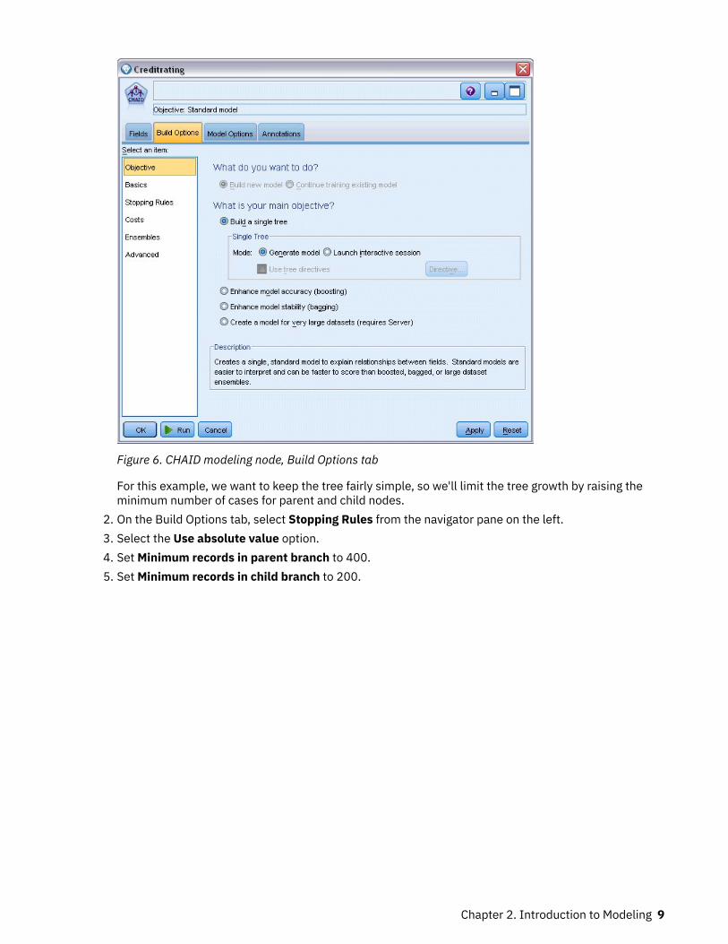
Figure 6. CHAID modeling node, Build Options tab

For this example, we want to keep the tree fairly simple, so we'll limit the tree growth by raising theminimum number of cases for parent and child nodes.

2. On the Build Options tab, select Stopping Rules from the navigator pane on the left.3. Select the Use absolute value option.4. Set Minimum records in parent branch to 400.5. Set Minimum records in child branch to 200.


Figure 7. Setting the stopping criteria for decision tree building

We can use all the other default options for this example, so click Run to create the model. (Alternatively,right-click on the node and choose Run from the context menu, or select the node and choose Run fromthe Tools menu.)

Browsing the ModelWhen execution completes, the model nugget is added to the Models palette in the upper right corner ofthe application window, and is also placed on the stream canvas with a link to the modeling node fromwhich it was created. To view the model details, right-click on the model nugget and choose Browse (onthe models palette) or Edit (on the canvas).

Figure 8. Models palette


In the case of the CHAID nugget, the Model tab displays the details in the form of a rule set--essentially aseries of rules that can be used to assign individual records to child nodes based on the values of differentinput fields.

Figure 9. CHAID model nugget, rule set

For each decision tree terminal node--meaning those tree nodes that are not split further--a prediction ofGood or Bad is returned. In each case the prediction is determined by the mode, or most commonresponse, for records that fall within that node.

To the right of the rule set, the Model tab displays the Predictor Importance chart, which shows therelative importance of each predictor in estimating the model. From this we can see that Income level iseasily the most significant in this case, and that the only other significant factor is Number of credit cards.

Figure 10. Predictor Importance chart

The Viewer tab in the model nugget displays the same model in the form of a tree, with a node at eachdecision point. Use the Zoom controls on the toolbar to zoom in on a specific node or zoom out to see themore of the tree.


Figure 11. Viewer tab in the model nugget, with zoom out selected

Looking at the upper part of the tree, the first node (Node 0) gives us a summary for all the records in thedata set. Just over 40% of the cases in the data set are classified as a bad risk. This is quite a highproportion, so let’s see if the tree can give us any clues as to what factors might be responsible.

We can see that the first split is by Income level. Records where the income level is in the Low categoryare assigned to Node 2, and it’s no surprise to see that this category contains the highest percentage ofloan defaulters. Clearly lending to customers in this category carries a high risk.

However, 16% of the customers in this category actually didn’t default, so the prediction won’t always becorrect. No model can feasibly predict every response, but a good model should allow us to predict themost likely response for each record based on the available data.

In the same way, if we look at the high income customers (Node 1), we see that the vast majority (89%)are a good risk. But more than 1 in 10 of these customers has also defaulted. Can we refine our lendingcriteria to minimize the risk here?

Notice how the model has divided these customers into two sub-categories (Nodes 4 and 5), based on thenumber of credit cards held. For high-income customers, if we lend only to those with fewer than 5 creditcards, we can increase our success rate from 89% to 97%--an even more satisfactory outcome.


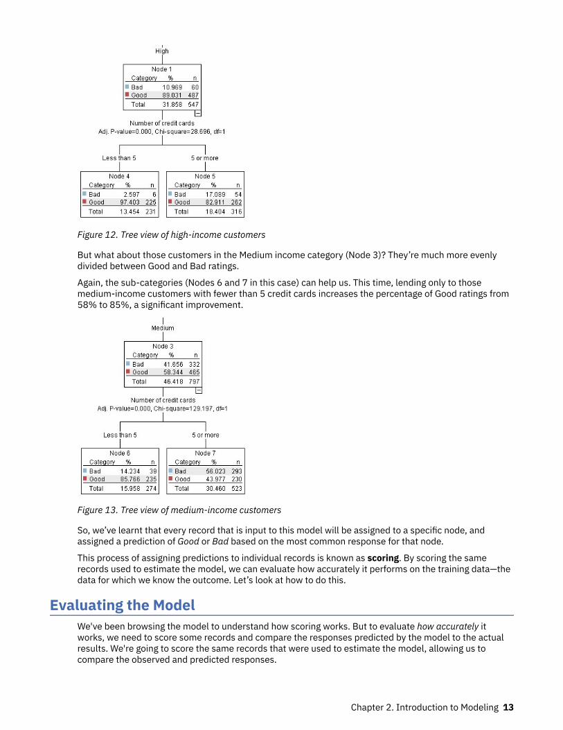
Figure 12. Tree view of high-income customers

But what about those customers in the Medium income category (Node 3)? They’re much more evenlydivided between Good and Bad ratings.

Again, the sub-categories (Nodes 6 and 7 in this case) can help us. This time, lending only to thosemedium-income customers with fewer than 5 credit cards increases the percentage of Good ratings from58% to 85%, a significant improvement.

Figure 13. Tree view of medium-income customers

So, we’ve learnt that every record that is input to this model will be assigned to a specific node, andassigned a prediction of Good or Bad based on the most common response for that node.

This process of assigning predictions to individual records is known as scoring. By scoring the samerecords used to estimate the model, we can evaluate how accurately it performs on the training data—thedata for which we know the outcome. Let’s look at how to do this.

Evaluating the ModelWe've been browsing the model to understand how scoring works. But to evaluate how accurately itworks, we need to score some records and compare the responses predicted by the model to the actualresults. We're going to score the same records that were used to estimate the model, allowing us tocompare the observed and predicted responses.


Figure 14. Attaching the model nugget to output nodes for model evaluation

1. To see the scores or predictions, attach the Table node to the model nugget, double-click the Tablenode and click Run.

The table displays the predicted scores in a field named $R-Credit rating, which was created by themodel. We can compare these values to the original Credit rating field that contains the actualresponses.

By convention, the names of the fields generated during scoring are based on the target field, but witha standard prefix. Prefixes $G and $GE are generated by the Generalized Linear Model, $R is the prefixused for the prediction generated by the CHAID model in this case, $RC is for confidence values, $X istypically generated by using an ensemble, and $XR, $XS, and $XF are used as prefixes in cases wherethe target field is a Continuous, Categorical, Set, or Flag field, respectively. Different model types usedifferent sets of prefixes. A confidence value is the model’s own estimation, on a scale from 0.0 to1.0, of how accurate each predicted value is.

Figure 15. Table showing generated scores and confidence values

As expected, the predicted value matches the actual responses for many records but not all. Thereason for this is that each CHAID terminal node has a mix of responses. The prediction matches the


most common one, but will be wrong for all the others in that node. (Recall the 16% minority of low-income customers who did not default.)

To avoid this, we could continue splitting the tree into smaller and smaller branches, until every nodewas 100% pure—all Good or Bad with no mixed responses. But such a model would be extremelycomplicated and would probably not generalize well to other datasets.

To find out exactly how many predictions are correct, we could read through the table and tally thenumber of records where the value of the predicted field $R-Credit rating matches the value of Creditrating. Fortunately, there’s a much easier way--we can use an Analysis node, which does thisautomatically.

2. Connect the model nugget to the Analysis node.3. Double-click the Analysis node and click Run.

Figure 16. Attaching an Analysis node

The analysis shows that for 1899 out of 2464 records--over 77%--the value predicted by the modelmatched the actual response.

Figure 17. Analysis results comparing observed and predicted responses


This result is limited by the fact that the records being scored are the same ones used to estimate themodel. In a real situation, you could use a Partition node to split the data into separate samples fortraining and evaluation.

By using one sample partition to generate the model and another sample to test it, you can get a muchbetter indication of how well it will generalize to other datasets.

The Analysis node allows us to test the model against records for which we already know the actualresult. The next stage illustrates how we can use the model to score records for which we don't know theoutcome. For example, this might include people who are not currently customers of the bank, but whoare prospective targets for a promotional mailing.

Scoring recordsEarlier, we scored the same records used to estimate the model in order to evaluate how accurate themodel was. Now we're going to see how to score a different set of records from the ones used to createthe model. This is the goal of modeling with a target field: Study records for which you know the outcome,to identify patterns that will allow you to predict outcomes you don't yet know.

Figure 18. Attaching new data for scoring

You could update the Statistics File source node to point to a different data file, or you could add a newsource node that reads in the data you want to score. Either way, the new dataset must contain the sameinput fields used by the model (Age, Income level, Education and so on) but not the target field Creditrating.

Alternatively, you could add the model nugget to any stream that includes the expected input fields.Whether read from a file or a database, the source type doesn't matter as long as the field names andtypes match those used by the model.

You could also save the model nugget as a separate file, or export the model in PMML format for use withother applications that support this format, or store the model in an IBM SPSS Collaboration andDeployment Services repository, which offers enterprise-wide deployment, scoring, and management ofmodels.

Regardless of the infrastructure used, the model itself works in the same way.

SummaryThis example demonstrates the basic steps for creating, evaluating, and scoring a model.

• The modeling node estimates the model by studying records for which the outcome is known, andcreates a model nugget. This is sometimes referred to as training the model.

• The model nugget can be added to any stream with the expected fields to score records. By scoring therecords for which you already know the outcome (such as existing customers), you can evaluate howwell it performs.


• Once you are satisfied that the model performs acceptably well, you can score new data (such asprospective customers) to predict how they will respond.

• The data used to train or estimate the model may be referred to as the analytical or historical data; thescoring data may also be referred to as the operational data.


Chapter 3. Modeling Overview

Overview of modeling nodesIBM SPSS Modeler offers a variety of modeling methods taken from machine learning, artificialintelligence, and statistics. The methods available on the Modeling palette allow you to derive newinformation from your data and to develop predictive models. Each method has certain strengths and isbest suited for particular types of problems.

The IBM SPSS Modeler Applications Guide provides examples for many of these methods, along with ageneral introduction to the modeling process. This guide is available as an online tutorial, and also in PDFformat. See the topic “Application examples” on page 4 for more information.

Modeling methods are divided into these categories:

• Supervised• Association• Segmentation

Supervised Models

Supervised models use the values of one or more input fields to predict the value of one or more output,or target, fields. Some examples of these techniques are: decision trees (C&R Tree, QUEST, CHAID andC5.0 algorithms), regression (linear, logistic, generalized linear, and Cox regression algorithms), neuralnetworks, support vector machines, and Bayesian networks.

Supervised models help organizations to predict a known result, such as whether a customer will buy orleave or whether a transaction fits a known pattern of fraud. Modeling techniques include machinelearning, rule induction, subgroup identification, statistical methods, and multiple model generation.

Supervised nodes

The Auto Classifier node creates and compares a number of different models forbinary outcomes (yes or no, churn or do not churn, and so on), allowing you tochoose the best approach for a given analysis. A number of modeling algorithms aresupported, making it possible to select the methods you want to use, the specificoptions for each, and the criteria for comparing the results. The node generates a setof models based on the specified options and ranks the best candidates accordingto the criteria you specify.

The Auto Numeric node estimates and compares models for continuous numericrange outcomes using a number of different methods. The node works in the samemanner as the Auto Classifier node, allowing you to choose the algorithms to useand to experiment with multiple combinations of options in a single modeling pass.Supported algorithms include neural networks, C&R Tree, CHAID, linear regression,generalized linear regression, and support vector machines (SVM). Models can becompared based on correlation, relative error, or number of variables used.

The Classification and Regression (C&R) Tree node generates a decision tree thatallows you to predict or classify future observations. The method uses recursivepartitioning to split the training records into segments by minimizing the impurity ateach step, where a node in the tree is considered “pure” if 100% of cases in thenode fall into a specific category of the target field. Target and input fields can benumeric ranges or categorical (nominal, ordinal, or flags); all splits are binary (onlytwo subgroups).

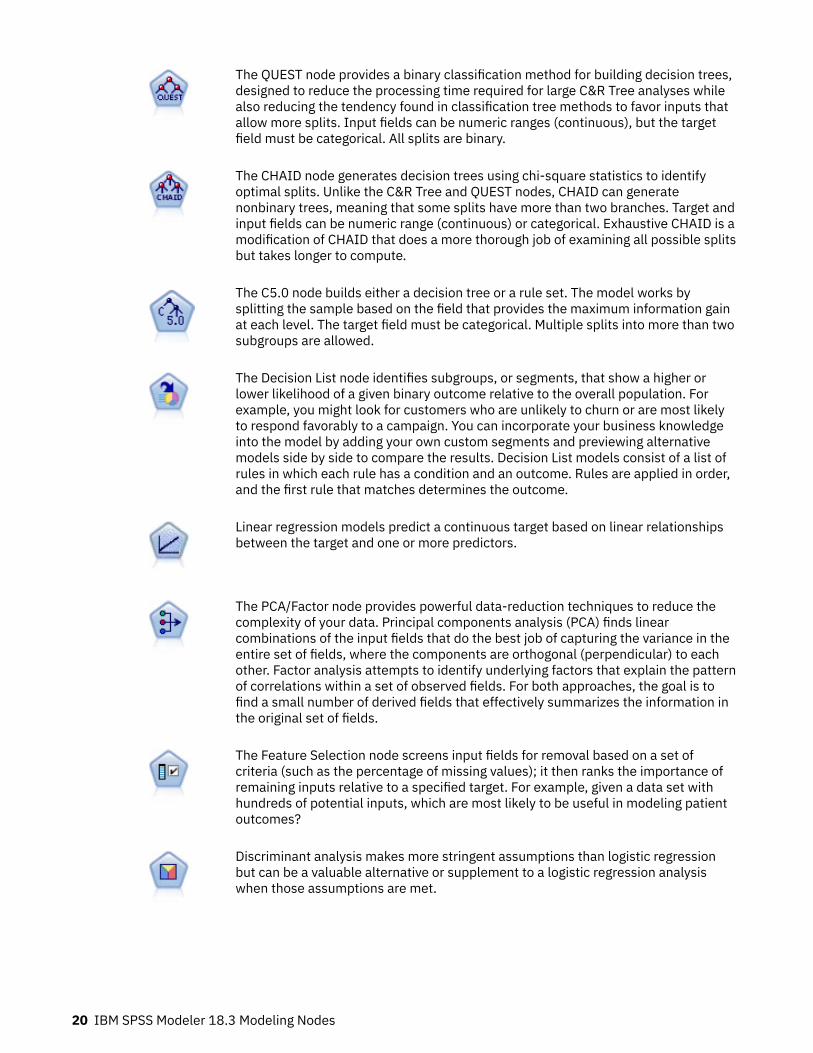
The QUEST node provides a binary classification method for building decision trees,designed to reduce the processing time required for large C&R Tree analyses whilealso reducing the tendency found in classification tree methods to favor inputs thatallow more splits. Input fields can be numeric ranges (continuous), but the targetfield must be categorical. All splits are binary.

The CHAID node generates decision trees using chi-square statistics to identifyoptimal splits. Unlike the C&R Tree and QUEST nodes, CHAID can generatenonbinary trees, meaning that some splits have more than two branches. Target andinput fields can be numeric range (continuous) or categorical. Exhaustive CHAID is amodification of CHAID that does a more thorough job of examining all possible splitsbut takes longer to compute.

The C5.0 node builds either a decision tree or a rule set. The model works bysplitting the sample based on the field that provides the maximum information gainat each level. The target field must be categorical. Multiple splits into more than twosubgroups are allowed.

The Decision List node identifies subgroups, or segments, that show a higher orlower likelihood of a given binary outcome relative to the overall population. Forexample, you might look for customers who are unlikely to churn or are most likelyto respond favorably to a campaign. You can incorporate your business knowledgeinto the model by adding your own custom segments and previewing alternativemodels side by side to compare the results. Decision List models consist of a list ofrules in which each rule has a condition and an outcome. Rules are applied in order,and the first rule that matches determines the outcome.

Linear regression models predict a continuous target based on linear relationshipsbetween the target and one or more predictors.

The PCA/Factor node provides powerful data-reduction techniques to reduce thecomplexity of your data. Principal components analysis (PCA) finds linearcombinations of the input fields that do the best job of capturing the variance in theentire set of fields, where the components are orthogonal (perpendicular) to eachother. Factor analysis attempts to identify underlying factors that explain the patternof correlations within a set of observed fields. For both approaches, the goal is tofind a small number of derived fields that effectively summarizes the information inthe original set of fields.

The Feature Selection node screens input fields for removal based on a set ofcriteria (such as the percentage of missing values); it then ranks the importance ofremaining inputs relative to a specified target. For example, given a data set withhundreds of potential inputs, which are most likely to be useful in modeling patientoutcomes?

Discriminant analysis makes more stringent assumptions than logistic regressionbut can be a valuable alternative or supplement to a logistic regression analysiswhen those assumptions are met.


Logistic regression is a statistical technique for classifying records based on valuesof input fields. It is analogous to linear regression but takes a categorical target fieldinstead of a numeric range.

The Generalized Linear model expands the general linear model so that thedependent variable is linearly related to the factors and covariates through aspecified link function. Moreover, the model allows for the dependent variable tohave a non-normal distribution. It covers the functionality of a wide number ofstatistical models, including linear regression, logistic regression, loglinear modelsfor count data, and interval-censored survival models.

A generalized linear mixed model (GLMM) extends the linear model so that thetarget can have a non-normal distribution, is linearly related to the factors andcovariates via a specified link function, and so that the observations can becorrelated. Generalized linear mixed models cover a wide variety of models, fromsimple linear regression to complex multilevel models for non-normal longitudinaldata.

The Cox regression node enables you to build a survival model for time-to-eventdata in the presence of censored records. The model produces a survival functionthat predicts the probability that the event of interest has occurred at a given time (t)for given values of the input variables.

The Support Vector Machine (SVM) node enables you to classify data into one of twogroups without overfitting. SVM works well with wide data sets, such as those with avery large number of input fields.

The Bayesian Network node enables you to build a probability model by combiningobserved and recorded evidence with real-world knowledge to establish thelikelihood of occurrences. The node focuses on Tree Augmented Naïve Bayes (TAN)and Markov Blanket networks that are primarily used for classification.

The Self-Learning Response Model (SLRM) node enables you to build a model inwhich a single new case, or small number of new cases, can be used to reestimatethe model without having to retrain the model using all data.

The Time Series node estimates exponential smoothing, univariate AutoregressiveIntegrated Moving Average (ARIMA), and multivariate ARIMA (or transfer function)models for time series data and produces forecasts of future performance. ThisTime Series node is similar to the previous Time Series node that was deprecated inSPSS Modeler version 18. However, this newer Time Series node is designed toharness the power of IBM SPSS Analytic Server to process big data, and display theresulting model in the output viewer that was added in SPSS Modeler version 17.

The k-Nearest Neighbor (KNN) node associates a new case with the category orvalue of the k objects nearest to it in the predictor space, where k is an integer.Similar cases are near each other and dissimilar cases are distant from each other.

Chapter 3. Modeling Overview 21

The Spatio-Temporal Prediction (STP) node uses data that contains location data,input fields for prediction (predictors), a time field, and a target field. Each locationhas numerous rows in the data that represent the values of each predictor at eachtime of measurement. After the data is analyzed, it can be used to predict targetvalues at any location within the shape data that is used in the analysis.

Association Models

Association models find patterns in your data where one or more entities (such as events, purchases, orattributes) are associated with one or more other entities. The models construct rule sets that definethese relationships. Here the fields within the data can act as both inputs and targets. You could findthese associations manually, but association rule algorithms do so much more quickly, and can exploremore complex patterns. Apriori and Carma models are examples of the use of such algorithms. One othertype of association model is a sequence detection model, which finds sequential patterns in time-structured data.

Association models are most useful when predicting multiple outcomes—for example, customers whobought product X also bought Y and Z. Association models associate a particular conclusion (such as thedecision to buy something) with a set of conditions. The advantage of association rule algorithms over themore standard decision tree algorithms (C5.0 and C&RT) is that associations can exist between any of theattributes. A decision tree algorithm will build rules with only a single conclusion, whereas associationalgorithms attempt to find many rules, each of which may have a different conclusion.

Association nodes

The Apriori node extracts a set of rules from the data, pulling out the rules with thehighest information content. Apriori offers five different methods of selecting rulesand uses a sophisticated indexing scheme to process large data sets efficiently. Forlarge problems, Apriori is generally faster to train; it has no arbitrary limit on thenumber of rules that can be retained, and it can handle rules with up to 32preconditions. Apriori requires that input and output fields all be categorical butdelivers better performance because it is optimized for this type of data.

The CARMA model extracts a set of rules from the data without requiring you tospecify input or target fields. In contrast to Apriori the CARMA node offers buildsettings for rule support (support for both antecedent and consequent) rather thanjust antecedent support. This means that the rules generated can be used for awider variety of applications—for example, to find a list of products or services(antecedents) whose consequent is the item that you want to promote this holidayseason.

The Sequence node discovers association rules in sequential or time-oriented data.A sequence is a list of item sets that tends to occur in a predictable order. Forexample, a customer who purchases a razor and aftershave lotion may purchaseshaving cream the next time he shops. The Sequence node is based on the CARMAassociation rules algorithm, which uses an efficient two-pass method for findingsequences.

The Association Rules Node is similar to the Apriori Node; however, unlike Apriori,the Association Rules Node can process list data. In addition, the Association RulesNode can be used with IBM SPSS Analytic Server to process big data and takeadvantage of faster parallel processing.

Segmentation Models

Segmentation models divide the data into segments, or clusters, of records that have similar patterns ofinput fields. As they are only interested in the input fields, segmentation models have no concept of


output or target fields. Examples of segmentation models are Kohonen networks, K-Means clustering,two-step clustering and anomaly detection.

Segmentation models (also known as "clustering models") are useful in cases where the specific result isunknown (for example, when identifying new patterns of fraud, or when identifying groups of interest inyour customer base). Clustering models focus on identifying groups of similar records and labeling therecords according to the group to which they belong. This is done without the benefit of prior knowledgeabout the groups and their characteristics, and it distinguishes clustering models from the other modelingtechniques in that there is no predefined output or target field for the model to predict. There are no rightor wrong answers for these models. Their value is determined by their ability to capture interestinggroupings in the data and provide useful descriptions of those groupings. Clustering models are oftenused to create clusters or segments that are then used as inputs in subsequent analyses (for example, bysegmenting potential customers into homogeneous subgroups).

Segmentation nodes

The Auto Cluster node estimates and compares clustering models, which identifygroups of records that have similar characteristics. The node works in the samemanner as other automated modeling nodes, allowing you to experiment withmultiple combinations of options in a single modeling pass. Models can becompared using basic measures with which to attempt to filter and rank theusefulness of the cluster models, and provide a measure based on the importance ofparticular fields.

The K-Means node clusters the data set into distinct groups (or clusters). Themethod defines a fixed number of clusters, iteratively assigns records to clusters,and adjusts the cluster centers until further refinement can no longer improve themodel. Instead of trying to predict an outcome, k-means uses a process known asunsupervised learning to uncover patterns in the set of input fields.

The Kohonen node generates a type of neural network that can be used to clusterthe data set into distinct groups. When the network is fully trained, records that aresimilar should be close together on the output map, while records that are differentwill be far apart. You can look at the number of observations captured by each unitin the model nugget to identify the strong units. This may give you a sense of theappropriate number of clusters.

The TwoStep node uses a two-step clustering method. The first step makes a singlepass through the data to compress the raw input data into a manageable set ofsubclusters. The second step uses a hierarchical clustering method to progressivelymerge the subclusters into larger and larger clusters. TwoStep has the advantage ofautomatically estimating the optimal number of clusters for the training data. It canhandle mixed field types and large data sets efficiently.

The Anomaly Detection node identifies unusual cases, or outliers, that do notconform to patterns of “normal” data. With this node, it is possible to identifyoutliers even if they do not fit any previously known patterns and even if you are notexactly sure what you are looking for.

In-Database Mining Models

IBM SPSS Modeler supports integration with data mining and modeling tools that are available fromdatabase vendors, including Oracle Data Miner and Microsoft Analysis Services. You can build, score, andstore models inside the database—all from within the IBM SPSS Modeler application. For full details, seethe IBM SPSS Modeler In-Database Mining Guide.

IBM SPSS Statistics Models


If you have a copy of IBM SPSS Statistics installed and licensed on your computer, you can access and runcertain IBM SPSS Statistics routines from within IBM SPSS Modeler to build and score models.

Building Split ModelsSplit modeling enables you to use a single stream to build separate models for each possible value of aflag, nominal, or continuous input field, with the resulting models all being accessible from a single modelnugget. The possible values for the input fields could have very different effects on the model. With splitmodeling, you can easily build the best-fitting model for each possible field value in a single execution ofthe stream.

Note that interactive modeling sessions cannot use splitting. With interactive modeling you specify eachmodel individually, so there would be no advantage in using splitting, which builds multiple modelsautomatically.

Split modeling works by designating a particular input field as a split field. You can do this by setting thefield role to Split in the Type specification.

You can designate only fields with a measurement level of Flag, Nominal, Ordinal, or Continuous as splitfields.

You can assign more than one input field as a split field. In this case, however, the number of modelscreated can be greatly increased. A model is built for each possible combination of the values of theselected split fields. For example, if three input fields, each having three possible values, are designatedas split fields, this will result in the creation of 27 different models.

Even after you assign one or more fields as split fields, you can still choose whether to create split modelsor a single model, by means of a check box setting on the modeling node dialog.

If split fields are defined but the check box is not selected, only a single model is generated. Likewise ifthe check box is selected but no split field is defined, splitting is ignored and a single model is generated.

When you run the stream, separate models are built behind the scenes for each possible value of the splitfield or fields, but only a single model nugget is placed in the models palette and the stream canvas. Asplit-model nugget is denoted by the split symbol; this is two gray rectangles overlaid on the nuggetimage.

When you browse the split-model nugget, you see a list of all the separate models that have been built.

You can investigate an individual model from a list by double-clicking its nugget icon in the viewer. Doingso opens a standard browser window for the individual model. When the nugget is on the canvas, double-clicking a graph thumbnail opens the full-size graph. See the topic “Split Model Viewer” on page 40 formore information.

Once a model has been created as a split model, you cannot remove the split processing from it, nor canyou undo splitting further downstream from a split-modeling node or nugget.

Example. A national retailer wants to estimate sales by product category at each of its stores around thecountry. Using split modeling, they designate the Store field of their input data as a split field, enablingthem to build separate models for each category at each store in a single operation. They can then use theresulting information to control stock levels much more accurately than they could with only a singlemodel.

Splitting and PartitioningSplitting has some features in common with partitioning, but the two are used in very different ways.

Partitioning divides the dataset randomly into either two or three parts: training, testing and (optionally)validation, and is used to test the performance of a single model.

Splitting divides the dataset into as many parts as there are possible values for a split field, and is used tobuild multiple models.


Partitioning and splitting operate completely independently of each other. You can choose either, both orneither in a modeling node.

Modeling nodes supporting split modelsA number of modeling nodes can create split models. The exceptions are Auto Cluster, PCA/Factor,Feature Selection, SLRM, Random Trees, Tree-AS, Linear-AS, LSVM, the association models (Apriori,Carma and Sequence), the clustering models (K-Means, Kohonen, Two Step and Anomaly), Statisticsmodels, and the nodes used for in-database modeling.

The modeling nodes that support split modeling are:

C&R Tree Bayes Net Linear

QUEST GenLin GLMM

CHAID KNN STP

C5.0 Cox One-Class SVM

Neural Net Auto Classifier XGBoost Tree

Decision List Auto Numeric XGBoost Linear

Regression Logistic HDBSCAN

Discriminant SVM Time Series

Features Affected by SplittingThe use of split models affects a number of IBM SPSS Modeler features in various ways. This sectionprovides guidance on using split models with other nodes in a stream.

Record Ops nodesWhen you use split models in a stream that contains a Sample node, stratify records by the split field toachieve an even sampling of records. This option is available when you choose Complex as the samplemethod.


If the stream contains a Balance node, balancing applies to the overall set of input records, not to thesubset of records inside a split.

When aggregating records by means of an Aggregate node, set the split fields to be key fields if you wantto calculate aggregates for each split.

Field Ops nodesThe Type node is where you specify which field or fields to use as split fields.

Note: While the Ensemble node is used to combine two or more model nuggets, it cannot be used toreverse the action of splitting, as the split models are contained inside a single model nugget.

Modeling nodesSplit models do not support the calculation of predictor importance (the relative importance of thepredictor input fields in estimating the model). Predictor importance settings are ignored when buildingsplit models.

Note: Adjusted propensity score settings are ignored when using a split model.

The KNN (nearest neighbor) node supports split models only if it is set to predict a target field. Thealternative setting (only identify nearest neighbors) does not create a model. If the option Automaticallyselect k is chosen, each of the split models might have a different number of nearest neighbors. Thus theoverall model has a number of generated columns equal to the largest number of nearest neighbors thatare found across all the split models. For those split models where the number of nearest neighbors isless than this maximum, there is a corresponding number of columns filled with $null values. See thetopic “KNN node” on page 313 for more information.

Database Modeling nodesThe in-database modeling nodes do not support split models.

Model nuggetsExport to PMML from a split model nugget is not possible, as the nugget contains multiple models andPMML does not support such a packaging. Export to text or HTML is possible.

Modeling Node Fields OptionsAll modeling nodes have a Fields tab, where you can specify the fields to be used in building the model.

Before you can build a model, you need to specify which fields you want to use as targets and as inputs.With a few exceptions, all modeling nodes will use field information from an upstream Type node. If youare using a Type node to select input and target fields, you don't need to change anything on this tab.(Exceptions include the Sequence node and the Text Extraction node, which require that field settings bespecified in the modeling node.)

Use type node settings. This option tells the node to use field information from an upstream Type node.This is the default.

Use custom settings. This option tells the node to use field information specified here instead of thatgiven in any upstream Type node(s). After selecting this option, specify the fields below as required.

Note: Not all fields are displayed for all nodes.

• Use transactional format (Apriori, CARMA, MS Association Rules and Oracle Apriori nodes only).Select this check box if the source data is in transactional format. Records in this format have twofields, one for an ID and one for content. Each record represents a single transaction or item, andassociated items are linked by having the same ID. Deselect this box if the data is in tabular format, inwhich items are represented by separate flags, where each flag field represents the presence or


absence of a specific item and each record represents a complete set of associated items. See the topic“Tabular versus Transactional Data” on page 232 for more information.

– ID. For transactional data, select an ID field from the list. Numeric or symbolic fields can be used asthe ID field. Each unique value of this field should indicate a specific unit of analysis. For example, ina market basket application, each ID might represent a single customer. For a Web log analysisapplication, each ID might represent a computer (by IP address) or a user (by login data).

– IDs are contiguous. (Apriori and CARMA nodes only) If your data are presorted so that all recordswith the same ID are grouped together in the data stream, select this option to speed up processing.If your data are not presorted (or you are not sure), leave this option unselected and the node willsort the data automatically.

Note: If your data are not sorted and you select this option, you may get invalid results in your model.– Content. Specify the content field(s) for the model. These fields contain the items of interest in

association modeling. You can specify multiple flag fields (if data are in tabular format) or a singlenominal field (if data are in transactional format).

• Target. For models that require one or more target fields, select the target field or fields. This is similarto setting the field role to Target in a Type node.

• Evaluation. (For Auto Cluster models only.) No target is specified for cluster models; however, you canselect an evaluation field to identify its level of importance. In addition, you can evaluate how well theclusters differentiate values of this field, which in turn indicates whether the clusters can be used topredict this field. Note The evaluation field must be a string with more than one value.

– Inputs. Select the input field or fields. This is similar to setting the field role to Input in a Type node.

– Partition. This field allows you to specify a field used to partition the data into separate samples forthe training, testing, and validation stages of model building. By using one sample to generate themodel and a different sample to test it, you can get a good indication of how well the model willgeneralize to larger datasets that are similar to the current data. If multiple partition fields have beendefined by using Type or Partition nodes, a single partition field must be selected on the Fields tab ineach modeling node that uses partitioning. (If only one partition is present, it is automatically usedwhenever partitioning is enabled.) Also note that to apply the selected partition in your analysis,partitioning must also be enabled in the Model Options tab for the node. (Deselecting this optionmakes it possible to disable partitioning without changing field settings.)

• Splits. For split models, select the split field or fields. This is similar to setting the field role to Split in aType node. You can designate only fields with a measurement level of Flag, Nominal, Ordinal orContinuous as split fields. Fields chosen as split fields cannot be used as target, input, partition,frequency or weight fields. See the topic “Building Split Models” on page 24 for more information.

• Use frequency field. This option enables you to select a field as a frequency weight. Use this if therecords in your training data represent more than one unit each--for example, if you are usingaggregated data. The field values should be the number of units represented by each record. See thetopic “Using Frequency and Weight Fields” on page 28 for more information.

Note: If you see the error message Metadata (on input/output fields) not valid, ensure that you havespecified all fields that are required, such as the frequency field.

• Use weight field. This option enables you to select a field as a case weight. Case weights are used toaccount for differences in variance across levels of the output field. See the topic “Using Frequency andWeight Fields” on page 28 for more information.

• Consequents. For rule induction nodes (Apriori), select the fields to be used as consequents in theresulting rule set. (This corresponds to fields with role Target or Both in a Type node.)

• Antecedents. For rule induction nodes (Apriori), select the fields to be used as antecedents in theresulting rule set. (This corresponds to fields with role Input or Both in a Type node.)

Some models have a Fields tab that differs from those described in this section.

• See the topic “Sequence Node Fields Options” on page 246 for more information.• See the topic “CARMA Node Fields Options” on page 235 for more information.


Using Frequency and Weight FieldsFrequency and weight fields are used to give extra importance to some records over others, for example,because you know that one section of the population is under-represented in the training data (weight) orbecause one record represents a number of identical cases (frequency).

• Values for a frequency field should be positive integers. Records with a negative or zero frequencyweight are excluded from the analysis. Non-integer frequency weights are rounded to the nearestinteger.

• Case weight values should be positive but need not be integer values. Records with a negative or zerocase weight are excluded from the analysis.

Scoring Frequency and Weight Fields

Frequency and weight fields are used in training models, but are not used in scoring, because the scorefor each record is based on its characteristics regardless of how many cases it represents. For example,suppose you have the data in the following table.

Table 1. Data example

Married Responded

Yes Yes

Yes Yes

Yes Yes

Yes No

No Yes

No No

No No

Based on this, you conclude that three out of four married people respond to the promotion, and two outof three unmarried people didn’t respond. So you will score any new records accordingly, as shown in thefollowing table.

Table 2. Scored records example

Married $-Responded $RP-Responded

Yes Yes 0.75 (three/four)

No No 0.67 (two/three)

Alternatively, you could store your training data more compactly, using a frequency field, as shown in thefollowing table.

Table 3. Scored records alternative example

Married Responded Frequency

Yes Yes 3

Yes No 1

No Yes 1

No No 2

Since this represents exactly the same dataset, you will build the same model and predict responsesbased solely on marital status. If you have ten married people in your scoring data, you will predict Yes for


each of them regardless of whether they are presented as ten separate records, or one with a frequencyvalue of 10. Weight, although generally not an integer, can be thought of as similarly indicating theimportance of a record. This is why frequency and weight fields are not used when scoring records.

Evaluating and Comparing Models

Some model types support frequency fields, some support weight fields, and some support both. But inall cases where they apply, they are used only for model building and are not considered when evaluatingmodels using an Evaluation node or Analysis node, or when ranking models using most of the methodssupported by the Auto Classifier and Auto Numeric nodes.

• When comparing models (using evaluation charts, for example), frequency and weight values will beignored. This enables a level comparison between models that use these fields and models that don't,but means that for an accurate evaluation, a dataset that accurately represents the population withoutrelying on a frequency or weight field must be used. In practical terms, you can do this by making surethat models are evaluated using a testing sample in which the value of the frequency or weight field isalways null or 1. (This restriction only applies when evaluating models; if frequency or weight valueswere always 1 for both training and testing samples, there would be no reason to use these fields in thefirst place.)

• If using Auto Classifier, frequency can be taken into account if ranking models based on Profit, so thismethod is recommended in that case.

• If necessary, you can split the data into training and testing samples using a Partition node.

Modeling Node Analyze OptionsMany modeling nodes include an Analyze tab that enables you to obtain predictor importance informationalong with raw and adjusted propensity scores.

Model Evaluation

Calculate predictor importance. For models that produce an appropriate measure of importance, youcan display a chart that indicates the relative importance of each predictor in estimating the model.Typically you will want to focus your modeling efforts on the predictors that matter most, and considerdropping or ignoring those that matter least. Note that predictor importance may take longer to calculatefor some models, particularly when working with large datasets, and is off by default for some models asa result. Predictor importance is not available for decision list models. See “Predictor Importance” onpage 37 for more information.

Propensity Scores

Propensity scores can be enabled in the modeling node, and on the Settings tab in the model nugget. Thisfunctionality is available only when the selected target is a flag field. See the topic “Propensity Scores” onpage 30 for more information.

Calculate raw propensity scores. Raw propensity scores are derived from the model based on thetraining data only. If the model predicts the true value (will respond), then the propensity is the same as P,where P is the probability of the prediction. If the model predicts the false value, then the propensity iscalculated as (1 – P).

• If you choose this option when building the model, propensity scores will be enabled in the modelnugget by default. However, you can always choose to enable raw propensity scores in the modelnugget whether or not you select them in the modeling node.

• When scoring the model, raw propensity scores will be added in a field with the letters RP appended tothe standard prefix. For example, if the predictions are in a field named $R-churn, the name of thepropensity score field will be $RRP-churn.

Calculate adjusted propensity scores. Raw propensities are based purely on estimates given by themodel, which may be overfitted, leading to over-optimistic estimates of propensity. Adjusted propensitiesattempt to compensate by looking at how the model performs on the test or validation partitions andadjusting the propensities to give a better estimate accordingly.

• This setting requires that a valid partition field is present in the stream.


• Unlike raw confidence scores, adjusted propensity scores must be calculated when building the model;otherwise, they will not be available when scoring the model nugget.

• When scoring the model, adjusted propensity scores will be added in a field with the letters APappended to the standard prefix. For example, if the predictions are in a field named $R-churn, thename of the propensity score field will be $RAP-churn. Adjusted propensity scores are not available forlogistic regression models.

• When calculating the adjusted propensity scores, the test or validation partition used for the calculationmust not have been balanced. To avoid this, be sure the Only balance training data option is selectedin any upstream Balance nodes. In addition, if a complex sample has been taken upstream this willinvalidate the adjusted propensity scores.

• Adjusted propensity scores are not available for "boosted" tree and rule set models. See the topic“Boosted C5.0 Models” on page 108 for more information.

Based on. For adjusted propensity scores to be computed, a partition field must be present in the stream.You can specify whether to use the testing or validation partition for this computation. For best results,the testing or validation partition should include at least as many records as the partition used to train theoriginal model.

Propensity ScoresFor models that return a yes or no prediction, you can request propensity scores in addition to thestandard prediction and confidence values. Propensity scores indicate the likelihood of a particularoutcome or response. The following table contains an example.

Table 4. Propensity scores

Customer Propensity to respond

Joe Smith 35%

Jane Smith 15%

Propensity scores are available only for models with flag targets, and indicate the likelihood of the Truevalue defined for the field, as specified in a source or Type node.

Propensity Scores Versus Confidence Scores

Propensity scores differ from confidence scores, which apply to the current prediction, whether yes or no.In cases where the prediction is no, for example, a high confidence actually means a high likelihood not torespond. Propensity scores sidestep this limitation to enable easier comparison across all records. Forexample, a no prediction with a confidence of 0.85 translates to a raw propensity of 0.15 (or 1 minus0.85).

Table 5. Confidence scores

Customer Prediction Confidence

Joe Smith Will respond .35

Jane Smith Won't respond .85

Obtaining Propensity Scores

• Propensity scores can be enabled on the Analyze tab in the modeling node or on the Settings tab in themodel nugget. This functionality is available only when the selected target is a flag field. See the topic“Modeling Node Analyze Options” on page 29 for more information.

• Propensity scores may also be calculated by the Ensemble node, depending on the ensemble methodused.

Calculating Adjusted Propensity Scores


Adjusted propensity scores are calculated as part of the process of building the model, and will not beavailable otherwise. Once the model is built, it is then scored using data from the test or validationpartition, and a new model to deliver adjusted propensity scores is constructed by analyzing the originalmodel’s performance on that partition. Depending on the type of model, one of two methods may be usedto calculate the adjusted propensity scores.

• For rule set and tree models, adjusted propensity scores are generated by recalculating the frequencyof each category at each tree node (for tree models) or the support and confidence of each rule (for ruleset models). This results in a new rule set or tree model which is stored with the original model, to beused whenever adjusted propensity scores are requested. Each time the original model is applied tonew data, the new model can subsequently be applied to the raw propensity scores to generate theadjusted scores.

• For other models, records produced by scoring the original model on the test or validation partition arethen binned by their raw propensity score. Next, a neural network model is trained that defines a non-linear function that maps from the mean raw propensity in each bin to the mean observed propensity inthe same bin. As noted earlier for tree models, the resulting neural net model is stored with the originalmodel, and can be applied to the raw propensity scores whenever adjusted propensity scores arerequested.

Caution regarding missing values in the testing partition. Handling of missing input values in thetesting/validation partition varies by model (see individual model scoring algorithms for details). The C5model cannot compute adjusted propensities when there are missing inputs.

Misclassification CostsIn some contexts, certain kinds of errors are more costly than others. For example, it may be more costlyto classify a high-risk credit applicant as low risk (one kind of error) than it is to classify a low-riskapplicant as high risk (a different kind of error). Misclassification costs allow you to specify the relativeimportance of different kinds of prediction errors.

Misclassification costs are basically weights applied to specific outcomes. These weights are factored intothe model and may actually change the prediction (as a way of protecting against costly mistakes).

With the exception of C5.0 models, misclassification costs are not applied when scoring a model and arenot taken into account when ranking or comparing models using an Auto Classifier node, evaluation chart,or Analysis node. A model that includes costs may not produce fewer errors than one that doesn't andmay not rank any higher in terms of overall accuracy, but it is likely to perform better in practical termsbecause it has a built-in bias in favor of less expensive errors.

The cost matrix shows the cost for each possible combination of predicted category and actual category.By default, all misclassification costs are set to 1.0. To enter custom cost values, select Usemisclassification costs and enter your custom values into the cost matrix.

To change a misclassification cost, select the cell corresponding to the desired combination of predictedand actual values, delete the existing contents of the cell, and enter the desired cost for the cell. Costs arenot automatically symmetrical. For example, if you set the cost of misclassifying A as B to be 2.0, the costof misclassifying B as A will still have the default value of 1.0 unless you explicitly change it as well.

Note: Only the Decision Trees model allows costs to be specified at build time.

Model Nuggets

Figure 19. Model nugget

A model nugget is a container for a model, that is, the set of rules, formulas or equations that representthe results of your model building operations in SPSS Modeler. The main purpose of a nugget is for scoringdata to generate predictions, or to enable further analysis of the model properties. Opening a model


nugget on the screen enables you to see various details about the model, such as the relative importanceof the input fields in creating the model. To view the predictions, you need to attach and execute a furtherprocess or output node. See the topic “Using Model Nuggets in Streams” on page 41 for moreinformation.

Figure 20. Model link from modeling node to model nugget

When you successfully execute a modeling node, a corresponding model nugget is placed on the streamcanvas, where it is represented by a gold, diamond-shaped icon (hence the name "nugget"). On thestream canvas, the nugget is shown with a connection (solid line) to the nearest suitable node before themodeling node, and a link (dotted line) to the modeling node itself.

The nugget is also placed in the Models palette in the upper right corner of the IBM SPSS Modelerwindow. From either location, nuggets can be selected and browsed to view details of the model.

Nuggets are always placed in the Models palette when a modeling node is successfully executed. You canset a user option to control whether the nugget is additionally placed on the stream canvas.

The following topics provide information on using model nuggets in IBM SPSS Modeler. For an in-depthunderstanding of the algorithms used, see the IBM SPSS Modeler Algorithms Guide, available as a PDF fileas part of your product download.

Model LinksBy default, a nugget is shown on the canvas with a link to the modeling node that created it. This isespecially useful in complex streams with several nuggets, enabling you to identify the nugget that will beupdated by each modeling node. Each link contains a symbol to indicate whether the model is replacedwhen the modeling node is executed. See the topic “Replacing a model” on page 34 for moreinformation.

Defining and Removing Model LinksYou can define and remove links manually on the canvas. When you are defining a new link, the cursorchanges to the link cursor.

Figure 21. Link cursor

Defining a new link (context menu)

1. Right-click on the modeling node from which you want the link to start.2. Choose Define Model Link from the context menu.3. Click the nugget where you want the link to end.

Defining a new link (main menu)

1. Click the modeling node from which you want the link to start.2. From the main menu, choose:

Edit > Node > Define Model Link3. Click the nugget where you want the link to end.

Removing an existing link (context menu)

1. Right-click on the nugget at the end of the link.2. Choose Remove Model Link from the context menu.


Alternatively:

1. Right-click on the symbol in the middle of the link.2. Choose Remove Link from the context menu.

Removing an existing link (main menu)

1. Click the modeling node or nugget from which you want to remove the link.2. From the main menu, choose:

Edit > Node > Remove Model Link

Copying and Pasting Model LinksIf you copy a linked nugget, without its modeling node, and paste it into the same stream, the nugget ispasted with a link to the modeling node. The new link has the same model replacement status (see“Replacing a model” on page 34) as the original link.

Figure 22. Copying and pasting a linked nugget

If you copy and paste a nugget together with its linked modeling node, the link is retained whether theobjects are pasted into the same stream or a new stream.

Figure 23. Copying and pasting a linked nugget

Note: If you copy a linked nugget, without its modeling node, and paste the nugget into a new stream (orinto a SuperNode that does not contain the modeling node), the link is broken and only the nugget ispasted.

Model Links and SuperNodesIf you define a SuperNode to include either the modeling node or the model nugget of a linked model (butnot both), the link is broken. Expanding the SuperNode does not restore the link; you can only do this byundoing creation of the SuperNode.


Replacing a modelYou can choose whether to replace (that is, update) an existing nugget on re-execution of the modelingnode that created the nugget. If you turn off the replacement option, a new nugget is created when youre-execute the modeling node.

Each link from modeling node to nugget contains a symbol to indicate whether the model is replacedwhen the modeling node is re-executed.

Figure 24. Model link with model replacement turned on

The link is initially shown with model replacement turned on, depicted by the small sunburst symbol inthe link. In this state, re-executing the modeling node at one end of the link simply updates the nugget atthe other end.

Figure 25. Model link with model replacement turned off

If model replacement is turned off, the link symbol is replaced by a gray dot. In this state, re-executingthe modeling node at one end of the link adds a new, updated version of the nugget to the canvas.

In either case, in the Models palette the existing nugget is updated or a new nugget is added, dependingon the setting of the Replace previous model system option.

Order of executionWhen you execute a stream with multiple branches containing model nuggets, the stream is firstevaluated to make sure that a branch with model replacement turned on is executed before any branchthat uses the resulting model nugget.

If your requirements are more complex, you can set the order of execution manually through scripting.

Changing the model replacement setting1. Right-click the symbol on the link.2. Choose Turn On(Off) Model Replacement as desired.

Note: The model replacement setting on a model link overrides the setting on the Notifications tab of theUser Options dialog (Tools > Options > User Options).

The models paletteThe models palette (on the Models tab in the managers window) enables you to use, examine, and modifymodel nuggets in various ways.


Figure 26. Models palette

Right-clicking a model nugget in the models palette opens a context menu with the following options:

• Add To Stream. Adds the model nugget to the currently active stream. If there is a selected node in thestream, the model nugget will be connected to the selected node when such a connection is possible, orotherwise to the nearest possible node. The nugget is displayed with a link to the modeling node thatcreated the model, if that node is still in the stream.

• Browse. Opens the model browser for the nugget.• Rename and Annotate. Allows you to rename the model nugget and/or modify the annotation for the

nugget.• Generate Modeling Node. If you have a model nugget that you want to modify or update and the

stream used to create the model is not available, you can use this option to recreate a modeling nodewith the same options used to create the original model.

• Save Model, Save Model As. Saves the model nugget to an external generated model (.gm) binary file.• Store Model. Stores the model nugget in IBM SPSS Collaboration and Deployment Services Repository.• Export PMML. Exports the model nugget as predictive model markup language (PMML), which can be

used for scoring new data outside of IBM SPSS Modeler. Export PMML is available for all generatedmodel nodes.

• Add to Project. Saves the model nugget and adds it to the current project. On the Classes tab, thenugget will be added to the Generated Models folder. On the CRISP-DM tab, it will be added to thedefault project phase.

• Delete. Deletes the model nugget from the palette.

Right-clicking an unoccupied area in the models palette opens a context menu with the following options:

• Open Model. Loads a model nugget previously created in IBM SPSS Modeler.• Retrieve Model. Retrieves a stored model from an IBM SPSS Collaboration and Deployment Services

repository.• Load Palette. Loads a saved models palette from an external file.• Retrieve Palette. Retrieves a stored models palette from an IBM SPSS Collaboration and Deployment

Services repository.• Save Palette. Saves the entire contents of the models palette to an external generated models palette

(.gen) file.• Store Palette. Stores the entire contents of the models palette in an IBM SPSS Collaboration and

Deployment Services repository.• Clear Palette. Deletes all nuggets from the palette.• Add Palette To Project. Saves the models palette and adds it to the current project. On the Classes tab,

the nugget will be added to the Generated Models folder. On the CRISP-DM tab, it will be added to thedefault project phase.


• Import PMML. Loads a model from an external file. You can open, browse, and score PMML modelscreated by IBM SPSS Statistics or other applications that support this format. See the topic “Importingand exporting models as PMML” on page 42 for more information.

Browsing model nuggetsThe model nugget browsers enable you to examine and use the results of your models. From the browser,you can save, print, or export the generated model, examine the model summary, and view or editannotations for the model. For some types of model nugget, you can also generate new nodes, such asFilter nodes or Rule Set nodes. For some models, you can also view model parameters, such as rules orcluster centers. For some types of models (tree-based models and cluster models), you can view agraphical representation of the structure of the model. Controls for using the model nugget browsers aredescribed below.

MenusFile menu. All model nuggets have a File menu, containing some subset of the following options:

• Save Node. Saves the model nugget to a node (.nod) file.• Store Node. Stores the model nugget in an IBM SPSS Collaboration and Deployment Services

repository.• Header and Footer. Allows you to edit the page header and footer for printing from the nugget.• Page Setup. Allows you to change the page setup for printing from the nugget.• Print Preview. Displays a preview of how the nugget will look when printed. Select the information you

want to preview from the submenu.• Print. Prints the contents of the nugget. Select the information you want to print from the submenu.• Print View. Prints the current view or all views.• Export Text. Exports the contents of the nugget to a text file. Select the information you want to export

from the submenu.• Export HTML. Exports the contents of the nugget to an HTML file. Select the information you want to

export from the submenu.• Export PMML. Exports the model as predictive model markup language (PMML), which can be used

with other PMML-compatible software. See the topic “Importing and exporting models as PMML” onpage 42 for more information.

• Export SQL. Exports the model as structured query language (SQL), which can be edited and used withother databases.

Note: SQL Export is available only from the following models: C5, C&RT, CHAID, QUEST, LinearRegression, Logistic Regression, Neural Net, PCA/Factor, and Decision List models.

• Publish for Server Scoring Adapter. Publishes the model to a database that has a scoring adapterinstalled, enabling model scoring to be performed within the database. See the topic “Publishingmodels for a scoring adapter” on page 44 for more information.

Generate menu. Most model nuggets also have a Generate menu, enabling you to generate new nodesbased on the model nugget. The options available from this menu will depend on the type of model youare browsing. See the specific model nugget type for details about what you can generate from aparticular model.

View menu. On the Model tab of a nugget, this menu enables you to display or hide the variousvisualization toolbars that are available in the current mode. To make the full set of toolbars available,select Edit Mode (the paintbrush icon) from the General toolbar.

Preview button. Some model nuggets have a Preview button, which enables you to see a sample of themodel data, including the extra fields created by the modeling process. The default number of rowsdisplayed is 10; however, you can change this in the stream properties.


Add to Current Project button. Saves the model nugget and adds it to the current project. On the Classestab, the nugget will be added to the Generated Models folder. On the CRISP-DM tab, it will be added to thedefault project phase.

Model Nugget Summary / InformationThe Summary tab or Information view for a model nugget displays information about the fields, buildsettings, and model estimation process. Results are presented in a tree view that can be expanded orcollapsed by clicking specific items.

Analysis. Displays information about the model. Specific details vary by model type, and are covered inthe section for each model nugget. In addition, if you execute an Analysis node that is attached to thismodeling node, information from that analysis is also displayed in this section.

Fields. Lists the fields that are used as the target and the inputs in building the model. For split models,also lists the fields that determined the splits.

Note: In the Information view for neural networks, linear, and other models with either boosting orbagging modes, the icon that is shown is the same (nominal icon), regardless of whether the type is a flag,nominal, or ordinal.

Build Settings / Options. Contains information about the settings that are used in building the model.

Training Summary. Shows the type of model, the stream that is used to create it, the user who created it,when it was built, and the elapsed time for building the model. Note that the elapsed time for building themodel is only available on the Summary tab, not the Information view.

Predictor ImportanceTypically, you will want to focus your modeling efforts on the predictor fields that matter most andconsider dropping or ignoring those that matter least. The predictor importance chart helps you do this byindicating the relative importance of each predictor in estimating the model. Since the values are relative,the sum of the values for all predictors on the display is 1.0. Predictor importance does not relate tomodel accuracy. It just relates to the importance of each predictor in making a prediction, not whether ornot the prediction is accurate.

Predictor importance is available for models that produce an appropriate statistical measure ofimportance, including neural networks, decision trees (C&R Tree, C5.0, CHAID, and QUEST), Bayesiannetworks, discriminant, SVM, and SLRM models, linear and logistic regression, generalized linear, andnearest neighbor (KNN) models. For most of these models, predictor importance can be enabled on theAnalyze tab in the modeling node. See the topic “Modeling Node Analyze Options” on page 29 for moreinformation. For KNN models, see “Neighbors” on page 315.

Note: Predictor importance is not supported for split models. Predictor importance settings are ignoredwhen building split models. See the topic “Building Split Models” on page 24 for more information.

Calculating predictor importance may take significantly longer than model building, particularly whenusing large datasets. It takes longer to calculate for SVM and logistic regression than for other models,and is disabled for these models by default. If using a dataset with a large number of predictors, initialscreening using a Feature Selection node may give faster results (see below).

• Predictor importance is calculated from the test partition, if available. Otherwise the training data isused.

• For SLRM models, predictor importance is available but is computed by the SLRM algorithm. See thetopic “SLRM Model Nuggets” on page 301 for more information.

• You can use IBM SPSS Modeler's graph tools to interact, edit, and save the graph.• Optionally, you can generate a Filter node based on the information in the predictor importance chart.

See the topic “Filtering Variables Based on Importance” on page 38 for more information.

Predictor Importance and Feature Selection


The predictor importance chart displayed in a model nugget may seem to give results similar to theFeature Selection node in some cases. While feature selection ranks each input field based on thestrength of its relationship to the specified target, independent of other inputs, the predictor importancechart indicates the relative importance of each input for this particular model. Thus feature selection willbe more conservative in screening inputs. For example, if job title and job category are both stronglyrelated to salary, then feature selection would indicate that both are important. But in modeling,interactions and correlations are also taken into consideration. Thus you might find that only one of twoinputs is used if both duplicate much of the same information. In practice, feature selection is most usefulfor preliminary screening, particularly when dealing with large datasets with large numbers of variables,and predictor importance is more useful in fine-tuning the model.

Predictor Importance Differences Between Single Models and Automated Modeling Nodes

Depending on whether you are creating a single model from an individual node, or using an automatedmodelling node to produce results, you may see slight differences in the predictor importance. Suchdifferences in implementation are due to some engineering restrictions.

For example, with single classifers such as CHAID the calculation applies a stopping rule and usesprobability values when computing importance values. In contrast, the Auto Classifer does not use astopping rule and uses predicted labels directly in the calculation. These differences can mean that if youproduce a single model using Auto Classifier, the importance value can be considered as a roughestimation, compared with that computed for a single classifier. To obtain the most accurate predictorimportance values we suggest using a single node instead of the automated modelling nodes.

Filtering Variables Based on ImportanceOptionally, you can generate a Filter node based on the information in the predictor importance chart.

Mark the predictors you want to include on the chart, if applicable, and from the menus choose:

Generate > Filter Node (Predictor Importance)

OR

> Field Selection (Predictor Importance)

Top number of variables. Includes or excludes the most important predictors up to the specified number.

Importance greater than. Includes or excludes all predictors with relative importance greater than thespecified value.

Ensemble Viewer

Models for ensemblesThe model for an ensemble provides information about the component models in the ensemble and theperformance of the ensemble as a whole.

The main (view-independent) toolbar allows you to choose whether to use the ensemble or a referencemodel for scoring. If the ensemble is used for scoring you can also select the combining rule. Thesechanges do not require model re-execution; however, these choices are saved to the model (nugget) forscoring and/or downstream model evaluation. They also affect PMML exported from the ensemble viewer.

Combining Rule. When scoring an ensemble, this is the rule used to combine the predicted values fromthe base models to compute the ensemble score value.

• Ensemble predicted values for categorical targets can be combined using voting, highest probability, orhighest mean probability. Voting selects the category that has the highest probability most often acrossthe base models. Highest probability selects the category that achieves the single highest probabilityacross all base models. Highest mean probability selects the category with the highest value when thecategory probabilities are averaged across base models.

• Ensemble predicted values for continuous targets can be combined using the mean or median of thepredicted values from the base models.


The default is taken from the specifications made during model building. Changing the combining rulerecomputes the model accuracy and updates all views of model accuracy. The Predictor Importance chartalso updates. This control is disabled if the reference model is selected for scoring.

Show All Combining rules. When selected , results for all available combining rules are shown in themodel quality chart. The Component Model Accuracy chart is also updated to show reference lines foreach voting method.

Model SummaryThe Model Summary view is a snapshot, at-a-glance summary of the ensemble quality and diversity.

Quality. The chart displays the accuracy of the final model, compared to a reference model and a naivemodel. Accuracy is presented in larger is better format; the "best" model will have the highest accuracy.For a categorical target, accuracy is simply the percentage of records for which the predicted valuematches the observed value. For a continuous target, accuracy is 1 minus the ratio of the mean absoluteerror in prediction (the average of the absolute values of the predicted values minus the observed values)to the range of predicted values (the maximum predicted value minus the minimum predicted value).

For bagging ensembles, the reference model is a standard model built on the whole training partition. Forboosted ensembles, the reference model is the first component model.

The naive model represents the accuracy if no model were built, and assigns all records to the modalcategory. The naive model is not computed for continuous targets.

Diversity. The chart displays the "diversity of opinion" among the component models used to build theensemble, presented in larger is more diverse format. It is a measure of how much predictions vary acrossthe base models. Diversity is not available for boosted ensemble models, nor is it shown for continuoustargets.


Predictor importance is not available for all ensemble models. The predictor set may vary acrosscomponent models, but importance can be computed for predictors used in at least one componentmodel.

Predictor FrequencyThe predictor set can vary across component models due to the choice of modeling method or predictorselection. The Predictor Frequency plot is a dot plot that shows the distribution of predictors acrosscomponent models in the ensemble. Each dot represents one or more component models containing thepredictor. Predictors are plotted on the y-axis, and are sorted in descending order of frequency; thus thetopmost predictor is the one that is used in the greatest number of component models and thebottommost one is the one that was used in the fewest. The top 10 predictors are shown.

Predictors that appear most frequently are typically the most important. This plot is not useful formethods in which the predictor set cannot vary across component models.

Component Model AccuracyThe chart is a dot plot of predictive accuracy for component models. Each dot represents one or morecomponent models with the level of accuracy plotted on the y-axis. Hover over any dot to obtaininformation on the corresponding individual component model.


Reference lines. The plot displays color coded lines for the ensemble as well as the reference model andnaïve models. A checkmark appears next to the line corresponding to the model that will be used forscoring.

Interactivity. The chart updates if you change the combining rule.

Boosted ensembles. A line chart is displayed for boosted ensembles.

Component Model DetailsThe table displays information on component models, listed by row. By default, component models aresorted in ascending model number order. You can sort the rows in ascending or descending order by thevalues of any column.

Model. A number representing the sequential order in which the component model was created.

Accuracy. Overall accuracy formatted as a percentage.

Method. The modeling method.

Predictors. The number of predictors used in the component model.

Model Size. Model size depends on the modeling method: for trees, it is the number of nodes in the tree;for linear models, it is the number of coefficients; for neural networks, it is the number of synapses.

Records. The weighted number of input records in the training sample.

Automatic Data PreparationThis view shows information about which fields were excluded and how transformed fields were derivedin the automatic data preparation (ADP) step. For each field that was transformed or excluded, the tablelists the field name, its role in the analysis, and the action taken by the ADP step. Fields are sorted byascending alphabetical order of field names.

The action Trim outliers, if shown, indicates that values of continuous predictors that lie beyond a cutoffvalue (3 standard deviations from the mean) have been set to the cutoff value.

Model Nuggets for Split ModelsThe model nugget for a split model provides access to all the separate models created by the splits.

A split-model nugget contains:

• a list of all the split models created, together with a set of statistics about each model• information about the overall model

From the list of split models, you can open up individual models to examine them further.

Split Model ViewerThe Model tab lists all the models contained in the nugget, and provides statistics in various forms aboutthe split models. It has two general forms, depending on the modeling node.

Sort by. Use this list to choose the order in which the models are listed. You can sort the list based on thevalues of any of the display columns, in ascending or descending order. Alternatively, click on a columnheading to sort the list by that column. Default is descending order of overall accuracy.

Show/hide columns menu. Click this button to display a menu from where you can choose individualcolumns to show or hide.

View. If you are using partitioning, you can choose to view the results for either the training data or thetesting data.

For each split, the details shown are as follows:

Graph. A thumbnail indicating the data distribution for this model. When the nugget is on the canvas,double-click the thumbnail to open the full-size graph.


Model. An icon of the model type. Double-click the icon to open the model nugget for this particular split.

Split fields. The fields designated in the modeling node as split fields, with their various possible values.

No. Records in Split. The number of records involved in this particular split.

No. Fields Used. Ranks split models based on the number of input fields used.

Overall Accuracy (%). The percentage of records that is correctly predicted by the split model relative tothe total number of records in that split.

Split. The column heading shows the field(s) used to create splits, and the cells are the split values.Double-click any split to open a Model Viewer for the model built for that split.

Accuracy. Overall accuracy formatted as a percentage.

Model Size. Model size depends on the modeling method: for trees, it is the number of nodes in the tree;for linear models, it is the number of coefficients; for neural networks, it is the number of synapses.

Records. The weighted number of input records in the training sample.

Using Model Nuggets in StreamsModel nuggets are placed in streams to enable you to score new data and generate new nodes. Scoringdata enables you to use the information gained from model building to create predictions for new records.To see the results of scoring, you need to attach a terminal node (that is, a processing or output node) tothe nugget and execute the terminal node.

For some models, model nuggets can also give you additional information about the quality of theprediction, such as confidence values or distances from cluster centers. Generating new nodes enablesyou to easily create new nodes based on the structure of the generated model. For example, most modelsthat perform input field selection enable you to generate Filter nodes that will pass only input fields thatthe model identified as important.

Note: There can be small differences in the scores assigned to a given case by a given model whenexecuted in different versions of IBM SPSS Modeler. This is usually a result of enhancements to thesoftware between versions.

To Use a Model Nugget for Scoring Data

1. Connect the model nugget to a data source or stream that will pass data to it.2. Add or connect one or more processing or output nodes (such as a Table or Analysis node) to the

model nugget.3. Execute one of the nodes downstream from the model nugget.

Note: You cannot use the Unrefined Rule node for scoring data. To score data based on an association rulemodel, use the Unrefined Rule node to generate a Rule Set nugget, and use the Rule Set nugget forscoring. See the topic “Generating a Rule Set from an Association Model Nugget” on page 242 for moreinformation.

To Use a Model Nugget for Generating Processing Nodes

1. On the palette, browse the model, or, on the stream canvas, edit the model.2. Select the desired node type from the Generate menu of the model nugget browser window. The

options available will vary, depending on the type of model nugget. See the specific model nugget typefor details about what you can generate from a particular model.

Regenerating a modeling nodeIf you have a model nugget that you want to modify or update and the stream used to create the model isnot available, you can regenerate a modeling node with the same options used to create the originalmodel.

To rebuild a model, right-click on the model in the models palette and choose Generate Modeling Node.


Alternatively, when browsing any model, choose Generate Modeling Node from the Generate menu.

The regenerated modeling node should be functionally identical to the one used to create the originalmodel in most cases.

• For Decision Tree models, additional settings specified during the interactive session may also be storedwith the node, and the Use tree directives option will be enabled in the regenerated modeling node.

• For Decision List models, the Use saved interactive session information option will be enabled. Seethe topic “Decision List Model Options” on page 134 for more information.

• For Time Series models, the Continue estimation using existing model(s) option is enabled, whichenables you to regenerate the previous model with current data.

Importing and exporting models as PMMLPMML, or predictive model markup language, is an XML format for describing data mining and statisticalmodels, including inputs to the models, transformations used to prepare data for data mining, and theparameters that define the models themselves. IBM SPSS Modeler can import and export PMML, makingit possible to share models with other applications that support this format, such as IBM SPSS Statistics.

For more information about PMML, see the Data Mining Group website (http://www.dmg.org).

To export a modelPMML export is supported for most of the model types generated in IBM SPSS Modeler. See the topic“Model types supporting PMML” on page 42 for more information.

1. Right-click a model nugget on the models palette. (Alternatively, double-click a model nugget on thecanvas and select the File menu.)

2. On the menu, click Export PMML.3. In the Export (or Save) dialog box, specify a target directory and a unique name for the model.

Note:

You can change options for PMML export in the User Options dialog box. On the main menu, click:

Tools > Options > User Options

and click the PMML tab.

To import a model saved as PMMLModels exported as PMML from IBM SPSS Modeler or another application can be imported into themodels palette. See the topic “Model types supporting PMML” on page 42 for more information.

1. In the models palette, right-click the palette and select Import PMML from the menu.2. Select the file to import and specify options for variable labels as required.3. Click Open.

Use variable labels if present in model. The PMML may specify both variable names and variable labels(such as Referrer ID for RefID) for variables in the data dictionary. Select this option to use variable labelsif they are present in the originally exported PMML.

If you have selected the variable label option but there are no variable labels in the PMML, the variablenames are used as normal.

Model types supporting PMML

PMML ExportIBM SPSS Modeler models. The following models created in IBM SPSS Modeler can be exported asPMML 4.0:


• C&R Tree• QUEST• CHAID• Neural Net• C5.0• Logistic Regression• Genlin• SVM• Apriori• Carma• K-Means• Kohonen• TwoStep• TwoStep-AS• GLMM (PMML is exported for all GLMM models, but the PMML has only fixed effects)• Decision List• Cox• Sequence (scoring for Sequence PMML models is not supported)• Random Trees• Tree-AS• Linear• Linear-AS• Regression• Logistic• GLE• LSVM• Anomaly Detection• KNN• Association Rules

Database native models. For models generated using database-native algorithms, PMML export is notavailable. Models created using Analysis Services from Microsoft or Oracle Data Miner cannot beexported.

PMML ImportIBM SPSS Modeler can import and score PMML models generated by current versions of all IBM SPSSStatistics products, including models exported from IBM SPSS Modeler as well as model ortransformation PMML generated by IBM SPSS Statistics 17.0 or later. Essentially, this means any PMMLthat the scoring engine can score, with the following exceptions:

• Apriori, CARMA, Anomaly Detection, Sequence, and Association Rules models cannot be imported.• PMML models may not be browsed after importing into IBM SPSS Modeler even though they can be

used in scoring. (Note that this includes models that were exported from IBM SPSS Modeler to beginwith. To avoid this limitation, export the model as a generated model file [*.gm] rather than PMML.)

• Limited validation occurs on import, but full validation is performed on attempting to score the model.Thus it is possible for import to succeed but scoring to fail or produce incorrect results.


Note: For third party PMML imported into IBM SPSS Modeler, IBM SPSS Modeler will attempt to scorevalid PMML that can be recognized and scored. But it is not guaranteed that all PMML will score or that itwill score in the same way as the application that generated it.

Publishing models for a scoring adapterYou can publish models to a database server that has a scoring adapter installed. A scoring adapterenables model scoring to be performed within the database by using the user-defined function (UDF)capabilities of the database. Performing scoring in the database avoids the need to extract the data beforescoring. Publishing to a scoring adapter also generates some example SQL to execute the UDF.

To publish a scoring adapter1. Double-click the model nugget to open it.2. From the model nugget menu, choose:

File > Publish for Server Scoring Adapter3. Fill in the relevant fields on the dialog box and click OK.

Database connection. The connection details for the database you want to use for the model.

Publish ID. (Db2 for z/OS databases only) An identifier for the model. If you rebuild the same model anduse the same publish ID, the generated SQL remains the same, so it is possible to rebuild a model withouthaving to change the application that uses the SQL previously generated. (For other databases thegenerated SQL is unique to the model.)

Generate Example SQL. If selected, generates the example SQL into the file specified in the File field.

Unrefined ModelsAn unrefined model contains information extracted from the data but is not designed for generatingpredictions directly. This means that it cannot be added to streams. Unrefined models are displayed as“diamonds in the rough” on the generated models palette.

Figure 27. Unrefined model icon

To see information about the unrefined rule model, right-click the model and choose Browse from thecontext menu. Like other models generated in IBM SPSS Modeler, the various tabs provide summary andrule information about the model created.

Generating nodes. The Generate menu enables you to create new nodes based on the rules.

• Select Node. Generates a Select node to select records to which the currently selected rule applies.This option is disabled if no rule is selected.

• Rule set. Generates a Rule Set node to predict values for a single target field. See the topic “Generatinga Rule Set from an Association Model Nugget” on page 242 for more information.


Chapter 4. Screening Models

Screening Fields and RecordsSeveral modeling nodes can be used during the preliminary stages of an analysis in order to locate fieldsand records that are most likely to be of interest in modeling. You can use the Feature Selection node toscreen and rank fields by importance and the Anomaly Detection node to locate unusual records that donot conform to the known patterns of "normal" data.

The Feature Selection node screens input fields for removal based on a set ofcriteria (such as the percentage of missing values); it then ranks the importance ofremaining inputs relative to a specified target. For example, given a data set withhundreds of potential inputs, which are most likely to be useful in modeling patientoutcomes?

The Anomaly Detection node identifies unusual cases, or outliers, that do notconform to patterns of “normal” data. With this node, it is possible to identifyoutliers even if they do not fit any previously known patterns and even if you are notexactly sure what you are looking for.

Note that anomaly detection identifies unusual records or cases through cluster analysis based on the setof fields selected in the model without regard for any specific target (dependent) field and regardless ofwhether those fields are relevant to the pattern you are trying to predict. For this reason, you may want touse anomaly detection in combination with feature selection or another technique for screening andranking fields. For example, you can use feature selection to identify the most important fields relative toa specific target and then use anomaly detection to locate the records that are the most unusual withrespect to those fields. (An alternative approach would be to build a decision tree model and thenexamine any misclassified records as potential anomalies. However, this method would be more difficultto replicate or automate on a large scale.)

Feature Selection nodeData mining problems may involve hundreds, or even thousands, of fields that can potentially be used asinputs. As a result, a great deal of time and effort may be spent examining which fields or variables toinclude in the model. To narrow down the choices, the Feature Selection algorithm can be used to identifythe fields that are most important for a given analysis. For example, if you are trying to predict patientoutcomes based on a number of factors, which factors are the most likely to be important?

Feature selection consists of three steps:

• Screening. Removes unimportant and problematic inputs and records, or cases such as input fieldswith too many missing values or with too much or too little variation to be useful.

• Ranking. Sorts remaining inputs and assigns ranks based on importance.• Selecting. Identifies the subset of features to use in subsequent models—for example, by preserving

only the most important inputs and filtering or excluding all others.

In an age where many organizations are overloaded with too much data, the benefits of feature selectionin simplifying and speeding the modeling process can be substantial. By focusing attention quickly on thefields that matter most, you can reduce the amount of computation required; more easily locate small butimportant relationships that might otherwise be overlooked; and, ultimately, obtain simpler, moreaccurate, and more easily explainable models. By reducing the number of fields used in the model, youmay find that you can reduce scoring times as well as the amount of data collected in future iterations.

Example. A telephone company has a data warehouse containing information about responses to aspecial promotion by 5,000 of the company's customers. The data includes a large number of fields

containing customers' ages, employment, income, and telephone usage statistics. Three target fieldsshow whether or not the customer responded to each of three offers. The company wants to use this datato help predict which customers are most likely to respond to similar offers in the future.

Requirements. A single target field (one with its role set to Target), along with multiple input fields thatyou want to screen or rank relative to the target. Both target and input fields can have a measurementlevel of Continuous (numeric range) or Categorical.

Feature Selection Model SettingsThe settings on the Model tab include standard model options along with settings that enable you to fine-tune the criteria for screening input fields.

Model name. You can generate the model name automatically based on the target or ID field (or modeltype in cases where no such field is specified) or specify a custom name.

Screening Input Fields

Screening involves removing inputs or cases that do not add any useful information with respect to theinput/target relationship. Screening options are based on attributes of the field in question withoutrespect to predictive power relative to the selected target field. Screened fields are excluded from thecomputations used to rank inputs and optionally can be filtered or removed from the data used inmodeling.

Fields can be screened based on the following criteria:

• Maximum percentage of missing values. Screens fields with too many missing values, expressed as apercentage of the total number of records. Fields with a large percentage of missing values provide littlepredictive information.

• Maximum percentage of records in a single category. Screens fields that have too many recordsfalling into the same category relative to the total number of records. For example, if 95% of thecustomers in the database drive the same type of car, including this information is not useful indistinguishing one customer from the next. Any fields that exceed the specified maximum are screened.This option applies to categorical fields only.

• Maximum number of categories as a percentage of records. Screens fields with too many categoriesrelative to the total number of records. If a high percentage of the categories contains only a single case,the field may be of limited use. For example, if every customer wears a different hat, this information isunlikely to be useful in modeling patterns of behavior. This option applies to categorical fields only.

• Minimum coefficient of variation. Screens fields with a coefficient of variance less than or equal to thespecified minimum. This measure is the ratio of the input field standard deviation to the mean of theinput field. If this value is near zero, there is not much variability in the values for the variable. Thisoption applies to continuous (numeric range) fields only.

• Minimum standard deviation. Screens fields with standard deviation less than or equal to the specifiedminimum. This option applies to continuous (numeric range) fields only.

Records with missing data. Records or cases that have missing values for the target field, or missingvalues for all inputs, are automatically excluded from all computations used in the rankings.

Feature Selection OptionsThe Options tab allows you to specify the default settings for selecting or excluding input fields in themodel nugget. You can then add the model to a stream to select a subset of fields for use in subsequentmodel-building efforts. Alternatively, you can override these settings by selecting or deselectingadditional fields in the model browser after generating the model. However, the default settings make itpossible to apply the model nugget without further changes, which may be particularly useful for scriptingpurposes.

See the topic “Feature Selection Model Results” on page 47 for more information.

The following options are available:


All fields ranked. Selects fields based on their ranking as important, marginal, or unimportant. You canedit the label for each ranking as well as the cutoff values used to assign records to one rank or another.

Top number of fields. Selects the top n fields based on importance.

Importance greater than. Selects all fields with importance greater than the specified value.

The target field is always preserved regardless of the selection.

Importance Ranking Options

All categorical. When all inputs and the target are categorical, importance can be ranked based on any offour measures:

• Pearson chi-square. Tests for independence of the target and the input without indicating the strengthor direction of any existing relationship.

• Likelihood-ratio chi-square. Similar to Pearson's chi-square but also tests for target-inputindependence.

• Cramer's V. A measure of association based on Pearson's chi-square statistic. Values range from 0,which indicates no association, to 1, which indicates perfect association.

• Lambda. A measure of association reflecting the proportional reduction in error when the variable isused to predict the target value. A value of 1 indicates that the input field perfectly predicts the target,while a value of 0 means the input provides no useful information about the target.

Some categorical. When some—but not all—inputs are categorical and the target is also categorical,importance can be ranked based on either the Pearson or likelihood-ratio chi-square. (Cramer's V andlambda are not available unless all inputs are categorical.)

Categorical versus continuous. When ranking a categorical input against a continuous target or viceversa (one or the other is categorical but not both), the F statistic is used.

Both continuous. When ranking a continuous input against a continuous target, the t statistic based onthe correlation coefficient is used.

Feature Selection Model NuggetsFeature Selection model nuggets display the importance of each input relative to a selected target, asranked by the Feature Selection node. Any fields that were screened out prior to the ranking are alsolisted. See the topic “Feature Selection node” on page 45 for more information.

When you run a stream containing a Feature Selection model nugget, the model acts as a filter thatpreserves only selected inputs, as indicated by the current selection on the Model tab. For example, youcould select all fields ranked as important (one of the default options) or manually select a subset of fieldson the Model tab. The target field is also preserved regardless of the selection. All other fields areexcluded.

Filtering is based on the field name only; for example, if you select age and income, any field that matcheseither of these names will be preserved. The model does not update field rankings based on new data; itsimply filters fields based on the selected names. For this reason, care should be used in applying themodel to new or updated data. When in doubt, regenerating the model is recommended.

Feature Selection Model ResultsThe Model tab for a Feature Selection model nugget displays the rank and importance of all inputs in theupper pane and enables you to select fields for filtering by using the check boxes in the column on theleft. When you run the stream, only the selected fields are preserved; the other fields are discarded. Thedefault selections are based on the options specified in the model-building node, but you can select ordeselect additional fields as needed.

The lower pane lists inputs that have been excluded from the rankings based on the percentage ofmissing values or on other criteria specified in the modeling node. As with the ranked fields, you can

Chapter 4. Screening Models 47

choose to include or discard these fields by using the check boxes in the column on the left. See the topic“Feature Selection Model Settings” on page 46 for more information.

• To sort the list by rank, field name, importance, or any of the other displayed columns, click on thecolumn header. Or, to use the toolbar, select the desired item from the Sort By list, and use the up anddown arrows to change the direction of the sort.

• You can use the toolbar to check or uncheck all fields and to access the Check Fields dialog box, whichenables you to select fields by rank or importance. You can also press the Shift and Ctrl keys whileclicking on fields to extend the selection and use the spacebar to toggle on or off a group of selectedfields. See the topic “Selecting Fields by Importance” on page 48 for more information.

• The threshold values for ranking inputs as important, marginal, or unimportant are displayed in thelegend below the table. These values are specified in the modeling node. See the topic “FeatureSelection Options” on page 46 for more information.

Selecting Fields by ImportanceWhen scoring data using a Feature Selection model nugget, all fields selected from the list of ranked orscreened fields--as indicated by the check boxes in the column on the left--will be preserved. Other fieldswill be discarded. To change the selection, you can use the toolbar to access the Check Fields dialog box,which enables you to select fields by rank or importance.

All fields marked. Selects all fields marked as important, marginal, or unimportant.

Top number of fields. Allows you to select the top n fields based on importance.

Importance greater than. Selects all fields with importance greater than the specified threshold.

Generating a Filter from a Feature Selection ModelBased on the results of a Feature Selection model, you can use the Generate Filter from Feature dialogbox to generate one or more Filter nodes that include or exclude subsets of fields based on importancerelative to the specified target. While the model nugget can also be used as a filter, this gives you theflexibility to experiment with different subsets of fields without copying or modifying the model. Thetarget field is always preserved by the filter regardless of whether include or exclude is selected.

Include/Exclude. You can choose to include or exclude fields—for example, to include the top 10 fields orexclude all fields marked as unimportant.

Selected fields. Includes or excludes all fields currently selected in the table.

All fields marked. Selects all fields marked as important, marginal, or unimportant.

Top number of fields. Allows you to select the top n fields based on importance.

Importance greater than. Selects all fields with importance greater than the specified threshold.

Anomaly Detection NodeAnomaly detection models are used to identify outliers, or unusual cases, in the data. Unlike othermodeling methods that store rules about unusual cases, anomaly detection models store information onwhat normal behavior looks like. This makes it possible to identify outliers even if they do not conform toany known pattern, and it can be particularly useful in applications, such as fraud detection, where newpatterns may constantly be emerging. Anomaly detection is an unsupervised method, which means that itdoes not require a training dataset containing known cases of fraud to use as a starting point.

While traditional methods of identifying outliers generally look at one or two variables at a time, anomalydetection can examine large numbers of fields to identify clusters or peer groups into which similarrecords fall. Each record can then be compared to others in its peer group to identify possible anomalies.The further away a case is from the normal center, the more likely it is to be unusual. For example, thealgorithm might lump records into three distinct clusters and flag those that fall far from the center of anyone cluster.


Each record is assigned an anomaly index, which is the ratio of the group deviation index to its averageover the cluster that the case belongs to. The larger the value of this index, the more deviation the casehas than the average. Under the usual circumstance, cases with anomaly index values less than 1 or even1.5 would not be considered as anomalies, because the deviation is just about the same or a bit morethan the average. However, cases with an index value greater than 2 could be good anomaly candidatesbecause the deviation is at least twice the average.

Anomaly detection is an exploratory method designed for quick detection of unusual cases or records thatshould be candidates for further analysis. These should be regarded as suspected anomalies, which, oncloser examination, may or may not turn out to be real. You may find that a record is perfectly valid butchoose to screen it from the data for purposes of model building. Alternatively, if the algorithm repeatedlyturns up false anomalies, this may point to an error or artifact in the data collection process.

Note that anomaly detection identifies unusual records or cases through cluster analysis based on the setof fields selected in the model without regard for any specific target (dependent) field and regardless ofwhether those fields are relevant to the pattern you are trying to predict. For this reason, you may want touse anomaly detection in combination with feature selection or another technique for screening andranking fields. For example, you can use feature selection to identify the most important fields relative toa specific target and then use anomaly detection to locate the records that are the most unusual withrespect to those fields. (An alternative approach would be to build a decision tree model and thenexamine any misclassified records as potential anomalies. However, this method would be more difficultto replicate or automate on a large scale.)

Example. In screening agricultural development grants for possible cases of fraud, anomaly detectioncan be used to discover deviations from the norm, highlighting those records that are abnormal andworthy of further investigation. You are particularly interested in grant applications that seem to claim toomuch (or too little) money for the type and size of farm.

Requirements. One or more input fields. Note that only fields with a role set to Input using a source orType node can be used as inputs. Target fields (role set to Target or Both) are ignored.

Strengths. By flagging cases that do not conform to a known set of rules rather than those that do,Anomaly Detection models can identify unusual cases even when they don't follow previously knownpatterns. When used in combination with feature selection, anomaly detection makes it possible to screenlarge amounts of data to identify the records of greatest interest relatively quickly.

Anomaly Detection Model OptionsModel name. You can generate the model name automatically based on the target or ID field (or modeltype in cases where no such field is specified) or specify a custom name.

Determine cutoff value for anomaly based on. Specifies the method used to determine the cutoff valuefor flagging anomalies. The following options are available:

• Minimum anomaly index level. Specifies the minimum cutoff value for flagging anomalies. Recordsthat meet or exceed this threshold are flagged.

• Percentage of most anomalous records in the training data. Automatically sets the threshold at alevel that flags the specified percentage of records in the training data. The resulting cutoff is includedas a parameter in the model. Note that this option determines how the cutoff value is set, not the actualpercentage of records to be flagged during scoring. Actual scoring results may vary depending on thedata.

• Number of most anomalous records in the training data. Automatically sets the threshold at a levelthat flags the specified number of records in the training data. The resulting threshold is included as aparameter in the model. Note that this option determines how the cutoff value is set, not the specificnumber of records to be flagged during scoring. Actual scoring results may vary depending on the data.

Note: Regardless of how the cutoff value is determined, it does not affect the underlying anomaly indexvalue reported for each record. It simply specifies the threshold for flagging records as anomalous whenestimating or scoring the model. If you later want to examine a larger or smaller number of records, youcan use a Select node to identify a subset of records based on the anomaly index value ($O-AnomalyIndex > X).


Number of anomaly fields to report. Specifies the number of fields to report as an indication of why aparticular record is flagged as an anomaly. The most anomalous fields are reported, defined as those thatshow the greatest deviation from the field norm for the cluster to which the record is assigned.

Anomaly Detection Expert OptionsTo specify options for missing values and other settings, set the mode to Expert on the Expert tab.

Adjustment coefficient. Value used to balance the relative weight given to continuous (numeric range)and categorical fields in calculating the distance. Larger values increase the influence of continuous fields.This must be a nonzero value.

Automatically calculate number of peer groups. Anomaly detection can be used to rapidly analyze alarge number of possible solutions to choose the optimal number of peer groups for the training data. Youcan broaden or narrow the range by setting the minimum and maximum number of peer groups. Largervalues will enable the system to explore a broader range of possible solutions; however, the cost isincreased processing time.

Specify number of peer groups. If you know how many clusters to include in your model, select thisoption and enter the number of peer groups. Selecting this option will generally result in improvedperformance.

Noise level and ratio. These settings determine how outliers are treated during two-stage clustering. Inthe first stage, a cluster feature (CF) tree is used to condense the data from a very large number ofindividual records to a manageable number of clusters. The tree is built based on similarity measures, andwhen a node of the tree gets too many records in it, it splits into child nodes. In the second stage,hierarchical clustering commences on the terminal nodes of the CF tree. Noise handling is turned on in thefirst data pass, and it is off in the second data pass. The cases in the noise cluster from the first data passare assigned to the regular clusters in the second data pass.

• Noise level. Specify a value between 0 and 0.5. This setting is relevant only if the CF tree fills during thegrowth phase, meaning that it cannot accept any more cases in a leaf node and that no leaf node can besplit.

If the CF tree fills and the noise level is set to 0, the threshold will be increased and the CF tree regrownwith all cases. After final clustering, values that cannot be assigned to a cluster are labeled outliers. Theoutlier cluster is given an identification number of –1. The outlier cluster is not included in the count ofthe number of clusters; that is, if you specify n clusters and noise handling, the algorithm will output nclusters and one noise cluster. In practical terms, increasing this value gives the algorithm more latitudeto fit unusual records into the tree rather than assign them to a separate outlier cluster.

If the CF tree fills and the noise level is greater than 0, the CF tree will be regrown after placing any datain sparse leaves into their own noise leaf. A leaf is considered sparse if the ratio of the number of casesin the sparse leaf to the number of cases in the largest leaf is less than the noise level. After the tree isgrown, the outliers will be placed in the CF tree if possible. If not, the outliers are discarded for thesecond phase of clustering.

• Noise ratio. Specifies the portion of memory allocated for the component that should be used for noisebuffering. This value ranges between 0.0 and 0.5. If inserting a specific case into a leaf of the tree wouldyield tightness less than the threshold, the leaf is not split. If the tightness exceeds the threshold, theleaf is split, adding another small cluster to the CF tree. In practical terms, increasing this setting maycause the algorithm to gravitate more quickly toward a simpler tree.

Impute missing values. For continuous fields, substitutes the field mean in place of any missing values.For categorical fields, missing categories are combined and treated as a valid category. If this option isdeselected, any records with missing values are excluded from the analysis.

Anomaly Detection Model NuggetsAnomaly Detection model nuggets contain all of the information captured by the Anomaly Detectionmodel as well as information about the training data and estimation process.


When you run a stream containing an Anomaly Detection model nugget, a number of new fields are addedto the stream, as determined by the selections made on the Settings tab in the model nugget. See thetopic “Anomaly Detection Model Settings” on page 51 for more information. New field names are basedon the model name, prefaced by $O, as summarized in the following table.

Table 6. New field name generation


$O-Anomaly Flag field indicating whether or not the record isanomalous.

$O-AnomalyIndex The anomaly index value for the record.

$O-PeerGroup Specifies the peer group to which the record isassigned.

$O-Field-n Name of the nth most anomalous field in terms ofdeviation from the cluster norm.

$O-FieldImpact-n Variable deviation index for the field. This valuemeasures the deviation from the field norm for thecluster to which the record is assigned.

Optionally, you can suppress scores for non-anomalous records to make the results easier to read. Seethe topic “Anomaly Detection Model Settings” on page 51 for more information.

Anomaly Detection model detailsThe Model tab for a generated Anomaly Detection model displays information about the peer groups inthe model.

Note that the peer group sizes and statistics reported are estimates based on the training data and maydiffer slightly from actual scoring results even if run on the same data.

The Residual of the unreported reasons is 1 minus the sum of the mean anomaly index values for eachof the anomaly columns for the records that are identified as anomalies. This percentage can serve as anindication of how much of the anomaly is explained by the fields that are reported. This might guide you indetermining how many anomaly fields to report.

Anomaly Detection Model SummaryThe Summary tab for an Anomaly Detection model nugget displays information about the fields, buildsettings, and estimation process. The number of peer groups is also shown, along with the cutoff valueused to flag records as anomalous.

Anomaly Detection Model SettingsUse the Settings tab to specify options for scoring the model nugget.

Indicate anomalous records with Specifies how anomalous records are treated in the output.

• Flag and index Creates a flag field that is set to True for all records that exceed the cutoff valueincluded in the model. The anomaly index is also reported for each record in a separate field. See thetopic “Anomaly Detection Model Options” on page 49 for more information.

• Flag only Creates a flag field but without reporting the anomaly index for each record.• Index only Reports the anomaly index without creating a flag field.

Number of anomaly fields to report Specifies the number of fields to report as an indication of why aparticular record is flagged as an anomaly. The most anomalous fields are reported, defined as those thatshow the greatest deviation from the field norm for the cluster to which the record is assigned.


Discard records Select this option to discard all Non anomalous records from the stream, making iteasier to focus on potential anomalies in any downstream nodes. Alternatively, you can choose to discardall Anomalous records in order to limit the subsequent analysis to those records that are not flagged aspotential anomalies based on the model.

Note: Due to slight differences in rounding, the actual number of records flagged during scoring may notbe identical to those flagged while training the model even if run on the same data.

Generate SQL for this model When using data from a database, SQL code can be pushed back to thedatabase for execution, providing superior performance for many operations.

Select one of the following options to specify how SQL generation is performed.

• Default: Score using Server Scoring Adapter (if installed) otherwise in process If connected to adatabase with a scoring adapter installed, generates SQL using the scoring adapter and associated userdefined functions (UDF) and scores your model within the database. When no scoring adapter isavailable, this option fetches your data back from the database and scores it in SPSS Modeler.

• Score outside of the Database If selected, this option fetches your data back from the database andscores it in SPSS Modeler.


Chapter 5. Automated Modeling Nodes

The automated modeling nodes estimate and compare a number of different modeling methods, enablingyou to try out a variety of approaches in a single modeling run. You can select the modeling algorithms touse, and the specific options for each, including combinations that would otherwise be mutually-exclusive. For example, rather than choose between the quick, dynamic, or prune methods for a NeuralNet, you can try them all. The node explores every possible combination of options, ranks each candidatemodel based on the measure you specify, and saves the best for use in scoring or further analysis.

You can choose from three automated modeling nodes, depending on the needs of your analysis:

The Auto Classifier node creates and compares a number of different models forbinary outcomes (yes or no, churn or do not churn, and so on), allowing you tochoose the best approach for a given analysis. A number of modeling algorithms aresupported, making it possible to select the methods you want to use, the specificoptions for each, and the criteria for comparing the results. The node generates a setof models based on the specified options and ranks the best candidates accordingto the criteria you specify.

The Auto Numeric node estimates and compares models for continuous numericrange outcomes using a number of different methods. The node works in the samemanner as the Auto Classifier node, allowing you to choose the algorithms to useand to experiment with multiple combinations of options in a single modeling pass.Supported algorithms include neural networks, C&R Tree, CHAID, linear regression,generalized linear regression, and support vector machines (SVM). Models can becompared based on correlation, relative error, or number of variables used.

The Auto Cluster node estimates and compares clustering models, which identifygroups of records that have similar characteristics. The node works in the samemanner as other automated modeling nodes, allowing you to experiment withmultiple combinations of options in a single modeling pass. Models can becompared using basic measures with which to attempt to filter and rank theusefulness of the cluster models, and provide a measure based on the importance ofparticular fields.

The best models are saved in a single composite model nugget, enabling you to browse and comparethem, and to choose which models to use in scoring.

• For binary, nominal, and numeric targets only you can select multiple scoring models and combine thescores in a single model ensemble. By combining predictions from multiple models, limitations inindividual models may be avoided, often resulting in a higher overall accuracy than can be gained fromany one of the models.

• Optionally, you can choose to drill down into the results and generate modeling nodes or model nuggetsfor any of the individual models you want to use or explore further.

Models and Execution Time

Depending on the dataset and the number of models, automated modeling nodes may take hours or evenlonger to execute. When selecting options, pay attention to the number of models being produced. Whenpractical, you may want to schedule modeling runs during nights or weekends when system resources areless likely to be in demand.

• If necessary, a Partition or Sample node can be used to reduce the number of records included in theinitial training pass. Once you have narrowed the choices to a few candidate models, the full dataset canbe restored.

• To reduce the number of input fields, use Feature Selection. See the topic “Feature Selection node” onpage 45 for more information. Alternatively, you can use your initial modeling runs to identify fields andoptions that are worth exploring further. For example, if your best-performing models all seem to usethe same three fields, this is a strong indication that those fields are worth keeping.

• Optionally, you can limit the amount of time spent estimating any one model and specify the evaluationmeasures used to screen and rank models.

Automated Modeling Node Algorithm SettingsFor each model type, you can use the default settings, or you can choose options for each model type. Thespecific options are similar to those available in the separate modeling nodes, with the difference thatrather than choosing one setting or another, you can choose as many as you want to apply in most cases.For example, if comparing Neural Net models, you can choose several different training methods, and tryeach method with and without a random seed. All possible combinations of the selected options will beused, making it very easy to generate many different models in a single pass. Use care, however, aschoosing multiple settings can cause the number of models to multiply very quickly.

To choose options for each model type

1. On the automated modeling node, select the Expert tab.2. Click in the Model parameters column for the model type.3. From the drop-down menu, choose Specify.4. On the Algorithm settings dialog, select options from the Options column.

Note: Further options are available on the Expert tab of the Algorithm settings dialog.

Automated Modeling Node Stopping RulesStopping rules specified for automated modeling nodes relate to the overall node execution, not thestopping of individual models built by the node.

Restrict overall execution time. (Neural Network, K-Means, Kohonen, TwoStep, SVM, KNN, Bayes Netand C&R Tree models only) Stops execution after a specified number of hours. All models generated up tothat point will be included in the model nugget, but no further models will be produced.

Stop as soon as valid models are produced. Stops execution when a model passes all criteria specifiedon the Discard tab (for the Auto Classifier or Auto Cluster node) or the Model tab (for the Auto Numericnode). See the topic “Auto Classifier Node Discard Options” on page 60 for more information. See thetopic “Auto Cluster Node Discard Options” on page 67 for more information.

Auto Classifier nodeThe Auto Classifier node estimates and compares models for either nominal (set) or binary (yes/no)targets, using a number of different methods, enabling you to try out a variety of approaches in a singlemodeling run. You can select the algorithms to use, and experiment with multiple combinations ofoptions. For example, rather than choose between Radial Basis Function, polynomial, sigmoid, or linearmethods for an SVM, you can try them all. The node explores every possible combination of options, rankseach candidate model based on the measure you specify, and saves the best models for use in scoring orfurther analysis. For more information, see Chapter 5, “Automated Modeling Nodes,” on page 53.Example

A retail company has historical data tracking the offers made to specific customers in past campaigns.The company now wants to achieve more profitable results by matching the right offer to eachcustomer.

RequirementsA target field with a measurement level of either Nominal or Flag (with the role set to Target), and atleast one input field (with the role set to Input). For a flag field, the True value defined for the target isassumed to represent a hit when calculating profits, lift, and related statistics. Input fields can have a


measurement level of Continuous or Categorical, with the limitation that some inputs may not beappropriate for some model types. For example, ordinal fields used as inputs in C&R Tree, CHAID, andQUEST models must have numeric storage (not string), and will be ignored by these models ifspecified otherwise. Similarly, continuous input fields can be binned in some cases. The requirementsare the same as when using the individual modeling nodes; for example a Bayes Net model works thesame whether generated from the Bayes Net node or the Auto Classifier node.

Frequency and weight fieldsFrequency and weight are used to give extra importance to some records over others because, forexample, the user knows that the build dataset under-represents a section of the parent population(Weight) or because one record represents a number of identical cases (Frequency). If specified, afrequency field can be used by C&R Tree, CHAID, QUEST, Decision List, and Bayes Net models. Aweight field can be used by C&RT, CHAID, and C5.0 models. Other model types will ignore these fieldsand build the models anyway. Frequency and weight fields are used only for model building, and arenot considered when evaluating or scoring models. For more information, see “Using Frequency andWeight Fields” on page 28.

PrefixesIf you attach a table node to the nugget for the Auto Classifier Node, there are several new variables inthe table with names that begin with a $ prefix.The names of the fields that are generated during scoring are based on the target field, but with astandard prefix. Different model types use different sets of prefixes.For example, the prefixes $G, $R, $C are used as the prefix for predictions that are generated by theGeneralized Linear model, CHAID model, and C5.0 model, respectively. $X is typically generated byusing an ensemble, and $XR, $XS, and $XF are used as prefixes in cases where the target field is aContinuous, Categorical, or Flag field, respectively.$..C prefixes are used for prediction confidence of a Categorical, or Flag target; for example, $XFC isused as a prefix for ensemble Flag prediction confidence. $RC and $CC are the prefixes for a singleprediction of confidence for a CHAID model and C5.0 model respectively.

Supported Model TypesSupported model types include Neural Net, C&R Tree, QUEST, CHAID, C5.0, Logistic Regression, DecisionList, Bayes Net, Discriminant, Nearest Neighbor, SVM, XGBoost Tree, and XGBoost-AS. See the topic “AutoClassifier Node Expert Options” on page 57 for more information.

Continuous machine learningAn inconvenience with modeling is models getting outdated due to changes to your data over time. This iscommonly referred to as model drift or concept drift. To help overcome model drift effectively, SPSSModeler provides continuous automated machine learning. This feature is available for Auto Classifiernode and Auto Numeric node model nuggets.

Auto Classifier Node Model OptionsThe Model tab of the Auto Classifier node enables you to specify the number of models to be created,along with the criteria used to compare models.


Use partitioned data. If a partition field is defined, this option ensures that data from only the trainingpartition is used to build the model.

Cross-validate. Cross-validation gives the model a dataset of known data on which to run training (atraining dataset), and a dataset of unknown data to test the model against (validation dataset or testingset). The goal of cross-validation is to test the model's ability to predict new data that was not used inestimating it, in order to flag problems like overfitting or selection bias.

Chapter 5. Automated Modeling Nodes 55

Create split models. Builds a separate model for each possible value of input fields that are specified assplit fields. See “Building Split Models” on page 24 for more information.

Rank models by. Specifies the criteria used to compare and rank models. Options include overallaccuracy, area under the ROC curve, profit, lift, and number of fields. Note that all of these measures willbe available in the summary report regardless of which is selected here.

Note: For a nominal (set) target, ranking is restricted to either Overall Accuracy or Number of Fields.

When calculating profits, lift, and related statistics, the True value defined for the target field is assumedto represent a hit.

• Overall accuracy. The percentage of records that is correctly predicted by the model relative to thetotal number of records.

• Area under the ROC curve. The ROC curve provides an index for the performance of a model. Thefurther the curve lies above the reference line, the more accurate the test.

• Profit (Cumulative). The sum of profits across cumulative percentiles (sorted in terms of confidence forthe prediction), as computed based on the specified cost, revenue, and weight criteria. Typically, theprofit starts near 0 for the top percentile, increases steadily, and then decreases. For a good model,profits will show a well-defined peak, which is reported along with the percentile where it occurs. For amodel that provides no information, the profit curve will be relatively straight and may be increasing,decreasing, or level, depending on the cost/revenue structure that applies.

• Lift (Cumulative). The ratio of hits in cumulative quantiles relative to the overall sample (wherequantiles are sorted in terms of confidence for the prediction). For example, a lift value of 3 for the topquantile indicates a hit rate three times as high as for the sample overall. For a good model, lift shouldstart well above 1.0 for the top quantiles and then drop off sharply toward 1.0 for the lower quantiles.For a model that provides no information, the lift will hover around 1.0.

• Number of fields. Ranks models based on the number of input fields used.

Rank models using. If a partition is in use, you can specify whether ranks are based on the trainingdataset or the testing set. With large datasets, use of a partition for preliminary screening of models maygreatly improve performance.

Number of models to use. Specifies the maximum number of models to be listed in the model nuggetproduced by the node. The top-ranking models are listed according to the specified ranking criterion. Notethat increasing this limit may slow performance. The maximum allowable value is 100.

Calculate predictor importance. For models that produce an appropriate measure of importance, youcan display a chart that indicates the relative importance of each predictor in estimating the model.Typically you will want to focus your modeling efforts on the predictors that matter most, and considerdropping or ignoring those that matter least. Note that predictor importance may extend the time neededto calculate some models, and is not recommended if you simply want a broad comparison across manydifferent models. It is more useful once you have narrowed your analysis to a handful of models that youwant to explore in greater detail. See the topic “Predictor Importance” on page 37 for more information.

Profit Criteria. Only for flag targets. Profit equals the revenue for each record minus the cost for therecord. Profits for a quantile are simply the sum of profits for all records in the quantile. Profits areassumed to apply only to hits, but costs apply to all records.

• Costs. Specify the cost associated with each record. You can select Fixed or Variable costs. For fixedcosts, specify the cost value. For variable costs, click the Field Chooser button to select a field as thecost field. (Costs is not available for ROC charts.)

• Revenue. Specify the revenue associated with each record that represents a hit. You can select Fixed orVariable costs. For fixed revenue, specify the revenue value. For variable revenue, click the FieldChooser button to select a field as the revenue field. (Revenue is not available for ROC charts.)

• Weight. If the records in your data represent more than one unit, you can use frequency weights toadjust the results. Specify the weight associated with each record, using Fixed or Variable weights. Forfixed weights, specify the weight value (the number of units per record). For variable weights, click theField Chooser button to select a field as the weight field. (Weight is not available for ROC charts.)


Lift Criteria. Only for flag targets. Specifies the percentile to use for lift calculations. Note that you canalso change this value when comparing the results. See the topic “Automated Model Nuggets” on page67 for more information.

Auto Classifier Node Expert OptionsThe Expert tab of the Auto Classifier node enables you to apply a partition (if available), select thealgorithms to use, and specify stopping rules.

Select models. By default, all models are selected to be built; however, if you have Analytic Server, youcan choose to restrict the models to those that can run on Analytic Server and preset them so that theyeither build split models or are ready to process very large data sets.

Note: Local building of Analytic Server models within the Auto Classifier node is not supported.

Models used. Use the check boxes in the column on the left to select the model types (algorithms) toinclude in the comparison. The more types you select, the more models will be created and the longer theprocessing time will be.

Model type. Lists the available algorithms (see below).

Model parameters. For each model type, you can use the default settings or select Specify to chooseoptions for each model type. The specific options are similar to those available in the separate modelingnodes, with the difference that multiple options or combinations can be selected. For example, ifcomparing Neural Net models, rather than choosing one of the six training methods, you can choose all ofthem to train six models in a single pass.

Number of models. Lists the number of models produced for each algorithm based on current settings.When combining options, the number of models can quickly add up, so paying close attention to thisnumber is strongly recommended, particularly when using large datasets.

Restrict maximum time spent building a single model. (K-Means, Kohonen, TwoStep, SVM, KNN, BayesNet and Decision List models only) Sets a maximum time limit for any one model. For example, if aparticular model requires an unexpectedly long time to train because of some complex interaction, youprobably don't want it to hold up your entire modeling run.

Note: If the target is a nominal (set) field, the Decision List option is unavailable.

Supported AlgorithmsThe Support Vector Machine (SVM) node enables you to classify data into one of twogroups without overfitting. SVM works well with wide data sets, such as those with avery large number of input fields.



The Bayesian Network node enables you to build a probability model by combiningobserved and recorded evidence with real-world knowledge to establish thelikelihood of occurrences. The node focuses on Tree Augmented Naïve Bayes (TAN)and Markov Blanket networks that are primarily used for classification.


The Decision List node identifies subgroups, or segments, that show a higher orlower likelihood of a given binary outcome relative to the overall population. Forexample, you might look for customers who are unlikely to churn or are most likelyto respond favorably to a campaign. You can incorporate your business knowledgeinto the model by adding your own custom segments and previewing alternativemodels side by side to compare the results. Decision List models consist of a list ofrules in which each rule has a condition and an outcome. Rules are applied in order,and the first rule that matches determines the outcome.






The Neural Net node uses a simplified model of the way the human brain processesinformation. It works by simulating a large number of interconnected simpleprocessing units that resemble abstract versions of neurons. Neural networks arepowerful general function estimators and require minimal statistical ormathematical knowledge to train or apply.


The Linear Support Vector Machine (LSVM) node enables you to classify data intoone of two groups without overfitting. LSVM is linear and works well with wide datasets, such as those with a very large number of records.


The Random Trees node is similar to the existing C&RT node; however, the RandomTrees node is designed to process big data to create a single tree and displays theresulting model in the output viewer that was added in SPSS Modeler version 17.The Random Trees tree node generates a decision tree that you use to predict orclassify future observations. The method uses recursive partitioning to split thetraining records into segments by minimizing the impurity at each step, where anode in the tree is considered pure if 100% of cases in the node fall into a specificcategory of the target field. Target and input fields can be numeric ranges orcategorical (nominal, ordinal, or flags); all splits are binary (only two subgroups).

The Tree-AS node is similar to the existing CHAID node; however, the Tree-AS nodeis designed to process big data to create a single tree and displays the resultingmodel in the output viewer that was added in SPSS Modeler version 17. The nodegenerates a decision tree by using chi-square statistics (CHAID) to identify optimalsplits. This use of CHAID can generate nonbinary trees, meaning that some splitshave more than two branches. Target and input fields can be numeric range(continuous) or categorical. Exhaustive CHAID is a modification of CHAID that doesa more thorough job of examining all possible splits but takes longer to compute.

XGBoost Tree© is an advanced implementation of a gradient boosting algorithm witha tree model as the base model. Boosting algorithms iteratively learn weakclassifiers and then add them to a final strong classifier. XGBoost Tree is veryflexible and provides many parameters that can be overwhelming to most users, sothe XGBoost Tree node in SPSS Modeler exposes the core features and commonlyused parameters. The node is implemented in Python.

XGBoost© is an advanced implementation of a gradient boosting algorithm. Boostingalgorithms iteratively learn weak classifiers and then add them to a final strongclassifier. XGBoost is very flexible and provides many parameters that can beoverwhelming to most users, so the XGBoost-AS node in SPSS Modeler exposes thecore features and commonly used parameters. The XGBoost-AS node isimplemented in Spark.

Note: If you select Tree-AS to run on Analytic Server, it will fail to build a model when there is a Partitionnode upstream. In this case, to make Auto Classifier work with other modeling nodes on Analytic Server,deselect the Tree-AS model type.







Auto Classifier Node Discard OptionsThe Discard tab of the Auto Classifier node enables you to automatically discard models that do not meetcertain criteria. These models will not be listed in the summary report.

You can specify a minimum threshold for overall accuracy and a maximum threshold for the number ofvariables used in the model. In addition, for flag targets, you can specify a minimum threshold for lift,profit, and area under the curve; lift and profit are determined as specified on the Model tab. See the topic“Auto Classifier Node Model Options” on page 55 for more information.

Optionally, you can configure the node to stop execution the first time a model is generated that meets allspecified criteria. See the topic “Automated Modeling Node Stopping Rules” on page 54 for moreinformation.

Auto Classifier Node Settings OptionsThe Settings tab of the Auto Classifier node enables you to pre-configure the score-time options that areavailable on the nugget.

Filter out fields generated by ensembled models. Removes from the output all of the additional fieldsgenerated by the individual models that feed into the Ensemble node. Select this check box if you areinterested only in the combined score from all of the input models. Ensure that this option is deselected if,for example, you want to use an Analysis node or Evaluation node to compare the accuracy of thecombined score with that of each of the individual input models.

Auto Numeric nodeThe Auto Numeric node estimates and compares models for continuous numeric range outcomes using anumber of different methods, enabling you to try out a variety of approaches in a single modeling run. Youcan select the algorithms to use, and experiment with multiple combinations of options. For example, youcould predict housing values using neural net, linear regression, C&RT, and CHAID models to see whichperforms best, and you could try out different combinations of stepwise, forward, and backwardregression methods. The node explores every possible combination of options, ranks each candidatemodel based on the measure you specify, and saves the best for use in scoring or further analysis. See thetopic Chapter 5, “Automated Modeling Nodes,” on page 53 for more information.

ExampleA municipality wants to more accurately estimate real estate taxes and to adjust values for specificproperties as needed without having to inspect every property. Using the Auto Numeric node, theanalyst can generate and compare a number of models that predict property values based on buildingtype, neighborhood, size, and other known factors.

RequirementsA single target field (with the role set to Target), and at least one input field (with the role set toInput). The target must be a continuous (numeric range) field, such as age or income. Input fields canbe continuous or categorical, with the limitation that some inputs may not be appropriate for somemodel types. For example, C&R Tree models can use categorical string fields as inputs, while linearregression models cannot use these fields and will ignore them if specified. The requirements are thesame as when using the individual modeling nodes. For example, a CHAID model works the samewhether generated from the CHAID node or the Auto Numeric node.

Frequency and weight fieldsFrequency and weight are used to give extra importance to some records over others because, forexample, the user knows that the build dataset under-represents a section of the parent population(Weight) or because one record represents a number of identical cases (Frequency). If specified, afrequency field can be used by C&R Tree and CHAID algorithms. A weight field can be used by C&RT,


CHAID, Regression, and GenLin algorithms. Other model types will ignore these fields and build themodels anyway. Frequency and weight fields are used only for model building and are not consideredwhen evaluating or scoring models. See the topic “Using Frequency and Weight Fields” on page 28 formore information.

PrefixesIf you attach a table node to the nugget for the Auto Numeric Node, there are several new variables inthe table with names that begin with a $ prefix.The names of the fields that are generated during scoring are based on the target field, but with astandard prefix. Different model types use different sets of prefixes.For example, the prefixes $G, $R, $C are used as the prefix for predictions that are generated by theGeneralized Linear model, CHAID model, and C5.0 model, respectively. $X is typically generated byusing an ensemble, and $XR, $XS, and $XF are used as prefixes in cases where the target field is aContinuous, Categorical, or Flag field, respectively.$..E prefixes are used for the prediction confidence of a Continuous target; for example, $XRE is usedas a prefix for ensemble Continuous prediction confidence. $GE is the prefix for a single prediction ofconfidence for a Generalized Linear model.

Supported model typesSupported model types include Neural Net, C&R Tree, CHAID, Regression, GenLin, Nearest Neighbor,SVM, XGBoost Linear, GLE, and XGBoost-AS. For more information, see “Auto Numeric Node ExpertOptions” on page 62.

Continuous machine learningAn inconvenience with modeling is models getting outdated due to changes to your data over time. This iscommonly referred to as model drift or concept drift. To help overcome model drift effectively, SPSSModeler provides continuous automated machine learning. This feature is available for Auto Classifiernode and Auto Numeric node model nuggets.

Auto Numeric node model optionsThe Model tab of the Auto Numeric node enables you to specify the number of models to be saved, alongwith the criteria used to compare models.



Cross-validate. Cross-validation gives the model a dataset of known data on which to run training (atraining dataset), and a dataset of unknown data to test the model against (validation dataset or testingset). The goal of cross-validation is to test the model's ability to predict new data that was not used inestimating it, in order to flag problems like overfitting or selection bias.


Rank models by. Specifies the criteria used to compare models.

• Correlation. The Pearson Correlation between the observed value for each record and the valuepredicted by the model. The correlation is a measure of linear association between two variables, withvalues closer to 1 indicating a stronger relationship. (Correlation values range between –1, for a perfectnegative relationship, and +1 for a perfect positive relationship. A value of 0 indicates no linearrelationship, while a model with a negative correlation would rank lowest of all.)

• Number of fields. The number of fields used as predictors in the model. Choosing models that usefewer fields may streamline data preparation and improve performance in some cases.


• Relative error. The relative error is the ratio of the variance of the observed values from those predictedby the model to the variance of the observed values from the mean. In practical terms, it compares howwell the model performs relative to a null or intercept model that simply returns the mean value of thetarget field as the prediction. For a good model, this value should be less than 1, indicating that themodel is more accurate than the null model. A model with a relative error greater than 1 is less accuratethan the null model and is therefore not useful. For linear regression models, the relative error is equalto the square of the correlation and adds no new information. For nonlinear models, the relative error isunrelated to the correlation and provides an additional measure for assessing model performance.

Rank models using. If a partition is in use, you can specify whether ranks are based on the trainingpartition or the testing partition. With large datasets, use of a partition for preliminary screening of modelsmay greatly improve performance.

Number of models to use. Specifies the maximum number of models to be shown in the model nuggetproduced by the node. The top-ranking models are listed according to the specified ranking criterion.Increasing this limit will enable you to compare results for more models but may slow performance. Themaximum allowable value is 100.

Calculate predictor importance. For models that produce an appropriate measure of importance, youcan display a chart that indicates the relative importance of each predictor in estimating the model.Typically you will want to focus your modeling efforts on the predictors that matter most, and considerdropping or ignoring those that matter least. Note that predictor importance may extend the time neededto calculate some models, and is not recommended if you simply want a broad comparison across manydifferent models. It is more useful once you have narrowed your analysis to a handful of models that youwant to explore in greater detail. See the topic “Predictor Importance” on page 37 for more information.

Do not keep models if. Specifies threshold values for correlation, relative error, and number of fieldsused. Models that fail to meet any of these criteria will be discarded and will not be listed in the summaryreport.

• Correlation less than. The minimum correlation (in terms of absolute value) for a model to be includedin the summary report.

• Number of fields used is greater than. The maximum number of fields to be used by any model to beincluded.

• Relative error is greater than. The maximum relative error for any model to be included.


Auto Numeric Node Expert OptionsThe Expert tab of the Auto Numeric node enables you to select the algorithms and options to use and tospecify stopping rules.


Note: Local building of Analytic Server models within the Auto Numeric node is not supported.







Supported algorithmsThe Neural Net node uses a simplified model of the way the human brain processesinformation. It works by simulating a large number of interconnected simpleprocessing units that resemble abstract versions of neurons. Neural networks arepowerful general function estimators and require minimal statistical ormathematical knowledge to train or apply.



Linear regression is a common statistical technique for summarizing data andmaking predictions by fitting a straight line or surface that minimizes thediscrepancies between predicted and actual output values.



The Support Vector Machine (SVM) node enables you to classify data into one of twogroups without overfitting. SVM works well with wide data sets, such as those with avery large number of input fields.



The Linear Support Vector Machine (LSVM) node enables you to classify data intoone of two groups without overfitting. LSVM is linear and works well with wide datasets, such as those with a very large number of records.



XGBoost Linear© is an advanced implementation of a gradient boosting algorithmwith a linear model as the base model. Boosting algorithms iteratively learn weakclassifiers and then add them to a final strong classifier. The XGBoost Linear node inSPSS Modeler is implemented in Python.

A GLE extends the linear model so that the target can have a non-normaldistribution, is linearly related to the factors and covariates via a specified linkfunction, and so that the observations can be correlated. Generalized linear mixedmodels cover a wide variety of models, from simple linear regression to complexmultilevel models for non-normal longitudinal data.


Auto Numeric Node Settings OptionsThe Settings tab of the Auto Numeric node enables you to pre-configure the score-time options that areavailable on the nugget.

Filter out fields generated by ensembled models. Removes from the output all of the additional fieldsgenerated by the individual models that feed into the Ensemble node. Select this check box if you areinterested only in the combined score from all of the input models. Ensure that this option is deselected if,


for example, you want to use an Analysis node or Evaluation node to compare the accuracy of thecombined score with that of each of the individual input models.

Calculate standard error. For a continuous (numeric range) target, a standard error calculation is run bydefault to calculate the difference between the measured or estimated values and the true values; and toshow how close those estimates matched.

Auto Cluster nodeThe Auto Cluster node estimates and compares clustering models that identify groups of records withsimilar characteristics. The node works in the same manner as other automated modeling nodes, enablingyou to experiment with multiple combinations of options in a single modeling pass. Models can becompared using basic measures with which to attempt to filter and rank the usefulness of the clustermodels, and provide a measure based on the importance of particular fields.

Clustering models are often used to identify groups that can be used as inputs in subsequent analyses.For example you may want to target groups of customers based on demographic characteristics such asincome, or based on the services they have bought in the past. This can be done without prior knowledgeabout the groups and their characteristics -- you may not know how many groups to look for, or whatfeatures to use in defining them. Clustering models are often referred to as unsupervised learning models,since they do not use a target field, and do not return a specific prediction that can be evaluated as true orfalse. The value of a clustering model is determined by its ability to capture interesting groupings in thedata and provide useful descriptions of those groupings. See Chapter 11, “Clustering models,” on page211 for more information.

Requirements. One or more fields that define characteristics of interest. Cluster models do not use targetfields in the same manner as other models, because they do not make specific predictions that can beassessed as true or false. Instead they are used to identify groups of cases that may be related. Forexample you cannot use a cluster model to predict whether a given customer will churn or respond to anoffer. But you can use a cluster model to assign customers to groups based on their tendency to do thosethings. Weight and frequency fields are not used.

Evaluation fields. While no target is used, you can optionally specify one or more evaluation fields to beused in comparing models. The usefulness of a cluster model may be evaluated by measuring how well(or badly) the clusters differentiate these fields.

Supported model typesSupported model types include TwoStep, K-Means, Kohonen, One-Class SVM, and K-Means-AS.

Auto Cluster Node Model OptionsThe Model tab of the Auto Cluster node enables you to specify the number of models to be saved, alongwith the criteria used to compare models.



Rank models by. Specifies the criteria used to compare and rank models.

• Silhouette. An index measuring both cluster cohesion and separation. See Silhouette Ranking Measurebelow for more information.

• Number of clusters. The number of clusters in the model.• Size of smallest cluster. The smallest cluster size.• Size of largest cluster. The largest cluster size.• Smallest / largest cluster. The ratio of the size of the smallest cluster to the largest cluster.


• Importance. The importance of the Evaluation field on the Fields tab. Note that this can only becalculated if an Evaluation field has been specified.

Rank models using. If a partition is in use, you can specify whether ranks are based on the trainingdataset or the testing set. With large datasets, use of a partition for preliminary screening of models maygreatly improve performance.

Number of models to keep. Specifies the maximum number of models to be listed in the nuggetproduced by the node. The top-ranking models are listed according to the specified ranking criterion. Notethat increasing this limit may slow performance. The maximum allowable value is 100.

Silhouette Ranking Measure

The default ranking measure, Silhouette, has a default value of 0 because a value of less than 0 (i.e.negative) indicates that the average distance between a case and points in its assigned cluster is greaterthan the minimum average distance to points in another cluster. Therefore, models with a negativeSilhouette can safely be discarded.

The ranking measure is actually a modified silhouette coefficient, which combines the concepts of clustercohesion (favoring models which contain tightly cohesive clusters) and cluster separation (favoringmodels which contain highly separated clusters). The average Silhouette coefficient is simply the averageover all cases of the following calculation for each individual case:

(B - A) / max(A, B)

where A is the distance from the case to the centroid of the cluster which the case belongs to; and B is theminimal distance from the case to the centroid of every other cluster.

The Silhouette coefficient (and its average) range between -1 (indicating a very poor model) and 1(indicating an excellent model). The average can be conducted on the level of total cases (which producestotal Silhouette) or the level of clusters (which produces cluster Silhouette). Distances may be calculatedusing Euclidean distances.

Auto Cluster Node Expert OptionsThe Expert tab of the Auto Cluster node enables you to apply a partition (if available), select thealgorithms to use, and specify stopping rules.


Note: Local building of Analytic Server models within the Auto Cluster node is not supported.







Supported algorithmsThe K-Means node clusters the data set into distinct groups (or clusters). Themethod defines a fixed number of clusters, iteratively assigns records to clusters,and adjusts the cluster centers until further refinement can no longer improve themodel. Instead of trying to predict an outcome, k-means uses a process known asunsupervised learning to uncover patterns in the set of input fields.



The One-Class SVM node uses an unsupervised learning algorithm. The node can beused for novelty detection. It will detect the soft boundary of a given set of samples,to then classify new points as belonging to that set or not. This One-Class SVMmodeling node in SPSS Modeler is implemented in Python and requires thescikit-learn© Python library.

K-Means is one of the most commonly used clustering algorithms. It clusters datapoints into a predefined number of clusters. The K-Means-AS node in SPSS Modeleris implemented in Spark. For details about K-Means algorithms, see https://spark.apache.org/docs/2.2.0/ml-clustering.html. Note that the K-Means-AS nodeperforms one-hot encoding automatically for categorical variables.

Auto Cluster Node Discard OptionsThe Discard tab of the Auto Cluster node enables you to automatically discard models that do not meetcertain criteria. These models will not be listed on the model nugget.

You can specify the minimum silhouette value, cluster numbers, cluster sizes, and the importance of theevaluation field used in the model. Silhouette and the number and size of clusters are determined asspecified in the modeling node. See the topic “Auto Cluster Node Model Options” on page 65 for moreinformation.


Automated Model NuggetsWhen an automated modeling node is executed, the node estimates candidate models for every possiblecombination of options, ranks each candidate model based on the measure you specify, and saves thebest models in a composite automated model nugget. This model nugget actually contains a set of one ormore models generated by the node, which can be individually browsed or selected for use in scoring. Themodel type and build time are listed for each model, along with a number of other measures asappropriate for the type of model. You can sort the table on any of these columns to quickly identify themost interesting models.


https://spark.apache.org/docs/2.2.0/ml-clustering.html


• To browse any of the individual model nuggets, double-click the nugget icon. From there you can thengenerate a modeling node for that model to the stream canvas, or a copy of the model nugget to themodels palette.

• Thumbnail graphs give a quick visual assessment for each model type, as summarized below. You candouble-click on a thumbnail to generate a full-sized graph. The full-sized plot shows up to 1000 pointsand will be based on a sample if the dataset contains more. (For scatterplots only, the graph isregenerated each time it is displayed, so any changes in the upstream data—such as updating of arandom sample or partition if Set Random Seed is not selected—may be reflected each time thescatterplot is redrawn.)

• Use the toolbar to show or hide specific columns on the Model tab or to change the column used to sortthe table. (You can also change the sort by clicking on the column headers.)

• Use the Delete button to permanently remove any unused models.• To reorder columns, click on a column header and drag the column to the desired location.• If a partition is in use, you can choose to view results for the training or testing partition as applicable.

The specific columns depend on the type of models being compared, as detailed below.

Binary Targets

• For binary models, the thumbnail graph shows the distribution of actual values, overlaid with thepredicted values, to give a quick visual indication of how many records were correctly predicted in eachcategory.

• Ranking criteria match the options in the Auto Classifier modeling node. See the topic “Auto ClassifierNode Model Options” on page 55 for more information.

• For the maximum profit, the percentile in which the maximum occurs is also reported.• For cumulative lift, you can change the selected percentile using the toolbar.

Nominal Targets

• For nominal (set) models, the thumbnail graph shows the distribution of actual values, overlaid with thepredicted values, to give a quick visual indication of how many records were correctly predicted in eachcategory.

• Ranking criteria match the options in the Auto Classifier modeling node. See the topic “Auto ClassifierNode Model Options” on page 55 for more information.

Continuous Targets

• For continuous (numeric range) models, the graph plots predicted against observed values for eachmodel, providing a quick visual indication of the correlation between them. For a good model, pointsshould tend to cluster along the diagonal rather than be scattered randomly across the graph.

• Ranking criteria match the options in the Auto Numeric modeling node. See the topic “Auto Numericnode model options” on page 61 for more information.

Cluster Targets

• For cluster models, the graph plots counts against clusters for each model, providing a quick visualindication of cluster distribution.

• Ranking criteria match the options in the Auto Cluster modeling node. See the topic “Auto Cluster NodeModel Options” on page 65 for more information.

Selecting Models for Scoring

The Use? column enables you to select the models to use in scoring.

• For binary, nominal, and numeric targets, you can select multiple scoring models and combine thescores in the single, ensembled model nugget. By combining predictions from multiple models,limitations in individual models may be avoided, often resulting in a higher overall accuracy than can begained from any one of the models.

• For cluster models, only one scoring model can be selected at a time. By default, the top ranked one isselected first.


Generating Nodes and ModelsYou can generate a copy of the composite automated model nugget, or the automated modeling nodefrom which it was built. For example, this may be useful if you do not have the original stream from whichthe automated model nugget was built. Alternatively, you can generate a nugget or modeling node for anyof the individual models listed in the automated model nugget.

Automated Modeling Nugget

From the Generate menu, select Model to Palette to add the automated model nugget to the Modelspalette. The generated model can be saved or used as is without rerunning the stream.

Alternatively, you can select Generate Modeling Node from the Generate menu to add the modeling nodeto the stream canvas. This node can be used to reestimate the selected models without repeating theentire modeling run.

Individual Modeling Nugget

1. In the Model menu, double-click on the individual nugget you require. A copy of that nugget opens in anew dialog.

2. From the Generate menu in the new dialog, select Model to Palette to add the individual modelingnugget to the Models palette.

3. Alternatively, you can select Generate Modeling Node from the Generate menu in the new dialog toadd the individual modeling node to the stream canvas.

Generating Evaluation ChartsFor binary models only, you can generate evaluation charts that offer a visual way to assess and comparethe performance of each model. Evaluation charts are not available for models generated by the AutoNumeric or Auto Cluster nodes.

1. Under the Use? column in the Auto Classifier automated model nugget, select the models that youwant to evaluate.

2. From the Generate menu, choose Evaluation Chart(s). The Evaluation Chart dialog box is displayed.3. Select the chart type and other options as desired.

Evaluation GraphsOn the Model tab of the automated model nugget you can drill down to display individual graphs for eachof the models shown. For Auto Classifier and Auto Numeric nuggets, the Graph tab displays both a graphand predictor importance that reflect the results of all the models combined. See the topic “PredictorImportance” on page 37 for more information.

For Auto Classifier a distribution graph is shown, whereas a multiplot (also known as a scatterplot) isshown for Auto Numeric.


Chapter 6. Decision Trees

Decision Tree ModelsUse decision tree models to develop classification systems that predict or classify future observationsbased on a set of decision rules. If you have data divided into classes that interest you (for example, high-versus low-risk loans, subscribers versus nonsubscribers, voters versus nonvoters, or types of bacteria),you can use your data to build rules that you can use to classify old or new cases with maximum accuracy.For example, you might build a tree that classifies credit risk or purchase intent based on age and otherfactors.

This approach, sometimes known as rule induction, has several advantages. First, the reasoning processbehind the model is clearly evident when browsing the tree. This is in contrast to other black boxmodeling techniques in which the internal logic can be difficult to work out.

Second, the process automatically includes in its rule only the attributes that really matter in making adecision. Attributes that do not contribute to the accuracy of the tree are ignored. This can yield veryuseful information about the data and can be used to reduce the data to relevant fields before traininganother learning technique, such as a neural net.

Decision tree model nuggets can be converted into a collection of if-then rules (a rule set), which in manycases show the information in a more comprehensible form. The decision-tree presentation is usefulwhen you want to see how attributes in the data can split, or partition, the population into subsetsrelevant to the problem. The Tree-AS node output is different from the other Decision tree nodes becauseit includes a list of rules directly in the nugget without having to create a rule set. The rule setpresentation is useful if you want to see how particular groups of items relate to a specific conclusion. Forexample, the following rule provides a profile for a group of cars that is worth buying:

IF tested = 'yes'AND mileage = 'low'THEN -> 'BUY'.

Tree-building algorithmsSeveral algorithms are available for performing classification and segmentation analysis. Thesealgorithms all perform basically the same thing, they examine all of the fields of your dataset to find theone that gives the best classification or prediction by splitting the data into subgroups. The process isapplied recursively, splitting subgroups into smaller and smaller units until the tree is finished (as definedby certain stopping criteria). The target and input fields used in tree building can be continuous (numericrange) or categorical, depending on the algorithm used. If a continuous target is used, a regression tree isgenerated; if a categorical target is used, a classification tree is generated.







General uses of tree-based analysisThe following are some general uses of tree-based analysis:

Segmentation: Identify persons who are likely to be members of a particular class.

Stratification: Assign cases into one of several categories, such as high-, medium-, and low-risk groups.

Prediction: Create rules and use them to predict future events. Prediction can also mean attempts torelate predictive attributes to values of a continuous variable.

Data reduction and variable screening: Select a useful subset of predictors from a large set of variables foruse in building a formal parametric model.

Interaction identification: Identify relationships that pertain only to specific subgroups and specify thesein a formal parametric model.

Category merging and banding continuous variables: Recode group predictor categories and continuousvariables with minimal loss of information.

The Interactive Tree BuilderYou can generate a tree model automatically, where the algorithm decides the best split at each level, oryou can use the interactive tree builder to take control, applying your business knowledge to refine orsimplify the tree before saving the model nugget.

1. Create a stream and add one of the decision tree nodes C&R Tree, CHAID, or QUEST.

Note: Interactive tree building is not supported for either Tree-AS or C5.0 trees.


2. Open the node and, on the Fields tab, select target and predictor fields and specify additional modeloptions as needed. For specific instructions, see the documentation for each tree-building node.

3. On the Objectives panel of the Build Options tab, select Launch interactive session.4. Click Run to launch the tree builder.

The current tree is displayed, starting with the root node. You can edit and prune the tree level-by-leveland access gains, risks, and related information before generating one or more models.

Comments• With the C&R Tree, CHAID, and QUEST nodes, any ordinal fields used in the model must have numeric

storage (not string). If necessary, the Reclassify node can be used to convert them.• Optionally, you can use a partition field to separate the data into training and test samples.• As an alternative to using the tree builder, you can also generate a model directly from the modeling

node as with other IBM SPSS Modeler models. See the topic “Building a Tree Model Directly” on page82 for more information.

Growing and Pruning the TreeThe Viewer tab in the tree builder enables you to view the current tree, starting with the root node.

1. To grow the tree, from the menus choose:

Tree > Grow Tree

The system builds the tree by recursively splitting each branch until one or more stopping criteria aremet. At each split, the best predictor is automatically selected based on the modeling method used.

2. Alternatively, select Grow Tree One Level to add a single level.3. To add a branch below a specific node, select the node and select Grow Branch.4. To choose the predictor used for a split, select the desired node and select Grow Branch with Custom

Split. See the topic “Defining Custom Splits” on page 74 for more information.5. To prune a branch, select a node and select Remove Branch to clear up the selected node.6. To remove the bottom level from the tree, select Remove One Level.7. For C&R Tree and QUEST trees only, select Grow Tree and Prune to prune based on a cost-complexity

algorithm that adjusts the risk estimate based on the number of terminal nodes, typically resulting in asimpler tree. See the topic “C&R Tree Node” on page 83 for more information.

Reading Split Rules on the Viewer Tab

When viewing split rules on the Viewer tab, square brackets mean that the adjacent value is included inthe range whereas parentheses indicate that the adjacent value is excluded from the range. Theexpression (23,37] therefore means from 23 exclusive to 37 inclusive; that is, from just above 23 to 37.On the Model tab, the same condition would be displayed as:

Age > 23 and Age <= 37

Interrupting tree growth. To interrupt a tree-growing operation (if it is taking longer than expected, forexample), click the Stop Execution button on the toolbar.

Figure 28. Stop Execution button

The button is enabled only during tree growth. It stops the current growing operation at its current point,leaving any nodes that have already been added, without saving changes or closing the window. The treebuilder remains open, enabling you to generate a model, update directives, or export output in theappropriate format, as needed.

Chapter 6. Decision Trees 73

Defining Custom SplitsThe Define Split dialog box enables you to select the predictor and specify conditions for each split.

1. In the tree builder, select a node on the Viewer tab, and from the menus choose:

Tree > Grow Branch with Custom Split2. Select the desired predictor from the drop-down list, or click on the Predictors button to view details

of each predictor. See the topic “Viewing Predictor Details” on page 74 for more information.3. You can accept the default conditions for each split or select Custom to specify conditions for the split

as appropriate.

• For continuous (numeric range) predictors, you can use the Edit Range Values fields to specify therange of values that fall into each new node.

• For categorical predictors, you can use the Edit Set Values or Edit Ordinal Values fields to specifythe specific values (or range of values in case of an ordinal predictor) that map to each new node.

4. Select Grow to regrow the branch using the selected predictor.

The tree can generally be split using any predictor, regardless of stopping rules. The only exceptions arewhen the node is pure (meaning that 100% of cases fall into the same target class, thus there is nothingleft to split) or the chosen predictor is constant (there is nothing to split against).

Missing values into. For CHAID trees only, if missing values are available for a given predictor, you havethe option when defining a custom split to assign them to a specific child node. (With C&R Tree andQUEST, missing values are handled using surrogates as defined in the algorithm. See the topic “SplitDetails and Surrogates” on page 74 for more information. )

Viewing Predictor DetailsThe Select Predictor dialog box displays statistics on available predictors (or "competitors" as they aresometimes called) that can be used for the current split.

• For CHAID and exhaustive CHAID, the chi-square statistic is listed for each categorical predictor; if apredictor is a numeric range, the F statistic is shown. The chi-square statistic is a measure of howindependent the target field is from the splitting field. A high chi-square statistic generally relates to alower probability, meaning that there is less chance that the two fields are independent—an indicationthat the split is a good one. Degrees of freedom are also included because these take into account thefact that it is easier for a three-way split to have a large statistic and small probability than it is for atwo-way split.

• For C&R Tree and QUEST, the improvement for each predictor is displayed. The greater theimprovement, the greater the reduction in impurity between the parent and child nodes if that predictoris used. (A pure node is one in which all cases fall into a single target category; the lower the impurityacross the tree, the better the model fits the data.) In other words, a high improvement figure generallyindicates a useful split for this type of tree. The impurity measure used is specified in the tree-buildingnode.

Split Details and SurrogatesYou can select any node on the Viewer tab and select the split information button on the right side of thetoolbar to view details about the split for that node. The split rule used is displayed, along with relevantstatistics. For C&R Tree categorical trees, improvement and association are displayed. The association is ameasure of correspondence between a surrogate and the primary split field, with the “best” surrogategenerally being the one that most closely mimics the split field. For C&R Tree and QUEST, any surrogatesused in place of the primary predictor are also listed.

To edit the split for the selected node, you can click the icon on the left side of the surrogates panel toopen the Define Split dialog box. (As a shortcut, you can select a surrogate from the list before clicking theicon to select it as the primary split field.)


Surrogates. Where applicable, any surrogates for the primary split field are shown for the selected node.Surrogates are alternate fields used if the primary predictor value is missing for a given record. Themaximum number of surrogates allowed for a given split is specified in the tree-building node, but theactual number depends on the training data. In general, the more missing data, the more surrogates arelikely to be used. For other decision tree models, this tab is empty.

Note: To be included in the model, surrogates must be identified during the training phase. If the trainingsample has no missing values, then no surrogates will be identified, and any records with missing valuesencountered during testing or scoring will automatically fall into the child node with the largest number ofrecords. If missing values are expected during testing or scoring, be sure that values are missing from thetraining sample, as well. Surrogates are not available for CHAID trees.

Although surrogates are not used for CHAID trees, when defining a custom split you have the option toassign them to a specific child node. See the topic “Defining Custom Splits” on page 74 for moreinformation.

Customizing the Tree ViewThe Viewer tab in the tree builder displays the current tree. By default, all branches in the tree areexpanded, but you can expand and collapse branches and customize other settings as needed.

• Click the minus sign (–) at the bottom right corner of a parent node to hide all of its child nodes. Clickthe plus sign (+) at the bottom right corner of a parent node to display its child nodes.

• Use the View menu or the toolbar to change the orientation of the tree (top-down, left-to-right, or right-to-left).

• Click the "Display field and value labels" button on the main toolbar to show or hide field and valuelabels.

• Use the magnifying glass buttons to zoom the view in or out, or click the tree map button on the rightside of the toolbar to view a diagram of the complete tree.

• If a partition field is in use, you can swap the tree view between training and testing partitions (View >Partition). When the testing sample is displayed, the tree can be viewed but not edited. (The currentpartition is displayed in the status bar in the lower right corner of the window.)

• Click the split information button (the "i" button on the far right of the toolbar) to view details on thecurrent split. See the topic “Split Details and Surrogates” on page 74 for more information.

• Display statistics, graphs, or both within each node (see below).

Displaying Statistics and Graphs

Node statistics. For a categorical target field, the table in each node shows the number and percentage ofrecords in each category and the percentage of the entire sample that the node represents. For acontinuous (numeric range) target field, the table shows the mean, standard deviation, number of records,and predicted value of the target field.

Node graphs. For a categorical target field, the graph is a bar chart of percentages in each category of thetarget field. Preceding each row in the table is a color swatch that corresponds to the color thatrepresents each of the target field categories in the graphs for the node. For a continuous (numeric range)target field, the graph shows a histogram of the target field for records in the node.

GainsThe Gains tab displays statistics for all terminal nodes in the tree. Gains provide a measure of how far themean or proportion at a given node differs from the overall mean. Generally speaking, the greater thisdifference, the more useful the tree is as a tool for making decisions. For example, an index or "lift" valueof 148% for a node indicates that records in the node are about one-and-a-half times as likely to fallunder the target category as for the dataset as a whole.

For C&R Tree and QUEST nodes where an overfit prevention set is specified, two sets of statistics aredisplayed:

• tree growing set - the training sample with the overfit prevention set removed


• overfit prevention set

For other C&R Tree and QUEST interactive trees, and for all CHAID interactive trees, only the tree growingset statistics are displayed.

The Gains tab enables you to:

• Display node-by-node, cumulative, or quantile statistics.• Display gains or profits.• Swap the view between tables and charts.• Select the target category (categorical targets only).• Sort the table in ascending or descending order based on the index percentage. If statistics for multiple

partitions are displayed, sorts are always applied on the training sample rather than on the testingsample.

In general, selections made in the gains table will be updated in the tree view and vice versa. Forexample, if you select a row in the table, the corresponding node will be selected in the tree.

Classification GainsFor classification trees (those with a categorical target variable), the gain index percentage tells you howmuch greater the proportion of a given target category at each node differs from the overall proportion.

Node-by-Node Statistics

In this view, the table displays one row for each terminal node. For example, if the overall response toyour direct mail campaign was 10% but 20% of the records that fall into node X responded positively, theindex percentage for the node would be 200%, indicating that respondents in this group are twice aslikely to buy relative to the overall population.

For C&R Tree and QUEST nodes where an overfit prevention set is specified, two sets of statistics aredisplayed:

• tree growing set - the training sample with the overfit prevention set removed• overfit prevention set

For other C&R Tree and QUEST interactive trees, and for all CHAID interactive trees, only the tree growingset statistics are displayed.

Nodes. The ID of the current node (as displayed on the Viewer tab).

Node: n. The total number of records in that node.

Node (%). The percentage of all records in the dataset that fall into this node.

Gain: n. The number of records with the selected target category that fall into this node. In other words,of all the records in the dataset that fall under the target category, how many are in this node?

Gain (%). The percentage of all records in the target category, across the entire dataset, that fall into thisnode.

Response (%). The percentage of records in the current node that fall under the target category.Responses in this context are sometimes referred to as "hits."

Index (%). The response percentage for the current node expressed as a percentage of the responsepercentage for the entire dataset. For example, an index value of 300% indicates that records in this nodeare three times as likely to fall under the target category as for the dataset as a whole.

Cumulative Statistics

In the cumulative view, the table displays one node per row, but statistics are cumulative, sorted inascending or descending order by index percentage. For example if a descending sort is applied, the nodewith the highest index percentage is listed first, and statistics in the rows that follow are cumulative forthat row and above.


The cumulative index percentage decreases row-by-row as nodes with lower and lower responsepercentages are added. The cumulative index for the final row is always 100% because at this point theentire dataset is included.

Quantiles

In this view, each row in the table represents a quantile rather than a node. The quantiles are eitherquartiles, quintiles (fifths), deciles (tenths), vingtiles (twentieths), or percentiles (hundredths). Multiplenodes can be listed in a single quantile if more than one node is needed to make up that percentage (forexample, if quartiles are displayed but the top two nodes contain fewer than 50% of all cases). The rest ofthe table is cumulative and can be interpreted in the same manner as the cumulative view.

Classification Profits and ROIFor classification trees, gains statistics can also be displayed in terms of profit and ROI (return oninvestment). The Define Profits dialog box enables you to specify revenue and expenses for each category.

1. On the Gains tab, click the Profit button (labeled $/$) on the toolbar to access the dialog box.2. Enter revenue and expense values for each category of the target field.

For example, if it costs you $0.48 to mail an offer to each customer and the revenue from a positiveresponse is $9.95 for a three-month subscription, then each no response costs you $0.48 and each yesearns you $9.47 (calculated as 9.95–0.48).

In the gains table, profit is calculated as the sum of revenues minus expenditures for each of the recordsat a terminal node. ROI is total profit divided by total expenditure at a node.

Comments

• Profit values affect only average profit and ROI values displayed in the gains table, as a way of viewingstatistics in terms more applicable to your bottom line. They do not affect the basic tree modelstructure. Profits should not be confused with misclassification costs, which are specified in the tree-building node and are factored into the model as a way of protecting against costly mistakes.

• Profit specifications are not persisted between one interactive tree-building session and the next.

Regression GainsFor regression trees, you can choose between node-by-node, cumulative node-by-node, and quantileviews. Average values are shown in the table. Charts are available only for quantiles.

Gains ChartsCharts can be displayed on the Gains tab as an alternative to tables.

1. On the Gains tab, select the Quantiles icon (third from left on the toolbar). (Charts are not available fornode-by-node or cumulative statistics.)

2. Select the Charts icon.3. Select the displayed units (percentiles, deciles, and so on) from the drop-down list as desired.4. Select Gains, Response, or Lift to change the displayed measure.

Gains Chart

The gains chart plots the values in the Gains (%) column from the table. Gains are defined as theproportion of hits in each increment relative to the total number of hits in the tree, using the equation:

(hits in increment / total number of hits) x 100%

The chart effectively illustrates how widely you need to cast the net to capture a given percentage of allthe hits in the tree. The diagonal line plots the expected response for the entire sample, if the model werenot used. In this case, the response rate would be constant, since one person is just as likely to respondas another. To double your yield, you would need to ask twice as many people. The curved line indicateshow much you can improve your response by including only those who rank in the higher percentiles


based on gain. For example, including the top 50% might net you more than 70% of the positiveresponses. The steeper the curve, the higher the gain.

Lift Chart

The lift chart plots the values in the Index (%) column in the table. This chart compares the percentage ofrecords in each increment that are hits with the overall percentage of hits in the training dataset, using theequation:

(hits in increment / records in increment) / (total number of hits / total number of records)

Response Chart

The response chart plots the values in the Response (%) column of the table. The response is apercentage of records in the increment that are hits, using the equation:

(responses in increment / records in increment) x 100%

Gains-Based SelectionThe Gains-Based Selection dialog box enables you to automatically select terminal nodes with the best(or worst) gains based on a specified rule or threshold. You can then generate a Select node based on theselection.

1. On the Gains tab, select the node-by-node or cumulative view and select the target category on whichyou want to base the selection. (Selections are based on the current table display and are not availablefor quantiles.)

2. On the Gains tab, from the menus choose:

Edit > Select Terminal Nodes > Gains-Based Selection

Select only. You can select matching nodes or nonmatching nodes—for example, to select all but thetop 100 records.

Match by gains information. Matches nodes based on gain statistics for the current target category,including:

• Nodes where the gain, response, or lift (index) matches a specified threshold—for example, responsegreater than or equal to 50%.

• The top n nodes based on the gain for the target category.• The top nodes up to a specified number of records.• The top nodes up to a specified percentage of training data.

3. Click OK to update the selection on the Viewer tab.4. To create a new Select node based on the current selection on the Viewer tab, choose Select Node

from the Generate menu. See the topic “Generating Filter and Select Nodes” on page 81 for moreinformation.

Note: Since you are actually selecting nodes rather than records or percentages, a perfect match with theselection criterion may not always be achieved. The system selects complete nodes up to the specifiedlevel. For example, if you select the top 12 cases and you have 10 in the first node and two in the secondnode, only the first node will be selected.

RisksRisks tell you the chances of misclassification at any level. The Risks tab displays a point risk estimate and(for categorical outputs) a misclassification table.

• For numeric predictions, the risk is a pooled estimate of the variance at each of the terminal nodes.• For categorical predictions, the risk is the proportion of cases incorrectly classified, adjusted for any

priors or misclassification costs.


Saving Tree Models and ResultsYou can save or export the results of your interactive tree-building sessions in a number of ways,including:

• Generate a model based on the current tree (Generate > Generate model).• Save the directives used to grow the current tree. The next time the tree-building node is executed, the

current tree will automatically be regrown, including any custom splits that you have defined.• Export model, gain, and risk information. See the topic “Exporting Model, Gain, and Risk Information”

on page 81 for more information.

From either the tree builder or a tree model nugget, you can:

• Generate a Filter or Select node based on the current tree. See “Generating Filter and Select Nodes” onpage 81 for more information.

• Generate a Rule Set nugget that represents the tree structure as a set of rules defining the terminalbranches of the tree. See “Generating a Rule Set from a Decision Tree” on page 82 for moreinformation.

• In addition, for tree model nuggets only, you can export the model in PMML format. See “The modelspalette” on page 34 for more information. If the model includes any custom splits, this information isnot preserved in the exported PMML. (The split is preserved, but the fact that it is custom rather thanchosen by the algorithm is not.)

• Generate a graph based on a selected part of the current tree. Note that this only works for a nuggetwhen it is attached to other nodes in a stream. See “Generating Graphs” on page 108 for moreinformation.

Note: The interactive tree itself cannot be saved. To avoid losing your work, generate a model and/orupdate tree directives before closing the tree builder window.

Generating a Model from the Tree BuilderTo generate a model based on the current tree, from the tree builder menus choose:

Generate > Model

In the Generate New Model dialog box you can choose from the following options:

Model name. You can specify a custom name or generate the name automatically based on the name ofthe modeling node.

Create node on. You can add the node on the Canvas, GM Palette, or Both.

Include tree directives. To include the directives from the current tree in the generated model, selectthis box. This enables you to regenerate the tree, if required. See the topic “Tree-Growing Directives” onpage 79 for more information.

Tree-Growing DirectivesFor C&R Tree, CHAID, and QUEST models, tree directives specify conditions for growing the tree, one levelat a time. Directives are applied each time the interactive tree builder is launched from the node.

• Directives are most safely used as a way to regenerate a tree created during a previous interactivesession. See the topic “Updating Tree Directives” on page 81 for more information. You can also editdirectives manually, but this should be done with care.

• Directives are highly specific to the structure of the tree they describe. Thus, any change to theunderlying data or modeling options may cause a previously valid set of directives to fail. For example, ifthe CHAID algorithm changes a two-way split to a three-way split based on updated data, any directivesbased on the previous two-way split would fail.

Note: If you choose to generate a model directly (without using the tree builder), any tree directives areignored.


Editing Directives

1. To view or edit saved directives, open the tree-building node and select the Objective panel of theBuild Options tab.

2. Select Launch interactive session to enable the controls, select Use tree directives, and clickDirectives.

Directive Syntax

Directives specify conditions for growing the tree, starting with the root node. For example to grow thetree one level:

Grow Node Index 0 Children 1 2

Since no predictor is specified, the algorithm chooses the best split.

Note that the first split must always be on the root node (Index 0) and the index values for both childrenmust be specified (1 and 2 in this case). It is invalid to specify Grow Node Index 2 Children 3 4unless you first grew the root that created Node 2.

To grow the tree:

Grow Tree

To grow and prune the tree (C&R Tree only):

Grow_And_Prune Tree

To specify a custom split for a continuous predictor:

Grow Node Index 0 Children 1 2 Spliton ( "EDUCATE", Interval ( NegativeInfinity, 12.5) Interval ( 12.5, Infinity ))

To split on a nominal predictor with two values:

Grow Node Index 2 Children 3 4 Spliton ( "GENDER", Group( "0.0" )Group( "1.0" ))

To split on a nominal predictor with multiple values:

Grow Node Index 6 Children 7 8 Spliton ( "ORGS", Group( "2.0","4.0" ) Group( "0.0","1.0","3.0","6.0" ))

To split on an ordinal predictor:

Grow Node Index 4 Children 5 6 Spliton ( "CHILDS", Interval ( NegativeInfinity, 1.0) Interval ( 1.0, Infinity ))

Note: When specifying custom splits, field names and values (EDUCATE, GENDER, CHILDS, etc.) are casesensitive.

Directives for CHAID Trees

Directives for CHAID trees are particularly sensitive to changes in the data or model because--unlike C&RTree and QUEST--they are not constrained to use binary splits. For example, the following syntax looksperfectly valid but would fail if the algorithm splits the root node into more than two children:

Grow Node Index 0 Children 1 2Grow Node Index 1 Children 3 4


With CHAID, it is possible that Node 0 will have 3 or 4 children, which would cause the second line ofsyntax to fail.

Using Directives in Scripts

Directives can also be embedded in scripts using triple quotation marks.

Updating Tree DirectivesTo preserve your work from an interactive tree-building session, you can save the directives used togenerate the current tree. Unlike saving a model nugget, which cannot be edited further, this enables youto regenerate the tree in its current state for further editing.

To update directives, from the tree builder menus choose:

File > Update Directives

Directives are saved in the modeling node used to create the tree (either C&R Tree, QUEST, or CHAID) andcan be used to regenerate the current tree. See the topic “Tree-Growing Directives” on page 79 for moreinformation.

Exporting Model, Gain, and Risk InformationFrom the tree builder, you can export model, gain, and risk statistics in text, HTML, or image formats asappropriate.

1. In the tree builder window, select the tab or view that you want to export.2. From the menus choose:

File > Export3. Select Text, HTML, or Graph as appropriate, and select the specific items you want to export from the

submenu.

Where applicable, the export is based on current selections.

Exporting Text or HTML formats. You can export gain or risk statistics for the training or testing partition(if defined). The export is based on the current selections on the Gains tab—for example, you can choosenode-by-node, cumulative, or quantile statistics.

Exporting graphics. You can export the current tree as displayed on the Viewer tab or export gains chartsfor the training or testing partition (if defined). Available formats include .JPEG, .PNG, and .BMP. For gains,the export is based on current selections on the Gains tab (available only when a chart is displayed).

Generating Filter and Select NodesIn the tree builder window, or when browsing a decision tree model nugget, from the menus choose:

Generate > Filter Node

or

> Select Node

Filter Node. Generates a node that filters any fields not used by the current tree. This is a quick way topare down the dataset to include only those fields that are selected as important by the algorithm. Ifthere is a Type node upstream from this decision tree node, any fields with the role Target are passed onby the Filter model nugget.

Select Node. Generates a node that selects all records that fall into the current node. This option requiresthat one or more tree branches be selected on the Viewer tab.

The model nugget is placed on the stream canvas.


Generating a Rule Set from a Decision TreeYou can generate a Rule Set model nugget that represents the tree structure as a set of rules that definethe terminal branches of the tree. Rule sets can often retain most of the important information from a fulldecision tree but with a less complex model. The most important difference is that with a rule set, morethan one rule might apply for any particular record or no rules at all might apply. For example, you mightsee all of the rules that predict a no outcome followed by all of the rules that predict yes. If multiple rulesapply, each rule gets a weighted "vote" based on the confidence that is associated with that rule, and thefinal prediction is decided by combining the weighted votes of all of the rules that apply to the record inquestion. If no rule applies, a default prediction is assigned to the record.

Note: When you score a rule set you might notice differences in scoring compared to scoring against thetree; this is because each terminal branch in a tree is scored independently. One area where thisdifference might become noticeable is when there are missing values in your data.

Rule sets can be generated only from trees with categorical target fields (no regression trees).

In the tree builder window, or when you browse a decision tree model nugget, from the menus choose:

Generate > Rule Set

Rule set name Specify the name of the new Rule Set model nugget.

Create node on Controls the location of the new Rule Set model nugget. Select Canvas, GM Palette, orBoth.

Minimum instances Specify the minimum number of instances (number of records to which the ruleapplies) to preserve in the Rule Set model nugget. Rules with support less than the specified value are notincluded in the new rule set.

Minimum confidence Specify the minimum confidence for rules to be preserved in the Rule Set modelnugget. Rules with confidence less than the specified value are not included in the new rule set.

Building a Tree Model DirectlyAs an alternative to using the interactive tree builder, you can build a decision tree model directly from thenode when the stream is run. This is consistent with most other model-building nodes. For C5.0 tree andTree-AS models, which are not supported by the interactive tree builder, this is the only method that canbe used.

1. Create a stream and add one of the decision tree nodes—C&R Tree, CHAID, QUEST, C5.0, or Tree-AS.2. For C&R Tree, QUEST or CHAID, on the Objective panel of the Build Options tab, choose one of the

main objectives. If you choose Build a single tree, ensure that Mode is set to Generate model.

For C5.0, on the Model tab, set Output type to Decision tree.

For Tree-AS, on the Basics panel of the Build Options tab, select the Tree growing algorithm type.3. Select target and predictor fields and specify additional model options, as needed. For specific

instructions, see the documentation for each tree-building node.4. Run the stream to generate the model.

Comments about tree building

• When generating trees using this method, tree-growing directives are ignored.• Whether interactive or direct, both methods of creating decision trees ultimately generate similar

models. It's just a question of how much control you want along the way.

Decision Tree NodesThe Decision Tree nodes in IBM SPSS Modeler provide access to the following tree-building algorithms:

• C&R Tree• QUEST


• CHAID• C5.0• Tree-AS• Random Trees

See the topic “Decision Tree Models” on page 71 for more information.

The algorithms are similar in that they can all construct a decision tree by recursively splitting the datainto smaller and smaller subgroups. However, there are some important differences.

Input fields. The input fields (predictors) can be any of the following types (measurement levels):continuous, categorical, flag, nominal or ordinal.

Target fields. Only one target field can be specified. For C&R Tree, CHAID, Tree-AS, and Random Trees,the target can be continuous, categorical, flag, nominal or ordinal. For QUEST it can be categorical, flag ornominal. For C5.0 the target can be flag, nominal or ordinal.

Type of split. C&R Tree, QUEST, and Random Trees support only binary splits (that is, each node of thetree can be split into no more than two branches). By contrast, CHAID, C5.0, and Tree-AS support splittinginto more than two branches at a time.

Method used for splitting. The algorithms differ in the criteria used to decide the splits. When C&R Treepredicts a categorical output, a dispersion measure is used (by default the Gini coefficient, though you canchange this). For continuous targets, the least squared deviation method is used. CHAID and Tree-AS usea chi-square test; QUEST uses a chi-square test for categorical predictors, and analysis of variance forcontinuous inputs. For C5.0 an information theory measure is used, the information gain ratio.

Missing value handling. All algorithms allow missing values for the predictor fields, though they usedifferent methods to handle them. C&R Tree and QUEST use substitute prediction fields, where needed,to advance a record with missing values through the tree during training. CHAID makes the missing valuesa separate category and enables them to be used in tree building. C5.0 uses a fractioning method, whichpasses a fractional part of a record down each branch of the tree from a node where the split is based ona field with a missing value.

Pruning. C&R Tree, QUEST and C5.0 offer the option to grow the tree fully and then prune it back byremoving bottom-level splits that do not contribute significantly to the accuracy of the tree. However, allof the decision tree algorithms allow you to control the minimum subgroup size, which helps avoidbranches with few data records.

Interactive tree building. C&R Tree, QUEST and CHAID provide an option to launch an interactivesession. This enables you to build your tree one level at a time, edit the splits, and prune the tree beforeyou create the model. C5.0, Tree-AS, and Random Trees do not have an interactive option.

Prior probabilities. C&R Tree and QUEST support the specification of prior probabilities for categorieswhen predicting a categorical target field. Prior probabilities are estimates of the overall relativefrequency for each target category in the population from which the training data are drawn. In otherwords, they are the probability estimates that you would make for each possible target value prior toknowing anything about predictor values. CHAID, C5.0, Tree-AS, and Random Trees do not supportspecifying prior probabilities.

Rule sets. Not available for Tree-AS or Random Trees. For models with categorical target fields, thedecision tree nodes provide the option to create the model in the form of a rule set, which can sometimesbe easier to interpret than a complex decision tree. For C&R Tree, QUEST and CHAID you can generate arule set from an interactive session; for C5.0 you can specify this option on the modeling node. Inaddition, all decision tree models enable you to generate a rule set from the model nugget. See the topic“Generating a Rule Set from a Decision Tree” on page 82 for more information.

C&R Tree NodeThe Classification and Regression (C&R) Tree node is a tree-based classification and prediction method.Similar to C5.0, this method uses recursive partitioning to split the training records into segments withsimilar output field values. The C&R Tree node starts by examining the input fields to find the best split,


measured by the reduction in an impurity index that results from the split. The split defines twosubgroups, each of which is subsequently split into two more subgroups, and so on, until one of thestopping criteria is triggered. All splits are binary (only two subgroups).

Pruning

C&R Trees give you the option to first grow the tree and then prune based on a cost-complexity algorithmthat adjusts the risk estimate based on the number of terminal nodes. This method, which enables thetree to grow large before pruning based on more complex criteria, may result in smaller trees with bettercross-validation properties. Increasing the number of terminal nodes generally reduces the risk for thecurrent (training) data, but the actual risk may be higher when the model is generalized to unseen data. Inan extreme case, suppose you have a separate terminal node for each record in the training set. The riskestimate would be 0%, since every record falls into its own node, but the risk of misclassification forunseen (testing) data would almost certainly be greater than 0. The cost-complexity measure attempts tocompensate for this.

Example. A cable TV company has commissioned a marketing study to determine which customerswould buy a subscription to an interactive news service via cable. Using the data from the study, you cancreate a stream in which the target field is the intent to buy the subscription and the predictor fieldsinclude age, sex, education, income category, hours spent watching television each day, and number ofchildren. By applying a C&R Tree node to the stream, you will be able to predict and classify the responsesto get the highest response rate for your campaign.

Requirements. To train a C&R Tree model, you need one or more Input fields and exactly one Target field.Target and input fields can be continuous (numeric range) or categorical. Fields set to Both or None areignored. Fields used in the model must have their types fully instantiated, and any ordinal (ordered set)fields used in the model must have numeric storage (not string). If necessary, the Reclassify node can beused to convert them.

Strengths. C&R Tree models are quite robust in the presence of problems such as missing data and largenumbers of fields. They usually do not require long training times to estimate. In addition, C&R Treemodels tend to be easier to understand than some other model types--the rules derived from the modelhave a very straightforward interpretation. Unlike C5.0, C&R Tree can accommodate continuous as well ascategorical output fields.

CHAID NodeCHAID, or Chi-squared Automatic Interaction Detection, is a classification method for building decisiontrees by using chi-square statistics to identify optimal splits.

CHAID first examines the crosstabulations between each of the input fields and the outcome, and testsfor significance using a chi-square independence test. If more than one of these relations is statisticallysignificant, CHAID will select the input field that is the most significant (smallest p value). If an input hasmore than two categories, these are compared, and categories that show no differences in the outcomeare collapsed together. This is done by successively joining the pair of categories showing the leastsignificant difference. This category-merging process stops when all remaining categories differ at thespecified testing level. For nominal input fields, any categories can be merged; for an ordinal set, onlycontiguous categories can be merged.

Exhaustive CHAID is a modification of CHAID that does a more thorough job of examining all possiblesplits for each predictor but takes longer to compute.

Requirements. Target and input fields can be continuous or categorical; nodes can be split into two ormore subgroups at each level. Any ordinal fields used in the model must have numeric storage (notstring). If necessary, the Reclassify node can be used to convert them.

Strengths. Unlike the C&R Tree and QUEST nodes, CHAID can generate nonbinary trees, meaning thatsome splits have more than two branches. It therefore tends to create a wider tree than the binarygrowing methods. CHAID works for all types of inputs, and it accepts both case weights and frequencyvariables.


QUEST NodeQUEST—or Quick, Unbiased, Efficient Statistical Tree—is a binary classification method for buildingdecision trees. A major motivation in its development was to reduce the processing time required for largeC&R Tree analyses with either many variables or many cases. A second goal of QUEST was to reduce thetendency found in classification tree methods to favor inputs that allow more splits, that is, continuous(numeric range) input fields or those with many categories.

• QUEST uses a sequence of rules, based on significance tests, to evaluate the input fields at a node. Forselection purposes, as little as a single test may need to be performed on each input at a node. UnlikeC&R Tree, all splits are not examined, and unlike C&R Tree and CHAID, category combinations are nottested when evaluating an input field for selection. This speeds the analysis.

• Splits are determined by running quadratic discriminant analysis using the selected input on groupsformed by the target categories. This method again results in a speed improvement over exhaustivesearch (C&R Tree) to determine the optimal split.

Requirements. Input fields can be continuous (numeric ranges), but the target field must be categorical.All splits are binary. Weight fields cannot be used. Any ordinal (ordered set) fields used in the model musthave numeric storage (not string). If necessary, the Reclassify node can be used to convert them.

Strengths. Like CHAID, but unlike C&R Tree, QUEST uses statistical tests to decide whether or not aninput field is used. It also separates the issues of input selection and splitting, applying different criteriato each. This contrasts with CHAID, in which the statistical test result that determines variable selectionalso produces the split. Similarly, C&R Tree employs the impurity-change measure to both select the inputfield and to determine the split.

Decision Tree Node Fields OptionsOn the Fields tab, you choose whether you want to use the field role settings already defined in upstreamnodes, or make the field assignments manually.

Use predefined roles This option uses the role settings (targets, predictors and so on) from an upstreamType node (or the Types tab of an upstream source node).

Use custom field assignments. To manually assign targets, predictors and other roles, select this option.

Fields. Use the arrow buttons to assign items manually from this list to the various role fields on the rightof the screen. The icons indicate the valid measurement levels for each role field.

To select all the fields in the list, click the All button, or click an individual measurement level button toselect all fields with that measurement level.

Target. Select one field as the target for the prediction.

Predictors (Inputs). Choose one or more fields as inputs for the prediction.

Analysis Weight. (CHAID, C&RT, and Trees-AS only) To use a field as a case weight, specify the field here.Case weights are used to account for differences in variance across levels of the output field. See thetopic “Using Frequency and Weight Fields” on page 28 for more information.

Decision Tree Node Build OptionsThe Build Options tab is where you set all the options for building the model. You can, of course, just clickthe Run button to build a model with all the default options, but normally you will want to customize thebuild for your own purposes.

The tab contains several different panes on which you set the customizations that are specific to yourmodel.

Decision Tree Nodes - ObjectivesFor the C&R Tree, QUEST, and CHAID nodes, in the Objectives pane on the Build Options tab, you canchoose whether to build a new model or update an existing one. You also set the main objective of the


node: to build a standard model, to build one with enhanced accuracy or stability, or to build one for usewith very large datasets.

What do you want to do?Build new model. (Default) Creates a completely new model each time you run a stream containing thismodeling node.

Continue training existing model. By default, a completely new model is created each time a modelingnode is executed. If this option is selected, training continues with the last model successfully producedby the node. This makes it possible to update or refresh an existing model without having to access theoriginal data and may result in significantly faster performance since only the new or updated records arefed into the stream. Details on the previous model are stored with the modeling node, making it possibleto use this option even if the previous model nugget is no longer available in the stream or Models palette.

Note: This option is activated only if you select Build a single tree (for C&R Tree, CHAID, and QUEST),Create a standard model (for Neural Net and Linear), or Create a model for very large datasets as theobjective.

What is your main objective?• Build a single tree. Creates a single, standard decision tree model. Standard models are generally

easier to interpret, and can be faster to score, than models built using the other objective options.

Note: For split models, to use this option with Continue training existing model you must beconnected to Analytic Server.

Mode. Specifies the method used to build the model. Generate model creates a model automaticallywhen the stream is run. Launch interactive session opens the tree builder, which enables you to buildyour tree one level at a time, edit splits, and prune as desired before creating the model nugget.

Use tree directives. Select this option to specify directives to apply when generating an interactive treefrom the node. For example, you can specify the first- and second-level splits, and these wouldautomatically be applied when the tree builder is launched. You can also save directives from aninteractive tree-building session in order to re-create the tree at a future date. See the topic “UpdatingTree Directives” on page 81 for more information.

• Enhance model accuracy (boosting). Choose this option if you want to use a special method, known asboosting, to improve the model accuracy rate. Boosting works by building multiple models in asequence. The first model is built in the usual way. Then, a second model is built in such a way that itfocuses on the records that were misclassified by the first model. Then a third model is built to focus onthe second model's errors, and so on. Finally, cases are classified by applying the whole set of models tothem, using a weighted voting procedure to combine the separate predictions into one overallprediction. Boosting can significantly improve the accuracy of a decision tree model, but it also requireslonger training.

• Enhance model stability (bagging). Choose this option if you want to use a special method, known asbagging (bootstrap aggregating), to improve the stability of the model and to avoid overfitting. Thisoption creates multiple models and combines them, in order to obtain more reliable predictions. Modelsobtained using this option can take longer to build and score than standard models.

• Create a model for very large datasets. Choose this option when working with datasets that are toolarge to build a model using any of the other objective options. This option divides the data into smallerdata blocks and builds a model on each block. The most accurate models are then automaticallyselected and combined into a single model nugget. You can perform incremental model updating if youselect the Continue training existing model option on this screen.

Note: This option for very large datasets requires a connection to IBM SPSS Modeler Server.

Decision Tree Nodes - BasicsSpecify the basic options about how the decision tree is to be built.


Tree growing algorithm (CHAID and Tree-AS only) Choose the type of CHAID algorithm you want to use.Exhaustive CHAID is a modification of CHAID that does a more thorough job of examining all possiblesplits for each predictor but takes longer to compute.

Maximum tree depth Specify the maximum number of levels below the root node (the number of timesthe sample will be split recursively). The default is 5; choose Custom and enter a value to specify adifferent number of levels.

Pruning (C&RT and QUEST only)Prune tree to avoid overfitting Pruning consists of removing bottom-level splits that do not contributesignificantly to the accuracy of the tree. Pruning can help simplify the tree, making it easier to interpretand, in some cases, improving generalization. If you want the full tree without pruning, leave this optiondeselected.

• Set maximum difference in risk (in Standard Errors) Enables you to specify a more liberal pruningrule. The standard error rule enables the algorithm to select the simplest tree whose risk estimate isclose to (but possibly greater than) that of the subtree with the smallest risk. The value indicates thesize of the allowable difference in the risk estimate between the pruned tree and the tree with thesmallest risk in terms of the risk estimate. For example, if you specify 2, a tree whose risk estimate is (2× standard error) larger than that of the full tree could be selected.

Maximum surrogates. Surrogates are a method for dealing with missing values. For each split in the tree,the algorithm identifies the input fields that are most similar to the selected split field. Those fields arethe surrogates for that split. When a record must be classified but has a missing value for a split field, itsvalue on a surrogate field can be used to make the split. Increasing this setting will allow more flexibilityto handle missing values but may also lead to increased memory usage and longer training times.

Decision Tree Nodes - Stopping RulesThese options control how the tree is constructed. Stopping rules determine when to stop splittingspecific branches of the tree. Set the minimum branch sizes to prevent splits that would create very smallsubgroups. Minimum records in parent branch prevents a split if the number of records in the node to besplit (the parent) is less than the specified value. Minimum records in child branch prevents a split if thenumber of records in any branch created by the split (the child) would be less than the specified value.

• Use percentage Specify sizes in terms of percentage of overall training data.• Use absolute value Specify sizes as the absolute numbers of records.

Decision Tree Nodes - EnsemblesThese settings determine the behavior of ensembling that occurs when boosting, bagging, or very largedatasets are requested in Objectives. Options that do not apply to the selected objective are ignored.

Bagging and Very Large Datasets. When scoring an ensemble, this is the rule used to combine thepredicted values from the base models to compute the ensemble score value.

• Default combining rule for categorical targets. Ensemble predicted values for categorical targets canbe combined using voting, highest probability, or highest mean probability. Voting selects the categorythat has the highest probability most often across the base models. Highest probability selects thecategory that achieves the single highest probability across all base models. Highest mean probabilityselects the category with the highest value when the category probabilities are averaged across basemodels.

• Default combining rule for continuous targets. Ensemble predicted values for continuous targets canbe combined using the mean or median of the predicted values from the base models.

Note that when the objective is to enhance model accuracy, the combining rule selections are ignored.Boosting always uses a weighted majority vote to score categorical targets and a weighted median toscore continuous targets.


Boosting and Bagging. Specify the number of base models to build when the objective is to enhancemodel accuracy or stability; for bagging, this is the number of bootstrap samples. It should be a positiveinteger.

C&R Tree and QUEST Nodes - Costs & Priors






PriorsThese options allow you to specify prior probabilities for categories when predicting a categorical targetfield. Prior probabilities are estimates of the overall relative frequency for each target category in thepopulation from which the training data are drawn. In other words, they are the probability estimates thatyou would make for each possible target value prior to knowing anything about predictor values. There arethree methods of setting priors:

• Based on training data. This is the default. Prior probabilities are based on the relative frequencies ofthe categories in the training data.

• Equal for all classes. Prior probabilities for all categories are defined as 1/k, where k is the number oftarget categories.

• Custom. You can specify your own prior probabilities. Starting values for prior probabilities are set asequal for all classes. You can adjust the probabilities for individual categories to user-defined values. Toadjust a specific category's probability, select the probability cell in the table corresponding to thedesired category, delete the contents of the cell, and enter the desired value.

The prior probabilities for all categories should sum to 1.0 (the probability constraint). If they do not sumto 1.0, a warning is displayed, with an option to automatically normalize the values. This automaticadjustment preserves the proportions across categories while enforcing the probability constraint. Youcan perform this adjustment at any time by clicking the Normalize button. To reset the table to equalvalues for all categories, click the Equalize button.

Adjust priors using misclassification costs. This option enables you to adjust the priors, based onmisclassification costs (specified on the Costs tab). This enables you to incorporate cost informationdirectly into the tree-growing process for trees that use the Twoing impurity measure. (When this option isnot selected, cost information is used only in classifying records and calculating risk estimates for treesbased on the Twoing measure.)


CHAID Node - CostsIn some contexts, certain kinds of errors are more costly than others. For example, it may be more costlyto classify a high-risk credit applicant as low risk (one kind of error) than it is to classify a low-riskapplicant as high risk (a different kind of error). Misclassification costs allow you to specify the relativeimportance of different kinds of prediction errors.





C&R Tree Node - AdvancedThe advanced options enable you to fine-tune the tree-building process.

Minimum change in impurity. Specify the minimum change in impurity to create a new split in the tree.Impurity refers to the extent to which subgroups defined by the tree have a wide range of output fieldvalues within each group. For categorical targets, a node is considered “pure” if 100% of cases in thenode fall into a specific category of the target field. The goal of tree building is to create subgroups withsimilar output values--in other words, to minimize the impurity within each node. If the best split for abranch reduces the impurity by less than the specified amount, the split will not be made.

Impurity measure for categorical targets. For categorical target fields, specify the method used tomeasure the impurity of the tree. (For continuous targets, this option is ignored, and the least squareddeviation impurity measure is always used.)

• Gini is a general impurity measure based on probabilities of category membership for the branch.• Twoing is an impurity measure that emphasizes the binary split and is more likely to lead to

approximately equal-sized branches from a split.• Ordered adds the additional constraint that only contiguous target classes can be grouped together, as

is applicable only with ordinal targets. If this option is selected for a nominal target, the standard twoingmeasure is used by default.

Overfit prevention set. The algorithm internally separates records into a model building set and an overfitprevention set, which is an independent set of data records used to track errors during training in order toprevent the method from modeling chance variation in the data. Specify a percentage of records. Thedefault is 30.

Replicate results. Setting a random seed enables you to replicate analyses. Specify an integer or clickGenerate, which will create a pseudo-random integer between 1 and 2147483647, inclusive.

QUEST Node - AdvancedThe advanced options enable you to fine-tune the tree-building process.

Significance level for splitting. Specifies the significance level (alpha) for splitting nodes. The value mustbe between 0 and 1. Lower values tend to produce trees with fewer nodes.


Overfit prevention set. The algorithm internally separates records into a model building set and an overfitprevention set, which is an independent set of data records used to track errors during training in order toprevent the method from modeling chance variation in the data. Specify a percentage of records. Thedefault is 30.


CHAID Node - AdvancedThe advanced options enable you to fine-tune the tree-building process.

Significance level for splitting. Specifies the significance level (alpha) for splitting nodes. The value mustbe between 0 and 1. Lower values tend to produce trees with fewer nodes.

Significance level for merging. Specifies the significance level (alpha) for merging categories. The valuemust be greater than 0 and less than or equal to 1. To prevent any merging of categories, specify a valueof 1. For continuous targets, this means the number of categories for the variable in the final tree matchesthe specified number of intervals. This option is not available for Exhaustive CHAID.

Adjust significance values using Bonferroni method. Adjusts significance values when testing thevarious category combinations of a predictor. Values are adjusted based on the number of tests, whichdirectly relates to the number of categories and measurement level of a predictor. This is generallydesirable because it better controls the false-positive error rate. Disabling this option will increase thepower of your analysis to find true differences, but at the cost of an increased false-positive rate. Inparticular, disabling this option may be recommended for small samples.

Allow resplitting of merged categories within a node. The CHAID algorithm attempts to mergecategories in order to produce the simplest tree that describes the model. If selected, this option enablesmerged categories to be resplit if that results in a better solution.

Chi-square for categorical targets. For categorical targets, you can specify the method used to calculatethe chi-square statistic.

• Pearson. This method provides faster calculations but should be used with caution on small samples.• Likelihood ratio. This method is more robust than Pearson but takes longer to calculate. For small

samples, this is the preferred method. For continuous targets, this method is always used.

Minimum change in expected cell frequencies. When estimating cell frequencies (for both the nominalmodel and the row effects ordinal model), an iterative procedure (epsilon) is used to converge on theoptimal estimate used in the chi-square test for a specific split. Epsilon determines how much changemust occur for iterations to continue; if the change from the last iteration is smaller than the specifiedvalue, iterations stop. If you are having problems with the algorithm not converging, you can increase thisvalue or increase the maximum number of iterations until convergence occurs.

Maximum iterations for convergence. Specifies the maximum number of iterations before stopping,whether convergence has taken place or not.

Overfit prevention set. (This option is only available when using the interactive tree builder.) Thealgorithm internally separates records into a model building set and an overfit prevention set, which is anindependent set of data records used to track errors during training in order to prevent the method frommodeling chance variation in the data. Specify a percentage of records. The default is 30.


Decision Tree Node Model OptionsOn the Model Options tab, you can choose whether to specify a name for the model, or generate a nameautomatically. You can also choose to obtain predictor importance information, as well as raw andadjusted propensity scores for flag targets.



Model Evaluation


Propensity Scores






• This setting requires that a valid partition field is present in the stream.• Unlike raw confidence scores, adjusted propensity scores must be calculated when building the model;

otherwise, they will not be available when scoring the model nugget.• When scoring the model, adjusted propensity scores will be added in a field with the letters AP

appended to the standard prefix. For example, if the predictions are in a field named $R-churn, thename of the propensity score field will be $RAP-churn. Adjusted propensity scores are not available forlogistic regression models.



Based on. For adjusted propensity scores to be computed, a partition field must be present in the stream.You can specify whether to use the testing or validation partition for this computation. For best results,the testing or validation partition should include at least as many records as the partition used to train theoriginal model.

C5.0 NodeThis feature is available in SPSS Modeler Professional and SPSS Modeler Premium.

This node uses the C5.0 algorithm to build either a decision tree or a rule set. A C5.0 model works bysplitting the sample based on the field that provides the maximum information gain. Each subsample


defined by the first split is then split again, usually based on a different field, and the process repeats untilthe subsamples cannot be split any further. Finally, the lowest-level splits are reexamined, and those thatdo not contribute significantly to the value of the model are removed or pruned.

Note: The C5.0 node can predict only a categorical target. When analyzing data with categorical (nominalor ordinal) fields, the node is more likely to group categories together than versions of C5.0 prior torelease 11.0.

C5.0 can produce two kinds of models. A decision tree is a straightforward description of the splits foundby the algorithm. Each terminal (or "leaf") node describes a particular subset of the training data, andeach case in the training data belongs to exactly one terminal node in the tree. In other words, exactly oneprediction is possible for any particular data record presented to a decision tree.

In contrast, a rule set is a set of rules that tries to make predictions for individual records. Rule sets arederived from decision trees and, in a way, represent a simplified or distilled version of the informationfound in the decision tree. Rule sets can often retain most of the important information from a fulldecision tree but with a less complex model. Because of the way rule sets work, they do not have thesame properties as decision trees. The most important difference is that with a rule set, more than onerule may apply for any particular record, or no rules at all may apply. If multiple rules apply, each rule getsa weighted "vote" based on the confidence associated with that rule, and the final prediction is decided bycombining the weighted votes of all of the rules that apply to the record in question. If no rule applies, adefault prediction is assigned to the record.

Example. A medical researcher has collected data about a set of patients, all of whom suffered from thesame illness. During their course of treatment, each patient responded to one of five medications. You canuse a C5.0 model, in conjunction with other nodes, to help find out which drug might be appropriate for afuture patient with the same illness.

Requirements. To train a C5.0 model, there must be one categorical (i.e., nominal or ordinal) Target field,and one or more Input fields of any type. Fields set to Both or None are ignored. Fields used in the modelmust have their types fully instantiated. A weight field can also be specified.

Strengths. C5.0 models are quite robust in the presence of problems such as missing data and largenumbers of input fields. They usually do not require long training times to estimate. In addition, C5.0models tend to be easier to understand than some other model types, since the rules derived from themodel have a very straightforward interpretation. C5.0 also offers the powerful boosting method toincrease accuracy of classification.

Note: C5.0 model building speed may benefit from enabling parallel processing.

C5.0 Node Model OptionsModel name. Specify the name of the model to be produced.

• Auto. With this option selected, the model name will be generated automatically, based on the targetfield name(s). This is the default.

• Custom. Select this option to specify your own name for the model nugget that will be created by thisnode.



Output type. Specify here whether you want the resulting model nugget to be a Decision tree or a Ruleset.

Group symbolics. If this option is selected, C5.0 will attempt to combine symbolic values that havesimilar patterns with respect to the output field. If this option is not selected, C5.0 will create a child nodefor every value of the symbolic field used to split the parent node. For example, if C5.0 splits on a COLORfield (with values RED, GREEN, and BLUE), it will create a three-way split by default. However, if this option


is selected, and the records where COLOR = RED are very similar to records where COLOR = BLUE, it willcreate a two-way split, with the GREENs in one group and the BLUEs and REDs together in the other.

Use boosting. The C5.0 algorithm has a special method for improving its accuracy rate, called boosting. Itworks by building multiple models in a sequence. The first model is built in the usual way. Then, a secondmodel is built in such a way that it focuses on the records that were misclassified by the first model. Thena third model is built to focus on the second model's errors, and so on. Finally, cases are classified byapplying the whole set of models to them, using a weighted voting procedure to combine the separatepredictions into one overall prediction. Boosting can significantly improve the accuracy of a C5.0 model,but it also requires longer training. The Number of trials option enables you to control how many modelsare used for the boosted model. This feature is based on the research of Freund & Schapire, with someproprietary improvements to handle noisy data better.

Cross-validate. If this option is selected, C5.0 will use a set of models built on subsets of the trainingdata to estimate the accuracy of a model built on the full dataset. This is useful if your dataset is too smallto split into traditional training and testing sets. The cross-validation models are discarded after theaccuracy estimate is calculated. You can specify the number of folds, or the number of models used forcross-validation. Note that in previous versions of IBM SPSS Modeler, building the model and cross-validating it were two separate operations. In the current version, no separate model-building step isrequired. Model building and cross-validation are performed at the same time.

Mode. For Simple training, most of the C5.0 parameters are set automatically. Expert training allowsmore direct control over the training parameters.

Simple Mode Options

Favor. By default, C5.0 will try to produce the most accurate tree possible. In some instances, this canlead to overfitting, which can result in poor performance when the model is applied to new data. SelectGenerality to use algorithm settings that are less susceptible to this problem.

Note: Models built with the Generality option selected are not guaranteed to generalize better than othermodels. When generality is a critical issue, always validate your model against a held-out test sample.

Expected noise (%). Specify the expected proportion of noisy or erroneous data in the training set.

Expert Mode Options

Pruning severity. Determines the extent to which the decision tree or rule set will be pruned. Increasethis value to obtain a smaller, more concise tree. Decrease it to obtain a more accurate tree. This settingaffects local pruning only (see "Use global pruning" below).

Minimum records per child branch. The size of subgroups can be used to limit the number of splits inany branch of the tree. A branch of the tree will be split only if two or more of the resulting subbrancheswould contain at least this many records from the training set. The default value is 2. Increase this valueto help prevent overtraining with noisy data.

Use global pruning. Trees are pruned in two stages: First, a local pruning stage, which examines subtreesand collapses branches to increase the accuracy of the model. Second, a global pruning stage considersthe tree as a whole, and weak subtrees may be collapsed. Global pruning is performed by default. To omitthe global pruning stage, deselect this option.

Winnow attributes. If this option is selected, C5.0 will examine the usefulness of the predictors beforestarting to build the model. Predictors that are found to be irrelevant are then excluded from the model-building process. This option can be helpful for models with many predictor fields and can help preventoverfitting.

Note: C5.0 model building speed may benefit from enabling parallel processing.

Tree-AS nodeThe Tree-AS node can be used with data in a distributed environment. In this node you can choose tobuild decision trees using either a CHAID or Exhaustive CHAID model.


CHAID, or Chi-squared Automatic Interaction Detection, is a classification method for building decisiontrees by using chi-square statistics to identify optimal splits.

CHAID first examines the crosstabulations between each of the input fields and the outcome, and testsfor significance using a chi-square independence test. If more than one of these relations is statisticallysignificant, CHAID will select the input field that is the most significant (smallest p value). If an input hasmore than two categories, these are compared, and categories that show no differences in the outcomeare collapsed together. This is done by successively joining the pair of categories showing the leastsignificant difference. This category-merging process stops when all remaining categories differ at thespecified testing level. For nominal input fields, any categories can be merged; for an ordinal set, onlycontiguous categories can be merged.

Exhaustive CHAID is a modification of CHAID that does a more thorough job of examining all possiblesplits for each predictor but takes longer to compute.

Requirements. Target and input fields can be continuous or categorical; nodes can be split into two ormore subgroups at each level. Any ordinal fields used in the model must have numeric storage (notstring). If necessary, use the Reclassify node to convert them.

Strengths. CHAID can generate nonbinary trees, meaning that some splits have more than two branches.It therefore tends to create a wider tree than the binary growing methods. CHAID works for all types ofinputs, and it accepts both case weights and frequency variables.

Tree-AS node fields optionsOn the Fields tab, you choose whether you want to use the field role settings already defined in upstreamnodes, or make the field assignments manually.






Predictors Select one or more fields as inputs for the prediction.

Analysis Weight To use a field as a case weight, specify the field here. Case weights are used to accountfor differences in variance across levels of the output field. For more information, see “Using Frequencyand Weight Fields” on page 28.

Tree-AS node build optionsThe Build Options tab is where you set all the options for building the model. You can, of course, just clickthe Run button to build a model with all the default options, but normally you will want to customize thebuild for your own purposes.


Tree-AS node - basicsSpecify the basic options about how the decision tree is to be built.

Tree growing algorithm Select the type of CHAID algorithm you want to use. Exhaustive CHAID is amodification of CHAID that does a more thorough job of examining all possible splits for each predictorbut takes longer to compute.


Maximum tree depth Specify the maximum number of levels below the root node (the number of timesthe sample is split recursively); the default is 5. The maximum number of levels (also referred to as nodes)is 50,000.

Binning If you use continuous data, you must bin the inputs. You can do this in a preceding node;however, the Tree-AS node automatically bins any continuous inputs. If you use the Tree-AS node toautomatically bin the data, select the Number of bins into which the inputs are to be divided. Data isdivided into bins with equal frequency; the available options are 2, 4, 5, 10, 20, 25, 50, or 100.

Tree-AS node - growingUse the growing options to fine-tune the tree-building process.

Record threshold for switching from p-values to effect sizes Specify the number of records at which themodel will switch from using the P-values settings to the Effect size settings when building the tree. Thedefault is 1,000,000.

Significance level for splitting Specify the significance level (alpha) for splitting nodes. The value mustbe between 0.01 and 0.99. Lower values tend to produce trees with fewer nodes.

Significance level for merging Specify the significance level (alpha) for merging categories. The valuemust be between 0.01 and 0.99. This option is not available for Exhaustive CHAID.

Adjust significance values using Bonferroni method Adjust significance values when you are testing thevarious category combinations of a predictor. Values are adjusted based on the number of tests, whichdirectly relates to the number of categories and measurement level of a predictor. This is generallydesirable because it better controls the false-positive error rate. Disabling this option increases the powerof your analysis to find true differences, but at the cost of an increased false-positive rate. In particular,disabling this option may be recommended for small samples.

Effect size threshold (continuous targets only) Set the effect size threshold to be used when splittingnodes and merging categories; when using a continuous target. The value must be between 0.01 and0.99.

Effect size threshold (categorical targets only) Set the effect size threshold to be used when splittingnodes and merging categories; when using a categorical target. The value must be between 0.01 and0.99.

Allow resplitting of merged categories within a node The CHAID algorithm attempts to mergecategories in order to produce the simplest tree that describes the model. If selected, this option enablesmerged categories to be resplit if that results in a better solution.

Significance level for grouping leaf nodes Specify the significance level that determines how groups ofleaf nodes are formed or how unusual leaf nodes are identified.

Chi-square for categorical targets For categorical targets, you can specify the method used to calculatethe chi-square statistic.

• Pearson This method provides faster calculations but should be used with caution on small samples.• Likelihood ratio This method is more robust than Pearson but takes longer to calculate. For small

samples, this is the preferred method. For continuous targets, this method is always used.

Tree-AS node - stopping rulesThese options control how the tree is constructed. Stopping rules determine when to stop splittingspecific branches of the tree. Set the minimum branch sizes to prevent splits that would create very smallsubgroups. Minimum records in parent branch prevents a split if the number of records in the node to besplit (the parent) is less than the specified value. Minimum records in child branch prevents a split if thenumber of records in any branch created by the split (the child) would be less than the specified value.

• Use percentage Specify sizes in terms of percentage of overall training data.• Use absolute value Specify sizes as the absolute numbers of records.


Minimum change in expected cell frequencies When estimating cell frequencies (for both the nominalmodel and the row effects ordinal model), an iterative procedure (epsilon) is used to converge on theoptimal estimate used in the chi-square test for a specific split. Epsilon determines how much changemust occur for iterations to continue; if the change from the last iteration is smaller than the specifiedvalue, iterations stop. If you are having problems with the algorithm not converging, you can increase thisvalue or increase the maximum number of iterations until convergence occurs.

Maximum iterations for convergence Specifies the maximum number of iterations before stopping,whether convergence has taken place or not.

Tree-AS node - costsIn some contexts, certain kinds of errors are more costly than others. For example, it may be more costlyto classify a high-risk credit applicant as low risk (one kind of error) than it is to classify a low-riskapplicant as high risk (a different kind of error). Misclassification costs allow you to specify the relativeimportance of different kinds of prediction errors.


A model that includes costs might not produce fewer errors than one that doesn't, and might not rank anyhigher in terms of overall accuracy, but it is likely to perform better in practical terms because it has abuilt-in bias in favor of less expensive errors.



For ordinal targets only, you can select the Default cost increase for ordinal target and set default valuesin the costs matrix. The available options are described in the following list.

• No increase - A default value of 1.0 for every correct prediction.• Linear - Each successive incorrect prediction increases the cost by 1.• Square - Each successive incorrect prediction is the square of the linear value. In this case, the values

might be: 1, 4, 9, and so on.• Custom - If you manually edit any values in the table, the drop-down option automatically changes to

Custom. If you change the drop-down selection to any of the other options your edited values arereplaced with the values for the selected option.

Tree-AS node model optionsOn the Model Options tab, you can choose whether to specify a name for the model, or generate a nameautomatically. You can also choose to calculate confidence values and add an identifying ID duringscoring of the model.


Calculate confidences To add a confidence field when the model is scored, select this check box.

Rule identifier To add a field when the model is scored that contains the ID of the leaf node a record wasassigned to, select this check box.


Tree-AS model nugget

Tree-AS model nugget outputAfter you create a Tree-AS model, the following information is available in the Output viewer.

Model Information tableThe Model Information table provides key information about the model. The table identifies some high-level model settings, such as:

• The algorithm type used; either CHAID or Exhaustive CHAID.• The name of the target field selected in either the Type node or the Tree-AS node Fields tab.• The names of the fields selected as predictors in either the Type node or the Tree-AS node Fields tab.• The number of records in the data. If you build a model with a frequency weight, this value is the

weighted, valid count which represents the records on which the tree is based.• The number of leaf nodes in the generated tree.• The number of levels in the tree; that is, the tree depth.

Predictor ImportanceThe Predictor Importance graph shows the importance of the top 10 inputs (predictors) in the model as abar chart.

If there are more than 10 fields in the chart, you can change the selection of predictors that are includedin the chart by using the slider beneath the chart. The indicator marks on the slider are a fixed width, andeach mark on the slider represents 10 fields. You can move the indicator marks along the slider to displaythe next or previous 10 fields, ordered by predictor importance.

You can double-click the chart to open a separate dialog box in which you can edit the graph settings. Forexample, you can amend items such as the size of the graph, and the size and color of the fonts used.When you close this separate editing dialog box, the changes are applied to the chart that is displayed inthe Output tab.

Top Decision Rules tableBy default, this interactive table displays the statistics of the rules for the top five leaf nodes in the output,based on the percentage of total records that are contained within the leaf node.

You can double-click the table to open a separate dialog box in which you can edit the rule informationthat is shown in the table. The information that is displayed, and the options that are available in thedialog box, depend on the data type of the target; such as, categorical, or continuous.

The following rule information is shown in the table:

• Rule ID• The details of how the rule is applied and made up• Record count for each rule. If you build a model with a frequency weight, this value is the weighted,

valid count which represents the records on which the tree is based.• Record percentage for each rule

In addition, for a continuous target, an extra column in the table shows the Mean value for each rule.

You can alter the rule table layout using the following Table contents options:

• Top decision rules The top five decision rules are sorted by the percentage of total records containedwithin the leaf nodes.


• All rules The table contains all of the leaf nodes produced by the model but only shows 20 rules perpage. When you select this layout, you can search for a rule by using the additional options of Find ruleby ID and Page.

In addition, for a categorical target, you can alter the rule table layout using the Top rules by categoryoption. The top five decision rules are sorted by the percentage of total records for a Target category thatyou select.

If you change the layout of the rules table, you can copy the modified rules table back to the Outputviewer by clicking the Copy to Viewer button at the upper-left of the dialog box.

Tree-AS model nugget settingsOn the Settings tab for a Tree-AS model nugget, you specify options for confidences and for SQLgeneration during model scoring. This tab is available only after the model nugget is added to a stream.

Calculate confidences To include confidences in scoring operations, select this check box. When youscore models in the database, excluding confidences means that you can generate more efficient SQL. Forregression trees, confidences are not assigned.

Rule identifier To add a field in the scoring output that indicates the ID for the terminal node to whicheach record is assigned, select this check box.


Select one of the following options to specify how SQL is generated:

• Default: Score using Server Scoring Adapter (if installed) otherwise in process If connected to adatabase with a scoring adapter installed, generates SQL by using the scoring adapter and associateduser-defined functions (UDF) and scores your model within the database. When no scoring adapter isavailable, this option fetches your data back from the database and scores it in SPSS Modeler.


Random Trees nodeThe Random Trees node can be used with data in a distributed environment. In this node, you build anensemble model that consists of multiple decision trees.

The Random Trees node is a tree-based classification and prediction method that is built on Classificationand Regression Tree methodology. As with C&R Tree, this prediction method uses recursive partitioning tosplit the training records into segments with similar output field values. The node starts by examining theinput fields available to it to find the best split, which is measured by the reduction in an impurity indexthat results from the split. The split defines two subgroups, each of which is then split into two moresubgroups, and so on, until one of the stopping criteria is triggered. All splits are binary (only twosubgroups).

The Random Trees node uses bootstrap sampling with replacement to generate sample data. The sampledata is used to grow a tree model. During tree growth, Random Trees will not sample the data again.Instead, it randomly selects part of the predictors and uses the best one to split a tree node. This processis repeated when splitting each tree node. This is the basic idea of growing a tree in random forest.

Random Trees uses C&R Tree-like trees. Since such trees are binary, each field for splitting results in twobranches. For a categorical field with multiple categories, the categories are grouped into two groupsbased on the inner splitting criterion. Each tree grows to the largest extent possible (there is no pruning).In scoring, Random Trees combines individual tree scores by majority voting (for classification) or average(for regression).

Random Trees differ from C&R Trees as follows:

• Random Trees nodes randomly select a specified number of predictors and uses the best one from theselection to split a node. In contrast, C&R Tree finds the best one from all predictors.


• Each tree in Random Trees grows fully until each leaf node typically contains a single record. So the treedepth could be very large. But standard C&R Tree uses different stopping rules for tree growth, whichusually leads to a much shallower tree.

Random Trees adds two features compared to C&R Tree:

• The first feature is bagging, where replicas of the training dataset are created by sampling withreplacement from the original dataset. This action creates bootstrap samples that are of equal size tothe original dataset, after which a component model is built on each replica. Together these componentmodels form an ensemble model.

• The second feature is that, at each split of the tree, only a sampling of the input fields is considered forthe impurity measure.

Requirements. To train a Random Trees model, you need one or more Input fields and one Target field.Target and input fields can be continuous (numeric range) or categorical. Fields that are set to either Bothor None are ignored. Fields that are used in the model must have their types fully instantiated, and anyordinal (ordered set) fields that are used in the model must have numeric storage (not string). Ifnecessary, the Reclassify node can be used to convert them.

Strengths. Random Trees models are robust when you are dealing with large data sets and numbers offields. Due to the use of bagging and field sampling, they are much less prone to overfitting and thus theresults that are seen in testing are more likely to be repeated when you use new data.

Random Trees node fields optionsOn the Fields tab, you choose whether you want to use the field role settings already defined in upstreamnodes, or make the field assignments manually.






Predictors Select one or more fields as inputs for the prediction.

Analysis Weight To use a field as a case weight, specify the field here. Case weights are used to accountfor differences in variance across levels of the output field. For more information, see “Using Frequencyand Weight Fields” on page 28.

Random Trees node build optionsThe Build Options tab is where you set all the options for building the model. You can, of course, just clickthe Run button to build a model with all the default options, but normally you will want to customize thebuild for your own purposes.


Random Trees node - basicsSpecify basic options for how to build the decision tree.

Number of models to build. Specify the maximum number of trees that the node can build.

Sample size. By default, the size of the bootstrap sample is equal to the original training data. Whendealing with large datasets, reducing the sample size can increase performance. It is a ratio from 0 to 1.For example, set the sample size to 0.6 to reduce it to 60% of the original training data size.


Handle imbalanced data. If the model's target is a flag outcome (for example, purchase or do notpurchase) and the ratio of the desired outcome to non-desired is very small, the data is imbalanced andthe bootstrap sampling that is conducted by the model could affect model accuracy. To improve accuracyselect this check box; the model then captures a larger proportion of the desired outcome and generatesa better model.

Use weighted sampling for variable selection. By default, variables for each leaf node are randomlyselected with the same probability. To apply weighting to variables and improve the selection process,select this check box. The weight is calculated by the Random Trees node itself. The more importantfields (with higher weight) are more likely to be selected as predictors.

Maximum number of nodes. Specify the maximum number of leaf nodes that are allowed in individualtrees. If the number would be exceeded on the next split, tree growth is stopped before the split occurs.

Maximum tree depth. Specify the maximum number of levels leaf nodes below the root node; that is, thenumber of times the sample is split recursively).

Minimum child node size. Specify the minimum number of records that must be contained in a childnode after the parent node is split. If a child node would contain fewer records than you enter, the parentnode will not be split.

Specify number of predictors to use for splitting. If you are building split models, set the minimumnumber of predictors to be used to build each split. This prevents the split from creating excessively smallsubgroups. If you don't select this option, the default value is ⌊sqrt(M)⌋ for classification and ⌊M/3⌋ forregression, where M is the total number of predictor variables. If this option is selected, the specifiednumber of predictors will be used.

Note: The number of predictors for splitting cannot be greater than the total number of predictors in thedata.

Stop building when accuracy can no longer be improved. Random Trees uses a particular procedure fordeciding when to stop training. Specifically, if the improvement of the current ensemble accuracy issmaller than a specified threshold, then it will stop adding new trees. This could result in a model withfewer trees than the value you specified for the Number of models to build option.

Random Trees node - costsIn some contexts, certain kinds of errors are more costly than others. For example, it may be more costlyto classify a high-risk credit applicant as low risk (one kind of error) than it is to classify a low-riskapplicant as high risk (a different kind of error). Misclassification costs allow you to specify the relativeimportance of different kinds of prediction errors.


A model that includes costs might not produce fewer errors than one that doesn't, and might not rank anyhigher in terms of overall accuracy, but it is likely to perform better in practical terms because it has abuilt-in bias in favor of less expensive errors.



For ordinal targets only, you can select the Default cost increase for ordinal target and set default valuesin the costs matrix. The available options are described in the following list.

• No increase - A default value of 1.0 for every incorrect prediction.• Linear - Each successive incorrect prediction increases the cost by 1.


• Square - Each successive incorrect prediction is the square of the linear value. In this case, the valuesmight be: 1, 4, 9, and so on.

• Custom - If you manually edit any values in the table, the drop-down option automatically changes toCustom. If you change the drop-down selection to any of the other options your edited values arereplaced with the values for the selected option.

Random Trees node - advancedSpecify advanced options for how to build the decision tree.

Maximum percentage of missing values. Specify the maximum percentage of missing values allowed inany input. If the percentage exceeds this number, the input is excluded from model building.

Exclude fields with a single category majority over. Specify the maximum percentage of records that asingle category can have within a field. If any category value represents a higher percentage of recordsthan specified, the entire field is excluded from model building.

Maximum number of field categories. Specify the maximum number of categories that can be containedwithin a field. If the number of categories exceeds this number, the field is excluded from model building.

Minimum field variation. If the coefficient of variation of a continuous field is smaller than the value youspecify here (in other words, the field is nearly constant), then field is excluded from model building.

Number of bins. Specify the number of equal frequency bins to be used for continuous inputs. Theavailable options are: 2, 4, 5, 10, 20, 25 ,50, or 100.

Number of interesting rules to report. Specify the number of rules to report (minimum of 1, maximum of1000, with a default of 50).

Random Trees node model optionsOn the Model Options tab, you can choose whether to specify a name for the model, or generate a nameautomatically. You can also choose to calculate the importance of the predictors during scoring of themodel.


Random Trees model nugget

Random Trees model nugget outputAfter you create a Random Trees model, the following information is available in the Output viewer:

Model information tableThe Model information table provides key information about the model. The table always includes thefollowing high-level model settings:

• The name of the target field that is selected in either the Type node or the Random Trees node Fieldstab.

• The model building method - Random Trees.• The number of predictors input into the model.

The additional details that are shown in the table depend on whether you build a classification orregression model, and if the model is built to handle imbalanced data:

• Classification model (default settings)

– Model accuracy– Misclassification rule


• Classification model (Handle imbalanced data selected)

– Gmean– True positive rate, which is subdivided into classes.

• Regression model

– Root mean squared error– Relative error– Variance explained

Records SummaryThe summary shows how many records were used to fit the model, and how many were excluded. Boththe number of records and the percentage of the whole number are shown. If the model was built toinclude frequency weight, the unweighted number of records that are included and excluded is alsoshown.



You can double-click the chart to open a separate dialog box in which you can edit the graph size. Whenyou close this separate editing dialog box, the changes are applied to the chart that is displayed in theOutput tab.

Top Decision Rules tableBy default, this interactive table displays the statistics of the top rules, which are sorted byinterestingness.

You can double-click the table to open a separate dialog box in which you can edit the rule informationthat is shown in the table. The information that is displayed, and the options that are available in thedialog box, depend on the data type of the target; such as, categorical, or continuous.

The following rule information is shown in the table:

• The details of how the rule is applied and made up• If the results are in the most frequent category• Rule accuracy• Trees accuracy• Interestingness index

The interestingness index is calculated by using the following formula:

In this formula:

• P(A(t)) is the trees accuracy• P(B(t)) is the rule accuracy• P(B(t)|A(t)) represents correct predictions by both the trees and the node• The remaining piece of the formula represents incorrect predictions by both the trees and the node.

You can alter the rule table layout by using the following Table contents options:


• Top decision rules The top five decision rules, which are sorted by the interestingness index.• All rules The table contains all of the rules that are produced by the model but shows only 20 rules per

page. When you select this layout, you can search for a rule by using the additional options of Find ruleby ID and Page.

In addition, for a categorical target, you can alter the rule table layout by using the Top rules by categoryoption. The top five decision rules are sorted by the percentage of total records for a Target category thatyou select.

Note: For categorical targets, the table is only available when Handle imbalanced data is not selected inthe Basics tab of the Build Options.

If you change the layout of the rules table, you can copy the modified rules table back to the Outputviewer by clicking the Copy to Viewer button at the upper left of the dialog box.

Confusion MatrixFor classification models, the confusion matrix shows the number of predicted results versus the actualobserved results, including the proportion of correct predictions.

Note: The confusion matrix is not available for regression models, nor when Handle imbalanced data isselected in the Basics tab of the Build Options.

Random Trees model nugget settingsOn the Settings tab for a Random Trees model nugget, you specify options for confidences and for SQLgeneration during model scoring. This tab is available only after the model nugget is added to a stream.

Calculate confidences To include confidences in scoring operations, select this check box. When youscore models in the database, excluding confidences means that you can generate more efficient SQL. Forregression trees, confidences are not assigned.





C&R Tree, CHAID, QUEST, and C5.0 decision tree model nuggetsDecision tree model nuggets represent the tree structures for predicting a particular output fielddiscovered by one of the decision tree modeling nodes (C&R Tree, CHAID, QUEST or C5.0). Tree modelscan be generated directly from the tree-building node, or indirectly from the interactive tree builder. Seethe topic “The Interactive Tree Builder” on page 72 for more information.

Scoring Tree ModelsWhen you run a stream containing a tree model nugget, the specific result depends on the type of tree.

• For classification trees (categorical target), two new fields, containing the predicted value and theconfidence for each record, are added to the data. The prediction is based on the most frequentcategory for the terminal node to which the record is assigned; if a majority of respondents in a givennode is yes, the prediction for all records assigned to that node is yes.

• For regression trees, only predicted values are generated; confidences are not assigned.


• Optionally, for CHAID, QUEST, and C&R Tree models, an additional field can be added that indicates theID for the node to which each record is assigned.

The new field names are derived from the model name by adding prefixes. For C&R Tree, CHAID, andQUEST, the prefixes are $R- for the prediction field, $RC- for the confidence field, and $RI- for the nodeidentifier field. For C5.0 trees, the prefixes are $C- for the prediction field and $CC- for the confidencefield. If multiple tree model nodes are present, the new field names will include numbers in the prefix todistinguish them if necessary—for example, $R1- and $RC1-, and $R2-.

Working with Tree Model NuggetsYou can save or export information related to the model in a number of ways.

Note: Many of these options are also available from the tree builder window.

From either the tree builder or a tree model nugget, you can:

• Generate a Filter or Select node based on the current tree. See “Generating Filter and Select Nodes” onpage 81 for more information.

• Generate a Rule Set nugget that represents the tree structure as a set of rules defining the terminalbranches of the tree. See “Generating a Rule Set from a Decision Tree” on page 82 for more information.

• In addition, for tree model nuggets only, you can export the model in PMML format. See “The modelspalette” on page 34 for more information. If the model includes any custom splits, this information isnot preserved in the exported PMML. (The split is preserved, but the fact that it is custom rather thanchosen by the algorithm is not.)

• Generate a graph based on a selected part of the current tree. Note that this only works for a nuggetwhen it is attached to other nodes in a stream. See “Generating Graphs” on page 108 for moreinformation.

• For boosted C5.0 models only, you can choose Single Decision Tree (Canvas) or Single Decision Tree(GM Palette) to create a new single rule set derived from the currently selected rule. See the topic“Boosted C5.0 Models” on page 108 for more information.

Note: Although the Build Rule node was replaced by the C&R Tree node, decision tree nodes in existingstreams that were originally created using a Build Rule node will still function properly.

Single Tree Model NuggetsIf you select Build a single tree as the main objective on the modeling node, the resulting model nuggetcontains the following tabs.

Table 7. Tabs on single tree nugget

Tab Description Further Information

Model Displays the rules that define themodel.

See the topic “Decision Tree ModelRules” on page 105 for moreinformation.

Viewer Displays the tree view of the model. See the topic “Decision Tree ModelViewer” on page 107 for moreinformation.

Summary Displays information about the fields,build settings, and model estimationprocess.

See the topic “Model NuggetSummary / Information” on page 37 formore information.

Settings Enables you to specify options forconfidences and for SQL generationduring model scoring.

See the topic “Decision Tree/Rule Setmodel nugget settings” on page 107 formore information.


Table 7. Tabs on single tree nugget (continued)

Tab Description Further Information

Annotation Enables you to add descriptiveannotations, specify a custom name,add tooltip text and specify searchkeywords for the model.

Decision Tree Model RulesThe Model tab for a decision tree nugget displays the rules that define the model. Optionally, a graph ofpredictor importance and a third panel with information about history, frequencies, and surrogates canalso be displayed.

Note: If you select the Create a model for very large datasets option on the CHAID node Build Optionstab (Objective panel), the Model tab displays the tree rule details only.

Tree RulesThe left pane displays a list of conditions defining the partitioning of data discovered by the algorithm—essentially a series of rules that can be used to assign individual records to child nodes based on thevalues of different predictors.

Decision trees work by recursively partitioning the data based on input field values. The data partitionsare called branches. The initial branch (sometimes called the root) encompasses all data records. The rootis split into subsets, or child branches, based on the value of a particular input field. Each child branch canbe further split into sub-branches, which can in turn be split again, and so on. At the lowest level of thetree are branches that have no more splits. Such branches are known as terminal branches (or leaves).

Tree rule detailsThe rule browser shows the input values that define each partition or branch and a summary of outputfield values for the records in that split. For general information on using the model browser, see“Browsing model nuggets” on page 36.

For splits based on numeric fields, the branch is shown by a line of the form:

fieldname relation value [summary]

where relation is a numeric relation. For example, a branch defined by values greater than 100 for therevenue field would be shown as:

revenue > 100 [summary]

For splits based on symbolic fields, the branch is shown by a line of the form:

fieldname = value [summary] or fieldname in [values] [summary]

where values represents the field values that define the branch. For example, a branch that includesrecords where the value of region can be North, West, or South would be represented as:

region in ["North" "West" "South"] [summary]

For terminal branches, a prediction is also given, adding an arrow and the predicted value to the end ofthe rule condition. For example, a leaf defined by revenue > 100 that predicts a value of high for theoutput field would be displayed as:

revenue > 100 [Mode: high] → high


The summary for the branch is defined differently for symbolic and numeric output fields. For trees withnumeric output fields, the summary is the average value for the branch, and the effect of the branch is thedifference between the average for the branch and the average of its parent branch. For trees withsymbolic output fields, the summary is the mode, or the most frequent value, for records in the branch.

To fully describe a branch, you need to include the condition that defines the branch, plus the conditionsthat define the splits further up the tree. For example, in the tree:

revenue > 100 region = "North" region in ["South" "East" "West"] revenue <= 200

the branch represented by the second line is defined by the conditions revenue > 100 and region ="North".

If you click Show Instances/Confidence on the toolbar, each rule will also show information about thenumber of records to which the rule applies (Instances) and the proportion of those records for which therule is true (Confidence).

Predictor ImportanceOptionally, a chart that indicates the relative importance of each predictor in estimating the model mayalso be displayed on the Model tab. Typically you will want to focus your modeling efforts on thepredictors that matter most and consider dropping or ignoring those that matter least.

Note: This chart is only available if Calculate predictor importance is selected on the Analyze tab beforegenerating the model. See the topic “Predictor Importance” on page 37 for more information.

Additional Model InformationIf you click Show Additional Information Panel on the toolbar, you will see a panel at the bottom of thewindow displaying detailed information for the selected rule. The information panel contains three tabs.

History. This tab traces the split conditions from the root node down to the selected node. This provides alist of conditions that determine when a record is assigned to the selected node. Records for which all ofthe conditions are true will be assigned to this node.

Frequencies. For models with symbolic target fields, this tab shows, for each possible target value, thenumber of records assigned to this node (in the training data) that have that target value. The frequencyfigure, expressed as a percentage (shown to a maximum of three decimal places) is also displayed. Formodels with numeric targets, this tab is empty.

Surrogates. Where applicable, any surrogates for the primary split field are shown for the selected node.Surrogates are alternate fields used if the primary predictor value is missing for a given record. Themaximum number of surrogates allowed for a given split is specified in the tree-building node, but theactual number depends on the training data. In general, the more missing data, the more surrogates arelikely to be used. For other decision tree models, this tab is empty.

Note: To be included in the model, surrogates must be identified during the training phase. If the trainingsample has no missing values, then no surrogates will be identified, and any records with missing valuesencountered during testing or scoring will automatically fall into the child node with the largest number ofrecords. If missing values are expected during testing or scoring, be sure that values are missing from thetraining sample, as well. Surrogates are not available for CHAID trees.

EffectThe effect of a node is the increase or decrease of the average value (predicted value compared to theparent node). For example, if the average of a node is 0.2 and the average of its parent is 0.6, then theeffect for the node is 0.2-0.6=-0.4. This statistic only applies for a continuous target.


Decision Tree Model ViewerThe Viewer tab for a decision tree model nugget resembles the display in the tree builder. The maindifference is that when browsing the model nugget, you can not grow or modify the tree. Other options forviewing and customizing the display are similar between the two components. See the topic “Customizingthe Tree View” on page 75 for more information.

Note: The Viewer tab is not displayed for CHAID model nuggets built if you select the Create a model forvery large datasets option on the Build Options tab - Objective panel.

When viewing split rules on the Viewer tab, square brackets mean that the adjacent value is included inthe range whereas parentheses indicate that the adjacent value is excluded from the range. Theexpression (23,37] therefore means from 23 exclusive to 37 inclusive, i.e. from just above 23 to 37. Onthe Model tab, the same condition would be displayed as:

Age > 23 and Age <= 37

Decision Tree/Rule Set model nugget settingsThe Settings tab for a decision tree or Rule Set model nugget enables you to specify options forconfidences and for SQL generation during model scoring. This tab is available only after the modelnugget has been added to a stream.

Calculate confidences Select to include confidences in scoring operations. When scoring models in thedatabase, excluding confidences enables you to generate more efficient SQL. For regression trees,confidences are not assigned.

Note: If you select the Create a model for very large datasets option on the Build Options tab - Methodpanel for CHAID models, this checkbox is available only in the model nuggets for categorical targets ofnominal or flag.

Calculate raw propensity scores For models with a flag target (which return a yes or no prediction), youcan request propensity scores that indicate the likelihood of the true outcome specified for the targetfield. These are in addition to other prediction and confidence values that may be generated duringscoring.

Note: If you select the Create a model for very large datasets option on the Build Options tab - Methodpanel for CHAID models, this checkbox is available only in model nuggets with a categorical target of flag.

Calculate adjusted propensity scores Raw propensity scores are based only on the training data andmay be overly optimistic due to the tendency of many models to overfit this data. Adjusted propensitiesattempt to compensate by evaluating model performance against a test or validation partition. This optionrequires that a partition field be defined in the stream and adjusted propensity scores be enabled in themodeling node before generating the model.

Note: Adjusted propensity scores are not available for boosted tree and rule set models. See the topic“Boosted C5.0 Models” on page 108 for more information.

Rule identifier For CHAID, QUEST, and C&R Tree models, this option adds a field in the scoring outputthat indicates the ID for the terminal node to which each record is assigned.

Note: When this option is selected, SQL generation is not available.





• Score by converting to native SQL without missing value support If selected, generates native SQL toscore the model within the database, without the overhead of handling missing values. This optionsimply sets the prediction to null ($null$) when a missing value is encountered while scoring a case.

Note: This option is not available for CHAID models. For other model types, it is only available fordecision trees (not rule sets).

• Score by converting to native SQL with missing value support For CHAID, QUEST, and C&R Treemodels, you can generate native SQL to score the model within the database with full missing valuesupport. This means that SQL is generated so that missing values are handled as specified in the model.For example, C&R Trees use surrogate rules and biggest child fallback.

Note: For C5.0 models, this option is only available for rule sets (not decision trees).• Score outside of the Database If selected, this option fetches your data back from the database and

scores it in SPSS Modeler.

Boosted C5.0 ModelsThis feature is available in SPSS Modeler Professional and SPSS Modeler Premium.

When you create a boosted C5.0 model (either a rule set or a decision tree), you actually create a set ofrelated models. The model rule browser for a boosted C5.0 model shows the list of models at the toplevel of the hierarchy, along with the estimated accuracy of each model and the overall accuracy of theensemble of boosted models. To examine the rules or splits for a particular model, select that model andexpand it as you would a rule or branch in a single model.

You can also extract a particular model from the set of boosted models and create a new Rule Set modelnugget containing just that model. To create a new rule set from a boosted C5.0 model, select the rule setor tree of interest and choose either Single Decision Tree (GM Palette) or Single Decision Tree (Canvas)from the Generate menu.

Generating GraphsThe Tree nodes provide a lot of information; however, it may not always be in an easily accessible formatfor business users. To provide the data in a way that can be easily incorporated into business reports,presentations, and so on, you can produce graphs of selected data. For example, from either the Model orthe Viewer tabs of a model nugget, or from the Viewer tab of an interactive tree, you can generate a graphfor a selected part of the tree, thereby only creating a graph for the cases in the selected tree or branchnode.

Note: You can only generate a graph from a nugget when it is attached to other nodes in a stream.

Generate a graph

The first step is to select the information to be shown on the graph:

• On the Model tab of a nugget, expand the list of conditions and rules in the left pane and select the onein which you are interested.

• On the Viewer tab of a nugget, expand the list of branches and select the node in which you areinterested.

• On the Viewer tab of an interactive tree, expand the list of branches and select the node in which youare interested.

Note: You cannot select the top node on either Viewer tab.

The way in which you create a graph is the same, regardless of how you select the data to be shown:

1. From the Generate menu, select Graph (from selection); alternatively, on the Viewer tab, click theGraph (from selection) button in the bottom left corner. The Graphboard Basic tab is displayed.

Note: Only the Basic and Detailed tabs are available when you display the Graphboard in this way.2. Using either the Basic or Detailed tab settings, specify the details to be displayed on the graph.3. Click OK to generate the graph.


The graph heading identifies the nodes or rules that were chosen for inclusion.

Model nuggets for boosting, bagging, and very large datasetsIf you select Enhance model accuracy (boosting), Enhance model stability (bagging), or Create amodel for very large datasets as the main objective on the modeling node, IBM SPSS Modeler builds anensemble of multiple models. See the topic “Models for ensembles” on page 38 for more information.

The resulting model nugget contains the following tabs. The Model tab provides a number of differentviews of the model.

Table 8. Tabs available in model nugget

Tab View Description Further Information

Model Model Summary Displays a summary of theensemble quality and(except for boosted modelsand continuous targets)diversity, a measure of howmuch the predictions varyacross the different models.

See the topic “ModelSummary ” on page 39 formore information.

Predictor Importance Displays a chart indicatingthe relative importance ofeach predictor (input field) inestimating the model.

See the topic “PredictorImportance ” on page 39 formore information.

Predictor Frequency Displays a chart showing therelative frequency withwhich each predictor is usedin the set of models.

See the topic “PredictorFrequency ” on page 39 formore information.

Component ModelAccuracy

Plots a chart of the predictiveaccuracy of each of thedifferent models in theensemble.

Component ModelDetails

Displays information on eachof the different models in theensemble.

See the topic “ComponentModel Details ” on page 40for more information.

Information Displays information aboutthe fields, build settings, andmodel estimation process.

See the topic “Model NuggetSummary / Information” onpage 37 for moreinformation.

Settings Enables you to includeconfidences in scoringoperations.

See the topic “DecisionTree/Rule Set model nuggetsettings” on page 107 formore information.

Annotation Enables you to adddescriptive annotations,specify a custom name, addtooltip text and specifysearch keywords for themodel.


C&R Tree, CHAID, QUEST, C5.0, and Apriori rule set model nuggetsA Rule Set model nugget represents the rules for predicting a particular output field discovered by theassociation rule modeling node (Apriori) or by one of the tree-building nodes (C&R Tree, CHAID, QUEST, orC5.0). For association rules, the rule set must be generated from an unrefined Rule nugget. For trees, arule set can be generated from the interactive tree builder, from a C5.0 model-building node, or from anytree model nugget. Unlike unrefined Rule nuggets, Rule Set nuggets can be placed in streams to generatepredictions.

When you run a stream containing a Rule Set nugget, two new fields are added to the stream containingthe predicted value and the confidence for each record to the data. The new field names are derived fromthe model name by adding prefixes. For association rule sets, the prefixes are $A- for the prediction fieldand $AC- for the confidence field. For C5.0 rule sets, the prefixes are $C- for the prediction field and $CC-for the confidence field. For C&R Tree rule sets, the prefixes are $R- for the prediction field and $RC- forthe confidence field. In a stream with multiple Rule Set nuggets in a series predicting the same outputfield(s), the new field names will include numbers in the prefix to distinguish them from each other. Thefirst association Rule Set nugget in the stream will use the usual names, the second node will use namesstarting with $A1- and $AC1-, the third node will use names starting with $A2- and $AC2-, and so on.

How rules are applied. Rule Sets generated from association rules are unlike other model nuggetsbecause for any particular record, more than one prediction can be generated, and those predictions maynot all agree. There are two methods for generating predictions from rule sets.

Note: Rule Sets that are generated from decision trees return the same results regardless of whichmethod is used, since the rules derived from a decision tree are mutually exclusive.

• Voting. This method attempts to combine the predictions of all of the rules that apply to the record. Foreach record, all rules are examined and each rule that applies to the record is used to generate aprediction and an associated confidence. The sum of confidence figures for each output value iscomputed, and the value with the greatest confidence sum is chosen as the final prediction. Theconfidence for the final prediction is the confidence sum for that value divided by the number of rulesthat fired for that record.

• First hit. This method simply tests the rules in order, and the first rule that applies to the record is theone used to generate the prediction.

The method used can be controlled in the stream options.

Generating nodes. The Generate menu enables you to create new nodes based on the rule set.

• Filter Node Creates a new Filter node to filter fields that are not used by rules in the rule set.• Select Node Creates a new Select node to select records to which the selected rule applies. The

generated node will select records for which all antecedents of the rule are true. This option requires arule to be selected.

• Rule Trace Node Creates a new SuperNode that will compute a field indicating which rule was used tomake the prediction for each record. When a rule set is evaluated using the first hit method, this issimply a symbol indicating the first rule that would fire. When the rule set is evaluated using the votingmethod, this is a more complex string showing the input to the voting mechanism.

• Single Decision Tree (Canvas) / Single Decision Tree (GM Palette). Creates a new single Rule Setnugget derived from the currently selected rule. Available only for boosted C5.0 models. See the topic“Boosted C5.0 Models” on page 108 for more information.

• Model to Palette Returns the model to the models palette. This is useful in situations where a colleaguemay have sent you a stream containing the model and not the model itself.

Note: The Settings and Summary tabs in the Rule Set nugget are identical to those for decision treemodels.

Rule Set Model TabThe Model tab for a Rule Set nugget displays a list of rules extracted from the data by the algorithm.


Rules are broken down by consequent (predicted category) and are presented in the following format:

if antecedent_1and antecedent_2...and antecedent_nthen predicted value

where consequent and antecedent_1 through antecedent_n are all conditions. The rule isinterpreted as "for records where antecedent_1 through antecedent_n are all true, consequent isalso likely to be true." If you click the Show Instances/Confidence button on the toolbar, each rule willalso show information on the number of records to which the rule applies--that is, for which theantecedents are true (Instances) and the proportion of those records for which the entire rule is true(Confidence).

Note that confidence is calculated somewhat differently for C5.0 rule sets. C5.0 uses the followingformula for calculating the confidence of a rule:

(1 + number of records where rule is correct)/(2 + number of records for which the rule's antecedents are true)

This calculation of the confidence estimate adjusts for the process of generalizing rules from a decisiontree (which is what C5.0 does when it creates a rule set).

Importing Projects from AnswerTree 3.0IBM SPSS Modeler can import projects saved in AnswerTree 3.0 or 3.1 using the standard File > Opendialog box, as follows:

1. From the IBM SPSS Modeler menus choose:

File > Open Stream2. From the Files of Type drop-down list, select AT Project Files (*.atp, *.ats).

Each imported project is converted into an IBM SPSS Modeler stream with the following nodes:

• One source node that defines the data source used (for example, an IBM SPSS Statistics data file ordatabase source).

• For each tree in the project (there can be several), one Type node is created that defines propertiesfor each field (variable), including type, role (input or predictor field versus output or predicted field),missing values, and other options.

• For each tree in the project, a Partition node is created that partitions the data for a training or testsample, and a tree-building node is created that defines parameters for generating the tree (either aC&R Tree, QUEST, or CHAID node).

3. To view the generated tree(s), run the stream.

Comments

• Decision trees generated in IBM SPSS Modeler cannot be exported to AnswerTree; the import fromAnswerTree to IBM SPSS Modeler is a one-way trip.

• Profits defined in AnswerTree are not preserved when the project is imported into IBM SPSS Modeler.


Chapter 7. Bayesian Network Models

Bayesian Network NodeThe Bayesian Network node enables you to build a probability model by combining observed andrecorded evidence with "common-sense" real-world knowledge to establish the likelihood of occurrencesby using seemingly unlinked attributes. The node focuses on Tree Augmented Naïve Bayes (TAN) andMarkov Blanket networks that are primarily used for classification.

Bayesian networks are used for making predictions in many varied situations; some examples are:

• Selecting loan opportunities with low default risk.• Estimating when equipment will need service, parts, or replacement, based on sensor input and existing

records.• Resolving customer problems via online troubleshooting tools.• Diagnosing and troubleshooting cellular telephone networks in real-time.• Assessing the potential risks and rewards of research-and-development projects in order to focus

resources on the best opportunities.

A Bayesian network is a graphical model that displays variables (often referred to as nodes) in a datasetand the probabilistic, or conditional, independencies between them. Causal relationships between nodesmay be represented by a Bayesian network; however, the links in the network (also known as arcs) do notnecessarily represent direct cause and effect. For example, a Bayesian network can be used to calculatethe probability of a patient having a specific disease, given the presence or absence of certain symptomsand other relevant data, if the probabilistic independencies between symptoms and disease as displayedon the graph hold true. Networks are very robust where information is missing and make the best possibleprediction using whatever information is present.

A common, basic, example of a Bayesian network was created by Lauritzen and Spiegelhalter (1988). It isoften referred to as the "Asia" model and is a simplified version of a network that may be used to diagnosea doctor's new patients; the direction of the links roughly corresponding to causality. Each noderepresents a facet that may relate to the patient's condition; for example, "Smoking" indicates that theyare a confirmed smoker, and "VisitAsia" shows if they recently visited Asia. Probability relationships areshown by the links between any nodes; for example, smoking increases the chances of the patientdeveloping both bronchitis and lung cancer, whereas age only seems to be associated with the possibilityof developing lung cancer. In the same way, abnormalities on an x-ray of the lungs may be caused byeither tuberculosis or lung cancer, while the chances of a patient suffering from shortness of breath(dyspnea) are increased if they also suffer from either bronchitis or lung cancer.

Figure 29. Lauritzen and Spegelhalter's Asia network example

There are several reasons why you might decide to use a Bayesian network:

• It helps you learn about causal relationships. From this, it enables you to understand a problem areaand to predict the consequences of any intervention.

• The network provides an efficient approach for avoiding the overfitting of data.• A clear visualization of the relationships involved is easily observed.

Requirements. Target fields must be categorical and can have a measurement level of Nominal, Ordinal,or Flag. Inputs can be fields of any type. Continuous (numeric range) input fields will be automaticallybinned; however, if the distribution is skewed, you may obtain better results by manually binning thefields using a Binning node before the Bayesian Network node. For example, use Optimal Binning wherethe Supervisor field is the same as the Bayesian Network node Target field.

Example. An analyst for a bank wants to be able to predict customers, or potential customers, who arelikely to default on their loan repayments. You can use a Bayesian network model to identify thecharacteristics of customers most likely to default, and build several different types of model to establishwhich is the best at predicting potential defaulters.

Example. A telecommunications operator wants to reduce the number of customers who leave thebusiness (known as "churn"), and update the model on a monthly basis using each preceding month'sdata. You can use a Bayesian network model to identify the characteristics of customers most likely tochurn, and continue training the model each month with the new data.

Bayesian Network Node Model OptionsModel name. You can generate the model name automatically based on the target or ID field (or modeltype in cases where no such field is specified) or specify a custom name.


Build model for each split. Builds a separate model for each possible value of input fields that arespecified as split fields. See the topic “Building Split Models” on page 24 for more information.

Partition. This field enables you to specify a field used to partition the data into separate samples for thetraining, testing, and validation stages of model building. By using one sample to generate the model anda different sample to test it, you can get a good indication of how well the model will generalize to larger


datasets that are similar to the current data. If multiple partition fields have been defined by using Type orPartition nodes, a single partition field must be selected on the Fields tab in each modeling node that usespartitioning. (If only one partition is present, it is automatically used whenever partitioning is enabled.)Also note that to apply the selected partition in your analysis, partitioning must also be enabled in theModel Options tab for the node. (Deselecting this option makes it possible to disable partitioning withoutchanging field settings.)

Splits. For split models, select the split field or fields. This is similar to setting the field role to Split in aType node. You can designate only fields with a measurement level of Flag, Nominal, Ordinal orContinuous as split fields. Fields chosen as split fields cannot be used as target, input, partition,frequency or weight fields. See the topic “Building Split Models” on page 24 for more information.

Continue training existing model. If you select this option, the results shown on the model nugget Modeltab are regenerated and updated each time the model is run. For example, you would do this when youhave added a new or updated data source to an existing model.

Note: This can only update the existing network; it cannot add or remove nodes or connections. Each timeyou retrain the model the network will be the same shape, only the conditional probabilities and predictorimportance will change. If your new data are broadly similar to your old data then this does not mattersince you expect the same things to be significant; however, if you want to check or update what issignificant (as opposed to how significant it is), you will need to build a new model, that is, build a newnetwork

Structure type. Select the structure to be used when building the Bayesian network:

• TAN. The Tree Augmented Naïve Bayes model (TAN) creates a simple Bayesian network model that isan improvement over the standard Naïve Bayes model. This is because it allows each predictor todepend on another predictor in addition to the target variable, thereby increasing the classificationaccuracy.

• Markov Blanket. This selects the set of nodes in the dataset that contain the target variable’s parents,its children, and its children’s parents. Essentially, a Markov blanket identifies all the variables in thenetwork that are needed to predict the target variable. This method of building a network is consideredto be more accurate; however, with large datasets there maybe a processing time-penalty due to thehigh number of variables involved. To reduce the amount of processing, you can use the FeatureSelection options on the Expert tab to select the variables that are significantly related to the targetvariable.

Include feature selection preprocessing step. Selecting this box enables you to use the FeatureSelection options on the Expert tab.

Parameter learning method. Bayesian network parameters refer to the conditional probabilities for eachnode given the values of its parents. There are two possible selections that you can use to control the taskof estimating the conditional probability tables between nodes where the values of the parents areknown:

• Maximum likelihood. Select this box when using a large dataset. This is the default selection.• Bayes adjustment for small cell counts. For smaller datasets there is a danger of overfitting the model,

as well as the possibility of a high number of zero-counts. Select this option to alleviate these problemsby applying smoothing to reduce the effect of any zero-counts and any unreliable estimate effects.

Bayesian Network Node Expert OptionsThe node expert options enable you to fine-tune the model-building process. To access the expertoptions, set Mode to Expert on the Expert tab.

Missing values. By default, IBM SPSS Modeler only uses records that have valid values for all fields usedin the model. (This is sometimes called listwise deletion of missing values.) If you have a lot of missingdata, you may find that this approach eliminates too many records, leaving you without enough data togenerate a good model. In such cases, you can deselect the Use only complete records option. IBM SPSSModeler then attempts to use as much information as possible to estimate the model, including recordswhere some of the fields have missing values. (This is sometimes called pairwise deletion of missing

Chapter 7. Bayesian Network Models 115

values.) However, in some situations, using incomplete records in this manner can lead to computationalproblems in estimating the model.

Append all probabilities. Specifies whether probabilities for each category of the output field are addedto each record processed by the node. If this option is not selected, the probability of only the predictedcategory is added.

Independence test. A test of independence assesses whether paired observations on two variables areindependent of each other. Select the type of test to be used, available options are:

• Likelihood ratio. Tests for target-predictor independence by calculating a ratio between the maximumprobability of a result under two different hypotheses.

• Pearson chi-square. Tests for target-predictor independence by using a null hypothesis that therelative frequencies of occurrence of observed events follow a specified frequency distribution.

Bayesian network models conduct conditional tests of independence where additional variables are usedbeyond the tested pairs. In addition, the models explore not only the relations between the target andpredictors, but also the relations among the predictors themselves

Note: The Independence test options are only available if you select either Include feature selectionpreprocessing step or a Structure type of Markov Blanket on the Model tab.

Significance level. Used in conjunction with the Independence test settings, this enables you to set a cut-off value to be used when conducting the tests. The lower the value, the fewer links remains in thenetwork; the default level is 0.01.

Note: This option is only available if you select either Include feature selection preprocessing step or aStructure type of Markov Blanket on the Model tab.

Maximal conditioning set size. The algorithm for creating a Markov Blanket structure uses conditioningsets of increasing size to carry out independence testing and remove unnecessary links from the network.Because tests involving a high number of conditioning variables require more time and memory forprocessing you can limit the number of variables to be included. This can be especially useful whenprocessing data with strong dependencies among many variables. Note however that the resultingnetwork may contain some superfluous links.

Specify the maximal number of conditioning variables to be used for independence testing. The defaultsetting is 5.

Note: This option is only available if you select either Include feature selection preprocessing step or aStructure type of Markov Blanket on the Model tab.

Feature selection. These options enable you to restrict the number of inputs used when processing themodel in order to speed up the model building process. This is especially useful when creating a MarkovBlanket structure due to the possible large number of potential inputs; it enables you to select the inputsthat are significantly related to the target variable.

Note: The feature selection options are only available if you select Include feature selectionpreprocessing step on the Model tab.

• Inputs always selected. Using the Field Chooser (button to the right of the text field), select the fieldsfrom the dataset that are always to be used when building the Bayesian network model. The target fieldis always selected. Note that the Bayesian network may still drop the items from this list during themodel building process if other tests do not consider it significant. So this option simply ensures thatthe items in the list are used in the model building process itself, not that they will absolutely appear inthe resulting Bayesian model.

• Maximum number of inputs. Specify the total number of inputs from the dataset to be used whenbuilding the Bayesian network model. The highest number you can enter is the total number of inputs inthe dataset.

Note: If the number of fields selected in Inputs always selected exceeds the value of Maximumnumber of inputs, an error message is displayed.


Bayesian Network Model NuggetsNote: If you select Continue training existing parameters on the modeling node Model tab, theinformation that is shown on the model nugget Model tab is updated each time that you regenerate themodel.

The model nugget Model tab is split into two panes.

Left PaneBasic This view contains a network graph of nodes that displays the relationship between the target andits most important predictors, and the relationship between the predictors. The importance of eachpredictor is shown by the density of its color; a strong color shows an important predictor, and vice versa.

The bin values for nodes that represent a range are displayed in a tooltip when you hover the mousepointer over the node.

You can use the graph tools in IBM SPSS Modeler to interact, edit, and save the graph. For example, foruse in other applications such as MS Word.

Tip: If the network contains many nodes, you can click to select a node and drag it to make the graphmore legible.

Distribution This view displays the conditional probabilities for each node in the network as a mini graph.Hover the mouse pointer over a graph to display its values in a tooltip.

Right PanePredictor Importance This displays a chart that indicates the relative importance of each predictor inestimating the model. For more information, see “Predictor Importance” on page 37.

Conditional Probabilities When you select a node or mini distribution graph in the left pane theassociated conditional probabilities table is displayed in the right pane. This table contains the conditionalprobability value for each node value and each combination of values in its parent nodes. In addition, itincludes the number of records that are observed for each record value and each combination of values inthe parent nodes.

Bayesian Network Model SettingsThe Settings tab for a Bayesian Network model nugget specifies options for modifying the built model. Forexample, you may use the Bayesian Network node to build several different models using the same dataand settings, then use this tab in each model to slightly modify the settings to see how that affects theresults.

Note: This tab is only available after the model nugget has been added to a stream.

Calculate raw propensity scores. For models with a flag target (which return a yes or no prediction), youcan request propensity scores that indicate the likelihood of the true outcome specified for the targetfield. These are in addition to other prediction and confidence values that may be generated duringscoring.

Calculate adjusted propensity scores. Raw propensity scores are based only on the training data andmay be overly optimistic due to the tendency of many models to overfit this data. Adjusted propensitiesattempt to compensate by evaluating model performance against a test or validation partition. This optionrequires that a partition field be defined in the stream and adjusted propensity scores be enabled in themodeling node before generating the model.

Append all probabilities Specifies whether probabilities for each category of the output field are addedto each record processed by the node. If this option is not selected, the probability of only the predictedcategory is added.

Chapter 7. Bayesian Network Models 117

The default setting of this check box is determined by the corresponding check box on the Expert tab ofthe modeling node. See the topic “Bayesian Network Node Expert Options” on page 115 for moreinformation.





Bayesian Network Model SummaryThe Summary tab of a model nugget displays information about the model itself (Analysis), fields used inthe model (Fields), settings used when building the model (Build Settings), and model training (TrainingSummary).

When you first browse the node, the Summary tab results are collapsed. To see the results of interest, usethe expander control to the left of an item to unfold it or click the Expand All button to show all results. Tohide the results when you have finished viewing them, use the expander control to collapse the specificresults that you want to hide or click the Collapse All button to collapse all results.

Analysis. Displays information about the specific model.

Fields. Lists the fields used as the target and the inputs in building the model.

Build Settings. Contains information about the settings used in building the model.

Training Summary. Shows the type of model, the stream used to create it, the user who created it, whenit was built, and the elapsed time for building the model.


Chapter 8. Neural networks

A neural network can approximate a wide range of predictive models with minimal demands on modelstructure and assumption. The form of the relationships is determined during the learning process. If alinear relationship between the target and predictors is appropriate, the results of the neural networkshould closely approximate those of a traditional linear model. If a nonlinear relationship is moreappropriate, the neural network will automatically approximate the "correct" model structure.

The trade-off for this flexibility is that the neural network is not easily interpretable. If you are trying toexplain an underlying process that produces the relationships between the target and predictors, it wouldbe better to use a more traditional statistical model. However, if model interpretability is not important,you can obtain good predictions using a neural network.

Figure 30. Fields tab

Field requirements. There must be at least one Target and one Input. Fields set to Both or None areignored. There are no measurement level restrictions on targets or predictors (inputs). See “ModelingNode Fields Options” on page 26 for more information.

The initial weights assigned to neural networks during model building, and therefore the final modelsproduced, depend on the order of the fields in the data. SPSS Modeler automatically sorts data by fieldname before presenting it to the neural network for training. This means that explicitly changing the orderof the fields in the data upstream will not affect the generated neural net models when a random seed isset in the model builder. However, changing the input field names in a way that changes their sort orderwill produce different neural network models, even with a random seed set in the model builder. Themodel quality will not be affected significantly given different sort order of field names.

The neural networks modelNeural networks are simple models of the way the nervous system operates. The basic units are neurons,which are typically organized into layers, as shown in the following figure.

Figure 31. Structure of a neural network

A neural network is a simplified model of the way the human brain processes information. It works bysimulating a large number of interconnected processing units that resemble abstract versions of neurons.

The processing units are arranged in layers. There are typically three parts in a neural network: an inputlayer, with units representing the input fields; one or more hidden layers; and an output layer, with aunit or units representing the target field(s). The units are connected with varying connection strengths (orweights). Input data are presented to the first layer, and values are propagated from each neuron to everyneuron in the next layer. Eventually, a result is delivered from the output layer.

The network learns by examining individual records, generating a prediction for each record, and makingadjustments to the weights whenever it makes an incorrect prediction. This process is repeated manytimes, and the network continues to improve its predictions until one or more of the stopping criteria havebeen met.

Initially, all weights are random, and the answers that come out of the net are probably nonsensical. Thenetwork learns through training. Examples for which the output is known are repeatedly presented to thenetwork, and the answers it gives are compared to the known outcomes. Information from thiscomparison is passed back through the network, gradually changing the weights. As training progresses,the network becomes increasingly accurate in replicating the known outcomes. Once trained, the networkcan be applied to future cases where the outcome is unknown.

Using neural networks with legacy streamsVersion 14 of IBM SPSS Modeler introduced a new Neural Net node, supporting boosting and baggingtechniques and optimization for very large datasets. Existing streams containing the old node may stillbuild and score models in later releases. However, this support will be removed in a future release, so werecommend using the new version.

From version 13 onwards, fields with unknown values (that is, values not present in the training data) areno longer automatically treated as missing values, and are scored with the value $null$. Thus if you wantto score fields with unknown values as non-null using an older (pre-13) Neural Net model in version 13 orlater, you should mark unknown values as missing values (for example, by means of the Type node).

Note that, for compatibility, any legacy streams that still contain the old node may still be using the Limitset size option from Tools > Stream Properties > Options; this option only applies to Kohonen nets and K-Means nodes from version 14 onwards.


Objectives

Figure 32. Objectives settings

What do you want to do?• Build a new model. Build a completely new model. This is the usual operation of the node.• Continue training an existing model. Training continues with the last model successfully produced by

the node. This makes it possible to update or refresh an existing model without having to access theoriginal data and may result in significantly faster performance since only the new or updated recordsare fed into the stream. Details on the previous model are stored with the modeling node, making itpossible to use this option even if the previous model nugget is no longer available in the stream orModels palette.

Note: When this option is enabled, all other controls on the Fields and Build Options tabs are disabled.

What is your main objective? Select the appropriate objective.

• Create a standard model. The method builds a single model to predict the target using the predictors.Generally speaking, standard models are easier to interpret and can be faster to score than boosted,bagged, or large dataset ensembles.

Note: For split models, to use this option with Continue training an existing model you must beconnected to Analytic Server.

• Enhance model accuracy (boosting). The method builds an ensemble model using boosting, whichgenerates a sequence of models to obtain more accurate predictions. Ensembles can take longer tobuild and to score than a standard model.

Boosting produces a succession of "component models", each of which is built on the entire dataset.Prior to building each successive component model, the records are weighted based on the previouscomponent model's residuals. Cases with large residuals are given relatively higher analysis weights sothat the next component model will focus on predicting these records well. Together these componentmodels form an ensemble model. The ensemble model scores new records using a combining rule; theavailable rules depend upon the measurement level of the target.

Chapter 8. Neural networks 121

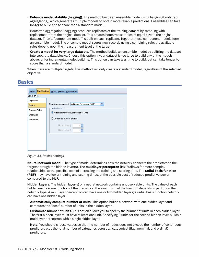
• Enhance model stability (bagging). The method builds an ensemble model using bagging (bootstrapaggregating), which generates multiple models to obtain more reliable predictions. Ensembles can takelonger to build and to score than a standard model.

Bootstrap aggregation (bagging) produces replicates of the training dataset by sampling withreplacement from the original dataset. This creates bootstrap samples of equal size to the originaldataset. Then a "component model" is built on each replicate. Together these component models forman ensemble model. The ensemble model scores new records using a combining rule; the availablerules depend upon the measurement level of the target.

• Create a model for very large datasets. The method builds an ensemble model by splitting the datasetinto separate data blocks. Choose this option if your dataset is too large to build any of the modelsabove, or for incremental model building. This option can take less time to build, but can take longer toscore than a standard model.

When there are multiple targets, this method will only create a standard model, regardless of the selectedobjective.

Basics

Figure 33. Basics settings

Neural network model. The type of model determines how the network connects the predictors to thetargets through the hidden layer(s). The multilayer perceptron (MLP) allows for more complexrelationships at the possible cost of increasing the training and scoring time. The radial basis function(RBF) may have lower training and scoring times, at the possible cost of reduced predictive powercompared to the MLP.

Hidden Layers. The hidden layer(s) of a neural network contains unobservable units. The value of eachhidden unit is some function of the predictors; the exact form of the function depends in part upon thenetwork type. A multilayer perceptron can have one or two hidden layers; a radial basis function networkcan have one hidden layer.

• Automatically compute number of units. This option builds a network with one hidden layer andcomputes the "best" number of units in the hidden layer.

• Customize number of units. This option allows you to specify the number of units in each hidden layer.The first hidden layer must have at least one unit. Specifying 0 units for the second hidden layer builds amultilayer perceptron with a single hidden layer.

Note: You should choose values so that the number of nodes does not exceed the number of continuouspredictors plus the total number of categories across all categorical (flag, nominal, and ordinal)predictors.


Stopping rules

Figure 34. Stopping Rules settings

These are the rules that determine when to stop training multilayer perceptron networks; these settingsare ignored when the radial basis function algorithm is used. Training proceeds through at least one cycle(data pass), and can then be stopped according to the following criteria.

Use maximum training time (per component model). Choose whether to specify a maximum number ofminutes for the algorithm to run. Specify a number greater than 0. When an ensemble model is built, thisis the training time allowed for each component model of the ensemble. Note that training may go a bitbeyond the specified time limit in order to complete the current cycle.

Customize number of maximum training cycles. The maximum number of training cycles allowed. If themaximum number of cycles is exceeded, then training stops. Specify an integer greater than 0.

Use minimum accuracy. With this option, training will continue until the specified accuracy is attained.This may never happen, but you can interrupt training at any point and save the net with the best accuracyachieved so far.

The training algorithm will also stop if the error in the overfit prevention set does not decrease after eachcycle, if the relative change in the training error is small, or if the ratio of the current training error is smallcompared to the initial error.


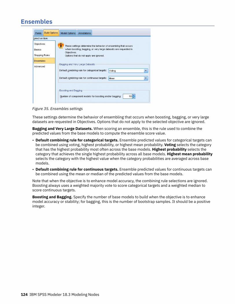
Ensembles

Figure 35. Ensembles settings

These settings determine the behavior of ensembling that occurs when boosting, bagging, or very largedatasets are requested in Objectives. Options that do not apply to the selected objective are ignored.


• Default combining rule for categorical targets. Ensemble predicted values for categorical targets canbe combined using voting, highest probability, or highest mean probability. Voting selects the categorythat has the highest probability most often across the base models. Highest probability selects thecategory that achieves the single highest probability across all base models. Highest mean probabilityselects the category with the highest value when the category probabilities are averaged across basemodels.





Advanced

Figure 36. Advanced settings

Advanced settings provide control over options that do not fit neatly into other groups of settings.

Overfit prevention set. The neural network method internally separates records into a model building setand an overfit prevention set, which is an independent set of data records used to track errors duringtraining in order to prevent the method from modeling chance variation in the data. Specify a percentageof records. The default is 30.

Replicate results. Setting a random seed allows you to replicate analyses. Specify an integer or clickGenerate, which will create a pseudo-random integer between 1 and 2147483647, inclusive. By default,analyses are replicated with seed 229176228.

Missing values in predictors. This specifies how to treat missing values. Delete listwise removes recordswith missing values on predictors from model building. Impute missing values will replace missingvalues in predictors and use those records in the analysis. Continuous fields impute the average of theminimum and maximum observed values; categorical fields impute the most frequently occurringcategory. Note that records with missing values on any other field specified on the Fields tab are alwaysremoved from model building.


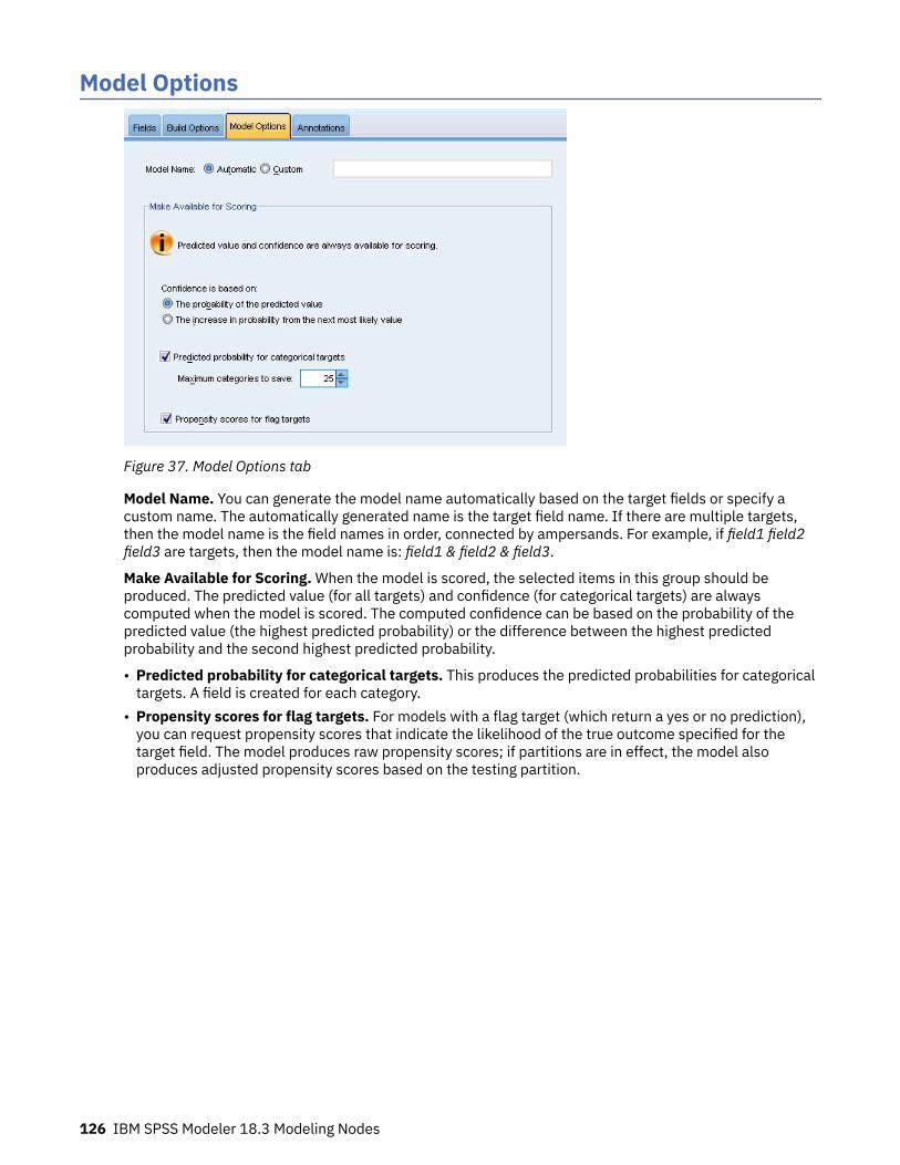
Model Options

Figure 37. Model Options tab

Model Name. You can generate the model name automatically based on the target fields or specify acustom name. The automatically generated name is the target field name. If there are multiple targets,then the model name is the field names in order, connected by ampersands. For example, if field1 field2field3 are targets, then the model name is: field1 & field2 & field3.

Make Available for Scoring. When the model is scored, the selected items in this group should beproduced. The predicted value (for all targets) and confidence (for categorical targets) are alwayscomputed when the model is scored. The computed confidence can be based on the probability of thepredicted value (the highest predicted probability) or the difference between the highest predictedprobability and the second highest predicted probability.

• Predicted probability for categorical targets. This produces the predicted probabilities for categoricaltargets. A field is created for each category.

• Propensity scores for flag targets. For models with a flag target (which return a yes or no prediction),you can request propensity scores that indicate the likelihood of the true outcome specified for thetarget field. The model produces raw propensity scores; if partitions are in effect, the model alsoproduces adjusted propensity scores based on the testing partition.


Model Summary

Figure 38. Neural Networks Model Summary view

The Model Summary view is a snapshot, at-a-glance summary of the neural network predictive orclassification accuracy.

Model summary. The table identifies the target, the type of neural network trained, the stopping rule thatstopped training (shown if a multilayer perceptron network was trained), and the number of neurons ineach hidden layer of the network.

Neural Network Quality. The chart displays the accuracy of the final model, which is presented in largeris better format. For a categorical target, this is simply the percentage of records for which the predictedvalue matches the observed value. For a continuous target, the accuracy is given as the R2 value.

Multiple targets. If there are multiple targets, then each target is displayed in the Target row of the table.The accuracy displayed in the chart is the average of the individual target accuracies.


Predictor Importance

Figure 39. Predictor Importance view

Typically, you will want to focus your modeling efforts on the predictor fields that matter most andconsider dropping or ignoring those that matter least. The predictor importance chart helps you do this byindicating the relative importance of each predictor in estimating the model. Since the values are relative,the sum of the values for all predictors on the display is 1.0. Predictor importance does not relate tomodel accuracy. It just relates to the importance of each predictor in making a prediction, not whether ornot the prediction is accurate.

Multiple targets. If there are multiple targets, then each target is displayed in a separate chart and thereis a Target drop-down that controls which target to display.


Predicted By Observed

Figure 40. Predicted By Observed view

For continuous targets, this displays a binned scatterplot of the predicted values on the vertical axis bythe observed values on the horizontal axis.

Multiple targets. If there are multiple continuous targets, then each target is displayed in a separatechart and there is a Target drop-down that controls which target to display.


Classification

Figure 41. Classification view, row percents style

For categorical targets, this displays the cross-classification of observed versus predicted values in a heatmap, plus the overall percent correct.

Table styles. There are several different display styles, which are accessible from the Style dropdown list.

• Row percents. This displays the row percentages (the cell counts expressed as a percent of the rowtotals) in the cells. This is the default.

• Cell counts. This displays the cell counts in the cells. The shading for the heat map is still based on therow percentages.

• Heat map. This displays no values in the cells, just the shading.• Compressed. This displays no row or column headings, or values in the cells. It can be useful when the

target has a lot of categories.

Missing. If any records have missing values on the target, they are displayed in a (Missing) row under allvalid rows. Records with missing values do not contribute to the overall percent correct.

Multiple targets. If there are multiple categorical targets, then each target is displayed in a separate tableand there is a Target dropdown list that controls which target to display.

Large tables. If the displayed target has more than 100 categories, no table is displayed.


Network

Figure 42. Network view, inputs on the left, effects style

This displays a graphical representation of the neural network.

Chart styles. There are two different display styles, which are accessible from the Style drop-down.

• Effects. This displays each predictor and target as one node in the diagram irrespective of whether themeasurement scale is continuous or categorical. This is the default.

• Coefficients. This displays multiple indicator nodes for categorical predictors and targets. Theconnecting lines in the coefficients-style diagram are colored based on the estimated value of thesynaptic weight.

Diagram orientation. By default, the network diagram is arranged with the inputs on the left and thetargets on the right. Using toolbar controls, you can change the orientation so that inputs are on top andtargets on the bottom, or inputs on the bottom and targets on top.

Predictor importance. Connecting lines in the diagram are weighted based on predictor importance, withgreater line width corresponding to greater importance. There is a Predictor Importance slider in thetoolbar that controls which predictors are shown in the network diagram. This does not change the model,but simply allows you to focus on the most important predictors.

Multiple targets. If there are multiple targets, all targets are displayed in the chart.


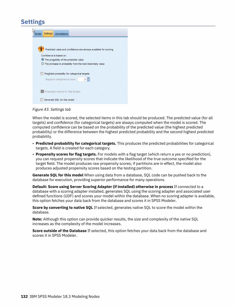
Settings

Figure 43. Settings tab

When the model is scored, the selected items in this tab should be produced. The predicted value (for alltargets) and confidence (for categorical targets) are always computed when the model is scored. Thecomputed confidence can be based on the probability of the predicted value (the highest predictedprobability) or the difference between the highest predicted probability and the second highest predictedprobability.




Default: Score using Server Scoring Adapter (if installed) otherwise in process If connected to adatabase with a scoring adapter installed, generates SQL using the scoring adapter and associated userdefined functions (UDF) and scores your model within the database. When no scoring adapter is available,this option fetches your data back from the database and scores it in SPSS Modeler.

Score by converting to native SQL If selected, generates native SQL to score the model within thedatabase.

Note: Although this option can provide quicker results, the size and complexity of the native SQLincreases as the complexity of the model increases.

Score outside of the Database If selected, this option fetches your data back from the database andscores it in SPSS Modeler.


Chapter 9. Decision List

Decision List models identify subgroups or segments that show a higher or lower likelihood of a binary(yes or no) outcome relative to the overall sample. For example, you might look for customers who areleast likely to churn or most likely to say yes to a particular offer or campaign. The Decision List Viewergives you complete control over the model, enabling you to edit segments, add your own business rules,specify how each segment is scored, and customize the model in a number of other ways to optimize theproportion of hits across all segments. As such, it is particularly well-suited for generating mailing lists orotherwise identifying which records to target for a particular campaign. You can also use multiple miningtasks to combine modeling approaches—for example, by identifying high- and low-performing segmentswithin the same model and including or excluding each in the scoring stage as appropriate.

Segments, Rules, and Conditions

A model consists of a list of segments, each of which is defined by a rule that selects matching records. Agiven rule may have multiple conditions; for example:

RFM_SCORE > 10 andMONTHS_CURRENT <= 9

Rules are applied in the order listed, with the first matching rule determining the outcome for a givenrecord. Taken independently, rules or conditions may overlap, but the order of rules resolves ambiguity. Ifno rule matches, the record is assigned to the remainder rule.

Complete Control over Scoring

The Decision List Viewer enables you to view, modify, and reorganize segments and to choose which toinclude or exclude for purposes of scoring. For example, you can choose to exclude one group ofcustomers from future offers and include others and immediately see how this affects your overall hitrate. Decision List models return a score of Yes for included segments and $null$ for everything else,including the remainder. This direct control over scoring makes Decision List models ideal for generatingmailing lists, and they are widely used in customer relationship management, including call center ormarketing applications.

Mining Tasks, Measures, and Selections

The modeling process is driven by mining tasks. Each mining task effectively initiates a new modeling runand returns a new set of alternative models to choose from. The default task is based on your initialspecifications in the Decision List node, but you can define any number of custom tasks. You can alsoapply tasks iteratively—for example, you can run a high probability search on the entire training set andthen run a low probability search on the remainder to weed out low-performing segments.

Data Selections

You can define data selections and custom model measures for model building and evaluation. Forexample, you can specify a data selection in a mining task to tailor the model to a specific region andcreate a custom measure to evaluate how well that model performs on the whole country. Unlike miningtasks, measures don't change the underlying model but provide another lens to assess how well itperforms.

Adding Your Business Knowledge

By fine-tuning or extending the segments identified by the algorithm, the Decision List Viewer enables youto incorporate your business knowledge right into the model. You can edit the segments generated by themodel or add additional segments based on rules that you specify. You can then apply the changes andpreview the results.

For further insight, a dynamic link with Excel enables you to export your data to Excel, where it can beused to create presentation charts and to calculate custom measures, such as complex profit and ROI,which can be viewed in the Decision List Viewer while you are building the model.

Example. The marketing department of a financial institution wants to achieve more profitable results infuture campaigns by matching the right offer to each customer. You can use a Decision List model toidentify the characteristics of customers most likely to respond favorably based on previous promotionsand to generate a mailing list based on the results.

Requirements. A single categorical target field with a measurement level of type Flag or Nominal thatindicates the binary outcome you want to predict (yes/no), and at least one input field. When the targetfield type is Nominal, you must manually choose a single value to be treated as a hit, or response; all theother values are lumped together as not hit. An optional frequency field may also be specified.Continuous date/time fields are ignored. Continuous numeric range inputs are automatically binned bythe algorithm as specified on the Expert tab in the modeling node. For finer control over binning, add anupstream binning node and use the binned field as input with a measurement level of Ordinal.

Decision List Model OptionsModel name. You can generate the model name automatically based on the target or ID field (or modeltype in cases where no such field is specified) or specify a custom name.



Mode. Specifies the method used to build the model.

• Generate model. Automatically generates a model on the models palette when the node is executed.The resulting model can be added to streams for purposes of scoring but cannot be further edited.

• Launch interactive session. Opens the interactive Decision List Viewer modeling (output) window,enabling you to pick from multiple alternatives and repeatedly apply the algorithm with differentsettings to progressively grow or modify the model. See the topic “ Decision List Viewer ” on page 136for more information.

• Use saved interactive session information. Launches an interactive session using previously savedsettings. Interactive settings can be saved from the Decision List Viewer using the Generate menu (tocreate a model or modeling node) or the File menu (to update the node from which the session waslaunched).

Target value. Specifies the value of the target field that indicates the outcome you want to model. Forexample, if the target field churn is coded 0 = no and 1 = yes, specify 1 to identify rules that indicatewhich records are likely to churn.

Find segments with. Indicates whether the search for the target variable should look for a Highprobability or Low probability of occurrence. Finding and excluding them can be a useful way to improveyour model and can be particularly useful when the remainder has a low probability.

Maximum number of segments. Specifies the maximum number of segments to return. The top Nsegments are created, where the best segment is the one with the highest probability or, if more than onemodel has the same probability, the highest coverage. The minimum allowed setting is 1; there is nomaximum setting.

Minimum segment size. The two settings below dictate the minimum segment size. The larger of the twovalues takes precedence. For example, if the percentage value equates to a number higher than theabsolute value, the percentage setting takes precedence.

• As percentage of previous segment (%). Specifies the minimum group size as a percentage of records.The minimum allowed setting is 0; the maximum allowed setting is 99.9.

• As absolute value (N). Specifies the minimum group size as an absolute number of records. Theminimum allowed setting is 1; there is no maximum setting.

Segment rules.


Maximum number of attributes. Specifies the maximum number of conditions per segment rule. Theminimum allowed setting is 1; there is no maximum setting.

• Allow attribute re-use. When enabled, each cycle can consider all attributes, even those that havebeen used in previous cycles. The conditions for a segment are built up in cycles, where each cycle addsa new condition. The number of cycles is defined using the Maximum number of attributes setting.

Confidence interval for new conditions (%). Specifies the confidence level for testing segmentsignificance. This setting plays a significant role in the number of segments (if any) that are returned aswell as the number-of-conditions-per-segment rule. The higher the value, the smaller the returned resultset. The minimum allowed setting is 50; the maximum allowed setting is 99.9.

Decision List Node Expert OptionsExpert options enable you to fine-tune the model-building process.

Binning method. The method used for binning continuous fields (equal count or equal width).

Number of bins. The number of bins to create for continuous fields. The minimum allowed setting is 2;there is no maximum setting.

Model search width. The maximum number of model results per cycle that can be used for the nextcycle. The minimum allowed setting is 1; there is no maximum setting.

Rule search width. The maximum number of rule results per cycle that can be used for the next cycle.The minimum allowed setting is 1; there is no maximum setting.

Bin merging factor. The minimum amount by which a segment must grow when merged with its neighbor.The minimum allowed setting is 1.01; there is no maximum setting.

• Allow missing values in conditions. True to allow the IS MISSING test in rules.• Discard intermediate results. When True, only the final results of the search process are returned. Afinal result is a result that is not refined any further in the search process. When False, intermediateresults are also returned.

Maximum number of alternatives. Specifies the maximum number of alternatives that can be returnedupon running the mining task. The minimum allowed setting is 1; there is no maximum setting.

Note that the mining task will only return the actual number of alternatives, up to the maximumspecified. For example, if the maximum is set to 100 and only 3 alternatives are found, only those 3 areshown.

Decision List Model NuggetA model consists of a list of segments, each of which is defined by a rule that selects matching records.You can easily view or modify the segments before generating the model and choose which ones toinclude or exclude. When used in scoring, Decision List models return Yes for included segments and $null$ for everything else, including the remainder. This direct control over scoring makes Decision List modelsideal for generating mailing lists, and they are widely used in customer relationship management,including call center or marketing applications.

When you run a stream containing a Decision List model, the node adds three new fields containing thescore, either 1 (meaning Yes) for included fields or $null$ for excluded fields, the probability (hit rate) forthe segment within which the record falls, and the ID number for the segment. The names of the newfields are derived from the name of the output field being predicted, prefixed with $D- for the score, $DP-for the probability, and $DI- for the segment ID.

The model is scored based on the target value specified when the model was built. You can manuallyexclude segments so that they score as $null$. For example, if you run a low probability search to findsegments with lower than average hit rates, these “low” segments will be scored as Yes unless youmanually exclude them. If necessary, nulls can be recoded as No using a Derive or Filler node.

PMML

Chapter 9. Decision List 135

A Decision List model can be stored as a PMML RuleSetModel with a “first hit” selection criterion.However, all of the rules are expected to have the same score. To allow for changes to the target field orthe target value, multiple rule set models can be stored in one file to be applied in order, cases notmatched by the first model being passed to the second, and so on. The algorithm name DecisionList isused to indicate this non-standard behavior, and only rule set models with this name are recognized asDecision List models and scored as such.

Decision List Model Nugget SettingsThe Settings tab for a Decision List model nugget enables you to obtain propensity scores and to enable ordisable SQL optimization. This tab is available only after adding the model nugget to a stream.






• Score by converting to native SQL If selected, generates native SQL to score the model within thedatabase.



Decision List ViewerThe easy-to-use, task-based Decision List Viewer graphical interface takes the complexity out of themodel building process, freeing you from the low-level details of data mining techniques and enabling youto devote your full attention to those parts of the analysis requiring user intervention, such as settingobjectives, choosing target groups, analyzing the results, and selecting the optimal model.

Working Model PaneThe working model pane displays the current model, including mining tasks and other actions that applyto the working model.

ID. Identifies the sequential segment order. Model segments are calculated, in sequence, according totheir ID number.

Segment Rules. Provides the segment name and defined segment conditions. By default, the segmentname is the field name or concatenated field names used in the conditions, with a comma as a separator.

Score. Represents the field that you want to predict, whose value is assumed to be related to the valuesof other fields (the predictors).


Note: The following options can be toggled to display via the “Organizing Model Measures” on page 145dialog.

Cover. The pie chart visually identifies the coverage each segment has in relation to the entire cover.

Cover (n). Lists the coverage for each segment in relation to the entire cover.

Frequency. Lists the number of hits received in relation to the cover. For example, when the cover is 79and the frequency is 50, that means that 50 out of 79 responded for the selected segment.

Probability. Indicates the segment probability. For example, when the cover is 79 and the frequency is50, that means that the probability for the segment is 63.29% (50 divided by 79).

Error. Indicates the segment error.

The information at the bottom of the pane indicates the cover, frequency, and probability for the entiremodel.

Working Model Toolbar

The working model pane provides the following functions via a toolbar.

Note: Some functions are also available by right-clicking a model segment.

Table 9. Working model toolbar buttons

Toolbar Button Description

Launches the Generate New Model dialog, which provides options for creatinga new model nugget.

Saves the current state of the interactive session. The Decision List modelingnode is updated with the current settings, including mining tasks, modelsnapshots, data selections, and custom measures. To restore a session to thisstate, check the Use saved session information box on the Model tab of themodeling node and click Run.

Displays the Organize Model Measures dialog. See the topic “Organizing ModelMeasures” on page 145 for more information.

Displays the Organize Data Selections dialog. See the topic “Organizing DataSelections” on page 141 for more information.

Displays the Snapshots tab. See the topic “Snapshots Tab” on page 138 formore information.

Displays the Alternatives tab. See the topic “Alternatives Tab” on page 138 formore information.

Takes a snapshot of the current model structure. Snapshots display on theSnapshots tab and are commonly used for model comparison purposes.

Launches the Inserting Segments dialog, which provides options for creatingnew model segments.

Launches the Editing Segment Rules dialog, which provides options for addingconditions to model segments or changing previously defined model segmentconditions.

Moves the selected segment up in the model hierarchy.

Moves the selected segment down in the model hierarchy.


Table 9. Working model toolbar buttons (continued)

Deletes the selected segment.

Toggles whether the selected segment is included in the model. Whenexcluded, the segment results are added to the remainder. This differs fromdeleting a segment in that you have the option of reactivating the segment.

Alternatives TabGenerated when you click Find Segments, the Alternatives tab lists all alternative mining results for theselected model or segment on the working model pane.

To promote an alternative to be the working model, highlight the required alternative and click Load; thealternative model is displayed in the working model pane.

Note: The Alternatives tab is only displayed if you have set Maximum number of alternatives on theDecision List modeling node Expert tab to create more than one alternative.

Each generated model alternative displays specific model information:

Name. Each alternative is sequentially numbered. The first alternative usually contains the best results.

Target. Indicates the target value. For example: 1, which equals "true".

No. of Segments. The number of segment rules used in the alternative model.

Cover. The coverage of the alternative model.

Freq. The number of hits in relation to the cover.

Prob. Indicates the probability percentage of the alternative model.

Note: Alternative results are not saved with the model; results are valid only during the active session.

Snapshots TabA snapshot is a view of a model at a specific point in time. For example, you could take a model snapshotwhen you want to load a different alternative model into the working model pane but do not want to losethe work on the current model. The Snapshots tab lists all model snapshots manually taken for anynumber of working model states.

Note: Snapshots are saved with the model. We recommend that you take a snapshot when you load thefirst model. This snapshot will then preserve the original model structure, ensuring that you can alwaysreturn to the original model state. The generated snapshot name displays as a timestamp, indicatingwhen it was generated.

Create a Model Snapshot

1. Select an appropriate model/alternative to display in the working model pane.2. Make any necessary changes to the working model.3. Click Take Snapshot. A new snapshot is displayed on the Snapshots tab.

Name. The snapshot name. You can change a snapshot name by double-clicking the snapshot name.

Target. Indicates the target value. For example: 1, which equals "true".

No. of Segments. The number of segment rules used in the model.

Cover. The coverage of the model.

Freq. The number of hits in relation to the cover.

Prob. Indicates the probability percentage of the model.


4. To promote a snapshot to be the working model, highlight the required snapshot and click Load; thesnapshot model is displayed in the working model pane.

5. You can delete a snapshot by clicking Delete or by right-clicking the snapshot and choosing Deletefrom the menu.

Working with Decision List ViewerA model that will best predict customer response and behavior is built in various stages. When DecisionList Viewer launches, the working model is populated with the defined model segments and measures,ready for you start a mining task, modify the segments/measures as required, and generate a new modelor modeling node.

You can add one or more segment rules until you have developed a satisfactory model. You can addsegment rules to the model by running mining tasks or by using the Edit Segment Rule function.

In the model building process, you can assess the performance of the model by validating the modelagainst measure data, by visualizing the model in a chart, or by generating custom Excel measures.

When you feel certain about the model's quality, you can generate a new model and place it on the IBMSPSS Modeler canvas or Model palette.

Mining TasksA mining task is a collection of parameters that determines the way new rules are generated. Some ofthese parameters are selectable to provide you with the flexibility to adapt models to new situations. Atask consists of a task template (type), a target, and a build selection (mining dataset).

The following sections detail the various mining task operations:

• “Running Mining Tasks” on page 139• “Creating and Editing a Mining Task” on page 140• “Organizing Data Selections” on page 141

Running Mining TasksDecision List Viewer enables you to manually add segment rules to a model by running mining tasks or bycopying and pasting segment rules between models. A mining task holds information on how to generatenew segment rules (the data mining parameter settings, such as the search strategy, source attributes,search width, confidence level, and so on), the customer behavior to predict, and the data to investigate.The goal of a mining task is to search for the best possible segment rules.

To generate a model segment rule by running a mining task:

1. Click the Remainder row. If there are already segments displayed on the working model pane, you canalso select one of the segments to find additional rules based on the selected segment. After selectingthe remainder or segment, use one of the following methods to generate the model, or alternativemodels:

• From the Tools menu, choose Find Segments.• Right-click the Remainder row/segment and choose Find Segments.• Click the Find Segments button on the working model pane.

While the task is processing, the progress is displayed at the bottom of the workspace and informs youwhen the task has completed. Precisely how long a task takes to complete depends on the complexity ofthe mining task and the size of the dataset. If there is only a single model in the results it is displayed onthe working model pane as soon as the task completes; however, where the results contain more thanone model they are displayed on the Alternatives tab.

Note: A task result will either complete with models, complete with no models, or fail.

The process of finding new segment rules can be repeated until no new rules are added to the model. Thismeans that all significant groups of customers have been found.


It is possible to run a mining task on any existing model segment. If the result of a task is not what you arelooking for, you can choose to start another mining task on the same segment. This will provide additionalfound rules based on the selected segment. Segments that are "below" the selected segment (that is,added to the model later than the selected segment) are replaced by the new segments because eachsegment depends on its predecessors.

Creating and Editing a Mining TaskA mining task is the mechanism that searches for the collection of rules that make up a data model.Alongside the search criteria defined in the selected template, a task also defines the target (the actualquestion that motivated the analysis, such as how many customers are likely to respond to a mailing), andit identifies the datasets to be used. The goal of a mining task is to search for the best possible models.

Create a mining task

To create a mining task:

1. Select the segment from which you want to mine additional segment conditions.2. Click Settings. The Create/Edit Mining Task dialog opens. This dialog provides options for defining the

mining task.3. Make any necessary changes and click OK to return to the working model pane. Decision List Viewer

uses the settings as the defaults to run for each task until an alternative task or settings is selected.4. Click Find Segments to start the mining task on the selected segment.

Edit a mining task

The Create/Edit Mining Task dialog provides options for defining a new mining task or editing an existingone.

Most parameters available for mining tasks are similar to those offered in the Decision List node. Theexceptions are shown below. See the topic “Decision List Model Options” on page 134 for moreinformation.

Load Settings: When you have created more than one mining task, select the required task.

New... Click to create a new mining task based on the settings of the task currently displayed.

Target

Target Field: Represents the field that you want to predict, whose value is assumed to be related to thevalues of other fields (the predictors).

Target value. Specifies the value of the target field that indicates the outcome you want to model. Forexample, if the target field churn is coded 0 = no and 1 = yes, specify 1 to identify rules that indicatewhich records are likely to churn.

Simple Settings

Maximum number of alternatives. Specifies the number of alternatives that will be displayed uponrunning the mining task. The minimum allowed setting is 1; there is no maximum setting.

Expert Settings

Edit... Opens the Edit Advanced Parameters dialog that enables you to define the advanced settings.See the topic “Edit Advanced Parameters” on page 141 for more information.

Data

Build selection. Provides options for specifying the evaluation measure that Decision List Viewer shouldanalyze to find new rules. The listed evaluation measures are created/edited in the Organize DataSelections dialog.

Available fields. Provides options for displaying all fields or manually selecting which fields to display.


Edit... If the Custom option is selected, this opens the Customize Available Fields dialog that enablesyou to select which fields are available as segment attributes found by the mining task. See the topic“Customize Available Fields” on page 141 for more information.

Edit Advanced Parameters

The Edit Advanced Parameters dialog provides the following configuration options.

Binning method. The method used for binning continuous fields (equal count or equal width).

Number of bins. The number of bins to create for continuous fields. The minimum allowed setting is 2;there is no maximum setting.

Model search width. The maximum number of model results per cycle that can be used for the nextcycle. The minimum allowed setting is 1; there is no maximum setting.

Rule search width. The maximum number of rule results per cycle that can be used for the next cycle.The minimum allowed setting is 1; there is no maximum setting.

Bin merging factor. The minimum amount by which a segment must grow when merged with its neighbor.The minimum allowed setting is 1.01; there is no maximum setting.

• Allow missing values in conditions. True to allow the IS MISSING test in rules.• Discard intermediate results. When True, only the final results of the search process are returned. Afinal result is a result that is not refined any further in the search process. When False, intermediateresults are also returned.

Customize Available Fields

The Customize Available Fields dialog enables you to select which fields are available as segmentattributes found by the mining task.

Available. Lists the fields that are currently available as segment attributes. To remove fields from thelist, select the appropriate fields and click Remove >>. The selected fields move from the Available list tothe Not Available list.

Not Available. Lists the fields that are not available as segment attributes. To include the fields in theavailable list, select the appropriate fields and click << Add. The selected fields move from the NotAvailable list to the Available list.

Organizing Data SelectionsBy organizing data selections (a mining dataset), you can specify which evaluation measures Decision ListViewer should analyze to find new rules and select which data selections are used as the basis formeasures.

To organize data selections:

1. From the Tools menu, choose Organize Data Selections, or right-click a segment and choose theoption. The Organize Data Selections dialog opens.

Note: The Organize Data Selections dialog also enables you to edit or delete existing data selections.2. Click the Add new data selection button. A new data selection entry is added to the existing table.3. Click Name and enter an appropriate selection name.4. Click Partition and select an appropriate partition type.5. Click Condition and select an appropriate condition option. When Specify is selected, the Specify

Selection Condition dialog opens, providing options for defining specific field conditions.6. Define the appropriate condition and click OK.

The data selections are available from the Build Selection drop-down list in the Create/Edit Mining Taskdialog. The list enables you to select which evaluation measure is used for a particular mining task.


Segment RulesYou find model segment rules by running a mining task based on a task template. You can manually addsegment rules to a model using the Insert Segment or Edit Segment Rule functions.

If you choose to mine for new segment rules, the results, if any, are displayed on the Viewer tab of theInteractive List dialog. You can quickly refine your model by selecting one of the alternative results fromthe Model Albums dialog and clicking Load. In this way, you can experiment with differing results until youare ready to build a model that accurately describes your optimum target group.

Inserting SegmentsYou can manually add segment rules to a model using the Insert Segment function.

To add a segment rule condition to a model:

1. In the Interactive List dialog, select a location where you want to add a new segment. The newsegment will be inserted directly above the selected segment.

2. From the Edit menu, choose Insert Segment, or access this selection by right-clicking a segment.

The Insert Segment dialog opens, enabling you to insert new segment rule conditions.3. Click Insert. The Insert Condition dialog opens, enabling you to define the attributes for the new rule

condition.4. Select a field and an operator from the drop-down lists.

Note: If you select the Not in operator, the selected condition will function as an exclusion conditionand displays in red in the Insert Rule dialog. For example, when the condition region = 'TOWN'displays in red, it means that TOWN is excluded from the result set.

5. Enter one or more values or click the Insert Value icon to display the Insert Value dialog. The dialogenables you to choose a value defined for the selected field. For example, the field married willprovide the values yes and no.

6. Click OK to return to the Insert Segment dialog. Click OK a second time to add the created segment tothe model.

The new segment will display in the specified model location.

Editing Segment RulesThe Edit Segment Rule functionality enables you to add, change, or delete segment rule conditions.

To change a segment rule condition:

1. Select the model segment that you want to edit.2. From the Edit menu, choose Edit Segment Rule, or right-click on the rule to access this selection.

The Edit Segment Rule dialog opens.3. Select the appropriate condition and click Edit.

The Edit Condition dialog opens, enabling you to define the attributes for the selected rule condition.4. Select a field and an operator from the drop-down lists.

Note: If you select the Not in operator, the selected condition will function as an exclusion conditionand displays in red in the Edit Segment Rule dialog. For example, when the condition region ='TOWN' displays in red, it means that TOWN is excluded from the result set.

5. Enter one or more values or click the Insert Value button to display the Insert Value dialog. The dialogenables you to choose a value defined for the selected field. For example, the field married willprovide the values yes and no.

6. Click OK to return to the Edit Segment Rule dialog. Click OK a second time to return to the workingmodel.

The selected segment will display with the updated rule conditions.


Deleting Segment Rule Conditions

To delete a segment rule condition:

1. Select the model segment containing the rule conditions that you want to delete.2. From the Edit menu, choose Edit Segment Rule, or right-click on the segment to access this selection.

The Edit Segment Rule dialog opens, enabling you to delete one or more segment rule conditions.3. Select the appropriate rule condition and click Delete.4. Click OK.

Deleting one or more segment rule conditions causes the working model pane to refresh its measuremetrics.

Copying SegmentsDecision List Viewer provides you with a convenient way to copy model segments. When you want toapply a segment from one model to another model, simply copy (or cut) the segment from one model andpaste it into another model. You can also copy a segment from a model displayed in the AlternativePreview panel and paste it into the model displayed in the working model pane. These cut, copy, andpaste functions use a system clipboard to store or retrieve temporary data. This means that in theclipboard the conditions and target are copied. The clipboard contents are not solely reserved to be usedin Decision List Viewer but can also be pasted in other applications. For example, when the clipboardcontents are pasted in a text editor, the conditions and target are pasted in XML-format.

To copy or cut model segments:

1. Select the model segment that you want to use in another model.2. From the Edit menu, choose Copy (or Cut), or right-click on the model segment and select Copy or

Cut.3. Open the appropriate model (where the model segment will be pasted).4. Select one of the model segments, and click Paste.

Note: Instead of the Cut, Copy, and Paste commands you can also use the key combinations: Ctrl+X, Ctrl+C, and Ctrl+V.

The copied (or cut) segment is inserted above the previously selected model segment. The measures ofthe pasted segment and segments below are recalculated.

Note: Both models in this procedure must be based on the same underlying model template and containthe same target, otherwise an error message is displayed.

Alternative ModelsWhere there is more than one result, the Alternatives tab displays the results of each mining task. Eachresult consists of the conditions in the selected data that most closely match the target, as well as any"good enough" alternatives. The total number of alternatives shown depends on the search criteria usedin the analysis process.

To view alternative models:

1. Click on an alternative model on the Alternatives tab. The alternative model segments display, orreplace the current model segments, in the Alternative Preview panel.

2. To work with an alternative model in the working model pane, select the model and click Load in theAlternative Preview panel or right-click an alternative name on the Alternatives tab and choose Load.

Note: Alternative models are not saved when you generate a new model.

Customizing a ModelData are not static. Customers move, get married, and change jobs. Products lose market focus andbecome obsolete.


Decision List Viewer offers business users the flexibility to adapt models to new situations easily andquickly. You can change a model by editing, prioritizing, deleting, or inactivating specific model segments.

Prioritizing SegmentsYou can rank model rules in any order you choose. By default, model segments are displayed in order ofpriority, the first segment having the highest priority. When you assign a different priority to one or more ofthe segments, the model is changed accordingly. You may alter the model as required by movingsegments to a higher or lower priority position.

To prioritize model segments:

1. Select the model segment to which you want to assign a different priority.2. Click one of the two arrow buttons on the working model pane toolbar to move the selected model

segment up or down the list.

After prioritization, all previous assessment results are recalculated and the new values are displayed.

Deleting SegmentsTo delete one or more segments:

1. Select a model segment.2. From the Edit menu, choose Delete Segment, or click the delete button on the toolbar of the working

model pane.

The measures are recalculated for the modified model, and the model is changed accordingly.

Excluding SegmentsAs you are searching for particular groups, you will probably base business actions on a selection of themodel segments. When deploying a model, you may choose to exclude segments within a model.Excluded segments are scored as null values. Excluding a segment does not mean the segment is notused; it means that all records matching this rule are excluded from the mailing list. The rule is stillapplied but differently.

To exclude specific model segments:

1. Select a segment from the working model pane.2. Click the Toggle Segment Exclusion button on the toolbar of the working model pane. Excluded is

now displayed in the selected Target column of the selected segment.

Note: Unlike deleted segments, excluded segments remain available for reuse in the final model.Excluded segments affect chart results.

Change Target ValueThe Change Target Value dialog enables you to change the target value for the current target field.

Snapshots and session results with a different target value than the Working Model are identified bychanging the table background for that row to yellow. This indicates that snapshot/session result isoutdated.

The Create/Edit Mining Task dialog displays the target value for the current working model. The targetvalue is not saved with the mining task. It is instead taken from the Working Model value.

When you promote a saved model to the Working Model that has a different target value from the currentworking model (for example, by editing an alternative result or editing a copy of a snapshot), the targetvalue of the saved model is changed to be the same as the working model (the target value shown in theWorking Model pane is not changed). The model metrics are reevaluated with the new target.


Generate New ModelThe Generate New Model dialog provides options for naming the model and selecting where the new nodeis created.

Model name. Select Custom to adjust the auto-generated name or to create a unique name for the nodeas displayed on the stream canvas.

Create node on. Selecting Canvas places the new model on the working canvas; selecting GM Paletteplaces the new model on the Models palette; selecting Both places the new model on both the workingcanvas and the Models palette.

Include interactive session state. When enabled, the interactive session state is preserved in thegenerated model. When you later generate a modeling node from the model, the state is carried over andused to initialize the interactive session. Regardless of whether the option is selected, the model itselfscores new data identically. When the option is not selected, the model is still able to create a build node,but it will be a more generic build node that starts a new interactive session rather than pick up where theold session left off. If you change the node settings but execute with a saved state, the settings you havechanged are ignored in favor of the settings from the saved state.

Note: The standard metrics are the only metrics that remain with the model. Additional metrics arepreserved with the interactive state. The generated model does not represent the saved interactivemining task state. Once you launch the Decision List Viewer, it displays the settings originally madethrough the Viewer.

See the topic “Regenerating a modeling node” on page 41 for more information.

Model AssessmentSuccessful modeling requires the careful assessment of the model before implementation in theproduction environment takes place. Decision List Viewer provides a number of statistical and businessmeasures that can be used to assess the impact of a model in the real world. These include gains chartsand full interoperability with Excel, thus enabling cost/benefit scenarios to be simulated for assessing theimpact of deployment.

You can assess your model in the following ways:

• Using the predefined statistical and business model measures available in Decision List Viewer(probability, frequency).

• Evaluating measures imported from Microsoft Excel.• Visualizing the model using a gains chart.

Organizing Model MeasuresDecision List Viewer provides options for defining the measures that are calculated and displayed ascolumns. Each segment can include the default cover, frequency, probability, and error measuresrepresented as columns. You can also create new measures that will be displayed as columns.

Defining Model Measures

To add a measure to your model or to define an existing measure:

1. From the Tools menu, choose Organize Model Measures, or right-click the model to make thisselection. The Organize Model Measures dialog opens.

2. Click the Add new model measure button (to the right of the Show column). A new measure isdisplayed in the table.

3. Provide a measure name and select an appropriate type, display option, and selection. The Showcolumn indicates whether the measure will display for the working model. When defining an existingmeasure, select an appropriate metric and selection and indicate if the measure will display for theworking model.

4. Click OK to return to the Decision List Viewer workspace. If the Show column for the new measure waschecked, the new measure will display for the working model.


Custom Metrics in Excel

See the topic “Assessment in Excel” on page 146 for more information.

Refreshing Measures

In certain cases, it may be necessary to recalculate the model measures, such as when you apply anexisting model to a new set of customers.

To recalculate (refresh) the model measures:

From the Edit menu, choose Refresh All Measures.

or

Press F5.

All measures are recalculated, and the new values are shown for the working model.

Assessment in ExcelDecision List Viewer can be integrated with Microsoft Excel, enabling you to use your own valuecalculations and profit formulas directly within the model building process to simulate cost/benefitscenarios. The link with Excel enables you to export data to Excel, where it can be used to createpresentation charts, calculate custom measures, such as complex profit and ROI measures, and viewthem in Decision List Viewer while building the model.

Note: In order for you to work with an Excel spreadsheet, the analytical CRM expert has to defineconfiguration information for the synchronization of Decision List Viewer with Microsoft Excel. Theconfiguration is contained in an Excel spreadsheet file and indicates which information is transferred fromDecision List Viewer to Excel, and vice versa.

The following steps are valid only when MS Excel is installed. If Excel is not installed, the options forsynchronizing models with Excel are not displayed.

To synchronize models with MS Excel:

1. Open the model, run an interactive session, and choose Organize Model Measures from the Toolsmenu.

2. Select Yes for the Calculate custom measures in Excel option. The Workbook field activates,enabling you to select a preconfigured Excel workbook template.

3. Click the Connect to Excel button. The Open dialog opens, enabling you to navigate to thepreconfigured template location on your local or network file system.

4. Select the appropriate Excel template and click Open. The selected Excel template launches; use theWindows taskbar (or press Alt-Tab) to navigate back to the Choose Inputs for Custom Measures dialog.

5. Select the appropriate mappings between the metric names defined in the Excel template and themodel metric names and click OK.

Once the link is established, Excel starts with the preconfigured Excel template that displays the modelrules in the spreadsheet. The results calculated in Excel are displayed as new columns in Decision ListViewer.

Note: Excel metrics do not remain when the model is saved; the metrics are valid only during the activesession. However, you can create snapshots that include Excel metrics. The Excel metrics saved in thesnapshot views are valid only for historical comparison purposes and do not refresh when reopened. Seethe topic “Snapshots Tab” on page 138 for more information. The Excel metrics will not display in thesnapshots until you reestablish a connection to the Excel template.

MS Excel Integration Setup

The integration between Decision List Viewer and Microsoft Excel is accomplished through the use of apreconfigured Excel spreadsheet template. The template consists of three worksheets:


Model Measures. Displays the imported Decision List Viewer measures, the custom Excel measures, andthe calculation totals (defined on the Settings worksheet).

Settings. Provides the variables to generate calculations based on the imported Decision List Viewermeasures and the custom Excel measures.

Configuration. Provides options for specifying which measures are imported from Decision List Viewerand for defining the custom Excel measures.

WARNING: The structure of the Configuration worksheet is rigidly defined. Do NOT edit any cells in thegreen shaded area.

• Metrics From Model. Indicates which Decision List Viewer metrics are used in the calculations.• Metrics To Model. Indicates which Excel-generated metric(s) will be returned to Decision List Viewer.

The Excel-generated metrics display as new measure columns in Decision List Viewer.

Note: Excel metrics do not remain with the model when you generate a new model; the metrics are validonly during the active session.

Changing the Model Measures

The following examples explain how to change Model Measures in several ways:

• Change an existing measure.• Import an additional standard measure from the model.• Export an additional custom measure to the model.

Change an existing measure

1. Open the template and select the Configuration worksheet.2. Edit any Name or Description by highlighting and typing over them.

Note that if you want to change a measure--for example, to prompt the user for Probability instead ofFrequency--you only need to change the name and description in Metrics From Model – this is thendisplayed in the model and the user can choose the appropriate measure to map.

Import an additional standard measure from the model

1. Open the template and select the Configuration worksheet.2. From the menus choose:

Tools > Protection > Unprotect Sheet3. Select cell A5, which is shaded yellow and contains the word End.4. From the menus choose:

Insert > Rows5. Type in the Name and Description of the new measure. For example, Error and Error associated

with segment.6. In cell C5, enter the formula =COLUMN('Model Measures'!N3).7. In cell D5, enter the formula =ROW('Model Measures'!N3)+1.

These formulae will cause the new measure to be displayed in column N of the Model Measuresworksheet, which is currently empty.

8. From the menus choose:

Tools > Protection > Protect Sheet9. Click OK.

10. On the Model Measures worksheet, ensure that cell N3 has Error as a title for the new column.11. Select all of column N.12. From the menus choose:


Format > Cells13. By default, all of the cells have a General number category. Click Percentage to change how the

figures are displayed. This helps you check your figures in Excel; in addition, it enables you to utilizethe data in other ways, for example, as an output to a graph.

14. Click OK.15. Save the spreadsheet as an Excel 2003 template, with a unique name and the file extension .xlt. For

ease of locating the new template, we recommend you save it in the preconfigured template locationon your local or network file system.

Export an additional custom measure to the model

1. Open the template to which you added the Error column in the previous example; select theConfiguration worksheet.

2. From the menus choose:

Tools > Protection > Unprotect Sheet3. Select cell A14, which is shaded yellow and contains the word End.4. From the menus choose:

Insert > Rows5. Type in the Name and Description of the new measure. For example, Scaled Error and Scaling

applied to error from Excel.6. In cell C14, enter the formula =COLUMN('Model Measures'!O3).7. In cell D14, enter the formula =ROW('Model Measures'!O3)+1.

These formulae specify that the column O will supply the new measure to the model.8. Select the Settings worksheet.9. In cell A17, enter the description '- Scaled Error.

10. In cell B17, enter the scaling factor of 10.11. On the Model Measures worksheet, enter the description Scaled Error in cell O3 as a title for the new

column.12. In cell O4, enter the formula =N4*Settings!$B$17.13. Select the corner of cell O4 and drag it down to cell O22 to copy the formula into each cell.14. From the menus choose:

Tools > Protection > Protect Sheet15. Click OK.16. Save the spreadsheet as an Excel 2003 template, with a unique name and the file extension .xlt. For

ease of locating the new template, we recommend you save it in the preconfigured template locationon your local or network file system.

When you connect to Excel using this template, the Error value is available as a new custom measure.

Visualizing ModelsThe best way to understand the impact of a model is to visualize it. Using a gains chart, you can obtainvaluable day-to-day insight into the business and technical benefit of your model by studying the effect ofmultiple alternatives in real time. The “Gains Chart” on page 148 section shows the benefit of a modelover randomized decision-making and enables the direct comparison of multiple charts when there arealternative models.

Gains ChartThe gains chart plots the values in the Gains % column from the table. Gains are defined as the proportionof hits in each increment relative to the total number of hits in the tree, using the equation:


(hits in increment / total number of hits) x 100%

Gains charts effectively illustrate how widely you need to cast the net to capture a given percentage of allof the hits in the tree. The diagonal line plots the expected response for the entire sample if the model isnot used. In this case, the response rate would be constant, since one person is just as likely to respondas another. To double your yield, you would need to ask twice as many people. The curved line indicateshow much you can improve your response by including only those who rank in the higher percentilesbased on gain. For example, including the top 50% might net you more than 70% of the positiveresponses. The steeper the curve, the higher the gain.

To view a gains chart:

1. Open a stream that contains a Decision List node and launch an interactive session from the node.2. Click the Gains tab. Depending on which partitions are specified, you may see one or two charts (two

charts would display, for example, when both the training and testing partitions are defined for themodel measures).

By default, the charts display as segments. You can switch the charts to display as quantiles by selectingQuantiles and then selecting the appropriate quantile method from the drop-down menu.

Chart Options

The Chart Options feature provides options for selecting which models and snapshots are charted, whichpartitions are plotted, and whether or not segment labels display.

Models to Plot

Current Models. Enables you to select which models to chart. You can select the working model or anycreated snapshot models.

Partitions to Plot

Partitions for left-hand chart. The drop-down list provides options for displaying all defined partitions orall data.

Partitions for right-hand chart. The drop-down list provides options for displaying all defined partitions,all data, or only the left-hand chart. When Graph only left is selected, only the left chart is displayed.

Display Segment Labels. When enabled, each segment label is displayed on the charts.


Chapter 10. Statistical Models

Statistical models use mathematical equations to encode information extracted from the data. In somecases, statistical modeling techniques can provide adequate models very quickly. Even for problems inwhich more flexible machine-learning techniques (such as neural networks) can ultimately give betterresults, you can use some statistical models as baseline predictive models to judge the performance ofmore advanced techniques.

The following statistical modeling nodes are available.



The PCA/Factor node provides powerful data-reduction techniques to reduce thecomplexity of your data. Principal components analysis (PCA) finds linearcombinations of the input fields that do the best job of capturing the variance in theentire set of fields, where the components are orthogonal (perpendicular) to eachother. Factor analysis attempts to identify underlying factors that explain the patternof correlations within a set of observed fields. For both approaches, the goal is tofind a small number of derived fields that effectively summarizes the information inthe original set of fields.



A generalized linear mixed model (GLMM) extends the linear model so that thetarget can have a non-normal distribution, is linearly related to the factors andcovariates via a specified link function, and so that the observations can becorrelated. Generalized linear mixed models cover a wide variety of models, fromsimple linear regression to complex multilevel models for non-normal longitudinaldata.

The Cox regression node enables you to build a survival model for time-to-eventdata in the presence of censored records. The model produces a survival functionthat predicts the probability that the event of interest has occurred at a given time (t)for given values of the input variables.

Linear NodeLinear regression is a common statistical technique for classifying records based on the values of numericinput fields. Linear regression fits a straight line or surface that minimizes the discrepancies betweenpredicted and actual output values.

Requirements. Only numeric fields can be used in a linear regression model. You must have exactly onetarget field (with the role set to Target) and one or more predictors (with the role set to Input). Fields witha role of Both or None are ignored, as are non-numeric fields. (If necessary, non-numeric fields can berecoded using a Derive node.)

Strengths. Linear regression models are relatively simple and give an easily interpreted mathematicalformula for generating predictions. Because linear regression is a long-established statistical procedure,the properties of these models are well understood. Linear models are also typically very fast to train. TheLinear node provides methods for automatic field selection in order to eliminate nonsignificant input fieldsfrom the equation.

Note: In cases where the target field is categorical rather than a continuous range, such as yes/no orchurn/don't churn, logistic regression can be used as an alternative. Logistic regression also providessupport for non-numeric inputs, removing the need to recode these fields. See the topic “Logistic Node”on page 161 for more information.

Linear modelsLinear models predict a continuous target based on linear relationships between the target and one ormore predictors.

Linear models are relatively simple and give an easily interpreted mathematical formula for scoring. Theproperties of these models are well understood and can typically be built very quickly compared to othermodel types (such as neural networks or decision trees) on the same dataset.

Example. An insurance company with limited resources to investigate homeowners' insurance claimswants to build a model for estimating claims costs. By deploying this model to service centers,representatives can enter claim information while on the phone with a customer and immediately obtainthe "expected" cost of the claim based on past data.

Field requirements. There must be a Target and at least one Input. By default, fields with predefinedroles of Both or None are not used. The target must be continuous (scale). There are no measurementlevel restrictions on predictors (inputs); categorical (flag, nominal, and ordinal) fields are used as factorsin the model and continuous fields are used as covariates.

Objectives

What do you want to do?• Build a new model. Build a completely new model. This is the usual operation of the node.• Continue training an existing model. Training continues with the last model successfully produced by

the node. This makes it possible to update or refresh an existing model without having to access theoriginal data and may result in significantly faster performance since only the new or updated recordsare fed into the stream. Details on the previous model are stored with the modeling node, making itpossible to use this option even if the previous model nugget is no longer available in the stream orModels palette.

Note: When this option is enabled, all other controls on the Fields and Build Options tabs are disabled.

What is your main objective? Select the appropriate objective.

• Create a standard model. The method builds a single model to predict the target using the predictors.Generally speaking, standard models are easier to interpret and can be faster to score than boosted,bagged, or large dataset ensembles.


Note: For split models, to use this option with Continue training an existing model you must beconnected to Analytic Server.

• Enhance model accuracy (boosting). The method builds an ensemble model using boosting, whichgenerates a sequence of models to obtain more accurate predictions. Ensembles can take longer tobuild and to score than a standard model.

Boosting produces a succession of "component models", each of which is built on the entire dataset.Prior to building each successive component model, the records are weighted based on the previouscomponent model's residuals. Cases with large residuals are given relatively higher analysis weights sothat the next component model will focus on predicting these records well. Together these componentmodels form an ensemble model. The ensemble model scores new records using a combining rule; theavailable rules depend upon the measurement level of the target.

• Enhance model stability (bagging). The method builds an ensemble model using bagging (bootstrapaggregating), which generates multiple models to obtain more reliable predictions. Ensembles can takelonger to build and to score than a standard model.

Bootstrap aggregation (bagging) produces replicates of the training dataset by sampling withreplacement from the original dataset. This creates bootstrap samples of equal size to the originaldataset. Then a "component model" is built on each replicate. Together these component models forman ensemble model. The ensemble model scores new records using a combining rule; the availablerules depend upon the measurement level of the target.

• Create a model for very large datasets. The method builds an ensemble model by splitting the datasetinto separate data blocks. Choose this option if your dataset is too large to build any of the modelsabove, or for incremental model building. This option can take less time to build, but can take longer toscore than a standard model.

See “Ensembles ” on page 154 for settings related to boosting, bagging, and very large datasets.

BasicsAutomatically prepare data. This option allows the procedure to internally transform the target andpredictors in order to maximize the predictive power of the model; any transformations are saved with themodel and applied to new data for scoring. The original versions of transformed fields are excluded fromthe model. By default, the following automatic data preparation are performed.

• Date and Time handling. Each date predictor is transformed into new a continuous predictor containingthe elapsed time since a reference date (1970-01-01). Each time predictor is transformed into a newcontinuous predictor containing the time elapsed since a reference time (00:00:00).

• Adjust measurement level. Continuous predictors with less than 5 distinct values are recast as ordinalpredictors. Ordinal predictors with greater than 10 distinct values are recast as continuous predictors.

• Outlier handling. Values of continuous predictors that lie beyond a cutoff value (3 standard deviationsfrom the mean) are set to the cutoff value.

• Missing value handling. Missing values of nominal predictors are replaced with the mode of the trainingpartition. Missing values of ordinal predictors are replaced with the median of the training partition.Missing values of continuous predictors are replaced with the mean of the training partition.

• Supervised merging. This makes a more parsimonious model by reducing the number of fields to beprocessed in association with the target. Similar categories are identified based upon the relationshipbetween the input and the target. Categories that are not significantly different (that is, having a p-valuegreater than 0.1) are merged. If all categories are merged into one, the original and derived versions ofthe field are excluded from the model because they have no value as a predictor.

Confidence level. This is the level of confidence used to compute interval estimates of the modelcoefficients in the Coefficients view. Specify a value greater than 0 and less than 100. The default is 95.

Chapter 10. Statistical Models 153

Model selectionModel selection method. Choose one of the model selection methods (details below) or Include allpredictors, which simply enters all available predictors as main effects model terms. By default, Forwardstepwise is used.

Forward Stepwise Selection. This starts with no effects in the model and adds and removes effects onestep at a time until no more can be added or removed according to the stepwise criteria.

• Criteria for entry/removal. This is the statistic used to determine whether an effect should be added toor removed from the model. Information Criterion (AICC) is based on the likelihood of the training setgiven the model, and is adjusted to penalize overly complex models. F Statistics is based on astatistical test of the improvement in model error. Adjusted R-squared is based on the fit of the trainingset, and is adjusted to penalize overly complex models. Overfit Prevention Criterion (ASE) is based onthe fit (average squared error, or ASE) of the overfit prevention set. The overfit prevention set is arandom subsample of approximately 30% of the original dataset that is not used to train the model.

If any criterion other than F Statistics is chosen, then at each step the effect that corresponds to thegreatest positive increase in the criterion is added to the model. Any effects in the model thatcorrespond to a decrease in the criterion are removed.

If F Statistics is chosen as the criterion, then at each step the effect that has the smallest p-value lessthan the specified threshold, Include effects with p-values less than, is added to the model. Thedefault is 0.05. Any effects in the model with a p-value greater than the specified threshold, Removeeffects with p-values greater than, are removed. The default is 0.10.

• Customize maximum number of effects in the final model. By default, all available effects can beentered into the model. Alternatively, if the stepwise algorithm ends a step with the specified maximumnumber of effects, the algorithm stops with the current set of effects.

• Customize maximum number of steps. The stepwise algorithm stops after a certain number of steps.By default, this is 3 times the number of available effects. Alternatively, specify a positive integermaximum number of steps.

Best Subsets Selection. This checks "all possible" models, or at least a larger subset of the possiblemodels than forward stepwise, to choose the best according to the best subsets criterion. InformationCriterion (AICC) is based on the likelihood of the training set given the model, and is adjusted to penalizeoverly complex models. Adjusted R-squared is based on the fit of the training set, and is adjusted topenalize overly complex models. Overfit Prevention Criterion (ASE) is based on the fit (average squarederror, or ASE) of the overfit prevention set. The overfit prevention set is a random subsample ofapproximately 30% of the original dataset that is not used to train the model.

The model with the greatest value of the criterion is chosen as the best model.

Note: Best subsets selection is more computationally intensive than forward stepwise selection. Whenbest subsets is performed in conjunction with boosting, bagging, or very large datasets, it can takeconsiderably longer to build than a standard model built using forward stepwise selection.

EnsemblesThese settings determine the behavior of ensembling that occurs when boosting, bagging, or very largedatasets are requested in Objectives. Options that do not apply to the selected objective are ignored.






AdvancedReplicate results. Setting a random seed allows you to replicate analyses. The random number generatoris used to choose which records are in the overfit prevention set. Specify an integer or click Generate,which will create a pseudo-random integer between 1 and 2147483647, inclusive. The default is54752075.

Model OptionsModel Name. You can generate the model name automatically based on the target fields or specify acustom name. The automatically generated name is the target field name.

Note that the predicted value is always computed when the model is scored. The name of the new field isthe name of the target field, prefixed with $L-. For example, for a target field named sales, the new fieldwould be named $L-sales.

Model SummaryThe Model Summary view is a snapshot, at-a-glance summary of the model and its fit.

TableThe table identifies some high-level model settings, including:

• The name of the target specified on the Fields tab,• Whether automatic data preparation was performed as specified on the Basics settings,• The model selection method and selection criterion specified on the Model Selection settings. The

value of the selection criterion for the final model is also displayed, and is presented in smaller isbetter format.

ChartThe chart displays the accuracy of the final model, which is presented in larger is better format. Thevalue is 100 × the adjusted R 2 for the final model.

Automatic Data PreparationThis view shows information about which fields were excluded and how transformed fields were derivedin the automatic data preparation (ADP) step. For each field that was transformed or excluded, the tablelists the field name, its role in the analysis, and the action taken by the ADP step. Fields are sorted byascending alphabetical order of field names. The possible actions taken for each field include:

• Derive duration: months computes the elapsed time in months from the values in a field containingdates to the current system date.

• Derive duration: hours computes the elapsed time in hours from the values in a field containing timesto the current system time.

• Change measurement level from continuous to ordinal recasts continuous fields with less than 5unique values as ordinal fields.

• Change measurement level from ordinal to continuous recasts ordinal fields with more than 10unique values as continuous fields.

• Trim outliers sets values of continuous predictors that lie beyond a cutoff value (3 standard deviationsfrom the mean) to the cutoff value.

• Replace missing values replaces missing values of nominal fields with the mode, ordinal fields with themedian, and continuous fields with the mean.


• Merge categories to maximize association with target identifies "similar" predictor categories basedupon the relationship between the input and the target. Categories that are not significantly different(that is, having a p-value greater than 0.05) are merged.

• Exclude constant predictor / after outlier handling / after merging of categories removes predictorsthat have a single value, possibly after other ADP actions have been taken.


Predicted By ObservedThis displays a binned scatterplot of the predicted values on the vertical axis by the observed values onthe horizontal axis. Ideally, the points should lie on a 45-degree line; this view can tell you whether anyrecords are predicted particularly badly by the model.

ResidualsThis displays a diagnostic chart of model residuals.

Chart styles. There are different display styles, which are accessible from the Style drop-down.

• Histogram. This is a binned histogram of the studentized residuals with an overlay of the normaldistribution. Linear models assume that the residuals have a normal distribution, so the histogramshould ideally closely approximate the smooth line.

• P-P Plot. This is a binned probability-probability plot comparing the studentized residuals to a normaldistribution. If the slope of the plotted points is less steep than the normal line, the residuals showgreater variability than a normal distribution; if the slope is steeper, the residuals show less variabilitythan a normal distribution. If the plotted points have an S-shaped curve, then the distribution ofresiduals is skewed.

OutliersThis table lists records that exert undue influence upon the model, and displays the record ID (if specifiedon the Fields tab), target value, and Cook's distance. Cook's distance is a measure of how much theresiduals of all records would change if a particular record were excluded from the calculation of themodel coefficients. A large Cook's distance indicates that excluding a record from changes thecoefficients substantially, and should therefore be considered influential.

Influential records should be examined carefully to determine whether you can give them less weight inestimating the model, or truncate the outlying values to some acceptable threshold, or remove theinfluential records completely.

EffectsThis view displays the size of each effect in the model.

Styles. There are different display styles, which are accessible from the Style dropdown list.

• Diagram. This is a chart in which effects are sorted from top to bottom by decreasing predictorimportance. Connecting lines in the diagram are weighted based on effect significance, with greater linewidth corresponding to more significant effects (smaller p-values). Hovering over a connecting linereveals a tooltip that shows the p-value and importance of the effect. This is the default.

• Table. This is an ANOVA table for the overall model and the individual model effects. The individualeffects are sorted from top to bottom by decreasing predictor importance. Note that by default, the


table is collapsed to only show the results for the overall model. To see the results for the individualmodel effects, click the Corrected Model cell in the table.

Predictor importance. There is a Predictor Importance slider that controls which predictors are shown inthe view. This does not change the model, but simply allows you to focus on the most importantpredictors. By default, the top 10 effects are displayed.

Significance. There is a Significance slider that further controls which effects are shown in the view,beyond those shown based on predictor importance. Effects with significance values greater than theslider value are hidden. This does not change the model, but simply allows you to focus on the mostimportant effects. By default the value is 1.00, so that no effects are filtered based on significance.

CoefficientsThis view displays the value of each coefficient in the model. Note that factors (categorical predictors) areindicator-coded within the model, so that effects containing factors will generally have multipleassociated coefficients; one for each category except the category corresponding to the redundant(reference) parameter.


• Diagram. This is a chart which displays the intercept first, and then sorts effects from top to bottom bydecreasing predictor importance. Within effects containing factors, coefficients are sorted by ascendingorder of data values. Connecting lines in the diagram are colored based on the sign of the coefficient(see the diagram key) and weighted based on coefficient significance, with greater line widthcorresponding to more significant coefficients (smaller p-values). Hovering over a connecting linereveals a tooltip that shows the value of the coefficient, its p-value, and the importance of the effect theparameter is associated with. This is the default style.

• Table. This shows the values, significance tests, and confidence intervals for the individual modelcoefficients. After the intercept, the effects are sorted from top to bottom by decreasing predictorimportance. Within effects containing factors, coefficients are sorted by ascending order of data values.Note that by default the table is collapsed to only show the coefficient, significance, and importance ofeach model parameter. To see the standard error, t statistic, and confidence interval, click theCoefficient cell in the table. Hovering over the name of a model parameter in the table reveals a tooltipthat shows the name of the parameter, the effect the parameter is associated with, and (for categoricalpredictors), the value labels associated with the model parameter. This can be particularly useful to seethe new categories created when automatic data preparation merges similar categories of a categoricalpredictor.

Predictor importance. There is a Predictor Importance slider that controls which predictors are shown inthe view. This does not change the model, but simply allows you to focus on the most importantpredictors. By default, the top 10 effects are displayed.

Significance. There is a Significance slider that further controls which coefficients are shown in the view,beyond those shown based on predictor importance. Coefficients with significance values greater than theslider value are hidden. This does not change the model, but simply allows you to focus on the mostimportant coefficients. By default the value is 1.00, so that no coefficients are filtered based onsignificance.

Estimated meansThese are charts displayed for significant predictors. The chart displays the model-estimated value of thetarget on the vertical axis for each value of the predictor on the horizontal axis, holding all other predictorsconstant. It provides a useful visualization of the effects of each predictor's coefficients on the target.

Note: If no predictors are significant, no estimated means are produced.

Model Building SummaryWhen a model selection algorithm other than None is chosen on the Model Selection settings, thisprovides some details of the model building process.


Forward stepwise. When forward stepwise is the selection algorithm, the table displays the last 10 stepsin the stepwise algorithm. For each step, the value of the selection criterion and the effects in the modelat that step are shown. This gives you a sense of how much each step contributes to the model. Eachcolumn allows you to sort the rows so that you can more easily see which effects are in the model at agiven step.

Best subsets. When best subsets is the selection algorithm, the table displays the top 10 models. Foreach model, the value of the selection criterion and the effects in the model are shown. This gives you asense of the stability of the top models; if they tend to have many similar effects with a few differences,then you can be fairly confident in the "top" model; if they tend to have very different effects, then someof the effects may be too similar and should be combined (or one removed). Each column allows you tosort the rows so that you can more easily see which effects are in the model at a given step.

SettingsNote that the predicted value is always computed when the model is scored. The name of the new field isthe name of the target field, prefixed with $L-. For example, for a target field named sales, the new fieldwould be named $L-sales.







Linear-AS NodeIBM SPSS Modeler has two different versions of the Linear node:

• Linear is the traditional node that runs on the IBM SPSS Modeler Server.• Linear-AS can run when connected to IBM SPSS Analytic Server.

Linear regression is a common statistical technique for classifying records based on the values of numericinput fields. Linear regression fits a straight line or surface that minimizes the discrepancies betweenpredicted and actual output values.

Requirements. Only numeric fields and categorical predictors can be used in a linear regression model.You must have exactly one target field (with the role set to Target) and one or more predictors (with therole set to Input). Fields with a role of Both or None are ignored, as are non-numeric fields. (If necessary,non-numeric fields can be recoded using a Derive node.)

Strengths. Linear regression models are relatively simple and give an easily interpreted mathematicalformula for generating predictions. Because linear regression is a long-established statistical procedure,the properties of these models are well understood. Linear models are also typically very fast to train. TheLinear node provides methods for automatic field selection in order to eliminate nonsignificant input fieldsfrom the equation.

Note: In cases where the target field is categorical rather than a continuous range, such as yes/no orchurn/don't churn, logistic regression can be used as an alternative. Logistic regression also providessupport for non-numeric inputs, removing the need to recode these fields. See the topic “Logistic Node”on page 161 for more information.


Linear-AS modelsLinear models predict a continuous target based on linear relationships between the target and one ormore predictors.

Linear models are relatively simple and give an easily interpreted mathematical formula for scoring. Theproperties of these models are well understood and can typically be built very quickly compared to othermodel types (such as neural networks or decision trees) on the same dataset.

Example. An insurance company with limited resources to investigate homeowners' insurance claimswants to build a model for estimating claims costs. By deploying this model to service centers,representatives can enter claim information while on the phone with a customer and immediately obtainthe "expected" cost of the claim based on past data.

Field requirements. There must be a Target and at least one Input. By default, fields with predefinedroles of Both or None are not used. The target must be continuous (scale). There are no measurementlevel restrictions on predictors (inputs); categorical (flag, nominal, and ordinal) fields are used as factorsin the model and continuous fields are used as covariates.

BasicsInclude intercept. This option includes an offset on the y axis when the x axis is 0. The intercept isusually included in the model. If you can assume the data pass through the origin, you can exclude theintercept.

Consider two way interaction. This option tells the model to compare each possible pair of inputs to seeif the trend of one affects the other. If it does, then those inputs are more likely to be included in thedesign matrix.

Confidence interval for coefficient estimates (%). This is the interval of confidence used to computeestimates of the model coefficients in the Coefficients view. Specify a value greater than 0 and less than100. The default is 95.

Sorting order for categorical predictors. These controls determine the order of the categories for thefactors (categorical inputs) for purposes of determining the "last" category. The sort order setting isignored if the input is not categorical or if a custom reference category is specified.

Model SelectionModel selection method. Choose one of the model selection methods (details below) or Include allpredictors, which simply enters all available predictors as main effects model terms. By default, Forwardstepwise is used.

Forward Stepwise Selection. This starts with no effects in the model and adds and removes effects onestep at a time until no more can be added or removed according to the stepwise criteria.

• Criteria for entry/removal. This is the statistic used to determine whether an effect should be added toor removed from the model. Information Criterion (AICC) is based on the likelihood of the training setgiven the model, and is adjusted to penalize overly complex models. F Statistics is based on astatistical test of the improvement in model error. Adjusted R-squared is based on the fit of the trainingset, and is adjusted to penalize overly complex models. Overfit Prevention Criterion (ASE) is based onthe fit (average squared error, or ASE) of the overfit prevention set. The overfit prevention set is arandom subsample of approximately 30% of the original dataset that is not used to train the model.

If any criterion other than F Statistics is chosen, then at each step the effect that corresponds to thegreatest positive increase in the criterion is added to the model. Any effects in the model thatcorrespond to a decrease in the criterion are removed.

If F Statistics is chosen as the criterion, then at each step the effect that has the smallest p-value lessthan the specified threshold, Include effects with p-values less than, is added to the model. Thedefault is 0.05. Any effects in the model with a p-value greater than the specified threshold, Removeeffects with p-values greater than, are removed. The default is 0.10.


• Customize maximum number of effects in the final model. By default, all available effects can beentered into the model. Alternatively, if the stepwise algorithm ends a step with the specified maximumnumber of effects, the algorithm stops with the current set of effects.

• Customize maximum number of steps. The stepwise algorithm stops after a certain number of steps.By default, this is 3 times the number of available effects. Alternatively, specify a positive integermaximum number of steps.

Best Subsets Selection. This checks "all possible" models, or at least a larger subset of the possiblemodels than forward stepwise, to choose the best according to the best subsets criterion. InformationCriterion (AICC) is based on the likelihood of the training set given the model, and is adjusted to penalizeoverly complex models. Adjusted R-squared is based on the fit of the training set, and is adjusted topenalize overly complex models. Overfit Prevention Criterion (ASE) is based on the fit (average squarederror, or ASE) of the overfit prevention set. The overfit prevention set is a random subsample ofapproximately 30% of the original dataset that is not used to train the model.

The model with the greatest value of the criterion is chosen as the best model.

Note: Best subsets selection is more computationally intensive than forward stepwise selection. Whenbest subsets is performed in conjunction with boosting, bagging, or very large datasets, it can takeconsiderably longer to build than a standard model built using forward stepwise selection.

Model OptionsModel Name. You can generate the model name automatically based on the target fields or specify acustom name. The automatically generated name is the target field name.

Note that the predicted value is always computed when the model is scored. The name of the new field isthe name of the target field, prefixed with $L-. For example, for a target field named sales, the new fieldwould be named $L-sales.

Interactive OutputAfter running a Linear-AS model, the following output is available.

Model InformationThe Model Information view provides key information about the model. The table identifies some high-level model settings, such as:

• The name of the target specified on the Fields tab• The regression weight field• The model building method specified on the Model Selection settings• The number of predictors input• The number of predictors in the final model• Akaike Information Criterion Corrected (AICC). AICC is a measure for selecting and comparing mixed

models based on the -2 (Restricted) log likelihood. Smaller values indicate better models. The AICC"corrects" the AIC for small sample sizes. As the sample size increases, the AICC converges to the AIC.

• R Square. This is the goodness-of-fit measure of a linear model, sometimes called the coefficient ofdetermination. It is the proportion of variation in the dependent variable explained by the regressionmodel. It ranges in value from 0 to 1. Small values indicate that the model does not fit the data well.

• Adjusted R Square

Records SummaryThe Records Summary view provides information about the number and percentage of records (cases)included and excluded from the model.



Predicted by ObservedThis displays a binned scatterplot of the predicted values on the vertical axis by the observed values onthe horizontal axis. Ideally, the points should lie on a 45-degree line; this view can tell you whether anyrecords are predicted particularly badly by the model.

SettingsNote that the predicted value is always computed when the model is scored. The name of the new field isthe name of the target field, prefixed with $L-. For example, for a target field named sales, the new fieldwould be named $L-sales.



• Default: Score using Server Scoring Adapter (if installed) otherwise in process. If connected to adatabase with a scoring adapter installed, generates SQL using the scoring adapter and associated userdefined functions (UDF) and scores your model within the database. When no scoring adapter isavailable, this option fetches your data back from the database and scores it in SPSS Modeler.

• Score outside of the Database. If selected, this option fetches your data back from the database andscores it in SPSS Modeler.

Logistic NodeLogistic regression, also known as nominal regression, is a statistical technique for classifying recordsbased on values of input fields. It is analogous to linear regression but takes a categorical target fieldinstead of a numeric one. Both binomial models (for targets with two discrete categories) and multinomialmodels (for targets with more than two categories) are supported.

Logistic regression works by building a set of equations that relate the input field values to theprobabilities associated with each of the output field categories. Once the model is generated, it can beused to estimate probabilities for new data. For each record, a probability of membership is computed foreach possible output category. The target category with the highest probability is assigned as thepredicted output value for that record.

Binomial example. A telecommunications provider is concerned about the number of customers it islosing to competitors. Using service usage data, you can create a binomial model to predict whichcustomers are liable to transfer to another provider and customize offers so as to retain as manycustomers as possible. A binomial model is used because the target has two distinct categories (likely totransfer or not).

Note: For binomial models only, string fields are limited to eight characters. If necessary, longer stringscan be recoded using a Reclassify node or by using the Anonymize node.

Multinomial example. A telecommunications provider has segmented its customer base by service usagepatterns, categorizing the customers into four groups. Using demographic data to predict groupmembership, you can create a multinomial model to classify prospective customers into groups and thencustomize offers for individual customers.

Requirements. One or more input fields and exactly one categorical target field with two or morecategories. For a binomial model the target must have a measurement level of Flag. For a multinomial


model the target can have a measurement level of Flag, or of Nominal with two or more categories. Fieldsset to Both or None are ignored. Fields used in the model must have their types fully instantiated.

Strengths. Logistic regression models are often quite accurate. They can handle symbolic and numericinput fields. They can give predicted probabilities for all target categories so that a second-best guess caneasily be identified. Logistic models are most effective when group membership is a truly categorical field;if group membership is based on values of a continuous range field (for example, high IQ versus low IQ),you should consider using linear regression to take advantage of the richer information offered by the fullrange of values. Logistic models can also perform automatic field selection, although other approachessuch as tree models or Feature Selection might do this more quickly on large datasets. Finally, sincelogistic models are well understood by many analysts and data miners, they may be used by some as abaseline against which other modeling techniques can be compared.

When processing large datasets, you can improve performance noticeably by disabling the likelihood-ratiotest, an advanced output option. See the topic “Logistic Regression Advanced Output” on page 166 formore information.

Important: If temporary disk space is low, Binomial Logistic Regression can fail to build, and will displayan error. When building from a large data set (10GB or more), the same amount of free disk space isneeded. You can use the environment variable SPSSTMPDIR to set the location of the temporarydirectory.

Logistic Node Model OptionsModel name. You can generate the model name automatically based on the target or ID field (or modeltype in cases where no such field is specified) or specify a custom name.



Procedure. Specifies whether a binomial or multinomial model is created. The options available in thedialog box vary depending on which type of modeling procedure is selected.

• Binomial. Used when the target field is a flag or nominal field with two discrete values (dichotomous),such as yes/no, on/off, male/female.

• Multinomial. Used when the target field is a nominal field with more than two values. You can specifyMain effects, Full factorial, or Custom.

Include constant in equation. This option determines whether the resulting equations will include aconstant term. In most situations, you should leave this option selected.

Binomial ModelsFor binomial models, the following methods and options are available:

Method. Specify the method to be used in building the logistic regression model.

• Enter. This is the default method, which enters all of the terms into the equation directly. No fieldselection is performed in building the model.

• Forwards Stepwise. The Forwards Stepwise method of field selection builds the equation in steps, asthe name implies. The initial model is the simplest model possible, with no model terms (except theconstant) in the equation. At each step, terms that have not yet been added to the model are evaluated,and if the best of those terms adds significantly to the predictive power of the model, it is added. Inaddition, terms that are currently in the model are reevaluated to determine if any of them can beremoved without significantly detracting from the model. If so, they are removed. The process repeats,and other terms are added and/or removed. When no more terms can be added to improve the model,and no more terms can be removed without detracting from the model, the final model is generated.

• Backwards Stepwise. The Backwards Stepwise method is essentially the opposite of the ForwardsStepwise method. With this method, the initial model contains all of the terms as predictors. At each


step, terms in the model are evaluated, and any terms that can be removed without significantlydetracting from the model are removed. In addition, previously removed terms are reevaluated todetermine if the best of those terms adds significantly to the predictive power of the model. If so, it isadded back into the model. When no more terms can be removed without significantly detracting fromthe model, and no more terms can be added to improve the model, the final model is generated.

Categorical inputs. Lists the fields that are identified as categorical, that is, those with a measurementlevel of flag, nominal, or ordinal. You can specify the contrast and base category for each categorical field.

• Field Name. This column contains the field names of the categorical inputs. To add continuous ornumerical inputs into this column, click the Add Fields icon to the right of the list and select the requiredinputs.

• Contrast. The interpretation of the regression coefficients for a categorical field depends on thecontrasts that are used. The contrast determines how hypothesis tests are set up to compare theestimated means. For example, if you know that a categorical field has implicit order, such as a patternor grouping, you can use the contrast to model that order. The available contrasts are:

Indicator. Contrasts indicate the presence or absence of category membership. This is the defaultmethod.

Simple. Each category of the predictor field, except the reference category, is compared to thereference category.

Difference. Each category of the predictor field, except the first category, is compared to the averageeffect of previous categories. Also known as reverse Helmert contrasts.

Helmert. Each category of the predictor field, except the last category, is compared to the averageeffect of subsequent categories.

Repeated. Each category of the predictor field, except the first category, is compared to the categorythat precedes it.

Polynomial. Orthogonal polynomial contrasts. Categories are assumed to be equally spaced.Polynomial contrasts are available for numeric fields only.

Deviation. Each category of the predictor field, except the reference category, is compared to theoverall effect.

• Base Category. Specifies how the reference category is determined for the selected contrast type.Select First to use the first category for the input field—sorted alphabetically—or select Last to use thelast category. The default base category applies to variables that are listed in the Categorical inputsarea.

Note: This field is unavailable if the contrast setting is Difference, Helmert, Repeated, or Polynomial.

The estimate of each field’s effect on the overall response is computed as an increase or decrease in thelikelihood of each of the other categories relative to the reference category. This can help you identify thefields and values that are more likely to give a specific response.

The base category is shown in the output as 0.0. This is because comparing it to itself produces an emptyresult. All other categories are shown as equations relevant to the base category. See the topic “LogisticNugget Model Details” on page 168 for more information.

Multinomial ModelsFor multinomial models the following methods and options are available:

Method. Specify the method to be used in building the logistic regression model.

• Enter. This is the default method, which enters all of the terms into the equation directly. No fieldselection is performed in building the model.

• Stepwise. The Stepwise method of field selection builds the equation in steps, as the name implies.The initial model is the simplest model possible, with no model terms (except the constant) in theequation. At each step, terms that have not yet been added to the model are evaluated, and if the bestof those terms adds significantly to the predictive power of the model, it is added. In addition, terms


that are currently in the model are reevaluated to determine if any of them can be removed withoutsignificantly detracting from the model. If so, they are removed. The process repeats, and other termsare added and/or removed. When no more terms can be added to improve the model, and no moreterms can be removed without detracting from the model, the final model is generated.

• Forwards. The Forwards method of field selection is similar to the Stepwise method in that the model isbuilt in steps. However, with this method, the initial model is the simplest model, and only the constantand terms can be added to the model. At each step, terms not yet in the model are tested based on howmuch they would improve the model, and the best of those terms is added to the model. When no moreterms can be added, or the best candidate term does not produce a large-enough improvement in themodel, the final model is generated.

• Backwards. The Backwards method is essentially the opposite of the Forwards method. With thismethod, the initial model contains all of the terms as predictors, and terms can only be removed fromthe model. Model terms that contribute little to the model are removed one by one until no more termscan be removed without significantly worsening the model, yielding the final model.

• Backwards Stepwise. The Backwards Stepwise method is essentially the opposite of the Stepwisemethod. With this method, the initial model contains all of the terms as predictors. At each step, termsin the model are evaluated, and any terms that can be removed without significantly detracting from themodel are removed. In addition, previously removed terms are reevaluated to determine if the best ofthose terms adds significantly to the predictive power of the model. If so, it is added back into themodel. When no more terms can be removed without significantly detracting from the model, and nomore terms can be added to improve the model, the final model is generated.

Note: The automatic methods, including Stepwise, Forwards, and Backwards, are highly adaptablelearning methods and have a strong tendency to overfit the training data. When using these methods, it isespecially important to verify the validity of the resulting model either with new data or a hold-out testsample created using the Partition node.

Base category for target. Specifies how the reference category is determined. This is used as thebaseline against which the regression equations for all other categories in the target are estimated. SelectFirst to use the first category for the current target field—sorted alphabetically—or select Last to use thelast category. Alternatively, you can select Specify to choose a specific category and select the desiredvalue from the list. Available values can be defined for each field in a Type node.

Often you would specify the category in which you are least interested to be the base category, forexample, a loss-leader product. The other categories are then related to this base category in a relativefashion to identify what makes them more likely to be in their own category. This can help you identify thefields and values that are more likely to give a specific response.

The base category is shown in the output as 0.0. This is because comparing it to itself produces an emptyresult. All other categories are shown as equations relevant to the base category. See the topic “LogisticNugget Model Details” on page 168 for more information.

Model type. There are three options for defining the terms in the model. Main Effects models includeonly the input fields individually and do not test interactions (multiplicative effects) between input fields.Full Factorial models include all interactions as well as the input field main effects. Full factorial modelsare better able to capture complex relationships but are also much more difficult to interpret and aremore likely to suffer from overfitting. Because of the potentially large number of possible combinations,automatic field selection methods (methods other than Enter) are disabled for full factorial models.Custom models include only the terms (main effects and interactions) that you specify. When selectingthis option, use the Model Terms list to add or remove terms in the model.

Model Terms. When building a Custom model, you will need to explicitly specify the terms in the model.The list shows the current set of terms for the model. The buttons on the right side of the Model Terms listenable you to add and remove model terms.

• To add terms to the model, click the Add new model terms button.• To delete terms, select the desired terms and click the Delete selected model terms button.


Adding Terms to a Logistic Regression ModelWhen requesting a custom logistic regression model, you can add terms to the model by clicking the Addnew model terms button on the Logistic Regression Model tab. The New Terms dialog box opens in whichyou can specify terms.

Type of term to add. There are several ways to add terms to the model, based on the selection of inputfields in the Available fields list.

• Single interaction. Inserts the term representing the interaction of all selected fields.• Main effects. Inserts one main effect term (the field itself) for each selected input field.• All 2-way interactions. Inserts a 2-way interaction term (the product of the input fields) for each

possible pair of selected input fields. For example, if you have selected input fields A, B, and C in theAvailable fields list, this method will insert the terms A * B, A * C, and B * C.

• All 3-way interactions. Inserts a 3-way interaction term (the product of the input fields) for eachpossible combination of selected input fields, taken three at a time. For example, if you have selectedinput fields A, B, C, and D in the Available fields list, this method will insert the terms A * B * C, A * B * D,A * C * D, and B * C * D.

• All 4-way interactions. Inserts a 4-way interaction term (the product of the input fields) for eachpossible combination of selected input fields, taken four at a time. For example, if you have selectedinput fields A, B, C, D, and E in the Available fields list, this method will insert the terms A * B * C * D, A *B * C * E, A * B * D * E, A * C * D * E, and B * C * D * E.

Available fields. Lists the available input fields to be used in constructing model terms.

Preview. Shows the terms that will be added to the model if you click Insert, based on the selected fieldsand term type.

Insert. Inserts terms in the model (based on the current selection of fields and term type) and closes thedialog box.

Logistic Node Expert OptionsIf you have detailed knowledge of logistic regression, expert options enable you to fine-tune the trainingprocess. To access expert options, set Mode to Expert on the Expert tab.

Scale (Multinomial models only). You can specify a dispersion scaling value that will be used to correctthe estimate of the parameter covariance matrix. Pearson estimates the scaling value by using thePearson chi-square statistic. Deviance estimates the scaling value by using the deviance function(likelihood-ratio chi-square) statistic. You can also specify your own user-defined scaling value. It must bea positive numeric value.

Append all probabilities. If this option is selected, probabilities for each category of the output field willbe added to each record processed by the node. If this option is not selected, the probability of only thepredicted category is added.

For example, a table containing the results of a multinomial model with three categories will include fivenew columns. One column will list the probability of the outcome being correctly predicted, the nextcolumn will show the probability that this prediction is a hit or miss, and a further three columns will showthe probability that each category's prediction is a miss or hit. See the topic “Logistic Model Nugget” onpage 168 for more information.

Note: This option is always selected for binomial models.

Singularity tolerance. Specify the tolerance used in checking for singularities.

Convergence. These options enable you to control the parameters for model convergence. When youexecute the model, the convergence settings control how many times the different parameters arerepeatedly run through to see how well they fit. The more often the parameters are tried, the closer theresults will be (that is, the results will converge). See the topic “Logistic Regression Convergence Options”on page 166 for more information.


Output. These options enable you to request additional statistics that will be displayed in the advancedoutput of the model nugget built by the node. See the topic “Logistic Regression Advanced Output” onpage 166 for more information.

Stepping. These options enable you to control the criteria for adding and removing fields with theStepwise, Forwards, Backwards, or Backwards Stepwise estimation methods. (The button is disabled ifthe Enter method is selected.) See the topic “Logistic Regression Stepping Options” on page 167 for moreinformation.

Logistic Regression Convergence OptionsYou can set the convergence parameters for logistic regression model estimation.

Maximum iterations. Specify the maximum number of iterations for estimating the model.

Maximum step-halving. Step-halving is a technique used by logistic regression to deal with complexitiesin the estimation process. Under normal circumstances, you should use the default setting.

Log-likelihood convergence. Iterations stop if the relative change in the log-likelihood is less than thisvalue. The criterion is not used if the value is 0.

Parameter convergence. Iterations stop if the absolute change or relative change in the parameterestimates is less than this value. The criterion is not used if the value is 0.

Delta (Multinomial models only). You can specify a value between 0 and 1 to be added to each emptycell (combination of input field and output field values). This can help the estimation algorithm deal withdata where there are many possible combinations of field values relative to the number of records in thedata. The default is 0.

Logistic Regression Advanced OutputSelect the optional output you want to display in the advanced output of the Regression model nugget. Toview the advanced output, browse the model nugget and click the Advanced tab. See the topic “LogisticModel Nugget Advanced Output” on page 170 for more information.

Binomial Options

Select the types of output to be generated for the model. See the topic “Logistic Model Nugget AdvancedOutput” on page 170 for more information.

Display. Select whether to display the results at each step, or to wait until all steps have been workedthrough.

CI for exp(B). Select the confidence intervals for each coefficient (shown as Beta) in the expression.Specify the level of the confidence interval (the default is 95%).

Residual Diagnosis. Requests a Casewise Diagnostics table of residuals.

• Outliers outside (std. dev.). List only residual cases for which the absolute standardized value of thelisted variable is at least as large as the value you specify. The default value is 2.

• All cases. Include all cases in the Casewise Diagnostic table of residuals.

Note: Because this option lists each of the input records, it may result in an exceptionally large table inthe report, with one line for every record.

Classification cutoff. This enables you to determine the cutpoint for classifying cases. Cases withpredicted values that exceed the classification cutoff are classified as positive, while those with predictedvalues smaller than the cutoff are classified as negative. To change the default, enter a value between0.01 and 0.99.

Multinomial Options

Select the types of output to be generated for the model. See the topic “Logistic Model Nugget AdvancedOutput” on page 170 for more information.


Note: Selecting the Likelihood ratio tests option greatly increases the processing time required to build alogistic regression model. If your model is taking too long to build, consider disabling this option or utilizethe Wald and Score statistics instead. See the topic “Logistic Regression Stepping Options” on page 167for more information.

Iteration history for every. Select the step interval for printing iteration status in the advanced output.

Confidence Interval. The confidence intervals for coefficients in the equations. Specify the level of theconfidence interval (the default is 95%).

Logistic Regression Stepping OptionsThese options enable you to control the criteria for adding and removing fields with the Stepwise,Forwards, Backwards, or Backwards Stepwise estimation methods.

Number of terms in model (Multinomial models only). You can specify the minimum number of terms inthe model for Backwards and Backwards Stepwise models and the maximum number of terms forForwards and Stepwise models. If you specify a minimum value greater than 0, the model will include thatmany terms, even if some of the terms would have been removed based on statistical criteria. Theminimum setting is ignored for Forwards, Stepwise, and Enter models. If you specify a maximum, someterms may be omitted from the model, even though they would have been selected based on statisticalcriteria. The Specify Maximum setting is ignored for Backwards, Backwards Stepwise, and Enter models.

Entry criterion (Multinomial models only). Select Score to maximize speed of processing. TheLikelihood Ratio option may provide somewhat more robust estimates but take longer to compute. Thedefault setting is to use the Score statistic.

Removal criterion. Select Likelihood Ratio for a more robust model. To shorten the time required to buildthe model, you can try selecting Wald. However, if you have complete or quasi-complete separation in thedata (which you can determine by using the Advanced tab on the model nugget), the Wald statisticbecomes particularly unreliable and should not be used. The default setting is to use the likelihood-ratiostatistic. For binomial models, there is the additional option Conditional. This provides removal testingbased on the probability of the likelihood-ratio statistic based on conditional parameter estimates.

Significance thresholds for criteria. This option enables you to specify selection criteria based on thestatistical probability (the p value) associated with each field. Fields will be added to the model only if theassociated p value is smaller than the Entry value and will be removed only if the p value is larger than theRemoval value. The Entry value must be smaller than the Removal value.

Requirements for entry or removal (Multinomial models only). For some applications, it doesn't makemathematical sense to add interaction terms to the model unless the model also contains the lower-orderterms for the fields involved in the interaction term. For example, it may not make sense to include A * B inthe model unless A and B are also included in the model. These options let you determine how suchdependencies are handled during stepwise term selection.

• Hierarchy for discrete effects. Higher-order effects (interactions involving more fields) will enter themodel only if all lower-order effects (main effects or interactions involving fewer fields) for the relevantfields are already in the model, and lower-order effects will not be removed if higher-order effectsinvolving the same fields are in the model. This option applies only to categorical fields.

• Hierarchy for all effects. This option works in the same way as the previous option, except that itapplies to all input fields.

• Containment for all effects. Effects can be included in the model only if all of the effects contained inthe effect are also included in the model. This option is similar to the Hierarchy for all effects optionexcept that continuous fields are treated somewhat differently. For an effect to contain another effect,the contained (lower-order) effect must include all of the continuous fields involved in the containing(higher-order) effect, and the contained effect's categorical fields must be a subset of those in thecontaining effect. For example, if A and B are categorical fields and X is a continuous field, the term A * B* X contains the terms A * X and B * X.

• None. No relationships are enforced; terms are added to and removed from the model independently.


Logistic Model NuggetA Logistic model nugget represents the equation estimated by a Logistic node. It contains all of theinformation captured by the logistic regression model, as well as information about the model structureand performance. This type of equation may also be generated by other models such as Oracle SVM.

When you run a stream containing a Logistic model nugget, the node adds two new fields containing themodel's prediction and the associated probability. The names of the new fields are derived from the nameof the output field being predicted, prefixed with $L- for the predicted category and $LP- for theassociated probability. For example, for an output field named colorpref, the new fields would be named$L-colorpref and $LP-colorpref. In addition, if you have selected the Append all probabilities option in theLogistic node, an additional field will be added for each category of the output field, containing theprobability belonging to the corresponding category for each record. These additional fields are namedbased on the values of the output field, prefixed by $LP-. For example, if the legal values of colorpref areRed, Green, and Blue, three new fields will be added: $LP-Red, $LP-Green, and $LP-Blue.

Generating a Filter node. The Generate menu enables you to create a new Filter node to pass input fieldsbased on the results of the model. Fields that are dropped from the model due to multicollinearity will befiltered by the generated node, as well as fields not used in the model.

Logistic Nugget Model DetailsFor multinomial models, the Model tab in a Logistic model nugget has a split display with model equationsin the left pane, and predictor importance on the right. For binomial models, the tab displays predictorimportance only. See the topic “Predictor Importance” on page 37 for more information.

Model Equations

For multinomial models, the left pane displays the actual equations estimated for the logistic regressionmodel. There is one equation for each category in the target field, except the baseline category. Theequations are displayed in a tree format. This type of equation may also be generated by certain othermodels such as Oracle SVM.

Equation For. Shows the regression equations used to derive the target category probabilities, given a setof predictor values. The last category of the target field is considered the baseline category; theequations shown give the log-odds for the other target categories relative to the baseline category for aparticular set of predictor values. The predicted probability for each category of the given predictorpattern is derived from these log-odds values.

How Probabilities Are Calculated

Each equation calculates the log-odds for a particular target category, relative to the baseline category.The log-odds, also called the logit, is the ratio of the probability for the specified target category to that ofthe baseline category, with the natural logarithm function applied to the result. For the baseline category,the odds of the category relative to itself is 1.0, and thus the log-odds is 0. You can think of this as animplicit equation for the baseline category where all coefficients are 0.

To derive the probability from the log-odds for a particular target category, you take the logit valuecalculated by the equation for that category and apply the following formula:

P(group i) = exp(g i) / Σk exp(g k)

where g is the calculated log-odds, i is the category index, and k goes from 1 to the number of targetcategories.


Optionally, a chart that indicates the relative importance of each predictor in estimating the model mayalso be displayed on the Model tab. Typically you will want to focus your modeling efforts on thepredictors that matter most and consider dropping or ignoring those that matter least. Note this chart isonly available if Calculate predictor importance is selected on the Analyze tab before generating themodel. See the topic “Predictor Importance” on page 37 for more information.


Note: Predictor importance may take longer to calculate for logistic regression than for other types ofmodels, and is not selected on the Analyze tab by default. Selecting this option may slow performance,particularly with large datasets.

Logistic Model Nugget SummaryThe summary for a logistic regression model displays the fields and settings used to generate the model.In addition, if you have executed an Analysis node attached to this modeling node, information from thatanalysis will also be displayed in this section. For general information on using the model browser, see“Browsing model nuggets” on page 36.

Logistic Model Nugget SettingsThe Settings tab in a Logistic model nugget specifies options for confidences, probabilities, propensityscores, and SQL generation during model scoring. This tab is only available after the model nugget hasbeen added to a stream and displays different options depending on the type of model and target.

Multinomial ModelsFor multinomial models, the following options are available.

Calculate confidences Specifies whether confidences are calculated during scoring.

Calculate raw propensity scores (flag targets only) For models with flag targets only, you can requestraw propensity scores that indicate the likelihood of the true outcome specified for the target field.These are in addition to standard prediction and confidence values. Adjusted propensity scores are notavailable. See the topic “Modeling Node Analyze Options” on page 29 for more information.

Append all probabilities Specifies whether probabilities for each category of the output field are addedto each record processed by the node. If this option is not selected, the probability of only the predictedcategory is added. For a nominal target with three categories, for example, the scoring output will includea column for each of the three categories, plus a fourth column indicating the probability for whichevercategory is predicted. For example if the probabilities for categories Red, Green, and Blue are 0.6, 0.3, and0.1 respectively, the predicted category would be Red, with a probability of 0.6.







Note: For multinomial models, SQL generation is unavailable if Append all probabilities has beenselected, or—for models with nominal targets—if Calculate confidences has been selected. SQLgeneration with confidence calculations is supported for multinomial models with flag targets only. SQLgeneration is not available for binomial models.

Binomial ModelsFor binomial models, confidences and probabilities are always enabled, and the settings that wouldenable you to disable these options are not available. SQL generation is not available for binomial models.


The only setting that can be changed for binomial models is the ability to calculate raw propensity scores.As noted earlier for multinomial models, this applies to models with flag targets only. See the topic“Modeling Node Analyze Options” on page 29 for more information.

Logistic Model Nugget Advanced OutputThe advanced output for logistic regression (also known as nominal regression) gives detailedinformation about the estimated model and its performance. Most of the information contained in theadvanced output is quite technical, and extensive knowledge of logistic regression analysis is required toproperly interpret this output.

Warnings. Indicates any warnings or potential problems with the results.

Case processing summary. Lists the number of records processed, broken down by each symbolic fieldin the model.

Step summary (optional). Lists the effects added or removed at each step of model creation, when usingautomatic field selection.

Note: Only shown for the Stepwise, Forwards, Backwards, or Backwards Stepwise methods.

Iteration history (optional). Shows the iteration history of parameter estimates for every n iterationsbeginning with the initial estimates, where n is the value of the print interval. The default is to print everyiteration (n=1).

Model fitting information (Multinomial models). Shows the likelihood-ratio test of your model (Final)against one in which all of the parameter coefficients are 0 (Intercept Only).

Classification (optional). Shows the matrix of predicted and actual output field values with percentages.

Goodness-of-fit chi-square statistics (optional). Shows Pearson's and likelihood-ratio chi-squarestatistics. These statistics test the overall fit of the model to the training data.

Hosmer and Lemeshow goodness-of-fit (optional). Shows the results of grouping cases into deciles ofrisk and comparing the observed probability with the expected probability within each decile. Thisgoodness-of-fit statistic is more robust than the traditional goodness-of-fit statistic used in multinomialmodels, particularly for models with continuous covariates and studies with small sample sizes.

Pseudo R-square (optional). Shows the Cox and Snell, Nagelkerke, and McFadden R-square measures ofmodel fit. These statistics are in some ways analogous to the R-square statistic in linear regression.

Monotonicity measures (optional). Shows the number of concordant pairs, discordant pairs, and tiedpairs in the data, as well as the percentage of the total number of pairs that each represents. The Somers'D, Goodman and Kruskal's Gamma, Kendall's tau-a, and Concordance Index C are also displayed in thistable.

Information criteria (optional). Shows Akaike’s information criterion (AIC) and Schwarz’s Bayesianinformation criterion (BIC).

Likelihood ratio tests (optional). Shows statistics testing of whether the coefficients of the model effectsare statistically different from 0. Significant input fields are those with very small significance levels in theoutput (labeled Sig.).

Parameter estimates (optional). Shows estimates of the equation coefficients, tests of thosecoefficients, odds ratios derived from the coefficients labeled Exp(B), and confidence intervals for theodds ratios.

Asymptotic covariance/correlation matrix (optional). Shows the asymptotic covariances and/orcorrelations of the coefficient estimates.

Observed and predicted frequencies (optional). For each covariate pattern, shows the observed andpredicted frequencies for each output field value. This table can be quite large, especially for models withnumeric input fields. If the resulting table would be too large to be practical, it is omitted, and a warning isdisplayed.


PCA/Factor NodeThe PCA/Factor node provides powerful data-reduction techniques to reduce the complexity of your data.Two similar but distinct approaches are provided.

• Principal components analysis (PCA) finds linear combinations of the input fields that do the best jobof capturing the variance in the entire set of fields, where the components are orthogonal(perpendicular) to each other. PCA focuses on all variance, including both shared and unique variance.

• Factor analysis attempts to identify underlying concepts, or factors, that explain the pattern ofcorrelations within a set of observed fields. Factor analysis focuses on shared variance only. Variancethat is unique to specific fields is not considered in estimating the model. Several methods of factoranalysis are provided by the Factor/PCA node.

For both approaches, the goal is to find a small number of derived fields that effectively summarize theinformation in the original set of fields.

Requirements. Only numeric fields can be used in a PCA-Factor model. To estimate a factor analysis orPCA, you need one or more fields with the role set to Input fields. Fields with the role set to Target, Both,or None are ignored, as are non-numeric fields.

Strengths. Factor analysis and PCA can effectively reduce the complexity of your data without sacrificingmuch of the information content. These techniques can help you build more robust models that executemore quickly than would be possible with the raw input fields.

PCA/Factor Node Model OptionsModel name. You can generate the model name automatically based on the target or ID field (or modeltype in cases where no such field is specified) or specify a custom name.


Extraction Method. Specify the method to be used for data reduction.

• Principal Components. This is the default method, which uses PCA to find components that summarizethe input fields.

• Unweighted Least Squares. This factor analysis method works by finding the set of factors that is bestable to reproduce the pattern of relationships (correlations) among the input fields.

• Generalized Least Squares. This factor analysis method is similar to unweighted least squares, exceptthat it uses weighting to de-emphasize fields with a lot of unique (unshared) variance.

• Maximum Likelihood. This factor analysis method produces factor equations that are most likely tohave produced the observed pattern of relationships (correlations) in the input fields, based onassumptions about the form of those relationships. Specifically, the method assumes that the trainingdata follow a multivariate normal distribution.

• Principal Axis Factoring. This factor analysis method is very similar to the principal componentsmethod, except that it focuses on shared variance only.

• Alpha Factoring. This factor analysis method considers the fields in the analysis to be a sample fromthe universe of potential input fields. It maximizes the statistical reliability of the factors.

• Image Factoring. This factor analysis method uses data estimation to isolate the common variance andfind factors that describe it.

PCA/Factor Node Expert OptionsIf you have detailed knowledge of factor analysis and PCA, expert options enable you to fine-tune thetraining process. To access expert options, set Mode to Expert on the Expert tab.

Missing values. By default, IBM SPSS Modeler only uses records that have valid values for all fields usedin the model. (This is sometimes called listwise deletion of missing values.) If you have a lot of missingdata, you may find that this approach eliminates too many records, leaving you without enough data to


generate a good model. In such cases, you can deselect the Only use complete records option. IBM SPSSModeler then attempts to use as much information as possible to estimate the model, including recordswhere some of the fields have missing values. (This is sometimes called pairwise deletion of missingvalues.) However, in some situations, using incomplete records in this manner can lead to computationalproblems in estimating the model.

Fields. Specify whether to use the correlation matrix (the default) or the covariance matrix of the inputfields in estimating the model.

Maximum iterations for convergence. Specify the maximum number of iterations for estimating themodel.

Extract factors. There are two ways to select the number of factors to extract from the input fields.

• Eigenvalues over. This option will retain all factors or components with eigenvalues larger than thespecified criterion. Eigenvalues measure the ability of each factor or component to summarize variancein the set of input fields. The model will retain all factors or components with eigenvalues greater thanthe specified value when using the correlation matrix. When using the covariance matrix, the criterion isthe specified value times the mean eigenvalue. That scaling gives this option a similar meaning for bothtypes of matrix.

• Maximum number. This option will retain the specified number of factors or components in descendingorder of eigenvalues. In other words, the factors or components corresponding to the n highesteigenvalues are retained, where n is the specified criterion. The default extraction criterion is fivefactors/components.

Component/factor matrix format. These options control the format of the factor matrix (or componentmatrix for PCA models).

• Sort values. If this option is selected, factor loadings in the model output will be sorted numerically.• Hide values below. If this option is selected, scores below the specified threshold will be hidden in the

matrix to make it easier to see the pattern in the matrix.

Rotation. These options enable you to control the rotation method for the model. See the topic “PCA/Factor Node Rotation Options” on page 172 for more information.

PCA/Factor Node Rotation OptionsIn many cases, mathematically rotating the set of retained factors can increase their usefulness andespecially their interpretability. Select a rotation method:

• No rotation. The default option. No rotation is used.• Varimax. An orthogonal rotation method that minimizes the number of fields with high loadings on each

factor. It simplifies the interpretation of the factors.• Direct oblimin. A method for oblique (non-orthogonal) rotation. When Delta equals 0 (the default),

solutions are oblique. As delta becomes more negative, the factors become less oblique. To override thedefault delta of 0, enter a number less than or equal to 0.8.

• Quartimax. An orthogonal method that minimizes the number of factors needed to explain each field. Itsimplifies the interpretation of the observed fields.

• Equamax. A rotation method that is a combination of the Varimax method, which simplifies the factors,and the Quartimax method, which simplifies the fields. The number of fields that load highly on a factorand the number of factors needed to explain a field are minimized.

• Promax. An oblique rotation, which enables factors to be correlated. It can be calculated more quicklythan a direct oblimin rotation, so it can be useful for large datasets. Kappa controls the obliqueness ofthe solution (the extent to which factors can be correlated).


PCA/Factor Model NuggetA PCA/Factor model nugget represents the factor analysis and principal component analysis (PCA) modelcreated by a PCA/Factor node. They contain all of the information captured by the trained model, as wellas information about the model's performance and characteristics.

When you run a stream containing a factor equation model, the node adds a new field for each factor orcomponent in the model. The new field names are derived from the model name, prefixed by $F- andsuffixed by -n, where n is the number of the factor or component. For example, if your model is namedFactor and contains three factors, the new fields would be named $F-Factor-1, $F-Factor-2, and $F-Factor-3.

To get a better sense of what the factor model has encoded, you can do some more downstream analysis.A useful way to view the result of the factor model is to view the correlations between factors and inputfields using a Statistics node. This shows you which input fields load heavily on which factors and can helpyou discover if your factors have any underlying meaning or interpretation.

You can also assess the factor model by using the information available in the advanced output. To viewthe advanced output, click the Advanced tab of the model nugget browser. The advanced output containsa lot of detailed information and is meant for users with extensive knowledge of factor analysis or PCA.See the topic “PCA/Factor Model Nugget Advanced Output” on page 173 for more information.

PCA/Factor Model Nugget EquationsThe Model tab for a Factor model nugget displays the factor score equation for each factor. Factor orcomponent scores are calculated by multiplying each input field value by its coefficient and summing theresults.

PCA/Factor Model Nugget SummaryThe Summary tab for a factor model displays the number of factors retained in the factor/PCA model,along with additional information on the fields and settings used to generate the model. See the topic“Browsing model nuggets” on page 36 for more information.

PCA/Factor Model Nugget Advanced OutputThe advanced output for factor analysis gives detailed information on the estimated model and itsperformance. Most of the information contained in the advanced output is quite technical, and extensiveknowledge of factor analysis is required to properly interpret this output.

Warnings. Indicates any warnings or potential problems with the results.

Communalities. Shows the proportion of each field's variance that is accounted for by the factors orcomponents. Initial gives the initial communalities with the full set of factors (the model starts with asmany factors as input fields), and Extraction gives the communalities based on the retained set of factors.

Total variance explained. Shows the total variance explained by the factors in the model. InitialEigenvalues shows the variance explained by the full set of initial factors. Extraction Sums of SquaredLoadings shows the variance explained by factors retained in the model. Rotation Sums of SquaredLoadings shows the variance explained by the rotated factors. Note that for oblique rotations, RotationSums of Squared Loadings shows only the sums of squared loadings and does not show variancepercentages.

Factor (or component) matrix. Shows correlations between input fields and unrotated factors.

Rotated factor (or component) matrix. Shows correlations between input fields and rotated factors fororthogonal rotations.

Pattern matrix. Shows the partial correlations between input fields and rotated factors for obliquerotations.

Structure matrix. Shows the simple correlations between input fields and rotated factors for obliquerotations.


Factor correlation matrix. Shows correlations among factors for oblique rotations.

Discriminant nodeDiscriminant analysis builds a predictive model for group membership. The model is composed of adiscriminant function (or, for more than two groups, a set of discriminant functions) based on linearcombinations of the predictor variables that provide the best discrimination between the groups. Thefunctions are generated from a sample of cases for which group membership is known; the functions canthen be applied to new cases that have measurements for the predictor variables but have unknowngroup membership.

Example. A telecommunications company can use discriminant analysis to classify customers into groupsbased on usage data. This allows them to score potential customers and target those who are most likelyto be in the most valuable groups.

Requirements. You need one or more input fields and exactly one target field. The target must be acategorical field (with a measurement level of Flag or Nominal) with string or integer storage. (Storage canbe converted using a Filler or Derive node if necessary. ) Fields set to Both or None are ignored. Fieldsused in the model must have their types fully instantiated.

Strengths. Discriminant analysis and Logistic Regression are both suitable classification models.However, Discriminant analysis makes more assumptions about the input fields—for example, they arenormally distributed and should be continuous, and they give better results if those requirements are met,especially if the sample size is small.

Discriminant Node Model OptionsModel name. You can generate the model name automatically based on the target or ID field (or modeltype in cases where no such field is specified) or specify a custom name.



Method. The following options are available for entering predictors into the model:

• Enter. This is the default method, which enters all of the terms into the equation directly. Terms that donot add significantly to the predictive power of the model are not added.

• Stepwise. The initial model is the simplest model possible, with no model terms (except the constant)in the equation. At each step, terms that have not yet been added to the model are evaluated, and if thebest of those terms adds significantly to the predictive power of the model, it is added.

Note: The Stepwise method has a strong tendency to overfit the training data. When using these methods,it is especially important to verify the validity of the resulting model with a hold-out test sample or newdata.

Discriminant Node Expert OptionsIf you have detailed knowledge of discriminant analysis, expert options allow you to fine-tune the trainingprocess. To access expert options, set Mode to Expert on the Expert tab.

Prior Probabilities. This option determines whether the classification coefficients are adjusted for a prioriknowledge of group membership.

• All groups equal. Equal prior probabilities are assumed for all groups; this has no effect on thecoefficients.

• Compute from group sizes. The observed group sizes in your sample determine the prior probabilitiesof group membership. For example, if 50% of the observations included in the analysis fall into the firstgroup, 25% in the second, and 25% in the third, the classification coefficients are adjusted to increasethe likelihood of membership in the first group relative to the other two.


Use Covariance Matrix. You can choose to classify cases using a within-groups covariance matrix or aseparate-groups covariance matrix.

• Within-groups. The pooled within-groups covariance matrix is used to classify cases.• Separate-groups. Separate-groups covariance matrices are used for classification. Becauseclassification is based on the discriminant functions (not based on the original variables), this option isnot always equivalent to quadratic discrimination.

Output. These options allow you to request additional statistics that will be displayed in the advancedoutput of the model nugget built by the node. See the topic “Discriminant Node Output Options” on page175 for more information.

Stepping. These options allow you to control the criteria for adding and removing fields with the Stepwiseestimation method. (The button is disabled if the Enter method is selected.) See the topic “DiscriminantNode Stepping Options” on page 176 for more information.

Discriminant Node Output OptionsSelect the optional output you want to display in the advanced output of the logistic regression modelnugget. To view the advanced output, browse the model nugget and click the Advanced tab. See the topic“Discriminant Model Nugget Advanced Output” on page 177 for more information.

Descriptives. Available options are means (including standard deviations), univariate ANOVAs, and Box'sM test.

• Means. Displays total and group means, as well as standard deviations for the independent variables.• Univariate ANOVAs. Performs a one-way analysis-of-variance test for equality of group means for each

independent variable.• Box's M. A test for the equality of the group covariance matrices. For sufficiently large samples, anonsignificant p value means there is insufficient evidence that the matrices differ. The test is sensitiveto departures from multivariate normality.

Function Coefficients. Available options are Fisher's classification coefficients and unstandardizedcoefficients.

• Fisher's. Displays Fisher's classification function coefficients that can be used directly for classification.A separate set of classification function coefficients is obtained for each group, and a case is assigned tothe group for which it has the largest discriminant score (classification function value).

• Unstandardized. Displays the unstandardized discriminant function coefficients.

Matrices. Available matrices of coefficients for independent variables are within-groups correlationmatrix, within-groups covariance matrix, separate-groups covariance matrix, and total covariance matrix.

• Within-groups correlation. Displays a pooled within-groups correlation matrix that is obtained byaveraging the separate covariance matrices for all groups before computing the correlations.

• Within-groups covariance. Displays a pooled within-groups covariance matrix, which may differ from thetotal covariance matrix. The matrix is obtained by averaging the separate covariance matrices for allgroups.

• Separate-groups covariance. Displays separate covariance matrices for each group.• Total covariance. Displays a covariance matrix from all cases as if they were from a single sample.

Classification. The following output pertains to the classification results.

• Casewise results. Codes for actual group, predicted group, posterior probabilities, and discriminantscores are displayed for each case.

• Summary table. The number of cases correctly and incorrectly assigned to each of the groups based onthe discriminant analysis. Sometimes called the "Confusion Matrix."

• Leave-one-out classification. Each case in the analysis is classified by the functions derived from allcases other than that case. It is also known as the "U-method."


• Territorial map. A plot of the boundaries used to classify cases into groups based on function values.The numbers correspond to groups into which cases are classified. The mean for each group isindicated by an asterisk within its boundaries. The map is not displayed if there is only one discriminantfunction.

• Combined-groups. Creates an all-groups scatterplot of the first two discriminant function values. If thereis only one function, a histogram is displayed instead.

• Separate-groups. Creates separate-group scatterplots of the first two discriminant function values. Ifthere is only one function, histograms are displayed instead.

Stepwise. Summary of Steps displays statistics for all variables after each step; F for pairwisedistances displays a matrix of pairwise F ratios for each pair of groups. The F ratios can be used forsignificance tests of the Mahalanobis distances between groups.

Discriminant Node Stepping OptionsMethod. Select the statistic to be used for entering or removing new variables. Available alternatives areWilks' lambda, unexplained variance, Mahalanobis distance, smallest F ratio, and Rao's V. With Rao's V,you can specify the minimum increase in V for a variable to enter.

• Wilks' lambda. A variable selection method for stepwise discriminant analysis that chooses variables forentry into the equation on the basis of how much they lower Wilks' lambda. At each step, the variablethat minimizes the overall Wilks' lambda is entered.

• Unexplained variance. At each step, the variable that minimizes the sum of the unexplained variationbetween groups is entered.

• Mahalanobis distance. A measure of how much a case's values on the independent variables differ fromthe average of all cases. A large Mahalanobis distance identifies a case as having extreme values on oneor more of the independent variables.

• Smallest F ratio. A method of variable selection in stepwise analysis based on maximizing an F ratiocomputed from the Mahalanobis distance between groups.

• Rao's V. A measure of the differences between group means. Also called the Lawley-Hotelling trace. Ateach step, the variable that maximizes the increase in Rao's V is entered. After selecting this option,enter the minimum value a variable must have to enter the analysis.

Criteria. Available alternatives are Use F value and Use probability of F. Enter values for entering andremoving variables.

• Use F value. A variable is entered into the model if its F value is greater than the Entry value and isremoved if the F value is less than the Removal value. Entry must be greater than Removal, and bothvalues must be positive. To enter more variables into the model, lower the Entry value. To remove morevariables from the model, increase the Removal value.

• Use probability of F. A variable is entered into the model if the significance level of its F value is less thanthe Entry value and is removed if the significance level is greater than the Removal value. Entry must beless than Removal, and both values must be positive. To enter more variables into the model, increasethe Entry value. To remove more variables from the model, lower the Removal value.

Discriminant Model NuggetDiscriminant model nuggets represent the equations estimated by Discriminant nodes. They contain all ofthe information captured by the discriminant model, as well as information about the model structure andperformance.

When you run a stream containing a Discriminant model nugget, the node adds two new fields containingthe model's prediction and the associated probability. The names of the new fields are derived from thename of the output field being predicted, prefixed with $D- for the predicted category and $DP- for theassociated probability. For example, for an output field named colorpref, the new fields would be named$D-colorpref and $DP-colorpref.


Generating a Filter node. The Generate menu allows you to create a new Filter node to pass input fieldsbased on the results of the model.



Discriminant Model Nugget Advanced OutputThe advanced output for discriminant analysis gives detailed information about the estimated model andits performance. Most of the information contained in the advanced output is quite technical, andextensive knowledge of discriminant analysis is required to properly interpret this output. See the topic“Discriminant Node Output Options” on page 175 for more information.

Discriminant Model Nugget SettingsThe Settings tab in a Discriminant model nugget allows you to obtain propensity scores when scoring themodel. This tab is available for models with flag targets only, and only after the model nugget has beenadded to a stream.







Discriminant Model Nugget SummaryThe Summary tab for a Discriminant model nugget displays the fields and settings used to generate themodel. In addition, if you have executed an Analysis node attached to this modeling node, informationfrom that analysis will also be displayed in this section. For general information on using the modelbrowser, see “Browsing model nuggets” on page 36.

GenLin NodeThe generalized linear model expands the general linear model so that the dependent variable is linearlyrelated to the factors and covariates via a specified link function. Moreover, the model allows for thedependent variable to have a non-normal distribution. It covers widely used statistical models, such aslinear regression for normally distributed responses, logistic models for binary data, loglinear models for


count data, complementary log-log models for interval-censored survival data, plus many other statisticalmodels through its very general model formulation.

Examples. A shipping company can use generalized linear models to fit a Poisson regression to damagecounts for several types of ships constructed in different time periods, and the resulting model can helpdetermine which ship types are most prone to damage.

A car insurance company can use generalized linear models to fit a gamma regression to damage claimsfor cars, and the resulting model can help determine the factors that contribute the most to claim size.

Medical researchers can use generalized linear models to fit a complementary log-log regression tointerval-censored survival data to predict the time to recurrence for a medical condition.

Generalized linear models work by building an equation that relates the input field values to the outputfield values. Once the model is generated, it can be used to estimate values for new data. For each record,a probability of membership is computed for each possible output category. The target category with thehighest probability is assigned as the predicted output value for that record.

Requirements. You need one or more input fields and exactly one target field (which can have ameasurement level of Continuous or Flag) with two or more categories. Fields used in the model musthave their types fully instantiated.

Strengths. The generalized linear model is extremely flexible, but the process of choosing the modelstructure is not automated and thus demands a level of familiarity with your data that is not required by"black box" algorithms.

GenLin Node Field OptionsIn addition to the target, input, and partition custom options typically offered on modeling node Fieldstabs (see “Modeling Node Fields Options” on page 26 ), the GenLin node offers the following extrafunctionality.

Use weight field. The scale parameter is an estimated model parameter related to the variance of theresponse. The scale weights are "known" values that can vary from observation to observation. If thescale weight variable is specified, the scale parameter, which is related to the variance of the response, isdivided by it for each observation. Records with scale weight values that are less than or equal to 0 or aremissing are not used in the analysis.

Target field represents number of events occurring in a set of trials. When the response is a number ofevents occurring in a set of trials, the target field contains the number of events and you can select anadditional variable containing the number of trials. Alternatively, if the number of trials is the same acrossall subjects, then trials may be specified using a fixed value. The number of trials should be greater thanor equal to the number of events for each record. Events should be non-negative integers, and trialsshould be positive integers.

GenLin Node Model OptionsModel name. You can generate the model name automatically based on the target or ID field (or modeltype in cases where no such field is specified) or specify a custom name.



Model type. There are two options for the type of model to build. Main effects only causes the model toinclude only the input fields individually, and not to test interactions (multiplicative effects) between inputfields. Main effects and all two-way interactions includes all two-way interactions as well as the inputfield main effects.

Offset. The offset term is a "structural" predictor. Its coefficient is not estimated by the model but isassumed to have the value 1; thus, the values of the offset are simply added to the linear predictor of the


target. This is especially useful in Poisson regression models, where each case may have different levelsof exposure to the event of interest.

For example, when modeling accident rates for individual drivers, there is an important differencebetween a driver who has been at fault in one accident in three years of experience and a driver who hasbeen at fault in one accident in 25 years! The number of accidents can be modeled as a Poisson ornegative binomial response with a log link if the natural log of the experience of the driver is included asan offset term.

Other combinations of distribution and link types would require other transformations of the offsetvariable.

Note: If a variable offset field is used, the specified field should not also be used as an input. Set the rolefor the offset field to None in an upstream source or Type node if necessary.

Base category for flag target.

For binary response, you can choose the reference category for the dependent variable. This can affectcertain output, such as parameter estimates and saved values, but it should not change the model fit. Forexample, if your binary response takes values 0 and 1:

• By default, the procedure makes the last (highest-valued) category, or 1, the reference category. In thissituation, model-saved probabilities estimate the chance that a given case takes the value 0, andparameter estimates should be interpreted as relating to the likelihood of category 0.

• If you specify the first (lowest-valued) category, or 0, as the reference category, then model-savedprobabilities estimate the chance that a given case takes the value 1.

• If you specify the custom category and your variable has defined labels, you can set the referencecategory by choosing a value from the list. This can be convenient when, in the middle of specifying amodel, you don't remember exactly how a particular variable was coded.

Include intercept in model. The intercept is usually included in the model. If you can assume the datapass through the origin, you can exclude the intercept.

GenLin Node Expert OptionsIf you have detailed knowledge of generalized linear models, expert options allow you to fine-tune thetraining process. To access expert options, set Mode to Expert on the Expert tab.

Target Field Distribution and Link Function

Distribution.

This selection specifies the distribution of the dependent variable. The ability to specify a non-normaldistribution and non-identity link function is the essential improvement of the generalized linear modelover the general linear model. There are many possible distribution-link function combinations, andseveral may be appropriate for any given dataset, so your choice can be guided by a priori theoreticalconsiderations or which combination seems to fit best.

• Binomial. This distribution is appropriate only for variables that represent a binary response or numberof events.

• Gamma. This distribution is appropriate for variables with positive scale values that are skewed towardlarger positive values. If a data value is less than or equal to 0 or is missing, then the corresponding caseis not used in the analysis.

• Inverse Gaussian. This distribution is appropriate for variables with positive scale values that areskewed toward larger positive values. If a data value is less than or equal to 0 or is missing, then thecorresponding case is not used in the analysis.

• Negative binomial. This distribution can be thought of as the number of trials required to observe ksuccesses and is appropriate for variables with non-negative integer values. If a data value is non-integer, less than 0, or missing, then the corresponding case is not used in the analysis. The fixed valueof the negative binomial distribution's ancillary parameter can be any number greater than or equal to 0.


When the ancillary parameter is set to 0, using this distribution is equivalent to using the Poissondistribution.

• Normal. This is appropriate for scale variables whose values take a symmetric, bell-shaped distributionabout a central (mean) value. The dependent variable must be numeric.

• Poisson. This distribution can be thought of as the number of occurrences of an event of interest in afixed period of time and is appropriate for variables with non-negative integer values. If a data value isnon-integer, less than 0, or missing, then the corresponding case is not used in the analysis.

• Tweedie. This distribution is appropriate for variables that can be represented by Poisson mixtures ofgamma distributions; the distribution is "mixed" in the sense that it combines properties of continuous(takes non-negative real values) and discrete distributions (positive probability mass at a single value,0). The dependent variable must be numeric, with data values greater than or equal to zero. If a datavalue is less than zero or missing, then the corresponding case is not used in the analysis. The fixedvalue of the Tweedie distribution's parameter can be any number greater than one and less than two.

• Multinomial. This distribution is appropriate for variables that represent an ordinal response. Thedependent variable can be numeric or string, and it must have at least two distinct valid data values.

Link Functions.

The link function is a transformation of the dependent variable that allows estimation of the model. Thefollowing functions are available:

• Identity. f(x)=x. The dependent variable is not transformed. This link can be used with any distribution.• Complementary log-log. f(x)=log(−log(1−x)). This is appropriate only with the binomial distribution.• Cumulative Cauchit. f(x) = tan(π (x – 0.5)), applied to the cumulative probability of each category of the

response. This is appropriate only with the multinomial distribution.• Cumulative complementary log-log. f(x)=ln(−ln(1−x)), applied to the cumulative probability of each

category of the response. This is appropriate only with the multinomial distribution.• Cumulative logit. f(x)=ln(x / (1−x)), applied to the cumulative probability of each category of the

response. This is appropriate only with the multinomial distribution.• Cumulative negative log-log. f(x)=−ln(−ln(x)), applied to the cumulative probability of each category of

the response. This is appropriate only with the multinomial distribution.• Cumulative probit. f(x)=Φ−1(x), applied to the cumulative probability of each category of the response,

where Φ−1 is the inverse standard normal cumulative distribution function. This is appropriate only withthe multinomial distribution.

• Log. f(x)=log(x). This link can be used with any distribution.• Log complement. f(x)=log(1−x). This is appropriate only with the binomial distribution.• Logit. f(x)=log(x / (1−x)). This is appropriate only with the binomial distribution.• Negative binomial. f(x)=log(x / (x+k −1)), where k is the ancillary parameter of the negative binomial

distribution. This is appropriate only with the negative binomial distribution.• Negative log-log. f(x)=−log(−log(x)). This is appropriate only with the binomial distribution.• Odds power. f(x)=[(x/(1−x))α−1]/α, if α ≠ 0. f(x)=log(x), if α=0. α is the required number specification

and must be a real number. This is appropriate only with the binomial distribution.• Probit. f(x)=Φ−1(x), where Φ−1 is the inverse standard normal cumulative distribution function. This is

appropriate only with the binomial distribution.• Power. f(x)=x α, if α ≠ 0. f(x)=log(x), if α=0. α is the required number specification and must be a real

number. This link can be used with any distribution.

Parameters. The controls in this group allow you to specify parameter values when certain distributionoptions are chosen.

• Parameter for negative binomial. For negative binomial distribution, choose either to specify a value orto allow the system to provide an estimated value.

• Parameter for Tweedie. For Tweedie distribution, specify a number between 1.0 and 2.0 for the fixedvalue.


Parameter Estimation. The controls in this group allow you to specify estimation methods and toprovide initial values for the parameter estimates.

– Method. You can select a parameter estimation method. Choose between Newton-Raphson, Fisherscoring, or a hybrid method in which Fisher scoring iterations are performed before switching to theNewton-Raphson method. If convergence is achieved during the Fisher scoring phase of the hybridmethod before the maximum number of Fisher iterations is reached, the algorithm continues with theNewton-Raphson method.

– Scale Parameter Method. You can select the scale parameter estimation method. Maximum-likelihood jointly estimates the scale parameter with the model effects; note that this option is notvalid if the response has a negative binomial, Poisson, or binomial distribution . The deviance andPearson chi-square options estimate the scale parameter from the value of those statistics.Alternatively, you can specify a fixed value for the scale parameter.

• Covariance matrix. The model-based estimator is the negative of the generalized inverse of theHessian matrix. The robust (also called the Huber/White/sandwich) estimator is a "corrected" model-based estimator that provides a consistent estimate of the covariance, even when the specification ofthe variance and link functions is incorrect.

Iterations. These options allow you to control the parameters for model convergence. See the topic“Generalized Linear Models Iterations” on page 181 for more information.

Output. These options allow you to request additional statistics that will be displayed in the advancedoutput of the model nugget built by the node. See the topic “Generalized Linear Models Advanced Output”on page 182 for more information.

Singularity Tolerance. Singular (or non-invertible) matrices have linearly dependent columns, which cancause serious problems for the estimation algorithm. Even near-singular matrices can lead to poorresults, so the procedure will treat a matrix whose determinant is less than the tolerance as singular.Specify a positive value.

Generalized Linear Models IterationsYou can set the convergence parameters for estimating the generalized linear model.

Iterations. The following options are available:

• Maximum iterations. The maximum number of iterations the algorithm will execute. Specify a non-negative integer.

• Maximum step-halving. At each iteration, the step size is reduced by a factor of 0.5 until the log-likelihood increases or maximum step-halving is reached. Specify a positive integer.

• Check for separation of data points. When selected, the algorithm performs tests to ensure that theparameter estimates have unique values. Separation occurs when the procedure can produce a modelthat correctly classifies every case. This option is available for binomial responses with binary format .

Convergence Criteria. The following options are available

• Change in parameter estimates. When selected, the algorithm stops after an iteration in which theabsolute or relative change in the parameter estimates is less than the value specified, which must bepositive.

• Change in log-likelihood. When selected, the algorithm stops after an iteration in which the absolute orrelative change in the log-likelihood function is less than the value specified, which must be positive.

• Hessian convergence. For the Absolute specification, convergence is assumed if a statistic based onthe Hessian convergence is less than the positive value specified. For the Relative specification,convergence is assumed if the statistic is less than the product of the positive value specified and theabsolute value of the log-likelihood.


Generalized Linear Models Advanced OutputSelect the optional output you want to display in the advanced output of the generalized linear modelnugget. To view the advanced output, browse the model nugget and click the Advanced tab. See the topic“GenLin Model Nugget Advanced Output” on page 183 for more information.

The following output is available:

• Case processing summary. Displays the number and percentage of cases included and excluded fromthe analysis and the Correlated Data Summary table.

• Descriptive statistics. Displays descriptive statistics and summary information about the dependentvariable, covariates, and factors.

• Model information. Displays the dataset name, dependent variable or events and trials variables, offsetvariable, scale weight variable, probability distribution, and link function.

• Goodness of fit statistics. Displays deviance and scaled deviance, Pearson chi-square and scaledPearson chi-square, log-likelihood, Akaike's information criterion (AIC), finite sample corrected AIC(AICC), Bayesian information criterion (BIC), and consistent AIC (CAIC).

• Model summary statistics. Displays model fit tests, including likelihood-ratio statistics for the model fitomnibus test and statistics for the Type I or III contrasts for each effect.

• Parameter estimates. Displays parameter estimates and corresponding test statistics and confidenceintervals. You can optionally display exponentiated parameter estimates in addition to the rawparameter estimates.

• Covariance matrix for parameter estimates. Displays the estimated parameter covariance matrix.• Correlation matrix for parameter estimates. Displays the estimated parameter correlation matrix.• Contrast coefficient (L) matrices. Displays contrast coefficients for the default effects and for the

estimated marginal means, if requested on the EM Means tab.• General estimable functions. Displays the matrices for generating the contrast coefficient (L) matrices.• Iteration history. Displays the iteration history for the parameter estimates and log-likelihood and

prints the last evaluation of the gradient vector and the Hessian matrix. The iteration history tabledisplays parameter estimates for every n th iterations beginning with the 0th iteration (the initialestimates), where n is the value of the print interval. If the iteration history is requested, then the lastiteration is always displayed regardless of n.

• Lagrange multiplier test. Displays Lagrange multiplier test statistics for assessing the validity of a scaleparameter that is computed using the deviance or Pearson chi-square, or set at a fixed number, for thenormal, gamma, and inverse Gaussian distributions. For the negative binomial distribution, this tests thefixed ancillary parameter.

Model Effects. The following options are available:

• Analysis Type. Specify the type of analysis to produce. Type I analysis is generally appropriate whenyou have a priori reasons for ordering predictors in the model, while Type III is more generallyapplicable. Wald or likelihood-ratio statistics are computed based upon the selection in the Chi-SquareStatistics group.

• Confidence Interval Level (%). Specify a confidence level greater than 50 and less than 100. Waldintervals are based on the assumption that parameters have an asymptotic normal distribution; profilelikelihood intervals are more accurate but can be computationally expensive. The tolerance level forprofile likelihood intervals is the criteria used to stop the iterative algorithm used to compute theintervals.

• Log-Likelihood Function. This controls the display format of the log-likelihood function. The fullfunction includes an additional term that is constant with respect to the parameter estimates; it has noeffect on parameter estimation and is left out of the display in some software products.


GenLin Model NuggetA GenLin model nugget represents the equations estimated by a GenLin node. They contain all of theinformation captured by the model, as well as information about the model structure and performance.

When you run a stream containing a GenLin model nugget, the node adds new fields whose contentsdepend on the nature of the target field:

• Flag target. Adds fields containing the predicted category and associated probability and theprobabilities for each category. The names of the first two new fields are derived from the name of theoutput field being predicted, prefixed with $G- for the predicted category and $GP- for the associatedprobability. For example, for an output field named default, the new fields would be named $G-defaultand $GP-default. The latter two additional fields are named based on the values of the output field,prefixed by $GP-. For example, if the legal values of default are Yes and No, the new fields would benamed $GP-Yes and $GP-No.

• Continuous target. Adds fields containing the predicted mean and standard error.• Continuous target, representing number of events in a series of trials. Adds fields containing the

predicted mean and standard error.• Ordinal target. Adds fields containing the predicted category and associated probability for each value

of the ordered set. The names of the fields are derived from the value of the ordered set beingpredicted, prefixed with $G- for the predicted category and $GP- for the associated probability.

Generating a Filter node. The Generate menu allows you to create a new Filter node to pass input fieldsbased on the results of the model.



GenLin Model Nugget Advanced OutputThe advanced output for generalized linear model gives detailed information about the estimated modeland its performance. Most of the information contained in the advanced output is quite technical, andextensive knowledge of this type of analysis is required to properly interpret this output. See the topic“Generalized Linear Models Advanced Output” on page 182 for more information.

GenLin Model Nugget SettingsThe Settings tab for a GenLin model nugget allows you to obtain propensity scores when scoring themodel, and also for SQL generation during model scoring. This tab is available for models with flag targetsonly, and only after the model nugget has been added to a stream.








GenLin Model Nugget SummaryThe Summary tab for a GenLin model nugget displays the fields and settings used to generate the model.In addition, if you have executed an Analysis node attached to this modeling node, information from thatanalysis will also be displayed in this section. For general information on using the model browser, see“Browsing model nuggets” on page 36.

Generalized Linear Mixed Models

GLMM NodeUse this node to create a generalized linear mixed model (GLMM).

Generalized linear mixed modelsGeneralized linear mixed models extend the linear model so that:

• The target is linearly related to the factors and covariates via a specified link function.• The target can have a non-normal distribution.• The observations can be correlated.

Generalized linear mixed models cover a wide variety of models, from simple linear regression to complexmultilevel models for non-normal longitudinal data.

Examples. The district school board can use a generalized linear mixed model to determine whether anexperimental teaching method is effective at improving math scores. Students from the same classroomshould be correlated since they are taught by the same teacher, and classrooms within the same schoolmay also be correlated, so we can include random effects at school and class levels to account fordifferent sources of variability.

Medical researchers can use a generalized linear mixed model to determine whether a newanticonvulsant drug can reduce a patient's rate of epileptic seizures. Repeated measurements from thesame patient are typically positively correlated so a mixed model with some random effects should beappropriate. The target field, the number of seizures, takes positive integer values, so a generalized linearmixed model with a Poisson distribution and log link may be appropriate.

Executives at a cable provider of television, phone, and internet services can use a generalized linearmixed model to know more about potential customers. Since possible answers have nominalmeasurement levels, the company analyst uses a generalized logit mixed model with a random interceptto capture correlation between answers to the service usage questions across service types (tv, phone,internet) within a given survey responder's answers.

The Data Structure tab allows you to specify the structural relationships between records in your datasetwhen observations are correlated. If the records in the dataset represent independent observations, youdo not need to specify anything on this tab.

Subjects. The combination of values of the specified categorical fields should uniquely define subjectswithin the dataset. For example, a single Patient ID field should be sufficient to define subjects in a singlehospital, but the combination of Hospital ID and Patient ID may be necessary if patient identificationnumbers are not unique across hospitals. In a repeated measures setting, multiple observations arerecorded for each subject, so each subject may occupy multiple records in the dataset.


A subject is an observational unit that can be considered independent of other subjects. For example, theblood pressure readings from a patient in a medical study can be considered independent of the readingsfrom other patients. Defining subjects becomes particularly important when there are repeatedmeasurements per subject and you want to model the correlation between these observations. Forexample, you might expect that blood pressure readings from a single patient during consecutive visits tothe doctor are correlated.

All of the fields specified as Subjects on the Data Structure tab are used to define subjects for theresidual covariance structure, and provide the list of possible fields for defining subjects for random-effects covariance structures on the Random Effect Block.

Repeated measures. The fields specified here are used to identify repeated observations. For example, asingle variable Week might identify the 10 weeks of observations in a medical study, or Month and Daymight be used together to identify daily observations over the course of a year.

Define covariance groups by. The categorical fields specified here define independent sets of repeatedeffects covariance parameters; one for each category defined by the cross-classification of the groupingfields. All subjects have the same covariance type; subjects within the same covariance grouping will havethe same values for the parameters.

Spatial covariance coordinates. The variables in this list specify the coordinates of the repeatedobservations when one of the spatial covariance types is selected for the repeated covariance type.

Repeated covariance type. This specifies the covariance structure for the residuals. The availablestructures are:

• First-order autoregressive (AR1)• Autoregressive moving average (1,1) (ARMA11)• Compound symmetry• Diagonal• Scaled identity• Spatial: Power• Spatial: Exponential• Spatial: Gaussian• Spatial: Linear• Spatial: Linear-log• Spatial: Spherical• Toeplitz• Unstructured• Variance components

TargetThese settings define the target, its distribution, and its relationship to the predictors through the linkfunction.

Target. The target is required. It can have any measurement level, and the measurement level of thetarget restricts which distributions and link functions are appropriate.

• Use number of trials as denominator. When the target response is a number of events occurring in aset of trials, the target field contains the number of events and you can select an additional fieldcontaining the number of trials. For example, when testing a new pesticide you might expose samples ofants to different concentrations of the pesticide and then record the number of ants killed and thenumber of ants in each sample. In this case, the field recording the number of ants killed should bespecified as the target (events) field, and the field recording the number of ants in each sample shouldbe specified as the trials field. If the number of ants is the same for each sample, then the number oftrials may be specified using a fixed value.


The number of trials should be greater than or equal to the number of events for each record. Eventsshould be non-negative integers, and trials should be positive integers.

• Customize reference category. For a categorical target, you can choose the reference category. Thiscan affect certain output, such as parameter estimates, but it should not change the model fit. Forexample, if your target takes values 0, 1, and 2, by default, the procedure makes the last (highest-valued) category, or 2, the reference category. In this situation, parameter estimates should beinterpreted as relating to the likelihood of category 0 or 1 relative to the likelihood of category 2. If youspecify a custom category and your target has defined labels, you can set the reference category bychoosing a value from the list. This can be convenient when, in the middle of specifying a model, youdon't remember exactly how a particular field was coded.

Target Distribution and Relationship (Link) with the Linear Model. Given the values of the predictors,the model expects the distribution of values of the target to follow the specified shape, and for the targetvalues to be linearly related to the predictors through the specified link function. Short cuts for severalcommon models are provided, or choose a Custom setting if there is a particular distribution and linkfunction combination you want to fit that is not on the short list.

• Linear model. Specifies a normal distribution with an identity link, which is useful when the target canbe predicted using a linear regression or ANOVA model.

• Gamma regression. Specifies a Gamma distribution with a log link, which should be used when thetarget contains all positive values and is skewed towards larger values.

• Loglinear. Specifies a Poisson distribution with a log link, which should be used when the targetrepresents a count of occurrences in a fixed period of time.

• Negative binomial regression. Specifies a negative binomial distribution with a log link, which shouldbe used when the target and denominator represent the number of trials required to observe ksuccesses.

• Multinomial logistic regression. Specifies a multinomial distribution, which should be used when thetarget is a multi-category response. It uses either a cumulative logit link (ordinal outcomes) or ageneralized logit link (multi-category nominal responses).

• Binary logistic regression. Specifies a binomial distribution with a logit link, which should be usedwhen the target is a binary response predicted by a logistic regression model.

• Binary probit. Specifies a binomial distribution with a probit link, which should be used when the targetis a binary response with an underlying normal distribution.

• Interval censored survival. Specifies a binomial distribution with a complementary log-log link, whichis useful in survival analysis when some observations have no termination event.

DistributionThis selection specifies the distribution of the target. The ability to specify a non-normal distributionand non-identity link function is the essential improvement of the generalized linear mixed model overthe linear mixed model. There are many possible distribution-link function combinations, and severalmay be appropriate for any given dataset, so your choice can be guided by a priori theoreticalconsiderations or which combination seems to fit best.Binomial

This distribution is appropriate only for a target that represents a binary response or number ofevents.

GammaThis distribution is appropriate for a target with positive scale values that are skewed towardlarger positive values. If a data value is less than or equal to 0 or is missing, then thecorresponding case is not used in the analysis.

Inverse GaussianThis distribution is appropriate for a target with positive scale values that are skewed towardlarger positive values. If a data value is less than or equal to 0 or is missing, then thecorresponding case is not used in the analysis.


MultinomialThis distribution is appropriate for a target that represents a multi-category response. The form ofthe model will depend on the measurement level of the target.

A nominal target will result in a nominal multinomial model in which a separate set of modelparameters are estimated for each category of the target (except the reference category). Theparameter estimates for a given predictor show the relationship between that predictor and thelikelihood of each category of the target, relative to the reference category.

An ordinal target will result in an ordinal multinomial model in which the traditional intercept termis replaced with a set of threshold parameters that relate to the cumulative probability of thetarget categories.

Negative binomialNegative binomial regression uses a negative binomial distribution with a log link, which should beused when the target represents a count of occurrences with high variance.

NormalThis is appropriate for a continuous target whose values take a symmetric, bell-shapeddistribution about a central (mean) value.

PoissonThis distribution can be thought of as the number of occurrences of an event of interest in a fixedperiod of time and is appropriate for variables with non-negative integer values. If a data value isnon-integer, less than 0, or missing, then the corresponding case is not used in the analysis.

Link functionThe link function is a transformation of the target that allows estimation of the model. The followingfunctions are available:Identity

f(x)=x. The target is not transformed. This link can be used with any distribution, except themultinomial.

Complementary log-logf(x)=log(−log(1−x)). This is appropriate only with the binomial or multinomial distribution.

Cauchitf(x) = tan(π (x − 0.5)). This is appropriate only with the binomial or multinomial distribution.

Logf(x)=log(x). This link can be used with any distribution, except the multinomial.

Log complementf(x)=log(1−x). This is appropriate only with the binomial distribution.

Logitf(x)=log(x / (1−x)). This is appropriate only with the binomial or multinomial distribution.

Negative log-logf(x)=−log(−log(x)). This is appropriate only with the binomial or multinomial distribution.

Probitf(x)=Φ−1(x), where Φ−1 is the inverse standard normal cumulative distribution function. This isappropriate only with the binomial or multinomial distribution.

Powerf(x)=x α, if α ≠ 0. f(x)=log(x), if α=0. α is the required number specification and must be a realnumber. This link can be used with any distribution, except the multinomial.

Fixed EffectsFixed effects factors are generally thought of as fields whose values of interest are all represented in thedataset, and can be used for scoring. By default, fields with the predefined input role that are notspecified elsewhere in the dialog are entered in the fixed effects portion of the model. Categorical (flag,nominal, and ordinal) fields are used as factors in the model and continuous fields are used as covariates.


Enter effects into the model by selecting one or more fields in the source list and dragging to the effectslist. The type of effect created depends upon which hotspot you drop the selection.

• Main. Dropped fields appear as separate main effects at the bottom of the effects list.• 2-way. All possible pairs of the dropped fields appear as 2-way interactions at the bottom of the effects

list.• 3-way. All possible triplets of the dropped fields appear as 3-way interactions at the bottom of the

effects list.• *. The combination of all dropped fields appear as a single interaction at the bottom of the effects list.

Buttons to the right of the Effect Builder allow you to perform various actions.

Table 10. Effect builder button descriptions

Icon Description

Delete terms from the fixed effects model by selecting the terms you want to deleteand clicking the delete button.

Reorder the terms within the fixed effects model by selecting the terms you want toreorder and clicking the up or down arrow.

Add nested terms to the model using the “Add a Custom Term ” on page 188 dialog,by clicking on the Add a Custom Term button.

Include Intercept. The intercept is usually included in the model. If you can assume the data passthrough the origin, you can exclude the intercept.

Add a Custom Term

You can build nested terms for your model in this procedure. Nested terms are useful for modeling theeffect of a factor or covariate whose values do not interact with the levels of another factor. For example, agrocery store chain may follow the spending habits of its customers at several store locations. Since eachcustomer frequents only one of these locations, the Customer effect can be said to be nested within theStore location effect.

Additionally, you can include interaction effects, such as polynomial terms involving the same covariate,or add multiple levels of nesting to the nested term.

Limitations: Nested terms have the following restrictions:

• All factors within an interaction must be unique. Thus, if A is a factor, then specifying A*A is invalid.• All factors within a nested effect must be unique. Thus, if A is a factor, then specifying A(A) is invalid.• No effect can be nested within a covariate. Thus, if A is a factor and X is a covariate, then specifying A(X)

is invalid.

Constructing a nested term1. Select a factor or covariate that is nested within another factor, and then click the arrow button.2. Click (Within).3. Select the factor within which the previous factor or covariate is nested, and then click the arrow

button.4. Click Add Term.

Optionally, you can include interaction effects or add multiple levels of nesting to the nested term.


Random EffectsRandom effects factors are fields whose values in the data file can be considered a random sample from alarger population of values. They are useful for explaining excess variability in the target. By default, if youhave selected more than one subject in the Data Structure tab, a Random Effect block will be created foreach subject beyond the innermost subject. For example, if you selected School, Class, and Student assubjects on the Data Structure tab, the following random effect blocks are automatically created:

• Random Effect 1: subject is school (with no effects, intercept only)• Random Effect 2: subject is school * class (no effects, intercept only)

You can work with random effects blocks in the following ways:

1. To add a new block, click Add Block... This opens the “Random Effect Block ” on page 189 dialog.2. To edit an existing block, select the block you want to edit and click Edit Block... This opens the

“Random Effect Block ” on page 189 dialog.3. To delete one or more blocks, select the blocks you want to delete and click the delete button.

Random Effect Block

Enter effects into the model by selecting one or more fields in the source list and dragging to the effectslist. The type of effect created depends upon which hotspot you drop the selection. Categorical (flag,nominal, and ordinal) fields are used as factors in the model and continuous fields are used as covariates.

• Main. Dropped fields appear as separate main effects at the bottom of the effects list.• 2-way. All possible pairs of the dropped fields appear as 2-way interactions at the bottom of the effects

list.• 3-way. All possible triplets of the dropped fields appear as 3-way interactions at the bottom of the

effects list.• *. The combination of all dropped fields appear as a single interaction at the bottom of the effects list.



Icon Description

Delete terms from the model by selecting the terms you want to delete and clickingthe delete button.

Reorder the terms within the model by selecting the terms you want to reorder andclicking the up or down arrow.

Add nested terms to the model using the “Add a Custom Term ” on page 188 dialog,by clicking on the Add a Custom Term button.

Include Intercept. The intercept is not included in the random effects model by default. If you canassume the data pass through the origin, you can exclude the intercept.

Display parameter predictions for this block. Specifies to display the random-effects parameterestimates.

Define covariance groups by. The categorical fields specified here define independent sets of randomeffects covariance parameters; one for each category defined by the cross-classification of the groupingfields. A different set of grouping fields can be specified for each random effect block. All subjects havethe same covariance type; subjects within the same covariance grouping will have the same values for theparameters.


Subject combination. This allows you to specify random effect subjects from preset combinations ofsubjects from the Data Structure tab. For example, if School, Class, and Student are defined as subjects onthe Data Structure tab, and in that order, then the Subject combination dropdown list will have None,School, School * Class, and School * Class * Student as options.

Random effect covariance type. This specifies the covariance structure for the residuals. The availablestructures are:

• First-order autoregressive (AR1)• Heterogeneous autoregressive (ARH1)• Autoregressive moving average (1,1) (ARMA11)• Compound symmetry• Heterogeneous compound symmetry (CSH)• Diagonal• Scaled identity• Toeplitz• Unstructured• Variance components

Weight and OffsetAnalysis weight. The scale parameter is an estimated model parameter related to the variance of theresponse. The analysis weights are "known" values that can vary from observation to observation. If theanalysis weight field is specified, the scale parameter, which is related to the variance of the response, isdivided by the analysis weight values for each observation. Records with analysis weight values that areless than or equal to 0 or are missing are not used in the analysis.

Offset. The offset term is a "structural" predictor. Its coefficient is not estimated by the model but isassumed to have the value 1; thus, the values of the offset are simply added to the linear predictor of thetarget. This is especially useful in Poisson regression models, where each case may have different levelsof exposure to the event of interest.

For example, when modeling accident rates for individual drivers, there is an important differencebetween a driver who has been at fault in one accident in three years of experience and a driver who hasbeen at fault in one accident in 25 years! The number of accidents can be modeled as a Poisson ornegative binomial response with a log link if the natural log of the experience of the driver is included asan offset term.


General Build OptionsThese selections specify some more advanced criteria used to build the model.

Sorting OrderThese controls determine the order of the categories for the target and factors (categorical inputs) forpurposes of determining the "last" category. The target sort order setting is ignored if the target is notcategorical or if a custom reference category is specified on the “Target ” on page 185 settings.

Stopping RulesYou can specify the maximum number of iterations the algorithm will execute. The algorithm uses adoubly iterative process that consists of an inner loop and an outer loop. The value that is specified forthe maximum number of iterations applies to both loops. Specify a non-negative integer. The defaultis 100.

Post-Estimation SettingsThese settings determine how some of the model output is computed for viewing.


Confidence level (%)This is the level of confidence used to compute interval estimates of the model coefficients.Specify a value greater than 0 and less than 100. The default is 95.Degrees of freedom

This specifies how degrees of freedom are computed for significance tests. Choose Residualmethod if your sample size is sufficiently large, or the data are balanced, or the model uses asimpler covariance type (for example, scaled identity or diagonal). This is the default setting.Choose Satterthwaite approximation if your sample size is small, or the data are unbalanced,or the model uses a complicated covariance type (for example, unstructured). ChooseKenward-Roger approximation if your sample size is small and you have a RestrictedMaximum Likelihood (REML) model.

Tests of fixed effects and coefficientsThis is the method for computing the parameter estimates covariance matrix. Choose therobust estimate if you are concerned that the model assumptions are violated.

EstimationThe model building algorithm uses a doubly iterative process that consists of an inner loop and an outerloop. The following settings apply to the inner loop.

Sorting OrderThese controls determine the order of the categories for the target and factors (categorical inputs) forpurposes of determining the "last" category. The target sort order setting is ignored if the target is notcategorical or if a custom reference category is specified on the “Target ” on page 185 settings.

Parameter Convergence.Convergence is assumed if the maximum absolute change or maximum relative change in theparameter estimates is less than the value specified, which must be non-negative. The criterion is notused if the value specified equals 0.

Log-likelihood Convergence.Convergence is assumed if the absolute change or relative change in the log-likelihood function is lessthan the value specified, which must be non-negative. The criterion is not used if the value specifiedequals 0.

Hessian Convergence.For the Absolute specification, convergence is assumed if a statistic based on the Hessian is less thanthe value specified. For the Relative specification, convergence is assumed if the statistic is less thanthe product of the value specified and the absolute value of the log-likelihood. The criterion is notused if the value specified equals 0.

Maximum Fisher scoring steps.Specify a non-negative integer. A value of 0 specifies the Newton-Raphson method. Values greaterthan 0 specify to use the Fisher scoring algorithm up to iteration number n, where n is the specifiedinteger, and Newton-Raphson thereafter.

Singularity tolerance.This value is used as the tolerance in checking singularity. Specify a positive value.

Stopping RulesYou can specify the maximum number of iterations the algorithm will execute. The algorithm uses adoubly iterative process that consists of an inner loop and an outer loop. The value that is specified forthe maximum number of iterations applies to both loops. Specify a non-negative integer. The defaultis 100.

Post-Estimation SettingsThese settings determine how some of the model output is computed for viewing.Confidence level (%)

This is the level of confidence used to compute interval estimates of the model coefficients.Specify a value greater than 0 and less than 100. The default is 95.


Degrees of freedomThis specifies how degrees of freedom are computed for significance tests. Choose Residual methodif your sample size is sufficiently large, or the data are balanced, or the model uses a simplercovariance type (for example, scaled identity or diagonal). This is the default setting. ChooseSatterthwaite approximation if your sample size is small, or the data are unbalanced, or the modeluses a complicated covariance type (for example, unstructured). Choose Kenward-Rogerapproximation if your sample size is small and you have a Restricted Maximum Likelihood (REML)model.

Tests of fixed effects and coefficientsThis is the method for computing the parameter estimates covariance matrix. Choose the robustestimate if you are concerned that the model assumptions are violated.

Note: By default, Parameter Convergence is used, where the maximum Absolute change at a tolerance of1E-6 is checked. This setting might produce results that differ from the results that are obtained inversions before version 22. To reproduce results from pre-22 versions, use Relative for the ParameterConvergence criterion and keep the default tolerance value of 1E-6.

GeneralModel Name. You can generate the model name automatically based on the target fields or specify acustom name. The automatically generated name is the target field name. If there are multiple targets,then the model name is the field names in order, connected by ampersands. For example, if field1 field2field3 are targets, then the model name is: field1 & field2 & field3.

Make Available for Scoring. When the model is scored, the selected items in this group should beproduced. The predicted value (for all targets) and confidence (for categorical targets) are alwayscomputed when the model is scored. The computed confidence can be based on the probability of thepredicted value (the highest predicted probability) or the difference between the highest predictedprobability and the second highest predicted probability.



Estimated MeansThis tab allows you to display the estimated marginal means for levels of factors and factor interactions.Estimated marginal means are not available for multinomial models.

TermsThe model terms in the Fixed Effects that are entirely comprised of categorical fields are listed here.Check each term for which you want the model to produce estimated marginal means.

Contrast TypeThis specifies the type of contrast to use for the levels of the contrast field.None

No contrasts are produced.Pairwise

Produces pairwise comparisons for all level combinations of the specified factors. This is the onlyavailable contrast for factor interactions.

DeviationContrasts compare each level of the factor to the grand mean.

SimpleContrasts compare each level of the factor, except the last, to the last level. The "last" level isdetermined by the sort order for factors specified on the Build Options. Note that all of thesecontrast types are not orthogonal.


Contrast FieldThis specifies a factor, the levels of which are compared using the selected contrast type. If None isselected as the contrast type, no contrast field can (or need) be selected.Continuous Fields

The listed continuous fields are extracted from the terms in the Fixed Effects that use continuousfields. When computing estimated marginal means, covariates are fixed at the specified values.Select the mean or specify a custom value.

Adjust for multiple comparisons usingWhen performing hypothesis tests with multiple contrasts, the overall significance level can beadjusted from the significance levels for the included contrasts. This allows you to choose theadjustment method.Least significant difference

This method does not control the overall probability of rejecting the hypotheses that some linearcontrasts are different from the null hypothesis values.

Sequential BonferroniThis is a sequentially step-down rejective Bonferroni procedure that is much less conservative interms of rejecting individual hypotheses but maintains the same overall significance level.

Sequential SidakThis is a sequentially step-down rejective Sidak procedure that is much less conservative in termsof rejecting individual hypotheses but maintains the same overall significance level.

The least significant difference method is less conservative than the sequential Sidak method, whichin turn is less conservative than the sequential Bonferroni; that is, least significant difference willreject at least as many individual hypotheses as sequential Sidak, which in turn will reject at least asmany individual hypotheses as sequential Bonferroni.

Display estimated means in terms ofThis specifies whether to compute estimated marginal means based on the original scale of the targetor based on the link function transformation.Original target scale

Computes estimated marginal means for the target. Note that when the target is specified usingthe events/trials option, this gives the estimated marginal means for the events/trials proportionrather than for the number of events.

Link function transformationComputes estimated marginal means for the linear predictor.

Model viewBy default, the Model Summary view is shown. To see another model view, select it from the viewthumbnails.

Model Summary

This view is a snapshot, at-a-glance summary of the model and its fit.

Table. The table identifies the target, probability distribution, and link function specified on the Targetsettings. If the target is defined by events and trials, the cell is split to show the events field and the trialsfield or fixed number of trials. Additionally the finite sample corrected Akaike information criterion (AICC)and Bayesian information criterion (BIC) are displayed.

• Akaike Corrected. A measure for selecting and comparing mixed models based on the -2 (Restricted) loglikelihood. Smaller values indicate better models. The AICC "corrects" the AIC for small sample sizes.As the sample size increases, the AICC converges to the AIC.

• Bayesian. A measure for selecting and comparing models based on the -2 log likelihood. Smaller valuesindicate better models. The BIC also "penalizes" overparameterized models (complex models with alarge number of inputs, for example), but more strictly than the AIC.


Chart. If the target is categorical, a chart displays the accuracy of the final model, which is the percentageof correct classifications.

Data Structure

This view provides a summary of the data structure you specified, and helps you to check that thesubjects and repeated measures have been specified correctly. The observed information for the firstsubject is displayed for each subject field and repeated measures field, and the target. Additionally, thenumber of levels for each subject field and repeated measures field is displayed.

Predicted by Observed

For continuous targets, including targets specified as events/trials, this displays a binned scatterplot ofthe predicted values on the vertical axis by the observed values on the horizontal axis. Ideally, the pointsshould lie on a 45-degree line; this view can tell you whether any records are predicted particularly badlyby the model.

Classification

For categorical targets, this displays the cross-classification of observed versus predicted values in a heatmap, plus the overall percent correct.

Table styles. There are several different display styles, which are accessible from the Style dropdown list.

• Row percents. This displays the row percentages (the cell counts expressed as a percent of the rowtotals) in the cells. This is the default.

• Cell counts. This displays the cell counts in the cells. The shading for the heat map is still based on therow percentages.

• Heat map. This displays no values in the cells, just the shading.• Compressed. This displays no row or column headings, or values in the cells. It can be useful when the

target has a lot of categories.

Missing. If any records have missing values on the target, they are displayed in a (Missing) row under allvalid rows. Records with missing values do not contribute to the overall percent correct.

Multiple targets. If there are multiple categorical targets, then each target is displayed in a separate tableand there is a Target dropdown list that controls which target to display.

Large tables. If the displayed target has more than 100 categories, no table is displayed.

Fixed Effects

This view displays the size of each fixed effect in the model.


• Diagram. This is a chart in which effects are sorted from top to bottom in the order in which they werespecified on the Fixed Effects settings. Connecting lines in the diagram are weighted based on effectsignificance, with greater line width corresponding to more significant effects (smaller p-values). This isthe default.

• Table. This is an ANOVA table for the overall model and the individual model effects. The individualeffects are sorted from top to bottom in the order in which they were specified on the Fixed Effectssettings.

Significance. There is a Significance slider that controls which effects are shown in the view. Effects withsignificance values greater than the slider value are hidden. This does not change the model, but simplyallows you to focus on the most important effects. By default the value is 1.00, so that no effects arefiltered based on significance.

Fixed Coefficients

This view displays the value of each fixed coefficient in the model. Note that factors (categoricalpredictors) are indicator-coded within the model, so that effects containing factors will generally have


multiple associated coefficients; one for each category except the category corresponding to theredundant coefficient.


• Diagram. This is a chart which displays the intercept first, and then sorts effects from top to bottom inthe order in which they were specified on the Fixed Effects settings. Within effects containing factors,coefficients are sorted by ascending order of data values. Connecting lines in the diagram are coloredand weighted based on coefficient significance, with greater line width corresponding to moresignificant coefficients (smaller p-values). This is the default style.

• Table. This shows the values, significance tests, and confidence intervals for the individual modelcoefficients. After the intercept, the effects are sorted from top to bottom in the order in which theywere specified on the Fixed Effects settings. Within effects containing factors, coefficients are sorted byascending order of data values.

Multinomial. If the multinomial distribution is in effect, then the Multinomial drop-down list controlswhich target category to display. The sort order of the values in the list is determined by the specificationon the Build Options settings.

Exponential. This displays exponential coefficient estimates and confidence intervals for certain modeltypes, including Binary logistic regression (binomial distribution and logit link), Nominal logistic regression(multinomial distribution and logit link), Negative binomial regression (negative binomial distribution andlog link), and Log-linear model (Poisson distribution and log link).

Significance. There is a Significance slider that controls which coefficients are shown in the view.Coefficients with significance values greater than the slider value are hidden. This does not change themodel, but simply allows you to focus on the most important coefficients. By default the value is 1.00, sothat no coefficients are filtered based on significance.

Random Effect Covariances

This view displays the random effects covariance matrix (G).


• Covariance values. This is a heat map of the covariance matrix in which effects are sorted from top tobottom in the order in which they were specified on the Fixed Effects settings. Colors in the corrgramcorrespond to the cell values as shown in the key. This is the default.

• Corrgram. This is a heat map of the covariance matrix.• Compressed. This is a heat map of the covariance matrix without the row and column headings.

Blocks. If there are multiple random effect blocks, then there is a Block dropdown list for selecting theblock to display.

Groups. If a random effect block has a group specification, then there is a Group dropdown list forselecting the group level to display.


Covariance Parameters

This view displays the covariance parameter estimates and related statistics for residual and randomeffects. These are advanced, but fundamental, results that provide information on whether the covariancestructure is suitable.

Summary table. This is a quick reference for the number of parameters in the residual (R) and randomeffect (G) covariance matrices, the rank (number of columns) in the fixed effect (X) and random effect (Z)design matrices, and the number of subjects defined by the subject fields that define the data structure.

Covariance parameter table. For the selected effect, the estimate, standard error, and confidenceinterval are displayed for each covariance parameter. The number of parameters shown depends uponthe covariance structure for the effect and, for random effect blocks, the number of effects in the block. If


you see that the off-diagonal parameters are not significant, you may be able to use a simpler covariancestructure.

Effects. If there are random effect blocks, then there is an Effect dropdown list for selecting the residualor random effect block to display. The residual effect is always available.

Groups. If a residual or random effect block has a group specification, then there is a Group dropdown listfor selecting the group level to display.


Estimated Means: Significant Effects

These are charts displayed for the 10 "most significant" fixed all-factor effects, starting with the three-way interactions, then the two-way interactions, and finally main effects. The chart displays the model-estimated value of the target on the vertical axis for each value of the main effect (or first listed effect inan interaction) on the horizontal axis; a separate line is produced for each value of the second listed effectin an interaction; a separate chart is produced for each value of the third listed effect in a three-wayinteraction; all other predictors are held constant. It provides a useful visualization of the effects of eachpredictor's coefficients on the target. Note that if no predictors are significant, no estimated means areproduced.

Confidence. This displays upper and lower confidence limits for the marginal means, using theconfidence level specified as part of the Build Options.

Estimated Means: Custom Effects

These are tables and charts for user-requested fixed all-factor effects.


• Diagram. This style displays a line chart of the model-estimated value of the target on the vertical axisfor each value of the main effect (or first listed effect in an interaction) on the horizontal axis; a separateline is produced for each value of the second listed effect in an interaction; a separate chart is producedfor each value of the third listed effect in a three-way interaction; all other predictors are held constant.

If contrasts were requested, another chart is displayed to compare levels of the contrast field; forinteractions, a chart is displayed for each level combination of the effects other than the contrast field.For pairwise contrasts, it is a distance network chart; that is, a graphical representation of thecomparisons table in which the distances between nodes in the network correspond to differencesbetween samples. Yellow lines correspond to statistically significant differences; black lines correspondto non-significant differences. Hovering over a line in the network displays a tooltip with the adjustedsignificance of the difference between the nodes connected by the line.

For deviation contrasts, a bar chart is displayed with the model-estimated value of the target on thevertical axis and the values of the contrast field on the horizontal axis; for interactions, a chart isdisplayed for each level combination of the effects other than the contrast field. The bars show thedifference between each level of the contrast field and the overall mean, which is represented by ablack horizontal line.

For simple contrasts, a bar chart is displayed with the model-estimated value of the target on thevertical axis and the values of the contrast field on the horizontal axis; for interactions, a chart isdisplayed for each level combination of the effects other than the contrast field. The bars show thedifference between each level of the contrast field (except the last) and the last level, which isrepresented by a black horizontal line.

• Table. This style displays a table of the model-estimated value of the target, its standard error, andconfidence interval for each level combination of the fields in the effect; all other predictors are heldconstant.

If contrasts were requested, another table is displayed with the estimate, standard error, significancetest, and confidence interval for each contrast; for interactions, there a separate set of rows for eachlevel combination of the effects other than the contrast field. Additionally, a table with the overall test


results is displayed; for interactions, there is a separate overall test for each level combination of theeffects other than the contrast field.

Confidence. This toggles the display of upper and lower confidence limits for the marginal means, usingthe confidence level specified as part of the Build Options.

Layout. This toggles the layout of the pairwise contrasts diagram. The circle layout is less revealing ofcontrasts than the network layout but avoids overlapping lines.

Settings

When the model is scored, the selected items in this tab should be produced. The predicted value (for alltargets) and confidence (for categorical targets) are always computed when the model is scored. Thecomputed confidence can be based on the probability of the predicted value (the highest predictedprobability) or the difference between the highest predicted probability and the second highest predictedprobability.







GLE NodeThe GLE model identifies the dependent variable that is linearly related to the factors and covariates via aspecified link function. Moreover, the model allows for the dependent variable to have a non-normaldistribution. It covers widely used statistical models, such as linear regression for normally distributedresponses, logistic models for binary data, loglinear models for count data, complementary log-logmodels for interval-censored survival data, plus many other statistical models through its very generalmodel formulation

Examples. A shipping company can use generalized linear models to fit a Poisson regression to damagecounts for several types of ships constructed in different time periods, and the resulting model can helpdetermine which ship types are most prone to damage.

A car insurance company can use generalized linear models to fit a gamma regression to damage claimsfor cars, and the resulting model can help determine the factors that contribute the most to claim size.

Medical researchers can use generalized linear models to fit a complementary log-log regression tointerval-censored survival data to predict the time to recurrence for a medical condition.

GLE models work by building an equation that relates the input field values to the output field values.Once the model is generated, it can be used to estimate values for new data.

For a categorical target, for each record, a probability of membership is computed for each possibleoutput category. The target category with the highest probability is assigned as the predicted output valuefor that record.


Requirements. You need one or more input fields and exactly one target field (which can have ameasurement level of Continuous, Categorical, or Flag) with two or more categories. Fields used in themodel must have their types fully instantiated.

TargetThese settings define the target, its distribution, and its relationship to the predictors through the linkfunction.

Target The target is required. It can have any measurement level, and the measurement level of the targetaffects which distributions and link functions are appropriate.

• Use predefined target To use the target settings from an upstream Type node (or the Types tab of anupstream source node), select this option.

• Use custom target To manually assign a target, select this option.• Use number of trials as denominator When the target response is a number of events occurring in a set

of trials, the target field contains the number of events and you can select an additional field containingthe number of trials. For example, when testing a new pesticide you might expose samples of ants todifferent concentrations of the pesticide and then record the number of ants killed and the number ofants in each sample. In this case, the field recording the number of ants killed should be specified as thetarget (events) field, and the field recording the number of ants in each sample should be specified asthe trials field. If the number of ants is the same for each sample, then the number of trials may bespecified using a fixed value.

The number of trials should be greater than or equal to the number of events for each record. Eventsshould be non-negative integers, and trials should be positive integers.

• Customize reference category. For a categorical target, you can choose the reference category. Thiscan affect certain output, such as parameter estimates, but it should not change the model fit. Forexample, if your target takes values 0, 1, and 2, by default, the procedure makes the last (highest-valued) category, or 2, the reference category. In this situation, parameter estimates should beinterpreted as relating to the likelihood of category 0 or 1 relative to the likelihood of category 2. If youspecify a custom category and your target has defined labels, you can set the reference category bychoosing a value from the list. This can be convenient when, in the middle of specifying a model, youdon't remember exactly how a particular field was coded.

Target Distribution and Relationship (Link) with the Linear Model Given the values of the predictors,the model expects the distribution of values of the target to follow the specified shape, and for the targetvalues to be linearly related to the predictors through the specified link function. Short cuts for severalcommon models are provided, or choose a Custom setting if there is a particular distribution and linkfunction combination you want to fit that is not on the short list.

• Linear model Specifies a normal distribution with an identity link, which is useful when the target canbe predicted using a linear regression or ANOVA model.

• Gamma regression Specifies a Gamma distribution with a log link, which should be used when thetarget contains all positive values and is skewed towards larger values.

• Loglinear Specifies a Poisson distribution with a log link, which should be used when the targetrepresents a count of occurrences in a fixed period of time.

• Negative binomial regression Specifies a negative binomial distribution with a log link, which should beused when the target and denominator represent the number of trials required to observe k successes.

• Tweedie regression Specifies a Tweedie distribution with identity, log, or power link functions and areuseful for modeling responses that are a mixture of zeros and positive real values. These distributionsare also called compound Poisson, compound gamma, and Poisson-gamma distributions.

• Multinomial logistic regression Specifies a multinomial distribution, which should be used when thetarget is a multi-category response. It uses either a cumulative logit link (ordinal outcomes) or ageneralized logit link (multi-category nominal responses).

• Binary logistic regression Specifies a binomial distribution with a logit link, which should be used whenthe target is a binary response predicted by a logistic regression model.


• Binary probit Specifies a binomial distribution with a probit link, which should be used when the targetis a binary response with an underlying normal distribution.

• Interval censored survival Specifies a binomial distribution with a complementary log-log link, which isuseful in survival analysis when some observations have no termination event.

• Custom Specify your own combination of distribution and link function.

DistributionThis selection specifies the Distribution of the target. The ability to specify a non-normal distribution andnon-identity link function is the essential improvement of the generalized linear model over the linearmodel. There are many possible distribution-link function combinations, and several may be appropriatefor any given dataset, so your choice can be guided by a priori theoretical considerations or whichcombination seems to fit best.

• Automatic If you are unsure which distribution to use, select this option; the node analyzes your data toestimate and apply the best distribution method.

• Binomial This distribution is appropriate only for a target that represents a binary response or numberof events.

• Gamma This distribution is appropriate for a target with positive scale values that are skewed towardlarger positive values. If a data value is less than or equal to 0 or is missing, then the corresponding caseis not used in the analysis.

• Inverse Gaussian This distribution is appropriate for a target with positive scale values that are skewedtoward larger positive values. If a data value is less than or equal to 0 or is missing, then thecorresponding case is not used in the analysis.

• Multinomial This distribution is appropriate for a target that represents a multi-category response. Theform of the model will depend on the measurement level of the target.

A nominal target will result in a nominal multinomial model in which a separate set of modelparameters are estimated for each category of the target (except the reference category). Theparameter estimates for a given predictor show the relationship between that predictor and thelikelihood of each category of the target, relative to the reference category.

An ordinal target will result in an ordinal multinomial model in which the traditional intercept term isreplaced with a set of threshold parameters that relate to the cumulative probability of the targetcategories.

• Negative binomial Negative binomial regression uses a negative binomial distribution with a log link,which should be used when the target represents a count of occurrences with high variance.

• Normal This is appropriate for a continuous target whose values take a symmetric, bell-shapeddistribution about a central (mean) value.

• Poisson This distribution can be thought of as the number of occurrences of an event of interest in afixed period of time and is appropriate for variables with non-negative integer values. If a data value isnon-integer, less than 0, or missing, then the corresponding case is not used in the analysis.

• Tweedie This distribution is appropriate for variables that can be represented by Poisson mixtures ofgamma distributions; the distribution is "mixed" in the sense that it combines properties of continuous(takes non-negative real values) and discrete distributions (positive probability mass at a single value,0). The dependent variable must be numeric, with data values greater than or equal to zero. If a datavalue is less than zero or missing, then the corresponding case is not used in the analysis. The fixedvalue of the Tweedie distribution's parameter can be any number greater than one and less than two.

Link functionsThe Link function is a transformation of the target that allows estimation of the model. The followingfunctions are available:

• Automatic If you are unsure which link to use, select this option; the node analyzes your data toestimate and apply the best link function.


• Identity f(x)=x. The target is not transformed. This link can be used with any distribution, except themultinomial.

• Complementary log-log f(x)=log(−log(1−x)). This is appropriate only with the binomial or multinomialdistribution.

• Cauchit f(x) = tan(π (x − 0.5)). This is appropriate only with the binomial or multinomial distribution.• Log f(x)=log(x). This link can be used with any distribution, except the multinomial.• Log complement f(x)=log(1−x). This is appropriate only with the binomial distribution.• Logit f(x)=log(x / (1−x)). This is appropriate only with the binomial or multinomial distribution.• Negative log-log f(x)=−log(−log(x)). This is appropriate only with the binomial or multinomial

distribution.• Probit f(x)=Φ−1(x), where Φ−1 is the inverse standard normal cumulative distribution function. This is

appropriate only with the binomial or multinomial distribution.• Power f(x)=x α, if α ≠ 0. f(x)=log(x), if α=0. α is the required number specification and must be a real

number. This link can be used with any distribution, except the multinomial.

Parameter for Tweedie Only available if you have selected either the Tweedie regression radio button orTweedie as the Distribution method. Select a value between 1 and 2.

Model effectsFixed effects factors are generally thought of as fields whose values of interest are all represented in thedataset, and can be used for scoring. By default, fields with the predefined input role that are notspecified elsewhere in the dialog are entered in the fixed effects portion of the model. Categorical (flag,nominal, and ordinal) fields are used as factors in the model and continuous fields are used as covariates.

Enter effects into the model by selecting one or more fields in the source list and dragging to the effectslist. The type of effect created depends upon which hotspot you drop the selection.

• Main Dropped fields appear as separate main effects at the bottom of the effects list.• 2-way All possible pairs of the dropped fields appear as 2-way interactions at the bottom of the effects

list.• 3-way All possible triplets of the dropped fields appear as 3-way interactions at the bottom of the

effects list.• * The combination of all dropped fields appear as a single interaction at the bottom of the effects list.



Icon Description

Delete terms from the fixed effects model by selecting the terms you want to deleteand clicking the delete button.

Reorder the terms within the fixed effects model by selecting the terms you want toreorder and clicking the up or down arrow.

Add nested terms to the model using the Add a Custom Term dialog, by clicking onthe Add a Custom Term button.

Include Intercept The intercept is usually included in the model. If you can assume the data passthrough the origin, you can exclude the intercept.


Add a custom termYou can build nested terms for your model in this procedure. Nested terms are useful for modeling theeffect of a factor or covariate whose values do not interact with the levels of another factor. For example, agrocery store chain may follow the spending habits of its customers at several store locations. Since eachcustomer frequents only one of these locations, the Customer effect can be said to be nested within theStore location effect.

Additionally, you can include interaction effects, such as polynomial terms involving the same covariate,or add multiple levels of nesting to the nested term.

Limitations. Nested terms have the following restrictions:

• All factors within an interaction must be unique. Thus, if A is a factor, then specifying A*A is invalid.• All factors within a nested effect must be unique. Thus, if A is a factor, then specifying A(A) is invalid.• No effect can be nested within a covariate. Thus, if A is a factor and X is a covariate, then specifying A(X)

is invalid.

Constructing a nested term1. Select a factor or covariate that is nested within another factor, and then click the arrow button.2. Click (Within).3. Select the factor within which the previous factor or covariate is nested, and then click the arrow

button.4. Click Add Term.

Optionally, you can include interaction effects or add multiple levels of nesting to the nested term.

Weight and OffsetAnalysis weight The scale parameter is an estimated model parameter related to the variance of theresponse. The analysis weights are "known" values that can vary from observation to observation. If theAnalysis weight field is specified, the scale parameter, which is related to the variance of the response, isdivided by the analysis weight values for each observation. Records with analysis weight values that areless than or equal to 0, or are missing, are not used in the analysis.

Offset The offset term is a structural predictor. Its coefficient is not estimated by the model but isassumed to have the value 1; thus, the values of the offset are simply added to the linear predictor of thetarget. This is especially useful in Poisson regression models, where each case may have different levelsof exposure to the event of interest.

For example, when modeling accident rates for individual drivers, there is an important differencebetween a driver who has been at fault in one accident in three years of experience and a driver who hasbeen at fault in one accident in 25 years. The number of accidents can be modeled as a Poisson ornegative binomial response with a log link if the natural log of the experience of the driver is included asan offset term.


Build optionsThese selections specify some more advanced criteria used to build the model.

Sorting Order These controls determine the order of the categories for the target and factors (categoricalinputs) for purposes of determining the "last" category. The target sort order setting is ignored if the targetis not categorical or if a custom reference category is specified on the “Target ” on page 198 settings.

Post-Estimation Settings These settings determine how some of the model output is computed forviewing.


• Confidence level % This is the level of confidence used to compute interval estimates of the modelcoefficients. Specify a value greater than 0 and less than 100. The default is 95.

• Degrees of freedom This specifies how degrees of freedom are computed for significance tests. ChooseFixed for all tests (Residual method) if your sample size is sufficiently large, or the data are balanced,or the model uses a simpler covariance type; for example, scaled identity or diagonal. This is thedefault. Choose Varied across tests (Satterthwaite approximation) if your sample size is small, or thedata are unbalanced, or the model uses a complicated covariance type; for example, unstructured.

• Tests of fixed effects and coefficients. This is the method for computing the parameter estimatescovariance matrix. Choose the robust estimate if you are concerned that the model assumptions areviolated.

Detect influential outliers For all distributions except multinomial distribution, select this option toidentify influential outliers.

Conduct trend analysis For a scatter plot, select this option to conduct trend analysis.

EstimationMethod Select the maximum likelihood estimation method to be used; the available options are:

• Fisher scoring• Newton-Raphson• Hybrid

Maximum Fisher iterations Specify a non-negative integer. A value of 0 specifies the Newton-Raphsonmethod. Values greater than 0 specify to use the Fisher scoring algorithm up to iteration number n, wheren is the specified integer, and Newton-Raphson thereafter.

Scale parameter method Select the method for the estimation of the scale parameter; the availableoptions are:

• Maximum likelihood estimate• Fixed value. You also set the Value to be used.• Deviance• Pearson Chi-square

Negative Binomial method Select the method for the estimation of the negative binomial ancillaryparameter; the available options are:

• Maximum likelihood estimate• Fixed value. You also set the Value to be used.

Perform non negative least squares. Select this option to perform non-negative least squares (NNLS)estimation. NNLS is a type of constrained least squares problem where the coefficients are not allowed tobecome negative. Not all data sets are suitable for NNLS, which requires a positive or no correlationbetween predictors and target.

Parameter Convergence Convergence is assumed if the maximum absolute change or maximum relativechange in the parameter estimates is less than the value specified, which must be non-negative. Thecriterion is not used if the value specified equals 0.

Log-Likelihood Convergence Convergence is assumed if the absolute change or relative change in thelog-likelihood function is less than the value specified, which must be non-negative. The criterion is notused if the value specified equals 0.

Hessian Convergence For the Absolute specification, convergence is assumed if a statistic based on theHessian is less than the value specified. For the Relative specification, convergence is assumed if thestatistic is less than the product of the value specified and the absolute value of the log-likelihood. Thecriterion is not used if the value specified equals 0.


Maximum iterations You can specify the maximum number of iterations the algorithm will execute. Thealgorithm uses a doubly iterative process that consists of an inner loop and an outer loop. The value thatis specified for the maximum number of iterations applies to both loops. Specify a non-negative integer.The default is 100.

Singularity tolerance This value is used as the tolerance in checking singularity. Specify a positive value.

Note: By default, Parameter Convergence is used, where the maximum Absolute change at a toleranceof 1E-6 is checked. This setting might produce results that differ from the results that are obtained inversions before version 17. To reproduce results from pre-17 versions, use Relative for the ParameterConvergence criterion and keep the default tolerance value of 1E-6.

Model selectionUse model selection or regularization To activate the controls on this pane, select this check box.

Method Select the method of model selection or (if using Ridge) the regularization to be used. You canchoose from the following options:

• Lasso Also known as L1 Regularization, this method is faster than Forward Stepwise if there are a largenumber of predictors. This method prevents overfitting by shrinking (that is, by imposing a penalty) onthe parameters. It can shrink some parameters to zero, performing a variable selection lasso.

• Ridge Also known as L2 Regularization, this method prevents overfitting by shrinking (that is, byimposing a penalty) on the parameters. It shrinks all the parameters by the same proportions buteliminates none and is not a variable selection method.

• Elastic Net Also known as L1 + L2 Regularization, this method prevents overfitting by shrinking (that is,by imposing a penalty) on the parameters. It can shrink some parameters to zero, performing variableselection.

• Forward Stepwise This method starts with no effects in the model and adds or removes effects onestep at a time until no more can be added or removed, according to the stepwise criteria.

Automatically detect two-way interactions To automatically detect two-way interactions, select thisoption.

Penalty ParametersThese options are only available if you select either the Lasso or Elastic Net Method.Automatically select penalty parameters If you are unsure what parameter penalties to set, selectthis check box and the node identifies and applies the penalties.Lasso penalty parameter Enter the penalty parameter to be used by the Lasso model selectionMethod.Elastic net penalty parameter 1 Enter the L1 penalty parameter to be used by the Elastic Net modelselection Method.Elastic net penalty parameter 2 Enter the L2 penalty parameter to be used by the Elastic Net modelselection Method.

Forward StepwiseThese options are only available if you select the Forward Stepwise Method.Include effects with p-value no less than Specify the minimum probability value that effects canhave to be included in the calculation.Remove effects with p-value greater than Specify the maximum probability value that effects canhave to be included in the calculation.Customize maximum number of effects in the final model To activate the Maximum number ofeffects option, select this check box.Maximum number of effects Specify the maximum number of effects when using the forwardstepwise building method.Customize maximum number of steps To activate the Maximum number of steps option, select thischeck box.


Maximum number of steps Specify the maximum number of steps when using the forward stepwisebuilding method.

Model optionsModel name You can generate the model name automatically based on the target field, or specify aCustom name. The automatically generated name is the target field name. If there are multiple targets,then the model name is the field names in order, connected by ampersands. For example, if field1, field2,and field3 are targets, then the model name is: field1 & field2 & field3.

Calculate predictor importance For models that produce an appropriate measure of importance, you candisplay a chart that indicates the relative importance of each predictor in estimating the model. Typicallyyou will want to focus your modeling efforts on the predictors that matter most, and consider dropping orignoring those that matter least. Note that predictor importance may take longer to calculate for somemodels, particularly when working with large datasets, and is off by default for some models as a result.

For more information, see “Predictor Importance” on page 37.

GLE model nugget

GLE model nugget outputAfter you create a GLE model, the following information is available in the output.

Model Information tableThe Model Information table provides key information about the model. The table identifies some high-level model settings, such as:

• The name of the target field selected in either the Type node or the GLE node Fields tab.• The modeled and reference target category percentages.• The probability distribution and associated link function.• The model building method used.• The number of predictors input and the number in the final model.• The classification accuracy percentage.• The model type.• The percentage accuracy of the model, if the target is continuous.

Records SummaryThe summary table shows how many records were used to fit the model, and how many were excluded.The details shown include the number and percantage of the records included and excluded, as well asthe unweighted number if you used frequency weighting.





Residual by Predicted plotYou can use this plot either to identify outliers, or to diagnose non-linearity or non constant error variance.An ideal plot will show the points randomly scattered about the zero line.

The expected pattern is that the distribution of standardized deviance residuals across predicted values ofthe linear predictor has a mean value of zero and a constant range. The expected pattern is a horizontalline through zero.

GLE model nugget settingsOn the Settings tab for a GLE model nugget, you specify options for raw propensity and for SQL generationduring model scoring. This tab is available only after the model nugget is added to a stream.

Calculate raw propensity scores For models with flag targets only, you can request raw propensityscores that indicate the likelihood of the true outcome specified for the target field. These are in additionto standard prediction and confidence values. Adjusted propensity scores are not available.





Cox NodeCox Regression builds a predictive model for time-to-event data. The model produces a survival functionthat predicts the probability that the event of interest has occurred at a given time t for given values of thepredictor variables. The shape of the survival function and the regression coefficients for the predictorsare estimated from observed subjects; the model can then be applied to new cases that havemeasurements for the predictor variables. Note that information from censored subjects, that is, thosethat do not experience the event of interest during the time of observation, contributes usefully to theestimation of the model.

Example. As part of its efforts to reduce customer churn, a telecommunications company is interested inmodeling the "time to churn" in order to determine the factors that are associated with customers whoare quick to switch to another service. To this end, a random sample of customers is selected, and theirtime spent as customers (whether or not they are still active customers) and various demographic fieldsare pulled from the database.

Requirements. You need one or more input fields, exactly one target field, and you must specify a survivaltime field within the Cox node. The target field should be coded so that the "false" value indicates survivaland the "true" value indicates that the event of interest has occurred; it must have a measurement level ofFlag, with string or integer storage. (Storage can be converted using a Filler or Derive node if necessary. )Fields set to Both or None are ignored. Fields used in the model must have their types fully instantiated.The survival time can be any numeric field.

Note: On scoring a Cox Regression model, an error is reported if empty strings in categorical variables areused as input to model building. Avoid using empty strings as input.

Dates & Times. Date & Time fields cannot be used to directly define the survival time; if you have Date &Time fields, you should use them to create a field containing survival times, based upon the differencebetween the date of entry into the study and the observation date.

Kaplan-Meier Analysis. Cox regression can be performed with no input fields. This is equivalent to aKaplan-Meier analysis.


Cox Node Fields OptionsSurvival time. Choose a numeric field (one with a measurement level of Continuous) in order to make thenode executable. Survival time indicates the lifespan of the record being predicted. For example, whenmodeling customer time to churn, this would be the field that records how long the customer has beenwith the organization. The date on which the customer joined or churned would not affect the model; onlythe duration of the customer’s tenure would be relevant.

Survival time is taken to be a duration with no units. You must make sure that the input fields match thesurvival time. For example, in a study to measure churn by months, you would use sales per month as aninput instead of sales per year. If your data has start and end dates instead of a duration, you must recodethose dates to a duration upstream from the Cox node.

The remaining fields in this dialog box are the standard ones used throughout IBM SPSS Modeler. See thetopic “Modeling Node Fields Options” on page 26 for more information.

Cox Node Model OptionsModel name. You can generate the model name automatically based on the target or ID field (or modeltype in cases where no such field is specified) or specify a custom name.



Method. The following options are available for entering predictors into the model:

• Enter. This is the default method, which enters all of the terms into the model directly. No field selectionis performed in building the model.

• Stepwise. The Stepwise method of field selection builds the model in steps, as the name implies. Theinitial model is the simplest model possible, with no model terms (except the constant) in the model. Ateach step, terms that have not yet been added to the model are evaluated, and if the best of thoseterms adds significantly to the predictive power of the model, it is added. In addition, terms that arecurrently in the model are reevaluated to determine if any of them can be removed without significantlydetracting from the model. If so, they are removed. The process repeats, and other terms are addedand/or removed. When no more terms can be added to improve the model, and no more terms can beremoved without detracting from the model, the final model is generated.

• Backwards Stepwise. The Backwards Stepwise method is essentially the opposite of the Stepwisemethod. With this method, the initial model contains all of the terms as predictors. At each step, termsin the model are evaluated, and any terms that can be removed without significantly detracting from themodel are removed. In addition, previously removed terms are reevaluated to determine if the best ofthose terms adds significantly to the predictive power of the model. If so, it is added back into themodel. When no more terms can be removed without significantly detracting from the model, and nomore terms can be added to improve the model, the final model is generated.

Note: The automatic methods, including Stepwise and Backwards Stepwise, are highly adaptable learningmethods and have a strong tendency to overfit the training data. When using these methods, it isespecially important to verify the validity of the resulting model either with new data or a hold-out testsample created using the Partition node.

Groups. Specifying a groups field causes the node to compute separate models for each category of thefield. It can be any categorical field (Flag or Nominal) with string or integer storage.

Model type. There are two options for defining the terms in the model. Main effects models include onlythe input fields individually and do not test interactions (multiplicative effects) between input fields.Custom models include only the terms (main effects and interactions) that you specify. When selectingthis option, use the Model Terms list to add or remove terms in the model.


Model Terms. When building a Custom model, you will need to explicitly specify the terms in the model.The list shows the current set of terms for the model. The buttons on the right side of the Model Terms listallow you to add and remove model terms.

• To add terms to the model, click the Add new model terms button.• To delete terms, select the desired terms and click the Delete selected model terms button.

Adding Terms to a Cox Regression ModelWhen requesting a custom model, you can add terms to the model by clicking the Add new model termsbutton on the Model tab. A new dialog box opens in which you can specify terms.

Type of term to add. There are several ways to add terms to the model, based on the selection of inputfields in the Available fields list.

• Single interaction. Inserts the term representing the interaction of all selected fields.• Main effects. Inserts one main effect term (the field itself) for each selected input field.• All 2-way interactions. Inserts a 2-way interaction term (the product of the input fields) for each

possible pair of selected input fields. For example, if you have selected input fields A, B, and C in theAvailable fields list, this method will insert the terms A * B, A * C, and B * C.

• All 3-way interactions. Inserts a 3-way interaction term (the product of the input fields) for eachpossible combination of selected input fields, taken three at a time. For example, if you have selectedinput fields A, B, C, and D in the Available fields list, this method will insert the terms A * B * C, A * B * D,A * C * D, and B * C * D.

• All 4-way interactions. Inserts a 4-way interaction term (the product of the input fields) for eachpossible combination of selected input fields, taken four at a time. For example, if you have selectedinput fields A, B, C, D, and E in the Available fields list, this method will insert the terms A * B * C * D, A *B * C * E, A * B * D * E, A * C * D * E, and B * C * D * E.

Available fields. Lists the available input fields to be used in constructing model terms. Note that the listmay include fields that are not legal input fields, so take care to ensure that all model terms include onlyinput fields.

Preview. Shows the terms that will be added to the model if you click Insert, based on the selected fieldsand the term type selected above.

Insert. Inserts terms in the model (based on the current selection of fields and term type) and closes thedialog box.

Cox Node Expert OptionsConvergence. These options allow you to control the parameters for model convergence. When youexecute the model, the convergence settings control how many times the different parameters arerepeatedly run through to see how well they fit. The more often the parameters are tried, the closer theresults will be (that is, the results will converge). See the topic “Cox Node Convergence Criteria” on page207 for more information.

Output. These options allow you to request additional statistics and plots, including the survival curve,that will be displayed in the advanced output of the generated model built by the node. See the topic “CoxNode Advanced Output Options” on page 208 for more information.

Stepping. These options allow you to control the criteria for adding and removing fields with the Stepwiseestimation method. (The button is disabled if the Enter method is selected.) See the topic “Cox NodeStepping Criteria” on page 208 for more information.

Cox Node Convergence CriteriaMaximum iterations. Allows you to specify the maximum iterations for the model, which controls howlong the procedure will search for a solution.


Log-likelihood convergence. Iterations stop if the relative change in the log-likelihood is less than thisvalue. The criterion is not used if the value is 0.

Parameter convergence. Iterations stop if the absolute change or relative change in the parameterestimates is less than this value. The criterion is not used if the value is 0.

Cox Node Advanced Output OptionsStatistics. You can obtain statistics for your model parameters, including confidence intervals for exp(B)and correlation of estimates. You can request these statistics either at each step or at the last step only.

Display baseline function. Allows you to display the baseline hazard function and cumulative survival atthe mean of the covariates.

Plots

Plots can help you to evaluate your estimated model and interpret the results. You can plot the survival,hazard, log-minus-log, and one-minus-survival functions.

• Survival. Displays the cumulative survival function on a linear scale.• Hazard. Displays the cumulative hazard function on a linear scale.• Log minus log. Displays the cumulative survival estimate after the ln(-ln) transformation is applied to

the estimate.• One minus survival. Plots one-minus the survival function on a linear scale.

Plot a separate line for each value. This option is available only for categorical fields.

Value to use for plots. Because these functions depend on values of the predictors, you must useconstant values for the predictors to plot the functions versus time. The default is to use the mean of eachpredictor as a constant value, but you can enter your own values for the plot using the grid. For categoricalinputs, indicator coding is used, so there is a regression coefficient for each category (except the last).Thus, a categorical input has a mean value for each indicator contrast, equal to the proportion of cases inthe category corresponding to the indicator contrast.

Cox Node Stepping CriteriaRemoval criterion. Select Likelihood Ratio for a more robust model. To shorten the time required to buildthe model, you can try selecting Wald. There is the additional option Conditional, which provides removaltesting based on the probability of the likelihood-ratio statistic based on conditional parameter estimates.

Significance thresholds for criteria. This option allows you to specify selection criteria based on thestatistical probability (the p value) associated with each field. Fields will be added to the model only if theassociated p value is smaller than the Entry value and will be removed only if the p value is larger than theRemoval value. The Entry value must be smaller than the Removal value.

Cox Node Settings OptionsPredict survival at future times. Specify one or more future times. Survival, that is, whether each case islikely to survive for at least that length of time (from now) without the terminal event occurring, ispredicted for each record at each time value, one prediction per time value. Note that survival is the"false" value of the target field.

• Regular intervals. Survival time values are generated from the specified Time interval and Number oftime periods to score. For example, if 3 time periods are requested with an interval of 2 between eachtime, survival will be predicted for future times 2, 4, 6. Every record is evaluated at the same timevalues.

• Time fields. Survival times are provided for each record in the time field chosen (one prediction field isgenerated), thus each record can be evaluated at different times.

Past survival time. Specify the survival time of the record so far—for example, the tenure of an existingcustomer as a field. Scoring the likelihood of survival at a future time will be conditional on past survivaltime.


Note: The values of future and past survival times must be within range of survival times in the data usedto train the model. Records whose times fall outside this range are scored as null.

Append all probabilities. Specifies whether probabilities for each category of the output field are addedto each record processed by the node. If this option is not selected, the probability of only the predictedcategory is added. Probabilities are computed for each future time.

Calculate cumulative hazard function. Specifies whether the value of the cumulative hazard is added toeach record. The cumulative hazard is computed for each future time.

Cox Model NuggetCox regression models represent the equations estimated by Cox nodes. They contain all of theinformation captured by the model, as well as information about the model structure and performance.

When you run a stream containing a generated Cox regression model, the node adds two new fieldscontaining the model's prediction and the associated probability. The names of the new fields are derivedfrom the name of the output field being predicted, prefixed with $C- for the predicted category and $CP-for the associated probability, suffixed with the number of the future time interval or the name of the timefield that defines the time interval. For example, for an output field named churn and two future timeintervals defined at regular intervals, the new fields would be named $C-churn-1, $CP-churn-1, $C-churn-2, and $CP-churn-2. If future times are defined with a time field tenure, the new fields would be $C-churn_tenure and $CP-churn_tenure.

If you have selected the Append all probabilities settings option in the Cox node, two additional fieldswill be added for each future time, containing the probabilities of survival and failure for each record.These additional fields are named based on the name of the output field, prefixed by $CP-<false value>-for the probability of survival and $CP-<true value>- for the probability the event has occurred, suffixedwith the number of the future time interval. For example, for an output field where the "false" value is 0and the "true" value is 1, and two future time intervals defined at regular intervals, the new fields wouldbe named $CP-0-1, $CP-1-1, $CP-0-2, and $CP-1-2. If future times are defined with a single time fieldtenure, the new fields would be $CP-0-1 and $CP-1-1, since there is a single future interval

If you have selected the Calculate cumulative hazard function settings option in the Cox Node, anadditional field will be added for each future time, containing the cumulative hazard function for eachrecord. These additional fields are named based on the name of the output field, prefixed by $CH-,suffixed with the number of the future time interval or the name of the time field that defines the timeinterval. For example, for an output field named churn and two future time intervals defined at regularintervals, the new fields would be named $CH-churn-1 and $CH-churn-2. If future times are defined witha time field tenure, the new field would be $CH-churn-1.

Cox Regression Output SettingsExcept tor SQL generation, the Settings tab of the nugget contains the same controls as the Settings tab ofthe model node. The default values of the nugget controls are determined by the values set in the modelnode. See the topic “Cox Node Settings Options” on page 208 for more information.






Cox Regression Advanced OutputThe advanced output for Cox regression gives detailed information about the estimated model and itsperformance, including the survival curve. Most of the information contained in the advanced output isquite technical, and extensive knowledge of Cox regression is required to properly interpret this output.


Chapter 11. Clustering models

Clustering models focus on identifying groups of similar records and labeling the records according to thegroup to which they belong. This is done without the benefit of prior knowledge about the groups andtheir characteristics. In fact, you may not even know exactly how many groups to look for. This is whatdistinguishes clustering models from the other machine-learning techniques—there is no predefinedoutput or target field for the model to predict. These models are often referred to as unsupervisedlearning models, since there is no external standard by which to judge the model's classificationperformance. There are no right or wrong answers for these models. Their value is determined by theirability to capture interesting groupings in the data and provide useful descriptions of those groupings.

Clustering methods are based on measuring distances between records and between clusters. Recordsare assigned to clusters in a way that tends to minimize the distance between records belonging to thesame cluster.

Figure 44. Simple clustering model

The following clustering methods are provided:

The K-Means node clusters the data set into distinct groups (or clusters). Themethod defines a fixed number of clusters, iteratively assigns records to clusters,and adjusts the cluster centers until further refinement can no longer improve themodel. Instead of trying to predict an outcome, k-means uses a process known asunsupervised learning to uncover patterns in the set of input fields.



Hierarchical Density-Based Spatial Clustering (HDBSCAN)© uses unsupervisedlearning to find clusters, or dense regions, of a data set. The HDBSCAN node in SPSSModeler exposes the core features and commonly used parameters of theHDBSCAN library. The node is implemented in Python, and you can use it to clusteryour dataset into distinct groups when you don't know what those groups are at first.

Clustering models are often used to create clusters or segments that are then used as inputs insubsequent analyses. A common example of this is the market segments used by marketers to partitiontheir overall market into homogeneous subgroups. Each segment has special characteristics that affectthe success of marketing efforts targeted toward it. If you are using data mining to optimize yourmarketing strategy, you can usually improve your model significantly by identifying the appropriatesegments and using that segment information in your predictive models.

Kohonen nodeKohonen networks are a type of neural network that perform clustering, also known as a knet or a self-organizing map. This type of network can be used to cluster the dataset into distinct groups when youdon't know what those groups are at the beginning. Records are grouped so that records within a group orcluster tend to be similar to each other, and records in different groups are dissimilar.

The basic units are neurons, and they are organized into two layers: the input layer and the output layer(also called the output map). All of the input neurons are connected to all of the output neurons, andthese connections have strengths, or weights, associated with them. During training, each unit competeswith all of the others to "win" each record.

The output map is a two-dimensional grid of neurons, with no connections between the units.

Input data is presented to the input layer, and the values are propagated to the output layer. The outputneuron with the strongest response is said to be the winner and is the answer for that input.

Initially, all weights are random. When a unit wins a record, its weights (along with those of other nearbyunits, collectively referred to as a neighborhood) are adjusted to better match the pattern of predictorvalues for that record. All of the input records are shown, and weights are updated accordingly. Thisprocess is repeated many times until the changes become very small. As training proceeds, the weightson the grid units are adjusted so that they form a two-dimensional "map" of the clusters (hence the termself-organizing map).

When the network is fully trained, records that are similar should be close together on the output map,whereas records that are vastly different will be far apart.

Unlike most learning methods in IBM SPSS Modeler, Kohonen networks do not use a target field. This typeof learning, with no target field, is called unsupervised learning. Instead of trying to predict an outcome,Kohonen nets try to uncover patterns in the set of input fields. Usually, a Kohonen net will end up with afew units that summarize many observations (strong units), and several units that don't really correspondto any of the observations (weak units). The strong units (and sometimes other units adjacent to them inthe grid) represent probable cluster centers.

Another use of Kohonen networks is in dimension reduction. The spatial characteristic of the two-dimensional grid provides a mapping from the k original predictors to two derived features that preservethe similarity relationships in the original predictors. In some cases, this can give you the same kind ofbenefit as factor analysis or PCA.

Note that the method for calculating default size of the output grid has changed from previous versions ofIBM SPSS Modeler. The new method will generally produce smaller output layers that are faster to train


and generalize better. If you find that you get poor results with the default size, try increasing the size ofthe output grid on the Expert tab. See the topic “Kohonen Node Expert Options” on page 214 for moreinformation.

Requirements. To train a Kohonen net, you need one or more fields with the role set to Input. Fields withthe role set to Target, Both, or None are ignored.

Strengths. You do not need to have data on group membership to build a Kohonen network model. Youdon't even need to know the number of groups to look for. Kohonen networks start with a large number ofunits, and as training progresses, the units gravitate toward the natural clusters in the data. You can lookat the number of observations captured by each unit in the model nugget to identify the strong units,which can give you a sense of the appropriate number of clusters.

Kohonen Node Model OptionsModel name. You can generate the model name automatically based on the target or ID field (or modeltype in cases where no such field is specified) or specify a custom name.


Continue training existing model. By default, each time you execute a Kohonen node, a completely newnetwork is created. If you select this option, training continues with the last net successfully produced bythe node.

Show feedback graph. If this option is selected, a visual representation of the two-dimensional array isdisplayed during training. The strength of each node is represented by color. Red denotes a unit that iswinning many records (a strong unit), and white denotes a unit that is winning few or no records (a weakunit). Feedback may not display if the time taken to build the model is relatively short. Note that thisfeature can slow training time. To speed up training time, deselect this option.

Stop on. The default stopping criterion stops training, based on internal parameters. You can also specifytime as the stopping criterion. Enter the time (in minutes) for the network to train.

Set random seed. If no random seed is set, the sequence of random values used to initialize the networkweights will be different every time the node is executed. This can cause the node to create differentmodels on different runs, even if the node settings and data values are exactly the same. By selecting thisoption, you can set the random seed to a specific value so the resulting model is exactly reproducible. Aspecific random seed always generates the same sequence of random values, in which case executing thenode always yields the same generated model.

Note: When using the Set random seed option with records read from a database, a Sort node may berequired prior to sampling in order to ensure the same result each time the node is executed. This isbecause the random seed depends on the order of records, which is not guaranteed to stay the same in arelational database.

Note: If you want to include nominal (set) fields in your model but are having memory problems inbuilding the model, or the model is taking too long to build, consider recoding large set fields to reducethe number of values, or consider using a different field with fewer values as a proxy for the large set. Forexample, if you are having a problem with a product_id field containing values for individual products, youmight consider removing it from the model and adding a less detailed product_category field instead.

Optimize. Select options designed to increase performance during model building based on your specificneeds.

• Select Speed to instruct the algorithm to never use disk spilling in order to improve performance.• Select Memory to instruct the algorithm to use disk spilling when appropriate at some sacrifice to

speed. This option is selected by default.

Note: When running in distributed mode, this setting can be overridden by administrator optionsspecified in options.cfg.

Append cluster label. Selected by default for new models, but deselected for models loaded from earlierversions of IBM SPSS Modeler, this creates a single categorical score field of the same type that is created

Chapter 11. Clustering models 213

by both the K-Means and TwoStep nodes. This string field is used in the Auto Cluster node whencalculating ranking measures for the different model types. See the topic “Auto Cluster node” on page 65for more information.

Kohonen Node Expert OptionsFor those with detailed knowledge of Kohonen networks, expert options allow you to fine-tune thetraining process. To access expert options, set the Mode to Expert on the Expert tab.

Width and Length. Specify the size (width and length) of the two-dimensional output map as number ofoutput units along each dimension.

Learning rate decay. Select either linear or exponential learning rate decay. The learning rate is aweighting factor that decreases over time, such that the network starts off encoding large-scale featuresof the data and gradually focuses on more fine-level detail.

Phase 1 and Phase 2. Kohonen net training is split into two phases. Phase 1 is a rough estimation phase,used to capture the gross patterns in the data. Phase 2 is a tuning phase, used to adjust the map to modelthe finer features of the data. For each phase, there are three parameters:

• Neighborhood. Sets the starting size (radius) of the neighborhood. This determines the number of"nearby" units that get updated along with the winning unit during training. During phase 1, theneighborhood size starts at Phase 1 Neighborhood and decreases to (Phase 2 Neighborhood + 1). Duringphase 2, neighborhood size starts at Phase 2 Neighborhood and decreases to 1.0. Phase 1Neighborhood should be larger than Phase 2 Neighborhood.

• Initial Eta. Sets the starting value for learning rate eta. During phase 1, eta starts at Phase 1 Initial Etaand decreases to Phase 2 Initial Eta. During phase 2, eta starts at Phase 2 Initial Eta and decreases to 0.Phase 1 Initial Eta should be larger than Phase 2 Initial Eta.

• Cycles. Sets the number of cycles for each phase of training. Each phase continues for the specifiednumber of passes through the data.

Kohonen Model NuggetsKohonen model nuggets contain all of the information captured by the trained Kohenen network, as wellas information about the network's architecture.

When you run a stream containing a Kohonen model nugget, the node adds two new fields containing theX and Y coordinates of the unit in the Kohonen output grid that responded most strongly to that record.The new field names are derived from the model name, prefixed by $KX- and $KY-. For example, if yourmodel is named Kohonen, the new fields would be named $KX-Kohonen and $KY-Kohonen.

To get a better sense of what the Kohonen net has encoded, click the Model tab on the model nuggetbrowser. This displays the Cluster Viewer, providing a graphical representation of clusters, fields, andimportance levels. See the topic “Cluster Viewer - Model Tab ” on page 225 for more information.

If you prefer to visualize the clusters as a grid, you can view the result of the Kohonen net by plotting the$KX- and $KY- fields using a Plot node. (You should select X-Agitation and Y-Agitation in the Plot node toprevent each unit's records from all being plotted on top of each other.) In the plot, you can also overlay asymbolic field to investigate how the Kohonen net has clustered the data.

Another powerful technique for gaining insight into the Kohonen network is to use rule induction todiscover the characteristics that distinguish the clusters found by the network. See the topic “C5.0 Node”on page 91 for more information.

For general information on using the model browser, see “Browsing model nuggets” on page 36

Kohonen Model SummaryThe Summary tab for a Kohonen model nugget displays information about the architecture or topology ofthe network. The length and width of the two-dimensional Kohonen feature map (the output layer) are


shown as $KX- model_name and $KY- model_name. For the input and output layers, the number of unitsin that layer is listed.

K-Means NodeThe K-Means node provides a method of cluster analysis. It can be used to cluster the dataset intodistinct groups when you don't know what those groups are at the beginning. Unlike most learningmethods in IBM SPSS Modeler, K-Means models do not use a target field. This type of learning, with notarget field, is called unsupervised learning. Instead of trying to predict an outcome, K-Means tries touncover patterns in the set of input fields. Records are grouped so that records within a group or clustertend to be similar to each other, but records in different groups are dissimilar.

K-Means works by defining a set of starting cluster centers derived from data. It then assigns each recordto the cluster to which it is most similar, based on the record's input field values. After all cases have beenassigned, the cluster centers are updated to reflect the new set of records assigned to each cluster. Therecords are then checked again to see whether they should be reassigned to a different cluster, and therecord assignment/cluster iteration process continues until either the maximum number of iterations isreached, or the change between one iteration and the next fails to exceed a specified threshold.

Note: The resulting model depends to a certain extent on the order of the training data. Reordering thedata and rebuilding the model may lead to a different final cluster model.

Requirements. To train a K-Means model, you need one or more fields with the role set to Input. Fieldswith the role set to Output, Both, or None are ignored.

Strengths. You do not need to have data on group membership to build a K-Means model. The K-Meansmodel is often the fastest method of clustering for large datasets.

K-Means Node Model OptionsModel name. You can generate the model name automatically based on the target or ID field (or modeltype in cases where no such field is specified) or specify a custom name.


Specified number of clusters. Specify the number of clusters to generate. The default is 5.

Generate distance field. If this option is selected, the model nugget will include a field containing thedistance of each record from the center of its assigned cluster.

Cluster label. Specify the format for the values in the generated cluster membership field. Clustermembership can be indicated as a String with the specified Label prefix (for example "Cluster 1","Cluster 2", and so on), or as a Number.

Note: If you want to include nominal (set) fields in your model but are having memory problems inbuilding the model or the model is taking too long to build, consider recoding large set fields to reduce thenumber of values, or consider using a different field with fewer values as a proxy for the large set. Forexample, if you are having a problem with a product_id field containing values for individual products, youmight consider removing it from the model and adding a less detailed product_category field instead.




Note: When running in distributed mode, this setting can be overridden by administrator optionsspecified in options.cfg.


K-Means Node Expert OptionsFor those with detailed knowledge of k-means clustering, expert options allow you to fine-tune thetraining process. To access expert options, set the Mode to Expert on the Expert tab.

Stop on. Specify the stopping criterion to be used in training the model. The Default stopping criterion is20 iterations or change < 0.000001, whichever occurs first. Select Custom to specify your own stoppingcriteria.

• Maximum Iterations. This option allows you to stop model training after the number of iterationsspecified.

• Change tolerance. This option allows you to stop model training when the largest change in clustercenters for an iteration is less than the level specified.

Encoding value for sets. Specify a value between 0 and 1.0 to use for recoding set fields as groups ofnumeric fields. The default value is the square root of 0.5 (approximately 0.707107), which provides theproper weighting for recoded flag fields. Values closer to 1.0 will weight set fields more heavily thannumeric fields.

K-Means Model NuggetsK-Means model nuggets contain all of the information captured by the clustering model, as well asinformation about the training data and the estimation process.

When you run a stream containing a K-Means modeling node, the node adds two new fields containing thecluster membership and distance from the assigned cluster center for that record. The new field namesare derived from the model name, prefixed by $KM- for the cluster membership and $KMD- for thedistance from the cluster center. For example, if your model is named Kmeans, the new fields would benamed $KM-Kmeans and $KMD-Kmeans.

A powerful technique for gaining insight into the K-Means model is to use rule induction to discover thecharacteristics that distinguish the clusters found by the model. See the topic “C5.0 Node” on page 91 formore information. You can also click the Model tab on the model nugget browser to display the ClusterViewer, providing a graphical representation of clusters, fields, and importance levels. See the topic“Cluster Viewer - Model Tab ” on page 225 for more information.


K-Means Model SummaryThe Summary tab for a K-Means model nugget contains information about the training data, theestimation process, and the clusters defined by the model. The number of clusters is shown, as well asthe iteration history. If you have executed an Analysis node attached to this modeling node, informationfrom that analysis will also be displayed in this section.

TwoStep Cluster nodeThe TwoStep Cluster node provides a form of cluster analysis. It can be used to cluster the dataset intodistinct groups when you don't know what those groups are at the beginning. As with Kohonen nodes andK-Means nodes, TwoStep Cluster models do not use a target field. Instead of trying to predict an outcome,TwoStep Cluster tries to uncover patterns in the set of input fields. Records are grouped so that recordswithin a group or cluster tend to be similar to each other, but records in different groups are dissimilar.

TwoStep Cluster is a two-step clustering method. The first step makes a single pass through the data,during which it compresses the raw input data into a manageable set of subclusters. The second stepuses a hierarchical clustering method to progressively merge the subclusters into larger and largerclusters, without requiring another pass through the data. Hierarchical clustering has the advantage of notrequiring the number of clusters to be selected ahead of time. Many hierarchical clustering methods startwith individual records as starting clusters and merge them recursively to produce ever larger clusters.Though such approaches often break down with large amounts of data, TwoStep's initial preclusteringmakes hierarchical clustering fast even for large datasets.


Note: The resulting model depends to a certain extent on the order of the training data. Reordering thedata and rebuilding the model may lead to a different final cluster model.

Requirements. To train a TwoStep Cluster model, you need one or more fields with the role set to Input.Fields with the role set to Target, Both, or None are ignored. The TwoStep Cluster algorithm does nothandle missing values. Records with blanks for any of the input fields will be ignored when building themodel.

Strengths. TwoStep Cluster can handle mixed field types and is able to handle large datasets efficiently.It also has the ability to test several cluster solutions and choose the best, so you don't need to know howmany clusters to ask for at the outset. TwoStep Cluster can be set to automatically exclude outliers, orextremely unusual cases that can contaminate your results.

IBM SPSS Modeler has two different versions of the TwoStep Cluster node:

• TwoStep Cluster is the traditional node that runs on the IBM SPSS Modeler Server.• TwoStep-AS Cluster can run when connected to IBM SPSS Analytic Server.

TwoStep Cluster Node Model OptionsModel name. You can generate the model name automatically based on the target or ID field (or modeltype in cases where no such field is specified) or specify a custom name.


Standardize numeric fields. By default, TwoStep will standardize all numeric input fields to the samescale, with a mean of 0 and a variance of 1. To retain the original scaling for numeric fields, deselect thisoption. Symbolic fields are not affected.

Exclude outliers. If you select this option, records that don't seem to fit into a substantive cluster will beautomatically excluded from the analysis. This prevents such cases from distorting the results.

Outlier detection occurs during the preclustering step. When this option is selected, subclusters with fewrecords relative to other subclusters are considered potential outliers, and the tree of subclusters isrebuilt excluding those records. The size below which subclusters are considered to contain potentialoutliers is controlled by the Percentage option. Some of those potential outlier records can be added tothe rebuilt subclusters if they are similar enough to any of the new subcluster profiles. The rest of thepotential outliers that cannot be merged are considered outliers and are added to a "noise" cluster andexcluded from the hierarchical clustering step.

When scoring data with a TwoStep model that uses outlier handling, new cases that are more than acertain threshold distance (based on the log-likelihood) from the nearest substantive cluster areconsidered outliers and are assigned to the "noise" cluster with the name -1.

Cluster label. Specify the format for the generated cluster membership field. Cluster membership can beindicated as a String with the specified Label prefix (for example, "Cluster 1", "Cluster 2", and soon) or as a Number.

Automatically calculate number of clusters. TwoStep cluster can very rapidly analyze a large number ofcluster solutions to choose the optimal number of clusters for the training data. Specify a range ofsolutions to try by setting the Maximum and the Minimum number of clusters. TwoStep uses a two-stageprocess to determine the optimal number of clusters. In the first stage, an upper bound on the number ofclusters in the model is selected based on the change in the Bayes Information Criterion (BIC) as moreclusters are added. In the second stage, the change in the minimum distance between clusters is foundfor all models with fewer clusters than the minimum-BIC solution. The largest change in distance is usedto identify the final cluster model.

Specify number of clusters. If you know how many clusters to include in your model, select this optionand enter the number of clusters.

Distance measure. This selection determines how the similarity between two clusters is computed.


• Log-likelihood. The likelihood measure places a probability distribution on the variables. Continuousvariables are assumed to be normally distributed, while categorical variables are assumed to bemultinomial. All variables are assumed to be independent.

• Euclidean. The Euclidean measure is the "straight line" distance between two clusters. It can be usedonly when all of the variables are continuous.

Clustering Criterion. This selection determines how the automatic clustering algorithm determines thenumber of clusters. Either the Bayesian Information Criterion (BIC) or the Akaike Information Criterion(AIC) can be specified.

TwoStep Cluster Model NuggetsTwoStep cluster model nuggets contain all of the information captured by the clustering model, as well asinformation about the training data and the estimation process.

When you run a stream containing a TwoStep cluster model nugget, the node adds a new field containingthe cluster membership for that record. The new field name is derived from the model name, prefixed by$T-. For example, if your model is named TwoStep, the new field would be named $T-TwoStep.

A powerful technique for gaining insight into the TwoStep model is to use rule induction to discover thecharacteristics that distinguish the clusters found by the model. See the topic “C5.0 Node” on page 91 formore information. You can also click the Model tab on the model nugget browser to display the ClusterViewer, providing a graphical representation of clusters, fields, and importance levels. See the topic“Cluster Viewer - Model Tab ” on page 225 for more information.


TwoStep Model SummaryThe Summary tab for a TwoStep cluster model nugget displays the number of clusters found, along withinformation about the training data, the estimation process, and build settings used.

See the topic “Browsing model nuggets” on page 36 for more information.

TwoStep-AS Cluster nodeIBM SPSS Modeler has two different versions of the TwoStep Cluster node:

• TwoStep Cluster is the traditional node that runs on the IBM SPSS Modeler Server.• TwoStep-AS Cluster can run when connected to IBM SPSS Analytic Server.

Twostep-AS cluster analysisTwoStep Cluster is an exploratory tool that is designed to reveal natural groupings (or clusters) within adata set that would otherwise not be apparent. The algorithm that is employed by this procedure hasseveral desirable features that differentiate it from traditional clustering techniques:

• Handling of categorical and continuous variables. By assuming variables to be independent, a jointmultinomial-normal distribution can be placed on categorical and continuous variables.

• Automatic selection of number of clusters. By comparing the values of a model-choice criterion acrossdifferent clustering solutions, the procedure can automatically determine the optimal number ofclusters.

• Scalability. By constructing a cluster feature (CF) tree that summarizes the records, the TwoStepalgorithm can analyze large data files.

For example, retail and consumer product companies regularly apply clustering techniques to informationthat describes their customers' buying habits, gender, age, income level, and other attributes. Thesecompanies tailor their marketing and product development strategies to each consumer group to increasesales and build brand loyalty.


Fields tabThe Fields tab specifies which fields are used in the analysis.

Use predefined roles. All fields with a defined role of Input are selected.

Use custom field assignments. Add and remove fields regardless of their defined role assignments. Youcan select fields with any role and move them in or out of the Predictors (Inputs) list.

Basics

Number of ClustersDetermine automatically

The procedure determines the best number of clusters, within the specified range. The Minimummust be greater than 1. This is the default option.

Specify fixedThe procedure generates the specified number of clusters. The Number must be greater than 1.

Clustering CriterionThis selection controls how the automatic clustering algorithm determines the number of clusters.

Bayesian Information Criterion (BIC)A measure for selecting and comparing models based on the -2 log likelihood. Smaller values indicatebetter models. The BIC also "penalizes" overparameterized models (complex models with a largenumber of inputs, for example), but more strictly than the AIC.

Akaike Information Criterion (AIC)A measure for selecting and comparing models based on the -2 log likelihood. Smaller values indicatebetter models. The AIC "penalizes" overparameterized models (complex models with a large numberof inputs, for example).

Automatic Clustering MethodIf you select Determine automatically, choose from the following clustering methods used toautomatically determine the number of clusters:

Use Clustering Criterion settingInformation criteria convergence is the ratio of information criteria corresponding to two currentcluster solutions and the first cluster solution. The criterion used is the one selected in the ClusteringCriterion group.

Distance jumpDistance jump is the ratio of distances corresponding to two consecutive cluster solutions.

MaximumCombine results from the information criteria convergence method and the distance jump method toproduce the number of clusters corresponding to the second jump.

MinimumCombine results from the information criteria convergence method and the distance jump method toproduce the number of clusters corresponding to the first jump.

Feature Importance MethodFeature Importance Method determines how important the features (fields) are in the cluster solution.The output includes information about overall feature importance and the importance of each featurefield in each cluster. Features that do not meet a minimum threshold are excluded.

Use Clustering Criterion setting.This is the default method, based on the criterion that is selected in the Clustering Criterion group.


Effect sizeFeature importance is based on effect size instead of significance values.

Feature Tree CriteriaThese settings determine how the cluster feature tree is built. By building a cluster feature tree andsummarizing the records, the TwoStep algorithm can analyze large data files. In other words, TwoStepCluster uses a cluster feature tree to build clusters, enabling it to process many cases.

Distance MeasureThis selection determines how the similarity between two clusters is computed.

Log-likelihood

The likelihood measure places a probability distribution on the fields. Continuous fields are assumedto be normally distributed, while categorical fields are assumed to be multinomial. All fields areassumed to be independent.

Euclidean

The Euclidean measure is the "straight line" distance between two clusters. Squared Euclideanmeasure and the Ward method are used to compute similarity between clusters. It can be used onlywhen all of the fields are continuous.

Outlier ClustersInclude outlier clusters

Include clusters for cases that are outliers from the regular clusters. If this option is not selected, allcases are included in regular clusters.Number of cases in feature tree leaf is less than.

If the number of cases in the feature tree leaf is less than the specified value, the leaf isconsidered an outlier. The value must be an integer greater than 1. If you change this value, highervalues are likely to result in more outlier clusters.

Top percentage of outliers.When the cluster model is built, outliers are ranked by outlier strength. The outlier strength that isrequired to be in the top percentage of outliers is used as the threshold for determining whether acase is classified as an outlier. Higher values mean that more cases are classified as outliers. Thevalue must be between 1 - 100.

Additional settingsInitial distance change threshold

The initial threshold that is used to grow the cluster feature tree. If insertion of a leaf into a leaf of thetree yields tightness less than this threshold, the leaf is not split. If the tightness exceeds thisthreshold, the leaf is split.

Leaf node maximum branches

The maximum number of child nodes that a leaf node can have.

Non-leaf node maximum branches

The maximum number of child nodes that a non-leaf node can have.

Maximum tree depth

The maximum number of levels that the cluster tree can have.


Adjustment weight on measurement levelReduces the influence of categorical fields by increasing the weight for continuous fields. This valuerepresents a denominator for reducing the weight for categorical fields. So a default of 6, for example,gives categorical feilds a weight of 1/6.

Memory allocation

The maximum amount of memory in megabytes (MB) that the cluster algorithm uses. If the procedureexceeds this maximum, it uses the disk to store information that does not fit in memory.

Delayed splitDelay rebuilding of the cluster feature tree. The clustering algorithm rebuilds the cluster feature treemultiple times as it evaluates new cases. This option can improve performance by delaying thatoperation and reducing the number of times the tree is rebuilt.

StandardizeThe clustering algorithm works with standardized continuous fields. By default, all continuous fields arestandardized. To save some time and computational effort, you can move continuous fields that arealready standardized to the Do not standardize list.

Feature SelectionOn the Feature Selection screen, you can set rules that determine when fields are excluded. For example,you can exclude fields that have numerous missing values.

Rules for Excluding FieldsPercentage of missing values is greater than.

Fields with a percentage of missing values greater than the specified value are excluded from theanalysis. The value must be a positive number greater than zero and less than 100.

Number of categories for categorical fields is greater than.Categorical fields with more than the specified number of categories are excluded from the analysis.The value must be a positive integer greater than 1.

Fields with a Tendency Toward a Single ValueCoefficient of variation for continuous fields is less than.

Continuous fields with a coefficient of variation less than the specified value are excluded from theanalysis. The coefficient of variation is the ratio of the standard deviation to the mean. Lowervalues tend to indicate less variation in values. The value must be between 0 and 1.

Percentage of cases in a single category for categorical fields is greater than.Categorical fields with a percentage of cases in a single category greater than the specified valueare excluded from the analysis. The value must be greater than 0 and less than 100.

Adaptive feature selectionThis option runs an extra data pass to find and remove the least important fields.

Model Output

Model Building SummaryModel specifications

Summary of model specifications, number of clusters in the final model, and inputs (fields) included inthe final model.

Record summaryNumber and percentage of records (cases) included and excluded from the model.

Excluded inputsFor any fields not included in the final model, the reason the field was excluded.


EvaluationModel quality

Table of goodness and importance for each cluster and overall model goodness of fit.Feature importance bar chart

Bar chart of feature (field) importance across all clusters. Features (fields) with longer bars in thechart are more important than fields with shorter bars. They are also sorted in descending order ofimportance (the bar at the top is the most important).

Feature importance word cloudWord cloud of feature (field) importance across all clusters. Features (fields) with larger text are moreimportant than those with smaller text.

Outlier clustersThese options are disabled if you chose not to include outliers.Interactive table and chart

Table and chart of outlier strength and the relative similarity of outlier clusters to regular clusters.Selecting different rows in the table displays information for different outlier clusters in the chart.

Pivot tableTable of outlier strength and the relative similarity of outlier clusters to regular clusters. This tablecontains the same information as the interactive display. This table supports all standard featuresfor pivoting and editing tables.

Maximum numberThe maximum number of outliers to display in the output. If there are more than twenty outlierclusters, a pivot table will be displayed instead.

InterpretationAcross cluster feature importance profiles

Interactive table and chart.Table and charts of feature importance and cluster centers for each input (field) used in the clustersolution. Selecting different rows in the table displays a different chart. For categorical fields, a barchart is displayed. For continuous fields, a chart of means and standard deviations is displayed.

Pivot table.Table of feature importance and cluster centers for each input (field). This table contains the sameinformation as the interactive display. This table supports all standard features for pivoting andediting tables.

Within cluster feature importanceFor each cluster, the cluster center and feature importance for each input (field). There is a separatetable for each cluster.

Cluster distancesA panel chart that displays the distances between clusters. There is a separate panel for each cluster.

Cluster labelText

The label for each cluster is the value that is specified for Prefix, followed by a sequential number.Number

The label for each cluster is a sequential number.

Model OptionsModel name. You can generate the model name automatically based on the target or ID field (or modeltype in cases where no such field is specified) or specify a custom name.


TwoStep-AS Cluster Model NuggetsThe TwoStep-AS model nugget displays details of the model in the Model tab of the Output Viewer. Formore information on using the viewer, see the section titled "Working with Output" in the Modeler User'sGuide (ModelerUsersGuide.pdf).

The TwoStep-AS cluster model nuggets contain all of the information captured by the clustering model, aswell as information about the training data and the estimation process.

When you run a stream containing a TwoStep-AS cluster model nugget, the node adds a new fieldcontaining the cluster membership for that record. The new field name is derived from the model name,prefixed by $AS-. For example, if your model is named TwoStep, the new field will be named $AS-TwoStep.

A powerful technique for gaining insight into the TwoStep-AS model is to use rule induction to discoverthe characteristics that distinguish the clusters found by the model. See the topic “C5.0 Node” on page 91for more information.


TwoStep-AS Cluster Model Nugget SettingsThe Settings tab provides additional options for the TwoStep-AS model nugget.






• Score outside of the database If selected, this option fetches your data back from the database andscores it in SPSS Modeler.

K-Means-AS nodeK-Means is one of the most commonly used clustering algorithms. It clusters data points into a predefinednumber of clusters.1 The K-Means-AS node in SPSS Modeler is implemented in Spark.

For details about K-Means algorithms, see https://spark.apache.org/docs/2.2.0/ml-clustering.html.

Note that the K-Means-AS node performs one-hot encoding automatically for categorical variables.1 "Clustering." Apache Spark. MLlib: Main Guide. Web. 3 Oct 2017.

K-Means-AS node FieldsThe Fields tab specifies which fields are used in the analysis.

Use predefined roles. This option tells the node to use field information from an upstream Type node. It'sselected by default.

Use custom field assignments. If you want to manually assign input fields, select this option and thenselect the input field or fields. Using this option is similar to setting the field role in Input in a Type node.



K-Means-AS node Build OptionsUse the Build Options tab to specify build options for the K-Means-AS node, including regular options formodel building, initialization options for initializing cluster centers, and advanced options for thecomputing iteration and random seed. For more information, see the JavaDoc for K-Means on SparkML.1

RegularModel Name. The name of the field generated after scoring to a specific cluster. Select Auto (default) orselect Custom and type a name.

Number of Clusters. Specify the number of clusters to generate. The default is 5 and the minimum is 2.

InitializationInitialization Mode. Specify the method for initializing the cluster centers. K-Means|| is the default. Fordetails about these two methods, see Scalable K-Means++. 2

Initialization Steps. If the K-Means|| initialization mode is selected, specify the number of initializationsteps. 2 is the default.

AdvancedAdvanced Settings. Select this option if you want to set advanced options as follows.

Max Iteration. Specify the maximum number of iterations to perform when searching cluster centers. 20is the default.

Tolerance. Specify the convergence tolerance for iterative algorithms. 1.0E-4 is the default.

Set Random Seed. Select this option and click Generate to generate the seed used by the randomnumber generator.

DisplayDisplay Graph. Select this option if you want a graph to be included in the output.

The following table shows the relationship between the settings in the SPSS Modeler K-Means-AS nodeand the K-Means Spark parameters.

Table 13. Node properties mapped to Spark parameters

SPSS Modeler setting Script name (property name) K-Means SparkML parameter

Input Fields features

Number of Clusters clustersNum k

Initialization Mode initMode initMode

Initialization Steps initSteps initSteps

Max Iteration maxIter maxIter

Toleration toleration tol

Random Seed randomSeed seed

1 "Class KMeans." Apache Spark. JavaDoc. Web. 3 Oct 2017.2 Bahmani, Moseley, et al. "Scalable K-Means++." Feb 28, 2012. http://theory.stanford.edu/%7Esergei/papers/vldb12-kmpar.pdf.


http://spark.apache.org/docs/latest/api/java/org/apache/spark/ml/clustering/KMeans.html

http://theory.stanford.edu/~sergei/papers/vldb12-kmpar.pdf

The Cluster ViewerCluster models are typically used to find groups (or clusters) of similar records based on the variablesexamined, where the similarity between members of the same group is high and the similarity betweenmembers of different groups is low. The results can be used to identify associations that would otherwisenot be apparent. For example, through cluster analysis of customer preferences, income level, and buyinghabits, it may be possible to identify the types of customers who are more likely to respond to a particularmarketing campaign.

There are two approaches to interpreting the results in a cluster display:

• Examine clusters to determine characteristics unique to that cluster. Does one cluster contain all thehigh-income borrowers? Does this cluster contain more records than the others?

• Examine fields across clusters to determine how values are distributed among clusters. Does one's levelof education determine membership in a cluster? Does a high credit score distinguish betweenmembership in one cluster or another?

Using the main views and the various linked views in the Cluster Viewer, you can gain insight to help youanswer these questions.

The following cluster model nuggets can be generated in IBM SPSS Modeler:

• Kohonen net model nugget• K-Means model nugget• TwoStep cluster model nugget

To see information about the cluster model nuggets, right-click the model node and choose Browse fromthe context menu (or Edit for nodes in a stream). Alternatively, if you are using the Auto Cluster modelingnode, double-click on the required cluster nugget within the Auto Cluster model nugget. See the topic“Auto Cluster node” on page 65 for more information.

Cluster Viewer - Model TabThe Model tab for cluster models shows a graphical display of summary statistics and distributions forfields between clusters; this is known as the Cluster Viewer.

Note: The Model tab is not available for models built in versions of IBM SPSS Modeler prior to 13.

The Cluster Viewer is made up of two panels, the main view on the left and the linked, or auxiliary, view onthe right. There are two main views:

• Model Summary (the default). See the topic “Model Summary View” on page 225 for more information.• Clusters. See the topic “Clusters View” on page 226 for more information.

There are four linked/auxiliary views:

• Predictor Importance. See the topic “Cluster Predictor Importance View” on page 227 for moreinformation.

• Cluster Sizes (the default). See the topic “Cluster Sizes View” on page 227 for more information.• Cell Distribution. See the topic “Cell Distribution View” on page 228 for more information.• Cluster Comparison. See the topic “Cluster Comparison View” on page 228 for more information.

Model Summary ViewThe Model Summary view shows a snapshot, or summary, of the cluster model, including a Silhouettemeasure of cluster cohesion and separation that is shaded to indicate poor, fair, or good results. Thissnapshot enables you to quickly check if the quality is poor, in which case you may decide to return to themodeling node to amend the cluster model settings to produce a better result.

The results of poor, fair, and good are based on the work of Kaufman and Rousseeuw (1990) regardinginterpretation of cluster structures. In the Model Summary view, a good result equates to data that


reflects Kaufman and Rousseeuw's rating as either reasonable or strong evidence of cluster structure, fairreflects their rating of weak evidence, and poor reflects their rating of no significant evidence.

The silhouette measure averages, over all records, (B−A) / max(A,B), where A is the record's distance toits cluster center and B is the record's distance to the nearest cluster center that it doesn't belong to. Asilhouette coefficient of 1 would mean that all cases are located directly on their cluster centers. A valueof −1 would mean all cases are located on the cluster centers of some other cluster. A value of 0 means,on average, cases are equidistant between their own cluster center and the nearest other cluster.

The summary includes a table that contains the following information:

• Algorithm. The clustering algorithm used, for example, "TwoStep".• Input Features. The number of fields, also known as inputs or predictors.• Clusters. The number of clusters in the solution.

Clusters ViewThe Clusters view contains a cluster-by-features grid that includes cluster names, sizes, and profiles foreach cluster.

The columns in the grid contain the following information:

• Cluster. The cluster numbers created by the algorithm.• Label. Any labels applied to each cluster (this is blank by default). Double-click in the cell to enter a

label that describes the cluster contents; for example, "Luxury car buyers".• Description. Any description of the cluster contents (this is blank by default). Double-click in the cell to

enter a description of the cluster; for example, "55+ years of age, professionals, earning over$100,000".

• Size. The size of each cluster as a percentage of the overall cluster sample. Each size cell within the griddisplays a vertical bar that shows the size percentage within the cluster, a size percentage in numericformat, and the cluster case counts.

• Features. The individual inputs or predictors, sorted by overall importance by default. If any columnshave equal sizes they are shown in ascending sort order of the cluster numbers.

Overall feature importance is indicated by the color of the cell background shading; the most importantfeature is darkest; the least important feature is unshaded. A guide above the table indicates theimportance attached to each feature cell color.

When you hover your mouse over a cell, the full name/label of the feature and the importance value forthe cell is displayed. Further information may be displayed, depending on the view and feature type. Inthe Cluster Centers view, this includes the cell statistic and the cell value; for example: “Mean: 4.32”. Forcategorical features the cell shows the name of the most frequent (modal) category and its percentage.

Within the Clusters view, you can select various ways to display the cluster information:

• Transpose clusters and features. See the topic “Transpose Clusters and Features” on page 226 for moreinformation.

• Sort features. See the topic “Sort Features” on page 227 for more information.• Sort clusters. See the topic “Sort Clusters” on page 227 for more information.• Select cell contents. See the topic “Cell Contents” on page 227 for more information.

Transpose Clusters and FeaturesBy default, clusters are displayed as columns and features are displayed as rows. To reverse this display,click the Transpose Clusters and Features button to the left of the Sort Features By buttons. Forexample you may want to do this when you have many clusters displayed, to reduce the amount ofhorizontal scrolling required to see the data.


Sort FeaturesThe Sort Features By buttons enable you to select how feature cells are displayed:

• Overall Importance. This is the default sort order. Features are sorted in descending order of overallimportance, and sort order is the same across clusters. If any features have tied importance values, thetied features are listed in ascending sort order of the feature names.

• Within-Cluster Importance. Features are sorted with respect to their importance for each cluster. Ifany features have tied importance values, the tied features are listed in ascending sort order of thefeature names. When this option is chosen the sort order usually varies across clusters.

• Name. Features are sorted by name in alphabetical order.• Data order. Features are sorted by their order in the dataset.

Sort ClustersBy default clusters are sorted in descending order of size. The Sort Clusters By buttons enable you to sortthem by name in alphabetical order, or, if you have created unique labels, in alphanumeric label orderinstead.

Features that have the same label are sorted by cluster name. If clusters are sorted by label and you editthe label of a cluster, the sort order is automatically updated.

Cell ContentsThe Cells buttons enable you to change the display of the cell contents for features and evaluation fields.

• Cluster Centers. By default, cells display feature names/labels and the central tendency for eachcluster/feature combination. The mean is shown for continuous fields and the mode (most frequentlyoccurring category) with category percentage for categorical fields.

• Absolute Distributions. Shows feature names/labels and absolute distributions of the features withineach cluster. For categorical features, the display shows bar charts overlaid with categories ordered inascending order of the data values. For continuous features, the display shows a smooth density plotwhich use the same endpoints and intervals for each cluster.

The solid red colored display shows the cluster distribution, whilst the paler display represents theoverall data.

• Relative Distributions. Shows feature names/labels and relative distributions in the cells. In generalthe displays are similar to those shown for absolute distributions, except that relative distributions aredisplayed instead.

The solid red colored display shows the cluster distribution, while the paler display represents theoverall data.

• Basic View. Where there are a lot of clusters, it can be difficult to see all the detail without scrolling. Toreduce the amount of scrolling, select this view to change the display to a more compact version of thetable.

Cluster Predictor Importance ViewThe Predictor Importance view shows the relative importance of each field in estimating the model.

Cluster Sizes ViewThe Cluster Sizes view shows a pie chart that contains each cluster. The percentage size of each cluster isshown on each slice; hover the mouse over each slice to display the count in that slice.

Below the chart, a table lists the following size information:

• The size of the smallest cluster (both a count and percentage of the whole).• The size of the largest cluster (both a count and percentage of the whole).


• The ratio of size of the largest cluster to the smallest cluster.

Cell Distribution ViewThe Cell Distribution view shows an expanded, more detailed, plot of the distribution of the data for anyfeature cell you select in the table in the Clusters main panel.

Cluster Comparison ViewThe Cluster Comparison view consists of a grid-style layout, with features in the rows and selectedclusters in the columns. This view helps you to better understand the factors that make up the clusters; italso enables you to see differences between clusters not only as compared with the overall data, but witheach other.

To select clusters for display, click on the top of the cluster column in the Clusters main panel. Use eitherCtrl-click or Shift-click to select or deselect more than one cluster for comparison.

Note: You can select up to five clusters for display.

Clusters are shown in the order in which they were selected, while the order of fields is determined by theSort Features By option. When you select Within-Cluster Importance, fields are always sorted by overallimportance .

The background plots show the overall distributions of each features:

• Categorical features are shown as dot plots, where the size of the dot indicates the most frequent/modal category for each cluster (by feature).

• Continuous features are displayed as boxplots, which show overall medians and the interquartileranges.

Overlaid on these background views are boxplots for selected clusters:

• For continuous features, square point markers and horizontal lines indicate the median and interquartilerange for each cluster.

• Each cluster is represented by a different color, shown at the top of the view.

Navigating the Cluster ViewerThe Cluster Viewer is an interactive display. You can:

• Select a field or cluster to view more details.• Compare clusters to select items of interest.• Alter the display.• Transpose axes.• Generate Derive, Filter, and Select nodes using the Generate menu.

Using the Toolbars

You control the information shown in both the left and right panels by using the toolbar options. You canchange the orientation of the display (top-down, left-to-right, or right-to-left) using the toolbar controls.In addition, you can also reset the viewer to the default settings, and open a dialog box to specify thecontents of the Clusters view in the main panel.

The Sort Features By, Sort Clusters By, Cells, and Display options are only available when you select theClusters view in the main panel. See the topic “Clusters View” on page 226 for more information.

Table 14. Toolbar icons

Icon Topic

See Transpose Clusters and Features


Table 14. Toolbar icons (continued)

Icon Topic

See Sort Features By

See Sort Clusters By

See Cells

Generating Nodes from Cluster Models

The Generate menu enables you to create new nodes based on the cluster model. This option is availablefrom the Model tab of the generated model and enables you to generate nodes based on either thecurrent display or selection (that is, all visible clusters or all selected ones). For example, you can select asingle feature and then generate a Filter node to discard all other (nonvisible) features. The generatednodes are placed unconnected on the canvas. In addition, you can generate a copy of the model nugget tothe models palette. Remember to connect the nodes and make any desired edits before execution.

• Generate Modeling Node. Creates a modeling node on the stream canvas. This would be useful, forexample, if you have a stream in which you want to use these model settings but you no longer have themodeling node used to generate them.

• Model to Palette. Creates a the nugget on the Models palette. This is useful in situations where acolleague may have sent you a stream containing the model and not the model itself.

• Filter Node. Creates a new Filter node to filter fields that are not used by the cluster model, and/or notvisible in the current Cluster Viewer display. If there is a Type node upstream from this Cluster node,any fields with the role Target are discarded by the generated Filter node.

• Filter Node (from selection). Creates a new Filter node to filter fields based on selections in the ClusterViewer. Select multiple fields using the Ctrl-click method. Fields selected in the Cluster Viewer arediscarded downstream, but you can change this behavior by editing the Filter node before execution.

• Select Node. Creates a new Select node to select records based on their membership in any of theclusters visible in the current Cluster Viewer display. A select condition is automatically generated.

• Select Node (from selection). Creates a new Select node to select records based on membership inclusters selected in the Cluster Viewer. Select multiple clusters using the Ctrl-click method.

• Derive Node. Creates a new Derive node, which derives a flag field that assigns records a value of Trueor False based on membership in all clusters visible in the Cluster Viewer. A derive condition isautomatically generated.

• Derive Node (from selection). Creates a new Derive node, which derives a flag field based onmembership in clusters selected in the Cluster Viewer. Select multiple clusters using the Ctrl-clickmethod.

In addition to generating nodes, you can also create graphs from the Generate menu. See the topic“Generating Graphs from Cluster Models” on page 230 for more information.

Control Cluster View Display

To control what is shown in the Clusters view on the main panel, click the Display button; the Displaydialog opens.

Features. Selected by default. To hide all input features, deselect the check box.

Evaluation Fields. Choose the evaluation fields (fields not used to create the cluster model, but sent tothe model viewer to evaluate the clusters) to display; none are shown by default. Note The evaluation fieldmust be a string with more than one value. This check box is unavailable if no evaluation fields areavailable.

Cluster Descriptions. Selected by default. To hide all cluster description cells, deselect the check box.

Cluster Sizes. Selected by default. To hide all cluster size cells, deselect the check box.


Maximum Number of Categories. Specify the maximum number of categories to display in charts ofcategorical features; the default is 20.

Generating Graphs from Cluster ModelsCluster models provide a lot of information; however, it may not always be in an easily accessible formatfor business users. To provide the data in a way that can be easily incorporated into business reports,presentations, and so on, you can produce graphs of selected data. For example, from the Cluster Vieweryou can generate a graph for a selected cluster, thereby only creating a graph for the cases in that cluster.

Note: You can only generate a graph from the Cluster Viewer when the model nugget is attached to othernodes in a stream.

Generate a graph

1. Open the model nugget containing the Cluster Viewer.2. On the Model tab select Clusters from the View drop-down list.3. In the main view, select the cluster, or clusters, for which you want to produce a graph.4. From the Generate menu, select Graph (from selection); the Graphboard Basic tab is displayed.


The graph heading identifies the model type and cluster, or clusters, that were chosen for inclusion.


Chapter 12. Association Rules

Association rules associate a particular conclusion (the purchase of a particular product, for example)with a set of conditions (the purchase of several other products, for example). For example, the rule

beer <= cannedveg & frozenmeal (173, 17.0%, 0.84)

states that beer often occurs when cannedveg and frozenmeal occur together. The rule is 84% reliable andapplies to 17% of the data, or 173 records. Association rule algorithms automatically find the associationsthat you could find manually using visualization techniques, such as the Web node.

Figure 45. Web node showing associations between market basket items

The advantage of association rule algorithms over the more standard decision tree algorithms (C5.0 andC&R Trees) is that associations can exist between any of the attributes. A decision tree algorithm willbuild rules with only a single conclusion, whereas association algorithms attempt to find many rules, eachof which may have a different conclusion.

The disadvantage of association algorithms is that they are trying to find patterns within a potentially verylarge search space and, hence, can require much more time to run than a decision tree algorithm. Thealgorithms use a generate and test method for finding rules--simple rules are generated initially, andthese are validated against the dataset. The good rules are stored and all rules, subject to variousconstraints, are then specialized. Specialization is the process of adding conditions to a rule. These newrules are then validated against the data, and the process iteratively stores the best or most interestingrules found. The user usually supplies some limit to the possible number of antecedents to allow in a rule,and various techniques based on information theory or efficient indexing schemes are used to reduce thepotentially large search space.

At the end of the processing, a table of the best rules is presented. Unlike a decision tree, this set ofassociation rules cannot be used directly to make predictions in the way that a standard model (such as adecision tree or a neural network) can. This is due to the many different possible conclusions for the rules.Another level of transformation is required to transform the association rules into a classification rule set.Hence, the association rules produced by association algorithms are known as unrefined models.Although the user can browse these unrefined models, they cannot be used explicitly as classification

models unless the user tells the system to generate a classification model from the unrefined model. Thisis done from the browser through a Generate menu option.

Two association rule algorithms are supported:

The Apriori node extracts a set of rules from the data, pulling out the rules with thehighest information content. Apriori offers five different methods of selecting rulesand uses a sophisticated indexing scheme to process large data sets efficiently. Forlarge problems, Apriori is generally faster to train; it has no arbitrary limit on thenumber of rules that can be retained, and it can handle rules with up to 32preconditions. Apriori requires that input and output fields all be categorical butdelivers better performance because it is optimized for this type of data.

The Sequence node discovers association rules in sequential or time-oriented data.A sequence is a list of item sets that tends to occur in a predictable order. Forexample, a customer who purchases a razor and aftershave lotion may purchaseshaving cream the next time he shops. The Sequence node is based on the CARMAassociation rules algorithm, which uses an efficient two-pass method for findingsequences.

Tabular versus Transactional DataData used by association rule models may be in transactional or tabular format, as described below.These are general descriptions; specific requirements may vary as discussed in the documentation foreach model type. Note that when scoring models, the data to be scored must mirror the format of the dataused to build the model. Models built using tabular data can be used to score only tabular data; modelsbuilt using transactional data can score only transactional data.

Transactional FormatTransactional data have a separate record for each transaction or item. If a customer makes multiplepurchases, for example, each would be a separate record, with associated items linked by a customer ID.This is also sometimes known as till-roll format.

Customer Purchase

1 jam

2 milk

3 jam

3 bread

4 jam

4 bread

4 milk

The Apriori, CARMA, and Sequence nodes can all use transactional data.

Tabular DataTabular data (also known as basket or truth-table data) have items represented by separate flags, whereeach flag field represents the presence or absence of a specific item. Each record represents a completeset of associated items. Flag fields can be categorical or numeric, although certain models may have morespecific requirements.

Customer Jam Bread Milk

1 T F F


Customer Jam Bread Milk

2 F F T

3 T T F

4 T T T

The Apriori, CARMA, GSAR, and Sequence nodes can all use tabular data.

Apriori nodeThe Apriori node also discovers association rules in the data. Apriori offers five different methods ofselecting rules and uses a sophisticated indexing scheme to efficiently process large data sets.

Requirements. To create an Apriori rule set, you need one or more Input fields and one or more Targetfields. Input and output fields (those with the role Input, Target, or Both) must be symbolic. Fields with therole None are ignored. Fields types must be fully instantiated before executing the node. Data can be intabular or transactional format. See the topic “Tabular versus Transactional Data” on page 232 for moreinformation.

Strengths. For large problems, Apriori is generally faster to train. It also has no arbitrary limit on thenumber of rules that can be retained and can handle rules with up to 32 preconditions. Apriori offers fivedifferent training methods, allowing more flexibility in matching the data mining method to the problem athand.

Apriori Node Model OptionsModel name. You can generate the model name automatically based on the target or ID field (or modeltype in cases where no such field is specified) or specify a custom name.

Minimum antecedent support. You can specify a support criterion for keeping rules in the rule set.Support refers to the percentage of records in the training data for which the antecedents (the "if" part ofthe rule) are true. (Note that this definition of support differs from that used in the CARMA and Sequencenodes. See the topic “Sequence Node Model Options” on page 247 for more information. ) If you aregetting rules that apply to very small subsets of the data, try increasing this setting.

Note: The definition of support for Apriori is based on the number of records with the antecedents. This isin contrast to the CARMA and Sequence algorithms for which the definition of support is based on thenumber of records with all the items in a rule (that is, both the antecedents and consequent). The resultsfor association models show both the (antecedent) support and rule support measures.

Minimum rule confidence. You can also specify a confidence criterion. Confidence is based on therecords for which the rule's antecedents are true and is the percentage of those records for which theconsequent(s) are also true. In other words, it's the percentage of predictions based on the rule that arecorrect. Rules with lower confidence than the specified criterion are discarded. If you are getting toomany rules, try increasing this setting. If you are getting too few rules (or no rules at all), try decreasingthis setting.

Note: If necessary, you can highlight the value and type in your own value. Be aware that if you reduce theconfidence value below 1.0, in addition to the process requiring a lot of free memory, you might find thatthe rules take an extremely long time to build.

Maximum number of antecedents. You can specify the maximum number of preconditions for any rule.This is a way to limit the complexity of the rules. If the rules are too complex or too specific, trydecreasing this setting. This setting also has a large influence on training time. If your rule set is taking toolong to train, try reducing this setting.

Only true values for flags. If this option is selected for data in tabular (truth table) format, then only truevalues will be included in the resulting rules. This can help make rules easier to understand. The optiondoes not apply to data in transactional format. See the topic “Tabular versus Transactional Data” on page232 for more information.

Chapter 12. Association Rules 233

Note: The CARMA model building node ignores empty records when building a model if the field type is aflag, whereas the Apriori model building node includes empty records. Empty records are records whereall the fields used in the model build have a false value.




Note: When running in distributed mode, this setting can be overridden by administrator optionsspecified in the options.cfg file. For more information, see the IBM SPSS Modeler Server Administrator'sGuide.

Apriori Node Expert OptionsFor those with detailed knowledge of Apriori's operation, the following expert options allow you to fine-tune the induction process. To access expert options, set the Mode to Expert on the Expert tab.

Evaluation measure. Apriori supports five methods of evaluating potential rules.

• Rule Confidence. The default method uses the confidence (or accuracy) of the rule to evaluate rules.For this measure, the Evaluation measure lower bound is disabled, since it is redundant with theMinimum rule confidence option on the Model tab. See the topic “Apriori Node Model Options” on page233 for more information.

• Confidence Difference. (Also called absolute confidence difference to prior.) This evaluation measureis the absolute difference between the rule's confidence and its prior confidence. This option preventsbias where the outcomes are not evenly distributed. This helps prevent "obvious" rules from being kept.For example, it may be the case that 80% of customers buy your most popular product. A rule thatpredicts buying that popular product with 85% accuracy doesn't add much to your knowledge, eventhough 85% accuracy may seem quite good on an absolute scale. Set the evaluation measure lowerbound to the minimum difference in confidence for which you want rules to be kept.

• Confidence Ratio. (Also called difference of confidence quotient to 1.) This evaluation measure is theratio of rule confidence to prior confidence (or, if the ratio is greater than one, its reciprocal) subtractedfrom 1. Like Confidence Difference, this method takes uneven distributions into account. It is especiallygood at finding rules that predict rare events. For example, suppose that there is a rare medicalcondition that occurs in only 1% of patients. A rule that is able to predict this condition 10% of the timeis a great improvement over random guessing, even though on an absolute scale, 10% accuracy mightnot seem very impressive. Set the evaluation measure lower bound to the difference for which you wantrules to be kept.

• Information Difference. (Also called information difference to prior.) This measure is based on theinformation gain measure. If the probability of a particular consequent is considered as a logical value(a bit), then the information gain is the proportion of that bit that can be determined, based on theantecedents. The information difference is the difference between the information gain, given theantecedents, and the information gain, given only the prior confidence of the consequent. An importantfeature of this method is that it takes support into account so that rules that cover more records arepreferred for a given level of confidence. Set the evaluation measure lower bound to the informationdifference for which you want rules to be kept.

Note: Because the scale for this measure is somewhat less intuitive than the other scales, you may needto experiment with different lower bounds to get a satisfactory rule set.

• Normalized Chi-square. (Also called normalized chi-squared measure.) This measure is a statisticalindex of association between antecedents and consequents. The measure is normalized to take valuesbetween 0 and 1. This measure is even more strongly dependent on support than the informationdifference measure. Set the evaluation measure lower bound to the information difference for whichyou want rules to be kept.


Note: As with the information difference measure, the scale for this measure is somewhat less intuitivethan the other scales, so you may need to experiment with different lower bounds to get a satisfactoryrule set.

Allow rules without antecedents. Select to allow rules that include only the consequent (item or itemset). This is useful when you are interested in determining common items or item sets. For example,cannedveg is a single-item rule without an antecedent that indicates purchasing cannedveg is a commonoccurrence in the data. In some cases, you may want to include such rules if you are simply interested inthe most confident predictions. This option is off by default. By convention, antecedent support for ruleswithout antecedents is expressed as 100%, and rule support will be the same as confidence.

CARMA NodeThe CARMA node uses an association rules discovery algorithm to discover association rules in the data.Association rules are statements in the form

if antecedent(s) then consequent(s)

For example, if a Web customer purchases a wireless card and a high-end wireless router, the customer isalso likely to purchase a wireless music server if offered. The CARMA model extracts a set of rules fromthe data without requiring you to specify input or target fields. This means that the rules generated can beused for a wider variety of applications. For example, you can use rules generated by this node to find alist of products or services (antecedents) whose consequent is the item that you want to promote thisholiday season. Using IBM SPSS Modeler, you can determine which clients have purchased theantecedent products and construct a marketing campaign designed to promote the consequent product.

Requirements. In contrast to Apriori, the CARMA node does not require Input or Target fields. This isintegral to the way the algorithm works and is equivalent to building an Apriori model with all fields set toBoth. You can constrain which items are listed only as antecedents or consequents by filtering the modelafter it is built. For example, you can use the model browser to find a list of products or services(antecedents) whose consequent is the item that you want to promote this holiday season.

To create a CARMA rule set, you need to specify an ID field and one or more content fields. The ID fieldcan have any role or measurement level. Fields with the role None are ignored. Field types must be fullyinstantiated before executing the node. Like Apriori, data may be in tabular or transactional format. Seethe topic “Tabular versus Transactional Data” on page 232 for more information.

Strengths. The CARMA node is based on the CARMA association rules algorithm. In contrast to Apriori,the CARMA node offers build settings for rule support (support for both antecedent and consequent)rather than antecedent support. CARMA also allows rules with multiple consequents. Like Apriori, modelsgenerated by a CARMA node can be inserted into a data stream to create predictions. See the topic“Model Nuggets” on page 31 for more information.

CARMA Node Fields OptionsBefore executing a CARMA node, you must specify input fields on the Fields tab of the CARMA node. Whilemost modeling nodes share identical Fields tab options, the CARMA node contains several uniqueoptions. All options are discussed below.

Use Type node settings. This option tells the node to use field information from an upstream type node.This is the default.

Use custom settings. This option tells the node to use field information specified here instead of thatgiven in any upstream Type node(s). After selecting this option, specify fields below according to whetheryou are reading data in transactional or tabular format.

Use transactional format. This option changes the field controls in the rest of this dialog box dependingon whether your data are in transactional or tabular format. If you use multiple fields with transactionaldata, the items specified in these fields for a particular record are assumed to represent items found in a


single transaction with a single timestamp. See the topic “Tabular versus Transactional Data” on page 232for more information.

Tabular data

If Use transactional format is not selected, the following fields are displayed.

• Inputs. Select the input field or fields. This is similar to setting the field role to Input in a Type node.

• Partition. This field allows you to specify a field used to partition the data into separate samples for thetraining, testing, and validation stages of model building. By using one sample to generate the modeland a different sample to test it, you can get a good indication of how well the model will generalize tolarger datasets that are similar to the current data. If multiple partition fields have been defined byusing Type or Partition nodes, a single partition field must be selected on the Fields tab in eachmodeling node that uses partitioning. (If only one partition is present, it is automatically used wheneverpartitioning is enabled.) Also note that to apply the selected partition in your analysis, partitioning mustalso be enabled in the Model Options tab for the node. (Deselecting this option makes it possible todisable partitioning without changing field settings.)

Transactional data

If you select Use transactional format, the following fields are displayed.

• ID. For transactional data, select an ID field from the list. Numeric or symbolic fields can be used as theID field. Each unique value of this field should indicate a specific unit of analysis. For example, in amarket basket application, each ID might represent a single customer. For a Web log analysisapplication, each ID might represent a computer (by IP address) or a user (by login data).

• IDs are contiguous. (Apriori and CARMA nodes only) If your data are presorted so that all records withthe same ID are grouped together in the data stream, select this option to speed up processing. If yourdata are not presorted (or you are not sure), leave this option unselected and the node will sort the dataautomatically.

Note: If your data are not sorted and you select this option, you may get invalid results in your model.• Content. Specify the content field(s) for the model. These fields contain the items of interest in

association modeling. You can specify multiple flag fields (if data are in tabular format) or a singlenominal field (if data are in transactional format).

CARMA Node Model OptionsModel name. You can generate the model name automatically based on the target or ID field (or modeltype in cases where no such field is specified) or specify a custom name.

Minimum rule support (%). You can specify a support criterion. Rule support refers to the proportion ofIDs in the training data that contain the entire rule. (Note that this definition of support differs fromantecedent support used in the Apriori nodes.) If you want to focus on more common rules, increase thissetting.

Minimum rule confidence (%). You can specify a confidence criterion for keeping rules in the rule set.Confidence refers to the percentage of IDs where a correct prediction is made (out of all IDs for which therule makes a prediction). It is calculated as the number of IDs for which the entire rule is found divided bythe number of IDs for which the antecedents are found, based on the training data. Rules with lowerconfidence than the specified criterion are discarded. If you are getting uninteresting or too many rules,try increasing this setting. If you are getting too few rules, try decreasing this setting.


Maximum rule size. You can set the maximum number of distinct item sets (as opposed to items) in arule. If the rules of interest are relatively short, you can decrease this setting to speed up building the ruleset.


Note: The CARMA model building node ignores empty records when building a model if the field type is aflag, whereas the Apriori model building node includes empty records. Empty records are records whereall the fields used in the model build have a false value.

CARMA Node Expert OptionsFor those with detailed knowledge of the CARMA node's operation, the following expert options allow youto fine-tune the model-building process. To access expert options, set the mode to Expert on the Experttab.

Exclude rules with multiple consequents. Select to exclude “two-headed” consequents—that is,consequents that contain two items. For example, the rule bread & cheese & fish -> wine&fruitcontains a two-headed consequent, wine&fruit. By default, such rules are included.

Set pruning value. To conserve memory, the CARMA algorithm used periodically removes (prunes)infrequent item sets from its list of potential item sets during processing. Select this option to adjust thefrequency of pruning, and the number you specify determines the frequency of pruning. Enter a smallervalue to decrease the memory requirements of the algorithm (but potentially increase the training timerequired), or enter a larger value to speed up training (but potentially increase memory requirements).The default value is 500.

Vary support. Select to increase efficiency by excluding infrequent item sets that seem to be frequentwhen they are included unevenly. This is achieved by starting with a higher support level and tapering itdown to the level specified on the Model tab. Enter a value for Estimated number of transactions tospecify how quickly the support level should be tapered.

Allow rules without antecedents. Select to allow rules that include only the consequent (item or itemset). This is useful when you are interested in determining common items or item sets. For example,cannedveg is a single-item rule without an antecedent that indicates purchasing cannedveg is a commonoccurrence in the data. In some cases, you may want to include such rules if you are simply interested inthe most confident predictions. This option is unselected by default.

Association Rule Model NuggetsAssociation rule model nuggets represent the rules discovered by one of the following association rulemodeling nodes:

• Apriori• CARMA

The model nuggets contain information about the rules extracted from the data during model building.

Note: Association rule nugget scoring may be incorrect if you do not sort transactional data by ID.

Viewing Results

You can browse the rules generated by association models (Apriori and CARMA) and Sequence modelsusing the Model tab on the dialog box. Browsing a model nugget shows you the information about therules and provides options for filtering and sorting results before generating new nodes or scoring themodel.

Scoring the Model

Refined model nuggets (Apriori, CARMA, and Sequence) may be added to a stream and used for scoring.See the topic “Using Model Nuggets in Streams” on page 41 for more information. Model nuggets used forscoring include an extra Settings tab on their respective dialog boxes. See the topic “ Association RuleModel Nugget Settings” on page 241 for more information.

An unrefined model nugget cannot be used for scoring in its raw format. Instead, you can generate a ruleset and use the rule set for scoring. See the topic “Generating a Rule Set from an Association ModelNugget” on page 242 for more information.


Association Rule model nugget detailsOn the Model tab of an Association Rule model nugget, you can see a table containing the rules extractedby the algorithm. Each row in the table represents a rule. The first column represents the consequents(the "then" part of the rule), while the next column represents the antecedents (the "if" part of the rule).Subsequent columns contain rule information, such as confidence, support, and lift.

Association rules are often shown in the format in the following table.

Table 15. Example of an association rule

Consequent Antecedent

Drug = drugY Sex = FBP = HIGH

The example rule is interpreted as if Sex = "F" and BP = "HIGH," then Drug is likely to be drugY; or tophrase it another way, for records where Sex = "F" and BP = "HIGH," Drug is likely to be drugY. Using thedialog box toolbar, you can choose to display additional information, such as confidence, support, andinstances.

Sort menu. The Sort menu button on the toolbar controls the sorting of rules. Direction of sorting(ascending or descending) can be changed using the sort direction button (up or down arrow).

You can sort rules by:

• Support• Confidence• Rule Support• Consequent• Evaluation• Lift• Deployability

Show/Hide menu. The Show/Hide menu (criteria toolbar button) controls options for the display of rules.

Figure 46. Show/Hide button

The following display options are available:

• Rule ID displays the rule ID assigned during model building. A rule ID enables you to identify whichrules are being applied for a given prediction. Rule IDs also allow you to merge additional ruleinformation, such as deployability, product information, or antecedents, at a later time.

• Instances displays information about the number of unique IDs to which the rule applies--that is, forwhich the antecedents are true. For example, given the rule bread -> cheese, the number of recordsin the training data that include the antecedent bread are referred to as instances.

• Support displays antecedent support—that is, the proportion of IDs for which the antecedents are true,based on the training data. For example, if 50% of the training data includes the purchase of bread, thenthe rule bread -> cheese will have an antecedent support of 50%. Note: Support as defined here isthe same as the instances but is represented as a percentage.

• Confidence displays the ratio of rule support to antecedent support. This indicates the proportion of IDswith the specified antecedent(s) for which the consequent(s) is/are also true. For example, if 50% of thetraining data contains bread (indicating antecedent support) but only 20% contains both bread andcheese (indicating rule support), then confidence for the rule bread -> cheese would be RuleSupport / Antecedent Support or, in this case, 40%.


• Rule Support displays the proportion of IDs for which the entire rule, antecedents, and consequent(s),are true. For example, if 20% of the training data contains both bread and cheese, then rule support forthe rule bread -> cheese is 20%.

• Evaluation is included if you select one of the expert association rule criterion (Confidence Difference,Confidence Ratio, Information Difference, or Normalized Chi-Square). These expert criteria measuresare compared to the Evaluation measure lower bound number set by the user (and only applies whenan expert criterion rule is selected). The Evaluation statistic has the following meanings for each expertassociation rule criterion:

– Confidence Difference: Posterior Confidence - Prior Confidence– Confidence Ratio: (Posterior Confidence - Prior Confidence)/Posterior Confidence– Information Difference: Information Gain Measure– Normalized Chi-Square: Normalized Chi-Square Statistic

Each of these statistics are compared to the Evaluation measure lower bound number set by the user,and a rule is selected if the statistics exceed this number.

• Lift displays the ratio of confidence for the rule to the prior probability of having the consequent. Forexample, if 10% of the entire population buys bread, then a rule that predicts whether people will buybread with 20% confidence will have a lift of 20/10 = 2. If another rule tells you that people will buybread with 11% confidence, then the rule has a lift of close to 1, meaning that having the antecedent(s)does not make a lot of difference in the probability of having the consequent. In general, rules with liftdifferent from 1 will be more interesting than rules with lift close to 1.

• Deployability is a measure of what percentage of the training data satisfies the conditions of theantecedent but does not satisfy the consequent. In product purchase terms, it basically means whatpercentage of the total customer base owns (or has purchased) the antecedent(s) but has not yetpurchased the consequent. The deployability statistic is defined as ((Antecedent Support in #of Records - Rule Support in # of Records) / Number of Records) * 100, whereAntecedent Support means the number of records for which the antecedents are true and Rule Supportmeans the number of records for which both antecedents and the consequent are true.

Filter button. The Filter button (funnel icon) on the menu expands the bottom of the dialog box to show apanel where active rule filters are displayed. Filters are used to narrow the number of rules displayed onthe Models tab.

Figure 47. Filter button

To create a filter, click the Filter icon to the right of the expanded panel. This opens a separate dialog boxin which you can specify constraints for displaying rules. Note that the Filter button is often used inconjunction with the Generate menu to first filter rules and then generate a model containing that subsetof rules. For more information, see “Specifying Filters for Rules” on page 240 below.

Find Rule button. The Find Rule button (binoculars icon) enables you to search the rules shown for aspecified rule ID. The adjacent display box indicates the number of rules currently displayed out of thenumber available. Rule IDs are assigned by the model in the order of discovery at the time and are addedto the data during scoring.

Figure 48. Find Rule button

To reorder rule IDs:

1. You can rearrange rule IDs in IBM SPSS Modeler by first sorting the rule display table according to thedesired measurement, such as confidence or lift.

2. Then using options from the Generate menu, create a filtered model.


3. In the Filtered Model dialog box, select Renumber rules consecutively starting with, and specify astart number.

See “Generating a Filtered Model” on page 242 for more information.

Specifying Filters for RulesBy default, rule algorithms, such as Apriori, CARMA, and Sequence, may generate a large andcumbersome number of rules. To enhance clarity when browsing or to streamline rule scoring, you shouldconsider filtering rules so that consequents and antecedents of interest are more prominently displayed.Using the filtering options on the Model tab of a rule browser, you can open a dialog box for specifyingfilter qualifications.

Consequents. Select Enable Filter to activate options for filtering rules based on the inclusion orexclusion of specified consequents. Select Includes any of to create a filter where rules contain at leastone of the specified consequents. Alternatively, select Excludes to create a filter excluding specifiedconsequents. You can select consequents using the picker icon to the right of the list box. This opens adialog box listing all consequents present in the generated rules.

Note: Consequents may contain more than one item. Filters will check only that a consequent containsone of the items specified.

Antecedents. Select Enable Filter to activate options for filtering rules based on the inclusion orexclusion of specified antecedents. You can select items using the picker icon to the right of the list box.This opens a dialog box listing all antecedents present in the generated rules.

• Select Includes all of to set the filter as an inclusionary one where all antecedents specified must beincluded in a rule.

• Select Includes any of to create a filter where rules contain at least one of the specified antecedents.• Select Excludes to create a filter excluding rules that contain a specified antecedent.

Confidence. Select Enable Filter to activate options for filtering rules based on the level of confidence fora rule. You can use the Min and Max controls to specify a confidence range. When you are browsinggenerated models, confidence is listed as a percentage. When you are scoring output, confidence isexpressed as a number between 0 and 1.

Antecedent Support. Select Enable Filter to activate options for filtering rules based on the level ofantecedent support for a rule. Antecedent support indicates the proportion of training data that containsthe same antecedents as the current rule, making it analogous to a popularity index. You can use the Minand Max controls to specify a range used to filter rules based on support level.

Lift. Select Enable Filter to activate options for filtering rules based on the lift measurement for a rule.Note: Lift filtering is available only for association models built after release 8.5 or for earlier models thatcontain a lift measurement. Sequence models do not contain this option.

Click OK to apply all filters that have been enabled in this dialog box.

Generating Graphs for RulesThe Association nodes provide a lot of information; however, it may not always be in an easily accessibleformat for business users. To provide the data in a way that can be easily incorporated into businessreports, presentations, and so on, you can produce graphs of selected data. From the Model tab, you cangenerate a graph for a selected rule, thereby only creating a graph for the cases in that rule.

1. On the Model tab, select the rule in which you are interested.2. From the Generate menu, select Graph (from selection). The Graphboard Basic tab is displayed.


The graph heading identifies the rule and antecedent details that were chosen for inclusion.


Association Rule Model Nugget SettingsThis Settings tab is used to specify scoring options for association models (Apriori and CARMA). This tab isavailable only after the model nugget has been added to a stream for purposes of scoring.

Note: The dialog box for browsing an unrefined model does not include the Settings tab, since it cannot bescored. To score the "unrefined" model, you must first generate a rule set. See the topic “Generating aRule Set from an Association Model Nugget” on page 242 for more information.

Maximum number of predictions Specify the maximum number of predictions included for each set ofbasket items. This option is used in conjunction with Rule Criterion below to produce the “top”predictions, where top indicates the highest level of confidence, support, lift, and so on, as specifiedbelow.

Rule Criterion Select the measure used to determine the strength of rules. Rules are sorted by thestrength of criteria selected here in order to return the top predictions for an item set. Available criteriaare shown in the following list.

• Confidence• Support• Rule support (Support * Confidence)• Lift• Deployability

Allow repeat predictions Select to include multiple rules with the same consequent when scoring. Forexample, selecting this option allows the following rules to be scored:

bread & cheese -> winecheese & fruit -> wine

Turn off this option to exclude repeat predictions when scoring.

Note: Rules with multiple consequents (bread & cheese & fruit -> wine & pate) areconsidered repeat predictions only if all consequents (wine & pate) have been predicted before.

Ignore unmatched basket items Select to ignore the presence of additional items in the item set. Forexample, when this option is selected for a basket that contains [tent & sleeping bag & kettle],the rule tent & sleeping bag -> gas_stove will apply despite the extra item (kettle) present inthe basket.

There may be some circumstances where extra items should be excluded. For example, it is likely thatsomeone who purchases a tent, sleeping bag, and kettle may already have a gas stove, indicated by thepresence of the kettle. In other words, a gas stove may not be the best prediction. In such cases, youshould deselect Ignore unmatched basket items to ensure that rule antecedents exactly match thecontents of a basket. By default, unmatched items are ignored.

Check that predictions are not in basket. Select to ensure that consequents are not also present in thebasket. For example, if the purpose of scoring is to make a home furniture product recommendation, thenit is unlikely that a basket that already contains a dining room table will be likely to purchase another one.In such a case, you should select this option. On the other hand, if products are perishable or disposable(such as cheese, baby formula, or tissue), then rules where the consequent is already present in thebasket may be of value. In the latter case, the most useful option might be Do not check basket forpredictions below.

Check that predictions are in basket Select this option to ensure that consequents are also present inthe basket. This approach is useful when you are attempting to gain insight into existing customers ortransactions. For example, you may want to identify rules with the highest lift and then explore whichcustomers fit these rules.

Do not check basket for predictions Select to include all rules when scoring, regardless of the presenceor absence of consequents in the basket.






Association Rule Model Nugget SummaryThe Summary tab of an association rule model nugget displays the number of rules discovered and theminimum and maximum for support, lift, confidence and deployability of rules in the rule set.

Generating a Rule Set from an Association Model NuggetAssociation model nuggets, such as Apriori and CARMA, can be used to score data directly, or you can firstgenerate a subset of rules, known as a rule set. Rule sets are particularly useful when you are workingwith an unrefined model, which cannot be used directly for scoring. See the topic “Unrefined Models” onpage 44 for more information.

To generate a rule set, choose Rule set from the Generate menu in the model nugget browser. You canspecify the following options for translating the rules into a rule set:

Rule set name. Allows you to specify the name of the new generated Rule Set node.

Create node on. Controls the location of the new generated Rule Set node. Select Canvas, GM Palette, orBoth.

Target field. Determines which output field will be used for the generated Rule Set node. Select a singleoutput field from the list.

Minimum support. Specify the minimum support for rules to be preserved in the generated rule set.Rules with support less than the specified value will not be included in the new rule set.

Minimum confidence. Specify the minimum confidence for rules to be preserved in the generated ruleset. Rules with confidence less than the specified value will not be included in the new rule set.

Default value. Allows you to specify a default value for the target field that is assigned to scored recordsfor which no rule fires.

Generating a Filtered ModelTo generate a filtered model from an association model nugget, such as an Apriori, CARMA, or SequenceRule Set node, choose Filtered Model from the Generate menu in the model nugget browser. This createsa subset model that includes only those rules currently displayed in the browser. Note: You cannotgenerate filtered models for unrefined models.

You can specify the following options for filtering rules:

Name for New Model. Allows you to specify the name of the new Filtered Model node.

Create node on. Controls the location of the new Filtered Model node. Select Canvas, GM Palette, orBoth.

Rule numbering. Specify how rule IDs will be numbered in the subset of rules included in the filteredmodel.

• Retain original rule ID numbers. Select to maintain the original numbering of rules. By default, rulesare given an ID that corresponds with their order of discovery by the algorithm. That order may varydepending on the algorithm employed.


• Renumber rules consecutively starting with. Select to assign new rule IDs for the filtered rules. NewIDs are assigned based on the sort order displayed in the rule browser table on the Model tab, beginningwith the number you specify here. You can specify the start number for IDs using the arrows to the right.

Scoring Association RulesScores produced by running new data through an association rule model nugget are returned in separatefields. Three new fields are added for each prediction, with P representing the prediction, C representingconfidence, and I representing the rule ID. The organization of these output fields depends on whetherthe input data are in transactional or tabular format. See “Tabular versus Transactional Data” on page 232for an overview of these formats.

For example, suppose you are scoring basket data using a model that generates predictions based on thefollowing three rules:

Rule_15 bread&wine -> meat (confidence 54%)Rule_22 cheese -> fruit (confidence 43%)Rule_5 bread&cheese -> frozveg (confidence 24%)

Tabular data. For tabular data, the three predictions (3 is the default) are returned in a single record.

Table 16. Scores in tabular format

ID Bread Wine Cheese P1 C1 I1 P2 C2 I2 P3 C3 I3

Fred 1 1 1 meat 0.54 15 fruit 0.43 22 frozveg .24 5

Transactional data. For transactional data, a separate record is generated for each prediction.Predictions are still added in separate columns, but scores are returned as they are calculated. Thisresults in records with incomplete predictions, as shown in the sample output below. The second andthird predictions (P2 and P3) are blank in the first record, along with the associated confidences and ruleIDs. As scores are returned, however, the final record contains all three predictions.

Table 17. Scores in transactional format

ID Item P1 C1 I1 P2 C2 I2 P3 C3 I3

Fred bread meat 0.54 14 $null$ $null$ $null$ $null$ $null$ $null$

Fred cheese meat 0.54 14 fruit 0.43 22 $null$ $null$ $null$

Fred wine meat 0.54 14 fruit 0.43 22 frozveg 0.24 5

To include only complete predictions for reporting or deployment purposes, use a Select node to selectcomplete records.

Note: The field names used in these examples are abbreviated for clarity. During actual use, results fieldsfor association models are named as shown in the following table.

Table 18. Names of results fields for association models

New field Example field name

Prediction $A-TRANSACTION_NUMBER-1

Confidence (or other criterion) $AC-TRANSACTION_NUMBER-1

Rule ID $A-Rule_ID-1

Rules with Multiple Consequents


The CARMA algorithm allows rules with multiple consequents—for example:

bread -> wine&cheese

When you are scoring such “two-headed” rules, predictions are returned in the format displayed in thefollowing table.

Table 19. Scoring results including a prediction with multiple consequents

ID Bread Wine Cheese P1 C1 I1 P2 C2 I2 P3 C3 I3

Fred 1 1 1 meat&veg 0.54 16 fruit 0.43 22 frozveg .24 5

In some cases, you may need to split such scores before deployment. To split a prediction with multipleconsequents, you will need to parse the field using the CLEM string functions.

Deploying Association ModelsWhen scoring association models, predictions and confidences are output in separate columns (where Prepresents the prediction, C represents confidence, and I represents the rule ID). This is the case whetherthe input data are tabular or transactional. See the topic “Scoring Association Rules” on page 243 formore information.

When preparing scores for deployment, you might find that your application requires you to transposeyour output data to a format with predictions in rows rather than columns (one prediction per row,sometimes known as "till-roll" format).

Transposing Tabular Scores

You can transpose tabular scores from columns to rows using a combination of steps in IBM SPSSModeler, as described in the steps that follow.

Figure 49. Example stream used to transpose tabular data into till-roll format

1. Use the @INDEX function in a Derive node to ascertain the current order of predictions and save thisindicator in a new field, such as Original_order.

2. Add a Type node to ensure that all fields are instantiated.3. Use a Filter node to rename the default prediction, confidence, and ID fields (P1, C1, I1) to common

fields, such as Pred, Crit, and Rule_ID, which will be used to append records later on. You will need oneFilter node for each prediction generated.


Figure 50. Filtering fields for predictions 1 and 3 while renaming fields for prediction 2.4. Use an Append node to append values for the shared Pred, Crit, and Rule_ID.5. Attach a Sort node to sort records in ascending order for the field Original_order and in descending

order for Crit, which is the field used to sort predictions by criteria such as confidence, lift, and support.6. Use another Filter node to filter the field Original_order from the output.

At this point, the data are ready for deployment.

Transposing Transactional Scores

The process is similar for transposing transactional scores. For example, the stream shown belowtransposes scores to a format with a single prediction in each row as needed for deployment.

Figure 51. Example stream used to transpose transactional data into till-roll format

With the addition of two Select nodes, the process is identical to that explained earlier for tabular data.

• The first Select node is used to compare rule IDs across adjacent records and include only unique orundefined records. This Select node uses the CLEM expression to select records: ID /=@OFFSET(ID,-1) or @OFFSET(ID,-1) = undef.

• The second Select node is used to discard extraneous rules, or rules where Rule_ID has a null value.This Select node uses the following CLEM expression to discard records: not(@NULL(Rule_ID)).

For more information on transposing scores for deployment, contact Technical Support.


Sequence nodeThe Sequence node discovers patterns in sequential or time-oriented data, in the format bread ->cheese. The elements of a sequence are item sets that constitute a single transaction. For example, if aperson goes to the store and purchases bread and milk and then a few days later returns to the store andpurchases some cheese, that person's buying activity can be represented as two item sets. The first itemset contains bread and milk, and the second one contains cheese. A sequence is a list of item sets thattend to occur in a predictable order. The Sequence node detects frequent sequences and creates agenerated model node that can be used to make predictions.

Requirements. To create a Sequence rule set, you need to specify an ID field, an optional time field, andone or more content fields. Note that these settings must be made on the Fields tab of the modeling node;they cannot be read from an upstream Type node. The ID field can have any role or measurement level. Ifyou specify a time field, it can have any role but its storage must be numeric, date, time, or timestamp. Ifyou do not specify a time field, the Sequence node will use an implied timestamp, in effect using rownumbers as time values. Content fields can have any measurement level and role, but all content fieldsmust be of the same type. If they are numeric, they must be integer ranges (not real ranges).

Strengths. The Sequence node is based on the CARMA association rules algorithm, which uses anefficient two-pass method for finding sequences. In addition, the generated model node created by aSequence node can be inserted into a data stream to create predictions. The generated model node canalso generate SuperNodes for detecting and counting specific sequences and for making predictionsbased on specific sequences.

Sequence Node Fields OptionsBefore executing a Sequence node, you must specify ID and content fields on the Fields tab of theSequence node. If you want to use a time field, you also need to specify that here.

ID field. Select an ID field from the list. Numeric or symbolic fields can be used as the ID field. Eachunique value of this field should indicate a specific unit of analysis. For example, in a market basketapplication, each ID might represent a single customer. For a Web log analysis application, each ID mightrepresent a computer (by IP address) or a user (by login data).

• IDs are contiguous. If your data are presorted so that all records with the same ID are groupedtogether in the data stream, select this option to speed up processing. If your data are not presorted (oryou are not sure), leave this option unselected, and the Sequence node will sort the data automatically.

Note: If your data are not sorted and you select this option, you may get invalid results in your Sequencemodel.

Time field. If you want to use a field in the data to indicate event times, select Use time field and specifythe field to be used. The time field must be numeric, date, time, or timestamp. If no time field is specified,records are assumed to arrive from the data source in sequential order, and record numbers are used astime values (the first record occurs at time "1"; the second, at time "2"; and so on).

Content fields. Specify the content field(s) for the model. These fields contain the events of interest insequence modeling.

The Sequence node can handle data in either tabular or transactional format. If you use multiple fieldswith transactional data, the items specified in these fields for a particular record are assumed torepresent items found in a single transaction with a single timestamp. See the topic “Tabular versusTransactional Data” on page 232 for more information.

Partition. This field allows you to specify a field used to partition the data into separate samples for thetraining, testing, and validation stages of model building. By using one sample to generate the model anda different sample to test it, you can get a good indication of how well the model will generalize to largerdatasets that are similar to the current data. If multiple partition fields have been defined by using Type orPartition nodes, a single partition field must be selected on the Fields tab in each modeling node that usespartitioning. (If only one partition is present, it is automatically used whenever partitioning is enabled.)Also note that to apply the selected partition in your analysis, partitioning must also be enabled in the


Model Options tab for the node. (Deselecting this option makes it possible to disable partitioning withoutchanging field settings.)

Sequence Node Model OptionsModel name. You can generate the model name automatically based on the target or ID field (or modeltype in cases where no such field is specified) or specify a custom name.


Minimum rule support (%) You can specify a support criterion. Rule support refers to the proportion ofIDs in the training data that contain the entire sequence. If you want to focus on more commonsequences, increase this setting.

Minimum rule confidence (%) You can specify a confidence criterion for keeping sequences in thesequence set. Confidence refers to the percentage of the IDs where a correct prediction is made, out of allthe IDs for which the rule makes a prediction. It is calculated as the number of IDs for which the entiresequence is found divided by the number of IDs for which the antecedents are found, based on thetraining data. Sequences with lower confidence than the specified criterion are discarded. If you aregetting too many sequences or uninteresting sequences, try increasing this setting. If you are getting toofew sequences, try decreasing this setting.


Maximum sequence size You can set the maximum number of distinct items in a sequence. If thesequences of interest are relatively short, you can decrease this setting to speed up building the sequenceset.

Predictions to add to stream Specify the number of predictions to be added to the stream by theresulting generated Model node. For more information, see “Sequence Model Nuggets” on page 248.

Sequence Node Expert OptionsFor those with detailed knowledge of the Sequence node's operation, the following expert options allowyou to fine-tune the model-building process. To access expert options, set the Mode to Expert on theExpert tab.

Set maximum duration. If this option is selected, sequences will be limited to those with a duration (thetime between the first and last item set) less than or equal to the value specified. If you haven't specifieda time field, the duration is expressed in terms of rows (records) in the raw data. If the time field used is atime, date, or timestamp field, the duration is expressed in seconds. For numeric fields, the duration isexpressed in the same units as the field itself.

Set pruning value. The CARMA algorithm used in the Sequence node periodically removes (prunes)infrequent item sets from its list of potential item sets during processing to conserve memory. Select thisoption to adjust the frequency of pruning. The number specified determines the frequency of pruning.Enter a smaller value to decrease the memory requirements of the algorithm (but potentially increase thetraining time required), or enter a larger value to speed up training (but potentially increase memoryrequirements).

Set maximum sequences in memory. If this option is selected, the CARMA algorithm will limit itsmemory store of candidate sequences during model building to the number of sequences specified.Select this option if IBM SPSS Modeler is using too much memory during the building of Sequencemodels. Note that the maximum sequences value you specify here is the number of candidate sequencestracked internally as the model is built. This number should be much larger than the number of sequencesyou expect in the final model.

Constrain gaps between item sets. This option allows you to specify constraints on the time gaps thatseparate item sets. If selected, item sets with time gaps smaller than the Minimum gap or larger than the


Maximum gap that you specify will not be considered to form part of a sequence. Use this option to avoidcounting sequences that include long time intervals or those that take place in a very short time span.

Note: If the time field used is a time, date, or timestamp field, the time gap is expressed in seconds. Fornumeric fields, the time gap is expressed in the same units as the time field.

For example, consider the following list of transactions.

Table 20. Example list of transactions

ID Time Content

1001 1 apples

1001 2 bread

1001 5 cheese

1001 6 dressing

If you build a model on these data with the minimum gap set to 2, you would get the following sequences:

apples -> cheese

apples -> dressing

bread -> cheese

bread -> dressing

You would not see sequences such as apples -> bread because the gap between apples and breadis smaller than the minimum gap. Similarly, consider the following alternative data.

Table 21. Example list of transactions

ID Time Content

1001 1 apples

1001 2 bread

1001 5 cheese

1001 20 dressing

If the maximum gap were set to 10, you would not see any sequences with dressing, because the gapbetween cheese and dressing is too large for them to be considered part of the same sequence.

Sequence Model NuggetsSequence model nuggets represent the sequences found for a particular output field discovered by theSequence node and can be added to streams to generate predictions.

When you run a stream containing a Sequence node, the node adds a pair of fields containing predictionsand associated confidence values for each prediction from the sequence model to the data. By default,three pairs of fields containing the top three predictions (and their associated confidence values) areadded. You can change the number of predictions generated when you build the model by setting theSequence node model options at build time, as well as on the Settings tab after adding the model nuggetto a stream. See the topic “Sequence Model Nugget Settings” on page 251 for more information.

The new field names are derived from the model name. The field names are $S-sequence-n for theprediction field (where n indicates the nth prediction) and $SC-sequence-n for the confidence field. In astream with multiple Sequence Rules nodes in a series, the new field names will include numbers in theprefix to distinguish them from each other. The first Sequence Set node in the stream will use the usualnames, the second node will use names starting with $S1- and $SC1-, the third node will use names


starting with $S2- and $SC2-, and so on. Predictions are displayed in order by confidence, so that $S-sequence-1 contains the prediction with the highest confidence, $S-sequence-2 contains the predictionwith the next highest confidence, and so on. For records where the number of available predictions issmaller than the number of predictions requested, remaining predictions contain the value $null$. Forexample, if only two predictions can be made for a particular record, the values of $S-sequence-3 and$SC-sequence-3 will be $null$.

For each record, the rules in the model are compared to the set of transactions processed for the currentID so far, including the current record and any previous records with the same ID and earlier timestamp.The k rules with the highest confidence values that apply to this set of transactions are used to generatethe k predictions for the record, where k is the number of predictions specified on the Settings tab afteradding the model to the stream. (If multiple rules predict the same outcome for the transaction set, onlythe rule with the highest confidence is used.) See the topic “Sequence Model Nugget Settings” on page251 for more information.

As with other types of association rule models, the data format must match the format used in buildingthe sequence model. For example, models built using tabular data can be used to score only tabular data.See the topic “Scoring Association Rules” on page 243 for more information.

Note: When scoring data using a generated Sequence Set node in a stream, any tolerance or gap settingsthat you selected in building the model are ignored for scoring purposes.

Predictions from Sequence Rules

The node handles the records in a time-dependent manner (or order-dependent, if no timestamp fieldwas used to build the model). Records should be sorted by the ID field and timestamp field (if present).However, predictions are not tied to the timestamp of the record to which they are added. They simplyrefer to the most likely items to occur at some point in the future, given the history of transactions for thecurrent ID up to the current record.

Note that the predictions for each record do not necessarily depend on that record's transactions. If thecurrent record's transactions do not trigger a specific rule, rules will be selected based on the previoustransactions for the current ID. In other words, if the current record doesn't add any useful predictiveinformation to the sequence, the prediction from the last useful transaction for this ID is carried forwardto the current record.

For example, suppose you have a Sequence model with the single rule

Jam -> Bread (0.66)

and you pass it the following records.

Table 22. Example records

ID Purchase Prediction

001 jam bread

001 milk bread

Notice that the first record generates a prediction of bread, as you would expect. The second record alsocontains a prediction of bread, because there's no rule for jam followed by milk; therefore, the milktransaction doesn't add any useful information, and the rule Jam -> Bread still applies.

Generating New Nodes

The Generate menu allows you to create new SuperNodes based on the sequence model.

• Rule SuperNode. Creates a SuperNode that can detect and count occurrences of sequences in scoreddata. This option is disabled if no rule is selected. See the topic “Generating a Rule SuperNode from aSequence Model Nugget” on page 251 for more information.

• Model to Palette. Returns the model to the Models palette. This is useful in situations where acolleague may have sent you a stream containing the model and not the model itself.


Sequence Model Nugget DetailsThe Model tab for a Sequence model nugget displays the rules extracted by the algorithm. Each row in thetable represents a rule, with the antecedent (the "if" part of the rule) in the first column followed by theconsequent (the "then" part of the rule) in the second column.

Each rule is shown in the following format.

Table 23. Rule format

Antecedent Consequent

beer and cannedveg beer

fish

fish

fish

The first example rule is interpreted as for IDs that had "beer" and "cannedveg" in the same transaction,there is likely a subsequent occurrence of "beer.” The second example rule can be interpreted as for IDsthat had "fish" in one transaction and then "fish" in another, there is a likely subsequent occurrence of"fish." Note that in the first rule, beer and cannedveg are purchased at the same time; in the second rule,fish is purchased in two separate transactions.

Sort menu. The Sort menu button on the toolbar controls the sorting of rules. Direction of sorting(ascending or descending) can be changed using the sort direction button (up or down arrow).

You can sort rules by:

• Support %• Confidence %• Rule Support %• Consequent• First Antecedent• Last Antecedent• Number of Items (antecedents)

For example, the following table is sorted in descending order by number of items. Rules with multipleitems in the antecedent set precede those with fewer items.

Table 24. Rules sorted by number of items

Antecedent Consequent

beer and cannedveg and frozenmeal frozenmeal

beer and cannedveg beer

fish

fish

fish

softdrink softdrink

Show/hide criteria menu. The Show/hide criteria menu button (grid icon) controls options for the displayof rules. The following display options are available:

• Instances displays information about the number of unique IDs for which the full sequence—bothantecedents and consequent—occurs. (Note this differs from Association models, for which the numberof instances refers to the number of IDs for which only the antecedents apply.) For example, given therule bread -> cheese, the number of IDs in the training data that include both bread and cheese arereferred to as instances.


• Support displays the proportion of IDs in the training data for which the antecedents are true. Forexample, if 50% of the training data includes the antecedent bread then the support for the bread ->cheese rule would be 50%. (Unlike Association models, support is not based on the number ofinstances, as noted earlier.)

• Confidence displays the percentage of the IDs where a correct prediction is made, out of all the IDs forwhich the rule makes a prediction. It is calculated as the number of IDs for which the entire sequence isfound divided by the number of IDs for which the antecedents are found, based on the training data. Forexample, if 50% of the training data contains cannedveg (indicating antecedent support) but only 20%contains both cannedveg and frozenmeal, then confidence for the rule cannedveg ->frozenmeal would be Rule Support / Antecedent Support or, in this case, 40%.

• Rule Support for Sequence models is based on instances and displays the proportion of trainingrecords for which the entire rule, antecedents, and consequent(s), are true. For example, if 20% of thetraining data contains both bread and cheese, then rule support for the rule bread -> cheese is 20%.

Note that the proportions are based on valid transactions (transactions with at least one observed item ortrue value) rather than total transactions. Invalid transactions—those with no items or true values—arediscarded for these calculations.

Filter button. The Filter button (funnel icon) on the menu expands the bottom of the dialog box to show apanel where active rule filters are displayed. Filters are used to narrow the number of rules displayed onthe Models tab.

Figure 52. Filter button

To create a filter, click the Filter icon to the right of the expanded panel. This opens a separate dialog boxin which you can specify constraints for displaying rules. Note that the Filter button is often used inconjunction with the Generate menu to first filter rules and then generate a model containing that subsetof rules. For more information, see “Specifying Filters for Rules” on page 240 below.

Sequence Model Nugget SettingsThe Settings tab for a Sequence model nugget displays scoring options for the model. This tab is availableonly after the model has been added to the stream canvas for scoring.

Maximum number of predictions. Specify the maximum number of predictions included for each set ofbasket items. The rules with the highest confidence values that apply to this set of transactions are usedto generate predictions for the record up to the specified limit.

Sequence Model Nugget SummaryThe Summary tab for a sequence rule model nugget displays the number of rules discovered and theminimum and maximum for support and confidence in the rules. If you have executed an Analysis nodeattached to this modeling node, information from that analysis will also be displayed in this section.

See the topic “Browsing model nuggets” on page 36 for more information.

Generating a Rule SuperNode from a Sequence Model NuggetTo generate a rule SuperNode based on a sequence rule:

1. On the Model tab for the sequence rule model nugget, click on a row in the table to select the desiredrule.

2. From the rule browser menus choose:

Generate > Rule SuperNode

Important: To use the generated SuperNode, you must sort the data by ID field (and Time field, if any)before passing them into the SuperNode. The SuperNode will not detect sequences properly in unsorteddata.


You can specify the following options for generating a rule SuperNode:

Detect. Specifies how matches are defined for data passed into the SuperNode.

• Antecedents only. The SuperNode will identify a match any time it finds the antecedents for theselected rule in the correct order within a set of records having the same ID, regardless of whether theconsequent is also found. Note that this does not take into account timestamp tolerance or item gapconstraint settings from the original Sequence modeling node. When the last antecedent item set isdetected in the stream (and all other antecedents have been found in the proper order), all subsequentrecords with the current ID will contain the summary selected below.

• Entire sequence. The SuperNode will identify a match any time it finds the antecedents and theconsequent for the selected rule in the correct order within a set of records having the same ID. Thisdoes not take into account timestamp tolerance or item gap constraint settings from the originalSequence modeling node. When the consequent is detected in the stream (and all antecedents havealso been found in the correct order), the current record and all subsequent records with the current IDwill contain the summary selected below.

Display. Controls how match summaries are added to the data in the Rule SuperNode output.

• Consequent value for first occurrence. The value added to the data is the consequent value predictedbased on the first occurrence of the match. Values are added as a new field named rule_n_consequent,where n is the rule number (based on the order of creation of Rule SuperNodes in the stream).

• True value for first occurrence. The value added to the data is true if there is at least one match for theID and false if there is no match. Values are added as a new field named rule_n_flag.

• Count of occurrences. The value added to the data is the number of matches for the ID. Values areadded as a new field named rule_n_count.

• Rule number. The value added is the rule number for the selected rule. Rule numbers are assignedbased on the order in which the SuperNode was added to the stream. For example, the first RuleSuperNode is considered rule 1, the second Rule SuperNode is considered rule 2, etc. This option ismost useful when you will be including multiple Rule SuperNodes in your stream. Values are added as anew field named rule_n_number.

• Include confidence figures. If selected, this option will add the rule confidence to the data stream aswell as the selected summary. Values are added as a new field named rule_n_confidence.

Association Rules nodeAssociation rules are statements of the following form.

For example, "If a customer purchases a razor and after shave, then that customer will purchase shavingcream with 80% confidence." The Association Rules node extracts a set of rules from the data, pulling outthe rules with the highest information content. The Association Rules node is very similar to the Apriorinode, however, there are some notable differences:

• The Association Rules node cannot process transactional data.• The Association Rules node can process data that has the List storage type and the Collection

measurement level.• The Association Rules node can be used with IBM SPSS Analytic Server. This provides scalability and

means that you can process big data and take advantage of faster parallel processing.• The Association Rules node provides additional settings, such as the ability to restrict the number of

rules that are generated, thereby increasing the processing speed.• Output from the model nugget is shown in the Output Viewer.

Note: The Association Rules node does not support the Model Evaluation or Champion Challenger steps inIBM SPSS Collaboration and Deployment Services.

Note: The Association Rules node ignores empty records when building a model if the field type is a flag.Empty records are records where all the fields used in the model build have a false value.


A stream that shows a working example of using Association Rules, namedgeospatial_association.str, and which references the data files InsuranceData.sav,CountyData.sav, and ChicagoAreaCounties.shpis available from the Demos directory of your IBMSPSS Modeler installation. You can access the Demos directory from the IBM SPSS Modeler programgroup on the Windows Start menu. The geospatial_association.str file is in the streamsdirectory.

Association Rules - Fields OptionsOn the Fields tab, you choose whether you want to use the field role settings that are already defined inupstream nodes, such as a previous Type node, or make the field assignments manually.

Use predefined rolesThis option uses the role settings (such as targets, or predictors) from an upstream Type node (or theTypes tab of an upstream source node). Fields with an input role are considered to be Conditions,fields with a target role are considered to be Predictions, and those fields that are used as inputs andtargets are considered to have both roles.

Use custom field assignmentsChoose this option if you want to assign targets, predictors, and other roles manually on this screen.

FieldsIf you selected Use custom field assignments, use the arrow buttons to assign items manually fromthis list to the boxes on the right of the screen. The icons indicate the valid measurement levels foreach field.

Both (Condition or Prediction)Fields added to this list can take either the condition or prediction role in rules that are generated bythe model. This is on a rule by rule basis, so a field might be a condition in one rule and a prediction inanother.

Prediction onlyFields added to this list can appear only as a prediction (also known as a "consequent") of a rule. Thepresence of a field in this list does not mean that the field is used in any rules, only that if it is used itcan be only a prediction.

Condition onlyFields added to this list can appear only as a condition (also known as an "antecedent) of a rule. Thepresence of a field in this list does not mean that the field is used in any rules, only that if it is used itcan be only a condition.

Association Rules - Rule building

Items per ruleUse these options to specify how many items, or values, can be used in each rule.

Note: The combined total of these two fields cannot exceed 10.

Maximum conditionsSelect the maximum number of conditions that can be included in a single rule.

Maximum predictionsSelect the maximum number of predictions that can be included in a single rule.

Rule buildingUse these options to specify the number and type of rules to build.

Maximum number of rulesSpecify the maximum number of rules that can be considered for use in the building of rules for yourmodel.


Rule criterion for top NSelect the criterion that is used to establish which are the top N rules, where N is the value that isentered in the Maximum number of rules field. You can choose from the following criterion.

• Confidence• Rule Support• Condition Support• Lift• Deployability

Only true values for flagsWhen your data is in tabular format, select this option to include only true values for flag fields in theresulting rules. Selecting true values can help make rules easier to understand. The option does notapply to data in transactional format. For more information, see “Tabular versus Transactional Data”on page 232.

Rule criterionIf you select Enable rule criterion, you can use these options to select the minimum strength that rulesmust meet to be considered for use in your model.

• Confidence Specify the minimum percentage value for the Confidence level for a rule that is producedby the model. If the model produces a rule with a level less than this amount, the rule is discarded.

• Rule Support Specify the minimum percentage value for the Rule Support level for a rule that isproduced by the model. If the model produces a rule with a level less than this amount, the rule isdiscarded.

• Condition Support Specify the minimum percentage value for the Condition Support level for a rule thatis produced by the model. If the model produces a rule with a level less than the specified amount, therule is discarded.

• Lift Specify the minimum Lift value that is allowed for a rule that is produced by the model. If the modelproduces a rule with a value less than the specified amount, the rule is discarded.

Exclude rulesIn some cases, the association between two or more fields is known or is self-evident, in such a case youcan exclude rules where the fields predict each other. By excluding rules that contain both values, youreduce irrelevant input and increase the chances of finding useful results.

FieldsSelect the associated fields that you do not want to use together in rule building. For example,associated fields might be Car Manufacturer and Car Model, or School Year and Age of Pupil. When themodel creates rules, if the rule contains at least one of the fields selected on either side of the rule(condition or prediction), the rule is discarded.

Association Rules - Transformations

BinningUse these options to specify how continuous (numeric range) fields are binned.

Number of binsAny continuous fields set to be automatically binned are divided into the number of equally spacedbins that you specify. You can select any number in the range 2 - 10.


List fieldsMaximum list length

To restrict the number of items to be included in the model if the length of a list field is unknown,enter the maximum length of the list. You can select any number in the range 1 - 100. If a list is longerthan the number you enter, the model will still use the field but only include values up to this number;any extra values in the field are ignored.

Association Rules - OutputUse the options in this pane to control what output is generated when the model is built.

Rules tablesUse these options to create one or more table types that display the best number of rules (based on anumber you specify) for each selected criterion.

ConfidenceConfidence is the ratio of rule support to condition support. Of the items with the listed conditionvalues, the percentage that has the predicted consequent values. Creates a table that contains thebest N association rules that are based on confidence to be included in the output (where N is theRules to display value).

Rule SupportThe proportion of items for which the entire rule, conditions, and predictions are true. For all items inthe dataset, the percentage that is correctly accounted for and predicted by the rule. This measuregives an overall importance of the rule. Creates a table that contains the best N association rules thatare based on rule support to be included in the output (where N is the Rules to display value).

LiftThe ratio of rule confidence and the prior probability of having the prediction. The ratio of theConfidence value for a rule versus the percentage the Consequent values occur in the overallpopulation. This ratio gives a measure of how well the rule improves over chance. Creates a table thatcontains the best N association rules that are based on lift to be included in the output (where N is theRules to display value).

Condition SupportThe proportion of items for which the conditions are true. Creates a table that contains the best Nassociation rules that are based on antecedent support to be included in the output (where N is theRules to display value).

DeployabilityA measure of what percentage of the training data satisfies the condition but not the prediction. Thismeasure shows how often the rule misses. It is effectively the opposite of Confidence. Creates a tablethat contains the best N association rules that are based on deployability to be included in the output(N is the Rules to display value).

Rules to displaySet the maximum number of rules to display in the tables.

Model information tablesUse one or more of these options to select which model tables to include in the output.

• Field Transformations• Records Summary• Rule Statistics• Most Frequent Values• Most Frequent Fields


Sortable word cloud of rules.Use these options to create a word cloud that displays the rules outputs. Words are displayed inincreasing text sizes to indicate their importance.

Create a sortable word cloud.Check this box to create a sortable word cloud in your output.

Default sortSelect the sort type to be used to when initially creating the word cloud. The word cloud is interactiveand you can change the criterion in the Model Viewer to see different rules and sorts. You can choosefrom the following sort options:

• Confidence.• Rule Support• Lift• Condition Support.• Deployability

Max rules to displaySet the number of rules to be displayed in the word cloud; the maximum you can choose is 20.

Association Rules - Model OptionsUse the settings on this tab to specify the scoring options for Association Rules models.

Model name You can generate the model name that is automatically based on the target field (or modeltype in cases where no such field is specified), or specify a custom name.

Maximum number of predictions Specify the maximum number of predictions that are included in thescore result. This option is used with the Rule Criterion entries to produce the “top” predictions, where"top" indicates the highest level of confidence, support, lift, and so on.

Rule Criterion Select the measure that is used to determine the strength of the rules. Rules are sorted bythe strength of criteria that are selected here in order to return the top predictions for an item set. You canchoose from 5 different criteria.

• Confidence Confidence is the ratio of rule support to condition support. Of the items with the listedcondition values, the percentage that has the predicted consequent values.

• Condition Support The proportion of items for which the conditions are true.• Rule Support The proportion of items for which the entire rule, conditions, and predictions are true.

Calculated by multiplying the Condition Support value by the Confidence value.• Lift The ratio of rule confidence and the prior probability of having the prediction.• Deployability A measure of what percentage of the training data satisfies the condition but not the

prediction.

Allow repeat predictions To include multiple rules with the same prediction during scoring, select thischeck box. For example, selecting this enables the following rules to be scored.


Note: Rules with multiple predictions (bread & cheese & fruit -> wine & pate) are consideredrepeat predictions only if all predictions (wine & pate) were predicted before.

Only score rules when predictions are not present in the input To ensure that predictions are not alsopresent in the input, select this option. For example, if the purpose of scoring is to make a home furnitureproduct recommendation, then it is unlikely that input that already contains a dining room table is likely topurchase another. In such a case, select this option. However, if products are perishable or disposable(such as cheese, baby formula, or tissue), then rules where the consequent is already present in the inputmight be of value. In the latter case, the most useful option might be Score all rules.


Only score rules when predictions are present in the input To ensure that predictions are also presentin the input, select this option. This approach is useful when you are attempting to gain insight intoexisting customers or transactions. For example, you might want to identify rules with the highest lift andthen explore which customers fit these rules.

Score all rules To include all rules during scoring, regardless of the presence or absence of predictions,select this option.

Association Rules Model NuggetsThe model nugget contains information about the rules extracted from your data during model building.

Viewing ResultsYou can browse the rules generated by Association Rules models by using the Model tab on the dialogbox. Browsing a model nugget shows you the information about the rules before generating new nodes orscoring the model.

Scoring the ModelRefined model nuggets may be added to a stream and used for scoring. See the topic “Using ModelNuggets in Streams” on page 41 for more information. Model nuggets used for scoring include an extraSettings tab on their respective dialog boxes. See the topic “Association Rules Model Nugget Settings” onpage 258 for more information.

Association Rules Model Nugget DetailsThe Association Rules model nugget displays details of the model in the Model tab of the Output Viewer.For more information on using the viewer, see the section titled "Working with Output" in the ModelerUser's Guide (ModelerUsersGuide.pdf).

The GSAR modeling operation creates a number of new fields with the prefix $A as shown in the followingtable.

Table 25. New fields created by the Association Rules modeling operation


$A-<prediction># This field contains the prediction from the model for the scored records.

<prediction> is the name of the field included in the Predictions role inthe model, and # is a sequence of numbers for the output rules (forexample, if the score is set to include 3 rules the sequence of numbers willbe from 1 to 3).

$AC-<prediction># This field contains the confidence in the prediction.

<prediction> is the name of the field included in the Predictions role inthe model, and # is a sequence of numbers for the output rules (forexample, if the score is set to include 3 rules the sequence of numbers willbe from 1 to 3).

$A-Rule_ID# This column contains the ID of the rule predicted for each record in thescored data set.

# is a sequence of numbers for the output rules (for example, if the score isset to include 3 rules the sequence of numbers will be from 1 to 3).


Association Rules Model Nugget SettingsThe Settings tab for an Association Rules model nugget displays scoring options for the model. This tab isavailable only after the model is added to the stream canvas for scoring.

Maximum number of predictions Specify the maximum number of predictions that are included for eachset of items. The rules with the highest confidence values that apply to this set of transactions are used togenerate predictions for the record up to the specified limit. Use this option with the Rule Criterion optionto produce the “top” predictions, where top indicates the highest level of confidence, support, lift, and soon.

Rule Criterion Select the measure that is used to determine the strength of rules. Rules are sorted by thestrength of criteria that are selected here in order to return the top predictions for an item set. You canchoose from the following criteria.

• Confidence• Rule Support• Lift• Condition Support• Deployability

Allow repeat predictions To include multiple rules with the same consequent when scoring, select thischeck box. For example, selecting this option means that the following rule can be scored:


To exclude repeat predictions when scoring, clear the check box.

Note: Rules with multiple consequents (bread & cheese & fruit -> wine & pate) areconsidered repeat predictions only if all consequents (wine & pate) have been predicted before.

Only score rules when predictions are not present in the input Select to ensure that consequents arenot also present in the input. For example, if the purpose of scoring is to make a home furniture productrecommendation, then it is unlikely that input that already contains a dining room table is likely topurchase another one. In such a case, select this option. On the other hand, if products are perishable ordisposable (such as cheese, baby formula, or tissue), then rules where the consequent is already presentin the input might be of value. In the latter case, the most useful option might be Score all rules.

Only score rules when predictions are present in the input Select this option to ensure thatconsequents are also present in the input. This approach is useful when you are attempting to gain insightinto existing customers or transactions. For example, you might want to identify rules with the highest liftand then explore which customers fit these rules.

Score all rules To include all rules when scoring, regardless of the presence or absence of consequents inthe input, select this option.


Chapter 13. Time Series Models

Why forecast?To forecast means to predict the values of one or more series over time. For example, you may want topredict the expected demand for a line of products or services in order to allocate resources formanufacturing or distribution. Because planning decisions take time to implement, forecasts are anessential tool in many planning processes.

Methods of modeling time series assume that history repeats itself—if not exactly, then closely enoughthat by studying the past, you can make better decisions in the future. To predict sales for next year, forexample, you would probably start by looking at this year's sales and work backward to figure out whattrends or patterns, if any, have developed in recent years. But patterns can be difficult to gauge. If yoursales increase several weeks in a row, for example, is this part of a seasonal cycle or the beginning of along-term trend?

Using statistical modeling techniques, you can analyze the patterns in your past data and project thosepatterns to determine a range within which future values of the series are likely to fall. The result is moreaccurate forecasts on which to base your decisions.

Time series dataA time series is an ordered collection of measurements taken at regular intervals--for example, dailystock prices or weekly sales data. The measurements may be of anything that interests you, and eachseries can generally be classified as one of the following:

• Dependent. A series that you want to forecast.• Predictor. A series that may help to explain the target--for example, using an advertising budget to

predict sales. Predictors can only be used with ARIMA models.• Event. A special predictor series used to account for predictable recurring incidents—for example, sales

promotions.• Intervention. A special predictor series used to account for one-time past incidents--for example, a

power outage or employee strike.

The intervals can represent any unit of time, but the interval must be the same for all measurements.Moreover, any interval for which there is no measurement must be set to the missing value. Thus, thenumber of intervals with measurements (including those with missing values) defines the length of time ofthe historical span of the data.

Characteristics of time seriesStudying the past behavior of a series will help you identify patterns and make better forecasts. Whenplotted, many time series exhibit one or more of the following features:

• Trends• Seasonal and nonseasonal cycles• Pulses and steps• Outliers

TrendsA trend is a gradual upward or downward shift in the level of the series or the tendency of the seriesvalues to increase or decrease over time.

Figure 53. Trend

Trends are either local or global, but a single series can exhibit both types. Historically, series plots of thestock market index show an upward global trend. Local downward trends have appeared in times ofrecession, and local upward trends have appeared in times of prosperity.

Trends can also be either linear or nonlinear. Linear trends are positive or negative additive increments tothe level of the series, comparable to the effect of simple interest on principal. Nonlinear trends are oftenmultiplicative, with increments that are proportional to the previous series value(s).

Global linear trends are fit and forecast well by both exponential smoothing and ARIMA models. Inbuilding ARIMA models, series showing trends are generally differenced to remove the effect of the trend.

Seasonal cyclesA seasonal cycle is a repetitive, predictable pattern in the series values.

Figure 54. Seasonal cycle

Seasonal cycles are tied to the interval of your series. For instance, monthly data typically cycles overquarters and years. A monthly series might show a significant quarterly cycle with a low in the first quarteror a yearly cycle with a peak every December. Series that show a seasonal cycle are said to exhibitseasonality.

Seasonal patterns are useful in obtaining good fits and forecasts, and there are exponential smoothingand ARIMA models that capture seasonality.

Nonseasonal cyclesA nonseasonal cycle is a repetitive, possibly unpredictable, pattern in the series values.


Figure 55. Nonseasonal cycle

Some series, such as unemployment rate, clearly display cyclical behavior; however, the periodicity of thecycle varies over time, making it difficult to predict when a high or low will occur. Other series may havepredictable cycles but do not neatly fit into the Gregorian calendar or have cycles longer than a year. Forexample, the tides follow the lunar calendar, international travel and trade related to the Olympics swellevery four years, and there are many religious holidays whose Gregorian dates change from year to year.

Nonseasonal cyclical patterns are difficult to model and generally increase uncertainty in forecasting. Thestock market, for example, provides numerous instances of series that have defied the efforts offorecasters. All the same, nonseasonal patterns must be accounted for when they exist. In many cases,you can still identify a model that fits the historical data reasonably well, which gives you the best chanceto minimize uncertainty in forecasting.

Pulses and stepsMany series experience abrupt changes in level. They generally come in two types:

• A sudden, temporary shift, or pulse, in the series level• A sudden, permanent shift, or step, in the series level

Figure 56. Series with a pulse

When steps or pulses are observed, it is important to find a plausible explanation. Time series models aredesigned to account for gradual, not sudden, change. As a result, they tend to underestimate pulses andbe ruined by steps, which lead to poor model fits and uncertain forecasts. (Some instances of seasonalitymay appear to exhibit sudden changes in level, but the level is constant from one seasonal period to thenext.)

If a disturbance can be explained, it can be modeled using an intervention or event. For example, duringAugust 1973, an oil embargo imposed by the Organization of Petroleum Exporting Countries (OPEC)caused a drastic change in the inflation rate, which then returned to normal levels in the ensuing months.By specifying a point intervention for the month of the embargo, you can improve the fit of your model,thus indirectly improving your forecasts. For example, a retail store might find that sales were much

Chapter 13. Time Series Models 261

higher than usual on the day all items were marked 50% off. By specifying the 50%-off promotion as arecurring event, you can improve the fit of your model and estimate the effect of repeating the promotionon future dates.

OutliersShifts in the level of a time series that cannot be explained are referred to as outliers. These observationsare inconsistent with the remainder of the series and can dramatically influence the analysis and,consequently, affect the forecasting ability of the time series model.

The following figure displays several types of outliers commonly occurring in time series. The blue linesrepresent a series without outliers. The red lines suggest a pattern that might be present if the seriescontained outliers. These outliers are all classified as deterministic because they affect only the meanlevel of the series.

Figure 57. Outlier types


• Additive Outlier. An additive outlier appears as a surprisingly large or small value occurring for a singleobservation. Subsequent observations are unaffected by an additive outlier. Consecutive additiveoutliers are typically referred to as additive outlier patches.

• Innovational Outlier. An innovational outlier is characterized by an initial impact with effects lingeringover subsequent observations. The influence of the outliers may increase as time proceeds.

• Level Shift Outlier. For a level shift, all observations appearing after the outlier move to a new level. Incontrast to additive outliers, a level shift outlier affects many observations and has a permanent effect.

• Transient Change Outlier. Transient change outliers are similar to level shift outliers, but the effect ofthe outlier diminishes exponentially over the subsequent observations. Eventually, the series returns toits normal level.

• Seasonal Additive Outlier. A seasonal additive outlier appears as a surprisingly large or small valueoccurring repeatedly at regular intervals.

• Local Trend Outlier. A local trend outlier yields a general drift in the series caused by a pattern in theoutliers after the onset of the initial outlier.

Outlier detection in time series involves determining the location, type, and magnitude of any outlierspresent. Tsay (1988) proposed an iterative procedure for detecting mean level change to identifydeterministic outliers. This process involves comparing a time series model that assumes no outliers arepresent to another model that incorporates outliers. Differences between the models yield estimates ofthe effect of treating any given point as an outlier.

Autocorrelation and partial autocorrelation functionsAutocorrelation and partial autocorrelation are measures of association between current and past seriesvalues and indicate which past series values are most useful in predicting future values. With thisknowledge, you can determine the order of processes in an ARIMA model. More specifically,

• Autocorrelation function (ACF). At lag k, this is the correlation between series values that are kintervals apart.

• Partial autocorrelation function (PACF). At lag k, this is the correlation between series values that arek intervals apart, accounting for the values of the intervals between.

Figure 58. ACF plot for a series

The x axis of the ACF plot indicates the lag at which the autocorrelation is computed; the y axis indicatesthe value of the correlation (between −1 and 1). For example, a spike at lag 1 in an ACF plot indicates astrong correlation between each series value and the preceding value, a spike at lag 2 indicates a strongcorrelation between each value and the value occurring two points previously, and so on.

• A positive correlation indicates that large current values correspond with large values at the specifiedlag; a negative correlation indicates that large current values correspond with small values at thespecified lag.

• The absolute value of a correlation is a measure of the strength of the association, with larger absolutevalues indicating stronger relationships.


Series transformationsTransformations are often useful for stabilizing a series before estimating models. This is particularlyimportant for ARIMA models, which require series to be stationary before models are estimated. A seriesis stationary if the global level (mean) and average deviation from the level (variance) are constantthroughout the series.

While most interesting series are not stationary, ARIMA is effective as long as the series can be madestationary by applying transformations, such as the natural log, differencing, or seasonal differencing.

Variance stabilizing transformations. Series in which the variance changes over time can often bestabilized using a natural log or square root transformation. These are also called functionaltransformations.

• Natural log. The natural logarithm is applied to the series values.• Square root. The square root function is applied to the series values.

Natural log and square root transformations cannot be used for series with negative values.

Level stabilizing transformations. A slow decline of the values in the ACF indicates that each seriesvalue is strongly correlated with the previous value. By analyzing the change in the series values, youobtain a stable level.

• Simple differencing. The differences between each value and the previous value in the series arecomputed, except the oldest value in the series. This means that the differenced series will have oneless value than the original series.

• Seasonal differencing. Identical to simple differencing, except that the differences between each valueand the previous seasonal value are computed.

When either simple or seasonal differencing is simultaneously in use with either the log or square roottransformation, the variance stabilizing transformation is always applied first. When simple and seasonaldifferencing are both in use, the resulting series values are the same whether simple differencing orseasonal differencing is applied first.

Predictor seriesPredictor series include related data that may help explain the behavior of the series to be forecast. Forexample, a Web- or catalog-based retailer might forecast sales based on the number of catalogs mailed,the number of phone lines open, or the number of hits to the company Web page.

Any series can be used as a predictor provided that the series extends as far into the future as you want toforecast and has complete data with no missing values.

Use care when adding predictors to a model. Adding large numbers of predictors will increase the timerequired to estimate models. While adding predictors may improve a model's ability to fit the historicaldata, it doesn't necessarily mean that the model does a better job of forecasting, so the added complexitymay not be worth the trouble. Ideally, the goal should be to identify the simplest model that does a goodjob of forecasting.

As a general rule, it is recommended that the number of predictors should be less than the sample sizedivided by 15 (at most, one predictor per 15 cases).

Predictors with missing data. Predictors with incomplete or missing data cannot be used in forecasting.This applies to both historical data and future values. In some cases, you can avoid this limitation bysetting the model's estimation span to exclude the oldest data when estimating models.

Spatio-Temporal Prediction modeling nodeSpatio-Temporal prediction (STP) has many potential applications such as energy management forbuildings or facilities, performance analysis and forecasting for mechanical service engineers, or publictransport planning. In these applications measurements such as energy usage are often taken over spaceand time. Questions that might be relevant to the recording of these measurements include what factors


will affect future observations, what can be done to effect a wanted change, or to better manage thesystem? To address these questions, you can use statistical techniques that can forecast future values atdifferent locations, and can explicitly model adjustable factors to perform what-if analysis.

STP analysis uses data that contains location data, input fields for prediction (predictors), a time field, anda target field. Each location has numerous rows in the data that represent the values of each predictor ateach time of measurement. After the data is analyzed, it can be used to predict target values at anylocation within the shape data that is used in the analysis. It can also forecast when input data for thefuture points in time are known.

Note: The STP node does not support the Model Evaluation or Champion Challenger steps in IBM SPSSCollaboration and Deployment Services.

A stream that shows a worked example of using STP, named stp_server_demo.str, and whichreferences the data files room_data.csv and score_data.csv is available from the Demos directory ofyour IBM SPSS Modeler installation. You can access the Demos directory from the IBM SPSS Modelerprogram group on the Windows Start menu. The stp_server_demo.str file is in the streams directory.

Spatio-Temporal Prediction - Fields OptionsOn the Fields tab, you choose whether you want to use the field role settings that are already defined inupstream nodes, or make the field assignments manually.

Use predefined rolesThis option uses the role settings (targets and predictors only) from an upstream Type node (or theTypes tab of an upstream source node).

Use custom field assignmentsTo assign targets, predictors, and other roles manually on this screen, select this option.

FieldsDisplays all of the fields in the data that can be selected. Use the arrow buttons to assign itemsmanually from this list to the various boxes on the right of the screen. The icons indicate the validmeasurement levels for each field.

Note: STP requires 1 record per location, per time interval to function correctly; therefore these aremandatory fields.

At the bottom of the Fields pane, either click the All button to select all fields, regardless ofmeasurement level, or click an individual measurement level button to select all fields with thatmeasurement level.

TargetSelect one field as the target for the prediction.

Note: You can only select fields with a measurement level of continuous.

LocationSelect the location type to be used in the model.

Note: You can only select fields with a measurement level of geospatial.

Location labelShape data often includes a field that shows the names of the features in the layer, for example, thismight be the names of states or counties. Use this field to associate a name, or label, with a locationby selecting a categorical field to label the chosen Location field in your output.

Time FieldSelect the time fields to use in your predictions.

Note: You can select only fields with a measurement level of continuous and a storage type of time,date, timestamp, or integer.

Predictors (Inputs)Choose one or more fields as inputs for the prediction.

Note: You can select only fields with a measurement level of continuous.


Spatio-Temporal Prediction - Time IntervalsIn the Time Intervals pane, you can select the options to set the time interval and any requiredaggregation over time.

Data preparation is required to convert time fields into an index before you can build an STP model; forconversion to be possible the time field must have a constant interval between records. If your data doesnot already contain this information, use the options in this pane to set this interval before you can usethe modeling node.

Time interval Select the interval that you want the data set to be converted to. Available options dependon the storage type of the field that is chosen as the Time Field for the model on the Fields tab.

• Periods Only available for integer time fields; this is a series of intervals, with a uniform intervalbetween each measurement, that does not match any of the other available intervals.

• Years Only available for Date or Timestamp time fields.• Quarters Only available for Date or Timestamp time fields. If you choose this option, you are prompted

to select the Start month of the first quarter.• Months Only available for Date or Timestamp time fields.• Weeks Only available for Date or Timestamp time fields.• Days Only available for Date or Timestamp time fields.• Hours Only available for Time or Timestamp time fields.• Minutes Only available for Time or Timestamp time fields.• Seconds Only available for Time or Timestamp time fields.

When you select the Time interval, you are prompted to complete further fields. The fields availabledepend on both the time interval and the storage type. The fields that might be displayed are shown in thefollowing list.

• Number of days per week• Number of hours in a day• Week begins on The first day of the week• Day begins at The time at which you consider a new day to start.• Interval value You can choose one of the following options: 1, 2, 3, 4, 5, 6, 10, 12, 15, 20, or 30.• Start month The month on which the financial year starts.• Starting period If you are using Periods, select the starting period.

Data matches specified time interval settings If your data already contains the correct time intervalsinformation and does not need to be converted, select this check box. When you select this box, the fieldsin the Aggregation area are unavailable.

AggregationOnly available if you clear the Data matches specified time interval settings check box; specify theoptions for aggregating fields to match the specified interval. For example, if you have a mix of weekly andmonthly data, you might aggregate, or "roll up", the weekly values to achieve a uniform monthly interval.Select the default settings to be used for aggregation of different field types and create any customsettings that you want for any specific fields.

• Continuous Set the default aggregation method to be applied to all continuous fields that are notindividually specified. You can choose from several methods:

– Sum– Mean– Minimum– Maximum


– Median– First quartile– Third quartile

Custom settings for specified fields To apply a specific aggregation function to individual fields, selectthem in this table and choose the aggregation method.

• Field Use the Add field button to display the Select Fields dialog box and choose the required fields.The chosen fields are displayed in this column.

• Aggregation function From the drop-down list, select the aggregation function to convert the field tothe specified time interval.

Spatio-Temporal Prediction - Basic Build OptionsUse the settings in this dialog box to set the basic model building options.

Model SettingsInclude intercept

Including the intercept (the constant term in the model) can increase the overall accuracy of thesolution. If you can assume the data passes through the origin, you can exclude the intercept.

Maximum autoregressive order

Autoregressive orders specify which previous values are used to predict current values. Use thisoption to specify the number of previous records that are used to calculate a new value. You canchoose any integer between 1 and 5.

Spatial CovarianceEstimation method

Select the estimation method to be used; you can choose either Parametric or Nonparametric. Forthe Parametric method you can choose from one of three Model types:

• Gaussian• Exponential• Powered Exponential If you select this option, you must also specify the Power level to be used.

This level can be any value between 1 and 2, changed in 0.1 increments.

Spatio-Temporal Prediction - Advanced Build OptionsUsers with detailed knowledge of STP can use the following options to fine-tune the model buildingprocess.

Maximum percentage of missing valuesSpecify the maximum percentage of records that contain missing values that can be included in themodel.

Significance level for hypotheses testing in model buildSpecify the significance level value to be used for all tests of STP model estimation, including twoGoodness of Fit tests, Effect F-tests and Coefficient T-tests. This level can be any value from 0 to 1,changed in 0.01 increments.

Spatio-Temporal Prediction - OutputBefore you build the model, use the options on this pane to select the output that you want to include inthe output viewer.


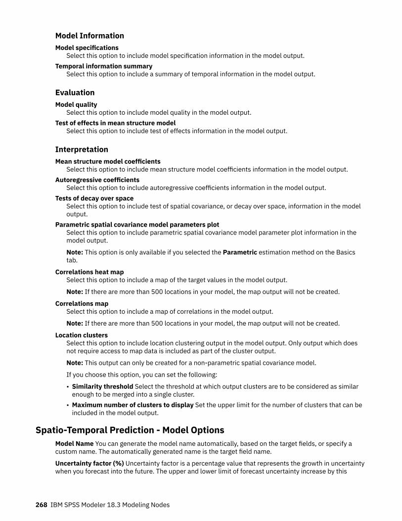
Model InformationModel specifications

Select this option to include model specification information in the model output.Temporal information summary

Select this option to include a summary of temporal information in the model output.

EvaluationModel quality

Select this option to include model quality in the model output.Test of effects in mean structure model

Select this option to include test of effects information in the model output.

InterpretationMean structure model coefficients

Select this option to include mean structure model coefficients information in the model output.Autoregressive coefficients

Select this option to include autoregressive coefficients information in the model output.Tests of decay over space

Select this option to include test of spatial covariance, or decay over space, information in the modeloutput.

Parametric spatial covariance model parameters plotSelect this option to include parametric spatial covariance model parameter plot information in themodel output.

Note: This option is only available if you selected the Parametric estimation method on the Basicstab.

Correlations heat mapSelect this option to include a map of the target values in the model output.

Note: If there are more than 500 locations in your model, the map output will not be created.

Correlations mapSelect this option to include a map of correlations in the model output.

Note: If there are more than 500 locations in your model, the map output will not be created.

Location clustersSelect this option to include location clustering output in the model output. Only output which doesnot require access to map data is included as part of the cluster output.

Note: This output can only be created for a non-parametric spatial covariance model.

If you choose this option, you can set the following:

• Similarity threshold Select the threshold at which output clusters are to be considered as similarenough to be merged into a single cluster.

• Maximum number of clusters to display Set the upper limit for the number of clusters that can beincluded in the model output.

Spatio-Temporal Prediction - Model OptionsModel Name You can generate the model name automatically, based on the target fields, or specify acustom name. The automatically generated name is the target field name.

Uncertainty factor (%) Uncertainty factor is a percentage value that represents the growth in uncertaintywhen you forecast into the future. The upper and lower limit of forecast uncertainty increase by this


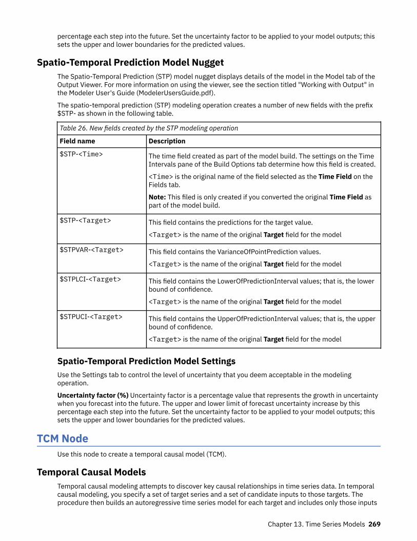
percentage each step into the future. Set the uncertainty factor to be applied to your model outputs; thissets the upper and lower boundaries for the predicted values.

Spatio-Temporal Prediction Model NuggetThe Spatio-Temporal Prediction (STP) model nugget displays details of the model in the Model tab of theOutput Viewer. For more information on using the viewer, see the section titled "Working with Output" inthe Modeler User's Guide (ModelerUsersGuide.pdf).

The spatio-temporal prediction (STP) modeling operation creates a number of new fields with the prefix$STP- as shown in the following table.

Table 26. New fields created by the STP modeling operation


$STP-<Time> The time field created as part of the model build. The settings on the TimeIntervals pane of the Build Options tab determine how this field is created.

<Time> is the original name of the field selected as the Time Field on theFields tab.

Note: This filed is only created if you converted the original Time Field aspart of the model build.

$STP-<Target> This field contains the predictions for the target value.

<Target> is the name of the original Target field for the model

$STPVAR-<Target> This field contains the VarianceOfPointPrediction values.


$STPLCI-<Target> This field contains the LowerOfPredictionInterval values; that is, the lowerbound of confidence.


$STPUCI-<Target> This field contains the UpperOfPredictionInterval values; that is, the upperbound of confidence.


Spatio-Temporal Prediction Model SettingsUse the Settings tab to control the level of uncertainty that you deem acceptable in the modelingoperation.

Uncertainty factor (%) Uncertainty factor is a percentage value that represents the growth in uncertaintywhen you forecast into the future. The upper and lower limit of forecast uncertainty increase by thispercentage each step into the future. Set the uncertainty factor to be applied to your model outputs; thissets the upper and lower boundaries for the predicted values.

TCM NodeUse this node to create a temporal causal model (TCM).

Temporal Causal ModelsTemporal causal modeling attempts to discover key causal relationships in time series data. In temporalcausal modeling, you specify a set of target series and a set of candidate inputs to those targets. Theprocedure then builds an autoregressive time series model for each target and includes only those inputs


that have a causal relationship with the target. This approach differs from traditional time series modelingwhere you must explicitly specify the predictors for a target series. Since temporal causal modelingtypically involves building models for multiple related time series, the result is referred to as a modelsystem.

In the context of temporal causal modeling, the term causal refers to Granger causality. A time series X issaid to "Granger cause" another time series Y if regressing for Y in terms of past values of both X and Yresults in a better model for Y than regressing only on past values of Y.

Note: The Temporal causal modeling node does not support the Model Evaluation or ChampionChallenger steps in IBM SPSS Collaboration and Deployment Services.

ExamplesBusiness decision makers can use temporal causal modeling to uncover causal relationships within alarge set of time-based metrics that describe the business. The analysis might reveal a few controllableinputs, which have the largest impact on key performance indicators.

Managers of large IT systems can use temporal causal modeling to detect anomalies in a large set ofinterrelated operational metrics. The causal model then allows going beyond anomaly detection anddiscovering the most likely root causes of the anomalies.

Field requirementsThere must be at least one target. By default, fields with a predefined role of None are not used.

Data structureTemporal causal modeling supports two types of data structures.

Column-based dataFor column-based data, each time series field contains the data for a single time series. This structureis the traditional structure of time series data, as used by the Time Series Modeler.

Multidimensional dataFor multidimensional data, each time series field contains the data for multiple time series. Separatetime series, within a particular field, are then identified by a set of values of categorical fields referredto as dimension fields. For example, sales data for two different sales channels (retail and web) mightbe stored in a single sales field. A dimension field that is named channel, with values 'retail' and 'web',identifies the records that are associated with each of the two sales channels.

Note: To build a temporal causal model, you need enough data points. The product uses the constraint:

m>(L + KL + 1)

where m is the number of data points, L is the number of lags, and K is the number of predictors. Makesure your data set is big enough so that the number of data points (m) satisfies the condition.

Time Series to ModelOn the Fields tab, use the Time Series settings to specify the series to include in the model system.

Select the option for the data structure that applies to your data. For multidimensional data, click SelectDimensions to specify the dimension fields. The specified order of the dimension fields defines the orderin which they appear in all subsequent dialogs and output. Use the up and down arrow buttons on theSelect Dimensions subdialog to reorder the dimension fields.

For column-based data, the term series has the same meaning as the term field. For multidimensionaldata, fields that contain time series are referred to as metric fields. A time series, for multidimensionaldata, is defined by a metric field and a value for each of the dimension fields. The following considerationsapply to both column-based and multidimensional data.


• Series that are specified as candidate inputs or as both target and input are considered for inclusion inthe model for each target. The model for each target always includes lagged values of the target itself.

• Series that are specified as forced inputs are always included in the model for each target.• At least one series must be specified as either a target or as both target and input.• When Use predefined roles is selected, fields that have a role of Input are set as candidate inputs. Nopredefined role maps to a forced input.

Multidimensional dataFor multidimensional data, you specify metric fields and associated roles in a grid, where each row in thegrid specifies a single metric and role. By default, the model system includes series for all combinations ofthe dimension fields for each row in the grid. For example, if there are dimensions for region and brandthen, by default, specifying the metric sales as a target means that there is a separate sales target seriesfor each combination of region and brand.

For each row in the grid, you can customize the set of values for any of the dimension fields by clicking theellipsis button for a dimension. This action opens the Select Dimension Values subdialog. You can alsoadd, delete, or copy grid rows.

The Series Count column displays the number of sets of dimension values that are currently specified forthe associated metric. The displayed value can be larger than the actual number of series (one series perset). This condition occurs when some of the specified combinations of dimension values do notcorrespond to series contained by the associated metric.

Select Dimension ValuesFor multidimensional data, you can customize the analysis by specifying which dimension values apply toa particular metric field with a particular role. For example, if sales is a metric field and channel is adimension with values 'retail' and 'web,' you can specify that 'web' sales is an input and 'retail' sales is atarget. You can also specify dimension subsets that apply to all metric fields used in the analysis. Forexample, if region is a dimension field that indicates geographical region, then you can limit the analysis toparticular regions.

All valuesSpecifies that all values of the current dimension field are included. This option is the default.

Select values to include or excludeUse this option to specify the set of values for the current dimension field. When Include is selectedfor the Mode, only values that are specified in the Selected values list are included. When Exclude isselected for the Mode, all values other than the values that are specified in the Selected values listare included.

You can filter the set of values from which to choose. Values that meet the filter condition appear inthe Matched tab and values that do not meet the filter condition appear in the Unmatched tab of theUnselected values list. The All tab lists all unselected values, regardless of any filter condition.

• You can use asterisks (*) to indicate wildcard characters when you specify a filter.• To clear the current filter, specify an empty value for the search term on the Filter Displayed Values

dialog.

ObservationsOn the Fields tab, use the Observations settings to specify the fields that define the observations.

Observations that are defined by date/times

You can specify that the observations are defined by a date, time, or timestamp field. In addition tothe field that defines the observations, select the appropriate time interval that describes theobservations. Depending on the specified time interval, you can also specify other settings, such asthe interval between observations (increment) or the number of days per week. The followingconsiderations apply to the time interval:


• Use the value Irregular when the observations are irregularly spaced in time, such as the time atwhich a sales order is processed. When Irregular is selected, you must specify the time interval thatis used for the analysis, from the Time Interval settings on the Data Specifications tab.

• When the observations represent a date and time and the time interval is hours, minutes, orseconds, then use Hours per day, Minutes per day, or Seconds per day. When the observationsrepresent a time (duration) without reference to a date and the time interval is hours, minutes, orseconds, then use Hours (non-periodic), Minutes (non-periodic), or Seconds (non-periodic).

• Based on the selected time interval, the procedure can detect missing observations. Detectingmissing observations is necessary since the procedure assumes that all observations are equallyspaced in time and that there are no missing observations. For example, if the time interval is Daysand the date 2014-10-27 is followed by 2014-10-29, then there is a missing observation for2014-10-28. Values are imputed for any missing observations. Settings for handling missing valuescan be specified from the Data Specifications tab.

• The specified time interval allows the procedure to detect multiple observations in the same timeinterval that need to be aggregated together and to align observations on an interval boundary, suchas the first of the month, to ensure that the observations are equally spaced. For example, if thetime interval is Months, then multiple dates in the same month are aggregated together. This type ofaggregation is referred to as grouping. By default, observations are summed when grouped. You canspecify a different method for grouping, such as the mean of the observations, from theAggregation and Distribution settings on the Data Specifications tab.

• For some time intervals, the additional settings can define breaks in the normal equally spacedintervals. For example, if the time interval is Days, but only weekdays are valid, you can specify thatthere are five days in a week, and the week begins on Monday.

Observations that are defined by periods or cyclic periods

Observations can be defined by one or more integer fields that represent periods or repeating cyclesof periods, up to an arbitrary number of cycle levels. With this structure, you can describe series ofobservations that don't fit one of the standard time intervals. For example, a fiscal year with only 10months can be described with a cycle field that represents years and a period field that representsmonths, where the length of one cycle is 10.

Fields that specify cyclic periods define a hierarchy of periodic levels, where the lowest level isdefined by the Period field. The next highest level is specified by a cycle field whose level is 1,followed by a cycle field whose level is 2, and so on. Field values for each level, except the highest,must be periodic with respect to the next highest level. Values for the highest level cannot be periodic.For example, in the case of the 10-month fiscal year, months are periodic within years and years arenot periodic.

• The length of a cycle at a particular level is the periodicity of the next lowest level. For the fiscal yearexample, there is only one cycle level and the cycle length is 10 since the next lowest levelrepresents months and there are 10 months in the specified fiscal year.

• Specify the starting value for any periodic field that does not start from 1. This setting is necessaryfor detecting missing values. For example, if a periodic field starts from 2 but the starting value isspecified as 1, then the procedure assumes that there is a missing value for the first period in eachcycle of that field.

Time Interval for AnalysisThe time interval that is used for the analysis can differ from the time interval of the observations. Forexample, if the time interval of the observations is Days, you might choose Months for the time interval foranalysis. The data are then aggregated from daily to monthly data before the model is built. You can alsochoose to distribute the data from a longer to a shorter time interval. For example, if the observations arequarterly then you can distribute the data from quarterly to monthly data.

The available choices for the time interval at which the analysis is done depend on how the observationsare defined and the time interval of those observations. In particular, when the observations are definedby cyclic periods, then only aggregation is supported. In that case, the time interval of the analysis mustbe greater than or equal to the time interval of the observations.


The time interval for the analysis is specified from the Time Interval settings on the Data Specificationstab. The method by which the data are aggregated or distributed is specified from the Aggregation andDistribution settings on the Data Specifications tab.

Aggregation and DistributionAggregation functions

When the time interval that is used for the analysis is longer than the time interval of the observations,the input data are aggregated. For example, aggregation is done when the time interval of theobservations is Days and the time interval for analysis is Months. The following aggregation functionsare available: mean, sum, mode, min, or max.

Distribution functionsWhen the time interval that is used for the analysis is shorter than the time interval of theobservations, the input data are distributed. For example, distribution is done when the time intervalof the observations is Quarters and the time interval for analysis is Months. The following distributionfunctions are available: mean or sum.

Grouping functionsGrouping is applied when observations are defined by date/times and multiple observations occur inthe same time interval. For example, if the time interval of the observations is Months, then multipledates in the same month are grouped and associated with the month in which they occur. Thefollowing grouping functions are available: mean, sum, mode, min, or max. Grouping is always donewhen the observations are defined by date/times and the time interval of the observations is specifiedas Irregular.

Note: Although grouping is a form of aggregation, it is done before any handling of missing valueswhereas formal aggregation is done after any missing values are handled. When the time interval ofthe observations is specified as Irregular, aggregation is done only with the grouping function.

Aggregate cross-day observations to previous daySpecifies whether observations with times that cross a day boundary are aggregated to the values forthe previous day. For example, for hourly observations with an eight-hour day that starts at 20:00, thissetting specifies whether observations between 00:00 and 04:00 are included in the aggregatedresults for the previous day. This setting applies only if the time interval of the observations is Hoursper day, Minutes per day or Seconds per day and the time interval for analysis is Days.

Custom settings for specified fieldsYou can specify aggregation, distribution, and grouping functions on a field by field basis. Thesesettings override the default settings for the aggregation, distribution, and grouping functions.

Missing ValuesMissing values in the input data are replaced with an imputed value. The following replacement methodsare available:Linear interpolation

Replaces missing values by using a linear interpolation. The last valid value before the missing valueand the first valid value after the missing value are used for the interpolation. If the first or lastobservation in the series has a missing value, then the two nearest non-missing values at thebeginning or end of the series are used.

Series meanReplaces missing values with the mean for the entire series.

Mean of nearby pointsReplaces missing values with the mean of valid surrounding values. The span of nearby points is thenumber of valid values before and after the missing value that are used to compute the mean.

Median of nearby pointsReplaces missing values with the median of valid surrounding values. The span of nearby points is thenumber of valid values before and after the missing value that are used to compute the median.


Linear trendThis option uses all non-missing observations in the series to fit a simple linear regression model,which is then used to impute the missing values.

Other settings:

Maximum percentage of missing values (%)Specifies the maximum percentage of missing values that are allowed for any series. Series with moremissing values than the specified maximum are excluded from the analysis.

General Data OptionsMaximum number of distinct values per dimension field

This setting applies to multidimensional data and specifies the maximum number of distinct valuesthat are allowed for any one dimension field. By default, this limit is set to 10000 but it can beincreased to an arbitrarily large number.

General Build OptionsConfidence interval width (%)

This setting controls the confidence intervals for both forecasts and model parameters. You canspecify any positive value less than 100. By default, a 95% confidence interval is used.

Maximum number of inputs for each targetThis setting specifies the maximum number of inputs that are allowed in the model for each target.You can specify an integer in the range 1 - 20. The model for each target always includes laggedvalues of itself, so setting this value to 1 specifies that the only input is the target itself.

Model toleranceThis setting controls the iterative process that is used for determining the best set of inputs for eachtarget. You can specify any value that is greater than zero. The default is 0.001. Model tolerance is astop criterion for predictor selection. It can affect the number of predictors that are included in thefinal model. But if a target can predict itself very well, other predictors may not be included in the finalmodel. Some trial and error may be required (for example, if you have this value set to high, you cantry setting it to a smaller value to see if other predictors can be included or not).

Outlier threshold (%)An observation is flagged as an outlier if the probability, as calculated from the model, that it is anoutlier exceeds this threshold. You can specify a value in the range 50 - 100.

Number of Lags for Each InputThis setting specifies the number of lag terms for each input in the model for each target. By default,the number of lag terms is automatically determined from the time interval that is used for theanalysis. For example, if the time interval is months (with an increment of one month) then thenumber of lags is 12. Optionally, you can explicitly specify the number of lags. The specified valuemust be an integer in the range 1 - 20.

Continue estimation using existing modelsIf you already generated a temporal causal model, select this option to reuse the criteria settings thatare specified for that model, rather than building a new model. In this way, you can save time byreestimating and producing a new forecast that is based on the same model settings as before butusing more recent data.

Series to DisplayThese options specify the series (targets or inputs) for which output is displayed. The content of theoutput for the specified series is determined by the Output Options settings.

Display targets associated with best-fitting modelsBy default, output is displayed for the targets that are associated with the 10 best-fitting models, asdetermined by the R square value. You can specify a different fixed number of best-fitting models oryou can specify a percentage of best-fitting models. You can also choose from the following goodnessof fit measures:


R squareGoodness-of-fit measure of a linear model, sometimes called the coefficient of determination. It isthe proportion of variation in the target variable explained by the model. It ranges in value from 0to 1. Small values indicate that the model does not fit the data well.

Root mean square percentage errorA measure of how much the model-predicted values differ from the observed values of the series.It is independent of the units that are used and can therefore be used to compare series withdifferent units.

Root mean square errorThe square root of mean square error. A measure of how much a dependent series varies from itsmodel-predicted level, expressed in the same units as the dependent series.

BICBayesian Information Criterion. A measure for selecting and comparing models based on the -2reduced log likelihood. Smaller values indicate better models. The BIC also "penalizes"overparameterized models (complex models with a large number of inputs, for example), butmore strictly than the AIC.

AICAkaike Information Criterion. A measure for selecting and comparing models based on the -2reduced log likelihood. Smaller values indicate better models. The AIC "penalizes"overparameterized models (complex models with a large number of inputs, for example).

Specify Individual Series

You can specify individual series for which you want output.

• For column-based data, you specify the fields that contain the series that you want. The order of thespecified fields defines the order in which they appear in the output.

• For multidimensional data, you specify a particular series by adding an entry to the grid for themetric field that contains the series. You then specify the values of the dimension fields that definethe series.

– You can enter the value for each dimension field directly into the grid or you can select from thelist of available dimension values. To select from the list of available dimension values, click theellipsis button in the cell for the dimension that you want. This action opens the Select DimensionValue subdialog.

– You can search the list of dimension values, on the Select Dimension Value subdialog, by clickingthe binoculars icon and specifying a search term. Spaces are treated as part of the search term.Asterisks (*) in the search term do not indicate wildcard characters.

– The order of the series in the grid defines the order in which they appear in the output.

For both column-based data and multidimensional data, output is limited to 30 series. This limitincludes individual series (inputs or targets) that you specify and targets that are associated with best-fitting models. Individually specified series take precedence over targets that are associated withbest-fitting models.

Output OptionsThese options specify the content of the output. Options in the Output for targets group generate outputfor the targets that are associated with the best-fitting models on the Series to Display settings. Optionsin the Output for series group generate output for the individual series that are specified on the Series toDisplay settings.

Overall model system

Displays a graphical representation of the causal relations between series in the model system. Tablesof both model fit statistics and outliers for the displayed targets are included as part of the outputitem. When this option is selected in the Output for series group, a separate output item is created foreach individual series that is specified on the Series to Display settings.


Causal relations between series have an associated significance level, where a smaller significancelevel indicates a more significant connection. You can choose to hide relations with a significance levelthat is greater than a specified value.

Model fit statistics and outliersTables of model fit statistics and outliers for the target series that are selected for display. Thesetables contain the same information as the tables in the Overall Model System visualization. Thesetables support all standard features for pivoting and editing tables.

Model effects and model parametersTables of model effects tests and model parameters for the target series that are selected for display.Model effects tests include the F statistic and associated significance value for each input included inthe model.

Impact diagram

Displays a graphical representation of the causal relations between a series of interest and otherseries that it affects or that affect it. Series that affect the series of interest are referred to as causes.Selecting Effects generates an impact diagram that is initialized to display effects. Selecting Causesgenerates an impact diagram that is initialized to display causes. Selecting Both causes and effectsgenerates two separate impact diagrams, one that is initialized to causes and one that is initialized toeffects. You can interactively toggle between causes and effects in the output item that displays theimpact diagram.

You can specify the number of levels of causes or effects to display, where the first level is just theseries of interest. Each additional level shows more indirect causes or effects of the series of interest.For example, the third level in the display of effects consists of the series that contain series in thesecond level as a direct input. Series in the third level are then indirectly affected by the series ofinterest since the series of interest is a direct input to the series in the second level.

Series plotPlots of observed and predicted values for the target series that are selected for display. Whenforecasts are requested, the plot also shows the forecasted values and the confidence intervals forthe forecasts.

Residuals plotPlots of the model residuals for the target series that are selected for display.

Top inputsPlots of each displayed target, over time, along with the top 3 inputs for the target. The top inputs arethe inputs with the lowest significance value. To accommodate different scales for the inputs andtarget, the y axis represents the z score for each series.

Forecast tableTables of forecasted values and confidence intervals of those forecasts for the target series that areselected for display.

Outlier root cause analysisDetermines which series are most likely to be the cause of each outlier in a series of interest. Outlierroot cause analysis is done for each target series that is included in the list of individual series on theSeries to Display settings.Output

Interactive outliers table and chartTable and chart of outliers and root causes of those outliers for each series of interest. Thetable contains a single row for each outlier. The chart is an impact diagram. Selecting a row inthe table highlights the path, in the impact diagram, from the series of interest to the seriesthat most likely causes the associated outlier.

Pivot table of outliersTable of outliers and root causes of those outliers for each series of interest. This tablecontains the same information as the table in the interactive display. This table supports allstandard features for pivoting and editing tables.


Causal levelsYou can specify the number of levels to include in the search for the root causes. The concept oflevels that is used here is the same as described for impact diagrams.

Model fit across all modelsHistogram of model fit for all models and for selected fit statistics. The following fit statistics areavailable:R square

Goodness-of-fit measure of a linear model, sometimes called the coefficient of determination. It isthe proportion of variation in the target variable explained by the model. It ranges in value from 0to 1. Small values indicate that the model does not fit the data well.

Root mean square percentage errorA measure of how much the model-predicted values differ from the observed values of the series.It is independent of the units that are used and can therefore be used to compare series withdifferent units.

Root mean square errorThe square root of mean square error. A measure of how much a dependent series varies from itsmodel-predicted level, expressed in the same units as the dependent series.

BICBayesian Information Criterion. A measure for selecting and comparing models based on the -2reduced log likelihood. Smaller values indicate better models. The BIC also "penalizes"overparameterized models (complex models with a large number of inputs, for example), butmore strictly than the AIC.

AICAkaike Information Criterion. A measure for selecting and comparing models based on the -2reduced log likelihood. Smaller values indicate better models. The AIC "penalizes"overparameterized models (complex models with a large number of inputs, for example).

Outliers over timeBar chart of the number of outliers, across all targets, for each time interval in the estimation period.

Series transformationsTable of any transformations that were applied to the series in the model system. The possibletransformations are missing value imputation, aggregation, and distribution.

Estimation PeriodBy default, the estimation period starts at the time of the earliest observation and ends at the time of thelatest observation across all series.

By start and end timesYou can specify both the start and end of the estimation period or you can specify just the start or justthe end. If you omit the start or the end of the estimation period, the default value is used.

• If the observations are defined by a date/time field, then enter values for start and end in the sameformat that is used for the date/time field.

• For observations that are defined by cyclic periods, specify a value for each of the cyclic periodsfields. Each field is displayed in a separate column.

By latest or earliest time intervals

Defines the estimation period as a specified number of time intervals that start at the earliest timeinterval or end at the latest time interval in the data, with an optional offset. In this context, the timeinterval refers to the time interval of the analysis. For example, assume that the observations aremonthly but the time interval of the analysis is quarters. Specifying Latest and a value of 24 for theNumber of time intervals means the latest 24 quarters.

Optionally, you can exclude a specified number of time intervals. For example, specifying the latest 24time intervals and 1 for the number to exclude means that the estimation period consists of the 24intervals that precede the last one.


Model OptionsModel Name

You can specify a custom name for the model or accept the automatically generated name, which isTCM.

ForecastThe option to Extend records into the future sets the number of time intervals to forecast beyond theend of the estimation period. The time interval in this case is the time interval of the analysis, which isspecified on the Data Specifications tab. When forecasts are requested, autoregressive models areautomatically built for any input series that are not also targets. These models are then used togenerate values for those input series in the forecast period. There is no maximum limit for thissetting.

Interactive OutputThe output from temporal causal modeling includes a number of interactive output objects. Interactivefeatures are available by activating (double-clicking) the object in the Output Viewer.

Overall model systemDisplays the causal relations between series in the model system. All lines that connect a particulartarget to its inputs have the same color. The thickness of the line indicates the significance of thecausal connection, where thicker lines represent a more significant connection. Inputs that are notalso targets are indicated with a black square.

• You can display relations for top models, a specified series, all series, or models with no inputs. Thetop models are the models that meet the criteria that were specified for best-fitting models on theSeries to Display settings.

• You can generate impact diagrams for one or more series by selecting the series names in the chart,right-clicking, and then choosing Create Impact Diagram from the context menu.

• You can choose to hide causal relations that have a significance level that is greater than a specifiedvalue. Smaller significance levels indicate a more significant causal relation.

• You can display relations for a particular series by selecting the series name in the chart, right-clicking, and then choosing Highlight relations for series from the context menu.

Impact diagramDisplays a graphical representation of the causal relations between a series of interest and otherseries that it affects or that affect it. Series that affect the series of interest are referred to as causes.

• You can change the series of interest by specifying the name of the series that you want. Double-clicking any node in the impact diagram changes the series of interest to the series associated withthat node.

• You can toggle the display between causes and effects and you can change the number of levels ofcauses or effects to display.

• Single-clicking any node opens a detailed sequence diagram for the series that is associated withthe node.

Outlier root cause analysisDetermines which series are most likely to be the cause of each outlier in a series of interest.

• You can display the root cause for any outlier by selecting the row for the outlier in the Outlierstable. You can also display the root cause by clicking the icon for the outlier in the sequence chart.

• Single-clicking any node opens a detailed sequence diagram for the series that is associated withthe node.

Overall model qualityHistogram of model fit for all models, for a particular fit statistic. Clicking a bar in the bar chart filtersthe dot plot so that it displays only the models that are associated with the selected bar. You can findthe model for a particular target series in the dot plot by specifying the series name.


Outlier distributionBar chart of the number of outliers, across all targets, for each time interval in the estimation period.Clicking a bar in the bar chart filters the dot plot so that it displays only the outliers that are associatedwith the selected bar.

TCM Model NuggetThe TCM modeling operation creates a number of new fields with the prefix $TCM- as shown in thefollowing table.

Table 27. New fields created by the TCM modeling operation


$TCM-colname The value forecasted by the model for each target series.

$TCMLCI-colname The lower confidence intervals for each forecasted series.

$TSUCI-colname The upper confidence intervals for each forecasted series.

$TCMResidual-colname The noise residual value for each column of the generated model data.

TCM Model Nugget SettingsThe Settings tab provides additional options for the TCM model nugget.

ForecastThe option to Extend records into the future sets the number of time intervals to forecast beyond theend of the estimation period. The time interval in this case is the time interval of the analysis, which isspecified on the Data Specifications tab of the TCM node. When forecasts are requested, autoregressivemodels are automatically built for any input series that are not also targets. These models are then usedto generate values for those input series in the forecast period.

Make available for scoringCreate new fields for each model to be scored. Enables you to specify the new fields to create for eachmodel to be scored.

• Noises Residuals. If selected, creates a new field (with the default prefix $TCM-) for the modelresiduals for each target field, together with a total of these values.

• Upper and lower confidence limits. If selected, creates new fields (with the default prefix $TCM-) forthe lower and upper confidence intervals, respectively, for each target field, together with totals of thesevalues.

Targets included for scoring. Select available targets to include in the model score.

Temporal Causal Model ScenariosThe Temporal Causal Model Scenarios procedure runs user-defined scenarios for a temporal causalmodel system, with the data from the active dataset. A scenario is defined by a time series, that isreferred to as the root series, and a set of user-defined values for that series over a specified time range.The specified values are then used to generate predictions for the time series that are affected by the rootseries. The procedure requires a model system file that was created by the Temporal Causal Modelingprocedure. It is assumed that the active dataset is the same data as was used to create the model systemfile.

ExampleUsing the Temporal Causal Modeling procedure, a business decision maker discovered a key metric thataffects a number of important performance indicators. The metric is controllable, so the decision maker


wants to investigate the effect of various sets of values for the metric over the next quarter. Theinvestigation is easily done by loading the model system file into the Temporal Causal Model Scenariosprocedure and specifying the sets of values for the key metric.

Defining the Scenario PeriodThe scenario period is the period over which you specify the values that are used to run your scenarios. Itcan start before or after the end of the estimation period. You can optionally specify to predict beyond theend of the scenario period. By default, predictions are generated through the end of the scenario period.All scenarios use the same scenario period and specifications for how far to predict.

Note: Predictions start at the first time period after the beginning of the scenario period. For example, ifthe scenario period starts on 2014-11-01 and the time interval is months, then the first prediction is for2014-12-01.

Specify by start, end and predict through times

• If the observations are defined by a date/time field, then enter values for start, end, and predictthrough in the same format that is used for the date/time field. Values for date/time fields arealigned to the beginning of the associated time interval. For example, if the time interval of theanalysis is months, then the value 10/10/2014 is adjusted to 10/01/2014, which is the beginning ofthe month.


Specify by time intervals relative to end of estimation period

Defines start and end in terms of the number of time intervals relative to the end of the estimationperiod, where the time interval is the time interval of the analysis. The end of the estimation period isdefined as time interval 0. Time intervals before the end of the estimation period have negative valuesand intervals after the end of the estimation period have positive values. You can also specify howmany intervals to predict beyond the end of the scenario period. The default is 0.

For example, assume that the time interval of the analysis is months and that you specify 1 for startinginterval, 3 for ending interval, and 1 for how far to predict beyond that. The scenario period is then the3 months that follow the end of the estimation period. Predictions are generated for the second andthird month of the scenario period and for 1 more month past the end of the scenario period.

Adding Scenarios and Scenario GroupsThe Scenarios tab specifies the scenarios that are to be run. To define scenarios, you must first define thescenario period by clicking Define Scenario Period. Scenarios and scenario groups (applies only tomultidimensional data) are created by clicking the associated Add Scenario or Add Scenario Groupbutton. By selecting a particular scenario or scenario group in the associated grid, you can edit it, make acopy of it, or delete it.

Column-based dataThe Root field column in the grid specifies the time series field whose values are replaced with thescenario values. The Scenario values column displays the specified scenario values in the order ofearliest to latest. If the scenario values are defined by an expression, then the column displays theexpression.

Multidimensional dataIndividual Scenarios

Each row in the Individual Scenarios grid specifies a time series whose values are replaced by thespecified scenario values. The series is defined by the combination of the field that is specified in theRoot Metric column and the specified value for each of the dimension fields. The content of theScenario values column is the same as for column-based data.


Scenario GroupsA scenario group defines a set of scenarios that are based on a single root metric field and multiplesets of dimension values. Each set of dimension values (one value per dimension field), for thespecified metric field, defines a time series. An individual scenario is then generated for each suchtime series, whose values are then replaced by the scenario values. Scenario values for a scenariogroup are specified by an expression, which is then applied to each time series in the group.

The Series Count column displays the number of sets of dimension values that are associated with ascenario group. The displayed value can be larger than the actual number of time series that areassociated with the scenario group (one series per set). This condition occurs when some of thespecified combinations of dimension values do not correspond to series contained by the root metricfor the group.

As an example of a scenario group, consider a metric field advertising and two dimension fields regionand brand. You can define a scenario group that is based on advertising as the root metric and thatincludes all combinations of region and brand. You might then specify advertising*1.2 as theexpression to investigate the effect of increasing advertising by 20 percent for each of the time seriesthat are associated with the advertising field. If there are 4 values of region and 2 values of brand,then there are 8 such time series and thus 8 scenarios defined by the group.

Scenario DefinitionSettings for defining a scenario depend on whether your data are column-based or multidimensional.

Root seriesSpecifies the root series for the scenario. Each scenario is based on a single root series. For column-based data, you select the field that defines the root series. For multidimensional data, you specifythe root series by adding an entry to the grid for the metric field that contains the series. You thenspecify the values of the dimension fields that define the root series. The following apply to specifyingthe dimension values:

• You can enter the value for each dimension field directly into the grid or you can select from the listof available dimension values. To select from the list of available dimension values, click the ellipsisbutton in the cell for the dimension that you want. This action opens the Select Dimension Valuesubdialog.

• You can search the list of dimension values, on the Select Dimension Value subdialog, by clickingthe binoculars icon and specifying a search term. Spaces are treated as part of the search term.Asterisks (*) in the search term do not indicate wildcard characters.

Specify affected targetsUse this option when you know specific targets that are affected by the root series and you want toinvestigate the effects on those targets only. By default, targets that are affected by the root series areautomatically determined. You can specify the breadth of the series that are affected by the scenariowith settings on the Options tab.

For column-based data, select the targets that you want. For multidimensional data, you specifytarget series by adding an entry to the grid for the target metric field that contains the series. Bydefault, all series that are contained in the specified metric field are included. You can customize theset of included series by customizing the included values for one or more of the dimension fields. Tocustomize the dimension values that are included, click the ellipsis button for the dimension that youwant. This action opens the Select Dimension Values dialog.

The Series Count column (for multidimensional data) displays the number of sets of dimension valuesthat are currently specified for the associated target metric. The displayed value can be larger thanthe actual number of affected target series (one series per set). This condition occurs when some ofthe specified combinations of dimension values do not correspond to series contained by theassociated target metric.

Scenario IDEach scenario must have a unique identifier. The identifier is displayed in output that is associatedwith the scenario. There are no restrictions, other than uniqueness, on the value of the identifier.


Specify scenario values for root seriesUse this option to specify explicit values for the root series in the scenario period. You must specify anumeric value for each time interval that is listed in the grid. You can obtain the values of the rootseries (actual or forecasted) for each interval in the scenario period by clicking Read, Forecast, orRead\Forecast.

Specify expression for scenario values for root seriesYou can define an expression for computing the values of the root series in the scenario period. Youcan enter the expression directly or click the calculator button and create the expression from theScenario Values Expression Builder.

• The expression can contain any target or input in the model system.• When the scenario period extends beyond the existing data, the expression is applied to forecasted

values of the fields in the expression.• For multidimensional data, each field in the expression specifies a time series that is defined by thefield and the dimension values that were specified for the root metric. It is those time series that areused to evaluate the expression.

As an example, assume that the root field is advertising and the expression is advertising*1.2.The values for advertising that are used in the scenario represent a 20 percent increase over theexisting values.

Note: Scenarios are created by clicking Add Scenario on the Scenarios tab.

Select Dimension Values

For multidimensional data, you can customize the dimension values that define the targets that areaffected by a scenario or scenario group. You can also customize the dimension values that define the setof root series for a scenario group.

All valuesSpecifies that all values of the current dimension field are included. This option is the default.

Select valuesUse this option to specify the set of values for the current dimension field. You can filter the set ofvalues from which to choose. Values that meet the filter condition appear in the Matched tab andvalues that do not meet the filter condition appear in the Unmatched tab of the Unselected valueslist. The All tab lists all unselected values, regardless of any filter condition.

• You can use asterisks (*) to indicate wildcard characters when you specify a filter.• To clear the current filter, specify an empty value for the search term on the Filter Displayed Values

dialog.

To customize dimension values for affected targets:

1. From the Scenario Definition or Scenario Group Definition dialog, select the target metric for which youwant to customize dimension values.

2. Click the ellipsis button in the column for the dimension that you want to customize.

To customize dimension values for the root series of a scenario group:

1. From the Scenario Group Definition dialog, click the ellipsis button (in the root series grid) for thedimension that you want to customize.

Scenario Group DefinitionRoot Series

Specifies the set of root series for the scenario group. An individual scenario is generated for eachtime series in the set. You specify the root series by adding an entry to the grid for the metric field thatcontains the series that you want. You then specify the values of the dimension fields that define theset. By default, all series that are contained in the specified root metric field are included. You cancustomize the set of included series by customizing the included values for one or more of the


dimension fields. To customize the dimension values that are included, click the ellipsis button for adimension. This action opens the Select Dimension Values dialog.

The Series Count column displays the number of sets of dimension values that are currently includedfor the associated root metric. The displayed value can be larger than the actual number of root seriesfor the scenario group (one series per set). This condition occurs when some of the specifiedcombinations of dimension values do not correspond to series contained by the root metric.

Specify affected target seriesUse this option when you know specific targets that are affected by the set of root series and you wantto investigate the effects on those targets only. By default, targets that are affected by each root seriesare automatically determined. You can specify the breadth of the series that are affected by eachindividiual scenario with settings on the Options tab.

You specify target series by adding an entry to the grid for the metric field that contains the series. Bydefault, all series that are contained in the specified metric field are included. You can customize theset of included series by customizing the included values for one or more of the dimension fields. Tocustomize the dimension values that are included, click the ellipsis button for the dimension that youwant. This action opens the Select Dimension Values dialog.

The Series Count column displays the number of sets of dimension values that are currently specifiedfor the associated target metric. The displayed value can be larger than the actual number of affectedtarget series (one series per set). This condition occurs when some of the specified combinations ofdimension values do not correspond to series contained by the associated target metric.

Scenario ID prefixEach scenario group must have a unique prefix. The prefix is used to construct an identifier that isdisplayed in output that is associated with each individual scenario in the scenario group. Theidentifier for an individual scenario is the prefix, followed by an underscore, followed by the value ofeach dimension field that identifies the root series. The dimension values are separated byunderscores. There are no restrictions, other than uniqueness, on the value of the prefix.

Expression for scenario values for root seriesScenario values for a scenario group are specified by an expression, which is then used to computethe values for each of the root series in the group. You can enter an expression directly or click thecalculator button and create the expression from the Scenario Values Expression Builder.

• The expression can contain any target or input in the model system.• When the scenario period extends beyond the existing data, the expression is applied to forecasted

values of the fields in the expression.• For each root series in the group, the fields in the expression specify time series that are defined by

those fields and the dimension values that define the root series. It is those time series that areused to evaluate the expression. For example, if a root series is defined by region='north' andbrand='X', then the time series that are used in the expression are defined by those samedimension values.

As an example, assume that the root metric field is advertising and that there are two dimension fieldsregion and brand. Also, assume that the scenario group includes all combinations of the dimensionfield values. You might then specify advertising*1.2 as the expression to investigate the effect ofincreasing advertising by 20 percent for each of the time series that are associated with theadvertising field.

Note: Scenario groups apply to multidimensional data only and are created by clicking Add ScenarioGroup on the Scenarios tab.

OptionsMaximum level for affected targets

Specifies the maximum number of levels of affected targets. Each successive level, up to themaximum of 5, includes targets that are more indirectly affected by the root series. Specifically, thefirst level includes targets that have the root series as a direct input. Targets in the second level have


targets in the first level as a direct input, and so on. Increasing the value of this setting increases thecomplexity of the computation and might affect performance.

Maximum auto-detected targetsSpecifies the maximum number of affected targets that are automatically detected for each rootseries. Increasing the value of this setting increases the complexity of the computation and mightaffect performance.

Impact diagramDisplays a graphical representation of the causal relations between the root series for each scenarioand the target series that it affects. Tables of both the scenario values and the predicted values for theaffected targets are included as part of the output item. The graph includes plots of the predictedvalues of the affected targets. Single-clicking any node in the impact diagram opens a detailedsequence diagram for the series that is associated with the node. A separate impact diagram isgenerated for each scenario.

Series plotsGenerates series plots of the predicted values for each of the affected targets in each scenario.

Forecast and scenario tablesTables of predicted values and scenario values for each scenario. These tables contains the sameinformation as the tables in the impact diagram. These tables support all standard features forpivoting and editing tables.

Include confidence intervals in plots and tablesSpecifies whether confidence intervals for scenario predictions are included in both chart and tableoutput.

Confidence interval width (%)This setting controls the confidence intervals for the scenario predictions. You can specify any positivevalue less than 100. By default, a 95% confidence interval is used.

Time Series nodeThe Time Series node can be used with data in either a local or distributed environment; in a distributedenvironment you can harness the power of IBM SPSS Analytic Server. With this node, you can choose toestimate and build exponential smoothing, univariate Autoregressive Integrated Moving Average (ARIMA),or multivariate ARIMA (or transfer function) models for time series, and produce forecasts based on thetime series data.

Exponential smoothing is a method of forecasting that uses weighted values of previous seriesobservations to predict future values. As such, exponential smoothing is not based on a theoreticalunderstanding of the data. It forecasts one point at a time, adjusting its forecasts as new data come in.The technique is useful for forecasting series that exhibit trend, seasonality, or both. You can choose fromvarious exponential smoothing models that differ in their treatment of trend and seasonality.

ARIMA models provide more sophisticated methods for modeling trend and seasonal components thando exponential smoothing models, and, in particular, they allow the added benefit of includingindependent (predictor) variables in the model. This involves explicitly specifying autoregressive andmoving average orders as well as the degree of differencing. You can include predictor variables anddefine transfer functions for any or all of them, as well as specify automatic detection of outliers or anexplicit set of outliers.

Note: In practical terms, ARIMA models are most useful if you want to include predictors that might helpto explain the behavior of the series that is being forecast, such as the number of catalogs that are mailedor the number of hits to a company web page. Exponential smoothing models describe the behavior of thetime series without attempting to understand why it behaves as it does. For example, a series thathistorically peaks every 12 months will probably continue to do so even if you don't know why.

An Expert Modeler option is also available, which attempts to automatically identify and estimate thebest-fitting ARIMA or exponential smoothing model for one or more target variables, thus eliminating theneed to identify an appropriate model through trial and error. If in doubt, use the Expert Modeler option.


If predictor variables are specified, the Expert Modeler selects those variables that have a statisticallysignificant relationship with the dependent series for inclusion in ARIMA models. Model variables aretransformed where appropriate using differencing and/or a square root or natural log transformation. Bydefault, the Expert Modeler considers all exponential smoothing models and all ARIMA models and picksthe best model among them for each target field. You can, however, limit the Expert Modeler only to pickthe best of the exponential smoothing models or only to pick the best of the ARIMA models. You can alsospecify automatic detection of outliers.

Time Series node - field optionsOn the Fields tab, you choose whether you want to use the field role settings already defined in upstreamnodes, or make the field assignments manually.





Targets. Select one or more of the fields as your target for the prediction.

Candidate inputs. Select one or more fields as inputs for the prediction. You can select only fields with ameasurement level of continuous.

Events and Interventions. Use this area to designate certain input fields as event or intervention fields.This designation identifies a field as containing time series data that can be affected by events(predictable recurring situations; for example, sales promotions) or interventions (one-time incidents; forexample, power outage or employee strike). The fields you select must be flags that have integer storage.

Time Series node - data specification optionsThe Data Specifications tab is where you set all the options for the data to be included in your model. Aslong as you specify both a Date/time field and Time interval, you can click the Run button to build amodel with all the default options, but normally you will want to customize the build for your ownpurposes.


Time Series node - observationsUse the settings in this pane to specify the fields that define the observations.

Observations that are specified by a date/time fieldYou can specify that the observations are defined by a date, time, or timestamp field. In addition to thefield that defines the observations, select the appropriate time interval that describes the observations.Depending on the specified time interval, you can also specify other settings, such as the interval betweenobservations (increment) or the number of days per week. The following considerations apply to the timeinterval:

• Use the value Irregular when the observations are irregularly spaced in time, such as the time at whicha sales order is processed. When Irregular is selected, you must specify the time interval that is usedfor the analysis, from the Time Interval settings on the Data Specifications tab.

• When the observations represent a date and time and the time interval is hours, minutes, or seconds,then use Hours per day, Minutes per day, or Seconds per day. When the observations represent a time


(duration) without reference to a date and the time interval is hours, minutes, or seconds, then useHours (non-periodic), Minutes (non-periodic), or Seconds (non-periodic).

• Based on the selected time interval, the procedure can detect missing observations. Detecting missingobservations is necessary since the procedure assumes that all observations are equally spaced in timeand that no observations are missing. For example, if the time interval is Days and the date 2015-10-27is followed by 2015-10-29, then an observation is missing for 2015-10-28. Values are imputed for anymissing observations; use the Missing Value Handling area of the Data Specifications tab to specifysettings for handling missing values.

• The specified time interval allows the procedure to detect multiple observations in the same timeinterval that need to be aggregated together and to align observations on an interval boundary, such asthe first of the month, to ensure that the observations are equally spaced. For example, if the timeinterval is Months, then multiple dates in the same month are aggregated together. This type ofaggregation is referred to as grouping. By default, observations are summed when grouped. You canspecify a different method for grouping, such as the mean of the observations, from the Aggregationand Distribution settings on the Data Specifications tab.

• For some time intervals, the additional settings can define breaks in the normal equally spacedintervals. For example, if the time interval is Days, but only weekdays are valid, you can specify thatthere are five days in a week, and the week begins on Monday.

Observations that are defined as periods or cyclic periodsObservations can be defined by one or more integer fields that represent periods or repeating cycles ofperiods, up to an arbitrary number of cycle levels. With this structure, you can describe series ofobservations that don't fit one of the standard time intervals. For example, a fiscal year with only 10months can be described with a cycle field that represents years and a period field that representsmonths, where the length of one cycle is 10.

Fields that specify cyclic periods define a hierarchy of periodic levels, where the lowest level is defined bythe Period field. The next highest level is specified by a cycle field whose level is 1, followed by a cyclefield whose level is 2, and so on. Field values for each level, except the highest, must be periodic withrespect to the next highest level. Values for the highest level cannot be periodic. For example, in the caseof the 10-month fiscal year, months are periodic within years and years are not periodic.

• The length of a cycle at a particular level is the periodicity of the next lowest level. For the fiscal yearexample, there is only one cycle level and the cycle length is 10 since the next lowest level representsmonths and there are 10 months in the specified fiscal year.

• Specify the starting value for any periodic field that does not start from 1. This setting is necessary fordetecting missing values. For example, if a periodic field starts from 2 but the starting value is specifiedas 1, then the procedure assumes that there is a missing value for the first period in each cycle of thatfield.

Time Series node - time interval for analysisThe time interval that you use for analysis can differ from the time interval of the observations. Forexample, if the time interval of the observations is Days, you might choose Months for the time interval foranalysis. The data is then aggregated from daily to monthly data before the model is built. You can alsochoose to distribute the data from a longer to a shorter time interval. For example, if the observations arequarterly then you can distribute the data from quarterly to monthly data.

Use the settings in this pane to specify the time interval for the analysis. The method by which the data isaggregated or distributed is specified from the Aggregation and Distribution settings on the DataSpecifications tab.

The available choices for the time interval at which the analysis is done depend on how the observationsare defined and the time interval of those observations. In particular, when the observations are definedby cyclic periods, only aggregation is supported. In that case, the time interval of the analysis must begreater than or equal to the time interval of the observations.


Time Series node - aggregation and distribution optionsUse the settings in this pane to specify settings for aggregating or distributing the input data with respectto the time intervals of the observations.

Aggregation functionsWhen the time interval that is used for the analysis is longer than the time interval of the observations,the input data are aggregated. For example, aggregation is done when the time interval of theobservations is Days and the time interval for analysis is Months. The following aggregation functionsare available: mean, sum, mode, min, or max.

Distribution functionsWhen the time interval that is used for the analysis is shorter than the time interval of theobservations, the input data are distributed. For example, distribution is done when the time intervalof the observations is Quarters and the time interval for analysis is Months. The following distributionfunctions are available: mean or sum.

Grouping functionsGrouping is applied when observations are defined by date/times and multiple observations occur inthe same time interval. For example, if the time interval of the observations is Months, then multipledates in the same month are grouped and associated with the month in which they occur. Thefollowing grouping functions are available: mean, sum, mode, min, or max. Grouping is always donewhen the observations are defined by date/times and the time interval of the observations is specifiedas Irregular.

Note: Although grouping is a form of aggregation, it is done before any handling of missing valueswhereas formal aggregation is done after any missing values are handled. When the time interval ofthe observations is specified as Irregular, aggregation is done only with the grouping function.

Aggregate cross-day observations to previous daySpecifies whether observations with times that cross a day boundary are aggregated to the values forthe previous day. For example, for hourly observations with an eight-hour day that starts at 20:00, thissetting specifies whether observations between 00:00 and 04:00 are included in the aggregatedresults for the previous day. This setting applies only if the time interval of the observations is Hoursper day, Minutes per day or Seconds per day and the time interval for analysis is Days.

Custom settings for specified fieldsYou can specify aggregation, distribution, and grouping functions on a field by field basis. Thesesettings override the default settings for the aggregation, distribution, and grouping functions.

Time Series node - missing value optionsUse the settings in this pane to specify how any missing values in the input data are to be replaced with animputed value. The following replacement methods are available:

Linear interpolationReplaces missing values by using a linear interpolation. The last valid value before the missing valueand the first valid value after the missing value are used for the interpolation. If the first or lastobservation in the series has a missing value, then the two nearest non-missing values at thebeginning or end of the series are used.Replaces missing values by using a linear interpolation.

• For non-seasonal data, the last valid value before the missing value and the first valid value after themissing value are used for the interpolation. If missing values are at the beginning or the end of atime series, then a linear extrapolation method is used based on the two nearest valid values.

• For seasonal data, a missing value is linearly interpolated using the last valid value of the sameperiod before the missing value and the first valid value of the same period after the missing value.If one of the two values of the same period can't be found for the missing value, then the data willbe regarded as non-seasonal data and linear interpolation of non-seasonal data is used to imputethe missing value.


Series meanReplaces missing values with the mean for the entire series.

Mean of nearby pointsReplaces missing values with the mean of valid surrounding values. The span of nearby points is thenumber of valid values before and after the missing value that are used to compute the mean.

Median of nearby pointsReplaces missing values with the median of valid surrounding values. The span of nearby points is thenumber of valid values before and after the missing value that are used to compute the median.

Linear trendThis option uses all non-missing observations in the series to fit a simple linear regression model,which is then used to impute the missing values.

Other settings:

Lowest data quality score (%)Computes data quality measures for the time variable and for input data corresponding to each timeseries. If the data quality score is lower that this threshold, the corresponding time series will bediscarded.

Time Series node - estimation periodIn the Estimation Period pane, you can specify the range of records to be used in model estimation. Bydefault, the estimation period starts at the time of the earliest observation and ends at the time of thelatest observation across all series.

By start and end timesYou can specify both the start and end of the estimation period or you can specify just the start or justthe end. If you omit the start or the end of the estimation period, the default value is used.

• If the observations are defined by a date/time field, enter values for start and end in the sameformat that is used for the date/time field.


By latest or earliest time intervals

Defines the estimation period as a specified number of time intervals that start at the earliest timeinterval or end at the latest time interval in the data, with an optional offset. In this context, the timeinterval refers to the time interval of the analysis. For example, assume that the observations aremonthly but the time interval of the analysis is quarters. Specifying Latest and a value of 24 for theNumber of time intervals means the latest 24 quarters.

Optionally, you can exclude a specified number of time intervals. For example, specifying the latest 24time intervals and 1 for the number to exclude means that the estimation period consists of the 24intervals that precede the last one.

Time Series node - build optionsThe Build Options tab is where you set all the options for building your model. You can, of course, justclick the Run button to build a model with all the default options, but normally you will want to customizethe build for your own purposes.

The tab contains two different panes on which you set the customizations that are specific to your model.

Time Series node - general build optionsThe options available on this pane depend on which of the following three settings you choose from theMethod list:

• Expert Modeler. Choose this option to use the Expert Modeler, which automatically finds the best-fittingmodel for each dependent series.


• Exponential Smoothing. Use this option to specify a custom exponential smoothing model.• ARIMA. Use this option to specify a custom ARIMA model.

Expert ModelerUnder Model Type, select the type of models you want to build:

• All models. The Expert Modeler considers both ARIMA and exponential smoothing models.• Exponential smoothing models only. The Expert Modeler considers only exponential smoothing

models.• ARIMA models only. The Expert Modeler considers only ARIMA models.

Expert Modeler considers seasonal models. This option is only enabled if a periodicity is defined for theactive dataset. When this option is selected, the Expert Modeler considers both seasonal andnonseasonal models. If this option is not selected, the Expert Modeler considers only nonseasonalmodels.

Expert Modeler considers sophisticated exponential smoothing models. When this option is selected,the Expert Modeler searches a total of 13 exponential smoothing models (7 of them existed in the originalTime Series node, and 6 of them were added in version 18.1). If this option is not selected, the ExpertModeler only searches the original 7 exponential smoothing models.

Under Outliers, select from the following options

Detect outliers automatically. By default, automatic detection of outliers is not performed. Select thisoption to perform automatic detection of outliers, then select the desired outlier types.

Input fields must have a measurement level of Flag, Nominal, or Ordinal and must be numeric (forexample, 1/0, not True/False, for a flag field), before they are included in this list.

The Expert Modeler considers only simple regression and not arbitrary transfer functions for inputs thatare identified as event or intervention fields on the Fields tab.

Exponential SmoothingModel Type. Exponential smoothing models are classified as either seasonal or nonseasonal.1 Seasonalmodels are only available if the periodicity defined by using the Time Intervals pane on the DataSpecifications tab is seasonal. The seasonal periodicities are: cyclic periods, years, quarters, months,days per week, hours per day, minutes per day, and seconds per day. The following model types areavailable:

• Simple. This model is appropriate for a series in which there is no trend or seasonality. Its only relevantsmoothing parameter is level. Simple exponential smoothing is most similar to an ARIMA with zeroorders of autoregression, one order of differencing, one order of moving average, and no constant.

• Holt's linear trend. This model is appropriate for a series in which there is a linear trend and noseasonality. Its relevant smoothing parameters are level and trend, and, in this model, they are notconstrained by each other's values. Holt's model is more general than Brown's model but may takelonger to compute estimates for large series. Holt's exponential smoothing is most similar to an ARIMAwith zero orders of autoregression, two orders of differencing, and two orders of moving average.

• Damped trend. This model is appropriate for a series in which there is a linear trend that is dying outand no seasonality. Its relevant smoothing parameters are level, trend, and damping trend. Dampedexponential smoothing is most similar to an ARIMA with one order of autoregression, one order ofdifferencing, and two orders of moving average.

• Multiplicative trend. This model is appropriate for a series in which there is a trend that changes withthe magnitude of the series and no seasonality. Its relevant smoothing parameters are level and trend.Multiplicative trend exponential smoothing is not similar to any ARIMA model.

1 Gardner, E. S. 1985. Exponential smoothing: The state of the art. Journal of Forecasting, 4, 1-28.


• Brown's linear trend. This model is appropriate for a series in which there is a linear trend and noseasonality. Its relevant smoothing parameters are level and trend, but, in this model, they are assumedto be equal. Brown's model is therefore a special case of Holt's model. Brown's exponential smoothingis most similar to an ARIMA with zero orders of autoregression, two orders of differencing, and twoorders of moving average, with the coefficient for the second order of moving average equal to one halfof the coefficient for the first order squared.

• Simple seasonal. This model is appropriate for a series in which there is no trend and a seasonal effectthat is constant over time. Its relevant smoothing parameters are level and season. Seasonalexponential smoothing is most similar to an ARIMA with zero orders of autoregression; one order ofdifferencing; one order of seasonal differencing; and orders 1, p, and p+1 of moving average, where p isthe number of periods in a seasonal interval. For monthly data, p = 12.

• Winters' additive. This model is appropriate for a series in which there is a linear trend and a seasonaleffect that is constant over time. Its relevant smoothing parameters are level, trend, and season.Winters' additive exponential smoothing is most similar to an ARIMA with zero orders of autoregression;one order of differencing; one order of seasonal differencing; and p+1 orders of moving average, wherep is the number of periods in a seasonal interval. For monthly data, p=12.

• Damped trend with additive seasonal. This model is appropriate for a series in which there is a lineartrend that is dying out and a seasonal effect that is constant over time. Its relevant smoothingparameters are level, trend, damping trend, and season. Damped trend and additive seasonalexponential smoothing is not similar to any ARIMA model.

• Multiplicative trend with additive seasonal. This model is appropriate for a series in which there is atrend that changes with the magnitude of the series and a seasonal effect that is constant over time. Itsrelevant smoothing parameters are level, trend, and season. Multiplicative trend and additive seasonalexponential smoothing is not similar to any ARIMA model.

• Multiplicative seasonal. This model is appropriate for a series in which there is no trend and a seasonaleffect that changes with the magnitude of the series. Its relevant smoothing parameters are level andseason. Multiplicative seasonal exponential smoothing is not similar to any ARIMA model.

• Winters' multiplicative. This model is appropriate for a series in which there is a linear trend and aseasonal effect that changes with the magnitude of the series. Its relevant smoothing parameters arelevel, trend, and season. Winters' multiplicative exponential smoothing is not similar to any ARIMAmodel.

• Damped trend with multiplicative seasonal. This model is appropriate for a series in which there is alinear trend that is dying out and a seasonal effect that changes with the magnitude of the series. Itsrelevant smoothing parameters are level, trend, damping trend, and season. Damped trend andmultiplicative seasonal exponential smoothing is not similar to any ARIMA model.

• Multiplicative trend with multiplicative seasonal. This model is appropriate for a series in which thereare a trend and a seasonal effect that both change with the magnitude of the series. Its relevantsmoothing parameters are level, trend, and season. Multiplicative trend and multiplicative seasonalexponential smoothing is not similar to any ARIMA model.

Target Transformation. You can specify a transformation to be performed on each dependent variablebefore it is modeled.

• None. No transformation is performed.• Square root. Square root transformation is performed.• Natural log. Natural log transformation is performed.

ARIMASpecify the structure of a custom ARIMA model.

ARIMA Orders. Enter values for the various ARIMA components of your model into the correspondingcells of the grid. All values must be non-negative integers. For autoregressive and moving averagecomponents, the value represents the maximum order. All positive lower orders are included in themodel. For example, if you specify 2, the model includes orders 2 and 1. Cells in the Seasonal column areonly enabled if a periodicity is defined for the active dataset.


• Autoregressive (p). The number of autoregressive orders in the model. Autoregressive orders specifywhich previous values from the series are used to predict current values. For example, anautoregressive order of 2 specifies that the value of the series two time periods in the past is used topredict the current value.

• Difference (d). Specifies the order of differencing applied to the series before estimating models.Differencing is necessary when trends are present (series with trends are typically nonstationary andARIMA modeling assumes stationarity) and is used to remove their effect. The order of differencingcorresponds to the degree of series trend; first-order differencing accounts for linear trends, second-order differencing accounts for quadratic trends, and so on.

• Moving Average (q). The number of moving average orders in the model. Moving average orders specifyhow deviations from the series mean for previous values are used to predict current values. Forexample, moving-average orders of 1 and 2 specify that deviations from the mean value of the seriesfrom each of the last two time periods be considered when predicting current values of the series.

Seasonal. Seasonal autoregressive, moving average, and differencing components play the same roles astheir nonseasonal counterparts. For seasonal orders, however, current series values are affected byprevious series values that are separated by one or more seasonal periods. For example, for monthly data(seasonal period of 12), a seasonal order of 1 means that the current series value is affected by the seriesvalue 12 periods before the current one. A seasonal order of 1, for monthly data, is then the same asspecifying a nonseasonal order of 12.

Detect outliers automatically. Select this option to perform automatic detection of outliers, and selectone or more of the outlier types available.

Type of Outliers to Detect. Select the outlier type(s) you want to detect. The supported types are:

• Additive (default)• Level shift (default)• Innovational• Transient• Seasonal additive• Local trend• Additive patch

Transfer Function Orders and Transformations. To specify transformations and to define transferfunctions for any or all of the input fields in your ARIMA model, click Set; a separate dialog box isdisplayed in which you enter the transfer and transformation details.

Include constant in model. Inclusion of a constant is standard unless you are sure that the overall meanseries value is 0. Excluding the constant is recommended when differencing is applied.

Further details• For more information on types of outliers, see “Outliers” on page 262.• For more information on transfer and transformation functiions, see “Transfer and transformation

functions” on page 291.

Transfer and transformation functionsUse the Transfer Function Orders and Transformations dialog box to specify transformations and to definetransfer functions for any or all of the input fields in your ARIMA model.

Target Transformations. In this pane you can specify a transformation to be performed on each targetvariable before it is modeled.



Candidate Inputs Transfer functions and Transformation. You use transfer functions to specify themanner in which past values of the input fields are used to forecast future values of the target series. Thelist on the left hand side of the pane shows all input fields. The remaining information in this pane isspecific to the input field you select.

Transfer Function Orders. Enter values for the various components of the transfer function into thecorresponding cells of the Structure. grid. All values must be non-negative integers. For numerator anddenominator components, the value represents the maximum order. All positive lower orders are includedin the model. In addition, order 0 is always included for numerator components. For example, if youspecify 2 for numerator, the model includes orders 2, 1, and 0. If you specify 3 for denominator, the modelincludes orders 3, 2, and 1. Cells in the Seasonal column are only enabled if a periodicity is defined for theactive dataset.

Numerator. The numerator order of the transfer function specifies which previous values from theselected independent (predictor) series are used to predict current values of the dependent series. Forexample, a numerator order of 1 specifies that the value of an independent series one time period in thepast, in addition to the current value of the independent series, is used to predict the current value ofeach dependent series.

Denominator. The denominator order of the transfer function specifies how deviations from the seriesmean, for previous values of the selected independent (predictor) series, are used to predict currentvalues of the dependent series. For example, a denominator order of 1 specifies that deviations from themean value of an independent series one time period in the past is considered when predicting thecurrent value of each dependent series.

Difference. Specifies the order of differencing applied to the selected independent (predictor) seriesbefore estimating models. Differencing is necessary when trends are present and is used to remove theireffect.

Seasonal. Seasonal numerator, denominator, and differencing components play the same roles as theirnonseasonal counterparts. For seasonal orders, however, current series values are affected by previousseries values that are separated by one or more seasonal periods. For example, for monthly data(seasonal period of 12), a seasonal order of 1 means that the current series value is affected by the seriesvalue 12 periods prior to the current one. A seasonal order of 1, for monthly data, is then the same asspecifying a nonseasonal order of 12.

Delay. Setting a delay causes the input field's influence to be delayed by the number of intervalsspecified. For example, if the delay is set to 5, the value of the input field at time t doesn't affect forecastsuntil five periods have elapsed (t + 5).

Transformation. Specification of a transfer function for a set of independent variables also includes anoptional transformation to be performed on those variables.


Time Series node - build output optionsMaximum number of lags in ACF and PACF output. Autocorrelation (ACF) and partial autocorrelation(PACF) are measures of association between current and past series values and indicate which past seriesvalues are most useful in predicting future values. You can set the maximum number of lags that areshown in tables and plots of autocorrelations and partial autocorrelations.

Calculate predictor importance. For models that produce an appropriate measure of importance, youcan display a chart that indicates the relative importance of each predictor in estimating the model.Typically you want to focus your modeling efforts on the predictors that matter most, and considerdropping or ignoring the predictors that matter least. Predictor importance can take longer to calculate forsome models, particularly when you are working with large datasets, and is off by default for somemodels as a result.


Time Series node - model optionsModel name. You can generate the model name automatically based on the target or ID field (or modeltype in cases where no such field is specified) or specify a custom name.

Confidence limit width (%). Confidence intervals are computed for the model predictions and residualautocorrelations. You can specify any positive value less than 100. By default, a 95% confidence intervalis used.

Continue estimation using existing model(s). If you already generated a time series model, select thisoption to reuse the criteria settings that are specified for that model and generate a new model node inthe Models palette, rather than building a new model from the beginning. In this way, you can save timeby re-estimating and producing a new forecast that is based on the same model settings as before butusing more recent data. Thus, for example, if the original model for a particular time series was Holt'slinear trend, the same type of model is used for reestimating and forecasting for that data. The systemdoes not reattempt to find the best model type for the new data.

Build scoring model only. To reduce the amount of data that is stored in the model, check this box. Usingthis option can improve performance when building models with large numbers of time series (tens ofthousands). You can still score the data in the usual way.

Extend records into the future. Enables the following Future Values to Use in Forecasting section,where you can set the number of time intervals to forecast beyond the end of the estimation period. Thetime interval in this case is the time interval of the analysis, which you specify on the Data Specificationstab. There is no maximum limit for this setting. Using the following options, you can automaticallycompute future values of inputs, or you can manually specify forecasting values for one or morepredictors.

Future Values to Use in Forecasting• Compute future values of inputs If you select this option, the forecast values for predictors, noise

predictions, variance estimation, and future time values are calculated automatically. When forecastsare requested, autoregressive models are automatically built for any input series that are not alsotargets. These models are then used to generate values for those input series in the forecast period.

• Select fields whose values you wish to add to the data. For each record that you want to forecast(excluding holdouts), if you are using predictor fields (with the role set to Input), you can specifyestimated values for the forecast period for each predictor. You can either specify values manually, orchoose from a list.

– Field. Click the field selector button and choose any fields that may be used as predictors. Note thatfields selected here may or may not be used in modeling; to actually use a field as a predictor, it mustbe selected in a downstream modeling node. This dialog box simply gives you a convenient place tospecify future values so they can be shared by multiple downstream modeling nodes withoutspecifying them separately in each node. Also note that the list of available fields may be constrainedby selections on the Build Options tab.

Note that if future values are specified for a field that is no longer available in the stream (because ithas been dropped or because of updated selections made on the Build Options tab), the field isshown in red.

– Values. For each field, you can choose from a list of functions, or click Specify to either enter valuesmanually or choose from a list of predefined values. If the predictor fields relate to items that areunder your control, or which are otherwise knowable in advance, you should enter values manually.For example, if you are forecasting next month's revenues for a hotel based on the number of roomreservations, you could specify the number of reservations you actually have for that period.Conversely, if a predictor field relates to something outside your control, such as a stock price, youcould use a function such as the most recent value or the mean of recent points.

The available functions depend on the measurement level of the field.


Table 28. Functions available for measurement levels

Measurement level Functions

Continuous or Nominal field BlankMean of recent pointsMost recent valueSpecify

Flag field BlankMost recent valueTrueFalseSpecify

Mean of recent points calculates the future value from the mean of the last three data points.

Most recent value sets the future value to that of the most recent data point.

True/False sets the future value of a flag field to True or False as specified.

Specify opens a dialog box for specifying future values manually, or choosing them from a predefinedlist.

Make Available for ScoringYou can set the default values here for the scoring options that appear on the dialog box for the modelnugget.

• Calculate upper and lower confidence limits. If selected, this option creates new fields (with thedefault prefixes $TSLCI- and $TSUCI-) for the lower and upper confidence intervals, for each targetfield.

• Calculate noise residuals. If selected, this option creates a new field (with the default prefix$TSResidual-) for the model residuals for each target field, together with a total of these values.

Model SettingsMaximum number of models to be displayed in output. Specify the maximum number of models youwant to include in the output. Note that if the number of models built exceeds this threshold, the modelsare not shown in the output but they're still available for scoring. Default value is 10. Displaying a largenumber of models may result in poor performance or instability.

Time Series model nugget

Time Series model nugget outputAfter you create a Time Series model, the following information is available in the Output viewer. Notethat there's a limit of 10 models that can be displayed in the Output viewer for Time Series models.

Temporal Information SummaryThe summary shows the following information:

• The Time field• The increment• The start and end point• The number of unique points


The summary applies to all targets.

Model information tableRepeated for each target, the Model information table provides key information about the model. Thetable always includes the following high-level model settings:

• The name of the target field that is selected in either the Type node or the Time Series node Fields tab.• The model building method - for example, Exponential Smoothing, or ARIMA.• The number of predictors input into the model.• The number of records that were used to fit the model type. Examples of the different types of models

might include: RMSE, MAE, AIC, BIC, and R Square.

In addition, the Ljunq-Box Q statistic might also be shown if your data meets the required conditions. Thisstatistic is not available under the following conditions:

• If the number of non-missing data points is less than or equal to the number of summation termsdesired (fixed at 18).

• If the number of parameters is greater than or equal to the number of summation terms desired.• If the number of summation terms that are computed is less than the smallest acceptable k value (fixed

at 7).• If the table repeats for each target.

Predictor ImportanceRepeated for each target, the Predictor Importance graph shows the importance of the top 10 inputs(predictors) in the model as a bar chart.



CorrelogramA correlogram, or autocorrelation plot, is shown for each target and shows the autocorrelation function(ACF), or partial autocorrelation function (PACF), of the residuals (the differences between expected andactual values) versus the time lags. The confidence interval is shown as a highlight across the chart.

Parameter EstimatesRepeated for each target, the Parameter Estimates table shows (where applicable) the following details:

• Target name• The transformation applied• The lags used for this parameter in the model (ARIMA)• The coefficient value• The standard error of the parameter estimate• The value of the parameter estimate divided by the standard error• The significance level for the parameter estimate.


Time Series model nugget settingsThe Settings tab provides additional options for the Time Series model nugget.

ForecastThe option to Extend records into the future. sets the number of time intervals to forecast beyond theend of the estimation period. The time interval in this case is the time interval of the analysis, which isspecified on the Data Specifications tab of the Time Series node. When forecasts are requested,autoregressive models are automatically built for any input series that are not also targets. These modelsare then used to generate values for those input series in the forecast period.

Compute future values of inputs. If you select this option, the forecast values for predictors, noisepredictions, variance estimation, and future time values are calculated.

Future Values to Use in Forecasting• Compute future values of inputs If you select this option, the forecast values for predictors, noise

predictions, variance estimation, and future time values are calculated automatically. When forecastsare requested, autoregressive models are automatically built for any input series that are not alsotargets. These models are then used to generate values for those input series in the forecast period.

• Select fields whose values you wish to add to the data. For each record that you want to forecast(excluding holdouts), if you are using predictor fields (with the role set to Input), you can specifyestimated values for the forecast period for each predictor. You can either specify values manually, orchoose from a list.

– Field. Click the field selector button and choose any fields that may be used as predictors. Note thatfields selected here may or may not be used in modeling; to actually use a field as a predictor, it mustbe selected in a downstream modeling node. This dialog box simply gives you a convenient place tospecify future values so they can be shared by multiple downstream modeling nodes withoutspecifying them separately in each node. Also note that the list of available fields may be constrainedby selections on the Build Options tab.

Note that if future values are specified for a field that is no longer available in the stream (because ithas been dropped or because of updated selections made on the Build Options tab), the field isshown in red.

– Values. For each field, you can choose from a list of functions, or click Specify to either enter valuesmanually or choose from a list of predefined values. If the predictor fields relate to items that areunder your control, or which are otherwise knowable in advance, you should enter values manually.For example, if you are forecasting next month's revenues for a hotel based on the number of roomreservations, you could specify the number of reservations you actually have for that period.Conversely, if a predictor field relates to something outside your control, such as a stock price, youcould use a function such as the most recent value or the mean of recent points.

The available functions depend on the measurement level of the field.

Table 29. Functions available for measurement levels


Continuous or Nominal field BlankMean of recent pointsMost recent valueSpecify


Table 29. Functions available for measurement levels (continued)


Flag field BlankMost recent valueTrueFalseSpecify

Mean of recent points calculates the future value from the mean of the last three data points.

Most recent value sets the future value to that of the most recent data point.

True/False sets the future value of a flag field to True or False as specified.

Specify opens a dialog box for specifying future values manually, or choosing them from a predefinedlist.

Make available for scoringCreate new fields for each model to be scored. Enables you to specify the new fields to create for eachmodel to be scored.

• Noises Residuals. If selected, creates a new field (with the default prefix $TSResidual-) for the modelresiduals for each target field, together with a total of these values.

• Upper and lower confidence limits. If selected, this option creates new fields (with the default prefixes$TSLCI- and $TSUCI-) for the lower and upper confidence intervals respectively, for each target field,together with totals of these values.

Targets included for scoring. Select available targets to include in the model score.


Chapter 14. Self-Learning Response Node Models

SLRM nodeThe Self-Learning Response Model (SLRM) node enables you to build a model that you can continuallyupdate, or reestimate, as a dataset grows without having to rebuild the model every time using thecomplete dataset. For example, this is useful when you have several products and you want to identifywhich product a customer is most likely to buy if you offer it to them. This model allows you to predictwhich offers are most appropriate for customers and the probability of the offers being accepted.

The model can initially be built using a small dataset with randomly made offers and the responses tothose offers. As the dataset grows, the model can be updated and therefore becomes more able topredict the most suitable offers for customers and the probability of their acceptance based upon otherinput fields such as age, gender, job, and income. The offers available can be changed by adding orremoving them from within the node dialog box, instead of having to change the target field of the dataset.

When coupled with IBM SPSS Collaboration and Deployment Services, you can set up automatic regularupdates to the model. This process, without the need for human oversight or action, provides a flexibleand low-cost solution for organizations and applications where custom intervention by a data miner is notpossible or necessary.

Example. A financial institution wants to achieve more profitable results by matching the offer that ismost likely to be accepted to each customer. You can use a self-learning model to identify thecharacteristics of customers most likely to respond favorably based on previous promotions and toupdate the model in real time based on the latest customer responses.

SLRM Node Fields OptionsBefore executing an SLRM node, you must specify both the target and target response fields on the Fieldstab of the node.

Target field. Select the target field from the list; for example, a nominal (set) field containing the differentproducts you want to offer to customers.

Note: The target field must have string storage, not numeric.

Target response field. Select the target response field from the list. For example, Accepted or Rejected.

Note: This field must be a Flag. The true value of the flag indicates offer acceptance and the false valueindicates offer refusal.

The remaining fields in this dialog box are the standard ones used throughout IBM SPSS Modeler. See thetopic “Modeling Node Fields Options” on page 26 for more information.

Note: If the source data includes ranges that are to be used as continuous (numeric range) input fields,you must ensure that the metadata includes both the minimum and maximum details for each range.

SLRM Node Model OptionsModel name. You can generate the model name automatically based on the target or ID field (or modeltype in cases where no such field is specified) or specify a custom name.


Continue training existing model. By default, a completely new model is created each time a modelingnode is executed. If this option is selected, training continues with the last model successfully producedby the node. This makes it possible to update or refresh an existing model without having to access theoriginal data and may result in significantly faster performance since only the new or updated records are

fed into the stream. Details on the previous model are stored with the modeling node, making it possibleto use this option even if the previous model nugget is no longer available in the stream or Models palette.

Target field values By default this is set to Use all, which means that a model will be built that containsevery offer associated with the selected target field value. If you want to generate a model that containsonly some of the target field's offers, click Specify and use the Add, Edit, and Delete buttons to enter oramend the names of the offers for which you want to build a model. For example, if you chose a targetthat lists all of the products you supply, you can use this field to limit the offered products to just a fewthat you enter here.

Model Assessment. The fields in this panel are independent from the model in that they don't affect thescoring. Instead they enable you to create a visual representation of how well the model will predictresults.

Note: To display the model assessment results in the model nugget you must also select the Displaymodel evaluation box.

• Include model assessment. Select this box to create graphs that show the model's predicted accuracyfor each selected offer.

• Set random seed. When estimating the accuracy of a model based on a random percentage, this optionallows you to duplicate the same results in another session. By specifying the starting value used by therandom number generator, you can ensure the same records are assigned each time the node isexecuted. Enter the desired seed value. If this option is not selected, a different sample will begenerated each time the node is executed.

• Simulated sample size. Specify the number of records to be used in the sample when assessing themodel. The default is 100.

• Number of iterations. This enables you to stop building the model assessment after the number ofiterations specified. Specify the maximum number of iterations; the default is 20.

Note: Bear in mind that large sample sizes and high numbers of iterations will increase the amount oftime it takes to build the model.

Display model evaluation. Select this option to display a graphical representation of the results in themodel nugget.

SLRM Node Settings OptionsThe node settings options allow you to fine-tune the model-building process.

Maximum number of predictions per record. This option allows you to limit the number of predictionsmade for each record in the dataset. The default is 3.

For example, you may have six offers (such as savings, mortgage, car loan, pension, credit card, andinsurance), but you only want to know the best two to recommend; in this case you would set this field to2. When you build the model and attach it to a table, you would see two prediction columns (and theassociated confidence in the probability of the offer being accepted) per record. The predictions could bemade up of any of the six possible offers.

Level of randomization. To prevent any bias—for example, in a small or incomplete dataset—and treat allpotential offers equally, you can add a level of randomization to the selection of offers and the probabilityof their being included as recommended offers. Randomization is expressed as a percentage, shown asdecimal values between 0.0 (no randomization) and 1.0 (completely random). The default is 0.0.

Set random seed. When adding a level of randomization to selection of an offer, this option allows you toduplicate the same results in another session. By specifying the starting value used by the randomnumber generator, you can ensure the same records are assigned each time the node is executed. Enterthe desired seed value. If this option is not selected, a different sample will be generated each time thenode is executed.

Note: When using the Set random seed option with records read from a database, a Sort node may berequired prior to sampling in order to ensure the same result each time the node is executed. This is


because the random seed depends on the order of records, which is not guaranteed to stay the same in arelational database.

Sort order. Select the order in which offers are to be displayed in the built model:

• Descending. The model displays offers with the highest scores first. These are the offers that have thegreatest probability of being accepted.

• Ascending. The model displays offers with the lowest scores first. These are the offers that have thegreatest probability of being rejected. For example, this may be useful when deciding which customersto remove from a marketing campaign for a specific offer.

Preferences for target fields. When building a model, there may be certain aspects of the data that youwant to actively promote or remove. For example, if building a model that selects the best financial offerto promote to a customer, you may want to ensure that one particular offer is always included regardlessof how well it scores against each customer.

To include an offer in this panel and edit its preferences, click Add, type the offer's name (for example,Savings or Mortgage), and click OK.

• Value. This shows the name of the offer that you added.• Preference. Specify the level of preference to be applied to the offer. Preference is expressed as a

percentage, shown as decimal values between 0.0 (not preferred) and 1.0 (most preferred). The defaultis 0.0.

• Always include. To ensure that a specific offer is always included in the predictions, select this box.

Note: If the Preference is set to 0.0, the Always include setting is ignored.

Take account of model reliability. A well-structured, data-rich model that has been fine-tuned throughseveral regenerations should always produce more accurate results compared to a brand new model withlittle data. To take advantage of the more mature model's increased reliability, select this box.

SLRM Model NuggetsNote: Results are only shown on this tab if you select both Include model assessment and Displaymodel evaluation on the Model options tab.

When you run a stream containing an SLRM model, the node estimates the accuracy of the predictions foreach target field value (offer) and the importance of each predictor used.

Note: If you selected Continue training existing model on the modeling node Model tab, the informationshown on the model nugget is updated each time you regenerate the model.

For models built using IBM SPSS Modeler 12.0 or later, the model nugget Model tab is divided into twocolumns:

Left column.

• View. When you have more than one offer, select the one for which you want to display results.• Model Performance. This shows the estimated model accuracy of each offer. The test set is generated

through simulation.

Right column.

• View. Select whether you want to display Association with Response or Variable Importance details.• Association with Response. Displays the association (correlation) of each predictor with the target

variable.• Predictor Importance. Indicates the relative importance of each predictor in estimating the model.

Typically you will want to focus your modeling efforts on the predictors that matter most and considerdropping or ignoring those that matter least. This chart can be interpreted in the same manner as forother models that display predictor importance, though in the case of SLRM the graph is generatedthrough simulation by the SLRM algorithm. This is done by removing each predictor in turn from the

Chapter 14. Self-Learning Response Node Models 301

model and seeing how this affects the model's accuracy. See the topic “Predictor Importance” on page37 for more information.

SLRM Model SettingsThe Settings tab for a SLRM model nugget specifies options for modifying the built model. For example,you may use the SLRM node to build several different models using the same data and settings, then usethis tab in each model to slightly modify the settings to see how that affects the results.

Note: This tab is only available after the model nugget has been added to a stream.

Maximum number of predictions per record. This option allows you to limit the number of predictionsmade for each record in the dataset. The default is 3.

For example, you may have six offers (such as savings, mortgage, car loan, pension, credit card, andinsurance), but you only want to know the best two to recommend; in this case you would set this field to2. When you build the model and attach it to a table, you would see two prediction columns (and theassociated confidence in the probability of the offer being accepted) per record. The predictions could bemade up of any of the six possible offers.

Level of randomization. To prevent any bias—for example, in a small or incomplete dataset—and treat allpotential offers equally, you can add a level of randomization to the selection of offers and the probabilityof their being included as recommended offers. Randomization is expressed as a percentage, shown asdecimal values between 0.0 (no randomization) and 1.0 (completely random). The default is 0.0.

Set random seed. When adding a level of randomization to selection of an offer, this option allows you toduplicate the same results in another session. By specifying the starting value used by the randomnumber generator, you can ensure the same records are assigned each time the node is executed. Enterthe desired seed value. If this option is not selected, a different sample will be generated each time thenode is executed.

Note: When using the Set random seed option with records read from a database, a Sort node may berequired prior to sampling in order to ensure the same result each time the node is executed. This isbecause the random seed depends on the order of records, which is not guaranteed to stay the same in arelational database.

Sort order. Select the order in which offers are to be displayed in the built model:

• Descending. The model displays offers with the highest scores first. These are the offers that have thegreatest probability of being accepted.

• Ascending. The model displays offers with the lowest scores first. These are the offers that have thegreatest probability of being rejected. For example, this may be useful when deciding which customersto remove from a marketing campaign for a specific offer.

Preferences for target fields. When building a model, there may be certain aspects of the data that youwant to actively promote or remove. For example, if building a model that selects the best financial offerto promote to a customer, you may want to ensure that one particular offer is always included regardlessof how well it scores against each customer.

To include an offer in this panel and edit its preferences, click Add, type the offer's name (for example,Savings or Mortgage), and click OK.

• Value. This shows the name of the offer that you added.• Preference. Specify the level of preference to be applied to the offer. Preference is expressed as a

percentage, shown as decimal values between 0.0 (not preferred) and 1.0 (most preferred). The defaultis 0.0.

• Always include. To ensure that a specific offer is always included in the predictions, select this box.

Note: If the Preference is set to 0.0, the Always include setting is ignored.

Take account of model reliability. A well-structured, data-rich model that has been fine-tuned throughseveral regenerations should always produce more accurate results compared to a brand new model withlittle data. To take advantage of the more mature model's increased reliability, select this box.






Chapter 14. Self-Learning Response Node Models 303

Chapter 15. Support Vector Machine Models

About SVMSupport Vector Machine (SVM) is a robust classification and regression technique that maximizes thepredictive accuracy of a model without overfitting the training data. SVM is particularly suited to analyzingdata with very large numbers (for example, thousands) of predictor fields.

SVM has applications in many disciplines, including customer relationship management (CRM), facial andother image recognition, bioinformatics, text mining concept extraction, intrusion detection, proteinstructure prediction, and voice and speech recognition.

How SVM WorksSVM works by mapping data to a high-dimensional feature space so that data points can be categorized,even when the data are not otherwise linearly separable. A separator between the categories is found,then the data are transformed in such a way that the separator could be drawn as a hyperplane. Followingthis, characteristics of new data can be used to predict the group to which a new record should belong.

For example, consider the following figure, in which the data points fall into two different categories.

Figure 59. Original dataset

The two categories can be separated with a curve, as shown in the following figure.

Figure 60. Data with separator added

After the transformation, the boundary between the two categories can be defined by a hyperplane, asshown in the following figure.

Figure 61. Transformed data

The mathematical function used for the transformation is known as the kernel function. SVM in IBM SPSSModeler supports the following kernel types:

• Linear• Polynomial• Radial basis function (RBF)• Sigmoid

A linear kernel function is recommended when linear separation of the data is straightforward. In othercases, one of the other functions should be used. You will need to experiment with the different functionsto obtain the best model in each case, as they each use different algorithms and parameters.

Tuning an SVM ModelBesides the separating line between the categories, a classification SVM model also finds marginal linesthat define the space between the two categories.

Figure 62. Data with a preliminary model

The data points that lie on the margins are known as the support vectors.

The wider the margin between the two categories, the better the model will be at predicting the categoryfor new records. In the previous example, the margin is not very wide, and the model is said to beoverfitted. A small amount of misclassification can be accepted in order to widen the margin; an exampleof this is shown in the following figure.

Figure 63. Data with an improved model

In some cases, linear separation is more difficult; an example of this is shown in the following figure.

Figure 64. A problem for linear separation


In a case like this, the goal is to find the optimum balance between a wide margin and a small number ofmisclassified data points. The kernel function has a regularization parameter (known as C) whichcontrols the trade-off between these two values. You will probably need to experiment with differentvalues of this and other kernel parameters in order to find the best model.

SVM nodeThe SVM node enables you to use a support vector machine to classify data. SVM is particularly suited foruse with wide datasets, that is, those with a large number of predictor fields. You can use the defaultsettings on the node to produce a basic model relatively quickly, or you can use the Expert settings toexperiment with different types of SVM model.

When the model has been built, you can:

• Browse the model nugget to display the relative importance of the input fields in building the model.• Append a Table node to the model nugget to view the model output.

Example. A medical researcher has obtained a dataset containing characteristics of a number of humancell samples extracted from patients who were believed to be at risk of developing cancer. Analysis of theoriginal data showed that many of the characteristics differed significantly between benign and malignantsamples. The researcher wants to develop an SVM model that can use the values of similar cellcharacteristics in samples from other patients to give an early indication of whether their samples mightbe benign or malignant.

SVM Node Model OptionsModel name. You can generate the model name automatically based on the target or ID field (or modeltype in cases where no such field is specified) or specify a custom name.



SVM Node Expert OptionsIf you have detailed knowledge of support vector machines, expert options allow you to fine-tune thetraining process. To access the expert options, set Mode to Expert on the Expert tab.

Append all probabilities (valid only for categorical targets). If selected (checked), specifies thatprobabilities for each possible value of a nominal or flag target field are displayed for each recordprocessed by the node. If this option is not selected, the probability of only the predicted value isdisplayed for nominal or flag target fields. The setting of this check box determines the default state of thecorresponding check box on the model nugget display.

Stopping criteria. Determines when to stop the optimization algorithm. Values range from 1.0E–1 to1.0E–6; default is 1.0E–3. Reducing the value results in a more accurate model, but the model will takelonger to train.

Regularization parameter (C). Controls the trade-off between maximizing the margin and minimizing thetraining error term. Value should normally be between 1 and 10 inclusive; default is 10. Increasing thevalue improves the classification accuracy (or reduces the regression error) for the training data, but thiscan also lead to overfitting.

Regression precision (epsilon). Used only if the measurement level of the target field is Continuous.Causes errors to be accepted provided that they are less than the value specified here. Increasing thevalue may result in faster modeling, but at the expense of accuracy.

Kernel type. Determines the type of kernel function used for the transformation. Different kernel typescause the separator to be calculated in different ways, so it is advisable to experiment with the variousoptions. Default is RBF (Radial Basis Function).

Chapter 15. Support Vector Machine Models 307

RBF gamma. Enabled only if the kernel type is set to RBF. Value should normally be between 3/k and 6/k,where k is the number of input fields. For example, if there are 12 input fields, values between 0.25 and0.5 would be worth trying. Increasing the value improves the classification accuracy (or reduces theregression error) for the training data, but this can also lead to overfitting.

Gamma. Enabled only if the kernel type is set to Polynomial or Sigmoid. Increasing the value improvesthe classification accuracy (or reduces the regression error) for the training data, but this can also lead tooverfitting.

Bias. Enabled only if the kernel type is set to Polynomial or Sigmoid. Sets the coef0 value in the kernelfunction. The default value 0 is suitable in most cases.

Degree. Enabled only if Kernel type is set to Polynomial. Controls the complexity (dimension) of themapping space. Normally you would not use a value greater than 10.

SVM Model NuggetThe SVM model creates a number of new fields. The most important of these is the $S-fieldname field,which shows the target field value predicted by the model.

The number and names of the new fields created by the model depend on the measurement level of thetarget field (this field is indicated in the following tables by fieldname).

To see these fields and their values, add a Table node to the SVM model nugget and execute the Tablenode.

Table 30. Target field measurement level is 'Nominal' or 'Flag'

New field name Description

$S-fieldname Predicted value of target field.

$SP-fieldname Probability of predicted value.

$SP-value Probability of each possible value of nominal or flag (displayed only if Append allprobabilities is checked on the Settings tab of the model nugget).

$SRP-value (Flag targets only) Raw (SRP) and adjusted (SAP) propensity scores, indicating thelikelihood of a "true" outcome for the target field. These scores are displayed only ifthe corresponding check boxes are selected on the Analyze tab of the SVM modelingnode before the model is generated. See the topic “Modeling Node Analyze Options”on page 29 for more information.

$SAP-value

Table 31. Target field measurement level is 'Continuous'


$S-fieldname Predicted value of target field.



Note: Predictor importance may take longer to calculate for SVM than for other types of models, and is notselected on the Analyze tab by default. Selecting this option may slow performance, particularly with largedatasets.


SVM Model SettingsThe Settings tab enables you to specify extra fields to be displayed when viewing the results (for exampleby executing a Table node attached to the nugget). You can see the effect of each of these options byselecting them and clicking the Preview button--scroll to the right of the Preview output to see the extrafields.

Append all probabilities (valid only for categorical targets). If this option is checked, probabilities foreach possible value of a nominal or flag target field are displayed for each record processed by the node.If this option is unchecked, only the predicted value and its probability are displayed for nominal or flagtarget fields.

The default setting of this check box is determined by the corresponding check box on the modeling node.







LSVM NodeThe LSVM node enables you to use a linear support vector machine to classify data. LSVM is particularlysuited for use with wide datasets, that is, those with a large number of predictor fields. You can use thedefault settings on the node to produce a basic model relatively quickly, or you can use the build optionsto experiment with different settings.

The LSVM node is similar to the SVM node, but it is linear and is better at handling a large number ofrecords.

When the model has been built, you can:

• Browse the model nugget to display the relative importance of the input fields in building the model.• Append a Table node to the model nugget to view the model output.

Example. A medical researcher has obtained a dataset containing characteristics of a number of humancell samples extracted from patients who were believed to be at risk of developing cancer. Analysis of theoriginal data showed that many of the characteristics differed significantly between benign and malignantsamples. The researcher wants to develop an LSVM model that can use the values of similar cellcharacteristics in samples from other patients to give an early indication of whether their samples mightbe benign or malignant.


LSVM Node Model OptionsModel name. You can generate the model name automatically based on the target or ID field (or modeltype in cases where no such field is specified) or specify a custom name.


LSVM Build Options

Model SettingsInclude intercept. Including the intercept (the constant term in the model) can increase the overallaccuracy of the solution. If you can assume the data passes through the origin, you can exclude theintercept.

Sorting order for categorical target. Specifies the sorting order for the categorical target. This setting isignored for continuous targets.

Regression precision (epsilon). Used only if the measurement level of the target field is Continuous.Causes errors to be accepted provided that they are less than the value specified here. Increasing thevalue may result in faster modeling, but at the expense of accuracy.

Exclude records with any missing values. When set to True, a record is excluded if any single value ismissing.

Penalty SettingsPenalty function. Specifies the type of penalty function that is used to reduce the likelihood of overfitting.The options are either L1 or L2.

L1 and L2 reduce the chance of overfitting by adding a penalty on the coefficients. The difference betweenthem is that when there is a large number of features, L1 uses feature selection by setting somecoefficients to 0 during model building. L2 does not have this ability so should not be used when you havea large number of features.

Penalty parameter (lambda). Specifies the penalty (regularization) parameter. This setting is enabled ifthe Penalty function is set.

LSVM Model Nugget (interactive output)After running an LSVM model, the following output is available.

Model InformationThe Model Information view provides key information about the model. The table identifies some high-level model settings, such as:

• The name of the target specified on the Fields tab• The model building method specified on the Model Selection settings• The number of predictors input• The number of predictors in the final model• The regularization type (L1 or L2)• The penalty paramater (lambda). This is the regularization parameter.


• The regression precision (epsilon). Errors are accepted if they are less than this value. A higher valuemay result in faster modeling, but at the expense of accuracy. It is only used only if the measurementlevel of the target field is Continuous.

• The classification accuracy percentage. This is only applicable for Classification.• The average squared error. This is only applicable for Regression.

Records SummaryThe Records Summary view provides information about the number and percentage of records (cases)included and excluded from the model.


Predicted by ObservedThis displays a binned scatterplot of the predicted values on the vertical axis by the observed values onthe horizontal axis. Ideally, the points should lie on a 45-degree line; this view can tell you whether anyrecords are predicted particularly badly by the model.

Note: Predictor importance may take longer to calculate for LSVM and SVM than for other types ofmodels. Selecting this option may slow performance, particularly with large datasets.

Confusion MatrixThe confusion matrix, sometimes referred to as the summary table, shows the number of cases correctlyand incorrectly assigned to each of the groups based on the LSVM analysis.

LSVM Model SettingsOn the Settings tab for an SVLM model nugget, you specify options for raw propensity and for SQLgeneration during model scoring. This tab is available only after the model nugget is added to a stream.

Calculate raw propensity scores For models with flag targets only, you can request raw propensityscores that indicate the likelihood of the true outcome specified for the target field. These are in additionto standard prediction and confidence values. Adjusted propensity scores are not available.


Select one of the following options to specify how SQL is generated.

• Default: Score using Server Scoring Adapter (if installed) otherwise in process. If connected to adatabase with a scoring adapter installed, generates SQL using the scoring adapter and associated userdefined functions (UDF) and scores your model within the database. When no scoring adapter isavailable, this option fetches your data back from the database and scores it in SPSS Modeler.

• Score outside of the Database. If selected, this option fetches your data back from the database andscores it in SPSS Modeler.


Chapter 16. Nearest Neighbor Models

KNN nodeNearest Neighbor Analysis is a method for classifying cases based on their similarity to other cases. Inmachine learning, it was developed as a way to recognize patterns of data without requiring an exactmatch to any stored patterns, or cases. Similar cases are near each other and dissimilar cases are distantfrom each other. Thus, the distance between two cases is a measure of their dissimilarity.

Cases that are near each other are said to be “neighbors.” When a new case (holdout) is presented, itsdistance from each of the cases in the model is computed. The classifications of the most similar cases –the nearest neighbors – are tallied and the new case is placed into the category that contains the greatestnumber of nearest neighbors.

You can specify the number of nearest neighbors to examine; this value is called k. The pictures show howa new case would be classified using two different values of k. When k = 5, the new case is placed incategory 1 because a majority of the nearest neighbors belong to category 1. However, when k = 9, thenew case is placed in category 0 because a majority of the nearest neighbors belong to category 0.

Nearest neighbor analysis can also be used to compute values for a continuous target. In this situation,the average or median target value of the nearest neighbors is used to obtain the predicted value for thenew case.

KNN Node Objectives OptionsThe Objectives tab is where you can choose either to build a model that predicts the value of a target fieldin your input data based on the values of its nearest neighbors, or to simply find which are the nearestneighbors for a particular case of interest.

What type of analysis do you want to perform?

Predict a target field. Choose this option if you want to predict the value of a target field based on thevalues of its nearest neighbors.

Only identify the nearest neighbors. Choose this option if you only want to see which are the nearestneighbors for a particular input field.

If you choose to identify only the nearest neighbors, the remaining options on this tab relating to accuracyand speed are disabled as they are relevant only for predicting targets.

What is your objective?

When predicting a target field, this group of options lets you decide whether speed, accuracy, or a blend ofboth, are the most important factors when predicting a target field. Alternatively you can choose tocustomize settings yourself.

If you choose the Balance, Speed, or Accuracy option, the algorithm preselects the most appropriatecombination of settings for that option. Advanced users may wish to override these selections; this can bedone on the various panels of the Settings tab.

Balance speed and accuracy. Selects the best number of neighbors within a small range.

Speed. Finds a fixed number of neighbors.

Accuracy. Selects the best number of neighbors within a larger range, and uses predictor importancewhen calculating distances.

Custom analysis. Choose this option to fine-tune the algorithm on the Settings tab.

Note: The size of the resulting KNN model, unlike most other models, increases linearly with the quantityof training data. If, when trying to build a KNN model, you see an error reporting an "out of memory" error,try increasing the maximum system memory used by IBM SPSS Modeler. To do so, choose

Tools > Options > System Options

and enter the new size in the Maximum memory field. Changes made in the System Options dialog do nottake effect until you restart IBM SPSS Modeler.

KNN Node SettingsThe Settings tab is where you specify the options that are specific to Nearest Neighbor Analysis. Thesidebar on the left of the screen lists the panels that you use to specify the options.

ModelThe Model panel provides options that control how the model is to be built, for example, whether to usepartitioning or split models, whether to transform numeric input fields so that they all fall within the samerange, and how to manage cases of interest. You can also choose a custom name for the model.

Note: The Use partitioned data and Use case labels can not use the same field.




To select fields manually... By default, the node uses the partition and split field settings (if any) from theType node, but you can override those settings here. To activate the Partition and Splits fields, select theFields tab and choose Use Custom Settings, then return here.

• Partition. This field allows you to specify a field used to partition the data into separate samples for thetraining, testing, and validation stages of model building. By using one sample to generate the modeland a different sample to test it, you can get a good indication of how well the model will generalize tolarger datasets that are similar to the current data. If multiple partition fields have been defined byusing Type or Partition nodes, a single partition field must be selected on the Fields tab in eachmodeling node that uses partitioning. (If only one partition is present, it is automatically used wheneverpartitioning is enabled.) Also note that to apply the selected partition in your analysis, partitioning mustalso be enabled in the Model Options tab for the node. (Deselecting this option makes it possible todisable partitioning without changing field settings.)

• Splits. For split models, select the split field or fields. This is similar to setting the field role to Split in aType node. You can designate only fields of type Flag, Nominal or Ordinal as split fields. Fields chosenas split fields cannot be used as target, input, partition, frequency or weight fields. See the topic“Building Split Models” on page 24 for more information.

Normalize range inputs. Check this box to normalize the values for continuous input fields. Normalizedfeatures have the same range of values, which can improve the performance of the estimation algorithm.Adjusted normalization, [2*(x−min)/(max−min)]−1, is used. Adjusted normalized values fall between −1and 1.

Use case labels. Check this box to enable the drop-down list, from where you can choose a field whosevalues will be used as labels to identify the cases of interest in the predictor space chart, peers chart, andquadrant map in the model viewer. You can choose any field with a measurement level of Nominal,Ordinal, or Flag to use as the labeling field. If you do not choose a field here, records are displayed in themodel viewer charts with nearest neighbors being identified by row number in the source data. If you willbe manipulating the data at all after building the model, use case labels to avoid having to refer back tothe source data each time to identify the cases in the display.

Identify focal record. Check this box to enable the drop-down list, which allows you to mark an inputfield of particular interest (for flag fields only). If you specify a field here, the points representing that fieldare initially selected in the model viewer when the model is built. Selecting a focal record here is optional;any point can temporarily become a focal record when selected manually in the model viewer.


NeighborsThe Neighbors panel has a set of options that control how the number of nearest neighbors is calculated.

Number of Nearest Neighbors (k). Specify the number of nearest neighbors for a particular case. Notethat using a greater number of neighbors will not necessarily result in a more accurate model.

If the objective is to predict a target, you have two choices:

• Specify fixed k. Use this option if you want to specify a fixed number of nearest neighbors to find.• Automatically select k. You can alternatively use the Minimum and Maximum fields to specify a range

of values and allow the procedure to choose the "best" number of neighbors within that range. Themethod for determining the number of nearest neighbors depends upon whether feature selection isrequested on the Feature Selection panel:

If feature selection is in effect, then feature selection is performed for each value of k in the requestedrange, and the k, and accompanying feature set, with the lowest error rate (or the lowest sum-of-squares error if the target is continuous) is selected.

If feature selection is not in effect, then V-fold cross-validation is used to select the “best” number ofneighbors. See the Cross-validation panel for control over assignment of folds.

Distance Computation. This is the metric used to specify the distance metric used to measure thesimilarity of cases.

• Euclidean metric. The distance between two cases, x and y, is the square root of the sum, over alldimensions, of the squared differences between the values for the cases.

• City Block metric. The distance between two cases is the sum, over all dimensions, of the absolutedifferences between the values for the cases. Also called Manhattan distance.

Optionally, if the objective is to predict a target, you can choose to weight features by their normalizedimportance when computing distances. Feature importance for a predictor is calculated by the ratio of theerror rate or sum-of-squares error of the model with the predictor removed from the model, to the errorrate or sum-of-squares error for the full model. Normalized importance is calculated by reweighting thefeature importance values so that they sum to 1.

Weight features by importance when computing distances. (Displayed only if the objective is to predicta target.) Check this box to cause predictor importance to be used when calculating the distancesbetween neighbors. Predictor importance will then be displayed in the model nugget, and used inpredictions (and so will affect scoring). See the topic “Predictor Importance” on page 37 for moreinformation.

Predictions for Range Target. (Displayed only if the objective is to predict a target.) If a continuous(numeric range) target is specified, this defines whether the predicted value is computed based upon themean or the median value of the nearest neighbors.

Feature SelectionThis panel is activated only if the objective is to predict a target. It allows you to request and specifyoptions for feature selection. By default, all features are considered for feature selection, but you canoptionally select a subset of features to force into the model.

Perform feature selection. Check this box to enable the feature selection options.

• Forced entry. Click the field chooser button next to this box and choose one or more features to forceinto the model.

Stopping Criterion. At each step, the feature whose addition to the model results in the smallest error(computed as the error rate for a categorical target and sum of squares error for a continuous target) isconsidered for inclusion in the model set. Forward selection continues until the specified condition is met.

• Stop when the specified number of features have been selected. The algorithm adds a fixed numberof features in addition to those forced into the model. Specify a positive integer. Decreasing values ofthe number to select creates a more parsimonious model, at the risk of missing important features.

Chapter 16. Nearest Neighbor Models 315

Increasing values of the number to select will capture all the important features, at the risk ofeventually adding features that actually increase the model error.

• Stop when the change in the absolute error ratio is less than or equal to the minimum. Thealgorithm stops when the change in the absolute error ratio indicates that the model cannot be furtherimproved by adding more features. Specify a positive number. Decreasing values of the minimumchange will tend to include more features, at the risk of including features that do not add much value tothe model. Increasing the value of the minimum change will tend to exclude more features, at the risk oflosing features that are important to the model. The “optimal” value of the minimum change willdepend upon your data and application. See the Feature Selection Error Log in the output to help youassess which features are most important. See the topic “Predictor selection error log ” on page 320 formore information.

Cross-ValidationThis panel is activated only if the objective is to predict a target. The options on this panel control whetherto use cross-validation when calculating the nearest neighbors.

Cross-validation divides the sample into a number of subsamples, or folds. Nearest neighbor models arethen generated, excluding the data from each subsample in turn. The first model is based on all of thecases except those in the first sample fold, the second model is based on all of the cases except those inthe second sample fold, and so on. For each model, the error is estimated by applying the model to thesubsample excluded in generating it. The "best" number of nearest neighbors is the one which producesthe lowest error across folds.

Cross-Validation Folds. V-fold cross-validation is used to determine the "best" number of neighbors. It isnot available in conjunction with feature selection for performance reasons.

• Randomly assign cases to folds. Specify the number of folds that should be used for cross-validation.The procedure randomly assigns cases to folds, numbered from 1 to V, the number of folds.

• Set random seed. When estimating the accuracy of a model based on a random percentage, this optionallows you to duplicate the same results in another session. By specifying the starting value used by therandom number generator, you can ensure the same records are assigned each time the node isexecuted. Enter the desired seed value. If this option is not selected, a different sample will begenerated each time the node is executed.

• Use field to assign cases. Specify a numeric field that assigns each case in the active dataset to a fold.The field must be numeric and take values from 1 to V. If any values in this range are missing, and onany split fields if split models are in effect, this will cause an error.

AnalyzeThe Analyze panel is activated only if the objective is to predict a target. You can use it to specify whetherthe model is to include additional variables to contain:

• probabilities for each possible target field value• distances between a case and its nearest neighbors• raw and adjusted propensity scores (for flag targets only)

Append all probabilities. If this option is checked, probabilities for each possible value of a nominal orflag target field are displayed for each record processed by the node. If this option is unchecked, only thepredicted value and its probability are displayed for nominal or flag target fields.

Save distances between cases and k nearest neighbors. For each focal record, a separate variable iscreated for each of the focal record’s k nearest neighbors (from the training sample) and thecorresponding k nearest distances.

Propensity Scores







• This setting requires that a valid partition field is present in the stream.• Unlike raw confidence scores, adjusted propensity scores must be calculated when building the model;

otherwise, they will not be available when scoring the model nugget.• When scoring the model, adjusted propensity scores will be added in a field with the letters AP

appended to the standard prefix. For example, if the predictions are in a field named $R-churn, thename of the propensity score field will be $RAP-churn. Adjusted propensity scores are not available forlogistic regression models.



KNN Model NuggetThe KNN model creates a number of new fields, as shown in the following table. To see these fields andtheir values, add a Table node to the KNN model nugget and execute the Table node, or click the Previewbutton on the nugget.

Table 32. KNN model fields


$KNN-fieldname Predicted value of target field.

$KNNP-fieldname Probability of predicted value.

$KNNP-value Probability of each possible value of a nominal or flag field. Included only ifAppend all probabilities is checked on the Settings tab of the model nugget.

$KNN-neighbor-n The name of the nth nearest neighbor to the focal record. Included only ifDisplay Nearest on the Settings tab of the model nugget is set to a non-zerovalue.

$KNN-distance-n The relative distance from the focal record of the nth nearest neighbor to thefocal record. Included only if Display Nearest on the Settings tab of themodel nugget is set to a non-zero value.


Nearest Neighbor Model View

Model ViewThe model view has a 2-panel window:

• The first panel displays an overview of the model called the main view.• The second panel displays one of two types of views:

An auxiliary model view shows more information about the model, but is not focused on the modelitself.

A linked view is a view that shows details about one feature of the model when the user drills down onpart of the main view.

By default, the first panel shows the predictor space and the second panel shows the predictorimportance chart. If the predictor importance chart is not available; that is, when Weight features byimportance was not selected on the Neighbors panel of the Settings tab, the first available view in theView dropdown is shown.

When a view has no available information, it is omitted from the View dropdown.

Predictor SpaceThe predictor space chart is an interactive graph of the predictor space (or a subspace, if there are morethan 3 predictors). Each axis represents a predictor in the model, and the location of points in the chartshow the values of these predictors for cases in the training and holdout partitions.

Keys. In addition to the predictor values, points in the plot convey other information.

• Shape indicates the partition to which a point belongs, either Training or Holdout.• The color/shading of a point indicates the value of the target for that case; with distinct color values

equal to the categories of a categorical target, and shades indicating the range of values of a continuoustarget. The indicated value for the training partition is the observed value; for the holdout partition, it isthe predicted value. If no target is specified, this key is not shown.

• Heavier outlines indicate a case is focal. Focal records are shown linked to their k nearest neighbors.

Controls and Interactivity. A number of controls in the chart allow you explore the predictor space.

• You can choose which subset of predictors to show in the chart and change which predictors arerepresented on the dimensions.

• “Focal records” are simply points selected in the Predictor Space chart. If you specified a focal recordvariable, the points representing the focal records will initially be selected. However, any point cantemporarily become a focal record if you select it. The “usual” controls for point selection apply; clickingon a point selects that point and deselects all others; Control-clicking on a point adds it to the set ofselected points. Linked views, such as the Peers Chart, will automatically update based upon the casesselected in the Predictor Space.

• You can change the number of nearest neighbors (k) to display for focal records.• Hovering over a point in the chart displays a tooltip with the value of the case label, or case number if

case labels are not defined, and the observed and predicted target values.• A “Reset” button allows you to return the Predictor Space to its original state.

Changing the axes on the Predictor Space chart

You can control which features are displayed on the axes of the Predictor Space chart.

To change the axis settings:1. Click the Edit Mode button (paintbrush icon) in the left-hand panel to select Edit mode for the Predictor

Space.


2. Change the view (to anything) on the right-hand panel. The Show zones panel appears between thetwo main panels.

3. Click the Show zones check box.4. Click any data point in the Predictor Space.5. To replace an axis with a predictor of the same data type:

• Drag the new predictor over the zone label (the one with the small X button) of the one you want toreplace.

6. To replace an axis with a predictor of a different data type:

• On the zone label of the predictor you want to replace, click the small X button. The predictor spacechanges to a two-dimensional view.

• Drag the new predictor over the Add dimension zone label.7. Click the Explore Mode button (arrowhead icon) in the left-hand panel to exit from Edit mode.


Nearest Neighbor DistancesThis table displays the k nearest neighbors and distances for focal records only. It is available if a focalrecord identifier is specified on the modeling node, and only displays focal records identified by thisvariable.

Each row of:

• The Focal Record column contains the value of the case labeling variable for the focal record; if caselabels are not defined, this column contains the case number of the focal record.

• The ith column under the Nearest Neighbors group contains the value of the case labeling variable forthe ith nearest neighbor of the focal record; if case labels are not defined, this column contains the casenumber of the ith nearest neighbor of the focal record.

• The ith column under the Nearest Distances group contains the distance of the ith nearest neighbor tothe focal record

PeersThis chart displays the focal cases and their k nearest neighbors on each predictor and on the target. It isavailable if a focal case is selected in the Predictor Space.

The Peers chart is linked to the Predictor Space in two ways.

• Cases selected (focal) in the Predictor Space are displayed in the Peers chart, along with their k nearestneighbors.

• The value of k selected in the Predictor Space is used in the Peers chart.

Select Predictors. Enables you to select the predictors to display in the Peers chart.

Quadrant MapThis chart displays the focal cases and their k nearest neighbors on a scatterplot (or dotplot, dependingupon the measurement level of the target) with the target on the y-axis and a scale predictor on the x-axis, paneled by predictors. It is available if there is a target and if a focal case is selected in the PredictorSpace.


• Reference lines are drawn for continuous variables, at the variable means in the training partition.

Select Predictors. Enables you to select the predictors to display in the Quadrant Map.

Predictor selection error logPoints on the chart display the error (either the error rate or sum-of-squares error, depending upon themeasurement level of the target) on the y-axis for the model with the predictor listed on the x-axis (plusall features to the left on the x-axis). This chart is available if there is a target and feature selection is ineffect.

Classification TableThis table displays the cross-classification of observed versus predicted values of the target, by partition.It is available if there is a target and it is categorical (flag, nominal, or ordinal).

• The (Missing) row in the Holdout partition contains holdout cases with missing values on the target.These cases contribute to the Holdout Sample: Overall Percent values but not to the Percent Correctvalues.

Error SummaryThis table is available if there is a target variable. It displays the error associated with the model; sum-of-squares for a continuous target and the error rate (100% − overall percent correct) for a categoricaltarget.

KNN Model SettingsThe Settings tab enables you to specify extra fields to be displayed when viewing the results (for exampleby executing a Table node attached to the nugget). You can see the effect of each of these options byselecting them and clicking the Preview button--scroll to the right of the Preview output to see the extrafields.

Append all probabilities (valid only for categorical targets). If this option is checked, probabilities foreach possible value of a nominal or flag target field are displayed for each record processed by the node.If this option is unchecked, only the predicted value and its probability are displayed for nominal or flagtarget fields.

The default setting of this check box is determined by the corresponding check box on the modeling node.



Display nearest. If you set this value to n, where n is a non-zero positive integer, the n nearest neighborsto the focal record are included in the model, together with their relative distances from the focal record.


Chapter 17. Python nodes

SPSS Modeler offers nodes for using Python native algorithms. The Python tab on the Nodes Palettecontains the following nodes you can use to run Python algorithms. These nodes are supported onWindows 64, Linux64, and Mac.

The Synthetic Minority Over-sampling Technique (SMOTE) node provides an over-sampling algorithm to deal with imbalanced data sets. It provides an advancedmethod for balancing data. The SMOTE process node in SPSS Modeler isimplemented in Python and requires the imbalanced-learn© Python library.

XGBoost Linear© is an advanced implementation of a gradient boosting algorithmwith a linear model as the base model. Boosting algorithms iteratively learn weakclassifiers and then add them to a final strong classifier. The XGBoost Linear node inSPSS Modeler is implemented in Python.

XGBoost Tree© is an advanced implementation of a gradient boosting algorithm witha tree model as the base model. Boosting algorithms iteratively learn weakclassifiers and then add them to a final strong classifier. XGBoost Tree is veryflexible and provides many parameters that can be overwhelming to most users, sothe XGBoost Tree node in SPSS Modeler exposes the core features and commonlyused parameters. The node is implemented in Python.

t-Distributed Stochastic Neighbor Embedding (t-SNE) is a tool for visualizing high-dimensional data. It converts affinities of data points to probabilities. This t-SNEnode in SPSS Modeler is implemented in Python and requires the scikit-learn©

Python library.

A Gaussian Mixture© model is a probabilistic model that assumes all the data pointsare generated from a mixture of a finite number of Gaussian distributions withunknown parameters. One can think of mixture models as generalizing k-meansclustering to incorporate information about the covariance structure of the data aswell as the centers of the latent Gaussians. The Gaussian Mixture node in SPSSModeler exposes the core features and commonly used parameters of the GaussianMixture library. The node is implemented in Python.

Kernel Density Estimation (KDE)© uses the Ball Tree or KD Tree algorithms forefficient queries, and combines concepts from unsupervised learning, featureengineering, and data modeling. Neighbor-based approaches such as KDE are someof the most popular and useful density estimation techniques. The KDE Modelingand KDE Simulation nodes in SPSS Modeler expose the core features and commonlyused parameters of the KDE library. The nodes are implemented in Python.

The Random Forest node uses an advanced implementation of a bagging algorithmwith a tree model as the base model. This Random Forest modeling node in SPSSModeler is implemented in Python and requires the scikit-learn© Python library.

Hierarchical Density-Based Spatial Clustering (HDBSCAN)© uses unsupervisedlearning to find clusters, or dense regions, of a data set. The HDBSCAN node in SPSSModeler exposes the core features and commonly used parameters of theHDBSCAN library. The node is implemented in Python, and you can use it to clusteryour dataset into distinct groups when you don't know what those groups are at first.

The One-Class SVM node uses an unsupervised learning algorithm. The node can beused for novelty detection. It will detect the soft boundary of a given set of samples,to then classify new points as belonging to that set or not. This One-Class SVMmodeling node in SPSS Modeler is implemented in Python and requires thescikit-learn© Python library.

SMOTE nodeThe Synthetic Minority Over-sampling Technique (SMOTE) node provides an over-sampling algorithm todeal with imbalanced data sets. It provides an advanced method for balancing data. The SMOTE processnode is implemented in Python and requires the imbalanced-learn© Python library. For details aboutthe imbalanced-learn library, see https://imbalanced-learn.org/stable/1.

The Python tab on the Nodes Palette contains the SMOTE node and other Python nodes.1Lemaître, Nogueira, Aridas. "Imbalanced-learn: A Python Toolbox to Tackle the Curse of ImbalancedDatasets in Machine Learning." Journal of Machine Learning Research, vol. 18, no. 17, 2017, pp. 1-5.(http://jmlr.org/papers/v18/16-365.html)

SMOTE node SettingsDefine the following settings on the SMOTE node's Settings tab.

Target SettingTarget Field. Select the target field. All flag, nominal, ordinal, and discrete measurement types aresupported. If the Use partitioned data option is selected in the Partition section, only training data will beover-sampled.

Over Sample RatioSelect Auto to automatically select an over-sample ratio, or select Set Ratio (minority over majority) toset a custom ratio value. The ratio is the number of samples in the minority class over the number ofsamples in the majority class. The value must be greater than 0 and less than or equal to 1.

Random SeedSet random seed. Select this option and click Generate to generate the seed used by the random numbergenerator.

MethodsAlgorithm Kind. Select the type of SMOTE algorithm you wish to use.

Samples RulesK Neighbours. Specify the number of the nearest neighbors to use for constructing synthetic samples

M Neighbours. Specify the number of nearest neighbors to use for determining if a minority sample is indanger. This will only be used if the Borderline1 or Borderline2 SMOTE algorithm type is selected.


https://imbalanced-learn.org/stable/

PartitionUse partitioned data. Select this option if you only want training data to be over-sampled.

The SMOTE node requires the imbalanced-learn© Python library. The following table shows therelationship between the settings in the SPSS Modeler SMOTE node dialog and the Python algorithm.

Table 33. Node properties mapped to Python library parameters

SPSS Modeler setting Script name (property name) Python API parameter name

Over sample ratio (number inputcontrol)

sample_ratio_value ratio

Random seed random_seed random_state

K_Neighbours k_neighbours k

M_Neighbours m_neighbours m

Algorithm kind algorithm_kind kind

XGBoost Linear nodeXGBoost Linear© is an advanced implementation of a gradient boosting algorithm with a linear model asthe base model. Boosting algorithms iteratively learn weak classifiers and then add them to a final strongclassifier. The XGBoost Linear node in SPSS Modeler is implemented in Python.

For more information about boosting algorithms, see the XGBoost Tutorials available at http://xgboost.readthedocs.io/en/latest/tutorials/index.html. 1

Note that the XGBoost cross-validation function is not supported in SPSS Modeler. You can use the SPSSModeler Partition node for this functionality. Also note that XGBoost in SPSS Modeler performs one-hotencoding automatically for categorical variables.1 "XGBoost Tutorials." Scalable and Flexible Gradient Boosting. Web. © 2015-2016 DMLC.

XGBoost Linear node FieldsThe Fields tab specifies which fields are used in the analysis.

Use predefined roles. This option uses the role settings (targets, predictors and so on) from an upstreamType node (or the Types tab of an upstream source node).

Use custom field assignments. To manually assign a target and predictors, select this option.

Fields. Use the arrow buttons to assign items manually from this list to the Target and Predictors rolefields on the right of the screen. The icons indicate the valid measurement levels for each role field. Toselect all the fields in the list, click the All button, or click an individual measurement level button toselect all fields with that measurement level.

Target. Select a field to use as the target for the prediction.

Predictors. Select one or more fields as inputs for the prediction.

XGBoost Linear node Build OptionsUse the Build Options tab to specify build options for the XGBoost Linear node, including basic optionssuch as linear boost parameters and model building, and learning task options for objectives. Foradditional information about these options, see the following online resources:

• XGBoost Parameter Reference1

• XGBoost Python API2

• XGBoost Home Page3

Chapter 17. Python nodes 323

http://xgboost.readthedocs.io/en/latest/tutorials/index.html


http://xgboost.readthedocs.io/en/latest/parameter.html

http://xgboost.readthedocs.io/en/latest/python/python_api.html#module-xgboost.plotting

http://xgboost.readthedocs.io/en/latest/

BasicHyper-Parameter Optimization (Based on Rbfopt). Select this option to enable Hyper-ParameterOptimization based on Rbfopt, which automatically discovers the optimal combination of parameters sothat the model will achieve the expected or lower error rate on the samples. For details about Rbfopt, seehttp://rbfopt.readthedocs.io/en/latest/rbfopt_settings.html.

Alpha. L1 regularization term on weights Increasing this value will make model more conservative.

Lambda. L2 regularization term on weights. Increasing this value will make the model more conservative.

Lambda bias. L2 regularization term on bias. (There is no L1 regularization term on bias because it is notimportant.)

Number boost round. The number of boosting iterations.

Learning TaskObjective. Select from the following learning task objective types: reg:linear, reg:logistic, reg:gamma,reg:tweedie, count:poisson, rank:pairwise, binary:logistic, or multi.

Random Seed. You can click Generate to generate the seed used by the random number generator.

The following table shows the relationship between the settings in the SPSS Modeler XGBoost Linearnode dialog and the Python XGBoost library parameters.


SPSS Modeler setting Script name (property name) XGBoost parameter

Target TargetField

Predictors InputFields

Lambda lambda lambda

Alpha alpha alpha

Lambda bias lambdaBias lambda_bias

Num boost round numBoostRound num_boost_round

Objective objectiveType objective

Random Seed random_seed seed

1 "XGBoost Parameters" Scalable and Flexible Gradient Boosting. Web. © 2015-2016 DMLC.2 "Plotting API" Scalable and Flexible Gradient Boosting. Web. © 2015-2016 DMLC.3 "Scalable and Flexible Gradient Boosting." Web. © 2015-2016 DMLC.

XGBoost Linear node Model OptionsModel name. You can generate the model name automatically based on the target or ID field (or modeltype in cases where no such field is specified) or specify a custom name.

XGBoost Tree nodeXGBoost Tree© is an advanced implementation of a gradient boosting algorithm with a tree model as thebase model. Boosting algorithms iteratively learn weak classifiers and then add them to a final strongclassifier. XGBoost Tree is very flexible and provides many parameters that can be overwhelming to mostusers, so the XGBoost Tree node in SPSS Modeler exposes the core features and commonly usedparameters. The node is implemented in Python.


http://rbfopt.readthedocs.io/en/latest/rbfopt_settings.html


Note that the XGBoost cross-validation function is not supported in SPSS Modeler. You can use the SPSSModeler Partition node for this functionality. Also note that XGBoost in SPSS Modeler performs one-hotencoding automatically for categorical variables.1 "XGBoost Tutorials." Scalable and Flexible Gradient Boosting. Web. © 2015-2016 DMLC.

XGBoost Tree node FieldsThe Fields tab specifies which fields are used in the analysis.






XGBoost Tree node Build OptionsUse the Build Options tab to specify build options for the XGBoost Tree node, including basic options formodel building and tree growth, learning task options for objectives, and advanced options for controloverfitting and handling of imbalanced datasets. For additional information about these options, see thefollowing online resources:


• XGBoost Python API2



Tree method. Select the XGBoost tree construction algorithm to use.

Num boost round. Specify the number of boosting iterations.

Max depth. Specify the maximum depth for trees. Increasing this value will make the model morecomplex and likely to be overfitting.

Min child weight. Specify the minimum sum of instance weight (hessian) needed in a child. If the treepartition step results in a leaf node with the sum of instance weight less than this Min child weight, thenthe building process will stop further partitioning. In linear regression mode, this simply corresponds tominimum number of instances needed in each node. The larger the weight, the more conservative thealgorithm will be.

Max delta step. Specify the maximum delta step to allow for each tree's weight estimation. If set to 0,there is no constraint. If set to a positive value, it can help the update step be more conservative. Usuallythis parameter is not needed, but it may help in logistic regression when a class is extremely imbalanced.





http://xgboost.readthedocs.io/en/latest/python/python_api.html#module-xgboost.plotting



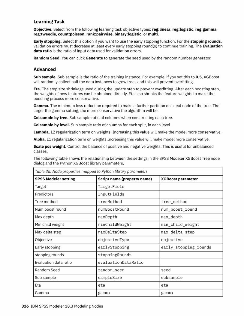
Learning TaskObjective. Select from the following learning task objective types: reg:linear, reg:logistic, reg:gamma,reg:tweedie, count:poisson, rank:pairwise, binary:logistic, or multi.

Early stopping. Select this option if you want to use the early stopping function. For the stopping rounds,validation errors must decrease at least every early stopping round(s) to continue training. The Evaluationdata ratio is the ratio of input data used for validation errors.

Random Seed. You can click Generate to generate the seed used by the random number generator.

AdvancedSub sample. Sub sample is the ratio of the training instance. For example, if you set this to 0.5, XGBoostwill randomly collect half the data instances to grow trees and this will prevent overfitting.

Eta. The step size shrinkage used during the update step to prevent overfitting. After each boosting step,the weights of new features can be obtained directly. Eta also shrinks the feature weights to make theboosting process more conservative.

Gamma. The minimum loss reduction required to make a further partition on a leaf node of the tree. Thelarger the gamma setting, the more conservative the algorithm will be.

Colsample by tree. Sub sample ratio of columns when constructing each tree.

Colsample by level. Sub sample ratio of columns for each split, in each level.

Lambda. L2 regularization term on weights. Increasing this value will make the model more conservative.


Scale pos weight. Control the balance of positive and negative weights. This is useful for unbalancedclasses.

The following table shows the relationship between the settings in the SPSS Modeler XGBoost Tree nodedialog and the Python XGBoost library parameters.



Target TargetField

Predictors InputFields

Tree method treeMethod tree_method

Num boost round numBoostRound num_boost_round

Max depth maxDepth max_depth

Min child weight minChildWeight min_child_weight

Max delta step maxDeltaStep max_delta_step


Early stopping earlyStopping early_stopping_rounds

stopping rounds stoppingRounds

Evaluation data ratio evaluationDataRatio

Random Seed random_seed seed

Sub sample sampleSize subsample

Eta eta eta

Gamma gamma gamma


Table 35. Node properties mapped to Python library parameters (continued)


Colsample by tree colsSampleRatio colsample_bytree

Colsample by level colsSampleLevel colsample_bylevel


Alpha alpha alpha

Scale pos weight scalePosWeight scale_pos_weight

1 "XGBoost Parameters" Scalable and Flexible Gradient Boosting. Web. © 2015-2016 DMLC.2 "Plotting API" Scalable and Flexible Gradient Boosting. Web. © 2015-2016 DMLC.3 "Scalable and Flexible Gradient Boosting." Web. © 2015-2016 DMLC.

XGBoost Tree node Model OptionsModel name. You can generate the model name automatically based on the target or ID field (or modeltype in cases where no such field is specified) or specify a custom name.

t-SNE nodet-Distributed Stochastic Neighbor Embedding (t-SNE)© is a tool for visualizing high-dimensional data. Itconverts affinities of data points to probabilities. The affinities in the original space are represented byGaussian joint probabilities and the affinities in the embedded space are represented by Student's t-distributions. This allows t-SNE to be particularly sensitive to local structure and has a few otheradvantages over existing techniques: 1

• Revealing the structure at many scales on a single map• Revealing data that lie in multiple, different, manifolds, or clusters• Reducing the tendency to crowd points together at the center

The t-SNE node in SPSS Modeler is implemented in Python and requires the scikit-learn© Pythonlibrary. For details about t-SNE and the scikit-learn library, see:

• https://scikit-learn.org/stable/modules/generated/sklearn.manifold.TSNE.html#sklearn.manifold.TSNE• https://scikit-learn.org/stable/modules/manifold.html#t-sne

The Python tab on the Nodes Palette contains this node and other Python nodes. The t-SNE node is alsoavailable on the Graphs tab.1 References:

van der Maaten, L.J.P.; Hinton, G. "Visualizing High-Dimensional Data using t-SNE." Journal of MachineLearning Research. 9:2579-2605, 2008.

van der Maaten, L.J.P. "t-Distributed Stochastic Neighbor Embedding."

van der Maaten, L.J.P. "Accelerating t-SNE using Tree-Based Algorithms." Journal of Machine LearningResearch. 15(Oct):3221-3245, 2014.

t-SNE node Expert optionsChoose Simple mode or Expert mode depending on which options you want to set for the t-SNE node.

Visualization type. Select 2D or 3D to specify whether to draw the graph as two-dimensional or three-dimensional.

Method. Select Barnes Hut or Exact. By default, the gradient calculation algorithm uses Barnes-Hutapproximation which runs must faster than the Exact method. Barnes-Hut approximation allows the t-


https://scikit-learn.org/stable/modules/generated/sklearn.manifold.TSNE.html#sklearn.manifold.TSNE

https://scikit-learn.org/stable/modules/manifold.html#t-sne

http://jmlr.org/papers/v9/vandermaaten08a.html

http://lvdmaaten.github.io/tsne/

https://lvdmaaten.github.io/publications/papers/JMLR_2014.pdf

SNE technique to be applied to large, real-world datasets. The Exact algorithm will do a better job ofavoiding nearest-neighbor errors.

Init. Select Random or PCA for the initialization of embedding.

Target Field. Select the target field to show as a colormap on the output graph. The graph will use onecolor if no target field is specified here.

OptimizationPerlexity. The perplexity is related to the number of nearest neighbors that are used in other manifoldlearning algorithms. Larger datasets usually required a larger perplexity. Consider selecting a valuebetween 5 and 50. Default is 30, and the range is 2 - 9999999.

Early exaggeration. This setting controls how tight natural clusters in the original space will be in theembedded space, and how much space will be between them. Default is 12, and the range is 2 -9999999.

Learning rate. If the learning rate is too high, the data might look like a "ball" with any pointapproximately equidistant from its nearest neighbors. If the learning rate is too low, most points may lookcompressed in a dense cloud with few outliers. If the cost function gets stuck in a bad local minimum,increasing the learning rate may help. Default is 200, and the range is 0 - 9999999.

Max iterations. The maximum number of iterations for the optimization. Default is 1000, and the range is250 - 9999999.

Angular size. The angular size of a distant node as measured from a point. Enter a value between 0 and 1.Default is 0.5.

Random seedSet random seed. Select this option and click Generate to generate the seed used by the random numbergenerator.

Optimization stop conditionMax iterations without progress. The maximum number of iterations without progress to perform beforestopping the optimization, used after 250 initial iterations with early exaggeration. Note that progress isonly checked every 50 iterations, so this value is rounded to the next multiple of 50. Default is 300, andthe range is 0 - 9999999.

Min gradient norm. If the gradient norm is below this minimum threshold, the optimization will stop.Default is 1.0E-7.

Metric. The metric to use when calculating distance between instances in a feature array. If the metric isa string, it must be one of the options allowed by scipy.spatial.distance.pdist for its metricparameter, or a metric listed in pairwise.PAIRWISE_DISTANCE_FUNCTIONS. Select one of theavailable metric types. Default is euclidean.

When number of records greater than. Specify a method for plotting large datasets. You can specify amaximum dataset size or use the default 2,000 points. Performance is enhanced for large datasets whenyou select the Bin or Sample options. Alternatively, you can choose to plot all data points by selectingUse all data, but you should note that this may dramatically decrease the performance of the software.

• Bin. Select to enable binning when the dataset contains more than the specified number of records.Binning divides the graph into fine grids before actually plotting and counts the number of connectionsthat would appear in each of the grid cells. In the final graph, one connection is used per cell at the bincentroid (average of all connection points in the bin).

• Sample. Select to randomly sample the data to the specified number of records.

The following table shows the relationship between the settings on the Expert tab of the SPSS Modeler t-SNE node dialog and the Python t-SNE library parameters.



SPSS Modeler setting Script name (property name) Python t-SNE parameter

Mode mode_type

Visualization type n_components n_components

Method method method

Initialization of embedding init init

Target target_field target_field

Perplexity perplexity perplexity

Early exaggeration early_exaggeration early_exaggeration

Learning rate learning_rate learning_rate

Max iterations n_iter n_iter

Angular size angle angle

Set random seed enable_random_seed


Max iterations without progress n_iter_without_progress n_iter_without_progress

Min gradient norm min_grad_norm min_grad_norm

Perform t-SNE with multipleperplexities

isGridSearch

t-SNE node Output optionsSpecify options for the t-SNE node output on the Output tab.

Output name. Specify the name of the output that is produced when the node runs. If you select Auto,the name of the output is automatically set.

Output to screen. Select this option to generate and display the output in a new window. The output isalso added to the Output manager.

Output to file. Select this option to save the output to a file. Doing so enables the File name and File typefields. The t-SNE node requires access to this output file if you want to create plots using other fields forcomparison purposes – or to use its output as predictors in classification or regression models. The t-SNEmodel creates a result file of x, y (and z) coordinate fields that is most easily accessed using a Fixed Filesource node.

t-SNE model nuggetst-SNE model nuggets contain all of the information captured by the t-SNE model. The following tabs areavailable.

GraphThe Graph tab displays chart output for the t-SNE node. A pyplot scatter chart shows the low dimensionsresult. If you didn't select the Perform t-SNE with multiple perplexities option on the Expert tab of the t-SNE node, only one graph is included rather than six graphs with different perplexities.


Text outputThe Text output tab displays the results of the t-SNE algorithm. If you chose the 2D visualization type onthe Expert tab of the t-SNE node, the result here is the point value in two dimensions. If you chose 3D, theresult is the point value in three dimensions.

Gaussian Mixture nodeA Gaussian Mixture© model is a probabilistic model that assumes all the data points are generated from amixture of a finite number of Gaussian distributions with unknown parameters. One can think of mixturemodels as generalizing k-means clustering to incorporate information about the covariance structure ofthe data as well as the centers of the latent Gaussians.1

The Gaussian Mixture node in SPSS Modeler exposes the core features and commonly used parameters ofthe Gaussian Mixture library. The node is implemented in Python.

For more information about Gaussian Mixture modeling algorithms and parameters, see the GaussianMixture documentation available at http://scikit-learn.org/stable/modules/mixture.html and https://scikit-learn.org/stable/modules/generated/sklearn.mixture.GaussianMixture.html. 2

1 "User Guide." Gaussian mixture models. Web. © 2007 - 2017. scikit-learn developers.2 Scikit-learn: Machine Learning in Python, Pedregosa et al., JMLR 12, pp. 2825-2830, 2011.

Gaussian Mixture node FieldsThe Fields tab specifies which fields are used in the analysis.

Use predefined roles. This option uses the input settings from an upstream Type node (or the Types tabof an upstream source node).

Use custom field assignments. To manually assign inputs, select this option.

Fields. Use the arrow buttons to assign items manually from this list to the Predictors list on the right ofthe screen. The icons indicate the valid measurement levels for each field. To select all the fields in thelist, click the All button, or click an individual measurement level button to select all fields with thatmeasurement level.

Predictors. Select one or more fields as predictors.

Gaussian Mixture node Build OptionsUse the Build Options tab to specify build options for the Gaussian Mixture node, including basic optionsand advanced options. For details about these options not covered in this section, see the followingonline resources:

• Gaussian mixture parameter reference1

• Gaussian mixture node user guide2

BasicCovariance type. Select one of the following covariance matrices:

• Full. Each component has its own general covariance matrix.• Tied. All components share the same general covariance matrix.• Diag. Each component has its own diagonal covariance matrix.• Spherical. Each component has its own single variance.

Number of components. Specify the number of mixture components to use when building the model.

Cluster Label. Specify whether the cluster label is a number or a string. If you choose String, specify aprefix for the cluster label (for example, the default prefix is cluster, which results in cluster labels suchas cluster-1, cluster-2, etc.).


http://scikit-learn.org/stable/modules/mixture.html

https://scikit-learn.org/stable/modules/generated/sklearn.mixture.GaussianMixture.html


https://scikit-learn.org/stable/modules/mixture.html

http://jmlr.csail.mit.edu/papers/v12/pedregosa11a.html



Random Seed. Select this option and click Generate to generate the seed used by the random numbergenerator.

AdvancedTolerance. Specify the convergence threshold. Default value is 0.001.

Number of iterations. Specify the maximum number of iterations to perform. Default value is 100.

Init parameters. Select the initialization parameter Kmeans (responsibilities are initialized using k-means) or Random (responsibilities are initialized randomly).

Warm start. If you select True, the solution of the last fitting will be used as the initialization for the nextfitting. This can speed up convergence when fitting is called several times on similar problems.

The following table shows the relationship between the settings in the SPSS Modeler Gaussian Mixturenode dialog and the Python Gaussian Mixture library parameters.


SPSS Modeler setting Script name (property name) Gaussian Mixture parameter

Use predefined roles / Usecustom field assignments

role_use

Inputs predictors

Use partitioned data use_partition

Covariance type covariance_type covariance_type

Number of components number_component n_components

Cluster Label component_lable

Label Prefix label_prefix

Set random seed enable_random_seed

Random Seed random_seed random_state

Tolerance tol tol

Number of iterations max_iter max_iter

Init parameters init_params init_params

Warm start warm_start warm_start

1 Scikit-learn: Machine Learning in Python, Pedregosa et al., JMLR 12, pp. 2825-2830, 2011.2 "User Guide." Gaussian mixture models. Web. © 2007 - 2017. scikit-learn developers.

Gaussian Mixture node Model OptionsModel name. You can generate the model name automatically based on the target or ID field (or modeltype in cases where no such field is specified) or specify a custom name.

KDE nodesKernel Density Estimation (KDE)© uses the Ball Tree or KD Tree algorithms for efficient queries, and walksthe line between unsupervised learning, feature engineering, and data modeling. Neighbor-basedapproaches such as KDE are some of the most popular and useful density estimation techniques. KDE canbe performed in any number of dimensions, though in practice high dimensionality can cause adegradation of performance. The KDE Modeling and KDE Simulation nodes in SPSS Modeler expose thecore features and commonly used parameters of the KDE library. The nodes are implemented in Python. 1


http://jmlr.csail.mit.edu/papers/v12/pedregosa11a.html


To use a KDE node, you must set up an upstream Type node. The KDE node will read input values from theType node (or the Types tab of an upstream source node).

The KDE Modeling node is available on SPSS Modeler's Modeling tab and Python tab. The KDE Modelingnode generates a model nugget, and the nugget's scored values are kernel density values from the inputdata.

The KDE Simulation node is available on the Output tab and the Python tab. The KDE Simulation nodegenerates a KDE Gen source node that can create some records that have the same distribution as theinput data. The KDE Gen node includes a Settings tab where you can specify how many records the nodewill create (default is 1) and generate a random seed.

For more information about KDE, including examples, see the KDE documentation available at http://scikit-learn.org/stable/modules/density.html#kernel-density-estimation. 1

1 "User Guide." Kernel Density Estimation. Web. © 2007-2018, scikit-learn developers.

KDE Modeling node and KDE Simulation node FieldsThe Fields tab specifies which fields are used in the analysis.



Fields. Use the arrow buttons to assign items manually from this list to the Inputs list on the right of thescreen. The icons indicate the valid measurement levels for each field. To select all the fields in the list,click the All button, or click an individual measurement level button to select all fields with thatmeasurement level.

Inputs. Select one or more fields as inputs for clustering. KDE can only deal with continuous fields.

KDE nodes Build OptionsUse the Build Options tab to specify build options for the KDE nodes, including basic options for kerneldensity parameters and cluster labels, and advanced options such as tolerance, leaf size, and whether touse a breadth-first approach. For additional information about these options, see the following onlineresources:

• Kernel Density Estimation Python API Parameter Reference1

• Kernel Density Estimation User Guide2

BasicBandwidth. Specify the bandwidth of the kernel.

Kernel. Select the kernel to use. Available kernels for the KDE Modeling node are Gaussian, Tophat,Epanechnikov, Eponential, Linear, or Cosine. Available kernels for the KDE Simulation node areGaussian or Tophat. For details about these available kernels, see the Kernel Density Estimation UserGuide.2

Algorithm. Select Auto, Ball Tree or KD Tree for the tree algorithm to use. For more information, see BallTree3 and KD Tree.4

Metric. Select a distance metric. Available metrics are Euclidean, Braycurtis, Chebyshev, Canberra,Cityblock, Dice, Hamming, Infinity, Jaccard, L1, L2, Matching, Manhattan, P, Rogerstanimoto,Russellrao, Sokalmichener, Sokalsneath, Kulsinski, or Minkowski. If you select Minkowski, set the PValue as desired.

The metrics available in this drop-down will vary depending on which algorithm you choose. Also notethat the normalization of the density output is correct only for the Euclidean distance metric.


http://scikit-learn.org/stable/modules/density.html#kernel-density-estimation


http://scikit-learn.org/stable/modules/generated/sklearn.neighbors.KernelDensity.html#sklearn.neighbors.KernelDensity




http://scikit-learn.org/stable/modules/neighbors.html#ball-tree


http://scikit-learn.org/stable/modules/neighbors.html#kd-tree

AdvancedAbsolute Tolerance. Specify the desired absolute tolerance of the result. A larger tolerance will generallyresult in faster run time. Default is 0.0.

Relative Tolerance. Specify the desired relative tolerance of the result. A larger tolerance will generallyresult in faster run time. Default is 1E-8.

Leaf Size. Specify the leaf size of the underlying tree. Default is 40. Changing the leaf size maysignificantly impact performance and required memory. For more information about the Ball Tree and KDTree algorithms, see Ball Tree3 and KD Tree.4

Breadth first. Select True if you want to use a breadth-first approach or False to use a depth-firstapproach.

The following table shows the relationship between the settings in the SPSS Modeler KDE node dialogsand the Python KDE library parameters.


SPSS Modeler setting Script name (property name) KDE parameter

Inputs inputs

Bandwidth bandwidth bandwidth

Kernel kernel kernel

Algorithm algorithm algorithm

Metric metric metric

P Value pValue pValue

Absolute Tolerance atol atol

Relative Tolerance rtol Rtol

Leaf Size leafSize leafSize

Breadth first breadthFirst breadthFirst

1 "API Reference." sklearn.neighbors.KernelDensity. Web. © 2007-2018, scikit-learn developers.2 "User Guide." Kernel Density Estimation. Web. © 2007-2018, scikit-learn developers.3 "Ball Tree." Five balltree construction algorithms. © 1989, Omohundro, S.M., International ComputerScience Institute Technical Report.4 "K-D Tree." Multidimensional binary search trees used for associative searching. © 1975, Bentley, J.L.,Communications of the ACM.

KDE Modeling node and KDE Simulation node Model OptionsModel name. You can generate the model name automatically based on the target or ID field (or modeltype in cases where no such field is specified) or specify a custom name.

Random Forest nodeRandom Forest© is an advanced implementation of a bagging algorithm with a tree model as the basemodel. In random forests, each tree in the ensemble is built from a sample drawn with replacement (forexample, a bootstrap sample) from the training set. When splitting a node during the construction of thetree, the split that is chosen is no longer the best split among all features. Instead, the split that is pickedis the best split among a random subset of the features. Because of this randomness, the bias of theforest usually slightly increases (with respect to the bias of a single non-random tree) but, due to






averaging, its variance also decreases, usually more than compensating for the increase in bias, henceyielding an overall better model.1

The Random Forest node in SPSS Modeler is implemented in Python. The Python tab on the Nodes Palettecontains this node and other Python nodes.

For more information about random forest algorithms, see https://scikit-learn.org/stable/modules/ensemble.html#forest.1L. Breiman, "Random Forests," Machine Learning, 45(1), 5-32, 2001.

Random Forest node FieldsThe Fields tab specifies which fields are used in the analysis.






Random Forest node Build OptionsUse the Build Options tab to specify build options for the Random Forest node, including basic optionsand advanced options. For more information about these options, see https://scikit-learn.org/stable/modules/ensemble.html#forest

BasicNumber of trees to build. Select the number of trees in the forest.

Specify max depth. If not selected, nodes are expanded until all leaves are pure or until all leavescontain less than min_samples_split samples.

Max depth. The maximum depth of the tree.

Minimum leaf node size. The minimum number of samples required to be at a leaf node.

Number of features to use for splitting. The number of features to consider when looking for the bestsplit:

• If auto, then max_features=sqrt(n_features) for classifier and max_features=n_featuresfor regression.

• If sqrt, then max_features=sqrt(n_features).• If log2, then max_features=log2(n_features).

AdvancedUse bootstrap samples when building trees. If selected, bootstramp samples are used when buildingtrees.

Use out-of-bag samples to estimate the generalization accuracy. If selected, out-of-bag samples areused to estimate the generalization accuracy.

Use extremely randomized trees. If selected, extremely randomized trees are used instead of generalrandom forests. In extremely randomized trees, randomness goes one step further in the way splits arecomputed. As in random forests, a random subset of candidate features is used, but instead of looking for


https://scikit-learn.org/stable/modules/ensemble.html#forest




the most discriminative thresholds, thresholds are drawn at random for each candidate feature and thebest of these randomly-generated thresholds is picked as the splitting rule. This usually allows thevariance of the model to be reduced a bit more, at the expense of a slightly greater increase in bias. 1

Replicate results. If selected, the model building process is replicated to achieve the same scoringresults.

Random seed. You can click Generate to generate the seed used by the random number generator.

Hyper-Parameter Optimization (Based on Rbfopt). Select this option to enable Hyper-ParameterOptimization based on Rbfopt, which automatically discovers the optimal combination of parameters sothat the model will achieve the expected or lower error rate on the samples. For details about Rbfopt, seehttp://rbfopt.readthedocs.io/en/latest/rbfopt_settings.html.

Target. The objective function value (error rate of the model on the samples) you want to reach (i.e., thevalue of the unknown optimum). Set to an acceptable value such as 0.01.

Max iterations. The maximum number of iterations to try the model. Default is 1000.

Max evaluations. The maximum number of function evaluations in accurate mode, for trying the model.Default is 300.

The following table shows the relationship between the settings in the SPSS Modeler Random Forest nodedialog and the Python Random Forest library parameters.


SPSS Modeler setting Script name (property name) Random Forest parameter

Target target

Predictors inputs

Number of trees to build n_estimators n_estimators

Specify max depth specify_max_depth specify_max_depth

Max depth max_depth max_depth

Minimum leaf node size min_samples_leaf min_samples_leaf

Number of features to use forsplitting

max_features max_features

Use bootstrap samples whenbuilding trees

bootstrap bootstrap

Use out-of-bag samples toestimate the generalizationaccuracy

oob_score oob_score

Use extremely randomized trees extreme

Replicate results use_random_seed

Random seed random_seed random_seed

Hyper-Parameter Optimization(based on Rbfopt)

enable_hpo

Target (for HPO) target_objval

Max iterations (for HPO) max_iterations

Max evaluations (for HPO) max_evaluations

1L. Breiman, "Random Forests," Machine Learning, 45(1), 5-32, 2001.



Random Forest node Model OptionsModel name. You can generate the model name automatically based on the target or ID field (or modeltype in cases where no such field is specified) or specify a custom name.

Random Forest model nuggetsRandom Forest model nuggets contain all of the information captured by the random forest model. Thefollowing sections are available.

Model InformationThis view provides key information about the model, including input fields, one-hot encoding values, andmodel parameters.

Predictor ImportanceThis view displays a chart that indicates the relative importance of each predictor in estimating the model.For more information, see “Predictor Importance” on page 37.

HDBSCAN nodeHierarchical Density-Based Spatial Clustering (HDBSCAN)© uses unsupervised learning to find clusters, ordense regions, of a data set. The HDBSCAN node in SPSS Modeler exposes the core features andcommonly used parameters of the HDBSCAN library. The node is implemented in Python, and you can useit to cluster your dataset into distinct groups when you don't know what those groups are at first. Unlikemost learning methods in SPSS Modeler, HDBSCAN models do not use a target field. This type of learning,with no target field, is called unsupervised learning. Rather than trying to predict an outcome, HDBSCANtries to uncover patterns in the set of input fields. Records are grouped so that records within a group orcluster tend to be similar to each other, but records in different groups are dissimilar. The HDBSCANalgorithm views clusters as areas of high density separate by areas of low density. Due this rather genericview, clusters found by HDBSCAN can be any shape, as opposed to k-means which assumes that clustersare convex shaped. Outlier points that lie alone in low-density regions are also marked. HDBSCAN alsosupports scoring of new samples.1

To use the HDBSCAN node, you must set up an upstream Type node. The HDBSCAN node will read inputvalues from the Type node (or the Types tab of an upstream source node).

For more information about HDBSCAN clustering algorithms, see the HDBSCAN documentation availableat http://hdbscan.readthedocs.io/en/latest/. 1

1 "User Guide / Tutorial." The hdbscan Clustering Library. Web. © 2016, Leland McInnes, John Healy, SteveAstels.

HDBSCAN node FieldsThe Fields tab specifies which fields are used in the analysis.

Important: To train an HDBSCAN model, you must use one or more fields with the role set to Input.Fields with the role set to Output, Both, or None are ignored.



Fields. Use the arrow buttons to assign items manually from this list to the Inputs list on the right of thescreen. The icons indicate the valid measurement levels for each field. To select all the fields in the list,click the All button, or click an individual measurement level button to select all fields with thatmeasurement level.

Inputs. Select one or more fields as inputs for clustering.


http://hdbscan.readthedocs.io/en/latest/

HDBSCAN node Build OptionsUse the Build Options tab to specify build options for the HDBSCAN node, including basic options forcluster parameters and cluster labels, and advanced options for advanced parameters and chart outputoptions. For additional information about these options, see the following online resources:

• HDBSCAN Python API Parameter Reference1

• HDBSCAN Home Page2


Min Cluster Size. Specify the minimum size of clusters. Single linkage splits that contain fewer pointsthan the value specified here will be considered points "falling out" of a cluster rather than a clustersplitting into two new clusters.

Min Samples. Specify the minimum number of samples in a neighborhood for a point to be considered acore point. If set to 0, the default value is the minimum cluster size value.

Algorithm. Select the algorithm to use. HDBSCAN has variants that are specialized for differentcharacteristics of the data. By default, BEST is used - which automatically chooses the best algorithmgiven the nature of the data. For details about these algorithm types, see the HDBSCAN documentation.1Note that the algorithm you choose will impact performance. For example, for large data we recommendtrying Boruvka KDTree or Boruvka BallTree.

Metric for Distance. Select the metric to use when calculating distance between instances in a featurearray.

Cluster Label. Specify whether the cluster label is a number or a string. If you choose String, specify aprefix for the cluster label (for example, the default prefix is cluster, which results in cluster labels suchas cluster-1, cluster-2, etc.).

AdvancedApproximate Minimum Spanning Tree. Select True if you want to accept an approximate minimumspanning tree. For some algorithms, this can improve performance, but the resulting clustering might beof marginally lower quality. If you are willing to sacrifice speed for correctness, you may want to try theFalse option. In most cases, True is recommended.

Method to Select Cluster. Select which method to use for selecting clusters from the condensed tree.The standard approach for HDBSCAN is to use an Excess of Mass (EOM) algorithm to find the mostpersistent clusters. Or you can select the clusters at the leaves of the tree, which provides the most fine-grained and homogeneous clusters.

Accept Single Cluster. Change this setting to True to allow single cluster results only if this is a validresult for your dataset.

P Value. If using the Minkowski metric for distance (under Basic build options), you can change this pvalue if desired.

Leaf Size. If using a space tree algorithm (Boruvka KDTree or Boruvka BallTree), this is the number ofpoints in a leaf node of the tree. This setting doesn't alter the resulting clustering, but it may impact therun time of the algorithm.

Validity Index. Select this option to include the Validity Index chart in the model nugget output.

Condensed Tree. Select this option to include the Condensed Tree chart in the model nugget output.

Single Linkage Tree. Select this option to include the Single Linkage Tree chart in the model nuggetoutput.


http://hdbscan.readthedocs.io/en/latest/api.html

http://hdbscan.readthedocs.io/en/latest/


http://hdbscan.readthedocs.io/en/latest/api.html

Min Span Tree. Select this option to include the Min Span Tree chart in the model nugget output.

The following table shows the relationship between the settings in the SPSS Modeler HDBSCAN nodedialog and the Python HDBSCAN library parameters.


SPSS Modeler setting Script name (property name) HDBSCAN parameter

Inputs inputs inputs

Hyper-Parameter Optimization useHPO

Min Cluster Size min_cluster_size min_cluster_size

Min Samples min_samples min_samples

Algorithm algorithm algorithm

Metric for Distance metric metric

Cluster Label useStringLabel

Label Prefix stringLabelPrefix

Approximate Minimum SpanningTree

approx_min_span_tree approx_min_span_tree

Method to Select Cluster cluster_selection_method cluster_selection_method

Accept Single Cluster allow_single_cluster allow_single_cluster

P Value p_value p_value

Leaf Size leaf_size leaf_size

Validity Index outputValidity

Condensed Tree outputCondensed

Single Linkage Tree outputSingleLinkage

Min Span Tree outputMinSpan

1 "API Reference." The hdbscan Clustering Library. Web. © 2016, Leland McInnes, John Healy, SteveAstels.2 "User Guide / Tutorial." The hdbscan Clustering Library. Web. © 2016, Leland McInnes, John Healy, SteveAstels.

HDBSCAN node Model OptionsModel name. You can generate the model name automatically based on the target or ID field (or modeltype in cases where no such field is specified) or specify a custom name.

One-Class SVM nodeThe One-Class SVM© node uses an unsupervised learning algorithm. The node can be used for noveltydetection. It will detect the soft boundary of a given set of samples, to then classify new points asbelonging to that set or not. This One-Class SVM modeling node is implemented in Python and requiresthe scikit-learn© Python library. For details about the scikit-learn library, see http://contrib.scikit-learn.org/imbalanced-learn/about.html1.

The Python tab on the Nodes Palette contains the One-Class SVM node and other Python nodes.

Note: One-Class SVM is used for usupervised outlier and novelty detection. In most cases, werecommend using a known, "normal" dataset to build the model so the algorithm can set a correct


http://scikit-learn.org/stable/modules/svm.html#svm-outlier-detection

http://scikit-learn.org/stable/modules/svm.html#svm-outlier-detection

boundary for the given samples. Parameters for the model – such as nu, gamma, and kernel – impact theresult significantly. So you may need to experiment with these options until you find the optimal settingsfor your situation.1Smola, Schölkopf. "A Tutorial on Support Vector Regression." Statistics and Computing Archive, vol. 14,no. 3, August 2004, pp. 199-222. (http://citeseerx.ist.psu.edu/viewdoc/summary?doi=10.1.1.114.4288)

One-Class SVM node FieldsThe Fields tab specifies which fields are used in the analysis.

Use predefined roles. Select this option to select all fields with a defined role of Input.

Use custom field assignments. To manually select fields, select this option and choose input fields andsplit fields:

Inputs. Select the input fields to use in the analysis. All storage types and measurement types aresupported, except for typeless or unknown. If a field has a String storage type, the values of this field willbe binarized in a one-vs-all fashion via a one-hot encoding algorithm.

Split. Select which field or fields to use as split fields. All flag, nominal, ordinal, and discretemeasurement types are supported.

Use partitioned data If a partition field is defined, this option ensures that data from only the trainingpartition is used to build the model.

One-Class SVM node ExpertOn the Expert tab of the One-Class SVM node, you can choose from Simple mode or Expert mode. If youchoose Simple, all parameters are set with the default values as shown below. If you select Expert, youcan specify custom values for these parameters. For further detail about these options, see http://scikit-learn.org/stable/modules/generated/sklearn.svm.OneClassSVM.html#sklearn.svm.OneClassSVM.

Stopping criteria. Specify the tolerance for stopping criteria. Default is 1.0E-3 (0.001).

Regression precision (nu). Bound on the fraction of training errors and support vectors. Default is 0.1.

Kernel type. The kernel type to use in the algorithm. Options include RBF, Polynomial, Sigmoid, Linear,or Precomputed. Default is RBF.

Specify Gamma. Select this option to specify the Gamma. Otherwise, the auto gamma will be applied.

Gamma. The Gamma setting is only available for the RBF, Polynomial, and Sigmoid kernel types.

Coef0. Coef0 is only available for the Polynomial and Sigmoid kernel types.

Degree. Degree is only available for the Polynomial kernel type.

Use the shrinking heuristic. Select this option to use the shrinking heuristic. This option is deselected bydefault.

Specify the size of the kernel cache (in MB). Select this option to specify the size of the kernel cache.This option is deselected by default. When selected, the default value is 200 MB.

Hyper-Parameter Optimization (Based on Rbfopt). Select this option to enable Hyper-ParameterOptimization based on Rbfopt, which automatically discovers the optimal combination of parameters sothat the model will achieve the expected or lower error rate on the samples. For details about Rbfopt, seehttp://rbfopt.readthedocs.io/en/latest/rbfopt_settings.html.

Target. The objective function value (error rate of the model on the samples) we want to reach (forexample, the value of the unknown optimum). Set to an acceptable value such as 0.01.

Max Iterations. Maximum number of iterations for trying the model. Default is 1000.

Max Evaluations. Maximum number of function evaluations for trying the model, where the focus isaccuracy over speed. Default is 300.


http://scikit-learn.org/stable/modules/generated/sklearn.svm.OneClassSVM.html#sklearn.svm.OneClassSVM

http://scikit-learn.org/stable/modules/generated/sklearn.svm.OneClassSVM.html#sklearn.svm.OneClassSVM


The One-Class SVM node requires the scikit-learn© Python library. The following table shows therelationship between the settings in the SPSS Modeler SMOTE node dialog and the Python algorithm.


Parameter name Script name (property name) Python API parameter name

Stopping criteria stopping_criteria tol

Regression precision precision nu

Kernel type kernel kernel

Gamma gamma gamma

Coef0 coef0 coef0

Degree degree degree

Use the shrinking heuristic shrinking shrinking

Specify the size of the kernelcache (number input box)

cache_size cache_size


One-Class SVM node OptionsOn the Options tab of the One-Class SVM node, you can set the following options.

Type of Parallel Coordinates graphic. SPSS Modeler draws parallel coordinates graphics to present thebuilt model. Sometimes, the values for some data columns/features will be displayed much larger thanothers, which can make some other portions of the graph hard to see. For cases like this, you can choosethe Independent vertical axes option to give all vertical axes a standalone axis scale, or select Generalvertical axes to force all vertical axes to share the same axes scale.

Maximum lines on the graphic. Specify the maximum number of data rows (lines) to display in graphoutput. The default is 100. For performance reasons, a maximum of 20 fields will be displayed.

Draw all input fields on the graphic. Select this option to show all input fields in the graph output. Bydefault, each data field will be drawn as a vertical axis. For performance reasons, a maximum of 30 fieldswill be displayed.

Custom fields to be drawn on the graphic. Rather than showing all input fields in the graph output, youcan select this option and choose a subset of fields to show. This can improve performance. Forperformance reasons, a maximum of 20 fields will be displayed.


Chapter 18. Spark nodes

SPSS Modeler offers nodes for using Spark native algorithms. The Spark tab on the Nodes Palettecontains the following nodes you can use to run Spark algorithms. These nodes are supported onWindows 64, Mac 64, and Linux 64. Note that these nodes don't support specifying an integer/doublecolumn as Flag/Nominal for building a model. To do this, you must convert the column value to 0/1 or0,1,2,3,4...

Isotonic Regression belongs to the family of regression algorithms. The Isotonic-ASnode in SPSS Modeler is implemented in Spark. For details about IsotonicRegression algorithms, see https://spark.apache.org/docs/2.2.0/mllib-isotonic-regression.html.


K-Means is one of the most commonly used clustering algorithms. It clusters datapoints into a predefined number of clusters. The K-Means-AS node in SPSS Modeleris implemented in Spark. For details about K-Means algorithms, see https://spark.apache.org/docs/2.2.0/ml-clustering.html. Note that the K-Means-AS nodeperforms one-hot encoding automatically for categorical variables.

Multilayer perceptron is a classifier based on the feedforward artificial neuralnetwork and consists of multiple layers. Each layer is fully connected to the nextlayer in the network. The MultiLayerPerceptron-AS node in SPSS Modeler isimplemented in Spark. For details about the multilayer perceptron classifier (MLPC),see https://spark.apache.org/docs/latest/ml-classification-regression.html#multilayer-perceptron-classifier.

Isotonic-AS nodeIsotonic Regression belongs to the family of regression algorithms. The Isotonic-AS node in SPSS Modeleris implemented in Spark.

For details about Isotonic Regression algorithms, see https://spark.apache.org/docs/2.2.0/mllib-isotonic-regression.html. 1

1 "Regression - RDD-based API." Apache Spark. MLlib: Main Guide. Web. 3 Oct 2017.

Isotonic-AS node FieldsThe Fields tab specifies which fields are used in the analysis.

Fields. Lists all fields in the data source. Use the arrow buttons to assign items manually from this list tothe Target, Input, and Weight fields on the right of the screen. The icons indicate the valid measurementlevels for each role field. To select all the fields in the list, click the All button, or click an individualmeasurement level button to select all fields with that measurement level.

Target. Select a field to use as the target.

Input. Select the input field or fields.

https://spark.apache.org/docs/2.2.0/mllib-isotonic-regression.html




https://spark.apache.org/docs/latest/ml-classification-regression.html#multilayer-perceptron-classifier




Weight. Select a weight field for exponential weight. If not set, the default weight value of 1 will be used.

Isotonic-AS node Build OptionsUse the Build Options tab to specify build options for the Isotonic-AS node, including the feature indexand isotonic type. For more information, see http://spark.apache.org/docs/latest/api/java/org/apache/spark/ml/regression/IsotonicRegression.html.1

Input Fields Index. Specify the index of the input fields. Default is 0.

Isotonic Type. This setting determines whether the output sequence should be isotonic/increasing orantitonic/decreasing. Default is Isotonic.1 "Class IsotonicRegression." Apache Spark. JavaDoc. Web. 3 Oct 2017.

Isotonic-AS model nuggetsIsotonic-AS model nuggets contain all of the information captured by the isotonic regression model. Thefollowing sections are available.

Model SummaryThis view provides key information about the model, including input fields, target field, and model buildingoptions.

Model ChartThis view displays a scatter diagram.

XGBoost-AS nodeXGBoost© is an advanced implementation of a gradient boosting algorithm. Boosting algorithmsiteratively learn weak classifiers and then add them to a final strong classifier. XGBoost is very flexible andprovides many parameters that can be overwhelming to most users, so the XGBoost-AS node in SPSSModeler exposes the core features and commonly used parameters. The XGBoost-AS node isimplemented in Spark.


Note that the XGBoost cross-validation function is not supported in SPSS Modeler. You can use the SPSSModeler Partition node for this functionality. Also note that XGBoost in SPSS Modeler performs one-hotencoding automatically for categorical variables.

Note: On Mac, version 10.12.3 or higher is required for building XGBoost-AS models.1 "XGBoost Tutorials." Scalable and Flexible Gradient Boosting. Web. © 2015-2016 DMLC.

XGBoost-AS node FieldsThe Fields tab specifies which fields are used in the analysis.






http://spark.apache.org/docs/latest/api/java/org/apache/spark/ml/regression/IsotonicRegression.html

http://spark.apache.org/docs/latest/api/java/org/apache/spark/ml/regression/IsotonicRegression.html




XGBoost-AS node Build OptionsUse the Build Options tab to specify build options for the XGBoost-AS node, including general options formodel building and handling imbalanced datasets, learning task options for objectives and evaluationmetrics, and booster parameters for specific boosters. For more information about these options, see thefollowing online resources:



• XGBoost Spark API3

GeneralNumber of Workers. Number of workers used to train the XGBoost model.

Number of Threads. Number of threads used per worker.

Use External Memory. Whether to use external memory as cache.

Booster Type. The booster to use (gbtree, gblinear, or dart).

Booster Rounds Number. The number of rounds for boosting.

Scale pos weight. This setting controls the balance of positive and negative weights, and is useful forunbalanced classes.

Random Seed. Click Generate to generate the seed used by the random number generator.

Learning TaskObjective. Select from the following learning task objective types: reg:linear, reg:logistic, reg:gamma,reg:tweedie, rank:pairwise, binary:logistic, or multi.

Evaluation Metrics. Evaluation metrics for validation data. A default metric will be assigned according tothe objective (rmse for regression, error for classification, or mean average precision for ranking).Available options are rmse, mae, logloss, error, merror, mlogloss, uac, ndcg, map, or gamma-deviance(default is rmse).

Booster ParametersLambda. L2 regularization term on weights. Increasing this value will make the model more conservative.


Lambda bias. L2 regularization term on bias. (There is no L1 regularization term on bias because it is notimportant.)

Tree method. Select the XGBoost tree construction algorithm to use.

Max depth. Specify the maximum depth for trees. Increasing this value will make the model morecomplex and likely to be overfitting.

Min child weight. Specify the minimum sum of instance weight (hessian) needed in a child. If the treepartition step results in a leaf node with the sum of instance weight less than this Min child weight, thenthe building process will stop further partitioning. In linear regression mode, this simply corresponds tominimum number of instances needed in each node. The larger the weight, the more conservative thealgorithm will be.

Max delta step. Specify the maximum delta step to allow for each tree's weight estimation. If set to 0,there is no constraint. If set to a positive value, it can help the update step be more conservative. Usuallythis parameter is not needed, but it may help in logistic regression when a class is extremely imbalanced.

Chapter 18. Spark nodes 343



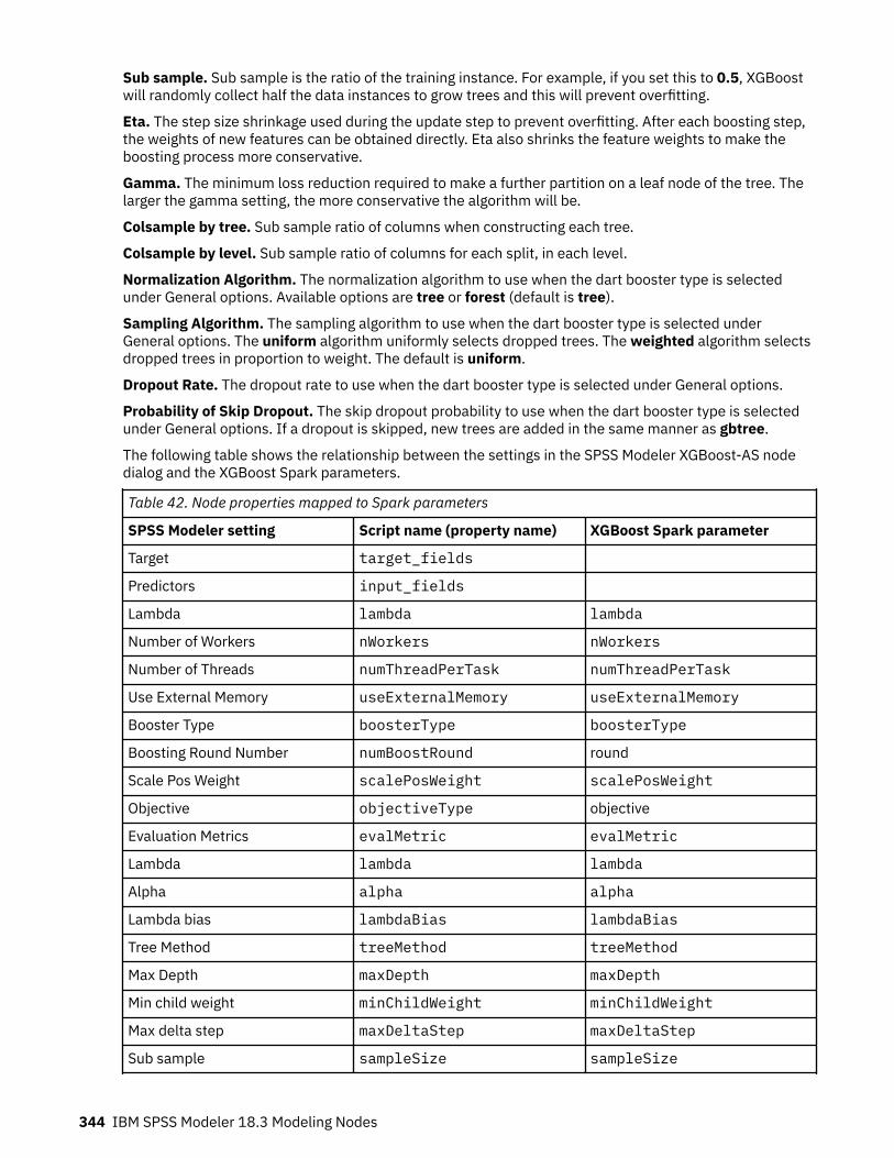
http://dmlc.ml/docs/scaladocs/xgboost4j-spark/index.html#ml.dmlc.xgboost4j.scala.spark.params.package

Sub sample. Sub sample is the ratio of the training instance. For example, if you set this to 0.5, XGBoostwill randomly collect half the data instances to grow trees and this will prevent overfitting.

Eta. The step size shrinkage used during the update step to prevent overfitting. After each boosting step,the weights of new features can be obtained directly. Eta also shrinks the feature weights to make theboosting process more conservative.

Gamma. The minimum loss reduction required to make a further partition on a leaf node of the tree. Thelarger the gamma setting, the more conservative the algorithm will be.

Colsample by tree. Sub sample ratio of columns when constructing each tree.

Colsample by level. Sub sample ratio of columns for each split, in each level.

Normalization Algorithm. The normalization algorithm to use when the dart booster type is selectedunder General options. Available options are tree or forest (default is tree).

Sampling Algorithm. The sampling algorithm to use when the dart booster type is selected underGeneral options. The uniform algorithm uniformly selects dropped trees. The weighted algorithm selectsdropped trees in proportion to weight. The default is uniform.

Dropout Rate. The dropout rate to use when the dart booster type is selected under General options.

Probability of Skip Dropout. The skip dropout probability to use when the dart booster type is selectedunder General options. If a dropout is skipped, new trees are added in the same manner as gbtree.

The following table shows the relationship between the settings in the SPSS Modeler XGBoost-AS nodedialog and the XGBoost Spark parameters.


SPSS Modeler setting Script name (property name) XGBoost Spark parameter

Target target_fields

Predictors input_fields


Number of Workers nWorkers nWorkers

Number of Threads numThreadPerTask numThreadPerTask

Use External Memory useExternalMemory useExternalMemory

Booster Type boosterType boosterType

Boosting Round Number numBoostRound round

Scale Pos Weight scalePosWeight scalePosWeight


Evaluation Metrics evalMetric evalMetric


Alpha alpha alpha

Lambda bias lambdaBias lambdaBias

Tree Method treeMethod treeMethod

Max Depth maxDepth maxDepth

Min child weight minChildWeight minChildWeight

Max delta step maxDeltaStep maxDeltaStep

Sub sample sampleSize sampleSize


Table 42. Node properties mapped to Spark parameters (continued)

SPSS Modeler setting Script name (property name) XGBoost Spark parameter

Eta eta eta

Gamma gamma gamma

Colsample by tree colsSampleRation colSampleByTree

Colsample by level colsSampleLevel colsSampleLevel

Normalization Algorithm normalizeType normalizeType

Sampling Algorithm sampleType sampleType

Dropout Rate rateDrop rateDrop

Probability of Skip Dropout skipDrop skipDrop

1 "Scalable and Flexible Gradient Boosting." Web. © 2015-2016 DMLC.2 "XGBoost Parameters" Scalable and Flexible Gradient Boosting. Web. © 2015-2016 DMLC.3 "ml.dmlc.xgboost4j.scala.spark Params." DMLC for Scalable and Reliable Machine Learning. Web. 3 Oct2017.

XGBoost-AS node Model OptionsModel name. You can generate the model name automatically based on the target or ID field (or modeltype in cases where no such field is specified) or specify a custom name.

K-Means-AS nodeK-Means is one of the most commonly used clustering algorithms. It clusters data points into a predefinednumber of clusters.1 The K-Means-AS node in SPSS Modeler is implemented in Spark.

For details about K-Means algorithms, see https://spark.apache.org/docs/2.2.0/ml-clustering.html.

Note that the K-Means-AS node performs one-hot encoding automatically for categorical variables.1 "Clustering." Apache Spark. MLlib: Main Guide. Web. 3 Oct 2017.

K-Means-AS node FieldsThe Fields tab specifies which fields are used in the analysis.

Use predefined roles. This option tells the node to use field information from an upstream Type node. It'sselected by default.

Use custom field assignments. If you want to manually assign input fields, select this option and thenselect the input field or fields. Using this option is similar to setting the field role in Input in a Type node.

K-Means-AS node Build OptionsUse the Build Options tab to specify build options for the K-Means-AS node, including regular options formodel building, initialization options for initializing cluster centers, and advanced options for thecomputing iteration and random seed. For more information, see the JavaDoc for K-Means on SparkML.1

RegularModel Name. The name of the field generated after scoring to a specific cluster. Select Auto (default) orselect Custom and type a name.

Number of Clusters. Specify the number of clusters to generate. The default is 5 and the minimum is 2.



http://spark.apache.org/docs/latest/api/java/org/apache/spark/ml/clustering/KMeans.html

InitializationInitialization Mode. Specify the method for initializing the cluster centers. K-Means|| is the default. Fordetails about these two methods, see Scalable K-Means++. 2

Initialization Steps. If the K-Means|| initialization mode is selected, specify the number of initializationsteps. 2 is the default.

AdvancedAdvanced Settings. Select this option if you want to set advanced options as follows.

Max Iteration. Specify the maximum number of iterations to perform when searching cluster centers. 20is the default.

Tolerance. Specify the convergence tolerance for iterative algorithms. 1.0E-4 is the default.

Set Random Seed. Select this option and click Generate to generate the seed used by the randomnumber generator.

DisplayDisplay Graph. Select this option if you want a graph to be included in the output.

The following table shows the relationship between the settings in the SPSS Modeler K-Means-AS nodeand the K-Means Spark parameters.


SPSS Modeler setting Script name (property name) K-Means SparkML parameter

Input Fields features

Number of Clusters clustersNum k

Initialization Mode initMode initMode

Initialization Steps initSteps initSteps

Max Iteration maxIter maxIter

Toleration toleration tol

Random Seed randomSeed seed

1 "Class KMeans." Apache Spark. JavaDoc. Web. 3 Oct 2017.2 Bahmani, Moseley, et al. "Scalable K-Means++." Feb 28, 2012. http://theory.stanford.edu/%7Esergei/papers/vldb12-kmpar.pdf.

MultiLayerPerceptron-AS nodeMultilayer perceptron is a classifier based on the feedforward artificial neural network and consists ofmultiple layers. Each layer is fully connected to the next layer in the network. For details about themultilayer perceptron classifier (MLPC), see https://spark.apache.org/docs/latest/ml-classification-regression.html#multilayer-perceptron-classifier. 1

The MultiLayerPerceptron-AS node in SPSS Modeler is implemented in Spark. To use a this node, youmust set up an upstream Type node. The MultiLayerPerceptron-AS node will read input values from theType node (or the Types tab of an upstream source node).1 "Multilayer perceptron classifier." Apache Spark. MLlib: Main Guide. Web. 5 Oct 2018.


http://theory.stanford.edu/~sergei/papers/vldb12-kmpar.pdf



MultiLayerPerceptron-AS node FieldsThe Fields tab specifies which fields are used in the analysis.

Use predefined roles. This option tells the node to use field information from an upstream Type node.This is the default.

Use custom field assignments. To manually assign target and predictors, select this option.


Predictors. Select one or more fields to use as inputs for the prediction.

MultiLayerPerceptron-AS node Build OptionsUse the Build Options tab to specify build options for the MultiLayerPerceptron-AS node, includingperformance, modeling building, and expert options. For more information about these options, seehttp://spark.apache.org/docs/latest/api/java/org/apache/spark/ml/classification/MultilayerPerceptronClassifier.html.1

PerformancePerceptrons Layer. Use this setting to define the number of perceptron layers to include. This value mustbe larger than the number of perceptron fields. The default value is 1.

Hidden Layers. Specify the number of hidden layers. Use a comma between multiple hidden layers. Thedefault value is 1.

Output Layer. Specify the number of output layers. The default value is 1.

Random Seed. Click Generate if you want to generate the seed used by the random number generator.

Model BuildingMax iterations. Specify the maximum number of iterations to perform. The default value is 10.

Expert OnlyBlockSize. Select the Expert Mode option in the Model Building section if you want to specify the blocksize for stacking input data in matrices. This can speed up the computation. The default block size is 128.

The following table shows the relationship between the settings in the SPSS ModelerMultiLayerPerceptron-AS node dialogs and the Spark KDE library parameters.


SPSS Modeler setting Script name (property name) Spark parameter

Predictors features

Target label

Perceptrons Layer layers[0] layers[0]

Hidden Layers layers[1…<latest-1>] layers[1…<latest-1>]

Output Layer layers[<latest>] layers[<latest>]

Random Seed seed seed

Max iterations maxiter maxiter

1 "Class MultilayerPerceptronClassifier." Apache Spark. JavaDoc. Web. 5 Oct 2018.


http://spark.apache.org/docs/latest/api/java/org/apache/spark/ml/classification/MultilayerPerceptronClassifier.html

http://spark.apache.org/docs/latest/api/java/org/apache/spark/ml/classification/MultilayerPerceptronClassifier.html

MultiLayerPerceptron node Model OptionsModel name. You can generate the model name automatically based on the target or ID field (or modeltype in cases where no such field is specified) or specify a custom name.


Notices

This information was developed for products and services offered in the US. This material might beavailable from IBM in other languages. However, you may be required to own a copy of the product orproduct version in that language in order to access it.

IBM may not offer the products, services, or features discussed in this document in other countries.Consult your local IBM representative for information on the products and services currently available inyour area. Any reference to an IBM product, program, or service is not intended to state or imply that onlythat IBM product, program, or service may be used. Any functionally equivalent product, program, orservice that does not infringe any IBM intellectual property right may be used instead. However, it is theuser's responsibility to evaluate and verify the operation of any non-IBM product, program, or service.

IBM may have patents or pending patent applications covering subject matter described in thisdocument. The furnishing of this document does not grant you any license to these patents. You can sendlicense inquiries, in writing, to:

IBM Director of LicensingIBM CorporationNorth Castle Drive, MD-NC119Armonk, NY 10504-1785US

For license inquiries regarding double-byte (DBCS) information, contact the IBM Intellectual PropertyDepartment in your country or send inquiries, in writing, to:

Intellectual Property LicensingLegal and Intellectual Property LawIBM Japan Ltd.19-21, Nihonbashi-Hakozakicho, Chuo-kuTokyo 103-8510, Japan

INTERNATIONAL BUSINESS MACHINES CORPORATION PROVIDES THIS PUBLICATION "AS IS"WITHOUT WARRANTY OF ANY KIND, EITHER EXPRESS OR IMPLIED, INCLUDING, BUT NOT LIMITED TO,THE IMPLIED WARRANTIES OF NON-INFRINGEMENT, MERCHANTABILITY OR FITNESS FOR APARTICULAR PURPOSE. Some jurisdictions do not allow disclaimer of express or implied warranties incertain transactions, therefore, this statement may not apply to you.

This information could include technical inaccuracies or typographical errors. Changes are periodicallymade to the information herein; these changes will be incorporated in new editions of the publication.IBM may make improvements and/or changes in the product(s) and/or the program(s) described in thispublication at any time without notice.

Any references in this information to non-IBM websites are provided for convenience only and do not inany manner serve as an endorsement of those websites. The materials at those websites are not part ofthe materials for this IBM product and use of those websites is at your own risk.

IBM may use or distribute any of the information you provide in any way it believes appropriate withoutincurring any obligation to you.

Licensees of this program who wish to have information about it for the purpose of enabling: (i) theexchange of information between independently created programs and other programs (including thisone) and (ii) the mutual use of the information which has been exchanged, should contact:

IBM Director of LicensingIBM CorporationNorth Castle Drive, MD-NC119Armonk, NY 10504-1785US

Such information may be available, subject to appropriate terms and conditions, including in some cases,payment of a fee.

The licensed program described in this document and all licensed material available for it are provided byIBM under terms of the IBM Customer Agreement, IBM International Program License Agreement or anyequivalent agreement between us.

The performance data and client examples cited are presented for illustrative purposes only. Actualperformance results may vary depending on specific configurations and operating conditions.

Information concerning non-IBM products was obtained from the suppliers of those products, theirpublished announcements or other publicly available sources. IBM has not tested those products andcannot confirm the accuracy of performance, compatibility or any other claims related to non-IBMproducts. Questions on the capabilities of non-IBM products should be addressed to the suppliers ofthose products.

Statements regarding IBM's future direction or intent are subject to change or withdrawal without notice,and represent goals and objectives only.

This information contains examples of data and reports used in daily business operations. To illustratethem as completely as possible, the examples include the names of individuals, companies, brands, andproducts. All of these names are fictitious and any similarity to actual people or business enterprises isentirely coincidental.

TrademarksIBM, the IBM logo, and ibm.com are trademarks or registered trademarks of International BusinessMachines Corp., registered in many jurisdictions worldwide. Other product and service names might betrademarks of IBM or other companies. A current list of IBM trademarks is available on the web at"Copyright and trademark information" at www.ibm.com/legal/copytrade.shtml.

Adobe, the Adobe logo, PostScript, and the PostScript logo are either registered trademarks ortrademarks of Adobe Systems Incorporated in the United States, and/or other countries.

Intel, Intel logo, Intel Inside, Intel Inside logo, Intel Centrino, Intel Centrino logo, Celeron, Intel Xeon,Intel SpeedStep, Itanium, and Pentium are trademarks or registered trademarks of Intel Corporation orits subsidiaries in the United States and other countries.

Linux is a registered trademark of Linus Torvalds in the United States, other countries, or both.

Microsoft, Windows, Windows NT, and the Windows logo are trademarks of Microsoft Corporation in theUnited States, other countries, or both.

UNIX is a registered trademark of The Open Group in the United States and other countries.

Java and all Java-based trademarks and logos are trademarks or registered trademarks of Oracle and/orits affiliates.

Terms and conditions for product documentationPermissions for the use of these publications are granted subject to the following terms and conditions.

ApplicabilityThese terms and conditions are in addition to any terms of use for the IBM website.

Personal useYou may reproduce these publications for your personal, noncommercial use provided that all proprietarynotices are preserved. You may not distribute, display or make derivative work of these publications, orany portion thereof, without the express consent of IBM.

350 Notices

http://www.ibm.com/legal/us/en/copytrade.shtml

Commercial useYou may reproduce, distribute and display these publications solely within your enterprise provided thatall proprietary notices are preserved. You may not make derivative works of these publications, orreproduce, distribute or display these publications or any portion thereof outside your enterprise, withoutthe express consent of IBM.

RightsExcept as expressly granted in this permission, no other permissions, licenses or rights are granted, eitherexpress or implied, to the publications or any information, data, software or other intellectual propertycontained therein.

IBM reserves the right to withdraw the permissions granted herein whenever, in its discretion, the use ofthe publications is detrimental to its interest or, as determined by IBM, the above instructions are notbeing properly followed.

You may not download, export or re-export this information except in full compliance with all applicablelaws and regulations, including all United States export laws and regulations.

IBM MAKES NO GUARANTEE ABOUT THE CONTENT OF THESE PUBLICATIONS. THE PUBLICATIONS AREPROVIDED "AS-IS" AND WITHOUT WARRANTY OF ANY KIND, EITHER EXPRESSED OR IMPLIED,INCLUDING BUT NOT LIMITED TO IMPLIED WARRANTIES OF MERCHANTABILITY, NON-INFRINGEMENT,AND FITNESS FOR A PARTICULAR PURPOSE.

Notices 351

Glossary

A

AICCA measure for selecting and comparing mixed models based on the -2 (Restricted) log likelihood. Smallervalues indicate better models. The AICC "corrects" the AIC for small sample sizes. As the sample sizeincreases, the AICC converges to the AIC.

B

Bayesian Information Criterion (BIC)A measure for selecting and comparing models based on the -2 log likelihood. Smaller values indicatebetter models. The BIC also "penalizes" overparameterized models (complex models with a large numberof inputs, for example), but more strictly than the AIC.

Box's M testA test for the equality of the group covariance matrices. For sufficiently large samples, a nonsignificant pvalue means there is insufficient evidence that the matrices differ. The test is sensitive to departures frommultivariate normality.

C

CasesCodes for actual group, predicted group, posterior probabilities, and discriminant scores are displayed foreach case.

Classification ResultsThe number of cases correctly and incorrectly assigned to each of the groups based on the discriminantanalysis. Sometimes called the "Confusion Matrix."

Combined-Groups PlotsCreates an all-groups scatterplot of the first two discriminant function values. If there is only one function,a histogram is displayed instead.

CovarianceAn unstandardized measure of association between two variables, equal to the cross-product deviationdivided by N-1.

F

Fisher'sDisplays Fisher's classification function coefficients that can be used directly for classification. A separateset of classification function coefficients is obtained for each group, and a case is assigned to the groupfor which it has the largest discriminant score (classification function value).

H

Hazard PlotDisplays the cumulative hazard function on a linear scale.

K

KurtosisA measure of the extent to which there are outliers. For a normal distribution, the value of the kurtosisstatistic is zero. Positive kurtosis indicates that the data exhibit more extreme outliers than a normaldistribution. Negative kurtosis indicates that the data exhibit less extreme outliers than a normaldistribution.

L

Leave-one-out ClassificationEach case in the analysis is classified by the functions derived from all cases other than that case. It isalso known as the "U-method."

M

MAEMean absolute error. Measures how much the series varies from its model-predicted level. MAE isreported in the original series units.

Mahalanobis DistanceA measure of how much a case's values on the independent variables differ from the average of all cases.A large Mahalanobis distance identifies a case as having extreme values on one or more of theindependent variables.

MAPEMean Absolute Percentage Error. A measure of how much a dependent series varies from its model-predicted level. It is independent of the units used and can therefore be used to compare series withdifferent units.

MaxAEMaximum Absolute Error. The largest forecasted error, expressed in the same units as the dependentseries. Like MaxAPE, it is useful for imagining the worst-case scenario for your forecasts. Maximumabsolute error and maximum absolute percentage error may occur at different series points--for example,when the absolute error for a large series value is slightly larger than the absolute error for a small seriesvalue. In that case, the maximum absolute error will occur at the larger series value and the maximumabsolute percentage error will occur at the smaller series value.

MaxAPEMaximum Absolute Percentage Error. The largest forecasted error, expressed as a percentage. Thismeasure is useful for imagining a worst-case scenario for your forecasts.


Maximizing the Smallest F Ratio Method of EntryA method of variable selection in stepwise analysis based on maximizing an F ratio computed from theMahalanobis distance between groups.

MaximumThe largest value of a numeric variable.

MeanA measure of central tendency. The arithmetic average, the sum divided by the number of cases.

MeansDisplays total and group means, as well as standard deviations for the independent variables.

MedianThe value above and below which half of the cases fall, the 50th percentile. If there is an even number ofcases, the median is the average of the two middle cases when they are sorted in ascending ordescending order. The median is a measure of central tendency not sensitive to outlying values (unlike themean, which can be affected by a few extremely high or low values).

Minimize Wilks' LambdaA variable selection method for stepwise discriminant analysis that chooses variables for entry into theequation on the basis of how much they lower Wilks' lambda. At each step, the variable that minimizes theoverall Wilks' lambda is entered.

MinimumThe smallest value of a numeric variable.

ModeThe most frequently occurring value. If several values share the greatest frequency of occurrence, each ofthem is a mode.

N

Normalized BICNormalized Bayesian Information Criterion. A general measure of the overall fit of a model that attemptsto account for model complexity. It is a score based upon the mean square error and includes a penaltyfor the number of parameters in the model and the length of the series. The penalty removes theadvantage of models with more parameters, making the statistic easy to compare across different modelsfor the same series.

O

One Minus SurvivalPlots one-minus the survival function on a linear scale.

Glossary 355

R

RangeThe difference between the largest and smallest values of a numeric variable, the maximum minus theminimum.

Rao's V (Discriminant Analysis)A measure of the differences between group means. Also called the Lawley-Hotelling trace. At each step,the variable that maximizes the increase in Rao's V is entered. After selecting this option, enter theminimum value a variable must have to enter the analysis.

RMSERoot Mean Square Error. The square root of mean square error. A measure of how much a dependentseries varies from its model-predicted level, expressed in the same units as the dependent series.

R-SquaredGoodness-of-fit measure of a linear model, sometimes called the coefficient of determination. It is theproportion of variation in the dependent variable explained by the regression model. It ranges in valuefrom 0 to 1. Small values indicate that the model does not fit the data well.

S

Separate-GroupsSeparate-groups covariance matrices are used for classification. Because classification is based on thediscriminant functions (not based on the original variables), this option is not always equivalent toquadratic discrimination.

Separate-Groups CovarianceDisplays separate covariance matrices for each group.

Separate-Groups PlotsCreates separate-group scatterplots of the first two discriminant function values. If there is only onefunction, histograms are displayed instead.

Sequential BonferroniThis is a sequentially step-down rejective Bonferroni procedure that is much less conservative in terms ofrejecting individual hypotheses but maintains the same overall significance level.

Sequential SidakThis is a sequentially step-down rejective Sidak procedure that is much less conservative in terms ofrejecting individual hypotheses but maintains the same overall significance level.

SkewnessA measure of the asymmetry of a distribution. The normal distribution is symmetric and has a skewnessvalue of 0. A distribution with a significant positive skewness has a long right tail. A distribution with asignificant negative skewness has a long left tail. As a guideline, a skewness value more than twice itsstandard error is taken to indicate a departure from symmetry.


standard deviationA measure of dispersion around the mean, equal to the square root of the variance. The standarddeviation is measured in the same units as the original variable.

Standard DeviationA measure of dispersion around the mean. In a normal distribution, 68% of cases fall within one standarddeviation of the mean and 95% of cases fall within two standard deviations. For example, if the mean ageis 45, with a standard deviation of 10, 95% of the cases would be between 25 and 65 in a normaldistribution.

Standard ErrorA measure of how much the value of a test statistic varies from sample to sample. It is the standarddeviation of the sampling distribution for a statistic. For example, the standard error of the mean is thestandard deviation of the sample means.

Standard Error of KurtosisThe ratio of kurtosis to its standard error can be used as a test of normality (that is, you can rejectnormality if the ratio is less than -2 or greater than +2). A large positive value for kurtosis indicates thatthe tails of the distribution are longer than those of a normal distribution; a negative value for kurtosisindicates shorter tails (becoming like those of a box-shaped uniform distribution).

Standard Error of MeanA measure of how much the value of the mean may vary from sample to sample taken from the samedistribution. It can be used to roughly compare the observed mean to a hypothesized value (that is, youcan conclude the two values are different if the ratio of the difference to the standard error is less than -2or greater than +2).

Standard Error of SkewnessThe ratio of skewness to its standard error can be used as a test of normality (that is, you can rejectnormality if the ratio is less than -2 or greater than +2). A large positive value for skewness indicates along right tail; an extreme negative value indicates a long left tail.

Stationary R-squaredA measure that compares the stationary part of the model to a simple mean model. This measure ispreferable to ordinary R-squared when there is a trend or seasonal pattern. Stationary R-squared can benegative with a range of negative infinity to 1. Negative values mean that the model under consideration isworse than the baseline model. Positive values mean that the model under consideration is better thanthe baseline model.

SumThe sum or total of the values, across all cases with nonmissing values.

Survival PlotDisplays the cumulative survival function on a linear scale.

Glossary 357

T

Territorial MapA plot of the boundaries used to classify cases into groups based on function values. The numberscorrespond to groups into which cases are classified. The mean for each group is indicated by an asteriskwithin its boundaries. The map is not displayed if there is only one discriminant function.

Total CovarianceDisplays a covariance matrix from all cases as if they were from a single sample.

U

Unexplained VarianceAt each step, the variable that minimizes the sum of the unexplained variation between groups is entered.

UniqueEvaluates all effects simultaneously, adjusting each effect for all other effects of any type.

Univariate ANOVAsPerforms a one-way analysis-of-variance test for equality of group means for each independent variable.

UnstandardizedDisplays the unstandardized discriminant function coefficients.

Use F ValueA variable is entered into the model if its F value is greater than the Entry value and is removed if the Fvalue is less than the Removal value. Entry must be greater than Removal, and both values must bepositive. To enter more variables into the model, lower the Entry value. To remove more variables from themodel, increase the Removal value.

Use Probability of FA variable is entered into the model if the significance level of its F value is less than the Entry value and isremoved if the significance level is greater than the Removal value. Entry must be less than Removal, andboth values must be positive. To enter more variables into the model, increase the Entry value. To removemore variables from the model, lower the Removal value.

V

ValidValid cases having neither the system-missing value, nor a value defined as user-missing.

VarianceA measure of dispersion around the mean, equal to the sum of squared deviations from the mean dividedby one less than the number of cases. The variance is measured in units that are the square of those ofthe variable itself.


W

Within-GroupsThe pooled within-groups covariance matrix is used to classify cases.

Within-Groups CorrelationDisplays a pooled within-groups correlation matrix that is obtained by averaging the separate covariancematrices for all groups before computing the correlations.

Within-Groups CovarianceDisplays a pooled within-groups covariance matrix, which may differ from the total covariance matrix. Thematrix is obtained by averaging the separate covariance matrices for all groups.

Glossary 359

Index

Aabsolute confidence difference to prior

apriori evaluation measure 234add model rules 142additive outliers

patches 262adjusted propensity scores

balancing data 30decision list models 136discriminant models 177generalized linear models 183

adjusted R-squarein linear models 154in linear-AS models 159

advanced outputCox regression models 208Factor/PCA node 173

advanced parameters 141Akaike information criterion

in linear models 154in linear-AS models 159

algorithms 31alternative models 143Alternative Rules pane 142Alternatives tab 138analysis of variance

in generalized linear mixed models 184anomaly detection models

adjustment coefficient 50anomaly fields 49, 51anomaly index 49cutoff value 49, 51missing values 50noise level 50peer groups 50, 51scoring 50, 51

ANOVAin linear models 156

antecedentrules without 237

application examples 3apriori models

evaluation measures 234expert options 234modeling node 233modeling node options 233tabular versus transactional data 26

ARIMA modelstransfer functions 291

assess a model 145assessment in Excel 146association rule models

apriori 233CARMA 235deploying 244for sequences 246

association rule models (continued)generating a filtered model 242generating a rule set 242graph generation 240model nugget 237model nugget details 238model nugget summary 242scoring rules 243settings 241specifying filters 240transposing scores 244

Association Rules 252Association Rules building 253Association Rules model options 256Association Rules models

field options 253model nugget 257model nugget details 257model nugget settings 258

Association Rules node 252Association Rules output 255Association Rules transformations 254asymptotic correlations

logistic regression models 166, 170asymptotic covariance

logistic regression models 166auto classifier models

algorithm settings 54discarding models 60evaluation charts 69evaluation graphs 69generating modeling nodes and nuggets 69introduction 54model nugget 67model types 57modeling node 54, 55partitions 57ranking models 55results browser window 67settings 60stopping rules 54

auto cluster modelsalgorithm settings 54discarding models 67evaluation charts 69generating modeling nodes and nuggets 69model nugget 67model types 66modeling node 65partitions 66ranking models 65results browser window 67stopping rules 54

Auto Cluster modelsmodeling node 65

auto numeric modelsalgorithm settings 54

Index 361

auto numeric models (continued)evaluation charts 69evaluation graphs 69generating modeling nodes and nuggets 69model nugget 67model types 62modeling node 60, 61modeling options 61results browser window 67settings 64stopping rules 54, 62

autocorrelation functionseries 263

automated modeling nodesauto classifier models 53auto cluster models 53auto numeric models 53

automatic data preparationin linear models 155

available fields 141

Bbagging

in linear models 152in neural networks 121

base categoryLogistic node 162

basket data 243, 244Bayesian network models

expert options 115model nugget 117model nugget settings 117model nugget summary 118model options 114modeling node 113

best subsetsin linear models 154in linear-AS models 159

binomial logistic regression models 161, 162Bonferroni adjustment

CHAID node 90Tree-AS node 95

boostingin linear models 152in neural networks 121

Box's M testDiscriminant node 175

build options for spatio-temporaral prediction 267Build Rule node 103build selections

defining 140building association rules 253

CC&R Tree models

build options 85case weights 26ensembling 87field options 85frequency weights 26graph generation from model nugget 108

C&R Tree models (continued)impurity measures 89misclassification costs 88model nugget 103modeling node 72, 82, 83, 107objectives 85prior probabilities 88pruning 86stopping options 87surrogates 86tree depth 86

C5.0 modelsboosting 92, 108graph generation from model nugget 108misclassification costs 92model nugget 103, 110modeling node 91, 92, 107, 108options 92pruning 92

CARMA modelscontent field(s) 235data formats 235expert options 237field options 235ID field 235modeling node 235modeling node options 236multiple consequents 243tabular versus transactional data 237time field 235

CHAID modelsbuild options 85ensembling 87exhaustive CHAID 86, 94field options 85graph generation from model nugget 108misclassification costs 89model nugget 103modeling node 72, 82, 84, 107objectives 85stopping options 87, 95tree depth 86, 94

change target value 144chart options 149chi-square

CHAID node 90feature selection 46Tree-AS node 95

classification gainsdecision trees 76, 77

classification tablein Nearest Neighbor Analysis 320logistic regression models 166

classification trees 83–85, 91, 93, 98cluster analysis

anomaly detection 50number of clusters 217Twostep Cluster 218–222

cluster viewerabout cluster models 225basic view 227cell content display 227cell distribution view 228cluster centers view 226


cluster viewer (continued)cluster comparison view 228cluster display sort 227cluster predictor importance view 227cluster sizes view 227clusters view 226comparison of clusters 228distribution of cells 228feature display sort 227flip clusters and features 226graph generation 230model summary 225overview 225predictor importance 227size of clusters 227sort cell contents 227sort clusters 227sort features 227summary view 225transpose clusters and features 226using 228

clusteringoverall display 225viewing clusters 225

clustering nodes 223, 224, 345coefficient of variance

screening fields 46combining rules

in linear models 154in neural networks 124

confidenceApriori node 233association rules 238, 240, 250CARMA node 236for sequences 250Sequence node 247

confidence differenceapriori evaluation measure 234

confidence intervalslogistic regression models 166

confidence ratioapriori evaluation measure 234

confidence scores 30confidences

decision tree models 98, 103, 107GLE models 205logistic regression models 169rule sets 107

confusion matrixLSVM models 310

consequentmultiple consequents 237

content field(s)CARMA node 235Sequence node 246

contrast coefficients matrixgeneralized linear models 182

convergence optionsCHAID node 90Cox regression models 207generalized linear models 181logistic regression models 166Tree-AS node 95

copying model links 33

correlation matrixgeneralized linear models 182

costsdecision trees 88, 89, 96, 100misclassification 31

covariance matrixgeneralized linear models 182

Cox regression modelsadvanced output 208, 210convergence criteria 207expert options 207field options 206model nugget 209model options 206modeling node 205settings options 208stepping criteria 208

Cramér's Vfeature selection 46

custom splitsdecision trees 74

customize a model 143

Ddata reduction

PCA/factor models 171decision list models

alternatives tab 138binning method 135expert options 135model options 134modeling node 133PMML 135requirements 133scoring 135search direction 134search width 135segments 135settings 136snapshots tab 138SQL generation 136target value 134viewer workspace 136working model pane 136working with viewer 139

decision tree modelscustom splits 74exporting results 81gains 75–78generating 79graph generation 108misclassification costs 88, 89, 96, 100modeling node 82predictors 74profits 77ROI 77surrogates 74viewer 107

deletingmodel links 32

deployability measure 238descriptive statistics

generalized linear models 182

Index 363

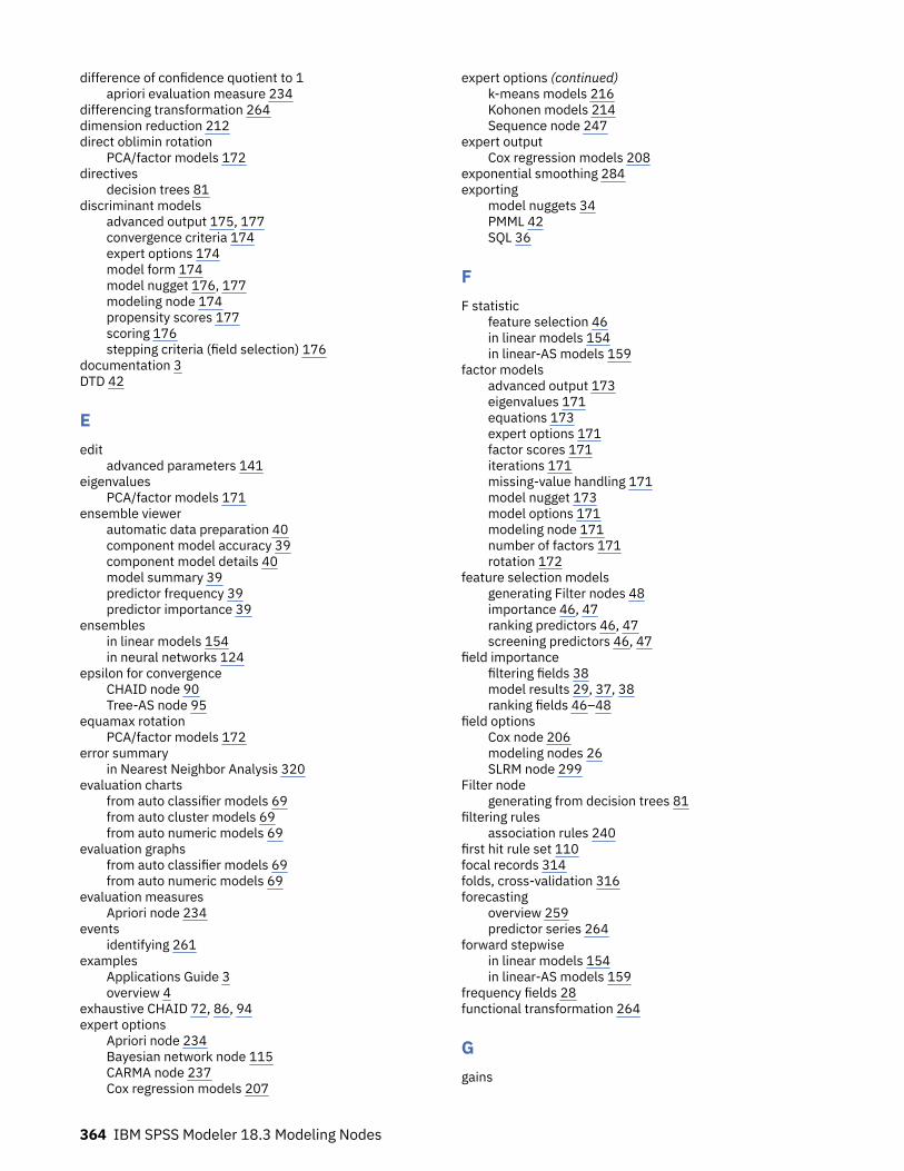
difference of confidence quotient to 1apriori evaluation measure 234

differencing transformation 264dimension reduction 212direct oblimin rotation

PCA/factor models 172directives

decision trees 81discriminant models

advanced output 175, 177convergence criteria 174expert options 174model form 174model nugget 176, 177modeling node 174propensity scores 177scoring 176stepping criteria (field selection) 176

documentation 3DTD 42

Eedit

advanced parameters 141eigenvalues

PCA/factor models 171ensemble viewer

automatic data preparation 40component model accuracy 39component model details 40model summary 39predictor frequency 39predictor importance 39

ensemblesin linear models 154in neural networks 124

epsilon for convergenceCHAID node 90Tree-AS node 95

equamax rotationPCA/factor models 172

error summaryin Nearest Neighbor Analysis 320

evaluation chartsfrom auto classifier models 69from auto cluster models 69from auto numeric models 69

evaluation graphsfrom auto classifier models 69from auto numeric models 69

evaluation measuresApriori node 234

eventsidentifying 261

examplesApplications Guide 3overview 4

exhaustive CHAID 72, 86, 94expert options

Apriori node 234Bayesian network node 115CARMA node 237Cox regression models 207

expert options (continued)k-means models 216Kohonen models 214Sequence node 247

expert outputCox regression models 208

exponential smoothing 284exporting

model nuggets 34PMML 42SQL 36

FF statistic

feature selection 46in linear models 154in linear-AS models 159

factor modelsadvanced output 173eigenvalues 171equations 173expert options 171factor scores 171iterations 171missing-value handling 171model nugget 173model options 171modeling node 171number of factors 171rotation 172

feature selection modelsgenerating Filter nodes 48importance 46, 47ranking predictors 46, 47screening predictors 46, 47

field importancefiltering fields 38model results 29, 37, 38ranking fields 46–48

field optionsCox node 206modeling nodes 26SLRM node 299

Filter nodegenerating from decision trees 81

filtering rulesassociation rules 240

first hit rule set 110focal records 314folds, cross-validation 316forecasting

overview 259predictor series 264

forward stepwisein linear models 154in linear-AS models 159

frequency fields 28functional transformation 264

Ggains


gains (continued)chart 148decision trees 75–77exporting 81

gains-based selection 78Gaussian Mixture node

inputs 330general estimable function(s)

generalized linear models 182general linear model

generalized linear mixed models 184generalized linear mixed models

analysis weight 190classification table 194covariance parameters 195custom terms 188data structure 194estimated marginal means 192estimated means 196fixed coefficients 194fixed effects 187, 194link function 185model summary 193model view 193offset 190predicted by observed 194random effect block 189random effect covariances 195random effects 189scoring options 192settings 197target distribution 185

generalized linear modelin generalized linear mixed models 184

generalized linear modelsadvanced output 182, 183convergence options 181expert options 179fields 178model form 178model nugget 183, 184modeling node 177, 197propensity scores 183

generate new model 145generated sequence rule set 242getting started 136Gini impurity measure 89GLE models

analysis weight 201build options 201custom terms 201link function 198model effects 200model information 204model selection options 203modeling node 205offset 201output 204predictor importance 204scoring options 204target distribution 198

GMM nodeinputs 330

goodness-of-fit statistics

goodness-of-fit statistics (continued)generalized linear models 182logistic regression models 170

graph generationassociation rules 240

HHDBSCAN node

inputs 336hierarchical models

generalized linear mixed models 184hits

decision tree gains 75Hosmer and Lemeshow goodness-of-fit

logistic regression models 170

IIBM SPSS Modeler

documentation 3IBM SPSS Modeler Server 1ID field

CARMA node 235Sequence node 246

importancefiltering fields 38predictors in models 29, 37, 38ranking predictors 46–48

importingPMML 34, 42

impurity measuresC&R Tree node 89decision trees 89

indexdecision tree gains 75

information criteriain linear models 154in linear-AS models 159

information differenceapriori evaluation measure 234

innovational outliers 262input fields

screening 46selecting for analysis 46

instances 238, 250interactions

logistic regression models 165interactive trees

custom splits 74exporting results 81gains 75–78generating models 79graph generation 108profits 77ROI 77surrogates 74

interventionsidentifying 261

Isotonic-AS model nuggets 342Isotonic-AS node 341, 342iteration history

generalized linear models 182

Index 365

iteration history (continued)logistic regression models 166

Kk-means models

clustering 215, 216distance field 215encoding value for sets 216expert options 216model nugget 216stopping criteria 216

K-Means modelsgraph generation from model nugget 230

K-Means-AS node 223, 224, 345KDE Modeling node 331KDE node

inputs 332kernel functions

support vector machine models 305KNN. See nearest neighbor models 313Kohonen models

binary set encoding option (removed) 213expert options 214feedback graph 213graph generation from model nugget 230learning rate 214model nugget 214modeling node 212neighborhood 212, 214neural networks 212, 214stopping criteria 213

LL matrix

generalized linear models 182labels

value 42variable 42

lagACF and PACF 263

Lagrange multiplier testgeneralized linear models 182

lambdafeature selection 46

level shift outliers 262level stabilizing transformation 264lift

association rules 240decision tree gains 75

lift chartsdecision tree gains 77

likelihood ratio testlogistic regression models 166, 170

likelihood-ratio chi-squareCHAID node 90feature selection 46Tree-AS node 95

linear kernelsupport vector machine models 305

linear modelsANOVA table 156

linear models (continued)automatic data preparation 153, 155coefficients 157combining rules 154confidence level 153ensembles 154estimated means 157information criterion 155model building summary 157model options 155model selection 154model summary 155nugget settings 158objectives 152outliers 156predicted by observed 156predictor importance 156R-square statistic 155replicating results 155residuals 156

linear regression modelsmodeling node 152, 158weighted least squares 26

linear support vector machine modelsbuild options 310model nugget 310model options 310modeling node 309settings 311

linear trendsidentifying 259

linear-AS modelsconfidence interval 159confidence level 159consider two way interaction 159include intercept 159information criterion 160model information 160model options 160model selection 159nugget settings 161output 160predicted by observed 160predictor importance 160R-square statistic 160records summary 160sorting order for categorical predictors 159

linear-AS node 159linearnode node 152link function

generalized linear mixed models 185GLE models 198

linksmodel 32

loadingmodel nuggets 34

local trend outliers 262log transformation

Time Series Modeler 291log-odds

logistic regression models 168logistic regression

generalized linear mixed models 184logistic regression models


logistic regression models (continued)adding terms 165advanced output 166, 170binomial options 162convergence options 166expert options 165interactions 165main effects 165model equations 168model nugget 168, 169modeling node 161multinomial options 162predictor importance 168stepping options 167

loglinear analysisin generalized linear mixed models 184

longitudinal modelsgeneralized linear mixed models 184

LSVM modelsconfusion matrix 310model information 310output 310predicted by observed 310predictor importance 310records summary 310

Mmain effects

logistic regression models 165managers

Models tab 34mining task

starting 140mining tasks

creating 140editing 140

misclassification costsC5.0 node 92

missing datapredictor series 264

missing valuesCHAID trees 74excluding from SQL 98, 103, 107, 205screening fields 46

mixed modelsgeneralized linear mixed models 184

MLP (multilayer perceptron)in neural networks 122

model fitlogistic regression models 170

model informationgeneralized linear models 182GLE models 204linear-AS models 160LSVM models 310Random Trees models 101Time Series models 294Tree-AS models 97

model linksand SuperNodes 33copying and pasting 33defining and removing 32

model measures

model measures (continued)defining 145refresh 146

model nuggetsensemble models 38exporting 34, 36generating processing nodes 41menus 36printing 36saving 36saving and loading 34scoring data with 41split models 40Summary tab 37using in streams 41

model optionsBayesian network node 114Cox regression models 206SLRM node 299

model options for spatio-temporaral prediction 268model refresh

self-learning response models 299model view

in generalized linear mixed models 193in Nearest Neighbor Analysis 318

modeling nodes 48, 91, 113, 212, 215, 216, 218, 223, 224,233, 246, 299, 341–343, 345–348models

importing 34replacing 34split 24, 25Summary tab 37

models palette 31, 34MS Excel setup integration format 146multilayer perceptron (MLP)

in neural networks 122MultiLayerPerceptron-AS node 346–348multilevel models

generalized linear mixed models 184multinomial logistic regression

generalized linear mixed models 184multinomial logistic regression models 161, 162

Nnatural log transformation

Time Series Modeler 291Nearest Neighbor Analysis

model view 318nearest neighbor distances

in Nearest Neighbor Analysis 319nearest neighbor models

about 313analyze options 316cross-validation options 316feature selection options 315model options 314modeling node 313neighbors options 315objectives options 313settings options 314

neural network modelsfield options 26

neural networks

Index 367

neural networks (continued)classification 130combining rules 124ensembles 124hidden layers 122missing values 125model options 126model summary 127multilayer perceptron (MLP) 122network 131nugget settings 132objectives 121overfit prevention 125predicted by observed 129predictor importance 128radial basis function (RBF) 122replicating results 125stopping rules 123

neuralnetwork node 119nodeName node 184nominal regression 161nonlinear trends

identifying 259nonparametric estimation 267nonseasonal cycles 260normalized chi-square

apriori evaluation measure 234

OOne-Class SVM node 338–340optimizing performance 233ordered twoing impurity measure 89organize data selections 141outliers

additive patches 262deterministic 262in series 261innovational 262level shift 262local trend 262seasonal additive 262transient change 262

output from Association Rules 255output from spatio-temporaral prediction 267overfit prevention

in neural networks 125overfit prevention criterion

in linear models 154in linear-AS models 159

overfitting SVM model 306

Pp value 46parameter estimates

generalized linear models 182logistic regression models 170

parametric estimation 267partial autocorrelation function

series 263partitions

selecting 246

PCA modelsadvanced output 173eigenvalues 171equations 173expert options 171factor scores 171iterations 171missing-value handling 171model nugget 173model options 171modeling node 171number of factors 171rotation 172

Pearson chi-squareCHAID node 90feature selection 46Tree-AS node 95

peer groupsanomaly detection 50

peersin Nearest Neighbor Analysis 319

performance enhancements 167, 233periodicity

Time Series Modeler 291PMML

exporting models 34, 42importing models 34, 42

point interventionsidentifying 261

Poisson regressiongeneralized linear mixed models 184

predicted by observedlinear-AS models 160LSVM models 310

predictor importancediscriminant models 176filtering fields 38generalized linear models 183GLE models 204in Nearest Neighbor Analysis 319linear models 156linear-AS models 160logistic regression models 168LSVM models 310model results 29, 37, 38neural networks 128Random Trees models 101Time Series models 294Tree-AS models 97

predictor selectionin Nearest Neighbor Analysis 320

predictor seriesmissing data 264

predictor space chartin Nearest Neighbor Analysis 318

predictorsdecision trees 74ranking importance 46–48screening 47, 48selecting for analysis 46–48surrogates 74

previewmodel contents 36

principal components analysis. See PCA models 171, 173


prior probabilitiesdecision trees 88

probabilitieslogistic regression models 168

probit analysisgeneralized linear mixed models 184

profitsdecision tree gains 77

promax rotationPCA/factor models 172

propensity scoresbalancing data 30decision list models 136discriminant models 177generalized linear models 183

pruning decision trees 83, 86pseudo R-square

logistic regression models 170pulses

in series 261python nodes 322–325, 327, 329–334, 336–340

Qquadrant map

in Nearest Neighbor Analysis 319quartimax rotation

PCA/factor models 172QUEST models

build options 85ensembling 87field options 85graph generation from model nugget 108misclassification costs 88model nugget 103modeling node 72, 82, 85, 107objectives 85prior probabilities 88pruning 86stopping options 87surrogates 86tree depth 86

RR-square

in linear models 155, 160radial basis function (RBF)

in neural networks 122Random Forest model nuggets 336Random Forest node 333, 334, 336Random Trees models

advanced settings 101binning 101build options 99field options 99misclassification costs 100model information 101modeling node 98, 103output 101predictor importance 101sample size 99tree depth 99

ranking predictors 46–48raw propensity scores 30RBF (radial basis function)

in neural networks 122records summary

linear-AS models 160LSVM models 310

reference categoryLogistic node 162

refreshing measures 146refreshing models

self-learning response models 299regression gains

decision trees 77, 78regression models

modeling node 152, 158regression trees 83–85, 93, 98removing model links 32replacing models 34response charts

decision tree gains 75, 77risk estimate

decision tree gains 78risks

exporting 81ROI

decision tree gains 77rotation

PCA/factor models 172rule ID 238rule induction 83–85, 91, 93, 98, 233rule set

generating from decision trees 82Rule SuperNode

generating from sequence rules 251rules

association rules 233, 235rule support 238, 250

run a mining task 139

Sscore statistic 166, 167scoring data 41screening input fields 46screening predictors 47, 48seasonal additive outliers 262seasonal differencing transformation 264seasonality

identifying 260segment rule generation 139segments

copy 143deleting 144deleting rule conditions 143editing 142excluding 144inserting 142prioritizing 144

Select nodegenerating from decision trees 81

self-learning response modelsfield options 299model nugget 301

Index 369

self-learning response models (continued)model refresh 299modeling node 299settings 302variable importance 301

self-organizing maps 212sequence browser 251sequence detection 246sequence models

content field(s) 246data formats 246expert options 247field options 246generating a rule SuperNode 251ID field 246model nugget 248, 250, 251model nugget details 250model nugget settings 251model nugget summary 251modeling node 246options 247predictions 248sequence browser 251sorting 251tabular versus transactional data 247time field 246

seriestransforming 264

settings optionsCox regression models 208SLRM node 300

significance levelsfor merging 90, 95

SLRM. See self-learning response models 299SMOTE node 322snapshot

creating 138Snapshots tab 138spark nodes 223, 224, 341–343, 345–348Spatio-Temporal Prediction 264spatio-temporaral prediction advanced build options 267spatio-temporaral prediction model options 268spatio-temporaral prediction output 267split models

building 24features affected by 25modeling nodes 25versus partitioning 24

split-model nuggetsSummary tab 37viewer 40

splitsdecision trees 74

SQLexport 36GLE models 205logistic regression models 169Random Trees models 103rule sets 107Tree-AS CHAID models 98

square root transformationTime Series Modeler 291

statistical models 151step interventions

step interventions (continued)identifying 261

stepping optionsCox regression models 208logistic regression models 167

stepwise field selectionDiscriminant node 176

STP modelsfield options 265model nugget 269time interval options 266

STP node 264SuperNodes

and model links 33support

antecedent support 238, 250Apriori node 233association rules 240CARMA node 236, 237for sequences 250rule support 238, 250Sequence node 247

support vector machine modelsabout 305expert options 307kernel functions 305model nugget 308, 317model options 307modeling node 307overfitting 306settings 309tuning 306

surrogatesdecision trees 74, 86, 94

SVM. See support vector machine models 305

Tt statistic

feature selection 46t-SNE model nuggets 329t-SNE node 327, 329tabular data

Apriori node 26CARMA node 235Sequence node 246transposing 244

TCM modelsmodel nugget 279model nugget settings 279modeling node 269

TCM node 269temporal causal model scenarios 279–283temporal causal modeling

model nugget 279model nugget settings 279

temporal causal modelsmodeling node 269

territorial mapDiscriminant node 175

till-roll data 243, 244time field

CARMA node 235Sequence node 246


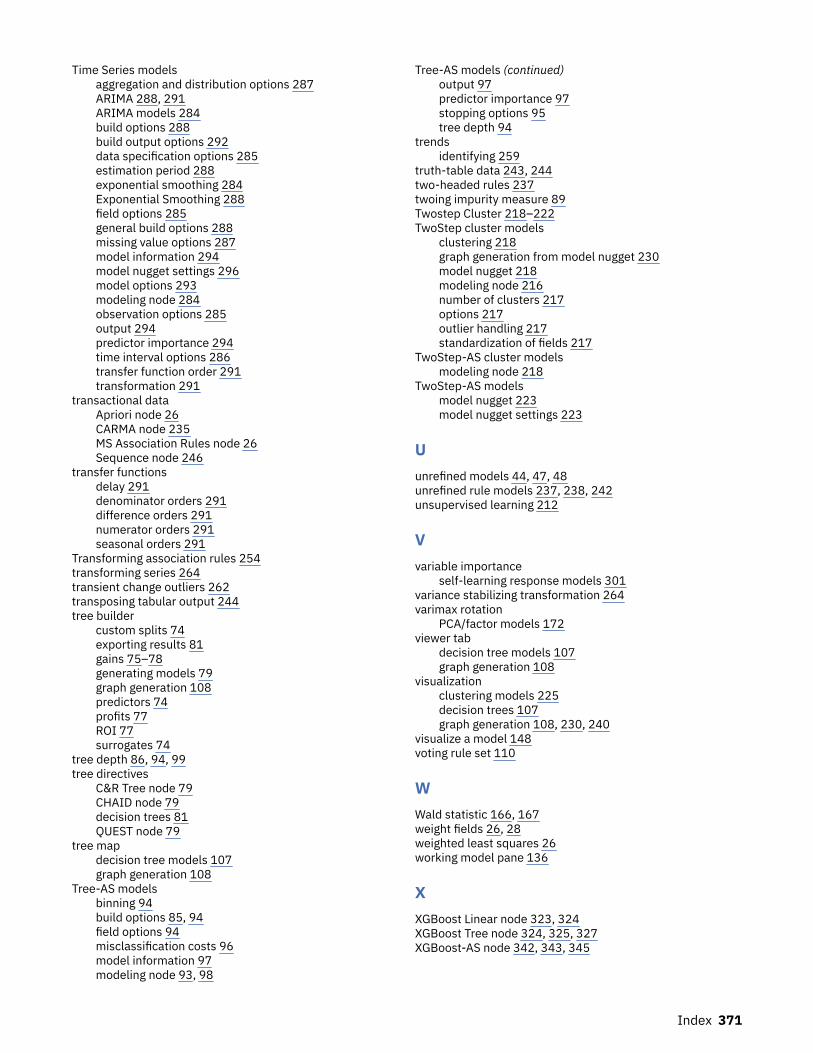
Time Series modelsaggregation and distribution options 287ARIMA 288, 291ARIMA models 284build options 288build output options 292data specification options 285estimation period 288exponential smoothing 284Exponential Smoothing 288field options 285general build options 288missing value options 287model information 294model nugget settings 296model options 293modeling node 284observation options 285output 294predictor importance 294time interval options 286transfer function order 291transformation 291

transactional dataApriori node 26CARMA node 235MS Association Rules node 26Sequence node 246

transfer functionsdelay 291denominator orders 291difference orders 291numerator orders 291seasonal orders 291

Transforming association rules 254transforming series 264transient change outliers 262transposing tabular output 244tree builder

custom splits 74exporting results 81gains 75–78generating models 79graph generation 108predictors 74profits 77ROI 77surrogates 74

tree depth 86, 94, 99tree directives

C&R Tree node 79CHAID node 79decision trees 81QUEST node 79

tree mapdecision tree models 107graph generation 108

Tree-AS modelsbinning 94build options 85, 94field options 94misclassification costs 96model information 97modeling node 93, 98

Tree-AS models (continued)output 97predictor importance 97stopping options 95tree depth 94

trendsidentifying 259

truth-table data 243, 244two-headed rules 237twoing impurity measure 89Twostep Cluster 218–222TwoStep cluster models

clustering 218graph generation from model nugget 230model nugget 218modeling node 216number of clusters 217options 217outlier handling 217standardization of fields 217

TwoStep-AS cluster modelsmodeling node 218

TwoStep-AS modelsmodel nugget 223model nugget settings 223

Uunrefined models 44, 47, 48unrefined rule models 237, 238, 242unsupervised learning 212

Vvariable importance

self-learning response models 301variance stabilizing transformation 264varimax rotation

PCA/factor models 172viewer tab

decision tree models 107graph generation 108

visualizationclustering models 225decision trees 107graph generation 108, 230, 240

visualize a model 148voting rule set 110

WWald statistic 166, 167weight fields 26, 28weighted least squares 26working model pane 136

XXGBoost Linear node 323, 324XGBoost Tree node 324, 325, 327XGBoost-AS node 342, 343, 345

Index 371

IBM SPSS Modeler 18.3 Modeling Nodes

Documents

Transcript of IBM SPSS Modeler 18.3 Modeling Nodes