National Library and Documentation Services Board

Workshop on Research Methodology

Prof. K.A.P. Siddhisena Department of Demography

University of Colombo

2nd and 3rd August, 2018

Lecture No. 6

Data Processing and Analysis using SPSS

Prof. K.A.P. Siddhisena

03rd August, 2018

Definitions of data/information

• Data:

• The literally meaning of data are factual information about observation or experiment.

• Data are what is actually recorded by the researcher.

• Data are known facts or factual information.

• Data are gathered body of facts.

• Information:

• Information is the knowledge derived from data/experience/study

• Data is raw material to derive information (Pauline Young, 1966)

(Ref: Scientific social surveys and research, 4thedition, New Jersey, Prentice Hall Inc.)

KAP Siddhisena

KAP Siddhisena 6

Data Plan

•Deciding the data plan is important before starting to analysis of data.

•The type of data needed: Primary or Secondary or both. Quantitative or qualitative or both. Methods of data collection or data collection instruments. Population or sample

• Primary Data : are those which are collected afresh and for the first time, for the researcher’s purpose.

• Secondary Data: are those which have already been collected by other person or agency and which have already been processed for their purposes.

•

KAP Siddhisena 7

Prerequisites for data Analysis – Processing of Data

• Processing of Primary and Secondary data

• -Primary Data : Assigning a serial number (Case ID), consistency checkup, editing, coding, classification, imputation etc. (in general -cleaning data).

• - Secondary Data : Assess the quality; accuracy and comparability of the data.

Assessment of quality of secondary data

Review of data Collection Procedure

- population and coverage

- Sample size and sample fraction

- sampling method

- sampling error & Non sampling error

- reference period

- definitions and concepts

Checking the results with expected

configuration/ par with theory

KAP Siddhisena

Contd

• Consistency Check up:

Check whether the responses are in consistent. Check filter or cross checks questions are consistently filled. Do in manually or machinery (use computer programming).

• Editing:

Edit the inconsistencies by manually or machinery.

• Coding:

Coding is the process by which basic research information is transformed into symbols compatible with computer analysis. It is possible to code information using alphabetical symbols. Eg.females-F; Males-M. However, we strongly urge to use numerical coding scheme. Three types of coding: Precoding, Post coding and Edge Coding.

KAP Siddhisena

Contd. Data Processing

• Classification:

categorization/stratification of the variables based on several criteria that enable to do analysis. E.g. poor vs. non –poor; high class, middle class, lower class.

• Imputation:

Feeding the data for missing responses. Missing data can be of various types – undecided, unknown or not stated, refuse to answer Don’t know, not applicable. The codes are arbitrary but number should be designated.

KAP Siddhisena

KAP Siddhisena 11

Types of Analysis

• Quantitative Data Analysis

• Qualitative Data Analysis

• What are quantitative data?

The data that are of numeric form referred to as quantitative data. In quantitative data analysis the researcher mostly use parametric statistics.

•What are qualitative data?

The data that are of non-numeric (label or groupings) form referred to as qualitative data. In qualitative analysis the researchers use non-parametric statistics.

Cont.

• Quantitative and qualitative research employ different types of data analysis.

• Quantitative data analysis entails data preparation, counting, grouping and presentation, relating, significance testing and predicting.

• Qualitative data analysis entails the narration, verbatim, quoting, and substantively describing.

• Quantitative data analysis depends upon

1. Types of variables and

2. Types of data used.

KAP Siddhisena

What is a variable?

Definition: A variable is any characteristic or attribute of an object under investigation that takes on numerical values.

•For example, variables associated with employees may be their talent, work-ethic, wage, gender, age, productivity level, etc.

Latent vs. Manifest Variables

A manifest variable can be observed. e.g. age, gender, productivity-level, tenure and wage

A latent variable is not observed and can only be measured indirectly. e.g. talent, work ethic

Dependent vs. Independent Variables

• An independent variable has an antecedent or causal role.

e.g. talent, work-ethic, age, tenure

• A dependent variable plays a consequent, or affected, role in relation to the independent variable.

e.g. productivity

KAP Siddhisena 16

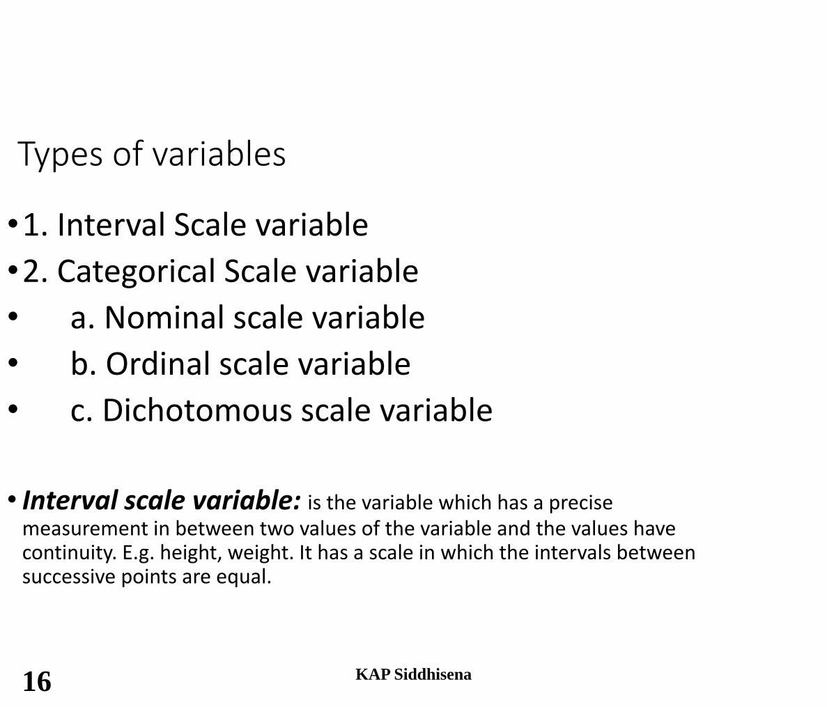
Types of variables

•1. Interval Scale variable

•2. Categorical Scale variable

• a. Nominal scale variable

• b. Ordinal scale variable

• c. Dichotomous scale variable

• Interval scale variable: is the variable which has a precise

measurement in between two values of the variable and the values have continuity. E.g. height, weight. It has a scale in which the intervals between successive points are equal.

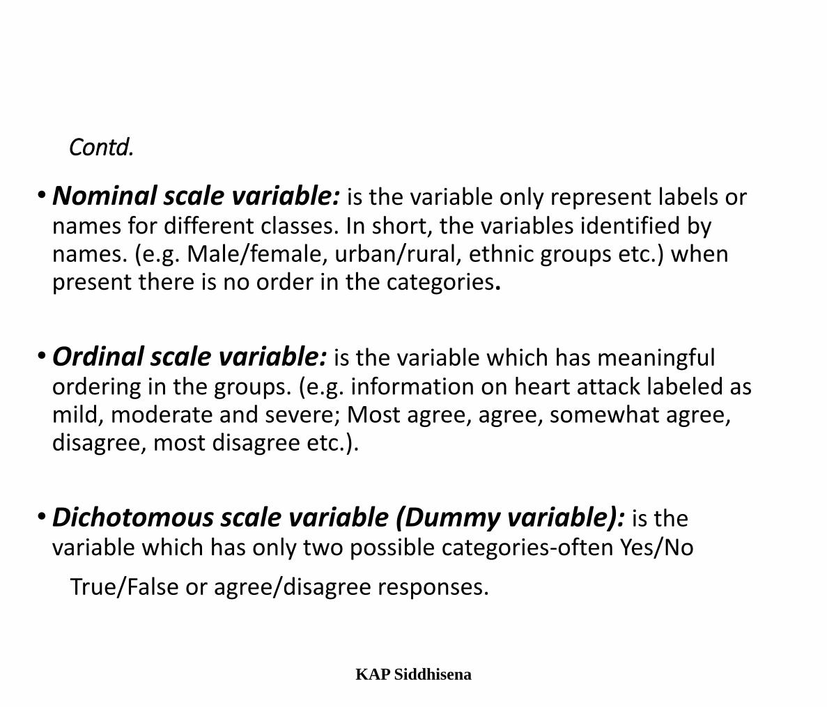
Contd.

• Nominal scale variable: is the variable only represent labels or names for different classes. In short, the variables identified by names. (e.g. Male/female, urban/rural, ethnic groups etc.) when present there is no order in the categories.

• Ordinal scale variable: is the variable which has meaningful ordering in the groups. (e.g. information on heart attack labeled as mild, moderate and severe; Most agree, agree, somewhat agree, disagree, most disagree etc.).

• Dichotomous scale variable (Dummy variable): is the variable which has only two possible categories-often Yes/No

True/False or agree/disagree responses.

KAP Siddhisena

KAP Siddhisena 18

Unit and level of analysis

• Unit of Analysis

• Level of Analysis:

• Uni-variate analysis

• Bi-variate analysis

• Multi-variate analysis

• Analysis using SPSS

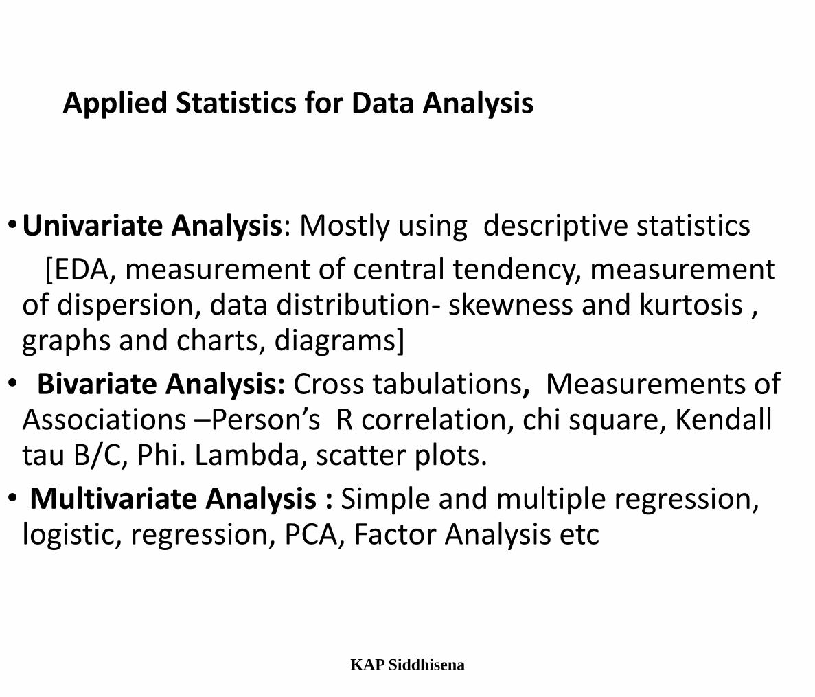
Applied Statistics for Data Analysis

•Univariate Analysis: Mostly using descriptive statistics

[EDA, measurement of central tendency, measurement of dispersion, data distribution- skewness and kurtosis , graphs and charts, diagrams]

• Bivariate Analysis: Cross tabulations, Measurements of Associations –Person’s R correlation, chi square, Kendall tau B/C, Phi. Lambda, scatter plots.

• Multivariate Analysis : Simple and multiple regression, logistic, regression, PCA, Factor Analysis etc

KAP Siddhisena

Percentage

• If the proportion is based on 100 is percentage.

% = category count x 10

N Three types of percentage:

•1. based on the total sample (pop)

•2. based on the total number of valid cases

•3. Cumulative percentage- sum of the valid percentage

KAP Siddhisena

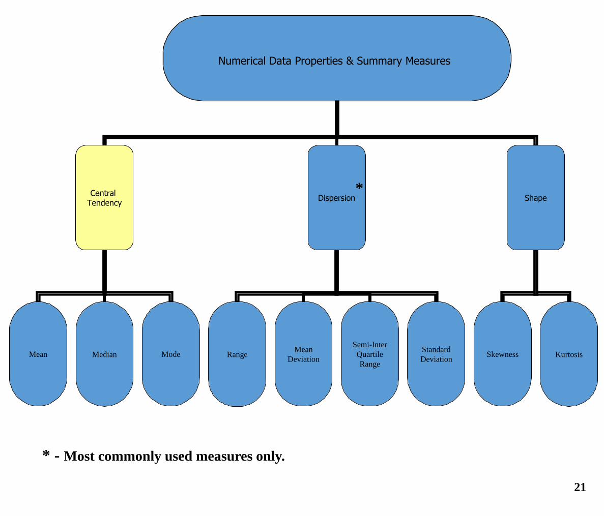
Numerical Data Properties & Summary Measures

Central Tendency

Dispersion Shape

Range Skewness Mean Mode Mean

Deviation

Semi-Inter

Quartile

Range

Standard

Deviation Kurtosis Median

*

21

* - Most commonly used measures only.

Describing Bivariate Analysis

• The second stage in the process of data analysis is to describe and summarize two variables in the data set. This is called bivariate analysis. In generally, the bivariate analysis means that the describing and exploring of relationships between two variables at a time.

• The measurement of association between variables will guide bivariate statistics.

Measures of Associations of two variables

•Bivariate relationship between Interval scale variables:

• Correlation analysis - correlation analysis involves measuring the

degree to which one interval/ratio variable is related to another interval/ratio variable.

• Where a change in one variable is related to a change in the second variable –covariance.

KAP Siddhisena

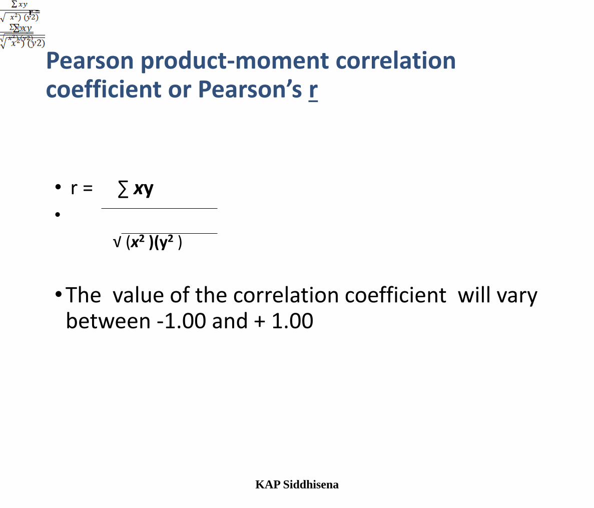
Pearson product-moment correlation coefficient or Pearson’s r

• r = ∑ xy

•

√ (x2 )(y2 )

•The value of the correlation coefficient will vary between -1.00 and + 1.00

KAP Siddhisena

r =

KAP Siddhisena

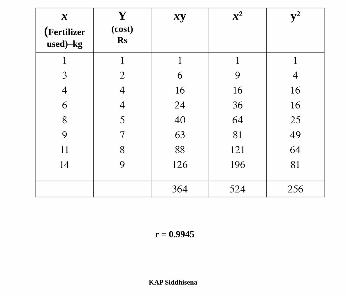
x (Fertilizer

used)–kg

Y (cost)

Rs

xy x2 y2

1 3 4 6 8 9 11 14

1 2 4 4 5 7 8 9

1 6 16 24 40 63 88 126

1 9 16 36 64 81 121 196

1 4 16 16 25 49 64 81

364 524 256

r = 0.9945

Drawbacks of Pearson’s r

• Pearson correlation is unduly influenced by outliers, unequal variances, non-normality, and nonlinearity.

• No direction of the association.

KAP Siddhisena

Scatter plots Scatter plots provide a visual representation of the relationship between two interval variables.

• As X axis and Y axis are used, the independent variable placed on X axis and the dependent variable is placed on vertical or Y axis.

KAP Siddhisena

Non-parametric Measures of Bivariate Relationships

Spearman’s Correlation

An important competitor of the Pearson correlation coefficient is the Spearman’s rank correlation coefficient. In cases where one or both variables are ordinal then spearman’s correlation is the appropriate measure.

Spearman’s correlation is calculated by applying the Pearson’s correlation formula to the ranks of the data rather than to the actual data values themselves.

In the case of nonlinear, but monotonic relationships, a useful measure is Spearman’s rank correlation coefficient, Rho, which is a Pearson’s type correlation coefficient computed on the ranks of X and Y values.

KAP Siddhisena

Bivariate relationships between Categorical variables

• Association (relationship) between Nominal and Nominal variable

• Chi–square (2)

• The chi-square test is used primarily in contingency table analysis, where the dependent variable is nominal one.

• It is based on a comparison of observed frequencies that show up in a sample to expected frequencies which would occur if there were no difference between categories in the population.

KAP Siddhisena

Bivariate relationship between ordinal-ordinal variables

• Kendall’s Tau This is a measure of correlation between two ordinal-level variables. For any sample of n observations, there are [n (n-1)/2] possible comparisons of points (XI, YI) and (XJ, YJ).

P Siddhisena

Contd.

• Tau-b requires binary or ordinal data. It reaches 1.0 (or -1.0 for negative relationships) only for square tables when all entries are on one diagonal.

• Tau-b equals 0 under statistical independence for both square and non-square tables. Tau-c is used for non-square tables.

KAP Siddhisena

KAP Siddhisena 32

SPSS

One of the most widely used, easy to operate, and complete package is the Statistical Package for the Social Scientists or SPSS. (Now called ‘Statistical Product and Service Solutions’) You may also encounter packages such as BMDP, SYSTAT, and SAS, all designed alone similar lines. Once you define and label data files in the format required by the package, you can easily apply any of its programme data.

KAP Siddhisena 33

History and special features

•SPSS was developed in the 1960s and has gone through a series of embellishments over the years.

• It is a user-friendly package. It is the mostly leading program for managing and analysing social science data. It has high quality graphics and tabulation facilities. It would be possible to ‘teach yourself/learn yourself’ with perseverance, practice and a good learning guide.

KAP Siddhisena 34

Getting Started

• Point curser to Start menu and then program and SPSS for windows or the SPSS object on the desktop.

• Select an existing worksheet from the dialog box that appears as soon as you launch SPSS (SPSS data files would have the extension “.sav”) or select new worksheet and create your own data base.

KAP Siddhisena 35

Windows in SPSS

• There are two windows in SPSS.

• 1. Data editor window

a. Data View - Provides a convenient, spreadsheet-

like structure for creating and editing

data files

b. Variable view – Includes variable name, type,

labels, missing values and

columns format.

2. Output Viewer Window (This window appears only after you have done an analysis

Thank you