Learn to Use the Multilevel Model Test in SPSS With Data ...

Learn to Use the Multilevel Model

Test in SPSS With Data From the

Longitudinal Educational

Outcomes Dataset (2017–18)

© 2019 SAGE Publications, Ltd. All Rights Reserved.

This PDF has been generated from SAGE Research Methods Datasets.

Learn to Use the Multilevel Model

Test in SPSS With Data From the

Longitudinal Educational

Outcomes Dataset (2017–18)

How-to Guide for IBM® SPSS® Statistics Software

Introduction

In this guide, you will learn how to produce a Multilevel Model (MLM) test in

IBM® SPSS® Statistics software (SPSS) using a practical example to illustrate

the process. You will find links to the example dataset, and you are encouraged

to replicate this example. An additional practice example is suggested at the end

of this guide. The example assumes that you have already opened the data file in

SPSS.

Contents

1. Multilevel Modelling

2. An Example in SPSS: Exploring the Differing Effect Graduates’ Gender

and Number of Years After Graduation Has on Median Annual

Earnings Between Universities Attended

2.1 The SPSS Procedure

2.2 Exploring the SPSS Output

2.3 How to Report the Findings

3. Your Turn

SAGE

2019 SAGE Publications, Ltd. All Rights Reserved.

SAGE Research Methods Datasets Part

2

of 34 Learn to Use the Multilevel Model Test in SPSS With Data From the

Longitudinal Educational Outcomes Dataset (2017–18)

1 Multilevel Modelling

An MLM test is a test used in research to determine the likelihood that a number

of variables have an effect on a particular dependent variable. This sounds very

similar to multiple regression; however, there may be a scenario where an MLM

is a more appropriate test to carry out. This is due to the nature of hierarchy that

at times can be found in a dataset. By hierarchy, we are referring to the levels

which each factor (or independent variable) is being measured. This is called a

clustering effect, due to the potential for Level 1 variables (i.e., Gender) to be

clustered via a Level 2 variable (i.e., University Studied). Level 3 variables could

also be recognized in a dataset (Location). It is important to recognize a potential

clustering effect in order to carry out the appropriate analysis.

2 An Example in SPSS: Exploring the Differing Effect Graduates’ Gender and

Number of Years After Graduation Has on Median Annual Earnings Between

Universities Attended

2.1 The SPSS Procedure

MLM tests are appropriate when certain assumptions have been met. To look

for normal distribution, we must carry out the appropriate analysis for each of

the variables we intend to use. Prior to running any statistical test, it is good

practice to examine each variable on its own, this is called univariate analysis.

This allows us an opportunity to describe the variable and get an initial “feel”

for our data. For categorical variables, frequency tables can show us whether

the number of cases in each group, which will show whether any groups are

significantly larger or smaller than others, could affect the results. For scale/

interval variables, measures of central tendency (MoCT) allow us to see whether

the data are skewed in any direction which can also affect results.

Univariate analysis can be carried out by selecting the following on SPSS:

SAGE



2



Analyze → Descriptive Statistics → Frequencies

By selecting the categorical variables, Gender and Years after graduation, we can

see that each variable is normally distributed with the groups all being equal in the

number of cases.

To carry out univariate analysis on scale interval variables, POLAR3 Quintile

1 Proportion and Median Annual Earnings, we must carry out the same steps

as with categorical variables and then select “statistics” to ensure we have the

information highlighted in Figure 1. A histogram is also useful as it allows us to

visual the distribution. This is done by selecting “charts” and “histogram” along

with “show normal curve on histogram” as shown in Figure 2.

Figure 1: Measures of Central Tendency.

SAGE



2



Figure 2: Selecting a Histogram.

SAGE



2



Table 1 and Figure 3 show that both variables are positively skewed with wider

range towards the higher end of each scale.

Table 1: MoCT for Scale/Interval Variables.

SAGE



2



POLAR3 Q1 Proportion Median Annual Earnings

N 7,216 14,453

Mean 11.6 22,801.63

Median 10.35 21,700

Standard deviation 6.75 6,802.74

Range 63 80,000

Minimum 1 5,500

Maximum 64 85,500

Figure 3: Histograms for Scale/Interval Variable.

As the data are skewed, recoding is necessary to provide normally distributed

variables for the MLM test. This is done by selecting the following

Transform → Recode into different variables

SAGE



2



It is important you select the correct variable and provide it with a new name and

appropriate label. Once you have done this, select “old and new values” to enter

the new values for your variables. Simply type the old value in the value box under

Old value and enter the new value you would like to change it to in the value box

under New value. Once you have entered all new values, select “All other values”

under Old value and select “System-missing” under New value. Figure 4 shows

how Years after graduation was recoded before being entered into the MLM.

Figure 4: Recoding Years After Graduation.

When recoding scale variables, it is more practical to select the ranges.

To reduce the wide range in the upper end of the scale for POLAR3 Q1 proportion,

the highest in the range was set at 34.6. This was done by entering 1, the lowest,

under the “range” box and entering 34.6 under the “through” box and selecting

“Copy old value(s)” box. Figure 5 shows what this looks like in SPSS.

SAGE



2



Figure 5: Recoding POLAR3 Q1.

To select a new range for Median annual earnings, the same process was applied

as with POLAR 3 Q1proportion with the minimum being 5,500 and the new highest

value as 51,200.

Along with univariate analysis, it is also important that you carry out parametric

assumptions before running an MLM test. It is good practice to ensure the data

have linearity, and it is good practice to run a Levene’s test for homogeneity.

Multicollinearity is also a common problem in MLMs due to the nature of the

clustering effect. We must therefore centre the scale measures of both Level 1

and levels above Level 1 variables.

POLAR3 Q1 Proportion was group mean centred as a Level 1 variable to be

appropriately placed into the MLM test. This was done by a number of steps, the

first aggregating the proportion according to university studied. This was done by

selecting the following

SAGE



2



Data → Aggregate

University studied was entered into the “Break variable” box, and POLAR3 Q1

Proportion was entered into the “Summaries of variables” box and then selecting

“OK.” Figure 6 shows what this looks like in SPSS.

Figure 6: Aggregating Data.

This step generated a new variable (POLARRecoded_mean) which was then

used to compute another new variable, which would in fact represent the group

mean centred variable for POLAR3 Q1 proportion. This was done by selecting:

Data → Compute Variable

SAGE



2



The variable consisted of the following numeric expression

“POLARRecoded_mean – POLARRecoded” to provide a reported group centred

value for each respondent. Figure 7 shows what this looks like in SPSS.

Figure 7: Computing New Variable.

To run an MLM in SPSS, select from the menu:

Analyze → Mixed Models → Linear

Figure 8 shows what this looks like in SPSS.

Figure 8: Mixed Models/Linear.

SAGE



2



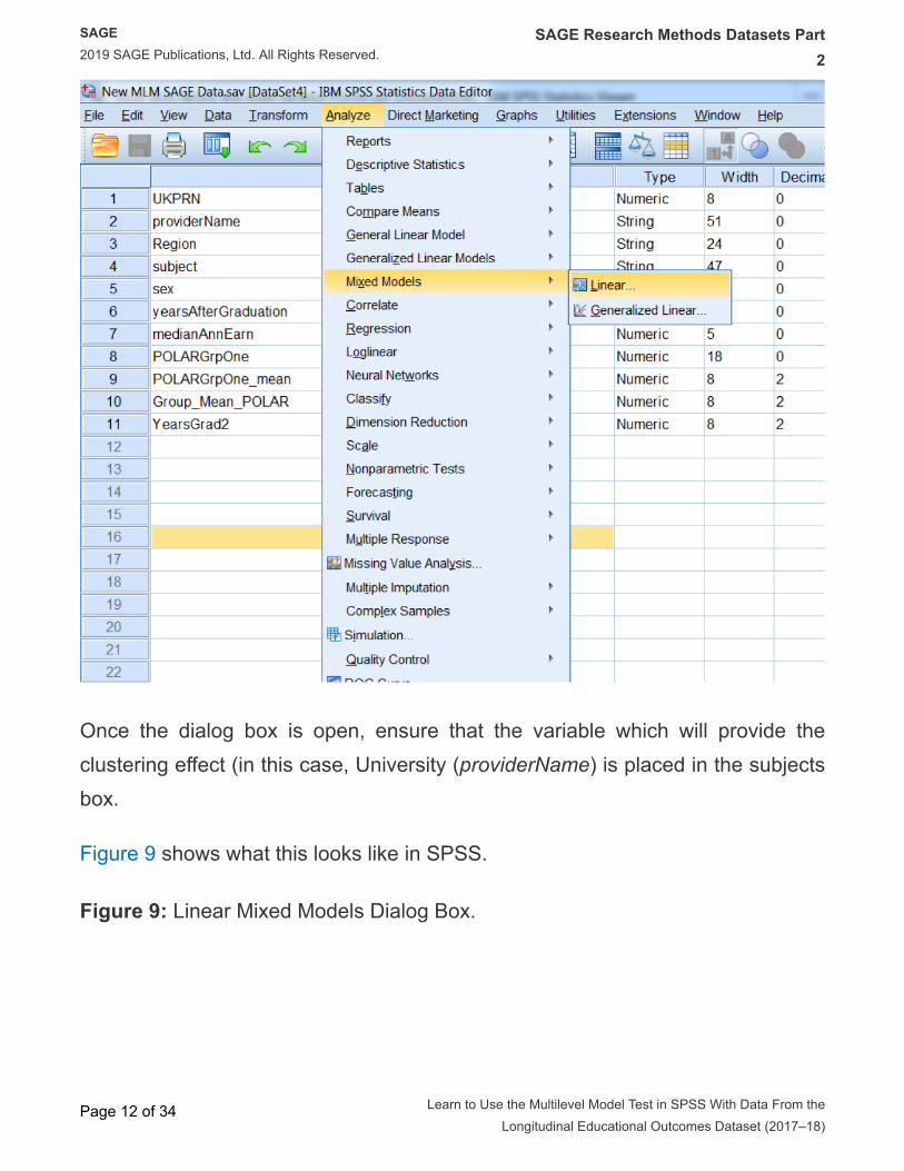
Once the dialog box is open, ensure that the variable which will provide the

clustering effect (in this case, University (providerName) is placed in the subjects

box.


Figure 9: Linear Mixed Models Dialog Box.

SAGE



2



Click Continue.

You have now began to build your MLM. The first step we need to carry out

is to test whether there is any variance in Graduates Median Annual Earnings

(dependent variable) between universities (Level 2 variable). This model is the

unconditional model. This tests variance without any additional factors that

provide conditions, hence the name.

SAGE



2



Once the Linear Mixed Models dialog box is open, ensure you place your

dependent variable (in this case Median Annual Earnings) in the dependent list.

Figure 10 shows what this looks like in SPSS

Figure 10: Linear Mixed Models/Placing Dependent Variable.

To test the unconditional model, we must examine the random effects of both

the intercept and the Level 2 variable. This is because we assume the intercepts

across the groups (Universities) vary. In simpler terms, we expect the different

contexts (Universities) to experience the same effect (increase/decrease in

median annual salary depending on factors) but that effect would begin from

different starting points in median annual salary (they have different intercepts).

We can acknowledge the varying intercepts by clicking “Random.” We must then

tick the “Include Intercept” box and place the Level 2 variable (Provider) in the

“Combinations” box. Therefore, we are looking to see whether there is variance in

the intercepts of each University.

SAGE



2




Figure 11: Random Effects With “Include Intercept” Ticked and “providerName” in

Combinations.

In order to examine the effects of the unconditional model, we also have to

examine the “Parameter estimates and covariance parameters.” These can both

be found in the “statistics” dialog box.

SAGE



2




Figure 12: Statistics Dialog Box With “Parameter Estimates” and “Tests for

Covariance Parameters.”

SAGE



2



SAGE



2



You are now ready to analyse the effects of your unconditional model. It’s time to

explore the SPSS Output.

2.2 Exploring the SPSS Output

Step 1: Examine the estimated Level 2 variance (L2V) and its significance in the

“Estimates of Covariance Parameters”

Step 2: Examine the estimated RV and its significance in “Estimates of

Covariance Parameters”

Step 3: Calculate the intra-class correlation coefficient (ICC) using the following

formula:

Intra-class correlation coefficient = Level 2 Variance (L2V)/Residual

Variance (RV)

ICC = L2V/(RV + L2V)

In the case of this example, the unconditional model reported the following:

Step 1: A statistically significant variance of 17,299,678.41 at the university level

was identified (p ≤ .001).

Step 2: A statistically significant residual variance of 31,009,294.65 was identified

(p ≤ .001).

Step 3: The ICC was computed to be .36 with the following formula:

ICC = 17,299,678.41/(31,009,294.65 + 17,299,678.41)

ICC = 17,299,678.41/48,303,973.06

ICC = .358

Figure 13 shows the output for the unconditional model in SPSS.

SAGE



2



Figure 13: Output for the Unconditional Model.

An example of how to report the unconditional model is below.

The unconditional model yielded a statistically significant University variance of

17,299,678.41 along with a statistically significant residual variance of

31,009,294.65 The ICC was calculated to be .358, indicating 36% of the total

variance of median annual earnings is associated with the university groupings.

The assumption that median annual earnings is independent of university studied

is therefore violated.

Moving On

We now have evidence to suggest that graduates’ median annual earnings

SAGE



2



depend on the university at which they studied. We can now test a conditional

model, which assesses the effects of Level 1 factors (Gender, Years after

Graduation, and proportion of students from POLAR3 Quintile 1) on median

annual earnings when also considering the universities at which the graduates

studied. However, in our first model, we will see whether those factors have an

effect on median annual earnings before determining whether those effects differ

between universities.

Running a Conditional Model With Gender, Number of Years After Graduation, and

Proportion of Students From POLAR3 Quintile 1 (Most Disadvantaged Area)

Since we already have an unconditional model built, we simply need to add to

the model. We therefore go back to our Linear Mixed Model dialog box and place

the variables we need to answer our hypothesis into the appropriate box. It is

important to remember that categorical variables are placed in the factor box (as

they usually consist of a small number of groups), and scale variables are placed

in the covariates box (as they usually consist of a wide range of groups/scores).

Figure 14 shows what this would look like in SPSS.

REMEMBER: Use the new recoded variables for the model. In this case, the

group mean centred variable for Proportion from POLAR3 Quintile 1 and Years

After Graduation.

Figure 14: Adding Level 1 Independent Variables to the Model.

SAGE



2



We then have to determine the tests for fixed effects. This is where we place the

factors we think will have the same rate of influence over the whole sample.

Figure 15 shows the fixed effects dialog box with both factors being added to the

model through assessing their rate of influence for the whole sample. This is done

by simply highlighting an individual variable and clicking “Add” (see figure below).

Figure 15: Fixed Effects.

SAGE



2



We are now ready to explore the output for our first model, which is assessing

the relationship between proportion of Students from POLAR3 Quintile 1 (Most

Disadvantaged) and median annual earnings, controlling the influence of both

Gender and Number of years since graduating.

Exploring the Output of the First Model on SPSS

Step 1: Examine the Estimates of Covariance Parameters.

Step 2: Determining whether the model is better than the unconditional model in

estimating the variance of graduate median annual earnings between universities.

Step 3: Examining the estimates of Fixed Effects of the Level 1 Independent

SAGE



2



Variables.

So,

Step 1: The ICC was calculated to be .531, estimating that 53% of the total

median annual earnings variance, up from 36% in the unconditional model, is

explained by the university groupings when controlling Gender, Number of Years

after graduation, and proportion of students from POLAR3 Quintile 1.

Step 2: The log likelihood of the first model (65,634.24) has also decreased from

the unconditional model (290,266.59) and is therefore a significantly better fit than

the unconditional model in estimating the variance of graduate median annual

earnings between universities.

Step 3: A statistical significant difference was found between Females and Males

in median annual earnings (B = −1067.42; SE = 133.98). A statistically significant

difference was found between years after graduation between 5 years (B =

7,470.48; SE = 168.08), 3 years (B = 4,380.92; SE = 160.17), and 1 year. A

statistically significant relationship was found between proportion of students from

POLAR3 Quintile 1 and median annual earnings (B = −61.95; SE = 15.9).

Figure 16 below displays the output of the first model in SPSS.

Figure 16: Output of the First Unconditional Model.

SAGE



2



An example of how to summarize the first conditional model will be provided below

after exploring the second and final model.

Running the Second Conditional Model

The second and final model to be ran in this guide will answer the following null

SAGE



2



hypothesis:

How the effect the proportion of students from POLAR3 Quintile 1 (most

disadvantaged) has on median annual earnings varies between the

Universities the graduates studied.

As we already have a conditional model built, we are simply adding to the model

we already have. In the case of answering this hypothesis, we do not need to

add any more variables. However, in order to identify if the effect a Level 1

variable has on the dependent variables varies by the Level 2 separator, we must

examine the random effects of the Level 1 variable. In other words, we must see

whether the significant effect (slope) and starting point (intercept) for graduates’

median annual earnings varies between the different universities the graduates’

studies. To do this, we simply click the “Random” dialog box and add the variable

to random effects (Figure 17) and change our covariance type to unstructured

(Figure 18).

Figure 17: Add the Variable to Random Effects.

SAGE



2



Figure 18: Change Covariance Type to Unstructured.

SAGE



2



We are now ready to explore the output for the second conditional model, which

will identify whether the effect proportion of students from POLAR3 Quintile 1

(most disadvantaged) on graduate median annual earnings varies between

universities the graduates studied.

Exploring the Output of the Second Model on SPSS

Step 1: Examine the Estimates of Covariance Parameters

SAGE



2



Step 2: Determining whether the model is better than the first model in estimating

the variance of graduate median annual earnings between universities

Step 3: Examining the estimates of Fixed Effects of the Level 1 Independent

Variables

Step 4: Examine the slope variance and slope intercept variance to identify

whether the effect the Level 1 variable has on the dependent variable varies

significantly as a result of the Level 2 separator.

So,

Step 1: The ICC was calculated to be .54, estimating that 54% of the total median

annual earnings variance, up from 53% in the first model, is explained by the

university groupings when controlling Gender, Number of Years after graduation,

and proportion of students from POLAR3 Quintile 1 varying between groups.

Step 2: The log likelihood of the second model (65,604.24) has also decreased

from the first model (65,634.24) and is therefore a significantly better fit than

the first model in estimating the variance of graduate median annual earnings

between universities.

Step 3: A statistically significant difference was found between Females and

Males in median annual earnings (B = −1,080.57; SE = 133.31). A statistically

significant difference was found between years after graduation between 5 years

(B = 7,486.77; SE = 167.19), 3 years (B = 4,394.63; SE = 159.16), and 1 year. A

statistically significant relationship was found between proportion of students from

POLAR3 Quintile 1 and median annual earnings (B = −89.71; SE = 24.91).

Step 4: The slope variance was 30,360.96 and was statistically significant (p ≤

.001). The slopes and intercept variance was −448,794.2 and was statistically

significant (p ≤ .000). It can therefore be assumed that there is variation in the

SAGE



2



effect (of proportion of students from POLAR3 Quintile 1 on graduate median

annual earnings) between both the intercepts (starting point) and the slopes

(effects) between universities.

Figure 19 below displays the output from SPSS for the second conditional model.

Figure 19: Output of the Second Conditional Model.

SAGE



2



Tables 2 and 3 provide an example of how to summarize the findings of all three

models. The paragraphs below are an example of how to report the summarized

findings for each model.

Table 2: Model Summaries.

SAGE



2



Empty model (random intercept only) Conditional Model 1 Conditional Model 2

Residual variance 31,009,294.7*** 15,076,192.37*** 14,710,127.75***

Intercept variance (university level) 17,299,678.4*** 17,101,812.45*** 17,202,605.75***

Slope variance 30,360.96**

Slopes and intercepts covariance −448,794.2**

Intra-class correlation .36 .53 .54

Log likelihood 290,266.59 65,634.24 65,604.24

*p < .05; **p < .01; ***p < .001.

Table 3: Estimates of Fixed Effects.

Predictors

Model 1 Model 2

Β SE Β SE

Intercept 17,813.25*** 410.3 17,810.2*** 411.23

Gender (female) −1,067.42*** 133.98 −1,080.57*** 133.31

Years after graduation:

5 7,470.48*** 168.08 6,486.77** 167.18

3 4,380.92*** 160.17 4,394.63** 159.16

Proportion from POLAR3 Q1 −61.95*** 15.9 −89.71** 24.91

*p < .05; **p < .01; ***p < .001.

2.3 How to Report the Findings

Model 1 Summary

The first model had three variables added. The ICC was calculated to be .531,

SAGE



2



estimating that 53% of the total median annual earnings variance, up from 36% in

the unconditional model, is explained by the university groupings when controlling

Gender, Number of Years after graduation, and proportion of students from

POLAR3 Quintile 1. The log likelihood of the first model (65,634.24) had also

decreased from the unconditional model (290,266.59). This is therefore a

significantly better fit than the unconditional model in estimating the variance of

graduate median annual earnings between universities.

Estimates of Fixed Effects

Level 1 Predictors

Females were found to be earn significantly less than males, with their median

annual earnings predicted to be approximately £1,067 less. Graduates of 5 years

were found to be earning approximately £7,470 more than those who had

graduated 3 or 1 year ago, and this was statistically significant. A significant

relationship was found between proportion of students from POLAR3 Quintile 1

(most disadvantaged) and graduate median annual earnings. More specifically, an

increase of 1 unit in proportion of students from POLAR3 Quintile 1 is associated

with a decrease of approximately £62. In other words, an increase of 1% in

intake of non-mature students who are most disadvantaged is associated with a

decrease of £62 pounds in graduates’ median annual salary. Therefore, it can be

estimated that an increase of 10% of most disadvantaged entering a university is

associated with a decrease of approximately £620 in median annual earnings.

Model 2 Summary

The second model consisted of the same number of variables as the first model,

with the level predictor “Proportion of students from POLAR3 Quintile 1” (most

disadvantaged) added to random effects in order to examine whether the

predictors effect varied between universities (the Level 2 separator). The ICC was

calculated to be .54, estimating that 54% of the total median annual earnings

SAGE



2



variance, up from 52% in the first model, is explained by the university groupings

when controlling Gender, Number of Years after graduation, and proportion of

students from POLAR3 Quintile 1. The log likelihood of the second model

(65,604.24) had also decreased from the first model (65,634.23). This is therefore

a significantly better fit than the first model.

Estimates of Fixed Effects

Level 1 Predictors

Females were found to earn significantly less than males, with their median annual

earnings predicted to be approximately £1,080 less. Graduates of 5 years were

to be earning approximately £7,487 more than those who had graduated 3 or 1

year ago, and this was statistically significant. A significant relationship was found

between proportion of students from POLAR3 Quintile 1 (most disadvantaged)

and graduate median annual earnings. More specifically, an increase of 1 unit in

proportion of students from POLAR3 Quintile 1 is associated with a decrease of

approximately £90. In other words, an increase of 1% in intake of non-mature

students who are most disadvantaged is associated with a decrease of £90

pounds. Therefore, it can be estimated that an increase of 10% of most

disadvantaged entering a university is associated with a decrease of

approximately £900 in median annual earnings.

Varying Effect of Proportion from POLAR3 Quintile 1

This effect was also found to significantly vary depending on the university

attended. A slope variance of 30,360.96 and slope and intercept variance of

−448794.2 were both statistically significant. Therefore, there is evidence to

suggest that the negative relationship between proportion of disadvantaged

students entering universities and graduates median annual earnings varies

between universities. We can therefore reject the null hypothesis.

SAGE



2



3 Your turn

Using the data provided, see whether you can run an MLM and replicate the

results using this step-by-step guide.

IBM® SPSS® Statistics software (SPSS) screenshots Republished Courtesy of

International Business Machines Corporation, © International Business Machines

Corporation. SPSS Inc. was acquired by IBM in October, 2009. IBM, the IBM logo,

ibm.com, and SPSS are trademarks or registered trademarks of International

Business Machines Corporation, registered in many jurisdictions worldwide. Other

product and service names might be trademarks of IBM or other companies. A

current list of IBM trademarks is available on the Web at “IBM Copyright and

trademark information” at http://www.ibm.com/legal/copytrade.shtml.

SAGE



2



http://ibm.com/

http://www.ibm.com/legal/copytrade.shtml

Learn to Use the Multilevel Model Test in SPSS With Data ...

Documents

Transcript of Learn to Use the Multilevel Model Test in SPSS With Data ...