
Using SPSS for Data Analysis
20
College of Medicine [email protected] By: M A Siddiqui 2013 Using SPSS for Data Analysis Data Manipulation Biostatistics College of Medicine Taif University
Transcript of Using SPSS for Data Analysis
College of Medicine
B
y:
M A
Sid
diq
ui
20
13
Usi
ng
SP
SS
fo
r D
ata
An
aly
sis
Data Manipulation
Biostatistics
College of Medicine Taif University
College of Medicine
Contents Introduction ............................................................................................................................................ 3
How to Start SPSS .............................................................................................................................. 4
Opening Data ................................................................................................................................... 5
SPSS Windows ................................................................................................................................. 5
Working with Data and Variables ............................................................................................................. 6
Viewing data and variables .............................................................................................................. 6
Define Variable Properties ............................................................................................................... 6
Missing Values ................................................................................................................................. 7
Modifying and Creating new variables ............................................................................................. 9
Analyzing Data ................................................................................................................................... 11
Descriptive Statistics ...................................................................................................................... 11
Compare Means ............................................................................................................................ 12
General Linear Model .................................................................................................................... 17
Regression ..................................................................................................................................... 17
Making Graphs .................................................................................................................................. 18
Scatter ........................................................................................................................................... 18
Histogram ...................................................................................................................................... 18
Q-Q................................................................................................................................................ 19
Help................................................................................................................................................... 20
College of Medicine
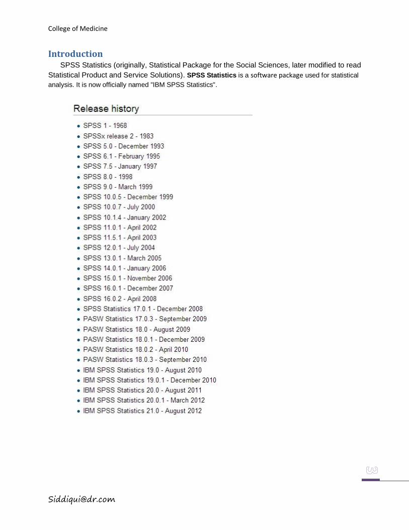
Introduction SPSS Statistics (originally, Statistical Package for the Social Sciences, later modified to read
Statistical Product and Service Solutions). SPSS Statistics is a software package used for statistical
analysis. It is now officially named "IBM SPSS Statistics".
College of Medicine
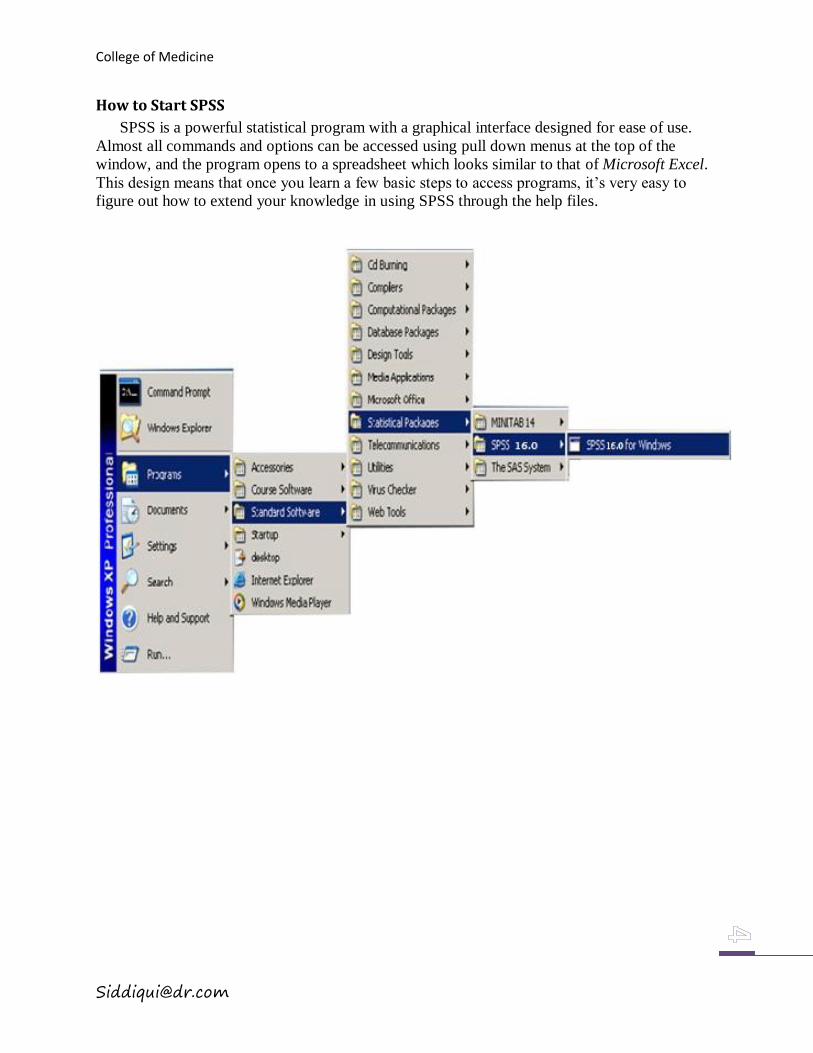
How to Start SPSS
SPSS is a powerful statistical program with a graphical interface designed for ease of use.
Almost all commands and options can be accessed using pull down menus at the top of the
window, and the program opens to a spreadsheet which looks similar to that of Microsoft Excel.
This design means that once you learn a few basic steps to access programs, it’s very easy to
figure out how to extend your knowledge in using SPSS through the help files.
College of Medicine
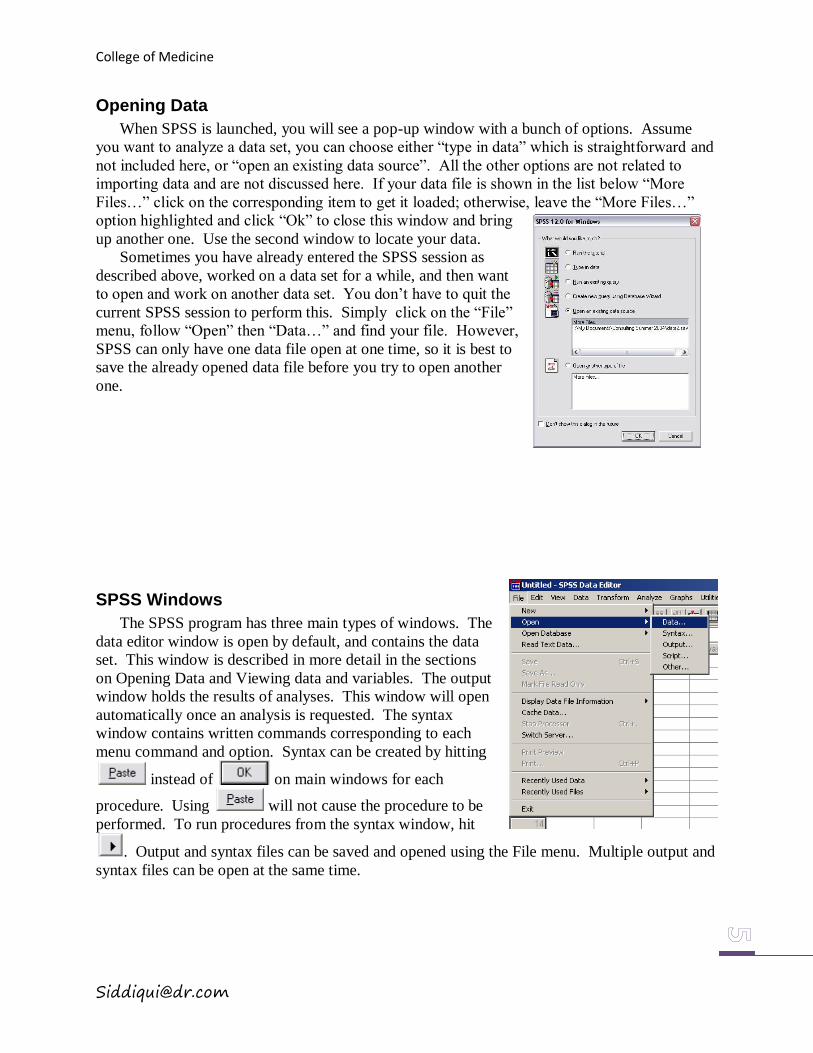
Opening Data
When SPSS is launched, you will see a pop-up window with a bunch of options. Assume
you want to analyze a data set, you can choose either “type in data” which is straightforward and
not included here, or “open an existing data source”. All the other options are not related to
importing data and are not discussed here. If your data file is shown in the list below “More
Files…” click on the corresponding item to get it loaded; otherwise, leave the “More Files…”
option highlighted and click “Ok” to close this window and bring
up another one. Use the second window to locate your data.
Sometimes you have already entered the SPSS session as
described above, worked on a data set for a while, and then want
to open and work on another data set. You don’t have to quit the
current SPSS session to perform this. Simply click on the “File”
menu, follow “Open” then “Data…” and find your file. However,
SPSS can only have one data file open at one time, so it is best to
save the already opened data file before you try to open another
one.
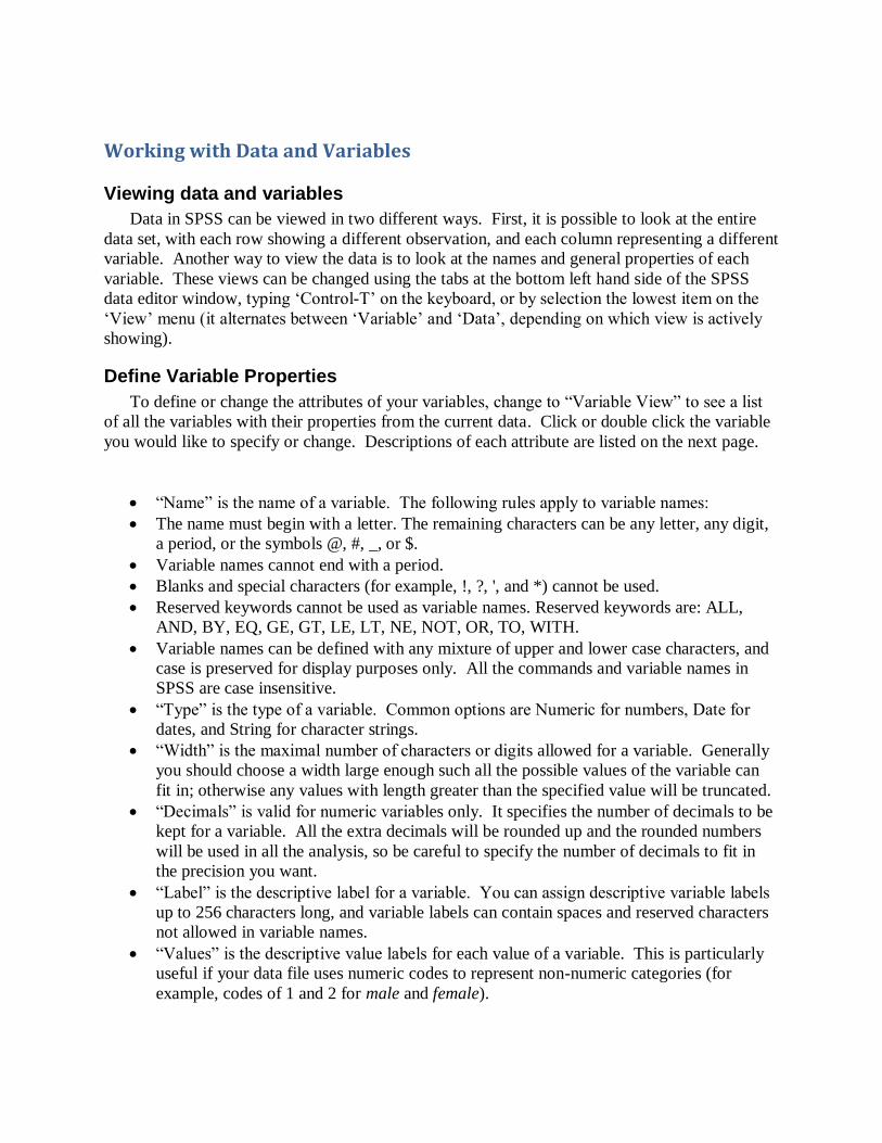
SPSS Windows
The SPSS program has three main types of windows. The
data editor window is open by default, and contains the data
set. This window is described in more detail in the sections
on Opening Data and Viewing data and variables. The output
window holds the results of analyses. This window will open
automatically once an analysis is requested. The syntax
window contains written commands corresponding to each
menu command and option. Syntax can be created by hitting
instead of on main windows for each
procedure. Using will not cause the procedure to be
performed. To run procedures from the syntax window, hit
. Output and syntax files can be saved and opened using the File menu. Multiple output and
syntax files can be open at the same time.
Working with Data and Variables
Viewing data and variables
Data in SPSS can be viewed in two different ways. First, it is possible to look at the entire
data set, with each row showing a different observation, and each column representing a different
variable. Another way to view the data is to look at the names and general properties of each
variable. These views can be changed using the tabs at the bottom left hand side of the SPSS
data editor window, typing ‘Control-T’ on the keyboard, or by selection the lowest item on the
‘View’ menu (it alternates between ‘Variable’ and ‘Data’, depending on which view is actively
showing).
Define Variable Properties
To define or change the attributes of your variables, change to “Variable View” to see a list
of all the variables with their properties from the current data. Click or double click the variable
you would like to specify or change. Descriptions of each attribute are listed on the next page.
“Name” is the name of a variable. The following rules apply to variable names:
The name must begin with a letter. The remaining characters can be any letter, any digit,
a period, or the symbols @, #, _, or $.
Variable names cannot end with a period.
Blanks and special characters (for example, !, ?, ', and *) cannot be used.
Reserved keywords cannot be used as variable names. Reserved keywords are: ALL,
AND, BY, EQ, GE, GT, LE, LT, NE, NOT, OR, TO, WITH.
Variable names can be defined with any mixture of upper and lower case characters, and
case is preserved for display purposes only. All the commands and variable names in
SPSS are case insensitive.
“Type” is the type of a variable. Common options are Numeric for numbers, Date for
dates, and String for character strings.
“Width” is the maximal number of characters or digits allowed for a variable. Generally
you should choose a width large enough such all the possible values of the variable can
fit in; otherwise any values with length greater than the specified value will be truncated.
“Decimals” is valid for numeric variables only. It specifies the number of decimals to be
kept for a variable. All the extra decimals will be rounded up and the rounded numbers
will be used in all the analysis, so be careful to specify the number of decimals to fit in
the precision you want.
“Label” is the descriptive label for a variable. You can assign descriptive variable labels
up to 256 characters long, and variable labels can contain spaces and reserved characters
not allowed in variable names.
“Values” is the descriptive value labels for each value of a variable. This is particularly
useful if your data file uses numeric codes to represent non-numeric categories (for
example, codes of 1 and 2 for male and female).
College of Medicine
“Missing” specifies some data values as user-missing values. Refer to the Missing
Values section for more detail.
“Columns” is the column width for a variable. Column formats affect only the display of
values in the Data Editor. Changing the column width does not change the defined width
of a variable. If the defined and actual width of a value are wider than the column,
asterisks (*) are displayed in the Data view. Column widths can also be changed in the
Data view by clicking and dragging the column borders.
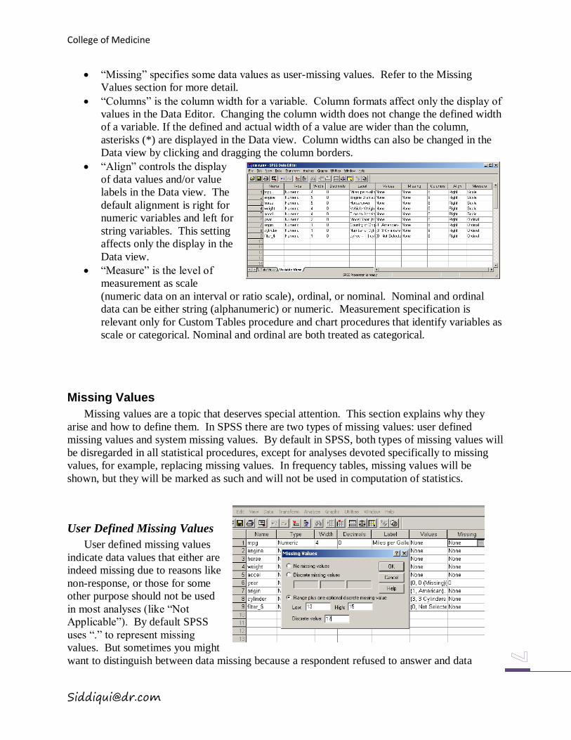
“Align” controls the display
of data values and/or value
labels in the Data view. The
default alignment is right for
numeric variables and left for
string variables. This setting
affects only the display in the
Data view.
“Measure” is the level of
measurement as scale
(numeric data on an interval or ratio scale), ordinal, or nominal. Nominal and ordinal
data can be either string (alphanumeric) or numeric. Measurement specification is
relevant only for Custom Tables procedure and chart procedures that identify variables as
scale or categorical. Nominal and ordinal are both treated as categorical.
Missing Values
Missing values are a topic that deserves special attention. This section explains why they
arise and how to define them. In SPSS there are two types of missing values: user defined
missing values and system missing values. By default in SPSS, both types of missing values will
be disregarded in all statistical procedures, except for analyses devoted specifically to missing
values, for example, replacing missing values. In frequency tables, missing values will be
shown, but they will be marked as such and will not be used in computation of statistics.
User Defined Missing Values
User defined missing values
indicate data values that either are
indeed missing due to reasons like
non-response, or those for some
other purpose should not be used
in most analyses (like “Not
Applicable”). By default SPSS
uses “.” to represent missing
values. But sometimes you might
want to distinguish between data missing because a respondent refused to answer and data
College of Medicine
missing because the question didn't apply to that respondent, and thus would like more than one
expression for missing values. You can achieve this by setting up the “Missing” property of the
corresponding variable to specify some data values as missing values. You can enter up to three
discrete (individual) missing values, a range of missing values, or a range plus one discrete
missing value. All string values, including null or blank values, are considered valid values
unless you explicitly define them as missing. To define null or blank values as missing for a
string variable, enter a single space in one of the fields for discrete missing values. The Figure
Shows how to specify user defined missing values for variable mpg by setting up its “Missing”
property.
System Missing Values
System missing values occur when no value can obtained for a variable during data
transformations. For example, if you have two variables, one indicating a person’s gender and
the other whether she or he is married and you create a new variable that tells you whether (a) a
person is male and married, (b) female and married, (c) male and not married, all females that are
not married will have a system missing value (“.”) instead of a real value.
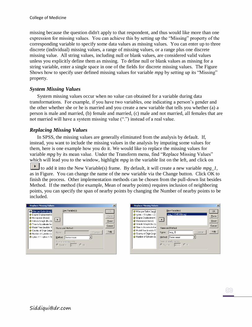
Replacing Missing Values
In SPSS, the missing values are generally eliminated from the analysis by default. If,
instead, you want to include the missing values in the analysis by imputing some values for
them, here is one example how you do it. We would like to replace the missing values for
variable mpg by its mean value. Under the Transform menu, find “Replace Missing Values”
which will lead you to the window, highlight mpg in the variable list on the left, and click on
to add it into the New Variable(s) frame. By default, it will create a new variable mpg_1,
as in Figure. You can change the name of the new variable via the Change button. Click OK to
finish the process. Other implementation methods can be chosen from the pull-down list besides
Method. If the method (for example, Mean of nearby points) requires inclusion of neighboring
points, you can specify the span of nearby points by changing the Number of nearby points to be
included.
College of Medicine
Modifying and Creating new variables
Insert
The easiest way to manually input a new variable is to scroll through the data-view spreadsheet
horizontally until the first empty column is encountered, and entering in the data. The new variable can
be named appropriately in the variable-view spreadsheet. Alternatively, selecting the ‘Insert Variable’
option under the ‘Data’ menu allows you to insert the new variable at other locations in the table. By
default, this inserts the new variable in the first column of the spreadsheet, but this can be changed by
highlighting the column to the right of the desired location.
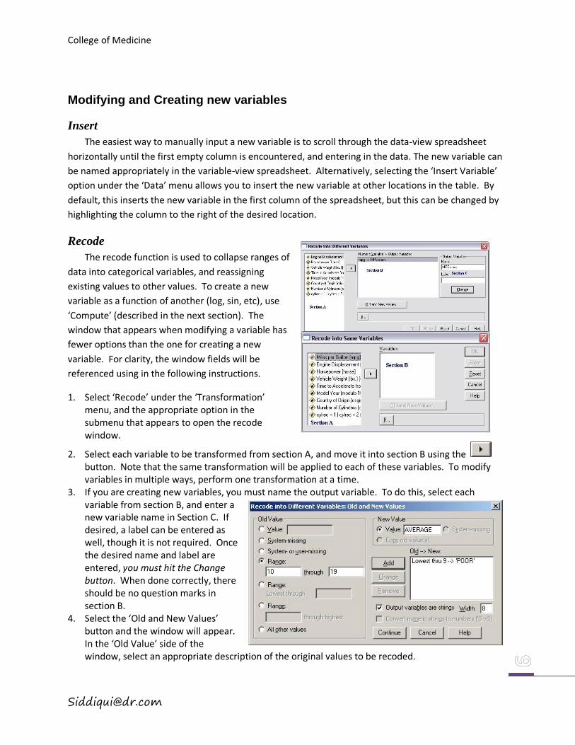
Recode
The recode function is used to collapse ranges of
data into categorical variables, and reassigning
existing values to other values. To create a new
variable as a function of another (log, sin, etc), use
‘Compute’ (described in the next section). The
window that appears when modifying a variable has
fewer options than the one for creating a new
variable. For clarity, the window fields will be
referenced using in the following instructions.
1. Select ‘Recode’ under the ‘Transformation’ menu, and the appropriate option in the submenu that appears to open the recode window.
2. Select each variable to be transformed from section A, and move it into section B using the button. Note that the same transformation will be applied to each of these variables. To modify variables in multiple ways, perform one transformation at a time.
3. If you are creating new variables, you must name the output variable. To do this, select each variable from section B, and enter a new variable name in Section C. If desired, a label can be entered as well, though it is not required. Once the desired name and label are entered, you must hit the Change button. When done correctly, there should be no question marks in section B.
4. Select the ‘Old and New Values’ button and the window will appear. In the ‘Old Value’ side of the window, select an appropriate description of the original values to be recoded.
College of Medicine
By selecting ‘Value’ you can specify a value to replace (e.g. ‘male’ or ‘1’). It is case sensitive, so ‘A’ and ‘a’ are considered two different values.
‘System-Missing’ and ‘System- or user-missing’ allows missing values to be replaced by actual values. Since this procedure does not allow computations, it is often better to use the ‘Replace Missing Values’ procedure (described on page 4) unless other changes are also desired.
The three range options partition numeric variables into categories. Demonstrates how a range of continuous variables can be condensed into categories. Rather than running any procedures to find out the range of variables, the range options with ‘Lowest through _____’ and ‘______ through highest’ can be used to catch every point in the data set.
All other values can also be used to pick up values not specifically referenced elsewhere. 5. On the ‘New Value’ side, type in the new value. Then hit the ‘Add’ button to add it to the ‘Old-
>New’ list. If you are creating a new variable, you have the option of changing numbers to strings, or converting numbers saved as strings to numbers. These options are not available when modifying a variable – the new variable will be saved in the same format as the original variable. Hit
‘Continue’ to close the window. On the main screen, hit or to finish.
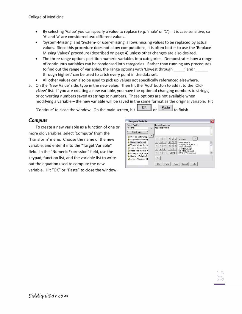
Compute
To create a new variable as a function of one or
more old variables, select ‘Compute’ from the
‘Transform’ menu. Choose the name of the new
variable, and enter it into the “Target Variable”
field. In the “Numeric Expression” field, use the
keypad, function list, and the variable list to write
out the equation used to compute the new
variable. Hit “OK” or “Paste” to close the window.
College of Medicine
Analyzing Data
Descriptive Statistics
In the ‘Analyze’ menu, the option ‘Descriptive Statistics’ produces a submenu with the choices
Frequencies, Descriptives, Explore, Crosstabs, and Ratio. Of these, Crosstabs and Descriptives have
some particularly useful features which this manual will cover. For more information on the other
three, more information can be found in the SPSS help menu, which is discussed on page 14 of this
manual.
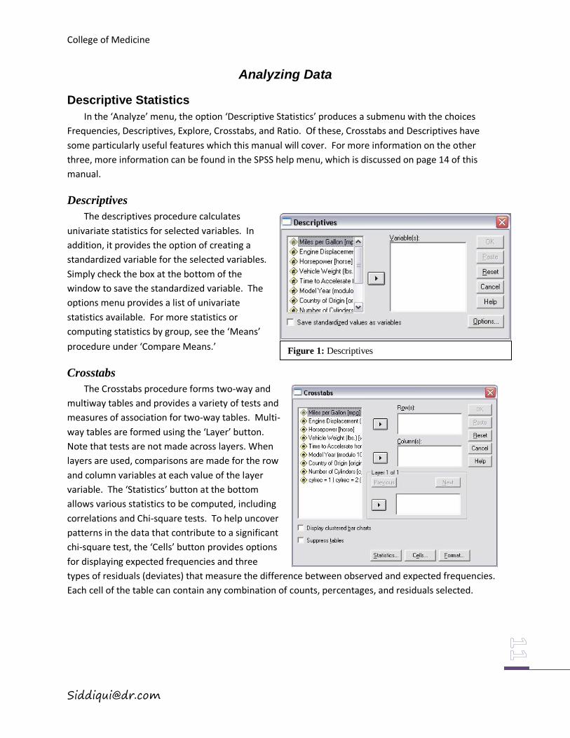
Descriptives
The descriptives procedure calculates
univariate statistics for selected variables. In
addition, it provides the option of creating a
standardized variable for the selected variables.
Simply check the box at the bottom of the
window to save the standardized variable. The
options menu provides a list of univariate
statistics available. For more statistics or
computing statistics by group, see the ‘Means’
procedure under ‘Compare Means.’
Crosstabs
The Crosstabs procedure forms two-way and
multiway tables and provides a variety of tests and
measures of association for two-way tables. Multi-
way tables are formed using the ‘Layer’ button.
Note that tests are not made across layers. When
layers are used, comparisons are made for the row
and column variables at each value of the layer
variable. The ‘Statistics’ button at the bottom
allows various statistics to be computed, including
correlations and Chi-square tests. To help uncover
patterns in the data that contribute to a significant
chi-square test, the ‘Cells’ button provides options
for displaying expected frequencies and three
types of residuals (deviates) that measure the difference between observed and expected frequencies.
Each cell of the table can contain any combination of counts, percentages, and residuals selected.
Figure 1: Descriptives
College of Medicine
Compare Means
From the ‘Compare Means option in the ‘Analyze’ menu, you can perform t-tests, and one-
way ANOVA, and calculate univariate statistics for variables.
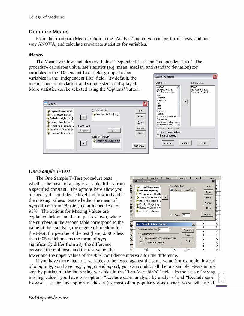
Means
The Means window includes two fields: ‘Dependent List’ and ’Independent List.’ The
procedure calculates univariate statistics (e.g. mean, median, and standard deviation) for
variables in the ‘Dependent List’ field, grouped using
variables in the ‘Independent List’ field. By default, the
mean, standard deviation, and sample size are displayed.
More statistics can be selected using the ‘Options’ button.
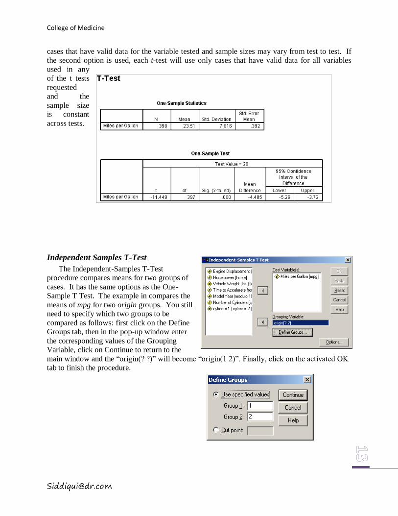
One Sample T-Test
The One Sample T-Test procedure tests
whether the mean of a single variable differs from
a specified constant. The options here allow you
to specify the confidence level and how to handle
the missing values. tests whether the mean of
mpg differs from 28 using a confidence level of
95%. The options for Missing Values are
explained below and the output is shown, where
the numbers in the second table correspond to the
value of the t statistic, the degree of freedom for
the t-test, the p-value of the test (here, .000 is less
than 0.05 which means the mean of mpg
significantly differ from 28), the difference
between the real mean and the test value, the
lower and the upper values of the 95% confidence intervals for the difference.
If you have more than one variables to be tested against the same value (for example, instead
of mpg only, you have mpg1, mpg2 and mpg3), you can conduct all the one sample t-tests in one
step by putting all the interesting variables in the “Test Variable(s)” field. In the case of having
missing values, you have two options “Exclude cases analysis by analysis” and “Exclude cases
listwise”. If the first option is chosen (as most often popularly done), each t-test will use all
College of Medicine
cases that have valid data for the variable tested and sample sizes may vary from test to test. If
the second option is used, each t-test will use only cases that have valid data for all variables
used in any
of the t tests
requested
and the
sample size
is constant
across tests.
Independent Samples T-Test
The Independent-Samples T-Test
procedure compares means for two groups of
cases. It has the same options as the One-
Sample T Test. The example in compares the
means of mpg for two origin groups. You still
need to specify which two groups to be
compared as follows: first click on the Define
Groups tab, then in the pop-up window enter
the corresponding values of the Grouping
Variable, click on Continue to return to the
main window and the “origin(? ?)” will become “origin(1 2)”. Finally, click on the activated OK
tab to finish the procedure.
College of Medicine
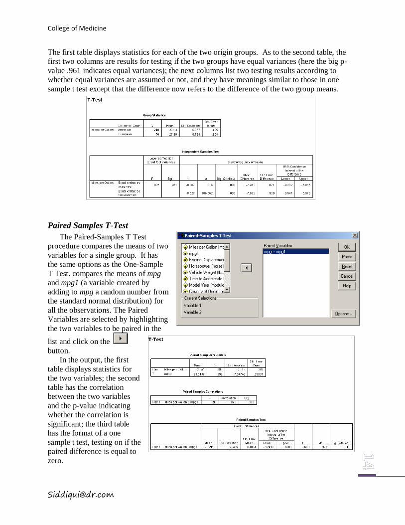
The first table displays statistics for each of the two origin groups. As to the second table, the
first two columns are results for testing if the two groups have equal variances (here the big p-
value .961 indicates equal variances); the next columns list two testing results according to
whether equal variances are assumed or not, and they have meanings similar to those in one
sample t test except that the difference now refers to the difference of the two group means.
Paired Samples T-Test
The Paired-Samples T Test
procedure compares the means of two
variables for a single group. It has
the same options as the One-Sample
T Test. compares the means of mpg
and mpg1 (a variable created by
adding to mpg a random number from
the standard normal distribution) for
all the observations. The Paired
Variables are selected by highlighting
the two variables to be paired in the
list and click on the
button.
In the output, the first
table displays statistics for
the two variables; the second
table has the correlation
between the two variables
and the p-value indicating
whether the correlation is
significant; the third table
has the format of a one
sample t test, testing on if the
paired difference is equal to
zero.
College of Medicine
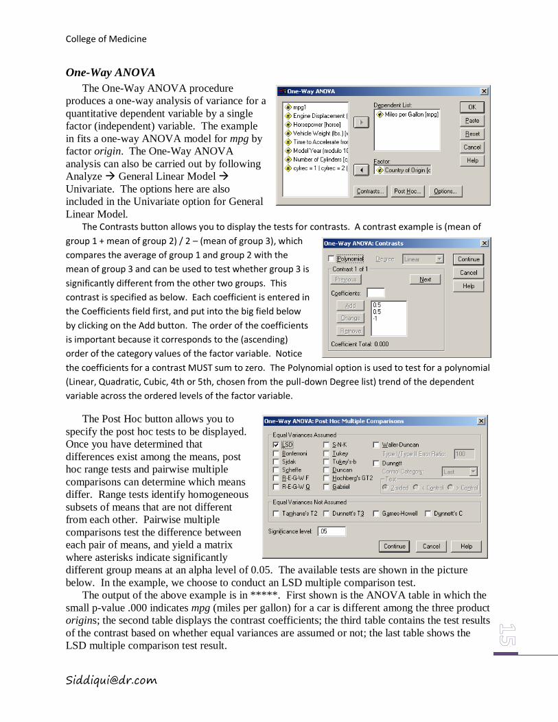
One-Way ANOVA
The One-Way ANOVA procedure
produces a one-way analysis of variance for a
quantitative dependent variable by a single
factor (independent) variable. The example
in fits a one-way ANOVA model for mpg by
factor origin. The One-Way ANOVA
analysis can also be carried out by following
Analyze General Linear Model
Univariate. The options here are also
included in the Univariate option for General
Linear Model. The Contrasts button allows you to display the tests for contrasts. A contrast example is (mean of
group 1 + mean of group 2) / 2 – (mean of group 3), which
compares the average of group 1 and group 2 with the
mean of group 3 and can be used to test whether group 3 is
significantly different from the other two groups. This
contrast is specified as below. Each coefficient is entered in
the Coefficients field first, and put into the big field below
by clicking on the Add button. The order of the coefficients
is important because it corresponds to the (ascending)
order of the category values of the factor variable. Notice
the coefficients for a contrast MUST sum to zero. The Polynomial option is used to test for a polynomial
(Linear, Quadratic, Cubic, 4th or 5th, chosen from the pull-down Degree list) trend of the dependent
variable across the ordered levels of the factor variable.
The Post Hoc button allows you to
specify the post hoc tests to be displayed.
Once you have determined that
differences exist among the means, post
hoc range tests and pairwise multiple
comparisons can determine which means
differ. Range tests identify homogeneous
subsets of means that are not different
from each other. Pairwise multiple
comparisons test the difference between
each pair of means, and yield a matrix
where asterisks indicate significantly
different group means at an alpha level of 0.05. The available tests are shown in the picture
below. In the example, we choose to conduct an LSD multiple comparison test.
The output of the above example is in *****. First shown is the ANOVA table in which the
small p-value .000 indicates mpg (miles per gallon) for a car is different among the three product
origins; the second table displays the contrast coefficients; the third table contains the test results
of the contrast based on whether equal variances are assumed or not; the last table shows the
LSD multiple comparison test result.
College of Medicine
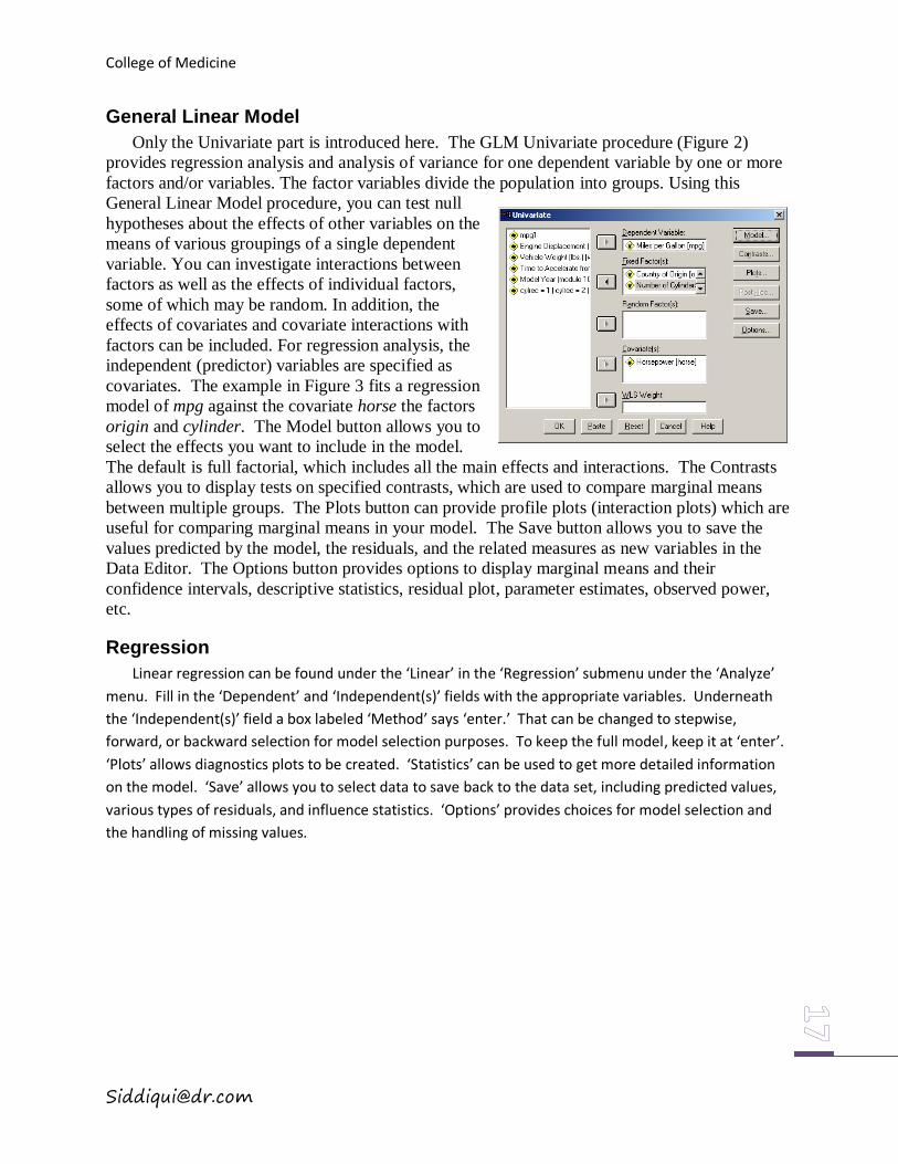
General Linear Model
Only the Univariate part is introduced here. The GLM Univariate procedure (Figure 2)
provides regression analysis and analysis of variance for one dependent variable by one or more
factors and/or variables. The factor variables divide the population into groups. Using this
General Linear Model procedure, you can test null
hypotheses about the effects of other variables on the
means of various groupings of a single dependent
variable. You can investigate interactions between
factors as well as the effects of individual factors,
some of which may be random. In addition, the
effects of covariates and covariate interactions with
factors can be included. For regression analysis, the
independent (predictor) variables are specified as
covariates. The example in Figure 3 fits a regression
model of mpg against the covariate horse the factors
origin and cylinder. The Model button allows you to
select the effects you want to include in the model.
The default is full factorial, which includes all the main effects and interactions. The Contrasts
allows you to display tests on specified contrasts, which are used to compare marginal means
between multiple groups. The Plots button can provide profile plots (interaction plots) which are
useful for comparing marginal means in your model. The Save button allows you to save the
values predicted by the model, the residuals, and the related measures as new variables in the
Data Editor. The Options button provides options to display marginal means and their
confidence intervals, descriptive statistics, residual plot, parameter estimates, observed power,
etc.
Regression
Linear regression can be found under the ‘Linear’ in the ‘Regression’ submenu under the ‘Analyze’
menu. Fill in the ‘Dependent’ and ‘Independent(s)’ fields with the appropriate variables. Underneath
the ‘Independent(s)’ field a box labeled ‘Method’ says ‘enter.’ That can be changed to stepwise,
forward, or backward selection for model selection purposes. To keep the full model, keep it at ‘enter’.
‘Plots’ allows diagnostics plots to be created. ‘Statistics’ can be used to get more detailed information
on the model. ‘Save’ allows you to select data to save back to the data set, including predicted values,
various types of residuals, and influence statistics. ‘Options’ provides choices for model selection and
the handling of missing values.
College of Medicine
Making Graphs
For any graph generated in SPSS, you can double click on the graph to invoke a Chart Editor window
with the graph, inside which you can double click on any part of the graph to edit that specific part, for
example, the title of the graph, the label for an axis, the type of points, the color of lines, the size of the
box, etc.
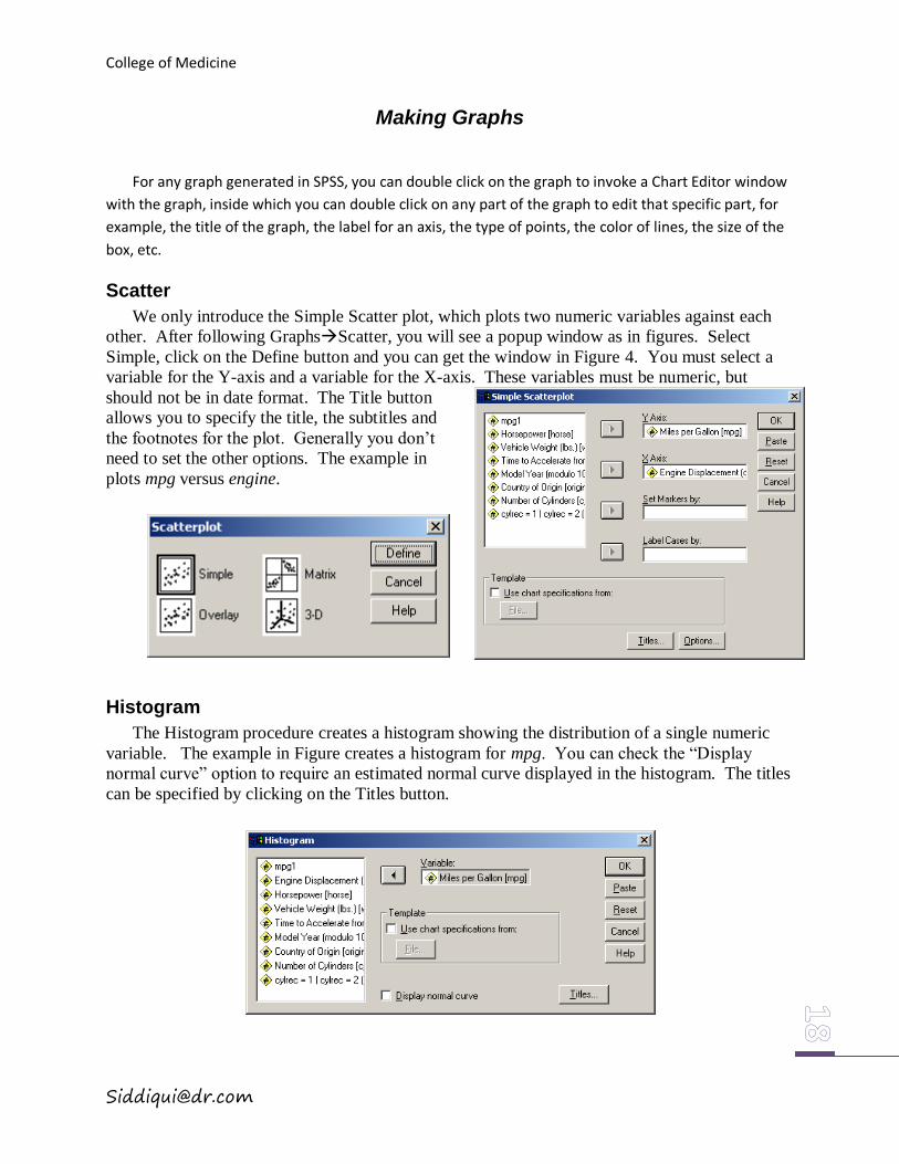
Scatter
We only introduce the Simple Scatter plot, which plots two numeric variables against each
other. After following GraphsScatter, you will see a popup window as in figures. Select
Simple, click on the Define button and you can get the window in Figure 4. You must select a
variable for the Y-axis and a variable for the X-axis. These variables must be numeric, but
should not be in date format. The Title button
allows you to specify the title, the subtitles and
the footnotes for the plot. Generally you don’t
need to set the other options. The example in
plots mpg versus engine.
Histogram
The Histogram procedure creates a histogram showing the distribution of a single numeric
variable. The example in Figure creates a histogram for mpg. You can check the “Display
normal curve” option to require an estimated normal curve displayed in the histogram. The titles
can be specified by clicking on the Titles button.
College of Medicine
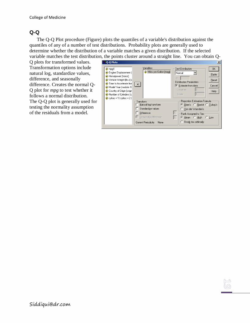
Q-Q
The Q-Q Plot procedure (Figure) plots the quantiles of a variable's distribution against the
quantiles of any of a number of test distributions. Probability plots are generally used to
determine whether the distribution of a variable matches a given distribution. If the selected
variable matches the test distribution, the points cluster around a straight line. You can obtain Q-
Q plots for transformed values.
Transformation options include
natural log, standardize values,
difference, and seasonally
difference. Creates the normal Q-
Q plot for mpg to test whether it
follows a normal distribution.
The Q-Q plot is generally used for
testing the normality assumption
of the residuals from a model.
College of Medicine
Help
The preceding sections have provided an overview of commonly used procedures to get you started
in using SPSS. If you need help with a procedure not mentioned here, or want to learn more, the best
place to look is the help docs that come with SPSS. SPSS has very good help documents – often
containing examples and tutorials to make the point clear. The help docs can be referenced two
different ways. First, almost every window in SPSS contains a ‘Help’ button. Clicking it takes you
immediately to the help documentation specific to that window. Second, the last menu in SPSS is a help
menu. The first option, ‘Topics’ brings up the help documentation. Use the index or a search command
to look up the options that will give you the right results. Sometimes the help docs have the words
‘Show me’ highlighted in blue. Clicking on ‘Show me’ will walk you through an example of the
procedure.
The ‘Statistics Coach’ option is useful when you have an idea of what you’re looking for, but don’t
know the name. Select an option on the right, and examples will appear on the left. If you find what
you are looking for, hit the next button. You’ll be guided through one or more screens asking you to
describe the data. When the program has the information it needs, it will open a window telling you
what the procedure’s called and where to find it in the future. It will also go ahead and open up the
menu for you.