SPSS for Windows

A brief tutorial

This tutorial is a brief look at what SPSS for Windows is capable of doing. Examples will come from Statistical Methods for Psychology by David C. Howell. It is not our intention to teach you about statistics in this tutorial. For that you should rely on your classes in statistics and/or a good textbook. If you're a novice this tutorial should give you a feel for the programme and how to navigate through the many options. Beyond that, the SPSS Help Files should be used as a resource. Further, SPSS sells a number of very good manuals.

The BasicsSPSS for Windows has the same general look a feel of most other programmes for Windows. Virtually anything statistic that you wish to perform can be accomplished in combination with pointing and clicking on the menus and various interactive dialog boxes. You may have noted that the examples in the Howell textbook are performed/analyzed via code. That is, SPSS, like many other packages, can be accessed by programming short scripts, instead of pointing and clicking. We will not cover any programming in this tutorial.

Presumeably, SPSS is already installed on your computer. If you don't have a shortcut on your desktop go to the [Start => Programs] menu and start the package by clicking on the SPSS icon.

Before proceeding I should say a few words about a very simple convention that will be used in this tutorial. In this point and click environment one often hasto navigate through many layers of menu items before encountering the required option. In the above paragraph the prescribed task was to locate the SPSS icon in the [Start] menu structure. To get to that icon, one must first click on [Start] then move the pointer to the [Programs] options, before locating the SPSS icon. This sequence of events can be conveyed by typing [Start => Programs] . That is, one must move from the outer layer of the menu structure tosome inner layer in sequence....

Now, back to the tutorial.

Once you've clicked on the SPSS icon a new window will appear on the screen. Theappearance is that of a standard programme for windows with a spreadsheet-like interface.

As you can see, there are a number of menu options relating to statistics, on the menu bar. There are also shortcut icons on the toolbar. These serve as quickaccess to often used options. Holding your mouse over one of these icons for a second or two will result in a short function description for that icon. The current display is that of an empty data sheet. Clearly, data can either be entered manually, or it can be read from an existing data file.

Browsing the file menu, below, reveals nothing too surprising - many of the options are familiar. Although, the details are specific to SPSS. For example, the [New] option is used to specify the type of window to open. The various options, under the [New] heading are,

[Data] Default window with a blank data sheet ready for analyses [Syntax] One can write scripts like those present in the Howell text, instead of using the menus. See

the SPSS manuals for help on this topic. [Output] Whenever a procedure is run, the out is directed to a separate window. One can also have

multiple [Output] windows open to organize the various analyses that might be conducted. Later, these results can be saved and/or printed.

[Script] This window provides the opportunity to write fullblown programmes, in a BASIC-like language. These programmes have access to functions that make up SPSS. With such access it is possible to write user-defined procedures - those not part of SPSS - by taking advantage of the SPSS functions. Again, this is beyond the scope of this tutorial.

Also present in the [File] menu are two separate avenues for reading data from existing files. The first is the [Open] option. Like other application packages (e.g., WordPerfect, Excel, ....) SPSS also has it's own format for saving data. In this case, the accepted extension for any file saved using the proprietary format is "sav". So, one can have a datafile saved as "data1.sav". Anyways, thisformat is not readable with a text editor, it is a binary format. The benefits are that all formatting changes are maintained and the file can be read faster, hence the [Open] option. It is specifically meant for files saved in the SPSS format. The second option, [Read ASCII Data], as the name suggests is to read files that are saved in ASCII format. As can be seen, there are two choices - [Freefield] and [Fixed Columns]. Clicking on one of these options will producea dialog box. One must specify a number of parameters before a file can be read successfully.

Reading ASCII files requires that the user know something about the format of the data file. Otherwise, one is likely get stuck in the process of reading, or

the result may be a costly error. The more restrictive format is [Fixed Columns]. One must know how many variables there are, whether a variable is in numeric or string format, and the first and last column of each variable. For example, think of the following as an excerpt from an ASCII datafile.

male 37 102male 22 115male 27 99.... .. ...female 48 107female 21 103female 28 122...... .. ...

An examination of the datafile provides several key pieces of information,

1.There are 3 variables2.Variable 1 is a string , Variable 2 and 3 are numeric3.Variable 1: first column=1, last column=6

o Notice that none of the columns overlap. The longest case for column one is the name "female", that spans from the first column to the sixth- or, the letter e. As you can see, one has to manually locate the first and last column, of each variable.

4.Variable 2: first column=9, last column=105.Variable 3: first column=12, last column=14

One needs all of the above information, in addition to, name for each of the three variables. It is a highly structured way of setting up and describing the data. For such files I would suggest becoming comfortable with a good text editor. Failing that, you may wish to try Notepad or WordPad in Win95, but ensure that you save as a textfile with WordPad. A fullfledged word processor like Word or WordPerfect will also work provided that you remember to save as a textfile. These same editors will allow you to figure out the column locations for each of the variables.

The [Freefield] option is less restrictive. Essentially, the columns can be ragged (i.e., overlapping). One need only preserve the order of each variable across all of the cases.

male 37 102male 22 115male 27 99.... .. ...female 48 107female 21 103female 28 122...... .. ...

Experiment with creating datafiles and reading them with this method. As for theSPSS format, there are a large number of sample datafiles included in your package. Just click on [Open] and find the SPSS home directory. Make sure the

filetype in the dialog box associated with [Open] is set to "*.sav" - the default...

Before we move onto actual data, click on [Statistics] . The menu that appears reveals many classes of statistics available for use. Each class is further subdivided into other options, as denoted by the little arrow at the right size of the menu selector. Explore what is offered by moving your mouse over the various procedures listed.

   

Data

To begin the process of adding data, just click on the first cell that is located in the upper left corner of the datasheet. It's just like a spreadsheet.You can enter your data as shown. Enter each datapoint then hit [Enter]. Once you're done with one column of data you can click on the first cell of the next column.

These data are taken from table2.1 in Howell's text. The first column represents"Reaction Time in 100ths of a second" and the second column indicates "Frequency".

If you're entering data for the first time, like the above example, the variablenames will be automatically generated (e.g., var00001, var00002,....). They are not very informative. To change these names, click on the variable name button. For example, double click on the "var00001" button. Once you have done that, a dialog box will appear. The simplest option is to change the name to something meaningful. For instance, replace "var00001" in the textbox with "RT" (see figure below).

In addition to changing the variable name one can make changes specific to [Type], [Labels], [Missing Values], and [Column Format].

[Type] One can specify whether the data are in numeric or string format, in addition to a few more formats. The default is numeric format.

[Labels] Using the labels option can enhance the readability of the output. A variable name is limited to a length of 8 characters, however, by using a variable label the length can be as much as 256 characters. This provides the ability to have very descriptive labels that will appear at the output.

Often, there is a need to code categorical variables in numeric format. For example, male and female can be coded as 1 and 2, respectively. To reduce confusion, it is recommended that one uses value labels . For the example of gender coding, Value:1 would have a correspoding Value label: male. Similarly, Value:2 would be coded with Value Label: female. (click onthe [Labels] button to verify the above)

[Missing Values] See the accompanying help. This option provides a means to code for various types of missing values.

[Column Format] The column format dialog provides control over several features of each column(e.g., width of column).

The next image reflects the variable name change.

Once data has been entered or modified, it is adviseable to save. In fact, save as often as possible [File => SaveAs].

SPSS offers a large number of possible formats, including their own. A list of the available formats can be viewed and selected by clicking on the Save as type: , on the SaveAs dialog box. If your intention is to only work in SPSS, then there may be some benefit to saving in the SPSS(*.sav) format. I assume that this format allows for faster reading and writing of the data file. However, if your data will be analyzed and looked by other packages (e.g., a spreadsheet), it would be adviseable to save in a more universal format (e.g., Excel(*.xls), 1-2-3 Rel 3.0 (*.wk3).

Once the type of file has been selected, enter a filename, minus the extension (e.g., sav, xls). You should also save the file in a meaningful directory, on your harddrive or floppy. That is, for any given project a separate directory should be created. You don't want your data to get mixed-up.

The process of reading already saved data can be painless if the saved format isin the SPSS or a spreadsheet format. All one has to do is,

o click on [File => New => Data]

o click on [File => Open] : a dialog box will appearo navigate to desired directory using the Look in: menu at the top of the

dialog boxo select file type in the Files of type menuo click on the filename that is needed.

The process of reading existing files is slightly more involved if the format isASCII/plain text (see the earlier description of [Freefield] and [Fixed Columns]). As an example, the ASCII data from table2.1 in the Howell text will be used. A file containing the data should be included in the accompanying disk for the text. [Note: It was not present in my disk, so I downloaded the file from Howell's webpage.] I've placed the files on my harddrive at c:\ascdat. In the case of this set of data,there are four columns representing observation number, reaction time, setsize, and the presence or absence of the target stimulus. This information can be found in the readme.txt file that is also on the disk. Typically, we are aware of the contents of our own data files, however, it doesn't hurt to keep a record of the contents of such files.

To make life easier the [File => Read ASCII Data => Freefield] will be used.

The resulting dialog box requires that a File , a Name and a Data Type be specified for each variable, or column of data. The desired file is accessed by clicking on the [Browse] button, and then navigating to the desired location. Since the extension for the sought after file is dat there is no need to change the Files of type: selection. However, if the extension is something else (e.g.,*.txt) then it would be necessary to select All files(*.*) from the Files of type: menu. Since there are 4 variables in this data set, 4 names with the corresponding type information must be specified. To Add the first variable, observations, to the list,

o type "obs" in the Name boxo the Data Type is set to Numeric by default. If "obs" was a string

variable, then one would have to click on Stringo click on the Add button to include this variable to the list.o repeat the above procedure with new names and data types for each of

the remaining variables. It is important that all variables be added tothe list. Otherwise, the data will be scrambled.

(Please explore the various options by clicking on any accessible menu item.)

The resulting data files appears in the data editor like the following.

The next section will cover some descriptive statistics.

   

Descriptive Statistics

We can replicate the frequency analyses that are described in chapter 2 of the text, by using the file that was just read into the data editor - tab2-1.dat. These analyses were conducted on the reaction time data. Recall, that we have labelled this data as RT.

To begin, click on [Statistics=>Summarize=>Frequencies]....

The result is a new dialog box that allows the user to select the variables of interest. Also, note the other clickable buttons along the border of the dialog box. The buttons labelled [Statistics...] and [Charts...]are of particular importance. Since we're interested in the reaction time data, click on rt followed by a mouse click on the arrow pointing right. The consequence of this action is a transference of the rt variable to the Variables list. At this point, clicking on the [OK] button would spawn an output window with the Frequency information for each of the reaction times. However, more information can be gathered by exploring the options offered by the [Statistics...] and [Charts...].

[Statistics...] offers a number of summary statistics. Any statistic that is selected will be summarized in the output window.

As for the options under [Charts...] click on Bar Charts to replicate the graph in the text.

Once the options have been selected, click on [OK] to run the procedure. The results are then displayed in an output window. In this particular instance the window will include summary statistics for the variable RT, the frequency distribution, and the frequency distribution. You can see all of this by scrolling down the window. The results should also be identical to those in the text.

You may have gathered from the above that calculating summary statistics requires nothing more than selecting variables, and then selecting the desired statistics. The frequency example allowed us to generate frequency information plus measures of central tendencies and dispersion. These statistics can be had by clicking directly on [Statistics=>Summarize=>Descriptives]. Not surprisingly,another dialog box is attached to this procedure. To control the type of statistics produced, click on the [Options...] button. Once again, the options include the typical measures of central tendency and dispersion.

Each time as statistical procedure is run, like [Frequencies...] and [Descriptives...] the results are posted to an Output Window. If several procedures are run during one session the results will be appended to the same window. However, greater organization can be reached by opening new Output windows before running each procedure - [File=>New=>Output]. Further, the contents of each of these windows can be saved for later review, orin the case of charts saved to be later included in formattted documents. [Explore by left mouse clicking on any of the output objects (e.g., a frequency table, a chart, ...) followed by a right button click. The left left button click will highlight the desired object, while the right button click will popupa new menu. The next step is to click on the copy option. This action will storethe object on the clipboard so that it can be pasted to Word for Windows document, for example.....]

   

Chi-Square & T-Test

The computation of the Chi-Square statistic can be accomplished by clicking on [Statistics => Summarize => Crosstabs...]. This particular procedure will be your first introduction to coding of data, in the data editor. To this point data have been entered in a column format. That is, one variable per column. However, that method is not sufficient in a number of situations, including the calculation of Chi-Square, Independent T-tests, and any Factorial ANOVA design with between subjects factors. I'm sure there are many other cases, but they will not be covered in this tutorial.  Essentially, the data have to be entered in a specific format that makes the analysis possible.  The format typcially reflects the design of the study, as will be demonstrated in the examples. 

In your text, the following data appear in section 6.????. Please read the text for a description of the study. Essentially, the table - below - includes the observed data and the expected data in parentheses.  

 

Fault Guilty Not Guilty TotalLow 153(127.559) 24(49.441) 177High 105(130.441) 76(50.559) 181Total 258 100 358

 

In the hopes of minimizing the load time for remaining pages,  I will make use of the built in table facilty of HTML to simulate the Data Editor in SPSS. This will reduce the number of images/screen captures to be loaded.

For the Chi-Square statistic, the table of data can be coded by indexing the column and row of the observations.  For example, the count for being guilty with Low fault is 153.  This specific cell can be indexed as comingfrom row=1 and column=1.  Similarly, Not Guilty with High fault is coded  as row=2 and column=2.  For each observation, four in this instance, there is unique code for location on the table.  These can be entered as follows,    

Row Column Count1 1 1531 2 242 1 1052 2 76

   

So, 2 rows * 2 columns equals 4 observations.  That should be clear. For each of the rows, there are 2 corresponding columns, that is reflected

in the Count column.  The Count column represents the number of time each unique combination Row and Column occurs.

The above presents the data in an unambigous manner.  Once entered, the analysisis a matter of selecting the desired menu items, and perhaps selecting additional options for that statistic.  [Don't forget to use the labelling facilities, as mentioned earlier, to meaningfully identify the columns/variables.  The labels that are chosen will appear in the output window.]

To perform the analysis,

The first step is to inform SPSS that the COUNT variable represents the frequency for each unique coding of ROW and COLUMN, by invoking the WEIGHT command. To do this, click on [Data => Weight Cases]. In the resultant dialog box, enable the Weight cases by option, then move the COUNT variableinto the Frequency Variable box. If this step is forgotten, the count for each cell will be 1 for the table.

Now that the COUNT variable has been processed as a weighted variable, select [Statistics => Summarize => Crosstabs...] to launch the controlling dialog box.

At the bottom of the dialog box are three buttons, with the most important being the [Statistics...] button. You must click on the [Statistics...] button and then select the Chi-square option, otherwisethe statistic will not be calculated. Exploring this dialog box makes it clear that SPSS can be forced to calcuate a number of other statistics in conjuction with Chi-square. For example, one can select the various measures of association (e.g., contingency coefficient, phi and cramer's v,...), among others.

Move the ROW variable into the Row(s): box, and the COLUMN variable into the Column(s):, then click [OK] to perform the analysis. A subset of the output looks like the following,

Although simple, the calculation of the Chi-square statistic is very particular about all the required steps being followed. More generally, as we enter hypothesis testing, the user should be very careful and should make use of manuals for the programme and textbooks for statistics.

T-tests

By now, you should know that there are two forms of the t-test, one for dependent variables and one for independent variables, or observations. To inform SPSS, or any stats package for that matter, of the type of design it is necessary to have to different ways of laying out the data. For the dependent design, the two variables in question must be entered in two columns. For independent t-tests, the observations for the two groups must be uniquely coded with a Gruop variable. Like the calculation of the Chi-square statistic, these calculations will reinforce the practice of thinking about, and laying out the data in the correct format.

Dependent T-TestTo calculate this statistic, one must select [Statistics => Compare Means => Paired-Samples T Test...] after enterin the data. For this analysis, we'll use the data from Table 7.3, in Howell.

Enter the data into a new datafile. Your data should look a bit like the following. That is, the two variables should occupy separate columns...

Mnths_6 Mnths_24124 11494 88115 102110 2

116 2139 2116 2110 2129 2120 2105 288 2120 2120 2116 2105 2... ...... ...123 132

Note that the variable names start with a letter and are less than 8 characters long. This is a bit constraining, however, one can use the variable label option to label the variable with a longer name. This more descriptive name will then be reproduced in the output window.

To calculate the t statistic click on [Statistics => Compare Means => Paired-Samples T Test...], then select the two variables of interest. To select the two variables, hold the [Shift] key down while using the mouse for selection. You will note that the selection box requires that variablesbe selected two at a time. Once the two variables have been selected, move

them to the Paired Variables: list. This procedure can be repeated for eachpair of variables to be analyzed. In this case, select MNTHS_6 and MNTHS_24together, then move them to the Paired Variables list. Finally, click the [OK]button.

The critical result for the current analysis will appear in the output window as follows,

As you can see an exact t-value is provided along with an exact p-value, and this p-value is greater that the expected value of 0.025, for a two-tailed assessment. Closer examination indicates several other statistics are presented in output window.

Quite simply, such calculations require very little effort! 

Independent T-testsWhen calculating an independent t-test, the only difference involves the way thedata are formatted in the datasheet. The datasheet must include both the raw data and group coding, for each variable. For this example, the data from table 7.5 will be used. As an added bonus, the number of observations are unequal for this example.

Take a look at the following table to get a feel for how to code the data.

Group Exp_Con1 961 1271 1271 1191 1091 1431 ...1 ...1 1061 1092 1142 882 104

2 1042 912 962 ...2 ...2 1142 132

From the above you can see that we used the "Group" variable to code for the twovariables. The value of 1 was used to code for "LBW-Experimental", while a valueof 2 was used to code for "LBW-Control". If you're confused please study the table, above.

To generate the t-statistic,

Clik on [Statistics => Compare Means => Independent-Samples T Test] to launch the appropriate dialog box.

Select "exp_con" - the dependent variable list - and move it to the Test Variable(s): box.

Select "group" - the grouping variable list - and move it to the Grouping Variable: box.

The final step requires that the groups be defined. That is, one must specify that Group1 - the experimental group in this case - is coded as 1, and Group2 - the control group in this case - is coded as 2. To do this,

click on the [Define Groups...] button. Click on the [Continue] button to return to the controlling dialog box.

Run the analysis by clicking on the [OK] button.

The output for the current analysis extracted from the output window looks like the following.

The p-value of .004 is way lower than the cutoff of 0.025, and that suggests that the means are significantly different. Further, a Levene's Test is performed to ensure that the correct results are used. In this case the variances are equal, however, the calculations for unequal variances are also presented, among some other statistics - some not presented.

In the next section we will briefly demonstrate the calculation of correlations and regression, as discussed in Chapter 9 of Howell. In truth, you should be able to work through many statistics with your current knowledge base and the help files, including correlations and regressions. Most statistics can be calculated with a few clicks of the mouse.

   

Correlations and Regression

This will be a brief tutorial, since there is very little that is required to calculate correlations and linear regressions. To calculate a simple correlationmatrix, one must use [Statistics => Correlate => Bivariate...], and [Statistics => Regression => Linear] for the calculation of a linear regression.

For this section, the analyses presented in the computer section of the Correlation and Regression chapter will be replicated. To begin, enter the data as follows,

IQ GPA

102 2.75

108 4.00

109 2.25

118 3.00

79 1.67

88 2.25

... ...

... ...

85 2.50

Simple Correlation

Click on [Statistics => Correlate => Bivariate...], then select and move "IQ" and "GPA" to the Variables: list. [Explore the options presented on this controlling dialog box.]

Click on [OK] to generate the requested statistics.

The results from output window should look like the following,

As you can see, r=0.702, and p=.000. The results suggest that the correlation issignificant.

Note: In the above example we only created a correlation matrix based on two variables. The process of generating a matrix based on more than two variables is not different. That is, if the dataset consisted of 10 variables, they could have all been placed in the Variables: list. The resulting matrix would include all the possible pairwise correlations.

Correlation and Regression

Linear regression....it is possible to output the regression coefficients necessary to predict one variable from the other - that minimize error. To do so, one must select the [Statistics => Regression => Linear...] option. Further,there is a need to know which variable will be used as the dependent variable and which will be used as the independent variable(s). In our current example, GPA will be the dependent variable, and IQ will act as the independent variable.Specifically,

Initiate the procedure by clicking on [Statistics => Regression => Linear...]

Select and move GPA into the Dependent: variable box Select andmove IQ into the Independent(s): variable box Click on the [OK] to generate the statistics.

Note: A variety of options can be accessed via the buttons on the bottom half of this controlling dialog box (e.g., Statistics, Plots,...). Many more statistics can be generated by explore the additional options via the Statistics button.

Some of the results of this analysis are presented below,

The correlation is still 0.702, and the p value is still 0.000. The additional statistics are "Constant", or a from the text, and "Slope", or B from the text. If you recall, the dependent variable is GPA, in this case. As such, one can predict GPA with the following,

GPA = -1.777 + 0.0448*IQ

The next section will discuss the calculation of the ANOVA.

   

One-Way ANOVA

As in the independent t-test datasheet, the data must be coded with a group variable. The data that will be used for the first part of this section is from Table 11.2, of Howell. There are 5 groups of 10 observations each - resulting ina total of 50 observations. The group variable will be coded from 1 to 5, for each group. Take a look at the following to get an idea of the coding.

Groups Scores1 91 81 6... ...1 72 72 92 6... ...... ...... ...

5 105 19... ...5 11

The coding scheme uniquely identifies the origin of each observation.

To complete the analysis,

Select [Statistics => Compare Means => One-Way ANOVA...] to launch the controlling dialog box.

Select and move "Scores" into the Dependent list: Select and move "Groups" into the Factor: list Click on [OK]

The preceeding is a complete spefication of the design for this oneway anova. The simple presentation of the results, as taken from the output window, will look like the following,

The analysis that was just performed provides minimal details with regard to thedata. If you take a look at the controlling dialog box, you will find 3 additional buttons on the bottom half - [Contrasts...],[Post Hoc..], and [Options...].

Selecting [Options...] you will find,

If Descriptive is enabled, then the descriptive statistics for each condition will be generated. Making Homogeneity-of-variance active forces a Levene's test on the data. The statistics from both of these analyses will be reproduced in the output window.

Selecting [Post Hoc] will launch the following dialog box,

One can active one or multiple post hoc tests to be performed. The results will then be placed in the output window. For example, performing a R-E-G-W F statistic on the current data would produce the following,

Finally, one can use the [Contrasts...] option to specify linear and/or orthogonal sets of contrasts. One can also perform trend analysis via this option. For example, we may wish to contrast the third condition with the fifth,

For each contrast, the coefficients must be entered individually, and in order. Once can also enter multiple contrasts, by using the [Next] present in the dialog box. The result for the example contrast would look like the following,

Further, one can use the Polynomial option to test whether a specific trend in the data exists.

Factorial designs will be covered in the next section.

   

Factorial ANOVA

To conduct a Factorial ANOVA one only need extend the logic of the oneway design. Table 13.2 presents the data for a 2 by 5 factorial ANOVA. The first factor, AGE, has two levels, and the second factor, CONDITION, has five levels. So, once again each observation can be uniquely coded.

AGE CONDITIONOld = 1 Counting = 1Young = 2 Rhyming = 2

Adjective = 3Imagery = 4

Intentional = 5

For each pairing of AGE and CONDITION, there are 10 observations. That is, 2*5 conditions by 10 observations per condition results in 100 observations, that can be coded as follows. [Note, that the names for the factors are meaniful.]

AGE CONDITIO Scores1 1 91 1 81 1 61 ... ...1 1 71 2 7

1 2 91 2 61 ... ...1 ... ...1 ... ...1 5 101 5 191 ... ...1 5 112 1 82 1 62 1 42 ... ...2 1 72 2 102 2 72 2 82 ... ...2 ... ...2 ... ...2 5 212 5 192 ... ...2 5 21

Examine the table carefully, until you understand how the coding has been implemented. Note: one can enhance the readability of the output by using Value Labels for the two factors.

To compute the relevant statistics - a simple approach,

Select [Statistics => General Linear Model => Simple Factorial...] Select and move "Scores" into the Dependent: box Select and move "Age" into the Factor(s): box. Click on [Define Range...] to specify the range of coding for the Age

factor. Recall that 1 is used for Old and 2 is used for Young. So,

the Minimum: value is <1>, and the Maximum: value is 2. Click on [Continue].

Select and move "Conditio" into the Dependent: box Click on [Define Range...] to specify the range of the Condition factor. In

this case the Minimum: value is 1 and the Maximum: value is 5.

By clicking on the [Options...] button one has the opportunity to select the Method used. According to the online help,

"Method: Allows you to choose an alternate method for decomposing sums of squares. Method selection controls how the effects are assessed."

For the our purposes, selecting the Hierarchical, or the Experimental method will make available the option to output Means and counts. --- Note: I don't know the details of these methods, however, they are probably documented.

Under [Options...] activate Hierarchical, or Experimental, then activate Means and counts - Click [Continue]

Click on [OK] to generate the output.

As you can see the use of the Means and count option produces a nice summary table, with all the Variable Labels and Value Labels that were incorporated into the datasheet. Again, the use of those options makes the output a great deal more readable.

The output is a complete source table with the factors identified with Variable Labels

As noted earlier, the analysis that was just conducted is the simplest approach to performing a Factorial ANOVA. If one uses [Statistics => General Linear Model=> GLM - General Factorial...], then more options become available. The specification of the Dependent and Independent factors is the as the method usedfor the Simple Factorial analysis. Beyond that, the options include,

By selecting [Model...], one can specify a Custom model. The default is fora Fully Factorial model, however, with the Custom option one can explicitlydetermine the effects to look at.

The Contasts option allows one "test the differences among the levels of a factor" (see the manual for greater detail).

Various graphs can be specified with the [Plots...] option. For example, one can plot "Conditio" on the Horizontal Axis:, and "Age" on Separate Lines:, to generate a simple "conditio*age" plot (see the dialog box for [Plots...],

The standard post-hoc tests for each factor can be calculated by selecting the desired options under [Post Hoc...]. All one has to do is select the factors to analyze and the appropriate post-hoc(s).

The [Options...] dialog box provides a number of diagnostic and descriptivefeatures. One can generate descriptive statistics, estimates of effect size, and tests for homogeneity of variance - among others. An example source table using some of these options would look like the following,

The use of the GLM - General Factorial procedure offers a great deal more than the Simple Factorial. Depending on your needs, the former procedure may provide greater insight into your data. Explore these options!

Higher order factorial designs are carried in the same manner as the two factor analysis presented above. One need only code the factors appropriately, and enter the corresponding observations.

Repeated measures designs will be discussed in the next section.

   

• HOME • WINSTAT • WEBMAIL • HELP DESK • STAT CONSULTING • 

SSCC Knowledge Base

Search

SPSS Statistics for Students: TheBasics

IBM SPSS Statistics (formerly SPSS Statistics) is software for managingdata and calculating a wide variety of statistics. This document is intended for students taking classes that use SPSS Statistics or anyoneelse who is totally new to the SPSS software. Those who plan on doing more involved research projects using SPSS should attend ourworkshop series.

The SPSS software is built around the SPSS programming language. The good news for beginners is that you can accomplish most basic data analysis through menus and dialog boxes without having to actually learn the SPSS language. Menus and dialog boxes are useful because theygive you reminders of (most of) your options with each step of your analysis. However, some tasks cannot be accomplished from the menus, and others are more quickly carried out by typing a few key words than by working through a long series of menus and dialogs. As a beginner, it will be strategic to learn a bit of both SPSS programming and the menus.

Contents:1. Starting SPSS Statistics 2. SPSS Windows and Files 3. Issuing Commands

4. Working with the Data Editor 5. Working with the Output Viewer 6. Working with the Syntax Editor 7. Learning More

Part two discusses common statistics, regression, and graphs.Starting SPSS Statistics

The SSCC has SPSS installed in our computer labs (4218 and 3218 Sewell Social Sciences Building) and on the Winstats. For information about SSCC lab accounts, the labs, Winstat and more see Information for SSCC Instructional Lab Users.To run SPSS, log in and click Start, Programs, IBM SPSS Statistics, andthen IBM SPSS Statistics 19.

When SPSS is first started you are presented with a dialog box asking you to open a file:

Typically you start your SPSS session by opening the data file that youneed to work with.

The SPSS Windows and Files

SPSS Statistics has three main windows, plus a menu bar at the top. These allow you to (1) see your data, (2) see your statistical output, and (3) see any programming commands you have written. Each window corresponds to a separate type of SPSS file.

Data Editor (.sav files)The Data Editor lets you see and manipulate your data. You will always have at least one Data Editor open (even if you have not yet opened a data set). When you open an SPSS data file, what you see is a working copy of your data. Changes you make to your data are not permanent until you save them (click File, Save or Save As). Data files are savedwith a file type of .sav, a file type that most other software cannot work with. When you close your last Data Editor you are shutting down SPSS and you will be prompted to save all unsaved files.

To open a different data set, click File, Open, Data. (It is also possible to open some non-SPSS data files by this method, such as Excel, Stata, or SAS files.) SPSS lets you have many data sets open simultaneously, and the data set that you are currently working with, the “active” data set, is always marked with a tiny red “plus” sign on the title bar. In order to avoid confusion it is usually a good strategy to close out any Data Editors you're done using.

Output Viewer (.spv files)As you ask SPSS to carry out various computations and other tasks, the results can show up in a variety of places. New data values will show up in the Data Editor. Statistical results will show up in the Output Viewer.

The Output Viewer shows you tables of statistical output and any graphsyou create. By default it also show you the programming language for

the commands that you issued (called “syntax” in SPSS jargon), and mosterror messages will also appear here. The Output Viewer also allows youto edit and print your results. The tables of the Output Viewer are saved (click File, Save or Save As) with a file type of .spv, which canonly be opened with SPSS software.

As with Data Editors, it is possible to open more than one Output Viewer to look at more than one output file. The “active” Viewer, marked with a tiny blue plus sign, will receive the results of any commands that you issue. If you close all the Output Viewers and then issue a new command, a fresh Output Viewer is started.

Syntax Editor (.sps files)If you are working with the SPSS programming language directly, you will also open a Syntax Editor.

The Syntax Editor allows you to write, edit, and run commands in the SPSS programming language. If you are also using the menus and dialog boxes, the Paste button automatically writes the syntax for the commandyou have specified into the active Syntax Editor. These files are savedas plain text and almost any text editor can open them, but with a fileextension of .sps.As with the other types of windows, you can have more than one Syntax Editor open and the “active” window is marked with a tiny orange plus sign. When you paste syntax from dialog boxes, it goes to the active Syntax Editor. If you close out all your Syntax Editors and then paste a command, a fresh Syntax Editor is opened.

Issuing CommandsUnless you command SPSS to do something, it just sits there looking at you. In general commands may be issued either through menus and dialog boxes that invoke the programming language behind the scenes, or by typing the programming language in a Syntax Editor and “running” the commands.

Dialog BoxesAlthough each dialog box is unique, they have many common features. A fairly typical example is the dialog box for producing frequency tables(tables with counts and percents). To bring up this dialog box from themenus, click on Analyze, Descriptive Statistics, Frequencies.

On the left is a variable selection list with all of the variables in your data set. If your variables have variable labels, what you see is the beginning of the variable label. To see the full label as well as the variable name [in square brackets], hold your cursor over the labelbeginning. Select the variables you want to analyze by clicking on them(you may have to scroll through the list). Then click the arrow button to the right of the selection list, and the variables are moved to the analysis list on the right. If you change your mind about a variable, you can select it in the list on the right and then click the arrow button to move it back out of the analysis list. On the far right of the dialog are several buttons that lead to further dialog boxes with

options for the frequencies command. At the bottom of the dialog box, click OK to issue your command to SPSS, or Paste to have the command written to a Syntax Editor.If you return to a dialog box you will find it opens with all the specifications you last used. This can be handy if you are trying a number of variations on your analysis, or if you are debugging something. If you'd prefer to start fresh you can click the Reset button.

Working with the Data EditorThe main use of the Data Editor is to show you (a portion of) the data values you are working with. It can also be used to redefine the characteristics of variables (change the type, add labels, define missing values, etc.), create new variables, and enter data by hand.

The Data Editor gives you two views of your data set: a Data View and aVariable View, selected by clicking on the appropriate tab in the lowerleft corner of the window.

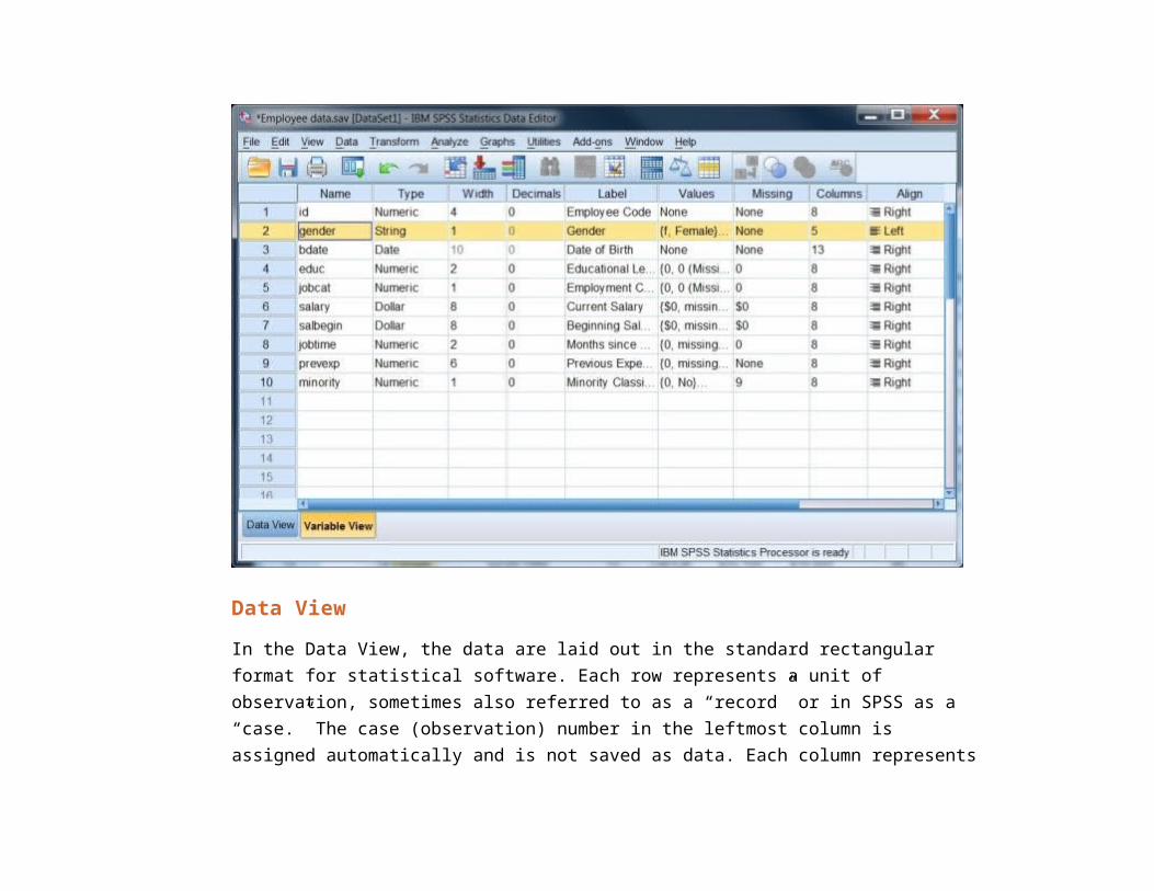
Data ViewIn the Data View, the data are laid out in the standard rectangular format for statistical software. Each row represents a unit of observation, sometimes also referred to as a “record” or in SPSS as a “case.” The case (observation) number in the leftmost column is assigned automatically and is not saved as data. Each column represents

a variable. All of the data in a column must be of the same “type,” either numeric or string (also called “character”).

Each data cell holds a data value. If data are missing, they are displayed as a period (“.”) or as a blank (“ “). Data values may be displayed as either the actual value or as a “formatted” value. For example, a data value about a person’s income might be 15000, while itsformatted value might be shown as “$15,000.” Formats can also take the form of value labels, for instance, data recorded as 1’s and 2’s might be labeled as “Male” and “Female.” While formatting makes it easier to interpret results, it is important to remember that the data values arewhat SPSS actually processes. In particular, when you set up a command that requires you to specify one or more data values, you use values and not formatted values.

You can switch the Data View between formatted and unformatted data by clicking on theValue Labels button on the Toolbar, the fourth button from the right. You can also see the actual values for a given variableby clicking on it and then looking at the bar just above the data. The box to the left indicates the observation number and variable selected,e.g. 1:sex, while the center box shows you the actual value, e.g. 2.Data values can be edited or added by typing them directly into the Data View. To enter data, type in the actual data value. However, asidefrom very small data sets for class exercises, you should almost never need to do this.

Variable ViewIn the Variable View you can see and edit the information that defines each variable (sometimes called “meta-data”) in your data set: each column of the Data View is described by a row of the Variable View.

The first attribute of each variable is its Name. The variable name is how the data column is identified in the programming language, and in order for the programming language to work gracefully variable names have to abide by certain restrictions: names must begin with a letter, and may be made up of characters, numerals, non-punctuation characters,and the period. Capitalization is ignored. Variable names may be up to 64 characters long. Other restrictions may apply – no coupons please. Variable names may be added or changed simply by typing them in.The basic variable types are either numeric or string. However, just tomake things confusing, SPSS allows you to select among several different standard formats for displaying numeric data (e.g. scientificnotation, comma formatting, currencies) and calls it Type. You set the variable type by clicking in the column, then clicking on the gray button that appears and working in a dialog box.The Label attribute allows you to give each variable a longer description that is displayed in place of the variable name, analogous to value labels for data values. The Valuesattribute allows you to create a list of value labels. Often several variables will share a common set of value labels, and in this window you can copy and paste

value label sets. Variable labels are set by typing them in, value labels work through a dialog box.The Missing attribute is a place for you to designate certain data values that you want SPSS to ignore when it calculates statistics. For instance, in survey data it is common practice to record a data value of “8” when a respondent says “I don’t know” in response to a question,and you can have SPSS treat the 8’s in a variable as if they were missing data.The other attributes, Width, Decimals, Columns, Align, Measure, and Role, are minor settings related to data display. Although Measure (level of measurement) is statistically a very important concept, it has little meaning within the SPSS software.

Working with the Output ViewerThe Output Viewer collects your statistical tables and graphs, and gives you the opportunity to edit them before you save or print them. The Output Viewer is divided into two main sections, an outline pane onthe left, and a tables pane on the right. When you print your output, it is the tables pane that is printed.

When SPSS creates output (tables, syntax, error messages, etc.) it addsthem to the tables pane as “objects,” and each object is noted in the outline pane. Individual objects may be opened and edited, deleted, hidden, rearranged, or printed. To select an object to work with, you can either click on it in the tables pane, or click on the corresponding entry in the outline pane. A red arrow appears next to the object in both panes.

To edit objects, double-click on them in the tables pane. Depending on whether you are trying to edit a simple object like a title (which is just a box with some text in it), or something more complicated like a table or a graph, you may be able to simply change the object in the Output Viewer, or another window may open. Except for editing the look of graphs, it will often be easier to edit your output by exporting it to Microsoft Word first, but in principle you can change anything you can see in your output, down to deleting columns and changing numbers. (But if your intent is to fake your results, you should attend our Simulations workshop for better methods of doing this.)To delete objects, select them in either pane and use the Delete key.To hide objects, double-click on the icon for each object in the outline pane. To make them visible, just double-click again. You can hide a whole section of the outline by clicking on the minus sign to the left of the group in the outline pane. Hidden objects are not printed, but are saved with the output file.To rearrange objects, select the object (or group of objects) in eitherpane, and drag them until the red arrow points to the object below which you want them to appear.To export your output, you go through a special procedure. In the Output Viewer clickFile, Export to invoke the Export dialog box. There are three main settings to look at. First, pick the type of file to which you want to export: useful file types include Excel, PDF, PowerPoint, or Word. Next, check that you are exporting as much of youroutput as you want, the Objects to Export at the top of the dialog. If

you have a part of your output selected, this option will default to exporting just your selection, otherwise you typically will export all your visible output. Finally, change the default file name to somethingmeaningful, and save your file to a location where you will be able to keep it, like your U:\drive.Once your options are set, click OK.

Working with the Syntax EditorLearning SPSS programming syntax is a separate topic; the fundamentals are addressed in our SSCC training workshops. But you don’t have to memorize a whole new language in order to paste and run SPSS syntax.

The fundamental unit of work in the SPSS language is the command: thinkof commands as analogous to well-formed sentences. In this language, commands begin with a keyword and end with a period. Commands should begin in the leftmost column in the editor. If they are wrapped onto more than one line, the continuing lines should begin with a blank space. Capitalization does not matter. The Syntax Editor displays syntax that SPSS cannot interpret in red type.

Like the Output Editor, the Syntax Editor has two panes. The tables pane on the right is what is actually saved in the .sps file.

Running syntax. To have SPSS actually carry out your command(s), you must “run” them. Click Run, and then one of the menu options. There is also an icon on the Toolbar to run your program, a right-facing triangle. You can run all the commands in the editor, or select a groupof commands and run just that (be careful that you highlight full commands, from the first keyword through the final period). You can also run the “current” command, which is whatever command the cursor islocated within.Pasting and running. From most dialog boxes you have the option of “pasting” commands instead of simply running them. SPSS then writes thecommand into a Syntax Editor. The syntax tends to be verbose, specifying many options that are the defaults--syntax you write

yourself tends to be much shorter and simpler. After you have pasted a command, you still need to run it to get any output.

Learning MoreNow that you understand the basics of using the SPSS windows, you can learn how to carry out statistical tasks by reading part two of SPSS for Students. It covers common statistics, regression, and graphs.To learn more about the SPSS user interface, you can look at the on-line tutorial that comes with the software: click Help, Tutorial.To learn more about specific data management or statistical tasks, you should try the on-line Help files. Click Help, Topics and you can read about a variety of basic SPSS topics, or search the index.

Your instructor and/or TA are your best resource for class-specific tasks.

If you are a student at UW-Madison, Doug Hemken, a statistical computing specialist for the SSCC, is available to help with SPSS homework and class projects. His hours are 10-2 Monday through Friday, or by appointment in 4226I Sewell Social Sciences Building. If he is not available, other SSCC staff may be able to assist you: go to 4226 and then look for the red “Stat Consultant” or the yellow “SSCC Consultant” sign.

Last Revised: 5/10/2011

©2009-2015 UW Board of Regents, University of Wisconsin - Madison

| Contact Us |  RSS |