
Energy Demand and Temperature: A Dynamic Panel Analysis
31
This paper can be downloaded without charge at: The Fondazione Eni Enrico Mattei Note di Lavoro Series Index: http://www.feem.it/Feem/Pub/Publications/WPapers/default.htm Social Science Research Network Electronic Paper Collection: http://ssrn.com/abstract=928798 The opinions expressed in this paper do not necessarily reflect the position of Fondazione Eni Enrico Mattei Corso Magenta, 63, 20123 Milano (I), web site: www.feem.it, e-mail: [email protected] Energy Demand and Temperature: A Dynamic Panel Analysis Andrea Bigano, Francesco Bosello and Giuseppe Marano NOTA DI LAVORO 112.2006 SEPTEMBER 2006 IEM - International Energy Markets Andrea Bigano, Fondazione Eni Enrico Mattei and Ref., Ricerche per l’Economia e la Finanza, Milan Francesco Borsello, Fondazione Eni Enrico Mattei and EEE Programme, International Centre for Theoretical Physics, Trieste Giuseppe Marano, Fondazione Eni Enrico Mattei
-
Upload
independent -
Category
Documents
-
view
3 -
download
0
Transcript of Energy Demand and Temperature: A Dynamic Panel Analysis
This paper can be downloaded without charge at:
The Fondazione Eni Enrico Mattei Note di Lavoro Series Index: http://www.feem.it/Feem/Pub/Publications/WPapers/default.htm
Social Science Research Network Electronic Paper Collection:
http://ssrn.com/abstract=928798
The opinions expressed in this paper do not necessarily reflect the position of Fondazione Eni Enrico Mattei
Corso Magenta, 63, 20123 Milano (I), web site: www.feem.it, e-mail: [email protected]
Energy Demand and Temperature: A Dynamic Panel Analysis
Andrea Bigano, Francesco Bosello and Giuseppe Marano
NOTA DI LAVORO 112.2006
SEPTEMBER 2006 IEM - International Energy Markets
Andrea Bigano, Fondazione Eni Enrico Mattei and Ref., Ricerche per l’Economia e la Finanza, Milan
Francesco Borsello, Fondazione Eni Enrico Mattei and EEE Programme, International Centre for Theoretical Physics, Trieste
Giuseppe Marano, Fondazione Eni Enrico Mattei
Energy Demand and Temperature: A Dynamic Panel Analysis
Summary This paper is a first attempt to investigate the effect of climate on the demand for different energy vectors from different final users. The ultimate motivation for this is to arrive to a consistent evaluation of the impact of climate change on key consumption goods and primary factors such as energy vectors. This paper addresses these issues by means of a dynamic panel analysis of the demand for coal, gas, electricity, oil and oil products by residential, commercial and industrial users in OECD and (a few) non-OECD countries. It turns out that temperature has a very different influence on the demand of energy vectors as consumption goods and on their demand as primary factors. In general, residential demand responds negatively to temperature increases, while industrial demand is insensitive to temperature increases. As to the service sector, only electricity demand displays a mildly significant negative elasticity to temperature changes. Keywords: Energy Demand, Temperature, Dynamic Panels JEL Classification: C3, Q41, Q54 The authors are very grateful to Carlo Carraro, Marzio Galeotti, Alessandro Lanza, Matteo Manera, Anil Markandya, Roberto Roson, Jim Sweeney and Richard Tol for their comments and suggestions. All errors and opinions are ours. Address for correspondence: Andrea Bigano Fondazione Eni Enrico Mattei Corso Magenta 63 20123 Milano Italy E-mail: [email protected]
1. Introduction The summer of 2003 will be remembered in Europe for its exceptional heat wave that hit the
continent from June to middle August causing more than 30,000 deaths. This was accompanied by a
sharp increase in electricity consumption that occasionally resulted in power outages and
blackouts1.
The summer of 2005, at least in southern Europe, has had hot spells as well, but this time the
consequences for the European citizens have been way less dire. The much feared heat wave did not
materialise, but, besides this lucky escape, one factor that may have also contributed to seriously
reduce the heat stress on the population, is that people seem to have learnt from the past and taken
countermeasures. It is interesting to note that these countermeasures should, in principle, affect
energy demand. In Italy for instance, the scalding hot last ten days of June 2005 has seen the all
time record (up to that day)in electricity consumption, peaking on June 28 at 11.30 a.m. with 54.1
GWh. The most likely direct cause for this increase in electricity consumption seems to be the
boom of air conditioners whose sales have increased fivefold in Italy from 2001 to 2004.
In short, it seems that people’s reaction to the steady increase in temperatures of the last few years
is affecting their energy use patterns. Installing more and more air conditioners is but one facet of
the phenomenon. Italy’s example is particularly striking, but similar patterns are occurring around
the world, with differences as to the pace and timing of the adaptation process.
However, the all time record for electricity consumption was again broken twice in Italy during this
exceptionally cold winter, peaking on January 25, 2006, with 55.5 GWh2, while gas strategic
reserves had to be tapped in February to compensate the reductions in Russian exports.
Thus, the question that arises from this anecdotal evidence is: if take a broader stance and look at
the effect of climate on the demand for different energy vectors, from different categories of final
users, and over the whole year, how important is climate in explaining energy demand, and in
which direction does climate affect it?
This paper addresses these issues by means of a dynamic panel analysis of the demand for coal, gas,
electricity, oil and oil products by residential, commercial and industrial users in OECD and (a few)
non-OECD countries. The ultimate motivation for investigating these issues is to derive long-run
elasticities for temperature, to be used as an input for a consistent evaluation of the impact of
climate change on a key class of consumption goods and primary factors such as energy vectors. It
turns out that temperature has a very different influence on the demand of energy vectors as
1 However in 2003, Italian electricity consumption peaked in December, with 53.4 GWh (GRTN, 2005). 2 See Terna (2006).

2
consumption goods and on the demand of energy vectors as primary factors. Residential demand
responds negatively to temperature increases, (but this does not happens for all energy vectors),
while industrial demand is insensitive to temperature increases. As to the service sector, only
electricity demand display a mildly significant negative elasticity to temperature changes.
In the empirical literature on energy demand, temperature is often considered a good candidate for
an explanatory variable of energy demand, but it is rarely the focus of analysis. The main exception
is the strand of literature that focuses on residential electricity demand, in which phenomena such as
the one described in the introduction are of primary relevance. Examples of these kind of studies are
Hanley and Peirson (1998) and Taylor and Buizza (2003) on Britain, Giannakopoulos and Psilogou
(2004) for Athens, Greece, Al-Zayer and Al Ibrahim (1996) for Saudi Arabia, Pardo et al.(2002)
and Valor et al. (2001) for Spain, Sailor (2001) for the US. These studies look at the relationship
between daily and seasonal load demand variability and temperature, often expressed in terms of
heating and cooling degree days. Given the very short run focus of these studies, their aim is mainly
to explain (and often forecast) the variability of electricity demand, rather than estimating demand
functions. Economic variables such as prices hardly play a role, except where time–use pricing is
enforced (e.g. Hanley and Peirson (1998)).
The study most akin in spirit to our analysis is the one by Amato et al. (2004), which has however a
very different geographical focus. By concentrating on the impacts on the residential and
commercial energy demand in Massachusetts, the authors are able to employ high quality monthly
data. They derive demand elasticities to temperature changes for electricity and heating oil fuels. In
a further step of analysis, they compute the impacts of climate change in terms of degree day units
variations on the energy vector demands using partial equilibrium simulations based on global
climate scenarios. They find notable changes in the overall energy consumption and in the energy
mix of the residential and commercial sectors in the region under scrutiny.
Bentzen and Engsted (2001) argue in favour of a rehabilitation of the standard autoregressive
distributed lag model (ARDL) in time-series energy demand estimation. Their point is that,
although when variables are non-stationary spurious regression and consequently invalid t-and F-
tests may results, short and long run parameters can be consistently estimated and valid inference
can be made if there is a unique cointegrating relationship between the variables. They compare
ARDL to Error Correction Models to Danish energy demand over the period 1960-1996 to find that
3
they give very similar results. Temperature (in the form of heating degree days) was included and
its elasticity found to be negative and significant.
There is quite a number of studies applying cointegration techniques to energy demand. These
studies generally focus on a single country or on a restricted group of countries. Glasure and Lee
(1997) study the cases of South Korea and Singapore, with no regard to temperature. Their interest
lies in finding out the direction of causality between energy demand and GDP growth, which they
can determine in the case of Singapore. Similar in spirit are the study by Stern (2000) on the US
economy, and Masih and Masih (1996) on South-East Asian economies. In both cases the focus is
on the cointegration of GDP and energy use, with particular regard on the direction of the causality
of changes in these variables. Silk and Louz (1997) look at US residential electricity demand by
means of a micro error correction model of residential demand. Variable used include degree days,
disposable income, interest rates electricity and fuel oil prices. Beenstock et al (1999) apply three
different estimation procedures (Dynamic Regression Model and OLS and Maximum Likelihood.
Cointegration) to Israel industrial and household energy demand. Their explanatory variables
include heating and cooling degree days. Their focus however is on the different capabilities of the
alternative estimation methods tested to account for seasonality and in particular, seasonal
cointegration.
The rest of this paper is organised as follows. The next section describes the dataset used. Section 3
introduces and discusses the methodology used. Section 4 presents the main results and Section 5
concludes.
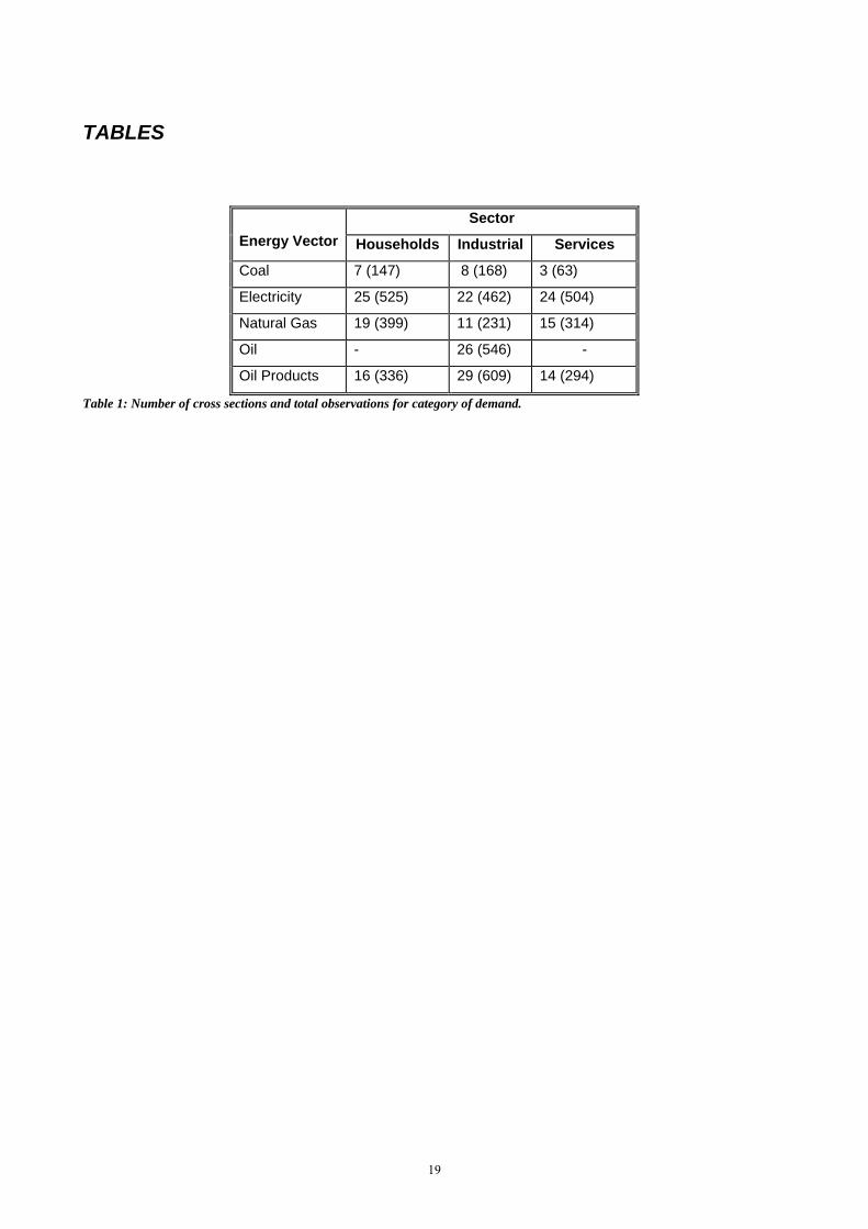
2. Data Our study concerns 13 categories of aggregate energy demand, classified by type of energy vector
(coal, natural gas, electricity, oil and oil products) and by type of user (households3, commercial
and industrial demand). For each category a dynamic model has been formulated and estimated,
using the following observed variables: Real Gross Domestic Product (RGDP), market price and
yearly average temperature, plus the first lag of the demand. Demand and GDP data were taken
from Energy Balances and Energy Statistics (IEA); price data were taken from: Energy Price and
Taxes, (IEA). Temperature data were derived from the High Resolution Gridded Dataset, (Climatic
Research Unit University of East Anglia, UK and the Tyndall Centre for Climate Change
Research). RGDP is expressed in billion 1995 US dollars, using exchange rates for the industrial
sector and using Purchasing Power Parities for households for the household models; in this case
3 Household and commercial demands of crude oil are negligible and hence not considered in this study.
4
RGDP is expressed in per capita terms. Temperatures are expressed in Fahrenheit degrees in order
to allow definite logarithm transformations. Demands are expressed in Ktoe, while prices are
expressed in real terms, in 1995 US dollars4.
For what concerns panel dimensions, the selected collections of data comprise the observations of a
varying number of nations along a period of 23 years, from 1978 to 2000. A problem not to be
overlooked is the occurrence of missing values, mainly among price data. We had to find a
compromise, for each model estimated, between their number and the number of cross sections
included in the panel. We followed simple, rough rules: first, we discarded country specific series
for which too many observations where missing; second, for the series included in each model’s
data, we replaced the remaining missing observations series with moving averages of five
contiguous years. This results in a varying number of countries included in each model., as shown
in table 1. The proportion of missing data filled in for each series using the procedure described
above is in any case, negligible. (below 4%). Therefore we expect the corresponding bias to be at
most of scarcely significant influence.
3. Methodology
3.1 The estimation strategy: GMM estimation of dynamic homogeneous panel data models with unobserved fixed effects
A widely used methodology for dynamic panel modelling applies General Method of Moments
(GMM) estimators. The rationale for relying on Generalized Method of Moments techniques is to
obtain estimates under fairly general assumptions, using at the same time relatively simple
techniques of analysis.
We focus our attention upon the following model:
T1,..., tN,1,...,i ; u c ρy y iti1-ti,it ==+++= βx'it (1)
where ci are the unobserved, specific characteristics of the cross-sections, uit is the error, and ρyi,t-1,
x’itβ is the whole set of regressors; the latter term represents a subset of k-1 generic observed
variables: xit(j) ; j=1,…,k-1. We are dealing with an AR(1) dynamic unobserved effect model,
4 Most data were already available at the desired level off sectoral aggregation, except for the prices of some energy vector prices, which we aggregate into more general categories in a preliminary stage. For the coal model for households, we considered only Steam Coal prices, while for the industrial oil products demand model we considered only Automotive Diesel ones. Moreover, the (industrial) demand for crude oil is mostly nought; thus we considered the correspondent entries for Petroleum Refineries.
5
homogenous in the parameters; throughout the discussion we will always keep the “fixed effects”
hypothesis, i.e. the presence of arbitrary correlation among regressors and unobserved effects.
These theoretical assumptions restrict the range of applicable techniques, which mainly have to do
with the with the treatment of asymptotic proprieties in the “large N, large T” case.
Let us reformulate the model (1) in a more useful expression, where all the regressors are grouped
together:
T1,..., tN,1,...,i ; u c y itiit ==++= γw'it
N1,...,i ; c i =++= iTii uγWy 1 (2)
where 1T is the T-dimensional vector of ones, and: yi = (yi1, …, yiT )’, γ = ( ρ, β’)’, wit = ( yi,t-1,
x’it)’, Wi = (wi1, …, wiT )’. One can obtain several estimators from an auxiliary regression, which is
derived from the original model by applying the First-Differences operator ∆:
N1,...,i ; =+= i'ii ∆uγ∆W∆y . (3)
This transformation removes the individual effects ci; it also inserts on the right-hand side of (3) a
lagged-differenced dependent variable: ∆yi,t-1; which is, by construction, correlated with the error
term ∆uit. Moreover, since the differenced errors derive from serial uncorrelated ones, it does not
necessarily preserve non-correlation among errors5. However, from our point of view, these are not
serious drawbacks of the method.
This method was originally developed by Anderson and Hsiao (1981,1982), who considered a
simple class of dynamic estimators; in particular, they obtained a consistent Instrumental Variables
estimator from model (3) with instruments corresponding to the lagged past differences: ∆yi,t-2; or
levels: yi,t-2; of the original dependent variables. In subsequent works, their strategy has been widely
expanded: on one hand, one can obtain GMM estimators by extending the set of instrumental
variables employed; on the other hand, much effort has been spent in the research of optimal
efficiency, by developing the best set of restrictions connected to the Instrumental Variables (IV)
themselves. The most interesting consequence from our point of view is that this approach allows
the handling of models with non-exogenous and exogenous regressors (other of lags of the
dependent) together, and/or with serially correlated errors (even integrated ones). The latter issues
go beyond the scope of this paper6.
5 Unless one resorts to the Forward Orthogonal Deviations operator, developed by Arellano and Bover (1995). 6 A comprehensive review can be found in Baltagi (1995); chapter 8.

6
3.2 Application to energy demand
Adopted strategy: advantages and drawbacks.
The alternative to GMM estimation would have been using panel data cointegration techniques,
which are extensively applied in the relevant literature on energy demand estimation. However, this
led to a tricky issue, related to the low power of preliminary unit root tests; the results of these tests
in our case were hardly decisive. In other words, the low power of the tests performed made it quite
likely to incur in a type II error. Therefore we could not safely assume that accepting the null
hypothesis of unit roots was justified by the results of the tests7.
It was thus decided to resort to Arellano-Bond estimators. This methodology has the following
advantages:
• it allows to handle strictly exogenous and predetermined regressors, even if arbitrarily
correlated with the unobserved effects;
• it yields robust estimates with respect to serial correlation and heteroskedasticity of errors;
• it does not require any assumption about the initial observations of the dependent variable.
The robustness of estimators is linked to the hypothetical cointegrating relations between the
reference variables: in particular, such estimates can be obtained whether the cointegrating relation
expressed by our particular model is significant (this implies a stationary error) or not (in this case
the error must be integrated).
Recalling the asymptotic results illustrated in the precedent paragraph, in our case the estimates
may be biased, since the panel dimensions of the data have the same order. However this drawback
is of relative importance, given the purposes of this analysis.
It is also worth noting the effects of sources of bias other than the one mentioned above.
1) Sample bias. The original series on which our data are based present some incongruities,
mostly in the form of more or less extended jumps in trends or in levels8. Such occurrences
can be considered outliers, and imputable to exogenous events, such as structural changes of
economies.
2) Cross-sectional correlation of observations. This issue implies the violation of one basic
assumption of general panel data estimators. In our case it appears to be inherent to the
characteristics of the phenomena under scrutiny: in particular, the unit of observations in the
panels are countries, mostly OECD, and one can reasonably expect some homogeneity in their
macroeconomic trends. More precisely, the observed demands may show a certain similarity in
7 For a survey of cointegration issues in panel data, see Banerjee (1999). 8 For instance, in the case of German households demand of electricity, there is a very wide jump imputable to a change
in classification, occurred in 1983. Fortunately in this case correcting the series has been quite straightforward.

7
behaviour, due either to their mutual relations, or to the influence from common economic
events.
These issues were dealt with in the course of a comprehensive data validation stage, using
residual analysis techniques. In brief, the effects of sample bias are more easily recognizable: they
generate a bias in the estimates and in an increase of their estimated variances and covariances;
however they have negligible consequences in presence of a wide number of observations (as in our
case). However, we do not know the effects of cross sectional correlation of observations, but after
some empirical check, we consider it to prevail over the other one, even if the obtained estimates
were considered to be acceptable. This outcome puts evidence, although not always fully
statistically significant, in favour of the hypothesis that the global amount of bias is limited9.
To summarize, the adopted strategy of estimation is not suitable in all circumstances, and in our
case it presents two drawbacks: namely, asymptotic bias and cross-correlation bias. As it will be
shown the estimates are however satisfactory for the purposes of the study. Moreover, alternative
estimators, such as those illustrated in the preceding paragraph, constitute only a partial remedy,
since they are also based on the basic hypothesis of cross-sectional lack of correlation.
It is interesting to note a link between the two drawbacks: the estimators behave optimally in the
fixed T, large N asymptotic context, that is typical of the studies regarding firms, countries, etc.,
where there is a great number of available cross-sections (and few periods observed, at least once
ago): for this reason it is implicitly assumed that the data comes from a random sample of units of
observation; for instance ideally one would have a cross sectional uncorrelated GDP.
9 The practical details will be illustrated in the next section.
8
TABLE 1 ABOUT HERE
3.3 Functional form Since our main interest is to derive long-run elasticities of energy demand to temperature, we focus
our attention upon log-log demand models having the following functional form:
T1,..., tj,i N,1,...,ji, ; u c Tβ Pβ Pβ Yβ ρD δt β D itiit4jt3it2it11-ti,0it =≠=++++++++= ; (4)
where Dit represents the logarithm of the demand, while Yit, Pit, Pjt and Tit stand for the logs of
RGDP, end-user prices (for the energy vector under scrutiny and for alternative fuels when
relevant10) and yearly average temperature11.
In terms of model (3), this becomes:
∆=≠=∆+∆+∆+∆+∆+∆+=∆ T1,..., tj,i N,1,...,ji, ; u Tβ Pβ Pβ Yβ Dρ δ D itit4jt3it2it11-ti,it (5)
Computations were performed using STATA’s xtabond procedure. We opted for robust estimators
as specified in the Appendix (equations (A3) and (A5)), which are the most suitable ones under
general assumptions of residual serial correlation and homoskedasticity. This choice however has
the drawback of invalidating the results of the Sargan specification test: consequently we assumed
the regressors to be all endogenous12. Moreover, the number of the available instrumental variables
used (described in Section 5.1) was kept to a minimum, in order to be as little as possible affected
by asymptotic biases.
3.4 Tests performed The xtabond procedure automatically performs two of the validation tests defined by Arellano and
Bond, i.e., the Sargan specification test and the lack of auto-correlation test. In particular, the first is
based upon the assumption of lack of serial correlation (of the differenced error ∆uit).
10 In practical terms, we considered only the cases of oil products as substitute for gas, and of gas as substitute for oil products. Note that, although demand theory often places restrictions on cross price elasticities for households, in our estimations we took a more agnostic approach and no restrictions were placed on the elasticities. 11 A trend term δt was also inserted into the equation, but it actually does not fully capture the trend behaviour of
observations, since the variables in the model are not de-trended: the specification of trend components of the variables would require, in our case, knowledge about unit roots. Thus the term only adjusts the trend slope of the fitted values of the original model.
12 Formally: CORR(Xis, uit) = 0 for t>s; with Xit representing each single regressor.
9
The second test, used to test lack of correlation of second order, provides a fundamental check for
the consistency of estimators. However, for what stated before it is best recommendable to do not
completely rely upon its results, and consider the estimates likely to be to a certain extent biased.
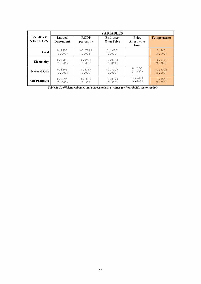
4. Results Tables 2, 3, 4 and 5 present, respectively for households, industrial and commercial users (service
sector, with two alternative specifications), the estimated values of elasticities and of the
autoregressive coefficient, together with the p-values of the respective significance test. The models
for households sector are mostly consistent with the underlying economic theory: with the
exception of coal demand, expectations upon sign and magnitude of the estimates have been
respected. In particular we observe a positive relationship between income and energy demand, and
negative relationships between energy vectors’ demands and own prices. By contrast, a (mildly)
significant and positive relationship with the price of alternative fuels is present only in the case of
gas, whose demand is positively affected by an increase in the price of oil products. Interestingly,
the reverse does not happen: the correspondent elasticity for the oil products model is negative but
not significant. A possible explanation is the different range of alternative household use of the two
energy vectors: gas is mainly used for heating, while oil products include heating diesel as well as
transportation fuels. Thus “oil products” can be a substitute for gas, (the switching costs are well
within a long–term family budget), but the scope for the reverse to happen is rather limited. The
negative relationship between coal for households use and RGDP may point to the nature of inferior
good of coal for heating use; the value pertinent to the lagged dependent variable is admissible and
consistent with the other cases. More puzzling appears the positive and significant sign of the
elasticity to temperature of coal demand: it might be partially due to the low popularity of coal for
heating use. Price seem not to bear a significant relationship with coal demand. The missing
observation bias, which in the case of coal is stronger due to the sensibly lesser amount of
observations, may have also partially caused these results. Some other statistically not-significant
estimates (e.g. the elasticity to RGDP in the case of oil products demand) can be regarded, in the
context of to the whole set of residential demand results, as acceptable.
Note that in all models presented, the constant, which captures the effect of the trend in the
differential approach of equation (11), is not included. It was decided to drop it because in the
alternative specification in which it was included, it was of negligible magnitude and, most
importantly, never significant in all the residential demand models. In other word, these models are
all stationary.
10
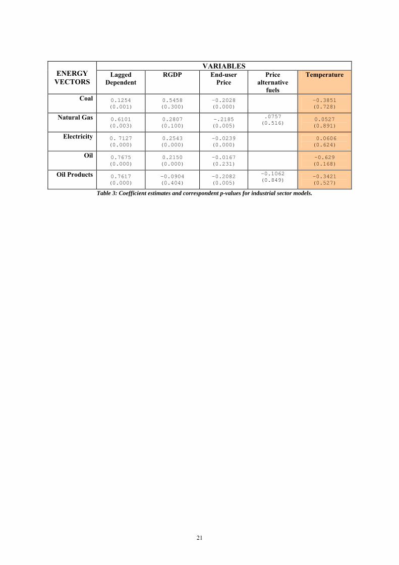
TABLE 2 ABOUT HERE The results are less reliable for industrial users demands: in this case the economic expectations are
still respected, including the non significance of the elasticities to the temperature, but the
significance of the remaining elasticities is rather uncertain, in particular in the case of prices. In
order to investigate this issue, we fitted models of the same general form for sub-aggregated voices
of demand13, because they can best take account of the phenomenon under investigation. A
comparison between original and restricted fitted models is available from the authors upon request.
Only for coal demand the restricted model’s can be considered a better specification, in the sense of
statistical significance of estimates, while the outcomes for the remaining vectors are uncertain.
A secondary issue, regarding the industrial demand of oil, is to establish at what extent the
disaggregated demand concerning High Sulphur Oil can provide a better result with respect to the
original one based on average prices14. The alternative model has practically the same estimated
parameters, but it does not yield any significant gain with respect the one based on average oil
prices in terms of variability of the estimates. Again, alternative estimates are available upon
request.
TABLE 3 ABOUT HERE
TABLE 4 ABOUT HERE
Table 4 and Table 5 illustrate the service sector case15. Here, a situation similar to the industrial
case arises: the lagged dependent turns out to be most significant explanatory variable, while the
relationship with the other explanatory variable is not very much supported by the data. Considering
GDP per capita instead of GDP brings about only modest improvements in the estimates: the
significance of the elasticity of prices and income increases. Also, temperatures display a mildly
significant negative effect on demand in the case of electricity and coal. The sample size for coal is
however too small to draw any robust conclusion.
TABLE 5 ABOUT HERE Finally, we looked at the relevance of the trend for the industrial and commercial demand models16.
It turns out that in the case of industrial demand, parameter estimates are not invariant to the
inclusion of the trend. In particular, both the sign and magnitude of the elasticity of industrial 13 The restricted models consider the demand of each energy vector by public and auto-producer electricity plants and
public and auto-producer CHP Plants. Other variables remained the same. 14 Because the price series for High Sulphur Oil has the highest number of observations. 15 Here we present both the models including GDP among the explanatory variables, and the alternative ones including GDP per capita, because there was no clear a priori reason to exclude either type of models. 16 Results for the model in which the trend is included are available upon request.

11
demand for coal and electricity to temperature are affected. However, temperature elasticity remains
non significant for all the energy vectors. The trend parameter itself is however often significant,
although it remains of negligible magnitude (bar the case of coal).
In the case of commercial demand, the trend is hardly ever significant (the only exception is again,
coal), and its inclusion makes the only mildly meaningful temperature elasticity (the electricity
demand’s one) to become not significant.
Thus from our particular point of view, including a trend parameter does not help; at most, it adds
evidence to the lack of relationship between industrial energy demand and temperature.
In all models, the estimates of the autoregressive parameter for the various categories of demand
are high, and, with no exception, highly significant. This result is consistent with the underlying
econometric theory, in the sense that demand for the various energy vectors display temporal
persistence. Moreover, the regressive relationship between the dependent variable and its first lag is
always highly significant. We regard this outcome as an indication of consistence of the whole set
of results, and thus, as stated before, that the sources of bias previously indicated in Section 3 do not
affect too heavily the results of the analysis.
Another argument in favour of the above statement derives from considering the results concerning
the efficiency of the estimates. Tables 6 shows the estimated standard errors and 95% confidence
intervals of the variables included in our household models (we do not include analogous tables for
the industrial and commercial sectors for economy of space). The estimation procedure performed
quite well. Once again, the best results pertain to the lagged dependent variable: in brief, by
considering 95% confidence intervals it is easily verifiable that the results are consistent with what
stated before. Aside from this, it is interesting to note that a certain amount of variability of
estimates is, on the theoretical ground, imputable to the parameter homogeneity of the model, i.e.,
the hypothesis of identity of the regression coefficients for each unity of the panels of data.
TABLE 6 ABOUT HERE
For household demand we observe in most cases appreciable values of standard errors of the
estimates, together with confidence intervals whose extremes have the same sign of the parameter
under scrutiny. Exceptions to the latter statement are Coal and Oil Products demand; however, they
always occur in concomitance with not significant estimates, and, consequently, does not point to a
mis-specified result. Given the values of variation coefficients in Table 7, we can conclude that the
estimates perform reasonably well in terms of efficiency: mostly, the standard errors approximately
possess half the magnitude of the estimates. The same conclusion can be drawn by considering the
respective 95% confidence intervals.

12
In the case of the industrial and commercial demand models, results are rather similar for what
concerns both the magnitude of variability and the sign of 95% confidence intervals. This however
is not the case for temperature in the industrial models. This is an admissible outcome, given that
temperature coefficient estimates never pass their own significance test. For the remaining variables
we observe once again a strict correspondence between mis-specified intervals and lack of
statistical significance of estimates; moreover, the estimates display once again appreciable
efficiency.
TABLE 7 ABOUT HERE
5. Conclusions This paper is a first attempt to investigate the effect of climate on the demand for different energy
vectors by residential, commercial and industrial users, by means of a dynamic panel analysis of the
demand for coal, gas, electricity, oil and oil products in OECD and (a few) non-OECD countries.
Previous studies on the relationship between energy demand and temperature generally focused on
single country (or even single province) time series analysis.
The main rationale for using a dynamic panel approach has been to try and extrapolate a long-run
relationship between temperature and energy demand, using cross-sectional variation as a spatial
analogy of different long-run equilibrium demands.
The ultimate motivation for this is to arrive to a consistent evaluation of the impact of climate
change on a key class of consumption goods and primary factors such as energy vectors, which can
be used as inputs for climate change simulations in an Integrated Assessment Model framework.
Results differ substantially across categories of users. Temperature has a very different influence on
the demand of energy as a consumption good and on the demand of energy as a primary factor.
Residential demand responds negatively to temperature increases, (but this does not happens for all
energy vectors), pointing at a prevalence of heating needs in determining residential demand. By
contrast, industrial demand is insensitive to temperature increases. In the case of the service sector,
only electricity demand displays a mildly significant negative elasticity to temperature changes.
These results appear to be invariant to variations in the specification of the models such as the
inclusion of a trend parameter, or different definitions of the reference price for oil, or the restriction
of the analysis of industrial demand to the most energy intensive sub-sector.
This study is quite preliminary and, as such, suffers from some obvious limitations.
Data limitations had a non-negligible role in shaping our analysis: we were confined to those data
series which are available for a reasonable number of countries, enough to build up a reliable panel.
13
In some cases this proved just impossible: price and demand data for coal are available for just an
handful of countries (particularly in the service sector case). For some explanatory variables, we
had to content ourselves with second-best choices. For instance, GDP and GDP per capita are just
proxies for sectoral value added and disposable income. The choice of yearly average temperature
as a temperature data was also a compromise. Ideally we would have used heating and cooling
degree days, which express how much temperature in a country has differed from a temperature
level conventionally regarded as thermally optimal, in a given year17. Reasonably long time-series
for these variables are only available for the USA and an handful of other OECD countries. We did
have at our disposal seasonal and monthly temperature averages, but the information provided was
no better than the yearly average one: the main conclusion that could be drawn from model
specification in which seasonal and monthly temperature averages were included was still that
heating demand was the main driver of the negative relationship between residential demand and
temperature. Thus we decided to present only the results on yearly temperature as the most
parsimonious ones18.
Another limitation of our analysis is that the equations estimated are reduced forms, which reflect
both demand and supply effects. The interpretation of our coefficients as elasticities of energy
vectors’ demand to the corresponding explanatory variable rests on the implicit assumption that, in
the long run, demand is more stable than supply. Simultaneous equations estimation for a complete
demand-supply equilibrium in a dynamic panel framework is a formidable task and goes beyond the
scope of our paper19.
Our current research is focused on improving the analysis in at least two regards. First, we are
interested in modelling non-linear temperature effects on demand. It is in fact very likely that not
only the level of the temperature matters, but also the intensity of the change. Second, we are
interested in the geographical implications of the relationships under scrutiny. For instance we
17 Heating Degree Days are defined as the cumulative number of degrees within the temporal unit of observation (generally month or year) by which the mean daily temperature falls below a reference value for thermal comfort, usually 18.3°C/65°F. Cooling Degree Days are defined analogously and apply to the days in which the mean temperature is above such reference value. 18 There were two practical reason for focusing on single yearly temperature elasticity parameter. The first is that, in our intention, these estimates should feed in an Integrated Assessment Model calibrated on yearly data. The second is that in order to fully account for seasonal variability, we would have needed quarterly data for prices and consumption for our panel (separately for household, industrial and commercial consumption). For any given annual temperature average , in fact, energy consumption can be very different according to whether that average is the result of a steady pattern of almost constant temperatures or of wide swings from a very cold winter to a very hot summer. The fact that climate change is expected to increase seasonal variability of temperatures adds to the relevance of this issues. We have been unable so far to access data of this kind of detail for the same sample used for the analysis presented in this paper. Nevertheless, we are aware of the implications of seasonal variability for energy demand, and our ongoing research is focusing on designing a strategy to tackle this issue. 19 In partial support to our approach Engsted and Bentzen (1997) broadly indicate our specification (energy demand dependent from prices income and temperature) as the “the way it has been usually done in the literature”.

14
intend to test the opportunity of using North /South sub-panels and the explore the issue of the
extrapolation of non-OECD temperature elasticities.
15
6. References
Al-Zayer J, Al-Ibrahim A. Modelling the impact of temperature on electricity consumption in the
eastern province of Saudi Arabia. Journal of Forecasting 1996; 15; 97-106
Amato, A.D, Ruth, M., Regional Responses to Climate Change: Methodology and Application to
the Commonwealth of Massachusetts University of Maryland, Mimeo, 2004; retrieved from
http://www.publicpolicy.umd.edu/faculty/ruth/Energy-Climate_M_Ruth.pdf.
Anderson, T.W., Hsiao, C. Estimation of Dynamic Models with Error Components, Journal of the
American Statistical Association, 1981;76; 598-606.
Anderson, T.W., Hsiao, C. 1982: Formulation and Estimation of Dynamic Models Using Panel
Data, Review of Economic Studies, 58, 277-297.
Arellano, M. Panel Data Econometrics, Oxford University Press: Oxford; 2003a.
Arellano, M. Modelling Optimal Instrumental Variables For Dynamic Panel Data Models.
CEMFI Working Paper wp2003_0310, CEMFI: Madrid; 2003b.
Arellano, M., Bover O. Another look at the instrumental Variable Estimator of Error-Component
Models. Journal of Econometrics 1995;68; 29-51.
Arellano, M., Bond S. Some Tests of Specification for Panel Data: Monte Carlo evidence and an
Application to Employment equations. Review of Economic Studies 1991;58; 277-297.
Baltagi, B.H.: Econometric Analysis of Panel Data, John Wiley: Chichester; 1995.
Banerjee, A Panel Data Unit Roots and Cointegration: an Overview. Oxford Bulletin of Statistics
1999;61 (Special Issue); 607-629.
Beenstock, M, Goldin, E., Nabot, D. The demand for electricity in Israel. Energy Economics
1999;21; 168-183.
Bentzen, J., Engsted, T. A Revival of the Autoregressive Distributed Lag Model in Estimating
Energy Demand Relationships. Energy 2001;26; 45-55.
Engsted, T., Bentzen, J. Dynamic Modelling of Energy Demand: A Guided Tour Through the
Jungle of Unit Roots and Cointegration" OPEC Review 1997;21; 261-293.
Giannakopoulos, C., Psiloglou, B. E. Majithia, S. Weather and non-weather related factors affecting
energy load demand: a comparison of the two cases of Greece and England. Geophysical
Research Abstracts 2005;7; retrieved from
http://www.cosis.net/abstracts/EGU05/06969/EGU05-J-06969.pdf.
16
Glasure Y. U., Lee, A-R. Cointegration, Error Correction and the Relationship between GDP and
Energy: the case of South Korea and Singapore. Resource and Energy Economics 1997;20,
17-25.
GRTN. Rapporto sulle attività del Gestore della Rete di Trasmissione Nazionale, GRTN: Rome;
2005; retrieved from http://www.grtn.it/ita/chisiamo/rapportoattivitadocs2005.asp
Hanley, A. and Peirson, J. Residential energy demand and the interaction of price and temperature:
British experimental evidence. Energy Economics 1998, 20, 157-171.
Masih, A.M.M., Masih, R. Energy Consumption, Real Income and Temporal Causality: Results
From a Multi-Country Study Based on Cointegration and Error-Correction Modelling
Techniques, Energy Economics, 1996;18; 165-183.
Pardo A, Meneu V, Valor E. Temperature and seasonality influences on Spanish electricity load.
Energy Economics 2002;24; 55-70.
Sailor D.J. Relating residential and commercial sector electricity loads to climate evaluating state
level sensitivities and vulnerabilities, Energy 2001;26;: 645-657.
Silk J.I., Louz, F. L. Short and Long-Run Elasticities in the US Residential Electricity Demand: a
Co-Integration Approach, Energy Economics 1997; 19; 493-513.
Stern, D.I, A Multivariate Cointegration Analysis of the Role of Energy in the US Macroeconomy.
Energy Economics 2000;22; 267-283.
Taylor, J. W., Buizza, R. Using weather ensemble predictions in electricity demand forecasting.
International Journal of Forecasting 2003;19; 57–70.
TERNA Rapporto mensile sul sistema elettrico. Consuntivo gennaio 2006. Terna S.p.A.: Rome;
2006; retrieved from
http://193.108.204.130/ita/sistemaelettrico/documenti/RM_20060131_20060210_GENNAIO_
2006.PDF.
Valor E, Meneu V, Caselles V. Daily air temperature and electricity load in Spain. Journal of
Applied Meteorology 2001;408; 1413-1421.

17
Appendix: Arellano-Bond estimators
General form of the estimators:
Arellano and Bond (1991) set up the GMM method of estimation in a wide class of models and
discuss three specification tests.
The construction of the matrixes of instrumental variables, which from now on will be indicated
with: Z = ( Z’1,…,Z’i,…,Z’N )’, follows the guideline of Anderson and Hsiao (1981). In brief,
considering the lagged endogenous variables: ∆yi,t-1, t=2,…,T; one can select all past levels of the
original dependent (more suitable than first differences); for any t as above the available IV are: yi,t-
2, …, yi1. It is also possible to employ all the first differences of the remaining variables (for
example: ∆xit(j) , t=2,…,T) if they satisfy the strict exogeneity assumption. If there exists some
endogenous or predetermined regressor, say xit(h), one must make a selection among the set of past
levels: ∆xit-1(h), …, ∆xi1
(h), t=2, …, T; which will play the role of instruments for ∆xit(h).
In any case one obtains block-diagonal matrixes Zi, which give rise to the moment restrictions:
[ ] ( )[ ] N1,...,i ; E E ==−= 0γ∆W∆yZ∆uZ 'ii
'ii
'i . (A1)
For example, in the case in which all the regressors xit(j) are exogenous, the generic Zi with the full
set of available IV has the form:
[ ] [ ] [ ]( ) ,y..., ,y , ... , ,y,y , ,y diag 1-iTi0i1i0i0'i
'i
'ii ∆x∆x∆xZ = . (A2)
where ∆xi is the stacked vector of: ∆xit ; t=2, …, T.
For any choice of the instruments, the general form of GMM estimators based on restrictions (A1)
is the following:
( )
;
ˆN
1i
N
1i
1N
1i
N
1i
1
⎟⎠
⎞⎜⎝
⎛⎟⎠
⎞⎜⎝
⎛⎥⎦
⎤⎢⎣
⎡⎟⎠
⎞⎜⎝
⎛⎟⎠
⎞⎜⎝
⎛=
==
∑∑∑∑==
−
==
−
i'iNi
'ii
'iNi
'i
'N
''N
'GMM
∆yZAZ∆W∆WZAZ∆W
∆yZZA∆W∆WZZA∆Wγ (A3)
where AN is an arbitrary N×N matrix of weights, ∆W = (∆W’1,…, ∆W’N )’, ∆y = (∆y’1,…, ∆y’N )’,
and Z defined as above. Thus we obtain:
• one-step estimator with 1N
1i
−
=
⎟⎠
⎞⎜⎝
⎛= ∑ i
'iN ZZA ; (A4)
• two-step estimators with 1N
1i
~ −
=
⎟⎠
⎞⎜⎝
⎛= ∑ i
'iN ZΩZA , or
1N
1i
~~ −
=
⎟⎠
⎞⎜⎝
⎛= ∑ i
'ii
'iN Zu∆u∆ZA (A5);

18
where ∑=
=N
1i
~~ ~ 'ii u∆u∆Ω is a matrix of arbitrary consistent estimates of the unrestricted variances and
covariances of the errors of model (3)20.
Asymptotic behaviour:
A relevant issue for the present discussion is that the Arellano-Bond estimators perform optimally
in the fixed T, large N context; however their performance worsens for large T, for any value of N.
In the case of T fixed, large N it is recommended to use the full set of instrumental variables
discussed above, and adopt the one-step estimator under homoskedasticity and lack of serial
correlation of the errors, or else the two-step estimators (7) and (8). Arellano (2003b) found, under
restrictive assumptions, that with large N, large T the one-step estimator is asymptotically biased of
order O(m*N-1), with m=k-1, i.e., the number of regressors other than ∆yi,t-1.
However, the loss of performance can be explained by the fact21 that the Arellano-Bond estimators
implicitly involve particular forms of (cross-section specific, unrestricted) linear projection of the
∆wit’s onto the columns of Zi; for example, if the xit(j) ‘s are all predetermined we can write:
T,...,2 tN,1,...,i ; ... ==+++= i1'tt-1ti,
't2it
't1it zπzπzπp (A6)
In any case the projections comprise a T-dependent, monotonically increasing number of addends,
giving rise to the problems of “consistently estimating” the respective coefficients: πts for large T.
In particular, it may cause asymptotical bias of the estimates for large N, large T, if the ratio T/N
tends to a non negligible constant.
In order to bypass this problem one can consider two strategies:
1) Adopt an alternative estimator.
Considering the class of the IV-based ones, Arellano (2003a) suggests a Two-Stage Least Squares
estimator in the case of exogenous regressors, which involves linear projections with a fixed
number of addends, or else a “stacked-IV” estimator, which uses the first J lags: zit,…,zi,t-J+1, J
fixed, to form common instruments for all periods.
2) Impose restrictions on the linear projections.
One technique that presents such feature is developed in Arellano (2003b), but it requires much
more complicated computations. However, intuitively this complexity is due to the objective of
obtaining an estimator with good performances in each asymptotic context, and this implies both
keeping constant the number of coefficients of the (restricted) linear projections, and exploiting the
information of all available periods.
20 The term iu∆~ stands for the estimated residuals of the same model. 21 For details see Arellano (2003a), paragraphs 7.3.2, 7.3.3 and 8.7.
19
TABLES
Sector Energy Vector Households Industrial Services
Coal 7 (147) 8 (168) 3 (63)
Electricity 25 (525) 22 (462) 24 (504)
Natural Gas 19 (399) 11 (231) 15 (314)
Oil - 26 (546) -
Oil Products 16 (336) 29 (609) 14 (294)
Table 1: Number of cross sections and total observations for category of demand.
20
VARIABLES ENERGY
VECTORS Lagged
Dependent RGDP
per capita End-user
Own Price Price
Alternative Fuel
Temperature
Coal 0.9357 (0.000)
-0.7599 (0.025)
0.1650 (0.022)
2.845 (0.000)
Electricity 0.8983 (0.000)
0.0977 (0.075)
-0.0183 (0.004) -0.5762
(0.000)
Natural Gas 0.8205 (0.000)
0.3169 (0.000)
-0.3208 (0.004)
0.1157 (0.037)
-1.8225 (0.000)
Oil Products 0.8194 (0.000)
0.1007 (0.532)
-0.0479 (0.653)
-0.1201 (0.219)
-3.0548 (0.023)
Table 2: Coefficient estimates and correspondent p-values for households sector models.
21
VARIABLES ENERGY
VECTORS Lagged
Dependent RGDP End-user
Price Price
alternative fuels
Temperature
Coal 0.1254 (0.001)
0.5458 (0.300)
-0.2028 (0.000)
-0.3851 (0.728)
Natural Gas 0.6101 (0.003)
0.2807 (0.100)
-.2185 (0.005)
.0757 (0.516)
0.0527 (0.891)
Electricity 0. 7127 (0.000)
0.2543 (0.000)
-0.0239 (0.000)
0.0606 (0.624)
Oil 0.7675 (0.000)
0.2150 (0.000)
-0.0167 (0.231)
-0.629 (0.168)
Oil Products 0.7617 (0.000)
-0.0904 (0.404)
-0.2082 (0.005)
-0.1062 (0.849)
-0.3421 (0.527)
Table 3: Coefficient estimates and correspondent p-values for industrial sector models.

22
VARIABLES ENERGY
VECTORS Lagged Dependent
RGDP End-user Price
Price alternative fuels
Temperature
Coal 0. 7589 (0.000)
-1.0514 (0.055)
0. 3212 (0.170)
-2.5484 (0.064)
Electricity 0. 9353 (0.000)
0.1031 (0.144)
-0.00954 (0.222)
-0.1984 (0.352)
Natural Gas 0.8057 (0.000)
0.5563 (0.023)
-0.1915 (0.434)
-0.1478 (0.910)
-0.1534 (0.440)
Oil Products 0.5195 (0.000)
-0.2344 (0.354)
0.3005 (0.111)
-.05852 (0.796)
-2.1340 (0.232)
Table 4: Coefficient estimates and correspondent p-values for service sector models.

23
VARIABLES ENERGY VECTORS Lagged
Dependent RGDP
per capita End-user
Price Price
alternative fuel Temperature
Coal 0.7851 (0.000)
-1.0631 (0.015)
0.2739 (0.166) - -2.7282
(0.026)
Electricity 0.9286 (0.000)
0.1497 (0.051)
-0.0155 (0.012) - -0.0332
(0.084) Natural Gas 0.7861
(0.000) 0.8812 (0.024)
-0.3147 (0.144)
0.0902 (0.462)
-2.0688 (0.280)
Oil Products 0.4919 (0.000)
-0.4849 (0.160)
0.4690 (0.057)
-0.3535 (0.239)
-1.940 (0.198)
Table 5: Coefficient estimates and correspondent p-values for service sector models (GDP per capita) sector.

24
VARIABLES ENERGY
VECTORS Lagged Dependent
RGDP pro capita End-user Price
Price alternative fuel
Temperature
Coal 0.06217 (0.81, 1.05)
0.3392 (-1.42, -0.95)
0.00722 (0.02, 0.3) 0.4353
(1.99, 3.69)
Electricity 0.0297 (0.84, 0.96)
0.055 (-0.01, 0.20)
0.0064 (-0.03, -0.006) 0.113
(-0.79, -0.35)
Natural Gas 0.0803 (0.66, 0.98)
0.0870 (0.15, 0.49)
0.1113 (-0.54, -0.1)
0.0553 (0.007, 0.22)
0.371 (-2.45, -1.1)
Oil Products
0.0589 (0.70, 0.93)
0.1061 (-0.21, 0.42)
0.106 (-0.16, 0.25)
0.0976 (-0.31, 0.07)
1.345 (-5.69, -0.42)
Table 6: Standard error and 95% confidence intervals of estimates for households sector models.

25
VARIABLES ENERGY
VECTORS Lagged
Dependent RGDP End-user
Price Price
alternative fuel
Temperature
Coal 0.07 -0.45 0.04 0.15 Electricity 0.03 0.06 -0.35 -0.20
Natural Gas 0.10 0.27 -0.35 0.48 -0.20 Oil Products 0.07 1.05 -2.21 -0.81 -0.44
Table 7: Variation coefficients of estimates for households sector models.
NOTE DI LAVORO DELLA FONDAZIONE ENI ENRICO MATTEI Fondazione Eni Enrico Mattei Working Paper Series
Our Note di Lavoro are available on the Internet at the following addresses: http://www.feem.it/Feem/Pub/Publications/WPapers/default.html
http://www.ssrn.com/link/feem.html http://www.repec.org
http://agecon.lib.umn.edu
NOTE DI LAVORO PUBLISHED IN 2006
SIEV 1.2006 Anna ALBERINI: Determinants and Effects on Property Values of Participation in Voluntary Cleanup Programs: The Case of Colorado
CCMP 2.2006 Valentina BOSETTI, Carlo CARRARO and Marzio GALEOTTI: Stabilisation Targets, Technical Change and the Macroeconomic Costs of Climate Change Control
CCMP 3.2006 Roberto ROSON: Introducing Imperfect Competition in CGE Models: Technical Aspects and Implications KTHC 4.2006 Sergio VERGALLI: The Role of Community in Migration Dynamics
SIEV 5.2006 Fabio GRAZI, Jeroen C.J.M. van den BERGH and Piet RIETVELD: Modeling Spatial Sustainability: Spatial Welfare Economics versus Ecological Footprint
CCMP 6.2006 Olivier DESCHENES and Michael GREENSTONE: The Economic Impacts of Climate Change: Evidence from Agricultural Profits and Random Fluctuations in Weather
PRCG 7.2006 Michele MORETTO and Paola VALBONESE: Firm Regulation and Profit-Sharing: A Real Option Approach SIEV 8.2006 Anna ALBERINI and Aline CHIABAI: Discount Rates in Risk v. Money and Money v. Money Tradeoffs CTN 9.2006 Jon X. EGUIA: United We Vote CTN 10.2006 Shao CHIN SUNG and Dinko DIMITRO: A Taxonomy of Myopic Stability Concepts for Hedonic Games NRM 11.2006 Fabio CERINA (lxxviii): Tourism Specialization and Sustainability: A Long-Run Policy Analysis
NRM 12.2006 Valentina BOSETTI, Mariaester CASSINELLI and Alessandro LANZA (lxxviii): Benchmarking in Tourism Destination, Keeping in Mind the Sustainable Paradigm
CCMP 13.2006 Jens HORBACH: Determinants of Environmental Innovation – New Evidence from German Panel Data SourcesKTHC 14.2006 Fabio SABATINI: Social Capital, Public Spending and the Quality of Economic Development: The Case of ItalyKTHC 15.2006 Fabio SABATINI: The Empirics of Social Capital and Economic Development: A Critical Perspective CSRM 16.2006 Giuseppe DI VITA: Corruption, Exogenous Changes in Incentives and Deterrence
CCMP 17.2006 Rob B. DELLINK and Marjan W. HOFKES: The Timing of National Greenhouse Gas Emission Reductions in the Presence of Other Environmental Policies
IEM 18.2006 Philippe QUIRION: Distributional Impacts of Energy-Efficiency Certificates Vs. Taxes and Standards CTN 19.2006 Somdeb LAHIRI: A Weak Bargaining Set for Contract Choice Problems
CCMP 20.2006 Massimiliano MAZZANTI and Roberto ZOBOLI: Examining the Factors Influencing Environmental Innovations
SIEV 21.2006 Y. Hossein FARZIN and Ken-ICHI AKAO: Non-pecuniary Work Incentive and Labor Supply
CCMP 22.2006 Marzio GALEOTTI, Matteo MANERA and Alessandro LANZA: On the Robustness of Robustness Checks of the Environmental Kuznets Curve
NRM 23.2006 Y. Hossein FARZIN and Ken-ICHI AKAO: When is it Optimal to Exhaust a Resource in a Finite Time?
NRM 24.2006 Y. Hossein FARZIN and Ken-ICHI AKAO: Non-pecuniary Value of Employment and Natural Resource Extinction
SIEV 25.2006 Lucia VERGANO and Paulo A.L.D. NUNES: Analysis and Evaluation of Ecosystem Resilience: An Economic Perspective
SIEV 26.2006 Danny CAMPBELL, W. George HUTCHINSON and Riccardo SCARPA: Using Discrete Choice Experiments toDerive Individual-Specific WTP Estimates for Landscape Improvements under Agri-Environmental SchemesEvidence from the Rural Environment Protection Scheme in Ireland
KTHC 27.2006 Vincent M. OTTO, Timo KUOSMANEN and Ekko C. van IERLAND: Estimating Feedback Effect in Technical Change: A Frontier Approach
CCMP 28.2006 Giovanni BELLA: Uniqueness and Indeterminacy of Equilibria in a Model with Polluting Emissions
IEM 29.2006 Alessandro COLOGNI and Matteo MANERA: The Asymmetric Effects of Oil Shocks on Output Growth: A Markov-Switching Analysis for the G-7 Countries
KTHC 30.2006 Fabio SABATINI: Social Capital and Labour Productivity in Italy ETA 31.2006 Andrea GALLICE (lxxix): Predicting one Shot Play in 2x2 Games Using Beliefs Based on Minimax Regret
IEM 32.2006 Andrea BIGANO and Paul SHEEHAN: Assessing the Risk of Oil Spills in the Mediterranean: the Case of the Route from the Black Sea to Italy
NRM 33.2006 Rinaldo BRAU and Davide CAO (lxxviii): Uncovering the Macrostructure of Tourists’ Preferences. A Choice Experiment Analysis of Tourism Demand to Sardinia
CTN 34.2006 Parkash CHANDER and Henry TULKENS: Cooperation, Stability and Self-Enforcement in International Environmental Agreements: A Conceptual Discussion
IEM 35.2006 Valeria COSTANTINI and Salvatore MONNI: Environment, Human Development and Economic Growth ETA 36.2006 Ariel RUBINSTEIN (lxxix): Instinctive and Cognitive Reasoning: A Study of Response Times
ETA 37.2006 Maria SALGADO (lxxix): Choosing to Have Less Choice
ETA 38.2006 Justina A.V. FISCHER and Benno TORGLER: Does Envy Destroy Social Fundamentals? The Impact of Relative Income Position on Social Capital
ETA 39.2006 Benno TORGLER, Sascha L. SCHMIDT and Bruno S. FREY: Relative Income Position and Performance: An Empirical Panel Analysis
CCMP 40.2006 Alberto GAGO, Xavier LABANDEIRA, Fidel PICOS And Miguel RODRÍGUEZ: Taxing Tourism In Spain: Results and Recommendations
IEM 41.2006 Karl van BIERVLIET, Dirk Le ROY and Paulo A.L.D. NUNES: An Accidental Oil Spill Along the Belgian Coast: Results from a CV Study
CCMP 42.2006 Rolf GOLOMBEK and Michael HOEL: Endogenous Technology and Tradable Emission Quotas
KTHC 43.2006 Giulio CAINELLI and Donato IACOBUCCI: The Role of Agglomeration and Technology in Shaping Firm Strategy and Organization
CCMP 44.2006 Alvaro CALZADILLA, Francesco PAULI and Roberto ROSON: Climate Change and Extreme Events: An Assessment of Economic Implications
SIEV 45.2006 M.E. KRAGT, P.C. ROEBELING and A. RUIJS: Effects of Great Barrier Reef Degradation on Recreational Demand: A Contingent Behaviour Approach
NRM 46.2006 C. GIUPPONI, R. CAMERA, A. FASSIO, A. LASUT, J. MYSIAK and A. SGOBBI: Network Analysis, CreativeSystem Modelling and DecisionSupport: The NetSyMoD Approach
KTHC 47.2006 Walter F. LALICH (lxxx): Measurement and Spatial Effects of the Immigrant Created Cultural Diversity in Sydney
KTHC 48.2006 Elena PASPALANOVA (lxxx): Cultural Diversity Determining the Memory of a Controversial Social Event
KTHC 49.2006 Ugo GASPARINO, Barbara DEL CORPO and Dino PINELLI (lxxx): Perceived Diversity of Complex Environmental Systems: Multidimensional Measurement and Synthetic Indicators
KTHC 50.2006 Aleksandra HAUKE (lxxx): Impact of Cultural Differences on Knowledge Transfer in British, Hungarian and Polish Enterprises
KTHC 51.2006 Katherine MARQUAND FORSYTH and Vanja M. K. STENIUS (lxxx): The Challenges of Data Comparison and Varied European Concepts of Diversity
KTHC 52.2006 Gianmarco I.P. OTTAVIANO and Giovanni PERI (lxxx): Rethinking the Gains from Immigration: Theory and Evidence from the U.S.
KTHC 53.2006 Monica BARNI (lxxx): From Statistical to Geolinguistic Data: Mapping and Measuring Linguistic Diversity KTHC 54.2006 Lucia TAJOLI and Lucia DE BENEDICTIS (lxxx): Economic Integration and Similarity in Trade Structures
KTHC 55.2006 Suzanna CHAN (lxxx): “God’s Little Acre” and “Belfast Chinatown”: Diversity and Ethnic Place Identity in Belfast
KTHC 56.2006 Diana PETKOVA (lxxx): Cultural Diversity in People’s Attitudes and Perceptions
KTHC 57.2006 John J. BETANCUR (lxxx): From Outsiders to On-Paper Equals to Cultural Curiosities? The Trajectory of Diversity in the USA
KTHC 58.2006 Kiflemariam HAMDE (lxxx): Cultural Diversity A Glimpse Over the Current Debate in Sweden KTHC 59.2006 Emilio GREGORI (lxxx): Indicators of Migrants’ Socio-Professional Integration
KTHC 60.2006 Christa-Maria LERM HAYES (lxxx): Unity in Diversity Through Art? Joseph Beuys’ Models of Cultural Dialogue
KTHC 61.2006 Sara VERTOMMEN and Albert MARTENS (lxxx): Ethnic Minorities Rewarded: Ethnostratification on the Wage Market in Belgium
KTHC 62.2006 Nicola GENOVESE and Maria Grazia LA SPADA (lxxx): Diversity and Pluralism: An Economist's View
KTHC 63.2006 Carla BAGNA (lxxx): Italian Schools and New Linguistic Minorities: Nationality Vs. Plurilingualism. Which Ways and Methodologies for Mapping these Contexts?
KTHC 64.2006 Vedran OMANOVIĆ (lxxx): Understanding “Diversity in Organizations” Paradigmatically and Methodologically
KTHC 65.2006 Mila PASPALANOVA (lxxx): Identifying and Assessing the Development of Populations of Undocumented Migrants: The Case of Undocumented Poles and Bulgarians in Brussels
KTHC 66.2006 Roberto ALZETTA (lxxx): Diversities in Diversity: Exploring Moroccan Migrants’ Livelihood in Genoa
KTHC 67.2006 Monika SEDENKOVA and Jiri HORAK (lxxx): Multivariate and Multicriteria Evaluation of Labour Market Situation
KTHC 68.2006 Dirk JACOBS and Andrea REA (lxxx): Construction and Import of Ethnic Categorisations: “Allochthones” in The Netherlands and Belgium
KTHC 69.2006 Eric M. USLANER (lxxx): Does Diversity Drive Down Trust?
KTHC 70.2006 Paula MOTA SANTOS and João BORGES DE SOUSA (lxxx): Visibility & Invisibility of Communities in Urban Systems
ETA 71.2006 Rinaldo BRAU and Matteo LIPPI BRUNI: Eliciting the Demand for Long Term Care Coverage: A Discrete Choice Modelling Analysis
CTN 72.2006 Dinko DIMITROV and Claus-JOCHEN HAAKE: Coalition Formation in Simple Games: The Semistrict Core
CTN 73.2006 Ottorino CHILLEM, Benedetto GUI and Lorenzo ROCCO: On The Economic Value of Repeated Interactions Under Adverse Selection
CTN 74.2006 Sylvain BEAL and Nicolas QUÉROU: Bounded Rationality and Repeated Network Formation CTN 75.2006 Sophie BADE, Guillaume HAERINGER and Ludovic RENOU: Bilateral Commitment CTN 76.2006 Andranik TANGIAN: Evaluation of Parties and Coalitions After Parliamentary Elections
CTN 77.2006 Rudolf BERGHAMMER, Agnieszka RUSINOWSKA and Harrie de SWART: Applications of Relations and Graphs to Coalition Formation
CTN 78.2006 Paolo PIN: Eight Degrees of Separation CTN 79.2006 Roland AMANN and Thomas GALL: How (not) to Choose Peers in Studying Groups
CTN 80.2006 Maria MONTERO: Inequity Aversion May Increase Inequity CCMP 81.2006 Vincent M. OTTO, Andreas LÖSCHEL and John REILLY: Directed Technical Change and Climate Policy
CSRM 82.2006 Nicoletta FERRO: Riding the Waves of Reforms in Corporate Law, an Overview of Recent Improvements in Italian Corporate Codes of Conduct
CTN 83.2006 Siddhartha BANDYOPADHYAY and Mandar OAK: Coalition Governments in a Model of Parliamentary Democracy
PRCG 84.2006 Raphaël SOUBEYRAN: Valence Advantages and Public Goods Consumption: Does a Disadvantaged Candidate Choose an Extremist Position?
CCMP 85.2006 Eduardo L. GIMÉNEZ and Miguel RODRÍGUEZ: Pigou’s Dividend versus Ramsey’s Dividend in the Double Dividend Literature
CCMP 86.2006 Andrea BIGANO, Jacqueline M. HAMILTON and Richard S.J. TOL: The Impact of Climate Change on Domestic and International Tourism: A Simulation Study
KTHC 87.2006 Fabio SABATINI: Educational Qualification, Work Status and Entrepreneurship in Italy an Exploratory Analysis
CCMP 88.2006 Richard S.J. TOL: The Polluter Pays Principle and Cost-Benefit Analysis of Climate Change: An Application of Fund
CCMP 89.2006 Philippe TULKENS and Henry TULKENS: The White House and The Kyoto Protocol: Double Standards on Uncertainties and Their Consequences
SIEV 90.2006 Andrea M. LEITER and Gerald J. PRUCKNER: Proportionality of Willingness to Pay to Small Risk Changes – The Impact of Attitudinal Factors in Scope Tests
PRCG 91.2006 Raphäel SOUBEYRAN: When Inertia Generates Political Cycles CCMP 92.2006 Alireza NAGHAVI: Can R&D-Inducing Green Tariffs Replace International Environmental Regulations?
CCMP 93.2006 Xavier PAUTREL: Reconsidering The Impact of Environment on Long-Run Growth When Pollution Influences Health and Agents Have Finite-Lifetime
CCMP 94.2006 Corrado Di MARIA and Edwin van der WERF: Carbon Leakage Revisited: Unilateral Climate Policy with Directed Technical Change
CCMP 95.2006 Paulo A.L.D. NUNES and Chiara M. TRAVISI: Comparing Tax and Tax Reallocations Payments in Financing Rail Noise Abatement Programs: Results from a CE valuation study in Italy
CCMP 96.2006 Timo KUOSMANEN and Mika KORTELAINEN: Valuing Environmental Factors in Cost-Benefit Analysis Using Data Envelopment Analysis
KTHC 97.2006 Dermot LEAHY and Alireza NAGHAVI: Intellectual Property Rights and Entry into a Foreign Market: FDI vs. Joint Ventures
CCMP 98.2006 Inmaculada MARTÍNEZ-ZARZOSO, Aurelia BENGOCHEA-MORANCHO and Rafael MORALES LAGE: The Impact of Population on CO2 Emissions: Evidence from European Countries
PRCG 99.2006 Alberto CAVALIERE and Simona SCABROSETTI: Privatization and Efficiency: From Principals and Agents to Political Economy
NRM 100.2006 Khaled ABU-ZEID and Sameh AFIFI: Multi-Sectoral Uses of Water & Approaches to DSS in Water Management in the NOSTRUM Partner Countries of the Mediterranean
NRM 101.2006 Carlo GIUPPONI, Jaroslav MYSIAK and Jacopo CRIMI: Participatory Approach in Decision Making Processes for Water Resources Management in the Mediterranean Basin
CCMP 102.2006 Kerstin RONNEBERGER, Maria BERRITTELLA, Francesco BOSELLO and Richard S.J. TOL: Klum@Gtap: Introducing Biophysical Aspects of Land-Use Decisions Into a General Equilibrium Model A Coupling Experiment
KTHC 103.2006 Avner BEN-NER, Brian P. McCALL, Massoud STEPHANE, and Hua WANG: Identity and Self-Other Differentiation in Work and Giving Behaviors: Experimental Evidence
SIEV 104.2006 Aline CHIABAI and Paulo A.L.D. NUNES: Economic Valuation of Oceanographic Forecasting Services: A Cost-Benefit Exercise
NRM 105.2006 Paola MINOIA and Anna BRUSAROSCO: Water Infrastructures Facing Sustainable Development Challenges:Integrated Evaluation of Impacts of Dams on Regional Development in Morocco
PRCG 106.2006 Carmine GUERRIERO: Endogenous Price Mechanisms, Capture and Accountability Rules: Theory and Evidence
CCMP 107.2006 Richard S.J. TOL, Stephen W. PACALA and Robert SOCOLOW: Understanding Long-Term Energy Use and Carbon Dioxide Emissions in the Usa
NRM 108.2006 Carles MANERA and Jaume GARAU TABERNER: The Recent Evolution and Impact of Tourism in theMediterranean: The Case of Island Regions, 1990-2002
PRCG 109.2006 Carmine GUERRIERO: Dependent Controllers and Regulation Policies: Theory and Evidence KTHC 110.2006 John FOOT (lxxx): Mapping Diversity in Milan. Historical Approaches to Urban Immigration KTHC 111.2006 Donatella CALABI: Foreigners and the City: An Historiographical Exploration for the Early Modern Period
IEM 112.2006 Andrea BIGANO, Francesco BOSELLO and Giuseppe MARANO: Energy Demand and Temperature: A Dynamic Panel Analysis

(lxxviii) This paper was presented at the Second International Conference on "Tourism and Sustainable Economic Development - Macro and Micro Economic Issues" jointly organised by CRENoS (Università di Cagliari and Sassari, Italy) and Fondazione Eni Enrico Mattei, Italy, and supported by the World Bank, Chia, Italy, 16-17 September 2005. (lxxix) This paper was presented at the International Workshop on "Economic Theory and Experimental Economics" jointly organised by SET (Center for advanced Studies in Economic Theory, University of Milano-Bicocca) and Fondazione Eni Enrico Mattei, Italy, Milan, 20-23 November 2005. The Workshop was co-sponsored by CISEPS (Center for Interdisciplinary Studies in Economics and Social Sciences, University of Milan-Bicocca). (lxxx) This paper was presented at the First EURODIV Conference “Understanding diversity: Mapping and measuring”, held in Milan on 26-27 January 2006 and supported by the Marie Curie Series of Conferences “Cultural Diversity in Europe: a Series of Conferences.
2006 SERIES
CCMP Climate Change Modelling and Policy (Editor: Marzio Galeotti )
SIEV Sustainability Indicators and Environmental Valuation (Editor: Anna Alberini)
NRM Natural Resources Management (Editor: Carlo Giupponi)
KTHC Knowledge, Technology, Human Capital (Editor: Gianmarco Ottaviano)
IEM International Energy Markets (Editor: Matteo Manera)
CSRM Corporate Social Responsibility and Sustainable Management (Editor: Giulio Sapelli)
PRCG Privatisation Regulation Corporate Governance (Editor: Bernardo Bortolotti)
ETA Economic Theory and Applications (Editor: Carlo Carraro)
CTN Coalition Theory Network