IDENTIFYING THE EFFECTS OF GENERIC ADVERTISING ON THE HOUSEHOLD DEMAND FOR FLUID MILK AND CHEESE: A...

Journal ofAgricultural and Resource Economics 27(1): 165-186Copyright 2002 Western Agricultural Economics Association

Identifying the Effects of GenericAdvertising on the Household Demand

for Fluid Milk and Cheese:A Two-Step Panel Data Approach

Todd M. Schmit, Diansheng Dong, Chanjin Chung,Harry M. Kaiser, and Brian W. Gould

A two-step model with sample selection is applied to panel data of U.S. householdsto estimate at-home demand for fluid milk and cheese, incorporating advertisingexpenditures. The model consistently accounts for sample-selection bias, unobservedhousehold heterogeneity, and temporal correlation. Generic advertising programs forfluid milk and cheese were effective at increasing conditional purchase quantities,with very little effect on the probability of purchase. In contrast to aggregate studies,the long-run generic advertising elasticities for cheese were larger than for those offluid milk. Advertising response varied considerably across sub-product classes,while branded advertising expenditures were largely insignificant.

Key words: cheese, fluid milk, generic advertising, household demand, sampleselection

Introduction

Since 1984, U.S. milk producers have contributed $0.15 per hundredweight of milk soldfor activities designed to increase the demand for dairy products through generic adver-tising, promotion, and product research. In 1995, fluid milk processors joined the effortby enacting processor assessments of $0.20 per hundredweight on fluid milk sales to beused for advertising through the MilkPEP program. The combined checkoff programsannually collect more than $300 million (Kaiser).

Prior research on the impacts of generic dairy advertising is substantial. However,most studies focus on either national- or state-level response. Much less empirical workhas been conducted on household-level, dairy product dem d and and determining the rela-tive effectiveness of a generic advertising message across individual dairy products. Amore micro-level approach can reveal information as to whether overall changes in de-mand are reflective of intensive responses (continuous adjustments), extensive responses

Todd M. Schmit is research support specialist and Diansheng Dong is research associate, both in the Department of AppliedEconomics and Management, Cornell University; Chanjin Chung is assistant professor, Department of Agricultural Econom-ics, Oklahoma State University; Harry M. Kaiser is professor, Department of Applied Economics and Management, CornellUniversity; and Brian W. Gould is senior scientist, Wisconsin Center for Dairy Research and Department of Agricultural andApplied Economics, University of Wisconsin-Madison.

This research was sponsored by the Agricultural Marketing Service, U.S. Department of Agriculture, and was funded byDairy Management, Inc., and MilkPEP. We wish to thank John Mengel and Madlyn Daley for coordinating this research. Wealso acknowledge ACNielsen in providing the household data used in this study. All statements in this article are theresponsibility of the authors; ACNielsen does not support or confirm any conclusions made by the authors based on ACNielseninformation.

Review coordinated by Gary D. Thompson.

Journal ofAgricultural and Resource Economics

(discrete changes), or both. The estimation approach used here extends previous two-step methods using cross-sectional data in two ways: first, we use a panel of U.S.households, and second, we account for unobserved household heterogeneity and serialcorrelation.

The objectives of this study are to (a) estimate household demands for both total anddisaggregated fluid milk and cheese products, (b) decomposethe demand effects intotheir discrete and continuous components, and (c) compare the relative effectiveness ofgeneric advertising across individual products. We proceed with a brief description ofthe model, followed by a summary of the data used in the empirical application. Next,our econometric results are reported which identify differences between discrete andcontinuous demand impacts. We close with a few summary conclusions and directionsfor future research.

The Model

Given the nature of household purchases of disaggregated food categories, zero-purchaseobservations are expected, necessitating the use of econometric approaches accountingfor censoring. One-step decision models, such as the tobit, imply simultaneity of thedecisions to consume and consumption amounts. Haines, Guilkey, and Popkin arguethat food consumption decisions should be modeled as a two-stage decision processwhere not only are the decisions separate, but also the determinants of each decisionmay differ. The general two-step process is typically represented by a first-stage dichoto-mous choice model (i.e., probit) ofwhether to purchase. Then a second-stage consumptionmodel using only purchase observations is augmented with an additional variable (i.e.,the inverse Mill's ratio) to control for selection bias (Heckman).

Such modeling procedures are common, and have been applied to general models offood consumption (e.g., Haines, Guilkey, and Popkin). Gould and Lin, and Heien andWessells examined dairy product demand using this methodology. In a more recentinvestigation, Ward, Moon, and Medina apply the methodology to beef demand, incor-porating generic beef promotion efforts as explanatory variables.

The estimation approach used here extends previous two-step methods using cross-sectional data via our use of a panel of U.S. households. Ignoring temporal and spatiallinkages yields a pooled cross-sectional, two-step model that can be estimated usingtraditional maximum-likelihood (ML) procedures. However, if we relax this assumptionand allow for unobserved household heterogeneity and state dependence, the second-stage process requires the use of all observations, both censored and uncensored, becausethere is an assumed relationship between current and prior period decisions.

Consider the demand for an individual product as follows:

Zht W y Vht and Z z ht = 1 if Zht > 0, otherwise Zht = 0

Yht J +Uht Yht = yt if Z > °0, otherwise ht = 0,

h =1,...,H; t =1,...,T,

where zh* and yh are the unobserved (latent) variables for household h at time t, corres-ponding to the observed dependent variables Zht (the binary response variable) and Yht

(the censored continuous consumption variable), respectively; Wht and Xht are vectors of

166 July 2002

Generic Advertising and Household Demandfor Fluid Milk and Cheese 167

exogenous variables related to the response and consumption equations, respectively;H is the total number of households observed over a total of T periods; and y and P areconformable parameter vectors. The two-step approach allows for the sets of explanatoryvariables to differ across equations; i.e., Wht and Xht may be different. In other words,some variables may be common to both equations, while other variables may be in oneset, but not in the other.

To complete the model specification, the relationship of the error terms across equa-tions, households, and time must be specified. Assuming the traditional probit specifica-tion for the first stage, we have:

(2) Zht = WhtY + Vht,

where

Zht { itrwtise, and N(, 1); h = 1, .. ,H; t = 1,..., T.

The log-likelihood function over H households can then be written as:

H

(3) lnL1 = E E ln((D(Whty)) + C ln(1 - ((WhtY))h=l Zht=l Zht =

where InL1 is the log-likelihood value of the first stage and 0(1) is the standard normalcumulative distribution function (CDF).

Equation (3) can be solved relatively easily by ML. However, when allowing for corre-lation among te the binary responses, the algorithm becomes computationally intractableas T increases because one is required to define the joint distribution of vh with a fullvariance-covariance matrix and solve over the T-fold integral. Although procedures formodeling dichotomous choice using time-series and panel data have been developed(e.g., Liang and Zeger; Butler and Moffitt; Dong and Gould), they have not been used inthe context of a two-step sample selection model. To the authors' knowledge, the appro-priate sample-correction procedure has not been developed for a two-step procedureunder a nonconstant unit variance assumption for the probit model in which the serialcorrelation coefficient of the first stage affects this correction.l

Our approach extends the traditional two-step approach to panel data by providingconsistent estimates of the dichotomous purchase decision and avoiding the evaluationof multi-dimensional integrals. Our procedure is similar to the two-step censored demandsystem approach of Shonkwiler and Yen, where the first stage is represented by single-equation probit models to provide consistent parameter estimates followed by a second-stage system estimation procedure accounting for across-equation correlation.

In our application, consistent estimates of y are obtained and then applied in thesecond-stage demand response relation with an error structure accounting for unob-served household heterogeneity and state dependence. Ignoring potential correlationin the dichotomous model still yields consistent, although not necessarily efficient,estimates of the bias correction factor. The approach provides a computationally less

1The authors recognize the contributions of alternative formulations of the panel data, sample-selection problem which

differ from the two-step approach (e.g., Kyriazidou; Wei; Charlier, Melenberg, and van Soest). Our goal here, however, is todevelop an approach that retains the two-step structure for application to panel data.

Schmit et al.


burdensome way to address sample selection, while ensuring the panel nature of thedata is exploited.

Given equations (1) and (2), the household error structure is defined as a multivariatenormal (MN):

(4) [v! u'] - MN[O, ,]V h= 1,...,H,

where

I T h

and where [vh uh] is a {2T x 1) stacked vector, and IT is a {T x T} identity matrix V h =1, ... ,H, and follows from the pooled cross-section specification of the standard probitmodel. The {T x T} covariance matrix Qh allows for unobserved household heterogeneityand state dependence. The error covariance is represented by cov(vh, uh) = 6Q(4 V h =1, .. .,H, where Q " is the Cholesky decomposition of Qh, and the correlation of error equa-tions is denoted by 6. Specifically, assume the error term uht consists of two components:

(5) Uht = ah + ht' h = 1, ..., H; t = 1,..., T,

where Oh is uncorrelated with eht being a household-specific, normal random variableused to capture household heterogeneity. State dependence is an empirical question, anda test for its existence can be quantified by adopting a particular autoregressive errorstructure. We assume Eht follows a first-order autoregressive process (AR1), i.e.:

(6) Cht = Pht-i + eht IPI < 1; h = ,... ,H; t = 1, ..., T,

where p is the autocorrelation coefficient and eht N(O, 02) V h and t. Additionally, Ah

N(0, ou) V h, and persists over time. To warrant stationarity, we assume ht ~ N(O, 12) anda2 = (1- p2)

Combining equations (5) and (6) yields the household covariance matrix, Qh:

(7)h = 2 JT + 01

1 p p2 ... pT-1

p 1 p ... pT-2

T-2 T-3pT- pT- ... ... pT-1 T-2p p ... p 1

where JT is a {T x T} matrix of ones, and Qh is invariant across households. 2

Following Shonkwiler and Yen, we can express unconditional expected householdpurchases as:

(8) E(yh) = [(Wh,)] * XhP + Qh )(WH), Vh = 1, ...,H,

2 Although not accounted for here, to correct for possible heteroskedasticity, one may specify oa, o2, or both as a functionof household variables such as income and household size.

168 July 2002

9


where yh is the {T x 1) vector of purchase quantities for household h; 4(Q) and 1(G) are{T x 11 standard normal probability density function (PDF) and CDF vectors evaluatedat each {t = 1, ... , T}, respectively; and Wh and Xh are matrices of exogenous variablesfor each household {h = 1, ..., HI. The second component of (8) represents the sample-selection correction factor given the error structure defined in (4). The unconditionalvariance of Yh can then be expressed as:

(9) var(yh) = var(yh z) = h- Q2 *IT *(/2

=h -62 h, Vh =1,...,H.

The model parameters in (1) can be estimated by the following two-step procedure:(a) using all observations, obtain pooled cross-section ML estimates of y, say Y via (1)and (2); and (b) use - to compute the PDF and CDF terms in (8) and obtain ML estimatesof p, 6, and Q from:

(10) 1/2(10) Yh = [((Whi)]XhP + 6Qh )(Wh¥) + Uh'

The log likelihood of the second-stage regression (lnL2) may now be written as:

H(11) lnL2 = [-/2T*ln(2Tt) - l1n(det(Qh)) - l/2u'[Q] l I

h=l

where uh is the household-specific {T x 11 residual vector derived from (10). Since the MLestimates oy are consistent, applying ML estimation to (10) produces consistent second-stage parameter estimates (Shonkwiler and Yen).

A problem caused by the use of the estimated Y in (9) is that the covariance matrixof the second-step estimator is incorrect. We correct for this by applying the Murphyand Topel procedure to derive the asymptotic covariance matrix of I, say V~, as follows(Greene, p. 142):

(12) V = V2 + V2 [CV1 C' - RV1 C' - CVR']V2,

where

V1 = var[y] from lnL1,

V2 = var[p] from lnL2 1 I,

C =E[( alnL lnLln 2) and

R ) 9Y ) 2ap )a y' l

To evaluate the decomposition of intensive and extensive effects of household purchasebehavior, we derive alternative elasticity measures. For time period t, expected purchaseprobabilities, conditional expected purchases, and unconditional expected purchases canbe expressed respectively as:

Pr[Zht = 1] = I(Wht)

Schmit et al.

(13)


(14) E(yht Yht > 0) = Xht 3 + 6a + J2 ((Whty)

and

(15) E(yht) = ID(Wht) *XhtP + 81 + o 2 4(WhtY).

The expected values of these equations, and ultimately the elasticities based on them,can be computed by substituting in the estimated coefficients of the model parameters.Because the unconditional expected purchase [equation (15)] is the product of the expectedpurchase probability [equation (13)] and the conditional expected purchase [equation(14)], it can be easily shown that the unconditional purchase elasticities are the sum ofthe conditional purchase and purchase probability elasticities. Approximate standarderrors of the elasticities can be derived from the estimated parameter variance-covari-ance matrix using the delta method (Greene, p. 278).

Description of the Household Panel Data

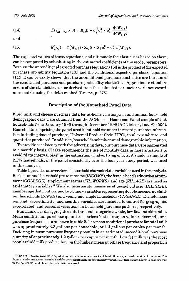
Fluid milk and cheese purchase data for at-home consumption and annual householddemographic data were obtained from the ACNielsen Homescan Panel sample of U.S.households from January 1996 through December 1999 (ACNielsen, Inc., © 2000).Households comprising the panel used hand-held scanners to record purchase informa-tion including date of purchase, Universal Product Code (UPC), total expenditure, andquantities purchased. In addition, households submit annual demographic information.

To provide consistency with the advertising data, our purchase data were aggregatedto a monthly basis. Clarke recommends the use of monthly data in most situations toavoid "data interval bias" in the estimation of advertising effects. A random sample of2,177 households, in the panel consistently over the four-year study period, was usedin this analysis.

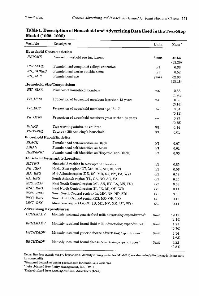
Table 1 provides an overview of household characteristic variables used in the analysis.Besides annual household pre-tax income (INCOME), the female head's education attain-ment (COLLEGE), employment status (FHWORKS), and age (FH_AGE) are used asexplanatory variables. 3 We also incorporate measures of household size (HH_SIZE),member age distribution, and two binary variables representing double income, no child-ren households (DINKS) and young and single households (YNGSNGL). Dichotomousregional, race/ethnicity, and monthly variables are included to control for geographic,race-related, and seasonal variations in household purchase patterns, respectively.

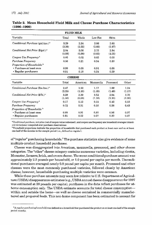
Fluid milk was disaggregated into three subcategories: whole, low fat, and skim milk.Mean conditional purchase quantities, prices (net of coupon value redeemed), andpurchase frequencies are shown in table 2. The mean conditional purchase for total milkwas approximately 3.3 gallons per household, or 1.4 gallons per capita per month.Factoring in mean purchase frequency results in an estimated unconditional purchasequantity of approximately 1.2 gallons per capita per month. Low fat milk was the mostpopular fluid milk product, having the highest mean purchase frequency and proportion

3 The FHWORKS variable is equal to one if the female head works at least 30 hours per week outside of the home. Thefemale head characteristic is also used for the classification of race/ethnicity variables. If there is not a female head presentin the household, male head characteristics are used.

170 July 2002


Table 1. Description of Household and Advertising Data Used in the Two-StepModel (1996-1999)

Variable Description Units Mean a

Household Characteristics:INCOME Annual household pre-tax income

COLLEGEFH_WORKSFHAGE

Female head completed college educationFemale head works outside homeFemale head age

Household Size/Composition:HH_SIZE Number of household members

PR_LT13 Proportion of household members less than 13 years

PR_1317 Proportion of household members age 13-17

PR_GT65 Proportion of household members greater than 65 years

DINKS Two working adults, no childrenYNGSNGL Young (< 35) and single household

Household Race/Ethnicity:BLACK Female head self-identifies as BlackASIAN Female head self-identifies as AsianHISPANIC Female head self-identifies as Hispanic (non-Black)

Household Geographic Location:METRO Household resides in metropolitan locationNE_REG North East region (CT, ME, MA, NH, RI, VT)MA_REG Mid-Atlantic region (DE, DC, MD, NJ, NY, PA, WV)SA_REG South Atlantic region (FL, GA, NC, SC, VA)ESC_REG East South Central region (AL, AR, KY, LA, MS, TN)ENC_REG East North Central region (IL, IN, MI, OH, WI)WNC_REG West North Central region (IA, MN, NE, ND, SD)WSC_REG West South Central region (KS, MO, OK, TX)MNT_REG Mountain region (AZ, CO, ID, MT, NV, NM, UT, WY)

Advertising Expenditures:USMLKADV Monthly, national generic fluid milk advertising expenditures b

BRMLKADV Monthly, national brand fluid milk advertising expendituresc

USCHZADV Monthly, national generic cheese advertising expenditures b

BRCHZADV Monthly, national brand cheese advertising expenditures c

$000s 48.54(33.20)

0/1 0.360/1 0.52

years 52.66(13.18)

no. 2.38(1.26)

no. 0.08(0.16)

no. 0.04(0.11)

no. 0.23(0.39)

0/1 0.140/1 0.01

0/10/10/1

0/10/10/10/10/10/10/10/10/1

0.07

0.010.05

0.850.060.130.200.030.140.080.120.11

$mil. 12.19(4.10)

$mil. 1.21(0.70)

$mil. 3.34(1.63)

$mil. 6.22(2.54)

Notes: Random sample = 2,177 households. Monthly dummy variables (M1-M11) are also included in the model to accountfor seasonality.a Standard deviations are in parentheses for continuous variables.bData obtained from Dairy Management, Inc. (DMI).cData obtained from Leading National Advertisers (LNA).

Schmit et al.

Journal of Agricultural and Resource Economics

Table 2. Mean Household Fluid Milk and Cheese Purchase Characteristics(1996-1999)

FLUID MILK

Variable Total Whole Low Fat Skim

Conditional Purchase (gal./mo.) 3.29 2.24 2.86 2.61(3.26) (2.55) (2.85) (2.87)

Conditional Net Price ($/gal.) a 2.84 3.06 2.73 2.84(0.88) (0.98) (0.83) (1.05)

Coupon Use Frequencya 0.05 0.02 0.05 0.05Purchase Frequency 0.86 0.21 0.54 0.30Proportion of Households: b· Purchase at least once 0.99 0.68 0.91 0.68· Regular purchasers 0.91 0.18 0.54 0.29

CHEESE

Variable Total American Mozzarella Processed Other

Conditional Purchase (lbs./mo.) 2.47 1.29 1.17 1.69 1.24(2.25) (1.16) (1.05) (1.49) (1.17)

Conditional Net Price ($/lb.) a 3.29 3.39 3.52 2.94 3.70(1.30) (0.99) (1.10) (1.19) (1.90)

Coupon Use Frequencya 0.17 0.13 0.11 0.12 0.13Purchase Frequency 0.72 0.31 0.18 0.38 0.43

Proportion of Households: b· Purchase at least once 0.99 0.91 0.81 0.96 0.97

Regular purchasers 0.81 0.22 0.07 0.30 0.37

"Conditional purchase, net price (net of coupon value redeemed), and coupon use frequency are household averages (stand-ard deviations) computed over purchase observations.b Household proportions indicate the proportion of households that purchased each product at least once and on at leastone-half of the months in the sample period (i.e., defined as regular).

of "regular" purchasing households.4 The purchase statistics also give evidence of somemultiple-product household purchases.

Cheese was disaggregated into American, mozzarella, processed, and other cheesecategories. The "other" cheese category contains numerous varieties, including ricotta,Muenster, farmers, brick, and cream cheese. The mean conditional purchase amount wasapproximately 2.5 pounds per household, or 1.0 pound per capita per month. Uncondi-tional purchases averaged nearly 0.8 pound per capita per month. Processed and othercheeses were the most commonly purchased varieties, followed closely by Americancheese; however, households purchasing multiple varieties were common.

While these purchase amounts may seem low relative to U.S. Department of Agricul-ture (USDA) disappearance estimates (e.g., USDA annual cheese disappearance for 1997was estimated at 28 pounds per capita), purchases in the data reflect purchases for at-home consumption only. The USDA estimate accounts for total cheese consumption-within and outside the home-as well as cheese contained in commercially manufac-tured and prepared foods. This non-home component has been estimated to account for

4 A regular purchasing household was defined as a household that purchased the product on at least one-half of the sampleperiod months.

172 July 2002


as much as two-thirds of total cheese consumption (USDA). As such, the at-home pur-chase estimates here (approximately 10 pounds per capita annually) are in line withUSDA projections.

Prices are not observed directly in the data. An estimate of price was obtained bydividing reported monthly expenditures (less any coupon value redeemed) by quantitypurchased. A number of alternative approaches were considered to obtain estimates ofunobserved prices during nonpurchase periods. For this analysis, we impute prices fornonpurchase observations for each household as being equal to the mean DominantMarket Area (DMA) net price for that monthly period.5 ' 6

As expected, coupon use was infrequent for the fluid milk products, but considerablylarger for the cheese products (table 2), and reflects use of either store or manufacturercoupons. The price effect of coupon redemption is reflected iten the Conditional Net Pricevariable. However a binary variable representing coupon use is also included to accountfor changes in purchase amounts from coupon redemption in addition to the price effect.Prices are converted to real 2000 dollars using the national Consumer Price Index (CPI)for nonalcoholic beverages (milk) and fats and oils (cheese). Household income is deflatedby the national CPI for all items.

Generic fluid milk and cheese advertising expenditure data were obtained from DairyManagement, Inc. (DMI), the firm that administers allocation of checkoff dollars. Theadvertising data are national in scope and aggregated across media type. As such, theadvertising data varied across time, but not across households.7 Monthly advertisingexpenditure data were not available at a regional or media-market level. Consideringthe advertising efforts are largely based on a national campaign, common expendituredata are hypothesized to adequately represent household advertising exposure. Thenational generic advertising expenditure data are also consistent with the availablebranded advertising expenditure data compiled from Leading National Advertiserss(LNA), on a monthly, national basis.

Mean levels of advertising expenditure are included in table 1 for both generic andbranded expenditures. Advertising expenditures were deflated by a composite mediacost index (2000 = 1) provided by DMI. While mean expenditures on generic fluid milkadvertising were higher than the corresponding branded expenditures, the opposite istrue for cheese.

There is a large body of empirical evidence suggesting both current and lagged adver-tising efforts affect current purchase behavior (Forker and Ward; Ferrero et al.). Tomitigate the impact of multicollinearity among the lagged advertising variables, the lagweights were approximated using a second-degree polynomial distributed lag (PDL)structure, with endpoints restricted to zero (e.g., see Liu et al.; Suzuki et al.; Kaiser). Thisstructure requires the estimation of only one parameter and represents the quadratic

5The DMA was created by Nielsen Media Research to measure television station ratings, and currently divides the UnitedStates into 210 market areas. Each county in the United States is assigned to only one DMA. Households were assigned aparticular DMA code by their county of residence.

6 The average price calculation was completed prior to the household random sampling to allow for a large number ofhouseholds in each DMA. As noted by Cox and Wohlgenant, and by Dong, Shonkwiler, and Capps, this average price calcu-lation reflects not only differences in market prices faced by each household, but also endogenously determined commodityquality.

7 Prior research explaining micro-decisions with macro-data exists. Some examples with household data and genericadvertising expenditures include Blisard et al.; Reynolds; and Ward, Moon, and Medina.

Schmit et al.


PDL parameter on the lag-weighted advertising variable. In general notation, the PDLstructure with end-point restrictions can be written as:

L

(16) Yt = + E PiADVt i + et,i=0

s.t.: pi = X0 + Xli + )2 i 2,

P-1 = PL+1 = 0,

where L is the total lag length, Pi is the ith lag advertising coefficient, ADV-i^ is the totaladvertising expenditure level for period t - i, and all other variables are suppressed intoa for notational convenience. After substituting, (16) simplifies to:

(17) Yt = a + X2ADV t * + et,L

ADV* = (i2 -Li -(L + 1))ADVt .i=o

Expenditures on generic and brand advertising are included as explanatory variablesin both stages of the milk and cheese models with a six-month PDL structure. Alter-native lag lengths were evaluated based on previous studies of generic advertising fordairy products (e.g., Kaiser; Lenz, Kaiser, and Chung). The six-month lag length selectedis within the boundaries established by Clarke, who concluded that 90% of the cumula-tive effects of advertising for frequently purchased products is captured within three tonine months. The estimated coefficient on the advertising lag-weighted variable repre-sents the quadratic PDL parameter as illustrated above, from which long-run advertisingeffects can be computed.8

Estimation Results

Following the model structure outlined above, two-stage models of sample selection wereestimated for aggregated fluid milk and cheese, as well as for the individual sub-productclasses. Parameter estimates were obtained by maximizing the likelihood functions in(3) and (11) using GAUSS software. Net price and income variables were included asnatural logarithm transformations of the original data to reflect the a priori hypothesisof diminishing marginal effects associated with these demand factors. For similarreasoning, but to avoid the possible problem of zero-level expenditures, advertisingexpenditures were transformed by their square root.

The estimated coefficients are included in appendix tables A1-A4. For brevity, werefer the reader to these tables for evaluation of specific estimated parameters. Webriefly highlight some of these results with respect to the sample-selection and varianceeffects. Because the conditional and unconditional demand effects are functions of theestimated parameters from both stages of estimation in a nonlinear fashion, it is bestto evaluate the effects using computed elasticities.

8 The individual lag advertising parameters can be recovered from the estimated value of X2; i.e., Pi = 2(i2 - Li - (L + 1)).

Since (i2 - Li - (L + 1)) < 0 V i, the sign(pi) = -sign(X 2 ) V i.

174 July 2002


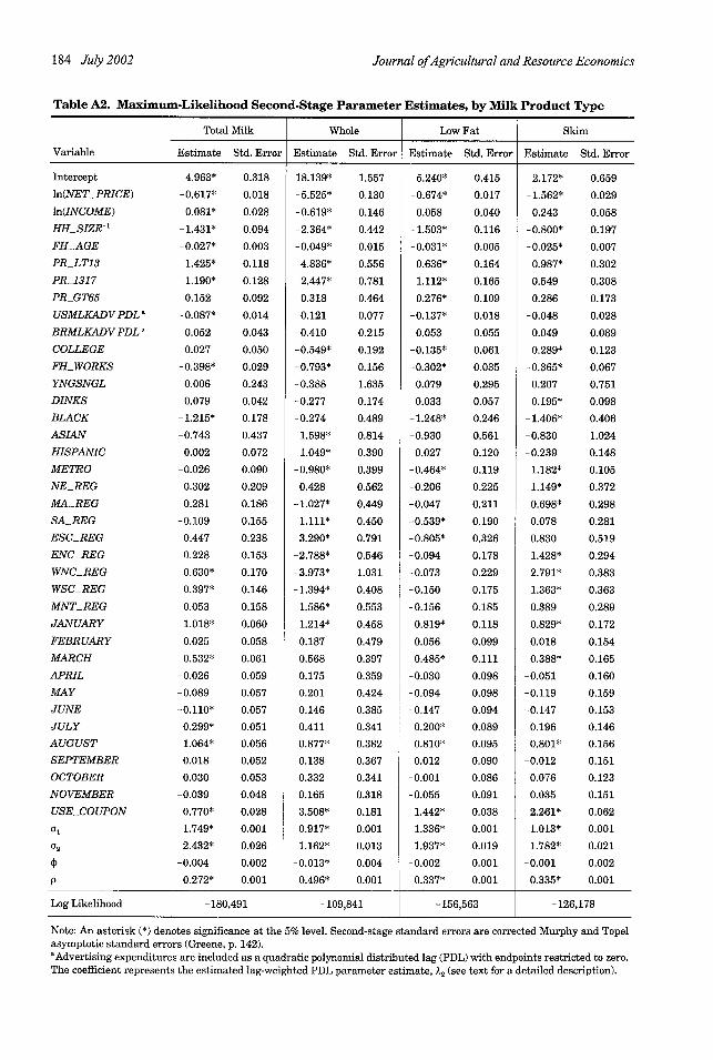
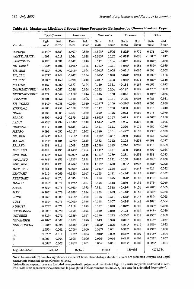
Significance of sample-selection bias is based on the significance of the estimated 6parameter on the PDF variable, ). Sample-selection bias was not statistically importantin either the aggregate fluid milk or cheese categories (appendix tables A2 and A4), butwas significant for whole milk and the mozzarella, processed, and other categories forcheese.

The estimated variance parameters associated with serial dependence ((o and p) andhousehold heterogeneity (0a) were significant in all equations. From these coefficients,the correlation between current and previous month's purchases can be calculated as(p = (oap + o2)/((J + 02). The estimated values for total milk and cheese were (pmilk = 0.75and pcheese = 0.33, implying current purchases are positively related to lagged purchases.Individual product classes had similar results, ranging from 0.79 to 0.84 for fluid milkproducts, and 0.23 to 0.35 for cheese products. 9

The overall effect can be decomposed into serial state dependence ((pSSD = o p/((o2 + 72))

and household heterogeneity ((pH = o2 /(o + o2)) components. The decomposition allowsfor segmenting the amount of correlation in the panel data into its time-series (e.g.,habit persistence) and cross-sectional (e.g., household variability) components. From thisdecomposition, we find both sub-effects are positive. Household heterogeneity effects((pmk = 0.66 and (pHHe = 0.29) contributed approximately 88% of the total correlation,and serial state dependence ((pSSk = 0.09 and (pHH = 0.04) about 12%. Sub-product class-es demonstrated similar proportional effects.

The positive correlation effects of household heterogeneity and serial dependencehave important implications when evaluating long-term shifts in purchases from adver-tising. If advertising results in a positive shift in household purchases, which is thenpersistent over time, the positive effect of this strategy ((pHH) is reinforced by the positiveserial correlation effect (psSSD).

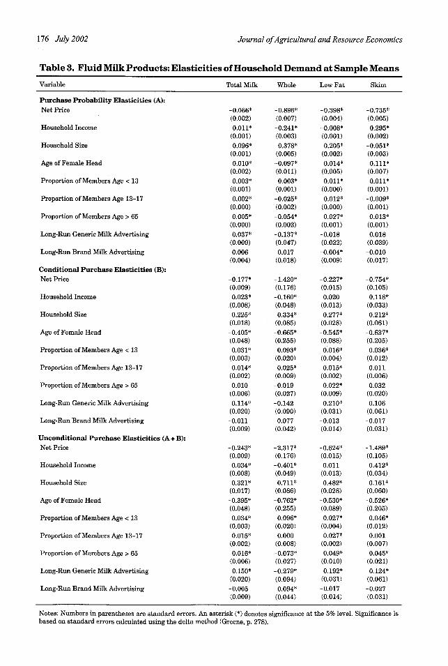
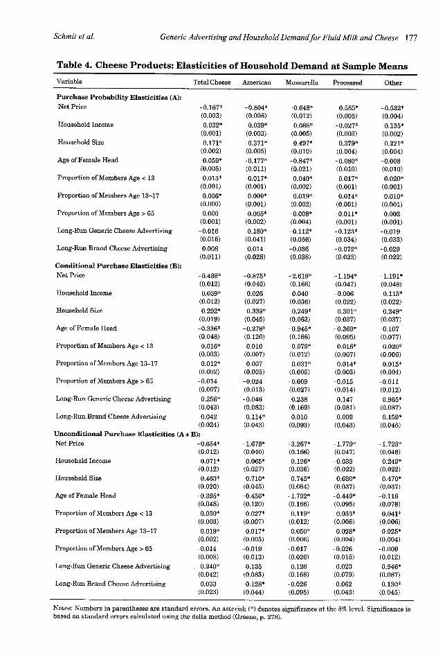
The elasticities for selected variables are included in table 3 for fluid milk and table4 for cheese. The purchase probability elasticity (the extensive effect) represents thepercentage change in purchase probability for a 1% change in the selected variable. 10

The conditional purchase elasticity (the intensive effect) represents the percentagechange in the quantity demanded, given a purchase, for a 1% change in the selectedvariable.

For both the total fluid milk and cheese categories, all unconditional elasticities aredominated by intensive, conditional purchase effects, rather than purchase probabilityeffects. This result could be due to the level of temporal aggregation (i.e., monthly)and the products' limited shelflife. The level of intensive effects is reduced for the sub-product categories and is dominated by purchase probability effects for some explana-tory variables and products. In particular, purchase probability effects for householdincome are generally much more elastic than the conditional purchase effects for thesub-product categories.

9 Approximate standard errors of the correlation coefficients were computed using the delta method (Greene, p. 278) andare available from the authors upon request. Given the strong significance of the residual variance and autocorrelation terms,it is not surprising that all correlation coefficients computed were also highly significant (i.e., all were above a 99% confidencelevel).

' 1Given the panel nature of the data, increases in purchase probability could be attributed either to new households pur-chasing the product that didn't purchase previously or to existing purchasing households purchasing the product morefrequently. As such, the terms "purchase probability" or "purchase frequency" are equally applicable.

Schmit et al.


Table 3. Fluid Milk Products: Elasticities of Household Demand at Sample Means

Variable Total Milk Whole Low Fat Skim

Purchase Probability Elasticities (A):Net Price -0.066* -0.896* -0.398* -0.735*

(0.002) (0.007) (0.004) (0.005)Household Income 0.011* -0.241* -0.008* 0.295*

(0.001) (0.003) (0.001) (0.002)Household Size 0.096* 0.378* 0.205* -0.051*

(0.001) (0.005) (0.002) (0.003)Age of Female Head 0.010* -0.097* 0.014* 0.111*

(0.002) (0.011) (0.005) (0.007)Proportion of Members Age < 13 0.003* 0.003* 0.011* 0.011*

(0.001) (0.001) (0.000) (0.001)Proportion of Members Age 13-17 0.002* -0.025* 0.012* -0.009*

(0.000) (0.002) (0.000) (0.001)Proportion of Members Age > 65 0.005* -0.054* 0.027* 0.013*

(0.000) (0.002) (0.001) (0.001)Long-Run Generic Milk Advertising 0.037* -0.137* -0.018 0.018

(0.009) (0.047) (0.022) (0.039)Long-Run Brand Milk Advertising 0.006 0.017 -0.004* -0.010

(0.004) (0.018) (0.009) (0.017)Conditional Purchase Elasticities (B):Net Price -0.177* -1.420* -0.227* -0.754*

(0.009) (0.176) (0.015) (0.105)Household Income 0.023* -0.160* 0.020 0.118*

(0.008) (0.048) (0.013) (0.033)Household Size 0.225* 0.334* 0.277* 0.212*

(0.018) (0.085) (0.028) (0.061)Age of Female Head -0.405* -0.665* -0.545* -0.637*


(0.003) (0.020) (0.004) (0.012)Proportion of Members Age 13-17 0.014* 0.025* 0.015* 0.011

(0.002) (0.009) (0.002) (0.006)Proportion of Members Age > 65 0.010 -0.019 0.022* 0.032

(0.006) (0.027) (0.009) (0.020)Long-Run Generic Milk Advertising 0.114* -0.142 0.210* 0.106

(0.020) (0.090) (0.031) (0.061)Long-Run Brand Milk Advertising -0.011 0.077 -0.013 -0.017

(0.009) (0.042) (0.014) (0.031)Unconditional Purchase Elasticities (A + B):Net Price -0.243* -2.317* -0.624* - 1.489*

(0.009) (0.176) (0.015) (0.105)Household Income 0.034* -0.401* 0.011 0.412*

(0.008) (0.049) (0.013) (0.034)Household Size 0.321* 0.711* 0.482* 0.161*

(0.017) (0.086) (0.028) (0.060)Age of Female Head -0.395* -0.762* -0.530* -0.526*


(0.003) (0.020) (0.004) (0.012)Proportion of Members Age 13-17 0.015* 0.000 0.027* 0.001

(0.002) (0.008) (0.002) (0.007)Proportion of Members Age > 65 0.016* -0.073* 0.049* 0.045*

(0.006) (0.027) (0.010) (0.021)Long-Run Generic Milk Advertising 0.150* -0.279* 0.192* 0.124*

(0.020) (0.094) (0.031) (0.061)Long-Run Brand Milk Advertising -0.005 0.094* -0.017 -0.027

(0.009) (0.044) (0.014) (0.031)

Notes: Numbers in parentheses are standard errors. An asterisk (*) denotes significance at the 5% level. Significance isbased on standard errors calculated using the delta method (Greene, p. 278).

176 July2002


Table 4. Cheese Products: Elasticities of Household Demand at Sample Means

Variable Total Cheese American Mozzarella Processed Other

Purchase Probability Elasticities (A):Net Price

(Household Income

(Household Size

(IAge of Female Head

Proportion of Members Age < 13(I

Proportion of Members Age 13-17(i

Proportion of Members Age > 650L

Long-Run Generic Cheese Advertising((

Long-Run Brand Cheese Advertising -((4

Conditional Purchase Elasticities (B):Net Price

((Household Income (

((Household Size (

((Age of Female Head

((Proportion of Members Age < 13 (

((

Proportion of Members Age 13-17 65 ((Proportion of Members Age > 65 -a

((Long-Run Generic Cheese Advertising C

(CLong-Run Brand Cheese Advertising C

(CUnconditional Purchase Elasticities (A + B):Net Price -C

(CHousehold Income C

(CHousehold Size 0

(CAge of Female Head -C

(CProportion of Members Age < 13 0

(0Proportion of Members Age 13-17 0

(0Proportion of Members Age > 65 -0

(0Long-Run Generic Cheese Advertising 0

(0Long-Run Brand Cheese Advertising 0

(0

0.167*0.003)0.032*0.001)0.171*0.002)0.059*0.005)0.013*0.001)0.006*0.000)0.0000.001)0.0160.016)0.0080.011)

0.488*0.012)0.039*).012)).292*).019)).336*).048)).016*).003)).012*).002)).014).007)).256*).043)).042D.024)

-0.804*(0.008)0.039*

(0.003)0.371*

(0.005)-0.177*(0.011)

0.017*(0.001)0.009*

(0.001)

0.005*(0.002)0.180*

(0.041)0.014

(0.028)

-0.875*(0.040)0.026

(0.027)0.339*

(0.045)-0.278*(0.120)0.010

(0.007)0.007

(0.005)-0.024(0.013)-0.046(0.083)0.114*

(0.043)

).654* -1.678*D.012) (0.040)).071* 0.065*).012) (0.027)).463* 0.710*).020) (0.045)).395* -0.456*).048) (0.120)).030* 0.027*).003) (0.007)).019* 0.017*).002) (0.005)).014 -0.019).008) (0.013)).240* 0.135).042) (0.083)).033 0.128*).023) (0.044)

Notes: Numbers in parentheses are standard errors. An asterisk (*) denotes significance at the 5% level. Significance isbased on standard errors calculated using the delta method (Greene, p. 278).

-0.648*(0.012)0.086*

(0.005)0.497*

(0.010)-0.847*(0.021)0.040*

(0.002)0.019*

(0.002)-0.008*(0.004)

-0.112*(0.056)

-0.036(0.038)

-2.619*(0.166)0.040

(0.036)0.249*

(0.063)-0.945*(0.166)0.079*

(0.012)0.031*

(0.005)-0.009(0.027)0.238

(0.169)0.010

(0.093)

-3.267*(0.166)0.126*

(0.036)0.745*

(0.064)- 1.792*(0.166)0.119*

(0.012)0.050*

(0.006)-0.017(0.026)0.126

(0.168)-0.026(0.095)

-0.585*(0.005)-0.027*(0.003)0.379*

(0.004)-0.080*(0.010)0.017*

(0.001)

0.014*(0.001)

-0.011*(0.001)

-0.123*(0.034)

-0.072*(0.023)

-1.194*(0.047)

-0.006(0.022)0.301*

(0.037)-0.369*(0.095)0.016*

(0.007)0.014*

(0.003)-0.015(0.014)0.147

(0.081)0.009

(0.043)

-1.779*(0.047)-0.033(0.022)0.680*

(0.037)-0.449*(0.095)0.033*

(0.008)0.028*

(0.004)-0.026(0.015)0.023

(0.079)-0.062(0.043)

-0.532*(0.004)0.135*

(0.002)0.221*

(0.004)-0.008(0.010)

0.020*(0.001)0.010*

(0.001)

0.002(0.001)

-0.019(0.033)-0.029(0.022)

-1.191*(0.048)0.115*

(0.022)0.249*

(0.037)-0.107(0.077)0.020*

(0.006)0.015*

(0.004)-0.011(0.012)0.965*

(0.087)0.159*

(0.045)

-1.723*(0.048)0.249*

(0.022)0.470*

(0.037)-0.116(0.078)0.041*

(0.006)0.025*

(0.004)-0.009(0.012)0.946*

(0.087)0.130*

(0.045)

Schmit et al.


Price elasticities are significant for all products and types of elasticity. Unconditionalprice responses are inelastic for both fluid milk (-0.24) and cheese (-0.65), but the cheeseprice response is nearly three times as large. Since the price offered for one product (fora particular household) is not available when an alternative product is purchased, wedo not include alternative product prices in the demand specifications. Consequently,sub-product elasticities are considerably higher than their respective aggregate-productlevels, likely due to product switching and households purchasing multiple products. Forexample, a decrease in the skim milk price may induce, say, regular low fat drinking

households to temporarily switch purchases to skim milk to take advantage of the price

reduction. This change in price would affect both sub-product purchases, but would have

no impact on the aggregate price effect, unless changes in purchased amounts also

resulted from the price reduction.The sub-product price elasticities for fluid milk are larger than elasticities reported

by Gould, but more similar in magnitude to those found by Boehm and by Reynolds. The

cheese price elasticities are similar to findings of Gould and Lin who estimated a totalcheese price elasticity of -0.57 and elastic price responses for nearly all sub-classesevaluated. An elastic price response for natural cheese was also obtained by Blisard andBlaylock using household cheese purchase data.

Household income elasticities are positive and slightly larger for cheese than fluid

milk. However, the sub-product categories demonstrate both positive and negative in-

come elasticities. While negative income effects for whole milk are not uncommon (e.g.,Cornick, Cox, and Gould; Boehm; Reynolds), the estimated income effect for low fat milk

is not statistically significant. Income elasticities are consistent with those estimated

by Cornick, Cox, and Gould, as well as Reynolds, where both studies report higher incomeelasticities for whole and skim milk products. For cheese, only the processed cheese cate-

gory has a negative income effect. The income elasticities are similar to the aggregate

cheese estimate of 0.045 in Gould and Lin, and in Gould, Cornick, and Cox for full fat

natural American (0.06) and processed (-0.05) cheeses.As expected, household size is positively related to both purchase probability and

purchase levels for fluid milk and cheese. The household size elasticities for fluid milk

are similar in magnitude to the elasticities found by Cornick, Cox, and Gould, and also

declined in magnitude as the fat content lowered. The age of the female household head

is negatively related to purchase probability and purchase levels for nearly all products

evaluated, especially for cheese products.Our findings reveal household composition is important, particularly highlighting

higher purchase probabilities for households with children (both teenagers and children

under the age of 13), relative to mature adult households. A higher proportion of seniorcitizens in the households also contributed positively to household milk purchases, but

was not significant for cheese. With the exception of whole milk, household compositioneffects on sub-products are of similar sign. The lower teenager elasticities relative to

young children seem consistent with higher dietary calcium needs of young children and

the concern of milk marketers that teenagers are turning toward other nonalcoholic

beverages as their diets become less closely monitored. Household composition elasti-

cities for cheese products demonstrate similar effects. Gould, Cornick, and Cox also

estimated positive age composition effects for household members under age 17 for cheeseproducts except for reduced-fat American cheese; however, they did show positive contri-

butions for households with members above age 65.

178 July 2002


Advertising expenditure elasticities are especially interesting. Branded advertisingefforts are not significant for either the total fluid milk or total cheese categories, andonly a few sub-product categories show significant results-American and other cheese,and whole milk. This result is intuitively appealing given brand advertising's focus onincreasing purchases at the expense of competitors, suggesting little, if any, effect at thenonbrand-specific product level. While a substantial amount of cheese advertising isbrand specific, neither Sun, Blisard, and Blaylock, nor Blisard et al. found significantbrand effects for natural cheese, and both studies combined the generic and brandadvertising expenditures in the processed cheese model due to the preponderance of onedominant advertiser in the brand market.

For both total fluid milk and cheese, the unconditional long-run elasticities for genericadvertising are positive, significant, and largely the result of intensive responses, i.e.,from the conditional purchase effects. Specifically, only 25% of the total long-run genericadvertising response for total fluid milk is the result of an increase in the probability ofpurchase, and the purchase probability effect is not significantly different from zero fortotal cheese.

The total milk and cheese generic advertising elasticities (0.15 for fluid milk, and 0.24for cheese) are higher than those estimated by Kaiser (0.05 for fluid milk and 0.02 forcheese) using aggregate quarterly disappearance data from 1975-1999. Differences inthe level of estimated elasticities could be due, in part, to differences in the level of tem-poral aggregation; however, the relative size of the elasticities between fluid milk andcheese is clearly different. Kaiser's aggregate estimates also use a more distant historyof disappearance data and account for both at-home and away-from-home purchases.The latter is particularly important for cheese, where as much as two-thirds of total dis-appearance is consumed away from home or contained in manufactured food products.Because generic advertising focuses predominantly on at-home consumption, it is appeal-ing to supporters of generic advertising that the estimated results here are above thoseestimated in more aggregated studies.

Interpretation of the sub-product generic advertising elasticities is less clear. Inparticular, while all unconditional long-run advertising elasticities are significant forthe fluid milk products, the whole milk category is negative in sign. Few sub-productadvertising elasticities are significant for the cheese products. One exception is the othercheese category, where the conditional and unconditional purchases are relatively largeand significant. American cheese purchases do demonstrate a positive and significantpurchase probability effect, giving some evidence of increasing household purchasefrequency; however, mozzarella and processed cheese purchase probability effects arenegative and significant. The generic advertising message is largely nonproduct specific,and the results shown here may be due to product switching and/or multiple productpurchases over time. The negative result for whole milk may be explained by a cohorteffect or households moving purchases to lower fat products. In any event, the genericadvertising results have significant long-run impacts on low fat and skim milk products,as well as on the other cheese category.

In the literature on household milk demand, it is rare to find advertising as anexplanatory variable. One exception is Reynolds, who used current national Canadianadvertising expenditures and aggregated household price and quantity data to estimateconsiderably higher elasticities for total and whole milk (0.37 and 1.04, respectively).However, no significant response was found for low fat or skim milk.

Schmit et al.


The generic cheese advertising results here are in contrast to those obtained by Blisardet al. Using cross-sectional data, Blisard et al. found generic advertising was successfulin inducing people into the natural cheese market, but this advertising did not influencecurrent consumers. However, for processed cheese, they concluded both effects contrib-uted positively to household demand. The results here demonstrate that generic cheeseadvertising has recently had no effect on increasing the probability of purchase orfrequency of purchases, but has had a significant impact on increasing overall purchasequantities through increased conditional purchases.

The overall impact of the generic advertising programs on total milk or cheese pur-chases is what is of most importance to milk marketers and producers. Positive andsignificant purchase effects from generic advertising suggest these efforts have beeneffective at enhancing demand at the household level. Furthermore, focusing specificallyon the at-home consumption component also confirms that cheese advertising efforts arerelatively more effective than efforts directed at fluid milk advertising-a comparisonnot available in more aggregate studies.

Conclusions

U.S. milk producers and processors contribute substantial dollars each year to fund na-tional generic advertising programs for fluid milk and cheese. Producers, marketers, andlegislators are all interested in whether generic advertising increases consumer demandfor dairy products. The household approach followed here allows for examination of therelative effectiveness of these programs on increasing at-home consumption of fluid milkand cheese products. In addition, a unique two-stage panel data estimation procedurepermits decomposition of the total advertising effects into their extensive (probabilityof purchase) and intensive (purchase quantity level) components, and accounts for unob-served household heterogeneity and temporal correlation.

In general, the demand effects for aggregate fluid milk and cheese products werepredominantly intensive-i.e., they affect the conditional purchase levels. However, thesub-product results reveal that household income and household size exhibited largerpurchase probability or frequency effects. These higher extensive contributions weremuted in the aggregate categorization, a possible result of product switching.

Brand advertising was largely ineffective at increasing household purchases of fluidmilk and cheese at the aggregate or sub-product levels. Given brand advertising's objec-tive of gaining market share from competing products, this is an intuitively appealingresult. Generic advertising, however, displayed positive and significant effects on bothaggregate fluid milk and cheese. Generic advertising appears more effective at increas-ing at-home purchases of cheese than purchases of fluid milk. These results are incontrast to more aggregate studies of generic advertising where national disappearancedata are used. The household approach used here directs the focus to at-home consump-tion effects only and is consistent with marketers' target audience and use of generic,nonproduct-specific advertising messages.

Given the higher response to generic advertising for cheese compared to the relativelylow estimates from aggregate studies using total cheese disappearance, it may be worth-while investigating the expansion of the cheese advertising program to purchases awayfrom home. The incidence of response to the advertising programs on purchases for at-home consumption was clearly from the intensive, purchase quantity effect. Fluid milk

180 July 2002


advertising had a small effect on increasing household purchase probabilities, whilecheese advertising showed no significant effect. Response across sub-product classesvaried considerably, highlighting the differences in response to specific products fromgeneric advertising messages.

Given the complexities associated with modeling household food purchase behavior,these estimates provide a preliminary assessment of household demand for dairy pro-ducts. Future research should analyze advertising response by specific product groupswithin fluid milk and cheese categories. Yet, modeling this response is more difficult.Because price, advertising, and other effects may induce product switching, a multi-nomial framework may be appropriate. However, the fact that the price of one productis not available when an alternative product is purchased leads to some difficult dataand modeling problems.

Specific advertising information by geographic area is needed to more accurately mea-sure household response to the advertising message received. If advertising expendituresare used, then accounting for differences in advertising costs (e.g., air time costs perminute) is needed across market areas. In this way, advertising expenditure dollars arereflective of actual advertising exposure across makearket areas. Finally, incorporating dif-ferences in product quality would help to isolate the quality component now includedin the total price effect.

[Received January 2001; final revision received March 2002.]

References

ACNielsen, Inc. ACNielsen Homescan Panel Household-Level Purchase and Demographic Informationfor Milk and Cheese (January 1996-December 1999). Cherry Hill NJ, © 2000.

Blisard, N., and J. R. Blaylock. "A Double-Hurdle Approach to Advertising: The Case of Cheese."Agribus.: An Internat. J. 8(March 1992):109-20.

Blisard, N., D. Blayney, R. Chandran, D. Smallwood, and J. Blaylock. "Evaluation of Fluid Milk andCheese Advertising, 1984-96." Tech. Bull. No. 1860, USDA/Economic Research Service, WashingtonDC, December 1997.

Boehm, W. T. "The Household Demand for Major Dairy Products in the Southern Region." S. J. Agr.Econ. 7(December 1975):187-96.

Butler, J. S., and R. Moffitt. "A Computationally Efficient Quadrature Procedure for the One-FactorMultinomial Probit Model." Econometrica 50(May 1982):761-64.

Charlier, E., B. Melenberg, and A. van Soest. "Estimation of a Censored Regression Panel Data ModelUsing Conditional Moment Restrictions Efficiently." J. Econometrics 95(March 2000):25-56.

Clarke, D. G. "Econometric Measurement of the Duration of Advertising Effect on Sales." J. Mktg. Res.13(November 1976):345-57.

Cornick, J., T. L. Cox, and B. W. Gould. "Fluid Milk Purchases: A Multivariate Tobit Analysis." Amer.J. Agr. Econ. 76(February 1994):74-82.

Cox, T. L., and M. K. Wohlgenant. "Prices and Quality Effects in Cross-Sectional Demand Analysis."Amer. J. Agr. Econ. 68(November 1986):908-19.

Dairy Management, Inc. Various generic fluid milk and cheese advertising data. DMI, Rosemont IL,1996-1999.

Dong, D., and B. W. Gould. "The Decision of When to Buy a Frequently Purchased Good: A Multi-PeriodProbit Model." J. Agr. and Resour. Econ. 25(December 2000):636-52.

Dong, D., J. S. Shonkwiler, and 0. Capps, Jr. "Estimation of Demand Functions Using Cross-SectionalHousehold Data: The Problem Revisited." Amer. J. Agr. Econ. 80(August 1998):466-73.

Schmit et al.


Ferrero, J., L. Boon, H. M. Kaiser, and 0. D. Forker. "Annotated Bibliography of Generic Commodity

Promotion Research" (revised). NICPRE Res. Bull. No. 96-3, National Institute for Commodity Pro-

motion Research and Evaluation, Dept. of Agr., Resour., and Managerial Econ., Cornell University,

Ithaca NY, February 1996.Forker, 0. D., and R. W. Ward. Commodity Advertising: The Economics and Measurement of Generic

Programs. New York: Lexington Books, 1993.Gould, B. W. "Factors Affecting U.S. Demand for Reduced-Fat Fluid Milk." J. Agr. and Resour. Econ.

21(July 1996):68-81.Gould, B. W., J. Cornick, and T. Cox. "Consumer Demand for New Reduced-Fat Foods: An Analysis of

Cheese Expenditures." Can. J. Agr. Econ. 42(November 1994):1-12.

Gould, B. W., and H. C. Lin. "The Demand for Cheese in the United States: The Role of Household Com-

position." Agribus.: An Internat. J. 10(January 1994):43-59.

Greene, W. H. Econometric Analysis, 3rd ed. Upper Saddle River NJ: Prentice-Hall, 1997.

Haines, P. S., D. K. Guilkey, and B. M. Popkin. "Modeling Food Consumption Decisions as a Two-Step

Process." Amer. J. Agr. Econ. 70(August 1988):543-52.Heckman, J. J. "Sample Selection Bias as a Specification Error." Econometrica 47(January 1979):

153-62.Heien, D. M., and C. R. Wessells. "The Demand for Dairy Products: Structure, Prediction, and Decompo-

sition." Amer. J. Agr. Econ. 70(May 1988):219-27.Kaiser, H. M. "Impact of Generic Fluid Milk and Cheese Advertising on Dairy Markets, 1984-99." Res.

Bull. No. 2000-02, Dept. of Agr., Resour., and Managerial Econ., Cornell University, Ithaca NY, July

2000.Kyriazidou, E. "Estimation of a Panel Data Sample Selection Model." Econometrica 65(November 1997):

1335-64.Leading National Advertisers, Inc. Leading National Advertisers, AD & Summary. New York. Various

issues, 1996-2000.Lenz, J., H. M. Kaiser, and C. Chung. "Economic Analysis of Generic Milk Advertising Impacts on Mar-

kets in New York State." Agribus.: An Internat. J. 14(January/February 1998):73-83.

Liang, K-Y., and S. L. Zeger. "Longitudinal Data Analysis Using Generalized Linear Models." Bio-

metrika 73(April 1986):13-22.Liu, D. J., H. M. Kaiser, O. D. Forker, and T. D. Mount. "An Economic Analysis of the U.S. Generic

Dairy Advertising Program Using an Industry Model."Northeast. J. Agr. and Resour. Econ. 19(April

1990):37-48.Murphy, K M., and R. H. Topel. "Estimation and Inference in Two-Step Econometric Models." J. Bus.

and Econ. Statis. 3(0ctober 1985):370-79.Reynolds, A. "Modeling Consumer Choice of Fluid Milk." Work. Pap. No. WP91/04, Dept. of Agr. Econ.

and Bus., University of Guelph, Guelph, Ontario, 1991.Shonkwiler, J. S., and S. T. Yen. "Two-Step Estimation of a Censored System of Equations." Amer. J.

Agr. Econ. 81(November 1999):972-82.Sun, T. Y., N. Blisard, and J. R. Blaylock. "An Evaluation of Fluid Milk and Cheese Advertising,

1978-1993." Tech. Bull. No. 1839, USDA/Economic Research Service, Washington DC, February

1995.Suzuki, N., H. M. Kaiser, J. E. Lenz, K. Kobayashi, and 0. D. Forker. "Evaluating Generic Milk

Promotion Effectiveness with an Imperfect Competition Model." Amer. J. Agr. Econ. 76(May

1994):296-302.U.S. Department of Agriculture. "Food Consumption, Prices, and Expenditures, 1970-97." Statis. Bull.

No. 965, USDA/Economic Research Service, Food and Rural Economics Div., Washington DC, April

1999.Ward, R. W., W. Moon, and S. Medina. "Measuring the Impact of Generic Promotions of U.S. Beef: An

Application of Double-Hurdle and Time Series Models." Internat. Food and Agribus. Mgmt. Rev.

(2001, forthcoming).Wei, S. X. "A Bayesian Approach to Dynamic Tobit Models." Econometric Reviews 18,4(1999):417-39.

182 July 2002


Table Al. Maximum-Likelihood First-Stage Probit Parameter Estimates, by Milk Product Type

Total Milk

Variable Estimate Std. Error

Intercept 1.270*

In(NET_PRICE) -0.280*

ln(INCOME) 0.046*

HH_SIZE1 -0.740*

FH_AGE 0.001*

PR_LT13 0.195*

PR_1317 0.169*

PR_GT65 0.099*

USMLKADVPDL -0.034*

BRMLKADVPDL a -0.034

COLLEGE -0.021*

FHWORKS -0.134*

YNGSNGL 0.359*

DINKS -0.004

BLACK -0.412*

ASIAN -0.354*

HISPANIC -0.165*

METRO -0.017*

NE_REG -0.003

MA_REG 0.098*

SA_REG 0.021*

ESC_REG -0.012

ENC_REG 0.114*

WNC_REG 0.149*

WSC_REG 0.029*

MNT_REG -0.136*

JANUARY 0.203*

FEBRUARY 0.040

MARCH 0.089*

APRIL -0.019

MAY 0.000

JUNE -0.022

JULY 0.066*

AUGUST 0.171*

SEPTEMBER 0.025

OCTOBER -0.003

NOVEMBER 0.034

0.090

0.009

0.002

0.007

0.000

0.013

0.019

0.006

0.008

0.021

0.003

0.004

0.016

0.005

0.005

0.010

0.007

0.004

0.006

0.005

0.004

0.009

0.006

0.007

0.005

0.005

0.040

0.036

0.037

0.035

0.036

0.035

0.032

0.034

0.032

0.033

0.033

Log Likelihood -34,647

Whole

Estimate Std. Error

1.139* 0.084

-0.640* 0.005

-0.172* 0.002

-0.492* 0.006

-0.001* 0.000

0.029* 0.009

-0.449* 0.011

-0.167* 0.004

0.021* 0.007

-0.016 0.018

-0.079* 0.002

-0.034* 0.003

-0.181* 0.011

-0.120* 0.004

0.345* 0.004

0.420* 0.008

0.307* 0.005

-0.040* 0.003

0.269* 0.005

0.009* 0.004

0.314* 0.004

0.370* 0.006

-0.318* 0.004

-0.574* 0.006

-0.059* 0.004

-0.012* 0.004

0.061 0.042

-0.017 0.041

0.038 0.039

-0.055 0.040

-0.070 0.040

-0.082* 0.039

-0.032 0.036

0.008 0.036

-0.059 0.036

-0.065 0.037

-0.006 0.037

-44,620

Low Fat

Estimate Std. Error

1.103*

-0.538*

-0.011*

-0.507*

0.000*

0.200*

0.409*

0.159*

0.005

0.007

-0.011*

-0.075*

0.494*

0.000

-0.381*

-0.508*

-0.195*

-0.044*

-0.149*

-0.062*

-0.215*

-0.457*

0.037*

0.020*

-0.103*

-0.040*

0.104*

0.013

0.042

-0.029

-0.015

-0.022

0.004

0.061

-0.020

-0.016

0.017

0.076

0.005

0.002

0.005

0.000

0.008

0.010

0.004

0.007

0.017

0.002

0.003

0.010

0.004

0.004

0.008

0.005

0.003

0.004

0.003

0.003

0.006

0.003

0.004

0.004

0.004

0.038

0.037

0.037

0.036

0.037

0.036

0.033

0.033

0.033

0.033

0.035

-60,720

Skim

Estimate Std. Error

-1.073*

-0.630*

0.253*

0.080*

0.002*

0.120*

-0.199*

0.048*

-0.003

0.011

0.143*

-0.130*

-0.202*

0.066*

-0.390*

-0.146*

-0.129*

0.183*

-0.195*

0.026*

-0.032*

-0.006

-0.054*

0.190*

-0.066*

-0.163*

0.111*

0.051

0.056

0.003

-0.007

-0.004

0.017

0.056

0.004

0.009

0.012

0.085

0.004

0.002

0.005

0.000

0.008

0.010

0.004

0.007

0.020

0.002

0.003

0.010

0.003

0.004

0.008

0.005

0.003

0.004

0.003

0.003

0.006

0.004

0.004

0.004

0.004

0.046

0.046

0.044

0.043

0.045

0.044

0.038

0.040

0.040

0.040

0.042

-53,938

Note: An asterisk (*) denotes significance at the 5% level.aAdvertising expenditures are included as a quadratic polynomial distributed lag (PDL) with endpoints restricted to zero.The coefficient represents the estimated lag-weighted PDL parameter estimate, X2 (see text for a detailed description).

Schmit et al.


Table A2. Maximum-Likelihood Second-Stage Parameter Estimates, by Milk Product Type

Total Milk

Variable Estimate Std. Error

Intercept

ln(NET_PRICE)

ln(INCOME)

HH_SIZE- 1

FHAGE

PRLT13

PR_1317

PRGT65

USMLKADV PDL a

BRMLKADVPDL a

COLLEGE

FH_WORKS

YNGSNGL

DINKS

BLACK

ASIAN

HISPANIC

METRO

NE_REG

MA_REG

SA_REG

ESC_REG

ENC_REG

WNC_REG

WSC_REG

MNTREG

JANUARY

FEBRUARY

MARCH

APRIL

MAY

JUNE

JULY

AUGUST

SEPTEMBER

OCTOBER

NOVEMBER

USECOUPON

1a

02

p

4.963*

-0.617*

0.081*

-1.431*

-0.027*

1.425*

1.190*

0.152

-0.087*

0.052

0.027

-0.398*

0.006

0.079

-1.215*

-0.743

0.002

-0.026

0.302

0.281

-0.109

0.447

0.228

0.630*

0.397*

0.053

1.018*

0.025

0.532*

-0.026

-0.089

-0.110*

0.299*

1.064*

0.018

0.030

-0.039

0.770*

1.749*

2.432*

-0.004

0.272*

0.318

0.018

0.028

0.094

0.003

0.118

0.128

0.092

0.014

0.043

0.050

0.029

0.243

0.042

0.178

0.437

0.072

0.090

0.209

0.186

0.155

0.238

0.153

0.170

0.146

0.158

0.060

0.058

0.061

0.059

0.057

0.057

0.051

0.056

0.052

0.053

0.048

0.028

0.001

0.026

0.002

0.001


Whole

Estimate Std. Error

18.139*

-5.525*

-0.619*

-2.364*

-0.049*

4.836*

2.447*

-0.318

0.121

-0.410

-0.549*

-0.793*

-0.388

-0.277

-0.274

1.598*

1.049*

-0.980*

0.428

-1.027*

1.111*

3.290*

-2.788*

-3.973*

-1.394*

-1.586*

1.214*

0.187

0.568

0.175

0.201

0.146

0.411

0.877*

0.138

0.332

0.165

3.508*

0.917*

1.162*

-0.013*

0.496*

1.557

0.130

0.146

0.442

0.015

0.556

0.781

0.464

0.077

0.215

0.192

0.156

1.635

0.174

0.489

0.814

0.390

0.399

0.562

0.449

0.450

0.791

0.546

1.031

0.408

0.553

0.458

0.479

0.397

0.359

0.424

0.385

0.341

0.382

0.367

0.341

0.318

0.181

0.001

0.013

0.004

0.001

-109,841

Low Fat

Estimate Std. Error

5.240* 0.415

-0.674* 0.017

0.058 0.040

-1.503* 0.116

-0.031* 0.005

0.636* 0.164

1.112* 0.165

0.276* 0.109

-0.137* 0.018

0.053 0.055

-0.135* 0.061

-0.302* 0.035

0.079 0.295

0.033 0.057

-1.248* 0.246

-0.930 0.561

0.027 0.120

-0.464* 0.119

-0.206 0.225

-0.047 0.211

-0.539* 0.190

-0.805* 0.326

-0.094 0.178

-0.073 0.229

-0.150 0.175

-0.156 0.185

0.819* 0.118

0.056 0.099

0.485* 0.111

-0.030 0.098

-0.094 0.098

-0.147 0.094

0.200* 0.089

0.810* 0.095

0.012 0.090

-0.001 0.086

-0.055 0.091

1.442* 0.038

1.336* 0.001

1.937* 0.019

-0.002 0.001

0.337* 0.001

-156,563

Skim

Estimate Std. Error

2.172* 0.659

-1.562* 0.029

0.243 0.058

-0.800* 0.197

-0.025* 0.007

0.987* 0.302

0.549 0.308

0.286 0.173

-0.048 0.028

0.049 0.089

0.289* 0.123

-0.365* 0.067

0.207 0.751

0.195* 0.098

-1.406* 0.406

-0.830 1.024

-0.239 0.148

1.182* 0.105

1.149* 0.372

0.698* 0.298

0.078 0.281

0.830 0.519

1.428* 0.294

2.791* 0.383

1.363* 0.363

0.389 0.289

0.829* 0.172

0.018 0.154

0.388* 0.165

-0.051 0.160

-0.119 0.159

-0.147 0.153

0.196 0.146

0.801* 0.156

-0.012 0.151

0.076 0.123

0.035 0.151

2.261* 0.062

1.013* 0.001

1.782* 0.021

-0.001 0.002

0.335* 0.001

-126,178

Note: An asterisk (*) denotes significance at the 5% level. Second-stage standard errors are corrected Murphy and Topelasymptotic standard errors (Greene, p. 142).aAdvertising expenditures are included as a quadratic polynomial distributed lag (PDL) with endpoints restricted to zero.The coefficient represents the estimated lag-weighted PDL parameter estimate, X2 (see text for a detailed description).

184 July 2002


Table A3. Maximum-Likelihood First-Stage Probit Parameter Estimates, by Cheese Product Type

Total Cheese

Esti- Std.Variable mate Error

Intercept

In(NET_PRICE)

In(INCOME)

HH_SIZE-1

FH_AGE

PR_LT13

PR_1317

PRGT65

USCHZADV PDL "

BRCHZADVPDL a

COLLEGE

FH_WORKS

YNGSNGL

DINKS

BLACK

ASIAN

HISPANIC

METRO

NE_REG

MAREG

SA_REG

ESC_REG

ENC_REG

WNC_REG

WSCREG

MNT_REG

JANUARY

FEBRUARY

MARCH

APRIL

MAY

JUNE

JULY

AUGUST

SEPTEMBER

OCTOBER

NOVEMBER

1.524* 0.109

-0.370* 0.007

0.070* 0.003

-0.693* 0.008

-0.003* 0.000

0.394* 0.015

0.343* 0.018

0.000 0.007

0.015 0.016

0.011 0.014

-0.064* 0.003

-0.044* 0.004

0.133* 0.016

0.129* 0.006

-0.414* 0.006

-0.702* 0.010

-0.060* 0.008

-0.048* 0.005

-0.027* 0.007

-0.015* 0.006

0.084* 0.005

0.069* 0.010

0.010 0.006

-0.128* 0.007

0.107* 0.006

-0.069* 0.006

-0.097* 0.025

-0.116* 0.025

0.073* 0.026

-0.130* 0.026

-0.160* 0.027

0.008 0.028

-0.161* 0.024

-0.017 0.024

-0.172* 0.023

-0.150* 0.022

0.119* 0.024


American

Esti- Std.mate Error

0.603* 0.104

-0.698* 0.007

0.034* 0.003

-0.587* 0.008

-0.003* 0.000

0.193* 0.012

0.207* 0.015

0.018* 0.006

-0.067* 0.015

-0.007 0.014

-0.009* 0.003

-0.058* 0.004

-0.089* 0.017

0.049* 0.005

-0.079* 0.006

-0.636* 0.015

-0.166* 0.006

-0.108* 0.004

-0.162* 0.007

-0.261* 0.006

-0.032* 0.005

0.145* 0.008

-0.018* 0.005

-0.215* 0.007

0.015* 0.006

-0.037* 0.006

-0.065* 0.025

-0.096* 0.025

-0.010 0.026

-0.134* 0.027

-0.184* 0.028

-0.064* 0.028

-0.181* 0.025

-0.040 0.024

-0.162* 0.023

-0.123* 0.024

0.089* 0.023

-54,197

Mozzarella


0.377* 0.111

-0.427* 0.008

0.057* 0.003

-0.597* 0.011

-0.011* 0.000

0.352* 0.016

0.314* 0.019

-0.024* 0.009

0.032* 0.016

0.013 0.014

0.071* 0.004

-0.013* 0.005

0.024 0.017

-0.015* 0.007

-0.465* 0.008

-0.372* 0.020

0.040* 0.009

-0.016* 0.005

0.038* 0.009

0.174* 0.007

0.001 0.007

-0.175* 0.012

0.017* 0.007

-0.071* 0.009

-0.107* 0.008

-0.060* 0.008

0.050 0.027

0.042 0.027

0.167* 0.028

0.008 0.030

-0.021 0.031

0.063* 0.031

-0.048 0.028

0.081* 0.027

0.019 0.026

-0.003 0.026

0.111* 0.026

-39,904

Processed


1.232* 0.099

-0.576* 0.005

-0.027* 0.003

-0.681* 0.008

-0.002* 0.000

0.225* 0.012

0.344* 0.015

-0.048* 0.006

0.052* 0.015

0.040* 0.013

-0.145* 0.003

-0.052* 0.004

0.088* 0.015

0.089* 0.005

-0.125* 0.006

-0.337* 0.014

-0.141* 0.007

-0.074* 0.004

0.029* 0.006

0.086* 0.005

0.229* 0.005

0.255* 0.009

0.211* 0.005

0.045* 0.007

0.381* 0.005

0.086* 0.006

-0.044 0.024

-0.097* 0.025

0.054* 0.025

-0.083* 0.027

-0.083* 0.027

0.048 0.027

-0.095* 0.024

0.020 0.023

-0.131* 0.023

-0.104* 0.023

0.044 0.023

-57,388

Other


0.383* 0.104

-0.575* 0.004

0.146* 0.003

-0.435* 0.008

0.000 0.000

0.294* 0.012

0.263* 0.016

0.010 0.007

0.009 0.015

0.018 0.013

0.038* 0.003

-0.044* 0.004

0.169* 0.017

0.072* 0.006

-0.659* 0.007

-0.527* 0.012

0.021* 0.007

0.118* 0.004

0.073* 0.007

0.034* 0.006

0.020* 0.005

-0.129* 0.010

-0.054* 0.006

-0.114* 0.006

-0.106* 0.006

-0.038* 0.006

-0.137* 0.023

-0.153* 0.023

0.028 0.023

-0.155* 0.025

-0.174* 0.026

-0.061* 0.026

-0.186* 0.023

-0.064* 0.022

-0.208* 0.022

-0.169* 0.021

0.088* 0.021

-58,736

Note: An asterisk (*) denotes significance at the 5% level.aAdvertising expenditures are included as a quadratic polynomial distributed lag (PDL) with endpoints restricted to zero.The coefficient represents the estimated lag-weighted PDL parameter estimate, X2 (see text for a detailed description).

i i

Schmit et al.


Table A4. Maximum-Likelihood Second-Stage Parameter Estimates, by Cheese Product Type

Total Cheese

Esti- Std.Variable mate Error

Intercept 5.140* 0.433

In(NET_PRICE) -1.506* 0.013

In(INCOME) 0.120* 0.037

HH_SIZE-1 -1.644* 0.102

FHAGE -0.020* 0.003

PR_LT13 0.671* 0.141

PR_1317 0.966* 0.159

PRGT65 -0.182 0.099

USCHZADV PDL a -0.339* 0.057

BRCHZADVPDL -0.074 0.042

COLLEGE -0.004 0.052

FH_WORKS -0.149* 0.038

YNGSNGL 0.060 0.257

DINKS 0.023 0.063

BLACK -0.697* 0.143

ASIAN -0.953* 0.232

HISPANIC 0.017 0.104

METRO -0.092 0.080

NE_REG -0.341* 0.144

MA_REG -0.344* 0.124

SA_REG -0.351* 0.114

ESCREG -0.333 0.195

ENC_REG -0.438* 0.131

WNC_REG -0.787* 0.151

WSC_REG -0.139 0.120

MNT_REG -0.061 0.124

JANUARY -0.510* 0.069

FEBRUARY -0.449* 0.073

MARCH -0.356* 0.071

APRIL -0.827* 0.076

MAY -0.769* 0.078

JUNE -0.560* 0.080

JULY -0.752* 0.075

AUGUST -0.373* 0.071

SEPTEMBER -0.633* 0.070

OCTOBER -0.315* 0.072

NOVEMBER -0.169* 0.067

USE_COUPON 1.934* 0.028

al 1.659* 0.001

02 1.073* 0.011

4) -0.001 0.004

p 0.054* 0.002


American


5.497* 0.530

-1.564* 0.020

0.047 0.048

-1.106* 0.136

-0.010* 0.004

0.247 0.184

0.328 0.213

-0.187 0.104

0.036 0.064

-0.116* 0.044

-0.002 0.066

-0.060 0.049

-0.098 0.382

-0.087 0.080

-0.179 0.168

-1.330* 0.319

0.135 0.101

-0.317* 0.102

-1.213* 0.198

-1.276* 0.159

-1.008* 0.125

-0.448* 0.214

-0.907* 0.145

-1.227* 0.181

-0.764* 0.128

-0.560* 0.133

-0.135* 0.067

0.035 0.074

0.175* 0.081

-0.162* 0.082

-0.238* 0.084

0.218* 0.090

-0.302* 0.076

-0.113 0.075

-0.059 0.075

-0.238* 0.067

0.033 0.070

3.316* 0.047

0.700* 0.000

0.452* 0.004

-0.008 0.006

0.082* 0.001

-99,671

Mozzarella


14.593* 1.506

-7.535* 0.132

0.117 0.104

-1.323* 0.321

-0.052* 0.008

3.025* 0.370

2.241* 0.403

-0.110 0.331

-0.292 0.204

-0.015 0.150

0.162 0.134

-0.217* 0.100

-0.142 0.700

0.070 0.176

-1.672* 0.363

-1.614* 0.452

0.471 0.311

-0.086 0.204

-0.858* 0.287

-0.352 0.242

-1.129* 0.243

-1.417* 0.551

-1.193* 0.280

-2.007* 0.371

-1.199* 0.250

-0.913* 0.278

-0.255 0.291

0.068 0.275

-0.478 0.312

-0.311 0.318

-0.255 0.328

-0.198 0.314

-0.275

-0.137

-0.050

-0.220

0.049

9.202*

0.537*

0.246*

0.076*

0.064*

0.307

0.313

0.259

0.293

0.276

0.205

0.001

0.002

0.024

0.001

-74,663

Processed


8.222*

-3.573*

-0.017

-1.649*

-0.021*

0.643*

1.038*

-0.188

-0.187

-0.015

-0.179

-0.260*

0.093

-0.033

0.018

-0.255

-0.320

-0.422*

-0.259

0.103

0.214

0.399

0.281

-0.158

0.894*

0.397

-0.476*

-0.326*

-0.260

-0.485*

-0.410*

-0.515*

-0.484*

-0.342*

-0.103

-0.250*

0.331*

4.841*

0.977*

0.607*

0.019*

0.017*

Other


0.638 0.379

-1.660* 0.017

0.161* 0.030

-0.637* 0.089

-0.003 0.002

0.382* 0.126

0.522* 0.148

-0.067 0.072

-0.573* 0.052

-0.125* 0.035

0.021 0.041

0.006 0.035

-0.015 0.349

0.075 0.050

-0.669* 0.160

-0.323 0.195

0.080 0.076

0.228* 0.072

0.033 0.093

-0.068 0.077

-0.116 0.069

-0.392* 0.164

-0.331* 0.093

-0.528* 0.106

-0.361* 0.092

-0.025 0.082

-0.489* 0.057

-0.475* 0.063

-0.578* 0.060

-0.861* 0 065

-0.803* 0.063

-0.859* 0.063

-0.764* 0.064

-0.588* 0.059

-0.643* 0.060

-0.250* 0.069

-0.415* 0.057

2.252* 0.032

0.791* 0.000

0.448* 0.004

0.023* 0.007

0.088* 0.001

-111,234

0.773

0.033

0.067

0.184

0.005

0.251

0.274

0.187

0.102

0.073

0.096

0.062

0.326

0.097

0.214

0.478

0.176

0.139

0.323

0.254

0.236

0.384

0.254

0.302

0.237

0.248

0.115

0.137

0.133

0.156

0.152

0.147

0.142

0.128

0.130

0.119

0.133

0.070

0.000

0.007

0.006

0.002

-130,002

Note: An asterisk (*) denotes significance at the 5% level. Second-stage standard errors are corrected Murphy and Topelasymptotic standard errors (Greene, p. 142).aAdvertising expenditures are included as a quadratic polynomial distributed lag (PDL) with endpoints restricted to zero.The coefficient represents the estimated lag-weighted PDL parameter estimate, X2 (see text for a detailed description).

.

.

I I i i

186 July 2002

IDENTIFYING THE EFFECTS OF GENERIC ADVERTISING ON THE HOUSEHOLD DEMAND FOR FLUID MILK AND CHEESE: A...

Documents

Transcript of IDENTIFYING THE EFFECTS OF GENERIC ADVERTISING ON THE HOUSEHOLD DEMAND FOR FLUID MILK AND CHEESE: A...