Instructor: Muhammad Imran

In the preceding chapters we discussed the relationship between the performance and the characteristic roots of feedback system

The root locus is a powerful tool for designing and analyzing feedback control system, it is a graphical method by determining the locus of roots in the s-plane as one system parameter is changed.

Closed-loop response depends on the location of closed-loop poles

If system has a variable design parameter (e.g., a simple gain adjustment or the location of compensation zero), then the closed-loop pole locations depend on the value of the design parameter.

Definition: The root locus is the path of the roots of the characteristic equation traced out in the s-plane as a system parameter is varied.

For the system shown below its transfer function can be written as

Where characteristic polynomial is

Or

Where G(s)H(s) is a ratio of polynomials in S It is a complex quantity and can be split into

two equations by equating angles and magnitudes on both sides, we obtain

Angle Condition

Magnitude Condition

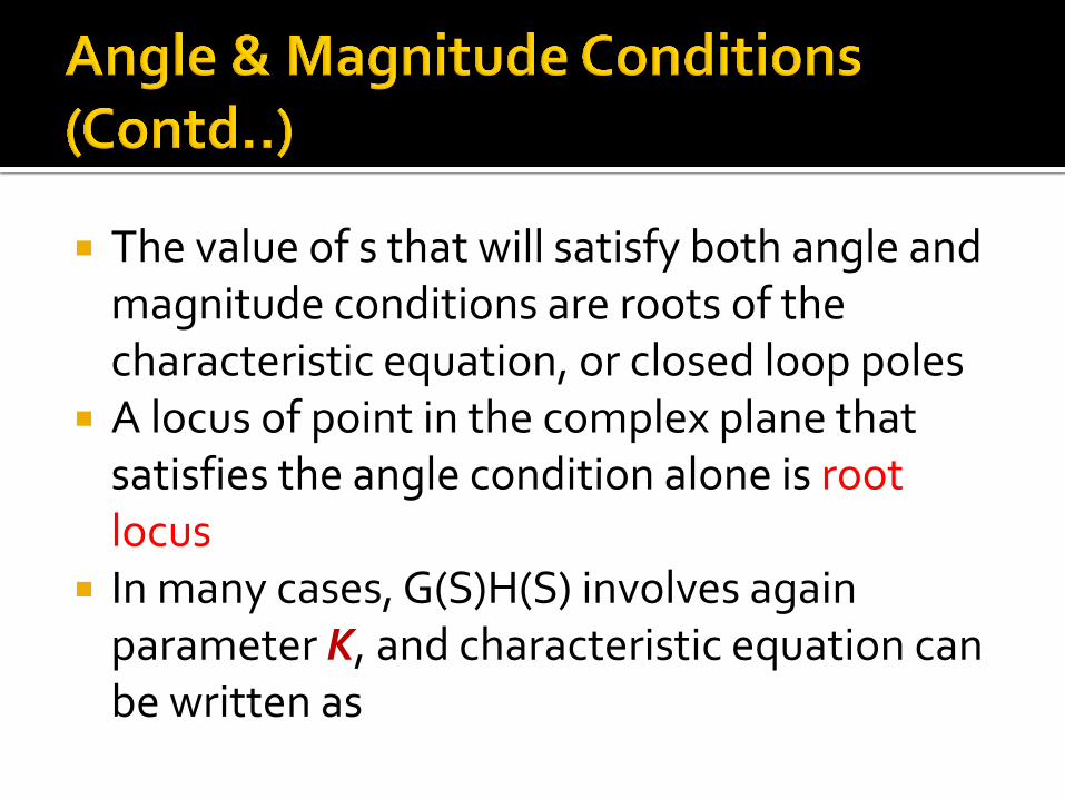
The value of s that will satisfy both angle and magnitude conditions are roots of the characteristic equation, or closed loop poles

A locus of point in the complex plane that satisfies the angle condition alone is root locus

In many cases, G(S)H(S) involves again parameter K, and characteristic equation can be written as

The root loci for the system are the loci of the

closed loop poles as the gain K is varied from zero to infinity (K >0 meaning –ve feedback)

Following key steps are involved in sketch of root locus Locate the poles and zeros of G(s)H(S) on s-plane

Determine root loci on the real axis

Determine the asymptotes of real loci

Find the breakaway and break-in points

Determine the angle of departure (angle of arrival) of root loci

Find the point where root loci may cross the imaginary axis

1. Locate poles and zeros of G(s)H(S) on real plane

From factored form of open loop transfer function locate the open loop poles and zeros in s-plane

Root locus plot has as many branches as there are roots of characteristic equation

Root locus branches start from open loop poles and terminate at zero (finite zero or zeros at infinity)

2. Determine root locus on real axis

Root loci on real axis are determined by open loop poles and zeros lying on it

The complex conjugate poles and zeros of open loop transfer function have no effect on location of root loci on real axis

Choose a test point on real axis , if total number of real poles and real zeros to the right of this point is odd, then this point lies on root locus

3. Determine the asymptotes of root loci

If number of poles and zeros are not same then some zero lies at infinity and we need to compute asymptotes

No. of asymptotes = no. of finite poles of G(S)H(S) n – no. of finite zeros of G(S)H(S) m

Angle of asymptotes =

All asymptotes intersect on real axis. This point is obtained as

Proof: (in lecture handout) Once S is obtained the asymptotes can be

drawn in complex plane

4. Find the breakaway and break-in points Because of conjugate symmetry of root loci the

break-in and breakaway points either lie on real axis or occur in complex conjugate pair

If root locus lies b/w two adjacent poles on real axis, then at least one breakaway point exist

If root locus lies b/w two adjacent zeros (one zero may be located at infinity) on real axis, then at least one break-in point exist

If root locus lies b/w open loop pole and zero (finite or infinite) on real axis, then there exist either no break-in or break away points or there may exists both break-in & break away points

Suppose characteristic equation is given by

B(s) + K A(s) = 0

Then breakaway and break-in points can be determined from the roots of

Proof :(Given in Lecture handout) Where prime indicates differentiation w.r.t S

If root of last equation lies on root locus portion of real axis , then it is actual breakaway or break-in point

If roots of last equation is not on root locus portion of real axis , then this root corresponds to neither breakaway nor break-in point

If roots of above equation occur in complex conjugate pair, and it is not certain whether they are on root locus, then check corresponding value of K. If the value of K is positive for that root , then root is an actual breakaway or break-in point and vise versa

5. Find the point where root loci may cross imaginary axis Points where root loci may intersect jw axis can be

found either by ▪ Use of Routh stability criterion or

▪ Put s=jw in characteristic equation, equating both real and imaginary parts to zero and solving for w & k

▪ the value of w found gives frequencies at which root loci crosses imaginary axis. The value of k corresponding to each frequency crossing gives the gain at that crossing point

6. Determine the angle of departure (angle of arrival) of the root locus from complex pole (at a complex zero) To sketch root locus with reasonable accuracy we

find direction of root loci near the complex poles and zeros

If test point S is chosen and moved in the vicinity of complex pole (or complex zero), the sum of the angular contribution form all poles and zeros can be considered to remain same

Angle of arrival (departure) can be found by subtracting from 1800 the sum of all angles of vectors from all poles and zeros to complex pole (or complex zero) with appropriate signs included

Angle of departure across complex pole P2 = 1800 – ( θ1 + θ3 + θ4) + Ø1)

Example 1: Consider the given system, sketch the root locus plot ?

From given system

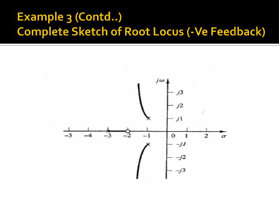
Example 2: Consider the given system, sketch the root locus plot ?

From given system

Following modifications should be made for construction of root locus for positive feedback systems Rule 2 Modification

▪ If total no. of real poles/zeros to the right side of test point on real axis is even, then this point is on root locus

Rule 3 Modification ▪ Equation for angle of asymptotes becomes

Rule 5 Modification

▪ All angles of open loop poles /zero are subtracted from 00 instead of 1800

Example 1: Consider the given system, sketch the root locus plot for positive feedback system?

Root Locus is a graphical method for determining the locations of all closed loop poles from knowledge of location of open loop poles and zeros as parameter (usually gain K) is varied from 0 to infinity

In practice, root locus plot of a system may indicate that desired performance cannot be achieved by adjustment of gain

Sometimes system may not be stable for all values of gain

So it become necessary to reshape root locus technique to meet performance specifications

In designing control system, if other than gain adjustment is required, we must modify the original root loci by inserting a suitable compensator

Compensator will reshape the root locus as desired by inserting a pair of dominant closed loop poles at desired location

Two types of effects are encountered by compensator

Effect s of addition of poles

Effect s of addition of zeros

Addition of poles to the open loop transfer function has an effect of pulling the root locus to the right

Consequences

Lowers the system relative stability

Slow down the settling time of response

Figure shows addition of pole to a single pole system and addition of two poles to a single pole system

Addition of zeros to the open loop transfer function has an effect of pulling the root locus to the left

Consequences

Make system more stable

Speed up the settling time of response

Given system is stable for small gain but become unstable for large gain

When zero is added to the system, then it become stable for all values of gain as shown