Measuring Plant Root Growth

Matthias Muhlich1, Daniel Truhn1, Kerstin Nagel2, Achim Walter2, HannoScharr2, and Til Aach1

1 Lehrstuhl fur Bildverarbeitung, RWTH Aachen University, Germany2 ICG-3, Forschungszentrum Julich, Germany{muehlich,aach,truhn}@lfb.rwth-aachen.de,{k.nagel,h.scharr,a.walter}@fz-juelich.de

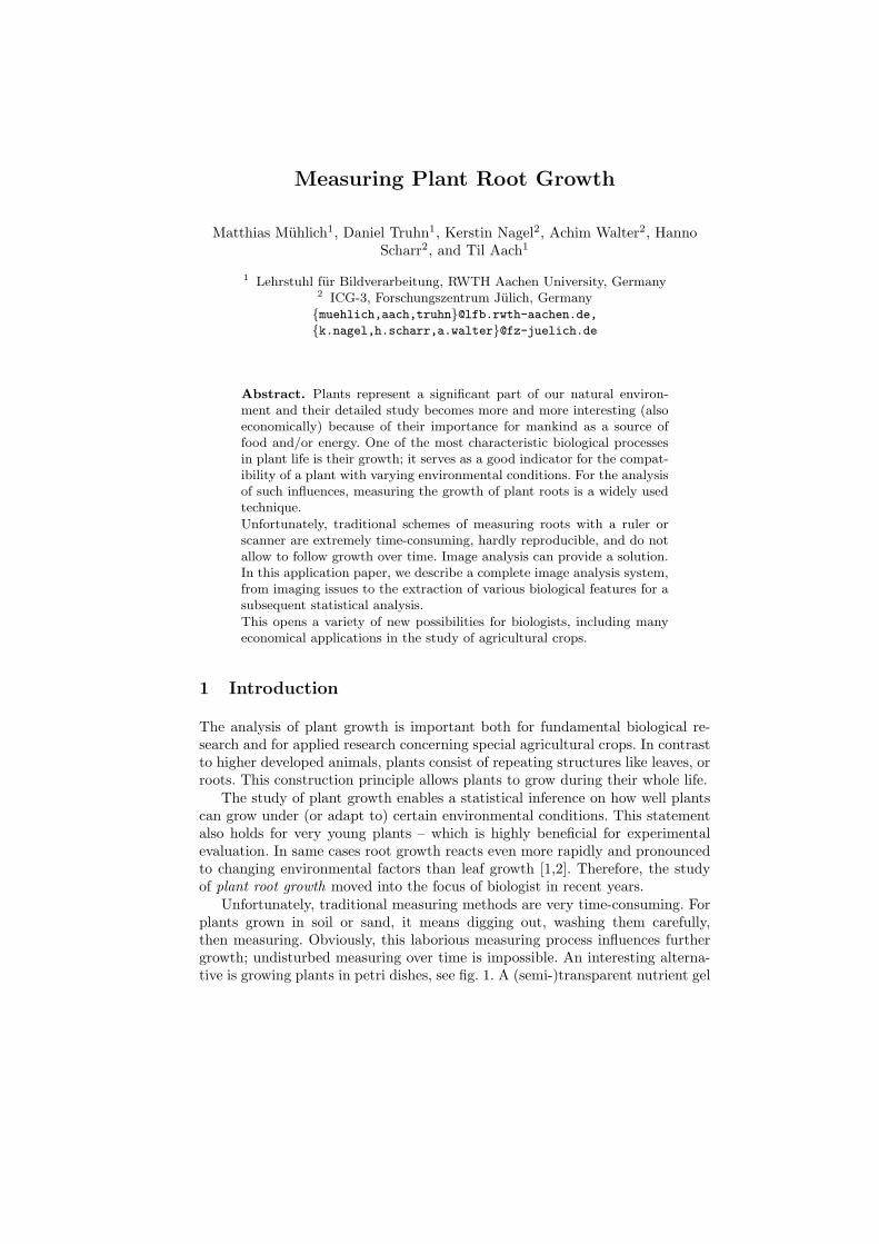
Abstract. Plants represent a significant part of our natural environ-ment and their detailed study becomes more and more interesting (alsoeconomically) because of their importance for mankind as a source offood and/or energy. One of the most characteristic biological processesin plant life is their growth; it serves as a good indicator for the compat-ibility of a plant with varying environmental conditions. For the analysisof such influences, measuring the growth of plant roots is a widely usedtechnique.

Unfortunately, traditional schemes of measuring roots with a ruler orscanner are extremely time-consuming, hardly reproducible, and do notallow to follow growth over time. Image analysis can provide a solution.In this application paper, we describe a complete image analysis system,from imaging issues to the extraction of various biological features for asubsequent statistical analysis.

This opens a variety of new possibilities for biologists, including manyeconomical applications in the study of agricultural crops.

1 Introduction

The analysis of plant growth is important both for fundamental biological re-search and for applied research concerning special agricultural crops. In contrastto higher developed animals, plants consist of repeating structures like leaves, orroots. This construction principle allows plants to grow during their whole life.

The study of plant growth enables a statistical inference on how well plantscan grow under (or adapt to) certain environmental conditions. This statementalso holds for very young plants – which is highly beneficial for experimentalevaluation. In same cases root growth reacts even more rapidly and pronouncedto changing environmental factors than leaf growth [1,2]. Therefore, the studyof plant root growth moved into the focus of biologist in recent years.

Unfortunately, traditional measuring methods are very time-consuming. Forplants grown in soil or sand, it means digging out, washing them carefully,then measuring. Obviously, this laborious measuring process influences furthergrowth; undisturbed measuring over time is impossible. An interesting alterna-tive is growing plants in petri dishes, see fig. 1. A (semi-)transparent nutrient gel

2

Fig. 1. Plants are grown in petri dishes filled with (half-)transparent nutrient gel. Thisallows imaging of root systems with transmitted light.

is filled in between two perspex panels which are a few millimeters apart. Thenplant seeds are put on the top such that the roots grow down into the gel.

Using this setup, it is possible to take images of the growing plant rootsat certain intervals (one image every 30 minutes, over a period of two or threeweeks, is common in our joint project between partners from biology and imageanalysis). Fig. 2 shows six images from such a time series. This setup also reducesthe problem of measuring roots from a 3d problem to a ‘almost 2d’ one. Whilea third dimension of just 3 millimeters width is indeed neglectable for lengthmeasurements, it does unfortunately not prevent roots from crossing each otherin different layers; this happens quite frequently in real data, see fig. 1.

The aim of our project was the extraction of tree-like structures for roots,augmented with several biologically interesting data values. These features in-clude lengths, thicknesses, growth rates, branching angles, or spatial densitiesof branching points; extension to further data should be possible. Additionally,simple access to theses features should be possible for a statistical analysis in or-der to make use of the primary strength of a computerized approach (in contrastto measurements by humans): the ability to measure hundreds or thousands ofplants, thus allowing valid and significant statistical statements.

This paper describes the build-up of a complete imaging system accordingto these requirements. Its organization reflects the various building blocks of thewhole system; each block is discussed in a seperate chapter. At the end, we willshow some results for the total length of the root system, divided into primary

3

Fig. 2. Growth of plant roots: the same three plants are imaged at six different times.

roots (i.e. roots starting at the origin), secondary roots (roots branching offfrom primary roots), and tertiary roots (which are branching off from secondaryroots).

2 Imaging Issues and Preprocessing

The first step which deserves some careful considerations is the image acquisitionitself. Imaging with visible light would disrupt the natural day and night cycleof plants. The solution is infra-red imaging, but a constant illumination of thewhole image is next to impossible with acceptable effort.

a b c d

Fig. 3. Compensation of varying illumination. See text for explanation.

Fortunately, varying background illumination can be compensated with stan-dard image processing techniques. Fig. 3 shows our preprocessing scheme: theinput image (a) is processed with a min/max nonlinear filter, resulting in im-age (b). This image is then smoothed (c). Rescaling the original image with thebackground brightness information from (c) then yields (d), the preprocessedimage which we use as input to our algorithm.

4

A few aspects which cannot be compensated properly with preprocessingare image artefacts due to condensing waterdrops or drying nutrient gel whichdissolves from the perspex wall. We mention these practical problems to illustratethat a high level of robustness is also required for our algorithm.

3 Modelling Roots I: A Steerable Filter Approach

Plant roots, even of the samt plant type, can look highly different. If one has todesign a computer program for the analysis of roots, it is therefore an apparentlyuseful first step to identify their common characteristic structural elements. Asthe number or shape of bifurcations (or other point-like structures, from roottips to root crossings) is rather difficult to predict or model, the starting pointfor our algorithm is the detection of linear structures: the roots. Such structurecan be found with a correlation based approach.

Let us postpone the treatment of branches and crossings to section 5 anddiscuss simple roots first; from an image analysis point of view, it is the detectionof dark lines on light background and these lines appear in arbitrary orientations.Within the class of correlation-based detectors for rotated lines, one approachpresented by Jacob and Unser in 2004 [3] can be considered state of the art. Thepresentation of this approach is the subject of this section.

Let f(x) denote an image within which we seek a feature (here: a line).Furthermore, let us assume that this feature can be modeled as a templatef0(x). Then filtering the image with a filter h(x) = f0(−x) yields an outputimage measuring how strong the feature is present at each location x. Thisprinciple is known as matched filter [4]. Its application to the detection of afamily of features is, in general, computationally inefficient, but for one specialclass of filters, namely rotated versions of some given template, the steerable filterapproach introduced by Freeman and Adelson in [5] offers a convenient solution:by limiting the class of possible (unrotated) templates to those templates whichcan be represented in polar coordinates in the form

h(r, φ) =P∑

p=−P

ap(r) exp(ipφ) , (1)

one can represent any rotated version of h(r, φ) as a linear combination of νbase filters, where the minimum number for ν is given as the number of non-zero Fourier coefficients in (1). (Note that, in slight abuse of notation, we willalways denote an image template as h, regardless whether it is represented inCartesian or polar coordinates.) Following the notation of Freeman & Adelsonand others, let us define a rotation operator: hα(r, φ) = h(r, φ − α). Differentvariants for designing steerable filters exist, but they all have in common thatrotation can be expressed as linear combination of a set of base templates:

hα(r, φ) =ν∑

i=1

wi(α)hi(r, φ) . (2)

5

Here, hi denote the set of base filters. In [3], Jacob and Unser applied this rotatedmatched filter approach to the detection of edges and lines in images. They alsothat using directional derivatives of a 2d Gaussian function up to fourth orderas base functions yields a very good orientation selectivity while still allowingan analytic solution for the optimal angle.

Fig. 4. Line template within theclass of steerable filters (rotated).

Fig. 5. Maximum filter response S(x) as ameasure of ‘line strength’.

Fig. 4 shows a contour plot for such an fourth order line template. Applyingthe steerable filter approach to the input image then leads to two values for everyimage location x: the orientation angle α(x) which fits best and the strength ofthe correlation S(x), i.e.

S(x) = f(x) ∗ hα(x)(x) . (3)

Then S(x) can be interpreted as a measure for the probability of a root atlocation x. Fig. 5 shows the “line strength image” S(x). Based on S(x), it ispossible to identify the origin of roots: high values of S(x) in a small horizontalstrip below the upper border of the petri dish indicate the presence of a rootorigin and all roots in a certain neighborhood are grouped together to a singleplant. These roots are called primary roots and followed downwards.

4 Modelling Roots II: Following Roots

The next image processing step is following roots from origin to root tip, passingthrough all branching points and potential crossings as straight as possible. Ouralgorithm is based on the image S(x) computed before (see fig. 5); for everypixel identified as root, the neighboring values of S(x) contribute a data termindicating the likelihood that the root continues this way.

However, basing a root following algorithm only on the imaga data wouldperform poorly in the presence of noise and the resulting root structures would

6

look unnatural. We therefore also added a model term which simply states thatroots usually grow straight. Instead of continuing roots in the direction whichmaximize S(x) directly, we maximize a modified quantity

S′(x) = S(x) ∗ c (4)

which introduces a correction term c. This correction term is based on the cur-rent root orientation α and the new orientation α′ which would be induced bycontinuing in the tested orientation. The more similar α and α′ are, i.e. the bet-ter the assumption of straight continuation is matched, the higher the correctionfactor c should be. On the other hand, strong bending should be penalized witha low value of c. This requirement is met with the exponential term

c = exp(

(α− α′)2

2σ2

). (5)

The choice of this function is motivated by a physical analogue: the bending ofan elastic rod leads to the same mathematical representation. Just like a highbending energy is required for a strong bending, the data term in our inputimage must sufficiently support the hypothesis of a direction change of a root.

If no acceptable continuation can be found, then we have to end the followingof the root – we have found its tip. Fig. 6 shows the detection result for a primary

Fig. 6. Tracked primary rootand 5-pixel distance lines onboth sides.

Fig. 7. Primary root (white) and potentialbranches indicated as small white dots 5pixels away from branch.

root. Additionally, two more lines are drawn left and right of the detected root.On these two lines, other roots are detected in order to analyze branches andcrossings in the following step.

7

5 Modelling Roots III: Crossing and Branching

With the algorithm described so far, it is possible to follow primary roots fromthe origin to the tip. This is possible because branching never happens in theway that a root tip splits in two and both new tips grow in directions whichare entirely different from the old one. In image analysis, such a model wouldalso be known as Y junction. Instead, a branch is created at the side of analready existing root, thus leading to a T junction (with the stem of the letterT “growing out of the horizontal bar”).

This biological background does not only allow an algorithm based on thefollowing of single root, it even calls for a recursive implementation of such astrategy. Note that this is completely different from other possible approaches toplant root measurement focussing on the detection of point features (branchingpoints, crossings, root tips) as underlying structural elements. The existence of Tjunctions instead of Y junctions also constitutes a notable difference to medicaldata (blood vessels, bronchial tubes) which might appear similar at first glance.

Fig. 8. Algorithms for the following of roots (left) and finding of branches (right).

The branch detection is carried out by searching for roots 5 pixels beside theprimary roots. For every found point (see fig. 6 for an example), we then tryto find a path to the original root. If this is not possible, then the found pointbelongs to a parallel root, not a branch. Furthermore, we search only upwardsfrom the tested point to the primary root (i.e. the test point 5 pixels away fromthe branch must lie below a potential branching point). All branches found inthis way are denoted secondary roots in biology and trigger a recursive rootfollowing just like the initial root following for primary roots. The same can becontinued for tertiary roots and so on.

8

Special care has to be applied to crossings. A downward branching has to beexcluded if there exists another upward branching on the opposite side with asimilar intersection angle to the original root. In this case, it represents a crossingwith a different root, not a branch. Fig. 8 illustrates this algorithm and the rootfollowing scheme from the previous section. Fig. 9 then shows the root detectionresult for a single input image.

6 Integrating Temporal Information

The basic algorithms shown in the previous sections are already sufficient tohandle single images. In practical applications, however, it is sometimes possibleto take multiple images of the same plant over time. How can we integrate thetemporal information?

Fig. 9. Detected root system. Primaryroots are shown in green, secondaryroots in red, tertiary roots in blue.

Fig. 10. Growth of the complete rootsystem (upper thick line) and the con-tribution of different root orders overtime.

The first step for the evaluation of an image series is obviously a registrationstep; this becomes especially important if the petri dish is not fixed in front of thecamera. In our application, a hundred individual petri dishes are mounted on acaroussel-like structure which rotates the different dishes in front of the camera(in order to allow a meaningful statistical evaluation). In this situation, thecompensation of a translational offset is always necessary. Nevertheless, we willnot discuss registration here; standard textbook approaches will work reasonablywell.

The desire for an algorithm with is capable of handling both single imagesand image series (in a sequential update mode) requires a modification of thealgorithm presented so far in a way such that it can additionally exploit infor-mation collected from previous images of the same plant. Most importantly, thiscan be used to disambiguate the crossing problem: which incoming root connects

9

to which outgoing root? This problem is inherently difficult to solve in single im-ages, but for image series, one can decide which root grew there first in 99.9 %of all cases. Time series processing offers a lot of advantages:

– If a root from the previous image was not found in the current image, thensearch again with modified threshold. Roots cannot disappear.

– Misdetections can be eliminated if a root cannot be detected again, evenwith lower threshold. This often applies to ‘ghost branches’: young brancheswhich have only grown a few pixels are extremely hard to distinguish fromnoise.

– The tree structure (branchings and especially crossings) can be recovered inmuch better quality.

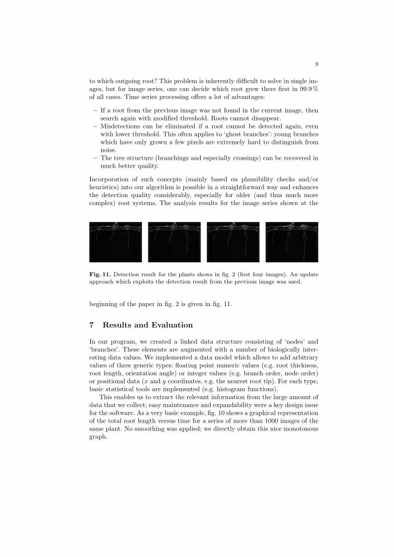
Incorporation of such concepts (mainly based on plausibility checks and/orheuristics) into our algorithm is possible in a straightforward way and enhancesthe detection quality considerably, especially for older (and thus much morecomplex) root systems. The analysis results for the image series shown at the

Fig. 11. Detection result for the plants shows in fig. 2 (first four images). An updateapproach which exploits the detection result from the previous image was used.

beginning of the paper in fig. 2 is given in fig. 11.

7 Results and Evaluation

In our program, we created a linked data structure consisting of ‘nodes’ and‘branches’. These elements are augmented with a number of biologically inter-esting data values. We implemented a data model which allows to add arbitraryvalues of three generic types: floating point numeric values (e.g. root thickness,root length, orientation angle) or integer values (e.g. branch order, node order)or positional data (x and y coordinates, e.g. the nearest root tip). For each type,basic statistical tools are implemented (e.g. histogram functions).

This enables us to extract the relevant information from the large amount ofdata that we collect; easy maintenance and expandability were a key design issuefor the software. As a very basic example, fig. 10 shows a graphical representationof the total root length versus time for a series of more than 1000 images of thesame plant. No smoothing was applied; we directly obtain this nice monotonousgraph.

10

8 Summary and Discussion

In this application paper, we presented and discussed a system for the comput-erized analysis of plant root growth. In a application problem like this one, theprogress does not lie in an exceptionally novel extension of one specific buildingblock; it is more like an engineering task where there basic problem consists inmaking a lot of different building blocks work together properly. Neither block iscomplicated by itself. A large part of the problem was decomposing a large andcomplex problem into small and easily digestible bits; we hope that this paperillustrates the basic ideas and reasonings behind our approach.

That key element of our software is the extraction of a tree model for plantroots. We developed an algorithm which is applicable to both single imagesand image series. Once the tree model is found, a variety of biological data(thicknesses, lengths, angles, etc) is computed with a number of rather simpletextbook algorithms (a later refinement of specific measurement tools is of coursepossible, if is should turn out to be necessary).

The progress of this approach becomes visible if we compare the huge amountof data which now becomes available to the traditional measuring of plant rootgrowth by hand. We are confident that our new software will turn out to be animportant tool for an increased understanding of plants and their interactionwith environmental influences.

References

1. Nagel, K., Schurr, U., Walter, A.: Dynamics of root growth stimulation in nicotianatabacum in increasing light intensity. Plant Cell Environ (2006) 1936–1945

2. Walter, A., Nagel, K.: Root growth reacts rapidly and more pronounced than shootgrowth towards increasing ligth intensity in tobacco seedlings. Plant Signaling &Behavior (2006) 225–226

3. Jacob, M., Unser, M.: Design of steerable filters for feature detection using canny-like criteria. IEEE Trans. PAMI 26 (2004) 1007–1019

4. Therrien, C.W.: Decision, Estimation and Classification: Introduction to PatternRecognition and Related Topics. John Wiley and Sons (1989)

5. Freeman, W., Adelson, E.: The design and use of steerable filters. IEEE Trans.PAMI 13 (1991) 891–906