Advancing Research on Well-Being Metrics beyond GDP
42
4. INEQUALITY OF OPPORTUNITY │ 3 FOR GOOD MEASURE: ADVANCING RESEARCH ON WELL-BEING METRICS BEYOND GDP © OECD 2018 Chapter 4. Inequality of opportunity François Bourguignon (Title, Paris School of Economics) 1 This chapter discusses what is meant by inequality of opportunity (i.e. “ex-ante inequality”), in the sense of how different circumstances involuntarily inherited or faced by individuals could affect their economic achievements later in life. This concept is also taken to include how fair the procedures are. The chapter presents the theoretical principles that can be used for measuring inequality of opportunity. Practical issues of measurement are illustrated through examples and stylised facts from the applied literature on inequality of opportunity and, in particular, on intergenerational economic mobility. The chapter summarises the nature of the data needed to monitor the observable dimensions of inequality of opportunity and makes recommendations on the statistics that should be regularly produced for effectively monitoring them.
-
Upload
khangminh22 -
Category
Documents
-
view
4 -
download
0
Transcript of Advancing Research on Well-Being Metrics beyond GDP

4. INEQUALITY OF OPPORTUNITY │ 3
FOR GOOD MEASURE: ADVANCING RESEARCH ON WELL-BEING METRICS BEYOND GDP © OECD 2018
Chapter 4. Inequality of opportunity
François Bourguignon (Title, Paris School of Economics)1
This chapter discusses what is meant by inequality of opportunity (i.e. “ex-ante
inequality”), in the sense of how different circumstances involuntarily inherited or faced
by individuals could affect their economic achievements later in life. This concept is also
taken to include how fair the procedures are. The chapter presents the theoretical
principles that can be used for measuring inequality of opportunity. Practical issues of
measurement are illustrated through examples and stylised facts from the applied
literature on inequality of opportunity and, in particular, on intergenerational economic
mobility. The chapter summarises the nature of the data needed to monitor the observable
dimensions of inequality of opportunity and makes recommendations on the statistics that
should be regularly produced for effectively monitoring them.
Fançois1
Highlight
Fançois1
Sticky Note
Emeritus Professor
4 │ 4. INEQUALITY OF OPPORTUNITY
FOR GOOD MEASURE: ADVANCING RESEARCH ON WELL-BEING METRICS BEYOND GDP © OECD 2018
4.1. Introduction
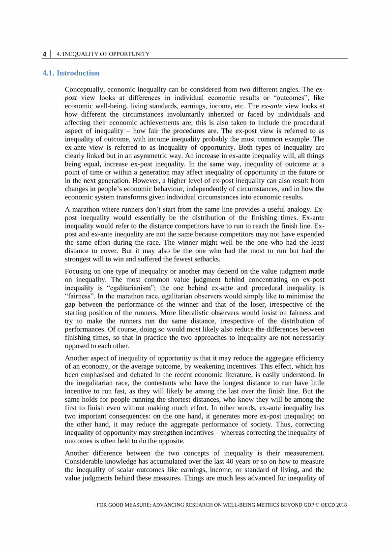
Conceptually, economic inequality can be considered from two different angles. The ex-
post view looks at differences in individual economic results or “outcomes”, like
economic well-being, living standards, earnings, income, etc. The ex-ante view looks at
how different the circumstances involuntarily inherited or faced by individuals and
affecting their economic achievements are; this is also taken to include the procedural
aspect of inequality – how fair the procedures are. The ex-post view is referred to as
inequality of outcome, with income inequality probably the most common example. The
ex-ante view is referred to as inequality of opportunity. Both types of inequality are
clearly linked but in an asymmetric way. An increase in ex-ante inequality will, all things
being equal, increase ex-post inequality. In the same way, inequality of outcome at a
point of time or within a generation may affect inequality of opportunity in the future or
in the next generation. However, a higher level of ex-post inequality can also result from
changes in people’s economic behaviour, independently of circumstances, and in how the
economic system transforms given individual circumstances into economic results.
A marathon where runners don’t start from the same line provides a useful analogy. Ex-
post inequality would essentially be the distribution of the finishing times. Ex-ante
inequality would refer to the distance competitors have to run to reach the finish line. Ex-
post and ex-ante inequality are not the same because competitors may not have expended
the same effort during the race. The winner might well be the one who had the least
distance to cover. But it may also be the one who had the most to run but had the
strongest will to win and suffered the fewest setbacks.
Focusing on one type of inequality or another may depend on the value judgment made
on inequality. The most common value judgment behind concentrating on ex-post
inequality is “egalitarianism”; the one behind ex-ante and procedural inequality is
“fairness”. In the marathon race, egalitarian observers would simply like to minimise the
gap between the performance of the winner and that of the loser, irrespective of the
starting position of the runners. More liberalistic observers would insist on fairness and
try to make the runners run the same distance, irrespective of the distribution of
performances. Of course, doing so would most likely also reduce the differences between
finishing times, so that in practice the two approaches to inequality are not necessarily
opposed to each other.
Another aspect of inequality of opportunity is that it may reduce the aggregate efficiency
of an economy, or the average outcome, by weakening incentives. This effect, which has
been emphasised and debated in the recent economic literature, is easily understood. In
the inegalitarian race, the contestants who have the longest distance to run have little
incentive to run fast, as they will likely be among the last over the finish line. But the
same holds for people running the shortest distances, who know they will be among the
first to finish even without making much effort. In other words, ex-ante inequality has
two important consequences: on the one hand, it generates more ex-post inequality; on
the other hand, it may reduce the aggregate performance of society. Thus, correcting
inequality of opportunity may strengthen incentives – whereas correcting the inequality of
outcomes is often held to do the opposite.
Another difference between the two concepts of inequality is their measurement.
Considerable knowledge has accumulated over the last 40 years or so on how to measure
the inequality of scalar outcomes like earnings, income, or standard of living, and the
value judgments behind these measures. Things are much less advanced for inequality of

4. INEQUALITY OF OPPORTUNITY │ 5
FOR GOOD MEASURE: ADVANCING RESEARCH ON WELL-BEING METRICS BEYOND GDP © OECD 2018
opportunity. Whereas statements like “there is less inequality in country A than in
country B” or “at time t than at time t-1” are easily understood and may be solidly
grounded in data in the case of outcomes, they are difficult to substantiate in the case of
inequality of opportunity.
Defining inequality of opportunity in the tradition of Dworkin (1981), Arneson (1989) or
Roemer (1998) as inequality in “the circumstances beyond the control of individuals”, the
view taken in this chapter is that it will never be possible to observe differences among
individuals across all the circumstances that may shape their economic success
independently of their will. (The fact that personal “will” may itself be a “circumstance”,
thus introducing a circularity into the definition of the inequality of opportunity, is
discussed below.) Besides, what is not under the control of individuals, i.e.
circumstances, and what is often referred to as “efforts”, may be extremely ambiguous. It
should also be mentioned that circumstances and efforts may interact in producing some
outcomes, thus making the distinction between them still more ambiguous. It follows that
it is not possible to measure inequality of opportunity in the most general sense as we
measure inequality of outcomes like earnings or income and compare it across space or
time. However, this does not mean that it is not possible to measure some observable
dimensions of inequality of opportunity and, most importantly, their impact on inequality
of outcomes. This is actually what the inequality of opportunity literature does without
always saying so. It is in this restricted sense that the expression will most often be used
throughout this chapter.
Analysing how a person’s income depends on the education or income of their parents
when that person was a child, on where they grew up, on gender, race, migration status,
etc. informs us as to the role of specific circumstances – family characteristics, region of
birth, or how the labour market discriminates across gender or race – in shaping the
distribution of income. It matters for policy to know whether this role has increased or
not, or that more inequality in the income of the present generation is likely to generate
more inequality in future generations. Yet such analysis is essentially partial. On the one
hand, non-observed circumstances may counteract the effect of observed ones, so that
concluding that there is more inequality of opportunity based on intergenerational
earnings mobility may be misleading. On the other hand, measuring the influence of a
given circumstance on outcomes does not say much about the channels through which
this effect takes place and on the policies to correct it. Deeper analysis is needed for some
specific policy to be recommended.
The ambition of this chapter is essentially practical. It is not to contribute to the
normative debate on the definition of inequality of opportunity in some absolute sense, or
to the positive debate on its potential efficiency cost. It is rather concerned with the
evaluation of the inequality specific to a given individual characteristic, duly considered
as a circumstance; and, more importantly, to measure its contribution to the inequality of
outcomes. The latter objective also applies to the case where several circumstances are
considered simultaneously, as there are various ways of mapping the inequality of
specific circumstances onto the inequality of given outcomes. In short, the chapter is
rather brief on purely conceptual issues, on whether such and such a type of inequality is
socially fair or unfair. The emphasis is on measurement issues and the practical use to be
made of available measures.
The chapter is organised into three sections. A first section addresses a few conceptual
issues, in particular what is meant by inequality of opportunity, and discusses the
theoretical principles that can be used for measuring it. Practical issues of measurement
Fançois1
Highlight
Fançois1
Sticky Note
ital

6 │ 4. INEQUALITY OF OPPORTUNITY
FOR GOOD MEASURE: ADVANCING RESEARCH ON WELL-BEING METRICS BEYOND GDP © OECD 2018
are taken up in the second section and illustrated through several examples and stylised
facts from the burgeoning applied literature on inequality of opportunity and in particular
on intergenerational economic mobility. The final section summarises the nature of the
data needed to monitor the observable dimensions of inequality of opportunity and makes
recommendations on the statistics that should be regularly produced for effectively
monitoring them.
4.2. Conceptual issues in defining and measuring inequality of opportunity
This section first addresses the definition of opportunity as distinct from other factors that
may contribute to the inequality of outcomes. It then discusses a few theoretical
principles that may guide the measurement of the inequality of opportunity.
4.2.1. Opportunities and economic outcomes: normative and positive issues
Figure 4.1 below summarises the debate about the definition of inequality of opportunity
as opposed to inequality of outcomes. The box on the left hand side of the figure refers to
factors beyond the control of an individual, called “circumstances”, and likely to affect
how she or he will manage and perform in the economic sphere. Some of them are
observable, like personal traits – gender, ethnicity, disabilities, place of birth – or parental
background. Others, like genetic traits, parents’ social capital, or cultural values,
generally are not. Together they form the basis for inequality of opportunity.
The circle beneath the circumstance box stands for individual preferences, supposed to be
independent from circumstances, thus with some genetic origin or resulting from all sorts
of life experiences with no relationship with parental background. This assumption of
course is quite debatable and will be discussed further below.
Circumstances, preferences and some key parameters from the economic sphere, like
prices and wages, determine individual economic decisions in the box at the bottom of the
figure – arrows (1), (2) and (6). To the extent these decisions determine the contribution
of the individual to the economic system, they are called “efforts”. A good example of
this is the supply of labour, which may depend on the wealth of an individual, i.e.
circumstances, the wage rate, taxes on labour income and, of course, preferences.
Given the market mechanisms and the policies implemented in the economic sphere, and
some randomness in those mechanisms, the individual contribution to the economic
sphere results – arrows (3) and (4) – in some individual economic outcomes, be they
earnings, income, consumption expenditures, etc. The key point, however, is that
circumstances may also determine outcomes, together with individual decisions, through
the economic sphere. This is the case for instance if some personal traits affect labour
market rewards, as where there is discrimination according to gender, migrant status,
ethnicity, or social origin. This direct influence of circumstances on outcomes through the
economic sphere is represented by arrow (5), going from the circumstance box to the
economic sphere. The corresponding inequality in outcomes has to do with what is often
termed “procedural” inequality. Circumstances may also indirectly affect individual
decisions by modifying the prices and wages faced by an individual – through arrow (6).
Within this representation of the determinants of economic outcomes, the latter thus result
directly from individual economic decisions, which result themselves from personal
preferences and economic conditions, and indirectly from the way personal traits and
parental influence may affect the rewards for a given effort in the economic sphere.
Fançois1
Sticky Note
Fançois1
Highlight
Fançois1
Sticky Note
circumstances if inherited

4. INEQUALITY OF OPPORTUNITY │ 7
FOR GOOD MEASURE: ADVANCING RESEARCH ON WELL-BEING METRICS BEYOND GDP © OECD 2018
In this framework, inequality of opportunity corresponds to the diversity of individual
circumstances and the way it maps onto unequal outcomes. However, in a dynamic
setting, unequal outcomes may themselves map onto unequal individual circumstance.
For instance, the thin dotted line (8) in Figure 4.1 may stand for the intergenerational
transmission of inequality: successful people in the current generation provide better
circumstances to their children in the next. Within a generation, that link may also stand
for a random event at some point of life, which, given individual preferences (in
particular with respect to risk), affects future earning potential, as in the case of poverty
trap phenomena.
Figure 4.1. The relationship between individual circumstances, opportunities and outcomes
In the economic inequality literature, a key distinction is made between defining
inequality in the space of circumstances and in the space of outcomes. This distinction
clearly matters from the point of view of moral philosophy and normative economics.2
For some authors, only the inequality of individual circumstances should matter as they
are, to some extent, forced upon individuals, and people are not morally responsible for
them. Social justice thus requires these sources of inequality to be compensated in the
outcome space, for instance through cash transfers. In contrast, the outcome inequality
that arises from individual decisions or efforts should not be a matter of social concern as
it essentially results from individuals’ free will, or preferences, so that individuals can be
taken as morally responsible for them.3 The opposite stream of the literature rejects this
distinction between circumstances and efforts on the basis of preferences being
themselves partly transmitted to individuals by their families or the social group they
belong to. If so, most outcome determinants may be understood as circumstances, and the
correction of inequality should entirely focus on the distribution of final outcomes.

8 │ 4. INEQUALITY OF OPPORTUNITY
FOR GOOD MEASURE: ADVANCING RESEARCH ON WELL-BEING METRICS BEYOND GDP © OECD 2018
At this stage, incentives must be taken into account. In the case where all determinants of
outcome, including the taste for hard work, are considered as circumstances,
compensating for all of them would lead to equalising outcomes irrespective of individual
actions and initiatives, thus eliminating work, entrepreneurship or innovation incentives.
In the case where only some income determinants are taken to be circumstances,
compensating for differences in circumstances and leaving uncorrected the inequality
arising from individual decisions may not always be possible or efficient. In the case of
labour market discrimination, for instance, we may know that women or children of
immigrants are discriminated against on average, but it would be difficult, and certainly
controversial, to establish this discrimination at the individual level. Even if it were
possible, compensating through lump-sum payments those who are discriminated against
would reinforce the market distortion created by discrimination, as people would get the
same wage as before but would possibly expend less effort due to the lump-sum transfer.
This is a clear case where inequality of opportunity is responsible for both inefficiency
and inequality of outcomes, and where the only efficient corrective policy is to eliminate
the market imperfection responsible for the inequality of opportunity in the first place.
4.2.2. Ambiguity and observability issues in defining opportunities
The framework shown in Figure 4.1, and the idea that inequality of opportunity could be
compensated by transfers in the outcome space, has three fundamental weaknesses for
practical application, in addition to the preceding inefficiency argument. First, there is a
fundamental ambiguity about what can be defined as circumstances and individual
decisions resulting from preferences supposedly independent of circumstances. Second,
even if the distinction between circumstances and efforts were unambiguous, there is a
problem with the fact that many circumstances and many efforts are not observable.
Third, the relationship between opportunities and outcomes is actually two-way. If, at a
point of time, inequality of opportunity is affecting inequality of outcomes when
Figure 4.1 is read from left to right, the dotted array (8) in Figure 4.1 stands for the fact
that inequality of outcome, possibly due to the free decisions of economic agents, may
dynamically affect future inequality of opportunity. Taken together, these weaknesses
justify focusing on the inequality of outcomes, while at the same time taking into account
the sources of the inequality related to specific observable circumstances. These points
are developed below.
The first critique of the distinction between circumstances outside individual control and
individual decisions reflecting independent personal preferences is precisely that it is
difficult to hold that preferences are under individual control, as if they were freely
chosen by people. An in-depth critique of that assumption has been made by Arneson
(1989). Somebody’s taste for work, for thrift or for entrepreneurship must come from
somewhere, possibly from family background.4 If so, the distinction between the
inequality in outcomes due to circumstances and due to individual decisions becomes
fuzzy and practically non-operational.
The fact that many circumstances are not observed is another reason why the distinction
between circumstances and efforts may have limited empirical relevance, at least as long
as one is not ready to make several restrictive assumptions. Many circumstances that
shape people’s professional and family trajectory are not observable. Yet they may affect
individual decisions as well as outcomes. For instance, parents may transmit to their
children values or talents that will make them decide to go to graduate school and at the
same time will help them in their career. If those values and talents are not observed,
however, how could we disentangle in observed outcomes what is actually due to
Fançois1
Highlight
Fançois1
Sticky Note
Replace "circumstances" by "them".

4. INEQUALITY OF OPPORTUNITY │ 9
FOR GOOD MEASURE: ADVANCING RESEARCH ON WELL-BEING METRICS BEYOND GDP © OECD 2018
observed efforts – i.e. graduate school – and what is due to unobserved circumstances? It
is only when it can be assumed that efforts do not depend on unobserved circumstances
that also affect outcomes that such identification is possible. If this is not the case, the
contribution of efforts to outcomes cannot be properly identified, which makes again the
distinction between circumstances and efforts somewhat artificial.5
Another weakness of the distinction between inequality of opportunity and inequality of
outcomes illustrated by Figure 4.1 is that, if outcomes are determined by circumstances
and individual decisions, then outcomes at one point of time may determine future
circumstances. As a matter of fact, the whole framework is set in static terms, when it
should actually be dynamic. Outcomes of one generation or at one point of time are likely
to affect circumstances in the next generation or at a future point of time, for instance
through accumulating or running down wealth or human capital, taken as a circumstance.
Under these conditions, ignoring that part of the inequality of outcomes that comes from
individual decisions implies ignoring a future source of inequality in the space of
circumstances. It may also be noted that, in such a dynamic framework, the measurement
of the inequality of outcomes raises some issues. If the unit of time is a generation, how
should outcomes be defined? Certainly not by their value at a point of time. Within a
dynamic intra-generational analysis, isn’t it the case that many ‘individual decisions’
quickly become circumstances, so that again the distinction between circumstances and
efforts yields limited insights?
Summing up, the focus put by some moral philosophers and normative economists on
inequality of opportunity rather than on inequality of outcomes may be perfectly justified
in theory. Practically, however, the distinction that has to be made between factors that
are under individual responsibility (efforts) and those that are not (circumstances) is most
often blurred, in part because of observability issues. Even when relying only on observed
circumstances and efforts, disentangling what part of inequality of outcome is due to one
or the other is difficult once it is admitted that observed and unobserved circumstances
may affect both outcomes and efforts. Actually, the only solid empirical evidence that can
be relied upon is the way outcomes depend on observed circumstances, i.e. essentially
some personal traits and family-related characteristics.
4.2.3. Measuring inequality of observed opportunities
Data on specific outcomes, some circumstances and, possibly, some types of efforts are
available in household surveys or from administrative sources. Based on them, it is
possible to estimate the relationship between specific outcomes, circumstances and
efforts.
Before getting into the measurement of inequality of opportunity, or rather some
dimensions of it, within these databases it is worth formalising that relationship and the
arguments in the preceding section. Assume that a survey sample of the population is
available with information on individual or household economic characteristics and
background. Denote by yi the outcome of interest for an individual i in the sample; his/her
observed circumstances by Ci; and his/her efforts by Ei. We can represent the way in
which circumstances and efforts determine outcome by the relationship:
𝑦𝑖 = 𝑓(𝐶𝑖, 𝐸𝑖) + 𝑢𝑖
where f( ) is some function to be specified below and 𝑢𝑖 stands for the role of unobserved
circumstances and efforts as well as temporary shocks or measurement errors on the
observed outcome. In empirical work, that relationship is often assumed to be log-linear:

10 │ 4. INEQUALITY OF OPPORTUNITY
FOR GOOD MEASURE: ADVANCING RESEARCH ON WELL-BEING METRICS BEYOND GDP © OECD 2018
𝐿𝑜𝑔 𝑦𝑖 = 𝑎. 𝐶𝑖 + 𝑏. 𝐸𝑖 + 𝑢𝑖 (1)
where a and b are vectors of parameters. Such a specification of the function 𝑓(, ) is very
restrictive, as one would expect some interaction between circumstances and efforts in
determining outcome. Yet, it is simple and quite sufficient for our purpose.
The argument in the preceding section and in the Annex 4.A suggests that Ei is correlated
to the observed circumstances Ci and the unobserved circumstances in ui. Because of the
latter, it is thus not possible to get unbiased estimates of a and b. Under these conditions,
the only empirical relationship that can be reliably estimated is a reduced form model
where the outcome depends only on observed circumstances:
𝐿𝑜𝑔 𝑦𝑖 = 𝛼. 𝐶𝑖 + 𝑣𝑖 (2) 6
where α is a set of coefficients that describe the effect of observed circumstances on the
outcome directly or indirectly through their correlation with efforts (observed or not
observed), and vi stands for all outcome determinants different from observed
circumstances. It should be noted, however, that for α to be estimated without bias, it is
necessary to assume that all these unobserved outcome determinants are independent of
the observed circumstances, Ci. Otherwise, the estimated α coefficients will also include
the effects of all unobserved outcome determinants that are correlated in one way or
another with Ci.
Estimating models of type (2) through ordinary least square (OLS) is a trivial exercise
that has been performed under a variety of specifications for the outcome variable, yi, and
the explanatory variables, Ci. Perhaps the most familiar specification is the famous
Mincer equation that includes the earnings rate of employed people as the outcome
variable, and schooling7 and personal traits as explanatory variables.
There is a burgeoning literature on the measurement of inequality of opportunity based on
models of type (1) or (2). Using model (1), it essentially consists of comparing the actual
inequality in outcomes to the inequality that would be observed if all individuals in the
data sample were facing the same circumstances, or were all expending a given level of
effort. This literature is exhaustively summarised in Ramos and Van de Gaer (2012) and
Brunori (2016). We take here a simpler approach based on the fact that efforts are either
not observed or endogenous – i.e. correlated with unobserved outcome determinants – so
that model (2) is the only solid basis to measure the inequality of opportunities described
by the variables in Ci.
It can be noted that, in some cases, it is possible to measure the inequality of single
components of C irrespectively of outcomes and model (2). For instance, parental income
or cognitive ability may be components of C, the inequality of which can be observed in
some databases.8 The higher the inequality a component of C, the more unequal the
distribution of outcomes, provided that the corresponding coefficient in α is strictly
positive.
The inequality of the distribution of C may also be expressed in terms of the inequality of
outcomes. When the latter is measured by the variance of logarithms and when there is a
single component in C, model (2) implies that:
𝑉𝑎𝑟(𝐿𝑜𝑔 𝑦) = 𝛼². 𝑉𝑎𝑟 (𝐶) + 𝑉𝑎𝑟 (𝑣)
Thus, the inequality of that single component of C can also be expressed as what could be
the inequality of outcomes if other determinants of outcomes were neutralised, i.e. in the
case where they were the same for all individuals. If the inequality of outcomes is
Fançois1
Highlight
Fançois1
Sticky Note
Add "of" between "inequality" and "a"

4. INEQUALITY OF OPPORTUNITY │ 11
FOR GOOD MEASURE: ADVANCING RESEARCH ON WELL-BEING METRICS BEYOND GDP © OECD 2018
measured by the variance of logarithms (VL), the inequality of C, IVL(C), could in that
case be written as:
𝐼𝑉𝐿(𝐶) = 𝛼². 𝑉𝑎𝑟 (𝐶) (3)
and 𝐼𝑉𝐿(𝐶 ) = 𝛼′. 𝐶𝑜𝑣𝑎𝑟 (𝐶). 𝛼
when there is more than one component in C.
This definition can be generalised to any measure of outcome inequality M{ } – i.e. Gini,
Theil, mean logarithmic deviation – and to any number of components in C in two ways.
First, define the “virtual” outcome, y°(Ci, ve), for every individual i, as what would be the
outcome of that individual if all the outcome determinants other than the opportunities in
C were equal to some exogenous value, ve, common to all, i.e.:
𝐿𝑜𝑔 𝑦°(𝐶𝑖, 𝑣𝑒) = 𝛼𝐶𝑖 + 𝑣𝑒 (4)
Then compute the measure of inequality M{ } on the distribution of y°(Ci, ve) in the whole
sample. An absolute measure of the inequality of opportunities in C is then given by M{
y°(C., ve) }, where y°(C., v
e) stands for the whole distribution of y°(Ci, v
e) in the sample.
Fleurbaey and Schokkaert (2009) labelled this measure the “direct unfairness” (du) of the
inequality of opportunity associated with C:
𝐼𝑀𝑑𝑢 (𝐶) = 𝑀{ 𝑦°(𝐶. , 𝑣𝑒) (5)
Thus, 𝐼𝑀𝑑𝑢 (𝐶) measures the inequality of opportunities in C by considering their impact
on the inequality of outcome, irrespective of all other outcome determinants. Of course, a
measure of inequality of opportunities in C can be defined for each measure M{ } of
outcome inequality. As most outcome inequality measures M{ } are scale invariant, the
arbitrary value of ve does not actually matter.
9
Second, one may use the "dual" of the preceding definition of inequality of opportunities
in the following sense. Instead of equalising the outcome determinants other than C, one
may define a virtual income resulting from the equalisation of the opportunities in C
across all individuals in the sample. Let Ce be the common value of opportunities and
y*(Ce, vi) the corresponding virtual income:
𝐿𝑜𝑔 𝑦∗(𝐶𝑒 , 𝑣𝑖) = 𝛼𝐶𝑒 + 𝑣𝑖 (6)
Then an another absolute measure of inequality of opportunities in C may be defined for
any outcome inequality measure M{ } as the difference between the actual inequality of
outcome and that which would result from equalising circumstances among all
individuals in the sample. Fleurbaey and Schokkaert (2009) proposed to label this the
“fairness gap” (fg) measure of inequality of opportunity associated with C:
𝐼𝑀𝑓𝑔
(𝐶. ) = 𝑀{𝑦. } − 𝑀{ 𝑦∗(𝐶𝑒 , 𝑣.) } (7)
As before, this measure is independent of the arbitrary value, Ce, taken for opportunities
when the outcome inequality measure is scale invariant.
Both measures of inequality of opportunities may also be defined in “relative” terms by
expressing them as a proportion of the actual inequality of the outcome being studied,
M{y.}. They will be denoted respectively IMdu(𝐶.) and IM
fg(𝐶.)
The preceding notations may seem a bit complicated. Their interpretation is extremely
simple and intuitive when applied to actual data, as illustrated by the few remarks below.
Fançois1
Highlight
Fançois1
Sticky Note
Delete

12 │ 4. INEQUALITY OF OPPORTUNITY
FOR GOOD MEASURE: ADVANCING RESEARCH ON WELL-BEING METRICS BEYOND GDP © OECD 2018
1. Consider equation (2) as a standard regression equation of outcomes on a set of
observed opportunities with the unobserved outcome determinants, v, as the
residuals of the regression. Then, if the inequality measure of outcome M{ } is the
variance of logarithms, then both the direct unfairness (5) and the fairness gap
measures (7) are equal to the variance of the logarithm of outcome explained by
the opportunities C, and the corresponding relative measure is simply the familiar
R² statistic associated with regression (2).
2. Consider now the individual “types” defined by combinations of the variables in
C with a minimum number of observations. For instance with only gender in C,
there would be two types. With gender and two possible values for the education
of the parents, there would be four types: men from low education parents,
women from high education parents, etc. It turns out then that the direct
unfairness inequality of opportunity (5) is very close to the familiar between
group inequality of outcomes when groups are defined by types, except that the
inequality is defined on the mean of the logarithm of outcomes rather than on the
outcome means.10
3. The preceding expressions to evaluate the inequality of observed of opportunities
refer to the linear case, where the opportunities being considered have
independent effects on the outcome of interest. Of course, it is also possible to
take into account interactions between opportunities, as for instance, between
gender and education in explaining the inequality of earnings.
4. When considering types, the above formulae seem to leave little room for the
inequality of outcomes within types. This is not completely true since the
outcome inequality between types corresponding to (5) is not the same as the
inequality between the types’ mean outcomes, the difference depending on the
distribution of outcomes within types. An approach that takes more explicitly into
account outcome inequality within types is the inequality of opportunity measure
that can be derived from the principles set in Roemer (1998).
𝐼𝑅 =1
��∫ [��(𝜋) − 𝑀𝑖𝑛𝑡{𝑞𝑡(𝜋)}]
1
0 𝑑𝜋 (8)
where 𝑞𝑡(𝜋) is the outcome of the quantile of order 𝜋 in the outcome distribution for type
t, ��(𝜋) is the (weighted) mean of those quantiles across types, and �� is the overall mean
outcome. In other words, inequality of the opportunities defined by types is the mean
across quantiles of a Rawlsian type of inequality measure across types for each quantile.11
The preceding inequality measure corresponds to the case where the residual term, v, in
(2) is heteroskedastic with a distribution, and hence a variance, that depends on the
observed circumstance variables, C, or differs across types. This is perfectly consistent
with the usual assumptions that the residual term v has zero expected value and is
orthogonal to C. With heteroskedasticity, however, defining the inequality of opportunity
through (5) or (7) is not possible anymore. The definition of the virtual income in (4)
ignores the dependency of the residual term on C and the equalising of circumstances in
(6) should require modifying the vi term, so that its distribution does not depend on C
anymore or, equivalently, is the same across types.

4. INEQUALITY OF OPPORTUNITY │ 13
FOR GOOD MEASURE: ADVANCING RESEARCH ON WELL-BEING METRICS BEYOND GDP © OECD 2018
4.3. Practical issues and some stylised facts in measuring the inequality of
opportunity
The discussion in the preceding section has focused on conceptual issues in the definition
and measurement of inequality of opportunities. We now turn to the way these principles
and approaches to measurement are handled in the empirical literature and present
stylised facts about some specific dimensions of inequality of opportunity.
The focus will first be on single dimensions of inequality of opportunities, without
necessarily making reference to specific outcomes. More direct applications of the
measurement tools discussed above will then be considered with various combinations of
outcomes (income, earning rates) and sets of opportunities. Special emphasis will be put
on the measurement of intergenerational transmission of inequality, which has attracted
much attention among social scientists, and which may be considered as a particular case
of the measurement principles set out above. Emphasis will also be put on labour market
discrimination, which raises some interesting questions when studied from the
perspective of inequality of opportunity.
4.3.1. Direct measures of some particular dimensions of the inequality of
opportunity
The measurement of specific dimensions of inequality of opportunities can be undertaken
in an autonomous way, without explicit reference to economic outcomes. This direct
approach simply consists of analysing the distribution of particular circumstances, C.
Many individual characteristics could be analysed in this way, provided they are
described by some quantitative index. Given its huge importance in the literature on
inequality of opportunity, this section focuses on cognitive ability and then briefly
considers the difficulty of handling directly other single dimensions of inequality of
opportunity.
Cognitive ability as an opportunity and as an outcome
The PISA initiative by the OECD provides first hand data to measure inequality in one of
the most important dimension of individual circumstances: cognitive ability. It now
gathers the scores of samples of 15-year old school children in more than 70 advanced
and emerging economies in three tests: one on reading, i.e. answering questions about a
short text; one on mathematics; and the third on science. This instrument has been fielded
at 3-year time intervals since 2000. In addition to students’ answers to these assessment
tests, the database also reports information on their family background and on the
characteristics of their schools.
Considering PISA scores as circumstances implicitly supposes looking at cognitive
ability at 15 as one of the important determinants of future individual economic
outcomes, earnings in particular, and acknowledging that it essentially depends on genetic
factors and the family context. Adults cannot be held responsible for that part of their life,
so that the inequality of PISA scores among 15 year-olds today will be responsible for
some of the inequality of opportunity they will face later in their lifetime. But PISA
scores may also be seen at the outcome of the educational process and, as such, dependent
on family circumstances, the efforts of the children, and the educational system itself.12
Hence the debate on how schools may correct for the inequality of opportunity arising
from family background. It is however the former perspective, i.e. cognitive scores as a
circumstance, that is discussed in what follows.
Fançois1
Highlight
Fançois1
Sticky Note
Replace "Adults" by "People"

14 │ 4. INEQUALITY OF OPPORTUNITY
FOR GOOD MEASURE: ADVANCING RESEARCH ON WELL-BEING METRICS BEYOND GDP © OECD 2018
Much publicity is given at each new edition of PISA to mean scores by country, to the
ranking of countries and how rankings change over time. From the viewpoint of
measuring inequality of opportunities, however, what matters most is the statistical
distribution of these scores, or their disparities across students.
Figure 4.2 plots the inequality of PISA scores in mathematics, as measured by the
coefficient of variation, against the mean score in the 2012 exercise for OECD countries.
Interestingly, there is a clear negative relationship between the inequality and the mean of
scores (putting aside the three emerging economies, Chile, Mexico and Turkey where the
coverage of the PISA survey is much lower than in advanced countries, essentially
because a non-negligible proportion of 15 year-olds have already dropped out of
school).13
This is presumably because better mean scores are logically obtained by
improving more the lower than the upper tail of the distribution. Yet what may be more
important is the substantial difference in the inequality of scores for countries in the same
range of average scores. For instance, inequality is 30% higher in Belgium than in
Finland or Estonia, in the upper part of the scale of mean scores; the same holds true for
France compared to Denmark in the middle.
Figure 4.2. Mean and coefficient of variation of PISA mathematics scores in OECD
countries, 2012
Source: OECD (2014), PISA 2012 Results: What Students Know And Can Do,
http://dx.doi.org/10.1787/9789264208780-en.
Cognitive ability can be considered as a dimension of economic opportunity only insofar
as it is a significant determinant of an outcome like earnings or the standard of living of
an individual. In this respect, it is important to stress that test scores in surveys like PISA,
the OECD’s Survey of Adult Skills (PIAAC) or its predecessor (the International Adult
Literacy Survey, IALS) only explain a limited part of earnings. Murnane et al. (2000) and
Levin (2012) make this point on the basis of US data. According to the former, a 1%
AUS
AUT
BEL
CAN
CHL
CZE
DNK EST FIN
FRA
DEU GRC
HUN
ISL
IRL
ISR
ITA
JPN KOR
LUX
MEX NLD
NZL
NOR POL
PRT
SVK
SVN ESP
SWE
CHE
TUR GBR
USA ARG BRA
BGR
COL
CRI
HRV
CYP
HKG
IDN
JOR
KAZ LVA
LIE
LTU
MAC
MYS
MNE
PER
QAT
ROU RUS
SRB
CHN
SGP
TWN
THA
TUN
URY
VNM
15
20
25
30
350 400 450 500 550 600 650
Co
eff
icie
nt
of
vari
atio
n (
%)
Mean score
Fançois1
Highlight
Fançois1
Highlight
Fançois1
Highlight
Fançois1
Sticky Note
This chart is wrong, as it does not refer to OECD countries. Use the 'Pisa CV_mean(OCDE)' rather than 'Pisa data' sheet in the 'HLEG_chapt. Fig2' Excel file.

4. INEQUALITY OF OPPORTUNITY │ 15
FOR GOOD MEASURE: ADVANCING RESEARCH ON WELL-BEING METRICS BEYOND GDP © OECD 2018
increase in high school test scores entails a 2% increase in earnings when students are
31 years old, which is substantial.14
However, the variance of adults’ (log) earnings
explained by high school test scores is small, slightly less than 5% for men (Murnane et
al. (2000, p. 556). Family background is a more powerful determinant of earnings, all the
more so when considering that test scores are very much dependent on the education and
income of parents.
Instead of cross country comparisons as in Figure 4.2, it would be interesting to see how
inequality, or more exactly the whole distribution of scores, changes over time in a given
country. Data reported by the OECD in 2012 include the 90/10 inter-decile and
75/25 inter-quartile ratios for the four exercises since 2003. These measures are
remarkably constant except for emerging economies where inequality goes down at the
same time as mean scores go up. France is one of the few advanced countries where the
90/10 inter-decile ratio increased significantly over time. As France’s mean score did not
change much, this would suggest that good performers do better and bad ones do worse,
possibly a clear sign of an increase in the inequality of that specific component of
opportunities. A careful study of the evolution of the whole distribution of test scores
country by country might reveal other interesting features and it is surprising that so
much emphasis is being put on the evolution of the means without considering
distributional features.
The same kind of analysis, based on quite different tests, is being performed at younger
ages by a number of organisations, for instance the Progress in International Reading
Literacy Study, led by the International Association for the Evaluation of Educational
Achievement. However, the results have not received as much publicity, even though
they are equally, if not more, relevant in the analysis of inequality of opportunity, as
numerous studies have shown that differences in individual cognitive abilities appear very
early in life. Pre-school tests already show high variability among children depending on
their family background, and several studies have shown that these differences might
have long-lasting effects, as school systems would at best compensate only part of them.
Experiments with preschool programmes aimed at levelling the playing field like the
Perry programme or the Abecedarian programme in United States have provided
evidence of this – see for instance Kautz et al. (2015). As shown in recent work by
Heckman,15
the origins of these preschool inequalities are due in large part both to
“parenting”, i.e. the care the parents devote to their young children, and to health factors.
Other single dimensions of the inequality of opportunity
Initial inequality in non-cognitive skills is also important throughout lifetime, and may be
considered as another dimension of the inequality of opportunity, even though no
synthetic measure is actually available, which makes comparing societies over space or
over time difficult.
Health status is another dimension of childhood circumstances related to family
background, and another component of human capital. In the same way that cognitive
skills at 15 influence future earnings and are heterogeneous across young people, health
status at earlier ages is known to potentially influence the whole career of people and to
be heterogeneous too.16
The difficulty here is to monitor inequality in health status. There
is an important literature for instance on birth weights as a predictor of health status,
future education achievements and adult earning levels (e.g. Currie, 2009). The same may
be true of anthropometric indices at early ages, although most indices are strongly
influenced by weight at birth. It is somewhat surprising that more attention is not given to
Fançois1
Sticky Note
Add:"due to the lower tail moving up"

16 │ 4. INEQUALITY OF OPPORTUNITY
FOR GOOD MEASURE: ADVANCING RESEARCH ON WELL-BEING METRICS BEYOND GDP © OECD 2018
the evolution of inequality in these indices and, as for educational test scores, their
dependency on parental characteristics.
Another single dimension of the inequality of opportunity, different from human capital,
is inherited financial capital. It is certainly possible to measure the inequality of
inheritance flows during a given period. Wolff (2015) does so for the United States using
data from the University of Michigan’s Panel Study of Income Dynamics (PSID) and
provides Gini coefficients of inheritance flows both for the whole population and among
recipients. However, this is not very informative because of the heterogeneity in the age
of inheritors. The extent to which inheriting the wealth of one’s parents at the age of 55,
something frequent these days, may be considered as a component of inequality of
opportunity is not totally clear, except if, somehow, one has been able to borrow,
effectively or virtually, much earlier in life against this future wealth flow. As the credit
market is highly imperfect, and the inheritance date or the amount to be inherited highly
uncertain, it is not even sure it would make much sense to try to estimate something like
the inequality in discounted expected inheritance flows of all 25 year-old individuals.
Further, donations as well as inheritances would have to be taken into account.
Inheritance is a dimension of the inequality of opportunity whose inequality is difficult to
evaluate as such, even though it is a key factor shaping inequality in economic outcomes
like income or standard of living when considering cohorts beyond a certain age.
4.3.2. Outcome-based measures of inequality of opportunities
Rather than considering the inequality of various dimensions of opportunities in an
isolated way, it is possible to measure it indirectly through their overall effect on the
inequality of the outcomes under study, using a relationship of type (2) above. It was seen
that, in various ways, this relationship provides an indirect scalar metric of inequality of
opportunity. Various illustrations of this approach are shown below, while also reporting
stylised facts on some key components of inequality of opportunities.
Intergenerational mobility of earnings
Much work has been devoted to the estimation of models of type (2) where the outcome
𝑦𝑖 is the (full-time) earnings of an observed individual, i, and Ci is the (log) (full-time)
earnings of their parents, most often their father, observed roughly at the same age.
Denoting the latter by y-1,i, the basic specification of the model is thus:
𝐿𝑜𝑔 𝑦𝑖 = 𝛾 𝐿𝑜𝑔 𝑦−1,𝑖 + 𝑎 + 𝑣𝑖 (9)17
where a is a constant and 𝑣𝑖 is a zero mean random term, standing for all unobserved
earnings determinants independent of fathers’ earnings. The coefficient 𝛾 summarizes all
the channels through which fathers’ earnings, and their own determinants like education,
may affect sons’ earnings.
This model, reminiscent of the famous Galton (1886) analysis of the correlation of height
across generations, is generally presented as belonging to the literature on
intergenerational mobility, with the least square estimate 𝛾 being interpreted as the
intergenerational elasticity (IGE), or the degree of immobility across generation.
Equivalently, in a Galtonian spirit, the coefficient 1 − 𝛾 is interpreted as the speed of the
regression towards the mean.
This approach to intergenerational mobility is based on a parametric specification and the
estimation of a specific parameter. Non-parametric specifications come under the form of
Fançois1
Sticky Note
Add: ", but hey are seldom reported in surveys"
Fançois1
Highlight
Fançois1
Sticky Note
Put the whole expression (three words) in simple quotes.

4. INEQUALITY OF OPPORTUNITY │ 17
FOR GOOD MEASURE: ADVANCING RESEARCH ON WELL-BEING METRICS BEYOND GDP © OECD 2018
mobility matrices showing the probabilities pij for the earnings of sons whose father's
earnings is in income bracket i to be in bracket j. We consider these two approaches in
turn.
Parametric representation of intergenerational mobility
To see more clearly the relationship between IGE and inequality of opportunity, one may
consider applying directly the alternative definition of inequality of opportunities
provided in the preceding section of this chapter. Applying (4)-(7) to model (9) and
assuming that the inequality measure M{ } is scale invariant, it can be shown easily that:
𝐼𝑀𝑑𝑢(𝑦−1.) = 𝑀 {𝑦−1.
��} and 𝐼𝑀
𝑓𝑔(𝑦−1.) = 𝑀{𝑦.} − 𝑀{exp (��.)}
where the notation ^ refers to least square estimates. In the particular case where M{ } is
the variance of logarithms, VL, it turns out that the two measures in absolute terms are
identical because of the additivity property of the variance:
𝐼𝑀𝑑𝑢(𝑦−1.) = 𝐼𝑀
𝑓𝑔(𝑦−1.) = 𝛾2𝑉𝐿{𝑦−1.}
while in relative terms:
𝐼𝑀𝑑𝑢(𝑦−1.) = 𝐼𝑀
𝑓𝑔(𝑦−1.) =��2𝑉𝐿{𝑦−1.}
𝑉𝐿{𝑦.}= 𝑅2 (10)
where 𝑅2 is the measure of the explanatory power of the independent variables in
regression (9) or, in the present case, the square of the correlation coefficient between the
(log) earnings of parents and children.
It can be seen that there is a difference between the intergenerational mobility of earnings
(IGE) and inequality of opportunity linked to father’s earnings. The former is
proportional to the latter with a coefficient equal to the ratio of the inequality of
children’s earnings to that of their fathers.18
In other words, it is only in a world where the
inequality of earnings does not change across generations that both the inequality of
opportunity, based on the variance of logarithm, and the IGE coincide.
In their study of geographical differences in intergenerational mobility in the United
States, Chetty et al. (2014a) use the ranks of parents and children in the earnings
distribution as a relative measure of mobility. Based on the ‘copula’ of the joint
distribution of the (log) earnings of the two generations, i.e. the joint distribution of
father/children ranks in their respective earnings distribution, this measure is independent
of the marginal distributions of log earnings. It turns out that the rank-rank correlation is
not very different from the log-earnings correlation for reasonable small values of the
latter. Through (10), it is thus possible to recover the IGE from the rank-rank correlation.
Non-parametric representation: mobility matrices
Another way of representing the intergenerational mobility of earnings is through a
transition matrix representing the way a two-generation dynasty transitions from a given
earnings level for fathers to another (or the same earnings) level for sons. Let there be N
earning brackets denoted Yk and denote pij the probability than the sons of fathers in
bracket Yi find themselves in bracket Yj. The distribution of earnings is given by the total
rows and columns of the matrix P={pij}, but it is also possible to break free from these
distributions by defining the income brackets as the quantiles (deciles, vintiles…) of the
distribution of the earnings for fathers, on the one hand, and for sons, on the other.19

18 │ 4. INEQUALITY OF OPPORTUNITY
FOR GOOD MEASURE: ADVANCING RESEARCH ON WELL-BEING METRICS BEYOND GDP © OECD 2018
Table 4.1. Intergenerational transition matrix for earnings
Fathers Y1 Y2 Y3 … YN Total
Sons
Y1 P11 P12 P13
P1N P1.
gY2 P21 P22 P23
P2N P2.
Y3 P31 P32 P33
P3N P3.
… … … … … … …
YN PN1 PN2 PN3
PNN PN.
Total P.1 P.2 P.3 … P.N 1
Whether the transition or ‘mobility’ matrix is defined in terms of income brackets or
quantiles is not without implications for the interpretation that may be given to the
comparison of two matrices. When referring to income brackets, the matrix shows
‘absolute’ mobility, i.e. the probability that children’s earnings could be higher, or lower,
than their parents’, a concern of many parents today. Conversely, defining the matrix in
terms of quantiles permits to analyse the ‘relative’ mobility, irrespectively of earnings
levels. The difference between the two approaches lies essentially in the fact that the
latter does not take into account the change in the distribution of earnings across
generations.20
There is a huge literature on how to draw mobility indicators from such a representation
of the influence of parents’ earnings on children’s earnings – see Fields and Ok (1999) or
the survey by Jäntti and Jenkins (2015). For instance, mobility is often measured by one
minus the trace of the mobility matrix. Shorrocks (1978) suggested a “Normalised Trace”
measure given by [N-trace(A)]/(N-1), where A is the matrix P with rows normalised to 1
– i.e. the N probabilities pij are divided by the row sum pi. Other measures are based on
the expected number of jumps from one bracket, or decile, to another.
Rather than comparing transition matrices on the basis of mobility indices, some
dominance criteria have also been developed, which may lead to incomplete ordering
and, thus, to cases of non-comparability between two matrices. For instance, the diagonal
criterion says there is less mobility in a transition matrix than in another if all diagonal
elements, rather than their sum, are smaller in the former than in the latter. Shorrocks
(1978) proposed a stronger criterion, the “strong diagonal view” according to which there
is more mobility in matrix A than in B if aij ≥ bij for all i≠ j.
Although related, this kind of measure based on the transition probabilities has only an
indirect link with measures of inequality of opportunity in the sense that it is not
expressed in terms of the distribution of outcomes, which logically should be here the
distribution of children’ earnings. There are various ways such a link may be established:
The Roemer inequality of opportunity formula (8) would be one way, although
apparently seldom used, mostly because the transition matrix consistent with it
would be conceptually different from P above. Indeed, the children’s earnings
brackets should be row dependent so as to correspond to the deciles – or other
quantiles – of the distribution of earnings among children from parents in a given
earnings bracket or quantile.
Fançois1
Highlight
Fançois1
Sticky Note
Consistency with the text would require to reppalce the upper case P by lower case p in the whole table
Fançois1
Highlight
Fançois1
Sticky Note
Delete "g"
Fançois1
Sticky Note
Add a dot for the end of the sentence. The dot there is a subindex of p.

4. INEQUALITY OF OPPORTUNITY │ 19
FOR GOOD MEASURE: ADVANCING RESEARCH ON WELL-BEING METRICS BEYOND GDP © OECD 2018
An alternative would consist of associating to each row of the matrix a scalar
depending on the mean earnings and its distribution within the row. In a more
general context, van de Gaer (1993) suggested measuring the inequality of
opportunity by the inequality of the mean earnings across “types”, i.e. fathers’
earnings here, which is actually a measure of type Idu
as defined in (4). Lefranc et
al. (2009) argued in favour of combining the mean with some inequality measure
within type. More generally, one could consider the observed distribution of
children’s earnings with the same father’s earnings, as being that of the ex-ante
random earnings of the typical child in that type. Then one would associate to
each row of the transition matrix the certainty equivalent of the distribution of
earnings in that row for a given level of risk aversion. This would be equivalent to
associating to each row of the matrix the equivalently distributed earnings (EDE)
for that row, in the sense of Atkinson (1970) and then defining inequality of
opportunity as the inequality of these EDEs across rows.21
A social welfare approach to the measurement of intergenerational mobility has
been proposed by Atkinson (1981) and Atkinson and Bourguignon (1982), which
differs somewhat from the inequality of opportunity analytical framework
presented here. It consists of defining social welfare on father-son pairs, so that
each cell of the transition matrix is given a utility U(Yi, Yj) and the social welfare
of society is defined by the mean value of this utility, weighted by the transition
probabilities, pij. The simplest case is when U( ) is additive in the earnings of
parents and children. Atkinson and Bourguignon (1982) derived dominance
criteria to compare transition matrices on that basis, depending on the properties
of the function U( ).
A similar line of thought has been pursued by Kanbur and Stiglitz (2015) who
extend the preceding approach by considering a steady state of an economy
consisting of infinitely lived dynasties under the assumption of constant transition
matrix and earnings distribution across generations. Within that framework, they
identify a social welfare based dominance criterion of one matrix over another or,
in other words, of one stationary state of an economy with some intergenerational
mobility feature over another stationary state with a different mobility matrix.
In the perspective of inequality of opportunity, there are problems with the last two
approaches. On the one hand, the assumption of a fully stationary economy and a social
welfare dominance comparison based on dynasties with an infinite number of generations
seems extreme, even though the stationarity assumption is often implicit in statements
about intergenerational earnings mobility. On the other hand, it is a problem that the very
nature of circumstances is used to make comparisons of outcomes across groups of
individuals with identical circumstances. In other words, the mobility of children with
rich parents may matter less than that of poor parents. What should matter from the point
of view of inequality of opportunity is how different the distribution of earnings is across
parents’ earnings levels, with no particular importance being given to those levels.
In summary, there is some ambiguity about the way in which inequality of opportunity
corresponding to non-parametric specifications of the intergenerational mobility of
earnings can be measured. There are various ways mobility can be evaluated or transition
matrices compared based on social welfare criteria. But the link with measures of
inequality of opportunity of the kind that can be derived from simple parametric models
of type (9) – at least under the assumption of homoscedasticity of the residual term, v – is
unclear. For this reason, the rest of this section looks at the parametric case.

20 │ 4. INEQUALITY OF OPPORTUNITY
FOR GOOD MEASURE: ADVANCING RESEARCH ON WELL-BEING METRICS BEYOND GDP © OECD 2018
Data requirements
A priori, the data requirement to estimate the IGE or the parents-children earnings
transition matrix seems extremely demanding. One should observe the earnings of
parents, generally the father, and that of the children, generally the sons, at more or less
the same age or during the same period of the lifecycle in both cases. Long panel data
bases extending over 20 years and more would allow this to be done. For instance, the
PSID (Panel Study of Income Dynamics) in the United States has been collecting data on
the same families and their descendants for almost 50 years. The British and the German
household panels also extend over 25 years and more. In some countries, register data,
most often tax data, allow researchers to follow people throughout their lifetime and from
one generation to the next, but only a few countries have open and anonymized register
data at this stage.
However, panel data are not really necessary to estimate model (9). The availability of
repeated cross-sections over long periods is sufficient. Moreover, they permit the IGE to
be estimated in a consistent – i.e. asymptotically unbiased – manner, something which is
not certain with panel data.
To see this, it must be noted that the observation of 𝐿𝑜𝑔 𝑦−1 is most likely to include
measurement errors or, at least, transitory components of fathers’ earnings which are
unlikely to have had any effect on their sons’ earnings. Estimating 𝛾 in (9) with OLS and
without precaution for measurement error will thus lead to the so-called attenuation bias,
a bias that has been shown to be quite substantial in intergenerational mobility studies.22
The solution is to “instrument” 𝐿𝑜𝑔 𝑦−1 by regressing that variable on some fathers’ or
parents’ characteristics, Z, at the same date, say 𝑡−1, and to use the predicted rather than
the observed value when estimating (9) with OLS. Thus, if the parents’ characteristics Z
are observed at time t in the same database as children’s earnings, and if an earlier cross-
section is available at time 𝑡−1, this allows us to estimate the log earnings of adults with
characteristics Z. Running OLS on (9) using the predicted earnings of the parents at time
𝑡−1 will yield an asymptotically unbiased estimator of the IGE. Through this so-called
two-sample instrumental variable (TSIV) estimation strategy (Björklund and Jäntti, 1997)
repeated cross-sections with information on respondents’ parents and covering a period
long enough are sufficient to estimate the IGE.23
There are two important caveats to the preceding method. First, the instrumental variable
approach just sketched is valid only to the extent that the instrument Z may be assumed to
be orthogonal to the income of the children. It must be recognised, however, that this is
unlikely to be the case, as most observable parents’ characteristics, like education,
occupation, wealth, etc., may be thought of as influencing the economic achievements of
children. Second, even if the TSIV strategy did allow the IGE to be estimated consistently
with repeated cross-sections rather than with panel data, it would not permit the
corresponding inequality of opportunity to be estimated as defined by (10). This is
because the variance of the instrumented earnings of parents is not the same as the
variance of their true earnings.
Measurement errors are also likely to affect the estimation of mobility measures, social
welfare dominance tests and inequality of opportunity through the transition probability
matrix methods mentioned above. In that case, both the error on fathers and sons matter.
The former may be responsible for misclassifying fathers in the income scale, whereas
the latter introduces noise in the transition probabilities.
Fançois1
Sticky Note
Add:"at that time"
4. INEQUALITY OF OPPORTUNITY │ 21
FOR GOOD MEASURE: ADVANCING RESEARCH ON WELL-BEING METRICS BEYOND GDP © OECD 2018
Stylised facts
The best illustration of this literature on the measurement of intergenerational mobility is
the well-known “Great Gatsby” curve, due to Miles Corak and popularised by Alan
Krueger. It plots estimates of IGE against the level of inequality – in the
contemporaneous generation – for a set of developed and developing countries. This
curve is shown in Figure 4.3 below.
Along the vertical scale of the chart, one observes a rather wide dispersion of the
estimated IGE, from 0.2 for Nordic countries – Sweden being a little above that level – to
0.5 in the United States and 0.6 in Latin American countries. If it is assumed that the
inequality of earnings is similar among parents and children, then (10) suggests that a
consistent measure of inequality of opportunity is the square of the IGE, or the R² of the
regression of the log of sons’ earnings over the log of fathers’. Then it can be seen that
inequality of opportunity corresponding to the fathers’ earnings alone is extremely low in
Nordic countries, amounting to less than 4% of the variance of log earnings, while it is
more substantial in the United States, amounting to 25% of sons’ earnings inequality.
Yet, this would still leave considerable room for mobility if it were the case that no other
circumstance, orthogonal to parents’ earnings, constrained children’s earnings, which
seems unlikely.
The plot also shows a strong correlation between earnings immobility, i.e. IGE or
inequality of opportunity, and the degree of inequality, as measured by the Gini
coefficient of household disposable income, at a point in time. Several explanations have
been given for the negative correlation shown in Figure 4.3. The most frequent one relies
on some kind of non-convexity in the way parents invest in the human capital of their
children, or possibly some unequal access to quality schooling depending on parents’
income. If rich parents invest a higher proportion of their own income in the education of
their children, or if only the children of parents above some level of income have access
to good quality schools, then more income inequality among parents should generate less
intergenerational mobility.
Fançois1
Sticky Note
Repalce by: "convexity in the relationship between parent's income and their investment"
Fançois1
Highlight

22 │ 4. INEQUALITY OF OPPORTUNITY
FOR GOOD MEASURE: ADVANCING RESEARCH ON WELL-BEING METRICS BEYOND GDP © OECD 2018
Figure 4.3. The Great Gatsby curve
Source: Corak (2012).
The preceding argument is equivalent to assuming some non-linearity in the basic model
(9) or, more exactly, that the IGE may depend on the level of income. If the IGE
increases with income, as just suggested, then the linear approximation (9) would indeed
yield an OLS estimate of the IGE that increases with the degree of income inequality.24
That the IGE may vary with the level of income is shown in the case of the United States
by Landersø and Heckman (2016), p. 22, as can be seen in Figure 4.4 below.25

4. INEQUALITY OF OPPORTUNITY │ 23
FOR GOOD MEASURE: ADVANCING RESEARCH ON WELL-BEING METRICS BEYOND GDP © OECD 2018
Figure 4.4. Non-linear IGE in the United States
Parents observed in 1987 and children 36-38 in 2011
Another, more mechanical, explanation of the negative slope of the Great Gatsby curve is
based on (10) above. If one compares two countries where income inequality was the
same in the older generation, then it is the case that with the same correlation coefficient
(R²) between the earnings of the two generations, the IGE will be higher in the country
with the highest inequality today. For instance, Landersø and Heckman (2016, p.17) show
that the IGE in Denmark would be much bigger than what it is if the distribution of
children’s earnings was identical to the US distribution. This again illustrates the
difference between the concept of immobility as described by IGE and inequality of
opportunity related to parents’ earnings. Yet it is unlikely that Figure 4.3 would be
fundamentally different if the IGE were replaced by the inequality of opportunity as
defined in (10).26
Other explanations of the upward sloping Gatsby curve are available that go from
mobility to inequality rather than the opposite. For instance, Berman (2016) stresses that
if the distribution of the residual term, v, is constant, model (9) leads to a steady-state
distribution of earnings whose inequality is given by: 𝑉𝐿(𝑦) = 𝑉𝑎𝑟(𝑣)
1−𝛾2 . Thus, the
inequality of income increases with IGE. As a matter of fact, it should be noted that this
property does not hold only at a steady state. Among two societies with the same
distribution of earnings in one generation, inequality will be higher, all things being
equal, in the society where parents transmit more of their earning capacity to their
children. Formally, (9) implies that:
𝑉𝐿(𝑦) = 𝛾2𝑉𝐿(𝑦−1) + 𝑉𝑎𝑟(𝑣)
which is increasing in 𝛾.
One might ask whether this positive relationship between inequality and intergenerational
immobility may also hold inter-temporally. Interestingly enough, Aaronsson and
Mazumder (2008) show that trends in wage inequality between 1940 and 2000 in the
United States coincide with trends in IGE, with a compression in the first part of the

24 │ 4. INEQUALITY OF OPPORTUNITY
FOR GOOD MEASURE: ADVANCING RESEARCH ON WELL-BEING METRICS BEYOND GDP © OECD 2018
period and increasing disparities in the later part.27
However not enough data are
available to test that hypothesis on a cross-country basis.
The same type of analysis may be undertaken with other economic outcomes. However to
keep with the spirit of model (9) it is important to make sure that the same variable can be
observed for both parents and children. For instance, having parents’ earnings on the right
hand side of the equation and income per capita (or per adult equivalent) on the left hand
side is interesting, but the interpretation is not anymore in terms of intergenerational
transmission of earning potential, as income per capita also depends on family size,
marriage, and labour supply. There is also an issue with the period of observation of the
right-hand variable. Presumably, one would expect parents’ income to influence the life-
time earnings of children. This may not be reflected when observing children during a
short period at some stage of their life.
Chetty et al. (2014a) address this issue when analysing the spatial heterogeneity of
intergenerational income mobility in the United States, as they indeed use lifetime pre-tax
family income as income variables in both generations as drawn from administrative tax
data. They find considerable spatial variation of income mobility across “commuting
zones”: “the probability that a child reaches the top quintile of the national income
distribution starting from a family in the bottom quintile is 4.4% in Charlotte (North
Carolina) but 12.9% in San Jose (California)”.
Taking advantage of the length of register data, Chetty et al. (2014b) also study the time
evolution of intergenerational mobility, in effect the rank correlation between fathers’ and
sons’ earnings. They find no significant change across birth cohorts born between 1971
and 1982. This is line with the results found earlier by Lee and Solon (2007) for the US
using the PSID panel dataset for cohorts born between 1952 and 1975. Both results
diverge somewhat from Aaronsson and Mazumder (2008). Non-consensual results are
also found in other countries, as shown by the critiques by Goldthrope (2012) to the
finding by Blanden et al. (2008) that mobility would have fallen in the UK.
Another interesting concept, closer to the sociological view on mobility, has recently
studied by Chetty et al. (2017). ‘Absolute mobility’, is defined as the proportion of 30-
year old children whose real income is higher than their parents’ when they were 30.
Combining register data since 1970 with assumptions on rank correlation together with
cross-sectional data for the period before, absolute mobility has declined continuously
from the 1940 to the 1965 birth cohort – i.e. the baby boomers. It then stabilized but fell
again soon because of the financial crisis – i.e. for cohorts born in the late 1970s.
Somewhat surprisingly, much less work has been done on the intergenerational
transmission of wealth inequality and on the key role of inheritance in the inequality of
opportunity. This is in part due to the availability of data. Typical household surveys
generally do not include data on wealth. When they do, they do not necessarily include
data on parents, or they are not repeated over a period long enough to apply the TSIV
methodology. As for panel data, some waves of PSID do include wealth questionnaires.
They have been used by Charles and Hust (2003) to estimate an IGE for wealth.
Unfortunately, no information is available that would allow to correct for measurement
error bias. The British and German household panels do include data on wealth but the
number of observations is too small to estimate IGE for wealth at mid-life, an age at
which the wealth concept becomes relevant for both parents and children. One could also
think of using estate statistics, but these actually lack relevance as their link to inequality
of opportunity is through the heirs, whose wealth is not observed.

4. INEQUALITY OF OPPORTUNITY │ 25
FOR GOOD MEASURE: ADVANCING RESEARCH ON WELL-BEING METRICS BEYOND GDP © OECD 2018
In Nordic countries, several recent studies of intergenerational wealth dynamics have
relied on administrative data. Boserup et al. (2014) provide estimates of the wealth IGE at
mid-life in Denmark, and Adermon et al. (2015) do the same for Sweden. Both studies
cover more than two generations. In both countries, the wealth IGE estimates are
comparable and of limited size (around 0.3), a value comparable to the earnings IGE in
Sweden but twice as large in Denmark.
Generalised intergenerational mobility analysis and inequality of observed
opportunities
Parental income is only one of the circumstances affecting the economic outcome of an
individual, even though it may be correlated with other circumstances. To provide a more
complete picture, fathers’ earnings, y-1 in equation (9) can be replaced or complemented
by a vector of variables referring to the parental characteristics of an individual in the
current generation. Labour force or household surveys often give information on the
parents of respondents (education, occupation, residence, age when respondent was 10).
Rather than using the TSIV approach to estimate parental earnings or income based on
these characteristics, one may simply measure the related inequality of opportunity by the
share of the inequality of income or earnings in the current generation that is accounted
for by parents’ earnings.
Formally, model (9) is replaced by:
𝐿𝑜𝑔 𝑦𝑖 = 𝛽 𝑍𝑖 + 𝑣𝑖 (11)
where 𝑦𝑖 is a particular economic outcome; 𝑍𝑖 a vector of variables that include all
observed parental characteristics and some other characteristics beyond individual
control, like gender; and 𝑣𝑖 all the unobserved determinants of the economic outcome that
are orthogonal to 𝑍𝑖. In agreement with the definition (7), the R² statistics of that
regression may be interpreted as the inequality of opportunities associated with individual
characteristics in 𝑍𝑖 when measuring the inequality of outcomes with the variance of
logarithms. Some authors prefer using other measures of inequality.28
In comparison with model (9), model (11) may be considered as a model of “generalised”
mobility in the sense that more parental characteristics are taken into account that do not
necessarily include the outcome being explained in the current generation. It can also be
noted that this model is identical to the model used in the intergenerational mobility
analysis of earnings when instrumenting the earnings of the parent by a set of
characteristics available in the data base – i.e. the TSIV approach. Model (11) would then
correspond to the “reduced” form of the earnings mobility model, necessarily less
restrictive than the structural form (9).
Figure 4.5 illustrates this approach to inequality of opportunity, drawing on a paper by
Brunori et al. (2013) that puts together estimates of some observed dimensions of
inequality of opportunity in selected countries as reported in several papers, including
Checchi et al. (2010) and Ferreira and Gignoux (2011b). The inequality of opportunities
measure used in these papers is the one defined in (5), with the mean logarithmic
deviation as a measure of inequality.29
The figure shows the relative inequality of
observed opportunities (vertical axis) against the total inequality of outcomes (horizontal
axis).
Figure 4.5 is in some sense the equivalent of the Great Gatsby curve, with the IGE being
replaced by the inequality of observed opportunities.30
This generalisation of the Great
Fançois1
Highlight
Fançois1
Sticky Note
Replace by: "characteristics, including the determinants of their own earnings"

26 │ 4. INEQUALITY OF OPPORTUNITY
FOR GOOD MEASURE: ADVANCING RESEARCH ON WELL-BEING METRICS BEYOND GDP © OECD 2018
Gatsby curve, which consists of replacing parental earnings by observed parents’
characteristics and individual traits, leads to a relationship between inequality of observed
opportunities and inequality of outcomes that is still positive. However that relationship
disappears when restricting the sample to advanced countries, unlike what observed in
Figure 4.3.
Figure 4.5. Inequality of outcomes and share due to observed dimensions of the inequality of
opportunity, selected countries around 2005
Source: Based on Brunori et al. (2013).
This difference must be taken with very much precaution, though. On the one hand,
countries are not the same. On the other hand, both the outcome variables and the
observed circumstances Z in Brunori et al. (2013) may not be the same across countries.
The economic outcome, y, refers to labour earnings for the EU countries and the United
States31
, household income per capita in Latin American countries, household earnings
per capita in India, and household gross income per capita in South Africa. An important
lesson to be drawn from these exercises is the need to use uniform definitions of
variables. This is not always possible across countries, but is absolutely necessary for
comparing the same country over time.
Another important caveat is that the inequality of observed opportunities reported in
Figure 4.5 is estimated on the whole population rather than specific age cohorts as in
studies of intergenerational earnings mobility. In other words, the implicit assumption is
that this inequality is uniform across age groups, or cohorts, in national populations. This
is far from granted. The way an economic outcome depends on individual and parental
circumstances may change over the life cycle, and may change across cohorts. Cohorts
are definitely the most relevant statistical reference. What policy makers and analysts are
NOR
SVN
POL
FIN
HUN EST
CZE SWE PRT LVA
FRA SVK ITA DNK
LTU GRC BEL
DEU USA
NLD ESP IND GBR
AUT IRL COL LUX ZAF
ECU TUR
PER CYP PAN
BRA GTM
0
0.05
0.1
0.15
0.2
0.25
0.3
0.35
0.4
0 0.1 0.2 0.3 0.4 0.5 0.6 0.7 0.8
Re
lati
ve in
eq
ual
ity
of
op
po
rtu
nit
y
Inequality of outcomes (Mean logarithmic deviation)

4. INEQUALITY OF OPPORTUNITY │ 27
FOR GOOD MEASURE: ADVANCING RESEARCH ON WELL-BEING METRICS BEYOND GDP © OECD 2018
interested in is whether younger cohorts are less dependent on their family background
than older cohorts, presumably at the same age.32
Improving and standardising generalised mobility analyses of the type described above –
to make them comparable across countries, over time, and across cohorts – might be
easier to implement than standardising intergenerational earnings mobility studies. It
should permit key determinants of the inequality of outcomes to be monitored effectively,
be it earnings, income or subjective well-being, and to identify forces behind the
evolution of the inequality, or possibly behind its stability. Done in a systematic way,
such analyses should be most helpful for policy making in the field of inequality.
It should also be noted that the same non-parametric matrix specification used for
intergenerational mobility analysis can be used here. The matrix P in Table 4.1 would
differ simply by the definition of the rows. Instead of referring to the earnings of parents,
they would refer to types of individuals in the current generation, the types being defined
by the most frequent combinations of individual characteristics, Z. This would not be a
mobility matrix or a copula anymore but simply a matrix comparing the distribution of a
given economic outcome across individuals with different social and family background
or individual traits. The corresponding inequality of opportunity could be measured using
the Roemer-like measure (8) above or some of the suggestions made when discussing the
measure of intergenerational mobility.
Sibling studies
Other approaches have been used in the literature to identifying what part of the
inequality of outcomes has its roots in family background in the strict sense, rather than in
the mixed bag of characteristics, Z, that can be found in household surveys. In this
context, the idea of using differences or similarities among siblings or twins is
particularly attractive.
If the economic outcome being studied is labour earnings, the square of the correlation
coefficient of earnings between siblings is a direct measure of the share of the inequality
of outcomes that comes from a common family context. This requires some assumptions
on the underlying earnings model.33
If these assumptions are found to be reasonable, then
this correlation coefficient logically account for all observed and unobserved family
background characteristics as well as presumably for other circumstances which were
common to siblings in their childhood or adolescence. Because of this, it is expected that
the share of outcome inequality explained in this way be higher than with other
estimations based on observed circumstances, even though siblings may not share all the
family background factors susceptible to affect their earnings later in life. At first sight,
however, orders of magnitude seem comparable to what is obtained in intergenerational
earnings mobility studies – in the few countries where both estimates are available. For
instance, the correlation coefficient between brothers’ earnings is 0.23 in Denmark (Jäntti
et al., 2002) and 0.49 in the United States (Mazumder, 2008). The former value is
somewhat above what is shown in Figure 4.4, whereas the latter is roughly the same.
Sibling analysis of this type may well be able to capture a bigger part of the overall effect
of family circumstances on outcome inequality but, contrary to the type of study
described in the preceding subsection, it does not say much about the channels behind this
effect. Also, this type of analysis cannot be performed on the basis of standard household
surveys, which are the most commonly used source for measuring outcome inequality.
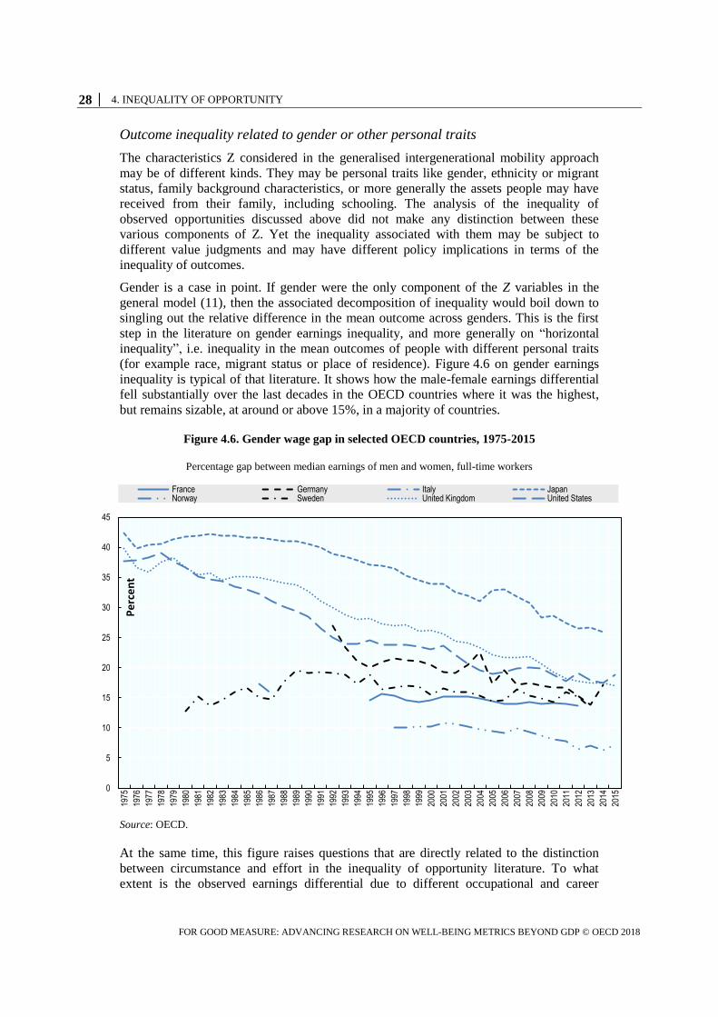
28 │ 4. INEQUALITY OF OPPORTUNITY
FOR GOOD MEASURE: ADVANCING RESEARCH ON WELL-BEING METRICS BEYOND GDP © OECD 2018
Outcome inequality related to gender or other personal traits
The characteristics Z considered in the generalised intergenerational mobility approach
may be of different kinds. They may be personal traits like gender, ethnicity or migrant
status, family background characteristics, or more generally the assets people may have
received from their family, including schooling. The analysis of the inequality of
observed opportunities discussed above did not make any distinction between these
various components of Z. Yet the inequality associated with them may be subject to
different value judgments and may have different policy implications in terms of the
inequality of outcomes.
Gender is a case in point. If gender were the only component of the Z variables in the
general model (11), then the associated decomposition of inequality would boil down to
singling out the relative difference in the mean outcome across genders. This is the first
step in the literature on gender earnings inequality, and more generally on “horizontal
inequality”, i.e. inequality in the mean outcomes of people with different personal traits
(for example race, migrant status or place of residence). Figure 4.6 on gender earnings
inequality is typical of that literature. It shows how the male-female earnings differential
fell substantially over the last decades in the OECD countries where it was the highest,
but remains sizable, at around or above 15%, in a majority of countries.
Figure 4.6. Gender wage gap in selected OECD countries, 1975-2015
Percentage gap between median earnings of men and women, full-time workers
Source: OECD.
At the same time, this figure raises questions that are directly related to the distinction
between circumstance and effort in the inequality of opportunity literature. To what
extent is the observed earnings differential due to different occupational and career
0
5
10
15
20
25
30
35
40
45
1975
1976
1977
1978
1979
1980
1981
1982
1983
1984
1985
1986
1987
1988
1989
1990
1991
1992
1993
1994
1995
1996
1997
1998
1999
2000
2001
2002
2003
2004
2005
2006
2007
2008
2009
2010
2011
2012
2013
2014
2015
Pe
rce
nt
France Germany Italy JapanNorway Sweden United Kingdom United States
4. INEQUALITY OF OPPORTUNITY │ 29
FOR GOOD MEASURE: ADVANCING RESEARCH ON WELL-BEING METRICS BEYOND GDP © OECD 2018
choices made by male and female workers or to features completely outside their own
control, like education or, most importantly, employer discrimination in the labour
market? Also, to what extent do the differentials shown in Figure 4.6 reflect differences
in labour force participation rates, themselves related to wage determinants like age or job
experience? The answer to these questions is of great importance for policy, in particular
to identify the role of labour market discrimination and the possible remedies to other
sources of earnings inequality. For instance, concluding from Figure 4.6 that gender
earnings discrimination has gone down by 15 to 20 percentage points in countries where
it was around 45% 40 years ago would not be correct if the composition of the female (or
male) labour force had changed over time or if the proportion of better paid women
increased.
Part of the answer to the questions mentioned above is obtained by adding other personal
traits and circumstances to gender as regressors in model (11). For instance, if schooling
is introduced as an additional circumstance variable, the coefficient of the gender
component would then reflect the male-female difference in earnings once the effect of
male-female differences in schooling on the earnings differential had been accounted for.
In a more general model, the gender coefficient would measure the gender earnings gap
that comes in addition to gender differences in all observed earnings determinants. This
coefficient is generally referred to as the ‘adjusted’ gender earnings gap.
It is possible to go further by making the model non-linear through interactions between
the gender and the other components of Z, namely:
𝐿𝑜𝑔 𝑦𝑖 = β𝑍𝑖 + 𝛿 𝑍𝑖 ∗ 𝐺𝑖 + 𝑣𝑖 (12)
where 𝐺𝑖 is a dummy variable that stands for the gender of person i and the 𝛿 coefficients
measure the earnings differential associated with the individual characteristics in 𝑍𝑖.
Alternatively, model (12) can be estimated separately for male and female workers:
𝐿𝑜𝑔 𝑦𝑖𝑔
= 𝛽𝑔 𝑍𝑖𝑔
+ 𝑣𝑖𝑔
, 𝑔 = 𝑀, 𝐹 (13)
Based on the estimates of the two sets of coefficients 𝛽𝑔, the gender earnings gap may be
decomposed into gender differences in the earnings determinants and differences in the
return to these determinants, i.e. between the estimated coefficients ��𝐹 and ��𝑀. For
instance, women may be paid at a lower rate than men because they have less education,
which was true for some time and still is for older cohorts, but they may also be paid less
than men for any additional year of schooling, which might be considered as pure
discrimination.
Formally, this so-called Blinder-Oaxaca decomposition is:
𝐿𝑜𝑔 ��𝐹 − 𝐿𝑜𝑔 ��𝑀 = (𝑛𝐹��𝐹 + 𝑛𝑀��𝑀)(��𝐹 − ��𝑀) + (��𝐹 − ��𝑀). (𝑛𝐹��𝐹 + 𝑛𝑀��𝑀) (14)34
where the notation refers to means, and 𝑛𝐹 and 𝑛𝑀 are the weight of female and male
workers respectively in the population sample. The first term corresponds to the
contribution of differences in individual characteristics between men and women, i.e. the
difference between the earnings gap and the adjusted earnings gap defined above. The
second term stands for the true discrimination, i.e. the fact that the same characteristics
are not rewarded in the same way among men and women. Actually, it is precisely the
adjusted earnings gap defined earlier, the interest of (14) being that this adjusted gap can
be decomposed into the contributions of the various components of Z. In the context of
gender inequality, this adjusted gap may be considered as a measure of procedural

30 │ 4. INEQUALITY OF OPPORTUNITY
FOR GOOD MEASURE: ADVANCING RESEARCH ON WELL-BEING METRICS BEYOND GDP © OECD 2018
inequality, i.e. the way the same characteristics are not rewarded in the same way for two
groups of individuals.
Figure 4.7 illustrates this decomposition and at the same time exhibits quite a remarkable
stylised fact. The figure is drawn from a meta-analysis of gender wage discrimination and
shows the mean gender earnings gap and the adjusted earnings gap in a set of 263 papers
covering a large number of countries at different points of time. The figure reports the
means of all studies reporting estimates for a given year, year by year. A remarkable
pattern emerges. Over time, the mean gender wage gap has declined substantially, as
shown in Figure 4.6 for selected countries. At the same time the mean adjusted gap, or the
second term in the Oaxaca-Blinder equation above, remains more or less constant on
average. In other words, on average across countries, the main reason why the gender
earnings gap declined is because the gender differences in wage determinants like
education or job experience have declined, not because the returns to these determinants
have become less unequal. Assuming the studies in this meta-analysis are fully
comparable, this would mean that the inequality of opportunity related to labour market
discrimination has not changed in the average country.
From a policy point of view, the Oaxaca-Blinder equation is of obvious interest since it
shows the orientation to be chosen in order to reduce gender inequality, and therefore
total earnings inequality. From a perspective of inequality of opportunity, however, it also
raises an interesting issue, which is that focusing exclusively on circumstances as the
source of inequality may not always be justified. The way efforts are rewarded by the
economic system, depending on individual circumstances or personal traits, matters too.
Fançois1
Highlight
Fançois1
Sticky Note
Delete this big space before Figure 4.7
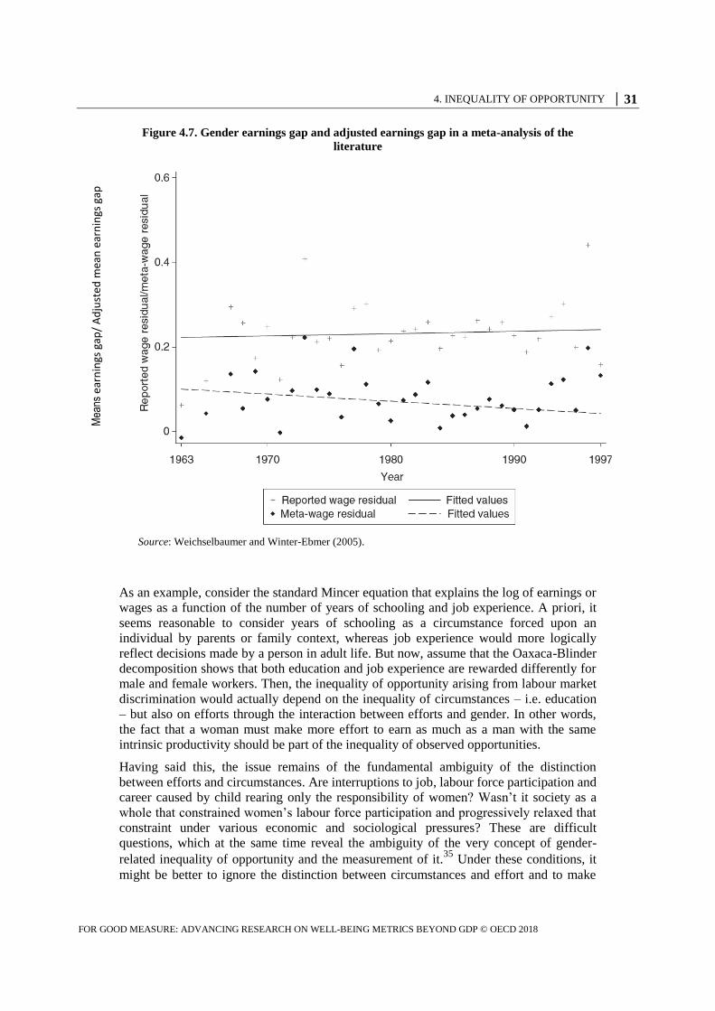
4. INEQUALITY OF OPPORTUNITY │ 31
FOR GOOD MEASURE: ADVANCING RESEARCH ON WELL-BEING METRICS BEYOND GDP © OECD 2018
Figure 4.7. Gender earnings gap and adjusted earnings gap in a meta-analysis of the
literature
Source: Weichselbaumer and Winter-Ebmer (2005).
As an example, consider the standard Mincer equation that explains the log of earnings or
wages as a function of the number of years of schooling and job experience. A priori, it
seems reasonable to consider years of schooling as a circumstance forced upon an
individual by parents or family context, whereas job experience would more logically
reflect decisions made by a person in adult life. But now, assume that the Oaxaca-Blinder
decomposition shows that both education and job experience are rewarded differently for
male and female workers. Then, the inequality of opportunity arising from labour market
discrimination would actually depend on the inequality of circumstances – i.e. education
– but also on efforts through the interaction between efforts and gender. In other words,
the fact that a woman must make more effort to earn as much as a man with the same
intrinsic productivity should be part of the inequality of observed opportunities.
Having said this, the issue remains of the fundamental ambiguity of the distinction
between efforts and circumstances. Are interruptions to job, labour force participation and
career caused by child rearing only the responsibility of women? Wasn’t it society as a
whole that constrained women’s labour force participation and progressively relaxed that
constraint under various economic and sociological pressures? These are difficult
questions, which at the same time reveal the ambiguity of the very concept of gender-
related inequality of opportunity and the measurement of it.35
Under these conditions, it
might be better to ignore the distinction between circumstances and effort and to make
Mea
ns e
arn
ings
gap
/ A
dju
sted
mea
n e
arn
ings
gap

32 │ 4. INEQUALITY OF OPPORTUNITY
FOR GOOD MEASURE: ADVANCING RESEARCH ON WELL-BEING METRICS BEYOND GDP © OECD 2018
sure that we measure correctly the effect on the overall inequality of earnings of different
personal characteristics, including job experience or part-time work, across gender, as
well as the effect of differentiated rewards to these characteristics by the economic
system.
To conclude these remarks on the measurement of the inequality of opportunity related to
gender, the fact that the earnings gap or adjusted earnings gap refers exclusively to
averaging operations within the two samples of male and female workers must be
stressed. The fact that the spread of earnings rates around the mean may be quite different
in the two groups should also be taken into account. In relation to model (11), this is
equivalent to allowing for a variance of the residual term, v, to depend itself on gender,
i.e. heteroscedasticity. This is a good case for using the Roemer measure defined in (8), or
to follow the suggestion made above to replace the mean earnings by some function of
the mean and the variance.
4.4. Overview of practical issues
Measuring inequality of opportunity, seen as the inequality of outcome due to all factors
completely outside individual control seems unrealistic. The best that can be done is to
measure the contribution to inequality of outcomes of some factors that seem beyond
individual responsibility. In that sense, it is only possible to measure some dimensions of
the inequality of opportunity. Yet even that distinction between circumstances outside
individual control and voluntary individual decisions in the determination of economic
outcomes is often ambiguous. Indeed, some dimensions of inequality of opportunity
depend on these individual decisions, as is the case with discrimination within the labour
market.
It is possible to measure directly some dimensions of inequality of opportunity,
independently of their impact on economic outcomes. This is true for instance of
cognitive ability, in adolescence or pre-school, potentially of non-cognitive ability if
some quantitative index is available36
, or of health status. Note also that these individual
characteristics may be considered as circumstances contributing to the inequality of
individual outcomes like earnings or standard of living, but also as an outcome whose
inequality may be explained by family-related characteristics. Most often, however,
measuring the observable dimensions of the inequality of opportunity goes through the
measurement of their impact on the inequality of economic outcomes.
The most obvious example of the measure of single dimensions of inequality of
opportunity is the sizable literature on the intergenerational mobility of earnings or other
economic, or socio-economic outcomes. The observed dimension of inequality of
opportunity is the earnings of parents and it is measured by its contribution to the
inequality of children’s earnings. This can be generalised to other observed family
characteristics that may or may not include parental income or earnings, as well as
personal traits like gender or ethnicity. Data requirements for this kind of analysis are
much less demanding than what is needed for measuring the intergenerational mobility of
earnings. Representative household surveys with recall information on the family
background of respondents are the basic input. Of course monitoring the corresponding
dimensions of the inequality of opportunity over time or making comparisons across
countries requires some uniformity of the information available in these surveys.
When applied to single personal traits, the preceding type of analysis is equivalent to
measuring what is called “horizontal inequality” in the inequality literature, typically

4. INEQUALITY OF OPPORTUNITY │ 33
FOR GOOD MEASURE: ADVANCING RESEARCH ON WELL-BEING METRICS BEYOND GDP © OECD 2018
inequality of earnings or other income variable across gender, race, migrant status or
other individual characteristics. Combined with other individual circumstances that may
depend themselves on individual traits, the measurement of these dimensions of
inequality of opportunity allows for a detailed analysis of the observed discrimination that
society exerts on individuals through the traits being studied.
The empirical literature on inequality of opportunity relies on various types of measures.
When focusing on single scalar dimensions of the inequality of opportunity, it is not clear
that the various measures available for economic outcomes – which are implicitly based
on value judgments – are relevant. For instance, is the Gini coefficient adequate to
represent the inequality of health status or cognitive ability? The variance, the coefficient
of variation or quantile ratios may be sufficient to describe the spread of the distribution.
Things are different when the observed dimensions of inequality of opportunity are
measured in the outcome space, or by their contribution to the inequality of outcomes. In
that case, a distinction must be made between parametric and non-parametric approaches.
A parametric specification of the relationship between outcomes and individual
characteristics allows us to figure out what the inequality would be if only outcome
differences due to individual characteristics were taken into account; or, alternatively,
what difference it would make with respect to the overall inequality of outcomes to
ignore them. Then the resulting “virtual” outcome inequality can be evaluated by the
usual measures of outcome inequality, including the Gini coefficient, the variance of
logarithms, the Atkinson measures, etc. Based on the familiar log-linear relationship
between economic outcomes and individual characteristics, this approach often leads to
quite simple measures of the observed dimensions of the inequality of opportunity: the R²
correlation coefficient when outcome inequality is measured with the variance of
logarithms; the between-group component of decomposable inequality measures when
the observed combinations of individual characteristics are used to define types of
individuals; or the mean income gap in the case of a single individual trait like gender. Of
course, as many measures of inequality of opportunity can be defined as there are
measures of inequality of outcomes.
Things are different with non-parametric specifications that fully take into account the
difference in the distribution of outcomes conditional on individual type. This includes
the case where types correspond to the level of parental income as the dimension of the
inequality of opportunity being studied, and where the intergenerational mobility of
outcomes is described through a transition matrix; in these cases, comparing distributions
requires comparing those matrices. Some interesting comparison criteria have been
proposed which generally rely on strong assumptions about the way the social welfare of
a society characterised by a given transition matrix is evaluated. At this stage, it cannot be
said there is a consensus about these criteria.
The case where inequality of outcomes is shown to result from different outcome
distributions across various types of people, defined by a set of characteristics assumed to
be outside their control, is the most general and realistic specification on which to ground
the measurement of the observed dimensions of inequality of opportunity. It is equivalent
to the parametric specification when the distribution of the effects of unobserved
determinants of outcomes depends on the individual characteristics under study, i.e.
heteroscedasticity in the core specification. Most measures used in the literature ignore
this aspect of the measurement problem. For instance, the adjusted gender earnings gap
ignores the fact that not only the mean but also the distribution of earnings expressed as a
Fançois1
Sticky Note
Add: "the overall"

34 │ 4. INEQUALITY OF OPPORTUNITY
FOR GOOD MEASURE: ADVANCING RESEARCH ON WELL-BEING METRICS BEYOND GDP © OECD 2018
proportion of the mean differs across gender. The inequality measure drawn from Roemer
(1998) would allow to remedy this.
4.5. Conclusions and key indicators for monitoring the observed dimensions of
inequality of opportunity
Until now, concern about inequality focused mostly on inequality in key outcomes like
earnings, gross or disposable income, standard of living or wealth. Monitoring inequality
of outcomes, or inequality ex-post, is crucial to monitor social progress and redistribution
instruments. Ideally, however, one would also want to monitor ex-ante inequality, or
inequality of opportunity, as it is a key determinant of ex-post inequality. As argued
throughout this chapter, however, there is something illusory in such an objective. The
best that can be done is to monitor the observed dimensions of inequality of opportunity,
or equivalently some determinants of inequality of outcomes that can be considered not to
be the result of individual decisions or economic behaviours. Of course, such monitoring
is of utmost importance for policy as it permits the sources of change in the distribution
of the outcome considered to be identified and to adopt corrective policies if deemed
necessary. These sources of change comprise the distribution in the population of
individual characteristics like individual traits, family background including parental
income or wealth, cognitive and non-cognitive abilities, and all assets people can rely on
to generate economic outcomes. They also include the way in which the economic sphere
rewards the efforts of people with different traits or background, i.e. procedural
inequality.
While some observed dimensions of the inequality of opportunity have received much
attention in the recent economic literature, it is fair to say that their measurement still
belongs to the realm of research. Unlike the inequality of disposable income or earnings
regularly monitored through Gini coefficients or other inequality measures, few statistics
related inequality of opportunity are regularly produced by statistical institutes and
publicly debated. For instance, we are ignorant in most countries about whether
intergenerational mobility, one among many possible indicators of inequality of
opportunity, has increased, remained the same or decreased in the last decades. Progress
has been made in monitoring mean educational achievements in many countries, most
notably under the PISA initiative, but no systematic reporting or discussion takes place on
the evolution of their dispersion. If the mean earnings gap across gender is reported
regularly in most advanced economies, the same cannot always be said of the adjusted
earnings gap or the gap across ethnic groups or between natives and first- and second-
generation migrants. Yet, in most countries, data to evaluate these indicators on a regular
basis and several others either are available or could be made available at little cost.
Based on the analysis in this chapter, we list below the data required to improve the
situation and monitor the observable dimensions of the inequality of opportunity in a
systematic way rather than relying on the work done irregularly by researchers. We also
list the statistics that should be published on a regular basis for a monitoring of inequality
that would go beyond the Gini coefficient or other usual inequality measures of
equivalised disposable income or earnings.
4.5.1. Data requirements
Knowledge of the role that family background plays in determining inequality of earnings
or income is essential for understanding the causes of inequality and possible changes in
them. From that point of view, the ideal data are by far long-term panels such as the PSID

4. INEQUALITY OF OPPORTUNITY │ 35
FOR GOOD MEASURE: ADVANCING RESEARCH ON WELL-BEING METRICS BEYOND GDP © OECD 2018
in the United States, which has been running since 1968, and covers 5 000 families and
all their descendants. With such long panels, one may observe many of the circumstances
that surrounded the childhood and the adolescence of the younger cohorts of the panel,
including parental income and wealth. Other long panels include the British BHPS or the
German Socio-Economic Panel. In Europe, the EU-SILC comprises longitudinal data but
these are generally much shorter and do not follow descendants, so that family economic
conditions during the youth of respondents are not observable.37
An alternative to long panels is the linkage of administrative data. Matching the tax
returns of parents 30 years ago to that of their 40-year old children today allows for the
direct observation of income mobility. In some cases, it is even possible to link family
characteristics other than income, thus allowing for more complete studies of the
intergenerational sources of inequality. It was seen above that such data permitted
detailed studies of the intergenerational transmission of wealth in Nordic countries and
the spatial heterogeneity analysis of intergenerational mobility in the United States – as in
Chetty et al. (2014). Unfortunately, data such as these are still extremely scarce, even
though steps could be taken by administrations to make them more systematically
available in the future.
It is not because long panels are not always available that it is impossible to monitor the
role of family background in generating inequality in economic outcomes. Repeated
standard cross-sectional household or labour force surveys with recall information on the
family characteristics of the respondents already allow the impact of family background
on the inequality of earnings, income or standard of living to be monitored. What is
needed is to make sure that such information is available at regular time intervals and
under the same, and possibly the most complete, format. It should not be too difficult to
establish international norms in this area. Possible biases arising from the imperfect
observation of top incomes in these data sources should not be ignored and measures to
prevent such biases should be seriously considered.
Some of the studies reviewed in this chapter show the use that could be made of such
information (see Figure 4.5). Note also that in a given cross-section, it is possible to
conduct the analysis at the cohort level. The way the earnings of the 40-50 year-old
depend at a given point of time on their family background is not the same as for the 30-
40 or the 50-60 year-old. With repeated cross-sections, it would then become possible to
distinguish the cohort and the age effect. Finally, note that if the repeated cross-sections
cover a period long enough, which is now the case in many advanced countries, then it is
possible to use family background variables as instruments to estimate the earnings or
income of parents, thus allowing for some monitoring of intergenerational income
mobility, as in the study by Aaronsson and Mazumder (2008) mentioned earlier.
In the field of the inequality of wealth, cross-sectional data are scarcer although several
countries are now following the example of the Survey of Consumer Finance in the
United States and its practice of oversampling the top of the distribution, where most
wealth is concentrated. These surveys are extremely useful and one may only hope they
will become more frequent. In particular, it would be interesting to investigate in more
depth how it would be possible to monitor the role of bequests in generating wealth and
income inequality, especially at a time where inheritance flows tend to grow faster than
income, as suggested by Piketty (2014).
Horizontal inequality across gender and other personal traits can be followed through
standard household or labour-force surveys. Here, the problem is not so much the
availability of data as the use being made of them and the depth of the analysis
Fançois1
Highlight
Fançois1
Sticky Note
Replace: "2014a"

36 │ 4. INEQUALITY OF OPPORTUNITY
FOR GOOD MEASURE: ADVANCING RESEARCH ON WELL-BEING METRICS BEYOND GDP © OECD 2018
conducted. As shown above, there is much to be learned from going beyond pure
differences in earnings means. At a time where migration has become such an important
issue in so many countries, data for monitoring the differences that natives and migrants
face in the labour market should also be made available.
Students’ skills surveys at various stages in childhood and adolescence of the PISA type
are extremely helpful for detecting changes in a dimension of inequality of opportunity
that is likely to entail changes in the inequality of outcomes later in life. PISA is a mine of
information, although it was suggested above that more emphasis should be put on the
inequality of test scores – on top of their differences across family backgrounds. Also,
developing PISA-type instruments to measure inequality in cognitive abilities at younger
school-age and pre-school is essential. For primary school, the data seem to exist, and it is
perhaps only a matter of analysing them in more detail, and certainly publicising them
better.
Priority statistics
These data could and probably will generate many different types of statistics, related to
various specific dimensions of the inequality of opportunity. It is important to define
those that are likely to be the most useful in assessing social and economic progress, the
most amenable to stimulating discussion between researchers, policy-makers, and civil
society, and the most likely to be available in a timely manner in a reasonably large
number of countries.
The lack of knowledge today in many countries of whether intergenerational mobility is
increasing or decreasing is symptomatic of the data deficit and, until now, of the lack of
interest by policy makers and statisticians in monitoring key sources of outcome
inequality beyond inequality itself as measured by the usual inequality indices. Yet the
social demand for such information is mounting.
Three basic statistics should receive priority attention and should be harmonised as much
as possible across countries and over time within countries.
Inequality of economic outcomes (earnings, income) arising from parental
background and its share in total inequality of outcome. Variance of logarithms of
outcomes among various types of individuals and the R² statistics of family
background variables (at least, education, occupation and age of the parents at
respondent’s birth) in explaining outcomes are the simplest examples of such
statistics. Statistical institutes could seek to publish these statistics at 5-year
intervals, possibly distinguishing across 5-year cohorts. Reflection should start
about the key family background variables that could be systematically included
in the analysis so as to develop international and inter-temporal comparability.
Variance analysis of scores in PISA and analogous surveys at earlier ages,
including pre-school, and the share of it explained by parental/social background,
or the gaps in scores between students from different families. The 3-year
periodicity of PISA seems adequate.
Gender inequality in earnings, unadjusted and adjusted for differences in
education, age, job experience, occupation, etc. Mentioning gender differences
explicitly in basic coefficients like the return to education or to job experience, or
simply showing both the unadjusted and the adjusted gaps as in Figure 4.7 would
be helpful. This could be done easily for gender, although this again requires
defining standards to allow for comparability. Depending on the country, the

4. INEQUALITY OF OPPORTUNITY │ 37
FOR GOOD MEASURE: ADVANCING RESEARCH ON WELL-BEING METRICS BEYOND GDP © OECD 2018
same type of analysis should also be performed for race, religion or migrant
status.
Concerning the nature of the statistics to be released, the simplest would be to rely on the
parametric approach emphasised in this chapter and on the measures it leads to, as they
are easily understood. But extending them to the non-parametric case where the observed
dimensions of the inequality of opportunity are represented in matrix form of individual
types by outcome level would also desirable.
Notes
1 The author wishes to thank Angus Deaton, Martine Durand, Marco Mira D’Ercole, Joseph
Stiglitz, other members of the High Level Expert Group and participants in seminars in Mexico
City and the World Bank for most helpful comments. The author also thanks the participants to the
HLEG workshop on “Inequality of Opportunity” held in Paris, France on 14 January 2015, hosted
by the Gulbenkian Foundation and organised in collaboration with the OECD. The author retains
full responsibility for any remaining error or inaccuracy.
2 This paragraph briefly summarises an important literature in economics and in moral
philosophy, which started with Rawls (1971) and whose major contributions are from Dworkin
(1981), Arneson (1989), Cohen (1989), Roemer (1998), Fleurbaey and Maniquet (2011).
3 This conclusion somewhat resembles Sen’s emphasis on the “equality of capabilities”
rather than “equality of functionings”, at least when capabilities are defined as the set of
functionings accessible to an individual (Sen, 1982, 1985). Interpreting functionings as a vector of
outcomes, Sen’s “capability equality” concept, similar to the concept of “equality of access to
advantage” in Cohen (1989), would consist of equalising the determinants of the set of accessible
functionings, which are conceptually very similar to “circumstances” in the “equality of
opportunity” framework. The only difference is that equalisation in that case would be through
equalising those circumstances rather than compensation in the space of outcomes.
4 The debate in the sociological literature about the idea that people raised in a low socio-
economic status environment may inherit low preferences for work effort illustrates that point. See
a summary of that discussion in Piketty (1998).
5 A rigorous econometric analysis of this issue is provided in Annex 4.A to this chapter.
6 The notation used for this equation is different from the one used in the Annex 4.A.
7 Schooling being considered as a “circumstance”, mostly determined by parental
background.
8 Both sources of inequality are analysed in detail below.
9 Thus, without loss of generality, v
e can be set to zero, its sample mean value when (2) is
estimated by Ordinary Least Squares.
10 With enough observations for each type, the two means differ by a factor that depends on
the inequality of unobserved outcome determinants within the type.
11 Roemer justifies comparing outcomes across types for given quantiles by considering that
individuals of different types (but in the same quantile of their own outcome distribution) expend
the same efforts. The above formula does not appear in Roemer (1998) but it ensues logically from
the specification of his objective function in the design of policies to minimise inequality of
opportunities. Note also that 𝑀𝑖𝑛𝑡{𝑞𝑡(𝜋)} in (8) could be replaced by any standard outcome
inequality measure across types.

38 │ 4. INEQUALITY OF OPPORTUNITY
FOR GOOD MEASURE: ADVANCING RESEARCH ON WELL-BEING METRICS BEYOND GDP © OECD 2018
12
This dependency of PISA scores on family background has been studied in detail by the
OECD (2015, vol. II) in an analysis where cognitive ability is precisely taken as an outcome rather
than a circumstance.
13 Ferreira and Gignoux (2011a) analyse carefully this source of bias in a cross-country
comparison.
14 The standard deviation in test scores being 7, this means that test scores at the end of high
school may be easily responsible for earnings differentials of close to 30%.
15 See for instance the survey by Conti and Heckman (2012).
16 An interesting paper shows for instance the influence of in utero factors on adult earnings:
see Almond et al. (2015)
17 Parameter notations differ from those used above or in the Annex 4.A.
18 Note that this is true only for the variance of logarithm as an inequality measure.
19 When brackets are deciles (or other quantiles) of the distribution of earnings of parents for
rows and of sons for columns, the transition matrix is bi-stochastic with the sum of columns and
rows being equal to 0.1 in the case of decile (and of 0.05 in the case of vintile, etc.). This mobility
matrix is a representation of the copula of the joint distribution of father/children earnings defined
above.
20 Sociologists, who are used to work with socioeconomic classes rather than earnings or
income, tend to emphasize ‘absolute’ mobility, i.e. moving from one rung of the social ladder to
another. Economists traditionally tend to work with ‘relative’ mobility – although see the analysis
of absolute earnings mobility in Chetty et al. (2017).
21 Note that this approach would also apply to the case where the parametric outcome model
(2) is heteroskedastic, as discussed above.
22 See for instance Jäntti and Jenkins (2015, pp. 899-905) for examples drawn from the US
literature.
23 Björklund and Jäntti (1997) apply this technique to compare mobility in Sweden and in
the United States, whereas Aaronson and Mazumder (2008) do so to compare earnings mobility in
the United States over time.
24 The argument is as follows. Let 𝛾 in (9) depend linearly on 𝑦−1,𝑖 for observation i, e.g.
𝛾𝑖 = 𝛾0 + 𝛾1𝑦−1,𝑖 with 𝛾1 > 0. Taking the means on both sides of (9), the average IGE for the
whole population is then given by: �� = 𝛾0 + 𝛾11
𝑛∑ 𝑦−1,𝑖
2𝑖 /��−1 where n is the size of the sample and
��−1 the mean of parents’ income. For a given mean parent income, the mean IGE in the sample
thus increases with the variance, or more generally with the inequality of parents’ income. Note
however that the Gatsby curve refers to the inequality of household income at the time children’s
earnings are observed.
25 See also Chetty et al. (2014, Figure Ib).
26 It is indeed unlikely that the change in inequality across generations could compensate for
the differences in IGE.
27 Aaronsson and Mazumder use the TSIV method sketched above with US census data.
28 For instance, Bourguignon et al. (2007) use the relative version of (7) with the Gini
coefficient for the inequality measure M{ } and the mean of Z for the reference circumstance Ce in
(6). Brunori et al. (2013) use the mean logarithmic deviation.

4. INEQUALITY OF OPPORTUNITY │ 39
FOR GOOD MEASURE: ADVANCING RESEARCH ON WELL-BEING METRICS BEYOND GDP © OECD 2018
29
The mean logarithmic deviation (MLD) in a sample of individuals with economic
outcome yi is simply the difference between the log of the mean of the y's and the mean of the log
y's. For some countries in Figure 4.5, a semi-parametric model is used, based on “types” of
individuals, as defined by specific combinations of characteristics Z, rather than by these
characteristics themselves.
30 It is the case that the relative inequality of observed opportunities based on the mean
logarithmic deviation is close to the R² of the regression of outcomes on observed opportunities.
From (9), this implies that the square root of that measure is comparable to the IGE.
31 This uniformity in the European case comes from being based on a common data source,
the EU-SILC which is roughly uniform across EU members. See Checchi et al. (2010).
32 Such an analysis by cohorts is performed in Bourguignon et al. (2007).
33 Essentially, homoscedasticity in a model of type (11).
34 Other expressions of the Oaxaca-Blinder decomposition use the β coefficients of one
group in the first term and the mean characteristics of the other in the second rather than means
over the two groups. The problem is that the decomposition then depends on what group is chosen
for β. The formulation used here is path independent.
35 Additional difficulties would appear if, instead of focusing on wages, gender inequality
focused on income, or more exactly household income (per capita or equivalised), as labour
supply, marriage, assortative mating, and fertility would become important issues, on top of the
fact that the distribution of income within the household is not directly observed. (On these issues,
see Meurs and Ponthieux, 2015).
36 For instance through principal component analysis of answers to questions on non-
cognitive ability in PISA.
37 In connection with EU-SILC, it should be noted that shorter panels may still be helpful in
analysing the inequality arising from involuntary shocks experienced by individuals in their recent
past, which may be the main source of inequality of opportunity appearing during adult life. In
particular, such data should help to evaluate the hysteresis of such events and the role of social
policies in neutralising their long-run effects.
References
Aaronson, D. and B. Mazumder (2008), “Intergenerational mobility in the United States: 1940 to 2000”,
The Journal of Human Resources, Vol. 43(1), p. 139-72
Adermon, A., M. Lindahl and D. Waldenström (2015), “Intergenerational wealth mobility and the role of
inheritance: Evidence from multiple generations”, IZA, Discussion Paper No. 10126.
Almond, D., B. Mazumder and R. van Ewijk (2015), “In utero Ramadan exposure and children’s
academic performance”, with Almond, D. and R. van Ewijk, The Economic Journal, Vol. 125,
pp. 1501-33.
Arneson, R. (1989), “Equality and equal opportunity for welfare”, Philosophical Studies, Vol. 56(1),
pp. 77-93.
Atkinson, A.B. (1981), “The measurement of economic mobility”, in Eggelshaven, P.J. and L.J. van der
Gemerden (eds.), Inkommenns verdeling en Openbare Financien (Het Spectrum).
40 │ 4. INEQUALITY OF OPPORTUNITY
FOR GOOD MEASURE: ADVANCING RESEARCH ON WELL-BEING METRICS BEYOND GDP © OECD 2018
Atkinson, A.B. (1970), “On the measurement of economic inequality”, The Journal of Economic Theory,
Vol. 2, pp. 244-263.
Atkinson , A.B. and F. Bourguignon (1982), “The comparison of multi-dimensioned distribution of
economic status”, The Review of Economic Studies, Vol. 49, pp. 183-201.
Berman, Y. (2016), “The Great Gatsby curve revisited – Understanding the relationship between
inequality and intergenerational mobility”, Mimeo, School of Physics and Astronomy, Tel-Aviv
University, Tel-Aviv, Israel.
Björklund, A. and M. Jäntti (1997), “Intergenerational income mobility in Sweden compared to the
United States”, The American Economic Review, Vol. 87(5), pp. 1009-18
Blanden, J. et al. (2011), “Changes in intergenerational mobility in Britain”, in Corak, M. (ed.),
Generational Income Mobility in the United States and in Europe, pp. 122-146, Cambridge
University Press, Cambridge.
Boserup, S.H., W. Kopczuk and C. Thustrup Kreiner (2014), “Intergenerational wealth mobility:
Evidence from Danish wealth records of three generations”, Working Paper, University of
Copenhagen.
Bourguignon, F., F. Ferreira and M. Menendez (2007), “Inequality of opportunity in Brazil”, The Review
of Income Wealth, Vol. 53(4), pp. 585-618.
Bourguignon, F., F. Ferreira and M. Menendez (2007), “Inequality of opportunity in Brazil: A
corrigendum”, The Review of Income Wealth, Vol. 59(3), pp. 551-555.
Brunori, P. (2016), “How to measure inequality of opportunity: A hands-on guide”, Working Paper
2016-04, The Life Course Center.
Brunori, P., F. Ferreira and V. Peragine (2013), “Inequality of opportunity, income inequality and
economic mobility: Some international comparisons”, IZA, Discussion Paper No. 7155.
Charles, K.K. and E. Hurst (2003), “The correlation of wealth across generations”, The Journal of
Political Economy, Vol. 111(6), p. 1155-1182.
Checchi, D., V. Peragine and L. Serlenga (2010), “Fair and unfair income inequalities in Europe”,
ECINEQ Working paper No. 174-2010.
Chetty, R. et al. (2017), “The fading American dream: Trends in absolute income mobility since 1940”,
NBER Working Paper No. 22910 (shortened version published in Science, Vol. 356(6336), pp. 398-
406).
Chetty, R. et al. (2014a), “Where is the land of opportunity? The geography of intergenerational mobility
in the United States”, The Quarterly Journal of Economics, Vol. 129(4), pp. 1553-1623.
Chetty, R. et al. (2014b), “Is the United States still a land of opportunity? Recent trends in
intergenerational mobility”, The American Economic Review, Vol. 104(5), pp. 141-147.
Cohen, G.A. (1989), “On the currency of egalitarian justice”, Ethics, Vol. 99(4), pp. 906-944.
Conti, G. and J. Heckman (2012), “The Economics of child well-being”, IZA, Discussion Paper
No. 6930.
Corak, M. (2013), “Income inequality, equality of opportunity, and intergenerational mobility”, The
Journal of Economic Perspectives, Vol. 27(3), pp. 79-102.
Corak, M. (2012), “Here is the source for the Great Gatsby Curve”, in the Alan Krueger speech at the
Center for American Progress on January 12, https://milescorak.com/2012/01/12/here-is-the-source-
for-the-great-gatsby-curve-in-the-alan-krueger-speech-at-the-center-for-american-progress/.

4. INEQUALITY OF OPPORTUNITY │ 41
FOR GOOD MEASURE: ADVANCING RESEARCH ON WELL-BEING METRICS BEYOND GDP © OECD 2018
Currie, J. (2009), “Healthy, wealthy, and wise: Socioeconomic status, poor health in childhood, and
human capital development”, The Journal of the Economic Literature, Vol. 47(1), pp. 87-122.
Decancq, K., M. Fleurbaey and E. Schokkaert (2015), “Inequality, income and well-being”, in Atkinson,
A.B. and F. Bourguignon (eds.), Handbook of Income Distribution, Vol. 2, pp. 67-140, Elsevier,
North Holland, Amsterdam.
Dworkin, R. (1981), “What is equality, Part 1”, Philosophy and Public Affairs, Vol. 10(3), pp. 185-246.
Dworkin, R. (1981), “What is equality, Part 2”, Philosophy and Public Affairs, Vol. 10(4), pp. 283-345.
Ferreira, F.H G. and J. Gignoux (2011a), “The measurement of educational inequality: Achievement and
opportunity”, IZA, Discussion Paper No. 6161.
Ferreira, F.H.G. and J. Gignoux (2011b), “The measurement of inequality of opportunity: Theory and an
application to Latin America”, The Review of Income and Wealth, Vol. 57(4), pp. 622-657.
Fields, G. and E. Ok (1999), “The measurement of income mobility: An introduction to the literature”, in
Silber J. (ed.), Handbook of Income Inequality Measurement, Series on recent economic thought,
Vol. 71, pp. 557-98, Kluwer Academic Publishers.
Fleurbaey, M. and E. Schokkaert (2012), Inequity in health and health care, in Barros, P., T. McGuire
and M. Pauly (eds.), Handbook of health economics, Vol. 2, pp. 1003-92, Elsevier, North Holland,
Amsterdam.
Fleurbaey, M. and F. Maniquet (2011), “Compensation and responsibility”, in Arrow, K.J., A.K. Sen and
K. Suzumura (eds.), Handbook of Social Choice and Welfare, Vol. 2, pp. 507-604, Elsevier, North
Holland, Amsterdam.
Galton, F. (1886), “Regression towards mediocrity in hereditary stature”, The Journal of the
Anthropological Institute of Great Britain and Ireland, XV, pp. 246-63.
Goldthorpe, J. (2012), “Understanding – and misunderstanding – social mobility in Britain: The entry of
the economists, the confusion of politicians and the limits of educational policy”, Barnett Papers in
Social Research, 2/2012, University of Oxford.
Jäntti, M. and S. Jenkins (2015), “Income mobility”, in Atkinson, A. and F. Bourguignon (eds.),
Handbook of Income Distribution, Vol. 2, pp. 807-935, Elsevier, North Holland, Amsterdam.
Jäntti, M. et al. (2002), “Brother correlations in earnings in Denmark, Finland, Norway and Sweden
compared to the United States”, The Journal of Population Economics, Vol. 15(4), pp. 757-772.
Kanbur, R. and J. Stiglitz (2015), “Dynastic inequality, mobility and equality of opportunity”, CEPR
Discussion Paper No. 10542.
Kautz, T., et al. (2014), “Fostering and Measuring Skills: Improving Cognitive and Non-cognitive Skills
to Promote Lifetime Success”, OECD Education Working Papers, No. 110, OECD Publishing, Paris,
http://dx.doi.org/10.1787/5jxsr7vr78f7-en.
Landersø R. and J.J. Heckman (2016), “The Scandinavian fantasy: The sources of intergenerational
mobility in Denmark and the US”, Centre for the economics of human development, University of
Chicago.
Lee, C.-I. and G. Solon (2009), “Trends in intergenerational income mobility”, The Review of Economics
and Statistics, Vol. 91, pp. 766-772.
Lefranc, A., N. Pistolesi and A. Trannoy (2009), “Equality of opportunity and luck: Definitions and
testable conditions, with an application to income in France”, The Journal of Public Economics,
Vol. 93, pp. 1189-1207.

42 │ 4. INEQUALITY OF OPPORTUNITY
FOR GOOD MEASURE: ADVANCING RESEARCH ON WELL-BEING METRICS BEYOND GDP © OECD 2018
Levin, H. (2012), “More than just test scores”, PROSPECTS, Vol. 42(3), pp. 269-284,
https://doi.org/10.1007/s11125-012-9240-z.
Mazumder, B. (2008), “Sibling similarities and economic inequality in the US”, The Journal of
Population Economics, Vol. 21(3), pp. 685-701.
Meurs, D. and S. Ponthieux (2015), “Gender inequality”, in Atkinson, A.B. and F. Bourguignon (eds.),
Handbook of Income Distribution, Vol. 2, pp. 981-1146, Elsevier, North Holland, Amsterdam.
Murnane, R. et al. (2000), “How important are the cognitive skills of teenagers in predicting subsequent
earnings?”, The Journal of Policy Analysis and Management, Vol. 19(4), pp.547-568.
OECD (2014), PISA 2012 Results: What Students Know and Can Do (Vol. I, Revised edition, February
2014): Student Performance in Mathematics, Reading and Science, PISA, OECD Publishing, Paris,
http://dx.doi.org/10.1787/9789264208780-en.
OECD (2013), PISA 2012 Results: Excellence through Equity (Vol. II): Giving Every Student the Chance
to Succeed, PISA, OECD Publishing, Paris, http://dx.doi.org/10.1787/9789264201132-en.
Piketty, T. (2014), Capital in the 21st
Century, Harvard University Press.
Piketty, T. (1998), “Self-fulfilling beliefs about social status”, The Journal of Public Economics, Vol. 70,
pp. 115-132.
Ramos, X. and D. van de Gaer (2012), “Empirical approaches to inequality of opportunity: Principles,
measures, and evidence”, IZA, Discussion Paper No. 6672.
Roemer, J. (1998), Equality of Opportunity, Harvard University Press, Cambridge.
Roemer, J. and A. Trannoy (2015), “Equality of Opportunity”, in Atkinson, A.B. and F. Bourguignon
(eds.), Handbook of Income Distribution, Vol. 2, pp. 217-296, Elsevier, North Holland, Amsterdam.
Sen A. (1985), Commodities And Capabilities, Elsevier, North Holland, Amsterdam.
Sen, A. (1980), “Equality of what?”, in McMurrin, S., Tanner Lectures on Human Values, Vol. 1,
Cambridge University Press.
Shorrocks, A. (1978), “The Measurement of Mobility”, Econometrica, Vol. 46(5), pp. 1013-1024.
van de Gaer, D. (1993), “Equality of opportunity and investment in human capital”, Ph.D. thesis, K.U.
Leuven.
Weichselbaumer, D. and R. Winter-Ebmer (2005), “A Meta-analysis of the international gender wage
gap”, The Journal of Economic Surveys, Vol. 19(3), pp. 479-511.
Wolff, E. (2015), Inheriting Wealth in America: Future boom or bust, Oxford University Press.

4. INEQUALITY OF OPPORTUNITY │ 43
FOR GOOD MEASURE: ADVANCING RESEARCH ON WELL-BEING METRICS BEYOND GDP © OECD 2018
Annex 4.A. The difficulty of empirically disentangling the role of opportunity
and effort in the determination of earnings
Consider a database with information on individual earnings, circumstances and efforts and a
linear model where (log) earnings of individual i, Log yi, depends on the circumstances, Ci , and
efforts, Ei , of the same person, both vectors being split into observed (Ci1, Ei1) and unobserved
(Ci2, Ei2) components:
𝐿𝑜𝑔 𝑦𝑖 = 𝑎 + 𝑏1𝐶𝑖1 + 𝑏2𝐶𝑖2 + 𝑐1𝐸𝑖1 + 𝑐2𝐸𝑖2 + 𝑢𝑖 (1)
where 𝑢𝑖 summarises all the other determinants of earnings, including luck and measurement
error, and where a, b, and c are parameters, or vectors of parameters.
While a specification with interactions between circumstances and efforts would be more
general, the points made below would be equally relevant with a more complete model – but a bit
more intricate from a notational point of view.
Rearranging the terms in the preceding equation leads to:
𝐿𝑜𝑔 𝑦𝑖 = 𝑎 + 𝑏1𝐶𝑖1 + 𝑐1𝐸𝑖1 + 휀𝑖 𝑤𝑖𝑡ℎ 휀𝑖 = 𝑏2𝐶𝑖2 + 𝑐2𝐸𝑖2 + 𝑢𝑖 (2)
Where, without loss of generality, the residual terms, 휀𝑖, may be assumed to have zero expected
value for each observation in the sample.
The objective is to estimate the two sets of coefficients 𝑏1 and 𝑐1 so as to disentangle the role of
observed circumstances and efforts in observed earnings. To do so with standard Ordinary Least
Squares would require the residual, 휀, to be independent of the explanatory variables C1 and E1.
This is problematic, however. Indeed, it is to be expected that the efforts expended by people to
increase their earnings depend on the circumstances they face. This can be formalised as:
𝐸𝑖1 = 𝛼1 + 𝛽11𝐶𝑖1 + 𝛽12𝐶𝑖2 + 𝜃𝑖1 (3)
𝐸𝑖2 = 𝛼2 + 𝛽21𝐶𝑖1 + 𝛽22𝐶𝑖2 + 𝜃𝑖2 (4)
where 𝜃𝑖1 and 𝜃𝑖2 stand for other determinants of efforts, presumably independent of
circumstances, but possibly mutually correlated. Substituting (3)-(4) into (2), it appears that 휀𝑖 is
correlated to observed circumstances 𝐶𝑖1 and observed efforts 𝐸𝑖1 through unobserved
circumstances and efforts, even when both are assumed to be orthogonal to their observed
counterparts.
It follows that equation (2) cannot be estimated without a bias, and that disentangling the role of
efforts and circumstances in the determination of earnings is generally impossible.*
This may not prevent estimating the total effect of observed circumstances on earnings.
Substituting (3) and (4) in (2), gives:
𝐿𝑜𝑔 𝑦𝑖 = 𝛿 + 𝛾. 𝐶𝑖1 + 𝜔𝑖 (5)
with:

44 │ 4. INEQUALITY OF OPPORTUNITY
FOR GOOD MEASURE: ADVANCING RESEARCH ON WELL-BEING METRICS BEYOND GDP © OECD 2018
𝛿 = 𝑎 + 𝑐1. 𝛼1 + 𝑐2. 𝛼2; 𝛾 = (𝑏1 + 𝑐1. 𝛽11 + 𝑐2. 𝛽21); 𝜔𝑖 = (𝑏2 + 𝑐1𝛽12). 𝐶𝑖2 + 𝑐2𝐸𝑖2 + 𝑢𝑖 +𝑐1𝜃𝑖1
For the residual term, 𝜔𝑖, in (5), to be independent of the observed circumstance variables in C1 it
must be assumed that the unobserved circumstances and efforts E2 and C2 are orthogonal to
observed circumstances. If this is not the case, this means that the coefficient 𝛾 in (5) accounts
not only for the effects of observed circumstances, both directly and through efforts, but also for
that part of unobserved circumstances and efforts correlated to observed circumstances.
Practically, parametric empirical analyses of the inequality of opportunity are based on a model
of type (5). This lessens the relevance of some of the theoretical measures of inequality of
opportunity proposed in the literature and justifies focusing on measures that can be derived from
the reduced form (5) as done in the main text.
* Bourguignon et al. (2007, 2013) tried to find bounds on the 𝑏1 and 𝑐1 coefficients, but they proved to be
too large to be of any use in identifying the inequality of opportunity conditional on efforts.