The demand for money and non-GDP transactions

ELSEVIER Economics Letters 48 (1995) 145-154

economics le t ters

The demand for money and non-GDP transactions

Thomas I. Palley

Department of Economics, New School for Social Research, New York, NY 10003, USA

Received 20 September 1993; accepted 29 August 1994

Abstract

This paper argues that transactions in non-GDP items have an important influence on the level of money demand. The paper provides empirical estimates of models of both M1 and M2 money demand that include variables proxying for the volume of transactions in real estate and financial assets. These variables have the theoretically-predicted positive sign, and are statistically significant. Their inclusion also improves out-of-sample forecasts.

Keywords: Money demand; Non-GDP transactions; Home sales; Financial trading

JEL classification: E00

I. Introduction

The demand for money represents the central analytic instrument of monetary macro- economic theory. Its importance derives from the notion that the terms on which economic agents are willing to hold the stock of money affects asset prices, interest rates, and spending plans. For this reason, there has developed a voluminous literature estimating money demand.

Conventional econometric models of money demand (see Goldfeld, 1973) relate the demand for money to the level of GDP, where GDP serves as the scale variable determining the transactions demand for money balances. However, transactions involving currently produced output (current GDP) represent only part of total transactions, and there are also significant non-GDP transactions involving sales of existing financial assets and real estate. These non-GDP transactions also need financing, and to the extent that they are financed through transfers of cash and title to bank deposits, they, too, impact money demand. This suggests that correctly specified empirical models of money demand should take account of these others transactions influences.

The current paper examines the effect on money demand of housing market activity as measured by the real value of sales of existing homes. In addition, the paper examines the money-demand effects of the level of transacting in existing financial assets as proxied by the

0165-1765/95/$09.50 (~) 1995 Elsevier Science B.V. All rights reserved SSDI 0 1 6 5 - 1 7 6 5 ( 9 4 ) 0 0 6 0 5 - 9

146 T.1. Palley / Economics Letters 48 (1995) 145-154

real value of transactions on the New York stock exchange. The principal finding is that housing market activity significantly affects both the demand for M1 and M2 balances, and greatly improves out-of-sample forecasts of M1 and M2 demand. Stock-market transactions also positively affect money demand, albeit with a lower elasticity.

2. Some descriptive evidence of the money-demand effects of housing sales

In a recent paper Duca (1990) has suggested that mortgage activity may have affected the recent growth of demand deposits. Using data on unscheduled repayments of mortgage- backed securities, residential mortgage refinancings, and new mortgage originations, Duca constructed measures of the effects of mortgage activity on the level of demand deposits for the period 1972.1-1988.2. His results showed that this effect has grown steadily, indicating that mortgage activity has become relatively more important as a determinant of money demand.

Duca's estimates were constructed by strict reference to the payments procedures governing mortgage transactions, and used cautious assumptions regarding average down-payments and timing of refinancings. Thus, in computing the money-demand effects of mortgage activity it was assumed that agents only obtained needed liquidity the day prior to the closing of the transaction. In practice, agents may actually begin to build up liquid balances significantly before the closing date as a precautionary step against asset price fluctuations. Second, agents may also build up liquid balances during the period when searching for houses, so that they can have funds on hand to make an offer. Third, agents may also build up liquid balances to finances purchases of consumer durables and home renovations, which are expenditures that often accompany house purchases. 1 In this case, housing market activity proxies for these other influences on money demand, which can be thought of as being jointly incurred with house purchases. Such considerations suggest that Duca's accounting exercise may understate the true effect of housing market activity on money demand, and this consideration prompts the use of regression techniques to estimate their full effect. 2

3. An empirical model of money demand

The standard model of money demand used for empirical purposes is the lagged-adjustment model (see Goldfeld, 1973). The empirical model that is estimated below uses this model, subject to the inclusion of additional variables in the desired money-balance equation that capture the effects of non-GDP transactions. Desired money balances are determined according to

~Indeed, both buyers and sellers may undertake these types of expenditures: for sellers the motivation is improved salability.

2 They also suggest that housing market activity should be included as an explanatory variable in structural equations estimating consumption of durable goods.

T.I. Palley / Economics Letters 48 (1995) 145-154 147

M * = a o + a l C O N , + a213 , + a 3 I N F , + a 4 n t -t- a s S , , (1)

where

M* = log of desired per capita real money (M1) balances, C O N t = log of real consumption expenditures, 13 t = nominal interest rate on the three-month T-bill, I N F , = rate of change of the G D P deflator (1987 = 100), H, = log of real value of sales of existing family homes, S t = log of real value of transactions on the NYSE.

M o n e y and consumpt ion are in log-level form, while the nominal interest rate and inflation are in level form. This is because for low levels of interest rates and inflation, small absolute changes represent large percentage changes but one does not expect such changes to have large percentage changes on money demand (see Fair, 1987). In the current exercise, consumpt ion expenditures were used as the scale variable to capture t ransact ions-demand effects. Mankiw and Summers (1986) have argued why consumpt ion may be a be t te r scale variable, and the econometr ic specification was improved by its adoption. The inclusion of the rate of inflation as a separate variable captures the fact that inflation has a 'direct ' own-re turn effect on money demand, as well as an 'indirect' opportuni ty-cost effect operat ing through its impact on nominal interest rates.

The adjus tment of actual to desired real money balances is governed by the following gradual-adjus tment mechanism: 3

M , - M,_~ = b [ M * - Mr_ l ] q- e t , (2)

where

M = log of actual real money (M1) balances, and e - - r a n d o m disturbance term.

Combining Eqs. (1) and (2) yields

M , = ba o + b a l C O N t + ba213 , + b a 3 I N F t + b a 4 H t + b a s S t

+ (1 - b ) M t _ 1 + e t , (3)

which can be est imated using linear regression techniques.

4. Empirical estimates

The model given by Eq. (3) was then est imated under a number of different coefficient restrictions using Fair 's (1970) two-stage least squares procedure with a correct ion for

3 In the literature on money demand there is some debate whether the adjustment of actual money balances is governed by a real partial-adjustment mechanism (RPAM) or a nominal partial-adjustment mechanism (NPAM). Fair (1987) finds that the RPAM has a superior econometric fit in the estimation of a model of desired money demand in which the only arguments are income and nominal interest rates. Goldfeld and Sichel (1987) show that when inflation is an argument of desired real money balances it is not possible to separately identify, and test for statistical significance, the coefficients of the RPAM and NPAM models.

148 T.I. PaUey / Economics Letters 48 (1995) 145-154

first-order serial correlation. 4 All data was drawn from CITIBASE, and was in quarterly average form. The definition of variables is provided in the appendix. The sample period was 1976.1-1991.2. The adoption of 1976.1 as the starting point for the sample period avoids the widely recognized problem of the break in money-demand behavior that occurred at that time (Goldfeld, 1976). 5

The estimation results are shown in Table 1. 6 The first column (headed, model 10) shows

Table 1 Alternative regression estimates of Eq. (3) under different sets of coefficient restrictions. The sample period was 1976.1-1991.2.

Model 10 Model 11 Model 12 Model 13

C -10.87 -0.951 3.873 3.633 ( - 1.88) a (-0.56) ( 1.65) (1.93)

M I ( - 1) 0.388 0.538 0.688 0.642 (2.88) (5.87) (4.82) (6.54)

13 -0.001 -0.002 -0.002 -0.002 (-0.46) ( - 1.81) (-0.78) ( - 1.56)

INF -0.786 - 1.090 - 1.650 - 1.536 ( - 1.24) (-2.90) (-2.57) (-3.39)

CON 1.023 0.340 0.112 0.099 (3.50) (2.95) (0.59) (0.65)

H 0.083 0.076 (5.99) ( ( 4 . 5 7 )

S 0.022 0.019 (1.91) (1.85)

AR(1) 0.960 0.848 0.800 0.697 (47.6) (12.01) (5.65) (4.15)

Adjusted R2 0.994 0.997 0.994 0.997 S.E. 0.009 0.007 0.009 0.007 D.W. 1.929 2.056 2.067 1.884

aFigures in parentheses are t-statistics.

4 The instrument list consisted of the constant; two lags of the money stock and the ten-year T-bill rate; one lag of the three-month T-bill rate, GNP, consumption, and unemployment: current and lagged values of cyclically adjusted federal government expenditures and revenues; and one lag of any other included independent variable.

5 Inclusion of the additional real estate and stock-market variables does not remedy the structural break problem.

6 All the estimated equations were tested using the Chow break test for the hypothesis of no structural break in 1983.1. In all cases, the null hypothesis of no structural break was accepted at the 1% significance level.


the estimates of Eq. (3) under the restriction a 4 = a 5 = 0: this column provides the benchmark equation against which alternative specifications should be compared. The second column (headed, model 11) shows estimates of (3) under the restriction a s = 0. This model shows the housing market variable to be statistically significant at the 1% level, and it also renders both the interest rate and inflation variables significant at the 8% and 1% levels, respectively. The goodness-of-fit measured by the adjusted R 2, standard error of the regression, and the sum of the squared residuals (not reported) are also all improved. The results, therefore, suggest that housing purchases are an important determinant of money demand. Per the estimated equation the one-quarter elasticity of money demand with respect to existing home purchases is 0.08, while the long-run elasticity is 0.18.

Furey (1993) argues for the inclusion in empirical money-demand equations of a variable capturing the level of transacting in financial markets) The logic behind this argument is that transactors in financial markets have recourse to money balances when settling trades, and money demand is, therefore, positively impacted by the level of financial market trading. To capture this effect, the benchmark model was re-estimated with the inclusion of a stock- market transactions variable. The results are shown in the third column (headed, model 12) of Table 1. All the independent variables have the right sign, and both the inflation rate and the stock-market variable are significant at the 1% and 10% level, respectively. However, the consumption variable is no longer significant. This is potentially due to multi-collinearity between the consumption and stock-market transactions variables, which is indicated by the matrix of correlation coefficients given by

C O N S H C O N 1.00 S 0.97 1.00 H 0.29 0.24 1.00

The goodness-of-fit measured by the adjusted R 2, standard error of the regression, and the sum of the squared residuals (not reported) were marginally improved relative to model 10, indicating that inclusion of the stock-market transactions variable may be warranted.

Model 12 was then augmented by the inclusion of the existing home-sales variable, and the results are shown in column four (headed, model 13) of Table 1. All the independent variables have the theoretically-correct sign. The homes variable and the inflation rate are significant at the 1% level, while the stock-market transactions variable is significant at the 7% level. The goodness-of-fit measured by the adjusted R 2, standard error of the regression, and the sum of the squared residuals (not reported) is the best of the four models. The one-quarter elasticity of money demand with respect to existing home sales is 0.08, while the long-run elasticity is 0.21.

To get further insight into the value of including a home-sales variable, the four models were re-estimated over the shortened sample period 1976.1-1988.4, and these estimates were

7 Field (1984) has also shown how asset exchanges on the New York stock exchange affected the demand for money in the period 1919-1929.

150 T.1, Palley / Economics Letters 48 (1995) 145-154

22.88 -

228, i 2 2 . 8 2

u

8 22.8 .. . . . /

22.78 . . . . . . . . . . . . . . . . . . . . . . . . . . . . . . . . . . . . . . . . . . . . . . . . . . . . . . .

2 2 . , 6 o

~ 22.7~ 2 2 . 7 2

22 .7

22.68 . . . . . . . . . . . . . . . . . . 1989.1 1990.1 1991.1 1992.1 1993.1

[ - -m-m1 - + - m l O --~--m13 I

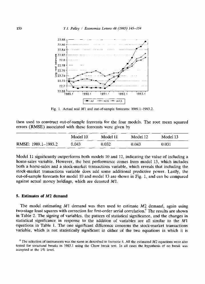
Fig. 1. Actual real M1 and out-of-sample forecasts: 1989.1-1993.2.

then used to construct out-of-sample forecasts for the four models. The root mean squared errors ( R M S E ) associated with these forecasts were given by


RMSE: 1989.1-1993.2 0.043 0.032 0.043 0.031

Model 11 significantly outperforms both models 10 and 12, indicating the value of including a home-sales variable. However , the best performance comes from model 13, which includes both a home-sales and a s tock-market transactions variable, which reveals that including the s tock-market transactions variable does add some additional predictive power. Lastly, the out-of-sample forecasts for model 10 and model 13 are shown in Fig. 1, and can be compared against actual money holdings, which are denoted M1.

5. Estimates of M2 demand

The model estimating M1 demand was then used to est imate M2 demand, again using two-stage least squares with correction for first-order serial correlation, s The results are shown in Table 2. The signing of variables, the pat tern of statistical significance, and the changes in statistical significance in response to the addition of variables are all similar to the M1 equat ions in Table 1. The one significant difference concerns the s tock-market transactions variable, which is not statistically significant in either of the two equat ions in which it is

8 The selection of instruments was the same as described in footnote 4. All the estimated M2 equations were also tested for structural breaks in 1983.1 using the Chow break test. In all cases the hypothesis of no break was accepted at the 1% level.

T.I. PaUey / Economics Letters 48 (1995) 145-154 151

Table 2 Alternative regression estimates of M2 demand under different sets of coefficient restrictions. The sample period was 1976.1-1991.2.


C 2.774 5.923 2.493 2.455 (2.64) a (0.97) (2.76) (1.88)

M2(- 1) 0.482 0.419 0.744 0.474 (3.75) (4.04) (6.45) (3.62)

13 -0.004 -0.003 -0.002 -0.003 (-3.65) (-3.00) ( - 1.57) (-3.05)

1NF -0.947 -0.492 - 1.816 -0.921 (-2.19) ( - 1.71) (-5.18) (-2.603)

CON 0.403 0.285 0.150 0.386 (3.47) (1.05) (1.38) (2.755)

H 0.055 0.037 (3.25) (2.76)

S 0.003 -0.005 (0.53) (-0.65)

AR(1) 0.743 0.970 0.220 0.804 (4.94) (23.58) (1.06) (5.50)

Adjusted R 2 0.998 0.998 0.998 0.998 S.E. 0.006 0.006 0.006 0.006 D.W. 2.374 2.064 2.047 2.210

aFigures in parentheses are t-statistics.

included. Thus, s tock-market transactions appear to have some significance for M1 demand, but are insignificant for M2 demand. Contrastingly, home sales have a strong positive and statistically significant impact on M2 money demand. In model 21 the one-quar ter elasticity of M2 demand with respect to home sales is 0.05, and the long-run elasticity is 0.10: in model 23 the one-quar te r elasticity is 0.04, and the long-run elasticity is 0.07.

This pat tern of effects across M1 demand and M2 demand suggests the following pat tern of portfolio adjustments in response to changes in s tock-market transactions and home sales. W h e n s tock-market transactions increase, this increases M1 demand, and the increase in M1 d e m a n d is equil ibrated by a shift out of the non-M1 component of M2: hence, total M2 is unchanged. When home sales increase, both M1 and M2 demand increases, which suggests that the increase in demand is equilibrated by shifts out of other assets on the less liquid end of the liquidity spectrum.

Models 20 ,21 ,22 , and 23 were then re-est imated over the shor tened sample per iod

152 T.I. Palley / Economics Letters 48 (1995) 145-154

24.2

2 4 . 1 8

24.16 o

~o 24.14

24.12- L

o ~ 24.1

24.08

24.06 . . . . . . . . . . . . . . . . . . 1989.1 1990.1 1991.1 1992.1 1995.1

[ - -~ -m2 ~ m20 --~--m21 ]

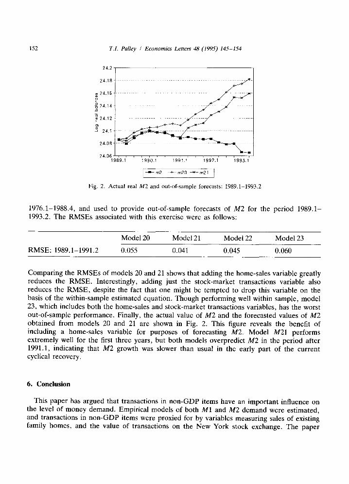
Fig. 2. Actual real M2 and out-of-sample forecasts: 1989.1-1993.2

1976.1-1988.4, and used to provide out-of-sample forecasts of M2 for the period 1989.1- 1993.2. The RMSEs associated with this exercise were as follows:


RMSE: 1989.1-1991.2 0.055 0.041 0.045 0.060

Comparing the RMSEs of models 20 and 21 shows that adding the home-sales variable greatly reduces the RMSE. Interestingly, adding just the stock-market transactions variable also reduces the RMSE, despite the fact that one might be tempted to drop this variable on the basis of the within-sample estimated equation. Though performing well within sample, model 23, which includes both the home-sales and stock-market transactions variables, has the worst out-of-sample performance. Finally, the actual value of M2 and the forecasted values of M2 obtained from models 20 and 21 are shown in Fig. 2. This figure reveals the benefit of including a home-sales variable for purposes of forecasting M2. Model M21 performs extremely well for the first three years, but both models overpredict M2 in the period after 1991.1, indicating that M2 growth was slower than usual in the early part of the current cyclical recovery.

6. Conclusion

This paper has argued that transactions in non-GDP items have an important influence on the level of money demand. Empirical models of both M1 and M2 demand were estimated, and transactions in non-GDP items were proxied for by variables measuring sales of existing family homes, and the value of transactions on the New York stock exchange. The paper


found that M1 demand is positively affected by both home-sales and stock-market transactions: the demand for M2 appears to be affected only by home sales. The home-sales variable also significantly improves the out-of-sample forecast of both M1 and M2 demand. Thus, to the extent that estimates of money demand are used to guide economic policy, or are used in the construction of economic forecasts, the paper suggests that such estimates should incorporate the effects of non-GDP transactions.

Appendix

This appendix defines the CITIBASE labels of the variables used in the estimates. These were:

FM1 = M1 money supply F M 2 = M2 money supply G C = Personal consumption expenditures G D P D = GDP deflator G D P C = consumption deflator F Y G M 3 = 3-month T-bill rate F Y G T I O = 10-year T-bill rate H E M P = median single family home price H E S H S = number of sales of existing single family homes F S V O L = NYSE share volume F S D J = Dow Jones industrial average

Regression variables were computed as follows:

M1 = log(FM1/GDPD) M 2 = l o g ( F M 2 / G D P D ) I N F = l o g G D P D - l o g G D P D ( - 1) C O N = I o g ( G C / G D P C ) S = log((FSOJ. F S V O L ) / G D P D ) H = I o g ( ( H E M P . H E S H S ) / G D P D ) 13 = F Y G M 3 I10 = F Y G T I O

regression

References

Duca, J.V., 1990, The impact of mortgage activity on recent demand growth, Economics Letters 32, 157-161. Fair, R.C., 1970, The estimation of simultaneous equation models with lagged endogenous variables and first order

serially correlated errors, Econometrica 38, 507-516. Fair, R.C., 1987, International evidence on the demand for money, Review of Economics and Statistics LXIX,

473-480.

154 T.I. PaUey / Economics Letters 48 (1995) 145-154

Field, A.J., 1984, Asset exchanges and the transactions demand for money, 1919-1929, American Economic Review 74, 43-59.

Furey, K., 1993, The effect of trading in financial markets on money demand, Eastern Economic Journal 19, 83 -90.

Goldfeld, S.M., 1973, The demand for money revisited, Brookings Papers on Economic Activity 3, 577-638. Goldfeld, S.M., 1976, The case of the missing money, Brookings Papers on Economic Activity 7, 683-730. Goldfeld, S.H. and D. Sichel, 1987, Money demand: The effects of inflation and alternative adjustment

mechanisms, Review of Economics and Statistics LXIX, 511-515. Mankiw, N.G. and L.H. Summers, 1986, Money demand and the effects of fiscal policies, Journal of Money,

Banking, and Credit 18, 415-429.

The demand for money and non-GDP transactions

Documents

Transcript of The demand for money and non-GDP transactions