MPRAMunich Personal RePEc Archive

Time is money

Marcel Ausloos and N. Vandewalle and K. Ivanova

University of Liege

2000

Online at http://mpra.ub.uni-muenchen.de/28703/MPRA Paper No. 28703, posted 9. February 2011 09:35 UTC

Time is Money

Marcel Ausloos1�, Nicolas Vandewalle1, and Kristinka Ivanova2,3

1 SUPRAS and GRASP, Institut de Physique B5, Universite de Liege, B-4000Liege, Belgium

2 Department of Meteorology, Pennsylvania State University, University Park, PA16802, USA

3 permanent address : Institute of Electronics, Bulgarian Academy of Sciences,Boul. Tzarigradsko chaussee 72, Sofia 1784, Bulgaria

Abstract. Specialized topics on financial data analysis from a numerical and phys-ical point of view are discussed when pertaining to the analysis of coherent andrandom sequences in financial fluctuations within (i) the extended detrended fluc-tuation analysis method, (ii) multi-affine analysis technique, (iii) mobile averageintersection rules and distributions, (iv) sandpile avalanches models for crash pre-diction, (v) the (m, k)-Zipf method and (vi) the i-variability diagram technique forsorting out short range correlations. The most baffling result that needs furtherthought from mathematicians and physicists is recalled: the crossing of two mobileaverages is an original method for measuring the ”signal” roughness exponent, butwhy it is so is not understood up to now.

1 Introduction

It is fortunate to recall from the start that Louis Bachelier (1870-1946) was amathematician at the University of Franche-Comte in Besancon. He was thefirst to develop a theory of Brownian motion, – in his Ph. D. thesis [1], infact for the pricing of options in speculative markets. Later on he wrote downwhat is known as the Chapman–Kolmogorov equation. Alas, he motivated hisapproach on what is known nowadays as the efficient market theory, basicallya Gaussian distribution for the price changes. This is known to be incorrect,at least for economic indices [2,3].

Recently the statistical physics community has been reattracted into in-vestigating economic and financial problems. Two modern reasons can cer-tainly be given: (i) economic systems, like stock markets produce quite com-plex signals due to a high number of parameters involved, and (ii) mod-els developed so far in actual econometry do seem irrelevant for mimickingavailable signals, – at least on the level expected by usual physical modelsfor natural phenomena. A list of recent progress is too long to be cited ordiscusssed here. Several books are already of interest. One aim should befirst to review a few technical details in a global context. Even for a generalaudience, with mathematical orientation, it is in fact hopefully possible to� ausloos@gw.unipc.ulg.ac.be

M. Planat (Ed.): LNP 550, pp. 156–171, 2000.c© Springer-Verlag Berlin Heidelberg 2000

Time is Money 157

give nonrigourous informations on how physicists pretend that an increase inrevenue can be obtained if general rules are found from non linear dynamic-like analysis of financial time series. Some general views have been alreadypresented in “Money Games Physicists Play” [4]. More specialized topics arediscussed here as were already sketched in ref. [5].

There are six methods or so that we have been discussing and using inthe Liege GRASP1, when performing investigations in the context of sortingdeterministic features from apparently stochastic noise contained in economicand financial data. The investigations pertain to considerations on differenttime correlation ranges. First it has been observed a long time ago that stockmarket fluctuations were not Brownian motion-like, but some long rangecorrelation existed [3]. We have tested that idea on foreign exchange currency(FXC) rates [6]. Using the detrended fluctuation analysis method (DFA), itwas shown that profit making in the FXC market can be made by bankers.This leads to the introduction of a turbulence-like picture in order to discussthe spareness and roughness of FXC rates. It can be shown that not all FXCrates belong to the same so-called universality class, but nobody knows atthis time why, nor what universality classes exist.

Next, some medium range correlation can be discussed. First, a techniquedue to stock analysts, known as the mobile (or moving) average techniquewhich allows for predicting gold or death crosses, whence suggesting buyingor selling conditions will be discussed. It can be shown to be a rather delicate(a euphemism !) way of predicting what to do on a market. This will lead toa very interesting, and apparently unsolved problem for mathematicians andphysicists. Moreover, the behavior of major stock market average indices willbe recalled, and it will be observed that so-called crashes have well definedprecursors. The crash of October 1987 could be seen as a phase transition [7].The amplitude and the universality class can be discussed as well, therebyindicating how the financial crash of October 1997 could have been (andwas) predicted. This will lead to indicate a microscopic model for such a setof crashes, model based on sandpile avalanches on fractal lattices. This willlead to emphasize a very interesting problem for the dynamics of numbers.

Moreover, a claim will be substantiated that the (m, k)-Zipf analysis andlow order variability diagrams can be used for demonstrating short rangecorrelation evidence in financial data.

2 Detrended Fluctuation Analysis Techniques

The Detrended Fluctuation Analysis technique consists in dividing a timeseries or random one-variable sequence y(n) of length N into N/T nonover-lapping boxes, each containing T points [8]. Then, the local trend in each box

1 GRASP = Group for Research in Applied Statistical Physicshttp://www.supras.phys.ulg.ac.be/statphys/statphys.html

158 M. Ausloos et al.

is a priori defined. A linear trend z(n) like

z(n) = an + b, (1)

or a cubic trend like

z(n) = cn3 + dn2 + en + f, (2)

can be assumed [6,9]. In a box, the linear trend might be way-off from theoverall intuitive trend, henceforth shorter scale fluctuations might be missedif the box size becomes quite large with respect to the apparent short timefluctuation scale of the signal. Thus the interest of using non linear trends.The parameters a to f are usually estimated through a linear least-squarefit of the data points in that box. The process is repeated for all boxes. Thedetrended fluctuation function F (T ) is then calculated following

F 2(T ) =1T

(k+1)T∑n=kT+1

|y(n)− z(n)|2, k = 0, 1, 2, · · · , (N

T− 1). (3)

Usually only one type of trend is taken for the whole analysis, but mixedsituations could be envisaged. Averaging F (T ) over all N/T box sizes centeredon time T gives the fluctuations 〈F (T )〉 as a function of T . If the y(n) dataare random uncorrelated variables or short range correlated variables, thebehavior is expected to be a power law

〈F 2(T )〉1/2 ∼ Tα (4)

with an exponent α =1/2 [8]. An exponent α �= 1/2 in a certain range of Tvalues implies the existence of long-range correlations in that time interval ase.g. in the fractional Brownian motion [10]. Correlations and anticorrelationscorrespond to α > 1/2 and α < 1/2 respectively.2

If a signal has a fractal dimension D, its power spectrum is supposed tobehave like

S(f) ∼ f−β (5)

where

D = E +(3− β)

2(6)

2 Notice that the procedure to estimate α in [11] includes an a priori integrationof the tested signal, and these authors measure in fact an α′ = α+ 1.

Time is Money 159

or

β = 2H + 1, (7)

in terms of the Hurst exponent H such that D = E + 1−H [10,12-14]; e.g.β = 2 for Brownian motion. Therefore, since α= H

β = 2α + 1. (8)

In so doing one defines pink (or black) noise depending whether H is less (orgreater) than 1/2. Black noise is related to long-memory effects, and pinknoise to anti-persistence. processes are dominant over the external influencesand perturbations [10].

Such power laws are the signature of a propagation of information acrossa hierachical system over very long times. Two cases are shown in Fig. 1. Fortime scales above 2 years, a crossover is however observed on studied financialdata. This crossover suggests that correlated sequences have a characteristicduration of ca. 2 years along the whole financial evolution at least for the 16years cases studied in ref. [6]. In order to probe the existence of correlatedand decorrelated sequences, a so-called observation box of “length” 2 yearwas constructed and placed at the beginning of the data. The exponent αfor the data contained in that box was calculated at each step. The box wasthen moved along the historical time axis by 20 points (4 weeks) toward theright along the financial sequence. Iterating this procedure for the sequence,a “local measurement” of the degree of “long-range correlations” is obtained,i.e. a local measure of the Hurst or α exponent. The results indicate thatthe α exponent value varies with the date. This is similar to what is alsoobserved along DNA sequences where the α exponent drops below 1/2 inso-called non-coding regions.

The opposite has been observed for the breaking apart and disappearanceof stratus clouds (over Oklahoma) [15]. The exponent α jumps from much be-low 1/2 to about 1/2 and drops back to a low value when the clouds scatteredall over the area. By analogy with DNA and cloud behaviors, our findingssuggest that financial markets loose the controlled structure (following someloss of “information”) at such a time. It should be noticed that in ref. [6]both sequences observed around 1983 and 1987 were not immediately seenfrom the rough data nor the value of α, and were missed by R/S and Fourieranalysis.

Therefore, two of the main advantages of the DFA over other techniqueslike Fourier transform, or R/S methods [3] are that (i) local and large scaletrends are avoided, and (ii) local correlations can be easily probed [6,9]. Ineconomic data like stock exchange and currency fluctuations, long or shortscale trends are a posteriori obvious and are of common evidence. The DFAmethod allows one to avoid such trend effects which can be considered as theenvelope of the signal and could mask interesting details. Thus, we expect

160 M. Ausloos et al.

that DFA allows a better understanding of apparently complex financialsignals.

In so doing, correlations can be sorted out and a strategy for profit makingcan be developed in terms of persistence and antipersistence signals [6].

0.1

1

1 0

100

1 1 0 100 1000 10000

<F

>

t

0.01

0.1

1

1 1 0 100 1000

<F

>

t

t*

Fig. 1. Linearly Detrended Fluctuation Analysis function for two typical foreigncurrency exchange rates, i.e. JPY/USD and NLG/BEF between Jan. 01, 1980 andDec. 31, 1995. The Brownian motion behavior corrresponds to a slope 1/2 on thislog-log plot as indicated. The notation 〈F 〉 is used for 〈F 2(T )〉1/2 for concisenessin labeling the y-axis.

3 Multiaffine Analysis Techniques

A locally varying value of α suggests a multifractal process. A multi-affineanalysis of several currency exchange rates has been performed in ref.[16–18],and also for Gold price, and Dow Jones Industrial Average (DJIA) in ref.[17].In order to do so the roughness (Hurst) exponent H1 and the intermittency

Time is Money 161

exponent C1 are calculated for the correlation function c(τ) supposed tobehave like

c1(τ) = 〈|y(t)− y(t′)|〉τ ∼ τH1 . (9)

The technique consists in calculating the so-called ‘qth order height-heightcorrelation function” [19] cq(τ) of the time-dependent signal y(t)

cq(τ) = 〈|y(t)− y(t′)|q〉τ (10)

where only non-zero terms are considered in the average 〈.〉τ taken over allcouples (t, t′) such that τ = |t− t′|. The roughness exponent H1 describes theexcursion of the signal. For the random walk (Brownian motion), H1 = 1/2 =H. In the case of white noise H1 = 0 [10]. Notice also that H1 ∼ H2 = H.

The generalized Hurst exponent Hq is defined through the relation

cq(τ) ∼ τ qHq . (11)

The C1 exponent [19–21] is a measure of the intermittency in the signal y(t)

C1 = − dHqdq

∣∣∣∣q=1

. (12)

which can be numerically estimated by measuring Hq around q = 1.It appears that in a (H1, C1) diagram (Fig. 2) the currency exchange rates

are dispersed over a wide region around the Brownian motion case (H1 =0.5, C1 = 0) and have a significantly non-zero thus intermittent component,i.e. (C1 �= 0) – the value of which might depend on the nature of the tradingmarket, thereby indicating that economic policy seems to be probed throughthe analysis and its role should be taken into account in further microscopicmodeling [17].

4 Moving Average Techniques

A stock market index has often been considered as cyclic, but so-called unpre-dictable events, like crashes are fascinating. It should be noted that they takeplace at the end of a period of euphory, when some anxiety builds in. Surely itis not obvious from the general trend nor from the apparently stochastic noisewhen a crash is forthcoming. Can we find some deterministic content besidethe official trend from a basic noise characteristic, e.g. the fractal dimensionhas beentaken as a fundamental question.

Roughness or Hurst exponents are commonly measured in surface science[22] and also in time series analysis [23]. From a usual technique by analysts,known as the mobile (or moving) average technique, an interesting way can

162 M. Ausloos et al.

0 0.2 0.4 0.6 0.8 10

0.05

0.1

0.15

0.2

0.25

0.3

GoldDow Jones

H1

C1

WN

fBm

less free market

capitalist market

Fig. 2. Roughness(H1), intermittency (C1) parameter phase diagram of a few typ-ical financial data and mathematical, i.e.fractional Brownian motion (fBm) andwhite noise (WN) signals.

be proposed for determining H and how to apply it right away to many caseswith persistent or antipersistent correlations.

Consider a time series y(n) given at discrete times n. At time n, themobile average y is defined as

y(n) =1N

N−1∑i=0

y(n− i), (13)

i.e. the average of y for the last N data points. One can easily show thatif y increases (resp. decreases) with time, y < y (resp. y > y). Thus, themobile average captures the trend of the signal over a time interval N . Sucha procedure can be used in fact on any time series like in atmospheric ormeteorological data, DNA, electronic noise, fracture, internet, traffic, andfractional Brownian motions.

Let two different mobile averages y1 and y2 be calculated respectively overe.g. T1 and T2 intervals such that T2 > T1. Since T1 �= T2, the crossings of y1and y2 coincide with drastic changes of the trend of y(n). If y(n) increasesfor a long period before decreasing rapidly, y1 will cross y2 from above. Thisevent is called a ”death cross” in empirical finance [24,25]. On the contrary,if y1 crosses y2 from below, the crossing point coincide with an upsurge ofthe signal y(n). This event is called a “gold cross”. Financial analysts usuallytry to ’“extrapolate” the evolution of y1 and y2 expecting “gold” or “death”crosses. Most computers on trading places are equiped for performing thiskind of analysis and forecasting [25]. Even though mobile averages seem to be”arbitrary” measures, they present some very practical interest for physicistsand raise new questions. It is paradoxical to have such a type of nalysis

Time is Money 163

performed while on the other hand the ”efficient market hypothesis” is thebasis of most econometry theories.

It is well known [23] that the set of crossing points between a signal y(n)and the y = 0-level is a Cantor set with a fractal dimension 1 − H. Therelated physics pertain to so-called studies about first return time problems[26]. However, we have checked that the density ρ of crossing points betweeny1 and y2 curves is homogeneous along a signal and is thus not a Cantor set.

In so doing, the fractal dimension of the set of crossing points is one, i.e.the points are homogeneously distributed in time along y1 and y2. Due tothe homogeneous distribution of crossing points, the forecasting of ‘gold” and“death” crosses even for self-affine signals y(n) seems unfounded.

However, it is of interest to observe how ρ behaves with respect to thechoice in the relative difference T1 − T2. More precisely, consider the relativedifference 0 < ∆T < 1 defined as ∆T = (T2 − T1)/T2. It has been found[27] that the density of crossing points ρ(∆T ) curve is fully symmetric, hasa minimum and diverges for ∆T = 0 and for ∆T = 1, with an exponentwhich is the Hurst exponent. This remarkable and puzzling result does notseem to have been mentioned previously to ref. [27] due to the fact thatsome theoretical framework for the mobile average method is missing. Thebehavior of ρ is analogous to the age distribution of domains after coarseningin spin-like models [28] and to the density of electronic states on a fractallattice in a tight binding approximation. This method of mobile averages canin fact serve to measure the Hurst exponent in a very fast and continuousway.

5 Sandpile Model for Rupture and Crashes

Another investigation of the relationship between the trend and local struc-ture of a signal, like that of stock market measures like the DJIA and theStandard & Poor 500 (S&P500) has led us into examining regions wherehuge variations were taking place. These are usually associated to rupturephenomena‘and ‘crashes”.

It has been proposed [29] that an economic index y(t) increases as acomplex power law, i.e.

y(t) = A + B

(tc − t

tc

)−m [1 + C sin

(ω ln(

tc − t

tc

)+ φ

)]for t < tc

(14)

where tc is the crash-time or rupture point, A, B, m, C, ω and φ are freeparameters. The law for y(t) diverges (converges) at t = tc if the exponentm is positive (negative) while the period of the oscillations converges to therupture point at t = tc. The real part of the law is similar to that of crit-ical points at so-called second order phase transitions [30] but generalizesthe scaleless situation to cases in which a discrete scale invariance [31] is

164 M. Ausloos et al.

presupposed when a complex exponent m + iω exists. This relationship wasalready proposed in order to fit experimental measurements of sound waverate emissions prior to the rupture of heterogeneous composite stressed upto failure [32]. Such log-periodic corrections have been recently reported inbiased diffusion on random lattices [33], and in our sandpile studies is foundwhen the underlying base is quasi-fractal [34]. Thus, an avalanche sand pilemodel can be imagined for financial indices [35]

A logarithmic divergence, corresponding to the m = 0 limit, can be alsoproposed, [36] i.e. the divergence of the index y for t close to tc should besuch that

y(t) = A + B ln(

tc − t

tc

)[1 + C sin

(ω ln(

tc − t

tc

)+ φ

)]for t < tc

(15)

In August 1997, a series of investigations was performed in order to testthe existence of crash precursors. Daily data of the DJIA and the S&P500was used. A strong indication of a crash event or a rupture point in betweenthe end of october 1997 to mid-november 1997 was numerically discovered[37], and later predicted to occur during the week of Oct. 27, 97, and itwas observed to occur on Oct. 27, 97 [38]. This resulted from an analysis ofthe similarities between two long periods: 1980-87 and 1990-97. The numberof open days per year on Wall Street is about 261 days, - the exact valuedepending on the number of holidays falling on week ends. For the first period,the analysis was performed on data ending two months before the so-calledBlack Monday, i.e. October 19, 1987. For the second period, the data wasconsidered till August 20th, 1997. In fact, we have separated the search ofthe crash day into two problems, that of the divergence itself and that ofthe oscillation convergences on the other hand, i.e. (i) tdivc for the power (orlogarithmic) divergence and (ii) toscc for the oscillation convergence.

Sometimes it might be natural to be contempting, and/or displeased by,the eye balling technique we are supposedly using [39–42]. We should totallydisagree concerning this gross misunderstanding of our technique. Our sta-tistical analysis takes into account the approximate location of the maxima,and in a recent paper it has been precisely shown one good way of takingthe maximum location into account. It is true that in ref.[37] the arrowspointing at maxima and minima look rather thick, but this is for a displaypurpose. In fact the statistical data analysis takes into account the num-ber of data points in the best possible interval, as it is standard in criticalpoint (exponent) analysis [43,44]. In so doing the origin of the time intervalis obtained indeed. This time origin the definition of the phase) should leadto some interesting questions in fact. It might be of interest to recall thatthe closing value of the DJIA was used. This is not necessarily the intradaymaximum value in fact, nor the intraday average value. One might wonder ifthe former or the latter would give a better estimate of the upper bound of

Time is Money 165

the predicted crash day. One might search whether rather than the closingvalue or the maximum the average DJIA, or average of range, or somethingelse over a one day interval should be better used for better predictability,etc. It is known that there are larger fluctuations at the begining and at theend of a day. These are left for further investigations. The stability of thefit parameters can also be checked on these closing values with respect torandom noise and through a Monte-Carlo data in order to take into accountsome sort of uncertainty in a bivariate data analysis (with error bars on thex and y axes). However due to the apparent precision of the technique at thistime no robustness test has been performed as of now.

It should be pointed out that we do not expect any real divergence in thestock market indices; this is total non sense of course. However a divergence ispredicted by us to occur at some upper bound of tc. This is exactly the sameas in phase transitions, where there is never any infinite divergence at thecritical temperature. The divergence of the correlation length, specific heat,etc. is a virtual (mathematical) image of physical reality. There is no infinity(nor zero in fact) in physics due to finite size effects, inhomogeneities, noise,etc. Therefore to argue on the true existence of zeroes and infinity [33,40–42]is rather meaningless. We consider that to give an upper bound is certainlyan as good predictive technique in data analysis and for modeling, as goodas to give a determinis tic finite value at tc.

Moreover a true drop certainly exists at a crash and is the signature ofthe crash, and the formula of ref. [29] would seem therefore appropriate.According to ref. [29,40], the drop goes to a finite value. Notice that there issome sense indeed to examine the size of jumps at crashes though. Such anattempt has been made in ref. [7].

index - (period) tdivc (m = 0) tdivc (m �= 0) tosccDJIA (80-87) 87.85± 0.02 88.46± 0.04 87.91± 0.10DJIA (90-97) 97.92± 0.02 98.68± 0.04 97.89± 0.06

S&P500 (80-87) 87.89± 0.03 88.78± 0.05 87.88± 0.07S&P500 (90-97) 97.90± 0.02 98.67± 0.04 97.85± 0.08

Table 1: Fundamental parameters found for the DJIA and S&P500 indicesduring 1980-87 and 1990-97 periods. Time is expressed in years. The notations fortc are such that e.g. 97.90 means the calendar date corresponding to the 90-th dayas if there are 100-days in 1997. Two values of tdivc correspond to a fit using alogarithmic divergence (m = 0) and a fit using a power law divergence (m �= 0)respectively. The true date of the October 1987 crash in the above units givestc = 87.79 and for the October 1997 crash is tc = 97.81, i.e. quasi the predicteddates.

6 (m, k)-Zipf Techniques

For testing and emphasizing short range correlations, the (m, k)-Zipf and the i-Variability Diagram (i-VD) techniques have been used. The Zipf analysis consists

166 M. Ausloos et al.

in counting the number of words of a certain type appearing in a text, calculatingthe frequency of occurence fo of each word in a given text, and sorting out thewords according to their frequency, i.e. a rank R is assigned to each word, withR = 1 for the most frequent one, and rank RM for the word appearing the less.Moreover call fM the frequency (occurrence) of the most often observed word.

For natural languages, one observes a power law

fo ∼ R−ζ (16)

with an exponent ζ close to one for any language. This has been applied to variouscomplex signals or “texts” [45–47], economy (size of sales and firms) data [48],financial data [5], meteorological [17,49], sociological [50] or even random walk[51] and percolation [52] after translating whatever signal into a text based on analphabet of k characters. The appearance of this power law is due to the presenceof a so-called hierarchical structure of long range correlations in words, sentences,paragraphs, and so on for the given set of characters in an alphabet used for writinga text [46]. A simple extension of the Zipf analysis is to consider m-words only, i.e.the words strictly made of m characters without considering the white spaces.

Let for the sake of argument, only a binary alphabet with u and d characters,and the translation of a signal into a text (Fig.3). Let the probability to find a uin the text be p. The deviation from p = 1

2 , i.e. p = 12 + ε where 0 ≤ ε ≤ 1

2 is calledthe bias. The bias is in fact a local measure of the trend in a stock price or indexvalue.

We have chosen to examine (m = 6, k = 2) cases. It may be remarked that thisis useful for attempting to observe short range (weekly) fluctuations in (weather orfinancial) data for example. The aim of the study is to find the exponent ζ. By theway, it has been conjectured [53,54] that ζ is related to the Hurst exponent H, thusto the fractal dimension D [10,12,14] of the signal as

ζ = |2H − 1|. (17)

Therefore, for H different from 0.5, and thus ζ different from zero, the signal isnot Brownian-like, whence some predictability can be expected because non trivialcorrelations exist between successive daily fluctuations.

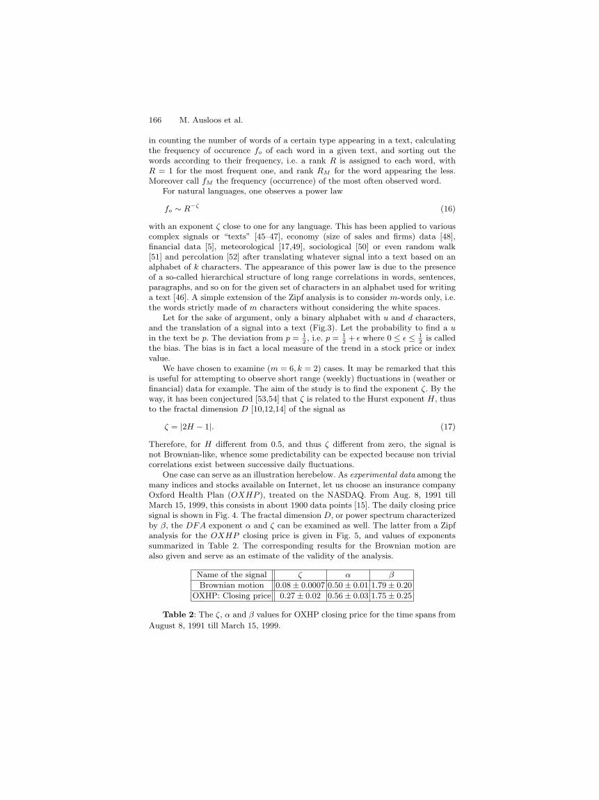
One case can serve as an illustration herebelow. As experimental data among themany indices and stocks available on Internet, let us choose an insurance companyOxford Health Plan (OXHP ), treated on the NASDAQ. From Aug. 8, 1991 tillMarch 15, 1999, this consists in about 1900 data points [15]. The daily closing pricesignal is shown in Fig. 4. The fractal dimension D, or power spectrum characterizedby β, the DFA exponent α and ζ can be examined as well. The latter from a Zipfanalysis for the OXHP closing price is given in Fig. 5, and values of exponentssummarized in Table 2. The corresponding results for the Brownian motion arealso given and serve as an estimate of the validity of the analysis.

Name of the signal ζ α β

Brownian motion 0.08± 0.0007 0.50± 0.01 1.79± 0.20OXHP: Closing price 0.27± 0.02 0.56± 0.03 1.75± 0.25

Table 2: The ζ, α and β values for OXHP closing price for the time spans fromAugust 8, 1991 till March 15, 1999.

Time is Money 167

u d u d d d u u d d u d u u d dFig. 3. Translation of part of a random walk sequence (“fluctuations”) into a binarysequence made of two characters u and d.

92 93 94 95 96 97 98 990

10

20

30

40

50

60

70

80

90

100

OX

HP

: Clo

sing

Pric

e

Time

Fig. 4. Daily closing price of Oxford Health Plan (OXHP ) stock, treated on theNASDAQ, from mid-91 till Jan. 99, i.e. about 1900 data points.

168 M. Ausloos et al.

0 0.5 1 1.5 2

0

0.5

1

1.5

2

log (R /R)

log

(fM

/f)

10 20 30 400.2

0.3

0.4

N

ζ

Fig. 5. (6,2)-Zipf analysis for the OXHP stock closing price; the estimate of the ζexponent is shown in the inset for R small and as a function of the number N ofdata points used to calculate the best slope from the main graph.

7 Basics of i-Variability Diagram Techniques

One disadvantage of the Zipf-method is that it is not possible to distinguishbetween persistent and antipersistent sequences. Only the departure fromrandomness is easily observed. Another way to sort out short range correla-tions is the i-Variability Diagram technique, used for example in heart beat[55] and meteorological [49] studies. Recall that the first return map (ri, ri−1)or the τ -return map (ri, ri−τ ) of a signal are often used for revealing a pos-sible dominant correlation between the events of the data set. This leads tostudies of strange attractors and the embedding dimension of a signal.

The return map of the first derivative of the signal, i.e. the so-calledfirst order variability diagram (1-V D) [55] correlates every three consecutivepoints of the series,

si+1 = ri+1 − ri (18)si = ri − ri−1

The curvature of the signal, thus relating every four consecutive events as

ui+1 = ri+1 − 2ri + ri−1 (19)ui = ri − 2ri−1 + ri−2.

is called the second order variability diagram (2-V D).The links between the 4-points e.g. defining the above relationship are

seen through a phase space diagram for the curvature. A non-trivial shape of

Time is Money 169

the point cloud and point distribution itself on such a diagram indicate anasymmetry between the different consecutive curvatures, and can be used forpredictability.

It has been found [56] that for free market financial series (DJIA and Goldprice) the local trend behaves like a

√t. However the BGL/USD exchange

rate variability seems to be different: the set of events leads to a line structurewith slope I = −1.21 in the curvature return map. The differences can beconjectured to depend on economic policy grounds.

A combination of Zipf and i-V D has been recently attempted for the localcurvature correlations in financial signals [56]. This method leads to suggesttests based on microscopic models.

Acknowledgments

KI thanks the hospitality of T. Ackerman and the Department of Meteorologyat Penn State University and NRC for a research grant during which part ofthis work was completed. Thanks to the F-532 grant of the Bulgarian NFSIas well. MA and NV thank the ARC 94-99/174 for financial support. MAthanks the organizers of the Ecole thematique de Chapelle des Bois and inparticular Michel Planat for inviting him to present the above results.

References

1. L. Bachelier, Theorie de la speculation, Ph. D. thesis, Acad. Paris (1900)2. R.N. Mantegna and H.E. Stanley Nature, 376, 46-49 (1995)3. E.E. Peters, Fractal Market Analysis : Applying Chaos Theory to Investment

and Economics, (Wiley Finance Edition, New York, 1994)4. M. Ausloos, Europhys. News 29, 70-72 (1998)5. N. Vandewalle and M. Ausloos, in Fractals and Beyond. Complexity in the Sci-

ences, M.M. Novak, Ed. (World Scient., Singapore, 1999) p.355-356.6. N. Vandewalle and M. Ausloos, Physica A, 246, 454-459 (1997)7. N. Vandewalle, Ph. Boveroux, A. Minguet and M. Ausloos, Physica A 255,201-210 (1998)

8. H. E. Stanley, S. V. Buldyrev, A. L. Goldberger, S. Havlin, C.-K. Peng and M.Simmons, Physica A 200, 4-24 (1996)

9. N. Vandewalle and M. Ausloos, Int. J. Comput. Anticipat. Syst. 1, 342-349(1998)

10. B. J. West and B. Deering, The Lure of Modern Science: Fractal Thinking,(World Scient., Singapore, 1995)

11. C.-K. Peng, J.M. Hausdorff, S. Havlin, J.E. Mietus, H.E. Stanley, and A.L.Goldberger, Physica A 249, 491-500 (1998)

12. M. Schroeder, Fractals, Chaos and Power Laws, (W.H. Freeman and Co., NewYork, 1991)

13. K. J. Falconer, The Geometry of Fractal Sets, (Cambridge Univ. Press, Cam-bridge, 1985)

170 M. Ausloos et al.

14. P. S. Addison, Fractals and Chaos, (Inst. of Phys., Bristol, 1997)15. K. Ivanova, unpublished16. N. Vandewalle and M. Ausloos, Int. J. Phys. C 9, 711-720 (1998)17. K. Ivanova and M. Ausloos, Eur. J. Phys. B 8 665-669 (1999)18. N. Vandewalle and M. Ausloos, Eur. J. Phys. B 4, 257-261 (1998)19. A. L. Barabasi and T. Vicsek, Phys. Rev. A 44, 2730-2733 (1991)20. A. Davis, A. Marshak, and W. Wiscombe, in Wavelets in Geophysics, E.Foufoula-Georgiou and P. Kumar, Eds. (Academic Press, New York, 1994) pp.249-298

21. A. Marshak, A. Davis, R. Cahalan, and W. Wiscombe Phys. Rev. E 49, 55-69(1994)

22. A.-L. Barabasi and H.E. Stanley, Fractal Concepts in Surface Growth, (Cam-bridge Univ. Press, Cambridge, 1995)

23. J. Feder, Fractals, (Plenum, New-York, 1988)24. E. Labie, private communication25. A.G. Ellinger, The Art of Investment, (Bowers & Bowers, London, 1971)26. J.-P. Bouchaud and A. Georges, Phys. Rep. 195, 127-294 (1990)27. N. Vandewalle and M. Ausloos, Phys. Rev. E 58, 6832-6834 (1998)28. L. Frachebourg, P.L. Krapivsky, and S. Redner, Phys. Rev. E 55, 6684-6689(1997)

29. D. Sornette, A. Johansen, and J.-Ph. Bouchaud, J. Phys. I (France) 6, 167-175(1996)

30. H.E. Stanley, Phase Transitions and Critical Phenomena, (Oxford Univ. Press,Oxford, 1971)

31. D. Sornette, Physics Reports 297, 239-270 (1998)32. J.C. Anifrani, C. Le Floc’h, D. Sornette and B. Souillard, J. Phys. I (France)

5, 631-63 (1995) 27733. D. Stauffer and D. Sornette, Physica A 252, 271- (1998)34. N. Vandewalle, R. D’hulst, and M. Ausloos, Phys. Rev. E 59, 631-635 (1999)35. M. Ausloos and N. Vandewalle, unpublished36. N. Vandewalle and M. Ausloos, Eur. J. Phys. B 4, 139-141 (1998)37. H. Dupuis, Trends Tendances 22(38), (september 18, 1997) p.26-2738. H. Dupuis, Trends Tendances 22(44), (october 30, 1997) p.1139. D. Daout, Le Vif L’Express (october 30, 1997) p.124-12540. D. Sornette and D. Stauffer, private communicaion41. J.-Ph. Bouchaud, P. Cizeau, L. Laloux, and M. Potters, Phys. World 12, 25-29(1999)

42. L. Laloux, M. Potters, R. Cont, J.-P. Aguilar, and J.-P. Bouchaud, Europhys.Lett. 45, 1-5 (1999)

43. J.R. Macdonald and M. Ausloos, Physica A 242, 150-160 (1997)44. M. Ausloos, J. Phys. A 22, 593-609 (1989)45. G.K. Zipf, Human Behavior and the Principle of Least Effort, (Addisson-Wesley, Cambridge, MA, 1949)

46. W. Ebeling and A. Neiman, Physica A 215, 233-241 (1995)47. B. Vilensky Physica A 231, 705-711 (1996)48. M.H.R. Stanley, S.V. Buldyrev, S. Havlin, R.N. Mantegna, M.A. Salinger, andH.E. Stanley, Ecomonics Letters, 49, 453-457 (1995)

49. K. Ivanova, M. Ausloos, A. Davis, and T. Ackerman, XXIV General Assemblyof the EGS, the Hague, Netherlands, April 19-23 (1999)

Time is Money 171

50. M. Marsili and Y.-C. Zhang, Phys. Rev. Lett. 80, 2741-2744 (1998)51. N. Vandewalle and M. Ausloos, unpublished52. M. S. Watanabe Phys. Rev. E 53, 4187-4190 (1996)53. A. Czirok, R.N. Mantegna, S. Havlin, and H.E. Stanley, Phys. Rev. E 52, 446-452 (1995)

54. G. Troll and P.B. Graben, Phys. Rev. E 57, 1347-1355 (1998)55. A. Babloyantz and P. Maurer, Phys. Lett. A 221, 43-55 (1996)56. K. Ivanova and M. Ausloos, Physica A 265, 279-286 (1999).