* © Willem H. Buiter 2003/4** The views and opinions expressed are those of the author. They do not represent the views and opinions ofthe European Bank for Reconstruction and Development. I would like to thank Niko Panigirtzoglou and AnneSibert for assistance and Richard Clarida, Greg Hess, Richard Burdekin, Danny Quah, Nobu Kiyotaki, LucienFoldes and other seminar participants at Columbia University and LSE for helpful comments.

Helicopter Money Irredeemable fiat money and the liquidity trap

Or: is money net wealth after all?

Willem H. Buiter * **

Chief Economist and Special Counsellor to the President,European Bank for Reconstruction and Development, CEPR and NBER

6-11-03

Revised 31-01-04

Abstract

The paper provides a formalisation of the monetary folk proposition that fiat(base) money is an asset of the holder (the private sector) but not a liability ofthe issuer (the monetary authority, as agent of the state). The issuance ofirredeemable fiat base money can have pure fiscal effects on private demand.With irredeemable fiat base money, weak restrictions on the monetary policyrule suffice to rule out liquidity trap equilibria, that is, equilibria in which allcurrent and future short nominal interest rates are at their lower bound. In amodel with flexible prices, liquidity trap equilibria cannot occur as long as theprivate sector does not expect the monetary authority to reduce the nominalmoney stock to zero in the long run. In a New-Keynesian model, liquiditytrap equilibria are ruled out provided the private sector expects the authoritiesnot to reduce the nominal stock of base money below a certain finite level inthe long run. Liquidity trap equilibria can exist if and for as long as theprivate sector expects that the monetary authorities will ultimately reverse anycurrent expansion of the monetary base in present value terms.

JEL classifications: E31, E41, E51, E52, E62, E63.

Key words: Helicopter money drop; irredeemable money; monetary policy effectiveness;zero bound, liquidity trap.

Author: Willem H. Buiter, European Bank for Reconstruction and Development, OneExchange Square, London EC2A 2JN. UKTel. #44-20-73386805Fax. #44-20-73386110/6111E-mail (office): buiterw@ebrd.comE-mail (home): willembuiter@whsmithnet.co.ukWeb page: http://www.nber.org/wbuiter/index.htm

1 The American Heritage Dictionary (2000) defines an irredeemable object as one ‘that cannot be bought backor paid off’ or ‘not convertible into coin’ The Concise Oxford Dictionary (1995) gives: ‘(of paper money) forwhich issuing authority does not undertake ever to pay coin.’ The meaning attached to it here is ‘does notrepresent a claim on the issuer for anything other than the equivalent amount of itself’.

1

1 Introduction

“Let us suppose now that one day a helicopter flies over this community anddrops an additional $1000 in bills from the sky, …. Let us suppose further thateveryone is convinced that this is a unique event which will never be repeated,”(Friedman [1969, pp 4-5].

This paper aims to provide a rigorous analysis of Milton Friedman’s famous parable

of the ‘helicopter’ drop of money. A related objective is to show that even when the

economy is in a liquidity trap (when all current and future short nominal interests rates are at

their lower bounds and there is satiation with real money balances), a helicopter drop of

money will stimulate demand, unlike a helicopter drop of government bonds.

The argument involves a number of steps. The first is a formal statement, in an

optimising dynamic general equilibrium model with money, of the ‘folk proposition’ that (fiat

base) money is an asset to the private holder but not a liability of the issuer - the government.

This is done through an asymmetric specification of the solvency constraints of the

households and the government, motivated by the assumption that fiat base money is

irredeemable.

The model has two financial stores of value: base money and one-period risk-free

non-monetary interest-bearing nominal debt. The solvency constraint for the household is the

requirement that the present discounted value of its terminal net financial wealth (the sum of

its money holdings and its net non-monetary financial assets) be non-negative.

The solvency constraint for the government is the requirement that the present

discounted value of its terminal non-monetary net financial debt be non-positive. The

government does not view its monetary debt as a liability that will eventually have to be

redeemed for something else of equal value. This formalisation of the concept of

irredeemable base money is the central new idea in this paper.1

2

From the point of view of the individual private holder of base money, it is an asset that

can be realised, that is, exchanged for other goods, services or financial instruments of equal

market value, at any time. The fact that the private sector as a whole cannot dispose of base

money at its discretion is not a constraint that is internalised by the individual household.

Each individual household believes and acts as if it can dispose of its holdings of base money

at any time, at a price in terms of goods and services given by the reciprocal of the general

price level at that time: the ‘hot potato theory of money’ is not perceived by any household as

a constraint on its own, individual ability to get rid of money balances. The aggregation of

the intertemporal budget constraints of the individual private households also does not

incorporate the irredeemability property of fiat base money. Neither the individual

household’s intertemporal budget constraint nor the aggregated household sector’s

intertemporal budget constraint incorporate the constraint recognised by the government that

the only claim a private holder of fiat base money has on the issuer is the right to exchange X

units of fiat base money for X units of fiat base money.

The next step is to show how the existence of irredeemable fiat base money implies

that fiat base money is, in a precise but non-standard way, net wealth to the consolidated

private and public sectors, and that this bestows on monetary policy a pure fiscal effect: in a

representative agent model with rational expectations, changes in the stock of nominal base

money can change real private consumption demand by changing the permanent income or

comprehensive (financial plus human) wealth of the household sector, after consolidation of

the private and government sectors’ intertemporal budget constraints. The definition of a

pure fiscal effect holds constant the sequences of current and future price levels, nominal and

real interest rates, real endowments and real public spending on goods and services.

This additional channel for monetary policy effectiveness is only operational, that is,

only makes a difference to equilibrium prices and quantities, real and/or nominal, when the

economy is in a liquidity trap, defined as an equilibrium when all current and future short

2 It would also hold with an Old-Keynesian supply side, e.g. an accelerationist Phillips curve.3 Obstfeld and Rogoff (1983, 1986, 1996) have shown this for models in which money is the only financialasset. Without irredeemable base money, deflationary bubbles cannot be rules out in the models of this paperwhich have both fiat money and non-monetary, interest-bearing government debt as stores of value.

3

nominal interest rates are at their lower bounds (conventionally zero). Next I show that, with

irredeemable fiat base money, liquidity trap equilibria cannot exist as rational expectations

equilibria, provided the monetary policy rule satisfies some simple and intuitive properties.

This is demonstrated both for a model with flexible prices and for a model with a New-

Keynesian Phillips curve.2 These same restrictions on the monetary policy rule also rule out

the existence of deflationary bubbles in models where money is not the only financial asset

(see Buiter and Sibert (2003)).3

Finally, the paper considers briefly the practical modalities of implementing a

helicopter drop of base money in an economy in which monetary policy and fiscal policy are

implemented through different institutions or agencies. How can the monetary authorities,

either on their own or jointly with the fiscal authorities, implement a helicopter drop of

money?

Central to the approach is the nature of government fiat base money as an irredeemable

final means of settlement of private sector claims on the public sector. In what follows,

‘irredeemable’ is used as a shorthand for ‘final and irredeemable’.

To the best of my knowledge, the particular formalisation proposed in this paper of the

notion that (fiat base) money is an asset to the private sector but not a liability to the public

sector, has not been proposed before. It was not part of the transmission mechanism of a

helicopter drop of money proposed by Friedman (1969). Whether and in what way ‘outside’

money is net wealth to the private sector or to the consolidated private sector and public

sector was the subject of much discussion in some of the great treatises on monetary

economics of the 1960s and 1970s, including Patinkin (1965), Gurley and Shaw (1960) and

Pesek and Saving (1967). None of these contributions proposes the approach advocated in

this paper, however. Clower (1967) stressed the unique properties of the monetary medium of

4 The Merriam-Webster Collegiate Dictionary defines convertible as: ‘capable of beingexchanged for a specified equivalent (as another currency or security) (a bond convertible to12 shares of common stock)’. Inconvertible is defined as ‘not redeemable for money in coin:inconvertible paper currency’, or ‘not able to be legally exchanged for another currency’.

4

exchange (money buys goods and goods buy money but goods do not buy goods), but the

cash-in-advance constraint he proposed did not require the monetary object to be an

irredeemable IOU of the state. The discussions in Hall (1983), Stockman (1983), King

(1983), Fama (1983), Sargent and Wallace (1984) and Sargent (1987) of outside money,

private money and the payment of interest on money ask some of the same questions as this

paper, but do not propose the same answer. Sargent (1987, Chapter 4) and many other

authors use the term ‘inconvertible currency’ or ‘unbacked paper currency’ to refer to a

monetary asset that is essentially the same as the irredeemable fiat base money of this paper.4

Inconvertible or unbacked currency is fiat money that cannot be presented by the holder to the

issuer for exchange into a fixed bundle of intrinsically valuable goods or services at a known

price. However, these authors do not develop the implications of the inconvertibility of fiat

base money for private and public sector budget constraints, which is the central concern of

this paper.

The endowment economy model with a flexible price level used in this paper is a

deterministic version of that found in Lucas (1980), but Lucas’s paper and the vast literature it

inspired do not impose the asymmetric household and government solvency constraints

proposed here. Variants of that same model have also been used in the debate on the Fiscal

Theory of the Price Level (see e.g. Woodford (1995) and Buiter (2002)). This literature

focused very closely on the government’s intertemporal budget constraint, but the special

significance of the irredeemability of government fiat money was not a theme that was

developed. The closest approximations to explicit references to the irredeemability property

of government fiat base money can be found in Sims (2000, 2003), Buiter (2003a,b),

5

Eggertson (2003) and Eggertsson and Woodford (2003), but the idea is never developed

formally and completely.

2 Fiat base money: the monetary authority’s irredeemable, finalmeans of settlement

Underlying the analysis that follows are the following three key primitive

assumptions

Assumption 1: Base money is perceived as an asset by each individual household. Eachhousehold believes it can always realise this asset in any period at the prevailing marketprice for money in that period.

Assumption 2: Base money does not have to be redeemed by the government – ever. It is thefinal means of settlement of government obligations vis-à-vis the private sector. It does notrepresent a claim on the issuer for anything other than the same amount of itself’.

Assumption 3: Additional base money can be created at zero incremental cost by thegovernment.

Most monetary general equilibrium models with a non-predetermined general price

level have at least one equilibrium in which the price of money is zero in each period. The

flexible price level model considered in this paper is no exception. The interesting results of

this paper apply only to equilibria in which there is a positive price of money in each period,

and I will only consider such equilibria. For reasons of space, the analysis will be further

restricted to fundamental equilibria; with one brief exception, bubbles and sunspots are not

considered.

In most of the paper, a positive demand for real money balances is generated by the

inclusion of real money balances as an argument in the direct utility function. A simple cash-

in-advance model is also considered (in Section 4.4). Both these approaches to motivating a

demand for fiat base money support equilibria in which the price of money is positive in each

period.

5 Indeed it would be as easy to pay a negative nominal interest rate on bank reserves as a positive interest rate. Paying interest, negative or positive on currency would be more difficult and costly, but administratively andtechnically possible (see Porter (1999), Goodfriend (2000), Buiter and Panigirtzoglou (2001, 2003)).

6

In what follows, ‘money’ means fiat base money – the monetary liabilities of the

sovereign (the state). The sovereign (the government in what follows) is the consolidated

General Government and Central Bank. Real world base money today is currency (notes and

coin which typically bear a zero nominal interest rate) plus commercial bank balances held

with the Central Bank (which can be either interest-bearing or non-remunerated).5 For the

purpose of this paper, base money is the only form of money (there are no banks whose

liabilities could serve as means of payment and medium of exchange) and all base money is

assumed to have a government-determined nominal rate of interest, which is treated as

exogenous (see Hall (1983) and Buiter and Panigirtzoglou (2001, 2003) for examples of

models where the nominal interest rate on money is determined by a simple rule).

Assumption 3 states that base money can be created at zero incremental cost by the

government. For simplicity, in the formal model we assume that there also is no fixed cost of

issuing money.

There are two key implications of Assumptions 1 and 2. First, once a private party

has accepted base money from the government in payment for goods or services or in

settlement of any other form of financial obligation of the government to the private party,

there is no further claim by the private party on the government: base money is a (in our

model the only) final means of settlement when the government settles an IOU with the

private sector. Second, there is no redemption date for base money: base money does not

have an infinite maturity - there is no redemption even in the infinitely distant future. As a

financial instrument, currency is like a zero coupon perpetuity. With a non-zero nominal

interest rate on base money, it would be like a positive or negative coupon perpetuity.

The property that base money is an irredeemable final means of settlement for

obligations of the government to the private sector, is central for what follows. It is related to

6 US Federal Reserve notes carry the inscription: “This note is legal tender for all debts, public and private”. This is a short summary of the Section 102 of the Coinage Act of 1965 (Title 31 United States Code, Section392), which contains the following text: " All coins and currencies of the United States, regardless of whencoined or issued, shall be legal tender for all debts, public and private, public charges, taxes, duties and dues."7The folk definition is the one found in generalist dictionaries. For instance, the Concise Oxford Dictionarydefines legal tender as "currency that cannot legally be refused in payment of debt (usually up a limited amountfor baser coins, etc.)". 8 Three successive monetary reforms encouraged holders of Confederate Treasury notes to exchange thesenotes for Confederate bonds by imposing deadlines on their convertibility (see Burdekin and Weidenmier(2003)).

7

but not the same as legal tender status of money.6 The popular definition of ‘legal tender’ is

that of a means of payment than cannot be refused if it is offered (tendered) to settle a debt or

other financial obligation.7 The folk definition of legal tender is stronger than the legal

definition. The folk definition of legal tender goes beyond the irredeemability property of

base money that is central to this paper, insofar as it relates to the settlement of all claims,

including claims among private parties. On the other hand, legal tender can be redeemable.

Confederate fiat base money (Confederate Treasury notes) were convertible into Confederate

bonds.8

The expression 'legal tender' has a technical meaning in relation to the settlement of a

debt. The legal definition does not imply that legal tender is a means of payment that must be

accepted by the parties to a transaction, but rather that it is a legally defined means of

payment that should not be refused by a creditor in satisfaction of a debt. Thus, if a debtor

pays in legal tender the exact amount he owes under the terms of a contract, he has a strong

prima-facie defence in law, if he is subsequently sued for non-payment of the debt.

However, in the US, there is no Federal statute which mandates that private businesses or

individuals must accept Federal Reserve notes or coin or Treasury notes as a form of

payment. Private businesses are free to develop their own policies on whether or not to

accept cash unless there is a State law which says otherwise.

The feature of irredeemable base money that is key for this paper is that the

acceptance of payment in base money by the government to a private agent constitutes a final

settlement between that private agent (and any other private agent with whom he exchanges

9 Note also that the expression “…promise to pay the bearer the sum of …” has nothing to do with the legaltender status of Bank of England notes.

8

that base money) and the government. It leaves the private agent without any further claim

on the government, now or in the future.

This irredeemability property is clearly attached to currency issued by the government

(generally through the Central Bank, although the US even today has Treasury notes

outstanding). It is brought out very nicely in the phrase "...promise to pay the bearer the sum

of ..." found on all Bank of England notes. It means that the Bank of England will pay out the

face value of any genuine Bank of England note no matter how old. The promise to pay

stands good for all time but simply means that the Bank will always be willing to exchange

one (old, faded) £10 Bank of England note for one (new, crisp) £ 10 Bank of England note

(or even for two £ 5 Bank of England notes). Because it promises only money in exchange

for money, this ‘promise to pay’ is, in fact, a statement of the irredeemable nature of Bank of

England notes.9 It is less clear whether the second conventional component of base money,

commercial bank balances held with the central bank, are irredeemable in the same sense as

currency. If they are not, the analysis that follows is applicable only to the currency

component of base money.

Inside money is money that is a claim by one private agent on another private agent.

Strong outside money is money that is an asset to the consolidated private and public sectors.

Commodity money is strong outside money. Weak outside money is money that is not a

claim by one private agent on another private agent. Thus all strong outside money is also

weak outside money, but in addition monetary liabilities of the government held by the

private sector are weak outside money. Fiat base money will be shown to be a limited form

of strong outside money - perhaps the term semi-strong should be borrowed from the

literature on the empirical testing of market efficiency to characterise it properly.

10 This is perhaps just as well. A helicopter drop of Yap-style stone money could be a serious health hazard forthose on the ground.11Yap money shares this property with intrinsically valuable commodity money.

9

Some commodity monies have intrinsic, that is, non-monetary, value as a

consumption, intermediate or capital good. Gold, salt, cattle and cigarettes are historical

examples. I do not consider this kind of intrinsically valuable strong outside money. There

is, however, a partial resemblance between the government-issued fiat base money

considered this paper and commodity money that does not have any intrinsic value. Pet

rocks, the candy wrappers that are part of many first expositions of Samuelson’s pure

consumption loans model (Samuelson (1958)), or the stone money used on the Micronesian

island state of Yap are examples.

However, Yap stone money differs from the fiat base money considered in this paper

in two ways. First, the stock outstanding can be varied only very slowly (if at all) and at

(prohibitively) high marginal cost. The monetary policy rules that prevent liquidity traps

would be hard to implement in a world with Yap-style outside money.10 Second, during any

period, t, say, strong outside money of the intrinsically worthless Yap variety constitutes net

wealth to the consolidated private and public sectors in an amount given by the period t value

of the period t stock.11 Fiat base money issued by the government constitutes net wealth to

the consolidated private and public sectors only in an amount given by the period t present

discounted value of the terminal base money stock.

Except in Section 4.4, when I consider overlapping generations (OLG) models, the

analysis uses a representative agent model in which debt neutrality or Ricardian equivalence

apply: holding constant the sequences of current and future real public spending on goods and

services and of nominal money stocks, the substitution of current borrowing for current lump-

sum taxes will not affect the real or nominal equilibrium allocations, provided the

government continues to satisfy its intertemporal budget constraint. Under the same

conditions, a helicopter drop of non-monetary government debt will have no effect on any

10

nominal or real equilibrium values. It seems preferable to establish the new transmission

channel for monetary policy in a model where conventional non-monetary deficit financing

does not have any real or nominal effects.

With irredeemable fiat base money, a current tax cut financed by printing money will

not, ceteris paribus, that is, at given current and future prices, nominal and real interest rates,

real activity and real public spending levels, have to be matched by a future increase in taxes

of equal present value. A current tax cut financed by borrowing using non-monetary debt

instruments, will, ceteris paribus, have to be matched by a future tax increase of equal

present value.

This difference between the effects of monetising a government deficit and financing it

by issuing non-monetary debt persists even if the interest rates on base money and on non-

monetary debt are the same (say zero), now and in the future. When both money and bonds

bear a zero nominal interest rate, there remains a key difference between them: the principal

of the bonds is redeemable, the principal of base money is not.

The paper shows how, with irredeemable fiat base money, the proper combination of

monetary and fiscal policies can almost always, ceteris paribus, boost aggregate demand.

The qualification almost reflects the existence of two possible exceptions. First, there is the

possibility that perverse future policies (future reversals of current expansionary monetary

policies) could, through the present rational anticipation of these policies, negate what would

otherwise be the expansionary effect of the current policy measures on demand. Then there

is the possibility that non-rational expectations of future offsetting policy actions could

neutralise current expansionary measures for as long as the non-rational expectations persist.

The proposed expansionary policy measure is the mundane version of the helicopter

drop of money proposed by Milton Friedman. The simplest example is a temporary tax cut or

increased transfer payment by the government to the household sector, financed through an

12 The General Government is the consolidated central (Federal) state (provincial, cantonal) and municipal(local) government sector. It also includes the off-budget or off-balance sheet public entities, like the socialsecurity funds, for whose liabilities the central, state or local government sector is ultimately responsible.13 Adding uncertainty and a richer menu of non-monetary securities would add notational complexity but wouldnot alter any results as long as markets are complete.

11

one-off, permanent expansion of the monetary base. It is key that the increase in the nominal

stock of money associated with the helicopter drop be permanent, or at least that it is

perceived as permanent. It will be effective only if it leads to an increase in the present

discounted value of current and future net increases in the stock of base money. If the

helicopter drop of money is expected to be reversed, in present value terms, in the future, the

current helicopter drop will not raise aggregate demand.

3 Modeling household and government behaviour

I consider a simple dynamic competitive equilibrium model of a perishable

endowment economy with a representative private agent and a government sector, consisting

of a consolidated fiscal authority and monetary authority. In what follows, ‘government’ will

be used to refer to the consolidated fiscal and monetary authorities. The words ‘state’ or

‘sovereign’ are probably better than the word ‘government’ to describe the consolidated

General Government sector and Central Bank, but the usage ‘government budget constraint’

is by now too firmly established.12 When the government is partitioned into distinct fiscal

and monetary authorities in Section 5, the fiscal authority is called the Treasury and the

monetary authority the Central Bank.

There is no uncertainty and markets are competitive.13 Time, indexed by t, is

measured in discrete intervals of equal length, normalised to unity. There is a countably

infinite number of periods, indexed by t ≥ 0. Household and government behaviour is

modeled starting in period 1, taking as given the contractual financial obligations inherited

from period 0.

14 The payment of interest on base money has been studied by Hall (1983) and by Sargent and Wallace (1984)and Sargent (1987, Chapter 5.5)

12

F ht%1 / (1%i M

t%1)Mt % (1%it%1)Bt (1)

vt ' j4

j't(1%ρ)&(j&t)u(cj, mj)

ρ > 0; cj , mj $ 0; ucm $ 0(2)

3.1 Household behaviour

Households are price takers in all markets in which they transact. There is a

continuum of households whose aggregate measure is normalised to unity. They receive an

exogenous perishable endowment, , each period, consume and pay net realyt > 0 ct $ 0

lump-sum taxes . They have access to two stores of value: fiat base money, a liability ofτt

the government, a unit of which, if acquired during period t and held at the end of period t,

, pays of money in period t+1, and a nominal one-period bond which, int $ 0 1%i Mt%1 $ 0

exchange for one unit of money in period t pays units of money in period t+1..141%it%1 $ 0

The quantities of money and nominal one period bonds outstanding at the end of period t (and

the beginning of period t+1) are denoted and respectively. The money price of outputMt Bt

in period t is . The government is assumed to have a monopoly of the issuance ofPt $ 0

base money, so . The nominal value of household net financial wealth at theMt $ 0, 0 # t

beginning of period t+1 (inclusive of interest due) is denoted , soF ht%1

The household objective function is given in equation (2); is the stock ofmj / Mj /Pj

real money balances at the end of period t .

13

For σ>0, σ…1

vt ' j4

j't(1%ρ)&(j&t)σ(σ&1)&1z (σ&1)σ&1

j

For σ'1

vt ' j4

j't(1%ρ)&(j&t)lnzj

For 0<α<1, n>0, n…1

zj ' α1nc

n&1n

j %(1&α)1n(Mj /Pj)

n&1n

nn&1

For n'1

zj ' c αj (Mj /Pj)

1&α

(3)

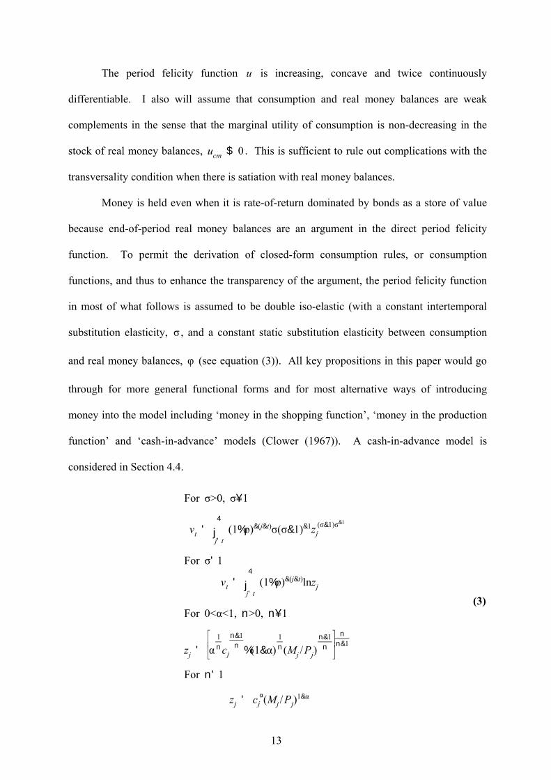
The period felicity function is increasing, concave and twice continuouslyu

differentiable. I also will assume that consumption and real money balances are weak

complements in the sense that the marginal utility of consumption is non-decreasing in the

stock of real money balances, . This is sufficient to rule out complications with theucm $ 0

transversality condition when there is satiation with real money balances.

Money is held even when it is rate-of-return dominated by bonds as a store of value

because end-of-period real money balances are an argument in the direct period felicity

function. To permit the derivation of closed-form consumption rules, or consumption

functions, and thus to enhance the transparency of the argument, the period felicity function

in most of what follows is assumed to be double iso-elastic (with a constant intertemporal

substitution elasticity, , and a constant static substitution elasticity between consumptionσ

and real money balances, (see equation (3)). All key propositions in this paper would goφ

through for more general functional forms and for most alternative ways of introducing

money into the model including ‘money in the shopping function’, ‘money in the production

function’ and ‘cash-in-advance’ models (Clower (1967)). A cash-in-advance model is

considered in Section 4.4.

15 An equivalent representation is: .Mt % Bt / (1 % i Mt )Mt&1 % (1 % it)Bt&1 % Pt (yt & τt & ct)

14

F ht%1 / (1%it%1)[F

ht % Pt(yt & τt & ct)] % (i M

t%1 & it%1)Mt (4)

B0 ' B0

M0 ' M0 > 0(5)

limN64

It%1,N F hN ' lim

N64It%1,N [(1%i M

N )MN&1 % (1%iN)BN&1]h $ 0 (7)

1 % rt%1 / (1 % it%1)Pt /Pt%1 (6)

The single-period household budget identity for is given by15t $ 1

Initial (period 0) financial asset stocks are predetermined:

Let and , where is the rate of inflation.bt / Bt /Pt, f ht / F h

t /Pt πt / (Pt/Pt&1) & 1 π t

The risk-free real interest rate is defined byrt

Let , be the nominal market discount factorIt0, t1/ k

t1

s't0

(1%is)&1, t1 $ t0; It0, t0&1 / 1

between periods and , and , the correspondingt1 t0 Rt0, t1/ k

t1

s't0

(1%rs)&1, t1 $ t0; Rt0, t0&1 / 1

real market discount factor. The solvency constraint of the household is that the present

discounted value of terminal financial wealth must, in the limit as the time horizon goes to

infinity, be non-negative, that is,

16 This follows from the simplest no-arbitrage argument. If the nominal interest rate on money were to exceedthe nominal interest rate on bonds, households would have a ‘risk-free pure profit machine’ by borrowingthrough the issuance of non-monetary bonds and investing the proceeds in money.

15

F ht / (1%i M

t )Mt&1 % (1%it)Bt&1

' j4

j'tIt%1, j [Pj(cj%τj&yj)%(ij%1&i M

j%1)(1%ij%1)&1Mj]% lim

N64It%1,N F h

N

(8)

f ht / (1%i M

t )(1%πt)&1mt&1 % (1%rt)bt&1

' j4

j'tRt%1, j [cj%τj&yj%(ij%1&i M

j%1)(1%ij%1)&1mj] % lim

N64Rt%1,N f h

N

(11)

f ht%1 / (1%rt%1)(f

ht % yt & τt & ct) % (i M

t%1 & it%1)(1%πt%1)&1 mt (9)

limN64

Rt%1,N fN' limN64

Rt%1,N [(1%i MN )(1%πN)&1)mN&1 % (1%rN)bN&1]

h $ 0 (10)

This no-Ponzi game condition in equation (7) incorporates the important assumption,

stated explicitly as Assumption 1 in Section 2, that base money is (and is perceived to be by

the household) an asset of the household that owns it.

Solving the household period budget identity forward yields

The household period budget identity (4) can also be written as:

The associated solvency constraint is

Solving the period budget identity (9) forward yields

There obviously exists no equilibrium supporting a negative differential between the

nominal interest on non-monetary financial claims and the nominal interest rate on money.16

I therefore consider only monetary policy rules that support equilibria in which money is

weakly dominated as a store of value, that is, equilibria supporting a non-negative

differential between the nominal interest rate and the nominal interest rate on money.

16

uc(cj , mj) ' (1%rj%1)(1%ρ)&1uc(cj%1, mj%1) (12)

uc(cj, mj) ' (1%ij%1)(ij%1&i Mj%1)&1um(cj, mj) (13)

limN64

(1%ρ)&(N&t)uc(cN, mN) f hN ' 0 (14)

uc(ct , mt) limN64

Rt%1,N f hN ' 0 (15)

limN64

Rt%1,N f hN ' P &1

t limN64

It%1,N F hN ' 0 (16)

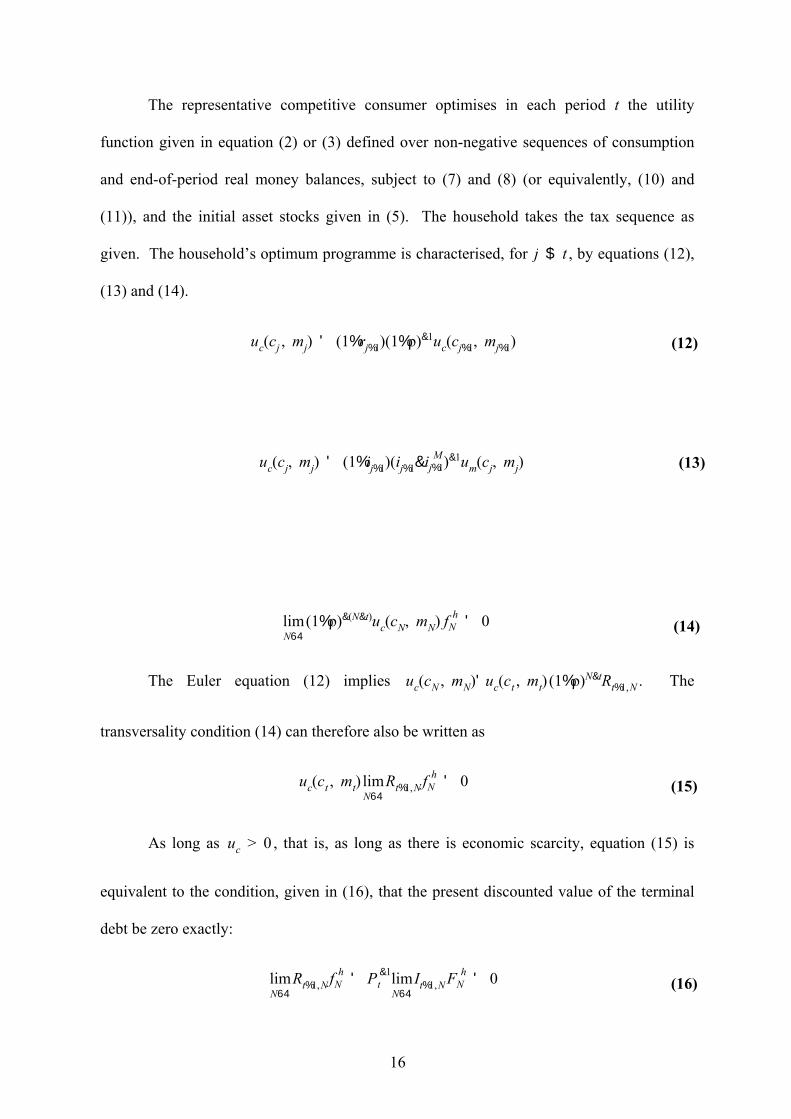
The representative competitive consumer optimises in each period t the utility

function given in equation (2) or (3) defined over non-negative sequences of consumption

and end-of-period real money balances, subject to (7) and (8) (or equivalently, (10) and

(11)), and the initial asset stocks given in (5). The household takes the tax sequence as

given. The household’s optimum programme is characterised, for , by equations (12),j $ t

(13) and (14).

The Euler equation (12) implies . Theuc(cN , mN)'uc(ct , mt) (1%ρ)N&tRt%1,N

transversality condition (14) can therefore also be written as

As long as , that is, as long as there is economic scarcity, equation (15) isuc > 0

equivalent to the condition, given in (16), that the present discounted value of the terminal

debt be zero exactly:

17

cj%1

cj

'1%rj%1

1%ρ

σ

Ωj%2Ω&1j%1

σ&nn&1

Ωj / 1% 1&αα

1%ij

ij&i Mj

n&1(17)

ct ' α(1&α)&1[(it%1&i Mt%1)(1%it%1)

&1]nmt

it%1 $ i Mt%1

(18)

ασ&1

(n&1)σc&

1σ

t Ωσ&n

σ(n&1)t%1 lim

N64Rt%1,N f h

N'

(1&α)σ&1

(n&1)σm&

1σ

t1%it%1

it%1&i Mt%1

1% α1&α

[(it%1&i Mt%1)(1%it%1)

&1]n&1σ&n

σ(n&1) limN64

Rt%1,Nf hN'0

(19)

For the iso-elastic utility function in (3), the household’s optimum programme

satisfies:

and

Equation (17) is the double iso-elastic version of the consumption Euler equation.

Equation (18) is the optimality condition relating the money stock in period t to consumption

in period t. Equation (19) is the transversality condition for the double isoelastic utility

function. Note that the analysis is restricted to those double iso-elastic functions for which

the assumption is satisfied. It is clear that there are such cases. First, considerucm $ 0

. In that case, . When , that is, when realn ' 1 uc 'α

c σ&1

α1&α

i&i M

1%i

(σ&1)(α&1)σ&1

i'i M

17 There is an extensive literature on the necessity and sufficiency of the transversality condition in infinitehorizon optimisation problems, see e.g. Arrow and Kurz (1970), Weitzman (1973), Araujo and Scheinkman(1983), Stokey and Lucas with Prescott (1989), Michel (1990) and Kamihigashi (2001, 2002). The conditionsstated in the body of the text are sufficient for the set-up under consideration. 18If we set up the household optimisation problem as an infinite horizon discrete time Hamiltonian problem towhich the discrete time maximum principle can be applied, there is no co-state variable associated with thestock of real money balances. Nor is there a transversality condition associated with the terminal value of the

18

money balances are unbounded, if (an intertemporal substitution elasticityuc ' 0 σ < 1

less than one) and . When , either is independent of the real stock of moneyc > 0 σ $ 1 uc

balances (when ), or increases with the stock of real money balances (whenσ ' 1 uc

). σ > 1

Next, consider . In this case . It is clear that is independentσ ' n uc ' (α /c)1/n uc

of the stock of real money balances and that for all bounded values of c. uc > 0

As long as , the household solvency constraint binds (holds with equality) anduc > 0

equation (16) is part of the optimal programme. Under the conditions imposed on the

household optimisation programme, the transversality condition (14) or (19) is sufficient

(together with the other optimality conditions (12) or (17) and (13) or (18)) for an optimum.17

If the money-in-the-direct-utility function of this Section is replaced a cash-in-advance

model of money demand (see Section 4.4), the condition that is always satisfied foruc > 0

bounded value s of c.

Note that the household’s optimisation problem contains but one state variable, the

net financial wealth of the household, . The stock of real money balances, , is not, fromf ht mt

a formal mathematical point of view, a state variable, although it is, economically, a durable

good. Formally, is like , a control variable. Efficient financial markets turn themt ct

individual portfolio allocation decision between money and nominal bonds into a decision

rule with a single state variable: the predetermined inherited net financial wealth of the

economic agent, .18 f ht

stock of real money balances. The stock of net financial wealth does have a co-state variable associated with it,and it also has the standard transversality condition (14) or (19) associate with its terminal value. 19The expression in (25) for the marginal propensity to consume out of comprehensive wealth simplifies whenfuture real and nominal interest rates are expected to be constant. In that case, we get:

. From this equation, the steady state marginal propensity to consume out ofµ ' Ω&1 (1%ρ)σ&(1%r)σ&1

(1%ρ)σ

comprehensive wealth is independent of the nominal interest rate only if the elasticity of substitution betweenconsumption and real money balances is one ( ). In that case the steady-state marginal propensity toφ ' 1

consume becomes . However, is not sufficient for the marginalµ ' α (1%ρ)σ & (1%r)σ&1

(1%ρ)σn ' 1

propensity to consume to be independent of the sequence of current and future nominal interest rates outsidesteady state. For that to be true we require both and , the intertemporal substitution elasticity, to be equal ton σunity (see Fischer (1979a,b) and Buiter (2003)). When (logarithmic intertemporal preferences andn ' σ ' 1a unitary elasticity of substitution between the composite consumption good and real money balances), themarginal propensity to consume out of comprehensive wealth simplifies to the expression given below. It is

now also independent of the real interest rate: .µ 'αρ

1%ρ

19

F ht / (1%i M

t )Mt&1 % (1%it)Bt&1 ' j4

j'tIt%1, j[Pj(cj%τj&yj)%(ij%1&i M

j%1)(1%ij%1)&1Mj]

or

f ht / (1%i M

t )(1%πt)&1mt&1%(1%rt)bt&1'j

4

j'tRt%1, j[cj%τj&yj%(ij%1&i M

j%1)(1%ij%1)&1mj]

(20)

ct ' µtwt (21)

When (16) holds, the household’s intertemporal budget constraint becomes

From the optimality conditions (17) and (18) and the intertemporal budget constraint

of the household (20), we obtain the household consumption function for given int $ 1

equations (21) to (25). Real comprehensive household wealth in period t is denoted ; it iswt

the sum of real household financial wealth held at the beginning of period t, , andf ht

household real human wealth (the present discounted value of current and future after-tax

endowment income), .19ht

20

wt ' f ht % ht (22)

f ht / (1%rt) (1%i M

t )(1%it)&1mt&1%bt&1 ' (1%i M

t )Mt&1/Pt % (1%it)Bt&1/Pt (23)

ht ' j4

j'tRt%1, j (yj & τj) (24)

µt / j4

j'tΩj%1 k

j

s't%1

(1%rs)σ&1

(1%ρ)σΩs%1

Ωs

σ&nn&1

&1

(25)

Monetary policy is said to have a pure fiscal effect on aggregate demand if changes in

the sequence of current and future nominal money stocks can change aggregate demand

holding constant the initial financial asset stocks and inherited financial obligations, the

sequences of current and future values of nominal and real interest rates, money prices, real

government spending on goods and services, and before-tax endowments.

From the consumption function given in equations (21) to (25), it follows that

monetary policy can have a pure fiscal effect on aggregate demand (in our model, on private

consumption) if and only if it affects the present discounted value of current and future taxes.

The key policy question thus becomes: holding constant the sequence of real public spending

20In overlapping generations models without operative intergenerational gift or bequest motives, postponingtaxes while keeping their present discounted value constant will boost consumption demand if this fiscal actionredistributes resources from households with long remaining time horizons (the young and the unborn) tohouseholds with short remaining time horizons (the old). See Section 4.21 Note that even when the nominal interest rate on bonds equals the nominal interest rate on money and even ifboth interest rates are zero, the principal of the bond has to be redeemed by the government, but not theprincipal of the base money ‘liability’.

21

on goods and services, can the authorities change the present discounted value of the

sequence of current and future expected real taxes and thus change real consumption demand?

In this representative agent model which exhibits debt neutrality or Ricardian equivalence, the

answer turns out to be ‘no’ unless base money is irredeemable.20

3.2 The government

The government sector is the consolidated fiscal and monetary authorities (the

Treasury and Central Bank). Its decision rules are exogenously given, and like the household

sector, it is subject to a solvency constraint or intertemporal budget constraint, which has to

hold identically, that is, for all feasible values of the variables entering into the intertemporal

budget constraint that are not choice variables of the government.

The government solvency constraint is the requirement that the present discounted

value of the government’s non-monetary debt must be non-positive in the limit as the time

horizon goes to infinity. This follows from Assumption 2. Unlike bonds, base money, by

assumption, does not have to be redeemed ever by the government. This means that while

money is in the legal sense a liability of the government, it does not represent an effective

liability of the government, in the sense that there is no obligation for the issuer ever to

redeem it (to extinguish it by forcing the issuer to exchange it for something else with an

equal market value). This is the key feature of the model that, even in a liquidity trap,

(almost) always (barring (expectations of) perverse policies that the government will, in the

long run, redeem its base money stock) makes a helicopter drop of money a means of

boosting aggregate demand - unlike a helicopter drop of bonds.21

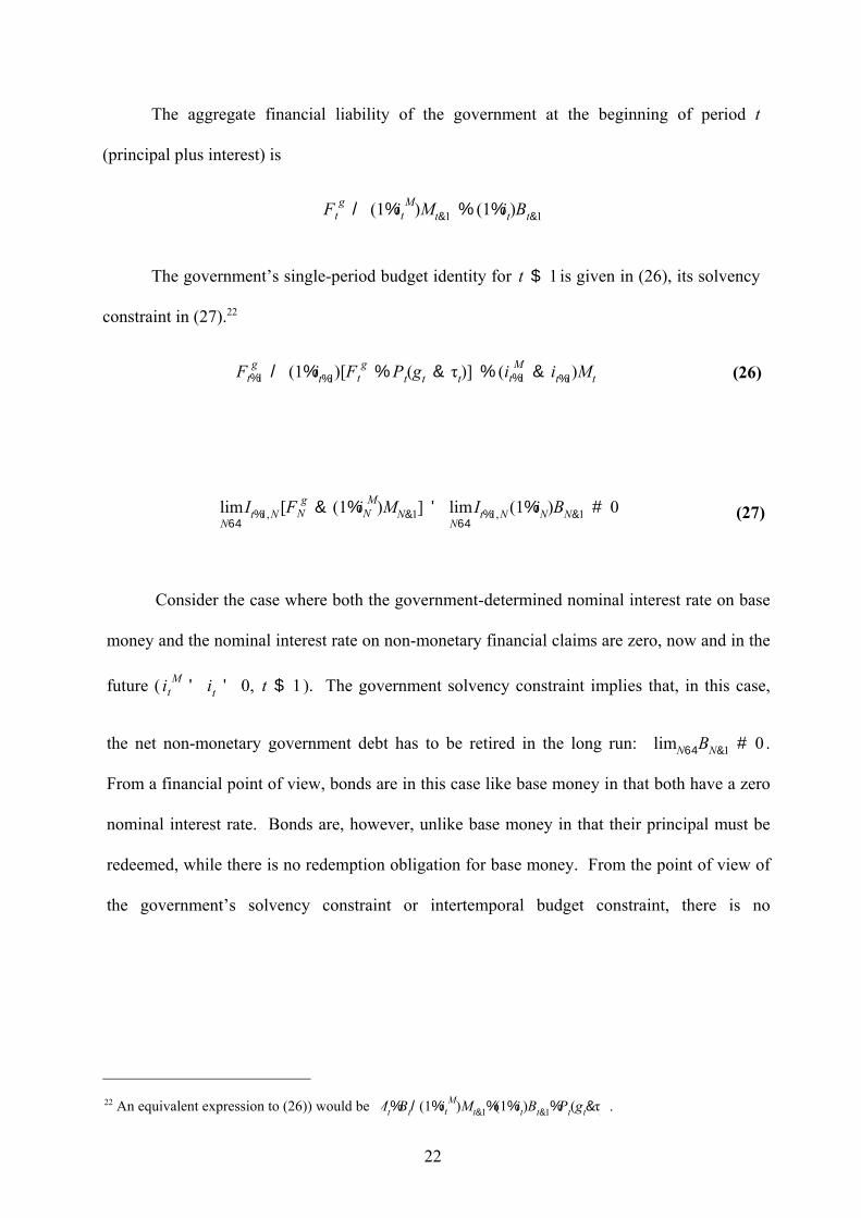
22 An equivalent expression to (26)) would be .Mt%Bt/(1%i Mt )Mt&1%(1%it)Bt&1%Pt(gt&τt

22

F gt / (1%i M

t )Mt&1 % (1%it)Bt&1

F gt%1 / (1%it%1)[F

gt % Pt(gt & τt)] % (i M

t%1 & it%1)Mt (26)

limN64

It%1,N [F gN & (1%i M

N )MN&1] ' limN64

It%1,N (1%iN)BN&1 # 0 (27)

The aggregate financial liability of the government at the beginning of period t

(principal plus interest) is

The government’s single-period budget identity for is given in (26), its solvencyt $ 1

constraint in (27).22

Consider the case where both the government-determined nominal interest rate on base

money and the nominal interest rate on non-monetary financial claims are zero, now and in the

future ( ). The government solvency constraint implies that, in this case,i Mt ' it ' 0, t $ 1

the net non-monetary government debt has to be retired in the long run: .limN64BN&1 # 0

From a financial point of view, bonds are in this case like base money in that both have a zero

nominal interest rate. Bonds are, however, unlike base money in that their principal must be

redeemed, while there is no redemption obligation for base money. From the point of view of

the government’s solvency constraint or intertemporal budget constraint, there is no

23The government’s solvency constraint in (27) in principle would also permit the government to be, in the longrun and in present discounted value, a net creditor in non-monetary financial claims, that is,

, but this possibility is not pursued further in this paper. If government behaviourlimN64

It%1,N (1%iN)BN&1 < 0

instead of being characterised by a number of ad-hoc policy rules, were to be derived from the optimisation of areasonable objective function (e.g. that of the representative household), and if there were any real resourcecosts associated with raising tax revenues (or if taxes were distortionary), the government would always satisfyits solvency constraint with equality. Here the requirement that the government solvency constraint binds is aprimitive assumption.24 Note that a non-zero value for the discounted terminal money stock satisfies the homogeneous equation of thegovernment’s period budget identity (28): .lim

N64Rt%2,N(1%i M

N )(1%πN)&1mN&1'(1%rt%1)limN64

Rt%1,N(1%i MN )(1%πN)&1mN&1

23

f gt%1 / (1%rt%1)(f

gt % gt & τt) % (i M

t%1&it%1)(1%πt%1)&1mt (28)

f gt / (1%i M

t )Mt&1/Pt % (1%it)Bt&1/Pt / (1%i Mt )(1%πt)

&1mt&1 % (1%rt)bt&1

' j4

j'tRt%1, j [τj&gj%(ij%1&i M

j%1)(1%πj%1)&1mj]%lim

N64Rt%1,N (1%i M

N )(1%πN)&1mN&1

(30)

limN64

Rt%1,N [f gN & (1%i M

N )(1%πN)&1mN&1] ' limN64

Rt%1,N&1 bN&1 # 0 (29)

requirement that, , regardless of whether the interest rate on non-limN64

It%1,N (1%i MN )MN&1 # 0

monetary financial instruments exceeds or equals the interest rate on base money.23

Using the definition , We can rewrite (26) and (27) asf gt / F g

t /Pt

and

From (28) and (29), assumed to hold with equality, we obtain the following

intertemporal budget constraint for the government:24

3.3 Consolidating the household and government accounts

The final step in the formal argument is that conditions (31) and (32) or,

equivalently, conditions (33) and (34) hold.

24

F gt ' F h

t ' Ft, t $ 0 (31)

f gt ' f h

t ' ft, t $ 0 (33)

limN64

Rt%1,N f hN ' 0

limN64

Rt%1,N f gN ' lim

N64Rt%1,N (1%i M

N )(1%πN)&1mN&1

(34)

The last term of equations (32) and (34) need not equal zero. In particular, if there is a

liquidity trap, that is, with, say, a constant nominal interest rate on base money,it ' i Mt , t $ 1

then = . As long as the initial stock of baselimN64

I1,N (1%i MN )MN&1 lim

N64(1%i M)&(N&1) MN&1

money is positive, if the growth rate of the nominal base money stock is not less than the

nominal interest rate on base money, that is, , thenMt /Mt&1 $ (1%i M)&1

. For instance, in the empirically relevant case where thelimN64(1%i M)&(N&1)MN&1 > 0

limN64

It%1,N F hN ' 0

limN64

It%1,N F gN ' lim

N64It%1,N (1%i M

N )MN&1

(32)

25

wt / (1%i Mt )Mt&1P

&1t % j

4

j'tRt%1, j yj & gj % [Mj&(1%i M

j )Mj&1]P&1j (38)

(1%rt)bt&1 / (1%it)Bt&1P&1t / j

4

j'tRt%1, j τj&gj%[Mj&(1%i M

j )Mj&1]P&1j (37)

bt / (1%rt)bt&1 % gt & τt & [Mt & (1%i Mt )Mt&1]P

&1t (35)

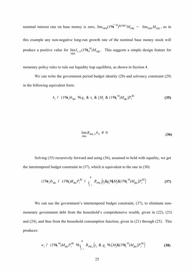
limN64

Rt%1,N bN # 0 (36)

nominal interest rate on base money is zero, = , so inlimN64(1%i M)&(N&1)MN&1 limN64MN&1

this example any non-negative long-run growth rate of the nominal base money stock will

produce a positive value for . This suggests a simple design feature forlimN64

I1,N (1%i MN )MN&1

monetary policy rules to rule out liquidity trap equilibria, as shown in Section 4.

We can write the government period budget identity (28) and solvency constraint (29)

in the following equivalent form:

Solving (35) recursively forward and using (36), assumed to hold with equality, we get

the intertemporal budget constraint in (37), which is equivalent to the one in (30):

We can use the government’s intertemporal budget constraint, (37), to eliminate non-

monetary government debt from the household’s comprehensive wealth, given in (22), (23)

and (24), and thus from the household consumption function, given in (21) through (25). This

produces:

26

(1%i Mt )Mt&1P

&1t %limN64j

N

j'tRt%1, j [Mj&(1%i M

j&1)Mj&1]P&1j

/ limN64jN

j't%1Rt%1, j (ij&i M

j )Mj&1P&1j % limN64Rt%1,N (1%i M

N )MN&1P&1N

(39)

ct ' µt wt (40)

wt ' j4

j'tRt%1, j(yj&gj)%limN64Rt%1,N(1%i M

N )(1%πN)&1mN&1

' j4

j'tRt%1, j(yj&gj)%P &1

t limN64It%1,N (1%i MN )MN&1

(41)

µt / j4

j'tk

j

s't%1

(1%rs)σ&1

(1%ρ)σΩs%1

Ωs

σ&nn&1

&1

(42)

Note that

Substituting (39) into (38), and using the money demand first-order condition (18), the

consumption function can be written as follows:

Equations (40) to (42) differ from the consumption function that would be obtained

without irredeemable base money (that is, with the solvency constraint for the government

specified symmetrically to that of the private sector) because of the presence of the present

discounted value of the terminal money stock, limN64

Rt%1,N (1%i MN )(1%πN)&1mN&1/

in the expression for the intertemporal budget constraint of theP &1t lim

N64It%1,N (1%i M

N )MN&1

25Equation (35) could have been obtained more directly by combining the household intertemporal budgetconstraint (12) and the government intertemporal budget constraint (25) and using the first-order conditions(13) and (14).

27

consolidated private and government sectors. Irredeemable base money is net wealth to the

consolidated private and public sectors in the limited sense that the present discounted value of

the terminal stock of base money is perceived as part of the consolidated resource base for

private consumption, alongside the present discounted value of the sequence of real

endowments net of real government spending, . Without the ‘irredeemability’j4

j'tRt%1, j (yj&gj)

assumption, this representative agent model would have the property, noted in Weil (1991), that

money is not net wealth, just as government debt is not net wealth. In Section 4, it is shown that

the present discounted value of the terminal money stock will be zero in well-behaved (non-

liquidity trap) equilibria. It can, however, be positive in liquidity trap equilibria. This will

suggest ways of specifying monetary policy rules in such a way that liquidity trap equilibria

cannot exist.

The intuition behind equation (42) is straightforward.25 From the perspective of the

government, there is no requirement that the present discounted value of its aggregate terminal

financial liabilities be non-positive. While the present discounted value of the government’s

terminal non-monetary liabilities must be non-positive, there is no non-positivity constraint on

the present discounted value of its irredeemable monetary liabilities. At the beginning of period

t, for given sequences of prices, real and nominal interest rates, real public spending and real

before-tax endowments, , the government can therefore, as far as itsPj, rj, ij, i Mj , gj, yj; j$t

perception of its own intertemporal budget constraint (30) or (37) is concerned, reduce the

present discounted value of its current and future real tax sequence by increasing the present

discounted value of its sequence of real ‘net’ monetary issuance (or real net seigniorage)

26It is important that, in this statement, the current and future values of the general price level are held constant. From the government’s intertemporal budget constraint, equation (37), any change in the initial general pricelevel, , would change the real value of the initial stock of non-monetary debt, if . EquilibriumPt Bt … 0changes in real taxes and net seigniorage would have to allow for this.

28

by that same amount.26 From (39), the sum of the real value of the(Mj&(1%i Mj )Mj&1)P

&1j ; j$t

initial stock of money balances plus the present value of current and future real net monetary

issues is given by . We will see in Section 4limN64

Rt%1,N (1%i MN )

MN&1

PN

%j4

j't%1Rt%1,j

ij&i Mj

1%πj

mj&

that in well-behaved equilibria (that is, non-liquidity traplimN64

Rt%1,N (1%i MN )MN&1P

&1N '0

equilibria, with ). If follows that the sum of the present discounted value of current andit > i Mt

future real net seigniorage plus the real value of the stock of initial money balances equals the

present discounted value of the interest bill saved because private agents hold base money rather

than non-monetary debt, . The sequences of nominal and realj4

j't%1Rt%1, j(ij&i M

j )(1%πj)&1mj&1

interest rates and, therefore also of real money demands (when the lower bounds on nominal

interest rates are not binding, see (18)) are held constant in the characterisation of the pure fiscal

effect of monetary policy. It follows that in well-behaved equilibria, there is no pure fiscal

effect of monetary policy.

Equations(40), (41) and (42) do not say that, if , monetarylimN64

Rt%1,N (1%i MN )MN&1P

&1N '0

policy cannot affect real consumption demand (it is clear that they say nothing about the ability

of monetary policy to influence nominal consumption demand). If the present value of the

terminal base money stock is zero, monetary policy can still affect real consumption if it can

27 is the stock of Yap money. Yap money is the numeraire and P is the price level in units of Yap money.M yt

29

wt ' j4

j'tRt%1, j (yj&gj)%P &1

t M yt (43)

0 # gt ' g t $ 1 (44)

affect either current or anticipated future real endowment income, or (more plausibly) current

and anticipated real and nominal interest rates.

Equations (40), (41) and (42) have nothing at all to say about the effect of monetary

policy on the current and future values of the general price level. Other equilibrium conditions,

including the monetary equilibrium condition, are required to determine these. The

intertemporal budget constraints then show what kind of restrictions must be imposed on the

government’s fiscal, financial and monetary programme (FFMP) to support the equilibrium in

question.

In a world with strong outside money, say Yap money, and without fiat base money

issued by the government, the analogue to the comprehensive wealth of the private sector given

in (42) would be 27:

For simplicity, I have assumed that Yap money does not bear interest and that nature is

not expected to provide future additions to the stock of Yap money. An endowment of

intrinsically valuable commodity money would be represented in a similar manner.

3.4 The Fiscal-Financial-Monetary Programme (FFMP) of the government

Real public spending on goods and services is assumed constant:

28It is a simplified Taylor rule, because the nominal interest rate does not respond to the output gap, . yt & y (

Nothing significant depends on this simplification.

30

τt ' g %rt%1

1%rt%1

f0 %i Mt%1&it%1

1%it%1

mt ' g %rt%1

1%rt%1

f0 %α&1α

it%1&i Mt%1

1%it%1

1&n

ct (45)

i Mt ' i M, t $ 1 (46)

Mt%1 ' (1 % ν)Mt , t $ 1 ; M0 > 0; ν $ (1%i M)(1%ρ)&1 (47)

Unless an alternative tax rule is specified, real lump-sum taxes are assumed to vary

endogenously to keep constant the real stock of government financial debt (monetary and non-

monetary). Using (28) and , it follows that:ft%1 ' ft ' f0, t $ 0

We assume that the nominal interest rate on base money is exogenous and constant, that

is,

I shall consider two kinds of monetary policy rules. The first is a constant growth rate

for the nominal stock of base money:

This is the only monetary rule considered for the flexible price level version of the

model. The second kind of monetary rule is the combination of a simplified Taylor rule for the

short nominal interest rate (when application of this rule does not cause the short nominal

interest rate to violate the lower bound constraint), and a constant growth rate of the nominal

money stock, when the application of the Taylor rule would cause the short nominal interest rate

to violate the lower bound.28 The nominal interest rate in that case is kept at the lower bound.

This rule is given in (48). It will be the rule considered for the New-Keynesian version of the

model.

31

bt / Bt /Pt ' f0 & (1%i M)(1%it%1)&1mt (50)

Mt /Pt / mt ' (1&α)α&1[(1%it%1)(it%1&i M)&1] n ct

it%1 $ i M(49)

If 1%π( % γ(πt%1&π() > (1%i M)(1%ρ)&1, γ > 1

1%it%1'(1%ρ)[1%π( % γ(πt%1&π()]

If 1%π( % γ(πt%1&π() # (1%i M)(1%ρ)&1

1%it%1'1%i M

and

Mt%1/Mt ' 1 % ν, 1 % ν > 1%i M

(48)

Equation (48) says that, as long as the lower bound constraint on the short nominal

interest rate is not binding, the short nominal interest rate rises more than one-for-one with the

(expected) inflation rate. When (the ‘normal’1%πt%1 > γ&1[(1%i M)(1%ρ)&1%(γ&1)(1%π()]

region) the nominal money stock is endogenously determined through the money demand

function:

The behaviour of the stock of non-monetary public debt follows from the constancy of ft

and the behaviour of the endogenous stock of real money balances:

Equation (48) also says that, if the application of the Taylor rule implies a value for the

short nominal rate of interest that is less than the value of the nominal interest rate on base

money, the short nominal interest rate instead is set equal to . From the money demandi M

equation (49) it then follows that, with the demand for real money balances unbounded when

29An alternative FFMP would keep the real value of non-monetary public debt constant, that is, total realfinancial wealth constant, rather than the real stock of non-monetary debt, that is, . Taxes inBt ' (1 % πt)Bt&1

that case would be given by: .τt ' g % rtb0 & [Mt & (1%i M)Mt&1]P&1t

32

yt ' ct % gt t $ 1 (51)

yt ' y ( (52)

0 # gt ' g < y (

, the authorities can choose any sequence for the nominal money stock, provided theyi ' i M

adjust the nominal stock of non-monetary debt appropriately (see (50)). This is consistent,

when , with the tax rule in (45) which keeps real net financial debt constant. Fori'i M

concreteness, I assume that the authorities choose a constant proportional growth rate for theν

nominal money stock.29

4. Irredeemable money in general equilibrium

I consider two alternative supply-side specifications: a flexible price or New-Classical

model with an exogenous and constant level of capacity output, , and a New-Keynesiany ( > 0

Phillips curve, with a predetermined general price level but a non-predetermined, forward-

looking rate of inflation. For both models, actual output always equals demand, so

4.1 A flexible price level

With a flexible price level actual output always equals the exogenous level of capacity

output:

For an equilibrium to exist, public spending must be less than capacity output:

It follows that any equilibrium must satisfy the following:

30 There also exists an equilibrium with a zero price of money in each period. In addition there are non-fundamental or bubble equilibria (see Buiter and Sibert (2003)). No comprehensive taxonomy and treatment isattempted here.

33

ct ' (y ( & g) µtj4

j'tRt%1, j % µt lim

N64Rt%1,N (1%i M)(1%πN)&1mN&1

' (y ( & g) µtj4

j'tRt%1, j % µt P &1

t limN64

It%1,N (1%i M)MN&1

(54)

ct ' y ( & g (53)

Mt/Pt ' (1&α)α&1 (1%rt%1)Pt%1P&1t [(1%rt%1)Pt%1P

&1t &(1%i M)]&1 n(y (&g)

1%it%1 / (1%rt%1)Pt%1P&1t $ 1%i M

(56)

1 % rj ' (1 % ρ)Ωj%2

Ωj%1

σ&nσ (1&n)

' 1 % ρ if either σ ' n or n ' 1

(55)

The propensity to consume out of consolidated comprehensive wealth, , is defined inµt

(42). Consider the case where the authorities fix the growth rate of the nominal stock of base

money (equation (47)). First, note that when there exists a stationary1%v > (1%i M)(1%ρ)&1

equilibrium, the fundamental equilibrium, with .30 The stock of real money balances isπ ' ν

constant and finite. In this stationary equilibrium, the constant real interest rate is positive

34

limN64

Rt%1,N (1%i M)(1%πN)&1mN&1 / P &1t lim

N64It%1,N (1%i M)MN&1 ' 0 (57)

limN64

(1%i M)&(N&1&t) kN&1

s't%1(1%πs)mN&1 ' P &1

t limN64

(1%i M)&(N&1&t)MN&1 ' 0

( ), and the discounted value of the terminal money stock is therefore zero. Ther ' ρ > 0

question of interest here is, does there exist a fundamental equilibrium that is also a liquidity

trap, that is, can equations (42), (47) and (52) to (56) be satisfied for all witht $ 1

?1 % it ' 1 % i M

Proposition 1.

A liquidity trap equilibrium does not exist in the flexible price model if thegrowth rate of the stock of nominal base money is equal to or greater than thenominal interest rate on base money, that is, if .ν $ i M

The proof of Proposition 1 is trivial. In a fundamental equilibrium, µt ' (j4

j'tRt%1, j)

&1

. Equations (53) and (54) can both hold only if ' ρ(1%ρ)&1

A liquidity trap is defined as a situation where . It follows that in ait ' i M , t $ 1

liquidity trap equation (57) can hold only if

If the initial nominal stock of base money (at time t say) is positive and the growth rate

of the nominal stock of base money is not less than the nominal interest rate on base money,

then . Equation (57) can then only be satisfied if .limN64

(1%i M)&(N&1&t)MN&1 > 0 Pt ' %4

However, if and the period t nominal money stock is finite, then the period t value ofPt ' %4

the real stock of base money is zero. If , then the monetary equilibrium conditionMt/Pt ' 0

35

(56) can only be satisfied with an infinite nominal interest rate. By assumption, . Withi ' i M

the iso-elastic money demand function of (56), the demand for real money balances becomes

unbounded when . This unbounded demand for real money balances when isit ' i M it ' i M

not necessary for Proposition 1 to hold, however. All that is required is that the demand for real

money balances be positive when . Proposition 1 therefore applies equally when theit ' i M

money demand function is derived from a strict cash-in-advance constraint (see Section 4.4).

Proposition 1 has the following implication for monetary policy in the practically

relevant case where the nominal interest rate on base money is zero.

Corollary 1

When the nominal interest rate on base money is zero, there can only be aliquidity trap equilibrium in the flexible price level model if, in the long run, theauthorities (are expected to) reduce the nominal stock of base money to zero.Any monetary rule that does not lead to eventual demonetisation of the economyrules out a liquidity trap equilibrium.

Proposition 1 also has obvious implications for the existence of deflationary bubbles in

the flexible price level model.

Corollary 2

In the flexible price level model, deflationary bubbles do not exist when basemoney is irredeemable, even though base money is not the only financial asset.Without the irredeemability of base money, deflationary bubbles would exist inmodels with non-monetary financial instruments in the private portfolio.

Proof: see Buiter and Sibert (2003) (see also. Obstfeld and Rogoff (1983, 1986, 1996)).

4.2 The helicopter drop of money

31They would be the same if there were no nominally denominated non-monetary debt.32The literal version of Friedman’s experiment has a constant nominal money stock in the benchmark economy(economy 1), that is, . The counterfactual economy (economy 2) hasM 1

j ' M 1, j$ t&1

.M 2j ' M 2

' (1%κ)M 1, j$ t&1

36

How should one represent a ‘helicopter drop of base money’ in this model? It is apparent

from the equilibrium conditions (42) and (52) to (56), that the neutral monetary operation

described by Friedman in the introductory quote to this paper can represent both an a-historical

(‘parallel universes’) counterfactual or a real-time (that is, calendar-time) counterfactual. The a-

historical interpretation of the neutral monetary operation requires a change in the predetermined

initial money stock. As long as the arrow of time moves just in one direction, initial conditions

cannot be varied in a real-time counterfactual: at the beginning of period t, is given. OneMt&1

can compare, starting in period t, two alternative economies that are identical in all but two

respects. First, in the second economy (indexed with superscript 2) the path of the nominal stock

of base money lies percent above that in the first economy (indexed with superscript 1) ,κ > 0

that is, . Second, the governments in both economies chooseM 2j ' (1 % κ)M 1

j , j $ t&1

sequences for non-monetary debt issuance and lump-sum taxes that satisfy their intertemporal

budget constraints (real government spending sequences and the nominal interest rates on base

money are the same in the two economies). An example would be the tax rule (45). The non-

monetary debt and tax sequences can therefore be different in the two economies.31 32

Consider an equilibrium for the benchmark economy given by . P 1j ; i 1

j ; r 1j ; c 1

j ; j $ t

Provided current and future equilibrium nominal interest rates are not at their lower bounds

( ), there exists an equilibrium in the counterfactual economy given byi 1j > i M , j $ t

33There may exist other equilibria also, including non-monetary and sunspot or bubble equilibria. That is notthe focus of this paper.34With a time-varying nominal money stock, the exercise would become an unanticipated equiproportionalincrease in the nominal money stocks in period t and beyond.

37

: money is neutral across these twoP 2j ' (1%ν)P 1

j ; i 2j ' i 1

j ; r 2j ' r 1

j ; c 2j ' c 1

j ; j $ t

equilibria.33

In general, an equiproportional increase in current and future nominal prices will reduce

the real value of any net non-monetary nominally denominated financial assets or liabilities the

private and public sectors may have. In the model this will be the case if

. Because of the government’s intertemporal budget constraint andBt … 0, for some j $ t&1

the debt-neutrality properties implied by the use of a representative agent, any change in the real

value of the net non-monetary debt of the government will be matched by a change in current

and expected future lump sum taxes of equal present discounted value.

The interpretation of Friedman’s helicopter drop of money as an event taking place in

real or calendar time formalises it as an unanticipated, temporary tax cut (or transfer payment

increase) in period t, financed through a permanent increase, starting in period t, in the nominal

stock of base money. For simplicity I consider again a world in which, before and after the

increase in the stock of base money, the stock of nominal base money is expected to stay

constant forever.34 I again consider only equilibria in which the lower bound on the nominal

interest rate is not a binding constraint. In this historical or real-time counterfactual, there again

exists an equilibrium in which money is neutral, even though the initial, predetermined stock of

money is not increased when the current, period t, nominal money stock and the nominal money

stocks expected beyond t increase.

It is clear, however, that, right from the initial period, t, on, the equilibrium price

sequence is the same as in the a-historical counterfactual, and that the same holds for the

38

equilibrium sequences of real and nominal interest rates and consumption; money is neutral

despite the fact that the increase in the period t price level by percent reduces the real value ofκ

the initial, predetermined, stock of base money, (in addition to the real value of theMt&1 /Pt

initial, predetermined, stock of nominal government debt, . The initial money stock doesBt&1/Pt

not figure in any of the equilibrium conditions (52) to (56) and only plays a role ‘in the

background’ through the government’s and the household sector’s intertemporal budget

constraints, and the government’s FFMP. With the tax rule given in (45) (or with the alternative

tax rule described in footnote (28), current and future lump-sum taxes adjust to absorb any

impact on the intertemporal budget constraints of a lower real value of the inherited stocks of

nominal base money and nominal non-monetary public debt. This suggests the following

proposition:

Proposition 2:

In the representative agent model, it does not matter how money gets into thesystem: Because of Ricardian equivalence, helicopter money drops have the sameeffect on real and nominal equilibrium prices and quantities as open marketpurchases.

Compare two economies, indexed by superscripts 1 and 2. Initial conditions are

identical. In one economy the government increases the current, period t, nominal stock of base

money by an amount , through a period t tax cut. In the other economy the same increase in∆Mt

the nominal stock of base money in period t is achieved through the purchase in period t of non-

monetary debt by the government (a so-called ‘open market purchase’). The sequences of real

public spending on goods and services are the same in the two economies, and so are the

nominal money stock sequences in period t and later. The government satisfies its intertemporal

budget constraint in both economies, for instance by applying the tax rule (45) after period t. In

follows that the equilibrium sequences for all nominal and real endogenous variables (except,

39

(1%it)Bt&1P&1t %lim

N64jN

j'tRt%1, j [Bj&(1%ij)Bj&1]P &1

j / limN64

Rt%1,N&1 bN&1 (58)

(1%it)Bt&1P&1t %lim

N64jN

j'tRt%1, j [Bj&(1%ij)Bj&1]P

&1j / 0 (59)

possibly, the real values of current and future nominal non-monetary debt stocks and the real

value of current and future lump-sum taxes) are the same in the two equilibria:

. P 1j 'P 2

j ; i 1j 'i 2

j ; r 1j 'r 2

j ;c 1j 'c 2

j ; j $ t

Proposition (2) is a direct implication of debt neutrality or Ricardian equivalence, and

many versions of it are around (see e.g. Wallace (1981) and Sargent (1987)). Proof is by

inspection of the equilibrium conditions (52) to (56) and the government’s intertemporal budget

constraint (37). Debt neutrality or Ricardian equivalence means that a helicopter drop of

government non-monetary debt makes no difference to any real or nominal equilibrium values,

except of course for the present value of current and future lump-sum taxes. Non-monetary debt

is redeemable, so the present value of the terminal stock of non-monetary debt is zero. Since

and , it follows that limN64

Rt%1,N&1 bN&1 ' 0

The ability to issue non-monetary debt does not relax the government’s intertemporal

budget constraint in any way: the sum of the value of the outstanding stock of non-monetary

debt and the present discounted value of net future non-monetary debt issuance is zero. Because

of debt neutrality, the timing of lump-sum taxes does not matter, only their present discounted

value. Therefore, issuing money by lowering taxes today by an amount x has the same effect on

the real and nominal equilibrium as issuing the same amount of money today by purchasing

35Both ways of increasing the nominal stock of base money today are likely to represent an incompletecharacterisation of set of changes in current and future lump-sum taxes that are necessary, in both cases, for thegovernment to satisfy its intertemporal budget constraint.

40

p it ' (1&δ)p i

t%1 % δ [pt % η(yt & y ()]

0 < δ < 1; η) > 0; η(0) ' 0; y # y < %4; limy8y

η(y & y () ' %4(60)

(retiring) non-monetary debt today and cutting future taxes by the same amount, x, in present

discounted value.35

4.3 A New-Keynesian Phillips curve

The validity of the result that liquidity trap equilibria can be ruled out once some mild

and sensible restrictions are imposed on permissible monetary policies, is not restricted to the

flexible price level model. Consider instead the New-Keynesian Phillips curve due to Calvo

(1983). Calvo’s model has monopolistically competitive price setting firms facing randomly

timed opportunities for changing the nominal price of their products. The timing of

opportunities to change the price is governed by a Poisson process with parameter where δ 1&δ

is the probability that a firm’s price set in period t will still be in effect the next period. There is

a continuum of price setters distributed evenly on the unit circle. The parameter thereforeδ

measures not only the probability of any price setter’s contract being up for a change the next

period, but also the fraction of the population of price setters changing their prices during any

given period. The simplest version of the model specifies the natural logarithm of the current

contract price of the firm, , as a forward-looking moving average withi th pi

t ' lnP it

exponentially declining weights, of the logarithm of the expected future general price level,

, and of expected future excess demand, that ispt ' lnPt

The current value of the general price level is a weighted average of the past general

price level and the current contract price, with the weights reflecting the shares of old and new

contracts in the population of firms:

36Woodford (1996) derives the marginal cost based New-Keynesian Phillips curve for an endowment economy. Chadka and Nolan (2002) extend it to an economy with capital accumulation.

41

πt%1 ' πt % η0 & η1 y ( & y % η1η&10

&1 (62)

η(y & y () ' (1&δ)&1δ2 η0 & η1 y ( & yt % η1η&10

&1

η0, η1 > 0 ; y / y ( % η1η&10

pt ' (1&δ)pt&1 % δp it (61)

The specification in (60) of the effect of current and future excess demand on the current

contract price implies a finite limit, , to the amount of output that can be produced withy > y (

existing, finite resources. This restriction is a-priori plausible, and resonates well with the

version of the New-Keynesian Phillips curve proposed by Woodford (1996). In that approach,

the price set in period t by firms that are free to do so is a weighted average of current and future

mark-ups over marginal cost.36 The assumption that there is an absolute ceiling, , to they

amount that can be produced from existing finite resources is the same as the assumption that the

marginal cost curve becomes vertical at . y

The specific functional form chosen for the function is:η

Using the approximation , the New-Keynesian Phillips curve is given by:πt . pt & pt&1

The discrete-time approach used in the paper thus far is certainly the most suitable

vehicle for the analysis of some of some of the finer points of intertemporal budget constraints

and solvency issues. However, a complete qualitative analysis of the dynamics of the New-

Keynesian model using the convenient two-dimensional phase diagram is possible only for the

continuous time analogue of the model. To keep the number of state variables down to 2, the

model is further restricted to the case of a unitary elasticity of substitution between consumption

and real money balances ( ) and a unitary intertemporal substitution elasticity ( ).n ' 1 σ ' 1

37 At http://www.nber.org/~wbuiter/heliap2.pdf

42

c(t) ' ρ m4

t

e&m

v

t

r(u)du

[y(v)&g(v)]dv%limv64

e&m

v

t

r(u)duM(v)P(v)

' ρ m4

t

e&m

v

t

r(u)du

[y(v)&g(v)]dv%P(t)&1limv64

e&m

v

t

i(u)du

M(v)

(64)

m / M /P ' (1&α)α&1(i&i M)&1c

0 < α <1; i $ i M; M, P $ 0(65)

0c ' (r & ρ)c

ρ > 0; c $ 0(63)

r / i & π (66)

The details of the derivation of the continuous time version of the model are available on

request.37 The key relations are the following:

43

0π ' η0 & η1 y ( & y % η1η&10

&1

η0, η1 > 0; 0 # y #y ' y ( % η1η&10

(70)

π ' γ&1[(γ&1)π( % i M& ρ] (71)

π /0P

P(67)

If ρ % π( % γ(π & π() $ i M

i ' ρ%π( % γ(π & π() γ > 1If ρ % π( % γ(π & π() < i M

i ' i M

and0M /M ' ν > i M

(68)

y ' c % g

0 # g # y ((69)

The state-space representation of this dynamic system consists of two first-order non-

linear differential equations, (72) and (73) the first of which has a regime switch when one of the

state variables, the rate of inflation, , crosses a threshold value, , given by π π

44

0c ' (γ & 1)(π & π()c if π > π

0c ' (i M& π & ρ)c if π # π

(72)

0π ' η0 & η1 y ( % η1η&10 & g & c &1 (73)

c ' y ( & g (74)

π ' π(

or

π ' i M& ρ

(75)

The steady states are:

and

I assume that , or, equivalently, that . This means that the steadyπ( > i M& ρ π < π(

state rate of inflation when the lower bound on the short nominal interest rate is not binding (and

which equals the ‘target rate of inflation’, , implicit in the Taylor rule), exceeds the steadyπ(

state of inflation when the lower bound on the short nominal interest rate is binding,

, say. The behaviour of the system when this condition is violated is not hard toi M& ρ / π((

analyse but is not economically interesting. The dynamic system given in (72) and (73), does

not incorporate the constraint on consumption implied by (64) and the assumption of that the

38 Note that from a welfare point of view, these explosively deflationary solutions are not obviouslyundesirable: consumption ends up at the physical maximum and there is satiation with real money balances.

45

growth rate of the nominal money stock exceeds the nominal interest rate on money when the

short nominal interest rate is at its lower bound (see equation (68)). Both consumption, c, and

the rate of inflation, , are non-predetermined state variables. The price level, P, isπ

predetermined, however.

Figure 1 shows the behaviour of the system near the two steady states.

FIGURE 1 HERE

The normal steady state is and the liquidity trap steady state is . The boundaryΩN ΩL

between the range of (high) inflation rates for which the lower bound is not a binding constraint

on the implementation of the Taylor rule and the range of (low) inflation rates where it is a

binding constraint is given by , where . The motion along each of theπ ' π π(( < π < π(

solution orbits to (72) and (73) is counter-clockwise. Any solution that starts on an orbit outside

the closed orbit, centered on that just touches from the right (the normal solution region),ΩN ΩL

will sooner or later end up in and forever after stay inside, the region where the lower bound on

the nominal interest rate is binding (to the left of ). π

Figure 2 shows the global behaviour of the system, with consumption constrained to lie

between 0 and . y

FIGURE 2 HERE

Ultimately, every solution trajectory outside the normal solution region will end up

moving in a north-westerly direction towards the upper boundary for consumption.38 When the

implication for private consumption demand of the irredeemability of base money is added as a

constraint on permissible solution trajectories, it is clear that none of the solution orbits that start

outside the normal solution region are permissible. At some point, say at time , thet ' t )

nominal interest rate sequence along such an explosive orbit would reach the lower bound and

46

stay there forever after. Base money growth at a rate no less than the nominal interest rate at the

lower bound (that is, ) would ensure that the present discounted value of the nominalv > i M

money stock would grow without bound. With the price level predetermined at , realt ' t )

consumption demand would be unbounded and would exceed the physical upper bound . Suchy

solutions to the system of differential equations (72) and (73), do therefore not satisfy (64). A

growth rate of the nominal stock of base money permanently higher than the nominal interest

rate on base money is sufficient but not necessary for this result. As long as the long-run

nominal stock of base money expected at satisfies , it cannott ' t ) lims64

M(s) > P(t ))ρ&1(y & g)

be a rational expectations solution to (72), (73) and (64).

The foregoing discussion implies that the following proposition holds:

Proposition 3.

In the New-Keynesian model, the augmented Taylor rule given in (68), whichstates that, when the nominal interest rate is at its lower bound, the growth rateof the nominal stock of base money exceeds the nominal interest rate on basemoney, suffices to rule out liquidity trap equilibria that are also rationalexpectation equilibria.

Corollary.

When the nominal interest rate on base money is zero, any monetary rule thatprescribes a positive growth rate of the nominal stock of base money when thenominal interest rate is at its zero lower bound, suffices to rule out liquidity trapequilibria that are also rational expectations equilibria.

The analysis also suggests a reason why liquidity traps may occur despite the authorities’ intent

to follow a monetary rule such as (68):

Proposition 4:

Perverse expectations can cause a liquidity trap.

39I only consider OLG models without intergenerational gift and bequest motives.

47

The earlier argument that the adoption of the rule given in (68) would preclude liquidity

trap equilibria relied on the effect on current consumption of private agent’s expectations

concerning the behaviour of the nominal money stock in the long run, should the economy land

in a liquidity trap. Specifically, the private sector is assumed to believe that, whenever the

current short nominal interest rate is at its lower bound, the growth rate of the nominal stock of

base money will exceed the nominal interest rate on base money. With a zero nominal interest

rate on base money, the private sector expects expansion of the nominal stock of base money

whenever the current short nominal interest rate is zero. The present discounted value of the

terminal stock of base money would be infinite in a liquidity trap under this rule, and

consumption would exceed the physical capacity of the economy to produce.

A liquidity trap therefore cannot be a rational expectations equilibrium. It can, however,

be a non-rational expectations equilibrium. If the private sector expects that any present increase

in the stock of nominal base money will eventually be reversed, the long-run expected value of

the nominal money stock would not become unbounded, and could be too low to rule out

liquidity trap equilibria. If the authorities persist in their expansionary monetary policies and

maintain the growth rate of the nominal money stock at of base money at a level in excess of the

nominal interest rate on base money, presumably learning would eventually take place and

eventually expectations concerning the long-run behaviour of the nominal stock of base money

would be revised upwards. This could, in the long run, provide an exit out of the liquidity trap.

4.4 Irredeemable money in overlapping generations models

In many ways, the asymmetric perception of base money by the private and public

sectors is more easily rationalised in an overlapping generations (OLG) model than in the

representative agent model used thus far.39 In overlapping generations models, new private

agents emerge over time if the birth rate, , is positive. Older generations will disappear if thereβ

40Due allowance will of course have to be made for the fact that base money and other financial claims maycarry different pecuniary rates of return.

48

is a positive death rate, . With new households/consumers being born, it is quite reasonable forθ

each individual household to hold the belief that base money is an asset that it can realise at any

time, now or in the future. Therefore, from the point of view of each household’s solvency

constraint, base money should be treated in the same way as non-monetary financial (or real)

claims.40 In the finite and certain horizon OLG models of Allais (1947) and Samuelson (1958),

each generation will aim for a life-time consumption profile that implies zero aggregate financial

wealth at the end of the last period of its life.

The Yaari-Blanchard model

In the ‘new generations and uncertain lifetimes’ version of the OLG model (see

Blanchard (1985), Yaari (1965), Buiter (1988, 1991, 2003a), Frenkel and Razin (1987) and Weil

(1989)), is the constant number of new households born in each period for everyβ $ 0

household alive at the beginning of that period and is the constant probabilityθ, with 1> θ $ 0

that a household alive at the beginning of period t will be dead by period t+1. Each generation

has a continuum of households, and is both the individual period probability of death and theθ

fraction of each generation (and therefore of the population as a whole) that dies each period.

All households receive the same (age-independent) endowments and pay the same taxes. Each

household is born with zero initial financial wealth and has zero financial wealth when it dies.

This is consistent with uncertain lifetimes (if ) because of perfect annuities markets withθ > 0

free entry. The representative household of each generation solves the same optimisation

problem as the earlier representative household, with two modifications. The effective

subjective period discount factor is instead of to allow for uncertain[(1%ρ)(1%θ)]&1 (1%ρ)&1

lifetimes. The risk-free rates of return earned by surviving households are rather than(1%i)(1%θ)

for bonds and rather than for base money, to allow for the actuarial1%i (1%i M)(1%θ) 1%i M

49

°µt / j4

j'tk

j

s't%1

(1%rs)σ&1

(1%θ)(1%ρ)σΩs%1

Ωs

σ&nn&1

&1

(80)

ct ' °µt °wt (79)

ct ' 7µt 7wt (76)

7µt / j4

j'tΩj%1 k

j

s't%1

(1%rs)σ&1

(1%θ)(1%ρ)σΩs%1

Ωs

σ&nn&1

&1

(77)

7wt / (1%i Mt )Mt&1P

&1t % j

4

j'tRt%1, j 1&(1%β)&(j&t) τj

% j4

j'tRt%1, j (1%β)&(j&t)yj & gj % [Mj&(1%i M

j )Mj&1]P&1j

(78)

premium earned by surviving households. Following aggregation and substitution of the

unchanged government’s intertemporal budget constraint into the household consumption

function, we get the following aggregate household consumption function:

Using (39) and the money demand function, which is unchanged from the representative

agent specification given in (18), we get:

50

°wt / j4

j'tRt%1, j[(1%β)1(j&t)yj & gj] % lim

N64Rt%1,N(1%i M)(1%πN)&1mN&1

% j4

j'tRt%1, j[1&(1%β)&(j&t)]τj

(81)

In equations (76) to (78) or from equations (79) till (81), we find the familiar property of

this type of OLG model, that postponing taxes by issuing non-monetary debt while keeping

constant the present discounted value of current and future taxes will, provided the birth rate, ,β

is strictly positive, boost the comprehensive wealth of the generations currently alive through a

boost to their human wealth. With taxes in each period by assumption falling equally on

everyone alive in the period, postponing taxes means that part of the postponed taxes will be

paid by future generations - the unborn. There is absence of debt neutrality or Ricardian

equivalence. The potential pure fiscal effect of irredeemable money, represented by the presence

of the term in the definition oflimN64

Rt%1,N (1%i M)(1%πN)&1mN&1 ' P &1t lim

N64It%1,N (1%i M)MN&1

consolidated comprehensive private wealth in equations (78) and (81) is the same in the OLG

model as in the representative agent model.

Because the OLG model does not exhibit Ricardian equivalence, a helicopter drop of

money (a permanent increase in the nominal money stock financed though a current tax cut) no

longer has the same effect as the same increase in the money stock financed through an open

market purchase of non-monetary debt (accompanied by cut in future taxes of equal present

discounted value, to satisfy the government’s intertemporal budget constraint). The key

assumptions that drive this are (1) given sequences of nominal base money and real public

spending on goods and services, and (2) the government satisfies its intertemporal budget

51

constraint under both policies. Since the deferral of taxes boosts current consumption demand,

the open market purchase will (at given nominal and relative prices, including intertemporal

prices) boost consumer demand less than the helicopter drop of money financed by a

contemporaneous tax cut. An open market purchase of non-monetary debt in period t is formally

the same as the combination of a helicopter drop of money in period t, that is, a tax cut in period

t to finance an increase in the money stock in period t, and a simultaneous reversal of that tax cut

to retire an amount of non-monetary debt equal to the increase in the stock of base money.

Postponing a tax cut, for given sequences of nominal base money and real public spending,

dampens demand.

The Allais-Samuelson OLG model

Probably the most convincing argument for the asymmetric treatment of terminal base

money balances in the solvency constraints of the government and the households comes from

the familiar finite-horizon OLG model. A simple example follows. Households live for 2

periods. All households of a given generation are identical. There is a continuum of households

in each generation, whose constant size is normalised to 1. Consumption of a member of

generation t while young (old) is denoted ( ), with similar notation for endowments, c 1t c 2

t y 1t

and , and taxes and . The amounts of base money and nominal bonds held be a membery 2t τ1

t τ2t

of generation t at the end of the period of its life are and . i th M it B i

t , i ' 1, 2

Money demand is motivated through a strict cash-in-advance constraint on private and

government consumption (see Lucas (1980, 1982) or Sargent (1987, Chapter 5, pp. 156-162)).

The unit period, t, say, is partitioned into three distinct sub-periods, each of which contains one

trading session. Households/portfolio holders in each generation, are divided into shoppers and

workers who do not communicate until the third sub-period. No household can consume its own

41 The assumption that the labour endowments of future generations are not owned by anyone alive today (thatis, the absence of hereditary slavery) is a key feature of the OLG model. The further simplifying assumptionmade here that the labour endowment when old is zero, is immaterial.

52

endowment. Purchases of consumption goods by households and by the government are subject

to a Clowerian cash-in-advance constraint (Clower (1967)). In sub-period one, only securities

are traded. During that sub-period, the consumption good cannot be traded and firms cannot pay

out the period-t endowments to households. The securities traded in sub-period one include

asset stocks, base money and interest-bearing non-monetary debt or bonds, carried over from the

previous period. Without affecting any of the results of this paper, the asset menu could be

extended to include tradable equity - ownership claims to the endowment streams - although in

our formal model, equity is not included in the tradable asset menu. The endowment is therefore

rather like labour time or labour services. There is a market for current labour services but, in

the absence of slavery, no market in ownership claims to future labour services.41

The government announces its taxes, public spending, net new money issuance and net

new debt issuance for period t at the beginning of the period, before the securities markets open

and pays interest and principal due on its outstanding stocks of debt instruments. Both the

household sector and the government are subject to a cash-in-advance constraint on their

purchases of the perishable consumption good. In sub-period one, when the financial markets

are open, the household sector (young and old) and the government have to acquire the money

balances each needs to purchase period t’s planned consumption. The amounts of money a

member of generation t acquires during the first sub-period of periods t and t+1 when the

financial markets are open are and respectively. Real financial wealth (including interestz 1t z 2

t

paid) held at the beginning of the ith period of its life by a member of generation t is

. It follows thatf it , i'1,2,3

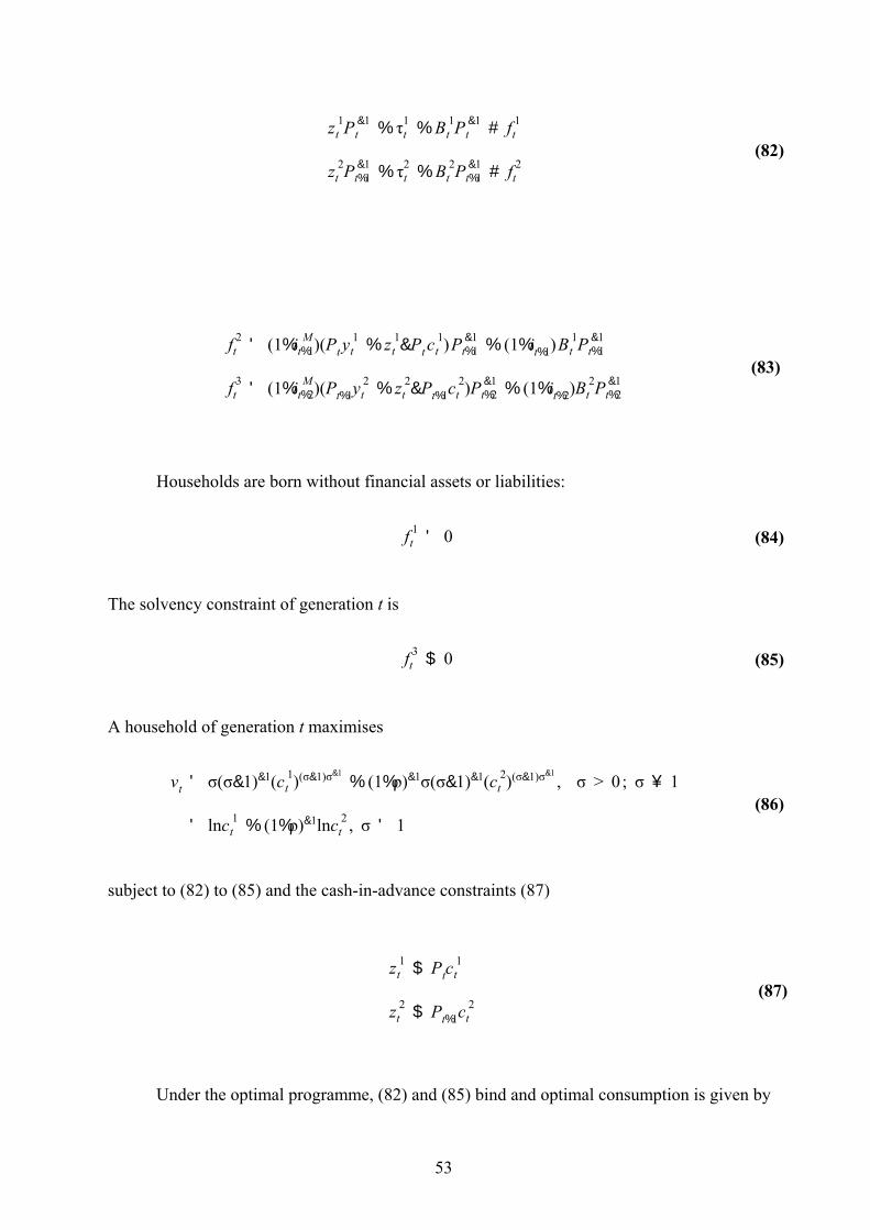
53

z 1t $ Ptc

1t

z 2t $ Pt%1c

2t

(87)

f 1t ' 0 (84)

f 3t $ 0 (85)

z 1t P &1

t % τ1t % B 1

t P &1t # f 1

t

z 2t P &1

t%1 % τ2t % B 2

t P &1t%1 # f 2

t

(82)

f 2t ' (1%i M

t%1)(Pt y1t % z 1

t &Pt c1t )P &1

t%1 % (1%it%1)B 1t P &1

t%1

f 3t ' (1%i M

t%2)(Pt%1y2t % z 2

t &Pt%1c2t )P &1

t%2 % (1%it%2)B2t P &1

t%2

(83)

vt ' σ(σ&1)&1(c 1t )(σ&1)σ&1

% (1%ρ)&1σ(σ&1)&1(c 2t )(σ&1)σ&1

, σ > 0; σ … 1

' lnc 1t % (1%ρ)&1lnc 2

t , σ ' 1(86)

Households are born without financial assets or liabilities:

The solvency constraint of generation t is

A household of generation t maximises

subject to (82) to (85) and the cash-in-advance constraints (87)

Under the optimal programme, (82) and (85) bind and optimal consumption is given by

54

c 1t '

(1%ρ)σ

(1%ρ)σ%(1%rt%1)σ&1

1%i Mt%1

1%it%1

y 1t & τ1

t %1

1%rt%1

1%i Mt%2

1%it%2

y 2t & τ2

t (88)

c 2t '

(1%rt%1)σ

(1%ρ)σ%(1%rt%1)σ&1

1%i Mt%1

1%it%1

y 1t & τ1

t %1

1%rt%1

1%i Mt%2

1%it%2

y 2t & τ2

t

' (1%i Mt%1)M

1t P &1

t%1 % (1%it%1)B1t P &1

t%1 %1%i M

t%2

1%it%2

y 2t & τ2

t

(89)

ct ' c 1t % c 2

t&1

yt ' y 1t % y 2

t&1

τt ' τ1t % τ2

t&1

z 1t $ Ptc

1t

' Ptc1t if it%1 > i M

t%1

z 2t $ Pt%1c

2t

' Pt%1c2t if it%2 > i M

t%2

(90)

with

Aggregate private consumption, aggregate output and aggregate taxes are given by

42This assumption is not fully satisfactory, as it is well-known that in finite-horizon OLG models such as theone considered here, (real) public debt can grow at any rate forever(including growth rates in excess of the realinterest rate and the growth rate of real productive potential), regardless of the relationship between the realinterest rate and the real growth rate. Ponzi finance is feasible if there are no restrictions on age-specific lump-sum taxes and transfers (see e.g. Buiter and Kletzer (1998)). I impose the usual solvency constraint on thegovernment for comparability with the representative agent discussion. The asymmetric perception of basemoney as an asset or liability has implications for monetary policy that do not depend on whether theconventional government solvency constraint is appropriate or not in the OLG model.

55

z gt ' Pt gt

Mt ' M 1t

Bt ' B 1t

Mt ' z 1t % z 2

t&1 % z gt

ct '(1%ρ)σ

(1%ρ)σ%(1%rt%1)σ&1

1%i Mt%1

1%it%1

y 1t &τ

1t %

11%rt%1

1%i Mt%2

1%it%2

y 2t &τ

2t

%1%i M

t%1

1%it%1

y 2t&1 & τ2

t&1 % j4

j'tRt%1, j(τ

1j%τ

2j&1&gj)

% (1%i Mt )Mt&1P

&1t %j

4

j'tRt%1, j[Mj&(1%i M

j )Mj&1]P&1j

The government’s period budget identity, solvency constraint and intertemporal budget

constraint (assuming its solvency constraint holds with equality) are assumed to be the same as

before (equations (35), (36) and (37) respectively),42 and the government’s cash-in-advance

constraint, assumed to be binding, is given by

At the end of each period, t say, and at the beginning of the next period, t+1, all financial

assets are owned by those born at the beginning of period t, that is,

Monetary equilibrium implies that

Aggregate consumption demand, after substituting out for the initial non-monetary public

debt using (37) is given by:

43 A cash-in-advance version of the representative agent model can be found inhttp://www.nber.org/~wbuiter/heliap1.pdf

56

ct '(1%ρ)σ

(1%ρ)σ%(1%rt%1)σ&1

1%i Mt%1

1%it%1

y 1t &τ

1t %

11%rt%1

1%i Mt%2

1%it%2

y 2t &τ

2t

%1%i M

t%1

1%it%1

y 2t&1 & τ2

t&1 % j4

j'tRt%1, j(τ

1j%τ

2j&1&gj)

% j4

j't%1Rt%1, j (ij&i M

j )(1%πj)&1yj&1 % P &1

t limN64

It%1,N (1%i MN )MN&1

(91)

Using (39) and noting that both when the(ij&i Mj )mj&1'(ij&i M

j )(cj&1%gj&1)'(ij&i Mj )yj&1

cash-in-advance constraint binds and when it does not, we can rewrite the aggregate

consumption function as:

The aggregate consumption function for period t depends on current and future

endowments, current and future real public spending, current and future taxes (because of the

absence of debt neutrality) and the present discounted value of the terminal stock of base

money: .P &1t lim

N64It%1,N (1%i M

N )MN&1

In this infinite-lived economy with overlapping finite-lived households, each of which

disposes of all its financial wealth, including base money, at the end of its life, the consolidated

aggregate consumption function very naturally includes the present value of the terminal stock of

base money as an argument. This provides further motivation for the asymmetric treatment of

base money in the solvency constraints of the household and government sectors in the infinite-

lived representative agent model.43

5. Institutional arrangements for a helicopter drop of base money:how much can the central bank do on its own?

44The model is of a closed economy, so I ignore official foreign exchange reserves, which are often held by theCentral Bank. 45It is common practice for the Treasury to appropriate the profits of the Central Bank. This would mean in ourmodel that . Under this tax rule, the change in the stock of base moneyτcb

t ' &ht % (itBt&1 & i M Mt&1)P&1t

would equal domestic credit expansion by the Central Bank: . There is an obvious generalisation∆Mt ' ∆B cbt

to the case of an open economy where the Central Bank holds international reserves as well as domestic debt onthe asset side of its balance sheet.

57

(Mt&B cbt )P &1

t / τcbt % ht & [(1%it)Bt&1 % (1%i M)Mt&1]P

&1t (93)

(Bt % B cbt )P &1

t / gt & τht & τcb

t % (1 % it)(Bt&1 % B cbt&1)P

&1t (92)

To evaluate implementation issues, I break down the consolidated period budget identity

and solvency constraint of the General Government and Central Bank into separate accounts

each for the General Government (the Treasury) and the Central Bank.

The Central Bank has the monetary base, , on the liability side of its financial balanceM

sheet. On the asset side it has the stock of domestic credit.44 For simplicity, domestic credit is

restricted to Central Bank credit to the General Government, that is, Central Bank holdings of

nominally denominated General Government interest-bearing debt or Treasury debt, . B cb

Equation (92) is the period budget identity of the Treasury and equation (93) that of the

Central Bank. B is the stock of Treasury interest-bearing debt held outside the Central Bank; τh

is real value of the tax payments by the domestic private sector (the household sector here) to the

Treasury; is the real value of taxes paid by the Central Bank to the Treasury and h the realτcb

value of the transfer payments made by the Central Bank to the private sector (the instrument

through which the Central Bank itself can engage in ‘helicopter drops’). For simplicity the

Central Bank is assumed not to spend anything on real goods and services.45

46 .b cbt / B cb

t /Pt

58

limN64

Rt%1,N b cbN $ 0 (94)

(1%it)Bcbt&1P

&1t $ j

4

j'tRt%1, j τ

cbj % hj & [Mj & (1%i M)Mj&1]P

&1j (97)

limN64

Rt%1,N (bN%b cbN ) # 0 (95)

(1%it)(Bt&1 % B cbt&1)P

&1t # j

4

j'tRt%1, j τ

hj % τcb

j &gj (96)

The solvency constraints of the Treasury and the Central Bank are given in (94) and (95)

respectively.46

Note that the Central Bank views its monetary liabilities as irredeemable. These

solvency constraints imply the following intertemporal budget constraints for the Treasury

(equation (96)) and the Central Bank (equation (97)).

Adding (92) and (93) together and noting that gives the period budgetτ / τh & h

identity of the state, that is, the consolidated General Government (Treasury) and Central Bank,

in (28). Subtracting (97) from (96) and assuming both of them to hold with equality, gives the

intertemporal budget constraint of the state in (37).

Consider the financial balance sheet of the Central Bank in Table 1.

59

Table1

Central Bank Balance Sheet

Assets Liabilities

MB cb

N cb

Central Bank financial net worth, , is the excess of the value of its financial assets,N cb

Treasury debt, , over its monetary liabilities, M. In principle, there is nothing to prevent B cb N cb

from being negative. There are two reasons for this. The first applies to any economic agent,

(including, in our case, the Treasury or the household sector). Financial net worth excludes the

present value of anticipated or planned future non-contractual outlays and revenues. It is

therefore perfectly possible, in principle, for an economic agent, including the Central Bank, to

survive and thrive with negative financial net worth, provided the present discounted value of its

future primary surpluses is sufficient to cover the negative financial net worth. The second

reason is specific to the Central Bank. Financial net worth includes the stock of base money as a

Central Bank liability. Since base money is irredeemable, the Central Bank does not need to

generate future primary surpluses to service the outstanding stock of base money. Indeed, the

current and future primary surpluses of the Central Bank (whose present discounted value should

at least be equal to the value of its outstanding non-monetary debt ) include the sequence of&B cb

future net seigniorage, . Mj & (1%i M)Mj&1

Can the Central Bank perform a ‘helicopter money drop’ on its own?

Technically, if the Central Bank could make transfer payments to the private sector, the

entire (real-time) Friedmanian helicopter money drop could be implemented by the Central Bank

without Treasury assistance. At time t there would be a (temporary) increase in (a transferht

payment to the household sector by the Central Bank) financed by increasing the monetary base

47In the US, the Treasury could, in principle, undertake both the fiscal and the monetary sides of the helicopterdrop of money, because the Treasury has the power to issue irredeemable Treasury notes, which areinterchangeable with Federal Reserve notes. US Treasury notes, issued by the Department of the Treasury sincethe Legal Tender Act of 1862 are part of the stock of US currency. Like Federal Reserve notes (authorised bythe Federal Reserve Act of 1913), they are non-interest-bearing irredeemable bearer notes and constitute legaltender. They were issued until January 21, 1971. Those that remain in circulation are obligations of the U.S.government.

60

(‘printing money’). An example would be for the Governor of the Central Bank to issue a

$1,000 cheque, drawn upon the Central Bank’s account, to every man, woman and child in the

country. After the event, this would show up the financial balance sheet of the Central Bank as

an increase in the stock of base money and a corresponding reduction in the financial net worth

of the Central Bank. In its budget identity and profit and loss account the monetary injection

would be recorded as a transfer payment from the Central Bank to the private sector.

The legality of such an implementation of the helicopter drop of money by the Central

Bank on its own would be doubtful in most countries with clearly drawn boundaries between the

Central Bank and the Treasury. The Central Bank would be undertaking an overtly fiscal act,

something which is normally the exclusive province of the Treasury.47

An economically equivalent (albeit less entertaining) implementation of the helicopter

drop of money would be a tax cut (or a transfer payment) implemented by the Treasury (a cut in

), financed through the sale of Treasury debt to the Central Bank (an increase in ), whichτht ∆B cb

t

would then monetise the transaction ( ). If the direct sale of Treasury debt to∆(∆Mt) ' ∆(∆B cbt )

the Central Bank (or direct Central Bank lending to the Treasury) is prohibited (as it is for the

countries that belong to the Euro area), the monetisation of the tax cut could be accomplished by

the Treasury financing the tax through the sale of Treasury debt to the domestic private sector

(or overseas), with the Central Bank purchasing that same amount of non-monetary interest-

bearing debt in the secondary market, thus expanding the base money supply.

6. Conclusion

48See Hicks (1935), Bryant and Wallace (1980) and Wallace (1990) for some of the important contributions tomonetary theory that were published under the “A suggestion for ..” heading.

61

The paper provides a formalisation of the monetary ‘folk’ proposition that fiat (base)

money is an asset of the holder (the private sector) but not a liability of the issuer (the monetary

authority, as agent of the state). Earlier versions of the paper had the subtitle “A suggestion for

slightly complicating the theory of money”, but fear of hubris caused me to drop this.48 I believe

that this paper shows that the irredeemable nature of the monetary liabilities of the state should

and can be incorporated into otherwise conventional approaches to monetary economics.

Following the proposed approach, fiat base money constitutes net wealth to the

consolidated private and public sectors in the sense that the present discounted value of the

terminal stock of base money, when that terminal date is infinitely far away, is part of the

consolidated comprehensive wealth that drives private consumption. The issuance of

irredeemable base money can therefore have pure fiscal effects. In well-behaved equilibria, that

is, equilibria that are not liquidity traps, this paper’s asymmetric treatment of the solvency

constraints of the private sector and the monetary authority has no implications for the behaviour

of nominal or real equilibrium prices and quantities. It does play a role when all current and

future risk-free nominal interest rates are at their lower bound, which is the definition of a

liquidity trap used in this paper.

When the monetary authorities view money as irredeemable but the private sector treats

it as a realizable financial asset, simple and plausible restrictions on the monetary policy rule

suffice to rule out liquidity trap equilibria as rational expectations equilibria. In the flexible

price level variant of the model, a liquidity trap equilibrium is only possible if the monetary

authorities are expected to de-monetise the economy in the long run, by reducing the nominal

money stock to zero. In the New-Keynesian variant, a liquidity trap equilibrium is ruled out

whenever the authorities are believed to keep the nominal stock of base money above a certain,

finite, threshold level in the long run. Any positive long-run growth rate for the nominal stock of

62

base money is sufficient to rule out a liquidity trap equilibrium when the nominal interest rate on

base money is zero, the institutionally most relevant case. Liquidity trap equilibria are possible

as rational expectations equilibria only if monetary policies are perverse. With non-rational

expectations - e.g. the belief that the monetary authorities will, in the long run, reverse and undo

any current and past increases in base money - liquidity trap equilibria can exist for as long as

these perverse expectations persist.

63

References

Allais, Maurice (1947), Economie et Intérêt, Paris, Imprimerie Nationale.

American Heritage Dictionary of the English Language (2000), Fourth Edition, the HoughtonMifflin Company.

Arrow, Kenneth J. and M. Kurtz (1970), Public Investment, Rate of Return and Optimal FiscalPolicy, Johns Hopkins Press, Baltimore, Maryland.

Araujo, A., and J. A. Scheinkman (1983), “Maximum Principle and Transversality Condition forConcave Infinite Horizon Economic Models.” Journal of Economic Theory 30, no. 1, June, pp.1-16.

Blanchard, Olivier J. (1985), “Debt, Deficits and Finite Horizons”, Journal of PoliticalEconomy, 93, pp. 223-247.

Bryant, John and Neil Wallace (1980), “A suggestion for further simplifying the theory ofmoney”, Federal Reserve Bank of Minneapolis Research Department Staff Report No. 62,revised December 1980

Buiter, Willem H. (1988), “Death, Birth, Productivity Growth and Debt Neutrality”, EconomicJournal, 98, June, pp. 279-93.

Buiter, Willem H. (1991), "Debt Neutrality, Redistribution and Consumer Heterogeneity: ASurvey and Some Extensions," in Money, Macroeconomics and Economic Policy; Essays inHonor of James Tobin, W.C. Brainard et al. (eds.), MIT Press.

Buiter, Willem H. (2002), "The Fiscal Theory of the Price Level: A Critique", EconomicJournal, Vol 112, July 2002, pp. 459-480.

Buiter, Willem H. (2003a), "Deflation; Prevention and Cure" , NBER Working Paper 9623,April 2003.

Buiter, Willem H. (2003b), "Two Naked Emperors? Concerns about the Stability and GrowthPact & Second Thoughts about Central Bank Independence", IFS Annual Lecture, given on 30thJune 2003, at the Institute for Fiscal Studies, London, UK, CEPR Discussion Paper No. 4001,August.

Buiter, Willem H. and Kenneth M. Kletzer (1998), “Uses and Limitations of Public Debt”, inSteven Brakman, Hans van Ees and Simon K. Kuipers eds. Market Behaviour andMacroeconomic Modelling, MacMillan Press Ltd, London, 1998, pp. 275-307.

Buiter, Willem H. and Nikolaos Panigirtzoglou (2001), "Liquidity Traps: How to Avoid Themand How to Escape Them", in Reflections on Economics and Econometrics, Essays in Honour ofMartin Fase, edited by Wim F.V. Vanthoor and Joke Mooij, 2001, pp. 13-58, De NederlandscheBank NV, Amsterdam.

64

Buiter, Willem H. (2003) and Nikolaos Panigirtzogou, "Overcoming the Zero Bound onNominal Interest Rates with Negative Interest on Currency: Gesell’s Solution", EconomicJournal, Vol 113, October 2003, pp. 723-746.

Buiter, Willem H. and Anne C. Sibert (2003), “Deflationary Bubbles”, mimeo, BirkbeckCollege, University of London, November.

Burdekin, Richard C. K. and Marc D. Weidenmier (2003), “Suppressing Asset Price Inflation:The Confederate Experience, 1861-1865", Economic Inquiry, 41(3), July, pp. 420-432.

Chadha, Jagit S. and Charles Nolan (2002), “Output, Inflation and the New Keynesian PhillipsCurve”, Mimeo, February.

Clower, R. W. (1967), ‘A reconsideration of the microfoundations of monetary theory.’, WesternEconomic Journal, 6, December, pp. 1-8.

Concise Oxford Dictionary (1995), Ninth Edition, Della Thompson ed., Clarendon Press,Oxford.

Eggertsson, Gauti B. (2003), "How to Fight Deflation in a Liquidity Trap: Committing to BeingIrresponsible," IMF Working Papers 03/64, International Monetary Fund.

Eggertsson, Gauti B. and Michael Woodford (2003), Optimal Monetary Policy in a LiquidityTrap”, NBER Working Paper No. W9968, September.

Fama, Eugene F. (1983), “Financial Intermediation and Price Level Control”, Journal ofMonetary Economics, 12(1), pp. 7-28.

Frenkel, Jacob and Assaf Razin (1987), Fiscal Policies and the World Economy, The MIT Press,Cambridge, Mass.

Friedman, Milton (1969), “The Optimum Quantity of Money”, in Milton Friedman, TheOptimum Quantity of Money and Other Essays, Chapter 1, pp.1-50, Adline Publishing Company,Chicago.

Goodfriend, Marvin (2000), “Overcoming the Zero Bound on Interest Rate Policy”, Journal ofMoney, Credit and Banking, Vol. 32, No. 4, Pt. 2, November, pp. 1007-1035.

Gurley, John G. and Edward S. Shaw (1960), Money in a Theory of Finance, The BrookingsInstitution, Washington D.C. Hall, Robert E. (1983), “Optimal fiduciary monetary systems”, Journal of Monetary Economics,Vol. 12(1), pp. 33-50.

Helpman, E. (1981), ‘An Exploration of the Theory of Exchange Rate Regimes’, Journal ofPolitical Economy, 89, October, pp. 865-890.

Hicks, J. (1935), "A Suggestion For Simplifying The Theory of Money", Economica (2),February, pp. 1-19.

65

Ireland, Peter N. (2001), “The Real Balance Effect”, NBER Working Paper No. 8136, February.

Kamihigashi, Takashi. “Necessity of Transversality Conditions for Infinite Horizon Problems.”Econometrica 69, no. 4 (July 2001): 995-1012.

Kamihigashi, Takashi. “A Simple Proof of the Necessity of the Transversality Condition.”Economic Theory 20, no. 2 (September 2002): 427-433.

King, Robert G. (1983), “On the Economics of Private Money”, Journal of MonetaryEconomics, 12(1), pp. 127-158.

Lucas, R. E. (1980), “Equilibrium in a pure currency economy”, Economic Inquiry, 18(2), pp.203-220.

Lucas, R. E. (1982), “Interest Rates and Currency Prices in a Two-Country World”, Journal ofMonetary Economics, 22, July, pp. 335-60.

Michel, Philippe (1990), “Some Clarifications on the Transversality Condition.”, Econometrica58, no. 3, May, pp. 705-723.

Obstfeld, M. and Rogoff, K. (1983), ‘Speculative hyperinflations in maximizing models: Can werule them out?’, Journal of Political Economy, 91, August, pp. 675-87.

Obstfeld, M. and Rogoff, K. (1986), ‘Ruling out divergent speculative bubbles’, Journal ofMonetary Economics, 17, May, pp. 346-62.

Obstfeld, M. and K. Rogoff (1996), Foundations of International Macroeconomics, The MITPress, Cambridge Mass.

Patinkin, Don (1965), Money, Interest and Prices; An Integration of Monetary and ValueTheory, Second Edition, Harper & Row, Publishers, New York.

Pesek, Boris P., and Thomas R. (1967), Saving, Money, Wealth, and Economic Theory, TheMacmillan Company, New York.

Porter, William (1999), “Negative Rates – An Exploration”, Credit Suisse First Boston MarketAnalysis, 25 May.

Samuelson, Paul A. (1958), “An Exact Consumption-Loan Model of Interest with orwithout the Social Contrivance of Money”, Journal of Political Economy 66, pp. 467-482.

Sargent, T. J. and Wallace, N. (1981), ‘Some Unpleasant Monetarist Arithmetic’, QuarterlyReview, Federal Reserve Bank of Minneapolis, Fall.

Sargent, Thomas J. and Neil Wallace (1984), “Interest on Reserves”, Journal of MonetaryEconomics 15(3), pp. 279-290.

Sargent, T. J. (1987), Dynamic Macroeconomic Theory, Harvard University Press, CambridgeMassachusetts.

66

Sims, Christopher A. (2000), “Fiscal Aspects of Central Bank Independence”, presented at aconference on European Monetary Union, Munich, December 2000 and to be published in aconference volume.

Sims, Christopher A. (2003), “Limits to inflation targeting”, paper presented at an NBERconference in Miami, January 2003.

Stockman, Alan C. (1983), “Comments;’Optimal Fiduciary Monetary Systems’ by Robert E.Hall, Journal of Monetary Economics 12(1), pp. 51-54.

Stokey, Nancy L., and Robert E. Lucas, Jr., with Edward C. Prescott (1989), Recursive Methodsin Economic Dynamics, Cambridge, MA: Harvard University Press.

Wallace, Neil (1981), “A Modigliani-Miller theorem for open market operations”, AmericanEconomic Review, 71(3), pp. 267-274.

Wallace, Neil (1990), “A suggestion for oversimplifying the theory of money”, Federal ReserveBank of Minneapolis Quarterly Review, , issue Wint, pp.19-26

Weil, Philippe (1989), “Overlapping Families of Infinitely-lived Agents”, Journal of PublicEconomics, 38, pp. 183-198.

Weil, Philippe (1991), “Is Money Net Wealth?”, International Economic Review, 32, February,pp. 37-53.

Weitzman, M. L. “Duality Theory for Infinite Horizon Convex Models.” Management Science19, no. 7 (March 1973): 783-789.

Woodford, Michael (1995), “Price level determinacy without control of a monetary aggregate”,Carnegie-Rochester Conference Series on Public Policy, 43, pp. 1-46.

Woodford, Michael (1996), “Control of the Public Debt: A Requirement for Price Stability?”,NBER Working Paper No. 5684, July.

Yaari, Menahem E. (1965), “Uncertain Lifetime, Life Insurance, and the Theory of theConsumer”, Review of Economic Studies, 32, April, pp. 137-150.