Scalable Stochastic Modelling for Resilience

Jeremy T. Bradley1, Lucia Cloth2, Richard Hayden1, Leıla Kloul3

Philipp Reinecke4, Markus Siegle5, Nigel Thomas6, and Katinka Wolter4

1 Department of Computing, Imperial College London, UK2 Department of Applied Information Technology, GU Tech, Oman

3 Laboratoire PRiSM, Universite de Versailles, France4 Institute of Computer Science, Freie Universitat Berlin, Germany

5 Department of Computer Science, Universitat der Bundeswehr Munchen, Germany6 School of Computing Science, Newcastle University

Abstract. This chapter summarises techniques that are suitable forperformance and resilience modelling and analysis of massive stochas-tic systems. We will introduce scalable techniques that can be applied tomodels constructed using DTMCs and CTMCs as well as compositionalformalisms such as stochastic automata networks, stochastic process al-gebras and queueing networks. We will briefly show how techniques suchas mean value analysis, mean-field analysis, symbolic data structuresand fluid analysis can be used to analyse massive models specifically forresilience in networks, communication and computer architectures.

1 Introduction

The techniques presented in this chapter represent the state of the art in per-formance and resilience analysis when it comes to coping with massive state-space models. Many existing analysis techniques rely on generating underlyingstochastic models, such as continuous-time Markov chains. Where there is tooclose a correspondence between the state space of the model and that of theunderlying stochastic process, the state-space explosion in the former can leadto intractability in the latter. The presented techniques in this chapter were cho-sen as they represent instances of the main approaches to state-space reductionin stochastic systems: aggregation, decomposition, symbolic representation andcontinuum approximation.

We realise that accurate resilience analysis relies on a detailed and complexmodel. This kind of model generates huge state spaces and computation time ifhandled naıvely. In this chapter, we are specifically interested in analysis tech-niques that side-step the state space explosion problem by making use of effi-cient representation mechanisms. This is necessary if we are to make headwayin directly analysing problems in mobile networks (Chapter 29), critical infras-tructures (Chapter 7 and 30) and Cloud systems (Chapter 13 and 28).

We summarise the techniques presented below. In each case, we indicate whattype of analysis result can be expected to be obtained using this method. Itis important to understand how these techniques are relevant and useful to theunderstanding of resilience of a system. The types of analysis that can be tackledusing these techniques can broadly be put into three categories. In the contextof resilience analysis: steady state distributions are useful for calculating theprobability that a fault state is ever reached; transient distributions are usefulfor calculating the probability that a fault state is entered in a particular timewindow; and response or passage time analysis is used to specify service levelagreements, along the lines of “The round-trip response of a service request to a

virtualised environment should be less that 1.8 seconds, with probability 0.95.”

Decomposition and phase-type representation We start with a techniquewhich combines simulation and decomposition, to generate simple approxi-mate models based on phase-type representation of key portions of a system’soperation (Section 2). A grey-box technique such as this avoids explicit in-vestigation or representation of individual states in the system. This will bea useful technique for deriving some aggregate steady-state and transientmeasures but will probably be most widely used for response-time results.

Product forms and MVA In Section 3, we explore two powerful techniquesfrom queueing theory, product form and mean value analysis (MVA). Thesepowerful techniques can be applied to very large or infinite state systems.They explore balanced flows of traffic between components and in doingso permit compositional rather than system-wide analysis. Product formswill tend to lead to rapid steady-state distribution results, while MVA cancalculate mean throughput, response time and job occupancy measures in asystem.

Tensor representation Section 4 presents a decomposition technique whichavoids the construction of the underlying explicit state space of a continuous-time Markov chain. Instead smaller submatrices are constructed which broadlyreflect the components of the stochastic automata network. Analysis tech-niques exist which maintain the decomposed tensor representation while pro-ducing accurate steady-state distribution results.

Symbolic representation The symbolic representation of a stochastic modelis described in Section 5. Multi-terminal Binary Decision Diagrams are usedto encode efficiently the real rate values of a variety of stochastic models,including CTMCs, DTMCs and MDPs (Markov Decision Processes). Steady-state analysis, transient analysis and passage-time analysis are all possibleusing exclusively MTBDD-based algorithms.

Mean-field analysis In Section 6, we present developments in mean-field anal-ysis as applied to massively distributed systems that are made up of identi-cal communicating components. Applied to discrete-time systems, mean-fieldtechniques generate sets of deterministic mean-difference equations (MDEs).Solving these MDEs gives access to both transient and passage-time mea-sures. They provide an interesting comparison to the continuous counterpart,fluid analysis, described in the next section.

Fluid analysis Finally, in Section 7, we show how a continuum approximationof the dynamics of a stochastic system can be encoded in a system of ordi-nary differential equations (ODEs). Fluid analysis can be applied to largedistributed systems that are comprised of groups of components of differenttypes. Usually generated from a higher level formalism such as a stochasticprocess algebra, the ODEs can encode steady-state, transient and passagetime questions. Higher moments of various model quantities are also avail-able to capture measure accuracy.

2 Efficient model representation and simulation

Discrete-event simulation is a widely-used approach for evaluating system prop-erties such as response-time. Compared to analytical closed-form approaches,discrete-event simulation has the advantage of allowing the construction andevaluation of highly-detailed models where the modelled behaviour is not lim-ited by the constraints of the formalism.

Unfortunately, the ability to easily build highly-detailed models often leads toscalability problems. While simulations modelling simple scenarios can be eval-uated efficiently, increasing the complexity of the scenario quickly results insimulation models whose evaluation takes too long for the results to be useful.In this case, one obvious solution would be to start from scratch with a less de-tailed model with better scalability. However, this solution is often not desirable,since the results from a less detailed model may not be sufficiently accurate, andbecause of time and cost constraints on the modelling process itself.

Increasing model complexity is a well-known problem with analytical approachesas well. These approaches often suffer from state-space explosion as the systemto be studied becomes more complex. Various solutions for this problem havebeen proposed [1]. In particular, decomposition/aggregation methods allow thesolution of highly-complex models by splitting the model into submodels, solv-ing the submodels independently, and aggregating the submodel solutions intoa solution for the whole system. This approach may be used to reduce bothprocessing time and memory requirements.

The general idea of decomposition and aggregation can also be applied to discrete-event simulations. In this section we describe a hybrid approach that combinesdecomposition and approximation using stochastic models to allow faster eval-uation of discrete-event simulation models. With this approach, the simulationmodel is split into blocks whose behaviour can be approximated by phase-type(PH) distributions (cf. chapter on phase-type distributions). The phase-type dis-tributions replace the approximated blocks in the simulation. The behaviour ofthe approximated blocks can then be reproduced by drawing random variatesfrom the approximating phase-type distributions. Since this is more efficientthan detailed discrete-event simulation, simulation of the whole system becomes

much faster. This method can be applied when delay metrics are to be deter-mined. Whether the method also applies for other metrics, such as throughput,availability or state probabilities in general, is as of yet unknown. The approachconsists of the following steps:

1. Decomposition of the simulation model into blocks that affect the

metrics. Starting from the complete simulation, one must identify partsthat can be approximated by phase-type distributions. These blocks shouldsatisfy a number of criteria: it should be simple to separate the simulationinto the blocks, and the blocks should be chosen such that increasing thecomplexity of the simulation corresponds to multiple application of identicalblocks. This step is shown in Figure 1, where block A of the simulationis affected by block B: The effect of block B on the metrics depends onits internal block B1. Increasing the size of system B corresponds to usingmultiple instances of B1 within B.

System A Subsystem B1

Subsystem B1

System B

Fig. 1. Example decomposition of a simulation.

2. Evaluation of simulation blocks. In order to approximate the behaviourof the simulation blocks identified in step 1 by phase-type distributions,data is needed that shows the effect of the blocks. Typically, this data willbe obtained from detailed simulations of the individual blocks, but if a blockcorresponds to a system where data from measurements is available, suchdata can also be used.

3. Approximation using phase-type distributions. The data obtained instep 2 is approximated by a phase-type distribution. The general process andtools for fitting PH distributions to data sets is described in detail in Chap-ter 1. For the application in the hybrid approach, the focus should be on cap-turing those properties well that strongly affect the metric. Furthermore, oneshould choose phase-type distributions that enable efficient random-variategeneration, so as to be able to reproduce the behaviour of the approximatedbuilding-blocks efficiently.

4. Integration of the phase-type distributions into the simulation

model. The phase-type models must be integrated into the simulation. Fordelay metrics, this requires drawing random variates from the distributionand delaying events caused by the approximated system blocks according tothese variates. For common discrete-event simulation toolkits such as NS-2 [2] and OMNeT++ [3], the libphprng [4] library provides the necessaryroutines for generating PH-distributed random numbers.

5. System evaluation. The whole system can now be evaluated. In order toscale system size/complexity, the number of blocks containing the approx-imating PH distribution is increased. As random-variate generation from aPH distribution is typically more efficient than detailed simulation of theblocks, the model can be expected to scale much better to higher numbersof building-blocks. On the other hand, the approximation process introducesan error, since the PH distribution does not represent all behaviour of thedetailed model.

2.1 Illustrative example

In [5] we have investigated timing behaviour in a tree-structured network acrossa variable number of identical switches. The topology is shown in Figure 2 andeach data stream is transmitted in a straight feed-forward fashion.

Source

Destination

Packet−Switched Network

Fig. 2. Data stream in packet-switched network with tree topology

Let us illustrate the approximation technique for the given example. In thisexample, the transmission delays encountered on the path between the sourceand the destination are investigated. More precisely, the metric of interest is the1% quantile of packet delay variation (PDV)7 of the high-priority packets in anetwork transporting two types of packets, the high priority traffic and the lowpriority background data. This implies that the subsystem models must onlyrepresent transmission delays, and we can abstract away from other aspects ofthe network, such as correctness of the content of transmitted messages.

In order to evaluate this scenario, a simulation has been built using the discrete-event network simulator NS-2 [2]. In this simulation, we model the internalbehaviour of switches in a detailed manner, and generate streams of high and lowpriority packets. Then the time is observed that it takes for high-priority packets

7 Packet delay variation is defined as the difference between the shortest and thelongest transmission time, where lost packets are ignored.

to traverse the network from the source to the destination. As illustrated by theupper curve in Figure 4(a), simulation run-times with this approach increasequickly as the number of switches is increased. Therefore the approximationmethod is applied as follows:

1. Decomposition of the simulation model into blocks that affect the

metrics. In this scenario, the obvious block is the individual switch. Forsimplicity, we assume that the network consists of switches whose behaviourwith respect to transmission delay is identical.

2. Evaluation of simulation blocks. The transmission delays incurred byeach switch must be assessed. As a network consisting of only one switch canstill be simulated within an acceptable time, transmission delays for a longsimulation run with only one such switch between source and destinationare obtained.

3. Approximation using phase-type distributions.We fit an acyclic phase-type distribution using the PhFIT tool [6] to the transmission delay of thehigh-priority stream such that the resulting distribution represents the 1%quantile well. See Chapter 1 for more details on phase-type distributions. Thephase-type distribution obtained here represents the transmission delay dis-tribution of a single switch. Figure 3(a) shows the packet delay distributionfrom step 2 and the cumulative density function of the phase-type distribu-tion fitted to the data. Note that the distribution fits the lower quantileswell and tends to diverge only on the higher quantiles.

4. Integration of the phase-type distributions into the simulation

model. Now, the phase-type distribution for the packet delay of the switchcan be used to simulate the behaviour of the switch. To this end, we builda simple queueing station whose service-time distribution is given by thephase-type distribution fitted to the data. Packets entering the station sys-tem are delayed according to the service-time distribution. Note that thepresence of a queue is only dictated by the fact that we cannot drop packets,and that this queue does not correspond to any part of the original model. Inthe considered scenario high-priority packets are sent very infrequently, andtherefore queueing is highly unlikely. If the arrival rate of high-priority pack-ets was higher, queueing might occur. The resulting queueing delay wouldincrease the error caused by the approximation, since this queueing is notpart of the original simulation.

5. System evaluation. The system can now be simulated by transmittinghigh-priority packets from the source to the destination. Note that it is notnecessary to simulate the low-priority stream anymore, since its effect on thepacket delay variation is already captured in the service-time distribution.

The advantages of the hybrid approach can be evaluated using a scenario wherethe number of switches that the data stream has to traverse is increased from 1to 20.

0 2000 4000 6000 8000 10000 12000

0.0

0.2

0.4

0.6

0.8

1.0

PTD (ns)F

n(x)

Detailed SimulationApproximating PH distribution

(a) CDF of simulation data for 1 switchand associated PH approximation.

50000 100000 150000

0.0

0.2

0.4

0.6

0.8

1.0

PTD (ns)

Fn(

x)

Detailed SimulationPH Approximation

(b) CDF of simulation data and PH approx-imation with 20 links using full simulationand PH approximation.

Fig. 3. Comparison of simulation data and PH approximation.

Figure 4(a) shows run-times for the detailed and approximating simulations forincreasing number n of links. Note that the run-times for the detailed simulationincrease sharply and reach values in the order of days, while run-times withPH approximation stay in the order of hours, even for a high number of links.Figure 4(b) illustrates the error incurred by using PH approximations for theswitches instead of simulating them in detail. As expected, the error does increasewith n, but it seems to converge, and the relative error even decreases.

2.2 Outlook

The decomposition and approximation approach should be extended in vari-ous directions. This has not been done yet and there might arise problems thatcannot be foreseen. First, the system model need not be a simulation model.Any stochastic discrete event model, such as a CTMC, should be applicable too.

1

10

100

1000

10000

100000

0 5 10 15 20

time

(sec

onds

)

Number of network links

runtime full simulationsimulation runtime with PH approximation

(a) Simulation runtimes for full simulation and withPH approximation.

0.001

0.01

0.1

1

10

100

1000

10000

100000

0 5 10 15 20

time

(nan

o-se

cond

s)

Number of network links

PDV using simulationPDV using PH approximation

absolute PDV errorrelative PDV error

(b) PDV error for full simulation and with PH ap-proximation.

Fig. 4. Evaluation of simulation time and the error introduced by approximation.

Second, the approximation technique need not be a PH distribution. Simplerapproximations could consist in Bernoulli variables, and more sophisticated ap-proximation may use correlated stochastic processes, that are still smaller thanthe original model. Third, metrics other than timing metrics should be consid-ered. Often of interest are system or service availability, throughput, or failurecharacteristics.

3 Product-form solution and mean value analysis

One approach to tackling the state space explosion problem common to all com-positional modelling techniques is to break the model into smaller parts thatcan then be solved separately and the solutions combined in some way to givemeasures for the whole system. This approach is generally known as model de-composition.

One of the most powerful model decomposition techniques are so called, product-form solutions. Essentially, a product-form is a decomposed solution where thesteady state distribution of a whole system can be found by multiplying themarginal distributions of its components. Thus, for a system described by thepair {S1, S2}, where Si is the local state of component Ci a product form solutionwould have the form

π(S1, S2) =1

Bπ(S1)π(S2)

where 1/B is the normalising constant (B ≤ 1), which is necessary if thereare combinations of possible local states which are prohibited in the systemevolution.

The conditions for such a solution to exist are clearly going to be restrictive, andas such product-form solutions are applicable only in a relatively small numberof cases. Despite the restrictions, product-forms are extremely powerful and sothe quest for new solutions in stochastic networks has been a major research areain performance modelling for over 30 years, giving rise to a number of seminalresults, such as Jackson queueing networks [7] and the BCMP result [8] for closedqueueing networks.

A Jackson network is a simple open queueing network with Poisson arrivals,negative exponentially distributed service times and unbounded FCFS queues,where the routing of jobs from one node to another is strictly a priori. Forstability it is also required that the utilisation at each node is strictly less thanone. In such a network each node can be considered as an independent FCFSM/M/k queue and the steady state probability of being in any given systemstate can be found simply by multiplying together the marginal probabilities ofeach node’s local state.

Jackson’s result does not apply to closed networks of M/M/k queues (where nojobs may enter or leave the network) because the population of a closed network

is bounded. This restriction was overcome by Gordon and Newell [9], with theintroduction of the normalising constant 1/G(K), where K is the populationsize. If the state is described by the tuple S = {S1, . . . , Sn} then G(K) is givenby,

G(K) =∑

S

n∏

i=1

π(Si)

The results of Jackson and Gordon and Newell were subsequently generalised byBaskett, Chandy, Muntz and Palacios [8] to allow four possible classes of networkfor which the product-form solution holds. The first class is FCFS queues withnegative exponentially distributed service times. The service rate may be statedependent, which allows the network to be open or closed. The subsequent classesslightly relax the condition of negative exponentially distributed service times,as long as the queueing discipline is either processor sharing, infinite server orLCFS with pre-emptive resume.

The BCMP characterisation of product-form networks greatly extended the po-tential for applying product-form solutions to real world problems. Subsequentlythere have been many further results extending the class of queueing networksamenable to product-form solution under specific conditions, for different kindsof queueing network and for different properties. One case worthy of specialmention is the work on product-form G-networks by Gelenbe [10]. G-networksare a variant of queueing networks that allow so-called negative customers. Anegative customer may potentially remove a job from the queue into which itarrives. As well as having external arrivals of negative customers, a normal (orpositive) customer may become a negative customer with some probability fol-lowing completion of service. Subject to similar conditions as Jackson’s resultdescribed above, a G-network can be shown to exhibit a product form solution.This result is more surprising than it might naively appear, as previously it wasassumed that there was a relationship between the product-form solution andthe existence of partial balance. Partial balance does not hold in G-networks,and so the proof of the product form solution changed the understanding of theconditions for product-form solution.

Most attention has been given to queueing networks and their variants (suchas G-networks), but there have also been other significant examples, for exam-ple [11–13]. Many of the approaches to efficiently solving stochastic process alge-bra models have been based on concepts of decomposition originally derived forqueueing networks [14]. Applying such approaches to stochastic process algebraallows the concepts to be understood in a more general modelling frameworkand applied to non-queueing models. More recently the Reversed CompoundAgent Theorem (RCAT) has been developed [15]. RCAT is a compositional re-sult that finds the reversed stationary Markov process of a cooperation betweentwo interacting components, under syntactically checkable conditions [15, 16].From this a product-form follows simply. RCAT thereby provides an alternativemethodology that unifies many product-forms, far beyond those for queueingnetworks.

Even when a product-form solution exists, or an approximation to a product-form can be derived, obtaining a numerical solution may still be computationallyexpensive. In particular, finding the normalising constant can be costly in gen-eral. Mean value analysis (MVA) [17] depends on the application of the arrival

theorem, first derived independently by Sevcik and Mitrani [18] and Lavenbergand Reiser [19]. This theorem states that, subject to certain conditions, a jobarriving in a queue will, on average, observe the queue to be in its steady stateaverage behaviour. Combining the arrival theorem with Little’s law gives riseto a method for deriving average performance metrics based on steady stateaverages directly from the queueing network specification, without the need toderive any of the underlying Markov chain.

Stated simply, the basic MVA algorithm, when the population size is N , is asfollows:

1. Set the population size, n, to be 1.

2. Compute the delay this single job will experience at each node as it traversesthe otherwise empty network (i.e. the average service time for one job).

3. Hence compute the probability that this job will be at any given node ata randomly observed instant. This gives the average queue length at eachnode when the total population consists of one job.

4. Increment the population size, n.

5. Compute the delay an arriving job will experience at each node (i.e. theaverage service time for one job plus average service time for the averagenumber of jobs in the queue when the population is n− 1).

6. Hence compute the average queue length at each node when the total pop-ulation consists of n jobs.

7. If n < N then go back to step 4.

As such it is relatively computationally efficient as long as the population size isnot excessively large. The computational cost for solving a network with a givenstructure grows linearly with N .

There are many generalisations and approximate solutions of the original meanvalue analysis algorithm. MVA has been applied to many classes of queueingnetwork, as well as other formalisms, including stochastic process algebra [20].The key observation in applying MVA to stochastic process algebra is that re-peated instances of a component in parallel may be treated as jobs in a queueingnetwork. If the interaction of these components with other components conformsto some simple set of restrictions, then a version of the arrival theorem can bederived relating a component evolving between derivatives (or behaviours) tothe steady state solution of a system with one fewer instance of the component.

4 Tensor Representation

The tensor representation or compact representation has been used for sometime as a means to address the problem of state space explosion to which state-based performance modelling formalisms are prone. This technique which aimsto keep the size of the model representation as small as possible falls into thelargeness avoidance category of techniques which also includes techniques suchas decomposition, aggregation and symbolic encodings [21]. However, unlike theaggregation which can result in a significant reduction in the size of the statespace, the tensor representation is not a state space reduction method, but ratheran alternative approach to state space explosion which handles the model so-lution in a decomposed form. The matrix representation of the Markov processunderlying a performance model may be decomposed so that the state space ofthe model, and its dynamics, are not represented by a single matrix but by anumber of smaller matrices. Nevertheless the model is solved as a single entityand the solution is exact, unlike the decomposition technique which, generally,gives rise to approximate solution of the original model [22].

The tensor representation has been developed for several state-based modellingformalisms. The pioneering work in this area was carried out, in 1984, by Plateauon Stochastic Automata Networks (SANs) [23]. Using a technique based on ten-sor or Kronecker algebra, it has been proved [23–25] that this method auto-matically provides an analytic derivation of a decomposed form of the generatormatrix called the descriptor. Compared to a monolithic description of the gener-ator, the structure of this descriptor leads to a considerable reduction in memoryrequirements during the model solution. Moreover, solution techniques have beenadapted to this representation [26–28].

In the following, we present the tensor representation in the context of the SANapproach and show how to derive the descriptor expression for the SAN model ofthe leacky bucket, an admission control mechanism in ATM networks. We finallydiscuss the impact of the tensor representation on both the memory requirementsand the computation time of the matrix-vector multiplications when solving themodel, and this regardless of the modelling formalism used.

4.1 Stochastic Automata Networks

In the SAN approach, a system is represented by a number of automata, eachautomaton capturing the dynamic behaviour of a component of the system.Within an individual automaton, the behaviour of a component is captured asa set of states and events causing transition from one state to another. A labelassociated with each transition allows us to specify the type of the event, and itsoccurrence date and probability [29]. The transitions in the network can be oftwo types: local or synchronised. A local transition occurs only in an automatonwhereas a synchronised transition occurs in several automata at the same time.

More formally, a SAN is a set of N automata in which each automaton Ai,1 ≤ i ≤ N , is defined by the tuple (Si, L,Qi) where

– Si is the set of states of the automaton,– L is the set of labels. Each label l ∈ L is a list that may contain either a

function τ , or a list of tuples (e, τe, pe), or both of them such that:• e is the name of a synchronising event or synchronisation,• τ and τe are the transition rates, functions defined from ΠN

i=1Si to R+,

• pe is the probability transition function defining a conditional routingprobability on e between local states.

– Qi is the transition function which associates a label from L with every arcof automaton Ai.

A label on an edge allows us to specify the type and the rate of the transitionas follows:

– If Qi(xi, yi) contains a function τ , then we have a local transition to Ai

between states xi and yi. If τ is not a constant, the transition is still localto automaton Ai, but its rate depends on the state of other automata of thenetwork.

– If (e, τe, pe(xi, yi)) ∈ Qi(xi, yi), then the transition between states xi and yiis a synchronised transition, e and τe being the name and the rate of the tran-sition of the synchronising event. pe(xi, yi) is the routing probability betweenlocal states xi and yi. The distinction between the rate and the probabilityis required because the first must be unique for a given synchronising event,thus the same on all concerned automata, whilst the probabilities may, andgenerally will, differ. The rate of synchronising events are determined at theglobal level.

4.2 The descriptor

In the seminal paper [24], Plateau proved that the generator matrix of theMarkov process underlying a SAN model can be analytically represented usingKronecker algebra. This matrix is automatically derived from the SAN descrip-tion, using the individual automata to generate the sub-matrices in the tensorexpression. It has been proved in [23, 24, 29] that, if the states are in a lexico-graphic order, then the generator matrix Q of the Markov process associatedwith a continuous-time SAN model is given by:

Q =N⊕

i=1

Fi +∑

e∈ε

τe

(N⊗

i=1

Ri,e −N⊗

i=1

Ri,e

)

(1)

where

– N is the total number of automata in the network.– ε is the set of synchronisations.– Fi is the local transition matrix of automaton Ai without synchronisations.– Ri,e is the transition matrix of automaton Ai due to synchronisation e whose

rate is τe.– Ri,e is a matrix representing the normalisation associated with the synchro-

nisation e on automaton Ai.–⊕

and⊗

denote the tensor sum and product, respectively.

Unlike the local transition matrices Fi, the synchronising matrices Ri,e are notgenerators, that is their rows do not sum to zero. The diagonal corrector matricesRi,e have been introduced to normalise these synchronising matrices.

In discrete-time, the transition matrix of the Markov process underlying a SANmodel is given by an expression similar to equation 1 where the tensor sum⊕

is replaced by the tensor product⊗

. Applying the tensor product on thelocal transition matrices Fi allows us to catch the phenomenon characterisingthe discrete-time, that is the occurrence of several events at the same time.

In both the continuous and discrete-time, the solution of the model, that isthe steady-state distribution, can then be achieved via the corresponding tensorexpression of sub-matrices; the complete generator or transition matrix does notneed to be generated.

4.3 Application

The leaky bucket is the admission control mechanism developed for ATM net-works [30]. Its simplest version [31] consists of two buffers Bc and Bt (see Fig. 5).Whilst the former is used to store the user’s data cells (packets), the latter isdedicated to the tokens. At its arrival to the access buffer, a cell is either lost ifthe buffer is full or stored before being served. The service of a cell consists ofassigning to it a token taken from buffer Bt. For the cell, this token constitutesits access permit to the network.

The generation rate of the tokens is equal to either the average throughput orthe peak cell rate characterising the user’s stream. Therefore, if there are notokens in Bt while data cells are still arriving to Bc, then the user’s throughputdoes not conform to the throughput he has initially specified. The cells in Bc

will have to wait until new tokens are generated and all the cells arriving whileBc is full are lost.

The SAN model As the data packets (cells), in ATM networks, have the samesize, a discrete-time performance analysis of the leacky-bucket would be moreappropriate. However, in order to keep the global automata simple, the SANmodel is built in continuous-time. The model parameters are the following:

λc

λt

C 1 Cell + 1 Tokenµ

T

Tokens

Cells

Fig. 5. The leaky bucket mechanism

– cell arrivals to Bc according to a Poisson process of parameter λc,

– token arrivals to Bt according to a constant distribution of parameter λt,

– cell service times exponentially distributed with rate µ.

The SAN modelling the leaky bucket mechanism consists of two automata, A1

and A2 [31]. Automaton A1 models the number of cells in Bc and A2 modelsthe number of tokens in Bt. We assume the buffer size limited to two cells. Thissize remains however sufficient to represent all possible transitions. Thus bothA1 and A2 have three states, noted s0, s1 and s2.

In the modelled system, the possible events are of three types: the cell arrivalwith rate λc, the token arrival with rate λt and the simultaneous departure ofa cell and a token with rate µ. Whilst the two first types of events are localevents to automaton A1, and A2 respectively, the third type of events, noted et,is a synchronising event between A1 and A2, since it has an impact on both thenumber of cells in Bc and the number of tokens in Bt. The SAN model {A1, A2}is depicted in Fig. 6.

µ µµ µ

λ t λ t

s0 s1 s2

(e , , 1)t (e , , 1)t

A :2

λ cλ c

s0 s1 s21A :

(e , , 1)t (e , , 1)t

Fig. 6. The SAN model

The descriptor matrices We first build F1 and F2, the matrices of the localtransitions associated with automaton A1 and A2, respectively. These matrices

are the following:

F1 =

−λc λc 00 −λc λc

0 0 0

F2 =

−λt λt 00 −λt λt

0 0 0

As only one synchronising event has an impact on automaton A1, we have onlya single matrix of synchronised transitions, noted R1,et , for this automation. Byconsidering the associated normalisation matrix R1,et , we have:

R1,et =

0 0 01 0 00 1 0

R1,et =

0 0 00 −1 00 0 −1

Similarly, only one synchronising event has an impact on automaton A2. Thus wehave a single matrix of synchronised transitions, noted R2,et for this automation.

R2,et =

0 0 01 0 00 1 0

R2,et =

0 0 00 −1 00 0 −1

Note that the transition rate of the synchronising event et, that is τet = µin the descriptor equation 1, is not reported in matrices Ri,et , i = 1, 2; onlythe transition probabilities are reported. As in continuous-time, the rate of asynchronising event is unique, and thus the same on all automata involved inthe synchronisation, this rate appears only once, when the tensor product ofmatrices Ri,et , i = 1, 2, is performed.

Once all the matrices built, the elements of the generator associated with theSAN model {A1, A2} can be computed, using equation 1. Thus the completegenerator, which is the 9× 9 matrix given below, does not need to be generated.

Q =

0,0 0,1 0,2 1,0 1,1 1,2 2,0 2,1 2,2

0,0 −λ λt λc

0,1 −λ λt λc

0,2 −λc λc

1,0 −λ λt λc

1,1 µ −(λ+ µ) λt λc

1,2 µ −(λc + µ) λc

2,0 −λt λt

2,1 µ −(λt + µ) λt

2,2 µ −µ

In this representation, where λ = λc + λt, a global state (C, T ) consists of thenumber of cells C and the number of tokens T . Thus, state (1, 2), for example,refers to the system global state when there are 1 cell in Bc and 2 tokens in Bt.Note that all the global states are reachable.

4.4 Memory requirements

Following the development of the tensor representation for the SAN models,Kronecker representation techniques have been proposed for several other state-based performance modelling formalisms such as Petri net based-formalisms [32–40] and stochastic process algebra [41, 42]. In all these models, the size of thestate space is open to several interpretations:

- the physical space T needed to store the model using the tensor representa-tion;

- the size of the state space S of the cartesian product of the model compo-nents;

- the size of the reachable state space S.

In general, in the Kronecker representation, the cartesian product space S is rep-resented, not the reachable state space S. When |S| = |S|, the benefit of usingthe tensor representation may be enormous compared to an explicit saving of thegenerator as a sparse matrix. Consider, for example, a model which consists ofN components and where ni is the size of component i, i = 1, . . . , N . If the gen-erator is full (no zero elements), the memory needs of the tensor representation

are given by∑N

i=1 n2i whereas the memory requirements of the sparse matrix

representation are of the order of (ΠNi=1ni)

2.

When |S| ≪ |S|, the benefit of the tensor representation may be lost because ofthe unreachable states. If the probability vectors used in the vector-descriptormultiplications are the extended vectors π, that is with an entry for each unreach-able state in S, the benefit of the tensor representation is lost not memory-wiseonly, but also because of unnecessary computations when solving the model.Therefore, the probability vectors used in the vector-descriptor multiplicationsmust be reduced to the reachable states entries only (π). While the sparse ma-trix representation avoids unnecessary computations when solving the model, itremains a memory consuming representation, specially when dealing with bigmodels.

In all the performance modelling formalisms for which a tensor representationhas been developed (for instance, SAN, GSPN, PEPA), the model componentsare connected by synchronisations and/or functions. From previous work onSAN, we know that the use of functions has a positive effect on both the sizeof the tensor representation and the size of the product state space. In particu-lar, if we remove a function it is generally necessary to introduce an additionalcomponent. If the new component has two or more states then we increase bothspaces T and S. However this should not change the reachable state space S. Todo so fundamental changes have to be considered in the model.

Sometimes, the use of functions, like in process algebra PEPA [43], allows the ten-sor representation to be more direct and similar to the one obtained by Plateau

for the SANs. The functional dependency on the state of a component can cap-ture the different apparent rates that the component may express with respectto an action type. There is an implicit assumption that an action type uniquelydefines a synchronisation event at the transition system level. This will not gen-erally be the case without restrictions on the use of types within cooperationsets [42, 43].

4.5 The model solution

The space efficiency of the tensor representation is obtained at the expenseof an increased computation time. Moreover, the presence of functional ratesin the components of a model introduces an extra computing time during thematrix-vector multiplications. Indeed when a model contains functional rates, anappropriate numerical value has to be recomputed each time a functional rate isneeded. Thus the presence of the functional rates may constitute a determinantfactor in the computing time requirements.

In [44, 26, 24], an efficient vector-descriptor multiplication algorithm, known asthe shuffle algorithm has been developed to be used when solving the station-ary distribution. This algorithm is the basic step in iterative methods such asthe Power method and Generalised Minimum Residual (GMRES) method [45].However, the algorithm, which is very efficient when |S| = |S|, requires the useof probability vectors π. In [35], the reachability states are stored using MDD(Multi-valued Decision Diagrams) while matrix diagrams are used to store theKronecker representation. The numerical results show that solving the modelusing a technique such as Gauss–Seidel requires less iterations and less time periteration than the shuffle algorithm. However, the matrix diagram solution re-quires twice the memory size required by the basic Kronecker representation.Alternative approaches have been developed [37, 46, 47]. In these approaches,the reachable state space S is first computed and the model is solved using thereduced probability vectors π. The algorithm proposed in [37, 46] is based on apermutation which reorders the states according to their reachability, and theuse of π.

Recently, a new version of the shuffle algorithm called FR-Sh (Fully Reduced

Shuffle) has been proposed in [27, 28]. This algorithm, which uses the probabilityvectors π, improves the memory needs and the computation time when thereare a lot of unreachable states. It has been proved that the algorithm allowsan important reduction in the memory requirements, in particular when usingiterative methods such as Arnoldi and GMRES.

In [48], iterative methods based on splittings, such as Jacobi and Gauss–Seidel,are proved to be better than the Power method.

4.6 Outlook

Currently there is a great need for a comparison between the different algorithms.In [35], a comparison between matrix diagrams and the original shuffle algorithmshowed a substantial advantage of the matrix diagrams in terms of computationtime. Several versions of the shuffle algorithms have been investigated in [27, 28],among which the PR-Sh (Partially Reduced Shuffle) and the FR-Sh algorithms.These new versions, in particular the FR-Sh algorithm, improve considerably theoriginal shuffle algorithm. These results will be fully validated if the FR-Sh algo-rithm, for example, is compared to the alternative approaches in the literature.Moreover, it will be interesting to consider in the future a combination of theshuffle algorithms and elaborated data structures such as decision diagrams [28].Such approaches may allow the analysis of larger systems.

5 Symbolic Data Structures in CTMCs and SPAs

This section summarises the state-of-the-art of symbolic approaches to statespace representation. In this context, the term “symbolic” – which was originallycoined in the context of model checking [49] – refers to the use of decisiondiagrams as a graph-based data structure for compactly encoding sets of statesor transition systems of various kinds. This approach has the potential to handlevery large models efficiently while utilising only small amounts of memory.

5.1 Introduction to BDDs

A Binary Decision Diagram (BDD) [50] is a symbolic representation of a Booleanfunction f : IBn 7→ IB. Its graphical interpretation is a rooted directed acyclicgraph with one or two terminal vertices, marked 1 and 0 (for “true” and “false”).Each non-terminal vertex x is associated with a Boolean variable var(x) and hastwo successor vertices, denoted by then(x) and else(x). The graph is ordered inthe sense that on each path from the root to a terminal vertex, the variablesare visited in the same order. A reduced BDD is essentially a collapsed binarydecision tree in which isomorphic subtrees are merged and “don’t care” verticesare skipped (a vertex is called “don’t care” if the truth value of the correspondingvariable is irrelevant for the truth value of the overall function). Reduced orderedBDDs are known to be a canonical representation of Boolean functions.

As a simple example, Fig. 7 (a) shows the full binary decision tree for the function(a∧ t)∨ (a∧ s∧ t), where all vertices drawn at one level are labelled by the sameBoolean variable, as indicated at the left of the graph. The edge from vertexx to then(x) represents the case where var(x) is true; conversely, the edge fromx to else(x) the case where var(x) is false. (In the graphical representation,then-edges are drawn solid, else-edges dashed.) Part (b) of the figure shows the

(c)(a) (b)

0 110 0 1 0 0 1 0

a

s

t

a

s

t

a

s

t

1

Fig. 7. (a) Binary decision tree, (b) reduced BDD and (c) simplified graphical repre-sentation for the Boolean function (a ∧ t) ∨ (a ∧ s ∧ t)

corresponding reduced BDD which can be obtained from the decision tree bymerging isomorphic subgraphs and leaving out don’t care vertices. For instance,in the diagrams shown in Fig. 7, if a = 0 then s is a don’t care variable. As shownin Fig. 7 (c), in the graphical representation of a BDD, for reasons of simplicity,the terminal vertex 0 and its adjacent edges are usually omitted. In all threegraphs shown in Fig. 7, the function value for a given truth assignment can bedetermined by following the corresponding edges from the root until a terminalvertex is reached.

A finite set, e.g. the reachability set of a state-based model, can be representedby a BDD via its characteristic functions, i.e. a function yielding one or zero,depending on whether the corresponding state – encoded as a bitstring – is inthe set or not. Similarly, a finite transition system can be represented by a BDD,as illustrated by the following example:

Example: Fig. 8 (left) shows the labelled transition system (LTS) of a simplefinite-buffer queueing process. The middle of the figure shows the way transi-tions are encoded, and the resulting BDD is depicted on the right. Action labelsenq and deq are encoded with the help of two Boolean variables8 a1 and a2. Inparticular, the encodings of action enq resp. deq is set to (0,1) resp. (1,0). TheLTS has four states, therefore two bits are needed to represent the state number.Note that this BDD uses a special “interleaved” ordering of the Boolean vari-ables encoding the source and target state. This interleaved ordering is a provenheuristics for obtaining small BDD sizes in the context of compositional modelconstruction [51].

8 Since there are only two distinct actions in the LTS, one bit would be enough toencode the action. However, the encoding 0 is often reserved for the special internalaction τ , and in any case it is not mandatory to use the smallest possible number ofbits.

0 31 2enq enq enq

deq deq deq

1

a1

a2

s1

t1

s2

t2

(a1, a2, s1, t1, s2, t2)

0enq99K 1 (0, 1, 0, 0, 0, 1)

1enq99K 2 (0, 1, 0, 1, 1, 0)

2enq99K 3 (0, 1, 1, 1, 0, 1)

1deq99K 0 (1, 0, 0, 0, 1, 0)

2deq99K 1 (1, 0, 1, 0, 0, 1)

3deq99K 2 (1, 0, 1, 1, 1, 0)

Fig. 8. Queue LTS, transition encoding and corresponding BDD

5.2 Related decision diagram data structures

Over the years, several variants of the basic BDD data structure have been de-veloped, mostly initiated by the wish to find a data structure perfectly suited toa particular verification or analysis problem. In this sections, the most prominentones are discussed briefly.

A Multi-terminal BDD (MTBDD) is a symbolic representation of a pseudo-Boolean function f : IBn 7→ ID, where ID is an arbitrary domain [52]. MTBDDsare constructed similarly to BDDs, but – as the name implies – there may bemore than two terminal vertices carrying the function values. If one wishes toencode labelled Markov chains symbolically, MTBDDs can be used, where thetransition rate of each encoded transition is stored in the corresponding terminalvertex of the MTBDD.

Example: As an example, consider the queueing process from Fig. 8, now witharrival rate λ and service rate µ, as depicted in Fig. 9 (left). Its MTBDD rep-resentation is shown in Fig. 9 (right). The set of paths leading to a non-zerovertex is of course the same as in Fig. 8, but the graph now has two branches,one for the enq- and one for the deq- transitions. We now consider a scaling ofthis model: The queueing system shown in Fig. 8 has a capacity of 3 customers.It can be generalised to an M/M/1 queue with capacity c = 2k−1, which meansthat the labelled Markov chain has 2k states. One can show that the MTBDDrepresentation of this Markov chain only requires 10k − 2 MTBDD vertices (bythe same argument as the one used in [53]), which means that for a family ofmodels whose state space grows exponentially, MTBDDs provide a representa-tion which only grows linearly! This nice result is of course related to the perfect

λ µ

t1

s1

a

s2

t2

deq, µdeq, µdeq, µ

enq, λ enq, λ enq, λ

Fig. 9. Labelled Markov chain and corresponding MTBDD

regularity of the M/M/1 model (in particular if the state space is a power of2), but many case studies have demonstrated the space efficiency of MTBDDrepresentations for a large class of models, especially if used in a compositionalcontext (see section 5.3 below).

An orthogonal strand of research has led to the class of zero-suppressed binarydecision diagrams (ZBDD). It is based on the observation that some Booleanfunctions whose set of minterms contains many negated variables do not havevery compact BDD representations. However, if one changes the reduction rulesfor the decision diagram, more compact representations can be obtained. So,instead of eliminating don’t care vertices (as in BDDs), in ZBDDs those ver-tices are eliminated whose then-successor is the terminal 0-vertex [54]. In otherwords, if a variable level is skipped from the root to the terminal 1-vertex, thismeans that the corresponding variable carries the value 0 (in a BDD setting thissituation would mean that the corresponding variable is don’t care). The useof ZBDDs and their multi-valued variants has been shown to be beneficial forthe analysis of Markov reward models [55]. A recent overview of zero-suppresseddecision diagrams can be found in [56].

Working with decision diagrams, the branching decision taken at every vertexof the graph does not necessarily have to be a binary decision. This observationled to a large class of multi-valued (or multiway) decision diagrams (MDD)[57], originally employed for logic synthesis and verification. Multiway decisiondiagrams are also very well suited to encode the reachability set of a decomposedPetri net (i.e. a Petri net whose set of places is partitioned into subsets). Thelocal marking of a subnet is hereby encoded as an integer, and there is a one-to-one correspondence between the subnets and the levels of the decision diagram.The maximum branching factor at a certain level is thus given by the numberof reachable markings of that subnet [58].

µ1λ

µµ2a1b1

Fig. 10. A tandem queueing network

5.3 Model generation and manipulation

Starting from a high-level model description, such as a Generalized StochasticPetri Net (GSPN) or a stochastic process algebra model, efficient proceduresare needed for generating the symbolic representation of the underlying labelledMarkov chain. For Markovian stochastic process algebra, symbolic semanticshave been developed which map a given process algebraic model directly to itsunderlying MTBDD-representation, without generating an intermediate labelledtransition system in explicit form [59]. The key point of this mapping consists ofthe exploitation of the compositional structure of the SPA model at hand: GivenM1 and M2, the MTBDD representations of two SPA processes P1 and P2, theMTBDD representation of their parallel composition P1|[S]|P2 is obtained as

M = (M1 · S) · (M2 · S)+ M1 · (1− S) · Id2+ M2 · (1− S) · Id1

(2)

where S is the BDD-encoding of the synchronisation set S, and the Idi are BDDsdenoting stability of processes Pi. This construction guarantees that the size ofthe resulting MTBDD M is linear in the sizes of the operand MTBDDs andthe number of action labels, which is a major source for the compactness of thesymbolic representation [60].

Example: As an extension of our previous example, consider the tandem queue-ing network shown in Fig. 10, where an upstream queue with Coxian service isconnected to a downstream queue with exponential service (the downstreamqueue is actually the one already considered in Sec. 5.2). Each of the queueshas finite capacity of c = 2k − 1, yielding a scalable model with altogether2k · 2k · 2 = 22k+1 states (the last factor of 2 is due to the two Coxian phases).Fig. 11, cited from [60], shows the growth of this model and of the associatedMTBDDs. The last two columns give the numbers of MTBDD vertices for twovariants of the symbolic representation. The numbers in column “monolithic”were obtained by directly encoding the labelled Markov chain of the overallmodel. Clearly, this approach does not lead to compact MTBDDs. In contrast,the numbers in column “compositional” were obtained by constructing the over-all MTBDD in a compositional fashion, which means that two MTBDDs (onefor the Coxian queue and one for the Markovian queue) were composed accord-ing to (2). This yields MTBDDs which grow only linearly with the parameter k,although the state space grows exponentially!

k c reachable transitions MTBDD sizestates monolithic compositional

3 7 128 378 723 148

4 15 512 1,650 1,575 197

7 127 32,768 113,538 11,480 341

10 1,023 2,097,152 7.3308e+06 – 485

14 16,383 5.36871e+08 1.8789e+09 – 677

Fig. 11. Statistics for the tandem queueing network

It is important to note that the above construction (2) yields an encoding of theso-called potential transition system which may also include transitions emanat-ing from non-reachable states of the product state space. Symbolic reachabilityalgorithms are employed to determine the set of reachable states. A mappingsimilar to (2) from the high-level model description to the symbolic represen-tation of the underlying labelled Markov chain is employed in the probabilisticmodel checker PRISM [61], where users specify their models with the help ofa guarded command language, based on Reactive Modules, which also featuressynchronisation between modules. In PRISM, not only CTMCs but also DTMCsand Markov decision processes can be specified, all of which are internally rep-resented using MTBDDs.

In contrast to these structure-oriented approaches, the activity-local state graphgeneration scheme [62] does not need any a priori structure information and istherefore applicable to a general class of Markovian models. It creates its own,very fine structure, by considering the local effect of every activity (i.e. event)within the model. Since it is a round-based scheme, where reachability analysisneeds to be performed in every round, an efficient variant of symbolic reachabilityanalysis was developed as part of this approach. The activity-local approach isimplemented (using zero-suppressed multi-terminal BDDs) in the framework ofthe Moebius modelling environment [63].

The saturation algorithm, first described in [64] also uses a fixpoint iterationscheme. Several variants of it have been described in the literature which workon different types of decomposition of the high-level model, see e.g. [65]. As theunderlying data structures, these algorithms use extensible versions of multi-valued decision diagrams and matrix diagrams [66, 67].

For models with both Markovian and immediate transitions, elimination of theso-called vanishing states is a prerequisite for numerical analysis. An efficientsymbolic elimination algorithm, which is implemented in the tool CASPA, hasbeen described in [68]. It consists three steps: 1. Some precomputations (in-cluding a realisation of the maximal progress assumption, i.e. the priority ofan immediate transition over any timed transition). 2. The main fully symbolicround-based elimination algorithm. 3. A semi-symbolic post-processing for elim-

inating transitions that form an immediate loop or cycle (of which there areusually very few).

Since numerical analysis of large models is expensive (in terms of processingtime and memory, see Sec. 5.4), it is desirable to reduce the size of the statespace, if anyway possible. Bisimulation minimisation is a fundamental concepton which such a reduction can be based, whereby exact performance and de-pendability measures of the modelled system are preserved (in the context ofMarkov chains, bisimulation is known as lumpability). An early approach tosymbolic bisimulation minimisation was described in [69], and more recentlysome very efficient symbolic bisimulation algorithms have been developed [70,71]. All of these algorithms follow the basic principle of partition-refinement,where initially all states are considered equivalent, and at every step the cur-rent state space partitioning is refined according to some lumpability criterion,until stability is reached. However, the representation techniques used by thesealgorithms for encoding the state space partitions as BDDs are very different,resulting in a runtime-memory tradeoff between the different algorithms.

5.4 Numerical analysis based on the structure of the decision

diagram

For computing the desired performance or dependability measures of the mod-elled system, numerical analysis of the underlying stochastic process needs tobe performed. In the case of CTMCs, this means that the vector of stationaryprobabilities has to be computed, which is typically done using iterative nu-merical methods such as Jacobi or Gauss-Seidel or their overrelaxed variants(or the well-known uniformization algorithm in case of transient state proba-bilities). In principle, such numerical calculations – which involve matrix-vectorcalculations as their basic operations – could work exclusively on symbolic datastructures [72]. However, storing vectors of state probabilities symbolically (e.g.as an MTBDD) has proved to be neither memory-efficient nor time-efficient.Therefore, a hybrid scheme was developed [73], where only the matrix of transi-tion rates is stored symbolically as an MTBDD while the vector of probabilities(of only the reachable states) is stored in explicit form as an array. Even withthis approach, the probability vector (and not the storage of the matrix) isstill the memory-bottleneck for large models! For speeding up the traversal ofthe MTBDD (which is done for looking up the transition rates), parts of it aresometimes replaced by sparse matrix data structures, which yields a typical time-space tradeoff. Parallel versions of symbolic numerical algorithms have also beendevelopd [74]. In [75], a symbolic version of the multilevel algorithm (a recursiveaggregation/disaggregation scheme) was described. Since the MTBDD possessesa recursive block-structure (due to the nature of its composition) this type ofalgorithm matches very well with the structure of the MTBDD. The multilevelscheme has also been combined with sparse representations of both terminal andintermediate blocks of the matrix, and some further accelerations of the calcula-

tions have been developed [76]. Numerical solution algorithms based on differenttypes of matrix-diagrams have been implemented in the tool SMART [66, 67],as well as approximate algorithms for stationary solution [77].

5.5 Outlook

The “symbolic” approach described in this section is now a mature method im-plemented in several successful tools (e.g. PRISM [61], SMART [67] and CASPA[68]). It supports all phases of modelling, from state space generation to variousforms of (qualitative and quantitative) analysis. Decision-diagram-based tech-niques are capable of dealing with very large state spaces, thus alleviating theproblem of state space explosion. They are therefore among the methods of choicefor constructing and analysing detailed and scalable resilience models. However,there are still many remaining research problems, for instance the question ofhow to further improve the numerical analysis of very large models with the helpof approximations or bounding methods.

6 Mean-Field Approximation

Mean-field methods were first used in Physics to describe the interaction ofparticles in systems like plasma or dense gases. Instead of providing a detailedmodel, the influence of the mean environment on a single particle is studied.Subsequently mean-field methods were introduced to many other topics, for anoverview see the introduction of [78].

The idea of aggregating the influence of the environment can also help in dealingwith the state space explosion problem. We consider large networks of identicalcomponents, for example, computers in the Internet running the same pieceof protocol software. Modelling each component and its interaction with theother components explicitly results in an intractable state space. Instead wefocus on an approximating model where only the average impact of the completesystem on the evolution of a component is considered. Results for this mean-fieldapproximation model are cheap to compute (matrix-vector multiplications). Itallows for statements about the average behaviour of the underlying originalmodel, especially when the number of components is large.

6.1 Computing the Mean-Field

In the following we describe the process of mean-field approximation for discrete-time Markov models. We then illustrate this process with an example.

Discrete-time model for single component At the beginning of the processwe have to determine a discrete-time probabilistic model for a single component.It will typically have a relatively small set of states S. The transition probabilitiesare allowed to depend on N , the total number of components in the system,and on the so-called occupancy measure m, a vector containing the fraction ofcomponents in each state. The model is then determined by a local probabilitymatrix PN (m).

The underlying stochastic process Even though we are never going to ex-plicitly construct it, we have to consider some properties of the stochastic processfor the complete system. It consists of the parallel composition of the models forall N components. If the model for a single component has K states, the statespace for the composed system would have KN states. Since all componentsbehave identically, we can aggregate the state space to the occupancy measurewhere we only keep track of the fraction of components in each state. The statespace still would consist of

(K+N−1K−1

)states. The mean-field method gives us

an approximation for the transient occupancy measure, that is, the occupancymeasure at a given point in time t.

The deterministic limit process Under certain convergence requirements [79]the local probability matrix has a limit if N goes to infinity:

P (m) = limN→∞

PN (m)

For a given initial occupancy measure µ(0), the matrix P (m) defines a deter-

ministic processµ(t+ 1) = µ(t) · P (µ(t))

This deterministic process approximates the occupancy measure for large N .The values of µ(t) for t ∈ N are easily determined by simple matrix-vectormultiplications. Note that the matrix P (µ(t)) has to be recalculated in eachstep.

Interpretation of results The mean-field method gives us a deterministicapproximation of the occupancy measure. For each point in time it predicts adistribution of components over the different possible states. If we evaluated theunderlying stochastic process we would get a different type of result: it would re-sult in a distribution over all possible occupancy measures, that is, a distributionof possible distributions. However, the larger N is, the more deterministic theoccupancy measure becomes (Central Limit Theorem). It is therefore justifiedto use the deterministic mean-field approximation of the number of componentsN is large. Even for small N the approximation gives valuable insight into theaverage behaviour of the system.

6.2 Illustrating Example

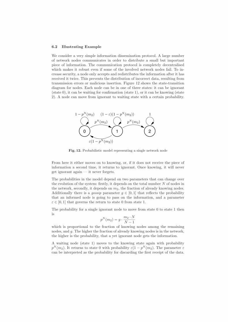
We consider a very simple information dissemination protocol. A large numberof network nodes communicates in order to distribute a small but importantpiece of information. The communication protocol is completely decentralisedwhich makes it robust even if some of the involved network nodes fail. To in-crease security, a node only accepts and redistributes the information after it hasreceived it twice. This prevents the distribution of incorrect data, resulting fromtransmission errors or malicious insertion. Figure 12 shows the state-transitiondiagram for nodes. Each node can be in one of three states: it can be ignorant(state 0), it can be waiting for confirmation (state 1), or it can be knowing (state2). A node can move from ignorant to waiting state with a certain probability.

0 1 2

ε(1− pN (m2))

pN (m2) pN (m2)

(1− ε)(1− pN (m2)) 11− pN (m2)

Fig. 12. Probabilistic model representing a single network node

From here it either moves on to knowing, or, if it does not receive the piece ofinformation a second time, it returns to ignorant. Once knowing, it will neverget ignorant again — it never forgets.

The probabilities in the model depend on two parameters that can change overthe evolution of the system: firstly, it depends on the total number N of nodes inthe network, secondly, it depends on m2, the fraction of already knowing nodes.Additionally there is a gossip parameter g ∈ [0, 1] that reflects the probabilitythat an informed node is going to pass on the information, and a parameterε ∈ [0, 1] that governs the return to state 0 from state 1.

The probability for a single ignorant node to move from state 0 to state 1 thenis

pN (m2) = g ·m2 ·N

N − 1which is proportional to the fraction of knowing nodes among the remainingnodes, and g. The higher the fraction of already knowing nodes is in the network,the higher is the probability, that a yet ignorant node gets the information.

A waiting node (state 1) moves to the knowing state again with probabilitypN (m2). It returns to state 0 with probability ε(1 − pN (m2). The parameter εcan be interpreted as the probability for discarding the first receipt of the data.

To represent all transition probabilities in the model, we state a probabilitymatrix that is local to each node. It depends on N and the occupancy measure

m = (m0,m1,m2).

PN (m) =

1− pN (m2) pN (m2) 0

ε(1− pN (m2)) (1− ε)(1− pN (m2)) pN (m2)

0 0 1

Considering all N network nodes in parallel would result in a state space with 3N

states. Even if we only recorded the occupancy measure, the state space would

still have N(N+1)(N+2)2 states – for three-state components!

Two avoid this blowup, we consider the mean-field limit for the occupancy mea-sure. The limit of the local probability matrix is

P (m) = limN→∞

PN (m) =

1− g ·m2 g ·m2 0ε(1− g ·m2) (1− ε)(1− g ·m2) g ·m2

0 0 1

For a given initial occupancy measure µ(0) we can then approximate the tran-sient evolution of the occupancy measure by the deterministic process [80, 79]

µ(t+ 1) = µ(t) · P (µ(t))

Figure 6.2 shows the deterministic occupancy measure µ(t) for t ∈ [0, 400] whenat the beginning the fraction of ignorant nodes is 99% and the fraction of knowingnodes is 1%, that is, µ(0) = (0.99, 0, 0.01). The figure represents the behaviourthat could be expected: the fraction of ignorant nodes decreases continually whilethe number of knowing nodes increases. Since all nodes have to move throughthe intermediate waiting state, the fraction of nodes in this state first increasesand then decreases again.

The mean-field approximation does not give us information about the possibledeviations from the computed deterministic value. However, the results depictedin Figure 6.2 allow a statement about the approximate time at which we expectall nodes to be knowing with high probability.

6.3 Outlook

Very often we encounter real-world systems that consist of a large number ofidentical replicas of the same component. In this section we have shown howthe mean-field approximation method can be employed if the components arerepresented by discrete-time models. The core computation for transient mea-sures then boils down to a series of cheap matrix-vector multiplications. Mean-field analysis is not restricted to discrete-time models. It can also be applied tocontinuous-time Markov chains [81, 79], to Markov decision processes [82], andprobably to many other probabilistic or stochastic modelling classes.

0

0.1

0.2

0.3

0.4

0.5

0.6

0.7

0.8

0.9

1

0 50 100 150 200 250 300 350 400

t

fraction ignorant components (state 0)fraction waiting components (state 1)

fraction knowing components (state 2)

Fig. 13. Mean-field approximation for the illustrating example

7 Fluid analysis in CTMCs and SPAs

Representing the explicit state space of performance models has inherent difficul-ties. Just as the state-space explosion effects functional correctness evaluation,so it can also be easily a problem in performance models. In particular, classi-cal Markov chain analysis of any variety requires exploration of the global statespace and, even for a simple system, this quickly becomes computationally in-feasible. One technique that attempts to side-step the state-space explosion isso-called fluid analysis.

In the discrete-time world of performance modelling, such techniques have al-ready been used by Benaım and Le Boudec [83] to good effect in mean-field

analysis of performance models. Similarly, Bakhshi et al. [80, 78] have developedsome discrete-time model-specific analysis techniques for gossip protocols usingthe mean-field technique.

In the field of stochastic process algebras, Hillston developed fluid-flow analy-sis [84] to make first-order approximations of massively parallel PEPA models.Bortolussi [85] presented a formulation for the stochastic constraint program-ming language, sCCP. Cardelli has a first-order fluid analysis translation toordinary differential equations (ODEs) for the π-calculus [86]. Petriu and Wood-side [87] have successfully used Mean Value Analysis of hierarchical queueingmodels such as Layered Queueing Networks (LQNs) to obtain mean responsetime results over large component-based systems.

In this section, we briefly outline a fluid analysis technique that is applied to avariety of the PEPA language known as Grouped PEPA (or GPEPA) [88]. It hasthe advantage over the original fluid approximation for PEPA or π-calculus of

having higher moment results available. These can be used to calculate varianceinformation and give a notion of accuracy of the first-order prediction. Addi-tionally, higher moments can also be used to create bounding approximationson some varieties of passage-time distribution [89].

7.1 GPEPA

Grouped PEPA (GPEPA) [88] is a simple syntactic extension to PEPA whichallows the straightforward identification of models that can be analysed usingfluid techniques. Specifically, the component grouping in GPEPA identifies theabstraction level at which the fluid analysis will take place. By adding compo-nent group labels to these structures, we also benefit from being able to identifyuniquely components in particular states in particular parts of the model struc-ture.

For a detailed summary of PEPA process algebra syntax and operational mean-ing we refer to the reader to the many papers that have been published discussingand using PEPA. The following is a small selection of such work [90–93].

A GPEPA model is formed by composing multiple labelled component groupstogether. The grammar for a GPEPA model G is:

G ::= G ✄✁L

G | Y {D} (3)

where Y is a group label, unique to each component group. The term G ✄✁L

Grepresents synchronisation over action types in the set L, where L ⊆ A is a setof possible action types in the model.

In this context, a component group is a parallel cooperation of a normally largenumber of fluid components. A fluid component is one whose state changes canbe captured by a random variable and ultimately a set of differential equations.Parallel, in this setting, means that there is no synchronisation between indi-vidual members of the component group. A component group D is specified asfollows:

D ::= D ‖ D | P (4)

where P is a fluid component, a standard PEPA process algebra term. The com-binator ‖ represents parallel, unsynchronised cooperation between fluid compo-nents.

7.2 A Client–Server Example of a Fluid model

To illustrate more clearly how component groups and fluid components are usedtogether to construct GPEPA models, we consider a GPEPA model of a simpleclient/server system from [89]. The type of model we wish to consider in this

section is one which exhibits massive parallelism. We present a simple systemwith n clients and m servers. The system uses a 2-stage fetch mechanism: a clientrequests data from the pool of servers; one of the servers receives the request,another server may then fetch the data for the client. At any stage, a server inthe pool may fail. Clients may also timeout when waiting for data after theirinitial request. We could capture this scenario of n clients cooperating on therequest and data actions with m resources with the following GPEPA systemequation:

CS(n,m)def

= Clients{Client [n]} ✄✁L

Servers{Server [m]} (5)

where L = {request , data} and C[n] represents n parallel cooperating copies ofcomponent C. Each client is represented as a Client component and each serveras a Server component. Each client operates forever in a loop, completing threetasks in sequence: request , data and then think ; and they may also perform atimeout action when waiting for data:

Clientdef

= (request , rr).Client waiting

Client waitingdef

= (data, rd).Client think + (timeout , rtmt).Client

Client thinkdef

= (think , rt).Client

The servers on the other hand first complete a request action followed by a data

action in cooperation with the clients but at either stage they may perform abreak action and enter a broken state in which a reset action is required beforethe server can be used again:

Serverdef

= (request , rr).Server get + (break , rb).Server broken

Server getdef

= (data, rd).Server + (break , rb).Server broken

Server brokendef

= (reset , rrst).Server

The request and data actions are shared actions between the clients and serversin order to model the fact that clients must perform these actions by interactingwith a server. The actions timeout , think , break and reset on the other hand arecompleted independently.

7.3 Generating ODEs for Fluid analysis

Fluid analysis is used to approximate the mean dynamics of a GPEPA model.That is, at a time t, fluid analysis will tell you how many components in eachnamed component group there are on average. As the size of the componentgroups increases, so the approximation can be shown to improve [89]. This con-vergence can also be demonstrated for higher moments of component counts [94].

In this section, we analyse the client/server model of Section 7.2 to show meancomponent counts for particular client and server states, Figures 14(a) and 14(c).

(a) Mean number of Clients (b) Standard deviation of numberof Clients

(c) Mean number of Servers (d) Standard deviation of numberof Servers

Fig. 14. Fluid analysis of the number of components in a Client/Server model. Simu-lations are given as dashed plots.

We show the standard deviation of the component counts for the client/servermodel in Figures 14(b) and 14(d). Where there is a local deviation from thesimulated results, this is due to the synchronisation model used in PEPA ratherthan fluid analysis in particular [88, 94].

We will skip any further preamble and write down the generating equation fora set of ODEs that gives a first-order fluid analysis of a GPEPA model. Thehigher order fluid analysis (that gives quantities can such as variance, standarddeviation and skewness) can be found in [88].

Let G be a GPEPA model. We define the evolution of the number of componentsof type P in group H over time, by vH,P (t). This quantity is defined by a systemof first-order coupled ODEs:

vH,P (t) =∑

α∈A

∑

Q∈B(G,H)

pα(Q,P )Rα(G,V (t), H,Q)

︸ ︷︷ ︸

incoming rate

−Rα(G,V (t), H, P )︸ ︷︷ ︸

exit rate

(6)

for all component group/component state pairs (H,P ) in the GPEPA model G.That is, we generate one ODE for each local state in the compositional model.Hence we avoid any association with the global state space.

This can broadly be explained by slitting Equation (6) into two parts, the in-

coming rate and the exit rate. The incoming rate part describes the total rate ofthe model that increases the number of components of type P in group H for agiven action α. This is calculated from the product of two quantities:

1. Rα(G,V (t), H,Q), the overall rate that component type Q enables doingactions of type α, where Q is also in group H, and;

2. pα(Q,P ), the probability that Q can evolve to become component type Pdoing an action α (it could perform an α and lead to another componenttype).

This is summed over all possible component types Q in group H to give theincoming rate to P for an action α.

The exit rate from P in group H for an action α is simply Rα(G,V (t), H, P ),overall rate that component type P enables doing actions of type α. The fulldefinition of the component rate function Rα(·) is given in [88].

Finally, the aggregate rate of change of components of type of P in group H canbe shown to equal to the total incoming rate minus the total exit rate, summedover all possible action types α.

Fig. 15. Fluid passage time analysis of a Client response time in the Client/Servermodel of Section 7.2

We have shown how first order fluid analysis of large stochastic processes can beused to create passage and response time distributions and related measures [95,

89]. This is done by performing the sort of fluid analysis described here on anappropriately modified model. Figure 15 shows a single Client response timedistribution (from steady-state) given all the synchronisations in the system. Aswith all fluid analysis, as the model gets larger, the distribution predicted by thefluid analysis (black line) becomes more accurate.

7.4 Outlook

Further developments in fluid analysis have shown how other types of passagetime distribution can be extracted from massively parallel systems [95]. Addi-tionally, real-valued rewards can be accumulated over the lifetime of a processmodel to capture quantities such as cost and energy consumption. For smallerscale models, these can be analysed using discrete-state Markov Reward Mod-els [96]; fluid analysis can be used here also to analyse larger scale reward mod-els [97] which would otherwise have a prohibitive state space size.

8 Conclusion

In this chapter we have presented a number of efficient representation and anal-ysis techniques that can aid resilience and performance analysis of large andcomplex systems. It is worth saying that there is no one best technique in allcases. As with many modelling and analysis problems, the best tool for the jobwill often depend on the problem being tackled and the type of answer beingsought. Some of the techniques discussed can be used to tackle many types ofperformance and resilience problem, while some are better suited to a particulartype of analysis. Some of the techniques will allow the user to recover an explicitstate representation, while others consider many model states in aggregation.

For a particular problem a modeller will wish to select those techniques thatcan produce the desired analysis. However, beyond that, it will be worth themodeller’s while to attempt a few of the remaining techniques to see whichscales best to their needs. They will find dramatic differences in operation andthose differences (in execution time and memory usage) will reflect many issues,such as how the model is originally represented, how many and indeed whetherparameters are available to the modeller and the level of complexity that themodeller wishes to capture in their model.

Finally, we would like to emphasise that these descriptions are by necessity briefsummaries of much more involved techniques. These topic introductions shouldbe treated as such and many references have been provided for the reader tofollow up if more information is required.

Acknowledgements

Jeremy Bradley, Richard Hayden and Nigel Thomas are supported by the UKEngineering and Physical Sciences Research Council on the AMPS project (ref-erence EP/G011737/1). Leıla Kloul is supported by the European Celtic projectHOMESNET [98].

References

1. W. J. Stewart, Probability, Markov Chains, Queues and Simulation. The Mathe-matical Basis of Performance Modeling. Princeton University Press, 2009.

2. Various authors, “The Network Simulator ns-2.” http://www.isi.edu/nsnam/ns/.(last seen May 11, 2010).

3. A. Varga, “The OMNeT++ discrete event simulation system,” in Proceedings ofthe European Simulation Multiconference (ESM’2001), June 2001.

4. P. Reinecke and K. Wolter, “Libphprng – A library to generate PH-distributedrandom numbers,” tech. rep., Freie Universitat Berlin, 2011. (to appear).

5. K. Wolter, P. Reinecke, and A. Mittermaier, “Evaluation and Improvement ofIEEE 1588 Frequency Synchronisation through Detailed Modelling and Simulationof Backhaul Networks.” (submitted for publication), 2011.

6. A. Horvath and M. Telek, “PhFit: A general phase-type fitting tool,” in TOOLS’02: Proceedings of the 12th International Conference on Computer PerformanceEvaluation, Modelling Techniques and Tools, (London, UK), pp. 82–91, Springer-Verlag, 2002.

7. J. Jackson, “Networks of waiting lines,” Operations Research, vol. 5, pp. 518–521,Aug. 1957.

8. F. Baskett, M. Chandy, R. Muntz, and F. Palacios, “Open, closed and mixed net-works of queues with different classes of customers,” Journal of the ACM, vol. 22,pp. 248–260, 1975.

9. W. Gordon and G. Newell, “Closed queueing systems with exponential servers,”Operations Research, vol. 15, no. 2, pp. 254–265, 1967.

10. E. Gelenbe, “Product-form queueing networks with negative and positive cus-tomers,” Journal of Applied Probability, vol. 28, no. 3, pp. 656–663, 1991.

11. G. Balbo, S. Bruell, and M. Sereno, “Embedded processes in generalized stochasticPetri nets,” in Proc. 9th Intl. Workshop on Petri Nets and Performance Models,pp. 71–80, 2001.

12. R. Boucherie, “A characterisation of independence for competing Markov chainswith applications to stochastic Petri nets,” IEEE Trans. on Software Eng., vol. 20,no. 7, pp. 536–544, 1994.

13. W. Henderson and P. Taylor, “Embedded processes in stochastic Petri nets,” IEEETrans. on Software Eng., vol. 17, no. 2, pp. 108–116, 1991.

14. J. Hillston, “Exploiting structure in solution: Decomposing compositional models,”in Lectures on Formal Methods and Performance Analysis (E. Brinksma et al, ed.),vol. 2090 of Lecture Notes in Computer Science, pp. 278–314, Springer-Verlag, 2001.

15. P. G. Harrison, “Turning back time in Markovian process algebra,” TheoreticalComputer Science, vol. 290, pp. 1947–1986, January 2003.

16. P. G. Harrison, “Compositional reversed Markov processes, with applications toG-networks,” Performance Evaluation, vol. 57, pp. 379–408, June 2004.

17. M. Reiser and S. Lavenberg, “Mean value analysis of closed multichain queueingnetworks,” JACM, vol. 22, no. 4, pp. 313–322, 1980.

18. K. Sevcik and I. Mitrani, “The distribution of queueing network states at inputand output instants,” JACM, vol. 28, no. 2, pp. 358–371, 1981.

19. S. Lavenberg and M. Reiser, “Stationary state space probabilities at arrival instantsfor closed queueing networks with multiple types of customers,” Journal of AppliedProbability, vol. 17, no. 4, pp. 1048–1061, 1980.

20. N. Thomas and Y. Zhao, “Mean value analysis for a class of PEPA models,” TheComputer Journal, 2011. 10.1093/comjnl/bxq064. accepted for publication.

21. K. Trivedi and M. Malhotra, Reliability and Performability Techniques and Tools:A Survey. In B. Walke and O. Spaniol, editors, Springer Verlag, Aachen, September1993.

22. P. Courtois, Decomposability, queueing and computer system applications. ACMmonograph series, 1977.

23. B. Plateau, De l’Evaluation du Parrallelisme et de la Synchronisation. PhD thesis,PhD Thesis, November 1984.

24. B. Plateau, “On the stochastic structure of parallelism and synchronisation modelsfor distributed algorithms,” in Proc. ACM Sigmetrics Conference on Measurementand Modelling of Computer Systems, 1985.

25. B. Plateau and J. Fourneau, “A methodology for solving markov models of parallelsystems,” Journal of Parallel and Distributed Computing, August 1991.

26. P. Fernandes, B. Plateau, and W. Stewart, “Efficient Descriptor-Vector Multipli-cations in Stochastic Automata Networks,” JACM, vol. 3, no. 45, pp. 381–414,1998.

27. A. Benoit, Methodes et Algorithmes pour l’evaluation des performances dessystemes informatiques a grands espaces d’etats. PhD thesis, PhD thesis, 2003.

28. A. Benoit, B. Plateau, and W. Stewart, “Memory-efficient algorithms with applica-tions to the modelling of parallel systems,” Future Generation Computer Systems,vol. 22, pp. 838–847, 2006.

29. B. Plateau, J. Fourneau, and K. Lee, “PEPS: A Package for Solving ComplexMarkov Models of Parallel Systems,” in Proc. of the 4th International Conferenceon Modelling Techniques and Tools for Computer Performance Evaluation, 1988.

30. I. Cidon and I. Gopal., “PARIS: An Appoach to Integrated High-Speed PrivateNetworks,” International Journal on Digital and Analog Cabled Systems, vol. 1,pp. 77–86, April-June 1988.

31. L. Kloul, Methodes d’evaluation des performances pour les reseaux ATM. PhDthesis, Universite de Versailles-St-Quentin-en-Yvelines, January 1996.

32. S. Donatelli, “Superposed Generalised Stochastic Petri Nets: Definition and Effi-cient Solution,” in Proc. of 15th Int. Conf. on Application and Theory of PetriNets (M. Silva, ed.), 1994.

33. P. Buchholz and P. Kemper, “Numerical analysis of stochastic marked graphs,” inProc. of Int. Workshop on Petri Nets and Performance Models, (Durham, NC),pp. 32–41, IEEE-Computer Society Press, oct 1995.

34. J. Campos, S. Donatelli, and M. Silva, “Structured solution of stochastic dsspsystems,” in Proc. of Int. Workshop on Petri Nets and Performance Models, (StMalo, France), pp. 91–100, IEEE-Computer Society Press, jun 1997.

35. G. Ciardo and A. Miner, “A data structure for the efficient kronecker solution ofgspns,” in In P. Buchholz editor, Proc. of the 8th International Workshop on PetriNets and Performance Models (PNPM’99), (Saragoza, Spain), pp. 22–31, 1999.

36. S. Donatelli, “Superposed Generalised Stochastic Petri Nets: Definition and Effi-cient Solution,” in Proc. of 15th Int. Conf. on Application and Theory of PetriNets (M. Silva, ed.), 1994.

37. P. Kemper, “Numerical Analysis of Superposed GSPNs,” IEEE Transactions onSoftware Engineering, vol. 22, no. 9, pp. 615–628, September 1996.

38. C. Ciardo and M.Tilgner, “On the use of Kronecker operators for the solutionof generalized stochastic Petri nets,” Tech. Rep. 96-35, Institute for ComputerApplications in Science and Engineering, Hampton, VA, May 1996.

39. P. Buchholz, “Hierarchical Structuring of Superposed GSPNs,” IEEE Transactionson Software Engineering, vol. 25, no. 2, pp. 166–181, March/April 1999.

40. S. Donatelli and P. Kemper, “Integrating synchronization with priority into a kro-necker representation,” Performance evaluation, vol. 44, no. 1–4, pp. 73–96, 2001.

41. P. Buchholz, “Compositional Analysis of a Markovian Process Algebra,” in Proc. of2nd Process Algebra and Performance Modelling Workshop (U. Herzog and M. Ret-telbach, eds.), 1994.

42. J. Hillston and L. Kloul, “An efficient kronecker representation for pepa mod-els,” in Proceedings of the Joint International Workshop, PAPM-PROBMIV 2001,vol. 2165 of LNCS, (Aachen, Germany), pp. 120–135, Springer, 2001.

43. J. Hillston and L. Kloul., “Formal Techniques for Performance Analysis: blendingSAN and PEPA,” Formal Aspects of Computing, vol. 19, pp. 3–33, 2007.

44. P. Fernandes, Methodes numeriques pour la solution de systemes Markoviens agrand espace d’etats. PhD thesis, PhD thesis, 1998.

45. W. Stewart, K. Atif, and B. Plateau, “The numerical solution of stochastic au-tomata networks,” European Journal of Operationnal Research, vol. 86, pp. 503–525, 1995.

46. P. Kemper, “Reachability analysis based on structured representations,” in Proc.of 17th International Conference on Application and Theory of Petri nets, pp. 269–288, LNCS,Springer Verlag, 1996.

47. S. D. P. Bucholtz, G. Ciardo and P. Kemper, “Complexity of memory-efficient kro-necker operations with applications to the solution of markov models,” INFORMSJournal on Computing, vol. 3, no. 12, pp. 203–222, 2000.

48. T. Dayar, “Iterative methods based on splittings for stochastic automata net-works,” European Journal of Operationnal Research, vol. 110, pp. 166–186, 1998.

49. K. McMillan, Symbolic Model Checking. Kluwer Academic Publishers, 1993.50. R. Bryant, “Graph-based Algorithms for Boolean Function Manipulation,” IEEE

Transactions on Computers, vol. C-35, pp. 677–691, August 1986.51. R. Enders, T. Filkorn, and D. Taubner, “Generating BDDs for symbolic model

checking in CCS,” Distributed Computing, no. 6, pp. 155–164, 1993.52. E. Clarke, M. Fujita, P. McGeer, K. McMillan, J. Yang, and X. Zhao, “Multi-

terminal Binary Decision Diagrams: An efficient data structure for matrix repre-sentation,” in IWLS: International Workshop on Logic Synthesis, (Tahoe City),May 1993.

53. H. Hermanns, J. Meyer-Kayser, and M. Siegle, “Multi Terminal Binary DecisionDiagrams to Represent and Analyse Continuous Time Markov Chains,” in 3rd Int.Workshop on the Numerical Solution of Markov Chains (B. Plateau, W. Stewart,and M. Silva, eds.), pp. 188–207, Prensas Universitarias de Zaragoza, 1999.

54. S. Minato, “Zero-suppressed BDDs for set manipulation in combinatorial prob-lems,” in 30th ACM/IEEE Design Automation Conference, pp. 272–277, 1993.

55. K. Lampka, A Symbolic Approach to the State Graph Based Analysis of High-LevelMarkov Reward Models. PhD thesis, University of Erlangen-Nurnberg, TechnischeFakultat, 2007.

56. K. Lampka, M. Siegle, J. Ossowski, and C. Baier, “Partially-shared zero-suppressedmulti-terminal BDDs: concept, algorithms and applications,” Formal Methods inSystem Design, vol. 36, no. 3, pp. 198–222, 2010.

57. T. Kam, T. Villa, R. Brayton, and A. Sangiovanni-Vincentelli, “Multi-valued de-cision diagrams: theory and applications,” Multiple-Valued Logic, vol. 4, no. 1-2,pp. 9–62, 1998.

58. A. Miner and G. Ciardo, “Efficient reachability set generation and storage usingdecision diagrams,” in Application and Theory of Petri Nets 1999 (H. Kleijn andS. Donatelli, eds.), (Williamsburg, VA, USA), pp. 6–25, Springer, LNCS 1639,1999.

59. M. Kuntz and M. Siegle, “Deriving symbolic representations from stochasticprocess algebras,” in Process Algebra and Probabilistic Methods, Proc. PAPM-PROBMIV’02, pp. 188–206, Springer, LNCS 2399, 2002.

60. H. Hermanns, M. Kwiatkowska, G. Norman, D. Parker, and M. Siegle, “On theuse of MTBDDs for performability analysis and verification of stochastic systems,”Journal of Logic and Algebraic Programming, vol. 56, no. 1-2, pp. 23–67, 2003.

61. M. Kwiatkowska, G. Norman, and D. Parker, “Prism: Probabilistic model check-ing for performance and reliability analysis,” ACM SIGMETRICS PerformanceEvaluation Review, vol. 36, no. 4, pp. 40–45, 2009.

62. K. Lampka and M. Siegle, “Activity-local Symbolic State Graph Generation forHigh-Level Stochastic Models,” in Proc. of 13th GI/ITG Conference on Measur-ing, Modelling and Evaluation of Computer and Communication Systems (MMB),(Nurnberg, Germany), pp. 245–263, VDE Verlag, 2006.

63. D. Deavours, G. Clark, T. Courtney, D. Daly, S. Derisavi, J. Doyle, W. Sanders,and P. Webster, “The Moebius Framework and its Implementation,” IEEE Trans-actions on Software Engineering, vol. 28, no. 10, pp. 956–969, 2002.

64. G. Ciardo, G. Luettgen, and R. Siminiceanu, “Saturation: An efficient strategy forsymbolic state-space generation,” in Proc. TACAS’01, (Genova, Italy), pp. 328–342, Springer, LNCS 2031, 2001.

65. M. Wan and G. Ciardo, “Symbolic state-space generation of asynchronous sys-tems using extensible decision diagrams,” in Proceedings of the 35th Conferenceon Current Trends in Theory and Practice of Computer Science, SOFSEM ’09,pp. 582–594, Springer-Verlag, 2009.

66. G. Ciardo and A. Miner, “A data structure for the efficient Kronecker solution ofGSPNs,” in PNPM’99 (P. Buchholz and M. Silva, eds.), pp. 22–31, IEEE computersociety, 1999.

67. A. Miner, “Efficient solution of GSPNs using canonical matrix diagrams,” in PetriNets and Performance models (PNPM’01) (R. German and B. Haverkort, eds.),pp. 101–110, IEEE Computer Society Press, 2001.

68. J. Bachmann, M. Riedl, J. Schuster, and M. Siegle, “An Efficient Symbolic Elimina-tion Algorithm for the Stochastic Process Algebra Tool CASPA,” in 35th Int. Conf.on Current Trends in Theory and Practice of Computer Science (SOFSEM’09),pp. 485–496, Springer LNCS 5404, 2009.

69. H. Hermanns and M. Siegle, “Bisimulation Algorithms for Stochastic Process Alge-bras and their BDD-based Implementation,” in ARTS’99, 5th Int. AMAST Work-shop on Real-Time and Probabilistic Systems (J.-P. Katoen, ed.), pp. 144–264,Springer, LNCS 1601, 1999.

70. S. Derisavi, “A Symbolic Algorithm for Optimal Markov Chain Lumping,” inTACAS 2007 (O. Grumberg and M. Huth, eds.), pp. 139–154, Springer, LNCS4424, 2007.

71. R. Wimmer, S. Derisavi, and H. Hermanns, “Symbolic partition refinement withautomatic balancing of time and space,” Performance Evaluation, vol. 67, no. 9,pp. 815–835, 2010.

72. M. Fujita, P. McGeer, and J.-Y. Yang, “Multi-terminal Binary Decision Diagrams:An efficient data structure for matrix representation,” Formal Methods in SystemDesign, vol. 10, pp. 149–169, April/May 1997.

73. D. Parker, Implementation of symbolic model checking for probabilistic systems.PhD thesis, School of Computer Science, Faculty of Science, University of Birm-ingham, 2002.

74. M. Kwiatkowska, D. Parker, Y. Zhang, and R. Mehmood, “Dual-Processor Paral-lelisation of Symbolic Probabilistic Model Checking,” in Proc. 12th InternationalSymposium on Modeling, Analysis, and Simulation of Computer and Telecommuni-cation Systems (MASCOTS’04) (D. DeGroot and P. Harrison, eds.), pp. 123–130,IEEE Computer Society Press, 2004.

75. J. Schuster and M. Siegle, “A symbolic multilevel method with sparse submatrixrepresentation for memory-speed tradeoff,” in 14. GI/ITG Conf. Measurement,Modelling and Evaluation of Computer and Communication Systems (MMB08),pp. 191–205, VDE Verlag, 2008.

76. J. Schuster and M. Siegle, “Speeding up the Symbolic Multilevel Algorithm,” in 6thInt Workshop on the Numerical Solution of Markov Chains (NSMC2010), pp. 79–82, 2010.

77. A. Miner, G. Ciardo, and S. Donatelli, “Using the exact state space of a Markovmodel to compute approximate stationary measures,” Performance Evaluation Re-view, vol. 28, pp. 207–216, June 2000. Proc. of ACM SIGMETRICS 2000.

78. R. Bakhshi, L. Cloth, W. Fokkink, and B. Haverkort, “Mean-field framework forperformance evaluation of push-pull gossip protocols,” Performance Evaluation,vol. 68, pp. 157–179, February 2011.

79. J.-Y. L. Boudec, D. McDonald, and J. Mundinger, “A generic mean field conver-gence result for systems of interacting objects,” in Proc. 4th Conf. on the Quanti-tative Evaluation of Systems (QEST’07), pp. 3–18, IEEE Computer Society, 2007.

80. R. Bakhshi, L. Cloth, W. Fokkink, and B. Haverkort, “Mean-field analysis for theevaluation of gossip protocols,” in Proc. 6th International Conference on the Quan-titative Evaluation of Systems (QEST’09), pp. 247–256, IEEE Computer Society,2009.

81. A. Bobbio, M. Gribaudo, and M. Telek, “Analysis of large scale interacting sys-tems by mean field method,” in Proc. 5th Conf. on the Quantitative Evaluation ofSystems (QEST’08), pp. 215–224, IEEE Computer Society, 2008.

82. N. Gast, B. Gaujal, and J.-Y. Le Boudec, “Mean field for Markov decision pro-cesses: from discrete to continuous optimization,” tech. rep., arXiv:1004.2342v2,2010.

83. M. Benaım and J.-Y. Le Boudec, “A class of mean field interaction models forcomputer and communication systems,” Performance Evaluation, vol. 65, no. 11-12, pp. 823–838, 2008.

84. J. Hillston, “Fluid flow approximation of PEPA models,” in QEST’05, Proceed-ings of the 2nd International Conference on Quantitative Evaluation of Systems,(Torino), pp. 33–42, IEEE Computer Society Press, September 2005.

85. L. Bortolussi and A. Policriti, “Stochastic concurrent constraint programming anddifferential equations,” in QAPL’07, 5th Workshop on Quantitative Aspects of Pro-gramming Languages, vol. 190 of Electronic Notes in Theoretical Computer Science,pp. 27–42, September 2007.

86. L. Cardelli, “On process rate semantics,” Theoretical Computer Science, vol. 391,pp. 190–215, February 2008.

87. D. C. Petriu and C. M. Woodside, “Approximate MVA for software client/servermodels by Markov chain task-directed aggregation,” in 3rd IEEE Symposium onParallel and Distributed Processing, pp. 322–329, Dec. 1991.

88. R. Hayden and J. T. Bradley, “A fluid analysis framework for a Markovian processalgebra,” Theoretical Computer Science, vol. 411, pp. 2260–2297, May 2010. doi://10.1016/j.tcs.2010.02.001.

89. R. Hayden, Scalable Performance Analysis of Massively Parallel Stochastic Sys-tems. PhD Thesis, Department of Computing, Imperial College London, 2011.

90. J. Hillston, A Compositional Approach to Performance Modelling, vol. 12 of Dis-tinguished Dissertations in Computer Science. Cambridge University Press, 1996.

91. G. Clark, S. Gilmore, J. Hillston, and N. Thomas, “Experiences with the PEPAperformance modelling tools,” in UKPEW’98, Proceedings of the 14th UK Perfor-mance Engineering Workshop, Edinburgh, July 1998.

92. J.-M. Fourneau, L. Kloul, and F. Valois, “Performance modelling of hierarchi-cal cellular networks using PEPA,” Performance Evaluation, vol. 50, pp. 83–99,November 2002.

93. S. Gilmore, J. Hillston, and M. Ribaudo, “An efficient algorithm for aggregat-ing PEPA models,” IEEE Transactions on Software Engineering, vol. 27, no. 5,pp. 449–464, 2001.

94. A. Stefanek, R. A. Hayden, and J. T. Bradley, “A new tool for the performanceanalysis of massively parallel computer systems,” in QAPL’10, 8th Workshop onQuantitative Aspects of Programming Languages, vol. 28 of Electronic Proceedingsof Theoretical Computer Science, pp. 159–181, 2010.

95. R. Hayden, A. Stefanek, and J. T. Bradley, “Fluid computation of passage time dis-tributions in large Markov models,” tech. rep., Dept. of Computing, Imperial Col-lege London, November 2010. http://pubs.doc.ic.ac.uk/fluid-passage-time/(Under review).

96. M. Telek and S. Racz, “Numerical analysis of large Markovian reward models,”Performance Evaluation, vol. 36–37, pp. 95–114, Aug. 1999.

97. A. Stefanek, R. Hayden, and J. T. Bradley, “Fluid analysis of energy consump-tion using rewards in massively parallel Markov models,” in ICPE 2011, 2ndACM/SPEC International Conference on Performance Engineering, March 14-16,2011, Karlsruhe, Germany, pp. 121–131, March 2011.

98. “HOMESNET: Home base station, an emerging network paradigm. CELTICeuropean project.” Available at http://www.celtic-initiative.org/Projects/Celtic-projects/Call6/HOMESNET/homesnet-default.asp, 2009–2011.