Scalable Adaptive Web Services Marin Litoiu, Mircea Mihaescu

IBM CAS Toronto and IBM USA Somers marin@ca.ibm.com, mircea@us.ibm.com

Bogdan Solomon, Dan Ionescu University of Ottawa, SITE

bsolomon@ncct.uottawa.ca, ionescu@ncct.uottawa.ca

ABSTRACT Software as a service creates the possibility of composing software applications from web services spread across different application domains. To guarantee certain quality of services of the composite service, one can think of two paths ahead: quality of service negotiation and guarantee prior to service deployment and bindings; or a more speculative and adaptive behavior at runtime. In this position paper we propose a hybrid approach, combining development and runtime information to make the web services adapt to workload variations. The approach combines control theory with performance modeling and is built around a model of the web service. A control loop theory approach is taken to model discovery. The control loop allows for keeping the web service’s performance even when the model is not completely known and failure of components of the control loop are likely to happen. The approach is related to robust state estimation. The robustness makes the model insensitive to parameter variations and to uncertainties in the model. With appropriate conditions, the above concept can be extended to the external environments in which the web service has to perform.

Categories and Subject Descriptors I.6.5 [Simulation and Modeling]: Model Development; K.6.0 [Management of Computing and Information Systems]: General; D.2.8 [Software Engineering]: Metrics | performance measures

General Terms Measurement, Performance, Experimentation

Keywords Web services, Service Oriented Architecture, Adaptive Computing, Robust Control

1. INTRODUCTION Service Oriented Architecture (SOA) relies on the concept of autonomic, loosely coupled web services. Moreover, autonomic services have been identified by Kontogiannis et al. [6] as an important area of research in SOA. Autonomic web services are those services that self-configure, self-heal, self-optimize and self-protect, in other words, self-manage. A service able to self-manage should monitor its states and the environment, analyze them, and make its own decision related to its behaviour. If the service is in or moving towards an undesired state, then a corrective plan should be devised and executed so that the service is moved in a desirable state.

Central to all the above is a need for a reference model which should cover in a unitary way all aspects of autonomic web services. Computing systems are usually modeled by finite state machines, timed automata, queuing theory based models, discrete event systems, discrete systems, etc. It is clear that it is a difficult task if not even impossible to uncover a model which has a large degree of generality and versatility covering all aspects of computation. A series of models have been therefore investigated and proposed by the research community for describing autonomic behaviours, while the industry is still in great expectation for the one.

Model based autonomic computing [4] assumes that change decisions in autonomic computing systems are based on the explicit model of the underlying software. In the self-optimization areas, several reference autonomic control loops have been proposed. They control single or collections of services, by either tuning parameters, reallocating the load or provisioning new instances of the service. Among those architectures, two seem to get traction: (a) performance model based adaptive control and (b) linearized feedback control.

Figure 1. Performance Model Based Adaptive Control.

Performance Model Based Adaptive Control. (Figure 1)[5]. An explicit queuing performance model of the system is created and maintained at run time. The model is maintained by an Estimator, which, based on the output of the system (y) and output of model (ý) computes new parameters (x) for the model. The model and the estimator work in a feedback loop. An example of estimator is the Kalman filter [3]. The role of controller is to achieve the performance goals, which are expressed as service level agreements. The controller consists of optimization algorithms and a policy based engine and computes the commands u that change the software resources in such a way that the goals are achieved in the presence of perturbations w. Examples of changes: caching policies, threading level, memory allocation, processor allocation, etc. Example of perturbations: change in the number of users interacting with the system, change in the usage patterns. Since the queuing models capture steady-state system behaviour, this type of architecture is appropriate for controlling long term trends in the service and therefore is very appropriate for provisioning.

Permission to make digital or hard copies of all or part of this work for personal or classroom use is granted without fee provided that copies are not made or distributed for profit or commercial advantage and that copies bear this notice and the full citation on the first page. To copy otherwise, or republish, to post on servers or to redistribute to lists, requires prior specific permission and/or a fee. SDSOA’08, May 11, 2008, Leipzig, Germany. Copyright 2008 ACM 978-1-60558-029-6/08/05...$5.00.

Controller

(Decision

Performance Model (QNM)

goals u

Estimator

y

e

ý

x

w

Web Service

47

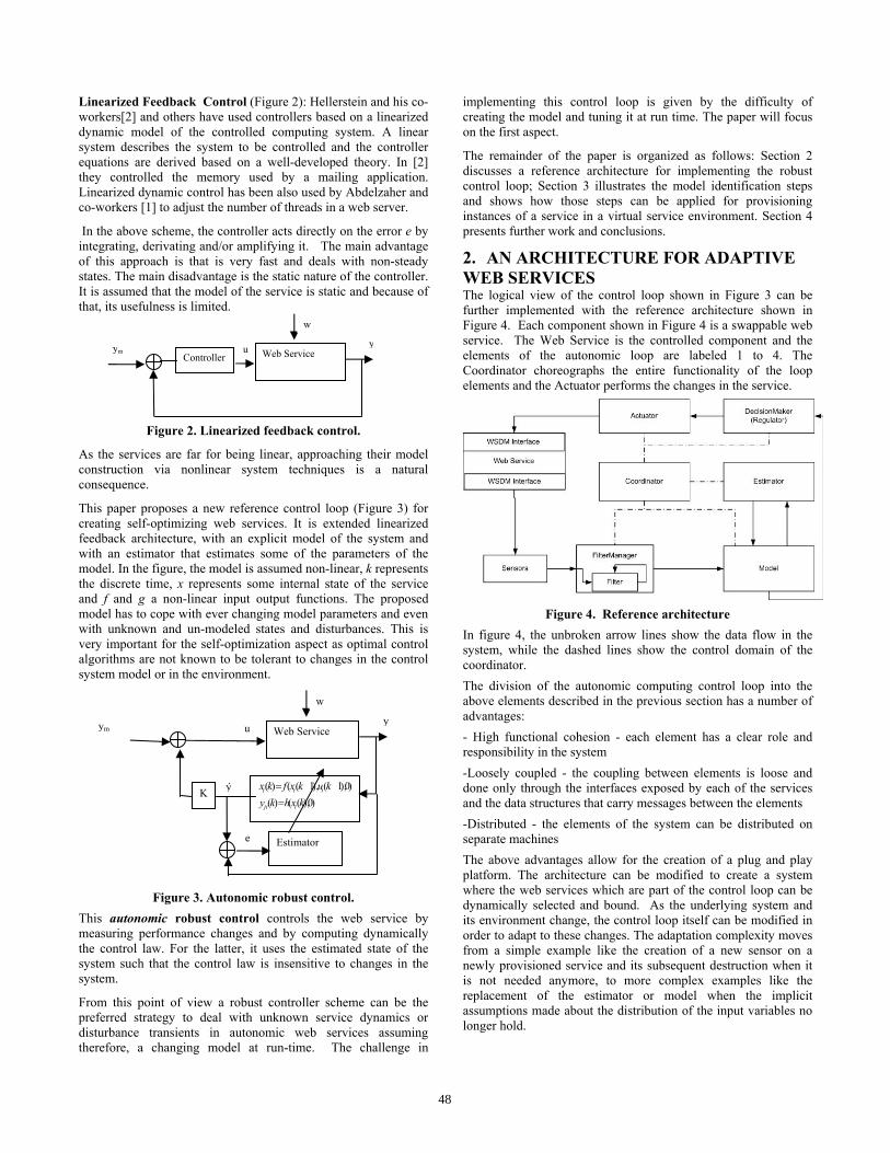
Linearized Feedback Control (Figure 2): Hellerstein and his co-workers[2] and others have used controllers based on a linearized dynamic model of the controlled computing system. A linear system describes the system to be controlled and the controller equations are derived based on a well-developed theory. In [2] they controlled the memory used by a mailing application. Linearized dynamic control has been also used by Abdelzaher and co-workers [1] to adjust the number of threads in a web server.

In the above scheme, the controller acts directly on the error e by integrating, derivating and/or amplifying it. The main advantage of this approach is that is very fast and deals with non-steady states. The main disadvantage is the static nature of the controller. It is assumed that the model of the service is static and because of that, its usefulness is limited.

Figure 2. Linearized feedback control.

As the services are far for being linear, approaching their model construction via nonlinear system techniques is a natural consequence.

This paper proposes a new reference control loop (Figure 3) for creating self-optimizing web services. It is extended linearized feedback architecture, with an explicit model of the system and with an estimator that estimates some of the parameters of the model. In the figure, the model is assumed non-linear, k represents the discrete time, x represents some internal state of the service and f and g a non-linear input output functions. The proposed model has to cope with ever changing model parameters and even with unknown and un-modeled states and disturbances. This is very important for the self-optimization aspect as optimal control algorithms are not known to be tolerant to changes in the control system model or in the environment.

Figure 3. Autonomic robust control.

This autonomic robust control controls the web service by measuring performance changes and by computing dynamically the control law. For the latter, it uses the estimated state of the system such that the control law is insensitive to changes in the system.

From this point of view a robust controller scheme can be the preferred strategy to deal with unknown service dynamics or disturbance transients in autonomic web services assuming therefore, a changing model at run-time. The challenge in

implementing this control loop is given by the difficulty of creating the model and tuning it at run time. The paper will focus on the first aspect.

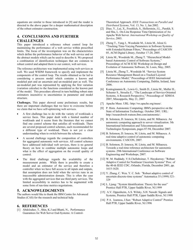
The remainder of the paper is organized as follows: Section 2 discusses a reference architecture for implementing the robust control loop; Section 3 illustrates the model identification steps and shows how those steps can be applied for provisioning instances of a service in a virtual service environment. Section 4 presents further work and conclusions. 2. AN ARCHITECTURE FOR ADAPTIVE WEB SERVICES The logical view of the control loop shown in Figure 3 can be further implemented with the reference architecture shown in Figure 4. Each component shown in Figure 4 is a swappable web service. The Web Service is the controlled component and the elements of the autonomic loop are labeled 1 to 4. The Coordinator choreographs the entire functionality of the loop elements and the Actuator performs the changes in the service.

Figure 4. Reference architecture

In figure 4, the unbroken arrow lines show the data flow in the system, while the dashed lines show the control domain of the coordinator. The division of the autonomic computing control loop into the above elements described in the previous section has a number of advantages: - High functional cohesion - each element has a clear role and responsibility in the system -Loosely coupled - the coupling between elements is loose and done only through the interfaces exposed by each of the services and the data structures that carry messages between the elements -Distributed - the elements of the system can be distributed on separate machines The above advantages allow for the creation of a plug and play platform. The architecture can be modified to create a system where the web services which are part of the control loop can be dynamically selected and bound. As the underlying system and its environment change, the control loop itself can be modified in order to adapt to these changes. The adaptation complexity moves from a simple example like the creation of a new sensor on a newly provisioned service and its subsequent destruction when it is not needed anymore, to more complex examples like the replacement of the estimator or model when the implicit assumptions made about the distribution of the input variables no longer hold.

e

)0),(()()0),1(),1(()(

kxhkykukxfkx

iji

iii

==

ym u

Estimator

y

ý

w

K

Web Service

u Web Service ym y

w

Controller

48

We implemented the reference architecture by using the Apache Muse framework [7] to provide encapsulation for the elements of the autonomic computing system. In this implementation each element is a Web Services Distributed Management (WSDM) resource, with a predefined life cycle managed by the Muse framework. The use of WSDM ensures that the autonomic computing elements can be accessed in a standard way, as well as that they have well defined lifecycles. In the WSDM implementation, each of the elements is seen as a resource that is addressable through the Web Services Addressing standard. Each element runs inside a container, which is also a WSDM resource, that takes care of creating, configuring and removing an element. This way there can be multiple elements for multiple autonomic systems running in parallel on the same machine, inside the same server. By using WSDM, each of the elements gets a unique endpoint through which it communicates with the rest of the autonomic system, and the routing of messages to each element is done by the Muse framework. Furthermore, the use of the WSDM standard allows for easy implementation of notification based messaging. While the first version of the system used direct web service calls, similar to RPC, for communication between elements, the WSDM based implementation uses notifications, where each element sends data that it has available to the next element in the chain. The WSDM framework also allows for a well defined lifecycle for the elements, starting with the creation of the element through a factory pattern, starting the created resource which represents the element, stopping the resource and finally destroying the resource once it is no longer needed. Another feature provided by the WSDM framework is failure recovery. The resource information is persisted periodically to the file system and in case the server crashes, on restart, the resource is reloaded with the latest information available before the crash.

3. TOWARDS A METHOD FOR BUILDING THE CONTROLLER AND THE ESTIMATOR

3.1 Building a performance model of the web service The turning point for a correct design of an autonomic web service is related to defining and building an accurate model of the service. The model provides a view of the controlled web service and both the estimation of the future state of the service and the change decision are based on that model. While a model can not perfectly represent the service under control, it is important that the model accurately represent the state of the service and more importantly accurately modify itself to changes in the environment. If the modifications in the system do not translate into correct modifications of the model, even an initial correct model will be out of tune with the modeled system after a number of iterations. The complexity of deriving a model which can be used for solving at least the self-optimizing aspect is greater than those encountered in linear control systems due to a combination of types of processes such as computing, task scheduling, resource allocation solutions, and many others. In such a complex model, one can encounter discrete and continuous processes, discrete event systems, finite state machines, timed automata, and so on. On the other hand, there are two contradictory requirements for building good models: i) the model has to be simple enough to

facilitate design and ii) complex enough to contain the basic dynamics of the modeled process.

Figure 5. Input-output channels for model identification

To build the controller and the estimator, for such a complex system a nonlinear model has to be considered [12]:

)0),(()()0),1(),1-(()(

kxhkykukxfkx

ij

iii

=−=

where x is a state variable, y is a measurable output, u is a measurable input and k is the discrete time. x and y are vectors and i and j denote the vector components. f and g are non linear functions. The linearized version of this performance model is described by the following equations:

)())(()()()1())1(()(

kVvkxHkzkykWwkxAkx

++≈−+−=

i=1,..,K

The accuracy of this model will dictate the quality of service of the controlled processes, in this case the Web Services. In order to improve the quality of control

• The structure and an initial value for A,W,H, and V are constructed off-line, through established system identification methods

• As the identification method selected (RPE) [14] depends on the quality of data collected from the process, a sampling rate has to be determined (the time interval between k and k-1 in the equations above)

• Once the model is obtained, an estimator and its associated controller will keep the QoS automatically in line with the SLA.

The design of the controller and of the estimator follows the ideas of a robust controller described in [13]. Due to the space constraints of this paper, we will focus the remainder of the section on the identification of the model and will sketch the design of the estimator. To identify the model of the service, a black box approach (Figure 5) can be taken. The following off-line steps will result in a model and runtime sampling rate:

• identify the input and the output variables of the system

• devise a set of input signals and measure the outputs

• identify the model by using the RPE method [14]

• determine the sampling rate. The next section exemplifies some of the above steps on a small case study.

3.2 Experimental setup and results To illustrate the methodology, we consider a cluster of identical web services that run on web servers. The system implements a

49

trade application. The cluster can expand or shrink by adding or removing instances of the web service. This change mechanism allows the controller to tune performance metrics of the service. The inputs are the load (number of users or the user think time) and the number of services in the cluster. The outputs are the service response time and CPU utilization. We varied the inputs by

• Holding the number of services constant at one, the think time constant at 30s and modifying the number of clients every one minute according to a Gaussian distribution

• Holding the number of clients constant at 50, the think time constant at 30s and modifying the number of services in the cluster stochastically, every five minutes

• Holding the number of clients constant at 50, the number of services constant at 1, and modifying the think time according to a Gaussian distribution every minute.

Figures 6a to 6f show the results of the experiments. Figure 6a shows the random variation of the client invocations and Figure 6b show the cluster response time to the above disturbance. In Figure 6c we show how we varied the number of service instances while 6d shows the response time as the result of the above random changes. In Figure 6e the think time was considered as a stochastic variable and the number of services and the number of clients were kept constant and Figure 6f shows the response time. To keep the presentation simple, only 200 sampling points were displayed in Figures 6a to 6f and each sample was taken at every 10s. The number of service instance graph is more complicated as it contains the number of servers that are in utilization at one time. Thus, a server is not considered to be available until it has finished provisioning, and it becomes unavailable the moment the stop command is sent. Due to the fact that sometimes it takes a longer time for servers to be added or removed, a situation where there are actually 0 servers in the cluster can happen if there are servers in the process of being added to the cluster, but the servers that were already in the cluster have been removed. This can be seen at time 20 in Figure 6c. For example if there are 2 servers in the cluster, and the next random is 5, the system will add 3 servers. While the 3 servers are in transition, and because the transition takes to long a new random is chosen that is 3. In such a case the already existing two servers will be deprovisioned, resulting for a short time in a cluster with 0 servers. To complicate things further while the servers are being stopped there are still clients that are finishing their requests resulting in non zero response times. The above reading rate was chosen for making an accurate representation of the input and output signals.

Figure 6a) Client variation

Figure 6b) Response Time for varying clients

Figure 6c) Varying service instances

For providing consistency to the experiment described above, these results were used to determine the appropriate sampling rate such that the Web Services model can be properly built.

50

Figure 6d) Response time for varying service instances

Figure 6e) Varying think time

Two more steps have to follow after the input and output data are collected:

• Calculate the correlation functions of the input and outputs listed above.

• Compute the gain and phase diagrams of the transfer functions for the information channels shown in Figure 5. Those are computed as the ratio of the Fourier transforms of the autocorrelation functions for the input and output system variables.

Figure 6f) Response time for varying think time

If the magnitude and phase of the transfer function versus the frequency are plotted in a Log-Log plot, the cut-off frequency of the system is found at the –3 db point on the gain diagram. Figure 7 shows the gain of the transfer function of the number of user invocations and response time in dbs versus logω.

In Figure 7 the frequency at which the amplitude is -3 db is equal to 10-1.17rad/s, which means a sampling rate of 0.01076Hz and a sampling period of 46.46s. A runtime sampling rate of 10s therefore, will satisfy the sampling theorem of Shannon [15] and will guarantee a correct set of data.

Figure 7: Sampling rate determination

The initial values for A,W,H, and V are computed using the RPE method[14] and, due to space limitations, are not shown here.

3.3 Building a robust estimator In the works structured around controlling computing processes using state space algorithms [12], [15], a state estimation technique has to be applied in order to build an appropriate control law for service provisioning. This is, however, a valid methodology only under severe model restrictions. It can be applied only when the service can be accurately modeled. If the model of the service is inaccurate due to uncertainties in service parameters, to un-modeled dynamics or to uncertainties in the disturbance representation, the inherent differences between the service and the model used in the state-estimator will inevitably lead to degradations in the overall system performance. In order to cope with the above model discrepancies robust state estimation techniques have been proposed in the domain literature [16]. In the works described in this paper a hybrid technique has been introduced. Initially the model parameters have been calculated using the RPE method [14] using an online procedure. The RPE was applied considering that the model parameters are piecewise constant, and that on the interval on which the output samples were collected the system model does not change. The well known Akaike information model was then applied to obtain the best order of the model which can represent the real process. A robust estimator was then built considering the initial model obtained. To the functions representing the model as in section 3.1 were given a first order variation and the result added to the initial model. The fact that the variation of these function was added to them might be seen as a simplification of the general problem, however, for the problem at hand the addition covers well the proposed goal of this research. The model and estimator

51

equations are similar to those introduced in [9] and the reader is directed to the above paper for a deeper mathematical description of the robust estimator construction.

4. CONCLUSIONS AND FURTHER CHALLENGES This paper introduced a reference robust control loop for maintaining the performance of a web service within prescribed limits. The focus of the investigation was on the characteristics which define the performance behavior of the web service and on the abstract models which can be used to describe it. We proposed a combination of identification techniques that are common to robust control and adapted them to our context, web services. The reference architecture was implemented using web services as well. We used WSDM framework to specify and implement the components of the control loop. The results obtained so far led to considering a process model which contains a known and modeled part and an uncertain and un-modeled part as well. The un-modeled part was represented by applying the first variation (variation calculus) to the functions considered as the known part of the model. This procedure allowed in turn building robust state estimators insensitive to uncertainties in parameter and model structure. Challenges. This paper showed some preliminary results, but there are important challenges that we have to overcome before we claim that we have self-optimizing web services.

• A first challenge has to do with the variety of workloads a service faces. This paper dealt with a limited number of workloads and it seems from the literature that we cannot find one control scheme that satisfies all workloads. There are several proposed control schemes, each recommended for a different type of workload. There is not yet a clear understanding when to switch between the schemes.

• A second challenge regards the composition of controllers for aggregated autonomic web services. All control schemes have addressed individual web services, there is no general theory on how to combine multiple autonomic loops and what is the effect of aggregation on the overall quality of control.

• The third challenge regards the availability of the measurement points. While there is possible to create a model and an estimator of the service and therefore a controller when we have full access to all inputs and outputs, that assumption does not hold when the service runs in an inaccessible administration domain. This is often the case with the aggregated services that use third party services. The limited accessibility to metrics has to be augmented with some form of run-time metrics negotiations.

5. ACKNOWLEDGMENTS The authors would like to thank the IBM Centre for Advanced Studies (CAS) for the research and technical help.

6. REFERENCES [1] Abdelzaher, T., Shin, K.J and Bhatti, N., Performance

Guarantees for Web Server End-Systems: A Control-

Theoretical Approach. IEEE Transactions on Parallel and Distributed Systems, Vol. 13, No. 1, Jan 2002.

[2] Diao, Y., Lui, X., Froehlich, S., Hellerstein, J.L., Parekh, S. and Sha, L. On-Line Response Time Optimization of An Apache Web Server. International Workshop on Quality of Service, 2003.

[3] Zheng T., Yang J., Woodside M., Litoiu M., Islzai G. “Tracking Time-Varying Parameters in Software Systems with Extended Kalman Filters,” Proceedings of CASCON 05, ACM Digital Library, October 17-20, 2005.

[4] Litoiu M., Woodside M., Zheng T. “Hierarchical Model-based Autonomic Control of Software Systems,” Proceedings of ACM ICSE Workshop on Design and Evolution of Autonomic Software, St. Louis, May, 2005.

[5] Litoiu M., Zheng T., Woodside M. “Service System Resource Management Based on a Tracked Layered Performance Model,” Proceedings of IEEE International Conference on Autonomic Computing, Dublin, Ireland, June 2006.

[6] Kontoginannis K., Lewis G., Smith D., Litoiu M., Muller H., Schuster S., Stroulia E., “The Landscape of Service-Oriented Systems, A Research Perspective,” Proceedings of SDSOA 2007, Mineappolis, May 21, 2007

[7] Apache Muse. URL: http://ws.apache.org/muse/. [8] P. Horn. Autonomic Computing: IBM's perspective on the

State of Information Technology. October 2001. URL: http://researchweb.watson.ibm.com/autonomic/.

[9] B. Solomon, D. Ionescu, M. Litoiu, and M. Mihaescu. An autonomic computing approach to server virtualization. 5th International Information and Telecommunication Technologies Symposium, pages 87-94, December 2007.

[10] B. Solomon, D. Ionescu, M. Litoiu, and M. Mihaescu. A real-time adaptive control of autonomic computing environments. CASCON, 2007.

[11] B. Solomon, D. Ionescu, M. Litoiu, and M. Mihaescu. Towards a real-time reference architecture for autonomic systems. 29th International Conference on Software Engineering and Workshops, 2007.

[12] W. M. Haddady, V.S.Chellaboinaz, T. Hayakaway: ”Robust Adaptive Control for Nonlinear Uncertain Systems” Proc. of the 40-th IEEE CDC, Orlando, Florida, December 2001, pp. 1615-1620.

[13] Y. Zhang, C. Wen, Y. C. Soh: “Robust adaptive control of uncertain discrete-time systems” Automatica 35 (1999) 321-329

[14] L. Ljung: “System Identification: Theory for the user” Prentice Hall PTR, Upper Saddle River, NJ.1999

[15] A.V. Oppenheim, A.S. Wilsky, S.H. Nawab: Signals and Systems, Prentice Hall PTR, Upper Saddle River, NJ.1998

[16] P.A. Ioannou, J.Sun: “Robust Adaptive Control” Prentice Hall PTR, Upper Saddle River, NJ.1996

52