Scalable Distributed Virtual Data Structures

Sushil Jajodia 1, Witold Litwin 2, Thomas Schwarz, SJ 3

1 George Mason University, Fairfax, Virginia, USA2 Universite Paris Dauphine, Paris, France

3 Universidad Catolica del Uruguay, Montevideo, Rep. Oriental del Uruguay

ABSTRACT

Big data stored in scalable, distributed data struc-tures is now popular. We extend the idea to big, vir-tual data. This data is not stored, but materializeda record at a time in the nodes of a scalable, dis-tributed, virtual data structure spanning up to thou-sands of nodes. The necessary cloud infrastructure isnow available for general use. The records are used bysome big computation that scans every records andretains (or aggregates) only a few based on criteriaprovided by the client. The client sets a time limit Rfor the scan at each node, e.g. R = 10 minutes.

We define two scalable distributed virtual data struc-tures called VH* and VR*. They use, respectively,hash and range partitioning. While scan speed candiffer between nodes, these seek to minimize the num-ber of nodes necessary to perform the scan in theallotted time R. We show the usefulness of our struc-tures by applying them to the problem of recoveringan encryption key and to the classic knapsack prob-lem.

I INTRODUCTION

The concept of Big Data, also called Massive DataSets [12], commonly refers to very large collections ofstored data. While this concept has become popularin recent years, it was already important in the eight-ies, although not under this monicker. In the earlynineties, it was conjectured that the most promisinginfrastructure to store and process Big Data is a setof mass-produced computers connected by a fast, butstandard network using Scalable Distributed DataStructures (SDDS). Such large-scaled infrastructuresnow are a reality as P2P systems, grids, or clouds.The first SDDS was LH* [1, 7, 9], which creates arbi-trarily large, hash-partitioned files consisting of recordsthat are key-value pairs. The next SDDS was RP*[8], based on range partitioning and capable of pro-cessing range queries efficiently. Many other SDDS

have since appeared; some are in world-wide use.BigTable, used by Google for its search engine, is arange-partitioned SDDS, as are Azur Table providedby MS Azur and MongoDB. Amazon’s EC2 uses adistributed hash table called Dynamo. VMWare’sGemfire provides its own hash scheme, etc. APIs forthe popular MapReduce framework, in its Google orHadoop version, have been created for some of theseofferings [2, 3].

As many data structures, an SDDS stores records inbuckets. Records are key-value pairs and are assignedto buckets based on the key. Buckets split incre-mentally to accommodate the growth of an SDDSfile whenever a bucket overflows its storage capac-ity. Every SDDS offers efficient access to records forkey-based operations; these are the read, write, up-date, and delete operations. LH∗ even offers con-stant access times regardless of the total number ofrecords. SDDS also support efficient scans over thevalue field. A scan explores every record, usually inparallel among buckets. During the scan, each nodeselects (typically a few) records or produces an ag-gregate (such as a count or a sum) according to someclient-defined criterion. The local results are then(usually) subjected to a (perhaps recursive) aggrega-tion among the buckets.

Below, we use the SDDS design principles to defineScalable Distributed Virtual (Data) Structure (SDVS).Similar to an SDDS, a SDVS deals efficiently with avery large number of records, but these records arevirtual records. As such, they are not stored, butmaterialized individually at the nodes. The scan op-eration in an SDVS visits every materialized recordand either retains if for further processing or discardsit before materializing the next record. Like an SDDSscan, the process typically retains very few records.

Virtual records have the same key-value structure asSDDS records. Similar to an SDDS with explicitlystored records, an SDVS deals efficiently with BigVirtual Data that consists of a large number of virtual

Page 1 of 10c©ASE 2014

records. Virtual data however are not stored, but arematerialized individually, one record at a time, ac-cording to a scheme provided by the client. As anexample, we consider the problem of maximizing anunruly function over a large, finite set, subject to anumber of constraints. We assume that we have anefficient enumeration of the set that we can thereforewrite as S = {si|i ∈ {0, 1, . . . ,M − 1}}. A virtualrecord then has the form (i, si) and the record is ma-terialized by calculating si from i. An SDVS doesnot support key-bases operations, but provides a scanprocedure. The scan materializes every record andeither retains and aggregates or discards the record.In our example, the scan evaluates whether the valuefield si fulfills the constraints, and if this is the case,evaluates the function on the field. It retains therecord if it is the highest value seen at the bucket.Often, a calculation with SDVS will also need to ag-gregate the local results. In our example, the localresults are aggregated by selecting the global maxi-mum of the local maxima obtained at each bucket.

A client needs to provide code for the materializationof records, the scan procedure, and the aggregationprocedure. These should typically be simple tasks.The SDVS provides the organization of the calcula-tion.

An SDVS distributes the records over an arbitrarilylarge number N of cloud nodes. For big virtual data,N should be at least in the thousands. Like in anSDDS, the key determines the location of a record.While an SDDS limits the number of records stored ata bucket, an SVDS limits the time to scan all recordsat a bucket to a value R. A typical value for R wouldbe 10 minutes.

The client of a computation using SDVS (the SDVSclient) requests an initial number Nc ≥ 1 of nodes.An SDVS determines whether the distribution of thevirtual records over that many buckets would leadto scan times less than R. If not, then the datastructure (not a central coordinator) would spreadthe records over a (possible many times) larger setN of buckets. The distribution of records tries tominimize N to save on the costs of renting nodes. Itadjusts to differences in capacity among the nodes.That nodes have different scanning speed is a typ-ical phenomenon. A node in the cloud is typicallya Virtual Machine (VM). The scanning throughputdepends on many factors. Besides differences in thehardware and software configuration, several VM aretypically collocated at the same physical machine andcompete for resources. Quite possibly, only the node

itself can measure the actual throughput. This typeof problem was already observed for MapReduce [14].

In what follows we illustrate the feasibility of ourparadigm by defining two different SDVS. Taking acue from the history of SDDS, we propose first VH∗,generating hash partitioned, scalable, distributed, vir-tual files and secondly VR∗, using scalable range par-titioning. In both structures, the keys of the virtualrecords are integers within some large range [0,M ],where for example M might be equal to 240. We dis-cuss each scheme and analyze its performance.

We show in particular that both schemes use on theaverage about 75% of its capacity for the scanningprocess. The time needed to request and initialize allN nodes is O(log2(N)). If N only grows by a smallfactor over Nc, say less than a dozen, then the com-pact VR∗ can use almost 100% of the scan capacityat each nodes at the expense however of O(N) timefor the growth to N nodes. The time to set up a VMappears to be 2-3 seconds based on experiments. Thiswas observed experimentally for the popular VagrantVM [4,13].

To show their usefulness, we apply our cloud-basedsolutions to two classical problems. First, we showhow to invert a hash, which is used to implement re-covery of an encryption key [5, 6]. The second is thegeneric knapsack problem, a famously hard problemin Operations Research [11]. Finally, we argue thatSDVS are a promising cloud-based solution for otherwell-known hard problems. Amongst these we men-tion those that rely on exploring all permutations orcombinations of a finite set such as the famous trav-eling salesman problem.

II SCALABLE DISTRIBUTED VIRTUALHASHING

Scalable Distributed Virtual Hash (VH*) is a hash-partitioned SDVS. VH* nodes are numbered consecu-tively, starting with 0. This unique number assignedto a node is its logical address. In addition, each nodehas a physical address such as its TCP/IP address.The scheme works on the basis of the following pa-rameters which are common, in fact, to any SDVSscheme we describe below.(a) Node capacity B. This is the number of virtualrecords that a node can scan within time R. Obvi-ously, B depends on the file, the processing speed ofthe node, on the actual load, e.g. on how many vir-tual machines actually share a physical machine, etc.There are also various ways to estimate B. The sim-

Page 2 of 10c©ASE 2014

plest one is to execute the scan for a sample of therecords located at a node. This defines the node’sthroughput T [6]. Obviously we have B = RT.(b) Node load L This is the total number of virtualrecords mapped to a node.(c) Node load factor α, defined by α = L/B.

This terminology also applies to schemes with storedrecords. In what follows, we assume that B is con-stant for the scan time at the node. The above pa-rameters depend on the node. We use subscripts toindicate this dependencies. A node n terminates itsscan in time only if αn ≤ 1. Otherwise, the node isoverloaded. For smaller values of αn the node is rea-sonably loaded and becomes underloaded for αn <1/2. An overloaded node splits dividing its load be-tween itself and a new node as we will explain below.The load at the splitting node is then halved. Eachsplit operation appends a new node to the file. Newnodes also follow the splitting rule. The resulting cre-ation phase stops when αn ≤ 1 for every node n inthe file.

In more detail, VH* grows as follows:1. The client sends a virtual file scheme SF where Fis a file, to a dedicated cloud node, called the coordi-nator (or master) and denoted by C in what follows.By default, C is Node 0. Every file scheme SF con-tains the maximally allowed time R and the key rangeM . These parameters determine the map phase as wehave just seen. We recall that the file F consists of Mvirtual records with keys numbered from 0 to M − 1.There are no duplicate keys. The rules for the materi-alization of value fields and the subsequent selectionof relevant records are also specified in SF . Thesedetermine the scan phase of the operation. Finally,the termination phase is also specified, determiningthe return of the result to the client. This includesperhaps the final inter-node aggregation (reduction).Details depend on the application.

2. Node 0 determines B based on SF . It calculatesα0 = M/B. If α0 ≤ 1 then node 0 scans all Mrecords. This is unlikely to happen, and normally,α0 >> 1. If α0 > 1, then Node 0 chooses additionalN0 − 1 nodes, sends SF to all nodes in N , sends alevel j = 0 to all nodes in N and labels the nodescontiguously as 1, . . ., N0 − 1.

The intention of this procedure is to evenly distributethe scan over N = N0 nodes (including the initialnode) in a single round of messages. By setting N0 =α0, the coordinator (Node 0) guesses that all N0

nodes have the same capacity as Node 0 and willnow have load factor α = 1. This is only a safe

bet if the nodes are homogeneous and have the sameload. This is the case when we are working with a ho-mogeneous cloud with private virtual machines. Bysetting N0 = 2, Node 0 chooses to not assume any-thing. In this strategy, the number of rounds couldbe markedly increased, but we avoid a low guess thatwill underutilize many of the allocated and paid fornodes.

3. Each node i in {0, . . . , N0} determines its loadfactor αi. If αi ≤ 1, Node i starts scanning. Nodei generates the records assigned to it by the LH ad-dressing principles [9]. In general, this means thatthe records have keys K with i = K mod 2jN0. Wewill see nodes with j ≥ 1 shortly and recall that thenodes in the set N all have j = 0.

4. If Node i has a load factor αi > 1, then this nodesplits. It requests from the coordinator (or from somevirtual agent serving as cloud administrator) the al-location of a new node. It gives this node numberi+ 2j , assigns itself and the new node level j = j+ 1.If finally sends this information and SF to the newnode.

5. All nodes, whether the original Node 0, the nodesin N or subsequentially generated nodes loop oversteps 3-4.

At the end of this possibly recursive loop, every nodeenters the scan phase. For every node, this phaseusually requires the scan of every record mapped tothe node. The scan therefore generates successivelyall keys in its assigned key space, materializes therecord according to the specifications in SF and cal-culates the resulting key-value pair to decide whetherto select the record for the final result. If a record isnot needed, it is immediately discarded.

VH* behaves in some aspects different than LH*,from which it inherits its addressing scheme. WhereasLH* creates buckets in a certain order and the set ofbucket addresses is always contiguous, this is not thecase for the node address space in VH*. For exam-ple, if the initial step creates N0 = 1000 nodes, itis possible that only Node 1 splits, leaving us withan address space of {0, 1, . . . , 999, 1001}. If the sameNode 1 splits again, we would add a node 2001. InLH*, buckets are loaded at about 70% and the samenumber should apply to VH*. We call the splittingnode the parent and the nodes it creates its children.

6. Once a node has finished scanning records, it en-ters the termination phase with its proper protocol.After the termination phase, the node always deallo-

Page 3 of 10c©ASE 2014

cates itself.

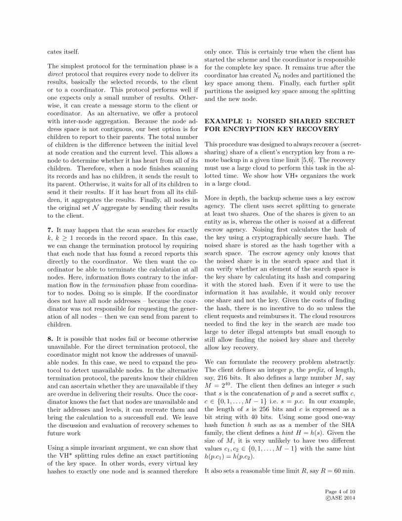
The simplest protocol for the termination phase is adirect protocol that requires every node to deliver itsresults, basically the selected records, to the clientor to a coordinator. This protocol performs well ifone expects only a small number of results. Other-wise, it can create a message storm to the client orcoordinator. As an alternative, we offer a protocolwith inter-node aggregation. Because the node ad-dress space is not contiguous, our best option is forchildren to report to their parents. The total numberof children is the difference between the initial levelat node creation and the current level. This allows anode to determine whether it has heart from all of itschildren. Therefore, when a node finishes scanningits records and has no children, it sends the result toits parent. Otherwise, it waits for all of its children tosend it their results. If it has heart from all its chil-dren, it aggregates the results. Finally, all nodes inthe original set N aggregate by sending their resultsto the client.

7. It may happen that the scan searches for exactlyk, k ≥ 1 records in the record space. In this case,we can change the termination protocol by requiringthat each node that has found a record reports thisdirectly to the coordinator. We then want the co-ordinator be able to terminate the calculation at allnodes. Here, information flows contrary to the infor-mation flow in the termination phase from coordina-tor to nodes. Doing so is simple. If the coordinatordoes not have all node addresses – because the coor-dinator was not responsible for requesting the gener-ation of all nodes – then we can send from parent tochildren.

8. It is possible that nodes fail or become otherwiseunavailable. For the direct termination protocol, thecoordinator might not know the addresses of unavail-able nodes. In this case, we need to expand the pro-tocol to detect unavailable nodes. In the alternativetermination protocol, the parents know their childrenand can ascertain whether they are unavailable if theyare overdue in delivering their results. Once the coor-dinator knows the fact that nodes are unavailable andtheir addresses and levels, it can recreate them andbring the calculation to a successfull end. We leavethe discussion and evaluation of recovery schemes tofuture work

Using a simple invariant argument, we can show thatthe VH* splitting rules define an exact partitioningof the key space. In other words, every virtual keyhashes to exactly one node and is scanned therefore

only once. This is certainly true when the client hasstarted the scheme and the coordinator is responsiblefor the complete key space. It remains true after thecoordinator has created N0 nodes and partitioned thekey space among them. Finally, each further splitpartitions the assigned key space among the splittingand the new node.

EXAMPLE 1: NOISED SHARED SECRETFOR ENCRYPTION KEY RECOVERY

This procedure was designed to always recover a (secret-sharing) share of a client’s encryption key from a re-mote backup in a given time limit [5,6]. The recoverymust use a large cloud to perform this task in the al-lotted time. We show how VH∗ organizes the workin a large cloud.

More in depth, the backup scheme uses a key escrowagency. The client uses secret splitting to generateat least two shares. One of the shares is given to anentity as is, whereas the other is noised at a differentescrow agency. Noising first calculates the hash ofthe key using a cryptographically secure hash. Thenoised share is stored as the hash together with asearch space. The escrow agency only knows thatthe noised share is in the search space and that itcan verify whether an element of the search space isthe key share by calculating its hash and comparingit with the stored hash. Even if it were to use theinformation it has available, it would only recoverone share and not the key. Given the costs of findingthe hash, there is no incentive to do so unless theclient requests and reimburses it. The cloud resourcesneeded to find the key in the search are made toolarge to deter illegal attempts but small enough tostill allow finding the noised key share and therebyallow key recovery.

We can formulate the recovery problem abstractly.The client defines an integer p, the prefix, of length,say, 216 bits. It also defines a large number M , sayM = 240. The client then defines an integer s suchthat s is the concatenation of p and a secret suffix c,c ∈ {0, 1, . . . ,M − 1} i.e. s = p.c. In our example,the length of s is 256 bits and c is expressed as abit string with 40 bits. Using some good one-wayhash function h such as as a member of the SHAfamily, the client defines a hint H = h(s). Given thesize of M , it is very unlikely to have two differentvalues c1, c2 ∈ {0, 1, . . . ,M − 1} with the same hinth(p.c1) = h(p.c2).

It also sets a reasonable time limit R, say R = 60 min.

Page 4 of 10c©ASE 2014

search space

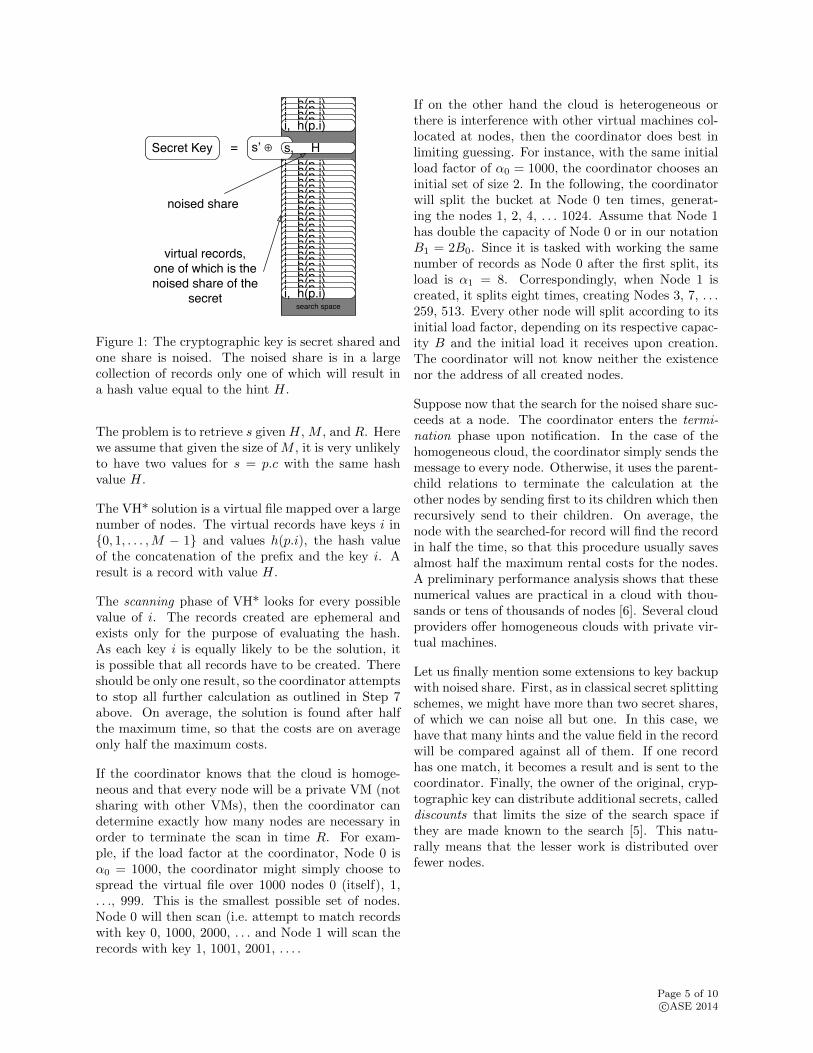
Secret Key = s’ ⊕ s, Hi, h(p.i)

noised share

i, h(p.i)i, h(p.i)i, h(p.i)i, h(p.i)i, h(p.i)i, h(p.i)i, h(p.i)i, h(p.i)i, h(p.i)i, h(p.i)

i, h(p.i)i, h(p.i)i, h(p.i)i, h(p.i)i, h(p.i)i, h(p.i)i, h(p.i)i, h(p.i)i, h(p.i)i, h(p.i)i, h(p.i)i, h(p.i)i, h(p.i)i, h(p.i)i, h(p.i)i, h(p.i)i, h(p.i)i, h(p.i)i, h(p.i)i, h(p.i)i, h(p.i)i, h(p.i)i, h(p.i)

i, h(p.i)i, h(p.i)i, h(p.i)i, h(p.i)i, h(p.i)

virtual records, one of which is the noised share of the

secret

Figure 1: The cryptographic key is secret shared andone share is noised. The noised share is in a largecollection of records only one of which will result ina hash value equal to the hint H.

The problem is to retrieve s given H, M , and R. Herewe assume that given the size of M , it is very unlikelyto have two values for s = p.c with the same hashvalue H.

The VH* solution is a virtual file mapped over a largenumber of nodes. The virtual records have keys i in{0, 1, . . . ,M − 1} and values h(p.i), the hash valueof the concatenation of the prefix and the key i. Aresult is a record with value H.

The scanning phase of VH* looks for every possiblevalue of i. The records created are ephemeral andexists only for the purpose of evaluating the hash.As each key i is equally likely to be the solution, itis possible that all records have to be created. Thereshould be only one result, so the coordinator attemptsto stop all further calculation as outlined in Step 7above. On average, the solution is found after halfthe maximum time, so that the costs are on averageonly half the maximum costs.

If the coordinator knows that the cloud is homoge-neous and that every node will be a private VM (notsharing with other VMs), then the coordinator candetermine exactly how many nodes are necessary inorder to terminate the scan in time R. For exam-ple, if the load factor at the coordinator, Node 0 isα0 = 1000, the coordinator might simply choose tospread the virtual file over 1000 nodes 0 (itself), 1,. . ., 999. This is the smallest possible set of nodes.Node 0 will then scan (i.e. attempt to match recordswith key 0, 1000, 2000, . . . and Node 1 will scan therecords with key 1, 1001, 2001, . . . .

If on the other hand the cloud is heterogeneous orthere is interference with other virtual machines col-located at nodes, then the coordinator does best inlimiting guessing. For instance, with the same initialload factor of α0 = 1000, the coordinator chooses aninitial set of size 2. In the following, the coordinatorwill split the bucket at Node 0 ten times, generat-ing the nodes 1, 2, 4, . . . 1024. Assume that Node 1has double the capacity of Node 0 or in our notationB1 = 2B0. Since it is tasked with working the samenumber of records as Node 0 after the first split, itsload is α1 = 8. Correspondingly, when Node 1 iscreated, it splits eight times, creating Nodes 3, 7, . . .259, 513. Every other node will split according to itsinitial load factor, depending on its respective capac-ity B and the initial load it receives upon creation.The coordinator will not know neither the existencenor the address of all created nodes.

Suppose now that the search for the noised share suc-ceeds at a node. The coordinator enters the termi-nation phase upon notification. In the case of thehomogeneous cloud, the coordinator simply sends themessage to every node. Otherwise, it uses the parent-child relations to terminate the calculation at theother nodes by sending first to its children which thenrecursively send to their children. On average, thenode with the searched-for record will find the recordin half the time, so that this procedure usually savesalmost half the maximum rental costs for the nodes.A preliminary performance analysis shows that thesenumerical values are practical in a cloud with thou-sands or tens of thousands of nodes [6]. Several cloudproviders offer homogeneous clouds with private vir-tual machines.

Let us finally mention some extensions to key backupwith noised share. First, as in classical secret splittingschemes, we might have more than two secret shares,of which we can noise all but one. In this case, wehave that many hints and the value field in the recordwill be compared against all of them. If one recordhas one match, it becomes a result and is sent to thecoordinator. Finally, the owner of the original, cryp-tographic key can distribute additional secrets, calleddiscounts that limits the size of the search space ifthey are made known to the search [5]. This natu-rally means that the lesser work is distributed overfewer nodes.

Page 5 of 10c©ASE 2014

0.2 0.4 0.6 0.8 1.0

0.5

1.0

1.5

2.0

Α=2, Β=2

Α=4, Β=4

-2 -1 1 2

0.2

0.4

0.6

0.8

1.0 truncated normal

normal

Figure 2: PDF for the two beta distributions (top)and the truncated normal distribution and normaldistribution (bottom).

EXAMPLE TWO: KNAPSACK PROBLEM

The client application considers a number Q of ob-jects, up to about 40 or 50. Each object has a cost cand a utility u. The client looks for the top-k sets (kin the few dozens at most) of objects that maximizethe aggregated utilities of the objects in the set whilekeeping the total costs below a cost limit C. Addi-tionally, the client wants to obtain the limit in timeless than R. Without this time limit, the knapsackproblem is a famously complex problem that arises inthis or a more general form in many different fields.It is NP-complete [11] and also attractive to databasedesigners [10].

To apply VH* to solve a knapsack problem of mediumsize with time limit, the client first numbers the ob-jects 0, 1, . . ., Q−1. Then the client creates a virtualkey space of {0, 1, . . .M = 2Q}. Each element of thekey space encodes a subset of {0, 1, . . . Q− 1} in theusual way. Bit ν of the key is set if and only if ν is anelement of the subset. If we denote by iν the value ofbit ν in the binary representation of i, then the valuefield for the virtual record with key i is

Q−1∑ν=0

iνuν ,

Q−1∑ν=0

iνcν

In other words, the value field consists of the utilityand the costs of the set encoded by the key. A matchattempt involves the calculation of the field and thedecision whether it is a feasable solution and is in thetop K of the records currently seen by the node. Atthe end of the scanning phase, each node has gener-ated a local top-k list.

In the termination phase, the local top k-lists areaggregated into a single top-k list. Following the ter-mination protocol is SF , this is done by the clientor by the cloud, with the advantages and disadvan-tages already outlined. In the cloud, we can aggre-gate by letting each child send its top-k list to theparent. When the parent has received all these lists,

1000 2000 3000 4000 5000M�B

0.5

0.6

0.7

0.8

0.9

1.0

Α

0.50.4

0.3

0.2

0.1

betaH2,2L0

1000 2000 3000 4000 5000M�B

0.5

0.6

0.7

0.8

0.9

1.0

Α

0.5

0.40.3

0.2

0.10betaH4,4L

1000 2000 3000 4000 5000M�B

0.5

0.6

0.7

0.8

0.9

1.0

Α

0.5

0.40.3

0.2

0.10

truncated normal

Figure 3: Values for average load factor α dependenton normalized total load M/B for three different dis-tributions. The labels give a measure of heterogeneityas explained in the text.

it creates an aggregated top-k list and sends it to itsparent. When Node 0 has received its lists and ag-gregates them, it sends the result as the final resultto the client.

Our procedure gives the exact solution to the knap-sack problem with a guaranteed termination time us-ing a cloud, which is a first to the best of our knowl-edge. Preliminary performance analysis shows thatvalues of Q ≈ 50 and R in the minutes are practicalif we can use a cloud with thousands of nodes. Suchclouds are offered by several providers.

An heuristic strategy for solving a knapsack problemthat is just too large for the available or affordable

Page 6 of 10c©ASE 2014

resources is to restrict ourselves to a random samplingof records. In the VH* solution, we determine thetotal feasible number of nodes and use the maximumload for any node. Each node uses a random numbergenerator to materialize only as many virtual recordsas it has capacity, that is, exactly B records, eachwith a key K = i + random(0,M − 1)2jN0. Theresulting random scan yields a heuristic, sub-optimalsolution that remains to be analyzed.

Our algorithm is a straight-forward brute force method.It offers a feasible solution where known single ma-chine OR algorithms fail. The method transfers im-mediately to problems of integer linear programming.There is much room for further investigation here.

VH* PERFORMANCE

The primary criteria for evaluation are (1) the re-sponse time and (2) the costs of renting nodes in thecloud. We can give average and worst case numbersfor both. The worst response time for both of ourexamples is R (with an adjustment for the times toinitialize and shut down the system), but with the keyrecovery problem, we will obtain the key on average inhalf the time, whereas for the knapsack problem theaverage value is very close to R. These values dependon the homogeneity of the cloud and whether the co-ordinator succeeds into taking heterogeneity into ac-count.

At a new node, the total time consists of the alloca-tion time, the start time to begin the scan, the timefor the scan, and the termination time. Scan time isclearly bound by R. Allocation involves communica-tion with the data center administrator and organi-zational overhead such as the administrator’s updat-ing allocation tables. This time usually requires lessthan a second [4] and is therefore negligible even whenthere are many round of allocation. The start timeinvolves sending a message to the node and the nodestarting the scan. Since no data is shipped (otherthan the file scheme SF ) this should take at worstmilli-seconds. The time to start up a node is thatof waking up a virtual machine. Experiments withVagrant VM have shown this time to be on average2.7 seconds [4].

While individual nodes might surpass R only negligi-bly, this is not true if we take the cumulative effects ofallocations by rounds into account. Fortunately, forVH∗, there will be about logN rounds. The largestclouds for rent may have 107 nodes, so that the num-ber of round is currently limited to 17 and might be

as small as 1.

The provider determines the cost structure of usingthe cloud. There is usually some fee for node setupand possibly costs for storage and network use. Ourapplications have more than enough with the minimaloptions offered. There is also a charge per time unit.In the case of VH∗, the use time is basically the scantime. The worst case costs are given by c1N + c2RNwhere c1 are the fixed costs per node and c2 the costsper time unit per node. The value of N depends onthe exact strategy employed by the coordinator.

A cloud can be homogeneous (all nodes have the samecapacity B) in which case every node has the same ca-pacity B. The coordinator then chooses a static strat-egy by choosing Nc to be the minimum number ofnodes without overloading. In this case, all nodes areset up in parallel in a single round and the maximumresponse time is essentially equal to R. If α0 is theload factor when the coordinator tests its capacity,then it will allocate N = Nc = α0 = dM/B0e nodesand the maximum cloud cost is c1α0 + c2α0R. Theaverage cost in this case depends on the application.While the knapsack problem causes them to be equalto the maximum cost, the key recovery problem useson average only half of R before it finds the soughtvalue. The average cost is then c1α0 + (1/2)c2α0R.

The general situation is however clearly that of a het-erogeneous cloud. The general choice of the coordi-nator is Nc = 1. The VH∗ structure then only growsby splits. The split behavior will depend on the loadfactor M/B and on the random node capacities inthe heterogeneous cloud. If the cloud is in fact ho-mogeneous unbeknown to the coordinator, then thenode capacity Bn at each node n is identical to theaverage node capacity B. In each round, each noden makes then identical split decisions and splits willcontinue until αn ≤ 1 at every node n. Therefore,VH∗ faced with a total load of M and an initial loadfactor α0 = M/B will allocate N = 2dlog2(α0)e nodes,which is the initial load rounded up to the next inte-ger power of two. Each node will have a load factorα = α02−dlog2(α0)e which varies between 0.5 and 1.0.The maximum scan time is equal to αR. The cloudcosts are c1N + c2αNR if we have to scan all records(the knapsack problem) and c1N + 0.5c2αNR for thekey-recovery problem.

We also simulated the behavior of VH∗ for variousdegrees of heterogeneity. We assumed that the ca-pacity of the node follows a certain distribution. Inthe absence of statistical measurements of cloud nodecapacities, we assumed that very large and very small

Page 7 of 10c©ASE 2014

capacities are impossible. Observing very small nodecapacities is a violation of quality of service guaran-tees, and the virtual machine would be migrated toanother setting. Very large capacities are impossiblesince the performance of a virtual machine cannotbe better than that of the host machine. Therefore,we can only consider distributions that yield capacityvalues in an interval. Since we have no argument foror against positive or negative skewness, we pickedsymmetric distributions in an interval (1 − δ)B and(1+δ)B and chose δ ∈ {0, 1/10, 2/10, 3/10, 4/10, 5/10}.For δ = 0, this models a homogeneous cloud. Ifδ = 5/10, then load capacities lie between 50% and150% of the average node capacity.

For the distributions, we picked a beta distributionwith shape parameters α = 2, β = 2, a beta distri-bution with shape parameters α = 4, β = 4, and atruncated normal distribution in the interval (1−δ)Band (1+δ)B where the standard deviation of the nor-mal distribution was δB. The truncated normal dis-tribution is generated by sampling from the normaldistribution, but rejecting any value outside of theinterval. We depict the probability density functionsof our distributions in Figure 2.

Figure 3 shows the average load factor α in depen-dence on the normalized total load M/B. This valueis the initial load factor α0 in the homogeneous case.In the homogeneous case, the average load factorshows a sawtooth behavior with maxima of 1 whenM/B is an integer power of two. For low hetero-geneity, the oscillation is less pronounced around thepowers of two. With increasing heterogeneity the de-pendence on the normalized total load decreases. Wealso see that α averaged over the normalized load be-tween 512 and 4096 decreases slightly with increasingheterogeneity. As we saw, it is exactly 0.75 for the ho-mogeneous case, and we measured 0.728 for δ = 0.1,0.709 for δ = 0.2, 0.692 for δ = 0.3, 0.678 for δ = 0.4,and 0.666 for δ = 0.5 in the case of the beta distri-bution with parameters α = 2, β = 2. We attributethis behavior to two effects. If a node has a lowerthan average capacity it is more likely to split in thelast round increasing the number of nodes. If the newnode has larger than usual capacity, then the addi-tional capacity is likely to remain unused. Increasedvariation in the node capacities then has only nega-tive consequences and the average load factor is likelyto decrease with variation.

In the heterogeneous case, the total number of nodesis N = M/(αB) and the average scan time is αR.The cloud costs are c1N + c2αNR for the knapsack

Node 0

2.1

Node 1

2.8

Node 2

1.5

Node 3

3.6

Node4

2.2

Node 5

2.0

Node 6

3.8

Node 7

3.1

Node 8

2.6

Node 9

2.1

Node 103.0

Node 113.5

Node 121.0

Node 131.7

Node 14 1.2

Node 152.7

Node 212.5

Node 243.4

Node183.7

Node 252.3

Node 261.8

50

25

12.5

Node 0

2.1 25

Node 1

2.8 12.5

Node 0

2.1 12.5 12.5

Node 2

1.5

Node 3

3.6 6.3

Node 1

2.8 6.3

Node 0

2.1 6.3 6.3 6.36.3 6.3 6.3

Node4

2.2

Node 5

2.0

Node 6

3.8

Node 7

3.1

Node 2

1.5

Node 3

3.6 3.6

Node 1

2.8 2.8

Node 0

2.1 2.1 3.2 3.22.2 3.8 3.1

4.2 3.5 3.2 2.6 4.1 3.2 2.5 3.3

Node 8

2.6

Node 9

2.1

Node 103.0

Node 113.5

Node 121.0

Node 131.7

Node 14 1.2

Node 152.7

Node4

2.2

Node 5

2.0

Node 6

3.8

Node 7

3.1

Node 2

1.5

Node 3

3.6 3.6

Node 1

2.8 2.8

Node 0

2.1 2.1 1.5 2.02.2 3.8 3.1

2.6 2.1 3.0 2.6 2.1 1.7 1.2 2.7

1.7 1.2

1.6 1.4 0.2

Node 283.5 2.1

Node 292.7 1.5

Node 30 2.3 1.3

Node 311.1 0.6

Node 212.5

Node 243.4

Node183.7

Node 252.3

Node 261.8

Node 8

2.6

Node 9

2.1

Node 103.0

Node 113.5

Node 121.0

Node 131.7

Node 14 1.2

Node 152.7

Node4

2.2

Node 5

2.0

Node 6

3.8

Node 7

3.1

Node 2

1.5

Node 3

3.6 3.6

Node 1

2.8 2.8

Node 0

2.1 2.1 1.5 2.02.2 3.8 3.1

2.6 2.1 3.0 2.6 1.0 1.7 1.2 2.7

1.7 1.2

1.6 1.4 0.2

Node 283.5 2.1

Node 292.7 1.5

Node 30 2.3 1.3

Node 311.1 0.6

Node 442.2 1.1

Figure 4: Example of the creation of a file using scal-able partitioning with limited load balancing.

problem and c1N + 0.5c2αRN in the key-recoverycase.

III SCALABLE DISTRIBUTED VIRTUALRANGE PARTITIONING

Scalable distributed virtual range partitioning or VR∗SDVS partitions the virtual key space [0,M) into Nsuccessive ranges

[0,M1) ∪ [M1,M2) ∪ . . . ∪ [MN−1,M)

Each range is mapped to a single and different nodesuch that [Ml,Ml+1) is mapped to Node l. The VR*mapping of keys by ranges allows to easily tune theload distribution over a heterogeneous cloud with re-spect to the hahs-based VH* mapping. This poten-tially reduces the extent of the file and hence thecosts of the cloud. The extent may be the minimalextent possible, i.e., the file is a compact file by anal-ogy with a well-known B-tree terminology. In thiscase, the load factor is α = 1 at each node. However,it can penalize the start time, and hence the responsetime.

Page 8 of 10c©ASE 2014

For the range j located on Node j, Mj−1 is the min-imal key while Mj − 1 is the maximum key. Thecoordinator starts by creating the file at one node,namely itself, with a range of [0,M). Next, as forVH*, the coordinator generates an initial mappingusing N0 nodes, where each node j carries the rangeof keys [Mj−1,Mj) each of the same length of M/N0.The coordinator chooses N0 = dα0e based on its ini-tial load factor. In an homogeneous cloud, the loadfactor at each node is therefore ≤ 1 and optimal. Thisyields a compact file.

In a heterogeneous cloud, we split every node withload factor α > 1. The basic scheme divides the cur-rent range into two equal halves. However, we canalso base the decision on the relative capacities ofthe nodes [6]. In previous work on recoverable en-cryption, we have the splitting node obtain the ca-pacity of itself and of the new node. This impliesthat the new node has to determine its capacity first,which implies scanning a certain number of records.Only then do we decide on how to split. This ap-pears to be a waste of time, but we notice that therecords used to assess the capacity are records thathave to be scanned anyway. Thus, postponing thedecision how to split does not mean that we loosetime processing records. However, if the second nodealso needs to split, then we have waited for bringingin the latest node. This means that these schemes donot immediately use all necessary nodes. If there aremany rounds of splitting, then the nodes that enterthe scheme latest either have to do less work or mightnot finish their work by the deadline. All in all, an op-timized protocol needs to divide the load among thenecessary number of nodes in a single step as muchas possible.

The scheme proposed in our previous work (scalablepartitioning with limited load balancing) [6] splitsevenly until the current load factor is ≤ 3. If a nodehas reached this bound through splits, we switch to adifferent strategy. The splitting node assigns to itselfall the load that it can handle and gives to the newnode the remaining load. There are two reasons forthis strategy: First, there is the mathematical ver-sion (the 0-1 law) of Murphy’s law: If there are manyinstances – in our case thousands of nodes – then badthings will happen with very high probability if theycan happen at all – in our case, one node will exhaustalmost all its allotted time to finish. Therefore, thereis no harm done by having a node use the maximumallotted time. Second, by assuming the maximumload, we minimize the load at the new node. There-fore, the total number of splits starting with the new

node is less likely. We also note that the new nodedoes not have to communicate its capacity with thesplitting node. The reason for not using this strategyfrom the beginning is that we want to reach close tothe necessary number of nodes as soon as possible.Thus, if the node load is very high, the current loadneeds to be distributed among many nodes and we doso more efficiently by splitting evenly. The number ofdescendants will then be about equal for both nodes.

We give a detailed example in Figure 4. The boxescontain the name of the node, which is its numberaccording to LH* addressing and encodes the parent-child relationship. With each node, we have the ca-pacity and outside the box, the current load. We gen-erated the capacities using a beta-distribution withparameters α = 4 and β = 2 and mean 8/3, but thenrounded to one fractional digit. In the first panel, theinitial load of 50 is assigned to Node 0 with a capacityof 2.1. This node makes a balanced split, requestingNode 1 and giving it half of its load. Both nodes splitagain in a balanced way, Node 0 gives half of its loadto Node 2 and Node 1 to Node 3. All four nodesare still overloaded and make balanced splits (fourthpanel). The load at all nodes is (rounded up) 6.3. Allnodes but Node 2 and Node 5 have capacity at leastone third of the load and split in an unbalanced way.For instance, Node 0 requests Node 8 to take care ofa load of 4.2 while it only assigns itself a load equal toits capacity, namely 2.1. Nodes 2 and 5 however makea balanced split. As a result, in the fifth panel, var-ious nodes are already capable of dealing with theirload. Also, all nodes that need to split have now atleast capacity one third of their assigned load. Afterthe splits, we are almost done. We can see in thesixth panel that there is only one node, namely Node12, that still needs to split, giving rise to Node 44(= 12+32). We have thus distributed the load over atotal of 26 nodes. Slightly more than half, namely 15nodes are working at full capacity. We notice that ourprocedure made all decisions with local information,that of the capacity and that of the assigned load. Ofthis, the assigned load is given and the capacity needsto be calculated only once. A drawback to splittingis that the final node to be generated, Node 44 in theexample, was put into service in the sixth generation,meaning that excluding its own capacity calculation,there were five times that a previous node generatedthe capacity. If we can estimate the average capacityof nodes reasonably well, we can avoid this by havingNode 0 use a conservative estimate to assign loads toa larger first generation of nodes.

A final enhancement uses the idea of balancing from

Page 9 of 10c©ASE 2014

B-trees. If a node has a load factor just a bit over1, it contacts its two neighbors, namely the nodesthat have the range just below and just above its ownrange to see whether these neigbors have now a loadfactor below 1. If this is the case, then we can handover part of the current node’s range to the neighbor.

We have shown by simulation that these enhance-ments can be effective, but that their effects dependheavily on assumptions about the heterogeneity ofthe nodes [6]. For an exact assessment, we need to ex-periment with actual cloud systems. As has becomeclear from our discussion, the final scheme shouldguess the number of nodes necessary, allocate them,verify that the capacity is sufficient and accept thatsometimes local nodes need to redistribute the work.We leave the exact design of such a protocol and itsevaluation through experiments and simulations tofuture work.

IV CONCLUSIONS

Scalable distributed hash and range partitioning arecurrently the basic structures to store very large datasets (big data) in the cloud. VH∗ and VR∗ applytheir design principles to very large virtual data setsin the cloud. They form possibly minimal clouds for agiven time limit for a complete scan. They work withhomogeneous and, more importantly because morefrequent, heterogeneous clouds. These schemes con-stitute to the best of our knowledge the first cloud-based and - more importantly - fixed execution timesolutions to two important applications, namely keyrecovery and knapsack problems.

Further work should implement these schemes at alarge scale and add details to the performance analy-sis. For instance, the behavior of actual node capac-ity in commercial cloud solutions needs to be mea-sured so that performance modeling can be placedon a firmer foundation.

The two schemes can be used for other difficult prob-lems in Operations Research such as 0-1 integer linearprogramming or the traveling salesman problem. Theproblems amenable to these solutions are search prob-lems where a large, search space S = {si|i = 1, . . .M}has to be scanned in fixed time.

References

[1] S. Abiteboul, I. Manolescu, P. Rigaux, M.-C.Rousset, P. Senellart et al.: Web data manage-

ment, Cambridge University Press, 2012.[2] F. Chang, J. Dean, S. Ghemawat, W. Hsieh, D.

Wallach, M. Burrows, T. Chandra, A. Fikes, andR. Gruber. “Bigtable: A distributed storage sys-tem for structured data.” ACM Transactions onComputer Systems (TOCS) 26, no. 2 (2008):4.

[3] J. Dean and S. Ghemawat. “MapReduce: simpli-fied data processing on large clusters.” Commu-nications of the ACM 51, no. 1 (2008): 107-113.

[4] W. Hajaji. “Scalable partitioning of a dis-tributed calculation over a cloud”. Master’sThesis, Universite Paris, Dauphine, 2013 (inFrench).

[5] S. Jajodia, W. Litwin, and T. Schwarz. “KeyRecovery using Noised Secret Sharing with Dis-counts over Large Clouds”. Proceedings ASE /IEEE Intl. Conf. on Big Data, Washington D.C.,2013.

[6] S. Jajodia, W. Litwin, T. Schwarz. “RecoverableEncryption through a Noised Secret over a LargeCloud”. Transactions on Large-Scale Data andKnowledge-Centered Systems 9, Springer, LNCS7980, pages 42-64, 2013

[7] W. Litwin, M.-A. Neimat, and D. A. Schneider.“LH∗: Linear Hashing for distributed files”. Pro-ceedings of ACM SIGMOD international confer-ence on management of data, 1993.

[8] W. Litwin, M.-A. Neimat, and D. Schneider.“RP*: A family of order preserving scalable dis-tributed data structures.” In VLDB, vol. 94, pp.12-15. 1994.

[9] W. Litwin, M.-A. Neimat, and D. Schneider.“LH∗ - a scalable, distributed data structure.”ACM Trans. on Database Systems (TODS) 21,no. 4 (1996): 480-525.

[10] W. Litwin and T. Schwarz. “Top kKnapsack Joins and Closure.” Keynoteaddress, Bases de Donnees Avancees2010, Toulouse, Fr, 19-22 Oct. 2010www.irit.fr/BDA2010/cours/LitwinBDA10.pdf

[11] S. Martello and P. Toth. Knapsack problems: al-gorithms and computer implementations. JohnWiley and Sons, Inc., 1990.

[12] A. Rajaraman, J. Leskovec, and J. Ullman. Min-ing of massive datasets. Cambridge UniversityPress, 2012.

[13] Vagrant. www.vagrantup.com[14] M. Zaharia, A. Konwinski, A. Joseph, R. Katz,

and I. Stoica. “Improving MapReduce Per-formance in Heterogeneous Environments.” InProc. of Symp. on Operating Systems Designand Implementation (OSDI), 2008.

Page 10 of 10c©ASE 2014