Wavelet-Based L-infinite Scalable Coding

A. Alecu, A. Munteanu, P. Schelkens, J. Cornelis and S. Dewitte

Authors’ affiliations:

A. Alecu, A. Munteanu, P. Schelkens, J. Cornelis and S. Dewitte (Vrije Universiteit Brussel,

Dept. of Electronics and Information Processing, Pleinlaan 2, 1050 Brussels, Belgium,

aalecu@etro.vub.ac.be)

S. Dewitte (Royal Meteorological Institute of Belgium, Ringlaan 3, 1180 Brussels, Belgium)

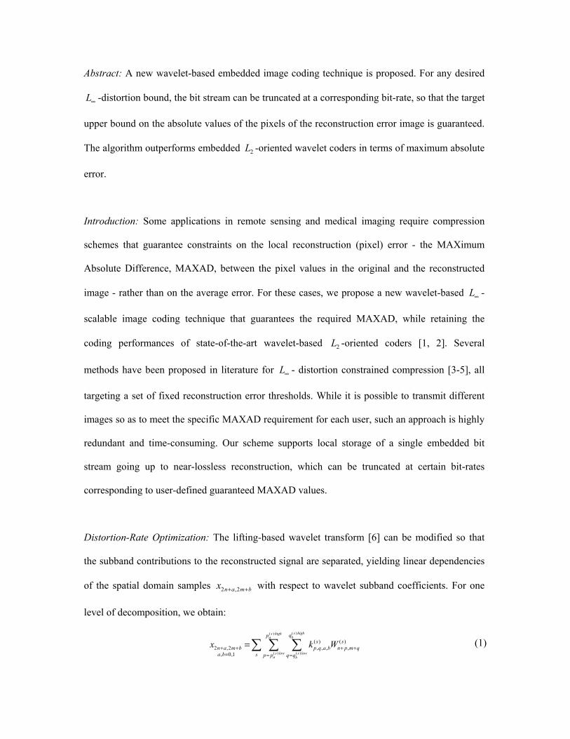
Abstract: A new wavelet-based embedded image coding technique is proposed. For any desired

L∞ -distortion bound, the bit stream can be truncated at a corresponding bit-rate, so that the target

upper bound on the absolute values of the pixels of the reconstruction error image is guaranteed.

The algorithm outperforms embedded 2L -oriented wavelet coders in terms of maximum absolute

error.

Introduction: Some applications in remote sensing and medical imaging require compression

schemes that guarantee constraints on the local reconstruction (pixel) error - the MAXimum

Absolute Difference, MAXAD, between the pixel values in the original and the reconstructed

image - rather than on the average error. For these cases, we propose a new wavelet-based L∞ -

scalable image coding technique that guarantees the required MAXAD, while retaining the

coding performances of state-of-the-art wavelet-based 2L -oriented coders [1, 2]. Several

methods have been proposed in literature for L∞ - distortion constrained compression [3-5], all

targeting a set of fixed reconstruction error thresholds. While it is possible to transmit different

images so as to meet the specific MAXAD requirement for each user, such an approach is highly

redundant and time-consuming. Our scheme supports local storage of a single embedded bit

stream going up to near-lossless reconstruction, which can be truncated at certain bit-rates

corresponding to user-defined guaranteed MAXAD values.

Distortion-Rate Optimization: The lifting-based wavelet transform [6] can be modified so that

the subband contributions to the reconstructed signal are separated, yielding linear dependencies

of the spatial domain samples 2 ,2n a m bx + + with respect to wavelet subband coefficients. For one

level of decomposition, we obtain:

( )( )

( ) ( )

( ) ( )2 ,2 , , , ,

, 0,1

s highs higha b

s low s lowa b

qps s

n a m b p q a b n p m qa b s p p q q

x k W+ + + += = =

=∑ ∑ ∑ (1)

where s identifies the four subbands and ( ),

sn p m qW + + are the wavelet coefficients belonging to

subband s that contribute to 2 ,2n a m bx + + . For every s, these coefficients define a window in the

wavelet domain of dimensions ( ) ( ) ( ) ( )( 1) ( 1)s high s low s high s lowa a b bp p q q− + × − + , located around and

including a central coefficient ( ),s

n mW , the position within the window being referred to by the

indices p,q (see Fig.1). For every such position there exists a corresponding constant coefficient

contribution factor ( ), , ,s

p q a bk ∈ , derived from the prediction and update coefficients of the lifting-

based wavelet transform.

The wavelet coefficients are fed into uniform quantizers with bin size ( , )s l∆ in each subband s of

decomposition level l. Hence, the upper bounds of the subband absolute errors are equal to

( , ) 2s l∆ . It can easily be shown that the linearity of eq. (1) is extended to the absolute error signal

components. As a result, for L levels of decomposition, one may write the upper bound of the

error signal as:

( ) ( ) ( ) ( )(LL, ) (LH, ) (HL, ) (HH, )1 1 1(LL) (LL) (LH) (LL) (HL) (LL) (HH)

, , , , , , ,12 2 2 2

L l l lLL l l l

a b a b a b a b a b a b a bl

M K K K K K K K− − −

′ ′ ′ ′ ′ ′ ′ ′ ′ ′ ′ ′ ′ ′=

∆ ∆ ∆ ∆= + + +

∑ (2)

where ( ) ( )

( ) ( )

( ) ( ), , , ,

s high s higha b

s low s lowa b

p qs s

a b p q a bp p q q

K k′ ′

′ ′

′ ′ ′ ′= =

= ∑ ∑ and ,a b′ ′ are derived from the one-level decomposition

situation, i.e. ( )( ,1)

( ),

, 0,1, arg max

2

ss

a ba b s

a b K=

∆′ ′ = ∑ . The proof of this proposition, and the analytical

expressions of eq. (2) for the most popular wavelet transforms, are given in [7].

We express the total bit rate in terms of the relative sizes ( , )s lβ of each subband ( , )s l with

respect to the original image size, and the rate contributions ( , ) ( , ) ( , )2log ( )s l s l s lR B= ∆ , with ( , )s lB

equal to the quantizer range [8]. By solving the D-R problem of minimizing the Rate given a

Distortion 0M , one easily obtains the set of solutions ( , ),{ }s l

s l∆ .

Scalable Coding: We derive for each subband ( , )s l a family of embedded quantizers, consisting

in a highest-rate symmetric uniform scalar quantizer 0

( , )s lQ , with quantization bin width ( , )0s l∆ ,

and lower-rates embedded deadzone uniform scalar quantizers ( , )n

s lQ , with zero-bin widths

( )( , ) 1 ( , ), 02 1s l n s l

zerobin n+∆ = − ∆ and widths ( , ) ( , )

, 02s l n s lbin n∆ = ∆ for all other bins, where n ∗∈ identifies

the number of discarded bit-planes.

Initial bin sizes ( , )0,s linitial∆ are computed for the quantizers

0

( , )s lQ , by solving the D-R optimization

problem. The resulting system is independent of the input signal and guarantees the L∞ -bound,

0M M= , expressed in eq. (2). The obtained MAXAD is in practice however smaller than 0M ,

due to the worst-case assumption of eq. (2). This drawback can be overcome by scaling up the

bin sizes while at the same time guaranteeing the required MAXAD. Thus, the quantizers 0

( , )s lQ

are optimized for the MAXAD 0M , by introducing a further refinement of the bin sizes to

( )( , ) ( , )0 0,

ls l s lf initialα∆ = ∆ , where the scaling factors ( )l

fα are given by:

( ) ( )

1

ll k

fk

α α=

= ∏ (3)

Let us denote by ( , )s lε the error contribution of subband ( , )s l , 1l L= … , to the total

reconstruction error. The cumulated error contributions can be written as ( ) ( , )L

L s l

l L sε ε

′′

=

=∑∑ ,

1 L L′≤ ≤ , and, moreover, according to the central limit theorem [9], can be modeled as having

Gaussian distributions. In view of these, the constants ( )lα can be derived according to the

following equation:

( )

0( ) ( )

erf 12

l

l l

Mβα σ ⋅

(4)

where ( )lβ is the relative size of the cumulated subbands from L to l and ( )lσ is the standard

deviation of ( )lε . The derivation of different scaling factors per decomposition level offers

superior compression performance compared to the derivation of a common scaling factor for all

{ }( , )0, ,

s linitial s l

∆ .

A) Encoding: Lossless coding of the quantized wavelet coefficients is performed using the QT-L

(QuadTree-Limited) coding technique described in [2]. The SAQ (successive approximation

quantization) principle employed in this algorithm, combined with the raster-scanning of the

subbands, enables us to organize our bitstream in a multi-layer, MAXAD progressive manner.

For 0n = , i.e. near-lossless compression, the standard deviations of the Gaussian distributions of

the error contributions of every subband ( , )s l , which we denote as ( , )0

s lσ , are inserted in a header

at the beginning of the bit stream, together with the quantization bin sizes ( , )0s l∆ .

B) Decoding: For every n, every family ( , )s l of embedded quantizers ( , )n

s lQ generates a Gaussian

error contribution having a standard deviation upper bound ( , ) 1 ( , )0(2 1)s l n s l

nσ σ+= − . We can derive

the upper bound ( , )s lnM of the error contribution of subband ( , )s l by solving the following

equation:

( , )

( , )erf 1

2

s ln

s ln

Mσ

(5)

In a similar manner, one can establish the upper bound nM for all the subbands combined, i.e.

for an entire bitplane.

Based on the standard deviations ( , )0

s lσ , the decoding decision process commences by computing

the upper bounds nM corresponding to each complete bit-plane n, where 1 0n N= − … , and N is

the total number of bitplanes. Subsequently, we select the two consecutive bit-planes 1n + and n

between which the desired user-defined MAXAD is located. The process continues by

computing the upper bounds ( , )1

s lnM + of the already received subbands, combined with the upper

bounds ( , )s lnM corresponding to the bit-plane n of each additional subband ( , )s l to be received.

The decision process stops once the decision is made concerning which additional subband bit-

planes n must be received.

Experimental Results: Compression results are given in Table 1, for different target MAXAD

values, comparing the results obtained by our Embedded Wavelet Maxad Coder (E-WMC)

against those obtained by the embedded 2L -oriented SPIHT [1] and QT-L [2] schemes, operating

at the same bit-rates. The obtained MAXAD is denoted in these tables as e∞

; the guaranteed

MAXAD, for the same bit-rate is denoted as g∞

.

E-WMC offers a guaranteed MAXAD that is comparable to the MAXAD obtained at the same

bit-rate by SPIHT and QT-L. In practice the obtained MAXAD is always slightly lower or at

most equal to the guaranteed MAXAD; we conclude that on average E-WMC outperforms

SPIHT and QT-L in terms of MAXAD, while remaining competitive in terms of PSNR.

Conclusions: Our new wavelet-based L∞ -scalable image coder outperforms state-of-the-art 2L -

oriented compression schemes in terms of MAXAD distortion, retaining comparable PSNR

values. Moreover, it supports progressive, controlled refinement of the MAXAD.

References

1. SAID, A. and PEARLMAN, W. A.: 'A New Fast and Efficient Image Codec Based on

Set Partitioning in Hierarchical Trees', IEEE Trans. Circuits and Systems for Video

Technology, 1996, 6, pp. 243-250

2. SCHELKENS, P., MUNTEANU, A., BARBARIEN, J., GALCA, M., NIETO, X. G. I.

and CORNELIS, J.: 'Wavelet Coding of Volumetric Medical Datasets', IEEE

Transactions on Medical Imaging, 2002, accepted for publication.

3. CHEN, K. and RAMABADRAN, T. V.: 'Near-lossless compression of medical images

through entropy-coded DPCM', IEEE Trans. Medical Imaging, 1994, 13, pp. 538-548

4. WU, X., CHOI, W. K. and BAO, P.: 'L-infinity-constrained high-fidelity image

compression via adaptive context modeling', in Proc. DCC. Snowbird, Utah: DCC, 1997,

pp. 91-100

5. KARRAY, L., DUHAMEL, P. and RIOUL, O.: 'Image Coding with an L-infinite Norm

and Confidence Interval Criteria', IEEE Trans. Image Processing, 1998, 7, pp. 621-631

6. SWELDENS, W.: 'Lifting Scheme: A New Philosophy in Biorthogonal Wavelet

Constructions', in Proc. of SPIE Wavelet Applications in Signal and Image Processing

III, 1995, 2569, pp. 68-79

7. ALECU, A., MUNTEANU, A., SCHELKENS, P., CORNELIS, J. and DEWITTE, S.:

'Wavelet-based fixed and embedded L-infinite-constrained image coding', Technical

Report, Vrije Universiteit Brussel, Dept. ETRO, IRIS-TR-0087, July 2002

8. GERSHO, A. and GRAY, R. M.: 'Vector Quantization and Signal Compression' (Kluwer

Academic Publishers, 1992)

9. PAPOULIS, A.: 'Probability, Random Variables, and Stochastic Processes' (McGraw-

Hill, 1965)

Figure captions:

Figure 1. The dependencies of the image samples 2 ,2n a m bx + + , , 0,1a b = , with respect to the

wavelet coefficients ( ),

sn p m qW + + , { }, , ,s LL LH HL HH∈ , for one level of decomposition.

The reference system ( ),n m refers to the subband s , with the (0,0) coordinates located

in the lower-left corner of each subband.

Table captions:

Table 1. Comparison of PSNR, obtained MAXAD, guaranteed MAXAD and bit-rates obtained

on 8-bit grey value images a) “Lena“, b) an ultrasound image, c) a remote sensing image.

Figure 1.

( )LL lowap

( )LL highap

( )LL highbq( )LL low

bq m m

n

n n

mm

p

q

( ),

LLn p m qW + +

q

q

(0,0)

p

( )HL highbq( )HL low

bq

( )HL lowap

( )HL highap

( ),

HLn p m qW + +

( ),

LHn p m qW + +

( )LH lowap

( )LH highap

n

( )LH highbq( )LH low

bq ( )HH highbq( )HH low

bq

q ( )HH lowap

( )HH highap

( ),

HHn p m qW + +

(0,0)

(0,0) (0,0)

p p

Table 1

a)

b)

c)

QT-L SPIHT E-WMC

PSNR e∞

PSNR e∞ PSNR e

∞ g

∞ bpp

58.87 1 60.46 1 63.00 1 1 4.473 49.93 3 51.73 3 52.15 2 3 3.298 44.72 7 45.27 7 45.49 6 7 2.040 40.17 14 40.36 14 40.22 13 14 0.992

QT-L SPIHT E-WMC

PSNR e∞

PSNR e∞ PSNR e

∞ g

∞ bpp

60.74 1 64.23 1 64.95 1 1 3.511 51.81 3 54.34 3 54.00 2 2 2.592 47.58 6 48.97 6 48.51 5 6 1.886 42.42 13 43.51 14 42.72 12 12 1.269

QT-L SPIHT E-WMC

PSNR e∞

PSNR e∞ PSNR e

∞ g

∞ bpp

58.81 1 60.91 1 63.67 1 1 5.429 50.31 3 52.35 2 52.59 3 3 4.283 45.78 6 46.47 8 46.55 5 7 3.138 40.33 12 40.60 13 40.57 12 14 2.128