
Scalable Computing: - Practice and Experience
131
Scalable Computing: Practice and Experience Scientific International Journal for Parallel and Distributed Computing ISSN: 1895-1767 ⑦ ⑦ ⑦ ⑦ ⑦ ⑦ Volume 19(4) December 2018
-
Upload
khangminh22 -
Category
Documents
-
view
0 -
download
0
Transcript of Scalable Computing: - Practice and Experience
Scalable Computing:Practice and Experience
Scientific International Journalfor Parallel and Distributed Computing
ISSN: 1895-1767
⑦⑦⑦⑦
⑦⑦
t
Volume 19(4) December 2018

Editor-in-Chief
Dana PetcuComputer Science DepartmentWest University of Timisoaraand Institute e-Austria TimisoaraB-dul Vasile Parvan 4, 300223Timisoara, [email protected]
Managinig and
TEXnical Editor
Silviu PanicaComputer Science DepartmentWest University of Timisoaraand Institute e-Austria TimisoaraB-dul Vasile Parvan 4, 300223Timisoara, [email protected]
Book Review Editor
Shahram RahimiDepartment of Computer ScienceSouthern Illinois UniversityMailcode 4511, CarbondaleIllinois [email protected]
Software Review Editor
Hong ShenSchool of Computer ScienceThe University of AdelaideAdelaide, SA [email protected]
Domenico TaliaDEISUniversity of CalabriaVia P. Bucci 41c87036 Rende, [email protected]
Editorial Board
Peter Arbenz, Swiss Federal Institute of Technology, Zurich,[email protected]
Dorothy Bollman, University of Puerto Rico,[email protected]
Luigi Brugnano, Universita di Firenze,[email protected]
Giacomo Cabri, University of Modena and Reggio Emilia,[email protected]
Bogdan Czejdo, Fayetteville State University,[email protected]
Frederic Desprez, LIP ENS Lyon, [email protected]
Yakov Fet, Novosibirsk Computing Center, [email protected]
Giancarlo Fortino, University of Calabria,[email protected]
Andrzej Goscinski, Deakin University, [email protected]
Frederic Loulergue, Northern Arizona University,[email protected]
Thomas Ludwig, German Climate Computing Center and Uni-versity of Hamburg, [email protected]
Svetozar Margenov, Institute for Parallel Processing and Bul-garian Academy of Science, [email protected]
Viorel Negru, West University of Timisoara,[email protected]
Moussa Ouedraogo, CRP Henri Tudor Luxembourg,[email protected]
Marcin Paprzycki, Systems Research Institute of the PolishAcademy of Sciences, [email protected]
Roman Trobec, Jozef Stefan Institute, [email protected]
Marian Vajtersic, University of Salzburg,[email protected]
Lonnie R. Welch, Ohio University, [email protected]
Janusz Zalewski, Florida Gulf Coast University,[email protected]
SUBSCRIPTION INFORMATION: please visit http://www.scpe.org

Scalable Computing: Practice and Experience
Volume 19, Number 4, December 2018
TABLE OF CONTENTS
Special Issue on Mobile Cloud Applications and Challenges:
Introduction to the Special Issue iii
A Survey on Mobile Cloud Computing: Mobile Computing + CloudComputing (MCC = MC + CC) 309
Ramasubbareddy Somula, Sasikala R.
Execution Analysis of Spatial Data Storage Indexing on CloudEnvironment 339
Karthi S., Prabu S.
Enhanced Data Security for Public Cloud Environment with SecuredHybrid Encryption Authentication Mechanisms 351
Prabu S., Gopinath Ganapathy, Ranjan Goyal
Cloud based Dynamic Course Selection Framework using NetworkGraphs with Term Difficulty Estimation 361
Jasem M. Alostad
Parallel Seed Selection Method for Overlapping Community Detectionin Social Network 375
Belfin R.V., E. Grace Mary Kanaga
Regular Papers:
Energy-Efficient Real-Time Scheduling Algorithm for Fault-TolerantAutonomous Systems 387
Hussein EL Ghor, Julia Hage, Nizar Hamadeh, Rafic Hage Chehade
Modelling and Simulation of GPU Processing in the MERPSYSEnvironment 401
Tomasz Gajger, Pawe l Czarnul
A Comparison of Message Passing Interface (MPI) and Co-arrayFORTRAN for Large Finite Element Variably Saturated FlowSimulations 423
Fred T. Tracy, Thomas C. Oppe, Maureen K. Corcoran
c⃝ SCPE, Timisoara 2018


Scalable Computing: Practice and Experience
Volume 19, Number 4, pp. iii–iv. http://www.scpe.org
DOI 10.12694/scpe.v19i4.1499ISSN 1895-1767c⃝ 2018 SCPE
INTRODUCTION TO THE SPECIAL ISSUE ON MOBILE CLOUD APPLICATIONS ANDCHALLENGES
We are happy to present this special issue of thee Scientific Journal Scalable Computing: Practice andExperience. In this special issue on Mobile Cloud Applications and Challenges (Volume 19 No 4 December2018), we have selected five papers, which gone through a peer review according to the journal policy. All thepapers represents novel results in the field of Mobile and Cloud Applications.
The first paper presents overview of mobile cloud computing, cloudlet technology, security and privacyissues and limitations of mobile cloud commuting. The second paper presents a spatial partition, global indexand map reduce operation were studied. The trail results that the proposed indexing cloud framework performsimproved results. The third paper proposes an authentication model along with data security in a publiccloud storage environment which successful detects the unauthenticated access or any anomaly in data. Thefourth paper analyses the student success ratio which uses a cloud based technology to implement and designSaaS. Graph based complex network are used for analysing the course. The fifth paper presents Overlappingcommunity detection in social networks. The proposed algorithm uses parallel processing engine to resolve thedelay problem.
We use this opportunity to thank all the contributors to this special issue. We would like to express ourspecial gratitude for the Editor-in-chief, Professor Dana Petcu for her constant support for carrying this specialissue.
Rajkumar Rajasekaran, Vellore Institute of Technology, India
iii


Scalable Computing: Practice and Experience
Volume 19, Number 4, pp. 309–337. http://www.scpe.org
DOI 10.12694/scpe.v19i4.1411ISSN 1895-1767c⃝ 2018 SCPE
A SURVEY ON MOBILE CLOUD COMPUTING: MOBILE COMPUTING + CLOUDCOMPUTING (MCC = MC + CC)
RAMASUBBAREDDY SOMULA∗AND SASIKALA R†
Abstract. In recent years, the mobile devices become popular for communication and running advanced real time applicationssuch as face reorganization and online games. Although, mobile devices advanced for providing significant benefits for mobile users.But still, these devices suffers with limited recourses such as computation power, battery and storage space due to the portablesize. However, The Cloud Technology overcome the limitations of mobile computing with better performance and recourses. Thecloud technology provides enough computing recourses to run mobile applications as storage computing power on cloud platform.Therefore, the novel technology called mobile cloud computing (MCC) is introduced by integrating two technologies (MobileComputing, Cloud Computing) in order to overcome the limitations(such as Battery life, Storage capacity, Processing capacity) ofMobile Devices by offloading application to recourse rich Remote server. This paper presents an overview of MCC, the advantagesof MCC, the related concepts and the technology beyond various offloading frameworks, the architecture of the MCC, Cloudlettechnology, security and privacy issues and limitations of mobile cloud computing. Finally, we conclude with feature researchdirections in MCC.
Key words: Mobile Computing, Cloud Computing, Mobile Cloud Computing, Cloudlet Selection, Computation offloading,Edge Computing, security.
AMS subject classifications. 15A15, 15A09, 15A23
1. Introduction. Over the past few decades, mobile devices have been playing an important role inour modern and virtual lifestyle. For instance, according to the survey by International Data Corporation(IDC) in 2016, the usage of mobile devices and tablets was increased by 1.6 billion units exponentially [1]. Inrecent years, mobile applications became popular in various categories such as news, entertainment, health,business and social networks. The mobile computing allows users to access all necessary applications fromapplication centres such as Android play store and Apple iTunes etc., irrespective of location. Even mobilecloud computing provides high-end features for running various real time applications but still users demandfor more computing resources. For mobile computing, the mobile devices are designed with limited batterylife, storage capacity, processing capacity and communication capabilities. Mobility is important feature onpervasive computing environment where the user is able to perform his work without any interruption. Thecloud computing is emerging technology which is formed with amalgamation of various technologies such asvirtualization, distributed computing, SOA, web services etc. Cloud computing provides massive computingresources (such as hardware, software, storage) in order to improve the performance of application as well asreducing processing cost. It allows users to access data from any location on demand basis. The mobile devicewill perform high computational tasks on cloud platform which require more computing resources. The cloudcomputing paradigm can be represented through three different service models. Platform as a service (paas),Infrastructure as a service (Iaas), software as a service (saas) as shown in Fig 1.1The author in [2], presentedthe annual growth rate of cloud service models, Iaas is 41%, paas holds 26.6% and Saas holds 17.4%. Theemerging technology, Mobile Cloud Computing has been introduced to overcome limitations of mobile devices.Recently, the mobile users demand for computing is being increased due to the development in mobile computingtechnology. Various studies define the importance and benefit of mobile cloud computing for mobile users andenterprisers. For example, according to the ABI, the usage of mobile devices reached to 280 million by 2015,the revenue of Mobile cloud computing reached to $ 5.2 billion [3]. Currently the growth of advanced mobiledevices developed rapidly with sufficient resources such as battery life, storage, processing power. Nonetheless,it is still suffering from processing real time application such as image recognition,video streaming, languagetranslation. Mobile devices are less compared to server systems and desktop computers in terms of computingpower and storage. When mobile device runs resource intensive task put heavy load on processor and reducebattery life.
∗School of Computer Science and Engineering (SCOPE), VIT University, Vellore, India ([email protected]).†School of Computer Science and Engineering (SCOPE), VIT University, Vellore,India.([email protected])
309

310 Ramasubbareddy Somula and Sasikala R
Fig. 1.1. Cloud Computing Services
Nowadays, the research work on cloud computing is aiming to enhance computing capabilities of mobiledevices by allowing Mobile users to access various service based models such as software, infrastructure andcomputing services. Amazon is one of the cloud service provider which provides security to user personal databy various storage service models (S3) [4]. MCC promises to improve performance of the mobile applicationbeyond mobile computing, with the help of cloud computing [5] [6]. Most of the data generated by the mobiledevice will be video content which is over 78% by 2021 forecast by cisco [7]. The concept of offloading fullyor part of the application into remote cloud environment to address limitations of mobile computing throughservice providers other than the mobile can deploy application on cloud where both storage and computationcan happen out of mobile device is known as Mobile Cloud.
In this paper, we aim to discuss Various categories of research areas in Mobile Cloud Computing such ascomputation offloading, cloudlet selection (or) edge computing, resource provisioning, security, privacy issuesand VM migration techniques. Furthermore, we plan to discuss proposed research works and also upcomingnovel solution for addressing Mobile Cloud Computing issues.
2. Mobile Cloud Computing Overview.
2.1. Definition of Mobile Cloud Computing. MCC is an emerging technology where it fill gap betweenlimited resources of Mobile devices as well as resource intensive applications required to run a resource richenvironment computing. According to the MCC forum definition: the execution of mobile application willhappen outside of mobile device. The computation power and storage of mobile application more to cloudenvironment for processing. The MCC allows mobile users to access computing services, it is not restricted toparticular mobile users [3]. In the second definition [8] [9]. The mobile cloud computing provides computingresources for mobile devices remotely. In the third destination [10] [11], the cloud server does not need to act aspowerful server. But enhancing mobile devices configuration setup in terms of storage and processing capacity.
2.2. Related concepts and technology.
2.2.1. Mobile Computing. Nowadays, Mobile Devices (MD) became an essential equipment for commu-nication in everyone life. Even though mobile devices are able to support real time resource hungry applicationsbut still they are limited in terms of storage, processor and power consumption. In order to address this issues,

A Survey on Mobile Cloud Computing: Mobile Computing + Cloud Computing (MCC = MC + CC) 311
the emerging cloud computing technology provides enough resources to optimize performance of the mobile ap-plications. Generally, mobile computing is a process of executing applications in mobile device and transferringresult to one (or) more devices. Mobile communication is able to make use of centrally located application (or)data with help of small (or) little portable computing devices. This technology make every application to beexecuted in single devices. The usage of mobile devices is increasing day by day, the requirement is to providebetter services for low cost and power consumption also increases. The list of issues in mobile computing isrepresented in following Fig 2.1.
2.2.2. Mobile Network Architecture. The classification of mobile network can be represented as fol-lowing Fig 2.2.
2.2.3. Cellular Architecture. Earlier, the mobile networks were intended to cover huge geographicalarea by using single transmitter with high power consumption. Even conventional architecture covers hugegeographical area, but it does not support frequency reuse technology.
In order to facilitate frequency reuse as well as large coverage, the cellular architecture was brought intomobile networks. This cellular architecture replaces high power consumption transmitter with low power trans-mitters. The large geographical area splits into number of hexagonal cells which are served by base station.
Each cell in cellular network is surrounded by number of independent cell. Each adjacent cell boundarytouches each other. The hexagonal cell covers certain area in geographical location. Each cell is served by nearbybase station. The base station which serves each cell is allotted with certain portion of frequency. The basestation of adjacent cell is allotted with different frequency ranges to overcome interruptions in communication.
The following formula depicts the frequency reuse distance:
d = r√
(3 ∗ n)(2.1)
Here, r represents distance between cell center and cell boundaryn represents adjacent cells around concerned cell
2.2.4. Mobile Ad Hoc Network Architecture (MANET). In MANET’s network, nodes, routers andswitches position are not fixed. It consists of mobile devices which communicate with each other through wirelessnetwork. In such network, the node is able to service and send or receive response from nearby neighboringnode. The positions of nodes in MANET can organize the network.
The following Fig 2.3 illustrates the behavior of the MANET architecture. It consists of 5 nodes, two aremobile nodes (mobile node 1& mobile node 2). One is to handle pc and the other is sensor node. The basestation acts as a router which routes messages to all involved nodes to MANET network.
Each node in MANET behaves like router to communicate with other neighboring nodes. It is also knownas self-organized network [12].
2.2.5. Mobile Wireless Sensor Network Architecture (MWSN). MWSN is similar to the MANETnetwork, except sensor nodes involvement. In MWSN, the sensor nodes having computing and communicationabilities [12].
In MWSN, the sensor nodes acts as routes to pass messages to neighbour nodes as well as to communicatewith other networks such as MANET, cellular network Fig 2.4 depicts the MWSN architecture.
The main advantage of MWSN over static sensor network is the expansion of no. of applications. It is usedin many real time applications such as health care to monitor blood pressure and heart rate [12].
2.3. Cloud Computing. Cloud Computing (CC) is an advanced technology that provides computingresources for Information Technology (IT) to increase capability and capacity over network [6]. Cloud is acollection of virtualized computers which provides resources dynamically on basis of pay as you go (or) pay-peruse model [12]. Cloud computing allows users to access application (or) data anytime from anywhere on demandbasis [6]. It is mainly focusing on development of advanced applications, computing models and using existingservices for developing new software [13]. Cloud computing technology is composed of various technologies suchas grid computing, SOA, virtualization, web services.
Various applications with client as a model. We can say Amazon web services (AWS) and Microsoft Azurecloud as example of public cloud. Azure cloud open and provide services to build, deploy and run applications

312 Ramasubbareddy Somula and Sasikala R
Fig. 2.1. Mobile Computing Challenges

A Survey on Mobile Cloud Computing: Mobile Computing + Cloud Computing (MCC = MC + CC) 313
Fig. 2.2. Classification of Mobile Network
Fig. 2.3. Architecture of MANET
Fig. 2.4. Wireless Sensor Network Architecture

314 Ramasubbareddy Somula and Sasikala R
on servicers [4]. AWS cloud provides services via two models, Infrastructure as a Service (Iaas) and software asa service (saas). The client can directly access applications without installing any software’s in local system [14].
2.3.1. Characteristics of cloud computing.
On demand self-service. Whenever user client require services such as virtual machine for processingand storage is being leveraged without any interaction between users and service providers.
Broad Network Access. Client can access services at anytime from anywhere through powerful devicessuch as laptops, smart phones and tablets.
Resource Polling. Multiple users can access computing resources (processing power, storage, bandwidth,memory) in multi-tenancy model. The user have no information about from where the services are provided byservice provider.
Rapid Elasticity. Based on subscriber demand, the resources are rapidly increased Automatically. Theuser thinks that cloud resources are limited and scalable at any time.
Measured Services. The service provider offer resources on pay-per-use Manner. the transparency is tobe maintained between users and service providers.
2.4. Cloud Computing Deployment Models. Cloud models can be used to deploy cloud services. Thedeployment models are classified into four types [15] [14] [16].1. Private cloud;2. Public cloud;3. Hybrid cloud;4. Community cloud.
Private Cloud. In this model, data center is owned by particular organization and managed by eitherorganization or third party. Private cloud is restricted to particular users [17].
Public cloud. Public cloud is not restricted to particular user. It can be used by all kinds of cloud userssuch as Research, Industry and Company [17].
Hybrid cloud. In this model, one or more deployment models are integrated to design single data centre.This model can be used to overcome issues arises by private cloud during accessing [14] [18] [19] [16] [17].
Community cloud. In this model, the data centre is owned by one or more organizations and managedeither by third party or only one of the community organization.
2.5. Architecture of Mobile cloud computing. Nowadays mobile devices became part of our dailylife style and can be connected to any cloud server at anytime from anywhere via wireless infrastructure.Cloud computing introduced concept: Bring Your Own Device(BYOD), which allows employees to leverageprivileged organization content and applications deployed in cloud server. The virtualization technology incloud computing enables multiple VMs (Virtual Machines) or operating systems to run on smart phone devicesincluding tablets, smart devices and laptops. That is cloud computing provides services in multi-tenant mannerto subscribers via mobile virtualization. The cloud computing offers task oriented services with virtualizationon mobile devices to provide unlimited computing power and storage on demand basis. Cloud computing buildMCC applications which are enhanced in terms of computing power and storage comparing with traditionalmobile computing applications.
Limited Battery Life. The battery capacity of mobile device is limited to run high-end application. Itis not possible to depend on other external power sources while moving (mobility). The charge of battery willbe lost in few hours.
Limited storage capacity. Every smart phone or mobile device is configured with 8 GB and laptop isconfigured with 500 GB. It can be expanded with external memory. It cannot support more than configuredstorage, when back is required.
Limited processing capacity. The smart phone having ARM processor, it can only run small and veryfew applications. In case of laptops with various processor (i3, i5 and i7) are available but not affordable dueto high cost. The processor in mobile device cannot be upgraded if anyone want to upgrade.

A Survey on Mobile Cloud Computing: Mobile Computing + Cloud Computing (MCC = MC + CC) 315
Fig. 2.5. Architecture of MCC
Low Bandwidth. The conventional technologies such as EDGE, GPRS and GSM provide low bandwidth.The advanced technologies 3G and 4G provides high bandwidth, but they are available only in developedcities/towns. Fig 2.5 depicts the architecture of MCC which is categorized into three different layers:1. User layer;2. Network layer;3. Service provider layer.
2.6. Benefits of Mobile Cloud Computing.
2.6.1. Extended battery lifetime. Battery consumption became a serious issue in mobile computing.There have been many proposed models in order to address battery issue. But they are focused on hardwaredesign. MCC provided solution for preserving battery life by offloading resource intensive applications ontocloud and then the entire process will be done at cloud side after that result is sent back to mobile device.
2.6.2. Data Storage. According to user perspective, MCC provides unlimited storage on demand basis.Cloud storage permits users to store and access data from anywhere at any time. The data stored in cloudcould be any multimedia data. The cloud storage stores data in an encryption format if any change causes tomobile, the data will remain safe in cloud as a backup.
2.6.3. Increasing processing power. The computing power could be saved in mobile device by pro-cessing applications on cloud and result depicted in device. The mobile user does not feel of having limitedprocessing power because cloud provides unlimited resources. the MCC allows users run complex resourceintensive applications without any resource restrictions.

316 Ramasubbareddy Somula and Sasikala R
2.6.4. Dynamic provisioning. Mobile users can access required resources on demand basis, dynamicprovisioning that permits users to have access resources without any advanced reservation by creating virtualmachines (VMs) with appropriate configuration. Whenever user occurs cloud services, the no. of CPU cores andstorage dynamically increased based on requirement. The self service provisioning is more beneficial comparedto hardware configuration enhancement.
2.6.5. Scalability. Scalability is one of the significant characteristics of cloud computing. The resourcesallocated to user will be increased or decreased based on user requirement. The cloud service provider ensureto manage resource requirement of mobile application.
2.6.6. Reliability. Cloud is always reliable compared to mobile device. Cloud renders provide securityapplication such as virus scanning and malicious code detection being executed in cloud. In order to save userfrom installing in local systems, MCC provides various authentication mechanisms for preventing unauthorizeduser from access cloud resources or confidential data.
2.6.7. Ease of integration. In mobile computing environment, the user cannot access resources or ser-vices. In MCC, the user can access all kind of services due to integration of various services into cloud. Theemerging advanced technologies such as Big Data and IOT can be easily integrated with MCC technology toenhance the Quality of Services (QOS).
3. Offloading Approach. The concept of offloading can be done by offloading resource intensive applica-tion partly or fully from mobile device (MD) to cloud. Offloading classified into two ways namely code offloadingand state offloading. Code offloading is achieved through sending part of the application to remote cloud forexecuting. On other hand, state offloading means transferring entire application to remote cloud. The processof offloading can be achieved by following three steps:1. Partitioning2. Preparation3. Offloading decision
Partitioning. Partition of an application is an initial step in which the entire application is divided intovarious components. These components are affordable and non-affordable which means the components run onlocal device or run at remote cloud server. Based on different information the component can be considered eitheraffordable or non-affordable. While designing application the programmer annotate local or remote executionthrough an API as affordable. The intensive part of application can be identified through code analysis andperformance prediction (application profiling). It is not efficient approach partitioning application at designingtime, because both techniques are not considering real-time execution context. So that the accuracy is veryless.
Preparation. In this step, the actions which are required for execution of mobile application at remoteserver. This action may be selection of server, installation of code and execution on account of mobile device.Both data and code needed for remote execution.
Offloading decision. This is final step in offloading, before offloading component onto remote server.When mobile device uses offloading component then it is not necessarily to depend on execution. The decisionis based on run time, then the real time information available such as battery consumption for sending data toremote server, wireless connection strength. Comparatively the runtime includes more overhead than decisionduring design time.
3.1. Types of Frameworks. The offloading frameworks can be classified into two categories. The firstcategory is static offloading frameworks. In which all discussed steps in above section can be achieved at designtime on other hand, the dynamic offloading framework can be achieved at runtime. It means the decision istaken at runtime whether to offload or not.
3.2. Offloading Mechanism. There have been various proposed works on offloading mechanism for of-floading resource intensive application into cloud. This can be classified into two offloading mechanisms:1. VMs offloading2. Code offloading
A Survey on Mobile Cloud Computing: Mobile Computing + Cloud Computing (MCC = MC + CC) 317
In code offloading, the computational intensive component is sent to remote server by invoking Remote Proce-dure Call (RPC) with the help of notations, compilers and binary code modifiers where as VMs offloading canbe achieved capturing mobile state and storing into cloud. During offloading the execution is stopped at mobiledevice and VM clone sends to cloud.
3.3. Comparison among various offloading mechanisms in MCC. The existing popular offloadingmechanisms would be discussed in this section. Each mechanism properties and offloading process concludes atend of the section [20].
3.3.1. Clonecloud Framework. The motivation behind clone cloud [21] is to reducing power consump-tion on mobile device by offloading computation intensive application into remote server. In clone cloud, theapplication partitioning can be achieved by integrating program profile with program partitioning in order toobtain constrains, for example the component which depends on local mobile device integrates parts like sensor, camera and speakers can be executed locally. The clone cloud mechanism will use threads functionalities atapplication portioning. The programming analysis aim to obtain possible migration points, in other hand theprofile is aimed to produce cost of migrating and processing at server.
In preparation step, the application of the mobile device is captured and stored in cloud server.In decision step, the decision is taken place at runtime which means all running threads on mobile device
are suspended and transferred to cloud server then all threads resumed in clone cloud to offload computation.The execution process in clone cloud is to create duplicate mobile software in cloud server. Then computationis offloaded to server and result s back later once the execution process is done. The distributed mechanism inclone cloud aims to implement partitioning process for given application in application layer virtual machine(VM).
The author Chan et al [21], tested clone cloud with different applications such as virus scanner, imagesearch and privacy preserving applications in various scenarios for example, clone cloud with Wi-Fi and clonecloud with 3G environment.
3.3.2. MAUI Framework. The MAUI [21]framework focusing on energy optimization by executingcomplex components at server in cloud. The execution of components in MAUI is done dynamically becausecontinuous profiling process. The MAUI tries to hide the difficulties of execution at remote server from mobileuser in order to make an impression that the entire application execution is done at local device. The developerof application can decide the annotations which component is to execute in mobile device or which is to executeat remote server.
In order to achieve MAUI partitioning framework the following conditions must be installed in both mobiledevice and remote server side. One is application binaries and other one is proxies, profilers and solvers.
The profile maintain information about network conditions which is helpful for MAUI to take appropriatedecision otherwise leads to wrong decision. The profiler keep on updating the information during whole executionof the application.
In MAUI, the profiler will collect information and gives it to the MAUI solver which can make decisionat runtime whether to offload or run it locally. Author has conducted various experiments using three variousapplications such as face recognition, chess and video. In first comparison, the author has composed energyconsumption of application on stand-alone mobile device and with MAUI framework. The energy consumptionis optimized with MAUI framework by offload nearby server. On other hand, the energy consumption is reducedby executing chess and video game respectively 45% and 25% with MAUI framework by offloading to nearbyserver.
3.3.3. Cloudlet Framework. Offloading mechanism is not always optimum solution because of networkfailure and long processing delay. The cloudlet is a cloud in box, which is situated nearby mobile device. Wecan say that cloudlet brings cloud closer to mobile devices.
The cloudlet reduces response time in milliseconds by executing application in nearby cloudlet that iscomparatively better than executing on remote cloud server. Satyanarayan et al in [22], introduced VM basedcloudlet framework in which, cloudlet for hosting offloaded task that is run on remote server for storage andprocessing purpose the cloudlet is not as same as cloud and any other parallel system. The cloudlet based VMsupports scalability, mobility and elasticity.

318 Ramasubbareddy Somula and Sasikala R
In preparation step, the cloudlet framework require mobile device application processing environment atremote server then offload complete application to remote server through VM which is based on dynamic VMsynthesis. The mobile device act as interface and the entire application execution can be achieved at cloudletinfrastructure. The user mobility is a primary challenge while processing application in cloudlet.
The cloudlets are distributed in geographical area, the users can easily access storage resources and com-puting cycles via internet infrastructure. In order to avoid long delays, generally cloudlets located at populationareas such as bus stops, coffee shops and colleges. Users can access distant cloud via cloudlet if the user mustoffload resource intensive application, then the application has to discover and send application to cloudlet [22],otherwise the application can select optimal cloudlet based on network status.
3.3.4. Jade Framework. Jade framework [23] is similar to other framework, but different perspective. Injade, the system consider both application and device status to make appropriate decision where the applicationmust be executed. This framework aims to reduce energy consumption for mobile devices as well as minimizeburden on application developer.
The application is partitioned into various classes based on available information. In partition step, thesystem verifies both application and device status through other information such as load variation, energy levelcommunication cost. The jade designed with enough number of APIS, this minimize the burden on developerto control the partition of application and remote server interact with local code.
In jade, the offloading decision is taken at run time whether to execute locally or remote server. Jade canbe performed on two different servers.1. Android server2. Non-android serverThe non-android server must maintain installation of java platform. Jade runs as normal java program at non-android server. The decision of offloading can be changed based on device status in result, energy consumptionis reduced. Jade can easily transform computational task from mobile device to available remote server tooptimize energy consumption.
The author conducted experiment using face recognition application. The experiment was done on 50pictures each with 200 kb size. In result, jade has outperformed on existing frameworks by reducing 34%average power consumption.
3.3.5. Mirror Server Framework. This mirror framework [24] use Telecommunication Service Provider(TSP) at remote server. TSP would provide services to landline mobile users. The mirror server can advancethe mobile devices by providing required resources storage, computation offloading and security on computationinfrastructure. The mirror server can maintain VM instances for various mobile devices. In mirror framework,the entire application is offloaded to remote server so the partition of application not necessary.
In preparation step, the new virtual machines (VMs) created, this VMs are managed and deployed byMirror server. The application execution is done at Mirror VM instance under control of mirror server. Mirrorserver optimize offload mechanism.
The mirror server is not specially designed for data analysis and provide limited services (i.e. file sharingand file scanning) are included. The author conducted experiments by installation of file scanner at mirrorserver. The applications are trying to access mirror. The energy is reduced considerably, execution time alsoincreased running scanner on mirrors.
3.3.6. Cuckoo Framework. The author in [25], has introduced new framework called as cuckoo, whichoffload resource-intensive code to remote server for mobile device. In this model, offloading can be achievedthrough java stub model. Cuckoo was designed to advances the performance and reduce battery utilization. Thepartition of application is adapted from existing android model, which separates affordable and non-affordablecomponents of the application. This process represents through user interface. The affordable components areoffloaded into any JVM resource. In preparation step, the application developer is required to write code twotimes, one for local execution and other is for remote execution. For this the require programming model whichis useful when connection is dropped support execution. This both codes combined to form single package.Cuckoo framework is dynamic offloading model and offload only well-identified components of application. Ifremote resource is not available for offloading task then execution will takes place in local device.

A Survey on Mobile Cloud Computing: Mobile Computing + Cloud Computing (MCC = MC + CC) 319
3.3.7. Phone2cloud Framework. In phone2cloud [26], the author has focused on energy efficiency andapplication performance by conducting quantitative experiments on various scenarios. This framework is notfully automatic offloading framework, if application needs to be executed over cloud then it requires to modifymanually at preparation stage. The delay-tolerance threshold and static analysis are required to make offloadingdecision. This threshold can be formed based on prediction of time taken for transferring data to remote cloudvia Wi-Fi network. This framework waits until Wi-Fi available rather than sending data directly.
The phone2cloud framework aimed to reduce power consumption and execution time while offloading. It wasimplemented on Android and Hadoop environment to analysis experiment results. There are various componentsinvolved in phone 2cloud framework, which would be helpful to make appropriate offloading decision to runeither locally or remotely. Components like bandwidth monitor, resource monitor, offload decision manager,remote execution manager, offloading predictor, local execution manager and offloading proxy.
The framework consider two parameters before offloading takes place. First one is execution time of appli-cation on mobile device and delay tolerance threshold. Second one is power consumption of application to runon both mobile device as well as cloud environment. If the user waiting time is (delay tolerance threshold) isless than average execution time on mobile device then application offload to cloud. The power consumption isalso considered as another constrain before application is offloaded to cloud. If power consumption is less forexecuting in mobile device, then application run locally.
The author examined phone2cloud by conducting experiments with various applications such as word count,path finder and sort application. In result, framework reduced energy consumption, improves preference ofapplication and experience of the user.
3.3.8. Thinkair Framework. ThinkAir framework aims to address issues raised by existing frameworkssuch as MAUI does not address issue of scalability while executing application over cloud. The clonecloudframework tries to extend binary pieces of process to make overall execution faster on cloud.
However, this approach will not support if any drastically changes happen to input or execution environment.In order to address these two challenges such as elasticity or scalability and power consumption in mobile device,the author in [27] introduced thinkair framework.
In preparation step, the methods are annotated as remote which are received to offload cloud server.Thinkair approach provide simple programmer API to reduce burden on application developers. The executioncomponent can detect whether method is affordable or not and handle all other necessary tasks such as decisionmaking and communication with remote server without developer involvement.
The execution encounter makes decision for the first method based on environment parameters such asWi-Fi signal, available sources. For example if the Wi-Fi signal is good then the method offloads to remotecloud otherwise executes on local mobile device. In profiling step, thinkair aims to predict make more accuratedecision with the help of variant profilers such as hardware profiler, software profiler and network profiler. Thesethree profilers together feed to estimate power consumption more accurately.
Hardware profiler.• The hardware profiler collects information related to hardware such as CPU, screen, 3G and Wi-Fiinterface.• The CPU utilization is measured from 1 to 100 in different frequencies.• Screen can be measured through brightness from 0 to 255.• The power consumption of Wi-Fi interface either low or high.• The 3G interface is either idle on shared with other channel.
Software profiler. The software profile collects information related to execution of program. This profilerecord following information:
• The total time required for executing method.• The total CPU time of the method.• No. of statements exist in method.• No. of times the method invokes.• The size of the thread.
Network profiler. Network profile involves overhead because it considers other profiles and parameters aswell. In previous model, we used to consider only RTT on network. Now, thinkair brings other parameters such

320 Ramasubbareddy Somula and Sasikala R
as number of packets sent/received per second, other parameters related to 3G/Wi-Fi interface, for exampleuplink and downlink rate for transferring and receiving data. These all measurements feeds to achieve betterestimation in offloading method.
In thinkair, the partition is done manually by providing programmer API. The offloading decision can bemade by considering variant profiles data. The author evaluated thinkair framework using four different applica-tions such as face detection, N-queens Problem, virus scanning application and image merging application. Thethinkair outperform in each experiment and reduced energy consumption and improved application performanceusing accurate prediction model.
3.4. Comparison Table among Different Offloading Frameworks. Table 5.1 presents our compari-son between different offloading frameworks.
4. Cloudlet: Bringing cloud closer [28]. Nowadays mobile devices gaining popularity for computationand storage capabilities. The applications on mobile devices require more resources to process, but mobiledevices due to lack of resources unable to provide required resources for resource-intensive applications. InMobile Cloud Computing (MCC), computing offloading mechanism address resource hungry application byexecuting partly or entire application on remote cloud server. The offloading approach also faces challengesuch as low bandwidth and high latencies. The computation offloading approach is not appropriate for real-time application such as face recognition, navigation and online video games. When network connectivityis poor then performance of application is affected. In order to address this problem, the cloudlet concepthas been proposed by satyanarayan [22] [29] [30]. Cloudlet aims to bring cloud closer to mobile users [31].Cloudlet is a sort of mini cloud which is formed by connecting various nearby mobile devices via Wi-Fi orBluetooth. The mobile devices which are involved in cloudlet termed as cloudlet nodes. The cloudlet nodescould be laptops, mobile devices, PDAs, tablets and palmtops. Cloudlet allows nearby mobile users to leverageavailable computational resources via Wi-Fi network. Therefore, the execution time of application is reducedto milliseconds comparatively less execution on remote cloud server. The cloudlet is dynamic in nature, it canmove and join at any point of time from network [32].
Nearby mobile users leverage cloudlet resources by running all resource-rich application and reduces end-to-end response time [33]. Cloudlet can act as static cloudlet and dynamic cloudlet. The static cloud is termedas cooperative cloudlet because established by cooperative organization. Besides, cloudlet can be formed withnearby mobile devices such as device connected each other in railway station. Cloudlet is a novel emergingtechnology for latency-sensitive application and computation intensive application to improve application per-formance and user experience with application [34] [35]. Fig 4.1 represents basic process of cloudlet concept.
4.1. Cloudlet characteristic. The purpose of mobile cloud is discussed in above section that bringscloud resources close to mobile users. The functioning of cloudlet can be represented through following fourcharacteristics briefly.
Soft-state. Generally, soft state is represented for efficiency in computer science, which can be replacedat any point of time. Soft-state is self-managing. It is completely different from hard-stated and holds catchstate for cloud. Soft state store all mobile users data in buffer for security concerns before transmitting toremote cloud. Soft-state implementation is much more efficient in network environment when compared withhard-state.
Close at hand. Cloudlet is available very close to mobile users in order to provide high bandwidth andlow latency in network.
Well Connected. Mobile Cloud Computing enhance battery power utilization by providing sufficientcomputational resources to processor offloaded resource rich mobile application over cloud.
Cloud Standards. Cloudlet functions as similar as remote cloud. The only difference is in bringing cloudresources to mobile user for reducing battery consumption and high latency issues. The offloaded task isexecuted on VMs running in cloud infrastructure.
4.2. Classification of cloudlet. Cloudlet can be classified into two types:1. Ad-hoc cloudlet;2. Elastic cloudlet.

A Survey on Mobile Cloud Computing: Mobile Computing + Cloud Computing (MCC = MC + CC) 321
Table3.1
Compa
risonTable
amongDifferen
tOffloa
dingFramew
orks
Fra
mework
Partitio
ning
Pre
para
tion
Offloading
Decisio
nObjectiv
ePartly
/Entire
App
Mech
ani-
zatio
n
VM
Clou
dlet
TheEntire
Application
isoffl
oaded
intheform
ofim
age
Mob
iledevice
proces-
singEnviron
mentis
re-quired
atrem
oteserv
erNO
Decision
Clou
dlet-B
ased
Mob
ileClou
dCom
putin
gEntire
Appli-
cation
Not
Avail-
able
Phon
e2Clou
dPartly
/Entire
Application
Can
Hap
pen
TheDevelop
erhas
toan
notate
application
toExecu
tein
cloud.
Static
Red
ucin
gPow
erCon
sumption
Improv
ingPerfo
rman
ceof
application
Part/E
ntire
Application
Partly
Mech
-an
ization
MAUI
Each
Meth
od
Lab
leeith
erLocal
orRem
ote
Each
application
isRequired
tocreate
twice,
oneis
forMob
ilean
dan
other
forclou
d.
Dynam
icoffl
oadingcan
be
achieved
based
onen
ergycon
sumptio
n.
Meth
od
Level
Manual
Mirror
Serv
erThe
entire
applica-
tionoffl
oaded
Mirror
Required
forSmart
phon
esNot
Avail-
able
thedevelop
ment
ofap
plication
canbeach
ievedeasily
anden
ergy
consumption
optim
ized
Entire
Appli-
cation
Not
Avail-
able
Cucko
o
Partition
canbe
don
eusin
gexistin
gactiv
itymodel
inan
droid
Rem
oteServ
erreq
uire
Java
Environ
ment
torunap
plication
Dynam
ic
Red
ucin
gPow
erCon
sumption
Increasin
gspeed
ofdynam
icinten
sive
operation
Meth
od
Level
Manual
Clon
eClou
d
Partition
isdon
eusin
gProgram
analy
sisan
dProfi
les
TheMob
ileOS
requires
tohost
onrem
oteserv
erDynam
ic
Prov
idingReso
urces
ondem
andbasis
while
execu
ting
applica
tiononclou
d
Thread
Autom
atic
Jad
eClass-lev
elPartition
ingis
don
e
itcon
sider
work
load,
communication
cost,energy
status.
Dynam
icen
ergycon
sumption
opti-
mized
Class
Level
Autom
atic
ThinkAir
Meth
od-lev
elPartition
ingis
don
e
itfocuses
onhard
ware,
software
andnetw
orkprofi
lesto
archive
accurate
offload
ing,
Dynam
ic
scalability
ofclou
den
han
cespow
erof
mob
ilecom
putin
g.parallelizin
gexecu
teap
plica
tiononmultip
leVM’s
concurren
tly,on
-dem
andresou
rceallo
cation.
Meth
od
Level
Autom
atic

322 Ramasubbareddy Somula and Sasikala R
Fig. 4.1. Basic Cloudlet View
Ad-hoc cloudlet can be formed with accumulation of mobile node [36]. This mobile node can join and leave atany point of time. All mobile nodes help to run agent, the agent is responsible for recreating migration anddeployment component whenever mobile nodes leave or join. Cloudlet helps to migrate a task from one cloudletto another cloudlet based on cloudlet configuration and vicinity in case of elastic cloudlet, the mobile nodesare allowed to run on VMs in virtual environment. The node agent can perform dynamic spawing for mobilenodes based on available resources. The concept of elastic cloudlet is comparable with the VM-based cloudletproposed by Sathyanarayan [22]. It solves the problem of lack of resources by offering pre-configured VM tocloudlet. Elastic cloudlet is formed through public cloud. The only one difference is that makes the both modelsdifferent with extra layer, which exist in elastic cloudlet to handle mobile user applications.
4.3. Architecture of cloudlet. Cloudlet architecture Fig 4.2 formed with additional layer between mobiledevices and cloud. Cloudlets are distributed in geographical area as Wi-Fi access points. The performance ofthe cloudlet can be calculated based on following three properties:1. cloudlet size;2. lifetime of cloudlet node;3. reachable time.
Cloudlet size. The size of cloudlet is defined based on number of mobile nodes connected to that masternode (initiator).
Life-time of cloudlet node. The lifetime of cloudlet node can be calculated based on how much timespent for processing task with initiator node.
Reachable time. The amount of time both mobile node and initiator (master node) in T. the cloudletarchitecture can be represented with combination of both Ad-hoc cloudlet and elastic cloudlet. The architecture

A Survey on Mobile Cloud Computing: Mobile Computing + Cloud Computing (MCC = MC + CC) 323
Fig. 4.2. Architecture of cloudlet
discuss about how mobile devices interact and communicate each other.The architecture is categorized into three layers.
Component layer. In component layer, the number of components (mobile device) together can formdeployment environment. Every component is handled by execution environment(EE) which decides whetherthe component is to run or stop. The components are distributed in area which can be facilitated by employingmore than one EE. Component can discover issues related to performance and disclose configuration details toEE. The EE can detect performance issues and provide appropriate solutions such as resource provisioning foroffloaded resource hungry tasks.
Node layer. The cloud environment can be formed with no. of servers each server is partitioned by runningVMs operating system resides on each Virtual Machine. EE will hold more than one VM for execution. Thenode can be formed with combination of both hardware and O.S. it is Node Agent [NA] responsibility to manageand monitor all running nodes in cloudlet. NA will also take decision to start or stop any EE. The resourceprovisioning among all nodes in cloudlet is done by node agent.
Cloudlet layer. The no. of nodes together can be formulated as cloudlet. The cloudlet agent (CA) isresponsible to manage all cloudlets and maintain communication with all node agents in cloudlet the node agentof one cloudlet can communication with other cloudlet in order to migrate resource hungry task for execution.The node can be set as cloudlet agent by considering maximum amount resources availability [37].
The following section describes briefly about categories of cloudlet. Fig 4.4 represents categories of cloudletarchitecture.
4.3.1. Network Based Architecture. The mobile devices can communicate with nearby cloudlet orother devices with help of network enhance as which is being used among servers in cloud. Mobile devicesalways connect to near cloudlet via popular networks 3G, 4G and Wi-Fi. The cloudlet distribute computational

324 Ramasubbareddy Somula and Sasikala R
Fig. 4.3. Classification of Cloudlet Architecture
tasks to available cloudlets for executing and send results back to them. The data among cloudlet can be sentand received through routing algorithms.Two popular algorithms can be used to make communication amongcloudlet in network i.e. distributed routing algorithm and centralized routing algorithm.
The distributed scheme uses peer-to-peer communication among cloudlets. The cloudlet distributes itspresent location to all nodes nearby, the node can receive and connect to the cloudlet. The mobile devicemaintains cloudlet table for storing ID of cloudlet whenever it receives presence of cloudlet information forfuture use. The cloudlet also maintain mobile table, which stores all mobile IDs that can be connected tocloudlet. The cloudlet broadcast mobile IDs table to other cloudlet to know. Each cloudlet shares mobile nodeinformation to ensure to make easy for resource allocation in future.
In centralized scheme, one server is established called as centralized server. The task of the centralizedserver is to store IDs of all available cloudlet. The broadcasting is done once all cloudlet gets registered withcentralized server by sending cloudlet ID whenever the mobile node connects to cloudlet, the cloudlet has tostore ID of cloudlet and all attached mobile nodes of cloudlet. It is centralized server task to maintain hugetable for storing cloudlet IDs and mobile node IDs. Whenever mobile node wants communicate with other nodein another cloudlet, the cloudlet has to send details of cloudlet Id and mobile node Id. The server acts as proxybetween cloudlet to send and receive data from one cloudlet to another cloudlet.
4.3.2. Service based architecture. This architecture aims to disclose how data is managed and sharedamong nodes in cloudlet and among cloudlet as well. The behaviour of service base architecture discussedthrough following two services.
File editing.. The file can be edited directly in remote cloud otherwise the whole file can be downloadedinto local cloudlet where mobile users can edit it. Once the editing is done that file send back to cloud throughwireless network. It is cloudlet agent responsibility to maintain synchronization between cloud and cloudlet.When multiple users are allowed to edit file in cloudlet [38].
The steps for file editing in service architecture are:• The node looks for nearby cloudlet and connect to it after successful connections. The node wouldcalculate the round trip cost from its location.• After successful connection with remote cloud server request for file editing then, node calculations theround trip cost from its location.• If the cost of the cloudlet file editing is less than remote cloud file editing, then file editing is done atcloudlet itself, otherwise in remote cloud server.• The cloudlet update file after successful editing.
Video streaming. The node does video streaming available in remote server by means of cloudlet nodesto save time and energy instead of streaming directly from remote server.
The steps for video streaming in service architecture are:• The node looks for nearby cloudlet and connects to it. After successful connections, the node calculatesround trip cost from its location.

A Survey on Mobile Cloud Computing: Mobile Computing + Cloud Computing (MCC = MC + CC) 325
Table 4.1
Mobile Configuration
Year Memory Device Type2018 1TB High-end devices2018 1TB Low-end devices
• After successful connection with remote servers the node requests for video streaming and then calcu-lates the round trip cost from its place.• If the round trip cost of cloudlet is less than remote server then video streaming would take place atcloudlet otherwise from remote server.• The synchronization concept is not here in video streaming unlike file editing, the video being whiledownloading into cloudlet.
4.4. Pocket cloudlet. The development of internet has been raising from last few decades by introducingvarious mobile devices such as smart phones, tablets and other PDAs. The mobile users are able to leveragecloud services by means of advent of internet. The communication channels help to mobile devices to accesscloud services. These challenges serves request and bring issues such as energy overhead and latency issues.Two major constrains are mainly raising from radio link i.e. network availability and energy consumption. Themobile communication is not able to serve increasing demands of mobile users the mobile cloud computingprovides solutions to address issues. The configuration of mobile devices can be developed in terms of processorand memory size. For example nowadays mobiles are manufactured with extension of memory about 64 GB ofnon-volatile. The expansion of mobile storage with nominal restrictions can be observed by researches.
Mobile devices having enough storage to store large amount of data locally. The storage availability isspecified in Table 4.1. The advent feature hash technology provides more storage irrespective of local storageof mobile device. Most of storage space in mobile devices remain unused. The availability of storage space inmobile device can be used for storing some cloud services locally.
In cloud, specific services are being used often by mobile users. The major usage of specific resources causesdata to be downloaded over and over when user download data recursively which causes high latency and moreenergy consumption. These problems can be solved by means of internal mobile storage to store cloud serviceswhich are accessed often. The concept of pocket cloud is formed by storing frequently used data [39]. Pocketcloud can reduce power consumption, high latency and other overhead issues. Storing part of service or entirecloud services into mobile devices. By increasing storage capacity of mobile device, more number of cloudservices can be stored in device. The pocket cloud make mobile device more efficient in every possible way.
The pocket cloud provides advantages to mobile users are:
• Pocket cloud enhance user experience by storing cloud services locally.• Mobile users can access data at any time without delay.• Pocket cloudlet minimizes burden on cloud servers and radio links in network.• Since every user have individual mobile device, it is easy to identify usage pattern, storing cloud servicesin mobile devices on demand basis.• Security levels has been enhanced for storing sensitive in mobile storage.
The data stored on mobile devices are updated in regular intervals sensitive data is updated frequently onother hand less sensitive data are updated when resource is not constrained i.e. when mobile is getting charged,when network connection is very high. Pocket cloud follows certain protocols before storing services:
• The size of storing data varies each service.• Security mechanism should be followed before storing data.• Efficient architecture should be used for storing and retrieving huge amount of data.• Updating of data by means of proper mechanism on real-time basis.
4.4.1. Pocket cloud architecture (PCA). Pocket cloud architecture Fig 4.4 provides the way in whichcloud services are accessed by mobile devices. According to research study, more than 90% user visit less than1000 URLs in the specific time period. Cloud services can be transferred from cloud to mobile devices by means

326 Ramasubbareddy Somula and Sasikala R
Fig. 4.4. Architecture of PCA
of 3G, 4G and Wi-Fi long range networks. Mobile devices store data for future use. Data can be classified intotwo categories static data and dynamic data.
Static data is updated periodically whenever network availability is high with more battery life for exampleat night time when mobile getting charged. Dynamic data is updated on real-time basis, which require highnetwork availability.
Mobile users access data stored in devices based on patterns which are formed by cloud. These patternsalso known as access pattern. Access pattern can be formed as personal model to maximize usage of cloudservices. By combining all individual personal models to be formed as community model.
4.5. Comparision between cloud and cloudlet. Many existing research work have mistaken by men-tioning that both cloud & cloudlet are same. But, it is not true, each of them have their own architecture, natureof functioning. There are various parameters to prove both technologies are different paradigms. Table 4.3 showscomparison between cloud and cloudlet.
4.6. Summary of Literature Review on Cloudlet. Modh et al [40]have characterized the idea ofblending of two new technologies which are mobile computing and cloud computing into one known as MobileCloud Computing (MCC). Mobile Cloud Computing (MCC) helps in providing rich benefits of both the com-bined technologies. Cloud computing helps to overcome the problem of storage limit as well as increasing thecomputational power, processing power and storage of various mobile applications. Mobile computing helps ineasy access and retrieval of any data stored in our mobile device. Still there are a few difficulties identifiedwith Mobile Cloud Computing. In this paper they have presented different difficulties of systems like Internetavailability, data transmission, dormancy, access speed and so on for MCC. They additionally discuss about theone cloudlet solution system for the fundamental system issue of idleness that influences the upgrade of MCC.
As mobile devices are being used widely they are playing an significant role in every individuals life. In any

A Survey on Mobile Cloud Computing: Mobile Computing + Cloud Computing (MCC = MC + CC) 327
case, mobile devices have the limitations, for example, low computational power and quick depletion of powerfrom their batteries. Loai et al in [41], have found the solution that the services of mobile cloud computing canbe utilized to run specific assignments at the cloud and send the results to end user devices addition memoryand then handles the power. This model of mobile computing is effective with the view of cloudlet scheme.This mobile cloud computing model reduces the expensive technologies such as Wi-Fi, 3G/4G, networks bycommunicating with the cloudlet directly rather than being in contact with venture cloud server. In additionto this model, a plan which involves the interaction of cloudlet with each other. This plan is certainly knownas ace cloudlet administration plan. Colleges, institutions and healthcare centre widely make use of effectiveMobile Cloud Computing (MCC) where it necessary to store and access the large amount of information. TheMCC model in which the results of non-cloudlet are outperformed is discussed in this model.
Mobile computing is restricted with limitations such as battery, memory and capacity etc. By overwhelmingthese restrictions the Mobile Cloud Computing has become familiar by offloading the tasks that are beyondthe range of end user device capacity to the cloud and later processing the those tasks in cloud are sent backto the user device. Utilization of mobile cloud computing tends to reduce the power consumption and timeconsumption to process the tasks that are offloaded to the cloud. MCC can be utilized efficiently to reducethe power consumption and time consumption with the help of cloudlet based MCC framework proposed byJaraweh et al in [42].Experiment outcomes have demonstrated that utilizing the proposed system lessens thepower utilization from the cell phone, in addition to decreasing the correspondence inactivity when the cellphone asks a task to occur remotely while keeping high calibre of administration stander.
Offloading of tasks with high intensity in the mobile into the cloud server by rising innovation mobile cloudcomputing. Raei et al in [42] proposed analytical based performance model to overcome the problems occurredin expecting results due to the MCC attributes like portability, unsteadiness of 3G/Wi-Fi and virtualizationthat cannot be predicted. A technique called fixed point iteration technique sets the cyclic reliance betweenthe problematic sub-models. Physical Machine (PM) acts as piece of cloudlet otherwise an open cloud whenvirtual machine (VM) is maintained on physical machine. This type of MCC is executed based on parameterslike network failure and workload. The effects caused due to this parameters are measured based on twomeasures: request dismissal likelihood and mean reaction delay. This model is understood by the use ofSHARPE programming bundle.
Although mobile devices are increasing rapidly in our day to day life. They are limited with certainconstraints. Assets in mobile device can be reduced by offloading the high intensity tasks into the nearby cloudwith the help of mobile distributed computing. Cloudlet is an essential part for the customer cloud systemin focalizing advancement in cloud registering and mobile computing. In this paper, Pang et al [43]exhibitsa broad review of examines on cloudlet based. They initially hindsight the development of cloudlet basedmobile computing. From that point forward, they audited the current research on the cloudlet based processingoffloading and information offloading. Two cases regarding the cloudlet are presented and examined the presentscenario, endeavours and upcoming bearings of this field.
According to Dinh et al in [3], MCC has been enlightened with the potential innovation for cloud adminis-trators along with the increase in mobile application and cloud computing idea. Whenever the tasks received bymobile cannot be processed by the mobile, MCC organizes the cloud computing into mobile condition such thatcloud computing process the task by overcoming the limitation of mobile device such as battery life, stockpilingand transmission capacity including condition i.e. how heterogeneous, versable and accessible it is and security.We discuss the basic outline of MCC with definition and how it is useful in engineering and its application.
Gai et al [44] stated that utilizing Mobile Cloud Computing (MCC) to empower cloud clients to procureadvantages of cloud computing by an ecological amicable technique is an effective procedure for taking care ofcurrent modern requests. However, the limitations of remote data transmission and gadget limit have broughtdifferent impediments, for example, additional vitality waste and idleness delay, while conveying MCC. Adynamic energy aware cloudlet-based mobile cloud computing model (DECM) has been proposed to overcomethe limitation such as additional vitality waste and idleness of remote data transmission and device limit. Thismodel DECM makes use of extra vitality during the interchanging of remote data by dynamic cloudlet-basedmodel (DCL). In this paper, they inspect their model by a recreation of functional situation and give strongoutcomes to the assessments. The principle commitments of this paper are twofold. In the first place, this paper

328 Ramasubbareddy Somula and Sasikala R
is the primary investigation in taking care of vitality squander issues inside the dynamic systems administrationcondition. Second, the proposed display furnishes future research with a rule and hypothetical backings.
According to Sanaei et al in [45], MCC is the resultant of rapid and repeated research exercises that areperformed in favour of increasing various mobile devices with the help of different cloud advantages. Encour-agement if interoperability, transportability and incorporation between the different stages is important in themiddle of such different condition. The facilitators in MCC helps in examining the heterogeneity to under-stand and also difficulties. The successful MCC undergoes literary struggles when cloud computing and cloudfiguring is integrated. In the present paper, we discuss about the characterization of MCC, how to illuminatethe important endeavours, testing diversification in figuring. Heterogeneity is classified as equipment, stage,highlight, API and system after the base of heterogeneity is explored. The improvement of cross-stage cloudapplications is blocked due to the multi-dimensional heterogeneity in MCC which develops application and codediscontinuity issues. Difficulties due to the effects of diversification are recognized through the research andwe discuss about the methodologies like virtualization, middleware and service oriented architecture (SOA) istaken care by overcoming heterogeneity.
The Table 4.2 points towards several papers on cloudlet.
5. Security, Privacy And Challenges In Mobile Cloud Computing (MCC).
5.1. Layers of cloud computing.
Data Centers Layer. It provides hardware facility and infrastructure for cloud. in which, numerousservers are connect via internet to provide services to users [56].
Infrastructure as a Service (IaaS). It provides hardware, storage, servers, networking component forusers, and users will pay as you go [56].
Platform as a Service (PaaS). It provides advanced environment for application developing, deploying,and testing [57].
Software as a Service (SaaS). It shares available applications and information remotely via internetwith multiple users and pay only for they use [57].
5.2. Security Breaches And Issues.
5.2.1. Data ownership. Cloud computing provide facility to user to store purchased data such as videofiles, audio files, e-books remotely. There can be a chance that user will not be able to access bought data fromserver and should be aware of access permission of bought data. Mobile cloud computing solve this kind ofbreaches by using context information like location, capabilities of device, user profile [56].
5.2.2. Privacy. Privacy is one of the significant challenge in mobile cloud computing. Some mobileapplications store users personal data in cloud by hiring storage. Third party companies share users sensitivedata with government agencies without users permission [45].
5.2.3. Security Issues. Mobile devices are venerable to attacks and chances of stolen data because mobiledevices are unprotected. An unauthorized user easily gets access of authorized users. Few security issuesmentioned as follows [58]:
• Data loss from loss/stolen devices.• Information stealing from mobile malware.• Data leakage happens with untrusted third party.• Insecure network access and unreliable access points.• Vulnerabilities with in devices, operating system, design and third party application.• Near field communication (NFC) proximity based hacking.
The concept of security breach is that the unauthorized user access sensitive data of other user withoutcorresponding user permission. Many organizations treat their data as voluble asset of their company. It is wellknown fact that ever user knows that it is impossible to avoid loss of data in network world. There are manyways that data could get lost [59].

A Survey on Mobile Cloud Computing: Mobile Computing + Cloud Computing (MCC = MC + CC) 329
Table 4.2
Summary of Literature Review on Cloudlet
Ref Cloud Cloudlet Problem Solution
[41] CLOptimizingpower consumptionand high latency.
MCCSIM
[42] CLMinimizingpower consumption and latency.
Cloudletbased MCC
[46] CL
Optimizingperformance of cloudletby considering workload,recourse capacity,connection failure rate,request rejection probability,mean response delay.
Fixed-pointiteration algorithm
[47] CLOptimizingcloudlet selection andresource provisioning.
RoundRobin withload-degree algorithm.
[44] C CLReducingpower usage for cloud selection.
Dynamiccloudletselection model
[48] C CL
Developinghybrid application byoptimizing power andlatency issues.
AutomationScript withExhaustive Search algorithm
[49] C CL
Cloudletselection and processingwith low power consumptionand latency .
Recourseallocation using centralizedproxy server.
[50] C CL
Optimizingpower consumption and latencyby distributing tasksamong cloudlets.
MILPlinear programming model
[51] C CLOptimizingbandwidth and resourcein cloudlet based MCC.
triple-stage Stackelberg gameusing backwardmethod.
[52] C CLMinimizingCPU execution timeand memory usage.
Bee’slife algorithm
[53] CL
Loadbalancing among fog nodesto optimize power and recourseusage.
OptimalMulti-UserSmall Cell Clustering
[54] CLOptimizinguser access mode selection.
EvolutionAlgorithm.
[55] CLDistributionof load among nodesto least latency.
Matchingtheory.

330 Ramasubbareddy Somula and Sasikala R
Table 4.3
Comparision Between Cloud computing and cloudlet
Parameters Cloud Computing(CC) CloudletState Hard and Soft State soft-state
ManagementProfessionally
ManagedSelf Managed
Environment
Large spaceRequired
for maintainingservers
Established at organization
ownershipCentralizedManagement
Decentralized Management
Network Internet LAN
SharingUnlimited devicesCommunicate and
share data
Limited Devices onlyshare data andcommunicate
cost Investment is high Investment is Lowsecurity More secure and Reliable Less secure
5.3. Mobile cloud computing suffers from following risks.• User does not know where exactly mobile data is stored in mobile cloud computing environment whichleads user does not have control over stored data.• Physical damage of cloud server, loss of encoding key and due to malicious insider, risk of data lossmay arise.• Customer may intentionally plant virus of phishing attack in to cloud server which may lead to lossof other users data, and cloud provide is unable to do anything because violation of privacy policy ofcompany.• When cloud provider services number of users, flaw in encryption may lead to unauthorized encryption.• As per service level agreement cloud provider should maintain security level Security risk may rise inIaas due to lack of isolation among hosted virtual machine in single server.• Most users share their sensitive and personal data through mobile application for instance online trans-action that can be attacker main target.
5.4. Security Issues of Mobile Cloud Computing. This section describe different possible attacks inmobile cloud computing.
SQL Injection Attack. The attacker adds malicious code in standard SQL so that attacker get unauthorizedaccess of database, is able to access sensitive data [60].
Browser Security. Every user use browser to transmit data over network. Browser uses SSL technology toprovide protection to user authentication details. But attacker always tries to break user credentials by usingsniffing package which is installed on intermediary host.
Denial of service. The attacker prevents user accessing services from cloud [61].Cookie poisoning. The attacker changes content of cookie to have illegal access of application [62].Flooding attacks. Attacker continuously sends resource required request to cloud server so that cloud get
flooded with ample requests. cloud has feature called scalability based on number of requests given send byusers but intruder stop server from serving actual users by sending requests rapidly [63].
Incomplete data deletion. When data is deleted, it does not remove copy of that data from backup serveruntil the operation system of the server is commanded specially by network service provider. Precise datadeletion is impossible because replicas stored in backup server [63].
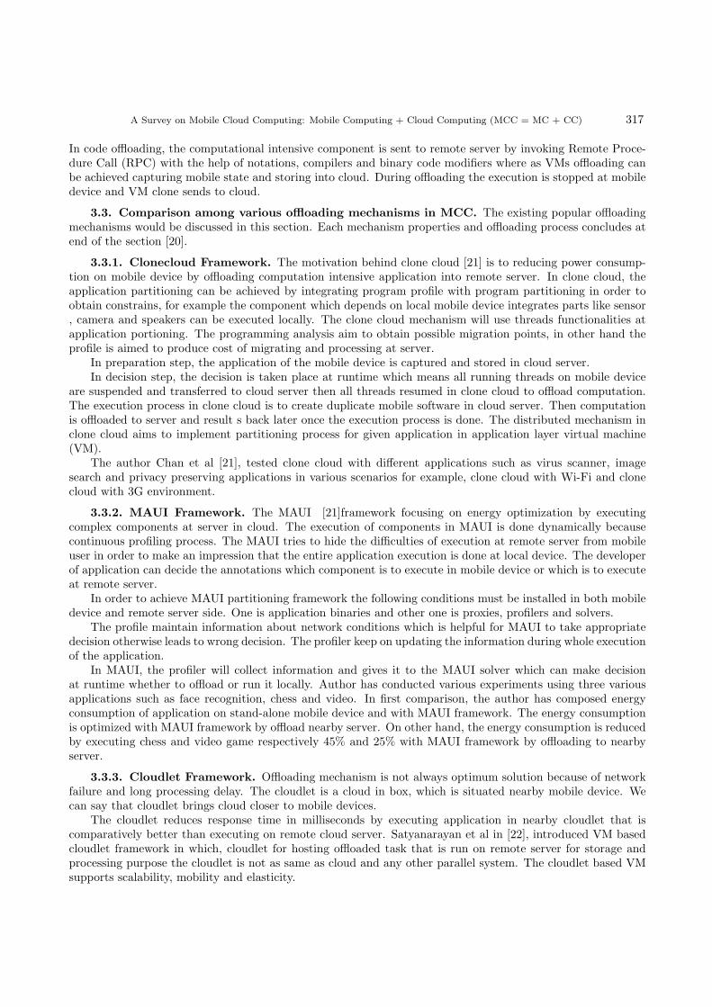
Usually user is able to connect cloud server by using web browser or web services [70]. Web service attacksalso effect cloud computing. In spite of cloud security uses XML signature for protecting an element name,attribute, value from attackers.

A Survey on Mobile Cloud Computing: Mobile Computing + Cloud Computing (MCC = MC + CC) 331
Tab
le5.1:
Com
parison
amon
gdifferentsecurity
modelsof
address-
ingsecu
rity
andprivacy
issues
inMCC
Auth
ors/year
Appro
ach
Tru
sted
level
Security
attribute
pro
vided
Benefits
Dra
wback
sConclusion
12
34
56
7
J.O
berheideet
al.
Virtualized
in-cloud
secu
rity
services
for
mob
iledevices
[62]
(200
8)
CloudAV
Fullytrusted
Antivirus,
Security
asa
Service
Red
uced
OnDevice
software
complexity
and
pow
erconsumption
Disconnected
operation
and
privacy
loss
Bymov
ingthedetection
capab
ilitiesto
anetwork
service,
wega
innumerou
sbenefi
tsincludingincreased
detection
coverage,less
complexmob
ilesoftware,
andreducedresource
consumption
.Zhan
get
al.
ACM
workshop
onCloud
computing
secu
rity
[64]
(200
9)
Cloudlet
Sem
i-trusted
Task
partition
ing
Good
trad
eoffs
between
processing
overhead
and
communicationcost
Security
ofWeblet
canbe
improved
with
other
techniques.su
pportflexible
and
efficientway
sto
augm
entcomputing,
storag
e,an
dcommunication
capab
ilitiesof
application
sforresource-constrained
Devices.
Xiao
andGon
get
al.
International
Con
ference
onMobile
Data
Man
agem
ent[65]
(201
0)
Lightw
eigh
talgo
rithm
Sem
itrusted
Authorization
of users
datain
clou
d
Automatic
Dynam
icupdating
ofcredential
inform
ation
More
processing
and
energy
burden
onmob
ile
device
meritof
dynam
iccredential
isthat
the
attackersdiffi
culty
tofakethecredential
grow
swithtime.

332 Ramasubbareddy Somula and Sasikala R
12
34
56
7Wan
gan
dWan
get
al.
11th
International
Con
ference
on Mob
ile
Data
Man
agem
ent,
MDM
[66]
(201
1)
Top
dow
nspatial
cloa
king
Distrusted
Privacy
preserving
fram
ework
in location
based
Schem
e
Red
uced
communication
cost
by
doingspatial
cloa
king
based
onthe
historical
datain
clou
d.
More
energy
consumption
and
processing
burden
onmob
iledevice
top-dow
nspatialcloa
king
algo
rithm,anddevised
optimizationareproposed
toreduce
thecommunication
cost.
Huan
get
al.
Mob
iCloud:
building
secu
reclou
dfram
ework
formob
ile
computing
and
communication[58]
(201
0)
Mob
iCloud
Distrusted
Security
in Storage
asa
Service
in MANET
Secured
datawhile
usingPublicCloud
Increased
cost
due
totw
oclou
dproviders
Themob
icloudfram
ework
willenhan
cecommunication
byad
dressingtrust
man
agem
ent,
secure
routing,
risk
man
agem
entissues
innetwork.
G.Portokalidis
etal.
Annual
Computer
Security
Application
Con
ference
(ACSAC)[67]
(201
0)
Threat
detection
in Smartphon
ebased
on CloudAV
Fullytrusted
Security
asa
Service
Red
uced
tran
smission
overheadan
denergy
consumption
More
Cloudusage
cost.
battery
life
isconsumed
more.
itoff
ersmorecomprehen
sive
security
than
possible
with
alternativemodels.
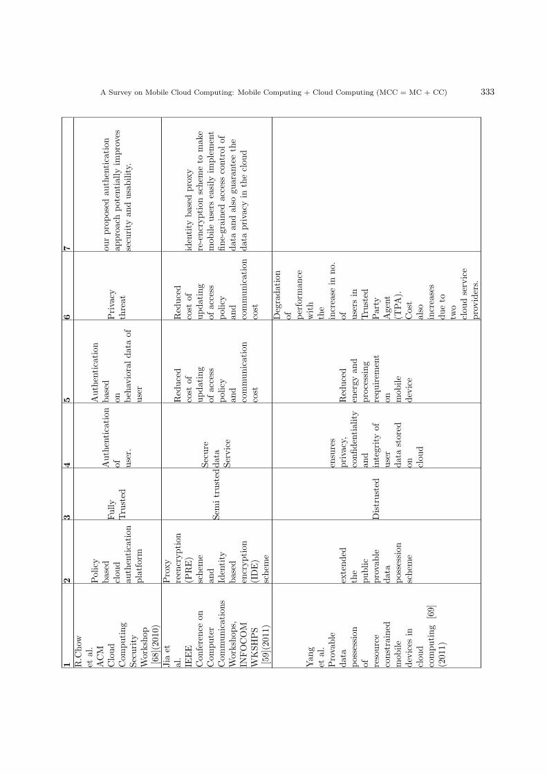
A Survey on Mobile Cloud Computing: Mobile Computing + Cloud Computing (MCC = MC + CC) 333
12
34
56
7R.Chow
etal.
ACM
Cloud
Com
puting
Security
Workshop
[68](201
0)
Policy
based
clou
dau
thentication
platform
Fully
Trusted
Authentication
of user.
Authentication
based
on behav
ioraldataof
user
Privacy
threat
ourproposed
authentication
approachpotentially
improves
security
andusability.
Jia
etal.
IEEE
Con
ference
onCom
puter
Com
munications
Workshop
s,IN
FOCOM
WKSHPS
[59](201
1)
Proxy
reen
cryption
(PRE)
schem
ean
dIdentity
based
encryption
(IDE)
schem
e
Sem
itrusted
Secure
data
Service
Red
uced
cost
ofupdating
ofaccess
policy
and
communication
cost
Red
uced
cost
ofupdating
ofaccess
policy
and
communication
cost
identity
based
proxy
re-encryption
schem
eto
mak
emob
ileusers
easily
implement
fine-grained
access
control
ofdataan
dalso
guaran
teethe
dataprivacy
intheclou
d
Yan
get
al.
Provable
data
possession
of resource
constrained
mob
ile
devices
inclou
dcomputing
[69]
(201
1)
extended
the
public
provable
data
possession
schem
e
Distrusted
ensures
privacy,
confidentiality
and
integrityof
user
datastored
on clou
d
Red
uced
energy
and
processing
requirem
ent
on mob
ile
device
Degradation
of perform
ance
with
the
increase
inno.
of users
inTrusted
Party
Agent
(TPA).
Cost
also
increases
dueto
two
clou
dservice
providers.

334 Ramasubbareddy Somula and Sasikala R
12
34
56
7
Sam
anZon
ouzet
al.
Scien
ceDirect
journal
ofCom
puters
and
secu
rity
[63]
(201
3)
Secloud
for
Smart
phones
Trusted
clou
dbased
comprehensive
and
ligh
tweigh
tsecu
rity
for
smart
phon
es
Red
uced
energy
and
processing
requirem
ent
on mob
ile
devicefor
providing
security
inmob
ile
device
Cloud
assumes
tobe
fullytrusted
which
needsto
be
reconsidered.
The
personal
dataof
users
accessed
tothe
clou
dcan
affect
theprivacy
issues
Secloudprovides
apow
erful,
yet
resource-friendly,
protectionforsm
art
phon
esbyperform
ing
thesecurity
analysis
onan
emulatedversion
ofthedevices,
runninginsideaclou
d
Vijay
Varad
harajanet
al.
IEEE
Transactions
On
Network
and
Service
Man
agem
ent
[70](201
4)
Security
asa
Service
Model
Trusted
Virtualization
technolog
yan
dVMM
secu
rity
functionalities
Offers
abaseline
security
tothe
provider
toprotect
its
own
clou
dinfrastructure
Insider
attack
from
Tenan
tDom
ain
and
Cloud
Service
Provider
security
asaservice
model
that
aclou
dprovider
canoff
erto
itsmultiple
tenan
tsan
dcustom
ers
ofitstenan
ts
Qiao
Yan
andF.
Richard
Yuet
al.
IEEE
Com
munications
Surveys
&Tutorials
[61](201
6)
Softw
ared
efined
networking
(SDN)
Trusted
Networking-asa-
service
(Naa
S),
control
and
dataplanes
are
decou
pled
software-based
traffi
can
alysis,
centralized
control,
glob
alview
ofthe
network,
dynam
icupdatingof
forw
arding
rules
Security
ofSDN
itself
remainsto
be
addressed
and
potential
DDoS
vulnerab
ilities
exist
across
SDN
platforms
DefendingDDOSattack
bymak
ingfulluse
ofSDN-baseclou
dad
vantagesin
clou
denviron
ment.

A Survey on Mobile Cloud Computing: Mobile Computing + Cloud Computing (MCC = MC + CC) 335
6. Conclusion. In this article, we have discussed about various concepts in mobile cloud computing:(1) Mobile computing, (2) cloud computing, (3) mobile cloud computing,(4) offloading approach, (5) cloudletapproach and (6)security and privacy. We have given extensive survey on existing frameworks on computationoffloading. Even through, there are various frameworks presented, but the objective of each framework is toimproving mobile performance by reducing energy consumption and response time.
We have provided a survey on emerging cloudlet technology and challenges. the concept of cloudlet aimsto address high latency and response time issues by brining cloud recourses closer to mobile user. We haveanalyzed comparison among popular cloudlet architecture and selection techniques; the secure routing protocolused to protect communication channel between devices and cloud as well as need to be addressed several issuessuch as data integrity, authentication, authorization and access control. We believe that by introducing edgecomputing architecture for optimizing mobile performance in MCC will take place in near feature.
REFERENCES
[1] R. Meulen, “Gartner Says Global Smartphone Sales to Only Grow 7 Per Cent in 2016.”[2] B. Butler, “Gartner: Cloud Putting Crimp in Traditional Software, Hardware Sales,” Network World, 2012.[3] H. T. Dinh, C. Lee, D. Niyato, and P. Wang, “A survey of mobile cloud computing: architecture, applications, and approaches,”
Wireless communications and mobile computing, vol. 13, no. 18, pp. 1587–1611, 2013.[4] M. Tulloch, Introducing Windows Azure for IT Professionals. Microsoft Press, 2013.[5] R. Buyya, “Introduction to the ieee transactions on cloud computing,” IEEE Transactions on Cloud Computing, vol. 1, no. 1,
pp. 3–21, 2013.[6] P. Mell, T. Grance, and Others, “The NIST definition of cloud computing,” 2011.[7] C. V. N. Index, “Global mobile data traffic forecast update 2014–2019 white paper, feb 2015,” See: http://www. cisco.
com/c/en/us/solutions/collateral/service-provider/visual-networking-index-vni/white paper c11-520862. html, 2015.[8] L. Yang, J. Cao, Y. Yuan, T. Li, A. Han, and A. Chan, “A framework for partitioning and execution of data stream applications
in mobile cloud computing,” ACM SIGMETRICS Performance Evaluation Review, vol. 40, no. 4, pp. 23–32, 2013.[9] A. Klein, C. Mannweiler, J. Schneider, and H. D. Schotten, “Access schemes for mobile cloud computing,” in Mobile Data
Management (MDM), 2010 Eleventh International Conference on. IEEE, 2010, pp. 387–392.[10] P. Bahl, R. Y. Han, L. E. Li, and M. Satyanarayanan, “Advancing the state of mobile cloud computing,” in Proceedings of
the third ACM workshop on Mobile cloud computing and services. ACM, 2012, pp. 21–28.[11] E. Miluzzo, R. Caceres, and Y.-F. Chen, “Vision: mClouds-computing on clouds of mobile devices,” in Proceedings of the
third ACM workshop on Mobile cloud computing and services. ACM, 2012, pp. 9–14.[12] R. Kamal, Mobile Computing. Oxford University Press, Inc., 2008.[13] L. S. Ashiho, “Mobile technology: Evolution from 1G to 4G,” Electronics for you, pp. 94–98, 2003.[14] M. Armbrust, A. Fox, R. Griffith, A. D. Joseph, R. Katz, A. Konwinski, G. Lee, D. Patterson, A. Rabkin, I. Stoica, and
Others, “A view of cloud computing,” Communications of the ACM, vol. 53, no. 4, pp. 50–58, 2010.[15] R. Buyya, J. Broberg, and A. M. Goscinski, Cloud computing: Principles and paradigms. John Wiley & Sons, 2010, vol. 87.[16] D. Durkee, “Why cloud computing will never be free,” Queue, vol. 8, no. 4, p. 20, 2010.[17] M. D. Dikaiakos, D. Katsaros, P. Mehra, G. Pallis, and A. Vakali, “Cloud computing: Distributed internet computing for IT
and scientific research,” IEEE Internet computing, vol. 13, no. 5, 2009.[18] K. Chard, S. Caton, O. Rana, and K. Bubendorfer, “Social cloud: Cloud computing in social networks,” in Cloud Computing
(CLOUD), 2010 IEEE 3rd International Conference on. IEEE, 2010, pp. 99–106.[19] B.-G. Chun, S. Ihm, P. Maniatis, M. Naik, and A. Patti, “Clonecloud: elastic execution between mobile device and cloud,”
in Proceedings of the sixth conference on Computer systems. ACM, 2011, pp. 301–314.[20] K. Akherfi, M. Gerndt, and H. Harroud, “Mobile cloud computing for computation offloading: Issues and challenges,” Applied
Computing and Informatics, 2016.[21] E. Cuervo, A. Balasubramanian, D.-k. Cho, A. Wolman, S. Saroiu, R. Chandra, and P. Bahl, “MAUI: making smartphones
last longer with code offload,” in Proceedings of the 8th international conference on Mobile systems, applications, andservices. ACM, 2010, pp. 49–62.
[22] M. Satyanarayanan, P. Bahl, R. Caceres, and N. Davies, “The case for vm-based cloudlets in mobile computing,” IEEEpervasive Computing, vol. 8, no. 4, 2009.
[23] H. Qian and D. Andresen, “Jade: Reducing energy consumption of android app,” the International Journal of Networkedand Distributed Computing (IJNDC), Atlantis press, vol. 3, no. 3, pp. 150–158, 2015.
[24] B. Zhao, Z. Xu, C. Chi, S. Zhu, and G. Cao, “Mirroring smartphones for good: A feasibility study,” in InternationalConference on Mobile and Ubiquitous Systems: Computing, Networking, and Services. Springer, 2010, pp. 26–38.
[25] R. Kemp, N. Palmer, T. Kielmann, and H. Bal, “Cuckoo: a computation offloading framework for smartphones,” in Interna-tional Conference on Mobile Computing, Applications, and Services. Springer, 2010, pp. 59–79.
[26] F. Xia, F. Ding, J. Li, X. Kong, L. T. Yang, and J. Ma, “Phone2Cloud: Exploiting computation offloading for energy savingon smartphones in mobile cloud computing,” Information Systems Frontiers, vol. 16, no. 1, pp. 95–111, 2014.
[27] S. Kosta, A. Aucinas, P. Hui, R. Mortier, and X. Zhang, “Thinkair: Dynamic resource allocation and parallel execution inthe cloud for mobile code offloading,” in Infocom, 2012 Proceedings IEEE. IEEE, 2012, pp. 945–953.
336 Ramasubbareddy Somula and Sasikala R
[28] T. Verbelen, P. Simoens, F. De Turck, and B. Dhoedt, “Cloudlets: Bringing the cloud to the mobile user,” in Proceedings ofthe third ACM workshop on Mobile cloud computing and services. ACM, 2012, pp. 29–36.
[29] M. Satyanarayanan, Z. Chen, K. Ha, W. Hu, W. Richter, and P. Pillai, “Cloudlets: at the leading edge of mobile-cloudconvergence,” in Mobile Computing, Applications and Services (MobiCASE), 2014 6th International Conference on.IEEE, 2014, pp. 1–9.
[30] S. Simanta, K. Ha, G. Lewis, E. Morris, and M. Satyanarayanan, “A reference architecture for mobile code offload in hostileenvironments,” in International Conference on Mobile Computing, Applications, and Services. Springer, 2012, pp.274–293.
[31] S. Clinch, J. Harkes, A. Friday, N. Davies, and M. Satyanarayanan, “How close is close enough? Understanding the role ofcloudlets in supporting display appropriation by mobile users,” in Pervasive Computing and Communications (PerCom),2012 IEEE International Conference on. IEEE, 2012, pp. 122–127.
[32] Z. Dou, “Benefits of utilizing an edge server (cloudlet) in the mocha architecture,” Ph.D. dissertation, University of Rochester.Department of Electrical and Computer Engineering, 2013.
[33] D. Fesehaye, Y. Gao, K. Nahrstedt, and G. Wang, “Impact of cloudlets on interactive mobile cloud applications,” in EnterpriseDistributed Object Computing Conference (EDOC), 2012 IEEE 16th International. IEEE, 2012, pp. 123–132.
[34] Y. Li and W. Wang, “Can mobile cloudlets support mobile applications?” in Infocom, 2014 proceedings ieee. IEEE, 2014,pp. 1060–1068.
[35] J. Flinn and M. Satyanarayanan, Energy-aware adaptation for mobile applications. ACM, 1999, vol. 33, no. 5.[36] Y.-C. Tseng, S.-Y. Ni, Y.-S. Chen, and J.-P. Sheu, “The broadcast storm problem in a mobile ad hoc network,” Wireless
networks, vol. 8, no. 2-3, pp. 153–167, 2002.[37] H. Wang, “Accelerating mobile-cloud computing using a cloudlet,” Ph.D. dissertation, University of Rochester. Department
of Electrical and Computer Engineering, 2013.[38] J. Wu and H. Li, “On calculating connected dominating set for efficient routing in ad hoc wireless networks,” in Proceedings of
the 3rd international workshop on Discrete algorithms and methods for mobile computing and communications. ACM,1999, pp. 7–14.
[39] E. Koukoumidis, D. Lymberopoulos, K. Strauss, J. Liu, and D. Burger, “Pocket cloudlets,” in ACM SIGPLAN Notices,vol. 46, no. 3. ACM, 2011, pp. 171–184.
[40] R. M. Modh and J. M. Patel, “A study on improving challenges of network with cloudlets for mobile cloud computing,”International Journal of Global Research in Computer Science (UGC Approved Journal), vol. 4, no. 4, pp. 143–146,2013.
[41] A. T. Lo’ai, W. Bakheder, and H. Song, “A mobile cloud computing model using the cloudlet scheme for big data applications,”in Connected Health: Applications, Systems and Engineering Technologies (CHASE), 2016 IEEE First InternationalConference on, 2016, pp. 73–77.
[42] Y. Jararweh, L. Tawalbeh, F. Ababneh, and F. Dosari, “Resource efficient mobile computing using cloudlet infrastructure,” inMobile Ad-hoc and Sensor Networks (MSN), 2013 IEEE Ninth International Conference on. IEEE, 2013, pp. 373–377.
[43] Z. Pang, L. Sun, Z. Wang, E. Tian, and S. Yang, “A survey of cloudlet based mobile computing,” in Cloud Computing andBig Data (CCBD), 2015 International Conference on. IEEE, 2015, pp. 268–275.
[44] K. Gai, M. Qiu, H. Zhao, L. Tao, and Z. Zong, “Dynamic energy-aware cloudlet-based mobile cloud computing model forgreen computing,” Journal of Network and Computer Applications, vol. 59, pp. 46–54, 2016.
[45] Z. Sanaei, S. Abolfazli, A. Gani, and R. Buyya, “Heterogeneity in mobile cloud computing: taxonomy and open challenges,”IEEE Communications Surveys & Tutorials, vol. 16, no. 1, pp. 369–392, 2014.
[46] H. Raei, N. Yazdani, and R. Shojaee, “Modeling and performance analysis of cloudlet in Mobile Cloud Computing,” Perfor-mance Evaluation, vol. 107, pp. 34–53, 2017.
[47] R. Somula and R. Sasikala, “Round robin with load degree: An algorithm for optimal cloudlet discovery in mobile cloudcomputing,” Scalable Computing: Practice and Experience, vol. 19, no. 1, pp. 39–52, 2018.
[48] A. Akbar and P. R. Lewis, “Towards the optimization of power and bandwidth consumption in mobile-cloud hybrid appli-cations,” in Fog and Mobile Edge Computing (FMEC), 2017 Second International Conference on. IEEE, 2017, pp.213–218.
[49] A. Mukherjee, D. De, and D. G. Roy, “A power and latency aware cloudlet selection strategy for multi-cloudlet environment,”IEEE Transactions on Cloud Computing, 2016.
[50] Y. Jararweh, M. Al-Ayyoub, M. Al-Quraan, A. T. Loai, and E. Benkhelifa, “Delay-aware power optimization model for mobileedge computing systems,” Personal and Ubiquitous Computing, vol. 21, no. 6, pp. 1067–1077, 2017.
[51] S. Meng, Y. Wang, Z. Miao, and K. Sun, “Joint optimization of wireless bandwidth and computing resource in cloudlet-basedmobile cloud computing environment,” Peer-to-Peer Networking and Applications, vol. 11, no. 3, pp. 462–472, 2018.
[52] S. Bitam, S. Zeadally, and A. Mellouk, “Fog computing job scheduling optimization based on bees swarm,” EnterpriseInformation Systems, vol. 12, no. 4, pp. 373–397, 2018.
[53] J. Oueis, E. C. Strinati, and S. Barbarossa, “The fog balancing: Load distribution for small cell cloud computing,” in VehicularTechnology Conference (VTC Spring), 2015 IEEE 81st. IEEE, 2015, pp. 1–6.
[54] S. Yan, M. Peng, M. A. Abana, and W. Wang, “An evolutionary game for user access mode selection in fog radio accessnetworks,” IEEE Access, vol. 5, pp. 2200–2210, 2017.
[55] M. S. Elbamby, M. Bennis, and W. Saad, “Proactive edge computing in latency-constrained fog networks,” in Networks andCommunications (EuCNC), 2017 European Conference on. IEEE, 2017, pp. 1–6.
[56] H. Wang, S. Wu, M. Chen, and W. Wang, “Security protection between users and the mobile media cloud,” IEEE Commu-nications Magazine, vol. 52, no. 3, pp. 73–79, 2014.
[57] D. Dev and K. L. Baishnab, “Notice of Violation of IEEE Publication Principles A Review and Research Towards Mobile

A Survey on Mobile Cloud Computing: Mobile Computing + Cloud Computing (MCC = MC + CC) 337
Cloud Computing,” in Mobile Cloud Computing, Services, and Engineering (MobileCloud), 2014 2nd IEEE InternationalConference on. IEEE, 2014, pp. 252–256.
[58] D. Huang, X. Zhang, M. Kang, and J. Luo, “MobiCloud: building secure cloud framework for mobile computing and commu-nication,” in Service Oriented System Engineering (SOSE), 2010 Fifth IEEE International Symposium on. Ieee, 2010,pp. 27–34.
[59] W. Jia, H. Zhu, Z. Cao, L. Wei, and X. Lin, “SDSM: a secure data service mechanism in mobile cloud computing,” in ComputerCommunications Workshops (INFOCOM WKSHPS), 2011 IEEE Conference on. IEEE, 2011, pp. 1060–1065.
[60] P. Garg and V. Sharma, “An efficient and secure data storage in Mobile Cloud Computing through RSA and Hash function,”in Issues and Challenges in Intelligent Computing Techniques (ICICT), 2014 International Conference on. IEEE, 2014,pp. 334–339.
[61] Q. Yan, F. R. Yu, Q. Gong, and J. Li, “Software-defined networking (SDN) and distributed denial of service (DDoS) attacksin cloud computing environments: A survey, some research issues, and challenges,” IEEE Communications Surveys &Tutorials, vol. 18, no. 1, pp. 602–622, 2016.
[62] J. Oberheide, K. Veeraraghavan, E. Cooke, J. Flinn, and F. Jahanian, “Virtualized in-cloud security services for mobiledevices,” in Proceedings of the first workshop on virtualization in mobile computing. ACM, 2008, pp. 31–35.
[63] S. Zonouz, A. Houmansadr, R. Berthier, N. Borisov, and W. Sanders, “Secloud: A cloud-based comprehensive and lightweightsecurity solution for smartphones,” Computers & Security, vol. 37, pp. 215–227, 2013.
[64] X. Zhang, J. Schiffman, S. Gibbs, A. Kunjithapatham, and S. Jeong, “Securing elastic applications on mobile devices forcloud computing,” in Proceedings of the 2009 ACM workshop on Cloud computing security. ACM, 2009, pp. 127–134.
[65] S. Xiao and W. Gong, “Mobility can help: protect user identity with dynamic credential,” in Mobile Data Management(MDM), 2010 Eleventh International Conference on. IEEE, 2010, pp. 378–380.
[66] S. Wang and X. S. Wang, “In-device spatial cloaking for mobile user privacy assisted by the cloud,” in Mobile Data Manage-ment (MDM), 2010 Eleventh International Conference on. IEEE, 2010, pp. 381–386.
[67] G. Portokalidis, P. Homburg, K. Anagnostakis, and H. Bos, “Paranoid android: versatile protection for smartphones,” inProceedings of the 26th Annual Computer Security Applications Conference. ACM, 2010, pp. 347–356.
[68] R. Chow, M. Jakobsson, R. Masuoka, J. Molina, Y. Niu, E. Shi, and Z. Song, “Authentication in the clouds: a frameworkand its application to mobile users,” in Proceedings of the 2010 ACM workshop on Cloud computing security workshop.ACM, 2010, pp. 1–6.
[69] J. Yang, H. Wang, J. Wang, C. Tan, and D. Yu, “Provable data possession of resource-constrained mobile devices in cloudcomputing.” JNW, vol. 6, no. 7, pp. 1033–1040, 2011.
[70] V. Varadharajan and U. Tupakula, “Security as a service model for cloud environment,” ieee transactions on network andservice management, vol. 11, no. 1, pp. 60–75, 2014.
Edited by: Rajkumar RajasekaranReceived: Jun 29, 2018Accepted: Oct 25, 2018

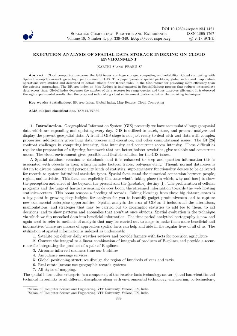
Scalable Computing: Practice and Experience
Volume 19, Number 4, pp. 339–349. http://www.scpe.org
DOI 10.12694/scpe.v19i4.1421ISSN 1895-1767c⃝ 2018 SCPE
EXECUTION ANALYSIS OF SPATIAL DATA STORAGE INDEXING ON CLOUDENVIRONMENT
KARTHI S∗AND PRABU S†
Abstract. Cloud computing overcome the GIS issues are huge storage, computing and reliability. Cloud computing withSpatialHadoop framework gives high performance in GIS. This paper presents spatial partition, global index and map reduceoperations were studied and described in detail. Bloom filter R-tree index in the Map-reduce for providing more efficiency thanthe existing approaches. The BR-tree index on Map-Reduce is implemented in SpatialHadoop process that reduces intermediatedata access time. Global index decreases the number of data accesses for range queries and thus improves efficiency. It is observedthrough experimental results that the proposed index along cloud environment performs better than existing techniques.
Key words: Spatialhadoop, BR-tree Index, Global Index, Map Reduce, Cloud Computing
AMS subject classifications. 68M14, 97R50
1. Introduction. Geographical Information System (GIS) presently we have accumulated huge geospatialdata which are expanding and updating every day. GIS is utilized to catch, store, and process, analyze anddisplay the present geospatial data. A fruitful GIS stage is not just ready to deal with vast data with complexproperties, additionally gives huge data process and execution, and other computational issues. The GI [26]confront challenges in computing intensity, data intensity and concurrent access intensity. These difficultiesrequire the preparation of a figuring framework that can better bolster revelation, give scalable and concurrentaccess. The cloud environment gives possible and flexible solution for the GIS issues.
A Spatial database remains as databank, and it is enhanced to keep and question information this isassociated with objects in area, which includes factors, traces, polygons etc..,. Though normal databases isdetain to diverse numeric and personality kinds of statistics, supplementary functionality desires to be deliveredfor records to system latitudinal statistics types. Spatial facts stand the numerical connection between people,region, and activities. This facts can explicitly illustrate what’s taking place (in which, why and how) to showthe perception and effect of the beyond, the present and the (probable) destiny [1]. The proliferation of cellularprograms and the huge of hardware sensing devices boom the streamed information towards the web hostingstatistics-centers. This boom reasons a flooding of records. Taking blessings from these big dataset stores isa key point in growing deep insights for analysts for you to beautify gadget productiveness and to capturenew commercial enterprise opportunities. Spatial analysis the crux of GIS as it includes all the alterations,manipulations, and strategies that may be carried out to geographic statistics to add fee to them, to aiddecisions, and to show patterns and anomalies that aren’t at once obvious. Spatial evaluation is the techniquevia which we flip uncooked data into beneficial information. The time period analytical cartography is now andagain used to refer to methods of analysis that may be carried out to maps to make them more beneficial andinformative. There are masses of approaches spatial facts can help and aide in the regular lives of all of us. Theutilization of spatial information is indexed as underneath:
1. Satellite pix deliver daily weather reviews and provide farmers with facts for precision agriculture2. Convert the integral to a linear combination of integrals of products of B-splines and provide a recur-
rence for integrating the product of a pair of B-splines.3. Airborne infra-red scanners tune our bushfires4. Ambulance message services5. Global positioning structures divulge the region of hundreds of vans and taxis6. Real estate income use geographic records systems7. All styles of mapping.
The spatial information enterprise is a component of the broader facts technology sector [3] and has scientific andtechnical hyperlinks to all different disciplines along with environmental technology, engineering, pc technology,
∗School of Computer Science and Engineering, VIT University, Vellore, TN, India†School of Computer Science and Engineering, VIT University, Vellore, TN, India
339

340 Karthi S and Prabu S
fitness shipping, logistics, planning, useful resource control and electronics.
1.1. Data categories in spatial warehouse. The maximum recycled the classification to signify theissues of spatial enquiry consider three sorts of statistics:
Points or Events Occurrences expressed via single value identified as factors in zone, denominated themetactics. Some samples are: sickness occurrences, crime spots, and the localization of botanical species.
Constant surfaces predicted can be beginning a hard and fast of vicinity examples which are regularlyor erratically disbursed. Typically, this kind of statistics consequences from herbal sources studies, whichincorporates topographical, biological, phytogeography, environmental and pedagogical charts. Zones withCalculations and Aggregation Tolls - it includes information linked to population studies, like census and fitnessinformation [10], and which is probably initially mentioned to people located in precise elements in universe.For secrecy motives those information are aggregated in analysis gadgets, usually enclosed thru locked polygons(postal addressing zones, census tracts, municipalities). The symmetrical representations used consist of thesubsequent alternatives: 2D Points: It is a well-ordered pair of x, y values of three-dimensional directs. A factorsuggests that vicinity of incidence of an occasion, like in the case of mortality via the use of outside causes.Polygons: It is a hard and fast of methodical pairs values that indicates x, y values of three-dimensional directs,in this type of method that the ultimate opinion is same to the prime for this reason forming closed vicinitywithin the aircraft. In the most effective situation, every polygon delimits a person item within the most famouscase; a man or woman area of interest may be delimited via numerous polygons [11, 14, 15]. Samples: encompasswith ordered pairs of x, y, and z values in which contains the x, y pairs mean the physical coordinates and then zsuggests that the price of the premeditated singularity aimed at that location of zones. Typically the examplesare related to area of studies, collectively with geochemical, oceanographic and then geo-physical records. Theidea of a example can be widespread to the event of numerous dimensions on the identical area. Regular Grid:It is an environment in which every part is related towards a numeric rate. In this matrix, we can calculatethe points which associated with a place on the ground floor. Preliminary from a initial coordinates typicallynoted the inferior left corner of the 10X30 matrix, and using spacing in equally to the straight and verticaldirections. Image: It is in the form of matrix in which every detail is related to a numeral value (commonlyfrom 0 to 255 variety), recycled for conception [14]. This type of condition is used to the photo presentationof a normal grid. The statistical standards in the network are ascended in shape with the production varietyof the image; the superior values stand to be proven in sunnier gray shades, and then decrease in duskier grayqualities. Maximum of the geographical information systems provide the ability of providing a fixed grid in thesystem of a picture (popular shades or in black & white), through a conversion that may remain computerizedor measured via purchaser. Three essential shapes of spatial facts is proven in Fig. 1.1.
Database systems exercise directories to unexpectedly analyze look of values and the manner that mostdatabases index records isn’t always maximum fulfilling for latitudinal queries. Instead, three-dimensionaldatabases practice a spatial catalog to hurry up database processes. Spatial directories are used by spatialrecord to enhance spatial queries [17]. Directories used by non-spatial records cannot efficaciously cope withlandscapes consisting of how a protracted manner factors varies and whether or not and also points collapseinside a longitudinal vicinity of interest.
2. Related Work. Analyzed indexing and question processing in spatial statistics. Indexing strategies areused to boom the velocity of the information retrieval. In the spatio-temporal area the information continuouslyincreases over a time and transferring item dispatched their positions. The principal drawback of spatio-temporalprocessing is maintaining all of the updates are not possible. The maximum of the indexing methods [1] are bestsupports few queries and beyond, present and destiny indexing methods shape are very complicated becauseit is integrated exclusive indexing methods. Interval bushes aren’t in particular designed for handling unsurestatistics; however one-dimensional uncertain items may be treated as durations by way of using their PDFendpoints. Both indices use a number one tree for layout and secondary structures to save the gadgets ateach node, but one has a dynamic number one tree as opposed to a static one. However, the downfall of eachinterval indices is that if many uncertainty periods overlap with the question intervals endpoints, then fewgadgets are pruned from the quest, and a number of times are wasted in calculating chances. The shape ofthe indexing strategies are very complex so performance is decreased and principal expectation of real timeutility is concurrent updation, it isn’t supported with the aid of maximum of the indexing strategies. Real time

Execution Analysis of Spatial Data Storage Indexing on Cloud Environment 341
Fig. 1.1. Shapes of Spatial data
application are need comparable object locate and grouping this is also now not possible in exiting indexingtechniques and eventually however now not least all of the query processing techniques aren’t helps to all thekinds of indexing strategies and queries.
Analyzed spatial statistics control in cloud environments. Principal use an R +-tree [3] to share the factsand the frames inside with go away nodes of the graphic index are preserved as active grids. First, may wantto get stability among the grid scopes and then the instances of grid entrees by regulating the 2 limitations, Nbesides n, contains of the R+-tree. Additional, in comparison through different variations with the R-tree, theleaf nodes ensure that which is not overlay every feature, and consequently it’s distant a assistance as there isno repeated recovery of the equal statistics from special solutions and it remains simple to outline distinctivesources for every rectangle of a leaf child. Moreover, the one task is the manner to layout the vital thing termsof these networks to help effectual inquiries on BigTable manipulates schemes. We positioned the developmentsof CDMs equally follows: which consumes a quick (key,value) are looking for and it remains to be rapid withImage keys and it can be ordered thru a dictionary format. Based on those traits, we recommend a method todefine the critical factor call of a network to help effective queries.
Presented polygon based spatial statistics assessment with map reduce. Geographic Information Systemwhich is an expedient intended to seizure, save, work, examine, manipulate, and gift completely styles oftopographical facts. Spatial evaluation is a terrific function that is combining with GIS. By way of one vitalprocess in three-dimensional evaluation, polygon overlap, that’s a complex geometric set of regulations, combinesthe spatial and characteristic statistics of dual enter map covers [2]. In such a process, every polygon of a coveris blended with some other layer in couple to reap the cease end result. Classically, particular thematic coversof the identical location are occupied and covered any on pinnacle with opportunity to yield an outcomelayer. Increasingly, the dimensions range, and replace charge of a few longitudinal datasets surpasses theability of three-dimensional computing generation. In a diffusion of times, overlap assessment will become ainefficient venture as commerce with big dimensions of three-dimensional statistics is needed. The computerGIS software normally takes times to perform overlap of this large spatial informations. Such consumption ontime is undesirable for lots packages, specifically for actual time coverage choices which encompass predictingwhich homes would be broken through manner of a transcontinental storm.
Analyzed spatial facts processing using Map-Reduce which is a programming version and computing plat-form well ideal for parallel computation. In Map Reduce, a application includes a map feature and a reducefunction that are consumer-described. The input facts layout is software particular, and is designated by way ofthe consumer [5]. At first, spatial splitting is adopted to distribute information to all nodes as even as possible,

342 Karthi S and Prabu S
and then strip-based two path sweeping set of rules can accelerate the computation instead of spatial index inconventional spatial packages. Finally, pending documents and redundant statistics are used to deal with therelationship between the spatial items. And adopted Map Reduce to process megastar catalog cross certificationin astronomical discipline. In order to take full use of the Map Reduce platform, it’s far better to make completeissues of parallel algorithm plant. In this section, Map Reduce is carried out to pass-certification, and then incomparison with conventional PostgreSQL DBMS. As a simple and quintessential step, the astronomical crosscertification is facing a data avalanche. With the of entirety of latest sky survey tasks and effective telescopes,present day go-certification methods cannot be done on call for large scale astronomical information units. Inthis paper, Map Reduce framework is delivered to clear up this trouble. The mapping of move-certificationalgorithm on Map and Reduce phases is carefully taken into consideration. Performance assessment has shownthat the Map Reduce-based totally move-certification can outperform the conventional one on PostgreSQL. Asour expertise, it is the first attempt to undertake Map Reduce for astronomical go-certification problem.
Implemented partition techniques in spatial hadoop. SpatialHadoop [4] offers a prevalent indexing set ofregulations which grow to be recycled to implement network, R-tree, and R+-tree primarily founded for parti-tioning. This paper spreads preceding observe by way of manner of introducing 4 new partitioning strategies,Hilbert curve, Z-curve, K-d tree and Quad tree and have a look at entirely the seven strategies. The partitioningsection of the indexing procedure turns in three steps, in which the initial step is regular and then closing dualsteps are custom designed for every partitioning methods. The initial step calculates amount of favorite dividersn based totally mostly on record length and the HDFS chunk functionality which may be each fixed for completepartitioning techniques. The distribution technique allocates an item to precisely one overlying cell and then thecellular desires to stand increased to surround all controlled statistics. The repetition method eludes growingcells with the useful resource of replicating every data to all overlying cells and query processor consumes tolease a reproduction evading approach to explanation for simulated facts. While range query executed similarlyon all of them, we showed that they will be tuned with device parameters which encompass block period in linewith the question paintings load. We additionally confirmed the overall performance of spatial be a part of isstrongly correlated with the fee of Q1 (average region of partitions) and placed that Quad tree outperformedunique techniques being experimented.
3. Existing Methodologies. The amount of data in spatial databases is developing as greater records aremade to be had. Spatial databases in particular store distinct varieties of facts: raster records (satellite/aerialvirtual pictures), and vector information (factors, polygons, lines). The complexity and environment of three-dimensional databases types them first-class for smearing similar processing [20]. The cutting-edge methods aremanaging Map-Reduce framework in indexing systems like as R tree. There are different variation in R-treethat is used of static databases and another one for dynamic databases. The overall performance of R-woodrelies upon at the exceptional of the set of rules that groups the data frames on a node.
3.1. Constructing R-Tree with Map Reduce. Let D be a spatial data set composed of devices. Eachitem i has attributes ¡i.Id,i.P¿, in which i.Id is referred as the items particular identifier and i.P is also known asobjects region in particular three-dimensional domain; different features are possible, but we can supply interestto those quality for R-Tree production cause. R-Tree is consist of minimum bounding rectangles (MBRs) thatare created primarily founded on the devices spatial characteristic of i.P. i.Id is used as references to itemssaved within the RTree in form of leaves. In a main, the spatial objects are divided into nodes. Then, each leafis processed to generate a minor R-Tree. Finally, the minor R-Trees are combined into the last R-Tree. Theprincipal degrees are carried out in Map Reduce, at the equal time because the remaining segment does notinvolve large number of computational steps, therefore it is far implemented consecutively out of entries in thecluster [17]. The levels in R tree index with Map-Reduce are shown in Fig. 3.1. The Major disadvantage withR tree with Map-reduce is aid only variety queries for future data retrieval in spatial records processing.
3.2. Hillbert R-Tree with Map Reduce. The basic presentation of R-tree relies upon at the great setof rules that groups the frames on a node, at the identical as Hilbert curve [23] which contains the quality ofspatial cluster belongings. Hilbert R-tree is extension of Hilbert space-filling-curves approach and in particularthe Hilbert value to execute a linear ordering on the information rectangles; then, it negotiates the sortedlisting, assigning each set of values at the equal node [20] in the linear ordering, and maximum likely in the

Execution Analysis of Spatial Data Storage Indexing on Cloud Environment 343
Fig. 3.1. Phases in R-tree indexing in Map-Reduce framework
neighborhood area; therefore, the following R-tree nodes could have the slighter regions. The Hilbert R-treeconsists of following structure.
The algorithm of build Hilbert R-tree is given as follows:
• Step 1 Compute the Hilbert cost for each nodes in database.• Step 2 Categorize statistics data and align as ascending Hilbert values.• Step 3 Build the R-tree from bottom to up recursively in step with the directive of Hilbert values
The assumption of the algorithm is that the data are static or the frequency of amendment is short. Theapproach is an easy heuristic for building an R-tree with 100 place of utilization, which at the equal time couldhave as proper reaction time as viable [18]. In precise, the set of guidelines might be very suitable for parallelbulk-loading processing.
Preliminaries of Hilbert Cost: The Hilbert cost of a node is described due to the fact the Hilbert fee of itscenter. The manner of calculating the Hilbert value for a data rectangle is split into two steps:
• Step 1 Compute the grid cell that the intermediate of a data are plotted in area• Step 2 Compute the Hilbert value of the every grid area
Figure 3.2 demonstrates some nodes ordered in a Hilbert R-tree which has the following structure. TheHilbert values of the facilities are the records near the x symbols (proven simplest for the determine node II).The LHVs are in [brackets].A leaf node contains a most Cl entries each of the shape (R, obj id) in which Clis the potential of the leaf, R is the MBR of the real object (xlow, xhigh, ylow, yhigh) and obj-identity is apointer to the item description document. The vital distinction between the Hilbert R-tree and the R*-tree isthat non-leaf nodes also include facts about the LHVs (Largest Hilbert Value). Thus, a non-leaf node in theHilbert R-tree contains a most Cn entries of the form (R, ptr, LHV) in which Cn is the capacity of a non-leafnode, R is the MBR that encloses all of the kids of that node, ptr is a pointer to the kid node, and LHV is the

344 Karthi S and Prabu S
Fig. 3.2. Hilbert R tree structure
largest Hilbert price the various facts rectangles enclosed by means of using R. Notice that because the non-leafnode alternatives one of the Hilbert values of the children to be the price of its non-public LHV, there isn’textra rate for calculating the Hilbert values of the MBR of non-leaf nodes.
4. Rapid Indexing Scheme for Spatial Data Processing in Cloud Enviroment. This work inte-grates a BR-tree index in MapReduce that results in a parallel B-Tree index. The significance of MapReduce-Hadoop and indexing in the Hadoop is described below.
4.1. Map Reduce. Large extent of facts has led to adoption of parallel processing. It provides a greenprocessing over a fixed of participating pc machines. It changed into expected that parallel processing mightoffer new ways of thinking about the prevailing concept of programming language, working machine and storagesystem for massive dispensed systems. Parallel processing is complex, however many frameworks have evolvedthat offer parallel processing the use of abstraction to simplify matters. Hadoop, a Java implementation ofMap Reduce, has emerged as one such framework. It works on key-price storage concept and has specificallytwo components, Map Reduce and HDFS. Map Reduce part of the Hadoop encapsulates all info of parallelprocessing from customers and they get a totally simplified framework for programming. Map Reduce has cometo be very famous for parallel dispensation of subjective information. It is mechanism and consists of divideand-conquers technique and pauses a calculation into sub-calculations over established of computer systems ina group that featured as equivalent. Every smaller calculation is dealt with independently and the cease resultof the calculation is lower back lower again at a vital issue. A Map Reduce application takes information in thekey-cost shape from HDFS and techniques it. It works through well-known features: map and decrease. Themap feature accepts input statistics inside the key-price shape and produces a few intermediate facts. Oncethe map characteristic is completed, reduce feature starts off evolved. The reduce characteristic takes as inputthe intermediate facts having identical key and produces output facts that is written returned to HDFS. Manymap and reduce functions paintings concurrently on one of a kind splits of the enter dataset in HDFS. A hugeamount of records switch takes place among the map and decrease features whilst intermediate records areproduced. A combiner function can be used to lessen intermediate facts and statistics transfers with the aid ofaggregating information on the premise of intermediate key.
4.2. Indexing Scheme With Mpa-Reduce. Initially, MapReduce has been used for large scale recordsin depth packages for records retrieval from semistructured and unstructured facts. The MR-LSI algorithmretrieves scalable statistics from the unstructured files quite effectively. It has been used correctly in the areaof based statistics for expressing queries. Hadoop by default shops facts in key-price form and distribution of
Execution Analysis of Spatial Data Storage Indexing on Cloud Environment 345
Fig. 4.1. Bloom filter Framework
data over computing nodes takes region via a hash function implemented on keys. The hash feature acts as theprimary index for speedy accessing records. However, search over non-key records calls for a secondary index forimmediate gaining access to. In the absence of a right secondary index, map tasks are wasted on the undesireddataset. A proper indexing over the input dataset higher organizes the dataset, and minimizes computation. Itutilizes map duties for only the desired and filtered dataset, and therefore, improves query resource time andsaves machine assets.
4.3. Constructing BR-Tree Indexing in Data Node. Bloom filters base R-tree (BR-tree) in whichbloom filter out is integrated to R-tree node. BR-tree is basically R-tree shape for assisting dynamic indexing.In it each node maintains range index to indicate characteristic of gift object. Range query and cowl questionsupported as it shop object and form of it together. A Bloom clean out is a area-green statistics shape to shop anindex of an object and may represent a hard and fast of items as a piece array the usage of numerous impartialhash abilities. BR-tree node is combination of R-tree node and Bloom clean out. BR-tree is likewise loadingbalanced tree. Overloaded bloom clears out produce excessive duplicate effective probabilities. It reconfiguresthe multidimensional variety using bounding boxes to cowl item. BR-tree help bound question the first indexstructure to speak about the certain question. Bound query result into range information of multidimensionalfunction of a queried object. It is not trivial due to the fact BR-tree maintains benefit of Bloom clean outand R-tree each. It mixes the queries like bound question and range question after thing question end result isincredible. BR-tree continues consistency between queried records and the characteristic sure in an integratedshape so that fast point question and accurate sure question viable. The number one format of Bloom clear outis tested in Fig 4.1.
Bloom filters are area-green probabilistic data systems to begin with idea to test whether or not or nownot an detail is member of a set or not. Bloom filters have a one hundred keep in mind charge, because fauxremarkable suits are viable, whereas fake horrible fits are not possible. It has been validated that Bloom filtersare very useful gear within Map Reduce obligations, thinking about that, given the truth that they keep away

346 Karthi S and Prabu S
from fake negatives, they allow for doing away with beside the point facts at some point of map levels of MapReduce duties, as a result configuring themselves as a very dependable area-green answer for Map Reduce. Thegain of Bloom clean out is space overall performance. The length of the Bloom clear out is constant neverthelessof the variety of the features n, however there may be a tradeoff among m and the false high pleasant opportunityp. The opportunity of a fake high great after placing n factors can be intended as follows:
p = (1− (1− 1/n)km)k ≈ (1− e(km/n))k—– Eqn(1)
4.4. Execution of proposed work.
1. Job suggestion. If an activity is acquiesced, m1 is the map task for R, m2 is map task for S, and r reduceduties are created. A task contains all crucial data to be track on a task tracker which incorporates theattention formation and the area of the matching input/output records.
2. First map phase. Activity tracker allocates the m1 map obligations or the reduce duties to lazy assign-ment trackers. The map task tracker reads the entire data and split it for the assignment, converts itto key or value pairs, and then performs the map feature for the every input dataset.
3. Local filter construction. The in-between pairs comprised of the map function are separated into rspilts, which may be dispatched to r project trackers respectively. Moreover, Bloom filters are builtat the bases in every partition and referred as filters in the name of community filters due to the factthey may be constructed for simplest the in-between effects in a sole undertaking tracker. If a venturetracker runs more than one map duties, it merges the close by filters of every assignment and thencontinues merely r filters.
4. Global filter merging. After all m1 map obligations are whole, the process tracker indicators all challengetrackers to ship the nearby filters through heartbeat messages. Then, all assignment trackers send theircommunity filters to the process tracker, and then process tracker concepts the overall filters to thedataset R. Next, the process tracker sends the overall filters to all project trackers. Until constructingand transmitting the global filters that are whole, the map tasks to the dataset S aren’t allocated.
5. Additional map segment. Then job tracker allocates the m2 map duties or the enduring lessens dutieswith task trackers. Task trackers track the allotted project with the established international filters.The enter key or cost pairs cant be set inside the global filters for filtered out.
6. Reduce segment. This step is the same as the lessen section in Hadoop. A reduce task tracker readsthe corresponding intermediate pairs from all map task trackers the usage of far flung system calls. Itkinds the all intermediary pairs and runs the lessen characteristic. Final output outcomes are writteninside the given output course. We have made modifications to the layout of Hadoop. First, we includesmap task inside the instruction of the information. Second, include assemble Bloom filters at the buildenter in allotted fashion to clear out the probe enter. The proposed format is shown in Fig.4.2.
The procedure of MR-BR-Tree takes inputs as various data types and produce output as spatial index. Thepseudo code of procedure is described as follows:
Algorithm 1: Rapid Indexing for Spatial Data (RISD)Input: Spatial Data points or Lines or Polygons D= {d1, d2, ..., dn}Output: Index tree IEStep 1: for all data types (d) in D doStep 2: spilt data into partitions Pi
Step 3: Normalize diStep 4: Compute (key,value) c of Pi using BR tree and add CStep 5: end forStep 6: I=BuildBRtree() as Eqn(2)Step 7: Send Index IE to admin
In this partition algorithm, we can read the spatial datasets as input they can be as many types.

Execution Analysis of Spatial Data Storage Indexing on Cloud Environment 347
Fig. 4.2. Proposed Framework
Algorithm 2: Partitioning algorithmInput: Spatial points Dfor all object Obj in mapper phase doif (D[i− 1] < Obj.V alue ≤ D[i])Send Obj to reducer iend for
This guarantees that the result of reducer i is less than the result of reducer i+1. Formerly, every reducercategories each map records directly and writes them into single partition task, the ones looked after partitiondocuments shape a globally taken care of document. Each spatial statistics factor di in D is normalized to [0, 1].
4.5. Build Bloom filter R Tree:. While a task tracker runs a map undertaking of the build the dataand send this data as input, and it makes the Bloom filters as intermediate records made out of the challenge.A Bloom filter is shaped for every map output partition allocated for each reduce assignment, and therefore thegeneral wide variety of the Bloom filters is the amount of lessen obligations. When more than one map dutiesare run on a undertaking tracker, the challenge tracker merges each Bloom filters from the responsibilitiesto keeps simplest unique kind of Bloom filters. And call this traditional of Bloom filters as close by filters.When complete map tasks aimed at the construct input are comprehensive, the pastime tracker has to fold allneighborhood filters to collect the global filters. And upload Task Tracker Action lessons, known as Local Filterapproach and Receive Global Filter Action, for the Global filter approach.
The task tracker shows the Local filter action is in the form of heartbeat reaction to entire challengetrackers, and that they direct the task tracker their native filters. The activity tracker joins all of the nearbystrainers to construct the worldwide sifters the usage of bitwise OR processes, and mentions the action asReceive Global Filter Action by means of the global filters in the heartbeat message towards total task trackers.The conversation price aimed at the filter for analyzed Cf is
Cf = 2ct · n · re · tk—– Eqn(2)
wherein ct is the amount to allocation data from single node to another, n remains the dimensions of Bloomfilter, re is the wide variety of lessen tasks, and tk is the amount of challenge trackers. The coefficient 2 isaccelerated for the reason that neighborhood filters and with the global filters are transmitted among the tasktracker and the project trackers. Our proposed structure significantly improves the execution time of queries.

348 Karthi S and Prabu S
Fig. 5.1. Performance chart
5. Experimental Results. Experiments are carried out for performance evaluation of search query onMR-BR-Tree indexed MapReduce The search query execution time of the R, Hilbert R and RISD Index onspatial data. The time taken to distribute the partitioned data onto cluster nodes and managing a global indexof the master node is almost similar in all the three approaches. The query execution time shrinkages as the sizeof cluster upsurges. It remains due to parallelization of query. The query completing time is composed of theamount of time elapsed in map and reduce phases. The search query is decomposed into sub-queries that runin parallel, and consequently, execution time decreases. Initially, there is a small rise in execution time whensecond and third node is added to the cluster. It is due to increased sorting and shuffling in intermediate stagesthat overcomes the gain in performance due to fast computation achieved with parallelization. But later on, theperformance gain achieved with parallel computation exceeds the burden of sorting and shuffling. Consequently,execution time decreases gradually with the addition of nodes in the cluster. In our proposed RISD framework,the index is built only one time on the complete dataset and only range search queries execute on the index.The indexing of the data reduces query execution time. The Performance chart is shown in Fig 5.1. The RISDperforms almost better than the B-Tree and Hilbert R tree in spatial datasets.
6. Conclusion. In this work we studied and implemented the performance of bloom filter R-Tree in cloudplatform. The results show that when using an instance with greater resources a better performance will begained. The Map-Reduce technology has proved very effective for large scale structured, semi-structured andunstructured data, for information processing and retrieval. In this connection, a B-Tree index, in a chained-MapReduce process, is designed and implemented. The proposed work compares various indexed data structuresthat include RISD, R, Hibert R of Hadoop, for range search queries. It is observed that a significant amount oftime is less to build indexes in proposed system than the existing system.

Execution Analysis of Spatial Data Storage Indexing on Cloud Environment 349
REFERENCES
[1] John, A., M, Sugumaran and R. S. Rajesh, Indexing and Query Pprocessing Techniques in Spatio-Temporal Data, ICTACTJournal on Soft Computing 6.3, 2016.
[2] Wang, Kai, Jizhong Han, Bibo Tu, Jiao Dai, Wei Zhou, and Xuan Song, Accelerating spatial data processing withmapreduce, Parallel and Distributed Systems (ICPADS), 2010 IEEE 16th International Conference on. IEEE, 2010.
[3] Eldawy, Ahmed, Louai Alarabi, and Mohamed F. Mokbel, Spatial partitioning techniques in SpatialHadoop, Proceedingsof the VLDB Endowment 8.12 ,1602-1605,2015.
[4] Wang, Yong, Zhenling Liu, Hongyan Liao, and Chengjun Li, Improving the performance of GIS polygon overlay com-putation with MapReduce for spatial big data processing., Cluster Computing 18.2, 507-516, 2015.
[5] Wei, Ling-Yin, Ya-Ting Hsu, Wen-Chih Peng, and Wang-Chien Lee, LU-Indexing spatial data in cloud data manage-ments, Pervasive and Mobile Computing 15 (2014): 48-616.
[6] Rajashekhar M. Arasanal and Daanish U. Rumani, Improving MapReduce Performance through Complexity and Per-formance Based Data Placement in Heterogeneous Hadoop Clusters, Distributed Computing and Internet Technology,Lecture Notes in Computer Science Volume 7753, 2013, pp. 115-125, 2013.
[7] Performance Measurement of a Hadoop Cluster, , http://www.acma.com/acma/pdfs/AMAX Emulex Hadoop Whitepa-per.pdf (Accessed on December 20, 2015.
[8] Jeffrey Dean and Sanjay Ghemawat, MapReduce: SimplifiedDataProcessing on Large Clusters, Magazine Communicationsof the ACM - 50th anniversary issue: 1958 2008, Vol. 51 Iss. 1, pp. 107-113, 2008.
[9] http://sortbenchmark.org/Yahoo2009.pdf (April 2009) (Accessed on February 22, 2016).[10] M.K. Aguilera, W. Golab, and M.A. Shah, A practical scalable distributed b-tree, PVLDB, Vol. 1, Iss. 1, pp. 598-609,
2008.[11] Burhan UI. Islam Khan, Rashidah F. Olanrewaju, Hunain Altaf and Asadullah Shah, Critical insight for MapReduce
optimization in Hadoop, International Journal of Computer Science and Control Engineering, Vol. 2, Iss. 1, pp. 1-7, 2014.[12] Matei Zaharia, Andy Konwinski, Anthony D. Joseph Randy Katz and Ion Stoica, Improving MapReduce Perfor-
mance in Heterogeneous Environments, In Proceedings of the 8th USENIX conference on Operating systems design andimplementation, pp. 29-42, USENIX Association Berkeley, CA, USA 2008.
[13] Jimmy Lin and Alek Kolcz, Large-scale machine learning at Twitter, Proceedings of the 2012 ACM SIGMOD InternationalConference on Management of Data, Scottsdale, AZ, USA, pp. 793 804, 2012
[14] Fan Zhang, Junwei Cao, Samee U. Khan, Keqin. Li and Kai Hwang, A task-level adaptive MapReduce framework forreal-time streaming data in healthcare applications, Future Generation Computer System, Vol. 43 44, pp. 149 160, 2015.
[15] David A. Patterson, Technical perspective: the data center is the computer, Communications of the ACM, Vol. 51, Iss.1,pp. 105-105, 2008.
[16] Eric Anderson and Joseph Tucek, Efficiency matters!. , ACM SIGPOS Operating Systems Review, Vol. 44, Iss. 1, pp.40-45, 2010.
[17] Feng Li, Beng Chin Ooi, M. Tamer Ozsu and Sai Wu, Distributed Data Management Using MapReduce, ACM ComputingSurveys, Vol. 46, Iss. 3, Article No. 31, 2014.
[18] H.V. Jagdish, B.C. Ooi, and Q.H. Vu. BATON, A balanced tree structure for peer-to-peer networks, In Proceedings of the31st International Conference on Very large data bases, VLDB Endowment, pp. 661-672, 2005.
[19] F.N. Aftari and J.D Ullman, Optimizing joins in a MapReduce environment, In Proceedings of the 13th InternationalConference on Extending Database Technology, EDBT, pp. 99-110, 2010.
[20] Sai Wu, Dawei Jiang, Beng Chin Ooi, and Kun-Lung Wu, Efficient b-tree based indexing for cloud data processing,Proceedings of VLDB Endowment,Vol. 3, Iss. 1, pp. 1207-1218, 2010.
[21] Ian H. Witten, Alistair Moffat, and Timothy C, Bell. Managing Gigabytes: Compressing and Indexing Documents andImages, Morgan Kaufmann, ISBN 1558605703, 1999.
[22] Steffen Heinz and Justin Zobel, Efficient single-pass index construction for text databases, JASIST, Vol. 54, Iss. 8, pp.713-729, 2003.
[23] Anthony Tomasic and Hector Garcia-Molina, Performance of inverted indices in shared-nothing distributed text docu-ment information retrieval systems, Proceedings of PDIS, pp. 8-17, 1993.
[24] Mike Cafarella and Doug Cutting, Building Nutch: Open source search, ACM Queue, Vol. 2, Iss. 2, pp. 54-61, 2004.[25] Mark Lillibridge, Kave Eshghi, Deepavali Bhagwat, Vinay Deolalikar, Greg Trezise and Peter Camble, Sparse
indexing: large scale, inline deduplication using sampling and locality, In proceedings of USENIX Conference - File andStorage Technologies (FAST), pp. 111-123, February 2009.
[26] Yang, Chaowei, Michael Goodchild, Qunying Huang, Doug Nebert, Robert Raskin, Yan Xu, Myra Bambacus, and
Daniel Fay, Spatial cloud computing: how can the geospatial sciences use and help shape cloud computing?, InternationalJournal of Digital Earth. 4(4) pp. 305-329, 2011.
Edited by: Rajkumar RajasekaranReceived: Jul 24, 2018Accepted: Dec 14, 2018


Scalable Computing: Practice and Experience
Volume 19, Number 4, pp. 351–360. http://www.scpe.org
DOI 10.12694/scpe.v19i4.1422ISSN 1895-1767c⃝ 2018 SCPE
ENHANCED DATA SECURITY FOR PUBLIC CLOUD ENVIRONMENT WITH SECUREDHYBRID ENCRYPTION AUTHENTICATION MECHANISMS
PRABU S∗, GOPINATH GANAPATHY†, AND RANJAN GOYAL‡
Abstract. Cloud computing is an evolving computing technology that provides many services such as software and storage.With the introduction of cloud storage, the security of outsourced data has become a major issue in cloud computing. Data storagein cloud computing environment needs to be secured in order to provide a safe and foolproof security for data outsourcing of thecloud service users. This paper presents a model for security of data in public cloud storage environment which successfully detectsthe unauthenticated access or any anomaly in the data. The proposed authentication model along with the data security modelpresented in this paper shows that this model is the best model suitable for securing the data in cloud computing environment.
Key words: Cloud Computing; Data Outsourcing; Data Security; Encryption model; Data Storage.
AMS subject classifications. 68M14, 68P25, 68P20
1. Inntroduction. Cloud Computing is an internet based computing technology that provides manyservices to the users including cloud storage. The cloud storage is a kind of cloud computing service thatprovides storage of data in logical pools, that is, the data is actually stored in some physical data centerspresent in some other location, but the user can access the data anywhere and on any device. The cloudcomputing is actually not a new technology, rather it is evolved from many existing technologies includinggrid computing, utility computing, parallel computing, distributed computing and virtualization. The cloudcomputing is a very powerful environment having pool of thousands of connected servers [1].
The cloud computing environment can be deployed as public, private, community or hybrid model. Thepublic cloud deployment model is openly accessible to the public. The use of public deployment model can helpin reducing computing costs making it economically inexpensive and efficient. The private cloud deploymentmodel is generally used by private organizations. This model utilizes the VPN (Virtual Private Network)which makes it more secure from outside intrusion as compared to public cloud model. The community clouddeployment model is shared by several organizations that leads to formation of a community. This model isonly suitable for the organizations working on the similar projects. The hybrid model can be a combination ofpublic, private or community models. Here, it is a notable point that among all the deployment models, thepublic cloud model is most insecure and generic model. The public model can be used by anyone irrespectiveof the fact whether the use is a part of organization or community thus making it a generic cloud model. Thus,data security to the public cloud model is required to be provided in order to secure the outsourced data of theusers.
This paper presents a model for enhanced data security for public cloud environment. The paper providesthe description of model and its analysis which shows that the proposed model is suitable for enhanced security ofdata in public cloud environment. Rest of the paper is organized as follows: Section 2 provides the description ofthe cloud security with respect to attacks and security issues, fraud detection and different security mechanisms.Section 3 provides a discussion on related works based on the data security issues and reviews of cloud storageenvironment. Section 4 provides detailed discussion on the existing security mechanisms used for proposingthe hybrid model. Section 5 provides the proposed model for enhanced security in (public) cloud environment.Section 6 provides an analysis on the proposed model followed by the conclusion in Section 7.
2. Cloud Security. Cloud Computing though being a powerful architecture, is vulnerable to many securityissues and attacks. A discussion on the attacks, fraud detection and security mechanisms are provided below.
2.1. Attacks and Security Issues. There are several number of possible attacks to which the cloudstorage is vulnerable. The attack can be a physical or a network based. The physical attack can be the attackfrom an unauthorized person, trying to access the data in cloud storage by breaking into the authentication
∗School of Computer Science, Engineering and Applications, Bharathidasan University, Tiruchirappalli, India†School of Computer Science, Engineering and Applications, Bharathidasan University, Tiruchirappalli, India‡School of Computing Science and Engineering, Vellore Institute of Technology, Vellore, India
351
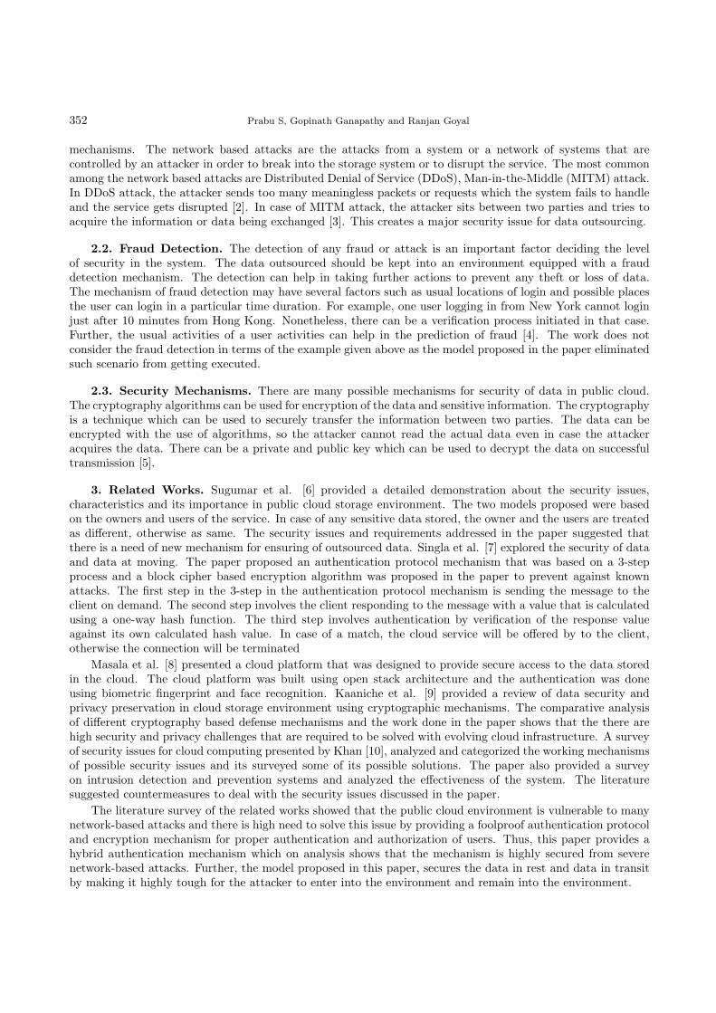
352 Prabu S, Gopinath Ganapathy and Ranjan Goyal
mechanisms. The network based attacks are the attacks from a system or a network of systems that arecontrolled by an attacker in order to break into the storage system or to disrupt the service. The most commonamong the network based attacks are Distributed Denial of Service (DDoS), Man-in-the-Middle (MITM) attack.In DDoS attack, the attacker sends too many meaningless packets or requests which the system fails to handleand the service gets disrupted [2]. In case of MITM attack, the attacker sits between two parties and tries toacquire the information or data being exchanged [3]. This creates a major security issue for data outsourcing.
2.2. Fraud Detection. The detection of any fraud or attack is an important factor deciding the levelof security in the system. The data outsourced should be kept into an environment equipped with a frauddetection mechanism. The detection can help in taking further actions to prevent any theft or loss of data.The mechanism of fraud detection may have several factors such as usual locations of login and possible placesthe user can login in a particular time duration. For example, one user logging in from New York cannot loginjust after 10 minutes from Hong Kong. Nonetheless, there can be a verification process initiated in that case.Further, the usual activities of a user activities can help in the prediction of fraud [4]. The work does notconsider the fraud detection in terms of the example given above as the model proposed in the paper eliminatedsuch scenario from getting executed.
2.3. Security Mechanisms. There are many possible mechanisms for security of data in public cloud.The cryptography algorithms can be used for encryption of the data and sensitive information. The cryptographyis a technique which can be used to securely transfer the information between two parties. The data can beencrypted with the use of algorithms, so the attacker cannot read the actual data even in case the attackeracquires the data. There can be a private and public key which can be used to decrypt the data on successfultransmission [5].
3. Related Works. Sugumar et al. [6] provided a detailed demonstration about the security issues,characteristics and its importance in public cloud storage environment. The two models proposed were basedon the owners and users of the service. In case of any sensitive data stored, the owner and the users are treatedas different, otherwise as same. The security issues and requirements addressed in the paper suggested thatthere is a need of new mechanism for ensuring of outsourced data. Singla et al. [7] explored the security of dataand data at moving. The paper proposed an authentication protocol mechanism that was based on a 3-stepprocess and a block cipher based encryption algorithm was proposed in the paper to prevent against knownattacks. The first step in the 3-step in the authentication protocol mechanism is sending the message to theclient on demand. The second step involves the client responding to the message with a value that is calculatedusing a one-way hash function. The third step involves authentication by verification of the response valueagainst its own calculated hash value. In case of a match, the cloud service will be offered by to the client,otherwise the connection will be terminated
Masala et al. [8] presented a cloud platform that was designed to provide secure access to the data storedin the cloud. The cloud platform was built using open stack architecture and the authentication was doneusing biometric fingerprint and face recognition. Kaaniche et al. [9] provided a review of data security andprivacy preservation in cloud storage environment using cryptographic mechanisms. The comparative analysisof different cryptography based defense mechanisms and the work done in the paper shows that the there arehigh security and privacy challenges that are required to be solved with evolving cloud infrastructure. A surveyof security issues for cloud computing presented by Khan [10], analyzed and categorized the working mechanismsof possible security issues and its surveyed some of its possible solutions. The paper also provided a surveyon intrusion detection and prevention systems and analyzed the effectiveness of the system. The literaturesuggested countermeasures to deal with the security issues discussed in the paper.
The literature survey of the related works showed that the public cloud environment is vulnerable to manynetwork-based attacks and there is high need to solve this issue by providing a foolproof authentication protocoland encryption mechanism for proper authentication and authorization of users. Thus, this paper provides ahybrid authentication mechanism which on analysis shows that the mechanism is highly secured from severenetwork-based attacks. Further, the model proposed in this paper, secures the data in rest and data in transitby making it highly tough for the attacker to enter into the environment and remain into the environment.

Enhanced Data Security for Public Cloud Environment with Secured Hybrid Encryption Authentication Mechanisms 353
Fig. 4.1. PAP 2-way handshake mechanism
4. Existing Mechanisms. The existing mechanisms for authentication and encryption are discussed asfollows:
4.1. Authentication Protocols. There are several existing authentication protocols proposed by re-searchers and scientists. The most common among them used to build the proposed mechanism includesPassword Authentication Protocol (PAP), Secure Socket Layer (SSL) and Challenge Handshake AuthenticationProtocol (CHAP). This paper only focuses on these methods to provide a multi-layered hybrid authenticationprotocol.
The PAP is a password based authentication protocol that provides two-way handshake mechanism. In thisprotocol, the client sends the details such as username and password to the server which gets verified on theserver side. In case the credentials match with the data present on the server-side database, the server sendsan acceptance acknowledgement to the client and a connection is established. In case of no match, the clientrequest is rejected and the connection request is terminated. Fig. 4.1 visualizes the PAP mechanism.
The issue in this protocol is that this protocol is highly vulnerable to network attacks such as Man-In-The-Middle Attack (MITM) which can lead to account hijacking and unauthorized access. This issue occurs in thecase of PAP as the credentials sent by the client are in clear or plain text, i.e. not encrypted. This issue is fixedup to some extent by encrypting the credentials with some cryptographic algorithm. Nonetheless, there is stilla chance that the attacker can decrypt the credentials making it still vulnerable to the MITM attacks.
The Secure Socket Layer (SSL) is a protocol used to establish a secure connection between the server andthe browser of the client by the use of encrypted links to make the transactions private. The SSL uses a publicand private key. The public key is used for asymmetric encryption and private key is used for symmetricencryption. The use of asymmetric key provides better authentication and the use of symmetric key providesfaster authentication. A SSL certificate is required to establish a SSL connection for which the submission ofCertificate Signing Request (CSR) is required to be done to the Certification Authority (CA). The CSR containsthe details and identity of the website along with the private key. The CA then validates the data and issues aSSL certificate which matches with the private key. Thus, the SSL is based on mutual authentication i.e. thedigital certificates verify the web servers and client identity before the establishment of the connection. If theweb page is SSL secured, then the web address will begin with HTTPS instead of HTTP and a lock icon withappear which contains the details of the website certificate. Also, if the SSL is having Extended Validation(EV) certification then a green address bar will appear instead of the usual address bar. The use of SSL canprevent fraud and hijacking as it relies on encryption and the originality of the website is also verified up to someextent but it may cause a slowdown in the performance. Thus, the SSL can be used along with the proposedmodel but the model did not consider the use of SSL. Another protocol is Extensible Authentication Protocol(EAP). EAP is an authentication framework. The EAS was originally an extension for Point-to-Point (PPP)authentication. EAP framework supports multiple authentication mechanisms. This framework can also beused but the proposed model did not consider the complete use of this framework.
Another method of authentication is Challenge Handshake Authentication Protocol (CHAP). It is an in-ternet standard that uses one-way MD5 hash function. The CHAP is based on a 3-way handshake mechanism[11]. In this type of authentication, instead of the actual password, the transmission of the hash result is per-formed over the network. As the password in this case, does not get transferred over the network, it cannot becaptured during the transmission. Also, the hash function generates the random string in such a manner thatthe operation cannot be reverse engineered to obtain the original password. Nonetheless, this method is vul-nerable to remote server impersonation. This vulnerability can be prevented by using a two-way authentication

354 Prabu S, Gopinath Ganapathy and Ranjan Goyal
Fig. 4.2. CHAP 3-way handshake mechanism
using separate keys for transmitted and received data to identity server as well as client. This concept is usedin MS-CHAP in which the challenge is sent repeatedly during the connection. Fig. 4.2 visualizes the CHAPmechanism.
4.2. Data Security. There are several existing algorithms proposed by researchers and scientists. Themost suitable is discussed in this paper that is used in proposing the encryption model, i.e. Advanced EncryptionStandard (AES). The AES is an encryption standard that is actually the 128-bit based symmetric block cipheralgorithm known as Rijndael algorithm [13-15]. The AES is being used worldwide and is the most securestandard at present. The AES is the successor of Data Encryption Standard (DES) [16]. The AES is faster andmore secure than DES. The Rijndael algorithm was based on 128, 192 and 256-bits block size but for the AES,only 128-bit block size was accepted. The AES thus have the block size of 128-bits and key size of 128, 192and 256-bits. The algorithm is based on combination of substitutions and permutations. It operates on a 4 by4 column major order matrix. There are 10 rounds for 128-bits key, 12 rounds for 192-bits key and 14 roundsfor 256-bits keys. Thus, the data-in-rest and data-in-transit can be handled securely using this algorithm. Thedata here refers to the plain text which on encryption becomes cipher text. The cipher text can be convertedback to plain text with the help of decryption. In symmetric encryption, the same key is used for encryptionand decryption. Fig. 3 depicts the AES encryption and decryption operations.
Fig. 4.3. AES Encryption and Decryption

Enhanced Data Security for Public Cloud Environment with Secured Hybrid Encryption Authentication Mechanisms 355
Fig. 5.1. Proposed Client-Side Authentication Mechanism
5. Proposed Method. The paper focuses on securing data present in the public cloud computing envi-ronment by providing a more secure hybrid of authentication and encryption mechanisms. The two mechanismsare discussed as follows:
5.1. Authentication Mechanism. The authentication protocol proposed in this paper, works on the ideaof the PAP and CHAP mechanisms along with TLS. The client-side mechanism for the proposed authenticationprotocol is depicted in the Fig. 5.1. The client sends a challenge to the server and waits for the response. Afterthe response is received, the response is verified and is either accepted or rejected. If the response is acceptedthen the client sends the username in encrypted format and waits for the challenge. In case of rejection, theconnection is terminated. When the challenge is received, the response is generated and is sent to the serverand the client waits for the acceptance of response from the server. Upon Acceptance, a timed connection isestablished. In case of rejection, the connection request is terminated. Upon connection time-out, the clientwaits for the challenge from the server and same procedure is repeated until the connection gets establishedagain. During the connection, any terminate request if given, terminates the connection.
The server-side mechanism depicted in Fig. 5.2, shows the authentication procedure from the server side.Initially, the server waits for the challenge from the client. When the challenge is received, a response agenerated and sent to the client. If the response is accepted by the client, the server waits for the client to send
356 Prabu S, Gopinath Ganapathy and Ranjan Goyal
Fig. 5.2. Proposed Server-Side Authentication Mechanism
the username. When the client sends the username, the server verifies the username by decrypting encryptedusing and matching it in the database. If the username is successfully verified, the server sends a challenge tothe client and waits for the response. When the response is received, it is verified and on acceptance of response,a timed connection is established. The mechanism leads to termination in the case of rejection of response,rejection of username or any termination request.
The combined Client-Server Authentication Mechanism is depicted in Fig. 5.3. The mechanism depictedin the figure is based on the interactions of the client and server that does not show the time of propagationand delay. This proposed mechanism is named as Improved Hybrid Authentication Mechanism (IHAP).
5.2. Data Security. The paper proposes the encryption mechanism using the AES algorithm. There areseveral attacks that AES can handle including brute force and biclique attack due to high time complexity.Nonetheless, the poor key management can compromise the data. Thus, there is a need to deal with thisproblem by using separate key management technique. For this, the paper suggests to use the algorithm knownas Secure Hash Algorithm 3 (SHA-3). This paper presents the key management using the SHA3-256 that havethe attack resistance of 2128. Fig. 7 depicts the data security proposed model using AES encryption and SHA-3

Enhanced Data Security for Public Cloud Environment with Secured Hybrid Encryption Authentication Mechanisms 357
Fig. 5.3. Proposed Client-Server Authentication
Fig. 5.4. Data Security Proposed Model using AES and SHA-3
hashing technique. The key used in AES for ciphering the text is of 256-bit. The size of block for SHA-3 is 256bits. The data securing is done by first encrypting the plain text of 128-bit block using a secret key [17]. Thecipher text obtained on encryption is the required encrypted data. Now, for key management, the secret key ishashed using the SHA-3 and the hashed key is obtained [18]. In recovering process, the original secret key thatclient is having, is hashed using the SHA-3. Then the hash value of that key is matched with the hashed valuereceived from the server. In case of match, the key can now be used to decrypt the cipher text using the AESalgorithm and the cipher text can be converted back into plain text.
6. Analysis. The proposed model for authentication for client and server side can be analyzed based onthe possible common network attacks. The possible common network attacks in this scenario are MITM, DoSand DDoS Attacks. Let us consider the more powerful attack DDoS alone among DoS and DDoS as the DDoS

358 Prabu S, Gopinath Ganapathy and Ranjan Goyal
is the distributed attack scenario of DoS attack. Therefore, considering the MITM and DDoS attack possibilityat every point of exchange of information, the authentication mechanism procedure is analyzed as follows:
Challenge and Response (Client and Server): In the case of DDoS attack, the attacker may try to sendmeaningless or irrelevant responses for the challenge. But this makes it impossible to continue the attack as therequests will be dropped after the limit is crossed. The limit is set for requests as it is impossible to receive alarge number of requests from a client in a particular time limit. Thus, this point is safe from DDoS attack. Incase of MITM attack, the attacker clones the client and tries to capture the response sent. Thereafter, there is apossibility that the attacker clones the server and sends the response to the client. But in this at the connectioncannot be established as the username step involves encryption that makes it hard to perform MITM as thecloning of client and server along with decryption of username without knowing the actual algorithm and keyis a complex process in real life scenario and hard to be implemented due to very high time complexity. Asthe time is limited for authentication, the attacker fails to perform the attack due to all this complex process.Also, there is a possibility that the attacker tries to fetch the challenge and solve it. In that case, the attackermay get the information of challenge that contains some random string along with hash of password. As theirreversible process is followed, the attacker cannot reverse engineer it, making it impossible to find the actualresponse value for that challenge thus making it highly safe from MITM attack at these points.
Username: In case of MITM attack, as the username sent is encrypted, so even if the attacker succeedsin capturing the username, it is hard to decrypt it without knowing the encryption algorithm and the value ofkey. Considering the worst-case scenario, the attacker successfully decrypts the username but in this case, thetime limit by that time is already crossed and the process is already completed thereby making it meaninglessto decrypt the username. Also, DDoS attack again becomes irrelevant at this point as the meaningless requestssent at this point will not be accepted thus making it highly safe from DDoS and MITM attack at this point.
Established Connection: In case of MITM attack, considering the only possibility that the attacker succeedsin bypassing authentication by somehow cloning the client successfully and establishes connection to server.Nonetheless, the attacker though gets the connection but as the connection is actually a timed connection, thusit will make it impossible to remain into the system after the time gets expired as the challenge and responseprocess is further continued after time gets expired. Also, in case of DDoS attack at the time of establishedconnection, no meaningless request is accepted from client and server side thus making it safe from MITM andDDoS attack at this point.
Thus, this proposed authentication mechanism is highly secure from common network attacks, MITM andDDoS attack. Considering the case of other attacks like phishing and sniffing attack etc., these attacks eithercomes under these MITM attacks which makes shows that this mechanism is secured from all these attacks.Consider an example of sniffing attack, where the attacker captures the packets being sent. As here the usernamesent is encrypted so it makes it safe from sniffing attack. Also, as the web page is SSL secured, it makes thewebpage safe from phishing attack. Therefore, the mechanism is safe from many network attacks including themost common ones, MITM and DDoS attack.
Now, for the proposed data security model, the securing and recovering mechanism was implemented usingthe python program and the simulation was done on the system having specifications as: 16GB RAM and Inteli7, 7th Generation Processor on the Windows 10 environment. The simulation results were received for 1 MB,10 MB, 100MB, 1GB and 10 GB file sizes and the running time for the securing and recovering process wasrecorded. The observed values for the proposed model of recovering and securing process is given in the TableI. Also, the graph depicting the securing and recovering time is shown in the Fig. 6.2. The securing processcontains the results for running time that involves the encryption using AES 256-bit key and the generation ofthe hash value using the SHA-3 256-bit for that key after the encryption process is completed. The recoveryprocess contains the results for the running time that involves generation of hash value for the clients key andmatching this hash value with the received hash value from the server followed by decryption of the data usingthe clients key if the hash value of the clients key matches with the hash value received from the server.
Therefore, the proposed model for securing the data using AES and SHA-3 is safe from most of the knownattacks including the password cracking brute force attack, birthday attack, biclique attack, timing attacks etc.as the AES is found to be safe from all these attacks. The only possible vulnerability was that the poor keymanagement can compromise the data encryption. This problem is also solved by the proposed mechanism as

Enhanced Data Security for Public Cloud Environment with Secured Hybrid Encryption Authentication Mechanisms 359
Fig. 6.1. Observed running time values for proposed model
Fig. 6.2. Graph depicting Securing and Recovering Time
the mechanism hashes the key with the help of SHA-3. So, overall the security get user enhanced in termsof authenticity and data security. Thus, due to highly enhanced security during authentication and duringaccessing the data, it becomes almost impossible for the intruder to fool the security mechanism to get accessto the resources and steal information and kept data in the cloud environment.
7. Conclusion. In this paper, a model for security of data in cloud computing environment is proposedthat provides a detailed visualization of the security mechanism. The work done in this paper contributes inproviding the highest possible security mechanism suitable for public cloud storage with the use of authenticationand encryption mechanisms. The proposed model uses the hybrid approach from the existing mechanisms thathelps in achieving the highly enhanced security. Future work is to implement further authentication mechanismssuch as biometric authentication that includes fingerprint, iris and face recognition techniques as multilevelauthentication mechanism. The biometric technique is currently not cost effective considering the cost of highlyaccurate iris and face recognition. Hence, this paper may also provide a scope for the integration of the biometricauthentication into the cloud security mechanism along with the use of proposed authentication mechanism.

360 Prabu S, Gopinath Ganapathy and Ranjan Goyal
REFERENCES
[1] M.G. Avram, Advantages and challenges of adopting cloud computing from an enterprise perspective, 7th InternationalConference Interdisciplinarity in Engineering (INTER-ENG 2013), Volume 12, pp. 529-534, 2014.
[2] Rashmi V. Deshmukh and Kailas K. Devadkar, Understanding DDoS Attack and Its Effect In Cloud Environment,Procedia Computer Science (2015), Vol. 49, pp. 202-210, 2015.
[3] S. Subashini and V. Kavitha, A survey on security issues in service delivery models of cloud computing, Journal of Networkand Computer Applications, Volume 34, pp. 1-11, July 2010.
[4] Md. Tanzim Khorshed, A.B.M. Shawkat Ali and Saleh A. Wasimi, A survey on gaps, threat remediation challenges andsome thoughts for proactive attack detection in cloud computing.
[5] Madhuri B. Shinde, Design and Implementation of Asymmetric Cryptography Using AES Algorithm, IJARIIE-ISSN(O)-2395-4396, Vol-1 Issue-4, pp. 371-378, 2015.
[6] Dr. Ramalingam Sugumar and Sharmila Banu Sheik Imam, Data Security in Public Cloud Storage Environment, In-ternational Journal of Engineering Research and Technology (IJERT), ISSN: 2278-0181, Vol. 4 Issue 06, pp. 101-105,June-2015.
[7] Sanjoli Singla and Jasmeet Singh, Survey on Enhancing Cloud Data Security using EAP with Rijndael EncryptionAlgorithm, Global Journal of Computer Science and Technology Software and Data Engineering, Volume 13, Issue 5,2013.
[8] G.L. Masala, P. Ruiu, A. Brunetti, O. Terzo and E. Grosso, Biometric Authentication and Data Security in CloudComputing, Int’l Conf. Security and Management, SAM’15, pp. 9-15.
[9] Nesrine Kaaniche and Maryline Laurent, Data Security and privacy preservations in cloud storage environments basedon cryptographic mechanisms, Computer Commincations (2017) Vol. 111, pp. 120-141, October 2017.
[10] Minhaj Ahmad Khan, A survey on security issues for cloud computing, Journal of Network and Computer Applications(2016), Vol. 71, pp. 11-29, August 2016.
[11] Sadia Marium, Qamar Nazir , Aftab Ahmed, Saira Ahthasham and Mirza Aamir Mehmood, Implementation of EAPwith RSA for Enhancing The Security of Cloud Computing, International Journal of Basic and Applied Sciences , Volume1, Issue 3, pp. 177-183, 2012.
[12] Atewologun Olumide, Abeer Alsadoon, P.W.C. Prasad and Linh Pham, A Hybrid Encryption model for Secure CloudComputing, 2015 Thirteenth International Conference on ICT and Knowledge Engineering, pp. 24-32, November 2015.
[13] Babitha M.P and K.R. Remesh Babu, Secure Cloud Storage Using AES Encryption, 2016 International Conference onAutomatic Control and Dynamic Optimization Techniques (ICACDOT), pp. 859-864, September 2016.
[14] Sanjoli Singla and Jasmeet Singh, Cloud Data Security using Authentication and Encryption Technique, InternationalJournal of Advanced Research in Computer Engineering and Technology (IJARCET), Volume 2, Issue 7, pp. 2232-2235,July 2013.
[15] Mrs. S. M. Barhate and Dr. M. P. Dhore, User Authentication Issues In Cloud Computing,, IOSR Journal of ComputerEngineering (IOSR-JCE), Volume 4, pp. 30-35, 2016.
[16] Shakeeba S. Khan and R.R. Tuteja, Security in Cloud Computing using Cryptographic Algorithms, International Journalof Innovative Research in Computer and Communication Engineering, Volume 3, Issue 1, pp. 148-154, January 2015.
[17] Zaid Kartit, Applying Encryption Algorithm to Enhance Data Security in Cloud Storage, Advances in Ubiquitous Network-ing. Lecture Notes in Electrical Engineering, Vol 366, pp. 141-154, Springer, Singapore.
[18] J R Ngnie Sighom, Pin Zhing and Lin You, Security Enhancement for Data Migration in the Cloud, Future Internet,Volume 9, Issue 3, pp. 1-13, June 2017.
Edited by: Rajkumar RajasekaranReceived: Jul 24, 2018Accepted: Dec 4, 2018

Scalable Computing: Practice and Experience
Volume 19, Number 4, pp. 361–373. http://www.scpe.org
DOI 10.12694/scpe.v19i4.1425ISSN 1895-1767c⃝ 2018 SCPE
CLOUD BASED DYNAMIC COURSE SELECTION FRAMEWORK USING NETWORKGRAPHS WITH TERM DIFFICULTY ESTIMATION∗
JASEM M. ALOSTAD †
Abstract. The system developed in this paper uses a cloud based technology to implement and design a software as a service(SAAS) application for adaptive course selection and term difficulty estimation for a networked curriculum. The choice of coursesin every term is completely in the hands of the students who enroll for a particular program in Universities. The order of coursestaken in every term is ad hoc due to different factors like student interests, uncertainty about the student pass rates, frequentchanges in admission policies and curriculum requirements. However, this choice of course plays a vital role in students graduatingin time from the university. In this paper, we analyze student success ratios in terms of time to graduation. To illustrate thedesigned models, data from different colleges of the Public Authority of Applied Education and Training (PAAET), Kuwait, isused. Graph-based complex networks are used for analyzing the courses and how crucial they are. The difficulty levels of coursesare estimated based on the institutional data from spring 2013 to fall 2016 and term difficulties are estimated based on the courseschosen. This work presents a robust framework which is adaptable to the courses chosen by the students and the ease of flow ofstudents through the curriculum with the aim of improving the universitys graduation rate.
Key words: Parallel processing, Data Analytics, Cloud computing, Graph Theory, Student Success Ratio, Time to Graduation,Course Cruciality, Course Difficulty
AMS subject classifications. 68M14, 90C35
1. Introduction.
1.1. Background. Prediction and investigations on academic performance and the factors affecting stu-dent success and the endurance of students are topics of utmost importance in higher education [18]. Academicperformance is a crucial factor in analyzing higher education levels and predicting other important job outcomeslike performance in the job hired for and salary predictions [19]. The success ratio is an important metric forthe students and the university. The success of a student has many definitions, varying from the grades toself-improvement[7, 8]. Most of the studies from the literature indicate student graduation in time as the mostimportant success metric. From the perspective of the university, and especially for public universities, factorslike graduation, student retention rate and time to degree are essential for the so called performance funding ofthe universities from the state. Generally, the final grades obtained by the student are used for analyzing theperformance of a student.
The graduation rate of students depends on two factors: institutional and pre-institutional factors [11,12]. The students perspective on the graduation rate depends on pre-institutional factors like High schoolperformance, the demographic status of the students, socio-economic data and some of the institutional factorsinclude the guidelines and policies of the university, tutoring, advisory arrangements and the competence of theinstructors [13, 14]. The success framework of students is shown in Fig.1.1 as discussed in [10]. Prediction andprogression results are used in [17] educational data mining to analyze student performance.
In this paper we are considering the optimal course choice models for The Public Authority of AppliedEducation and Training (PAAET), a higher education institute in Kuwait, offering a range of programs throughits various colleges across the country. There are five different colleges and two campuses differentiated genderwise, for each college. PAAET is considered as one of the largest institutes in the Middle East, taking studentenrollment as a factor in the measurement. Every term approximately 40000 students are admitted to differentcolleges in PAAET. There are 5 different colleges, namely College of Basic Education, College of BusinessStudies, College of Health Sciences, College of Nursing and College of Technological Studies under PAAET. Ofall the colleges, the College of Basic Education has more number of students enrolled each term. BA0106, a fouryear degree program of the college of Basic Education, PAAET, is considered for further processing, analysisand discussion in this paper.
∗This work was supported by The Public Authority of Applied Education and Training, Kuwait.†College of Basic Education, The Public Authority of Applied Education and Training (PAAET),
Kuwait,([email protected]).
361

362 J.M. Alostad
Fig. 1.1. Student success framework.
1.2. Problem Statement. Student graduation rate is one of the most important metric in evaluatingthe rank of a College or University. Universities where the success ratio is large, has largest enrollments inyears to come. E-Advisor is a web based application providing online guidance to the students of PAAET. Hereguidelines are given in the direction of finding appropriate disciplines so they can succeed by graduating in-time.The e-advisor system provides the detailed information of the different colleges in PAAET, their major courses,the success rate in each of the course in the previous years and the rules and regulations of the Authority. Thecurrent system lacks options for guiding student about the subjects that has to be chosen in future semesters.Hence, for the objective of increasing the Graduation rate of the student, choice of courses in every term istaken into consideration in this work. The proposed solution acts as an advising system for the students. Thissolution helps students who are below average and who are unaware of being expelled from college for reachingthe maximum allowed semesters in their period of graduation. They system alerts the students as early inhis/her 3 rd semester about his delay in graduation and time to graduation.
1.3. Proposed Solution. A critical institutional factor that is often glossed over is the order of coursechoices every term i.e. the structure of the curriculum, which is linked with the program which a student hasselected. This is one of the most relevant perspectives in understanding the academic performance of a student.Hence, in this paper we analyze the course choices in every term and identify the most crucial courses in thecurriculum. The key point is failure in such crucial courses or if the courses are not taken according to schedulethis will directly lead to delay in graduation. This analysis is carried out program wise. In this process wedeveloped an adaptable framework which is used to guide the student on choosing courses every term so thathe is not delayed in graduation.
Contributions: In this paper the problem of student success ratio is addressed in terms of his/her graduationin-time from the university. The proposed algorithm incorporates the following unique features
1. A network graph for the entire courses in a particular program is constructed for the algorithm imple-mentation.
2. Course prerequisites, co requisites and level of the courses are taken into consideration.3. An important feature for student success; choice of courses in every allowed term by students in order
to identify their time to graduation is considered. As an advisory system, our algorithm gives an optimal set ofcourses for a student for a term in order to graduate in time.
4. A dynamic course selection algorithm is developed which displays the optimal choice and allows a stu-dent to decide the courses on his own. Depending on the courses chosen; the algorithm dynamically recomputesthe optimal choice of courses from the next term and an alert is generated if the student is expected to exceedthe number of allowed terms.
5. The difficulty of every course in the program is identified using the institutional data from the years

Cloud based Dynamic Course Selection Framework using Network Graphs with Term Difficulty Estimation 363
2013 to 2016.6. With the calculated course difficulty, term difficulty is computed and future term difficulty is also
predicted with the current selection of courses.Organization: The rest of the paper is organized as follows. Section 2 gives a brief review of the literatureconsidering the work done earlier in this field. In section 3 the proposed adaptive course selection framework ispresented in detail, considering the static and dynamic selections. Section 4 presents details about the difficultyanalysis of every course in the chosen program. Section 5 discusses the numerical results obtained with thesample data and Section 6 concludes the work.
2. Related Works. A student performance analysis system presented in [1] uses students’ grades toclassify students into different clusters. The performance of a student on a particular course is analyzed andpredicted using data mining techniques. A case study on the Educational data mining techniques is presentedin [2], where classification based data mining algorithms are presented for analyzing the student performance.Similarly in an exhaustive study in the field of educational data mining [3], the prediction algorithms used forstudent performance analysis and their comparison is presented.
Abeer and Elaraby [4] used the demographic information about students, including their behaviour andactivities, with rules for classification and predicted the performance of students. The approximate grades ofthe students are predicted, which helped in improving the student performance on future courses.
An association rule based performance prediction and improvement in higher education is proposed in[6]. The work presented in [5] is based on knowledge mining from the educational data using a decisiontree and identifying the students with low performance ranges and it suggests improvements in their learningmethodology.
In [15] different metrics for measuring student success are analyzed. The five most important metricsincluded in the discussion are: retention rates, graduation rates, time to completion, academic performance,and tracking educational goals. The graduation rate and the retention rate are closely related and the factorsaffecting both the metrics are almost the same. The most important factor to be considered in these twometrics is the unpredictability in students’ paths. A prediction model for identifying the social, economic andpsychological factors a student is facing in his adolescence is analyzed in [16]. The model takes data balancing,dimensionality reduction, discretization and normalization to pre process the data and predictor construction.
In all the work proposed in the literature in the direction of analysis of student success or performanceanalysis recent data mining techniques have been used to analyze the performance of the students and identifygood or bad performance, enabling the teacher and the student himself to explore different ways to improveperformance in future terms. We recognize an important factor in student success as the courses taken duringhis period of study. Difficulty analysis is done for different courses in [22], where different data such as highschool GPA, ICT scores, demographic data and the grades obtained by the students in the previous years aretaken into consideration. The institutional data plays a major role in deciding the difficulty of the coursesconducted in the university. Hence, in this work we build upon this to identify the static and dynamic termdifficulty as a warning or information for students, providing awareness about the level of his course. Curriculumdesign patterns and applications are explained in detail in [20, 21], which is the basis of the work presented inthis paper. The difficulty level and how crucial courses are considered to be should be known before choosing acourse. Hence, in this work we present a framework for providing an optimal choice of courses for a particularterm for a student so that the success rate of the student increases, enabling a high graduation rate from theuniversity.
3. Adaptive Course Selection Framework. The proposed course selection framework is explained indetail in what follows. The network construction of courses in the curriculum of a program is described firstand the algorithm for deciding the optimal course choice is discussed later.
3.1. Course Network Construction. As a measure of a students success, graduating in time from theuniversity is considered as an important institutional factor. For a student to graduate in time the requirementis completion of the courses and earning the required credits. The order of course choice plays an important rolein time to graduation as the courses in the curriculum are sometimes not dependent but some of the courseshas pre-requisites which have to be completed before taking them up. Hence, in this paper the curriculum

364 J.M. Alostad
associated with a particular degree program is taken and the choice of courses in different terms is identifiedusing the course selection algorithm. Due to the nature of course networks, graph theory and complex networkanalysis is used to find out the most crucial courses in the curriculum mathematically. This calculation of howcrucial a course is can guide the student in deciding when to choose a particular course in order to avoid delayin graduation.
The curriculum graphs are constructed using graph theory. Here the courses in the curriculum are rep-resented as the nodes and two nodes are connected if the course has a direct prerequisite. Hence, the coursenetwork is represented as an NxN adjacency matrix M, where N is the number of courses in a program. Ifthere is a vertex between two nodes the corresponding entry in the adjacency matrix Mij = 1, 0 otherwise .
We define two properties, the Delay factor and blocking factor for each course. The Delay and Blockingfactor is 0 for courses that are independent, i.e courses without any prerequisites. Hence, for the courses withprerequisites the length of the longest path from a node to its leaf node is the delay factorDfi. The delay factoridentifies courses that drive a student to being at risk if it is not finished on time. Connectivity of a node isconsidered in calculating the blocking factor of the node Bfi. The Blocking factor identifies the courses that areprerequisites for a large number of courses. If such a course is not completed at the right time a student maybe blocked from the follow-on courses, which means negative progress towards graduation. The total numberof nodes connected to a particular node gives Bfi of a node. Bfi is defined by equation 3.1:
Bfi =∑
j
nij(3.1)
where nij = 1 if there is a path from i to j , 0 otherwise. Cruciality of a node is calculated as the sum of theblocking factor and the delay factor. Cruciality Ci is given in equation 3.2:
Ci = Bfi +Dfi(3.2)
Hence cruciality factor of a course plays a vital role in deciding when to take a particular course. Since delayand blocking both are taken into consideration, a high crucial course implies that the course has to be givenpreference and taken in appropriate time failing which results in delay in graduation.
3.2. Static Course Preference Algorithm. The Algorithm for course selection is given in Fig.3.1. LetCr be the number of courses in the curriculum, T be the number of terms, assign the credit points to all the
Algorithm 1 Static Course Preference
Let N be number of courses in each termInitialize t = 1while Cr is not empty and t < T do
1. Calculate the cruciality of the courses listed in the curriculum2. Sort the list of courses in ascending order of course levels and descendingorder of the cruciality factor3. Select the first N courses from the list so as to satisfy the limits in the sumof credits that can be registered.4. Select the courses such that there are no prerequisites.5. Check if any of the selected coursehas co-requisites. if true the co-requisitesand its corresponding prerequisites if any has to be processed first.6. These courses will fill term .7. Remove the selected coursesfrom Cr and M8. t = t+ 1
end while
Fig. 3.1. Course Preference algorithm

Cloud based Dynamic Course Selection Framework using Network Graphs with Term Difficulty Estimation 365
Algorithm 2 Dynamic Course Preference
Let N be number of courses in each termInitialize t = 1Read student inputwhile input is not empty do
Update the courses already chosen by the student in the selected arrayUpdate term t if necessaryRemove the selected courses from Cr and M
end whilewhile Cr is not empty and t < T do
Calculate the cruciality of the courses listed in the curriculumSort the list of courses in ascending order of course levels and descendingorder of the cruciality factorSelect the first N courses from the list so as to satisfy the limits in the sumof credits that can be registered.Select the courses such that there are no prerequisites.Check if any of the selected course has co-requisites. if true the co-requisitesand its corresponding prerequisites if any has to be processed first.These courses will fill term .Remove the selected coursesfrom Cr and Mt = t+ 1
end while
Fig. 3.2. Dynamic Course Preference algorithm
terms as mentioned, and let M be the adjacency matrix representing the course and the prerequisite relation.The algorithm generates an ordered list of courses term-wise for the student, so that he can graduate in timewithin the allowed terms.
3.3. Dynamic Course Preference algorithm. The Dynamic course preference algorithm allows a stu-dent to choose a course on his own (which may or may not be from the output of the static algorithm), andfor the rest of the terms the ordered courses list is displayed to the student. The number of terms required tograduate with the current choice of courses is also displayed in the output of the algorithm. The algorithm isshown in Fig. 3.2.
4. Course Difficulty: Institutional Data Analysis. Institutional Data for 8 terms from spring 2013to fall 2016 are analyzed to identify the difficulty of courses. The difficulty estimations are done based on theprevious grades. Mean and standard deviations are calculated for the grade distributions for all the courses foreach of the 8 terms. Some of the courses are not taught in some terms and, hence, the means of the courses forthose particular terms are not available. The rank for each course in each term is calculated and as a samplethe ranks of 25 courses are shown in Table 4.1. The ranks indicate there is a considerable amount of variationin grade distribution in every term.
In order to ensure stability of course difficulty over time, mean of the grade values are ranked. In spiteof ranking the mean of the grade values there are difference in some mean grades because not all the coursesare taught in all the semesters, it depends on the choice of the students. To analyze these variations further,correlation among the 8 terms are calculated using pearson’s R method. On examining the correlation coefficientssupports the general idea that the grade distributions are consistent across several semesters. The calculatedcorrelations are plotted in the correlation plot shown in Fig.4.1. The correlation matrix is shown table 4.2. Theminimum correlation exists between the terms Spring2016 and Fall 2016, on examining the mean grade valuesof these terms reveals that several courses had their extreme values in these semesters. The correlation graph

366 J.M. Alostad
Table 4.1
Rank of Courses (mean grades) in Various Terms
Courses S13 F13 S14 F14 S15 F15 S16 F16X101.102 5 6 6 29 47 9 1 NAX102.101 3 3 2 1 6 2 4 13X102.102 4 5 4 6 10 3 8 7X103.105 1 1 3 4 5 5 2 3X103.115 2 2 1 2 3 1 3 4X106.101 9 13 11 12 14 4 13 11X106.104 10 4 5 11 7 7 10 8X107.104 55 10 48 25 54 51 40 45X107.121 54 54 52 50 46 46 38 46X107.124 39 35 39 36 20 32 35 38X107.131 42 41 50 47 31 34 31 20X107.134 51 16 18 22 8 37 22 26X107.154 26 32 35 32 18 8 42 12X107.161 45 33 43 31 36 36 30 47X107.171 52 47 45 33 41 40 29 35X107.194 41 27 26 35 13 21 5 32X107.214 33 38 46 45 23 30 39 17X107.244 28 34 41 38 19 24 25 25X107.251 48 48 54 26 21 22 37 30X107.254 35 36 22 43 22 42 6 48X107.264 50 42 21 42 26 23 9 44X107.331 53 51 53 51 51 49 48 31X107.341 49 53 42 46 43 33 32 43X107.342 43 40 40 49 37 48 45 40X107.372 44 52 44 18 27 20 43 23
Table 4.2
Correlation of mean grades for 8 terms
S13 F13 S14 F14 S15 F15 S16 F16S13 1.0000000 0.77334600 0.86108600 0.7729660 0.6197429 0.7623634 0.6105081 0.6783107F13 0.7733460 1.00000000 0.85515533 0.8075693 0.6784647 0.7075601 0.6590922 0.6438203S14 0.8610860 0.85515533 1.00000000 0.8437116 0.7005898 0.7777775 0.6910246 0.6487445F14 0.7729660 0.80756928 0.84371157 1.0000000 0.6835913 0.8127427 0.6042601 0.7371457S15 0.6197429 0.67846468 0.70058981 0.6835913 1.0000000 0.6993695 0.7079145 0.5426127F15 0.7623634 0.70756014 0.77777746 0.8127427 0.6993695 1.0000000 0.5991665 0.7315858S16 0.6105081 0.65909216 0.69102459 0.6042601 0.7079145 0.5991665 1.0000000 0.5144824F16 0.6783107 0.64382030 0.64874449 0.7371457 0.5426127 0.7315858 0.5144824 1.0000000
indicates that there is no correlation in the opposite direction. Deviations from normality are also identifiedusing the Shapiro-Wilk’s test. The sample normality plots for fall 2014 and spring 2016 shown in Fig.4.2 showno traces of lack of normality. The p values range from 0.1895 to 0.9958.
5. Numerical Results and Discussions.
5.1. Static Course Choices. To showcase the above mentioned process we have selected the courses ofthe BA0106 program of the College of Basic Education, PAAET. There are 90 courses in total and these arecategorized as mandatory courses for the Major, Elective courses, and General courses. Of the three categoriesthe student has to choose courses totaling 130 credits in 4 years to graduate. The number of credits a studentcan register for a term is restricted to 18 in fall and spring and 7 in summer. The summer terms are optionalfor the students. The entire set of courses in the program is represented as the network shown in Fig.5.1. Thenodes in the network represent the courses. Courses are named as a combination of the department id and thecourse id. The courses without any prerequisites are represented as nodes without any edges and the coursesconnected by prerequisites have edges between them.
The cruciality factor is calculated for the courses in the program according to equation 3.1. The most

Cloud based Dynamic Course Selection Framework using Network Graphs with Term Difficulty Estimation 367
Fig. 4.1. Correlation among the 8 terms
(a) Case I (b) Case II
Fig. 4.2. Sample normality plots for Fall 2014 and Spring 2016
crucial 10 courses are shown in Table 5.1.The static course preference algorithm is executed on the network constructed. The different courses that a
student has to choose in order to graduate in time are the output generated from the algorithm. These lists ofcourses are shown in Table 5.2. The co-requisites and prerequisites are handled optimally and the course levelsare also taken into consideration. The total number of credits earned is 130.
5.2. Adaptive course choices. The actual choice of courses is in the hands of the students. Hence, wehave also presented a dynamic version of the algorithm which initially displays the optimal choice of coursesand reads the input file containing the actual courses chosen by the student and, based on the courses chosen;the set of optimal choices for the upcoming terms is displayed to the student. The algorithm also displays thenumber of terms a student will actually need for graduation with his current choice of courses. Based on theoutput the student may choose to take one or more summer terms as per his requirements. As an illustration
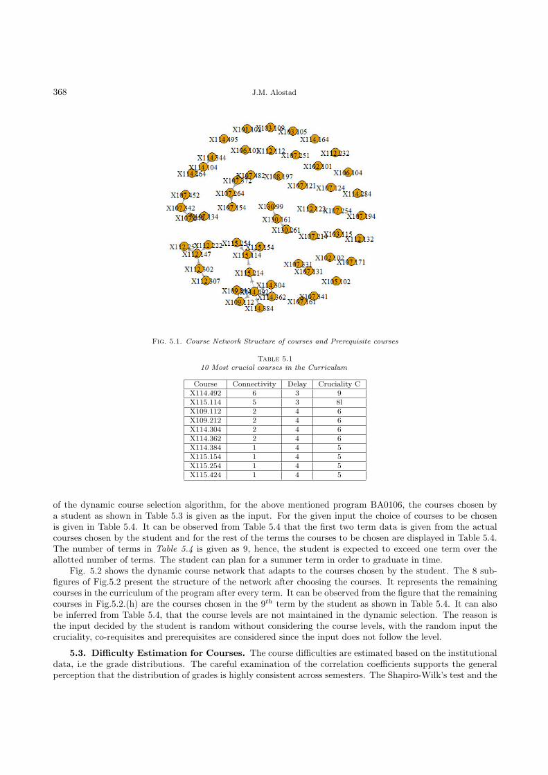
368 J.M. Alostad
Fig. 5.1. Course Network Structure of courses and Prerequisite courses
Table 5.1
10 Most crucial courses in the Curriculum
Course Connectivity Delay Cruciality CX114.492 6 3 9X115.114 5 3 8lX109.112 2 4 6X109.212 2 4 6X114.304 2 4 6X114.362 2 4 6X114.384 1 4 5X115.154 1 4 5X115.254 1 4 5X115.424 1 4 5
of the dynamic course selection algorithm, for the above mentioned program BA0106, the courses chosen bya student as shown in Table 5.3 is given as the input. For the given input the choice of courses to be chosenis given in Table 5.4. It can be observed from Table 5.4 that the first two term data is given from the actualcourses chosen by the student and for the rest of the terms the courses to be chosen are displayed in Table 5.4.The number of terms in Table 5.4 is given as 9, hence, the student is expected to exceed one term over theallotted number of terms. The student can plan for a summer term in order to graduate in time.
Fig. 5.2 shows the dynamic course network that adapts to the courses chosen by the student. The 8 sub-figures of Fig.5.2 present the structure of the network after choosing the courses. It represents the remainingcourses in the curriculum of the program after every term. It can be observed from the figure that the remainingcourses in Fig.5.2.(h) are the courses chosen in the 9th term by the student as shown in Table 5.4. It can alsobe inferred from Table 5.4, that the course levels are not maintained in the dynamic selection. The reason isthe input decided by the student is random without considering the course levels, with the random input thecruciality, co-requisites and prerequisites are considered since the input does not follow the level.
5.3. Difficulty Estimation for Courses. The course difficulties are estimated based on the institutionaldata, i.e the grade distributions. The careful examination of the correlation coefficients supports the generalperception that the distribution of grades is highly consistent across semesters. The Shapiro-Wilk’s test and the

Cloud based Dynamic Course Selection Framework using Network Graphs with Term Difficulty Estimation 369
Table 5.2
Term wise courses
Term 1 X130.99 X102.101 X106.101 X102.102 X101.102 X114.103 X114.104 X106.104Term 2 X107.104 X103.105 X109.112 X112.112 X115.114 X103.115 X107.121Term 3 X112.122 X107.124 X107.131 X112.132 X107.134 X112.147 X115.154 X107.154Term 4 X130.161 X107.161 X114.164 X107.171 X107.194 X108.197 X109.212 X115.214Term 5 X107.214 X112.222 X112.232 X107.244 X107.251 X115.254 X107.254 X112.257Term 6 X130.261 X107.264 X114.284 X112.302 X114.304 X107.331 X107.341Term 7 X112.307 X107.342 X114.344 X114.362 X107.372 X114.384 X114.464Term 8 X114.492 X114.495 X107.482 X107.452
Table 5.3
Student Course Choice input
Term Dept code Course Number1 114 3841 103 1051 115 1142 114 2842 101 1022 114 3042 108 197
Pearson’s coefficients determine the stability of average grades. It appears to be a reasonable assertion that thegrade distribution of individual courses does not change considerably from term to term. To be certain somevariations indeed do occur in a minimal number of courses.
Nevertheless, the average grades appear to be stable enough to be used for estimating course difficulties.Hence, the eight term grade distributions are combined into one set of 57 grade distributions. Hence, averagegrades and their standard deviation are calculated, a sample of the first 25 courses is shown in Table 5.5 andthese means are ranked in ascending order to identify the most difficult course.
The difficulty levels of the courses are represented in a heat map in Fig. 5.3. The colors vary from dark redto yellow for courses that are more difficult to easy.
With these course difficulty levels we also calculate the term difficulty by averaging the difficulty level ofcourses chosen for a particular term. Term difficulty is calculated both for the static course choices as in Fig.5.4.(a) and dynamic course choices as in Fig. 5.4.(b). In the dynamic algorithm the term difficulty of the futureterms is also predicted. This is given as advice to the student so that the courses can be chosen according tohis convenience.
In another direction, this dynamic course preference algorithm can be used for identifying the students whowill not graduate with the maximum allowed terms for graduation. Every program has the designated numberof terms for a student to graduate in-time from the university. There is also a maximum allowed term forgraduation beyond which a student can never graduate. Such a category of student who is anticipated not tograduate is identified early by the proposed algorithm, so that the management can decide upon such studentsin their early terms instead of allowing them for the maximum terms and terminating them from the university.On the other hand, a student is also given an opportunity to decide on his future in his early college life.
The cruciality analysis for different courses can be expanded department-wise and college-wise in order toidentify the department with more crucial courses and the college with the most crucial departments. Thisdata can be used further in allotting grade ranges for different subjects. The future direction of this work isallocating grade ranges for subjects within the curriculum. The grade ranges may vary based on the crucialityof the course. Less crucial courses have different ranges of values for grades compared to more crucial courses.The outcome GPA, which counts in factors like employment and higher education, will there for be fair to allstudents, be it a student who graduated studying less crucial courses or more crucial courses.
6. Conclusion and future enhancement. In this paper, network analysis and graph theory have beenused to propose a framework to understand the structure of University courses by calculating the crucialityfactor. Using this framework, the course selection algorithm shows the optimal choice of courses to be selected

370 J.M. Alostad
Table 5.4
Student Course Choice input
1 X114.384 X103.105 X115.1142 X114.284 X101.102 X114.304 X108.1973 X109.112 X114.362 X112.147 X115.154 X115.254 X107.134 X107.154 X114.1044 X109.212 X107.244 X107.264 X115.214 X112.222 X112.257 X112.302 X114.3445 X114.492 X114.495 X107.372 X107.342 X112.307 NA NA NA6 X107.452 X107.482 X130.99 X107.121 X107.131 X107.161 X107.171 X107.2517 X130.161 X112.112 X107.331 X107.341 X107.124 X107.194 X107.214 X107.2548 X130.261 X102.102 X106.104 X103.115 X112.132 X114.164 X112.232 NA9 X102.101 X106.101 X114.264 X105.102 X112.122 X103.109 NA NA
(a) Case I (b) Case II
(c) Case III (d) Case IV
(e) Case V (f) Case VI
(g) Case VII (h) Case VIII
Fig. 5.2. Structure of the course network after removing courses every term
by a student in order to graduate in time. This choice of courses keeps track of his time to graduation. Thedynamic course preference algorithm takes the student decision and based on the decision his courses andnumber of terms required to graduation is presented which enables the student to plan for extra courses in theupcoming terms and supports him in deciding on the summer term. The framework can be extended to tracethe progress of the students based on the grades obtained and the number of courses chosen along with thecruciality factor to have a positive impact on the graduation rates. The difficulty analysis helps in maintaining

Cloud based Dynamic Course Selection Framework using Network Graphs with Term Difficulty Estimation 371
Table 5.5
Mean Grades indicating the course difficulty
Courses Mean grades SDX103.115 1.287398716 0.222689073X103.105 1.394775842 0.276204191X102.101 1.555222426 0.356798592X102.102 1.819692206 0.203383015X106.104 2.016552526 0.210480467X114.344 2.164735106 0.51446792X101.102 2.206264413 0.69981009X106.101 2.235902851 0.249309948X114.284 2.30080383 0.502985535X115.214 2.328451714 0.595838926X109.112 2.410101831 0.316662409X114.104 2.449580312 0.41757027X114.164 2.506503807 0.791445629X114.304 2.524069967 0.82630547X112.147 2.547242765 0.341405059X114.384 2.594689678 0.654464115X115.254 2.623985029 0.672616448X115.154 2.634053128 0.324480842X130.261 2.636714159 0.318058341X112.232 2.654884638 0.416786992X107.194 2.704502393 0.590925762X115.114 2.716668919 0.314458112X130.161 2.764785793 0.561615129X112.112 2.768196564 0.4150545X107.154 2.771499036 0.468601654
Fig. 5.3. Difficulty level of all courses in the network.

372 J.M. Alostad
(a) Case I (b) Case II
Fig. 5.4. Difficulty level of terms (a) static term difficulty (b) Dynamic term difficulty
a medium hard semester for the student. The student can decide for himself the hardness of a term based onhis personal conditions. The entire system is provided as software as service application in the cloud and enablestudent to register for course from any where irrespective of his location.
REFERENCES
[1] C. L. Sa, D. H. B. Abang Ibrahim, E. Dahliana Hossain, M. Bin Hossin, ”Student performance analysis system (SPAS),Information and Communication Technology for The Muslim World (ICT4M) 2014 The 5th International Conference on,pp. 1-6, 2014.
[2] Kundariya, Daxa and Vaseem, ,A Case Study For Student Performance Analysis Based On Educational Data Mining(Edm), (2016), 10.5281/zenodo.168107.
[3] Pooja Thakar, Anil Mehta, Manisha ,Performance Analysis and Prediction in Educational Data Mining: A ResearchTravelogue, International Journal of Computer Applications (0975 8887) Volume 110 No. 15, January 2015
[4] Ahmed, A.B.E.D. and Elaraby, I.S.,Data Mining: A prediction for Students Performance Using Classification Method,World Journal of Computer Application and Technology, 2014 2(2), pp.43-47.
[5] Al-Radaideh, Q., Al-Shawakfa, E. and Al-Najjar, M., Mining Student Data Using Decision Trees, The 2006 InternationalArab Conference on Information Technology(ACIT2006),2006, Conference Proceedings.
[6] Zhu, Li, Yanli Li, and Xiang Li,Research on EarlyWarning Model of Students Academic Records Based on AssociationRules, Computer Science and Information Engineering, 2009 WRI World Congress on. Vol. 4. IEEE, 2009.
[7] G. D. Kuh, J. Kinzie, J. A. Buckley, B. K. Bridges, and J. C. Hayek,What matters to student success: A review of theliterature, National Postsecondary Education Cooperative, U.S. Department of Education, Commissioned Report for theNational Symposium on PostsecondaryStudent Success: Spearheading a Dialog on Student Success, Tech. Rep.,2006
[8] G. D. Kuh, J. Kinzie, J. H. Schuh, and E. J. Whitt,Student Success in College: Creating Conditions That Matter, SanFrancisco, CA: Jossey- Bass, 2010.
[9] Ahmad Slim, Jarred Kozlick, Gregory L. Heileman, Jeff Wigdahl and Chaouki T. Abdallah,Network Analysis ofUniversity Courses, International World Wide Web Conference Committee (IW3C2), WWW14 Companion, April 7-11,2014, Seoul, Korea. ACM 978-1-4503-2745-9/14/04.
[10] Tushar Ojha, Prediction of Graduation Delay Based on Student Characteristics and Performance, University of New Mexico,UNM Digital Repository, Electrical and Computer Engineering ETDs 2017.
[11] Vincent Tinto, Dropout from higher education: A theoretical synthesis of recent research, Review of Educational Research,1(45):89-125, 1975.
[12] George D. Kuh, Jillian Kinzie, John H. Schuh, and Elizabeth J. Whitt. Stu- dent Success in College: Creating
Conditions That Matter,Jossey-Bass, San Francisco, CA, 2010.[13] Ahmad Slim, Jarred Kozlick, Gregory L. Heileman, and Chaouki T.Abdallah, The complexity of university curricula
according to course cruciality, In Proceed ings of the 8th International Conference on Complex, Intelligent, and SoftwareIntensive Systems, Birmingham City University, Birmingham, UK, 2014. IEEE.
[14] Ahmad Slim, Jarred Kozlick, Gregory L. Heileman, Jeo Wigdahl, and Chaouki T. Abdallah. Network analysis ofuniversity courses. In Proceedings of the 6th Annual Workshop on Simplifying Complex Networks for Practitioners, Seoul,Korea, 2014. ACM.

Cloud based Dynamic Course Selection Framework using Network Graphs with Term Difficulty Estimation 373
[15] Jonathan Kim, The 5 Most Commonly Found Metrics for Student Success, Envisions resources, 2017.[16] A. T. M. Shakil Ahamed, Navid Tanzeem Mahmood and Rashedur M Rahman, An intelligent system to predict academic
performance based on different factors during adolescence, Journal of Information and Telecommunication,(2017) 1:2,155-175, DOI: 10.1080/24751839.2017.1323488
[17] RaheelaAsif, Agathe Merceron, Syed AbbasAli and Najmi Ghani- Haider, Analyzing undergraduate students perfor-mance using educational data mining, Computers & Education, Volume 113, October 2017, pp. 177-194.
[18] Ruban, L. M., McCoach, D. B.,Gender differences in explaining grades using structural equation modelling, Review ofHigher Education 28475502 2005.
[19] Kuncel, N. R., Crede, M., Thomas, L. L., The validity of selfreported grade point averages, class ranks, and test scores:A meta analysis and review of the literature, Review of Educational Research 75 1 6382 2005.
[20] A. Slim.,Curricular Analytics in Higher Education. PhD thesis, University of New Mexico, 2016[21] J. Wigdahl, G. L. Heileman, A. Slim, and C. T. Abdallah, Curricular efficiency: What role does it play in student
success?, In 2014 ASEE Annual Conference & Exposition, Indianapolis, Indiana, June 2014. ASEE Conferences.[22] Daniel James Mundfrom, Estimating course difficulty, IOWA State University, Digital repository, 1991.
Edited by: Rajkumar RajasekaranReceived: Jul 29, 2018Accepted: Dec 3, 2018


Scalable Computing: Practice and Experience
Volume 19, Number 4, pp. 375–385. http://www.scpe.org
DOI 10.12694/scpe.v19i4.1429ISSN 1895-1767c⃝ 2018 SCPE
PARALLEL SEED SELECTION METHOD FOR OVERLAPPING COMMUNITYDETECTION IN SOCIAL NETWORK
BELFIN R.V.& E. GRACE MARY KANAGA∗
Abstract. Social network analysis is one of the key areas of research during modern times. The social network is growingwith more users and the ties between them day by day. This reason brings out many research queries and new conclusions fromthis area. Overlapping community detection in the social network is one such research problem which has acquired interest amongresearchers nowadays. Earlier, the investigation was in finding out algorithms to detect communities in the network sequentially.There are many distinguished findings toward overlapping community detection. Due to the velocity of data in the current era, theavailable algorithms will be a bit sluggish in processing the data. The proposed algorithm uses parallel processing engine to resolvethis delay problem in the current scenario. The algorithm in parallel finds out the superior seed set in the network and expands itin parallel to find out the community. The work shows amazing improvement in the runtime and also detects quality groups in thenetwork.
Key words: Overlapping community detection, Seed selection, Graph parallel processing, seed expansion
AMS subject classifications. 65Y05, 68R10, 91D30
1. Introduction. Complex networks are commonly utilized for modeling the synergies in real-world sys-tems in various areas, such as sociology, biology, knowledge dispersion and many different fields. One importantfeature of this complex network is that the nodes are tightly connected with each other in groups and in turn,the groups will be loosely connected to each other. The tightly connected groups are called as communities.The communities usually have common properties. Therefore, finding the communities from a complex networkcould give many insights about the network. The community detection can be done in two different ways:Firstly, the network partition can be calculated to cut the graph into partitions. Secondly, the selection of seednodes will be done and the local communities will be centered around these seeds.
The proposed work is of the latter category where, the most important nodes in the community will beidentified using a parallel superior seed set selection (P4S) algorithm. The identified superior seeds will be ex-panded by their neighborhood till it reaches the next seed. Since the algorithm expands using the neighborhood,it will form the closely knitted group around the seed nodes.
Seed selection process is an important process in the field of network science. Usually, the measures forcalculating the important nodes from the target network is named as centrality measures [24, 25]. There aremany centrality measures, to name a few, Degree [31], Betweenness [34], Closeness [18], Eigen vector [35], PageRank [32] and so on. These seed nodes play an important role in finding a good community in communitydetection problem and fast spreading in information diffusion application.
2. Related Works. Data nowadays is huge and need to be processed as fast as possible. There is aneed of parallel algorithms to process the volume of data which comes in high velocity. Processing the data inthe faster may fetch the organizations a good profit. There are lots of seed selection algorithms available fordifferent applications. Each application might have to adopt different seed selection algorithms which match theapplication requirement. For example, if the application is a marketing application, the out-degree centralityor the page rank centrality may be used for the seed selection process. So, each centrality measures[9, 10, 2]will have their own limitations with various applications. The proposed method finds out a generic seed bycombining various centralities.
There are some related works available in the literature. There are some diffusion models [40, 28, 21, 7]and community detection algorithms [36, 3, 26, 14, 11] which will have a seed selection part in their model[22, 12, 27, 6]. Some of the algorithms selects the seeds in random and optimize its result at the end of theprocess [15]. There is a excellent study on seed nodes in [13]. Evolutionary algorithms are used to find out theseed nodes in some cases [34].
∗Department of Computer Science and Engineering, Karunya institute of technology and sciences, Coimbatore, Tamilnadu,India. ([email protected], [email protected]).
375

376 Belfin R.V. and E. Grace Mary Kanaga
There are several graph computations algorithm available for large-scale graphs, various parallel moduleshave been developed, e.g., Pregel [20], GraphLab [19] Giraph++ [8], GraphX [37], GRACE [30], GPS [23] andBlogel [38] ,based on MapReduce [5] and BSP (Bulk Synchronous Parallel) models [29].
The proposed algorithm uses GraphX to process the graph in parallel. Our previous work Superior seedset selection algorithm (4S) [1] was extended to parallel processing in this article. The experiment result provesthat the proposed parallel algorithm can find out the good clusters fastest then the available algorithms.
3. Problem Statement. Some of the seed selection algorithms which are already available are usingrandom nodes for selecting the seed node. The selection of a seed node or a seed set is really important in thealgorithms which use seeds to find out communities. Since, the community detection algorithm needs to work inunsupervised way the seeds should be excellent to obtain a perfect local community. The selection of excellentseeds will reduce the number iterations in the community detection algorithm.
Nowadays the data need to be processed is large because of the growing use of internet and social media.Reducing iterations will not be enough to make the algorithm work faster. There is a need of parallel algorithmswhich can process the data in a synchronized manner. Parallel processing algorithms are modern nowadays.The uses of these kinds of algorithms will be fast and effective.
4. Problem Formulation. Assuming an undirected graph G = (V,E). The nodes of the graph G ben = |V | nodes and the edges of the graph G be m = |E|. The overlapping community detection algorithm is usedto determine the community C = C1, ...., Cx of all the nodes of G. |C| be the number of communities identified.In the proposed work, |C| is the number of seed node selected from parallel superior seed set selection algorithm.
Various centrality measures µi for a node i can be calculated which will be the importance measure ofnode i. Let us assume the graph to be undirected. The traditional methods uses any one of the centralitymeasures with respect to the use case, to define its seed set S(G) = si, sj , . . . , sκ where si, sj , . . . , sκ ∈ V .Some models pick seed set randomly and gets the parameter κ as input, to decide the number of seeds inthe set. The difficulty in the conventional methods is that, the seed set need to be adjusted according to thecircumstances of the problem. The proposed parallel, unified model determines the superior seed set S(G) fromthe centrality measures collectively. This article introduces a threshold value τ , which limits the number of seednodes selected for the S(G).
A community may be basically described as a collection of nodes that may share common features, or engagein similar roles in the network. Also, it is tightly knitted groups with a high density of inter community ties anda low density of intra-community ties. The proposed algorithm produces results that are composed of one oftwo types of assignments, crisp assignment of nodes or fuzzy assignment of nodes. With crisp assignment, therelationship between a node and a cluster is binary. That is, a node i either belongs to community C or doesnot. With fuzzy assignment, each node is associated with two or more communities. Throughout the article,the terms set, cluster, and community are used interchangeably.
5. Proposed work. The main idea of this work is to use the parallel processing architecture to find outthe best seeds and subsequently the best seeds from P4S algorithm will be used to find out the communitieshidden in the network. The work has been done with GraphX a module in spark parallel processing engine.The algorithms for the Parallel seed selection and parallel community detection has been explained below inthe following sections. The parallel community detection framework is depicted in the Fig 5.1. The input of thealgorithm will be the unlabeled network, for example, social graph or collaboration networks or the network ofweb pages. The output of the work will be the expanded communities from the selected seeds. The goodness ofthe communities is tested by comparing the inter-density and intra-density of the communities along with thegraph density. The algorithm for the P4S has been given in the Algorithm 1. Algorithm 2 shows the parallelseed set expansion algorithm which finds out the communities.
GraphX is the Apache Spark ingredient for graph-parallel calculations, developed upon a division of math-ematics called graph theory. It is a distributed graph processing framework that lies on top of the Spark core.GraphX inherits the Spark RDD with a Resilient Distributed Property Graph. The property graph is a di-rected multi-graph. The multiple edges it has will be parallel. The parallel edges permit multiple relationshipsbetween the same vertices. The Fig. 5.2 shows the architecture of the parallel 4S and parallel communitydetection implemented in the spark.

Parallel seed selection method for overlapping community detection in social network 377
Fig. 5.1. Parallel community detection framework
Algorithm 1 Parallel Superior Seed Set Selection Algorithm (P4S)
1: procedure P4S(g, τ) ◃ Parallel Superior Seed set selection(P4S)2: READ graph G(V,E)3: COMPUTE4: degree centrality d5: eigen value centrality e6: local clustering coefficient l7: page rank centrality p ◃ Parallel8: SORT d, e, l, p9: for δ do ◃ Parallel
10: Threshold τ ← vertex count/δ11: Fetch τ count of top nodes from list of d, e, l, p12: Intersect (d, e, l, p)
13: return SuperiorSeedsSet S(g) ◃ top seeds
Algorithm 2 Parallel community detection using neighborhood expansion
1: procedure SeedExpansion(g, S(g)) ◃ Parallel Seed Expansion2: COMPUTE3: DistanceMatrix/S(g)4: MaximumExpansionThreshold ExMax
τ
5: for S(g) do ◃ Parallel6: while ( do!ExMax
τ )7: NeighbourhoodExpansion
8: DETERMINE nor selected nodes V φ9: for V φ do ◃ Parallel
10: DETERMINE Neighbors of V φ−NeiV φ11: Degree NeiV φ12: Assign node to the max degree nodes community
13: return SuperiorSeedsSetS(g) ◃ top seeds

378 Belfin R.V. and E. Grace Mary Kanaga
Fig. 5.2. Implementation of Parallel 4S and Parallel community detection algorithm in Spark architecture
The GraphX processors will be used to compute the superior seed set and the seed expansion of the nodeto form community in parallel. Three node clusters was used for computing the communities in parallel.
5.1. Parallel Superior Seed Set Selection (P4S). Parallel superior seed set selection algorithm ex-tracts the very important nodes in the input graph. The input data will be stored in the distributed file systemfor further processing. Centrality measures are used to coin out the important nodes in the network. Eachcentrality measure will have its own importance and use cases to work on. Combining these centrality measurescan identify good seeds across all the centrality measures. For the experiment done for this work Page rank,Degree, Eigen value, Local clustering coefficient centralities was used. The centralities measure calculation willautomatically run in parallel when GraphX is used. Sorting according to the centrality ranks will be done forall centrality measures used. A threshold value will be used to split the top ranks for all measures. Finally, setintersection of the top nodes from each centrality measure will be done to get the superior seed set. Fig. 5.3depicts the process of finding the superior seed set.
5.2. Parallel Community Detection. Community detection from seed by expanding greedily throughneighbors is a classical process. The proposed work is the modified version of the seed expansion in a parallelway. Since we have multiple seeds the algorithm will expand in parallel from the seeds till it reaches the nextseed and stops expanding. The distance between the seeds will be calculated by the distance matrix. TheExMax
τ defined in the Algorithm 2 is the maximum expansion limit. The nodes which are not selected in thefirst iteration will be picked and added to its neighbors community. In case of more than one neighbor thehighest degree node will add the ungrouped node to its community.
6. Experiment. The real-world datasets used for the experiments are from [17]. All the datasets areconnected, undirected graphs. The datasets are from various categories like collaboration networks and productnetworks. The detailed information about the datasets is given in the Table 6.1.
Collaboration networks. In a collaboration network, vertices denote authors, and edges denote co-authorship. If authors u and v are co-authors, they will be connected by an edge. So, if an article is written

Parallel seed selection method for overlapping community detection in social network 379
Fig. 5.3. Parallel 4S algorithm for finding top seed set
Table 6.1
Summary of real-world networks used
GraphNo. ofVertices
No. ofedges
Max.Deg
Avg.Deg
Avg. CCGround-truth
HepPh 11,204 117,619 491 21.00 0.6216 N/AAstroPh 17,903 196,972 504 22.00 0.6328 N/ACondMat 21,363 91,286 279 8.50 0.6417 N/ADBLP 317,080 1,049,866 343 6.60 0.6324 YesAmazon 334,863 925,872 549 5.50 0.3967 YesOrkut 731,332 21,992,171 6933 60.10 0.2468 Yes
by n authors, then their relationship will be represented as a clique in the network. HepPh, AstroPh, andCondMat networks are formed based on the journal submitted to High Energy Physics (Phenomenology) group,Astrophysics group, and Condensed Matter Physics group under the arXiv e-print service, respectively. TheDBLP network is formed based on the DBLP computer science bibliography website.
Product network. In the Amazon product network, vertices denote products and edges denote co-purchasing information. If products u and v are frequently co-purchased, then there will be an undirectededge between them.
Social networks. In a social network, vertices denote users of the social network and the edges denotesocial communications between them. Users can construct a friendship relationship with each other in this webapplication.
7. Community Evaluation.
7.1. Intra-Density, Inter-Density and Graph Density. The cohesiveness of the edges in a graph Gcan be readily attained by calculating the graph density ρ.
ρ =|E|
n(n− 1)/2(7.1)
where n is the count of nodes in the network and n(n − 1)/2 is the maximum possible edges and |E| is thenumber of edges in graph G.

380 Belfin R.V. and E. Grace Mary Kanaga
Consider c is a community in the given network G where |G| = n and |c| = nc. Internal edges are edgeswhich have it both sides situated inside the community c and the external edges of community c refer to theedges which connect a vertex in c to the rest of the graph. The internal degree of vertex v in community c isdenoted by kintv is the number of edges connecting v to other vertices in c and the external degree of v denoted askextv is the number of edges connecting v to the rest of the graph. The intra cluster density δi(c) of a communityc is the ratio between the number of internal edges of c and the number of all possible internal edges:
δi(C) =|Ei|
nc(nc − 1)/2(7.2)
where |Ei| is the count of internal edges in the community.Similarly, the inter-cluster density δe(c) is the ratio between the number of inter-cluster edges of c and the
number of all possible inter-cluster edges:
δe(C) =|Ee|
nc(n− nc)(7.3)
where|Ee| is the count of inter community edges in the community.The proposed parallel seed set selection algorithm has been implemented in the real-world datasets and has
given a better result. The goodness of the community has been tested with the inter-cluster and intra-clusterdensity. Usually For overlapping communities, internal and external metric values will be used. Because,combination metrics and modularity scores will result in confusing values that should be inconsistent[15]. Thegoodness of the community using graph density ρ, intra-cluster density δi(c) and inter cluster density δe(c) canbe given as:
δi(C) > ρ > δe(C)(7.4)
The comparison of inter-cluster density, intra-cluster density and graph density of the real datasets areplotted in the result and discussion section. The experiment was done for the seed sizes 71, 84, 114, 128, 152,172, 207, 240 and 270.
7.2. Clustering Coefficient. A clustering coefficient is a measure of the degree to which nodes in agraph are inclined to tie together. Research results suggests that in most real-world networks, and in somesocial networks, nodes are likely to create tightly connected groups characterized by a pretty high density ofties; this likelihood will greater than the average probability of a connection randomly established between twonodes [33].
The local clustering coefficient li for a vertex i is then given by the ratio of links between the nodes withinits neighbors divided by the number of edges possible between them. The local clustering coefficient for anundirected graph is given as:
Ci =2|ej,nei : vj , vnei ∈ Ni, ej,nei ∈ E|
neii(neii − 1)/2(7.5)
where vertex vj , has neii neighbors, neii(neii−1)2 edges will be the maximum possible edges exist among the
vertices within the neighborhood.
8. Result and discussion. The problem of community assessment is still an open and difficult problemin spite of huge sum of work addressing this topic [13]. The experiment done on the real-world datasets aregiven on the summary Table 6.1. The values of inter-density, intra-density and graph density are compared tofind the goodness of the cluster. The result from the six real-world datasets specified in Table 6.1 has beenplotted in the Fig 8.1. Every dataset used for the experiment passes the test and it goes hand in hand with theEq. (7.4). In all cases the intra-cluster density δi(c) from Eq. (7.2) of all the communities identified is greaterthan the graph density ρ and the inter-cluster density δe(c) from Eq. 7.3 of nodes after finding communities islesser then the graph density ρ from Eq. 7.1.

Parallel seed selection method for overlapping community detection in social network 381
Fig. 8.1. Data comparison between the inter-cluster density, intra-cluster density and graph density: (a) Amazon dataset (b)AstroPh (c) CondMat (d) DBLP (e) HepPh (f) Orkut
The clustering coefficient can be a measure to find out the closely connected groups. The clustering coeffi-cient equation is given the Eq. 7.5. The comparisons of clustering coefficient with the number of communitiesare given in the Fig. 8.2. The clustering coefficient of two datasets namely Amazon Fig. 8.2a and AstroPhFig. 8.2b are shown. The result shows an increasing trend in the clustering coefficient as the number of seedsincreases. This shows that the larger the seed set higher the density of the community. Fig. 8.3 shows thecomparison of clustering coefficient and number of nodes in each community. The result of comparison of av-erage clustering coefficient of the entire network and the average community clustering coefficient is comparedin the Fig. 8.4a and the comparison of average degree of the entire graph and the average degree of all thecommunities detected are shown as a bar plot in Fig. 8.4b. The plots clearly show that the density of the subgraphs increases after the community detection.
The running time factor is one of the important problems in community detection algorithms. When theinput graph becomes larger the operations in graph will become complex and operations on it will be costly.The running time of the algorithm was compared with five important algorithms from the literature shown in
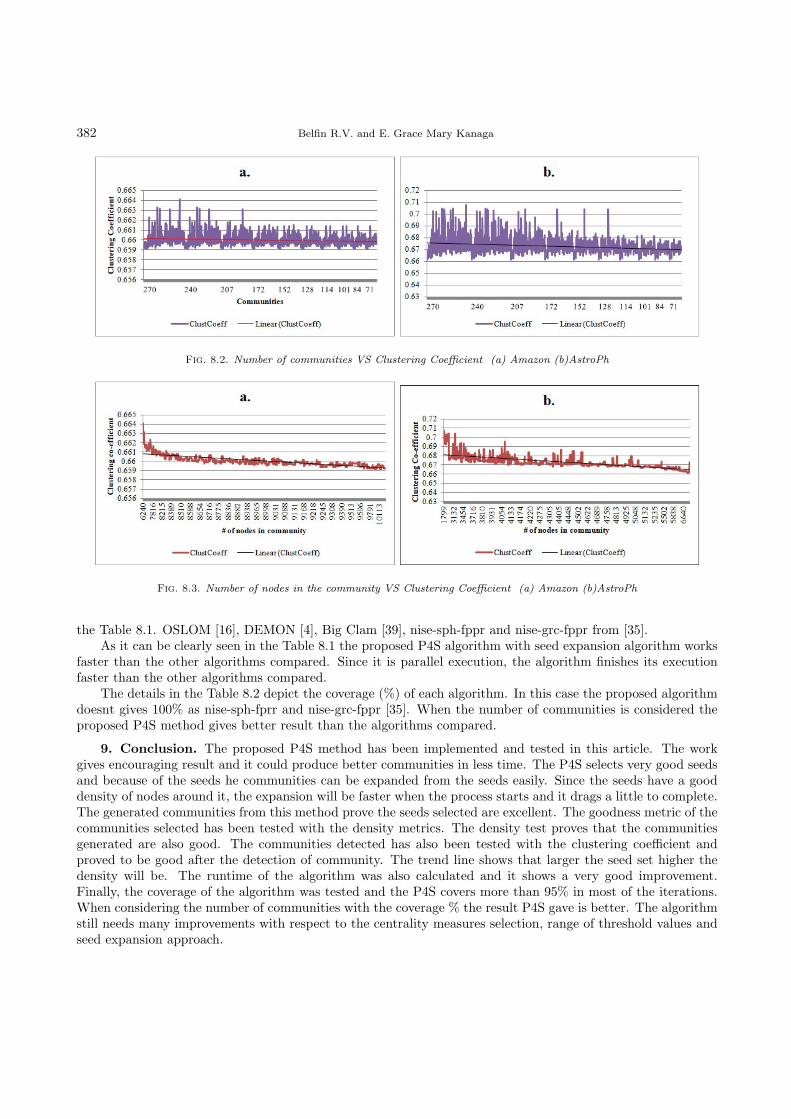
382 Belfin R.V. and E. Grace Mary Kanaga
Fig. 8.2. Number of communities VS Clustering Coefficient (a) Amazon (b)AstroPh
Fig. 8.3. Number of nodes in the community VS Clustering Coefficient (a) Amazon (b)AstroPh
the Table 8.1. OSLOM [16], DEMON [4], Big Clam [39], nise-sph-fppr and nise-grc-fppr from [35].As it can be clearly seen in the Table 8.1 the proposed P4S algorithm with seed expansion algorithm works
faster than the other algorithms compared. Since it is parallel execution, the algorithm finishes its executionfaster than the other algorithms compared.
The details in the Table 8.2 depict the coverage (%) of each algorithm. In this case the proposed algorithmdoesnt gives 100% as nise-sph-fprr and nise-grc-fppr [35]. When the number of communities is considered theproposed P4S method gives better result than the algorithms compared.
9. Conclusion. The proposed P4S method has been implemented and tested in this article. The workgives encouraging result and it could produce better communities in less time. The P4S selects very good seedsand because of the seeds he communities can be expanded from the seeds easily. Since the seeds have a gooddensity of nodes around it, the expansion will be faster when the process starts and it drags a little to complete.The generated communities from this method prove the seeds selected are excellent. The goodness metric of thecommunities selected has been tested with the density metrics. The density test proves that the communitiesgenerated are also good. The communities detected has also been tested with the clustering coefficient andproved to be good after the detection of community. The trend line shows that larger the seed set higher thedensity will be. The runtime of the algorithm was also calculated and it shows a very good improvement.Finally, the coverage of the algorithm was tested and the P4S covers more than 95% in most of the iterations.When considering the number of communities with the coverage % the result P4S gave is better. The algorithmstill needs many improvements with respect to the centrality measures selection, range of threshold values andseed expansion approach.

Parallel seed selection method for overlapping community detection in social network 383
Fig. 8.4. (a) Comparison of average clustering coefficient of nodes before and after community detection. (b) Comparison ofaverage degree of nodes before and after community detection.
Table 8.1
Running times of different methods on our test networks in (Minutes)
Graph oslom demon bigclam nise-sph-fppr nise-grc-fppr P4SHepPh 19.26 0.45 11.383 0.36 2.8 0.3AstroPh 38.05 0.7 48.016 0.6 2.43 0.483CondMat 20.65 0.83 7.35 0.6 1.23 0.45DBLP 350 233 433 18.33 29.733 12.6Amazon 175 115 85 37.6 42.716 20.3Orkut N/A N/A 4199 43.916 236 31.83
Table 8.2
Returned number of communities and graph coverage of each algorithm
Graph oslom demon bigclam nise-sph-fppr nise-grc-fppr P4S
HepPhCoverage (%)no.of.clusters
100608
88.35,147
84.37100
10099
10090
94.83270
AstroPhCoverage (%)no.of.clusters
1001,241
94.158,259
91.11200
100212
100246
95.4270
CondMatCoverage (%)no.of.clusters
1001,534
91.1610,474
99.96200
100201
100249
98.5270
DBLPCoverage (%)no.of.clusters
10017,519
84.89174,560
10025,000
10026,503
10018,477
97.4270
AmazonCoverage (%)no.of.clusters
10017,082
79.16105,685
10025,000
10027,763
10020,036
96.71270
OrkutCoverage (%)no.of.clusters
N/AN/A
N/AN/A
82.1325,000
99.9925,204
99.9932,622
98.5270

384 Belfin R.V. and E. Grace Mary Kanaga
REFERENCES
[1] R. Belfin, G. E., and P. Brodka. Overlapping community detection using superior seed set selection in social networks.Computers and Electrical Engineering, 2018.
[2] P. Bonacich. Power and Centrality: A Family of Measures. American Journal of Sociology, 1987.[3] T. Chakraborty, S. Srinivasan, N. Ganguly, A. Mukherjee, and S. Bhowmick. Permanence and Community Structure in
Complex Networks. 11(2), 2016.[4] M. Coscia, G. Rossetti, F. Giannotti, and D. Pedreschi. DEMON: a Local-First Discovery Method for Overlapping Commu-
nities. 2012.[5] J. Dean and S. Ghemawat. MapReduce: Simplified Data Processing on Large Clusters. Communications of the ACM, 2008.[6] S. Dhamal, P. K. J., and Y. Narahari. Information Diffusion in Social Networks in Two Phases. IEEE Transactions on
Network Science and Engineering, 4697(c):1–1, 2016.[7] F. Erlandsson, P. Brdoka, and A. Borg. Seed selection for information cascade in multilayer networks. Studies in Computational
Intelligence, 689:426–436, 2018.[8] W. Fan, J. Xu, X. Luo, Y. Wu, W. Yu, and R. Xu. GRAPE: Conducting Parallel Graph Computations without Developing
Parallel Algorithms. pages 30–41.[9] L. C. Freeman. Centrality in Social Networks. Social Networks, 1978.
[10] L. C. Freeman. Centrality in social networks conceptual clarification. Social Networks, 1978.[11] J. Han, W. Li, Z. Su, L. Zhao, and W. Deng. Community detection by label propagation with compression of flow. 2016.[12] L. G. S. Jeub, M. W. Mahoney, P. J. Mucha, and M. A. Porter. A Local Perspective on Community Structure in Multilayer
Networks. volume 5, pages 144–163, 2015.[13] R. Kanawati. Seed-Centric Approaches for Community Seed-Centric Algorithms : A Classification Study. pages 197–208,
2014.[14] R. Kanawati. YASCA: An Ensemble-Based Approach for Community Detection in Complex Networks. Algorithmica,
76(4):657–666, 2014.[15] A. Lancichinetti and S. Fortunato. Community detection algorithms: A comparative analysis. Physical Review E - Statistical,
Nonlinear, and Soft Matter Physics, 80(5):1–11, 2009.[16] A. Lancichinetti, F. Radicchi, J. J. Ramasco, and S. Fortunato. Finding statistically significant communities in networks.
PLoS ONE, 6(4), 2011.[17] S. Large and N. Dataset. Stanford Large Network Dataset Collection, 2013.[18] Y. Li, Y. Wang, J. Chen, L. Jiao, and R. Shang. Overlapping community detection through an improved multi-objective
quantum-behaved particle swarm optimization. Journal of Heuristics, 21(4):549–575, 2015.[19] Y. Low, J. Gonzalez, A. Kyrola, D. Bickson, C. Guestrin, and J. M. Hellerstein. GraphLab: A New Framework for Parallel
Machine Learning. The 26th Conference on Uncertainty in Artificial Intelligence (UAI 2010), 2010.[20] G. Malewicz, M. H. Austern, A. J. Bik, J. C. Dehnert, I. Horn, N. Leiser, and G. Czajkowski. Pregel: a system for large-scale
graph processing. Proceedings of the 2010 international conference on Management of data - SIGMOD ’10, 2010.[21] R. Michalski, T. Kajdanowicz, P. Brodka, and P. Kazienko. Seed selection for spread of influence in social networks: Temporal
vs. static approach. New Generation Computing, 32(3-4):213–235, 2014.[22] C. H. Mu, J. Xie, Y. Liu, F. Chen, Y. Liu, and L. C. Jiao. Memetic algorithm with simulated annealing strategy and tightness
greedy optimization for community detection in networks. Applied Soft Computing Journal, 34:485–501, 2015.[23] S. Salihoglu and J. Widom. GPS : A Graph Processing System. SSDBM Proceedings of the 25th International Conference
on Scientific and Statistical Database Management, 2013.[24] A. Sol, S. G. e-Ribalta, Manlio De Domenico, and A. A. Omez. Random walk centrality in interconnected multilayer networks.
Physica D: Nonlinear Phenomena, 323-324:73–79, 2016.[25] L. Sola, M. Romance, R. Criado, J. Flores, A. Garcıa del Amo, and S. Boccaletti. Eigenvector centrality of nodes in multiplex
networks. Chaos, 23(3):1–11, 2013.[26] G. Song, Y. Li, X. Chen, X. He, and J. Tang. Influential Node Tracking on Dynamic Social Network: An Interchange Greedy
Approach. IEEE Transactions on Knowledge and Data Engineering, 29(2):359–372, 2017.[27] A. Srivastava, C. Chelmis, and V. Prasanna. Social influence computation and maximization in signed networks with compet-
ing cascades. Proceedings of the 2015 IEEE/ACM International Conference on Advances in Social Networks Analysisand Mining, ASONAM 2015, pages 41–48, 2015.
[28] V. Tejaswi, P. V. Bindu, and P. S. Thilagam. Diffusion models and approaches for influence maximization in social networks.In 2016 International Conference on Advances in Computing, Communications and Informatics, ICACCI 2016, pages1345–1351, 2016.
[29] L. G. . V. . Valiant. A Bridging Model for Parallel Computation. Communications of the ACM, 1990.[30] G. Wang, W. Xie, A. Demers, and J. Gehrke. Asynchronous Large-Scale Graph Processing Made Easy. Cidr, 2013.[31] M. Wang, C. Wang, J. X. Yu, and J. Zhang. Community Detection in Social Networks : An In-depth Benchmarking Study
with a Procedure-Oriented Framework. Proceedings of the VLDB Endowment, pages 998–1009, 2015.[32] Y. Wang, B. Zhang, A. V. Vasilakos, and J. Ma. PRDiscount: A Heuristic scheme of initial seeds selection for diffusion
maximization in social networks. In Lecture Notes in Computer Science (including subseries Lecture Notes in ArtificialIntelligence and Lecture Notes in Bioinformatics), volume 8588 LNCS, pages 149–161, 2014.
[33] D. J. Watts and S. H. Strogatz. Collective dynamics of small-world’ networks. Nature, 393(6684):440–442, 1998.[34] M. Weskida. Evolutionary Algorithm for Seed Selection in Social Influence Process. pages 1189–1196, 2016.[35] J. J. Whang, D. F. Gleich, and I. S. Dhillon. Overlapping Community Detection Using Neighborhood-Inflated Seed Expansion.
IEEE Transactions on Knowledge and Data Engineering, 28(5):1272–1284, 2016.

Parallel seed selection method for overlapping community detection in social network 385
[36] J. J. Whang, P. Rai, and I. S. Dhillon. Stochastic blockmodel with cluster overlap, relevance selection, and similarity-basedsmoothing. Proceedings - IEEE International Conference on Data Mining, ICDM, pages 817–826, 2013.
[37] R. S. Xin, J. E. Gonzalez, M. J. Franklin, and I. Stoica. GraphX. In First International Workshop on Graph Data ManagementExperiences and Systems - GRADES ’13, pages 1–6, 2013.
[38] D. Yan, J. Cheng, Y. Lu, and W. Ng. Blogel - a block-centric framework for distributed computation on real-world graphs.Proceedings of the VLDB Endowment, 7(14):1981–1992, 2014.
[39] J. Yang and J. Leskovec. Overlapping community detection at scale: A Nonnegative Matrix Factorization Approach. SixthACM international conference on Web search and data mining, page 587, 2013.
[40] J. U. N. Zhang, F. Xia, S. Member, and Z. Ning. A Hybrid Mechanism for Innovation Diffusion in Social Networks. 4, 2016.
Edited by: Rajkumar RajasekaranReceived: Jul 30, 2018Accepted: Dec 14, 2018


Scalable Computing: Practice and Experience
Volume 19, Number 4, pp. 387–400. http://www.scpe.org
DOI 10.12694/scpe.v19i4.1438ISSN 1895-1767c⃝ 2018 SCPE
ENERGY-EFFICIENT REAL-TIME SCHEDULING ALGORITHM FORFAULT-TOLERANT AUTONOMOUS SYSTEMS∗
HUSSEIN EL GHOR†, JULIA HAGE‡, NIZAR HAMADEH§, AND RAFIC HAGE CHEHADE¶
Abstract. For the past decades, we have experienced an aggressive technology scaling due to the tremendous advancementsof Integrated Circuit technology. As massive integration continues, the power consumption of the IC chips exponentially increaseswhich further degraded the system reliability. This in turn poses significant challenges to the design of real-time autonomoussystems. In this paper, we target the problem of designing advanced real-time scheduling algorithms that are subject to timing,energy consumption and fault-tolerant design constraints. To this end, we first investigated the problem of developing schedulingtechniques for uniprocessor real-time systems that minimizes energy consumption while still tolerating up to k transient faults topreserve the system’s reliability. Two scheduling algorithms are proposed: the first scheduler is an extension of an optimal fault-free energy-efficient scheduling algorithm, named ES-DVFS. The second algorithm aims to enhance the energy saving by reservingadequate slack time for recovery when faults strike. We derive a necessary and sufficient condition that must be efficiently checkedfor the time and energy feasibility of aperiodic jobs in the presence of failures. Later, we formally prove that the proposed algorithmis optimal for a k-fault-tolerant model. Our simulation results demonstrate that the proposed schedulers can efficiently improveenergy savings when compared with previous works.
Key words: Real-time systems, real-time scheduling, fault tolerance, energy consumption, processor demand, ES-DVFSscheduler
AMS subject classifications. 68M15, 94C12
1. Introduction. Autonomous systems are becoming increasingly important in our lives. In these au-tonomous devices, the management of energy is a crucial issue. They are more and more varied and appear inextremely diverse sectors such as transport (avionics, cars, buses, ..), multimedia, mobile phones, game consoles,etc. A large part of autonomous systems have needs for autonomy and limitations of space (small size) andenergy (limited consumption). As a result, the major technological and scientific challenge is to build systemsof trust from the point of view of the functionalities provided and the rendered quality of service. Its moreabout designing these systems at an acceptable cost.
For the past several decades, we have experienced tremendous growth of real-time systems and applicationslargely due to the remarkable advancements of IC technology. However, as transistor scaling and massive in-tegration continue, the dramatically increased power/energy consumption and degraded reliability of IC chipshave posed signficant challenges to the design of real-time embedded systems [1]. Hence, it is imperative to pro-pose efficient and effective power/energy management techniques for real-time systems while still guaranteeingthe timing constraints. For the past years, extensive real-time energy-efficient scheduling algorithms have beenproposed to minimize the processor energy consumption for embedded systems [2], [3].
Such a problem is usually treated by Dynamic Voltage and Frequency Scaling (DVFS) methods that affectthe processor speed, which directly affects the energy consumption of the system. The energy-efficient schedulingof real-time jobs on a DVFS processor has been extensively studied in the previous decade [4], [5], [6].
At the same time, it is observed that as autonomous real-time systems become more and more complex,the required level of reliability for such systems appears to be another open problem. Such comples systemsare usually situated at harsh, remote or inaccessible locations. Consequently, it is often difficult and sometimeseven impossible to repair and to perform maintenance. This necessitates the use of fault-tolerant techniques.Fault-tolerant computing stands for the reliable (correct) execution of system software and user programs inthe presence of failures [7]. Nowadays, the impacts of system failures become more and more substantial,ranging from personal inconvenience, disruption of our daily lives, to some catastrophic consequences suchas huge financial loss. Conceivably, guaranteeing the reliability of computing systems has also been raised
∗This work was supported by the Laboratory of Embedded and Networked Systems at the Lebanese University.†LENS Laboratory, Faculty of Technology, Lebanese University, B.P. 813 Saida, LEBANON. ([email protected]).‡Faculty of Technology, Lebanese University, B.P. 813 Saida, LEBANON.§LENS Laboratory, Faculty of Technology, Lebanese University, B.P. 813 Saida, LEBANON ([email protected]).¶LENS Laboratory, Faculty of Technology, Lebanese University, B.P. 813 Saida, LEBANON ([email protected]).
387
388 H. EL Ghor, J. Hage, N. Hamadeh and R. Hage Chehade
to be a first-class design concern. Recent studies indicate that the emerging energy-efficient design techniquesfurther increase the susceptibility of VLSI circuits to transient faults [4]. Left unchecked, the high power/energyconsumption and deteriorating reliability of IC chips will handicap the availability of future generations of real-time computing systems. Hence, faults have to be detected and convenient recovery methods must be performedwithin the timing constraints.
Processor faults can be mainly seperated into two categories: transient and permanent faults [8]. Transientfaults are temporary malfunctioning of the computing unit or any other associated components caused by factorssuch as electromagnetic interference and cosmic ray radiations, which causes incorrect results to be computed.On the contrary, a permanent or hard fault in hardware is an erroneous state that is continuous and stable.Permanent faults in hardware are caused by the failure of the computing unit. We focus in this paper on thetransient fault since, in most computing systems, the majority of errors are due to transient faults [9]. In thecase of an energy-efficient system, reliability also means ensuring that the system will never be short of energyto ensure its treatment. Anticipation of possible cases of energy can, again, be implemented on the basis of theflexibility offered by the system at the level of the execution of the tasks.
In this work, we target the problem of real-time scheduling under reliability and energy constraints. Itsabout considering real-time tasks that have needs which are expressed on the one hand in terms of processingtime and energy consumed by the processor and on the other hand in terms of the number of tolerated faults.A task configuration is energy overloaded, this means that the amount of energy consumed is greater than theamount of energy available. In addition, the amount of execution time requested is smaller than the availablecapacity, the system will therefore typically be able to meet all its deadlines or else catastrophic consequenceswill occur. A major question that needs to be answered is: how to schedule real-time tasks in case of energywhere the system keeps reliable and able to tolerate up to k faults.
To answer this question, a uniprocessor Earliest Deadline First (EDF) scheduler is first analyzed to derivean efficient and exact feasibility condition by considering energy management and fault-tolerance. Second, theproposed algorithm is designed to achieve energy autonomous utilization of the processor while meeting thetask deadlines.
The rest of the paper is organized as follows. In the next section, we summarize the related work. In section3, we introduce the model and terminology. The fault tolerant speed schedule was then presented in section 4.Section 5 presents the experimental results to demonstrate energy savings and Section 6 concludes the paper.
2. Related Work. Researchers in both academia and industry have resorted to various techniques to min-imize energy consumption in computing systems. Among these, DVFS technique has risen as one of the bestframework level methods for energy consumption. DVFS scheduling reduces the supply voltage and frequencywhen conceivable for preserving energy consumption. Subsequently, a great number of procedures consideringthe issue of limiting the energy consumption without jeopardizing the timing constraints on uniprocessor plat-forms are widely proposed in literature for different task models. Many of the previous work that studied theproblem of energy efficient frameworks for real-time embedded systems employ the DVFS technique [4], [10],[11], [12], [13].
Yao et al. [10] developed a DVFS scheme for a set of aperiodic real-time tasks scheduled under EDFpolicy with a focus of minimizing dynamic power consumption for real-time systems. In [12], authors consid-ered the temperate and leakage dependencies and proposed an efficient DVFS scheme to minimize the overallenergy consumption while guaranteeing the timing constraints of a real-time system. Later in [13], we settlethe hypothesis for enhancing energy saving in real-time systems, we proposed an energy-efficient schedulingalgorithm for aperiodic tasksin real-time embedded systems. Specifically, we applied the DVFS technique tothe concept of real-time process scheduling. Further, we proposed in [14] an energy guarantee scheduling andvoltage/frequency selection algorithm targeting at real-time systems with energy harvesting capability. Weshow that our scheduler achieves capacity savings when compared to other schedulers.
On the other side, fault tolerance, and in general reliability, objectives are of paramount importance forembedded systems [15]: faults and failures can occur in real-time computing systems and can result in deadlineviolations and/or hardware errors. Since soft errors are more common in computing systems, most researchesrelated to fault tolerance focus on soft errors. Such research efforts was done on scheduling techniques with thejoint consideration of energy efficiency and fault tolerance.

Energy-Efficient Real-Time Scheduling Algorithm for Fault-Tolerant Autonomous Systems 389
Zhu et al. [16] investigated the reliability problem of a real-time system as the probability to execute alltasks, in abscence or presence of faults. Following this, authors proposed a linear and an exponential modelthat can detect the effects of DVFS technique on the transient fault rate. They demonstrated that minimizingenergy consumption through DVFS can reduce the system reliability. For this sake, they presented a recoveryscheme to schedule a recovery for each scaled job to compensate the reliability loss caused by DVFS.
Melhem et al. [17] targeted the reliability problem for a set of periodic tasks scheduled under EDF ona monoprocessor with the restriction that there is at most one failure (i.e. k = 1). Authors presented acheckpointing scheme that can reduce the fault-recovery overhead significantly at the cost of runtime overhead,this means by inserting checkpoints, which may potentially improve the system schedulability and leave morespace for energy management. Zhang et al. [18] investigated the same problem but on fixed-priority real-timetasks. For this sake, authors proposed a DVFS scheme combined with checkpointing that is able to toleratefaults for a set of periodic tasks to minimize energy consumption.
More recently, Zhao et al. [19] proposed the Generalized Shared Recovery (GSHR) technique to reservecomputing resources, which can be used by other tasks to enhance the energy efficiency. Later, this work wasextended to be applied to a real-time periodic task model [15]. The proposed algorithms aim to determine theprocessor scaling factor and the reserved resources for every task to enhance the minimization of energy whilestill guaranteeing the reliability requirement at the task-level. The advantage of the GSHR scheduler comesfrom the fact that the reliability of the system can be increased when aplying the DVFS technique.
Recently, Han et al. developed effective scheduling algorithms that can save energy when considering thatthe proposed real-time system can tolerate up to k failures when scheduling a set of aperiodic tasks on a singleprocessor under the EDF policy [20]. For this sake, authors proposed three algorithms: The first two algorithmsare based on the previous work performed in [10]. The third algorithm extends the first two by considering thatthe computing resources are no longer reserved and hence better energy saving performance can be achieved.The main drawback of this work is that the problem of improving the system reliability in presence of failurescannot be solved by a simple modification to the work done in [10].
3. Model and Terminology. We consider the system model and their corresponding notations. Then,we present the problem formulation.
3.1. Task Model. We consider a set of n independent aperiodic real-time jobs J = {J1, J2, · · · , Jn}, whereJi denotes the ith job in J and is characterized by a three tuple (ai, ci, di). The definition of these parametersare as follows:
• ai is referred to the arrival time, this means that the time when job Ji is ready for execution.• ci stands for the worst case execution time (WCET) under the maximum available speed Smax of theprocessor.• di is considered as the absolute deadline of job Ji.
We denote the laxity of the job Ji by di − (ai − ci). We consider that the job set J is said to be feasible inthe real-time manner and under fault-free scenario. In other words, there exists a feasible schedule for J inabscence of energy considerations, where all deadlines in are respected.
3.2. Power and Energy Model. We assume the speed / frequency of the processor is equipped with aDVFS-enabled with N discrete frequencies f ranging from fmin = f1 ≤ f2 ≤ · · · ≤ fN = fmax. We consider thenotation processor speed SN , or slowdown factor, as the ratio of the computed speed to the maximum processorspeed, this means that SN = fN/fmax [13]. The CPU speed can be changed continuously in [Smin, Smax].Consequently, when a job Ji is executed under speed Si, the worst case execution time of Ji becomes equal toci/Si.
For embedded systems, the processor and off-chip devices such as memory, I/O interfaces and underlyingcircuits mainly consume the major part of the energy [21]. In this paper, we distinguish between frequency-dependent and frequency-independent power components. Specifically, we adopt the overall power consumption(P ) at a slowdown factor S as follows:
P = Pind + Pdep = Pind + CefSα(3.1)
Where Pind stands for the frequency-independent power that includes the constant leakage power and the power

390 H. EL Ghor, J. Hage, N. Hamadeh and R. Hage Chehade
consumed by off-chip devices [20], which is independent of the system frequency and supply voltage. Cef isdenoted as the effective switching capacitance. α is the dynamic power exponent, which is a constant usuallylarger than or equal to 2.Pdep is considered to be the frequency-dependent active power, which includes not only the processor power,but also any power that depends on the processing speed S. Consequently, the energy consumption of a job Jithat runs at the speed Si, denoted as Ei(Si), can be expressed as:
Ei(Si) = (Pind + CefSαi ).
ciSi
(3.2)
3.3. Energy Storage Model. Our system relies on an energy storage unit (battery or supercapacitor)with a nominal capacity, namely C, that corresponds to a maximum stored energy. The energy level of thebattery must remain between two predefined boundaries, namely Cmin and Cmax, where C = Cmax − Cmin.We consider that C(t) stands for the energy level in the energy storage unit at time t. We state that the energystored in the battery at any time is less than the storage capacity, that is
C(t) ≤ C ∀ t(3.3)
3.4. Fault Model. During the execution of an operation computing system, both permanent and transientfaults may occur due to various reasons, like hardware defects or system errors. In this paper, we focus ontransient faults since it has been shown to be dominant over permanent faults especially with scaled technologysizes [23].
We consider that the proposed system can afford a maximum of k transient faults. The used system isusually able to detect faults when a job ends its execution. We assume that the energy and time overheadcaused by fault detection, denoted as EOi and TOi respectively, are not negligible and are independent of thevariations in the processor frequency.
Generally, there is not restriction on the occurrence of faults during the execution of jobs and multiple faultsmay occur when executing a single job [20]. The fault recovery scheme in this paper is based on re-executingthe affected job. Consequently, Ri stands for the maximum recovery overhead for executing a job Ji under themaximum speed Smax, which is equal to ci, or Ri = ci . When a fault occurs during any job execution, say Ji, a recovery job is released having the same deadline di, which is subject to preemption as well.
3.5. Terminology. We now give some definitions we will be useful throughout the rest of this paper.Definition 3.1. A schedule Γ for a job set J is said to be valid if the deadlines of all jobs of J are met
in Γ, starting with a storage fully charged [13].Definition 3.2. A system is said to be feasible if there exists at least one valid schedule Γ for J with a
given energy source. Otherwise, it is infeasible [13].In this paper, we consider that the limiting factors are not only time but are either, both time and energy,
only energy or only time. We focus here on feasible systems only.Formally, we introduce a novel terminology that is peculiar to energy constrained real-time computing systems.
Definition 3.3. A schedule Γ for a job set J is said to be time-valid if the deadlines of all jobs of J aremet in Γ, considering that ∀ 1 ≤ i ≤ n, Ei(Si) = 0 [13].
Definition 3.4. A system is said to be time-feasible if there exists at least one time-valid schedule Γ forJ . Otherwise, it is infeasible [13].
Definition 3.5. A schedule Γ for a job set J is said to be energy-valid if the deadlines of all jobs of Jare met in Γ, considering that ∀ 1 ≤ i ≤ n, ci = 0 [13].
Definition 3.6. A system is said to be energy-feasible if there exists at least one time-valid schedule Γ forJ . Otherwise, it is infeasible [13].
3.6. Problem Formulation. We formulate the problem in this paper as follows:Given a set of real-time jobs J of n independent aperiodic jobs J = {J1, J2, · · · , Jn} having the followingparameters: a release time, a worst-case execution time (WCET) and a deadline, that are executed on aDVS-enabled processor. Is it possible to minimize the overall energy consumption for all jobs in J alongwith the potential recovery operations without deadline violations under any fault scenario with at most k

Energy-Efficient Real-Time Scheduling Algorithm for Fault-Tolerant Autonomous Systems 391
transient faults? In our work, we use the ES-DVFS scheduling policy [13], which was proved to be optimalin minimizing the total energy consumption for uniprocessor systems under conventional or non-fault-tolerantanalysis techniques. To answer this question, we have to find the CPU speed decisions (including the recoveries)in order to minimize the overall energy consumption within predefined timing constraints when no more thank faults occur.We consider that the processor is equipped with a set of discrete speed values for the whole time interval whereJ is executed as a speed schedule.
4. Fault Tolerant Speed Schedule.
4.1. Overview of the Scheduling Scheme. We develop an approach of a fault-tolerant DVFS schedulingfor dynamic-priority real-time job set on uniprocessor systems to enhance energy savings while still guaranteeingthe timing constraints. The proposed algorithm is based on the Energy Saving - Dynamic Voltage and FrequencyScaling (ES-DVFS) algorithm that we previously proposed in [13].
Definition 4.1. A job set J is said to be k-fault tolerant if all jobs and potential recovery operations canbe completed before their corresponding deadlines under any fault scenario with at most k transient faults.
To better understand our approach and before proceeding, we first state some basic definitions and then brieflyreiterate the general concept of ES-DVFS.
Definition 4.2. Given a real-time job set J of n independent aperiodic jobs such that J = {J1, J2, · · · , Jn}.
• J (ts, tf ) stands for the set of jobs contained in the time interval ϕ = [ts, tf ], i.e jobs that are ready tobe processed at time ts and with deadlines not more than tf . J (ϕ) = {Ji | ts ≤ ai < di ≤ tf}.• W (ϕ) denotes the total amount of workload of jobs in J (ϕ) in the time interval [ts, tf ], that means that
the total worst case execution time of jobs that are completely contained in the time interval,
W (ϕ) =∑
JiϵJ (ϕ)
ci(4.1)
• The processor load h(ϕ) over an interval ϕ = [ts, tf ] is defined as
h(ϕ) =W (ϕ)
tf − ts(4.2)
• The intensity of jobs in the time interval ϕ = [ts, tf ], denoted as I(ϕ), is defined as
I(ϕ) = maxJjϵJ (ϕ)
(
∑
di≤dj
ci
dj − (tf − ts)
)
(4.3)
• We consider that the fault-related overhead of a time interval ϕ = [ts, tf ], denoted as Wk(ϕ) is
Wk(ϕ) = Wr(ϕ) +WTO(ϕ)(4.4)
Where Wr(ϕ) stands for the worst-case reserved workload to be used in case of recovery, i.e. Wr(ϕ) =k × (Rl + TOl) and l represents the index of the job with the longest recovery time in J (ϕ). Jl ={Ji | max(Ri + TOi), JiϵJ (tϕ)} and WTO(ϕ) denotes the overhead imposed by fault detection fromregular jobs, i.e.
WTO(ϕ) =∑
JiϵJ (ϕ)
TOi(4.5)
Further, Wk(ϕ) ≥Wk−1(ϕ) for k ≥ 1, since all the jobs’ recovery have strictly positive execution times.For this sake, we restrict our analysis to the k-fault tolerance in such a way that there exists exactly kfaults when we investigate the worst-case reserved recovery of failures with at most k faults.

392 H. EL Ghor, J. Hage, N. Hamadeh and R. Hage Chehade
• The energy demand of a job set J on the time interval ϕ = [ts, tf ] is
g(ϕ) =∑
ts≤rk,dk≤tf
Ek(Sk)(4.6)
Given a real-time job set J , ES-DVFS was provably optimal in minimizing energy consumption in on-lineenergy-constrained setting by providing sound dynamic speed reduction mechanisms [13]. ES-DVFS producesan energy efficient technique by scaling down the processor frequency iwhile still guaranteeing the timingconstraints. Using this framework, the slowdown factor of the ready jobs to be executed is not fixed in the usedinterval as the previous work in [10] but is dynamically adjusted on the fly. ES-DVFS is employed as follows:
• Step 1: Identify an interval ϕ = [ts, tf ], add the ready jobs to the job queue Q and select the job Jiwith the highest priority.• Step 2: Calculate the effective processor load h(ϕ) and intensity I(ϕ) using equations 4.2 and 4.3respectively.• Step 3: Set the speed Si of job Ji to the maximum between h(ϕ) and I(ϕ).• Step 4: In case of preemption, update Si.• Step 5: Remove job Ji from the queue Q.• Step 6: Repeat step (1) - (6) until Q is empty.
Moreover, we proved that ES-DVFS provides an optimal speed schedule for a given job set J .Lemma 4.3. [13] An optimal speed schedule for a job set J is defined on a set of time intervals ϕ = [ts, tf ]
in which the processor maintains a constant speed Si = max
(
I(ϕ), h(ϕ)
)
where h(ϕ) and I(ϕ) are respectively
the workload and intensity of jobs in ϕ = [ts, tf ] and each of these intervals [ts, tf ] must start at ts and withdeadlines at or earlier than tf .
4.2. Concepts for the EMES-DVFS Model. ES-DVFS is proved to be optimal in case of fault-freeconditions. Hence, To make the above ES-DVFS fault-tolerant, we adopt an approach, named MES-DVFS,that takes the fault recovery into consideration when calculating the effective processor load and intensity inany interval ϕ = [ts, tf ], i.e. to replace h(ϕ) and I(ϕ) with hm(ϕ) and Im(ϕ) respectively, such that
hm(ϕ) =
∑
JiϵJ (ϕ)
ci + k ×Rl
dmax −WTO(ϕ)− k × TOl(4.7)
Where dmax is the longest deadline in J (ϕ), l stands for the index of the job with the maximum recovery inJ (tϕ) and WTO(ϕ) stands for the overall fault-detection overheads for regular jobs as stated in Definition 4.2.
In addition, the intensity of the jobs in J (ϕ) at current time t is
Im(t) = maxJjϵJ (ϕ)
(
∑
di≤dj
ci + k ×Rl
dj − t−WTO(ϕ)− k × TOl)
)
(4.8)
Aydin, in [25], showed that the feasibility condition of scheduling a job set J by using EDF scheduler on amonoprocessor that can tolerate up to k transient faults can be summarized as
Theorem 4.4. [25] Given a real-time job set J that can tolerate a maximum of k faults and with maximumprocessor speed (Smax = 1), if for each interval [ts, tf ] , we have
∑
JiϵJ (ts,tf )
ci +Wft(ts, tf )
tf − ts≤ 1(4.9)
When a fault is detected, and for the sake of enhancing the total savings for both the original jobs and theirrecovery copies, MES-DVFS runs the copy of the recovered job using a scaled processor speed (Si ≤ Smax).

Energy-Efficient Real-Time Scheduling Algorithm for Fault-Tolerant Autonomous Systems 393
However, this may not be energy efficient since, in practice, the fault rate is usually very low.
An extended approach for MES-DVFS (we call it EMES-DVFS), is to execute the recovery copies under themaximum possible processor speed, usually at Smax.
Hence, the intensity calculation of the jobs in J (ϕ) can be modified correspondingly, as equation 4.10
Ie(t) = maxJjϵJ (ϕ)
(
∑
di≤dj
ci
dj − t−Wk(ϕ)
)
(4.10)
Further, the effective processor load of the jobs in J (ϕ) can also be modified correspondingly, as equation4.11
he(ϕ) =
∑
JiϵJ (ϕ)
ci
dmax −Wk(ϕ)(4.11)
4.3. Description of the EMES-DVFS Scheduler. In what follows, we consider a given set of n jobsJ = {J1, J2, · · · , Jn} that can tolerate up to k faults. Let Q(ϕ) be the list of uncompleted jobs ready for exe-cution at in the time interval ϕ = [ts, tf ]. We can formulate our EMLPEDF algorithm to obey the following rules:
Rule 1: The EDF priority order is used to select the future running jobs in Q(ϕ).Rule 2: The processor is imperatively idle in [ts, ts + 1) if Q(ϕ) is empty.Rule 3: The processor is imperatively busy in [ts, ts + 1) if Q(ϕ) is not empty and 0 < C(ts) ≤ C. Hence, thefollowing steps must be performed:
1. Select the job, say Ji with the highest priority.2. Calculate the effective processor load he(ϕ) and intensity Ie(ϕ) using equations 4.11 and 4.10 respec-
tively.3. Set the speed Sei of job Ji to the maximum between he(ϕ) and Ie(ϕ).
Rule 4: If Sei < Smin, then Sei = Smin ∀ JiϵJ (ϕ).Rule 5: If job, say Jj is released with dj < di, then update Sei by Rule 3.Rule 6: If job, say Jk is released with dk > di, then complete the execution of Ji.Rule 7: If job, say Jk is released with dk > di, and ck > dk − di then update Sei by Rule 3.Rule 8: Calculate the energy consumption Ei(Sei) according to eq. (3.2).Rule 9: Calculate the remaining energy in the battery at the end of the execution.Rule 10: Remove job Ji from the queue Q(ϕ).Rule 11: Repeat step (1) - (8) until the queue Q is empty.
4.4. Feasibility Analysis. When the job set J is feasible, it is not difficult to verify that Se(ϕ) ≤Sm(ϕ) for a given interval ϕ = [ts, tf ] since
∑
JiϵJ (ϕ)
ci +Wk(ϕ) ≤ tf − ts, where Sm(ϕ) and Se(ϕ) are equal to
max
(
Im(ϕ), hm(ϕ)
)
and max
(
Ie(ϕ), he(ϕ)
)
respectively.
More importantly, since EMES-DVFS can successfully schedule a given job set J , then we can guaranteethe feasibility of the resulted schedule. This is stated in the theorem below.
Theorem 4.5. EMES-DVFS can guarantee that the deadlines of all jobs in J can be met as long as thefollowing two constraints are satisfied : (1) no more than k faults occur; (2) ∀ i ϵ [1, n], where n is the numberof jobs in the job set J , we have Sei ≤ 1 and C(t) > 0 ∀ t.
Proof. In EMES-DVFS, for a given time interval ϕ = [ts, tf ], we can only execute jobs and their recoverycopies included in the interval. For any job with higher priority, say Jh, and ready at time t, with possibleexecution overlapping with ϕ , the EMES-DVFS scheduler must preempt the running job and begin executingJh and hence we will have a new slowdown factor that forces Jh to finish within the interval ϕ. Similarly, for

394 H. EL Ghor, J. Hage, N. Hamadeh and R. Hage Chehade
any job with lower priority (e.g. Jl ) with an execution time that can possibly overlap with ϕ, the EMES-DVFSscheduler will update the processor speed and continue execution. Jl is excluded from execution in the timeinterval ϕ and will be postponed to the next interval. Hence, scheduling decisions are only applied online whenany of the following events occur: 1) Event 1: a new aperiodic job arrives and is added to the job queue. 2)Event 2: the current job is completely executed.Hence, for proving this theorem, it is sufficient to prove that when the processor speed is set to Sei, then wecan guarantee that all jobs in ϕ are scheduled in the worst case scenario (i.e. against k faults), as long asSei ≤ 1 and the energy reservoir is not fully depleted (C(ϕ) > 0). We prove this by contradiction. Considerthat Jb = (rb, cb, db) ϵ J (ϕ) misses its deadline when the processor speed is set to Sei. Here, we have 2 cases:Case 1: Jb misses its deadline because of time starvation. Then we must be able to find a time t ≤ rb, such
that for interval ϕ′ = [t, db], we have W (ϕ′)Sei
+Wk(ϕ′) ≥ db − t. Here we have 2 cases:
Case 1a: Jb is not contained in the time interval ϕ (i.e. db ≥ tf ). In this case, event 2 occurs, which meansthat the current running job, say Ji, will complete its execution without being preempted and job Jb will beexecuted in the next time interval. This contradicts that Jb misses its deadline.
Case 1b: Jb is contained in the time interval ϕ (i.e. db ≤ tf ). In this case, event 1 occurs, which meansthat the EMES-DVFS scheduler updates the processor speed schedule for all the ready jobs including the newlyarrived one and consequently Sei is updated to another slowdown value S′
ei such that S′ei ≥ Sei and ϕ′ ⊆ ϕ.
Here we have 2 cases:
Case 1b1: Effective processor load he(ϕ′) is greater than the intensity Ie(ϕ
′). This means that S′ei(ϕ
′) =
he(ϕ′). But, he(ϕ
′) is equal to W (ϕ′)dmax−Wk(ϕ′) which is greater than or equal to Sei. Since S′
ei(ϕ′) ≥ Sei, then we
have W (ϕ′)S′ei
≤ W (ϕ′)Sei
. Take Eq. 4.11 into the right-hand side of the above inequality and add Wk(ϕ′) to both
sides. We get W (ϕ′)S′ei
+Wk(ϕ′) ≤ db − t ≤ dmax − t. This violates the assumption that Jb misses its deadline.
Case 1b2: Effective processor load he(ϕ′) is smaller than the intensity Ie(ϕ
′). This means that S′ei(ϕ
′) =
Ie(ϕ′). But, Ie(ϕ
′) is equal to maxJjϵJ (ϕ′)
(
∑
di≤dj
ci
dj−t−Wk(ϕ′)
)
which is greater than or equal to Sei. Since S′ei(ϕ
′) ≥ Sei,
then we have
∑
di≤dj
ci
S′ei
≤
∑
di≤dj
ci
Sei. Take Eq. 4.10 into the right-hand side of the above inequality and add Wk(ϕ
′)
to both sides. We have W (ϕ′)S′ei
+Wk(ϕ′) ≤ db − t. This violates the assumption that Jb misses its deadline.
Case 2: Jb misses its deadline because of energy starvation. This means that .db is missed with energydemand g(db) = 0. Then, we must find a time t0 ≤ db where a job with deadline after db is released and noother job is ready just before t0 and the battery is fully replenished i.e. C(t0) = C. The processor is busy atleast in the time interval ϕ′ = [t0, db]. Here we also have 2 cases:
Case 2a: No job with deadline greater than db executes within the time interval ϕ′. This means that allthe jobs that execute within ϕ′ have release time greater than or equal to t0 and a deadline no more than db.The amount of energy needed to fully execute these tasks is g(ϕ′). But since the processor is always busy inthe time interval ϕ′, then jobs are executed with the minimum possible speed. Further, the energy reservoir isfully charged at t0. Consequently, g(ϕ′) < C(t0) < C. We conclude that all ready jobs within ϕ′ can be fullyexecuted with no energy starvation, which contradicts the deadline violation at db with C(db) = 0.
Case 2b: At least one job, say Jm is released within time interval ϕ′ and with with rm > rb. Here we have2 cases:
Case 2b1: Jm is released with dm < db, therefore we have to update Sei by Rule 3. Let t2 be the latesttime where Jm is executed. As dm is lower than db and jobs are executed according to preemptive EDF, wehave rm ≥ rb and Jb is preempted by the higher priority job Jm. Thus, the processsor speed must be updated,otherwise dm will be violated. Since the processor is busy all the times in [t2, db] and the job set J is time-feasible, then Sem will be the minimum speed for the execution of Jm and consequently g(t2, db) < C(db).Hence, the amount of energy that Jm require is at most g(t2, db). That contradicts deadline violation and

Energy-Efficient Real-Time Scheduling Algorithm for Fault-Tolerant Autonomous Systems 395
C(db) = 0.
Case 2b2: Jm is released with dm > db. We consider two cases: (i) cm < dk − db, hence Jb will complete itsexecution (Rule 6) and the proof is therefore similar to case 2a. (ii) cm > dk − db, hence Seb must be updated(Rule 7) and the proof is therefore similar to case 2b1.
Since all jobs in J are successfully executed within time intervals in EMES-DVFS and all running jobswithin the corresponding time intervals are still schedulable when applying their corresponding speed, we provethe theorem.
We state the optimality of EMES-DVFS by proving that a job set J is feasible in a k-fault-tolerant if andonly if all the jobs in J are executed without violating time and energy constraints. This violation is due to oneof the two following reasons: either job, say Ji lacks time (Lemma 4.6) or job Ji lacks energy (Lemma 4.7) tocomplete its execution before or at deadline di. The time starvation occurs when deadline di is missed with theenergy reservoir not exhausted at di. On the other side, the energy starvation case is when the energy reservoiris fully depleted at di and Ji is not completed.
Further, the feasibility of the EMES-DVFS scheduler is guaranteed, which is formulated in Lemma 4.6 andLemma 4.7.
Lemma 4.6. A real-time job set J can be time-feasible in a k-fault-tolerant manner by EMES-DVFS if andonly if all the jobs in J can still respect their deadlines when they are executed according to the processor speedsdetermined by EMES-DVFS for every time interval [ts, tf ].
Proof. Only if part. Directly follows Theorem 4.5.If part. Suppose the contrary. Let us consider J (ϕ) as the set of jobs contained in the time interval ϕ = [ts, tf ],this means jobs that are ready to be processed at or after time ts and with deadlines at or earlier than tf .We denote a fault pattern f = {f1, f2, · · · , fn}, where fi refers to the number of faults affecting job Ji and itsrecovery. Hence, we say that f is a k-fault pattern if the total number of faults is exactly k. Formally he(ϕ) ≤ 1for all intervals [ts, tf ]. However, there is a j-fault pattern j ≤ k (say f j) resulting in deadline miss(es). Let usassume that the first deadline violation occurs at t = di and that t0 is the latest time preceding di such thateither the processor is idle or a job (recovery) of deadline > di is executing.We note that the time t0 is well-defined in a way that it corresponds to a job release time. In addition, theprocessor is continuously busy executing jobs (recovery) in the time interval ϕ0 = [t0, di). Now, let us denotef0 ⊂ f j be the subset of faults affecting jobs in the time interval ϕ0. Note that the number of faults in f0 isobviously smaller than k. Since EDF is a work-conserving scheduling algorithm, this means that the processoris never kept idle unless there are no ready jobs, the deadline violation at di and the above definition of t0imply that the available processor time in the interval time interval ϕ0 was not sufficient to accommodate theincrease in the processor demand even there is no energy starvation in the interval ϕ0 (the battery is not fullyreplenished at time di). Consequently, we obtain
∑
JiϵJ (ϕ0)
ci + j × Rl > dmax −WTO(ϕ0) − j × TOl, where j
is the number of faults in ϕ0 and l stands for the index of the job with the longest recovery time in J (ϕ0).But since
∑
JiϵJ (ϕ)
ci + Wk(ϕ) ≤ di − t0 (he(ϕ) ≤ 1) and Wk(ϕ) > Wk(ϕ0) and
∑
JiϵJ (ϕ)
ci >∑
JiϵJ (ϕ0)
ci, we get
∑
JiϵJ (ϕ0)
ci +Wk(ϕ0) ≤ di − t0 contradicting our assumption that a deadline violation occurs at di.
Lemma 4.7. A real-time job set J can be energy-feasible in a k-fault-tolerant manner by EMES-DVFS ifand only if the deadlines of all the jobs in J can be met when they are executed based on the processor speedsdetermined by EMES-DVFS considering that for every time interval [ts, tf ], g(ts, tf ) > 0.
Proof. Only if part. Directly follows Theorem 4.5.If part. Suppose the contrary. Let us consider J (ϕ) as the set of jobs contained in the time interval ϕ = [ts, tf ].We also denote a fault pattern f = {f1, f2, · · · , fn}, where fi refers to the number of faults affecting job Ji andits recovery. Hence, we say that f is a k-fault pattern if the total number of faults is exactly k and the energyin the reservoir is sufficient to execute all jobs in ϕ. Formally g(ϕ) > 0 for all intervals [ts, tf ]. However, thereis a j-fault pattern j ≤ k (say f j) resulting in deadline miss(es) due to energy starvation. Let us assume thatthe energy reservoir becomes empty at t = di (C(di) = 0) and that t0 is the latest time preceding di such that

396 H. EL Ghor, J. Hage, N. Hamadeh and R. Hage Chehade
the processor is still executing a job (recovery) of deadline < di.We note that the time t0 is well-defined in a way that it corresponds to a job release time. In addition,the processor is continuously busy executing jobs (recovery) in the time interval ϕ0 = [t0, di). Now, let usdenote f0 ⊂ f j be the subset of faults affecting jobs in the time interval ϕ0. Note that the number of faultsin f0 is obviously smaller than k. Since EDF is a work-conserving scheduling algorithm, this means thatthe processor is never kept idle unless there are no ready jobs, the deadline violation at di and the abovedefinition of t0 imply that the available energy in the reservoir in the time interval ϕ0 was not sufficient toaccommodate the increase in the energy demand even there is no time starvation in the interval ϕ0, this means∑
JiϵJ (ϕ0)
ci+ j×Rl ≤ dmax−WTO(ϕ0)− j×TOl, where j is the number of faults in ϕ0 and l stands for the index
of the job with the maximum recovery time in J (ϕ0). But since the job set J (ϕ) is feasible, then g(ϕ) > 0. Inaddition, the energy demand in ϕ is greater than the energy demand in ϕ0, since the number of faults in ϕ (k)is more than that in ϕ0 (j), i.e. g(ϕ) > g(ϕ0). Hence, we get g(ϕ) > g(ϕ0) > 0 contradicting our assumptionthat a deadline violation occurs at di because of energy starvation.
Now, we may draw Theorem 4.8, a major result of optimality for uniprocessor scheduling in a k-fault-tolerantmanner by EMES-DVFS with time and energy constraints.
Theorem 4.8. The EMES-DVFS scheduling algorithm is optimal for a k-fault-tolerant model.Proof. According to Lemma 4.6, EMES-DVFS can schedule a given set of jobs J in a k-fault-tolerant
manner, without violating timing constraints when the energy demand is lower than the maximum energy thatis available in the reservoir. According to Lemma 4.7, EMES-DVFS can schedule a given set of jobs Γ in ak-fault-tolerant manner, without violating energy constraints when the processor demand is cannot exceed themaximum available processor time that could be available in any given time interval. As a conclusion, if EMES-DVFS can schedule a given set of jobs J for a given time or/and energy constraints without time starvationand energy starvation, are the only two reasons for deadline violations, then we conclude that EMES-DVFS isoptimal.
5. Evaluation. In this section, we study the performance of four scheduling algorithms: EMES-DVFS,MES-DVFS, NPM and LPSSR proposed in [20]. NPM scheme executes jobs with maximum frequency and doesnot scale down the voltage/frequency.
We developed a discrete event-driven simulator in C that generates a job set J where the number of jobsvaries from 10 to 50. The simulation is repeated 100 times for the same number of jobs.
For the sake of clarity, we use NPM as a reference schedule that represents the schedule of given set of jobsJ without incorporating DVFS. This means that all jobs or recoveries in J are executed under the maximumprocessor speed Smax. We consider that all the plotted energy consumptions are normalized to NPM. However,to give LPSSR a fair chance, we consider the same parameters as used in [20]. Hence, we consider the followingparameters: We assumed that α = 2, Cef = 1, Pind = 0.05, and Smin is set to 0.25.The proposed algorithms are tested with randomly generated job sets as follows: the choice of the arrival time aiand the relative deadline of each job Ji is assumed to be distributed uniformly in the time interval [0s, 100s] and[50s, 100s] respectively. Moreover, the worst case execution time ci is randomly generated such that ci < di. Thetiming and energy overhead of detecting faults is considered as 10% of the WCET and its energy consumptionrespectively. As for the fault arrival rate, we consider 2 cases: safety-critical real-time system with range of10−10 to 10−5 /hour or in harsh environment with a range between 10−2 and 102 /hour.
All simulation results are computed on a discrete DVFS processor that operates on 8 frequency levels{1.00, 0.86, 0.76, 0.67, 0.57, 0.47, 0.38, 0.28} as in the PentiumM processor.
We report here two sets of experiments. The first set is designed to show the energy consumption of the 4approaches by varying the number of jobs. In the second experiment set-up, we compare the energy consumptionby varying the number of faults.
5.1. Experiment 1: Energy Consumption by Varying the Number of Faults. In this set ofsimulations, we evaluated the impact of the number of faults on energy savings. In this experiment, we took afixed number of jobs equal to 15 and the number of tolerated faults varies between 1 and 10. Again, we repeatthe experiment for 100 times with different generated test cases but with the same number of faults. We tookthen the average results, which are shown in figure 5.1.
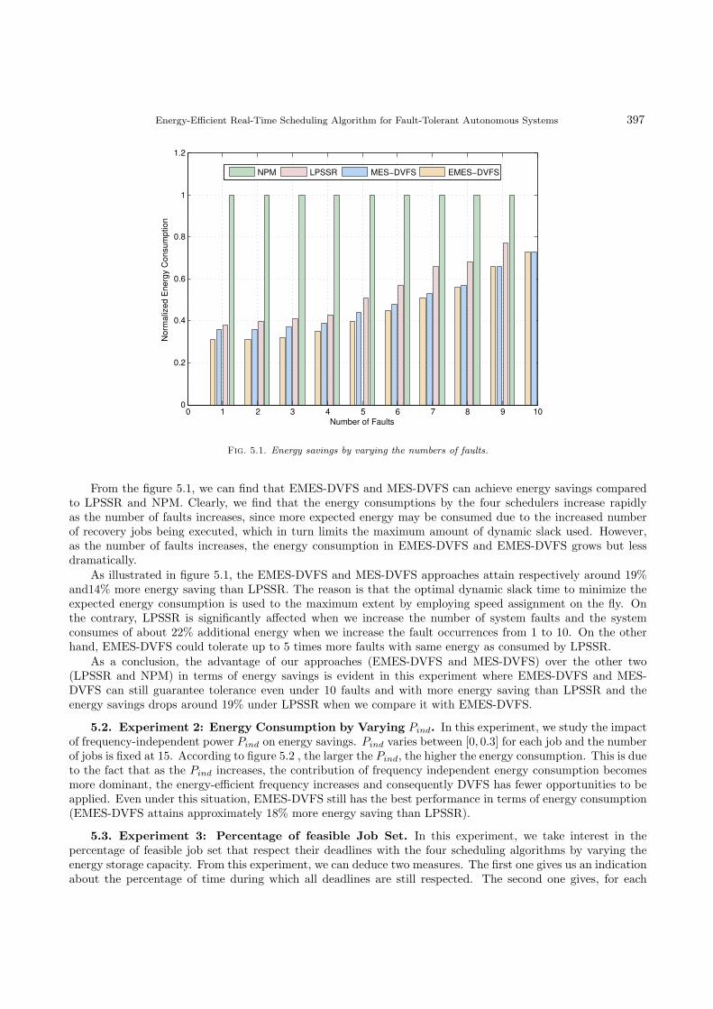
Energy-Efficient Real-Time Scheduling Algorithm for Fault-Tolerant Autonomous Systems 397
0 1 2 3 4 5 6 7 8 9 100
0.2
0.4
0.6
0.8
1
1.2
Number of Faults
No
rma
lize
d E
ne
rgy C
on
su
mp
tio
n
NPM LPSSR MES−DVFS EMES−DVFS
Fig. 5.1. Energy savings by varying the numbers of faults.
From the figure 5.1, we can find that EMES-DVFS and MES-DVFS can achieve energy savings comparedto LPSSR and NPM. Clearly, we find that the energy consumptions by the four schedulers increase rapidlyas the number of faults increases, since more expected energy may be consumed due to the increased numberof recovery jobs being executed, which in turn limits the maximum amount of dynamic slack used. However,as the number of faults increases, the energy consumption in EMES-DVFS and EMES-DVFS grows but lessdramatically.
As illustrated in figure 5.1, the EMES-DVFS and MES-DVFS approaches attain respectively around 19%and14% more energy saving than LPSSR. The reason is that the optimal dynamic slack time to minimize theexpected energy consumption is used to the maximum extent by employing speed assignment on the fly. Onthe contrary, LPSSR is significantly affected when we increase the number of system faults and the systemconsumes of about 22% additional energy when we increase the fault occurrences from 1 to 10. On the otherhand, EMES-DVFS could tolerate up to 5 times more faults with same energy as consumed by LPSSR.
As a conclusion, the advantage of our approaches (EMES-DVFS and MES-DVFS) over the other two(LPSSR and NPM) in terms of energy savings is evident in this experiment where EMES-DVFS and MES-DVFS can still guarantee tolerance even under 10 faults and with more energy saving than LPSSR and theenergy savings drops around 19% under LPSSR when we compare it with EMES-DVFS.
5.2. Experiment 2: Energy Consumption by Varying Pind. In this experiment, we study the impactof frequency-independent power Pind on energy savings. Pind varies between [0, 0.3] for each job and the numberof jobs is fixed at 15. According to figure 5.2 , the larger the Pind, the higher the energy consumption. This is dueto the fact that as the Pind increases, the contribution of frequency independent energy consumption becomesmore dominant, the energy-efficient frequency increases and consequently DVFS has fewer opportunities to beapplied. Even under this situation, EMES-DVFS still has the best performance in terms of energy consumption(EMES-DVFS attains approximately 18% more energy saving than LPSSR).
5.3. Experiment 3: Percentage of feasible Job Set. In this experiment, we take interest in thepercentage of feasible job set that respect their deadlines with the four scheduling algorithms by varying theenergy storage capacity. From this experiment, we can deduce two measures. The first one gives us an indicationabout the percentage of time during which all deadlines are still respected. The second one gives, for each
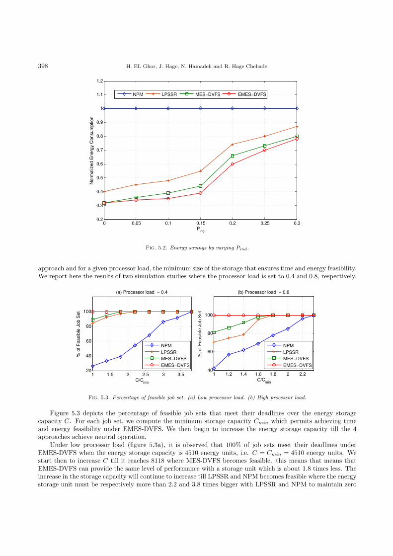
398 H. EL Ghor, J. Hage, N. Hamadeh and R. Hage Chehade
0 0.05 0.1 0.15 0.2 0.25 0.30.2
0.3
0.4
0.5
0.6
0.7
0.8
0.9
1
1.1
1.2
Pind
No
rma
lize
d E
ne
rgy C
on
su
mp
tio
n
NPM LPSSR MES−DVFS EMES−DVFS
Fig. 5.2. Energy savings by varying Pind.
approach and for a given processor load, the minimum size of the storage that ensures time and energy feasibility.We report here the results of two simulation studies where the processor load is set to 0.4 and 0.8, respectively.
1 1.5 2 2.5 3 3.520
40
60
80
100
(a) Processor load = 0.4
C/Cmin
% o
f F
easib
le J
ob S
et
1 1.2 1.4 1.6 1.8 2 2.2
40
60
80
100
(b) Processor load = 0.8
C/Cmin
% o
f F
easib
le J
ob S
et
NPM
LPSSR
MES−DVFS
EMES−DVFS
NPM
LPSSR
MES−DVFS
EMES−DVFS
Fig. 5.3. Percentage of feasible job set. (a) Low processor load. (b) High processor load.
Figure 5.3 depicts the percentage of feasible job sets that meet their deadlines over the energy storagecapacity C. For each job set, we compute the minimum storage capacity Cmin which permits achieving timeand energy feasibility under EMES-DVFS. We then begin to increase the energy storage capacity till the 4approaches achieve neutral operation.
Under low processor load (figure 5.3a), it is observed that 100% of job sets meet their deadlines underEMES-DVFS when the energy storage capacity is 4510 energy units, i.e. C = Cmin = 4510 energy units. Westart then to increase C till it reaches 8118 where MES-DVFS becomes feasible. this means that means thatEMES-DVFS can provide the same level of performance with a storage unit which is about 1.8 times less. Theincrease in the storage capacity will continue to increase till LPSSR and NPM becomes feasible where the energystorage unit must be respectively more than 2.2 and 3.8 times bigger with LPSSR and NPM to maintain zero

Energy-Efficient Real-Time Scheduling Algorithm for Fault-Tolerant Autonomous Systems 399
deadline miss, compared with EMES-DVFS.
The results for high processor load (figure 5.3b) follow the same trend. Unlike the previous experiment, therelative performance gain of EMES-DVFS in terms of capacity savings is decreasing when the processor loadis increasing. EMES-DVFS obtains respectively capacity savings of about 37%, 44% and 57% compared withMES-DVFS, LPSSR and NPM.
It is important here to note that the four approaches require exactly the same storage size when the processorload is equal to 1 since the processor is continuously busy and there is no chance to apply DVFS.
In summary, this experiment points out that the proposed EMES-DVFS approach is very effective inreducing deadline miss rate and storage size even under high processor load. And lower is the processor loadrate, higher is the capacity saving and our approach will then outperform the others by a high amount of energysavings.
6. Conclusions. In this paper, we presented and evaluated a novel approach, which aims to minimizeenergy consumption when scheduling a set of real-time jobs that can tolerate up to k transient faults whilestill respecting time and energy constraints. We explore the reserved slacks generated during run-time to themaximum extent in such a way that all the available slack time is used for energy reduction, which is carried outusing dynamic voltage and frequency scaling (DVFS). Under this notion, we propose an algorithm that estimatesan optimal speed reduction mechanism which maintains feasibility within predefined timing constraints whenno more than k faults occur.
Our scheduler dynamically adjusts the jobs’ slowdown factors by utilizing run-time slacks which may beincreased for recovery demands of the system. It differs from the existing approach where job frequenciesassignments are predetermined, and hence it is more flexible and adaptive in minimizing energy consumptionwhile still keeping the systems reliability at a desired level. In addition, we presented two feasibility testsfor recovery schemes under variable processor speed which decouples the time and energy constraints. Theexperimental results demonstrate that the proposed algorithm can significantly improve the energy savingscompared with the previous works.
For future work, we will explore the adaptation of the proposed approaches to fixed priority environmentsin real-time energy harvesting systems.
Acknowledgments. This work was fully supported by a research grant from the Lebanese University.
REFERENCES
[1] E. Bini and G. C. Buttazzo. Measuring the performance of schedulability tests. Real-Time Systems, 30(1-2):129-154, May2005.
[2] D. Brooks, P. Bose, S. Schuster, H. Jacobson, P. Kudva, A. Buyuktosunoglu, J.-D. Wellman, V. Zyuban, M. Gupta,
and P. Cook. Power-aware microarchitecture: Design and modeling challenges for next-generation microprocessors.Micro, IEEE, 20(6):26-44, Nov 2000.
[3] R. Gupta. Dynamic voltage scaling for system-wide energy minimization in real-time embedded systems. Proceedings of theInternational Symposium on Low Power Electronics and Design ISLPED ’04, pages 78-81, Aug 2004.
[4] H. Aydin, R. Melhem, D. Mosse, and P. Mejia-Alvarez. Power-aware scheduling for periodic real-time tasks. IEEETransactions on Computers, 53(5):584-600, 2004.
[5] H. Aydin, V. Devadas, and D. Zhu. System-level energy management for periodic real-time tasks. In Proc. of IEEE Real-Time Systems Symposium (RTSS), pages 313322, Dec. 2006.
[6] V. Devadas and H. Aydin. On the interplay of dynamic voltage scaling and dynamic power management in real-timeembedded applications. In Proc. ACM Conference on Embedded Systems Software (EMSOFT’08), 2008.
[7] D. Siewiorek and R. Swarz. Reliable Computer Systems: Design and Evaluation. Natick, MA: A. K. Peters, Ltd., 1998.[8] Srinivasan J, Adve SV, Bose P, Rivers J, Hu CK. Ramp: A model for reliability aware microprocessor design. IBM
Research Report, RC23048, 2003.[9] Castillo X, McConnel SR, Siewiorek DP. Derivation and calibration of a transient error reliability model. IEEE Trans
Comput 31:658671, 1982.[10] F. Yao, A. Demers, and S. Shenker. A scheduling model for reduced cpu energy. In Foundations of Computer Science,
Proceedings., 36th Annual Symposium on, pages 374-382, oct 1995.[11] Y. Zhang, K. Chakrabarty, and V. Swaminathan. Energy-aware fault tolerance in fixed-priority real-time embedded
systems. In Proceedings of the 2003 IEEE/ACM international conference on Computer-aided design, ICCAD’03, 2003.[12] H. Huang and G. Quan. Leakage aware energy minimization for real-time systems under the maximum temperature con-
straint. In Design, Automation Test in Europe Conference Exhibition (DATE), 2011, pages 1-6, March, 2011.

400 H. EL Ghor, J. Hage, N. Hamadeh and R. Hage Chehade
[13] Hussein El Ghor, E. M. Aggoune. Energy efficient scheduler of aperiodic jobs for real-time embedded systems, InternationalJournal of Automation and Computing, pages 1-11, 2016.
[14] Hussein EL GHOR, Maryline CHETTO. Energy Guarantee Scheme for Real-time Systems with Energy Harvesting Con-straints. International Journal of Automation and Computing, to appear.
[15] Baoxian Zhao, Hakan Aydin and Dakai Zhu. Energy Management under General Task-Level Reliability Con-
straints. IEEE 18th Real Time and Embedded Technology and Applications Symposium, 2012.[16] Zhu D, Melhem R, Mosse D. The effects of energy management on reliability in real-time embedded systems. In: ICCAD
’04, Proceedings of the 2004 IEEE/ACM International conference on Computer-aided design, IEEE Computer Society,Washington, DC, pp 35-40, 2004.
[17] R. Melhem, D. Mosse, and E. Elnozahy. The interplay of power management and fault recovery in real-time
systems, IEEE Transactions on Computers, 53(2):217-231, Feb 2004.[18] Y. Zhang and K. Chakrabarty. A unified approach for fault tolerance and dynamic power management in fixed-priority
real-time embedded systems. IEEE Transactions on Computer-Aided Design of Integrated Circuits and Systems, 25(1):111-125, jan. 2006.
[19] B. Zhao, H. Aydin, and D. Zhu. Generalized reliability-oriented energy management for real-time embedded applications.In 48th ACM/EDAC/IEEE Design Automation Conference (DAC), pages 381-386, june 2011.
[20] Qiushi Han, Linwei Niu, Gang Quan, Shaolei Ren and Shangping Ren. Energy efficient fault-tolerant earliest deadlinefirst scheduling for hard real-time systems. Real-Time Systems 50:592-619, 2014.
[21] T. D. Burd and R. W. Brodersen. Energy efficient cmos microprocessor design. In Proc. of The HICSS Conference, Jan.1995.
[22] J. W. S. W. Liu. Real-time Systems, NJ, USA: Prentice Hall, 2000.[23] P. Hazucha and C. Svensson. Impact of cmos technology scaling on the atmospheric neutron soft error rate. IEEE Trans.
on Nuclear Science, 47(6) 2586-2594, 2000.[24] Pradhan DK. Fault-tolerant computer system design. Prentice-Hall Inc, Upper Saddle River, 1996.[25] Aydin H. Exact fault-sensitive feasibility analysis of real-time tasks. IEEE Trans Comput 56(10):1372-1386, 2007.
Edited by: Dana PetcuReceived: Sep 4, 2018Accepted: Nov 3, 2018

Scalable Computing: Practice and ExperienceVolume 19, Number 4, pp. 401–422. http://www.scpe.org
DOI 10.12694/scpe.v19i4.1439ISSN 1895-1767
© 2018 SCPE
MODELLING AND SIMULATION OF GPU PROCESSINGIN THE MERPSYS ENVIRONMENT
TOMASZ GAJGER‡∗AND PAWEŁ CZARNUL‡†
Abstract. In this work, we evaluate an analytical GPU performance model based on Little’s law, that expresses the kernelexecution time in terms of latency bound, throughput bound, and achieved occupancy. We then combine it with the results of severalresearch papers, introduce equations for data transfer time estimation, and finally incorporate it into the MERPSYS framework,which is a general-purpose simulator for parallel and distributed systems. The resulting solution enables the user to express a CUDAapplication in a MERPSYS editor using an extended Java language and then conveniently evaluate its performance for variouslaunch configurations using different hardware units. We also provide a systematic methodology for extracting kernel characteristics,that are used as input parameters of the model. The model was evaluated using kernels representing different traits and for a largevariety of launch configurations. We found it to be very accurate for computation bound kernels and realistic workloads, whilst formemory throughput bound kernels and uncommon scenarios the results were still within acceptable limits. We have also proven itsportability between two devices of the same hardware architecture but different processing power. Consequently, MERPSYS withthe theoretical models embedded in it can be used for prediction of application performance on various GPUs.
Key words: Performance simulation, Simulation environment, GPGPU, CUDA
AMS subject classifications. 68M20, 65Y05, 68U20
1. Introduction. Graphics processing units (GPUs) are highly data-parallel devices that are nowadaysubiquitously used for a variety of applications by employing the GPGPU paradigm. GPGPU stands for general-purpose computing on a GPU and refers to the GPU being used to execute tasks, which are not necessarilyrelated to graphics - general purpose tasks, e.g. numerical algorithms, neural networks training, data analysis,and many more. In order to use what the GPU offers effectively, the programmer needs to write a dedicatedapplication. Furthermore, the GPU differs greatly from the CPU both in terms of a hardware design andprocessing model. It would be of a great help to such a programmer to have a tool that allows creation ofa theoretical model of an application and provides means to assess it in terms of computational performance,scalability and behaviour on different hardware units. This becomes even more important when the GPUsare used in highly parallel and distributed environments such as HPC clusters, grids or volunteer computingnetworks. What is more, according to the recent TOP500 [1] list of the fastest supercomputers, the accelerators(mostly NVIDIA GPUs) are an important component used in 22% of these systems.
Considering NVIDIA’s dominance in this field, the size of the CUDA community and maturity of availablesoftware tools, we have decided to focus our efforts on the NVIDIA GPUs. Nevertheless, we have developed ageneric solution for simulation of running applications on GPUs. Use of a simulator equipped with a propertheoretical model, such as MERPSYS described later, may be beneficial in many ways, one can use it to analysethe behaviour of an application in hardware setups which may be unavailable for testing purposes, such asbefore purchasing. It also allows to exceed limits imposed by the hardware, e.g. assess the relation betweenexecution time and data size for very large data sets. Despite providing estimations for application executiontime, a simulator may also compute the predicted energy consumption or failure chance. These values may bethen used for multi-criteria optimisation [44], including energy efficiency and reliability. For a GPU, a simulatorcan allow easy assessment of application execution using various configurations such as grid configuration orapplication parameters. When searching for an appropriate theoretical model one should consider only these ofacceptable (preferably as high as possible) accuracy, but this is not the only expected trait. Ease of use, thepossibility to extend and customise the model are important as well and lastly, the closer the model resembles theactual processing that happens on the GPU, the better. The complexity of the GPU hardware and abundance ofinternal parallelism makes such a theoretical model harder to develop, but as we will further show in Section 4.1,
∗[email protected]†[email protected]‡Department of Computer Architecture, Faculty of Electronics, Telecommunications and Informatics, Gdansk University of
Technology, Narutowicza 11/12, 80-233 Gdańsk, Poland
401
402 T. Gajger and P. Czarnul
this is still a manageable task. We have analysed existing solutions, based on which we propose a performancemodel for a GPU.
In this paper we contribute by incorporation of modelling parallel processing on a GPU into an existingsimulator – MERPSYS [15], validate the model against real results for a parallel GPU-enabled applicationwith various launch configurations on three different GPUs and emphasise benefits from using MERPSYS forsimulation using various GPUs from its database. Details of our contribution are described in the context ofintroduced models in Section 3.3. The paper is organised as follows: Section 2 explains important aspectsrelated to the GPU processing and briefly describes the MERPSYS framework, Section 3 lists related work andmotivations for developing the modelling solution. In Section 4, we propose our own solution, explain it in detail,and show its implementation in Section 5. Section 6 describes our testbed, testing methodology, validation ofthe model, and presents the results. Finally, Section 7 summarises results and outlines the proposed directionof future research.
2. Background.
2.1. GPU architecture and programming model. GPU is a many-core device that exemplifies aSIMD (Single Instruction Multiple Data) architecture type per Flynn’s taxonomy [32]. Although the GPUitself does not contain vector units but rather simple cores capable of executing one instruction on a singleoperand at a time (or two instructions if we consider FMAC operations), it acts in a very similar manner. Allthe threads comprising a single work group (called warp) in a single clock cycle execute the same instruction ondifferent operands, that is why NVIDIA describes this architecture as SIMT [39] (Single Instruction MultipleThreads). This term is obviously a direct derivative of SIMD but expresses the internal architecture of thedevice more clearly - multiple threads executing an instruction instead of a single thread executing it on a wideregister containing multiple operands. GPU is perfectly suited for handling tasks that are highly data paralleland compute intensive, yet simple in terms of the control logic.
A CUDA program is heterogeneous in its nature and consists of two parts: one that executes on the CPUand one that is offloaded to the GPU. Upon program launch the code is executed by the CPU until a kernelinvocation is encountered. When it happens, two important parameters are specified: grid size and block size[37]. As the grid may be comprised of many threads, it is logical that only a limited number will be loaded to theStreaming Multiprocessors (SMs) at a given time, allocation is done at the block level and once a block finishesits execution a new one will be scheduled. This process continues until all of the blocks are processed [19].
Without going into deeper details, from our perspective the following facts are important:1. SM may hold a limited number of blocks at a time;2. blocks have their requirements for shared memory and registers which need to be allocated from the
pool available on the SM;3. threads are executed in groups of 32, called warps;4. there are constraints regarding maximum number of active warps as well as rules affecting warps
execution;5. SM can perform zero-overhead context switches between warps.
The above directly affect the capability of the SM to execute the instructions effectively. If the number ofactive warps is not large enough to cover the stalls (caused by memory accesses, conditional branches resultingin warp divergence, etc.) then performance will be suboptimal [45]. The process of calculating the numberof threads that may be loaded to a single SM considering shared memory and register constraints is calledoccupancy calculation. Shortly speaking, if the occupancy is poor then likely the performance of the applicationwill decrease. It should be noted, however, that increasing occupancy may not lead to any performance gainsor may even result in a performance degradation [46] because of an increased contention for shared resources aswas experimentally proven in [6]. It is also possible to achieve optimal performance with a very low occupancyif thread granularity (number of instructions executed per thread) is sufficient [50]. Given all these, it is clearthat the effectiveness of warps execution depends on the characteristics of the specific kernel.
2.1.1. Compiled CUDA code. CUDA code can be compiled into two representations: PTX (ParallelThread Execution) or SASS (Shader Assembly). PTX is a model of a virtual machine and a definition of ISAto be used with this machine, it exposes GPU to the higher layers as a data-parallel computing device. PTX

Modelling and Simulation of GPU Processing in the MERPSYS Environment 403
code is an intermediate representation of a program and an abstraction over GPU architecture that is not tiedto any hardware type, thus it does not directly resemble the instructions that are executed by the GPU. It isultimately translated into a machine code (cubin object) either by nvcc in a separate compilation step or byleveraging just-in-time compilation by the CUDA runtime driver upon being scheduled for launch on a specificdevice [38]. This allows a high level of interoperability between varying GPU architectures. SASS is the machinecode for GPU, generated for a specific architecture and maps directly to instructions being processed by thefunctional units. It can be either generated directly by nvcc during the compilation process or, as it was alreadymentioned, generated on-the-fly from PTX source code.
2.2. MERPSYS. Developed at the ETI faculty of Gdansk University of Technology, MERPSYS1 [13, 15]is a simulation environment for distributed systems that allows its users to predict execution time, powerusage and failure probability of their applications. The application is described in a form of Java code imbuedwith special functions implementing communication (MPI-like) and computation primitives. The system ismodelled as a hierarchical structure of components representing computational devices and interconnects, eachof them having its own characteristics defined. It consists of four software components: GUI, server, databaseand simulator. Block based representation [12] is employed as a theoretical concept behind the applicationmodel, the environment provides a set of extensions to the Java language that allow to define computation andcommunication blocks while preserving the original structure of the code. An application model can be expressedin Java with additional message passing communication primitives using properly parametrized (input data size,operation type, etc.) MERPSYS-specific constructs in place of actual computation or communication code.
A system model is created by selecting hardware components and placing them in the editor’s workspace.It may consist of several nested levels, e.g., two machines connected using an InfiniBand network and insideeach of them a GPU and a processor connected via a PCIe bus. The hardware model is a term used to describethe characteristics of a given hardware setup. A model has special functions associated with it that reflect, e.g.:power usage equation for an active or idle component, communication time for point-to-point, scatter or gatheroperations, etc. These functions are then used by the simulator to calculate the effective time taken by variousoperations. Hardware components have attributes that describe their characteristics. A database of hardwarecomponents is provided, that can be extended with new records. It should be further noted that the hardwaremodel is sometimes referred to as a computational model. For each computational component a user defines anarbitrary number of labels that are used to tie application and hardware models together. They are used in theapplication model to mark parts of the code representing distinct processes or threads and allow the schedulerto map them to the hardware components. A simulation configuration screen also allows to define attributesthat are passed to the application model, an example of such may be data size, block configuration of a GPU,etc. A request to launch a simulation is passed from GUI to the server which in turn directs it to one of thesimulators connected to one of its simulation queues [13]. The simulation queue to be used may be specifiedas well.
MERPSYS was successfully used by its authors to model execution time, energy consumption and reliabilityof divide-and-conquer (DAC [18, 13]) and geometric single program multiple data (SPMD [13]) applications [16],K-means algorithm [17] and volunteer computing systems [14]. For a more detailed description providing betterinsight into the whole MERPSYS environment see [15].
3. Related Work.
3.1. GPU performance models. When considering performance models targeted specifically at GPUs,several approaches are to be distinguished, three of the most common are [30]: analytical methods, quantitativeand compiler-based methods, statistical and machine learning methods. The first kind focuses on creation of atheoretical model for a kernel execution expressed as set of equations and feeding it with parameters obtainedby direct analysis of the kernel’s code and the underlying hardware. Amaris et al. have proposed an analyticalmodel [2] based on BSP [49], that estimates kernel execution time using an equation combining global andshared memory access times, with computation time and available GPU hardware resources. Another model[23] focuses on highly parallel aspects of GPU processing, discerning ones originating from parallel execution of
1http://merpsys.eti.pg.gda.pl

404 T. Gajger and P. Czarnul
warps and memory accesses. It enumerates as many as 21 distinct parameters obtained via source code analysis,microbenchmarking, or defined by user. These are then used to estimate kernel’s execution time.
The model proposed by Volkov [51] leverages Little’s Law by defining the parallel process using threemetrics: warp latency bound, warp throughput bound and occupancy. Execution of a kernel is modelled at awarp level in the scope of a single SM with the findings extrapolated to reflect the overall kernel execution time.The model focuses on obtaining a key metric describing the parallel process - a warp throughput, from whichthe total kernel execution time can be derived. Concurrency in this case is synonymous to occupancy throughthe number of active warps residing at an SM at a given time. Furthermore, an assumption is made that boththe occupancy and the throughput are sustained for the entire time of the kernel’s execution. An importantpart of the model are the bounds for warp throughput and latency, warp throughput is limited by throughputbound imposed by the hardware and its latency may not be lower than the one resulting from the instructionsequence comprising the kernel. Warp latency bound is obtained by direct inspection of the compiled kernelassembly code. Warp throughput bound is calculated based on requirements for resources available on the SM.
Quantitative methods, on the other hand, evaluate the characteristics and behaviour of a given kernel eitherby measuring or microbenchmarking kernel execution on actual hardware or by executing it, or parts of it, ina GPU simulator. These are often integrated into a compilation process of a kernel and are more automatedthan analytical ones. Examples include the following: an automated approach where the kernel is analysedto create a work flow graph [5] that focuses on measuring warp and instruction level parallelism, that is laterparametrized to reflect execution process on a specific GPU unit; a microbenchmark based [53] method whereinstructions are extracted directly from the compiled source code of a kernel, backed by a functional simulatorfor memory accesses; Ocelot dynamic compilation framework [27, 28] leveraging PTX representation of a kernel,that is transformed into a form feasible to be modelled on a single CPU thread. Lastly, an interval analysis [24]technique, which is based on an assumption that by locating events causing performance degradation (memorystalls, cache misses, etc.), one can reason about the overall execution time of a kernel.
Statistical and machine learning methods [25, 52, 31] are often implemented as separate frameworks thatare highly automated and require additional training so that the neural network correctly recognises patternsand behaviour of the kernel code. The network learns the kernel’s instructions composition given a set ofinput data and is then able to reason about the performance of subsequent kernel executions for differentlaunch configurations. Consequently, they provide a complete simulation environment on their own and arenot suitable for developing a new model that could be used within MERPSYS. Given the aim of this work isextending MERPSYS with a performance model for a GPU, we find them not relevant in our analysis.
3.2. GPU modelling in general-purpose simulators. General-purpose simulators are not tied to anyspecific device type or programming language and provide means to perform various kinds of simulation formany processing paradigms on parallel and distributed systems. Designing an application for such environmentsis not a trivial task as one needs to consider execution time, energy efficiency, reliability, maintainability andmany other factors [48]. This is why most of the simulators a layer of abstraction over the actual hardware,what is a good thing when we consider a use case like modelling a complex grid system, but it may also be asignificant drawback if one needs to model the parallel process on a specific hardware unit with a greater detail.All of further mentioned simulators implement the discrete-event simulation model [43], which means that theentire process of simulation is governed by events being processed and passed between entities. Such an eventmay represent a computation, communication, synchronisation or a resource access, with the details specifiedby the simulation environment itself. We have looked at the following tools with the focus on GPU simulation:GridSim [8], SimGrid [42, 21], CloudSim [9, 41, 47], GSSIM [29, 7], and MARS [20]. Table 3.1 summarises theirsuitability for this purpose, a general overview of their functionality was given in [15].
We have found that none of these simulators offers a convenient way to incorporate GPU modelling withinit with the level of detail we require. This is mostly because their focus is on a different area of modelling,i.e. an HPC system as a whole, where computational units are described in terms of overall computationalpower. CloudSim with GPU extension [47] is closest to our requirements, but it still operates at the GPUcomputational task level and does not allow for precise modelling of kernels comprising the application. Onthe contrary, MERPSYS whilst being a general-purpose simulator itself, is a highly customizable solution thatallows to drill down deep into internals of a single hardware unit, in our case a GPU. It allows easy modification

Modelling and Simulation of GPU Processing in the MERPSYS Environment 405
Table 3.1General-purpose simulators comparison
SimulatorLevel of detail available for modelling ahardware component
Suitability for GPU modelling
GridSimPoor - computational power defined in termsof MIPS or SPEC rating.
Not with the required level of detail.
SimGridHigh - complex analytical models may beused.
Theoretically yes, would require morein-depth investigation of the possibility toextend the existing framework with a customcomputational resource.
CloudSim High if extensions to the framework are used. Yes, but not with the required level of detail.
GSSIMPlugins that take many factors into accountmay be written to describe the performance.
Possibly, by writing plugins to define complexapplication performance models.
MARSTask modules execute logs containing MPIcall traces. There’s no room forcustomisation.
Not at all.
of the model by substitution of other hardware such as GPUs and repeating simulations, easy modification offormulas modelling execution and communication times, as well as relevant constants and coefficients.
3.3. Contributions of this work. Contributions of this work are as follows:• We have incorporated the model proposed by Volkov [51] within the MERPSYS simulator [15], showing
that it is well suited for practical implementations. We have used a simplified version of this model byreducing the scope of hardware units considered to CUDA cores, schedulers, and global memory system,for which we decided to use a trivial non-parametrized access model. For this version, we provide acomplete set of equations (Eqs. 4.1 - 4.6) together with a detailed description of input parameters,creating an easy to grasp explanation of all the building blocks of the model.
• We have also extended the model with a scaling parameter, allowing to fine-tune it to better fit hardwareand kernel characteristics. We propose Eq. 4.5 for calculating global memory bandwidth and introducedata transfer time calculation, whilst the original model considered only kernel execution time.
• We show that for the considered model configuration derived from results on one GPU of a givenarchitecture can be directly applied to another GPU of the same architecture, introducing only thesecond GPU’s specifications into the model. This makes the MERPSYS environment with the modeldeployed in it a suitable tool that is able to verify performance of a given application on potentiallyseveral cards without even having physical access to them.
4. Proposed Approach. Compared to other general-purpose simulators, MERPSYS is a much better fitfor GPU modelling. It is mainly because of the very high level of detail available when modelling a hardware piececombined with a possibility to add custom functions describing device’s behaviour. Hence, the computationaldevices are highly customizable which allows implementation of complex analytical models like the one beingdescribed in this section. Additionally, the hardware (computational) model may be customised to use additionaldata needed for GPU modelling. This data may be specified in the application model, which allows for easyparametrization of simulation runs. Another advantage is an extensible database of hardware components andease of hardware model customisation, which allows for convenient evaluation of various setups. These canbe activated just by selecting other GPUs, that have all the parameters in the database, through a graphicalinterface.
4.1. GPU Performance Model. To model the execution time of a single kernel on a single GPU we willrely on a model proposed by Volkov [51], we define Eq. 4.1 for this purpose. The number of warps launched iscomputed as shown in Eq. 4.2. For warp throughput, we use Eq. 4.3 (proposed by Volkov), the methodologyfor obtaining occupancy, latency bound, and throughput bound will follow. This model considers all of theimportant elements that contribute to the overall execution time of a kernel in most of the scenarios. Later on,

406 T. Gajger and P. Czarnul
we explain the meaning of each of these elements and the approach used to determine their values. Since theentire model is based on a concept of modelling a concurrent process in terms of a warp being executed on aStreaming Multiprocessor (SM) and the metrics are calculated for that single warp, it is required to extrapolatethe findings to reflect the actual number of warps that were executed on the GPU and thus compute the result.For this purpose, Eq. 4.2 is used that takes as an input the launch configuration of a kernel i.e. the sizes of gridand block, and the result is the total number of warps that were launched to process the kernel.
Tk =WL
WT h × SMs × SMclock × λk
(4.1)
WL = grid size ×
⌈
block size
warp size
⌉
(4.2)
WT h ≈ min
(
occupancy
Latbound
, Thbound
)
(4.3)
where: Tk – estimated kernel execution time [s]; WL – number of warps launched; WT h – processing rate ofwarps [1 / cycle]; SMs – number of streaming multiprocessors; SMclock – SM core clock [cycles / s]; λk – scalingparameter; grid size – number of blocks in a grid; block size – number of threads in a block; warp size – 32for all GPU architectures; Thbound – throughput bound [1 / cycles]; Latbound – latency bound [cycles].
SMs and SMclock parameters are needed to extrapolate the model from a single warp in scope of a singlemultiprocessor to one that fits the processing model of the GPU. These two parameters, when multiplied, yieldthe processing power of the entire device in cycles per second. The λk value is a ratio between estimated andmeasured execution times that adjusts the model to fit the characteristics of a given kernel launched on a specificdevice architecture. It shall be obtained experimentally by measuring the execution time of a real applicationcombined with running a simulation with an initial model. Once calculated the new λk can be used to performsimulation across varying data sizes and different GPUs. It was experimentally proven by the authors of anothermodel [2, 3] that a single λk value is sufficient for accurate simulations in scope of a single device architecture.When used for a different architecture the accuracy of the model drops and it is advised that λk is recalculated.To calculate the λk we divide the estimated execution time, by the measured one: λk =
Testimated
Tmeasured.
Calculation of warp throughput, the most essential part of the model, as given by Eq. 4.3, is the mostchallenging task. Three parameters need to be extracted from the kernel code in close consideration of a specificGPU architecture that one intends to model. These parameters are warp latency and throughput bounds, andthe achieved occupancy, we will describe them in detail in subsequent sections.
4.1.1. Occupancy. The first method of retrieving the parameters needed for occupancy calculation is tocompile the code with verbose ptxas output, this is done by passing ’-Xptxas -v’ command line option to nvcc
[38]. A sample result is shown in Listing 1. It tells us that the kernel uses 8 registers per thread and does notuse any shared memory, otherwise information about the amount of shared memory used would be includedin the output. cmem stands for constant memory and does not concern our analysis. Having determined thenumber of registers and amount of shared memory required, we enter these together with threads per blockcount (block size) into the NVIDIA occupancy calculator [34] to get the theoretical occupancy. Another way isto profile the application, NVIDIA Visual Profiler not only displays the values of shared memory and registersused but it is even capable of calculating both the theoretical and achieved occupancies.
Listing 1Verbose ptxas output for saxpy2 kernel
ptxas i n f o : Function p r o p e r t i e s f o r saxpy2Used 8 r e g i s t e r s , 344 bytes cmem [ 0 ]

Modelling and Simulation of GPU Processing in the MERPSYS Environment 407
4.1.2. Latency bound. We construct an execution graph of the kernel with nodes representing instruc-tions and edges representing latencies as shown in Volkov’s work [51] and then apply a critical path method toit to find the latency. Critical path is the latency bound only if we assume that all of the warps are the same- they execute the very same instructions, so this approach will not work if there is a substantial control flowdivergence in a kernel. In such a case, a different set of instructions resulting from different branches beingexecuted should be considered.
The graph considers latencies of the following kind: register dependencies and thus instruction executionlatency, instruction issue latency, and memory stalls to describe how the instructions comprising the kernel aredepend between themselves. This approach is valid because there is no out-of-order execution present in theGPUs, meaning that the sequencing of the instructions is maintained in a strict order. It is also more precisethan when making an assumption that a kernel is a simple sequence of dependent instructions as in [2, 11, 40]and simply summing the latencies of all instructions comprising the sequence, treating the result as a totalcost in clock cycles of executing this kernel by a single warp. The latter approaches fall short because thereare independent functional units within the SM, which results in latency hiding, e.g. in case of waiting formemory accesses. Furthermore, even in the case of a single functional unit type the instructions are processedin a pipelined-based manner and thus ILP (Instruction Level Parallelism) exists.
Volkov reports [51] that there are two other types of latency, the latency between two independent in-structions from a single warp, called ILP latency and latency resulting from a replacement of a terminatedthread block, we address both of these. What is more, depending on the architecture, multiple warp schedulersper SM may be present and two instructions per warp may be issued every instruction issue time if mutuallyindependent instructions are available for execution. The effect of dual issue is considered as well, in which casethe ILP latency is expressed as 0 cycles. We omit double precision and special function units, both of whichhave their own pipelines with different latencies for various instructions. Moreover, our approach to modellingglobal memory accesses is simplified as we do not consider gradual saturation effect [51], which manifests itselfin a form of increasing memory access latency as the number of memory transaction increases and memorybus gets saturated. It should also be noted that the modelling of shared memory accesses was omitted. Theseomissions do not affect results of our work as we have deliberately chosen a simple kernel, which does not makeuse of aforementioned functional units. Furthermore, the model is designed in such a way that it may easily beextended with these elements in the future.
4.1.3. Throughput bound. To obtain the throughput bound, each of the hardware resources available onthe SM must be considered separately, including: CUDA cores, Special Function Units (SFUs), double precisionunits, schedulers, and global and shared memories. We will narrow our analysis to three of them as denoted byEq. 4.4. The tightest bound, that is the highest number of cycles required to execute the warp’s instructionsdue to a limited processing power of the functional units, is selected as the limiter of the performance and thena reciprocal is calculated to obtain the bound represented in warps per cycle.
Thbound ≈1
max
(
Wsz×INSCUDA
CUDA cores, INSissued
schedulers,
GMembytes
GMembw
) (4.4)
GMembw ≈GMemclock ×
bus width8 × data rate
SMs × SMclock
(4.5)
where: Wsz – warp size; INScuda – number of instructions to be executed by CUDA cores; INSissued – totalnumber of instructions issued (including dual-issues and re-issues); CUDA cores – number of CUDA coresavailable on the SM; schedulers – number of schedulers available on the SM; GMembytes – number of bytestransferred with global memory for each warp [bytes]; GMembw – peak throughput of the memory systemper SM [bytes / cycle]; GMemclock – global memory clock [Hz]; bus width – global memory bus width [bits];data rate – data rate multiplier depending on the kind of memory used.
4.2. Obtaining hardware parameters. Each of the instructions issued by a thread is assumed to requirea well-known number of clock cycles to complete, this is a simplified approach not considering varying memory

408 T. Gajger and P. Czarnul
Table 4.1Instructions latencies for Maxwell architecture
Operation Latencyadd, sub (integer, 32-bit FP) 6mad (32-bit FP) 6shl, shr 6mov, setp 6bra (taken) 12bra (not taken) 10ILP latency 3Terminated block replacement 150Global memory access 350
access times, varying instruction latency depending on the instruction sequence and other effects. Based onpapers [4, 51] and additional reasoning, Table 4.1 presents latencies we assumed in this work. For latencies ofTesla, Fermi and Kepler architectures see [4], for Pascal and Volta see [26]. For a detailed information regardingmeaning of the mnemonics refer to [36].
There are two sets of parameters in Eq. 4.4. The first one is related directly to the hardware characteristicsof a given device, it includes: warp size, number of CUDA cores and warp schedulers, and the throughput of theglobal memory. At the time of writing the warp size is a constant value of 32 for all GPU architectures. Thenumber of CUDA cores and warp schedulers may be obtained from GPU hardware specification. Theoreticalbandwidth of the GPU’s global memory available per single SM every cycle is given by Eq. 4.5, for which allthe parameters are available in hardware specification except the data rate that is derived from memory typeand equals 2 or 4 respectively for GDDR3 and GDDR5 [33]. Although the peak bandwidth is not sustainablein practice for the entire execution of a kernel because the memory clock may drop due to dynamic frequencyscaling and furthermore would require an ideal access pattern and sufficient occupancy, a value close to thistheoretical limit is attainable [51]. Considering this fact, we use this bandwidth in the proposed model. What ismore, we do not differentiate between loads and stores and assume them to behave in the same way. Additionally,we limit the model to a scenario where there are no cache hits and the accesses are fully coalesced. If we were toinclude the possibility of cached accesses in the model then we would need to consider the fact that dependingon the device architecture accesses to global memory are cached in L1 and L2 caches, hence the number ofcache hits should be subtracted from the actual number of DRAM accesses. The ratio of cache hits could beobtained by launching the application in a profiler [11].
The second set of parameters: INSCUDA, INSissued and GMembytes describes application execution char-acteristics, all three are extracted directly from compiled SASS code of the kernel, description of these follows.To calculate the number of CUDA core instructions we count all occurrences of operations that are executedusing these cores: FP32, INT32, logical, etc. Getting a sum of all instructions that were issued is a little moredemanding because dual-issues and re-issues of instructions need to be accounted for. In the former case, twoinstructions are issued in a single issue cycle and hence are counted as one. In the latter, a single instructionmust be counted multiple times depending on the number of re-issues. A re-issue typically occurs when thereare bank conflicts when accessing shared memory or when an access to global memory is uncoalesced and mustbe split into several separate transactions. This also affects number of bytes transferred per warp, for examplewhen fetching a single 32-bit value per thread, a stride of two would result in 256 bytes transferred instead of 128and a single additional re-issue of memory transaction instruction, stride of 4 would cause 3 additional re-issuesand increase the number of bytes to be transferred to 512. Numbers of functional units and clock values for thedevices as listed in Section 6.1 were obtained from vendor’s documentation and using ndivia-smi [35].
4.3. Modelling communication time. Performing computations on a GPU requires the data to betransferred to the device prior to launching a kernel and once its execution completes the results must be fetchedback to the main operating memory. Memory transfer between the host and the device may be considered aninstance of a point-to-point communication, for which the communication time is given by the following equation

Modelling and Simulation of GPU Processing in the MERPSYS Environment 409
[12]:
Tc = ts +n
bw × λc
(4.6)
where: Tc – data transfer time; ts – startup time; n – data size; bw – bandwidth; λc – scaling parameter.Startup time is the time needed to initiate data transfer that depends on latency and runtime overhead, it
can be measured by sending a very small data packet. Bandwidth is dependent on the configuration of the PCIebus that connects the devices, for example a theoretical bandwidth of PCIe v3.1 16x bus in single direction is16GB/s or 15.8 GB/s if we consider 128b/130b encoding. Furthermore, we have noticed that the bus is betterutilised for larger data sizes but even for the largest transfer of 2GB the throughput was noticeably lower thanthe theoretically achievable one. Due to this fact, in our implementation we introduce an additional scalingparameter λc to Eq. 4.6 that allows us to fine-tune the link bandwidth so that it reflects the actual characteristicof a given hardware setup.
Note that both the λc and ts will have different values for each transfer direction. The scaling parametercan be obtained similarly to the one for the kernel execution time (λk), i.e. by dividing the estimated transfertime by the measured one. To get the value of the bandwidth parameter we first need to determine the PCIeconfiguration, for this purpose we have used nvidia-smi. Having obtained these two values, we can refer tohardware documentation to get the bandwidth parameter.
5. Implementation. It is easiest to present how the performance model is constructed by example. Forthis purpose we use saxpy2 kernel (Listing 2) that is a slightly modified version of a kernel from the blog post [22].The main difference when compared to a regular saxpy is that instead of a single multiplication an equivalentnumber of additions is performed, this allows us to benchmark kernels of various compute intensities. Thehighlighted part of the code is responsible for a compute intensity of the kernel, i.e. the number of arithmeticinstructions executed by each warp. Input data size is determined by the number of elements in the vectors as:number_of_elements_per_vector × 2 × 4 Bytes.
Listing 2Testbed CUDA kernel
__global__ void saxpy2 ( i n t n , i n t a , f l o a t ∗x , f l o a t ∗y ) {i n t i = blockIdx . x ∗ blockDim . x + threadIdx . x ;i f ( i < n) {
f l o a t va l = x [ i ] , tmp = 0 ;#pragma unroll 1for ( int cnt = 0; cnt < a ; ++cnt) tmp += val ;y [ i ] += tmp ;
}}
To accurately determine the kernel’s instruction composition, we cannot simply analyse the C or C++source code since we do not know the optimisations that took place and thus the actual instructions that weregenerated by the compiler. For this purpose we need to analyse SASS code (see Section 2.1.1), to extract itfrom a compiled binary file we use cuobjdump [36]. Listing 3 is a SASS representation of the saxpy2 kernel thatwas compiled for sm_52, for the sake of brevity we skip the irrelevant NOP instructions from the very end. Thehighlighted part represents the loop governing the kernel’s arithmetic intensity.
Listing 3SASS representation of the saxpy2 kernel
MOV R1 , c [ 0 x0 ] [ 0 x20 ] ;S2R R0 , SR_CTAID.X;S2R R2 , SR_TID.X;XMAD.MRG R3 , R0 . reuse , c [ 0 x0 ] [ 0 x8 ] . H1 ,RZ;XMAD R2 , R0 . reuse , c [ 0 x0 ] [ 0 x8 ] , R2 ;XMAD. PSL .CBCC R0 , R0 . H1 , R3 . H1 , R2 ;

410 T. Gajger and P. Czarnul
ISETP .GE.AND P0 , PT, R0 , c [ 0 x0 ] [ 0 x140 ] ,PT;@P0 EXIT ;MOV R3 , c [ 0 x0 ] [ 0 x144 ] ;SHL R6 , R0 . reuse , 0x2ISETP .LT.AND P0 , PT, R3 , 0x1 , PT;SHR R7 , R0 , 0x1e ;IADD R2 .CC, R6 , c [ 0 x0 ] [ 0 x148 ] ;MOV R0 , RZ;{ IADD.X R3 , R7 , c [ 0 x0 ] [ 0 x14c ] ;@P0 BRA 0x100 ; }{ MOV R5 , RZ;LDG.E R0 , [ R2 ] ; }MOV R4 , RZ;IADD32I R4, R4, 0x1 ;ISETP.LT.AND P0, PT, R4, c [0x0 ] [ 0 x144 ] ,PT;{ FADD R5, R0, R5;@P0 BRA 0xd0; }MOV R0 , R5 ;IADD R2 .CC, R6 , c [ 0 x0 ] [ 0 x150 ] ;IADD.X R3 , R7 , c [ 0 x0 ] [ 0 x154 ] ;LDG.E R5 , [ R2 ] ;FADD R0 , R0 , R5 ;STG.E [ R2 ] , R0 ;EXIT ;
5.1. Creating kernel execution graph. To construct an execution graph of saxpy2 kernel we start offby creating a directed graph representing the sequence of instructions comprising the kernel based on Listing 3.Each instruction is a single node, additional start and end nodes mark respectively the entry and exit point ofthe kernel. Edges represent the dependencies between the instructions and are labelled with latency values fromTable 4.1. Straight, solid arrows are used for the ILP latency, which equals 3 cycles for Maxwell architecture.There are total of 3 dual-issues, these edges are labelled with 0. The next step is to include latencies fromregister dependency, these are shown as dotted arrows. We do this by reading the SASS line by line andverifying whether any of the input registers of the current instruction has its value written to by one of thepreceding instructions, if so then a register dependency exists and we add a new edge connecting the predecessorwith successor labelled with latency value of the preceding instruction. If this instruction is a memory access,then we use the latency of the storage area being referenced, which in case of this kernel is always the globalmemory as cache hit ratio equals 0%. This is true because there is no re-use of data - each element is accessedby a single thread and exactly once. We verified correctness of this assumption by inspecting the profiler outputfor this kernel regarding the memory throughputs. Lastly, we label the inbound edge of the virtual end nodewith a terminated thread block replacement latency.
Once the graph is complete and labelled we use the critical path method to find the latency bound of thekernel. Figure 5.1 shows the resulting graph with critical path highlighted in blue. The part of the graph wherenodes are ellipses is the computational loop, which may execute multiple times depending on the computeintensity parameter passed to the kernel. When calculating the latency bound, the critical path of the loopneeds to be multiplied by the number of loop iterations. The final equation for latency bound is as follows:latency bound = 92 + 700 + 150 + 24a = 942 + 24a where the first term is sum of instructions’ latencies, thesecond one is latency of memory accesses, the third is thread block replacement latency, and the fourth one islatency of the loop multiplied by the compute intensity parameter ’a’. We have created and analysed the graphmanually, but creation of an automated tool is entirely possible.
5.2. Obtaining throughput limits. As the first step in throughput limit calculation for the saxpy2kernel we need to count instructions in the generated SASS. It can be done either by reading directly from

Modelling and Simulation of GPU Processing in the MERPSYS Environment 411
start
MOVS2RS2R
XMAD XMAD
XMAD
ISETP
EXIT
MOV
SHL
ISETP
SHR
IADD
MOV
IADD
BRA
MOV
LDG
MOV IADD32I
ISETP
FADD
BRA
MOVIADD
IADD LDG
FADD
STG EXIT end
0
33
3
3
3
3
3 3 3 3
3
3
3
3
0
3
0
3
3
3
3
0
3
3
3
3
3 3
3 150
6 6
6
6
6
6
6
6
6
6
6
350
6
6
taken(12)
6
6
6
66
6
6
nottaken(10)
6
6
nottaken(10)
350 6
Fig. 5.1. Execution graph for saxpy2 kernel
the assembly listing (Listing 3) or based on the kernel execution graph (Fig. 5.1). In our example, we have23 CUDA core instructions that are executed once and 4 instructions in a loop, so the resulting equation is:INSCUDA = 23 + 4a. It should be noted that in this kernel everything except memory accesses is processedby CUDA cores, this would not be the case if there were any instructions designated for a double precisionor SFU units. When getting the number of instructions issued we must remember to address the dual-issuesand re-issues. In our kernel, we have 3 accesses to global memory, all three are fully coalesced so there are nore-issues taking place. There are 3 dual-issues, each resulting in a pair of instructions being issued togetherduring a single cycle.
Summing up, we have 23 CUDA core instructions issued once and four of these in a loop, three memoryinstructions, and three dual-issues which we subtract from the total number, so we get: INSissued = 23+3−3+
4a = 23+4a. The number of bytes transferred to and from a global memory depends on four factors: the numberof the memory access instructions, cache hit rate, operand size, and access pattern. The saxpy2 kernel contains3 memory access instructions: two loads and a single store, but for the sake of brevity we do not differentiatebetween these two as the difference is marginal. In all three cases, a single 4-byte value is accessed per threadand as was mentioned in preceding paragraph, the accesses are fully coalesced so there are no redundant memorytransactions when accessing the data, this gives us: GMembytes = 3 × 4 bytes × 32 = 384 bytes. Furthermore,there are no cache hits hence all these bytes are accessed directly in the global memory and we can entirely omitboth the L2 and L1 caches. If this was not the case then we would separately consider a fraction of GMembytes
equal to cache hit ratio as being accessed from cache, which has a higher throughput than the global memory.Now that we have all the throughput related parameters extracted from the kernel we need to list those
specific to the device the application will run on, which is NVIDIA GeForce GTX 970 in our case. The firsttwo parameters can be obtained directly from card specifications shown in Section 6.1, compute capability ofour card is 5.2, hence we have: CUDA cores = 128, schedulers = 4. The third parameter - bandwidth of theglobal memory can be calculated using Eq. 4.5 substituting the required values as: GMemclock = 1753MHz,bus width = 256 bits, data rate = 4, SMs = 13, SMclock = 1253 MHz. This gives us: GMembw = 13.78
Bytescycle
The final step is to gather up all these parameters and substitute them to Eq. 4.4:
Thbound ≈1
max
(
32×(23+4a)128 , 23+4a
4 , 38413.78
)
5.3. Equations for communication time. Our testbed with GTX 970 uses PCIe v3.1 16x. Based onthis fact and our measurements we substitute the parameters of Eq. 4.6 and thus we get the equation for data

412 T. Gajger and P. Czarnul
Fig. 5.2. Hardware units with customised attributes: GPU (left), interconnect (right)
transfer time in function of its size for both directions as shown below.
THost to Device = 3.9687 × 10⁻⁶
+n
15.8 × 109 × 0.689and TDevice to Host = 5.1569 × 10
−6+
n
15.8 × 109 × 0.653.
5.4. Incorporating the model within MERPSYS. In this section, we show how the theoretical modelwas implemented in MERPSYS. At first, we demonstrate how to create a system model representing our testbed,including the creation of new hardware units. Then we proceed to computational model definition, i.e. theprogrammatic representation of what was shown in previous sections. Next, we move to the application modeldefinition, which will represent the CUDA application being modelled, explaining how all these pieces are tiedtogether and finally elaborate on how to customise the application launch parameters and execute the simulation.Creation of hardware units that are customised with parameters required by our theoretical model was the firstimplementation step. All previous measurements were performed using GTX 970 and PCIe v3.1 16x. For thesetwo devices we have created a representation in MERPSYS’ database as shown in Fig. 5.2. It should be furthernoted that the λc parameter from Eq. 4.6 was included as an attribute of the PCIe hardware unit. We assumedthat the effective bus utilisation is a parameter of the hardware itself and its value does not change for differentapplication types if the memory transfers are performed using the same functions. Shall a requirement for thisparameter be customizable via application model arise, it can be moved there and passed in the function callsthe same way it was done for kernel parameters, as shown in Section 5.4.2.
The next step to perform is creation of a testbed representation using the hardware model editor in MERP-SYS editor application. Two hardware units that we have just created are used in this model together with aunit representing the CPU. Note that this model directly resembles the actual hardware structure where GPUand CPU are connected using a PCIe bus.

Modelling and Simulation of GPU Processing in the MERPSYS Environment 413
Fig. 5.3. Testbed configuration in MERPSYS system model editor
Figure 5.3 is a screenshot from the editor application showing the created model, GPU unit is selected withits properties visible on the right side, moving from the top to the bottom:
1. Hardware - hardware unit represented by this element, in our case the GTX 970 GPU visible on theleft of Fig. 5.2;
2. Count - the number of hardware units of a given type, for example in a multi-GPU setup we could setthe count to 2, 3, 4, etc.;
3. Name - displayed name of the element;4. Model - computational model connected to the element, in our case the one from Listing 4, description
of which will follow;5. Labels - labels assigned to the element, these form the connection between hardware and application
models. Name is the identifier of the label and multiplicity denotes the number of processes with thislabel that may be executed on a single unit of this type.
5.4.1. Computational model. Another crucial component of the simulation suite is the computationalmodel, in which we have implemented the equations comprising the model. These are written in JavaScript usingMERPSYS’ so-called shallow functions, one of them (an implementation of Eq. 4.1) is depicted in Listing 4.Others are not presented for the sake of brevity, but their implementation is similar. Parameters characterisinghardware, i.e. hardware unit attributes are directly accessible from within the computational model functions.For example: SMCoreClock or SMs which reference attributes of the GPU (the ones from Fig. 5.2). On theother hand, application specific parameters are passed from the application model using proper arguments of thecomputation or communication function calls. These are then accessible as JSON objects containing key-valuepairs. When we look at the signature of getTimeGPUModel() we can notice params argument, which is thisJSON object. The value stored under a specific key is accessed using params.get() method.

414 T. Gajger and P. Czarnul
Listing 4Part of the computational model
f unc t i on getTimeGPUModel ( params ) {var warpsLaunched = getWarpsLaunched ( params . get ( ’ g r i dS i z e ’ ) , params . get ( ’
b lockS ize ’ ) ) ;var throughputBound = getThroughputBound ( params . get ( ’ CUDACoreInstructions ’ ) ,
params . get ( ’ i s s u e d I n s t r u c t i o n s ’ ) , params . get ( ’ GMEMBytesTransferred ’ ) ) ;var latencyBound_WPC = params . get ( ’ occupancy ’ ) / params . get ( ’ latencyBound ’ ) ;var warpThroughput = Math . min ( latencyBound_WPC , throughputBound ) ;var execTime_cycles = warpsLaunched / ( warpThroughput ∗ SMs ∗ params . get ( ’
kernelExecutionLambda ’ ) ) ;var execTime_seconds = execTime_cycles / ( SMCoreClock ∗ Math . pow(10 ,6 ) ) ;r e turn execTime_seconds ∗ 1000000;
}
5.4.2. Application model. The application model is an abstract representation of the program beingmodelled, in our case it consists of few data transfers and a kernel launch, the model is depicted in Listing 5 andthe source code for the host part of the CUDA application is given in Listing 6. At the very beginning parameterscharacterising the kernel are defined, this part is based on the idea described in the section concerning extractionof kernel parameters. Next we have the actual application divided into two branches that are distinguishedbased on labels (types of processes), one for a CPU and one for a GPU. It is visible that the CPU onlyhandles data transfers and each of the communication functions specified for it has its counterpart presentin the GPU section. Sequencing of the operations that originate from the communication functions calls ismanaged internally in MERPSYS. Also note the artificial synchronisation point (marked with a comment in thesource code), send in MERPSYS is non-blocking whilst cudaMemcpy() is blocking, hence the next transfer canonly be performed when the preceding one is complete. The input parameters of the theoretical model for thekernel execution time are specified in the GPU section, these are put into a key-value map, that is convertedby MERPSYS into a JSON object and passed to the appropriate function of the computational model, in ourcase it is getTimeGPUModel(). For the sake of brevity we have omitted most of the parameters and left onlyCUDACoreInstructions as an example, the others are set similarly.
Listing 5Application model
I n t eg e r CUDACoreInstr = new In t eg e r (23 + 4 ∗ computeIntens i ty ) ;I n t eg e r i s s u e d I n s t r u c t i o n s = new In t eg e r (26 + 4 ∗ computeIntens i ty ) ;I n t eg e r GMEMBytesTransferred = new In t eg e r (384) ;I n t eg e r latencyBound = new In t eg e r (942 + 24 ∗ computeIntens i ty ) ;I n t eg e r g r i d S i z e = new In t eg e r ( (N+blockSz −1) / blockSz ) ;Double kernelExecutionLambda = new Double (0 . 703787) ;
i f ( tag . equa l s ( "CPU" ) ) {sim . p2pCommunicationSend (4∗ ( double )N, "GPU" , ConstVar . HostToDevice ) ;// a r t i f i c i a l s ynch ron i s a t i on po intsim . p2pCommunicationReceive ( "GPU" ) ;sim . p2pCommunicationSend (4∗ ( double )N, "GPU" , ConstVar . HostToDevice ) ;sim . p2pCommunicationReceive ( "GPU" ) ;
} e l s e {sim . p2pCommunicationReceive ( "CPU" ) ;// a r t i f i c i a l s ynch ron i s a t i on po intsim . p2pCommunicationSend (0 , "CPU" ) ;sim . p2pCommunicationReceive ( "CPU" ) ;Map GPUModelParams = new HashMap ( ) ;GPUModelParams . put ( " CUDACoreInstructions " , CUDACoreInstr ) ;

Modelling and Simulation of GPU Processing in the MERPSYS Environment 415
Fig. 5.4. Simulation launch screen
// ( . . . ) r e s t o f the model parameterssim . computation (GPUModelParams , SoftwareStack . Undefined , OptimizationType . None
) ;sim . p2pCommunicationSend (4∗ ( double )N, "CPU" , ConstVar . DeviceToHost ) ;
}
Most of the parameters defined in the application model are not constant values, but are instead computedbased on the model input parameters (e.g. occupancy), that are specified in the Variables section of the editorapplication, which may be customised either from the application model editor screen or simulation launchscreen, the latter is shown in Fig. 5.4. The Variables section is in the bottom left corner, values located theremay be easily changed between simulation runs which allows for an effortless customisation. For example, if wewant to test the application’s behaviour for a different number of input elements or change the characteristicsof the kernel by tweaking computeIntensity parameter. In the Labels section of the simulation screen, we definewhat processes are going to be launched. A label represents a process or a thread and its value is the numberof processes or threads of this type, note that these are not the same labels that we have already seen in thehardware model, although both kinds are directly related. The relation is that a process identified by labelGPU requires the very same label to be assigned to at least one of the hardware components.
Furthermore, the maximum number of processes or threads of a given type that may be launched dependson the hardware units’ execution capacity, which we may compute by inspecting the hardware model andmultiplying the label multiplicity by the count of hardware units. For example, in Fig. 5.3 label GPU hasmultiplicity of 1 and there is only a single unit, hence when launching the simulation, the number of processes ofthis type must not exceed 1. This label is also referenced in the application model using tag.equals() construction,this demonstrates that the labels are what binds all of the simulation pieces together. With the variables andlabels defined, a simulation can be launched. We first specify the name of a simulation queue, gajgerqueue in ourcase, this name must match the one that was used when a simulator application was started. After specifyinga proper name of the simulation queue, we start the simulation, and once it finishes its execution the outcomeis presented in the top right corner in the Results section. The simulated application execution time is listed asthe Overall time in simulation results (Fig. 5.4), we will refer to it in the next section when comparing predictedvalues with the ones measured from the actual runs.
6. Experiments and Results. We have performed numerous tests for various configurations to verifyaccuracy of the implemented solution in four scenarios where different parameters change. In the first case, allparameters but the compute intensity were constant, the second one included modification of the block size in

416 T. Gajger and P. Czarnul
Table 6.1Testbed GPUs
GTX970 TITAN X GTX1070SMs 13 24 15SM clock [MHz] 1253 1076 1923Compute capability 5.2 6.1Schedulers per SM 4CUDA cores per SM 128Memory clock [MHz] 1753 2002Bus width [bits] 256 384 256Data rate 4 (GDDR5)Global memory throughput per SM [bytes / cycle] 13.78 13.03 8.88Kernel execution λk 0.703787
Table 6.2PCIe bus characteristics for testbeds
Bus v3.1 x16 v2.0 x4 v3.1 x16OS Ubuntu 14 Ubuntu 16 Windows 10Driver ver. 352.21 384.111 388.19ts HtD [ms] 0.00397 0.00733 0.0244ts DtH [ms] 0.00516 0.01168 0.0283λc HtD 0.689 0.844 0.452λc DtH 0.653 0.842 0.447bw [GB/s] 15.8 2 15.8
addition to compute intensity, the third scenario concerned varying occupancy and the fourth changing inputdata size. In the first three scenarios, we measured only the kernel execution time as the data size was constantand memory copying could be omitted. In the last one, however, we included the measurements of the datatransfer times in both directions, as well as the execution time of the entire application. All measurements inthis section were repeated 10 times and then a mean value was used.
6.1. Testbed Environment. The tests were performed using three testbeds, one with GTX 970 andPCIe v3.1 16x, the second with GTX TITAN X (Maxwell edition) and PCIe v2.0 4x, and the last one withGTX 1070 and PCIe v3.1 16x. The first two were running Linux, and the last one Windows (see Table 6.2).The model was calibrated for the setup with GTX 970 and the kernel execution λk was found to equal 0.703787,it also turned out that the value of λk did not change for the second GPU. This is expected behaviour sinceboth devices are of the same architecture (compute capability), which proves the correctness of the model. Wehave also used the same λk for the third GPU, representing a newer architecture (Pascal). The results were stillaccurate, it is likely because both architectures do not differ much in terms of instruction types and latencies.The devices differ in number of SMs, SM clock and in terms of memory system, with GTX TITAN X havingwider memory bus, the differences and similarities are summarised in Table 6.1.
For interconnects we have measured data transfer startup time (ts) and PCIe bus utilisation (λc) separatelyfor each transfer direction: host to device (HtD) and device to host (DtH), the results are shown in Table 6.2.The transfer is slightly more efficient in the former case. We have also observed that bus utilisation was loweron Windows, when compared to Linux. This was likely caused by additional overhead incurred by WindowsDisplay Driver Model (WDDM) [10].
6.2. Testbed Application. We have prepared a sample CUDA application that allocates the data, copiesit from host to the device, calls saxpy2 kernel (Listing 2) and then fetches the results back into the host memory.The code of the application used for tests is given in Listing 6 and its representation in MERPSYS applicationmodel was already presented in the previous section (Listing 5).
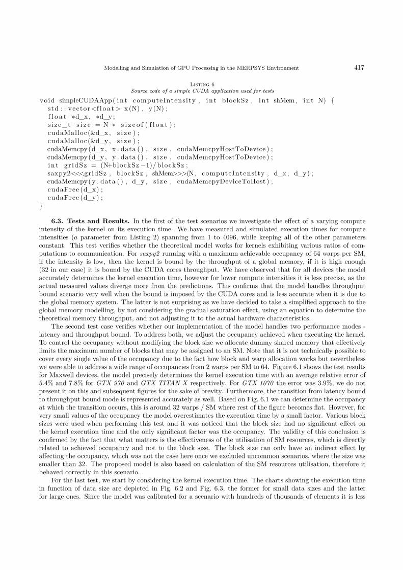
Modelling and Simulation of GPU Processing in the MERPSYS Environment 417
Listing 6Source code of a simple CUDA application used for tests
void simpleCUDAApp( i n t computeIntens ity , i n t blockSz , i n t shMem, i n t N) {std : : vector<f l o a t > x (N) , y (N) ;f l o a t ∗d_x , ∗d_y ;s i z e_t s i z e = N ∗ s i z e o f ( f l o a t ) ;cudaMalloc(&d_x , s i z e ) ;cudaMalloc(&d_y , s i z e ) ;cudaMemcpy(d_x , x . data ( ) , s i z e , cudaMemcpyHostToDevice ) ;cudaMemcpy(d_y , y . data ( ) , s i z e , cudaMemcpyHostToDevice ) ;i n t gr idSz = (N+blockSz −1)/ blockSz ;saxpy2<<<gridSz , blockSz , shMem>>>(N, computeIntens ity , d_x , d_y) ;cudaMemcpy( y . data ( ) , d_y , s i z e , cudaMemcpyDeviceToHost ) ;cudaFree (d_x) ;cudaFree (d_y) ;
}
6.3. Tests and Results. In the first of the test scenarios we investigate the effect of a varying computeintensity of the kernel on its execution time. We have measured and simulated execution times for computeintensities (a parameter from Listing 2) spanning from 1 to 4096, while keeping all of the other parametersconstant. This test verifies whether the theoretical model works for kernels exhibiting various ratios of com-putations to communication. For saxpy2 running with a maximum achievable occupancy of 64 warps per SM,if the intensity is low, then the kernel is bound by the throughput of a global memory, if it is high enough(32 in our case) it is bound by the CUDA cores throughput. We have observed that for all devices the modelaccurately determines the kernel execution time, however for lower compute intensities it is less precise, as theactual measured values diverge more from the predictions. This confirms that the model handles throughputbound scenario very well when the bound is imposed by the CUDA cores and is less accurate when it is due tothe global memory system. The latter is not surprising as we have decided to take a simplified approach to theglobal memory modelling, by not considering the gradual saturation effect, using an equation to determine thetheoretical memory throughput, and not adjusting it to the actual hardware characteristics.
The second test case verifies whether our implementation of the model handles two performance modes -latency and throughput bound. To address both, we adjust the occupancy achieved when executing the kernel.To control the occupancy without modifying the block size we allocate dummy shared memory that effectivelylimits the maximum number of blocks that may be assigned to an SM. Note that it is not technically possible tocover every single value of the occupancy due to the fact how block and warp allocation works but neverthelesswe were able to address a wide range of occupancies from 2 warps per SM to 64. Figure 6.1 shows the test resultsfor Maxwell devices, the model precisely determines the kernel execution time with an average relative error of5.4% and 7.8% for GTX 970 and GTX TITAN X respectively. For GTX 1070 the error was 3.9%, we do notpresent it on this and subsequent figures for the sake of brevity. Furthermore, the transition from latency boundto throughput bound mode is represented accurately as well. Based on Fig. 6.1 we can determine the occupancyat which the transition occurs, this is around 32 warps / SM where rest of the figure becomes flat. However, forvery small values of the occupancy the model overestimates the execution time by a small factor. Various blocksizes were used when performing this test and it was noticed that the block size had no significant effect onthe kernel execution time and the only significant factor was the occupancy. The validity of this conclusion isconfirmed by the fact that what matters is the effectiveness of the utilisation of SM resources, which is directlyrelated to achieved occupancy and not to the block size. The block size can only have an indirect effect byaffecting the occupancy, which was not the case here once we excluded uncommon scenarios, where the size wassmaller than 32. The proposed model is also based on calculation of the SM resources utilisation, therefore itbehaved correctly in this scenario.
For the last test, we start by considering the kernel execution time. The charts showing the execution timein function of data size are depicted in Fig. 6.2 and Fig. 6.3, the former for small data sizes and the latterfor large ones. Since the model was calibrated for a scenario with hundreds of thousands of elements it is less

418 T. Gajger and P. Czarnul
0 8 16 24 32 40 48 56 640
500
1,000
1,500
2,000
2,500
Occupancy [warps / SM]
Ker
nel
exec
uti
on
tim
e[m
s]
GTX970 - measured
GTX970 - predicted
TITAN X - measured
TITAN X - predicted
Fig. 6.1. Kernel execution time in function of occupancy
0 0.1 0.2 0.3 0.4 0.5 0.6 0.7 0.8 0.9 1
·106
0
0.1
0.2
0.3
0.4
Data size [elements]
Ker
nel
exec
uti
on
tim
e[m
s]
GTX970 - measured
GTX970 - predicted
TITAN X - measured
TITAN X - predicted
Fig. 6.2. Kernel execution time for small data sizes
accurate when the data size is small and improves its accuracy as the number of elements to process increases.The average error for large data size was 3.7% (GTX 970 ), 4.6% (GTX TITAN X) and 13.6% (GTX 1070 ).The last one was expected to be higher since the model was calibrated for a different hardware architecture. Theimportant fact is that even for the overestimated results, the functional relation between the data size and theexecution time is maintained. This is acceptable since in real world scenarios the computations are performedfor large data sizes and a case where the data is relatively small may be considered an uncommon one.
Since this test concerns a varying data size it must include data transfer time estimation, unlike the previousones which focused only on the kernel execution. Given that our testbeds used different configurations of thePCIe bus we measured λc and ts separately for each of them. The results are presented in Table 6.2, these werethen used as the parameters of the hardware unit, which are substituted to Eq. 4.6 in the computational model.
Measured and estimated data transfer times are shown in Fig. 6.4. A decrease in accuracy for smaller datasizes resulting from an overestimation can be noticed, this is the same observation as in the case of the kernelexecution time. Note that the transfers from host to the device take twice as much time because there are twoarrays of N elements to be transferred in this direction, compared to only a single array that is transferred back.We have also proved experimentally here what was pointed out earlier, that the λc and ts assume differentvalues depending on the transfer direction. If this effect was not considered, then the accuracy of the resultswould be lower. For large data sizes the predicted values very closely resemble the measured ones, thus we mayconclude that the methodology proposed for measuring data transfer times is valid.
Finally, the total execution time of the application for large data sizes is presented in Fig. 6.5. Technically,it sums up the results from the previous figures presented earlier in this section, since what comprises theapplication execution time is the data transfer in both directions and the kernel execution. It also concludesour work and proves its correctness by showing that the model we have implemented is capable of accurate

Modelling and Simulation of GPU Processing in the MERPSYS Environment 419
0.5 1 1.5 2 2.5 3 3.5 4 4.5 5
·108
0
50
100
150
200
Data size [elements]
Ker
nel
exec
uti
on
tim
e[m
s]
GTX970 - measured
GTX970 - predicted
TITAN X - measured
TITAN X - predicted
Fig. 6.3. Kernel execution time for large data sizes
0.5 1 1.5 2 2.5 3 3.5 4 4.5 5
·108
0
500
1,000
1,500
2,000
2,500
Data size [elements]
Data
tran
sfer
tim
e[m
s]
GTX970 - DtH measured
GTX970 - DtH predicted
GTX970 - HtD measured
GTX970 - HtD predicted
TITAN X - DtH measured
TITAN X - DtH predicted
TITAN X - HtD measured
TITAN X - HtD predicted
Fig. 6.4. Data transfer times for large data sizes
prediction of the application execution time for the most essential scenario, achieving 1.8%, 0.5% and 1.5% meanrelative error for large data size (≥10000000 elements, where 1 element = 8 Bytes as described in Section 5), fortested GPUs respectively. From the end user perspective, parameters like occupancy, block size and computeintensity will likely be determined once and then kept constant. What is probably the most common real-worlduse case, is verification of the application on different hardware setups and for different data sizes.
6.4. Discussion. For the most essential scenario with a varying data size, when this size was not verysmall, the mean values of the error were 1.8% for GTX 970 and 0.5% for GTX TITAN X. Tests of a computebound kernel with varying occupancy yielded an average prediction error of 5.4% and 7.8% respectively which isalso a very good result. When the input data size was small or the kernel was bound by a memory throughput,the relative prediction error had a mean value of 32.8% for GTX 970 and 9.9% for GTX TITAN X. Significantlyworse results for a memory throughput bound kernel are caused by a highly simplified memory access model. Forcompute throughput bound kernels, the error went down to a few percent depending on the launch configuration.It should be further noted that for every test case the functional relationship between the launch configurationparameter being investigated and the application execution time was very closely reproduced by the model.
7. Summary and Future Work. We have implemented adaptation of a performance model proposedby Volkov in the MERPSYS simulator for simulation of parallel applications on GPUs. We have verifiedthe correctness of the model for various launch configurations and representative scenarios on three testbeds.MERPSYS has been proven to be an easily extendable and feasible tool for GPU modelling, and it was also

420 T. Gajger and P. Czarnul
0.5 1 1.5 2 2.5 3 3.5 4 4.5 5
·108
0
1,000
2,000
3,000
4,000
Data size [elements]
Ap
pli
cati
on
exec
uti
on
tim
e[m
s]
GTX970 - measured
GTX970 - predicted
TITAN X - measured
TITAN X - predicted
Fig. 6.5. Application execution times for large data sizes
shown that processing on a GPU may be conveniently modelled with a high degree of accuracy using a general-purpose simulator. MERPSYS, with the deployed model, allows its users to assess the behaviour of theirapplications for data sizes exceeding the hardware capabilities of units available to them and even use ones thatare not in their possession, given that these are available in MERPSYS’ database. It allows to evaluate theapplication on hardware setups, on which testing prior to actual computational runs, would not otherwise befeasible, e.g. large clusters with a high cost per core-hour. It also allows to estimate the costs by predicting howlong it will take for the computations to finish. In case of long-running applications, this allows for significantlyshorter simulation times than the real runs.
The scope of modelling can be extended in the future as we have omitted double precision units, SFUs andshared memory, all of these could be fairly easy added to the model. Moreover, the approach to modelling ofglobal memory accesses can be extended to consider caches, gradual saturation effect and varying access timedepending on the transfer direction. So far we did include CUDA and NVIDIA GPUs in the model, possibleextension includes its generalisation to be applicable to units produced by AMD and the OpenCL framework.The model can be extended with inclusion of an equation for occupancy calculation, which could be incorporatedinto the existing set of the equations and hence remove the need of relying on an external tool for this purpose.The solution would also largely benefit from an automation of the kernel analysis process. The behaviour ofthe model could also be verified on different GPU hardware architectures.
Acknowledgements. The work has been supported partially by the Polish Ministry of Science and HigherEducation.
REFERENCES
[1] Top 500 list. [accessed November-2018].[2] M. Amaris, D. Cordeiro, A. Goldman, and R. Y. d. Camargo, A simple bsp-based model to predict execution time
in gpu applications, in 2015 IEEE 22nd International Conference on High Performance Computing (HiPC), Dec 2015,pp. 285–294.
[3] M. Amaris, R. Y. de Camargo, M. Dyab, A. Goldman, and D. Trystram, A comparison of gpu execution time predictionusing machine learning and analytical modeling, in 2016 IEEE 15th International Symposium on Network Computingand Applications (NCA), Oct 2016, pp. 326–333.
[4] M. Andersch, J. Lucas, M. Alvarez-Mesa, and B. Juurlink, Analyzing gpgpu pipeline latency, in Proc. 10th Int. SummerSchool on Advanced Computer Architecture and Compilation for High-Performance and Embedded Systems, Fiuggi, Italy(ACACES’ 14), July 2014.
[5] S. S. Baghsorkhi, M. Delahaye, S. J. Patel, W. D. Gropp, and W.-m. W. Hwu, An adaptive performance modelingtool for gpu architectures, in Proceedings of the 15th ACM SIGPLAN Symposium on Principles and Practice of ParallelProgramming, PPoPP ’10, New York, NY, USA, 2010, ACM, pp. 105–114.
[6] A. Bakhoda, G. L. Yuan, W. W. L. Fung, H. Wong, and T. M. Aamodt, Analyzing cuda workloads using a detailedgpu simulator, in 2009 IEEE International Symposium on Performance Analysis of Systems and Software, April 2009,pp. 163–174.

Modelling and Simulation of GPU Processing in the MERPSYS Environment 421
[7] S. Bąk, M. Krystek, K. Kurowski, A. Oleksiak, W. Piątek, and J. Węglarz, Gssim – a tool for distributed computingexperiments, Sci. Program., 19 (2011), pp. 231–251.
[8] R. Buyya and M. Murshed, Gridsim: a toolkit for the modeling and simulation of distributed resource management andscheduling for grid computing, Concurrency and Computation: Practice and Experience, 14 (2002), pp. 1175–1220.
[9] R. N. Calheiros, R. Ranjan, A. Beloglazov, C. A. F. De Rose, and R. Buyya, Cloudsim: A toolkit for modeling andsimulation of cloud computing environments and evaluation of resource provisioning algorithms, Softw. Pract. Exper.,41 (2011), pp. 23–50.
[10] N. Capodieci and P. Burgio, Efficient implementation of genetic algorithms on gp-gpu with scheduled persistent cudathreads, in 2015 Seventh International Symposium on Parallel Architectures, Algorithms and Programming (PAAP), Dec2015, pp. 6–12.
[11] Z. Cui, Y. Liang, K. Rupnow, and D. Chen, An accurate gpu performance model for effective control flow divergenceoptimization, in 2012 IEEE 26th International Parallel and Distributed Processing Symposium, May 2012, pp. 83–94.
[12] P. Czarnul, ed., Modeling Large-Scale Computing Systems. Concepts and Models, Gdańsk University of Technology, Gdańsk,Poland, 2013.
[13] , ed., Modeling Large-Scale Computing Systems. Practical Approaches in MERPSYS, Gdańsk University of Technology,Gdańsk, Poland, 2016.
[14] P. Czarnul, J. Kuchta, and M. Matuszek, Parallel computations in the volunteer–based comcute system, in ParallelProcessing and Applied Mathematics, R. Wyrzykowski, J. Dongarra, K. Karczewski, and J. Waśniewski, eds., Berlin,Heidelberg, 2014, Springer Berlin Heidelberg, pp. 261–271.
[15] P. Czarnul, J. Kuchta, M. Matuszek, J. Proficz, P. Rościszewski, M. Wójcik, and J. Szymański, Merpsys: Anenvironment for simulation of parallel application execution on large scale hpc systems, Simulation Modelling Practiceand Theory, 77 (2017), pp. 124 – 140.
[16] P. Czarnul, J. Kuchta, P. Rościszewski, and J. Proficz, Modeling energy consumption of parallel applications, in 2016Federated Conference on Computer Science and Information Systems (FedCSIS), Sept 2016, pp. 855–864.
[17] P. Czarnul, P. Rościszewski, M. Matuszek, and J. Szymański, Simulation of parallel similarity measure computationsfor large data sets, in 2015 IEEE 2nd International Conference on Cybernetics (CYBCONF), June 2015, pp. 472–477.
[18] P. Czarnul, K. Tomko, and H. Krawczyk, Dynamic partitioning of the divide-and-conquer scheme with migration in pvmenvironment, in Recent Advances in Parallel Virtual Machine and Message Passing Interface, Y. Cotronis and J. Dongarra,eds., Berlin, Heidelberg, 2001, Springer Berlin Heidelberg, pp. 174–182.
[19] T. T. Dao, J. Kim, S. Seo, B. Egger, and J. Lee, A performance model for gpus with caches, IEEE Transactions on Paralleland Distributed Systems, 26 (2015), pp. 1800–1813.
[20] W. E. Denzel, J. Li, P. Walker, and Y. Jin, A framework for end-to-end simulation of high-performance computing systems,in Proceedings of the 1st International Conference on Simulation Tools and Techniques for Communications, Networks andSystems & Workshops, Simutools ’08, ICST, Brussels, Belgium, Belgium, 2008, ICST (Institute for Computer Sciences,Social-Informatics and Telecommunications Engineering), pp. 21:1–21:10.
[21] B. Donassolo, H. Casanova, A. Legrand, and P. Velho, Fast and scalable simulation of volunteer computing systemsusing simgrid, in Proceedings of the 19th ACM International Symposium on High Performance Distributed Computing,HPDC ’10, New York, NY, USA, 2010, ACM, pp. 605–612.
[22] M. Harris, An easy introduction to cuda c and c++, October 2012. [accessed November-2018].[23] S. Hong and H. Kim, An analytical model for a gpu architecture with memory-level and thread-level parallelism awareness,
in Proceedings of the 36th Annual International Symposium on Computer Architecture, ISCA ’09, New York, NY, USA,2009, ACM, pp. 152–163.
[24] J. C. Huang, J. H. Lee, H. Kim, and H. H. S. Lee, Gpumech: Gpu performance modeling technique based on intervalanalysis, in 2014 47th Annual IEEE/ACM International Symposium on Microarchitecture, Dec 2014, pp. 268–279.
[25] W. Jia, K. A. Shaw, and M. Martonosi, Stargazer: Automated regression-based gpu design space exploration, in 2012 IEEEInternational Symposium on Performance Analysis of Systems Software, April 2012, pp. 2–13.
[26] Z. Jia, M. Maggioni, B. Staiger, and D. P. Scarpazza, Dissecting the NVIDIA Volta GPU Architecture via Microbench-marking, ArXiv e-prints, (2018).
[27] A. Kerr, G. Diamos, and S. Yalamanchili, A characterization and analysis of ptx kernels, in Workload Characterization,2009. IISWC 2009. IEEE International Symposium on, oct. 2009, pp. 3 –12.
[28] , Modeling gpu-cpu workloads and systems, in Proceedings of the 3rd Workshop on General-Purpose Computation onGraphics Processing Units, GPGPU-3, New York, NY, USA, 2010, ACM, pp. 31–42.
[29] K. Kurowski, J. Nabrzyski, A. Oleksiak, and J. Węglarz, Gssim - grid scheduling simulator, Computational Methodsin Science and Technology, 13 (2007), pp. 121–129.
[30] S. Madougou, A. Varbanescu, C. de Laat, and R. van Nieuwpoort, The landscape of gpgpu performance modeling tools,Parallel Comput., 56 (2016), pp. 18–33.
[31] S. Madougou, A. L. Varbanescu, C. D. Laat, and R. V. Nieuwpoort, A tool for bottleneck analysis and performanceprediction for gpu-accelerated applications, in 2016 IEEE International Parallel and Distributed Processing SymposiumWorkshops (IPDPSW), May 2016, pp. 641–652.
[32] O. Maitre, Understanding NVIDIA GPGPU Hardware, Springer-Verlag, Berlin, 2013.[33] Micron Technology, Gddr5 sgram introduction, 2014.[34] NVIDIA Corporation, Cuda occupancy calculator, December 2016. [accessed November-2018].[35] , nvidia-smi - nvidia system management interface, July 2016. [accessed November-2018].[36] , Cuda binary utilities, March 2017. [accessed November-2018].[37] , Cuda c programming guide, June 2017. [accessed November-2018].

422 T. Gajger and P. Czarnul
[38] , Nvidia cuda compiler driver nvcc, March 2017. [accessed November-2018].[39] , Parallel thread execution isa, March 2017. [accessed November-2018].[40] A. K. Parakh, M. Balakrishnan, and K. Paul, Performance estimation of gpus with cache, in 2012 IEEE 26th International
Parallel and Distributed Processing Symposium Workshops PhD Forum, May 2012, pp. 2384–2393.[41] S. F. Piraghaj, A. V. Dastjerdi, R. N. Calheiros, and R. Buyya, Containercloudsim: An environment for modeling and
simulation of containers in cloud data centers, Software: Practice and Experience, 47 (2017), pp. 505–521. spe.2422.[42] M. Quinson, Simgrid: a generic framework for large-scale distributed experiments, in 2009 IEEE Ninth International Con-
ference on Peer-to-Peer Computing, Sept 2009, pp. 95–96.[43] H. Rashidi, Discrete simulation software: a survey on taxonomies, Journal of Simulation, 11 (2017), pp. 174–184.[44] P. Rościszewski, Modeling and simulation for exploring power/time trade-off of parallel deep neural network training,
Procedia Computer Science, 108 (2017), pp. 2463 – 2467. International Conference on Computational Science, ICCS2017, 12-14 June 2017, Zurich, Switzerland.
[45] T. Scudiero, Memory bandwidth bootcamp: Best practices, in Proceedings of the GPU Technology Conference, GTC, 2015.[46] , Memory bandwidth bootcamp: Beyond best practices, in Proceedings of the GPU Technology Conference, GTC, 2015.[47] A. Siavashi and M. Momtazpour, Gpucloudsim: an extension of cloudsim for modeling and simulation of gpus in cloud
data centers, The Journal of Supercomputing, (2018).[48] A. Sulistio, C. S. Yeo, and R. Buyya, A taxonomy of computer-based simulations and its mapping to parallel and distributed
systems simulation tools, Softw., Pract. Exper., 34 (2004), pp. 653–673.[49] L. G. Valiant, A bridging model for parallel computation, Commun. ACM, 33 (1990), pp. 103–111.[50] V. Volkov, Better performance at lower occupancy, in Proceedings of the GPU Technology Conference, GTC, vol. 10, 2015.[51] , Understanding Latency Hiding on GPUs, PhD thesis, EECS Department, University of California, Berkeley, Aug
2016.[52] G. Wu, J. L. Greathouse, A. Lyashevsky, N. Jayasena, and D. Chiou, Gpgpu performance and power estimation using
machine learning, in 2015 IEEE 21st International Symposium on High Performance Computer Architecture (HPCA),Feb 2015, pp. 564–576.
[53] Y. Zhang and J. D. Owens, A quantitative performance analysis model for gpu architectures, in 2011 IEEE 17th InternationalSymposium on High Performance Computer Architecture, Feb 2011, pp. 382–393.
Edited by: Dana PetcuReceived: Sep 7, 2018Accepted: Nov 3, 2018

Scalable Computing: Practice and ExperienceVolume 19, Number 4, pp. 423–432. http://www.scpe.org
DOI 10.12694/scpe.v19i4.1468ISSN 1895-1767
© 2018 SCPE
A COMPARISON OF MESSAGE PASSING INTERFACE (MPI) AND CO-ARRAYFORTRAN FOR LARGE FINITE ELEMENT VARIABLY SATURATED FLOW
SIMULATIONS ∗
FRED T. TRACY†, THOMAS C. OPPE‡, AND MAUREEN K. CORCORAN§
Abstract. The purpose of this research is to determine how well co-array FORTRAN (CAF) performs relative to MessagePassing Interface (MPI) on unstructured mesh finite element groundwater modelling applications with large problem sizes and corecounts. This research used almost 150 million nodes and 300 million 3-D prism elements. Results for both the Cray XE6 and CrayXC30 are given. A comparison of the ghost-node update algorithms with source code provided for both MPI and CAF is alsopresented.
Key words: Co-array FORTRAN, MPI, finite element method, variably saturated seepage flow modelling
AMS subject classifications. 35J66, 65Y05, 76S05
1. Introduction. Several parallel programming paradigms have been developed in recent years as alterna-tives to the popular software Message Passing Interface (MPI) [1] used for passing messages among the processesof a distributed memory parallelized program. One of these new ways is the Partitioned Global Address Space(PGAS) [2] paradigm where arrays partitioned across processes can be referenced by special syntax implementedin the language. A popular PGAS language for FORTRAN users is co-array FORTRAN (CAF) [3], and a CAFspecification has been adopted in the FORTRAN 2008 standard. CAF has performed better than MPI forcertain applications, and it was found easier to program than MPI. A recent example tested structured-gridpartial-differential-equation applications [4].
A recent paper [7] describing the challenges and scalability results of running a large finite element modelof variably saturated flow [5] in a three-dimensional (3-D) levee on a large high performance, parallel computerwhere MPI was used for the communication was published. Using the same levee model, this current researchexpands that work by using CAF for the communication and comparing these results with the results usingMPI. The original finite element model consisted of 3,017,367 nodes and 5,836,072 3-D prism elements runningon 32 cores, and the problem and core count were magnified as much as 350 times to achieve 1,044,246,303nodes and 2,042,625,200 elements.
A traditional partitioning of the mesh achieved approximately the same number of finite element nodes oneach core. Thus, the main communication challenge was updating ghost-node information on the different coresfor a solution of a system of simultaneous, linear equations at each nonlinear iteration. In both the MPI andCAF versions, the ghost node data are first buffered and then sent to the different cores where they are needed.Details of the FORTRAN coding for both MPI and CAF are described herein.
2. Description of the problem. The problem consists of steady-state seepage flow through a levee asshown in Fig. 2.1 and idealised in Fig. 2.2 where there are several soil layers. A detailed description of thisproblem is given in [6, 7]. The challenges of parallelization using MPI of the groundwater program used in thisresearch, when the problem size is approximately one billion nodes and two billion elements, are given in [7].Performance results are also given. Fig. 2.3 shows a portion of the 3-D mesh of the levee system before a treewith its root system was added at the toe. More details of the modelling of the woody vegetation are givenin [6]. To model the tree root at the toe of the levee, a 5 ft × 6 ft × 6 ft heterogeneous zone was added inwhich the mesh was refined using 1 in × 1 in × 1 in 3-D prism elements (Fig. 2.4). To simulate heterogeneities,a randomly generated hydraulic conductivity was assigned to each element in this zone. The resulting meshconsisted of 3,017,367 nodes and 5,836,072 3-D prism elements.
∗This work was supported in part by a grant of computer time from the Department of Defense High Performance ComputingModernization Program (HPCMP).
†Information Technology Laboratory (ITL), Engineer Research and Development Center (ERDC), Vicksburg, MS.‡ITL, ERDC, Vicksburg, MS.§Geotechnical and Structures Laboratory, ERDC, Vicksburg, MS.
423

424 F. T. Tracy, T. C. Oppe and M. K. Corcoran
Fig. 2.1. River side of a levee with trees.�
�
�����
����
�
������������������
������ �����������
������������
�������
�����������������������
���
�������������
Fig. 2.2. Cross section of a levee with material types and elevation of the river.
3. High performance parallel computing. The parallel 3-D groundwater finite element program men-tioned above was run on Garnet, the Cray XE6 at the U.S. Army Engineer Research and Development Center(ERDC) [8], and on Lightning, the Cray XC30 at the Air Force Research Laboratory, Aberdeen, MD [9]. At thetime of this study, Garnet consisted of 4,716 dual-socket compute nodes with each socket populated with a 2.5GHz 16-core AMD 6200 Opteron (Interlagos) processor. Each node had 64 GB memory (60 GB user-accessible)or an average of 1.875 GB memory per core. The interconnect type was Cray Gemini in a 3-D torus topology.Garnet was rated at 1.5 peak PFLOPS or 10 GFLOPS per core when these computations were done. Garnethad a large Lustre file system that was tuned for parallel I/O. At the time of this research, Lightning consistedof 2,360 dual-socket compute nodes with each socket populated with a 2.7 GHz 12-core Intel Xeon E5-2697v2(Ivy Bridge) processor. Each node had 64 GB memory (63 GB user-accessible) or an average of 2.625 GBmemory per core. The interconnect type was Cray Aries in a Dragonfly topology. Lightning was rated at 1.2peak PFLOPS or 21.6 GFLOPS per core when the data in this paper were collected. Lightning had a largeLustre file system that was also tuned for parallel I/O.
The parallelization of the 3-D seepage/groundwater program was separated into four parts or programs.One MPI process or one CAF image was placed on each core of a compute node. The four programs are (1)a partitioner using the Parallel Graph Partitioning and Fill-reducing Matrix Ordering program, ParMETIS[10], to divide the mesh into approximately equal pieces among the MPI processes or CAF images, (2) apreparer to provide data, such as owned nodes, ghost nodes, owned elements, ghost elements, and communicationdata, needed for each MPI process or CAF image, (3) a finite element program that does the finite elementcomputations with output files containing results for each owned node of that MPI process or CAF image, and(4) a post processor that combines all data from each MPI process or CAF image into the final output files.

A Comparison of MPI and Co-array FORTRAN for Large Finite Element Variably Saturated Flow Simulations 425
Fig. 2.3. Portion of the 3-D mesh before the root zone was added.
The primary communication challenge is ghost node updates in the conjugate gradient or BICG-STAB[11] linear solvers using either a Picard or Newton linearization [12, 13] of the governing nonlinear equation ofRichards’ equation [14]. As in [7], only times to solution for the finite element part of the program suite werecollected for MPI and CAF and reported in this paper. The ghost node update routine for both MPI and CAFis examined in detail in the following section.
4. Ghost node update.
4.1. MPI. Table 4.1 gives the ghost node update subroutine for MPI and a description of the importantvariables. The subroutine has three steps: (1) a set-up phase in which data are to be received from the differentcores, (2) send data to the different cores, and (3) wait until all the MPI messages have been processed. Thearrays, nstngh, ighost, and nodgh have all been supplied by the preparer program. There are no global arraysin the parallel versions of the finite element program, i.e., no arrays with sizes of the total number of nodes orthe total number of elements. The elimination of global arrays allowed for much larger finite element meshesto be run.
4.2. CAF. Table 4.2 gives the ghost node update subroutine for CAF and a description of the importantvariables. The same data provided in the MPI version were also provided to the CAF subroutine. The CAFversion of ghost node updating is simpler than the MPI version in that for CAF, data are first placed in a bufferand then directly “put” into the different cores by the statement,
vc(nst : nst + num - 1)[i] = buff(:)
While in the MPI case, the efficiency of the data transfer is dependent on how well MPI_IRECV, MPI_SEND, andMPI_WAIT are implemented, the efficiency of the CAF routine is dependent on the quality of the FORTRANcompiler implementation and internal data transfer capability. It is also important to note that two explicitbarrier calls,
call sync_all
were required in the CAF implementation, whereas none were required in the MPI version. Also, the huge pageoption described by
module load craype-hugepages2M
was required to run the CAF version.
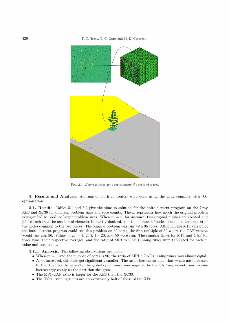
426 F. T. Tracy, T. C. Oppe and M. K. Corcoran�
�
�
�
�
�
�
����
����
�
����
Fig. 2.4. Heterogeneous zone representing the roots of a tree.
5. Results and Analysis. All runs on both computers were done using the Cray compiler with -O1optimisation.
5.1. Results. Tables 5.1 and 5.2 give the time to solution for the finite element program on the CrayXE6 and XC30 for different problem sizes and core counts. The m represents how much the original problemis magnified to produce larger problem sizes. When m = 2, for instance, two original meshes are created andjoined such that the number of elements is exactly doubled, and the number of nodes is doubled less one set ofthe nodes common to the two pieces. The original problem was run with 96 cores. Although the MPI version ofthe finite element program could run this problem on 32 cores, the first multiple of 32 where the CAF versionwould run was 96. Values of m = 1, 2, 5, 10, 20, and 50 were run. The running times for MPI and CAF forthree runs, their respective averages, and the ratio of MPI to CAF running times were tabulated for each m
value and core count.
5.1.1. Analysis. The following observations are made:• When m = 1 and the number of cores is 96, the ratio of MPI / CAF running times was almost equal.• As m increased, this ratio got significantly smaller. The ratios become so small that m was not increased
further than 50. Apparently, the global synchronisations required by the CAF implementation becameincreasingly costly as the partition size grew.
• The MPI/CAF ratio is larger for the XE6 than the XC30.• The XC30 running times are approximately half of those of the XE6.

A Comparison of MPI and Co-array FORTRAN for Large Finite Element Variably Saturated Flow Simulations 427
Table 4.1Ghost node update for MPI.
Receive FORTRAN code
do i = 1, noprocnum = numngh(i)if (num .ne. 0) then
itag = 100nst = nstngh(i)call MPI_IRECV (v(nst), num, MPI_REAL8, i - 1, itag, MPI_COMM_WORLD, &
ireq(i), ierror)end if
end do
Send FORTRAN code
allocate (buff(num_max))
do i = 1, noprocnum = ighost(i + 1) - ighost(i)if (num .ne. 0) then
do j = 1, numjloc = nodgh(ighost(i) + j)buff(j) = v(jloc)
end doitag = 100call MPI_SEND (buff, num, MPI_REAL8, i - 1, itag, MPI_COMM_WORLD, ierror)
end ifend do
deallocate (buff)
Wait FORTRAN code
do i = 1, noprocif (numngh(i) .ne. 0) then
call MPI_WAIT (ireq(i), istat, ierror)end if
end do
noproc = number of cores or MPI processesnum_max = maximum number of ghost node data to send
v = variable to be updatednstngh(i) = the starting address of v where data are to be received from core, i - 1
numngh(i) = the number of values be received in v from core, i - 1nodgh = array containing local node numbers whose data are to be sent to other coresighost = array containing the accumulated number of ghost nodes whose data
are to be sent

428 F. T. Tracy, T. C. Oppe and M. K. Corcoran
Table 4.2Ghost node update for CAF.
Special CAF variables
common / caf / nstnghc(npmx)[*], vc(ndlmx)[*]
CAF put FORTRAN code
call sync_allallocate (buff(num_max))
do i = 1, noprocnum = ighost(i + 1) - ighost(i)if (num .ne. 0) then
nst = nstnghc(image)[i]do j = 1, num
jloc = nodgh(ighost(i) + j)buff(j) = v(jloc)
end dovc(nst : nst + num - 1)[i] = buff(:)
end ifend do
call sync_alldeallocate (buff)
do i = nnpown + 1, nnplv(i) = vc(i)
end do
noproc = number of cores or CAF imagesimage = CAF image numbernpmx = maximum number of CAF images
nnpl = number of local nodesndlmx = maximum number of local nodes
v = variable to be updatedvc = CAF array containing the updated ghost node data
nstnghc(i) = CAF array containing the starting address of v where data areto be received from core, i
nodgh = array containing local node numbers whose data are to be sentto other cores
ighost = array containing the accumulated number of ghost nodes whose dataare to be sent

A Comparison of MPI and Co-array FORTRAN for Large Finite Element Variably Saturated Flow Simulations 429
Table 5.1Time (sec) for MPI and CAF on the Cray XE6 and XC30 for m = 1, 2, and 5.
m Nodes Elements Cores CrayTime Time RatioMPI CAF MPI/CAF
1 3017367 5836072 96XE6 788.0 816.0XC30 323.6 376.6
XE6 786.6 826.7XC30 324.8 379.2
XE6 767.7 820.7XC30 322.1 375.3
XE6Avg.
780.8Avg.
820.8 0.95XC30 323.5 377.0 0.86
128XE6 601.1 658.8XC30 252.1 322.6
XE6 597.3 723.7XC30 258.4 325.4
XE6 596.6 628.9XC30 257.0 343.3
XE6Avg.
598.3Avg.
670.5 0.89XC30 255.8 330.4 0.77
2 6000831 11672144 192XE6 804.1 1028.7XC30 283.0 393.6
XE6 788.8 850.2XC30 281.5 363.7
XE6 786.3 896.4XC30 281.4 397.8
XE6Avg.
793.1Avg.
925.1 0.86XC30 282.0 385.0 0.73
256XE6 642.1 914.4XC30 255.8 408.5
XE6 604.0 692.1XC30 258.1 383.5
XE6 659.4 917.5XC30 256.0 386.7
XE6Avg.
645.2Avg.
841.3 0.76XC30 256.6 392.9 0.65
5 14951223 29180360 480XE6 878.3 1361.8XC30 344.0 636.8
XE6 819.0 1292.5XC30 347.3 630.1
XE6 829.4 1287.3XC30 347.1 635.3
XE6Avg.
842.2Avg.
1313.9 0.64XC30 346.1 634.1 0.55
640XE6 708.8 1491.8XC30 260.5 576.3
XE6 599.6 1254.0XC30 264.4 671.2
XE6 663.4 1241.4XC30 267.5 595.9
XE6Avg.
657.3Avg.
1328.1 0.49XC30 264.1 614.5 0.43

430 F. T. Tracy, T. C. Oppe and M. K. Corcoran
Table 5.2Time (sec) for MPI and CAF on the Cray XE6 and XC30 for m = 10, 20, and 50.
m Nodes Elements Cores CrayTime Time RatioMPI CAF MPI/CAF
10 3017367 58360720 960XE6 862.0 1691.6XC30 344.7 910.7
XE6 881.2 1730.2XC30 353.1 912.2
XE6 867.5 1473.4XC30 349.5 907.5
XE6Avg.
870.2Avg.
1631.7 0.53XC30 349.1 910.1 0.38
1280XE6 632.9 1309.0XC30 266.9 995.1
XE6 624.6 1584.0XC30 267.6 999.3
XE6 609.4 1768.6XC30 267.6 998.2
XE6Avg.
622.3Avg.
1553.9 0.40XC30 267.4 997.5 0.27
20 59703183 116721440 1920XE6 957.7 2685.8XC30 351.0 1330.3
XE6 852.6 3031.6XC30 356.3 1465.0
XE6 874.4 2760.2XC30 363.9 1326.6
XE6Avg.
894.9Avg.
2825.9 0.32XC30 357.1 1374.0 0.26
2560XE6 659.8 2609.2XC30 276.5 1496.1
XE6 651.8 2641.7XC30 276.1 1755.5
XE6 651.2 2283.0XC30 274.9 1473.7
XE6Avg.
654.3Avg.
2511.3 0.26XC30 275.8 1575.1 0.18
50 149207103 291803600 4800XE6 882.9 5242.1XC30 374.6 2990.1
XE6 883.0 5704.6XC30 356.7 3133.1
XE6 923.0 5255.3XC30 359.4 3140.2
XE6Avg.
896.3Avg.
5400.7 0.17XC30 363.6 3087.8 0.12
6400XE6 703.2 5792.8XC30 306.9 3801.3
XE6 739.6 6902.2XC30 302.3 3833.0
XE6 749.1 6256.4XC30 300.3 3796.7
XE6Avg.
730.6Avg.
6317.1 0.12XC30 303.2 3810.3 0.08

A Comparison of MPI and Co-array FORTRAN for Large Finite Element Variably Saturated Flow Simulations 431
Table 6.1Consistency check comparing values of pressure head from the original mesh and the mesh for m = 50 for the first 10 nodes
and last 6 nodes of each mesh.
m = 1 m = 50
Node MPI CAF Node MPI CAF
1 129.00000 129.00000 1 129.00000 129.00000
2 128.99678 128.99678 2 128.99678 128.99678
3 128.99345 128.99345 3 128.99345 128.99345
4 119.00000 119.00000 4 119.00000 119.00000
5 118.99735 118.99735 5 118.99735 118.99735
6 124.23808 124.23808 6 124.23808 124.23808
7 118.99464 118.99464 7 118.99464 118.99464
8 123.54520 123.54520 8 123.54520 123.54520
9 128.98993 128.98993 9 128.98993 128.98993
10 110.50000 110.50000 10 110.50000 110.50000
6000826 0.0000000 0.0000000 149207098 0.0000000 0.0000000
6000827 0.041718483 0.041718484 149207099 0.041718479 0.041718479
6000828 3.0365778 3.0365778 149207100 3.0365779 3.0365779
6000829 0.036494873 0.036494870 149207101 0.036494875 0.036494875
6000830 0.0000000 0.0000000 149207102 0.0000000 0.0000000
6000831 0.0000000 0.0000000 149207103 0.0000000 0.0000000
6. Consistency check. A check for consistency for the first 10 nodes and last 6 nodes of the meshes form = 1 and m = 50 was done with pressure head results placed in Table 6.1. The MPI and CAF results shouldbe the same and because of symmetry, the values for m = 1 and m = 50 should also be the same. A comparisonof the MPI and CAF results in Table 6.1 shows excellent consistency.
7. Conclusions. The following conclusions can be drawn:1. Both MPI and CAF versions ran successfully and gave the same results.2. As the problem size and process count increased, the results remained consistent.3. The update routine for CAF was simpler than that for MPI.4. CAF required more memory than MPI to run the same size mesh.5. CAF required huge pages, but MPI did not.6. CAF required explicit barriers, but MPI did not.7. For the original problem, CAF and MPI performed almost the same when using 96 cores.8. As the problem size and process count grew, MPI performed much better than CAF.9. The MPI/CAF ratio is larger for the XE6 than the XC30.
10. The XC30 running times are approximately half of those of the XE6.
REFERENCES
[1] Message Passing Interface Forum, MPI: A Message-Passing Interface Standard, Version 3.0, http://www.mpi-forum.org/docs/mpi-3.0/mpi30-report.pdf, 2012.
[2] PGAS, Partitioned Global Address Space, http://pgas.org, 2015.[3] R. W. Numrich and J. K. Reid, Co-arrays in the next FORTRAN Standard, Scientific Programming, 14 (2006), pp. 1-18.[4] S. Garain, D. S. Balsara, and J. Reid, Comparing Co-array FORTRAN (CAF) with MPI for several structured mesh
PDE applications, J. of Comp. Physics, 297 (2015), pp. 237-253.[5] J. Istok, Groundwater modelling by the finite element method, AGU, 1989.[6] M. Corcoran, J. Peters, J. Dunbar, J. Llopis, F. Tracy, J. Wibowo, J. Simms, C. Kees, S. McKay, J. Fischenich,
M. Farthing, M. Glynn, B. Robbins, R. Strange, M. Schultz, J. Clarke, T. Berry, C. Little, and L. Lee, Initialresearch into the effects of woody vegetation on levees, volume I of IV: project overview, volume II of IV: field datacollection, volume III of IV: numerical model simulation, and volume IV of IV: summary of results and conclusions,U.S. Army Engineer Research and Development Center, Vicksburg, MS, 2011.
[7] F. T. Tracy, T. C. Oppe, W. A. Ward, and M. K. Corcoran, A scalability study using supercomputers for huge finiteelement variably saturated flow simulations, Scalable Computing: Practice and Experience, 16 (2015), pp. 153-162.

432 F. T. Tracy, T. C. Oppe and M. K. Corcoran
[8] ERDC DSRC, http://www.erdc.hpc.mil/hardware/index.html, Department of Defense Supercomputing Resource Center,Vicksburg, MS, 2014.
[9] AFRL DSRC, http://www.afrl.hpc.mil/index.html, Department of Defense Supercomputing Resource Center, Aberdeen, MD,2014.
[10] G. Karypis, ParMETIS - Parallel Graph Partitioning and Fill-reducing Matrix Ordering, http://glaros.dtc.umn.edu/gkhome/metis/parmetis/overview, 2014.
[11] Y. Saad, Iterative Methods for Sparse Linear Systems, SIAM, Philadelphia, 2003.[12] S. Mehl, Use of Picard and Newton iteration for solving nonlinear ground water flow equations, Ground Water, 44 (2006),
pp. 583-594.[13] C. T. Kelley, Solving nonlinear equations with Newton’s method, SIAM, 2003.[14] L. A. Richards, Capillary conduction of liquids through porous mediums, J. of Physics, 1 (1931), pp. 318-333.
Edited by: Dana PetcuReceived: Nov 23, 2018Accepted: Dec 23, 2018

AIMS AND SCOPE
The area of scalable computing has matured and reached a point where new issues and trends require a pro-fessional forum. SCPE will provide this avenue by publishing original refereed papers that address the presentas well as the future of parallel and distributed computing. The journal will focus on algorithm development,implementation and execution on real-world parallel architectures, and application of parallel and distributedcomputing to the solution of real-life problems. Of particular interest are:
Expressiveness:• high level languages,• object oriented techniques,• compiler technology for parallel computing,• implementation techniques and their effi-ciency.
System engineering:• programming environments,• debugging tools,• software libraries.
Performance:• performance measurement: metrics, evalua-tion, visualization,
• performance improvement: resource allocationand scheduling, I/O, network throughput.
Applications:
• database,
• control systems,
• embedded systems,
• fault tolerance,
• industrial and business,
• real-time,
• scientific computing,
• visualization.
Future:
• limitations of current approaches,
• engineering trends and their consequences,
• novel parallel architectures.
Taking into account the extremely rapid pace of changes in the field SCPE is committed to fast turnaroundof papers and a short publication time of accepted papers.
INSTRUCTIONS FOR CONTRIBUTORS
Proposals of Special Issues should be submitted to the editor-in-chief.The language of the journal is English. SCPE publishes three categories of papers: overview papers,
research papers and short communications. Electronic submissions are preferred. Overview papers and shortcommunications should be submitted to the editor-in-chief. Research papers should be submitted to the editorwhose research interests match the subject of the paper most closely. The list of editors’ research interests canbe found at the journal WWW site (http://www.scpe.org). Each paper appropriate to the journal will berefereed by a minimum of two referees.
There is no a priori limit on the length of overview papers. Research papers should be limited to approx-imately 20 pages, while short communications should not exceed 5 pages. A 50–100 word abstract should beincluded.
Upon acceptance the authors will be asked to transfer copyright of the article to the publisher. Theauthors will be required to prepare the text in LATEX2ε using the journal document class file (based on theSIAM’s siamltex.clo document class, available at the journal WWW site). Figures must be prepared inencapsulated PostScript and appropriately incorporated into the text. The bibliography should be formattedusing the SIAM convention. Detailed instructions for the Authors are available on the SCPE WWW site athttp://www.scpe.org.
Contributions are accepted for review on the understanding that the same work has not been publishedand that it is not being considered for publication elsewhere. Technical reports can be submitted. Substantiallyrevised versions of papers published in not easily accessible conference proceedings can also be submitted. Theeditor-in-chief should be notified at the time of submission and the author is responsible for obtaining thenecessary copyright releases for all copyrighted material.