A Scalable Relational Database Model for Cloud

Computing

Otara Paul Richard

Reg. No: 2005/HD18/0105U

B.Sc (Computer Science, Mathematics)(Mak), OCP

A Dissertation Submitted to the Directorate of Research and Graduate

Training in Partial Fulfillment for the Award of the Degree of

In MSc DCSE (Software Enginerinng Option) of Makerere University

Contents

1 Introduction 1

1.1 Motivation . . . . . . . . . . . . . . . . . . . . . . . . . . . . . . . . . . . . . . . . . 1

1.2 Background to the Study . . . . . . . . . . . . . . . . . . . . . . . . . . . . . . . . . 2

1.3 Problem Statement . . . . . . . . . . . . . . . . . . . . . . . . . . . . . . . . . . . . 3

1.4 Objectives . . . . . . . . . . . . . . . . . . . . . . . . . . . . . . . . . . . . . . . . . 3

1.5 Justification . . . . . . . . . . . . . . . . . . . . . . . . . . . . . . . . . . . . . . . . 4

1.6 Scope . . . . . . . . . . . . . . . . . . . . . . . . . . . . . . . . . . . . . . . . . . . . 4

1.7 Research Questions . . . . . . . . . . . . . . . . . . . . . . . . . . . . . . . . . . . . 4

1.8 Contribution of The Research . . . . . . . . . . . . . . . . . . . . . . . . . . . . . . 5

2 Literature Review 6

2.1 Concepts and Terminology . . . . . . . . . . . . . . . . . . . . . . . . . . . . . . . . 6

2.1.1 Database Sharding . . . . . . . . . . . . . . . . . . . . . . . . . . . . . . . . 6

2.1.1.1 Database Sharding Techniques . . . . . . . . . . . . . . . . . . . . 7

2.1.2 CAP Theorem . . . . . . . . . . . . . . . . . . . . . . . . . . . . . . . . . . . 8

2.1.3 BASE Transactions . . . . . . . . . . . . . . . . . . . . . . . . . . . . . . . . 9

2.1.4 Data Sparsity Problem . . . . . . . . . . . . . . . . . . . . . . . . . . . . . . 9

2.2 Entity Relationship Model of Relational Database . . . . . . . . . . . . . . . . . . 9

2.3 Database Scaling Methodologies . . . . . . . . . . . . . . . . . . . . . . . . . . . . 10

2.3.1 Database Replication . . . . . . . . . . . . . . . . . . . . . . . . . . . . . . 11

2.3.2 Database Clustering . . . . . . . . . . . . . . . . . . . . . . . . . . . . . . . 13

2.3.3 Data warehousing . . . . . . . . . . . . . . . . . . . . . . . . . . . . . . . . 14

2.4 Scalable Cloud Data Models . . . . . . . . . . . . . . . . . . . . . . . . . . . . . . . 17

2.4.1 Key-value Stores . . . . . . . . . . . . . . . . . . . . . . . . . . . . . . . . . 18

2.4.2 Document Stores . . . . . . . . . . . . . . . . . . . . . . . . . . . . . . . . . 19

2.4.3 Extensible Record Stores (Column Family Databases) . . . . . . . . . . . 21

i

2.4.4 Scaling Key-value, Document and Column Family Databases . . . . . . . 23

2.5 Related Work . . . . . . . . . . . . . . . . . . . . . . . . . . . . . . . . . . . . . . . 23

2.5.1 Denormalization For Scalability . . . . . . . . . . . . . . . . . . . . . . . . 24

2.5.2 Collapsing Relational Tables . . . . . . . . . . . . . . . . . . . . . . . . . . 24

3 Methodology 27

4 A Scalable Relational Database Model for Cloud Computing 29

4.1 Binary First Search Algorithm . . . . . . . . . . . . . . . . . . . . . . . . . . . . . . 29

4.2 Physical Architecture . . . . . . . . . . . . . . . . . . . . . . . . . . . . . . . . . . . 30

4.3 Mapping Relational to Non Relational Data . . . . . . . . . . . . . . . . . . . . . . 31

4.3.1 Mapping ER Models to Directed Graphs . . . . . . . . . . . . . . . . . . . 31

4.3.1.1 Directed Graphs and Adjacency Lists . . . . . . . . . . . . . . . . 32

4.3.1.2 Transforming a Relational ER Model to Directed Graph Mode . 33

4.3.1.3 Transforming a Directed Graph Model to Adjacency List . . . . 34

4.3.1.4 Leveling of Directed Graph . . . . . . . . . . . . . . . . . . . . . . 35

4.3.1.5 Heuristic for labeling non root or leaf nodes . . . . . . . . . . . . 36

4.3.1.6 Parallelism of BFS . . . . . . . . . . . . . . . . . . . . . . . . . . . 38

4.3.2 Application of BFS to Directed Graph Model of Relational Database . . . 39

4.3.2.1 Binary First Search Algorithm . . . . . . . . . . . . . . . . . . . . 39

4.3.2.2 Binary First Search Algorithm and Relational Database Denor-

malization . . . . . . . . . . . . . . . . . . . . . . . . . . . . . . . . 41

4.3.2.3 Prototyping . . . . . . . . . . . . . . . . . . . . . . . . . . . . . . . 42

4.4 Interpretation of Results . . . . . . . . . . . . . . . . . . . . . . . . . . . . . . . . . 43

5 Conclusions and Recommendations 50

5.1 Conclusions . . . . . . . . . . . . . . . . . . . . . . . . . . . . . . . . . . . . . . . . 50

5.2 Recommendations . . . . . . . . . . . . . . . . . . . . . . . . . . . . . . . . . . . . . 51

5.3 Future Work . . . . . . . . . . . . . . . . . . . . . . . . . . . . . . . . . . . . . . . . 51

Bibliography 52

ii

DECLARATION

I, Otara Paul Richard, do hereby declare that this research has never been done before and the thesis

has not been submitted to any institution of higher learning for any academic award. This is my own

original piece of work except where literature has been cited and authors acknowledged.

Signature: . Date: .

Otara Paul Richard

B.Sc (Computer Science, Mathematics) (Makerere University),

Department of Networks,

College of Computing and Information Sciences,

Makerere University,

Kampala, Uganda.

iii

APPROVAL

This dissertation entitled A Scalable Relational Database Model for Cloud Computing has been un-

der my supervision and is ready for submission to the College of Computing and Information Sciences

for examination.

This is in partial fulfillment for the award of Master of Science in Data Communications and Software

Engineering, Software Engineering Option.

Signature. Date.

Dr. Benjamin Kanagwa

Supervisor

iv

DEDICATION

I would like to dedicate this thesis to the following people, My Father Dr James Shergold Epila-Otara

who really encouraged and pushed me to complete this degree my boss and mentor Dr George Washing-

ton Okori whose inspiration made me hang in when things were turning complicated.

My mother Mrs Dorcas Epila-Otara who has always believed in me even though I have acted stub-

born and has always ensured that I excel, my children Aaliyah Zaneta Epila-Otara and James Shergold

Epila-Otara II my main inspirations, my brothers Andrew Banana Epila-Otara and Thomas Otim Epila-

Otara and sisters Grace Epila-Otara Okuyu, Ingnieur Jackie Epila-Otara and Rudia Achan Epila-Otara. I

would also like to dedicate it to the mother of my children Miss Amule Gloria.

God knows why he does things, mere mortals may want to be against you but never give up if a hu-

man being is planning on letting you down, God rules and will always make you overcome and run them

down .

v

ACKNOWLEDGEMENTS

I would like to thank my supervisor Dr Benjamin Kanagwa for providing me his time as well as contribu-

tion to the completion of this research as well as all members of the Software engineering research group

of School of computing and information technology of Makerere University for their valuable inputs.

In addition I would like to acknowledge all that have proof read the dissertation for grammatical errors

as well as provided suggestions in one way or another.

vi

LIST OF ACRONYMS AND ABBREVIATIONS

ACID Atomicity Completeness Isolation Durability

API Application Programming Interface

BASE Basically Available Soft-state Eventually Consistent

CAP Consistency Availability Partition

DaaS Database as a Service

DBMS Database Management System

EAV Entity Attribute Value

ER Entity Relationship

ERN Entity Relationship Network

FIFO First in First out

GIGO Garbage In Garbage Out

GUI Graphical User Interface

JSON Java Script Object Notation

NoSQL Non-Relational Database

OLAP On line Analytical Processing

OLTP On line Transactional Processing

OO Object Oriented

RDBMS Relational Database Management System

REST Representational state transfer

SNA Shared Nothing Architecture

SQL Structured Querying Language

XML xExtensible Markup Language

vii

ABSTRACT

Relational databases introduce transitive dependencies between the various tables from the perspective of

a particular table as a result of database normalization and these dependencies prevent one from achiev-

ing parallel dynamic on demand horizontal scaling of data in hot spots of the database using database

sharding.

Cloud databases address this problem by modeling databases as non relational and hence allow for it

to support dynamic scaling in a parallel manner, this research was undertaken to show how we can use

a hybrid relational and non relational database in cloud computing with each model supporting a subset

of transactions where by reads are executed off the horizontally scalable non relational model and writes

on the relational model.

This research shows how the Binary First Search algorithm could be used on a directed graph repre-

sentation of a relational database model to derive a horizontally scalable non relational database model

which can be used by cloud applications that require data storage, the database will still retain the rela-

tional structure when executing writes so as to ensure that the data stored conforms to data integrity rules

and is hence reliable while the non relational database will support reads resulting in a hybrid database.

The Binary First Search algorithm was chosen since it has been proven to visit all nodes in this case

all tables provided it is reachable from the root node and terminate once it has visited all the nodes in a

logically correct and complete manner hence ensuring that all reads would reflect the correct state of the

relational writes.

i

List of Tables

2.1 Range partitioning Database Sharding . . . . . . . . . . . . . . . . . . . . . . . . . . . 7

2.2 Amazon S3 Pricing . . . . . . . . . . . . . . . . . . . . . . . . . . . . . . . . . . . . . 12

2.3 Billing Plan For Windows Azure SQL Database . . . . . . . . . . . . . . . . . . . . . . 12

2.4 Cloud Database Data Storage Categories . . . . . . . . . . . . . . . . . . . . . . . . . . 18

2.5 Collapsed Table Representation of Relational Model of Figure 2.1 . . . . . . . . . . . . 25

4.1 Adjacent List Representation of Directed Graph Shown in Figure 4.4 . . . . . . . . . . 34

4.2 In and Out Degrees of Directed Graph Shown in Figure 4.5 . . . . . . . . . . . . . . . 35

4.3 In and Out Degrees of Directed Graph Shown in Figure 4.3 . . . . . . . . . . . . . . . 36

4.4 Graph Levels For Directed Graph in Figure 4.6 . . . . . . . . . . . . . . . . . . . . . . 37

4.5 Adjacent List Representation of Directed Graph Shown in Figure 4.7 . . . . . . . . . . 38

4.6 Adjacent List Representation of Directed Graph For Parallel Execution of BFS Algorithm 39

4.7 Modified Adjacent List Representation of Directed Graph Shown in Figure 4.4 . . . . . 41

i

List of Figures

1.1 Relational to Non Relational Database Model Mapping . . . . . . . . . . . . . . . . . . 2

2.1 Relational Database ER Model . . . . . . . . . . . . . . . . . . . . . . . . . . . . . . . 10

2.2 Relational Database Horizontal Scaling Using Replication . . . . . . . . . . . . . . . . 11

2.3 Relational Database Clustering Using Oracle RAC . . . . . . . . . . . . . . . . . . . . 14

2.4 Scalable Star Schema Model of Relational Data . . . . . . . . . . . . . . . . . . . . . . 16

2.5 Star Schema Stripping and Database Sharding . . . . . . . . . . . . . . . . . . . . . . . 17

2.6 Key-Value Data Storage Sample Row Content based on ER model shown in Figure 2.1 . 19

2.7 Relational to Document Store Mapping . . . . . . . . . . . . . . . . . . . . . . . . . . 21

2.8 Relational to Column Family Database Mapping . . . . . . . . . . . . . . . . . . . . . 22

2.9 Extensible Record Store based on ER model shown in Figure 2.1 . . . . . . . . . . . . 22

2.10 Hybrid Model Cloud Computing Database Transactions . . . . . . . . . . . . . . . . . . 24

2.11 Northwind Relational Database Model . . . . . . . . . . . . . . . . . . . . . . . . . . . 26

4.1 Queue Abstract Data Type . . . . . . . . . . . . . . . . . . . . . . . . . . . . . . . . . 30

4.2 Architecture of Mapping System . . . . . . . . . . . . . . . . . . . . . . . . . . . . . . 31

4.3 Deriving Adjacency List From Directed Graph . . . . . . . . . . . . . . . . . . . . . . 32

4.4 Directed Graph Mapping of ER Model . . . . . . . . . . . . . . . . . . . . . . . . . . . 34

4.5 Directed Graph To Level . . . . . . . . . . . . . . . . . . . . . . . . . . . . . . . . . . 35

4.6 Directed Graph To Demonstrate Graph Levelling . . . . . . . . . . . . . . . . . . . . . 37

4.7 Parallelism of BFS Algorithm . . . . . . . . . . . . . . . . . . . . . . . . . . . . . . . 38

4.8 Execution Flow of Prototype . . . . . . . . . . . . . . . . . . . . . . . . . . . . . . . . 42

4.9 Simple Relational Model and Nested Loop Join Algorithm . . . . . . . . . . . . . . . . 44

4.10 Dynamic Scaling of Relational Databases . . . . . . . . . . . . . . . . . . . . . . . . . 45

4.11 Dynamic Scaling of Relational Databases and Data Shipping . . . . . . . . . . . . . . . 46

4.12 Parallel Sharding of Relational Databases . . . . . . . . . . . . . . . . . . . . . . . . . 47

ii

Chapter 1

Introduction

1.1 Motivation

Cloud storage offers a cloud based service where your data is stored, managed and made available in

the cloud usually by a third party [23] that usually have the computing resources to manage the data,

common database centric cloud applications include dynamic Web 2.0 applications that allow us to per-

form transactions over the Internet1 like online E-Bill payments, purchasing and booking services. It is

a cheaper alternative to hosting application databases as opposed to attempting to store your data in your

own data centers as it ensures that all your legacy as well as current data is available provided you and

your customers have access to the internet as it does not require you to invest in resources or worry about

the management of the data.

Using cloud services the owner of the data pays a fee based on the storage providers offers and then

leaves the management of the data to the provider using a ”pay-as-you-use” billing option where the

provider will only charge you for the volume of data you store. It will be shown later in this dissertation

that this billing option affects why current cloud database providers prefer non relational data models to

relational data models when storing data in the cloud since they support dynamic scaling based on data

contention based on hot spots on the database.

One of the mandatory requirements of cloud databases is that they require data to be in a format that is

dynamically horizontally scalable based on data contention in parallel using cheap commodity comput-

ing resources and consequently they prefer that all databases model their databases to store non relational

denormalized data. The motivation for undertaking this research was to understand why cloud databases1Cloud.

1

do not use the relational model for storing their data in relation to need for dynamic horizontal scalability

using parallelism and from this understanding study why non relational models are preferred and hence

provide an algorithm that could be used to map a relational database model to an horizontally scalable

non relational database model for cloud computing to handle database reads while maintaining the rela-

tional model for database writes hence having a hybrid relational and non relational database model for

cloud computing.

Figure 1.1 shows how the mapping algorithm will relate the two data models and store the same records

only that the non relational model will eliminate relational joins and hence prove to be more scalable

horizontally using database sharding and is the model being used by cloud databases.

Figure 1.1: Relational to Non Relational Database Model Mapping

This mapping in cloud computing will ensure that we can still maintain the positive benefits of relational

models when performing writes but have a dynamically scalable non relational model to support more

frequently performed database reads.

1.2 Background to the Study

Normalization is not good for reads since during reads the fragmented tables usually needs to be re-

composed using a process called joining of tables and any database developer will know how the cost

of executing joins is very expensive notably as the number of tables to join increases as well as their

volumes.

Horizontal scaling in the cloud has been shown to be best performed using sharding or row based data

partitioning [6] which involves partitioning data in a table based on its rows using a common key at-

tribute referred to as the shard key as opposed to the common database partitioning scheme that is based

on columns. However if one does not want to kill the sharded database performance as well as avoid

the problem of loss of availability in event of failure in networks connecting the distributed shard servers

2

described by CAP theorem [14], they need to shard it in such a way that does not introduce data shipping

between the various smaller shard servers when manipulating the data by storing the shards in a shared

nothing architecture [6] configuration such that all the data needed to complete a transaction is stored on

the same server.

1.3 Problem Statement

Cloud databases store their data in non relational denormalized databases as they are dynamically scal-

able horizontally using parallesim based on areas where there exists hot spots on data. The reason is

mainly due to the fact that relational database joins are expensive to perform over large datasets [17] and

this cost increases proportionally to the number of related tables as well as the volume of data stored[7],

dynamic scaling in parallel of relational databases is impossible due to the relational nature of the data a

term described as existence dependency of data in this research introduced due to transitive dependencies

between the various tables and a single root table.

There is need for an algorithm that can be used to map a relational database model to horizontally scal-

able denormalized data model [13]. Such an algorithm must allow one identify which table to initiate the

mapping process from as well allow it to terminate once the all tables have been correctly and completely

mapped putting into consideration sparse datasets in respect to the related tables so as to ensure that the

mapped relational model provides a correct representation of the underlying relational data model it is

derived from.

1.4 Objectives

The objectives of undertaking this research was to.

1. Analyze why relational database models are not horizontally scalable using database sharding due

to the need to execute expensive joins when attempting to shard them dynamically and in parallel

to shared nothing architecture shard servers and are consequently not good for cloud computing.

2. Provide an algorithm that could be used to map relational database model to a denormalized non

relational database model in a logically correct and complete manner by using concepts of directed

graphs. This model would then be shown to be horizontally scalable as current cloud based NoSQL

databases like MongoDB.

3

3. Validate the correctness and completeness of the algorithm in terms of mapping all the relational

data to the non relational database model so as to ensure the model provides an accurate represen-

tation of the underlying relational database it was derived from by building a prototype to execute

the algorithm using Oracle and Perl.

4. Show why non relational databases achieve dynamic scalability using parallelism by eliminating

joins.

1.5 Justification

Correct and complete data translates to reliable data and in order for one to guarantee reliability of data

stored in an embedded data structure. There needs to be a set of rules or an algorithm that one can use

so as to ensure that the process that performs the mapping from a relational to an embedded data model

executes in a correct and complete manner based on the relational data model defined relations.

An algorithm that can take as its input a relational data model and output its correct and complete

non-relational denormalized embedded data structure can help resolve issues of correctness, reliabil-

ity, integrity, accuracy and completeness during the mapping process so as to ensure that the mapped

embedded data structure stores the correct representation of the relational data structure it was derived

from.

1.6 Scope

The scope of the research was limited to providing an algorithm that could correctly and completely map

a relational database model to a dynamically horizontally scalable non relational database that can be

used in cloud computing hence allowing for existence of hybrid models in the cloud to support database

writes and reads.

1.7 Research Questions

Since this research was based on a qualitative study, the following questions formed the basis for under-

taking this research.

1. What are the mandatory characteristics of scalable databases in the cloud?

4

2. Why are relational data models complex to horizontally scale using sharding based on the manda-

tory characteristics identified in one(1) above?

3. What are the current data models being used to build scalable databases in the cloud and how

do they support the mandatory requirements stated in one(1) above, how can we model relational

database data in such models in a correct and complete manner so as to allow relational databases

to be used in cloud computing?

4. How can we validate that the non relational model represents the actual data stored in the relational

database it was derived from in terms of completeness and correctness?

5. How can we validate that the non relational model is more scalable than the relational model when

using sharding?

1.8 Contribution of The Research

Adoption of Binary First Search graph algorithm [9] using graph theory concepts to map a relational

database model to a dynamically horizontally scalable non relational databases for cloud computing.

5

Chapter 2

Literature Review

In this section an overview of methods that are currently being used to scale relational databases will be

briefly described looking at their problems when used in cloud computing mainly with respect to the ex-

istent billing options in cloud computing data storage and their ability to support dynamic scaling of data.

The review is not merely going to criticize such methods rather it will try and look at their weakness

and complexities notably in execution costs, economical costs as well as ease to provision and ability to

support in parallel dynamic scalability so as to provide a justification as to why non relational databases

are prefered in cloud computing .

In order to introduce the reader to terminology and concepts that will be used during the dissertation

this section will start by briefly describing them.

2.1 Concepts and Terminology

2.1.1 Database Sharding

Database sharding a term popularized by [6] is a horizontal scaling technique used to scale cloud

databases in which data in a table is partitioned based on rows as opposed to the traditional column

based partitioning. Sharding works by reducing the volumes of data stored in a database as well as the

user contention for the data by not only partitioning the data but as well as partitioning the user requests

amongst the various shards hence allowing for dynamic scalabilty of databases.

6

2.1.1.1 Database Sharding Techniques

Database sharding is done in terms of rows in a table, based on the value in the shard key column of a

row the data can be sharded using the following methods.

1. Range partitioning.

Using this simple method we define a range based strategy prior to the sharding process and use

it to partition the data. Consider Table 2.1 it can be seen that based on the value in the shard key

column the row will be distributed to any of the available three shard servers.

Table 2.1: Range partitioning Database Sharding

Range Shard Key Shard Database Distributed To

1-1000 A

1001-2000 B

3001-4000 C

2. List partitioning.

A partition is assigned a list of values and if a partitioning key has one of these assigned values,

the partition is chosen. For example consider a table that has a column containing country name

we can assign all rows where the column Country is either Uganda, Kenya, Tanzania, Burundi or

Rwanda to be shared to the server holding East Africa data.

3. Hash partitioning.

The value of a hash function determines membership in a partition, using this method a hash

function is applied on a key value and its’ result will determine the shard it will be partitioned to.

The advantage of this method over the other two (2) is that it ensures an even distribution of data

among a predetermined number of partitions

It can be seen from these methods that a relational model is not a natural fit for such sharding techniques

mainly because it is composed of more than one table with these tables having different record unique

identifiers or shard keys. A general rule required of data so in order to be able to support sharding is

that all data stored regarding an object should have one and only one unique identifier hence it should be

7

denormalized to a level where this rule can be achieved.

2.1.2 CAP Theorem

CAP theorem[14] states that it is impossible for a distributed tightly coupled database system to provide

all three of the following guarantees, one will always have to be discarded if there exists distributed

atomic transactions.

1. Consistency

If their exists dependencies between database servers when executing atomic transactions and the

communication link between them fails and consistency is required then one will have to trade off

availability.

2. Availability

Node failures do not prevent survivors from continuing to operate correctly to an acceptable de-

gree regardless of whether the data they store is consistent. This is an impossibility in a relational

distributed database that is not running in a shared nothing architecture due to ACID properties of

transactions.

3. Partition tolerance

The system continues to operate despite arbitrary message loss due to some partitions failing or

assumed to have failed since failure in networks is a normal occurrence in distributed systems. If

we need to trade this off we can guarantee consistency and availability.

The importance of CAP theorem in horizontal scaling of database using sharding is to show that rela-

tional database models need to be carefully sharded in an expensive resource intensive manner in order

for it to be effective in the cloud as opposed to non relational database models that do not need to con-

sider CAP theorem effects during the sharding process as they eliminate relational joins and hence will

never have to worry about data shipping since each shard will reside in a SNA servers.

8

An ideal system in the cloud should be one that will allow for both consistency and availability in

event of partition tolerance after being sharded hence it should ensure that it stores data in a model that

will avoid distributed transactions or data shipping after sharding when executing transactions.

2.1.3 BASE Transactions

Basically Available Soft State Eventually Consistent [22] abbreviated as BASE is a set of properties that

cloud databases use to describe their transactions. Unlike their relational database equivalent ACID when

using BASE atomicity as well as consistency of an atomic transaction is not of paramount concern in

event that some distributed shards fail to complete a transaction as required by ACID. BASE will allow

the transaction complete on those replicas that are able with the guarantee that those that have initially

failed will eventually be synchronized with the ones that successfully completed once they are restored.

Cloud databases utilize BASE during transactions to ensure constant availability though their data may or

may not be consistent at all times however since most cloud based applications do not store real time data

it is not considered a big issue since eventually after some time due to BASE the data will be consistent

at least as of time the synchronization between the various data sources.

2.1.4 Data Sparsity Problem

In relational databases sparse datasets are database attributes of a record in a table that are not populated

or are null [2]. In the scope of this research the concept of sparse datasets was extended to scenarios

where their exists data in a parent table while its child related tables do not have related data simply

because they were not yet entered however the concept of referential integrity exists between the two

relations, an example would be a customer makes an order but does not pay for it, the payments table

will be sparse not because their is an error but merely because no payment has been recorded for that

particualar transaction.

2.2 Entity Relationship Model of Relational Database

In this section I present a simple normalized relational database entity relational (ER) model that was

used as the database of reference when explaining as well as researching concepts during the course of

the research shown in Figure 2.1.

9

Figure 2.1: Relational Database ER Model

From the ER data model it is seen that for each transaction we will need to have an existing customer,

however it is not mandatory that they should make orders or that the orders they make should have pay-

ments made this consequently will introduce data sparsity [2] for some records in the various tables with

respect to the customers.

It can be seen that the tables customers and payments are transitively related through the orders table

when we extend the definition of Armstrong axioms [1] to imply table relations. This transitivity implies

that a payment cannot be associated with a customer without prior knowledge of the order that asso-

ciates them. This transitivity will be explained later to have a high impact in costs of sharding relational

databases if we need to avoid data shipping after sharding the relational database.

2.3 Database Scaling Methodologies

This section will look at the current methods being used to scale relational database and show that these

methods all rely on scaling the infrastructure as opposed to the data model and are consequently not good

for cloud computing in terms of the available billing methods as well as need for dynamic scalability.

It will identify their strengths as well as weakness and also describe why they are more expensive to

implement as opposed to the sharding based method which looks at building a easily scalable model that

can take advantage of cheap commodity computing resources.

10

2.3.1 Database Replication

Data replication refers to storing the same copy of the data on multiple storage devices, using this method

we copy the relational database on multiple servers and then use load balancers to distribute requests to

them. In addition to ensuring availability when some replicas fail we can also attempt to improve per-

formance by distributing client requests to various servers that are still alive usually based on factors like

geographical proximity or current replica data and user contention, google search engine uses the princi-

ple of geographical proximity when serving its search engine and it is this same principle that replication

based on geographical proximity works 1.

Figure 2.2 shows how the method can be used to scale a relational database in the cloud, usually one will

use this method in a master/slave configuration and tend to replicate the database to handle reads as they

are the one that usually are affected by performance in relational databases. Writes are usually directed

to a single server and then propagated to the various read servers either synchronously or asynchronously

so as to ensure that their exists some consistency between the read slaves and the master write server as

required by BASE.

Figure 2.2: Relational Database Horizontal Scaling Using Replication

This scaling technique will definitely not have to worry about CAP theorem if one of the read servers

fails or the connection between a read server and master write server fails the system can still work i.e.

availability in event of failures because there will exist other fall back servers holding the same data that

reads can be directed to. If performance is degraded one can simply provision a new read server theoret-

ically to infinity servers so as to scale the reads, in addition to prevent a single point of failure to handle

the writes the master server can also be replicated to handle failures in write servers. The method is good

as it supports horizontal scaling of the database, but why are cloud database developers not convinced1google.co.ug and google.co.ke is an example of geographical distribution of user requests based on the location of the IP

accessing the service.

11

with this method for scaling databases in cloud computing?.

Cloud data storage is synonymous with large data, so by ignoring the volume of data and attempting

to scale by adding more infrastructure will not yield the best/anticipated results. One of the barriers in

scaling databases is the economical impact, the costs associated with a method will determine whether a

method is feasible for the many cash strapped web 2.0 companies that want to use the cloud as a cheap

alternate method to store there data. Replicating a one (1) TB database on multiple computers will now

have moved us for requesting the cloud service provider from hosting a 1 TB database to n TB databases

where n is the number of replicas provisioned.

The cost factor will have to be factored in when using replication over large data because the current

cloud data storage payment options will charge you for the volume of data stored in respective of whether

it is used or not, Tables 2.2 and Tables 2.3 shows how storage is billed for redundant replicas by Amazon

Web services and Windows Azure SQL Database some of the current cloud database stores.

Table 2.2: Amazon S3 Pricing

Standard Storage Per Database Reduced Redundancy Storage

First 1 TB per month $0.085 per GB $0.068 per GB

Next 49 TB per month $0.075 per GB $0.060 per GB

Next 450 TB per month $0.065 per GB $0.048 per GB

Next 500 TB per month $0.055 per GB $0.044 per GB

Next 4000 TB per month $0.051 per GB $0.041 per GB

Over 5000 TB $0.043 per GB $0.034 per GB

Table 2.3: Billing Plan For Windows Azure SQL Database

Database Size Price Per Database Per Month

0 to 100 MB Flat $4.995

100 MB to 1 GB Flat $9.99

1 GB to 10 GB $9.99 for first GB, $3.996 for each additional GB

10 GB to 50 GB $45.954 for first 10 GB, $1.998 for each additional GB

50 GB to 150 GB $125.874 for first 50 GB, $0.999 for each additional GB

12

Replication will consequently introduce extra costs as the volume of the data increases and more replicas

are provisioned to scale the database due to the ‘”pay as you use” billing method.

Another factor to consider is that scaling is best done based on data contention or dynamically, it is

more logical to scale only parts of data that have hot spots or high contention as to opposed to the whole

database however this is an impossible feat to achieve when using replication of realtional databases due

to existence dependencies between the relational tables that it is composed of.

2.3.2 Database Clustering

Clustering in the context of databases refers to the ability of several database instances to connect to a

single database file. An instance is the collection of memory and processes that interacts with a database

file, which is the set of physical files that actually store data. When using clustering we can provision

multiple database instances to connect and handle client requests by simultenously accessing the database

file. Since database transactions use memory and only periodically flush their contents to the database

files we can use clustering to improve performance by provisioning high memory intensive servers to

hold the instances that process the client applications as opposed to using a single instance and conse-

quently improve performance.

A common example of such scaling of databases is seen in Oracle RAC, Oracle RAC allows multi-

ple computers to run Oracle RDBMS software simultaneously while accessing a single database, thus

providing clustering. In a non-RAC Oracle database, a single instance accesses a single database, 2 or

more computers (each with an Oracle RDBMS instance) concurrently access a single database file. This

allows an application or user to connect to either computer and have access to a single coordinated set

of data. Figure 2.3 shows how Oracle RAC can be configured using clustering so as to allow multiple

Oracle clients to process client requests as well as scale the application horizontally as opposed to a

single instance being used.

13

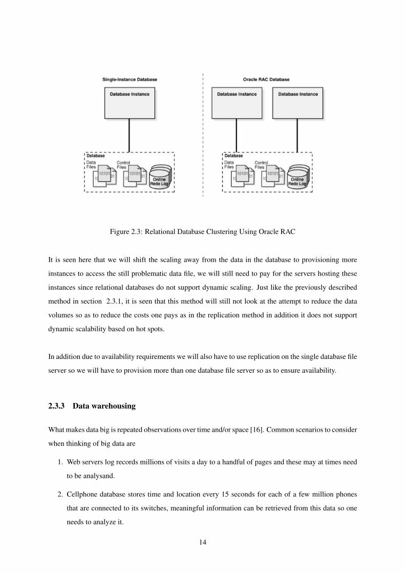
Figure 2.3: Relational Database Clustering Using Oracle RAC

It is seen here that we will shift the scaling away from the data in the database to provisioning more

instances to access the still problematic data file, we will still need to pay for the servers hosting these

instances since relational databases do not support dynamic scaling. Just like the previously described

method in section 2.3.1, it is seen that this method will still not look at the attempt to reduce the data

volumes so as to reduce the costs one pays as in the replication method in addition it does not support

dynamic scalability based on hot spots.

In addition due to availability requirements we will also have to use replication on the single database file

server so we will have to provision more than one database file server so as to ensure availability.

2.3.3 Data warehousing

What makes data big is repeated observations over time and/or space [16]. Common scenarios to consider

when thinking of big data are

1. Web servers log records millions of visits a day to a handful of pages and these may at times need

to be analysand.

2. Cellphone database stores time and location every 15 seconds for each of a few million phones

that are connected to its switches, meaningful information can be retrieved from this data so one

needs to analyze it.

14

3. A retailer has thousands of stores, tens of thousands of products, and millions of customers but

logs billions and billions of individual transactions in a year for which meaningful information can

be retrieved from.

Over time as the data grows manipulating it in a relational database will be more expensive mainly if

analysis of the data involves reading the tables using relational joins, to counteract this most developers

usually migrate their legacy non transactional data to data warehouses where they are usually modeled

in a way that is best suited to handle this expansion in data and are optimized for reads.

The most commonly used data warehousing model is the star schema[18]model that is designed using

the concepts of dimensional modeling, it uses the concepts of facts (measures), and dimensions (context).

Facts are typically (but not always) numeric values that can be aggregated, and dimensions are groups of

hierarchies and descriptors that define the facts.

When applied to the simple database model we can see we can actually build many dimensional ta-

bles to answer or group data then actually group the facts of those groupings in one single fact table with

relevant foreign key references to the relational values in the dimension tables. Basing on the relational

model shown in Figure 2.1, assume a typical question that we want our users of the cloud based applica-

tion to be able to answer is. ”How much did I order and how much did I pay for in a given year ?”. When

we need to answer such a question using a relational database we will usually have to join the customers,

orders and payments tables aggregate the orders and payments and then group each per customer per year.

When we use dimensional modeling we can actually build two tables as below

1. A dimension table holding all the customer details.

2. A fact table holding aggregated values of orders and payments per year 2per customer.

Figure 2.4 shows how we can remodel our database using the star schema and hence achieve a highly

scalable mapping of the relational database. Based on user requirements we can model as many measur-

able dimensions as needed and associate them to a fact in the fact table, the fact table is dynamic so we

can add as many facts as possible and as needed when user requirements change.

Common facts that we can model include total orders, payments and balances such that if for a given

customer we need to view a fact about say their total orders and payments in a given time granularity we

can actually join the dimension table and the fact table as shown in SQL statement below that associates2granularity of data.

15

for a particular customer dimension value all the details of the related orders and payments.

select a.customer_name,b.date,b.orders,b.payments from

customer_dimension_table a, customer_fact_table b

where a.customer_id = b.customer_id

Figure 2.4: Scalable Star Schema Model of Relational Data

According to [18] we can horizontally scale the resultant star schema model using a concept called data

warehouse stripping where by we shard both the fact table and the associated dimensions to different

shard servers and access them as shown in Figure 2.5. Sharding this model is easier than the relational

model because we can actually shard the various tables independently without having to traverse the

relational arcs/joins since all dimension tables have a corresponding foreign key in the fact table.

Application of any sharding technique can be applied to the shard key columns of the dimension and

fact table in parallel, it also supports dynamic scalability based on hot spots on the data where by we can

only shard the dimension and fact records that are currently in high contention and leave those that are

not in high contention alone this will minimize of the volumes we have to pay for.

16

Figure 2.5: Star Schema Stripping and Database Sharding

The main drawback for using data warehousing concepts using models like star schema in cloud databases

is that user requirements as well as business requirements are dynamic as has been seen from experience

by any software engineer. The model does not support dynamic application development notably due

the rigidness in building the dimensions as one will never know the types of dimensions and facts that

will be needed until the cloud based application is running and these dimensions will constantly keep on

changing based on requirements changing.

However from my perspective it is seen that this model could actually be used in cloud computing

provided the dimensions and facts are correctly identified and modeled from the initial stages and remain

static since it supports dynamic scaling of data in parallel over large data sets.

2.4 Scalable Cloud Data Models

Cloud databases achieve scalability because they look at partitioning the volume of data so as to reduce

its volumes and hence allow it to support dynamic scaling using parallelism on portions of the data that

have a high contention. According to [4] there are three main models currently being used to store data by

cloud databases and they all have one common factor they are all non relational denormalized database

models.

From literature review during the research it was seen that all the models in one way or another consist

of a common key attribute and a string representing the actual data that is considered to be the value(s)

17

related to that key using a key→value relationship mapping data model. The data itself is usually some

kind of primitive of the programming language a string, integer, array or a object that is being marshaled

by the programming language’s bindings to the key→value store.

Key→value model relationship mapping models always have a cardinality of 1 key → ∞ values, the

data stored in the values would have usually been stored in related tables if the same data was to be stored

in a relational database hence they eliminate relationships between data tables by storing all related at-

tributes of an entity as embedded columns in a single table.

These databases are dynamically scalable horizontally as they have no relational joins so they can easily

be sharded to shared nothing architectures using parallelism. Table 2.4 summarizes how [4] generalized

the various types of current cloud databases based on how they store their data based on the key→value

relationship mapping model.

Table 2.4: Cloud Database Data Storage Categories

Key-values Documents Extensible Records

Redis SimpleDB Google Bigtable

Scalaris CouchDB HyperTable

Tokyo Tyrant MongoDB Apache Cassandra 3

Voldemort Terrastore HBase

Riak

2.4.1 Key-value Stores

Key value stores allow the application developer to store schema-less data consisting of a string which

represents the key and a pointer to the actual data record(s) related to that key which is considered to

be the value(s), this data is usually a string of variable length and embedded as a single row with the

associated key.

Considering the data model shown in Figure 2.1 in order to store it in a key value database we will

need to first denormalize it and then use the attribute cust reg num to be the key other denormalized

attributes will be stored as the values of that key, Figure 2.6 shows how a typical row will exist in a

18

database that uses such models and it can be noted that for 1 key value we usually have 1→ ∞ related

records in the same table 4 each representing the value associated to a particular observation of that key

as per a single transaction, if we want to shard a record stored in such a data model knowledge of the key

is sufficient to allow us shard it.

Figure 2.6: Key-Value Data Storage Sample Row Content based on ER model shown in Figure 2.1

It is seen that all we need to know is the key attribute value during the sharding process and use our

sharding algorithm and technique using that column since all denormalized records are uniquely identi-

fied by the same key attribute and if we shard based on that key since the previously relationally related

information regarding the orders and payments are now embedded in one bucket we will ensure that all

related information will be sharded with the same correct key and in addition this model can be sharded

in parallel.

This model supports dynamic sharding in parallel based on existence of hot spots on data, assume we

only have a high contention on orders made at a particular date, we can actually shard only records for

that date and not have to worry about data shipping in addition we can run the sharding in parallel for a

set of customers to the shard servers.

2.4.2 Document Stores

A document store is a data model designed for storing document-oriented information using encodings

like XML, JSON or BSON, it allows for a denormalized representation of a database reord to be stored as4Defying the First Normal Rule of Database normalization.

19

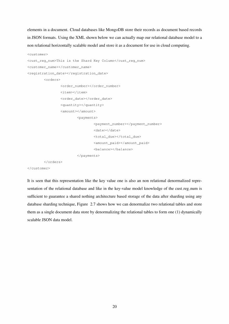
elements in a document. Cloud databases like MongoDB store their records as document based records

in JSON formats. Using the XML shown below we can actually map our relational database model to a

non relational horizontally scalable model and store it as a document for use in cloud computing.

<customer>

<cust_reg_num>This is the Shard Key Column</cust_reg_num>

<customer_name></customer_name>

<registration_date></registration_date>

<orders>

<order_number></order_number>

<item></item>

<order_date></order_date>

<quantity></quantity>

<amount></amount>

<payments>

<payment_number></payment_number>

<date></date>

<total_due></total_due>

<amount_paid></amount_paid>

<balance></balance>

</payments>

</orders>

</customer>

It is seen that this representation like the key value one is also an non relational denormalized repre-

sentation of the relational database and like in the key-value model knowledge of the cust reg num is

sufficient to guarantee a shared nothing architecture based storage of the data after sharding using any

database sharding technique, Figure 2.7 shows how we can denormalize two relational tables and store

them as a single document data store by denormalizing the relational tables to form one (1) dynamically

scalable JSON data model.

20

Figure 2.7: Relational to Document Store Mapping

This model supports dynamic sharding in parallel based on existence of hot spots on data, assume we

only have a high contention on orders made at a particular date, we can actually shard only records for

that date and not have to worry about data shipping in addition we can run the sharding in parallel for a

set of customers to the shard servers.

2.4.3 Extensible Record Stores (Column Family Databases)

Extensible data stores use the concept of column families to store relational data in a denormalized data

model and they are usually referred to as Column family databases, they offer a more column centric

approach to storing data and consequently provide a model that can support a denormalized embedded

model of data [10] .

A column in such databases can be taken as a nested table that can be seen in some RDBMS like or-

acle, the data stored in it is usually all related data of a particular key. Each column will contain a group

of related information for a particular key value, these information in a relational database would have

been stored in other tables but column family databases allow us to store the related information as a

column of a table. Figure 2.8 shows how one can map a relational data model into a simple column

family database by denormalizing the related tables and storing related data as a column family.

21

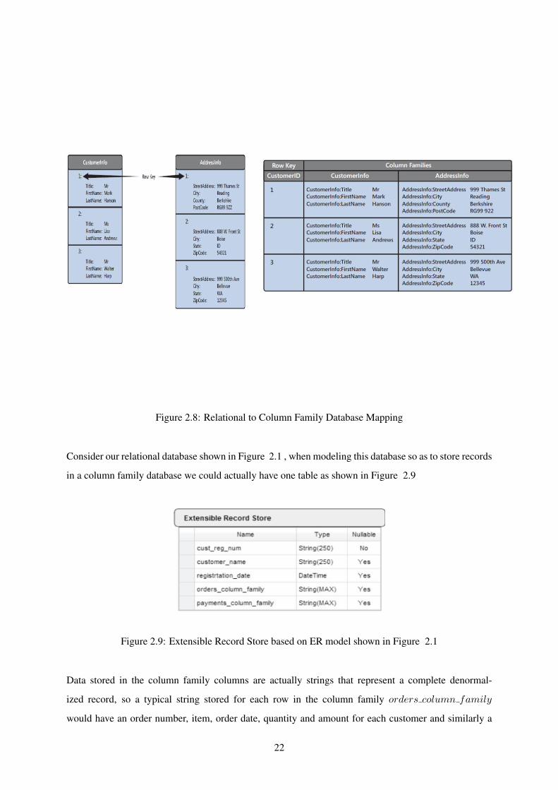
Figure 2.8: Relational to Column Family Database Mapping

Consider our relational database shown in Figure 2.1 , when modeling this database so as to store records

in a column family database we could actually have one table as shown in Figure 2.9

Figure 2.9: Extensible Record Store based on ER model shown in Figure 2.1

Data stored in the column family columns are actually strings that represent a complete denormal-

ized record, so a typical string stored for each row in the column family orders column family

would have an order number, item, order date, quantity and amount for each customer and similarly a

22

payments column family would contain for each associated orders column family order number

a string containing a payment date, amount, payment number and balance due.

Sharding such a database model is seen to be as easy as the previously described models since knowl-

edge of the cust reg num is sufficient to enable a sharding process to run in parallel and ensure that the

resultant shards do not introduce data shipping.

2.4.4 Scaling Key-value, Document and Column Family Databases

The models described in Sections 2.4.1 2.4.2 2.4.3 all support dynamic scaling using parallelism and

are used in cloud computing simply due to the non relational nature they store data, assume that we

have a model of any of the above types that has eventually used a table T to store their data and assume

that Equation 2.1 holds for random subsets ti of the table holding either the key-value pairs, document

representations or column family database records.

t1 ∪ t2 ∪ . . . ∪ tn = T

t1 ∩ t2 ∩ . . . ∩ tn = ∅(2.1)

We can easily see that if a subset ti of the table T is in a hot spot we can actually shard only that part of

the table as opposed to the whole table hence have less volume of data to pay for, also if more than one

subset is in a hot spot the sharding process can be done in parralel since the subsets are not dependent on

each other.

2.5 Related Work

This section will look at previous works that have been undertaken in attempts to provide algorithms for

correct and complete denormalization of relational data to simple key→value non relational dynamically

horizontal scalable models. The works will be analyzed based on available literature so as to see if

they provide a logical well defined algorithm [3] to complete the process in a correct and complete

manner.5.5No Algorithm was found after intense literature review, that is why I decided to propose using the Binary First Search

algorithm to perform the denormalization.

23

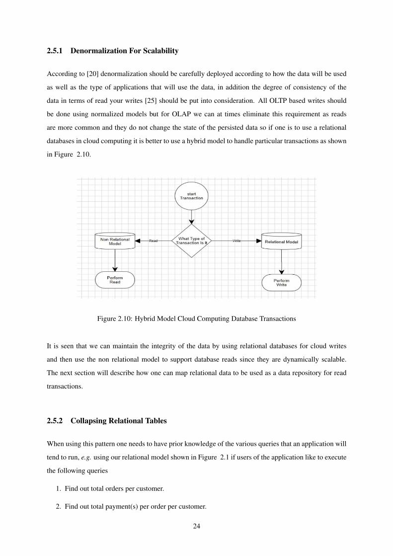
2.5.1 Denormalization For Scalability

According to [20] denormalization should be carefully deployed according to how the data will be used

as well as the type of applications that will use the data, in addition the degree of consistency of the

data in terms of read your writes [25] should be put into consideration. All OLTP based writes should

be done using normalized models but for OLAP we can at times eliminate this requirement as reads

are more common and they do not change the state of the persisted data so if one is to use a relational

databases in cloud computing it is better to use a hybrid model to handle particular transactions as shown

in Figure 2.10.

Figure 2.10: Hybrid Model Cloud Computing Database Transactions

It is seen that we can maintain the integrity of the data by using relational databases for cloud writes

and then use the non relational model to support database reads since they are dynamically scalable.

The next section will describe how one can map relational data to be used as a data repository for read

transactions.

2.5.2 Collapsing Relational Tables

When using this pattern one needs to have prior knowledge of the various queries that an application will

tend to run, e.g. using our relational model shown in Figure 2.1 if users of the application like to execute

the following queries

1. Find out total orders per customer.

2. Find out total payment(s) per order per customer.

24

Using this pattern we can actually create an object like a materialized view where we pre-join the tables

into a denormalized non relational data structure and then use this object as the data source of the cloud

application that users interact with. This object can periodically be refreshed so as to hold a consistent

state of data as of a given time, the structure of our collapse table can be as shown in Table 2.5

Table 2.5: Collapsed Table Representation of Relational Model of Figure 2.1

Column Name Comments

customer reg number Record Key attribute

order number Order Reference Number

order date Date an Order was made

item Item ordered

quantity Quantity of Item ordered

total cost Total Cost of all Items

payment number Payment Reference Number

payment date Payment Date

amount paid Amount

balance due Balance due on total amount

It can see that we now can avoid joins by carefully writing our queries to manipulate data from this now

simple non relational horizontally scalable database by simply aggregating the columns shown in bold

i.e. total cost and amount paid which are all stored in a single table as opposed to the previously stored

data in relational tables as shown in Figure 2.1 when performing reads. In additon since we are storing

the time aspect of the transaction we can query the table based on any level of granuality as desired

yearly, monthly, daily the data model allows us to analyze the data based on whatever desirable cube we

need and is actually more dynamic than the star schema that was described in Section 2.3.3 since all the

data to answer any feasible possible question can be derived from the collapsed table.

The described pattern of collapsing tables is easily performed when our relational database has a small

number of related tables for which their relations are easily derived, however if the database contains a

high number of related tables collapsing them correctly and completely will not be as easy and straight

forward provided we want a correct representation of the underlying relational database.

Consider the Northwind relational database ER model shown in Figure 2.11 you will notice that un-

25

like our simple database it has many related tables and hence when using the described denormalization

pattern the following questions need to be considered when we need to have a complete and correct

denormalized database derived from the relational database.

Figure 2.11: Northwind Relational Database Model

1. Which table(s) should we start the process from or do we randomly pick a table and if we ran-

domly pick a table what effect will it have on process throughput as well as the resultant database

correctness and completeness.

2. Which table(s) should we terminate the process at or do we randomly pick a table and if we

randomly pick a table what effect will it have on process correctness and completeness.

3. How can we know whether we have checked all the tables for related data so as to be guaranteed

of correctness and completeness.

By attempting to answer these questions it was seen that the theoretical approach of collapsing relational

tables does not provide an algorithm that would guarantee each question would be covered provided the

relational database had many relational tables. However it is noted that if we do not put into consideration

the questions above we may have a inconsistent representation of the relational data or spend more time

checking the data for correctness and completeness, so a mapping algorithm that avoids the loopholes of

random collapsing of tables is a justifiable contribution to software engineering.

26

Chapter 3

Methodology

Using the research questions presented in Section 1.7 as a guideline as well as strategy to understand the

cause of the problem it was seen that problems in scaling relational data models was due to normalization

which introduced joins. The methodology used then was to try and understand as well as analyze why

relational models are not easily dynamically scalable using database sharding and why current models

being developed for use in cloud environments avoid the existence of relational joins so as to achieve

scalability using database sharding.

Reviews of peer reviewed journals, literature and publications available was done to understand why

relational data models were not highly scalable in cloud environments as well as why denormalized data

models are highly scalable in cloud environments using database sharding technique in terms of costs,

dynamic scalability and parallelism.

It was easily seen that in order to map a relational data model to a scalable non relational data model

for cloud computing a correct and complete algorithm was required, however after analyzing literature

regarding algorithms for mapping relational to non relational data model no algorithm was identified

so the main deliverable or contribution of this research was going to be an algorithm to map relational

databases to non relational databases so as to allow one use a hybrid model in cloud computing.v

Literature on graph theory was also studied so as to see how we can relate it to relational database

modeling so as to adapt it to use the Binary First Search algorithm for the correct and reliable mapping.

The resultant database model was validated for correctness and completeness by confirming that the

BFS algorithm visited the nodes in a logically correct manner with respect to the model of the relational

database it was supposed to denormalize and in each stage of the algorithm performed the correct col-

27

lapsing of the current table and all the tables that were adjacent to it. The validation of the dynamic

scalability of the model was done by showing that by eliminating joins not only would we improve the

throughput of the process we could store the data in a format that allowed for parallel sharding of the

database dynamically based on existence of hot spots on the database hence have an economical method

to store data based on available billing options in cloud computing.

28

Chapter 4

A Scalable Relational Database Model for Cloud Computing

This section will describe how the Binary First Search algorithm [24] and concepts of directed graphs

theory [24] were used in proposing a relational database model denormalization algorithm that can be

used to map relational data to formats that can be used in cloud computing using the pattern of collapsing

tables described in Section 2.5.1. It will start by describing briefly the concept behind the Binary First

Search algorithm then procede to describing the physical proposed architecture that the algorithm can be

run on and conclude by describing how the we can actually use Binary First Search algorithm to achieve

our objective.

4.1 Binary First Search Algorithm

In graph theory the binary first search (BFS) algorithm is a strategy for searching in a graph when search

is limited to essentially two basic operations [19]:

1. Starting from a root node, visit and inspect a node of a graph.

2. Gain access to visit the nodes that neighbor the currently visited node refereed to as the adjacent

nodes to the node currently being visited.

3. Repeat steps one(1) and two (2) above till we have visited all the reachable nodes in the directed

graph from the perspective of the root node.

The BFS begins at a root node it then inspects all the neighbors of the root before marking the root as

visited, then for each neighbor of the current root node it will mark it as current root and then conse-

quently visit all the neighbors. It explores all nodes in this manner until it finds the goal of executing the

algorithm then it will terminate. The goal can range from many requirements like finding shortest paths

between a root node and all reachable nodes or as in the case of this research ensuring that the relational

29

tables are collapsed in a logically correct manner, it works on the concept of queues an abstract data type

in which only two operations are permitted [24].

1. Enqueue an Element.

This operation will add an element to the queue using a First in ordering method to the end of

the queue.

2. Dequeue an Element.

This operation will remove an element to the queue using a First out ordering method from the

top of the queue.

Figure 4.1 shows how elements are enqueued and dequeued from a queue abstract data type and it can

be seen that the order in which an element was added will determine the order it will be removed.

Figure 4.1: Queue Abstract Data Type

A queue consequently is a First-In-First-Out (FIFO) data structure and this is how nodes are visited when

using the BFS algorithm with respect to the current node, the adjacent nodes are queued and then visited

using the FIFO method.

4.2 Physical Architecture

The algorithm is expected to be executed on a simple architecture, it runs on a server that lies between

the relational database server and the cloud data repository server. Data in the cloud data repository acts

as a data source for export/import to either traditional cloud databases like MongoDB or as a direct data

source for a cloud application.

30

The process initiates by issuing a handshake command between itself and the two databases and as a

fail safe if one of the databases fails to acknowledge it terminates.If both databases acknowledge the

handshake it then performs the mapping from relational to non relational data model, Figure 4.2 shows

the architectural layout as well as brief descriptions of processes that will be executed by each component

of the architecture.

Figure 4.2: Architecture of Mapping System

4.3 Mapping Relational to Non Relational Data

This section will describe the actual mapping process from transforming the relational model to a directed

graph model and then applying the BFS algorithm on it to collapse the tables provided a table is reachable

from a root table.

4.3.1 Mapping ER Models to Directed Graphs

Database developers use the ER model [8] to logically model their relational databases, however the BFS

algorithm is suited for a directed graph model so the first step in the mapping will involve transforming

the ER model to the logically correct directed graph model taking into account properties of directed

graphs.

31

4.3.1.1 Directed Graphs and Adjacency Lists

Graph problems pervade computer science and algorithms for working with them are fundamental to the

computing field [9]. In mathematics a directed graph is a graph, or set of nodes connected by edges,

where the edges have a direction associated with them.

In formal terms, a digraph G is a relation:

G = (V,A) (4.1)

where

1. V are called vertices or nodes.

2. A are called arcs.

Graphs are represented either as a adjacency lists or matrices however the adjacency list is a more pre-

ferred method as it provides a way to represent sparse graphs. An adjacency list is a representation of a

directed graph with n vertices using an array of n lists of vertices where list i contains vertex j if there is

an directed edge originating from vertex i and terminating on vertex j.

Figure 4.3 shows how we can use the definition of an adjacency list on a directed graph to identify

for each node its associated adjacent nodes.

Figure 4.3: Deriving Adjacency List From Directed Graph

In mathematical terms Equation 4.2 shows how one can identify the adjacent list nodes of a particular

node based on the existence of a directed arc between the node u and other nodes v in the graph G.

Adj|Guv| =

1 if their is a directed arc from node u to node v

0 otherwise.(4.2)

32

4.3.1.2 Transforming a Relational ER Model to Directed Graph Mode

Consider the data model shown in Figure 2.1, the nodes of the graph will be the following tables cus-

tomers, orders and payments the non transactional generally look up tables need not be included in the

model as they will rarely be updated during atomic transactions in addition look up tables are usually

very small and can easily be replicated to the various shard server if we need them.

The following heuristic was developed to help in drawing directed arcs between related tables so as

to ensure that the model transformation from ER to directed graph did not in anyway alter the initially

normalized database structure and that it resulted in the correct transformation, it is based entirely on

the redefined existence dependency concept of relational tables introduced in this research as well as

parent/child hierarchal relationship concepts of hierarchal database models [5].

In the scope of this research the concept of existence dependency describes whether a table can exist

without the occurrence of its related table, it was used to map the ER model of a relational database to

a directed graph model based on parent/child hierarchies. Using the existence dependency theory a pro-

vided we have two related tables, the one that can have existing records without the existence of records

in the other is then taken as the parent while the dependent table is taken as the child table, consider our

three (3) tables in the relational model shown in Figure 2.1 the heuristic for for drawing directed arcs

between the various tables is as below.

1. Can a Customer record exist without a Order record? Yes, one can register and not make orders.

2. Can a Customer record exist without a Payment record ? Yes, one can register and not make

payments for orders.

3. Can a Order record exist without a Customer record? No, you can not make an order without

registering.

4. Can a Payment record exist without a Customer record? No, you can not make a payment if you

are not registered.

5. Can a Order record exist without a Payment record? Yes, one can order and not make payments.

6. Can a Payment record exist without a Order record? No, you can not make payments for non

existent orders.

The matrix shown in Equation 4.3 shows the existence dependency matrix of the three (3) tables/nodes

customer (C), orders (O) and payments (P). The table elements are populated using 1 if the cell in the

33

current horizontal row and column can exist without the existence of its corresponding vertical current

row and column cell table, 0 if it is a self existence test i.e. if a table is being tested against its self and

-1 if it can exist without the existence of its corresponding vertical current row and column cell table.

∣∣∣∣∣∣∣∣∣∣∣∣

CanExistWithout C O P

C 0 −1 −1

O 1 0 −1

P 1 1 0

∣∣∣∣∣∣∣∣∣∣∣∣(4.3)

It is then seen that since a customer can exist without both payments and orders it is the root table

similarly since a order can exist without a payment while a payment needs an order it shows that the

order table is the parent of payments table or the payments table is the child of the orders table in

accordance to hierarchal database modeling concepts, the resultant directed graph representation is then

modeled as in Figure 4.4.

Figure 4.4: Directed Graph Mapping of ER Model

4.3.1.3 Transforming a Directed Graph Model to Adjacency List

From the model shown in Figure 4.4 the adjacency list was derived as shown in Table 4.1 using Equation

4.2.

Table 4.1: Adjacent List Representation of Directed Graph Shown in Figure 4.4

Node Neighbor (Adjacent List Element(s))

Customer Order

Order Payment

Payment

It is seen from the adjacency list will allow one logically know which relation should be joined with

another so as to ensure a correct denormalization process when collapsing the tables, it also allows us to

34

answer questions that were proposed in Section 2.5.2 regarding which nodes to join to which ones to

ensure correctness of the mapped data.

4.3.1.4 Leveling of Directed Graph

The BFS algorithm uses the concept of node levels, it will always need a root node to initiate from as

well as a set of leaf node(s) to terminate on consequently the nodes have to be labelled as a root and leaf

to provide a start and stop point for the algorithm, the following heuristics was used when identifying the

root node and leaf node(s) so as to provide a start and stop node for the algorithm, it is based on concepts

of directed graphs.

The in-degree of a node in a graph is equal to the number of directed navigational arcs that terminate

on it while its out-degree is the number of directed navigational arcs that originate from it. Consider the

directed graph shown in Figure 4.5 made up of six (6) nodes (1,2,3,4,5,6) Table 4.2shows for each node

based on definition the corresponding in and out degrees.

Figure 4.5: Directed Graph To Level

Table 4.2: In and Out Degrees of Directed Graph Shown in Figure 4.5

Node In-degree Out-degree

1 0 2

2 1 1

3 1 1

4 2 1

5 1 1

6 1 0

35

The following conclusions can be made regarding the root and leaf node(s) of the directed graph shown

in Figure 4.5.

1. The root node is the one with in degree equal zero, it is taken as the root since it is not a successor

of any node.

2. The leaf node(s) is any node that has it out degree equal zero, it is taken as a leaf since no arcs

originate from it consequently it has no successor node(s) and neither is it a predecessor of any

node.

Table 4.3 shows how we applied the heuristic to level the nodes of the directed graph shown in Figure

4.4.

Table 4.3: In and Out Degrees of Directed Graph Shown in Figure 4.3

Node In-degree Out-degree

Customer 0 1

Order 1 1

Payment 1 0

Consequently it can easily be seen that the root relation is the customers relation as its in degree is zero

(0) and the payments the leaf relation as its out degree is zero (0) , any node not in this set will need to

be placed in an appropriate level as will be described in the next section.

4.3.1.5 Heuristic for labeling non root or leaf nodes

It has been shown that by using in and out degrees of the various nodes of the directed graph represen-

tation of the relational database we were able to identify the root and all leaf node(s), however we need

to label all other nodes according to their appropriate levels since the application of the BFS algorithm

works on levels.

This research devised a simplified heuristic to label the nodes with respect to the root nodes provided the

node was not a leaf node and was reachable from the root node called the Transitive Graph Leveling

Heuristic For Directed Graphs and is described below.

36

1. For all nodes that are directly connected to the root node level them as one (1) since the number

of nodes between it and the root is zero (0). This deviates from the traditional labeling techniques

that requires each node to be uniquely labeled [12] but the rationale for this will be described later.

2. For all nodes that are transitively related to the root their levels are got by adding to one (1) to

the number of nodes that transitively connected it to the root node. Equation 4.4 shows how

mathematically we can apply a formula to use during the heuristic for i nodes.

Level(Nodei) = 1 + Number of Nodes Between it and the Root Node (4.4)

Consider the graph shown in Figure 4.6 if we are to apply Equation 4.4 to it we can see we can label

the nodes as required by the BFS algorithm in the scope of this research.

Figure 4.6: Directed Graph To Demonstrate Graph Levelling

Applying the heuristic to it we would see that since the root node is A and the leaf node F we only need

to label nodes B, D, C and E.

Table 4.4: Graph Levels For Directed Graph in Figure 4.6

Node Number Nodes Transitively Relating it to Root Level

B 0 1

C 1 2

D 1 2

E 2 3

Applying the heuristic to the graph shown in Figure 4.4 it can be seen that the levelling would be simple

since there are only three tables where two are the root and the leaf leaving the orders table to be at level

1, however an evident application for this heuristic will be visible when leveling graphs as those shown

in Figure 2.11.

37

4.3.1.6 Parallelism of BFS

In a relational database a 1 . . .∞ cardinality refers to scenarios where one (1) table is related to more than

one (1) table usually on different foreign key attributes. It was seen that if we could enable parallelism

when such cardinalities existed in the directed model we would gain improvements in process costs as

predicted by [15].

When a a 1 . . .∞ cardinality exists it is suggested we store it in the adjacency list as a separate record

as opposed to a collection of adjacent nodes to a particular node. To achieve parallelism when executing

the BFS we would then execute it on all nodes that have the same level from the current node being

inspected i.e. for each adjacent node to the current node we would execute the BFS in parallel. Consider

the directed graph shown in Figure 4.7

Figure 4.7: Parallelism of BFS Algorithm

It is seen that a 1 . . .∞ cardinality exists for node 1 between it and nodes 2 and 3 usually one would

create an adjacency list as shown in Table 4.5.

Table 4.5: Adjacent List Representation of Directed Graph Shown in Figure 4.7

Node Level Adjacent Node

1 2,3

2 4

3 4

4 5

5 6

4

38

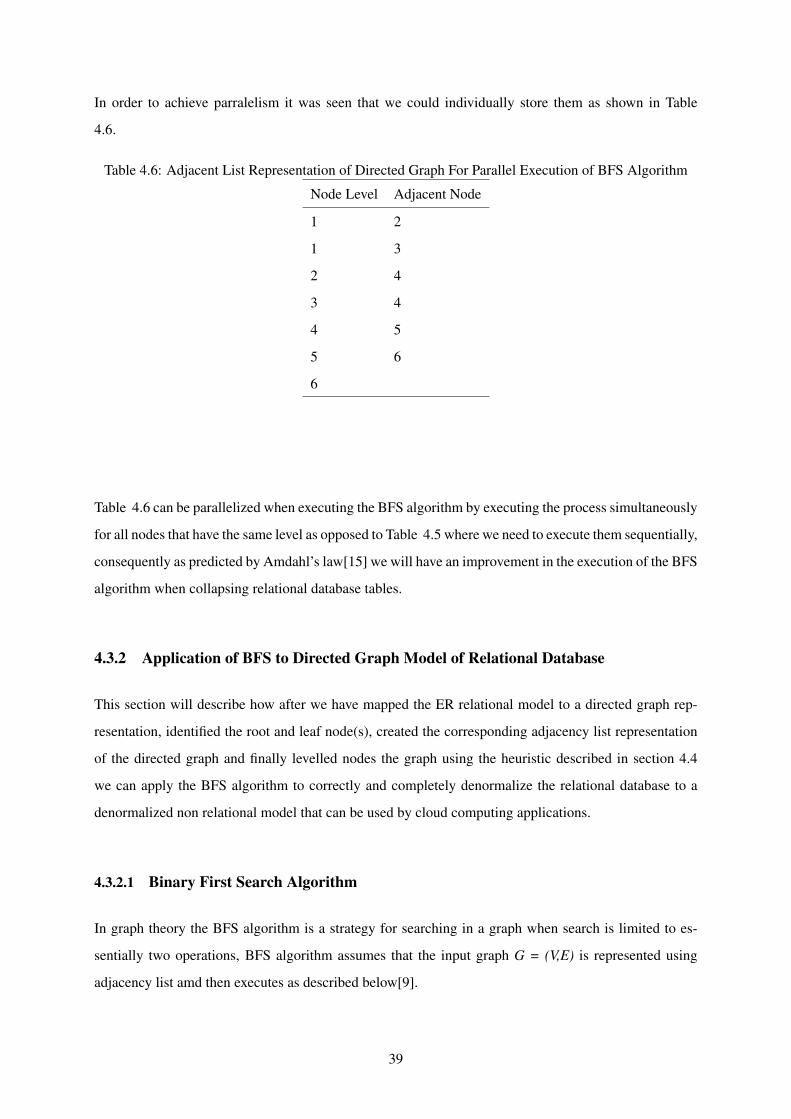
In order to achieve parralelism it was seen that we could individually store them as shown in Table

4.6.

Table 4.6: Adjacent List Representation of Directed Graph For Parallel Execution of BFS Algorithm

Node Level Adjacent Node

1 2

1 3

2 4

3 4

4 5

5 6

6

Table 4.6 can be parallelized when executing the BFS algorithm by executing the process simultaneously

for all nodes that have the same level as opposed to Table 4.5 where we need to execute them sequentially,

consequently as predicted by Amdahl’s law[15] we will have an improvement in the execution of the BFS

algorithm when collapsing relational database tables.

4.3.2 Application of BFS to Directed Graph Model of Relational Database

This section will describe how after we have mapped the ER relational model to a directed graph rep-

resentation, identified the root and leaf node(s), created the corresponding adjacency list representation

of the directed graph and finally levelled nodes the graph using the heuristic described in section 4.4

we can apply the BFS algorithm to correctly and completely denormalize the relational database to a

denormalized non relational model that can be used by cloud computing applications.

4.3.2.1 Binary First Search Algorithm

In graph theory the BFS algorithm is a strategy for searching in a graph when search is limited to es-

sentially two operations, BFS algorithm assumes that the input graph G = (V,E) is represented using

adjacency list amd then executes as described below[9].

39

begin

for u ∈ V do

u.color =WHITE

u.d = 1

u.d =∞

u.π = NIL

s.color = GRAY

s.d = 0

s.π = NIL

Q =

ENQUEUE(Q, s)

while Q 6= ∅

for v ∈ G.Adj[u]

do if v.color ==WHITE

v.color = GRAY

v.d = u.d+ 1

v.π = u

ENQUEUE(Q, v)

end

end

end

u.color = BLACK

end

The proof of the correctness and completeness is not in the scope of this research but can be found in [9]

and so will not be provided however it is evident that it always needs a root node to initiate the process as

well as a leaf node or set of leaf nodes to terminate hence its completeness property. In addition it needs

an adjacency list to guide it to the nodes it should visit based on the node it is currently inspecting hence

its correctness property. Based on the fact that the BFS visits the nodes from a single node in a correct

manner by inspecting the elements that are adjacent to it and it repeats the same process till it terminates

it can be seen that one can easily apply it when collapsing relational database tables to a non relational

database model.

40

4.3.2.2 Binary First Search Algorithm and Relational Database Denormalization

From the previously described concepts regarding the directed graph model shown in Figure 4.4 we will

assume the following.

1. The root node is the customers table C.

2. The leaf node is the the payments table P.

3. The table orders is a non root or leaf node and is levelled 1 and denoted as O.

4. The adjacency list is as in Table 4.7.

Table 4.7: Modified Adjacent List Representation of Directed Graph Shown in Figure 4.4

Level Node Adjacent List Element(s)

r Customer Order

1 Order Payment

t Payment

If we apply the BFS algorithm on the modified adjacency list representation of the directed graph shown

in Table 4.7 we will have it execute as described below. Read the adjacency list and identify the entry

labeled r this is the root start from there by placing it in the queue. At this stage we will have the node C

as the current node and the only node in the queue, for this node we read the adjacency list for all nodes

that are adjacent to it and enqueue them then for each adjacent node we will collapse it with the node C

to create partially denormalized nodes C.(Node), in this case we only have one node so at the completion

of this stage we will have a collapsed table represented by joining nodes C.O.

Once the adjacent nodes of C have all been visited we color it GRAY and dequeue it, we then read

the queue for the next item to process which will logically be the node at the head of the queue in this

case node O, we will then read all the nodes adjacent to it enqueue them and collapse them. At the end

of this stage since we have only one adjacent node we will end up with a collapsed table O.P, we then

color the node O GRAY and will now have only one element in the queue P.

Since the node P is the leaf node and it has no adjacent nodes we can then dequeue it and terminate

the process since the queue is now empty, at this stage we have two partially collapsed tables C.O and

41

O.P related by a common functionally dependent set of attributes we can now collapse them using this

set of attributes and end up with a fully collapsed representation of the complete relational database

C.O.P.

4.3.2.3 Prototyping

A practical prototype of the application of the algorithm was done using Perl and an Oracle database

to see if provided the adjacency list input to the algorithm the resultant mapping was correct and com-

plete, initially the Perl script will compose a graphical representation of the ER database that it needs

to denormalize based on the adjacency list input. The output of this stage should represent the correct

model if the graphical model does not match the initial model then the adjacency list was not correctly

created. One should always endeavour to correctly create the adjacency list as this is the basis on which

the correctness and completeness of the algorithm will be determined from, if wrongly created then the

results will not be correct and the BFS algorithm may fail to complete and if it completes it may create a

hazard[21] and consequently not actually reflect the actual logical representation of the underlying rela-

tional database it is supposed to denormalize.

The output of executing the script is shown below based on the adjacency list input it was provided and

shown in Table 4.7, Figure 4.8 shows the screen shot process execution steps when it was prototyped

using Perl running off an Oracle database on a Windows system.

Figure 4.8: Execution Flow of Prototype

42

4.4 Interpretation of Results

This section will provide an interpretation of the results of the questions that were used as the guidelines

during the course of the research as poised in Section 1.7, it will for each question show how the answers

were derived providing justification as well as validations as needed.

1. What are the mandatory characteristics of scalable databases in the cloud?

(a) Dynamic scale based on hot spots and high data contention on a subset of the data.

Databases in the cloud must be able to scale in a dynamic nature, usually one does not have

to scale the whole database just the areas where their is a high contention of data refereed to

as hot spots need to be scaled so as to gracefully handle the data contention effect on perfor-

mance. If we have a small subset of the data currently residing in a hot spot in order to ensure

that we do not incur extra costs in the cloud for storing redundant data we should ensure that

the database only shards the data in the subset that is currently in high contention.

(b) Ability to run in parallel the sharding process.

Amdahl’s argument [15] proves that in order to improve the throughput of a process one

should always run it in parallel, consequently if we want to scale a database in the cloud with

a good throughput we need to ensure that we can shard it with a 100% parallel method.

2. Why are relational data models complex to horizontally scale using sharding?

From this research it was seen that the simplest approach that could be used to shard a relational

database would be to use a nested loop join algorithm. The nested loop join algorithm uses one join

input as the outer input table and one as the inner input table, the outer loop consumes the inner

input table row by row searching for related records and the algorithm will terminate once all rows

in the outer loop have been checked for matching related records in the inner loop. The algorithm

can be as shown below when we are joining two tables R and S on a relational key attribute ri and

sj usually refereed to as a primary and foreign key relationship [11].

begin

for r ∈ R do

for s ∈ S do

do if ri = sj

43

shard < r, s >

end

end

end

end

If the table R has n records and the table S has m records, Equation 4.5 shows how many times the

loop will be run during the sharding process.

cost = |n||m| (4.5)

It is seen that in the cloud where we have big data, when using such a algorithm to shard the data

the costs will increase as the volumes of the data increase.

The algorithm also depends on the number of tables that need to be joined, assume we have k

related tables in the relational database and assume that the relational model is a simple one as

shown in Figure 4.9

Figure 4.9: Simple Relational Model and Nested Loop Join Algorithm

The total cost C will be given by Equation 4.6 since for each pair of related tables |Tablek.Tablek−1|

where (k=1,2,3, . . .,k) we will need to execute Equation 4.5.

C =k−1∑k=1

|Tablek.Tablek+1| (4.6)

Nested loop join algorithms for sharding relational databases to shared nothing architectures in

cloud computing will not be good due to the large volumes of data as well as the number of related

44

tables as they affect overall cost of completing the sharding process as compared to a non relational

model where the overhead of executing joins is eliminated.

Existence dependence due to transitive dependencies between the various nodes will also prevent

dynamic scaling of tables that are holding data that have a high contention provided we do not want

the shards to experience data shipping, consider Figure 4.10 where we have three relational tables

related on the basis of referential integrity, transitive dependencies and existence independence.

Figure 4.10: Dynamic Scaling of Relational Databases

The following conclusions can be derived from the model.

(a) Tables A and C are transitively related through Table B i.e. one can not join them directly as

they do not contain a common attribute relating them.

(b) Table B has an existence dependence on Table A i.e. a record in Table B can not exist minus

a record in Table A. In database terminology Table A is the parent of Table B.

(c) Table C has an existence dependence on Table B i.e. a record in Table C can not exist minus

a record in Table B. In database terminology Table B is the parent of Table C.

(d) Tables B and C have an existence dependence on Table A i.e. records that are not in Table A

can never have related data in either Tables B or C.

45

If user transactions are causing a high contention on table C their is no way we can only shard

table C and leave tables A and B because by doing so we will not have a shared nothing based

architecture after the sharding process and will consequently introduce data shipping between the

various shards of table C and tables A and B as shown in Figure 4.11.

Figure 4.11: Dynamic Scaling of Relational Databases and Data Shipping

Failure between the connections between any of the shards of Table C and Table B will render

that shard unavailable, however if Table B for some reason fails then the overall database will be

rendered unavailable because the transitively dependent shards will no longer be related to table

A and in terms of existence dependence, ACID properties and CAP theorem we no longer have a

consistent database and to avoid corrupting the data we turn it off till table B is restored.

Data dependency in computer science is a situation in which a statement refers to the data of a

preceding statement, in terms of a relational database this can be redefined to imply existence de-

pendencies between records of tables in a relational database. Data dependencies affect parallelism

if dependent data that exhibit some sort of dependency transitively are attempted to be parallelized

we may end up with a situation called a hazard [21] which can potentially lead to incorrect com-

putation results. Consider Figure 4.10 it is seen that though Tables A and B are directly dependent

on each other based on their primary and foreign key relationships and hence can be parallelized

when sharding, Table C is transitively related to Table A and we can not parallelize sharding it

with the others, the only option if we want to avoid existence of harzards is to first complete shard-

ing of Table B then we can initiate sharding of Table C consequently it can be seen that transitive

dependencies as well as existence dependence affects the ability to parallelize the sharding process

46

of relational databases.

One can argue that we can run in parallel the related tables the sharding process as shown in

Figure 4.12

Figure 4.12: Parallel Sharding of Relational Databases

However this is not how it can be done because we can not initiate the sharding of Table C without

knowing which record in Table A it is related to so the only feasible way when one wants to avoid

data harzards we need to first shard Tables A and B hence their is no way we can paralleize the

process.

3. What are the current data models being used to build scalable databases in the cloud?

From research it was concluded that all current cloud database models denormalize their data

to allow for horizontal scaling using sharding due to the reduction in cost when executing the

sharding process on such a model as well as to allow for dynamic scalability using parallelism.

The aim of denormalizing their data is to reduce the number of relational tables as well as store it

in a data model that can be sharded in parallel or based on current data hot spots.

Simple key-value data models are used where by all data is denormalized and a common key

is used to uniquely identify each record such a model can be sharded on demand based on current

needs like existence of hot spots on the data and can also be executed in parallel.

When modelled as a denormalized non relational data structure we will not have to execute the

47

expensive nested loop join algorithm that has a cost as shown in Equation 4.6 one can merely

based on the sharding technique being used run in parallel the sharding process, using such a

model the cost based on number of loops to execute of this algorithm given that the table R has

n records will be zero (0) and since existence dependence does not exist in such a model we can

actually improve this cost by running in parallel the process which according to [15] will further

improve the cost to Equation 4.7.

Cost =MAX|n1, n2 . . . nk| (4.7)

Where k is the total number of sharding processes that we can run in parallel based on the tech-

nique being used.

Since all their data are stored in non relational formats there will not exist any data dependen-

cies between the table and any other object so we can actually perform dynamic scaling based on

existence of hot spots on the data and this dynamic sharding can be done in parallel. Denormal-

ized databases are currently being used in cloud computing and the main reason as deduced from

this research is that since their eliminate the existence of relational modeling which consequently

eliminates joins as they exhibit a data model that allows for both dynamic scaling and parallelism

of the scaling process.

4. What validation can we provide that the denormalized non relational model is more scalable

than the relational model when using sharding?

The validation that can be drawn from this research regarding the scalability of non relational

models over relational models using sharding techniques are:

(a) Non relational models allow for dynamic sharding based on the current need in terms of

data contention, this is impossible in relational databases because according to CAP theorem

[14] as well as ACID properties of relational databases if we shard only a subset of the rela-

tional tables we will introduce data shipping between this subset of sharded data and the non

sharded data and this may lead to loss of availability in event of failure between the connec-

tions of the shards and non sharded data.

The only efficient way to shard a database so as to avoid loss of consistency of data in event

of failure of one or more shards is to ensure that we shard the data to a shared nothing based

architecture and if we are to achieve this for relational databases we will have to execute

the expensive nested loop join algorithm described in this dissertation usually over a large

48

data set with many relational tables as opposed to the same process when the database is non

relational.

(b) Non relational models allow for parallelism during sharding since their is usually only one

table with each record having common attribute(s) uniquely identifying it we can apply our

sharding algorithm using any technique on these attributes/shard keys and run them in paral-

lel, in relational models since there exists a lot of transitive dependencies between the various

tables as well as the concept of existence dependency of the data we can not parallelize tran-

sitively related tables because doing so will lead to data hazards in the sharded databases.

This dissertation has shown that a non relational database is more scalable than a relational database,

however it has also shown that if one is to carefully map a relational database for cloud computing

writes should be done on the relational model and the usually high data contention reads be done

off non relational databases consequently the database will run in a hybrid mode based on the

transaction being performed.

49

Chapter 5

Conclusions and Recommendations

5.1 Conclusions

The main objective of this research was to provide a cost effective correct and complete algorithm that

could be used to denormalize a relational database which would consequently transform it to a horizon-

tally scalable embedded data structure so that it could be used by cloud applications.

In this thesis the contributions that were made can be concluded as.

1. Adoption of BFS algorithm to denormalize a relational database.

The BFS algorithm was shown to be able to correctly and completely denormalize a relational

database. However this algorithm will work correctly if the adjacency list of the directed graph

representation of the relational model is correctly done.

2. Introduction of a graph labeling heuristic.

In order to run correctly and completely it was seen that all the nodes had to be labeled correctly

based on the level it was from the root node. This research presented a heuristic that can be used

to achieve this goal so as to ensure that the adjacency list input to the process was correct.

3. Prototyping of the algorithm to confirm its correctness and completeness.

A prototype that implements the BFS algorithm was designed and from the results it is seen that for

every input relational database adjacency list mapping the process run correctly and completely.

50

5.2 Recommendations

The following recommendations are to be considered.

1. Use the data model of the relational database to generate the mapped directed graph model. There

are many reverse engineering tools that can easily generate an ER diagram of a relational database

Toad Modeler being one of them.

2. Always respect the levels of nodes, if a node is placed on a level where it is not supposed to be the

results may be unpredictable or the cost of execution maybe higher as opposed to if it was placed

in correct level.

3. In the tested version the attribute names are the actual attributes that have been stored in their

respective relations so always build the attribute list based on actual attributes of the various re-

lations, the implementation will fail if the attribute name is not an actual attribute of a particular

relation.

4. Always ensure that writes are executed off the relational database as it offers guarantees of data cor-

rectness, integrity and reliability while eliminating possibilities of insert, delete or update anoma-

lies and hence GIGO data.

5.3 Future Work

Implementation of a working module that can be used in a scripting language like Perl is what am

currently working on so as to allow for an automated process that can be integrated in Perl scripting

language so as to allow one easily use a hybrid relational and non relational database model in cloud

computing based on the transaction being performed.

51

Bibliography

[1] W. W. ARMSTRONG, Dependency structures of data base relationships, in Dependency Structures

of Data Base Relationships, 1974.

[2] J. L. BECKMANN, A. HALVERSON, R. KRISHNAMURTHY, AND J. F. NAUGHTON, Extending

rdbmss to support sparse datasets using an interpreted attribute storage format, in Extending

RDBMSs To Support Sparse Datasets Using An Interpreted Attribute Storage Format, 2006.

[3] M. BURGIN, Languages, algorithms, procedures, calculi, and metalogic, Department of Mathe-

matics University of California, Los Angeles, (2007).

[4] R. CATTELL, Scalable sql and nosql data stores, SIGMOD Rec., (2011), pp. 12–27.

[5] J. CELKO, Joe Celko’s Trees and Hierarchies in SQL for Smarties, (The Morgan Kaufmann Series

in Data Management Systems), Morgan Kaufmann, 2004.

[6] F. CHANG, J. DEAN, S. GHEMAWAT, W. C. HSIEH, D. A. WALLACH, M. BURROWS, T. CHAN-

DRA, A. FIKES, AND R. E. GRUBER, Bigtable: A distributed storage system for structured data,

2006.

[7] S. CHAUDHURI, An overview of query optimization in relational systems, in Proceedings of the

17th ACM Symposium on Principles of Database Systems (PODS’98), 1998, pp. 34–43.

[8] P. P.-S. CHEN, The entity-relationship model toward a unified view of data, ACM Trans. Database

Syst., (1976), pp. 9–36.

[9] T. H. CORMEN, C. E. LEISERSON, R. L. RIVEST, AND C. STEIN, Introduction to Algorithms,

The MIT Press, 2 ed., 2001.

[10] O. CUR, M. LAMOLLE, AND C. L. DUC, Ontology based data integration over document and

column family oriented nosql., CoRR, (2013).

[11] D. J. DEWITT, J. F. NAUGHTON, AND J. BURGER, Nested loops revisited, in In Proceedings of

the Symposium on Parallel and Distributed Information Systems, 1993, pp. 216–226.

52

[12] J. A. GALLIAN, A dynamic survey of graph labeling, The Electronic Journal of Combinatorics, 6

(2000).

[13] A. GARCIA-SILVA, J.-H. KANG, K. LERMAN, AND O. CORCHO, Characterising emergent se-

mantics in twitter lists, in Proceedings of Extended Semantic Web Conference, 2012.

[14] S. GILBERT AND N. LYNCH, Brewer’s Conjecture and the feasibility of consistent available

partition-tolerant web services, in Brewer’s Conjecture and the Feasibility of Consistent Available

Partition-Tolerant Web Services, 2002.

[15] M. D. HILL AND M. R. MARTY, Amdahls law in the multicore era, IEEE COMPUTER, (2008).

[16] A. JACOBS, The pathologies of big data, Commun. ACM, (2009), pp. 36–44.

[17] D. JIANG, A. K. H. TUNG, AND G. CHEN, Map-join-reduce: Toward scalable and efficient

data analysis on large clusters, IEEE Transactions on Knowledge and Data Engineering, (2011),

pp. 1299–1311.

[18] R. KIMBALL AND M. ROSS, The Data Warehouse Toolkit: The Complete Guide to Dimensional

Modeling, John Wiley & Sons, Inc., 2002.

[19] M. KURANT, A. MARKOPOULOU, AND P. THIRAN, On the bias of bfs, CoRR, (2010).

[20] S. S. LIGHTSTONE, T. J. TEOREY, AND T. NADEAU, Physical Database Design: The Database

Professional’s Guide to Exploiting Indexes, Views, Storage, and More, Morgan Kaufmann Publish-

ers Inc., San Francisco, CA, USA, 2007.

[21] D. A. PATTERSON AND J. L. HENNESSY, Computer Organization and Design, Fourth Edition,

Fourth Edition: The Hardware/Software Interface (The Morgan Kaufmann Series in Computer

Architecture and Design), 2008.

[22] D. PRITCHETT, Base: An acid alternative, Queue, (2008), pp. 48–55.

[23] A. RAKESH, A. AILAMAKI, P. A. BERNSTEIN, E. A. BREWER, M. J. CAREY, S. CHAUDHURI,

A. DOAN, D. FLORESCU, M. J. FRANKLIN, H. GARCIA-MOLINA, J. GEHRKE, L. GRUEN-

WALD, L. M. HAAS, A. Y. HALEVY, J. M. HELLERSTEIN, Y. E. IOANNIDIS, H. F. KORTH,

D. KOSSMANN, S. MADDEN, R. MAGOULAS, B. C. OOI, T. O’REILLY, R. RAMAKRISHNAN,

S. SARAWAGI, M. STONEBRAKER, A. S. SZALAY, AND G. WEIKUM, The claremont report on

database research, SIGMOD Rec.

[24] R. SEDGEWICK AND K. WAYNE, Algorithms, 4th Edition, Addison-Wesley, 2011.

[25] W. VOGELS, Eventually consistent, Commun. ACM, (2009), pp. 40–44.

53