A relational database approach to a linear programming-based decision support system for production...

www.elsevier.com/locate/dsw

Decision Support Systems 40 (2005) 183–196

A relational database approach to a linear programming-based

decision support system for production planning in

secondary wood product manufacturing

Ross R. Farrella,*, Thomas C. Manessb

aWoodFlow Systems Corp., Burnaby, BC, Canada V5A 1R2bFaculty of Forestry, University of British Columbia, 2424 Main Mall, Vancouver, BC, Canada V6T 1Z4

Received 5 September 2003; received in revised form 5 September 2003; accepted 3 February 2004

Available online 30 April 2004

Abstract

Secondary manufacturers in the forest products industry face a complex production planning process. Linear programming

(LP)-based applications have addressed this production planning issue. However, most models have been developed for a

specific plant configuration and cannot readily be applied to others. A relational database approach was used to create an

integrated linear programming-based decision support system that can be used to analyze production planning issues in a wide

variety of secondary wood product manufacturers. The flexibility of the resultant system indicated the potential to analyze

production strategies in the highly dynamic environment characteristic of secondary manufacturers.

D 2004 Elsevier B.V. All rights reserved.

Keywords: Decision support system; Linear programming; Flexibility; Relational database; Production planning; Secondary wood product

manufacturing

1. Introduction turing sector has resulted in fewer but larger more

The expansion of the secondary manufacturing

industry is a common interest for the major timber

producing, importing and exporting regions of the

world [19]. Governments recognize the potential of

the secondary industry to stimulate economic devel-

opment through job creation and economic diversifi-

cation in forest dependent economies [6,20,21].

Furthermore, rationalization in the primary manufac-

0167-9236/$ - see front matter D 2004 Elsevier B.V. All rights reserved.

doi:10.1016/j.dss.2004.02.001

* Corresponding author. Tel.: +1-604 822-86-39; fax: +1-604-

822-91-04.

E-mail addresses: [email protected] (R.R. Farrell),

[email protected] (T.C. Maness).

efficient sawmills in the ECE region (Europe, North

America and the CIS) [19]. This has resulted in

downward pressure on employment in the primary

manufacturing industry and may exacerbate the need

for increased activity in the secondary industry to

support these economies.

Secondary manufacturers are typified by a wide

variety of raw materials, manufacturing processes and

potential products. Consequently, the production plan-

ning process can be highly complex. This complexity

is further increased by the dynamic nature of the

market environment [16].

A limited number of linear programming (LP)-

based applications have addressed this complex

R.R. Farrell, T.C. Maness / Decision Support Systems 40 (2005) 183–196184

production planning issue in secondary manufactur-

ing. However, most models have been developed for

a specific application domain and cannot readily be

applied to others [2,3,5,12,15]. This may help ex-

plain an observation made by Carino and Willis [4]

regarding the lack of optimization modeling appli-

cations in small and medium forest products com-

panies. Srinivasan and Sundaram [18], and Muhanna

and Pick [11] convey the importance of flexible

approaches to model design, in order to broaden the

scope of potential applications. Furthermore, Olh-

ager and Rapp [14] suggest that specific operations

research applications may have a short life span due

to the highly dynamic nature of the manufacturing

environment.

The research objective was thus to develop a generic

linear programming-based modeling application that

will provide a flexible DSS for production planning in a

wide variety of secondary manufacturing plants. The

DSS was implemented and validated in a secondary

manufacturing operation in British Columbia, Canada

and is currently being used for production planning

purposes at this operation. This paper presents the

architecture of the resultant DSS and the mathematical

formulation to the underlying LP.

Examples of generic operations research models

that incorporate a high degree of application flexibility

can be found in a variety of manufacturing environ-

ments. Metaxiotis et al. [10] present an object oriented

approach to an advanced DSS that is integrated with a

Management Information System. The software pack-

age was integrated with a management information

system in a customized industrial environment in

Greece, and uses dynamic simulation techniques to

provide production planning and scheduling on a

daily basis. Fourer [7] implemented a generic linear

programming model via a database system for pro-

duction planning in the American steel industry. The

design of the database is closely related to the struc-

ture of the mathematical formulation. Gazmuri and

Arrate [8] discuss the development of a system to

build optimization models for a variety of applica-

tions. They employed a number of software tools from

a prototype of a modeling system, and implement a

general production-planning model in an appliance

manufacturer in Chile.

Zhang [22] provides the only example found by the

authors in the secondary manufacturing sector of the

forest products industry by developing a multi-period

model for furniture manufacturing. Flexibility is pro-

vided by viewing the manufacturing operation as a

number of processing stages that possess generic

attributes, rather than focusing on the specific attrib-

utes of each. The model incorporates a user interface

programmed in Fortran that generates the linear

programming model from user inputs and creates an

optimal solution report.

The work presented in this research is similar to

that carried out by Zhang in that the manufacturing

process is considered in general terms. However, a

relational database approach is employed to utilize the

data management and manipulation capability offered

by modern database systems [9,13].

2. DSS structure

The architecture of the DSS is shown in Fig. 1.

The foundation of the DSS is the database manage-

ment software, Microsoft (MS) Access. The rationale

for this was based on the popularity of MS Office

that includes Access as a standard component. The

MS Access components are linked to the LP opti-

mizer (XA) by an external program named XAEZ.

XAEZ instantiates and transfers the model from the

database to the optimizer for solving. XAEZ is also

responsible for transferring the LP results back to the

database. The external programs are shaded grey in

Fig. 1. Each component of the DSS is described in

the following sections.

2.1. Relational database

The relational database is responsible for storing and

managing all model data. The design of the relational

database adheres to the principles of normalization [17]

focusing on data handling efficiency and flexibility.

This contrasts with the work carried out by Fourer [7]

who designs a database system that is directly related to

the structure of the mathematical model (in terms of

variables, constraints and coefficients).

Our database design relates both to the data re-

quired to build the LP and the way in which we define

the structure of a secondary manufacturing plant. Any

plant may be represented as a system of machine

centers, with linkages that facilitate the transfer of

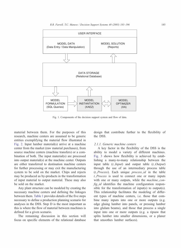
Fig. 1. Components of the decision support system and flow of data.

R.R. Farrell, T.C. Maness / Decision Support Systems 40 (2005) 183–196 185

material between them. For the purposes of this

research, machine centers are assumed to be generic

entities exemplifying the material flow illustrated in

Fig. 2. Input lumber material(s) arrive at a machine

center from the market (raw material purchases), from

source machine centers (machine transfers) or a com-

bination of both. The input material(s) are processed

into output material(s) at the machine center. Outputs

are either transferred to destination machine centers

for further processing or may exit the manufacturing

system to be sold on the market. Chips and rejects

may be produced as by-products in the transformation

of input material to output material. These may also

be sold on the market.

Any plant structure can be modeled by creating the

necessary machine centers and defining the linkages

between them. Table 1 provides details of the five steps

necessary to define a production planning scenario for

analyses in the DSS. Step D is the most important as

this is where the flow of material between machines is

defined for a given scenario.

The remaining discussion in this section will

focus on specific elements of the relational database

design that contribute further to the flexibility of

the DSS.

2.1.1. Generic machine centers

A key factor in the flexibility of the DSS is the

ability to model a variety of different machines.

Fig. 3 shows how flexibility is achieved by estab-

lishing a many-to-many relationship between the

input table (t_Input) and output table (t_Output)

through the use of an intermediary process table

(t_Process). Each unique process_id in the table

t_Process is used to connect one or many inputs

with one or many outputs, while the machine_con-

fig_id identifies the machine configuration respon-

sible for the transformation of input(s) to output(s).

This relationship facilitates the modeling of differ-

ent types of machine centers, i.e. those that com-

bine many inputs into one or more outputs (e.g.

edge gluing lumber into panels, or pressing lumber

into glulam beams), and those that process a single

input into one or more outputs (e.g. a ripsaw that

splits lumber into smaller dimensions, or a planer

that smoothes lumber surfaces).

includes spare parts and labor.

Fig. 2. Material flow for a generic machine center.


All machine centers have the same generic attrib-

utes. However, kilns are recognized as a special type

of machine center because material is processed

(dried) in batches referred to as charges. Additional

parameters are provided for machines identified as

kilns in order to compose input materials into charges.

2.1.2. Machine costs

A machine center may be configured in a variety of

ways for different processing functions, and may thus

incur different processing costs based on the machine

set-up and labor requirements. An example of a

versatile machine having different processing func-

tions would be a moulder. This machine can be used

for moulding, grooving or splitting lumber. Each

processing function may incur different processing

costs. The machine configuration attribute permits

the user to apply a different processing cost based

on the specific machine configuration utilized. Further

flexibility for modeling machine costs is provided by

subdividing the costs into groups and allowing these

costs to be applied on a volume or hourly basis.

Costs can be subdivided into:

n OSE: operating supplies and expenses—includes

glue and packaging.

n MSE: maintenance supplies and expenses—

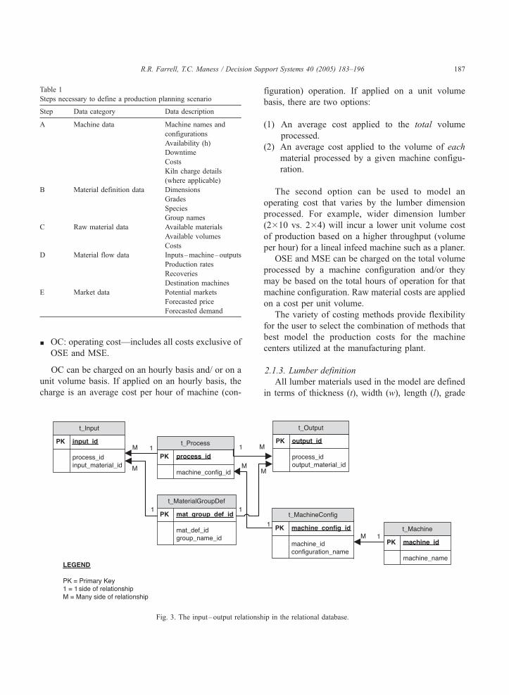
Table 1

Steps necessary to define a production planning scenario

Step Data category Data description

A Machine data Machine names and

configurations

Availability (h)

Downtime

Costs

Kiln charge details

(where applicable)

B Material definition data Dimensions

Grades

Species

Group names

C Raw material data Available materials

Available volumes

Costs

D Material flow data Inputs–machine–outputs

Production rates

Recoveries

Destination machines

E Market data Potential markets

Forecasted price

Forecasted demand


n OC: operating cost—includes all costs exclusive of

OSE and MSE.

OC can be charged on an hourly basis and/ or on a

unit volume basis. If applied on an hourly basis, the

charge is an average cost per hour of machine (con-

Fig. 3. The input–output relationsh

figuration) operation. If applied on a unit volume

basis, there are two options:

(1) An average cost applied to the total volume

processed.

(2) An average cost applied to the volume of each

material processed by a given machine configu-

ration.

The second option can be used to model an

operating cost that varies by the lumber dimension

processed. For example, wider dimension lumber

(2�10 vs. 2�4) will incur a lower unit volume cost

of production based on a higher throughput (volume

per hour) for a lineal infeed machine such as a planer.

OSE and MSE can be charged on the total volume

processed by a machine configuration and/or they

may be based on the total hours of operation for that

machine configuration. Raw material costs are applied

on a cost per unit volume.

The variety of costing methods provide flexibility

for the user to select the combination of methods that

best model the production costs for the machine

centers utilized at the manufacturing plant.

2.1.3. Lumber definition

All lumber materials used in the model are defined

in terms of thickness (t), width (w), length (l), grade

ip in the relational database.


( g), species (s) and material group name (n). The

dimension, species and grade attributes of a material

are obvious. However, the group name requires fur-

ther explanation. The group name allows one to group

associated materials together. For example, materials

of the same dimension, grade and species can be given

different group names in order to distinguish between

different raw material sources.

Another example is the use of group names to

identify different types of business. For example, a

secondary manufacturer may be involved in custom

processing (processing of customer’s wood) and mar-

ket processing (processing of purchased raw materials

into products for market sale). It can be useful to

Fig. 4. Defining materials in

differentiate between these two types of business

during the production planning process (i.e. quantify-

ing custom processing business and market processing

business). Lumber group names can be used for this

purpose. Fig. 4 illustrates how materials are defined in

the relational database.

2.1.4. Market demand

Three demand groups are provided to model the

sale of each output material (lumber products) on the

market. A demand group for each material is defined

by a market price and a volume capacity. Demand

groups are filled in ascending order (i.e. demand

group 1 before demand group 2) until their volume

the relational database.


capacity is attained. The three demand groups provide

modeling flexibility in that it is possible to define a

more realistic price–volume relationship for an output

material than would be possible if each product was

assigned a fixed price (i.e. a price fixed independently

of sale volume).

2.1.5. Units

The database has been designed to incorporate

different unit measurements. A unit table in the

database defines all the units that may be used in

the DSS. In addition, a unit conversion table stores

conversion factors that enable conversion between

different units. This is important as it facilitates the

modeling of products destined for different interna-

tional markets. For example, products destined for the

North American market are defined in imperial units,

while those destined for Europe or Japan are defined

in metric units.

2.2. User interface—data entry/manipulation

MS Access forms are developed to provide a user

interface that facilitates data entry and manipulation.

The forms allow the user to enter or modify data from

a number of tables on a single form. In this way, the

DSS is easier to use as one need only be concerned

with a small number of forms (to view or enter data)

rather than navigate the plethora of individual data

tables that make up the database. In addition, forms

allow the data requirements to be presented to the user

in an intuitive manner. The forms also provide fea-

tures that help minimize data entry error. For example,

filters are used on combo-boxes to ensure that the

species of an output material matches that of the input

material.

2.3. Model formulation

The model developed in this research is a single

period planning model. Such a model is appropriate

for short term production planning ranging from a

weekly to quarterly time period. The model is

formulated as a MILP. The kiln charge variables

(CHRGnimf) were modeled as integers as kiln mate-

rial can only be dried in full charges, i.e. it is not

economically viable to load a kiln below charge

volume capacity. Furthermore, a number of binary

(0,1) indicator variables are used to compose market

material into the demand groups.

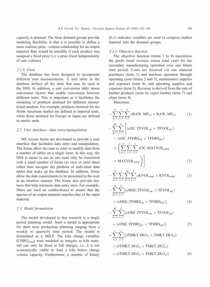
2.3.1. Objective function

The objective function (terms 1 to 8) maximizes

the profit (total revenue minus total cost) for the

secondary manufacturing operation over one future

time period. Costs are incurred via raw material

purchases (term 1) and machine operation through

operating costs (terms 2 and 3), maintenance supplies

and expenses (term 4), and operating supplies and

expenses (term 5). Revenue is derived from the sale of

lumber products (term 6), reject lumber (term 7) and

chips (term 8).

Maximize:

�XNn¼1

XIi¼1

XLl¼1

cRAW MPnil � RAW MPnil ð1Þ

�XMm¼1

XFf¼1

"ðcOC TFVOLmf � TFVOLmf Þ

þ ðcOC TFHRSmf � TFHRSmf Þ

þXNn¼1

XIi¼1

XLl¼1

cOC MATVOLnilmf

�MATVOLnilmf

!#ð2Þ

�XNn¼1

XIi¼1

XMm¼1

XFf¼1

cKVOLnimf � KVOLnimf ð3Þ

�XMm¼1

XFf¼1

½ðcMSE TFVOLmf � TFVOLmf Þ

þ ðcMSE TFHRSmf � TFHRSmf Þ� ð4Þ

�XMm¼1

XFf¼1

½ðcOSE TFVOLmf � TFVOLmf Þ

þ ðcOSE TFHRSmf � TFHRSmf Þ� ð5Þ

þXIi¼1

XLl¼1

½ðrTMKT DG1il � TMKT DG1ilÞ

þ ðrTMKT DG2il � TMKT DG2ilÞ

þ ðrTMKT DG3il � TMKT DG3ilÞ� ð6Þ


þXIi¼1

XLl¼1

rREJil � TREJil ð7Þ

þrCHIP BDU� CHIP BDU ð8Þ

subject to Section 2.3.2.

2.3.2. Raw material constraints

RAW MPnilVMAX MPnilbn;i;l ð9Þ

RAW MPnilzMIN MPnilbn;i;l ð10Þ

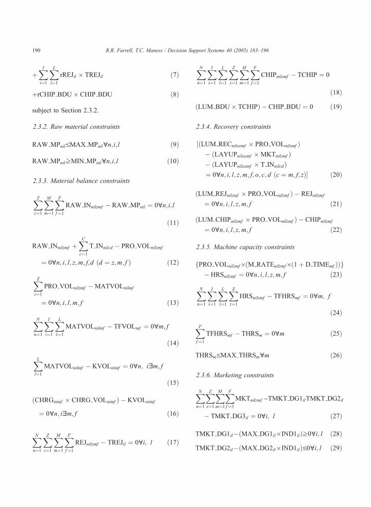
2.3.3. Material balance constraints

XZz¼1

XMm¼1

XFf¼1

RAW INnilzmf � RAW MPnil ¼ 0bn;i;l

ð11Þ

RAW INnilzmf þXCc¼1

T INnilcd � PRO VOLnilzmf

¼ 0bn; i; l; z;m; f;d ðd ¼ z;m; f Þ ð12Þ

XZz¼1

PRO VOLnilzmf �MATVOLnilmf

¼ 0bn; i; l;m; f ð13Þ

XNn¼1

XIi¼1

XLl¼1

MATVOLnilmf � TFVOLmf ¼ 0bm; f

ð14Þ

XLl¼1

MATVOLnilmf � KVOLnimf ¼ 0bn; iam; f

ð15Þ

ðCHRGnimf � CHRG VOLnimf Þ � KVOLnimf

¼ 0bn; iam; f ð16Þ

XNn¼1

XZz¼1

XMm¼1

XFf¼1

REJnilzmf � TREJil ¼ 0bi; l ð17Þ

XNn¼1

XIi¼1

XLl¼1

XZz¼1

XMm¼1

XFf¼1

CHIPnilzmf � TCHIP ¼ 0

ð18Þ

ðLUM BDU � TCHIPÞ � CHIP BDU ¼ 0 ð19Þ

2.3.4. Recovery constraints

½ðLUM RECnilozmf � PRO VOLnilzmf Þ� ðLAYUPnilozmf �MKTnilzmf Þ� ðLAYUPnilozmf � T INnilcdÞ¼ 0bn; i; l; z;m; f; o; c; d ðc ¼ m; f; zÞ� ð20Þ

ðLUM REJnilzmf � PRO VOLnilzmf Þ � REJnilzmf

¼ 0bn; i; l; z;m; f ð21Þ

ðLUM CHIPnilzmf � PRO VOLnilzmf Þ � CHIPnilzmf

¼ 0bn; i; l; z;m; f ð22Þ

2.3.5. Machine capacity constraints

fPRO VOLnilzmf�ðM RATEnilzmf�ð1þ D TIMEmf ÞÞg� HRSnilzmf ¼ 0bn; i; l; z;m; f ð23Þ

XNn¼1

XIi¼1

XLl¼1

XZz¼1

HRSnilzmf � TFHRSmf ¼ 0bm; f

ð24Þ

XFf¼1

TFHRSmf � THRSm ¼ 0bm ð25Þ

THRSmVMAX THRSmbm ð26Þ

2.3.6. Marketing constraints

XNn¼1

XZz¼1

XMm¼1

XFf¼1

MKTnilzmf �TMKT DG1ilTMKT DG2il

� TMKT DG3il ¼ 0bi; l ð27Þ

TMKT DG1il�ðMAX DG1il�IND1ilÞz0bi; l ð28Þ

TMKT DG2il�ðMAX DG2il�IND1ilÞV0bi; l ð29Þ

CHIPnilzmf Volume of chips produced processing

material (n,i,l) via manufacturing option

(z) at machine (m) configuration ( f).

CHIP_BDU Bone dry units (BDU) of chips produced.

One BDU is equal to the chip quantity

that would weigh 2400 lb at 0% moisture

content.

CHRGnimf Number of charges of material (n,i) into

kiln (m) configuration ( f).

HRSnilzmf Hours utilized processing material (n,i,l)

via manufacturing option (z) by machine

(m) configuration ( f).

IND1il Binary (0,1) indicator variable for

demand group 1.

IND2il Binary (0,1) indicator variable for

demand group 2.

KVOLnimf Volume of material (n,i) to be dried at

kiln (m) configuration ( f).

MATVOLnilmf Total volume of material (n,i,l)

processed by machine (m)

configuration ( f).

MKTnilzmf Volume of output material (n,i,l)

produced via manufacturing option

(z) at machine (m) configuration ( f)

for market sale.

PRO_VOLnilzmf Volume of material (n,i,l) processed via

manufacturing option (z) at machine (m)

configuration ( f).

RAW_INnilzmf Volume of raw material (n,i,l) processed

via manufacturing option (z) at machine


RAW_MPnil Total volume of raw material (n,i,l)

purchased.

REJnilzmf Volume of material (n,i,l) rejected via

manufacturing option (z) at machine (m)

configuration ( f).

TCHIP Total volume of chips produced.

TFHRSmf Total hours utilized by machine (m)

configuration ( f).

TFVOLmf Total volume of material processed at

machine (m) configuration ( f).

THRSm Total hours utilized by machine (m).

T_INnilcd Volume of output material (n,i,l)

produced at source (c) transferred

to destination (d)

for further processing.

TMKT_DG1il Total volume of material (i,l) sold in

market demand group 1.





TREJil Total volume of reject material (i,l).


TMKT DG2il�ðMAX DG2il�IND2ilÞz0bi; l ð30Þ

TMKT DG3il�ðMAX DG3il� 0bi; l ð31Þ

TMKT DG1ilVMAX DG1ilbi; l ð32Þ

TMKT DG1ilzMIN DG1ilbi; l ð33Þ

IND1ilV1 ð34Þ

IND2ilV1 ð35Þ

IND1il ¼ AIntegerA ð36Þ

IND2il ¼ AIntegerA ð37Þ

CHRGnimf ¼ AIntegerA ð38Þ

All variables z0.

2.4. Definitions

2.4.1. Subscripts

The (c) and (d) subscripts are used in the T_INnilcd

variables to transfer material between machine con-

figurations.

(c)=specifies source machine (m) configuration ( f )

manufacturing option (z) that transforms input

material (n,i,l) into output material (n,i,l).

(d)=specifies the destination machine (m) config-

uration ( f ) that will process material transferred

from all sources (c) via manufacturing option (z).

( f )=different configurations (machine set-up, work

force and processing functions) available for

machine center (m).

(i)=material defined by thickness (t), width (w),

grade ( g) and species (s).

(l)=material length.

(m)=machine center.

(n)=combines materials (i,l) into a material group

(n).

(o)=denotes output material (n,i,l) produced from

input material (n,i,l) via manufacturing option

(z).

(z)=manufacturing option where input material

(n,i,l) is processed into output material (n,i,l) via

machine (m) configuration ( f). The inputs and

outputs may be singular or multiple, depending on

the type of machine.

2.4.2. Variables

LUM_CHIPnilzmf Percentage of input material (n,i,l)


2.4.3. Cost coefficients

cKVOLnimf Cost per unit volume for drying

material (n,i) at kiln (m)

configuration ( f).

cMSE_TFHRSmf Average cost of maintenance supplies

and expenses, per hour of operation of


cMSE_TFVOLmf Average cost of maintenance supplies

and expenses, per unit volume

processed at machine (m)

configuration ( f).

cOC_MATVOLnilmf Operating cost per unit volume, for

processing input material (n,i,l) by


cOC_TFHRSmf Average operating cost, per hour of

operation for processing material at


cOC_TFVOLmf Average operating cost, per unit

volume for processing material at


cOSE_TFHRSmf Average cost of operating supplies

and expenses, per hour of operation

at machine (m) configuration ( f).

cOSE_TFVOLmf Average cost of operating supplies

and expenses, per unit volume

processed at machine (m)

configuration ( f).

cRAW_MPnil Cost per unit volume for purchasing

raw material (n,i,l).

rCHIP_BDU Revenue per bone dry unit,

for selling chips.

rTMKT_DG1il Revenue per unit volume, for selling

material (i,l) in demand group 1.





rTREJil Revenue per unit volume, for selling

reject material (i,l).

chipped via manufacturing option (z)


LUM_RECnilozmf Percentage of input material (n,i,l)

recovered as output material (o) via

manufacturing option (z) at machine


LUM_REJnilzmf Percentage of input material (n,i,l)

rejected via manufacturing option (z)


MAX_DG1il Maximum volume of material (i,l) that

can be sold in demand group 1.





MAX_MPnil Maximum volume of raw material

(n,i,l) available for purchase.

MAX_THRSm Maximum operating hours available

for machine (m).

MIN_DG1il Minimum sale requirements for material

(i,l) in demand group 1. Used to

model orders.

MIN_MPnil Minimum permissible purchase volume

for raw material (n,i,l).

M_RATEnilzmf Machine hours utilized per unit

volume of input material (n,i,l) processed

via manufacturing option (z) at machine


2.4.4. Other coefficients

CHRGnimf Kiln charge volume capacity for

material group (n,i) kiln (m)

configuration ( f).

D_TIMEmf Percentage downtime for machine (m)

configuration ( f).

LAYUPnilozmf Percentage of input material (n,i,l)

required in output material (o) according

to manufacturing option (z) at machine


LUM_BDU Coefficient used to convert volume of

wood chips produced to BDU.

2.5. Constraints

2.5.1. Raw material constraints

(9) Raw material purchase volume cannot exceed

the available volume for each raw material.

(10) Applies a minimum permissible purchase

volume to applicable raw materials.

2.5.2. Material balance constraints

These constraints ensure that total inputs equal

total outputs.

(11) Total volume of raw material (n,i,l) input to all

manufacturing options (z) must equal the

volume of raw material (n,i,l) purchased.

(12) The sum of raw material (n,i,l) purchases and

material (n,i,l) transfers from all sources (c)

equals the total volume of material (n,i,l)

processed by manufacturing option (z) at



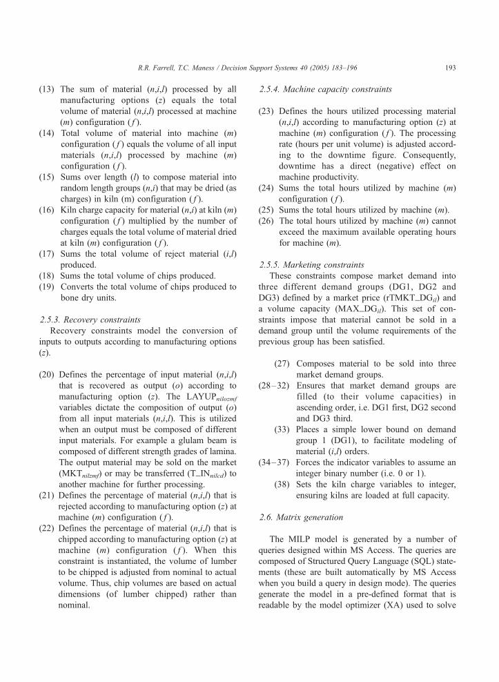
(13) The sum of material (n,i,l) processed by all

manufacturing options (z) equals the total

volume of material (n,i,l) processed at machine

(m) configuration ( f ).

(14) Total volume of material into machine (m)

configuration ( f ) equals the volume of all input

materials (n,i,l) processed by machine (m)

configuration ( f ).

(15) Sums over length (l) to compose material into

random length groups (n,i) that may be dried (as

charges) in kiln (m) configuration ( f ).

(16) Kiln charge capacity for material (n,i) at kiln (m)

configuration ( f ) multiplied by the number of

charges equals the total volume of material dried

at kiln (m) configuration ( f ).

(17) Sums the total volume of reject material (i,l)

produced.

(18) Sums the total volume of chips produced.

(19) Converts the total volume of chips produced to

bone dry units.

2.5.3. Recovery constraints

Recovery constraints model the conversion of

inputs to outputs according to manufacturing options

(z).

(20) Defines the percentage of input material (n,i,l)

that is recovered as output (o) according to

manufacturing option (z). The LAYUPnilozmfvariables dictate the composition of output (o)

from all input materials (n,i,l). This is utilized

when an output must be composed of different

input materials. For example a glulam beam is

composed of different strength grades of lamina.

The output material may be sold on the market

(MKTnilzmf) or may be transferred (T_INnilcd) to

another machine for further processing.

(21) Defines the percentage of material (n,i,l) that is

rejected according to manufacturing option (z) at

machine (m) configuration ( f ).

(22) Defines the percentage of material (n,i,l) that is

chipped according to manufacturing option (z) at

machine (m) configuration ( f ). When this

constraint is instantiated, the volume of lumber

to be chipped is adjusted from nominal to actual

volume. Thus, chip volumes are based on actual

dimensions (of lumber chipped) rather than

nominal.

2.5.4. Machine capacity constraints

(23) Defines the hours utilized processing material

(n,i,l) according to manufacturing option (z) at

machine (m) configuration ( f ). The processing

rate (hours per unit volume) is adjusted accord-

ing to the downtime figure. Consequently,

downtime has a direct (negative) effect on

machine productivity.

(24) Sums the total hours utilized by machine (m)

configuration ( f ).

(25) Sums the total hours utilized by machine (m).

(26) The total hours utilized by machine (m) cannot

exceed the maximum available operating hours

for machine (m).

2.5.5. Marketing constraints

These constraints compose market demand into

three different demand groups (DG1, DG2 and

DG3) defined by a market price (rTMKT_DGil) and

a volume capacity (MAX_DGil). This set of con-

straints impose that material cannot be sold in a

demand group until the volume requirements of the

previous group has been satisfied.

(27) Composes material to be sold into three

market demand groups.

(28–32) Ensures that market demand groups are

filled (to their volume capacities) in

ascending order, i.e. DG1 first, DG2 second

and DG3 third.

(33) Places a simple lower bound on demand

group 1 (DG1), to facilitate modeling of

material (i,l) orders.

(34–37) Forces the indicator variables to assume an

integer binary number (i.e. 0 or 1).

(38) Sets the kiln charge variables to integer,

ensuring kilns are loaded at full capacity.

2.6. Matrix generation

The MILP model is generated by a number of

queries designed within MS Access. The queries are

composed of Structured Query Language (SQL) state-

ments (these are built automatically by MS Access

when you build a query in design mode). The queries

generate the model in a pre-defined format that is

readable by the model optimizer (XA) used to solve


the LP. A row, column, coefficient (RCC) format is

used to present the coefficient matrix in triplet arrays,

consisting of a row (or constraint) index, a column (or

variable) index and a coefficient. It should be noted

that queries could also be employed to present the

MILP in the commonly used MPS format.

Each query is constructed to define a specific

component of a particular constraint. For example

constraint (11)�PZ

z¼1

PMm¼1

PFf¼1 RAW INnilzmf �

RAW MPnil ¼ 0bn; i;�is generated by three different

queries. One query generates the�PZ

z¼1

PMm¼1

PFf¼1

RAWINnilzmf � coefficients, returning N�I�L�Z�M�F records, another generates [�RAW_MPnil]

returning N�I�L records, and the third generates

the right hand side [=0] returning N�I�L records. In

this way, each query produces a triplet array repre-

senting a particular component of the mathematical

model.

In any LP application, it is fundamental that

variable and constraint names or indexes are unique.

A feature of relational database theory whereby every

record in a data table must have a unique identifier

(referred to as a primary key) facilitates the develop-

ment of such a naming convention. Furthermore, by

utilizing the primary key succinct names can be

created. For example, the subscript (i)=material de-

fined by thickness (t), width (w), grade ( g) and

species (s), rather than explicitly recording each in

the variable or constraint name, one can use the

primary key or index number that relates to that

specific material. Thus, the material is entirely repre-

sented by just one index number (i).

The names of all the queries that need to be

executed to build the MILP are stored in a designated

table t_LPmodel.

2.7. XAEZ (model instantiation)

A production planning scenario is instantiated by

executing the queries that define the mathematical

model. XAEZ executes all the queries listed in the

designated table t_LPmodel. The queries retrieve

data from the database and generate the MILP

model instance in the prescribed (RCC) format.

The RCC data from each query is stored in

memory and passed to the optimizer XA for

solving. Each model instance is based on the data

records currently stored in the database (i.e. ma-

chine centers, raw materials, material transfers and

market products currently defined). A number of

related scenarios can be compared by creating

duplicates of the database and modifying specific

production parameters in each.

2.8. XA (solving the model)

The model is solved by XA, and the solution

written back to pre-defined tables in the database.

XAEZ facilitates the transfer of the MILP model

between the database and the optimizer.

2.9. User interface—reports

Using MS Access’s reporting features a number of

reports are developed to convey key information

provided in the model solution back to the user.

Before meaningful reports can be developed, the

constraint and variable names must be decoded.

Another set of queries are constructed to perform this

task. The reports are based on these queries and are

activated when the reports are initialized.

Key reports provided include:

(1) Financial summary

(2) Optimal lumber purchasing strategy

(3) Machine utilization

(4) Selected manufacturing options

(5) Lumber sales

(6) Reject sales

(7) Chip sales

All data-entry forms and reports are accessed via

the central switchboard form to help the user navigate

through the DSS and facilitate data management.

3. Conclusion

Production planning in the secondary manufactur-

ing sector is a complex task. The interactions of raw

materials, with process and marketing factors produce

complex interrelationships that require simultaneous

analysis in order to find the optimal operating strategy.

An examination of the literature on operations re-

search techniques for production planning in second-

ary manufacturing revealed the specificity of existing


applications. Most models have been designed for

specific secondary manufacturing plants or focus on

solving specific problems. The decision support sys-

tem developed in this research has the flexibility to

model a wide variety of secondary manufacturing

plants and can be used to address a range of short-

term production planning issues.

The widely available relational database manage-

ment tool MS Access provided an appropriate design

environment for building the DSS. The relational

database provides an efficient data management tool

for handling potentially large data sets. Model data

can be easily updated through the appropriate forms

and re-use of common data is facilitated by their

storage in the database. Model-data independence is

provided by a database that manages all model data,

and SQL queries that define the mathematical model.

As noted by other authors [1,9,11] model-data inde-

pendence facilitates data manipulation, reuse of the

same mathematical model in different specific mod-

eling applications, and provides greater design robust-

ness and clarity.

The DSS has a broad application domain, and can

be used to provide insight on decisions concerned

with product mix, raw material sourcing, production

strategies, pricing strategies, resource valuation and

capital appropriations requests. Furthermore, the life

span of the resultant DSS should be increased through

the flexible design that allows one to model a wide

variety of machine centers and the ability to customize

the process flow to model specific production plan-

ning scenarios. This flexibility is a major advantage in

a manufacturing sector characterized by a highly

dynamic operating environment.

Acknowledgements

The authors would like to thank Mr. Andre Schuetz

for his assistance in the development of the DSS

discussed in this paper.

References

[1] A. Atamturk, E.L. Johnson, J.T. Linderoth, M.W.P. Savels-

bergh, A relational modeling system for linear and integer

programming, Operations Research 48 (6) (2000) 846–857.

[2] H.F. Carino, S.U. Foronda, A model for minimizing blank

costs in hardwood furniture manufacturing, Forest Products

Journal 40 (5) (1990) 10–19.

[3] H.F. Carino, C.H. Lenoir, Optimizing wood procurement in

cabinet manufacturing, Interfaces 18 (2) (1988) 21–26.

[4] H.F. Carino, D.B. Willis, Enhancing the profitability of a ver-

tically integrated wood products production system: Part 1. A

multistage modeling approach, Forest Products Journal 51 (4)

(2001) 37–44.

[5] W.S. Donald, Production Planning for Value Added Lumber

Manufacturing, M.Sc. Thesis, Department of Wood Science,

University of British Columbia, Vancouver, B.C., Canada,

1996.

[6] Forum Consulting Group, Jurisdictional Review: Policies and

Incentives to Promote Investment in Secondary Wood Manu-

facturing, Forest Enterprise Branch, Victoria, BC, 1999, Pre-

pared for Ministry of Forests.

[7] R. Fourer, Database structures for mathematical programming

models, Decision Support Systems 20 (1997) 317–344.

[8] P. Gazmuri, I. Arrate, Modeling and visualization for a pro-

duction planning decision support system, International Trans-

actions in Operational Research 2 (3) (1995) 249–258.

[9] A.M. Geoffrion, An introduction to structured modeling,

Management Science 33 (5) 547–588.

[10] K. Metaxiotis, D. Askounis, J. Psarras, An object oriented

analysis and design of a model for production planning and

control in industry, The International Journal of Advanced

Manufacturing Technology 18 (9) (2001) 657–664.

[11] W.A. Muhanna, R.A. Pick, Meta-modeling concepts and tools

for model management: a systems approach, Management

Science 40 (9) (1994) 1093–1123.

[12] W.P. Mundie, Linear Programming for a Lumber Remanufac-

turing Plant, B.Sc. Thesis, Faculty of Forestry, University of

British Columbia, Vancouver, B.C., Canada, 1977.

[13] F.H. Murphy, E.A. Stohr, A. Asthana, Representation schemes

for linear programming models, Management Science 38 (7)

964–991.

[14] J. Olhager, B. Rapp, Operations research techniques in man-

ufacturing planning and control systems, International Trans-

actions in Operational Research 2 (1) (1995) 29–43.

[15] E.B. Penick, A linear programming application to machine

loading in a furniture plant, Forest Products Journal 2

(1968) 21–26.

[16] Price Waterhouse, Performance of the Value-added Wood

Products Industry in British Columbia, FRDA Report 193.

Available through: Forestry Canada, Pacific Forestry Cen-

tre, Victoria, BC or Ministry of Forests, Victoria, BC.,

1992.

[17] R.M. Riordan, Designing Relational Database Systems,

Microsoft Press, 1999. ISBN 0-7356-0634-X

[18] A. Srinivasan, D. Sundaram, An object relational approach for

the design of decision support systems, European Journal of

Operational Research (127) (2000) 594–610.

[19] UN/ECE Timber Committee, Forest products annual market

review 1998–1999, Timber Bulletin LII (1999) (ECE/TIM/

BULL/52/3). http://www.unece.org/trade/timber/docs/

rev-99/rev99.htm.

http://www.unece.org/trade/timber/docs/rev-99/rev99.htm


[20] R.P. Vlosky, N.P. Chance, An analysis of state-level economic

development programs targeting the wood products industry,

Forest Products Journal 46 (9) (1996) 23–30.

[21] R.P. Vlosky, N.P. Chance, P.A. Monroe, D.W. Hughes, L.B.

Blalock, An integrated market-based methodology for val-

ue-added solid wood products, Forest Products Journal 48

(11) (1998) 29–35.

[22] T. Zhang, A linear programming formulation and user-friendly

computer interface for furniture manufacturing analysis, M.Sc.

Thesis, North Carolina State University, 1990.

Ross Farrell is an Operations Research Analyst with WoodFlow

Systems Corp. Vancouver, BC, Canada. His research interests relate

to the development of DSSs for the forest industry. He received an

MSc. in Wood Products Processing from the University of British

Columbia in 2002. He also holds a BSc. in Forest Management

from the University of Aberdeen.

A relational database approach to a linear programming-based decision support system for production...

Documents

Transcript of A relational database approach to a linear programming-based decision support system for production...