
The future of quality control for wood & wood products
648
The future of quality control for wood & wood products Proceedings of the final conference of COST Action E53: ‘Quality control for wood & wood products’ 4 – 7th May 2010, Edinburgh, UK Incorporating the European Wood Drying Group workshop http://cte.napier.ac.uk/e53
-
Upload
khangminh22 -
Category
Documents
-
view
0 -
download
0
Transcript of The future of quality control for wood & wood products

The future of quality control for wood & wood products
Proceedings of the final conference of COST Action E53: ‘Quality control for wood & wood products’
4 – 7th May 2010, Edinburgh, UK
Incorporating the European Wood Drying Group workshop
http://cte.napier.ac.uk/e53

‘The Future of Quality Control for Wood & Wood Products’, 4-7th May 2010, Edinburgh The Final Conference of COST Action E53
“The future of quality control for wood & wood products”
4 – 7th May 2010, Edinburgh, UK
The final conference of COST Action E53: ‘Quality control for wood & wood products’
http://cte.napier.ac.uk/e53 / http://www.coste53.net
“The future of quality control for wood & wood products”, Proceedings of the final conference of COST Action E53, Editors D.J. Ridley-Ellis & J.R. Moore, Edinburgh (UK),
2010. ISBN 978-09566187-0-2 [electronic proceedings]
Technical Committee
Robert Kliger (chair), Sweden Arto Usenius, Finland (WG 1: Scanning for wood properties) Johannes Welling, Germany (WG 2: Moisture content and distortion) Charlotte Bengtsson, Sweden (WG 3: Strength, stiffness and appearance grading) Dan Ridley-Ellis, UK (Local host) John Moore, UK (Local host)
With thanks to Tom Drewett, Stefan Lehneke, James Ramsay and Greg Searles for assistance in reviewing the papers.
Copyright of contents remains with the authors and their respective institutions, but these conference proceedings may be stored, copied and distributed for the purposes of dissemination.
The authors are responsible for the content of their papers, which does not necessarily reflect the opinion of the editors, the technical committee or the publisher.
Electronic proceedings published by: Forest Products Research Institute / Centre for Timber Engineering Edinburgh Napier University 10 Colinton Road, Edinburgh EH10 5DT, UK http://cte.napier.ac.uk
http://cte.napier.ac.uk/e53 2

‘The Future of Quality Control for Wood & Wood Products’, 4-7th May 2010, Edinburgh The Final Conference of COST Action E53
COST Action E53
The principal aim of the COST Action E53 was to improve methods of quality control in processing round wood and timber to ensure that timber products and components meet the requirements of the users. The Action also promoted the improvement of specifications for timber products and contributed toward the economic optimisation of production so that the full environmental and sustainability benefits of the forestry wood chain might be realised in future. Improved quality control systems will help to increase the competitiveness of the wood sector, as well as ensuring that round wood is optimally processed, and that the European wood industry provides wood products which are well suited to end user requirements.
Within the Action, special attention was paid to the following:
• Scanning of stems, logs and boards for characterisation of geometrical and quality properties.
• Wood drying, distortion and determination of moisture content.
• Assessment of strength, stiffness and visual appearance of timber and wood products.
• Understanding end user requirements for wood and wood products.
The first three of these areas were addressed by separate Working Groups (WG1 – Scanning for wood properties; WG2 – Moisture content and distortion; WG3 – Strength, stiffness and appearance grading), while a Task Group focussed on better understanding end user requirements.
COST is an inter-governmental European framework for international co-operation between nationally funded research activities. http://www.cost.esf.org/
http://cte.napier.ac.uk/e53 3

‘The Future of Quality Control for Wood & Wood Products’, 4-7th May 2010, Edinburgh The Final Conference of COST Action E53
Foreword
We would like to thank the authors and delegates who contributed to a successful conference to mark the end of this popular COST Action. Pan European cooperation is enormously valuable: International trade and harmonised standards require it, but it also allows pooling of expertise and sharing of knowledge among a research community that is relatively small and fragmented.
The papers in these proceedings show how important research is to the timber industry by helping it to manufacture products that are competitive against other materials. It is not simply a matter of ensuring that wood products meet the requirements of customers, but understanding those requirements and setting standards accordingly. Crucially it also requires the dissemination of research into industry and, to a certain extent, also the public at large who are the ultimate users of most wood products. This is why a special effort was made to widen the participation for the closing conference.
Hosting the conference in the UK provided an excellent opportunity for members of the local forest products industry to attend and to learn more about the latest advances in scanning, drying and grading research in Europe. While the extent of forest cover and size of the industry in this country is relatively small in comparison to the rest of Europe, the UK still produces enough sawn softwood and panel products to build a typical timber framed house every 30 seconds. However, only one-third of the sawn softwood produced by the UK’s larger sawmills is currently sold as construction timber and very little home-grown timber is used in volume house production; particularly the manufacture of timber frames and trussed rafters. Instead, the majority of domestically produced sawn timber is sold into lower value markets (fencing, packaging and pallets), and the vast majority of softwood for house construction is imported from countries such as Sweden, Finland, Latvia, Germany and Russia.
High levels of afforestation in the 1970s and 1980s means that UK softwood production is set to increase by 20% from current levels over the next decade. This is seen by the forest and timber industries as a significant opportunity for the UK construction industry to use a greater proportion of home-grown timber, but there are questions surrounding the motivation to do so that are related to the reality, and perception, of timber quality. This COST Action has therefore been particularly relevant to the UK’s timber industry and our research at Edinburgh Napier University. We were very pleased to host the closing conference.
Dan Ridley-Ellis & John Moore
Edinburgh Napier University
http://cte.napier.ac.uk/e53 4

‘The Future of Quality Control for Wood & Wood Products’, 4-7th May 2010, Edinburgh The Final Conference of COST Action E53
Participation in the final conference of COST Action E53
The conference contained fifty nine oral presentations and ten poster papers. There were a particularly large number of papers on topics related to grading (Working Group 3), but also a large number of papers on drying topics (Working Group 2). The most industry relevant papers were grouped into a single day in order to encourage delegates from industry who would not wish to attend the full conference (the ‘industry focussed day’). This day included keynote talks for the Task Group (end user requirements) and each of the Working Groups in order to help disseminate the work of the COST Action as a whole. In order to fit all the papers within the four day conference programme, there were two parallel sessions for most of the ‘research focussed day’. A day of presentations related to Working Group 2 was run in conjunction with the European Drying Group.
One hundred and forty one people were registered for at least one of the technical sessions of the conference (not counting the attendees representing the COST Office). About a quarter of the delegates came from outside the research community; representing the interests of timber producers and end users of timber products.
Twenty one of the twenty five countries that signed up to the COST E53 Memorandum of Understanding were represented at the conference (Austria, Belgium, Bulgaria, Finland, Germany, Greece, Hungary, Italy, Latvia, Lithuania, Netherlands, Norway, Poland, Portugal, Serbia, Slovakia, Slovenia, Spain, Sweden, Switzerland and UK). A further two were unable to attend due to the travel disruption caused by the volcanic ash cloud (France and Ireland). Delegates also came from a number of countries not formally involved in COST E53 (Australia, Canada, Iran, Luxemburg, Romania, South Korea and USA).
Map of countries represented by delegates
(yellow indicates countries where delegates registered but could not attend due to travel disruption)
http://cte.napier.ac.uk/e53 5

‘The Future of Quality Control for Wood & Wood Products’, 4-7th May 2010, Edinburgh The Final Conference of COST Action E53
Tuesday 4th May
Wood drying workshop (European Drying Group, EDG) 1st session chair: J. Welling
[11] Introduction to the European Drying Group (The Netherlands) W. Gard
[13] Investigations concerning the possibility to minimize the stacks aerodynamic resistance (Romania) I.B. Bedelean & D. Sova
[22] Pre-sorting for density in drying batches of Norway spruce boards (Norway) Y. Steiner & A. Øvrum
[30] Dtouch – drying has never been so easy (Italy) O. Allegretti, I. Cuccui, S. Ferrari & A. Sione
[39] Impact of various conventional drying conditions on drying rate and on moisture content gradient during early stage of beechwood drying (Slovenia/Croatia) A. Straže, S. Pervan, Ž. Gorišek
2nd session chair: W. Gard [49] Electrical impedance measurement of green Scots pine (Finland) L. Tomppo, M. Tiitta
& R. Lappalainen [57] Eucalyptus drying process: qualitative comparison of different clones cultivated in Italy (Italy)
L. Travan, O. Allegretti & M.Negri [71] Criterial assessment of the drying quality (Romania) D. Şova, A. Postelnicu & B. Bedelean
[80] Quality control by colour measurements after different drying schedules of solid plantation teakwood (Austria) H.L. Pleschberger, A. Teischinger, U. Müller & C. Hansmann
3rd session chair: K.M. Sandland [91] Inclusion of the sorption hysteresis phenomenon in future drying models. Some basic considerations.
(Finland) J-G. Salin [100] Fibre level modelling of free water behaviour in drying and wetting (Finland) J-G. Salin
[109] The water vapour sorption kinetics of Sitka spruce at different temperatures analysed using the parallel exponential kinetics model (UK) C.A.S. Hill , Y-J Xie
[116] Tracing thermal treatment in wood using RFID (Greece) G. Ntalos, M. Skarvelis & D. Karampatzakis
http://www.cte.napier.ac.uk/e53/ 6

‘The Future of Quality Control for Wood & Wood Products’, 4-7th May 2010, Edinburgh The Final Conference of COST Action E53
Wednesday 5th May
Industry focussed day 1st session chair: I.R. Kliger
[124] Opening presentation (UK) R. Coppock
[130] Timber quality for the construction industry (Sweden) I.R. Kliger
[133] Norwegian architects’ and civil engineers’ attitudes to wood in urban construction (Norway) K. Bysheim & A.Q. Nyrud
[141] The problems with standardisation? (UK) J. Park
[152] Practical engineering considerations when using solid hardwood to replace steel and concrete structure (UK) R. Thorniley-Walker
2nd session chair: A. Usenius (Working Group 1 chair) [164] Sawmilling and Sawing Process in the Future (Finland) A. Usenius, P. Holmila, A. Heikkilä
&, T. Usenius [173] Deciding log grade for payment based on X-ray scanning of logs (Sweden)
J. Oja, J. Skog, J. Edlund & L. Björklund [180] Assessing timber quality of Scots pine (Pinus sylvestris L.) (UK) E. Macdonald, J. Moore,
T. Connolly & B. Gardiner [191] Using acoustic tools to improve the efficiency of the forestry wood chain in eastern Canada (Canada)
A. Achim, N. Paradis, A. Salenikovich & H. Power 3rd session chair: J. Welling (Working Group 2 chair)
[201] Drying quality - an important topic for business and research (Germany) J. Welling
[204] Do’s and don’ts in respect to moisture measurement (The Netherlands) P. Rozema
[213] Sorting of logs and planks before drying for improved drying process and panel board quality (Norway) K.M. Sandland & P. Gjerdrum
[222] Emissions of volatile organic compounds from convection dried Norway spruce timber (Germany) V. Steckel, J. Welling & M. Ohlmeyer
4th session chair C. Bengtsson (Working Group 3 chair) [232] Advances and the future of grading structural timber (Sweden) C. Bengtsson
[249] Strength grading of wet Norway spruce side boards for use as laminations in wet-glued laminated beams (Sweden) J. Oscarsson, A. Olsson, M. Johansson, B. Enquist & E. Serrano
[258] The potential for estimation of log value by the use of traceability concepts (Norway) A. Øvrum
[266] Potential of poplar and willow wood for load-bearing constructions (Belgium) L. De Boever & J. Van Acker
[282] Thermo-mechanical densification of Pannónia Poplar (Hungary) J. Ábrahám, R. Németh & S. Molnár
http://www.cte.napier.ac.uk/e53/ 7

‘The Future of Quality Control for Wood & Wood Products’, 4-7th May 2010, Edinburgh The Final Conference of COST Action E53
Thursday 6th May
Research focussed day Plenary session chair: J. Moore
[294] Quality control and improvement of structural timber (Switzerland) M. Deublein, R. Steiger & J. Köhler
[303] Influence of the origin on specific properties of European spruce and pine (Germany / Austria) P. Stapel, J.K. Denzler
[312] Variability of strength of in-grade spruce timber (Finland) A. Ranta-Maunus
[324] The influence of knot size and location on the yield of grading machines (Germany) A. Rais, P. Stapel, & J.W.G. van de Kuilen
[332] Near-infrared technology applications for quality control in wood processing (Canada) K.Watanabe, J.F. Hart, S.D. Mansfield & S. Avramidis (recorded presentation)
Parallel 1A chair A. Usenius Parallel 1B chair J. Denzler [343] Knots in CT scans of Scots pine logs (Germany)
R. Baumgartner, F. Brüchert & U. H. Sauter [379] Grading characteristics of structural Slovak spruce timber
determined by ultrasonic and bending methods (Slovakia) A. Rohanová, R. Lagaňa & J. Dubovský
[352] The use of log geometry variables to determine the stiffness of Sitka spruce (UK) T. N. Reynolds , S. Porter
[388] Strategies for quality control of strength graded timber (Netherlands / Germany) G.J.P.Ravenshorst & J.W.G. van de
Kuilen [360] Tensile strain fields around an edge knot in a spruce specimen (Sweden) J. Oscarsson A. Olsson & B. Enquist
[397] Machine strength grading – prediction limits – evaluation of a new method for derivation of settings (Sweden) R. Ziethén &
C. Bengtsson [369] Modelling behaviour of timber from images analysis
(France) J.L. Coureau, A. Cointe & M. Giton (not presented due to travel difficulties)
[406] Development of a simulation-evaluation program for introducing and using output control in the sawmill industry
(Sweden) A. Lycken, R. Ziethén & C. Bengtsson Parallel 2A chair: M. Deublein Parallel 2B chair: R. Harris
[416] The use of non-destructive methods for the evaluation of fungal decay in field testing by dynamic vibration (Germany)
A. Krause, A. Pfeffer & H. Militz
[453] Quality control of glulam: Improved method for shear testing of glue lines (Switzerland) R. Steiger & E. Gehri
[425] Strength estimation of aged wood by means of ultrasonic devices (Switzerland) K. Kránitz, M. Deublein & P. Niemz
[464] Assessment of the shear strength of glued-laminated timber in existing structures (Switzerland) T. Tannert, A. Müller
& T. Vallée [434] Wood windows in the 21st Century: end user requirements, limits and opportunities (Hungary) L. Elek, Zs. Kovacs & L. Denes
[473] Validity of bending tests on strip-shaped specimens to derive bending strength & stiffness properties of cross-laminated
solid timber (X-lam) (Switzerland) R. Steiger & A. Gülzow [444] A few elastic properties of drilled rectangular bars of poplar
wood (Iran) A.Yavari , M. Roohnia & A. Tajdini [484] An objective method to measure and evaluate the quality of
sanded wood surfaces (Romania) L. Gurau
Parallel session 3A chair C. Bengtsson Parallel session 3B chair J. Moore [494] Early-stage prediction and modeling strength properties of
Lithuanian-grown Scots Pine (Pinus Sylvestris L.) (Lithuania) A. Baltrusaitis, M. Aleinikovas & L. Kudakas
[522] Assessing stiffness on finger-jointed timber with different non-destructive testing techniques (Germany / Canada)
T. Biechele, Y.H. Chui & M. Gong [504] Strength grading of Slovenian structural sawn timber
(Slovenia) J. Srpcic, M. Plos, T. Pazlar & G. Turk [529] Dynamic excitation and higher bending modes for prediction
of timber bending strength (Sweden) A.M.J. Olsson, J. Oscarsson, B.M. Johansson & B. Källsner
[512] A multidisciplinary study assessing the properties of Douglas-fir grown in the South West region of England (UK) J.M.
Bawcombe, R. Harris, P. Walker & M.P. Ansell
[538] Strength Grading of Structural Lumber by Portable Lumber Grading - effect of knots (Hungary) F. Divos , F. Sismandy Kiss
http://www.cte.napier.ac.uk/e53/ 8

‘The Future of Quality Control for Wood & Wood Products’, 4-7th May 2010, Edinburgh The Final Conference of COST Action E53
Friday 7th May
Technical tour Session chair: D. Ridley-Ellis
[546] The resurgence of timber as a primary building material in Edinburgh's architecture (UK) P. Wilson (delegates will receive a copy of “New Timber Architecture in Scotland”)
[559] The John Hope Gateway Biodiversity Centre (UK) R. Harris, P. Roberts & I. Hargreaves
[566] Structural Performance of thinned oak containers (UK) N. Savage & A. Kermani
Poster papers
[576] Bark recognition on Robinia pseudoacacia L. logs using computer tomography (Germany) M. J. Diaz Baptista, F. Brüchert & U. H. Sauter
[579] Acoustic tools for seedling, tree and log selection (Hungary) F. Divos
[584] Fracture toughness and shear yield strength determination of steam kiln–dried wood (Poland) K.A. Orlowski & M.A. Wierzbowski
[592] Experimental study and numerical simulation of flow pattern and heat transfer during steam drying wood (Poland) J. Barański, M. A. Wierzbowski, J. A. Stasiek
[605] Novel non-destructive methods for wood (Finland) M. Tiitta, L. Tomppo & R. Lappalainen.
[611] Photodegradation and weathering effects on timber surface moisture profiles as studied using Dynamic Vapour Sorption (UK) V.Sharratt, C.A.S.Hill, S.F.Curling, J.Zaihan & D.P.R.Kint.
[617] Experiments for wood cup description (Slovakia) R. Hrčka & R. Lagaňa
[627] Ultrasound measurements of glulam beams to assess bending stiffness and strength (Finland) R. Stöd & H. Heräjärvi
[635] Quality Approval System for Wood Products in Korea (South Korea) S.M. Kang, D.Y. Kang, W.M. Koo, K.M. Kim & J.Y. Park
[644] Lumber value of dead and sound black spruce trees in the boreal forest of Québec (Canada) J.Barrette, D.Pothier, I. Duchesne & N. Gélinas
[-] The use and specification of appropriate timber in traditionally built structures (UK) C.J. Kennedy & C. McGregor (withdrawn from conference)
http://www.cte.napier.ac.uk/e53/ 9

‘The Future of Quality Control for Wood & Wood Products’, 4-7th May 2010, Edinburgh The Final Conference of COST Action E53
Tuesday 4th May Wood drying workshop (European Drying Group)
1st session
http://www.cte.napier.ac.uk/e53/ 10

European Drying Group (EDG)
Aim of EDG•promote research regarding wood drying throughout Europe
•exchange of technical information on wood drying
•facilitate co-operation among members
•facilitate collaborative research projects
•organizing seminars, workshops and conferences
European Drying Group (EDG)
History•EDG started its activities in 1987 under the umbrella of the European SPRINT program. •EDG work was continued by COST Action E15 "Advances in the drying of wood“•2005 the former members of EDG revitalize EDG•EDG came back with a modernized concept.•2006 EDG Drying Seminar was held in Hamburg/Germany•2007 EDG Drying Seminar was held in Riga/Latvia•2008 EDG Drying Seminar was held in Oslo/Norway•2008 local EDG Drying Seminar was held in Ljubljana/Slovenia •2009 EDG Drying Seminar was held in Bled /Slovenia•2010 EDG Drying Seminar was held in Edinburgh/UK
Membership of EDG•Industrial members
•Scientific members
‘The Future of Quality Control for Wood & Wood Products’, 4-7th May 2010, EdinburghThe Final Conference of COST Action E53
http://cte.napier.ac.uk/e53 11

European Drying Group (EDG)
Web-site
www.timberdry.net
Discussion forum
www.torkeklubben.no/forum
‘The Future of Quality Control for Wood & Wood Products’, 4-7th May 2010, EdinburghThe Final Conference of COST Action E53
http://cte.napier.ac.uk/e53 12
‘The Future of Quality Control for Wood & Wood Products’, 4-7th May 2010, Edinburgh The Final Conference of COST Action E53
Investigations concerning the possibility to minimize the stacks aerodynamic resistance
I.B. Bedelean1 & D. Sova2
Abstract The task of this research was to elaborate and to test a solution for minimizing the aerodynamic resistance of the stacks. According to the theoretical approach this task might be achieved by attaching some aerodynamic profiles. The numerical results have shown that the proposed solution assures a minimization of the local resistance stacks. For the current variant, assuming that the volume of air delivered by the fans would remain constant and using numerical analysis, it has been established that 45 mm stickers generate the same pressure loss, like in the proposed variant. But, the air velocity was diminished by 33% because the stacks open area has increased. In what concern the drying capacity, it was found that both variants involved a decrease of the capacity between 20% - 25%. Two experimental tests were performed in a lab kiln in order to establish if the proposed solution generates enough advantages to compensate the drying capacity decrease. The material which was used was taken from green logs of spruce. For each run, 36 pieces - 50 x 150 mm2 in the cross section and 1.45 m long – were dried to a target of the moisture content equal with 30%, because the air velocity has an important effect on the drying time only during the first period of drying. The stickers’ thickness was 25 mm for both variants. The aerodynamic profiles were attached only in the proposed variant. For each run the drying time and the power energy consumption were established.
1. Introduction In a drying kiln the air flow is constrained to overcome a series of local resistances: heat exchangers, fan cases, stacks, and those which are caused by the kiln geometry (the change of the flow direction of air). From all of these resistances the researchers have decided to intervene on those that are caused by the kiln geometry (Nijdam & Keey 2002), and very rare on those generated by the stacks. Since the kiln operators, during the kiln operation, cannot intervene on the local resistances, which are caused by the stacks, the development of the current possibilities is necessary and they refer to the minimizing of the stacks local resistance, with the purpose to reduce the absorbed electric energy.
The average velocity in the stack active channels is related to the stack pressure drop
mv
stackpΔ , which is determined by use of the pressure-loss
1 Teaching assistant, [email protected] Associate Professor, [email protected] University of Brasov, Romania
http://cte.napier.ac.uk/e53 13
‘The Future of Quality Control for Wood & Wood Products’, 4-7th May 2010, Edinburgh The Final Conference of COST Action E53
coefficient ζ (Equation1). This coefficient takes into account the pressure losses which appear at the inlet iζ and the outlet of air from the timber stack
oζ , the losses that are stimulated by the channel length and its roughness fζ and the losses due to the gaps existing between the boards gζ (Equation 2) (Ledig et al. 2008).
2
2 mstack vp ρξ=Δ Equation 1
ogfi ζζζζζ +++= Equation 2
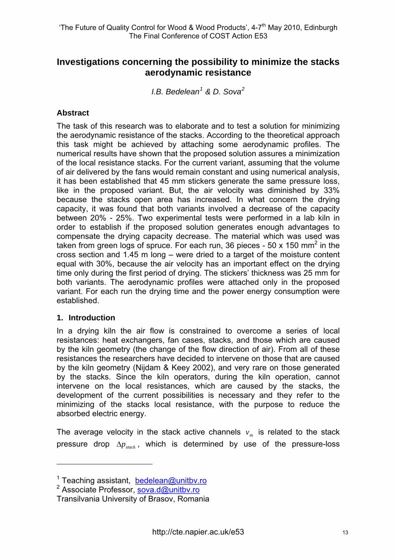
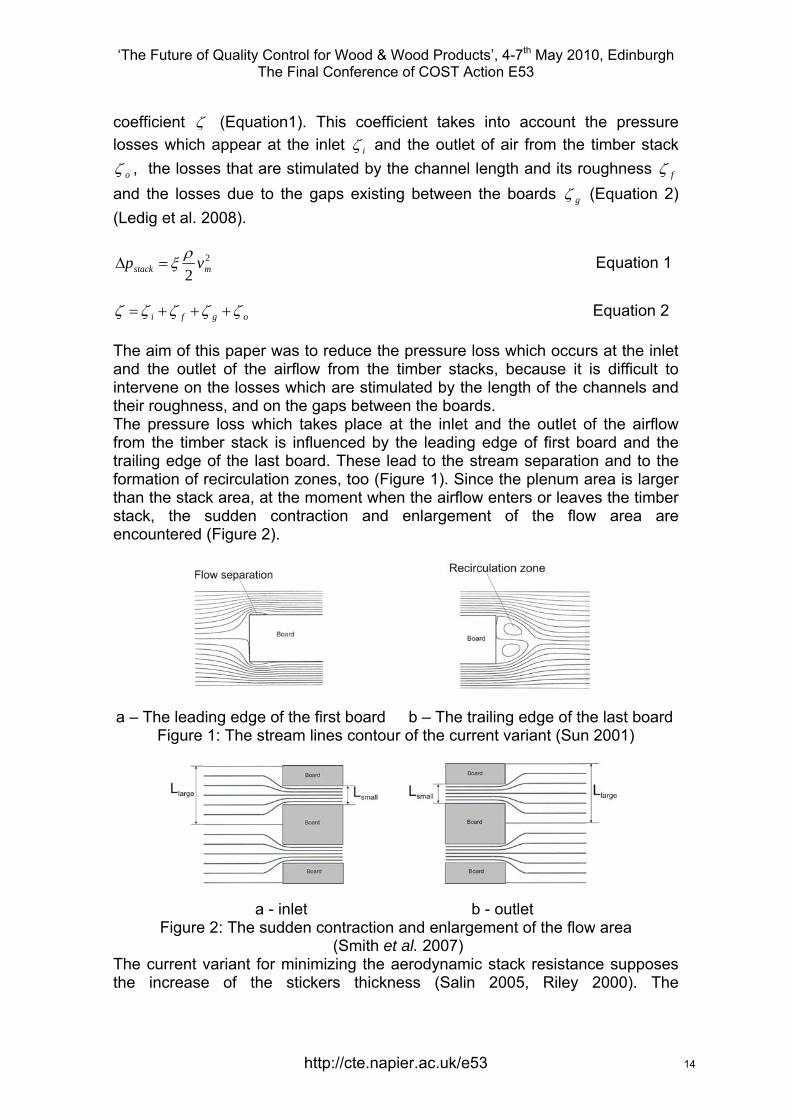
The aim of this paper was to reduce the pressure loss which occurs at the inlet and the outlet of the airflow from the timber stacks, because it is difficult to intervene on the losses which are stimulated by the length of the channels and their roughness, and on the gaps between the boards. The pressure loss which takes place at the inlet and the outlet of the airflow from the timber stack is influenced by the leading edge of first board and the trailing edge of the last board. These lead to the stream separation and to the formation of recirculation zones, too (Figure 1). Since the plenum area is larger than the stack area, at the moment when the airflow enters or leaves the timber stack, the sudden contraction and enlargement of the flow area are encountered (Figure 2).
a – The leading edge of the first board b – The trailing edge of the last board Figure 1: The stream lines contour of the current variant (Sun 2001)
a - inlet b - outlet Figure 2: The sudden contraction and enlargement of the flow area
(Smith et al. 2007) The current variant for minimizing the aerodynamic stack resistance supposes the increase of the stickers thickness (Salin 2005, Riley 2000). The
http://cte.napier.ac.uk/e53 14
‘The Future of Quality Control for Wood & Wood Products’, 4-7th May 2010, Edinburgh The Final Conference of COST Action E53
disadvantage of this solution refers to the diminishing of the drying capacity. In order to eliminate the disadvantage of the current solution, a documentation stage was carried out in the Fluid Mechanics field upon current types of inputs and outputs. The results have shown that the current type of input generates a pressure loss coefficient iζ equal to 0.5, and if the edges are rounded, the pressure loss coefficient iζ is equal to 0.04 (Table 1). The pressure loss coefficient for both types of outputs is equal to 1 (Table 2).
Table 1: The local resistance coefficient for various kinds of inlets (Fox et al. 1972)
The kind of inlet Figure Local resistance coefficient
Square – edged
inlet (current variant)
0.5
Rounded inlet (r/R = 0.25)
0.04
Table 2: The local resistance coefficient for various kinds of outlets (Fox et al. 1972)
The kind of outlet Figure Local resistance coefficient
Square – edged
outlet (current variant)
1
Rounded inlet
1
Therefore, if the variant which implies the rounding of the board edges, at both stack inlet and outlet, would be chosen, this would generate only the minimizing of the pressure losses which take place when the air enters the stack. The deepening of the research has shown that the local resistance, due to the sudden contraction and enlargement, may be diminished by attaching a cone at the inlet and the outlet of the air flow from the stack channels. The advantage of this solution consists in fact that the proposed variant is able to ensure a gradual transition from the larger area of the plenum to the smaller area of the stack channels. This advantage will ensure the minimizing of the local resistance coefficient compared with the current variant (Table 3).
http://cte.napier.ac.uk/e53 15
‘The Future of Quality Control for Wood & Wood Products’, 4-7th May 2010, Edinburgh The Final Conference of COST Action E53
Table 3: The local resistance coefficient for gradual contraction (Fox et al. 1972)
Figure Cone angle
Local resistance coefficient
30 0.02
45 0.04 60 0.07
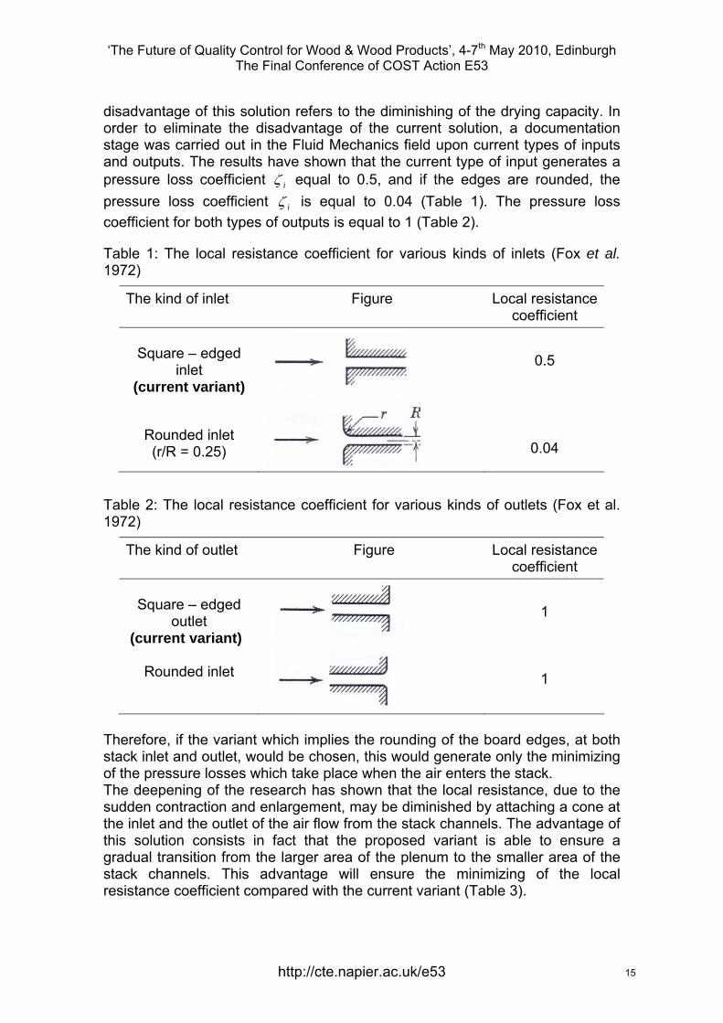
In order to create the cone effect at the inlet and the outlet of the air flow, in and from the stack channels, the solution of attaching some wood profiles in front and back of each board row was chosen (Figure 3).
a – current variant b – proposed variant Figure 3: The evidence of how the cone effect is created at the stack channels
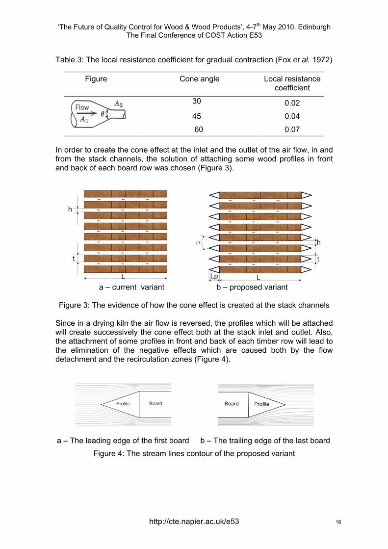
Since in a drying kiln the air flow is reversed, the profiles which will be attached will create successively the cone effect both at the stack inlet and outlet. Also, the attachment of some profiles in front and back of each timber row will lead to the elimination of the negative effects which are caused both by the flow detachment and the recirculation zones (Figure 4).
a – The leading edge of the first board b – The trailing edge of the last board Figure 4: The stream lines contour of the proposed variant
http://cte.napier.ac.uk/e53 16
‘The Future of Quality Control for Wood & Wood Products’, 4-7th May 2010, Edinburgh The Final Conference of COST Action E53
2. Materials and methods
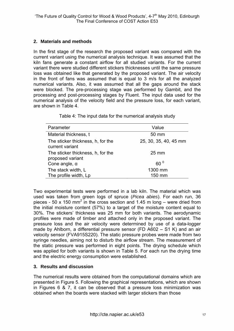
In the first stage of the research the proposed variant was compared with the current variant using the numerical analysis technique. It was assumed that the kiln fans generate a constant airflow for all studied variants. For the current variant there were studied different stickers thicknesses until the same pressure loss was obtained like that generated by the proposed variant. The air velocity in the front of fans was assumed that is equal to 3 m/s for all the analyzed numerical variants. Also, it was assumed that all the gaps around the stack were blocked. The pre-processing stage was performed by Gambit, and the processing and post-processing stages by Fluent. The input data used for the numerical analysis of the velocity field and the pressure loss, for each variant, are shown in Table 4.
Table 4: The input data for the numerical analysis study
Parameter Value Material thickness, t 50 mm The sticker thickness, h, for the current variant
25, 30, 35, 40, 45 mm
The sticker thickness, h, for the proposed variant
25 mm
Cone angle, α 60 0 The stack width, L 1300 mm The profile width, Lp 150 mm
Two experimental tests were performed in a lab kiln. The material which was used was taken from green logs of spruce (Picea abies). For each run, 36 pieces - 50 x 150 mm2 in the cross section and 1.45 m long – were dried from the initial moisture content (57%) to a target of the moisture content equal to 30%. The stickers’ thickness was 25 mm for both variants. The aerodynamic profiles were made of timber and attached only in the proposed variant. The pressure loss and the air velocity were determined by use of a data-logger made by Ahlborn, a differential pressure sensor (FD A602 – S1 K) and an air velocity sensor (FVA915S220). The static pressure probes were made from two syringe needles, aiming not to disturb the airflow stream. The measurement of the static pressure was performed in eight points. The drying schedule which was applied for both variants is shown in Table 5. For each run the drying time and the electric energy consumption were established.
3. Results and discussion
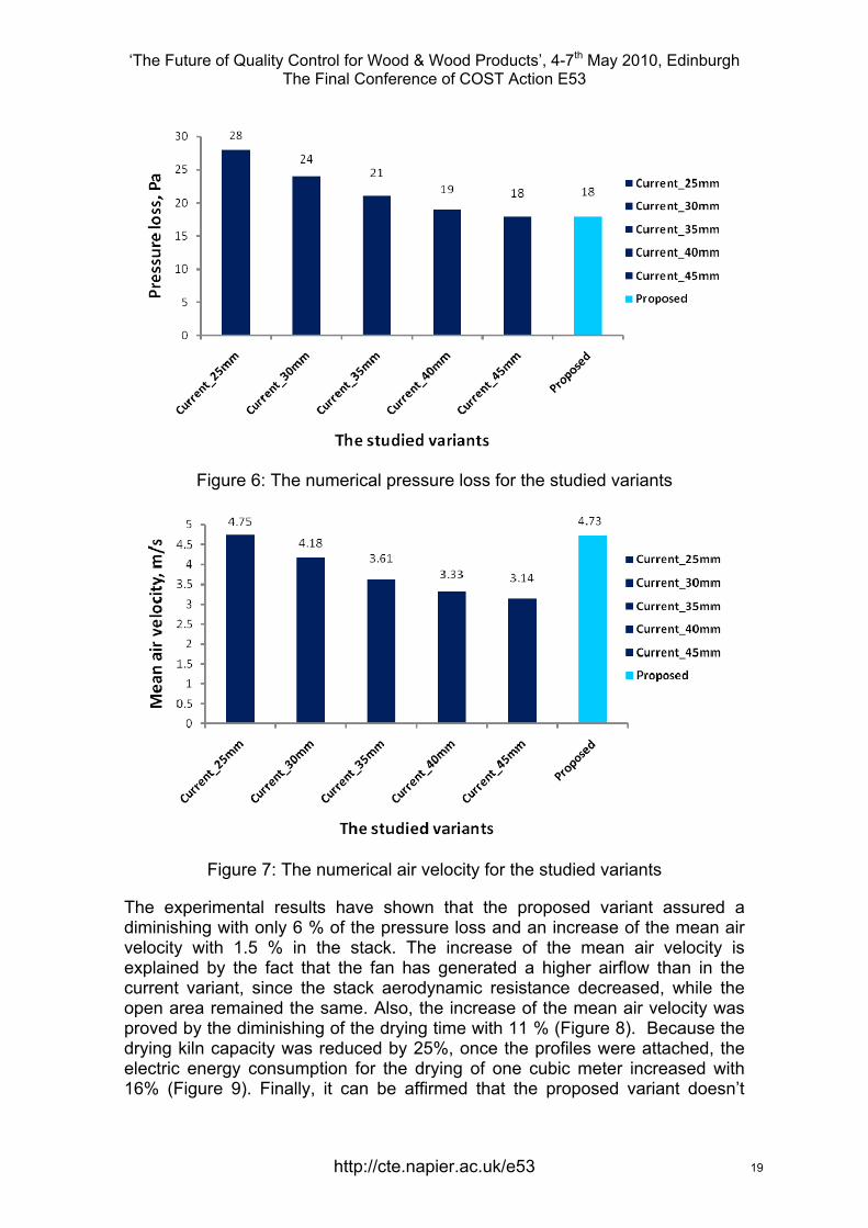
The numerical results were obtained from the computational domains which are presented in Figure 5. Following the graphical representations, which are shown in Figures 6 & 7, it can be observed that a pressure loss minimization was obtained when the boards were stacked with larger stickers than those
http://cte.napier.ac.uk/e53 17
‘The Future of Quality Control for Wood & Wood Products’, 4-7th May 2010, Edinburgh The Final Conference of COST Action E53
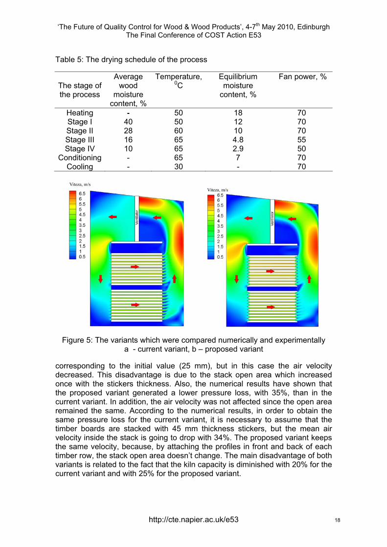
Table 5: The drying schedule of the process
The stage of the process
Average wood
moisture content, %
Temperature, 0C
Equilibrium moisture
content, %
Fan power, %
Heating - 50 18 70 Stage I 40 50 12 70 Stage II 28 60 10 70 Stage III 16 65 4.8 55 Stage IV 10 65 2.9 50
Conditioning - 65 7 70 Cooling - 30 - 70
Figure 5: The variants which were compared numerically and experimentally a - current variant, b – proposed variant
corresponding to the initial value (25 mm), but in this case the air velocity decreased. This disadvantage is due to the stack open area which increased once with the stickers thickness. Also, the numerical results have shown that the proposed variant generated a lower pressure loss, with 35%, than in the current variant. In addition, the air velocity was not affected since the open area remained the same. According to the numerical results, in order to obtain the same pressure loss for the current variant, it is necessary to assume that the timber boards are stacked with 45 mm thickness stickers, but the mean air velocity inside the stack is going to drop with 34%. The proposed variant keeps the same velocity, because, by attaching the profiles in front and back of each timber row, the stack open area doesn’t change. The main disadvantage of both variants is related to the fact that the kiln capacity is diminished with 20% for the current variant and with 25% for the proposed variant.
http://cte.napier.ac.uk/e53 18
‘The Future of Quality Control for Wood & Wood Products’, 4-7th May 2010, Edinburgh The Final Conference of COST Action E53
Figure 6: The numerical pressure loss for the studied variants
Figure 7: The numerical air velocity for the studied variants
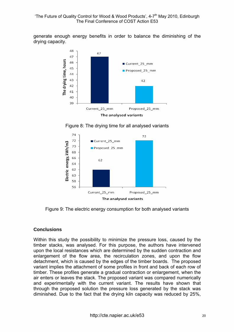
The experimental results have shown that the proposed variant assured a diminishing with only 6 % of the pressure loss and an increase of the mean air velocity with 1.5 % in the stack. The increase of the mean air velocity is explained by the fact that the fan has generated a higher airflow than in the current variant, since the stack aerodynamic resistance decreased, while the open area remained the same. Also, the increase of the mean air velocity was proved by the diminishing of the drying time with 11 % (Figure 8). Because the drying kiln capacity was reduced by 25%, once the profiles were attached, the electric energy consumption for the drying of one cubic meter increased with 16% (Figure 9). Finally, it can be affirmed that the proposed variant doesn’t
http://cte.napier.ac.uk/e53 19
‘The Future of Quality Control for Wood & Wood Products’, 4-7th May 2010, Edinburgh The Final Conference of COST Action E53
generate enough energy benefits in order to balance the diminishing of the drying capacity.
Figure 8: The drying time for all analysed variants
Figure 9: The electric energy consumption for both analysed variants
Conclusions
Within this study the possibility to minimize the pressure loss, caused by the timber stacks, was analysed. For this purpose, the authors have intervened upon the local resistances which are determined by the sudden contraction and enlargement of the flow area, the recirculation zones, and upon the flow detachment, which is caused by the edges of the timber boards. The proposed variant implies the attachment of some profiles in front and back of each row of timber. These profiles generate a gradual contraction or enlargement, when the air enters or leaves the stack. The proposed variant was compared numerically and experimentally with the current variant. The results have shown that through the proposed solution the pressure loss generated by the stack was diminished. Due to the fact that the drying kiln capacity was reduced by 25%,
http://cte.napier.ac.uk/e53 20

‘The Future of Quality Control for Wood & Wood Products’, 4-7th May 2010, Edinburgh The Final Conference of COST Action E53
when the profiles were used, the proposed variant doesn’t generate enough energy benefits in order to balance this disadvantage.
References Bedelean, I.B. (2009) – Contributions to the aerodynamic study of wood drying kilns. PhD thesis. Transilvania University of Brasov, Romania.
Fox, W. R., McDonald, A.T. (1973) - Introduction to Fluid Mechanics. Second Edition. John Wiley & Sons, New York, Toronto. Ledig, S.F., Paarhuis, B., Riepen, M. (2008) - Airflow within kilns. In Fundamentals of wood drying. A.R.BO.LOR. Nancy, Chapter 13, 311 – 332. Nijdam, J., Keey, R. (2002) ”An experimental study of airflow in lumber kilns”. Wood Science and Technology, Vol. 36, pp. 19 – 26. Riley, S. (2000) ”Selection of kiln fillets”. Wood Proccesing Newsletter, No. 28, pp. 14 – 15. Salin, J.G. (2005) “The influence of some factors on the timber drying process, analyzed by a global simulation model”. Maderas. Ciencia Tecnologia, Vol. 7 (3), pp. 195 – 204. Smith, G.J.F., Du Plessis, J.P., Du Plessis (Sr), J.P. (2007) “Modelling of airflow through a stack in a timber-drying kiln “. Applied mathematical modelling, Vol. 31, pp. 270 – 282.
Sun, Z. F. (2001) “Numerical simulation of flow in an array of in – line blunt boards: mass transfer and flow patterns”. Chemical Engineering Science, Vol. 56, pp. 1883 – 1896.
http://cte.napier.ac.uk/e53 21
‘The Future of Quality Control for Wood & Wood Products’, 4-7th May 2010, Edinburgh The Final Conference of COST Action E53
http://cte.napier.ac.uk/e53
Pre-sorting for density in drying batches of Norway spruce boards
Y. Steiner1 & A. Øvrum
2
Abstract
One of the key processes for product performance, and the most energy consuming process in the production of solid timber, is the drying process, a process heavily influenced by the wood density. Normally no information of density in a timber drying batch is known today, apart from previous experience of the level of density for the timber of that particular mill. In this study the effect of dividing boards into a high and a low density drying batch was investigated.
66 boards of 50 x 150 mm2 were collected randomly from the green sorting at a Norwegian sawmill. The boards were cut into 1200 mm long pieces and grouped in a high density group, low density group and a mixed density group. The batches were dried in a laboratory kiln with a constant dry bulb temperature of 70 °C and a decreasing wet bulb temperature. The drying schedule was designed with the help of simulation software and was adapted to the average density and average moisture content of each batch. Total drying times for the low, mixed and high density batch was 58 h, 63 h and 70 h respectively.
The downgrading due to checks showed no statistically significant difference between the density batches and the final moisture content was statistically equal. Only the level of case hardening was significantly lower for the low density batch. This density separation resulted in a net saving of 4 % in drying time at the test mill.
1 Introduction
One of the key processes for product performance, and the most energy consuming process in the production of solid timber, is the drying process. A pre-sorting of timber prior to drying should be performed after the drying rates of the timber, i.e. by moisture content and density (Avramidis et al. 2004). This will yield a more homogenous moisture content after drying, decreasing the amount of over-dried and under-dried boards. It also allows the use of more efficient drying schedules. According to Esping (1992) the drying time is doubled if the density is doubled when drying green 50 mm thick Scots pine boards down to 20 % MC in a constant climate with a temperature of 50 °C, RH of 60 % and air velocity of 1.3 m/s. Under the fiber saturation point (FSP) the drying time may quadruple if the density of a board is doubled (Esping 1992) given the same climate conditions as above. This increase in drying time due to increased density is stronger the higher the temperature in the kiln is (Esping 1992) when
1 Master in Forestry, [email protected] 2 Senior researcher, [email protected] Norsk Treteknisk Institutt, Norway
22
‘The Future of Quality Control for Wood & Wood Products’, 4-7th May 2010, Edinburgh The Final Conference of COST Action E53
http://cte.napier.ac.uk/e53
drying timber under the FSP. This makes density in the drying process increasingly relevant in modern sawmilling since the temperature in the kilns has been raised substantially the later years. The density influence on drying time is the main cause of spread in the moisture content within a drying batch (Esping 1992) since the density range is large between boards within a normal drying batch.
As Rozema and Schuijl (2005) shows, a pre-sorting of boards by an in-line moisture meter using the capacitance method is not sufficiently accurate, and will require a density measurement and possibly some kind of heartwood/sapwood separation as well. However, Elustondo and Oliveira (2009) found a reduction in drying time of 7 percent by dividing boards in three groups according to the measured MC in green boards with an in-line capacitance moisture meter.
Normally no information of density in a drying batch is known in a sawmill today, apart from previous experience of the level of density for the timber of that particular mill. This implies that the sawmills must let the highest density boards in a batch decide the drying schedule in a kiln, since they are most prone to develop checks, and need the longest time to obtain the target moisture content. This results in a drying schedule with too mild climate for most of the boards in a drying batch, and as such a great reduction in drying can be achieved by homogenization of the density in a drying batch. A division of boards in two groups of density level can be imagined as a homogenization that could be obtained in practice. The effect of such a homogenization will give reduced drying time, decreased spread in moisture content and possibly reduced occurrence of drying checks, distortion and case hardening. The challenge is to find accurate means of finding the density in each board and allocate it to different density groups. Most sawmills do not have density measurement systems for green boards installed, although technology is available, mainly through x-ray or weighing equipment. Such equipment do, however, need some kind of moisture content approximations either through measurements in-line or of quality control of drying batches. This will not make them possible to use early in the process either on logs or on green boards with high accuracy due to the high and varying moisture content in green timber.
A number of prediction models for basic density in Norway spruce exists, for example; for individual annual rings (Mäkinen et al. 2007), for 20 mm segments from the pith and outwards on several stem heights (Lindström 2000), for different cross-sections in stems (Ikonen et al. 2008; Wilhelmsson et al. 2002), for different logs (Duchesne et al. 1997) and for individual stems (Bergstedt and Olesen 2000). From such models a division into density classes could be implemented, the simplest system using the dimension of the boards as the prediction parameter. Another, or sometimes additional separation, will be to separate inner boards, i.e. boards adjacent to the pith from the boards further from the pith. The inner boards probably will have a lower density due to more juvenile wood which has a lower density than wood closer to the bark. Typically the first fifteen to twenty annual rings consist of juvenile wood. Such a differentiation is done in several mills when producing sound knot timber or
23
‘The Future of Quality Control for Wood & Wood Products’, 4-7th May 2010, Edinburgh The Final Conference of COST Action E53
http://cte.napier.ac.uk/e53
heartwood timber. More advanced models for density separation could include forest data like site or tree variables, giving a higher prediction accuracy.
This study has been performed to investigate the benefits of knowing the density and reducing the density spread in drying batches. The study used data from timber collected in the running production at a Norwegian sawmill.
2 Materials and methods
66 boards of 50 x 150 mm2 were collected randomly from the green sorting at a Norwegian sawmill. From each board three 1200 mm long samples were cut and both ends of the samples were sealed with silicone prior to drying. From the remaining piece of the boards, density and moisture content were measured. Moisture content and basic density were measured by the oven-dry method according to EN 13183-1, and volume determined by immersion of the samples in water according to Kučera (1992).
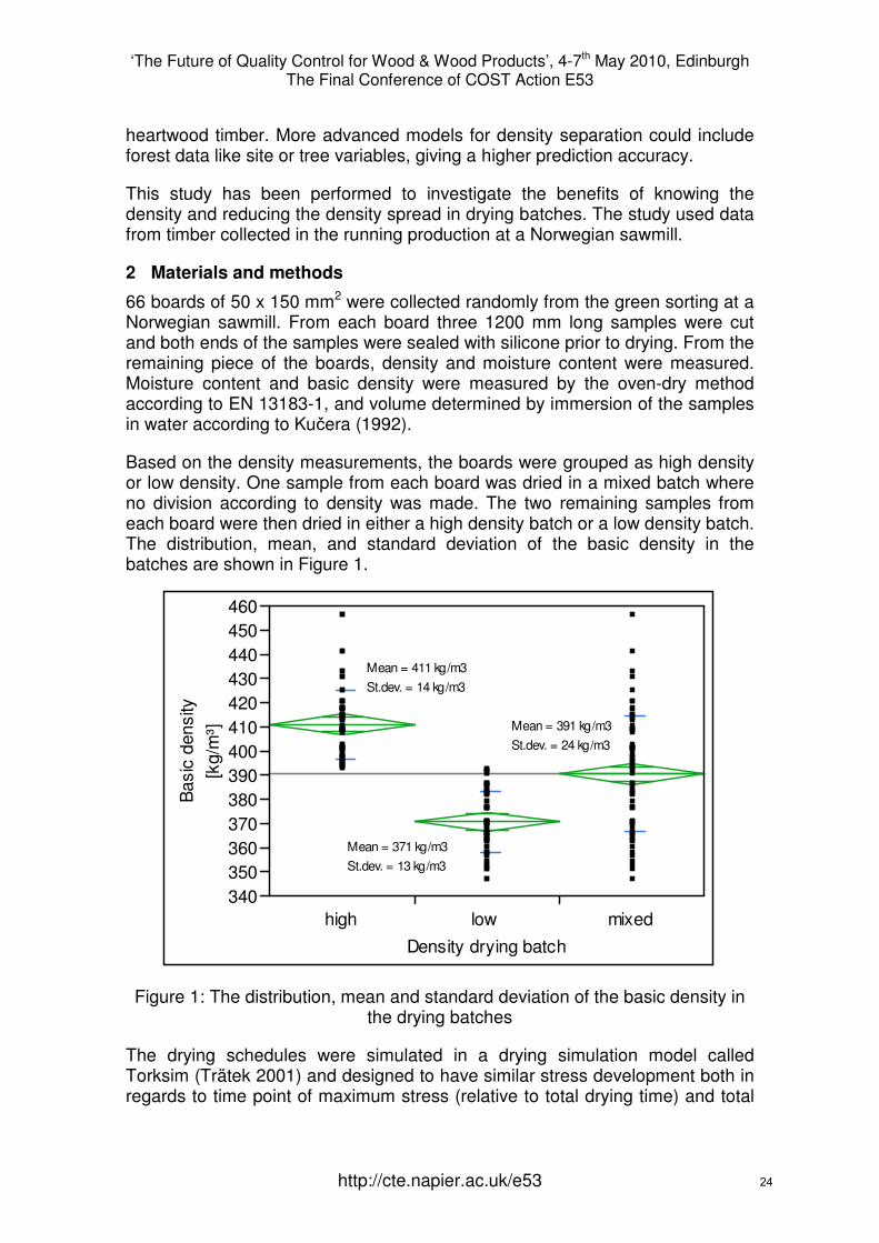
Based on the density measurements, the boards were grouped as high density or low density. One sample from each board was dried in a mixed batch where no division according to density was made. The two remaining samples from each board were then dried in either a high density batch or a low density batch. The distribution, mean, and standard deviation of the basic density in the batches are shown in Figure 1.
340350360370380390400410420430440450460
Bas
ic d
ensi
ty[k
g/m
³]
high low mixed
Density drying batch
Mean = 411 kg/m3
St.dev. = 14 kg/m3
Mean = 371 kg/m3
St.dev. = 13 kg/m3
Mean = 391 kg/m3
St.dev. = 24 kg/m3
Figure 1: The distribution, mean and standard deviation of the basic density in the drying batches
The drying schedules were simulated in a drying simulation model called Torksim (Trätek 2001) and designed to have similar stress development both in regards to time point of maximum stress (relative to total drying time) and total
24
‘The Future of Quality Control for Wood & Wood Products’, 4-7th May 2010, Edinburgh The Final Conference of COST Action E53
http://cte.napier.ac.uk/e53
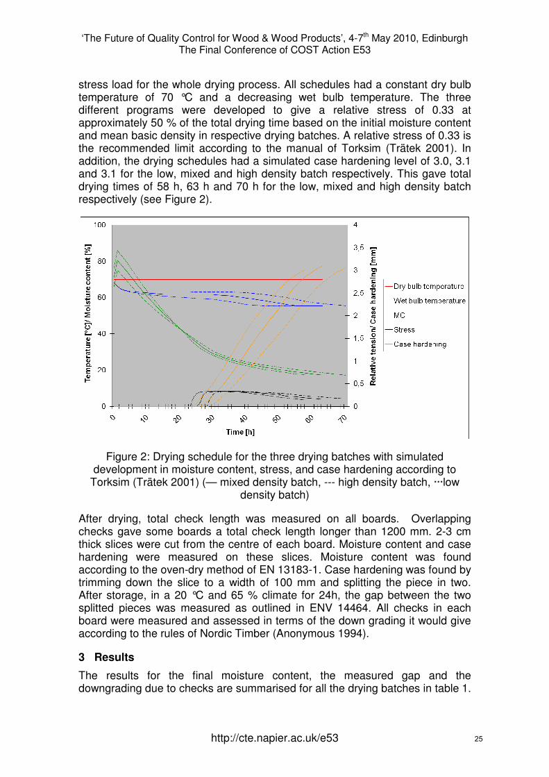
stress load for the whole drying process. All schedules had a constant dry bulb temperature of 70 °C and a decreasing wet bulb temperature. The three different programs were developed to give a relative stress of 0.33 at approximately 50 % of the total drying time based on the initial moisture content and mean basic density in respective drying batches. A relative stress of 0.33 is the recommended limit according to the manual of Torksim (Trätek 2001). In addition, the drying schedules had a simulated case hardening level of 3.0, 3.1 and 3.1 for the low, mixed and high density batch respectively. This gave total drying times of 58 h, 63 h and 70 h for the low, mixed and high density batch respectively (see Figure 2).
Figure 2: Drying schedule for the three drying batches with simulated development in moisture content, stress, and case hardening according to
Torksim (Trätek 2001) (— mixed density batch, --- high density batch, ···low density batch)
After drying, total check length was measured on all boards. Overlapping checks gave some boards a total check length longer than 1200 mm. 2-3 cm thick slices were cut from the centre of each board. Moisture content and case hardening were measured on these slices. Moisture content was found according to the oven-dry method of EN 13183-1. Case hardening was found by trimming down the slice to a width of 100 mm and splitting the piece in two. After storage, in a 20 °C and 65 % climate for 24h, the gap between the two splitted pieces was measured as outlined in ENV 14464. All checks in each board were measured and assessed in terms of the down grading it would give according to the rules of Nordic Timber (Anonymous 1994).
3 Results
The results for the final moisture content, the measured gap and the downgrading due to checks are summarised for all the drying batches in table 1.
25
‘The Future of Quality Control for Wood & Wood Products’, 4-7th May 2010, Edinburgh The Final Conference of COST Action E53
http://cte.napier.ac.uk/e53
An analysis of variance showed no significant differences in MC between the batches in MC.
A higher tendency of checking was found in the high density batch, but a Chi Square test gave no statistically significant difference.
The gap in the low density batch was found to be smaller than in the other batches by a student-t test of variance with a level of significance of over 99 %.
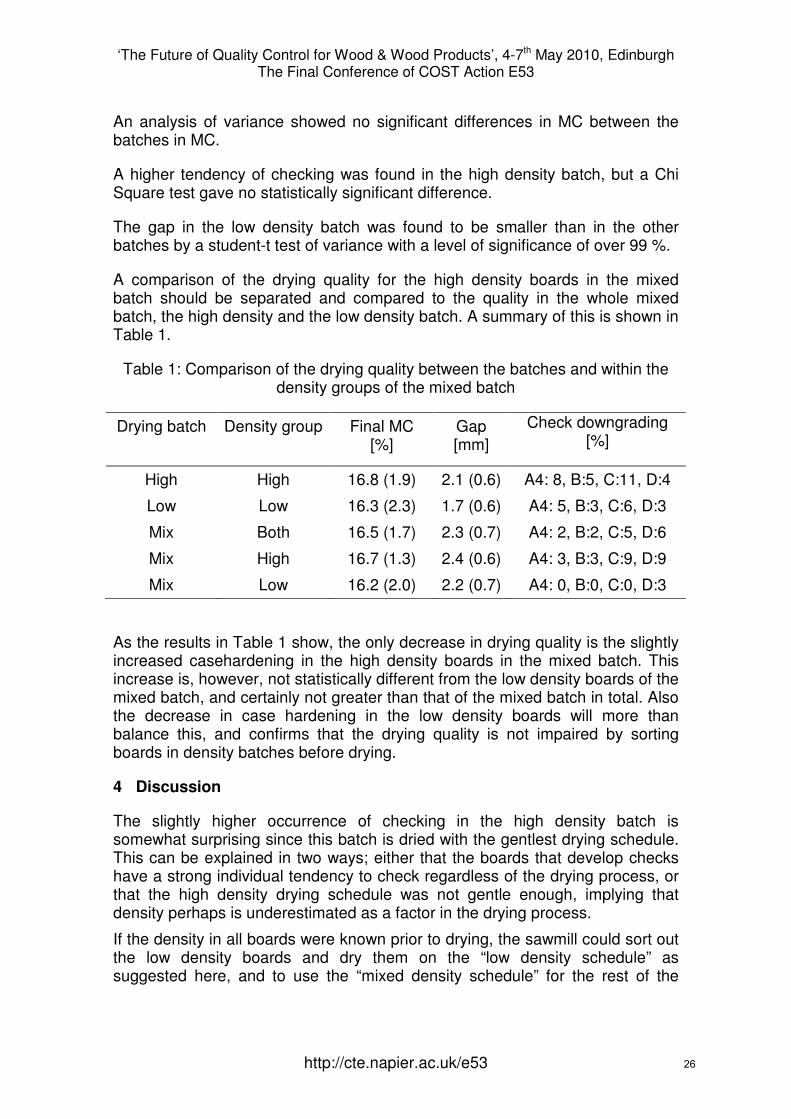
A comparison of the drying quality for the high density boards in the mixed batch should be separated and compared to the quality in the whole mixed batch, the high density and the low density batch. A summary of this is shown in Table 1.
Table 1: Comparison of the drying quality between the batches and within the density groups of the mixed batch
Drying batch Density group Final MC [%]
Gap [mm]
Check downgrading [%]
High High 16.8 (1.9) 2.1 (0.6) A4: 8, B:5, C:11, D:4
Low Low 16.3 (2.3) 1.7 (0.6) A4: 5, B:3, C:6, D:3
Mix Both 16.5 (1.7) 2.3 (0.7) A4: 2, B:2, C:5, D:6
Mix High 16.7 (1.3) 2.4 (0.6) A4: 3, B:3, C:9, D:9
Mix Low 16.2 (2.0) 2.2 (0.7) A4: 0, B:0, C:0, D:3
As the results in Table 1 show, the only decrease in drying quality is the slightly increased casehardening in the high density boards in the mixed batch. This increase is, however, not statistically different from the low density boards of the mixed batch, and certainly not greater than that of the mixed batch in total. Also the decrease in case hardening in the low density boards will more than balance this, and confirms that the drying quality is not impaired by sorting boards in density batches before drying.
4 Discussion
The slightly higher occurrence of checking in the high density batch is somewhat surprising since this batch is dried with the gentlest drying schedule. This can be explained in two ways; either that the boards that develop checks have a strong individual tendency to check regardless of the drying process, or that the high density drying schedule was not gentle enough, implying that density perhaps is underestimated as a factor in the drying process.
If the density in all boards were known prior to drying, the sawmill could sort out the low density boards and dry them on the “low density schedule” as suggested here, and to use the “mixed density schedule” for the rest of the
26
‘The Future of Quality Control for Wood & Wood Products’, 4-7th May 2010, Edinburgh The Final Conference of COST Action E53
http://cte.napier.ac.uk/e53
boards (the high density boards). One condition for such a choice is that the drying quality is maintained.
In practice the only difference in drying quality between the batches is a smaller level of case hardening in the batches of low density timber. This tendency of smaller case hardening in the low density batch implies that a shorter period of conditioning in timber meant for splitting in further processing could be imposed.
Based on this study, the net effect of this density separation in batches will be the decreased drying time of 5 h for the low density batches compared to the mixed batch. For the sawmill, this means a time save of 5 h for half of the drying batches, or 2.5 per batch in their total timber production. This constitutes a net saving in drying time of 4 % in the kiln drying of timber at this sawmill.
In a study of drying of hem-fir squares of 101 x101 mm2 Zhang et al.(1996) found a decrease in drying time of 24, 22 and 15 % respectively for low density batches of hem-fir, all hemlock and all-fir batches compared to high density batches. Their separation was done similarly as in this study, but the difference in mean density was larger. 447 to 376 for hem-fir, 472 to 395 for all-hemlock and 386 to 325 for all-fir respectively. This could explain the larger saving in drying time in their study.
Time saving in kiln drying in itself is positive for a saw mill since the drying capacity often is the bottleneck in timber production. This allows a saw mill to increase the production capacity without kiln investments, and also in the long run decrease the volume of kilns making the need for capital invested in production equipment smaller.
The initial moisture content is also important for the drying time and quality as is shown by Elustondo and Oliveira (2009) and Sugimori et al. (2006), but did not affect the drying quality significantly in this study.
References
Anonymous (1994) “Nordic Timber. Grading rules for pine (Pinus silvestris) and spruce (Picea abies) sawn timber: Commercial grading based on evaluation of the four sides of sawn timber”. Treindustriens tekniske forening, Oslo
Avramidis, S, Aune, JE, and Oliveira, L (2004) “Exploring pre-sorting and re-drying strategies for Pacific coast hemlock square timbers”. Journal of the Institute of Wood Science 16(4):189-198
Bergstedt, A, and Olesen, PO (2000) “Models for Predicting Dry Matter Content of Norway spruce”. Scandinavian Journal of Forest Research 15(6):633 - 644
CEN (2002) “EN 13183-1 Moisture content of a piece of sawn timber – Part 1: Determination by oven dry method (Corrigendum AC:2003 incorporated)”, European Committee for Standardization.
27

‘The Future of Quality Control for Wood & Wood Products’, 4-7th May 2010, Edinburgh The Final Conference of COST Action E53
http://cte.napier.ac.uk/e53
CEN (2002) “ENV 14464 Sawn timber – Method for assessment of case-hardening”, European Committee for Standardization.
Duchesne, I, Wilhelmsson, L, and Spangberg, K (1997) “Effects of in-forest sorting of Norway spruce (Picea abies) and Scots pine (Pinus sylvestris) on wood and fibre properties”. Canadian Journal of Forest Research-Revue Canadienne De Recherche Forestiere 27(5):790-795
Elustondo, DM, and Oliveira, L (2009) “A method for optimizing lumber sorting before kiln-drying”. Forest Products Journal 59(9):45-50
Esping, B (1992) “Grunder i torkning [Basics in drying]”. Trätek, Stockholm [In Swedish]
Ikonen, V-P, Peltola, H, Wilhelmsson, L, Kilpeläinen, A, Väisänen, H, Nuutinen, T, and Kellomäki, S (2008) “Modelling the distribution of wood properties along the stems of Scots pine (Pinus sylvestris L.) and Norway spruce (Picea abies (L.) Karst.) as affected by silvicultural management” Forest Ecology and Management, 256(6):1356-1371
Kučera, B (1992) “Skandinaviske normer for testing av små feilfrie prøver av heltre [Scandinavian norms for testing of clearwood samples of solid wood]”. Skogforsk, Ås [In Norwegian]
Lindström, H (2000) “Intra-tree models of basic density in Norway spruce as an input to simulation software”. Silva Fennica 34(4):411-421
Mäkinen, H, Jaakkola, T, Piispanen, R, and Saranpaa, P (2007) “Predicting wood and tracheid properties of Norway spruce”. Forest Ecology and Management 241(1-3):175-188
Rozema, P, and Schuijl, M (2005) “Pre-sorting of timber according to green moisture and density”. P. 38-40 in Measures for improving quality and shape stability of sawn softwood timber during drying and under service conditions. Best practice manual to improve straightness of sawn timber, Tarvainen, V. (ed.). VTT
Sugimori, M, Hayashi, K, and Takechi, M (2006) “Sorting sugi lumber by criteria determined with cluster analysis to improve drying”. Forest Products Journal 56(2)
Tronstad, S (2001) ”Tørking av trevirke [Drying of timber]”. Byggenæringens forlag, Lillestrøm [In Norwegian]
Trätek (2001) ”Manual och användarbeskrivning till programmet TORKSIM ver. 3.0.1”, Stockholm (in Swedish)
Wilhelmsson, L, Arlinger, J, Spångberg, K, Lundqvist, SO, Grahn, T, Hedenberg, O, and Olsson, L (2002) “Models for predicting wood properties in
28

‘The Future of Quality Control for Wood & Wood Products’, 4-7th May 2010, Edinburgh The Final Conference of COST Action E53
http://cte.napier.ac.uk/e53
stems of Picea abies and Pinus sylvestris in Sweden”. Scandinavian Journal of Forest Research 17(4):330-350
Zhang, Y, Oliveira, L, and Avramidis, S (1996) “Drying characteristics of hem-fir squares as affected by species and basic density presorting”. Forest Products Journal 46(2):44-50
29

‘The Future of Quality Control for Wood & Wood Products’, 4-7th May 2010, Edinburgh The Final Conference of COST Action E53
http://cte.napier.ac.uk/e53
Dtouch – drying has never been so easy
O. Allegretti 1, I. Cuccui1, S. Ferrari1 & A. Sione2
Abstract The paper reports experience about an in progress project for the develop of a new control for kiln wood drying process. The control contains a database of standard and special drying schedules and other technological parameters for more than 400 temperate and tropical species. These data, coming from different sources, allow to generate a suitable initial drying schedule for a given species and thickness. A series of functions and algorithms implemented in the control allow to customize the initial schedule by defining the best parameters to obtain a final specific result priority (colour, internal stresses, drying time). The control has auto learning functions for the optimisation of the drying schedule. The expert system is based on the analysis of data process automatically acquired by the control during drying and on input data inserted by the operator at the end of the process answering to a questionnaire related to drying quality and drying kinetic. At the present stage of the project, the debugged beta version of the control is installed in kilns of selected industrial operators involved in the project.
1 Introduction A kiln dryer control system keeps the parameters of air within the kiln (Temperature, Relative Humidity, and occasionally air speed) on a set-up values defined by the drying schedule (DS). MC-DS in which change of air conditions occurs depending on current value of lumber MC loaded in the kiln are the most used in the industry. They have a multistage structure with a rising temperature and a decreasing RH. The initial and final values of air parameters of the DS depends on wood species on the thickness and on the initial MC. The past information from different sources and existing DS for similar woods are usually utilised in developing schedules.
Even in the best conditions (i.e. good control of air parameters, homogeneous distributions of air, correct stacking) the results of drying in term of quality and time is usually unpredictable, unreliable and non-repeatable. This due to:
◘ Complexity and non-linearity of the drying process; ◘ Heterogeneity of the wood;
1 LABESS (Wood Drying Lab) of CNR-IVALSA Italian Research Council – Timber and Trees Institute, S. Michele all’Adige, Trento - ITALY, [email protected] 2 LOGICA H&S- Drying process and moisture testing, Udine - ITALY, www.logica-hs.com, [email protected]
30

‘The Future of Quality Control for Wood & Wood Products’, 4-7th May 2010, Edinburgh The Final Conference of COST Action E53
http://cte.napier.ac.uk/e53
◘ Inaccuracy of the quality/quantity of input data, i.e. the MC of the lumbers in the stack.
◘ Unattended operations and events. The research activity in the last 30 years in the field of wood drying has contributed to a better understanding of the drying process and many works were focused of the improvement of control systems. In particular numerical modelling techniques and adaptative/intelligent control techniques were the most explored and they are currently investigated in industrial applications.
Numerical Models had a huge development in the last 10 years, also thank to the increasing power/cost ratio of commercial PC. Nevertheless they are only sporadically applied on commercial on-line controls. One of the reason is the high number of variable and constants of constituent equations involved and the high range of variability of their value. By this point of view, the variability of the stack in the kiln drying process make difficult the control of the drying process by means of an average calculated value.
Intelligent controls based on fuzzy-logic or on other statistical analysis were successfully developed and implemented in the automation of industrial system above all for on line control of drying parameters based on the existing input data. However, the input data, above all concerning the drying quality evaluation, are still nowadays one of the main problem for their full application.
For those reason kiln drying process still requires a constant presence of a kiln operator for frequent monitoring and appropriate parameter adjustment. By this point of view, the kiln operator’s skill and experience is still nowadays one of the most important capital of companies, especially the ones involved in drying of hardwood.
This paper describes a project for the develop of a new control system for the wood drying process carried out by the author’s affiliations.
Logica H&S has been founded in 1991, it provides services and products for industrial process controls, for test and measurement devices in industrial, consumer and automotive applications, wood drying and wood moisture measuring fields. Initially the production was directed only to Italian KD producers, then the commercialization has been extended to all over the world, with special attention to the East Europe and Asian markets. In almost 19 years of activity, its products have been installed in over 50 Countries.
The project concerns the develop of the software, firmware and part of the hardware design. It started about one and half year ago and at the present the beta version of the control is at a testing stage in drying kilns of some factories in Italy.
31

‘The Future of Quality Control for Wood & Wood Products’, 4-7th May 2010, Edinburgh The Final Conference of COST Action E53
http://cte.napier.ac.uk/e53
The core concepts at the basis of the control are :
◘ state of the art of the scientific knowledge about drying process of many wood species already codified in the memory of the control for a safety starting point;
◘ an integration between human and machine through a friendly interface towards a cross-learning path;
◘ a structure of data storage and data mining which allows an accumulation of knowledge and a reduction of the variability effect of the drying process factors.
The goal of the project is to make available on the market a control system that can be used worldwide on every type of conventional kiln drying for every species, temperate and tropical, softwood and hardwood, easy to install to configure and to use and flexible enough to ensure a good and safe starting point towards an optimised drying schedule whatever the operative condition and the operator’s training level is.
2 The drying schedule creation
dTOUCH aims to be a step ahead in the control systems for kiln dryers, since it combines an advanced and flexible control system with the know-how of international experts in the timber drying field. It includes a wide range of base drying programs for over 400 timber species, including also some special DS to maintaining/changing the natural colour of the wood, for fast drying and so on. It uses this data base, together with the information received from the sensors and the inputs from the user (such as thickness, required quality, priority to time or to quality, particular requirements..) to create the program suitable to drying the wood according to the specific needs of the user. The system can automatically identify some critical conditions (like frozen wood, possible casehardened wood etc.) and modify the base drying program in order to include the most suitable remedy for the identified problem.
The creation of a customized program using dTOUCH does not require the operator to learn about drying methods and programming details (temperature, humidity, time, etc..); it is enough to “explain” to the system what are the special requirements by answering to some questions.
2.1 The database At the moment, the control system contains a database with about 500 records corresponding to the same number of basic drying schedules for about 400 wood species. Every species is identified by the botanical name or by the commercial name in different languages. Some species have more than one record for different proveniences or for special drying schedules. For example the beech (Fagus sylvatica) has standard schedule as well as special schedule for different final colours.
32

‘The Future of Quality Control for Wood & Wood Products’, 4-7th May 2010, Edinburgh The Final Conference of COST Action E53
http://cte.napier.ac.uk/e53
Others information are associated to each records. Basically they concern technological information (density, shrinkages…), information on possible defects that could influence the drying quality (collapses, water pockets…) and, when available comments, prescriptions and warnings that, displayed on the screen, could help the user to get a better results (air pre-drying suggested, end coat suggested, tendency to warp…). Some of those information are used by the system for different purposes such as for the optimisation process or for some other calculation.
2.2 The drying schedule The drying schedule system used in the control has been developed assembling, modifying and simplifying different systems already existing. The main kiln drying schedule sources are the Dry Kiln Operator’s Manual by USDA, the Timber Drying Manual by BRE and the Cividini’s Conventional Drying of lumber (Essiccazione convenzionale dei Legnami). Further information comes from the internal LABESS database, a collection of data from drying tests during ‘60s and ‘70’s by Prof. Cividini and Giordano at IVALSA.
Specifications of the dTouch drying schedule system (dT DS) implemented in the control are:
1. The input data to create the basic drying schedule is species and thickness of lumber. For some of these species/thickness combination there are more options such as different final colour or special end product request.
2. Like in the USDA system the schedules are identified by a code of three numbers (ID-Code): the first identifies the temperature profile, the second the critical MC (MCcr) at which there is the first change of the EMC and the third the EMC profile.
3. A ID-Code corresponding to a given dT DS is assigned to each record (wood species) of the database. The combination of species/ drying schedule is done on the basis of the existing DS systems.
4. There are 14 temperature (T) profiles MC dependents. T start to increase when the MC is 35% and linearly increase up 15% MC. Each profile is characterised by a minimum and maximum T.
5. There are 12 EMC profiles MC dependents. EMC is usually directly measured by the cellulose plates but it can be also calculated from RH or dry/wet bulb by mean of the Hailwood Horrobin equation. Each EMC profiles is identified by a nominal drying Gradient (G) = MC/EMC. Each EMC profile is characterised by a constant EMC (varying G) during the 1st drying stage and constant G (decreasing EMC) starting from MCcr and during all the 2nd and 3rd drying stage.
6. Depending of the thickness (th) of lumber the nominal G is transformed in the real G. A two parameters first degree function G =f(th) is used to calculate real G as a function of thickness. T does not vary with lumber thickness.
33
‘The Future of Quality Control for Wood & Wood Products’, 4-7th May 2010, Edinburgh The Final Conference of COST Action E53
http://cte.napier.ac.uk/e53
7. the USDA system has 6 MCcr values from 30% to 70%. The dTouch drying schedule system was simplified to only three value from 30% to 45%. The reason of this simplification is that the electrical MC measure is not accurate for value higher than about 45%.
8. An air velocity profile (V) wood density and thickness dependent is also generated.
9. Complementary phases such as warm-up, equalisation and conditioning is also generated by the system. Other supplementary phases such as re-conditioning for collapse or defrost are suggested when appropriate.
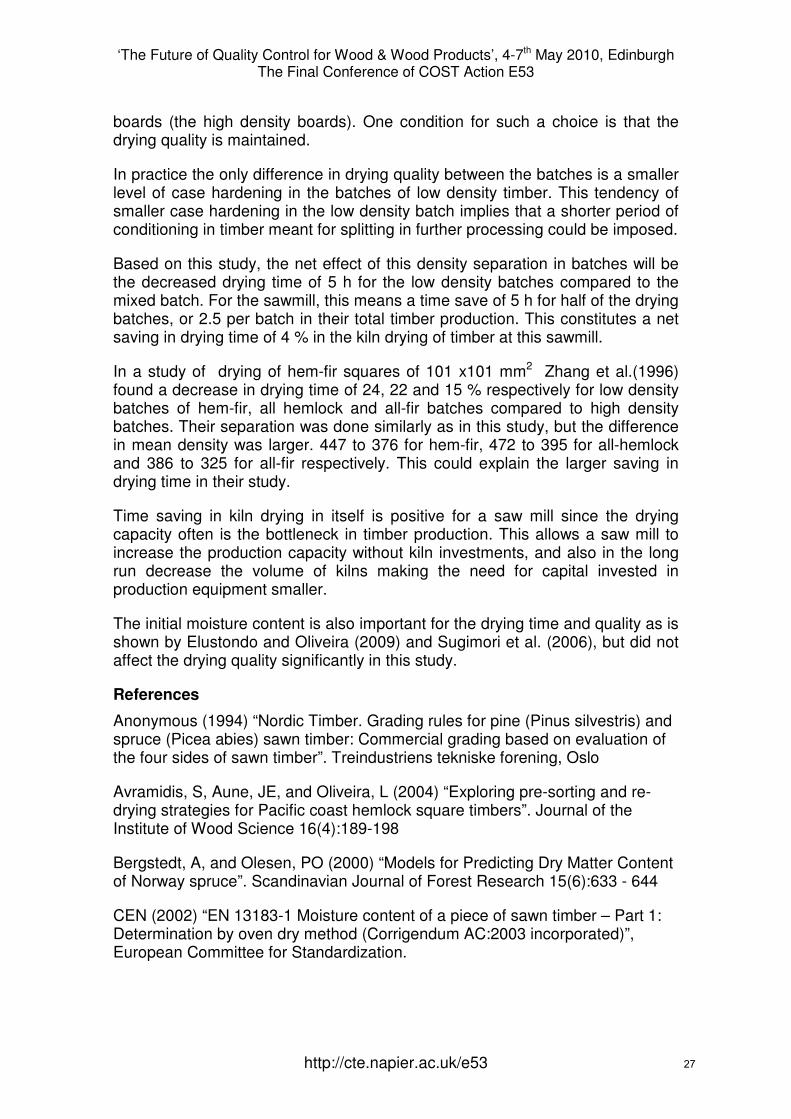
10. supplementary outputs are information such as estimated partial and total drying time and energy consumption.
0
10
20
30
40
50
60
10 20 30 40 50 60MC%
T °C
, EM
C%
0
1
2
3
4
G
TEMCGV
Figure 1: example of Drying schedule profile.
3 An evolving system
dTOUCH is a control system with a great potential, which is now at the first stage of its development and which will be expanded in the next future, thanks to already running validation tests on pilot plants. An automatic upgrade function (available when connected to a PC running XYLON software) allow the system to be upgraded.
The system has self-learning features: the Drying cycle evaluation function -especially useful in case of repeated drying cycles in homogeneous conditions- allows to optimise the drying cycles according to the specific kiln characteristics and to the user’s specific requirements. At the end of the cycle, the user has the opportunity to answer to a few questions on the touch screen and to give an evaluation about the completed cycle in terms of drying speed and drying quality. The questionnaire is structured on different levels for different operator profiles. Some levels are access-free only to expert operators. This structure
34

‘The Future of Quality Control for Wood & Wood Products’, 4-7th May 2010, Edinburgh The Final Conference of COST Action E53
http://cte.napier.ac.uk/e53
allows to filter bad data due to inexperience or to some psychological behaviour that could lead the operator to force the system. The multi-level structure also allows to separate the learning procedure in two stages: a first testing stage (already running) and a second optimisation stage during the working service. Questions about quality allows graded answers according to standards to the wood drying quality. As a consequence some answers requires specific measurement or test such as for the measure of internal stress.
Outputs concerning the drying process parameters automatically recorded from the sensors and the additional information from the questionnaire are codified in a report file. The report file is stored in the internal database (single level) and, when Internet connected, to the shared database on the server (central level).
Quantity and quality of information are different at the two levels. The auto - learning efficiency of the control is different as well. The expert system analysis the report file and it proposes possible modification in the drying parameters. The modification process requires:
1. Homogeneous Conditions (same initial and boundary conditions, same species and thickness. If possible same or similar secondary conditions such as provenience, period of the year);
2. Sufficient feedback given by input data related to the process parameters, process kinetic; results of the process in terms of quality/time;
3. A consistent statistical population of data (data from several homogenous drying process);
4. an input/output model. Single and central levels have different data analysis procedures and different input/output models. The rate of modification of some parameters can be adjusted according to presets corresponding to different operator’s profiles (risk attitude). At the end of the modified drying process the expert system start to analyse the history of changes and to collect information about the variability and the error. An increasing quantity of data (increasing experience) increases the probability to reach an effective and stable optimisation.
35
‘The Future of Quality Control for Wood & Wood Products’, 4-7th May 2010, Edinburgh The Final Conference of COST Action E53
http://cte.napier.ac.uk/e53
speciesPROPERTIES
COMMENTS
TECHNOLOGICAL PROPERTIES
T, EMC, V =f (MC)
speciesscolourinternal stressdistorsionscollapsesplitsmouldsdrying time1
OUTPUT
QUESTIONAIRE
INPUT
INPUT1
T
EMC
V
MODIFICATION EXPERT
MC
prop
drying paramettime
DRYING TIMECALCULATOR
speciess
thickness
MCi
DMCi
Ti
MCf
Q/T
special drying
T
EMC
V
DRYING SCHEDULE GENERATOR
DRYING ID
time
drying parameters
INPUT
OUT
DRYING REPORT FILE
0
DISPLAY
INPUT OUTPUT
DATABASE
STOP
15DRYING TIME
14MOULD
13SPLIT
12COLLAPSE
11DISTORTION
10INT STRESS
9COLOUR
8SPECIAL DRYING
7EXPECTED QUALITY
6FINAL MC
5INITIAL T
4MC GRADIENT
3INITIAL MC
2THICKNESS
1SPECIES
T
EMC
V
FEEDBACK
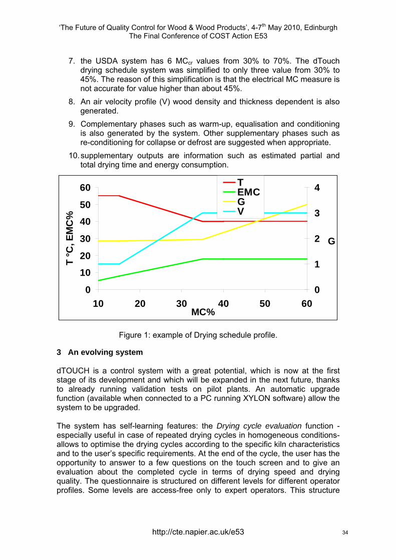
Figure 2. Diagram of control system: green: input from users; red: input from sensors; orange: elaboration units; blue: output.
4 The friendly expert
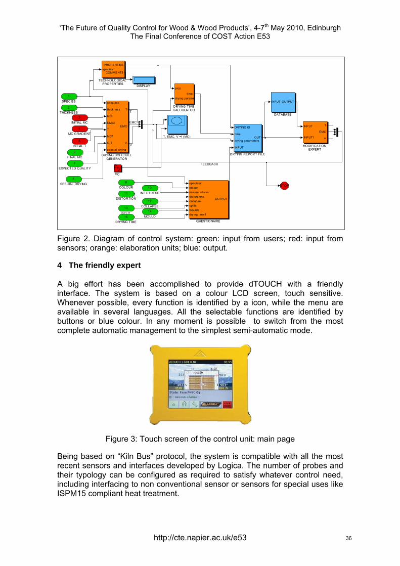
A big effort has been accomplished to provide dTOUCH with a friendly interface. The system is based on a colour LCD screen, touch sensitive. Whenever possible, every function is identified by a icon, while the menu are available in several languages. All the selectable functions are identified by buttons or blue colour. In any moment is possible to switch from the most complete automatic management to the simplest semi-automatic mode.
Figure 3: Touch screen of the control unit: main page
Being based on “Kiln Bus” protocol, the system is compatible with all the most recent sensors and interfaces developed by Logica. The number of probes and their typology can be configured as required to satisfy whatever control need, including interfacing to non conventional sensor or sensors for special uses like ISPM15 compliant heat treatment.
36
‘The Future of Quality Control for Wood & Wood Products’, 4-7th May 2010, Edinburgh The Final Conference of COST Action E53
http://cte.napier.ac.uk/e53
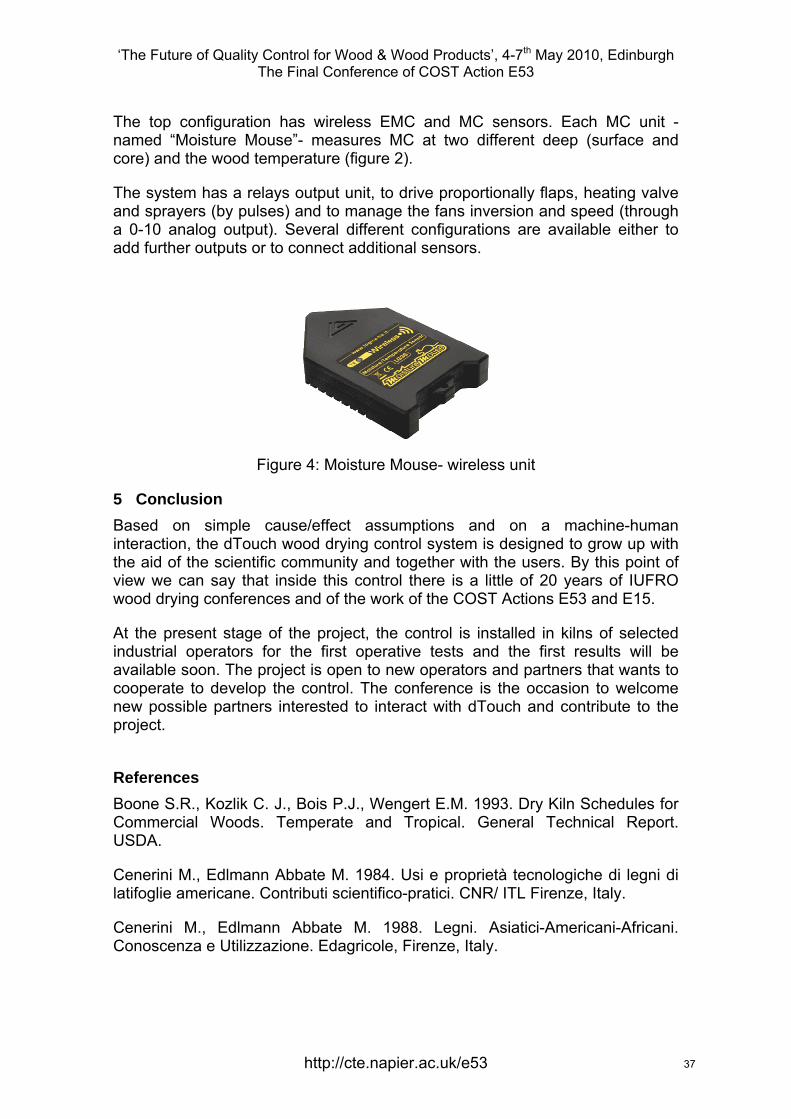
The top configuration has wireless EMC and MC sensors. Each MC unit -named “Moisture Mouse”- measures MC at two different deep (surface and core) and the wood temperature (figure 2).
The system has a relays output unit, to drive proportionally flaps, heating valve and sprayers (by pulses) and to manage the fans inversion and speed (through a 0-10 analog output). Several different configurations are available either to add further outputs or to connect additional sensors.
Figure 4: Moisture Mouse- wireless unit
5 Conclusion Based on simple cause/effect assumptions and on a machine-human interaction, the dTouch wood drying control system is designed to grow up with the aid of the scientific community and together with the users. By this point of view we can say that inside this control there is a little of 20 years of IUFRO wood drying conferences and of the work of the COST Actions E53 and E15.
At the present stage of the project, the control is installed in kilns of selected industrial operators for the first operative tests and the first results will be available soon. The project is open to new operators and partners that wants to cooperate to develop the control. The conference is the occasion to welcome new possible partners interested to interact with dTouch and contribute to the project.
References Boone S.R., Kozlik C. J., Bois P.J., Wengert E.M. 1993. Dry Kiln Schedules for Commercial Woods. Temperate and Tropical. General Technical Report. USDA.
Cenerini M., Edlmann Abbate M. 1984. Usi e proprietà tecnologiche di legni di latifoglie americane. Contributi scientifico-pratici. CNR/ ITL Firenze, Italy.
Cenerini M., Edlmann Abbate M. 1988. Legni. Asiatici-Americani-Africani. Conoscenza e Utilizzazione. Edagricole, Firenze, Italy.
37
‘The Future of Quality Control for Wood & Wood Products’, 4-7th May 2010, Edinburgh The Final Conference of COST Action E53
http://cte.napier.ac.uk/e53
Cenerini M., Edlmann Abbate M. 1996. Usi e proprietà tecnologiche di legni di conifere. Contributi scientifico-pratici. CNR/ ITL Firenze, Italy.
Cividini R., Travan L. 2000. Conventional Drying of lumbers - Essiccazione Convenzionale dei Legnami. Compendio. Nardi ed., Verona, Italy
Denig J., Wengert E.M., Simpson W.T. 2000. Drying Hardwood Lumber. General Technical Report USDA.
Drenier K., J. Welling, (1992), “ Self-Tuning controllerws for the kiln drying process” proceedings of the 3rd Int. IUFRO Wood Drying Conf., Vienna, Austria, pp 205-216
F. M. Chevalier, J-M. Frayret, (1996), «A fuzzy logic application to kiln dryer regulatuion », proceedings of the 5th Int. IUFRO Wood Drying Conf., Quebec City, Canada, pp 221-229
Gann. Table of Timber Species. GANN und Regeltechnik GmbH, Stuttgart.
Giordano G. 1980. I Legnami del mondo. Dizionario Enciclopedico. Il Cerilo Editrice.
Giordano G. 1988. Tecnologia del Legno – I legnami del commercio. Volume III: Parte seconda. UTET.
Pratt, G. H., Timber drying manual; 1997, BRE, Watword, GB.
Rijsdijk J.F. and Laming P.B. 1994. Physical and Related Properties of 145 Timbers. Information for Practice. TNO Kluwer Academic Publishers.
Simpson W. T. 1996. Method to Estimate Dry-Kiln Schedules and Species Groupings. Tropical and Temperate Hardwoods. Res. Pap. USDA.
Simpson W.T. 1991. Dry Kiln Operator’s Manual. USDA Agricultural Handbook.
Skuratov N. V., (2005) “Schedules and Quality Control at Kiln Drying”, proceedings of the 9th Int. IUFRO Wood Drying Conf., Nanjing, China, pp 308-311
Wang X. G.. W. Liu, L. Gu, C. J. Sun, C. E. Gu, C. W. de Silva, (2001), „Development of an Intelligent control system for wood drying processes” IEEE/ASME Intern. Conf. On Advanced Intelligent Mechatronichs Proceedings, Como, Italy, pp 371-376;
38
‘The Future of Quality Control for Wood & Wood Products’, 4-7th May 2010, Edinburgh The Final Conference of COST Action E53
Impact of various conventional drying conditions on drying rate and on moisture content gradient during early stage of
beechwood drying
A. Straže1, S. Pervan2 & Ž. Gorišek3
Abstract An appropriate moisture transport and a control of moisture distribution are needed from the early beginning of drying process, especially at drying of high dense and less permeable hardwoods. For determination of suitable process conditions at drying of European beechwood (Fagus sylvatica L.) the unidirectional drying kinetics, with an emphasis of free water removal was researched. We used radially oriented sapwood specimens, having thickness from 6 mm to 24 mm (ΔL = 6 mm). Series of conventional drying processes were carried out in the laboratory tunnel drier at constant climate (T = 30 °C) RH = 85%) and with varying air velocity (v) from 0.6 m/s to 7.6 m/s. During the drying, moisture content (MC), MC gradient and moisture flow were gravimetrically determined at successive time intervals. Drying rate generally increased with rising of air velocity and decreased with increasing thickness of wood. Relatively constant drying rate was present at the initial stage of drying of thin specimens (≤ 12 mm) in a short time interval, when low air velocity was used (≤ 2.5 m/s). Increasing of the air velocity (> 2.5 m/s) lead to early irreversible reduction of initial moisture flow and transition to the period of significantly falling drying rate, where the internal mass resistance predominated and caused high initial moisture content gradient. The diffusion barrier was induced at too fast free water removal which controlled further drying rate and significantly prolonged the drying process in continuation.
1 Introduction Beechwood (Fagus sylvatica L.), an important wood species in European wood industry, is mostly dried in convective kilns, where generally two most common drying problems are present: oxidative discolouring and case hardening in thicker material.
Fast drying in the initial drying rate period, using low temperature, even below 30 °C is generally prescribed to diminish beechwood discolouration (Gorišek et al., 2000; Koch, 2008). In this period, if a constant drying temperature is used, the drying gradient and the air velocity have the most significant impact on surface mass transfer and consequently on the drying rate (Salin, 2007). Using
1 Research Assistant, [email protected], Department of Wood Science and Technology, Biotechnical Faculty, University of Ljubljana, Slovenia 2 Assoc. Prof., [email protected], Faculty of Forestry, University of Zagreb, Croatia 3 Assoc. Prof., [email protected], Department of Wood Science and Technology, Biotechnical Faculty, University of Ljubljana, Slovenia
http://cte.napier.ac.uk/e53 39
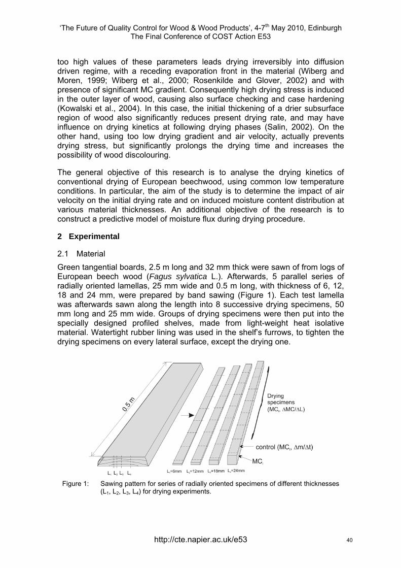
‘The Future of Quality Control for Wood & Wood Products’, 4-7th May 2010, Edinburgh The Final Conference of COST Action E53
too high values of these parameters leads drying irreversibly into diffusion driven regime, with a receding evaporation front in the material (Wiberg and Moren, 1999; Wiberg et al., 2000; Rosenkilde and Glover, 2002) and with presence of significant MC gradient. Consequently high drying stress is induced in the outer layer of wood, causing also surface checking and case hardening (Kowalski et al., 2004). In this case, the initial thickening of a drier subsurface region of wood also significantly reduces present drying rate, and may have influence on drying kinetics at following drying phases (Salin, 2002). On the other hand, using too low drying gradient and air velocity, actually prevents drying stress, but significantly prolongs the drying time and increases the possibility of wood discolouring.
The general objective of this research is to analyse the drying kinetics of conventional drying of European beechwood, using common low temperature conditions. In particular, the aim of the study is to determine the impact of air velocity on the initial drying rate and on induced moisture content distribution at various material thicknesses. An additional objective of the research is to construct a predictive model of moisture flux during drying procedure.
2 Experimental
2.1 Material Green tangential boards, 2.5 m long and 32 mm thick were sawn of from logs of European beech wood (Fagus sylvatica L.). Afterwards, 5 parallel series of radially oriented lamellas, 25 mm wide and 0.5 m long, with thickness of 6, 12, 18 and 24 mm, were prepared by band sawing (Figure 1). Each test lamella was afterwards sawn along the length into 8 successive drying specimens, 50 mm long and 25 mm wide. Groups of drying specimens were then put into the specially designed profiled shelves, made from light-weight heat isolative material. Watertight rubber lining was used in the shelf’s furrows, to tighten the drying specimens on every lateral surface, except the drying one.
Figure 1: Sawing pattern for series of radially oriented specimens of different thicknesses
(L1, L2, L3, L4) for drying experiments.
http://cte.napier.ac.uk/e53 40

‘The Future of Quality Control for Wood & Wood Products’, 4-7th May 2010, Edinburgh The Final Conference of COST Action E53
2.2 Drying conditions Shelves with sealed groups of drying specimens were put into the laboratory drying tunnel, regulated by PID controller. Climatic conditions in the dryer stayed constant throughout the whole drying procedure, with the temperature (T) of 30 °C (± 0.2 °C) and the relative air humidity (RH) of 85% (± 1%). The air velocity (v) was set as an average of precise measuring at the multiple points on the holding shelf, 1 cm above the surface of drying specimens, using hot-wire anemometer (Testo 435-4). Five average air velocities were established: 0.6 m/s, 1.1 m/s, 2.5 m/s, 4.5 m/s and 7.6 m/s (± 0.1 m/s) (Figure 2).
Figure 2: Conventional drying tunnel TLS-01 (top-left) with PLC controller (bottom-left)
and experimental chamber with holding isolative shelves and drying specimens (bottom-right).
2.3 Analysis of moisture transport The average moisture content (MC) of the control specimens was gravimetrically determined during the drying (0.001 g precision) at 2 hours interval, using the equation:
( ) 100100 −+= ii
tt MC
mm
MC (1)
MCt, MCi = the temporary and initial moisture content [%], mt, mi = the temporary and initial weight of drying specimen [g].
The moisture flow was additionally calculated between each successive weighting:
⎥⎦⎤
⎢⎣⎡
Δ⋅−
= −
hmg
tAmm
Am tt
21
m = moisture flow [g/h],
http://cte.napier.ac.uk/e53 41

‘The Future of Quality Control for Wood & Wood Products’, 4-7th May 2010, Edinburgh The Final Conference of COST Action E53
mt, mt-1 = two successive weights of drying specimen at measured time interval (Δt [h]) [g], A = evaporating surface of drying specimen [m2].
Dependency of moisture flow on average MC of wood was analytically modelled afterwards using the least square regression method. Several empirical models were tested to fit the S-shaped experimental data, wherefrom the asymmetrical Gompertz function gave the most reliable results:
( )( )cMCMCkeeaAm −−−⋅= (3)
a = asymptote, i.e. maximum moisture flow at initial MC [g/m2h], k = maximum rate of change of moisture flow, reached at the pass from the initial to the falling drying rate period [1/%], MCc = moisture content at maximum rate of change of moisture flow, i.e. at inflection point of the model (MCc, a/e) [%].
The first derivative of the Gompertz function at the inflection point (MCc, a/e) was used for determining the equation of a tangent to the moisture flow curve. The theoretical transition point, i.e. transition moisture content (TT), at which moisture flow significantly sinks, to 84% of initial, maximum value were additionally calculated from the equation of the tangent to the moisture curve, used also in earlier research (Straže and Gorišek, 2009).
The MC distribution was determined by cleaving drying specimens, from surface to the core, into 3 mm thick slices. Seven moisture content profiles (ΔMC/ΔL), at every 10% MC decrease, were additionally acquired during drying process from initial (MCi) to the final MC (MCf).
3 Results and discussion The drying kinetics varied with thickness of wood specimen and with used air velocity, as well as with MC and induced MC gradient. An increase of the initial drying rate with rising of the air velocity was present at early stage of drying, at high moisture content (MC >> FSP; FSP = fibre saturation point), at all tested thicknesses of wood. Increment of the initial moisture flow (a) by the increasing of the air velocity (v) had the non-linear rise, the more at low air velocities, up to 2.5 m/s (Figure 3; Table 1). Drying of thinner wood specimens (L ≤ 12 mm) with lower air velocity (v < 2.5 m/s) enabled an initial short-term period of relatively constant drying rate. It is believed, that the surface mass transfer resistance was predominant at these drying conditions, as confirmed in related studies (Perre et al., 1993; Perre and Martin, 1994; Rosenkilde and Glover, 2002; Straže, 2010). On the other hand, significant decrease of drying rate was determined already from the early beginning of the process at thicker wood specimens (L ≥ 18 mm), irrespective of the used air velocity.
http://cte.napier.ac.uk/e53 42
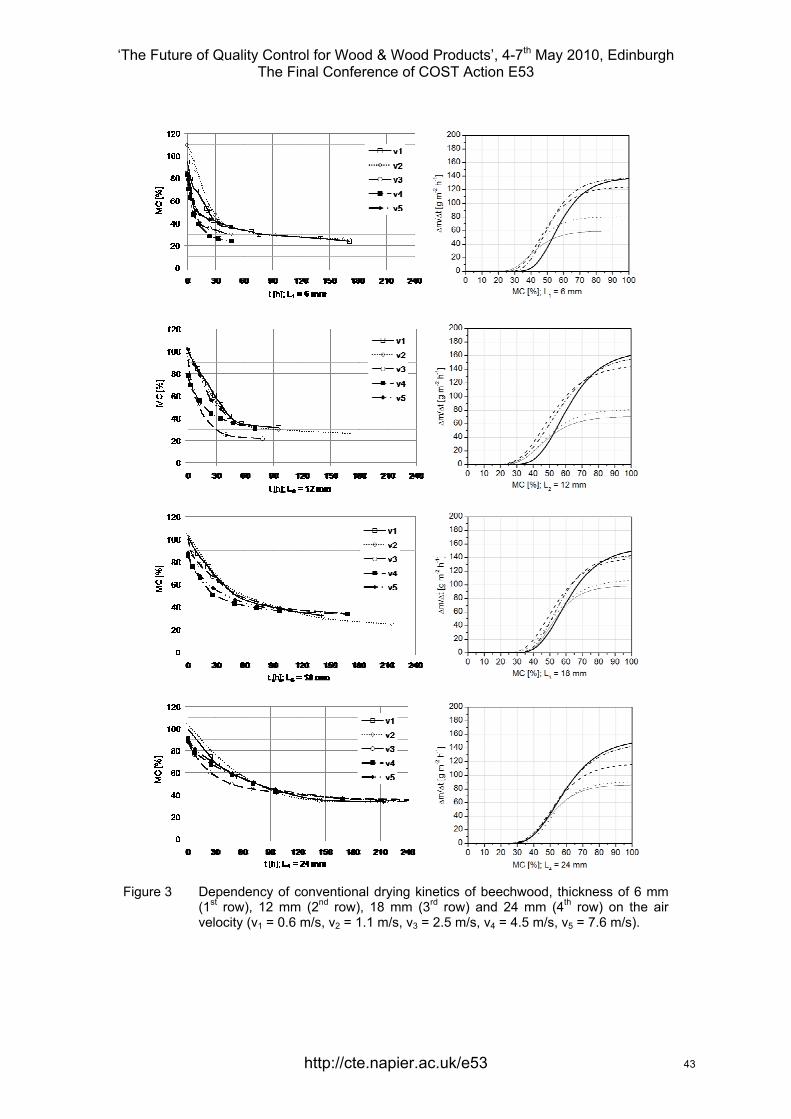
‘The Future of Quality Control for Wood & Wood Products’, 4-7th May 2010, Edinburgh The Final Conference of COST Action E53
Figure 3 Dependency of conventional drying kinetics of beechwood, thickness of 6 mm
(1st row), 12 mm (2nd row), 18 mm (3rd row) and 24 mm (4th row) on the air velocity (v1 = 0.6 m/s, v2 = 1.1 m/s, v3 = 2.5 m/s, v4 = 4.5 m/s, v5 = 7.6 m/s).
http://cte.napier.ac.uk/e53 43
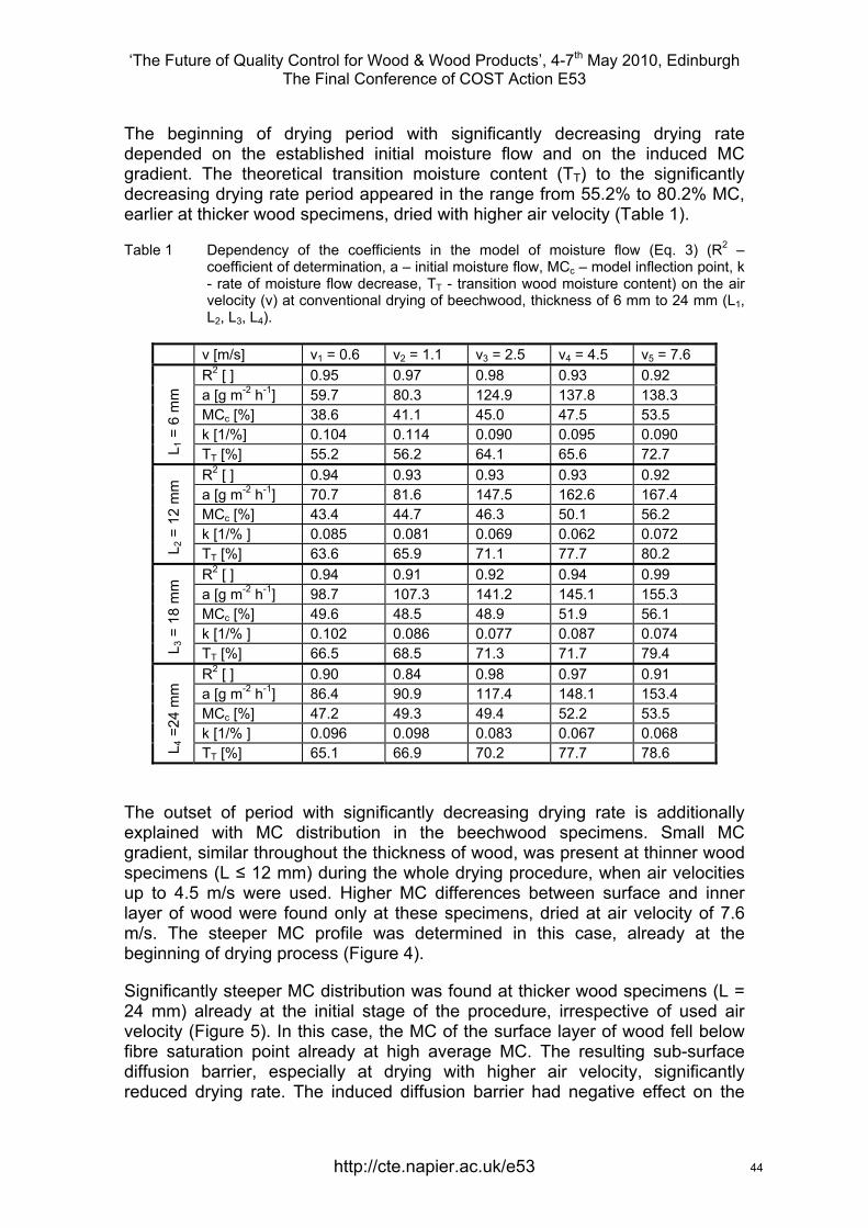
‘The Future of Quality Control for Wood & Wood Products’, 4-7th May 2010, Edinburgh The Final Conference of COST Action E53
The beginning of drying period with significantly decreasing drying rate depended on the established initial moisture flow and on the induced MC gradient. The theoretical transition moisture content (TT) to the significantly decreasing drying rate period appeared in the range from 55.2% to 80.2% MC, earlier at thicker wood specimens, dried with higher air velocity (Table 1).
Table 1 Dependency of the coefficients in the model of moisture flow (Eq. 3) (R2 –coefficient of determination, a – initial moisture flow, MCc – model inflection point, k - rate of moisture flow decrease, TT - transition wood moisture content) on the air velocity (v) at conventional drying of beechwood, thickness of 6 mm to 24 mm (L1, L2, L3, L4).
v [m/s] v1 = 0.6 v2 = 1.1 v3 = 2.5 v4 = 4.5 v5 = 7.6 R2 [ ] 0.95 0.97 0.98 0.93 0.92 a [g m-2 h-1] 59.7 80.3 124.9 137.8 138.3 MCc [%] 38.6 41.1 45.0 47.5 53.5 k [1/%] 0.104 0.114 0.090 0.095 0.090
L 1 =
6 m
m
TT [%] 55.2 56.2 64.1 65.6 72.7 R2 [ ] 0.94 0.93 0.93 0.93 0.92 a [g m-2 h-1] 70.7 81.6 147.5 162.6 167.4 MCc [%] 43.4 44.7 46.3 50.1 56.2 k [1/% ] 0.085 0.081 0.069 0.062 0.072
L 2 =
12
mm
TT [%] 63.6 65.9 71.1 77.7 80.2 R2 [ ] 0.94 0.91 0.92 0.94 0.99 a [g m-2 h-1] 98.7 107.3 141.2 145.1 155.3 MCc [%] 49.6 48.5 48.9 51.9 56.1 k [1/% ] 0.102 0.086 0.077 0.087 0.074
L 3 =
18
mm
TT [%] 66.5 68.5 71.3 71.7 79.4 R2 [ ] 0.90 0.84 0.98 0.97 0.91 a [g m-2 h-1] 86.4 90.9 117.4 148.1 153.4 MCc [%] 47.2 49.3 49.4 52.2 53.5 k [1/% ] 0.096 0.098 0.083 0.067 0.068
L 4 =
24 m
m
TT [%] 65.1 66.9 70.2 77.7 78.6
The outset of period with significantly decreasing drying rate is additionally explained with MC distribution in the beechwood specimens. Small MC gradient, similar throughout the thickness of wood, was present at thinner wood specimens (L ≤ 12 mm) during the whole drying procedure, when air velocities up to 4.5 m/s were used. Higher MC differences between surface and inner layer of wood were found only at these specimens, dried at air velocity of 7.6 m/s. The steeper MC profile was determined in this case, already at the beginning of drying process (Figure 4).
Significantly steeper MC distribution was found at thicker wood specimens (L = 24 mm) already at the initial stage of the procedure, irrespective of used air velocity (Figure 5). In this case, the MC of the surface layer of wood fell below fibre saturation point already at high average MC. The resulting sub-surface diffusion barrier, especially at drying with higher air velocity, significantly reduced drying rate. The induced diffusion barrier had negative effect on the
http://cte.napier.ac.uk/e53 44
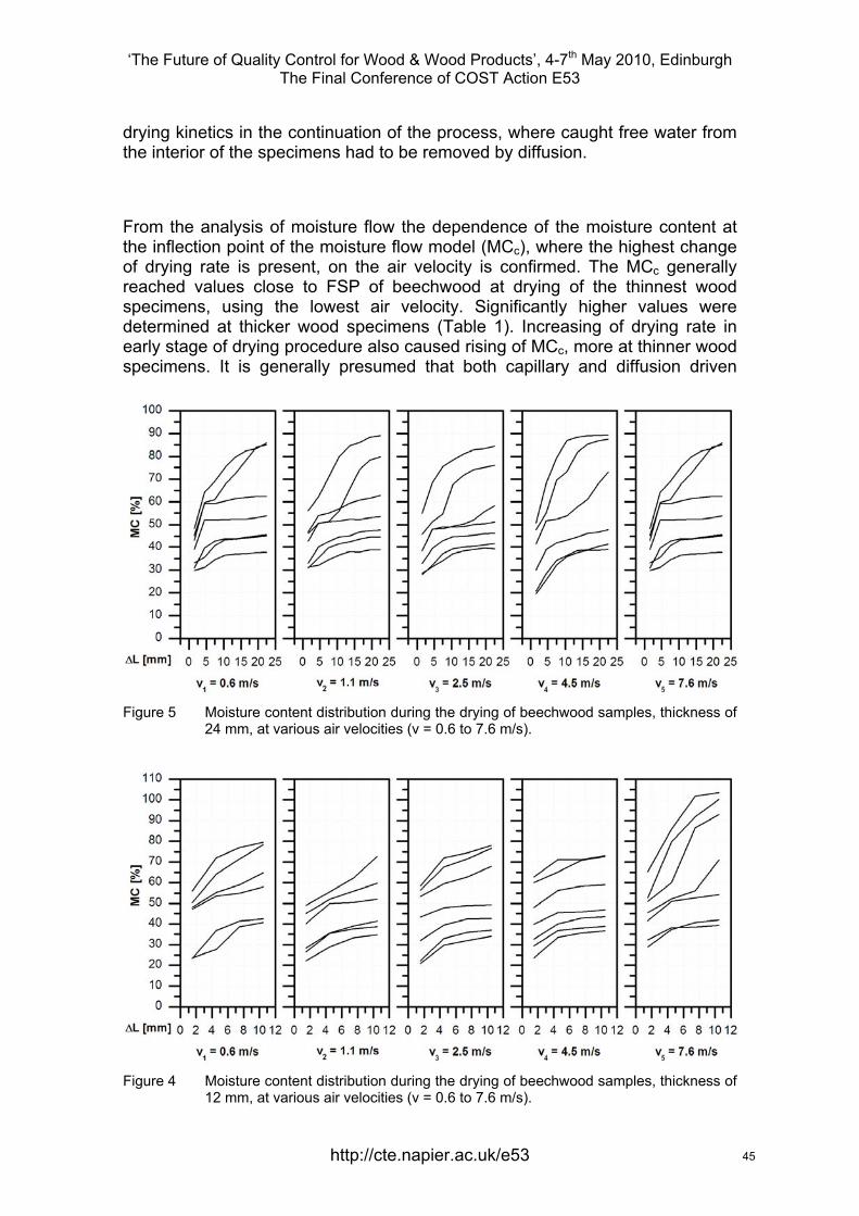
‘The Future of Quality Control for Wood & Wood Products’, 4-7th May 2010, Edinburgh The Final Conference of COST Action E53
drying kinetics in the continuation of the process, where caught free water from the interior of the specimens had to be removed by diffusion.
From the analysis of moisture flow the dependence of the moisture content at the inflection point of the moisture flow model (MCc), where the highest change of drying rate is present, on the air velocity is confirmed. The MCc generally reached values close to FSP of beechwood at drying of the thinnest wood specimens, using the lowest air velocity. Significantly higher values were determined at thicker wood specimens (Table 1). Increasing of drying rate in early stage of drying procedure also caused rising of MCc, more at thinner wood specimens. It is generally presumed that both capillary and diffusion driven
Figure 5 Moisture content distribution during the drying of beechwood samples, thickness of 24 mm, at various air velocities (v = 0.6 to 7.6 m/s).
Figure 4 Moisture content distribution during the drying of beechwood samples, thickness of 12 mm, at various air velocities (v = 0.6 to 7.6 m/s).
http://cte.napier.ac.uk/e53 45
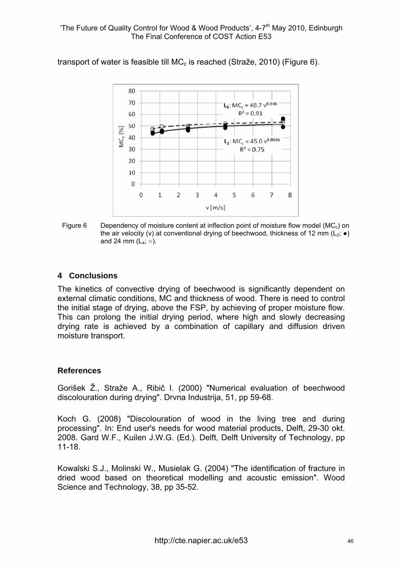
‘The Future of Quality Control for Wood & Wood Products’, 4-7th May 2010, Edinburgh The Final Conference of COST Action E53
transport of water is feasible till MCc is reached (Straže, 2010) (Figure 6).
Figure 6 Dependency of moisture content at inflection point of moisture flow model (MCc) on
the air velocity (v) at conventional drying of beechwood, thickness of 12 mm (L2; ●) and 24 mm (L4; ○).
4 Conclusions The kinetics of convective drying of beechwood is significantly dependent on external climatic conditions, MC and thickness of wood. There is need to control the initial stage of drying, above the FSP, by achieving of proper moisture flow. This can prolong the initial drying period, where high and slowly decreasing drying rate is achieved by a combination of capillary and diffusion driven moisture transport.
References
Gorišek Ž., Straže A., Ribič I. (2000) "Numerical evaluation of beechwood discolouration during drying". Drvna Industrija, 51, pp 59-68.
Koch G. (2008) "Discolouration of wood in the living tree and during processing". In: End user's needs for wood material products, Delft, 29-30 okt. 2008. Gard W.F., Kuilen J.W.G. (Ed.). Delft, Delft University of Technology, pp 11-18.
Kowalski S.J., Molinski W., Musielak G. (2004) "The identification of fracture in dried wood based on theoretical modelling and acoustic emission". Wood Science and Technology, 38, pp 35-52.
http://cte.napier.ac.uk/e53 46
‘The Future of Quality Control for Wood & Wood Products’, 4-7th May 2010, Edinburgh The Final Conference of COST Action E53
Perre P., Martin M. (1994) "Drying at high temperature of heartwood and sapwood: theory, experiment and practical consequence of kiln control". Drying Technology, 12, pp 1915-1941.
Perre P., Moser M., Martin M. (1993) "Advances in transport phenomena during convective drying with superheated steam or moist air". International Journal of Heat and Mass Transfer, 36, pp 2725-2746.
Rosenkilde A., Glover P. (2002) "High Resolution Measurement of the Surface Layer Moisture Content during Drying of Wood using a Novel Magnetic Resonance Imaging Technique". Holzforschung, 56, pp 312-317.
Salin J.G. (2002) "Theoretical analysis of mass transfer from wooden surfaces". In: 13th International Drying Symposium, Beijing, 27-30 avg. 2002. Mujumbdar (Ed.). Beijing, pp 1826-1834.
Salin J.G. (2007) "External heat and mass transfer". In: Fundamentals of wood drying. Perre P. (Ed.). Nancy, A.R.BO.LOR., pp 175-201.
Straže A. (2010) "Impact of external and internal mass transfer resistance on kinetics of convective wood drying". Doctoral Dissertation. Ljubljana, University of Ljubljana, 114 p.
Straže A., Gorišek Ž. (2009) "Research on internal and external mass transfer at convective drying of European beechwood (Fagus sylvatica L.)". In: Proceedings of the COST E53 Meeting and EDG Wood Drying Seminar, Bled, Slovenia, 23rd April 2009. Gorišek Ž. (Ed.). Bled, Slovenia, Biotechnical Faculty, Department of Wood Science and Technology, pp 93-102.
Wiberg P., Moren T.J. (1999) "Moisture flux determination in wood during drying above fiber saturation point using CT-scanning and digital imaging processing". Holz als Roh- und Werkstoff, 57, pp 137-144.
Wiberg P., Sehlstedt S.M.B., Moren T.J. (2000) "Heat and mass transfer during sapwood drying above fiber saturation point". Drying Technology, 18, pp 1647-1664.
http://cte.napier.ac.uk/e53 47

‘The Future of Quality Control for Wood & Wood Products’, 4-7th May 2010, Edinburgh The Final Conference of COST Action E53
Tuesday 4th May Wood drying workshop (European Drying Group)
2nd session
http://www.cte.napier.ac.uk/e53/ 48

‘The Future of Quality Control for Wood & Wood Products’, 4-7th May 2010, Edinburgh The Final Conference of COST Action E53
http://cte.napier.ac.uk/e53
Electrical impedance measurement of green Scots pine
L. Tomppo1, M. Tiitta2 & R. Lappalainen3
Abstract Electrical impedance spectroscopy method is based on the measurement of electrical response at multiple frequencies. The measurement technique was studied in relation to the moisture content and density of green Scots pine sapwood and heartwood. For heartwood, resin acid content was also used as a reference parameter. Small samples were measured in green moisture state. The through-transmission measurements were conducted at frequency range from 1 Hz to 10 MHz. Parallel samples from the same tree were used in measurements in tangential and longitudinal directions. The moisture content range of sapwood pieces was 87 – 169 % (dry basis). For heartwood pieces the range was 23 – 44 %.
The measurements were conducted firstly with plastic sheet between the sample and electrodes. The plastic sheet acted as a dielectric layer, and in addition it protected the samples from drying during the measurement. Secondly, the measurements were made without the plastic cover to compare the results. At low frequencies, the electrical impedance responses measured with and without plastic cover differed greatly. At higher frequencies the responses approached each other. For heartwood specimens, there were significant correlations between impedance modulus and moisture content (e.g. r = -0.65, p < 0.001, N = 42 at 10 kHz) and density (e.g. r = -0.34, p < 0.05, N = 42, at 2.5 MHz). The impedance phase angle correlated with resin acid content at low frequencies (e.g. r = -0.46, p < 0.01 at 100 Hz).
1 Introduction Electrical impedance spectroscopy (EIS) is a technique, in which alternating electric field at different frequencies is induced into a specimen, and the complex electric response is measured. Impedance modulus |Z| and phase angle can be further calculated from the complex impedance.
Physical and chemical properties of wood affect its EIS response. Moisture content (MC) of wood is the dominant factor and in addition, for example, density and grain angle affect the measurement. Below fibre saturation point (FSP) electrical impedance decreases as a function of MC, but above FSP the effect of MC on EIS response is reduced.
1 Researcher, [email protected] 2 Researcher, [email protected] 3 Professor, [email protected] Department of Physics and Mathematics, University of Eastern Finland, Finland
49
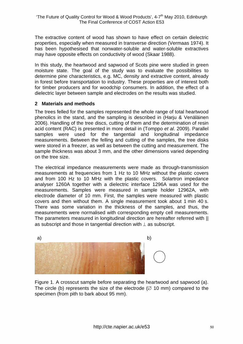
‘The Future of Quality Control for Wood & Wood Products’, 4-7th May 2010, Edinburgh The Final Conference of COST Action E53
http://cte.napier.ac.uk/e53
The extractive content of wood has shown to have effect on certain dielectric properties, especially when measured in transverse direction (Vermaas 1974). It has been hypothesised that nonwater-soluble and water-soluble extractives may have opposite effects on conductivity of wood (Skaar 1988).
In this study, the heartwood and sapwood of Scots pine were studied in green moisture state. The goal of the study was to evaluate the possibilities to determine pine characteristics, e.g. MC, density and extractive content, already in forest before transportation to industry. These properties are of interest both for timber producers and for woodchip consumers. In addition, the effect of a dielectric layer between sample and electrodes on the results was studied.
2 Materials and methods The trees felled for the samples represented the whole range of total heartwood phenolics in the stand, and the sampling is described in (Harju & Venäläinen 2006). Handling of the tree discs, cutting of them and the determination of resin acid content (RAC) is presented in more detail in (Tomppo et al. 2009). Parallel samples were used for the tangential and longitudinal impedance measurements. Between the felling and cutting of the samples, the tree disks were stored in a freezer, as well as between the cutting and measurement. The sample thickness was about 3 mm, and the other dimensions varied depending on the tree size.
The electrical impedance measurements were made as through-transmission measurements at frequencies from 1 Hz to 10 MHz without the plastic covers and from 100 Hz to 10 MHz with the plastic covers. Solartron impedance analyser 1260A together with a dielectric interface 1296A was used for the measurements. Samples were measured in sample holder 12962A, with electrode diameter of 10 mm. First, the samples were measured with plastic covers and then without them. A single measurement took about 1 min 40 s. There was some variation in the thickness of the samples, and thus, the measurements were normalised with corresponding empty cell measurements. The parameters measured in longitudinal direction are hereafter referred with || as subscript and those in tangential direction with as subscript.
Figure 1. A crosscut sample before separating the heartwood and sapwood (a). The circle (b) represents the size of the electrode ( 10 mm) compared to the specimen (from pith to bark about 95 mm).
a) b)
50
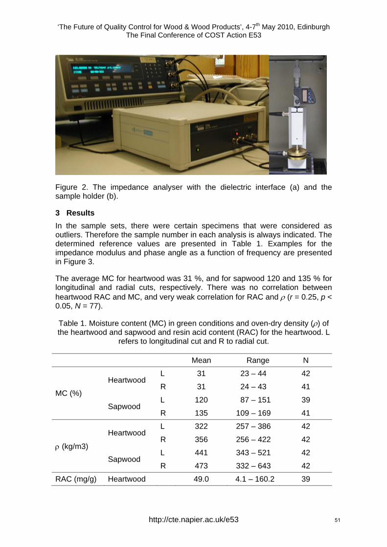
‘The Future of Quality Control for Wood & Wood Products’, 4-7th May 2010, Edinburgh The Final Conference of COST Action E53
http://cte.napier.ac.uk/e53
Figure 2. The impedance analyser with the dielectric interface (a) and the sample holder (b).
3 Results In the sample sets, there were certain specimens that were considered as outliers. Therefore the sample number in each analysis is always indicated. The determined reference values are presented in Table 1. Examples for the impedance modulus and phase angle as a function of frequency are presented in Figure 3.
The average MC for heartwood was 31 %, and for sapwood 120 and 135 % for longitudinal and radial cuts, respectively. There was no correlation between heartwood RAC and MC, and very weak correlation for RAC and (r = 0.25, p < 0.05, N = 77).
Table 1. Moisture content (MC) in green conditions and oven-dry density () of the heartwood and sapwood and resin acid content (RAC) for the heartwood. L
refers to longitudinal cut and R to radial cut.
Mean Range N
MC (%)
Heartwood L 31 23 – 44 42
R 31 24 – 43 41
Sapwood L 120 87 – 151 39
R 135 109 – 169 41
(kg/m3)
Heartwood L 322 257 – 386 42
R 356 256 – 422 42
Sapwood L 441 343 – 521 42
R 473 332 – 643 42
RAC (mg/g) Heartwood 49.0 4.1 – 160.2 39
51
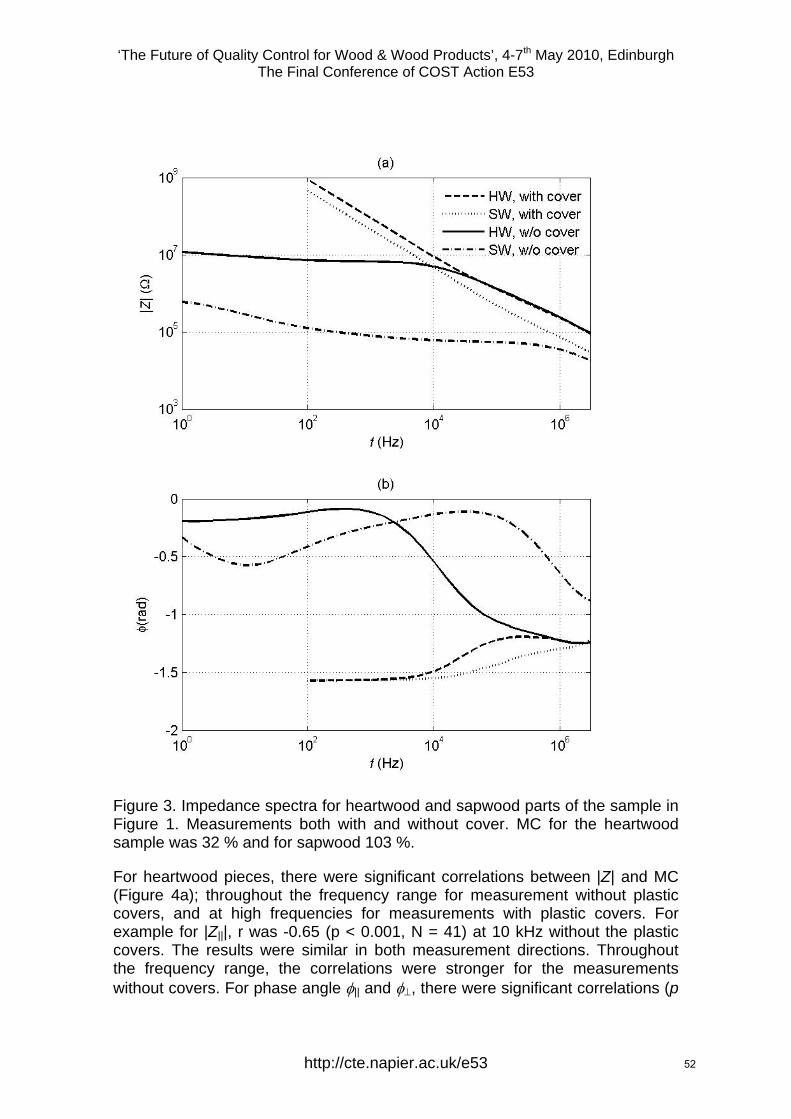
‘The Future of Quality Control for Wood & Wood Products’, 4-7th May 2010, Edinburgh The Final Conference of COST Action E53
http://cte.napier.ac.uk/e53
Figure 3. Impedance spectra for heartwood and sapwood parts of the sample in Figure 1. Measurements both with and without cover. MC for the heartwood sample was 32 % and for sapwood 103 %.
For heartwood pieces, there were significant correlations between |Z| and MC (Figure 4a); throughout the frequency range for measurement without plastic covers, and at high frequencies for measurements with plastic covers. For example for |Z|||, r was -0.65 (p < 0.001, N = 41) at 10 kHz without the plastic covers. The results were similar in both measurement directions. Throughout the frequency range, the correlations were stronger for the measurements without covers. For phase angle || and , there were significant correlations (p
52
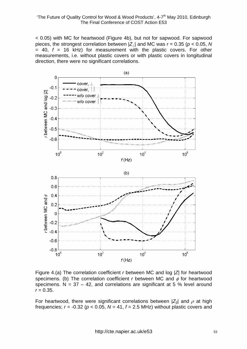
‘The Future of Quality Control for Wood & Wood Products’, 4-7th May 2010, Edinburgh The Final Conference of COST Action E53
http://cte.napier.ac.uk/e53
< 0.05) with MC for heartwood (Figure 4b), but not for sapwood. For sapwood pieces, the strongest correlation between |Z| and MC was r = 0.35 (p < 0.05, N = 40, f = 16 kHz) for measurement with the plastic covers. For other measurements, i.e. without plastic covers or with plastic covers in longitudinal direction, there were no significant correlations.
Figure 4.(a) The correlation coefficient r between MC and log |Z| for heartwood specimens. (b) The correlation coefficient r between MC and for heartwood specimens. N = 37 – 42, and correlations are significant at 5 % level around r = 0.35.
For heartwood, there were significant correlations between |Z||| and at high frequencies; r = -0.32 (p < 0.05, N = 41, f = 2.5 MHz) without plastic covers and
53
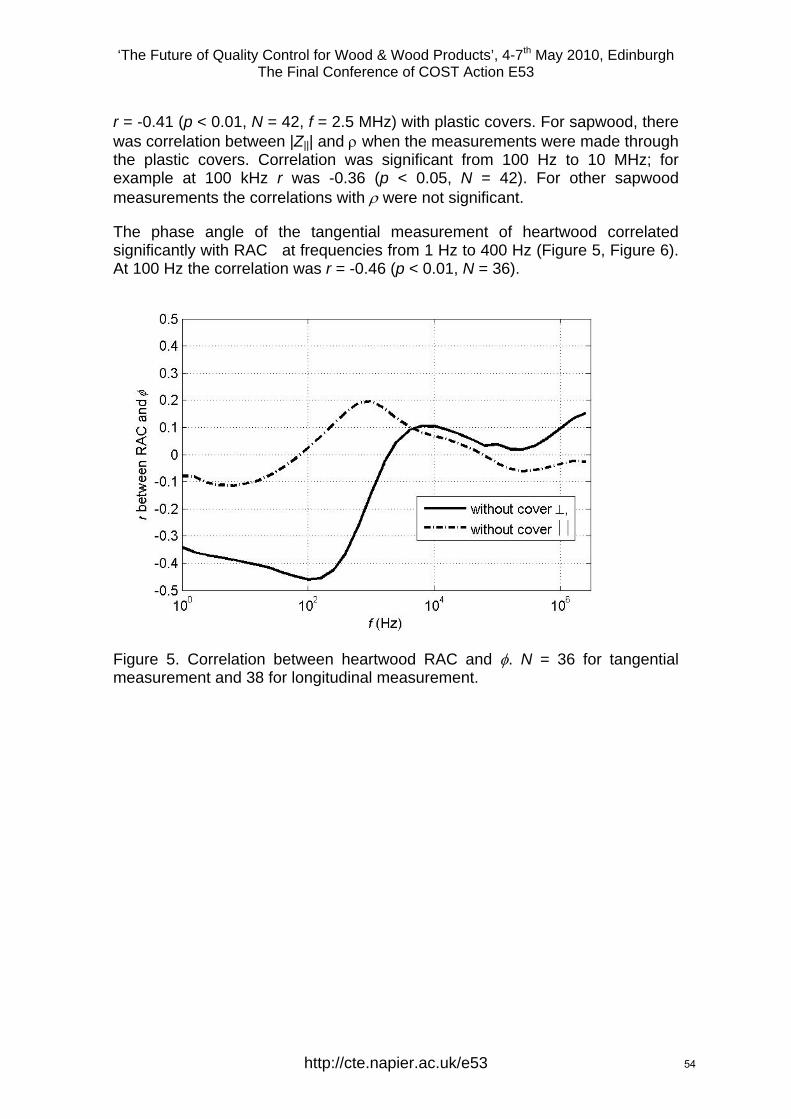
‘The Future of Quality Control for Wood & Wood Products’, 4-7th May 2010, Edinburgh The Final Conference of COST Action E53
http://cte.napier.ac.uk/e53
r = -0.41 (p < 0.01, N = 42, f = 2.5 MHz) with plastic covers. For sapwood, there was correlation between |Z||| and when the measurements were made through the plastic covers. Correlation was significant from 100 Hz to 10 MHz; for example at 100 kHz r was -0.36 (p < 0.05, N = 42). For other sapwood measurements the correlations with were not significant.
The phase angle of the tangential measurement of heartwood correlated significantly with RAC at frequencies from 1 Hz to 400 Hz (Figure 5, Figure 6). At 100 Hz the correlation was r = -0.46 (p < 0.01, N = 36).
Figure 5. Correlation between heartwood RAC and . N = 36 for tangential measurement and 38 for longitudinal measurement.
54
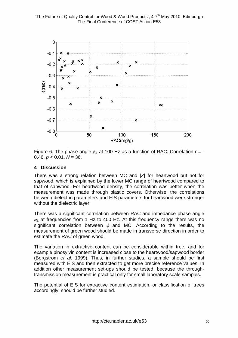
‘The Future of Quality Control for Wood & Wood Products’, 4-7th May 2010, Edinburgh The Final Conference of COST Action E53
http://cte.napier.ac.uk/e53
Figure 6. The phase angle at 100 Hz as a function of RAC. Correlation r = -0.46, p < 0.01, N = 36.
4 Discussion There was a strong relation between MC and |Z| for heartwood but not for sapwood, which is explained by the lower MC range of heartwood compared to that of sapwood. For heartwood density, the correlation was better when the measurement was made through plastic covers. Otherwise, the correlations between dielectric parameters and EIS parameters for heartwood were stronger without the dielectric layer.
There was a significant correlation between RAC and impedance phase angle at frequencies from 1 Hz to 400 Hz. At this frequency range there was no significant correlation between and MC. According to the results, the measurement of green wood should be made in transverse direction in order to estimate the RAC of green wood.
The variation in extractive content can be considerable within tree, and for example pinosylvin content is increased close to the heartwood/sapwood border (Bergström et al. 1999). Thus, in further studies, a sample should be first measured with EIS and then extracted to get more precise reference values. In addition other measurement set-ups should be tested, because the through-transmission measurement is practical only for small laboratory scale samples.
The potential of EIS for extractive content estimation, or classification of trees accordingly, should be further studied.
55
‘The Future of Quality Control for Wood & Wood Products’, 4-7th May 2010, Edinburgh The Final Conference of COST Action E53
http://cte.napier.ac.uk/e53
Acknowledgements
The Finnish Forest Research Institute provided the material and the chemical characterisation for this study. The authors thank especially Dr. Anni Harju, Dr. Martti Venäläinen and Mr. Tapio Laakso for the co-operation.
References
Bergström, B., Gustafsson, G., Gref, R. & Ericsson, A. (1999), Seasonal changes of pinosylvin distribution in the sapwood/heartwood boundary of Pinus sylvestris, Trees - Structure and Function, Vol 14, no. 2, pp 65-71.
Harju, A. M. & Venäläinen, M. (2006), Measuring the decay resistance of Scots pine heartwood indirectly by the Folin-Ciocalteu assay, Canadian Journal of Forest Research, Vol 36, no. 7, p. 1797-1804.
Skaar, C. (1988) Wood-Water Relations, Springer Verlag, Berlin, Germany.
Tomppo, L., Tiitta, M., Laakso, T., Harju, A., Venäläinen, M., & Lappalainen, R. (2009), Dielectric spectroscopy of Scots pine, Wood Science and Technology, Vol 43, no. 7, pp 653-667.
Vermaas, H. F. (1974), Dielectric properties of Pinus pinaster as a function of its alcohol-benzen-soluble content, Wood Science, Vol 6, no. 4, pp 363-367.
56
‘The Future of Quality Control for Wood & Wood Products’, 4-7th May 2010, Edinburgh The Final Conference of COST Action E53
Eucalyptus drying process: qualitative comparison of different clones cultivated in Italy
L. Travan1, O. Allegretti2 & M.Negri3
Abstract Kiln-drying process of Eucalyptus timber can be critical because of the possible occurrence of collapses, fissures and other defects related to the moisture decrease. The occurrence and the incidence of these defects is related to both the drying process and the wood, namely species and/or clone and individual factors related to the site of growing.
Nardi International Srl and IVALSA-CNR, Trees and Timber Institute, performed various drying cycles on four clones of Eucalyptus grandis, Italian grown, in order to determine the quality decrease due to the process.
Prudential basic drying schedules were chosen according to the technical literature available and the tests were focused to compare the behaviour of the various clones.
Moreover, some tests were performed by using both conventional drying kilns (Nardi International Srl and IVALSA-CNR) and continuous press-dryer (IVALSA-CNR).
The quality of the sawn timber (planarity, checking, deformations, etc.) was measured before and after the drying process. The results showed that relevant differences exist among the clones and that it is possible to increase the final quality of sawn timber by choosing a suitable drying schedule.
1 Introduction Eucalyptus grandis has been tested in Italy for forestry purposes since the last century, but the scarce utilisation of timber until now did not provide experiences concerning drying. According to literature a lot of technological problems of this species are strictly related to a suitable drying process, which is the most relevant step for the utilisation of E.grandis as solid timber raw material.
1 Technological Department, [email protected] Nardi International Srl, Via Ritonda 79, 37047 San Bonifacio (Verona), ITALY 2 Phd Researcher, [email protected] IVALSA-CNR, Trees and Timber Institute, S.Michele all’Adige, ITALY 2 Phd Researcher, [email protected] IVALSA-CNR, Trees and Timber Institute, S.Michele all’Adige, ITALY
http://cte.napier.ac.uk/e53 57
‘The Future of Quality Control for Wood & Wood Products’, 4-7th May 2010, Edinburgh The Final Conference of COST Action E53
This comparative kiln drying tests performed on E. grandis clones grown in Italy are to be considered a first approach to the problem, investigating the behaviour of each clone in different kiln conditions, in relationship to drying quality.
Of course a successive characterisation should later be envisaged, limited to the clones which have given a good response to this test.
The emergence of the drying quality issue, assessed in accordance to the EDG recommendation, is relevant to the subsequent processing of dried timber. In fact part of the material tested was then used for manufacturing Poplar-Eucalyptus mixed glue laminated timber (Castro et al.).
Quality grading is not only used to select material for subsequent uses, but also define a more or less successful kiln run in the sense of moisture content spread, moisture gradient, casehardening and other drying defects occurrence. In this case it was used as a method of classification of the drying response of each clone.
2 Background The drying behaviour of Eucalypts as well as of many other species, and the related problems are basically different during the first (above the fibre saturation point) and the last stage (below the FSP) of drying process. For example collapses are typically related to the first stage of drying while degradations due to the shrinkage phenomena are produced during the last drying stage.
The kiln drying of Eucalypts has been for a long time considered a two-stage process: pre-drying in mild conditions to fibre saturation point and then conventional drying in controlled regimes. This method is slow and, in dry climates, can induce degrade during pre-drying.
Different experiences, in north of Spain (for Eucalyptus globulus) and in south America countries (for Eucalyptus grandis), suggest to pre-dry Eucalyptus for a long period in air conditions not exceeding the 30° C and 2° C psychometric difference with 1 m/sec air flow speed (Baso et al, 2000; Vermaas, 2000) Such drying treatment allows to reduce the defects of the first stage of drying but it is also very expensive comparing to a natural pre-drying in non-controlled air conditions and it is practicable only on industrial scale. At present, the tendency is drying directly rather wet material using appropriate climatic conditions in the kilns.
The choice of the drying regimes in our tests was of course based on the existing literature concerning Eucalypt processing (Kauman, Gerard, Jiquing and Wang, 1995) and the drying schedules included in the publication by Campbell (Campbell, 1980) “Index of Kiln Drying Schedules for Timbers Dried in Australia” (updated by Rosza and Mills, 1991). Much of the parameters used in the test runs where then re-viewed and corrected according to every day practical information obtained from kiln operators throughout the world.
http://cte.napier.ac.uk/e53 58
‘The Future of Quality Control for Wood & Wood Products’, 4-7th May 2010, Edinburgh The Final Conference of COST Action E53
The extensive presence of Nardi kilns in regions where plantation-grown Eucalpytus grandis is diffused, facilitated the exchange of information. Drying schedules can in fact change consistently for the same species in relation to different provenances but also to many other factors including the quality expectations of the user: it is not at all unusual to find, even in scientific literature, very different schedules for the same wood type.
The huge variability of the genus Eucalyptus intrinsically complicates the research of an appropriate drying schedule.
The main issues concerning Eucalyptus drying are: growth stresses which can induce later gradient stresses but that mainly cause extensive splitting of boards and strong deformation, before drying already, surface checking due to high shrinkage rates particularly in backsawn boards and collapse caused by capillary tensions in wood cell lumens when moisture content is higher than fibre saturation.
Collapse is more pronounced in the radial board then in the tangential ones because of the better permeability in radial direction and it can be reduced by reconditioning treatment at the end of drying (better still at 20% moisture content level).
The growth stresses are related to the grow conditions of the tree and to the species (it is more pronounced in fast grown trees). They produce radial checks from the pith to the bark in the round timber of the felled tree. The degradations produced by growth stresses on the sawn boards are considered one of the main problems for the utilisation of Eucalyptus for timber. Their effects are quite different in tangential and radial boards: in the tangential and sub-tangential ones the stresses produce splitting and bow deformation; in the radial one they produce mainly crook deformation. To solve the problem of growth stresses, caused by longitudinal tensions in the annular peripheral volume under the bark, some methods, such as storage under water or ringing, are under investigation but they seem not able to provide a definite solution. At the moment the best solution to reduce the growth stresses damages seems to be in the appropriate sawing pattern procedure of the round timber suitable to maximise the number of radial boards rejecting the peripheral side of the log.
Surface checking can of course be prevented by appropriate drying methods.
Another issue related to drying is the measurement reliability of the moisture content of the boards: electrical hygrometers are extensively used, as compared to oven sampling, but can induce errors especially in the application of drying schedules to green sawn timber. When the moisture content is below the fibre saturation point we can obtain a rather precise indication of moisture content measured by the moisture meter, while above it the results are strongly biased by increasing errors. Beside this, the statistical classification of timbers into groups, each represented by a resistance curve, as done by many moisture meter manufacturers, does not take into account that several species have a different electrical behaviour which does not fit at all in these groups (Geissen
http://cte.napier.ac.uk/e53 59
‘The Future of Quality Control for Wood & Wood Products’, 4-7th May 2010, Edinburgh The Final Conference of COST Action E53
and Noack, 1991). Some reference will be made to this aspect later in the paper.
3 Materials and methods The trials were performed at two different sites: A) at Nardi International Srl in San Bonifacio and B) at IVALSA-CNR, Trees and Timber Institute, (S.Michele all’Adige, Trento – Italy). The material, derived from the cutting of different Eucalyptus grandis clones (358, 330, 7, 329) and Eucalyptus trabutii planted in a trial plot in Salerno (Southern Italy).
All the material consists in boards 2 m long, 20 mm thick and different width depending on the dimension of the original round timber and on the sawn pattern. From the sawing process to the drying tests the stacks were pre-dried for a variable period ranging from 22 days until 3 months in a shaded environment. This phase was nor planned neither controlled but it was due to the organisation of delivering of the testing material. The climate in the spring and early summer season being rather dry, a rather rapid water evaporation from the boards took place, fortunately not causing any additional defect to the rather intense splitting and bow deformation by growth stresses. Initial moisture (MC) ranged from approximately 50% to 20% (oven samples) according to the period of the test-trials At Nardi International Srl the testing conditions were as follows:
• three stacks were dried in a small laboratory kiln of conventional type
• kiln configuration: outer dimensions: 2350 mm x 2400 mm x 2750 mm, with two 800 mm fans with 3kW motors at 1400 rpm (air speed: approximately 2.6-2.7 m/s). Heating by electrical resistances 12 +12 kW. Dehumidification through 100mm diameter vents (2+2) on the roof and humidification either by steam or by cold water spray. Six moisture content probes, two temperature;
• the three stacks had the following dimensions: 1500mm x 800mm x 900mm (boards being 30mm x 1500mm x 150-300mm). Stickers had 15mm thickness. In all the three stacks, the layers were 17. Plenum width was approximately 550-660mm. Baffling was not considered necessary, as the stack fitted snugly in the lab kiln;
At IVALSA-CNR, Trees and Timber Institute, the testing conditions were as follows:
• four stacks were dried in a laboratory kiln of conventional type;
• kiln configuration: total internal volume 16.8 m3; stack dimension: 400 x 120 x 100 cm; stack volume: 2.5 - 4 m3; air volume: 12.7 - 14 m3; filling coefficient 21 ÷ 30 %. Single fan (∅900 mm, powered by a 5.5 kW motor) located in the back side of the kiln providing an horizontal air flow. Two vents (300 x 400 mm) are located on the left and right side of the fan. The kiln is heated by means of a gas boiler (837360 kJ/h) supplying thermal oil (up to 240°C) flowing throw the heating coil. The humidity is provided by water
http://cte.napier.ac.uk/e53 60
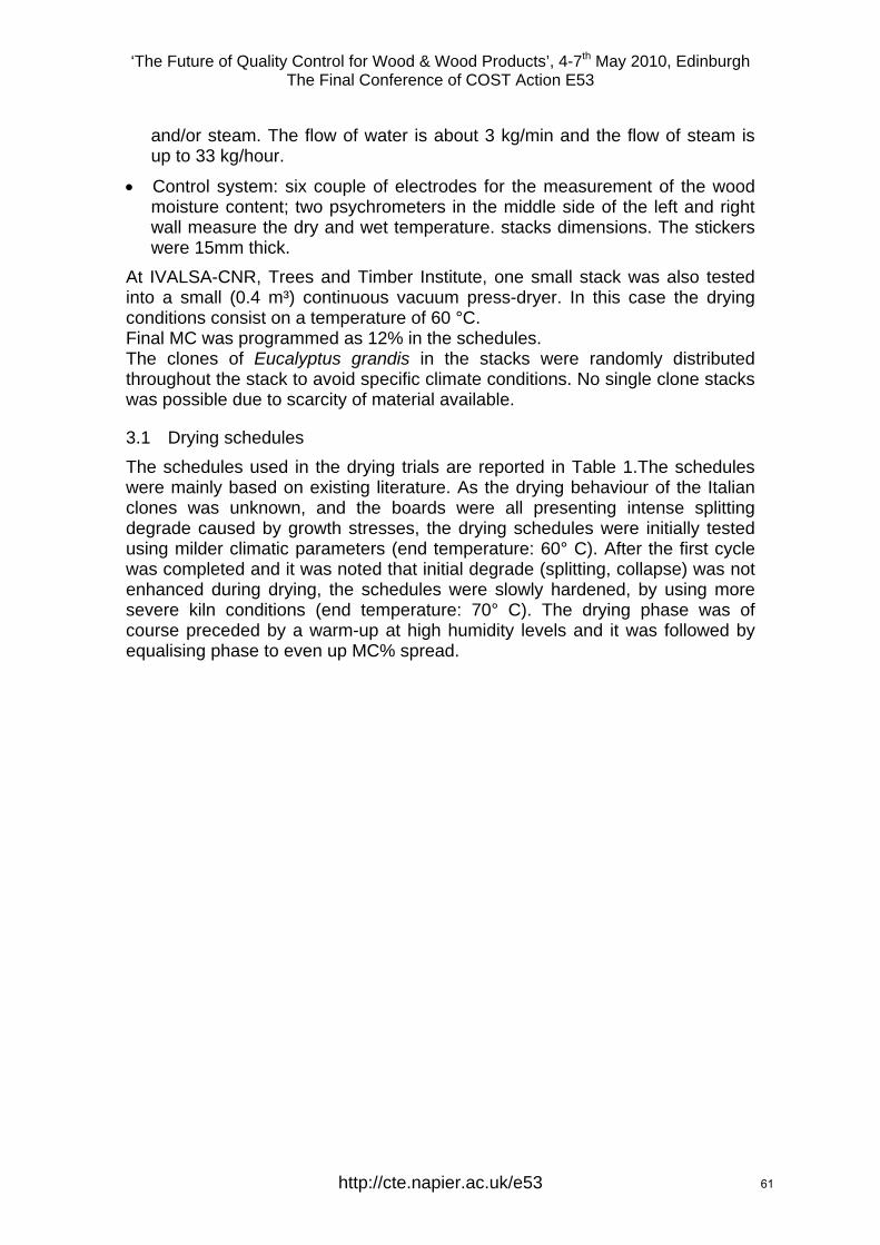
‘The Future of Quality Control for Wood & Wood Products’, 4-7th May 2010, Edinburgh The Final Conference of COST Action E53
and/or steam. The flow of water is about 3 kg/min and the flow of steam is up to 33 kg/hour.
• Control system: six couple of electrodes for the measurement of the wood moisture content; two psychrometers in the middle side of the left and right wall measure the dry and wet temperature. stacks dimensions. The stickers were 15mm thick.
At IVALSA-CNR, Trees and Timber Institute, one small stack was also tested into a small (0.4 m³) continuous vacuum press-dryer. In this case the drying conditions consist on a temperature of 60 °C. Final MC was programmed as 12% in the schedules. The clones of Eucalyptus grandis in the stacks were randomly distributed throughout the stack to avoid specific climate conditions. No single clone stacks was possible due to scarcity of material available.
3.1 Drying schedules The schedules used in the drying trials are reported in Table 1.The schedules were mainly based on existing literature. As the drying behaviour of the Italian clones was unknown, and the boards were all presenting intense splitting degrade caused by growth stresses, the drying schedules were initially tested using milder climatic parameters (end temperature: 60° C). After the first cycle was completed and it was noted that initial degrade (splitting, collapse) was not enhanced during drying, the schedules were slowly hardened, by using more severe kiln conditions (end temperature: 70° C). The drying phase was of course preceded by a warm-up at high humidity levels and it was followed by equalising phase to even up MC% spread.
http://cte.napier.ac.uk/e53 61
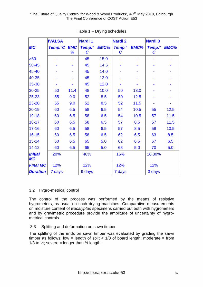
‘The Future of Quality Control for Wood & Wood Products’, 4-7th May 2010, Edinburgh The Final Conference of COST Action E53
Table 1 – Drying schedules
IVALSA Nardi 1 Nardi 2 Nardi 3 MC Temp.°C EMC
% Temp.°
C EMC% Temp.°
C EMC% Temp.°
C EMC%
>50 - - 45 15.0 - - - - 50-45 - - 45 14.5 - - - - 45-40 - - 45 14.0 - - - - 40-35 - - 45 13.0 - - - - 35-30 - - 45 12.0 - - - - 30-25 50 11.4 48 10.0 50 13.0 - - 25-23 55 9.0 52 8.5 50 12.5 - - 23-20 55 9.0 52 8.5 52 11.5 - - 20-19 60 6.5 58 6.5 54 10.5 55 12.5 19-18 60 6.5 58 6.5 54 10.5 57 11.5 18-17 60 6.5 58 6.5 57 8.5 57 11.5 17-16 60 6.5 58 6.5 57 8.5 59 10.5 16-15 60 6.5 58 6.5 62 6.5 63 8.5 15-14 60 6.5 65 5.0 62 6.5 67 6.5 14-12 60 6.5 65 5.0 68 5.0 70 5.0 Initial MC
20% 40% 16% 16.30%
Final MC 12% 12% 12% 12% Duration 7 days 9 days 7 days 3 days
3.2 Hygro-metrical control
The control of the process was performed by the means of resistive hygrometers, as usual on such drying machines. Comparative measurements on moisture content of Eucalyptus specimens carried out both with hygrometers and by gravimetric procedure provide the amplitude of uncertainty of hygro-metrical controls.
3.3 Splitting and deformation on sawn timber The splitting of the ends on sawn timber was evaluated by grading the sawn timber as follows: low = length of split < 1/3 of board length; moderate = from 1/3 to ½; severe = longer than ½ length.
http://cte.napier.ac.uk/e53 62

‘The Future of Quality Control for Wood & Wood Products’, 4-7th May 2010, Edinburgh The Final Conference of COST Action E53
The shape of sawn timber was measured by mean of a three point reference bar, one meter long, able to carry out a one-shot measurement.
The bar is instrumented with digital gauges connected with a data-logging system, and it is able to measure at the same time bow, cup and twist (see Figure 1). Crook was not measured because of its low presence and amplitude. The shape was measured on a large sample of sawn timber before and after the drying process.
The initial deformations (DEF.i) are reported as absolute value of the distance from the central measurement point from the plane determined by the three reference points. According to the figure the three reference point are 10 and 100 cm distanced from each other3.
After the drying process the final deformation (DEF.f) were measured and are reported as percentage variation (d DEF.) respect to the initial average value: d DEF.= (DEF.i –DEF.f)/av. DEF.i x 100.
According to such formulation a negative variation means an increase of the deformation, a positive value a decreasing deformation.
3.4 Quality of dried sawn timber on small specimens The tests on the quality of drying process are carried out according to the EDG-European Drying Group Recommendations.
The main tests performed at present are the following:
• internal stresses;
• check occurrence;
• collapses;
• moisture gradients.
3 The base distance is for cup 10 cm, for bow 100 cm, 10 cm on a distance of 100 cm for twist.
http://cte.napier.ac.uk/e53 63
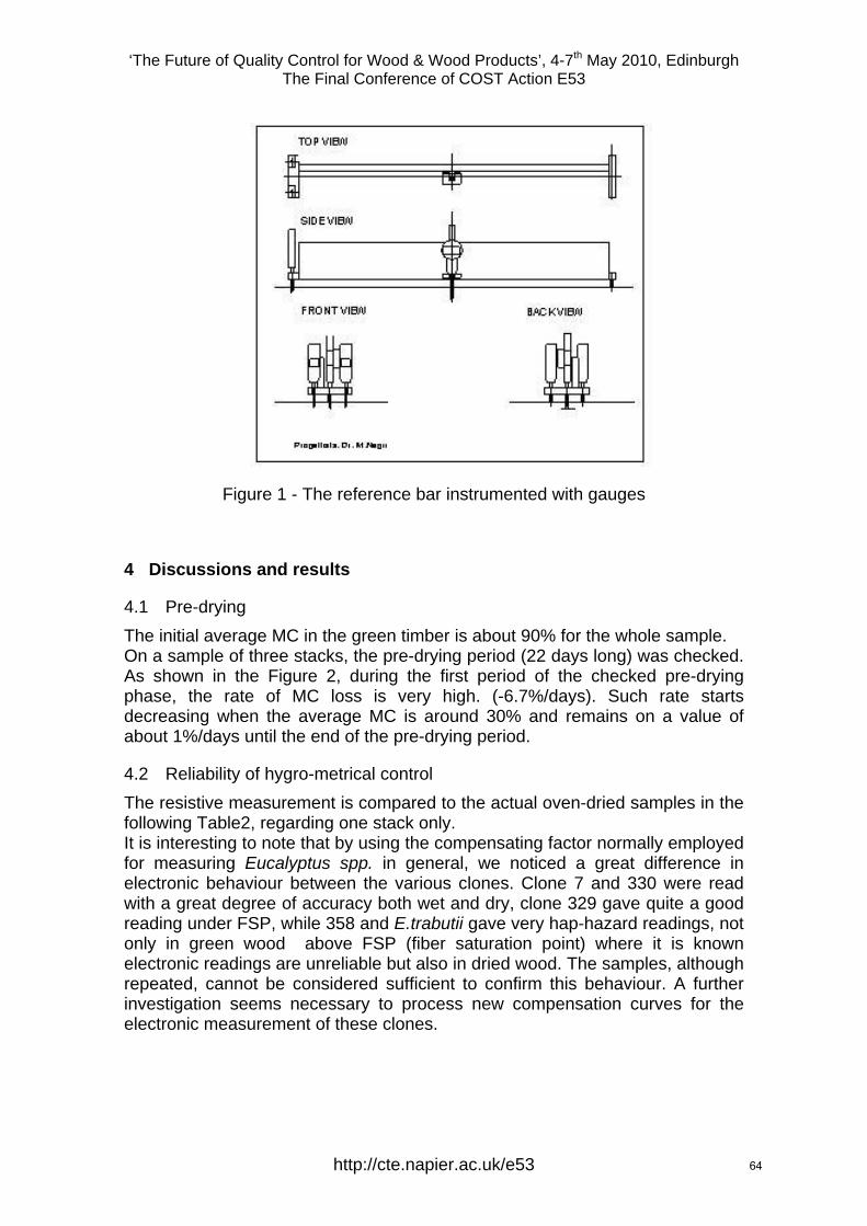
‘The Future of Quality Control for Wood & Wood Products’, 4-7th May 2010, Edinburgh The Final Conference of COST Action E53
Figure 1 - The reference bar instrumented with gauges
4 Discussions and results
4.1 Pre-drying The initial average MC in the green timber is about 90% for the whole sample. On a sample of three stacks, the pre-drying period (22 days long) was checked. As shown in the Figure 2, during the first period of the checked pre-drying phase, the rate of MC loss is very high. (-6.7%/days). Such rate starts decreasing when the average MC is around 30% and remains on a value of about 1%/days until the end of the pre-drying period.
4.2 Reliability of hygro-metrical control The resistive measurement is compared to the actual oven-dried samples in the following Table2, regarding one stack only. It is interesting to note that by using the compensating factor normally employed for measuring Eucalyptus spp. in general, we noticed a great difference in electronic behaviour between the various clones. Clone 7 and 330 were read with a great degree of accuracy both wet and dry, clone 329 gave quite a good reading under FSP, while 358 and E.trabutii gave very hap-hazard readings, not only in green wood above FSP (fiber saturation point) where it is known electronic readings are unreliable but also in dried wood. The samples, although repeated, cannot be considered sufficient to confirm this behaviour. A further investigation seems necessary to process new compensation curves for the electronic measurement of these clones.
http://cte.napier.ac.uk/e53 64
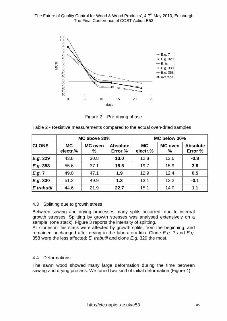
‘The Future of Quality Control for Wood & Wood Products’, 4-7th May 2010, Edinburgh The Final Conference of COST Action E53
101520253035404550556065707580859095
100105
0 5 10 15 20 25days
MC
%E.g. 7E.g. 329E. tr.E.g. 330E.g. 358average
Figure 2 – Pre-drying phase
Table 2 - Resistive measurements compared to the actual oven-dried samples
MC above 30% MC below 30% CLONE MC
electr.% MC oven
% Absolute Error %
MC electr.%
MC oven %
Absolute Error %
E.g. 329 43.8 30.8 13.0 12.8 13.6 -0.8 E.g. 358 55.6 37.1 18.5 19.7 15.9 3.8 E.g. 7 49.0 47.1 1.9 12.9 12.4 0.5 E.g. 330 51.2 49.9 1.3 13.1 13.2 -0.1 E.trabutii 44.6 21.9 22.7 15.1 14.0 1.1
4.3 Splitting due to growth stress Between sawing and drying processes many splits occurred, due to internal growth stresses. Splitting by growth stresses was analysed extensively on a sample, (one stack). Figure 3 reports the intensity of splitting. All clones in this stack were affected by growth splits, from the beginning, and remained unchanged after drying in the laboratory kiln. Clone E.g. 7 and E.g. 358 were the less affected; E. trabutii and clone E.g. 329 the most.
4.4 Deformations The sawn wood showed many large deformation during the time between sawing and drying process. We found two kind of initial deformation (Figure 4):
http://cte.napier.ac.uk/e53 65
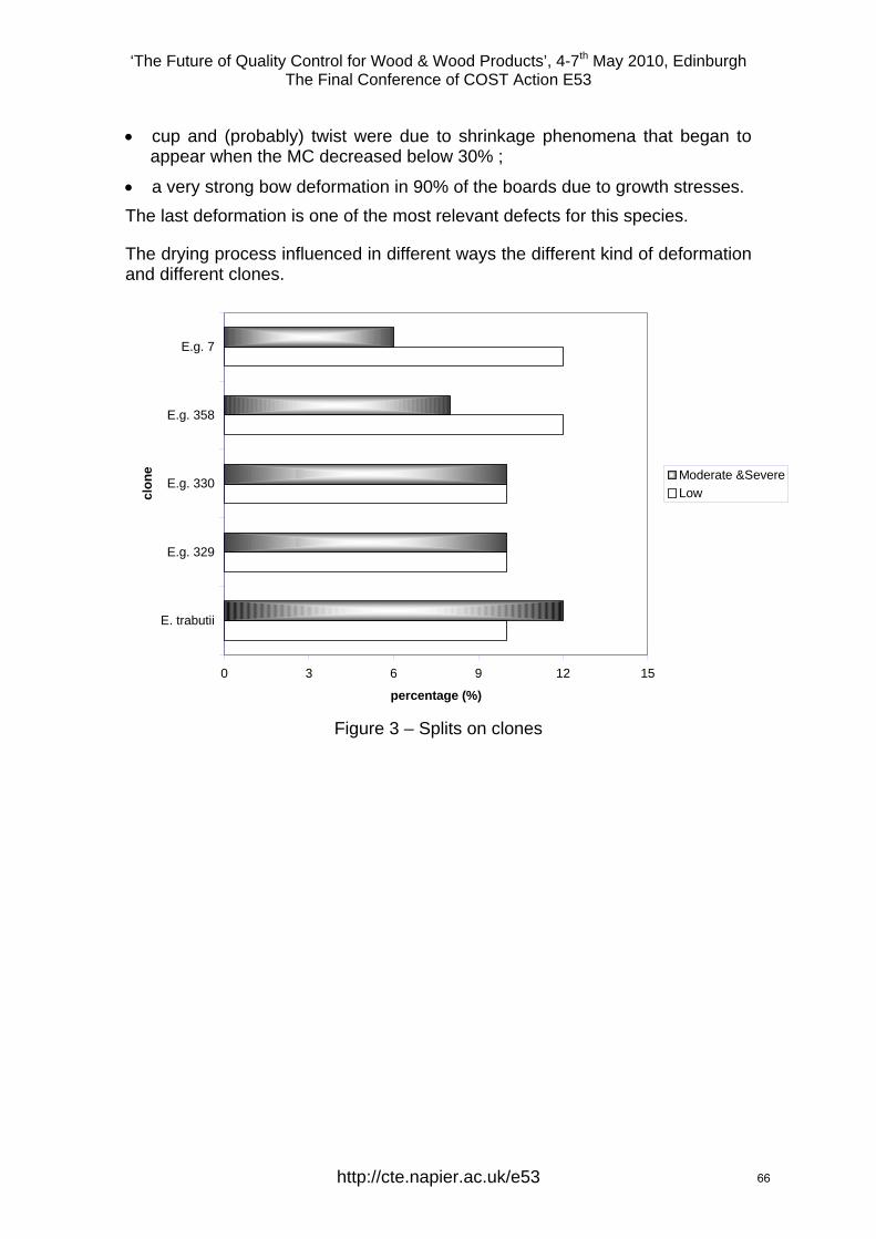
‘The Future of Quality Control for Wood & Wood Products’, 4-7th May 2010, Edinburgh The Final Conference of COST Action E53
• cup and (probably) twist were due to shrinkage phenomena that began to appear when the MC decreased below 30% ;
• a very strong bow deformation in 90% of the boards due to growth stresses. The last deformation is one of the most relevant defects for this species.
The drying process influenced in different ways the different kind of deformation and different clones.
0 3 6 9 12 15
E. trabutii
E.g. 329
E.g. 330
E.g. 358
E.g. 7
clon
e
percentage (%)
Moderate &SevereLow
Figure 3 – Splits on clones
http://cte.napier.ac.uk/e53 66
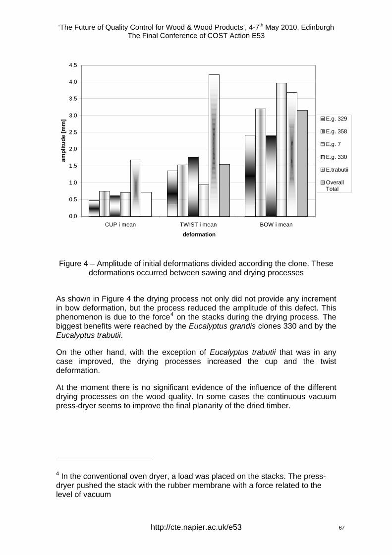
‘The Future of Quality Control for Wood & Wood Products’, 4-7th May 2010, Edinburgh The Final Conference of COST Action E53
0,0
0,5
1,0
1,5
2,0
2,5
3,0
3,5
4,0
4,5
CUP i mean TWIST i mean BOW i mean
deformation
ampl
itude
[mm
] E.g. 329
E.g. 358
E.g. 7
E.g. 330
E.trabutii
OverallTotal
Figure 4 – Amplitude of initial deformations divided according the clone. These deformations occurred between sawing and drying processes
As shown in Figure 4 the drying process not only did not provide any increment in bow deformation, but the process reduced the amplitude of this defect. This phenomenon is due to the force4 on the stacks during the drying process. The biggest benefits were reached by the Eucalyptus grandis clones 330 and by the Eucalyptus trabutii.
On the other hand, with the exception of Eucalyptus trabutii that was in any case improved, the drying processes increased the cup and the twist deformation.
At the moment there is no significant evidence of the influence of the different drying processes on the wood quality. In some cases the continuous vacuum press-dryer seems to improve the final planarity of the dried timber.
4 In the conventional oven dryer, a load was placed on the stacks. The press-dryer pushed the stack with the rubber membrane with a force related to the level of vacuum
http://cte.napier.ac.uk/e53 67
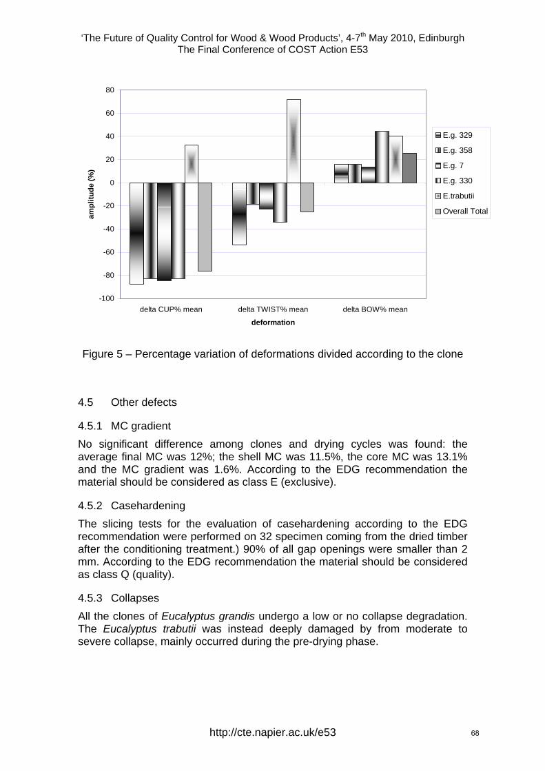
‘The Future of Quality Control for Wood & Wood Products’, 4-7th May 2010, Edinburgh The Final Conference of COST Action E53
-100
-80
-60
-40
-20
0
20
40
60
80
delta CUP% mean delta TWIST% mean delta BOW% mean
deformation
ampl
itude
(%)
E.g. 329
E.g. 358
E.g. 7
E.g. 330
E.trabutii
Overall Total
Figure 5 – Percentage variation of deformations divided according to the clone
4.5 Other defects
4.5.1 MC gradient No significant difference among clones and drying cycles was found: the average final MC was 12%; the shell MC was 11.5%, the core MC was 13.1% and the MC gradient was 1.6%. According to the EDG recommendation the material should be considered as class E (exclusive).
4.5.2 Casehardening The slicing tests for the evaluation of casehardening according to the EDG recommendation were performed on 32 specimen coming from the dried timber after the conditioning treatment.) 90% of all gap openings were smaller than 2 mm. According to the EDG recommendation the material should be considered as class Q (quality).
4.5.3 Collapses All the clones of Eucalyptus grandis undergo a low or no collapse degradation. The Eucalyptus trabutii was instead deeply damaged by from moderate to severe collapse, mainly occurred during the pre-drying phase.
http://cte.napier.ac.uk/e53 68
‘The Future of Quality Control for Wood & Wood Products’, 4-7th May 2010, Edinburgh The Final Conference of COST Action E53
5 Conclusions According to how reported in literature, the main problem we have found in our experience was the degradation of the Eucalyptus timber during the first pre-drying phase due to the growth stresses. Those stresses produced huge splits and bow deformations mainly in the tangential board of all the clones.
At the moment no significant difference seems to exist between clones. Only the E. trabutii quality of sawn timber at the end of the pre-drying period showed collapses and growth stress degradations significantly higher than the other specie.
In many cases we have found that a well performed drying treatment can improve the quality of the end-product even if the low quantity of the tested material did not permit yet to have statistical confirmation.
References Campbell G.S., , “Index of Kiln Drying Schedules for Timbers Dried in Australia”, C.S.I.R.O., Australia, 1980
Baso C., Bouzòn A. & Furones P. “Metodologia y primera experiencia de presecado y secado de Eucalyptus globulus”, Centro Universidad de Vigo, Proyecto Iberoeka de I+D, confidential report., 1999-2000.
Baso C., Casas J.M., Furones P. & Bouzòn A. “Steam treatment to improve the quality and increase the rate of drying of Eucalyptus globulus Labill.. Proposal and execution of a test on quarter-sawn boards”, Proceedings of 4th Cost E15 Workshop, 30th and 31st May 2002, Santiago de Compostela, Spain.
Du Q.P., Geissen A &, Noack, „Die Genauigkeit der elektrischen Holzfeuchtemessung nach dem Widerstandprinzip“, Holz als Roh- und Werkstoff, 49 pp.1-6, 1991.
Du Q.P., Geissen A. & Noack, “Widerstandkennlinien einiger Handelshölzer und ihre Meßbarkeit bei der elektrischen Holzfeuchtemessung“, Holz als Roh- und Werkstoff, 49 pp.305-31, 1991.
Kauman W.G., Gerard J., Jiqing H. & Huaijun W., “Processing of Eucalypts” Commonwealth Forestry Review, 74 (2) pp. 147-154, 1995.
Lima J.T., Breese M.C. & Cahalan C.M., “Variation in wood density and mechanical properties in Eucalyptus clones, proceedings of the Future of Eucalypts for wood products”, IUFRO, 19-24th march 2000Australia, pp. 282-290, 2000.
Nardi in collaboration with European drying Group, 1994, Assessment of drying quality of timber, pp 31.
Rosza A. & Mills R.G., “Index of Kiln Drying Schedules”, C.S.I.R.O., Australia, pp. 30, 1991.
http://cte.napier.ac.uk/e53 69

‘The Future of Quality Control for Wood & Wood Products’, 4-7th May 2010, Edinburgh The Final Conference of COST Action E53
Santos J.A. “Recovering dimension and form in collapse distorted boards”, Proceedings of 4th Cost E15 Workshop, 30th and 31st May 2002, Santiago de Compostela, Spain.
Vermaas H.F., “Drying of Eucalypts with special reference to young, fast-grown plantation material”, 1° seminàrio internacional sobre produtos solidos de madeira de alta tecnologia, Decembre 1988, Brasil, pp. 107-118, 1998.
Vermaas H.F., “A review of drying technology for young fast –grown eucalypts, proceedings of the Future of Eucalypts for wood products”, IUFRO, 19-24th March 2000 Australia, pp. 193-203, 2000.
Vermaas H.F., “State of the art and latest technological advances in the drying of fast-grown eucalypts”, Proceedings of 4th Cost E15 Workshop, 30th and 31st May 2002, Santiago de Compostela, Spain.
http://cte.napier.ac.uk/e53 70
‘The Future of Quality Control for Wood & Wood Products’, 4-7th May 2010, Edinburgh The Final Conference of COST Action E53
Criterial assessment of the drying quality
D. Şova1, A. Postelnicu 2 & B. Bedelean 3
Abstract The present paper aims to determine the moisture content distribution of a wood board during drying by numerical modelling and to use a criterion of similarity which is able to describe the moisture content when there is a probability for the surface cracks to occur. The constant-rate drying period will be considered, when the mass transfer intensity is maximum. The system of partial differential equations governing the phenomenon consists in the unsteady energy and mass (moisture) equations and is considered in its 1D version. One way to tackle the problem is to use the analytical solution given by Luikov and the other is to use the numerical simulation performed with Torksim (version 5.0); our strategy is to combine these two ways in order to derive an appropriate hygrometric criterion.
The proposed hygrometric criterion assesses the moisture content distribution of the body, being a measure of the inner stresses magnitude. The criterion is related to the velocity, temperature and relative humidity of the drying agent. They are to be selected in such a way that they can determine, at all times of the drying process, a lower value than the maximum value of the criterion. By use of this method an optimal domain of the drying schedules, with respect to the wood quality, can be recommended, and consequently the drying schedule with the maximum drying intensity can be chosen. In order to obtain the hygrometric criterion from the moisture content distributions, four drying schedules are applied to pine samples.
1 Introduction The heat and mass transfer that occurs at the surface of wet bodies during convective drying is accompanied by changes in the physical and mechanical properties of the body. These changes may lead to undesired quality defects if inappropriate drying schedules are applied.
1 Associate Professor, [email protected] Department of Thermodynamics and Fluid Mechanics, Transilvania University of Brasov, Romania 2 Professor, [email protected] Department of Thermodynamics and Fluid Mechanics, Transilvania University of Brasov, Romania 3 Teaching Assistant, [email protected] of Wood Industry, Transilvania University of Brasov, Romania
http://cte.napier.ac.uk/e53 71
‘The Future of Quality Control for Wood & Wood Products’, 4-7th May 2010, Edinburgh The Final Conference of COST Action E53
The moisture evaporation in the boundary layer results in a continuous change of the inner moisture content and thus the dimensional change will be different in different layers on the body thickness and at different drying times. Accordingly, tension stresses are developed at the surface and inside the body, which determine cracks if the moisture content drop exceeds a maximum value. Since the absence of cracks is the main requirement of the wood quality during drying, it is necessary to determine the moisture content gradient in the wood board and accordingly to use a criterion of similarity which can assess the moisture profile when there is a risk for the surface cracks development. The main reason for stresses is the moisture gradient and the outcome consists in micro- and macro-cracking.
During lumber drying above fibre saturation point, capillary flow frequently leads to drying defects in various wood species. Drying above FSP has been described as a two-stage process (Keey 1994): in the first stage, the wetline remains close to the surface (at approximately 50% MC – Scheepers et al. 2005), in the second stage the wetline starts to move towards the core.
Song & Shida (2010) by examining the effects of the surface temperature on the surface checking using the infrared thermography technique, have obtained a relationship between moisture content and surface checking, with the observation that above the fibre saturation point checking developed as the drying advanced.
The radial, tangential and volumetric shrinkages occur above FSP, behaviour that can be explained by the effect of hysteresis at saturation on wood properties, according to which the loss of bound water takes place in the presence of free water (Almeida et al. 2005).
The present paper aims to determine the moisture distribution of the board during drying above fibre saturation point by numerical modelling and to use a similarity criterion which is able to describe the moisture content when there is a probability for the surface cracks to occur.
2 Mathematical model The temperature and moisture content fields of a body submitted to convective drying can be determined from the solution of the coupled system of differential equations of heat and mass transfer (Luikov 1966):
taMaMmm
22 ∇+∇=∂∂ δτ
Equation 1
ττ ∂∂
+∇=∂∂ Mktat
e2
Equation 2
where is the moisture diffusion coefficient, ma δ - coefficient of thermal diffusion, - coefficient of thermal diffusivity, - constant coefficient, equal to ea k
http://cte.napier.ac.uk/e53 72

‘The Future of Quality Control for Wood & Wood Products’, 4-7th May 2010, Edinburgh The Final Conference of COST Action E53
crak m1=
Equation 3
where is the mass transfer coefficient corresponding to the liquid, - the latent heat of vaporisation,
1ma rc - specific heat of the body.
For very long boards of thickness 2R, assuming the symmetry of the heat and mass transfer related to the board sides, the following initial and boundary conditions can be written:
( ) ( )( ) ( ) consttxtxt
constMxMxM===
===
00
00
0
0
,,
Equation 4
and
( ) ( )
( ) ( ) ( )( ) ( )( ) ( ) ( 01
0
000
11
100
=−−−+∇−
=+∇+∇
=∂
∂=
∂∂
τταλτδρρ
)
ττ
JarRtttJtaMa
xt
xM
mairs
smsm
,
,, Equation 5
where subscript s refers to the surface (x=R), 0ρ - ovendry density of the body, ( )τ1J - mass flux per unit area, λ - coefficient of thermal conductivity, α - heat
transfer coefficient. If the thermal diffusion is neglected ( )0=δ , then Equations 1 and 5 become:
( )2
2
2
xxMaM
m ∂∂
=∂∂ ττ
,
( ) ( ) 010 =+∂
∂ ττρ JxRMam
,
Equation 6
Luikov’s solution of Equation 6 is:
( ) ( ) ( )
( )
( ) ( )⎥⎦
⎤⎢⎣
⎡⎟⎟⎠
⎞⎜⎜⎝
⎛+
×⎟⎠⎞
⎜⎝⎛−−
+−
−=−−
∫
∑
∫
∗
+∞
=
∗
τ
τ
ττττπ
τπππ
ττρττ
0 2
22
222
22
1
1
2
22
000
1
0
0
21
63
dd
dKiR
anKi
Ran
Rxn
n
RxRKid
MRJ
EMCMxMM
m
mn
n
exp
expcos
, Equation 7
where ( ) ( )00
1
MaRJKi
mρττ =∗ is the hygrometric Kirpichev similarity criterion
(Kirpichev number).
http://cte.napier.ac.uk/e53 73

‘The Future of Quality Control for Wood & Wood Products’, 4-7th May 2010, Edinburgh The Final Conference of COST Action E53
If checking takes place during the constant drying-rate period, when the mass transfer reaches its maximum intensity and is constant during this period of
time, meaning that ( ) 01 =ττ
ddJ , then a constant value of the hygrometric criterion
can be assumed ( ) 0=ττ
ddKi . With this assumption, Equation 7 becomes:
( ) ( ) ( )⎥⎥⎦
⎤
⎢⎢⎣
⎡−−+
−−=
−− ∗
+∞
=
∗∗ ∑ FonR
xnnR
xRFoKiEMCM
xMM n
n
2222
1
12
22
0
0 216
3 πππ
τ expcos, Equation 8
where 2RaFo mτ=∗ is the hygrometric Fourier number. The increase of Fourier
number, as time elapses, determines the series members from Equation 8 to become rapidly convergent and for values beginning with , they can be neglected with respect to the first two members and thus the solution can be written as (Luikov&Mikhailov 1965):
540.≥Fo
( )⎟⎟⎠
⎞⎜⎜⎝
⎛ −−=
−− ∗∗
2
22
0
0
63
RxRFoKi
EMCMxMM τ,
Equation 9
In this case the local moisture content on the board thickness will be a linear time function and its distribution along the board thickness is a parabolic one.
Considering that the surface checking occurs in the first drying period, a criterion can be adopted for describing the moisture content field which is able to develop surface cracks, namely:
( ) ( )EMCM
RMMK−−
=0
0 ττ ,, Equation 10
where ( )τ,0M and ( )τ,RM correspond to the moisture content in the centre and on the surface of the board, 0M - the average initial moisture content, EMC – the equilibrium moisture content. Considering Equation 9, the dimensionless criterion K will be:
( ) ( ) ∗=−−
= KiEMCM
RMMK210
0
ττ ,, Equation 11
For boards with a symmetric distribution of the moisture content along the thickness, the average moisture content is:
( ) ( )dxxMR
MR
∫=0
1 ττ , Equation 12
and on using Equation 9, the following relation can be obtained:
http://cte.napier.ac.uk/e53 74
‘The Future of Quality Control for Wood & Wood Products’, 4-7th May 2010, Edinburgh The Final Conference of COST Action E53
( ) ( ) ∗∗−−= FoKiEMCMMM 00τ Equation 13
For constant , ∗Ki ( )τM is a linear function ofτ . From Equation 13 we have:
( ) ( )( ) ∗∗
∗
−−
=⎟⎟⎠
⎞⎜⎜⎝
⎛−
=FoEMCM
MMMEMC
MdFo
dKi0
0
0
ττ Equation 14
which can be also written as:
( )( )
( ) ( ) KEMCM
RMMFoEMCM
MMKi 20200
0 =−−
=−−
= ∗∗ τττ ,, Equation 15
Kirpichev number ranges between 0 and 2. A small value determines a small internal resistance to diffusion and vice versa. Equation 15 shows the relationship among the hygrometric criterion and the average board moisture content. The moisture content gradient along the board thickness determines the magnitude of the hygrometric criterion.
The Kirpichev hygrometric number can be used as a criterion for the assessment of the moisture content field on the board thickness in the constant drying rate period, being thus a quantitative measure for the stresses that determine surface cracks. Since the mass flux depends on the drying schedule (velocity, temperature and relative humidity of air), then a relationship between the hygrometric criterion (moisture profile) and the drying air properties can be settled. In order to prevent surface checking, the temperature and relative humidity must be thus chosen so as to get lower values of the hygrometric criterion than the maximum (critical) one that corresponds to the moment when surface cracks occur. By use of this method an optimal domain of the drying schedules, with respect to the wood quality, can be recommended, and thus a drying schedule with the maximum drying intensity can be chosen.
3 Method and material Pine wood samples with two different initial moisture contents, 130% and 60% and a thickness of 28 mm are submitted to four drying schedules. The first drying schedule is a standard one, tested in practice, as proposed by Seba Industrial Company, whilst the other three ones correspond to constant velocity (3 m/s), temperature (50, 60, 70, 80 oC) and RH values (60, 50 and 40%). Two methods for the determination of the hygrometric criterion are applied; one is aimed for the calculation of the criterion variation across the board thickness (Eq. 9), while the second one is that of its time dependence with respect to the applied drying schedule (Eq. 15). The moisture content - time variation, average board temperature and moisture content are obtained by use of the wood drying simulation package TORKSIM, version 5.0.
http://cte.napier.ac.uk/e53 75
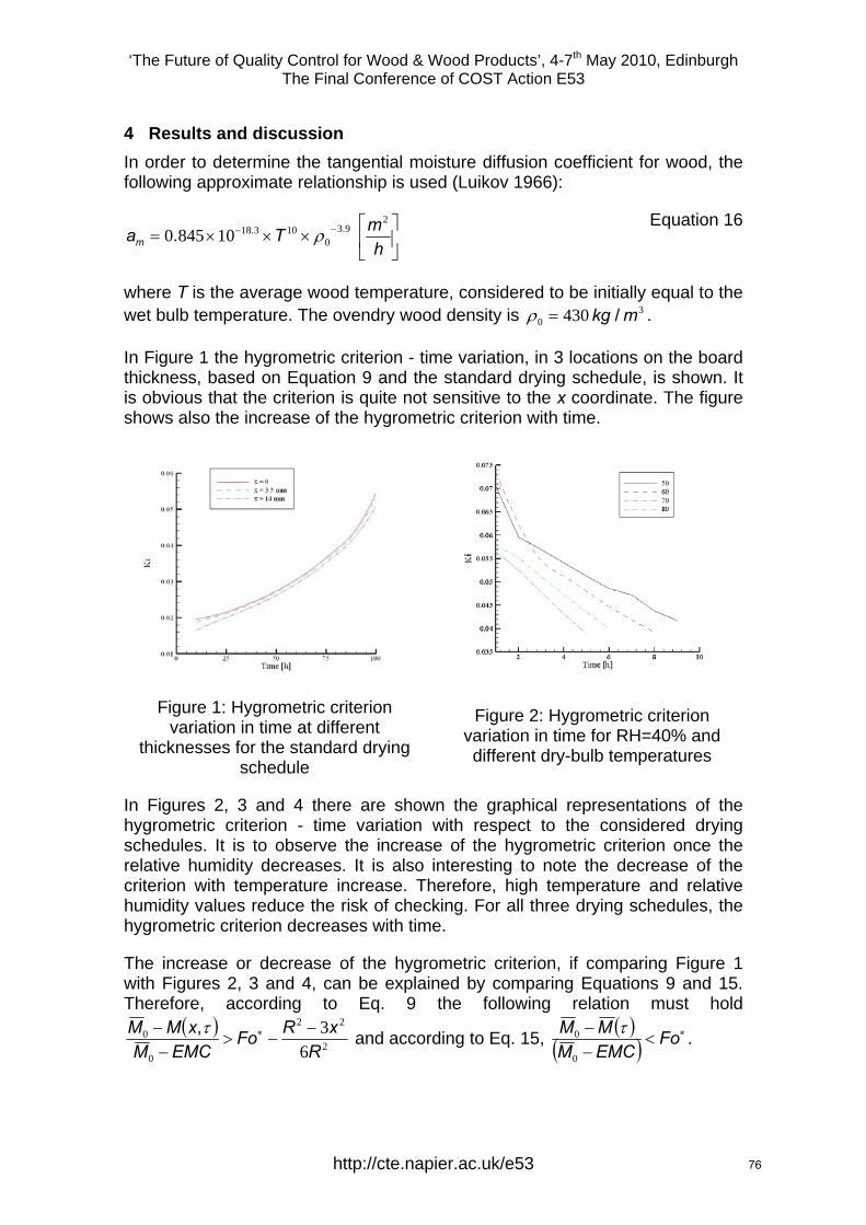
‘The Future of Quality Control for Wood & Wood Products’, 4-7th May 2010, Edinburgh The Final Conference of COST Action E53
4 Results and discussion In order to determine the tangential moisture diffusion coefficient for wood, the following approximate relationship is used (Luikov 1966):
⎥⎦
⎤⎢⎣
⎡×××= −−
hmTam
293
010318108450 ... ρ
Equation 16
where T is the average wood temperature, considered to be initially equal to the wet bulb temperature. The ovendry wood density is . 3
0 430 mkg /=ρ
In Figure 1 the hygrometric criterion - time variation, in 3 locations on the board thickness, based on Equation 9 and the standard drying schedule, is shown. It is obvious that the criterion is quite not sensitive to the x coordinate. The figure shows also the increase of the hygrometric criterion with time.
Figure 1: Hygrometric criterion variation in time at different
thicknesses for the standard drying schedule
Figure 2: Hygrometric criterion variation in time for RH=40% and different dry-bulb temperatures
In Figures 2, 3 and 4 there are shown the graphical representations of the hygrometric criterion - time variation with respect to the considered drying schedules. It is to observe the increase of the hygrometric criterion once the relative humidity decreases. It is also interesting to note the decrease of the criterion with temperature increase. Therefore, high temperature and relative humidity values reduce the risk of checking. For all three drying schedules, the hygrometric criterion decreases with time.
The increase or decrease of the hygrometric criterion, if comparing Figure 1 with Figures 2, 3 and 4, can be explained by comparing Equations 9 and 15. Therefore, according to Eq. 9 the following relation must hold
( )2
22
0
0
63
RxRFo
EMCMxMM −
−>−− ∗τ, and according to Eq. 15, ( )
( )∗<
−− Fo
EMCMMM
0
0 τ .
http://cte.napier.ac.uk/e53 76
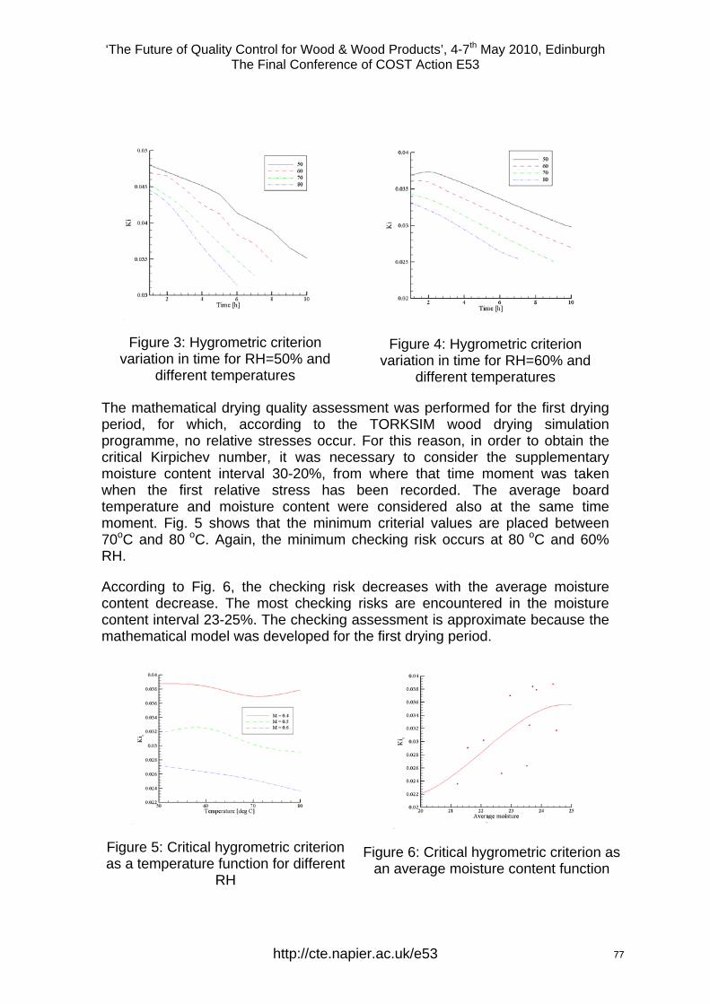
‘The Future of Quality Control for Wood & Wood Products’, 4-7th May 2010, Edinburgh The Final Conference of COST Action E53
Figure 3: Hygrometric criterion variation in time for RH=50% and
different temperatures
Figure 4: Hygrometric criterion variation in time for RH=60% and
different temperatures
The mathematical drying quality assessment was performed for the first drying period, for which, according to the TORKSIM wood drying simulation programme, no relative stresses occur. For this reason, in order to obtain the critical Kirpichev number, it was necessary to consider the supplementary moisture content interval 30-20%, from where that time moment was taken when the first relative stress has been recorded. The average board temperature and moisture content were considered also at the same time moment. Fig. 5 shows that the minimum criterial values are placed between 70oC and 80 oC. Again, the minimum checking risk occurs at 80 oC and 60% RH.
According to Fig. 6, the checking risk decreases with the average moisture content decrease. The most checking risks are encountered in the moisture content interval 23-25%. The checking assessment is approximate because the mathematical model was developed for the first drying period.
Figure 5: Critical hygrometric criterion as a temperature function for different
RH
Figure 6: Critical hygrometric criterion as an average moisture content function
http://cte.napier.ac.uk/e53 77
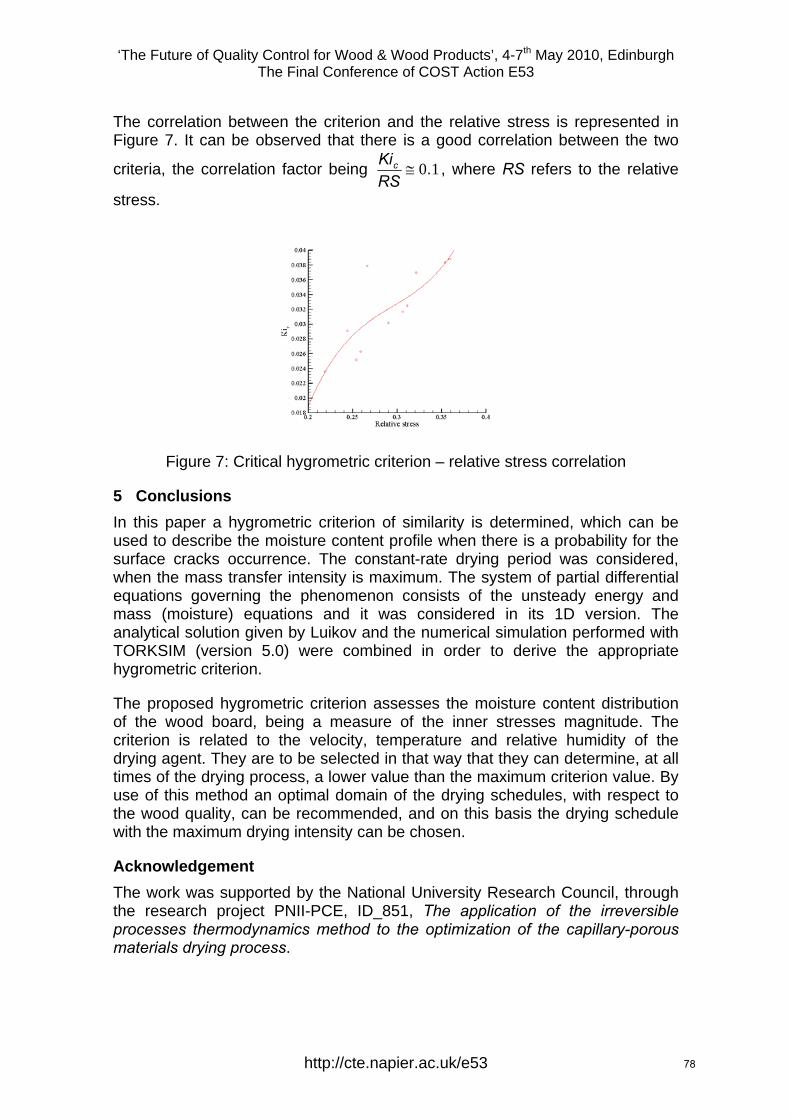
‘The Future of Quality Control for Wood & Wood Products’, 4-7th May 2010, Edinburgh The Final Conference of COST Action E53
The correlation between the criterion and the relative stress is represented in Figure 7. It can be observed that there is a good correlation between the two
criteria, the correlation factor being 10.≅RSKic , where RS refers to the relative
stress.
Figure 7: Critical hygrometric criterion – relative stress correlation
5 Conclusions In this paper a hygrometric criterion of similarity is determined, which can be used to describe the moisture content profile when there is a probability for the surface cracks occurrence. The constant-rate drying period was considered, when the mass transfer intensity is maximum. The system of partial differential equations governing the phenomenon consists of the unsteady energy and mass (moisture) equations and it was considered in its 1D version. The analytical solution given by Luikov and the numerical simulation performed with TORKSIM (version 5.0) were combined in order to derive the appropriate hygrometric criterion.
The proposed hygrometric criterion assesses the moisture content distribution of the wood board, being a measure of the inner stresses magnitude. The criterion is related to the velocity, temperature and relative humidity of the drying agent. They are to be selected in that way that they can determine, at all times of the drying process, a lower value than the maximum criterion value. By use of this method an optimal domain of the drying schedules, with respect to the wood quality, can be recommended, and on this basis the drying schedule with the maximum drying intensity can be chosen.
Acknowledgement The work was supported by the National University Research Council, through the research project PNII-PCE, ID_851, The application of the irreversible processes thermodynamics method to the optimization of the capillary-porous materials drying process.
http://cte.napier.ac.uk/e53 78

‘The Future of Quality Control for Wood & Wood Products’, 4-7th May 2010, Edinburgh The Final Conference of COST Action E53
References Almeida, G., Pontin, M., Hernández, R.E. (2005) “Changes in shrinkage of temperate and tropical hardwoods below and above the fiber saturation point”, 9th International IUFRO Wood Drying Conference, Nanjing, pp. 453-458.
Keey, R.B. (1994) “Heat and mass transfer in kiln drying: a review”, 4th
International IUFRO Wood Drying Conference, Rotorua, pp 22-44.
Luikov, A.V. &Mikhailov, Yu.A. (1965) “Theory of energy and mass transfer”, Pergamon Press.
Luikov, A.V. (1966) “Heat and mass transfer in capillary-porous bodies”, Pergamon Press.
Scheepers, G., Danvind, J., Morén, T. Rypstra T. (2005) “An investigation of fluid water movement in birch during drying through variation of wood sap surface tension and initial average moisture content”, 9th International IUFRO Wood Drying Conference, Nanjing, pp. 57-62.
Song, J.H.& Shida, S. (2010) “Infrared thermography for monitoring surface checking of wood during drying”, 11th International IUFRO Wood Drying Conference, Skelleftea, pp 70-75.
Seba Industrial “User manual”.
TORKSIM ver. 5.0 ”User manual and instructions for evaluation of calculated results”, SP Wood Technology, SP Technical Research Institute of Sweden.
http://cte.napier.ac.uk/e53 79
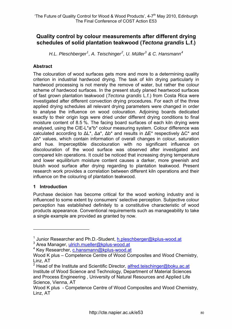
‘The Future of Quality Control for Wood & Wood Products’, 4-7th May 2010, Edinburgh The Final Conference of COST Action E53
Quality control by colour measurements after different drying schedules of solid plantation teakwood (Tectona grandis L.f.)
H.L. Pleschberger1, A. Teischinger2, U. Müller3 & C. Hansmann4
Abstract The colouration of wood surfaces gets more and more to a determining quality criterion in industrial hardwood drying. The task of kiln drying particularly in hardwood processing is not merely the remove of water, but rather the colour scheme of hardwood surfaces. In the present study planed heartwood surfaces of fast grown plantation teakwood (Tectona grandis L.f.) from Costa Rica were investigated after different convection drying procedures. For each of the three applied drying schedules all relevant drying parameters were changed in order to analyse the influence on wood colouration. Adjoining boards dedicated exactly to their origin logs were dried under different drying conditions to final moisture content of 8.5 %. The facing board surfaces of each kiln drying were analysed, using the CIE-L*a*b* colour measuring system. Colour difference was calculated according to ΔL*, Δa*, Δb* and results in ΔE* respectively ΔC* and Δh* values, which contain information of overall changes in colour, saturation and hue. Imperceptible discolouration with no significant influence on discolouration of the wood surface was observed after investigated and compared kiln operations. It could be noticed that increasing drying temperature and lower equilibrium moisture content causes a darker, more greenish and bluish wood surface after drying regarding to plantation teakwood. Present research work provides a correlation between different kiln operations and their influence on the colouring of plantation teakwood.
1 Introduction Purchase decision has become critical for the wood working industry and is influenced to some extent by consumers’ selective perception. Subjective colour perception has established definitely to a constitutive characteristic of wood products appearance. Conventional requirements such as manageability to take a single example are provided as granted by now.
1 Junior Researcher and Ph.D.-Student, [email protected] Area Manager, [email protected] Key Researcher, [email protected] K plus – Competence Centre of Wood Composites and Wood Chemistry, Linz, AT 2 Head of the Institute and Scientific Director, [email protected] of Wood Science and Technology, Department of Material Sciences and Process Engineering , University of Natural Resources and Applied Life Science, Vienna, AT Wood K plus - Competence Centre of Wood Composites and Wood Chemistry, Linz, AT
http://cte.napier.ac.uk/e53 80
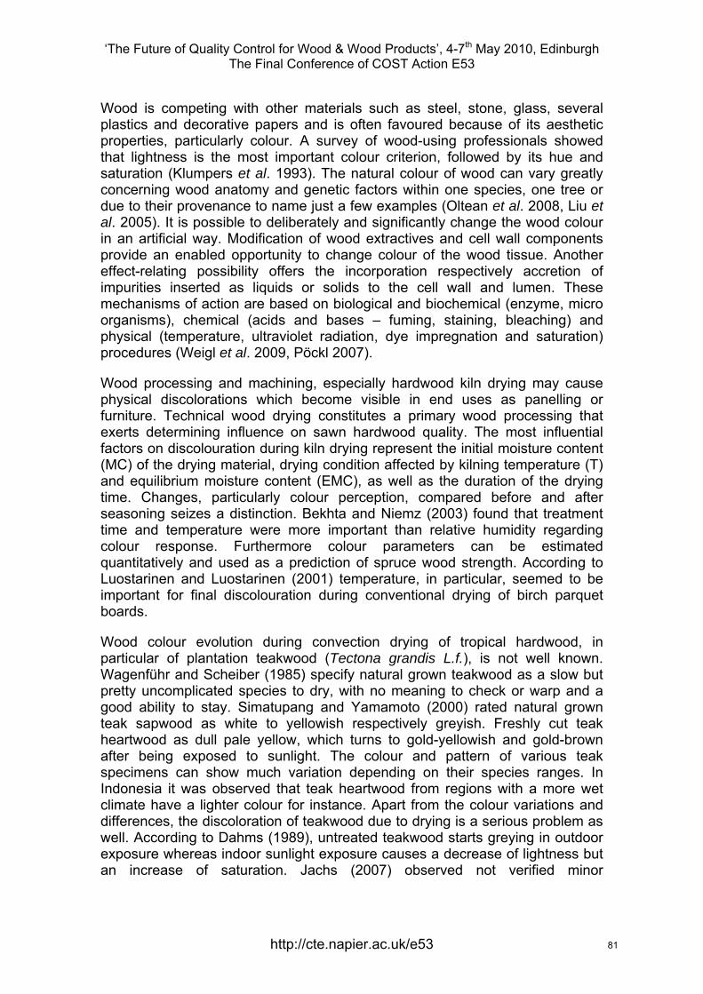
‘The Future of Quality Control for Wood & Wood Products’, 4-7th May 2010, Edinburgh The Final Conference of COST Action E53
Wood is competing with other materials such as steel, stone, glass, several plastics and decorative papers and is often favoured because of its aesthetic properties, particularly colour. A survey of wood-using professionals showed that lightness is the most important colour criterion, followed by its hue and saturation (Klumpers et al. 1993). The natural colour of wood can vary greatly concerning wood anatomy and genetic factors within one species, one tree or due to their provenance to name just a few examples (Oltean et al. 2008, Liu et al. 2005). It is possible to deliberately and significantly change the wood colour in an artificial way. Modification of wood extractives and cell wall components provide an enabled opportunity to change colour of the wood tissue. Another effect-relating possibility offers the incorporation respectively accretion of impurities inserted as liquids or solids to the cell wall and lumen. These mechanisms of action are based on biological and biochemical (enzyme, micro organisms), chemical (acids and bases – fuming, staining, bleaching) and physical (temperature, ultraviolet radiation, dye impregnation and saturation) procedures (Weigl et al. 2009, Pöckl 2007).
Wood processing and machining, especially hardwood kiln drying may cause physical discolorations which become visible in end uses as panelling or furniture. Technical wood drying constitutes a primary wood processing that exerts determining influence on sawn hardwood quality. The most influential factors on discolouration during kiln drying represent the initial moisture content (MC) of the drying material, drying condition affected by kilning temperature (T) and equilibrium moisture content (EMC), as well as the duration of the drying time. Changes, particularly colour perception, compared before and after seasoning seizes a distinction. Bekhta and Niemz (2003) found that treatment time and temperature were more important than relative humidity regarding colour response. Furthermore colour parameters can be estimated quantitatively and used as a prediction of spruce wood strength. According to Luostarinen and Luostarinen (2001) temperature, in particular, seemed to be important for final discolouration during conventional drying of birch parquet boards.
Wood colour evolution during convection drying of tropical hardwood, in particular of plantation teakwood (Tectona grandis L.f.), is not well known. Wagenführ and Scheiber (1985) specify natural grown teakwood as a slow but pretty uncomplicated species to dry, with no meaning to check or warp and a good ability to stay. Simatupang and Yamamoto (2000) rated natural grown teak sapwood as white to yellowish respectively greyish. Freshly cut teak heartwood as dull pale yellow, which turns to gold-yellowish and gold-brown after being exposed to sunlight. The colour and pattern of various teak specimens can show much variation depending on their species ranges. In Indonesia it was observed that teak heartwood from regions with a more wet climate have a lighter colour for instance. Apart from the colour variations and differences, the discoloration of teakwood due to drying is a serious problem as well. According to Dahms (1989), untreated teakwood starts greying in outdoor exposure whereas indoor sunlight exposure causes a decrease of lightness but an increase of saturation. Jachs (2007) observed not verified minor
http://cte.napier.ac.uk/e53 81
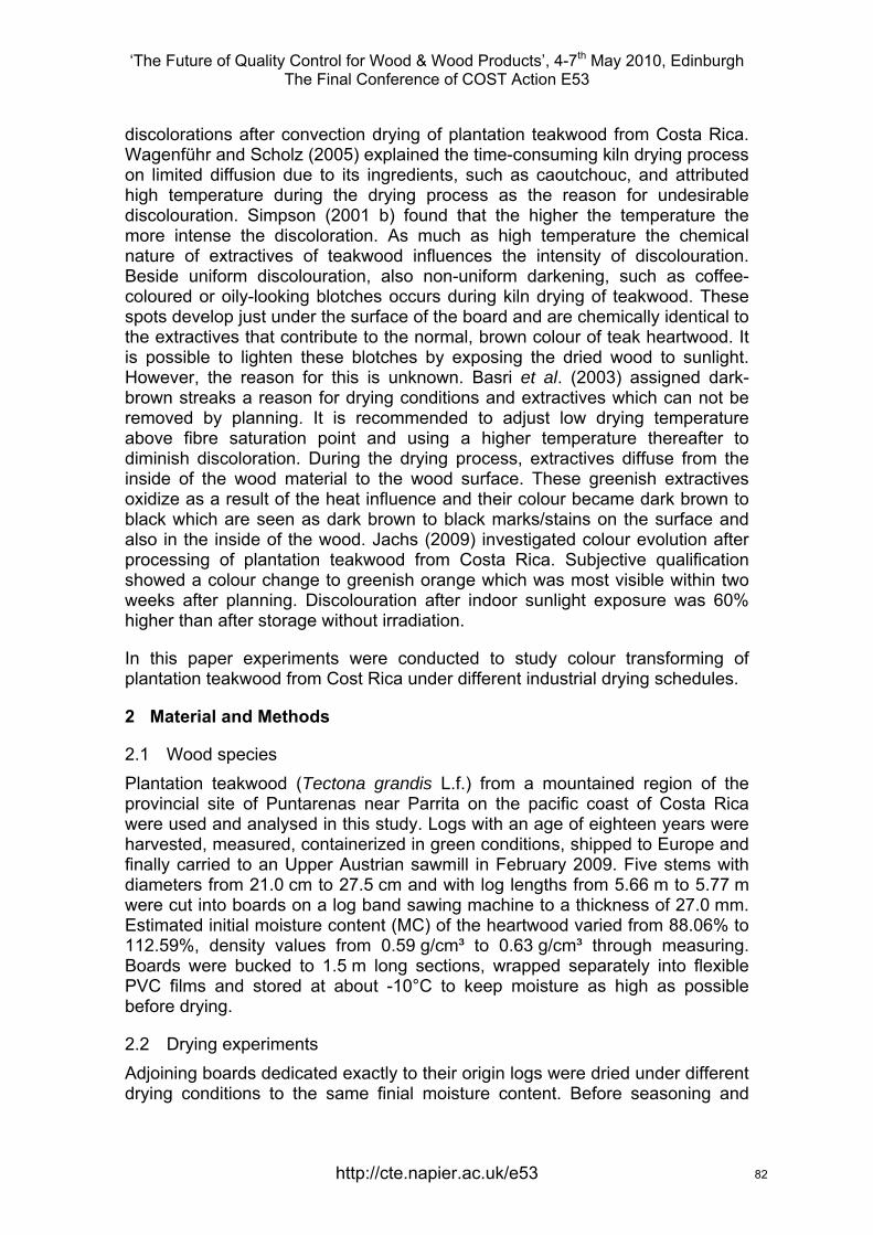
‘The Future of Quality Control for Wood & Wood Products’, 4-7th May 2010, Edinburgh The Final Conference of COST Action E53
discolorations after convection drying of plantation teakwood from Costa Rica. Wagenführ and Scholz (2005) explained the time-consuming kiln drying process on limited diffusion due to its ingredients, such as caoutchouc, and attributed high temperature during the drying process as the reason for undesirable discolouration. Simpson (2001 b) found that the higher the temperature the more intense the discoloration. As much as high temperature the chemical nature of extractives of teakwood influences the intensity of discolouration. Beside uniform discolouration, also non-uniform darkening, such as coffee-coloured or oily-looking blotches occurs during kiln drying of teakwood. These spots develop just under the surface of the board and are chemically identical to the extractives that contribute to the normal, brown colour of teak heartwood. It is possible to lighten these blotches by exposing the dried wood to sunlight. However, the reason for this is unknown. Basri et al. (2003) assigned dark-brown streaks a reason for drying conditions and extractives which can not be removed by planning. It is recommended to adjust low drying temperature above fibre saturation point and using a higher temperature thereafter to diminish discoloration. During the drying process, extractives diffuse from the inside of the wood material to the wood surface. These greenish extractives oxidize as a result of the heat influence and their colour became dark brown to black which are seen as dark brown to black marks/stains on the surface and also in the inside of the wood. Jachs (2009) investigated colour evolution after processing of plantation teakwood from Costa Rica. Subjective qualification showed a colour change to greenish orange which was most visible within two weeks after planning. Discolouration after indoor sunlight exposure was 60% higher than after storage without irradiation.
In this paper experiments were conducted to study colour transforming of plantation teakwood from Cost Rica under different industrial drying schedules.
2 Material and Methods
2.1 Wood species Plantation teakwood (Tectona grandis L.f.) from a mountained region of the provincial site of Puntarenas near Parrita on the pacific coast of Costa Rica were used and analysed in this study. Logs with an age of eighteen years were harvested, measured, containerized in green conditions, shipped to Europe and finally carried to an Upper Austrian sawmill in February 2009. Five stems with diameters from 21.0 cm to 27.5 cm and with log lengths from 5.66 m to 5.77 m were cut into boards on a log band sawing machine to a thickness of 27.0 mm. Estimated initial moisture content (MC) of the heartwood varied from 88.06% to 112.59%, density values from 0.59 g/cm³ to 0.63 g/cm³ through measuring. Boards were bucked to 1.5 m long sections, wrapped separately into flexible PVC films and stored at about -10°C to keep moisture as high as possible before drying.
2.2 Drying experiments Adjoining boards dedicated exactly to their origin logs were dried under different drying conditions to the same finial moisture content. Before seasoning and
http://cte.napier.ac.uk/e53 82
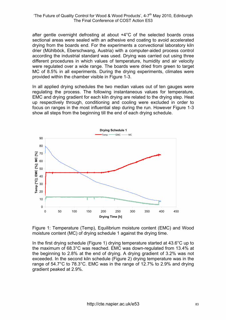
‘The Future of Quality Control for Wood & Wood Products’, 4-7th May 2010, Edinburgh The Final Conference of COST Action E53
after gentle overnight defrosting at about +4°C of the selected boards cross sectional areas were sealed with an adhesive end coating to avoid accelerated drying from the boards end. For the experiments a convectional laboratory kiln drier (Mühlböck, Eberschwang, Austria) with a computer-aided process control according the industrial standard was used. Drying was carried out using three different procedures in which values of temperature, humidity and air velocity were regulated over a wide range. The boards were dried from green to target MC of 8.5% in all experiments. During the drying experiments, climates were provided within the chamber visible in Figure 1-3.
In all applied drying schedules the two median values out of ten gauges were regulating the process. The following instantaneous values for temperature, EMC and drying gradient for each kiln drying are related to the drying step. Heat up respectively through, conditioning and cooling were excluded in order to focus on ranges in the most influential step during the run. However Figure 1-3 show all steps from the beginning till the end of each drying schedule.
Drying Schedule 1
0
10
20
30
40
50
60
70
80
90
0 50 100 150 200 250 300 350 400 450
Drying Time [h]
Tem
p [°
C];
EMC
[%];
MC
[%]
Temp EMC MC
Figure 1: Temperature (Temp), Equilibrium moisture content (EMC) and Wood moisture content (MC) of drying schedule 1 against the drying time.
In the first drying schedule (Figure 1) drying temperature started at 43.6°C up to the maximum of 68.3°C was reached. EMC was down-regulated from 13.4% at the beginning to 2.8% at the end of drying. A drying gradient of 3.2% was not exceeded. In the second kiln schedule (Figure 2) drying temperature was in the range of 54.7°C to 78.3°C. EMC was in the range of 12.7% to 2.9% and drying gradient peaked at 2.9%.
http://cte.napier.ac.uk/e53 83
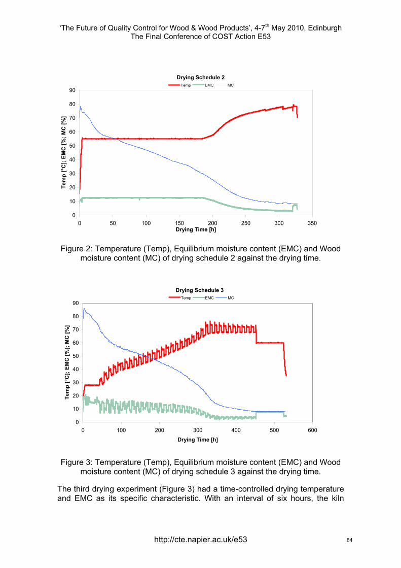
‘The Future of Quality Control for Wood & Wood Products’, 4-7th May 2010, Edinburgh The Final Conference of COST Action E53
Drying Schedule 2
0
10
20
30
40
50
60
70
80
90
0 50 100 150 200 250 300 350Drying Time [h]
Tem
p [°
C];
EMC
[%; M
C [%
]
Temp EMC MC
Figure 2: Temperature (Temp), Equilibrium moisture content (EMC) and Wood moisture content (MC) of drying schedule 2 against the drying time.
Drying Schedule 3
0
10
20
30
40
50
60
70
80
90
0 100 200 300 400 500 600
Drying Time [h]
Tem
p [°
C];
EMC
[%];
MC
[%]
Temp EMC MC
Figure 3: Temperature (Temp), Equilibrium moisture content (EMC) and Wood moisture content (MC) of drying schedule 3 against the drying time.
The third drying experiment (Figure 3) had a time-controlled drying temperature and EMC as its specific characteristic. With an interval of six hours, the kiln
http://cte.napier.ac.uk/e53 84
‘The Future of Quality Control for Wood & Wood Products’, 4-7th May 2010, Edinburgh The Final Conference of COST Action E53
schedule was switched between a gentler program and a more severe one, which is clearly recognizable in the temperature and EMC curve in Figure 3. Dual drying procedure started with 5°C alternating difference in the temperature, where EMC alternated initially 5.0% and in the end only 0.5%. 76.3°C was the peak value in temperature and EMC decreased from 17.3% at the beginning to 2.0% in the end with a maximal drying gradient of 6.4%.
2.3 Colour measurements The facing board surfaces of each kiln drying were compared and analysed, using the CIE-L*a*b* colour measuring system according to the ISO 7724-3 (1984) standard. The CIE-L*a*b* colour space is characterized by three parameters, L* for lightness and a* and b* for colour opponent dimensions. L* values vary from +100 (+L*) for white to zero (-L*) for black and the chromaticity coordinates range from +128 (+a*) for red to -127 (-a*) for green and from +128 (+b*) for yellow to -127 (–b*) for blue. Colorimeter device a Chroma Meter CR-410 (Konica Minolta, Tokyo, Japan) equipped with a measuring orifice of 50 mm was used. D65 light source (daylight) and an observation angle of 2° were adjusted. Colour difference was calculated according to ΔL*, Δa*, Δb* and results in ΔE* (distance in L*a*b* colour space), Δa* and Δb* in ΔC* (saturation) and a* and b* in h* (hue) values, which contain information of overall changes in colour using equations 1-6.
*** yx LLL −=Δ Equation 1
*** yx aaa −=Δ Equation 2
*** yx bbb −=Δ Equation 3
)**(*
abArctgh = Equation 4
*)²(*)²(*)²(* baLE Δ+Δ+Δ=Δ Equation 5
*)²(*)²(* baC Δ+Δ=Δ Equation 6
ΔL*, Δa* and Δb* are the changes between coupled facing measuring points (initials x and y) of different drying experiments. A low value of ΔE* respectively ΔC* corresponds to a marginal change in colour respectively in saturation. The calculated hue angle h*, which ranges from 0° to 90°, suggests little or no effect on discolouration concerning redness (close to 0°) or yellowness (close to 90°) Charrier et al. (2002).
After all drying experiments were finished the adjoining heartwood board surfaces were planed and stored over three month at constant climate (20°C/65% relative humidity) without exposure to light. Measuring points positioned face to face of clear heartwood sections of comparable boards of the same origin log with a measuring orifice of 50 mm were performed. The
http://cte.napier.ac.uk/e53 85
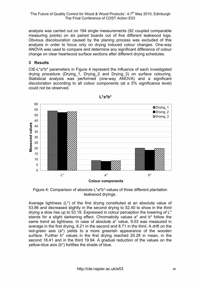
‘The Future of Quality Control for Wood & Wood Products’, 4-7th May 2010, Edinburgh The Final Conference of COST Action E53
analysis was carried out on 184 single measurements (92 coupled comparable measuring points) on six paired boards out of five different teakwood logs. Obvious discolouration caused by the planing process was excluded of this analysis in order to focus only on drying induced colour changes. One-way ANOVA was used to compare and determine any significant difference of colour change on clear heartwood surface sections after different drying schedules.
3 Results CIE-L*a*b* parameters in Figure 4 represent the influence of each investigated drying procedure (Drying_1, Drying_2 and Drying_3) on surface colouring. Statistical analysis was performed (one-way ANOVA) and a significant discoloration according to all colour components (at a 5% significance level) could not be observed.
L*a*b*
0
5
10
15
20
25
30
35
40
45
50
55
60
L* a* b*
Colour components
Mea
sure
d va
lues
Drying_1Drying_2Drying_3
Figure 4: Comparison of absolute L*a*b*-values of three different plantation teakwood dryings.
Average lightness (L*) of the first drying constituted at an absolute value of 53.86 and decreased slightly in the second drying to 52.40 to show in the third drying a slow rise up to 53.18. Expressed in colour perception the lowering of L* stands for a slight darkening effect. Chromaticity values a* and b* follow the same trend as lightness. In case of absolute a* value, 9.03 was measured in average in the first drying, 8.21 in the second and 8.71 in the third. A drift on the red-green axis (a*) yields to a more greenish appearance of the wooden surface. Further b* values in the first drying reached 20.28 in mean, in the second 18.41 and in the third 19.94. A gradual reduction of the values on the yellow-blue axis (b*) fortifies the shade of blue.
http://cte.napier.ac.uk/e53 86
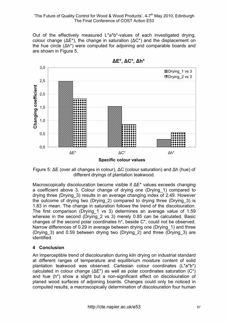
‘The Future of Quality Control for Wood & Wood Products’, 4-7th May 2010, Edinburgh The Final Conference of COST Action E53
Out of the effectively measured L*a*b*-values of each investigated drying, colour change (ΔE*), the change in saturation (ΔC*) and the displacement on the hue circle (Δh*) were computed for adjoining and comparable boards and are shown in Figure 5.
ΔE*, ΔC*, Δh*
0,0
0,5
1,0
1,5
2,0
2,5
3,0
ΔE* ΔC* Δh*
Specific colour values
Cha
ngin
g co
effic
ient
Drying_1 vs 3Drying_2 vs 3
Figure 5: ΔE (over all changes in colour), ΔC (colour saturation) and Δh (hue) of different dryings of plantation teakwood.
Macroscopically discolouration become visible if ΔE* values exceeds changing a coefficient above 3. Colour change of drying one (Drying_1) compared to drying three (Drying_3) results in an average changing index of 2.49. However the outcome of drying two (Drying_2) compared to drying three (Drying_3) is 1.83 in mean. The change in saturation follows the trend of the discolouration. The first comparison (Drying_1 vs 3) determines an average value of 1.59 whereas in the second (Drying_2 vs 3) merely 0.85 can be calculated. Basic changes of the second polar coordinates h*, beside C*, could not be observed. Narrow differences of 0.29 in average between drying one (Drying_1) and three (Drying_3) and 0.59 between drying two (Drying_2) and three (Drying_3) are identified.
4 Conclusion An imperceptible trend of discolouration during kiln drying on industrial standard at different ranges of temperature and equilibrium moisture content of solid plantation teakwood was observed. Cartesian colour coordinates (L*a*b*) calculated in colour change (ΔE*) as well as polar coordinates saturation (C*) and hue (h*) show a slight but a non-significant effect on discolouration of planed wood surfaces of adjoining boards. Changes could only be noticed in computed results, a macroscopically determination of discolouration four human
http://cte.napier.ac.uk/e53 87
‘The Future of Quality Control for Wood & Wood Products’, 4-7th May 2010, Edinburgh The Final Conference of COST Action E53
eyes is not visible. In general, if process-related discolouration during drying is neglected, increasing drying temperature and lower equilibrium moisture content cause a darker, more greenish and bluish teakwood surface. However, for a detailed research of discolouration during kiln drying, we have to leave industrial kiln drying standard and compare gentler to more severe drying procedures. In case of plantation teakwood, colour measurements after industrial convection drying could be applied as a quality control in the investigated range of drying parameters used in this study. Almost unnoticeable discolouration after different drying schedules indicates a constant surface performance regarding colour and optical requirements.
Acknowledgement Financial support by Teak Holz Handels- Verarbeitungs GmbH is gratefully acknowledged.
References Basri, E. Rohadi, D. & Priadi, T. (2003). “The Alleviation of Discoloration in Teak (Tectona grandis) Wood through Drying and Chemical Treatment”. 8th International IUFRO Wood Drying Conference, pp 319-323.
Bekhta, P. & Niemz, P. (2003). “Effect of High Temperature on the Change in Color, Dimension Stability and Mechanical Properties of Spruce Wood”. Holzforschung, Vol. 57, pp 539-547.
Brischke, C. Welzbacher, R.C. Brandt, K. & Rapp, O.A. (2007). “Quality control of thermally modified wood: Interrelationship between heat treatment and intensities and CIE L* a* b* colour data on homogenized wood samples”. Holzforschung Vol. 61, pp 19-22.
Charrier, B. Charrier, F. Janin, G. Kamdem, P.D. Irmouli, M. & Goncalez, J. (2002). “Study of industrial boiling process on walnut colour: Experimental study under industrial conditions”. Holz als Roh- und Werkstoff, Vol. 60, pp 259-264.
Dahms, K.-G. (1989). “Das Holzportrait Teak”. Holz als Roh- und Werkstoff, Vol. 47, pp 81-85.
Jachs, M. (2007). “Utilization of plantation teakwood (Tectona grandes L.f.) as solid wood”. Part I: Chemical an mechanical characteristics of Costa Rica plantation teak. Bachelor Thesis. Department of Material Science and Process Engineering, Institute of Wood Science and Technology, University of Natural Resources and Applied Life Science, Vienna.
Jachs, M. (2009). “Zerspanungseigenschaften von Teak (Tectona grandis L.f.) am Beispiel Hobeln sowie die Beobachtung der Farbveränderung nach dem Bearbeitungsschritt”. Master Thesis. Department of Material Science and Process Engineering, Institute of Wood Science and Technology, University of Natural Resources and Applied Life Science, Vienna.
http://cte.napier.ac.uk/e53 88
‘The Future of Quality Control for Wood & Wood Products’, 4-7th May 2010, Edinburgh The Final Conference of COST Action E53
Liu, S. Loup, C. Gril, J. Dumonceaud, O. Thibaut A. & Thibaut B. (2005). “Studies on European beech (Fagus sylvatica L.). Part 1: Variations of wood colour parameters”. Annals of Forest Science, 62, pp 625-632.
Luostarinen, K. & Luostarinen, J. (2001). “Discolouration and Deformation of birch parquet boards during conventional drying”. Wood Science and Technology 35, pp 517-528.
Klumpers, J. Janin, G. Becker, M. & Lévy, G. (1993). “The influence of age, extractive content and soil water on wood color in oak: the possible genetic determination of wood color”. Annals of Forest Science, 50, pp 403s-409s.
Oltean, L. Teischinger, A. & Hansmann, C. (2008) “Wood surface discolouration due to simulated indoor sunlight exposure”. Holz als Roh- und Werkstoff, Vol. 66, pp 51-66.
Pöckl, M.J. (2007) “Neue Methoden der Laubholzvergütung”. Dissertation. Department of Material Science and Process Engineering, Institute of Wood Science and Technology, University of Natural Resources and Applied Life Science, Vienna.
Simatupang, H.M. & Yamamoto, K. (2000). “Properties of teakwood (Tectona grandis L.f.) and mahogani (Swietenia Macrophylla King) from manmade forest and influence on utilization”. In: Hing Hon , C. & Matsumoto, K. (Eds.), Proceedings of the Seminar on High Value Timber of Plantation Establishment, Conferérence Tawan, Sabah, Japan. JIRCAS. Working Report No.16, pp 103-114.
Simpson, T. (2001) b. “Drying Defects”. Chapter 8, http://www.fpl.fs.fed.us/documnts/usda/ah188/chapter08.pdf [Accessed 9 March 2010].
Wagenführ, R. & Scheiber, C. (1985). “Holzatlas”. 2. Auflage, Fachbuchverlag, Leipzig, Carl Hanser Verlag, pp 626-628.
Wagenführ, R. & Scholz, F. (2005). “Taschenbuch der Holztechnik”. Carl Hanser Verlag, München.
Weigl, M. Kandlbauer, A. Hansmann, C. Pöckl, J. Müller, U. & Grabner M. (2009). “Application of natural dyes in the colouration of wood”. In: Bechthold, T. & Mussak, R. (Eds.), Handbook of natural colourants, John Wiley and Sons, Inc.
http://cte.napier.ac.uk/e53 89

‘The Future of Quality Control for Wood & Wood Products’, 4-7th May 2010, Edinburgh The Final Conference of COST Action E53
Tuesday 4th May Wood drying workshop (European Drying Group)
3rd session
http://www.cte.napier.ac.uk/e53/ 90
’The Future of Quality Control for Wood & Wood Products’, 4-7th May 2010, Edinburgh The Final Conference of COST Action E53
Inclusion of the sorption hysteresis phenomenon in future drying models. Some basic considerations.
J-G. Salin1
Abstract
The sorption hysteresis effect, i.e. different wood equilibrium moisture contents (EMCs) in desorption and absorption for the same relative humidity, is well known. It is qualitatively described in most textbooks in wood science. However, quantitative sorption isotherms, in the form of tables or analytical correlations, are almost always given as the average of the desorption and absorption curves. Consequently most drying simulation models use these average curves, i.e. the sorption hysteresis phenomenon is not accounted for. The equilibrium state of a wood sample is thus not a function of the relative humidity only, but depends on the moisture history also. This means that Fick's equations - with moisture content as a single driving force - are not valid any more. For a pure desorption process the state of the sample follows the desorption isotherm, but a problem arises when desorption is followed by absorption - as for instance in the timber conditioning phase. It seems reasonable to assume that for each EMC point, on or between the desorption/absorption isotherms, the moisture content change follows a unique path, when the surrounding climate changes. This path - the so called scanning curve - does not need to be the same in desorption and absorption. Some selected results and corresponding scanning curve suggestions are presented and discussed. Drying models with the sorption hysteresis phenomenon included should be developed for the analysis of experimental data and more generally for use as an improved tool in practical applications. 1 Introduction
The sorption hysteresis is a well known phenomenon for wood. It is mentioned in almost all textbooks on wood science. Hysteresis means in this context that the equilibrium moisture content (EMC) is different in desorption and absorption processes. However, when quantitative sorption isotherms are presented in the literature, normally only one curve is given, i.e. the average (AvEMC) of the desorption (DeEMC) and absorption (AbEMC) curves. Perhaps due to this, almost all drying simulation models are also based on the AvEMC curves for different temperatures. This introduces an error in the models, which to some extent has been handled by introducing correction factors.
1 Drying model evangelist, [email protected]ägen 12 A, FI-02210 Esbo, Finland
http://cte.napier.ac.uk/e53 91

’The Future of Quality Control for Wood & Wood Products’, 4-7th May 2010, Edinburgh The Final Conference of COST Action E53
In the following the need to include the sorption hysteresis phenomenon in model work is discussed. After that some problems and solutions in connection with such a model extension are presented. 2 Is the sorption hysteresis important in modelling?
The interaction between a piece of wood and the surrounding climate (air temperature and humidity) is of course one of the two main parts in all drying models. The other part is the moisture migration inside the wood. The external interaction includes transfer of heat (energy) as well as moisture (mass) to and from the wood surface. The heat and mass transfer are expressed with the following equations.
)( sTTA −=Φ ∞α Equation 1
)( ∞−= ccAm sβ Equation 2 Φ/A = heat flux per unit area (W/m2) α = heat transfer coefficient (W/m2/K) T∞ , Ts = temperature of surrounding air and wood surface, resp. (K)
Am = moisture flux per unit area (kg/m2/s) β = mass transfer coefficient (m/s) c∞ , cs = vapour concentration of surrounding air and in equilibrium with the wood surface, resp. (kg/m3) Vapour concentration is here used as the driving force in Equation 2, but it can be discussed whether partial pressure would be a better choice. Anyway, cs is here the point where the sorption curve enters, as it gives the connection between surface moisture content (MC) and the vapour concentration in the air in equilibrium with the surface. For a pure drying process the DeEMC curve should be used for determination of this connection. As the transfer of both heat and moisture occurs through the same air-side boundary layer, it seems reasonable that there should be a coupling between the transfer coefficients α and β. This is referred to as the analogy between heat and mass transfer, which with a good approximation can be expressed as:
ρcβα p= Equation 3 where cpρ is the volumetric heat capacity of the humid air in the boundary layer. Equation 3 is important as the mass transfer coefficient can be determined from the heat transfer coefficient which normally is more easily predicted. However, when drying model simulations have been compared with experimental data, it
http://cte.napier.ac.uk/e53 92
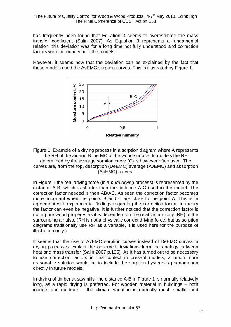
’The Future of Quality Control for Wood & Wood Products’, 4-7th May 2010, Edinburgh The Final Conference of COST Action E53
has frequently been found that Equation 3 seems to overestimate the mass transfer coefficient (Salin 2007). As Equation 3 represents a fundamental relation, this deviation was for a long time not fully understood and correction factors were introduced into the models. However, it seems now that the deviation can be explained by the fact that these models used the AvEMC sorption curves. This is illustrated by Figure 1.
0
5
10
15
20
25
0 0,5
Relative humidity
Moi
stur
e co
nten
t, %
1
B C
A
Figure 1: Example of a drying process in a sorption diagram where A represents the RH of the air and B the MC of the wood surface. In models the RH
determined by the average sorption curve (C) is however often used. The curves are, from the top, desorption (DeEMC) average (AvEMC) and absorption
(AbEMC) curves.
In Figure 1 the real driving force (in a pure drying process) is represented by the distance A-B, which is shorter than the distance A-C used in the model. The correction factor needed is then AB/AC. As seen the correction factor becomes more important when the points B and C are close to the point A. This is in agreement with experimental findings regarding the correction factor. In theory the factor can even be negative. It is further noticed that the correction factor is not a pure wood property, as it is dependent on the relative humidity (RH) of the surrounding air also. (RH is not a physically correct driving force, but as sorption diagrams traditionally use RH as a variable, it is used here for the purpose of illustration only.) It seems that the use of AvEMC sorption curves instead of DeEMC curves in drying processes explain the observed deviations from the analogy between heat and mass transfer (Salin 2007 p.195). As it has turned out to be necessary to use correction factors in this context in present models, a much more reasonable solution would be to include the sorption hysteresis phenomenon directly in future models. In drying of timber at sawmills, the distance A-B in Figure 1 is normally relatively long, as a rapid drying is preferred. For wooden material in buildings – both indoors and outdoors – the climate variation is normally much smaller and
http://cte.napier.ac.uk/e53 93

’The Future of Quality Control for Wood & Wood Products’, 4-7th May 2010, Edinburgh The Final Conference of COST Action E53
changes frequently from absorption to desorption and vice versa. As noticed above, the correction factor becomes more important when the points A, B and C are close to each other. This means that the sorption hysteresis phenomenon becomes especially important in such building applications. It can be argued that for pure drying processes it is sufficient to use the DeEMC sorption curves instead of the AvEMC curves. However, nowadays the drying process is frequently ended with an equalisation and conditioning phase, which normally means that at least the wood surface will absorb moisture. If so, the error is ‘doubled’ in this part. For big batch kilns it may also occur that timber on the leeward side absorbs moisture just after a fan reversal. Based on these arguments, there is definitely a need to include the sorption hysteresis phenomenon in future drying models and as well in models for the interaction between climate and wood in buildings. Why has this not been done earlier? One reason is certainly that it is a more complicated issue than it may seem at first hand. Some of the main problems will be discussed in the following. 3 Modelling sorption hysteresis One important feature that is introduced when sorption hysteresis is included in the model is illustrated by the following imagined experiment. Consider a completely dry stick of wood. One end of the stick is dipped into water for a moment and the MC in the end increases to, let’s say, 20 %. After that the stick is stored in a climate corresponding to an AvEMC of 10 %. The dry end MC will then gradually approach 10 % but will stop at about 9 % due to the hysteresis effect (AbEMC ~9 %). In the same way the wet end of the stick will also approach 10 % but stops at about 11 % as DeEMC ~11 %. This situation is illustrated in Figure 2. The interesting question is now; will there be a bound water migration from the higher MC towards the lower MC?
Bound water migration driving force?
Climate corresponding to AvEMC = 10 %
Absorption Desorption
MC = 9 % MC = 11 %
Figure 2: Imagined experiment to describe the bound water driving force problem.
http://cte.napier.ac.uk/e53 94
’The Future of Quality Control for Wood & Wood Products’, 4-7th May 2010, Edinburgh The Final Conference of COST Action E53
As both ends of the stick are in thermodynamic equilibrium with the same climate, they should be in mutual equilibrium also, i.e. no moisture migration should occur. This shows that Fick’s law with MC (or any other ‘moisture concentration in wood’ variable) is not valid any more when sorption hysteresis is taken into account. The state of the wood is not defined by the MC alone, but depends also on how this MC has been reached, i.e. the history of its moisture changes. This means that the driving force for bound water migration has to be changed. The logical solution is to use the state of the air in equilibrium with the wood as the driving force. This idea was suggested already 30 years ago by (Bramhall 1979) who proposed vapour partial pressure as driving force and by (Kawai et al 1978 and Stanish 1986) that proposed chemical potential as driving force. In addition to this change of driving force, it has to be established how the state point of the wood changes, i.e. in which direction will the state move, expressed as a point on or between the DeEMC and AbEMC curves. This is discussed later on. In this context another, rather similar, imagined experiment may be presented. Consider now a thin wood stick initially with an MC corresponding to the fibre saturation point (FSP). One end is dipped into water for a relatively long time so that this becomes completely saturated with water, i.e. an MC in the range 120-250 % depending on wood density. Will there now be a flow of moisture from the very wet end towards the FSP (MC ~30 %) in the other end? Certainly, a flow of free water will occur due to capillary forces. The saturated end is in equilibrium with 100 % RH as there is free water at the surface. This proves that wood with an MC corresponding to FSP is not in equilibrium with 100 % RH, which however often is inaccurately stated. In addition many textbooks and handbooks present diagrams and tables where an EMC of about 30 % is given for 100 % RH. Kelvin’s law that states that the vapour pressure above a curved liquid surface (meniscus) is lower than above a flat surface is important in this context. This imagined experiment brings of course the focus on the definition of the FSP. Equilibrium with 100 % RH is thus not a useful definition. In the authors opinion, the most useful FSP definition is the point when the cell wall is water saturated but with no free water present. It is generally accepted that several mechanical wood properties – shrinkage/swelling, MOE, MOR, mechano-sorptive creep, etc. – depend on the amount of bound water but not on the amount of free water. There may be a transition zone and not a well defined transition point, but as these mechanical properties are very important for drying induced stress development as well as for shape deformations etc., this definition seems appropriate. Experimental determination of FSP values according to this definition constitutes a problem (as with many other FSP definitions). In addition modelling moisture migration just below or above FSP is still a problem. From a drying modelling point of view it seems logical to extrapolate experimental sorption curves towards 100 % RH – using one of the many sorption models suggested in the literature (Vidal & Cloutier 2005) – and define this point as “EMC for 100 % RH”. In addition Kelvin’s law should be neglected above FSP. However, it is not given that extrapolation of the DeEMC and AbEMC curves give the same FSP value, and this constitutes still a
http://cte.napier.ac.uk/e53 95
’The Future of Quality Control for Wood & Wood Products’, 4-7th May 2010, Edinburgh The Final Conference of COST Action E53
problem in the modelling procedure. Finally an interesting detail related to the EMC should be mentioned. In textbooks the EMC is normally defined as the MC which a piece of wood gradually attains when stored in a certain climate. (It is in most cases not mentioned that the result depends on the starting point of the state of the wood – see Section 4 on Scanning curves.) It is then implied that the climate is not affected by the moisture flow to or from the sample. But there is another alternative to determine the EMC. If the sample is put into a small compartment, then the climate (air RH) will gradually attain equilibrium with the sample and an EMC situation is the result in this case also. This method has actually been used for certain materials to indirectly determine the MC by measuring the RH in the compartment. In this case it is assumed that the moisture flow to or from the sample can be neglected in comparison with the total wood moisture, i.e. MC is not changed. Again, the result is not depending only on the sample MC, but also on how this MC has been attained (Section 4). An immediate question is whether these two alternatives represent the same basic EMC definition. It is perhaps not a priori self-evident, but by considering an intermediate situation where both air RH and sample MC change towards a mutual equilibrium, it is obviously correct. One should however be careful when comparing desorption from the wood and absorption by the air (and vice versa). This is illustrated by the following example. Consider a cell wall that separates two air volumes (lumina) and that both the air and the wall are initially completely dry. Increase the RH on the ‘left hand side’ of the wall to a constant value. Then the wall absorbs moisture and the MC is increasing. Eventually the air RH on the ‘right hand side’ will start to increase as moisture is transferred through the wall. What will the final RH be? The air absorbs moisture from the cell wall, which looks like the wall would be in a desorption state and the air would follow the DeEMC curve, i.e. approach a lower RH on the ‘right hand side’. But the cell wall MC is continuously increasing, i.e. the wall is actually in an absorption state and thus the AbEMC curve is followed and the RH will finally be the same on both sides. Both the wall and the ‘right hand side’ air are absorbing moisture, although there is a moisture flow from the wall to the air. It should be kept in mind that the hysteresis phenomenon concerns the wood, not the air. Finally a surprising experimental result should be mentioned. There are indications that the EMC and the hysteresis effect are dependent on the sample size (Shmulsky et al 2001). It is known from both experimental results and theoretical principles, that mechanical stress in the wood will influence the EMC. This has been suggested as an explanation, as very small samples should be free of stress. This is in the author’s opinion not a very convincing explanation as tensile stress in the sample should be balanced by compression stress elsewhere – in the absence of external forces. Anyway, such phenomena have to be investigated further.
http://cte.napier.ac.uk/e53 96
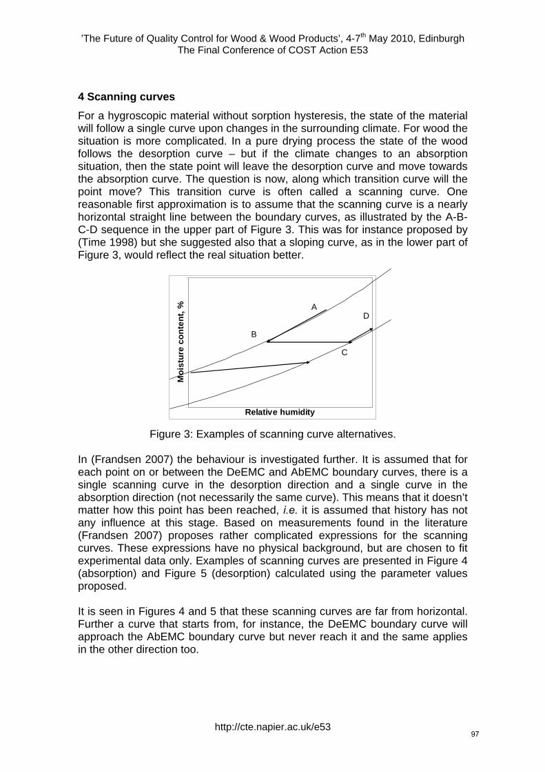
’The Future of Quality Control for Wood & Wood Products’, 4-7th May 2010, Edinburgh The Final Conference of COST Action E53
4 Scanning curves
For a hygroscopic material without sorption hysteresis, the state of the material will follow a single curve upon changes in the surrounding climate. For wood the situation is more complicated. In a pure drying process the state of the wood follows the desorption curve – but if the climate changes to an absorption situation, then the state point will leave the desorption curve and move towards the absorption curve. The question is now, along which transition curve will the point move? This transition curve is often called a scanning curve. One reasonable first approximation is to assume that the scanning curve is a nearly horizontal straight line between the boundary curves, as illustrated by the A-B-C-D sequence in the upper part of Figure 3. This was for instance proposed by (Time 1998) but she suggested also that a sloping curve, as in the lower part of Figure 3, would reflect the real situation better.
Relative humidity
Moi
stur
e co
nten
t, % A
B
C
D
Figure 3: Examples of scanning curve alternatives.
In (Frandsen 2007) the behaviour is investigated further. It is assumed that for each point on or between the DeEMC and AbEMC boundary curves, there is a single scanning curve in the desorption direction and a single curve in the absorption direction (not necessarily the same curve). This means that it doesn’t matter how this point has been reached, i.e. it is assumed that history has not any influence at this stage. Based on measurements found in the literature (Frandsen 2007) proposes rather complicated expressions for the scanning curves. These expressions have no physical background, but are chosen to fit experimental data only. Examples of scanning curves are presented in Figure 4 (absorption) and Figure 5 (desorption) calculated using the parameter values proposed. It is seen in Figures 4 and 5 that these scanning curves are far from horizontal. Further a curve that starts from, for instance, the DeEMC boundary curve will approach the AbEMC boundary curve but never reach it and the same applies in the other direction too.
http://cte.napier.ac.uk/e53 97
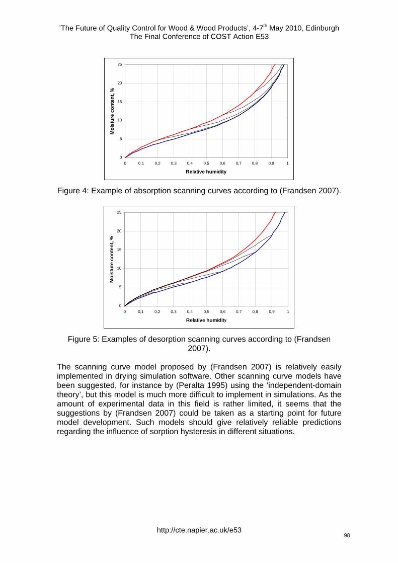
’The Future of Quality Control for Wood & Wood Products’, 4-7th May 2010, Edinburgh The Final Conference of COST Action E53
0
5
10
15
20
25
0 0,1 0,2 0,3 0,4 0,5 0,6 0,7 0,8 0,9 1
Relative humidity
Moi
stur
e co
nten
t, %
Figure 4: Example of absorption scanning curves according to (Frandsen 2007).
0
5
10
15
20
25
0 0,1 0,2 0,3 0,4 0,5 0,6 0,7 0,8 0,9 1
Relative humidity
Moi
stur
e co
nten
t, %
Figure 5: Examples of desorption scanning curves according to (Frandsen 2007).
The scanning curve model proposed by (Frandsen 2007) is relatively easily implemented in drying simulation software. Other scanning curve models have been suggested, for instance by (Peralta 1995) using the ‘independent-domain theory’, but this model is much more difficult to implement in simulations. As the amount of experimental data in this field is rather limited, it seems that the suggestions by (Frandsen 2007) could be taken as a starting point for future model development. Such models should give relatively reliable predictions regarding the influence of sorption hysteresis in different situations.
http://cte.napier.ac.uk/e53 98
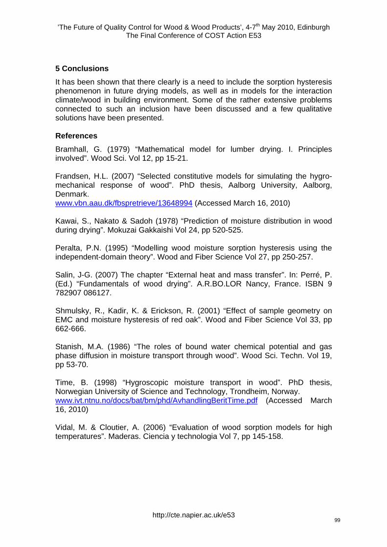
’The Future of Quality Control for Wood & Wood Products’, 4-7th May 2010, Edinburgh The Final Conference of COST Action E53
5 Conclusions
It has been shown that there clearly is a need to include the sorption hysteresis phenomenon in future drying models, as well as in models for the interaction climate/wood in building environment. Some of the rather extensive problems connected to such an inclusion have been discussed and a few qualitative solutions have been presented. References
Bramhall, G. (1979) “Mathematical model for lumber drying. I. Principles involved”. Wood Sci. Vol 12, pp 15-21. Frandsen, H.L. (2007) “Selected constitutive models for simulating the hygro-mechanical response of wood”. PhD thesis, Aalborg University, Aalborg, Denmark. www.vbn.aau.dk/fbspretrieve/13648994 (Accessed March 16, 2010) Kawai, S., Nakato & Sadoh (1978) “Prediction of moisture distribution in wood during drying”. Mokuzai Gakkaishi Vol 24, pp 520-525. Peralta, P.N. (1995) “Modelling wood moisture sorption hysteresis using the independent-domain theory”. Wood and Fiber Science Vol 27, pp 250-257. Salin, J-G. (2007) The chapter “External heat and mass transfer”. In: Perré, P. (Ed.) “Fundamentals of wood drying”. A.R.BO.LOR Nancy, France. ISBN 9 782907 086127. Shmulsky, R., Kadir, K. & Erickson, R. (2001) “Effect of sample geometry on EMC and moisture hysteresis of red oak”. Wood and Fiber Science Vol 33, pp 662-666. Stanish, M.A. (1986) “The roles of bound water chemical potential and gas phase diffusion in moisture transport through wood”. Wood Sci. Techn. Vol 19, pp 53-70. Time, B. (1998) “Hygroscopic moisture transport in wood”. PhD thesis, Norwegian University of Science and Technology, Trondheim, Norway. www.ivt.ntnu.no/docs/bat/bm/phd/AvhandlingBeritTime.pdf (Accessed March 16, 2010) Vidal, M. & Cloutier, A. (2006) “Evaluation of wood sorption models for high temperatures”. Maderas. Ciencia y technologia Vol 7, pp 145-158.
http://cte.napier.ac.uk/e53 99
‘The Future of Quality Control for Wood & Wood Products’, 4-7th May 2010. Edinburgh The Final Conference of COST Action E53
Fibre level modelling of free water behaviour in drying and wetting
J-G. Salin1
Abstract
Almost all drying simulation models describe the moisture migration in wood as a diffusion process. This includes free water flow above the fibre saturation point. This means that wood is seen as a homogeneous material without internal structure. However, especially in softwood narrow sections, bordered pits, divide the free water phase into rather distinct units. It is thus quite clear that the flow of free water is governed by capillary forces and not by diffusion. A model has been developed that investigates how water filled units are emptied one by one in a drying process. Simulations with the model explain some experimentally seen features that cannot be obtained using pure diffusion type models. In the same way absorption of water into a piece of dried wood is of course governed by capillary forces. An additional feature is that a considerable part of the bordered pits have been aspirated, i.e. closed, in the drying process and the number of possible flow paths is thus reduced. The driving force for water flow is the capillary suction in the lumen. Modelling wetting according to these principles introduces also some interesting specific features. In summary it is found that specific behaviour seen on a real macroscopic level originates from properties on a microscopic, fibre level. This indicates clearly that experience from fibre level models should be included in future drying and wetting simulation models. The work in this direction so far, has been promising. 1 Introduction
Timber drying models are almost always describing the moisture migration as a diffusion process, i.e. caused by a gradient in the moisture content (MC). This is a reasonable assumption for MC:s below the fibre saturation point (FSP) but is obviously not true for free water. The flow of free water is clearly governed by capillary forces in the fibre network. This free water flow process should thus be strongly dependent on the microscopic structure of the fibre matrix. As there are experimentally observed features of the drying process that cannot be explained by pure diffusion models, there is a need to investigate the influence of capillarity on the process. Absorption of water into a dried piece of wood is an important process. This is especially true for outdoor wooden elements/constructions exposed to rain, as an increased MC will affect the durability of the construction. In this case also, the absorption has often been modelled as a diffusion process, i.e. wood has 1 Drying model evangelist, [email protected] Romensvägen 12 A, FI-02210 Esbo, Finland
http://cte.napier.ac.uk/e53 100

‘The Future of Quality Control for Wood & Wood Products’, 4-7th May 2010. Edinburgh The Final Conference of COST Action E53
been viewed as a homogeneous material without internal structure. It is however obvious that capillarity is the driving force in the absorption process. Again the microscopic structure of the material should have a strong influence on the process. There is thus a need to try to model both drying and wetting of solid wood taking into account the capillary network, in order to get a better understanding of these processes and their reflections on the macroscopic scale. 2 Modelling drying of free water
Softwoods have a relatively simple fibre level structure. The tracheids are the dominating structural elements and their lumina represent the main volume available for free water. In the cell walls there are tiny openings, bordered pits, through which lumina of adjacent fibres are interconnected. These bordered pits are mainly concentrated to the overlapping fibre ends, i.e. to surfaces in the radial-longitudinal (R-L) direction. A few openings are also found along the fibres, at the R-L cell wall. Connections in the radial direction are mainly created by the ray cells. A total of 50-300 bordered pits per fibre is normal, and in never dried sapwood these openings are available for water flow, i.e. pits are not aspirated. The order of magnitude lumen diameter is 30 µm and the bordered pit opening diameter 1 µm. A free water surface, meniscus, in the pit opening will thus create a 30 times stronger capillary force than a meniscus in the lumen. From a modelling point of view softwood can be seen as a regular network of rather distinct units (tracheids) but that are connected through the bordered pit flow paths. Consider a cluster of fibres more or less filled by a continuous, interconnected water phase. In a drying process evaporation of this water phase occurs from the free water surfaces and as bound water flow through cell walls. As the amount of free water decreases the meniscus with the lowest capillary force (lowest resistance) will retract. For slow drying processes the pressure in the liquid phase remains almost equal throughout the cluster. The meniscus that retracts is thus the one with the widest diameter. Only partly filled lumina will thus be emptied first and after that all menisci will be located at the bordered pits. As drying continues the meniscus in the widest opening cannot resist the suction any more and retracts into the corresponding lumen which is then gradually emptied. This will uncover new opening where the meniscus stops, and the process is repeated. This rather simple process description forms the basis for a theoretical model for free water behaviour in wood drying. Although there are a lot of openings between adjacent fibres, only the widest opening can have any influence on the process in this model. As the opening size certainly is a stochastic variable, this introduces a stochastic element into the model. It should further be noticed that the lumen being emptied at each stage does not need to be close to the point of highest moisture removal from the water phase in the cluster. The lumen volume is also a stochastic variable with a certain average and standard deviation. In addition this average varies across the annual ring.
http://cte.napier.ac.uk/e53 101
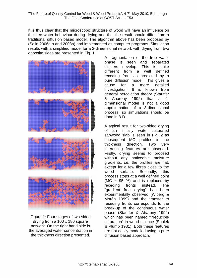
‘The Future of Quality Control for Wood & Wood Products’, 4-7th May 2010. Edinburgh The Final Conference of COST Action E53
It is thus clear that the microscopic structure of wood will have an influence on the free water behaviour during drying and that the result should differ from a traditional diffusion based model. The algorithm above has been proposed by (Salin 2006a,b and 2008a) and implemented as computer programs. Simulation results with a simplified model for a 2-dimensional network with drying from two opposite sides are presented in Fig. 1.
Figure 1: Four stages of two-sided
drying from a 100 x 180 square network. On the right hand side is
the averaged water concentration in the thickness direction presented.
A fragmentation of the free water phase is seen and separated clusters develop. This is quite different from a well defined receding front as predicted by a pure diffusion model. This gives a cause for a more detailed investigation. It is known from general percolation theory (Stauffer & Aharony 1992) that a 2-dimensional model is not a good approximation of a 3-dimensional process, so simulations should be done in 3-D. A typical result for two-sided drying of an initially water saturated sapwood slab is seen in Fig. 2 as subsequent MC profiles in the thickness direction. Two very interesting features are observed. Firstly, drying seems to proceed without any noticeable moisture gradients, i.e. the profiles are flat, except for a few fibres close to the wood surface. Secondly, this process stops at a well defined point (MC ~ 95 %) and is replaced by receding fronts instead. The “gradient free drying” has been experimentally observed (Wiberg & Morén 1999) and the transfer to receding fronts corresponds to the break-up of the continuous water phase (Stauffer & Aharony 1992) which has been named “irreducible saturation” in wood science (Spolek & Plumb 1981). Both these features are not easily modelled using a pure diffusion based approach.
http://cte.napier.ac.uk/e53 102
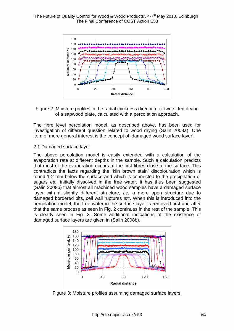
‘The Future of Quality Control for Wood & Wood Products’, 4-7th May 2010. Edinburgh The Final Conference of COST Action E53
0
20
40
60
80
100
120
140
160
180
0 20 40 60 80 10
Radial distance
Moi
stur
e co
nten
t, %
0
Figure 2: Moisture profiles in the radial thickness direction for two-sided drying of a sapwood plate, calculated with a percolation approach.
The fibre level percolation model, as described above, has been used for investigation of different question related to wood drying (Salin 2008a). One item of more general interest is the concept of ‘damaged wood surface layer’. 2.1 Damaged surface layer
The above percolation model is easily extended with a calculation of the evaporation rate at different depths in the sample. Such a calculation predicts that most of the evaporation occurs at the first fibres close to the surface. This contradicts the facts regarding the ‘kiln brown stain’ discolouration which is found 1-2 mm below the surface and which is connected to the precipitation of sugars etc. initially dissolved in the free water. It has thus been suggested (Salin 2008b) that almost all machined wood samples have a damaged surface layer with a slightly different structure, i.e. a more open structure due to damaged bordered pits, cell wall ruptures etc. When this is introduced into the percolation model, the free water in the surface layer is removed first and after that the same process as seen in Fig. 2 continues in the rest of the sample. This is clearly seen in Fig. 3. Some additional indications of the existence of damaged surface layers are given in (Salin 2008b).
020406080
100120140160180
0 40 80 120 160
Radial distance
Moi
stur
e co
nten
t, %
Figure 3: Moisture profiles assuming damaged surface layers.
http://cte.napier.ac.uk/e53 103
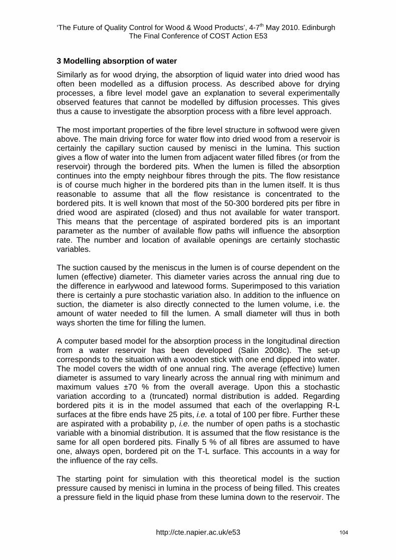
‘The Future of Quality Control for Wood & Wood Products’, 4-7th May 2010. Edinburgh The Final Conference of COST Action E53
3 Modelling absorption of water
Similarly as for wood drying, the absorption of liquid water into dried wood has often been modelled as a diffusion process. As described above for drying processes, a fibre level model gave an explanation to several experimentally observed features that cannot be modelled by diffusion processes. This gives thus a cause to investigate the absorption process with a fibre level approach. The most important properties of the fibre level structure in softwood were given above. The main driving force for water flow into dried wood from a reservoir is certainly the capillary suction caused by menisci in the lumina. This suction gives a flow of water into the lumen from adjacent water filled fibres (or from the reservoir) through the bordered pits. When the lumen is filled the absorption continues into the empty neighbour fibres through the pits. The flow resistance is of course much higher in the bordered pits than in the lumen itself. It is thus reasonable to assume that all the flow resistance is concentrated to the bordered pits. It is well known that most of the 50-300 bordered pits per fibre in dried wood are aspirated (closed) and thus not available for water transport. This means that the percentage of aspirated bordered pits is an important parameter as the number of available flow paths will influence the absorption rate. The number and location of available openings are certainly stochastic variables. The suction caused by the meniscus in the lumen is of course dependent on the lumen (effective) diameter. This diameter varies across the annual ring due to the difference in earlywood and latewood forms. Superimposed to this variation there is certainly a pure stochastic variation also. In addition to the influence on suction, the diameter is also directly connected to the lumen volume, i.e. the amount of water needed to fill the lumen. A small diameter will thus in both ways shorten the time for filling the lumen. A computer based model for the absorption process in the longitudinal direction from a water reservoir has been developed (Salin 2008c). The set-up corresponds to the situation with a wooden stick with one end dipped into water. The model covers the width of one annual ring. The average (effective) lumen diameter is assumed to vary linearly across the annual ring with minimum and maximum values ±70 % from the overall average. Upon this a stochastic variation according to a (truncated) normal distribution is added. Regarding bordered pits it is in the model assumed that each of the overlapping R-L surfaces at the fibre ends have 25 pits, i.e. a total of 100 per fibre. Further these are aspirated with a probability p, i.e. the number of open paths is a stochastic variable with a binomial distribution. It is assumed that the flow resistance is the same for all open bordered pits. Finally 5 % of all fibres are assumed to have one, always open, bordered pit on the T-L surface. This accounts in a way for the influence of the ray cells. The starting point for simulation with this theoretical model is the suction pressure caused by menisci in lumina in the process of being filled. This creates a pressure field in the liquid phase from these lumina down to the reservoir. The
http://cte.napier.ac.uk/e53 104
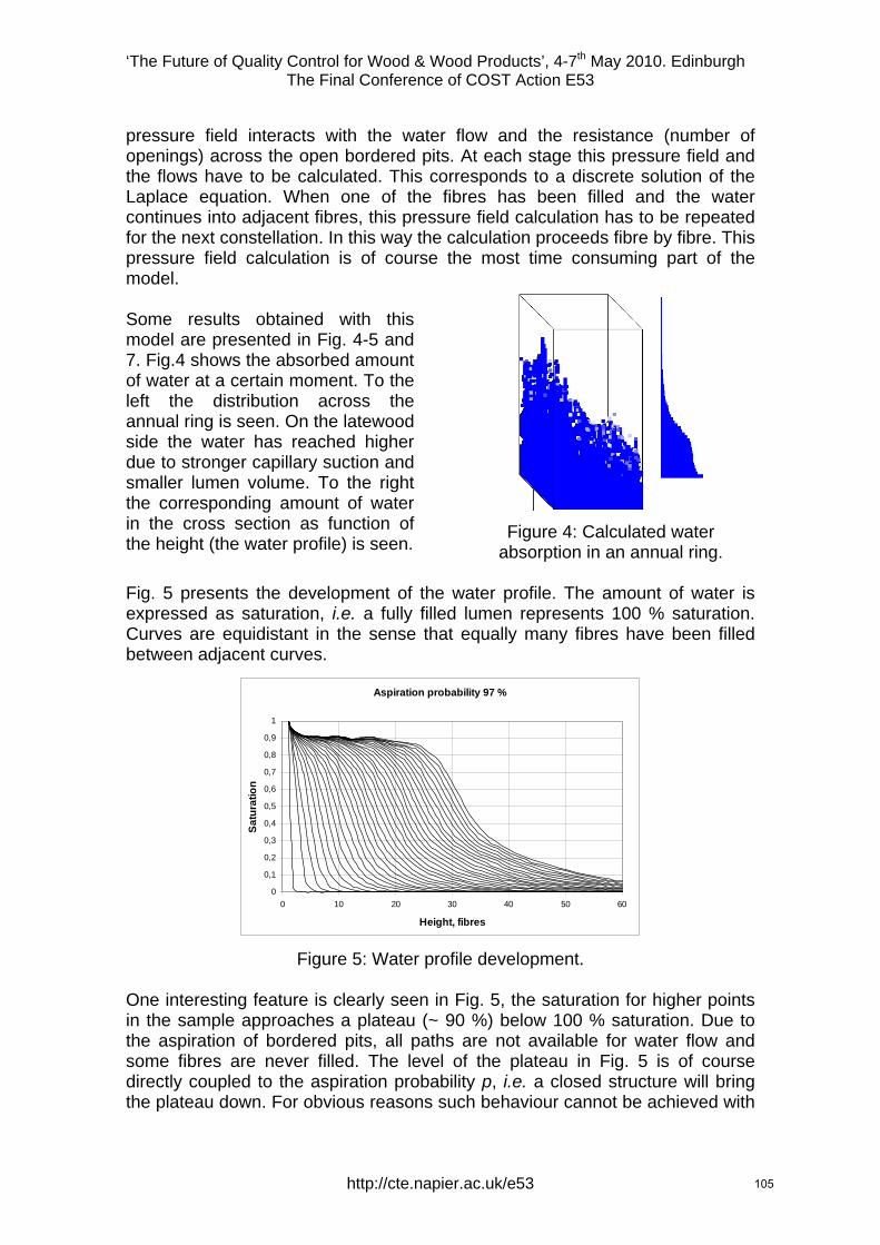
‘The Future of Quality Control for Wood & Wood Products’, 4-7th May 2010. Edinburgh The Final Conference of COST Action E53
pressure field interacts with the water flow and the resistance (number of openings) across the open bordered pits. At each stage this pressure field and the flows have to be calculated. This corresponds to a discrete solution of the Laplace equation. When one of the fibres has been filled and the water continues into adjacent fibres, this pressure field calculation has to be repeated for the next constellation. In this way the calculation proceeds fibre by fibre. This pressure field calculation is of course the most time consuming part of the model. Some results obtained with this model are presented in Fig. 4-5 and 7. Fig.4 shows the absorbed amount of water at a certain moment. To the left the distribution across the annual ring is seen. On the latewood side the water has reached higher due to stronger capillary suction and smaller lumen volume. To the right the corresponding amount of water in the cross section as function of the height (the water profile) is seen.
Figure 4: Calculated water absorption in an annual ring.
Fig. 5 presents the development of the water profile. The amount of water is expressed as saturation, i.e. a fully filled lumen represents 100 % saturation. Curves are equidistant in the sense that equally many fibres have been filled between adjacent curves.
Aspiration probability 97 %
0
0,1
0,2
0,3
0,4
0,5
0,6
0,7
0,8
0,9
1
0 10 20 30 40 50 60
Height, fibres
Satu
ratio
n
Figure 5: Water profile development.
One interesting feature is clearly seen in Fig. 5, the saturation for higher points in the sample approaches a plateau (~ 90 %) below 100 % saturation. Due to the aspiration of bordered pits, all paths are not available for water flow and some fibres are never filled. The level of the plateau in Fig. 5 is of course directly coupled to the aspiration probability p, i.e. a closed structure will bring the plateau down. For obvious reasons such behaviour cannot be achieved with
http://cte.napier.ac.uk/e53 105
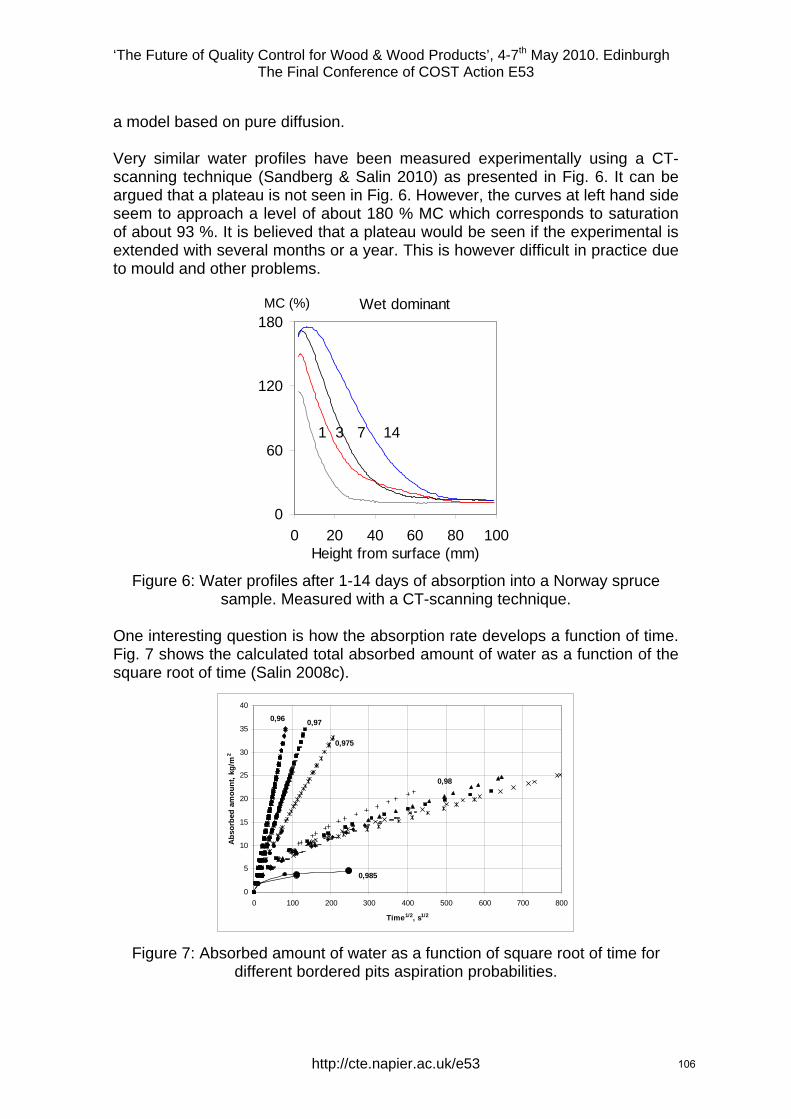
‘The Future of Quality Control for Wood & Wood Products’, 4-7th May 2010. Edinburgh The Final Conference of COST Action E53
a model based on pure diffusion. Very similar water profiles have been measured experimentally using a CT-scanning technique (Sandberg & Salin 2010) as presented in Fig. 6. It can be argued that a plateau is not seen in Fig. 6. However, the curves at left hand side seem to approach a level of about 180 % MC which corresponds to saturation of about 93 %. It is believed that a plateau would be seen if the experimental is extended with several months or a year. This is however difficult in practice due to mould and other problems.
Wet dominant
0
60
120
180
0 20 40 60 80 100Height from surface (mm)
MC (%)
1 3 7 14
Figure 6: Water profiles after 1-14 days of absorption into a Norway spruce
sample. Measured with a CT-scanning technique.
One interesting question is how the absorption rate develops a function of time. Fig. 7 shows the calculated total absorbed amount of water as a function of the square root of time (Salin 2008c).
0
5
10
15
20
25
30
35
40
0 100 200 300 400 500 600 700 800
Time1/2, s1/2
Abso
rbed
am
ount
, kg/
m2
0,96 0,97
0,975
0,98
0,985
Figure 7: Absorbed amount of water as a function of square root of time for different bordered pits aspiration probabilities.
http://cte.napier.ac.uk/e53 106
‘The Future of Quality Control for Wood & Wood Products’, 4-7th May 2010. Edinburgh The Final Conference of COST Action E53
As seen, except for an initial phase, the absorption is a linear function of the square root of time. In the model the first layer of fibres in the wet end of the sample is assumed to have an open structure – in accordance with the damaged surface layer concept discussed in section 2.1. After that the number of available flow paths drops to a level corresponding to the plateau seen in Fig. 5. There is thus an enhanced absorption rate in the very beginning which is seen as the curved initial part in Fig. 7. The linear dependence on the square root of time – including the deviating initial part – has been observed in accurate experiments (Candanedo & Derome 2005). It should finally be remarked that diffusion into a semi-infinite solid will in the same way produce a linear dependence on the square root of time. As shown this linearity cannot be taken as a proof of a pure diffusion driven process. As seen in Fig. 7 the absorption rate is strongly dependent on how open the structure is. For a very closed structure the absorption will stop as all flow paths eventually reach dead ends. This is the case for the lowest curves in Fig. 7 which stop at the black circles. 4 Some additional considerations
The discussion has so far been focused on sapwood of softwood. The heartwood of softwood constitutes a problem. As the tree grows heartwood is gradually formed from the sapwood and most of the free water is repelled, although the capillary geometry is essentially unchanged. This indicates perhaps that the hydrophilic cell wall has become hydrophobic, i.e. the wetting angle has changed. Experimental data show that dried heartwood samples absorb liquid water, but much slower than sapwood (Sandberg & Salin 2010). However, most of the water seems to migrate as bound water, except for a few layers of fibres in the wet end where free water is seen. Absorption in heartwood of softwood is thus governed more by bound water diffusion than by capillarity. Regarding drying processes, the initial MC in heartwood is normally low and the amount of free water so low that drying can be treated as a diffusion process. The microscopic structure of hardwoods is more complicated, with different structural elements. One could thus expect that free water behaviour should differ from softwoods. Absorption of liquid water in aspen, oak and pine has been investigated by (Johansson & Kifetew 2010). Some differences were seen but these are difficult to specify. 5 Conclusions
The simulations reported above, regarding both drying and wetting, have clearly shown that there are several features experimentally seen on a macroscopic scale that originate from the microscopic wood structure. These features cannot be explained by pure diffusion based models that assume a homogeneous material. There is thus a need to include fibre level descriptions for free water behaviour in future models. The calculations referred to above are however extremely time consuming and are thus useful mainly for scientific
http://cte.napier.ac.uk/e53 107

‘The Future of Quality Control for Wood & Wood Products’, 4-7th May 2010. Edinburgh The Final Conference of COST Action E53
investigations of basic questions. Models for more practical use have to use simplified sub-models that take into account the most important fibre level influences. It is suggested that future work in this field should on one hand investigate how structural details influence the behaviour, and on the other hand try to find efficient model simplifications as supplement to diffusion based approaches. References
Candanedo, L. & Derome, D. (2005) “Numerical simulation of water absorption in softwoods”. Proceedings of the 9th International IBPSA Conference, August 15-18, Montreal, Canada. pp 123-130. www.ibpsa.org Johansson, J. & Kifetew, G. (2010) “CT-scanning and modelling of the capillary water uptake in aspen, oak and pine”. Eur. J. Wood Prod. Vol 68, pp 77-85. Salin, J-G. (2006a) “Modelling of the behaviour of free water in sapwood during drying. Part I. A new percolation approach. Wood Material Science & Engi-neering, Vol 1, pp 4-11. Salin, J-G. (2006b) “Modelling of the behaviour of free water in sapwood during drying”. Part II. Some simulation results. Wood Material Science & Engineering, Vol 1, pp 45-51. Salin, J-G. (2008a) “Drying of liquid water in wood as influenced by the capillary fiber network”. Drying Technology, Vol 26, pp 560-567. Salin, J-G. (2008b) “Almost all wooden pieces have a damaged surface layer – impact on some properties and quality”. Proceedings of COST Action E53 Conference 29-30th October, Delft, The Netherlands, pp 135-143. Salin, J-G. (2008c) “Modelling water absorption in wood”. Wood Material Sci-ence & Engineering, Vol 3, pp 102-108. Sandberg, K. & Salin, J-G. (2010) “Liquid water absorption in dried Norway spruce measured with CT scanning and viewed as a percolation process”. Submitted to Wood Sci. Technol. Spolek, G.A. & Plumb, O.A. (1981) “Capillary pressure in softwoods”. Wood Sci. Technol., Vol 15, pp. 189-199. Stauffer, D. & Aharony, A. (1992) “Introduction to percolation theory”. London: Taylor & Francis. Wiberg, P. & Morén, T.J. (1999) “Moisture flux determination in wood during drying above fibre saturation point using CT-scanning and digital image proc-essing”. Holz als Roh- und Werkstoff, Vol 57, pp 137-144.
http://cte.napier.ac.uk/e53 108
‘The Future of Quality Control for Wood & Wood Products’, 4-7th May 2010, Edinburgh The Final Conference of COST Action E53
The water vapour sorption kinetics of Sitka spruce at different temperatures analysed using the parallel
exponential kinetics model
C.A.S. Hill1, Y-J Xie2
Abstract In this study the water vapour sorption of Sitka spruce (Picea sitchensis (Bongard) Carr.) was measured using a Dynamic Vapour Sorption (DVS) apparatus and then analysed using the parallel exponential kinetics (PEK) model. The water vapour sorption rate of wood quickly increased when the relative humidity was changed. With the elapse of time, the sorption rate gradually decreased within any specific relative humidity range. The sorption hysteresis of wood reduced with increasing isotherm temperature. The equilibrium moisture contents obtained from DVS measurements were comparable to these derived from PEK model in the full relative humidity range. The PEK model deconvolutes the sorption kinetics curve into two exponential kinetics processes (fast and slow) which have characteristic times and moisture contents associated with them. The slow adsorption and desorption processes exhibited important differences in their characteristic times, although hysteresis in the moisture contents was found to be variably distributed between the fast and slow processes depending on isotherm temperature.
1 Introduction Wood is a hygroscopic material because the cell walls contain abundant water sorption sites (hydroxyl groups). Most of the wood properties concerning utilization, such as dimensional instability and fungal decay, are closely related to the wood’s water sorption behaviour (Hon 2001). The interaction of water with cellulosic materials involves a dynamic proton exchange on the cellulose internal pore surfaces (Carles and Scallan 1972). The water sorption behaviour of cellulosic and lignocellulosic materials is complicated due to the complex internal geometry of the cell wall and also the continuous structural change resulting from cell wall dimensional variation. It has been demonstrated that the water vapour sorption behaviour of both natural fibres (Kohler et al. 2003, Hill et al. 2010a), regenerated cellulose fibres (Okubayashi et al. 2004, 2005a, 2005b), microcrystalline cellulose (Kachrimanis 2006) and some foodstuffs (Madamba et al. 1996, Rahman et al. 1998, Tang et al. 2008) can be accurately described using the parallel exponential kinetics (PEK) model (Equation 1).
MC = MC0 + MC1[1 – exp(-t/t1)] + MC2[1 - exp(-t/t2)] (1)
1 Proffessor, [email protected] Research Fellow, [email protected] for Timber Engineering, Edinburgh Napier University, UK
http://cte.napier.ac.uk/e53 109
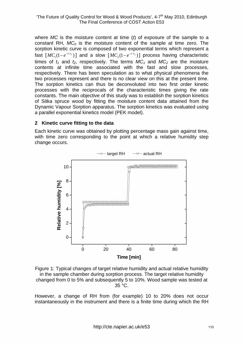
‘The Future of Quality Control for Wood & Wood Products’, 4-7th May 2010, Edinburgh The Final Conference of COST Action E53
where MC is the moisture content at time (t) of exposure of the sample to a constant RH, MC0 is the moisture content of the sample at time zero. The sorption kinetic curve is composed of two exponential terms which represent a fast [ ] and a slow [ ] process having characteristic times of t
)1( 1/1
tteMC −− )1( 2/2
tteMC −−1 and t2, respectively. The terms MC1 and MC2 are the moisture
contents at infinite time associated with the fast and slow processes, respectively. There has been speculation as to what physical phenomena the two processes represent and there is no clear view on this at the present time. The sorption kinetics can thus be deconvoluted into two first order kinetic processes with the reciprocals of the characteristic times giving the rate constants. The main objective of this study was to establish the sorption kinetics of Sitka spruce wood by fitting the moisture content data attained from the Dynamic Vapour Sorption apparatus. The sorption kinetics was evaluated using a parallel exponential kinetics model (PEK model).
2 Kinetic curve fitting to the data Each kinetic curve was obtained by plotting percentage mass gain against time, with time zero corresponding to the point at which a relative humidity step change occurs.
0 20 40 60 80
0
2
4
6
8
10
Rel
ativ
e hu
mid
ity [%
]
Time [min]
target RH actual RH
Figure 1: Typical changes of target relative humidity and actual relative humidity in the sample chamber during sorption process. The target relative humidity
changed from 0 to 5% and subsequently 5 to 10%. Wood sample was tested at 35 °C.
However, a change of RH from (for example) 10 to 20% does not occur instantaneously in the instrument and there is a finite time during which the RH
http://cte.napier.ac.uk/e53 110
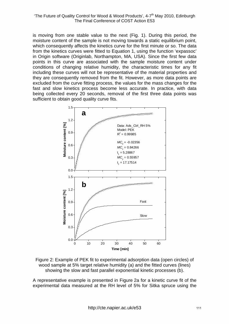
‘The Future of Quality Control for Wood & Wood Products’, 4-7th May 2010, Edinburgh The Final Conference of COST Action E53
is moving from one stable value to the next (Fig. 1). During this period, the moisture content of the sample is not moving towards a static equilibrium point, which consequently affects the kinetics curve for the first minute or so. The data from the kinetics curves were fitted to Equation 1, using the function ‘expassoc’ in Origin software (Originlab, Northampton, MA, USA). Since the first few data points in this curve are associated with the sample moisture content under conditions of changing relative humidity, the characteristic times for any fit including these curves will not be representative of the material properties and they are consequently removed from the fit. However, as more data points are excluded from the curve fitting process, the values for the mass changes for the fast and slow kinetics process become less accurate. In practice, with data being collected every 20 seconds, removal of the first three data points was sufficient to obtain good quality curve fits.
0 10 20 30 40 50 600.0
0.3
0.6
0.9
1.2
1.5
Slow
Fast
Moi
stur
e co
nten
t [%
]
Time [min]
0.0
0.3
0.6
0.9
1.2
1.5
Data: Ads_Ctrl_RH 5%Model: PEK R2 = 0.99985 MC0 = -0.02356MC1 = 0.84266t1 = 5.28867MC
2 = 0.55957
t2 = 17.17514
Moi
stur
e co
nten
t [%
]
a
b
Figure 2: Example of PEK fit to experimental adsorption data (open circles) of wood sample at 5% target relative humidity (a) and the fitted curves (lines)
showing the slow and fast parallel exponential kinetic processes (b).
A representative example is presented in Figure 2a for a kinetic curve fit of the experimental data measured at the RH level of 5% for Sitka spruce using the
http://cte.napier.ac.uk/e53 111
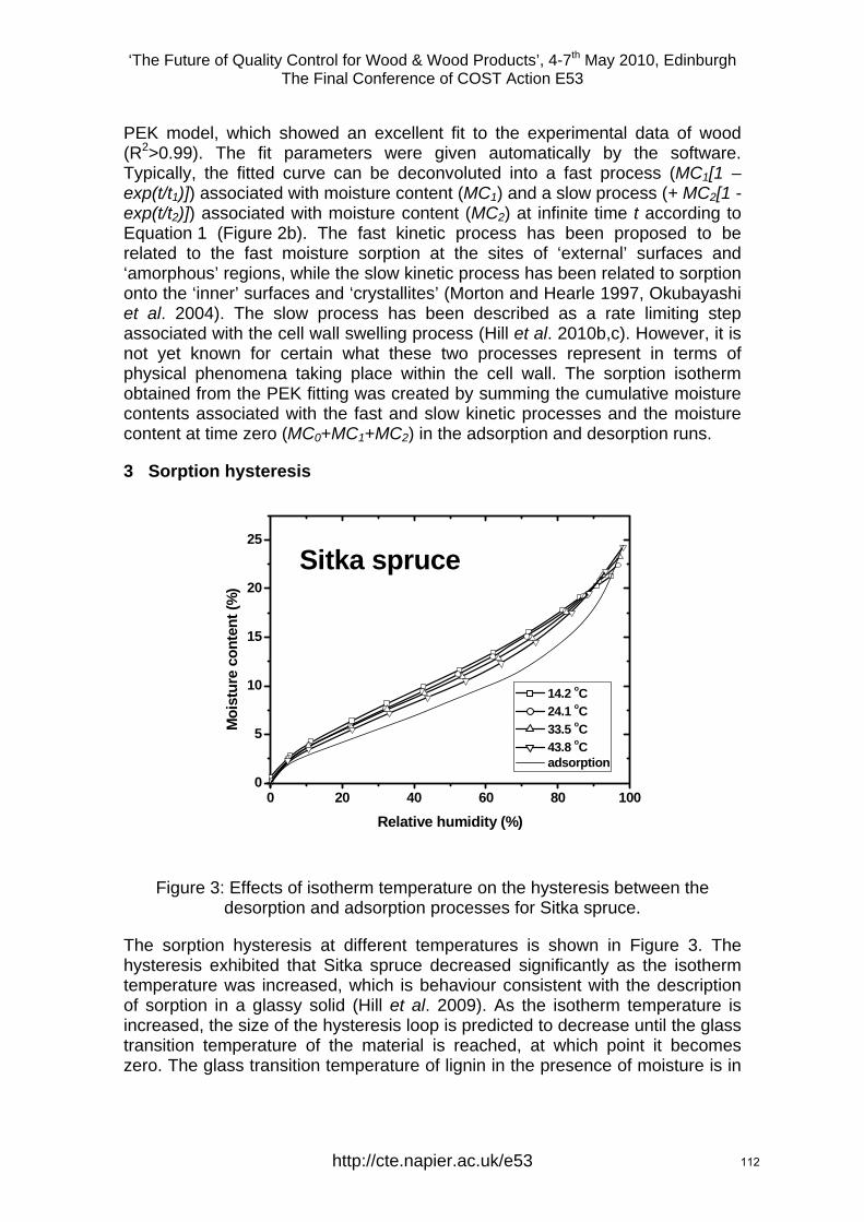
‘The Future of Quality Control for Wood & Wood Products’, 4-7th May 2010, Edinburgh The Final Conference of COST Action E53
PEK model, which showed an excellent fit to the experimental data of wood (R2>0.99). The fit parameters were given automatically by the software. Typically, the fitted curve can be deconvoluted into a fast process (MC1[1 – exp(t/t1)]) associated with moisture content (MC1) and a slow process (+ MC2[1 - exp(t/t2)]) associated with moisture content (MC2) at infinite time t according to Equation 1 (Figure 2b). The fast kinetic process has been proposed to be related to the fast moisture sorption at the sites of ‘external’ surfaces and ‘amorphous’ regions, while the slow kinetic process has been related to sorption onto the ‘inner’ surfaces and ‘crystallites’ (Morton and Hearle 1997, Okubayashi et al. 2004). The slow process has been described as a rate limiting step associated with the cell wall swelling process (Hill et al. 2010b,c). However, it is not yet known for certain what these two processes represent in terms of physical phenomena taking place within the cell wall. The sorption isotherm obtained from the PEK fitting was created by summing the cumulative moisture contents associated with the fast and slow kinetic processes and the moisture content at time zero (MC0+MC1+MC2) in the adsorption and desorption runs.
3 Sorption hysteresis
0 20 40 60 80 1000
5
10
15
20
25
Sitka spruce
Moi
stur
e co
nten
t (%
)
Relative humidity (%)
14.2 oC 24.1 oC 33.5 oC 43.8 oC adsorption
Figure 3: Effects of isotherm temperature on the hysteresis between the desorption and adsorption processes for Sitka spruce.
The sorption hysteresis at different temperatures is shown in Figure 3. The hysteresis exhibited that Sitka spruce decreased significantly as the isotherm temperature was increased, which is behaviour consistent with the description of sorption in a glassy solid (Hill et al. 2009). As the isotherm temperature is increased, the size of the hysteresis loop is predicted to decrease until the glass transition temperature of the material is reached, at which point it becomes zero. The glass transition temperature of lignin in the presence of moisture is in
http://cte.napier.ac.uk/e53 112
‘The Future of Quality Control for Wood & Wood Products’, 4-7th May 2010, Edinburgh The Final Conference of COST Action E53
the region of 60 to 90 °C and linear projections of the decrease in hysteresis loops reached zero in this temperature range for Sitka spruce.
A model for sorption hysteresis based upon adsorption and desorption processes on glassy solids below the glass transition temperature has been presented (Hill et al. 2009). The model considers the dynamic response of the substrate during the ingress or egress of water molecules into or out of the matrix of a glassy polymer. When water molecules enter the matrix, the structure expands with the creation of molecular sized nanopores to accommodate the water molecules, whereas during desorption, the matrix responds with the collapse of these nanopores as water molecules exit the structure. However, because the process takes place below the Tg of the material, the matrix does not respond instantaneously to the ingress or egress of the water molecules; there is a time lag in the response of the matrix. This process takes place on a molecular time scale, but there will be a connection through to the sorption kinetics observed on macroscopic time scales if the matrix deformation processes are rate determining steps. There are certainly differences observed in the characteristic times observed for the adsorption and desorption processes. The time to obtain equilibrium is always longer for the slow desorption compared to the fast desorption processes, which shows that there is a lack of symmetry between the adsorption and desorption that presumably has its origin in the micromechanical behaviour of the cell wall in the presence of moisture. However, there is no significant difference between the adsorption and desorption characteristic times with the fast kinetic processes, which was also found by Kohler et al. (2003). A possible interpretation of this observation is that the fast sorption processes are connected with readily accessible sorption sites in the cell wall internal surface, whereas the slow process is linked to the production of new sites as the cell wall expands or the loss of these sites as the cell wall contracts.
Other studies of water vapour sorption kinetic processes on wood invariably invoke diffusion-based models with varying degrees of success. However, this study has found that the PEK model gave excellent fits to the data in all cases. It has been reported that the swelling of cereal grains in the presence of moisture obeys a PEK model. It is suggested that the rate limiting step in such cases is determined by the rate at which the material can expand to accommodate the cell wall bound water. Further studies are presently underway to examine this possible explanation.
4 Conclusions This study has shown that water vapour sorption and desorption kinetic behaviour on wood is accurately described by the parallel exponential kinetics (PEK) model. With increasing the temperature, wood exhibited a lower hysteresis in the full RH range. The reduction in hysteresis with temperature can be explained by a model invoking the phenomenon of sorption on a glassy solid below the glass transition temperature.
http://cte.napier.ac.uk/e53 113
‘The Future of Quality Control for Wood & Wood Products’, 4-7th May 2010, Edinburgh The Final Conference of COST Action E53
5 Acknowledgements Support from the Scottish Funding Council for the Joint Research Institute in Civil Engineering (part of the Edinburgh Research Partnership in Engineering and Mathematics) is acknowledged.
6 References Carles, J E and Scallan, A M (1972) The determination of the amount of bound water within cellulosic gels by NMR spectroscopy. Journal of Applied Polymer Science, Vol 17, pp 1855-1865. Hill, C A S, Norton, A J and Newman, G (2009) The water vapor sorption behavior of natural fibers. Journal of Applied Polymer Science, Vol 112, pp 1524-1537. Hill, C A S, Norton, A J and Newman, G (2010a) The water vapor sorption behavior of flax fibers-analysis using the parallel exponential kinetics model and determination of the activation energies of sorption. Journal of Applied Polymer Science, Vol 116, pp 2166-2173. Hill, C A S, Norton, A J and Newman, G (2010b) The water vapour sorption properties of Sitka spruce determined using a dynamic vapour sorption apparatus. Wood Science and Technology DOI: 10.1007/s00226-010-0305-y. Hill, C A S, Norton, A J and Newman, G (2010c) Analysis of the water vapour sorption behaviour of Sitka spruce (Picea sitchensis (Bongard) Carr.) based on the parallel exponential kinetics model. Holzforschung DOI.1515/HF.2010.059 Hon, D N S and Shiraishi, N. Wood and cellulosic chemistry. 2nd edition, Marcel Dekker, Inc.: New York, 2001. Kachrimanis, K, Noisternig, M F, Griesser, U J and Malamataris, S (2006) Dynamic moisture sorption and desorption of standard and silicified microcrystalline cellulose. European Journal of Pharmaceutics and Biopharmaceutics, Vol 64, pp 307-315. Kohler, R., Dück, R., Ausperger, B. and Alex, R. (2003) A numeric model for the kinetics of water vapor sorption on cellulosic reinforcement fibers. Composite Interfaces, Vol 10, pp 255-276. Madamba, P.S., Driscol, R.H. and Buckle, K. A. J. (1996) The thin layer drying characteristics of garlic slices. Journal of Food Engineering, Vol 29, pp 75-97. Morton, W E and Hearle, J W S. Physical properties of textile fibers. UK: The Textile Institute, 1997.
http://cte.napier.ac.uk/e53 114
‘The Future of Quality Control for Wood & Wood Products’, 4-7th May 2010, Edinburgh The Final Conference of COST Action E53
Okubayashi, S, Griesser, U J and Bechtold, T (2004) A kinetic study of moisture sorption and desorption on lyocell fibers. Carbohydrate Polymers, Vol 58, pp 293-299. Okubayashi, S, Griesser, U J, Bechtold, T (2005a) Water accessibilities of man-made cellulosic fibers – effects of fiber characteristics. Cellulose, Vol 12, pp 403-410. Okubayashi, S, Griesser, U J and Bechtold, T (2005b) Moisture sorption/desorption behavior of various manmade cellulosic fibers. Journal of Applied Polymer Science, Vol 97, pp 1621-1625. Rahman, M S, Perera, C O and Thebaud, C (1998) Desorption isotherm and heat pump drying kinetics of peas. Food Research International Vol 30, pp 485-491. Tang, X, De Rooij, M R, Van Duynhoven, J and Van Breugel, K J (2008) Dynamic volume change measurements of cereal materials by environmental scanning electron microscopy and videomicroscopy. Microsc.-Oxford, Vol 230, pp 100-107.
http://cte.napier.ac.uk/e53 115
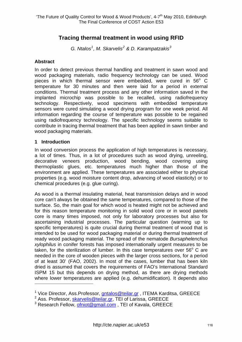
‘The Future of Quality Control for Wood & Wood Products’, 4-7th May 2010, Edinburgh The Final Conference of COST Action E53
Tracing thermal treatment in wood using RFID
G. Ntalos1, M. Skarvelis2 & D. Karampatzakis3
Abstract In order to detect previous thermal handling and treatment in sawn wood and wood packaging materials, radio frequency technology can be used. Wood pieces in which thermal sensor were embedded, were cured in 56o C temperature for 30 minutes and then were laid for a period in external conditions. Thermal treatment process and any other information saved in the implanted microchip was possible to be recalled, using radiofrequency technology. Respectively, wood specimens with embedded temperature sensors were cured simulating a wood drying program for one week period. All information regarding the course of temperature was possible to be regained using radiofrequency technology. The specific technology seems suitable to contribute in tracing thermal treatment that has been applied in sawn timber and wood packaging materials.
1 Introduction In wood conversion process the application of high temperatures is necessary, a lot of times. Thus, in a lot of procedures such as wood drying, unreeling, decorative veneers production, wood bending, wood covering using thermoplastic glues, etc. temperatures much higher than those of the environment are applied. These temperatures are associated either to physical properties (e.g. wood moisture content drop, advancing of wood elasticity) or to chemical procedures (e.g. glue curing).
As wood is a thermal insulating material, heat transmission delays and in wood core can’t always be obtained the same temperatures, compared to those of the surface. So, the main goal for which wood is heated might not be achieved and for this reason temperature monitoring in solid wood core or in wood panels core is many times imposed, not only for laboratory processes but also for ascertaining industrial processes. The particular question (warming up to specific temperatures) is quite crucial during thermal treatment of wood that is intended to be used for wood packaging material or during thermal treatment of ready wood packaging material. The spread of the nematode Bursaphelenchus xylophilus in conifer forests has imposed internationally urgent measures to be taken, for the sterilization of lumber. In this case temperatures over 56o C are needed in the core of wooden pieces with the larger cross sections, for a period of at least 30’ (FAO, 2002). In most of the cases, lumber that has been kiln dried is assumed that covers the requirements of FAO’s International Standard ISPM 15 but this depends on drying method, as there are drying methods where lower temperatures are applied (e.g. dehumidification). It depends also
1 Vice Director, Ass.Professor, [email protected] , ITEMA Karditsa, GREECE 2 Ass. Professor, [email protected], TEI of Larissa, GREECE 3 Research Fellow, [email protected] , TEI of Kavala, GREECE
http://cte.napier.ac.uk/e53 116

‘The Future of Quality Control for Wood & Wood Products’, 4-7th May 2010, Edinburgh The Final Conference of COST Action E53
on the initial moisture content of wood, as over FSP wood behaves like a wet-bulb thermometer, and it results in showing temperatures that do not correspond to reality. As a more precise method, temperature measuring in wood core is assumed (Welling and Lambertz, 2009). The procedure should be recorded and data should be stored, so in case of complaint it can be investigated whether the specific batch has been cured in the proper way, according to ISPM 15. This is legislated in many countries and so there exists traceability, in order to examine whether the procedure has been carried out properly in a batch. Nevertheless, some questions can still occur:
• What happens when there are not any data stored?
• What happens when there aren’t mentioned (next to FAO stamp) the batch number or the date, when batch was cured?
• How could be sure that the wood packaging material examined is really the same with that who was cured?
• How can ensure that temperature sensors work properly?
In many cases, as the above mentioned, no safe conclusions could be derived, because some “traces” have been lost and the chain of traceability is broken. So, it is new advances in electronics that might give us some solutions.
In the last years you can hear “RFID” as word more and more often and most of us believe that it is really a new technology. The truth is that the RFID systems with low frequency are existing from the decade of ‘70. The reason that this technology did not manage to expand all these years was the high cost of the microprocessors construction and the cost of the reading equipment. Another reason was the lack of common software, in order all the readers to be able to recognize all the microprocessors. RFID technology was developed over several decades, as reviewed in the works of Landt (2001), Lahiri (2005), and Dew (2006). Ngai et al. (2008a, b) presented a literature review of 85 academic journal papers that were published on RFID between 1995 and 2005, organized into four main categories: technological issues, applications areas, policy and security issues and miscellaneous. Since then, several other academic studies have been written about the benefits (and costs) of adopting RFID. Doerr et al. (2006), Niederman et al. (2007), De Kok et al. (2008), Rekik et al. (2008), Szmerekovsky & Zhang (2008), Veeramani et al. (2008) and Kim et al. (2008) studied the use of RFID to improve supply chain and inventory operations
All the above mentioned now are changing in RFID technology and all the producers are looking in a more promising, reliable and lasting more than the barcode system which very often presents problems, when barcodes are not in front of the scanner or when they are scratched, etc. RFID tags carry a larger set of IDs and more information than barcodes. RFID readers can identify RFID tags from a distance, without requiring a line of sight. Furthermore, RFID application systems can distinguish among many different RFID tags in the same area, without human help. Therefore, RFID is becoming a mainstream technology.
http://cte.napier.ac.uk/e53 117

‘The Future of Quality Control for Wood & Wood Products’, 4-7th May 2010, Edinburgh The Final Conference of COST Action E53
Cost is the primary reason for the popularity of this technology lately. To compete with the cheapest barcode technology, electronic identification technology must be equally inexpensive or add adequate added value, to improve its applications.
1.1 What is the RFID? Radio Frequency IDentification (RFID) represents a significant change in information tracking applications. RFID can be used to trace objects and assets worldwide. The RFID are using radiowaves and they allow automatic recognition of items that are carrying RFID tags. They can be tracked automatically from stable or portable readers and without any need to be scanned separately. For information applications, industries can reduce the investment in management and improve the high-quality services by attaching smart RFID tags to objects.
1.2 Description of RFID The basic system of an RFID is based in three parts:
• One or more antennas (RFID antennas).
• One or more readers (RFID readers)
• One or more tags (LF - HF – UHF RFID tags)
In Figure 1 we can see a basic RFID system.
Figure 1. The basic elements of an RFID system
The antenna transmits radio signals in order to activate the tag and also can read or write data on it. The antennas transmit the signals for the communication between the tag and the transmitter – receiver, which controls the communication of the data also. Usually the antenna is packed together with the transmitter and receiver in order to become a reader which can be portable or not. An RFID Reader obtains object information from its RFID tags. The Object Naming Service (ONS), a protocol resembling Domain Name Server (DNS) concept, has been proposed to enable Internet users to access the object information from RFID Readers.
The reader transmits radio waves in a distance between 3 cm up to 30 m or more, depending on the output power and the radiofrequency.
http://cte.napier.ac.uk/e53 118

‘The Future of Quality Control for Wood & Wood Products’, 4-7th May 2010, Edinburgh The Final Conference of COST Action E53
1.3 Characteristics Tags can be separated into categories, as:
Active tags: The active tags have a transmitter and their own power source (usually a battery), which is used for the microprocessor and for the transmission of the signal to the reader. Passive tags: The passive tags do not have any power supply and they are taking the necessary energy from the reader which transmits electromagnetic waves, which in turn produce a field in the tags antenna. There are also semi active tags (or semi passive), which use a battery for the microprocessor but they need energy from the transmitter for the communication. The active and semi active tags are used for high value items and the others for the low cost products. There are also tag categories only for reading (“read-only”) and for reading but also capable for changing the data (“read-write”). In the second case we can add information or we can write on the existing data when the tag is in the radius of the reader. Usually these tags have a serial number that we cannot change or we can also lock some data, in order not to be removed. The “read-only” tags are providing us with information that we put during the construction and we cannot change them.
1.4 Frequency zones of RFID Several different types of RFID tags in different frequencies can be found in the market. The different zones of frequencies are the following:
Low frequency zone (LF) in 100-500 KHz, with low speed of reading. High frequency zone (HF) in 13.56 MHz, with medium distance and low speed of reading. Ultra high frequency (UHF) from 850 to 950 MHz and from 2.4 to 2.5 GHz, with big distance and high speed of reading.
For wood the most suitable frequencies are LF and UHF. Each country has different zones of frequencies for RFID uses.
1.5 The Electronic Product Code (EPC) The electronic product code is a number that is used together with the RFID technology to improve the management of the supply chain and to eliminate costs. This code provides us with detailed information about the product in high speed. This code is a unique number which is similar to the numbers for barcodes (Figure 2).
This number contains:
a. Header with 8-bits and gives the length of the UPC b. EPC manager and gives the producer of the product c. Object Class and gives the certain type of the item with the same way as the
Stock Keeping Unit (SKU) d. Serial number and gives the unique number of the certain item.
http://cte.napier.ac.uk/e53 119
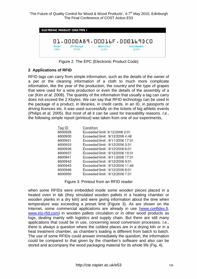
‘The Future of Quality Control for Wood & Wood Products’, 4-7th May 2010, Edinburgh The Final Conference of COST Action E53
Figure 2. The EPC (Electronic Product Code)
2 Applications of RFID RFID tags can carry from simple information, such as the details of the owner of a pet or the cleaning information of a cloth to much more complicate information, like the year of the production, the country and the type of grapes that were used for a wine production or even the details of the assembly of a car (Kim et al. 2008). The quantity of the information that usually a tag can carry does not exceed the 2 Kbytes. We can say that RFID technology can be used in the package of a product, in libraries, in credit cards, in an ID, in passports or driving licences etc. It was used successfully on the tickets of big athletic events (Philips et al. 2005). But most of all it can be used for traceability reasons. I.e., the following simple report (printout) was taken from one of our experiments,
Figure 3. Printout from an RFID reader
when some RFIDs were embedded inside some wooden pieces placed in a heated oven in lab (they simulated wooden pallets in a heating chamber or wooden planks in a dry kiln) and were giving information about the time when temperature was exceeding a preset limit (Figure 3). As are shown on the Internet, some commercial applications are already in use (www.confidex.fi, www.iris-rfid.com) in wooden pallets circulation or in other wood products as logs, dealing mainly with logistics and supply chain. But there are still many applications that could be in use, concerning wood conversion processes. I.e., there is always a question where the coldest places are in a drying kiln or in a heat treatment chamber, as chamber’s loading is different from batch to batch. The use of some RFIDs could answer immediately the question, the information could be compared to that given by the chamber’s software and also can be stored and accompany the wood packaging material for its whole life (Fig. 4).
http://cte.napier.ac.uk/e53 120
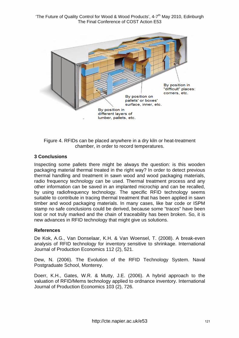
‘The Future of Quality Control for Wood & Wood Products’, 4-7th May 2010, Edinburgh The Final Conference of COST Action E53
Figure 4. RFIDs can be placed anywhere in a dry kiln or heat-treatment chamber, in order to record temperatures.
3 Conclusions Inspecting some pallets there might be always the question: is this wooden packaging material thermal treated in the right way? In order to detect previous thermal handling and treatment in sawn wood and wood packaging materials, radio frequency technology can be used. Thermal treatment process and any other information can be saved in an implanted microchip and can be recalled, by using radiofrequency technology. The specific RFID technology seems suitable to contribute in tracing thermal treatment that has been applied in sawn timber and wood packaging materials. In many cases, like bar code or ISPM stamp no safe conclusions could be derived, because some “traces” have been lost or not truly marked and the chain of traceability has been broken. So, it is new advances in RFID technology that might give us solutions.
References De Kok, A.G., Van Donselaar, K.H. & Van Woensel, T. (2008). A break-even analysis of RFID technology for inventory sensitive to shrinkage. International Journal of Production Economics 112 (2), 521.
Dew, N. (2006). The Evolution of the RFID Technology System. Naval Postgraduate School, Monterey.
Doerr, K.H., Gates, W.R. & Mutty, J.E. (2006). A hybrid approach to the valuation of RFID/Mems technology applied to ordnance inventory. International Journal of Production Economics 103 (2), 726.
http://cte.napier.ac.uk/e53 121

‘The Future of Quality Control for Wood & Wood Products’, 4-7th May 2010, Edinburgh The Final Conference of COST Action E53
IPPC, FAO. (2002). INTERNATIONAL STANDARDS FOR PHYTOSANITARY MEASURES. Publication No. 15: Guidelines for regulating Wood Packaging Material in International Trade.
Kim, J., Tang, K., Kumara, S., Yee, S. & Tew, J. (2008). Value analysis of location- enabled radio-frequency identification information on delivery chain performance. International Journal of Production Economics 112 (1), 403.
Lahiri, S. (2005). RFID Sourcebook. IBM Press, Upper Saddle River, NJ.
Landt, J. (2001). Shrouds of Time. The History of RFID AIM, Inc.
Ngai, E.W.T., Cheng, T.C.E., Au, S. & Lai, K.-H. (2007). Mobile commerce integrated with RFID technology in a container depot. Decision Support Systems 43 (1), 62.
Ngai, E.W.T., Moon, K.K.L., Riggins, F.J. & Yi, C.Y. (2008a). RFID research: an academic literature review (1995–2005) and future research directions. International Journal of Production Economics 112 (2), 510–520.
Ngai, E.W.T., Suk, F.F.C. & Lo, S.Y.Y. (2008b). Development of an RFID-based sushi management system: the case of a Conveyor-Belt Sushi Restaurant. International Journal of Production Economics 112 (2), 630–645.
Niederman, F., Mathieu, R.G., Morley, R. & Kwon, I.-W. (2007). Examining RFID applications in supply chain management. Communications of the ACM 50 (7), 93–101.
Phillips, T., Karygiannis, T. & Kuhn, R., (2005). Security standards for the RFID market. IEEE Security & Privacy Magazine 3 (6), 85–89.
Rekik, Y., Sahin, E. & Dallery, Y. (2008). Analysis of the impact of the RFID technology on reducing product misplacement errors at retail stores. International Journal of Production Economics 112 (1), 164.
Szmerekovsky, J.G. & Zhang, J. (2008). Coordination and adoption of item-level RFID with vendor managed inventory. International Journal of Production Economics 114 (1), 388–398.
Veeramani, D., Tang, J. & Gutierrez, A. (2008). A framework for assessing the value of RFID implementation by tier-one suppliers to major retailers. Journal of Theoretical and Applied Electronic Commerce Research 3 (1), 55–70.
Welling J. & Lambertz G. (2009). Phytosanitary treatment during kiln drying: Pre-conditions and advantages. In Proceedings of COST E53 Conference in Lisbon on “Economic and Technical aspects of quality control for wood and wood products” , 22-23 October 2009, pp. 5.
http://cte.napier.ac.uk/e53 122

‘The Future of Quality Control for Wood & Wood Products’, 4-7th May 2010, Edinburgh The Final Conference of COST Action E53
Wednesday 5th May Industry focussed day
1st session
http://www.cte.napier.ac.uk/e53/ 123

Scotland’s Forest Industries
COST Action E53Edinburgh
5th May 2010
Roger CoppockHead of Specialist Advisors
5th May 2010 COST E53
Introduction
• Scottish forestry in a European context• Scotland’s forest history• Industry today• Forest research• Current research• Future challenges
‘The Future of Quality Control for Wood & Wood Products’, 4-7th May 2010, EdinburghThe Final Conference of COST Action E53
http://cte.napier.ac.uk/e53 124

5th May 2010 COST E53
Forest cover
01020304050607080
United King
dom
Scotla
nd
Finlan
d
France
German
yIta
lySpa
in
Sweden
Forest area (Ha)Land area (M Ha)Forest cover%
5th May 2010 COST E53
Sustaining the forest area
Annual rates of Planting 1979 - 2008
0
5
10
15
20
25
1979-80
1989-90
1994-95
1995-96
1996-97
1997-98
1998-99
1999-00
2000-01
2001-02
2002-03
2003-04
2004-05
2005-06
2006-07
2007-08
2008-09
Year
Hect
ares
(000
's)
NP BlvsNP ConTotal NP
‘The Future of Quality Control for Wood & Wood Products’, 4-7th May 2010, EdinburghThe Final Conference of COST Action E53
http://cte.napier.ac.uk/e53 125
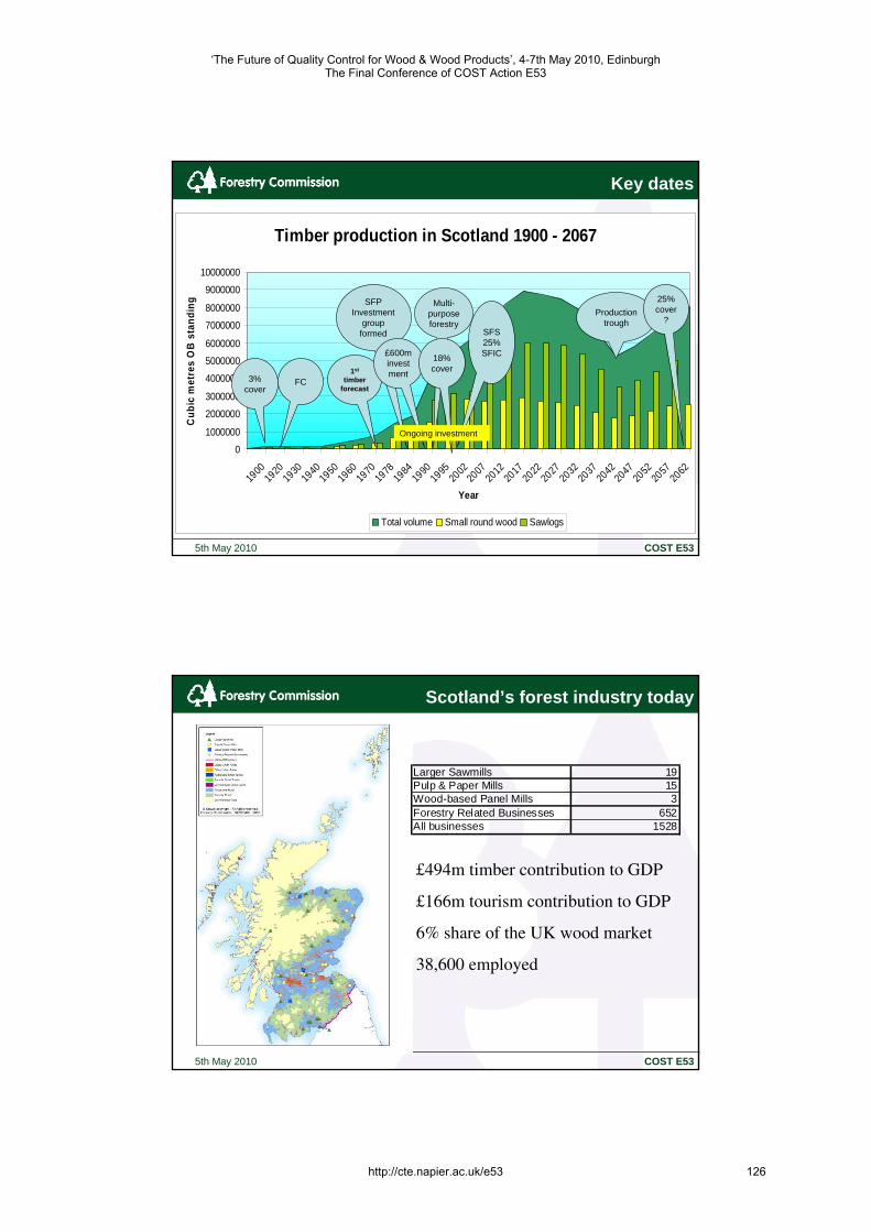
5th May 2010 COST E53
Timber production in Scotland 1900 - 2067
01000000
20000003000000
4000000
50000006000000
70000008000000
900000010000000
1900
1920
1930
1940
1950
1960
1970
1978
1984
1990
1995
2002
2007
2012
2017
2022
2027
2032
2037
2042
2047
2052
2057
2062
Year
Cub
ic m
etre
s O
B s
tand
ing
Total volume Small round wood Sawlogs
Key dates
3% cover
FC1st
timberforecast
SFS25%SFIC
Production trough
25% cover
?
SFPInvestment
groupformed
£600m investment
Multi-purpose forestry
18% cover
Ongoing investment
5th May 2010 COST E53
Scotland’s forest industry today
Larger Sawmills 19Pulp & Paper Mills 15Wood-based Panel Mills 3Forestry Related Businesses 652All businesses 1528
£494m timber contribution to GDP
£166m tourism contribution to GDP
6% share of the UK wood market
38,600 employed
‘The Future of Quality Control for Wood & Wood Products’, 4-7th May 2010, EdinburghThe Final Conference of COST Action E53
http://cte.napier.ac.uk/e53 126
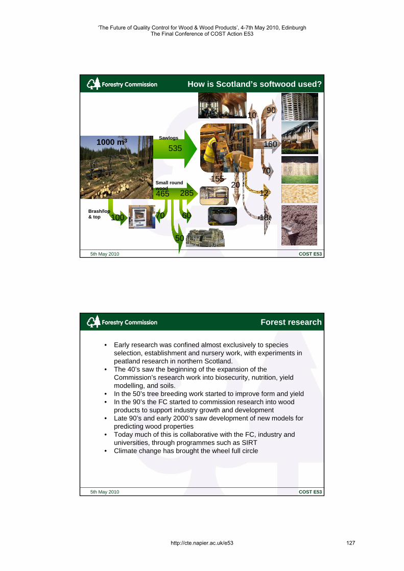
5th May 2010 COST E53
12
18
20155
How is Scotland’s softwood used?
70
50
60
90
70
10
160535Sawlogs
465Small round wood
1000 m3
100Brash/lop & top
285
5th May 2010 COST E53
Forest research
• Early research was confined almost exclusively to species selection, establishment and nursery work, with experiments in peatland research in northern Scotland.
• The 40’s saw the beginning of the expansion of the Commission’s research work into biosecurity, nutrition, yield modelling, and soils.
• In the 50’s tree breeding work started to improve form and yield• In the 90’s the FC started to commission research into wood
products to support industry growth and development• Late 90’s and early 2000’s saw development of new models for
predicting wood properties• Today much of this is collaborative with the FC, industry and
universities, through programmes such as SIRT• Climate change has brought the wheel full circle
‘The Future of Quality Control for Wood & Wood Products’, 4-7th May 2010, EdinburghThe Final Conference of COST Action E53
http://cte.napier.ac.uk/e53 127

5th May 2010 COST E53 2004 2005 2006 2007 2008
Recent wood and timber research•British and Irish Hardwood Improvement Programme
•Modifying the density of pine and Spruce•Machine grading re-engineered structural timber •Advanced timber grading and scanning techniques •Modelling timber characteristics•Evaluation of machine grading of finger jointed timber •Incising UK-grown Sitka spruce Incising pre-treatment technology
•Life Cycle Assessment of Timber Frame Manufacture
•High temperature drying of Sitka spruce •Innovative Timber Engineering in the Countryside: Bridge Design Test: 20 m Arch•A review of UK larch species in relation to end use
•Use of incising to develop new markets for home grown timber•Manual of Added Value opportunities
•High Temp Kiln Drying •Inside Out Beams •Examination of the opportunities for industrial use of home grown timber for piling•Best practice in construction using timber frame systems
•Development of UK grown spruce for industrial applications•Obtaining better utilisation of UK-grown small diameter hardwood stems using novel conversion and re-engineering. Phase 2
•Maximising the potential of UK-grown Scots pine falling boards •Machine grade settings for re-engineered UK-grown Scots pine
•Sitka spruce for high performance cladding (phase 2)•A guide to appearance grading UK grown hardwood timber
5th May 2010 COST E53
Current research
• Acoustics• Laser scanning• Supply chain• E-business• Timber form and straightness• Timber stiffness
‘The Future of Quality Control for Wood & Wood Products’, 4-7th May 2010, EdinburghThe Final Conference of COST Action E53
http://cte.napier.ac.uk/e53 128

5th May 2010 COST E53
Future challenges
• Adding greater value• Exploring new markets• New products and processes• Concerted research effort across sector• Cross sectoral approaches• Increasing timber’s relevance to society• Understanding the carbon benefits• Adapting to a changing environment
5th May 2010 COST E53
A final thoughtWell sited, well designed and well managed forests really are one of the few 'no regrets’ options for an
incredibly uncertain future. They can provide society with an extremely affordable, flexible insurance policy,
which will add value for the whole forest industry.
‘The Future of Quality Control for Wood & Wood Products’, 4-7th May 2010, EdinburghThe Final Conference of COST Action E53
http://cte.napier.ac.uk/e53 129

‘The Future of Quality Control for Wood & Wood Products’, 4-7th May 2010, Edinburgh The Final Conference of COST Action E53
Timber quality for the construction industry
I.R. Kliger1
Extended abstract The Action E53 focuses on timber quality and aims to improve existing methods and techniques for fast, accurate quality assessment at every link in the forestry wood chain. The development of novel methods and techniques is another aim. This presentation gives a short background to timber quality in the past, aims with respect to timber quality in this Action, the results of the internet survey conducted last year and some conclusions about what needs to be done in the future.
The background is based on more than twenty years’ experience of research on the subject of timber quality as a building material used in Sweden, the UK and Germany. Many of the problems associated with poor timber quality have been attributed to communication problems and questionable attitudes on the part of the industry. Different interested parties were identified (Johansson et al. 1994), together with their roles and importance when it comes to various requirements set for timber products along the forest-sawmill-building chain. Product specifications were drawn up for a number of structural timber and other wood products based on analyses and end-user requirements. The main conclusion twenty years ago was that timber must be fit for purpose. This conclusion was the starting point for this Action E53.
The technology used to produce timber using scanning, drying, advanced measurements and monitoring, as well as new grading equipment, is being continuously developed and is making it possible to produce sawn timber with more reliable properties and probably in accordance with end-user expectations.
However, the old questions still apply. For example, are we focusing on the correct requirements and right properties? What kind of knowledge does a producer of timber or a trader have of end-user needs? Does timber come up to end-user expectations? Is timber production governed by the property push or the property pull?
The internet survey was carried out in this Action in order to generate qualitative and quantitative knowledge about the demands and expectations that end-users in 25 European countries impose on various timber products. I would like to acknowledge the team at NTI, Norway, under the leadership of Anders Nyrud, and Ulrike Heinemann, for their tremendous work on the survey and the
1 Professor, Chalmers University of Technology, Building and Environmental Engineering, Steel and Timber Structures, GÖTEBORG, SWEDEN, Email: [email protected]
http://cte.napier.ac.uk/e53 130

‘The Future of Quality Control for Wood & Wood Products’, 4-7th May 2010, Edinburgh The Final Conference of COST Action E53
results and conclusions presented here are based on their work. Different parts of the survey are divided between, firstly, the secondary processing and integrated processing of soft wood and, secondly, trading companies and building construction and design. The companies defined in the group of integrated processing are companies producing their own sawn timber products and subsequently processing these products. Each group generated more than 100 responses, apart from traders who produced 80. Some of the preliminary conclusions from the survey now follow.
The survey revealed that the companies in the processing industry feel that the timber market is producer driven (property push), as customers have to accept what is offered by producers. More than half the companies in the integrated industry and about 45% of the companies in the secondary processing industry regard wood as a natural product and this is the reason for some quality defects and shortcomings which customers have to accept. The producers said that moisture content is one of the most important parameters when defining the quality of timber products. When specifying the moisture content in contracts, most companies in the secondary and the integrated processing industry use a plus/minus interval, e.g. 16% ± 4%.
More than 75% of the companies in the secondary processing industry do not use limits regarding distortion in quality control, do not know and do not answer questions relating to twist distortion or to bow, spring and cup distortion. The percentage of companies in the integrated processing industry responding to distortion is approximately 65% for twist, bow and spring and about 75% for cup. In relation to their own products, companies in the secondary processing industry seldom reflect on the modes of distortion. The industries within integrated processing accept these defects more frequently than companies in secondary processing and are able to specify some acceptable distortion limits. When it comes to causes of distortion, the poor knowledge of the producing industry is striking. Only a small number of companies recognise that incorrect storage and small-diameter timber are causes of twist distortion.
Strength grading (visual, visual assisted by scanning, machine) is rarely applied in the industry. If it is applied, visual grading is most common. The least common is visual grading assisted by any scanning technology. A certain desire or demand for machine settings for a large variety of classes and raw materials from different regions can be observed, but most of the companies did not answer this question, so the general interest in strength grading appears not to be especially great. Most of the interested companies work in the integrated processing industry. Scanning techniques over and above machine strength grading are rarely used in the processing industries and the tendency to start using them is not very great. As far as questions about quality parameters are concerned, it is also possible that companies that do not answer focus on other parameters in their production.
http://cte.napier.ac.uk/e53 131

‘The Future of Quality Control for Wood & Wood Products’, 4-7th May 2010, Edinburgh The Final Conference of COST Action E53
Trading and building companies’ answers revealed that customer requirements are not always met by the industry, even if customers feel that the industry is capable of delivering the right quality. It was assumed that one reason for customer dissatisfaction could be the cost of quality control in the industry. While trading companies usually work with flooring and with joinery, including windows, door manufacture and so on, building companies focus on other activities related to building and construction and within building/construction with timber kits. A fairly small number of the respondents in both groups work in fields that are not directly affiliated to building and construction, such as furniture production, fencing, garden and other outdoor use and pallets/packaging. The visible quality parameters, such as the extent of twist, spring and/or bow distortion, discoloration or mould, and the extent of visual defects, such as knots, cracks, wane (but not including colour), have higher priority, i.e. they are the highest priority for most companies. Twist distortion is recognised by building companies as the most important defect. Strength and strength class (the mechanical quality parameters) are the top priorities for both trading and building companies. Stiffness and density have medium-high priority for most trading companies. Building companies regard these two parameters as slightly more important. The importance of a low price for timber products in general varies for trading companies and building companies. Companies from the Nordic countries in particular regard price as a high priority, while it is a lower priority for companies in Central Europe and in the Mediterranean countries. It can be assumed that they are more willing than Nordic companies to pay more for better quality.
The internet survey conducted in this Action showed very clearly that the situation is improving and the awareness of timber quality is better now than 20 years ago. The majority of the respondents agree that the timber industry is capable of delivering products that match customer requirements. All of us working with building companies must have a mission. To speed up and improve communication between timber producers and users of timber as a building material, we need to improve the education of builders, buyers of building products and engineers.
References
Johansson G., Kliger R. and Perstorper M. (1994). Quality of Structural Timber-Product Specification System Required by End-Users. Holz Als Roh-Und Werkstoff, 52(1), 42-48.
Heinemann, U., Nyrud, A. (2010); Results from COST E53-inquiry: “Quality control for wood and wood products”
http://cte.napier.ac.uk/e53 132
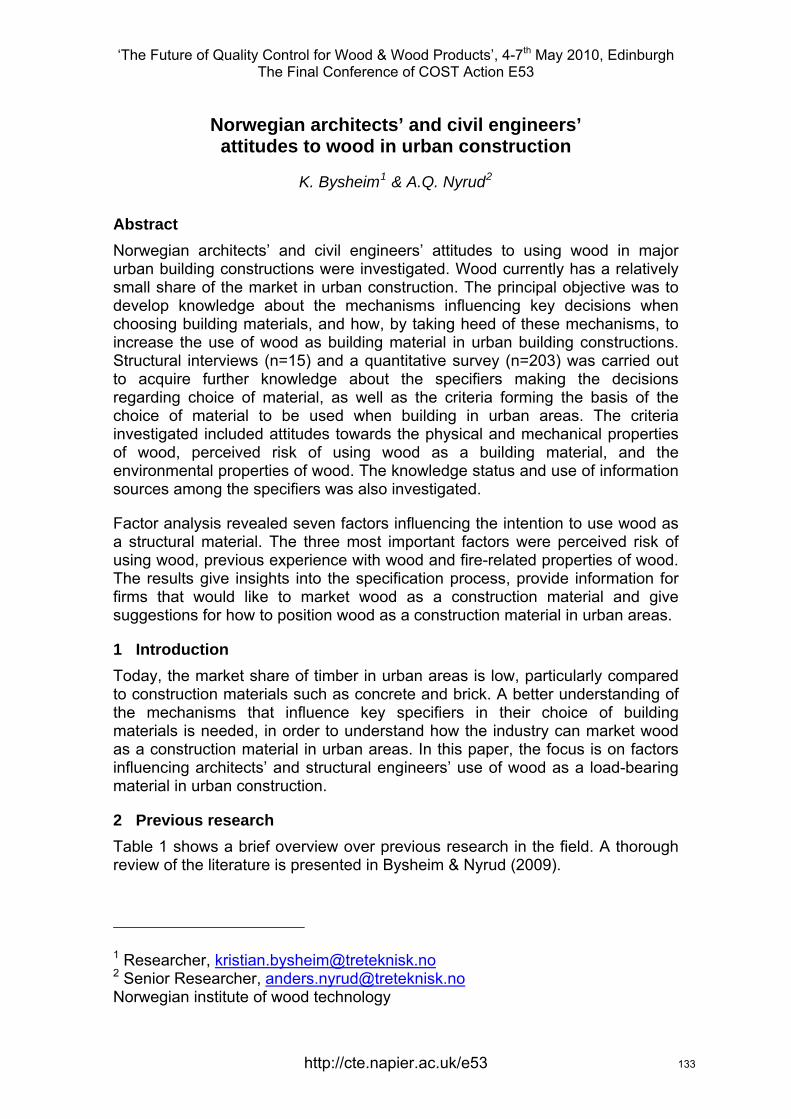
‘The Future of Quality Control for Wood & Wood Products’, 4-7th May 2010, Edinburgh The Final Conference of COST Action E53
Norwegian architects’ and civil engineers’ attitudes to wood in urban construction
K. Bysheim1 & A.Q. Nyrud2
Abstract Norwegian architects’ and civil engineers’ attitudes to using wood in major urban building constructions were investigated. Wood currently has a relatively small share of the market in urban construction. The principal objective was to develop knowledge about the mechanisms influencing key decisions when choosing building materials, and how, by taking heed of these mechanisms, to increase the use of wood as building material in urban building constructions. Structural interviews (n=15) and a quantitative survey (n=203) was carried out to acquire further knowledge about the specifiers making the decisions regarding choice of material, as well as the criteria forming the basis of the choice of material to be used when building in urban areas. The criteria investigated included attitudes towards the physical and mechanical properties of wood, perceived risk of using wood as a building material, and the environmental properties of wood. The knowledge status and use of information sources among the specifiers was also investigated.
Factor analysis revealed seven factors influencing the intention to use wood as a structural material. The three most important factors were perceived risk of using wood, previous experience with wood and fire-related properties of wood. The results give insights into the specification process, provide information for firms that would like to market wood as a construction material and give suggestions for how to position wood as a construction material in urban areas.
1 Introduction Today, the market share of timber in urban areas is low, particularly compared to construction materials such as concrete and brick. A better understanding of the mechanisms that influence key specifiers in their choice of building materials is needed, in order to understand how the industry can market wood as a construction material in urban areas. In this paper, the focus is on factors influencing architects’ and structural engineers’ use of wood as a load-bearing material in urban construction.
2 Previous research Table 1 shows a brief overview over previous research in the field. A thorough review of the literature is presented in Bysheim & Nyrud (2009).
1 Researcher, [email protected] Senior Researcher, [email protected] institute of wood technology
http://cte.napier.ac.uk/e53 133

‘The Future of Quality Control for Wood & Wood Products’, 4-7th May 2010, Edinburgh The Final Conference of COST Action E53
Table 1: Previous research
Important factors influencing choice of building material Author
Previous experience with wood, perceived behavioural control, building height.
Bysheim & Nyrud (2009)
Knowledge and experience, common knowledge, building type, building codes, example buildings, tech. solutions, economic and environmental issues.
Roos et. al (2008)
Codes, cost, performance, infrastructure in design and construction industry.
O’Connor et al. (2004)
Dimensional stability and uniform quality important. Fire, price and environmental properties less important.
Wagner & Hansen (2004)
3 Methods Using theoretical models by Emmitt & Yeomans (2008) and Ajzen (1991), a model for the specifiers’ decision making process was developed. Based on the model and previous research (Emmitt & Yeomans, 2008; Bysheim & Nyrud, 2009) an interview guide was developed. Six building projects in urban areas in Norway were chosen as case studies, and a total of 15 interviews were conducted among key players in the construction industry, such as engineers, architects and builders.
3.1 Structured interviews The interviews were mainly focusing on three different main themes:
1. Knowledge and previous experience with wood as a building material 2. Important criteria for the selection of building materials 3. Role of decision makers and stakeholders in the building process
3.2 Survey The results from the structural interviews, along with findings in previous research, formed the basis for a quantitative survey among key specifiers in the Norwegian construction sector. The criteria investigated included:
1. Attitudes towards the physical and mechanical properties of wood
2. Perceived risk of using wood as a building material
3. The environmental properties of wood
4. The knowledge status and use of information sources among the specifiers
http://cte.napier.ac.uk/e53 134

‘The Future of Quality Control for Wood & Wood Products’, 4-7th May 2010, Edinburgh The Final Conference of COST Action E53
5. Choice of building materials in the different stages of the building process An invitation to a web-based questionnaire was sent by email to 2374 Norwegian architects, engineers, builders and contractors. This resulted in 203 answers, yielding a response rate of 8.6 percent. The educational background of the respondents were mainly architecture (N=139) and engineering (N=60). The questions in the questionnaire used a seven-point scale (1=to a small degree; 7=to a large degree). High value reflected a stronger preference for wood, except for items regarding risk and fire. Seven items were reverse-scored.
4 Results
4.1 Structured interviews Some common features in the six case projects were identified: Most of the specifiers had previous experience with using wood. In the cases where wood had been used extensively the builder had a positive attitude towards using wood in the project. Also, wood had been chosen at an early stage in the specifying process. The specifiers who were interviewed were also satisfied with the use of wood in the case projects.
4.2 Descriptive statistics Figure 1 to 5 shows mean values for selected items from the survey. The values reported are mean values for the various items. Figure 1 shows which of the actors involved in the specification process that was perceived as most influential by the architects and engineers. The actors perceived to be most influential were engineer, architect and contractor. Public authorities and real estate agencies were perceived as having little influence over the choice of structural materials, while the builder had a somewhat moderate influence.
Figure 1. To what degree did the following actors influence the choice of structural material? (1=to a small degree; 7=to a large degree)
Figure 2 shows when decisions regarding the choice of building material for structural purposes were made. The most important phase, as perceived by the
http://cte.napier.ac.uk/e53 135
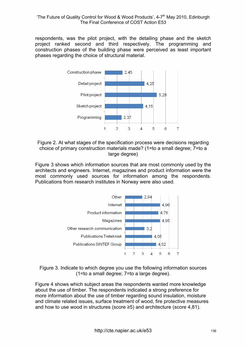
‘The Future of Quality Control for Wood & Wood Products’, 4-7th May 2010, Edinburgh The Final Conference of COST Action E53
respondents, was the pilot project, with the detailing phase and the sketch project ranked second and third respectively. The programming and construction phases of the building phase were perceived as least important phases regarding the choice of structural material.
Figure 2. At what stages of the specification process were decisions regarding choice of primary construction materials made? (1=to a small degree; 7=to a
large degree)
Figure 3 shows which information sources that are most commonly used by the architects and engineers. Internet, magazines and product information were the most commonly used sources for information among the respondents. Publications from research institutes in Norway were also used.
Figure 3. Indicate to which degree you use the following information sources (1=to a small degree; 7=to a large degree).
Figure 4 shows which subject areas the respondents wanted more knowledge about the use of timber. The respondents indicated a strong preference for more information about the use of timber regarding sound insulation, moisture and climate related issues, surface treatment of wood, fire protective measures and how to use wood in structures (score ≥5) and architecture (score 4,81).
http://cte.napier.ac.uk/e53 136
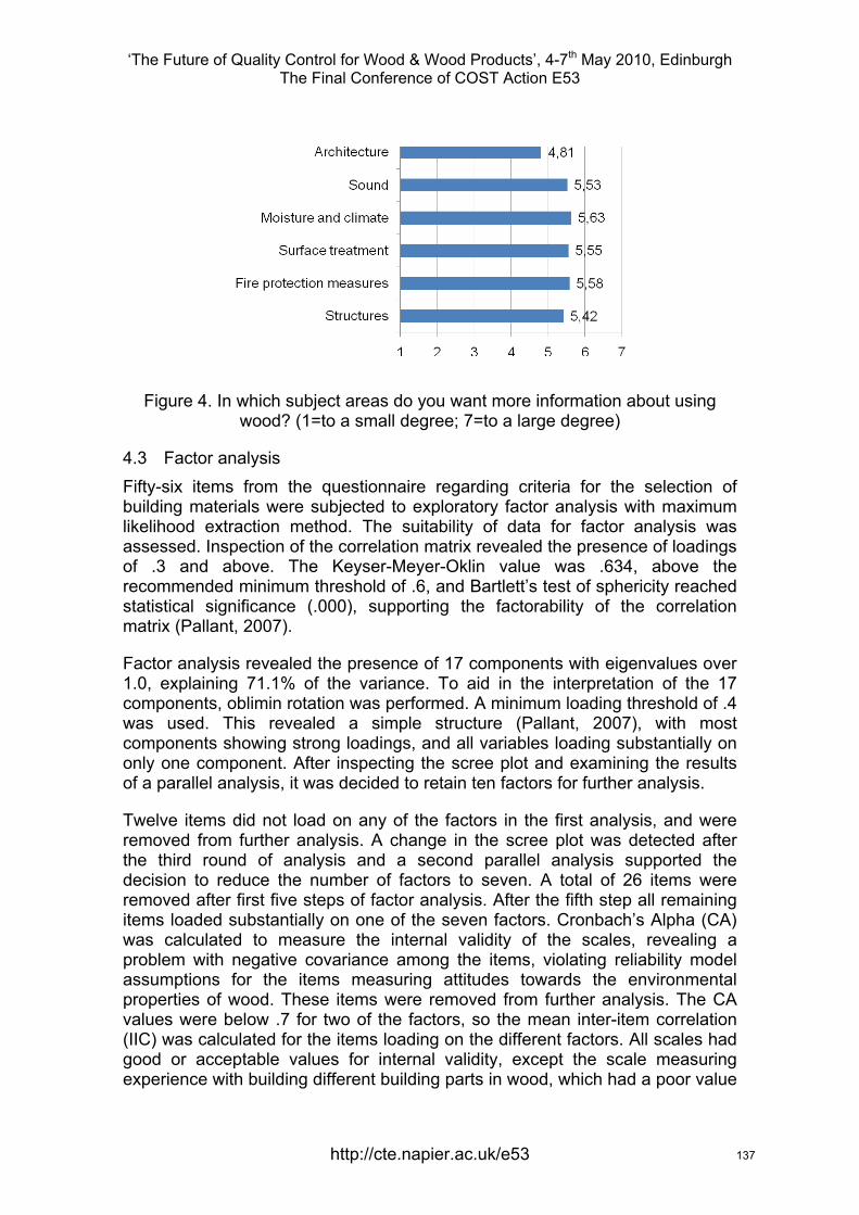
‘The Future of Quality Control for Wood & Wood Products’, 4-7th May 2010, Edinburgh The Final Conference of COST Action E53
Figure 4. In which subject areas do you want more information about using wood? (1=to a small degree; 7=to a large degree)
4.3 Factor analysis Fifty-six items from the questionnaire regarding criteria for the selection of building materials were subjected to exploratory factor analysis with maximum likelihood extraction method. The suitability of data for factor analysis was assessed. Inspection of the correlation matrix revealed the presence of loadings of .3 and above. The Keyser-Meyer-Oklin value was .634, above the recommended minimum threshold of .6, and Bartlett’s test of sphericity reached statistical significance (.000), supporting the factorability of the correlation matrix (Pallant, 2007).
Factor analysis revealed the presence of 17 components with eigenvalues over 1.0, explaining 71.1% of the variance. To aid in the interpretation of the 17 components, oblimin rotation was performed. A minimum loading threshold of .4 was used. This revealed a simple structure (Pallant, 2007), with most components showing strong loadings, and all variables loading substantially on only one component. After inspecting the scree plot and examining the results of a parallel analysis, it was decided to retain ten factors for further analysis.
Twelve items did not load on any of the factors in the first analysis, and were removed from further analysis. A change in the scree plot was detected after the third round of analysis and a second parallel analysis supported the decision to reduce the number of factors to seven. A total of 26 items were removed after first five steps of factor analysis. After the fifth step all remaining items loaded substantially on one of the seven factors. Cronbach’s Alpha (CA) was calculated to measure the internal validity of the scales, revealing a problem with negative covariance among the items, violating reliability model assumptions for the items measuring attitudes towards the environmental properties of wood. These items were removed from further analysis. The CA values were below .7 for two of the factors, so the mean inter-item correlation (IIC) was calculated for the items loading on the different factors. All scales had good or acceptable values for internal validity, except the scale measuring experience with building different building parts in wood, which had a poor value
http://cte.napier.ac.uk/e53 137
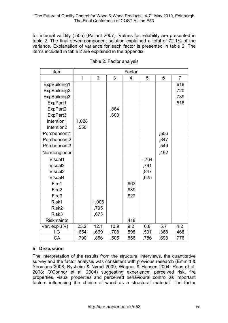
‘The Future of Quality Control for Wood & Wood Products’, 4-7th May 2010, Edinburgh The Final Conference of COST Action E53
for internal validity (.505) (Pallant 2007). Values for reliability are presented in table 2. The final seven-component solution explained a total of 72.1% of the variance. Explanation of variance for each factor is presented in table 2. The items included in table 2 are explained in the appendix.
Table 2: Factor analysis
Item Factor 1 2 3 4 5 6 7
ExpBuilding1 ,618 ExpBuilding2 ,720 ExpBuilding3 ,789
ExpPart1 ,516 ExpPart2 ,864 ExpPart3 ,603 Intention1 1,028 Intention2 ,550
Percbehcont1 ,506 Percbehcont2 ,847 Percbehcont3 ,549 Normengineer ,492
Visual1 -,764 Visual2 ,791 Visual3 ,847 Visual4 ,625 Fire1 ,863 Fire2 ,889 Fire3 ,827 Risk1 1,006 Risk2 ,795 Risk3 ,673
Riskmaintn ,418 Var. expl.(%) 23.2 12.1 10.9 9.2 6.8 5.7 4.2
IIC .654 .669 .708 .595 .591 .368 .468 CA .790 .856 .505 .856 .786 .698 .776
5 Discussion The interpretation of the results from the structural interviews, the quantitative survey and the factor analysis was consistent with previous research (Emmitt & Yeomans 2008; Bysheim & Nyrud 2009; Wagner & Hansen 2004; Roos et al. 2008; O’Connor et al. 2004) suggesting experience, perceived risk, fire properties, visual properties and perceived behavioural control as important factors influencing the choice of wood as a structural material. The factor
http://cte.napier.ac.uk/e53 138

‘The Future of Quality Control for Wood & Wood Products’, 4-7th May 2010, Edinburgh The Final Conference of COST Action E53
analysis indicated that the following four factors were most important for architects’ and engineers’ use of timber as a structural material in urban areas:
• Intentions to use wood as a structural material in urban areas
• Attitudes towards the perceived risk of using wood
• Previous experience with wood in structures and wood surfaces
• Attitudes towards fire properties of wood
Intentions explain 23.2% of the variance in the data set. This variable will in a subsequent analysis be used to predict specifiers’ intentions to use of wood as a structural material in urban areas. The results indicate that firms that would like to market wood as a construction material in urban areas should focus on using the familiarity of wood construction in different building parts and types. When marketing new wood products or building concepts, incorporating building techniques that are already familiar to architects and engineers when promoting wood as a structural material can be one way of reducing the perceived risk of using wood. Examples of successful wood construction projects in urban areas should be available to architects and engineers in order to minimize perceived risk (budget overruns, etc.), and workshops were more experienced architects and engineers share their expertise and knowledge with less experienced colleagues is one way of transferring knowledge and expertise. Also, updated technical and professional information about the fire related properties of wood should be readily available to architects and engineers.
References Ajzen, I. 1991. The theory of planned behavior. Organizational Behavior and Human Decision Processes 50:179-211.
Bysheim, K., and Nyrud, A.Q. 2009. Using a predictive model to analyze architects’ intententions of using wood as a structural material. Forest Products Journal 59:65-74.
Emmitt, S., and D.T. Yeomans. 2008. Specifying Buildings: A Design Management Perspective. Elsevier, Amsterdam. VII, 261 p.
O'Connor, J., R. Kozak, C. Gaston, and D. Fell. 2004. Wood use in nonresidential buildings: Opportunities and barriers. Forest Products Journal 54:19-28.
Pallant, J. 2007. SPSS Survival Manual: A Step by Step Guide to Data Analyzing Using SPSS for Windows. McGraw-Hill ; Open University Press, Maidenhead, the United Kingdom. 335 p.
Roos, A., L. Woxblom, and D. McCluskey. 2008. Architects’, and Building Engineers, and Stakeholders’ Perceptions to Wood in Construction – Results from a Qualitative Study. In: Bergseng E., Belbeck G, and Hoen H. (ed).
http://cte.napier.ac.uk/e53 139

‘The Future of Quality Control for Wood & Wood Products’, 4-7th May 2010, Edinburgh The Final Conference of COST Action E53
Scandinavian Scandinavian Forest Economics No 42, 2008., proceedings of the biennal meeting of the Scandinavian Society of Forest Economics. Lom, Norway, 6.- 9. April 2008.
Wagner, E., and E. Hansen. 2004. A method for identifying and assessing key customer group needs. Industrial Marketing Management 33(7):643-655.
Appendix
Explanation Item
Experience with wood in apartment buildings ExpBuilding1 Experience with wood in buildings for commercial purposes ExpBuilding2 Experience with wood in public buildings ExpBuilding3 Experience with wood used as facade material ExpPart1 Experience with wood in primary construction ExpPart2 Experience with wood in wood surfaces (flooring, etc.) ExpPart2 I want to use wood in primary constructions Intention1 I plan to use wood in primary constructions Intention2 I am qualified to do the building design in projects with wood Percbehcont1It is easy to use wood in the projects I design Percbehcont2If I want to, I can use wood in projects were I do the design Percbehcont3The engineers attitude towards using wood NormengineerWood is visually appealing Visual1 Visual aspects are important when choosing wood Visual2 Wood is easy to combine with other materials Visual3 Wood is suitable for my design tasks Visual4 Use of wood increase the risk of damage in case of fire Fire1 Wood used as a facade material increase the risk of fire Fire2 Wood used as a structural material increase the risk of fire Fire3 Using wood increases the risk of budget overruns Risk1 Using wood increases the risk of delays in a project Risk2 Using wood increases the risk of building-related errors Risk3 Risk of maintenance problems increases when using wood Riskmaintn
http://cte.napier.ac.uk/e53 140

COST Action E53Edinburgh
4-7 May, 2010
J.H.ParkConvenor, CEN/TC175/WG1
Round and sawn timber, general matters.
The problems with standardisation?
Wood is different!
The problem is, too many people forget that!
Anyone in the wood industry who does not understand and appreciate this is in the wrong business!
It is not sufficient to market wood in the same way as baked beans or underpants!
‘The Future of Quality Control for Wood & Wood Products’, 4-7th May 2010, EdinburghThe Final Conference of COST Action E53
http://cte.napier.ac.uk/e53 141

Wood or Timber
• Timber is as different from wood as concrete is different from cement
– The two products – wood in the sense of clear, defect-free wood and timber, in the sense of commercial timber – have to be considered as two different materials and that must be respected when strength properties are developed for engineering purposes
Borg Madsen – from:
‘Structural Behaviour of Timber’He also notes the truism that,
“The longer the human race has used a material the less it knows about it”
Isambard Kingdom Brunel’s approach!Walkham Viaduct – 1858 The zenith of on-site quality control!
Length - 367 yards Height - 132 feet
‘The Future of Quality Control for Wood & Wood Products’, 4-7th May 2010, EdinburghThe Final Conference of COST Action E53
http://cte.napier.ac.uk/e53 142
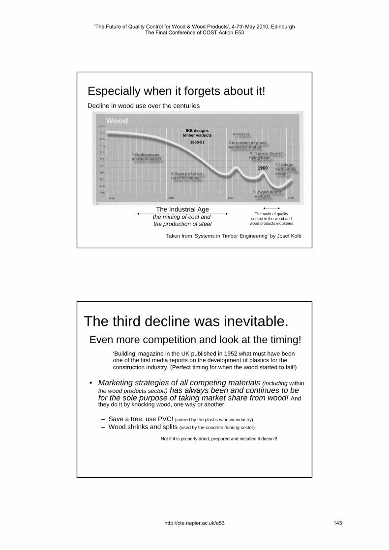
Taken from ‘Systems in Timber Engineering’ by Josef Kolb
Especially when it forgets about it! Decline in wood use over the centuries
1960
The Industrial Agethe mining of coal and the production of steel
IKB designs timber viaducts
1850-51
The nadir of quality control in the wood and
wood products industries
The third decline was inevitable.Even more competition and look at the timing!
‘Building’ magazine in the UK published in 1952 what must have been one of the first media reports on the development of plastics for theconstruction industry. (Perfect timing for when the wood started to fail!)
• Marketing strategies of all competing materials (including withinthe wood products sector!) has always been and continues to be for the sole purpose of taking market share from wood! And they do it by knocking wood, one way or another!
– Save a tree, use PVC! (coined by the plastic window industry)
– Wood shrinks and splits (used by the concrete flooring sector)
Not if it is properly dried, prepared and installed it doesn’t!
‘The Future of Quality Control for Wood & Wood Products’, 4-7th May 2010, EdinburghThe Final Conference of COST Action E53
http://cte.napier.ac.uk/e53 143

Bouncing back!• At long last the benefits of wood are becoming
widely recognised but it is not enough to hope to succeed based on the green building agenda alone!
• The loss of higher education in wood was at long last recognised and acted upon!
• With this we must strive to increase product knowledge amongst specifiers and users to ensure that wood and wood products deliver optimum serviceability performance!
• Appropriate quality control will ensure they have a head start!
But we are still in need of an understanding of ‘the common good’!
• (Named product) offers all of the advantages of regular wood siding but contrary to regular wood, it resists termite damage and will not rot, crack or split.The creators of such product marketing are quite unconcerned as to the possibility of the negative impact such words might have on theacceptance of ALL wood throughout the entire construction industry!
So, where do we go from here?
‘The Future of Quality Control for Wood & Wood Products’, 4-7th May 2010, EdinburghThe Final Conference of COST Action E53
http://cte.napier.ac.uk/e53 144

European Standardisation
• Addressing the requirements of the European Commission for the EU ‘single market’ for construction products
• In support of the ‘Construction Products Directive’
• Endeavouring to ensure the optimum performance of wood and wood products used in construction
Still a little bit divided in more ways than one!
• CEN/TC112 - Wood-based panels• CEN/TC124 - Timber Structures• CEN/TC175 - Round and sawn timber
to name but three!
To structural timber committees non-structural timber is to all intents and purposes irrelevant!
Unfortunately as we have just seen it was premature failure of non-structural components that has influenced the attitude, to all wood in construction, of several generations!
It’s all wood, so where is the problem?!
‘The Future of Quality Control for Wood & Wood Products’, 4-7th May 2010, EdinburghThe Final Conference of COST Action E53
http://cte.napier.ac.uk/e53 145

Moisture content• Possibly the single most influential property of wood on
its long-term serviceability and performance.• Much, perhaps most, premature failure of wood in
construction can be attributed to moisture content.• For glued structural components the requirements for
moisture content are simplicity itself when compared with those for joinery components!
• Wood is different and in terms of moisture content, very different indeed!
• Kiln drying is a good average process at best!
CEN/TC175 DocumentsMoisture content requirements
The highlighted values are in the format as presented in the documents; the italic values are the equivalent moisture contents in the alternate format
To develop a degree of consistency!
‘The Future of Quality Control for Wood & Wood Products’, 4-7th May 2010, EdinburghThe Final Conference of COST Action E53
http://cte.napier.ac.uk/e53 146

Summary of Table 1 Moisture Content
A clearly apparent degree of consistency in relation to heating conditions but nothing relating to variability of geographical location.
Proposed ‘Introduction’ for moisture content for all TC175 Product Standards.
The serviceability and long-term performance of wood products is influenced in nearly all cases by the moisture content of the wood used in the manufacture of those products. This standard sets out the requirements for moisture content suited to different environments and tolerance limits appropriate for those moisture contents.
The variability inherent in all timber and the ease or difficulty of drying different species with available kiln technology makes drying to constant moisture contents effectively impossible. A range of target moisture contents, and an allowable range of average moisture content around each target moisture content, for ‘standard drying’ is set out in EN 14298.
This does not, however, guarantee that all pieces within the same batch/consignment will be within the target moisture content tolerance limits. For this reason EN 14298 also specifies the number of pieces in a single batch or lot which shall have individual moisture content between the stipulated upper and lower limits.
In some cases it may be appropriate to specify target moisture content with tighter tolerances than those available with ‘standard drying’. EN 14298 sets out what should be stipulated for ‘Drying for specific end-use and certain species’ and provides guidance on what tolerances should be expected with this enhanced drying. EN 14298 also sets out requirements for what should be expected as maximum amounts of non-compliant pieces within a batch of kiln dried timber.’
‘The Future of Quality Control for Wood & Wood Products’, 4-7th May 2010, EdinburghThe Final Conference of COST Action E53
http://cte.napier.ac.uk/e53 147

EN 14298 – Drying quality
Clause 5.3 of EN 14298 to be revised in recognition of variability prevalent in the process and the material:
Revised wording 5.3 ‘Drying for specific end-use and certain species’
EN 942 as an example• product standards, unlike the target moisture content approach of
EN 14298, should include moisture contents as the expected range(e.g. 8% to 11%) likely to be encountered and best suited to individual Member States’ climatic conditions and so potentially quite variable in countries such as Italy for example. This detail could also highlight seasonal variability in addition to longer term EMC.
• EN 942 – suggested amendment to Annex B, Table B.1; table heading to be:– ‘Equilibrium moisture content of solid timber by category – regional and
seasonal moisture content range related to in-service climates’– column 3 headed ‘Expected moisture content range in %’
‘The Future of Quality Control for Wood & Wood Products’, 4-7th May 2010, EdinburghThe Final Conference of COST Action E53
http://cte.napier.ac.uk/e53 148

The knowledge does exist!• Whilst just-in-time delivery may be perfect for the
automotive industry …
… it is not the best option for manufacturers of joinery -unless, of course, the wood has been appropriately dried and supplied by specialist timber merchants!
No just-in-time delivery here!
Grade marks left off for aesthetic reasons?
‘The Future of Quality Control for Wood & Wood Products’, 4-7th May 2010, EdinburghThe Final Conference of COST Action E53
http://cte.napier.ac.uk/e53 149

CE marking of strength graded timberor
does graded structural timber really need factory production control?
• At least ten years in the making but still some countries were not ready! Was it too costly for small producers?
• EN 14081-1 date of applicability 01/09/2006 followed by an unprecedented three extensions of the co-existence period now ending 01/09/2012.
• CE marking has already been adopted for machine grading at least by a number of producers within the EU but …
• … the majority within the timber trade and structural products sectors are still wholly uninformed about this! What is an ‘ACD’?
• How can they be properly informed or producers gear up for implementation with such wildly unpredictable dates!!
The marking of strength graded timber
• The simple process of individual piece marking claimed by a number of countries to be too difficult to implement!
• The Commission lobbied to overturn the committee decision to not permit batch marking (this to avoid piece marking or to avoid grading?!)
• A seriously retrograde step in Member States where strength grading and individual piece marking is considered essential.
• Fortunately batch marking not allowed for machine graded timber!
‘The Future of Quality Control for Wood & Wood Products’, 4-7th May 2010, EdinburghThe Final Conference of COST Action E53
http://cte.napier.ac.uk/e53 150

Eurocode 5 – premature and imperfect?
• Eurocodes implemented throughout the EU March 2010Just one simple point of many much more complex -• EC 5 Clause 2.4.2 (1) - ‘Geometrical data for cross-sections
and systems may be taken as nominal values from product standards hEN or drawings for the execution’.
• EN 336 Clause 3.1 Target size – ‘size specified (at the reference moisture content) and to which the deviations, which would ideally be zero, are to be related’.
• EN 336 is not included in EC5 normative references or bibliography!
• Target Size (effectively ‘actual’ size) was adopted to overcome the problems associated with the term ‘nominal’and structural timber design!
And finally, talking of targets, what do we do to overcome this?
If a picture paint a thousand words …
…we must tell the whole story, somehow!
Yet more incomplete information and knocking shock horror tactics for self-serving ends making our job that little bit harder! Where do they think the wood comes from, for goodness sake!
‘The Future of Quality Control for Wood & Wood Products’, 4-7th May 2010, EdinburghThe Final Conference of COST Action E53
http://cte.napier.ac.uk/e53 151

‘The Future of Quality Control for Wood & Wood Products’, 4-7th May 2010, Edinburgh The Final Conference of COST Action E53
Practical engineering considerations when using solid hardwood to replace steel and concrete structure
R. Thorniley-Walker1
Abstract This paper by a practising engineer discusses opportunities and challenges in the use of solid timber and particularly local hardwoods in a rapidly evolving market. Case studies are taken from both the restoration of historic buildings and the provision of genuine low-carbon structures in new-build.
The Author argues that the timber industry needs to prepare for a surge in demand from construction as structural alternatives are sought to high-carbon steel and concrete. This need will be particularly exacerbated once the hazards from carbon emissions start to be included in risk assessments. Opinions from a survey of engineers indicate that timescales could be very short and that many codes of practice will need to be revised to meet the new challenges.
There is a need for hardwood to be prepared and made ready for use in the construction industry, and this would add significant value to the timber. Data is also needed for all the varieties of local timbers that could be adopted for structural use covering curing, shrinkage, practical methods to assess the structural capacity of one-off old or new logs, and guidance on the strength of timber connections for the various and diverse species. Regional expertise and education in timber engineering needs to be developed and this could be assisted through widespread research at universities.
1 Introduction The use of timber in construction is on the cusp of a revolution and is already entering very exciting times. Approaches that were reserved for historic monuments are now being introduced to public buildings and domestic houses. Varieties of solid timber are being used in structural ways probably not previously considered in current codes of practice. Joints are being created such as moment connections in mortice and tenon sway frames and in curved knee braces, which by definition fall well outside the normal visual grading requirements.
There is growing demand for green buildings that utilise well-established timber stud panels (timber framing), but which also need to use solid chunky timber or glued laminated sections in place of steelwork or precast concrete beams and lintels. It is worth noting that this usage already has to compete with growing demand for logs for domestic fuel and commercial power stations. With the onset of measures to fight global warming, timber will shortly be needed in forms and quantities that are difficult to grasp. This paper sets out to illustrate some of the issues and challenges for a re-emerging rural industry.
1 Director of Structural & Civil Consultants, Northallerton, UK, MA(Oxon) CEng FICE FISructE MIHT IHBC, [email protected]
http://cte.napier.ac.uk/e53 152

‘The Future of Quality Control for Wood & Wood Products’, 4-7th May 2010, Edinburgh The Final Conference of COST Action E53
2 Use of Hardwoods 2.1 Challenges with solid hardwood in typical projects
While the design and supply of sawn softwood, ply sheets and engineered products appear to be very efficiently managed, engineers working on historic structures have long been aware of the problems of assessing the structural capacity of historic timbers and with replacing them if necessary (see paper by Kennedy and McGregor at this conference). As new buildings increasingly seek authentic or low carbon solutions, the design team face several challenges:
1. Finding a source of suitable timber, especially if there is a requirement for it to be locally sourced and a structural need for a hardwood grade to take high loads. Leaving the sourcing in the hands of the contractor raises its own problems.
2. Deciding on the structural properties of the timber logs and the connections based on a visual assessment of the members and tables of properties that are readily available (Figure 1).
Figure 1 Extent of easily available data on British hardwoods
3. Havin have a hidden weaknesss, especially if it is an un-sawn log or second-hand beam.
4. r to follow the engineering drawings, or to design and draw the required details.
g confidence that any critical structural member does not
Assessing timbers in the round that have “history” is very different from grading straight-sawn new hardwood to BS 5756.
Finding a manufacturing facility or a carpenter eithe
http://cte.napier.ac.uk/e53 153

‘The Future of Quality Control for Wood & Wood Products’, 4-7th May 2010, Edinburgh The Final Conference of COST Action E53
5. Having some measure of confidence that curing has progressed far enough to prevent major defects appearing as the timber dries.
6. ement that might be expected as the timber dries out and as it moves with each season change.
Forinsurmountable. Design teams and their clients need to be very dedicated to
Gaining agreement from the client on the degree of mov
most clients and design teams, these problems are currently almost
avoid using engineered timbers, steel sections or the precast concrete.
2.2 Case Study 1 – School Building in Oak
Figures: 2-4 School Structure in oak, but occurred at the bearing above the ceiling
l problems arose when trying to use local timber instead of steel at the central hub and in the library of a primary school.
e was not structurally or visually significant.
r supplier insisted on importing the
• • hardwood timbers with more suitable properties than oak were not
• No official grading was carried out.
it was fortunate that the major shake line and could only be seen from a
service area.
Several typica
• The timber was not seasoned – it was fortunate that the large shak
• The timber could not be supplied from local woods as they were not certified as “sustainable”, so the timbeoak. Oak was not the best type of timber for such internal use. Otheravailable (at any price).
http://cte.napier.ac.uk/e53 154

‘The Future of Quality Control for Wood & Wood Products’, 4-7th May 2010, Edinburgh The Final Conference of COST Action E53
• There were numerous telephone calls from concerned architects, builders and timber suppliers.
2.3 cal timbers
improving use of local timbers at a
techniques etc.
2
eering does not generally appear to be taught to undergraduates.
ale isolated suppliers of hardwoods
5
On othresource. been managed for timber production (as in France), most trees could yield at least a lintel if harvested
add value to unused hardwoods by preparation for use in construction. The
also needed to fabricate a mobile test rig so that the stiffness of un-graded species, structurally critical members, or possibly sub-standard logs
l interest with helping with this development project, another e.
Promotion of regional use for lo
There appear to be several impediments toregional level:
1 Very few engineers and architects appear to have knowledge of timber frame sheathed construction never mind other timbers, grading
Timber research in the UK appears to take place at very few locations and there are no trade bodies to promote use of small-scale production.
3 Most universities have little or no expertise with structural timber and timber engin
4 The steel and concrete industries have powerful trade bodies, which even appear to state that use of steel or concrete is more carbon-friendly than timber. Small-schave no such support and even sustainability measures prevent them using timber in construction (Case Study 1).
The growing need of bio-fuel industrial furnaces and domestic stoves provide a convenient outlet for all timber.
the er hand, hardwoods could be used as a valuable rural or even urban Although British woods have not usually
before decay sets in.
The author’s practice, with help from Sustainability Development Grants from the Yorkshire National Parks, set up GreenBeams.com as a way to develop and
web site acts as a forum to pass on the limited knowledge on hardwoods, but was particularly intended to promote the storage of hardwoods to allow curing to commence.
After training for the visual grading of hardwoods to BS5756, the practice realised that it
could be checked on site, in the forest or at the sawmill (Figure 5). It has also been interesting to correlate the ultimate capacity of sawn members with their visual grading.
While the Institution of Civil Engineers and the Centre for Timber Engineering expressed initiaofficial research body has strongly opposed the initiativ
http://cte.napier.ac.uk/e53 155
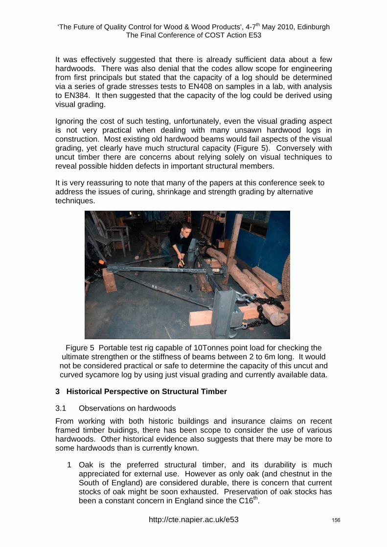
‘The Future of Quality Control for Wood & Wood Products’, 4-7th May 2010, Edinburgh The Final Conference of COST Action E53
It was effectively suggested that there is already sufficient data about a few hardwoods. There was also denial that the codes allow scope for engineering from first principals but stated that the capacity of a log should be determined via a series of grade stresses tests to EN408 on samples in a lab, with analysis
st existing old hardwood beams would fail aspects of the visual grading, yet clearly have much structural capacity (Figure 5). Conversely with
Figure 5 Portable test rig capable of 10Tonnes point load for checking the ultimate strengthen or the stiffness of beams between 2 to 6m long. It would
not be considered practical or safe to determine the capacity of this uncut and curved sycamore log by using just visual grading and currently available data.
3
3insurance claims on recent consider the use of various
ce also suggests that there may be more to e h own.
urable, there is concern that current stocks of oak might be soon exhausted. Preservation of oak stocks has been a constant concern in England since the C16th.
to EN384. It then suggested that the capacity of the log could be derived using visual grading.
Ignoring the cost of such testing, unfortunately, even the visual grading aspect is not very practical when dealing with many unsawn hardwood logs in construction. Mo
uncut timber there are concerns about relying solely on visual techniques to reveal possible hidden defects in important structural members.
It is very reassuring to note that many of the papers at this conference seek to address the issues of curing, shrinkage and strength grading by alternative techniques.
Historical Perspective on Structural Timber
.1 Observations on hardwoods From working with both historic buildings and framed timber buidings, there has been scope tohardwoods. Other historical evidensom ardwoods than is currently kn
1 Oak is the preferred structural timber, and its durability is much appreciated for external use. However as only oak (and chestnut in the South of England) are considered d
http://cte.napier.ac.uk/e53 156

‘The Future of Quality Control for Wood & Wood Products’, 4-7th May 2010, Edinburgh The Final Conference of COST Action E53
2 For internal use, the curing times for oak and its continuing dimensional changes with moisture is a problem. Other hardwoods might have better properties, (Figure 1) while Douglas Fir will often suffice and is much more geometrically stable if appearance is not critical.
3 Elm was usually only used where anti-splitting properties were needed
hard and durable condition.
4
5 ines, buildings were historically constructed in ash yet local sawmills refused to sell for that purpose until recently. The Author is now
While r major advantage of oak is that it has value, so it is stored for profit and made available ovegeneraso the previously discussed, there is much scope to research other hardwoods to reveal ‘lost’ knowledge of
ember, but in a local timber such as beech or ash. onable moisture content, it was se imported pitch pine.
nections than with many common bolted joints. However the characteristics of the joints
and 6 million elm trees were destroyed in the 80s after Duch Elm Disease. Timber in the open decayed within months and very little now remains of the stock. However elm was frequently used for structural members in C19th and is usually now in an extremely
Similarly, alder was historically renowned for its soft texture, which then became hard and durable once cured. (See reported problems with decaying alder piles in the reconstructed crannog on Loch Tay)
In the Penn
involved with the design of a whole building in ash.
oak has properties that allow it to endure for centuries, anothe
r a range of moisture contents. Other British hardwoods timbers are not lly available in this way, mainly because no one has developed a market
trees are left to rot, or are cut up for firewood. As
their properties and to develop a market for timbers that have been cured and are ready for construction
3.2 Case Study 2 – Historical Church Roof A fire destroyed the roofs to the Norman and Mediaeval Grade I Listed St Michael and All Angels, Newburn on the banks of the River Tyne in 2006. It was hoped that the nave roof could be reconstruct with trusses similar to the single surviving Victorian mAs such timbers were not available at a reasdecided to follow the Victorian precedent and u
The Victorians used wrought iron strap at connections which were a conveniently clue to their construction date. The new trusses would have used Black Bolts if they had been constructed in the late C20th. As an indication of the green C21st, the trusses were designed with all timber joints. It is generally found that relatively high loads are easier to design with timber con
reflect the species, and there was surprise over how weak the tenons were to shear or shrinkage on a tangential plane to the growth of the pine. More advice needs to be given on this crucial aspect of timber engineering.
The trusses were intended to be manufactured off site under the management of the contractor. While this approach works in the steel industry, the timber industry has inadequate experience and much time had to be spent on site
http://cte.napier.ac.uk/e53 157
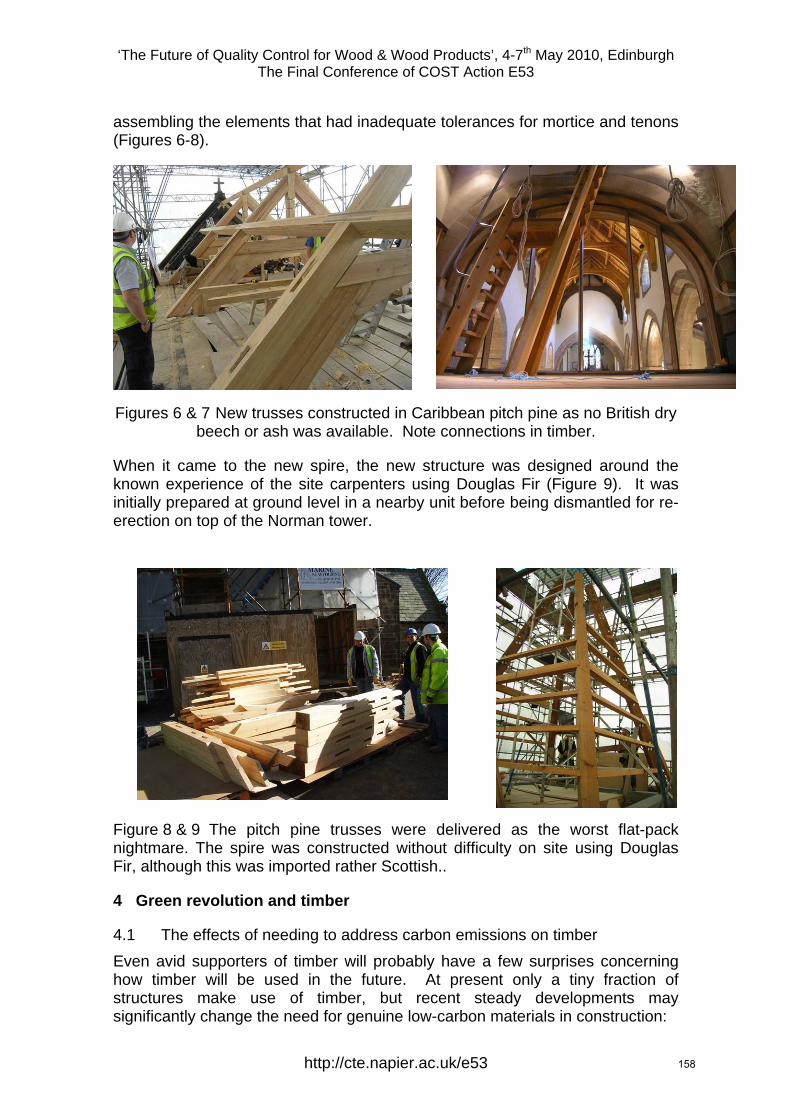
‘The Future of Quality Control for Wood & Wood Products’, 4-7th May 2010, Edinburgh The Final Conference of COST Action E53
assembling the elements that had inadequate tolerances for mortice and tenons (Figures 6-8).
Figures 6 & 7 New trusses constructed in Caribbean pitch pine as no British dry beech or ash was available. Note connections in timber.
When it came to the new spire, the new structure was designed around the known experience of the site carpenters using Douglas Fir (Figure 9). It was initially prepared at ground level in a nearby unit before being dismantled for re-
nightmare. The spire was constructed without difficultFir, although this was imported rather Scottish..
4 Green revolution and timber
resent only a tiny fraction of structures make use of timber, but recent steady developments may significantly change the need for genuine low-carbon materials in construction:
erection on top of the Norman tower.
Figure 8 & 9 The pitch pine trusses were delivered as the worst flat-pack y on site using Douglas
4.1 The effects of needing to address carbon emissions on timber Even avid supporters of timber will probably have a few surprises concerning how timber will be used in the future. At p
http://cte.napier.ac.uk/e53 158

‘The Future of Quality Control for Wood & Wood Products’, 4-7th May 2010, Edinburgh The Final Conference of COST Action E53
1. The 2009 State of the Nation Report on climate change by the Institution of Civil Engineers advised that carbon should become a key feature of all
This last paper uses “reasonable” values for dangers and probabilities derived
their associates in the Northeast of
assCO rthermore, the paper suggests that mitigation of emissions
design. 2. The Engineering Council (UK) issued advice in 2009 that risk assessments
should be carried out on all projects to include the long-term effects of carbon emissions.
3. The early May 2010 edition of the Structural Engineer will have a paper by RThorniley-Walker on “Data for Inclusion of Carbon Emissions in Risk Assessments”.
with opinions from a questionnaire survey of members of both the Institution of Structural Engineers (IStructE) and the Institution of Civil Engineers (ICE) and
England, supplemented by data from IPCC(2007). The hazards and the probabilities are orders of magnitude higher than normal civilian projects and it is suggested that risk assessments should
ume that one person will die from climate change for every twenty tonnes of 2 released. Fu
from construction should not consider benefits beyond 10 years into the future. Although it is possible that climate change will continue to be ignored for a few more years, clients, consultants and site staff may be looking much harder for green alternatives to high carbon materials such as steel, concrete, bricks and blocks and the timber industry could face an insatiable demand. Another linked aspect of such foreseeable change is that timber codes will need to be revised to cater for new conditions associated with global warming, but also to realign the new definitions of ‘safe’ under the new forms of risk assessment (Figure 10).
Figure 10 Results of questionnaire survey from and engineering-
based study of attitudes to climate change indicating a mean of 73%
http://cte.napier.ac.uk/e53 159

‘The Future of Quality Control for Wood & Wood Products’, 4-7th May 2010, Edinburgh The Final Conference of COST Action E53
4.2 Case Study 3 – North York Moors National Park Visitor Centre This 2006 structure a By rejecting the sedum roof, the steel in the concept design could be replaced
timber. The project had the following unusual characteristics:
green on
further sharp edges a year after installation where shakes had raised splinters.
• e project the design team questioned whether there might have been scope to cut the concrete foundations to reduce the carbon
•
and processed for the purpose and detailed to allow for shrinkage.
project illustrates a project where the client wanted a low carbonnd was delighted to find that the structure could be sourced locally.
by
• The oak was felled and sawn to order and was therefore veryarrival at site.
• The architects took some persuasion that clean Ikea-type sharp edges would not be advisable due to shrinkage and distortion. All arises needed to be shamfered and the caretaker had to remove
At the end of th
footprint still further.
6.7 Tonnes of CO2 were saved by avoiding a steel frame and 9.3 Tonnes of CO2 have been captured in the oak for the next few centuries.
Figures: 11-13 Use of local oak felled
http://cte.napier.ac.uk/e53 160

‘The Future of Quality Control for Wood & Wood Products’, 4-7th May 2010, Edinburgh The Final Conference of COST Action E53
5 Concluding Study
.1 Conclusion he engineering profession has and an excellent choice of sawn softwood ists, ply and engineered beams available for most engineering applications.
have not been through the normal quality n e is much scope to develop the training of engineers
along with the supply and fabrication processes to timber engineering up to with steelwork. Engineers need to be equipped with
5TjoHowever such members are not suitable for all locations and there can be real challenges for structural engineers when trying to assess existing timbers or when using large solid timbers thatco trol measures. Ther
standards expected research data on how the timbers will behave structurally and during the process of moisture changes.
5.2 Case Study 4 – Three planned Park and Ride Terminals
Figure 14 – One of three terminals which would ideally be constructed with a timber sub-structure and super-structure
Many projects use cedar cladding to disguise high-carbon construction but still achieve very good BREEAM assessments. A set of three projects for the City of York gave an opportunity to try from the concept stage to minimise the carbon footprint of the structure. Potential timber aspects include:
have the
1 One of the terminal buildings will be sat on 5m of household waste. It is proposed to use 35 Scots Pine timber piles, 10m long, which would
following advantages:
a. “Stout” poles 285 tapering to 190mm would be adequate to take the 110kN required load down to the ground beneath the waste.
http://cte.napier.ac.uk/e53 161

‘The Future of Quality Control for Wood & Wood Products’, 4-7th May 2010, Edinburgh The Final Conference of COST Action E53
b. The poles would be naturally tapered so that negative skin friction will be reduced as the waste settles, but resistance in the underlying clay would be increased.
aquifers by driving through the waste rather than displacing it in the manner of rectangular concrete
d. The timber would not be durable, but the pine can be thoroughly
e. UK but can be easily driven and cut to length. Many historic buildings have timber piles.
2 Theusewould ideally be ash or beech if they can be supplied at the reasonable moisture content, but can be engineered beams if
3 There have been discussions over using timber poles to support
tim nded
d any maintenance while adjacent street furniture was
With suchstatus tha
ReferencThe Instituhttp://www
c. The tapered and pointed piles would minimise risk of contamination of underlying
piles..
treated to give the 50 year life expectancy.
Timber piles are rarely used in the
terminal building will have a completely timber structure making of stud walling and large section timber beams and posts. These
necessary.
lighting. Limited research found recent examples where varnished ber poles were manufactured using dried and glued strips bo
around a steel pole. The design team had reservations that timber could comply with the codes of practice (EN40), but these boiled down to aspects such as fatigue (a problem with metals) and flexure (a structural problem). Field research found plenty of impregnated timber poles dating back to 1951 and last inspected in 2002 that had never needeabout to be replaced for the third generation. features, the project stands a good chance of gaining the landmark t the client is seeking.
es tion of Civil Engineers 2009 State of the Nation report .ice.org.uk/about_ice/aboutice_lci_ice_recommendations.asp
g Council UK Guidance on Sustainability for the Engineering -
EngineerinProfession www.enge.org.uk/sustainability The Structural Engineer – due publication 5th May 2010 http://www.istructe.org/thestructuralengineer/index.asp
d
Results of questionnaire in advance of a paper presented by Robert Thorniley-Walker MA(Oxon) CEng FICE FISructE MIHT IHBC to a joint meeting of the Institution of Civil Engineers with the Institution of Structural Engineers anguests held at Teesside University in November 2008, professor David Lilley in the chair www.Structural.org.uk/Climate.html
http://cte.napier.ac.uk/e53 162

‘The Future of Quality Control for Wood & Wood Products’, 4-7th May 2010, Edinburgh The Final Conference of COST Action E53
Wednesday 5th May Industry focussed day
2nd session
http://www.cte.napier.ac.uk/e53/ 163

‘The Future of Quality Control for Wood & Wood Products’, 4-7th May 2010, Edinburgh The Final Conference of COST Action E53
Sawmilling and Sawing Process in the Future
A. Usenius1, P. Holmila2, A. Heikkilä3 & T. Usenius4
Abstract Major part of present sawmills are volume, high speed and bulk product oriented. Normally the focus is minimisation of costs – not maximising profit. Production typically yields also so called “falling” products which are not desired and may cause big economical losses. At present sawmills it is not possible to manufacture products with specific properties according to the customers specific needs. Profitability of conventional sawmill business is very sensitive to economic fluctuations.
New business concepts and processes for sawmill industry are needed in order to improve radically value yield through increased customer orientation and satisfaction. Only very few small mills can manufacture special wooden components according to the actual needs of customers. Future sawmill business has to support also sustainable development.
VTT Technical Research Centre of Finland is realising several projects mapping future production and business concepts for sawmills. This paper presents results and ideas in the field COST Action 53 from the research point of view and from industrial point of view. The focus is how the future scanning, sorting and grading of wood raw materials, semi finished and finished products supports optimisation of conversion chains from the forest to the final products in order to
• convert non-homogenous wood raw material to the products with defined properties with maximum yield and minimum waste
• shift from bulk products towards value added products • improve flexibility of manufacturing systems • make business and processing adaptive
The investigations clearly show that it is possible to increase considerably sales value and profit of the conversion by implementing new concepts and technologies in the production.
1Professor, VTT Technical Research Centre of Finland, [email protected] 2Manager, UPM Kymmene Finland, [email protected] 3Research Scientist, VTT Technical Research Centre of Finland, [email protected] 4System Designer, VTT Technical Research Centre of Finland, [email protected]
http://cte.napier.ac.uk/e53 164

‘The Future of Quality Control for Wood & Wood Products’, 4-7th May 2010, Edinburgh The Final Conference of COST Action E53
1 Introduction Sawmill industries are very important in many countries. Sawmills are utilising forest recourses by producing sawn timber to be used in construction, manufacturing of furniture, windows and doors industry etc. Sawmills are also supplying pulp mills chips. Typical production and business features of sawmills are following.
1. Conversion from the forest to the customer is not considered as an unbroken chain. Delivery and processing time may require weeks or months.
2. Volumes and cost minimisation is emphasized in production. 3. Production is not flexible allowing only marginal freedom. Production and
business are not adaptive. Feed back information is not generated and cannot be utilised.
4. Limited volume of reliable and less reliable data is measured, however only locally used.
5. Product properties vary considerably due to the inhomogeneous wood raw material. It is not possible to produce special products with desired, specified properties. Products which are not desired fall in the manufacturing processes.
In the present sawmills it is not easy to produce products with specific properties. Big problem is also so called “falling” products which may cause considerable economical losses. Modern and future scanning technologies provide efficient tools to handle and reduce radically these problems. They are very important for improving value yield and developing customer orientated sawmilling business.
Essential elements of the new business and production system concepts are:
1. Sawmills are moving forward in value chain by manufacturing more value added components.
2. Control and optimisation of information and material flows in planning and production systems.
3. Integrated information systems covering entire conversion and supply chains.
4. Intelligent, flexible and self learning scanning, production and logistic systems.
5. Creation and utilization of the feed back information in order to make manufacturing adaptive.
6. Optimised mechanics and conveyer systems for production concepts and cells.
http://cte.napier.ac.uk/e53 165
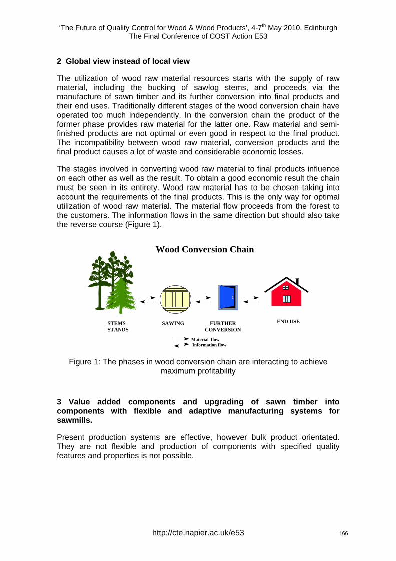
‘The Future of Quality Control for Wood & Wood Products’, 4-7th May 2010, Edinburgh The Final Conference of COST Action E53
2 Global view instead of local view
The utilization of wood raw material resources starts with the supply of raw material, including the bucking of sawlog stems, and proceeds via the manufacture of sawn timber and its further conversion into final products and their end uses. Traditionally different stages of the wood conversion chain have operated too much independently. In the conversion chain the product of the former phase provides raw material for the latter one. Raw material and semi-finished products are not optimal or even good in respect to the final product. The incompatibility between wood raw material, conversion products and the final product causes a lot of waste and considerable economic losses.
The stages involved in converting wood raw material to final products influence on each other as well as the result. To obtain a good economic result the chain must be seen in its entirety. Wood raw material has to be chosen taking into account the requirements of the final products. This is the only way for optimal utilization of wood raw material. The material flow proceeds from the forest to the customers. The information flows in the same direction but should also take the reverse course (Figure 1).
Wood Conversion Chain
SAWING FURTHERCONVERSION
STEMSSTANDS
END USE
Information flowMaterial flow
Figure 1: The phases in wood conversion chain are interacting to achieve maximum profitability
3 Value added components and upgrading of sawn timber into components with flexible and adaptive manufacturing systems for sawmills.
Present production systems are effective, however bulk product orientated. They are not flexible and production of components with specified quality features and properties is not possible.
http://cte.napier.ac.uk/e53 166
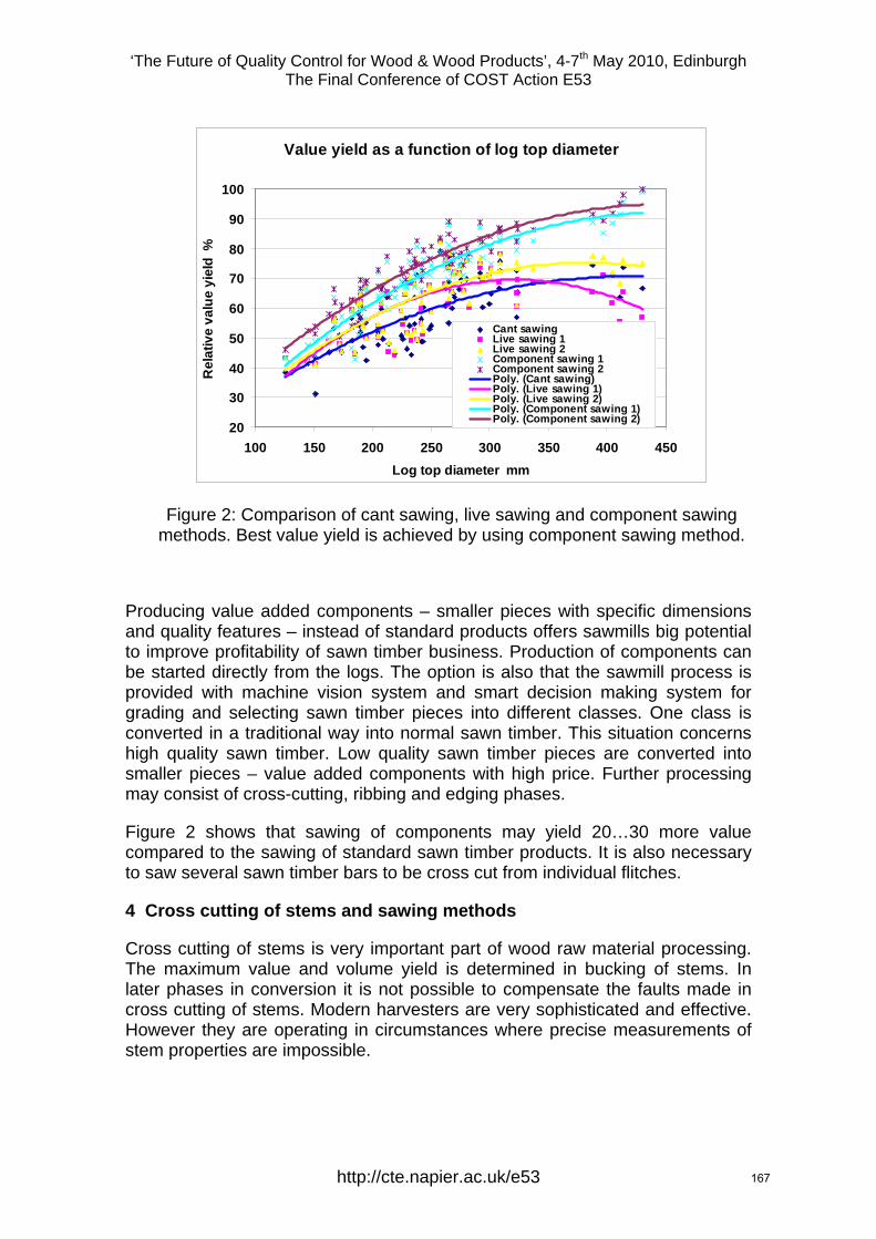
‘The Future of Quality Control for Wood & Wood Products’, 4-7th May 2010, Edinburgh The Final Conference of COST Action E53
Value yield as a function of log top diameter
20
30
40
50
60
70
80
90
100
100 150 200 250 300 350 400 450Log top diameter mm
Rel
ativ
e va
lue
yiel
d %
Cant sawingLive sawing 1Live sawing 2Component sawing 1Component sawing 2Poly. (Cant sawing)Poly. (Live sawing 1)Poly. (Live sawing 2)Poly. (Component sawing 1)Poly. (Component sawing 2)
Figure 2: Comparison of cant sawing, live sawing and component sawing methods. Best value yield is achieved by using component sawing method.
Producing value added components – smaller pieces with specific dimensions and quality features – instead of standard products offers sawmills big potential to improve profitability of sawn timber business. Production of components can be started directly from the logs. The option is also that the sawmill process is provided with machine vision system and smart decision making system for grading and selecting sawn timber pieces into different classes. One class is converted in a traditional way into normal sawn timber. This situation concerns high quality sawn timber. Low quality sawn timber pieces are converted into smaller pieces – value added components with high price. Further processing may consist of cross-cutting, ribbing and edging phases.
Figure 2 shows that sawing of components may yield 20…30 more value compared to the sawing of standard sawn timber products. It is also necessary to saw several sawn timber bars to be cross cut from individual flitches.
4 Cross cutting of stems and sawing methods
Cross cutting of stems is very important part of wood raw material processing. The maximum value and volume yield is determined in bucking of stems. In later phases in conversion it is not possible to compensate the faults made in cross cutting of stems. Modern harvesters are very sophisticated and effective. However they are operating in circumstances where precise measurements of stem properties are impossible.
http://cte.napier.ac.uk/e53 167

‘The Future of Quality Control for Wood & Wood Products’, 4-7th May 2010, Edinburgh The Final Conference of COST Action E53
Best bucking and cross cutting result can be achieved when the stems or part of stems are transported to cross cutting station. In the station stems can be measured very accurately using different scanning methods i.e. x-ray scanning. Scanning and information processing provides the model of the stem. Sophisticated software can calculate optimised bucking result for the stem based on sawn timber order file. This method is very interesting especially for high quality raw material.
Sawing method is also affecting considerable on the yield in sawmilling. Figure 2 shows that live sawing method produces more value than conventional cant sawing method. This is because of increased flexibility. The economical impact is increased by decreased top diameter of the log.
5 Information systems and intelligent material flow control
Figure 3 presents in principle the amount of information in different stages of the forest - wood chain. Measurements and observations throughout the chain produce data and information. In individual stages information is growing rapidly. This information is, however, used only locally. After the wood material has left the processing phase, almost all specific information has been lost. This happens all the way throughout the supply chain. It is not possible to link final products, raw materials and processing parameters together. The picture also shows an accumulated curve assuming that all the information from previous phases would be available in the later phases. If the lost information could be regained, much more effective business could be realised. Information "recovery" can be achieved through marking pieces, reading of the markings and storing the corresponding data in a database.
Figure 3: Recorded and lost information can be recovered through marking / reading pieces and advanced data processing.
http://cte.napier.ac.uk/e53 168

‘The Future of Quality Control for Wood & Wood Products’, 4-7th May 2010, Edinburgh The Final Conference of COST Action E53
Information system for an advanced control of forest - wood chain through marking pieces, reading the markings and data processing establishes a strong opportunity to make better business (Figure 4). Marking of pieces can be done using different techniques i.e. RF-tags and ink jet markings. Reading of marking can be done using antennas or cameras.
Figure 4: Marking of logs and sawn timber pieces in different production phases .
Marking - reading – information (MRI) system applications concern quality control, process control, planning procedures and customer service. Marking of pieces is also a way to show the origin of pieces and can be for instance used to ensure that the material originates from a certified source. MRI provides a quite new approach for the management of material and information flows from forest to the end products supporting customer oriented business and added value production. Information system is covering whole chain –from the forest to the end products. Integration of data throughout whole conversion chain can be done by marking wood raw material, logs, in the forest and storing data into information system. Marking can be i.e. electronic tag which provides address in the information system. When a piece is passing a process phase the tag is read and the measured data stored into the information system. The linked data and information is available for planning systems and process control ensuring precise management of business processes.
http://cte.napier.ac.uk/e53 169

‘The Future of Quality Control for Wood & Wood Products’, 4-7th May 2010, Edinburgh The Final Conference of COST Action E53
6 Scanning of internal properties of stems and logs for characterisation wood raw material and for optimisation of sawing operations.
Log scanner systems for measuring shape and internal properties of logs can be used in the following processes:
• Log sorting station - optimisation of borders of log classes based on order files
• Bucking and cross cutting terminal - optimisation of cross-cutting of stems and sorting of logs
• Just before sawing - optimisation of log rotation angle and sawing set up for individual logs
• Harvesting machines - optimisation of cross-cutting of stems
Figure 5: 2D X-ray picture of a log
The purpose of X-ray inspection system (Figure 5) is to show the accurate position of internal wood properties and defects, knots and heartwood / sapwood areas. It can also detect defects, which are not visible on any surfaces of wood. X-ray system can be used at inspecting boards, planks and logs depending on the configuration of the system. The analysis software is tailored
http://cte.napier.ac.uk/e53 170
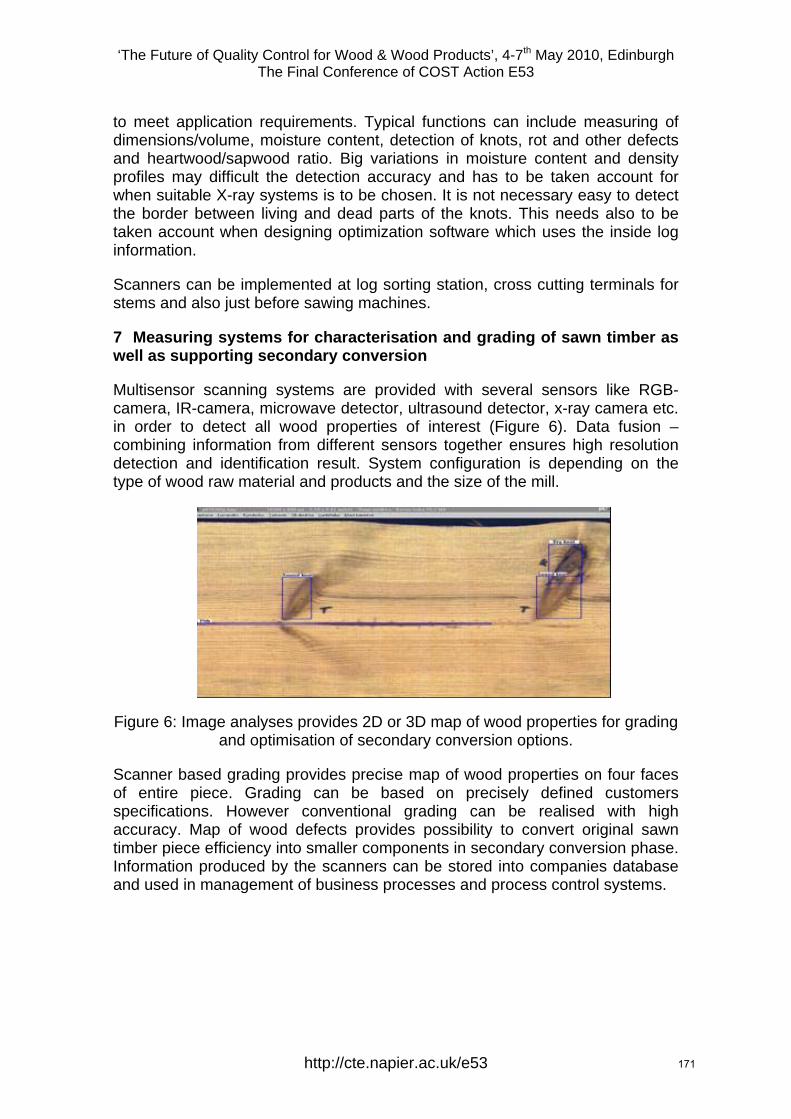
‘The Future of Quality Control for Wood & Wood Products’, 4-7th May 2010, Edinburgh The Final Conference of COST Action E53
to meet application requirements. Typical functions can include measuring of dimensions/volume, moisture content, detection of knots, rot and other defects and heartwood/sapwood ratio. Big variations in moisture content and density profiles may difficult the detection accuracy and has to be taken account for when suitable X-ray systems is to be chosen. It is not necessary easy to detect the border between living and dead parts of the knots. This needs also to be taken account when designing optimization software which uses the inside log information.
Scanners can be implemented at log sorting station, cross cutting terminals for stems and also just before sawing machines.
7 Measuring systems for characterisation and grading of sawn timber as well as supporting secondary conversion
Multisensor scanning systems are provided with several sensors like RGB-camera, IR-camera, microwave detector, ultrasound detector, x-ray camera etc. in order to detect all wood properties of interest (Figure 6). Data fusion – combining information from different sensors together ensures high resolution detection and identification result. System configuration is depending on the type of wood raw material and products and the size of the mill.
Figure 6: Image analyses provides 2D or 3D map of wood properties for grading and optimisation of secondary conversion options.
Scanner based grading provides precise map of wood properties on four faces of entire piece. Grading can be based on precisely defined customers specifications. However conventional grading can be realised with high accuracy. Map of wood defects provides possibility to convert original sawn timber piece efficiency into smaller components in secondary conversion phase. Information produced by the scanners can be stored into companies database and used in management of business processes and process control systems.
http://cte.napier.ac.uk/e53 171
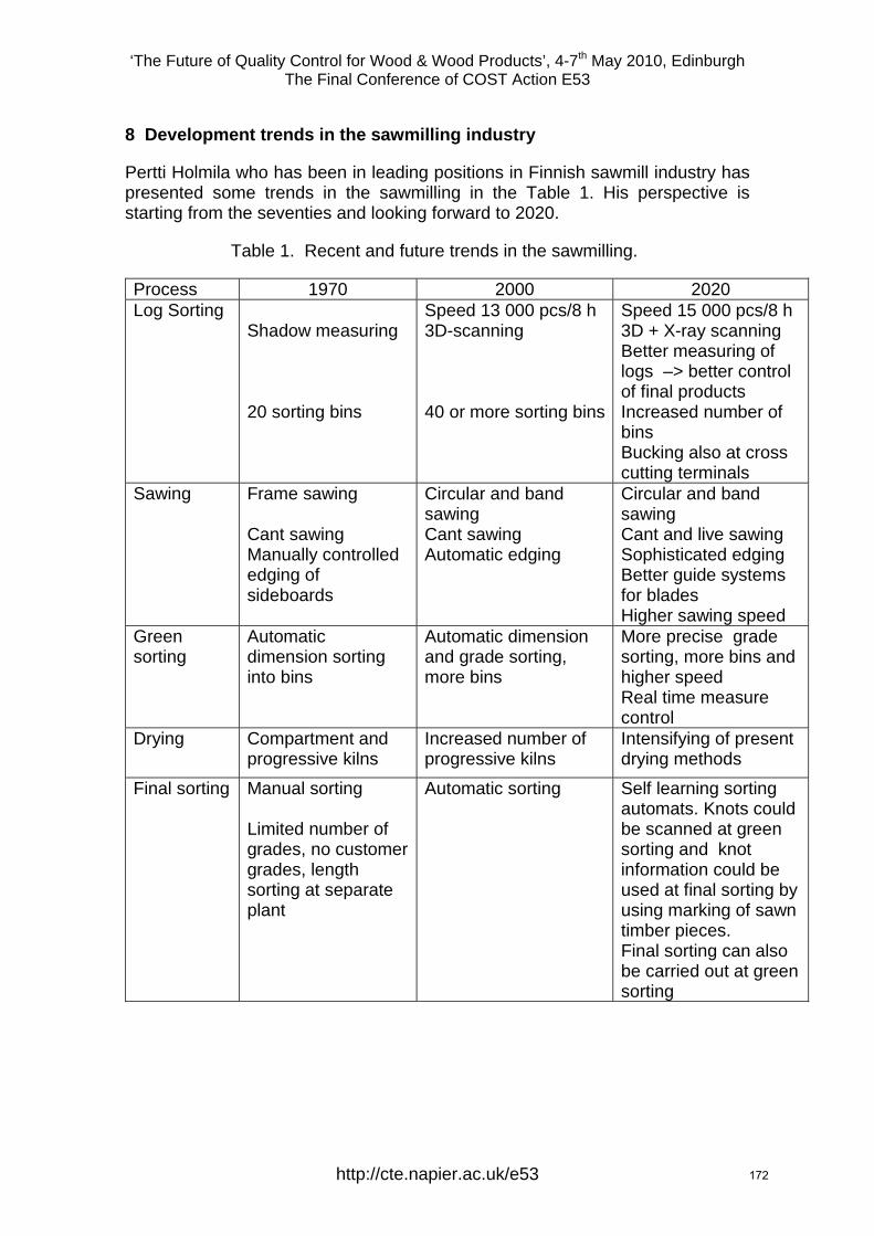
‘The Future of Quality Control for Wood & Wood Products’, 4-7th May 2010, Edinburgh The Final Conference of COST Action E53
8 Development trends in the sawmilling industry
Pertti Holmila who has been in leading positions in Finnish sawmill industry has presented some trends in the sawmilling in the Table 1. His perspective is starting from the seventies and looking forward to 2020.
Table 1. Recent and future trends in the sawmilling.
Process 1970 2000 2020 Log Sorting
Shadow measuring 20 sorting bins
Speed 13 000 pcs/8 h 3D-scanning 40 or more sorting bins
Speed 15 000 pcs/8 h 3D + X-ray scanning Better measuring of logs –> better control of final products Increased number of bins Bucking also at cross cutting terminals
Sawing
Frame sawing Cant sawing Manually controlled edging of sideboards
Circular and band sawing Cant sawing Automatic edging
Circular and band sawing Cant and live sawing Sophisticated edging Better guide systems for blades Higher sawing speed
Green sorting
Automatic dimension sorting into bins
Automatic dimension and grade sorting, more bins
More precise grade sorting, more bins and higher speed Real time measure control
Drying Compartment and progressive kilns
Increased number of progressive kilns
Intensifying of present drying methods
Final sorting Manual sorting Limited number of grades, no customer grades, length sorting at separate plant
Automatic sorting Self learning sorting automats. Knots could be scanned at green sorting and knot information could be used at final sorting by using marking of sawn timber pieces. Final sorting can also be carried out at green sorting
http://cte.napier.ac.uk/e53 172
‘The Future of Quality Control for Wood & Wood Products’, 4-7th May 2010, Edinburgh The Final Conference of COST Action E53
Deciding log grade for payment based on X-ray scanning of logs
J. Oja1,2, J. Skog1,2, J. Edlund3 & L. Björklund3
Abstract In Sweden, the payment for a large part of the saw logs is based on both grade and volume. The volume is measured automatically using optical 3D or shadow scanners. The log grade is decided manually by visual inspection. The manual inspection is expensive and often limits the production speed. This makes it interesting to find an automatic method of grading logs for payment.
X-ray scanning of logs is today used at some sawmills for measuring inner properties of logs and based on this information choose the best logs for different products. Hence, this paper aims at studying if X-ray scanning of logs also can be used to decide grade for payment.
The study is based on 160 Norway spruce logs (Picea abies (L.) Karst.) and 160 Scots pine logs (Pinus sylvestris L.), all with a top diameter of around 180 mm. The logs were scanned with an industrial X-ray scanner and an optical 3D scanner, and then graded by a skilled log grader. Models for prediction of log grade based on X-ray and 3D data were calibrated using partial least squares (PLS) regression.
The log grade was correctly predicted for 86 % of the spruce logs and 81 % of the pine log. For spruce, bow height was the only significant variable while knot parameters were also important for pine logs.
The results are very promising, but must be tested on a larger and more representative material.
1 SP Technical Research Institute of Sweden, SP Trätek, SKERIA 2, 931 77 Skellefteå, Sweden. www.sp.se. E-mail: [email protected]. 2 Luleå University of Technology, Division of Wood Science and Technology, SKERIA 3, 931 87 Skellefteå, Sweden. www.ltu.se/ske/wood 3 SDC, VMK/VMU, Uppsala Science Park, 751 83 Uppsala, Sweden. www.virkesmatning.se
http://cte.napier.ac.uk/e53 173
‘The Future of Quality Control for Wood & Wood Products’, 4-7th May 2010, Edinburgh The Final Conference of COST Action E53
1 Introduction At Swedish sawmills, logs are measured and graded for two different reasons. One objective is to sort the logs based on dimension and quality, in order to fit each individual log to the right product. The other objective is to collect information for payment.
The log sorting for process control is based on automatic measurements of dimension and properties such as knot structure and heartwood diameter. The length and diameter are in most cases measured using a 3D scanner (Grundberg et al. 2001). The idea of this is to fit each log to the sawing pattern that produces the highest yield. But today, an increasing amount of customers is asking for sawn products with a specific combination of thickness, width, length and other properties such as heartwood content, distance between whorls and high strength. To produce this type of products in an efficient way, it is necessary to choose the right logs already before sawing. Otherwise, the sawmill will produce a large amount of products with low value due to unwanted combinations of dimension and wood properties.
When sorting the logs based on properties of the sawn wood, one alternative is to use data describing the external shape of the log to predict the properties of the sawn wood (Grace 1994). For more detailed non-destructive measurements of inner properties of saw logs, most industrial applications are based on X-ray scanning (Fig. 1). Industrial X-ray scanning of logs makes it possible to measure properties such as heartwood content (Skog & Oja 2009a), density (Oja et al. 2001), knot structure (Pietikäinen 1996; Grundberg & Grönlund 1997), or annual ring width (Wang et al. 1997; Burian 2006). X-ray scanning of logs can also be combined with 3D scanning for improved measurements of heartwood and density (Skog & Oja 2009b) and combined with acoustic measurements to improve the predictions of strength and stiffness (Lycken et al. 2009).
The payment of logs is at all large sawmills in Sweden based on a combination of automatic measurements of volume and manual grading. For most loads of logs, each log is individually graded. This means that the grader has to make decisions about species, amount and thickness of bark and log grade according to the rules defined by the Timber Measurement Council (Anon. 1999). The large number of decisions that have to be made by the grader limits the speed at the log sorting. At many sawmills this fact makes the log sorting, i.e. the manual grading, a bottle neck in the production chain.
Consequently, an automatic grading for payment would be a significant improvement and much work has been done to make this possible. Oja et al. (1998) describe a system that helps the grader by taking high quality pictures of the log ends and combines this information with an automatic log grade based on the external shape of the log. Edlund (2004) presents further development of
http://cte.napier.ac.uk/e53 174
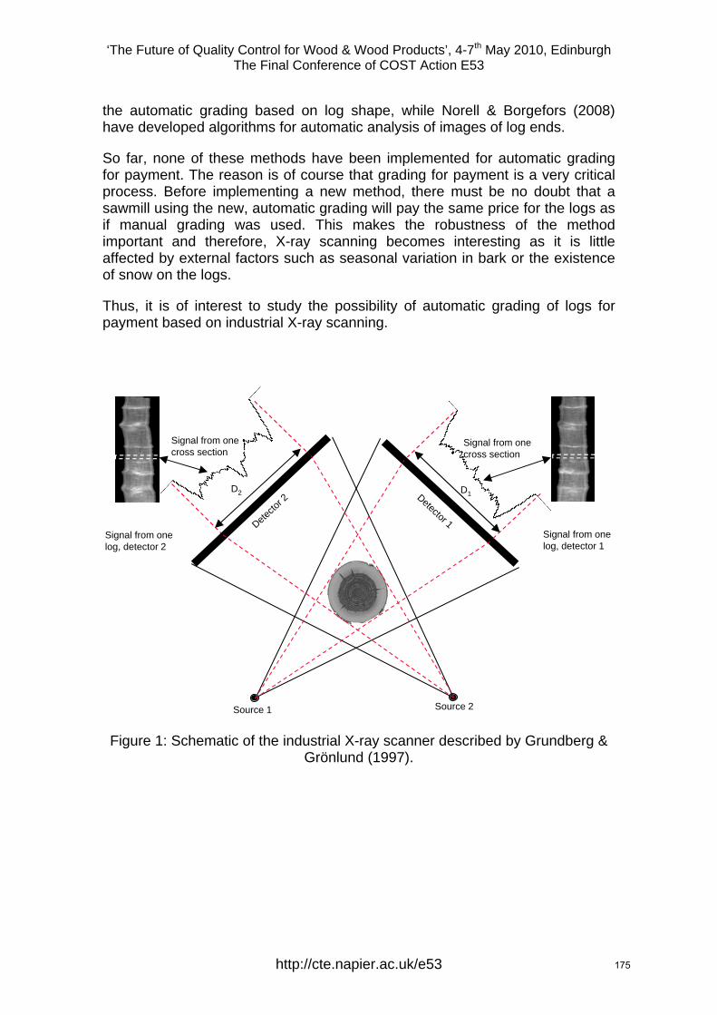
‘The Future of Quality Control for Wood & Wood Products’, 4-7th May 2010, Edinburgh The Final Conference of COST Action E53
the automatic grading based on log shape, while Norell & Borgefors (2008) have developed algorithms for automatic analysis of images of log ends.
So far, none of these methods have been implemented for automatic grading for payment. The reason is of course that grading for payment is a very critical process. Before implementing a new method, there must be no doubt that a sawmill using the new, automatic grading will pay the same price for the logs as if manual grading was used. This makes the robustness of the method important and therefore, X-ray scanning becomes interesting as it is little affected by external factors such as seasonal variation in bark or the existence of snow on the logs.
Thus, it is of interest to study the possibility of automatic grading of logs for payment based on industrial X-ray scanning.
Signal from onelog, detector 1
Signal from onelog, detector 2
Source 1 Source 2
Detector 1Detecto
r 2D2 D1
Signal from onecross section
Signal from onecross section
X-ray LogScanner
Figure 1: Schematic of the industrial X-ray scanner described by Grundberg & Grönlund (1997).
http://cte.napier.ac.uk/e53 175
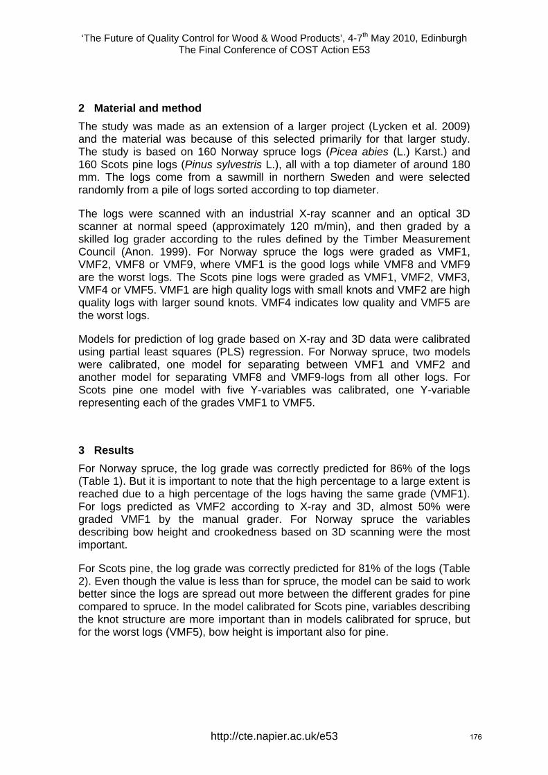
‘The Future of Quality Control for Wood & Wood Products’, 4-7th May 2010, Edinburgh The Final Conference of COST Action E53
2 Material and method The study was made as an extension of a larger project (Lycken et al. 2009) and the material was because of this selected primarily for that larger study. The study is based on 160 Norway spruce logs (Picea abies (L.) Karst.) and 160 Scots pine logs (Pinus sylvestris L.), all with a top diameter of around 180 mm. The logs come from a sawmill in northern Sweden and were selected randomly from a pile of logs sorted according to top diameter.
The logs were scanned with an industrial X-ray scanner and an optical 3D scanner at normal speed (approximately 120 m/min), and then graded by a skilled log grader according to the rules defined by the Timber Measurement Council (Anon. 1999). For Norway spruce the logs were graded as VMF1, VMF2, VMF8 or VMF9, where VMF1 is the good logs while VMF8 and VMF9 are the worst logs. The Scots pine logs were graded as VMF1, VMF2, VMF3, VMF4 or VMF5. VMF1 are high quality logs with small knots and VMF2 are high quality logs with larger sound knots. VMF4 indicates low quality and VMF5 are the worst logs.
Models for prediction of log grade based on X-ray and 3D data were calibrated using partial least squares (PLS) regression. For Norway spruce, two models were calibrated, one model for separating between VMF1 and VMF2 and another model for separating VMF8 and VMF9-logs from all other logs. For Scots pine one model with five Y-variables was calibrated, one Y-variable representing each of the grades VMF1 to VMF5.
3 Results For Norway spruce, the log grade was correctly predicted for 86% of the logs (Table 1). But it is important to note that the high percentage to a large extent is reached due to a high percentage of the logs having the same grade (VMF1). For logs predicted as VMF2 according to X-ray and 3D, almost 50% were graded VMF1 by the manual grader. For Norway spruce the variables describing bow height and crookedness based on 3D scanning were the most important.
For Scots pine, the log grade was correctly predicted for 81% of the logs (Table 2). Even though the value is less than for spruce, the model can be said to work better since the logs are spread out more between the different grades for pine compared to spruce. In the model calibrated for Scots pine, variables describing the knot structure are more important than in models calibrated for spruce, but for the worst logs (VMF5), bow height is important also for pine.
http://cte.napier.ac.uk/e53 176
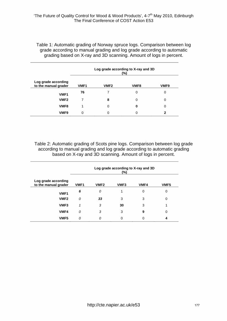
‘The Future of Quality Control for Wood & Wood Products’, 4-7th May 2010, Edinburgh The Final Conference of COST Action E53
Table 1: Automatic grading of Norway spruce logs. Comparison between log grade according to manual grading and log grade according to automatic
grading based on X-ray and 3D scanning. Amount of logs in percent.
Log grade according to X-ray and 3D
(%)
Log grade according to the manual grader
VMF1
VMF2
VMF8
VMF9
VMF1 76 7 0 0
VMF2 7 8 0 0
VMF8 1 0 0 0
VMF9 0 0 0 2
Table 2: Automatic grading of Scots pine logs. Comparison between log grade according to manual grading and log grade according to automatic grading
based on X-ray and 3D scanning. Amount of logs in percent.
Log grade according to X-ray and 3D (%)
Log grade according to the manual grader
VMF1
VMF2
VMF3
VMF4
VMF5
VMF1 6 0 1 0 0
VMF2 0 33 3 3 0
VMF3 1 3 30 3 1
VMF4 0 3 3 9 0
VMF5 0 0 0 0 4
http://cte.napier.ac.uk/e53 177
‘The Future of Quality Control for Wood & Wood Products’, 4-7th May 2010, Edinburgh The Final Conference of COST Action E53
4 Discussion The study is based on a very limited material but indicates that the combination of X-ray and 3D scanning can be a possible method to reach a system for automatic grading for payment. For Norway spruce it is possible that only 3D scanning is enough but for Scots pine the results indicate that X-ray scanning is a necessary addition.
Future work should focus on studies based on a more representative material. The material must be representative with respect to dimension and properties of logs as well as geographic origin of the material. It is also important to register the exact reason for downgrading for each log. This would make it possible to develop specific algorithms for defects such as rot or spike knots.
References Anon. (1999) “REGULATIONS FOR MEASURING OF ROUNDWOOD recommended by the Timber Measurement Council”, Circular VMR 1-99, The Timber Measurement Council. www.virkesmatning.se/Admin/html/vmr/html/ pdf/199en.pdf
Burian B. (2006) “Verbesserung der Rundholzvorsortierung durch die automatisierte Bestimmung von Holzstrukturmerkmalen am Beispiel der durchschnittlichen Jahrringbreite [mm] under Einsatz der Röntgentechnologie”, Dissertation, Freiburger Forstliche Forschung 35, Forstliche Versuchs- und Forschungsanstalt Baden-Württemberg, Freiburg, Germany, 205 pp. (In German with English summary.)
Grace L. A. (1994) “Design and evaluation of an optical scanner based log grading and sorting system for Scots pine (Pinus sylvestris L.) sawlogs”, Dissertation, The Swedish University of Agricultural Sciences, Uppsala, Sweden, 1994, pp. 7-21.
Grundberg, S. & Grönlund, A. (1997) “Simulated Grading of Logs with an X-ray Log Scanner – Grading Accuracy Compared with Manual Grading”, Scandinavian Journal of Forest Research, 1997, pp. 12:70-76.
Edlund, Jacob (2004) “Methods for automatic grading of saw logs” Doctoral diss. Dept. of Forest Products and Markets, SLU. Acta Universitatis agriculturae Sueciae. Silvestria vol. 335.
Grundberg, S., Fredriksson, J., Oja, J. & Andersson, C. (2001) ”Förbättrade metoder vid användning av 3D-mätramar” Trätek rapport P nr 0112048, Trätek, Stockholm. 101 pp.
http://cte.napier.ac.uk/e53 178
‘The Future of Quality Control for Wood & Wood Products’, 4-7th May 2010, Edinburgh The Final Conference of COST Action E53
Lycken, A., Oja, J. & Lundahl, C. G. (2009) ”Kundanpassad optimering i såglinjen - Virkeskvalitet On-line” SP Rapport 2009:15. ISBN 978-91-85829-76-7. ISSN 0284-5172.
Norell, K. & Borgefors, G. (2008) “Estimation of Pith Position in Untreated Log Ends in Sawmill Environments” Computers and Electronics in Agriculture, vol 63, pp 155-167.
Oja, J., Broman, O. & Lindfors, S-E. (1999) ”Projektrapport: Timmerinmätnings-stöd” Teknisk rapport 1999:15, Luleå tekniska universitet. 70 pp. ISSN: 1402-1536.
Oja J., S. Grundberg, and A. Grönlund, (2001) “Predicting the Stiffness of Sawn Products by X-ray Scanning of Norway Spruce Saw Logs”, Scandinavian Journal of Forest Research, pp. 16:88-96.
Pietikäinen M. (1996) “Detection of knots in logs using x-ray imaging”, Dissertation, VTT Publications 266, Technical Research Centre of Finland, Espoo, Finland, 1996, 88 pp.
Skog, J & Oja, J (2009a) “Heartwood diameter measurements in Pinus sylvestris sawlogs combining X-ray and three-dimensional scanning”, Scandinavian Journal of Forest Research, pp. 24:182-188.
Skog, J. & Oja, J. (2009b) ”Combining X-ray and Three-Dimensional Scanning of Sawlogs – Comparison between One and Two X-ray Directions” ISPA 2009, 6th International Symposium on Image and Signal Processing and Analysis. September 16-18, 2009, Salzburg, Austria, pp. 343-348.
Wang X., O. Hagman, and S. Grundberg, (1997) “Sorting Pulpwood by X-ray Scanning”, International Mechanical Pulping Conference, Stockholm, Sweden, pp. 395-399.
http://cte.napier.ac.uk/e53 179
‘The Future of Quality Control for Wood & Wood Products’, 4-7th May 2010, Edinburgh The Final Conference of COST Action E53
Assessing timber quality of Scots pine (Pinus sylvestris L.)
E. Macdonald1, J. Moore2, T. Connolly3 & B. Gardiner4
Abstract Scots pine (Pinus sylvestris L.) is the only conifer species native to Great Britain that has the potential to produce significant volumes of timber, and as such it has a key role to play in the rural economy. Timber production from Scots pine forests in northern Scotland is forecast to increase over the next 15 years. An evaluation of the timber quality of the Scots pine resource is a key requirement to inform industry and support strategic investment and marketing decisions. In this paper we describe the validation of methods developed for assessing the quality of standing Scots pine timber from measurements on trees and logs. A standing tree visual assessment was based on a stem straightness scoring system developed for Sitka spruce, with the addition of an estimate of the height of the lowest dead branch, known to be an important indicator of quality in pine. These measurements could be used to estimate of the proportion of sawlogs meeting the requirements for higher quality log grades and to give an indication of the likely appearance grade of the sawn timber. Measurements of stress wave velocity in trees and logs, using portable acoustic tools, were found to be good predictors of the mechanical properties of sawn timber. Segregating trees or logs on the basis of acoustic measurements had the potential to increase the strength class assigned to sawn timber.
1 Introduction Scots pine (Pinus sylvestris L.) is the most widely distributed conifer species in the world with a natural range stretching from Spain to Norway and from Scotland to Siberia (Mason, 2000). This species is found in all member states of the EU, where it constitutes approximately 20% of the commercial forest area, and it is of considerable importance as a timber producing species, particularly in Nordic countries (Mason and Alia, 2000). In Great Britain the area of Scots pine is approximately 220 000 hectares, representing around 16% of the conifer forest area and 10% of the total forest area (Forestry Commission, 2007). Almost two-thirds of the Scots pine forest area is in Scotland, and the species is of particular importance in northern Scotland (Grampian and Highland areas) where it represents about 30% of the conifer resource.
1 Project Leader, [email protected] Forest Research, Northern Research Station, Roslin, UK 2 Principal Research Fellow, [email protected] Centre for Timber Engineering, Edinburgh Napier University, UK 3 Statistician, [email protected] 4 Programme Leader, [email protected] Forest Research, Northern Research Station, Roslin, UK
http://cte.napier.ac.uk/e53 180
‘The Future of Quality Control for Wood & Wood Products’, 4-7th May 2010, Edinburgh The Final Conference of COST Action E53
The availability of Scots pine timber from northern Scotland is predicted to increase by about 15% per annum over the next 15 years (after Halsall et al., 2006), and it will represent approximately 20% of the softwood timber harvest in these areas. The management of Scots pine forests, including timber marketing and utilisation, is therefore of considerable importance to the local economy. Over the last four years a number of studies have been conducted with the overall aim of increasing the value of the Scots pine resource in north Scotland to the rural economy (Macdonald et al., 2008). For example, a questionnaire-type survey reviewed the management, harvesting and utilisation of the Scots pine timber resource. Results showed that primary processing of around 80% of the Scots pine timber harvested took place within 80 km of where it was grown, emphasising the importance to the local economy. About half of the Scots pine roundwood harvested in the study area was processed into wood-based panels. Most (90%) of the remaining material was converted into agricultural and domestic fencing. Only small quantities were used in higher added-value markets such as construction products (4%), decking (2%) and sleepers (1%).
A subsequent market development study evaluated opportunities for Scots pine timber, focusing on the potential for processing and adding value locally. Outdoor uses such as garden, landscaping and playground products or stress-laminated timber bridges scored highly in the assessment, due to the ability to improve durability through preservative treatment. In construction the use of Scots pine in massive timber panels was considered a viable option, should a manufacturing plant be established in Scotland. External cladding, either coated or preservative treated, was identified as a potential market for boards cut from the outer part of Scots pine logs, provided these were graded to meet market requirements in terms of allowable numbers and sizes of knots.
The possible expansion of the use of Scots pine in any of these added-value markets is dependant on a reliable supply of timber of the required quality being available. Log straightness and knottiness (number, size and condition of knots) are key factors which determine product potential. Variability in quality characteristics within and between stands is also a key issue, highlighting the need for techniques to identify better quality stands, and the best trees in stands. Here we report on work to test and validate methods for assessing Scots pine timber quality in standing trees and logs, and to link these assessments to sawn timber properties and performance. In this study the application of a stem straightness scoring system developed for Sitka spruce (Macdonald et al., 2009) was tested in Scots pine, together with a number of different branching indices. The use of portable acoustic tools to assess wood properties in standing trees and logs was also evaluated.
2 Materials and Methods Six Scots pine sample stands were assessed in two linked studies:
2.1 Study 1 Three Scots pine sample stands located within 50 km of Inverness were selected for this study (Table 1). The age and Yield Class were chosen to be
http://cte.napier.ac.uk/e53 181
‘The Future of Quality Control for Wood & Wood Products’, 4-7th May 2010, Edinburgh The Final Conference of COST Action E53
http://cte.napier.ac.uk/e53
representative of typical Scots pine stands towards the end of normal rotation lengths in north Scotland. Ten sample plots were randomly located within each stand. In each plot the diameter at breast height (DBH), stem straightness and stress wave velocity of every live tree were measured in accordance with standard procedures (Matthews and Mackie, 2006; Macdonald et al., 2009; Mochan et al., 2009). Three trees were selected at random from each plot from amongst those with a DBH of 28 cm or greater, and for each selected tree the following branching characteristics were visually estimated:
• Height to the lowest dead branch, estimated to nearest 0.5 m.
• Height to the lowest live branch, estimated to nearest 0.5 m
• Height of the lowest live whorl (defined as the whorl where > 75% of branches are green), estimated to nearest 0.5 m
• Diameter of the lowest dead branch – to nearest cm
• Diameter of the lowest live branch – to nearest cm After each sample tree was felled, the total volume of sawlog size material (16 cm diameter overbark) in the tree was calculated in accordance with normal measurement conventions (Matthews and Mackie, 2006). . The position of “green” logs, as defined in Forestry Commission (1993), that met roundwood specifications for current markets for Scots pine in the study area (Table 2) were marked on the stem and their volume assessed. The highest preference were given to sleepers followed by longer green log lengths since they attract a price premium. Up to two 3.7 m long green sawlogs were then cut from each sample tree (160 logs in total). and the following measurements made on each:
• Log length
• Log top (small-end) diameter over bark
• Stress wave velocity using the HM-200 log tool (Fibre-gen, New Zealand) Logs were processed into structural timber with dimensions of 47x100 mm, 47x 150 mm and 47x200 mm, and falling boards of 19 mm thickness with widths of 75 mm, 100 mm and 150 mm. All timber was kiln dried using a standard schedule for Scots pine. Falling boards were appearance graded following the G4 method in EN 1611-1:2000 (CEN, 2003b), which applies to softwoods for non-structural applications (e.g., cladding, joinery and furniture). The possibility of predicting falling board appearance grade from standing tree measurements was explored.
182
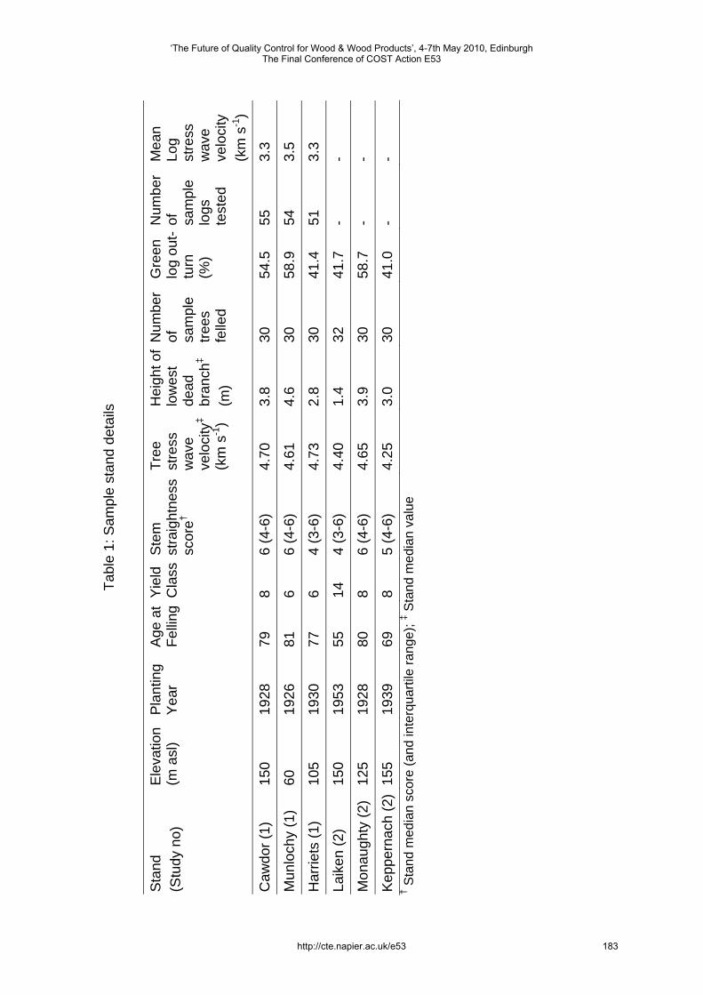
Tabl
e 1:
Sam
ple
stan
d de
tails
† Sta
nd m
edia
n sc
ore
(and
inte
rqua
rtile
rang
e); ‡ S
tand
med
ian
valu
e
Sta
nd
(Stu
dy n
o)
Ele
vatio
n (m
asl
) P
lant
ing
Yea
r A
ge a
t Fe
lling
Yie
ld
Cla
ssS
tem
st
raig
htne
ss
scor
e†
Tree
st
ress
w
ave
velo
city
‡ (k
m s
-1)
Hei
ght o
f lo
wes
t de
ad
bran
ch‡
(m)
Num
ber
of
sam
ple
trees
fe
lled
Gre
en
log
out-
turn
(%
)
Num
ber
of
sam
ple
logs
te
sted
Mea
n Lo
g st
ress
w
ave
velo
city
(k
m s
-1)
Caw
dor (
1)
150
1928
79
8
6 (4
-6)
4.70
3.
8 30
54
.5
55
3.3
Mun
loch
y (1
) 60
19
26
81
6 6
(4-6
) 4.
61
4.6
30
58.9
54
3.
5
Har
riets
(1)
105
1930
77
6
4 (3
-6)
4.73
2.
8 30
41
.4
51
3.3
Laik
en (2
) 15
0 19
53
55
14
4 (3
-6)
4.40
1.
4 32
41
.7
- -
Mon
augh
ty (2
) 12
5 19
28
80
8 6
(4-6
) 4.
65
3.9
30
58.7
-
-
Kep
pern
ach
(2)
155
1939
69
8
5 (4
-6)
4.25
3.
0 30
41
.0
- -
‘The Future of Quality Control for Wood & Wood Products’, 4-7th May 2010, EdinburghThe Final Conference of COST Action E53
http://cte.napier.ac.uk/e53 183
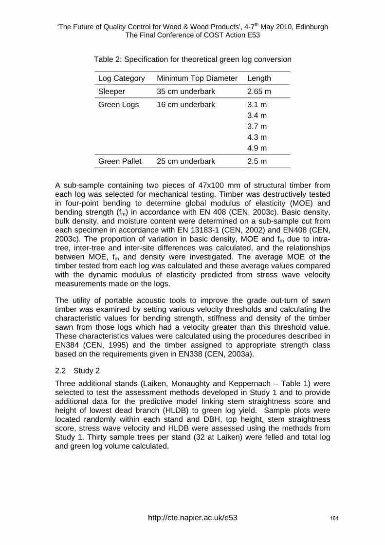
‘The Future of Quality Control for Wood & Wood Products’, 4-7th May 2010, Edinburgh The Final Conference of COST Action E53
Table 2: Specification for theoretical green log conversion
Log Category Minimum Top Diameter Length
Sleeper 35 cm underbark 2.65 m
Green Logs 16 cm underbark 3.1 m 3.4 m 3.7 m 4.3 m 4.9 m
Green Pallet 25 cm underbark 2.5 m A sub-sample containing two pieces of 47x100 mm of structural timber from each log was selected for mechanical testing. Timber was destructively tested in four-point bending to determine global modulus of elasticity (MOE) and bending strength (fm) in accordance with EN 408 (CEN, 2003c). Basic density, bulk density, and moisture content were determined on a sub-sample cut from each specimen in accordance with EN 13183-1 (CEN, 2002) and EN408 (CEN, 2003c). The proportion of variation in basic density, MOE and fm due to intra-tree, inter-tree and inter-site differences was calculated, and the relationships between MOE, fm and density were investigated. The average MOE of the timber tested from each log was calculated and these average values compared with the dynamic modulus of elasticity predicted from stress wave velocity measurements made on the logs.
The utility of portable acoustic tools to improve the grade out-turn of sawn timber was examined by setting various velocity thresholds and calculating the characteristic values for bending strength, stiffness and density of the timber sawn from those logs which had a velocity greater than this threshold value. These characteristics values were calculated using the procedures described in EN384 (CEN, 1995) and the timber assigned to appropriate strength class based on the requirements given in EN338 (CEN, 2003a).
2.2 Study 2 Three additional stands (Laiken, Monaughty and Keppernach – Table 1) were selected to test the assessment methods developed in Study 1 and to provide additional data for the predictive model linking stem straightness score and height of lowest dead branch (HLDB) to green log yield. Sample plots were located randomly within each stand and DBH, top height, stem straightness score, stress wave velocity and HLDB were assessed using the methods from Study 1. Thirty sample trees per stand (32 at Laiken) were felled and total log and green log volume calculated.
http://cte.napier.ac.uk/e53 184
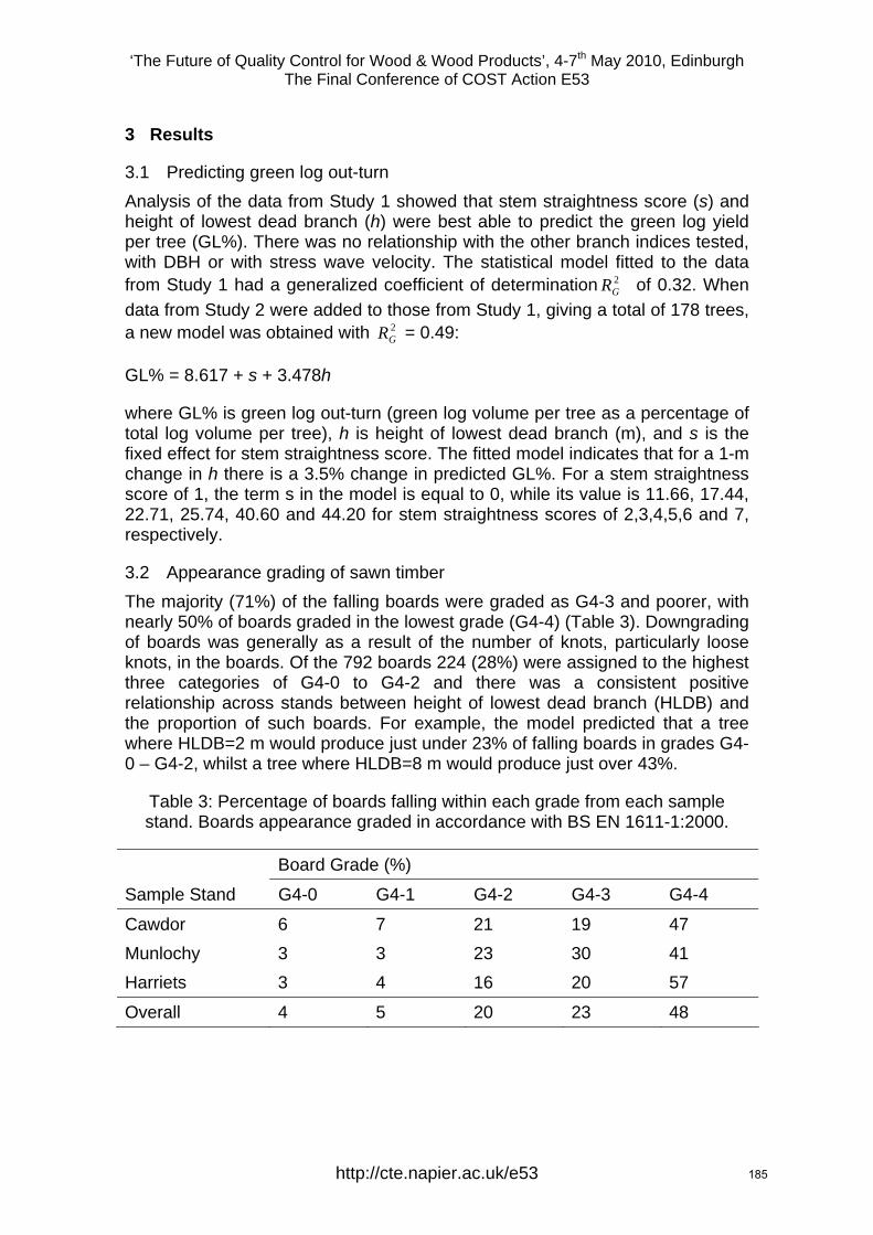
‘The Future of Quality Control for Wood & Wood Products’, 4-7th May 2010, Edinburgh The Final Conference of COST Action E53
3 Results
3.1 Predicting green log out-turn Analysis of the data from Study 1 showed that stem straightness score (s) and height of lowest dead branch (h) were best able to predict the green log yield per tree (GL%). There was no relationship with the other branch indices tested, with DBH or with stress wave velocity. The statistical model fitted to the data from Study 1 had a generalized coefficient of determination of 0.32. When data from Study 2 were added to those from Study 1, giving a total of 178 trees, a new model was obtained with = 0.49:
2GR
2GR
GL% = 8.617 + s + 3.478h
where GL% is green log out-turn (green log volume per tree as a percentage of total log volume per tree), h is height of lowest dead branch (m), and s is the fixed effect for stem straightness score. The fitted model indicates that for a 1-m change in h there is a 3.5% change in predicted GL%. For a stem straightness score of 1, the term s in the model is equal to 0, while its value is 11.66, 17.44, 22.71, 25.74, 40.60 and 44.20 for stem straightness scores of 2,3,4,5,6 and 7, respectively.
3.2 Appearance grading of sawn timber The majority (71%) of the falling boards were graded as G4-3 and poorer, with nearly 50% of boards graded in the lowest grade (G4-4) (Table 3). Downgrading of boards was generally as a result of the number of knots, particularly loose knots, in the boards. Of the 792 boards 224 (28%) were assigned to the highest three categories of G4-0 to G4-2 and there was a consistent positive relationship across stands between height of lowest dead branch (HLDB) and the proportion of such boards. For example, the model predicted that a tree where HLDB=2 m would produce just under 23% of falling boards in grades G4-0 – G4-2, whilst a tree where HLDB=8 m would produce just over 43%.
Table 3: Percentage of boards falling within each grade from each sample stand. Boards appearance graded in accordance with BS EN 1611-1:2000.
Board Grade (%)
Sample Stand G4-0 G4-1 G4-2 G4-3 G4-4
Cawdor 6 7 21 19 47 Munlochy 3 3 23 30 41 Harriets 3 4 16 20 57
Overall 4 5 20 23 48
http://cte.napier.ac.uk/e53 185
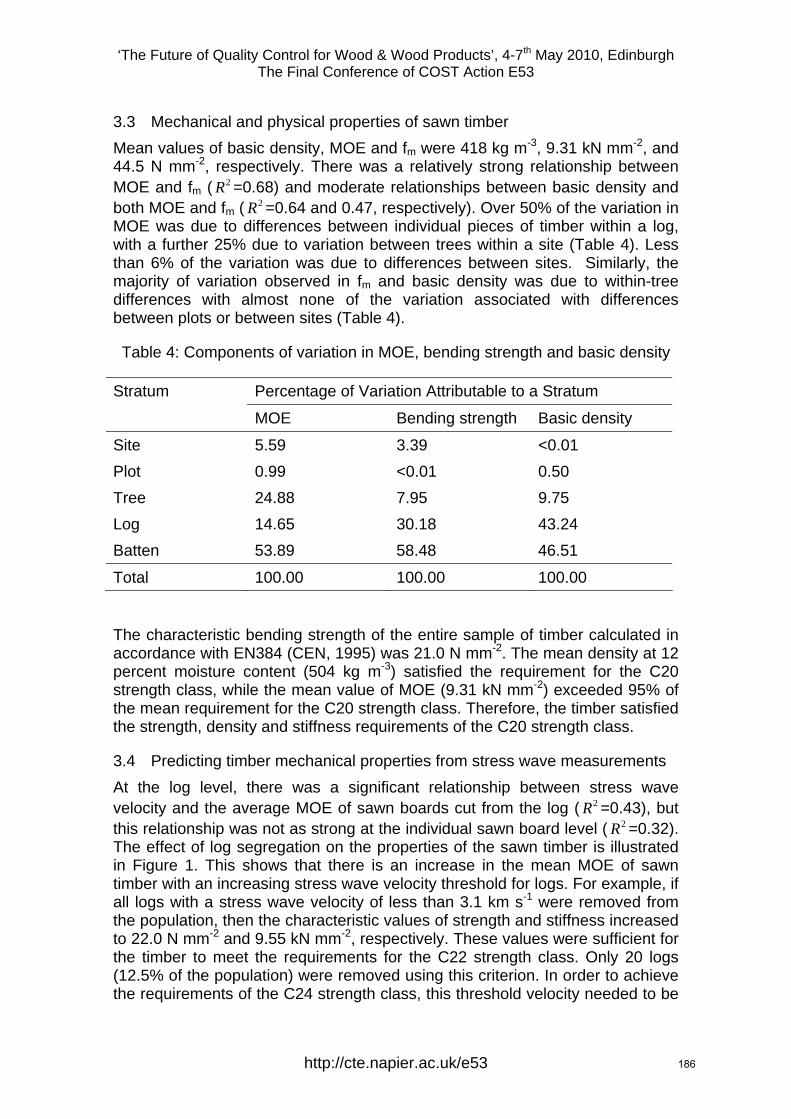
‘The Future of Quality Control for Wood & Wood Products’, 4-7th May 2010, Edinburgh The Final Conference of COST Action E53
3.3 Mechanical and physical properties of sawn timber Mean values of basic density, MOE and fm were 418 kg m-3, 9.31 kN mm-2, and 44.5 N mm-2, respectively. There was a relatively strong relationship between MOE and fm ( 2R =0.68) and moderate relationships between basic density and both MOE and fm ( 2R =0.64 and 0.47, respectively). Over 50% of the variation in MOE was due to differences between individual pieces of timber within a log, with a further 25% due to variation between trees within a site (Table 4). Less than 6% of the variation was due to differences between sites. Similarly, the majority of variation observed in fm and basic density was due to within-tree differences with almost none of the variation associated with differences between plots or between sites (Table 4).
Table 4: Components of variation in MOE, bending strength and basic density
Stratum Percentage of Variation Attributable to a Stratum
MOE Bending strength Basic density
Site 5.59 3.39 <0.01 Plot 0.99 <0.01 0.50 Tree 24.88 7.95 9.75 Log 14.65 30.18 43.24 Batten 53.89 58.48 46.51
Total 100.00 100.00 100.00
The characteristic bending strength of the entire sample of timber calculated in accordance with EN384 (CEN, 1995) was 21.0 N mm-2. The mean density at 12 percent moisture content (504 kg m-3) satisfied the requirement for the C20 strength class, while the mean value of MOE (9.31 kN mm-2) exceeded 95% of the mean requirement for the C20 strength class. Therefore, the timber satisfied the strength, density and stiffness requirements of the C20 strength class.
3.4 Predicting timber mechanical properties from stress wave measurements At the log level, there was a significant relationship between stress wave velocity and the average MOE of sawn boards cut from the log ( 2R =0.43), but this relationship was not as strong at the individual sawn board level ( 2R =0.32). The effect of log segregation on the properties of the sawn timber is illustrated in Figure 1. This shows that there is an increase in the mean MOE of sawn timber with an increasing stress wave velocity threshold for logs. For example, if all logs with a stress wave velocity of less than 3.1 km s-1 were removed from the population, then the characteristic values of strength and stiffness increased to 22.0 N mm-2 and 9.55 kN mm-2, respectively. These values were sufficient for the timber to meet the requirements for the C22 strength class. Only 20 logs (12.5% of the population) were removed using this criterion. In order to achieve the requirements of the C24 strength class, this threshold velocity needed to be
http://cte.napier.ac.uk/e53 186
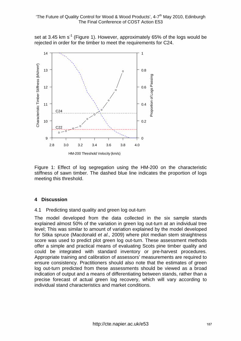
‘The Future of Quality Control for Wood & Wood Products’, 4-7th May 2010, Edinburgh The Final Conference of COST Action E53
set at 3.45 km s-1 (Figure 1). However, approximately 65% of the logs would be rejected in order for the timber to meet the requirements for C24.
2.8 3.0 3.2 3.4 3.6 3.8 4.0
9
10
11
12
13
14
HM-200 Threshold Velocity (km/s)
Cha
ract
eris
tic T
imbe
r Stif
fnes
s (k
N/m
m²)
C22
C24
0
0.2
0.4
0.6
0.8
1
Pro
porti
on o
f Log
s P
assi
ng
Figure 1: Effect of log segregation using the HM-200 on the characteristic stiffness of sawn timber. The dashed blue line indicates the proportion of logs meeting this threshold.
4 Discussion
4.1 Predicting stand quality and green log out-turn The model developed from the data collected in the six sample stands explained almost 50% of the variation in green log out-turn at an individual tree level; This was similar to amount of variation explained by the model developed for Sitka spruce (Macdonald et al., 2009) where plot median stem straightness score was used to predict plot green log out-turn. These assessment methods offer a simple and practical means of evaluating Scots pine timber quality and could be integrated with standard inventory or pre-harvest procedures. Appropriate training and calibration of assessors’ measurements are required to ensure consistency. Practitioners should also note that the estimates of green log out-turn predicted from these assessments should be viewed as a broad indication of output and a means of differentiating between stands, rather than a precise forecast of actual green log recovery, which will vary according to individual stand characteristics and market conditions.
http://cte.napier.ac.uk/e53 187

‘The Future of Quality Control for Wood & Wood Products’, 4-7th May 2010, Edinburgh The Final Conference of COST Action E53
4.2 Appearance grading of sawn timber The results of the appearance grading of falling board material were broadly in agreement with those in previous similar studies (Cooper, 2005; Cooper et al., 2008), in which the proportion of boards meeting the requirements of the three highest appearance grades averaged approximately 30%. Sorting in the sawmill to identify the boards which meet the requirements of the higher quality grades would be required if Scots pine timber were to be used in applications such as cladding or joinery.
Results of this study suggest that the height of the lowest dead branch assessment could provide a preliminary method for identifying trees likely to produce a greater proportion of higher quality boards. This is consistent with work on Scots pine by Uusitalo (1997), who found that height of the lowest dead branch was correlated with timber quality of the butt log.
4.3 Mechanical and physical properties of sawn timber Scots pine structural timber in this study met the requirements for the C20 strength class, which is suitable for a wide range of construction applications. Where higher strength class timber is required, approximately 35-40% of the timber from the stands tested met the requirements for the C24 strength class. This is in agreement with results obtained for a wider range of sites by as part of a study to develop grading machine settings for Scots pine (Chris Holland, pers. comm.). Analysis of the sources of variation in MOE and MOR suggests that there is the potential to improve these values in a population of timber by initial segregation of trees and logs using portable acoustic tools.
Sorting logs on the basis of acoustic measurements is an efficient means of segregating out timber with inferior stiffness and improving the recovery of higher strength class material. This approach has the potential to be useful when sourcing logs for specific end-uses where there are particular stiffness and strength requirements. At a larger scale, it is possible to integrate acoustic log testing technology with sawmill lines which offers timber processors the option of in-line sorting of logs to maximise output of higher strength class material. Future developments in this field include a prototype harvester-mounted acoustic tool, capable of measuring acoustic velocity of logs before they are cut, thus facilitating decision making regarding log specification.
5 Conclusions This work has shown that non-destructive assessments on trees and logs can be used to predict timber quality in Scots pine in the following ways:
• Visual assessments of stem straightness and the height of the lowest dead branch can be used to estimate the proportion of higher value green sawlog material in an individual tree;
• The height of the lowest dead branch can be used to indicate the likely proportion of falling boards from a tree that will be assigned to the three highest quality appearance classes;
http://cte.napier.ac.uk/e53 188
‘The Future of Quality Control for Wood & Wood Products’, 4-7th May 2010, Edinburgh The Final Conference of COST Action E53
• Portable acoustic tools can be used to assess the mechanical properties of Scots pine timber in standing trees and logs, and offer a means of segregating out trees and logs which are likely to produce timber with inferior mechanical properties.
Integrating these assessment techniques with standard inventory procedures, pre-harvest assessments or log-sorting operations has the potential to provide valuable resource information and to improve the allocation of Scots pine timber to the most appropriate end-products.
Acknowledgements The work reported here was funded jointly by the Forestry Commission, Scottish Enterprise and Highlands & Islands Enterprise. The following organisations and their staff assisted with the study: Cawdor Estate; Forestry Commission Scotland; John Gordon and Son Sawmills: James Jones & Sons Sawmills and Seafield Estates. Thanks are also due to colleagues in Forest Research’s Technical Support Unit at Newton and to Dave Auty, Barney Freke, Stefan Lehneke, Andrew Lyon and Steve Osborne for their valuable input to this work.
References CEN (1995). Structural timber – determination of characteristic values of mechanical properties and density. EN384:1995. European Committee for Standardisation, Brussels. 14 p.
CEN (2002). Moisture content of a piece of sawn timber – Part 1: Determination by oven dry method. EN13183-1:2002. European Committee for Standardisation, Brussels. 8 p.
CEN (2003a). Structural timber - Strength classes. EN338:2003. European Committee for Standardisation, Brussels. 14 p
CEN (2003b). Sawn timber — Appearance grading of softwoods — Part 1: European spruces, firs, pines, Douglas fir and larches. European Committee for Standardisation, .Brussels. 12p.
CEN (2003c). Timber structures – Structural timber and glued laminated timber – Determination of some physical and mechanical properties. EN408:2003. European Committee for Standardisation, Brussels. 13 p.
Cooper, G. (2005). An assessment of the quality of Scots pine from the Grampian and Cairngorm regions of Scotland. Client Report 221-884. BRE, Watford. 58p.
Cooper, G., Freke, B. and Holland, C. (2008) Maximising the potential of UK grown Scots pine falling boards. Client Report 225-822. BRE, Watford. 42p.
http://cte.napier.ac.uk/e53 189

‘The Future of Quality Control for Wood & Wood Products’, 4-7th May 2010, Edinburgh The Final Conference of COST Action E53
Forestry Commission (1993). Classification and presentation of softwood sawlogs. Forestry Commission Field Book 9. HMSO, London.
Forestry Commission (2007). Forestry Statistics 2007 – A compendium of statistics about woodland, forestry and primary wood processing in the United Kingdom (available from http://www.forestry.gov.uk/statistics), 150 p.
Halsall, L., Gilbert, J., Matthews, R. and Fairgreave, M. (2006). United Kingdom: New Forecast of Softwood Availability. Forestry and British Timber. October 2006.
Macdonald, E., Cooper, G., Davies, I. and Freke, B. (2008). Scots pine timber: current utilisation and future market prospects in Scotland. Scottish Forestry, 62 (4) pp 19-21.
Macdonald, E., Mochan, S. and Connolly, T. (2009). Validation of a stem straightness scoring system for Sitka spruce (Picea sitchensis (Bong.) Carr.). Forestry 82 (4), 419-429. doi:10.1093/forestry/cpp011
Mason, W.L. (2000) Silviculture and stand dynamics in Scots pine forests in Great Britain: Implications for biodiversity. Invest. Agr.: Sist. Recur. For.: Fuera de Serie n.o 1-2000, 175-197.
Mason, W.L. And Alía, R. (2000) Current and future status Scots pine (Pinus sylvestris L.) forests in Europe. Invest. Agr.: Sist. Recur. For.: Fuera de Serie n.o 1-2000, 317-333.
Matthews, R. and Mackie, E. (2006). Forest Mensuration: A Handbook for Practitioners. Forestry Commission, Edinburgh.
Mochan, S., Moore, J, and Connolly, T. (2009). Using acoustics tools in forestry and the wood supply chain. Forestry Commission Technical Note 18, Forestry Commission, Edinburgh.
Uusitalo, J. 1997. Pre-harvest measurement of pine stands for sawing production planning. Acta Forestalia Fennica 259. 56p.
http://cte.napier.ac.uk/e53 190
‘The Future of Quality Control for Wood & Wood Products’, 4-7th May 2010, Edinburgh The Final Conference of COST Action E53
Using acoustic tools to improve the efficiency of the forestry wood chain in eastern Canada
A. Achim1, N. Paradis2, A. Salenikovich3 & H. Power4
Abstract The use of acoustic tools at an industrial scale could provide information on the average wood properties of timber supplies and thus help identify timber suitable for Machine-Stress-Rated (MSR) lumber production in Canada. However, a number of challenges remain to be faced before the technology is applied at an industrial scale. We describe the early results of a research programme which aims to address these challenges for four species of the Canadian boreal forest. The strength of the relationship between acoustic velocity in logs and static MOE on 2’x4’ (38 x 89 mm) pieces varied between species. In a white spruce (Picea glauca) spacing trial, we found a weaker relationship between log velocity and plank stiffness than generally reported (R2=0.41, n=94 logs). However, the strength of the relationship increased when we accounted for variations in sapwood width (i.e. moisture content) and wood density (R2=0.69). This suggests that sawmills equipped with 3D scanners and scales could obtain more accurate MSR grade predictions from acoustic measurements, particularly in situations where timber supplies are heterogeneous in dimensions and growth rates. Acoustic velocity can be used to predict the likelihood of producing planks of a given MSR grade and, in turn, their expected value.
1 Introduction As a result of low demand for construction lumber in the U.S. market, the forest industry in eastern Canada has been facing some serious financial difficulties in recent years. Sawmillers, which were largely focused on producing visually-graded lumber, now have to find ways to add value to their products. One potential way to achieve this is to produce Machine-Stress-Rated (MSR) lumber which can be used for structural applications requiring high stiffness and strength.
Operationally, most coniferous species from the boreal forest are harvested, sawn and marketed in the same “spruce-pine-fir” (SPF) group. The main species included in this group are black spruce (Picea mariana), white spruce (Picea glauca), balsam fir (Abies balsamea) and jack pine (Pinus banksiana). This implies that in addition to the normal variation in wood properties within a
1 Assistant professor, [email protected] M.Sc. candidate, [email protected] Associate professor, [email protected] de recherche sur le bois, Université Laval, Québec, Canada 4 Ph.D. candidate, [email protected] d’étude de la forêt, Université du Québec à Montréal, Québec, Canada
http://cte.napier.ac.uk/e53 191
‘The Future of Quality Control for Wood & Wood Products’, 4-7th May 2010, Edinburgh The Final Conference of COST Action E53
species, a significant source of variation is also attributable to differences between species. Balsam fir is the species of the SPF group which has the weakest mechanical properties (Jessome 2000). For this reason, it is generally disregarded as a species which can produce MSR lumber. The other three species can be considered for producing MSR lumber, with black spruce and white spruce generally showing the best potential due to their inherently high mechanical properties.
Despite this variation in wood properties, all species from the group can be visually graded and sold on the construction market. This situation means that the extra handling necessary to sort the trees or logs destined to an MSR production line must be justified by an increase in value. Hence, the inherent variability in wood properties added to the limited difference in value brought by the mechanical grading exercise (see methodology section) means that sawmillers generally choose to focus on visual grades only.
In this context, we hypothesise that acoustic tools, which can be used to measure the stiffness of wood on standing trees or logs, could help sort the wood resource prior to processing. Up until now, little industrial use had been made of acoustic tools in eastern Canada. Because acoustic technology has been tested in various species and areas of the world (e.g. Matheson et al. 2002, Carter et al. 2006, Wang et al. 2007, Mora et al. 2009), there is little doubt that it can help predict stiffness and strength in species from the Canadian boreal forest. However, the relationships between acoustic speed, stiffness and, in turn, MSR grades remain to be calibrated. This paper describes the early results of a research programme setup to help the industry apply the technology at an operational level. In order to do so, several challenges remain to be faced. Here we focus on two of these which are: 1. to examine the effect of the variations in wood density and moisture content in logs; 2. to identify potential thresholds above which a log is likely to produce lumber of a given MSR grade.
2 Methodology Four species from the boreal forest were sampled for this study: black spruce, white spruce, jack pine and trembling aspen (Populus tremuloides). The first three were selected because of their potential to produce MSR lumber. Trembling aspen was chosen because of its omnipresence in several parts of the boreal forest and its potential to be used for Laminated-Veneer-Lumber. Fifteen trees were sampled from each of black spruce, jack pine and trembling aspen. The sampling locations were all within naturally regenerated forests in areas where each species is typically found. One 2.5 m log per tree was brought back to the Centre de recherche sur le bois at Laval University where logs were sawn into 2’x4’ pieces (38 X 89 mm) using a portable sawmill.
Our white spruce samples came from the Petawawa research station located in eastern Ontario. Thirty-two trees were sampled from a thinning trial established in 1936. Eight trees were selected from each of four treatments designed to maintain some target basal areas through time: control, 18 m2/ha, 25 m2/ha, 32 m2/ha. Our objective in obtaining these samples was to induce some
http://cte.napier.ac.uk/e53 192
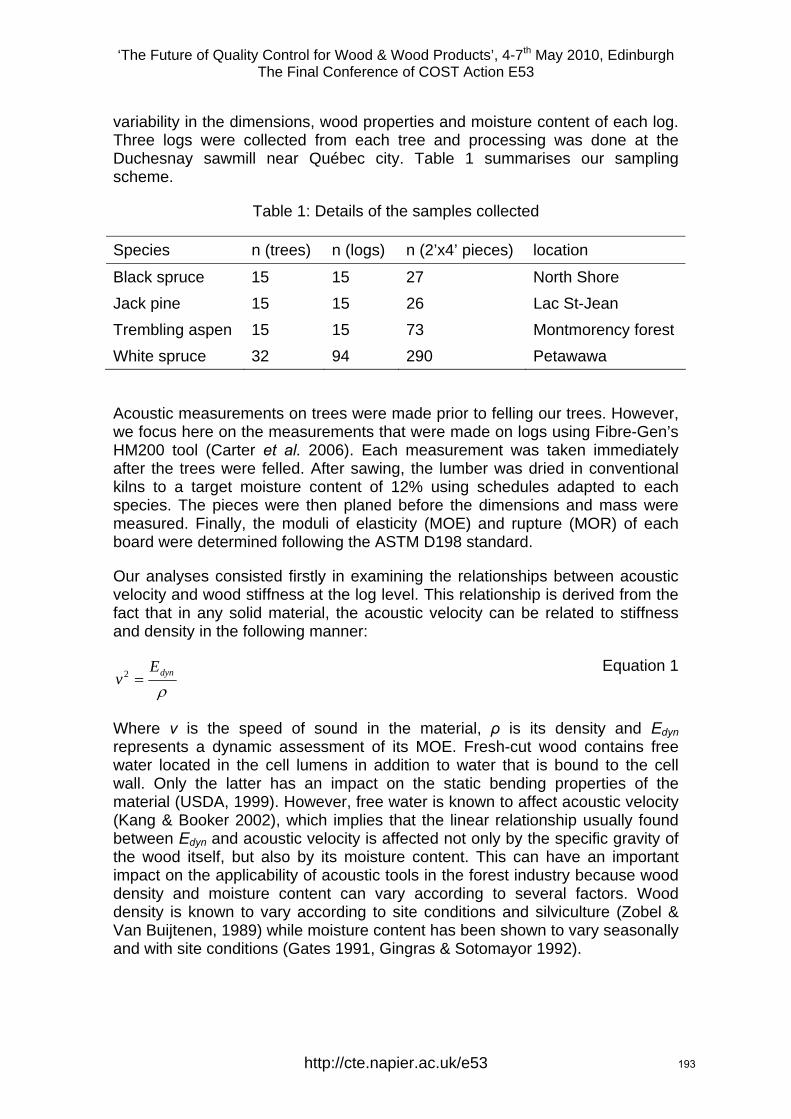
‘The Future of Quality Control for Wood & Wood Products’, 4-7th May 2010, Edinburgh The Final Conference of COST Action E53
variability in the dimensions, wood properties and moisture content of each log. Three logs were collected from each tree and processing was done at the Duchesnay sawmill near Québec city. Table 1 summarises our sampling scheme.
Table 1: Details of the samples collected
Species n (trees) n (logs) n (2’x4’ pieces) location
Black spruce 15 15 27 North Shore Jack pine 15 15 26 Lac St-Jean Trembling aspen 15 15 73 Montmorency forest White spruce 32 94 290 Petawawa
Acoustic measurements on trees were made prior to felling our trees. However, we focus here on the measurements that were made on logs using Fibre-Gen’s HM200 tool (Carter et al. 2006). Each measurement was taken immediately after the trees were felled. After sawing, the lumber was dried in conventional kilns to a target moisture content of 12% using schedules adapted to each species. The pieces were then planed before the dimensions and mass were measured. Finally, the moduli of elasticity (MOE) and rupture (MOR) of each board were determined following the ASTM D198 standard.
Our analyses consisted firstly in examining the relationships between acoustic velocity and wood stiffness at the log level. This relationship is derived from the fact that in any solid material, the acoustic velocity can be related to stiffness and density in the following manner:
ρdynE
v =2 Equation 1
Where v is the speed of sound in the material, ρ is its density and Edyn represents a dynamic assessment of its MOE. Fresh-cut wood contains free water located in the cell lumens in addition to water that is bound to the cell wall. Only the latter has an impact on the static bending properties of the material (USDA, 1999). However, free water is known to affect acoustic velocity (Kang & Booker 2002), which implies that the linear relationship usually found between Edyn and acoustic velocity is affected not only by the specific gravity of the wood itself, but also by its moisture content. This can have an important impact on the applicability of acoustic tools in the forest industry because wood density and moisture content can vary according to several factors. Wood density is known to vary according to site conditions and silviculture (Zobel & Van Buijtenen, 1989) while moisture content has been shown to vary seasonally and with site conditions (Gates 1991, Gingras & Sotomayor 1992).
http://cte.napier.ac.uk/e53 193
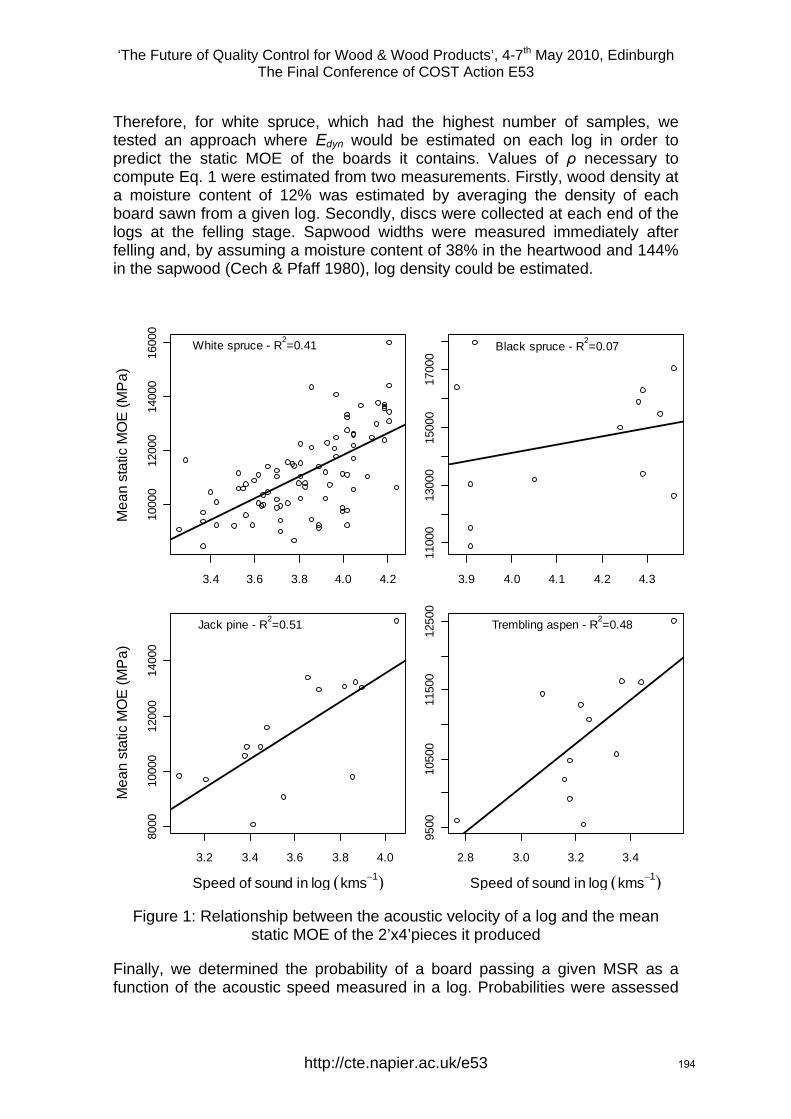
‘The Future of Quality Control for Wood & Wood Products’, 4-7th May 2010, Edinburgh The Final Conference of COST Action E53
Therefore, for white spruce, which had the highest number of samples, we tested an approach where Edyn would be estimated on each log in order to predict the static MOE of the boards it contains. Values of ρ necessary to compute Eq. 1 were estimated from two measurements. Firstly, wood density at a moisture content of 12% was estimated by averaging the density of each board sawn from a given log. Secondly, discs were collected at each end of the logs at the felling stage. Sapwood widths were measured immediately after felling and, by assuming a moisture content of 38% in the heartwood and 144% in the sapwood (Cech & Pfaff 1980), log density could be estimated.
3.4 3.6 3.8 4.0 4.2
1000
012
000
1400
016
000
Mea
n st
atic
MO
E (M
Pa)
White spruce - R2=0.41
3.9 4.0 4.1 4.2 4.3
1100
013
000
1500
017
000
Black spruce - R2=0.07
3.2 3.4 3.6 3.8 4.0
8000
1000
012
000
1400
0
Speed of sound in log (kms−1)
Mea
n st
atic
MO
E (M
Pa)
Jack pine - R2=0.51
2.8 3.0 3.2 3.4
9500
1050
011
500
1250
0
Speed of sound in log (kms−1)
Trembling aspen - R2=0.48
Figure 1: Relationship between the acoustic velocity of a log and the mean static MOE of the 2’x4’pieces it produced
Finally, we determined the probability of a board passing a given MSR as a function of the acoustic speed measured in a log. Probabilities were assessed
http://cte.napier.ac.uk/e53 194
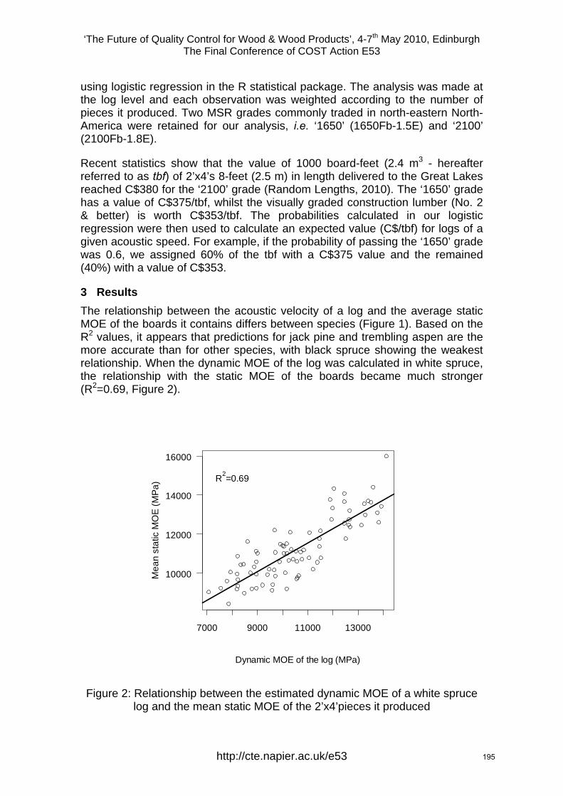
‘The Future of Quality Control for Wood & Wood Products’, 4-7th May 2010, Edinburgh The Final Conference of COST Action E53
using logistic regression in the R statistical package. The analysis was made at the log level and each observation was weighted according to the number of pieces it produced. Two MSR grades commonly traded in north-eastern North-America were retained for our analysis, i.e. ‘1650’ (1650Fb-1.5E) and ‘2100’ (2100Fb-1.8E).
Recent statistics show that the value of 1000 board-feet (2.4 m3 - hereafter referred to as tbf) of 2’x4’s 8-feet (2.5 m) in length delivered to the Great Lakes reached C$380 for the ‘2100’ grade (Random Lengths, 2010). The ‘1650’ grade has a value of C$375/tbf, whilst the visually graded construction lumber (No. 2 & better) is worth C$353/tbf. The probabilities calculated in our logistic regression were then used to calculate an expected value (C$/tbf) for logs of a given acoustic speed. For example, if the probability of passing the ‘1650’ grade was 0.6, we assigned 60% of the tbf with a C$375 value and the remained (40%) with a value of C$353.
3 Results The relationship between the acoustic velocity of a log and the average static MOE of the boards it contains differs between species (Figure 1). Based on the R2 values, it appears that predictions for jack pine and trembling aspen are the more accurate than for other species, with black spruce showing the weakest relationship. When the dynamic MOE of the log was calculated in white spruce, the relationship with the static MOE of the boards became much stronger (R2=0.69, Figure 2).
7000 9000 11000 13000
10000
12000
14000
16000
Dynamic MOE of the log (MPa)
Mea
n st
atic
MO
E (M
Pa) R2=0.69
Figure 2: Relationship between the estimated dynamic MOE of a white spruce log and the mean static MOE of the 2’x4’pieces it produced
http://cte.napier.ac.uk/e53 195
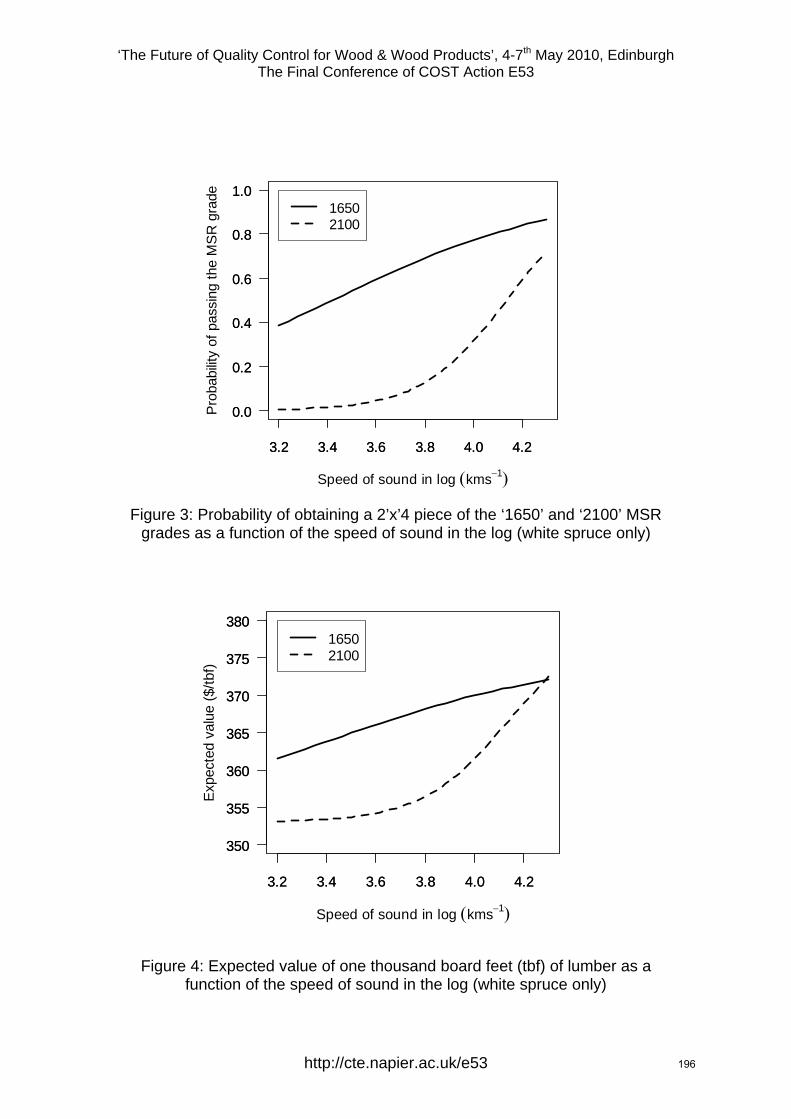
‘The Future of Quality Control for Wood & Wood Products’, 4-7th May 2010, Edinburgh The Final Conference of COST Action E53
3.2 3.4 3.6 3.8 4.0 4.2
0.0
0.2
0.4
0.6
0.8
1.0
Speed of sound in log (kms−1)
Prob
abilit
y of
pas
sing
the
MSR
gra
de
3.2 3.4 3.6 3.8 4.0 4.2
0.0
0.2
0.4
0.6
0.8
1.016502100
Figure 3: Probability of obtaining a 2’x’4 piece of the ‘1650’ and ‘2100’ MSR
grades as a function of the speed of sound in the log (white spruce only)
3.2 3.4 3.6 3.8 4.0 4.2
350
355
360
365
370
375
380
Speed of sound in log (kms−1)
Exp
ecte
d va
lue
($/tb
f)
3.2 3.4 3.6 3.8 4.0 4.2
350
355
360
365
370
375
38016502100
Figure 4: Expected value of one thousand board feet (tbf) of lumber as a function of the speed of sound in the log (white spruce only)
http://cte.napier.ac.uk/e53 196
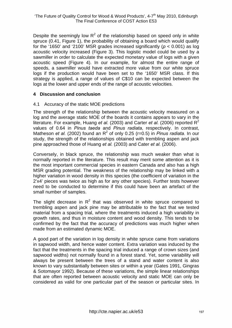
‘The Future of Quality Control for Wood & Wood Products’, 4-7th May 2010, Edinburgh The Final Conference of COST Action E53
Despite the seemingly low R2 of the relationship based on speed only in white spruce (0.41, Figure 1), the probability of obtaining a board which would qualify for the ‘1650’ and ‘2100’ MSR grades increased significantly (p < 0.001) as log acoustic velocity increased (Figure 3). This logistic model could be used by a sawmiller in order to calculate the expected monetary value of logs with a given acoustic speed (Figure 4). In our example, for almost the entire range of speeds, a sawmiller would have extracted more value from our white spruce logs if the production would have been set to the ‘1650’ MSR class. If this strategy is applied, a range of values of C$10 can be expected between the logs at the lower and upper ends of the range of acoustic velocities.
4 Discussion and conclusion
4.1 Accuracy of the static MOE predictions The strength of the relationship between the acoustic velocity measured on a log and the average static MOE of the boards it contains appears to vary in the literature. For example, Huang et al. (2003) and Carter et al. (2006) reported R2 values of 0.64 in Pinus taeda and Pinus radiata, respectively. In contrast, Matheson et al. (2002) found an R2 of only 0.25 (r=0.5) in Pinus radiata. In our study, the strength of the relationships obtained with trembling aspen and jack pine approached those of Huang et al. (2003) and Cater et al. (2006).
Conversely, in black spruce, the relationship was much weaker than what is normally reported in the literature. This result may merit some attention as it is the most important commercial species in eastern Canada and also has a high MSR grading potential. The weakness of the relationship may be linked with a higher variation in wood density in this species (the coefficient of variation in the 2’x4’ pieces was twice as high as for any other species). Further tests however need to be conducted to determine if this could have been an artefact of the small number of samples.
The slight decrease in R2 that was observed in white spruce compared to trembling aspen and jack pine may be attributable to the fact that we tested material from a spacing trial, where the treatments induced a high variability in growth rates, and thus in moisture content and wood density. This tends to be confirmed by the fact that the accuracy of predictions was much higher when made from an estimated dynamic MOE.
A good part of the variation in log density in white spruce came from variations in sapwood width, and hence water content. Extra variation was induced by the fact that the treatments in the spacing trial induced a range of crown sizes (and sapwood widths) not normally found in a forest stand. Yet, some variability will always be present between the trees of a stand and water content is also known to vary substantially between sites or within a year (Gates 1991, Gingras & Sotomayor 1992). Because of these variations, the simple linear relationships that are often reported between acoustic velocity and static MOE can only be considered as valid for one particular part of the season or particular sites. In
http://cte.napier.ac.uk/e53 197

‘The Future of Quality Control for Wood & Wood Products’, 4-7th May 2010, Edinburgh The Final Conference of COST Action E53
order to make acoustic assesments applicable at an industrial scale it is important to devise a system which accounts for variations in moisture content.
Our results suggest that a good approach to counter this problem may involve making predictions from a dynamic MOE rather than only acoustic velocity. The advantage is that predictions should remain unbiased for a wider range of conditions. However, a potential disadvantage is that it will necessitate an estimation of log density. At an operational level, one possibility would be to use a generic correction factor based on the mass-volume relationships that are available to sawmills which collect this information at their gate. Such a strategy could at least help take into account seasonal variations in moisture content.
However, sawmillers may also opt for measuring the density of each log prior to processing. Most sawmills in eastern Canada are equipped with a 3D scanner which provides a volume measurement. Installing a scale could then provide the mass measurement needed to calculate a dynamic MOE. The results from our white spruce samples suggest that the accuracy of predictions can be substantially improved if the dynamic MOE of each log is calculated.
4.2 Potential for adding value The C$10/tbf difference in value that was found between the logs with the lowest and highest velocities may appear insignificant. However, considering the fact that production costs are currently estimated at C$350/tbf, i.e. very close to the value of visually graded construction lumber, an added-value of C$10 may represent the difference between losses and profits.
The information provided by this part of our analysis could be used in different ways in practice. For example, a sawmiller could set a threshold acoustic speed, or dynamic MOE, at which the extra effort needed to produce MSR lumber would be matched by the increase in expected value. This would normally require testing all logs entering the sawmill with an automated acoustic tool.
Alternatively, a sawmiller may test a sample of logs coming from a given source with a hand tool in order to predetermine its potential for producing lumber of a given MSR class. Our study provided a good example of this possibility as it appeared that the highest value would be obtained from our white spruce logs if the sawmill were set to produce the ‘1650’ grade. Due to lower probabilities of obtaining the desired stiffness, focusing on the ‘2100’ MSR grade would have resulted in losses in value. Conversely, focusing only on visually graded lumber at C$353/tbf would not have extracted the best potential value from the resource. In our example, the white spruce samples were of a plantation origin, a relatively rare occurrence in current wood supplies in eastern Canada. Information on the likelihood of meeting the MOE thresholds of different MSR grades would not have been available prior to processing in a normal industrial setup. Acoustic technology may therefore be very useful in the current economical context and in situations where the variability in the properties of the wood supplies can represent an issue.
http://cte.napier.ac.uk/e53 198
‘The Future of Quality Control for Wood & Wood Products’, 4-7th May 2010, Edinburgh The Final Conference of COST Action E53
Acknowledgements The authors would like to thank the Canadian Wood Fibre Centre for allowing us to collect samples in the Petawawa research station. Thanks also to Amélie Denoncourt and several other assistants and technicians who provided precious help in the field and in the lab. Funding for this project was provided by NSERC, through the ForValueNet strategic network.
References (2010) Random Lengths. Volume 66. Issue 10.
Carter, P., Chauhan, S. & Walker, J. (2006) “Sorting logs and lumber using Director HM200”. Wood Fiber Sci. 38(1): 36-48.
Cech M.Y & F.Pfaff (1980) “Kiln operator's manual for eastern Canada.” Special publication (Forintek Canada Corp.); SP504TR, 209 p.
Gates D.M. (1991) “Water relations of forest trees” IEEE Transactions on geoscience and remote sensing. 29 (6): 836-842.
Gingras J.-F., & Sotomayor, J. (1992) “Wood moisture variation in woodlands inventory: A case study”. FERIC, Technical note TN-192, 6 p.
Jessome, A.P. (2000) "Résistance et propriétés connexes des bois indigènes au Canada". SP 514-F, Forintek Canada Corp., Québec. 27 p.
Kang, H. & Booker, R.E. (2002) Variation of stress wave velocity with MC and temperature. Wood Sci. Technol. 36: 41-54.
Matheson, A.C., Dickson, R.L., Spencer, D.J., Joe, B. & Ilic, J. (2002) “Acoustic segregation of Pinus radiate logs according to stiffness”. Ann. For. Sci. 59 : 471-477.
Mora C.R., Schimleck, L.R. , Isik, F., Mahon Jr., J.M., Clark III, A. & Daniels, R.F. (2009) “Relationships between acoustic variables and different measures of stiffness in standing Pinus taeda trees”. Can. J. For. Res. 39 : 1421-1429.
Tsehaye A., Buchanan, A.H. & Walker, J.C.F. (2000) “Sorting of logs using acoustics.” Wood science and technology 34 : 337-344.
USDA (1999) “Wood Handbook - Wood as an engineering material.” FPL-GTR-113, U.S. Department of Agriculture, Forest Service, Forest Products Laboratory, Madison, WI. 463 p.
Wang, X., Carter, P., Ross, R.J. & Brashaw, B.K. (2007) “Acoustic assessment of wood quality of raw forest materials – a path to increased profitability.” Forest Products Journal. 57 (5): 6-14.
Zobel, B.J. & Van Buijtenen, J.P. (1989). “Wood variations - its causes and control.” Springer, Berlin. 300 p.
http://cte.napier.ac.uk/e53 199

‘The Future of Quality Control for Wood & Wood Products’, 4-7th May 2010, Edinburgh The Final Conference of COST Action E53
Wednesday 5th May Industry focussed day
3rd session
http://www.cte.napier.ac.uk/e53/ 200

‘The Future of Quality Control for Wood & Wood Products’, 4-7th May 2010, Edinburgh The Final Conference of COST Action E53
Drying quality - an important topic for business and research
J.Welling1
Extended abstract In a living tree water is an indispensible and integral part of the organism. Without sufficient water no transport processes would be possible and the metabolism of the tree would come to an end. When a tree is felled and processed the transformation of wood into timber takes place. Starting from this point water is not anymore a desired and needed component of the raw material but rather an obstacle for further processing and utilisation. It causes various types of problems and must be removed from the material. The technical term we normally use for this physical process is “WOOD DRYING”. We do not anymore speak about water in wood but rather about wood moisture content.
The technical process drying does not only involve the removal of water, it strongly influences the properties and usability of the timber. Drying needs a lot of energy and time, it is costly and involves high risk, it requires a lot of expertise and practical experience. False drying conditions may lead to serious devaluation or even complete loss of the timber.
In the context of timber drying, the term “Drying Quality” was first introduced by the European Drying Group (EDG) in the 80-ties of the last century. At that time the only available standard relating to the drying process was the standard describing the oven dry test for determination of moisture content. Starting in the 50-ties many scientific publications were produced describing the drying process of wood, predicting drying time and moisture distribution within the material during drying, describing and explaining stress development during the drying, investigating the reasons for deformation and discolouration during drying.
The so-called “EDG Recommendation on Assessment of Drying Quality of Timber”, which was published in 1996, was the first approach to provide a written guideline with respect to drying quality to industrial practice . The EDG Recommendation was a combination of text book, standard and manual for practitioners. It was written in a form which was understandable to practitioners, it described all methods needed to assess the various aspects of drying quality and - most important – for the first time ever - formed a framework which allowed practitioners to specify and control drying quality of timber.
In the middle of the 90-ties, CEN took up the task to harmonise the manifold standards in the various countries of the European Union. Common standards were considered important for free trade and exchange of goods between
1 Dr., Johann Heinrich von Thuenen-Institute, Institute of Woodtechnology and Woodbiologie, HAMBURG, Germany, E-Mail: [email protected]
http://cte.napier.ac.uk/e53 201

‘The Future of Quality Control for Wood & Wood Products’, 4-7th May 2010, Edinburgh The Final Conference of COST Action E53
European nations. Trade barriers within Europe caused by national standards were reduced and, at the same time, a protective system against import of low quality good from Non-European countries was built up. Nowadays importers have to accept EN standards.
Within the framework of the activities of the CEN Technical Committee 175 “Round and Sawn Timber” a series of EN standards related to moisture content (EN 13183 Part 1-3), casehardening (ENV 14464), drying quality (EN 14298) and acceptance control (ENV 12169) was developed over a period of approximately 10 years. Timber industry and users of timber now have all the tools necessary to specify and control drying quality in production, further processing, trade and end use.
Even though the system of standards is available now for almost 10 years, diffusion into and application by industrial practice has not sufficiently happened in all European countries. It is quite clear that new standards need a long time until they are accepted by practitioners. But, taking into account how important moisture content and drying quality are for the application of wood in the various fields of end use, the question must be posed, why practitioners have not yet fully implemented the drying quality concept in their daily business.
Reasons for this are manifold: new standards are not sufficiently visible to practitioner, new standards are not fully understood, practitioners hesitate to change their attitude towards specification and quality control, additional requirements might lead to additional cost, customers (buyers) are not aware of the necessity or of the advantages of specifying drying quality for timber and timber products, practitioners do not fully understand how to use the new EN standards, European product standards do not refer to the drying quality standards (revision needed!).
Working Group 2 in COST Action E53 has taken up this topic and dedicated a good deal of its activities to overcome this situation. Besides the “normal” COST activities, comprising in providing a platform for exchanging scientific information in a specific field of interest, three COST E53 task groups were created which have produced tailor made publications for practitioners.
The drying quality task group has taken up the job to review the TRÄTEK publication “Torkat virke” dating back to 1998. This publication was a valuable tool to instruct practitioners on how to specify moisture content and drying quality. The disadvantage of this brochure was that it only existed in Swedish language and that it was not up-to-date anymore because of several new EN standards. “Torkat virke” referred to the EDG Recommendation, but with the existence of the new EN standards the brochure had to be up-dated. Now, at the end of COST Action E53, the 38-page coloured leaflet is available in English language, several other European languages will follow.
A second task group concentrated on distortions which can be observed during drying. Wood scientists, and also the sawn timber producing practitioners, know that most distortions of timber develop during drying and/or while moisture
http://cte.napier.ac.uk/e53 202

‘The Future of Quality Control for Wood & Wood Products’, 4-7th May 2010, Edinburgh The Final Conference of COST Action E53
content changes. But, in most cases, inherent wood properties are the reasons for the distortions. Therefore, distortion are a problem of wood/timber quality and not so much of drying quality. The COST E53 task group produced a leaflet which will help produces and users of sawn timber to better understand the processes, conditions and inherent properties leading to distortions.
Task group number three concentrated on discolourations of sawn timber. Many discolourations occur during drying, some can be avoided if certain protective measures are taken. The discolouration leaflet produced by the task group addresses the most important types of discolourations present in European and tropical sawn timber. It explains how theses discolourations develop and how they can be avoided.
COST Action E53 will provide these publications free of cost via its web-page (www.costE53.net). After the end of COST E53 the European Drying Group (EDG) will take over dissemination and up-dating of the brochures. Therefore, the documents will also be available via the EDG web-page (www.timberdry.net).
With the support of Cost Action E53 the existing information gap with respect to standardisation, assessment and control of drying quality will be closed. The wood sector and - which is considered very important – the buyers (users) of sawn timber will be given the chance to use the information contained in three leaflets to install a more profound quality thinking in the field of wood drying and utilisation of dried sawn timber and derived products.
References
TRÄTEK (1998). Torkat virke. Publ nr 9811077, Stockholm, ISBN 91-88170-26-8
Welling, J. (Editor) (1994): EDG-Recommendation “Assessment of Drying Quality of Timber). www.timberdry.net
EN 13183-1:2002. Moisture content of a piece of sawn timber – Part 1: Determination by oven dry method
EN 13183-2:2002. Moisture content of a piece of sawn timber - Estimation by electrical resistance method
EN 13183-3:2005. Moisture content of a piece of sawn timber - Estimation by capacitance method
ENV 14464:2003. Sawn timber - Method for assessment of case-hardening
EN 14298:2006. Sawn timber - Assessment of drying quality
ENV 12169:2000. Criteria for the assessment of conformity of a lot of sawn timber
http://cte.napier.ac.uk/e53 203
‘The Future of Quality Control for Wood & Wood Products’, 4-7th May 2010, Edinburgh The Final Conference of COST Action E53
Do’s and don’ts in respect to moisture measurement
P. Rozema1
Abstract As a manufacturer of moisture meters for wood and construction materials as well as wood strength measurement systems we are often confronted with several questions from the industry related to wood moisture content. Questions can seem to be easy, but answering them can turn out to be very complex. Although the questions generally relate to (kiln dried) wood, we often notice that it is also about the type of moisture meter which is used, or about drying quality, that customers have rejected the wood, or that sizes have changed over time. Also it is not always known which settings must be used for a certain wood species. Questions which probably are known or logical for scientists, but the industry has difficulties with it and therefore is also is confronted with problems.
1 Introduction Firstly we can ask ourselves why we need to know the moisture content, what the moisture content should be and what the spreading of the moisture content is. Subsequently we can ask ourselves how the moisture content can be determined, how we know that the moisture content found is correct, which tolerances the moisture measurement has, how the different types of moisture measurement methods can be compared to each other, but also what the influence of the drying process is on the moisture measurement as well as the wood species.
2 Equilibrium moisture content Wood is a hygroscopic material which yields moisture to its surroundings or absorbs moisture from its surroundings. If it yields moisture then the wood shrinks, if it absorbs moisture it will swell. It is a fact that the wood shall try to reach an equilibrium with its surroundings, whereby a small difference will be noticeable if the equilibrium moisture content gets lower with regard to when it gets higher. This difference is called hysteresis.
1 Brookhuis Micro-Electronics, Enschede, NETHERLANDS, [email protected]
http://cte.napier.ac.uk/e53 204
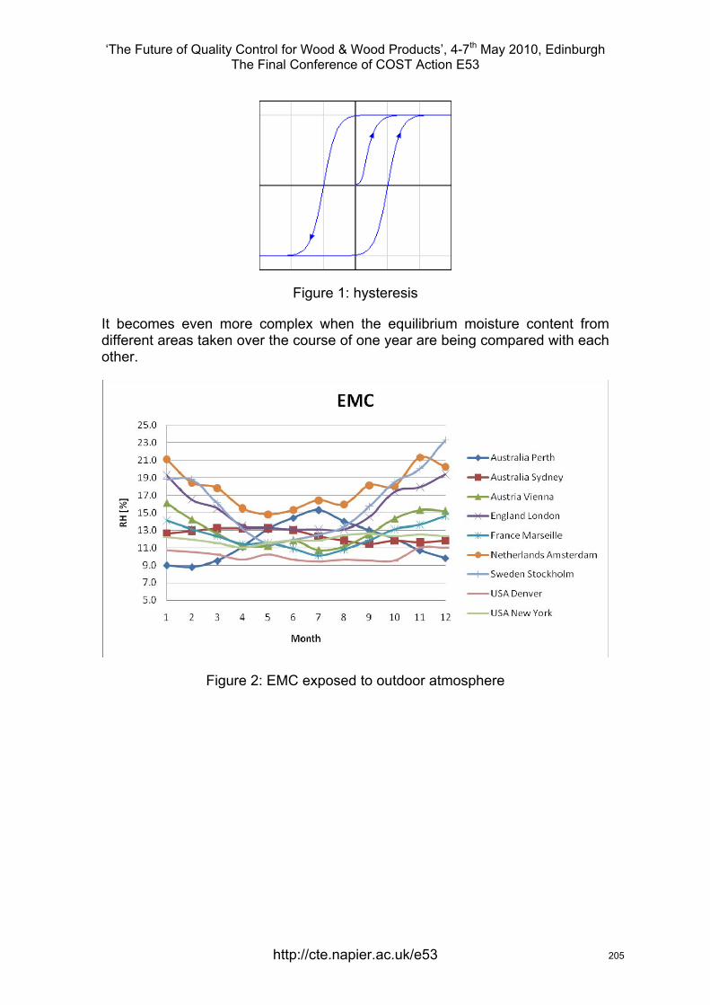
‘The Future of Quality Control for Wood & Wood Products’, 4-7th May 2010, Edinburgh The Final Conference of COST Action E53
Figure 1: hysteresis
It becomes even more complex when the equilibrium moisture content from different areas taken over the course of one year are being compared with each other.
Figure 2: EMC exposed to outdoor atmosphere
http://cte.napier.ac.uk/e53 205

‘The Future of Quality Control for Wood & Wood Products’, 4-7th May 2010, Edinburgh The Final Conference of COST Action E53
Indoor applied wood shall also want to reach an equilibrium with its surroundings.
Table 1: EMC of wood species at different RH
Species 40% RH 60% RH 85% RH 90% RH 100% RH
Pine 9 – 10% 12 – 13% 15 – 18% 17 – 19% 30%
Fir 8 – 9% 11 – 13% 17 – 20% 20 – 22% 30%
Oak 9 – 10% 12 – 13% 17 – 20% 19 – 22% 32%
Meranti 8 – 9% 11 – 13% 17 – 20% 18 – 22% 29%
3 EN 13183 Moisture Content In Europe the determination of the moisture content of sawn timber is recorded in the following standards.
EN 13183-1 Moisture content of a piece of sawn timber – Part 1: Determination by oven dry method
EN 13183-2 Moisture content of a piece of sawn timber – Part 2: Estimation by electrical resistance method
EN 13183-3 Moisture content of a piece of sawn timber – Part 3: Estimation by capacitance method
In praxis the moisture content is measured with different types of moisture meters and users consider their own moisture meter best. Problems related to moisture measurements can come up when the buyer measures with another moisture meter than the supplier, or when the moisture meter is compared with the oven dryer. Before the user doubts the device, the method or the result it is important to check if the measurement was performed in a correct manner and if it is possible at all to electrically measure that wood species.
http://cte.napier.ac.uk/e53 206
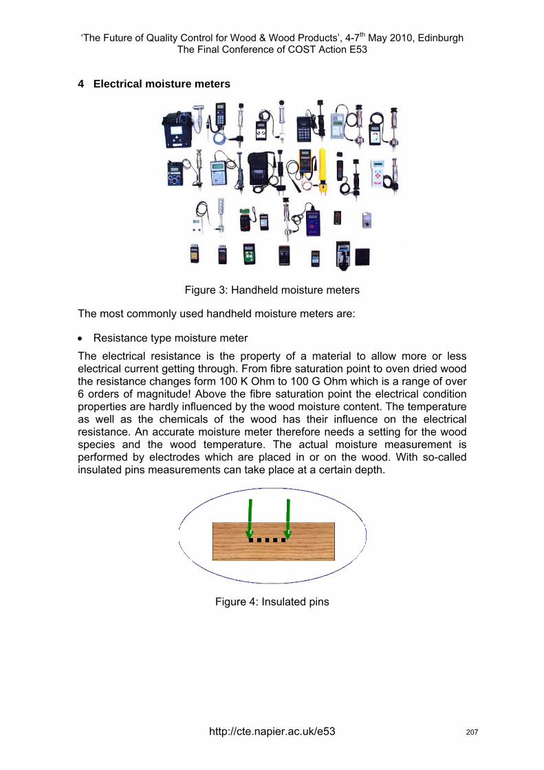
‘The Future of Quality Control for Wood & Wood Products’, 4-7th May 2010, Edinburgh The Final Conference of COST Action E53
4 Electrical moisture meters
Figure 3: Handheld moisture meters
The most commonly used handheld moisture meters are:
• Resistance type moisture meter The electrical resistance is the property of a material to allow more or less electrical current getting through. From fibre saturation point to oven dried wood the resistance changes form 100 K Ohm to 100 G Ohm which is a range of over 6 orders of magnitude! Above the fibre saturation point the electrical condition properties are hardly influenced by the wood moisture content. The temperature as well as the chemicals of the wood has their influence on the electrical resistance. An accurate moisture meter therefore needs a setting for the wood species and the wood temperature. The actual moisture measurement is performed by electrodes which are placed in or on the wood. With so-called insulated pins measurements can take place at a certain depth.
Figure 4: Insulated pins
http://cte.napier.ac.uk/e53 207
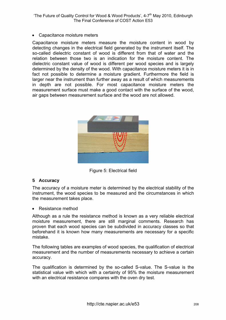
‘The Future of Quality Control for Wood & Wood Products’, 4-7th May 2010, Edinburgh The Final Conference of COST Action E53
• Capacitance moisture meters Capacitance moisture meters measure the moisture content in wood by detecting changes in the electrical field generated by the instrument itself. The so-called dielectric constant of wood is different from that of water and the relation between those two is an indication for the moisture content. The dielectric constant value of wood is different per wood species and is largely determined by the density of the wood. With capacitance moisture meters it is in fact not possible to determine a moisture gradient. Furthermore the field is larger near the instrument than further away as a result of which measurements in depth are not possible. For most capacitance moisture meters the measurement surface must make a good contact with the surface of the wood, air gaps between measurement surface and the wood are not allowed.
Figure 5: Electrical field
5 Accuracy The accuracy of a moisture meter is determined by the electrical stability of the instrument, the wood species to be measured and the circumstances in which the measurement takes place.
• Resistance method Although as a rule the resistance method is known as a very reliable electrical moisture measurement, there are still marginal comments. Research has proven that each wood species can be subdivided in accuracy classes so that beforehand it is known how many measurements are necessary for a specific mistake.
The following tables are examples of wood species, the qualification of electrical measurement and the number of measurements necessary to achieve a certain accuracy.
The qualification is determined by the so-called S-value. The S-value is the statistical value with which with a certainty of 95% the moisture measurement with an electrical resistance compares with the oven dry test.
http://cte.napier.ac.uk/e53 208

‘The Future of Quality Control for Wood & Wood Products’, 4-7th May 2010, Edinburgh The Final Conference of COST Action E53
Table 2: Qualification measuring accuracy
Class Qualification Accuracy
1 Well measurable 2S < 1.6%
2 Measurable 1.6% < 2S < 2.5%
3 Poorly measurable 2.5% < 2S < 3.5%
4 Not measurable 3.5% < 2S
Table 3: Qualification wood species
Class 1 Class 2 Class 3 Class 4
Oak Beech Abachi Afzelia
Spruce Maple Alder Poplar
Cherry wood Merbau Sapeli
Pine Meranti Teak
Table 4: Accuracy in relation to number of readings and classification
Class 1 2 3
2S < 1.6% 1.6% < 2S < 2.5% 2.5% < 2S < 3.5%
Number of measurements
Accuracy
3 +/- 0.92%
6 +/- 1.02%
9 +/- 1.1%
18 +/- 0.51%
25 +/- 0.5%
35 +/- 0.59%
http://cte.napier.ac.uk/e53 209
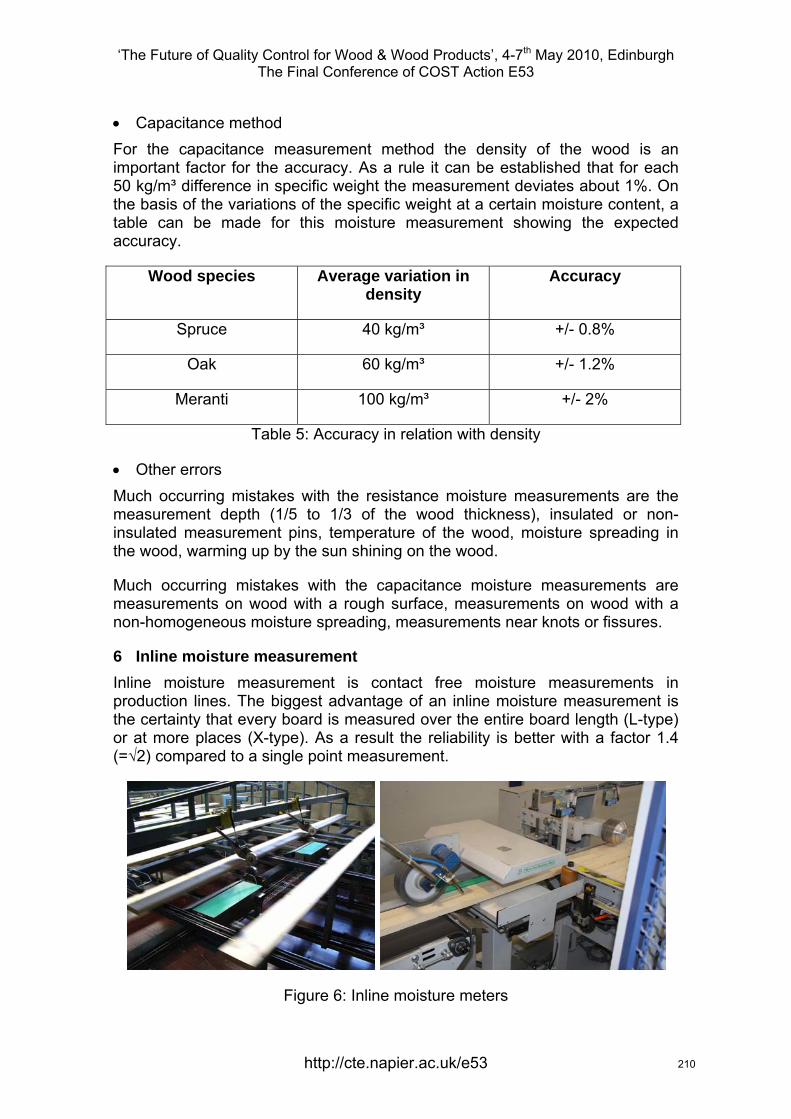
‘The Future of Quality Control for Wood & Wood Products’, 4-7th May 2010, Edinburgh The Final Conference of COST Action E53
• Capacitance method For the capacitance measurement method the density of the wood is an important factor for the accuracy. As a rule it can be established that for each 50 kg/m³ difference in specific weight the measurement deviates about 1%. On the basis of the variations of the specific weight at a certain moisture content, a table can be made for this moisture measurement showing the expected accuracy.
Wood species Average variation in density
Accuracy
Spruce 40 kg/m³ +/- 0.8%
Oak 60 kg/m³ +/- 1.2%
Meranti 100 kg/m³ +/- 2%
Table 5: Accuracy in relation with density
• Other errors Much occurring mistakes with the resistance moisture measurements are the measurement depth (1/5 to 1/3 of the wood thickness), insulated or non-insulated measurement pins, temperature of the wood, moisture spreading in the wood, warming up by the sun shining on the wood.
Much occurring mistakes with the capacitance moisture measurements are measurements on wood with a rough surface, measurements on wood with a non-homogeneous moisture spreading, measurements near knots or fissures.
6 Inline moisture measurement Inline moisture measurement is contact free moisture measurements in production lines. The biggest advantage of an inline moisture measurement is the certainty that every board is measured over the entire board length (L-type) or at more places (X-type). As a result the reliability is better with a factor 1.4 (=√2) compared to a single point measurement.
Figure 6: Inline moisture meters
http://cte.napier.ac.uk/e53 210
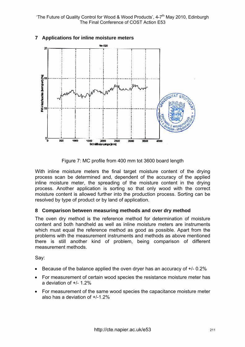
‘The Future of Quality Control for Wood & Wood Products’, 4-7th May 2010, Edinburgh The Final Conference of COST Action E53
7 Applications for inline moisture meters
Figure 7: MC profile from 400 mm tot 3600 board length
With inline moisture meters the final target moisture content of the drying process scan be determined and, dependent of the accuracy of the applied inline moisture meter, the spreading of the moisture content in the drying process. Another application is sorting so that only wood with the correct moisture content is allowed further into the production process. Sorting can be resolved by type of product or by land of application.
8 Comparison between measuring methods and over dry method The oven dry method is the reference method for determination of moisture content and both handheld as well as inline moisture meters are instruments which must equal the reference method as good as possible. Apart from the problems with the measurement instruments and methods as above mentioned there is still another kind of problem, being comparison of different measurement methods.
Say:
• Because of the balance applied the oven dryer has an accuracy of +/- 0.2%
• For measurement of certain wood species the resistance moisture meter has a deviation of +/- 1.2%
• For measurement of the same wood species the capacitance moisture meter also has a deviation of +/-1.2%
http://cte.napier.ac.uk/e53 211

‘The Future of Quality Control for Wood & Wood Products’, 4-7th May 2010, Edinburgh The Final Conference of COST Action E53
Now in order to enable comparison of the accuracy between two measurement devices, the so-called absolute faults must be added up. This will then result in the following maximum fault tolerances:
• oven dryer +/- 0.2% & resistance moisture meters +/- 1.2% +/- 1.4%
• oven dryer +/- 0.2% & capacitance moisture meters +/- 1.2% +/- 1.4%
• capacitance moisture meter +/- 1.2% & resistance moisture meter +/- 1.2% +/- 2.4%
9 Summary Wood moisture measurement is not difficult if the rules are well obeyed and generally better than what the wood needs when professional instruments are used.
References William T. Simpson. (1998) “Equilibrium moisture content of wood in outdoor conditions in the United States and worldwide”.
CEN (2002) “EN 13183-1 Moisture content of a piece of sawn timber – Part 1 Determination by oven dry method”.
CEN (2002) “EN 13183-2 Moisture content of a piece of sawn timber – Part 2: Estimation by electrical resistance method”.
CEN (2005) “EN 13183-3 Moisture content of a piece of sawn timber – Part 3: Estimation by capacitance method”.
http://cte.napier.ac.uk/e53 212
‘The Future of Quality Control for Wood & Wood Products’, 4-7th May 2010, Edinburgh The Final Conference of COST Action E53
Sorting of logs and planks before drying for improved drying process and panel board quality
K.M. Sandland1 & P. Gjerdrum2
Abstract The objective of the research work has been to investigate whether the quality of dried and planed sawn timber can be improved by sorting logs and planks before the drying process. The research material was selected by randomly choosing 30 butt logs and 30 middle logs in a given diameter class at a sawmill. The logs were sawn in a 4 x log pattern, and one inner plank (near pith) and one outer plank (near bark) were chosen from each log. Various properties were measured on the logs and on the sawn timber before and after drying. The material was then planed, and the quality of the panel boards was registered.
Based on the results, different models for sorting the timber before drying to optimise the drying process are proposed. One of them is to separate outer and inner planks. An evident improvement is then expected, both due to possibilities for adjusting the drying process to the moisture content before and after drying, and the possibilities for optimising the drying process in accordance with the requirements of the various wood products. In addition to a separation of inner and outer planks, it is also of interest to separate planks from different types of logs (e.g. butt logs and middle logs) to be able to further optimise the drying process according to the wood properties.
The project results also show that the best wood quality for production of panel boards is found in the inner planks from middle logs, mainly due to the knot pattern in the stems.
1 Introduction In the growing stem of a tree, there will be more or less systematic variations in the wood properties from pith to bark, and from butt end to the top. This is also the case for Norway spruce (Picea abies), the most industrial utilised wood species in Norway. In the stems of Norway spruce, there is a clear difference in moisture content between heartwood and sapwood, which will influence the drying behaviour of the wood. And in addition, the portion of heartwood in the cross section will be dependent on the height in the stem.
Other wood properties also have a regular variation in the stems. Near the pith, the juvenile zone is localised, with higher fibre angle than the mature wood. This will influence the amount of twist in the dried sawn timber.
1 Research leader, [email protected], Treteknisk, Norway 2 Senior Researcher, [email protected], The Norwegian Forest and Landscape Institute, Norway
http://cte.napier.ac.uk/e53 213

‘The Future of Quality Control for Wood & Wood Products’, 4-7th May 2010, Edinburgh The Final Conference of COST Action E53
Another important property is the knot pattern in the stems. In the zone nearest to the pith, there are sound knots, while in the outer parts of the stem there will be more dead knots/black knots. The size of the dead knot zone is dependent on the age of the tree and the site conditions. In older trees, where the branches have felled off in the lower parts of the stems, a knot free zone can be formed in the outer part of the stem. Typical knot pattern in stems of Norway spruce is more closely described by Vestøl (1998) and Øien (1999). However, for wood panel for indoor use, the occurrence of the various knot types is very important. Dead knots/black knots are not accepted. Therefore, the raw material for producing indoor wooden panel should mainly contain sound knots, and should therefore be taken near the pith in the stem to avoid risk for dead knots.
With this background, the objective of the research work was to examine:
- Possible advantages concerning the drying quality by sorting logs and planks before drying.
- The effect of a sorting system for logs and planks for selecting raw material for indoor panel production.
This paper is based on the work of Sandland, Gjerdrum & Hamar (2001).
2 Material and methods The research material was selected by randomly choosing 30 butt logs and 30 middle logs (middle log is the log above the butt log in the stem) in a given diameter class (240-250 mm) at a sawmill (Moelven Soknabruket AS). The logs were sawn in a 4 x log pattern, and the nominal dimension of the four planks in the centre yield was 44 mm x 125 mm. A total of 120 planks were produced, 30 planks in each of the following groups:
- Butt logs, inner planks - Butt logs, outer planks - Middle logs, inner planks - Middle logs, outer planks
The inner planks are the planks nearest the pith, while the outer planks are nearest the bark. The butt logs and the middle logs did not come from the same stems.
The planks were dried at a constant wet bulb temperature of 55-56 °C, with an increasing dry bulb temperature during the drying phase, from 58 °C in the beginning to 67-68 °C at the end. Finally, a conditioning phase of 12 hours was performed after the drying phase.
The moisture content was measured by the oven dry method (according to EN 13183-1) before and after drying, both in the top and butt end of each plank.
After drying, the casehardening level was measured by using the 2-slice method (according to ENV 14464), and the twist was measured in mm rise over
http://cte.napier.ac.uk/e53 214
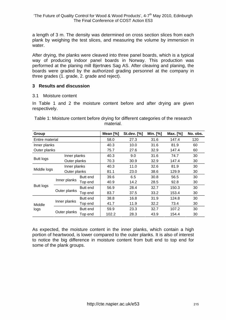
‘The Future of Quality Control for Wood & Wood Products’, 4-7th May 2010, Edinburgh The Final Conference of COST Action E53
a length of 3 m. The density was determined on cross section slices from each plank by weighing the test slices, and measuring the volume by immersion in water.
After drying, the planks were cleaved into three panel boards, which is a typical way of producing indoor panel boards in Norway. This production was performed at the planing mill Bjertnæs Sag AS. After cleaving and planing, the boards were graded by the authorized grading personnel at the company in three grades (1. grade, 2. grade and reject).
3 Results and discussion
3.1 Moisture content In Table 1 and 2 the moisture content before and after drying are given respectively.
Table 1: Moisture content before drying for different categories of the research material.
Group Mean [%] St.dev. [%] Min. [%] Max. [%] No. obs.Entire material 58.0 27.3 31.6 147.4 120 Inner planks 40.3 10.0 31.6 81.9 60 Outer planks 75.7 27.6 32.9 147.4 60
Inner planks 40.3 9.0 31.6 74.7 30 Butt logs Outer planks 70.3 30.9 32.9 147.4 30
Inner planks 40.3 11.0 32.6 81.9 30 Middle logs Outer planks 81.1 23.0 38.6 129.9 30
Butt end 39.6 6.5 30.8 56.5 30 Inner planks Top end 40.9 14.2 28.5 92.8 30
Butt end 56.9 28.4 32.7 150.3 30 Butt logs Outer planks Top end 83.7 37.5 33.2 153.4 30
Butt end 38.8 16.8 31.9 124.8 30 Inner planks Top end 41.7 11.9 32.2 73.4 30
Butt end 59.9 23.3 32.7 107.2 30 Middle logs
Outer planks Top end 102.2 28.3 43.9 154.4 30
As expected, the moisture content in the inner planks, which contain a high portion of heartwood, is lower compared to the outer planks. It is also of interest to notice the big difference in moisture content from butt end to top end for some of the plank groups.
http://cte.napier.ac.uk/e53 215
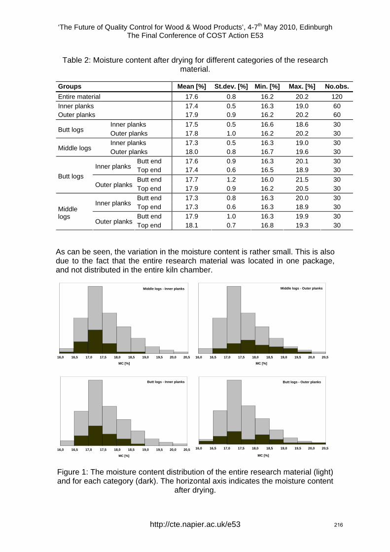
‘The Future of Quality Control for Wood & Wood Products’, 4-7th May 2010, Edinburgh The Final Conference of COST Action E53
Table 2: Moisture content after drying for different categories of the research material.
Groups Mean [%] St.dev. [%] Min. [%] Max. [%] No.obs. Entire material 17.6 0.8 16.2 20.2 120 Inner planks 17.4 0.5 16.3 19.0 60 Outer planks 17.9 0.9 16.2 20.2 60
Inner planks 17.5 0.5 16.6 18.6 30 Butt logs Outer planks 17.8 1.0 16.2 20.2 30
Inner planks 17.3 0.5 16.3 19.0 30 Middle logs Outer planks 18.0 0.8 16.7 19.6 30
Butt end 17.6 0.9 16.3 20.1 30 Inner planks Top end 17.4 0.6 16.5 18.9 30
Butt end 17.7 1.2 16.0 21.5 30 Butt logs Outer planks Top end 17.9 0.9 16.2 20.5 30
Butt end 17.3 0.8 16.3 20.0 30 Inner planks Top end 17.3 0.6 16.3 18.9 30
Butt end 17.9 1.0 16.3 19.9 30 Middle logs
Outer planks Top end 18.1 0.7 16.8 19.3 30
As can be seen, the variation in the moisture content is rather small. This is also due to the fact that the entire research material was located in one package, and not distributed in the entire kiln chamber.
Middle logs - Inner planks
16,0 20,520,019,519,018,518,017,517,016,5
MC [%]
Middle logs - Outer planks
16,0 20,520,019,519,018,518,017,517,016,5
MC [%]
MC [%]
Butt logs - Inner planks
16,0 20,520,019,519,018,518,017,517,016,5
MC [%]
Butt logs - Outer planks
16,0 20,520,019,519,018,518,017,517,016,5
Figure 1: The moisture content distribution of the entire research material (light) and for each category (dark). The horizontal axis indicates the moisture content
after drying.
http://cte.napier.ac.uk/e53 216
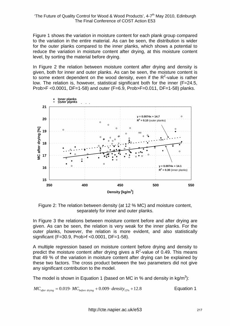
‘The Future of Quality Control for Wood & Wood Products’, 4-7th May 2010, Edinburgh The Final Conference of COST Action E53
Figure 1 shows the variation in moisture content for each plank group compared to the variation in the entire material. As can be seen, the distribution is wider for the outer planks compared to the inner planks, which shows a potential to reduce the variation in moisture content after drying, at this moisture content level, by sorting the material before drying.
In Figure 2 the relation between moisture content after drying and density is given, both for inner and outer planks. As can be seen, the moisture content is to some extent dependent on the wood density, even if the R2-value is rather low. The relation is, however, statistical significant both for the inner (F=24.5, Prob>F <0.0001, DF=1-58) and outer (F=6.9, Prob>F=0.011, DF=1-58) planks.
y = 0.0074x + 14.1R2 = 0.30 (inner planks)
y = 0.0074x + 14.7R2 = 0.10 (outer planks)
15
16
17
18
19
20
21
350 400 450 500 550
Density [kg/m3]
MC
afte
r dry
ing
[%]
Inner planksOuter planksLi (I l k )
Figure 2: The relation between density (at 12 % MC) and moisture content, separately for inner and outer planks.
In Figure 3 the relations between moisture content before and after drying are given. As can be seen, the relation is very weak for the inner planks. For the outer planks, however, the relation is more evident, and also statistically significant (F=30.9, Prob>f <0.0001, DF=1-58).
A multiple regression based on moisture content before drying and density to predict the moisture content after drying gives a R2-value of 0.49. This means that 49 % of the variation in moisture content after drying can be explained by these two factors. The cross product between the two parameters did not give any significant contribution to the model.
The model is shown in Equation 1 (based on MC in % and density in kg/m3):
8.12009.0019.0 %12 +⋅+⋅= densityMCMC dryingbeforedryingafter Equation 1
http://cte.napier.ac.uk/e53 217
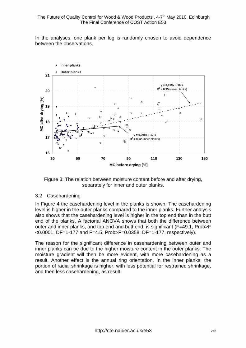
‘The Future of Quality Control for Wood & Wood Products’, 4-7th May 2010, Edinburgh The Final Conference of COST Action E53
In the analyses, one plank per log is randomly chosen to avoid dependence between the observations.
y = 0,008x + 17,1R2 = 0,02 (inner planks)
y = 0,019x + 16,5R2 = 0,35 (outer planks)
16
17
18
19
20
21
30 50 70 90 110 130 150MC before drying [%]
MC
afte
r dry
ing
[%]
Inner planks
Outer planks
Figure 3: The relation between moisture content before and after drying, separately for inner and outer planks.
3.2 Casehardening In Figure 4 the casehardening level in the planks is shown. The casehardening level is higher in the outer planks compared to the inner planks. Further analysis also shows that the casehardening level is higher in the top end than in the butt end of the planks. A factorial ANOVA shows that both the difference between outer and inner planks, and top end and butt end, is significant (F=49.1, Prob>F <0.0001, DF=1-177 and F=4.5, Prob>F=0.0358, DF=1-177, respectively).
The reason for the significant difference in casehardening between outer and inner planks can be due to the higher moisture content in the outer planks. The moisture gradient will then be more evident, with more casehardening as a result. Another effect is the annual ring orientation. In the inner planks, the portion of radial shrinkage is higher, with less potential for restrained shrinkage, and then less casehardening, as result.
http://cte.napier.ac.uk/e53 218
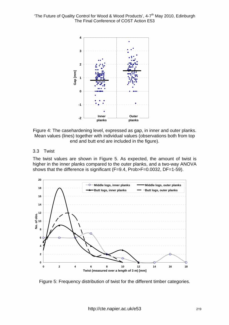
‘The Future of Quality Control for Wood & Wood Products’, 4-7th May 2010, Edinburgh The Final Conference of COST Action E53
-2
-1
0
1
2
3
4
Gap
[mm
]
Innerplanks
Outerplanks
Figure 4: The casehardening level, expressed as gap, in inner and outer planks. Mean values (lines) together with individual values (observations both from top
end and butt end are included in the figure).
3.3 Twist The twist values are shown in Figure 5. As expected, the amount of twist is higher in the inner planks compared to the outer planks, and a two-way ANOVA shows that the difference is significant (F=9.4, Prob>F=0.0032, DF=1-59).
0
2
4
6
8
10
12
14
16
18
20
0 2 4 6 8 10 12 14 16 18Twist (measured over a length of 3 m) [mm]
No.
of o
bs.
Middle logs, inner planks Middle logs, outer planksButt logs, inner planks Butt logs, outer planks
Figure 5: Frequency distribution of twist for the different timber categories.
http://cte.napier.ac.uk/e53 219
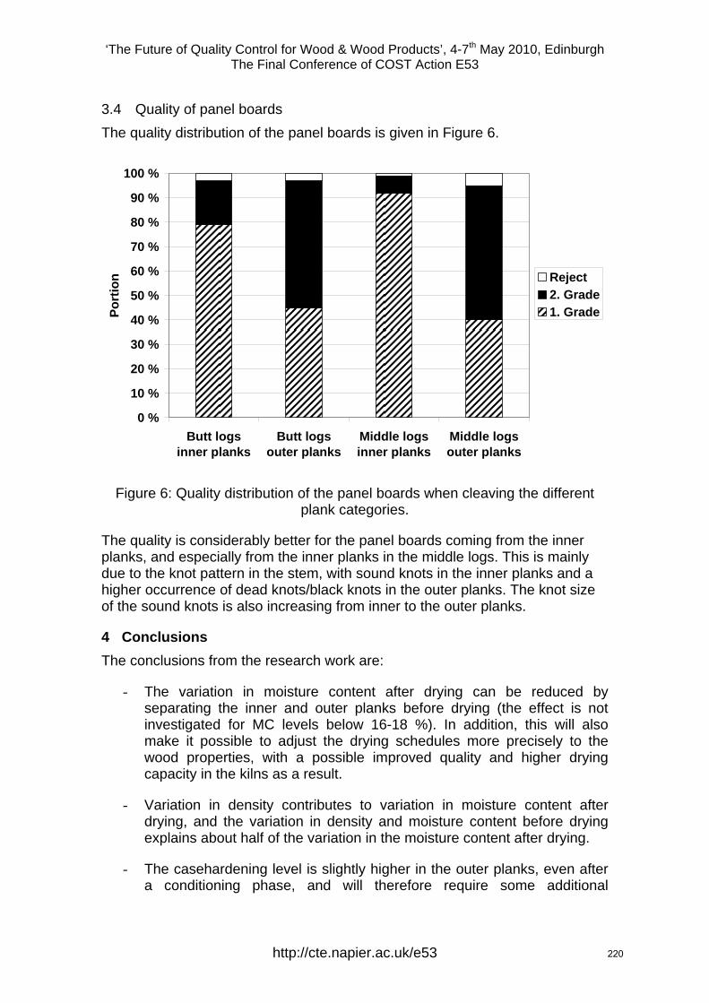
‘The Future of Quality Control for Wood & Wood Products’, 4-7th May 2010, Edinburgh The Final Conference of COST Action E53
3.4 Quality of panel boards The quality distribution of the panel boards is given in Figure 6.
0 %
10 %
20 %
30 %
40 %
50 %
60 %
70 %
80 %
90 %
100 %
Butt logsinner planks
Butt logsouter planks
Middle logsinner planks
Middle logsouter planks
Port
ion Reject
2. Grade1. Grade
Figure 6: Quality distribution of the panel boards when cleaving the different plank categories.
The quality is considerably better for the panel boards coming from the inner planks, and especially from the inner planks in the middle logs. This is mainly due to the knot pattern in the stem, with sound knots in the inner planks and a higher occurrence of dead knots/black knots in the outer planks. The knot size of the sound knots is also increasing from inner to the outer planks.
4 Conclusions The conclusions from the research work are:
- The variation in moisture content after drying can be reduced by separating the inner and outer planks before drying (the effect is not investigated for MC levels below 16-18 %). In addition, this will also make it possible to adjust the drying schedules more precisely to the wood properties, with a possible improved quality and higher drying capacity in the kilns as a result.
- Variation in density contributes to variation in moisture content after drying, and the variation in density and moisture content before drying explains about half of the variation in the moisture content after drying.
- The casehardening level is slightly higher in the outer planks, even after a conditioning phase, and will therefore require some additional
http://cte.napier.ac.uk/e53 220
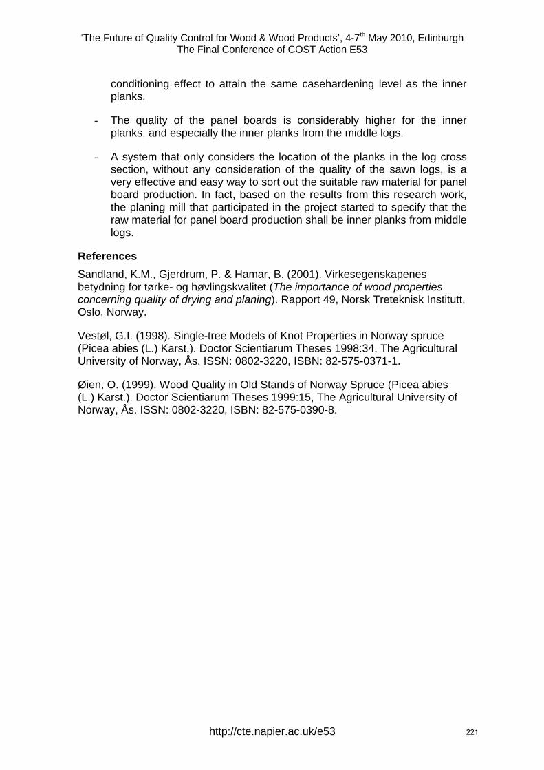
‘The Future of Quality Control for Wood & Wood Products’, 4-7th May 2010, Edinburgh The Final Conference of COST Action E53
conditioning effect to attain the same casehardening level as the inner planks.
- The quality of the panel boards is considerably higher for the inner planks, and especially the inner planks from the middle logs.
- A system that only considers the location of the planks in the log cross section, without any consideration of the quality of the sawn logs, is a very effective and easy way to sort out the suitable raw material for panel board production. In fact, based on the results from this research work, the planing mill that participated in the project started to specify that the raw material for panel board production shall be inner planks from middle logs.
References Sandland, K.M., Gjerdrum, P. & Hamar, B. (2001). Virkesegenskapenes betydning for tørke- og høvlingskvalitet (The importance of wood properties concerning quality of drying and planing). Rapport 49, Norsk Treteknisk Institutt, Oslo, Norway.
Vestøl, G.I. (1998). Single-tree Models of Knot Properties in Norway spruce (Picea abies (L.) Karst.). Doctor Scientiarum Theses 1998:34, The Agricultural University of Norway, Ås. ISSN: 0802-3220, ISBN: 82-575-0371-1.
Øien, O. (1999). Wood Quality in Old Stands of Norway Spruce (Picea abies (L.) Karst.). Doctor Scientiarum Theses 1999:15, The Agricultural University of Norway, Ås. ISSN: 0802-3220, ISBN: 82-575-0390-8.
http://cte.napier.ac.uk/e53 221
‘The Future of Quality Control for Wood & Wood Products’, 4-7th May 2010, Edinburgh The Final Conference of COST Action E53
Emissions of volatile organic compounds from convection dried Norway spruce timber
V. Steckel1, J. Welling2 & M. Ohlmeyer3
Abstract Building products and furnishing are, among others, sources that emit volatile organic compounds (VOCs). The Construction Products Directive of the European Union (CPD) establishes requirements for building products, including demands regarding emission properties. Also harmonised standardisation related to the CPD is under way, implying that VOC emissions will be a relevant property of building products in the future. Objective of this study was to look into the effect of the drying schedule on VOC emissions from convection dried Norway spruce timber. Four different drying schedules, mainly varying in temperature, were employed. Samples dried at high temperature emitted noticeably less VOCs compared to samples dried at low temperature. With less varying temperatures, no clear effects were observed. Further, the amount of moisture lost during drying seems to affect product emissions. The composition of compounds was not influenced by the drying schedule and no harmful compounds could be detected. Emissions did not exceed concentrations of 300 µg m-3. In contrast, preliminary tests on other Norway spruce samples showed emissions up to one order of magnitude higher, due to stress-induced high extractives content of the wood. This example illustrates that spruce wood, being a natural material, may vary considerably regarding its emissions.
1 Introduction The term volatile organic compounds (VOCs) indicates a very diverse group of hydrocarbons that are volatile at ambient temperature. VOCs are emitted into the air by, e.g., plants, animals, microorganisms and most production processes and products. Human exposure to VOCs is regarded as a public health issue. Major sources influencing indoor air quality are polluted outdoor air, human activities such as cooking, use of cleaning agents or smoking as well as building products and furnishing. For reduction and control of potential indoor emission sources several national and European activities like health-related assessment schemes or eco-labelling were started. The European Construction Products Directive (CPD, 89/106/EEC) established a framework of requirements for building products to ensure their free circulation and unrestricted use in the European single market. The essential requirement No. 3 of the CPD states that hygiene and health of occupants must not be put at risk by dangerous substances emitted from the building. In 2008, the European Commission
1 PhD student, [email protected] of Wood Technology and Wood Biology, vTI, Germany 2 Senior Scientist, [email protected] Senior Scientist, [email protected]
http://cte.napier.ac.uk/e53 222

‘The Future of Quality Control for Wood & Wood Products’, 4-7th May 2010, Edinburgh The Final Conference of COST Action E53
proposed substituting the CPD by an EU regulation with the same objective (Anonymous 2008). Concurrently, harmonised standardisation related to the specifications of the CPD is under way (Anonymous 2005). These developments show that VOC emissions will be a relevant property of building products in the future.
Kiln dried timber of Norway spruce (Picea abies) is commonly used in Central and Northern Europe for manufacturing building products and furniture. However, softwoods are usually rich in extractives and therefore can release substantial amounts of VOCs, mainly terpenes and aldehydes. While terpenes are constituent parts of softwood resin and responsible for the typical smell of softwood timber, aldehydes are secondary emissions that are formed by oxidation of fatty acids in the wood. They mostly smell dull and rancid. The amount of both terpenes and fatty acids varies from tree to tree and also depends on the location in the tree (Back and Allan 2000). Besides, stress of the tree can result in an increased extractives content. In contrast to synthetic products, emissions of timber cannot be influenced by changing its composition. Instead manipulation of the drying schedule might be a tool to affect subsequent emissions, assuming that compounds that are emitted in the drying process cannot contribute to emissions of the dried timber later.
Wu and Milota (1999) showed that the cumulated emissions of a drying run were increased at higher drying temperatures compared to lower temperatures. If the target moisture content (MC) was constant, higher initial MC resulted in higher absolute process emissions. The authors concluded that increasing the temperature results in increased volatilisation of compounds. Further, higher initial MC means that more water and, correspondingly, more volatile compounds are transported to the wood surface and evaporate. Also drying time is prolonged with higher green MC, resulting in a longer impact of temperature. Bengtsson and Sanati (2004) compared the total hydrocarbon emissions of Scots pine sapwood and heartwood during drying at different temperatures. An increase in temperature resulted in higher process emissions, especially of terpenes. Comparing drying runs at 90 °C with runs at 50 °C, the total amount of emitted α-pinene (a terpene) increased threefold. Using a laboratory drier allowed for exact control of exhaust air streams. Englund and Nussbaum (2000) studied the terpene content of Norway spruce timber before and after drying at 60 °C or 110 °C. The depletion of the wood was higher after high-temperature drying than after drying at normal temperature.
The aim of the study presented was to look into the effect of drying temperature on the emissions of convection dried Norway spruce timber. Four different schedules, varying chiefly in temperature, were applied. Samples taken from the dried boards were emission tested. The results were compared regarding amount and composition of the released compounds. Besides, the results were compared to preliminary emission tests of other dried Norway spruce samples.
http://cte.napier.ac.uk/e53 223

‘The Future of Quality Control for Wood & Wood Products’, 4-7th May 2010, Edinburgh The Final Conference of COST Action E53
2 Material Six logs of Norway spruce (Picea abies) with a length of three meters and a mid-diameter of 30 to 35 cm were selected for cutting sample boards. The logs had been harvested two months before drying in the Black Forest (south-western Germany). From each log, four to six sample boards were prepared with the dimensions 2000 x 100 x 27 mm3. The quarter sawn boards contained both sapwood and heartwood in similar amounts. Additional logs of the same origin were cut for being used for protection during transport and as filling material in the kiln. The material was grouped in four packages according to the four drying schedules. The objective was to prevent effects of the drying schedule being biased due to differences in the extractives content of the wood. Extractives content can vary considerably between trees. Therefore, by distributing the boards from each log evenly on the four packages, comparable material was provided to go into each drying run. Until drying, the wrapped packages were stored in a refrigerated storage house. A lab convection kiln was used for drying. One charge contained 0.85 m3 of material in total, with the sample boards stacked in the middle of the pile. The following drying schedules were applied:
• Normal temperature schedule (NT): Starting at a dry bulb temperature (DBT) of 55 °C and an equilibrium moisture content (EMC) of 12 %. The temperature was raised to a maximum of 65 °C while the EMC was decreased to 5 %
• Normal temperature schedule with increased final temperature (NTplus): See NT schedule, but with a final temperature of 85 °C instead of 65 °C.
• High temperature schedule (HT): Starting at a DBT of 85 °C and an EMC of 12 %. The temperature was increased to 115 °C while the EMC was decreased to 4 %.
• Low temperature schedule (LT): On the basis of the System 603 by Muehlboeck GmbH (Eberschwang, Austria). At minimum EMCs, increased air flow, and 45 °C DBT, the timber is dried until fiber saturation. Then temperature and EMC are increased to 65 °C and 12 %, respectively. An additional fan was installed in a side opening of the pilot kiln, and the exhaust air-outlet was opened permanently during the first part of the schedule to ensure increased airflow. Minimum EMC was 3.75 %.
Each drying schedule ended with a conditioning phase of three hours at 12 % EMC. An equalisation phase at 20 to 25 °C with slowly rotating fans followed for at least three days. Since wood MC influences emissions, very homogeneous MCs were essential. Prior to and after drying, a bar (cross section) was cut from each sample board to determine the MC. Immediately after unstacking, the sample boards were cut to prepare specimens for emission testing. Knots, cracks, resin pockets as well as material from the ends of the boards were excluded. The area of a single emission test specimen was 200 x 60.2 mm2, with a thickness of 25 to 26.5 mm. The edges of the specimens were sealed with self-adhesive aluminium foil to test faces exclusively. Emission testing was accomplished using test chambers with controlled climatic parameters. The total
http://cte.napier.ac.uk/e53 224
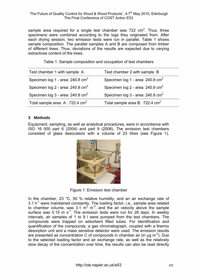
‘The Future of Quality Control for Wood & Wood Products’, 4-7th May 2010, Edinburgh The Final Conference of COST Action E53
sample area required for a single test chamber was 722 cm2. Thus, three specimens were combined according to the logs they originated from. After each drying session, two emission tests were run in parallel. Table 1 shows sample composition. The parallel samples A and B are composed from timber of different trees. Thus, deviations of the results are expected due to varying extractives content of the trees.
Table 1: Sample composition and occupation of test chambers
Test chamber 1 with sample A Test chamber 2 with sample B
Specimen log 1 - area: 240.8 cm2 Specimen log 1 - area: 240.8 cm2
Specimen log 2 - area: 240.8 cm2 Specimen log 2 - area: 240.8 cm2
Specimen log 3 - area: 240.8 cm2 Specimen log 3 - area: 240.8 cm2
Total sample area A : 722.4 cm2 Total sample area B: 722.4 cm2
3 Methods Equipment, sampling, as well as analytical procedures, were in accordance with ISO 16 000 part 6 (2004) and part 9 (2008). The emission test chambers consisted of glass desiccators with a volume of 23 litres (see Figure 1).
Figure 1: Emission test chamber
In the chamber, 23 °C, 50 % relative humidity, and an air exchange rate of 3.1 h-1 were maintained constantly. The loading factor, i.e., sample area related to chamber volume, was 3.1 m2 m-3, and the air velocity above the sample surface was 0.15 m s-1. The emission tests were run for 28 days. In weekly intervals, air samples of 1 to 9 l were pumped from the test chambers. The compounds were trapped on adsorbent filled tubes. For identification and quantification of the compounds, a gas chromatograph, coupled with a thermo desorption unit and a mass sensitive detector were used. The emission results are presented as concentration C of compounds in chamber air (in µg m-3). Due to the selected loading factor and air exchange rate, as well as the relatively slow decay of the concentration over time, the results can also be read directly
http://cte.napier.ac.uk/e53 225
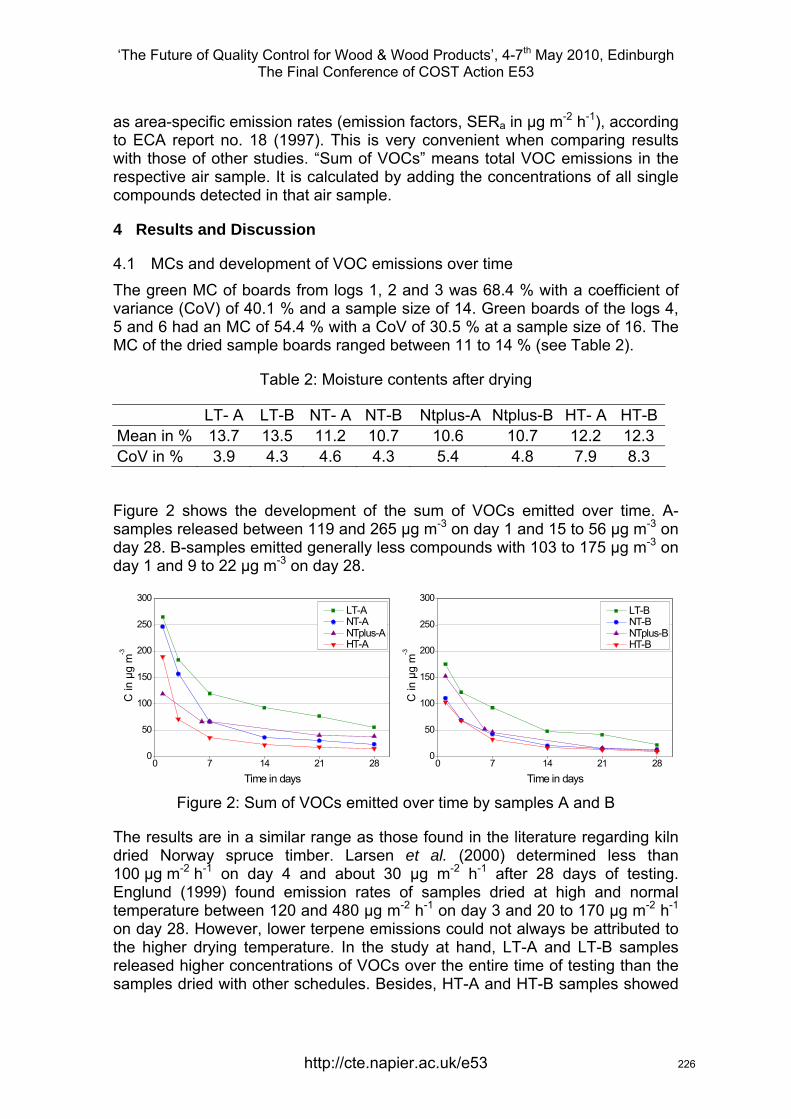
‘The Future of Quality Control for Wood & Wood Products’, 4-7th May 2010, Edinburgh The Final Conference of COST Action E53
as area-specific emission rates (emission factors, SERa in µg m-2 h-1), according to ECA report no. 18 (1997). This is very convenient when comparing results with those of other studies. “Sum of VOCs” means total VOC emissions in the respective air sample. It is calculated by adding the concentrations of all single compounds detected in that air sample.
4 Results and Discussion
4.1 MCs and development of VOC emissions over time The green MC of boards from logs 1, 2 and 3 was 68.4 % with a coefficient of variance (CoV) of 40.1 % and a sample size of 14. Green boards of the logs 4, 5 and 6 had an MC of 54.4 % with a CoV of 30.5 % at a sample size of 16. The MC of the dried sample boards ranged between 11 to 14 % (see Table 2).
Table 2: Moisture contents after drying
LT- A LT-B NT- A NT-B Ntplus-A Ntplus-B HT- A HT-BMean in % 13.7 13.5 11.2 10.7 10.6 10.7 12.2 12.3 CoV in % 3.9 4.3 4.6 4.3 5.4 4.8 7.9 8.3
Figure 2 shows the development of the sum of VOCs emitted over time. A-samples released between 119 and 265 µg m-3 on day 1 and 15 to 56 µg m-3 on day 28. B-samples emitted generally less compounds with 103 to 175 µg m-3 on day 1 and 9 to 22 µg m-3 on day 28.
0 7 14 21 280
50
100
150
200
250
300
C in
µg
m -3
Time in days
LT-A NT-A NTplus-A HT-A
0 7 14 21 280
50
100
150
200
250
300
C in
µg
m -3
Time in days
LT-B NT-B NTplus-B HT-B
Figure 2: Sum of VOCs emitted over time by samples A and B
The results are in a similar range as those found in the literature regarding kiln dried Norway spruce timber. Larsen et al. (2000) determined less than 100 µg m-2 h-1 on day 4 and about 30 µg m-2 h-1 after 28 days of testing. Englund (1999) found emission rates of samples dried at high and normal temperature between 120 and 480 µg m-2 h-1 on day 3 and 20 to 170 µg m-2 h-1 on day 28. However, lower terpene emissions could not always be attributed to the higher drying temperature. In the study at hand, LT-A and LT-B samples released higher concentrations of VOCs over the entire time of testing than the samples dried with other schedules. Besides, HT-A and HT-B samples showed
http://cte.napier.ac.uk/e53 226
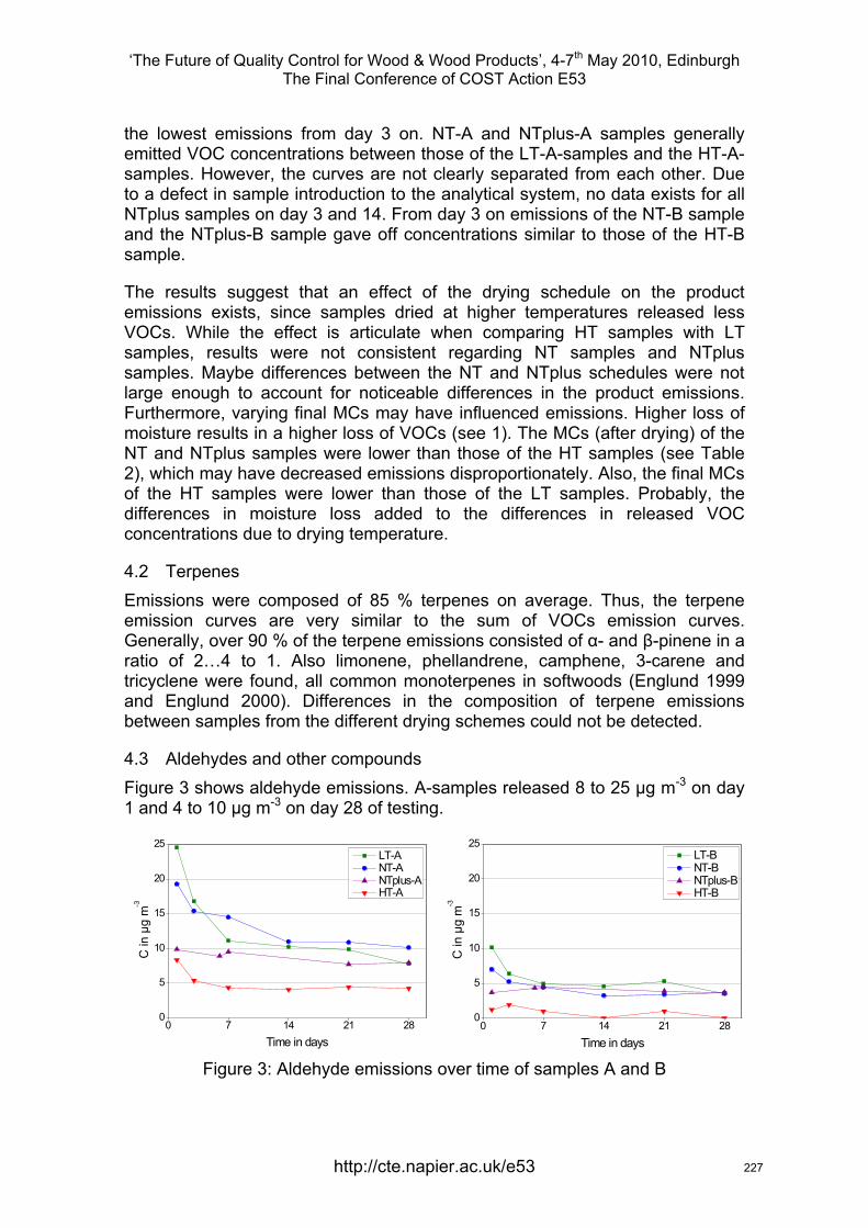
‘The Future of Quality Control for Wood & Wood Products’, 4-7th May 2010, Edinburgh The Final Conference of COST Action E53
the lowest emissions from day 3 on. NT-A and NTplus-A samples generally emitted VOC concentrations between those of the LT-A-samples and the HT-A-samples. However, the curves are not clearly separated from each other. Due to a defect in sample introduction to the analytical system, no data exists for all NTplus samples on day 3 and 14. From day 3 on emissions of the NT-B sample and the NTplus-B sample gave off concentrations similar to those of the HT-B sample.
The results suggest that an effect of the drying schedule on the product emissions exists, since samples dried at higher temperatures released less VOCs. While the effect is articulate when comparing HT samples with LT samples, results were not consistent regarding NT samples and NTplus samples. Maybe differences between the NT and NTplus schedules were not large enough to account for noticeable differences in the product emissions. Furthermore, varying final MCs may have influenced emissions. Higher loss of moisture results in a higher loss of VOCs (see 1). The MCs (after drying) of the NT and NTplus samples were lower than those of the HT samples (see Table 2), which may have decreased emissions disproportionately. Also, the final MCs of the HT samples were lower than those of the LT samples. Probably, the differences in moisture loss added to the differences in released VOC concentrations due to drying temperature.
4.2 Terpenes Emissions were composed of 85 % terpenes on average. Thus, the terpene emission curves are very similar to the sum of VOCs emission curves. Generally, over 90 % of the terpene emissions consisted of α- and β-pinene in a ratio of 2…4 to 1. Also limonene, phellandrene, camphene, 3-carene and tricyclene were found, all common monoterpenes in softwoods (Englund 1999 and Englund 2000). Differences in the composition of terpene emissions between samples from the different drying schemes could not be detected.
4.3 Aldehydes and other compounds Figure 3 shows aldehyde emissions. A-samples released 8 to 25 µg m-3 on day 1 and 4 to 10 µg m-3 on day 28 of testing.
0 7 14 21 280
5
10
15
20
25
C in
µg
m -3
Time in days
LT-A NT-A NTplus-A HT-A
0 7 14 21 280
5
10
15
20
25
C in
µg
m -3
Time in days
LT-B NT-B NTplus-B HT-B
Figure 3: Aldehyde emissions over time of samples A and B
http://cte.napier.ac.uk/e53 227
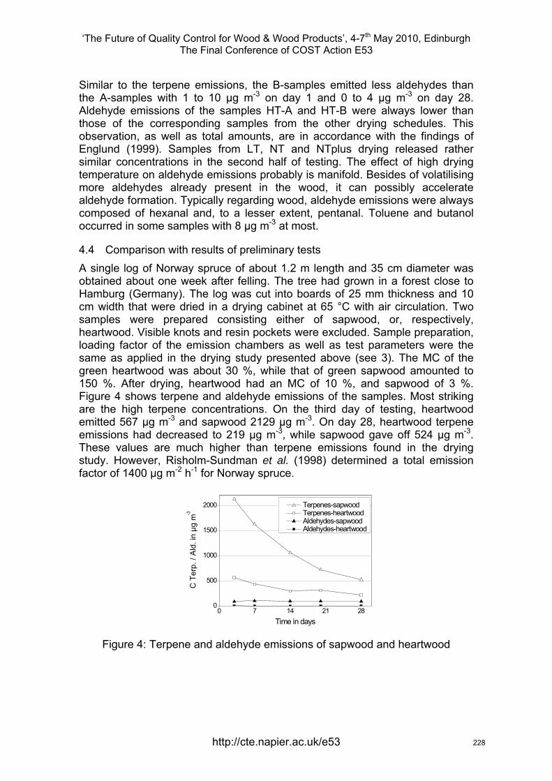
‘The Future of Quality Control for Wood & Wood Products’, 4-7th May 2010, Edinburgh The Final Conference of COST Action E53
Similar to the terpene emissions, the B-samples emitted less aldehydes than the A-samples with 1 to 10 µg m-3 on day 1 and 0 to 4 µg m-3 on day 28. Aldehyde emissions of the samples HT-A and HT-B were always lower than those of the corresponding samples from the other drying schedules. This observation, as well as total amounts, are in accordance with the findings of Englund (1999). Samples from LT, NT and NTplus drying released rather similar concentrations in the second half of testing. The effect of high drying temperature on aldehyde emissions probably is manifold. Besides of volatilising more aldehydes already present in the wood, it can possibly accelerate aldehyde formation. Typically regarding wood, aldehyde emissions were always composed of hexanal and, to a lesser extent, pentanal. Toluene and butanol occurred in some samples with 8 µg m-3 at most.
4.4 Comparison with results of preliminary tests A single log of Norway spruce of about 1.2 m length and 35 cm diameter was obtained about one week after felling. The tree had grown in a forest close to Hamburg (Germany). The log was cut into boards of 25 mm thickness and 10 cm width that were dried in a drying cabinet at 65 °C with air circulation. Two samples were prepared consisting either of sapwood, or, respectively, heartwood. Visible knots and resin pockets were excluded. Sample preparation, loading factor of the emission chambers as well as test parameters were the same as applied in the drying study presented above (see 3). The MC of the green heartwood was about 30 %, while that of green sapwood amounted to 150 %. After drying, heartwood had an MC of 10 %, and sapwood of 3 %. Figure 4 shows terpene and aldehyde emissions of the samples. Most striking are the high terpene concentrations. On the third day of testing, heartwood emitted 567 µg m-3 and sapwood 2129 µg m-3. On day 28, heartwood terpene emissions had decreased to 219 µg m-3, while sapwood gave off 524 µg m-3. These values are much higher than terpene emissions found in the drying study. However, Risholm-Sundman et al. (1998) determined a total emission factor of 1400 µg m-2 h-1 for Norway spruce.
0 7 14 21 280
500
1000
1500
2000
C T
erp.
/ A
ld. i
n µg
m
-3
Time in days
Terpenes-sapwood Terpenes-heartwood Aldehydes-sapwood Aldehydes-heartwood
Figure 4: Terpene and aldehyde emissions of sapwood and heartwood
http://cte.napier.ac.uk/e53 228
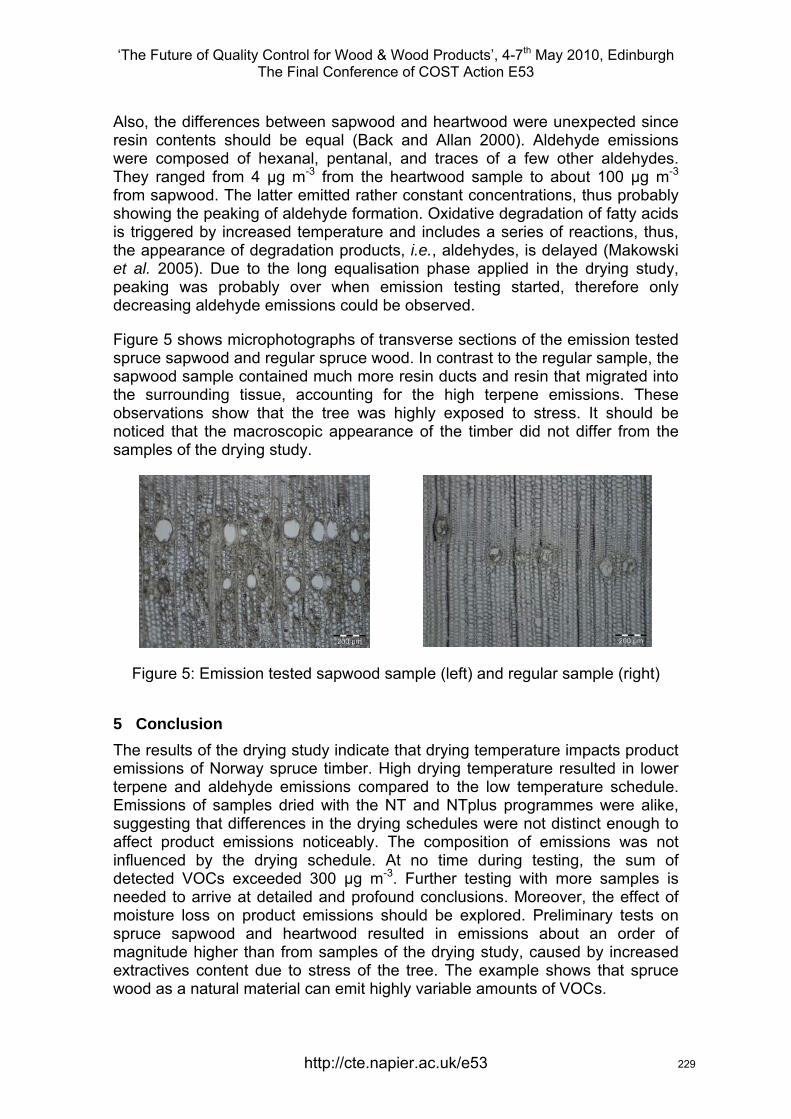
‘The Future of Quality Control for Wood & Wood Products’, 4-7th May 2010, Edinburgh The Final Conference of COST Action E53
Also, the differences between sapwood and heartwood were unexpected since resin contents should be equal (Back and Allan 2000). Aldehyde emissions were composed of hexanal, pentanal, and traces of a few other aldehydes. They ranged from 4 µg m-3 from the heartwood sample to about 100 µg m-3 from sapwood. The latter emitted rather constant concentrations, thus probably showing the peaking of aldehyde formation. Oxidative degradation of fatty acids is triggered by increased temperature and includes a series of reactions, thus, the appearance of degradation products, i.e., aldehydes, is delayed (Makowski et al. 2005). Due to the long equalisation phase applied in the drying study, peaking was probably over when emission testing started, therefore only decreasing aldehyde emissions could be observed.
Figure 5 shows microphotographs of transverse sections of the emission tested spruce sapwood and regular spruce wood. In contrast to the regular sample, the sapwood sample contained much more resin ducts and resin that migrated into the surrounding tissue, accounting for the high terpene emissions. These observations show that the tree was highly exposed to stress. It should be noticed that the macroscopic appearance of the timber did not differ from the samples of the drying study.
Figure 5: Emission tested sapwood sample (left) and regular sample (right)
5 Conclusion The results of the drying study indicate that drying temperature impacts product emissions of Norway spruce timber. High drying temperature resulted in lower terpene and aldehyde emissions compared to the low temperature schedule. Emissions of samples dried with the NT and NTplus programmes were alike, suggesting that differences in the drying schedules were not distinct enough to affect product emissions noticeably. The composition of emissions was not influenced by the drying schedule. At no time during testing, the sum of detected VOCs exceeded 300 µg m-3. Further testing with more samples is needed to arrive at detailed and profound conclusions. Moreover, the effect of moisture loss on product emissions should be explored. Preliminary tests on spruce sapwood and heartwood resulted in emissions about an order of magnitude higher than from samples of the drying study, caused by increased extractives content due to stress of the tree. The example shows that spruce wood as a natural material can emit highly variable amounts of VOCs.
http://cte.napier.ac.uk/e53 229
‘The Future of Quality Control for Wood & Wood Products’, 4-7th May 2010, Edinburgh The Final Conference of COST Action E53
6 References Anonymous (2005): “Development of horizontal standardised assessment methods for harmonised approaches (…)” http://www.umweltbundesamt.de/ bauprodukte/dokumente/m366en.pdf [Accessed 18th February 2010].
Anonymous (2008): “Proposal for a regulation of the European parliament and of the council (…)” http://www.umweltbundesamt.de/building-products/archive/ proposal_cpr_23-5-2008.pdf [Accessed 18th February 2010].
DIN EN ISO 16000 - 6 (2004) "Indoor air - Determination of volatile organic compounds in indoor and test chamber air by active sampling on Tenax TA® sorbent, thermal desorption and gas chromatography using MS/FID".
DIN EN ISO 16000 - 9 (2008) "Indoor air - Determination of the emission of volatile organic compounds from building products and furnishing".
Back, E.L. and Allan, L.H. (Eds.) (2000) "Pitch Control, Wood Resin and Deresination". TAPPI Press, Atlanta, 392 pp.
Bengtsson, P. and Sanati, M. (2004) "Evaluation of hydrocarbon emissions from heart- and sapwood of Scots pine using a laboratory-scale wood drier", Holzforschung, 58(6), pp 660-665.
ECA (1997) Report No. 18 "Evaluation of VOC Emissions from Building Products. Solid Flooring Materials". European Collaborative Action, 121 pp.
Englund, F. (1999) "Emissions of volatile organic compounds from wood". Trätek - Swedish Institute for Wood Technology Research Stockholm, 44 pp.
Englund, F. and Nussbaum, R.M. (2000) "Monoterpenes in Scots pine and Norway spruce and their emission during kiln drying", Holzforschung, 54(5), pp 449-456.
Larsen, A., Frost, L. and Funch, L.W. (2000) "Emission of Volatile Organic Compounds from Wood and Wood-based Materials - Working Report No. 15", Danish Technological Institute, 77 pp.
Makowski, M., Ohlmeyer, M. and Meier, D. (2005) “Long-term developement of VOC emissions from OSB after hot-pressing”, Holzforschung, 59(4) pp 519-523.
Risholm-Sundman, M., Lundgren, M., Vestin, E. and Herder, P. (1998) "Emissions of acetic acid and other volatile organic compounds from different species of solid wood", Holz als Roh- und Werkstoff, 56 pp 125–129.
Wu, J. and Milota, M.R. (1999) “Effect of temperature and humidity on total hydrocarbon emissions from Douglas-fir lumber”, Forest Products Journal, 49(6) pp 52-60.
http://cte.napier.ac.uk/e53 230

‘The Future of Quality Control for Wood & Wood Products’, 4-7th May 2010, Edinburgh The Final Conference of COST Action E53
Wednesday 5th May Industry focussed day
4th session
http://www.cte.napier.ac.uk/e53/ 231
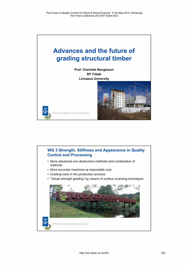
Advances and the future of grading structural timber
Prof. Charlotte BengtssonSP Trätek
Linnaeus University
WG 3 Strength, Stiffness and Appearance in Quality Control and Processing • More advanced non-destructive methods and combination of
methods• More accurate machines at reasonable cost• Grading early in the production process• ”Visual strength grading” by means of surface scanning techniques
‘The Future of Quality Control for Wood & Wood Products’, 4-7th May 2010, EdinburghThe Final Conference of COST Action E53
http://cte.napier.ac.uk/e53 232
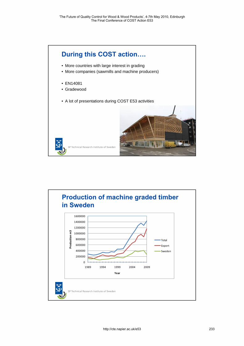
During this COST action….• More countries with large interest in grading• More companies (sawmills and machine producers)
• EN14081• Gradewood
• A lot of presentations during COST E53 activities
Production of machine graded timber in Sweden
0
200000
400000
600000
800000
1000000
1200000
1400000
1600000
1989 1994 1999 2004 2009
Prod
uction
m3
Year
Total
Export
Sweden
‘The Future of Quality Control for Wood & Wood Products’, 4-7th May 2010, EdinburghThe Final Conference of COST Action E53
http://cte.napier.ac.uk/e53 233
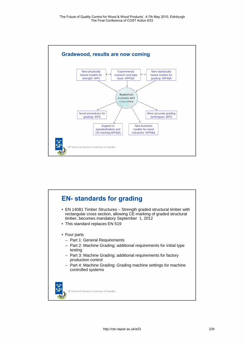
Gradewood, results are now coming
New physically based models for
strength: WP1
Experimental research and data
base: WP2&3
Novel procedures for grading: WP5
New statistically based models for grading: WP4&5
Numerical analysis and simulation
Support to standardisation and CE-marking:WP5&6
New business models for wood
industries: WP5&6
More accurate grading techniques: WP5
EN- standards for grading• EN 14081 Timber Structures – Strength graded structural timber with
rectangular cross section, allowing CE-marking of graded structural timber, becomes mandatory September 1, 2012
• This standard replaces EN 519
• Four parts– Part 1: General Requirements– Part 2: Machine Grading; additional requirements for initial type
testing– Part 3: Machine Grading; additional requirements for factory
production control– Part 4: Machine Grading; Grading machine settings for machine
controlled systems
‘The Future of Quality Control for Wood & Wood Products’, 4-7th May 2010, EdinburghThe Final Conference of COST Action E53
http://cte.napier.ac.uk/e53 234

EN- standards for grading• ”New” procedure for derivation of machine settings
• Settings applicable for one country or some countries
• Two principles– Machine control– Output control
• The standard covers both visual and machine strength grading
• Visual override requirements as previously
Example from 14081 - 4Source country or countries
Source mark a)
Species Permitted timber sizes b) (mm)
Grade or grade combination
Settings IP (machine units)
Comments and additional requirements
C24 4 300 000 TR26 C16
6 150 000 4 300 000
TR26 C18
6 150 000 4 300 000
C27 C18
6 150 000 4 420 000
C30 C18
6 900 000 4 300 000
C30 C24 C18
6 900 000 5 770 000 4 650 000
Finland Norway Sweden Estonia Latvia Russiad)
Poland Germany Austria Czech Republic
FI NO SE ES LV RU PL DE AT CZ
Spruce, Picea abies Fir Abies alba
31 ≤ tn ≤ 110 63 ≤ bn ≤ 264
Actual setting, IP is given in machine units and it is not effected by the timber dimensions.
Requirements for grading: − Air temperature 10°C – 50 °C − Relative humidity in the air < 85 % − Timber temperature > -10 °C − Timber mean moisture content between 10% and 16% Dynagrade − Conveyor speed ≤ 1 m/sec − Spacing between pieces ≥ 200mm − Grading speed ≤ 100 pieces/min Dynagrade HC − Conveyor speed ≤ 1,3 m/sec − Spacing between pieces ≥ 225mm − Grading speed for widths ≤ 250mm: ≤ 150 pieces/min Dynagrade XHC − Conveyor speed ≤ 1,3 m/sec − Spacing between pieces ≥ 225mm − Grading speed for width (w) ≤ 100mm: ≤ 240 pieces/min
where 100 < w ≤ 250 grading speed = 78000/(w+225) pieces/min
Where timber has a mean moisture content between 16% and 20% with a minimum value of 14% and a maximum value of 22% then the settings shall be calculated according to equation (1) and rounded to 3 significant digits.
IPIPIP 0738,018 −= (1) a) See clause 7.3 in EN14081-1 b) Timber sizes shall be to EN 336. c) Grades prefixed by C are strength classes given in EN 338 d) Settings apply only to timber grown west of the Ural mountain range in Russia
Dynagrade
‘The Future of Quality Control for Wood & Wood Products’, 4-7th May 2010, EdinburghThe Final Conference of COST Action E53
http://cte.napier.ac.uk/e53 235

Machine grading principles• Measurement of bending stiffness• Optical detection of knots and other characteristics• Near-Infrared-Reflection spectroscopy (NIR)• Resonant vibrations• Wave propagation speed• Neural nets• Deconvolution technique• Radiation methods
– micro waves– x-ray– γ-radiation
• Combination of techniques
Machine grading principles
Pressroller
Air AirDisplacement
LoadcellReferenceroller
ReferencerollerComputer
Loadroller
Timber
Flatwise bending•Span ca 900 mm•Deflection const. measure load•Load const. measure deflection
Densityγ-ray
x-ray
Density profile
Detectors
Resonant vibrations•Measures
•length
•frequency
•density
fLE AA2
124 −⋅⋅⋅= ρ
‘The Future of Quality Control for Wood & Wood Products’, 4-7th May 2010, EdinburghThe Final Conference of COST Action E53
http://cte.napier.ac.uk/e53 236

Grading machines on the European marketName PrincipleComputermatic/Micromatic Flatwise bending, measurement of deflection
CookBolinders/Techmach Flatwise bending, measurement of load
Grademaster Vibration and scanning
GoldenEye 702/EuroGreComat 702 X-ray
EuroGreComat 704 X-ray and bending
GoldenEye 706/EuroGreComat 706 X-ray and vibrations
GoldenEye 80/1 X-ray and laser scanner
GoldenEye 80/2 X-ray and laser scanner
VM Grader 1.0 Visual grading & gravimetric density
Dynagrade Vibrations in longitudinal direction
Raute Timgrader Flatwise bending, measurement of load
Newnes X-ray
Ersson ESG-240 Flatwise bending, measurement of load
Metriguard 7200 HCLT Flatwise bending, measurement of load
Sylvatest Ultrasonic waves
Grading machines on the European market, cont.
Name PrinciplePrecigrader Vibration and density
Timber Grader MTG Vibration
VISCAN Vibration
Triomatic Ultrasonic waves
E-Scan Vibration
JRT MSR Machine Bending, measurement of deflection
Noesys Vibration
Xyloclass T, Xyloclass F Vibration
CRP360 Bending
Rosgrade Vibration
•Machines with settings according to EN 14081
‘The Future of Quality Control for Wood & Wood Products’, 4-7th May 2010, EdinburghThe Final Conference of COST Action E53
http://cte.napier.ac.uk/e53 237

Why strength grading?
• Accurate knowledge about timber characteristics – strength, stiffness, appearance
• Have a common classification within a market• Obtain an engineering material, gives possibilities to develop the
timber building technique • Optimise the yield
– Adding value– Use of resources– Optimise the use (use good enough quality)
• Timber for structural applications requires grading• Strength, stiffness and density properties need to be known and
to be controlled to stay within desirable limits
Examples from EN 338Strength class Characteristic property C18 C24 C30
Strength properties (MPa), 5%-percentile Bending strength kmf , 18 24 30
Tension strength, parallel to the grain ktf .0. 11 14 18
Tension strength, perpendicular to the grain ktf .90. 0,3 0,4 0,4
Compression strength, parallel to the grain kcf .0. 18 21 23
Compression strength, perpendicular to the grain kcf .90, 4,8 5,3 5,7
Shear strength kf .ν 2,0 2,5 3,0
Stiffness properties (MPa)
MoE parallel to the grain, mean value meanE ,0 9 000 11 000 12 000
MoE parallel to the grain, 5%-percentile 05,0E 6 000 7 400 8 000
MoE, perpendicular to the grain, mean value meanE ,90 300 370 400
Shear modulus, mean value meanG 560 690 750
Density (kg/m³) Density, 5%-percentile
k,12ρ 320 350 380 Density, mean value
mean,12ρ
380 420 460
• Grades can also be defined elsewhere, ex. LS, L, LD for glulam laminations
‘The Future of Quality Control for Wood & Wood Products’, 4-7th May 2010, EdinburghThe Final Conference of COST Action E53
http://cte.napier.ac.uk/e53 238

Basics
• Visual grading–Grading rules, with maximum knot size etc–Trained graders–Scanners
• Machine strength grading–Prediction of strength properties–Classification into strength classes, i.e C18, C24 etc
Visual grading• Visual strength grading has a long tradition• Formal grading rules were established beginning of 20th century (US)• 1930 and onwards visual grading rules were introduced in Europe
‘The Future of Quality Control for Wood & Wood Products’, 4-7th May 2010, EdinburghThe Final Conference of COST Action E53
http://cte.napier.ac.uk/e53 239

Visual grading
• Basis– Rules with criteria for each grade– Trained graders
• Advantages– Simple and cheap– Easy to check the quality
• Disadvantage – Low capacity– Low yield
• Only visually recognisable characteristics can be used• Only simple combinations possible
Machine grading• NDT for grading timber introduced in US and Australia late
1950s• The ”Machine control” system was developed in Europe in the
late 1960s• EN 519 was published 1995• Focus on softwood species• Machine strength grading is
usually complemented with visual override requirements
• More ”complicated” combinationspossible, also high grades
‘The Future of Quality Control for Wood & Wood Products’, 4-7th May 2010, EdinburghThe Final Conference of COST Action E53
http://cte.napier.ac.uk/e53 240
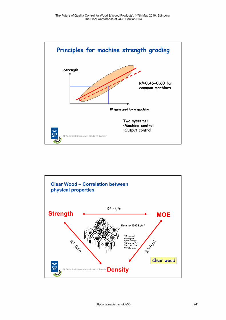
Principles for machine strength grading
Strength
IP measured by a machine
Två system finns:•Maskin kontroll•Out-put kontroll (resultatstyrd metod)
Strength
IP measured by a machine
Strength
IP measured by a machine
Två system finns:•Maskin kontroll•Out-put kontroll (resultatstyrd metod)
R2≈0.45-0.60 for common machines
Two systems:•Machine control•Output control
Clear Wood – Correlation between physical properties
Strength MOE
Density
R²=0,76
R²=0,66 R²=0,6
4
Density 1500 kg/m³
Clear wood
‘The Future of Quality Control for Wood & Wood Products’, 4-7th May 2010, EdinburghThe Final Conference of COST Action E53
http://cte.napier.ac.uk/e53 241
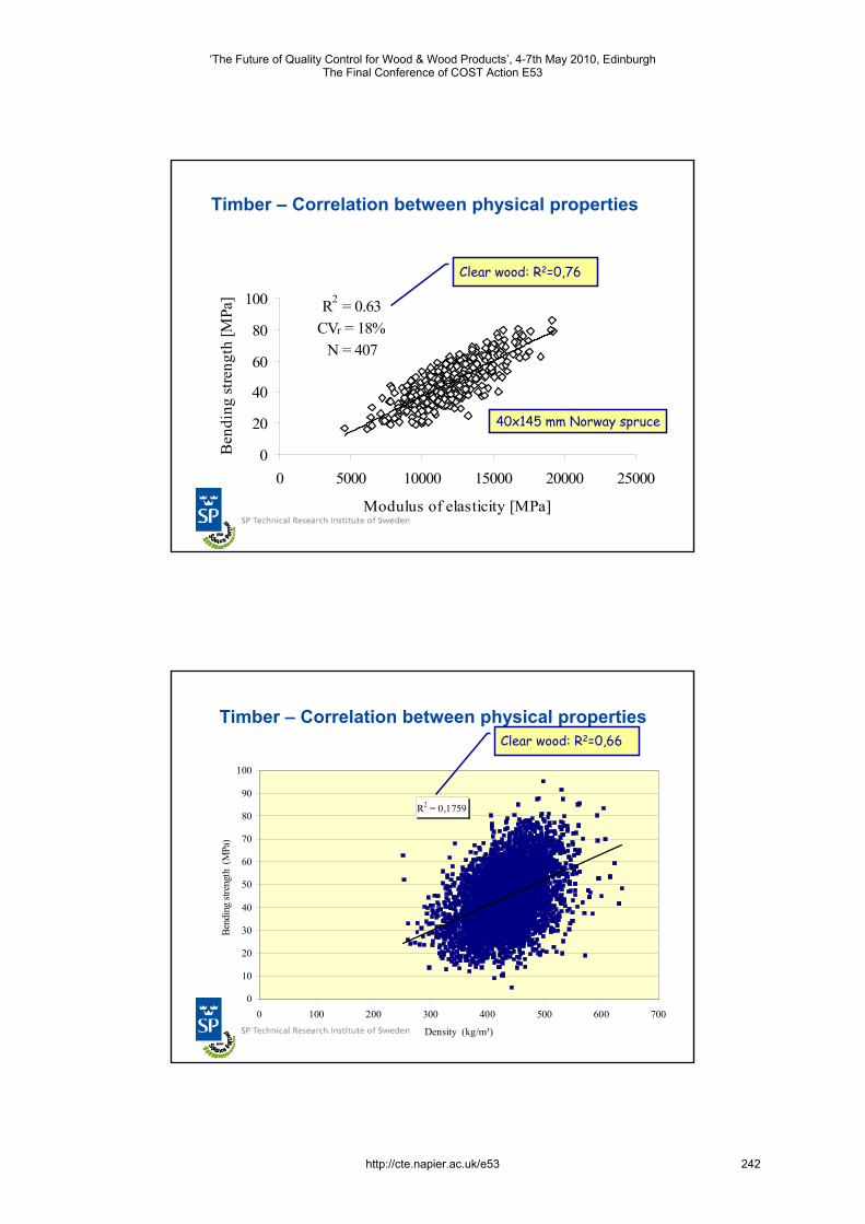
Timber – Correlation between physical properties
R2 = 0.63CVr = 18%
N = 407
0
20
40
60
80
100
0 5000 10000 15000 20000 25000
Modulus of elasticity [MPa]
Ben
ding
stre
ngth
[MPa
]
40x145 mm Norway spruce
Clear wood: R2=0,76
Timber – Correlation between physical properties
R2 = 0,1759
0
10
20
30
40
50
60
70
80
90
100
0 100 200 300 400 500 600 700
Density (kg/m³)
Bend
ing
stren
gth
(MPa
)
Clear wood: R2=0,66
‘The Future of Quality Control for Wood & Wood Products’, 4-7th May 2010, EdinburghThe Final Conference of COST Action E53
http://cte.napier.ac.uk/e53 242
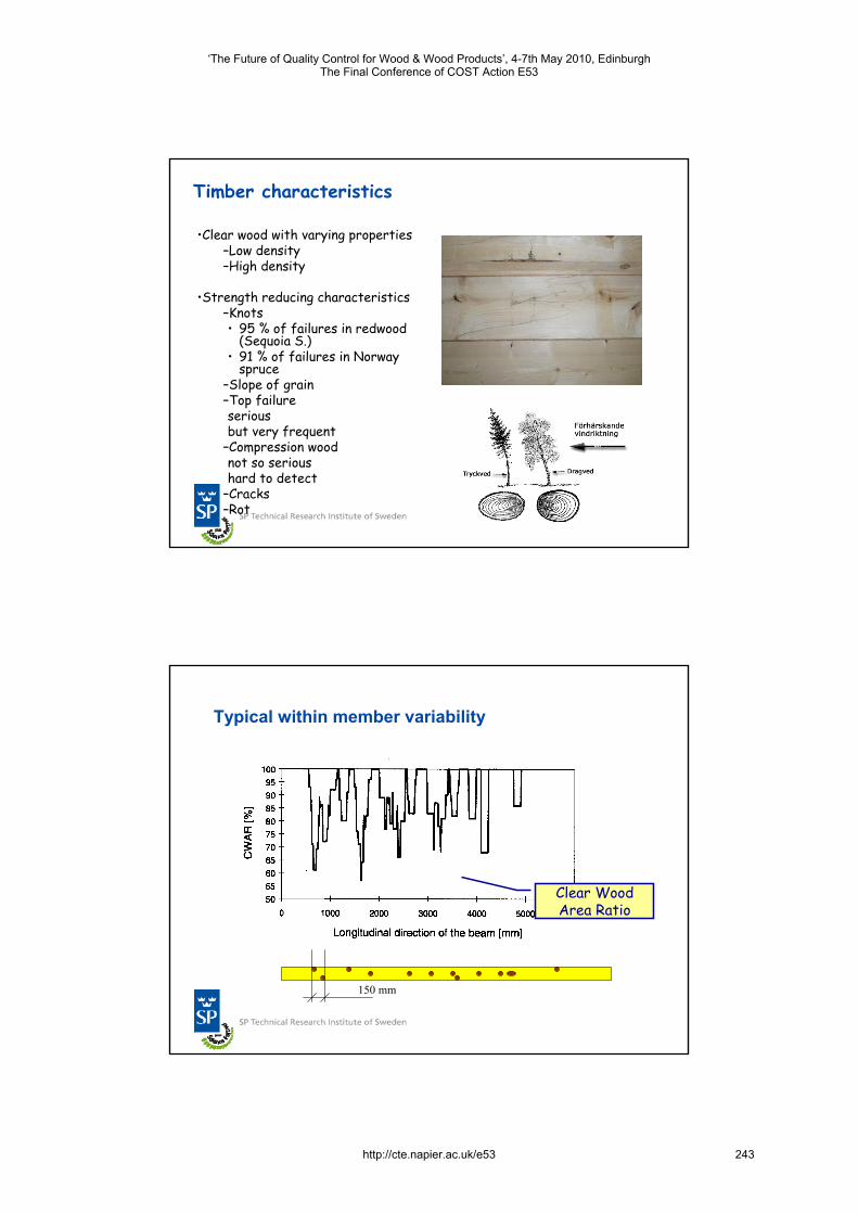
Timber characteristics
•Clear wood with varying properties–Low density–High density
•Strength reducing characteristics–Knots• 95 % of failures in redwood
(Sequoia S.) • 91 % of failures in Norway
spruce–Slope of grain–Top failureseriousbut very frequent
–Compression woodnot so serioushard to detect
–Cracks–Rot
Typical within member variability
150 mm
Clear Wood Area Ratio
‘The Future of Quality Control for Wood & Wood Products’, 4-7th May 2010, EdinburghThe Final Conference of COST Action E53
http://cte.napier.ac.uk/e53 243
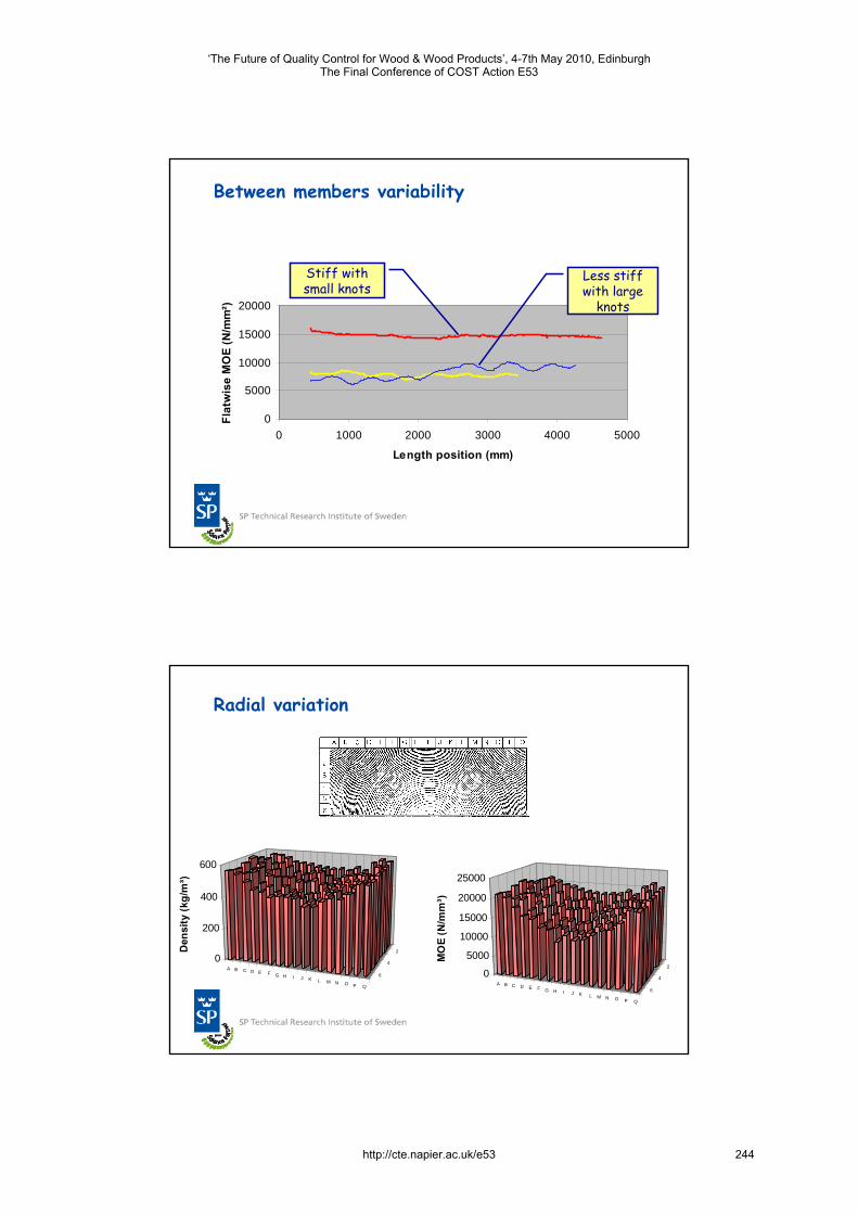
Between members variability
0
5000
10000
15000
20000
0 1000 2000 3000 4000 5000
Length position (mm)
Flat
wis
e M
OE
(N/m
m²)
Less stiff with large
knots
Stiff with small knots
Radial variation
A B C D E F G H I J K L M N O P Q
6
4
2
0
200
400
600
Den
sity
(kg/
m³)
A B C D E F G H I J K L M N O P Q
6
4
2
0
5000
10000
15000
20000
25000
MO
E (N
/mm
³)
‘The Future of Quality Control for Wood & Wood Products’, 4-7th May 2010, EdinburghThe Final Conference of COST Action E53
http://cte.napier.ac.uk/e53 244
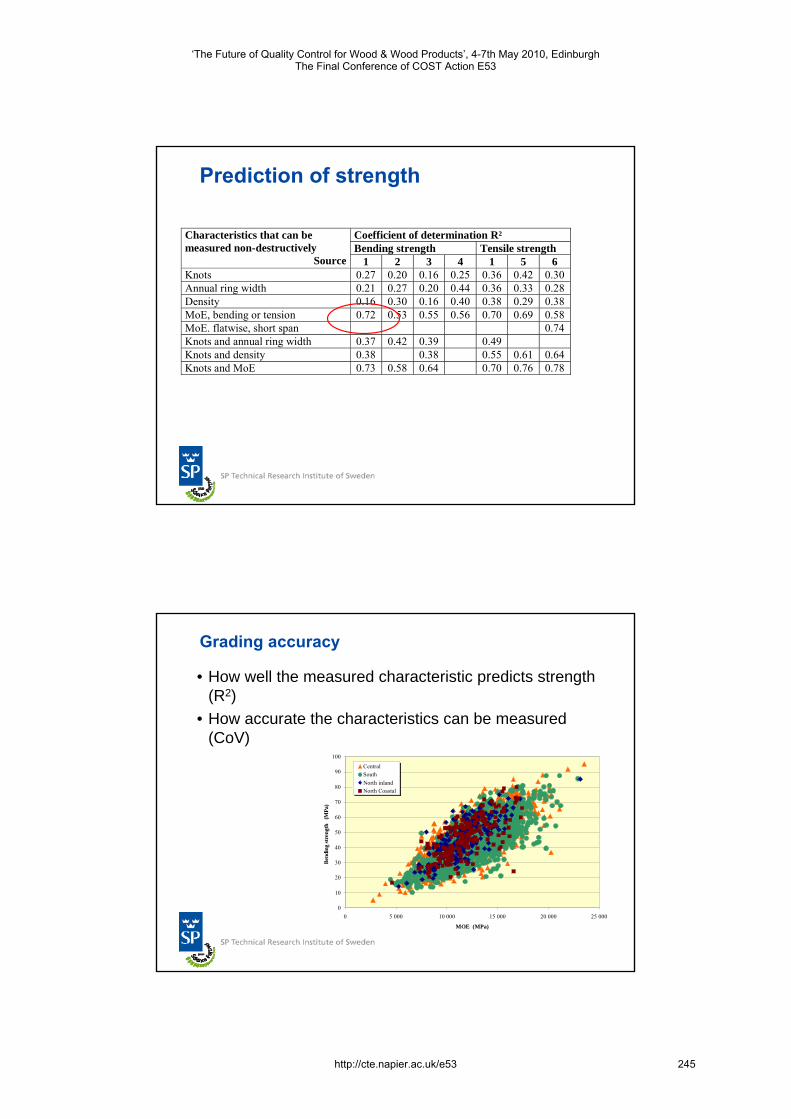
Prediction of strength
Coefficient of determination R² Bending strength Tensile strength
Characteristics that can be measured non-destructively
Source 1 2 3 4 1 5 6 Knots 0.27 0.20 0.16 0.25 0.36 0.42 0.30 Annual ring width 0.21 0.27 0.20 0.44 0.36 0.33 0.28 Density 0.16 0.30 0.16 0.40 0.38 0.29 0.38 MoE, bending or tension 0.72 0.53 0.55 0.56 0.70 0.69 0.58 MoE. flatwise, short span 0.74 Knots and annual ring width 0.37 0.42 0.39 0.49 Knots and density 0.38 0.38 0.55 0.61 0.64 Knots and MoE 0.73 0.58 0.64 0.70 0.76 0.78
Grading accuracy
• How well the measured characteristic predicts strength (R2)
• How accurate the characteristics can be measured (CoV)
0
10
20
30
40
50
60
70
80
90
100
0 5 000 10 000 15 000 20 000 25 000
MOE (MPa)
Bend
ing
stre
ngth
(M
Pa)
CentralSouth North inlandNorth Coastal
‘The Future of Quality Control for Wood & Wood Products’, 4-7th May 2010, EdinburghThe Final Conference of COST Action E53
http://cte.napier.ac.uk/e53 245
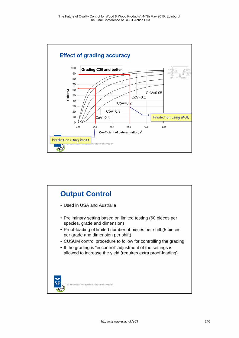
Effect of grading accuracyPressroller
Air AirDisplacement
LoadcellReferenceroller
ReferencerollerComputer
Loadroller
Timber
Grading C30 and better
0
10
20
30
40
50
60
70
80
90
100
0,0 0,2 0,4 0,6 0,8 1,0
Coefficient of determination, r2
Yiel
d (%
)
CoV=0.4CoV=0.3
CoV=0.2CoV=0.1
CoV=0.05
Prediction using MOE
Prediction using knots
Output Control• Used in USA and Australia
• Preliminary setting based on limited testing (60 pieces per species, grade and dimension)
• Proof-loading of limited number of pieces per shift (5 pieces per grade and dimension per shift)
• CUSUM control procedure to follow for controlling the grading• If the grading is “in control” adjustment of the settings is
allowed to increase the yield (requires extra proof-loading)
‘The Future of Quality Control for Wood & Wood Products’, 4-7th May 2010, EdinburghThe Final Conference of COST Action E53
http://cte.napier.ac.uk/e53 246
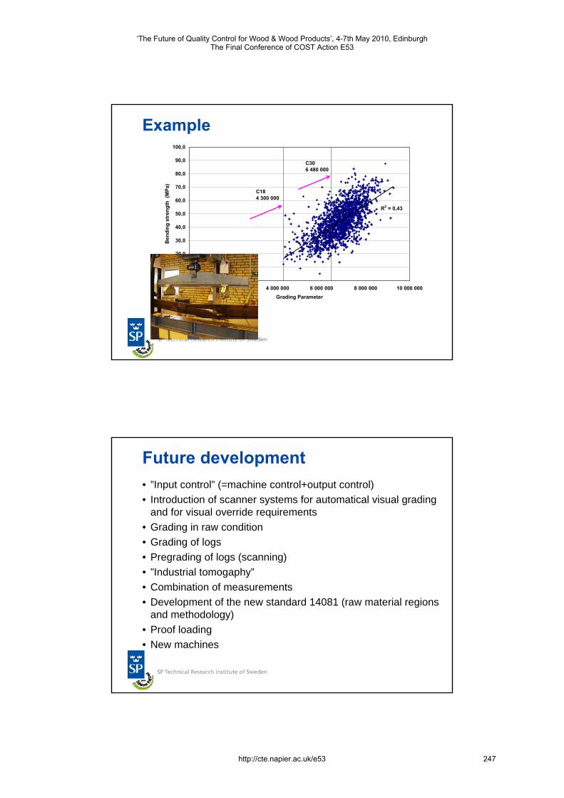
Example
R2 = 0,43
0,0
10,0
20,0
30,0
40,0
50,0
60,0
70,0
80,0
90,0
100,0
0 2 000 000 4 000 000 6 000 000 8 000 000 10 000 000Grading Parameter
Ben
ding
str
engt
h (M
Pa)
C184 300 000
C306 480 000
Future development• ”Input control” (=machine control+output control)• Introduction of scanner systems for automatical visual grading
and for visual override requirements• Grading in raw condition• Grading of logs• Pregrading of logs (scanning)• ”Industrial tomogaphy”• Combination of measurements• Development of the new standard 14081 (raw material regions
and methodology)• Proof loading• New machines
‘The Future of Quality Control for Wood & Wood Products’, 4-7th May 2010, EdinburghThe Final Conference of COST Action E53
http://cte.napier.ac.uk/e53 247

Challenges• Find funding for new R&I-projects• Make a ”better” standard för graded timber• Find better grading methods and procedures so that
timber can be used in a safe way for demanding structures
Thanks for listening!
‘The Future of Quality Control for Wood & Wood Products’, 4-7th May 2010, EdinburghThe Final Conference of COST Action E53
http://cte.napier.ac.uk/e53 248
‘The Future of Quality Control for Wood & Wood Products’, 4-7th May 2010, Edinburgh The Final Conference of COST Action E53
http://cte.napier.ac.uk/e53
Strength grading of wet Norway spruce side boards for use as laminations in wet-glued laminated beams
J. Oscarsson1, A. Olsson2, M. Johansson3, B. Enquist4 & E. Serrano5
Abstract Strength grading of Norway spruce side boards in the wet state was investigated. For a sample of 58 boards of dimensions 25×120×3000 mm3, density and dynamic modulus of elasticity in the axial direction, MOEdyn, were determined in the wet state. The boards were then split into two parts and the procedure of determining MOEdyn was repeated both before and after the boards were dried to a target moisture content of 12 %. Tensile strength of the split boards was finally measured and its relation to MOEdyn for both split and unsplit boards determined. The investigation also included an evaluation of a so called reversed lamination effect on the stiffness caused by the splitting of boards into two parts. The results show that strength grading of split boards in the wet state could give just as good results as grading performed after drying. The coefficient of determination between MOEdyn in wet and dried states was as high as R2=0.92, and the relation between MOEdyn in the wet state and tensile strength in the dried state, σt, was of the same order (R2=0.55) as the relation between MOEdyn in the dried state and σt (R2=0.52). Regarding the reversed lamination effect on the stiffness of split boards, it was found to be of low order.
1 Introduction About 30 % of the volume of sawn timber produced at a typical Swedish sawmill consists of side boards, i.e. boards of narrow dimensions sawn from the outer parts of a log. Large production volumes and small dimensions imply that considerable numbers of side board pieces have to be handled in the sawmilling process and the costs for production, storage and sales are in many cases not met by the selling price on the market.
From previous research it is well known that several wood characteristics that influence the structural properties of sawn timber vary in a distinct way in the direction from pith to bark. For example, the modulus of elasticity (MOE) in softwood trees increases significantly from the pith and outwards (Wormuth
1 PhD Student, [email protected] SP Technical Research Institute of Sweden, Sweden 2 Professor, [email protected] Linnæus University, Sweden 3 Senior University Lecturer, [email protected] Linnæus University, Sweden 4 Research Engineer, [email protected] Linnæus University, Sweden 5 Professor, [email protected] Linnæus University, Sweden
249
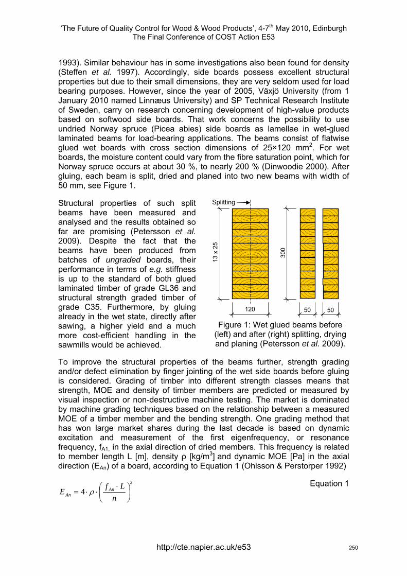
‘The Future of Quality Control for Wood & Wood Products’, 4-7th May 2010, Edinburgh The Final Conference of COST Action E53
http://cte.napier.ac.uk/e53
1993). Similar behaviour has in some investigations also been found for density (Steffen et al. 1997). Accordingly, side boards possess excellent structural properties but due to their small dimensions, they are very seldom used for load bearing purposes. However, since the year of 2005, Växjö University (from 1 January 2010 named Linnæus University) and SP Technical Research Institute of Sweden, carry on research concerning development of high-value products based on softwood side boards. That work concerns the possibility to use undried Norway spruce (Picea abies) side boards as lamellae in wet-glued laminated beams for load-bearing applications. The beams consist of flatwise glued wet boards with cross section dimensions of 25×120 mm2. For wet boards, the moisture content could vary from the fibre saturation point, which for Norway spruce occurs at about 30 %, to nearly 200 % (Dinwoodie 2000). After gluing, each beam is split, dried and planed into two new beams with width of 50 mm, see Figure 1.
Structural properties of such split beams have been measured and analysed and the results obtained so far are promising (Petersson et al. 2009). Despite the fact that the beams have been produced from batches of ungraded boards, their performance in terms of e.g. stiffness is up to the standard of both glued laminated timber of grade GL36 and structural strength graded timber of grade C35. Furthermore, by gluing already in the wet state, directly after sawing, a higher yield and a much more cost-efficient handling in the sawmills would be achieved.
Figure 1: Wet glued beams before
(left) and after (right) splitting, drying and planing (Petersson et al. 2009).
To improve the structural properties of the beams further, strength grading and/or defect elimination by finger jointing of the wet side boards before gluing is considered. Grading of timber into different strength classes means that strength, MOE and density of timber members are predicted or measured by visual inspection or non-destructive machine testing. The market is dominated by machine grading techniques based on the relationship between a measured MOE of a timber member and the bending strength. One grading method that has won large market shares during the last decade is based on dynamic excitation and measurement of the first eigenfrequency, or resonance frequency, fA1, in the axial direction of dried members. This frequency is related to member length L [m], density ρ [kg/m3] and dynamic MOE [Pa] in the axial direction (EAn) of a board, according to Equation 1 (Ohlsson & Perstorper 1992)
2
4 ⎟⎠⎞
⎜⎝⎛ ⋅⋅⋅=
nLf
E AnAn ρ
Equation 1
Splitting
13 x
25
120
300
50 50
250
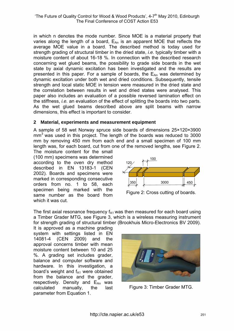
‘The Future of Quality Control for Wood & Wood Products’, 4-7th May 2010, Edinburgh The Final Conference of COST Action E53
http://cte.napier.ac.uk/e53
in which n denotes the mode number. Since MOE is a material property that varies along the length of a board, EAn is an apparent MOE that reflects the average MOE value in a board. The described method is today used for strength grading of structural timber in the dried state, i.e. typically timber with a moisture content of about 16-18 %. In connection with the described research concerning wet glued beams, the possibility to grade side boards in the wet state by axial dynamic excitation has been investigated and the results are presented in this paper. For a sample of boards, the EAn was determined by dynamic excitation under both wet and dried conditions. Subsequently, tensile strength and local static MOE in tension were measured in the dried state and the correlation between results in wet and dried states were analysed. This paper also includes an evaluation of a possible reversed lamination effect on the stiffness, i.e. an evaluation of the effect of splitting the boards into two parts. As the wet glued beams described above are split beams with narrow dimensions, this effect is important to consider.
2 Material, experiments and measurement equipment A sample of 58 wet Norway spruce side boards of dimensions 25×120×3900 mm3 was used in this project. The length of the boards was reduced to 3000 mm by removing 450 mm from each end and a small specimen of 100 mm length was, for each board, cut from one of the removed lengths, see Figure 2. The moisture content for the small (100 mm) specimens was determined according to the oven dry method described in EN 13183-1 (CEN 2002). Boards and specimens were marked in corresponding consecutive orders from no. 1 to 58, each specimen being marked with the same number as the board from which it was cut.
Figure 2: Cross cutting of boards.
The first axial resonance frequency fA1 was then measured for each board using a Timber Grader MTG, see Figure 3, which is a wireless measuring instrument for strength grading of structural timber (Brookhuis Micro-Electronics BV 2009).It is approved as a machine grading system with settings listed in EN 14081-4 (CEN 2009) and the approval concerns timber with mean moisture content between 10 and 25 %. A grading set includes grader, balance and computer software and hardware. In this investigation, a board’s weight and fA1 were obtained from the balance and the grader, respectively. Density and EAn was calculated manually, the last parameter from Equation 1.
Figure 3: Timber Grader MTG.
450 350
100120
3000
251
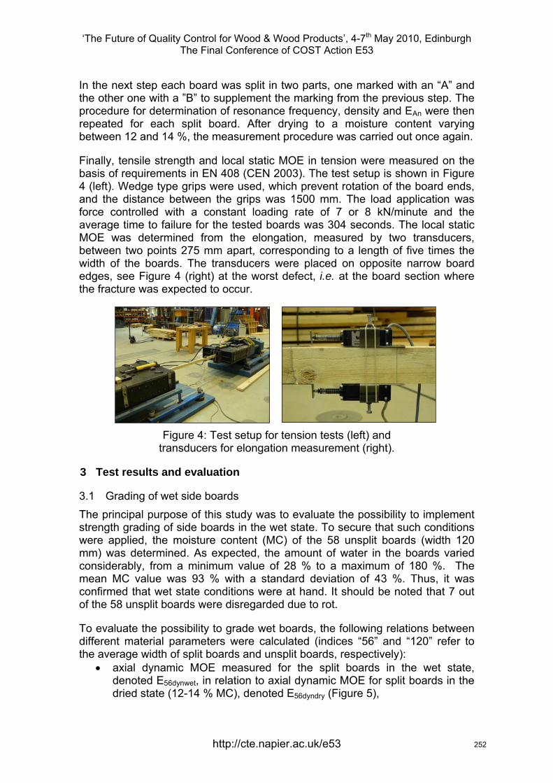
‘The Future of Quality Control for Wood & Wood Products’, 4-7th May 2010, Edinburgh The Final Conference of COST Action E53
http://cte.napier.ac.uk/e53
In the next step each board was split in two parts, one marked with an “A” and the other one with a ”B” to supplement the marking from the previous step. The procedure for determination of resonance frequency, density and EAn were then repeated for each split board. After drying to a moisture content varying between 12 and 14 %, the measurement procedure was carried out once again.
Finally, tensile strength and local static MOE in tension were measured on the basis of requirements in EN 408 (CEN 2003). The test setup is shown in Figure 4 (left). Wedge type grips were used, which prevent rotation of the board ends, and the distance between the grips was 1500 mm. The load application was force controlled with a constant loading rate of 7 or 8 kN/minute and the average time to failure for the tested boards was 304 seconds. The local static MOE was determined from the elongation, measured by two transducers, between two points 275 mm apart, corresponding to a length of five times the width of the boards. The transducers were placed on opposite narrow board edges, see Figure 4 (right) at the worst defect, i.e. at the board section where the fracture was expected to occur.
Figure 4: Test setup for tension tests (left) and
transducers for elongation measurement (right).
3 Test results and evaluation
3.1 Grading of wet side boards The principal purpose of this study was to evaluate the possibility to implement strength grading of side boards in the wet state. To secure that such conditions were applied, the moisture content (MC) of the 58 unsplit boards (width 120 mm) was determined. As expected, the amount of water in the boards varied considerably, from a minimum value of 28 % to a maximum of 180 %. The mean MC value was 93 % with a standard deviation of 43 %. Thus, it was confirmed that wet state conditions were at hand. It should be noted that 7 out of the 58 unsplit boards were disregarded due to rot.
To evaluate the possibility to grade wet boards, the following relations between different material parameters were calculated (indices “56” and “120” refer to the average width of split boards and unsplit boards, respectively):
• axial dynamic MOE measured for the split boards in the wet state, denoted E56dynwet, in relation to axial dynamic MOE for split boards in the dried state (12-14 % MC), denoted E56dyndry (Figure 5),
252
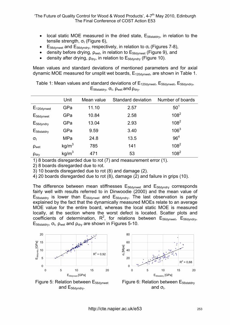
‘The Future of Quality Control for Wood & Wood Products’, 4-7th May 2010, Edinburgh The Final Conference of COST Action E53
http://cte.napier.ac.uk/e53
• local static MOE measured in the dried state, E56statdry, in relation to the tensile strength, σt (Figure 6),
• E56dynwet and E56dyndry, respectively, in relation to σt (Figures 7-8), • density before drying, ρwet, in relation to E56dynwet (Figure 9), and • density after drying, ρdry, in relation to E56dyndry (Figure 10).
Mean values and standard deviations of mentioned parameters and for axial dynamic MOE measured for unsplit wet boards, E120dynwet, are shown in Table 1.
Table 1: Mean values and standard deviations of E120dynwet, E56dynwet, E56dyndry, E56statdry, σt, ρwet and ρdry.
Unit Mean value Standard deviation Number of boards
E120dynwet GPa 11.10 2.57 501
E56dynwet GPa 10.84 2.58 1082
E56dyndry GPa 13.04 2.93 1082
E56statdry GPa 9.59 3.40 1063
σt MPa 24.8 13.5 964
ρwet kg/m3 785 141 1082
ρdry kg/m3 471 53 1082
1) 8 boards disregarded due to rot (7) and measurement error (1). 2) 8 boards disregarded due to rot. 3) 10 boards disregarded due to rot (8) and damage (2). 4) 20 boards disregarded due to rot (8), damage (2) and failure in grips (10).
The difference between mean stiffnesses E56dynwet and E56dyndry corresponds fairly well with results referred to in Dinwoodie (2000) and the mean value of E56statdry is lower than E56dynwet and E56dyndry. The last observation is partly explained by the fact that the dynamically measured MOEs relate to an average MOE value for the entire board, whereas the local static MOE is measured locally, at the section where the worst defect is located. Scatter plots and coefficients of determination, R2, for relations between E56dynwet, E56dyndry, E56statdry, σt, ρwet and ρdry are shown in Figures 5-10.
R2 = 0,92
0
5
10
15
20
0 5 10 15 20E56dynwet [GPa]
E56
dynd
ry [G
Pa]
Figure 5: Relation between E56dynwet
and E56dyndry.
R2 = 0,680
20
40
60
80
0 5 10 15 20E56statdry [GPa]
σ t [M
pa]
Figure 6: Relation between E56statdry
and σt.
253
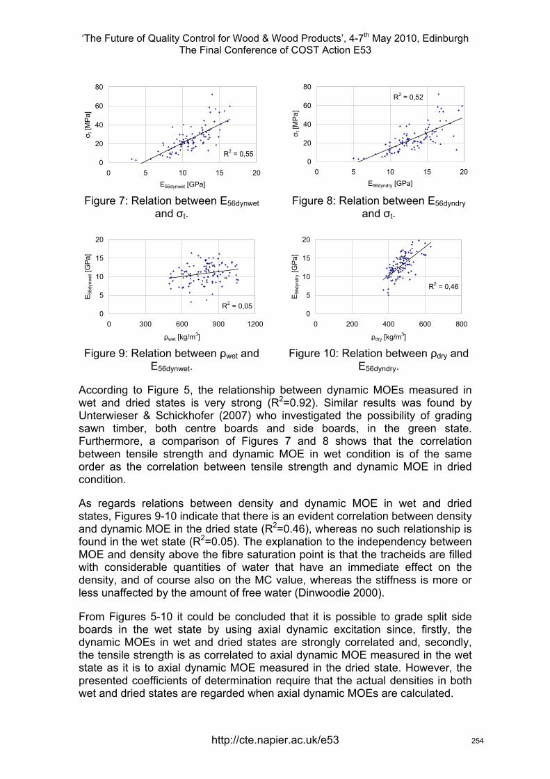
‘The Future of Quality Control for Wood & Wood Products’, 4-7th May 2010, Edinburgh The Final Conference of COST Action E53
http://cte.napier.ac.uk/e53
R2 = 0,550
20
40
60
80
0 5 10 15 20E56dynwet [GPa]
σ t [M
Pa]
Figure 7: Relation between E56dynwet
and σt.
R2 = 0,050
5
10
15
20
0 300 600 900 1200
ρwet [kg/m3]
E 56d
ynw
et [G
Pa]
Figure 9: Relation between ρwet and
E56dynwet.
R2 = 0,52
0
20
40
60
80
0 5 10 15 20E56dyndry [GPa]
σ t [M
Pa]
Figure 8: Relation between E56dyndry
and σt.
R2 = 0,46
0
5
10
15
20
0 200 400 600 800
ρdry [kg/m3]
E56
dynd
ry [G
Pa]
Figure 10: Relation between ρdry and
E56dyndry.
According to Figure 5, the relationship between dynamic MOEs measured in wet and dried states is very strong (R2=0.92). Similar results was found by Unterwieser & Schickhofer (2007) who investigated the possibility of grading sawn timber, both centre boards and side boards, in the green state. Furthermore, a comparison of Figures 7 and 8 shows that the correlation between tensile strength and dynamic MOE in wet condition is of the same order as the correlation between tensile strength and dynamic MOE in dried condition.
As regards relations between density and dynamic MOE in wet and dried states, Figures 9-10 indicate that there is an evident correlation between density and dynamic MOE in the dried state (R2=0.46), whereas no such relationship is found in the wet state (R2=0.05). The explanation to the independency between MOE and density above the fibre saturation point is that the tracheids are filled with considerable quantities of water that have an immediate effect on the density, and of course also on the MC value, whereas the stiffness is more or less unaffected by the amount of free water (Dinwoodie 2000).
From Figures 5-10 it could be concluded that it is possible to grade split side boards in the wet state by using axial dynamic excitation since, firstly, the dynamic MOEs in wet and dried states are strongly correlated and, secondly, the tensile strength is as correlated to axial dynamic MOE measured in the wet state as it is to axial dynamic MOE measured in the dried state. However, the presented coefficients of determination require that the actual densities in both wet and dried states are regarded when axial dynamic MOEs are calculated.
254
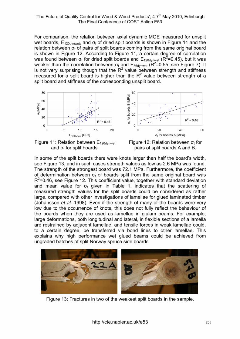
‘The Future of Quality Control for Wood & Wood Products’, 4-7th May 2010, Edinburgh The Final Conference of COST Action E53
http://cte.napier.ac.uk/e53
For comparison, the relation between axial dynamic MOE measured for unsplit wet boards, E120dynwet, and σt of dried split boards is shown in Figure 11 and the relation between σt of pairs of split boards coming from the same original board is shown in Figure 12. According to Figure 11, a certain degree of correlation was found between σt for dried split boards and E120dynwet (R2=0.45), but it was weaker than the correlation between σt and E56dynwet (R2=0.55, see Figure 7). It is not very surprising though that the R2 value between strength and stiffness measured for a split board is higher than the R2 value between strength of a split board and stiffness of the corresponding unsplit board.
R2 = 0,450
20
40
60
80
0 5 10 15 20E120dynwet [GPa]
σ t [M
Pa]
Figure 11: Relation between E120dynwet
and σt for split boards.
R2 = 0,46
0
20
40
60
0 20 40 60σt for boards A [MPa]
σ t fo
r boa
rds
B [M
Pa]
Figure 12: Relation between σt for
pairs of split boards A and B.
In some of the split boards there were knots larger than half the board’s width, see Figure 13, and in such cases strength values as low as 2.6 MPa was found. The strength of the strongest board was 72.1 MPa. Furthermore, the coefficient of determination between σt of boards split from the same original board was R2=0.46, see Figure 12. This coefficient value, together with standard deviation and mean value for σt given in Table 1, indicates that the scattering of measured strength values for the split boards could be considered as rather large, compared with other investigations of lamellae for glued laminated timber (Johansson et al. 1998). Even if the strength of many of the boards were very low due to the occurrence of knots, this does not fully reflect the behaviour of the boards when they are used as lamellae in glulam beams. For example, large deformations, both longitudinal and lateral, in flexible sections of a lamella are restrained by adjacent lamellae, and tensile forces in weak lamellae could, to a certain degree, be transferred via bond lines to other lamellae. This explains why high performance wet glued beams could be achieved from ungraded batches of split Norway spruce side boards.
Figure 13: Fractures in two of the weakest split boards in the sample.
255
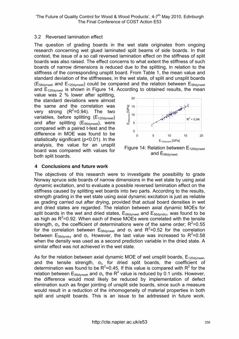
‘The Future of Quality Control for Wood & Wood Products’, 4-7th May 2010, Edinburgh The Final Conference of COST Action E53
http://cte.napier.ac.uk/e53
3.2 Reversed lamination effect The question of grading boards in the wet state originates from ongoing research concerning wet glued laminated split beams of side boards. In that context, the issue of a so call reversed lamination effect on the stiffness of split boards was also raised. The effect concerns to what extent the stiffness of such boards of narrow dimensions is reduced due to the splitting, in relation to the stiffness of the corresponding unsplit board. From Table 1, the mean value and standard deviation of the stiffnesses, in the wet state, of split and unsplit boards (E56dynwet and E120dynwet) could be compared and the relation between E56dynwet and E120dynwet is shown in Figure 14. According to obtained results, the meanvalue was 2 % lower after splitting, the standard deviations were almost the same and the correlation was very strong (R2=0.94). The two variables, before splitting (E120dynwet) and after splitting (E56dynwet), were compared with a paired t-test and the difference in MOE was found to be statistically significant (p<0.01). In the analysis, the value for an unsplit board was compared with values for both split boards.
R2 = 0,94
0
5
10
15
20
0 5 10 15 20E120dynwet [GPa]
E56
dynw
et [G
Pa]
Figure 14: Relation between E120dynwet
and E56dynwet.
4 Conclusions and future work The objectives of this research were to investigate the possibility to grade Norway spruce side boards of narrow dimensions in the wet state by using axial dynamic excitation, and to evaluate a possible reversed lamination effect on the stiffness caused by splitting wet boards into two parts. According to the results, strength grading in the wet state using axial dynamic excitation is just as reliable as grading carried out after drying, provided that actual board densities in wet and dried states are regarded. The relation between axial dynamic MOEs for split boards in the wet and dried states, E56dynwet and E56dyndry, was found to be as high as R2=0.92. When each of these MOEs were correlated with the tensile strength, σt, the coefficient of determinations were of the same order; R2=0.55 for the correlation between E56dynwet and σt and R2=0.52 for the correlation between E56dyndry and σt. However, the last value was increased to R2=0.58 when the density was used as a second prediction variable in the dried state. A similar effect was not achieved in the wet state.
As for the relation between axial dynamic MOE of wet unsplit boards, E120dynwet, and the tensile strength, σt, for dried split boards, the coefficient of determination was found to be R2=0.45. If this value is compared with R2 for the relation between E56dynwet and σt, the R2 value is reduced by 0.1 units. However, the difference would most likely be reduced by implementation of defect elimination such as finger jointing of unsplit side boards, since such a measure would result in a reduction of the inhomogeneity of material properties in both split and unsplit boards. This is an issue to be addressed in future work.
256

‘The Future of Quality Control for Wood & Wood Products’, 4-7th May 2010, Edinburgh The Final Conference of COST Action E53
http://cte.napier.ac.uk/e53
Regarding the reversed lamination effect on the stiffness of split boards, it was in this investigation found to be of lower order.
References Brookhuis Micro-Electronics BV (2009) “MTG Manual GB 12062009-C”.
CEN (2002) “EN 13183-1 Moisture content of a piece of sawn timber – Part 1: Determination by oven dry method”, European Committee for Standardization.
CEN (2003) “EN 408 Timber structures – Structural timber and glued laminated timber – Determination of some physical and mechanical properties”, European Committee for Standardization.
CEN (2009) “EN 14081-4 Timber structures – Strength graded structural timber with rectangular cross section – Part 4: Machine grading – Grading machine settings for machine controlled systems”, European Comm. for Standardization
Dinwoodie, J. M. (2000) “Timber: Its nature and behaviour”, Second Edition, E & FN Spon, London, UK.
Johansson, C.-J., Boström, L., Bräuner, L., Hoffmeyer, P., Holmqvist, C. & Sollie, K. H., (1998) ”Laminations for glued laminated timber – Establishment of strength classes for visual strength grades and machine settings for glulam laminations of Nordic origin”. SP Swedish National Testing and Research Institute, SP REPORT 1998:38.
Ohlsson, S. & Perstorper, M. (1992) “Elastic Wood Properties from Dynamic Tests and Computer Modeling”. Journal of Structural Engineering-Asce, 118(10), pp 2677-2690.
Petersson, H., Bengtsson, T., Blixt, J., Enquist, B., Källsner, B., Oscarsson, J. (ed.), Serrano, E. & Sterley, M. (2009) ”Increased value yield by wet and dry gluing of sawn side boards into property optimized wood products for the construction market” (in Swedish). School of Technology and Design, Reports, No 53, Växjö University, Sweden.
Steffen, A., Johansson, C.-J. & Wormuth, E.-W. (1997) “Study of the relationship between flatwise and edgewise moduli of elasticity of sawn timber as a means to improve mechanical strength grading technology”. Holz als Roh- und Werkstoff, Vol 55, pp 245-253.
Unterwieser, H. & Schickhofer, G. (2007) “Pre-grading of sawn timber in green condition”, COST E53 Conference – Quality Control for Wood and Wood Products, 15-17 October 2007, Warzaw, Poland.
Wormuth, E.-W. (1993) “Study of the relation between flatwise and edgewise modulus of elasticity of sawn timber for the purpose of improving mechanical stress grading methods” (in German), Master’s Thesis, Department of Wood Technology, University of Hamburg.
257
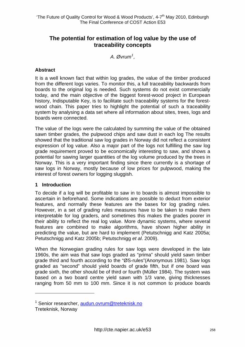
‘The Future of Quality Control for Wood & Wood Products’, 4-7th May 2010, Edinburgh The Final Conference of COST Action E53
The potential for estimation of log value by the use of traceability concepts
A. Øvrum1,
Abstract It is a well known fact that within log grades, the value of the timber produced from the different logs varies. To monitor this, a full traceability backwards from boards to the original log is needed. Such systems do not exist commercially today, and the main objective of the biggest forest-wood project in European history, Indisputable Key, is to facilitate such traceability systems for the forest-wood chain. This paper tries to highlight the potential of such a traceability system by analysing a data set where all information about sites, trees, logs and boards were connected.
The value of the logs were the calculated by summing the value of the obtained sawn timber grades, the pulpwood chips and saw dust in each log The results showed that the traditional saw log grades in Norway did not reflect a consistent expression of log value. Also a major part of the logs not fulfilling the saw log grade requirement proved to be economically interesting to saw, and shows a potential for sawing larger quantities of the log volume produced by the trees in Norway. This is a very important finding since there currently is a shortage of saw logs in Norway, mostly because of low prices for pulpwood, making the interest of forest owners for logging sluggish.
1 Introduction To decide if a log will be profitable to saw in to boards is almost impossible to ascertain in beforehand. Some indications are possible to deduct from exterior features, and normally these features are the bases for log grading rules. However, in a set of grading rules measures have to be taken to make them interpretable for log graders, and sometimes this makes the grades poorer in their ability to reflect the real log value. More dynamic systems, where several features are combined to make algorithms, have shown higher ability in predicting the value, but are hard to implement (Petutschnigg and Katz 2005a; Petutschnigg and Katz 2005b; Petutschnigg et al. 2009).
When the Norwegian grading rules for saw logs were developed in the late 1960s, the aim was that saw logs graded as “prima” should yield sawn timber grade third and fourth according to the “ØS-rules”(Anonymous 1981). Saw logs graded as “second” should yield boards of grade fifth, but if one board was grade sixth, the other should be of third or fourth (Müller 1984). The system was based on a two board centre yield sawn with 1/3 vane, giving thicknesses ranging from 50 mm to 100 mm. Since it is not common to produce boards
1 Senior researcher, [email protected], Norway
http://cte.napier.ac.uk/e53 258
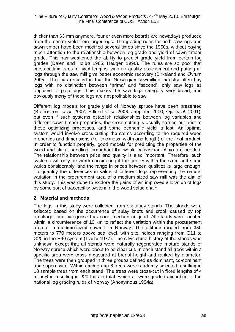
‘The Future of Quality Control for Wood & Wood Products’, 4-7th May 2010, Edinburgh The Final Conference of COST Action E53
thicker than 63 mm anymore, four or even more boards are nowadays produced from the centre yield from larger logs. The grading rules for both saw logs and sawn timber have been modified several times since the 1960s, without paying much attention to the relationship between log grade and yield of sawn timber grade. This has weakened the ability to predict grade yield from certain log grades (Dalen and Høibø 1985; Haugen 1996). The rules are so poor that cross-cutting trees in fixed lengths, with no quality assessment and putting all logs through the saw mill give better economic recovery (Birkeland and Øvrum 2005). This has resulted in that the Norwegian sawmilling industry often buy logs with no distinction between “prima” and “second”, only saw logs as opposed to pulp logs. This makes the saw logs category very broad, and obviously many of these logs are not profitable to saw.
Different log models for grade yield of Norway spruce have been presented (Brännström et al. 2007; Edlund et al. 2006; Jäppinen 2000; Oja et al. 2001), but even if such systems establish relationships between log variables and different sawn timber properties, the cross-cutting is usually carried out prior to these optimizing processes, and some economic yield is lost. An optimal system would involve cross-cutting the stems according to the required wood properties and dimensions (i.e. thickness, width and length) of the final product. In order to function properly, good models for predicting the properties of the wood and skilful handling throughout the whole conversion chain are needed. The relationship between price and quality is also important. Therefore, such systems will only be worth considering if the quality within the stem and stand varies considerably, and the range in prices between qualities is large enough. To quantify the differences in value of different logs representing the natural variation in the procurement area of a medium sized saw mill was the aim of this study. This was done to explore the gains of an improved allocation of logs by some sort of traceability system in the wood value chain.
2 Material and methods The logs in this study were collected from six study stands. The stands were selected based on the occurrence of splay knots and crook caused by top breakage, and categorised as poor, medium or good. All stands were located within a circumference of 10 km to reflect the variation within the procurement area of a medium-sized sawmill in Norway. The altitude ranged from 350 meters to 770 meters above sea level, with site indices ranging from G11 to G20 in the H40 system (Tveite 1977). The silvicultural history of the stands was unknown except that all stands were naturally regenerated mature stands of Norway spruce which were about to be clear cut. In each stand all trees within a specific area were cross measured at breast height and ranked by diameter. The trees were then grouped in three groups defined as dominant, co-dominant and suppressed. Within each group 6 trees were randomly selected resulting in 18 sample trees from each stand. The trees were cross-cut in fixed lengths of 4 m or 6 m resulting in 229 logs in total, which all were graded according to the national log grading rules of Norway (Anonymous 1994a).
http://cte.napier.ac.uk/e53 259

‘The Future of Quality Control for Wood & Wood Products’, 4-7th May 2010, Edinburgh The Final Conference of COST Action E53
The logs were sawn according to Nordic practice (Anonymous 1994), with heart splitting giving either 2, 4 or 6 cant in the centre yield depending on the small-end diameter of the log processed. Boards were commercially dimensioned as determined by the sawing pattern giving the maximum volume yield from each log, and the dimensions ranged from 38 x 100 mm2 to 50 x 225 mm2.
All boards were graded for general appearance according to the grading rules in Nordic Timber (Anonymous 1994b) and for a sound knot grade using the market norm for sound knot timber for interior panelling and flooring in Norway. Boards thicker than 32 mm were also strength graded by visual inspection according to INSTA 142 (Anonymous 1997). Based on the current market values for the respective grades, the value of the sawn timber from each log was calculated. The value of the pulp wood chips and saw dust produced was also added to get the total value of the log. Table 1 summarizes the grades and their respective values in the calculations.
Table 1 Set market value of the different sawn timber grades
Grade Value (NOK/m3) Nordic Timber, grade A3 2000 Nordic Timber, grade A4 1800 Nordic Timber, grade B 1500 Nordic Timber, grade C 1000 Nordic Timber, grade D 700 Sound knot timber 1900 INSTA 142, grade T3/C30 1700 INSTA 142, grade T2/C24 1600 INSTA 142, grade T1/C18 1550 Pulp wood chips 250 Saw dust 150
3 Results The mean log value was found to be 924 NOK/m3, with a standard deviation of 171 NOK/m3. In Figure 1 the distribution of the value in the logs is shown in NOK/m3.
http://cte.napier.ac.uk/e53 260
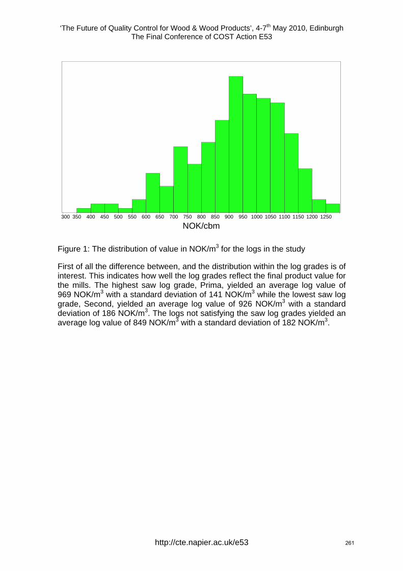
‘The Future of Quality Control for Wood & Wood Products’, 4-7th May 2010, Edinburgh The Final Conference of COST Action E53
300 350 400 450 500 550 600 650 700 750 800 850 900 950 1000 1050 1100 1150 1200 1250
NOK/cbm
Figure 1: The distribution of value in NOK/m3 for the logs in the study
First of all the difference between, and the distribution within the log grades is of interest. This indicates how well the log grades reflect the final product value for the mills. The highest saw log grade, Prima, yielded an average log value of 969 NOK/m3 with a standard deviation of 141 NOK/m3 while the lowest saw log grade, Second, yielded an average log value of 926 NOK/m3 with a standard deviation of 186 NOK/m3. The logs not satisfying the saw log grades yielded an average log value of 849 NOK/m3 with a standard deviation of 182 NOK/m3.
http://cte.napier.ac.uk/e53 261
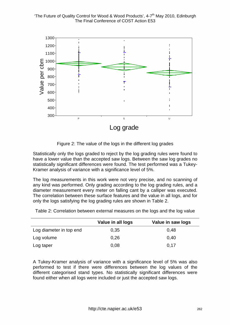
‘The Future of Quality Control for Wood & Wood Products’, 4-7th May 2010, Edinburgh The Final Conference of COST Action E53
300
400
500
600
700
800
900
1000
1100
1200
1300V
alue
per
cbm
P S U
Log grade
Figure 2: The value of the logs in the different log grades
Statistically only the logs graded to reject by the log grading rules were found to have a lower value than the accepted saw logs. Between the saw log grades no statistically significant differences were found. The test performed was a Tukey-Kramer analysis of variance with a significance level of 5%.
The log measurements in this work were not very precise, and no scanning of any kind was performed. Only grading according to the log grading rules, and a diameter measurement every meter on falling cant by a calliper was executed. The correlation between these surface features and the value in all logs, and for only the logs satisfying the log grading rules are shown in Table 2.
Table 2: Correlation between external measures on the logs and the log value
Value in all logs Value in saw logs Log diameter in top end 0,35 0,48 Log volume 0,26 0,40 Log taper 0,08 0,17
A Tukey-Kramer analysis of variance with a significance level of 5% was also performed to test if there were differences between the log values of the different categorised stand types. No statistically significant differences were found either when all logs were included or just the accepted saw logs.
http://cte.napier.ac.uk/e53 262
‘The Future of Quality Control for Wood & Wood Products’, 4-7th May 2010, Edinburgh The Final Conference of COST Action E53
Between tree statuses within a stand however, statistically significant differences in log values were found both when all logs were included, and when only the saw logs were considered. The ranking was from highest value to lowest; dominant, co-dominant and suppressed trees.
4 Discussion The results show a very large difference in final product value between logs. This is in itself not a big surprise, and to be able to get only profitable logs in to a saw mill is probably not achievable. In the forest business today saw mills have to purchase logs not being profitable in order to get access to the more profitable logs from their suppliers. In practice this means buying logs from top diameter 13 ub and upwards. Most mills would, if they had the chance, only saw logs from 18 to 30 in top diameter since their technology is optimized for these dimensions, and the sawing patterns are also yielding the most interesting dimensions in these log diameters. However, if saw mills get a better knowledge of which logs they are profiting on, they will be able to consider other use of logs not profitable to saw. Alternatives can be chipping for pulpwood, bio energy, or simplified sawing to “rougher” products with lower quality requirements.
Countless models for wood properties and grade yield exist, but are not able to explain the variance in log conversion one hundred percent. A traceability system could in an ideal situation make it possible for log suppliers to get paid based on the log value obtained for the primary processer. However this appears a bit naive since a lot of process conditions will influence the yield, and there is also a business transaction involved. However, some kind of bonus for suppliers delivering high value logs could be imagined.
As Birkeland and Øvrum (2005) showed, sawing the whole tree may be in many cases yield the highest economic recovery. However, this result is based on a lot of assumptions in the processes from forest to final product. The sawmilling industry is on the other hand constantly making progress technically, and especially the increased use of scanners for grading and other kinds of quality management make the sawmilling process more flexible and efficient in terms of separating different qualities to their respective end products. This will make the sawmills more able to process a larger spectre of log qualities. Also the small difference between the values in the log grades indicates that one can consider sawing the whole tree, and deal with the grading later on in the process.
New 3D scanners and x-ray scanners will give much more measuring points making it possible to define value in logs more precisely. If traceability concepts like the ones displayed in the Indisputable Key is implemented in the wood value chain this might facilitate a new way of purchasing logs by sharing the surplus of a produced logs between the buyer and seller of the logs. An example of such integration in Norway is planing mills not accepting delivered timber batches yielding more reject than a defined threshold value when splitting, planing and grading for interior panelling.
http://cte.napier.ac.uk/e53 263
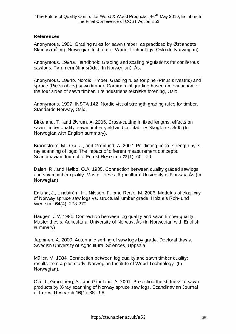
‘The Future of Quality Control for Wood & Wood Products’, 4-7th May 2010, Edinburgh The Final Conference of COST Action E53
References Anonymous. 1981. Grading rules for sawn timber: as practiced by Østlandets Skurlastmåling. Norwegian Institute of Wood Technology, Oslo (In Norwegian).
Anonymous. 1994a. Handbook: Grading and scaling regulations for coniferous sawlogs. Tømmermålingsrådet (In Norwegian), Ås.
Anonymous. 1994b. Nordic Timber. Grading rules for pine (Pinus silvestris) and spruce (Picea abies) sawn timber: Commercial grading based on evaluation of the four sides of sawn timber. Treindustriens tekniske forening, Oslo.
Anonymous. 1997. INSTA 142 Nordic visual strength grading rules for timber. Standards Norway, Oslo.
Birkeland, T., and Øvrum, A. 2005. Cross-cutting in fixed lengths: effects on sawn timber quality, sawn timber yield and profitability Skogforsk. 3/05 (In Norwegian with English summary).
Brännström, M., Oja, J., and Grönlund, A. 2007. Predicting board strength by X-ray scanning of logs: The impact of different measurement concepts. Scandinavian Journal of Forest Research 22(1): 60 - 70.
Dalen, R., and Høibø, O.A. 1985. Connection between quality graded sawlogs and sawn timber quality. Master thesis. Agricultural University of Norway, Ås (In Norwegian)
Edlund, J., Lindström, H., Nilsson, F., and Reale, M. 2006. Modulus of elasticity of Norway spruce saw logs vs. structural lumber grade. Holz als Roh- und Werkstoff 64(4): 273-279.
Haugen, J.V. 1996. Connection between log quality and sawn timber quality. Master thesis. Agricultural University of Norway, Ås (In Norwegian with English summary)
Jäppinen, A. 2000. Automatic sorting of saw logs by grade. Doctoral thesis. Swedish University of Agricultural Sciences, Uppsala
Müller, M. 1984. Connection between log quality and sawn timber quality: results from a pilot study. Norwegian Institute of Wood Technology (In Norwegian).
Oja, J., Grundberg, S., and Grönlund, A. 2001. Predicting the stiffness of sawn products by X-ray scanning of Norway spruce saw logs. Scandinavian Journal of Forest Research 16(1): 88 - 96.
http://cte.napier.ac.uk/e53 264

‘The Future of Quality Control for Wood & Wood Products’, 4-7th May 2010, Edinburgh The Final Conference of COST Action E53
Petutschnigg, A.J., and Katz, H. 2005a. A loglinear model approach for evaluating and adopting log and lumber strategies. For. Prod. J. 55(7-8): 67-71.
Petutschnigg, A.J., and Katz, H. 2005b. A loglinear model to predict lumber quality depending on quality parameters of logs. Holz Roh- Werkst. 63(2): 112-117.
Petutschnigg, A.J., Pferschy, U., Katz, H., Kain, G., and Teischinger, A. 2009. Algorithms to define limits for wood property categorization. For. Prod. J. 59(7/8): 75-83.
Tveite, B. 1977. Site-index curves for Norway Spruce (Picea abies (L.) Karst.). Norwegian Research Forest Institute. Rapport 33(1).
http://cte.napier.ac.uk/e53 265

²
Final COST Action E53 meeting
The future of quality control for wood and wood products
Our Dynamic Earth, Edinburgh, 4-7 may 2010
Potential of poplar and willow wood for load-bearing constructions
Lieven DE BOEVER1, Joris VAN ACKER2
Ghent University (UGent), Laboratory of Wood Technology, CoupureLinks 653, 9000 Gent, Belgium.
1 e-mail: [email protected] 2 e-mail: [email protected]
²
Final COST Action E53 meeting
The future of quality control for wood and wood products
Our Dynamic Earth, Edinburgh, 4-7 may 2010
OUTLINE
• Introduction – Why ?
• Selected topics
• Variability physical-mechanical properties
• Grading
• Veneer based products
• Conclusions – Economical relevance
‘The Future of Quality Control for Wood & Wood Products’, 4-7th May 2010, EdinburghThe Final Conference of COST Action E53
http://cte.napier.ac.uk/e53 266

²
Final COST Action E53 meeting
The future of quality control for wood and wood products
Our Dynamic Earth, Edinburgh, 4-7 may 2010
INTRODUCTION
0%
10%
20%
30%
40%
50%
60%
70%
80%
90%
100%
1700 1800 1900 2000
3 Theory of structures for timber
1 Apprenticeships 4 Glued laminated timber
2 Long-span bridges
5 Wood based panels
6 Ecology, technology and design
²
Final COST Action E53 meeting
The future of quality control for wood and wood products
Our Dynamic Earth, Edinburgh, 4-7 may 2010
INTRODUCTION
‘The Future of Quality Control for Wood & Wood Products’, 4-7th May 2010, EdinburghThe Final Conference of COST Action E53
http://cte.napier.ac.uk/e53 267

²
Final COST Action E53 meeting
The future of quality control for wood and wood products
Our Dynamic Earth, Edinburgh, 4-7 may 2010
INTRODUCTIONTheir main impact on the forestry-wood chain :
• Man-made plantations taking pressure away from native forests.
• Quantity does not imply poor quality.
• Environmental discussion will lead to “Save the environment, use wood!”
• New players on the market for the same kind of raw material.
• Narrowing price settings.
‘The Future of Quality Control for Wood & Wood Products’, 4-7th May 2010, EdinburghThe Final Conference of COST Action E53
http://cte.napier.ac.uk/e53 268

²
Final COST Action E53 meeting
The future of quality control for wood and wood products
Our Dynamic Earth, Edinburgh, 4-7 may 2010
INTRODUCTION
Local harvested Volume of natural fo-
rests
Imported raw wood
material
TRANSFORMATON
Veneer and
veneer based products
Sawn wood
products (solid wood)
Wood based
panels
Pulp and
paper
WOOD RESIDUES
FINAL PRODUCTS
RECOVERED WOOD
Bio-energy
Other wood sources (SRC, wood plantati-
ons,…)
²
Final COST Action E53 meeting
The future of quality control for wood and wood products
Our Dynamic Earth, Edinburgh, 4-7 may 2010
INTRODUCTION
Potential
According to “The Webster English dictionary”, potential is defined as:
“POTENTIAL ADJ. EXISTING IN UNDEVELOPED FORM, LATENT; CAPABLE OF COMING INTO EXISTENCE OR ACTIVITY; HAVING
INHERENT BUT UNUSED POWERS; (GRAMM) EXPRESSING POSSIBILITY”.
Adopted to this research, potential is defined as:
The possibility to describe the inherent properties of poplar and willow wood with special emphasis on assessing their variability and
the possibility to select, control and improve the properties ofinterest.
‘The Future of Quality Control for Wood & Wood Products’, 4-7th May 2010, EdinburghThe Final Conference of COST Action E53
http://cte.napier.ac.uk/e53 269
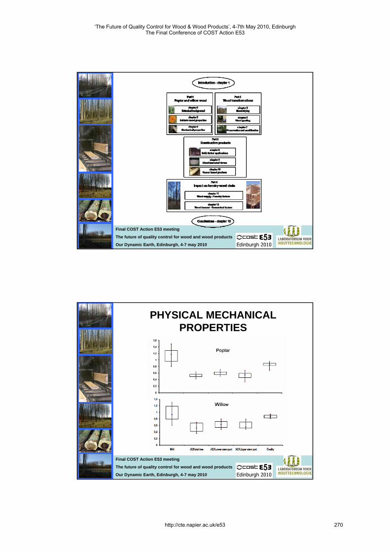
²
Final COST Action E53 meeting
The future of quality control for wood and wood products
Our Dynamic Earth, Edinburgh, 4-7 may 2010
²
Final COST Action E53 meeting
The future of quality control for wood and wood products
Our Dynamic Earth, Edinburgh, 4-7 may 2010
PHYSICAL MECHANICAL PROPERTIES
‘The Future of Quality Control for Wood & Wood Products’, 4-7th May 2010, EdinburghThe Final Conference of COST Action E53
http://cte.napier.ac.uk/e53 270
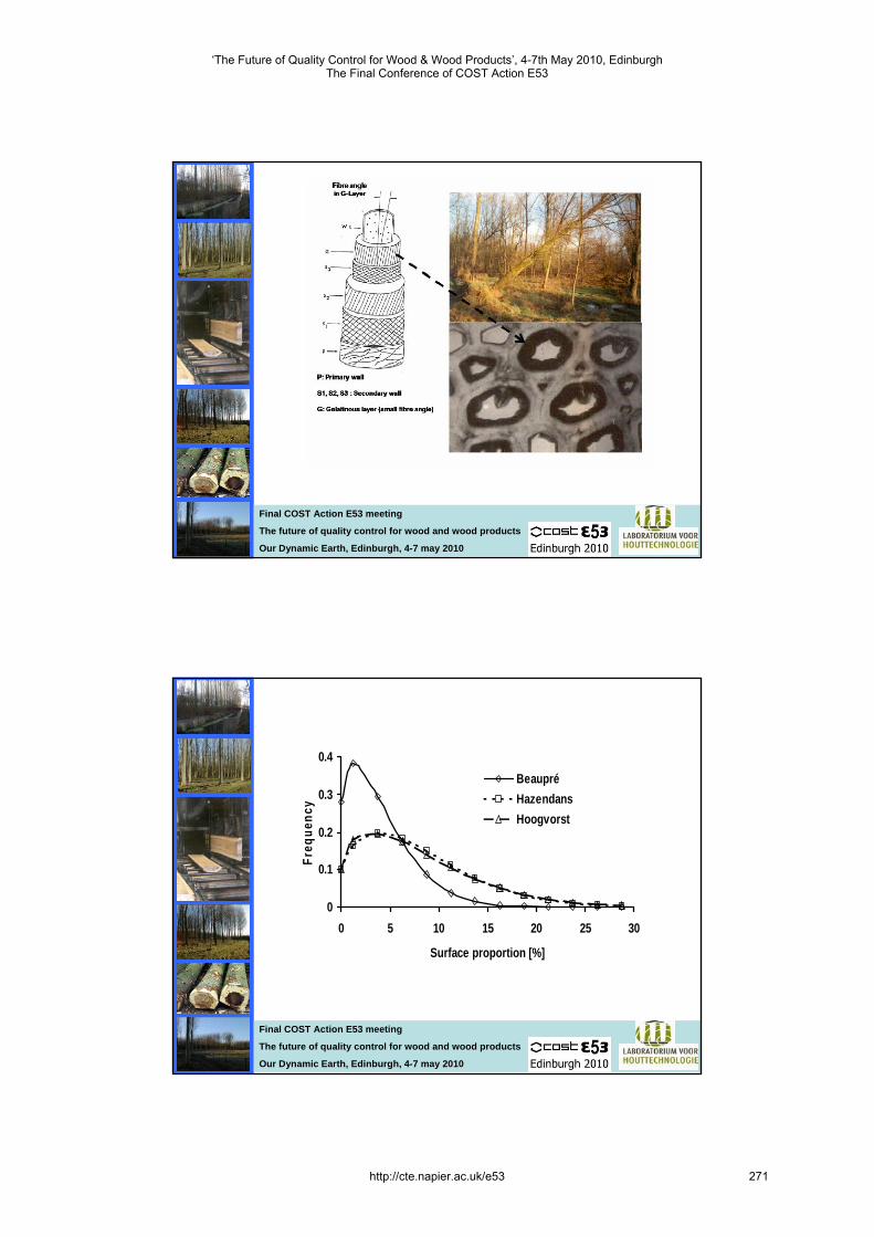
²
Final COST Action E53 meeting
The future of quality control for wood and wood products
Our Dynamic Earth, Edinburgh, 4-7 may 2010
²
Final COST Action E53 meeting
The future of quality control for wood and wood products
Our Dynamic Earth, Edinburgh, 4-7 may 2010
0
0.1
0.2
0.3
0.4
0 5 10 15 20 25 30
Surface proportion [%]
Freq
uenc
y
BeaupréHazendansHoogvorst
‘The Future of Quality Control for Wood & Wood Products’, 4-7th May 2010, EdinburghThe Final Conference of COST Action E53
http://cte.napier.ac.uk/e53 271
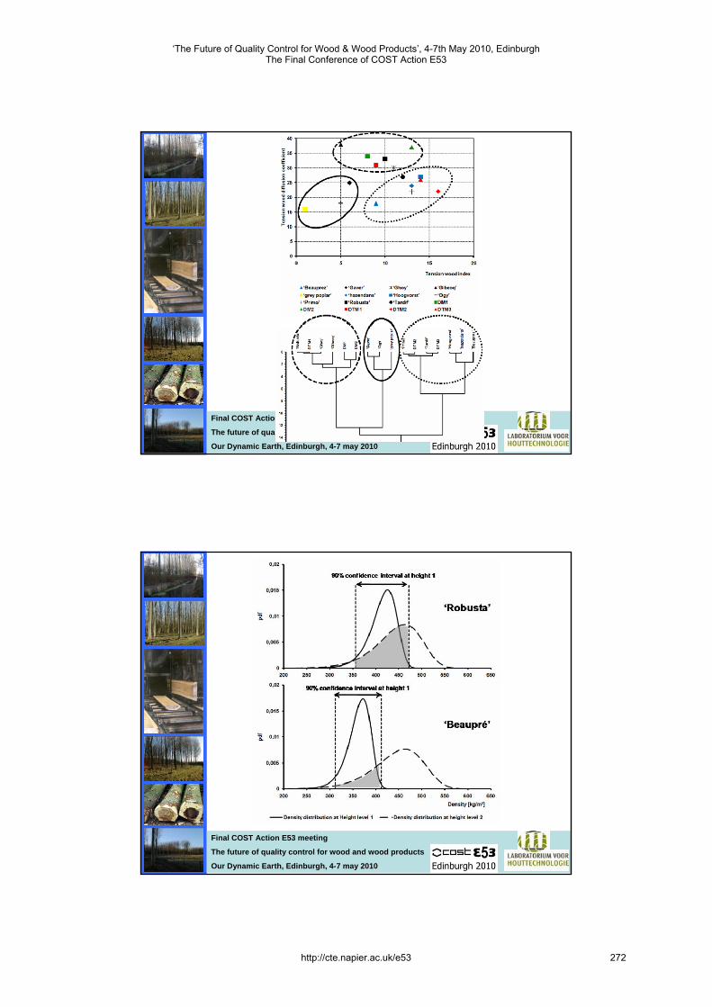
²
Final COST Action E53 meeting
The future of quality control for wood and wood products
Our Dynamic Earth, Edinburgh, 4-7 may 2010
²
Final COST Action E53 meeting
The future of quality control for wood and wood products
Our Dynamic Earth, Edinburgh, 4-7 may 2010
‘The Future of Quality Control for Wood & Wood Products’, 4-7th May 2010, EdinburghThe Final Conference of COST Action E53
http://cte.napier.ac.uk/e53 272
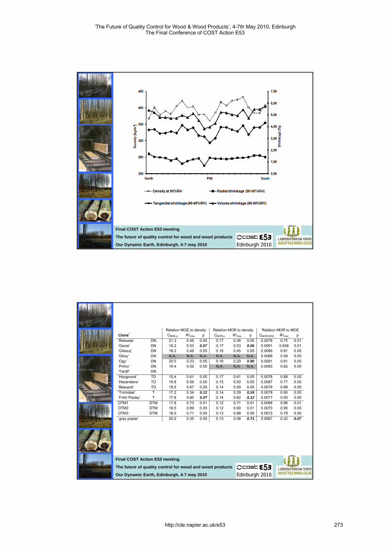
²
Final COST Action E53 meeting
The future of quality control for wood and wood products
Our Dynamic Earth, Edinburgh, 4-7 may 2010
²
Final COST Action E53 meeting
The future of quality control for wood and wood products
Our Dynamic Earth, Edinburgh, 4-7 may 2010
Relation MOE to density Relation MOR to density Relation MOR to MOE Clone* CMOE,ρ R²max p CMOR,ρ R²max p CMOR,MOE R²max p ‘Robusta’ DN 21.3 0.46 0.05 0.17 0.38 0.05 0.0078 0.75 0.01 ‘Gaver’ DN 18.2 0.53 0.07 0.17 0.53 0.08 0.0091 0.836 0.01 ‘Gibecq’ DN 18.2 0.48 0.05 0.16 0.45 0.05 0.0090 0.81 0.05 ‘Ghoy’ DN N.A. N.A. N.A. N.A. N.A. N.A. 0.0088 0.59 0.05 ‘Ogy’ DN 20.0 0.33 0.05 0.16 0.29 0.90 0.0081 0.81 0.05 ‘Primo’ DN 19.4 0.52 0.05 N.A. N.A. N.A. 0.0083 0.62 0.05 ‘Tardif’ DN ‘Hoogvorst’ TD 15.4 0.61 0.05 0.17 0.61 0.05 0.0078 0.88 0.05 ‘Hazendans’ TD 16.8 0.56 0.05 0.15 0.50 0.05 0.0087 0.77 0.05 ‘Beaupré’ TD 18.0 0.67 0.05 0.14 0.59 0.05 0.0079 0.88 0.05 ‘Trichobel’ T 17.2 0.34 0.12 0.14 0.29 0.24 0.0078 0.90 0.05 ‘Fritzi Pauley’ T 17.8 0.60 0.07 0.14 0.62 0.12 0.0077 0.93 0.05 DTM1 DTM 17.8 0.73 0.01 0.12 0.71 0.01 0.0068 0.86 0.01 DTM2 DTM 18.5 0.89 0.05 0.12 0.90 0.01 0.0070 0.95 0.05 DTM3 DTM 18.0 0.71 0.05 0.13 0.88 0.05 0.0072 0.78 0.05 ‘grey poplar’ 20.0 0.35 0.05 0.13 0.08 0.71 0.0067 0.32 0.07
‘The Future of Quality Control for Wood & Wood Products’, 4-7th May 2010, EdinburghThe Final Conference of COST Action E53
http://cte.napier.ac.uk/e53 273
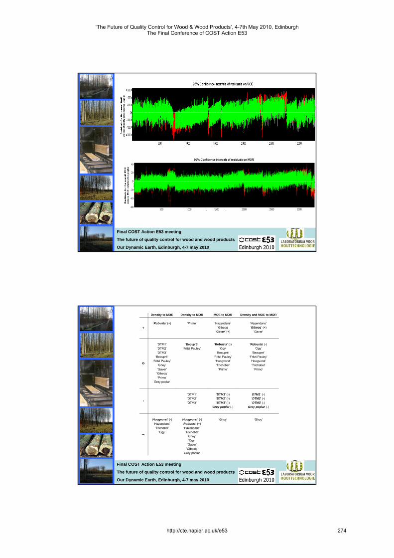
²
Final COST Action E53 meeting
The future of quality control for wood and wood products
Our Dynamic Earth, Edinburgh, 4-7 may 2010
²
Final COST Action E53 meeting
The future of quality control for wood and wood products
Our Dynamic Earth, Edinburgh, 4-7 may 2010
Density to MOE Density to MOR MOE to MOR Density and MOE to MOR
+
‘Robusta’ (+)
‘Primo’
‘Hazendans’
‘Gibecq’ ‘Gaver’ (+)
‘Hazendans’ ‘Gibecq’ (+)
‘Gaver’
0
‘DTM1’ ‘DTM2’ ‘DTM3’
‘Beaupré’ ‘Fritzi Pauley’
‘Ghoy’ ‘Gaver’ ‘Gibecq’ ‘Primo’
Grey poplar
‘Beaupré’
‘Fritzi Pauley’
‘Robusta’ (-)
‘Ogy’ ‘Beaupré’
‘Fritzi Pauley’ ‘Hoogvorst’ ‘Trichobel’
’Primo’
‘Robusta’ (-)
‘Ogy’ ‘Beaupré’
‘Fritzi Pauley’ ‘Hoogvorst’ ‘Trichobel’
’Primo’
-
‘DTM1’ ‘DTM2’ ‘DTM3’
‘DTM1’ (-) ‘DTM2’ (-) ‘DTM3’ (-)
Grey poplar (-)
DTM1’ (-) ‘DTM2’ (-) ‘DTM3’ (-)
Grey poplar (-)
/
‘Hoogvorst’ (-)
‘Hazendans’ ‘Trichobel’
‘Ogy’
‘Hoogvorst’ (-) ‘Robusta’ (+) ‘Hazendans’ ‘Trichobel’
‘Ghoy’ ‘Ogy’
‘Gaver’ ‘Gibecq’
Grey poplar
‘Ghoy’
‘Ghoy’
‘The Future of Quality Control for Wood & Wood Products’, 4-7th May 2010, EdinburghThe Final Conference of COST Action E53
http://cte.napier.ac.uk/e53 274

²
Final COST Action E53 meeting
The future of quality control for wood and wood products
Our Dynamic Earth, Edinburgh, 4-7 may 2010
Relation MOE to density Relation MOR to density Relation MOR to MOE Clone* CMOE,ρ R²max p CMOR,ρ R²max p CMOR,MOE R²max p Sem_1 A N.A. N.A. N.A. N.A. N.A. N.A. 0.0082 0.42 0.05 Sem_2 R 16.8 0.40 0.08 N.A. N.A. N.A. 0.0085 0.48 0.05 Sem_3 A 16.7 0.45 0.05 0.14 0.47 0.05 0.0079 0.49 0.05 Sem_4 A 16.6 0.35 0.05 N.A. N.A. N.A. N.A. N.A. N.A. Sem_5 A 17.9 0.16 0.10 0.13 0.30 0.05 0.0073 0.52 0.05 Sem_6 A 15.7 0.45 0.05 N.A. N.A. N.A. N.A. N.A. N.A. Sem_7 A 16.2 0.51 0.05 N.A. N.A. N.A. N.A. N.A. N.A. Sem_8 A 16.4 0.23 0.12 N.A. N.A. N.A. 0.0082 0.42 0.05 Sem_9 R N.A. N.A. N.A. N.A. N.A. N.A. 0.0085 0.36 0.05 Sem_10 R 16.1 0.67 0.05 N.A. N.A. N.A. N.A. N.A. N.A. Bree A 16.0 0.46 0.05 0.09 0.40 0.08 0.0053 0.26 0.07
²
Final COST Action E53 meeting
The future of quality control for wood and wood products
Our Dynamic Earth, Edinburgh, 4-7 may 2010
GRADING
• Visual grading
• According French standard (R – C18 – C24)
• Also attention to tension wood (Wooliness) and grain angle
• Free-free bending frequency (mode 1)
• Destructive testing (manual determination of strength class)
• Modulus of elasticity
• Bending strength
• Shear modulus
‘The Future of Quality Control for Wood & Wood Products’, 4-7th May 2010, EdinburghThe Final Conference of COST Action E53
http://cte.napier.ac.uk/e53 275
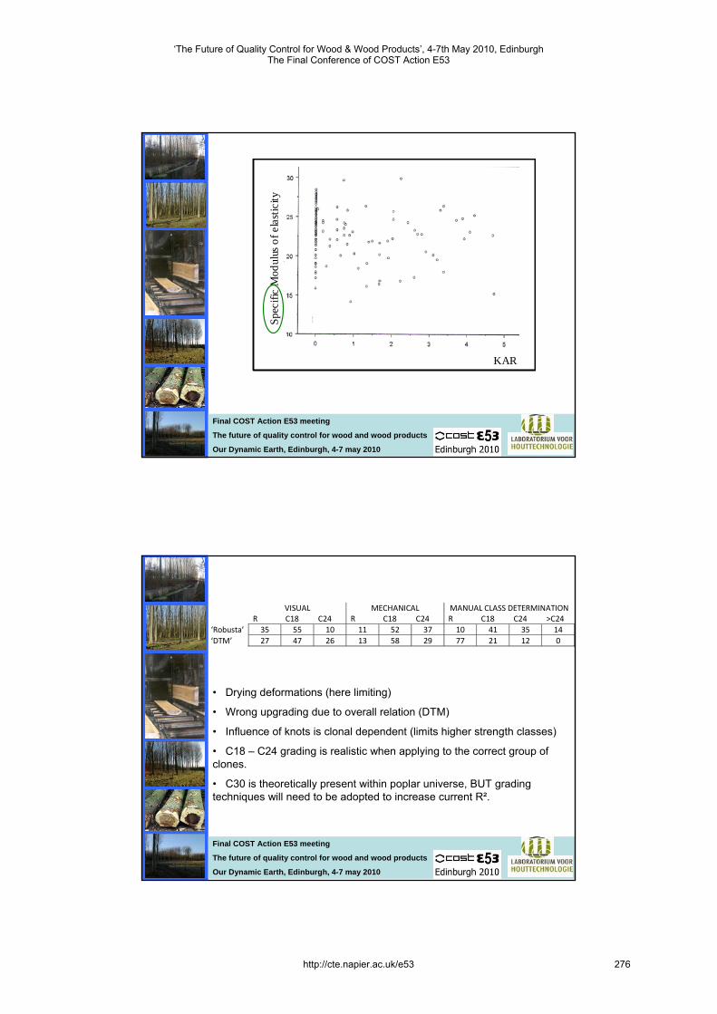
²
Final COST Action E53 meeting
The future of quality control for wood and wood products
Our Dynamic Earth, Edinburgh, 4-7 may 2010
KAR
Spec
ific
Mod
ulus
of e
last
icity
²
Final COST Action E53 meeting
The future of quality control for wood and wood products
Our Dynamic Earth, Edinburgh, 4-7 may 2010
VISUAL MECHANICAL MANUAL CLASS DETERMINATION R C18 C24 R C18 C24 R C18 C24 >C24
‘Robusta’ 35 55 10 11 52 37 10 41 35 14 ‘DTM’ 27 47 26 13 58 29 77 21 12 0
• Drying deformations (here limiting)
• Wrong upgrading due to overall relation (DTM)
• Influence of knots is clonal dependent (limits higher strength classes)
• C18 – C24 grading is realistic when applying to the correct group of clones.
• C30 is theoretically present within poplar universe, BUT grading techniques will need to be adopted to increase current R².
‘The Future of Quality Control for Wood & Wood Products’, 4-7th May 2010, EdinburghThe Final Conference of COST Action E53
http://cte.napier.ac.uk/e53 276

²
Final COST Action E53 meeting
The future of quality control for wood and wood products
Our Dynamic Earth, Edinburgh, 4-7 may 2010
VENEER BASED PRODUCTS
Clone
Site
Heartwood proportion
[%]
Tension wood proportion
[%]
Density
[Kg/m³]
MOE
[N/mm²]
MOR
[N/mm²] 70 078 /2 Holsbeek 28 24 380 7700 48 - 70 078 /6 Basilly 48 21 360 7400 47 - 70 078 /11 Holsbeek 38 29 385 8100 51 Basilly 41 32 365 7600 48 71 106 /1 Holsbeek 54 42 365 7300 44 - 71 106 /5 Holsbeek 60 38 345 6900 42 Basilly 65 35 355 6700 44
²
Final COST Action E53 meeting
The future of quality control for wood and wood products
Our Dynamic Earth, Edinburgh, 4-7 may 2010
Veneer quality grade A B1 B3 C D and NC 70 078 /2 Holsbeek - - 35 % 62 % 3 % 70 078 /6 Basilly 3 % 10 % 34 % 49 % 4 % 70 078 /11 Holsbeek - 7 % 37 % 47 % 10 % Basilly 2 % 18 % 30 % 44 % 6 % 71 106 /1 Holsbeek - 5 % 33 % 62 % 3 % 71 106 /5 Holsbeek - 2 % 33 % 61 % 3 % Basilly 2 % 17 % 47 % 31 % 3 %
Abbreviation Description A Closed veneers, absence of defects, even coloured B1 Closed veneers, sound knots allowed up till 15 mm B3 Cracks up till 40 cm (not wide open) but maximum 3
Sound knots allowed up till 30 mm Defects can be technically repaired
C No limit for sound knots Loose knots allowed up till 30 mm No limit on cracks (but cracks are not wide open) Interior plies only
D Not classified in the above. Can not be used as such (re-cut) Interior plies only
NC Not classified (to wet, to small dimensions)
‘The Future of Quality Control for Wood & Wood Products’, 4-7th May 2010, EdinburghThe Final Conference of COST Action E53
http://cte.napier.ac.uk/e53 277

²
Final COST Action E53 meeting
The future of quality control for wood and wood products
Our Dynamic Earth, Edinburgh, 4-7 may 2010
DTM DM Duncan ranking Density of the board 485 ± 12 415 ± 21 ab Modulus of elasticity ⊥ 2830 ± 280 2315 ± 64 ab // 4435 ± 255 3820 ± 246 ab Modulus of rupture ⊥ 28.1 ± 1.8 26.8 ± 2.3 aa // 44.3 ± 1.4 42.4 ± 2.5 aa
²
Final COST Action E53 meeting
The future of quality control for wood and wood products
Our Dynamic Earth, Edinburgh, 4-7 may 2010
LAMINATED TIMBER
Type III Type II Type I Type I*
Lamella 5 Grade B Grade B Grade A Grade A Lamella 4 Grade B Grade C Grade B Grade A Lamella 3 Grade B Grade C Grade B Grade A Lamella 2 Grade B Grade C Grade B Grade A Lamella 1 Grade B Grade B Grade A Grade A
‘The Future of Quality Control for Wood & Wood Products’, 4-7th May 2010, EdinburghThe Final Conference of COST Action E53
http://cte.napier.ac.uk/e53 278

²
Final COST Action E53 meeting
The future of quality control for wood and wood products
Our Dynamic Earth, Edinburgh, 4-7 may 2010
RESULTS AND DISCUSSION
Ogy Gaver Statistics Anova/Duncan
Density [kg/m³] 425 ± 35 422 ± 33 aa KAR [%] 0.6 ± 1.1 0.6 ± 0.9 aa Moisture content [%] 8.2 ± 0.2 8.3 ± 0.3 aa Tension wood [%] 10.5 ± 0.8 5.5 ± 0.5 ab MOE [N/mm²] 8200 ± 221 7560 ± 126 ab MOR [N/mm²] 68.2 ± 7.4 71.8 ± 6.7 aa
²
Final COST Action E53 meeting
The future of quality control for wood and wood products
Our Dynamic Earth, Edinburgh, 4-7 may 2010
Type Glue Classification based on Beam properties
Classification based on lamella properties
II PUR Not classified Not classified II III
ISO PUR ISO
GL 24 Not classified
II III
PR PR
GL 28 GL 24
I ISO PR PUR
GL 32 GL 24
OGY
‘The Future of Quality Control for Wood & Wood Products’, 4-7th May 2010, EdinburghThe Final Conference of COST Action E53
http://cte.napier.ac.uk/e53 279
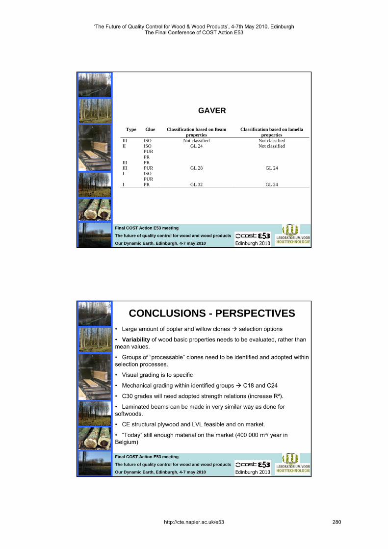
²
Final COST Action E53 meeting
The future of quality control for wood and wood products
Our Dynamic Earth, Edinburgh, 4-7 may 2010
Type Glue Classification based on Beam properties
Classification based on lamella properties
III ISO Not classified Not classified II III
ISO PUR PR PR
GL 24 Not classified
III I
PUR ISO PUR
GL 28 GL 24
I PR GL 32 GL 24
GAVER
²
Final COST Action E53 meeting
The future of quality control for wood and wood products
Our Dynamic Earth, Edinburgh, 4-7 may 2010
CONCLUSIONS - PERSPECTIVES• Large amount of poplar and willow clones selection options
• Variability of wood basic properties needs to be evaluated, rather than mean values.
• Groups of “processable” clones need to be identified and adopted within selection processes.
• Visual grading is to specific
• Mechanical grading within identified groups C18 and C24
• C30 grades will need adopted strength relations (increase R²).
• Laminated beams can be made in very similar way as done for softwoods.
• CE structural plywood and LVL feasible and on market.
• “Today” still enough material on the market (400 000 m³/ year in Belgium)
‘The Future of Quality Control for Wood & Wood Products’, 4-7th May 2010, EdinburghThe Final Conference of COST Action E53
http://cte.napier.ac.uk/e53 280

²
Final COST Action E53 meeting
The future of quality control for wood and wood products
Our Dynamic Earth, Edinburgh, 4-7 may 2010
THANK YOU
This work has been financed by the Institute of Nature and Forest Research (INBO – Geraardsbergen, Belgium) of the Ministry of the Flemish Community within the framework of the project “Tree and Wood Quality Research for the
Flemish Forest-Wood Chain”.
‘The Future of Quality Control for Wood & Wood Products’, 4-7th May 2010, EdinburghThe Final Conference of COST Action E53
http://cte.napier.ac.uk/e53 281
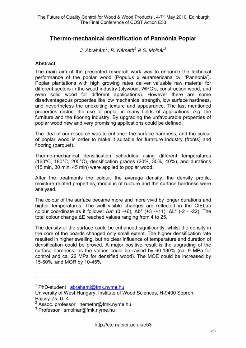
‘The Future of Quality Control for Wood & Wood Products’, 4-7th May 2010, Edinburgh The Final Conference of COST Action E53
Thermo-mechanical densification of Pannónia Poplar
J. Ábrahám1, R. Németh2 & S. Molnár3
Abstract The main aim of the presented research work was to enhance the technical performance of the poplar wood (Populus x euramericana cv. ‘Pannonia’). Poplar plantations with high growing rates deliver valuable raw material for different sectors in the wood industry (plywood, WPC’s, construction wood, and even solid wood for different applications). However there are some disadvantageous properties like low mechanical strength, low surface hardness, and nevertheless the unexciting texture and appearance. The last mentioned properties restrict the use of poplar in many fields of applications, e.g. the furniture and the flooring industry. By upgrading the unfavourable properties of poplar wood new and very promising applications could be defined.
The idea of our research was to enhance the surface hardness, and the colour of poplar wood in order to make it suitable for furniture industry (fronts) and flooring (parquet).
Thermo-mechanical densification schedules using different temperatures (160°C, 180°C, 200°C), densification grades (20%, 30%, 40%), and durations (15 min, 30 min, 45 min) were applied to poplar wood.
After the treatments the colour, the average density, the density profile, moisture related properties, modulus of rupture and the surface hardness were analysed.
The colour of the surface became more and more vivid by longer durations and higher temperatures. The well visible changes are reflected in the CIELab colour coordinate as it follows: Δa* (0 -+6), Δb* (+3 -+11), ΔL* (-2 - -22). The total colour change ΔE reached values ranging from 4 to 25.
The density of the surface could be enhanced significantly, whilst the density in the core of the boards changed only small extent. The higher densification rate resulted in higher swelling, but no clear influence of temperature and duration of densification could be proved. A major positive result is the upgrading of the surface hardness, as the values could be raised by 60-130% (ca. 9 MPa for control and ca. 22 MPa for densified wood). The MOE could be increased by 15-60%, and MOR by 10-45%.
1 PhD-student [email protected] of West Hungary, Institute of Wood Sciences, H-9400 Sopron, Bajcsy-Zs. U. 4 2 Assoc. professor [email protected] 3 Professor [email protected]
http://cte.napier.ac.uk/e53 282
‘The Future of Quality Control for Wood & Wood Products’, 4-7th May 2010, Edinburgh The Final Conference of COST Action E53
Introduction Poplars play an important role in the plantation forestry in Hungary. Nowadays the share of poplars in the afforestations amounts to ca. 30%, the fellings come to 1 Million m3/year. However the utilisation of poplar timber shows many difficulties. Top quality logs are processed in the plywood industry, while sawlogs deliver the raw material for pallets and boxes. The short logs are utilised in the particle board and fibreboard mills. Recently poplar species are grown on energy plantations as well. The major problem is that even quality sawlogs are processed to low price pallets, thus the technology is uneconomical. In spite of some positive examples (e.g. in the building sector), the utilisation of poplar timber in Hungary is still an unsolved challenge.
Possible outbreak from this situation could be the production of furniture and other interior products. Unfavourable properties of poplar, such as low strength and stiffness, low durability, inexpressive colour and texture are a clear hindrance for widespread utilisation of the material in the furniture industry.
In order to surmount the obstacles we focussed our research work to enhance the relevant physical, mechanical and esthetical properties of poplar wood. The specific aim of our work was to establish the scientific background for a thermo-mechanical modification method. The process should enhance the surface hardness, the strength and the appearance of this low density wood with thin fibre walls.
Studying the literature there is a lack of scientific results concerning thermo-mechanical densification of poplar wood. Basically conifers were studied as reported by Welzbacher et al 2008, Unsala et al 2009, Navi and Girardet 2000, Unsala et al 2009. Recently results were published concerning hardwoods by Rautkari et al 2009, and Gong et al 2010. A good summary about the densification of wood was given by Kuatnar and Sernek 2007. The future potential in Europe of poplar is justified eg. by the work of De Boever (2010).
Material and methods Poplar boards for the investigations were delivered by the KAEG Zrt. The freshly cut boards were dried in a conventional dryer down to 12% MC. The boards were than cut into laths. The laths were densified in hot press across the grain at 3 different temperatures. 160°C, 180°C and 200°C. Three different starting thicknesses (25.0mm, 28.5mm and 33.3mm) were used. The final thickness of the laths was set to 20mm fro all laths. Thus the grade of the densification was 20%, 30% and 40%. After the densification under heat, the wood material was kept for 10, 20 and 30 minutes in the hot press at the corresponding temperature.
After the treatment the change in different material properties were studied. The investigated properties were: the colour change, moisture related shrinking and swelling, surface hardness, MOR and the grade of densification across the thickness.
http://cte.napier.ac.uk/e53 283
‘The Future of Quality Control for Wood & Wood Products’, 4-7th May 2010, Edinburgh The Final Conference of COST Action E53
The colour properties were measures by a CM-2600d spectrophotometer working in the CIELab system. The device calculated and delivered directly the required colour coordinates L*, a* and b*. A CIE D65 xenon lamp served as light source, the window for measurements had a diameter of 10mm. The colour coordinates were measured prior and after the treatments (thermal densification). The chroma (C) and the total colour change (ΔE) were calculated regarding Eq. 1 and Eq. 2.
22 ∗∗∗ += baC Equation 1
222 ∗∗∗∗ Δ+Δ+Δ=Δ baLE Equation 2
The ovendry density was determined according to MSZ 6786-3:1988 using specimen with the dimension of 20mmx20mmx30mm (RxTxL).
The shrinking properties were measured following the standard MSZ 6786-18:1989, with the deviation that the directions across the grain were defined as directions parallel and perpendicular to the pressing force rather than radial and tangential anatomical directions. The density and shrinking were determined on the same samples. Shrinking values were determined during drying from ca. 10% MC to ovendry state. The shrinking coefficient were than calculated as the ratio of the measured swelling (%) and the MC change (10%).
The surface hardness (Brinell-Mörath) was determined according to MSZ 6786-11:1982. A ball with the diameter (D) of 10mm penetrated the surface of the specimen with a maximum force (F) of 500N, the penetration depth (h in mm) was measured as well. The Brinell-Mörath hardness value (N/mm2) was calculated using Eq. 3.
hDFH BM ⋅⋅
=π
Equation 3
The hardness was determined prior and after the densification, so the change in percentage caused by the treatment could be calculated.
The modulus of rupture was measured following the standard MSZ 6786-5:1976. The dimension of specimen was 20mmx20mmx300mm (RxTxL). The distance between the supports was 240mm. The tests were carried out by using one force, where the direction of the testing force corresponded to the treating force (pressure). .
After the treatment the degree of the densification was determined across the thickness. In order to be able to detect the deformations in different depths, liens in 45°to the pressing direction were drawn onto the side surface of the laths. The curving of the straight lines (Fig. 10) deliver data on the deformations of the material. The lines were photographed after the treatment and analysed by sectioning them into 20 parts.
http://cte.napier.ac.uk/e53 284
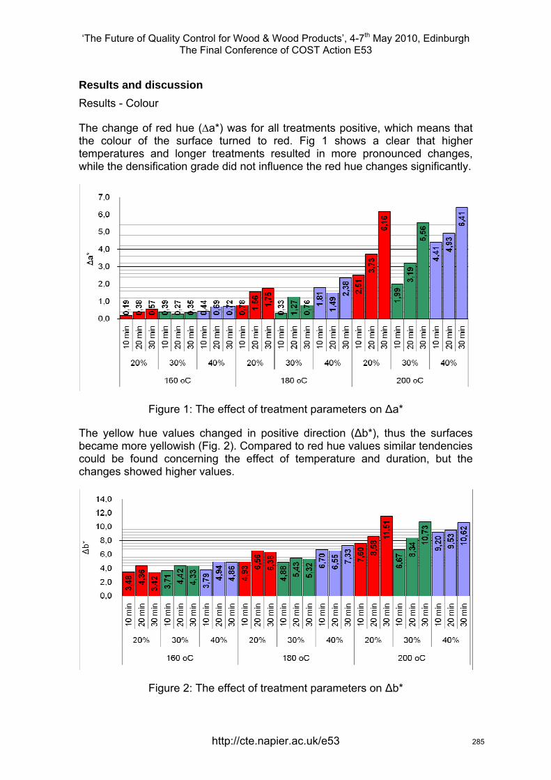
‘The Future of Quality Control for Wood & Wood Products’, 4-7th May 2010, Edinburgh The Final Conference of COST Action E53
Results and discussion Results - Colour
The change of red hue (Δa*) was for all treatments positive, which means that the colour of the surface turned to red. Fig 1 shows a clear that higher temperatures and longer treatments resulted in more pronounced changes, while the densification grade did not influence the red hue changes significantly.
Figure 1: The effect of treatment parameters on Δa*
The yellow hue values changed in positive direction (Δb*), thus the surfaces became more yellowish (Fig. 2). Compared to red hue values similar tendencies could be found concerning the effect of temperature and duration, but the changes showed higher values.
Figure 2: The effect of treatment parameters on Δb*
http://cte.napier.ac.uk/e53 285
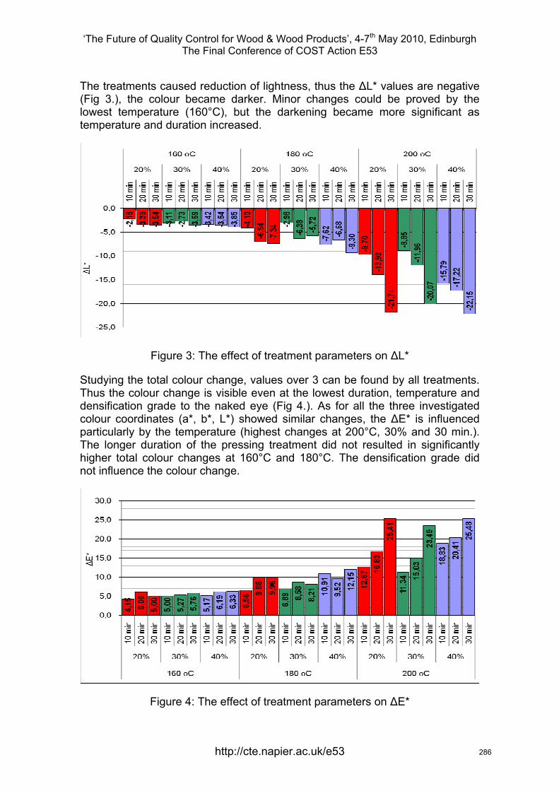
‘The Future of Quality Control for Wood & Wood Products’, 4-7th May 2010, Edinburgh The Final Conference of COST Action E53
The treatments caused reduction of lightness, thus the ΔL* values are negative (Fig 3.), the colour became darker. Minor changes could be proved by the lowest temperature (160°C), but the darkening became more significant as temperature and duration increased.
Figure 3: The effect of treatment parameters on ΔL*
Studying the total colour change, values over 3 can be found by all treatments. Thus the colour change is visible even at the lowest duration, temperature and densification grade to the naked eye (Fig 4.). As for all the three investigated colour coordinates (a*, b*, L*) showed similar changes, the ΔE* is influenced particularly by the temperature (highest changes at 200°C, 30% and 30 min.). The longer duration of the pressing treatment did not resulted in significantly higher total colour changes at 160°C and 180°C. The densification grade did not influence the colour change.
Figure 4: The effect of treatment parameters on ΔE*
http://cte.napier.ac.uk/e53 286
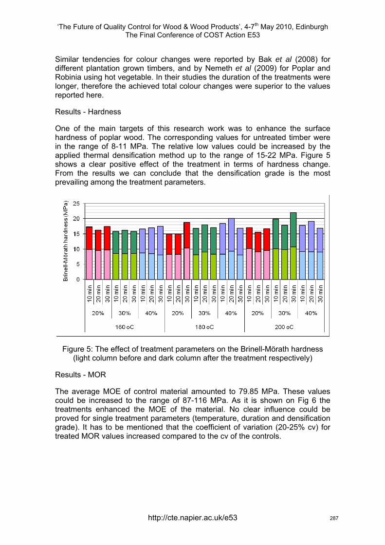
‘The Future of Quality Control for Wood & Wood Products’, 4-7th May 2010, Edinburgh The Final Conference of COST Action E53
Similar tendencies for colour changes were reported by Bak et al (2008) for different plantation grown timbers, and by Nemeth et al (2009) for Poplar and Robinia using hot vegetable. In their studies the duration of the treatments were longer, therefore the achieved total colour changes were superior to the values reported here.
Results - Hardness
One of the main targets of this research work was to enhance the surface hardness of poplar wood. The corresponding values for untreated timber were in the range of 8-11 MPa. The relative low values could be increased by the applied thermal densification method up to the range of 15-22 MPa. Figure 5 shows a clear positive effect of the treatment in terms of hardness change. From the results we can conclude that the densification grade is the most prevailing among the treatment parameters.
Figure 5: The effect of treatment parameters on the Brinell-Mörath hardness (light column before and dark column after the treatment respectively)
Results - MOR
The average MOE of control material amounted to 79.85 MPa. These values could be increased to the range of 87-116 MPa. As it is shown on Fig 6 the treatments enhanced the MOE of the material. No clear influence could be proved for single treatment parameters (temperature, duration and densification grade). It has to be mentioned that the coefficient of variation (20-25% cv) for treated MOR values increased compared to the cv of the controls.
http://cte.napier.ac.uk/e53 287
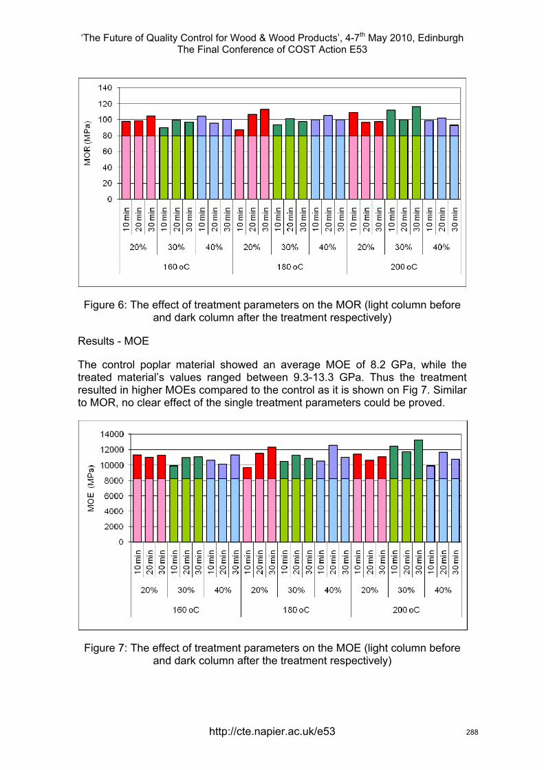
‘The Future of Quality Control for Wood & Wood Products’, 4-7th May 2010, Edinburgh The Final Conference of COST Action E53
Figure 6: The effect of treatment parameters on the MOR (light column before and dark column after the treatment respectively)
Results - MOE
The control poplar material showed an average MOE of 8.2 GPa, while the treated material’s values ranged between 9.3-13.3 GPa. Thus the treatment resulted in higher MOEs compared to the control as it is shown on Fig 7. Similar to MOR, no clear effect of the single treatment parameters could be proved.
Figure 7: The effect of treatment parameters on the MOE (light column before and dark column after the treatment respectively)
http://cte.napier.ac.uk/e53 288
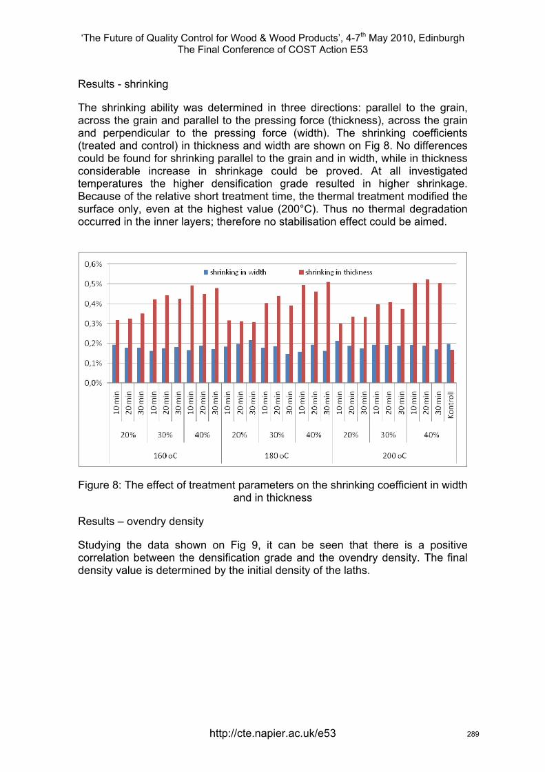
‘The Future of Quality Control for Wood & Wood Products’, 4-7th May 2010, Edinburgh The Final Conference of COST Action E53
Results - shrinking
The shrinking ability was determined in three directions: parallel to the grain, across the grain and parallel to the pressing force (thickness), across the grain and perpendicular to the pressing force (width). The shrinking coefficients (treated and control) in thickness and width are shown on Fig 8. No differences could be found for shrinking parallel to the grain and in width, while in thickness considerable increase in shrinkage could be proved. At all investigated temperatures the higher densification grade resulted in higher shrinkage. Because of the relative short treatment time, the thermal treatment modified the surface only, even at the highest value (200°C). Thus no thermal degradation occurred in the inner layers; therefore no stabilisation effect could be aimed.
Figure 8: The effect of treatment parameters on the shrinking coefficient in width and in thickness
Results – ovendry density
Studying the data shown on Fig 9, it can be seen that there is a positive correlation between the densification grade and the ovendry density. The final density value is determined by the initial density of the laths.
http://cte.napier.ac.uk/e53 289
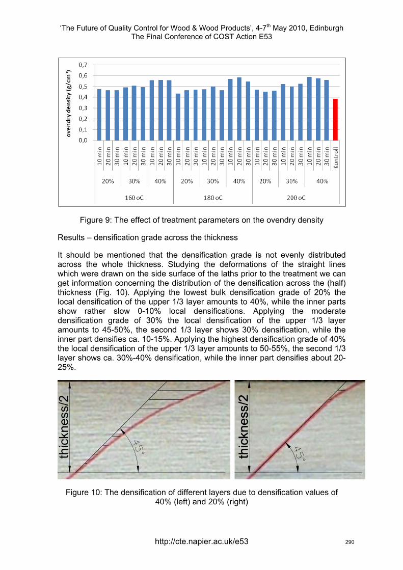
‘The Future of Quality Control for Wood & Wood Products’, 4-7th May 2010, Edinburgh The Final Conference of COST Action E53
Figure 9: The effect of treatment parameters on the ovendry density
Results – densification grade across the thickness
It should be mentioned that the densification grade is not evenly distributed across the whole thickness. Studying the deformations of the straight lines which were drawn on the side surface of the laths prior to the treatment we can get information concerning the distribution of the densification across the (half) thickness (Fig. 10). Applying the lowest bulk densification grade of 20% the local densification of the upper 1/3 layer amounts to 40%, while the inner parts show rather slow 0-10% local densifications. Applying the moderate densification grade of 30% the local densification of the upper 1/3 layer amounts to 45-50%, the second 1/3 layer shows 30% densification, while the inner part densifies ca. 10-15%. Applying the highest densification grade of 40% the local densification of the upper 1/3 layer amounts to 50-55%, the second 1/3 layer shows ca. 30%-40% densification, while the inner part densifies about 20-25%.
Figure 10: The densification of different layers due to densification values of 40% (left) and 20% (right)
http://cte.napier.ac.uk/e53 290
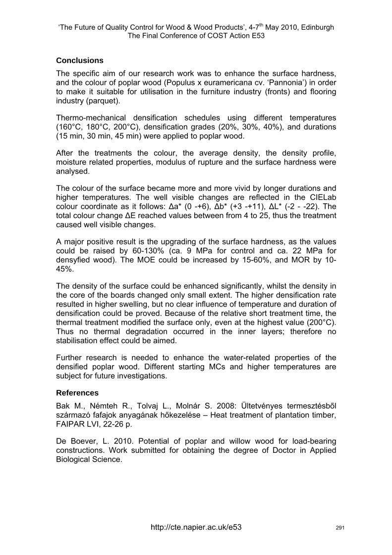
‘The Future of Quality Control for Wood & Wood Products’, 4-7th May 2010, Edinburgh The Final Conference of COST Action E53
Conclusions The specific aim of our research work was to enhance the surface hardness, and the colour of poplar wood (Populus x euramericana cv. ‘Pannonia’) in order to make it suitable for utilisation in the furniture industry (fronts) and flooring industry (parquet).
Thermo-mechanical densification schedules using different temperatures (160°C, 180°C, 200°C), densification grades (20%, 30%, 40%), and durations (15 min, 30 min, 45 min) were applied to poplar wood.
After the treatments the colour, the average density, the density profile, moisture related properties, modulus of rupture and the surface hardness were analysed.
The colour of the surface became more and more vivid by longer durations and higher temperatures. The well visible changes are reflected in the CIELab colour coordinate as it follows: Δa* (0 -+6), Δb* (+3 -+11), ΔL* (-2 - -22). The total colour change ΔE reached values between from 4 to 25, thus the treatment caused well visible changes.
A major positive result is the upgrading of the surface hardness, as the values could be raised by 60-130% (ca. 9 MPa for control and ca. 22 MPa for densyfied wood). The MOE could be increased by 15-60%, and MOR by 10-45%.
The density of the surface could be enhanced significantly, whilst the density in the core of the boards changed only small extent. The higher densification rate resulted in higher swelling, but no clear influence of temperature and duration of densification could be proved. Because of the relative short treatment time, the thermal treatment modified the surface only, even at the highest value (200°C). Thus no thermal degradation occurred in the inner layers; therefore no stabilisation effect could be aimed.
Further research is needed to enhance the water-related properties of the densified poplar wood. Different starting MCs and higher temperatures are subject for future investigations.
References Bak M., Némteh R., Tolvaj L., Molnár S. 2008: Ültetvényes termesztésből származó fafajok anyagának hőkezelése – Heat treatment of plantation timber, FAIPAR LVI, 22-26 p.
De Boever, L. 2010. Potential of poplar and willow wood for load-bearing constructions. Work submitted for obtaining the degree of Doctor in Applied Biological Science.
http://cte.napier.ac.uk/e53 291
‘The Future of Quality Control for Wood & Wood Products’, 4-7th May 2010, Edinburgh The Final Conference of COST Action E53
Gong M., Lamasona C., Lia L. 2010: Interactive effect of surface densification and post-heat-treatment on aspen wood. Journal of Materials Processing Technology. Volume 210, Issue 2, 19 January 2010, Pages 293-296
Kutnar A., Šernek M. 2007: Densification of wood. Zbornik gozdarstva in lesarstva 82 (2007), s. 53–62
Németh R., Bak M., Tolvaj L., Molnár S. 2009: The effect of thermal treatment using vegetable oils on physical and mechanical properties of Poplar and Robinia wood. Pro Ligno, 5(2), pp. 33-37. ISSN 1841-4737
Rautkari L., Properzi M., Pichelin F., Hughes M. 2009: Properties and set-recovery of surface densified Norway spruce and European beech. Wood Science and Technology. Published online: 10 November 2009
Unsala O., S. Nami Kartala S. N., Candana Z., Arangob R. A., Clausenb C. A., Green F. 2009: Decay and termite resistance, water absorption and swelling of thermally compressed wood panels. International Biodeterioration & Biodegradation. Volume 63, Issue 5, July 2009, Pages 548-552
Welzbacher C. R., Wehsener J., Rapp A. O., Haller P. 2008: Thermo-mechanical densification combined with thermal modification of Norway spruce (Picea abies Karst) in industrial scale –Dimensional stability and durability aspects. Holz Roh Werkst (2008) 66: 39–49
http://cte.napier.ac.uk/e53 292

‘The Future of Quality Control for Wood & Wood Products’, 4-7th May 2010, Edinburgh The Final Conference of COST Action E53
Thursday 6th May Research focussed day
Plenary
http://www.cte.napier.ac.uk/e53/ 293
‘The Future of Quality Control for Wood & Wood Products’, 4-7th May 2010, Edinburgh The Final Conference of COST Action E53
Quality control and improvement of structural timber
M. Deublein1, R. Steiger2 & J. Köhler3
Abstract Modern applications of structural timber like e.g. in the field of multi-storey domiciles or large span structures require graded timber products with sufficient and in many cases high performing mechanical properties. This can only be reached by means of advanced methods for quality control within the production process of structural timber. In this paper, quality control and improvement of structural timber is subdivided into three constitutive sub-items: 1) process monitoring, 2) process calibration and 3) process optimization. The paper at hand can be considered as a summary of the authors’ investigations and contributions within COST action E53. Different approaches for quality control and improvement of structural timber by means of machine grading are described. An optimized combination of the three sub-items of process control may lead to an enhanced recovery of the timber material quality and to an improved benefit and reliability in the graded timber material.
1 Introduction Modern grading machines facilitate the integration of the grading process into the industrialized production scheme with its high demand for production rate. Besides the speed the efficiency of the grading machines depends on the machine’s capability to divide the gross supply of ungraded timber into sub-sets of graded timber that fulfil some predefined requirements. Several types of grading machines can be found on the market, measuring different sets of particular indicative properties during the grading process, e.g. bending deflection, ultrasound velocity, natural frequency, x-ray absorption, etc.. However, independent from the type of the grading machine and the number of measured properties, grading machines generate one compound variable as an output, which is a function of all particular properties measurable by the machine as a prediction of the grade determining property (e.g. strength, stiffness or density). Disregarding the fact that this variable is an artifact composed from the machine measurements and the underlying function or algorithm the indicative variable is generally termed indicating property and this is the term also used in the remainder of the present paper. For every grading machine acceptance criteria are formulated in form of intervals for the corresponding indicating property that have to be matched to qualify a piece of timber to a certain grade. These boundaries are termed grading machine settings. The performance, i.e. the statistical characteristics of the output of grading machines strongly depends on these settings, and in general very much attention is kept on how to control these machine settings.
1 ETH Zurich / EMPA, Switzerland, mail: [email protected] EMPA Dübendorf, Switzerland, mail: [email protected] ETH Zurich, Switzerland, mail: [email protected]
http://cte.napier.ac.uk/e53 294
‘The Future of Quality Control for Wood & Wood Products’, 4-7th May 2010, Edinburgh The Final Conference of COST Action E53
The present European practice for machine based grading of structural timber is specified in the European Standard EN 14081. According to this standard the control of machine settings relies on two procedures, the so-called machine control (cost matrix) method and the output control (CUSUM) method. These two methods are broadly considered to be either too complex or expensive. Hence, investigations have been conducted by the participants of COST Action E53 for each of the sub-items of quality control. Some of the contributions of this paper’s authors are summarized in the subsequent chapters. Different aspects of quality control and optimization are combined to achieve a coherent and overall strategy for quality control of structural timber based on machine assessment of timber properties; applicable for both, revision of existing codes and standards as well as for company-internal product optimization.
In the following chapters the overall quality control procedure is subdivided into three main topics: process monitoring, process calibration and process optimization. Due to the limited length of this paper the particular approaches and methods are described just briefly. Hence, for better understanding and additional information references to the relevant publications are provided within every chapter.
2 Quality control and improvement of structural timber Graded timber material can be utilized for structural purposes either directly as solid timber columns and beams or indirectly in the form of basic raw material for engineered timber products. In both cases, when timber products are utilized in high performance timber structures i.e. whenever the load bearing capacity or the stiffness determines the design, it is a requirement that the timber products are classified to ensure adequately performing mechanical properties. In modern production management, where speed, reliability and costs are prerequisites for competitiveness, machine grading is in reality the only viable option. As a consequence, advanced and modern methods for the calibration and running assessment of grading machines have to be developed and implemented into practice. However, since wood is a natural grown building material deviations in timber quality may occur during the grading process over time. This has been observed within industrial environment [1] as well as within a pan-European scientific project [5]. Major fluctuations may be caused either by different sources of the raw material (growth areas, supplier) or by different cutting patterns and dimensions.
2.1 Process monitoring In general, when considering the control of manufacturing processes, the problem is to maintain a production process in such a state that the output from the process conforms to given design requirements (e.g. characteristic values for strength, stiffness and density). During the operation phase the process will be subject to changes which cause the quality of the output to deteriorate. And also the quality of the input material quality of the process may already be subject to significant aberrations.
http://cte.napier.ac.uk/e53 295
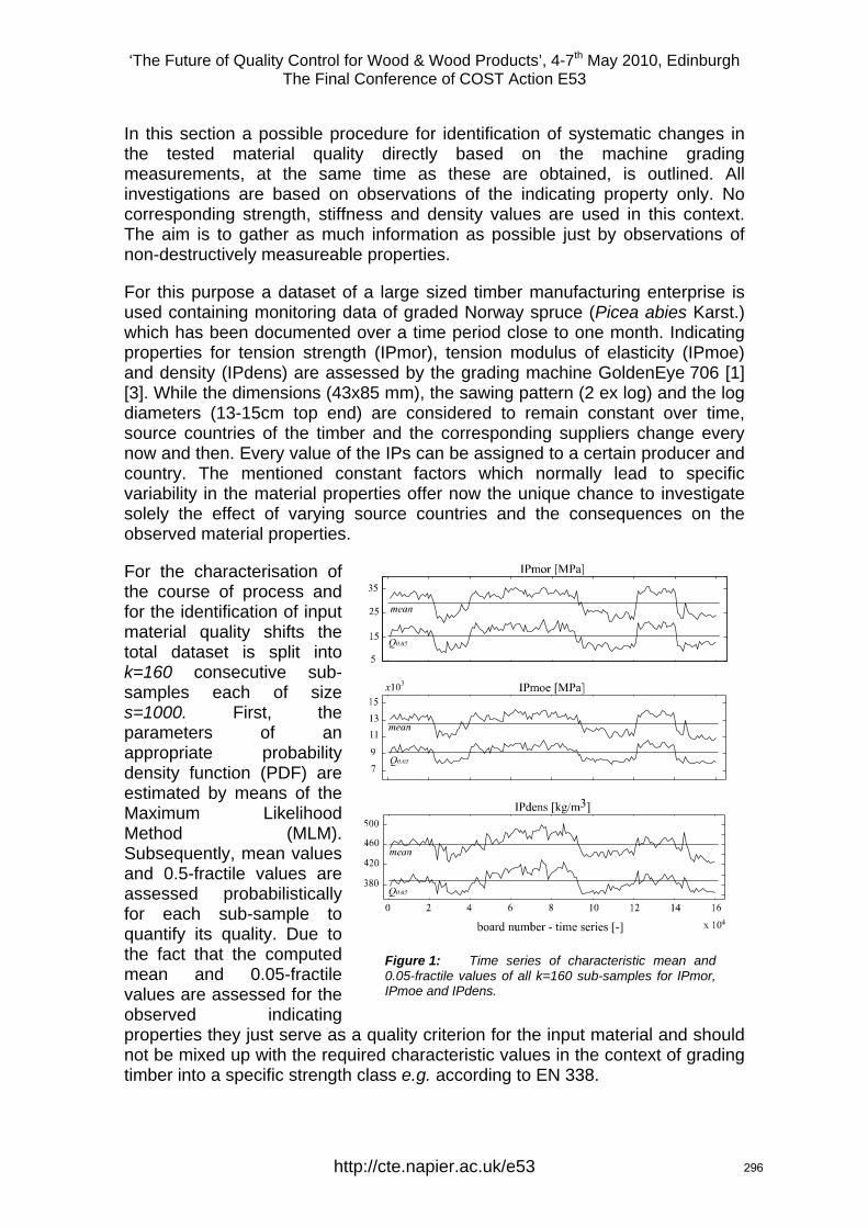
‘The Future of Quality Control for Wood & Wood Products’, 4-7th May 2010, Edinburgh The Final Conference of COST Action E53
In this section a possible procedure for identification of systematic changes in the tested material quality directly based on the machine grading measurements, at the same time as these are obtained, is outlined. All investigations are based on observations of the indicating property only. No corresponding strength, stiffness and density values are used in this context. The aim is to gather as much information as possible just by observations of non-destructively measureable properties.
For this purpose a dataset of a large sized timber manufacturing enterprise is used containing monitoring data of graded Norway spruce (Picea abies Karst.) which has been documented over a time period close to one month. Indicating properties for tension strength (IPmor), tension modulus of elasticity (IPmoe) and density (IPdens) are assessed by the grading machine GoldenEye 706 [1] [3]. While the dimensions (43x85 mm), the sawing pattern (2 ex log) and the log diameters (13-15cm top end) are considered to remain constant over time, source countries of the timber and the corresponding suppliers change every now and then. Every value of the IPs can be assigned to a certain producer and country. The mentioned constant factors which normally lead to specific variability in the material properties offer now the unique chance to investigate solely the effect of varying source countries and the consequences on the observed material properties.
For the characterisation of the course of process and for the identification of input material quality shifts the total dataset is split into k=160 consecutive sub-samples each of size s=1000. First, the parameters of an appropriate probability density function (PDF) are estimated by means of the Maximum Likelihood Method (MLM). Subsequently, mean values and 0.5-fractile values are assessed probabilistically for each sub-sample to quantify its quality. Due to the fact that the computed mean and 0.05-fractile values are assessed for the observed indicating properties they just serve as a quality criterion for the input material and should not be mixed up with the required characteristic values in the context of grading timber into a specific strength class e.g. according to EN 338.
Figure 1: Time series of characteristic mean and 0.05-fractile values of all k=160 sub-samples for IPmor, IPmoe and IPdens.
http://cte.napier.ac.uk/e53 296
‘The Future of Quality Control for Wood & Wood Products’, 4-7th May 2010, Edinburgh The Final Conference of COST Action E53
Figure 1 shows the assessed mean and 0.05-fractile values for each sub-sample and every type of indicating property. The straight line in the middle of the figures illustrates the average value of all 160 sub-sample mean values. Equivalently, the lower straight line indicates the average value of all 160 sub-sample 0.05-fractiles. The jagged lines represent the mean and 0.05-fractiles of the three indicating properties for every particular sub-sample probability distribution. Definite shifts in the jagged lines of the indicating properties are observable. The most significant fluctuations can be found in the grading process starting at board numbers about 2,000, 22,000, 40,000, 122,000 and 142,000.
For the IPmor and IPdens the average of the 0.05-fractiles is taken as desired characteristic of timber material input quality. Lower Control Limits (LCL) and Upper Control Limits (UCL) can be defined based on these desired quality characteristics. For MOE the average value of the sub-sample means is used as desired quality level. That means that the timber material as it is delivered to the manufacturing enterprise should in average exhibit these statistical characteristics.
Three methods for the identification of deviations in the quality of the input timber material are applied to the dataset. The first one adapts the CUSUM control chart method which is given in the European Standard EN 14081, part 3 as one of two possibilities for the control of machine strength grading in Europe. In the context of the investigations of this paper this method is denoted as the non-destructive CUSUM method. Instead of really proof loading the timber specimens physically just the predicted grade determining properties are evaluated. The second method, the control limit method, first defines desired values for the overall input timber material properties and based on these, upper and lower control limits are calculated to control the quality of the input timber material. A third method quantifies differences in the regression coefficients where the relationships of the different IPs are compared to each other between the different source countries of the timber. The effect of growth areas is discussed based on this method. Additionally the regression coefficients of the three IPs assessed on data of remarkably varying input timber material quality are compared.
The results of the application of these three methods are presented in detail at the World Conference of Timber Engineering 2010 in [2].
The core element for the detection of quality shifts is the continuous real-time monitoring of the grading machine measured strength, stiffness and density indicating properties. Different approaches can be used to indicate quality deviations directly based on these non-destructive data measurements. On this way both of the following items can be avoided: 1) Expensive destructive testing procedures although the material quality and production process is “under control”. 2) Inefficient exploitation of the timber material potential since settings of the grading machine would be too conservative for extraordinarily good timber quality.
http://cte.napier.ac.uk/e53 297
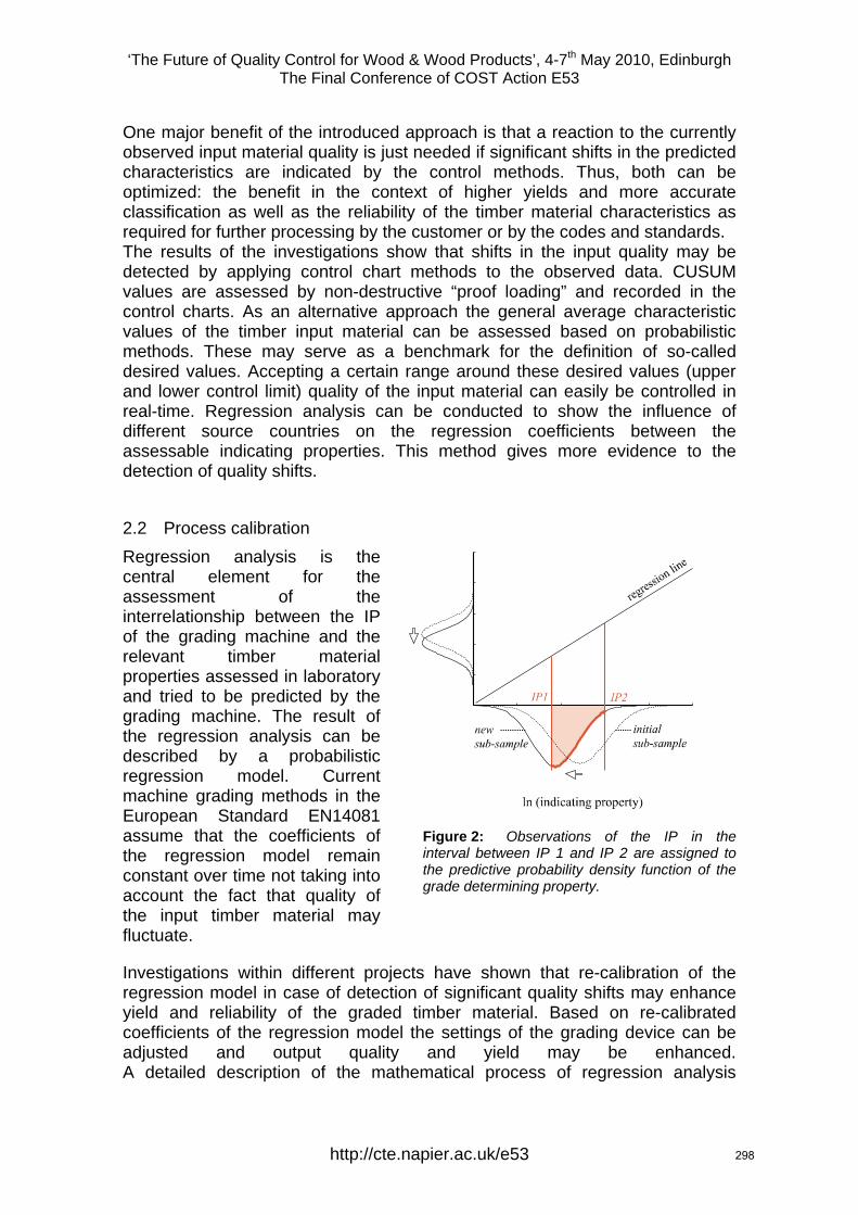
‘The Future of Quality Control for Wood & Wood Products’, 4-7th May 2010, Edinburgh The Final Conference of COST Action E53
One major benefit of the introduced approach is that a reaction to the currently observed input material quality is just needed if significant shifts in the predicted characteristics are indicated by the control methods. Thus, both can be optimized: the benefit in the context of higher yields and more accurate classification as well as the reliability of the timber material characteristics as required for further processing by the customer or by the codes and standards. The results of the investigations show that shifts in the input quality may be detected by applying control chart methods to the observed data. CUSUM values are assessed by non-destructive “proof loading” and recorded in the control charts. As an alternative approach the general average characteristic values of the timber input material can be assessed based on probabilistic methods. These may serve as a benchmark for the definition of so-called desired values. Accepting a certain range around these desired values (upper and lower control limit) quality of the input material can easily be controlled in real-time. Regression analysis can be conducted to show the influence of different source countries on the regression coefficients between the assessable indicating properties. This method gives more evidence to the detection of quality shifts.
2.2 Process calibration Regression analysis is the central element for the assessment of the interrelationship between the IP of the grading machine and the relevant timber material properties assessed in laboratory and tried to be predicted by the grading machine. The result of the regression analysis can be described by a probabilistic regression model. Current machine grading methods in the European Standard EN14081 assume that the coefficients of the regression model remain constant over time not taking into account the fact that quality of the input timber material may fluctuate.
Figure 2: Observations of the IP in the interval between IP 1 and IP 2 are assigned to the predictive probability density function of the grade determining property.
Investigations within different projects have shown that re-calibration of the regression model in case of detection of significant quality shifts may enhance yield and reliability of the graded timber material. Based on re-calibrated coefficients of the regression model the settings of the grading device can be adjusted and output quality and yield may be enhanced. A detailed description of the mathematical process of regression analysis
http://cte.napier.ac.uk/e53 298
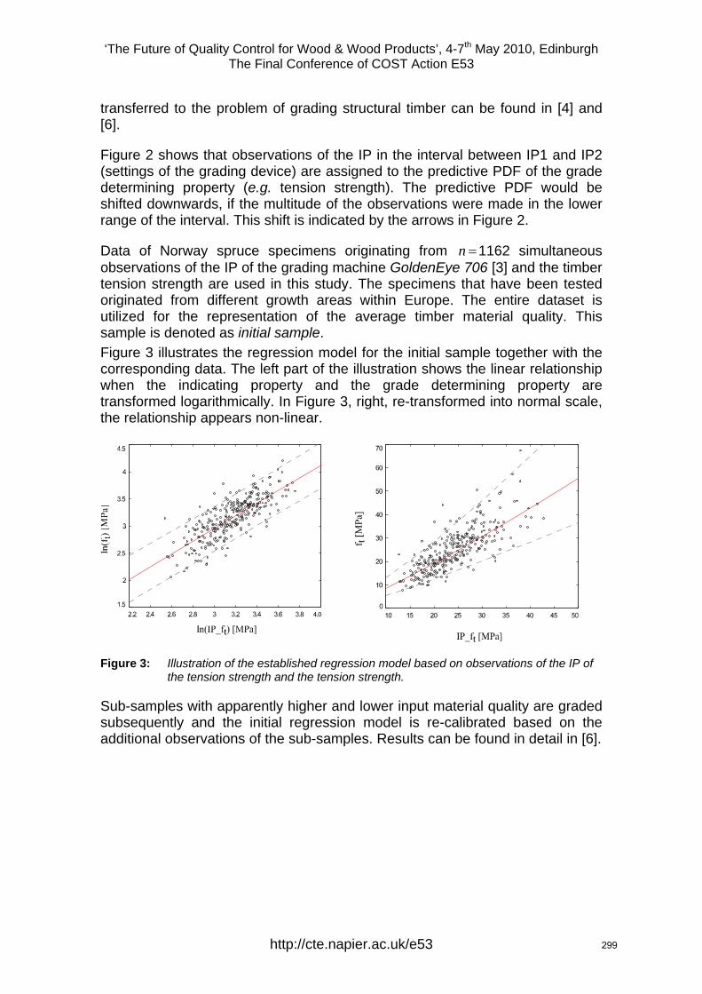
‘The Future of Quality Control for Wood & Wood Products’, 4-7th May 2010, Edinburgh The Final Conference of COST Action E53
transferred to the problem of grading structural timber can be found in [4] and [6].
Figure 2 shows that observations of the IP in the interval between IP1 and IP2 (settings of the grading device) are assigned to the predictive PDF of the grade determining property (e.g. tension strength). The predictive PDF would be shifted downwards, if the multitude of the observations were made in the lower range of the interval. This shift is indicated by the arrows in Figure 2.
Data of Norway spruce specimens originating from n =1162 simultaneous observations of the IP of the grading machine GoldenEye 706 [3] and the timber tension strength are used in this study. The specimens that have been tested originated from different growth areas within Europe. The entire dataset is utilized for the representation of the average timber material quality. This sample is denoted as initial sample. Figure 3 illustrates the regression model for the initial sample together with the corresponding data. The left part of the illustration shows the linear relationship when the indicating property and the grade determining property are transformed logarithmically. In Figure 3, right, re-transformed into normal scale, the relationship appears non-linear.
Figure 3: Illustration of the established regression model based on observations of the IP of the tension strength and the tension strength.
Sub-samples with apparently higher and lower input material quality are graded subsequently and the initial regression model is re-calibrated based on the additional observations of the sub-samples. Results can be found in detail in [6].
http://cte.napier.ac.uk/e53 299
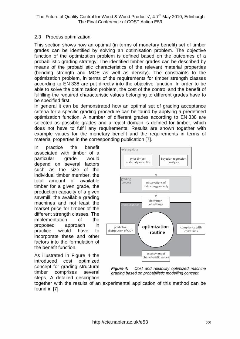
‘The Future of Quality Control for Wood & Wood Products’, 4-7th May 2010, Edinburgh The Final Conference of COST Action E53
2.3 Process optimization This section shows how an optimal (in terms of monetary benefit) set of timber grades can be identified by solving an optimisation problem. The objective function of the optimization problem is defined based on the outcomes of a probabilistic grading strategy. The identified timber grades can be described by means of the probabilistic characteristics of the relevant material properties (bending strength and MOE as well as density). The constraints to the optimization problem, in terms of the requirements for timber strength classes according to EN 338 are put directly into the objective function. In order to be able to solve the optimization problem, the cost of the control and the benefit of fulfilling the required characteristic values belonging to different grades have to be specified first. In general it can be demonstrated how an optimal set of grading acceptance criteria for a specific grading procedure can be found by applying a predefined optimization function. A number of different grades according to EN 338 are selected as possible grades and a reject domain is defined for timber, which does not have to fulfil any requirements. Results are shown together with example values for the monetary benefit and the requirements in terms of material properties in the corresponding publication [7]. In practice the benefit associated with timber of a particular grade would depend on several factors such as the size of the individual timber member, the total amount of available timber for a given grade, the production capacity of a given sawmill, the available grading machines and not least the market price for timber of the different strength classes. The implementation of the proposed approach in practice would have to incorporate these and other factors into the formulation of the benefit function. As illustrated in Figure 4 the introduced cost optimized concept for grading structural timber comprises several steps. A detailed description together with the results of an experimental application of this method can be found in [7].
Figure 4: Cost and reliability optimized machine grading based on probabilistic modelling concept.
http://cte.napier.ac.uk/e53 300

‘The Future of Quality Control for Wood & Wood Products’, 4-7th May 2010, Edinburgh The Final Conference of COST Action E53
The selection of a grading procedure can be made in relation to cost benefit considerations. Based on the proposed statistical modelling of timber properties as a function of the type and efficiency of the grading procedures, a cost optimization routine may be formulated for the identification of optimal grading. Therefore, the cost of the control and the benefit of fulfilling the requirements set for the material characteristics belonging to different grades have to be given.
3 Summary & Outlook Different investigations have shown that there may be serious periodical variations in the input quality of the timber material which is used for industrial manufacturing of structural timber products. The core element for the detection of such quality shifts is the continuous real-time monitoring of the grading machine measured strength, stiffness and density indicating properties. Based on this, a consistent and efficient strategy for control and improvement of structural timber material quality should involve three basic control elements: process monitoring, process calibration and process optimization. It is shown that an optimized combination of these three elements may lead to improved benefit and reliability in the graded timber material. The objective for future investigations is seen in the application of the proposed approaches under practical and industrial environment. Furthermore, ways of reaction with regard to adjustment of grading machine settings have to be defined and the consequences for the reliability of the output material properties have to be assessed.
4 Acknowledgment DOKA GmbH (Amstetten, Austria) and MiCROTEC (Brixen, Italy) are acknowledged with gratitude for allowing us to publish the results of machine strength grading.
http://cte.napier.ac.uk/e53 301
‘The Future of Quality Control for Wood & Wood Products’, 4-7th May 2010, Edinburgh The Final Conference of COST Action E53
References
[1] Bacher M. (2008): Comparison of different Machine Strength Grading Principles. COST E53 Conference Proceedings. “End User’s Needs for Wood Material and Products”. 29th – 30th October 2008. Delft. The Netherlands. pp. 183-193.
[2] Deublein M., Mauritz R., Köhler J. (2010): Real-time Quality Evaluation of Structural Timber. Proceedings of 11th World Conference on Timber Engineering (WCTE2010). 20th – 24th June 2010. Riva del Garda, Italy.
[3] Giudiceandrea F. (2005). Stress grading lumber by a combination of vibration stress waves and X-ray scanning. Proceedings of the 11th International Conference on Scanning Technology and Process Optimization in the Wood Industry (ScanTech 2005), July 24th-26th 2005, Las Vegas, Nevada U.S.A., pp. 99-108.
[4] Köhler J. (2006). Reliability of Timber Structures. Dissertation ETH no. 16378. Swiss Federal Institute of Technology, Zurich, Switzerland.
[5] Ranta-Maunus A., Denzler J. K. (2009): Variability of Strength of European Spruce. Proceedings of the 42nd Meeting. International Council for Research and Innovation in Building and Construction. CIB Working Commission W18 – Timber Structures. Paper No. 42-6-1. Zurich, Switzerland.
[6] Sandomeer M., Köhler J., Faber M. H. (2008): Probabilistic Output Control for Structural Timber – Modelling Approach. Proceedings of the 41st Meeting. International Council for Research and Innovation in Building and Construction. CIB Working Commission W18 – Timber Structures. Paper No. 41-5-1. St. Andrews, Canada.
[7] Sandomeer M., Steiger R., Köhler J. (2009): Cost optimized Timber Machine Strength Grading. COST E53 Conference Proceedings. “Economic and Technical Aspects of Quality Control for Wood and Wood Products”. 22nd – 23rd October 2009. Lisbon, Portugal.
EN 338 (2009): Structural Timber – Strength Classes. Comité Européen de Normalisation, Brussels, Belgium.
EN 14081 (2005): Timber structures – Strength graded structural timber with rectangular cross section; Comité Européen de Normalisation, Brussels, Belgium.
http://cte.napier.ac.uk/e53 302
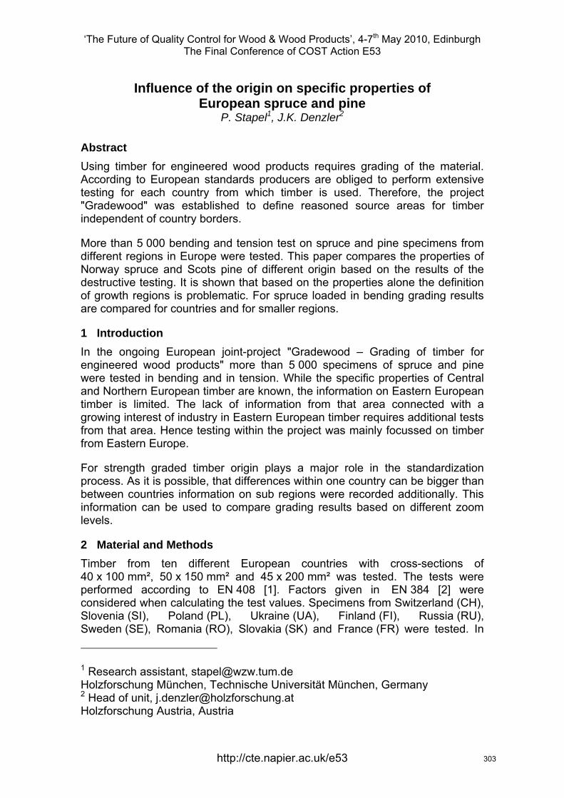
‘The Future of Quality Control for Wood & Wood Products’, 4-7th May 2010, Edinburgh The Final Conference of COST Action E53
http://cte.napier.ac.uk/e53
Influence of the origin on specific properties of European spruce and pine
P. Stapel1, J.K. Denzler2
Abstract Using timber for engineered wood products requires grading of the material. According to European standards producers are obliged to perform extensive testing for each country from which timber is used. Therefore, the project "Gradewood" was established to define reasoned source areas for timber independent of country borders.
More than 5 000 bending and tension test on spruce and pine specimens from different regions in Europe were tested. This paper compares the properties of Norway spruce and Scots pine of different origin based on the results of the destructive testing. It is shown that based on the properties alone the definition of growth regions is problematic. For spruce loaded in bending grading results are compared for countries and for smaller regions.
1 Introduction In the ongoing European joint-project "Gradewood – Grading of timber for engineered wood products" more than 5 000 specimens of spruce and pine were tested in bending and in tension. While the specific properties of Central and Northern European timber are known, the information on Eastern European timber is limited. The lack of information from that area connected with a growing interest of industry in Eastern European timber requires additional tests from that area. Hence testing within the project was mainly focussed on timber from Eastern Europe.
For strength graded timber origin plays a major role in the standardization process. As it is possible, that differences within one country can be bigger than between countries information on sub regions were recorded additionally. This information can be used to compare grading results based on different zoom levels.
2 Material and Methods Timber from ten different European countries with cross-sections of 40 x 100 mm², 50 x 150 mm² and 45 x 200 mm² was tested. The tests were performed according to EN 408 [1]. Factors given in EN 384 [2] were considered when calculating the test values. Specimens from Switzerland (CH), Slovenia (SI), Poland (PL), Ukraine (UA), Finland (FI), Russia (RU), Sweden (SE), Romania (RO), Slovakia (SK) and France (FR) were tested. In
1 Research assistant, [email protected] Holzforschung München, Technische Universität München, Germany 2 Head of unit, [email protected] Holzforschung Austria, Austria
303
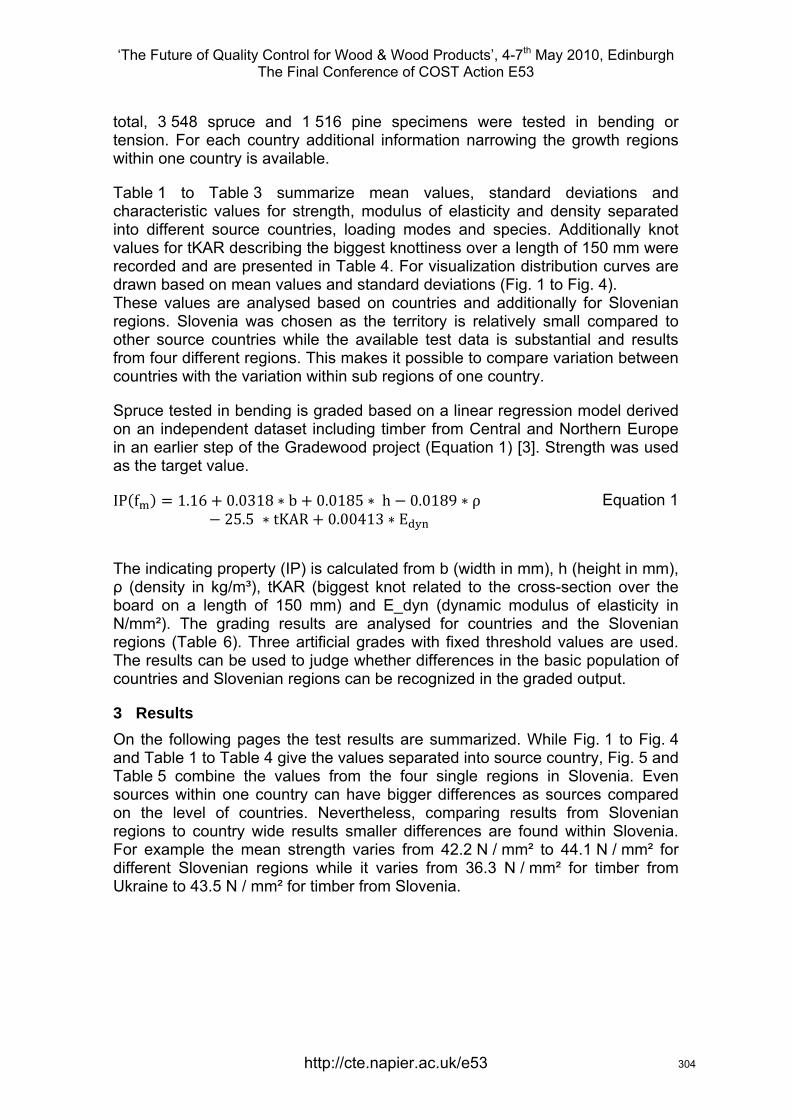
‘The Future of Quality Control for Wood & Wood Products’, 4-7th May 2010, Edinburgh The Final Conference of COST Action E53
http://cte.napier.ac.uk/e53
total, 3 548 spruce and 1 516 pine specimens were tested in bending or tension. For each country additional information narrowing the growth regions within one country is available.
Table 1 to Table 3 summarize mean values, standard deviations and characteristic values for strength, modulus of elasticity and density separated into different source countries, loading modes and species. Additionally knot values for tKAR describing the biggest knottiness over a length of 150 mm were recorded and are presented in Table 4. For visualization distribution curves are drawn based on mean values and standard deviations (Fig. 1 to Fig. 4). These values are analysed based on countries and additionally for Slovenian regions. Slovenia was chosen as the territory is relatively small compared to other source countries while the available test data is substantial and results from four different regions. This makes it possible to compare variation between countries with the variation within sub regions of one country.
Spruce tested in bending is graded based on a linear regression model derived on an independent dataset including timber from Central and Northern Europe in an earlier step of the Gradewood project (Equation 1) [3]. Strength was used as the target value.
IP f 1.16 0.0318 b 0.0185 h 0.0189 ρ25.5 tKAR 0.00413 E
Equation 1
The indicating property (IP) is calculated from b (width in mm), h (height in mm), ρ (density in kg/m³), tKAR (biggest knot related to the cross-section over the board on a length of 150 mm) and E_dyn (dynamic modulus of elasticity in N/mm²). The grading results are analysed for countries and the Slovenian regions (Table 6). Three artificial grades with fixed threshold values are used. The results can be used to judge whether differences in the basic population of countries and Slovenian regions can be recognized in the graded output.
3 Results On the following pages the test results are summarized. While Fig. 1 to Fig. 4 and Table 1 to Table 4 give the values separated into source country, Fig. 5 and Table 5 combine the values from the four single regions in Slovenia. Even sources within one country can have bigger differences as sources compared on the level of countries. Nevertheless, comparing results from Slovenian regions to country wide results smaller differences are found within Slovenia. For example the mean strength varies from 42.2 N / mm² to 44.1 N / mm² for different Slovenian regions while it varies from 36.3 N / mm² for timber from Ukraine to 43.5 N / mm² for timber from Slovenia.
304
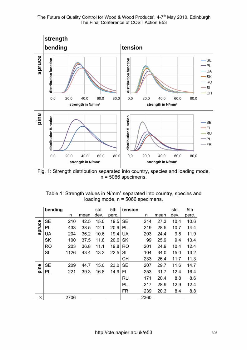
‘The Future of Quality Control for Wood & Wood Products’, 4-7th May 2010, Edinburgh The Final Conference of COST Action E53
http://cte.napier.ac.uk/e53
strength bending tension
spru
ce
pine
Fig. 1: Strength distribution separated into country, species and loading mode, n = 5066 specimens.
Table 1: Strength values in N/mm² separated into country, species and
loading mode, n = 5066 specimens.
bending
n mean std.dev.
5th perc.
tensionn mean
std. dev.
5th perc.
spru
ce SE 210 42.5 15.0 19.5 SE 214 27.3 10.4 10.6
PL 433 38.5 12.1 20.9 PL 219 28.5 10.7 14.4 UA 204 36.2 10.6 19.4 UA 203 24.4 9.8 11.9 SK 100 37.5 11.8 20.6 SK 99 25.9 9.4 13.4 RO 203 36.8 11.1 19.8 RO 201 24.9 10.4 12.4 SI 1126 43.4 13.3 22.5 SI 104 34.0 15.0 13.2
CH 233 26.4 11.7 11.3
pine
SE 209 44.7 15.0 23.0 SE 207 29.7 11.6 14.7 PL 221 39.3 16.8 14.9 FI 253 31.7 12.4 16.4
RU 171 20.4 8.8 8.6 PL 217 28.9 12.9 12.4 FR 239 20.3 8.4 8.8
2706 2360
0,0 20,0 40,0 60,0 80,0
dist
ribut
ion
func
tion
strength in N/mm²0,0 20,0 40,0 60,0 80,0
dist
ribut
ion
func
tion
strength in N/mm²
SEPLUASKROSICH
0,0 20,0 40,0 60,0 80,0
dist
ribut
ion
func
tion
strength in N/mm²0,0 20,0 40,0 60,0 80,0
dist
ribut
ion
func
tion
strength in N/mm²
SEFIRUPLFR
305
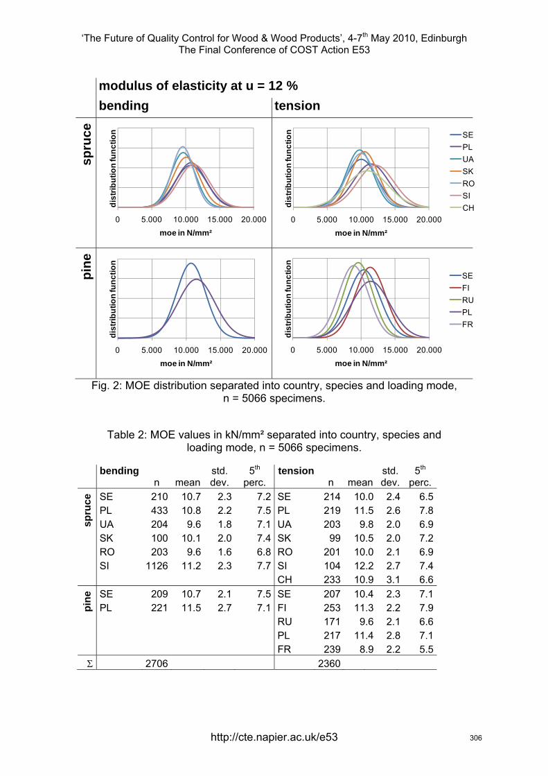
‘The Future of Quality Control for Wood & Wood Products’, 4-7th May 2010, Edinburgh The Final Conference of COST Action E53
http://cte.napier.ac.uk/e53
modulus of elasticity at u = 12 % bending tension
spru
ce
pine
Fig. 2: MOE distribution separated into country, species and loading mode, n = 5066 specimens.
Table 2: MOE values in kN/mm² separated into country, species and
loading mode, n = 5066 specimens.
bending
n mean std.dev.
5th perc.
tensionn mean
std. dev.
5th perc.
spru
ce SE 210 10.7 2.3 7.2 SE 214 10.0 2.4 6.5
PL 433 10.8 2.2 7.5 PL 219 11.5 2.6 7.8 UA 204 9.6 1.8 7.1 UA 203 9.8 2.0 6.9 SK 100 10.1 2.0 7.4 SK 99 10.5 2.0 7.2 RO 203 9.6 1.6 6.8 RO 201 10.0 2.1 6.9 SI 1126 11.2 2.3 7.7 SI 104 12.2 2.7 7.4
CH 233 10.9 3.1 6.6
pine
SE 209 10.7 2.1 7.5 SE 207 10.4 2.3 7.1 PL 221 11.5 2.7 7.1 FI 253 11.3 2.2 7.9
RU 171 9.6 2.1 6.6 PL 217 11.4 2.8 7.1 FR 239 8.9 2.2 5.5
2706 2360
0 5.000 10.000 15.000 20.000
dist
ribut
ion
func
tion
moe in N/mm²0 5.000 10.000 15.000 20.000
dist
ribut
ion
func
tion
moe in N/mm²
SEPLUASKROSICH
0 5.000 10.000 15.000 20.000
dist
ribut
ion
func
tion
moe in N/mm²0 5.000 10.000 15.000 20.000
dist
ribut
ion
func
tion
moe in N/mm²
SEFIRUPLFR
306
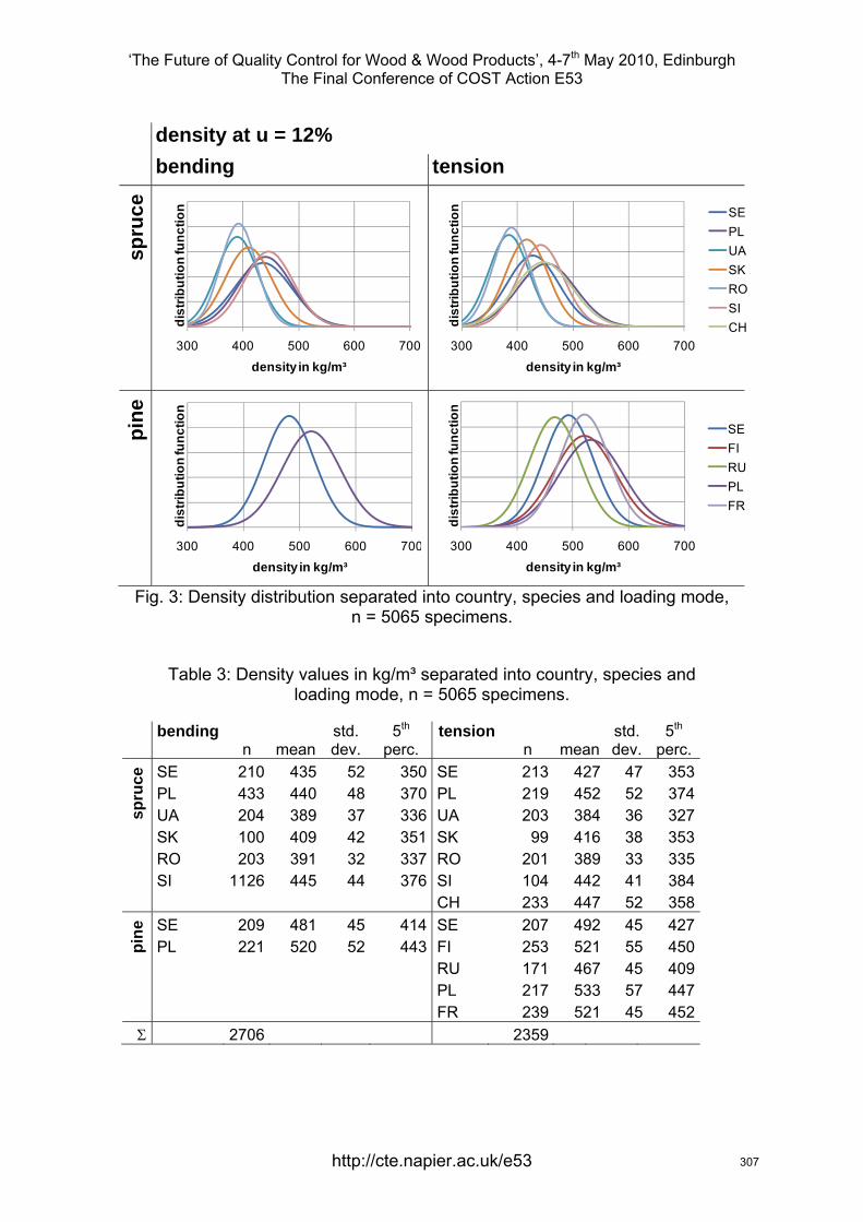
‘The Future of Quality Control for Wood & Wood Products’, 4-7th May 2010, Edinburgh The Final Conference of COST Action E53
http://cte.napier.ac.uk/e53
density at u = 12% bending tension
spru
ce
pine
Fig. 3: Density distribution separated into country, species and loading mode, n = 5065 specimens.
Table 3: Density values in kg/m³ separated into country, species and
loading mode, n = 5065 specimens.
bending
n mean std.dev.
5th perc.
tensionn mean
std. dev.
5th perc.
spru
ce SE 210 435 52 350 SE 213 427 47 353
PL 433 440 48 370 PL 219 452 52 374 UA 204 389 37 336 UA 203 384 36 327 SK 100 409 42 351 SK 99 416 38 353 RO 203 391 32 337 RO 201 389 33 335 SI 1126 445 44 376 SI 104 442 41 384
CH 233 447 52 358
pine
SE 209 481 45 414 SE 207 492 45 427 PL 221 520 52 443 FI 253 521 55 450
RU 171 467 45 409 PL 217 533 57 447 FR 239 521 45 452
2706 2359
300 400 500 600 700
dist
ribut
ion
func
tion
density in kg/m³300 400 500 600 700
dist
ribut
ion
func
tion
density in kg/m³
SEPLUASKROSICH
300 400 500 600 700
dist
ribut
ion
func
tion
density in kg/m³300 400 500 600 700
dist
ribut
ion
func
tion
density in kg/m³
SEFIRUPLFR
307
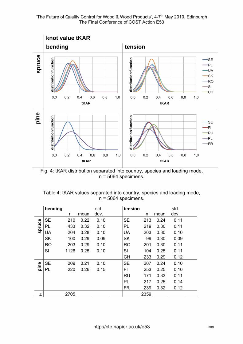
‘The Future of Quality Control for Wood & Wood Products’, 4-7th May 2010, Edinburgh The Final Conference of COST Action E53
http://cte.napier.ac.uk/e53
knot value tKAR bending tension
spru
ce
pine
Fig. 4: tKAR distribution separated into country, species and loading mode, n = 5064 specimens.
Table 4: tKAR values separated into country, species and loading mode,
n = 5064 specimens.
bending n mean
std. dev.
tensionn mean
std. dev.
spru
ce SE 210 0.22 0.10 SE 213 0.24 0.11
PL 433 0.32 0.10 PL 219 0.30 0.11 UA 204 0.28 0.10 UA 203 0.30 0.10 SK 100 0.29 0.09 SK 99 0.30 0.09 RO 203 0.29 0.10 RO 201 0.30 0.11 SI 1126 0.25 0.10 SI 104 0.25 0.11
CH 233 0.29 0.12
pine
SE 209 0.21 0.10 SE 207 0.24 0.10 PL 220 0.26 0.15 FI 253 0.25 0.10
RU 171 0.33 0.11 PL 217 0.25 0.14 FR 239 0.32 0.12
2705 2359
0,0 0,2 0,4 0,6 0,8 1,0
dist
ribut
ion
func
tion
tKAR0,0 0,2 0,4 0,6 0,8 1,0
dist
ribut
ion
func
tion
tKAR
SEPLUASKROSICH
0,0 0,2 0,4 0,6 0,8 1,0
dist
ribut
ion
func
tion
tKAR0,0 0,2 0,4 0,6 0,8 1,0
dist
ribut
ion
func
tion
tKAR
SEFIRUPLFR
308
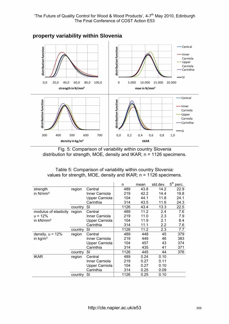
‘The Future of Quality Control for Wood & Wood Products’, 4-7th May 2010, Edinburgh The Final Conference of COST Action E53
http://cte.napier.ac.uk/e53
property variability within Slovenia
Fig. 5: Comparison of variability within country Slovenia distribution for strength, MOE, density and tKAR; n = 1126 specimens.
Table 5: Comparison of variability within country Slovenia:
values for strength, MOE, density and tKAR; n = 1126 specimens.
n mean std.dev. 5th perc. strength region Central 489 43.8 14.2 22.9 in N/mm² Inner Carniola 219 42.2 14.4 19.8
Upper Carniola 104 44.1 11.8 24.1 Carinthia 314 43.5 11.6 24.3
country SI 1126 43.4 13.3 22.5 modulus of elasticity region Central 489 11.2 2.4 7.6 u = 12% Inner Carniola 219 11.0 2.3 7.9 in kN/mm² Upper Carniola 104 11.9 2.1 8.4
Carinthia 314 11.1 2.2 7.6 country SI 1126 11.2 2.3 7.7 density, u = 12% region Central 489 448 45 379 in kg/m³ Inner Carniola 219 449 46 383
Upper Carniola 104 457 43 374 Carinthia 314 435 41 371
country SI 1126 445 44 376 tKAR region Central 489 0.24 0.10
Inner Carniola 219 0.27 0.11 Upper Carniola 104 0.27 0.10
Carinthia 314 0.25 0.09 country SI 1126 0.25 0.10
0,0 20,0 40,0 60,0 80,0 100,0
distribu
tion
function
strength in N/mm²
0 5.000 10.000 15.000 20.000
distribu
tion
function
moe in N/mm²
Central
Inner CarniolaUpper CarniolaCarinthia
SI
300 400 500 600 700
distribu
tion
function
density in kg/m³
0,0 0,2 0,4 0,6 0,8 1,0
distribu
tion
function
tKAR
Central
Inner CarniolaUpper CarniolaCarinthia
SI
309
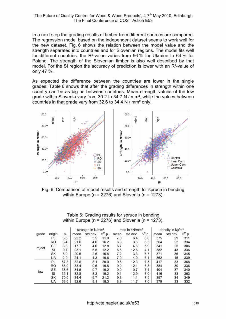
‘The Future of Quality Control for Wood & Wood Products’, 4-7th May 2010, Edinburgh The Final Conference of COST Action E53
http://cte.napier.ac.uk/e53
In a next step the grading results of timber from different sources are compared. The regression model based on the independent dataset seems to work well for the new dataset. Fig. 6 shows the relation between the model value and the strength separated into countries and for Slovenian regions. The model fits well for different countries: the R²-value varies from 56 % for Ukraine to 64 % for Poland. The strength of the Slovenian timber is also well described by that model. For the SI region the accuracy of prediction is lower with an R²-value of only 47 %.
As expected the difference between the countries are lower in the single grades. Table 6 shows that after the grading differences in strength within one country can be as big as between countries. Mean strength values of the low grade within Slovenia vary from 30.2 to 34.7 N / mm², while the values between countries in that grade vary from 32.6 to 34.4 N / mm² only.
Fig. 6: Comparison of model results and strength for spruce in bending within Europe (n = 2276) and Slovenia (n = 1273).
Table 6: Grading results for spruce in bending within Europe (n = 2276) and Slovenia (n = 1273).
strength in N/mm² moe in kN/mm² density in kg/m³ grade origin % mean std.dev. 5th p. mean std.dev. 5th p. mean std.dev. 5th p.
reject
PL 3.5 22.2 5.5 11.0 7.0 6.4 6.0 375 29 311 RO 3.4 21.6 4.0 16.2 6.8 3.6 6.3 364 22 334 SE 3.3 17.7 4.0 12.8 6.7 4.6 5.9 341 25 306 SI 0.7 23.1 6.5 12.2 6.6 12.6 4.1 382 43 336 SK 5.0 20.5 2.6 16.8 7.2 3.3 6.7 371 36 345 UA 2.9 24.1 4.3 19.6 7.0 4.9 6.1 362 15 339
low
PL 57.3 32.6 8.1 20.0 9.6 12.3 7.5 417 33 368 RO 68.0 33.4 9.6 19.8 9.0 12.1 6.8 384 30 336 SE 38.6 34.6 9.7 19.2 9.0 10.7 7.1 404 37 340 SI 35.1 32.8 8.3 19.2 9.1 12.9 7.0 416 33 363 SK 70.0 34.4 9.7 21.2 9.3 11.1 7.5 397 34 349 UA 68.6 32.6 8.1 18.3 8.9 11.7 7.0 379 33 332
310
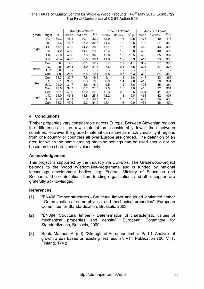
‘The Future of Quality Control for Wood & Wood Products’, 4-7th May 2010, Edinburgh The Final Conference of COST Action E53
http://cte.napier.ac.uk/e53
strength in N/mm² moe in kN/mm² density in kg/m³ grade origin % mean std.dev. 5th p. mean std.dev. 5th p. mean std.dev. 5th p.
high
PL 39.3 48.5 10.1 32.0 12.9 1.6 10.5 478 40 418 RO 28.6 46.7 8.0 32.6 11.3 1.0 9.5 413 27 362 SE 58.1 49.2 14.2 28.0 12.1 1.9 9.9 462 43 393 SI 64.2 49.5 11.7 29.9 12.4 1.8 9.8 462 40 405 SK 25.0 49.6 7.6 34.9 12.8 1.3 10.5 450 35 387 UA 28.4 46.3 9.5 30.1 11.8 1.2 9.9 417 33 353
reject
Cen. 0.6 19.5 8.1 12.2 5.7 1.7 4.1 359 27 336 I. C. 0.9 24.4 3.9 21.7 7.6 0.1 7.5 394 27 374 U. C. 0.0 - - - - - - - - - Cari. 1.0 25.9 6.5 19.1 6.8 0.7 6.3 398 64 352
low
Cen. 33.3 32.7 7.6 19.2 9.1 1.2 6.8 417 33 363 I. C. 36.1 30.2 9.3 18.6 8.9 1.4 7.0 418 30 364 U. C. 24.0 31.7 8.6 18.9 9.5 1.2 6.6 423 45 364 Cari. 40.8 34.7 8.2 21.5 9.3 1.3 7.0 410 32 361
high
Cen. 66.1 49.6 13.2 27.8 12.3 2.0 9.6 464 41 405 I. C. 63.0 49.3 11.8 28.4 12.2 1.8 9.8 468 42 407 U. C. 76.0 48.1 9.9 30.7 12.7 1.6 10.1 467 36 400 Cari. 58.3 49.9 9.2 34.0 12.4 1.6 10.0 454 36 404
4 Conclusions Timber properties vary considerable across Europe. Between Slovenian regions the differences in the raw material are considerably lower than between countries. However the graded material can show as much variability if regions from one country or countries all over Europe are graded. The definition of an area for which the same grading machine settings can be used should not be based on the characteristic values only.
Acknowledgement This project is supported by the industry via CEI-Bois. The Gradewood-project belongs to the Wood Wisdom.Net-programme and is funded by national technology development bodies, e.g. Federal Ministry of Education and Research. The contributions from funding organisations and other support are gratefully acknowledged.
References [1] "EN408 Timber structures - Structural timber and glued laminated timber
- Determination of some physical and mechanical properties". European Committee for Standardization, Brussels, 2003.
[2] "EN384. Structural timber - Determination of characteristic values of mechanical properties and density". European Committee for Standardization, Brussels, 2009.
[3] Ranta-Maunus, A. (ed): "Strength of European timber. Part 1. Analysis of growth areas based on existing test results". VTT Publication 706, VTT, Finland. 174 p.
311
‘The Future of Quality Control for Wood & Wood Products’, 4-7th May 2010, Edinburgh The Final Conference of COST Action E53
Variability of strength of in-grade spruce timber
A. Ranta-Maunus1
Abstract Bending strength of machine strength graded spruce timber has been studied based on GoldenEye-706 grading machine data and simulated strength values. Data of nearly 200,000 boards has been available, from which 16 sub-samples of 2000 were selected to represent different dimensions and low and high ends of material properties. Grading is made according to European machine control method and standard settings. For comparison, results for knot size based grading are also shown.
Main objective of the work has been to determine a quantitative relation between the average properties of timber measured by grading machine and the characteristic strength of in-grade timber. The relation has been determined both based on average modelled strength of total population to be graded, and based on average for in-grade timber.
Results indicate that characteristic strength of in-grade timber strongly depends on quality of mother population when grading is made to one or two grades allowing very high yield to a grade (80%). When grading is made to three grades with maximum yield of 50% each, strength of in-grade timber is less dependent of quality of material to be graded, and deviation of strength is only in conservative direction for high quality material.
1 Introduction Strength grading methods are not perfect, as is generally known. Accordingly, in-grade timber has higher strength when the initial unsorted population is of high quality and vice versa. Recently a new concept of adaptive settings for machine grading was proposed to react to occurring quality shifts (Sandomeer et.al 2007, 2008). Such quality shifts can be detected on several measured parameters simultaneously and can be quite dramatic (Figure 1). This kind of quality variation was first shown in COST E53 Conferences (Bacher 2008, 2009) with conclusion concerning settings used in grading: "For standard or high quality raw material these settings may be too conservative and for the low quality material still too optimistic. Adaptive thresholds have the potential to improve the overall yield for the producer and simultaneously also to increase the reliability in the product for the end user". Further results on the quality variation have been published in recent papers (Ranta-Maunus & Denzler 2009, Ranta-Maunus 2009). This paper has the objective to quantify the influence of quality of the mother population to the strength of in-grade timber. European "machine control" method is studied.
1 Professor Emeritus, VTT, Finland, [email protected]
http://cte.napier.ac.uk/e53 312
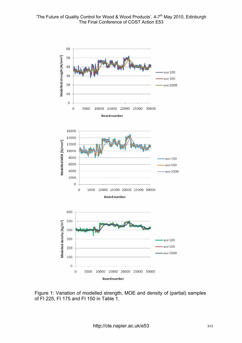
‘The Future of Quality Control for Wood & Wood Products’, 4-7th May 2010, Edinburgh The Final Conference of COST Action E53
Figure 1: Variation of modelled strength, MOE and density of (partial) samples of FI 225, FI 175 and FI 150 in Table 1.
http://cte.napier.ac.uk/e53 313
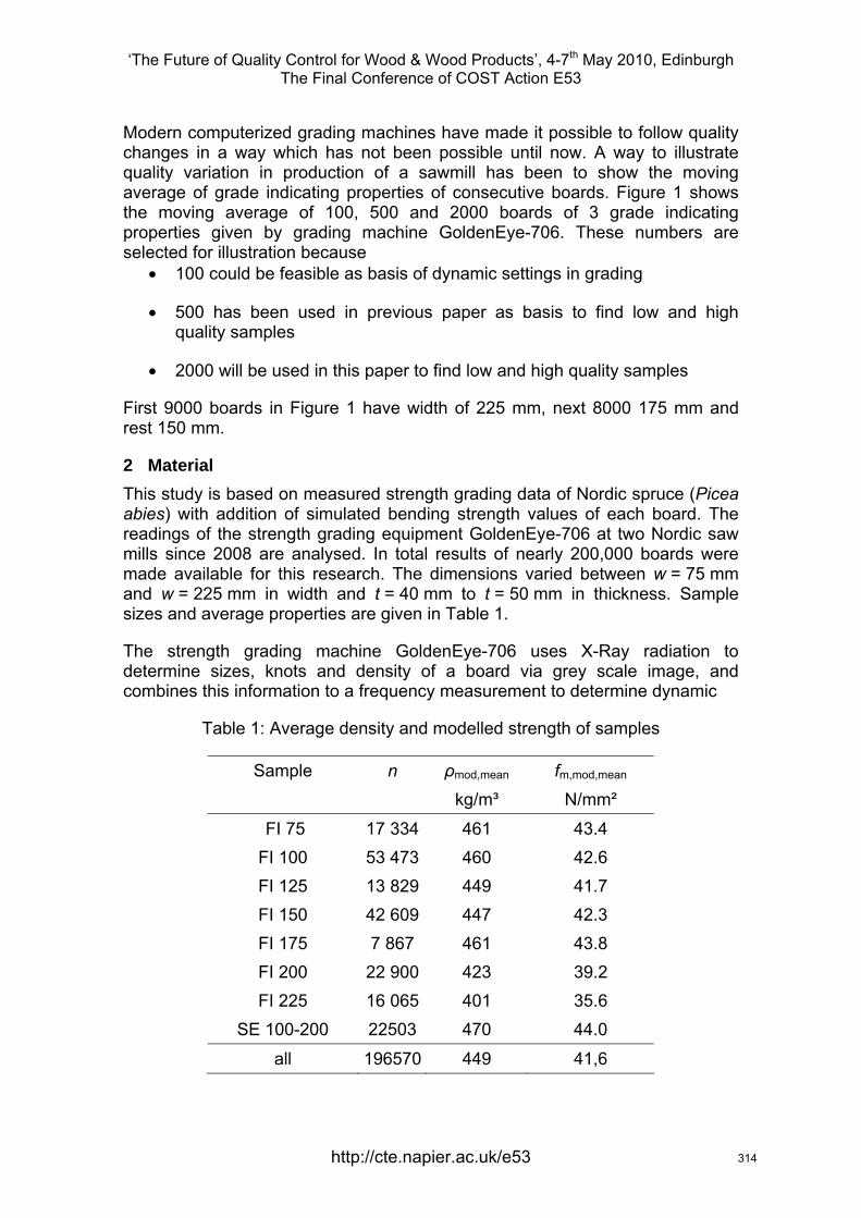
‘The Future of Quality Control for Wood & Wood Products’, 4-7th May 2010, Edinburgh The Final Conference of COST Action E53
Modern computerized grading machines have made it possible to follow quality changes in a way which has not been possible until now. A way to illustrate quality variation in production of a sawmill has been to show the moving average of grade indicating properties of consecutive boards. Figure 1 shows the moving average of 100, 500 and 2000 boards of 3 grade indicating properties given by grading machine GoldenEye-706. These numbers are selected for illustration because
• 100 could be feasible as basis of dynamic settings in grading
• 500 has been used in previous paper as basis to find low and high quality samples
• 2000 will be used in this paper to find low and high quality samples
First 9000 boards in Figure 1 have width of 225 mm, next 8000 175 mm and rest 150 mm.
2 Material This study is based on measured strength grading data of Nordic spruce (Picea abies) with addition of simulated bending strength values of each board. The readings of the strength grading equipment GoldenEye-706 at two Nordic saw mills since 2008 are analysed. In total results of nearly 200,000 boards were made available for this research. The dimensions varied between w = 75 mm and w = 225 mm in width and t = 40 mm to t = 50 mm in thickness. Sample sizes and average properties are given in Table 1.
The strength grading machine GoldenEye-706 uses X-Ray radiation to determine sizes, knots and density of a board via grey scale image, and combines this information to a frequency measurement to determine dynamic
Table 1: Average density and modelled strength of samples
Sample n ρmod,mean fm,mod,mean kg/m³ N/mm²
FI 75 17 334 461 43.4 FI 100 53 473 460 42.6 FI 125 13 829 449 41.7 FI 150 42 609 447 42.3 FI 175 7 867 461 43.8 FI 200 22 900 423 39.2 FI 225 16 065 401 35.6
SE 100-200 22503 470 44.0
all 196570 449 41,6
http://cte.napier.ac.uk/e53 314
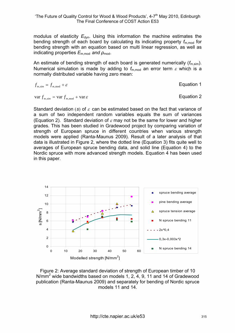
‘The Future of Quality Control for Wood & Wood Products’, 4-7th May 2010, Edinburgh The Final Conference of COST Action E53
modulus of elasticity Edyn. Using this information the machine estimates the bending strength of each board by calculating its indicating property fm,mod for bending strength with an equation based on multi linear regression, as well as indicating properties Em,mod and ρmod.
An estimate of bending strength of each board is generated numerically (fm,sim). Numerical simulation is made by adding to fm,mod an error term ε which is a normally distributed variable having zero mean:
ε+= mod,, msimm ff Equation 1
εvarvarvar mod,, += msimm ff Equation 2
Standard deviation (s) of ε can be estimated based on the fact that variance of a sum of two independent random variables equals the sum of variances (Equation 2). Standard deviation of ε may not be the same for lower and higher grades. This has been studied in Gradewood project by comparing variation of strength of European spruce in different countries when various strength models were applied (Ranta-Maunus 2009). Result of a later analysis of that data is illustrated in Figure 2, where the dotted line (Equation 3) fits quite well to averages of European spruce bending data, and solid line (Equation 4) to the Nordic spruce with more advanced strength models. Equation 4 has been used in this paper.
0
2
4
6
8
10
12
14
0 10 20 30 40 50 60
Modelled strength [N/mm2]
s [N
/mm
2 ]
spruce bending average
pine bending average
spruce tension average
N spruce bending 11
2x^0,4
0,3x-0,003x^2
N spruce bending 14
Figure 2: Average standard deviation of strength of European timber of 10 N/mm2 wide bandwidths based on models 1, 2, 4, 9, 11 and 14 of Gradewood publication (Ranta-Maunus 2009) and separately for bending of Nordic spruce
models 11 and 14.
http://cte.napier.ac.uk/e53 315
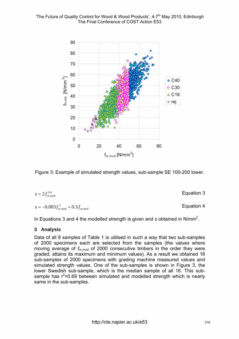
‘The Future of Quality Control for Wood & Wood Products’, 4-7th May 2010, Edinburgh The Final Conference of COST Action E53
0
10
20
30
40
50
60
70
80
90
0 20 40 60 80
fm,mod [N/mm2]
fm,s
im [N
/mm
2 ]
C40C30C18rej
Figure 3: Example of simulated strength values, sub-sample SE 100-200 lower.
4.0mod,2 mfs = Equation 3
mod,2
mod, 3.0003.0 mm ffs +−= Equation 4
In Equations 3 and 4 the modelled strength is given and s obtained in N/mm2.
3 Analysis Data of all 8 samples of Table 1 is utilised in such a way that two sub-samples of 2000 specimens each are selected from the samples (the values where moving average of fm,mod of 2000 consecutive timbers in the order they were graded, attains its maximum and minimum values). As a result we obtained 16 sub-samples of 2000 specimens with grading machine measured values and simulated strength values. One of the sub-samples is shown in Figure 3, the lower Swedish sub-sample, which is the median sample of all 16. This sub-sample has r2=0.69 between simulated and modelled strength which is nearly same in the sub-samples.
http://cte.napier.ac.uk/e53 316
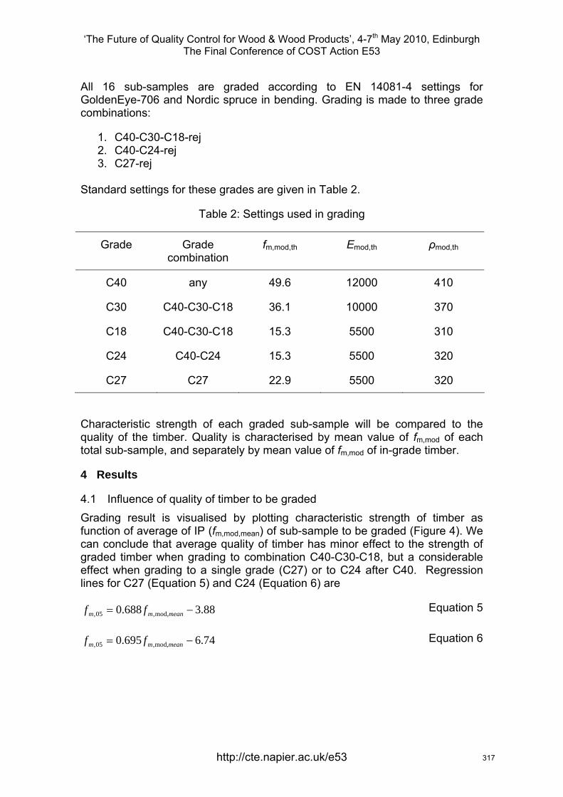
‘The Future of Quality Control for Wood & Wood Products’, 4-7th May 2010, Edinburgh The Final Conference of COST Action E53
All 16 sub-samples are graded according to EN 14081-4 settings for GoldenEye-706 and Nordic spruce in bending. Grading is made to three grade combinations:
1. C40-C30-C18-rej 2. C40-C24-rej 3. C27-rej
Standard settings for these grades are given in Table 2.
Table 2: Settings used in grading
Grade Grade combination
fm,mod,th Emod,th ρmod,th
C40 any 49.6 12000 410
C30 C40-C30-C18 36.1 10000 370
C18 C40-C30-C18 15.3 5500 310
C24 C40-C24 15.3 5500 320
C27 C27 22.9 5500 320
Characteristic strength of each graded sub-sample will be compared to the quality of the timber. Quality is characterised by mean value of fm,mod of each total sub-sample, and separately by mean value of fm,mod of in-grade timber.
4 Results
4.1 Influence of quality of timber to be graded Grading result is visualised by plotting characteristic strength of timber as function of average of IP (fm,mod,mean) of sub-sample to be graded (Figure 4). We can conclude that average quality of timber has minor effect to the strength of graded timber when grading to combination C40-C30-C18, but a considerable effect when grading to a single grade (C27) or to C24 after C40. Regression lines for C27 (Equation 5) and C24 (Equation 6) are
88.3688.0 mod,,05, −= meanmm ff Equation 5
74.6695.0 mod,,05, −= meanmm ff Equation 6
http://cte.napier.ac.uk/e53 317
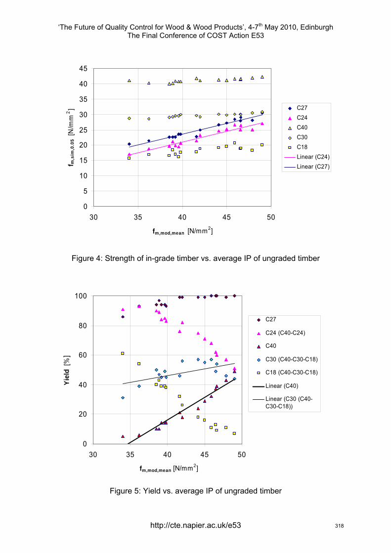
‘The Future of Quality Control for Wood & Wood Products’, 4-7th May 2010, Edinburgh The Final Conference of COST Action E53
0
5
10
15
20
25
30
35
40
45
30 35 40 45 50
fm,mod,mean [N/mm2]
f m,s
im,0
.05
[N/m
m2] C27
C24C40C30C18Linear (C24)Linear (C27)
Figure 4: Strength of in-grade timber vs. average IP of ungraded timber
0
20
40
60
80
100
30 35 40 45 50
fm,mod,mean [N/mm2]
Yiel
d [%
]
C27
C24 (C40-C24)
C40
C30 (C40-C30-C18)
C18 (C40-C30-C18)
Linear (C40)
Linear (C30 (C40-C30-C18))
Figure 5: Yield vs. average IP of ungraded timber
http://cte.napier.ac.uk/e53 318
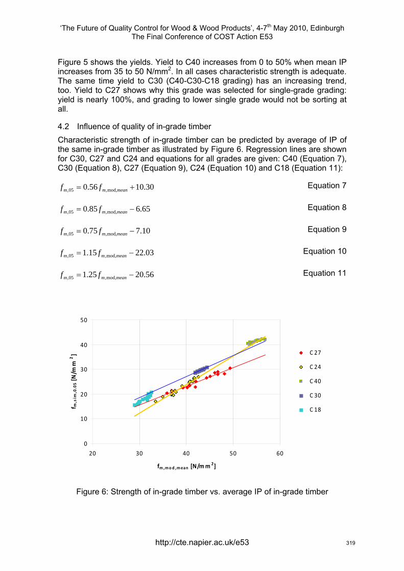
‘The Future of Quality Control for Wood & Wood Products’, 4-7th May 2010, Edinburgh The Final Conference of COST Action E53
Figure 5 shows the yields. Yield to C40 increases from 0 to 50% when mean IP increases from 35 to 50 N/mm2. In all cases characteristic strength is adequate. The same time yield to C30 (C40-C30-C18 grading) has an increasing trend, too. Yield to C27 shows why this grade was selected for single-grade grading: yield is nearly 100%, and grading to lower single grade would not be sorting at all.
4.2 Influence of quality of in-grade timber Characteristic strength of in-grade timber can be predicted by average of IP of the same in-grade timber as illustrated by Figure 6. Regression lines are shown for C30, C27 and C24 and equations for all grades are given: C40 (Equation 7), C30 (Equation 8), C27 (Equation 9), C24 (Equation 10) and C18 (Equation 11):
30.1056.0 mod,,05, += meanmm ff Equation 7
65.685.0 mod,,05, −= meanmm ff Equation 8
10.775.0 mod,,05, −= meanmm ff Equation 9
03.2215.1 mod,,05, −= meanmm ff Equation 10
56.2025.1 mod,,05, −= meanmm ff Equation 11
0
10
20
30
40
50
20 30 40 50 60
fm ,mo d ,mean [N/mm 2]
f m,sim
,0.05[N
/mm
2] C 27
C 24
C 40
C 30
C 18
Figure 6: Strength of in-grade timber vs. average IP of in-grade timber
http://cte.napier.ac.uk/e53 319
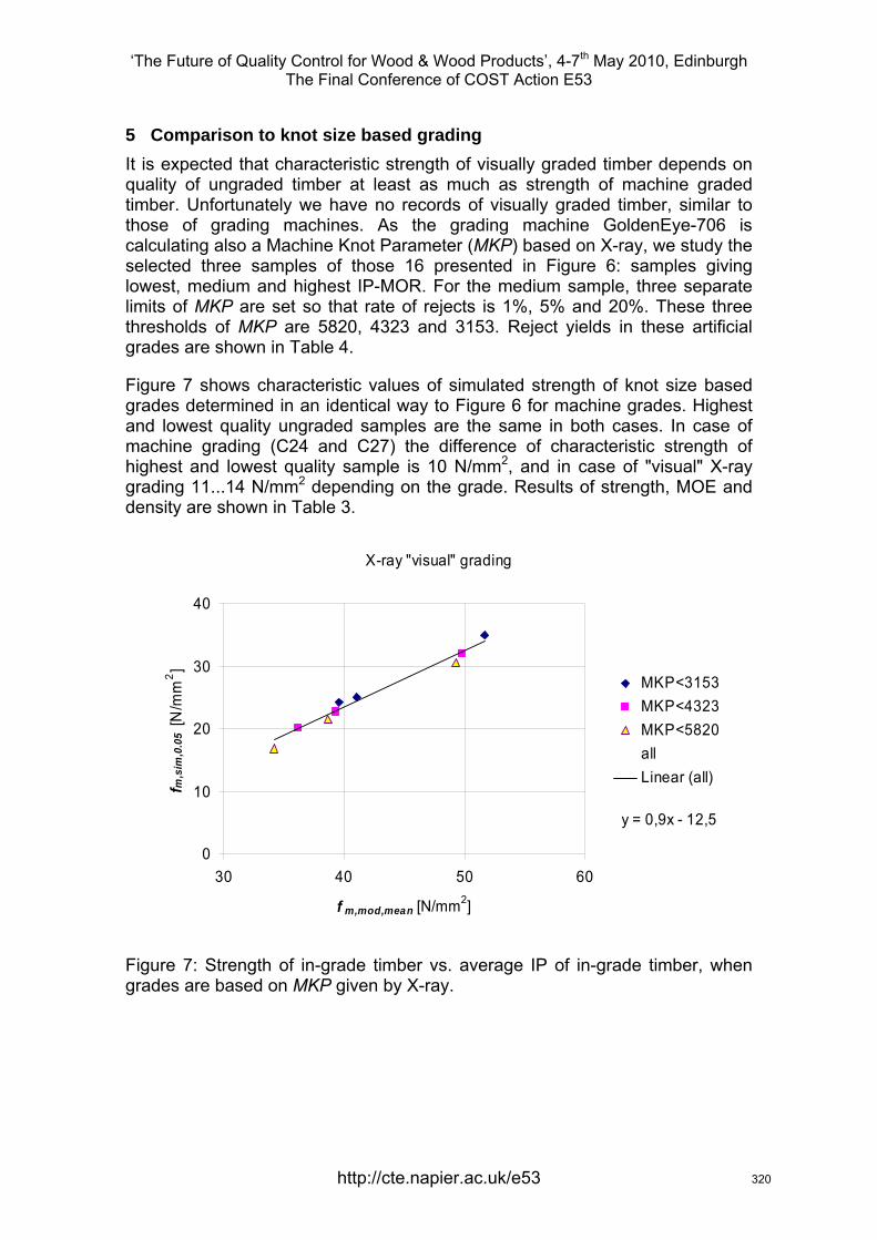
‘The Future of Quality Control for Wood & Wood Products’, 4-7th May 2010, Edinburgh The Final Conference of COST Action E53
5 Comparison to knot size based grading It is expected that characteristic strength of visually graded timber depends on quality of ungraded timber at least as much as strength of machine graded timber. Unfortunately we have no records of visually graded timber, similar to those of grading machines. As the grading machine GoldenEye-706 is calculating also a Machine Knot Parameter (MKP) based on X-ray, we study the selected three samples of those 16 presented in Figure 6: samples giving lowest, medium and highest IP-MOR. For the medium sample, three separate limits of MKP are set so that rate of rejects is 1%, 5% and 20%. These three thresholds of MKP are 5820, 4323 and 3153. Reject yields in these artificial grades are shown in Table 4.
Figure 7 shows characteristic values of simulated strength of knot size based grades determined in an identical way to Figure 6 for machine grades. Highest and lowest quality ungraded samples are the same in both cases. In case of machine grading (C24 and C27) the difference of characteristic strength of highest and lowest quality sample is 10 N/mm2, and in case of "visual" X-ray grading 11...14 N/mm2 depending on the grade. Results of strength, MOE and density are shown in Table 3.
X-ray "visual" grading
y = 0,9x - 12,5
0
10
20
30
40
30 40 50 60
f m,mod,mean [N/mm2]
f m,s
im,0
.05
[N/m
m2 ]
MKP<3153MKP<4323MKP<5820allLinear (all)
Figure 7: Strength of in-grade timber vs. average IP of in-grade timber, when grades are based on MKP given by X-ray.
http://cte.napier.ac.uk/e53 320
‘The Future of Quality Control for Wood & Wood Products’, 4-7th May 2010, Edinburgh The Final Conference of COST Action E53
Table 3: Characteristic values obtained for 3 samples in knot based grading
Sample MKP threshold
fm,mod,mean fm,sim,05 fm,sim,005 Emod,mean ρmod,05
N/mm2 N/mm2 N/mm2 N/mm2 kg/m3 FI 225 lo 5820 34.2 16.9 10 9700 343
4323 36.2 20.2 13 10000 345 3153 39.6 24.3 16 10700 351
FI 75 lo 5820 38.7 21.6 14 10800 373 4323 39.3 22.7 15 10900 373 3153 41.0 25.1 18 11200 378
FI 150 hi 5820 49.3 30.9 21 14200 419 4323 49.8 32.0 23 14400 421 3153 51.7 35.0 27 14700 427
Table 4: Yields to reject in knot size based grading
Grade Sample quality
High Medium Low
MKP<5820 0.00 0.01 0.04
MKP<4323 0.03 0.05 0.18
MKP<3153 0.20 0.20 0.45
6 Discussion Characteristic strength of in-grade timber is lower than required when yield to any grade is more than 80%, and the average quality of timber is lower than in the sample used for determination of settings. In these cases, strength is observed to be dependent of material to be sorted so that in the highest quality case of 16 analysed samples (n=2000) fm,05 of C24 is 27 N/mm2 and in the lowest 17 N/mm2. For C27 the results are between fm,05=20...30 N/mm2. In knot size based grading, variation within a grade is still larger: fm,05=17...31 N/mm2 in the lowest artificial grade and fm,05=24...35 N/mm2 in the highest grade analysed. The used Machine Knot Parameter (MKP) has higher correlation to strength than visual KAR. MKP is the same as "X-ray knot b" in Table 16 of Combigrade project report which gives r2= 0.40 whereas r2= 0.20 for TKAR in bending of spruce (Hanhijärvi et al 2008).
In C40-C24 grading of the better half of material, strength of both grades is above requirement, and there would be potential to allow higher yield to C40.
http://cte.napier.ac.uk/e53 321

‘The Future of Quality Control for Wood & Wood Products’, 4-7th May 2010, Edinburgh The Final Conference of COST Action E53
When grading to three grades C40-C24-C18, yield to any grade is below 80%, and strength is generally above required value, for high quality material more than for low quality material. Obtained values are however closer to requirement than in case of grading to C40-C24 or to C27 alone.
More even strength values could be obtained if we would use dynamic settings adapting information of the previously graded timber collected by the grading machine. Based on Equations 7 to 11 we can conclude that one N/mm2 higher mean of IP-MOR results in 0.6 to 1.2 N/mm2 higher characteristic strength of in-grade timber. This information can be utilised in determination of dynamic settings and is the topic of a coming WCTE paper (Ranta-Maunus & Turk, 2010). It will further develop the approach described in COST E53 Lisbon paper (Ranta-Maunus, 2009). Basically the approach is to adjust settings for each board based on the mean of a number of previous boards:
( )meanNrefmeaninithth ffff mod,,mod,,mod,mod, −+= α Equation 12
where fmod,th,ini are the initial settings based on reference sample which gives average IP for strength of in-grade timber: fmod,mean,ref. fmod,meanN is mean of IP of previous N pieces graded to the grade according to initial settings. N and α are to be optimised to give maximum yield within the requirements for grades. Initially, based on Equations 7 to 11, we can select
C03.075.1 −=α Equation 13
where C means C-class (i.e. C=24 for C24). A method for determination initial settings is also presented in coming paper (Ranta-Maunus & Turk, 2010).
Acknowledgement This work is part of Gradewood-project which is based on a feasibility study made by the European wood industries under the Roadmap 2010 Building With Wood programme, and this project is supported by the industry via CEI-Bois. The Gradewood-project belongs to the Wood Wisdom.Net-programme and is funded by national technology development bodies like TEKES in Finland.
Stora Enso Timber and MiCROTEC are owners of the strength grading data of sawmills and they kindly forwarded the data to be analysed.
The contributions from funding organisations and other support are gratefully acknowledged.
References Bacher, M. (2008) "Comparison of different machine strength grading principles". Cost Action E53, Quality control in production of wood and wood based material. Conference in Delft, The Netherlands. 10p.
http://cte.napier.ac.uk/e53 322

‘The Future of Quality Control for Wood & Wood Products’, 4-7th May 2010, Edinburgh The Final Conference of COST Action E53
Bacher, M. (2009) "GoldenEye-706 Quality shifts". Cost Action E53, Topic 4: Quality control in production of wood and wood based material. Meeting in Bled, Slovenia. 5p.
CEN (2008) "EN 14081-4:2009 Timber structures – Strength graded structural timber with rectangular cross section – Part 4: Machine grading – Grading machine settings for machine controlled systems". European Committee for Standardization. 69 p.
Hanhijärvi A., Ranta-Maunus A. (2008) "Development of strength grading of timber using combined measurement techniques – Report of the Combigrade-project – phase 2". VTT Publications 686, Espoo, Finland, 55 p. http://www.vtt.fi/inf/pdf/publications/2008/P686.pdf
Ranta-Maunus, A. (ed) (2009) "Strength of European timber. Part 1. Analysis of growth areas based on existing test results". VTT Publication 706, VTT, Finland. 174 p, http://www.vtt.fi/inf/pdf/publications/2009/P706.pdf
Ranta-Maunus, A. and Denzler J.K. (2009) "Variability of strength of European spruce", CIB W18-meeting, paper 42-6-1 ,10 p.
Ranta-Mauns, A. (2009) " Comparison of four basic approaches in machine strength grading", COST Action E53 Conference in Lisbon. 9p.
Ranta-Maunus, A. and Turk, G. (2010) "Approaches of dynamic production settings for machine strength grading", WCTE 2010 conference, submitted for publication. 9p.
Sandomeer (ne Deublein) M.K., Köhler J., Linsenmann P. (2007) The efficient control of grading machine settings. Proceedings of the 40th Meeting, International Council for Research and Innovation in Building and Construction, Working Commission W18 – Timber Structures, CIB-W18, Paper No. 40-5-2, Bled, Slovenia, 2007
Sandomeer, M., Köhler, J.; Faber, M.H. (2008) "Probabilistic output control for structural timber – Modelling approach". Proc. of CIB-W18 Meeting, Paper 45-5-1. St.Andrews-by-the-Sea, New Brunswick, Canada. 12 p.
http://cte.napier.ac.uk/e53 323
‘The Future of Quality Control for Wood & Wood Products’, 4-7th May 2010, Edinburgh The Final Conference of COST Action E53
http://cte.napier.ac.uk/e53
The influence of knot size and location on the yield of grading machines
A. Rais1, P. Stapel2, J.W.G. van de Kuilen3
Abstract
The basis for the derivation of settings for a grading machine is a comparison between destructive test data and data recorded by the machine. If the knots are part of the strength predicting model, the model covers the length effect in timber as it predicts the relatively lower strength for longer boards. This paper discusses the influence of the location of the maximum knot value on the performance of the machine. The maximum knot value between the inner load points is used for model derivation in approval bending tests. In practise, these machines do not only consider knots in the centre part of the board, but over the full length. Therefore, the indicating properties during deriving settings and during grading in practise differ from each other. The grading machine detects the largest knot value independent of the position along the length of the board; by means of this value the strength class is predicted. The influence of these differences is discussed. Finally, the effect on yield is shown.
1 Introduction The object of this investigation is to show the difference between indicating property during grading and indicating property during testing of the very same board. It is not always possible to test the section with the maximum knot value due to the test setup in the laboratory. In practise however, the strength class is determined during grading in sawmills based on the maximum knot value of the entire board. This causes an influence on the yield which is based on the method of derivation only.
Grading machines based on optical or X-ray scanners can use the knot value to predict the strength class. These machines are able to detect knots over the complete length. In contrast to other machine grading parameters such as eigenfrequency or density, the knot value differs over the length of boards.
1 Research assistant, [email protected] Holzforschung München, Technische Universität München, Germany 2 Research assistant, [email protected] Holzforschung München, Technische Universität München, Germany 3 Professor, [email protected] Holzforschung München, Technische Universität München, Germany TU Delft, the Netherlands
324
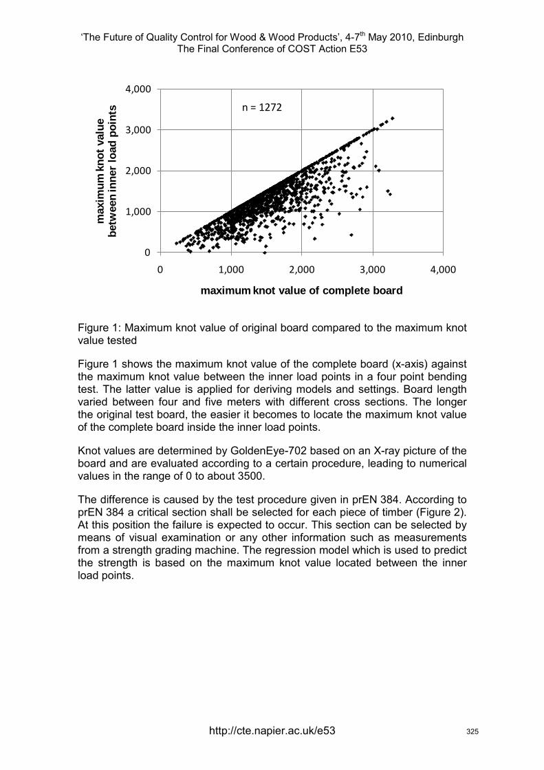
‘The Future of Quality Control for Wood & Wood Products’, 4-7th May 2010, Edinburgh The Final Conference of COST Action E53
http://cte.napier.ac.uk/e53
Figure 1: Maximum knot value of original board compared to the maximum knot value tested
Figure 1 shows the maximum knot value of the complete board (x-axis) against the maximum knot value between the inner load points in a four point bending test. The latter value is applied for deriving models and settings. Board length varied between four and five meters with different cross sections. The longer the original test board, the easier it becomes to locate the maximum knot value of the complete board inside the inner load points.
Knot values are determined by GoldenEye-702 based on an X-ray picture of the board and are evaluated according to a certain procedure, leading to numerical values in the range of 0 to about 3500.
The difference is caused by the test procedure given in prEN 384. According to prEN 384 a critical section shall be selected for each piece of timber (Figure 2). At this position the failure is expected to occur. This section can be selected by means of visual examination or any other information such as measurements from a strength grading machine. The regression model which is used to predict the strength is based on the maximum knot value located between the inner load points.
0
1,000
2,000
3,000
4,000
0 1,000 2,000 3,000 4,000
max
imum
kno
t val
ue
betw
een
inne
r lo
ad p
oint
s
maximum knot value of complete board
n = 1272
325
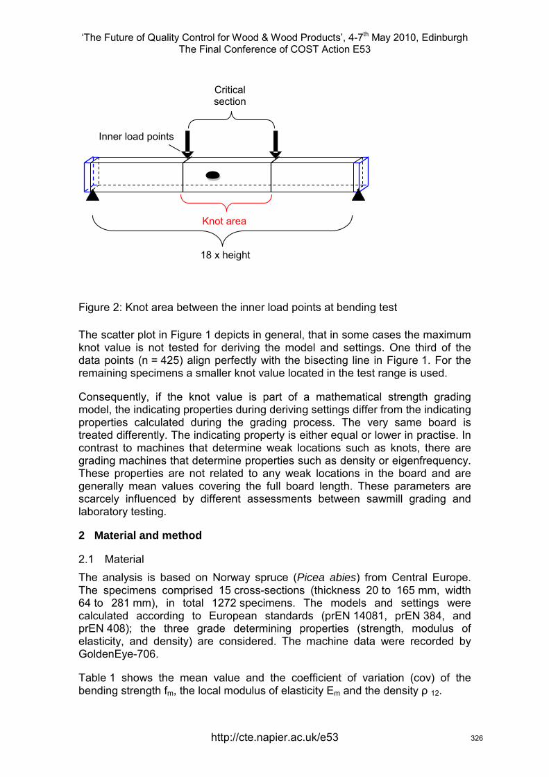
‘The Future of Quality Control for Wood & Wood Products’, 4-7th May 2010, Edinburgh The Final Conference of COST Action E53
http://cte.napier.ac.uk/e53
The scatter plot in Figure 1 depicts in general, that in some cases the maximum knot value is not tested for deriving the model and settings. One third of the data points (n = 425) align perfectly with the bisecting line in Figure 1. For the remaining specimens a smaller knot value located in the test range is used.
Consequently, if the knot value is part of a mathematical strength grading model, the indicating properties during deriving settings differ from the indicating properties calculated during the grading process. The very same board is treated differently. The indicating property is either equal or lower in practise. In contrast to machines that determine weak locations such as knots, there are grading machines that determine properties such as density or eigenfrequency. These properties are not related to any weak locations in the board and are generally mean values covering the full board length. These parameters are scarcely influenced by different assessments between sawmill grading and laboratory testing.
2 Material and method
2.1 Material The analysis is based on Norway spruce (Picea abies) from Central Europe. The specimens comprised 15 cross-sections (thickness 20 to 165 mm, width 64 to 281 mm), in total 1272 specimens. The models and settings were calculated according to European standards (prEN 14081, prEN 384, and prEN 408); the three grade determining properties (strength, modulus of elasticity, and density) are considered. The machine data were recorded by GoldenEye-706.
Table 1 shows the mean value and the coefficient of variation (cov) of the bending strength fm, the local modulus of elasticity Em and the density ρ 12.
Knot area
18 x height
Critical section
Inner load points
Figure 2: Knot area between the inner load points at bending test
326

‘The Future of Quality Control for Wood & Wood Products’, 4-7th May 2010, Edinburgh The Final Conference of COST Action E53
http://cte.napier.ac.uk/e53
Table 1: Description of sample
n fm Em ρ12 mean cov mean cov mean cov N/mm² % N/mm² % kg/m³ %
1272 39.0 31.5 11300 25.6 438 11.3
2.2 Method
2.2.1 Knot values during laboratory testing Based on these specimens two different models are calculated. These two models could be applied in practise as well. The first model (model 1) simulates a grading machine which is capable to detect the eigenfrequency and the density; the outcome of this is an indicating property (IP1) based on the dynamic modulus of elasticity (MOE).
The second machine is also able to detect and calculate the dynamic modulus of elasticity. Additionally, this kind of machine is able to detect knots. Therefore, the knot information is used in the second model to predict the strength more accurately (IP2).
Equation 1
Equation 2
The indicating property (IPi) is calculated from MOE (dynamic modulus of elasticity in N/mm²) and knot (biggest knot related to the cross-section). Model 2 considers the maximum knot value measured in the range between the inner load points. According to the current method, this knot value is used to develop the model as well as to derive settings. By means of 1272 specimens of Norway spruce the regression coefficients (a, b, c, d, and e) are calculated. The knot value is multiplied by a negative factor, i.e. the larger the knot, the lower the corresponding indicating property (IP2).
2.2.2 Knot values during grading During grading in practise the length of the entire board needs to be considered since the cross section with the lowest strength is governing strength class assignment. Software calculates the maximum knot value. This value is plugged in the developed model, the indicating property is generated.
3 Results It is obvious, that the coefficient of determination (r²) between the bending strength and the indicating property of model 2 is higher than that of model 1. The additional parameter leads to an increased r²-value of about five percent. In machine grading the correlation between indicating property and bending strength plays an important role, if different models are compared.
327
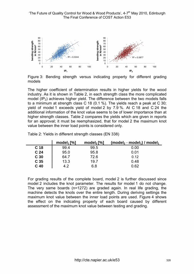
‘The Future of Quality Control for Wood & Wood Products’, 4-7th May 2010, Edinburgh The Final Conference of COST Action E53
http://cte.napier.ac.uk/e53
Figure 3: Bending strength versus indicating property for different grading models
The higher coefficient of determination results in higher yields for the wood industry. As it is shown in Table 2, in each strength class the more complicated model (IP2) achieves higher yield. The difference between the two models falls to a minimum at strength class C 18 (0.1 %). The yields reach a peak at C 30; yield of model 1 exceeds yield of model 2 by 7.9 %. At C 18 and C 24 the additional information of the knot value seems to be of lower importance than at higher strength classes. Table 2 compares the yields which are given in reports for an approval; it must be reemphasized, that for model 2 the maximum knot value between the inner load points is considered only.
Table 2: Yields in different strength classes (EN 338)
model1 [%] model2 [%] (model2 - model1) / model1 C 18 99.4 99.5 0.00 C 24 95.0 95.8 0.01 C 30 64.7 72.6 0.12 C 35 13.3 19.7 0.48 C 40 4.2 6.8 0.62
For grading results of the complete board, model 2 is further discussed since model 2 includes the knot parameter. The results for model 1 do not change. The very same boards (n=1272) are graded again. In real life grading, the machine detects the knots over the entire length. During deriving settings the maximum knot value between the inner load points are used. Figure 4 shows the effect on the indicating property of each board caused by different assessment of the maximum knot value between testing and grading.
R² = 0.5344
0102030405060708090
0 20 40 60 80 100
ben
din
g s
tren
gth
in N
/mm
²
IP1
R² = 0.5877
0102030405060708090
0 20 40 60 80 100
ben
din
g s
tren
gth
in N
/mm
²
IP2
328
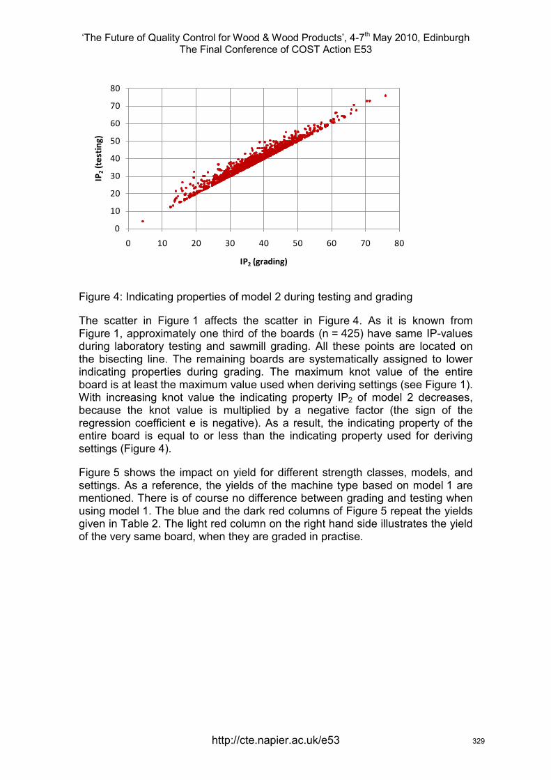
‘The Future of Quality Control for Wood & Wood Products’, 4-7th May 2010, Edinburgh The Final Conference of COST Action E53
http://cte.napier.ac.uk/e53
Figure 4: Indicating properties of model 2 during testing and grading
The scatter in Figure 1 affects the scatter in Figure 4. As it is known from Figure 1, approximately one third of the boards (n = 425) have same IP-values during laboratory testing and sawmill grading. All these points are located on the bisecting line. The remaining boards are systematically assigned to lower indicating properties during grading. The maximum knot value of the entire board is at least the maximum value used when deriving settings (see Figure 1). With increasing knot value the indicating property IP2 of model 2 decreases, because the knot value is multiplied by a negative factor (the sign of the regression coefficient e is negative). As a result, the indicating property of the entire board is equal to or less than the indicating property used for deriving settings (Figure 4).
Figure 5 shows the impact on yield for different strength classes, models, and settings. As a reference, the yields of the machine type based on model 1 are mentioned. There is of course no difference between grading and testing when using model 1. The blue and the dark red columns of Figure 5 repeat the yields given in Table 2. The light red column on the right hand side illustrates the yield of the very same board, when they are graded in practise.
0
10
20
30
40
50
60
70
80
0 10 20 30 40 50 60 70 80
IP2
(tes
ting
)
IP2 (grading)
329
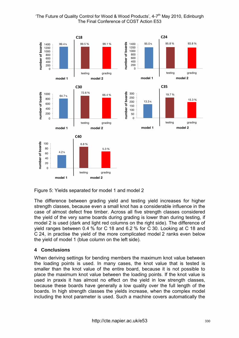
‘The Future of Quality Control for Wood & Wood Products’, 4-7th May 2010, Edinburgh The Final Conference of COST Action E53
http://cte.napier.ac.uk/e53
Figure 5: Yields separated for model 1 and model 2
The difference between grading yield and testing yield increases for higher strength classes, because even a small knot has a considerable influence in the case of almost defect free timber. Across all five strength classes considered the yield of the very same boards during grading is lower than during testing, if model 2 is used (dark and light red columns on the right side). The difference of yield ranges between 0.4 % for C 18 and 6.2 % for C 30. Looking at C 18 and C 24, in practise the yield of the more complicated model 2 ranks even below the yield of model 1 (blue column on the left side).
4 Conclusions When deriving settings for bending members the maximum knot value between the loading points is used. In many cases, the knot value that is tested is smaller than the knot value of the entire board, because it is not possible to place the maximum knot value between the loading points. If the knot value is used in praxis it has almost no effect on the yield in low strength classes, because these boards have generally a low quality over the full length of the boards. In high strength classes the yields increase, when the complex model including the knot parameter is used. Such a machine covers automatically the
0200400600800
100012001400
testing grading
nu
mb
er o
f b
oar
ds
model 1 model 2
C18
99.4 % 99.5 % 99.1 %
0200400600800
100012001400
testing grading
nu
mb
er o
f b
oar
ds
model 1 model 2
C24
95.0 % 95.8 % 93.8 %
0
200
400
600
800
1000
testing grading
nu
mb
er o
f b
oar
ds
model 1 model 2
C30
64.7 %72.6 %
66.4 %
050
100150200250300
testing gradingn
um
ber
of
bo
ard
smodel 1 model 2
C35
13.3 %
19.7 %
15.3 %
0
20
40
60
80
100
testing grading
nu
mb
er o
f b
oar
ds
model 1 model 2
C40
4.2 %
6.8 %
5.3 %
330
‘The Future of Quality Control for Wood & Wood Products’, 4-7th May 2010, Edinburgh The Final Conference of COST Action E53
http://cte.napier.ac.uk/e53
length effect in timber as it predicts the relatively lower strength for longer boards (Isaksson and Thelandersson 1995). The indicating property differs between the derivation of settings and the practice for one and the same board. This is the case, if the knot value is included in the model, but the maximum knot value cannot be placed between the load points. Hence, the yields in practise differ from those calculated during the derivation of settings. Grading machines that are able to detect local weaknesses (for example knots) perform better than grading machines that determine only average board parameters. In principle, grading machines that detect local weaknesses are also able to correctly grade correctly also longer boards than used in the approval testing. However, this higher performance is not considered when machines are approved according to the European standard EN 14081. The effect also depends on:
- the model used - the species - the original length of the boards tested - the width of the boards tested at bending tests
Acknowledgement We acknowledge MiCROTEC for providing the data and Martin Bacher for his advice and support.
References prEN 14081-2:2008 Timber structures – Strength graded structural timber with rectangular cross section – Part 2: Machine grading; additional requirements for initial type testing. prEN 408:2009 Timber structures – Structural timber and glued laminated timber – Determination of some physical and mechanical properties. prEN 384:2008 Timber structures – Determination of characteristic values of mechanical properties and density. Isaksson T, Thelandersson S (1995) Effect of test standard, length and load configuration on bending strength of structural timber. CIB-W18, Copenhagen, Denmark.
331
‘The Future of Quality Control for Wood & Wood Products’, 4-7th May 2010, Edinburgh The Final Conference of COST Action E53
Near-infrared technology applications for quality control in wood processing
K.Watanabe1, J.F. Hart2, S.D. Mansfield3 & S. Avramidis4
Abstract Wet-pockets are a common processing issue with some wood species in board lamination for gluelam manufacturing and in just simple structural lumber production. Swift in-line detection of wet-pockets before and/or after kiln drying is thus essential to quality control and process optimization.
An in-line pilot-plant near-infrared (NIR) system with line speeds of 0, 500 and 1000 mm s-1 combined with the developed partial least square (PLS) models tested the capacity to predict surface moisture content of kiln-dried western hemlock full-length lamination boards. The system showed high prediction ability. It is concluded that NIR spectroscopy has a potential to sort green lumber before drying based on moisture content, and that the NIR system with line speed of 0 to 1000 mm s-1 is capable of providing entire surface moisture distribution, and of detecting wet-pockets in lamina for industry applications.
Visible and NIR spectroscopy combined with discriminant analysis was used to distinguish wet-pockets from normal wood in subalpine fir samples. A soft independent modeling of class (SIMCA) model using the wavelength range of 650 to 1150 nm succeeded in 98% distinguishing wet-pockets from normal wood in the green state, while the model resulted in the misclassification for air-dried samples. The discriminant PLS model showed excellent correct classification results of 96% for green samples and 100% for dried samples, respectively. The analysis confirms that wet-pockets could be readily distinguished from normal wood using the discriminant PLS.
1 Introduction Wet-pockets (also known as “wetwood” or “wet-spots”) are commonly referred to as localized areas in heartwood with abnormally high moisture content. Wet-pockets are severe processing problem and cause serious drying defects in lumber. It has been speculated that a wet-pocket is a consequence of bacterial activity (Bauch et al. 1975, Ward & Zeikus 1980, Schink & Ward 1984) and causes excessive honeycomb, ring shake and deep surface checks during kiln-drying (Ward & Groom 1983, Ross et al. 1994). Due to high moisture and slow drying characteristics compared to normal heartwood (Ward 1986), drying
1 Post Doctoral Fellow, [email protected] 2 Undergraduate Student, [email protected] 3 Professor, [email protected] 4 Professor, stavros.avramidis@ ubc.ca Department of Wood Science, University of British Columbia, Vancouver, BC, Canada
http://cte.napier.ac.uk/e53 332
‘The Future of Quality Control for Wood & Wood Products’, 4-7th May 2010, Edinburgh The Final Conference of COST Action E53
lumber containing wet-pockets results in uneven final moisture contents between and within boards, and long drying times (Kozlik & Ward 1981, Simpson 1991). Invariably the areas containing wet-pockets are still wet after drying, and consequently wet-pockets on the surface interfere with the gluing process of lamination stock, ultimately creating zones of weakness and substandard adhesion. Therefore, swift in-line detection of wet-pockets before and/or after kiln drying is thus essential to quality control and process optimization. Watanabe et al. (2010) demonstrated that the pilot-plant NIR system was accurate for the detection of wet-pockets on the surface of kiln-dried hemlock. However the achieved line speed is deemed too slow for industrial application. The improvement of line speed is the remaining task for wood industry to detect lamina with wet-pockets allowing lumber to be sorted accordingly.
NIR spectroscopy has been used as a nondestructive measurement of material composition because of its accuracy and rapidity. The characteristic physical and chemical properties of wet-pockets, such as moisture (Mackay 1975, Schneider & Zhou 1989) and extractives content (Schroeder & Kozlik 1972, Bauch et al. 1975) have been successfully predicted by NIR spectroscopy combined with the power of multivariate statistical modeling. For example, the use of NIR technology to predict moisture content (Hoffmeyer & Pedersen 1995, Karttunen et al. 2008, Adedipe & Dawson-Andoh 2008, Watanabe et al.2010) and extractives content (Gierlinger et al. 2002, Taylor et al. 2008, Poke et al. 2006) have been evaluated. It is expected that NIR spectroscopy could possibly be used to detect wet-pockets based on wood chemistry, such as extractives content, allowing for more accurate detection than the one based on moisture content.
The objective of this study was to assess NIR technology as a potential non-destructive method to detect wet-pockets. The high-speed detection of surface wet-pockets in kiln-dried western hemlock lumber destined for lamination and the classification of wet-pockets in wood piece of sub-alpine fir were evaluated.
2 Materials and Methods
2.1 High-speed detection of surface wet-pockets
2.1.1 Derivation of calibration models using small samples Forty-three kiln dried timber pieces (105 x 105 mm in cross-section and 2.5 m long) of western hemlock (Tsuga heterophylla) were obtained from two BC coastal sawmills. Thereafter, they were cut into small samples of 100 mm long (fiber direction) 105 mm wide and 45 mm thick. The NIR spectrum was captured from three surfaces, offering the range of grain orientations, namely, flat-grain, edge-grain, and in-between grain. In addition, three types of wood (juvenile, sapwood, and heartwood) were evaluated. This experimental design resulted in a total of nine combinations (3 orientations x 3 wood types) for a total of 270 samples (25 replications for each combination).
http://cte.napier.ac.uk/e53 333
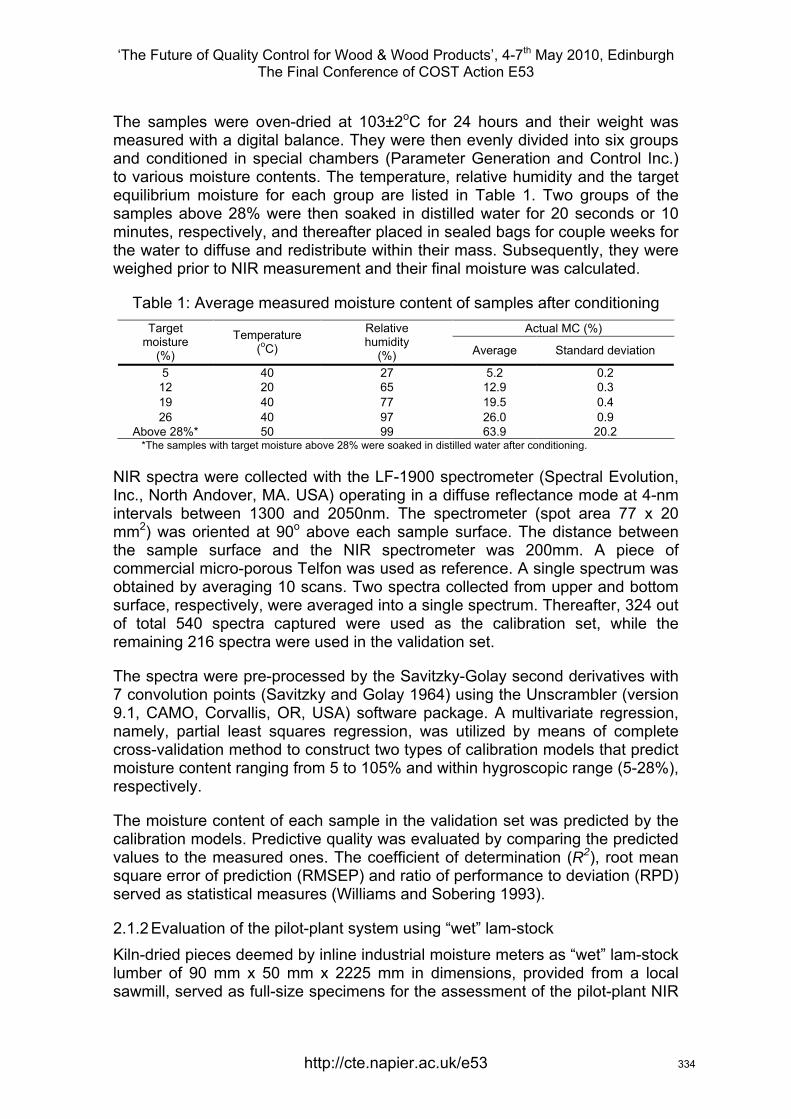
‘The Future of Quality Control for Wood & Wood Products’, 4-7th May 2010, Edinburgh The Final Conference of COST Action E53
The samples were oven-dried at 103±2oC for 24 hours and their weight was measured with a digital balance. They were then evenly divided into six groups and conditioned in special chambers (Parameter Generation and Control Inc.) to various moisture contents. The temperature, relative humidity and the target equilibrium moisture for each group are listed in Table 1. Two groups of the samples above 28% were then soaked in distilled water for 20 seconds or 10 minutes, respectively, and thereafter placed in sealed bags for couple weeks for the water to diffuse and redistribute within their mass. Subsequently, they were weighed prior to NIR measurement and their final moisture was calculated.
Table 1: Average measured moisture content of samples after conditioning Actual MC (%) Target
moisture (%)
Temperature (oC)
Relative humidity
(%) Average Standard deviation
5 40 27 5.2 0.2 12 20 65 12.9 0.3 19 40 77 19.5 0.4 26 40 97 26.0 0.9
Above 28%* 50 99 63.9 20.2 *The samples with target moisture above 28% were soaked in distilled water after conditioning.
NIR spectra were collected with the LF-1900 spectrometer (Spectral Evolution, Inc., North Andover, MA. USA) operating in a diffuse reflectance mode at 4-nm intervals between 1300 and 2050nm. The spectrometer (spot area 77 x 20 mm2) was oriented at 90o above each sample surface. The distance between the sample surface and the NIR spectrometer was 200mm. A piece of commercial micro-porous Telfon was used as reference. A single spectrum was obtained by averaging 10 scans. Two spectra collected from upper and bottom surface, respectively, were averaged into a single spectrum. Thereafter, 324 out of total 540 spectra captured were used as the calibration set, while the remaining 216 spectra were used in the validation set.
The spectra were pre-processed by the Savitzky-Golay second derivatives with 7 convolution points (Savitzky and Golay 1964) using the Unscrambler (version 9.1, CAMO, Corvallis, OR, USA) software package. A multivariate regression, namely, partial least squares regression, was utilized by means of complete cross-validation method to construct two types of calibration models that predict moisture content ranging from 5 to 105% and within hygroscopic range (5-28%), respectively.
The moisture content of each sample in the validation set was predicted by the calibration models. Predictive quality was evaluated by comparing the predicted values to the measured ones. The coefficient of determination (R2), root mean square error of prediction (RMSEP) and ratio of performance to deviation (RPD) served as statistical measures (Williams and Sobering 1993).
2.1.2 Evaluation of the pilot-plant system using “wet” lam-stock Kiln-dried pieces deemed by inline industrial moisture meters as “wet” lam-stock lumber of 90 mm x 50 mm x 2225 mm in dimensions, provided from a local sawmill, served as full-size specimens for the assessment of the pilot-plant NIR
http://cte.napier.ac.uk/e53 334
‘The Future of Quality Control for Wood & Wood Products’, 4-7th May 2010, Edinburgh The Final Conference of COST Action E53
system. In preliminary experiments, some of lumbers were dried and their average moisture content was less than 12%. In addition, the lumbers contained little local wet-spots on the surface. Therefore, wet-spots were created on surface artificially. Fifteen kiln-dried pieces of lam-stock lumber were used as specimens. They were divided into three groups (5 specimens for each group), namely, dried, partially dried and wet. The partially dried and wet specimens were prepared by spraying 16 ml of distilled water locally or all-over the top and bottom surfaces, respectively, every two days for three weeks. Thereafter, the specimens were covered by plastic sheet for more than three weeks.
A variable speed table was built and the NIR spectrometer was mounted on it to produce a pilot-plant in-line NIR system. The top and bottom surfaces of each specimen were scanned by passing it under the NIR spectrometer at a fixed speed. The conveyor system was moving at 500 and 1000 mm/s during which time 82 and 41 scans were taken per pass, respectively. Next, the specimen was scanned at 50 mm intervals along longitudinal direction under static condition (called “line speed 0 mm/s”). A single spectrum was obtained from one scan instead of averaging 10 scans. This trial resulted in a time reduction between each scan, so that only approximately 0.06 seconds were required to obtain a single spectrum.
After acquiring the spectra, slices of 40 mm in thickness were cut from the upper and bottom surfaces of each specimen, respectively. These slices were then re-cut into thin slices at 50 mm intervals along the longitudinal direction. Once the weight of all thin slices was measured, they were oven-dried and their moisture content was calculated gravimetrically. A total of 1382 data points of surface moisture from the thin slices were obtained.
Surface moisture content of the full-size specimens was predicted from the collected spectra using the calibration models. The predicted moisture was then compared with the calculated ones to assess the accuracy of the new NIR system.
2.2 Wet-pockets classification Small samples of 40 x 40 x 4 mm in thickness were cut and planed from the heartwood zone of green subalpine fir lumbers. Wet-pocket areas in each sample were immediately identified visually and marked. The samples were then classified into two groups, namely, “wet wood (WW)” of which more than half of its surface was covered by wet-pockets and “normal wood (NW)” that was completely free of any wet-pockets. One hundred samples were prepared for each WW and NW group, respectively. Three-quarters of the samples were randomly selected and assigned to the calibration set, while the remaining quarter was employed as the validation set.
Visible and near infrared (Vis-NIR) spectra of samples in the green state were collected with a QualitySpec Pro (Analytical Spectral Devices Inc. Boulder, CO, USA) operating in a reflectance mode at 1 nm intervals between 650 and 1150
http://cte.napier.ac.uk/e53 335
‘The Future of Quality Control for Wood & Wood Products’, 4-7th May 2010, Edinburgh The Final Conference of COST Action E53
nm. Previously visible range plus only a short NIR range are shown to be useful for the prediction of chemical components in wood (Kelly et al. 2004) and the discrimination of wood-based materials (Tsuchikawa et al. 2003). NIR spot area had approximately 20 mm diameter. Twenty scans were collected and averaged into a single spectrum for each sample. Thereafter, each sample was weighed and air-dried in a conditioning room (20±3oC and 50±2% relative humidity). Again Vis-NIR spectra of the samples in the dried state were collected and their sample weight was re-measured to calculate moisture content gravimetrically. More details of the hardware are given in Watanabe et al. (2010).
Prior to discriminant analysis, the reflectance spectra were converted to absorbance spectra, and pre-processed with second derivatives with 23 convolution points. Two different discriminant analyses, soft independent modeling of class analogy (SIMCA) and partial least squares (PLS) discriminant analysis were performed by Unscrambler software. SIMCA is one of the most common discriminant tools that was introduced by Wold (Wold 1976), and has successfully been applied on wood-based materials (Tsuchikawa et al. 2003). PLS discriminant analysis is not inherently designed for problems of classification (Geladi 1988), however, it is routinely used for classification and there is substantial empirical evidence to suggest that it performs well for these purposes (Barker & Rayens 2003).
Principal component analysis (PCA) with full cross-validation was performed for the four types of wood samples, namely, NW in the green state, WW in the green state, NW in the dried state and WW in the dried state, respectively, to construct four individual PCA models. The PCA models were used in the SIMCA classification of the samples in the validation set, with an alpha level of 0.5.
A PLS regression model was constructed with the calibration set using full cross-validation. The γ variables for WW and NW were labelled with +1 and 0, respectively. The models were then used to distinguish wet-pockets from normal wood in the validation set by means of discriminant PLS. Correct classification of wet-pockets was arbitrarily assigned to samples with predicted γ > 0.5, and correct classification of normal wood was assigned when γ < 0.5. The percentage correct classification is defined as the proportion of number of wet-pockets and normal wood predicted correctly to the total number of each class for green and dried sample, respectively.
3 Results and Discussion
3.1 High-speed detection of surface wet-pockets Table 2 shows the summary regression statistics of the calibration models for the hygroscopic range of moisture (5-28%) and the wide moisture range (5-105%), respectively. Both models resulted in high R2 of 0.98 and 0.96 in the validation set. The RPD values were over 5, which mean that the models are adequate for quality control.
http://cte.napier.ac.uk/e53 336
‘The Future of Quality Control for Wood & Wood Products’, 4-7th May 2010, Edinburgh The Final Conference of COST Action E53
Table 2: Calibration statistics for the hygroscopic range of moisture (5-28%) and wide range of moisture (5-105%)
Calibration model Calibration set Validation set MC range
(%) Wavelength
(nm) Number of
optimum PCs n R2 RMSECV (%) RPD n R2 RMSEP
(%) RPD
5-28 1300-2050 2 216 0.98 0.98 7.89 144 0.98 0.96 8.17 5-105 1300-2050 2 324 0.96 4.96 5.39 216 0.96 5.12 5.25
PCs: Principal components, RMSECV: Root mean square error of cross validation, RMSEP: Root mean square error of prediction, RPD: Ratio of performance to deviation.
The results of the gravimetrically measured surface moisture content versus the estimated values with line speed 1000 mm s-1 determined by the calibration model for the wide range of moisture are presented in Figure 1 (a). The measured surface moisture ranged from 10 to 82%. The model showed high R2 values of 0.87, 0.87 and 0.85, and low RMSEP of 4.52, 4.84 and 4.94 corresponding to line speeds of 0, 500 and 1000 mm/s, respectively. RMSEP was slightly poorer with increasing line speed. RPD for all line speeds was over 2.5, pointing to the fact that the NIR system has an adequate ability to screen wood based on moisture. These results indicate that the NIR system with line speed of 0 to 1000 mm s-1 is able to measure surface moisture distribution of “wet” lam-stock up to 105% rapidly and accurately, and that NIR spectroscopy has a potential to sort green lumber before drying based on moisture content.
(a) (b)
Figure 1: Measured vs. NIR estimated moisture for wide range of moisture (a) and hygroscopic range of moisture (b) with line 1000 mm/s. The dotted line is the regression - solid line R2=1.
The results of the gravimetrically measured surface moisture content versus the estimated values determined by the calibration model for the hygroscopic range of moisture are presented in Figure 1 (b). The model resulted in R2 of 0.85, 0.85 and 0.86, and low RMSEP of 2.12, 2.41 and 2.41 corresponding to the line speed 0, 500 and 1000 mm s-1, respectively. These results suggest that the model is expected to have an average prediction error up to the RMSEP. RPD
http://cte.napier.ac.uk/e53 337
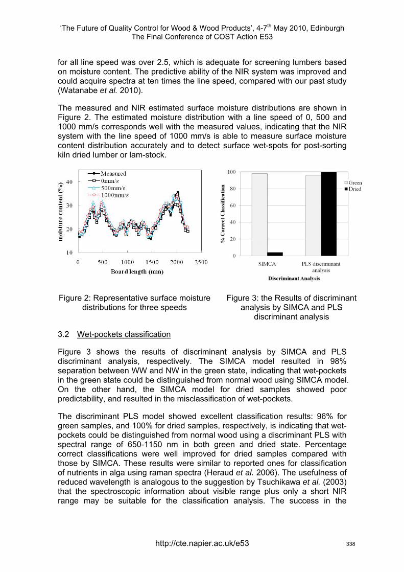
‘The Future of Quality Control for Wood & Wood Products’, 4-7th May 2010, Edinburgh The Final Conference of COST Action E53
for all line speed was over 2.5, which is adequate for screening lumbers based on moisture content. The predictive ability of the NIR system was improved and could acquire spectra at ten times the line speed, compared with our past study (Watanabe et al. 2010).
The measured and NIR estimated surface moisture distributions are shown in
Figure 3: the Results of discriminant
3.2 Wet-pockets classification
Figure 2. The estimated moisture distribution with a line speed of 0, 500 and 1000 mm/s corresponds well with the measured values, indicating that the NIR system with the line speed of 1000 mm/s is able to measure surface moisture content distribution accurately and to detect surface wet-spots for post-sorting kiln dried lumber or lam-stock.
Figure 2: Representative surface moisture distributions for three speeds analysis by SIMCA and PLS
discriminant analysis
Figure 3 shows the results of discriminant analysis by SIMCA and PLS discriminant analysis, respectively. The SIMCA model resulted in 98% separation between WW and NW in the green state, indicating that wet-pockets in the green state could be distinguished from normal wood using SIMCA model. On the other hand, the SIMCA model for dried samples showed poor predictability, and resulted in the misclassification of wet-pockets.
The discriminant PLS model showed excellent classification results: 96% for green samples, and 100% for dried samples, respectively, is indicating that wet-pockets could be distinguished from normal wood using a discriminant PLS with spectral range of 650-1150 nm in both green and dried state. Percentage correct classifications were well improved for dried samples compared with those by SIMCA. These results were similar to reported ones for classification of nutrients in alga using raman spectra (Heraud et al. 2006). The usefulness of reduced wavelength is analogous to the suggestion by Tsuchikawa et al. (2003) that the spectroscopic information about visible range plus only a short NIR range may be suitable for the classification analysis. The success in the
http://cte.napier.ac.uk/e53 338
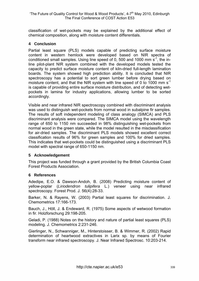
‘The Future of Quality Control for Wood & Wood Products’, 4-7th May 2010, Edinburgh The Final Conference of COST Action E53
classification of wet-pockets may be explained by the additional effect of chemical composition, along with moisture content differentials.
4 Conclusion are (PLS) models capable of predicting surface moisture
Visible and near infrared NIR spectroscopy combined with discriminant analysis
5 Acknowledgement through a grant provided by the British Columbia Coast
6 References & Dawson-Andoh, B. (2008) Predicting moisture content of
least squares for discrimination. J.
rd, R. (1975) Some aspects of wetwood formation
tory and nature of partial least squares (PLS)
toisser, B. & Wimmer, R. (2002) Rapid
Partial least squcontent in western hemlock were developed based on NIR spectra of conditioned small samples. Using line speed of 0, 500 and 1000 mm s-1, the in-line pilot-plant NIR system combined with the developed models tested the capacity to predict surface moisture content of kiln-dried full-length lamination boards. The system showed high prediction ability. It is concluded that NIR spectroscopy has a potential to sort green lumber before drying based on moisture content, and that the NIR system with line speed of 0 to 1000 mm s-1 is capable of providing entire surface moisture distribution, and of detecting wet-pockets in lamina for industry applications, allowing lumber to be sorted accordingly.
was used to distinguish wet-pockets from normal wood in subalpine fir samples. The results of soft independent modeling of class analogy (SIMCA) and PLS discriminant analysis were compared. The SIMCA model using the wavelength range of 650 to 1150 nm succeeded in 98% distinguishing wet-pockets from normal wood in the green state, while the model resulted in the misclassification for air-dried samples. The discriminant PLS models showed excellent correct classification results of 96% for green samples and 100% for dried samples. This indicates that wet-pockets could be distinguished using a discriminant PLS model with spectral range of 650-1150 nm.
This project was funded Forest Products Association.
Adedipe, E.O. yellow-poplar (Liriodendron tulipifera L.) veneer using near infrared spectroscopy. Forest Prod. J. 56(4):28-33. Barker, N. & Rayens, W. (2003) Partial Chemometrics 17:166-173. Bauch, J., Höll, J. & Endewain fir. Holzforschung 29:198-205. Geladi, P. (1988) Notes on the hismodeling. J. Chemometrics 2:231-246. Gierlinger, N., Schwanniger, M., Hintersdetermination of heartwood extractives in Larix sp. by means of Fourier transform near infrared spectroscopy. J. Near Infrared Spectrosc. 10:203-214.
http://cte.napier.ac.uk/e53 339
‘The Future of Quality Control for Wood & Wood Products’, 4-7th May 2010, Edinburgh The Final Conference of COST Action E53
Hoffmeyer, P. & Pedersen, J.G. (1995) Evaluation of density and strength of Norway spruce wood by near infrared reflectance spectroscopy. Holz Roh-Werkst. 53:165-170. Karttunen, K., Leinonen, A. & Sarén, M.-P. (2008) A survey of moisture distribution in two sets of Scots pine logs by NIR-spectroscopy. Holzforschung 62:435-440. Kozlik, C.J. & Ward, J.C. (1981) Properties and kiln-drying characteristics of young-growth western hemlock dimension lumber. Forest Prod. J. 31(6): 45-53.Mackay, J.F.K. (1975) Properties of northern aspen discolored wood related to drying problems. Wood Fiber 6(4):319-326. Poke, F.S. & Raymond, C.A. (2006) Predicting extractives, lignin, and cellulose contents using near infrared spectroscopy on solid wood in Eucalyptus globules using near infrared reflectance analysis. J. Wood Chem. Technol. 26:187-199. Ross, R.J., Ward, J.C. & TenWolde, A. (1994) Stress wave nondestructive evaluation of wetwood. Forest Prod. J. 44(7/8):79-83. Savitzky, A. & Golay, M.J.E. (1964) Smoothing and differentiation of data by simplified least square procedures. Anal. Chem. 36(8):1627-1639. Schink, B. & Ward, J.C. (1984) Microaerobic and anaerobic bacterial activities involved in formation of wetwood and discoloured wood. IAWA Bull. New Ser. 5(2):105-109. Schneider, M.H. & Zhou, L. (1989) Characterization of wet-wood from four balsam fir trees. Wood Fiber Sci. 21:1-16. Schroeder, H.A. & Kozlik, C.J. (1972) The characterization of wetwood in western hemlock (Tsuga heterophylla). Wood Sci. Technol. 6(2):85-94. Simpson, W. (1991) Dry kiln operator’s manual, Forest products laboratory, Madison, Wisconsin. pp274. Taylor, A.M., Freitag, C., Cadot, E. & Morrell, J.J. (2008) Potential of near infrared spectroscopy to assess hot-water-soluble extractive content and decay resistance of a tropical hardwood. Holz Roh Werkst 66:107-111. Tsuchikawa, S., Yamato, K. & Inoue, K. (2003) Discriminant analysis of wood-based materials using near-infrared spectroscopy. J. Wood Sci. 49:275-280. Ward, J.C. & Zeikus, J.G. (1980) Bacteriological, chemical and physical properties of wetwood in living trees. In Natural variations of wtwood in living properties. Edited by J. Bauch. Mitt. Bundesforschungsanst. Forest Holzwirtsch, Hamburg, No.131:133-165. Ward, J.C. & Groom, D. (1983) Bacterial oak: drying problems. Forest Prod. J. 33(10):57-65. Ward, J.C. (1986) The effect of wetwood on lumber drying times and rates: An exploratory evaluation with longitudinal gas permeability. Wood Fibre Sci. 18(2): 288-307.
http://cte.napier.ac.uk/e53 340

‘The Future of Quality Control for Wood & Wood Products’, 4-7th May 2010, Edinburgh The Final Conference of COST Action E53
Watanabe, K., Hart, F., Mansfield, S.D. & Avramidis, S. (2010) Detection of wet-pockets on the surface of Tsuga heterophylla (Raf.) Sarg. by near infrared (NIR) spectroscopy, Holzfolschung 64:55-60. Williams, P.C. & Sobering, D.C. (1993) Comparison of commercial near infrared transmittance and reflectance instruments for analysis of whole grains and seeds. J. Near Infrared Spec. 1:25-32. Wold, S. (1976) Pattern recognition by means of disjoint principal components models. Pattern Recognit. 8:127-139.
http://cte.napier.ac.uk/e53 341

‘The Future of Quality Control for Wood & Wood Products’, 4-7th May 2010, Edinburgh The Final Conference of COST Action E53
Thursday 6th May Research focussed day
Parallel session 1A
http://www.cte.napier.ac.uk/e53/ 342
‘The Future of Quality Control for Wood & Wood Products’, 4-7th May 2010, Edinburgh The Final Conference of COST Action E53
http://cte.napier.ac.uk/e53
Knots in CT scans of Scots pine logs
R. Baumgartner1, F. Brüchert
2 & U. H. Sauter
3
Abstract
Outer dimensions of logs can be detected by modern optical scanners to a high precision. Quality parameters describing the outer shape as taper and curvature can be calculated from this data, based on algorithms agreed between the trade partners. The detection of inner log features is not used in the industry to a standardised and wide spread so far. However inner log features can affect the products sawn from a log. Knots, for example, can limit the utilisation for construction purpose or optical usage.
In this study computed tomography (CT) was used to detect the three-dimensional shape of knots in Scots pine logs grown in the southern part of Sweden. In the CT images different densities are represented by different grey-values. Regions with the same or similar density will show the same grey-value and thus can not be distinguished in these images. The absorption characteristics of wood lead to a contrast between knot material and regular stem wood in the heartwood part of the log, but to very low contrast in the sapwood. As the sapwood’s high water content absorbs radiation in similar way as branch wood the knots and the surrounding material have a similar density and therefore a similar grey-value. Thus knot detection in sapwood by CT methodology is restricted.
For this investigation the main focus was set on the automatic detection of the three-dimensional shape of the knots in the heartwood applying image analysis methodology. In a first step an algorithm was developed to eliminate the sapwood area in the CT images. It uses a polar transform with the pith as pole for each slice, followed by a detection of the heartwood-sapwood-boundary on the radial coordinate. The obtained values are afterwards corrected by interpolation, to bypass the whorls, and smoothing in longitudinal direction of the log. In the main step threshold values and morphological procedures were applied to detect the knots – resulting in a 3D representation of the log with the shape (including position, orientation and size) of all knots in the heartwood.
1 Scientist, [email protected] Forest Research Institute Baden-Württemberg, Dep. of Forest Utilisation, Freiburg, Germany 2 Senior scientist, [email protected] Forest Research Institute Baden-Württemberg, Dep. of Forest Utilisation, Freiburg, Germany 3 Head of Department, [email protected] Forest Research Institute Baden-Württemberg, Dep. of Forest Utilisation, Freiburg, Germany
343
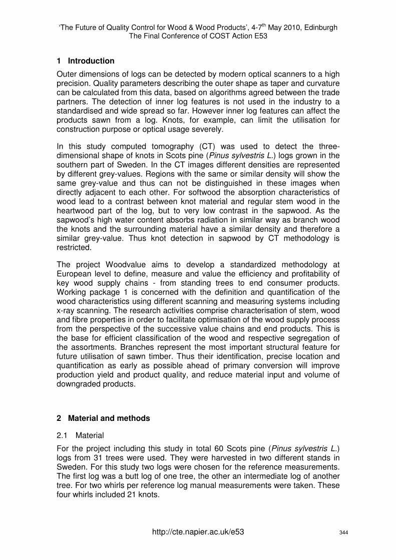
‘The Future of Quality Control for Wood & Wood Products’, 4-7th May 2010, Edinburgh The Final Conference of COST Action E53
http://cte.napier.ac.uk/e53
1 Introduction
Outer dimensions of logs can be detected by modern optical scanners to a high precision. Quality parameters describing the outer shape as taper and curvature can be calculated from this data, based on algorithms agreed between the trade partners. The detection of inner log features is not used in the industry to a standardised and wide spread so far. However inner log features can affect the products sawn from a log. Knots, for example, can limit the utilisation for construction purpose or optical usage severely.
In this study computed tomography (CT) was used to detect the three-dimensional shape of knots in Scots pine (Pinus sylvestris L.) logs grown in the southern part of Sweden. In the CT images different densities are represented by different grey-values. Regions with the same or similar density will show the same grey-value and thus can not be distinguished in these images when directly adjacent to each other. For softwood the absorption characteristics of wood lead to a contrast between knot material and regular stem wood in the heartwood part of the log, but to very low contrast in the sapwood. As the sapwood’s high water content absorbs radiation in similar way as branch wood the knots and the surrounding material have a similar density and therefore a similar grey-value. Thus knot detection in sapwood by CT methodology is restricted.
The project Woodvalue aims to develop a standardized methodology at European level to define, measure and value the efficiency and profitability of key wood supply chains - from standing trees to end consumer products. Working package 1 is concerned with the definition and quantification of the wood characteristics using different scanning and measuring systems including x-ray scanning. The research activities comprise characterisation of stem, wood and fibre properties in order to facilitate optimisation of the wood supply process from the perspective of the successive value chains and end products. This is the base for efficient classification of the wood and respective segregation of the assortments. Branches represent the most important structural feature for future utilisation of sawn timber. Thus their identification, precise location and quantification as early as possible ahead of primary conversion will improve production yield and product quality, and reduce material input and volume of downgraded products.
2 Material and methods
2.1 Material
For the project including this study in total 60 Scots pine (Pinus sylvestris L.) logs from 31 trees were used. They were harvested in two different stands in Sweden. For this study two logs were chosen for the reference measurements. The first log was a butt log of one tree, the other an intermediate log of another tree. For two whirls per reference log manual measurements were taken. These four whirls included 21 knots.
344
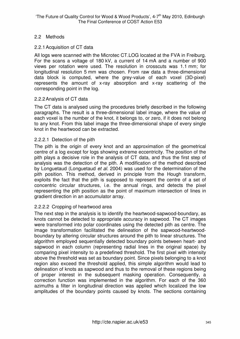
‘The Future of Quality Control for Wood & Wood Products’, 4-7th May 2010, Edinburgh The Final Conference of COST Action E53
http://cte.napier.ac.uk/e53
2.2 Methods
2.2.1 Acquisition of CT data
All logs were scanned with the Microtec CT.LOG located at the FVA in Freiburg. For the scans a voltage of 180 kV, a current of 14 mA and a number of 900 views per rotation were used. The resolution in crosscuts was 1.1 mm; for longitudinal resolution 5 mm was chosen. From raw data a three-dimensional data block is computed, where the grey-value of each voxel (3D-pixel) represents the amount of x-ray absorption and x-ray scattering of the corresponding point in the log.
2.2.2 Analysis of CT data
The CT data is analysed using the procedures briefly described in the following paragraphs. The result is a three-dimensional label image, where the value of each voxel is the number of the knot, it belongs to, or zero, if it does not belong to any knot. From this label image the three-dimensional shape of every single knot in the heartwood can be extracted.
2.2.2.1 Detection of the pith The pith is the origin of every knot and an approximation of the geometrical centre of a log except for logs showing extreme eccentricity. The position of the pith plays a decisive role in the analysis of CT data, and thus the first step of analysis was the detection of the pith. A modification of the method described by Longuetaud (Longuetaud et al. 2004) was used for the determination of the pith position. This method, derived in principle from the Hough transform, exploits the fact that the pith is supposed to represent the centre of a set of concentric circular structures, i.e. the annual rings, and detects the pixel representing the pith position as the point of maximum intersection of lines in gradient direction in an accumulator array.
2.2.2.2 Cropping of heartwood area The next step in the analysis is to identify the heartwood-sapwood-boundary, as knots cannot be detected to appropriate accuracy in sapwood. The CT images were transformed into polar coordinates using the detected pith as centre. The image transformation facilitated the delineation of the sapwood-heartwood-boundary by altering circular structures around the pith to linear structures. The algorithm employed sequentially detected boundary points between heart- and sapwood in each column (representing radial lines in the original space) by comparing pixel intensity to a predefined threshold. The first pixel with intensity above the threshold was set as boundary point. Since pixels belonging to a knot region also exceed the threshold applied, this simple algorithm would lead to delineation of knots as sapwood and thus to the removal of these regions being of proper interest in the subsequent masking operation. Consequently, a correction function was implemented in the algorithm. For each of the 360 azimuths a filter in longitudinal direction was applied which localized the low amplitudes of the boundary points caused by knots. The sections containing
345
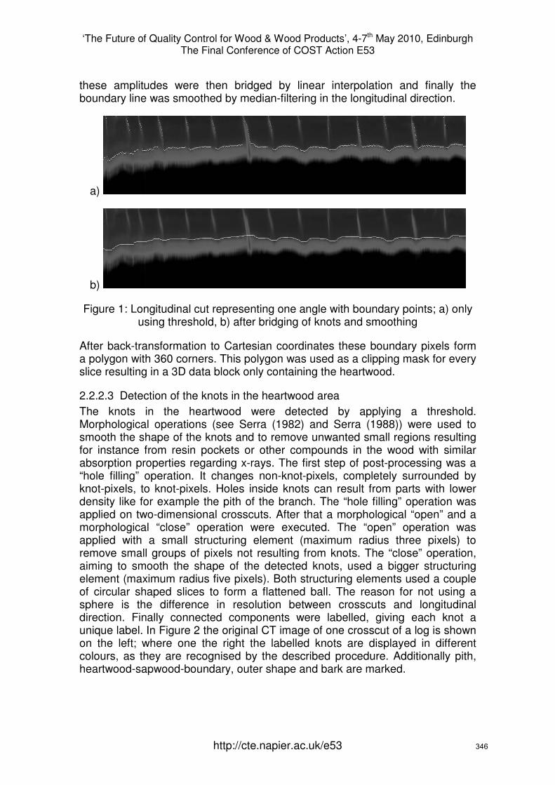
‘The Future of Quality Control for Wood & Wood Products’, 4-7th May 2010, Edinburgh The Final Conference of COST Action E53
http://cte.napier.ac.uk/e53
these amplitudes were then bridged by linear interpolation and finally the boundary line was smoothed by median-filtering in the longitudinal direction.
a)
b)
Figure 1: Longitudinal cut representing one angle with boundary points; a) only using threshold, b) after bridging of knots and smoothing
After back-transformation to Cartesian coordinates these boundary pixels form a polygon with 360 corners. This polygon was used as a clipping mask for every slice resulting in a 3D data block only containing the heartwood.
2.2.2.3 Detection of the knots in the heartwood area The knots in the heartwood were detected by applying a threshold. Morphological operations (see Serra (1982) and Serra (1988)) were used to smooth the shape of the knots and to remove unwanted small regions resulting for instance from resin pockets or other compounds in the wood with similar absorption properties regarding x-rays. The first step of post-processing was a “hole filling” operation. It changes non-knot-pixels, completely surrounded by knot-pixels, to knot-pixels. Holes inside knots can result from parts with lower density like for example the pith of the branch. The “hole filling” operation was applied on two-dimensional crosscuts. After that a morphological “open” and a morphological “close” operation were executed. The “open” operation was applied with a small structuring element (maximum radius three pixels) to remove small groups of pixels not resulting from knots. The “close” operation, aiming to smooth the shape of the detected knots, used a bigger structuring element (maximum radius five pixels). Both structuring elements used a couple of circular shaped slices to form a flattened ball. The reason for not using a sphere is the difference in resolution between crosscuts and longitudinal direction. Finally connected components were labelled, giving each knot a unique label. In Figure 2 the original CT image of one crosscut of a log is shown on the left; where one the right the labelled knots are displayed in different colours, as they are recognised by the described procedure. Additionally pith, heartwood-sapwood-boundary, outer shape and bark are marked.
346
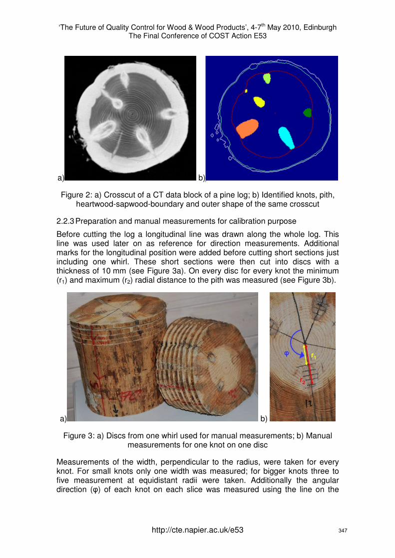
‘The Future of Quality Control for Wood & Wood Products’, 4-7th May 2010, Edinburgh The Final Conference of COST Action E53
http://cte.napier.ac.uk/e53
a) b)
Figure 2: a) Crosscut of a CT data block of a pine log; b) Identified knots, pith, heartwood-sapwood-boundary and outer shape of the same crosscut
2.2.3 Preparation and manual measurements for calibration purpose
Before cutting the log a longitudinal line was drawn along the whole log. This line was used later on as reference for direction measurements. Additional marks for the longitudinal position were added before cutting short sections just including one whirl. These short sections were then cut into discs with a thickness of 10 mm (see Figure 3a). On every disc for every knot the minimum (r1) and maximum (r2) radial distance to the pith was measured (see Figure 3b).
a) b)
Figure 3: a) Discs from one whirl used for manual measurements; b) Manual measurements for one knot on one disc
Measurements of the width, perpendicular to the radius, were taken for every knot. For small knots only one width was measured; for bigger knots three to five measurement at equidistant radii were taken. Additionally the angular direction (φ) of each knot on each slice was measured using the line on the
347
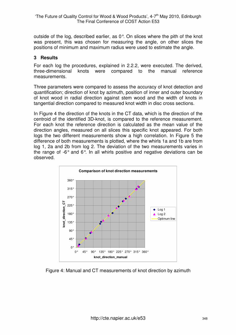
‘The Future of Quality Control for Wood & Wood Products’, 4-7th May 2010, Edinburgh The Final Conference of COST Action E53
http://cte.napier.ac.uk/e53
outside of the log, described earlier, as 0°. On slices where the pith of the knot was present, this was chosen for measuring the angle, on other slices the positions of minimum and maximum radius were used to estimate the angle.
3 Results
For each log the procedures, explained in 2.2.2, were executed. The derived, three-dimensional knots were compared to the manual reference measurements.
Three parameters were compared to assess the accuracy of knot detection and quantification; direction of knot by azimuth, position of inner and outer boundary of knot wood in radial direction against stem wood and the width of knots in tangential direction compared to measured knot width in disc cross sections.
In Figure 4 the direction of the knots in the CT data, which is the direction of the centroid of the identified 3D-knot, is compared to the reference measurement. For each knot the reference direction is calculated as the mean value of the direction angles, measured on all slices this specific knot appeared. For both logs the two different measurements show a high correlation. In Figure 5 the difference of both measurements is plotted, where the whirls 1a and 1b are from log 1, 2a and 2b from log 2. The deviation of the two measurements varies in the range of -6° and 6°. In all whirls positive and negative deviations can be observed.
Comparison of knot direction measurements
0°
45°
90°
135°
180°
225°
270°
315°
360°
0° 45° 90° 135° 180° 225° 270° 315° 360°
knot_direction_manual
kn
ot_
dir
ec
tio
n_
CT
Log 1
Log 2
Optimum line
Figure 4: Manual and CT measurements of knot direction by azimuth
348
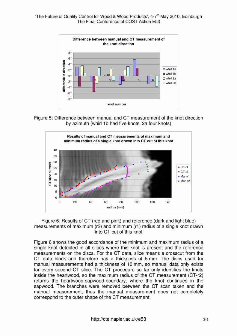
‘The Future of Quality Control for Wood & Wood Products’, 4-7th May 2010, Edinburgh The Final Conference of COST Action E53
http://cte.napier.ac.uk/e53
Difference between manual and CT measurement of
the knot direction
-8°
-6°
-4°
-2°
0°
2°
4°
6°
8°
1 2 3 4 5 6
knot number
dif
fere
nc
e in
dir
ec
tio
n
whirl 1a
whirl 1b
whirl 2a
whirl 2b
Figure 5: Difference between manual and CT measurement of the knot direction by azimuth (whirl 1b had five knots, 2a four knots)
Results of manual and CT measurements of maximum and
minimum radius of a single knot drawn into CT cut of this knot
0
5
10
15
20
25
30
35
40
0 20 40 60 80 100 120 140
radius [mm]
CT
slic
e n
um
be
r
CT-r1
CT-r2
Man-r1
Man-r2
Figure 6: Results of CT (red and pink) and reference (dark and light blue) measurements of maximum (r2) and minimum (r1) radius of a single knot drawn
into CT cut of this knot
Figure 6 shows the good accordance of the minimum and maximum radius of a single knot detected in all slices where this knot is present and the reference measurements on the discs. For the CT data, slice means a crosscut from the CT data block and therefore has a thickness of 5 mm. The discs used for manual measurements had a thickness of 10 mm, so manual data only exists for every second CT slice. The CT procedure so far only identifies the knots inside the heartwood, so the maximum radius of the CT measurement (CT-r2) returns the heartwood-sapwood-boundary, where the knot continues in the sapwood. The branches were removed between the CT scan taken and the manual measurement, thus the manual measurement does not completely correspond to the outer shape of the CT measurement.
349
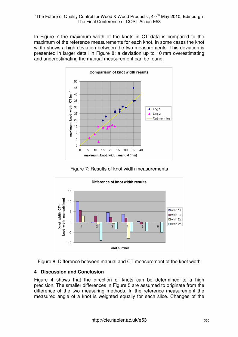
‘The Future of Quality Control for Wood & Wood Products’, 4-7th May 2010, Edinburgh The Final Conference of COST Action E53
http://cte.napier.ac.uk/e53
In Figure 7 the maximum width of the knots in CT data is compared to the maximum of the reference measurements for each knot. In some cases the knot width shows a high deviation between the two measurements. This deviation is presented in larger detail in Figure 8; a deviation up to 10 mm overestimating and underestimating the manual measurement can be found.
Comparison of knot width results
0
5
10
15
20
25
30
35
40
45
50
0 5 10 15 20 25 30 35 40
maximum_knot_width_manual [mm]
ma
xim
um
_k
no
t_w
idth
_C
T [
mm
]
Log 1
Log 2
Optimum line
Figure 7: Results of knot width measurements
Difference of knot width results
-10
-5
0
5
10
15
1 2 3 4 5 6
knot number
(kn
ot_
wid
th_
CT
-
kn
ot_
wid
th_
ma
nu
al) [
mm
]
whirl 1a
whirl 1b
whirl 2a
whirl 2b
Figure 8: Difference between manual and CT measurement of the knot width
4 Discussion and Conclusion
Figure 4 shows that the direction of knots can be determined to a high precision. The smaller differences in Figure 5 are assumed to originate from the difference of the two measuring methods. In the reference measurement the measured angle of a knot is weighted equally for each slice. Changes of the
350
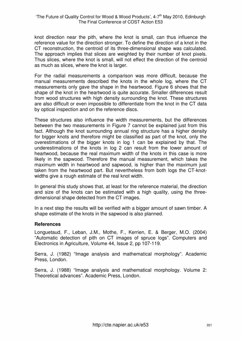
‘The Future of Quality Control for Wood & Wood Products’, 4-7th May 2010, Edinburgh The Final Conference of COST Action E53
http://cte.napier.ac.uk/e53
knot direction near the pith, where the knot is small, can thus influence the reference value for the direction stronger. To define the direction of a knot in the CT reconstruction, the centroid of its three-dimensional shape was calculated. The approach implies that slices are weighted by their number of knot pixels. Thus slices, where the knot is small, will not effect the direction of the centroid as much as slices, where the knot is larger.
For the radial measurements a comparison was more difficult, because the manual measurements described the knots in the whole log, where the CT measurements only gave the shape in the heartwood. Figure 6 shows that the shape of the knot in the heartwood is quite accurate. Smaller differences result from wood structures with high density surrounding the knot. These structures are also difficult or even impossible to differentiate from the knot in the CT data by optical inspection and on the reference discs.
These structures also influence the width measurements, but the differences between the two measurements in Figure 7 cannot be explained just from this fact. Although the knot surrounding annual ring structure has a higher density for bigger knots and therefore might be classified as part of the knot, only the overestimations of the bigger knots in log 1 can be explained by that. The underestimations of the knots in log 2 can result from the lower amount of heartwood, because the real maximum width of the knots in this case is more likely in the sapwood. Therefore the manual measurement, which takes the maximum width in heartwood and sapwood, is higher than the maximum just taken from the heartwood part. But nevertheless from both logs the CT-knot-widths give a rough estimate of the real knot width.
In general this study shows that, at least for the reference material, the direction and size of the knots can be estimated with a high quality, using the three-dimensional shape detected from the CT images.
In a next step the results will be verified with a bigger amount of sawn timber. A shape estimate of the knots in the sapwood is also planned.
References
Longuetaud, F., Leban, J.M., Mothe, F., Kerrien, E. & Berger, M.O. (2004) “Automatic detection of pith on CT images of spruce logs”. Computers and Electronics in Agriculture, Volume 44, Issue 2, pp 107-119.
Serra, J. (1982) “Image analysis and mathematical morphology”. Academic Press, London.
Serra, J. (1988) “Image analysis and mathematical morphology. Volume 2: Theoretical advances”. Academic Press, London.
351
‘The Future of Quality Control for Wood & Wood Products’, 4-7th May 2010, Edinburgh The Final Conference of COST Action E53
The use of log geometry variables to determine the stiffness of Sitka spruce
T. N. Reynolds1, S. Porter 2
Abstract A key limiting property in the utilisation of British grown Sitka spruce is its lower stiffness when compared to slower grown softwood from northern Europe. With better knowledge of the variables affecting timber performance, better sorting regimes might be determined. Three dimensional log shape scanners are used in many sawmills to optimise volumetric recovery. These scanners also have the potential to be used to indicate timber quality.
In this paper the relationship between axial position within the stem, log shape variables (taper, ovality, pith eccentricity) and MOE as indicated by Cook Bolinder grading machine and static bending tests to EN 408 are examined for sample batches of Sitka spruce. A particular feature noted is the existence of a zone of low stiffness material near to the butt. The low stiffness was determined to be due to high microfibril angle (MFA), and not other factors such as low density or slope of grain. The effect was noted to be variable between the individual trees and stands of material.
1 Introduction Sitka spruce (Picea Sitchensis) is the UK’s most important commercial species, providing over half of the total volume of softwood timber produced. British-grown Sitka spruce trees reach maturity relatively quickly; as a consequence the timber differs significantly from slower grown softwoods imported from northern Europe. British-grown Sitka spruce tends to meet a lower structural grade than imported softwood, which can exclude it from certain markets. For example, none at present is used for trussed rafters.
Although density has, historically, been considered one of the main properties influencing the mechanical performance of timber, Brazier (1986) questioned its significance for Sitka spruce. He identified two features of greater influence, grain inclination and presence of juvenile wood.
Brazier (1991) found in a study on the effect of spacing on the vigour of 41 Sitka spruce trees that the timber at the base of the tree was of poorer quality (i.e. was less stiff), and that stem size had no apparent effect on structural wood performance. He suggested that the reason for the low performance of the near butt wood might be due to a combination of low density, irregular grain associated with a buttressing effect from the roots, and possibly also “unusual”
1 Senior Consultant, [email protected] Consultant Building Research Establishment, UK
http://cte.napier.ac.uk/e53 352
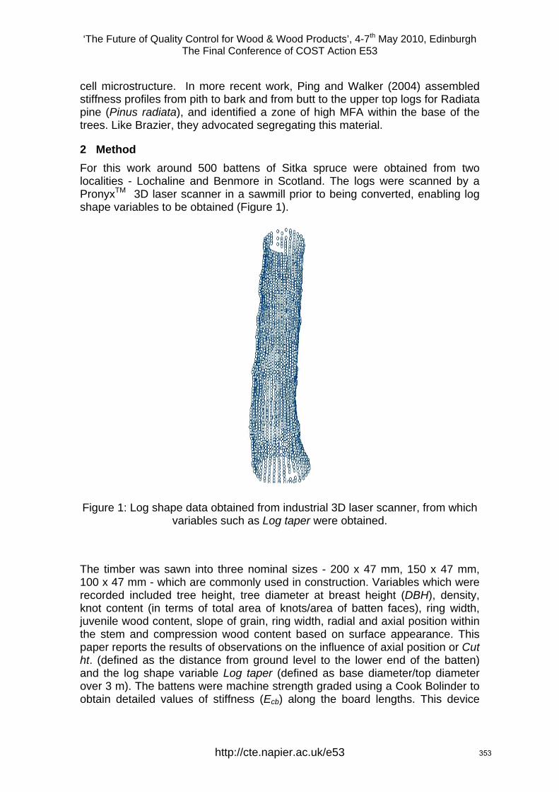
‘The Future of Quality Control for Wood & Wood Products’, 4-7th May 2010, Edinburgh The Final Conference of COST Action E53
cell microstructure. In more recent work, Ping and Walker (2004) assembled stiffness profiles from pith to bark and from butt to the upper top logs for Radiata pine (Pinus radiata), and identified a zone of high MFA within the base of the trees. Like Brazier, they advocated segregating this material.
2 Method For this work around 500 battens of Sitka spruce were obtained from two localities - Lochaline and Benmore in Scotland. The logs were scanned by a PronyxTM 3D laser scanner in a sawmill prior to being converted, enabling log shape variables to be obtained (Figure 1).
Figure 1: Log shape data obtained from industrial 3D laser scanner, from which variables such as Log taper were obtained.
The timber was sawn into three nominal sizes - 200 x 47 mm, 150 x 47 mm, 100 x 47 mm - which are commonly used in construction. Variables which were recorded included tree height, tree diameter at breast height (DBH), density, knot content (in terms of total area of knots/area of batten faces), ring width, juvenile wood content, slope of grain, ring width, radial and axial position within the stem and compression wood content based on surface appearance. This paper reports the results of observations on the influence of axial position or Cut ht. (defined as the distance from ground level to the lower end of the batten) and the log shape variable Log taper (defined as base diameter/top diameter over 3 m). The battens were machine strength graded using a Cook Bolinder to obtain detailed values of stiffness (Ecb) along the board lengths. This device
http://cte.napier.ac.uk/e53 353

‘The Future of Quality Control for Wood & Wood Products’, 4-7th May 2010, Edinburgh The Final Conference of COST Action E53
obtains an indicative stiffness parameter using three-point bending via a system of rollers (Figure 2), based on a nominal batten size. Values of stiffness and strength (i.e. E m,g and fm) were also determined by tests to EN 408.
Figure 2: Schematic of Cook Bolinder strength grader.
Since the position of every batten was known within each tree stiffness profiles both axially and radially could be established. MFA measurements were carried out on samples from selected butt log battens using microscopic examination of cross-field pit angle relative to the axis of the cell wall. In addition, MFA measurements on batten cross sections were also obtained on several battens using the SilviscanTM instrument at STFI-Packforst, Sweden, which measures MFA based on X-ray diffractometry. A full description of the operating principle of this device is given by Evans (1997).
3 Results and discussion Figure 3 shows an example of tree stiffness profiles assembled from Cook Bolinder grader data. For the Benmore material (stand nos. FR3 and FR4), in particular, there was a marked tendency for low stiffness material to be evident at the butt; however this feature was noted to be variable between individual trees.
Figure 4 shows Ecb plotted against Cut ht. (i.e. axial position) for the FR3 150 x 47 mm butt log subgroup. A similar effect was noted in other (but not all) butt log subgroups. Figure 5 shows Ecb plotted against Log taper for groups of upper log and butt log material. It can be seen that the butt log battens are generally of lower stiffness than the upper log material.
Microscopic examination of material taken from a number of boards which showed particularly marked trends for lower stiffness towards the butt indicated that this effect was related to MFA (Figures 6 and 7). Marked differences in the MFA trends from pith to bark between butt and upper sections were also obtained in several other battens using the SilivscanTM instrument.
http://cte.napier.ac.uk/e53 354
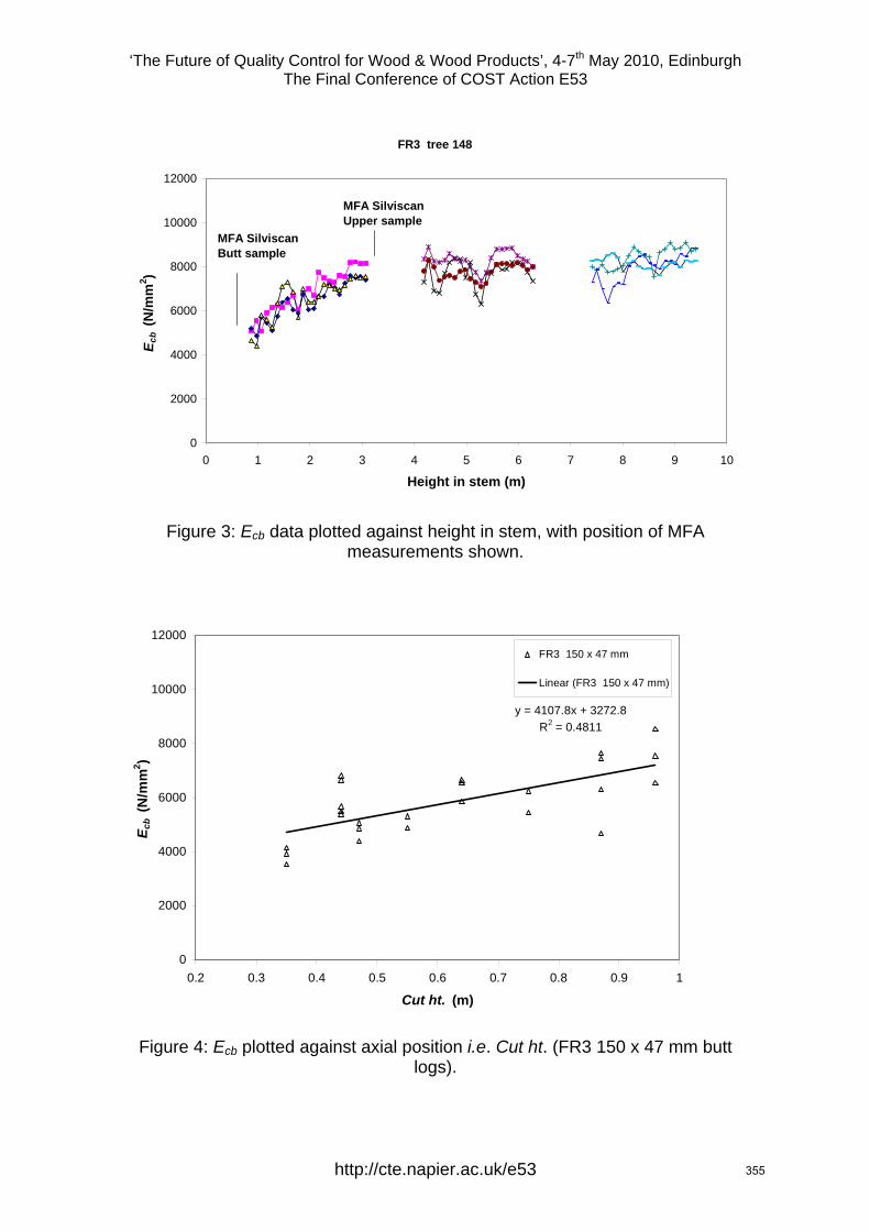
‘The Future of Quality Control for Wood & Wood Products’, 4-7th May 2010, Edinburgh The Final Conference of COST Action E53
FR3 tree 148
0
2000
4000
6000
8000
10000
12000
0 1 2 3 4 5 6 7 8 9 1
Height in stem (m)
E cb
(N/m
m2 )
MFA SilviscanButt sample
MFA SilviscanUpper sample
0
Figure 3: Ecb data plotted against height in stem, with position of MFA measurements shown.
y = 4107.8x + 3272.8R2 = 0.4811
0
2000
4000
6000
8000
10000
12000
0.2 0.3 0.4 0.5 0.6 0.7 0.8 0.9 1
Cut ht. (m)
E cb
(N/m
m2 )
FR3 150 x 47 mm
Linear (FR3 150 x 47 mm)
Figure 4: Ecb plotted against axial position i.e. Cut ht. (FR3 150 x 47 mm butt logs).
http://cte.napier.ac.uk/e53 355
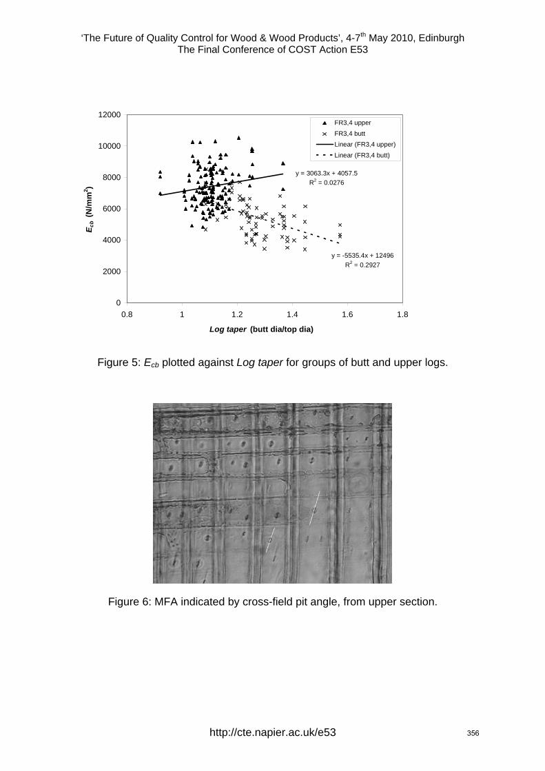
‘The Future of Quality Control for Wood & Wood Products’, 4-7th May 2010, Edinburgh The Final Conference of COST Action E53
y = 3063.3x + 4057.5R2 = 0.0276
y = -5535.4x + 12496R2 = 0.2927
0
2000
4000
6000
8000
10000
12000
0.8 1 1.2 1.4 1.6 1.8
Log taper (butt dia/top dia)
E cb
(N/m
m2 )
FR3,4 upperFR3,4 buttLinear (FR3,4 upper)Linear (FR3,4 butt)
Figure 5: Ecb plotted against Log taper for groups of butt and upper logs.
Figure 6: MFA indicated by cross-field pit angle, from upper section.
http://cte.napier.ac.uk/e53 356
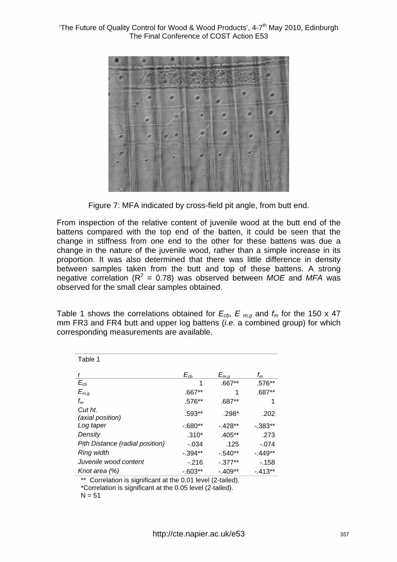
‘The Future of Quality Control for Wood & Wood Products’, 4-7th May 2010, Edinburgh The Final Conference of COST Action E53
Figure 7: MFA indicated by cross-field pit angle, from butt end.
From inspection of the relative content of juvenile wood at the butt end of the battens compared with the top end of the batten, it could be seen that the change in stiffness from one end to the other for these battens was due a change in the nature of the juvenile wood, rather than a simple increase in its proportion. It was also determined that there was little difference in density between samples taken from the butt and top of these battens. A strong negative correlation (R2 = 0.78) was observed between MOE and MFA was observed for the small clear samples obtained. Table 1 shows the correlations obtained for Ecb, E m,g and fm for the 150 x 47 mm FR3 and FR4 butt and upper log battens (i.e. a combined group) for which corresponding measurements are available.
Table 1 r Ecb Em,g fm Ecb 1 .667** .576**Em,g .667** 1 .687**fm .576** .687** 1Cut ht. (axial position) .593** .298* .202
Log taper -.680** -.428** -.383**Density .310* .405** .273Pith Distance (radial position) -.034 .125 -.074Ring width -.394** -.540** -.449**Juvenile wood content -.216 -.377** -.158Knot area (%) -.603** -.409** -.413**** Correlation is significant at the 0.01 level (2-tailed). *Correlation is significant at the 0.05 level (2-tailed). N = 51
http://cte.napier.ac.uk/e53 357

‘The Future of Quality Control for Wood & Wood Products’, 4-7th May 2010, Edinburgh The Final Conference of COST Action E53
From the above table it can be seen that Ecb is more strongly related to Log taper and Cut ht. than Em,g. This is likely to be due to the nature of the test set up whereby for butt log battens the Cook Bolinder effectively measures the stiffness at the lower end near to the ground, whilst the EN 408 determined stiffness using a four point bending arrangement is more biased towards the middle of the batten. The relationship between Ecb and E m,g is quite poor (R2 = 0.44), probably due to the random arrangement of the battens with respect to the position of knots. Inaccuracies within the grader derived stiffness values are likely due to batten distortion and the use of nominal rather than precisely determined batten dimensions. The battens are also bent about different axes. However, it can be seen that Ecb, Em,g and fm all correlate negatively to knot content, albeit very weakly, whilst correlations between Ecb, Em.g and fm are poor for both density and radial position. No correlation between these mechanical properties and either compression wood content or slope of grain, or DBH was observed. No significant relationships between these mechanical properties and log shape variables based on ovality, pith eccentricity or arc (i.e. curvature) were observed. Batten knot content was noted to be related positively to log taper (R2 = 0.46). It appears probable that the axial variation in stiffness observed, and the variation of this effect between individual trees, causes relationships between stiffness and other variables such as batten knot content, juvenile wood content, density, radial position and ring width to be poor – and hence ineffective sorting parameters in an industrial setting where upper and butt log material would likely be mixed.
4 Conclusions This work identified the causal relation between MFA and the relatively low stiffness of butt wood material observed in the Cook Bolinder derived Ecb trends, and is in agreement with recent work by McLean (2007). This feature was, however, noted in some of the earliest Forest Products Research Laboratory studies on British grown Sitka spruce. In particular the relationship between stiffness and Log taper reported in this work indicates that 3D log shape scanners, which are currently used to maximise recovery in terms of quantity by optimising the cutting pattern, also have the potential to be used to sort timber on the basis of quality (i.e. stiffness). Logs containing near butt wood material of lower stiffness could be readily identified, and the battens processed into non-structural sizes. In particular, butt logs with both high levels of taper and knot content should be avoided. The absence of radial variation in both stiffness and strength for the batten size examined means that it is not only the central batten containing pith that should be avoided. Forest practice which involves felling trees close to ground level may risk reducing structural timber quality. The variation in the so-called weak butt effect observed between individual trees and stands warrants further investigation.
http://cte.napier.ac.uk/e53 358

‘The Future of Quality Control for Wood & Wood Products’, 4-7th May 2010, Edinburgh The Final Conference of COST Action E53
Acknowledgments
This work was funded by the Forestry Commission and BRE Trust. The authors are grateful for the assistance provided by Forest Research (UK) and STFI-Packforst.
References Brazier, J. D. (1986) Man’s use of Sitka spruce DoE/BRE/PRL Report PD 175/68 (Limited Circulation, held at BRE Library)
Brazier, J. D. (1991) The influence on growing space on stem size and structural wood out-turn in plantation grown Sitka spruce. BRE Report Contract No. MA1B/0029 9 (Limited Circulation, held at BRE Library)
Evans, R. (1997) Rapid scanning of microfibril angle in increment cores by x-ray diffractometry (in) Microfibril Angle in Wood, The proceedings of the IAWA/IUFRO International Workshop on the Significance of Microbril Angle in Wood. Westport NZ. Nov 1997 pp 116-137. Published by University of Canterbury, Christchurch.
McLean, J. P. (2007) Wood properties of four genotypes of Sitka spruce. PhD thesis. University of Glasgow, Dept of Chemistry.
Ping, Xu and Walker, J.C.F (2004) Stiffness gradients in Radiata pine trees Wood Sci Technol 38 (2004) 1-9.
http://cte.napier.ac.uk/e53 359
‘The Future of Quality Control for Wood & Wood Products’, 4-7th May 2010, Edinburgh The Final Conference of COST Action E53
http://cte.napier.ac.uk/e53
Tensile strain fields around an edge knot in a spruce specimen
J. Oscarsson1, A. Olsson2 & B. Enquist3
Abstract Strain fields around a traversing edge knot in a spruce specimen subjected to tensile loading were measured using a contact-free measuring technique based on digital image correlation. The strain fields were measured by consecutive load tests in which one side of the specimen was studied during each test. The objectives were to examine 1. to what extent the strain fields could be detected, 2. the correlation between strain fields on different sides of the specimen, and 3. the strain distribution around the knot. It was shown that the applied technique is very useful for catching both overall and detailed information about the behaviour of knots in wood members exposed to loading. Both clear wood defects that could not have been detected by visual inspection or scanning and the release of internal stresses were identified. The correlation between strain fields on different sides of the specimen was very good. The correspondence between measurement results and comparative finite element calculations was surprisingly good, considering the fact that the used model was fairly simple.
1 Introduction Present day methods for machine strength grading of structural timber are based on somewhat limited relations between measured characteristics and predicted strength properties. The latter are to a large extent dependent on the occurrence of defects. The degree of importance that different defects have on strength and stiffness has been investigated by e.g. Johansson et al. (1998) and Johansson (2003). It was found that knots were by far the type of defects that had the largest influence on the grading and that the major cause of fracture was the presence of knots. Hence it follows that a thorough understanding of the behaviour of knots and surrounding wood fibres in timber members exposed to loading is of great importance for the development of more accurate grading methods. In this matter, techniques for contact-free strain measurement on timber surfaces could be very useful. One such method, today widely used in for example the vehicle and aviation industries, is based on white-light digital image correlation (DIC). The use of DIC in relation to wood is, however, limited. A review of research carried out up to the year of 2005 was presented by Serrano & Enquist (2005) who investigated strain distribution along wood adhesive bonds using DIC technique. A number of additional papers have been published in recent years (e.g. Young Jeong et al. 2009).
1 PhD Student, [email protected] SP Technical Research Institute of Sweden, Sweden 2 Professor, [email protected] Linnæus University, Sweden 3 Research Engineer, [email protected] Linnæus University, Sweden
360
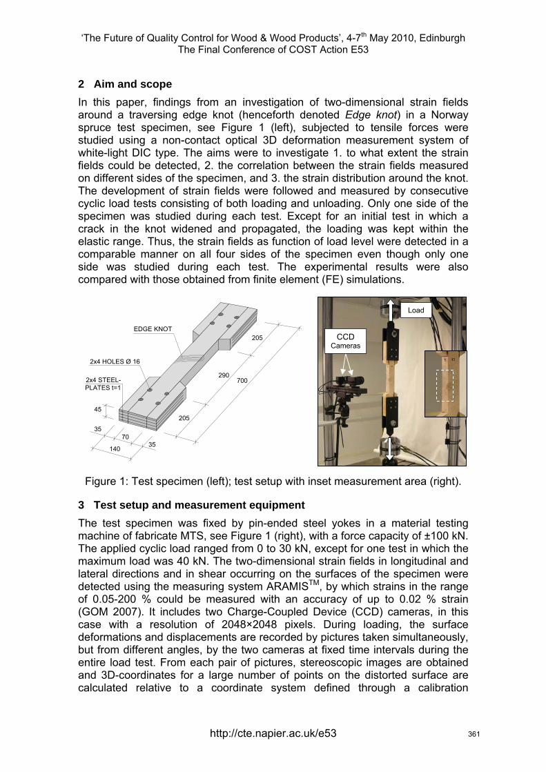
‘The Future of Quality Control for Wood & Wood Products’, 4-7th May 2010, Edinburgh The Final Conference of COST Action E53
http://cte.napier.ac.uk/e53
2 Aim and scope In this paper, findings from an investigation of two-dimensional strain fields around a traversing edge knot (henceforth denoted Edge knot) in a Norway spruce test specimen, see Figure 1 (left), subjected to tensile forces were studied using a non-contact optical 3D deformation measurement system of white-light DIC type. The aims were to investigate 1. to what extent the strain fields could be detected, 2. the correlation between the strain fields measured on different sides of the specimen, and 3. the strain distribution around the knot. The development of strain fields were followed and measured by consecutive cyclic load tests consisting of both loading and unloading. Only one side of the specimen was studied during each test. Except for an initial test in which a crack in the knot widened and propagated, the loading was kept within the elastic range. Thus, the strain fields as function of load level were detected in a comparable manner on all four sides of the specimen even though only one side was studied during each test. The experimental results were also compared with those obtained from finite element (FE) simulations.
Figure 1: Test specimen (left); test setup with inset measurement area (right).
3 Test setup and measurement equipment The test specimen was fixed by pin-ended steel yokes in a material testing machine of fabricate MTS, see Figure 1 (right), with a force capacity of ±100 kN. The applied cyclic load ranged from 0 to 30 kN, except for one test in which the maximum load was 40 kN. The two-dimensional strain fields in longitudinal and lateral directions and in shear occurring on the surfaces of the specimen were detected using the measuring system ARAMISTM, by which strains in the range of 0.05-200 % could be measured with an accuracy of up to 0.02 % strain (GOM 2007). It includes two Charge-Coupled Device (CCD) cameras, in this case with a resolution of 2048×2048 pixels. During loading, the surface deformations and displacements are recorded by pictures taken simultaneously, but from different angles, by the two cameras at fixed time intervals during the entire load test. From each pair of pictures, stereoscopic images are obtained and 3D-coordinates for a large number of points on the distorted surface are calculated relative to a coordinate system defined through a calibration
CCD Cameras
Load
35
45
7035
140
205
205
700290
2x4 HOLES Ø 16
2x4 STEEL-PLATES t=1
EDGE KNOT
361
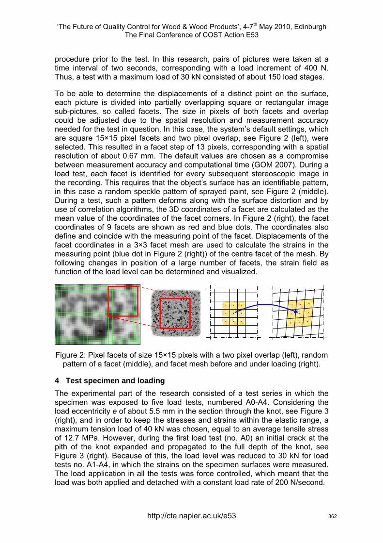
‘The Future of Quality Control for Wood & Wood Products’, 4-7th May 2010, Edinburgh The Final Conference of COST Action E53
http://cte.napier.ac.uk/e53
procedure prior to the test. In this research, pairs of pictures were taken at a time interval of two seconds, corresponding with a load increment of 400 N. Thus, a test with a maximum load of 30 kN consisted of about 150 load stages.
To be able to determine the displacements of a distinct point on the surface, each picture is divided into partially overlapping square or rectangular image sub-pictures, so called facets. The size in pixels of both facets and overlap could be adjusted due to the spatial resolution and measurement accuracy needed for the test in question. In this case, the system’s default settings, which are square 15×15 pixel facets and two pixel overlap, see Figure 2 (left), were selected. This resulted in a facet step of 13 pixels, corresponding with a spatial resolution of about 0.67 mm. The default values are chosen as a compromise between measurement accuracy and computational time (GOM 2007). During a load test, each facet is identified for every subsequent stereoscopic image in the recording. This requires that the object’s surface has an identifiable pattern, in this case a random speckle pattern of sprayed paint, see Figure 2 (middle). During a test, such a pattern deforms along with the surface distortion and by use of correlation algorithms, the 3D coordinates of a facet are calculated as the mean value of the coordinates of the facet corners. In Figure 2 (right), the facet coordinates of 9 facets are shown as red and blue dots. The coordinates also define and coincide with the measuring point of the facet. Displacements of the facet coordinates in a 3×3 facet mesh are used to calculate the strains in the measuring point (blue dot in Figure 2 (right)) of the centre facet of the mesh. By following changes in position of a large number of facets, the strain field as function of the load level can be determined and visualized.
Figure 2: Pixel facets of size 15×15 pixels with a two pixel overlap (left), random pattern of a facet (middle), and facet mesh before and under loading (right).
4 Test specimen and loading The experimental part of the research consisted of a test series in which the specimen was exposed to five load tests, numbered A0-A4. Considering the load eccentricity e of about 5.5 mm in the section through the knot, see Figure 3 (right), and in order to keep the stresses and strains within the elastic range, a maximum tension load of 40 kN was chosen, equal to an average tensile stress of 12.7 MPa. However, during the first load test (no. A0) an initial crack at the pith of the knot expanded and propagated to the full depth of the knot, see Figure 3 (right). Because of this, the load level was reduced to 30 kN for load tests no. A1-A4, in which the strains on the specimen surfaces were measured. The load application in all the tests was force controlled, which meant that the load was both applied and detached with a constant load rate of 200 N/second.
362
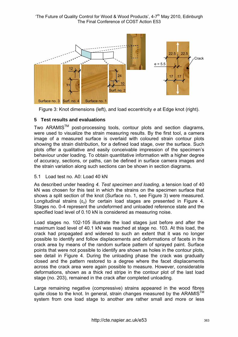
‘The Future of Quality Control for Wood & Wood Products’, 4-7th May 2010, Edinburgh The Final Conference of COST Action E53
http://cte.napier.ac.uk/e53
Figure 3: Knot dimensions (left), and load eccentricity e at Edge knot (right).
5 Test results and evaluations Two ARAMISTM post-processing tools, contour plots and section diagrams, were used to visualize the strain measuring results. By the first tool, a camera image of a measured surface is overlaid with coloured strain contour plots showing the strain distribution, for a defined load stage, over the surface. Such plots offer a qualitative and easily conceivable impression of the specimen’s behaviour under loading. To obtain quantitative information with a higher degree of accuracy, sections, or paths, can be defined in surface camera images and the strain variation along such sections can be shown in section diagrams.
5.1 Load test no. A0: Load 40 kN As described under heading 4. Test specimen and loading, a tension load of 40 kN was chosen for this test in which the strains on the specimen surface that shows a split section of the knot (Surface no. 1, see Figure 3) were measured. Longitudinal strains (εy) for certain load stages are presented in Figure 4. Stages no. 0-4 represent the undeformed and unloaded reference state and the specified load level of 0.10 kN is considered as measuring noise.
Load stages no. 102-105 illustrate the load stages just before and after the maximum load level of 40.1 kN was reached at stage no. 103. At this load, the crack had propagated and widened to such an extent that it was no longer possible to identify and follow displacements and deformations of facets in the crack area by means of the random surface pattern of sprayed paint. Surface points that were not possible to identify are shown as holes in the contour plots, see detail in Figure 4. During the unloading phase the crack was gradually closed and the pattern restored to a degree where the facet displacements across the crack area were again possible to measure. However, considerable deformations, shown as a thick red stripe in the contour plot of the last load stage (no. 203), remained in the crack after completed unloading.
Large remaining negative (compressive) strains appeared in the wood fibres quite close to the knot. In general, strain changes measured by the ARAMISTM system from one load stage to another are rather small and more or less
Surf. no. 4 Surface no. 1
Surf. no. 2
Surface no. 3
31
24
10
12
22.5 22.5
17
e = 5.5 Crack
17
363
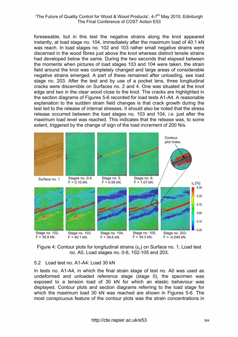
‘The Future of Quality Control for Wood & Wood Products’, 4-7th May 2010, Edinburgh The Final Conference of COST Action E53
http://cte.napier.ac.uk/e53
foreseeable, but in this test the negative strains along the knot appeared instantly, at load stage no. 104, immediately after the maximum load of 40.1 kN was reach. In load stages no. 102 and 103 rather small negative strains were discerned in the wood fibres just above the knot whereas distinct tensile strains had developed below the same. During the two seconds that elapsed between the moments when pictures of load stages 103 and 104 were taken, the strain field around the knot was completely changed and large areas of considerable negative strains emerged. A part of these remained after unloading, see load stage no. 203. After the test and by use of a pocket lens, three longitudinal cracks were discernible on Surfaces no. 2 and 4. One was situated at the knot edge and two in the clear wood close to the knot. The cracks are highlighted in the section diagrams of Figures 5-6 recorded for load tests A1-A4. A reasonable explanation to the sudden strain field changes is that crack growth during the test led to the release of internal stresses. It should also be noted that the stress release occurred between the load stages no. 103 and 104, i.e. just after the maximum load level was reached. This indicates that the release was, to some extent, triggered by the change of sign of the load increment of 200 N/s.
Figure 4: Contour plots for longitudinal strains (εy) on Surface no. 1, Load test no. A0, Load stages no. 0-6, 102-105 and 203.
5.2 Load test no. A1-A4: Load 30 kN In tests no. A1-A4, in which the final strain stage of test no. A0 was used as undeformed and unloaded reference stage (stage 0), the specimen was exposed to a tension load of 30 kN for which an elastic behaviour was displayed. Contour plots and section diagrams referring to the load stage for which the maximum load 30 kN was reached are shown in Figures 5-6. The most conspicuous feature of the contour plots was the strain concentrations in
Surface no. 1 Stages no. 0-4. F = 0.10 kN.
Stage no. 5. F = 0.59 kN.
Stage no. 6. F = 1.07 kN.
Stage no. 203. F = -0.049 kN.
Stage no. 102. F = 39.9 kN.
Stage no. 103. F = 40.1 kN.
Stage no. 104. F = 39.6 kN.
Contour plot holes.
Stage no. 105. F = 39.3 kN.
0.30
0.20
0.10
0.00
– 0.10
– 0.20
εy [%]
364
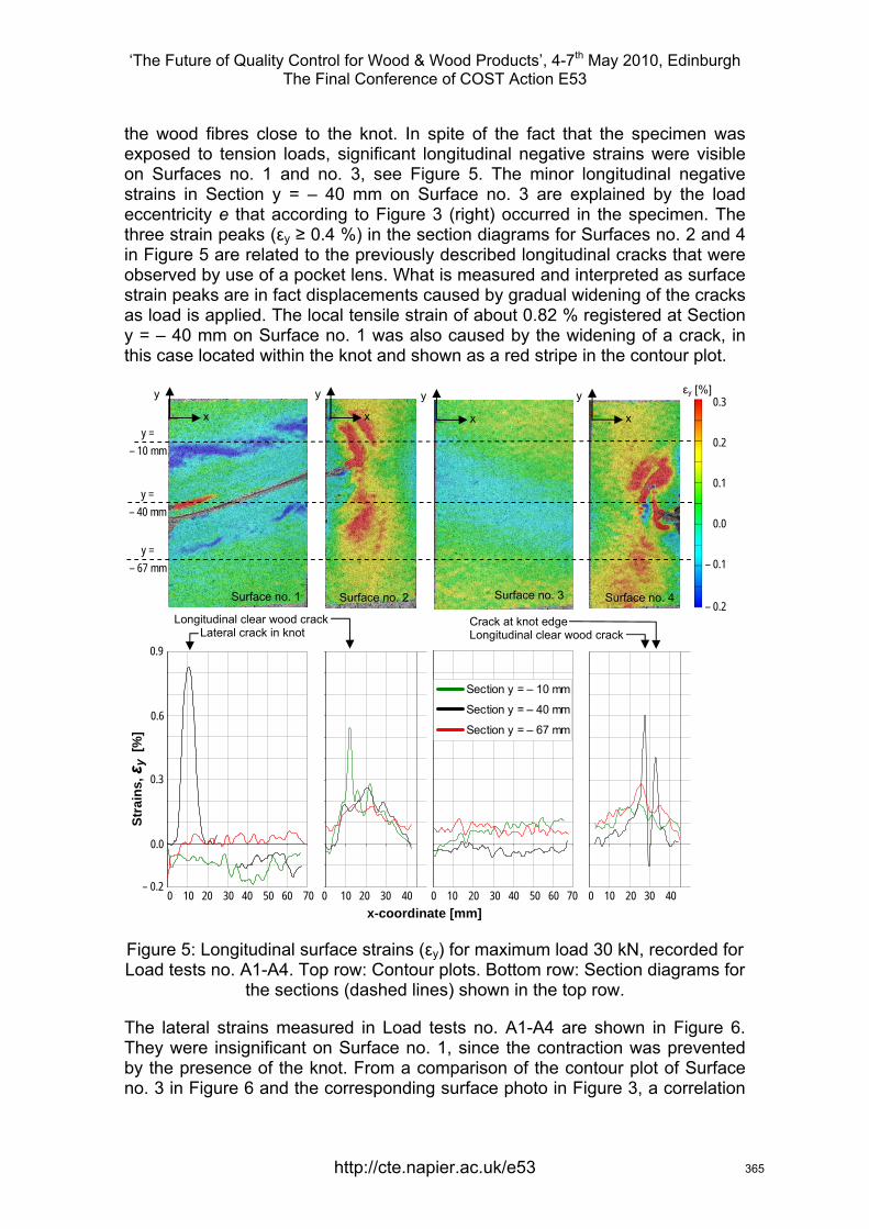
‘The Future of Quality Control for Wood & Wood Products’, 4-7th May 2010, Edinburgh The Final Conference of COST Action E53
http://cte.napier.ac.uk/e53
the wood fibres close to the knot. In spite of the fact that the specimen was exposed to tension loads, significant longitudinal negative strains were visible on Surfaces no. 1 and no. 3, see Figure 5. The minor longitudinal negative strains in Section y = – 40 mm on Surface no. 3 are explained by the load eccentricity e that according to Figure 3 (right) occurred in the specimen. The three strain peaks (εy ≥ 0.4 %) in the section diagrams for Surfaces no. 2 and 4 in Figure 5 are related to the previously described longitudinal cracks that were observed by use of a pocket lens. What is measured and interpreted as surface strain peaks are in fact displacements caused by gradual widening of the cracks as load is applied. The local tensile strain of about 0.82 % registered at Section y = – 40 mm on Surface no. 1 was also caused by the widening of a crack, in this case located within the knot and shown as a red stripe in the contour plot.
Figure 5: Longitudinal surface strains (εy) for maximum load 30 kN, recorded for Load tests no. A1-A4. Top row: Contour plots. Bottom row: Section diagrams for
the sections (dashed lines) shown in the top row.
The lateral strains measured in Load tests no. A1-A4 are shown in Figure 6. They were insignificant on Surface no. 1, since the contraction was prevented by the presence of the knot. From a comparison of the contour plot of Surface no. 3 in Figure 6 and the corresponding surface photo in Figure 3, a correlation
x
y
Surface no. 3
εy [%]
x-coordinate [mm]
– 0.2
0.9
0.6
Surface no. 1 Surface no. 2 Surface no. 4
0.0
y = – 40 mm
y = – 67 mm
0.3
0.2
0.1
0.0
– 0.1
– 0.2
y = – 10 mm
Section y = – 10 mm
Section y = – 40 mm
Section y = – 67 mm
Crack at knot edge Longitudinal clear wood crack
Longitudinal clear wood crack Lateral crack in knot
0 10 20 30 40 50 60 70 0 10 20 30 40 0 10 20 30 40 50 60 70 0 10 20 30 40
Stra
ins,
εy
[%]
0.3
x
y
x
y
x
y
365
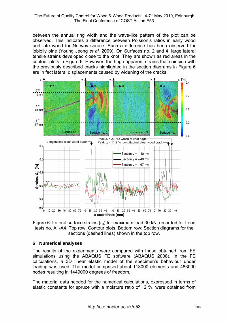
‘The Future of Quality Control for Wood & Wood Products’, 4-7th May 2010, Edinburgh The Final Conference of COST Action E53
http://cte.napier.ac.uk/e53
between the annual ring width and the wave-like pattern of the plot can be observed. This indicates a difference between Poisson’s ratios in early wood and late wood for Norway spruce. Such a difference has been observed for loblolly pine (Young Jeong et al. 2009). On Surfaces no. 2 and 4, large lateral tensile strains developed close to the knot. They are shown as red areas in the contour plots in Figure 6. However, the huge apparent strains that coincide with the previously described cracks highlighted in the section diagrams in Figure 6 are in fact lateral displacements caused by widening of the cracks.
Figure 6: Lateral surface strains (εx) for maximum load 30 kN, recorded for Load tests no. A1-A4. Top row: Contour plots. Bottom row: Section diagrams for the
sections (dashed lines) shown in the top row.
6 Numerical analyses The results of the experiments were compared with those obtained from FE simulations using the ABAQUS FE software (ABAQUS 2008). In the FE calculations, a 3D linear elastic model of the specimen’s behaviour under loading was used. The model comprised about 113000 elements and 483000 nodes resulting in 1449000 degrees of freedom.
The material data needed for the numerical calculations, expressed in terms of elastic constants for spruce with a moisture ratio of 12 %, were obtained from
Surface no. 3
εx [%]
0 10 20 30 40 50 60 70 0 10 20 30 40 0 10 20 30 40 50 60 70 0 10 20 30 40 x-coordinate [mm]
Stra
ins,
εx
[%]
0.9
0.3
0.6
Surface no. 1 Surface no. 2 Surface no. 4
0.0
y = – 40 mm
y = – 67 mm
0.4
0.2
0.0
– 0.2
– 0.4
– 0.3
– 0.5
Peak εx = 2.1 %: Crack at knot edge Peak εx = 11.2 %: Longitudinal clear wood crack
Section y = – 10 mm
Section y = – 40 mm
Section y = – 67 mm
Longitudinal clear wood crack
x
y
x
y
x
y
x
y
y = – 10 mm
366
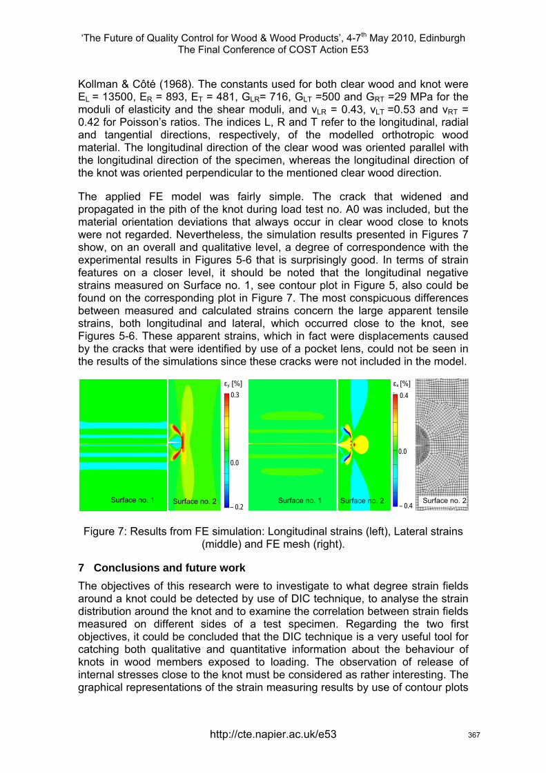
‘The Future of Quality Control for Wood & Wood Products’, 4-7th May 2010, Edinburgh The Final Conference of COST Action E53
http://cte.napier.ac.uk/e53
Kollman & Côté (1968). The constants used for both clear wood and knot were EL
= 13500, ER = 893, ET = 481, GLR= 716, GLT =500 and GRT =29 MPa for the moduli of elasticity and the shear moduli, and νLR = 0.43, νLT
=0.53 and νRT = 0.42 for Poisson’s ratios. The indices L, R and T refer to the longitudinal, radial and tangential directions, respectively, of the modelled orthotropic wood material. The longitudinal direction of the clear wood was oriented parallel with the longitudinal direction of the specimen, whereas the longitudinal direction of the knot was oriented perpendicular to the mentioned clear wood direction.
The applied FE model was fairly simple. The crack that widened and propagated in the pith of the knot during load test no. A0 was included, but the material orientation deviations that always occur in clear wood close to knots were not regarded. Nevertheless, the simulation results presented in Figures 7 show, on an overall and qualitative level, a degree of correspondence with the experimental results in Figures 5-6 that is surprisingly good. In terms of strain features on a closer level, it should be noted that the longitudinal negative strains measured on Surface no. 1, see contour plot in Figure 5, also could be found on the corresponding plot in Figure 7. The most conspicuous differences between measured and calculated strains concern the large apparent tensile strains, both longitudinal and lateral, which occurred close to the knot, see Figures 5-6. These apparent strains, which in fact were displacements caused by the cracks that were identified by use of a pocket lens, could not be seen in the results of the simulations since these cracks were not included in the model.
Figure 7: Results from FE simulation: Longitudinal strains (left), Lateral strains (middle) and FE mesh (right).
7 Conclusions and future work The objectives of this research were to investigate to what degree strain fields around a knot could be detected by use of DIC technique, to analyse the strain distribution around the knot and to examine the correlation between strain fields measured on different sides of a test specimen. Regarding the two first objectives, it could be concluded that the DIC technique is a very useful tool for catching both qualitative and quantitative information about the behaviour of knots in wood members exposed to loading. The observation of release of internal stresses close to the knot must be considered as rather interesting. The graphical representations of the strain measuring results by use of contour plots
Surface no. 2
εy [%] 0.3
– 0.2 Surface no. 1 Surface no. 2 – 0.4
0.4 εx [%]
0.0 0.0
Surface no. 1 Surface no. 2
367
‘The Future of Quality Control for Wood & Wood Products’, 4-7th May 2010, Edinburgh The Final Conference of COST Action E53
http://cte.napier.ac.uk/e53
and section diagrams for all load stages in a load test provide valuable information about the strain distribution and development around knots. It is also possible to detect clear wood defects that are difficult to identify otherwise. For example, the three cracks on Surfaces no. 2 and 4 of the specimen could not have been detected neither by scanning nor visual inspection. It is very likely that the cracks will serve as indications of fracture and in the plans for future work, a fracture test of the specimen is included. In such a test, the progress of fracture will be documented by use of the ARAMISTM system.
With reference to the objective concerning correlation between strain fields on different specimen surfaces, it has been demonstrated that the strain match between adjacent sides is very good, taken into account that only one specimen surface was measured during each load test.
Finally, the correspondence between measurement results and FE simulations are indeed very promising, especially considering the fact that the applied model was rather simple. The DIC technique used in this research will, with a high degree of probability, be of great interest for calibration of finite element models for analyses of fracture mechanical behaviour of knots in wood members. Such models would be of great importance for the development of more accurate strength grading methods based on scanned information concerning the occurrence of knots liable to initiate fractures in wood members.
References ABAQUS Inc (2008) “ABAQUS/CAE Version 6.8, User’s Manuals”.
GOM mbH (2007) “ARAMIS User Manual – Software”. aramis_v6_1st_en_rev-c, 25-Apr-2007.
Johansson, C.-J., Boström, L., Bräuner, L., Hoffmeyer, P., Holmquist, C. & Solli, K. H. (1998) “Laminations for glued laminated timber – Establishment of strength classes for visual strength grades and machine settings for glulam laminations of Nordic origin”. SP Swedish National Testing and Research Institute, SP REPORT 1998:38.
Johansson, C.-J. (2003) “Grading of timber with respect to mechanical properties”. In S. Thelandersson and H. J. Larsen, editors, Timber Engineering, pp 23-43. John Wiley & Sons Ltd, Chichester, England.
Kollman, F.F.P., Côté, W.A. (1968) “Principles of Wood Science and Technology”. Springer Verlag, Berlin Heidelberg, Germany.
Serrano, E. & Enquist, B. (2005) “Contact-free measurement and non-linear finite element analyses of strain distribution along wood adhesive bonds”. Holzforschung, Vol 59, pp 641-646.
Young Jeong, G., Zink-Sharp, A. & Hindman, D. P. (2009) “Tensile properties of earlywood and latewood from Loblolly Pine (Pinus Taeda) using Digital Image Correlation”. Wood and Fibre Science, Vol 41, No 1, pp 51-63.
368
‘The Future of Quality Control for Wood & Wood Products’, 4-7th May 2010, Edinburgh The Final Conference of COST Action E53
http://cte.napier.ac.uk/e53
Modelling behaviour of timber from images analysis
J.L. Coureau1, A. Cointe1 & M. Giton1
Abstract The present study aims at investigating the effect of spatial distributions of defects on the mechanical properties of timber. It proposes to establish formalized method to link mechanics of composite materials (anisotropic solid) to the morpho-structure of timber. Regarding the spatial location of defects, the main objective focuses on analysing the variability of timber. The objectives improve obviously knowledge on the material for construction by proposing approaches dealing with scale effect between clear wood and timber. The investigation requires developing methods linking numerical calculation (finite element computations) and image analysis. A large database (900 full size beams) relative to maritime pine was composed in order to obtain external images of structural components and their corresponding MOE and MOR determined experimentally. It is possible by image analysis to extract parameters characterising the distribution of heterogeneities. The main goal is to locate knots in determining simultaneously the shape and size of each defect and to also qualify the corresponding surrounding material due to the grain orientation variation around defaults. Toolkits are developed to establish maps of knots presence for each side of structural beam and the maps relative to the evolution of the slope of the grain. It is also possible to implement these maps in finite elements software (CAST3M). First results exhibit the possibility, by the association of FE computations and image analysis, to localise zones where failure can occur in structural element.
1 Introduction Wood and Timber are well known terms, which define the material extracted from trees. From a scientist point of view, significant differences between both are mentioned and declined. Wood is classically used for small pieces in which a minimum of defects is included; wood without defect is commonly called “clear wood” (free-defects specimen). Due to the tree growth, this material is anisotropic. The stiffest direction corresponds to the grain orientation (longitudinal direction). This one exhibits the most important strength in comparison with the radial and tangential directions (transverse directions). Timber term is appropriated to material used in construction. It defines a material investigated for a larger scale than wood (higher than 0.01m3). Timber contains singularities of various kinds such as knots, compression wood, slope of the grain, wane and resin pockets. Knots are regarded as very serious defects, which can significantly reduce strength; their effects affect bending or tensile strength by reducing the effective cross-section of beams. They reduce
1 Université Bordeaux I, US2B, {coureau,cointe,giton}@us2b.pierroton.inra.fr
369
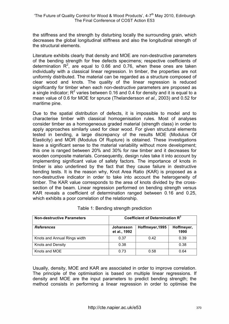
‘The Future of Quality Control for Wood & Wood Products’, 4-7th May 2010, Edinburgh The Final Conference of COST Action E53
http://cte.napier.ac.uk/e53
the stiffness and the strength by disturbing locally the surrounding grain, which decreases the global longitudinal stiffness and also the longitudinal strength of the structural elements.
Literature exhibits clearly that density and MOE are non-destructive parameters of the bending strength for free defects specimens; respective coefficients of determination R2, are equal to 0.66 and 0.76, when these ones are taken individually with a classical linear regression. In timber, the properties are not uniformly distributed. The material can be regarded as a structure composed of clear wood and knots. The quality of the linear regression is reduced significantly for timber when each non-destructive parameters are proposed as a single indicator; R2 varies between 0.16 and 0.4 for density and it is equal to a mean value of 0.6 for MOE for spruce (Thelandersson et al., 2003) and 0.52 for maritime pine.
Due to the spatial distribution of defects, it is impossible to model and to characterise timber with classical homogenisation rules. Most of analyses consider timber as a homogeneous graded material (strength class) in order to apply approaches similarly used for clear wood. For given structural elements tested in bending, a large discrepancy of the results MOE (Modulus Of Elasticity) and MOR (Modulus Of Rupture) is obtained. These investigations leave a significant sense to the material variability without more development; this one is ranged between 20% and 30% for raw timber and it decreases for wooden composite materials. Consequently, design rules take it into account by implementing significant value of safety factors. The importance of knots in timber is also underlined by the fact that they cause failure in destructive bending tests. It is the reason why, Knot Area Ratio (KAR) is proposed as a non-destructive indicator in order to take into account the heterogeneity of timber. The KAR value corresponds to the area of knots divided by the cross-section of the beam. Linear regression performed on bending strength versus KAR reveals a coefficient of determination ranged between 0.16 and 0.25, which exhibits a poor correlation of the relationship.
Table 1: Bending strength prediction
Non-destructive Parameters Coefficient of Determination R2
References Johansson et al., 1992
Hoffmeyer,1995 Hoffmeyer, 1990
Knots and Annual Rings width 0.37 0.42 0.39
Knots and Density 0.38 0.38
Knots and MOE 0.73 0.58 0.64
Usually, density, MOE and KAR are associated in order to improve correlation. The principle of the optimisation is based on multiple linear regressions. If density and MOE are the input parameters to predict bending strength; the method consists in performing a linear regression in order to optimise the
370
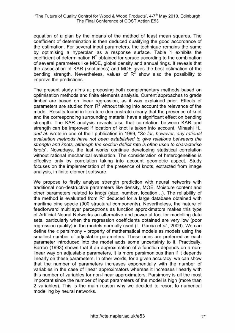
‘The Future of Quality Control for Wood & Wood Products’, 4-7th May 2010, Edinburgh The Final Conference of COST Action E53
http://cte.napier.ac.uk/e53
equation of a plan by the means of the method of least mean squares. The coefficient of determination is then deduced qualifying the good accordance of the estimation. For several input parameters, the technique remains the same by optimising a hyperplan as a response surface. Table 1 exhibits the coefficient of determination R2 obtained for spruce according to the combination of several parameters like MOE, global density and annual rings. It reveals that the association of KAR (knottiness) and MOE gives the best estimation of the bending strength. Nevertheless, values of R2 show also the possibility to improve the predictions.
The present study aims at proposing both complementary methods based on optimisation methods and finite elements analysis. Current approaches to grade timber are based on linear regression, as it was explained prior. Effects of parameters are studied from R2 without taking into account the relevance of the model. Results found in literature demonstrate clearly that the presence of knot and the corresponding surrounding material have a significant effect on bending strength. The KAR analysis reveals also that correlation between KAR and strength can be improved if location of knot is taken into account. Mihashi H., and al. wrote in one of their publication in 1999, “So far, however, any rational evaluation methods have not been established to give relations betweens the strength and knots, although the section deficit rate is often used to characterise knots”. Nowadays, the last works continue developing statistical correlation without rational mechanical evaluation. The consideration of heterogeneities is effective only by correlation taking into account geometric aspect. Study focuses on the implementation of the presence of knots, extracted from image analysis, in finite-element software.
We propose to firstly analyse strength prediction with neural networks with traditional non-destructive parameters like density, MOE, Moisture content and other parameters related to knots (size, number, location…). The reliability of the method is evaluated from R2 deduced for a large database obtained with maritime pine specie (900 structural components). Nevertheless, the nature of feedforward multilayer perceptrons as function approximators makes this type of Artificial Neural Networks an alternative and powerful tool for modelling data sets, particularly when the regression coefficients obtained are very low (poor regression quality) in the models normally used (L. Garcia et al., 2009). We can define the « parsimony » property of mathematical models as models using the smallest number of adjustable parameters. These ones are preferred as each parameter introduced into the model adds some uncertainty to it. Practically, Barron (1993) shows that if an approximation of a function depends on a non-linear way on adjustable parameters, it is more parsimonious than if it depends linearly on these parameters. In other words, for a given accuracy, we can show that the number of parameters increases exponentially with the number of variables in the case of linear approximators whereas it increases linearly with this number of variables for non-linear approximators. Parsimony is all the most important since the number of input parameters of the model is high (more than 2 variables). This is the main reason why we decided to resort to numerical modelling by neural networks.
371
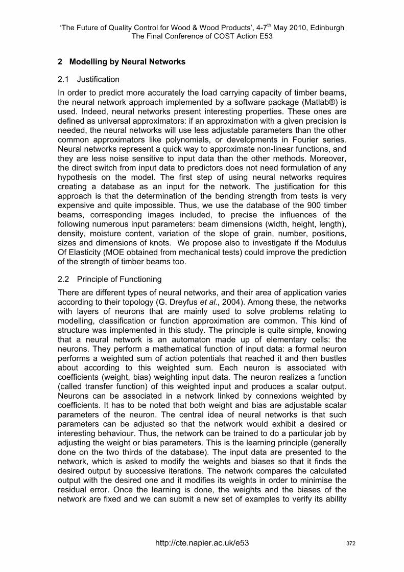
‘The Future of Quality Control for Wood & Wood Products’, 4-7th May 2010, Edinburgh The Final Conference of COST Action E53
http://cte.napier.ac.uk/e53
2 Modelling by Neural Networks
2.1 Justification In order to predict more accurately the load carrying capacity of timber beams, the neural network approach implemented by a software package (Matlab®) is used. Indeed, neural networks present interesting properties. These ones are defined as universal approximators: if an approximation with a given precision is needed, the neural networks will use less adjustable parameters than the other common approximators like polynomials, or developments in Fourier series. Neural networks represent a quick way to approximate non-linear functions, and they are less noise sensitive to input data than the other methods. Moreover, the direct switch from input data to predictors does not need formulation of any hypothesis on the model. The first step of using neural networks requires creating a database as an input for the network. The justification for this approach is that the determination of the bending strength from tests is very expensive and quite impossible. Thus, we use the database of the 900 timber beams, corresponding images included, to precise the influences of the following numerous input parameters: beam dimensions (width, height, length), density, moisture content, variation of the slope of grain, number, positions, sizes and dimensions of knots. We propose also to investigate if the Modulus Of Elasticity (MOE obtained from mechanical tests) could improve the prediction of the strength of timber beams too.
2.2 Principle of Functioning There are different types of neural networks, and their area of application varies according to their topology (G. Dreyfus et al., 2004). Among these, the networks with layers of neurons that are mainly used to solve problems relating to modelling, classification or function approximation are common. This kind of structure was implemented in this study. The principle is quite simple, knowing that a neural network is an automaton made up of elementary cells: the neurons. They perform a mathematical function of input data: a formal neuron performs a weighted sum of action potentials that reached it and then bustles about according to this weighted sum. Each neuron is associated with coefficients (weight, bias) weighting input data. The neuron realizes a function (called transfer function) of this weighted input and produces a scalar output. Neurons can be associated in a network linked by connexions weighted by coefficients. It has to be noted that both weight and bias are adjustable scalar parameters of the neuron. The central idea of neural networks is that such parameters can be adjusted so that the network would exhibit a desired or interesting behaviour. Thus, the network can be trained to do a particular job by adjusting the weight or bias parameters. This is the learning principle (generally done on the two thirds of the database). The input data are presented to the network, which is asked to modify the weights and biases so that it finds the desired output by successive iterations. The network compares the calculated output with the desired one and it modifies its weights in order to minimise the residual error. Once the learning is done, the weights and the biases of the network are fixed and we can submit a new set of examples to verify its ability
372
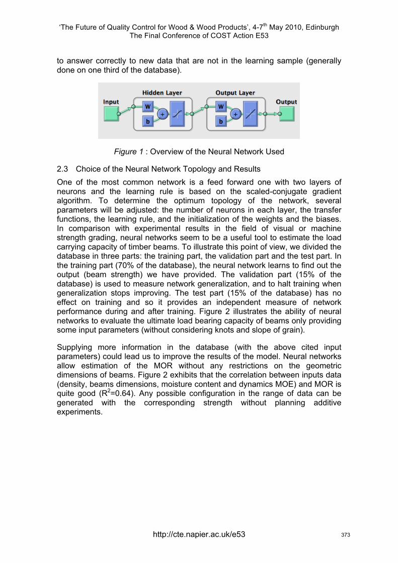
‘The Future of Quality Control for Wood & Wood Products’, 4-7th May 2010, Edinburgh The Final Conference of COST Action E53
http://cte.napier.ac.uk/e53
to answer correctly to new data that are not in the learning sample (generally done on one third of the database).
Figure 1 : Overview of the Neural Network Used
2.3 Choice of the Neural Network Topology and Results One of the most common network is a feed forward one with two layers of neurons and the learning rule is based on the scaled-conjugate gradient algorithm. To determine the optimum topology of the network, several parameters will be adjusted: the number of neurons in each layer, the transfer functions, the learning rule, and the initialization of the weights and the biases. In comparison with experimental results in the field of visual or machine strength grading, neural networks seem to be a useful tool to estimate the load carrying capacity of timber beams. To illustrate this point of view, we divided the database in three parts: the training part, the validation part and the test part. In the training part (70% of the database), the neural network learns to find out the output (beam strength) we have provided. The validation part (15% of the database) is used to measure network generalization, and to halt training when generalization stops improving. The test part (15% of the database) has no effect on training and so it provides an independent measure of network performance during and after training. Figure 2 illustrates the ability of neural networks to evaluate the ultimate load bearing capacity of beams only providing some input parameters (without considering knots and slope of grain).
Supplying more information in the database (with the above cited input parameters) could lead us to improve the results of the model. Neural networks allow estimation of the MOR without any restrictions on the geometric dimensions of beams. Figure 2 exhibits that the correlation between inputs data (density, beams dimensions, moisture content and dynamics MOE) and MOR is quite good (R2=0.64). Any possible configuration in the range of data can be generated with the corresponding strength without planning additive experiments.
373
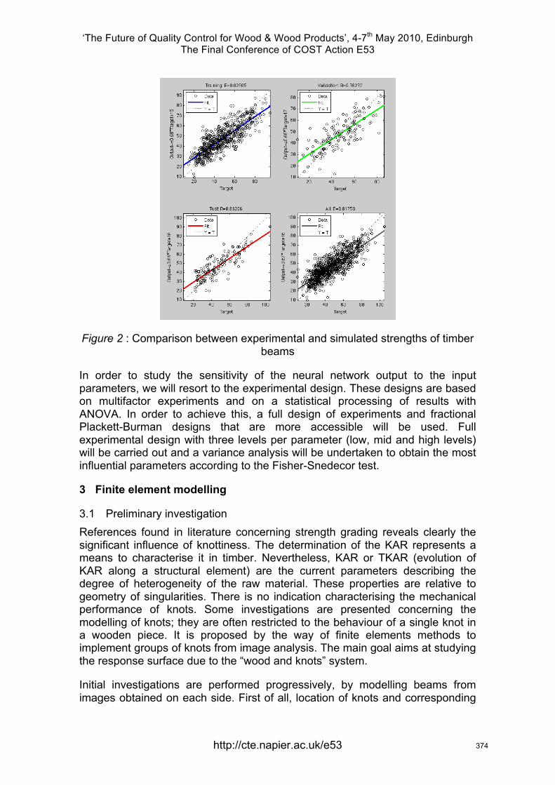
‘The Future of Quality Control for Wood & Wood Products’, 4-7th May 2010, Edinburgh The Final Conference of COST Action E53
http://cte.napier.ac.uk/e53
Figure 2 : Comparison between experimental and simulated strengths of timber beams
In order to study the sensitivity of the neural network output to the input parameters, we will resort to the experimental design. These designs are based on multifactor experiments and on a statistical processing of results with ANOVA. In order to achieve this, a full design of experiments and fractional Plackett-Burman designs that are more accessible will be used. Full experimental design with three levels per parameter (low, mid and high levels) will be carried out and a variance analysis will be undertaken to obtain the most influential parameters according to the Fisher-Snedecor test.
3 Finite element modelling
3.1 Preliminary investigation References found in literature concerning strength grading reveals clearly the significant influence of knottiness. The determination of the KAR represents a means to characterise it in timber. Nevertheless, KAR or TKAR (evolution of KAR along a structural element) are the current parameters describing the degree of heterogeneity of the raw material. These properties are relative to geometry of singularities. There is no indication characterising the mechanical performance of knots. Some investigations are presented concerning the modelling of knots; they are often restricted to the behaviour of a single knot in a wooden piece. It is proposed by the way of finite elements methods to implement groups of knots from image analysis. The main goal aims at studying the response surface due to the “wood and knots” system.
Initial investigations are performed progressively, by modelling beams from images obtained on each side. First of all, location of knots and corresponding
374

‘The Future of Quality Control for Wood & Wood Products’, 4-7th May 2010, Edinburgh The Final Conference of COST Action E53
http://cte.napier.ac.uk/e53
surrounding material is undertaken manually, according to information given by Foley (2003). Each face is divided in multiple regions (close to 100) describing knot location and clear wood presence. The divisions of both sides take into account the relative grain distortion around each knot; for each region average value of the grain slope is declined. According to this manual mapping, implementation in Cast3M FE software is achieved in order to simulate bending test (EN 408) performed on the corresponding beam. The main objective is to evaluate the MOE, the MOR and the location of the failure initiation. Timber is considered in this study as a heterogeneous material composed of knots and oriented clear wood. Corresponding mechanical properties for clear wood are deduced from data given by D. Guitard (1987) for standard softwood. These values can also be updated according to the density and the moisture content. Concerning the mechanical properties of knot, hypothesis of isotropic material is chosen: E= 820 MPa and ν=0.5. Sensitivity test on Young modulus according to a COV equal to 20% reveals that the rigidity of the beams remains quasi unchanged.
The first step of the simulations consisted in comparing simulated MOE given with implemented mechanical properties related to standard softwood (450 kg/m3 and 12% for moisture content). MOE of elements is computed from the deflection obtained by FE analysis, according to four point bending test. A lower modulus is obtained, with a discrepancy equal to 50%. This significant difference is mainly due to the effect of density of the tested specimen, which is equal to 590 kg/m3. In order to improve estimation, correlation between clear wood density and corresponding MOE is implemented according to Guitard. Computation updated reveals that the global MOE (average value of both faces) of timber can be estimated with a precision close to 15%.
Figure 3 : Failure location obtained with FE simulations for both faces
The interest of the FE-simulations is to locate by mapping the high MOE zones and stress concentrations due to the knots presence. Another interesting result is to determine the potential failure zone. It can be established with a classic criterion considering the local stress due to bending moment (σm) and the corresponding tensile strength according to the grain slope fα. The location of failure zone is realised where the ratio σm/fα is maximum for each face. Figure 3 exhibits the good agreement between simulation and experiment. Nevertheless, the failure load prediction is too lower with this kind of criteria. Investigation must be undertaken to define one more accurately.
375
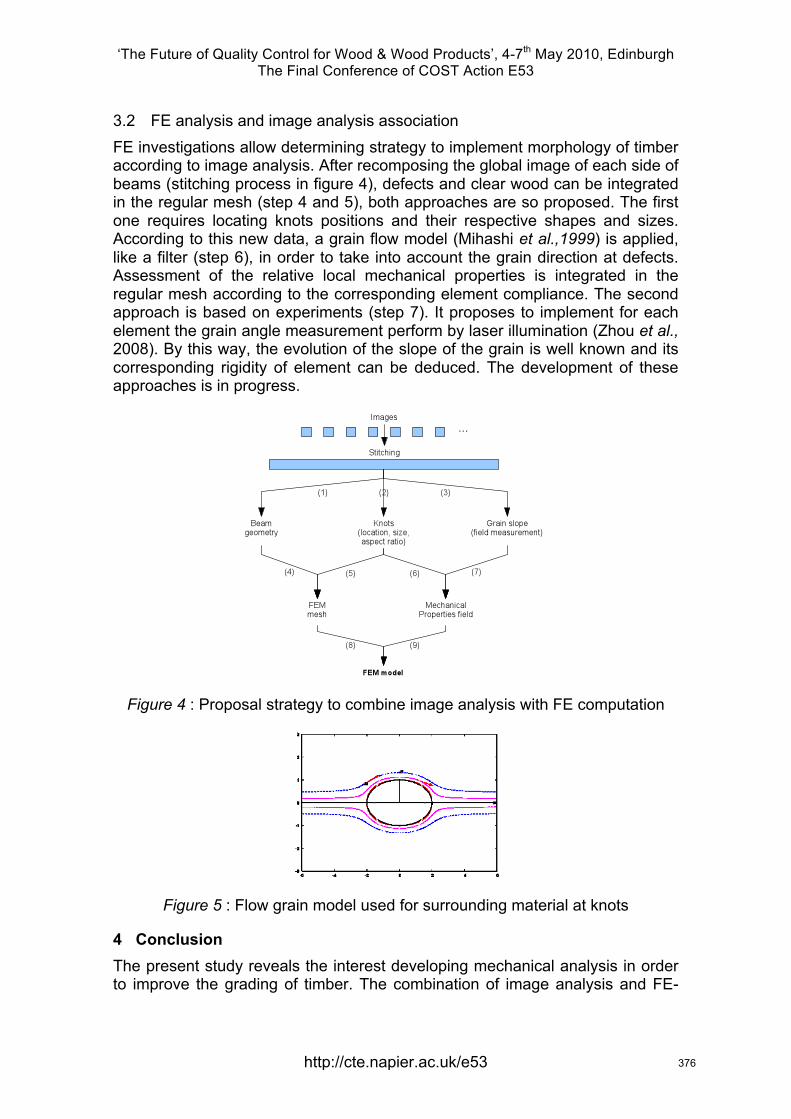
‘The Future of Quality Control for Wood & Wood Products’, 4-7th May 2010, Edinburgh The Final Conference of COST Action E53
http://cte.napier.ac.uk/e53
3.2 FE analysis and image analysis association FE investigations allow determining strategy to implement morphology of timber according to image analysis. After recomposing the global image of each side of beams (stitching process in figure 4), defects and clear wood can be integrated in the regular mesh (step 4 and 5), both approaches are so proposed. The first one requires locating knots positions and their respective shapes and sizes. According to this new data, a grain flow model (Mihashi et al.,1999) is applied, like a filter (step 6), in order to take into account the grain direction at defects. Assessment of the relative local mechanical properties is integrated in the regular mesh according to the corresponding element compliance. The second approach is based on experiments (step 7). It proposes to implement for each element the grain angle measurement perform by laser illumination (Zhou et al., 2008). By this way, the evolution of the slope of the grain is well known and its corresponding rigidity of element can be deduced. The development of these approaches is in progress.
Figure 4 : Proposal strategy to combine image analysis with FE computation
Figure 5 : Flow grain model used for surrounding material at knots
4 Conclusion The present study reveals the interest developing mechanical analysis in order to improve the grading of timber. The combination of image analysis and FE-
376
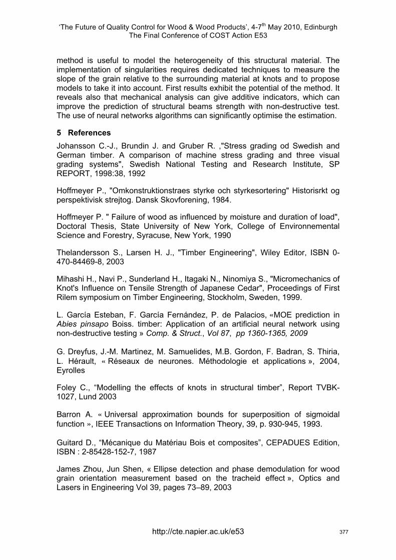
‘The Future of Quality Control for Wood & Wood Products’, 4-7th May 2010, Edinburgh The Final Conference of COST Action E53
http://cte.napier.ac.uk/e53
method is useful to model the heterogeneity of this structural material. The implementation of singularities requires dedicated techniques to measure the slope of the grain relative to the surrounding material at knots and to propose models to take it into account. First results exhibit the potential of the method. It reveals also that mechanical analysis can give additive indicators, which can improve the prediction of structural beams strength with non-destructive test. The use of neural networks algorithms can significantly optimise the estimation.
5 References Johansson C.-J., Brundin J. and Gruber R. ,"Stress grading od Swedish and German timber. A comparison of machine stress grading and three visual grading systems", Swedish National Testing and Research Institute, SP REPORT, 1998:38, 1992
Hoffmeyer P., "Omkonstruktionstraes styrke och styrkesortering" Historisrkt og perspektivisk strejtog. Dansk Skovforening, 1984.
Hoffmeyer P. " Failure of wood as influenced by moisture and duration of load", Doctoral Thesis, State University of New York, College of Environnemental Science and Forestry, Syracuse, New York, 1990
Thelandersson S., Larsen H. J., "Timber Engineering", Wiley Editor, ISBN 0-470-84469-8, 2003
Mihashi H., Navi P., Sunderland H., Itagaki N., Ninomiya S., "Micromechanics of Knot's Influence on Tensile Strength of Japanese Cedar", Proceedings of First Rilem symposium on Timber Engineering, Stockholm, Sweden, 1999.
L. García Esteban, F. García Fernández, P. de Palacios, «MOE prediction in Abies pinsapo Boiss. timber: Application of an artificial neural network using non-destructive testing » Comp. & Struct., Vol 87, pp 1360-1365, 2009 G. Dreyfus, J.-M. Martinez, M. Samuelides, M.B. Gordon, F. Badran, S. Thiria, L. Hérault, « Réseaux de neurones. Méthodologie et applications », 2004, Eyrolles
Foley C., “Modelling the effects of knots in structural timber”, Report TVBK-1027, Lund 2003
Barron A. « Universal approximation bounds for superposition of sigmoidal function », IEEE Transactions on Information Theory, 39, p. 930-945, 1993. Guitard D., “Mécanique du Matériau Bois et composites”, CEPADUES Edition, ISBN : 2-85428-152-7, 1987
James Zhou, Jun Shen, « Ellipse detection and phase demodulation for wood grain orientation measurement based on the tracheid effect », Optics and Lasers in Engineering Vol 39, pages 73–89, 2003
377

‘The Future of Quality Control for Wood & Wood Products’, 4-7th May 2010, Edinburgh The Final Conference of COST Action E53
Thursday 6th May Research focussed day
Parallel session 1B
http://www.cte.napier.ac.uk/e53/ 378
‘The Future of Quality Control for Wood & Wood Products’, 4-7th May 2010, Edinburgh The Final Conference of COST Action E53
Grading characteristics of structural Slovak spruce timber determined by ultrasonic and bending methods
A. Rohanová1, R. Lagaňa2 & J. Dubovský3
Abstract The paper deals with evaluation of characteristics of structural Slovak spruce timber using an ultrasonic and a bending method. A destructive bending method was performed according to EN 408 and evaluated according EN 384. An ultrasonic device, Sylvatest-Duo, with build-in structural timber grading standards was used for measuring wave propagations velocity and gain of energy in wood.
Result analysis showed differences in strength-modulus relations between the methods. Objectives results provided by the bending method give more reliable and real characteristics of MOEstat. Significant correlation between MOEstat and MORstat (r~0,7) was confirmed. Moreover, another strong correlation between MOR and wood density enhance reliability of the ultrasonic method. Strength and dynamic modulus characteristics from the ultrasonic method correspond to characteristic values of spruce timber according to EN 338, which can be consider as a simple and approximate grading method for structural timber. A part of the results can be used for determination of characteristic values of the Slovak spruce timber.
1 Introduction Utilization of wood in constructions has lots of advantages due to natural origin and unique properties. Unfortunately, using wood in building industry must take into account variability of properties used for grading purposes, namely strength, elasticity, and density.
Large dimensions of structural timber is used in wooden construction, therefore, one has to consider more factors related to strength properties of a construction element during utilization. Two methods are used for determination of strength and stiffness properties of wood: visual grading and machine grading. The machine grading is based on bending principle or other principles such as ultrasound, vibration, radiation, or combination of several indicating properties (Weidenhiller & Denzler 2009) related to stiffness or strength.
Determination of construction timber wood quality parameters is based according to EN 408. The most important characteristic are:
1 Research associate, [email protected] Department of Furniture and Wood Products, Technical University in Zvolen, Slovakia 2 Research associate, [email protected] Department of Wood Science, Technical University in Zvolen, Slovakia 3 Professor, [email protected]
http://cte.napier.ac.uk/e53 379
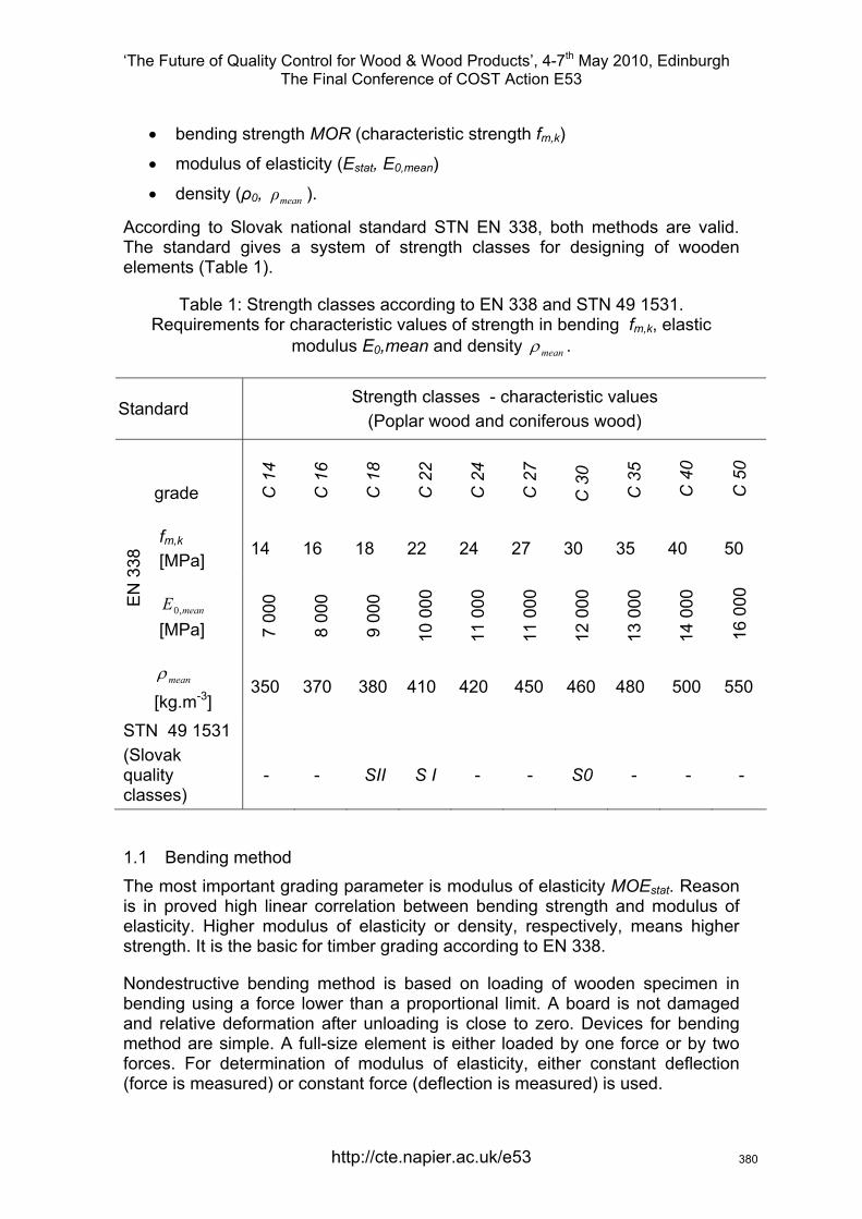
‘The Future of Quality Control for Wood & Wood Products’, 4-7th May 2010, Edinburgh The Final Conference of COST Action E53
• bending strength MOR (characteristic strength fm,k)
• modulus of elasticity (Estat, E0,mean)
• density (ρ0, meanρ ).
According to Slovak national standard STN EN 338, both methods are valid. The standard gives a system of strength classes for designing of wooden elements (Table 1).
Table 1: Strength classes according to EN 338 and STN 49 1531. Requirements for characteristic values of strength in bending fm,k, elastic
modulus E0,mean and density meanρ .
Standard Strength classes - characteristic values
(Poplar wood and coniferous wood)
grade C
14
C 1
6
C 1
8
C 2
2
C 2
4
C 2
7
C 3
0
C 3
5
C 4
0
C 5
0
fm,k 14 16 18 22 24 27 30 35 40 50
EN
338
[MPa]
16 0
00
10 0
00
11 0
00
11 0
00
12 0
00
13 0
00
14 0
00
7 00
0
8 00
0
9 00
0
meanE ,0 [MPa]
meanρ350 370 380 410 420 450 460 480 500 550
[kg.m-3] STN 49 1531
(Slovak quality classes)
- - - - - - - SII S I S0
1.1 Bending method The most important grading parameter is modulus of elasticity MOEstat. Reason is in proved high linear correlation between bending strength and modulus of elasticity. Higher modulus of elasticity or density, respectively, means higher strength. It is the basic for timber grading according to EN 338.
Nondestructive bending method is based on loading of wooden specimen in bending using a force lower than a proportional limit. A board is not damaged and relative deformation after unloading is close to zero. Devices for bending method are simple. A full-size element is either loaded by one force or by two forces. For determination of modulus of elasticity, either constant deflection (force is measured) or constant force (deflection is measured) is used.
http://cte.napier.ac.uk/e53 380
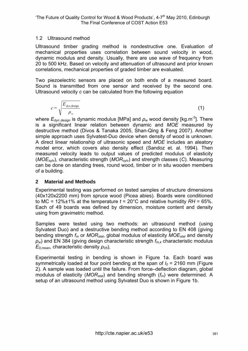
‘The Future of Quality Control for Wood & Wood Products’, 4-7th May 2010, Edinburgh The Final Conference of COST Action E53
1.2 Ultrasound method Ultrasound timber grading method is nondestructive one. Evaluation of mechanical properties uses correlation between sound velocity in wood, dynamic modulus and density. Usually, there are use wave of frequency from 20 to 500 kHz. Based on velocity and attenuation of ultrasound and prior known correlations, mechanical properties of graded timber are evaluated.
Two piezoelectric sensors are placed on both ends of a measured board. Sound is transmitted from one sensor and received by the second one. Ultrasound velocity c can be calculated from the following equation
w
dyn
ρE
=c design, (1)
where Edyn design is dynamic modulus [MPa] and ρw wood density [kg.m-3]. There is a significant linear relation between dynamic and MOE measured by destructive method (Divos & Tanaka 2005, Shan-Qing & Feng 2007). Another simple approach uses Sylvatest-Duo device when density of wood is unknown. A direct linear relationship of ultrasonic speed and MOE includes an aleatory model error, which covers also density effect (Sandoz et. al. 1994). Then measured velocity leads to output values of predicted modulus of elasticity (MOEsylv), characteristic strength (MORsylv) and strength classes (C). Measuring can be done on standing trees, round wood, timber or in situ wooden members of a building.
2 Material and Methods Experimental testing was performed on tested samples of structure dimensions (40x120x2200 mm) from spruce wood (Picea abies). Boards were conditioned to MC = 12%±1% at the temperature t = 20°C and relative humidity RH = 65%. Each of 49 boards was defined by dimension, moisture content and density using from gravimetric method.
Samples were tested using two methods: an ultrasound method (using Sylvatest Duo) and a destructive bending method according to EN 408 (giving bending strength fm or MORstat, global modulus of elasticity MOEstat and density ρw) and EN 384 (giving design characteristic strength fm,k characteristic modulus E0 mean, characteristic density ρ05), ,
Experimental testing in bending is shown in Figure 1a. Each board was symmetrically loaded at four point bending at the span of l0 = 2160 mm (Figure 2). A sample was loaded until the failure. From force–deflection diagram, global modulus of elasticity (MORstat) and bending strength (fm) were determined. A setup of an ultrasound method using Sylvatest Duo is shown in Figure 1b.
http://cte.napier.ac.uk/e53 381
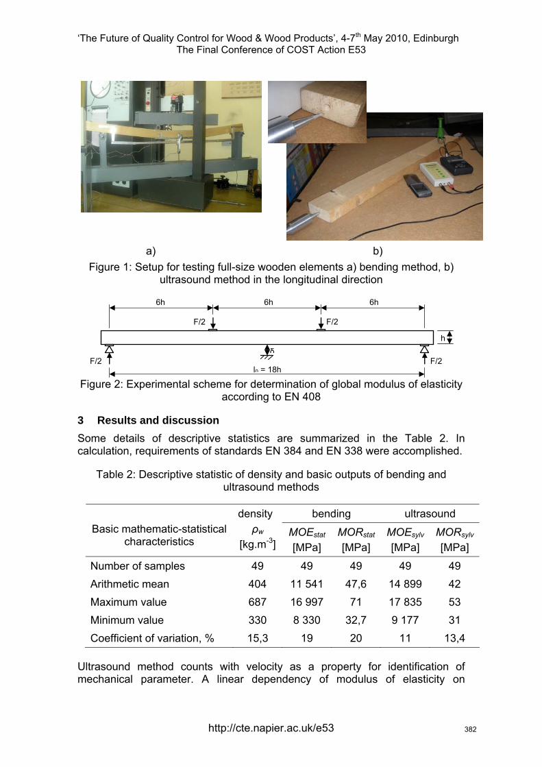
‘The Future of Quality Control for Wood & Wood Products’, 4-7th May 2010, Edinburgh The Final Conference of COST Action E53
a) b) Figure 1: Setup for testing full-size wooden elements a) bending method, b)
ultrasound method in the longitudinal direction
Figure 2: Experimental scheme for determination of global modulus of elasticity
according to EN 408
3 Results and discussion Some details of descriptive statistics are summarized in the Table 2. In calculation, requirements of standards EN 384 and EN 338 were accomplished.
Table 2: Descriptive statistic of density and basic outputs of bending and ultrasound methods
bending ultrasound Basic mathematic-statistical
characteristics
density ρw
[kg.m-3] MOEstat
[MPa] MORstat
[MPa] MOEsylv
[MPa] MORsylv
[MPa]
Number of samples 49 49 49 49 49 Arithmetic mean 404 11 541 47,6 14 899 42 Maximum value 687 16 997 71 17 835 53 Minimum value 330 8 330 32,7 9 177 31 Coefficient of variation, % 15,3 19 20 11 13,4
Ultrasound method counts with velocity as a property for identification of mechanical parameter. A linear dependency of modulus of elasticity on
l0 = 18h
6h 6h 6h
F/2F/2
h δ
F/2 F/2
http://cte.napier.ac.uk/e53 382
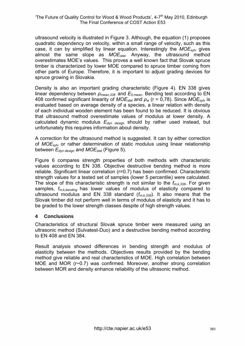
‘The Future of Quality Control for Wood & Wood Products’, 4-7th May 2010, Edinburgh The Final Conference of COST Action E53
ultrasound velocity is illustrated in Figure 3. Although, the equation (1) proposes quadratic dependency on velocity, within a small range of velocity, such as this case, it can by simplified by linear equation. Interestingly the MOEsylv gives almost the same slope as MOEstat. Anyway, the ultrasound method overestimates MOE’s values. This proves a well known fact that Slovak spruce timber is characterized by lower MOE compared to spruce timber coming from other parts of Europe. Therefore, it is important to adjust grading devices for spruce growing in Slovakia.
Density is also an important grading characteristic (Figure 4). EN 338 gives linear dependency between ρmean 338 and E0, ,mean. Bending test according to EN 408 confirmed significant linearity of MOEstat and ρw (r = 0,78). Since MOEsylv is evaluated based on average density of a species, a linear relation with density of each individual wooden element has been found to be reduced. It is obvious that ultrasound method overestimate values of modulus at lower density. A calculated dynamic modulus Edyn design should by rather used instead, but unfortunately this requires information about density.
A correction for the ultrasound method is suggested. It can by either correction of MOEsylv or rather determination of static modulus using linear relationship between Edyn design and MOEstat (Figure 5).
Figure 6 compares strength properties of both methods with characteristic values according to EN 338. Objective destructive bending method is more reliable. Significant linear correlation (r=0.7) has been confirmed. Characteristic strength values for a tested set of samples (lower 5 percentile) were calculated. The slope of this characteristic strength is not similar to the fm,k,338. For given samples, fm,k,bending has lower values of modulus of elasticity compared to ultrasound modulus and EN 338 standard (fm,k,338). It also means that the Slovak timber did not perform well in terms of modulus of elasticity and it has to be graded to the lower strength classes despite of high strength values.
4 Conclusions Characteristics of structural Slovak spruce timber were measured using an ultrasonic method (Sulvatest-Duo) and a destructive bending method according to EN 408 and EN 384.
Result analysis showed differences in bending strength and modulus of elasticity between the methods. Objectives results provided by the bending method give reliable and real characteristics of MOE. High correlation between MOE and MOR (r~0.7) was confirmed. Moreover, another strong correlation between MOR and density enhance reliability of the ultrasonic method.
http://cte.napier.ac.uk/e53 383
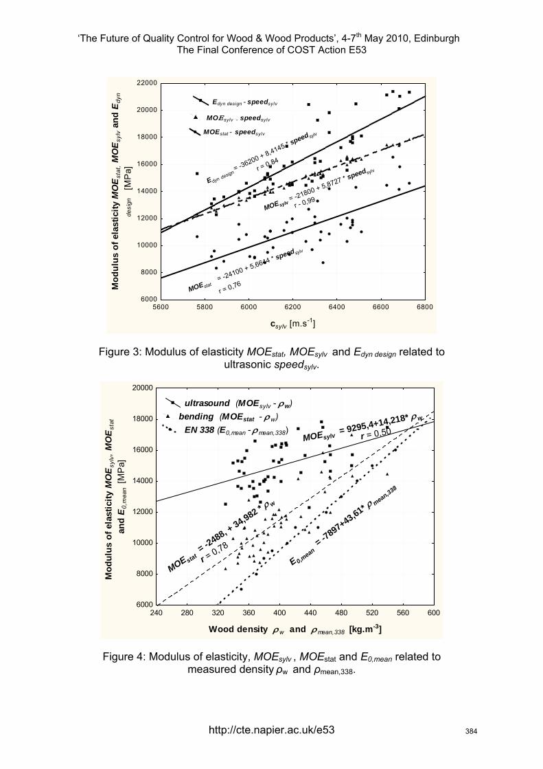
‘The Future of Quality Control for Wood & Wood Products’, 4-7th May 2010, Edinburgh The Final Conference of COST Action E53
5600 5800 6000 6200 6400 6600 6800
csylv [m.s-1]
6000
8000
10000
12000
14000
16000
18000
20000
22000
Mod
ulus
of e
last
icity
MO
E sta
t, M
OE
sylv a
nd E
dyn
desi
gn
[M
Pa]
r = 0,76MOEstat
= -24100 + 5,6644 * speedsylv
MOEsylv = -21800 + 5,8727 * speedsylv
r - 0,99
E dyn design = -36200 + 8,4145 * speed sylv
r = 0,84
Edyn design - speedsylv
MOΕsylv - speedsylv
MOEstat - speedsylv
Figure 3: Modulus of elasticity MOEstat, MOEsylv and Edyn design related to ultrasonic speedsylv.
240 280 320 360 400 440 480 520 560 600
Wood density ρw and ρmean,338 [kg.m-3]
6000
8000
10000
12000
14000
16000
18000
20000
Mod
ulus
of e
last
icity
MO
Esy
lv, M
OE
stat
an
d E 0
,mea
n [M
Pa]
MOE stat = -2488, + 34,982 * ρ
w
MOEsylv = 9295,4+14,218* ρ w
E 0,mean
= -7897+43,61* ρ mean,338
r = 0,78
r = 0,50
ultrasound (MOEsylv - ρw) bending (MOEstat - ρw)
EN 338 (E0,mean - ρmean,338)
Figure 4: Modulus of elasticity, MOEsylv , MOEstat and E0,mean related to measured density ρw and ρmean 338. ,
http://cte.napier.ac.uk/e53 384
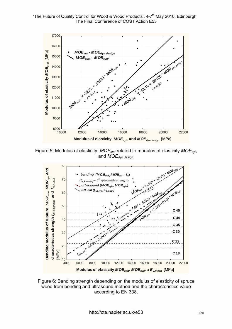
‘The Future of Quality Control for Wood & Wood Products’, 4-7th May 2010, Edinburgh The Final Conference of COST Action E53
10000 12000 14000 16000 18000 20000 22000
Modulus of elasticity MOEsylv and MOEdyn design [MPa]
8000
9000
10000
11000
12000
13000
14000
15000
16000
17000
Mod
ulus
of e
last
icity
MO
Est
at [M
Pa]
r = 0,90
MOE stat
= -78,19 + ,6
9126 * MOE dyn desig
n
MOE stat = -3
220, +
,966
83 * M
OE sylv
r = 0,
74
MOEstat - MOEdyn design MOEstat - MORsylv
Figure 5: Modulus of elasticity MOEstat related to modulus of elasticity MOEsylv and MOEdyn design.
4000 6000 8000 10000 12000 14000 16000 18000 20000 22000
Modulus of elasticity MOEstat, MOEsylv a E0,mean [MPa]
10
20
30
40
50
60
70
80
Bend
ing
mod
ulus
of r
uptu
re Μ
ΟR
stat
, MO
Rsy
lv a
nd
char
acte
ristic
s st
reng
th f m
,k,b
endi
ng a
nd f
m,k
,338
[M
Pa]
ΜΟR stat = 13,039 + ,00303 * M
OE stat
MOR sylv = 17,7694+0,004 * M
OE sylv
f m, k,3
38 = -1
8,53 + 0,00416 * E0,mean
r = 0,70
C 30
C 35
bending (M OΕstat, ΜΟRstat - fm)
(fm,k,bending− 5th -percentile strength) ultrasound (M OEsylv, M ORsylv) EN 338 (fm,k,338, E0,mean)
C 40
C 45
C 22
C 18
f m,k,bending = 1,627 + ,00303 * M
OE stat
Figure 6: Bending strength depending on the modulus of elasticity of spruce wood from bending and ultrasound method and the characteristics value
according to EN 338.
http://cte.napier.ac.uk/e53 385

‘The Future of Quality Control for Wood & Wood Products’, 4-7th May 2010, Edinburgh The Final Conference of COST Action E53
An ultrasound method overestimated MOE values at low density and underestimate bending strength at high density of spruce wood. Measured density could enhance ultrasound method. Results proves a well known fact that in general, Slovak spruce timber is characterized by lower MOE compared to spruce timber coming from other parts of Europe. Therefore, it is important to adjust grading devices for spruce coming from Slovakia. Correction relations of MOE values for Sylvates Duo were proposed.
A part of the results will be used for determination of characteristic values of the Slovak spruce timber.
5 Acknowledgment This study was supported by Slovak Research and Development Agency under the contract No. APVV-0282-06 “Timber quality parameters determining its final utilization” and VEGA 1/0549/08 “Quality of wood for building structures and its experimental analysis and verification in situ”.
6 References Sandoz J.L. (1996) ”Ultrasonic solid wood evaluation in industrial application”. In: Proceedings of the 10th International Symposium on Nondestructive Testing of Wood Proceedings. Lausanne, 26.-28.09.1996, p.135.
Shan-Qing, L., Feng, F. (2007) “Comparative study on three dynamic modulus of elasticity and static modulus of elasticity for Lodgepole pine lumber”. Journal of Forestry Research, 18(4): 309–312.
Požgaj, A.- Chovanec, D. - Kurjatko, S. - Babiak, M. (1997) “Štruktúra a vlastnosti dreva” [Wood structure and properties]. Príroda, a.s., Bratislava, 485 p.
Weidenhiller A., Denzler, J. K. (2009) “Optimising machine strength grading with three indicating properties”. In: Proceedings of the Economic and technical aspects of quality control for wood and wood products. Cost Action E53 Conference 22nd – 23rd October 2009, Lisbon, Portugal. Paper #7.
CEN (2004) “EN 338 Structural timber. Strength classes”.
CEN (2004) “EN 384 Structural timber. Determination of characteristic of mechanical properties and density”.
CEN (2003) “EN 408 Timber structures - Structural timber and glued laminated timber - Determination of some physical and mechanical properties.”
SÚTN (2001) “STN 49 1531 Drevo na stavebné konštrukcie.” [Wood for timber structures].
http://cte.napier.ac.uk/e53 386

‘The Future of Quality Control for Wood & Wood Products’, 4-7th May 2010, Edinburgh The Final Conference of COST Action E53
7 Used symbols
Symbol Unit Description
[m.s-1] velocity of stress wave c [m.s-1] velocity of stress wave given by SYLVATES DUO csylv [kg.m-3] wood density at moisture content “w” ρw
[kg.m-3] average density to EN 338 ρmean [MPa] modulus of elasticity in bending according to EN 408 MOEstat
[MPa] modulus of elasticity in bending given by SYLVATES DUO
MOEsylv
[MPa] dynamic modulus, calculated by the equation
Edyn design
wdyn cE ρ.2=
[MPa] average elasticity modulus parallel to the grain according to EN 338
E0,mean
[MPa] bending strength according to EN 408 MORstat
[MPa] bending strength given by SYLVATEST DUO MORsylv lower 5th percentile of bending strength according to EN 408
[MPa] fm,k ,bending
[MPa] characteristic bending strength according to EN 338 fm 338 ,k ,
http://cte.napier.ac.uk/e53 387
‘The Future of Quality Control for Wood & Wood Products’, 4-7th May 2010, Edinburgh The Final Conference of COST Action E53
Strategies for quality control of strength graded timber
G.J.P.Ravenshorst1 & J.W.G. van de Kuilen2
Abstract The strength properties of timber are based on statistical principles. To determine settings for visual or machine grading a representative sample has to be tested. The settings for the non-destructive measurements in practice are not based on the distributions of the model, but on the non-parametric 5-percentile values of the test pieces. The purpose of the quality control of grading in practice is not clear defined in the relevant parts of EN 14081 (CEN 2005). For machine grading it is stated that for grades with a characteristic value above 30 N/mm2 in every shift 2 beams have to be tested destructively. For visual grading it is stated that the process has to be controlled. It is not stated what has to be done when the control does not comply.
It is shown in this paper that the destructive testing for machine grading for grades with a characteristic value above 30 N/mm2 does not give clarification whether the model or settings used are correct. The only use of control in the grading process is detecting of mistakes by machine or man, which can by controlled by periodic regrading of pieces. Verification of the model and the settings derived from the original sample could be done by regularly updating the test data from the growth area with new samples comprising the whole strength range. However, this seems to be more the responsibility of the strength grading machine manufacturer than the grading machine user, as written in the present standard.
Test samples from one location in a defined growth area for visual grading questions the applicability of the used model for this location. When samples from different locations in the growth area are both visual graded and machine graded, the applicability of the model for visual grading can be evaluated.
1 Introduction The strength properties of timber are based on statistical principles. Strength properties are derived from representative samples. The rules for control in practice are different from those for deriving the initial settings. For machine grading beams assigned to strength classes with a characteristic bending strength higher than 30 N/mm2 a small percentage should be destructively tested on a regularly basis. The characteristic bending strength for the last 100 consecutive destructively tested beams from the production line should meet
1 Lecturer/Researcher, [email protected] Timber Structures and Wood Technology, Delft University of Technology, Netherlands. 2 Professor, [email protected] Holzforschung München, Technical University München, Germany.
http://cte.napier.ac.uk/e53 388
‘The Future of Quality Control for Wood & Wood Products’, 4-7th May 2010, Edinburgh The Final Conference of COST Action E53
the requirements for the strength class. It is not clearly stated what the purpose of this procedure is. There can be two reasons:
1. To verify if the derived settings are correct for the timber graded by the producer.
2. To check whether there has been an error in the data processing in the grading procedure and beams are assigned to the wrong strength class.
Ravenshorst and van de Kuilen (2008) have shown that to address reason 2 it is more effective to regrade beams and evaluate the p-values (a derivation of the model value) then to test them destructively.
Concerning the first reason for performing the quality control it is not stated in EN 14081-3 (CEN 2005) what has to be done when the requirements are not met. Settings are normally derived for a growth area consisting of a number of countries. It is a fact that the timber for some subsamples for some locations can be stronger and for some locations be weaker than predicted by the models. For producers located in the defined growth area but at a location where not was sampled the strength of the timber is assumed to be represented by the original samples. If the requirements are not met, should the manufacturer of the machine adjust the settings for the location of this producer or for the entire growth area? The question arises whether it is possible to verify the strength properties of samples in practice with enough accuracy to conclude the used settings are not correct.
For visual grading the only requirement according to EN 14081-1 (CEN 2005) is that during each shift the grading should be controlled. This means that for every shift the assignment to a visual grade is checked based on the visual characteristics for an undefined number of beams. The relation between strength class and visual grade is given in EN 1912 (CEN 2009). This correctness of this relation is not checked in the control procedure.
In this paper the effects of different control methods are investigated.
2 Material For the analysis in this paper the following subsamples for spruce are used: 2 from Belgium, one from South-Germany and one from Germany/Czech Republic. The growth area is then defined as Belgium, Germany and Czech Republic. It is assumed that the settings are derived for a machine with already accepted settings; then a minimum of 450 test pieces is necessary. As a model parameter for the bending strength the dynamic Modulus of Elasticity is used. The dynamic Modulus of Elasticity is determined by the stress waves method. This is referred to as model 1, ƒmod1. The r-squared value of the regression line is 0,50. All pieces were tested according to EN 408 (CEN 2003) and the characteristic values were determined according to EN 384 (CEN 2004), with the necessary adjustments for size and moisture content. In table 1 the values for the mean and standard deviation for the bending strength for grade are listed. Also the mean and standard deviations for the model values are given. In
http://cte.napier.ac.uk/e53 389
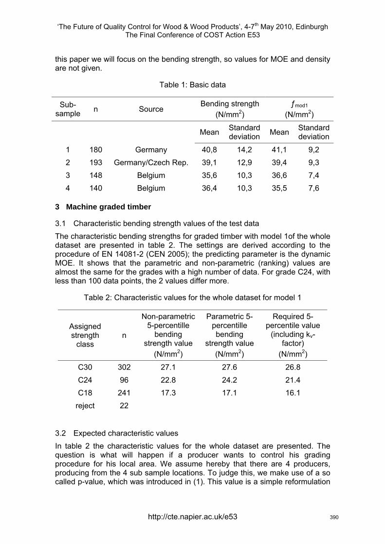
‘The Future of Quality Control for Wood & Wood Products’, 4-7th May 2010, Edinburgh The Final Conference of COST Action E53
this paper we will focus on the bending strength, so values for MOE and density are not given.
Table 1: Basic data
Sub-sample n Source
Bending strength (N/mm2)
ƒmod1
(N/mm2)
Mean Standard deviation Mean Standard
deviation
1 180 Germany 40,8 14,2 41,1 9,2 2 193 Germany/Czech Rep. 39,1 12,9 39,4 9,3 3 148 Belgium 35,6 10,3 36,6 7,4 4 140 Belgium 36,4 10,3 35,5 7,6
3 Machine graded timber
3.1 Characteristic bending strength values of the test data The characteristic bending strengths for graded timber with model 1of the whole dataset are presented in table 2. The settings are derived according to the procedure of EN 14081-2 (CEN 2005); the predicting parameter is the dynamic MOE. It shows that the parametric and non-parametric (ranking) values are almost the same for the grades with a high number of data. For grade C24, with less than 100 data points, the 2 values differ more.
Table 2: Characteristic values for the whole dataset for model 1
Assigned strength
class n
Non-parametric 5-percentille
bending strength value
(N/mm2)
Parametric 5-percentille bending
strength value (N/mm2)
Required 5-percentile value
(including kv-factor)
(N/mm2)
C30 302 27.1 27.6 26.8 C24 96 22.8 24.2 21.4 C18 241 17.3 17.1 16.1
reject 22
3.2 Expected characteristic values In table 2 the characteristic values for the whole dataset are presented. The question is what will happen if a producer wants to control his grading procedure for his local area. We assume hereby that there are 4 producers, producing from the 4 sub sample locations. To judge this, we make use of a so called p-value, which was introduced in (1). This value is a simple reformulation
http://cte.napier.ac.uk/e53 390
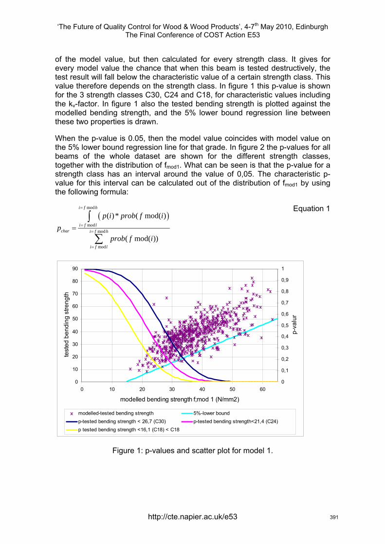
‘The Future of Quality Control for Wood & Wood Products’, 4-7th May 2010, Edinburgh The Final Conference of COST Action E53
of the model value, but then calculated for every strength class. It gives for every model value the chance that when this beam is tested destructively, the test result will fall below the characteristic value of a certain strength class. This value therefore depends on the strength class. In figure 1 this p-value is shown for the 3 strength classes C30, C24 and C18, for characteristic values including the kv-factor. In figure 1 also the tested bending strength is plotted against the modelled bending strength, and the 5% lower bound regression line between these two properties is drawn.
When the p-value is 0.05, then the model value coincides with model value on the 5% lower bound regression line for that grade. In figure 2 the p-values for all beams of the whole dataset are shown for the different strength classes, together with the distribution of fmod1. What can be seen is that the p-value for a strength class has an interval around the value of 0,05. The characteristic p-value for this interval can be calculated out of the distribution of fmod1 by using the following formula:
( )mod
modmod
mod
( )* ( mod( )
( mod( ))
i f h
i f lchar i f h
i f l
p i prob f ip
prob f i
=
==
=
=∫
∑
Equation 1
0
10
20
30
40
50
60
70
80
90
0 10 20 30 40 50 60
modelled bending strength f;mod 1 (N/mm2)
test
ed b
endi
ng s
treng
th
0
0,1
0,2
0,3
0,4
0,5
0,6
0,7
0,8
0,9
1
p-va
lur
modelled-tested bending strength 5%-lower boundp-tested bending strength < 26,7 (C30) p-tested bending strength<21,4 (C24)p tested bending strength <16,1 (C18) < C18
Figure 1: p-values and scatter plot for model 1.
http://cte.napier.ac.uk/e53 391
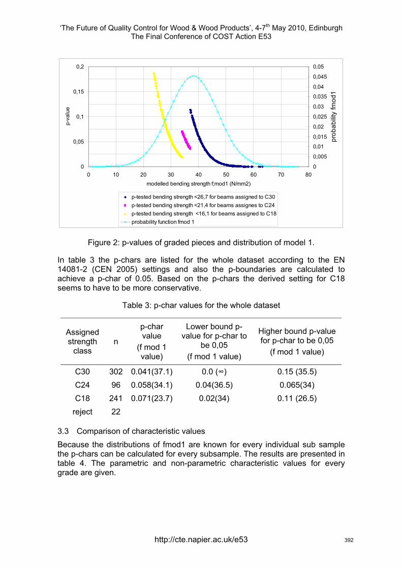
‘The Future of Quality Control for Wood & Wood Products’, 4-7th May 2010, Edinburgh The Final Conference of COST Action E53
0
0,05
0,1
0,15
0,2
0 10 20 30 40 50 60 70 80modelled bending strength f;mod1 (N/mm2)
p-va
lue
0
0,005
0,01
0,015
0,02
0,025
0,03
0,035
0,04
0,045
0,05
prob
abilit
y fm
od1
p-tested bending strength <26,7 for beams assigned to C30p-tested bending strength <21,4 for beams assignes to C24p-tested bending strength <16,1 for beams assigned to C18probability function fmod 1
Figure 2: p-values of graded pieces and distribution of model 1.
In table 3 the p-chars are listed for the whole dataset according to the EN 14081-2 (CEN 2005) settings and also the p-boundaries are calculated to achieve a p-char of 0.05. Based on the p-chars the derived setting for C18 seems to have to be more conservative.
Table 3: p-char values for the whole dataset
Assigned strength
class n
p-char value
(f mod 1 value)
Lower bound p-value for p-char to
be 0,05 (f mod 1 value)
Higher bound p-value for p-char to be 0,05
(f mod 1 value)
C30 302 0.041(37.1) 0.0 (∞) 0.15 (35.5) C24 96 0.058(34.1) 0.04(36.5) 0.065(34) C18 241 0.071(23.7) 0.02(34) 0.11 (26.5)
reject 22
3.3 Comparison of characteristic values Because the distributions of fmod1 are known for every individual sub sample the p-chars can be calculated for every subsample. The results are presented in table 4. The parametric and non-parametric characteristic values for every grade are given.
http://cte.napier.ac.uk/e53 392
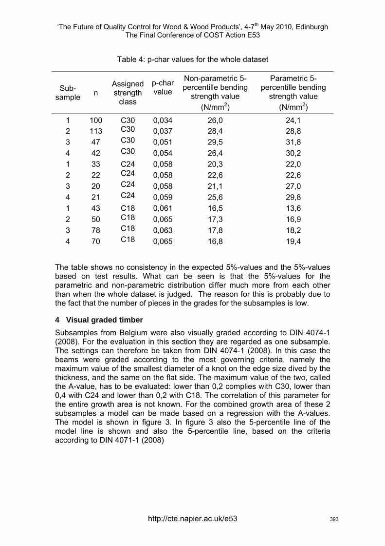
‘The Future of Quality Control for Wood & Wood Products’, 4-7th May 2010, Edinburgh The Final Conference of COST Action E53
Table 4: p-char values for the whole dataset
Sub-sample n
Assigned strength
class
p-char value
Non-parametric 5-percentille bending
strength value (N/mm2)
Parametric 5-percentille bending
strength value (N/mm2)
1 100 C30 0,034 26,0 24,1 2 113 C30 0,037 28,4 28,8 3 47 C30 0,051 29,5 31,8 4 42 C30 0,054 26,4 30,2 1 33 C24 0,058 20,3 22,0 2 22 C24 0,058 22,6 22,6 3 20 C24 0,058 21,1 27,0 4 21 C24 0,059 25,6 29,8 1 43 C18 0,061 16,5 13,6 2 50 C18 0,065 17,3 16,9 3 78 C18 0,063 17,8 18,2 4 70 C18 0,065 16,8 19,4
The table shows no consistency in the expected 5%-values and the 5%-values based on test results. What can be seen is that the 5%-values for the parametric and non-parametric distribution differ much more from each other than when the whole dataset is judged. The reason for this is probably due to the fact that the number of pieces in the grades for the subsamples is low.
4 Visual graded timber Subsamples from Belgium were also visually graded according to DIN 4074-1 (2008). For the evaluation in this section they are regarded as one subsample. The settings can therefore be taken from DIN 4074-1 (2008). In this case the beams were graded according to the most governing criteria, namely the maximum value of the smallest diameter of a knot on the edge size dived by the thickness, and the same on the flat side. The maximum value of the two, called the A-value, has to be evaluated: lower than 0,2 complies with C30, lower than 0,4 with C24 and lower than 0,2 with C18. The correlation of this parameter for the entire growth area is not known. For the combined growth area of these 2 subsamples a model can be made based on a regression with the A-values. The model is shown in figure 3. In figure 3 also the 5-percentile line of the model line is shown and also the 5-percentile line, based on the criteria according to DIN 4071-1 (2008)
http://cte.napier.ac.uk/e53 393
‘The Future of Quality Control for Wood & Wood Products’, 4-7th May 2010, Edinburgh The Final Conference of COST Action E53
y = x + 0,001R2 = 0,262
0
10
20
30
40
50
60
70
0 10 20 30 40 50 6modelled bending strength f;mod 2 (N/mm2)
test
ed b
endi
ng s
treng
th (N
/mm
2
0
)
modelled (max A) - tested bedning strength 5-percentile lower bound of fmod2 (max A)5-percentile lower bound according to DIN 4071-4 Linear (modelled (max A) - tested bedning strength)Linear (5-percentile lower bound of fmod2 (max A))
Figure 3: p-values of graded pieces and distribution of model 1.
For visual grading the required characteristic bending strengths for beams graded in strengths classes until C30 are higher than for machine grading. This is due to the kv – factor of 1,12 that may be used in machine grading to reduce the required settings. This factor brings into account the difference in accuracy of the grading procedure in practice. In table 5 the 5%-values are listed according to the grading by DIN 4074-1(2008).
Table 5: Characteristic values for the whole dataset for model 2
Non-parametric 5-percentille
bending strength value
Parametric 5-percentille
bending strength value
Assigned strength class n
(N/mm2) (N/mm2)
Required 5-percentile
value (no kv-factor)
C30 71 27,8 28 30 C24 163 21,2 20,2 24 C18 46 15,1 15,3 18
reject 8
The required 5% values are not met. Figure 4 gives the p-values for model 2 for the graded beams. The required p-values to reach a value for p-char for every grade are represented by the dotted horizontal lines. Interesting is then that the upper boundary for C30 is only met by 12 beams. Looking at the distribution of fmod2 it is in practice not possible to grade beams in C30 based on this model, although it is allowed according to the defined growth area in EN 1912 (2009) for grading from DIN 4074-1 (2008). Because the values differ that much from the DIN settings, it is questionable if these are representative for the Belgium
http://cte.napier.ac.uk/e53 394
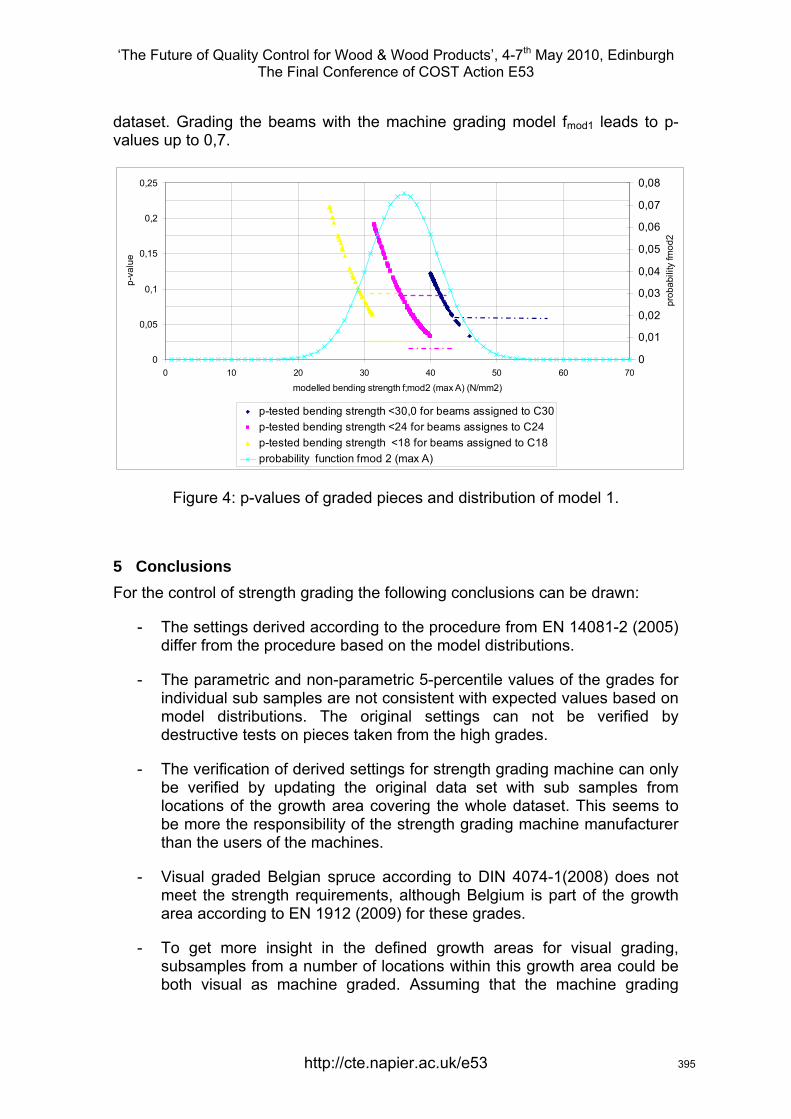
‘The Future of Quality Control for Wood & Wood Products’, 4-7th May 2010, Edinburgh The Final Conference of COST Action E53
dataset. Grading the beams with the machine grading model fmod1 leads to p-values up to 0,7.
0
0,05
0,1
0,15
0,2
0,25
0 10 20 30 40 50 60 70
modelled bending strength f;mod2 (max A) (N/mm2)
p-va
lue
0
0,01
0,02
0,03
0,04
0,05
0,06
0,07
0,08
prob
abili
ty fm
od2
p-tested bending strength <30,0 for beams assigned to C30p-tested bending strength <24 for beams assignes to C24p-tested bending strength <18 for beams assigned to C18probability function fmod 2 (max A)
Figure 4: p-values of graded pieces and distribution of model 1.
5 Conclusions For the control of strength grading the following conclusions can be drawn:
- The settings derived according to the procedure from EN 14081-2 (2005) differ from the procedure based on the model distributions.
- The parametric and non-parametric 5-percentile values of the grades for individual sub samples are not consistent with expected values based on model distributions. The original settings can not be verified by destructive tests on pieces taken from the high grades.
- The verification of derived settings for strength grading machine can only be verified by updating the original data set with sub samples from locations of the growth area covering the whole dataset. This seems to be more the responsibility of the strength grading machine manufacturer than the users of the machines.
- Visual graded Belgian spruce according to DIN 4074-1(2008) does not meet the strength requirements, although Belgium is part of the growth area according to EN 1912 (2009) for these grades.
- To get more insight in the defined growth areas for visual grading, subsamples from a number of locations within this growth area could be both visual as machine graded. Assuming that the machine grading
http://cte.napier.ac.uk/e53 395

‘The Future of Quality Control for Wood & Wood Products’, 4-7th May 2010, Edinburgh The Final Conference of COST Action E53
model is more correct, the correctness of the visual grading models can be evaluated.
- To verify the correctness of the grading process in a company regrading by a controller can be an effective method.
References CEN (2005) “EN 14081-1 Timber structures – Strength Graded Structural Timber with Rectangular Cross Section – Part 1: General Requirements”, European Committee for Standardization.
CEN (2005) “EN 14081-2 Timber structures – Strength Graded Structural Timber with Rectangular Cross Section – Part 2: Machine grading- additional requirements for initial type testing”, European Committee for Standardization.
CEN (2005) “EN 14081-3 Timber structures – Strength Graded Structural Timber with Rectangular Cross Section – Part 3: Machine grading- additional requirements for factory production control”, European Committee for Standardization.
CEN (2009) “EN 1912 Structural Timber – Assignment of visual grades and species”, European Committee for Standardization.
CEN (2003) “EN 408 Timber structures – Structural Timber and Glues Laminated Timber- Determination of some physical and mechanical properties”, European Committee for Standardization
CEN (2004) “EN 384 Structural Timber – Determination of characteristic values of mechanical properties and density”, European Committee for Standardization
DIN (2008) “DIN 4074-1 Strength grading of wood – Part1 : Coniferous sawn timber”, Deutches Institut für Normung.
Ravenshorst, G.J.P. & van de Kuilen, J.W.G. (2008)”A method for quality control of strength grading machines using non-destructive measurements”. Cost Action E53 Conference 29th-30th October 2008 Delft.
http://cte.napier.ac.uk/e53 396
‘The Future of Quality Control for Wood & Wood Products’, 4-7th May 2010, Edinburgh The Final Conference of COST Action E53
Machine strength grading – prediction limits – evaluation of a new method for derivation of settings
R. Ziethén1 & C. Bengtsson2
Abstract This paper presents and analyses a new method for derivation of setting values for strength grading machines. The method uses a model for the relationship between indicating property (measured by a grading machine, IP) and the grade determining property (GDP). This model is of course not perfect and by summarising the errors in the model a confidence interval for the model can be calculated. The confidence interval is used for creating a prediction interval. The lower limit of the prediction interval, the prediction limit, is used to predict the GDP. The prediction limit method is analysed and evaluated by well defined input data. It is shown that fewer experimental data than required by the method in EN 14081-2 today is needed to determine reliable settings but the producer is awarded with less conservative settings with an increased number of experimental data. A weak correlation between IP and GDP or a high coefficient of variation also results in conservative settings. The settings are not dependent on average strength of the raw material used for deriving the settings.
1 Introduction The results presented in this paper come from the European research project “GRADEWOOD”. The main objective of the GRADEWOOD project is to enhance the use and to improve the reliability of wood as a structural material. One of the tasks in the project is to evaluate the European standard EN 14081 part 1 to 4 and to suggest possible improvements of the standard. The Standard EN 14081 consists of four parts:
14081-1 General requirements for machine strength grading 14081-2 Derivation and supervision of settings using the machine control method 14081-3 Derivation and supervision of settings using the output control method 14081-4 Approved settings for existing grading machines This paper describes an alternative to the procedure described in EN 14081 part 2, the so called “Cost matrix method”, Rouger 1997.
2 Background
2.1 Complexity
The method described in EN 14081-2 is complicated and it is also an issue of several interpretations of the text written. Because of this a special task group TG1 was established to interpret the standard and to assess reports with settings for strength grading machines based on these interpretations. An effect of this is an ongoing change of requested information and provisions for sampling and calculations. Today it
1 Researcher, Email: [email protected] Trätek, Box 857, SE-501 15 Borås, Sweden 2 Head of section. Email: [email protected] Trätek, Box 857, SE-501 15 Borås, Sweden, School of Engineering, Linnaeus University, SE-351 95 Växjö, Sweden
http://cte.napier.ac.uk/e53 397

‘The Future of Quality Control for Wood & Wood Products’, 4-7th May 2010, Edinburgh The Final Conference of COST Action E53
is not possible for anyone to have settings approved based on a report in accordance with the valid standard.
The determination of settings is based on the 5th-percentile for each grade in each grade combination. A result of this is several settings for each grade. Examples exist where one grade for one species from one geographic area has eight different settings, dependent on grade combination and the combination of countries covered. This leads to confusion. It is difficult to explain for producers and users of graded timber that different settings can be used depending on if the strongest material is included or if it is graded to higher grade.
The optimum grading in the standard is based on destructive bending or tension tests according to the European standards EN 384 and EN 408 and it serves as a “key” for the cost matrix analysis which is central for the determination of settings. The optimum grading is defined to be “the highest grade, of those for which settings are required, to which a piece of timber can be assigned, such that the grade determining properties of the graded sample will meet the values required for the grade”. This definition is unambiguous only if one grade and rejects are graded. When a combination of grades is graded a higher number of pieces in the highest class also results in a higher number of rejects. So far the optimum grading has been interpreted to be optimized from the highest grade and a higher number of rejects have been accepted although the yield from this grading has not been in line with the demands from the end-users. This interpretation can have a significant effect on the results from the cost-matrix analysis and thus a major effect on the determined settings.
2.2 Sensitivity
The standard requires a minimum sample of 900 pieces sampled in at least 8 sub-samples. For additional grades, origins or species the requirement is 450 pieces from at least 4 sub-samples. Although this high number of required test pieces the results are sensitive to small variations in properties of a few of the test pieces.
The minimum allowed setting for any class is based on a requirement of 0.5% or 5 pieces rejected from the samples used. For the most common commercial grades, C16, C18 and C24, this is generally the used requirement. For these grades more than 99% of the tested material is not at all used for the determination of the settings. For the lower tail of the distribution the measured values and also the relation between the machine value and the grade determining property is unstable. An element of random has a not negligible effect on settings determined by this requirement.
Also for other grades the settings are highly depending on a few observations. One example (based on real data) shows that a change of density of 2 to 4 kg/m³ for 7 out of 700 pieces in a sample can change the settings more than 5% and change the yield when grading with almost 10%. The economic effect of this change is large and can be the difference on the market between a competitive and a useless grading machine.
3 Theory
3.1 Linear regression
The examples above show some severe shortcomings of the present standard. An alternative to the method described in the standard is needed, Ziethén, R, Bengtsson C., 2009. A method that uses more of the information given by the tests, one
http://cte.napier.ac.uk/e53 398
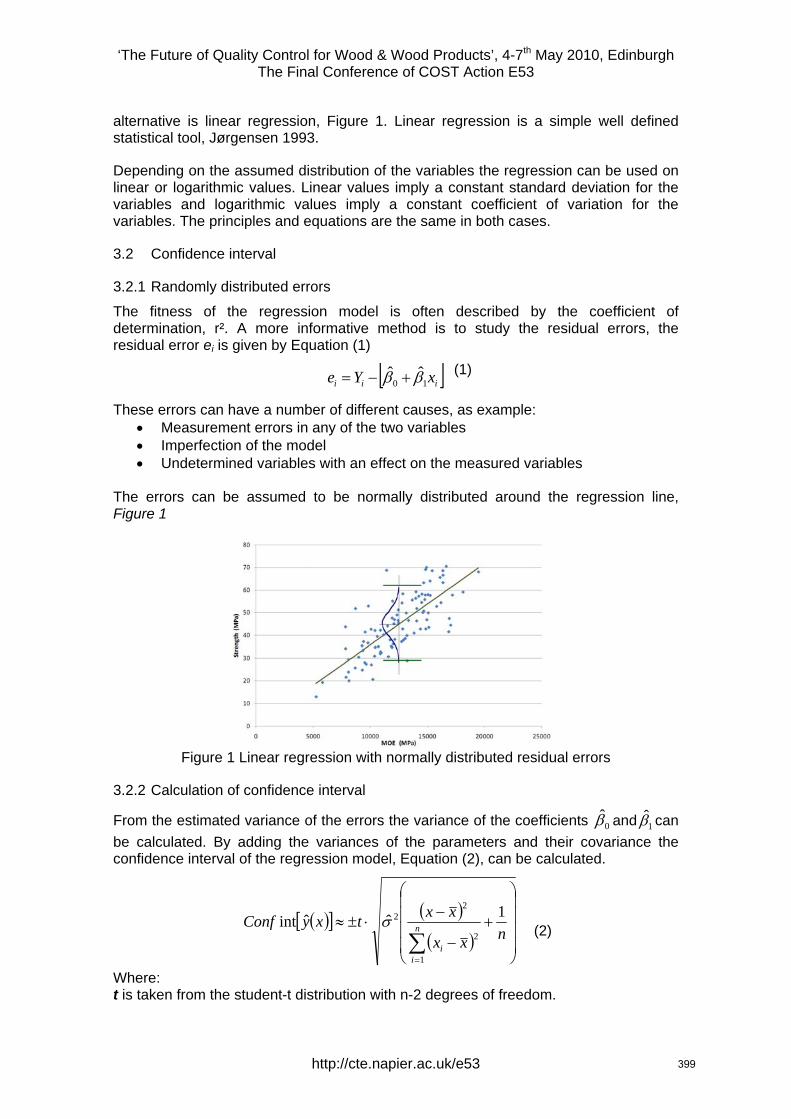
‘The Future of Quality Control for Wood & Wood Products’, 4-7th May 2010, Edinburgh The Final Conference of COST Action E53
alternative is linear regression, Figure 1. Linear regression is a simple well defined statistical tool, Jørgensen 1993.
Depending on the assumed distribution of the variables the regression can be used on linear or logarithmic values. Linear values imply a constant standard deviation for the variables and logarithmic values imply a constant coefficient of variation for the variables. The principles and equations are the same in both cases.
3.2 Confidence interval
3.2.1 Randomly distributed errors
The fitness of the regression model is often described by the coefficient of determination, r². A more informative method is to study the residual errors, the residual error ei is given by Equation (1)
[ ]iii xYe 10ˆˆ ββ +−= (1)
These errors can have a number of different causes, as example: • Measurement errors in any of the two variables • Imperfection of the model • Undetermined variables with an effect on the measured variables
The errors can be assumed to be normally distributed around the regression line, Figure 1
Figure 1 Linear regression with normally distributed residual errors
3.2.2 Calculation of confidence interval
From the estimated variance of the errors the variance of the coefficients and can be calculated. By adding the variances of the parameters and their covariance the confidence interval of the regression model, Equation (2), can be calculated.
0β̂ 1̂β
( )[ ] ( )( ) ⎟
⎟⎟⎟
⎠
⎞
⎜⎜⎜⎜
⎝
⎛
+−
−⋅±≈
∑=
nxx
xxtxyConf n
ii
1ˆˆint
1
2
22σ
(2)
Where: t is taken from the student-t distribution with n-2 degrees of freedom.
http://cte.napier.ac.uk/e53 399
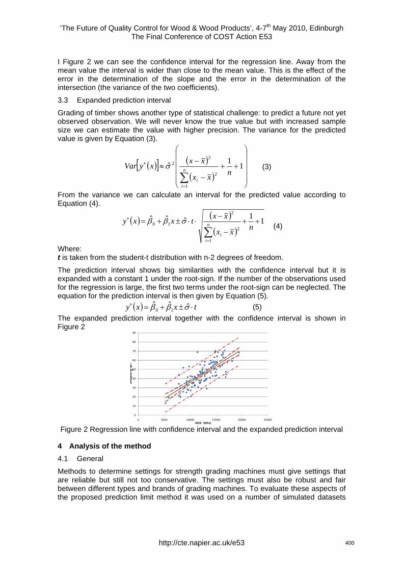
‘The Future of Quality Control for Wood & Wood Products’, 4-7th May 2010, Edinburgh The Final Conference of COST Action E53
I Figure 2 we can see the confidence interval for the regression line. Away from the mean value the interval is wider than close to the mean value. This is the effect of the error in the determination of the slope and the error in the determination of the intersection (the variance of the two coefficients).
3.3 Expanded prediction interval
Grading of timber shows another type of statistical challenge: to predict a future not yet observed observation. We will never know the true value but with increased sample size we can estimate the value with higher precision. The variance for the predicted value is given by Equation (3).
( )[ ] ( )( ) ⎟
⎟⎟⎟
⎠
⎞
⎜⎜⎜⎜
⎝
⎛
++−
−≈
∑=
∗ 11ˆ
1
2
22
nxx
xxxyVar n
ii
σ
(3)
From the variance we can calculate an interval for the predicted value according to Equation (4).
( ) ( )( )
11ˆˆˆ
1
2
2
10 ++−
−⋅⋅±+=
∑=
∗
nxx
xxtxxy n
ii
σββ(4)
Where: t is taken from the student-t distribution with n-2 degrees of freedom.
The prediction interval shows big similarities with the confidence interval but it is expanded with a constant 1 under the root-sign. If the number of the observations used for the regression is large, the first two terms under the root-sign can be neglected. The equation for the prediction interval is then given by Equation (5).
( ) txxy ⋅±+=∗ σββ ˆˆˆ10 (5)
The expanded prediction interval together with the confidence interval is shown in Figure 2
0
10
20
30
40
50
60
70
80
90
0 5000 10000 15000 20000 25000
Strength (MPa)
MOE (MPa) Figure 2 Regression line with confidence interval and the expanded prediction interval
4 Analysis of the method 4.1 General
Methods to determine settings for strength grading machines must give settings that are reliable but still not too conservative. The settings must also be robust and fair between different types and brands of grading machines. To evaluate these aspects of the proposed prediction limit method it was used on a number of simulated datasets
http://cte.napier.ac.uk/e53 400
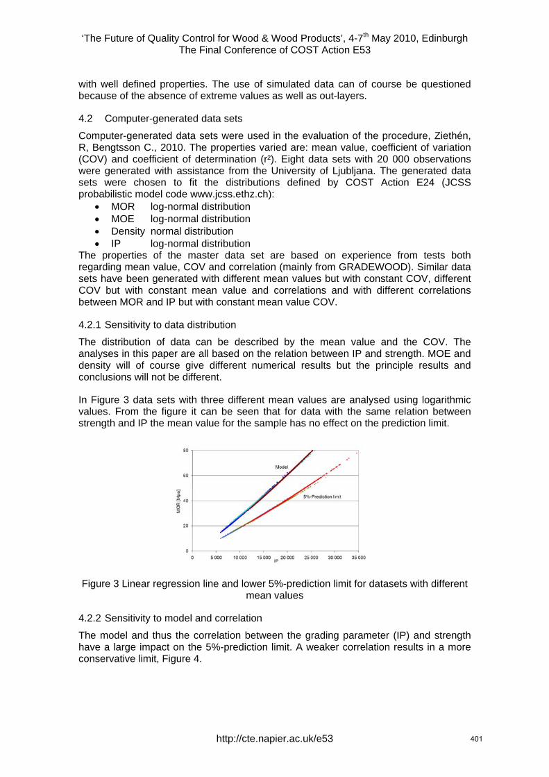
‘The Future of Quality Control for Wood & Wood Products’, 4-7th May 2010, Edinburgh The Final Conference of COST Action E53
with well defined properties. The use of simulated data can of course be questioned because of the absence of extreme values as well as out-layers.
4.2 Computer-generated data sets
Computer-generated data sets were used in the evaluation of the procedure, Ziethén, R, Bengtsson C., 2010. The properties varied are: mean value, coefficient of variation (COV) and coefficient of determination (r²). Eight data sets with 20 000 observations were generated with assistance from the University of Ljubljana. The generated data sets were chosen to fit the distributions defined by COST Action E24 (JCSS probabilistic model code www.jcss.ethz.ch):
• MOR log-normal distribution • MOE log-normal distribution • Density normal distribution • IP log-normal distribution
The properties of the master data set are based on experience from tests both regarding mean value, COV and correlation (mainly from GRADEWOOD). Similar data sets have been generated with different mean values but with constant COV, different COV but with constant mean value and correlations and with different correlations between MOR and IP but with constant mean value COV.
4.2.1 Sensitivity to data distribution
The distribution of data can be described by the mean value and the COV. The analyses in this paper are all based on the relation between IP and strength. MOE and density will of course give different numerical results but the principle results and conclusions will not be different.
In Figure 3 data sets with three different mean values are analysed using logarithmic values. From the figure it can be seen that for data with the same relation between strength and IP the mean value for the sample has no effect on the prediction limit.
Figure 3 Linear regression line and lower 5%-prediction limit for datasets with different mean values
4.2.2 Sensitivity to model and correlation
The model and thus the correlation between the grading parameter (IP) and strength have a large impact on the 5%-prediction limit. A weaker correlation results in a more conservative limit, Figure 4.
http://cte.napier.ac.uk/e53 401
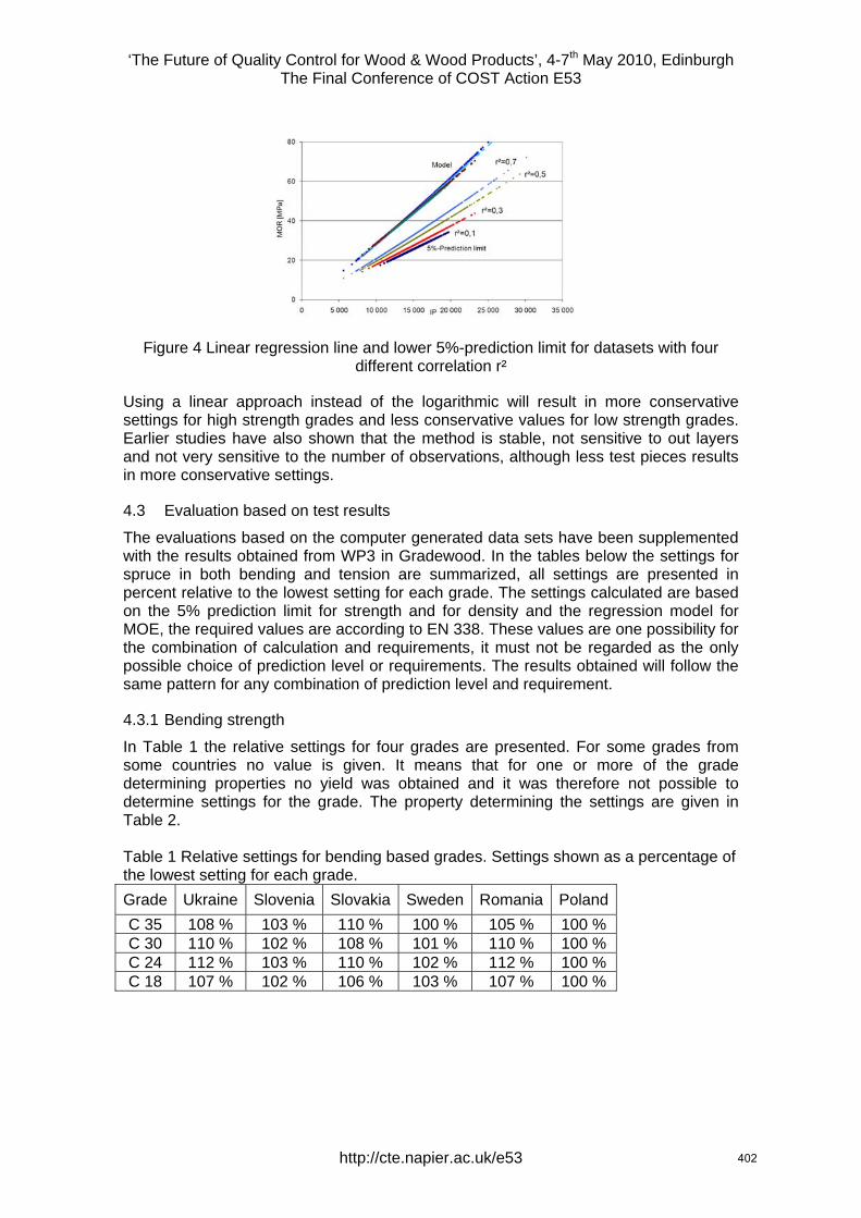
‘The Future of Quality Control for Wood & Wood Products’, 4-7th May 2010, Edinburgh The Final Conference of COST Action E53
Figure 4 Linear regression line and lower 5%-prediction limit for datasets with four different correlation r²
Using a linear approach instead of the logarithmic will result in more conservative settings for high strength grades and less conservative values for low strength grades. Earlier studies have also shown that the method is stable, not sensitive to out layers and not very sensitive to the number of observations, although less test pieces results in more conservative settings.
4.3 Evaluation based on test results
The evaluations based on the computer generated data sets have been supplemented with the results obtained from WP3 in Gradewood. In the tables below the settings for spruce in both bending and tension are summarized, all settings are presented in percent relative to the lowest setting for each grade. The settings calculated are based on the 5% prediction limit for strength and for density and the regression model for MOE, the required values are according to EN 338. These values are one possibility for the combination of calculation and requirements, it must not be regarded as the only possible choice of prediction level or requirements. The results obtained will follow the same pattern for any combination of prediction level and requirement.
4.3.1 Bending strength
In Table 1 the relative settings for four grades are presented. For some grades from some countries no value is given. It means that for one or more of the grade determining properties no yield was obtained and it was therefore not possible to determine settings for the grade. The property determining the settings are given in Table 2. Table 1 Relative settings for bending based grades. Settings shown as a percentage of the lowest setting for each grade.
Grade Ukraine Slovenia Slovakia Sweden Romania PolandC 35 108 % 103 % 110 % 100 % 105 % 100 % C 30 110 % 102 % 108 % 101 % 110 % 100 % C 24 112 % 103 % 110 % 102 % 112 % 100 % C 18 107 % 102 % 106 % 103 % 107 % 100 %
http://cte.napier.ac.uk/e53 402

‘The Future of Quality Control for Wood & Wood Products’, 4-7th May 2010, Edinburgh The Final Conference of COST Action E53
Table 2 Critical property for different grades and counties for determination of settings Grade Ukraine Slovenia Slovakia Sweden Romania PolandC 35 MOR MOR MOR MOR MOE MOR C 30 MOE MOR MOR MOR MOE MOR C 24 MOE MOE MOE MOR MOE MOR C 18 MOE MOR MOE MOR MOE MOR
From Table 1 it is difficult to find a systematic geographic reason for the differences of settings. But it can be seen, from Table 2, that MOE is more common to be the critical property for the countries with higher settings.
4.3.2 Tension strength
In an earlier part of Gradewood it was shown that similar settings could be used for large parts of Europe, that result is not confirmed here. In Table 3 the settings for four different grades based on tension strength is presented for different countries. The property determining the settings are given in Table 4. Table 3 Relative settings for tension based grades. Settings shown as a percentage of the lowest setting for each grade. No value indicates no yield for the grade.
Grade Ukraine Slovenia Slovakia Sweden Romania Poland Switzer- land
L36 120 % 107 % 100 % 116 % L30 112 % 112 % 107 % 100 % 121 % L25 108 % 104 % 101 % 121 % 100 % 120 % L17 106 % 113 % 108 % 100 % 111 % 103 % 115 %
Table 4 Critical property for different grades and counties for determination of settings
Grade Ukraine Slovenia Slovakia Sweden Romania Poland Switzer- land
L36 Density Density Density Density Density Density MOE L30 Density Density Density Density Density MOR MOE L25 Density MOR MOE MOE Density MOR MOE L17 MOR MOR MOR MOR MOR MOR MOE
In Table 4 it can be see that density is the critical property for almost all data-sets for high grades. This raises the question whether the requirement profile really is the optimal. If we only look at the strength there are settings for all classes. However, even for settings based on strength there are significantly high differences between different countries,
http://cte.napier.ac.uk/e53 403

‘The Future of Quality Control for Wood & Wood Products’, 4-7th May 2010, Edinburgh The Final Conference of COST Action E53
Table 5 Relative settings for tension based grades. Settings determined only based on strength and shown as a percentage of the lowest setting for each grade.
Grade Ukraine Slovenia Slovakia Sweden Romania Poland Switzer- land
L36 104 % 106 % 104 % 101 % 124 % 100 % 104 % L30 104 % 108 % 104 % 100 % 121 % 100 % 104 % L25 105 % 110 % 105 % 100 % 116 % 102 % 106 % L17 106 % 113 % 108 % 100 % 111 % 103 % 107 %
4.3.3 Splitted or combined growth areas
Today there is a focus on nation based settings. However, it is difficult to see a reason for a change of wood properties based on borders between nations. In this section it is shown how the differences between nations can be reflected in a calculation of an area with more than one country, Table 6. Sweden and Romania are chosen as an example. The number of observations is close to the same for both countries and there is a small difference for the settings. The calculations are based only on bending strength.
Table 6 Relative settings for bending based grades. Settings determined as a percentage of the lowest setting for each grade.
Grade Sweden Romania Combined Sweden and Romania
C 35 100 % 101 % 101 % C 30 100 % 102 % 102 % C 24 100 % 103 % 103 % C 18 100 % 105 % 104 %
We can see in this case that the conservative settings are dominating. This is however depending on a number of conditions such as the number of observations in the different data sets and the correlation between IP and the grade determining property for the combined data set compared to the correlations for each of the original data sets. It may be necessary to include requirements for data sets possible to combine into a common area. The smallest area with the same settings allowed in the present standard is a country. When we evaluate possibilities to combine countries into larger areas it is important to look at the differences we must accept within a country when we are looking at restrictions for combined areas. As an example of this the settings for pine in bending are presented. Table 7 Relative settings for bending based grades. Settings based only on bending strength are determined as a percentage of the lowest setting for each grade.
Grade Sweden South Sweden
North Sweden Poland Poland,
Swietjana Poland, Murow
C 35 100 % 105 % 100 % 112 % 104 % 119 % C 30 100 % 104 % 100 % 111 % 106 % 117 % C 24 100 % 103 % 100 % 112 % 107 % 116 % C 18 100 % 103 % 102 % 113 % 110 % 117 %
http://cte.napier.ac.uk/e53 404

‘The Future of Quality Control for Wood & Wood Products’, 4-7th May 2010, Edinburgh The Final Conference of COST Action E53
A first look at settings shows a rather big difference between Sweden and Poland, app. 12 %. A closer look reveals that it is mainly one sample from Poland deviating from the rest with a difference of 15 – 20 % whilst the other Polish sample is close to the Swedish samples, Table 7. It is important that the requirements for different sub areas, when countries are combined, are of the same order as the differences that can be seen within the smallest allowed areas.
5 Conclusions The evaluation of the proposed prediction limit method for calculation of settings has shown that:
• The calculated settings are not dependent on average strength of the raw material • Weak correlation between indicating property and grade determining property
results in more conservative settings • Few observations for calculation of settings results in more conservative settings • A combination of samples with slightly different regression models (from different
areas) gives more conservative settings than for each of the areas alone. • For a combination of samples were the differences in regression models are large
the settings are less conservative than the most conservative settings for the sub-areas
• This indicates that special requirements on sample sizes and regression models can be needed if samples are combined.
• The differences within the present minimum acceptable grading area(country) are big. It is not reasonable to have harder restrictions when settings are determined for areas combining a number of countries than for the determination of settings for areas within a country.
6 References Jørgensen, B.: The theory of linear models, CRC Press, 1993.
Rouger, F.: A new statistical method for the establishment of machine settings, CIB W18, proceedings paper 30-17-1, Vancouver, Canada, 1997.
EN 384 Structural timber – Determination of characteristic values of mechanical properties
EN 408 Structural timber – Test methods
EN 338 Structural timber – Strength classes
EN 14081 Timber structures – Strength graded structural timber with rectangular cross section, part 1-4
Ziethén, R, Bengtsson C.: Machine Strength Grading – a New Method for Derivation of Settings, CIB W18, proceedings paper 42-5-1, Dübendorf, Switzerland, 2009
Ziethén, R, Bengtsson C.: Machine strength grading – Prediction limits – evaluation of a new method for derivation of settings, WCTE, Riva de Garda, 2010
http://cte.napier.ac.uk/e53 405
‘The Future of Quality Control for Wood & Wood Products’, 4-7th May 2010, Edinburgh The Final Conference of COST Action E53
Development of a simulation-evaluation program for introducing and using output control in the sawmill industry
A. Lycken1, R. Ziethén2 & C. Bengtsson3
Abstract A computer program for simulating output control has been developed. The calculations in the program follow the standard EN 14081-3:2005, where output control is described. The purpose of the simulator is to make it possible to improve the yield without jeopardizing the safety of the produced boards by testing different approaches in grading. The program is a research tool, as well as a program to use in production where output control is used. In the program is it possible to test e.g. the influence of change of IP-values, number of grades, pre-grading of logs, raw material region, etc. The result of a simulation is shown both as diagrams and numeral. The standard C-grades are pre-programmed with K-, Y- and Z-coefficients according to the standard. Other grades can be added by the user.
1 Introduction Output control as a method for production control of machine strength graded timber has been present in European strength grading standards for a long time. However, the machine control method is dominating and therefore little experience on how the output control method works is present in Europe. Pilot studies have earlier shown that there seems to be a potential for European sawmills to use this quality control method and get good yields in high strength classes [1].
Grading of structural timber is a compromise between yield and safety. The grading procedure shall guarantee that the graded timber fulfils all strength requirements belonging to the marked grade. The producer shall have the possibility to produce strength graded timber with a reasonable yield, without jeopardizing the safety.
A computer program for simulating and testing output control as described in EN 14081 “Timber Structures – Strength graded structural timber with rectangular cross section, part 1-4” [2] is developed, to make analysis of
1 Researcher, [email protected] Trätek, Box 5609, 114 86 Stockholm, Sweden 2 Researcher, [email protected] Trätek, Box 857, SE-501 15 Borås, Sweden. 3 Head of section, [email protected] Trätek, Box 857, SE-501 15 Borås, Sweden. School of Engineering, Linnaeus University, SE-351 95 Växjö, Sweden.
http://cte.napier.ac.uk/e53 406
‘The Future of Quality Control for Wood & Wood Products’, 4-7th May 2010, Edinburgh The Final Conference of COST Action E53
settings faster and more flexible. The program can use data from real boards or data from simulated boards. It is also possible to combine data from logs (e.g. information from a log scanner) with data from associated boards. Input data can be predicted strength (other than ordinary indicating property IP-values) from logs and/or boards and machine graded IP-values, which is correlated to actual measured modulus of elasticity (MOE) and strength (MOR, modulus of rupture). In the program it is possible to change IP boundaries, test yield differences and risks of being “Out of control”.
The paper presents the program as well as some results of analyses of sensitivity in IP settings. One aspect presented is the method’s sensitivity of variation in incoming raw material quality of the material to be graded. Another aspect presented is the results of the grading procedure if the strength graded material comes from logs which are pre-graded.
2 Background The cusum-method for output control in the European standard 14081-3 is based on and to large extent copied from an American procedure for output control that was originally created in the late sixties and early seventies. It was aimed for a production of a few grades with a few dimensions where only one, or maybe two, grades were graded simultaneously. The situation today in Europe is another. Now a number of different grades are graded simultaneously with a large amount of different dimensions.
3 Description of Machine control and of Output control
3.1 Machine control Machine control is the dominating method used to grade timber in Europe. Each grading machine type has an IP setting that corresponds to the wanted grade, see EN14081-4. Each grade and combination of grades needs a special setting, which means that the IP value for one grade is depending which other grades are graded at the same time. When determining the IP values, an initial test of at least 900 boards is needed. The tested boards should be representative for the region for which settings are determined. In machine control it is not allowed to change the settings to improve the yield. This means that the settings must consider the difference in correlation between IP value and strength to fit the whole population in the region.
3.2 Output control Output control put the responsibility more on the producer of the boards than on the grading machine. In output control of structural timber a test scheme is used that follows the standard EN14081, to ensure that timber that doesn’t fulfil the requirements for structural timber doesn’t leave the sawmill.
Initial settings shall be tested by proof loading “a random sample of 60 specimen of each combination of strength class/species/size/source combinations” in accordance with EN 14081-2. To test the production ten specimens from each class produced during each shift shall be proof loaded to
http://cte.napier.ac.uk/e53 407
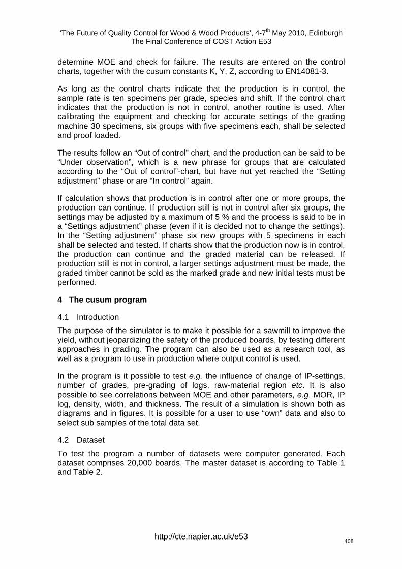
‘The Future of Quality Control for Wood & Wood Products’, 4-7th May 2010, Edinburgh The Final Conference of COST Action E53
determine MOE and check for failure. The results are entered on the control charts, together with the cusum constants K, Y, Z, according to EN14081-3.
As long as the control charts indicate that the production is in control, the sample rate is ten specimens per grade, species and shift. If the control chart indicates that the production is not in control, another routine is used. After calibrating the equipment and checking for accurate settings of the grading machine 30 specimens, six groups with five specimens each, shall be selected and proof loaded.
The results follow an “Out of control” chart, and the production can be said to be “Under observation”, which is a new phrase for groups that are calculated according to the “Out of control”-chart, but have not yet reached the “Setting adjustment” phase or are “In control” again.
If calculation shows that production is in control after one or more groups, the production can continue. If production still is not in control after six groups, the settings may be adjusted by a maximum of 5 % and the process is said to be in a “Settings adjustment” phase (even if it is decided not to change the settings). In the “Setting adjustment” phase six new groups with 5 specimens in each shall be selected and tested. If charts show that the production now is in control, the production can continue and the graded material can be released. If production still is not in control, a larger settings adjustment must be made, the graded timber cannot be sold as the marked grade and new initial tests must be performed.
4 The cusum program
4.1 Introduction The purpose of the simulator is to make it possible for a sawmill to improve the yield, without jeopardizing the safety of the produced boards, by testing different approaches in grading. The program can also be used as a research tool, as well as a program to use in production where output control is used.
In the program is it possible to test e.g. the influence of change of IP-settings, number of grades, pre-grading of logs, raw-material region etc. It is also possible to see correlations between MOE and other parameters, e.g. MOR, IP log, density, width, and thickness. The result of a simulation is shown both as diagrams and in figures. It is possible for a user to use “own” data and also to select sub samples of the total data set.
4.2 Dataset To test the program a number of datasets were computer generated. Each dataset comprises 20,000 boards. The master dataset is according to Table 1 and Table 2.
http://cte.napier.ac.uk/e53 408

‘The Future of Quality Control for Wood & Wood Products’, 4-7th May 2010, Edinburgh The Final Conference of COST Action E53
Table 1: Mean values, coefficient of variation and 5th-percentile of the master dataset.
MOR MOE Density IP Mean 44.9 12,503 450 14,788 CoV 0.35 0.26 0.12 0.22
5th-percentile 24.2 7,930 361 10,133
Table 2: R2-values of the master dataset.
MOR MOE Density IP MOR 1 MOE 0.57 1 Density 0.17 0.26 1 IP 0.48 0.65 0.10 1
From the master dataset the characteristics of the data was varied 1. The same CoV (35 %) for MOR and r² (0.5) between IP and MOR but with
three different mean values of MOR (30, 45 and 60 MPa) 2. The same mean value of MOR (45 MPa) and r² (0.5) between IP and MOR
but with three different CoV (20, 35 and 50 %) for MOR 3. The same mean value of MOR (45 MPa) and CoV (35 %) for MOR but with
four different r² (0.1, 0.3, 0.5 and 0.7) between IP and MOR.
The first condition represents a difference between batches in mean strength of the timber. The second represents a difference in Coefficient of Variation, or normalized standard deviation, and the third condition represents different correlations, r2 values, between IP and the grade determining properties (MOR, MOE and density), or how well the IP can predict the property.
4.3 Description of the program The K-, Y- and Z-coefficients for standard C-grades according to EN14081 are preset in the parameter file, which can be appended with user defined classes. The IP-values are user changeable to be able to simulate grading with different settings to maximize the yield. The calculations follow the standard EN 14081-3:2005.
It is possible to select a whole data file or a subset thereof. The selected data can be sorted according to any column before calculation. By this is it possible to simulate pre-sorting of boards or logs. If there are log-values in the data file, e.g. density or frequency, it is possible to sort by that column and select boards from only the wanted logs. There is also a “random number” column, which can be re-randomized and resorted to simulate a new random appearance of the boards.
http://cte.napier.ac.uk/e53 409
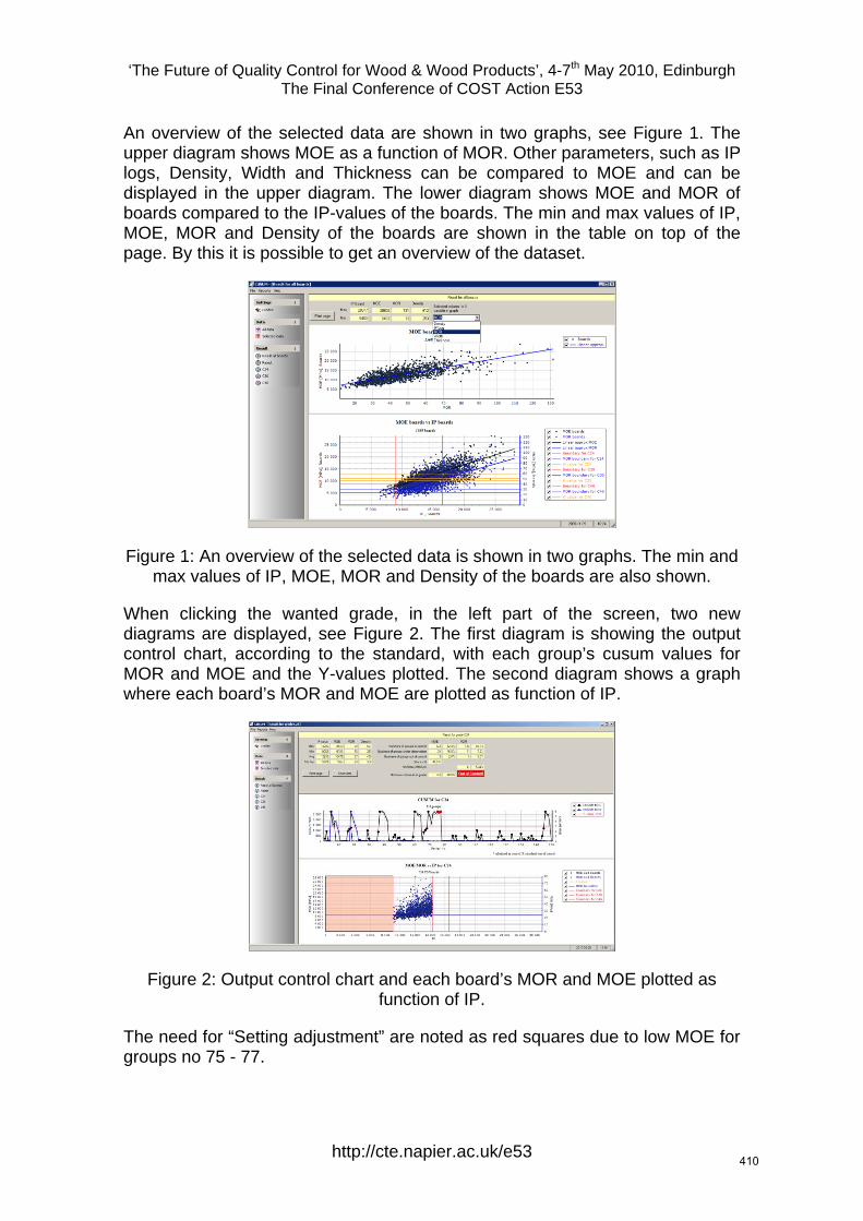
‘The Future of Quality Control for Wood & Wood Products’, 4-7th May 2010, Edinburgh The Final Conference of COST Action E53
An overview of the selected data are shown in two graphs, see Figure 1. The upper diagram shows MOE as a function of MOR. Other parameters, such as IP logs, Density, Width and Thickness can be compared to MOE and can be displayed in the upper diagram. The lower diagram shows MOE and MOR of boards compared to the IP-values of the boards. The min and max values of IP, MOE, MOR and Density of the boards are shown in the table on top of the page. By this it is possible to get an overview of the dataset.
Figure 1: An overview of the selected data is shown in two graphs. The min and max values of IP, MOE, MOR and Density of the boards are also shown.
When clicking the wanted grade, in the left part of the screen, two new diagrams are displayed, see Figure 2. The first diagram is showing the output control chart, according to the standard, with each group’s cusum values for MOR and MOE and the Y-values plotted. The second diagram shows a graph where each board’s MOR and MOE are plotted as function of IP.
Figure 2: Output control chart and each board’s MOR and MOE plotted as function of IP.
The need for “Setting adjustment” are noted as red squares due to low MOE for groups no 75 - 77.
http://cte.napier.ac.uk/e53 410
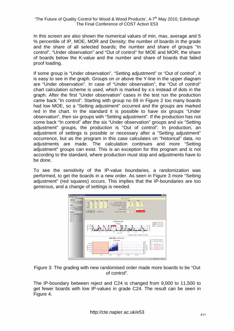
‘The Future of Quality Control for Wood & Wood Products’, 4-7th May 2010, Edinburgh The Final Conference of COST Action E53
In this screen are also shown the numerical values of min, max, average and 5 % percentile of IP, MOE, MOR and Density; the number of boards in the grade and the share of all selected boards; the number and share of groups “In control”, “Under observation” and “Out of control” for MOE and MOR; the share of boards below the K-value and the number and share of boards that failed proof loading.
If some group is “Under observation”, “Setting adjustment” or “Out of control”, it is easy to see in the graph. Groups on or above the Y-line in the upper diagram are “Under observation”. In case of “Under observation”, the “Out of control” chart calculation scheme is used, which is marked by x:s instead of dots in the graph. After the first “Under observation” cases in the test run the production came back “In control”. Starting with group no 69 in Figure 2 too many boards had low MOE, so a “Setting adjustment” occurred and the groups are marked red in the chart. In the standard it is possible to have six groups “Under observation”, then six groups with “Setting adjustment”. If the production has not come back “In control” after the six “Under observation” groups and six “Setting adjustment” groups, the production is “Out of control”. In production, an adjustment of settings is possible or necessary after a “Setting adjustment” occurrence, but as the program in this case calculates on “historical” data, no adjustments are made. The calculation continues and more “Setting adjustment” groups can exist. This is an exception for this program and is not according to the standard, where production must stop and adjustments have to be done.
To see the sensitivity of the IP-value boundaries, a randomization was performed, to get the boards in a new order. As seen in Figure 3 more “Setting adjustment” (red squares) occurs. This implies that the IP-boundaries are too generous, and a change of settings is needed.
Figure 3: The grading with new randomised order made more boards to be “Out of control”.
The IP-boundary between reject and C24 is changed from 9,000 to 11,500 to get fewer boards with low IP-values in grade C24. The result can be seen in Figure 4.
http://cte.napier.ac.uk/e53 411
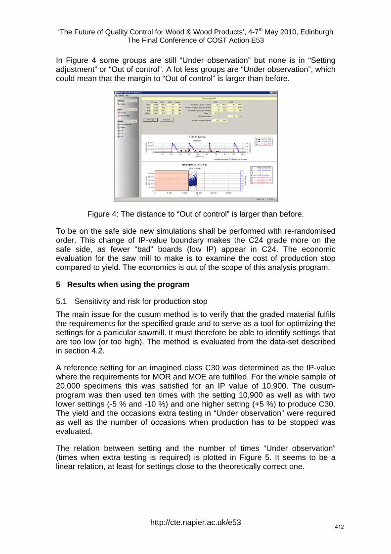
‘The Future of Quality Control for Wood & Wood Products’, 4-7th May 2010, Edinburgh The Final Conference of COST Action E53
In Figure 4 some groups are still “Under observation” but none is in “Setting adjustment” or “Out of control”. A lot less groups are “Under observation”, which could mean that the margin to “Out of control” is larger than before.
Figure 4: The distance to “Out of control” is larger than before.
To be on the safe side new simulations shall be performed with re-randomised order. This change of IP-value boundary makes the C24 grade more on the safe side, as fewer “bad” boards (low IP) appear in C24. The economic evaluation for the saw mill to make is to examine the cost of production stop compared to yield. The economics is out of the scope of this analysis program.
5 Results when using the program
5.1 Sensitivity and risk for production stop The main issue for the cusum method is to verify that the graded material fulfils the requirements for the specified grade and to serve as a tool for optimizing the settings for a particular sawmill. It must therefore be able to identify settings that are too low (or too high). The method is evaluated from the data-set described in section 4.2.
A reference setting for an imagined class C30 was determined as the IP-value where the requirements for MOR and MOE are fulfilled. For the whole sample of 20,000 specimens this was satisfied for an IP value of 10,900. The cusum-program was then used ten times with the setting 10,900 as well as with two lower settings (-5 % and -10 %) and one higher setting (+5 %) to produce C30. The yield and the occasions extra testing in “Under observation” were required as well as the number of occasions when production has to be stopped was evaluated.
The relation between setting and the number of times “Under observation” (times when extra testing is required) is plotted in Figure 5. It seems to be a linear relation, at least for settings close to the theoretically correct one.
http://cte.napier.ac.uk/e53 412
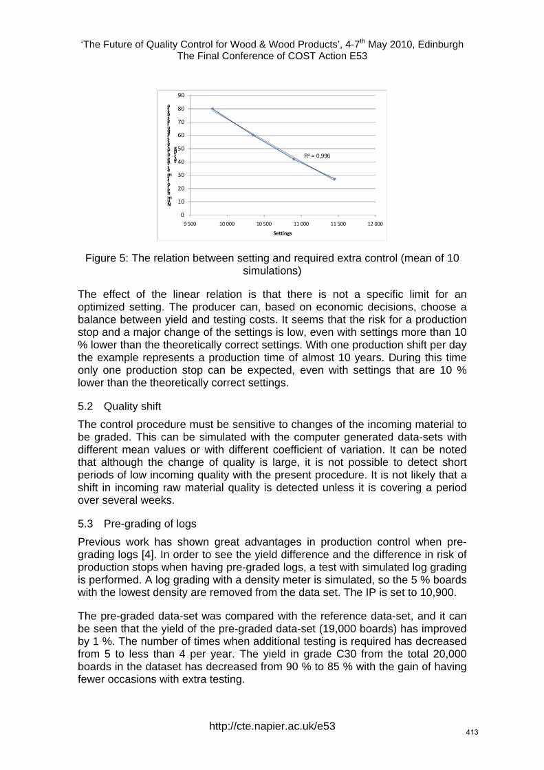
‘The Future of Quality Control for Wood & Wood Products’, 4-7th May 2010, Edinburgh The Final Conference of COST Action E53
R² = 0,996
0
10
20
30
40
50
60
70
80
90
9 500 10 000 10 500 11 000 11 500 12 000
Number of times the process requires extra
testing
Settings
Figure 5: The relation between setting and required extra control (mean of 10 simulations)
The effect of the linear relation is that there is not a specific limit for an optimized setting. The producer can, based on economic decisions, choose a balance between yield and testing costs. It seems that the risk for a production stop and a major change of the settings is low, even with settings more than 10 % lower than the theoretically correct settings. With one production shift per day the example represents a production time of almost 10 years. During this time only one production stop can be expected, even with settings that are 10 % lower than the theoretically correct settings.
5.2 Quality shift The control procedure must be sensitive to changes of the incoming material to be graded. This can be simulated with the computer generated data-sets with different mean values or with different coefficient of variation. It can be noted that although the change of quality is large, it is not possible to detect short periods of low incoming quality with the present procedure. It is not likely that a shift in incoming raw material quality is detected unless it is covering a period over several weeks.
5.3 Pre-grading of logs Previous work has shown great advantages in production control when pre-grading logs [4]. In order to see the yield difference and the difference in risk of production stops when having pre-graded logs, a test with simulated log grading is performed. A log grading with a density meter is simulated, so the 5 % boards with the lowest density are removed from the data set. The IP is set to 10,900.
The pre-graded data-set was compared with the reference data-set, and it can be seen that the yield of the pre-graded data-set (19,000 boards) has improved by 1 %. The number of times when additional testing is required has decreased from 5 to less than 4 per year. The yield in grade C30 from the total 20,000 boards in the dataset has decreased from 90 % to 85 % with the gain of having fewer occasions with extra testing.
http://cte.napier.ac.uk/e53 413
‘The Future of Quality Control for Wood & Wood Products’, 4-7th May 2010, Edinburgh The Final Conference of COST Action E53
6 Discussion From the analysis made on the cusum-procedure it can be seen that the procedure is able to identify productions where too low (or too high) settings are used. However, it is a coarse method and the consequence for the company using too low settings is mainly an increased number of pieces to be tested and increased costs due to that. The linear increase of required amount of tests with less conservative settings makes the determination of settings into an economical decision for the producer; a lower setting increases the yield but also the number of tests that can be expected. The risk of a stop of the production with downgraded material and restart of the verification process of the cusum is small. The high number of possibilities to come back into control, 12 groups to be tested, minimises this risk even with settings much lower than the required.
The method is not suitable for determination of short time variations of the quality of the incoming material. Due to coarseness of the method, the large amount of testing required before any actions are necessary a shift of quality can last for weeks before it is discovered.
Pre-grading of logs can increase the reliability of the settings and decrease the number of extra tests required. However the producer has to pay with a lower total yield. The effect is very similar to the effect of an increase of the setting but since it is made at the beginning of the production chain it may still be profitable.
Acknowledgement This work was mainly carried out within the GRADEWOOD project, WoodWisdom-Net Project 112006B and Vinnova Dnr 2007-0126. The financial support is gratefully acknowledged. Comprehensive contributions to this paper were given by Prof. Goran Turk, University of Ljubljana, who prepared the data sets.
References [1] Bengtsson, C., Serrano, E., Fonselius, M. & Riipola, K. (2008) Conformity
assessment for machine graded timber by using output control, SP Report 2008:01.
[2] CEN (2005) EN 14081 Timber structures – Strength graded structural timber with rectangular cross section, part 1-4.
[3] CEN (2003) EN 338 Structural timber – Strength classes. [4] Lycken, A., Oja, J. & Lundahl, C.G. (2009) Kundanpassad optimering i
såglinjen - Virkeskvalitet On-line. SP Rapport 2009:05 (In Swedish).
http://cte.napier.ac.uk/e53 414

‘The Future of Quality Control for Wood & Wood Products’, 4-7th May 2010, Edinburgh The Final Conference of COST Action E53
Thursday 6th May Research focussed day
Parallel session 2A
http://www.cte.napier.ac.uk/e53/ 415
‘The Future of Quality Control for Wood & Wood Products’, 4-7th May 2010, Edinburgh The Final Conference of COST Action E53
The use of non-destructive methods for the evaluation of fungal decay in field testing by dynamic vibration
A. Krause1, A. Pfeffer2 & H. Militz3
Abstract This study investigated the suitability of dynamic MOE measurements for an evaluation of the durability in field tests under use class 3 conditions. The decay of specimens was assessed by the so called “pick-test” (EN 252) and the determination of the dynamic modulus of elasticity (MOEdyn). Furthermore the evaluation of the influence of wood moisture content on the accuracy of the measurements was investigated. The results show the feasibility of dry and wet specimens to reliably determine the MOEdyn. Storing specimens in water, thus using (wet specimens) saves time during field tests. The determination of strength losses by means of MOEdyn provides additional information to pick-test and visual assessments of wood particularly in early stages of decay.
1 Introduction In field tests, a periodical evaluation of the wood specimens is required to determine the infestation of micro-organisms, particularly wood destroying fungi. Basic visual assessments such as the “pick-test” with a sharp pointed knife or blows with a hammer (EN 252) are widely used. Since those methods lack objectivity, results are often difficult to compare. Furthermore fungal attack causes strength loss of the wood specimens even before a degradation becomes visible according visual rating schemes (Grinda and Göller 2005). The fungal decay must not necessarily become visible on the wood surface in early stages, but can cause significant losses in strength (Tsuomis 1993). Therefore the use of non-destructive strength evaluation (Stephan et al. 1996) and dynamic methods for the determination of the modulus of elasticity (MOEdyn) can be an effective complement (Machek et al. 1997, Pfeffer et al. 2008). The dynamic methods are based on resonant vibration excitation or ultrasonic pulse excitation of the test specimens (Görlacher 1984). The objective of this study was to investigate the suitability of resonant vibration excitation for an evaluation of outside field tests under use class 3 conditions. Therefore, the measurement of MOEdyn is compared to the evaluation of the specimens by a conventional pick-test. Furthermore the influence of wood moisture content on the accuracy of the measurements is investigated.
1 Postdoctoral Research Fellow, [email protected] 2 Research Fellow, [email protected] 3 Professor, Head of Wood Biology and Wood Products, [email protected] Georg-August-University Göttingen, Burckhardt-Institute, Wood Biology and Wood Products, Germany
http://cte.napier.ac.uk/e53 416

‘The Future of Quality Control for Wood & Wood Products’, 4-7th May 2010, Edinburgh The Final Conference of COST Action E53
2 Material and methods
2.1 Measurement of MOEdyn depending on different wood moisture conditions It is shown that the MOE is influenced by the moisture content (mc). In field tests, the mc can vary. To guarantee a mc above fibre saturation, samples must be wetted. Prior to measuring the MOEdyn the specimens were soaked in water for different durations (Table 1) in order to investigate the influence of the wood moisture content. Twenty replicates per wood species were used to determine the MOEdyn. They were submerged (held down by weights) in tap-water in plastic boxes, separated according to wood species.
Table 1: Moisture condition for measurements of MOEdyn
Wood species Specimen size [mm³]
Moisture condition
Scots pine sapwood (Pinus sylvestris L.)
Beech wood (Fagus sylvatica L.)
20 x 30 x 300 20°C / 65% RH
Water storage for 24h, 48h, 72h, 7d
Vacuum pressure impregnation with water (30min vacuum at 60mbar, 2h pressure at 12bar)
Each specimen was supported horizontally on two sponge rubber pieces located equidistant at 0.224 x length from the ends of the specimen (67.2mm). The measuring device was a GRINDOSONIC MK 4-1 (J.W. Lemmens N.V., Belgium). Slightly tapping the center of the specimen with a hammer initiates the vibration energy into the specimen, a transducer in contact with the specimen quantifies the resulting vibration. The MOEdyn calculation was based on the following formula, derived by Hearmon (1966), shown in Equation 1.
⎟⎠⎞
⎜⎝⎛ ×
×+×
××××××
= ll
dyn KAL
ILIm
AfLMOE²
²²44
4 ρπ Equation 1
I = moment of inertia [mm4] A = area of the cross section [mm²] f = frequency [kHz] r = density [g/mm³] L = length [mm] Kl = 49.48 ml = 4.72
http://cte.napier.ac.uk/e53 417
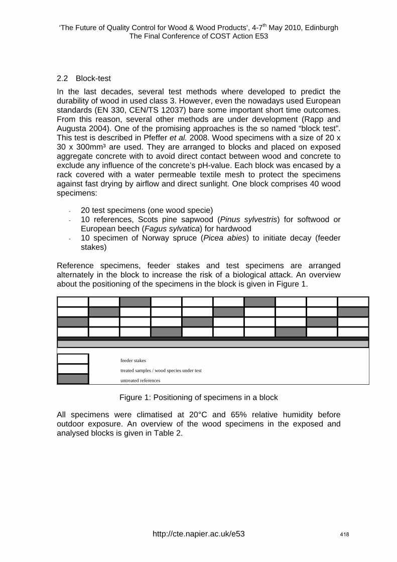
‘The Future of Quality Control for Wood & Wood Products’, 4-7th May 2010, Edinburgh The Final Conference of COST Action E53
2.2 Block-test In the last decades, several test methods where developed to predict the durability of wood in used class 3. However, even the nowadays used European standards (EN 330, CEN/TS 12037) bare some important short time outcomes. From this reason, several other methods are under development (Rapp and Augusta 2004). One of the promising approaches is the so named “block test”. This test is described in Pfeffer et al. 2008. Wood specimens with a size of 20 x 30 x 300mm³ are used. They are arranged to blocks and placed on exposed aggregate concrete with to avoid direct contact between wood and concrete to exclude any influence of the concrete’s pH-value. Each block was encased by a rack covered with a water permeable textile mesh to protect the specimens against fast drying by airflow and direct sunlight. One block comprises 40 wood specimens:
- 20 test specimens (one wood specie) - 10 references, Scots pine sapwood (Pinus sylvestris) for softwood or
European beech (Fagus sylvatica) for hardwood - 10 specimen of Norway spruce (Picea abies) to initiate decay (feeder
stakes) Reference specimens, feeder stakes and test specimens are arranged alternately in the block to increase the risk of a biological attack. An overview about the positioning of the specimens in the block is given in Figure 1.
feeder stakes
treated samples / wood species under test
untreated references
Figure 1: Positioning of specimens in a block
All specimens were climatised at 20°C and 65% relative humidity before outdoor exposure. An overview of the wood specimens in the exposed and analysed blocks is given in Table 2.
http://cte.napier.ac.uk/e53 418
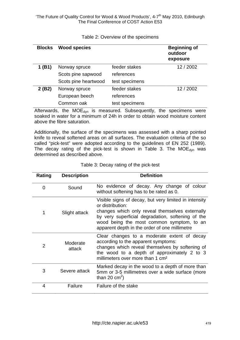
‘The Future of Quality Control for Wood & Wood Products’, 4-7th May 2010, Edinburgh The Final Conference of COST Action E53
Table 2: Overview of the specimens
Blocks Wood species Beginning of outdoor exposure
Norway spruce feeder stakes 12 / 2002 Scots pine sapwood references
1 (B1)
Scots pine heartwood test specimens Norway spruce feeder stakes 12 / 2002 European beech references
2 (B2)
Common oak test specimens Afterwards, the MOEdyn is measured. Subsequently, the specimens were soaked in water for a minimum of 24h in order to obtain wood moisture content above the fibre saturation.
Additionally, the surface of the specimens was assessed with a sharp pointed knife to reveal softened areas on all surfaces. The evaluation criteria of the so called “pick-test” were adopted according to the guidelines of EN 252 (1989). The decay rating of the pick-test is shown in Table 3. The MOEdyn was determined as described above.
Table 3: Decay rating of the pick-test
Rating Description Definition
0 Sound No evidence of decay. Any change of colour without softening has to be rated as 0.
1 Slight attack
Visible signs of decay, but very limited in intensity or distribution: changes which only reveal themselves externally by very superficial degradation, softening of the wood being the most common symptom, to an apparent depth in the order of one millimetre
2 Moderate attack
Clear changes to a moderate extent of decay according to the apparent symptoms: changes which reveal themselves by softening of the wood to a depth of approximately 2 to 3 millimeters over more than 1 cm²
3 Severe attack Marked decay in the wood to a depth of more than 5mm or 3-5 millimetres over a wide surface (more than 20 cm2)
4 Failure Failure of the stake
http://cte.napier.ac.uk/e53 419
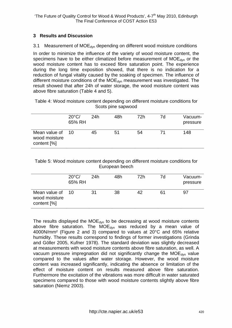
‘The Future of Quality Control for Wood & Wood Products’, 4-7th May 2010, Edinburgh The Final Conference of COST Action E53
3 Results and Discussion
3.1 Measurement of MOEdyn depending on different wood moisture conditions In order to minimize the influence of the variety of wood moisture content, the specimens have to be either climatized before measurement of MOEdyn or the wood moisture content has to exceed fibre saturation point. The experience during the long time exposition showed, that there is no indication for a reduction of fungal vitality caused by the soaking of specimen. The influence of different moisture conditions of the MOEdyn measurement was investigated. The result showed that after 24h of water storage, the wood moisture content was above fibre saturation (Table 4 and 5).
Table 4: Wood moisture content depending on different moisture conditions for Scots pine sapwood
20°C/ 65% RH
24h 48h 72h 7d Vacuum-pressure
Mean value of wood moisture content [%]
10 45 51 54 71 148
Table 5: Wood moisture content depending on different moisture conditions for European beech
20°C/ 65% RH
24h 48h 72h 7d Vacuum-pressure
Mean value of wood moisture content [%]
10 31 38 42 61 97
The results displayed the MOEdyn to be decreasing at wood moisture contents above fibre saturation. The MOEdyn was reduced by a mean value of 4000N/mm² (Figure 2 and 3) compared to values at 20°C and 65% relative humidity. These results correspond to findings of former investigations (Grinda and Göller 2005, Kufner 1978). The standard deviation was slightly decreased at measurements with wood moisture contents above fibre saturation, as well. A vacuum pressure impregnation did not significantly change the MOEdyn value compared to the values after water storage. However, the wood moisture content was increased significantly, indicating the absence or limitation of the effect of moisture content on results measured above fibre saturation. Furthermore the excitation of the vibrations was more difficult in water saturated specimens compared to those with wood moisture contents slightly above fibre saturation (Niemz 2003).
http://cte.napier.ac.uk/e53 420
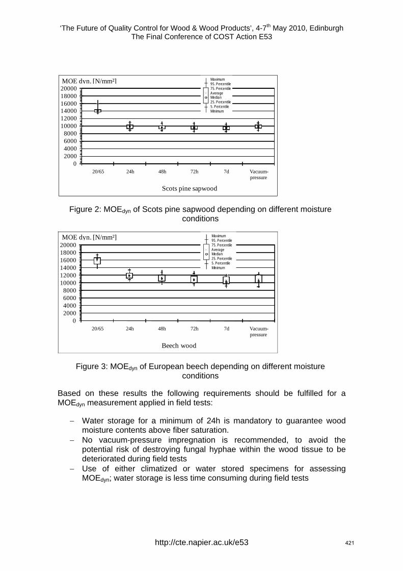
‘The Future of Quality Control for Wood & Wood Products’, 4-7th May 2010, Edinburgh The Final Conference of COST Action E53
02000400060008000
100001200014000160001800020000
20/65 24h 48h 72h 7d Vacuum-pressure
Scots pine sapwood
MOE dyn. [N/mm²] Maximum95. Percentile75. PercentileAverageMedian25. Percentile5. PercentileMinimum
Figure 2: MOEdyn of Scots pine sapwood depending on different moisture conditions
02000400060008000
100001200014000160001800020000
20/65 24h 48h 72h 7d Vacuum-pressure
Beech wood
MOE dyn. [N/mm²] Maximum95. Percentile75. PercentileAverageMedian25. Percentile5. PercentileMinimum
Figure 3: MOEdyn of European beech depending on different moisture conditions
Based on these results the following requirements should be fulfilled for a MOEdyn measurement applied in field tests:
− Water storage for a minimum of 24h is mandatory to guarantee wood moisture contents above fiber saturation.
− No vacuum-pressure impregnation is recommended, to avoid the potential risk of destroying fungal hyphae within the wood tissue to be deteriorated during field tests
− Use of either climatized or water stored specimens for assessing MOEdyn; water storage is less time consuming during field tests
http://cte.napier.ac.uk/e53 421
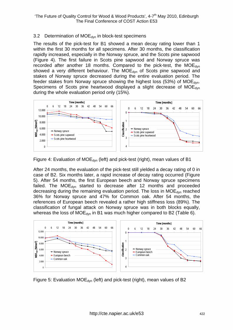
‘The Future of Quality Control for Wood & Wood Products’, 4-7th May 2010, Edinburgh The Final Conference of COST Action E53
3.2 Determination of MOEdyn in block-test specimens The results of the pick-test for B1 showed a mean decay rating lower than 1 within the first 30 months for all specimens. After 30 months, the classification rapidly increased, especially in the Norway spruce, and the Scots pine sapwood (Figure 4). The first failure in Scots pine sapwood and Norway spruce was recorded after another 18 months. Compared to the pick-test, the MOEdyn showed a very different behaviour. The MOEdyn of Scots pine sapwood and stakes of Norway spruce decreased during the entire evaluation period. The feeder stakes from Norway spruce showing the highest loss (53%) of MOEdyn. Specimens of Scots pine heartwood displayed a slight decrease of MOEdyn during the whole evaluation period only (15%).
0
2.000
4.000
6.000
8.000
10.000
12.0000 6 12 18 24 30 36 42 48 54 60 66
Time [months]
MOE d
yn [N
/mm
²]
Norway spruceScots pine sapwoodScots pine heartwood
0
1
2
3
4
0 6 12 18 24 30 36 42 48 54 60 66
Time [months]
Clas
sifica
tion
Norway spruceScots pine sapwoodScots pine heartwood
Figure 4: Evaluation of MOEdyn (left) and pick-test (right), mean values of B1
After 24 months, the evaluation of the pick-test still yielded a decay rating of 0 in case of B2. Six months later, a rapid increase of decay rating occurred (Figure 5). After 54 months, the first European beech and Norway spruce specimens failed. The MOEdyn started to decrease after 12 months and proceeded decreasing during the remaining evaluation period. The loss in MOEdyn reached 36% for Norway spruce and 47% for Common oak. After 54 months, the references of European beech revealed a rather high stiffness loss (89%). The classification of fungal attack on Norway spruce was in both blocks equally, whereas the loss of MOEdyn in B1 was much higher compared to B2 (Table 6).
0
2.000
4.000
6.000
8.000
10.000
12.0000 6 12 18 24 30 36 42 48 54 60 66
Time [months]
MOE d
yn [N
/mm
²]
Norway spruceEuropean beechCommon oak
0
1
2
3
4
0 6 12 18 24 30 36 42 48 54 60 66
Time [months]
class
ifica
tion
Norway spruceEuropean beechCommon oak
Figure 5: Evaluation MOEdyn (left) and pick-test (right), mean values of B2
http://cte.napier.ac.uk/e53 422
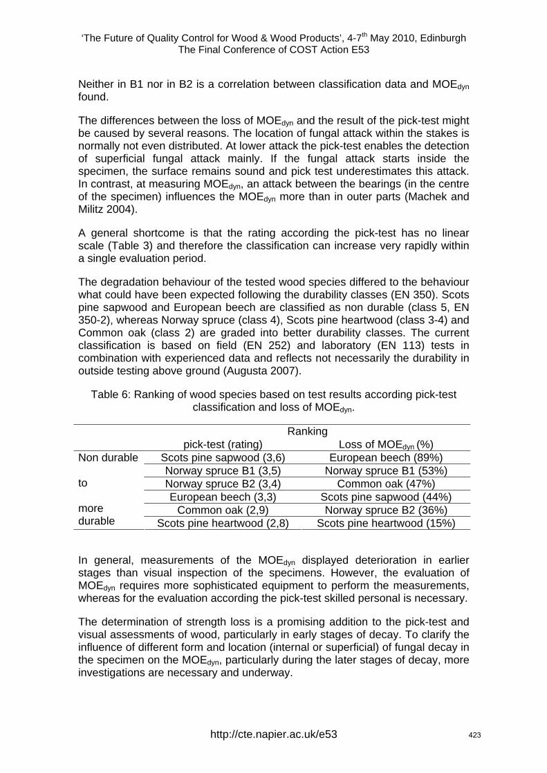
‘The Future of Quality Control for Wood & Wood Products’, 4-7th May 2010, Edinburgh The Final Conference of COST Action E53
Neither in B1 nor in B2 is a correlation between classification data and MOEdyn found.
The differences between the loss of MOEdyn and the result of the pick-test might be caused by several reasons. The location of fungal attack within the stakes is normally not even distributed. At lower attack the pick-test enables the detection of superficial fungal attack mainly. If the fungal attack starts inside the specimen, the surface remains sound and pick test underestimates this attack. In contrast, at measuring MOEdyn, an attack between the bearings (in the centre of the specimen) influences the MOEdyn more than in outer parts (Machek and Militz 2004).
A general shortcome is that the rating according the pick-test has no linear scale (Table 3) and therefore the classification can increase very rapidly within a single evaluation period.
The degradation behaviour of the tested wood species differed to the behaviour what could have been expected following the durability classes (EN 350). Scots pine sapwood and European beech are classified as non durable (class 5, EN 350-2), whereas Norway spruce (class 4), Scots pine heartwood (class 3-4) and Common oak (class 2) are graded into better durability classes. The current classification is based on field (EN 252) and laboratory (EN 113) tests in combination with experienced data and reflects not necessarily the durability in outside testing above ground (Augusta 2007).
Table 6: Ranking of wood species based on test results according pick-test classification and loss of MOEdyn.
Ranking pick-test (rating) Loss of MOEdyn (%)
Scots pine sapwood (3,6) European beech (89%) Norway spruce B1 (3,5) Norway spruce B1 (53%) Norway spruce B2 (3,4) Common oak (47%) European beech (3,3) Scots pine sapwood (44%)
Common oak (2,9) Norway spruce B2 (36%)
Non durable to more durable Scots pine heartwood (2,8) Scots pine heartwood (15%)
In general, measurements of the MOEdyn displayed deterioration in earlier stages than visual inspection of the specimens. However, the evaluation of MOEdyn requires more sophisticated equipment to perform the measurements, whereas for the evaluation according the pick-test skilled personal is necessary.
The determination of strength loss is a promising addition to the pick-test and visual assessments of wood, particularly in early stages of decay. To clarify the influence of different form and location (internal or superficial) of fungal decay in the specimen on the MOEdyn, particularly during the later stages of decay, more investigations are necessary and underway.
http://cte.napier.ac.uk/e53 423
‘The Future of Quality Control for Wood & Wood Products’, 4-7th May 2010, Edinburgh The Final Conference of COST Action E53
4 References Augusta, U. (2007) Untersuchung der natürlichen Dauerhaftigkeit wirtschaftlich bedeutender Holzarten bei verschiedener Beanspruchung im Außenbereich. Dissertation University of Hamburg, Germany
Görlacher, R. (1984): Ein neues Messverfahren zur Bestimmung des Elastizitätsmoduls von Holz. Holz als Roh- und Werkstoff Volume 42, pp 219-222
Grinda, M.; Göller, S. (2005) Some experiences with stake tests at BAM test fields and in the BAM fungus cellar. Part 1: Comparison of results of visual assessments and determinations of static Modulus of Elasticity (MOE). International Research Group on Wood Preservation, Doc. No.: 05/20319
Grinda, G.; Göller, S. (2005). Some experieces with stake test at BAM test fields and in the BAM fungus cellar. Part 2: Comparison of static and dynamic moduli of elasticity (MOE). International Research Group on Wood Preservation, Doc. No.: 96/20333
Hearmon, R.F.S. (1966) Vibration testing of wood. Forests Products Journal, Volume 16, pp 29-39
Kufner, M. (1978). Elastizitätsmodul und Zugfestigkeit von Holz verschiedener Rohdichte in Abhängigkeit vom Feuchtegehalt. Holz als Roh- und Werkstoff, Volume 36, pp 435 – 439
Machek, L.; Militz, H.; Gard, W. (1997): Use of modulus of rupture and modulus of elasticity in natural durability testing. International Research Group on Wood Preservation, Doc. No.: 97/20117
Machek, L.; Militz, H. (2004): The influence of the location of a wood defect on the modulus of elasticity determination in wood durability testing. International Research Group on Wood Preservation, Doc. No.: 04/20287
Niemz, P. (2003): Schallausbreitung in Holz und Holzwerkstoffen. Holz-Zentralblatt, Volume 102, pp 1470-1471
Pfeffer, A.; Krause, A.; Militz, H. (2008): Testing modified wood and natural durability in use class 3 with the block-test approach. Proceedings of the COST E 37 Final Conference, Bordeaux, France, pp 77-84
Rapp, A.O.; Augusta, U. (2004): The full guideline for the “double layer test method” – A field test method for determining the durability of wood out of ground. International Research Group on Wood Preservation, Doc. No.: 04-20290
Stephan, I.; Göller, S.; Rudolph, D. (1996): Improvement of monitoring the effects of soil organisms on wood in fungus cellar tests. International Research Group on Wood Preservation, Doc. No.: 96/20093
Tsuomis, G. (1993): Degradation of wood. Science and technology of wood: structure, properties and utilisation, pp 213-233
http://cte.napier.ac.uk/e53 424
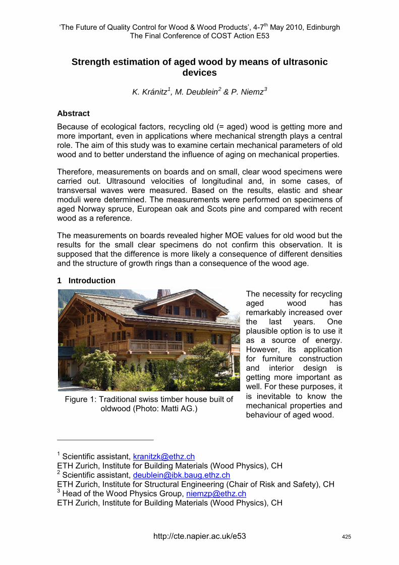
‘The Future of Quality Control for Wood & Wood Products’, 4-7th May 2010, Edinburgh The Final Conference of COST Action E53
http://cte.napier.ac.uk/e53
Strength estimation of aged wood by means of ultrasonic devices
K. Kránitz1, M. Deublein2 & P. Niemz3
Abstract
Because of ecological factors, recycling old (= aged) wood is getting more and more important, even in applications where mechanical strength plays a central role. The aim of this study was to examine certain mechanical parameters of old wood and to better understand the influence of aging on mechanical properties.
Therefore, measurements on boards and on small, clear wood specimens were carried out. Ultrasound velocities of longitudinal and, in some cases, of transversal waves were measured. Based on the results, elastic and shear moduli were determined. The measurements were performed on specimens of aged Norway spruce, European oak and Scots pine and compared with recent wood as a reference.
The measurements on boards revealed higher MOE values for old wood but the results for the small clear specimens do not confirm this observation. It is supposed that the difference is more likely a consequence of different densities and the structure of growth rings than a consequence of the wood age.
1 Introduction The necessity for recycling aged wood has remarkably increased over the last years. One plausible option is to use it as a source of energy. However, its application for furniture construction and interior design is getting more important as well. For these purposes, it is inevitable to know the mechanical properties and behaviour of aged wood.
1 Scientific assistant, [email protected] ETH Zurich, Institute for Building Materials (Wood Physics), CH 2 Scientific assistant, [email protected] ETH Zurich, Institute for Structural Engineering (Chair of Risk and Safety), CH 3 Head of the Wood Physics Group, [email protected] ETH Zurich, Institute for Building Materials (Wood Physics), CH
Figure 1: Traditional swiss timber house built of oldwood (Photo: Matti AG.)
425
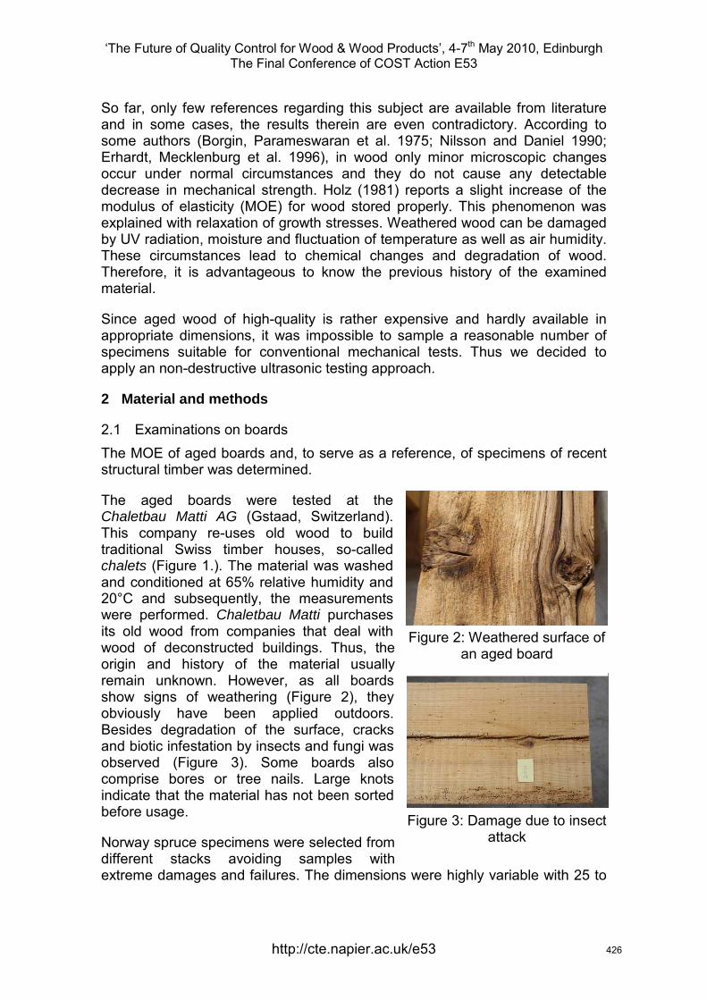
‘The Future of Quality Control for Wood & Wood Products’, 4-7th May 2010, Edinburgh The Final Conference of COST Action E53
http://cte.napier.ac.uk/e53
So far, only few references regarding this subject are available from literature and in some cases, the results therein are even contradictory. According to some authors (Borgin, Parameswaran et al. 1975; Nilsson and Daniel 1990; Erhardt, Mecklenburg et al. 1996), in wood only minor microscopic changes occur under normal circumstances and they do not cause any detectable decrease in mechanical strength. Holz (1981) reports a slight increase of the modulus of elasticity (MOE) for wood stored properly. This phenomenon was explained with relaxation of growth stresses. Weathered wood can be damaged by UV radiation, moisture and fluctuation of temperature as well as air humidity. These circumstances lead to chemical changes and degradation of wood. Therefore, it is advantageous to know the previous history of the examined material.
Since aged wood of high-quality is rather expensive and hardly available in appropriate dimensions, it was impossible to sample a reasonable number of specimens suitable for conventional mechanical tests. Thus we decided to apply an non-destructive ultrasonic testing approach.
2 Material and methods
2.1 Examinations on boards The MOE of aged boards and, to serve as a reference, of specimens of recent structural timber was determined.
The aged boards were tested at the Chaletbau Matti AG (Gstaad, Switzerland). This company re-uses old wood to build traditional Swiss timber houses, so-called chalets (Figure 1.). The material was washed and conditioned at 65% relative humidity and 20°C and subsequently, the measurements were performed. Chaletbau Matti purchases its old wood from companies that deal with wood of deconstructed buildings. Thus, the origin and history of the material usually remain unknown. However, as all boards show signs of weathering (Figure 2), they obviously have been applied outdoors. Besides degradation of the surface, cracks and biotic infestation by insects and fungi was observed (Figure 3). Some boards also comprise bores or tree nails. Large knots indicate that the material has not been sorted before usage.
Norway spruce specimens were selected from different stacks avoiding samples with extreme damages and failures. The dimensions were highly variable with 25 to
Figure 3: Damage due to insect attack
Figure 2: Weathered surface of an aged board
426
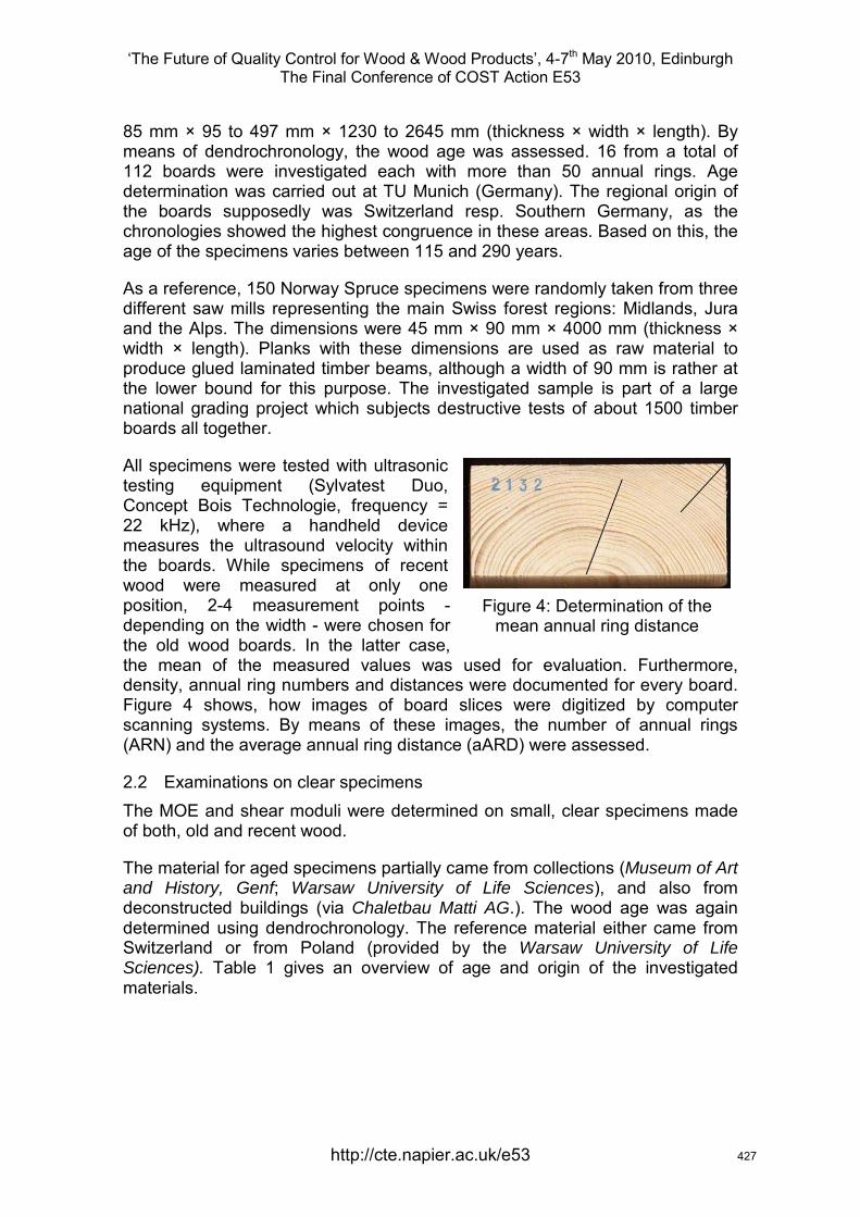
‘The Future of Quality Control for Wood & Wood Products’, 4-7th May 2010, Edinburgh The Final Conference of COST Action E53
http://cte.napier.ac.uk/e53
85 mm × 95 to 497 mm × 1230 to 2645 mm (thickness × width × length). By means of dendrochronology, the wood age was assessed. 16 from a total of 112 boards were investigated each with more than 50 annual rings. Age determination was carried out at TU Munich (Germany). The regional origin of the boards supposedly was Switzerland resp. Southern Germany, as the chronologies showed the highest congruence in these areas. Based on this, the age of the specimens varies between 115 and 290 years.
As a reference, 150 Norway Spruce specimens were randomly taken from three different saw mills representing the main Swiss forest regions: Midlands, Jura and the Alps. The dimensions were 45 mm × 90 mm × 4000 mm (thickness × width × length). Planks with these dimensions are used as raw material to produce glued laminated timber beams, although a width of 90 mm is rather at the lower bound for this purpose. The investigated sample is part of a large national grading project which subjects destructive tests of about 1500 timber boards all together.
All specimens were tested with ultrasonic testing equipment (Sylvatest Duo, Concept Bois Technologie, frequency = 22 kHz), where a handheld device measures the ultrasound velocity within the boards. While specimens of recent wood were measured at only one position, 2-4 measurement points -depending on the width - were chosen for the old wood boards. In the latter case, the mean of the measured values was used for evaluation. Furthermore, density, annual ring numbers and distances were documented for every board. Figure 4 shows, how images of board slices were digitized by computer scanning systems. By means of these images, the number of annual rings (ARN) and the average annual ring distance (aARD) were assessed.
2.2 Examinations on clear specimens The MOE and shear moduli were determined on small, clear specimens made of both, old and recent wood.
The material for aged specimens partially came from collections (Museum of Art and History, Genf; Warsaw University of Life Sciences), and also from deconstructed buildings (via Chaletbau Matti AG.). The wood age was again determined using dendrochronology. The reference material either came from Switzerland or from Poland (provided by the Warsaw University of Life Sciences). Table 1 gives an overview of age and origin of the investigated materials.
Figure 4: Determination of the mean annual ring distance
427
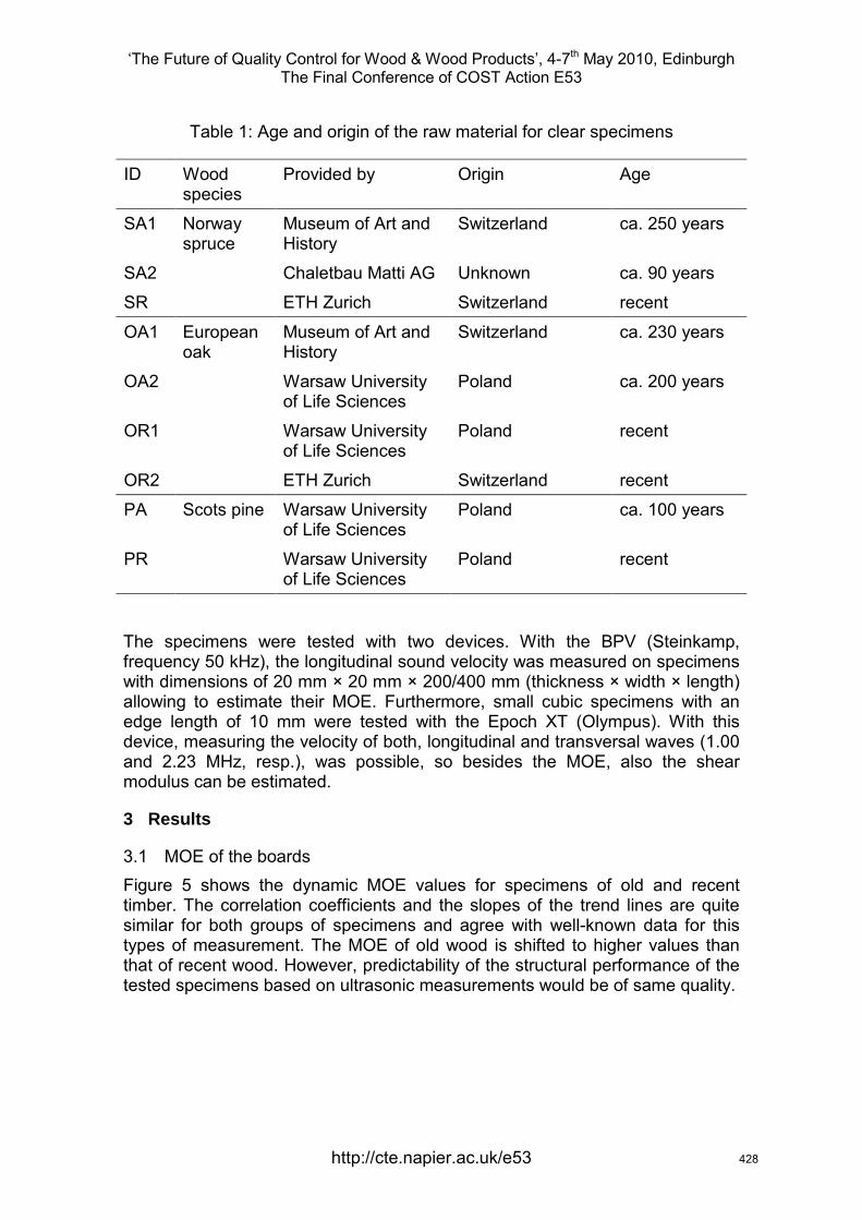
‘The Future of Quality Control for Wood & Wood Products’, 4-7th May 2010, Edinburgh The Final Conference of COST Action E53
http://cte.napier.ac.uk/e53
Table 1: Age and origin of the raw material for clear specimens
ID Wood species
Provided by Origin Age
SA1 Norway spruce
Museum of Art and History
Switzerland ca. 250 years
SA2 Chaletbau Matti AG Unknown ca. 90 years
SR ETH Zurich Switzerland recent
OA1 European oak
Museum of Art and History
Switzerland ca. 230 years
OA2 Warsaw University of Life Sciences
Poland ca. 200 years
OR1 Warsaw University of Life Sciences
Poland recent
OR2 ETH Zurich Switzerland recent
PA Scots pine Warsaw University of Life Sciences
Poland ca. 100 years
PR Warsaw University of Life Sciences
Poland recent
The specimens were tested with two devices. With the BPV (Steinkamp, frequency 50 kHz), the longitudinal sound velocity was measured on specimens with dimensions of 20 mm × 20 mm × 200/400 mm (thickness × width × length) allowing to estimate their MOE. Furthermore, small cubic specimens with an edge length of 10 mm were tested with the Epoch XT (Olympus). With this device, measuring the velocity of both, longitudinal and transversal waves (1.00 and 2.23 MHz, resp.), was possible, so besides the MOE, also the shear modulus can be estimated.
3 Results
3.1 MOE of the boards Figure 5 shows the dynamic MOE values for specimens of old and recent timber. The correlation coefficients and the slopes of the trend lines are quite similar for both groups of specimens and agree with well-known data for this types of measurement. The MOE of old wood is shifted to higher values than that of recent wood. However, predictability of the structural performance of the tested specimens based on ultrasonic measurements would be of same quality.
428
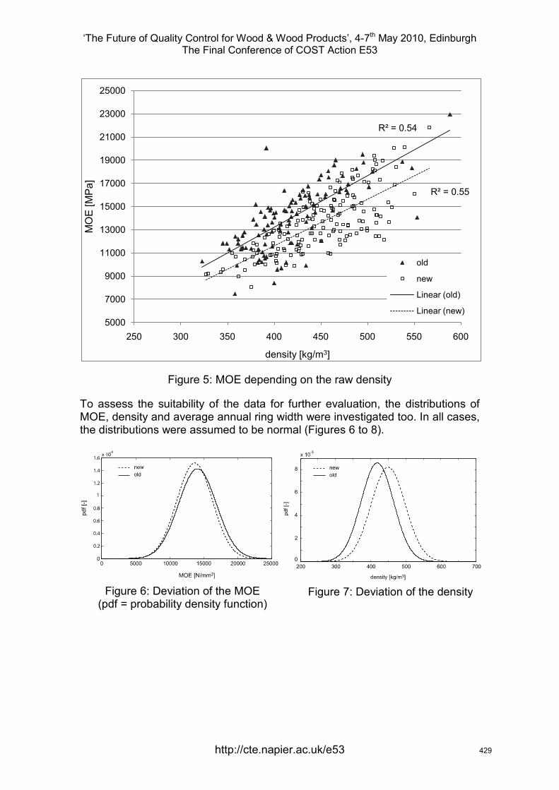
‘The Future of Quality Control for Wood & Wood Products’, 4-7th May 2010, Edinburgh The Final Conference of COST Action E53
http://cte.napier.ac.uk/e53
Figure 5: MOE depending on the raw density
To assess the suitability of the data for further evaluation, the distributions of MOE, density and average annual ring width were investigated too. In all cases, the distributions were assumed to be normal (Figures 6 to 8).
R² = 0.54
R² = 0.55
5000
7000
9000
11000
13000
15000
17000
19000
21000
23000
25000
250 300 350 400 450 500 550 600
MO
E [M
Pa]
density [kg/m3]
old
new
Linear (old)
Linear (new)
Figure 7: Deviation of the density Figure 6: Deviation of the MOE (pdf = probability density function)
429
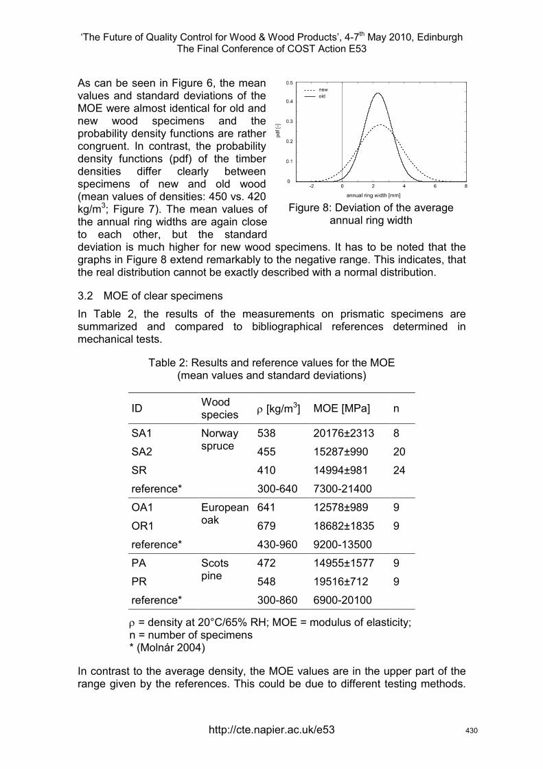
‘The Future of Quality Control for Wood & Wood Products’, 4-7th May 2010, Edinburgh The Final Conference of COST Action E53
http://cte.napier.ac.uk/e53
As can be seen in Figure 6, the mean values and standard deviations of the MOE were almost identical for old and new wood specimens and the probability density functions are rather congruent. In contrast, the probability density functions (pdf) of the timber densities differ clearly between specimens of new and old wood (mean values of densities: 450 vs. 420 kg/m3; Figure 7). The mean values of the annual ring widths are again close to each other, but the standard deviation is much higher for new wood specimens. It has to be noted that the graphs in Figure 8 extend remarkably to the negative range. This indicates, that the real distribution cannot be exactly described with a normal distribution.
3.2 MOE of clear specimens In Table 2, the results of the measurements on prismatic specimens are summarized and compared to bibliographical references determined in mechanical tests.
Table 2: Results and reference values for the MOE (mean values and standard deviations)
ID Wood species ρ [kg/m3] MOE [MPa] n
SA1 Norway spruce
538 20176±2313 8
SA2 455 15287±990 20
SR 410 14994±981 24
reference* 300-640 7300-21400
OA1 European oak
641 12578±989 9
OR1 679 18682±1835 9
reference* 430-960 9200-13500
PA Scots pine
472 14955±1577 9
PR 548 19516±712 9
reference* 300-860 6900-20100
ρ = density at 20°C/65% RH; MOE = modulus of elasticity; n = number of specimens * (Molnár 2004)
In contrast to the average density, the MOE values are in the upper part of the range given by the references. This could be due to different testing methods.
Figure 8: Deviation of the average annual ring width
430
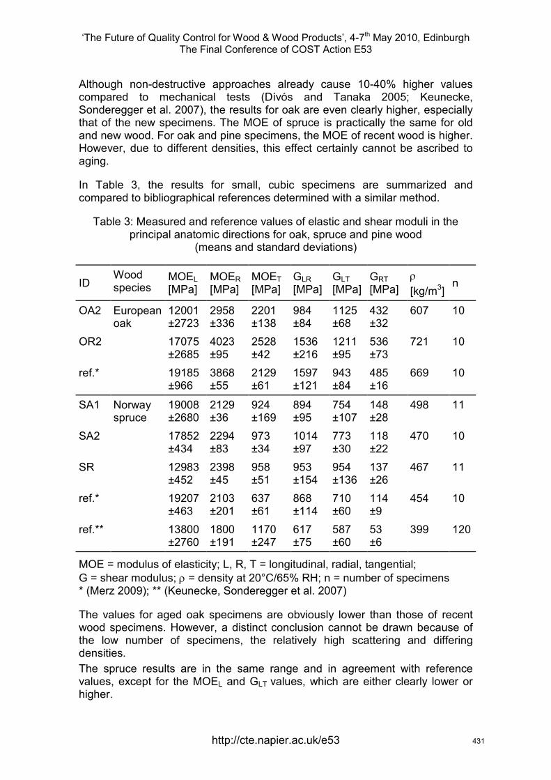
‘The Future of Quality Control for Wood & Wood Products’, 4-7th May 2010, Edinburgh The Final Conference of COST Action E53
http://cte.napier.ac.uk/e53
Although non-destructive approaches already cause 10-40% higher values compared to mechanical tests (Dívós and Tanaka 2005; Keunecke, Sonderegger et al. 2007), the results for oak are even clearly higher, especially that of the new specimens. The MOE of spruce is practically the same for old and new wood. For oak and pine specimens, the MOE of recent wood is higher. However, due to different densities, this effect certainly cannot be ascribed to aging.
In Table 3, the results for small, cubic specimens are summarized and compared to bibliographical references determined with a similar method.
Table 3: Measured and reference values of elastic and shear moduli in the principal anatomic directions for oak, spruce and pine wood
(means and standard deviations)
ID Wood species
MOEL [MPa]
MOER [MPa]
MOET [MPa]
GLR [MPa]
GLT [MPa]
GRT [MPa]
ρ [kg/m3]
n
OA2 European oak
12001 2958 2201 984 1125 432 607 10 ±2723 ±336 ±138 ±84 ±68 ±32
OR2 17075 4023 2528 1536 1211 536 721 10 ±2685 ±95 ±42 ±216 ±95 ±73
ref.* 19185 3868 2129 1597 943 485 669 10 ±966 ±55 ±61 ±121 ±84 ±16
SA1 Norway spruce
19008 2129 924 894 754 148 498 11 ±2680 ±36 ±169 ±95 ±107 ±28
SA2 17852 2294 973 1014 773 118 470 10 ±434 ±83 ±34 ±97 ±30 ±22
SR 12983 2398 958 953 954 137 467 11 ±452 ±45 ±51 ±154 ±136 ±26
ref.* 19207 2103 637 868 710 114 454 10 ±463 ±201 ±61 ±114 ±60 ±9
ref.** 13800 1800 1170 617 587 53 399 120 ±2760 ±191 ±247 ±75 ±60 ±6
MOE = modulus of elasticity; L, R, T = longitudinal, radial, tangential; G = shear modulus; ρ = density at 20°C/65% RH; n = number of specimens * (Merz 2009); ** (Keunecke, Sonderegger et al. 2007)
The values for aged oak specimens are obviously lower than those of recent wood specimens. However, a distinct conclusion cannot be drawn because of the low number of specimens, the relatively high scattering and differing densities. The spruce results are in the same range and in agreement with reference values, except for the MOEL and GLT values, which are either clearly lower or higher.
431
‘The Future of Quality Control for Wood & Wood Products’, 4-7th May 2010, Edinburgh The Final Conference of COST Action E53
http://cte.napier.ac.uk/e53
4 Discussion For the boards, higher values of MOE were measured for the old wood than for the recent timber specimens within the same density range. On the other hand, the results for clear specimens did not show any obvious differences. An explanation for this discrepancy can be the low number of specimens and the differing densities of the latter, which make a clear statement impossible. In case of the boards, a possible influence of the annual ring structure on the elastic behaviour can be taken into account. As a consequence, an aging effect on the mechanical properties could not be ascertained.
The relation between MOE and wood density was nearly the same for old and recent wood specimens, as similar trend lines and correlation coefficients show for the measurements on boards. As a result, grading methods developed for recent wood may also work for old wood. However, due to the frequent occurrence of fungal decay and infestation of insects, a previous control is inevitable.
Acknowledgements Investigations on clear specimens and oldwood boards were carried out within the COST Action IE0601 (Wood Science for Conservation of Cultural Heritage). Testing of the ‘new’ timber sample has been conducted within a national research project at ETH which is closely connected to COST action E53 ‘Quality control of wood and wood products’.
References Borgin K., Parameswaran N. & Liese W.(1975) “The effect of aging on the ultrastructure of wood”, Wood Science and Technology, Vol 9, pp 87-98.
Erhardt, D., Mecklenburg, M.F., Tumosa C.S. & Olstad, T.M. (1996) “New versus old wood: differences and similarities in physical, mechanical, and chemical properties”, in Bridgeland, J. (ed.): Preprints of the International Council of Museums-Committee for Conservation 11th Triennial Meeting. James&James, London, pp 903-910.
Nilsson, T. & Daniel, G.: (1990) “Structure and the aging process of dry archaeological wood”. In: Rowell RM, Barbour RJ (eds) Archaelogical wood: properties, chemistry, and preservation. American Chemical Society, Washington Dc., Advances in Chemistry Series No.225, pp 67-86.
Holz, D. (1981) “Zum Alterungsverhalten des Werkstoffes Holz – einige Ansichten, Untersuchungen, Ergebnisse.“ Holztechnologie, Vol 22, No. 2, pp 80-85.
Niemz, P.(1993) „Physik des Holzes und der Holzwerkstoffe“. DRW-Verlag, Leinfelden-Echterdingen, 243 pp.
Dívós, F. & Tanaka, T. (2005) “Relation Between Static and Dynamic Modulus of Elasticity of Wood.” Acta Silvatica & Lignaria Hungarica, Vol 1, pp 105-110.
432

‘The Future of Quality Control for Wood & Wood Products’, 4-7th May 2010, Edinburgh The Final Conference of COST Action E53
http://cte.napier.ac.uk/e53
Keunecke, D., Sonderegger, W., Pereteanu, K., Lüthi, Th. & Niemz, P.(2007) “Determination of Young´s moduli of common yew and Norway spruce by means of ultrasonic waves.” Wood Science and Technology, Vol 41, pp 309-327.
Molnár, S. (2004) „Faanyagismeret“, Szaktudás Kiadó Ház, Budapest, 471 pp.
Merz, T. (2009) “Messung der Schallgeschwindigkeit in den drei Hauptschnittrichtungen mit Longitudinal- und Transversalwellen.“ BSc Thesis, ETH Zürich.
433

‘The Future of Quality Control for Wood & Wood Products’, 4-7th May 2010, Edinburgh The Final Conference of COST Action E53
Wood windows in the 21st Century: end user requirements, limits and opportunities
L. Elek1, Zs. Kovacs2 & L. Denes3
Abstract
The increasing pressure on construction industry for development of energy efficient structures and building elements resulted in the appearance of new products and manufacturing technologies. Considering the ever increasing demand on low energy consumption, more and more attention is to be paid to enhance the thermal insulation of the weak points of buildings, which are the windows. In this paper the optimization of heat transfer coefficient (U-value or U-factor) for a conventional wood-frame window is presented using different glazing systems and frame materials. For the U-value calculations and isotherms determination WINDOW and THERM software have been used. According to the results sufficiently low U-value of the glazing can be attained with triple glazing systems, using inert gas cavity fills and soft-coat technology (i.e. Low-E coatings). However, frames of drastically reduced U-values can be only attained by using profiles comprising thick layers of materials of low thermal conductance, resulting in unusually deep profiles. Therefore potential new directions of research and development may include improvement of the heat mirror techniques for windows, development of intelligent glazing, and development of novel concepts for installing and operating windows.
1. Introduction
One of the most important challenges of today is to find new possibilities and solutions to an efficient and reasonable use of energy. This is a pressing necessity not only because of the limited resources but is also a demand of sustainability. In the course of the last decades, as a development of the technology used in the Scandinavian residential houses of low energy consumption in the mid-80s, a new, more economical building standard that provides comfort of the occupants in an energy-efficient and environmental friendly manner has been introduced. The new notion of passive house is used for buildings in which the climatic conditions necessary for the continuous presence of human can be assured exclusively by tempering the amount of air that is necessary for ventilation. This notion has been introduced by Dr. Wolfgang Feist the founder of the Passivhaus Institut Darmstadt, Germany (Feist, 1997).
In Hungary, there are currently a few passive houses only. Their spread is restrained by the fact that their design and implementation requires such a complex approach that is not yet common in the Hungarian building business. Furthermore, the roles of the state and subsidisation have not yet been clarified. Nevertheless, similarly to the other countries in Europe, energy saving, environmental friendly building and sustainability is more and more at issue.
1 Graduate Research Fellow, [email protected] 2 Professor, [email protected] 3 Associate Professor, Director [email protected] of Product Development and Manufacturing, University of West Hungary, HUNGARY
http://cte.napier.ac.uk/e53 434

‘The Future of Quality Control for Wood & Wood Products’, 4-7th May 2010, Edinburgh The Final Conference of COST Action E53
The energy-efficiency of the existing stock of buildings in Hungary is rather low (the consumption index being twice as high as the average of the EU countries). The European Union regulates the energy consumption of buildings through directives. From these follows the decree of 7/2006 that contains the requirements on the heat transfer coefficient of fenestration products (Prohászka 2007). Today the upper limit of the overall heat transfer coefficient (U-value or U-factor) for a wood-frame or PVC-frame window is Uw=1.60 W/m2K. Apart from the ever more severe stipulations the users of a building are interested in consuming the less possible energy while sustaining the occupants’ comfort. Out-of-date types of windows still in use generally occupy a relatively low percentage of a façade, nevertheless, they are responsible for a majority of heat-loss through the envelope of a building. Even the thermally insulated windows lag behind the rest of the wall (Thomas 2006). The ideal solution would be to improve the windows’ thermal insulation to be equal with that of the wall.
Considering the ever increasing demand on energy efficiency, more and more attention is to be paid to enhance the thermal insulation of the weak points of buildings, that is of windows. This can be achieved by decreasing the heat loss on the one hand, and by increasing solar gain through the window on the other. The heating energy consumption of a household is largely contributed to by ventilation and by thermal bridging. Heat flow is higher, thus in side surface temperature is lower at locations of higher thermal conductance, causing not only increased heat loss but impairing of comfort. Besides, low surface temperatures may give place to mould development (Zöld 1999).
2. Material and methods
The U-factor of a window is defined by the glazing system, the material and profile of the frame and casement(s), way of fitting casement to frame and by the method of jointing the window to the wall. The heat flow directed outwards through a window is composed of the heat transfer by transmission, and the convective flow due to the air permeability of the window. A window’s operation can not be conceived without the presence of fitting surfaces, with their inherent imperfectness that is the presence of gaps trough which air filtrates due to the pressure difference between the inside and the outside. This pressure difference results from the difference between the inside and outside air temperature and from the effect of wind; thus it can be purposefully influenced by the orientation of the windows with respect to the prevailing wind directions. Air filtration through the window is increasing when due to environmental effects the sealing profiles (weather-strips) used for the frame-casement fitting become aged and get brittle or wear up in some other way so that can not provide their function properly any more. Besides, locks and hinges wear in the course of use and/or their adjustment may be spoiled, leading to imperfect closing of the casement to the frame, hence increase of filtration heat loss. As far as the heat transfer by transmission through double or triple glazing is concerned, an important part of it happens by radiation due to the different temperature of the glass surfaces facing each other. Therefore it is largely influenced by the emissivity (ε) of those surfaces. Purposefully designed coatings applied on the glass surfaces result in the reduction of the emissivity in the near-infrared range of wavelength lowering thereby the heat transfer by radiation substantially (Kovács 2000).
In the case of passive houses outstanding thermal insulation of the walls, highly insulated windows, connections free of thermal bridges, air tightness and
http://cte.napier.ac.uk/e53 435
‘The Future of Quality Control for Wood & Wood Products’, 4-7th May 2010, Edinburgh The Final Conference of COST Action E53
controlled ventilation with heat recuperation assure that there is no heat loss due to filtration and extra ventilation and the total heat energy consumption is not more than one tenth of that of a traditional building. The solar heat is transmitted to the inside of the house through the windows where an equilibrium state is arrived at between the total heat loss and the solar gain. From these it follows that windows have a decisive role in passive houses. The total heat loss of a building is such a low value that its replacement does not need the building of an active heating system. Passive houses react to outside temperature drop with retardation, thus it takes a few days while inside temperature decreases to a sensible extent. There is a ratio of five to one between the U-values specified for windows and wall units in the case of passive houses. Considering the very low U-values (in the order of 0.1 W/m2K) of walls this justifies the need for an enhancement of the thermal performance of windows. The thermal analysis of windows is a complex problem. The U-factor of glazing alone, though decisive, does not characterise a window’s thermal behaviour with the required exactness. At the same time, data for a more detailed calculation is seldom at hand. From the point of heat transfer, a windows is made of two parts, glazing and frame (fix frame and framing of movable parts). Correspondingly, its U-factor can be composed of the two partial U-factors of Ug of glazing and Uf of frame.
A less known property of glazing is the g-value, showing the proportion of the solar heat flux that is transmitted through the glass sheets. Windows for passive houses have to have a glazing U-factor not worse than Ug= 0.50 to 0.60 W/m2K while the overall window’s U-value not higher than Uw=0.8 W/m2K; at the same time the proposed minimum value for solar heat transfer is g=50%. This latter requirement can be interpreted in the way that the solar heat transmitted through the window should be at least half of what could get in through a corresponding opening of the wall without a window. Windows with traditional, double glazed thermal insulation unit are not capable of providing the required thermal insulation. A solution frequently applied for their improvement is the use of an additional sheet of glass fixed onto the casement. Newer glazing systems are triple glazing units with inert gas fill and Low-E coatings. A crucial point of comfort in passive houses is the inside surface temperature of the glazing units in windows. Low surface temperatures result in a downward air flow on the cold surface that in the case of a French window spreading horizontally on the floor forms a cool layer of air. This phenomenon is so much important that in contrast with traditional buildings, in passive houses there is no heater below the window to counterbalance this effect (Pflunger 2003.).
The required thermal performance of the frame can be attained with wood, plastic or aluminium profile or a combination thereof, but generally with the inclusion of a layer of highly insulating foam. The sealing between the fix frame and movable parts shall guarantee an airtight closing so that the air permeability at 50 Pa pressure difference should not exceed the value of Q50=0.0006 m3/h. In the case of such airtight buildings ventilation has multiple advantages over fresh air ingress through windows. On the one hand it assures controlled air volume exchange. On the other hand via central air supply unit the temperature and relative humidity of the fresh air can be controlled easily while the heat of used air is regained. Ventilation apparatuses used in passive houses are not simply air-conditioning apparatuses.
Windows with 68 mm thick frame profile (see Figure 1.) can meet the current Hungarian specifications relating the thermal efficiency of buildings. In three-
http://cte.napier.ac.uk/e53 436

‘The Future of Quality Control for Wood & Wood Products’, 4-7th May 2010, Edinburgh The Final Conference of COST Action E53
layer profiles mostly made of European softwoods, glazing units of 4-16-4 mm with air fill are most often installed
Figure 1. – Horizontal section of a window system typically used in Hungary (sizes in mm)
Due to its more favourable properties, gaps filled with Argon result in increased thermal insulation. Wooden windows of profiles 68 mm thick and glazed with a double insulation unit with aluminium edge spacer and air fill may have an overall heat transfer coefficient (U-factor) of UW=2.8 W/m2K. This value can be improved to UW=1.7 W/m2K when applying Argon fill instead of air. An even better thermal insulation can be attained by applying Low-E coating (imparting low emissivity in the infrared wavelength range) on the outward surface of the inside glass pane. Such a coating does not impede solar radiation energy to pass through from the outside to the inside while reduces considerably the heat flow from the inside to the outside. Thanks to this so-called soft coats technology, an overall heat transfer coefficient of UW=1.1 W/m2K can easily be attained.
The total product U-factor for a window can be calculated by using the expression below:
fg
ggfgw AA
lUUU
+
⋅+⋅+⋅=
ψfg AA [1]
where: Uw - U-factor of the window [W/m2·K] Ag - glazing area [m2] Ug - glazing U-factor [W/m2·K] Af - projected area of the frame and sashes [m2] Uf - frame U-factor[W/m2·K] lg - perimeter length of the glazed area [m] ψg - linear heat transfer coefficient of the perimeter of the glazed area
[W/m·K]
3. Results
In the case of a window, frame and glazing has to be analysed separately because of the difference in thermal properties. The overall U-value of a window is influenced to a large extent by the nature of gas fill and edge spacing applied between the individual glass panes, whereas glass thicknesses are only
http://cte.napier.ac.uk/e53 437
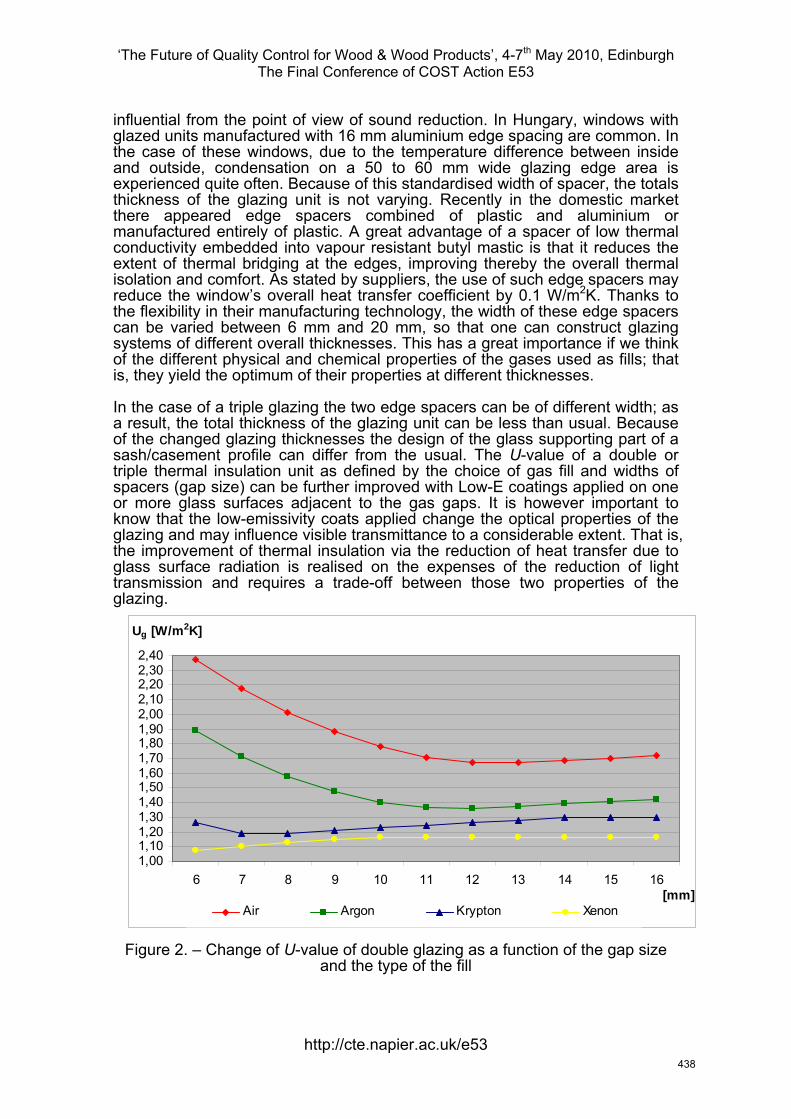
‘The Future of Quality Control for Wood & Wood Products’, 4-7th May 2010, Edinburgh The Final Conference of COST Action E53
influential from the point of view of sound reduction. In Hungary, windows with glazed units manufactured with 16 mm aluminium edge spacing are common. In the case of these windows, due to the temperature difference between inside and outside, condensation on a 50 to 60 mm wide glazing edge area is experienced quite often. Because of this standardised width of spacer, the totals thickness of the glazing unit is not varying. Recently in the domestic market there appeared edge spacers combined of plastic and aluminium or manufactured entirely of plastic. A great advantage of a spacer of low thermal conductivity embedded into vapour resistant butyl mastic is that it reduces the extent of thermal bridging at the edges, improving thereby the overall thermal isolation and comfort. As stated by suppliers, the use of such edge spacers may reduce the window’s overall heat transfer coefficient by 0.1 W/m2K. Thanks to the flexibility in their manufacturing technology, the width of these edge spacers can be varied between 6 mm and 20 mm, so that one can construct glazing systems of different overall thicknesses. This has a great importance if we think of the different physical and chemical properties of the gases used as fills; that is, they yield the optimum of their properties at different thicknesses.
In the case of a triple glazing the two edge spacers can be of different width; as a result, the total thickness of the glazing unit can be less than usual. Because of the changed glazing thicknesses the design of the glass supporting part of a sash/casement profile can differ from the usual. The U-value of a double or triple thermal insulation unit as defined by the choice of gas fill and widths of spacers (gap size) can be further improved with Low-E coatings applied on one or more glass surfaces adjacent to the gas gaps. It is however important to know that the low-emissivity coats applied change the optical properties of the glazing and may influence visible transmittance to a considerable extent. That is, the improvement of thermal insulation via the reduction of heat transfer due to glass surface radiation is realised on the expenses of the reduction of light transmission and requires a trade-off between those two properties of the glazing.
1,001,101,201,301,401,501,601,701,801,902,002,102,202,302,40
6 7 8 9 10 11 12 13 14 15 16[mm]
Ug [W/m2K]
Air Argon Krypton Xenon
Figure 2. – Change of U-value of double glazing as a function of the gap size and the type of the fill
http://cte.napier.ac.uk/e53 438
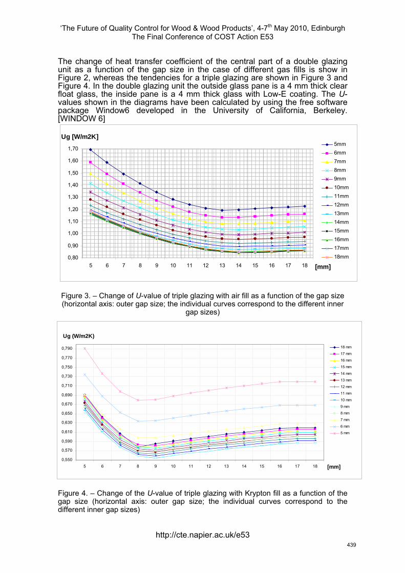
‘The Future of Quality Control for Wood & Wood Products’, 4-7th May 2010, Edinburgh The Final Conference of COST Action E53
The change of heat transfer coefficient of the central part of a double glazing unit as a function of the gap size in the case of different gas fills is show in Figure 2, whereas the tendencies for a triple glazing are shown in Figure 3 and Figure 4. In the double glazing unit the outside glass pane is a 4 mm thick clear float glass, the inside pane is a 4 mm thick glass with Low-E coating. The U-values shown in the diagrams have been calculated by using the free software package Window6 developed in the University of California, Berkeley. [WINDOW 6]
Figure 3. – Change of U-value of triple glazing with air fill as a function of the gap size
0,80
0,90
1,00
1,10
1,20
1,30
1,40
1,50
1,60
1,70
5 6 7 8 9 10 11 12 13 14 15 16 17 18 [mm]
Ug [W/m2K]5mm6mm7mm8mm9mm10mm11mm12mm13mm14mm15mm16mm17mm18mm
(horizontal axis: outer gap size; the individual curves correspond to the different inner gap sizes)
Figure 4. – Change of the U-value of triple glazing with Krypton fill as a function of the gap size (horizontal axis: outer gap size; the individual curves correspond to the different inner gap sizes)
0,770
0,790
Ug (W/m2K)
5 6 7 8 9 10 11 12 13 14 15 16 17 18 [mm]
18 mm
17 mm
16 mm
0,670
0,690
0,710
0,730
0,750 15 mm
14 mm
13 mm
12 mm
11 mm
10 mm
9 mm
8 mm
0,550
0,570
0,590
0,610
0,630
0,6507 mm
6 mm
5 mm
http://cte.napier.ac.uk/e53 439

‘The Future of Quality Control for Wood & Wood Products’, 4-7th May 2010, Edinburgh The Final Conference of COST Action E53
The glazing units are generally positioned by means of setting blocks and shear blocks and fixed in the casement by means of glass beads. In the case of triple glazing systems the increased mass requires reconsidering the casement profile and using hinges of increased load-bearing capacity. A relatively new
s which have much better thermal insulation value as compared to solid wood, significantly increased profile depth can be attained
e of frame is underestimated, while it may amount to 30-35% of the total product area. The
6] was used to study the overall thermal performance of windows of different frame and glazing systems.
he software supports steady-state thermal problems only; therefore we assumed constant boundary conditions both for the inside and outside surfaces.
utoCad drawings were made for the sections of the windows necessary for the analysis. The parameters used are listed in Table 1.
solution is that the glazing unit is fixed beside the edges to the casement profile by continuous adhesive joint. Beyond a gap-free sealing between the glass and the casement profile it has the additional advantage of improved stability and operational safety.
Windows of wood frames in Hungary are mostly manufactured of 3-layer laminated Scots pine (Pinus sylvestris) wood. Profiles of 68 mm deep are generally applied for windows of double glazing systems, the heat transfer coefficient of the frame is typically Uf =1.3 W/m2K. With a same profile depth, air gaps formed in the solid wood cross section may result in a more favourable value of Uf =1.0 W/m2K, while the same solution in the case of a 78 mm deep profile results Uf =0.94 W/m2K. It holds for most types of windows that the sill part is characterised by a worse U-factor than the upright and bottom parts due to the difference in the frame and sash/casement profile that allows water canalisation. When required, one can attain lower heat transfer coefficients for the frame by applying sandwich-type cross section profiles. Thanks to certain light-weight synthetic foam
without important increase of the total mass of the window. The arrangement of the individual layers and the thickness of the different materials in these profiles may be varied. This way a value of Uf =0.75 W/m2K is easily attained with a depth of profile of 85 mm.
An optimally designed sandwich profile with purposeful glazing system may meet the requirements of passive houses. The depth of the frame and casement/sash profile can be reduced if an additional aluminium profile filled with polyurethane foam of suitable thickness is fixed on their outer surfaces. This additional thermal insulation may add significantly to the cost of the window, however one can attain more easily or even exceed the required thermal insulation value. In the overall heat transfer coefficient of a window, the heat transfer of the glazing unit is dominating, since glazing area is generally much larger than the projection area of the frame. However, the smaller the window, the higher is the share of frame area. Very often the shar
change in the nominal sizes of a window directly affects the size of the glazing unit(s); in the case of identical profile cross section, an absolute increase of the nominal sizes entails the same absolute increase of the corresponding size of glazing unit, thus resulting in a more favourable overall U-value.
The overall U-value of a window is defined jointly by the glazing unit and the frame. The Finite Element Analysis based software package Therm developed in the University of California, Berkeley [THERM
T
A
http://cte.napier.ac.uk/e53 440
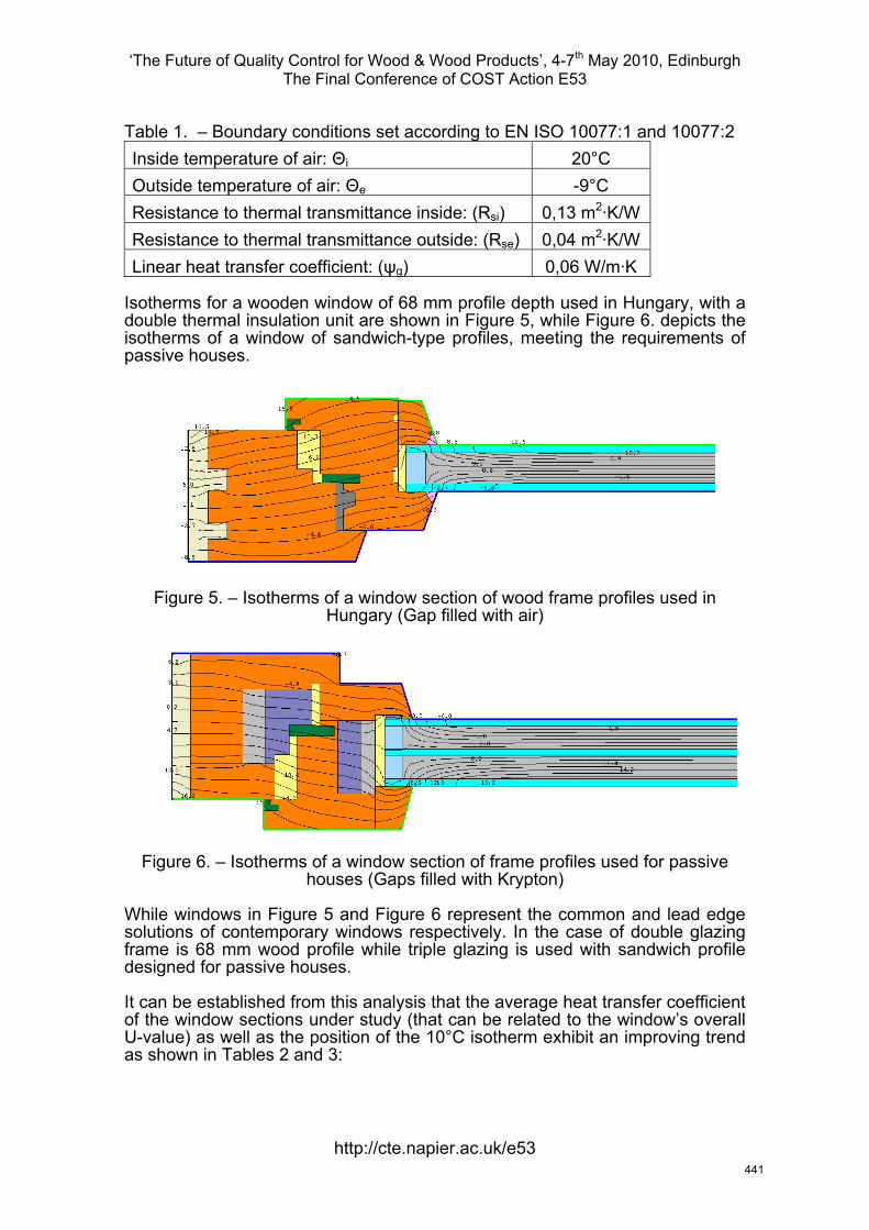
‘The Future of Quality Control for Wood & Wood Products’, 4-7th May 2010, Edinburgh The Final Conference of COST Action E53
T N I d 10077:2 able 1. – Boundary conditions set according to E SO 10077:1 anInside temperature of air: Θi 20°C Outside temperature of air: Θe -9°C Resistance to thermal transmittance inside: (R ) 0,13 m ·K/W 2
si
Resistance to thermal transmittance outside: (Rse) 0,04 m2·K/W Linear heat transfer coefficient: (ψg) 0,06 W/m·K
Isotherms for a wooden window of 68 mm profile depth used in Hungary, with a
While windows in Figure 5 and Figure 6 represent the common and lead edge
It can be established from this analysis that the average heat transfer coefficient f the window sections under study (that can be related to the window’s overall
U-value) as well as the position of the 10°C isotherm exhibit an improving trend
double thermal insulation unit are shown in Figure 5, while Figure 6. depicts the isotherms of a window of sandwich-type profiles, meeting the requirements of passive houses.
Figure 5. – Isotherms of a window section of wood frame profiles used in Hungary (Gap filled with air)
Figure 6. – Isotherms of a window section of frame profiles used for passive houses (Gaps filled with Krypton)
solutions of contemporary windows respectively. In the case of double glazing frame is 68 mm wood profile while triple glazing is used with sandwich profile designed for passive houses.
o
as shown in Tables 2 and 3:
http://cte.napier.ac.uk/e53 441
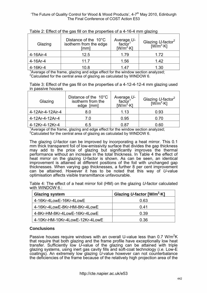
‘The Future of Quality Control for Wood & Wood Products’, 4-7th May 2010, Edinburgh The Final Conference of COST Action E53
Table 2: Effect of t s of 4 mm gla
g Distance of the 10°C
isotherm from the edge Average U-
f [W ]
Glazin ctor2 [W ]
he gas fill on the propertie a 4-16- zing
Glazin[mm]
actor1
/m2·Kg U-fa
2/m ·K
4-16Air-4 12.5 1.79 1.72 4-16Ar-4 11.7 1.56 1.42 4-16Kr-4 10.8 1.47 1.30 1Average of the frame, glazing and edge effect for the window section analyzed; 2Calculated for the central area of glazing as calculatad by WINDOW 6.
Table 3: Effect of the s 12- in passive houses
Distance of the 10°C isotherm from the
edge [mm]
Average U-f
[W ] Glazin ctor2
[W ]
gas fill on the propertie of a 4-12-4- 4 mm glazing used
Glazing actor1
/m2·Kg U-fa
2/m ·K
4-12Air-4-12Air-4 8.0 1.13 0.93 4-12Ar-4-12Ar-4 7.0 0.95 0.70 4-12Kr-4-12Kr-4 6.5 0.87 0.60 1Average of the frame, glazing and edge effect for the window section analyzed; 2Calculated for the central area of glazing as calculatad by WINDOW 6.
The glazing U-factor can be improved by incorporating a heat mirror. This 0.1 mm thick transparent foil of low-emissivity surface that divides the gap thickness may add to the price of glazing but significantly improves the thermal performance without an increase in the total thickness. In Table 4 the effect of heat mirror on the glazing U-factor is shown. As can be seen, an identical improvement is attained at different positions of the foil with unchanged gap thicknesses. When varying gap thicknesses, a further 8 per cent improvement
visible transmittance unfavourable.
Ta of a heat mirror foil (HM) lated wi
Glazing U-factor [W/m2·K]
can be attained. However it has to be noted that this way of U-value optimisation affects
ble 4: The effect on the glazing U-factor calcuth WINDOW 6.: Glazing system 4-16Kr-4LowE-16Kr-4LowE 0.63 4-16Kr-4LowE-8Kr-HM-8Kr-4LowE 0.41 4-8Kr-HM-8Kr-4LowE-16Kr-4LowE 0.39 4-10Kr-HM-10Kr-4LowE-12Kr-4LowE 0.36
Conclusions
Passive houses require windows with an overall U-value less than 0.7 W/m2K that require that both glazing and the frame profile have exceptionally low heat transfer. Sufficiently low U-value of the glazing can be attained with triple glazing systems, using inert gas cavity fills and soft-coat technology (i.e. Low-E coatings). An extremely low glazing U-value however can not counterbalance the deficiencies of the frame because of the relatively high projection area of the
http://cte.napier.ac.uk/e53 442
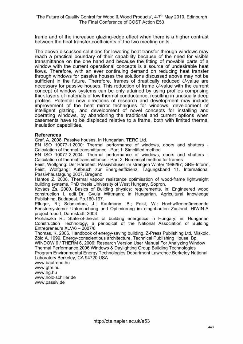
‘The Future of Quality Control for Wood & Wood Products’, 4-7th May 2010, Edinburgh The Final Conference of COST Action E53
frame and of the increased glazing-edge effect when there is a higher contrast between the heat transfer coefficients of the two meeting units..
The above discussed solutions for lowering heat transfer through windows may reach a practical boundary of their capability because of the need for visible transmittance on the one hand and because the fitting of movable parts of a window with the current operational concepts is a source of undesirable heat flows. Therefore, with an ever continuing demand on reducing heat transfer through windows for passive houses the solutions discussed above may not be sufficient in the future. Therefore, frames of drastically reduced U-value are necessary for passive houses. This reduction of frame U-value with the current concept of window systems can be only attained by using profiles comprising thick layers of materials of low thermal conductance, resulting in unusually deep profiles. Potential new directions of research and development may include improvement of the heat mirror techniques for windows, development of intelligent glazing, and development of novel concepts for installing and operating windows, by abandoning the traditional and current options when
ve to be displaced relative to a frame, both with limited thermal
shutters -
e - Part 2: Numerical method for frames
11. International
sity of West Hungary, Sopron.
7.
ding
skolc.
ch Version User Manual For Analyzing Window ce 2006 Windows & Daylighting Group Building Technologies
onmental Energy Technologies Department Lawrence Berkeley National erkeley, CA 94720 USA
www.hg.hu www.holz-schiller.de www.passiv.de
casements hainsulation capabilities.
References Graf, A. 2008. Passive houses. In Hungarian. TERC Ltd. EN ISO 10077-1:2000: Thermal performance of windows, doors andCalculation of thermal transmittance - Part 1: Simplified method EN ISO 10077-2:2004: Thermal performance of windows, doors and shutters - Calculation of thermal transmittancFeist, Wolfgang: Der Härtetest: Passivhäuser im strengen Winter 1996/97; GRE-Inform, Feist, Wolfgang: Aufbruch zur Energieeffizienz; TagungsbandPassivhaustagung 2007, Bregenz Hantos Z. 2008. Thermal vapour resistance optimisation of wood-frame lightweight building systems. PhD thesis UniverKovács Zs. 2000. Basics of Building physics; requirements. in: Engineered wood construction I. edit.:Dr. Gyula Wittmann; in Hungarian. Agricultural knowledge Publishing, Budapest. Pp.160-19Pfluger, R.; Schnieders, J.; Kaufmann, B.; Feist, W.: Hochwärmedämmende Fenstersysteme: Untersuchung und Optimierung im eingebauten Zustand, HIWIN-A project report, Darmstadt, 2003 Prohászka R.: State-of-the-art of building energetics in Hungary. in: Hungarian Construction Technology, a periodical of the National Association of BuilEntrepreneurs XLV/6 – 2007/6 Thomas, K. 2006. Handbook of energy-saving building. Z-Press Publishing Ltd, MiZöld A. 1999. Energy-conscientious architecture. Technical Publishing House, Bp. WINDOW 6 / THERM 6, 2006: ResearThermal PerformanProgram EnvirLaboratory Bwww.bautrend.hu www.gtm.hu
http://cte.napier.ac.uk/e53 443
‘The Future of Quality Control for Wood & Wood Products’, 4-7th May 2010, Edinburgh The Final Conference of COST Action E53
A few Elastic Properties of Drilled Rectangular Bars of Poplar Wood
A.Yavari1, M. Roohnia2& A. Tajdini3
Abstract
Some elastic properties of 13 rectangular clear bars of poplar wood in “free vibration of a free-free bar” method were examined with and without presence of drilled holes in different diameters of zero, three, five and eight millimeters on tangential surface exactly on the anti-node of the 1st mode of vibration, visible on two tangential surfaces. Specimens originated from planting region in Zanjan – Iran. Nominal dimensions of the bars were 20*20*360 mm. Considering three first modes of vibration, longitudinal modulus of elasticity and two shear moduli (GLR and GLT) were evaluated in Timoshenko beam theory and damping factor (tandLT and tandLR) evaluated from logarithmic decrement calculations for both radial and tangential impacts of hammer. Step wise drilling showed no significant effect on EL, GLR and GLT and tandLT. But when the bars were impacted on tangential surface, the drilling holes, on their largest diameters could affect the tandLR while the effects of smaller holes on above mentioned factors were not obvious.
1 Introduction
In this research, Eastern poplar (Populus Deltoides) was used in free flexural vibration on free free bar. Each of the specimens vibrated based on their mechanical properties. Even small mechanical variations within the specimen due to anisotropy or defects can result in modal frequencies of vibration. The objective of this experiment was to detect these defects (especially hole) for longer and better performances of poplar wood.
The sound absorption and acoustical impedance in poplar over different frequencies studied and compared with beech and alder. It was found that poplar solid wood has the highest absorption, and observed the resonance in beech due to higher density and more proportion of rays( Noorbakhsh 1997). ultrasonic longitudinal and shear wave velocities and densities for 12 Australian wood species were measured, comprising eleven hard woods and one soft wood by comparing the results with those obtained for European woods and similar ranges have found (Bucur 1991). In order to compare the mode shapes of vibration before and after damage in timbers, modal-based testing was applied on wood bars in order to propose a new statistical algorithm for
1 Corresponding author, PhD Candidate, [email protected] Azad University, Science and Research Branch – IRAN 2 Assistant Professor, [email protected] Azad University, Karaj Branch – IRAN 3 Assistant Professor, [email protected] Islamic Azad University, Karaj Branch – IRAN
http://cte.napier.ac.uk/e53 444
‘The Future of Quality Control for Wood & Wood Products’, 4-7th May 2010, Edinburgh The Final Conference of COST Action E53
obtaining a defect indicator (Hu et al., 2006). Free vibration testing was used to generate the two initial mode shapes for damage detection in timbers and it was proved that the chosen Daubechies 3 wavelet was suitable and sufficiently sensitive to identify the location, extent and number of different damages(Hu et al., 2006). ultrasonic study has sought to 1) determine the ultrasonic parameters that are most sensitive to pallet part defects; and 2) specify which aspects of ultrasonic response signals best characterize defect size and location (Daniel L. Schmoldt.,1994). By Assessment of Decay in Standing Timber Using Stress Wave Timing Nondestructive Evaluation Tools , the use of stress wave timing instruments to locate and define areas of decay in standing timber, the guide was prepared to assist field foresters. (Xiping Wang.,2004). Ultrasonic scanning experiments were conducted for detecting defects in wood pallet parts using rolling transducers. The paper reports the scanning results for stringers and deckboards. Sound and unsound knots,bark pockets, decay, splits, holes, and wane were characterized using several ultrasonic parameters. (M. Firoz Kabir., 2002). ULTRASONIC SIGNAL CHARACTERIZATION FOR DEFECTS IN THIN UNSURFACED HARDWOOD LUMBER describes initial work aiming to create an automated grading/sorting system for hardwood pallet parts using ultrasonic. Experiments were conducted on yellow-poplar (Liriodendron tulipifera, L.) and red oak (Quercus rubra, L.). Sound and unsound knots, cross grain, bark pockets, holes, splits, and decay were characterized using six ultrasound variables calculated from the received waveforms. (Mohammed F. Kabir ,.2001)
2 Materials and methods
The specific longitudinal modulus of elasticity (MOEL/ρ) and the shear modulus can be evaluated based on Timoshenko bar equations and Bordonné Solution (Bordonné, 1989; Brancheriau et al., 2002). In this equation, after obtaining the kth frequency through Fourier Transform, considering ak and bk, the value of longitudinal specific modulus of elasticity was determined using a linear regression formula as following:
http://cte.napier.ac.uk/e53 445
‘The Future of Quality Control for Wood & Wood Products’, 4-7th May 2010, Edinburgh The Final Conference of COST Action E53
where I; moment of inertia, A; cross section area, l; length of the specimen, K;shape coefficient (the value of 5/6 can be used for a rectangular cross section), Gij; shear modulus in plane of vibration (GLT or GLR), ρ; specific gravity, fk; frequency of the kth mode of vibration obtained from FFT spectrum mk; the kth results in following Equation:
In Equations 1 and 2, F1k and F2k can be calculated as following:
Higher correlation coefficients of the estimated trend lines in Equation 1 benefit the specimens with more homogeneity, where the Timoshenko model has been fitted initially to isotropic materials, and next to the clearest specimens. The selection was made based on trends with correlation coefficients higher than 0.99. Sampling was made selectively, numbers of wooden-sample and wholesome in shape were selected from spruce, the reason of selecting was: 1-this species was accessible 2-this species is homogametic and it is categorized as a fast growth species (4 times faster than eucalyptus and 7 times faster than softwoods ) 3-it can grow in many and different weather conditions 4-we could place the knot like real one in it and finally this species is commonly used in Iran (cutting species and then drying them was done very slowly and without tension in the air at low temperature).
In this study, Eastern poplar (Populus Deltoides) timbers were randomly collected from plantations in Zanjan province in the region between West Alborz and North Zagros Mountains. Following ISO 3129 international standard. Rectangular and visually clear wooden bars (specimens) were obtained. The specimens were cut to their final nominal dimensions of 2*2*36 cm, R*T*L, and kept in a conditioning chamber at 21°C and 65 percent relative humidity for two
http://cte.napier.ac.uk/e53 446
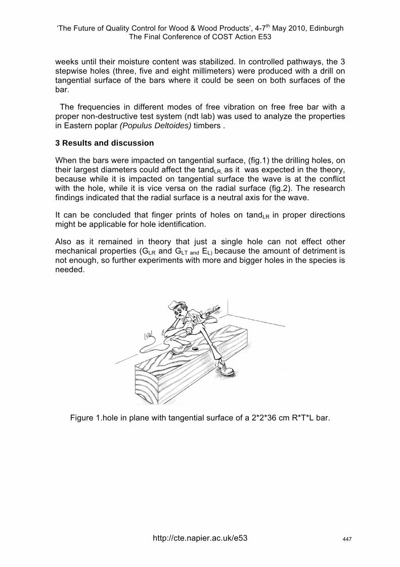
‘The Future of Quality Control for Wood & Wood Products’, 4-7th May 2010, Edinburgh The Final Conference of COST Action E53
weeks until their moisture content was stabilized. In controlled pathways, the 3 stepwise holes (three, five and eight millimeters) were produced with a drill on tangential surface of the bars where it could be seen on both surfaces of the bar.
The frequencies in different modes of free vibration on free free bar with a proper non-destructive test system (ndt lab) was used to analyze the properties in Eastern poplar (Populus Deltoides) timbers .
3 Results and discussion
When the bars were impacted on tangential surface, (fig.1) the drilling holes, on their largest diameters could affect the tandLR, as it was expected in the theory, because while it is impacted on tangential surface the wave is at the conflict with the hole, while it is vice versa on the radial surface (fig.2). The research findings indicated that the radial surface is a neutral axis for the wave.
It can be concluded that finger prints of holes on tandLR in proper directions might be applicable for hole identification.
Also as it remained in theory that just a single hole can not effect other mechanical properties (GLR and GLT and EL) because the amount of detriment is not enough, so further experiments with more and bigger holes in the species is needed.
Figure 1.hole in plane with tangential surface of a 2*2*36 cm R*T*L bar.
http://cte.napier.ac.uk/e53 447
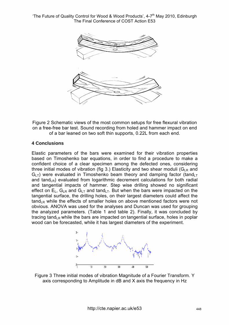
‘The Future of Quality Control for Wood & Wood Products’, 4-7th May 2010, Edinburgh The Final Conference of COST Action E53
Figure 2 Schematic views of the most common setups for free flexural vibration on a free-free bar test. Sound recording from holed and hammer impact on end
of a bar leaned on two soft thin supports, 0.22L from each end.
4 Conclusions
Elastic parameters of the bars were examined for their vibration properties based on Timoshenko bar equations, in order to find a procedure to make a confident choice of a clear specimen among the defected ones, considering three initial modes of vibration (fig 3.) Elasticity and two shear moduli (GLR and GLT) were evaluated in Timoshenko beam theory and damping factor (tandLT and tandLR) evaluated from logarithmic decrement calculations for both radial and tangential impacts of hammer. Step wise drilling showed no significant effect on EL, GLR and GLT and tandLT. But when the bars were impacted on the tangential surface, the drilling holes, on their largest diameters could affect the tandLR while the effects of smaller holes on above mentioned factors were not obvious. ANOVA was used for the analyses and Duncan was used for grouping the analyzed parameters. (Table 1 and table 2). Finally, it was concluded by tracing tandLR while the bars are impacted on tangential surface, holes in poplar wood can be forecasted, while it has largest diameters of the experiment.
Figure 3 Three initial modes of vibration Magnitude of a Fourier Transform. Y axis corresponding to Amplitude in dB and X axis the frequency in Hz
http://cte.napier.ac.uk/e53 448
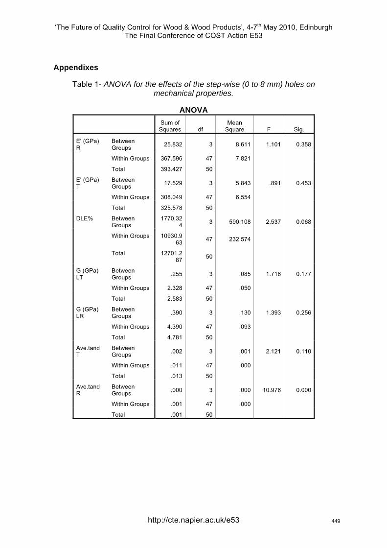
‘The Future of Quality Control for Wood & Wood Products’, 4-7th May 2010, Edinburgh The Final Conference of COST Action E53
Appendixes
Table 1- ANOVA for the effects of the step-wise (0 to 8 mm) holes on mechanical properties.
ANOVA
Sum of
Squares df Mean
Square F Sig.
E' (GPa) R
Between Groups 25.832 3 8.611 1.101 0.358
Within Groups 367.596 47 7.821
Total 393.427 50
E' (GPa) T
Between Groups 17.529 3 5.843 .891 0.453
Within Groups 308.049 47 6.554
Total 325.578 50
DLE% Between Groups
1770.324 3 590.108 2.537 0.068
Within Groups 10930.963 47 232.574
Total 12701.287 50
G (GPa) LT
Between Groups .255 3 .085 1.716 0.177
Within Groups 2.328 47 .050
Total 2.583 50
G (GPa) LR
Between Groups .390 3 .130 1.393 0.256
Within Groups 4.390 47 .093
Total 4.781 50
Ave.tand T
Between Groups .002 3 .001 2.121 0.110
Within Groups .011 47 .000
Total .013 50
Ave.tand R
Between Groups .000 3 .000 10.976 0.000
Within Groups .001 47 .000
Total .001 50
http://cte.napier.ac.uk/e53 449

‘The Future of Quality Control for Wood & Wood Products’, 4-7th May 2010, Edinburgh The Final Conference of COST Action E53
Table 2- Duncan multiple comparison tests for the affect the tandLR
Duncan
Subset for alpha = .05
HOLE N 1 2
1 13 .005710
2 13 .005805
3 12 .007106
4 13 .012178
Sig. .324 1.000
Means for groups in homogeneous subsets are displayed.
a Uses Harmonic Mean Sample Size = 12.735.
b The group sizes are unequal. The harmonic mean of the group sizes is used. Type I error levels are not guaranteed.
Acknowledgements
we sincerely thank Mr. Rahi Gaffarian from Islamic Azad University, Karaj Branch for their caricatures and drawings.
References
Bucur,v.1991.acoustics properties and anisotropy of some Australian wood species acousticas.Hizel verlag stuttgat vol 75
Daniel L. Schmoldt, John C. Duke, Jr.,Michael Morrone, and Chris M. Jennings.,1994.Application of ultrasound nondestructive evaluation to grading pallet parts
Hu C., & Afzal M.T., 2006. A wavelet analysis-based approach for damage localization in wood beams. Journal of Wood Science. 52: 456 – 460.
Hu C., & Afzal M.T., 2006. A statistical algorithm for comparing mode shapes of vibration testing before and after damage in timbers. Journal of Wood Science. 52:348 – 352
http://cte.napier.ac.uk/e53 450
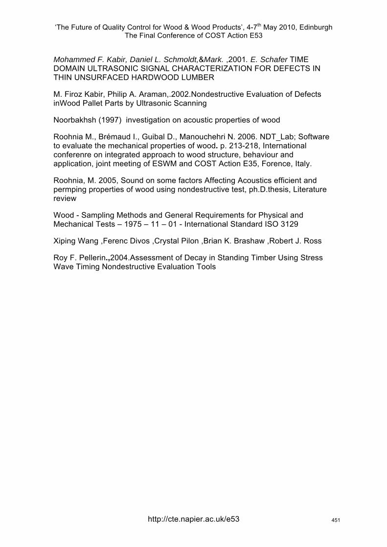
‘The Future of Quality Control for Wood & Wood Products’, 4-7th May 2010, Edinburgh The Final Conference of COST Action E53
Mohammed F. Kabir, Daniel L. Schmoldt,&Mark. ,2001. E. Schafer TIME DOMAIN ULTRASONIC SIGNAL CHARACTERIZATION FOR DEFECTS IN THIN UNSURFACED HARDWOOD LUMBER
M. Firoz Kabir, Philip A. Araman,.2002.Nondestructive Evaluation of Defects inWood Pallet Parts by Ultrasonic Scanning
Noorbakhsh (1997) investigation on acoustic properties of wood
Roohnia M., Brémaud I., Guibal D., Manouchehri N. 2006. NDT_Lab; Software to evaluate the mechanical properties of wood. p. 213-218, International conferenre on integrated approach to wood structure, behaviour and application, joint meeting of ESWM and COST Action E35, Forence, Italy.
Roohnia, M. 2005, Sound on some factors Affecting Acoustics efficient and permping properties of wood using nondestructive test, ph.D.thesis, Literature review
Wood - Sampling Methods and General Requirements for Physical and Mechanical Tests – 1975 – 11 – 01 - International Standard ISO 3129
Xiping Wang ,Ferenc Divos ,Crystal Pilon ,Brian K. Brashaw ,Robert J. Ross
Roy F. Pellerin.,2004.Assessment of Decay in Standing Timber Using Stress Wave Timing Nondestructive Evaluation Tools
http://cte.napier.ac.uk/e53 451

‘The Future of Quality Control for Wood & Wood Products’, 4-7th May 2010, Edinburgh The Final Conference of COST Action E53
Thursday 6th May Research focussed day
Parallel session 2B
http://www.cte.napier.ac.uk/e53/ 452
‘The Future of Quality Control for Wood & Wood Products’, 4-7th May 2010, Edinburgh The Final Conference of COST Action E53
http://cte.napier.ac.uk/e53
Quality control of glulam: Improved method for shear testing of glue lines
R. Steiger 1 & E. Gehri 2
Abstract Among other tests, shear tests of glue lines are required in the course of quality control measures to be carried out in glulam plants. The procedures to be followed are given in different standards like for example EN 392:1995 and ISO 12579:2006. In most of the standards the method of applying shear stress to the glue line is only given by a principle scheme. Based on this scheme a variety of test equipment has been produced and is in use by materials testing laboratories, glulam manufacturers and producers of adhesives. Depending on the actual construction of the test equipment as well as on the procedure of testing, the resulting stress in the glue line is not pure shear but rather a combination of shear and normal stresses. In case of simultaneously acting shear stress and tensile stress perpendicular to the grain, the shear strength values can drop dramatically, whereas compression stresses perpendicular to the grain lead to an overestimation of the shear strength of the bond line. Starting from an explanation of the multiaxial stress situation by static equilibrium analysis, parameters are identified which influence the test results. To avoid the statically indeterminate loading situation, a prototype of a shear test device has been developed aiming to ensure a clearly defined state of shear loading of the specimens. Extensive test results on the comparison of the prototype device with the established one in terms of shear strengths and percentages of wood failure are presented and discussed.
1 Introduction Shear tests of the glue lines are required in the course of quality control measures to be carried out in glulam plants. The procedures to be followed are given in various standards like for example EN 392 (CEN 1995), ASTM D 905-03 (ASTM 2003) and ISO 12579 (ISO 2006). However, the method of applying shear stress to the glue line is only given by a principle scheme (Figure 1). Based on this scheme a variety of test equipment has been produced and is used by test laboratories and by producers of glulam and adhesives.
Depending on the actual construction of the test equipment as well as the procedure of testing, the resulting stress in the glue line is neither uniformly distributed nor pure shear but rather a combination of shear and normal stresses. In case of simultaneously acting shear stress and tensile stress
1 Senior Scientist, [email protected] Empa, Wood Laboratory, Dübendorf, Switzerland 2 Professor emeritus ETH Zurich, [email protected]
453
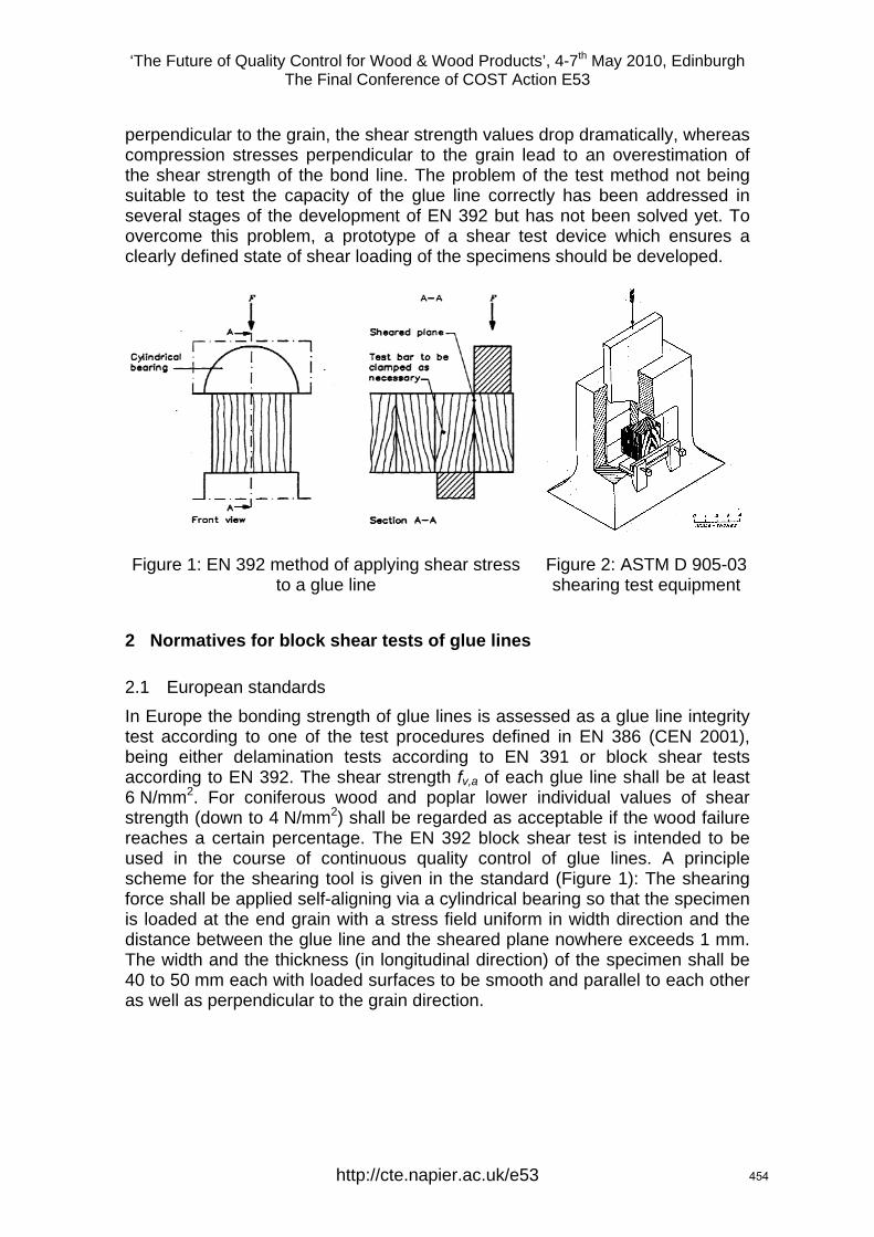
‘The Future of Quality Control for Wood & Wood Products’, 4-7th May 2010, Edinburgh The Final Conference of COST Action E53
http://cte.napier.ac.uk/e53
perpendicular to the grain, the shear strength values drop dramatically, whereas compression stresses perpendicular to the grain lead to an overestimation of the shear strength of the bond line. The problem of the test method not being suitable to test the capacity of the glue line correctly has been addressed in several stages of the development of EN 392 but has not been solved yet. To overcome this problem, a prototype of a shear test device which ensures a clearly defined state of shear loading of the specimens should be developed.
Figure 1: EN 392 method of applying shear stress to a glue line
Figure 2: ASTM D 905-03 shearing test equipment
2 Normatives for block shear tests of glue lines
2.1 European standards In Europe the bonding strength of glue lines is assessed as a glue line integrity test according to one of the test procedures defined in EN 386 (CEN 2001), being either delamination tests according to EN 391 or block shear tests according to EN 392. The shear strength fv,a of each glue line shall be at least 6 N/mm2. For coniferous wood and poplar lower individual values of shear strength (down to 4 N/mm2) shall be regarded as acceptable if the wood failure reaches a certain percentage. The EN 392 block shear test is intended to be used in the course of continuous quality control of glue lines. A principle scheme for the shearing tool is given in the standard (Figure 1): The shearing force shall be applied self-aligning via a cylindrical bearing so that the specimen is loaded at the end grain with a stress field uniform in width direction and the distance between the glue line and the sheared plane nowhere exceeds 1 mm. The width and the thickness (in longitudinal direction) of the specimen shall be 40 to 50 mm each with loaded surfaces to be smooth and parallel to each other as well as perpendicular to the grain direction.
454

‘The Future of Quality Control for Wood & Wood Products’, 4-7th May 2010, Edinburgh The Final Conference of COST Action E53
http://cte.napier.ac.uk/e53
2.2 American standards In the United States shear testing of glue lines is addressed by the standard ASTM D 905-03 (ASTM 2003). The standard makes aware of the fact that "this test method cannot be assumed to measure the true shear strength of the adhesive bond" because "many factors interfere or bias the measurement including the strength of the wood, the specimen, the shear tool design themselves and the rate of loading". It is also mentioned, that "stress concentrations at the notches of the specimen tend to lower the measured strength". The shearing tool to be used shall have a self-aligning seat ensuring uniform lateral distribution of the load. Figure 2 shows a respective tool.
2.3 ISO standards The formulations in the ISO standards are similar to the European pendants. For block shear tests the standards ISO 12579 (ISO 2006) and ISO 6238 (ISO 2001) are ruling. ISO 12579 provides a combination of rules taken from EN 392 and ASTM D 905. Concerning the apparatus to be used for the shear tests, the ISO standard as well gives only a schematic sketch similar to EN 392. In ISO 6238 (ISO 2001) a shearing tool for compressive shear block tests being identical to the one shown in ASTM D 905-03 (Figure 2) is mentioned.
3 Advantages and shortcomings of the block shear test method The block shear test method has the advantage of being simple with regard to the preparation of the test specimen, the test equipment needed, the overall procedure and the analysis of the test results. But on the other hand there are several shortcomings to be mentioned:
The test method suffers from a non uniform shear stress distribution with a stress concentration near the corner as it was shown by experimental and theoretical stress analysis (Coker & Coleman 1935, Radcliffe & Suddarth 1955).
The test results are influenced by the actual materialisation of the principal sketch in EN 392 (Figure 1) as well as by the person carrying out the test (see 4).
During the shear test, the specimen is subjected to a shear strain. Most of the existing shearing devices hinder this strain. This results in unknown side effects on the test results.
Test results derived using different test devices cannot be compared directly. Strictly said: the method only serves the glulam producer as a kind of warning sign if the test values drop below a certain threshold.
4 Analysis of static equilibrium The state of static equilibrium in specimens tested according to EN 392 is shown in Figure 3. Being not aligned but rather eccentric (with a gap e depending on the dimensions of the stamps A of the actual test equipment) the acting shearing forces Av cause a moment Ave, which has to be compensated
455

‘The Future of Quality Control for Wood & Wood Products’, 4-7th May 2010, Edinburgh The Final Conference of COST Action E53
http://cte.napier.ac.uk/e53
by a counteracting moment hAh. Both the eccentricity e and the counteracting moment are indeterminate, depending on the shearing device. Actually there is a state of compression at an angle to the grain ( arctan (Ah/Av)) and a counteracting moment is built up when the zone of maximum compression stress is deformed. The deformation leads to an uplift of the test bar. If the uplift is prevented for example by holding down the test bar, significant bending stresses are added to the acting shear stresses and the specimen tends to fail early at low level of shear stress.
Figure 3: Static equilibrium in specimens tested according to EN 392
5 Optimized block shear test
5.1 Approach Shear strength can also be derived by carrying out compression tests with a certain inclination between load and grain direction. Panel shear tests to derive shear strength according to EN 408 (CEN 2003) for example are based on that. There an oblique angle between the loading direction and the longitudinal axis of the specimen (which is actually the grain direction) of 14° is used.
5.2 Compression and tension stresses at an angle to the grain
Different angles between loading directions and grain can e. g. be modelled by the Hankinson-formula (Hankinson 1921), which independently was also found by Kollmann (1934) based on scientific findings in crystal physics by Hörig (1931). However, the Hankinson formula does not provide any information on failure modes to be expected with varying angles . Analysing stress equilibrium of an isotropic plane strain element subjected to a stress inclined by an angle with reference to the grain direction Stüssi (1946, 1949) showed a relation between normal stresses and shear stresses . The principle stresses 1 and 2 are:
456
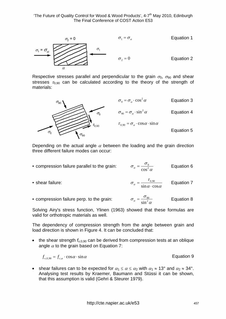
‘The Future of Quality Control for Wood & Wood Products’, 4-7th May 2010, Edinburgh The Final Conference of COST Action E53
http://cte.napier.ac.uk/e53
1 Equation 1
02 Equation 2
Respective stresses parallel and perpendicular to the grain 0, 90 and shear stresses 0,90 can be calculated according to the theory of the strength of materials:
2
0 cos Equation 3
2
90 sin Equation 4
sincos90,0 Equation 5
Depending on the actual angle between the loading and the grain direction three different failure modes can occur:
• compression failure parallel to the grain:
20
cos Equation 6
• shear failure:
cossin
90,0
Equation 7
• compression failure perp. to the grain:
290
sin Equation 8
Solving Airy's stress function, Ylinen (1963) showed that these formulas are valid for orthotropic materials as well.
The dependency of compression strength from the angle between grain and load direction is shown in Figure 4. It can be concluded that:
the shear strength fv,0,90 can be derived from compression tests at an oblique angle to the grain based on Equation 7:
sincos,90,0, cv ff Equation 9
shear failures can to be expected for 1 2 with 1 13° and 2 34°. Analysing test results by Kraemer, Baumann and Stüssi it can be shown, that this assumption is valid (Gehri & Steurer 1979).
457
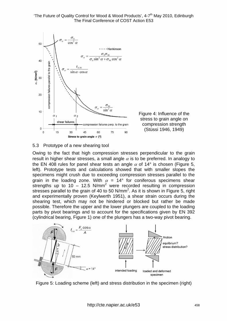
‘The Future of Quality Control for Wood & Wood Products’, 4-7th May 2010, Edinburgh The Final Conference of COST Action E53
http://cte.napier.ac.uk/e53
Figure 4: Influence of the stress to grain angle on compression strength (Stüssi 1946, 1949)
5.3 Prototype of a new shearing tool Owing to the fact that high compression stresses perpendicular to the grain result in higher shear stresses, a small angle is to be preferred. In analogy to the EN 408 rules for panel shear tests an angle of 14° is chosen (Figure 5, left). Prototype tests and calculations showed that with smaller slopes the specimens might crush due to exceeding compression stresses parallel to the grain in the loading zone. With = 14° for coniferous specimens shear strengths up to 10 – 12.5 N/mm2 were recorded resulting in compression stresses parallel to the grain of 40 to 50 N/mm2. As it is shown in Figure 5, right and experimentally proven (Keylwerth 1951), a shear strain occurs during the shearing test, which may not be hindered or blocked but rather be made possible. Therefore the upper and the lower plungers are coupled to the loading parts by pivot bearings and to account for the specifications given by EN 392 (cylindrical bearing, Figure 1) one of the plungers has a two-way pivot bearing.
Figure 5: Loading scheme (left) and stress distribution in the specimen (right)
,cosu
v aFf
A
458
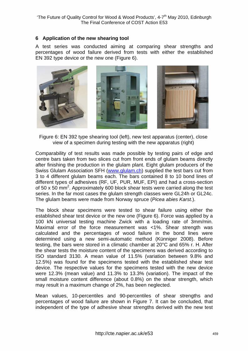
‘The Future of Quality Control for Wood & Wood Products’, 4-7th May 2010, Edinburgh The Final Conference of COST Action E53
http://cte.napier.ac.uk/e53
6 Application of the new shearing tool A test series was conducted aiming at comparing shear strengths and percentages of wood failure derived from tests with either the established EN 392 type device or the new one (Figure 6).
Figure 6: EN 392 type shearing tool (left), new test apparatus (center), close view of a specimen during testing with the new apparatus (right)
Comparability of test results was made possible by testing pairs of edge and centre bars taken from two slices cut from front ends of glulam beams directly after finishing the production in the glulam plant. Eight glulam producers of the Swiss Glulam Association SFH (www.glulam.ch) supplied the test bars cut from 3 to 4 different glulam beams each. The bars contained 8 to 10 bond lines of different types of adhesives (RF, UF, PUR, MUF, EPI) and had a cross-section of 50 x 50 mm2. Approximately 600 block shear tests were carried along the test series. In the far most cases the glulam strength classes were GL24h or GL24c. The glulam beams were made from Norway spruce (Picea abies Karst.).
The block shear specimens were tested to shear failure using either the established shear test device or the new one (Figure 6). Force was applied by a 100 kN universal testing machine Zwick with a loading rate of 3mm/min. Maximal error of the force measurement was <1%. Shear strength was calculated and the percentages of wood failure in the bond lines were determined using a new semi-automatic method (Künniger 2008). Before testing, the bars were stored in a climatic chamber at 20°C and 65% r. H. After the shear tests the moisture content of the specimens was derived according to ISO standard 3130. A mean value of 11.5% (variation between 9.8% and 12.5%) was found for the specimens tested with the established shear test device. The respective values for the specimens tested with the new device were 12.3% (mean value) and 11.3% to 13.3% (variation). The impact of the small moisture content difference (about 0.8%) on the shear strength, which may result in a maximum change of 2%, has been neglected.
Mean values, 10-percentiles and 90-percentiles of shear strengths and percentages of wood failure are shown in Figure 7. It can be concluded, that independent of the type of adhesive shear strengths derived with the new test
459
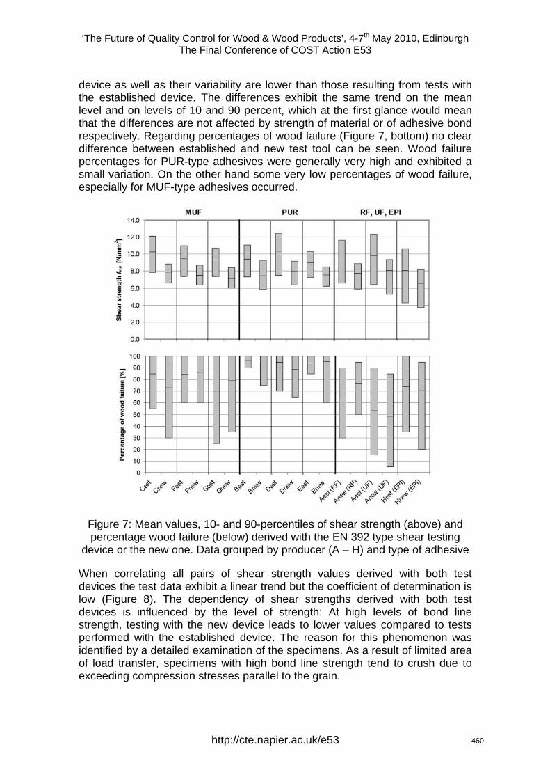
‘The Future of Quality Control for Wood & Wood Products’, 4-7th May 2010, Edinburgh The Final Conference of COST Action E53
http://cte.napier.ac.uk/e53
device as well as their variability are lower than those resulting from tests with the established device. The differences exhibit the same trend on the mean level and on levels of 10 and 90 percent, which at the first glance would mean that the differences are not affected by strength of material or of adhesive bond respectively. Regarding percentages of wood failure (Figure 7, bottom) no clear difference between established and new test tool can be seen. Wood failure percentages for PUR-type adhesives were generally very high and exhibited a small variation. On the other hand some very low percentages of wood failure, especially for MUF-type adhesives occurred.
Figure 7: Mean values, 10- and 90-percentiles of shear strength (above) and percentage wood failure (below) derived with the EN 392 type shear testing
device or the new one. Data grouped by producer (A – H) and type of adhesive
When correlating all pairs of shear strength values derived with both test devices the test data exhibit a linear trend but the coefficient of determination is low (Figure 8). The dependency of shear strengths derived with both test devices is influenced by the level of strength: At high levels of bond line strength, testing with the new device leads to lower values compared to tests performed with the established device. The reason for this phenomenon was identified by a detailed examination of the specimens. As a result of limited area of load transfer, specimens with high bond line strength tend to crush due to exceeding compression stresses parallel to the grain.
460
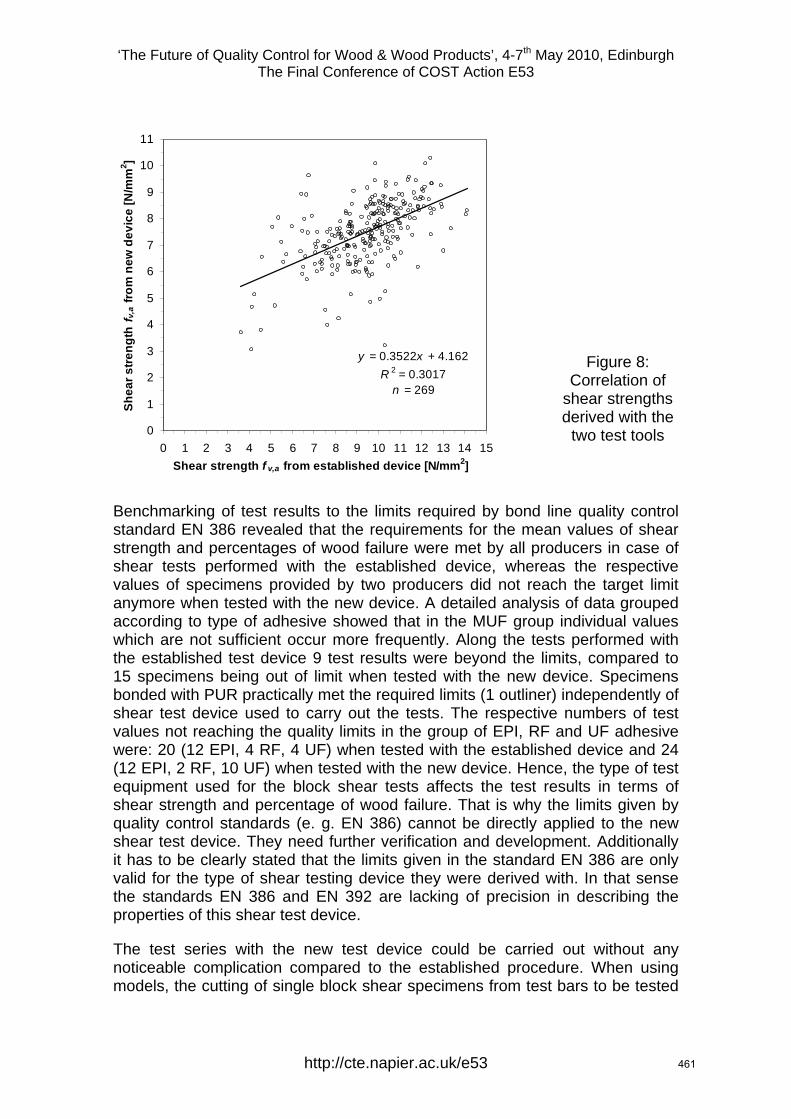
‘The Future of Quality Control for Wood & Wood Products’, 4-7th May 2010, Edinburgh The Final Conference of COST Action E53
http://cte.napier.ac.uk/e53
y = 0.3522x + 4.162R 2 = 0.3017
n = 269
0
1
2
3
4
5
6
7
8
9
10
11
0 1 2 3 4 5 6 7 8 9 10 11 12 13 14 15Shear strength f v,a from established device [N/mm2]
Shea
r stre
ngth
f v,a
from
new
dev
ice
[N/m
m2 ]
Figure 8: Correlation of
shear strengths derived with the
two test tools
Benchmarking of test results to the limits required by bond line quality control standard EN 386 revealed that the requirements for the mean values of shear strength and percentages of wood failure were met by all producers in case of shear tests performed with the established device, whereas the respective values of specimens provided by two producers did not reach the target limit anymore when tested with the new device. A detailed analysis of data grouped according to type of adhesive showed that in the MUF group individual values which are not sufficient occur more frequently. Along the tests performed with the established test device 9 test results were beyond the limits, compared to 15 specimens being out of limit when tested with the new device. Specimens bonded with PUR practically met the required limits (1 outliner) independently of shear test device used to carry out the tests. The respective numbers of test values not reaching the quality limits in the group of EPI, RF and UF adhesive were: 20 (12 EPI, 4 RF, 4 UF) when tested with the established device and 24 (12 EPI, 2 RF, 10 UF) when tested with the new device. Hence, the type of test equipment used for the block shear tests affects the test results in terms of shear strength and percentage of wood failure. That is why the limits given by quality control standards (e. g. EN 386) cannot be directly applied to the new shear test device. They need further verification and development. Additionally it has to be clearly stated that the limits given in the standard EN 386 are only valid for the type of shear testing device they were derived with. In that sense the standards EN 386 and EN 392 are lacking of precision in describing the properties of this shear test device.
The test series with the new test device could be carried out without any noticeable complication compared to the established procedure. When using models, the cutting of single block shear specimens from test bars to be tested
461
‘The Future of Quality Control for Wood & Wood Products’, 4-7th May 2010, Edinburgh The Final Conference of COST Action E53
http://cte.napier.ac.uk/e53
with the new device can easily be done. Request on geometrical precision of trimming the single block shear specimens however is higher, especially regarding the correct position of the bond line with respect to the sheared area within the new test device (Figure 6, centre and right). Due to limited travel of piston of the new test device some specimens could not be sheared completely until failure occurred. This shortcoming has to be overcome by a further development of the test device, since manually splitting the bond lines perpendicular to the grain after the test can provoke misinterpretation of percentages of wood failure. One main advantage of the new test device lies in the fact that the test results may not be influenced by the person who carries out the test, since the test specimen is not touched during the shear test.
7 Summary and conclusions Common shear tests suffer from a non uniform shear stress distribution with a stress concentration near the corner of the specimens. The test results are influenced by the actual materialisation of the shearing tool as well as by the person carrying out the test. Furthermore, the hindering of shear strains developed during testing shows side effects on the test results. To overcome these limitations, a prototype of a shear test device has been developed aiming to ensure a clearly defined state of shear loading of the specimens and to make test results independent from manipulations. The test principle is to perform axial compression tests with an oblique angle between the grain and the loading direction of 14° (slope 1:4). Test performed with the prototype device show that the new shearing tool has the potential of deriving reproducible shear strength values not being influenced by the operator. Shear strengths of bond lines exhibited lower variation when the tests were carried out with the new shearing tool, whereas with regard to percentages of wood failure no differences were found. The validity of target limits of shear strength and percentages of wood failure in glulam quality control standards has to be questioned. Actual limits seem to be related to certain types of shearing tools. Hence, construction details of these tools have to be prescribed more precisely in the respective standards. For the new test device respective limits for shear strength and percentage of wood failure have to be developed yet. In the course of quality control of glulam the main focus has to be given to shear strength, the latter directly influencing the mechanical properties of the glued-laminated timber. Here percentages of wood failure are of lower interest. When investigating and further developing adhesives, percentages of wood failure gain of importance since they help improving adhesive products and application technique.
Acknowledgements The study was financially supported by the Swiss Federal Office for the Environment FOEN (Fonds zur Förderung der Wald- und Holzforschung, project number 2007.04). The prototype of the new shear test device was designed by Prof. em. E. Gehri and produced by Zum Wald Maschinen- und Apparatebau, CH-3762 Erlenbach, Switzerland (www.zum-wald.ch).
462

‘The Future of Quality Control for Wood & Wood Products’, 4-7th May 2010, Edinburgh The Final Conference of COST Action E53
http://cte.napier.ac.uk/e53
References ASTM (2003) "ASTM D 905-03: Standard test method for strength properties of adhesive bonds in shear by compression loading", American Society for Testing and Materials. Coker, E. G. & Coleman, G. P. (1935) "Photo-elastic investigations of shear-tests of timber". Institution of Civil Engineers, London. CEN (1995) "EN 392: Glued laminated timber - Shear test of glue lines", European Committee for Standardization. CEN (2001) "EN 386: Glued laminated timber - Performance requirements and minimum production requirements", European Committee for Standardization. CEN (2001) "EN 391: Glued laminated timber – Delamination test of glue lines", European Committee for Standardization. CEN (2003) "EN 408: Timber structures - Structural Timber and glued laminated timber - Determination of some physical and mechanical properties", European Committee for Standardization. Gehri, E. & Steurer, T. (1979). "Holzfestigkeit bei Beanspruchung schräg zur Faser". SAH Bulletin, Vol 7, Issue 2, pp 1-27. Schweizerische Arbeitsgemein-schaft für Holzforschung SAH. Hankinson, R. L. (1921) "Investigation of crushing strength of spruce at varying angles of grain". U. S. Air Service Information Circular 3 (Circular No. 259). Hörig, H. (1931) "Zur Elastizität des Fichtenholzes". Zeitschrift für technische Physik, Vol 12, Issue 8, pp 369-379. ISO (2001) "ISO 6238: Adhesives - Wood-to-wood adhesive bonds - Determination of shear strength by compressive loading", International Organization for Standardization. ISO (2006) "Draft ISO 12579.2: Timber structures - Glued laminated timber - Method of test for shear strength of glue lines", International Organization for Standardization. Keylwerth, R. (1951) "Die anisotrope Elastizität des Holzes und der Lagenhölzer". Düsseldorf, Germany. Kollmann, F. (1934) "Die Abhängigkeit der Festigkeit und der Dehnungszahl der Hölzer vom Faserverlauf". Der Bauingenieur, Vol 15, Issue 19/20, pp 198-200. Künniger, T. (2008) "A semi-automatic method to determine the wood failure percentage on shear test specimens". Holz als Roh- und Werkstoff, Vol 66, Issue 3, pp 229-232. Radcliffe, B. M. & Suddarth, S. K. (1955) "The notched beam shear test for wood". Forest Products Journal, Vol 5, Issue 2, pp 131-135. Stüssi, F. (1946) "Holzfestigkeit bei Beanspruchung schräg zur Faser". Schweizerische Bauzeitung, Vol 64, Issue 128/20, pp. 251-252. Stüssi, F. (1949) "Holzfestigkeit schräg zur Faser". Schweizerische Bauzeitung, Vol 67, Issue 6, p 90. Ylinen, A. (1963) "A comparative study of different types of shear test of wood". Helsinki, Finland.
463
‘The Future of Quality Control for Wood & Wood Products’, 4-7th May 2010, Edinburgh The Final Conference of COST Action E53
Assessment of the shear strength of glued-laminated timber in existing structures
T. Tannert 1, A. Müller
2 & T. Vallée 3
Abstract Civil engineering codes and standards reflect the knowledge in designing new structures. But when it comes to the assessment of existing structures, the engineers are often left with little guidance regarding their remaining structural performance. One example is glued-laminated timber; for new material, there are standard methods such as the shear test of glue-lines according to EN 392 and codes for the performance requirements of products such as EN 386. These codes are also applied when evaluating the remaining structural integrity of aged or damaged components of existing structures. This paper reports on experimental and statistical research regarding the problematic of making inference on the performance of glue-lam beams based on the shear strength of glue-lines. Since the quality of the glue-line can vary significantly within and between members, multiple samples must to be taken to account for these effects and to get global estimations of mechanical beam properties. Structural scale specimens were taken from timber beams of a decommissioned skating rink in Switzerland. A total of 20 bending and 128 shear tests were carried out on representative large scale; additionally, 608 shear tests on small scale core samples were conducted. The results demonstrate that core samples can be used to derive the shear strength of glue-lines; however, no correlation with the shear and bending strength of adjacent large scale specimens was found. The results demonstrate that the common practise of deriving the strength of glued laminated timber based on the glue-line strength of core samples has to be re-evaluated.
1 Introduction
1.1 On site evaluation of timber structures Timber has been a structural material for centuries, and numerous examples throughout the world demonstrate its durability. The advantages of glued laminated timber, including its suitability for long spans, diverse shapes and attractive appearance make it the preferred material in wide span timber structures. But timber is biodegradable, and damage attributed to deterioration decreases the capacity of structural members. At best, replacement of damaged members is an acceptable option; at worst, decommissioning of the complete structure is necessary.
1 Research Associate, [email protected], Timber and Composite Construction, Bern University of Applied Sciences, Switzerland 2 Professor, [email protected], Bern University of Applied Sciences 3 Professor, [email protected], College of Eng. & Arch. of Fribourg
http://cte.napier.ac.uk/e53 464
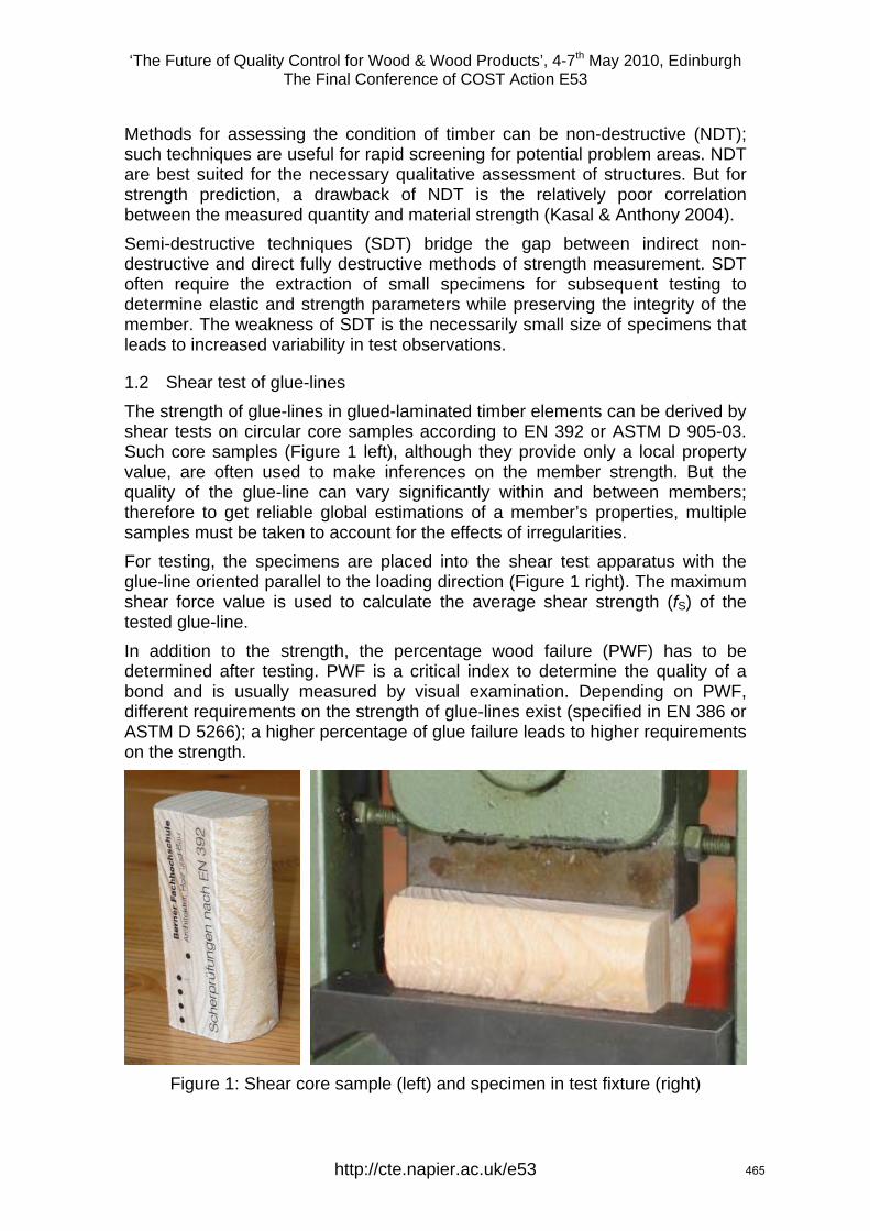
‘The Future of Quality Control for Wood & Wood Products’, 4-7th May 2010, Edinburgh The Final Conference of COST Action E53
Methods for assessing the condition of timber can be non-destructive (NDT); such techniques are useful for rapid screening for potential problem areas. NDT are best suited for the necessary qualitative assessment of structures. But for strength prediction, a drawback of NDT is the relatively poor correlation between the measured quantity and material strength (Kasal & Anthony 2004). Semi-destructive techniques (SDT) bridge the gap between indirect non-destructive and direct fully destructive methods of strength measurement. SDT often require the extraction of small specimens for subsequent testing to determine elastic and strength parameters while preserving the integrity of the member. The weakness of SDT is the necessarily small size of specimens that leads to increased variability in test observations.
1.2 Shear test of glue-lines The strength of glue-lines in glued-laminated timber elements can be derived by shear tests on circular core samples according to EN 392 or ASTM D 905-03. Such core samples (Figure 1 left), although they provide only a local property value, are often used to make inferences on the member strength. But the quality of the glue-line can vary significantly within and between members; therefore to get reliable global estimations of a member’s properties, multiple samples must be taken to account for the effects of irregularities. For testing, the specimens are placed into the shear test apparatus with the glue-line oriented parallel to the loading direction (Figure 1 right). The maximum shear force value is used to calculate the average shear strength (fS) of the tested glue-line. In addition to the strength, the percentage wood failure (PWF) has to be determined after testing. PWF is a critical index to determine the quality of a bond and is usually measured by visual examination. Depending on PWF, different requirements on the strength of glue-lines exist (specified in EN 386 or ASTM D 5266); a higher percentage of glue failure leads to higher requirements on the strength.
Figure 1: Shear core sample (left) and specimen in test fixture (right)
http://cte.napier.ac.uk/e53 465
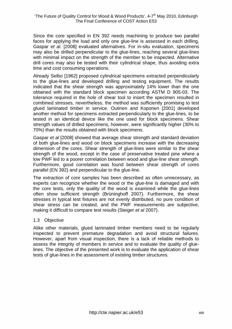
‘The Future of Quality Control for Wood & Wood Products’, 4-7th May 2010, Edinburgh The Final Conference of COST Action E53
Since the core specified in EN 392 needs machining to produce two parallel faces for applying the load and only one glue-line is assessed in each drilling, Gaspar et al. [2008] evaluated alternatives. For in-situ evaluation, specimens may also be drilled perpendicular to the glue-lines, reaching several glue-lines with minimal impact on the strength of the member to be inspected. Alternative drill cores may also be tested with their cylindrical shape, thus avoiding extra time and cost consuming operations. Already Selbo [1962] proposed cylindrical specimens extracted perpendicularly to the glue-lines and developed drilling and testing equipment. The results indicated that the shear strength was approximately 14% lower than the one obtained with the standard block specimen according ASTM D 905-03. The tolerance required in the hole of shear tool to insert the specimen resulted in combined stresses, nevertheless, the method was sufficiently promising to test glued laminated timber in service. Outinen and Koponen [2001] developed another method for specimens extracted perpendicularly to the glue-lines, to be tested in an identical device like the one used for block specimens. Shear strength values of drilled specimens, however, were significantly higher (30% to 70%) than the results obtained with block specimens. Gaspar et al [2008] showed that average shear strength and standard deviation of both glue-lines and wood on block specimens increase with the decreasing dimension of the cores. Shear strength of glue-lines were similar to the shear strength of the wood, except in the case of preservative treated pine where a low PWF led to a poorer correlation between wood and glue-line shear strength. Furthermore, good correlation was found between shear strength of cores parallel (EN 392) and perpendicular to the glue-line. The extraction of core samples has been described as often unnecessary, as experts can recognize whether the wood or the glue-line is damaged and with the core tests, only the quality of the wood is examined while the glue-lines often show sufficient strength (Brüninghoff 2007). Furthermore, the shear stresses in typical test fixtures are not evenly distributed, no pure condition of shear stress can be created, and the PWF measurements are subjective, making it difficult to compare test results (Steiger et al 2007).
1.3 Objective Alike other materials, glued laminated timber members need to be regularly inspected to prevent premature degradation and avoid structural failures. However, apart from visual inspection, there is a lack of reliable methods to assess the integrity of members in service and to evaluate the quality of glue-lines. The objective of the presented work is to evaluate the application of shear tests of glue-lines in the assessment of existing timber structures.
http://cte.napier.ac.uk/e53 466
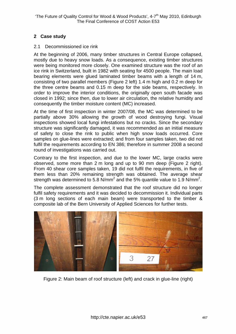
‘The Future of Quality Control for Wood & Wood Products’, 4-7th May 2010, Edinburgh The Final Conference of COST Action E53
2 Case study
2.1 Decommissioned ice rink At the beginning of 2006, many timber structures in Central Europe collapsed, mostly due to heavy snow loads. As a consequence, existing timber structures were being monitored more closely. One examined structure was the roof of an ice rink in Switzerland, built in 1982 with seating for 4500 people. The main load bearing elements were glued laminated timber beams with a length of 14 m, consisting of two parallel members (Figure 2 left) 1.4 m high and 0.2 m deep for the three centre beams and 0.15 m deep for the side beams, respectively. In order to improve the interior conditions, the originally open south facade was closed in 1992; since then, due to lower air circulation, the relative humidity and consequently the timber moisture content (MC) increased. At the time of first inspection in winter 2007/08, the MC was determined to be partially above 30% allowing the growth of wood destroying fungi. Visual inspections showed local fungi infestations but no cracks. Since the secondary structure was significantly damaged, it was recommended as an initial measure of safety to close the rink to public when high snow loads occurred. Core samples on glue-lines were extracted; and from four samples taken, two did not fulfil the requirements according to EN 386; therefore in summer 2008 a second round of investigations was carried out. Contrary to the first inspection, and due to the lower MC, large cracks were observed, some more than 2 m long and up to 90 mm deep (Figure 2 right). From 40 shear core samples taken, 19 did not fulfil the requirements, in five of them less than 20% remaining strength was obtained. The average shear strength was determined to 5.8 N/mm2 and the 5% quantile value to 1.9 N/mm2. The complete assessment demonstrated that the roof structure did no longer fulfil safety requirements and it was decided to decommission it. Individual parts (3 m long sections of each main beam) were transported to the timber & composite lab of the Bern University of Applied Sciences for further tests.
Figure 2: Main beam of roof structure (left) and crack in glue-line (right)
http://cte.napier.ac.uk/e53 467
‘The Future of Quality Control for Wood & Wood Products’, 4-7th May 2010, Edinburgh The Final Conference of COST Action E53
2.2 Material A total of 10 beam segments were cut into smaller parts. From each 200 mm wide beam segment, 2 bending test specimen, 16 large scale shear specimen and 60 core samples were cut, see Figure 3. From the 150 mm wide beam segments, 2 bending test specimen, 8 shear specimen and 30 core samples were cut. To study the variation of shear strength within one glue-line, eight additional cores were takes from 4 glue-lines each. Therefore a total of 20 bending, 128 large scale shear and 608 core samples were extracted. The bending specimen were 3 m long and 300 mm high; the large scale shear specimen were 600 mm long and 300 mm high, and the small scale core samples followed the requirements of EN 392. The core samples were taken from strips which were located between the large scale shear specimens in order to facilitate correlating the strength of the core samples to the strength of the large scale shear samples within one segment. Five cores were taken from each strip, four of those with glue-lines and one without a glue-line.
Original beam segment
Shear test specimen
Bending test specimen
Figure 3: Test specimens cut from beam segments
http://cte.napier.ac.uk/e53 468
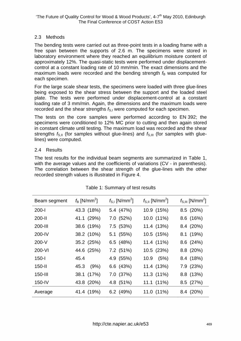
‘The Future of Quality Control for Wood & Wood Products’, 4-7th May 2010, Edinburgh The Final Conference of COST Action E53
2.3 Methods The bending tests were carried out as three-point tests in a loading frame with a free span between the supports of 2.6 m. The specimens were stored in laboratory environment where they reached an equilibrium moisture content of approximately 12%. The quasi-static tests were performed under displacement-control at a constant loading rate of 10 mm/min. The exact dimensions and the maximum loads were recorded and the bending strength fB was computed for each specimen. For the large scale shear tests, the specimens were loaded with three glue-lines being exposed to the shear stress between the support and the loaded steel plate. The tests were performed under displacement-control at a constant loading rate of 3 mm/min. Again, the dimensions and the maximum loads were recorded and the shear strengths fS,I were computed for each specimen. The tests on the core samples were performed according to EN 392; the specimens were conditioned to 12% MC prior to cutting and then again stored in constant climate until testing. The maximum load was recorded and the shear strengths fS,II (for samples without glue-lines) and fS,III (for samples with glue-lines) were computed.
2.4 Results The test results for the individual beam segments are summarized in Table 1, with the average values and the coefficients of variations (CV - in parenthesis). The correlation between the shear strength of the glue-lines with the other recorded strength values is illustrated in Figure 4.
Table 1: Summary of test results
Beam segment fB [N/mm2] fS,I [N/mm2] fS,II [N/mm2] fS,III [N/mm2]
200-I 43.3 (18%) 5.4 (47%) 10.9 (15%) 8.5 (20%) 200-II 41.1 (29%) 7.0 (52%) 10.0 (11%) 8.6 (16%) 200-III 38.6 (19%) 7.5 (53%) 11.4 (13%) 8.4 (20%) 200-IV 38.2 (10%) 5.1 (55%) 10.5 (15%) 8.1 (19%) 200-V 35.2 (25%) 6.5 (48%) 11.4 (11%) 8.6 (24%) 200-VI 44.6 (25%) 7.2 (51%) 10.5 (23%) 8.8 (20%) 150-I 45.4 4.9 (55%) 10.9 (5%) 8.4 (18%) 150-II 45.3 (9%) 6.6 (43%) 11.4 (13%) 7.9 (23%) 150-III 38.1 (17%) 7.0 (37%) 11.3 (11%) 8.8 (13%) 150-IV 43.8 (20%) 4.8 (51%) 11.1 (11%) 8.5 (27%)
Average 41.4 (19%) 6.2 (49%) 11.0 (11%) 8.4 (20%)
http://cte.napier.ac.uk/e53 469
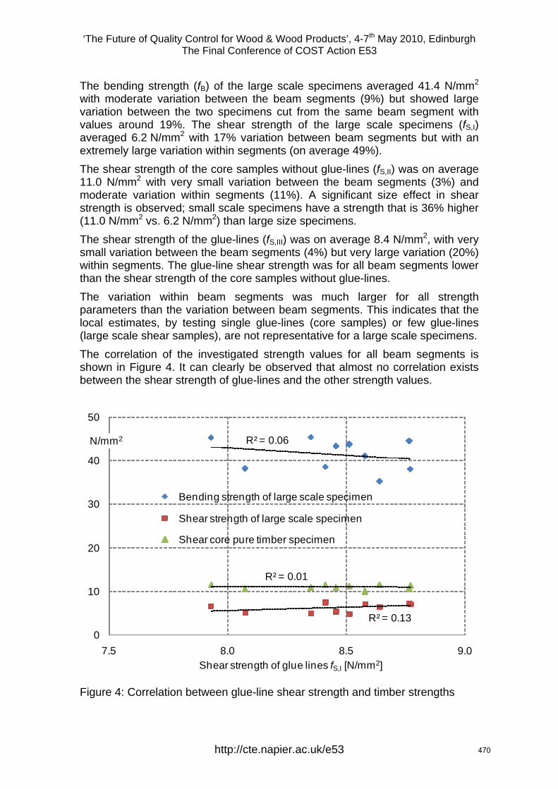
‘The Future of Quality Control for Wood & Wood Products’, 4-7th May 2010, Edinburgh The Final Conference of COST Action E53
The bending strength (fB) of the large scale specimens averaged 41.4 N/mm2 with moderate variation between the beam segments (9%) but showed large variation between the two specimens cut from the same beam segment with values around 19%. The shear strength of the large scale specimens (fS,I) averaged 6.2 N/mm2 with 17% variation between beam segments but with an extremely large variation within segments (on average 49%). The shear strength of the core samples without glue-lines (fS,II) was on average 11.0 N/mm2 with very small variation between the beam segments (3%) and moderate variation within segments (11%). A significant size effect in shear strength is observed; small scale specimens have a strength that is 36% higher (11.0 N/mm2 vs. 6.2 N/mm2) than large size specimens. The shear strength of the glue-lines (fS,III) was on average 8.4 N/mm2, with very small variation between the beam segments (4%) but very large variation (20%) within segments. The glue-line shear strength was for all beam segments lower than the shear strength of the core samples without glue-lines. The variation within beam segments was much larger for all strength parameters than the variation between beam segments. This indicates that the local estimates, by testing single glue-lines (core samples) or few glue-lines (large scale shear samples), are not representative for a large scale specimens. The correlation of the investigated strength values for all beam segments is shown in Figure 4. It can clearly be observed that almost no correlation exists between the shear strength of glue-lines and the other strength values.
R² = 0.06
R² = 0.13
R² = 0.01
0
10
20
30
40
50
7.5 8.0 8.5 9.0
N/mm2
Shear strength of glue lines fS,I [N/mm2]
Bending strength of large scale specimen
Shear strength of large scale specimen
Shear core pure timber specimen
Figure 4: Correlation between glue-line shear strength and timber strengths
http://cte.napier.ac.uk/e53 470
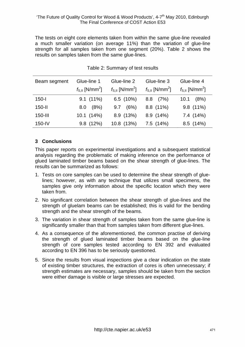
‘The Future of Quality Control for Wood & Wood Products’, 4-7th May 2010, Edinburgh The Final Conference of COST Action E53
The tests on eight core elements taken from within the same glue-line revealed a much smaller variation (on average 11%) than the variation of glue-line strength for all samples taken from one segment (20%). Table 2 shows the results on samples taken from the same glue-lines.
Table 2: Summary of test results
Beam segment Glue-line 1 fS,II [N/mm2]
Glue-line 2 fS,II [N/mm2]
Glue-line 3 fS,II [N/mm2]
Glue-line 4 fS,II [N/mm2]
150-I 9.1 (11%) 6.5 (10%) 8.8 (7%) 10.1 (8%) 150-II 8.0 (8%) 9.7 (6%) 8.8 (11%) 9.8 (11%) 150-III 10.1 (14%) 8.9 (13%) 8.9 (14%) 7.4 (14%) 150-IV 9.8 (12%) 10.8 (13%) 7.5 (14%) 8.5 (14%)
3 Conclusions This paper reports on experimental investigations and a subsequent statistical analysis regarding the problematic of making inference on the performance of glued laminated timber beams based on the shear strength of glue-lines. The results can be summarized as follows: 1. Tests on core samples can be used to determine the shear strength of glue-
lines; however, as with any technique that utilizes small specimens, the samples give only information about the specific location which they were taken from.
2. No significant correlation between the shear strength of glue-lines and the strength of gluelam beams can be established; this is valid for the bending strength and the shear strength of the beams.
3. The variation in shear strength of samples taken from the same glue-line is significantly smaller than that from samples taken from different glue-lines.
4. As a consequence of the aforementioned, the common practise of deriving the strength of glued laminated timber beams based on the glue-line strength of core samples tested according to EN 392 and evaluated according to EN 396 has to be seriously questioned.
5. Since the results from visual inspections give a clear indication on the state of existing timber structures, the extraction of cores is often unnecessary; if strength estimates are necessary, samples should be taken from the section were either damage is visible or large stresses are expected.
http://cte.napier.ac.uk/e53 471
‘The Future of Quality Control for Wood & Wood Products’, 4-7th May 2010, Edinburgh The Final Conference of COST Action E53
References Kasal, B., Anthony, R.W. 2004. Advances in in-situ evaluation of timber structures. Progress in Structural Engineering and Materials. Vol. 6, pp.94-103.
EN 392. 1995. Glued laminated timber. Shear test of glue-lines. CEN, Brussels.
ASTM D 905-03. 2003. Standard Test Method for Strength Properties of Adhesive Bonds in Shear by Compression Loading. ASTM International, West Conshohocken.
EN 386. 2001. Glued laminated timber - Performance requirements and minimum production requirements. CEN, Brussels.
ASTM D 5266. 2003. Standard Practice for Estimating the Percentage of Wood Failure in Adhesive Bonded Joints. ASTM International, West Conshohocken.
Brüninghoff, H. 2007. Reinforcement / rehabilitation of glulam structures. In Proc. of Int. Holzbauforum Garmisch-Partenkirchen. www.forumholzbau.com/.
Steiger, R., Risi, W. and Gehri E. 2007. Quality control of glulam: shear tests of glue-lines. Paper 40-12-7, Proceedings. 40th meeting CIB-W18, Bled, Slovenia.
Gaspar, F., Helena Cruz, H. and Gomes, A. 2008. Evaluation of glued laminated timber structures – core extraction and shear testing. Proceedings 10th World conference on timber engineering, June 2–5; Miyazaki, Japan.
Selbo M.L. 1962. A new method for testing glue joints of laminated timber in service, Forest Products Journal, Vol 12(2), pp. 65-67.
Outinen K., Koponen S., “Drilled shear specimen (DSS)”, European Science Foundation, COST E13 - Conference Edinburgh, 2001.
http://cte.napier.ac.uk/e53 472
‘The Future of Quality Control for Wood & Wood Products’, 4-7th May 2010, Edinburgh The Final Conference of COST Action E53
http://cte.napier.ac.uk/e53
Validity of bending tests on strip-shaped specimens to derive bending strength and stiffness properties of cross-laminated
solid timber (X-lam)
R. Steiger 1 & A. Gülzow 2
Abstract The application of cross-laminated solid timber (CLT, X-lam) used as load-bearing plates requires information on the product’s strength properties; the design, however, is often governed by serviceability criterions. Hence, predicting the respective behaviour of such panels requires accurate information about their bending and shear strength as well as their elastic properties. Bending strength and stiffness of CLT have to be assessed following the procedures in EN 789. The latter requires 4-point bending tests of strip-shaped specimens with a width of 300 mm, cut from the panels. By comparing results of bending tests on 100 mm and 300 mm wide strip-shaped specimens and on full panels it is shown, that neither MOR nor stiffness properties derived by testing single 100 mm wide strip-shaped specimens are appropriate to assess the respective properties of the original panels. However, with regard to stiffness properties, single 300 mm wide strips or samples of at least 5 to 6 100 mm wide strips lead to acceptable results. The analysis of the test data covers MOR, bending MOE parallel and perpendicular to the grain direction of the face layers as well as shear moduli. Rolling shear failures which frequently occurred when testing the 100 mm wide strip-shaped specimens could not be observed in destructive tests of gross CLT panels. It is concluded that tests on single strip-shaped specimens should only be used in the course of quality control of CLT (i.e. to check sufficient adhesive bond of the layers) but not to derive mechanical properties of gross panels.
1 Introduction Cross-laminated solid timber (CLT) is assembled of cross-wise oriented layers of lamellas (mostly softwood). Compared to the raw material, CLT benefits from homogenised mechanical properties. CLT is not only used as component of structural elements, but rather for load bearing plates and shear walls. In practice the design of plates loaded perpendicular to the plane is often governed by serviceability criterions like maximal deflection and vibration susceptibility. Appropriate verification of ultimate and serviceability limits of such panels is only possible when relying on accurate information about the elastic properties as well as on the strength properties of the respective CLT product.
1 Senior Scientist, [email protected] Empa, Wood Laboratory, Dübendorf, Switzerland 2 Planning Engineer, [email protected] Carbo-Link GmbH, Fehraltorf, Switzerland
473
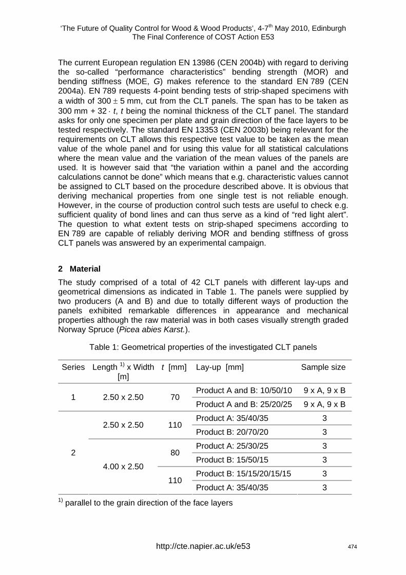
‘The Future of Quality Control for Wood & Wood Products’, 4-7th May 2010, Edinburgh The Final Conference of COST Action E53
http://cte.napier.ac.uk/e53
The current European regulation EN 13986 (CEN 2004b) with regard to deriving the so-called “performance characteristics” bending strength (MOR) and bending stiffness (MOE, G) makes reference to the standard EN 789 (CEN 2004a). EN 789 requests 4-point bending tests of strip-shaped specimens with a width of 300 5 mm, cut from the CLT panels. The span has to be taken as 300 mm + 32 t, t being the nominal thickness of the CLT panel. The standard asks for only one specimen per plate and grain direction of the face layers to be tested respectively. The standard EN 13353 (CEN 2003b) being relevant for the requirements on CLT allows this respective test value to be taken as the mean value of the whole panel and for using this value for all statistical calculations where the mean value and the variation of the mean values of the panels are used. It is however said that “the variation within a panel and the according calculations cannot be done” which means that e.g. characteristic values cannot be assigned to CLT based on the procedure described above. It is obvious that deriving mechanical properties from one single test is not reliable enough. However, in the course of production control such tests are useful to check e.g. sufficient quality of bond lines and can thus serve as a kind of “red light alert”. The question to what extent tests on strip-shaped specimens according to EN 789 are capable of reliably deriving MOR and bending stiffness of gross CLT panels was answered by an experimental campaign.
2 Material The study comprised of a total of 42 CLT panels with different lay-ups and geometrical dimensions as indicated in Table 1. The panels were supplied by two producers (A and B) and due to totally different ways of production the panels exhibited remarkable differences in appearance and mechanical properties although the raw material was in both cases visually strength graded Norway Spruce (Picea abies Karst.).
Table 1: Geometrical properties of the investigated CLT panels
Series Length 1) x Width [m]
t [mm] Lay-up [mm] Sample size
Product A and B: 10/50/10 9 x A, 9 x B 1 2.50 x 2.50 70
Product A and B: 25/20/25 9 x A, 9 x B
Product A: 35/40/35 3 2.50 x 2.50 110
Product B: 20/70/20 3
Product A: 25/30/25 3 80
Product B: 15/50/15 3
Product B: 15/15/20/15/15 3
2
4.00 x 2.50
110 Product A: 35/40/35 3
1) parallel to the grain direction of the face layers
474
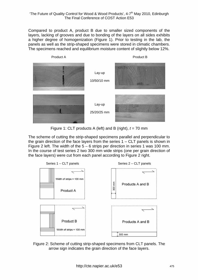
‘The Future of Quality Control for Wood & Wood Products’, 4-7th May 2010, Edinburgh The Final Conference of COST Action E53
http://cte.napier.ac.uk/e53
Compared to product A, product B due to smaller sized components of the layers, lacking of grooves and due to bonding of the layers on all sides exhibits a higher degree of homogenization (Figure 1). Prior to testing in the lab, the panels as well as the strip-shaped specimens were stored in climatic chambers. The specimens reached and equilibrium moisture content of slightly below 12%.
Product A Product B
Lay-up
10/50/10 mm
Lay-up
25/20/25 mm
Figure 1: CLT products A (left) and B (right), t = 70 mm
The scheme of cutting the strip-shaped specimens parallel and perpendicular to the grain direction of the face layers from the series 1 – CLT panels is shown in Figure 2 left. The width of the 5 – 6 strips per direction in series 1 was 100 mm. In the course of test series 2 two 300 mm wide strips (one per grain direction of the face layers) were cut from each panel according to Figure 2 right.
Series 1 – CLT panels Series 2 – CLT panels
Figure 2: Scheme of cutting strip-shaped specimens from CLT panels. The
arrow sign indicates the grain direction of the face layers.
475
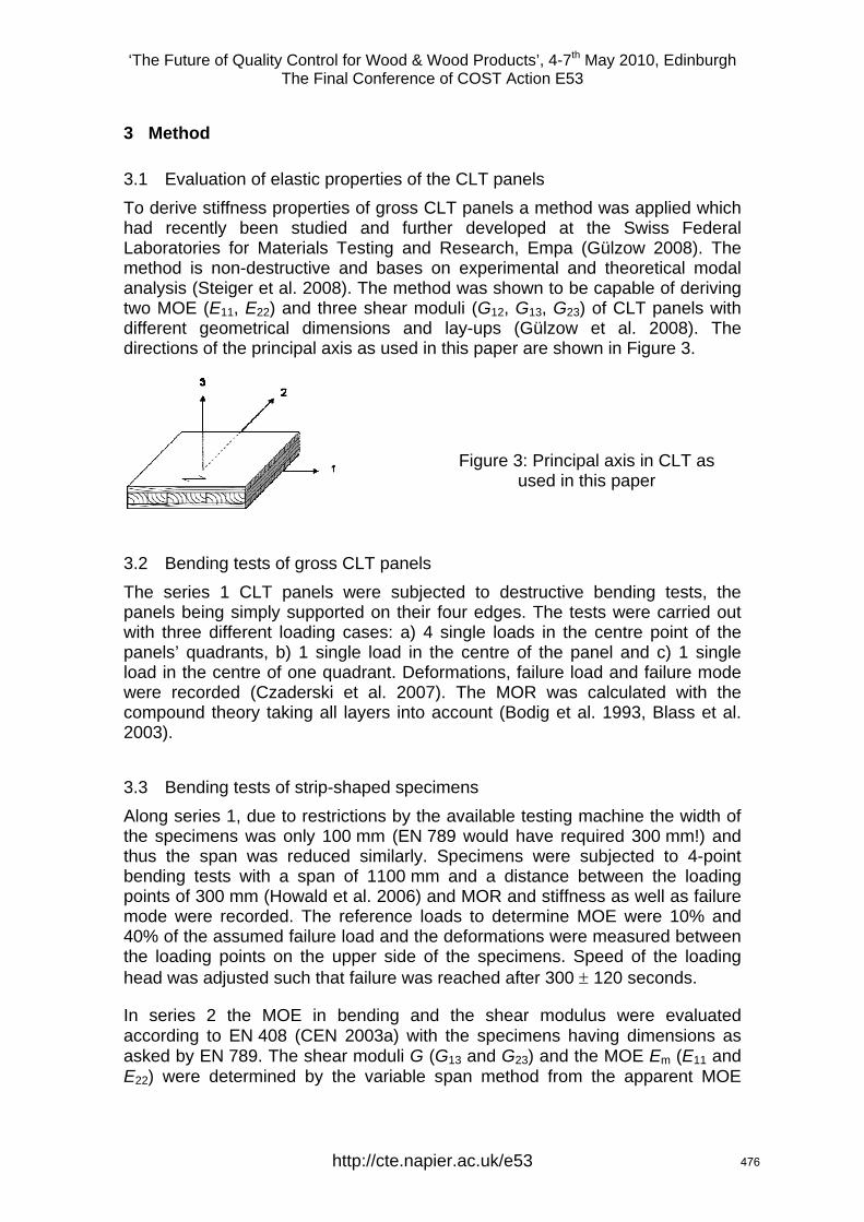
‘The Future of Quality Control for Wood & Wood Products’, 4-7th May 2010, Edinburgh The Final Conference of COST Action E53
http://cte.napier.ac.uk/e53
3 Method
3.1 Evaluation of elastic properties of the CLT panels To derive stiffness properties of gross CLT panels a method was applied which had recently been studied and further developed at the Swiss Federal Laboratories for Materials Testing and Research, Empa (Gülzow 2008). The method is non-destructive and bases on experimental and theoretical modal analysis (Steiger et al. 2008). The method was shown to be capable of deriving two MOE (E11, E22) and three shear moduli (G12, G13, G23) of CLT panels with different geometrical dimensions and lay-ups (Gülzow et al. 2008). The directions of the principal axis as used in this paper are shown in Figure 3.
Figure 3: Principal axis in CLT as used in this paper
3.2 Bending tests of gross CLT panels The series 1 CLT panels were subjected to destructive bending tests, the panels being simply supported on their four edges. The tests were carried out with three different loading cases: a) 4 single loads in the centre point of the panels’ quadrants, b) 1 single load in the centre of the panel and c) 1 single load in the centre of one quadrant. Deformations, failure load and failure mode were recorded (Czaderski et al. 2007). The MOR was calculated with the compound theory taking all layers into account (Bodig et al. 1993, Blass et al. 2003).
3.3 Bending tests of strip-shaped specimens Along series 1, due to restrictions by the available testing machine the width of the specimens was only 100 mm (EN 789 would have required 300 mm!) and thus the span was reduced similarly. Specimens were subjected to 4-point bending tests with a span of 1100 mm and a distance between the loading points of 300 mm (Howald et al. 2006) and MOR and stiffness as well as failure mode were recorded. The reference loads to determine MOE were 10% and 40% of the assumed failure load and the deformations were measured between the loading points on the upper side of the specimens. Speed of the loading head was adjusted such that failure was reached after 300 120 seconds.
In series 2 the MOE in bending and the shear modulus were evaluated according to EN 408 (CEN 2003a) with the specimens having dimensions as asked by EN 789. The shear moduli G (G13 and G23) and the MOE Em (E11 and E22) were determined by the variable span method from the apparent MOE
476
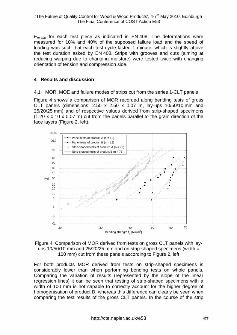
‘The Future of Quality Control for Wood & Wood Products’, 4-7th May 2010, Edinburgh The Final Conference of COST Action E53
http://cte.napier.ac.uk/e53
Em,app for each test piece as indicated in EN 408. The deformations were measured for 10% and 40% of the supposed failure load and the speed of loading was such that each test cycle lasted 1 minute, which is slightly above the test duration asked by EN 408. Strips with grooves and cuts (aiming at reducing warping due to changing moisture) were tested twice with changing orientation of tension and compression side.
4 Results and discussion
4.1 MOR, MOE and failure modes of strips cut from the series 1-CLT panels Figure 4 shows a comparison of MOR recorded along bending tests of gross CLT panels (dimensions: 2.50 x 2.50 x 0.07 m, lay-ups 10/50/10 mm and 25/20/25 mm) and of respective values derived from strip-shaped specimens (1.20 x 0.10 x 0.07 m) cut from the panels parallel to the grain direction of the face layers (Figure 2, left).
.01
.1
1
510
2030
50
7080
9095
99
99.9
99.99Panel tests of product A (n = 12)Panel tests of product B (n = 12)Strip-shaped tests of product A (n = 70)Strip-shaped tests of product B (n = 78)
20 30 40 50 60Bending strength f
m [N/mm2]
[%]
70
Figure 4: Comparison of MOR derived from tests on gross CLT panels with lay-ups 10/50/10 mm and 25/20/25 mm and on strip-shaped specimens (width =
100 mm) cut from these panels according to Figure 2, left
For both products MOR derived from tests on strip-shaped specimens is considerably lower than when performing bending tests on whole panels. Comparing the variation of results (represented by the slope of the linear regression lines) it can be seen that testing of strip-shaped specimens with a width of 100 mm is not capable to correctly account for the higher degree of homogenisation of product B, whereas this difference can clearly be seen when comparing the test results of the gross CLT panels. In the course of the strip
477
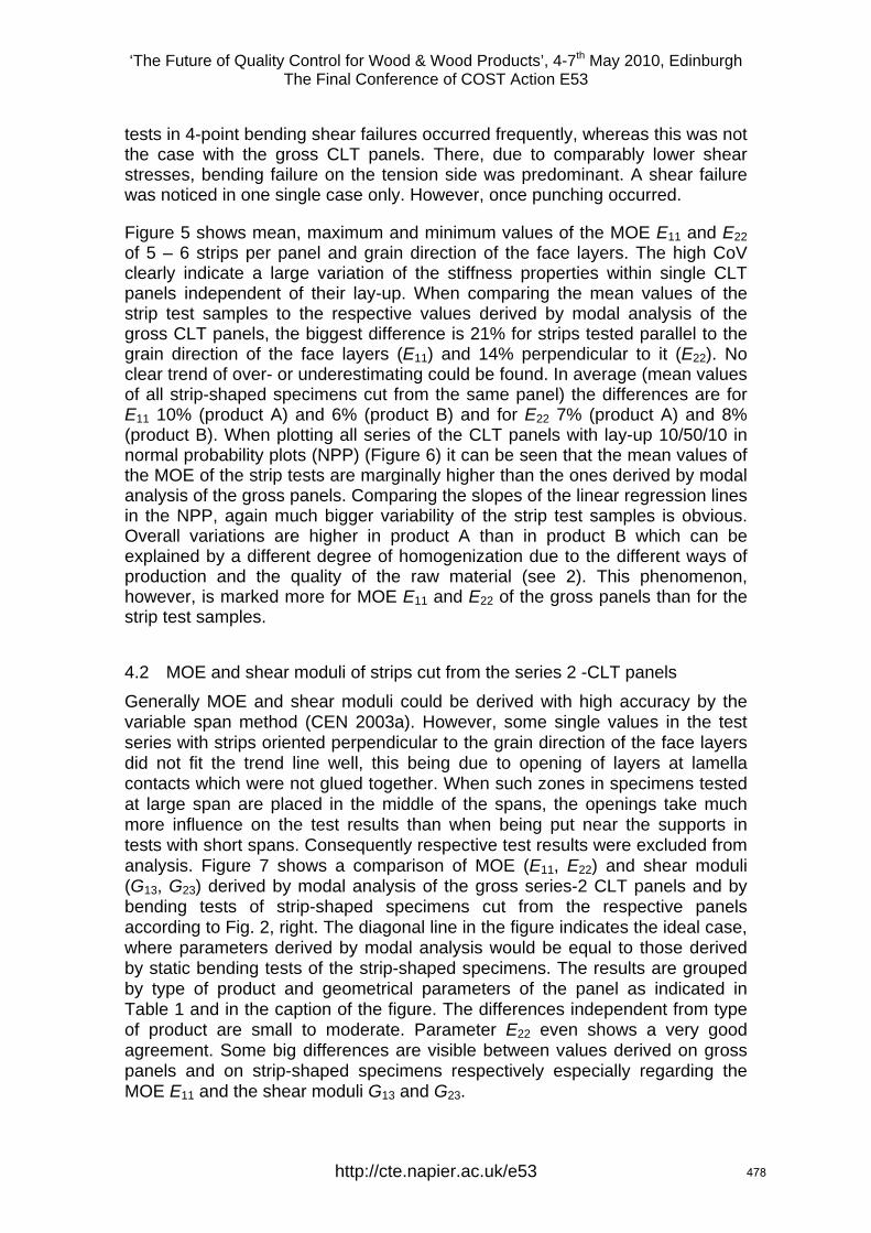
‘The Future of Quality Control for Wood & Wood Products’, 4-7th May 2010, Edinburgh The Final Conference of COST Action E53
http://cte.napier.ac.uk/e53
tests in 4-point bending shear failures occurred frequently, whereas this was not the case with the gross CLT panels. There, due to comparably lower shear stresses, bending failure on the tension side was predominant. A shear failure was noticed in one single case only. However, once punching occurred.
Figure 5 shows mean, maximum and minimum values of the MOE E11 and E22 of 5 – 6 strips per panel and grain direction of the face layers. The high CoV clearly indicate a large variation of the stiffness properties within single CLT panels independent of their lay-up. When comparing the mean values of the strip test samples to the respective values derived by modal analysis of the gross CLT panels, the biggest difference is 21% for strips tested parallel to the grain direction of the face layers (E11) and 14% perpendicular to it (E22). No clear trend of over- or underestimating could be found. In average (mean values of all strip-shaped specimens cut from the same panel) the differences are for E11 10% (product A) and 6% (product B) and for E22 7% (product A) and 8% (product B). When plotting all series of the CLT panels with lay-up 10/50/10 in normal probability plots (NPP) (Figure 6) it can be seen that the mean values of the MOE of the strip tests are marginally higher than the ones derived by modal analysis of the gross panels. Comparing the slopes of the linear regression lines in the NPP, again much bigger variability of the strip test samples is obvious. Overall variations are higher in product A than in product B which can be explained by a different degree of homogenization due to the different ways of production and the quality of the raw material (see 2). This phenomenon, however, is marked more for MOE E11 and E22 of the gross panels than for the strip test samples.
4.2 MOE and shear moduli of strips cut from the series 2 -CLT panels Generally MOE and shear moduli could be derived with high accuracy by the variable span method (CEN 2003a). However, some single values in the test series with strips oriented perpendicular to the grain direction of the face layers did not fit the trend line well, this being due to opening of layers at lamella contacts which were not glued together. When such zones in specimens tested at large span are placed in the middle of the spans, the openings take much more influence on the test results than when being put near the supports in tests with short spans. Consequently respective test results were excluded from analysis. Figure 7 shows a comparison of MOE (E11, E22) and shear moduli (G13, G23) derived by modal analysis of the gross series-2 CLT panels and by bending tests of strip-shaped specimens cut from the respective panels according to Fig. 2, right. The diagonal line in the figure indicates the ideal case, where parameters derived by modal analysis would be equal to those derived by static bending tests of the strip-shaped specimens. The results are grouped by type of product and geometrical parameters of the panel as indicated in Table 1 and in the caption of the figure. The differences independent from type of product are small to moderate. Parameter E22 even shows a very good agreement. Some big differences are visible between values derived on gross panels and on strip-shaped specimens respectively especially regarding the MOE E11 and the shear moduli G13 and G23.
478
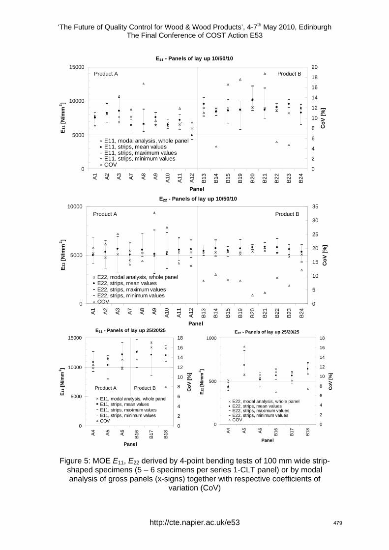
‘The Future of Quality Control for Wood & Wood Products’, 4-7th May 2010, Edinburgh The Final Conference of COST Action E53
http://cte.napier.ac.uk/e53
E11 - Panels of lay up 10/50/10
0
5000
10000
15000
A1
A2
A3
A7
A8
A9
A10
A11
A12
B13
B14
B15
B19
B20
B21
B22
B23
B24
Panel
E11 [
N/m
m2 ]
0
2
4
6
8
10
12
14
16
18
20
CoV
[%]
E11, modal analysis, whole panelE11, strips, mean valuesE11, strips, maximum valuesE11, strips, minimum valuesCOV
.
Product A Product B
E22 - Panels of lay up 10/50/10
0
5000
10000
A1
A2
A3
A7
A8
A9
A10
A11
A12
B13
B14
B15
B19
B20
B21
B22
B23
B24
Panel
E22 [
N/m
m2 ]
0
5
10
15
20
25
30
35
CoV
[%]
E22, modal analysis, whole panelE22, strips, mean valuesE22, strips, maximum valuesE22, strips, minimum valuesCOV
Product A Product B
E11 - Panels of lay up 25/20/25
0
5000
10000
15000
A4
A5
A6
B16
B17
B18
Panel
E11 [
N/m
m2 ]
0
2
4
6
8
10
12
14
16
18
CoV
[%]
E11, modal analysis, whole panelE11, strips, mean valuesE11, strips, maximum valuesE11, strips, minimum valuesCOV
Product A Product B
E22 - Panels of lay up 25/20/25
0
500
1000
A4
A5
A6
B16
B17
B18
Panel
E22 [
N/m
m2 ]
0
2
4
6
8
10
12
14
16
18
CoV
[%]
E22, modal analysis, whole panelE22, strips, mean valuesE22, strips, maximum valuesE22, strips, minimum valuesCOV
Figure 5: MOE E11, E22 derived by 4-point bending tests of 100 mm wide strip-shaped specimens (5 – 6 specimens per series 1-CLT panel) or by modal analysis of gross panels (x-signs) together with respective coefficients of
variation (CoV)
479
‘The Future of Quality Control for Wood & Wood Products’, 4-7th May 2010, Edinburgh The Final Conference of COST Action E53
http://cte.napier.ac.uk/e53
.01
.1
1
510
2030
50
7080
9095
99
99.9
99.99
E11-Product A-PanelsE11-Product B-PanelsE11-Product A-Strip-shaped specimnesE11-Product B-Strip-shaped specimnes
0 5000 10000 15000 MOE [N/mm2]
[%]
.01
.1
1
510
2030
50
7080
9095
99
99.9
99.99
E22-Product A-PanelsE22-Product B-PanelsE22-Product A-Strip-shaped specimensE22-Product B-Strip-shaped specimens
0 1000 2000 3000 4000 5000 6000 7000 8000 MOE [N/mm2]
[%]
Figure 6: NPP of MOE E11 and E22 derived by 4-point bending tests of 100 mm wide strip-shaped specimens (5 6 specimens per series 1-CLT panel) and by
modal analysis of gross panels (lay-up 10/50/10 mm only)
A closer look on the specimens turned out, that big differences mainly resulted from striking non-homogeneities in the used raw material. Since specimens with marked cuts and grooves were tested twice with changing orientation of the tension side in bending, it could be concluded that the test procedure did not systematically affect the data. Differences between values derived by modal analysis and by static testing, however, also result from the well-known fact that stiffness parameters derived by means of dynamic methods due to the high speed of action are approximately 6% higher than those determined on base of static experiments at comparably lower loading rate (Görlacher 1984).
480
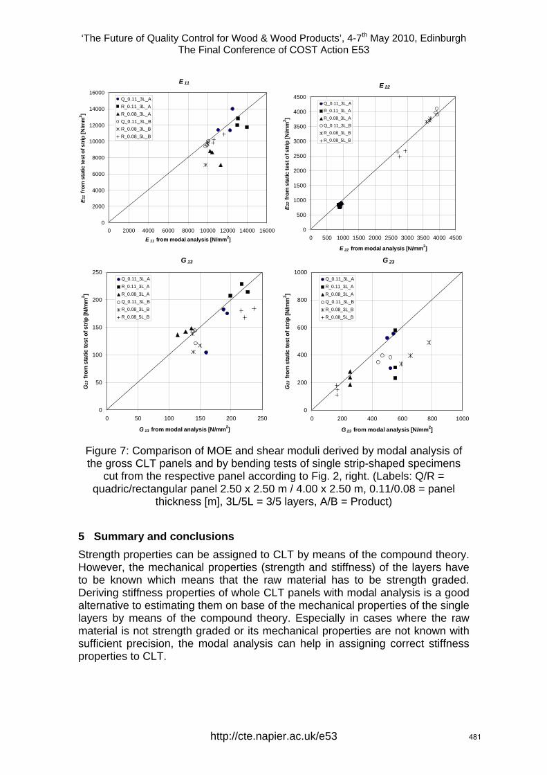
‘The Future of Quality Control for Wood & Wood Products’, 4-7th May 2010, Edinburgh The Final Conference of COST Action E53
http://cte.napier.ac.uk/e53
E 11
0
2000
4000
6000
8000
10000
12000
14000
16000
0 2000 4000 6000 8000 10000 12000 14000 16000E 11 from modal analysis [N/mm2]
E 11 fr
om s
tatic
test
of s
trip
[N/m
m2 ]
Q_0.11_3L_AR_0.11_3L_AR_0.08_3L_AQ_0.11_3L_BR_0.08_3L_BR_0.08_5L_B
E 22
0
500
1000
1500
2000
2500
3000
3500
4000
4500
0 500 1000 1500 2000 2500 3000 3500 4000 4500
E 22 from modal analysis [N/mm2]
E22
from
sta
tic te
st o
f stri
p [N
/mm
2 ]
Q_0.11_3L_AR_0.11_3L_AR_0.08_3L_AQ_0.11_3L_BR_0.08_3L_BR_0.08_5L_B
G 13
0
50
100
150
200
250
0 50 100 150 200 250
G 13 from modal analysis [N/mm2]
G13
from
sta
tic te
st o
f stri
p [N
/mm
2 ]
Q_0.11_3L_AR_0.11_3L_AR_0.08_3L_AQ_0.11_3L_BR_0.08_3L_BR_0.08_5L_B
G 23
0
200
400
600
800
1000
0 200 400 600 800 1000
G 23 from modal analysis [N/mm2]
G23
from
sta
tic te
st o
f stri
p [N
/mm
2 ]Q_0.11_3L_AR_0.11_3L_AR_0.08_3L_AQ_0.11_3L_BR_0.08_3L_BR_0.08_5L_B
Figure 7: Comparison of MOE and shear moduli derived by modal analysis of the gross CLT panels and by bending tests of single strip-shaped specimens
cut from the respective panel according to Fig. 2, right. (Labels: Q/R = quadric/rectangular panel 2.50 x 2.50 m / 4.00 x 2.50 m, 0.11/0.08 = panel
thickness [m], 3L/5L = 3/5 layers, A/B = Product)
5 Summary and conclusions Strength properties can be assigned to CLT by means of the compound theory. However, the mechanical properties (strength and stiffness) of the layers have to be known which means that the raw material has to be strength graded. Deriving stiffness properties of whole CLT panels with modal analysis is a good alternative to estimating them on base of the mechanical properties of the single layers by means of the compound theory. Especially in cases where the raw material is not strength graded or its mechanical properties are not known with sufficient precision, the modal analysis can help in assigning correct stiffness properties to CLT.
481
‘The Future of Quality Control for Wood & Wood Products’, 4-7th May 2010, Edinburgh The Final Conference of COST Action E53
http://cte.napier.ac.uk/e53
After having proven the correctness of the modal analysis method by static proof loading, the panel properties were compared to bending MOE and shear moduli derived from tests on strip-shaped specimens cut from the CLT panels. One part of the tests additionally focused on bending strength and failure modes. From the tests the following conclusions could be drawn:
Bending strength and stiffness of CLT panels can vary quite strongly within one single panel. For both parameters differences in strength and stiffness of strip-shaped specimens cut from the panels of up to 100% have been found. Hence it is not possible to derive strength and stiffness properties of CLT panels from bending tests of few or single strip-shaped specimens.
The accuracy of the test results when performing bending tests of strip-shaped specimens according to EN 789 is increased with increasing sample size. Mean values of at least 5 – 6 specimens better describe the actual bending stiffness of the panels. Average differences in MOE then amount to 10% (E11) and 6% (E22) but can still reach 20%.
The variation of the stiffness properties depends on the degree of homogenisation of the actual CLT product. The smaller the components (lamellas) are and the less the variation in mechanical properties is (due to e.g. a strength grading of the raw material), the better it can be concluded from tests on strip-shaped specimens to the bending strength and stiffness properties of the gross CLT panel.
Compared to gross CLT panels, local non-homogeneities and faults (knots, pitch pockets, deviated grain, not adhesively bonded contacts, grooves, cracks) take more influence on the mechanical properties of the strip-shaped specimens. The smaller the width of such specimens is, the more their load-bearing behaviour is affected by local defects and non-homogeneities due to the quality of the raw material or due to the way of producing the panels.
The distances between middle layer parts not adhesively bonded at their edges and the number of grooves, which are aimed at reducing the deformations of the CLT panel in case of changing moisture, take a big influence on the shear moduli. When deriving respective values on base of testing strip-shaped specimens this possible variation has to be taken into account by using empirical relationships.
When testing strip-shaped specimens in 4-point bending, (rolling) shear failures occur quite frequently, whereas such failure modes could not be observed when testing gross CLT panels to failure in loading situations occurring in practice. There bending failure was dominating. Punching, however, should be regarded, especially with thin panels and products with grooves and layers not adhesively bonded at their edges.
Single tests on strip-shaped specimens may serve as an instrument of production control especially regarding the quality of bonding. They should, however not be used to derive mechanical properties of CLT panels. In scientific studies testing of strip-shaped specimens should only be carried out on big samples. Geometrical dimensions should not be taken smaller than asked by the standards and generalization of conclusions in most cases is not possible (e.g. type of failure).
482

‘The Future of Quality Control for Wood & Wood Products’, 4-7th May 2010, Edinburgh The Final Conference of COST Action E53
http://cte.napier.ac.uk/e53
Acknowledgments The study was financially supported by the Swiss Federal Office for Professional Education and Technology OPET (Innovation Promotion Agency CTI) and by the Swiss Federal Office for the Environment FOEN (Wald- und Holzforschungsfonds WHFF). The test specimens were supplied by Pius Schuler AG, CH-6418 Rothenturm, Switzerland (www.pius-schuler.ch) and by Schilliger Holz AG, Haltikon 33, CH-6403 Küssnacht (www.schilliger.ch).
References Blass, H. J. & Görlacher, R. (2003) "Bemessung im Holzbau: Brettsperrholz – Berechnungsgrundlagen". Holzbau-Kalender, pp 580-598. Bruderverlag, Karlsruhe, Germany. Bodig, J. & Jayne, B. A. (1993) "Mechanics of wood and wood composites". Krieger Publishing Company, Malabar, Florida, USA. CEN (2003a) "EN 408: Timber structures - Structural timber and glued laminated timber - Determination of some physical and mechanical properties, European Committee for Standardization. CEN (2003b) "EN 13353: Solid wood panels (SWP) - Requirements, European Committee for Standardization. CEN (2004a) "EN 789: Timber structures - Test methods - Determination of mechanical properties of wood based panels", European Committee for Standardization. CEN (2004b) "EN 13986: Wood-based panels for use in construction - Characteristics, evaluation of conformity and marking, European Committee for Standardization. Czaderski, C., Steiger, R., Howald, M., Olia, S., Gülzow, A. & Niemz, P. (2007) "Versuche und Berechnungen an allseitig gelagerten 3-schichtigen Brettsperrholzplatten". Holz als Roh- und Werkstoff, Vol 65, pp 383-402. Görlacher, R. (1984) "Ein neues Messverfahren zur Bestimmung des Elastizitätsmoduls von Holz". Holz als Roh- und Werkstoff, Vol 42, pp 219-222. Gülzow, A. (2008) "Zerstörungsfreie Bestimmung der Biegesteifigkeiten von Brettsperrholzplatten". PhD Thesis Nr. 17944, ETH Zürich, Switzerland. Gülzow, A., Gsell, D. & Steiger, R. (2008) "Zerstörungsfreie Bestimmung elastischer Eigenschaften quadratischer 3-schichtiger Brettsperrholzplatten mit symmetrischem Aufbau". Holz als Roh- und Werkstoff Vol 66, pp 19-37. Howald, M. & Niemz, P. (2006) "Massivholzplatten für das Bauwesen – Be-richtsteil I/1: Berechnungsmodell für Massivholzplatten - Ermittlung mechani-scher Eigenschaften anhand von Ultraschall-Messungen und Biegeversuchen an Kleinproben". Institut für Baustoffe, ETH Zürich, Switzerland. Steiger, R., Gülzow, A. & Gsell, D. (2008) "Non-destructive evaluation of elastic material properties of cross-laminated timber". Proceedings of COST E53 Conference on "End user's needs for wood material and products". 29th – 30th October 2008, Delft, The Netherlands, pp 171-182.
483
‘The Future of Quality Control for Wood & Wood Products’, 4-7th May 2010, Edinburgh The Final Conference of COST Action E53
An objective method to measure and evaluate the quality of sanded wood surfaces
L. Gurau1
Abstract No agreed guidelines exist in wood surface metrology about how to objectively measure and evaluate the surface quality and existing general standard methods and corresponding software are not usually applicable to wood. This paper presents a review of a method developed for sanded wood surfaces, which covers the choice of instrument type, the measuring resolution, the minimum evaluation length, aspects of filtering and the separation of processing roughness from anatomical irregularities. Compared with previous studies in the literature, processing roughness parameters calculated in this study excluded the influence of wood anatomy and represent objective references for the quality of sanding.The method was tested on several sanding variables, but was used in this paper to evaluate the influence of grit size on the quality of European oak (Quercus robur L.) sanded with P120, P150, P180, P240 and P1000. Grit size measured with the method above had a clear influence on surface roughness, the finer were the grits the smoother was the surface. Roughness values were fairly close together with P120, P150 and P180 and much smaller with P240 and P1000. This indicates that for oak it is not economical to have a sequence of sanding operations in the domain of fine grit sizes. The method can further be used to evaluate roughness parameters for different combinations of sanding variables to optimise the sanding process.
1 Introduction The quality of sanding determines the final quality of a finished wood surface and influences the finishing costs. The principal measure of the quality of sanding is the surface roughness, so a greater understanding of the effect of process parameters on surface roughness would encourage the optimisation of sanding operations. Although methods for measuring surface roughness have been standardised for homogenous materials, they are not applicable to wood, and no other specific guidelines have been developed (Krish & Csiha 1999).
Roughness represents the finer irregularities of the surface texture that are inherent in a machining process (ASME B46.1 1995). However, profile data from any nominally flat surface contains not only roughness, but also form errors and waviness that do not characterise the processing. Form errors and waviness should be excluded from any assessment of the surface roughness. Form errors constitute large deviations from the nominal shape of the workpiece. They may be due to internal stresses in the wood or inaccuracies in the machine- tool- workpiece system.
1 Associate professor, [email protected] Faculty of Wood Industry, Transilvania University of Brasov, Romania
http://cte.napier.ac.uk/e53 484
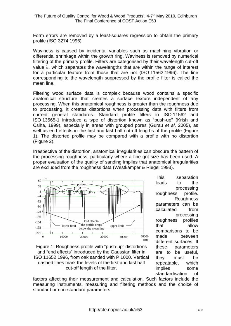
‘The Future of Quality Control for Wood & Wood Products’, 4-7th May 2010, Edinburgh The Final Conference of COST Action E53
Form errors are removed by a least-squares regression to obtain the primary profile (ISO 3274 1996).
Waviness is caused by incidental variables such as machining vibration or differential shrinkage within the growth ring. Waviness is removed by numerical filtering of the primary profile. Filters are categorised by their wavelength cut-off value λ, which separates the wavelengths that are within the range of interest for a particular feature from those that are not (ISO 11562 1996). The line corresponding to the wavelength suppressed by the profile filter is called the mean line.
Filtering wood surface data is complex because wood contains a specific anatomical structure that creates a surface texture independent of any processing. When this anatomical roughness is greater than the roughness due to processing, it creates distortions when processing data with filters from current general standards. Standard profile filters in ISO 11562 and ISO 13565-1 introduce a type of distortion known as “push-up” (Krish and Csiha, 1999), especially in areas with grouped pores (Gurau et al. 2005), as well as end effects in the first and last half cut-off lengths of the profile (Figure 1). The distorted profile may be compared with a profile with no distortion (Figure 2).
Irrespective of the distortion, anatomical irregularities can obscure the pattern of the processing roughness, particularly where a fine grit size has been used. A proper evaluation of the quality of sanding implies that anatomical irregularities are excluded from the roughness data (Westkämper & Riegel 1993).
This separation leads to the
processing roughness profile.
Roughness parameters can be calculated from
processing roughness profiles that allow comparisons to be made between different surfaces. If these parameters are to be useful, they must be repeatable, which implies some standardisation of
factors affecting their measurement and calculation. Such factors include the measuring instruments, measuring and filtering methods and the choice of standard or non-standard parameters.
lower limit upper limit
40000 500003000020000 10000 0
μm
μm
-80 -108 -136
-164
-192
-220
4 -24
-52
60
32 push-up
End effects- the profile drops
below the mean line
Figure 1: Roughness profile with “push-up” distortions and “end effects” introduced by the Gaussian filter in
ISO 11652 1996, from oak sanded with P 1000. Vertical dashed lines mark the levels of the first and last half
cut-off length of the filter.
http://cte.napier.ac.uk/e53 485
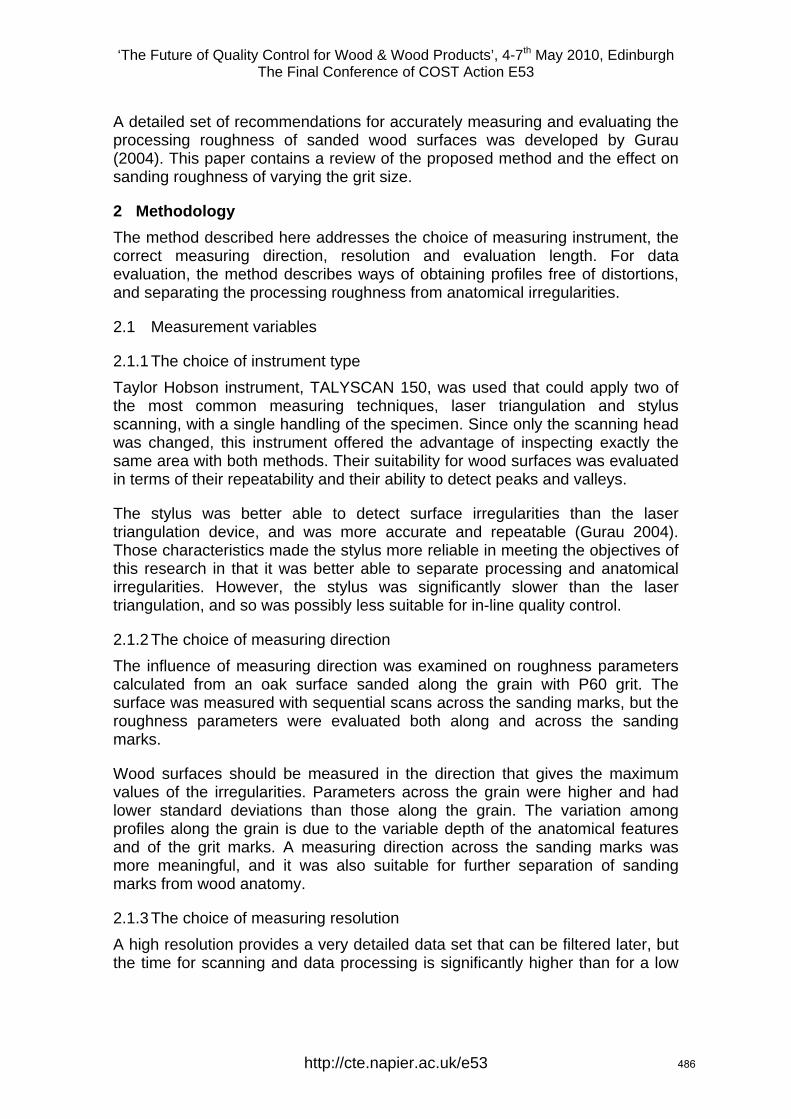
‘The Future of Quality Control for Wood & Wood Products’, 4-7th May 2010, Edinburgh The Final Conference of COST Action E53
A detailed set of recommendations for accurately measuring and evaluating the processing roughness of sanded wood surfaces was developed by Gurau (2004). This paper contains a review of the proposed method and the effect on sanding roughness of varying the grit size.
2 Methodology The method described here addresses the choice of measuring instrument, the correct measuring direction, resolution and evaluation length. For data evaluation, the method describes ways of obtaining profiles free of distortions, and separating the processing roughness from anatomical irregularities.
2.1 Measurement variables
2.1.1 The choice of instrument type Taylor Hobson instrument, TALYSCAN 150, was used that could apply two of the most common measuring techniques, laser triangulation and stylus scanning, with a single handling of the specimen. Since only the scanning head was changed, this instrument offered the advantage of inspecting exactly the same area with both methods. Their suitability for wood surfaces was evaluated in terms of their repeatability and their ability to detect peaks and valleys.
The stylus was better able to detect surface irregularities than the laser triangulation device, and was more accurate and repeatable (Gurau 2004). Those characteristics made the stylus more reliable in meeting the objectives of this research in that it was better able to separate processing and anatomical irregularities. However, the stylus was significantly slower than the laser triangulation, and so was possibly less suitable for in-line quality control.
2.1.2 The choice of measuring direction The influence of measuring direction was examined on roughness parameters calculated from an oak surface sanded along the grain with P60 grit. The surface was measured with sequential scans across the sanding marks, but the roughness parameters were evaluated both along and across the sanding marks.
Wood surfaces should be measured in the direction that gives the maximum values of the irregularities. Parameters across the grain were higher and had lower standard deviations than those along the grain. The variation among profiles along the grain is due to the variable depth of the anatomical features and of the grit marks. A measuring direction across the sanding marks was more meaningful, and it was also suitable for further separation of sanding marks from wood anatomy.
2.1.3 The choice of measuring resolution A high resolution provides a very detailed data set that can be filtered later, but the time for scanning and data processing is significantly higher than for a low
http://cte.napier.ac.uk/e53 486
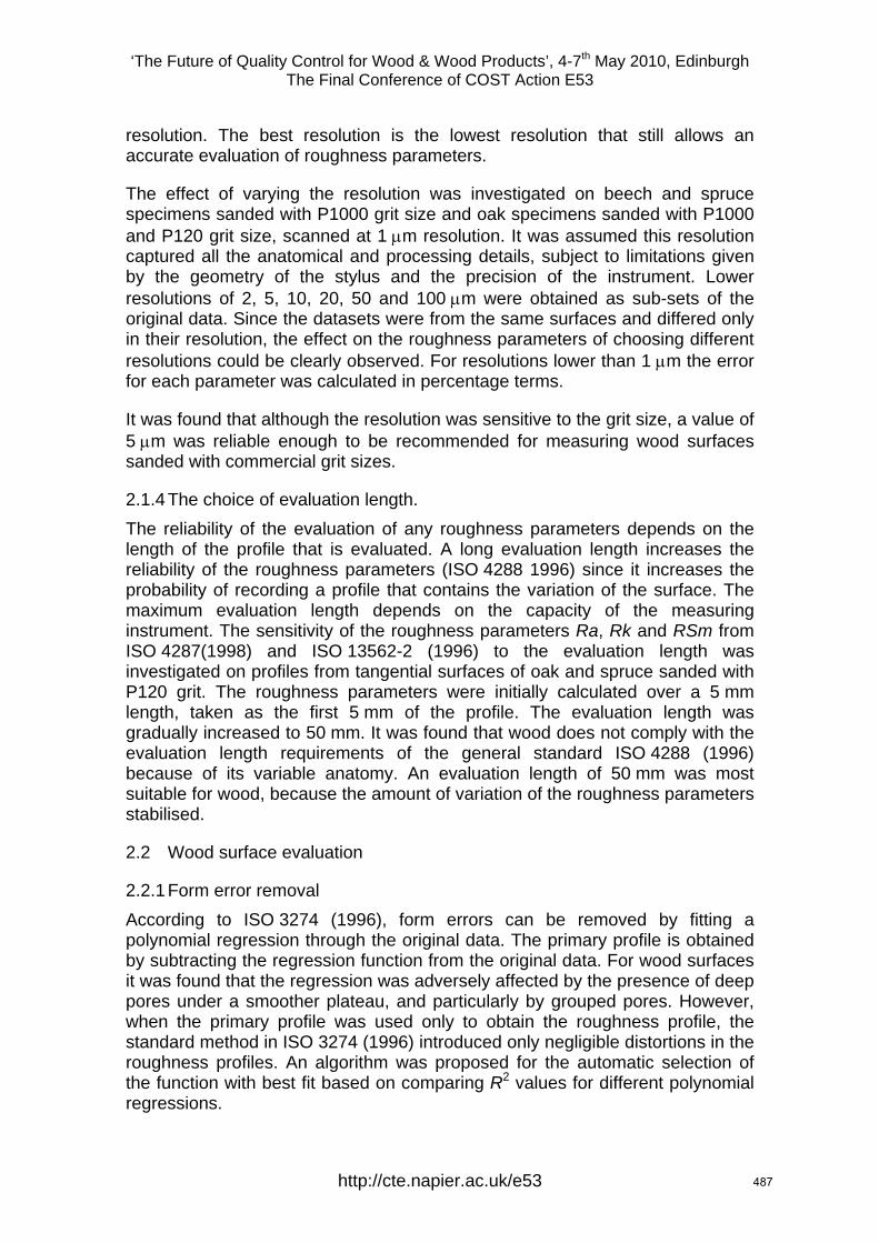
‘The Future of Quality Control for Wood & Wood Products’, 4-7th May 2010, Edinburgh The Final Conference of COST Action E53
resolution. The best resolution is the lowest resolution that still allows an accurate evaluation of roughness parameters.
The effect of varying the resolution was investigated on beech and spruce specimens sanded with P1000 grit size and oak specimens sanded with P1000 and P120 grit size, scanned at 1 μm resolution. It was assumed this resolution captured all the anatomical and processing details, subject to limitations given by the geometry of the stylus and the precision of the instrument. Lower resolutions of 2, 5, 10, 20, 50 and 100 μm were obtained as sub-sets of the original data. Since the datasets were from the same surfaces and differed only in their resolution, the effect on the roughness parameters of choosing different resolutions could be clearly observed. For resolutions lower than 1 μm the error for each parameter was calculated in percentage terms.
It was found that although the resolution was sensitive to the grit size, a value of 5 μm was reliable enough to be recommended for measuring wood surfaces sanded with commercial grit sizes.
2.1.4 The choice of evaluation length. The reliability of the evaluation of any roughness parameters depends on the length of the profile that is evaluated. A long evaluation length increases the reliability of the roughness parameters (ISO 4288 1996) since it increases the probability of recording a profile that contains the variation of the surface. The maximum evaluation length depends on the capacity of the measuring instrument. The sensitivity of the roughness parameters Ra, Rk and RSm from ISO 4287(1998) and ISO 13562-2 (1996) to the evaluation length was investigated on profiles from tangential surfaces of oak and spruce sanded with P120 grit. The roughness parameters were initially calculated over a 5 mm length, taken as the first 5 mm of the profile. The evaluation length was gradually increased to 50 mm. It was found that wood does not comply with the evaluation length requirements of the general standard ISO 4288 (1996) because of its variable anatomy. An evaluation length of 50 mm was most suitable for wood, because the amount of variation of the roughness parameters stabilised.
2.2 Wood surface evaluation
2.2.1 Form error removal According to ISO 3274 (1996), form errors can be removed by fitting a polynomial regression through the original data. The primary profile is obtained by subtracting the regression function from the original data. For wood surfaces it was found that the regression was adversely affected by the presence of deep pores under a smoother plateau, and particularly by grouped pores. However, when the primary profile was used only to obtain the roughness profile, the standard method in ISO 3274 (1996) introduced only negligible distortions in the roughness profiles. An algorithm was proposed for the automatic selection of the function with best fit based on comparing R2 values for different polynomial regressions.
http://cte.napier.ac.uk/e53 487
‘The Future of Quality Control for Wood & Wood Products’, 4-7th May 2010, Edinburgh The Final Conference of COST Action E53
2.2.2 Filtering the primary profile The “push-up” and end effects produced by ISO 11562 (1996) and ISO 13565-1 (1996) can be fully corrected, as Figure 2 shows when compared with Figure 1.
A number of profile filters were examined and the one that introduced the least distortion was the Robust
Gaussian Regression Filter (RGRF), described in a standard in preparation, ISO/DTS 16610-31 (2002). It is a modification of the Gaussian filter from ISO 11562 (1996) and is applied iteratively to a data set until a convergence condition is met.
10000 20000 30000 40000 500000
-80 -108
-136 -164 -192
-220
4 -24 -52
μm 60 32
μm
Figure 2: Roughness profile with no distortions, oak sanded with P1000.
2.2.3 Separating the processing roughness from the wood anatomy The Abbot curve is a material ratio curve defined in ISO 13565-2 (1996). It is a straightforward tool for calculating the real distribution of the profile heights from a distortion-free roughness profile.
In Figure 3, the Abbot curve is constructed by sorting the profile data in descending order. Statistically outlying peaks and valleys appear as non-linear regions in the Abbot-curve, and can be excluded. The upper and lower points of abrupt change in the local curvature of the Abbot-curve were identified by monitoring the variation of its second derivatives (Figure 3). These points were taken to mark the thresholds for the core data (Figure 4).
Processing roughness was defined as the core roughness of a profile where the outlying peaks and valleys have been replaced with zeros. The anatomical roughness was taken as the valleys below the lower threshold, while the peaks above the upper threshold represent the fuzziness.
Fuzziness is caused by groups of fibres that are attached to the surface at only one end; it varies with species, density and moisture content and to a lesser extent with processing.
http://cte.napier.ac.uk/e53 488
‘The Future of Quality Control for Wood & Wood Products’, 4-7th May 2010, Edinburgh The Final Conference of COST Action E53
upper threshold
lower threshold
the Abbot curve
second derivatives of the Abbot curve
10000 0 20000 30000 40000 50000
-100
-200
0
80μm
μm
Figure 3: Detection of the lower and upper thresholds in the Abbot curve, oak sanded with P1000.
upper threshold
lower threshold
10000 200000 4000030000 50000
0
-20
20 μm
μm
Figure 4: Separation of the core roughness profile from wood anatomy, oak sanded with P1000.
10000 200000 4000030000 50000-4
-2
0
2
4 μm
μm
Figure 5: Processing roughness of an oak profile sanded with P1000.
Figure 5 shows the processing roughness of an oak profile sanded with P1000, after the separation. Note the small range on the y-axis for this fine grit size.
2.2.4 Calculation of processing roughness parameters The general standards ISO 4287 (1998) and ISO 13565-2 (1996) give a variety of quantitative measures of surface roughness. A single value of these parameters is defined on a nominal interval called the sampling length. The length used for assessing the profile is called the evaluation length, which in general should contain five sampling lengths. However, given the variability in wood anatomy, roughness parameters calculated over the evaluation length were more reliable than those defined on sampling lengths, and therefore are recommended for a wood surface.
http://cte.napier.ac.uk/e53 489
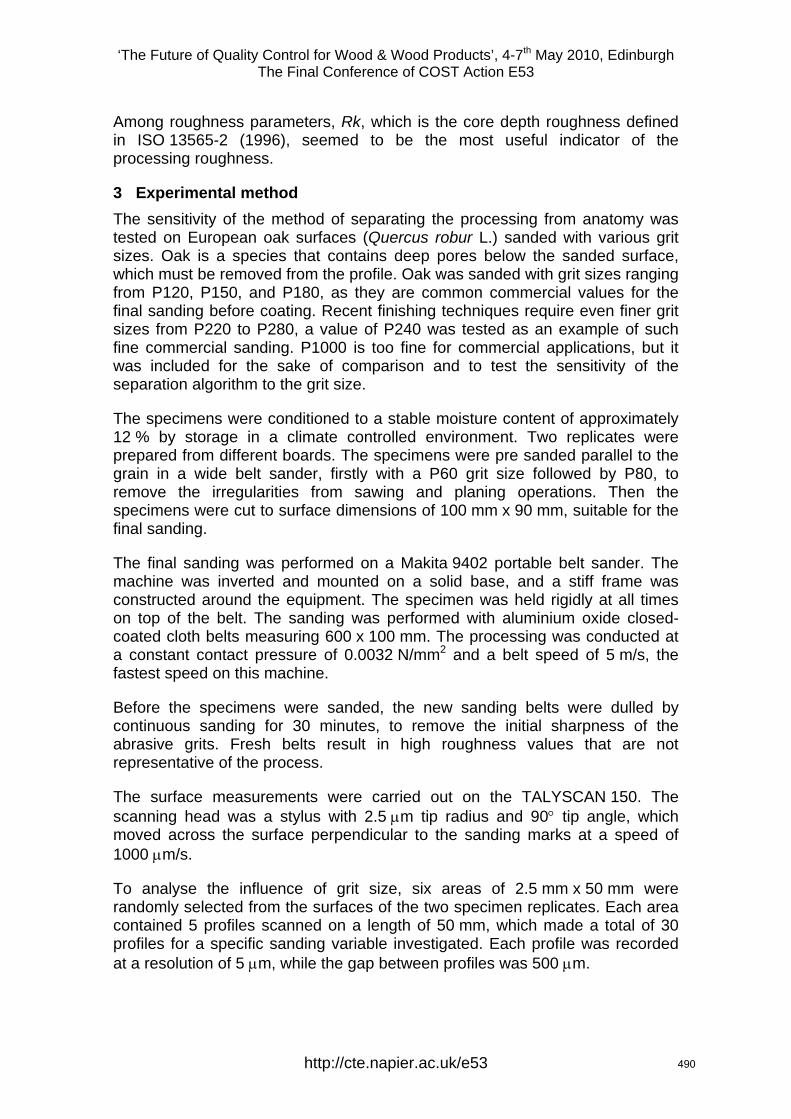
‘The Future of Quality Control for Wood & Wood Products’, 4-7th May 2010, Edinburgh The Final Conference of COST Action E53
Among roughness parameters, Rk, which is the core depth roughness defined in ISO 13565-2 (1996), seemed to be the most useful indicator of the processing roughness.
3 Experimental method The sensitivity of the method of separating the processing from anatomy was tested on European oak surfaces (Quercus robur L.) sanded with various grit sizes. Oak is a species that contains deep pores below the sanded surface, which must be removed from the profile. Oak was sanded with grit sizes ranging from P120, P150, and P180, as they are common commercial values for the final sanding before coating. Recent finishing techniques require even finer grit sizes from P220 to P280, a value of P240 was tested as an example of such fine commercial sanding. P1000 is too fine for commercial applications, but it was included for the sake of comparison and to test the sensitivity of the separation algorithm to the grit size.
The specimens were conditioned to a stable moisture content of approximately 12 % by storage in a climate controlled environment. Two replicates were prepared from different boards. The specimens were pre sanded parallel to the grain in a wide belt sander, firstly with a P60 grit size followed by P80, to remove the irregularities from sawing and planing operations. Then the specimens were cut to surface dimensions of 100 mm x 90 mm, suitable for the final sanding.
The final sanding was performed on a Makita 9402 portable belt sander. The machine was inverted and mounted on a solid base, and a stiff frame was constructed around the equipment. The specimen was held rigidly at all times on top of the belt. The sanding was performed with aluminium oxide closed-coated cloth belts measuring 600 x 100 mm. The processing was conducted at a constant contact pressure of 0.0032 N/mm2 and a belt speed of 5 m/s, the fastest speed on this machine.
Before the specimens were sanded, the new sanding belts were dulled by continuous sanding for 30 minutes, to remove the initial sharpness of the abrasive grits. Fresh belts result in high roughness values that are not representative of the process.
The surface measurements were carried out on the TALYSCAN 150. The scanning head was a stylus with 2.5 μm tip radius and 90° tip angle, which moved across the surface perpendicular to the sanding marks at a speed of 1000 μm/s.
To analyse the influence of grit size, six areas of 2.5 mm x 50 mm were randomly selected from the surfaces of the two specimen replicates. Each area contained 5 profiles scanned on a length of 50 mm, which made a total of 30 profiles for a specific sanding variable investigated. Each profile was recorded at a resolution of 5 μm, while the gap between profiles was 500 μm.
http://cte.napier.ac.uk/e53 490
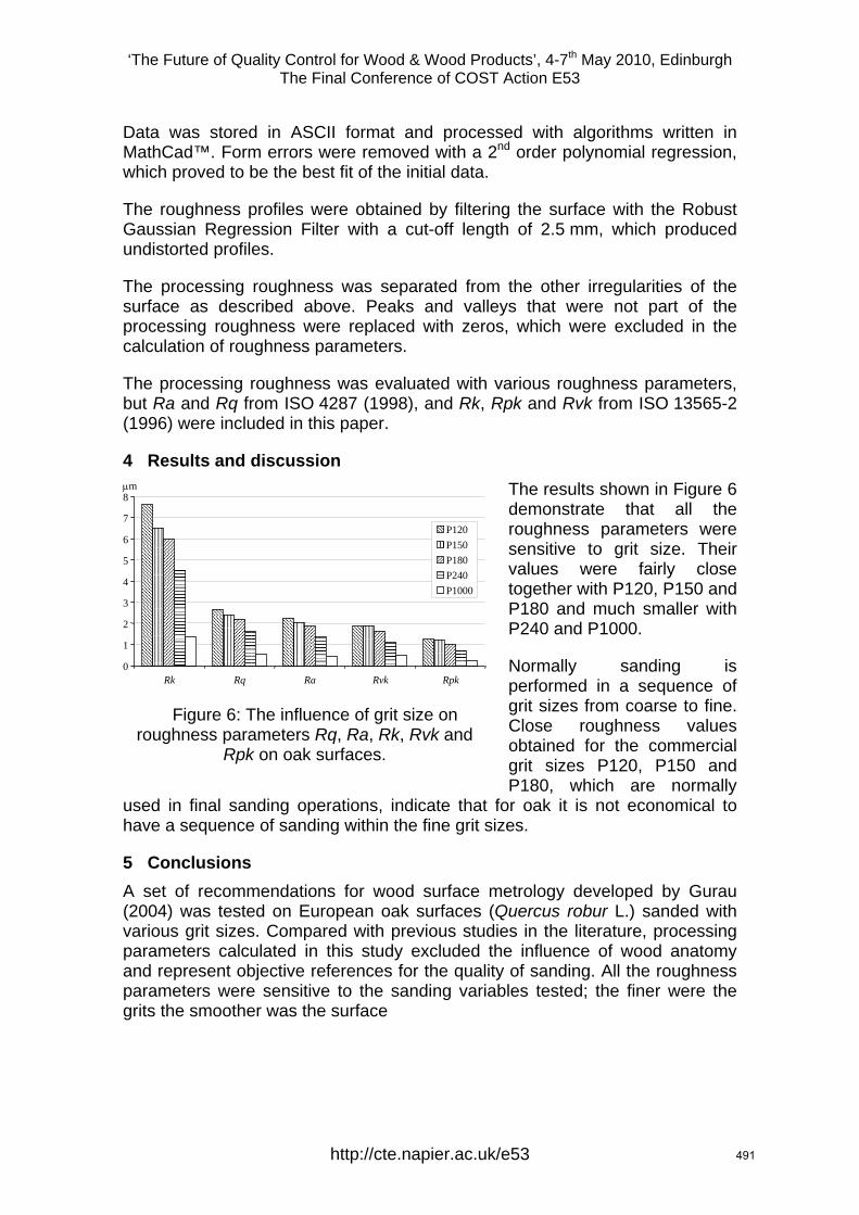
‘The Future of Quality Control for Wood & Wood Products’, 4-7th May 2010, Edinburgh The Final Conference of COST Action E53
Data was stored in ASCII format and processed with algorithms written in MathCad™. Form errors were removed with a 2nd order polynomial regression, which proved to be the best fit of the initial data.
The roughness profiles were obtained by filtering the surface with the Robust Gaussian Regression Filter with a cut-off length of 2.5 mm, which produced undistorted profiles.
The processing roughness was separated from the other irregularities of the surface as described above. Peaks and valleys that were not part of the processing roughness were replaced with zeros, which were excluded in the calculation of roughness parameters.
The processing roughness was evaluated with various roughness parameters, but Ra and Rq from ISO 4287 (1998), and Rk, Rpk and Rvk from ISO 13565-2 (1996) were included in this paper.
4 Results and discussion The results shown in Figure 6 demonstrate that all the roughness parameters were sensitive to grit size. Their values were fairly close together with P120, P150 and P180 and much smaller with P240 and P1000.
Normally sanding is performed in a sequence of grit sizes from coarse to fine. Close roughness values obtained for the commercial grit sizes P120, P150 and P180, which are normally
used in final sanding operations, indicate that for oak it is not economical to have a sequence of sanding within the fine grit sizes.
0
1
2
3
4
5
6
7
8
Rk Rq Ra Rvk Rpk
P120P150P180P240P1000
μm
Figure 6: The influence of grit size on roughness parameters Rq, Ra, Rk, Rvk and
Rpk on oak surfaces.
5 Conclusions A set of recommendations for wood surface metrology developed by Gurau (2004) was tested on European oak surfaces (Quercus robur L.) sanded with various grit sizes. Compared with previous studies in the literature, processing parameters calculated in this study excluded the influence of wood anatomy and represent objective references for the quality of sanding. All the roughness parameters were sensitive to the sanding variables tested; the finer were the grits the smoother was the surface
http://cte.napier.ac.uk/e53 491

‘The Future of Quality Control for Wood & Wood Products’, 4-7th May 2010, Edinburgh The Final Conference of COST Action E53
However, sanding with finishing grit sizes P120, P150 and P180 produced very close roughness values for oak. This indicates that for oak it is not economical to have a sequence of sanding operations in the domain of fine grit sizes.
The method can further be used to evaluate roughness parameters for different combinations of sanding variables to optimise the sanding process.
References ASME B46.1. (1995) “Surface Texture. (Surface Roughness, Waviness, Lay)”.
Gurau, L., Mansfield-Williams, H. & Irle, M. (2005) “Processing Roughness of Sanded Wood Surfaces”. Holz als Roh- und Werkstoff. 63(1), pp.43-52.
Gurau, L. (2004) “The Roughness of Sanded Wood Surfaces”. Doctoral thesis. Forest Products Research Centre. Buckinghamshire Chilterns University College. Brunel University.
ISO 11562 (1996) “Geometrical Product Specifications (GPS) – Surface Texture: Profile Method – Metrological Characteristics of Phase Correct Filters”.
ISO 13565-1 (1996) “Geometrical Product Specifications (GPS) – Surface Texture. Profile Method. Surfaces Having Stratified Functional Properties. Part 1: Filtering and General Measurement Conditions”.
ISO 13565-2 (1996) “Geometrical Product Specifications (GPS) – Surface Texture: Profile Method; Surfaces Having Stratified Functional Properties – Part 2: Height Characterisation Using the Linear Material Ratio Curve”.
ISO 13565–3 (2000) “Geometrical product specification (GPS). – Profile method. Surfaces having stratified functional properties”.
ISO 3274 (1996) “Geometrical Product Specifications (GPS) – Surface Texture. Profile Method –Nominal characteristics of contact (stylus) instruments”.
ISO 4287 (1998) “Geometrical Product Specifications (GPS). Surface Texture. Profile Method. Terms. Definitions and Surface Texture Parameters”.
ISO 4288 (1996) “Geometrical Product Specifications (GPS) – Surface Texture. Profile Method – Rules and Procedures for the Assessment of Surface Texture”.
ISO/DTS 16610-31 (2002(E)) “Geometrical product specification (GPS) – Filtration. Part 31: Robust profile filters. Gaussian regression filters”. In Draft.
Krish, J. & Csiha, C. (1999) “Analysing Wood Surface Roughness Using an S3P Perthometer and Computer Based Data Processing”. In:Proc. XIII Sesja Naukowa “Badania dla Meblarstwa”. Poland. pp.145-154
Westkämper, E. & Riegel, A. (1993) „Qualitätskriterien fur Geschlieffene Massivholzoberflächen“. Holz als Roh- und Werkstoff. 51(2), pp.121-125.
http://cte.napier.ac.uk/e53 492

‘The Future of Quality Control for Wood & Wood Products’, 4-7th May 2010, Edinburgh The Final Conference of COST Action E53
Thursday 6th May Research focussed day
Parallel session 3A
http://www.cte.napier.ac.uk/e53/ 493
‘The Future of Quality Control for Wood & Wood Products’, 4-7th May 2010, Edinburgh The Final Conference of COST Action E53
Early-stage prediction and modeling strength properties of Lithuanian-grown Scots Pine (Pinus Sylvestris L.)
A.Baltrusaitis1, M. Aleinikovas2 & L. Kudakas3
1. Introduction Timber properties and their dependence on various factors are quite extensively studied world-wide. The analyses on the distribution of coniferous timber to the strength classes are becoming more and more sophisticated. The objective of the studies is to create the databases on the distribution of the main commercial tree species in each European country to the standardized strength classes. The integrated European base will allow the tenders of wood industry to be oriented in raw wood market and to be competitive in furniture and, particularly, in the timber building and construction industry. As for the design of load-bearing structures it is necessary to supply wood of reliable strength characteristics. In addition, it is very important to determinate the roundwood stiffness-strength characteristics and the correlations with the sawn timber strength and stiffness. It is also essential then the roundwood for structural use could be pre-graded in earliest possible stage. The aims of this article – (1) to determine the distribution of Lithuanian pine wood according to the international strength classes and (2) to establish correlations of roundwood and sawn timber viscous-elastic properties.
2. Materials and methods
At least 6 model trees (total 42 trees) from Scots pine (Pinus Sylvestris L.) stands were selected in seven forest regions of Lithuania representing typical growing sites. Three logs (2.4-3.0 m length) but log, middle log and top log were sampled from each tree. There were 8 - 12 model logs (total 78 logs) taken for testing. Integrated comparative non-destructive methodology was used for the analysis of saw timber taken from the model logs focused on modulus of elasticity, strength and the distribution into strength class according the EN 338. The non-destructive tests were done using following devices: 1. The Timber Grader MTG, used for measuring the timber strength and
stiffness (Brookhuis Microelectronics BV, Holland). Log dynamic modulus of elasticity was calculated according the natural frequency, average wood density and moisture content of the log.
1 Department of Wood Technology, Faculty of Design and Technologies, Kaunas University of Technology, Kaunas, Lithuania. [email protected] Department of Forest Resources, Economics and Policy, Lithuanian Forest Research Institute, Girionys, Lithuania. [email protected] Stora Enso Timber, Alytus sawmill, Alytus, Lithuania. [email protected]
http://cte.napier.ac.uk/e53 494
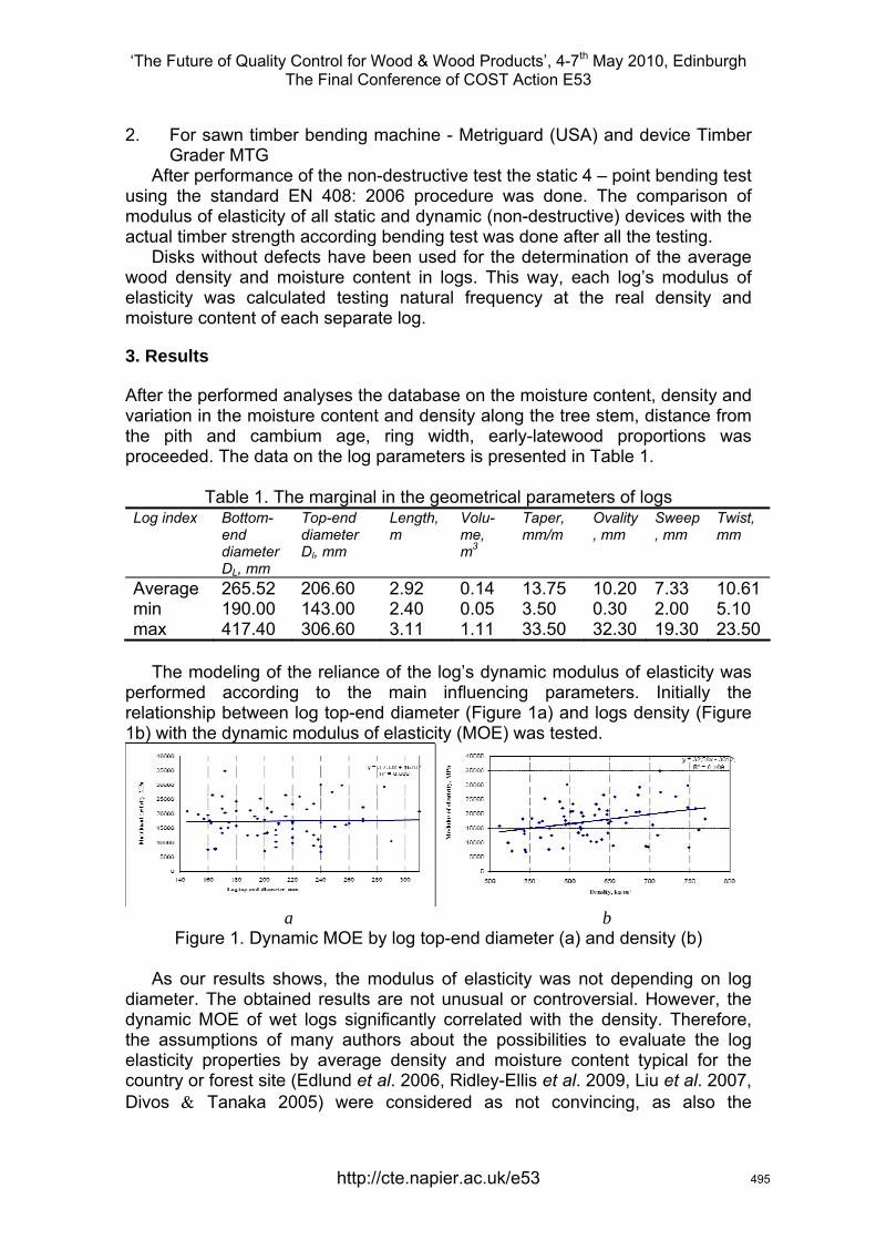
‘The Future of Quality Control for Wood & Wood Products’, 4-7th May 2010, Edinburgh The Final Conference of COST Action E53
2. For sawn timber bending machine - Metriguard (USA) and device Timber Grader MTG
After performance of the non-destructive test the static 4 – point bending test using the standard EN 408: 2006 procedure was done. The comparison of modulus of elasticity of all static and dynamic (non-destructive) devices with the actual timber strength according bending test was done after all the testing.
Disks without defects have been used for the determination of the average wood density and moisture content in logs. This way, each log’s modulus of elasticity was calculated testing natural frequency at the real density and moisture content of each separate log.
3. Results
After the performed analyses the database on the moisture content, density and variation in the moisture content and density along the tree stem, distance from the pith and cambium age, ring width, early-latewood proportions was proceeded. The data on the log parameters is presented in Table 1.
Table 1. The marginal in the geometrical parameters of logs Log index Bottom-
end diameter DL, mm
Top-end diameter Dl, mm
Length, m
Volu-me, m3
Taper, mm/m
Ovality, mm
Sweep, mm
Twist, mm
Average 265.52 206.60 2.92 0.14 13.75 10.20 7.33 10.61min 190.00 143.00 2.40 0.05 3.50 0.30 2.00 5.10 max 417.40 306.60 3.11 1.11 33.50 32.30 19.30 23.50
The modeling of the reliance of the log’s dynamic modulus of elasticity was
performed according to the main influencing parameters. Initially the relationship between log top-end diameter (Figure 1a) and logs density (Figure 1b) with the dynamic modulus of elasticity (MOE) was tested.
a b
Figure 1. Dynamic MOE by log top-end diameter (a) and density (b)
As our results shows, the modulus of elasticity was not depending on log diameter. The obtained results are not unusual or controversial. However, the dynamic MOE of wet logs significantly correlated with the density. Therefore, the assumptions of many authors about the possibilities to evaluate the log elasticity properties by average density and moisture content typical for the country or forest site (Edlund et al. 2006, Ridley-Ellis et al. 2009, Liu et al. 2007, Divos & Tanaka 2005) were considered as not convincing, as also the
http://cte.napier.ac.uk/e53 495
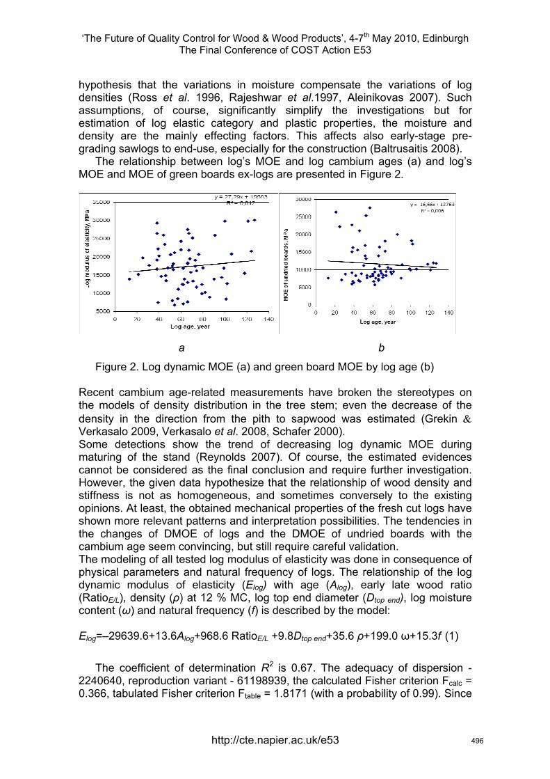
‘The Future of Quality Control for Wood & Wood Products’, 4-7th May 2010, Edinburgh The Final Conference of COST Action E53
hypothesis that the variations in moisture compensate the variations of log densities (Ross et al. 1996, Rajeshwar et al.1997, Aleinikovas 2007). Such assumptions, of course, significantly simplify the investigations but for estimation of log elastic category and plastic properties, the moisture and density are the mainly effecting factors. This affects also early-stage pre-grading sawlogs to end-use, especially for the construction (Baltrusaitis 2008).
The relationship between log’s MOE and log cambium ages (a) and log’s MOE and MOE of green boards ex-logs are presented in Figure 2.
a b
Figure 2. Log dynamic MOE (a) and green board MOE by log age (b)
Recent cambium age-related measurements have broken the stereotypes on the models of density distribution in the tree stem; even the decrease of the density in the direction from the pith to sapwood was estimated (Grekin & Verkasalo 2009, Verkasalo et al. 2008, Schafer 2000). Some detections show the trend of decreasing log dynamic MOE during maturing of the stand (Reynolds 2007). Of course, the estimated evidences cannot be considered as the final conclusion and require further investigation. However, the given data hypothesize that the relationship of wood density and stiffness is not as homogeneous, and sometimes conversely to the existing opinions. At least, the obtained mechanical properties of the fresh cut logs have shown more relevant patterns and interpretation possibilities. The tendencies in the changes of DMOE of logs and the DMOE of undried boards with the cambium age seem convincing, but still require careful validation. The modeling of all tested log modulus of elasticity was done in consequence of physical parameters and natural frequency of logs. The relationship of the log dynamic modulus of elasticity (Elog) with age (Alog), early late wood ratio (RatioE/L), density (ρ) at 12 % MC, log top end diameter (Dtop end), log moisture content (ω) and natural frequency (f) is described by the model:
Elog=–29639.6+13.6Alog+968.6 RatioE/L +9.8Dtop end+35.6 ρ+199.0 ω+15.3f (1)
The coefficient of determination R2 is 0.67. The adequacy of dispersion -
2240640, reproduction variant - 61198939, the calculated Fisher criterion Fcalc = 0.366, tabulated Fisher criterion Ftable = 1.8171 (with a probability of 0.99). Since
http://cte.napier.ac.uk/e53 496
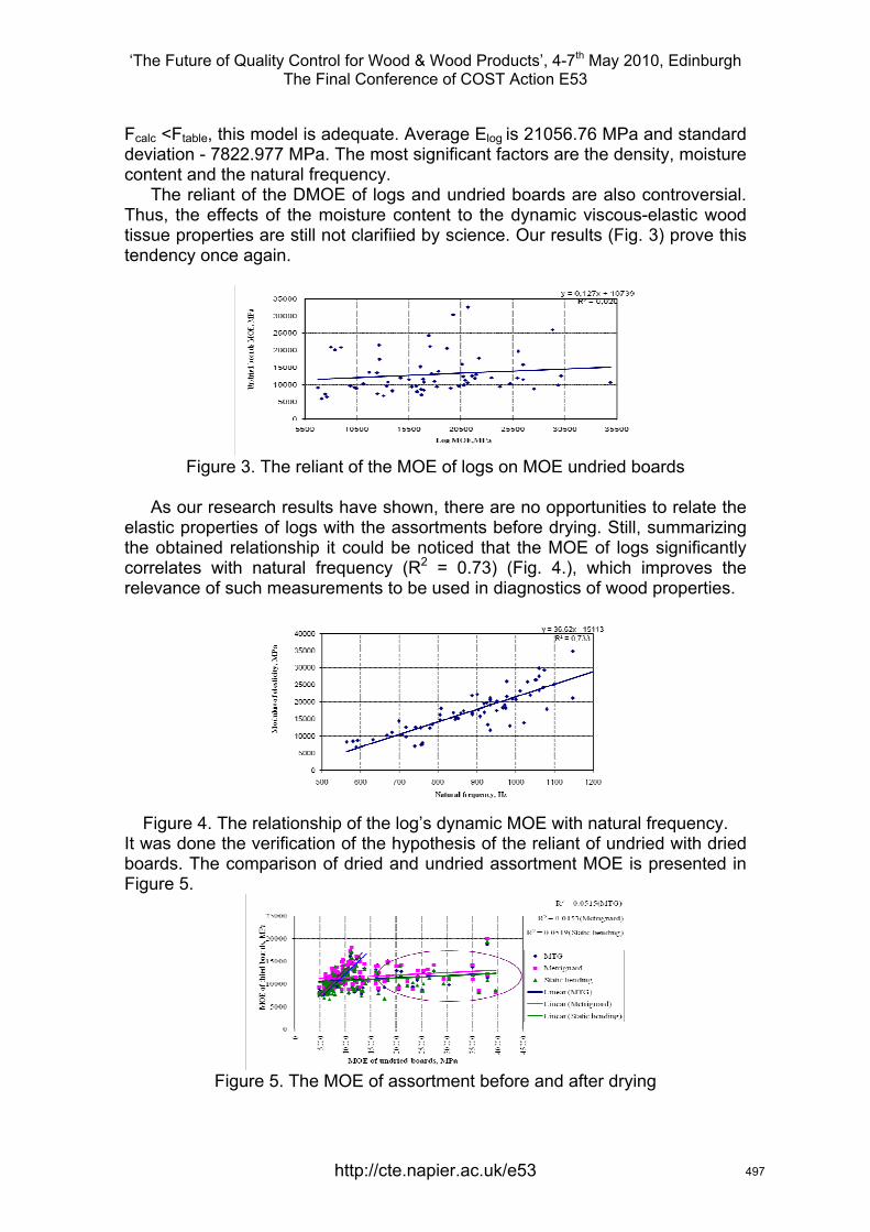
‘The Future of Quality Control for Wood & Wood Products’, 4-7th May 2010, Edinburgh The Final Conference of COST Action E53
Fcalc <Ftable, this model is adequate. Average Elog is 21056.76 MPa and standard deviation - 7822.977 MPa. The most significant factors are the density, moisture content and the natural frequency.
The reliant of the DMOE of logs and undried boards are also controversial. Thus, the effects of the moisture content to the dynamic viscous-elastic wood tissue properties are still not clarifiied by science. Our results (Fig. 3) prove this tendency once again.
Figure 3. The reliant of the MOE of logs on MOE undried boards
As our research results have shown, there are no opportunities to relate the
elastic properties of logs with the assortments before drying. Still, summarizing the obtained relationship it could be noticed that the MOE of logs significantly correlates with natural frequency (R2 = 0.73) (Fig. 4.), which improves the relevance of such measurements to be used in diagnostics of wood properties.
Figure 4. The relationship of the log’s dynamic MOE with natural frequency.
It was done the verification of the hypothesis of the reliant of undried with dried boards. The comparison of dried and undried assortment MOE is presented in Figure 5.
Figure 5. The MOE of assortment before and after drying
http://cte.napier.ac.uk/e53 497
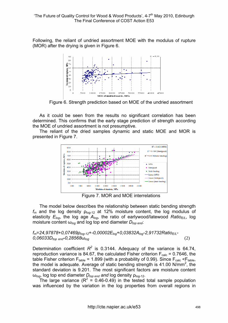
‘The Future of Quality Control for Wood & Wood Products’, 4-7th May 2010, Edinburgh The Final Conference of COST Action E53
Following, the reliant of undried assortment MOE with the modulus of rupture (MOR) after the drying is given in Figure 6.
Figure 6. Strength prediction based on MOE of the undried assortment
As it could be seen from the results no significant correlation has been determined. This confirms that the early stage prediction of strength according the MOE of undried assortment is not presumptive.
The reliant of the dried samples dynamic and static MOE and MOR is presented in Figure 7.
Figure 7. MOR and MOE interrelations
The model below describes the relationship between static bending strength
fm and the log density ρlog-12 at 12% moisture content, the log modulus of elasticity Elog, the log age Alog, the ratio of earlywood/latewood RatioE/L, log moisture content ωlog and log top end diameter Dtop end: fm=24,97878+0,07469ρlog-12+-0,00002Elog+0,03832Alog-2,91732RatioE/L-0,06033Dtop end-0,28568ωlog (2) Determination coefficient R2 is 0.3144. Adequacy of the variance is 64.74, reproduction variance is 84.67, the calculated Fisher criterion Fcalc = 0.7646, the table Fisher criterion Ftable = 1.899 (with a probability of 0.99). Since Fcalc <Ftable, the model is adequate. Average of static bending strength is 41.00 N/mm2, the standard deviation is 9.201. The most significant factors are moisture content ωlog, log top end diameter Dtop end and log density ρlog-12.
The large variance (R2 = 0.46-0.49) in the tested total sample population was influenced by the variation in the log properties from overall regions in
http://cte.napier.ac.uk/e53 498
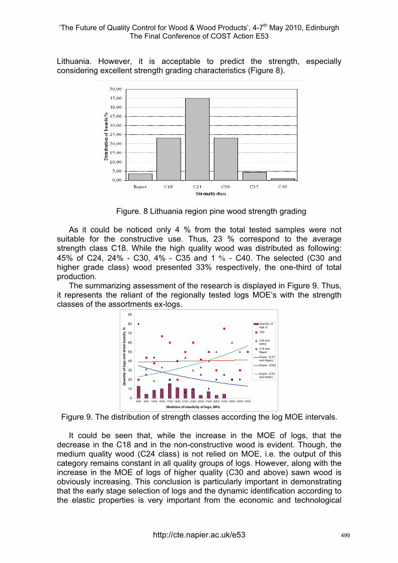
‘The Future of Quality Control for Wood & Wood Products’, 4-7th May 2010, Edinburgh The Final Conference of COST Action E53
Lithuania. However, it is acceptable to predict the strength, especially considering excellent strength grading characteristics (Figure 8).
Figure. 8 Lithuania region pine wood strength grading
As it could be noticed only 4 % from the total tested samples were not suitable for the constructive use. Thus, 23 % correspond to the average strength class C18. While the high quality wood was distributed as following: 45% of C24, 24% - C30, 4% - C35 and 1 % - C40. The selected (C30 and higher grade class) wood presented 33% respectively, the one-third of total production.
The summarizing assessment of the research is displayed in Figure 9. Thus, it represents the reliant of the regionally tested logs MOE’s with the strength classes of the assortments ex-logs.
0
10
20
30
40
50
60
70
80
90
7000 9000 13000 15000 17000 19000 21000 23000 25000 27000 29000 31000 33000 35000 37000
Modulus of elasticity of logs, MPa
Qua
ntity
of l
ogs
and
drie
d bo
ards
, %
Quantity oflogs,%
C24
C30 andbetter
C18 andReject
Expon. (C18and Reject)
Expon. (C24)
Expon. (C30and better)
Figure 9. The distribution of strength classes according the log MOE intervals.
It could be seen that, while the increase in the MOE of logs, that the
decrease in the C18 and in the non-constructive wood is evident. Though, the medium quality wood (C24 class) is not relied on MOE, i.e. the output of this category remains constant in all quality groups of logs. However, along with the increase in the MOE of logs of higher quality (C30 and above) sawn wood is obviously increasing. This conclusion is particularly important in demonstrating that the early stage selection of logs and the dynamic identification according to the elastic properties is very important from the economic and technological
http://cte.napier.ac.uk/e53 499
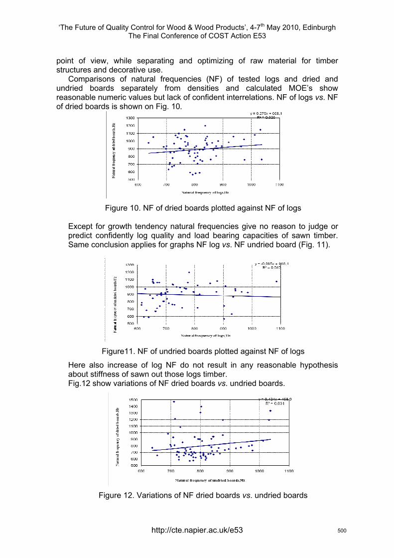
‘The Future of Quality Control for Wood & Wood Products’, 4-7th May 2010, Edinburgh The Final Conference of COST Action E53
point of view, while separating and optimizing of raw material for timber structures and decorative use.
Comparisons of natural frequencies (NF) of tested logs and dried and undried boards separately from densities and calculated MOE’s show reasonable numeric values but lack of confident interrelations. NF of logs vs. NF of dried boards is shown on Fig. 10.
Figure 10. NF of dried boards plotted against NF of logs
Except for growth tendency natural frequencies give no reason to judge or predict confidently log quality and load bearing capacities of sawn timber. Same conclusion applies for graphs NF log vs. NF undried board (Fig. 11).
Figure11. NF of undried boards plotted against NF of logs
Here also increase of log NF do not result in any reasonable hypothesis about stiffness of sawn out those logs timber. Fig.12 show variations of NF dried boards vs. undried boards.
Figure 12. Variations of NF dried boards vs. undried boards
http://cte.napier.ac.uk/e53 500
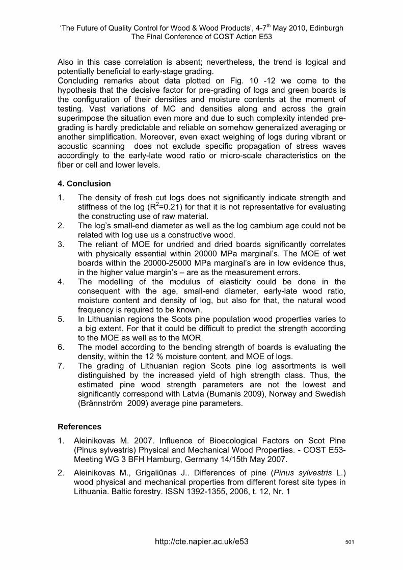
‘The Future of Quality Control for Wood & Wood Products’, 4-7th May 2010, Edinburgh The Final Conference of COST Action E53
Also in this case correlation is absent; nevertheless, the trend is logical and potentially beneficial to early-stage grading. Concluding remarks about data plotted on Fig. 10 -12 we come to the hypothesis that the decisive factor for pre-grading of logs and green boards is the configuration of their densities and moisture contents at the moment of testing. Vast variations of MC and densities along and across the grain superimpose the situation even more and due to such complexity intended pre-grading is hardly predictable and reliable on somehow generalized averaging or another simplification. Moreover, even exact weighing of logs during vibrant or acoustic scanning does not exclude specific propagation of stress waves accordingly to the early-late wood ratio or micro-scale characteristics on the fiber or cell and lower levels.
4. Conclusion 1. The density of fresh cut logs does not significantly indicate strength and
stiffness of the log (R2=0.21) for that it is not representative for evaluating the constructing use of raw material.
2. The log’s small-end diameter as well as the log cambium age could not be related with log use us a constructive wood.
3. The reliant of MOE for undried and dried boards significantly correlates with physically essential within 20000 MPa marginal’s. The MOE of wet boards within the 20000-25000 MPa marginal’s are in low evidence thus, in the higher value margin’s – are as the measurement errors.
4. The modelling of the modulus of elasticity could be done in the consequent with the age, small-end diameter, early-late wood ratio, moisture content and density of log, but also for that, the natural wood frequency is required to be known.
5. In Lithuanian regions the Scots pine population wood properties varies to a big extent. For that it could be difficult to predict the strength according to the MOE as well as to the MOR.
6. The model according to the bending strength of boards is evaluating the density, within the 12 % moisture content, and MOE of logs.
7. The grading of Lithuanian region Scots pine log assortments is well distinguished by the increased yield of high strength class. Thus, the estimated pine wood strength parameters are not the lowest and significantly correspond with Latvia (Bumanis 2009), Norway and Swedish (Brännström 2009) average pine parameters.
References 1. Aleinikovas M. 2007. Influence of Bioecological Factors on Scot Pine
(Pinus sylvestris) Physical and Mechanical Wood Properties. - COST E53-Meeting WG 3 BFH Hamburg, Germany 14/15th May 2007.
2. Aleinikovas M., Grigaliūnas J.. Differences of pine (Pinus sylvestris L.) wood physical and mechanical properties from different forest site types in Lithuania. Baltic forestry. ISSN 1392-1355, 2006, t. 12, Nr. 1
http://cte.napier.ac.uk/e53 501
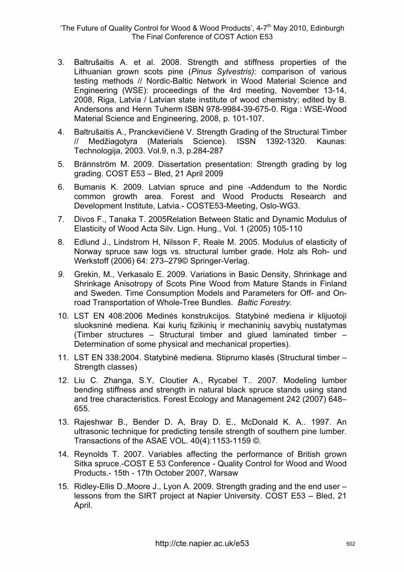
‘The Future of Quality Control for Wood & Wood Products’, 4-7th May 2010, Edinburgh The Final Conference of COST Action E53
3. Baltrušaitis A. et al. 2008. Strength and stiffness properties of the Lithuanian grown scots pine (Pinus Sylvestris): comparison of various testing methods // Nordic-Baltic Network in Wood Material Science and Engineering (WSE): proceedings of the 4rd meeting, November 13-14, 2008, Riga, Latvia / Latvian state institute of wood chemistry; edited by B. Andersons and Henn Tuherm ISBN 978-9984-39-675-0. Riga : WSE-Wood Material Science and Engineering, 2008, p. 101-107.
4. Baltrušaitis A., Pranckevičienė V. Strength Grading of the Structural Timber // Medžiagotyra (Materials Science). ISSN 1392-1320. Kaunas: Technologija, 2003. Vol.9, n.3, p.284-287
5. Brännström M. 2009. Dissertation presentation: Strength grading by log grading. COST E53 – Bled, 21 April 2009
6. Bumanis K. 2009. Latvian spruce and pine -Addendum to the Nordic common growth area. Forest and Wood Products Research and Development Institute, Latvia.- COSTE53-Meeting, Oslo-WG3.
7. Divos F., Tanaka T. 2005Relation Between Static and Dynamic Modulus of Elasticity of Wood Acta Silv. Lign. Hung., Vol. 1 (2005) 105-110
8. Edlund J., Lindstrom H, Nilsson F, Reale M. 2005. Modulus of elasticity of Norway spruce saw logs vs. structural lumber grade. Holz als Roh- und Werkstoff (2006) 64: 273–279© Springer-Verlag.
9. Grekin, M., Verkasalo E. 2009. Variations in Basic Density, Shrinkage and Shrinkage Anisotropy of Scots Pine Wood from Mature Stands in Finland and Sweden. Time Consumption Models and Parameters for Off- and On-road Transportation of Whole-Tree Bundles. Baltic Forestry.
10. LST EN 408:2006 Medinės konstrukcijos. Statybinė mediena ir klijuotoji sluoksninė mediena. Kai kurių fizikinių ir mechaninių savybių nustatymas (Timber structures – Structural timber and glued laminated timber – Determination of some physical and mechanical properties).
11. LST EN 338:2004. Statybinė mediena. Stiprumo klasės (Structural timber – Strength classes)
12. Liu C. Zhanga, S.Y, Cloutier A., Rycabel T.. 2007. Modeling lumber bending stiffness and strength in natural black spruce stands using stand and tree characteristics. Forest Ecology and Management 242 (2007) 648–655.
13. Rajeshwar B., Bender D. A, Bray D. E., McDonald K. A.. 1997. An ultrasonic technique for predicting tensile strength of southern pine lumber. Transactions of the ASAE VOL. 40(4):1153-1159 ©.
14. Reynolds T. 2007. Variables affecting the performance of British grown Sitka spruce.-COST E 53 Conference - Quality Control for Wood and Wood Products.- 15th - 17th October 2007, Warsaw
15. Ridley-Ellis D.,Moore J., Lyon A. 2009. Strength grading and the end user – lessons from the SIRT project at Napier University. COST E53 – Bled, 21 April.
http://cte.napier.ac.uk/e53 502

‘The Future of Quality Control for Wood & Wood Products’, 4-7th May 2010, Edinburgh The Final Conference of COST Action E53
16. Ross R. S., McDonald K. A., Green D. W.,. Shad K.C.1996. Relationship between log and lumber modulus of elasticity.- FOREST PRODUCTS JOURNAL VOL. .47, No. 2,
17. Schafer M. C.. Ultrasound for defect detection and grading in wood and lumber. Perceptron, Inc. Ultrasound Technology Group, 5 185 Campus Drive, Plymouth Meeting, PA 19462. 2000 IEEE ULTRASONICS SYMPOSIUM
18. Searles G & Moore J. 2009. Measurement of Wood Stiffness in Standing Trees and Logs: Implications for End-Product Quality. COST E53 – Bled, 21 April 2009
19. Verkasalo E., Riekkinen M., Lindström H. 2008. Specific wood and timber properties and competitive ability of Nordic Scots pine in mechanical wood processing. COST Action E44 Wood Processisg Strategy.
http://cte.napier.ac.uk/e53 503
‘The Future of Quality Control for Wood & Wood Products’, 4-7th May 2010, Edinburgh The Final Conference of COST Action E53
Strength grading of Slovenian structural sawn timber
J. Srpcic1, M. Plos2, T. Pazlar3 & G. Turk4
Abstract In the paper preliminary results of the research project dealing with introduction of grading methods into Slovenian sawmills and creating the database of Slovenian timber is presented. The aim of the project, partly financed by the Slovenian Research Agency and partly by the industry, is practical implementation of European standards into the production of sawn timber, finding the correlation between indicative properties of Slovenian timber and grading characteristics, and grading more than 1000 boards of Picea Abies Mill. The presented research is closely related with the work package WP3 “Experimental research” in the GRADEWOOD project.
1 Introduction Although 60% of Slovenia is covered by forests, timber is relatively rarely used for construction. Whereas in the past the main products were wood-based panels recently the focus has been put on timber structures. However, the use of timber for roof and floor structures is still based on visual assessment of wood quality which is a combination of strength grading criteria (knots, annual rings) and visual appearance grading. Very few sawmills perform grading properly therefore the introduction of harmonized standard for strength grading of structural timber was quite a shock for Slovenian sawn timber companies.
To overcome this situation three Slovenian research organizations: Faculty for Civil and Geodetic Engineering, Department for Wood and Wood Technology of Biotechnical Faculty (both from University of Ljubljana), and Slovenian National Building and Civil Engineering Institute (ZAG, Ljubljana) started the second project aiming to inform producers about principles of grading of structural timber and to suggest the best grading method.
2 Current status of grading in Slovenia As in Slovenia more than 25% of sawmills are small (production of sawn timber less then 10.000 m3/year), and only 40% of sawmills have production exceeding 25.000 m3/year (Kovac 2003). Some years ago an investigation into methods for visual grading used in several sawmills and wood suppliers was performed
1 Head of the Section for Timber Structures, [email protected] 2 Research Assistant, [email protected] 3 Researcher, [email protected] Slovenian National Building and Civil Engineering Institute, ZAG, Ljubljana, Slovenia 4 Professor, Chair for Mechanics, [email protected] University of Ljubljana, Faculty for Civil and Geodetic Engineering, Ljubljana, Slovenia
http://cte.napier.ac.uk/e53 504
‘The Future of Quality Control for Wood & Wood Products’, 4-7th May 2010, Edinburgh The Final Conference of COST Action E53
(Zorko 2005). The conclusion has been drawn that in smaller production sites no grading is performing whereas bigger producers use the internal methods which are the mixture of old Yugoslav standards (JUS) and the appearance grading standards. Even the producers who performed grading, did not mark structural timber.
In 2004 first national project aiming to introduce valid European grading rules into sawmills and inform the industry about the potentials of grading methods has been launched. In the framework of this project several seminars for producers have been performed but practically no interest for introducing grading methods into production has been shown. One of the reasons may be the fact, that at that time CE marking of structural timber has not been commonly accepted.
The continuation of this work is research project presented here where much more interest of producers is observed. Their representatives attended four workshops concerning the relevant topics, such as introduction of EN 14081-1 into sawmills, visual and machine grading, factory production control, certification principles, etc. They also participated in practical workshops where they visually graded timber and also attended the non-destructive and destructive tests. As sawmills produce on the average only approx. 10% of structural wood, the introduction of grading systems is according to their opinion complicated and quite costly. If the size of the sawmill and the share of structural timber in the production is taken into account, their decision that at least at the beginning they prefer visual grading is understandable.
3 Tests for determining properties The cooperation in the GRADEWOOD project was among other the best opportunity to create the comprehensive database of Slovenian structural timber. We have carried out the non-destructive tests on more than 1000 boards of Slovenian Picea Abies Mill. sawn timber taken from several Slovenian forestry regions. The cross sections of the boards were adjusted to the proposed specimens in the GRADEWOOD project (40x100 mm2, 50 x 150 mm2, 44 x 210 mm2), and at the end 74 boards of cross section 140x140 mm2 were added. All boards were tested by 5 machine grading equipment from Sweden, Nederland, France, Belgium and Italy. They were also tested by simple non-destructive laboratory methods (using vibrations, ultrasound, static bending loading) to get relevant indicative properties. At the end all boards were loaded to the failure and before that MC and density were measured.
After obtaining properties (MOR, MOE, density) of Slovenian structural timber, the correlation between indicative properties obtained by non-destructive methods and strength has been found. The expected research outcome of the project is the initial database of Slovenian structural timber properties, and the practical one will be the machine settings for commercially available grading machines valid for Slovenia.
http://cte.napier.ac.uk/e53 505
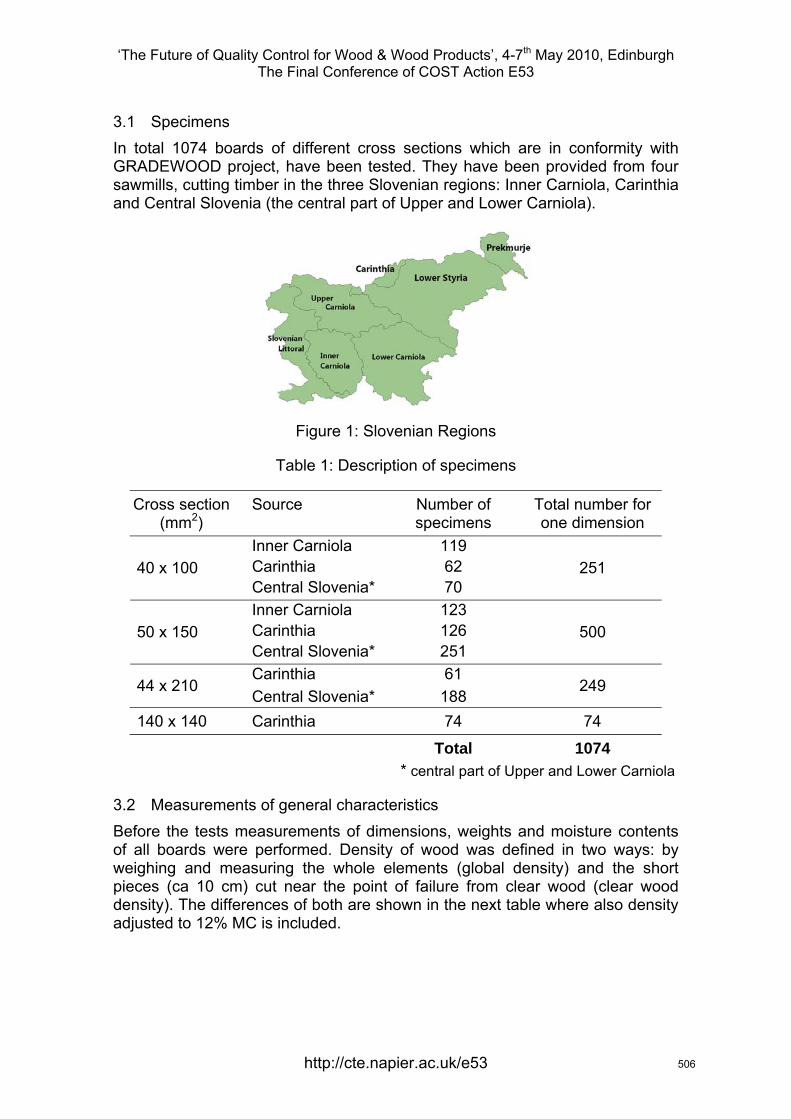
‘The Future of Quality Control for Wood & Wood Products’, 4-7th May 2010, Edinburgh The Final Conference of COST Action E53
3.1 Specimens In total 1074 boards of different cross sections which are in conformity with GRADEWOOD project, have been tested. They have been provided from four sawmills, cutting timber in the three Slovenian regions: Inner Carniola, Carinthia and Central Slovenia (the central part of Upper and Lower Carniola).
Figure 1: Slovenian Regions
Table 1: Description of specimens
Cross section (mm2)
Source Number of specimens
Total number for one dimension
Inner Carniola 119 Carinthia 62 40 x 100 Central Slovenia* 70
251
Inner Carniola 123 Carinthia 126 50 x 150 Central Slovenia* 251
500
Carinthia 61 44 x 210
Central Slovenia* 188 249
140 x 140 Carinthia 74 74
Total 1074 * central part of Upper and Lower Carniola
3.2 Measurements of general characteristics Before the tests measurements of dimensions, weights and moisture contents of all boards were performed. Density of wood was defined in two ways: by weighing and measuring the whole elements (global density) and the short pieces (ca 10 cm) cut near the point of failure from clear wood (clear wood density). The differences of both are shown in the next table where also density adjusted to 12% MC is included.
http://cte.napier.ac.uk/e53 506
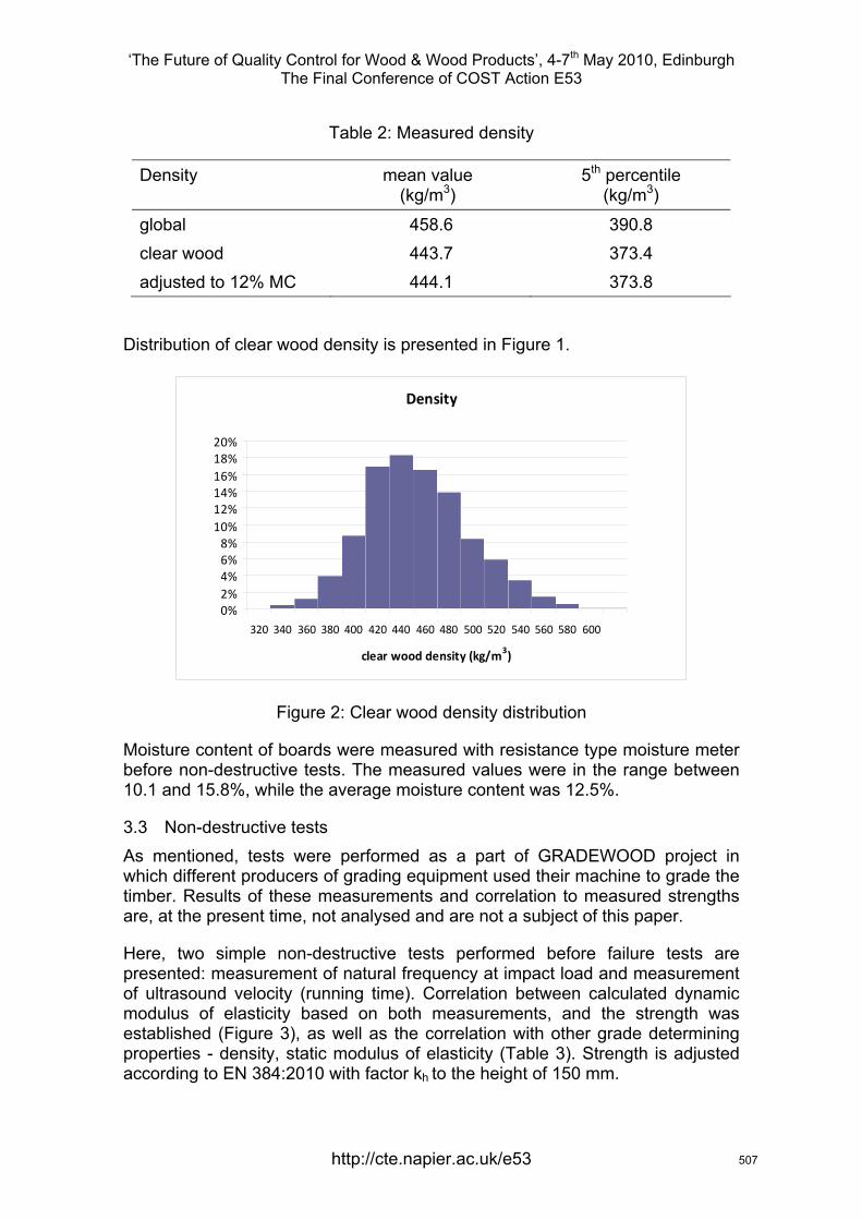
‘The Future of Quality Control for Wood & Wood Products’, 4-7th May 2010, Edinburgh The Final Conference of COST Action E53
Table 2: Measured density
Density mean value (kg/m3)
5th percentile (kg/m3)
global 458.6 390.8 clear wood 443.7 373.4 adjusted to 12% MC 444.1 373.8
Distribution of clear wood density is presented in Figure 1.
Density
0%2%4%6%8%
10%12%14%16%18%20%
320 340 360 380 400 420 440 460 480 500 520 540 560 580 600
clear wood density (kg/m3)
Figure 2: Clear wood density distribution
Moisture content of boards were measured with resistance type moisture meter before non-destructive tests. The measured values were in the range between 10.1 and 15.8%, while the average moisture content was 12.5%.
3.3 Non-destructive tests As mentioned, tests were performed as a part of GRADEWOOD project in which different producers of grading equipment used their machine to grade the timber. Results of these measurements and correlation to measured strengths are, at the present time, not analysed and are not a subject of this paper.
Here, two simple non-destructive tests performed before failure tests are presented: measurement of natural frequency at impact load and measurement of ultrasound velocity (running time). Correlation between calculated dynamic modulus of elasticity based on both measurements, and the strength was established (Figure 3), as well as the correlation with other grade determining properties - density, static modulus of elasticity (Table 3). Strength is adjusted according to EN 384:2010 with factor kh to the height of 150 mm.
http://cte.napier.ac.uk/e53 507
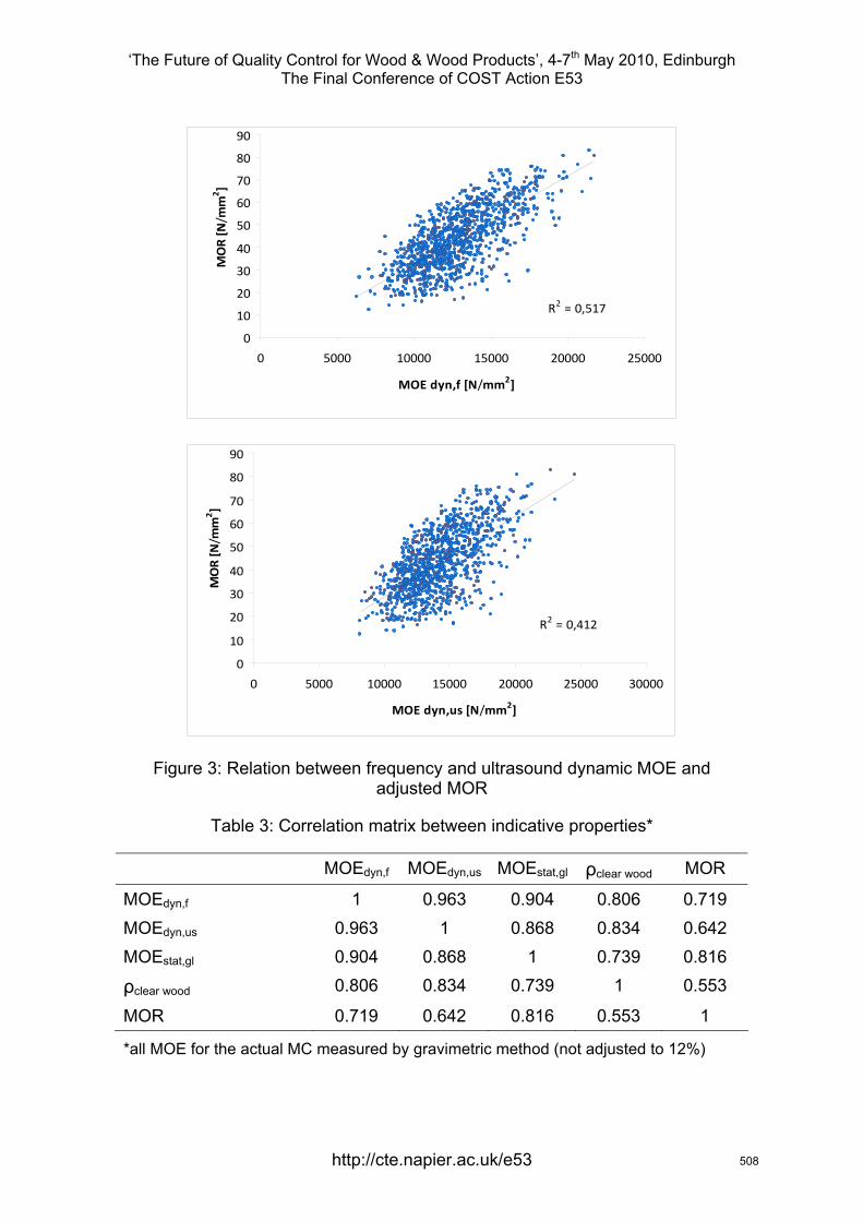
‘The Future of Quality Control for Wood & Wood Products’, 4-7th May 2010, Edinburgh The Final Conference of COST Action E53
R2 = 0,517
0
10
20
30
40
50
60
70
80
90
0 5000 10000 15000 20000 25000
MOE dyn,f [N/mm2]
MOR [N/m
m2 ]
R2 = 0,412
0
10
20
30
40
50
60
70
80
90
0 5000 10000 15000 20000 25000 30000
MOE dyn,us [N/mm2]
MOR [N/m
m2 ]
Figure 3: Relation between frequency and ultrasound dynamic MOE and adjusted MOR
Table 3: Correlation matrix between indicative properties*
MOEdyn,f MOEdyn,us MOEstat,gl ρclear wood MOR
MOEdyn,f 1 0.963 0.904 0.806 0.719 MOEdyn,us 0.963 1 0.868 0.834 0.642 MOEstat,gl 0.904 0.868 1 0.739 0.816
ρclear wood 0.806 0.834 0.739 1 0.553
MOR 0.719 0.642 0.816 0.553 1
*all MOE for the actual MC measured by gravimetric method (not adjusted to 12%)
http://cte.napier.ac.uk/e53 508
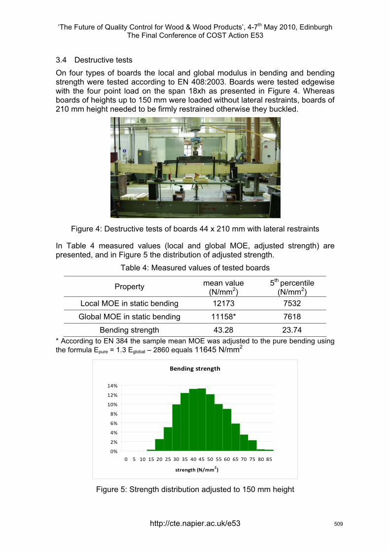
‘The Future of Quality Control for Wood & Wood Products’, 4-7th May 2010, Edinburgh The Final Conference of COST Action E53
3.4 Destructive tests On four types of boards the local and global modulus in bending and bending strength were tested according to EN 408:2003. Boards were tested edgewise with the four point load on the span 18xh as presented in Figure 4. Whereas boards of heights up to 150 mm were loaded without lateral restraints, boards of 210 mm height needed to be firmly restrained otherwise they buckled.
Figure 4: Destructive tests of boards 44 x 210 mm with lateral restraints
In Table 4 measured values (local and global MOE, adjusted strength) are presented, and in Figure 5 the distribution of adjusted strength.
Table 4: Measured values of tested boards
Property mean value (N/mm2)
5th percentile (N/mm2)
Local MOE in static bending 12173 7532
Global MOE in static bending 11158* 7618
Bending strength 43.28 23.74 * According to EN 384 the sample mean MOE was adjusted to the pure bending using the formula Epure = 1.3 Eglobal – 2860 equals 11645 N/mm2
Bending strength
0%
2%
4%
6%
8%
10%
12%
14%
0 5 10 15 20 25 30 35 40 45 50 55 60 65 70 75 80 85
strength (N/mm2)
Figure 5: Strength distribution adjusted to 150 mm height
http://cte.napier.ac.uk/e53 509
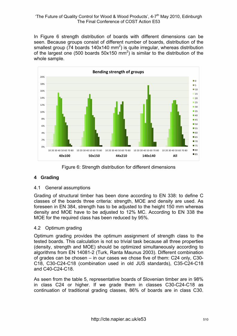
‘The Future of Quality Control for Wood & Wood Products’, 4-7th May 2010, Edinburgh The Final Conference of COST Action E53
In Figure 6 strength distribution of boards with different dimensions can be seen. Because groups consist of different number of boards, distribution of the smallest group (74 boards 140x140 mm2) is quite irregular, whereas distribution of the largest one (500 boards 50x150 mm2) is similar to the distribution of the whole sample.
Bending strength of groups
0%
2%
4%
6%
8%
10%
12%
14%
16%
18%
20%
10 20 30 40 50 60 70 80 10 20 30 40 50 60 70 80 10 20 30 40 50 60 70 80 10 20 30 40 50 60 70 80 10 20 30 40 50 60 70 80
40x100 50x150 44x210 140x140 All
0
5
10
15
20
25
30
35
40
45
50
55
60
65
70
75
80
85
Figure 6: Strength distribution for different dimensions
4 Grading
4.1 General assumptions Grading of structural timber has been done according to EN 338: to define C classes of the boards three criteria: strength, MOE and density are used. As foreseen in EN 384, strength has to be adjusted to the height 150 mm whereas density and MOE have to be adjusted to 12% MC. According to EN 338 the MOE for the required class has been reduced by 95%.
4.2 Optimum grading Optimum grading provides the optimum assignment of strength class to the tested boards. This calculation is not so trivial task because all three properties (density, strength and MOE) should be optimized simultaneously according to algorithms from EN 14081-2 (Turk, Ranta Maunus 2003). Different combination of grades can be chosen – in our cases we chose five of them: C24 only, C30-C18, C30-C24-C18 (combination used in old JUS standards), C35-C24-C18 and C40-C24-C18.
As seen from the table 5, representative boards of Slovenian timber are in 98% in class C24 or higher. If we grade them in classes C30-C24-C18 as continuation of traditional grading classes, 86% of boards are in class C30.
http://cte.napier.ac.uk/e53 510
‘The Future of Quality Control for Wood & Wood Products’, 4-7th May 2010, Edinburgh The Final Conference of COST Action E53
Even when we grade boards in the classes C40-C24-C18, 52% of boards are in the highest class – the yields of Slovenian spruce are obviously quite high.
Table 5: Optimum grading – share of boards assigned to classes
Grade combination C24 C30-C18 C30-C24-C18 C35-C24-C18 C40-C24-C18C40 52%C35 71% C30 86% 86% C24 98% 3% 12% 34%C18 12% 8% 10% 3%
reject 2% 2% 3% 7% 10%
5 Conclusion The presented results show that all correlations are in the expected boundaries. Simple non-destructive tests e.g. measuring dynamic MOE are the strength indicators, but for reliable grading process measurement of additional quantities (e.g. density, knots) are needed. We expect that on the basis of the further investigations inclusion of Slovenian timber into wider region “Central Europe” can be confirmed.
References Kovac F. (2003) Analysis of status and improvement possibilities of Slovenian sawmill industry, M.Sc. Thesis, University of Ljubljana, Faculty for Economics
Zorko B. (2005) Methods of timber strength grading, B.Sc. Thesis, University of Ljubljana, Faculty of Civil and Geodetic Engineering
CEN (2003) EN 338 Structural timber - Strength classes
CEN (2010) EN 384 Structural timber - Determination of characteristic values of mechanical properties and density
CEN (2003) EN 408 Timber structures - Structural timber and glued laminated timber - Determination of some physical and mechanical properties
CEN (2005) EN 14081-1 and -2 Timber structures – Strength graded structural timber with rectangular cross section – Part 1: General requirements, Part 2: Machine grading; additional requirements for initial type testing
CEN (2006) EN 14358 Timber structures - Calculation of characteristic 5-percentile values and acceptance criteria for a sample
Turk G., Ranta Maunus A. (2003) Analysis of strength grading of sawn timber based on numerical simulation, VTT research notes 2224, Espoo, Finland
http://cte.napier.ac.uk/e53 511
‘The Future of Quality Control for Wood & Wood Products’, 4-7th May 2010, Edinburgh The Final Conference of COST Action E53
A multidisciplinary study assessing the properties of Douglas-fir grown in the South West region of England
J.M. Bawcombe1, R. Harris2, P. Walker3 & M.P. Ansell4
Abstract This paper presents a review of research assessing the relationship between anatomical and mechanical properties of Douglas-fir grown in South West England. Testing methods being utilised include the mapping of variations in wood density, microfibril angle and ring widths using Silviscan-3, assessment of the radial and longitudinal change in stiffness and strength through three point bending tests of small clear specimens, and the measurement of dynamic modulus on standing trees. In providing a clear description of these methods and the importance of the links between them, a concise overview is given of a repeatable study which has the potential to provide valuable information to the local forestry industry, timber graders, and further the exploitation of local timber resources in high value structural applications.
1 Introduction The South Western region of the United Kingdom (UK) presents excellent conditions for growing trees due to its mild oceanic climate, good quality soils and topography. Douglas-fir (Pseudotsuga menziesii (Mirb.) Franco) is the most abundant conifer species found in the region, accounting for almost 25% of the growing stock. The species is well established on international timber markets, where its reputation for producing high quality material sees it used in a wide range of structural applications. Despite this, utilisation of material from the South West in these higher value end uses is poor; due in part to a lack of knowledge regarding the quality of the standing resource.
Timber quality is a subjective term, dependent upon both the end product being produced and on the position in the wood supply chain from which it is judged. Principally it can be described in two ways; as the resultant of physical and chemical characteristics that allow a tree to meet the property requirements of different end uses (Mitchell 1961), or as a set of attributes that do not necessarily impact product performance, but which do affect the cost of other operations throughout the supply chain (Zhang 1997).
1 PhD Research Student, [email protected] 2 Professor of Timber Engineering, [email protected] Director BRE Centre for Innovative Construction Materials (CICM), [email protected] CICM, Department of Architecture and Civil Engineering, University of Bath, Bath, BA2 7AY, England. 4 Deputy Director BRE CICM, [email protected] CICM, Department of Mechanical Engineering, University of Bath, Bath, BA2 7AY, England.
http://cte.napier.ac.uk/e53 512
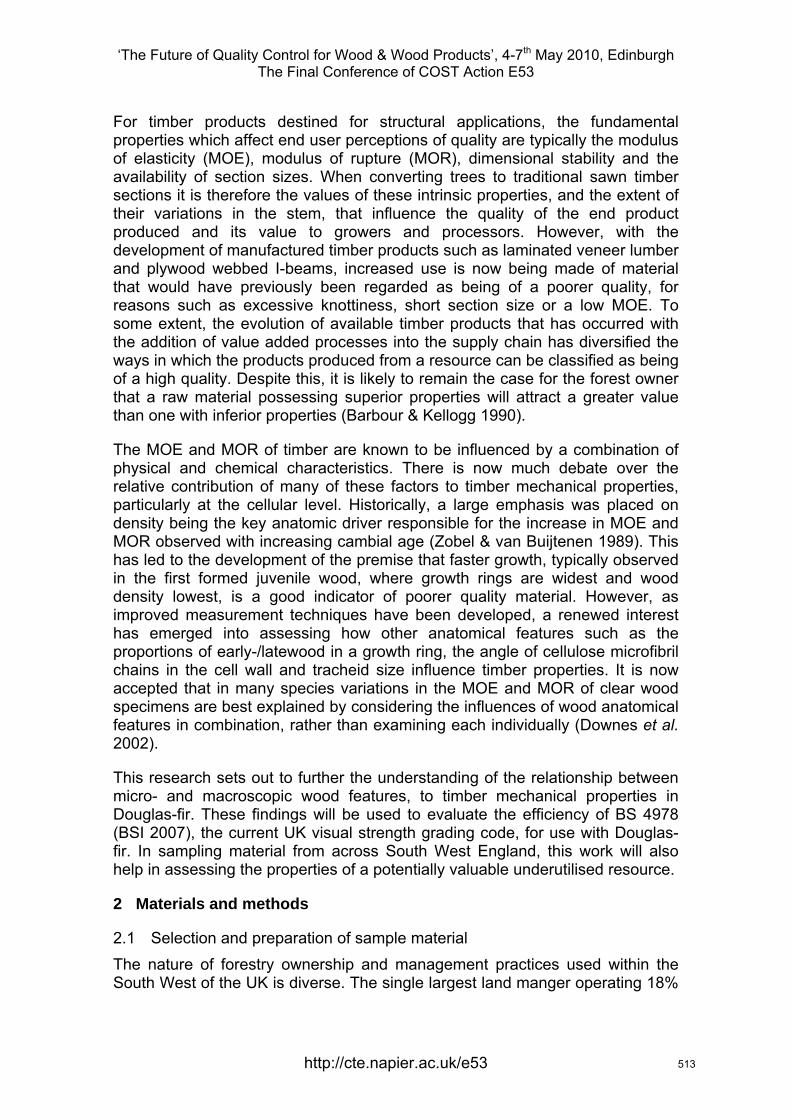
‘The Future of Quality Control for Wood & Wood Products’, 4-7th May 2010, Edinburgh The Final Conference of COST Action E53
For timber products destined for structural applications, the fundamental properties which affect end user perceptions of quality are typically the modulus of elasticity (MOE), modulus of rupture (MOR), dimensional stability and the availability of section sizes. When converting trees to traditional sawn timber sections it is therefore the values of these intrinsic properties, and the extent of their variations in the stem, that influence the quality of the end product produced and its value to growers and processors. However, with the development of manufactured timber products such as laminated veneer lumber and plywood webbed I-beams, increased use is now being made of material that would have previously been regarded as being of a poorer quality, for reasons such as excessive knottiness, short section size or a low MOE. To some extent, the evolution of available timber products that has occurred with the addition of value added processes into the supply chain has diversified the ways in which the products produced from a resource can be classified as being of a high quality. Despite this, it is likely to remain the case for the forest owner that a raw material possessing superior properties will attract a greater value than one with inferior properties (Barbour & Kellogg 1990).
The MOE and MOR of timber are known to be influenced by a combination of physical and chemical characteristics. There is now much debate over the relative contribution of many of these factors to timber mechanical properties, particularly at the cellular level. Historically, a large emphasis was placed on density being the key anatomic driver responsible for the increase in MOE and MOR observed with increasing cambial age (Zobel & van Buijtenen 1989). This has led to the development of the premise that faster growth, typically observed in the first formed juvenile wood, where growth rings are widest and wood density lowest, is a good indicator of poorer quality material. However, as improved measurement techniques have been developed, a renewed interest has emerged into assessing how other anatomical features such as the proportions of early-/latewood in a growth ring, the angle of cellulose microfibril chains in the cell wall and tracheid size influence timber properties. It is now accepted that in many species variations in the MOE and MOR of clear wood specimens are best explained by considering the influences of wood anatomical features in combination, rather than examining each individually (Downes et al. 2002).
This research sets out to further the understanding of the relationship between micro- and macroscopic wood features, to timber mechanical properties in Douglas-fir. These findings will be used to evaluate the efficiency of BS 4978 (BSI 2007), the current UK visual strength grading code, for use with Douglas-fir. In sampling material from across South West England, this work will also help in assessing the properties of a potentially valuable underutilised resource.
2 Materials and methods
2.1 Selection and preparation of sample material The nature of forestry ownership and management practices used within the South West of the UK is diverse. The single largest land manger operating 18%
http://cte.napier.ac.uk/e53 513
‘The Future of Quality Control for Wood & Wood Products’, 4-7th May 2010, Edinburgh The Final Conference of COST Action E53
of the resource is the Forestry Commission (FC). Ownership of the remainder of the resource is highly fragmented and is split between a number of private estates, charities and local authorities. This research is primarily concerned with the relationships that exist within individual trees, rather than quantifying the influences of specific external factors such as stand location and silvicultural practices. However, in order to capture the likely range of variations in wood properties that can be found, sample stands are to be selected so as to reflect the range of yield classes and felling ages typical of Douglas-fir harvested in the region.
Despite only managing a relatively small proportion of the regions forests, the FC was responsible for approximately 45 % of softwood harvesting during 2008 (Ekosgen 2009). Due to this, the first stage of experimental work is to focus on obtaining sample material from FC operated Douglas-fir stands, before moving on to privately operated estates. The nature of the two resources can be very different. Typically, FC operated stands are single species, even aged plantations thinned at five yearly intervals from age 20 until clear felling at an age ranging from 50-55 years. Management practices employed on privately operated estates are much more diverse with mixed species, mixed aged sites common, along with longer rotation lengths resulting in stems that contain a much larger proportion of mature wood.
Within the FC operated resource six even aged stands with ages ranging between 50-55 years and yield classes between 10 (slower growth) to 20 (faster growth) are to be selected for the extraction of sample trees. Within each stand three 0.03 ha (300 m2) circular survey plots are to be established, with all Douglas-fir found within each plot having diameter at breast height (DBH) recorded, and an assessment made of dynamic modulus taken on the Northern and Southern face of the stem. After calculating the distribution of growth rates present in each stand determined by DBH, six trees from each will then be selected for felling so as to cover the range of growth rates present. This will give a sample size of 36 trees for the first stage of the experimental work.
Prior to felling, all sample trees are to have 5 mm diameter, 100 mm long increment cores extracted from the Northern and Southern faces at breast height, to be used for establishing outer wood density for dynamic modulus assessments. Upon felling the total height and the length of the live crown of each tree will also assessed. Following this, sample stems are to be processed by removing two 0.5 m logs, the first centred on breast height and the second at a height of 8 m. These logs are to be used for the preparation of small clear bending specimens to determine mechanical properties. Adjacent to each log, a disc measuring 100 mm is also to be taken and used to study variations in anatomical properties.
2.2 Dynamic modulus assessment At present the sorting of trees and logs into quality classes prior to removal from the forest for processing is conducted largely by means of an assessment of characteristics such as their diameter, stem straightness and the size of
http://cte.napier.ac.uk/e53 514
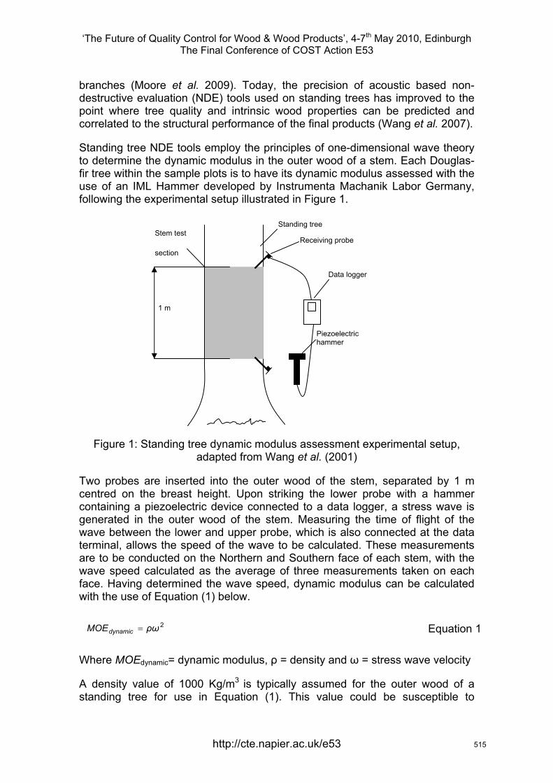
‘The Future of Quality Control for Wood & Wood Products’, 4-7th May 2010, Edinburgh The Final Conference of COST Action E53
branches (Moore et al. 2009). Today, the precision of acoustic based non-destructive evaluation (NDE) tools used on standing trees has improved to the point where tree quality and intrinsic wood properties can be predicted and correlated to the structural performance of the final products (Wang et al. 2007).
Standing tree NDE tools employ the principles of one-dimensional wave theory to determine the dynamic modulus in the outer wood of a stem. Each Douglas-fir tree within the sample plots is to have its dynamic modulus assessed with the use of an IML Hammer developed by Instrumenta Machanik Labor Germany, following the experimental setup illustrated in Figure 1.
Standing tree
Receiving probe
Data logger
1 m
Stem test
section
Piezoelectric hammer
Figure 1: Standing tree dynamic modulus assessment experimental setup, adapted from Wang et al. (2001)
Two probes are inserted into the outer wood of the stem, separated by 1 m centred on the breast height. Upon striking the lower probe with a hammer containing a piezoelectric device connected to a data logger, a stress wave is generated in the outer wood of the stem. Measuring the time of flight of the wave between the lower and upper probe, which is also connected at the data terminal, allows the speed of the wave to be calculated. These measurements are to be conducted on the Northern and Southern face of each stem, with the wave speed calculated as the average of three measurements taken on each face. Having determined the wave speed, dynamic modulus can be calculated with the use of Equation (1) below.
2ρωMOEdynamic = Equation 1
Where MOEdynamic= dynamic modulus, ρ = density and ω = stress wave velocity
A density value of 1000 Kg/m3 is typically assumed for the outer wood of a standing tree for use in Equation (1). This value could be susceptible to
http://cte.napier.ac.uk/e53 515
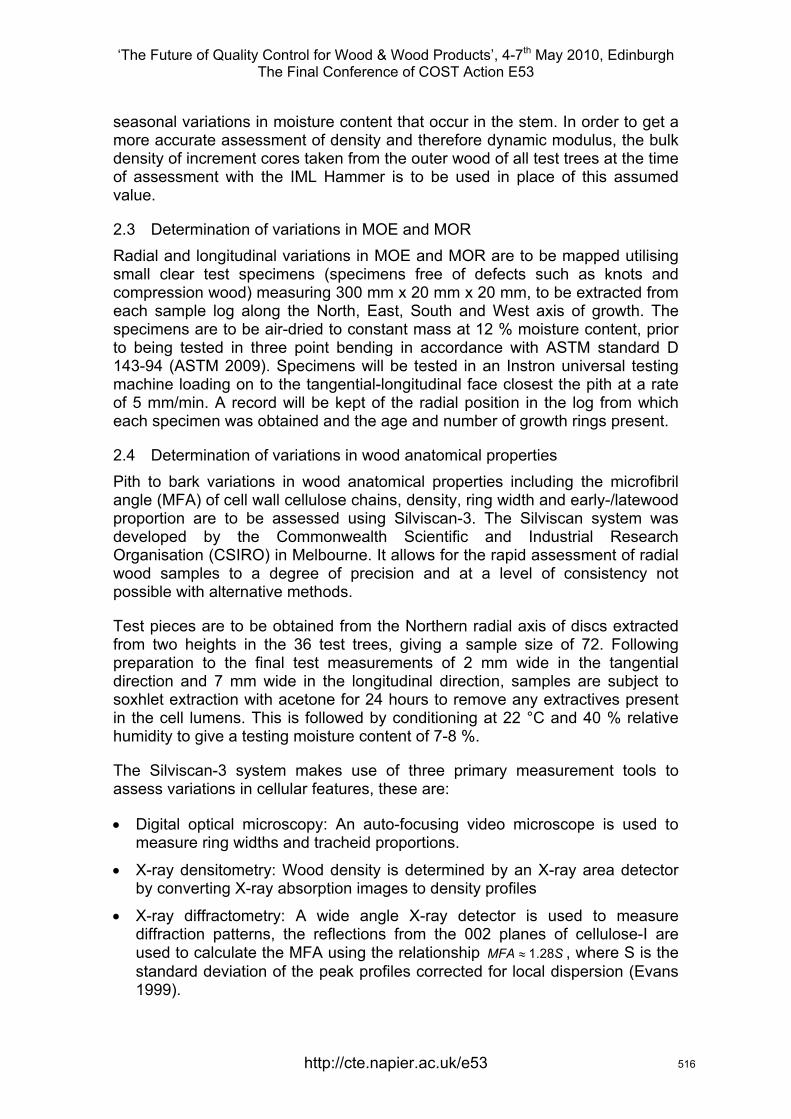
‘The Future of Quality Control for Wood & Wood Products’, 4-7th May 2010, Edinburgh The Final Conference of COST Action E53
seasonal variations in moisture content that occur in the stem. In order to get a more accurate assessment of density and therefore dynamic modulus, the bulk density of increment cores taken from the outer wood of all test trees at the time of assessment with the IML Hammer is to be used in place of this assumed value.
2.3 Determination of variations in MOE and MOR Radial and longitudinal variations in MOE and MOR are to be mapped utilising small clear test specimens (specimens free of defects such as knots and compression wood) measuring 300 mm x 20 mm x 20 mm, to be extracted from each sample log along the North, East, South and West axis of growth. The specimens are to be air-dried to constant mass at 12 % moisture content, prior to being tested in three point bending in accordance with ASTM standard D 143-94 (ASTM 2009). Specimens will be tested in an Instron universal testing machine loading on to the tangential-longitudinal face closest the pith at a rate of 5 mm/min. A record will be kept of the radial position in the log from which each specimen was obtained and the age and number of growth rings present.
2.4 Determination of variations in wood anatomical properties Pith to bark variations in wood anatomical properties including the microfibril angle (MFA) of cell wall cellulose chains, density, ring width and early-/latewood proportion are to be assessed using Silviscan-3. The Silviscan system was developed by the Commonwealth Scientific and Industrial Research Organisation (CSIRO) in Melbourne. It allows for the rapid assessment of radial wood samples to a degree of precision and at a level of consistency not possible with alternative methods.
Test pieces are to be obtained from the Northern radial axis of discs extracted from two heights in the 36 test trees, giving a sample size of 72. Following preparation to the final test measurements of 2 mm wide in the tangential direction and 7 mm wide in the longitudinal direction, samples are subject to soxhlet extraction with acetone for 24 hours to remove any extractives present in the cell lumens. This is followed by conditioning at 22 °C and 40 % relative humidity to give a testing moisture content of 7-8 %.
The Silviscan-3 system makes use of three primary measurement tools to assess variations in cellular features, these are:
• Digital optical microscopy: An auto-focusing video microscope is used to measure ring widths and tracheid proportions.
• X-ray densitometry: Wood density is determined by an X-ray area detector by converting X-ray absorption images to density profiles
• X-ray diffractometry: A wide angle X-ray detector is used to measure diffraction patterns, the reflections from the 002 planes of cellulose-I are used to calculate the MFA using the relationship SMFA 28.1≈ , where S is the standard deviation of the peak profiles corrected for local dispersion (Evans 1999).
http://cte.napier.ac.uk/e53 516

‘The Future of Quality Control for Wood & Wood Products’, 4-7th May 2010, Edinburgh The Final Conference of COST Action E53
Alongside these direct observations, the radial MOE profile of the samples is also predicted with use of a semi-empirical model based on the available MFA and density information (Keunecke et al. 2009). The techniques used in Silviscan-3 assessment are summarised in Figure 2 below.
Digital optical microscopy
Figure 2: Silviscan-3 measurement principles Upon completion of testing the data collected is processed and presented in the form of tables relating measured properties to radial position and the average of the properties for growth rings and early-/latewood bands.
3 Analysis of results
3.1 Relating dynamic modulus measurements to the MOE and MOR of small clear specimens
The relationship between the speed of an induced stress wave, density and dynamic modulus given in Equation (1) was developed through the use of one-dimensional wave theory, typically applied to homogeneous or isotropic materials. Its application in assessing the properties of timber, an anisotropic material, with the use of standing tree NDE tools has been the subject of a number of previous studies. Results have shown that a good correlation exists between dynamic modulus and the MOE derived through static bending tests of both small clear specimens, and larger sawn sections in the juvenile and mature wood of a number of species (Lindstrom et al. 2002, Ishiguri et al. 2008). However, no significant relationship has been found between time of flight measurements and MOR (e.g. Ishiguri et al. 2008).
By assessing the values of dynamic modulus evaluated in sample Douglas-fir trees and correlating these results with those obtained for the MOE and MOR of small clear specimens, this work aims to further the understanding of the ability of acoustic NDE tools to predict the properties of standing Douglas-fir trees. It is expected that the correlation between dynamic and static modulus will be highest when evaluating bending specimens taken from the outer portion of the stem, through which induced stress waves pass. In assessing how static MOE and MOR vary in test specimens closer to the pith, an empirical model will be developed allowing the dynamic modulus of outer wood to be related to the properties of core wood.
X-ray diffractometry X-ray densitometry
http://cte.napier.ac.uk/e53 517
‘The Future of Quality Control for Wood & Wood Products’, 4-7th May 2010, Edinburgh The Final Conference of COST Action E53
3.2 Relating variations in anatomical properties to those in MOE and MOR The influence of anatomical properties including MFA, density, ring width and early-/latewood proportion on MOE and MOR will be determined through analysis of results from three point bending tests of small clear specimens, and the variations in cellular properties evaluated in pith to bark radial samples taken in adjacent discs. Results will be analysed with the use of simple correlation coefficients and path analysis in order to better understand both the dependent and independent relationships that exist between the variables.
A recent study of Douglas-fir mature wood examining the influence of anatomical variations on mechanical properties, found that the best predictor of static MOE in defect free specimens was the proportions of latewood within the growth rings present in test pieces (Lachenbruch et al. 2010). This was attributed to latewood being denser and having a lower MFA than earlywood and therefore contributing a larger proportion to the samples stiffness. This finding could have important implications for BS 4978 (BSI 2007) the current softwood visual strength grading code utilised in the UK, in which ring width is one of the criteria assessed during grading. If it can be shown that in juvenile, as well as mature wood, that the proportion of latewood in a ring has a larger impact on timber properties than ring width, more efficient visual grading methods for Douglas-fir could be established in the future.
4 Continuing work The work outlined in this paper has summarised testing to be conducted on material extracted from Forestry Commission Douglas-fir sites in the South West of the UK. Following completion of this, similar test methods are to be employed on older sample trees with ages greater than 80 years. Results gathered from these older trees, more reflective of material harvested from privately owned sites, will be used alongside previously gathered data in the development of empirical methods to predict anatomical and mechanical properties at different locations within the stem. It is expected that these trees will exhibit superior outer wood properties due to the greater proportions of mature wood in the stems.
Future testing including an evaluation of the efficiency of visual grading techniques is also to be conducted on structurally sized Douglas-fir sections. This will allow the magnitude of the effects of anatomical properties on MOE and MOR studied in earlier work to be evaluated in sections containing defects such as knots and a sloping grain.
5 Concluding remarks It is anticipated, that alongside the primary aim of this research to gain a greater understanding of the factors that may influence timber quality in South West Douglas-fir, that further knowledge may be developed in a number of areas of interest to timber growers, processors and graders.
Furthering the understanding of relationships that exist between the dynamic modulus obtained using acoustic NDE tools on standing trees and the
http://cte.napier.ac.uk/e53 518
‘The Future of Quality Control for Wood & Wood Products’, 4-7th May 2010, Edinburgh The Final Conference of COST Action E53
properties of timber sections produced from a tree could allow for increased future usage of NDE equipment within the forestry industry. This will enable more accurate preliminary estimations of timber quality to be made prior to felling, ensuring that material is sent to the most appropriate end use, potentially improving the grade outturn of a forest and therefore profitability. An improved understanding of the relationships that exist between mechanical and anatomical properties could lead to the development of more efficient visual grading standards for UK grown Douglas-fir, making home-grown material more competitive in a marketplace currently dominated by imported wood products.
Acknowledgments This research is funded by the Silvanus trust through donations from the South West forest industry, Great Western Research and the University of Bath. Thanks goes to Jez Ralph from the Silvanus trust and Barry Gardiner from Forest Research for their support with the project to date.
References ASTM (2009) “Annual book of ASTM Standards”. American Society for Testing and Materials, West Consohocken, Vol. 04.10 Wood. Barbour, R. & Kellogg, R. (1990) “Forest management and end-product quality: a Canadian perspective”. Canadian Journal of Forest Research, Vol 20(4), pp 405-414. BSI (2007) “BS 4978: Visual strength grading of softwood”. British Standards Institution. Downes, G., Nyakuengama, J., Evans, R., Northway, R., Blakemore, P., Dickson, R. & Lausberg, M. (2002) “Relationship between wood density, microfibril angle and stiffness in thinned and fertilized Pinus radiata”. IAWA Journal, Vol 23, pp 253-266. Ekosgen (2009) “Strategic economic study of South West England woodland and forestry”. Evans, R. (1999) “A variance approach to the X-ray diffractometric estimation of microfibril angle in wood”. Appita Journal, Vol 52, pp 283-289. Ishiguri, F., Matsui, R., Iizuka, K., Yokota, S. & Yoshizawa, N. (2008) “Prediction of the mechanical properties of lumber by stress-wave velocity and Pilodyn penetration of 36-year-old Japanese larch trees”. Holz als Roh-und Werkstoff, Vol 66(4), pp 275-280. Keunecke, D., Evans, R. & Niemz, P. (2009) “Microstrucutral properties of common yew and Norway Spruce determined with Silviscan”. IAWA Journal, Vol 30(2), pp 165-178.
http://cte.napier.ac.uk/e53 519
‘The Future of Quality Control for Wood & Wood Products’, 4-7th May 2010, Edinburgh The Final Conference of COST Action E53
Lachenbruch, B., Johnson, G., Downes, G. & Evans, R. (2010) “Relationships of density, microfibril angle and sound velocity with stiffness and strength in mature wood of Douglas-fir”. The Canadian Journal of Forest Research, Vol 40(1), pp 55-64. Lindstrom, H., Harris, P. & Nakada, R. (2002) “Methods for measuring stiffness of young trees”. Holz als Roh-und Werkstoff, Vol 60(3), pp 165-174. Mitchell, H. (1961) “A concept of intrinsic wood quality, and non-destructive methods for determining quality in standing timber”. U.S. Forest Products Laboratory, Report No. 2233. Moore, J., Lyon, A., Searles, G. & Ridley-Ellis, D (2009) “The use of acoustic-based NDT to predict the wood propertied of UK-grown Sitka Spruce at different stages in the wood supply chain”. The 16th International Non-destructive Testing and Evaluation of Wood Symposium, Beijing. Wang, X., Carter, P., Ross, R. & Brashaw, B. (2007) “Acoustic assessment of wood quality of forest raw materials – a path to increased profitability”. Forest Products Journal, Vol 57(5), pp 6-14. Wang, X., Ross, R., Erickson, J., Forsman, J., McClellan, M., Barbour, R. & Pellerin, R. (2001) “Non-destructive evaluation of standing trees with stress wave methods”. Wood and Fibre Science, Vol 33(4), pp 522-533. Zhang, S. (1997) “Wood quality: Its definition, impact, and implications for value-added timber management and end Uses”. In: CTIA/IUFRO International Wood Quality Workshop – Timber Management Toward Wood Quality and End-Product Value, pp 117-139. Zobel, B. & van Buijtenen, J. (1989) “Wood variation: its causes and control”. Springer-Verlag Berlin.
http://cte.napier.ac.uk/e53 520

‘The Future of Quality Control for Wood & Wood Products’, 4-7th May 2010, Edinburgh The Final Conference of COST Action E53
Thursday 6th May Research focussed day
Parallel session 3B
http://www.cte.napier.ac.uk/e53/ 521
‘The Future of Quality Control for Wood & Wood Products’, 4-7th May 2010, Edinburgh The Final Conference of COST Action E53
Assessing stiffness on finger-jointed timber with different non-destructive testing techniques
T. Biechele 1, Y.H. Chui 2 & M. Gong 3
Abstract Non-destructive testing (NDT) is a common method to determine the stiffness of timber before its utilisation for construction purposes. In this project a total of 188 pieces of 2” x 4” black spruce unjointed and finger-jointed timber (38 x 89 x 2438mm) were tested with different NDT techniques. Testing was applied on three main specimen groups: 1.) unjointed timber, 2.) finger-jointed timber with 2-3 joints and 3.) finger-jointed timber with 5-7 joints. Three NDT techniques were chosen. These were stress wave propagation, transverse vibration and bending as applied by a grading machine. The stress wave technique was applied via a commercial machine (Timber Grader MTG) which is a hand-held device. Transverse vibration was applied by using a spectrum analyser, an accelerometer and an instrumented hammer. The main objective of this study was to evaluate the application of present NDT techniques to finger-jointed timber. The modulus predicted on unjointed sawn timber and timber with different number of finger joints were correlated with three-point bending test results, which are used as a reference for the “real” stiffness. The results showed that modulus values measured using the three NDT methods correlate well with three-point bending modulus for both unjointed and finger-jointed timber. The regression coefficient between NDT modulus and three-point bending modulus (R²) ranged from 0.80 to as high as 0.97. The grading machine provided the lowest R² values than stress wave and transverse vibration. Similar R² values were observed for both unjointed and finger-jointed timber, indicating that these NDT techniques can be used for grading finger-jointed timber with the same degree of accuracy as solid sawn timber. Furthermore, results show that modulus decreases with any increase in number of finger joints.
1 Introduction Non-destructive testing (NDT) techniques are commonly used by the wood industry and wood research community to evaluate quality and strength properties of timber. For residential constructions finger-jointed timber is often utilized. Literature provides a wide range of NDT testing on unjointed timber of
1 PhD. Candidate, [email protected], Institute of Forest Utilization and Work Science, Albert- Ludwigs- University of Freiburg, Germany 2 Wood Science and Technology Centre, , [email protected], University of New Brunswick, Canada 3 Wood Science and Technology Centre, , [email protected], University of New Brunswick, Canada
http://cte.napier.ac.uk/e53 522

‘The Future of Quality Control for Wood & Wood Products’, 4-7th May 2010, Edinburgh The Final Conference of COST Action E53
different tree species all over the world (Auty & Achim 2008; Carter et al. 2006; Mišeikyte et al. 2008; Sandoz 1989) whereas non destructive measurements on finger-jointed timber are less found in literature.
In the present study different NDT techniques for stiffness measurement were selected using stress wave propagation and transverse vibration. Furthermore the test specimens were Centre point loaded as well as run through an MSR machine.
Based on the intention of this study to examine and analyse mechanical properties on unjointed and finger-jointed timber the following main research questions were formulated.
- Can NDT techniques be applied on finger-jointed timber for stiffness measurement?
- Is accuracy influenced by the finger-joints?
- Is the stiffness of unjointed and finger-jointed wood comparable?
- Is there an effect of number of finger-joints on stiffness of timber?
2 Material and Method Stiffness and strength was measured on 2 by 4” studs (38x89x2438mm). These studs were sawn from Black spruce (Picea mariana) trees, grown in the Northern Parts of Quebec. Testing was applied on three main specimen groups: 1.) unjointed timber (n=40), 2.) finger-jointed timber with 2-3 joints (n=47) and 3.) finger-jointed timber with 5-7 joints (n=101). For density calculation the exact dimensions and weight of the specimens was taken. Before the stiffness and strength measurements the moisture content (MC) was measured with a moisture meter. The average MC was calculated from three measurement points on the unjointed wood specimens and from each finger-jointed piece of the finger-jointed timber. The experimental Modulus of Elasticity testing contained four non-destructive methods using a Stress wave timer, Transverse Vibration, Centre Point Loading and a MSR machine. These NDT techniques are used in the industry and wood science for assessing stiffness on timber.
2.1 NDT techniques used for stiffness measurement
Stress wave propagation
The stress wave timer used in this study is called Timber Grader MTG, which is a handheld strength grading device for sawn wood developed by Brookhuis Micro-Electronics and TNO (Netherlands). The measurement principle of the Timber Grader MTG is based on stress wave propagation in the wood. It
http://cte.napier.ac.uk/e53 523
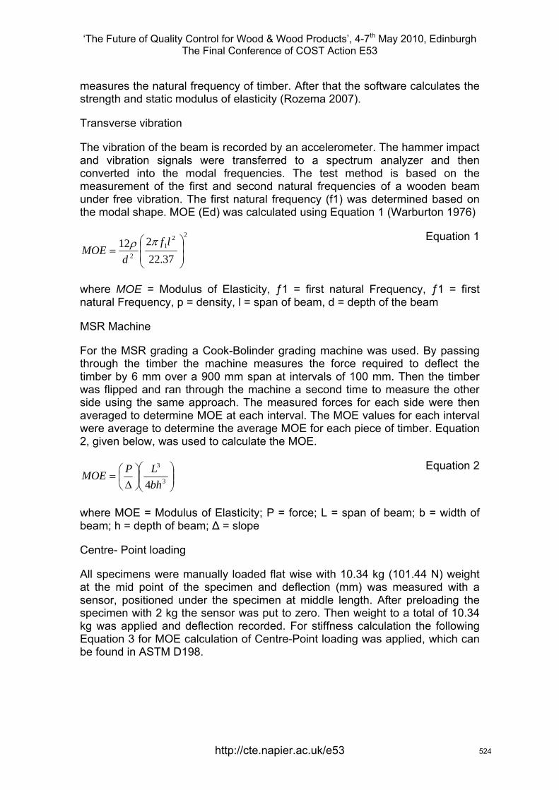
‘The Future of Quality Control for Wood & Wood Products’, 4-7th May 2010, Edinburgh The Final Conference of COST Action E53
measures the natural frequency of timber. After that the software calculates the strength and static modulus of elasticity (Rozema 2007).
Transverse vibration
The vibration of the beam is recorded by an accelerometer. The hammer impact and vibration signals were transferred to a spectrum analyzer and then converted into the modal frequencies. The test method is based on the measurement of the first and second natural frequencies of a wooden beam under free vibration. The first natural frequency (f1) was determined based on the modal shape. MOE (Ed) was calculated using Equation 1 (Warburton 1976)
221
2 37.22212
⎟⎟⎠
⎞⎜⎜⎝
⎛=
lfd
MOEπρ
Equation 1
where MOE = Modulus of Elasticity, ƒ1 = first natural Frequency, ƒ1 = first natural Frequency, p = density, l = span of beam, d = depth of the beam
MSR Machine
For the MSR grading a Cook-Bolinder grading machine was used. By passing through the timber the machine measures the force required to deflect the timber by 6 mm over a 900 mm span at intervals of 100 mm. Then the timber was flipped and ran through the machine a second time to measure the other side using the same approach. The measured forces for each side were then averaged to determine MOE at each interval. The MOE values for each interval were average to determine the average MOE for each piece of timber. Equation 2, given below, was used to calculate the MOE.
⎟⎟⎠
⎞⎜⎜⎝
⎛⎟⎠⎞
⎜⎝⎛Δ
= 3
3
4bhLPMOE
Equation 2
where MOE = Modulus of Elasticity; P = force; L = span of beam; b = width of beam; h = depth of beam; Δ = slope
Centre- Point loading
All specimens were manually loaded flat wise with 10.34 kg (101.44 N) weight at the mid point of the specimen and deflection (mm) was measured with a sensor, positioned under the specimen at middle length. After preloading the specimen with 2 kg the sensor was put to zero. Then weight to a total of 10.34 kg was applied and deflection recorded. For stiffness calculation the following Equation 3 for MOE calculation of Centre-Point loading was applied, which can be found in ASTM D198.
http://cte.napier.ac.uk/e53 524
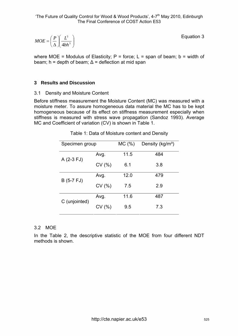
‘The Future of Quality Control for Wood & Wood Products’, 4-7th May 2010, Edinburgh The Final Conference of COST Action E53
⎟⎟⎠
⎞⎜⎜⎝
⎛⎟⎠⎞
⎜⎝⎛Δ
= 3
3
4bhLPMOE
Equation 3
where MOE = Modulus of Elasticity; P = force; L = span of beam; b = width of beam; h = depth of beam; Δ = deflection at mid span
3 Results and Discussion
3.1 Density and Moisture Content Before stiffness measurement the Moisture Content (MC) was measured with a moisture meter. To assure homogeneous data material the MC has to be kept homogeneous because of its effect on stiffness measurement especially when stiffness is measured with stress wave propagation (Sandoz 1993). Average MC and Coefficient of variation (CV) is shown in Table 1.
Table 1: Data of Moisture content and Density
Specimen group MC (%) Density (kg/m³)
Avg. 11.5 484 A (2-3 FJ)
CV (%) 6.1 3.8
Avg. 12.0 479 B (5-7 FJ)
CV (%) 7.5 2.9
Avg. 11.6 487 C (unjointed)
CV (%) 9.5 7.3
3.2 MOE In the Table 2, the descriptive statistic of the MOE from four different NDT methods is shown.
http://cte.napier.ac.uk/e53 525
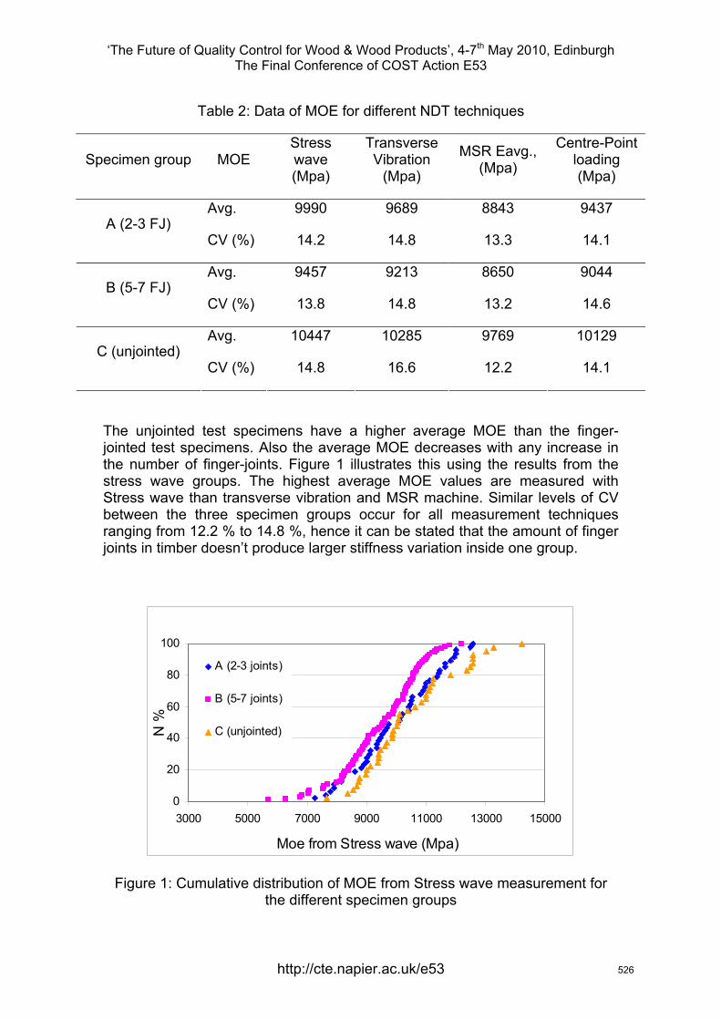
‘The Future of Quality Control for Wood & Wood Products’, 4-7th May 2010, Edinburgh The Final Conference of COST Action E53
Table 2: Data of MOE for different NDT techniques
Specimen group MOE Stress wave (Mpa)
Transverse Vibration
(Mpa)
MSR Eavg., (Mpa)
Centre-Point loading (Mpa)
Avg. 9990 9689 8843 9437 A (2-3 FJ)
CV (%) 14.2 14.8 13.3 14.1
Avg. 9457 9213 8650 9044 B (5-7 FJ)
CV (%) 13.8 14.8 13.2 14.6
Avg. 10447 10285 9769 10129 C (unjointed)
CV (%) 14.8 16.6 12.2 14.1
The unjointed test specimens have a higher average MOE than the finger-jointed test specimens. Also the average MOE decreases with any increase in the number of finger-joints. Figure 1 illustrates this using the results from the stress wave groups. The highest average MOE values are measured with Stress wave than transverse vibration and MSR machine. Similar levels of CV between the three specimen groups occur for all measurement techniques ranging from 12.2 % to 14.8 %, hence it can be stated that the amount of finger joints in timber doesn’t produce larger stiffness variation inside one group.
0
20
40
60
80
100
3000 5000 7000 9000 11000 13000 15000
Moe from Stress wave (Mpa)
N %
A (2-3 joints)
B (5-7 joints)
C (unjointed)
Figure 1: Cumulative distribution of MOE from Stress wave measurement for the different specimen groups
http://cte.napier.ac.uk/e53 526
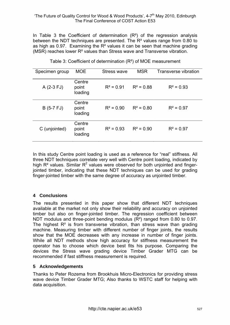
‘The Future of Quality Control for Wood & Wood Products’, 4-7th May 2010, Edinburgh The Final Conference of COST Action E53
In Table 3 the Coefficient of determination (R²) of the regression analysis between the NDT techniques are presented. The R² values range from 0.80 to as high as 0.97. Examining the R² values it can be seen that machine grading (MSR) reaches lower R² values than Stress wave and Transverse vibration.
Table 3: Coefficient of determination (R²) of MOE measurement
Specimen group MOE Stress wave MSR Transverse vibration
A (2-3 FJ) Centre point loading
R² = 0.91 R² = 0.88 R² = 0.93
B (5-7 FJ) Centre point loading
R² = 0.90 R² = 0.80 R² = 0.97
C (unjointed) Centre point loading
R² = 0.93 R² = 0.90 R² = 0.97
In this study Centre point loading is used as a reference for “real” stiffness. All three NDT techniques correlate very well with Centre point loading, indicated by high R² values. Similar R2 values were observed for both unjointed and finger-jointed timber, indicating that these NDT techniques can be used for grading finger-jointed timber with the same degree of accuracy as unjointed timber.
4 Conclusions The results presented in this paper show that different NDT techniques available at the market not only show their reliability and accuracy on unjointed timber but also on finger-jointed timber. The regression coefficient between NDT modulus and three-point bending modulus (R²) ranged from 0.80 to 0.97. The highest R² is from transverse vibration, than stress wave than grading machine. Measuring timber with different number of finger joints, the results show that the MOE decreases with any increase in number of finger joints. While all NDT methods show high accuracy for stiffness measurement the operator has to choose which device best fits his purpose. Comparing the devices the Stress wave grading device Timber Grader MTG can be recommended if fast stiffness measurement is required.
5 Acknowledgements Thanks to Peter Rozema from Brookhuis Micro-Electronics for providing stress wave device Timber Grader MTG; Also thanks to WSTC staff for helping with data acquisition.
http://cte.napier.ac.uk/e53 527
‘The Future of Quality Control for Wood & Wood Products’, 4-7th May 2010, Edinburgh The Final Conference of COST Action E53
References ASTM D198 Standard American Society for Testing and Materials Test Methods of Static Tests of Lumber in Structural Sizes
Auty, D., Achim, A. 2008 The relationship between standing tree acoustic assessment and lumber quality in Scots pine and the practical implications for assessing lumber quality from naturally regenerated stands. Forestry Advance Access published April 28. Forestry 2008 81: 475-487
Carter, P., Chauhan S., Walker J. 2006 Sorting logs and Lumber for Stiffness using Director HM200
Ing. Rozema, P. 2007. Timber Grader MTG-Brookhuis Micro-Eletronics BV, the Netherlands. Mišeikyte, S., Baltrušaitis, A., Kudakas, L. (2008) Strength and Stiffness Properties of the Lithuanian Grown Scots Pine (Pinus sylvestris): Comparison of various Testing Methods Proceedings of the 4th meeting of the Nordic Baltic Network in Wood Material Science & Engineering (WSE), November 13-14, 2008, Riga, Latvia / Ed. by B. Andersons and H. Tuherm. Riga: Latvian State Institute of Wood Chemistry, 2008. p. 101-107
Sandoz, J. L. 1989 Grading of construction timber by ultrasound. Wood Sci. Technol. 23: 95–108
Sandoz, J.L. 1993 Moisture content and temperature effect on ultrasound timber grading. Wood Sci. Technol. 23: 95–108
Warburton, G. B. 1976 The dynamical behaviour of structures, Pergamon Press, Oxford.
http://cte.napier.ac.uk/e53 528
‘The Future of Quality Control for Wood & Wood Products’, 4-7th May 2010, Edinburgh The Final Conference of COST Action E53
http://cte.napier.ac.uk/e53
Dynamic excitation and higher bending modes for prediction of timber bending strength
A.M.J. Olsson1, J. Oscarsson2, B.M. Johansson3 & B. Källsner4
Abstract The potential of utilizing eigenfrequencies corresponding to edgewise bending modes for predicting the bending strength of timber is investigated. The research includes measurements of axial and transversal resonance frequencies, laboratory assessment of density, static bending stiffness and bending strength of 105 boards of Norway spruce of dimensions 45×145×3600 mm. It is shown that Eb,1, (MOE based on the eigenfrequency of the first bending mode) gives a higher coefficient of determination to the bending strength than what Ea,1 (MOE based on the first axial eigenfrequency) does. It is also shown that eigenfrequencies corresponding to higher bending modes can be used in the definition of a new prediction variable, the modulus of inhomogeneity (MOI). This is a scalar value representing the lack of fit between the true, measured eigenfrequencies and the expected (assuming homogeneity) eigenfrequencies of a board. The results show that using the MOI as a third prediction variable, in addition to Eb,1 and density, increases the coefficient of determination with respect to bending strength from R2 = 0.69 to R2 = 0.75.
1 Introduction Machine strength grading of timber based on dynamic excitation of boards has won large market shares in the last decade. The vibration content is detected using a microphone or a laser vibrometer and fast Fourier transformation is used for calculation of eigenfrequencies (also called resonance frequencies or natural frequencies) corresponding to axial modes of vibration. The common way of utilizing the information from the measured vibration content is to calculate the modulus of elasticity (MOE), or actually a mean axial stiffness, using the eigenfrequency corresponding to the first axial mode. One aim of this paper is to investigate how the dynamic board stiffness or MOE based on the eigenfrequency of the first edgewise bending mode correlates with the bending strength and compare with the correlation between the dynamic axial MOE and the bending strength.
1 Professor, [email protected] Linnæus University, Sweden 2 PhD Student, [email protected] SP Technical Research Institute of Sweden, Sweden 3 Senior University Lecturer, [email protected] Linnæus University, Sweden 4 Professor, [email protected] Linnæus University, Sweden
529
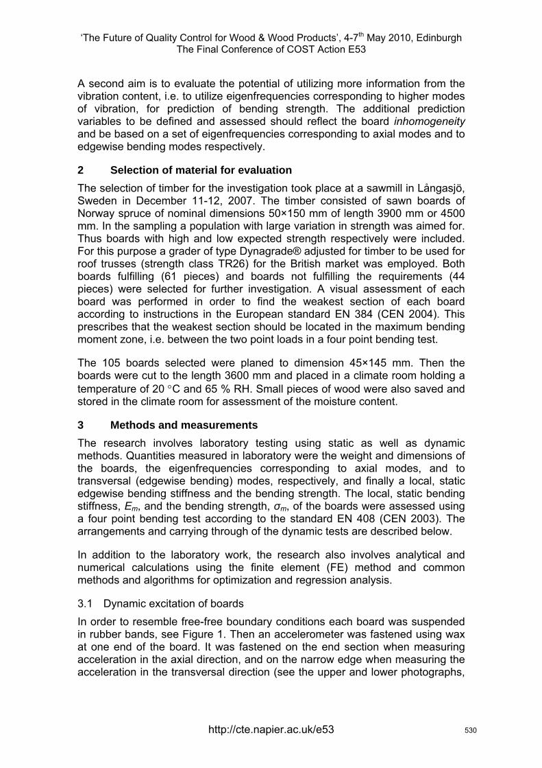
‘The Future of Quality Control for Wood & Wood Products’, 4-7th May 2010, Edinburgh The Final Conference of COST Action E53
http://cte.napier.ac.uk/e53
A second aim is to evaluate the potential of utilizing more information from the vibration content, i.e. to utilize eigenfrequencies corresponding to higher modes of vibration, for prediction of bending strength. The additional prediction variables to be defined and assessed should reflect the board inhomogeneity and be based on a set of eigenfrequencies corresponding to axial modes and to edgewise bending modes respectively.
2 Selection of material for evaluation The selection of timber for the investigation took place at a sawmill in Långasjö, Sweden in December 11-12, 2007. The timber consisted of sawn boards of Norway spruce of nominal dimensions 50×150 mm of length 3900 mm or 4500 mm. In the sampling a population with large variation in strength was aimed for. Thus boards with high and low expected strength respectively were included. For this purpose a grader of type Dynagrade® adjusted for timber to be used for roof trusses (strength class TR26) for the British market was employed. Both boards fulfilling (61 pieces) and boards not fulfilling the requirements (44 pieces) were selected for further investigation. A visual assessment of each board was performed in order to find the weakest section of each board according to instructions in the European standard EN 384 (CEN 2004). This prescribes that the weakest section should be located in the maximum bending moment zone, i.e. between the two point loads in a four point bending test.
The 105 boards selected were planed to dimension 45×145 mm. Then the boards were cut to the length 3600 mm and placed in a climate room holding a temperature of 20 °C and 65 % RH. Small pieces of wood were also saved and stored in the climate room for assessment of the moisture content.
3 Methods and measurements The research involves laboratory testing using static as well as dynamic methods. Quantities measured in laboratory were the weight and dimensions of the boards, the eigenfrequencies corresponding to axial modes, and to transversal (edgewise bending) modes, respectively, and finally a local, static edgewise bending stiffness and the bending strength. The local, static bending stiffness, Em, and the bending strength, σm, of the boards were assessed using a four point bending test according to the standard EN 408 (CEN 2003). The arrangements and carrying through of the dynamic tests are described below.
In addition to the laboratory work, the research also involves analytical and numerical calculations using the finite element (FE) method and common methods and algorithms for optimization and regression analysis.
3.1 Dynamic excitation of boards In order to resemble free-free boundary conditions each board was suspended in rubber bands, see Figure 1. Then an accelerometer was fastened using wax at one end of the board. It was fastened on the end section when measuring acceleration in the axial direction, and on the narrow edge when measuring the acceleration in the transversal direction (see the upper and lower photographs,
530
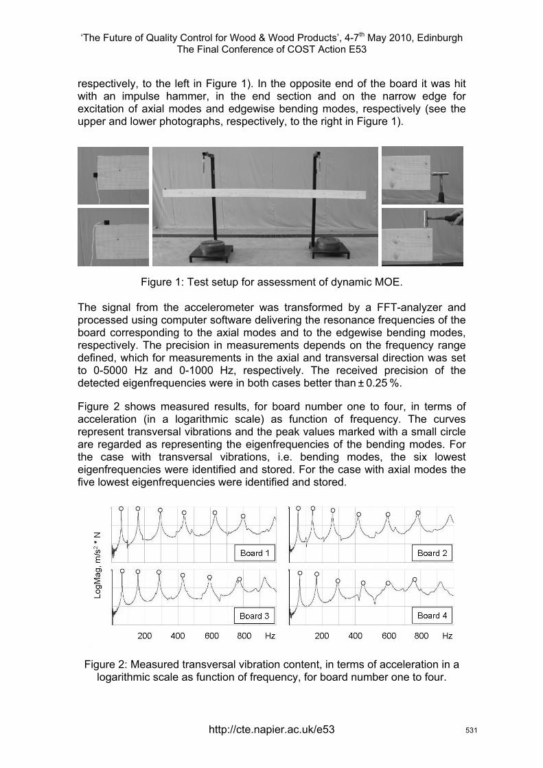
‘The Future of Quality Control for Wood & Wood Products’, 4-7th May 2010, Edinburgh The Final Conference of COST Action E53
http://cte.napier.ac.uk/e53
respectively, to the left in Figure 1). In the opposite end of the board it was hit with an impulse hammer, in the end section and on the narrow edge for excitation of axial modes and edgewise bending modes, respectively (see the upper and lower photographs, respectively, to the right in Figure 1).
Figure 1: Test setup for assessment of dynamic MOE.
The signal from the accelerometer was transformed by a FFT-analyzer and processed using computer software delivering the resonance frequencies of the board corresponding to the axial modes and to the edgewise bending modes, respectively. The precision in measurements depends on the frequency range defined, which for measurements in the axial and transversal direction was set to 0-5000 Hz and 0-1000 Hz, respectively. The received precision of the detected eigenfrequencies were in both cases better than ± 0.25 %.
Figure 2 shows measured results, for board number one to four, in terms of acceleration (in a logarithmic scale) as function of frequency. The curves represent transversal vibrations and the peak values marked with a small circle are regarded as representing the eigenfrequencies of the bending modes. For the case with transversal vibrations, i.e. bending modes, the six lowest eigenfrequencies were identified and stored. For the case with axial modes the five lowest eigenfrequencies were identified and stored.
Figure 2: Measured transversal vibration content, in terms of acceleration in a logarithmic scale as function of frequency, for board number one to four.
531
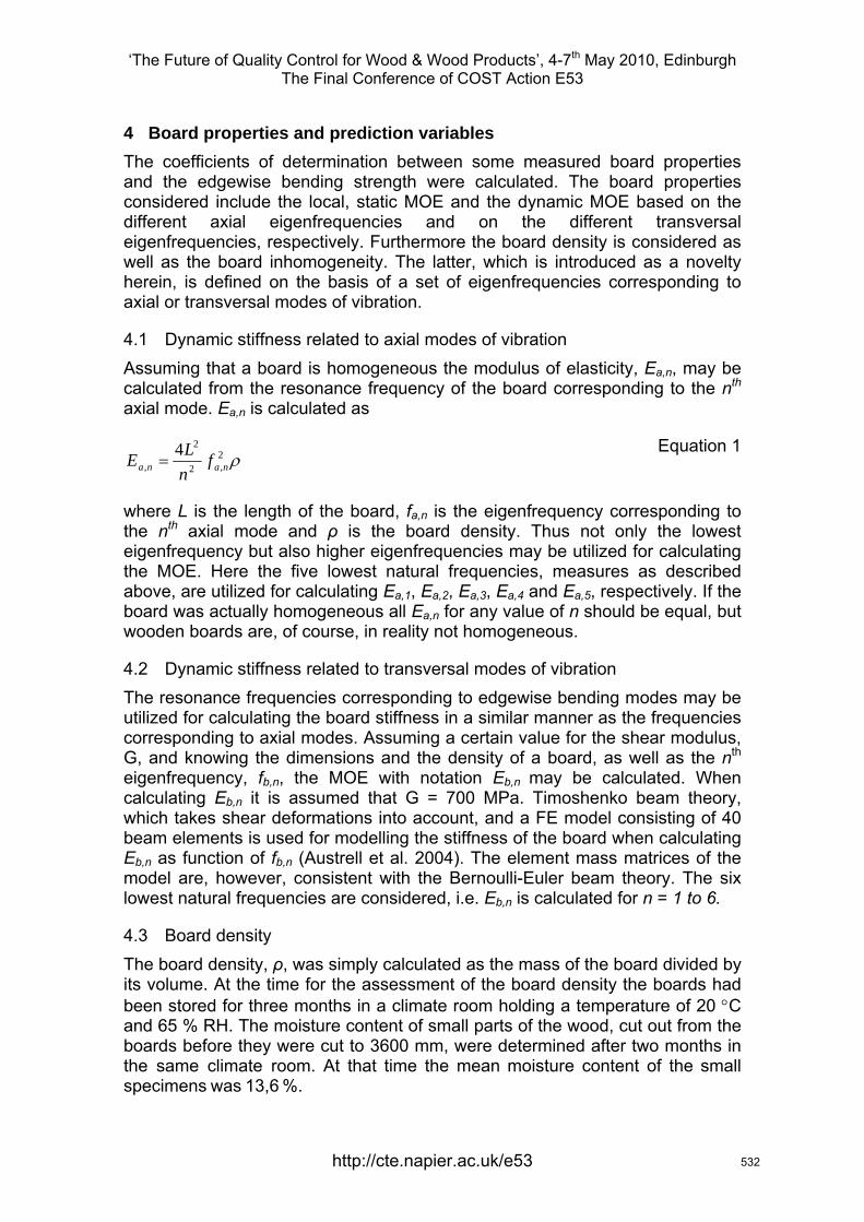
‘The Future of Quality Control for Wood & Wood Products’, 4-7th May 2010, Edinburgh The Final Conference of COST Action E53
http://cte.napier.ac.uk/e53
4 Board properties and prediction variables The coefficients of determination between some measured board properties and the edgewise bending strength were calculated. The board properties considered include the local, static MOE and the dynamic MOE based on the different axial eigenfrequencies and on the different transversal eigenfrequencies, respectively. Furthermore the board density is considered as well as the board inhomogeneity. The latter, which is introduced as a novelty herein, is defined on the basis of a set of eigenfrequencies corresponding to axial or transversal modes of vibration.
4.1 Dynamic stiffness related to axial modes of vibration Assuming that a board is homogeneous the modulus of elasticity, Ea,n, may be calculated from the resonance frequency of the board corresponding to the nth axial mode. Ea,n is calculated as
ρ2,2
2
,4
nana fnLE =
Equation 1
where L is the length of the board, fa,n is the eigenfrequency corresponding to the nth axial mode and ρ is the board density. Thus not only the lowest eigenfrequency but also higher eigenfrequencies may be utilized for calculating the MOE. Here the five lowest natural frequencies, measures as described above, are utilized for calculating Ea,1, Ea,2, Ea,3, Ea,4 and Ea,5, respectively. If the board was actually homogeneous all Ea,n for any value of n should be equal, but wooden boards are, of course, in reality not homogeneous.
4.2 Dynamic stiffness related to transversal modes of vibration The resonance frequencies corresponding to edgewise bending modes may be utilized for calculating the board stiffness in a similar manner as the frequencies corresponding to axial modes. Assuming a certain value for the shear modulus, G, and knowing the dimensions and the density of a board, as well as the nth eigenfrequency, fb,n, the MOE with notation Eb,n may be calculated. When calculating Eb,n it is assumed that G = 700 MPa. Timoshenko beam theory, which takes shear deformations into account, and a FE model consisting of 40 beam elements is used for modelling the stiffness of the board when calculating Eb,n as function of fb,n (Austrell et al. 2004). The element mass matrices of the model are, however, consistent with the Bernoulli-Euler beam theory. The six lowest natural frequencies are considered, i.e. Eb,n is calculated for n = 1 to 6.
4.3 Board density The board density, ρ, was simply calculated as the mass of the board divided by its volume. At the time for the assessment of the board density the boards had been stored for three months in a climate room holding a temperature of 20 °C and 65 % RH. The moisture content of small parts of the wood, cut out from the boards before they were cut to 3600 mm, were determined after two months in the same climate room. At that time the mean moisture content of the small specimens was 13,6 %.
532
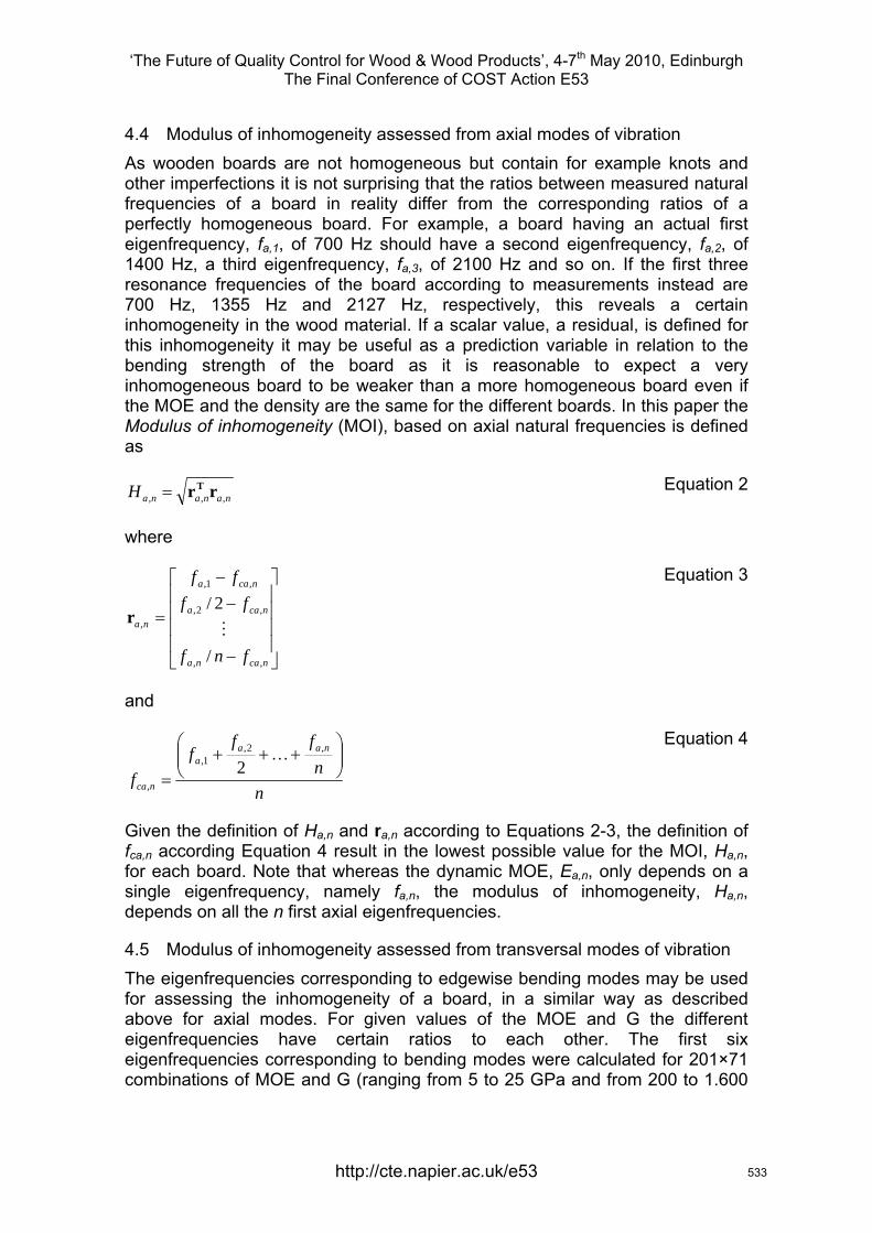
‘The Future of Quality Control for Wood & Wood Products’, 4-7th May 2010, Edinburgh The Final Conference of COST Action E53
http://cte.napier.ac.uk/e53
4.4 Modulus of inhomogeneity assessed from axial modes of vibration As wooden boards are not homogeneous but contain for example knots and other imperfections it is not surprising that the ratios between measured natural frequencies of a board in reality differ from the corresponding ratios of a perfectly homogeneous board. For example, a board having an actual first eigenfrequency, fa,1, of 700 Hz should have a second eigenfrequency, fa,2, of 1400 Hz, a third eigenfrequency, fa,3, of 2100 Hz and so on. If the first three resonance frequencies of the board according to measurements instead are 700 Hz, 1355 Hz and 2127 Hz, respectively, this reveals a certain inhomogeneity in the wood material. If a scalar value, a residual, is defined for this inhomogeneity it may be useful as a prediction variable in relation to the bending strength of the board as it is reasonable to expect a very inhomogeneous board to be weaker than a more homogeneous board even if the MOE and the density are the same for the different boards. In this paper the Modulus of inhomogeneity (MOI), based on axial natural frequencies is defined as
nananaH ,,, rrT= Equation 2
where
⎥⎥⎥⎥
⎦
⎤
⎢⎢⎢⎢
⎣
⎡
−
−−
=
ncana
ncaa
ncaa
na
fnf
ffff
,,
,2,
,1,
,
/
2/M
r
Equation 3
and
nn
fff
f
naaa
nca
⎟⎟⎠
⎞⎜⎜⎝
⎛+++
=
,2,1,
,2
K
Equation 4
Given the definition of Ha,n and ra,n according to Equations 2-3, the definition of fca,n according Equation 4 result in the lowest possible value for the MOI, Ha,n, for each board. Note that whereas the dynamic MOE, Ea,n, only depends on a single eigenfrequency, namely fa,n, the modulus of inhomogeneity, Ha,n, depends on all the n first axial eigenfrequencies.
4.5 Modulus of inhomogeneity assessed from transversal modes of vibration The eigenfrequencies corresponding to edgewise bending modes may be used for assessing the inhomogeneity of a board, in a similar way as described above for axial modes. For given values of the MOE and G the different eigenfrequencies have certain ratios to each other. The first six eigenfrequencies corresponding to bending modes were calculated for 201×71 combinations of MOE and G (ranging from 5 to 25 GPa and from 200 to 1.600
533
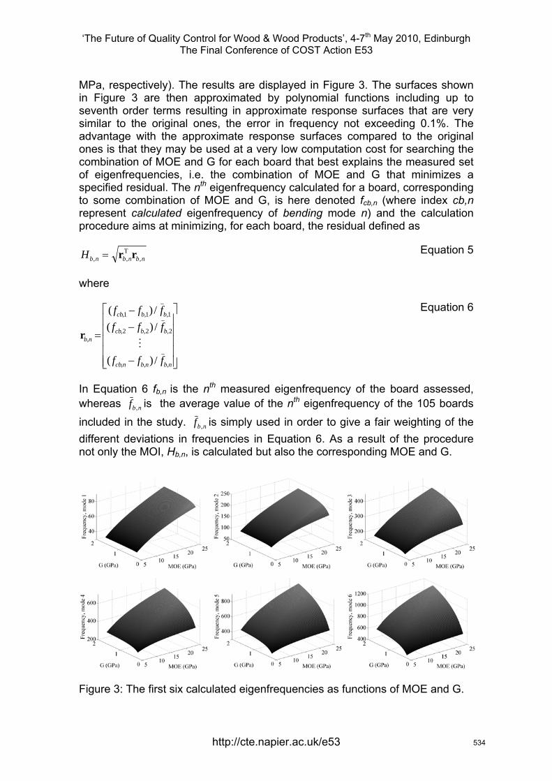
‘The Future of Quality Control for Wood & Wood Products’, 4-7th May 2010, Edinburgh The Final Conference of COST Action E53
http://cte.napier.ac.uk/e53
MPa, respectively). The results are displayed in Figure 3. The surfaces shown in Figure 3 are then approximated by polynomial functions including up to seventh order terms resulting in approximate response surfaces that are very similar to the original ones, the error in frequency not exceeding 0.1%. The advantage with the approximate response surfaces compared to the original ones is that they may be used at a very low computation cost for searching the combination of MOE and G for each board that best explains the measured set of eigenfrequencies, i.e. the combination of MOE and G that minimizes a specified residual. The nth eigenfrequency calculated for a board, corresponding to some combination of MOE and G, is here denoted fcb,n (where index cb,n represent calculated eigenfrequency of bending mode n) and the calculation procedure aims at minimizing, for each board, the residual defined as
nbnbnbH ,T,, rr= Equation 5
where
⎥⎥⎥⎥⎥
⎦
⎤
⎢⎢⎢⎢⎢
⎣
⎡
−
−−
=
nbnbncb
bbcb
bbcb
nb
fff
ffffff
,,,
2,2,2,
1,1,1,
,
/)(
/)(/)(
Mr
Equation 6
In Equation 6 fb,n is the nth measured eigenfrequency of the board assessed, whereas nbf , is the average value of the nth eigenfrequency of the 105 boards
included in the study. nbf , is simply used in order to give a fair weighting of the different deviations in frequencies in Equation 6. As a result of the procedure not only the MOI, Hb,n, is calculated but also the corresponding MOE and G.
Figure 3: The first six calculated eigenfrequencies as functions of MOE and G.
534
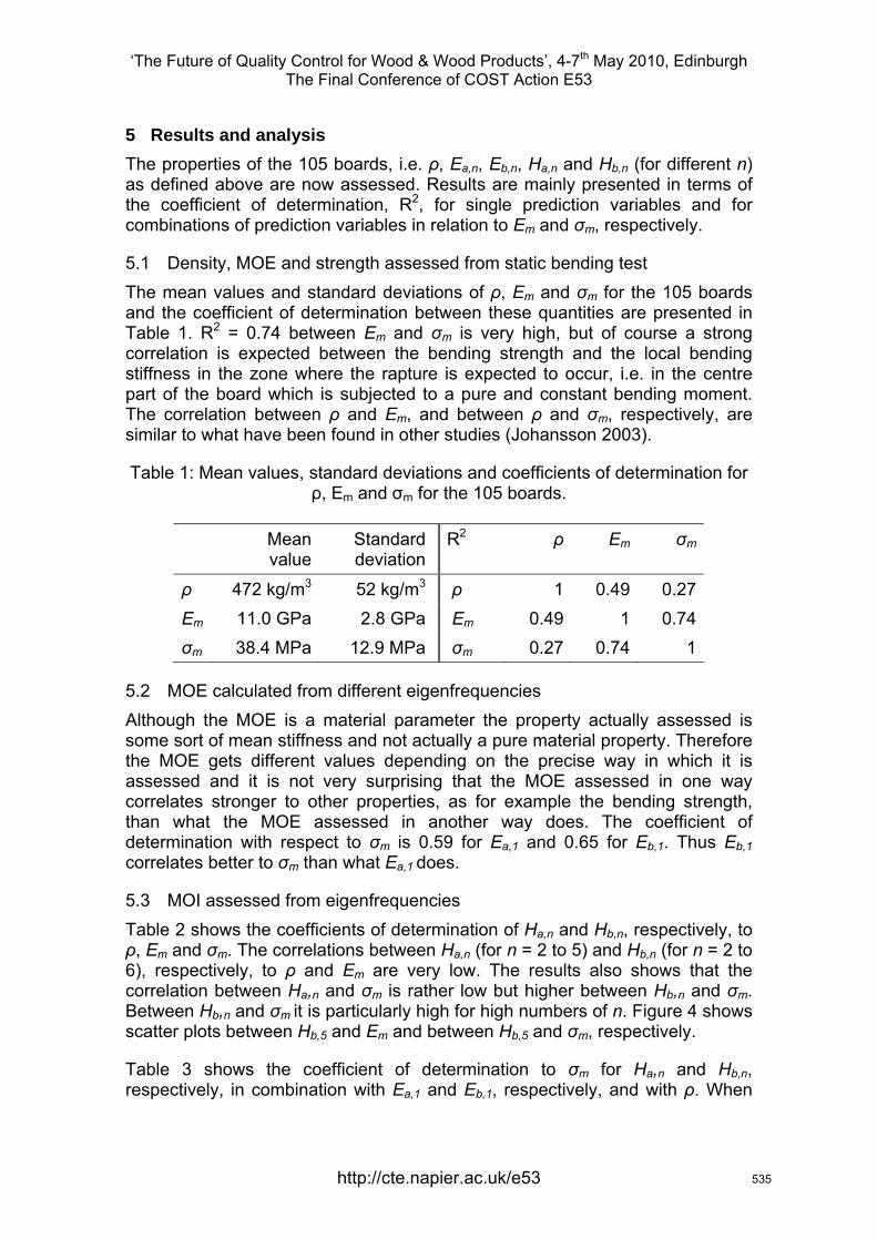
‘The Future of Quality Control for Wood & Wood Products’, 4-7th May 2010, Edinburgh The Final Conference of COST Action E53
http://cte.napier.ac.uk/e53
5 Results and analysis The properties of the 105 boards, i.e. ρ, Ea,n, Eb,n, Ha,n and Hb,n (for different n) as defined above are now assessed. Results are mainly presented in terms of the coefficient of determination, R2, for single prediction variables and for combinations of prediction variables in relation to Em and σm, respectively.
5.1 Density, MOE and strength assessed from static bending test The mean values and standard deviations of ρ, Em and σm for the 105 boards and the coefficient of determination between these quantities are presented in Table 1. R2 = 0.74 between Em and σm is very high, but of course a strong correlation is expected between the bending strength and the local bending stiffness in the zone where the rapture is expected to occur, i.e. in the centre part of the board which is subjected to a pure and constant bending moment. The correlation between ρ and Em, and between ρ and σm, respectively, are similar to what have been found in other studies (Johansson 2003).
Table 1: Mean values, standard deviations and coefficients of determination for ρ, Em and σm for the 105 boards.
Mean value
Standard deviation
R2 ρ Em σm
ρ 472 kg/m3 52 kg/m3 ρ 1 0.49 0.27 Em 11.0 GPa 2.8 GPa Em 0.49 1 0.74 σm 38.4 MPa 12.9 MPa σm 0.27 0.74 1
5.2 MOE calculated from different eigenfrequencies Although the MOE is a material parameter the property actually assessed is some sort of mean stiffness and not actually a pure material property. Therefore the MOE gets different values depending on the precise way in which it is assessed and it is not very surprising that the MOE assessed in one way correlates stronger to other properties, as for example the bending strength, than what the MOE assessed in another way does. The coefficient of determination with respect to σm is 0.59 for Ea,1 and 0.65 for Eb,1. Thus Eb,1 correlates better to σm than what Ea,1 does.
5.3 MOI assessed from eigenfrequencies Table 2 shows the coefficients of determination of Ha,n and Hb,n, respectively, to ρ, Em and σm. The correlations between Ha,n (for n = 2 to 5) and Hb,n (for n = 2 to 6), respectively, to ρ and Em are very low. The results also shows that the correlation between Ha,n and σm is rather low but higher between Hb,n and σm. Between Hb,n and σm it is particularly high for high numbers of n. Figure 4 shows scatter plots between Hb,5 and Em and between Hb,5 and σm, respectively.
Table 3 shows the coefficient of determination to σm for Ha,n and Hb,n, respectively, in combination with Ea,1 and Eb,1, respectively, and with ρ. When
535
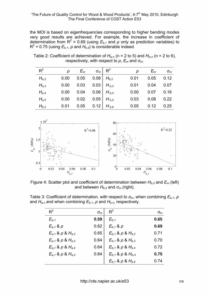
‘The Future of Quality Control for Wood & Wood Products’, 4-7th May 2010, Edinburgh The Final Conference of COST Action E53
http://cte.napier.ac.uk/e53
the MOI is based on eigenfrequencies corresponding to higher bending modes very good results are achieved. For example, the increase in coefficient of determination from R2 = 0.69 (using Eb,1 and ρ only as prediction variables) to R2 = 0.75 (using Eb,1, ρ and Hb,5) is considerable indeed.
Table 2: Coefficient of determination of Ha,n (n = 2 to 5) and Hb,n (n = 2 to 6), respectively, with respect to ρ, Em and σm.
R2 ρ Em σm R2 ρ Em σm
Ha,2 0.00 0.05 0.08 Hb,2 0.01 0.05 0.12 Ha,3 0.00 0.03 0.03 H b,3 0.01 0.04 0.07 Ha,4 0.00 0.04 0.06 H b,4 0.00 0.07 0.16 Ha,5 0.00 0.02 0.05 H b,5 0.03 0.08 0.22 Hb,2 0.01 0.05 0.12 H b,6 0.05 0.12 0.25
Figure 4: Scatter plot and coefficient of determination between Hb,5 and Em (left) and between Hb,5 and σm (right).
Table 3: Coefficient of determination, with respect to σm, when combining Ea,1, ρ and Ha,n and when combining Eb,1, ρ and Hb,n, respectively.
R2 σm R2 σm
Ea,1 0.59 Eb,1 0.65 Ea,1 & ρ 0.62 Eb,1 & ρ 0.69 Ea,1 & ρ & Ha,2 0.65 Eb,1 & ρ & Hb,2 0.71 Ea,1 & ρ & Ha,3 0.64 Eb,1 & ρ & Hb,3 0.70 Ea,1 & ρ & Ha,4 0.64 Eb,1 & ρ & Hb,4 0.72 Ea,1 & ρ & Ha,5 0.64 Eb,1 & ρ & Hb,5 0.75 Eb,1 & ρ & Hb,6 0.74
536
‘The Future of Quality Control for Wood & Wood Products’, 4-7th May 2010, Edinburgh The Final Conference of COST Action E53
http://cte.napier.ac.uk/e53
5.4 Shear modulus assessed from eigenfrequencies A reasonable mean value for the shear modulus of timber of Norway spruce is about 700 MPa and when assessing Eb,n (for n = 1 to 6) this value of G was assumed for all the boards. In reality, however, the shear stiffness differs between different boards and this was taken account of when calculating Hb,n. The MOE and the shear modulus, the latter denoted Gb,n, that minimized Hb,n, were calculated in the same process. The estimated shear modulus varies considerably between different boards. The mean value for Gb,5 was 739 MPa and the standard deviation was 116 MPa. No significant correlation was found between Gb,5 and Em or between Gb,5 and σm.
6 Conclusions Machine strength grading of timber is often based on dynamic excitation of boards in axial direction and on basis of the first axial eigenfrequency an average MOE, Ea,1, is calculated. In this paper it was shown, however, that the MOE calculated on basis of the eigenfrequency corresponding to the first bending mode, Eb,1, had a better correlation to the bending strength, σm than what Ea,1 had. For a material consisting of 105 boards of Norway spruce of dimensions 45×145×3600 mm the received coefficient of determination between Ea,1 and σm was R2 = 0.59, but between Eb,1 and σm it was R2 = 0.65.
It was also shown that eigenfrequencies corresponding to higher modes of vibration may be used in the definition of a new prediction variable, the modulus of inhomogeneity, MOI. It was shown that the MOI based on eigenfrequencies corresponding to edgewise bending modes increased the coefficient of determination when combined with Eb,1 and ρ. Using Eb,1 and ρ in combination resulted in R2 = 0.69 but using Eb,1, ρ and Hb,5 in combination resulted in R2 = 0.75. This is indeed a considerable improvement. Some improvement was also achieved when the MOI was based on axial eigenfrequencies and used in
combination with Ea,1 and ρ.
7 References C.-J. Johansson. Grading of Timber with Respect to Mechanical Properties. In S. Thelandersson and H. J. Larsen, editors, Timber Engineering, pages 23–43. Wiley, Hoboken, NJ, USA, 2003.
EN 384 Structural timber – Determination of characteristic values of mechanical properties and density. European Committee for Standardization, Brussels, Belgium, 2004.
EN 408 Timber structures – Structural timber and glued laminated timber – Determination of some physical and mechanical properties. European Committee for Standardization, Brussels, Belgium, 2003.
P.-E. Austrell, O. Dahlblom, J. Lindemann, A. Olsson, K.-G. Olsson, K. Persson, H. Petersson, M Ristinmaa, G. Sandberg and P.-A. Wernberg. CALFEM A finite element toolbox, Version 3.4. Studentlittertur, Lund, Sweden, 2004.
537
‘The Future of Quality Control for Wood & Wood Products’, 4-7th May 2010, Edinburgh The Final Conference of COST Action E53
Strength Grading of Structural Lumber by Portable Lumber Grading - effect of knots
F. Divos1 & F. Sismandy Kiss2
Abstract
Strength grading of structural lumber is not a new concept in Hungary. A special wooden dome structure - made from high strength lumber was constructed in 2000 at the campus of University of West Hungary, Sopron. The materials of the dome is Siberian Larch, strength grade is C40. The triangle truss structure covers 65 m2 are by 0.7 m3 structural wood. After 10 years of service, the dome structure is intact, demonstrates the benefits of graded lumber.
For grading the lumber of the dome structure, we measured the dynamic modulus of elasticity by longitudinal vibration. Density is measured by weighing the lumber. We have incorporated a parameter in the grading process determined by visual evaluation. It takes into account the effect of knots, and their concentration. This parameter is the Concentrated Knot Diameter Ratio: CKDR.
In 1986 Mr. Sobue in Japan introduced a method of calculation of the dynamic modulus of elasticity using Fast Fourier Transformation of the power spectrum in the vibrating specimen. The parameter measured was the natural frequency of the piece. Strong correlation coefficients were found for structural size specimens (Sobue 1986).
Due to the recent changes in wood structure design - moving from Hungarian design code MSz14081 to Euro Code 5 - we decided to verify the grading machine according to the EN 14025. The paper shows the partial results of the initial type testing of the Portable Lumber Grader (PLG) tool. 243 pieces of full size soft wood lumber has been and after the grading process the edge wise bending strength has been determined. The effect of knots are analysed carefully.
1 Materials and Methods Mixed quality 5 by 10 cm cross-section, 2 m long softwood lumber, grown in the Western Carpathian region was tested. The number of specimens totalled is 243. The test material were mixture of Picea, Pinus and Larix species. Moisture content of the samples were not controlled, they were in air-dry condition. The moisture content was 16+/- 2 %.
The primary goal of our investigation was to perform the initial type testing of the– Portable Lumber Grader – tool (Divos 2002). Parallel with the initial type
1 Professor, University of West Hungary, [email protected] PhD student, University of West Hungary [email protected]
http://cte.napier.ac.uk/e53 538

‘The Future of Quality Control for Wood & Wood Products’, 4-7th May 2010, Edinburgh The Final Conference of COST Action E53
test we determined other strength predictor parameters like dynamic bending Modulus Of Elasticity (MOE), shear modulus, logarithmic decrement, and different knot parameters, like knot diameter ratio, knot area ratio and these parameters restricted to the edge of the lumber.
PLG measures the dynamic MOE of lumber using longitudinal vibration and density. The concentrated knot diameter ratio: CKDR is also involved in the grade decision process. Definition of CKDR is given later in this paper.
Figure 1. The setup of the Portable Lumber Grader
Most of the time, the moisture content of the lumber during the grading process is different from the moisture content in service condition. We define moisture difference using the following term: moisture difference = actual moisture content – future moisture content in service condition
The EN-338 norm is dealing with static MOE. The Portable Lumber Grader software determines the dynamic MOE first then applies a correction factor to predict the static MOE. The following term defines the measured MOEmea:
( ) ( ) 6.050187.02**
2 ++= ulfhwl
mMOEmea
where f: frequency of the longitudinal vibration, mode number is 1. u: moisture difference in %. If u > 18 than u=18. l: length w: width h: height The calculated MOE takes the effect of knots into account using the highest concentrated knot diameter ratio CKDR:
CKDRMOEMOE mea 2.6−=
Before the destructive test, we have determined the following strength predictor parameters, because we wanted to improve the strength prediction capability of our grading tool:
• Knot Area Ratio (KAR), which requires a grader to visualise the knots going right through the cross-section. The KAR is the ratio of the cross -section that is taken up by knots, see figure 2. If two or more knots exist in any 15 cm long section, we are using the sum of the particular KAR values.
http://cte.napier.ac.uk/e53 539
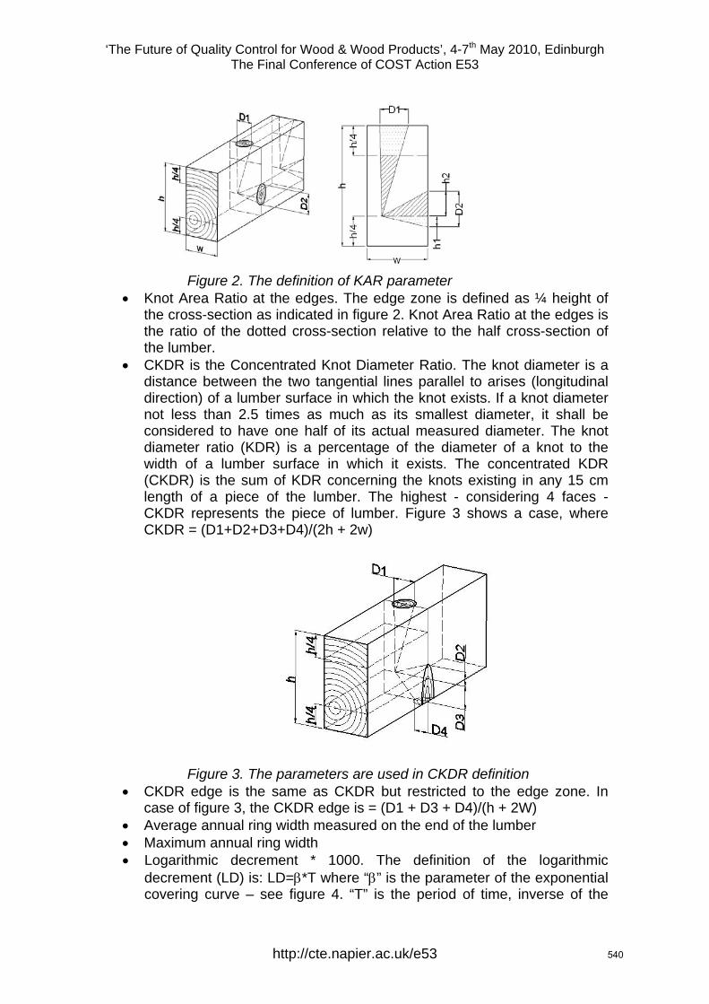
‘The Future of Quality Control for Wood & Wood Products’, 4-7th May 2010, Edinburgh The Final Conference of COST Action E53
Figure 2. The definition of KAR parameter
• Knot Area Ratio at the edges. The edge zone is defined as ¼ height of the cross-section as indicated in figure 2. Knot Area Ratio at the edges is the ratio of the dotted cross-section relative to the half cross-section of the lumber.
• CKDR is the Concentrated Knot Diameter Ratio. The knot diameter is a distance between the two tangential lines parallel to arises (longitudinal direction) of a lumber surface in which the knot exists. If a knot diameter not less than 2.5 times as much as its smallest diameter, it shall be considered to have one half of its actual measured diameter. The knot diameter ratio (KDR) is a percentage of the diameter of a knot to the width of a lumber surface in which it exists. The concentrated KDR (CKDR) is the sum of KDR concerning the knots existing in any 15 cm length of a piece of the lumber. The highest - considering 4 faces - CKDR represents the piece of lumber. Figure 3 shows a case, where CKDR = (D1+D2+D3+D4)/(2h + 2w)
Figure 3. The parameters are used in CKDR definition
• CKDR edge is the same as CKDR but restricted to the edge zone. In case of figure 3, the CKDR edge is = (D1 + D3 + D4)/(h + 2W)
• Average annual ring width measured on the end of the lumber • Maximum annual ring width • Logarithmic decrement * 1000. The definition of the logarithmic
decrement (LD) is: LD=β*T where “β” is the parameter of the exponential covering curve – see figure 4. “T” is the period of time, inverse of the
http://cte.napier.ac.uk/e53 540
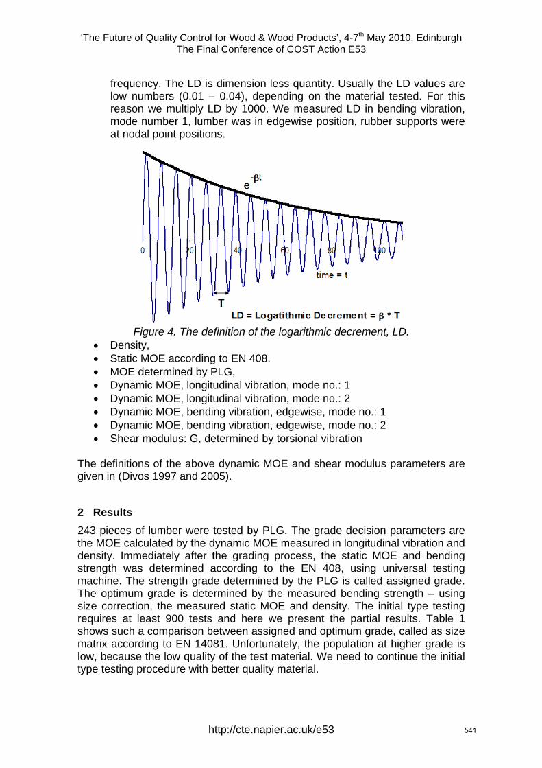
‘The Future of Quality Control for Wood & Wood Products’, 4-7th May 2010, Edinburgh The Final Conference of COST Action E53
frequency. The LD is dimension less quantity. Usually the LD values are low numbers (0.01 – 0.04), depending on the material tested. For this reason we multiply LD by 1000. We measured LD in bending vibration, mode number 1, lumber was in edgewise position, rubber supports were at nodal point positions.
Figure 4. The definition of the logarithmic decrement, LD.
• Density, • Static MOE according to EN 408. • MOE determined by PLG, • Dynamic MOE, longitudinal vibration, mode no.: 1 • Dynamic MOE, longitudinal vibration, mode no.: 2 • Dynamic MOE, bending vibration, edgewise, mode no.: 1 • Dynamic MOE, bending vibration, edgewise, mode no.: 2 • Shear modulus: G, determined by torsional vibration
The definitions of the above dynamic MOE and shear modulus parameters are given in (Divos 1997 and 2005).
2 Results 243 pieces of lumber were tested by PLG. The grade decision parameters are the MOE calculated by the dynamic MOE measured in longitudinal vibration and density. Immediately after the grading process, the static MOE and bending strength was determined according to the EN 408, using universal testing machine. The strength grade determined by the PLG is called assigned grade. The optimum grade is determined by the measured bending strength – using size correction, the measured static MOE and density. The initial type testing requires at least 900 tests and here we present the partial results. Table 1 shows such a comparison between assigned and optimum grade, called as size matrix according to EN 14081. Unfortunately, the population at higher grade is low, because the low quality of the test material. We need to continue the initial type testing procedure with better quality material.
http://cte.napier.ac.uk/e53 541
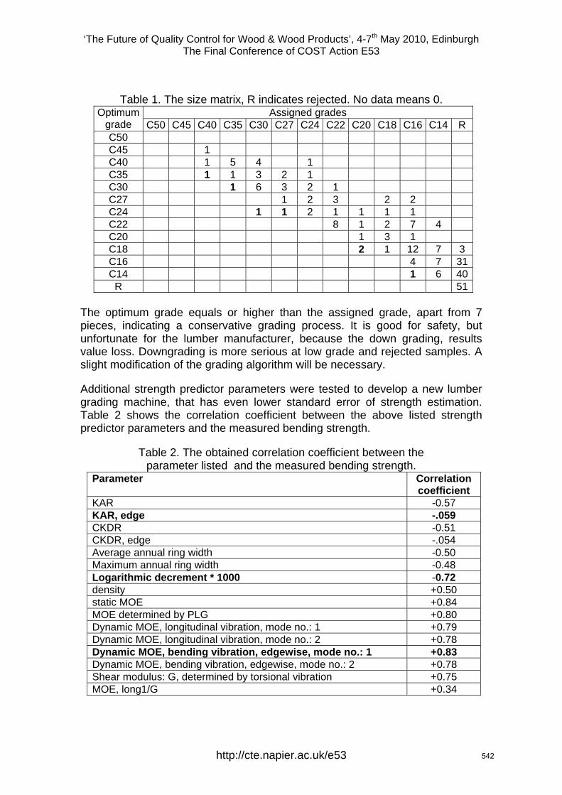
‘The Future of Quality Control for Wood & Wood Products’, 4-7th May 2010, Edinburgh The Final Conference of COST Action E53
Table 1. The size matrix, R indicates rejected. No data means 0.
Assigned grades Optimum grade C50 C45 C40 C35 C30 C27 C24 C22 C20 C18 C16 C14 R C50 C45 1 C40 1 5 4 1 C35 1 1 3 2 1 C30 1 6 3 2 1 C27 1 2 3 2 2 C24 1 1 2 1 1 1 1 C22 8 1 2 7 4 C20 1 3 1 C18 2 1 12 7 3 C16 4 7 31C14 1 6 40
R 51 The optimum grade equals or higher than the assigned grade, apart from 7 pieces, indicating a conservative grading process. It is good for safety, but unfortunate for the lumber manufacturer, because the down grading, results value loss. Downgrading is more serious at low grade and rejected samples. A slight modification of the grading algorithm will be necessary.
Additional strength predictor parameters were tested to develop a new lumber grading machine, that has even lower standard error of strength estimation. Table 2 shows the correlation coefficient between the above listed strength predictor parameters and the measured bending strength.
Table 2. The obtained correlation coefficient between the parameter listed and the measured bending strength.
Parameter Correlation coefficient
KAR -0.57 KAR, edge -.059 CKDR -0.51 CKDR, edge -.054 Average annual ring width -0.50 Maximum annual ring width -0.48 Logarithmic decrement * 1000 -0.72 density +0.50 static MOE +0.84 MOE determined by PLG +0.80 Dynamic MOE, longitudinal vibration, mode no.: 1 +0.79 Dynamic MOE, longitudinal vibration, mode no.: 2 +0.78 Dynamic MOE, bending vibration, edgewise, mode no.: 1 +0.83 Dynamic MOE, bending vibration, edgewise, mode no.: 2 +0.78 Shear modulus: G, determined by torsional vibration +0.75 MOE, long1/G +0.34
http://cte.napier.ac.uk/e53 542
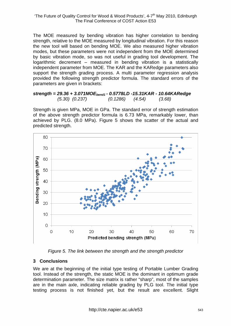
‘The Future of Quality Control for Wood & Wood Products’, 4-7th May 2010, Edinburgh The Final Conference of COST Action E53
The MOE measured by bending vibration has higher correlation to bending strength, relative to the MOE measured by longitudinal vibration. For this reason the new tool will based on bending MOE. We also measured higher vibration modes, but these parameters were not independent from the MOE determined by basic vibration mode, so was not useful in grading tool development. The logarithmic decrement – measured in bending vibration is a statistically independent parameter from MOE. The KAR and the KARedge parameters also support the strength grading process. A multi parameter regression analysis provided the following strength predictor formula. The standard errors of the parameters are given in brackets:
strength = 29.36 + 3.071MOEbend1 - 0.5778LD -15.31KAR - 10.64KARedge (5.30) (0.237) (0.1286) (4.54) (3.68)
Strength is given MPa, MOE in GPa. The standard error of strength estimation of the above strength predictor formula is 6.73 MPa, remarkably lower, than achieved by PLG. (8.0 MPa). Figure 5 shows the scatter of the actual and predicted strength.
Figure 5. The link between the strength and the strength predictor
3 Conclusions We are at the beginning of the initial type testing of Portable Lumber Grading tool. Instead of the strength, the static MOE is the dominant in optimum grade determination parameter. The size matrix is rather “sharp”, most of the samples are in the main axle, indicating reliable grading by PLG tool. The initial type testing process is not finished yet, but the result are excellent. Slight
http://cte.napier.ac.uk/e53 543
‘The Future of Quality Control for Wood & Wood Products’, 4-7th May 2010, Edinburgh The Final Conference of COST Action E53
modification of the grading algorithm will be necessary to avoid downgrading at low grades. We need to restart the initial type testing procedure. The standard error of strength estimation by PLG is 8.0 MPa.
The additional test shows, that the strength prediction of the grading process can be improved by changing the predictor parameters. Using dynamic bending MOE, logarithmic decrement, knot area ratio and knot area ratio restricted to the edge zone provides 6.73 MPa standard error of strength estimation. Unfortunately grading by bending vibration is much slower, comparing to the longitudinal vibration because the frequency of bending vibration is much lower.
Literature
Sobue, N. (1986) Measurement of Young’s modulus by the transient longitudinal vibration of wooden beams using a FFT spectrum analyser. Mokuzai Gakkaishi, Japan, 32(9): 744-747. Divos F., Tanaka T. (1997) Lumber Strength Estimation by Multiple Regression, Holzforschung 51 1997 467-471 Divos, F. (2002) Portable Lumber Grader. 13th International Symposium on Non-destructive Testing of Wood. Berkeley, California, USA. Divos, F., Denes, L. and Íñiguez, G. (2005) Effect of cross-sectional change on stress wave velocity determination. Holzforschung; Vol.: 59 (2), pp.: 230-231. EN 14081-2 (2005) Timber structures. Strength graded structural timber with rectangular cross section. Part 2: Machine grading; additional requirements for initial type testing. EN 338. (2003) Structural timber. Strength classes. EN 408. (2003) Timber structures. Sawn timber and glued laminated timber for structural use. Determination of some physical and mechanical properties. EN 14081-2 (2005) Timber structures. Strength graded structural timber with rectangular cross section. Part 2: Machine grading; additional requirements for initial type testing.
http://cte.napier.ac.uk/e53 544

‘The Future of Quality Control for Wood & Wood Products’, 4-7th May 2010, Edinburgh The Final Conference of COST Action E53
Friday 7th May Technical tour
http://www.cte.napier.ac.uk/e53/ 545

timber’s resurgenceas a primary construction material in edinburgh’s architecture
Peter Wilson, director, the Wood Studio
Medieval Edinburgh
‘The Future of Quality Control for Wood & Wood Products’, 4-7th May 2010, EdinburghThe Final Conference of COST Action E53
http://cte.napier.ac.uk/e53 546

Tron HousingFishmarket Close
Housing Fairmilehead
‘The Future of Quality Control for Wood & Wood Products’, 4-7th May 2010, EdinburghThe Final Conference of COST Action E53
http://cte.napier.ac.uk/e53 547

HousingFairmilehead
House ExtensionCumin Place
‘The Future of Quality Control for Wood & Wood Products’, 4-7th May 2010, EdinburghThe Final Conference of COST Action E53
http://cte.napier.ac.uk/e53 548

House ExtensionGranby Road
House ExtensionBoswall Road
‘The Future of Quality Control for Wood & Wood Products’, 4-7th May 2010, EdinburghThe Final Conference of COST Action E53
http://cte.napier.ac.uk/e53 549

House ExtensionWightman House
House ExtensionFernieside
‘The Future of Quality Control for Wood & Wood Products’, 4-7th May 2010, EdinburghThe Final Conference of COST Action E53
http://cte.napier.ac.uk/e53 550

St Serf’s SchoolMurrayfield
St Paul’s SchoolMorningside
‘The Future of Quality Control for Wood & Wood Products’, 4-7th May 2010, EdinburghThe Final Conference of COST Action E53
http://cte.napier.ac.uk/e53 551

Rick’s Bar & Hotel
Scottish Poetry Library
‘The Future of Quality Control for Wood & Wood Products’, 4-7th May 2010, EdinburghThe Final Conference of COST Action E53
http://cte.napier.ac.uk/e53 552

Water of Leith Visitor Centre
Visitor CentreHM Prison Saughton
‘The Future of Quality Control for Wood & Wood Products’, 4-7th May 2010, EdinburghThe Final Conference of COST Action E53
http://cte.napier.ac.uk/e53 553

Visitor CentreHM Prison Saughton
Lindsay Stewart Theatre Edinburgh Napier University
‘The Future of Quality Control for Wood & Wood Products’, 4-7th May 2010, EdinburghThe Final Conference of COST Action E53
http://cte.napier.ac.uk/e53 554

Lindsay Stewart Theatre Edinburgh Napier University
Lindsay Stewart Theatre Edinburgh Napier University
‘The Future of Quality Control for Wood & Wood Products’, 4-7th May 2010, EdinburghThe Final Conference of COST Action E53
http://cte.napier.ac.uk/e53 555

Engineered TimberScottish Parliament
Debating Chamber Scottish Parliament
‘The Future of Quality Control for Wood & Wood Products’, 4-7th May 2010, EdinburghThe Final Conference of COST Action E53
http://cte.napier.ac.uk/e53 556

Roof StructureScottish Parliament
Royal Botanic Gardens
‘The Future of Quality Control for Wood & Wood Products’, 4-7th May 2010, EdinburghThe Final Conference of COST Action E53
http://cte.napier.ac.uk/e53 557

Royal Botanic Gardens
Royal Botanic Gardens
‘The Future of Quality Control for Wood & Wood Products’, 4-7th May 2010, EdinburghThe Final Conference of COST Action E53
http://cte.napier.ac.uk/e53 558

‘The Future of Quality Control for Wood & Wood Products’, 4-7th May 2010, Edinburgh The Final Conference of COST Action E53
http://cte.napier.ac.uk/e53
The John Hope Gateway Biodiversity Centre
Richard Harris1, Paul Roberts2 & Ian Hargreaves3
Abstract The architectural concept of the John Hope Gateway is that of a floating timber canopy over the entrance to the Royal Botanic Garden, Edinburgh.
This paper presents the Engineering challenges encountered and the bespoke solutions that were generated, which include a diagrid of tapering glulam beams at roof level and the use of cross-laminated timber floors and walls. Slim cruciform steel columns are used to emphasise the elegance of the supported timber structure.
The building is on two storeys with an overall dimension of approximately 100 metres x 50 metres. Spans between columns vary between 8 and 6 metres. It uses 2750 square metres of cross-laminated timber slabs, 226mm thick on the first floor and 146mm at roof level.
Although timber is becoming used more and more regularly for structures in Scotland, this building is not only very high profile, but also it is also structurally demanding. Amongst the issues discussed in the paper are: Connection details at the tops of the column heads, where the roof is carried on thin steel rods; the use of large areas of exposed cross-laminated timber in a building with public access; fire resistance and the use of timber in an external environment
1 Introduction The John Hope Gateway Biodiversity Centre was won in an architectural competition in July 2003 and opened to the public in October 2009.
The overall mission of the Client, The Royal Botanic Gardens Edinburgh (RBGE) is “to explore and explain the world of plants”. Their Edinburgh site was established in 1670 as a physic garden. The organisation has grown substantially since then and is now a world-renowned centre for plant science, research and education.
1 Prof of Timber Engineering [email protected] BRE Centre for Innovative Construction Materials, University of Bath, UK 2 Structural Engineer [email protected] Buro Happold, Denmark 3 Associate Director [email protected] Buro Happold, UK
559

‘The Future of Quality Control for Wood & Wood Products’, 4-7th May 2010, Edinburgh The Final Conference of COST Action E53
http://cte.napier.ac.uk/e53
The new building combines the practical need for improved visitor facilities with an opportunity to engage visitors in the work of RBGE and the exploration of the relevance of plants to the critical issues of our time. Thus, as well as office space, a restaurant, an outdoor café, a plant sales area and visitor restrooms, the new centre houses exhibitions and a studio space for demonstrations and exploration into the world of plants.
The Client challenged the design team to use ecologically sensitive construction materials and environmentally friendly building services.
The exposed structure is a key feature of the building, consisting of intricate cruciform steel columns, supporting a series of glulam timber beams and cross-laminated solid timber floor slabs.
2 Concept Design The pre-eminence of the Garden is the conceptual driver for the design. The Gateway marks the entrance to the gardens by facing a road to the west (Figure 1). On the garden side, stepped biodiversity ponds extend from the glass wall of the exhibition space and blend into the surrounding landscape. The glass wall is some 60 metres long and enables the message of the interpretation delivered within the building to be extended into the Garden and vice versa. At first floor, a roof terrace overlooks the biodiversity pond and garden (Figure2).
Figure 1: Figure 2: The building in context The garden terrace and biodiversity ponds (Image copyright: Edward Cullinan Architects) (Image copyright: Buro Happold)
Given the botanical nature of the project, it was natural that the structure should use timber extensively. It uses an innovative combination of glued-laminated timber and cross-laminated timber for its walls, floors and roof. Although timber was considered for the columns, they are made from slender fabricated steel elements.
560
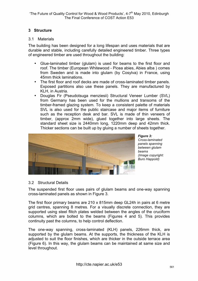
‘The Future of Quality Control for Wood & Wood Products’, 4-7th May 2010, Edinburgh The Final Conference of COST Action E53
http://cte.napier.ac.uk/e53
3 Structure
3.1 Materials The building has been designed for a long lifespan and uses materials that are durable and stable, including carefully detailed engineered timber. Three types of engineered timber are used throughout the building:
• Glue-laminated timber (glulam) is used for beams to the first floor and roof. The timber (European Whitewood - Picea abies, Abies alba ) comes from Sweden and is made into glulam (by Cosylva) in France, using 45mm thick laminations.
• The first floor and roof decks are made of cross-laminated timber panels. Exposed partitions also use these panels. They are manufactured by KLH, in Austria.
• Douglas Fir (Pseudotsuga menziesii) Structural Veneer Lumber (SVL) from Germany has been used for the mullions and transoms of the timber-framed glazing system. To keep a consistent palette of materials SVL is also used for the public staircase and major items of furniture such as the reception desk and bar. SVL is made of thin veneers of timber, (approx 2mm wide), glued together into large sheets. The standard sheet size is 2440mm long, 1220mm deep and 42mm thick. Thicker sections can be built up by gluing a number of sheets together.
Figure 3: Cross-laminated panels spanning between glulam beams (Image copyright: Buro Happold)
3.2 Structural Details The suspended first floor uses pairs of glulam beams and one-way spanning cross-laminated panels as shown in Figure 3.
The first floor primary beams are 210 x 815mm deep GL24h in pairs at 6 metre grid centres, spanning 8 metres. For a visually discrete connection, they are supported using steel flitch plates welded between the angles of the cruciform columns, which are bolted to the beams (Figures 4 and 5). This provides continuity past the columns, to help control deflection.
The one-way spanning, cross-laminated (KLH) panels, 226mm thick, are supported by the glulam beams. At the supports, the thickness of the KLH is adjusted to suit the floor finishes, which are thicker in the outside terrace area (Figure 6). In this way, the glulam beams can be maintained at same size and level throughout.
561
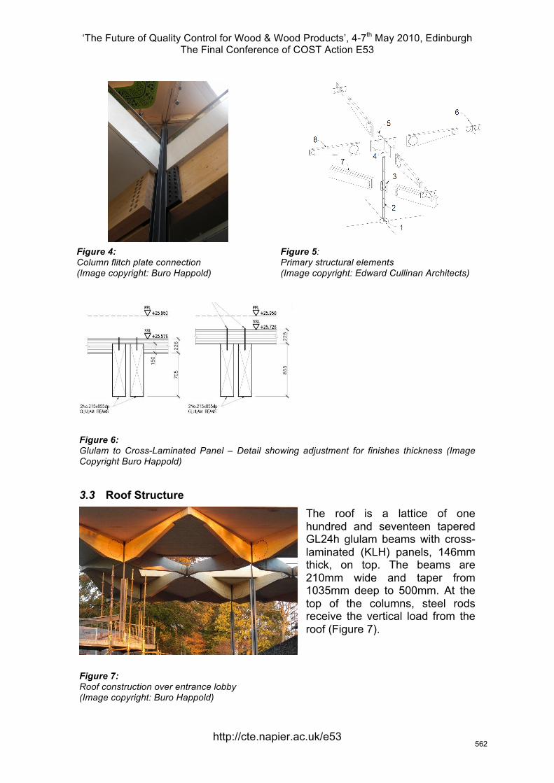
‘The Future of Quality Control for Wood & Wood Products’, 4-7th May 2010, Edinburgh The Final Conference of COST Action E53
http://cte.napier.ac.uk/e53
Figure 4: Figure 5: Column flitch plate connection Primary structural elements (Image copyright: Buro Happold) (Image copyright: Edward Cullinan Architects)
Figure 6: Glulam to Cross-Laminated Panel – Detail showing adjustment for finishes thickness (Image Copyright Buro Happold)
3.3 Roof Structure
The roof is a lattice of one hundred and seventeen tapered GL24h glulam beams with cross-laminated (KLH) panels, 146mm thick, on top. The beams are 210mm wide and taper from 1035mm deep to 500mm. At the top of the columns, steel rods receive the vertical load from the roof (Figure 7).
Figure 7: Roof construction over entrance lobby (Image copyright: Buro Happold)
562

‘The Future of Quality Control for Wood & Wood Products’, 4-7th May 2010, Edinburgh The Final Conference of COST Action E53
http://cte.napier.ac.uk/e53
Being on a diagonal grid, the beams meet at the centre of the rectangular grid. Steel flitch plates bolted into the timber are welded to a central bar. This provides moment continuity in the structure and creates a strong visual location to the centre of the coffered slab.
Whilst at first floor the bolts to the column flitch plates are arranged in rectangular groups, at roof level, for visual reasons and for structural efficiency, the bolts are arranged in circular groups. This provides a strong visual contrast. (Figure 8)
Particular features of the roof structure are as follows:
• Diagonal grid arrangement • Flitch plates allow moment
continuity across the column head detail
• Low stiffness of column leads to small moment transfer from the beam into the column. By reducing the bending moment, the use of a slender steel rod is permitted at the top of the column.
• As an equal and large lever arm is provided from the centre of the beam to each fixing, the annular ring of dowels resists the bending applied to the beam in a very efficient manner. It also creates a striking visual effect when contrasting with the orthogonal arrangement at first floor level.
• Connection design to EC5. • Countersunk bolt detail leads to a
loss of section, which affects the local stress in the timber
• Great care was taken to ensure that edge distances complied with the minimum spacing requirements of EC5
Figure 8: Column elevation showing glulam to column connections at roof (circular bolt arrangement) and first floor (rectangular bolt arrangement)(Image copyright: Buro Happold)
563
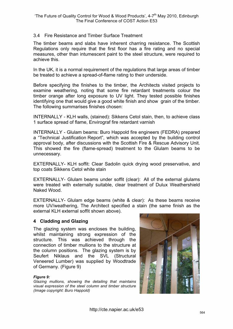
‘The Future of Quality Control for Wood & Wood Products’, 4-7th May 2010, Edinburgh The Final Conference of COST Action E53
http://cte.napier.ac.uk/e53
3.4 Fire Resistance and Timber Surface Treatment The timber beams and slabs have inherent charring resistance. The Scottish Regulations only require that the first floor has a fire rating and no special measures, other than intumescent paint to the steel structure, were required to achieve this.
In the UK, it is a normal requirement of the regulations that large areas of timber be treated to achieve a spread-of-flame rating to their underside.
Before specifying the finishes to the timber, the Architects visited projects to examine weathering, noting that some fire retardant treatments colour the timber orange after long exposure to UV light. They tested possible finishes identifying one that would give a good white finish and show grain of the timber. The following summarises finishes chosen:
INTERNALLY - KLH walls, (stained): Sikkens Cetol stain, then, to achieve class 1 surface spread of flame, Envirograf fire retardant varnish
INTERNALLY - Glulam beams: Buro Happold fire engineers (FEDRA) prepared a “Technical Justification Report”, which was accepted by the building control approval body, after discussions with the Scottish Fire & Rescue Advisory Unit. This showed the fire (flame-spread) treatment to the Glulam beams to be unnecessary.
EXTERNALLY- KLH soffit: Clear Sadolin quick drying wood preservative, and top coats Sikkens Cetol white stain
EXTERNALLY- Glulam beams under soffit (clear): All of the external glulams were treated with externally suitable, clear treatment of Dulux Weathershield Naked Wood.
EXTERNALLY- Glulam edge beams (white & clear): As these beams receive more UV/weathering, The Architect specified a stain (the same finish as the external KLH external soffit shown above).
4 Cladding and Glazing The glazing system was encloses the building, whilst maintaining strong expression of the structure. This was achieved through the connection of timber mullions to the structure at the column positions. The glazing system is by Seufert Niklaus and the SVL (Structural Veneered Lumber) was supplied by Woodtrade of Germany. (Figure 9) Figure 9: Glazing mullions, showing the detailing that maintains visual expression of the steel column and timber structure (Image copyright: Buro Happold)
564

‘The Future of Quality Control for Wood & Wood Products’, 4-7th May 2010, Edinburgh The Final Conference of COST Action E53
http://cte.napier.ac.uk/e53
The building is clad with vertical boards of Scottish larch (Larix decidua) sourced from Russwood timber in the Cairngorms, ship-lapped in a vertical manner. (Figure 14)
Figure 10: Larch cladding (Image copyright: Buro Happold)
5 Conclusions A clear concept remained a consistent driver of design from the competition through to the completion of the building. However it was hard to maintain this clarity. Many of the details appear to be simple, but the variations in a building of this shape, which is moulded to fit the contours of the landscape of the site, lead to many permutations of the “standard” details.
The final building maintains clarity in the expression of the structure, particularly in the use of timber. Success in projects of this type can only be achieved by close integrated working of the design team with the Client, contractor and specialist sub-contractors.
The chosen solution meets the client’s goals in a variety of ways, including the sustainable nature of the materials used.
ACKNOWELEDGEMENTS Client: Royal Botanic Garden, Edinburgh
Architect: Edward Cullinan Architects
Structural Engineer: Buro Happold Ltd.
Building Services Engineer: Max Fordham
Main Contractor: Xircon
Timber Sub-Contractor: Donaldson & McConnell
Cross- Laminated Floors: KLH
565
‘The Future of Quality Control for Wood & Wood Products’, 4-7th May 2010, Edinburgh The Final Conference of COST Action E53
Structural Performance of thinned oak containers
N. Savage1, A. Kermani2
Abstract Traditional containers such as barrels, used in the transportation and storage of food and liquid, have been constructed from timber for thousands of years. The design of the container has evolved over time and the original design specifications have not altered until recent times. Storage of high strength spirit such as whisky has lead to the containers being used for flavour purposes as well as storage. Consequently the inner surface of the barrel is becoming thinner, raising concerns regarding the structural integrity of the barrel in modern warehousing. Warehousing of timber barrels in modern industry utilises palletising techniques made possible by advances in transportation technology, such as forklift trucks. In-turn, this has placed a modern day requirement for the barrel to withstand additional and non-traditional loading within a palletised system. Consequently, under load, the curved timber of the barrel has a stress concentration generated about the mid-line, leading to concerns regarding structural integrity. The six supporting hoops of the barrel are traditionally used for maintaining shape and retention performance. However, under the new loading conditions of palletisation, they absorb the stress as the barrel displaces, reducing the stress concentration about the mid-line, up to the ultimate loading of the timber. The effect of hoop arrangements on structural integrity during palletised loading has been investigated using FEM to establish the optimal orientation with the aim of increasing the overall stiffness of the structure. Experimental validation of the optimal hoop locations about the cask established in the FEM environment has been conducted. The experimental investigation compares modified and un-modified barrels with respect to their limiting stress conditions, comparative stiffness’ and curvature displacement magnitudes.
1 Introduction Traditional oak containers, such as barrels, have been used for over 2000 years in the storage and transportation of food, liquid, meats and even gun-powder (Kilby 1989). Over the past 200 years, the oak barrel has been adopted by the alcoholic drinks industry, largely Scotch and American Bourbon, due to the flavour impact the timber has on the liquid. The flavour is derived from the firing of the internal surface of the barrel whereby the natural components of the timber (i.e. lignin, cellulose, hemi-cellulose etc.) are degraded to produce flavour compounds such as vanillin and syringealdehyde. These flavour components add to the new make alcohol during the maturation of the liquid as
1 KTP Associate, [email protected] Centre for Timber Engineering, Edinburgh Napier University, UK 2 Professor of Timber Engineering, [email protected] for Timber Engineering, Edinburgh Napier University, UK
http://cte.napier.ac.uk/e53 566

‘The Future of Quality Control for Wood & Wood Products’, 4-7th May 2010, Edinburgh The Final Conference of COST Action E53
spirit interacts with the timber. The flavours of the barrel will eventually become exhausted after a number of consecutive fillings and therefore be returned to the cooperage for “rejuvenation”. The rejuvenation process involves a flailing and firing process whereby the internal surface of the barrel is scrapped to remove old/ exhausted timber to allow for a re-heating of new timber to regenerate flavour compounds, thereby extending the working life of the barrel. Evolution of warehousing and transport technology, such as forklifts, and consequently barrels are stored vertically in palletised warehousing instead of the traditional horizontal storage. With modern techniques of flailing now able to remove 2mm per rejuvenation, concerns have been raised as to the structural integrity of the barrel structure with the additional loading. These concerns are amplified with respect to ‘thinned’ barrels becoming more common, especially within the wine and spirits industries.
2 Methodology The structural optimisation of the barrel design was based on firstly quantifying the current “thinned” barrel performance under load and quantification of mechanical timber properties of the American oak material under investigation. Following the experimental analysis, Finite Element Analysis techniques were used to optimise the orientation of supporting hoops to provide the maximum possible strength under load.
2.1 Experimental Test barrels were constructed from “thinned” staves at approximately 12mm, 14mm, 16 mm and 18 mm. Barrels of regular stave thickness (approximately 26mm) were also tested. The barrels were filled with water, kept for a minimum of 2 weeks and emptied before filling to ensure similar moisture content to that of barrels in warehousing.
The assessment of structural performance of thinned barrels was conducted to determine the load-deformation characteristics before optimisation of hoop orientation. Displacement transducers were placed around the centreline of the barrel bilge (the widest circumference of the barrel) to monitor deformation of global circumference. Displacement in stave bilge around the barrel is due to the stress concentration at the weakest component of the timber (transverse grain of the stave under combined bending and tensile stresses) and therefore requires optimisation. Figure 1 shows the schematic of displacement transducer locations (a total of 8) about the barrel bilge for monitoring stave displacement.
http://cte.napier.ac.uk/e53 567
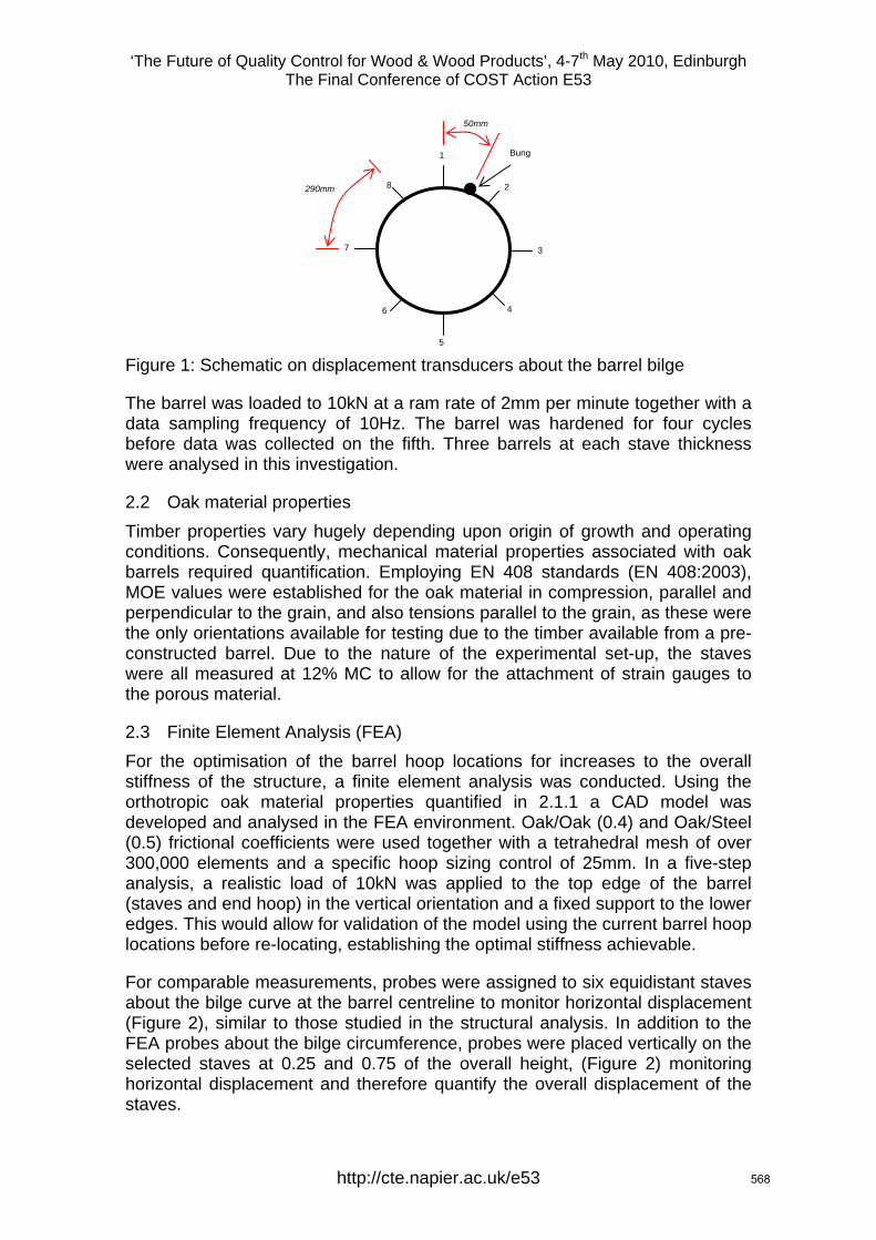
‘The Future of Quality Control for Wood & Wood Products’, 4-7th May 2010, Edinburgh The Final Conference of COST Action E53
Figure 1: Schematic on displacement transducers about the barrel bilge
The barrel was loaded to 10kN at a ram rate of 2mm per minute together with a data sampling frequency of 10Hz. The barrel was hardened for four cycles before data was collected on the fifth. Three barrels at each stave thickness were analysed in this investigation.
2.2 Oak material properties Timber properties vary hugely depending upon origin of growth and operating conditions. Consequently, mechanical material properties associated with oak barrels required quantification. Employing EN 408 standards (EN 408:2003), MOE values were established for the oak material in compression, parallel and perpendicular to the grain, and also tensions parallel to the grain, as these were the only orientations available for testing due to the timber available from a pre-constructed barrel. Due to the nature of the experimental set-up, the staves were all measured at 12% MC to allow for the attachment of strain gauges to the porous material.
2.3 Finite Element Analysis (FEA) For the optimisation of the barrel hoop locations for increases to the overall stiffness of the structure, a finite element analysis was conducted. Using the orthotropic oak material properties quantified in 2.1.1 a CAD model was developed and analysed in the FEA environment. Oak/Oak (0.4) and Oak/Steel (0.5) frictional coefficients were used together with a tetrahedral mesh of over 300,000 elements and a specific hoop sizing control of 25mm. In a five-step analysis, a realistic load of 10kN was applied to the top edge of the barrel (staves and end hoop) in the vertical orientation and a fixed support to the lower edges. This would allow for validation of the model using the current barrel hoop locations before re-locating, establishing the optimal stiffness achievable.
For comparable measurements, probes were assigned to six equidistant staves about the bilge curve at the barrel centreline to monitor horizontal displacement (Figure 2), similar to those studied in the structural analysis. In addition to the FEA probes about the bilge circumference, probes were placed vertically on the selected staves at 0.25 and 0.75 of the overall height, (Figure 2) monitoring horizontal displacement and therefore quantify the overall displacement of the staves.
1
2
3
4 6
8
7
5
Bung
50mm
290mm
http://cte.napier.ac.uk/e53 568
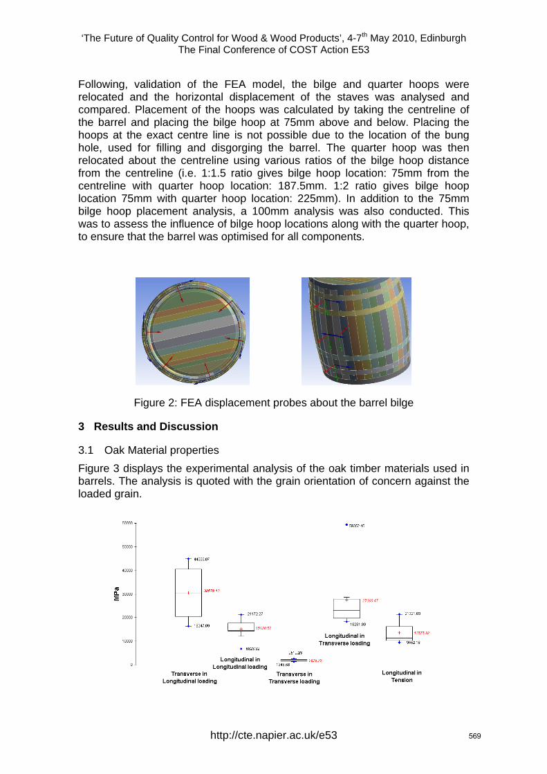
‘The Future of Quality Control for Wood & Wood Products’, 4-7th May 2010, Edinburgh The Final Conference of COST Action E53
Following, validation of the FEA model, the bilge and quarter hoops were relocated and the horizontal displacement of the staves was analysed and compared. Placement of the hoops was calculated by taking the centreline of the barrel and placing the bilge hoop at 75mm above and below. Placing the hoops at the exact centre line is not possible due to the location of the bung hole, used for filling and disgorging the barrel. The quarter hoop was then relocated about the centreline using various ratios of the bilge hoop distance from the centreline (i.e. 1:1.5 ratio gives bilge hoop location: 75mm from the centreline with quarter hoop location: 187.5mm. 1:2 ratio gives bilge hoop location 75mm with quarter hoop location: 225mm). In addition to the 75mm bilge hoop placement analysis, a 100mm analysis was also conducted. This was to assess the influence of bilge hoop locations along with the quarter hoop, to ensure that the barrel was optimised for all components.
Figure 2: FEA displacement probes about the barrel bilge
3 Results and Discussion
3.1 Oak Material properties ental analysis of the oak timber materials used in d with the grain orientation of concern against the
Figure 3 displays the experimbarrels. The analysis is quoteloaded grain.
http://cte.napier.ac.uk/e53 569
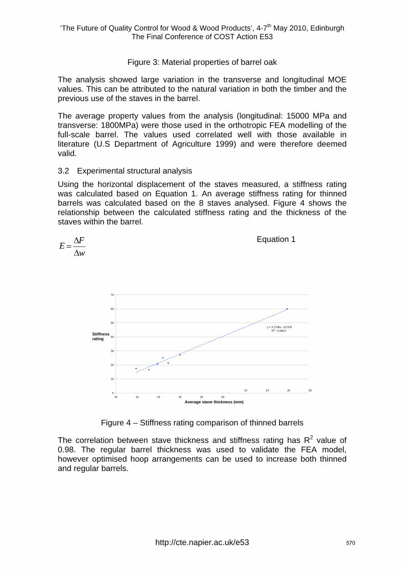
‘The Future of Quality Control for Wood & Wood Products’, 4-7th May 2010, Edinburgh The Final Conference of COST Action E53
Figure 3: Material properties of barrel oak
The analysis showed large variation in the transverse and longitudinal MOE values. This can be attributed to the natural variation in both the timber and the previous use of the staves in the barrel.
The average property values from the analysis (longitudinal: 15000 MPa and transverse: 1800MPa) were those used in the orthotropic FEA modelling of the full-scale barrel. The values used correlated well with those available in literature (U.S Department of Agriculture 1999) and were therefore deemed valid.
3.2 Experimental structural analysis Using the horizontal displacement of the staves measured, a stiffness rating was calculated based on Equation 1. An average stiffness rating for thinned barrels was calcul ure 4 shows the relationship between the calculated stiffness rating and the thickness of the
ated based on the 8 staves analysed. Fig
staves within the barrel.
wΔ
FΔ=E
Equation 1
Figure 4 – Stiffness rating comparison of thinned barrels
The correlation between stave thickness and stiffness rating has R2 value of 0.98. The regular barrel thickness was used to validate the FEA model, however optimised hoop arrangements can be used to increase both thinned and regular barrels.
y = 3.1706x - 22.978 R2 = 0.9813
20
30
40
50
0
10
70
10 12 14 16 18 20
22 24 26 28
60
Stiffness rating
Average stave thickness (mm)
http://cte.napier.ac.uk/e53 570
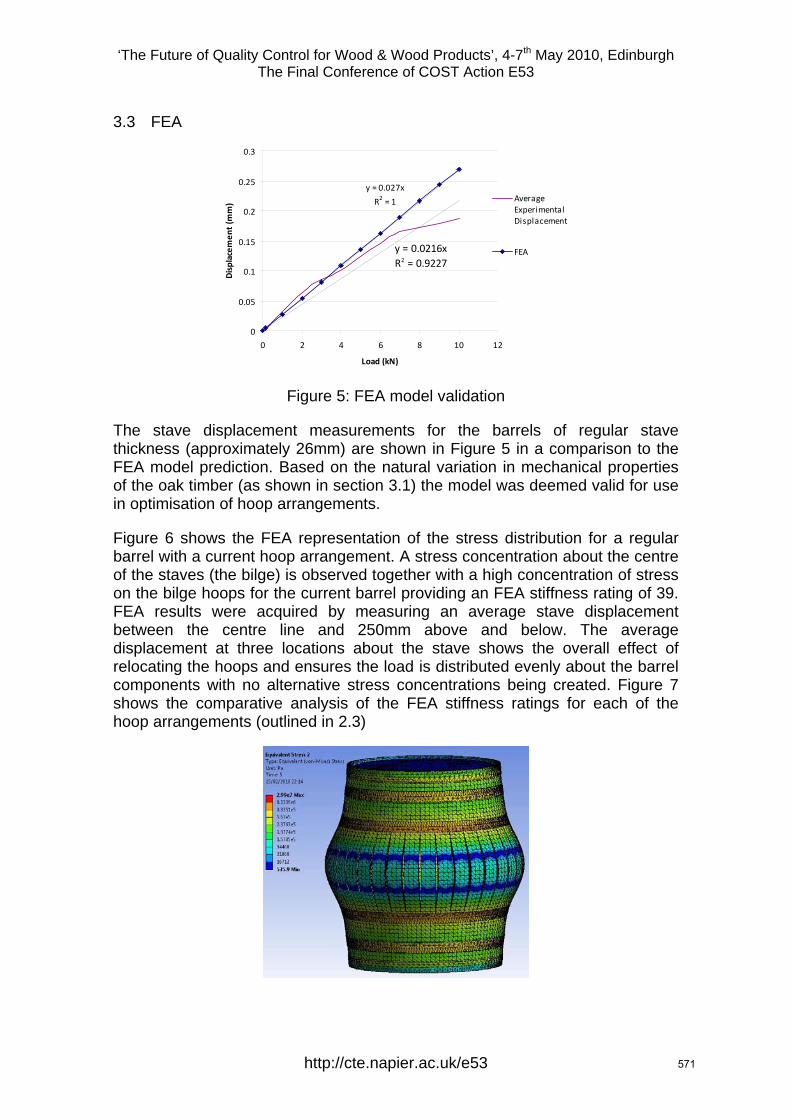
‘The Future of Quality Control for Wood & Wood Products’, 4-7th May 2010, Edinburgh The Final Conference of COST Action E53
3.3 FEA
y = 0.0216xR2 = 0.9227
y = 0.027x
R2 = 1
0
0.05
0.1
0.15
0.2
0.25
0.3
0 2 4 6 8 10 12
Load (kN)
Displacem
ent (m
m) Average
ExperimentalDisplacement
FEA
Figure 5: FEA model validation
The stave displacement measurements for the barrels of regular stave thickness (approximately 26mm) are shown in Figure 5 in a comparison to the FEA model prediction. Based on the natural variation in mechanical properties of the oak timber (as shown in section 3.1) the model was deemed valid for use
n of hoop arrangements.
Figure 6 shows the FEA representation of the stress distribution for a regular barrel with a current hoop arrangement. A stress concentration about the centre of the staves (the bilge) is observed together with a high concentration of stress on the bilge hoops for the current barrel providing an FEA stiffness rating of 39. FEA results were acquired by measuring an average stave displacement between the centre line and 250mm above and below. The average displacement at three locations about the stave shows the overall effect of relocating the hoops and ensures the load is distributed evenly about the barrel components with no alternative stress concentrations being created. Figure 7 shows the comparative analysis of the FEA stiffness ratings for each of the hoop arrangements (outlined in 2.3)
in optimisatio
http://cte.napier.ac.uk/e53 571
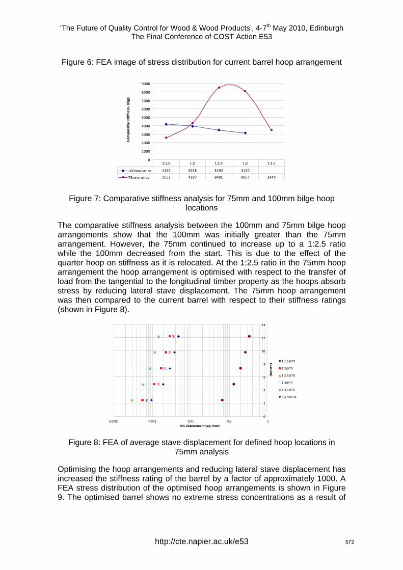
‘The Future of Quality Control for Wood & Wood Products’, 4-7th May 2010, Edinburgh The Final Conference of COST Action E53
Figure 6: FEA image of stress distribution for current barrel hoop arrangement
0
1000
2000
3000
4000
5000
6000
7000
8000
9000
le stiffne
ss‐ B
ilge
Comparab
100mm ratios 4169 3928 3492 3120
75mm ratios 2552 4287 8481 8067 3444
1:1,5 1:2 1:2.5 1:3 1:3.5
Figure 7: Comparative stiffness analysis for 75mm and 100mm bilge hoop locations
The comparative stiffness analysis between the 100mm and 75mm bilge hoop arrangements show that the 100mm was initially greater than the 75mm arrangement. However, the 75mm continued to increase up to a 1:2.5 ratio while the 100mm decreased from the start. This is due to the effect of the q arrangement the hoop arrangement is optimised with respect to the transfer of load from the tangential to the longitudinal timber property as the hoops absorb stress by reducing lateral stave displacement. The 75mm hoop arrangement was then compared to the current barrel with respect to their stiffness ratings (shown in Figure 8).
uarter hoop on stiffness as it is relocated. At the 1:2.5 ratio in the 75mm hoop
0
4
6
8
10
12
14
Load (kN)
1:1.5@75
1:2@75
1:2.5@75
1:3@75
1:3.5@75
Current Ba
2
0.0001 0.001 0.01 0.1 1FEA Displacement Log. (mm)
Figure 8: FEA of average stave displacement for defined hoop locations in 75mm analysis
Optimising the hoop arrangements and reducing lateral stave displacement has increased the stiffness rating of the barrel by a factor of approximately 1000. A FEA stress distribution of the optimised hoop arrangements is shown in Figure 9. The optimised barrel shows no extreme stress concentrations as a result of
http://cte.napier.ac.uk/e53 572
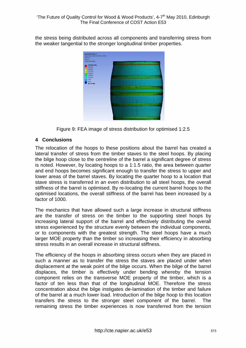
‘The Future of Quality Control for Wood & Wood Products’, 4-7th May 2010, Edinburgh The Final Conference of COST Action E53
the stress being distributed across all components and transferring stress from the weaker tangential to the stronger longitudinal timber properties.
Figure 9: FEA image of stress distribution for optimised 1:2.5
4 Conclusions The relocation of the hoops to these positions about the barrel has created a lateral transfer of stress from the timber staves to the steel hoops. By placing the bilge hoop close to the centreline of the barrel a significant degree of stress is noted. However, by locating hoops to a 1:1.5 ratio, the area between quarter and end hoops becomes significant enough to transfer the stress to upper and lower areas of the barrel staves. By locating the quarter hoop to a location that stave stress is transferred in an even distribution to all steel hoops, the overall stiffness of the barrel is optimised. By re-locating the current barrel hoops to the optimised locations, the overall stiffness of the barrel has been increased by a factor of 1000.
The mechanics that have allowed such a large increase in structural stiffness are the transfer of stress on the timber to the supporting steel hoops by increasing lateral support of the barrel and effectively distributing the overall stress experienced by the structure evenly between the individual components, or to components with the greatest strength. The steel hoops have a much larger MOE property than the timber so increasing their efficiency in absorbing stress results in an overall increase in structural stiffness.
The effici laced in such a manner as to transfer the stress the staves are placed under when
weak point of the bilge occurs. When the bilge of the barrel
ency of the hoops in absorbing stress occurs when they are p
displacement at thedisplaces, the timber is effectively under bending whereby the tension component relies on the transverse MOE property of the timber, which is a factor of ten less than that of the longitudinal MOE. Therefore the stress concentration about the bilge instigates de-lamination of the timber and failure of the barrel at a much lower load. Introduction of the bilge hoop to this location transfers the stress to the stronger steel component of the barrel. The remaining stress the timber experiences is now transferred from the tension
http://cte.napier.ac.uk/e53 573
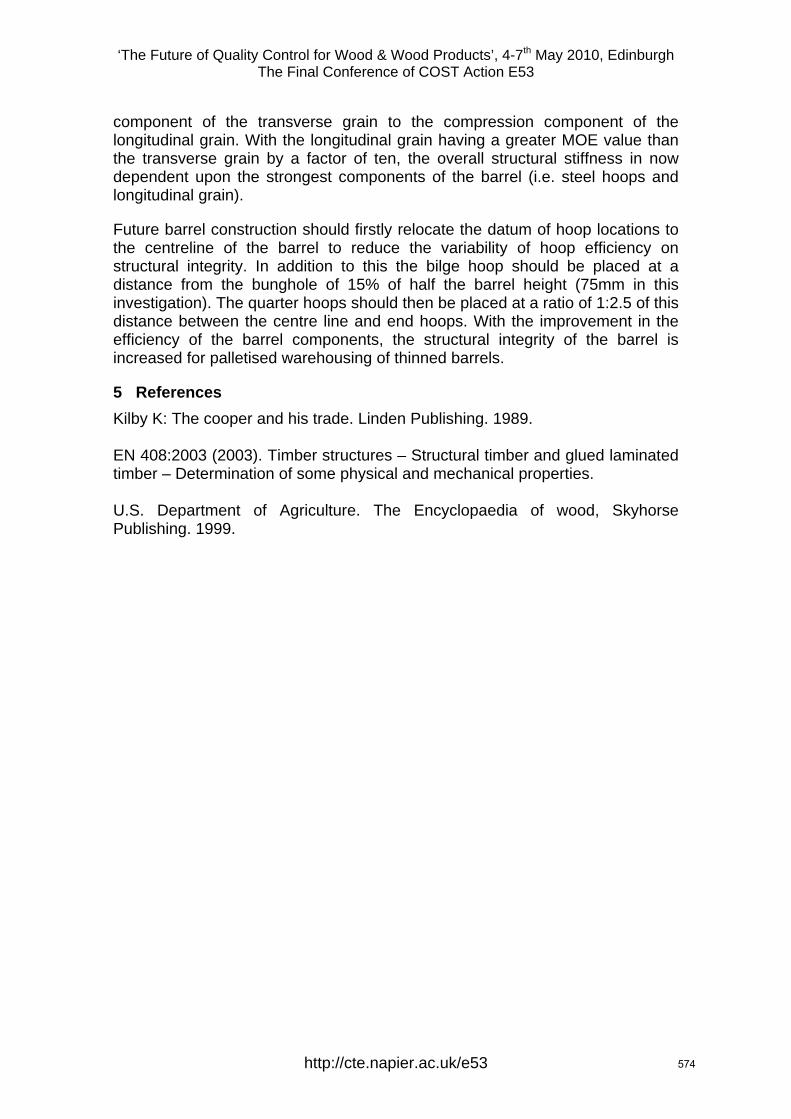
‘The Future of Quality Control for Wood & Wood Products’, 4-7th May 2010, Edinburgh The Final Conference of COST Action E53
component of the transverse grain to the compression component of the longitudinal grain. With the longitudinal grain having a greater MOE value than the transverse grain by a factor of ten, the overall structural stiffness in now dependent upon the strongest components of the barrel (i.e. steel hoops and
a ratio of 1:2.5 of this distance between the centre line and end hoops. With the improvement in the
longitudinal grain).
Future barrel construction should firstly relocate the datum of hoop locations to the centreline of the barrel to reduce the variability of hoop efficiency on structural integrity. In addition to this the bilge hoop should be placed at a distance from the bunghole of 15% of half the barrel height (75mm in this investigation). The quarter hoops should then be placed at
efficiency of the barrel components, the structural integrity of the barrel is increased for palletised warehousing of thinned barrels.
5 References Kilby K: The cooper and his trade. Linden Publishing. 1989. EN 408:2003 (2003). Timber structures – Structural timber and glued laminated timber – Determination of some physical and mechanical properties. U.S. Department of Agriculture. The Encyclopaedia of wood, Skyhorse Publishing. 1999.
http://cte.napier.ac.uk/e53 574

‘The Future of Quality Control for Wood & Wood Products’, 4-7th May 2010, Edinburgh The Final Conference of COST Action E53
Poster papers
http://www.cte.napier.ac.uk/e53/ 575
‘The Future of Quality Control for Wood & Wood Products’, 4-7th May 2010, Edinburgh The Final Conference of COST Action E53
Bark recognition on Robinia pseudoacacia L. logs using computer tomography
M. J. Diaz Baptista1, F. Brüchert2 & U. H. Sauter3
1 Introduction Information on log dimension and its internal wood properties are very important to determine the quality of wood. Computer tomography can support decisions on wood products and the way they should be used as it creates a model of the internal stems properties. A CT.LOG scanner is installed at FVA Baden-Württemberg, which allows such investigations. This project aimed to develop an automated method to detect the boundary between bark and wood in Robinia pseudoacacia L. using in CT reconstructions of cross-sectional slices, in order to calculate the wood dimension under bark for further use of the logs in round shape for construction purposes.
2 Material and methods Seven trees of Robinia pseudoacacia L. were felled and cross-cut into 21 logs of different length. The logs were scanned on a CT.log® tomograph and disc slices reconstructed in 5 mm slices along the log length (Figure 1). Stem diameter under bark was derived from the CT reconstruction using image analysis procedures. Physical reference measurements of stem diameter under bark were carried out on stem discs taken at defined positions in the log to match with the disc slices of the CT scan, and compared to the diameters extracted from the CT.
An individual grey scale threshold value was derived for selected disc slices to mark all pixels representing wood/bark boundary as accurate as possible. This way a preliminary interval of potential threshold values was determined representing grey values between 750 to 850. It was found that using these threshold values, the boundary between wood and bark could be detected in good approximation. In a second step the sensitivity of the threshold values in the identified grey values interval was tested. Four diameters per slice were measured step-wisely increasing the threshold values in the given interval and
1 Scientist, [email protected] Forest Research Institute Baden-Württemberg, Dep. of Forest Utilisation, Freiburg, Germany 2 Senior scientist, [email protected] Forest Research Institute Baden-Württemberg, Dep. of Forest Utilisation, Freiburg, Germany 3 Head of Department, [email protected] Forest Research Institute Baden-Württemberg, Dep. of Forest Utilisation, Freiburg, Germany
http://cte.napier.ac.uk/e53 576
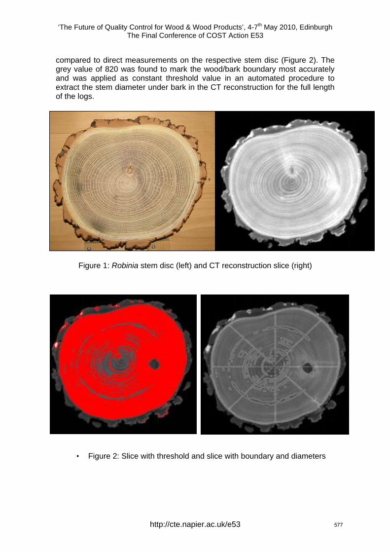
‘The Future of Quality Control for Wood & Wood Products’, 4-7th May 2010, Edinburgh The Final Conference of COST Action E53
compared to direct measurements on the respective stem disc (Figure 2). The grey value of 820 was found to mark the wood/bark boundary most accurately and was applied as constant threshold value in an automated procedure to extract the stem diameter under bark in the CT reconstruction for the full length of the logs.
Figure 1: Robinia stem disc (left) and CT reconstruction slice (right)
• Figure 2: Slice with threshold and slice with boundary and diameters
http://cte.napier.ac.uk/e53 577

‘The Future of Quality Control for Wood & Wood Products’, 4-7th May 2010, Edinburgh The Final Conference of COST Action E53
Validation on an independent set of slices and discs however showed that the diameter of the woody cylinder was systematically overestimated by 0.5 to 1.1 cm. Further refinement of the settings of the threshold value for an automated detection procedure is ongoing.
Key words: Computer tomography, wood/bark boundary, automated detection procedure
http://cte.napier.ac.uk/e53 578
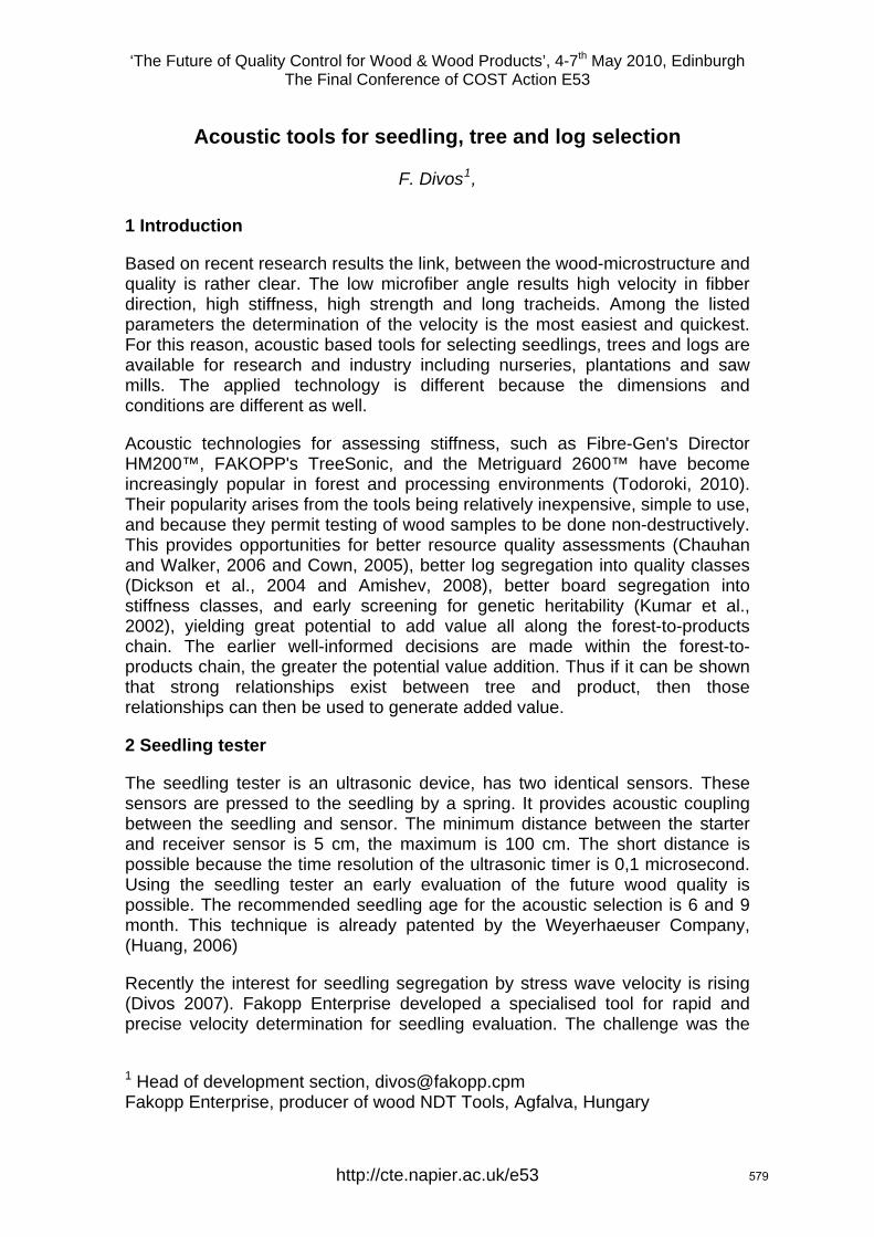
‘The Future of Quality Control for Wood & Wood Products’, 4-7th May 2010, Edinburgh The Final Conference of COST Action E53
Acoustic tools for seedling, tree and log selection
F. Divos1,
1 Introduction
Based on recent research results the link, between the wood-microstructure and quality is rather clear. The low microfiber angle results high velocity in fibber direction, high stiffness, high strength and long tracheids. Among the listed parameters the determination of the velocity is the most easiest and quickest. For this reason, acoustic based tools for selecting seedlings, trees and logs are available for research and industry including nurseries, plantations and saw mills. The applied technology is different because the dimensions and conditions are different as well.
Acoustic technologies for assessing stiffness, such as Fibre-Gen's Director HM200™, FAKOPP's TreeSonic, and the Metriguard 2600™ have become increasingly popular in forest and processing environments (Todoroki, 2010). Their popularity arises from the tools being relatively inexpensive, simple to use, and because they permit testing of wood samples to be done non-destructively. This provides opportunities for better resource quality assessments (Chauhan and Walker, 2006 and Cown, 2005), better log segregation into quality classes (Dickson et al., 2004 and Amishev, 2008), better board segregation into stiffness classes, and early screening for genetic heritability (Kumar et al., 2002), yielding great potential to add value all along the forest-to-products chain. The earlier well-informed decisions are made within the forest-to-products chain, the greater the potential value addition. Thus if it can be shown that strong relationships exist between tree and product, then those relationships can then be used to generate added value.
2 Seedling tester
The seedling tester is an ultrasonic device, has two identical sensors. These sensors are pressed to the seedling by a spring. It provides acoustic coupling between the seedling and sensor. The minimum distance between the starter and receiver sensor is 5 cm, the maximum is 100 cm. The short distance is possible because the time resolution of the ultrasonic timer is 0,1 microsecond. Using the seedling tester an early evaluation of the future wood quality is possible. The recommended seedling age for the acoustic selection is 6 and 9 month. This technique is already patented by the Weyerhaeuser Company, (Huang, 2006)
Recently the interest for seedling segregation by stress wave velocity is rising (Divos 2007). Fakopp Enterprise developed a specialised tool for rapid and precise velocity determination for seedling evaluation. The challenge was the
1 Head of development section, [email protected] Fakopp Enterprise, producer of wood NDT Tools, Agfalva, Hungary
http://cte.napier.ac.uk/e53 579
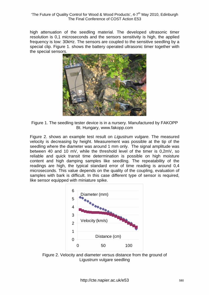
‘The Future of Quality Control for Wood & Wood Products’, 4-7th May 2010, Edinburgh The Final Conference of COST Action E53
high attenuation of the seedling material. The developed ultrasonic timer resolution is 0,1 microseconds and the sensors sensitivity is high, the applied frequency is low: 30kHz. The sensors are coupled to the sensitive seedling by a special clip. Figure 1. shows the battery operated ultrasonic timer together with the special sensors.
Figure 1. The seedling tester device is in a nursery. Manufactured by FAKOPP Bt. Hungary, www.fakopp.com
Figure 2. shows an example test result on Ligustrum vulgare. The measured velocity is decreasing by height. Measurement was possible at the tip of the seedling where the diameter was around 1 mm only. The signal amplitude was between 40 and 10 mV, while the threshold level of the timer is 0,2mV, so reliable and quick transit time determination is possible on high moisture content and high damping samples like seedling. The repeatability of the readings are high, the typical standard error of time reading is around 0,4 microseconds. This value depends on the quality of the coupling, evaluation of samples with bark is difficult. In this case different type of sensor is required, like sensor equipped with miniature spike.
0
1
2
3
4
5
6
0 50 100
Diameter (mm)
Velocity (km/s)
Distance (cm)
Figure 2. Velocity and diameter versus distance from the ground of
Ligustrum vulgare seedling
http://cte.napier.ac.uk/e53 580
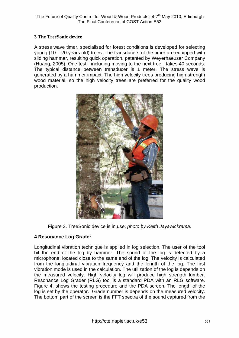
‘The Future of Quality Control for Wood & Wood Products’, 4-7th May 2010, Edinburgh The Final Conference of COST Action E53
3 The TreeSonic device
A stress wave timer, specialised for forest conditions is developed for selecting young (10 – 20 years old) trees. The transducers of the timer are equipped with sliding hammer, resulting quick operation, patented by Weyerhaeuser Company (Huang, 2005). One test - including moving to the next tree - takes 40 seconds. The typical distance between transducer is 1 meter. The stress wave is generated by a hammer impact. The high velocity trees producing high strength wood material, so the high velocity trees are preferred for the quality wood production.
Figure 3. TreeSonic device is in use, photo by Keith Jayawickrama.
4 Resonance Log Grader
Longitudinal vibration technique is applied in log selection. The user of the tool hit the end of the log by hammer. The sound of the log is detected by a microphone, located close to the same end of the log. The velocity is calculated from the longitudinal vibration frequency and the length of the log. The first vibration mode is used in the calculation. The utilization of the log is depends on the measured velocity. High velocity log will produce high strength lumber. Resonance Log Grader (RLG) tool is a standard PDA with an RLG software. Figure 4. shows the testing procedure and the PDA screen. The length of the log is set by the operator. Grade number is depends on the measured velocity. The bottom part of the screen is the FFT spectra of the sound captured from the
http://cte.napier.ac.uk/e53 581
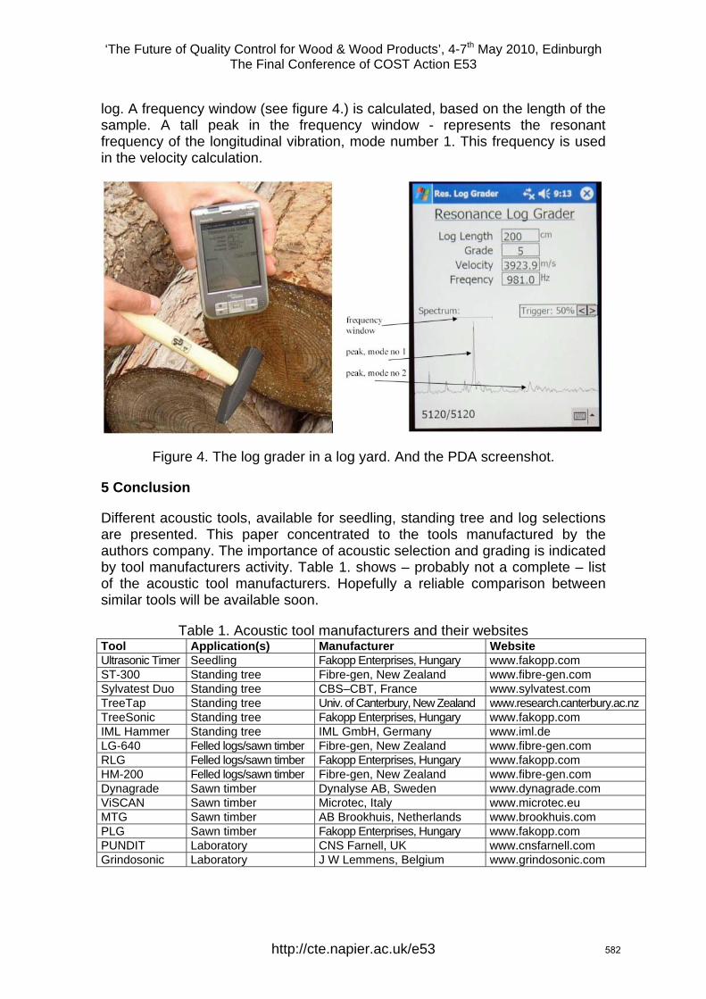
‘The Future of Quality Control for Wood & Wood Products’, 4-7th May 2010, Edinburgh The Final Conference of COST Action E53
log. A frequency window (see figure 4.) is calculated, based on the length of the sample. A tall peak in the frequency window - represents the resonant frequency of the longitudinal vibration, mode number 1. This frequency is used in the velocity calculation.
Figure 4. The log grader in a log yard. And the PDA screenshot.
5 Conclusion
Different acoustic tools, available for seedling, standing tree and log selections are presented. This paper concentrated to the tools manufactured by the authors company. The importance of acoustic selection and grading is indicated by tool manufacturers activity. Table 1. shows – probably not a complete – list of the acoustic tool manufacturers. Hopefully a reliable comparison between similar tools will be available soon.
Table 1. Acoustic tool manufacturers and their websites Tool Application(s) Manufacturer Website Ultrasonic Timer Seedling Fakopp Enterprises, Hungary www.fakopp.com ST-300 Standing tree Fibre-gen, New Zealand www.fibre-gen.com Sylvatest Duo Standing tree CBS–CBT, France www.sylvatest.com TreeTap Standing tree Univ. of Canterbury, New Zealand www.research.canterbury.ac.nz TreeSonic Standing tree Fakopp Enterprises, Hungary www.fakopp.com IML Hammer Standing tree IML GmbH, Germany www.iml.de LG-640 Felled logs/sawn timber Fibre-gen, New Zealand www.fibre-gen.com RLG Felled logs/sawn timber Fakopp Enterprises, Hungary www.fakopp.com HM-200 Felled logs/sawn timber Fibre-gen, New Zealand www.fibre-gen.com Dynagrade Sawn timber Dynalyse AB, Sweden www.dynagrade.com ViSCAN Sawn timber Microtec, Italy www.microtec.eu MTG Sawn timber AB Brookhuis, Netherlands www.brookhuis.com PLG Sawn timber Fakopp Enterprises, Hungary www.fakopp.com PUNDIT Laboratory CNS Farnell, UK www.cnsfarnell.com Grindosonic Laboratory J W Lemmens, Belgium www.grindosonic.com
http://cte.napier.ac.uk/e53 582
‘The Future of Quality Control for Wood & Wood Products’, 4-7th May 2010, Edinburgh The Final Conference of COST Action E53
References Amishev and Murphy, (2008) D. Amishev and G.E. Murphy, In-forest assessment of veneer grade Douglas-fir logs based on acoustic measurement of wood stiffness, For. Prod. J. 58 (11) (2008), pp. 42–47.
Briggs G. D. et al., (2008), Influence of thinning on acoustic velocity of Douglas-fir trees in Western Washington and Western Oregon, Proceedings of the 15th International Symposium on Nondestructive Testing of Wood Duluth, MN, Sept. 10–12, 2007 (2008), pp. 113–123.
Chauhan and Walker, (2006) S.S. Chauhan and J.C.F. Walker, Variations in acoustic velocity and density with age, and their interrelationships in radiata pine, For. Ecol. Manage. 229 (1–3) (2006), pp. 388–394.
Cown, (2005) D. Cown, Understanding and managing wood quality for improving product value in New Zealand, N. Z. J. For. Sci. 35 (2–3) (2005), pp. 205–220.
Dickson et al., (2004) R.L. Dickson, B. Joe, P. Harris, S. Holtorf and C. Wilkinson, Acoustic segregation of Australian-grown Pinus radiata logs for structural board production, Aust. Forestry 67 (4) (2004), pp. 261–266.
Divos F., Divos P., Divos Gy.: (2008) Acoustic Technique ues from Seedling to Wooden Structures, , Proceedings of the 15th International Symposium on Nondestructive Testing of Wood Duluth, MN, Sept. 10–12, 2007 (2008),
Huang, Chih-Lin, Lambeth, Clements C. (2006) Methods for determining potential characteristics of a specimen based on stress wave velocity measurements, United States Patent: 20060288784 Huang, Chih-Lin (2005): System and method for measuring stiffness in standing trees, US patent US6871545 Weyerhaeuser Company,
Kumar et al.,(2002) S. Kumar, K.J.S. Jayawickrama, J. Lee and M. Lausberg, Direct and indirect measures of stiffness and strength show high heritability in a wind-pollinated radiata pine progeny test in New Zealand, Silvae Genet. 51 (5–6) (2002), pp. 256–261.
Todoroki C.L., Lowell E.C., Dykstra D. (2010): Automated knot detection with visual post-processing of Douglas-fir veneer images, Computers and Electronics in Agriculture, Volume 70, Issue 1, January 2010, Pages 163-171
http://cte.napier.ac.uk/e53 583
‘The Future of Quality Control for Wood & Wood Products’, 4-7th May 2010, Edinburgh The Final Conference of COST Action E53
Fracture toughness and shear yield strength determination of steam kiln–dried wood
K.A. Orlowski 1 & M.A. Wierzbowski 2
Abstract Results of fracture toughness (specific work of fracture) and shear yield strength of steam kiln–dried wood simultaneously determined on the basis of cutting power measurement are presented. Wood species, namely oak (Quercus robur L.) and pine (Pinus sylvestris L.) from the northern part of Pomerania region in Poland, were subject of steam kiln–drying process in a laboratory kiln, specially designed and manufactured for the Gdansk University of Technology. While the colour changes have been observed directly after process, changes in mechanical properties have to be measured. The samples, after drying, were subject of examination during cutting tests on the modern narrow-kerf frame sawing machine PRW15M. Measurements of cutting power for steam dried and air dried samples, as a reference, allowed to reveal the effect of wood steam drying on mechanical properties of wood. It has been recognized that steam wood drying causes a decrease of the mechanical properties of the wood such as: fracture toughness and shear yield strength. Those mechanical properties were determined on the basis of the modern fracture mechanics.
1 Introduction In the lumber manufacturing process, drying is one of the most costly consuming operation in terms of energy and time. Reduction of the energy consumption and drying processing time are currently two important objectives of timber industry. Many scientific researches have been done and are still in progress to determine the optimal drying strategy to achieve the required timber quality at minimum cost. Drying in superheated steam is economically justified because of the shorter processing time and reduced energy consumption in comparison to drying in hot air. Evaporation of free water does not change wood shape and main dimensions during process of wood drying. With the loss of water evaporation zone moves deeper into the wood. The proper conduct of the drying process allows faster extraction of water (Gard 1999, Wierzbowski et al. 2009).
The drying process was conducted in the experimental kiln of 0.55 m3 load capacity, especially designed at the GUT (Figure 1a). There are two chimneys at the top to control pressure and environment conditions inside the kiln. The test stand is equipped with a heat exchanger, which is supplied by exhausting gases from a furnace, allowing spread water to evaporate on its surface.
1 Professor, [email protected] Mechanical Engineering Faculty, Gdansk University of Technology, Poland 2 Senior Research Fellow, [email protected] Mechanical Engineering Faculty, Gdansk University of Technology, Poland
http://cte.napier.ac.uk/e53 584
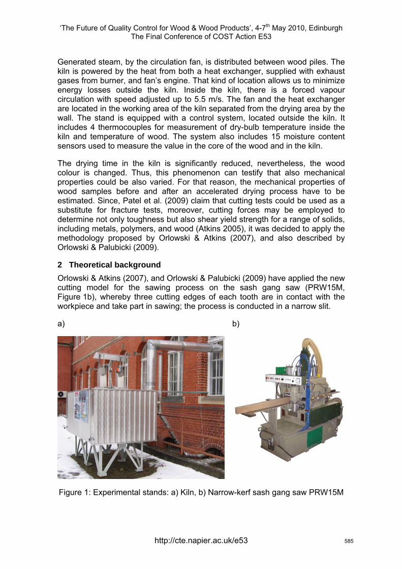
‘The Future of Quality Control for Wood & Wood Products’, 4-7th May 2010, Edinburgh The Final Conference of COST Action E53
Generated steam, by the circulation fan, is distributed between wood piles. The kiln is powered by the heat from both a heat exchanger, supplied with exhaust gases from burner, and fan’s engine. That kind of location allows us to minimize energy losses outside the kiln. Inside the kiln, there is a forced vapour circulation with speed adjusted up to 5.5 m/s. The fan and the heat exchanger are located in the working area of the kiln separated from the drying area by the wall. The stand is equipped with a control system, located outside the kiln. It includes 4 thermocouples for measurement of dry-bulb temperature inside the kiln and temperature of wood. The system also includes 15 moisture content sensors used to measure the value in the core of the wood and in the kiln.
The drying time in the kiln is significantly reduced, nevertheless, the wood colour is changed. Thus, this phenomenon can testify that also mechanical properties could be also varied. For that reason, the mechanical properties of wood samples before and after an accelerated drying process have to be estimated. Since, Patel et al. (2009) claim that cutting tests could be used as a substitute for fracture tests, moreover, cutting forces may be employed to determine not only toughness but also shear yield strength for a range of solids, including metals, polymers, and wood (Atkins 2005), it was decided to apply the methodology proposed by Orlowski & Atkins (2007), and also described by Orlowski & Palubicki (2009).
2 Theoretical background Orlowski & Atkins (2007), and Orlowski & Palubicki (2009) have applied the new cutting model for the sawing process on the sash gang saw (PRW15M, Figure 1b), whereby three cutting edges of each tooth are in contact with the workpiece and take part in sawing; the process is conducted in a narrow slit.
a) b)
Figure 1: Experimental stands: a) Kiln, b) Narrow-kerf sash gang saw PRW15M
http://cte.napier.ac.uk/e53 585
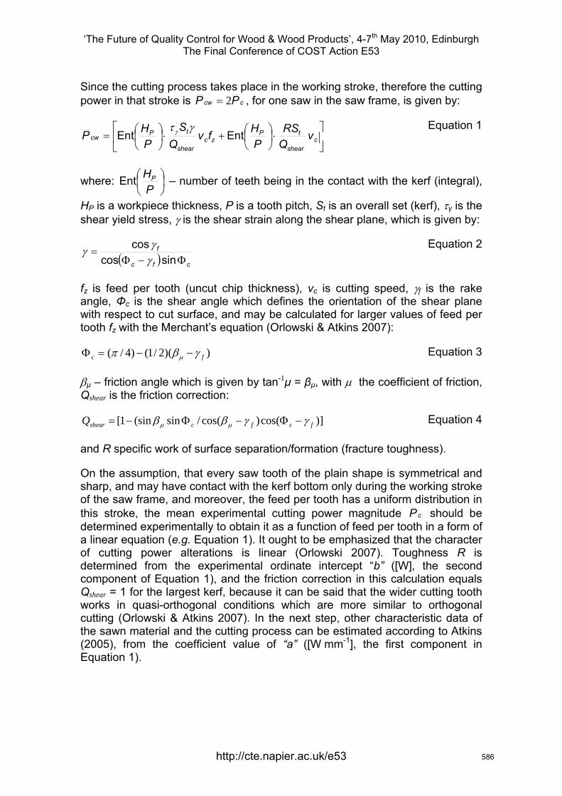
‘The Future of Quality Control for Wood & Wood Products’, 4-7th May 2010, Edinburgh The Final Conference of COST Action E53
Since the cutting process takes place in the working stroke, therefore the cutting power in that stroke is ccw PP 2= , for one saw in the saw frame, is given by:
⎥⎦
⎤⎢⎣
⎡⋅⎟
⎠⎞
⎜⎝⎛+⋅⎟
⎠⎞
⎜⎝⎛= c
shear
tPzc
shear
tPcw v
QRS
PHfv
QS
PHP EntEnt
γτγ Equation 1
where: ⎟⎠⎞
⎜⎝⎛
PHPEnt – number of teeth being in the contact with the kerf (integral),
HP is a workpiece thickness, P is a tooth pitch, St is an overall set (kerf), τγ is the shear yield stress, γ is the shear strain along the shear plane, which is given by:
( ) cfc
f
Φ−Φ=
sincoscos
γγγ Equation 2
fz is feed per tooth (uncut chip thickness), vc is cutting speed, γf is the rake angle, Φc is the shear angle which defines the orientation of the shear plane with respect to cut surface, and may be calculated for larger values of feed per tooth fz with the Merchant’s equation (Orlowski & Atkins 2007):
))(2/1()4/( fc γβπ μ −−=Φ Equation 3
βμ – friction angle which is given by tan-1μ = βμ, with μ the coefficient of friction, Qshear is the friction correction:
)]cos()cos(/sin(sin1[ fcfcshearQ γγββ μμ −Φ−Φ−= Equation 4
and R specific work of surface separation/formation (fracture toughness).
On the assumption, that every saw tooth of the plain shape is symmetrical and sharp, and may have contact with the kerf bottom only during the working stroke of the saw frame, and moreover, the feed per tooth has a uniform distribution in this stroke, the mean experimental cutting power magnitude cP should be determined experimentally to obtain it as a function of feed per tooth in a form of a linear equation (e.g. Equation 1). It ought to be emphasized that the character of cutting power alterations is linear (Orlowski 2007). Toughness R is determined from the experimental ordinate intercept “b” ([W], the second component of Equation 1), and the friction correction in this calculation equals Qshear = 1 for the largest kerf, because it can be said that the wider cutting tooth works in quasi-orthogonal conditions which are more similar to orthogonal cutting (Orlowski & Atkins 2007). In the next step, other characteristic data of the sawn material and the cutting process can be estimated according to Atkins (2005), from the coefficient value of “a” ([W mm-1], the first component in Equation 1).
http://cte.napier.ac.uk/e53 586

‘The Future of Quality Control for Wood & Wood Products’, 4-7th May 2010, Edinburgh The Final Conference of COST Action E53
3 Material and methods Samples were dried in the experimental kiln, in which the drying process consists of three phases. In the first phase wood material temperature was increased up to 95°C with scheduled progress, and water is supplied to the kiln to maintain proper humidity inside the kiln. This phase was not a really drying phase. Temperature was measured and used by the control system to switch to the next phase. In the second phase wood was dried to the final MC. After the drying phase timber was cooled down and conditioned at the programmed temperature. At this temperature MC-sensors can be used to confirm that the final MC was achieved. Those three phases comprised the drying schedule. The duration of those phases depends on the wood species and its thickness. For pine (Pinus sylvestris L.) the third phase was the longest while for oak (Quercus robur L.) the second phase lasted the longest. The oak samples were dried in three different patterns: air, steam with a manual control and steam with an automatic control (Table 1). Pine lumber was dried only with an automatic control in cases of both prisms and boards.
Table 1: Drying patterns, initial and final MC for oak and pine samples
Type of wood and drying pattern
Drying time Initial MC [%]
Final MC in kiln [%]
Final MC before sawing [%]
Comments
Oak / air Appr. 3 months
58 - 9.7
Oak/ system control
4 weeks 58 13 10.2 Water nozzles directed on wood
Oak/ manual control
31 hours 47 7 6.8 Water nozzles directed on exchanger
Pine / air Appr. 2 months
25 - 6.5–9.8
Pine prism / system control
58 hours 24 13 9.5–10.3 Water nozzles directed on exchanger
Pine board / system control
72 hours 25 12 7.2–9.4 Water nozzles directed on exchanger
http://cte.napier.ac.uk/e53 587
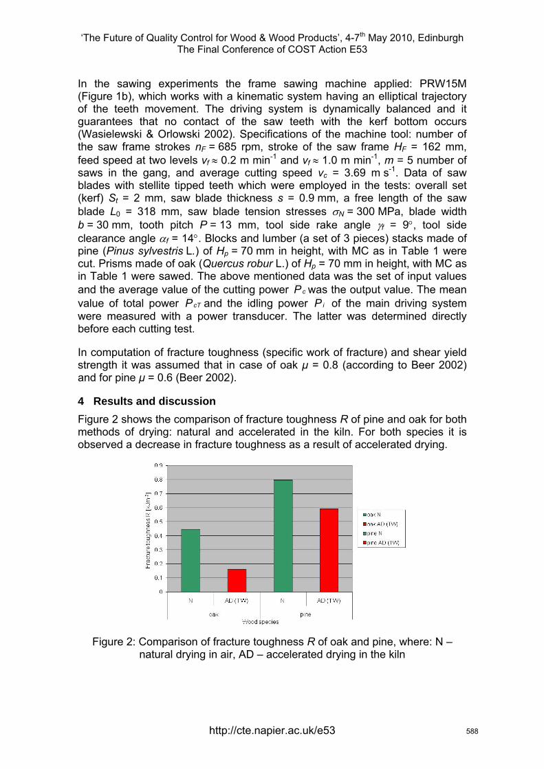
‘The Future of Quality Control for Wood & Wood Products’, 4-7th May 2010, Edinburgh The Final Conference of COST Action E53
In the sawing experiments the frame sawing machine applied: PRW15M (Figure 1b), which works with a kinematic system having an elliptical trajectory of the teeth movement. The driving system is dynamically balanced and it guarantees that no contact of the saw teeth with the kerf bottom occurs (Wasielewski & Orlowski 2002). Specifications of the machine tool: number of the saw frame strokes nF = 685 rpm, stroke of the saw frame HF = 162 mm, feed speed at two levels vf ≈ 0.2 m min-1 and vf ≈ 1.0 m min-1, m = 5 number of saws in the gang, and average cutting speed vc = 3.69 m s-1. Data of saw blades with stellite tipped teeth which were employed in the tests: overall set (kerf) St = 2 mm, saw blade thickness s = 0.9 mm, a free length of the saw blade L0 = 318 mm, saw blade tension stresses σN = 300 MPa, blade width b = 30 mm, tooth pitch P = 13 mm, tool side rake angle γf = 9°, tool side clearance angle αf = 14°. Blocks and lumber (a set of 3 pieces) stacks made of pine (Pinus sylvestris L.) of Hp = 70 mm in height, with MC as in Table 1 were cut. Prisms made of oak (Quercus robur L.) of Hp = 70 mm in height, with MC as in Table 1 were sawed. The above mentioned data was the set of input values and the average value of the cutting power cP was the output value. The mean value of total power cTP and the idling power iP of the main driving system were measured with a power transducer. The latter was determined directly before each cutting test.
In computation of fracture toughness (specific work of fracture) and shear yield strength it was assumed that in case of oak μ = 0.8 (according to Beer 2002) and for pine μ = 0.6 (Beer 2002).
4 Results and discussion Figure 2 shows the comparison of fracture toughness R of pine and oak for both methods of drying: natural and accelerated in the kiln. For both species it is observed a decrease in fracture toughness as a result of accelerated drying.
Figure 2: Comparison of fracture toughness R of oak and pine, where: N – natural drying in air, AD – accelerated drying in the kiln
http://cte.napier.ac.uk/e53 588
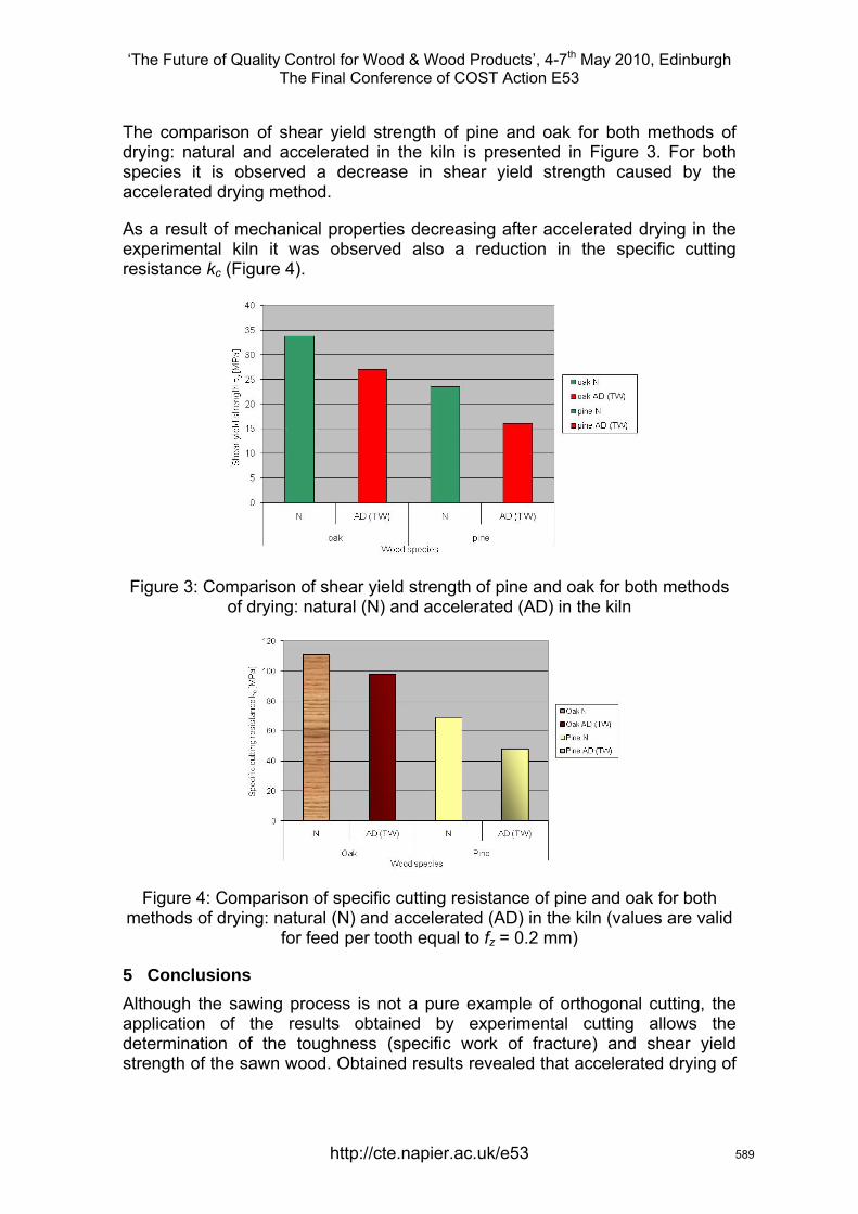
‘The Future of Quality Control for Wood & Wood Products’, 4-7th May 2010, Edinburgh The Final Conference of COST Action E53
The comparison of shear yield strength of pine and oak for both methods of drying: natural and accelerated in the kiln is presented in Figure 3. For both species it is observed a decrease in shear yield strength caused by the accelerated drying method.
As a result of mechanical properties decreasing after accelerated drying in the experimental kiln it was observed also a reduction in the specific cutting resistance kc (Figure 4).
Figure 3: Comparison of shear yield strength of pine and oak for both methods of drying: natural (N) and accelerated (AD) in the kiln
Figure 4: Comparison of specific cutting resistance of pine and oak for both methods of drying: natural (N) and accelerated (AD) in the kiln (values are valid
for feed per tooth equal to fz = 0.2 mm)
5 Conclusions Although the sawing process is not a pure example of orthogonal cutting, the application of the results obtained by experimental cutting allows the determination of the toughness (specific work of fracture) and shear yield strength of the sawn wood. Obtained results revealed that accelerated drying of
http://cte.napier.ac.uk/e53 589

‘The Future of Quality Control for Wood & Wood Products’, 4-7th May 2010, Edinburgh The Final Conference of COST Action E53
pine and oak conducted in the experimental kiln, according to the drying patterns as is shown in Table 1, caused a decrease of wood mechanical properties such as fracture toughness and shear yield strength. Moreover, these phenomena caused also a reduction in the specific cutting resistance. Thus, mechanical properties of wood dried using described schedule may decrease up to 30% of reference value.
cience and Higher Education, grant N512 01232/3058 is kindly acknowledged.
ness and strength”. Engineering Fracture Mechanics, Vol 72, pp 849–860
eszyt Rolniczej im. Augusta Cieszkowskiego w
Poznaniu, Poznan, pp. 108.
shop “State of the art for kiln drying”: Advances in drying of wood, Edinburgh.
e
d ood
olytechniques et Universitaires Romandes, Lausanne. pp 171–174
hile es in Manufacturing Science and
Technology. Vol. 31, No 1, pp 49–63
machining – micromechanics and fracture”. Holzforschung, Vol 63, pp181–185
. IMechE Vol. 223 Part C: J. Mechanical Engineering Science, pp 2861–2869.
balanced saw frame drive”. Holz als Roh- und Werkstoff, Vol 60, pp 202–206.
6 Acknowledgement The financial assistance of Polish Ministry of S
References Atkins, A.G. (2005) “Toughness and cutting: a new way of simultaneously determining ductile fracture tough
Beer, P. (2002) „Obróbka skrawaniem obwodowym drewna nowo opracowanymi narzędziami” (In Polish: Wood peeling with new elaborated tools). Roczniki Akademii Rolniczej w Poznaniu, Rozprawy Naukowe, Z330. Wydawnictwo Akademii
Gard, W.F. (1999) “High temperature drying on industrial scale". 1st Work
Orlowski, K.A. & Atkins, A.(2007) “Determination of the cutting power of thsawing process using both preliminary sawing data and modern fracture mechanics”. In: Proceedings of the Third International Symposium on WooMachining. Fracture Mechanics and Micromechanics of Wood and WComposites with regard to Wood Machining, 21–23 May, Lausanne, Switzerland. Eds. Navi, P., Guidoum, A. Presses P
Orlowski, K. (2007) “Experimental studies on specific cutting resistance wcutting with narrow-kerf saws”. Advanc
Orlowski, K.A. & Pałubicki, B. (2009) “Recent progress in research on thecutting process of wood. A review COST Action E35 2004–2008: Wood
Patel, Y., Blackman, B.R.K. & Williams, J.G. (2009) “Measuring fracture toughness from machining tests”. Proc
Wasielewski, R. & Orlowski, K. (2002) “Hybrid dynamically
http://cte.napier.ac.uk/e53 590

‘The Future of Quality Control for Wood & Wood Products’, 4-7th May 2010, Edinburgh The Final Conference of COST Action E53
http://cte.napier.ac.uk/e53
ucts’’: EDG Drying Seminar ''Improvement of Wood Drying Quality by Conventional and Advanced Drying Techniques'', Bled, Slovenia, April 21-
w d”. Paper accepted for:
ASME-ATI-UIT 2010 Conference on Thermal and Environmental Issues in nergy Systems, 16–19 May, 2010, Sorrento, Italy.
Wierzbowski, M., Barański, J. & Stąsiek, J. (2009) “Gas-steam mixture wood drying”. In proceedings of: COST E53 Meeting ''Quality Control for Wood and Wood Prod
23, 2009.
Wierzbowski, M., Barański, J. & Stąsiek, J. (2010) “Experimental study of flopattern and heat transfer during steam drying of woo
E
591
‘The Future of Quality Control for Wood & Wood Products’, 4-7th May 2010, Edinburgh The Final Conference of COST Action E53
Experimental study and numerical simulation of flow pattern and heat transfer during steam drying wood
J. Barański1, M. A. Wierzbowski2, J. A. Stasiek3
Abstract The high cost of fossil fuel and soaring consumer interest have encouraged people in the wood industry to look for faster and more energy-efficient methods to dry lumber. In this paper results of experimental study and numerical simulation of flow pattern and heat transfer during steam wood drying are presented. Wood species, namely oak (Quercus L.) and pine (Pinus L.), were subject of steam drying process in a laboratory kiln especially arranged for that reason (Wierzbowski et al., 2008). Main focus of those tests was to shorten the time of drying process and afterward to check properties of wood. As results of mechanical properties checking are presented in separate paper, here authors focused on numerical predictions of uniform velocity and temperature profiles through the drying kiln, which is of great importance for drying and also for energy saving. Predicted velocities were used in the laboratory kiln for tests. Satisfactory results were obtained as the time of drying process was significantly reduced. The kiln is equipped with heat exchanger supplied by exhaust gases from furnace allowing spread water to evaporate on its surface. Generated steam, by circulation fan, is distributed between the wood stake. The dryer is for all timber species in terms of final moisture content to 6 % in the high temperature of up to 150oC. Model of drying chamber was created consistent with existing experimental rig. The flow pattern around and through an array of in-line truncated boards of oak and pine have been simulated numerically. The Renormalization Group k-ε turbulence model and model for the near-wall treatments have been used for simulation. Vortex shedding from in-line boards separated by small gaps have also been numerically investigated. Small gaps between in-line boards have an insignificant effect on the mass transfer.
1 Introduction Reduction of energy consumption and drying processing time are currently two important objectives of timber industry, as drying is one of the most costly consuming steps in terms of energy and time. Extensive researches have been done and are still in progress to determine the optimal drying strategy to achieve the required timber quality at minimum cost. However, most of
1 Senior Research Fellow, [email protected] Mechanical Engineering Faculty, Gdansk University of Technology, Poland 2 Senior Research Fellow, [email protected] Mechanical Engineering Faculty, Gdansk University of Technology, Poland 3 Professor, [email protected] Mechanical Engineering Faculty, Gdansk University of Technology, Poland
http://cte.napier.ac.uk/e53 592
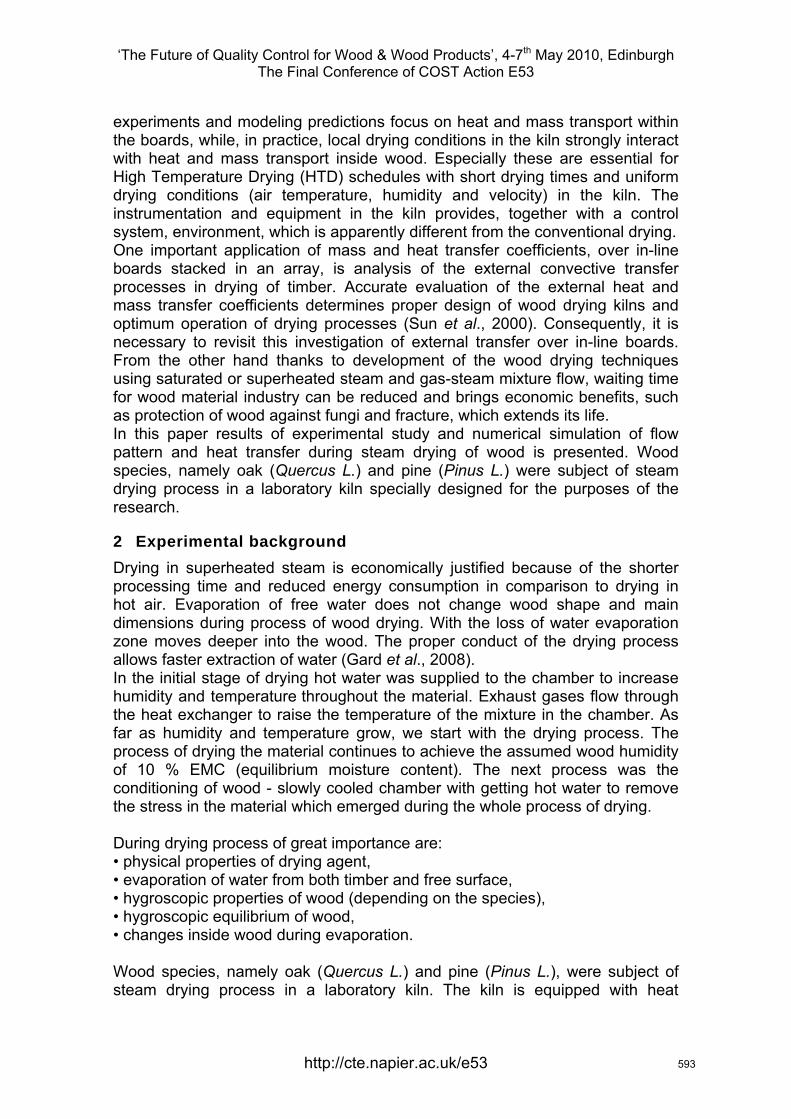
‘The Future of Quality Control for Wood & Wood Products’, 4-7th May 2010, Edinburgh The Final Conference of COST Action E53
experiments and modeling predictions focus on heat and mass transport within the boards, while, in practice, local drying conditions in the kiln strongly interact with heat and mass transport inside wood. Especially these are essential for High Temperature Drying (HTD) schedules with short drying times and uniform drying conditions (air temperature, humidity and velocity) in the kiln. The instrumentation and equipment in the kiln provides, together with a control system, environment, which is apparently different from the conventional drying. One important application of mass and heat transfer coefficients, over in-line boards stacked in an array, is analysis of the external convective transfer processes in drying of timber. Accurate evaluation of the external heat and mass transfer coefficients determines proper design of wood drying kilns and optimum operation of drying processes (Sun et al., 2000). Consequently, it is necessary to revisit this investigation of external transfer over in-line boards. From the other hand thanks to development of the wood drying techniques using saturated or superheated steam and gas-steam mixture flow, waiting time for wood material industry can be reduced and brings economic benefits, such as protection of wood against fungi and fracture, which extends its life. In this paper results of experimental study and numerical simulation of flow pattern and heat transfer during steam drying of wood is presented. Wood species, namely oak (Quercus L.) and pine (Pinus L.) were subject of steam drying process in a laboratory kiln specially designed for the purposes of the research.
2 Experimental background Drying in superheated steam is economically justified because of the shorter processing time and reduced energy consumption in comparison to drying in hot air. Evaporation of free water does not change wood shape and main dimensions during process of wood drying. With the loss of water evaporation zone moves deeper into the wood. The proper conduct of the drying process allows faster extraction of water (Gard et al., 2008). In the initial stage of drying hot water was supplied to the chamber to increase humidity and temperature throughout the material. Exhaust gases flow through the heat exchanger to raise the temperature of the mixture in the chamber. As far as humidity and temperature grow, we start with the drying process. The process of drying the material continues to achieve the assumed wood humidity of 10 % EMC (equilibrium moisture content). The next process was the conditioning of wood - slowly cooled chamber with getting hot water to remove the stress in the material which emerged during the whole process of drying. During drying process of great importance are: • physical properties of drying agent, • evaporation of water from both timber and free surface, • hygroscopic properties of wood (depending on the species), • hygroscopic equilibrium of wood, • changes inside wood during evaporation. Wood species, namely oak (Quercus L.) and pine (Pinus L.), were subject of steam drying process in a laboratory kiln. The kiln is equipped with heat
http://cte.napier.ac.uk/e53 593
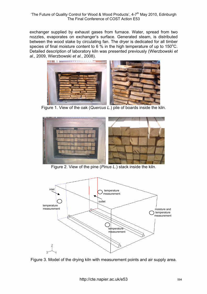
‘The Future of Quality Control for Wood & Wood Products’, 4-7th May 2010, Edinburgh The Final Conference of COST Action E53
exchanger supplied by exhaust gases from furnace. Water, spread from two nozzles, evaporates on exchanger’s surface. Generated steam, is distributed between the wood stake by circulating fan. The dryer is dedicated for all timber species of final moisture content to 6 % in the high temperature of up to 150oC. Detailed description of laboratory kiln was presented previously (Wierzbowski et al., 2009, Wierzbowski et al., 2008).
Figure 1. View of the oak (Quercus L.) pile of boards inside the kiln.
Figure 2. View of the pine (Pinus L.) stack inside the kiln.
inlet temperature measurement
outlettemperature measurement moisture and
temperature measurement
temperature measurement
Figure 3. Model of the drying kiln with measurement points and air supply area.
http://cte.napier.ac.uk/e53 594
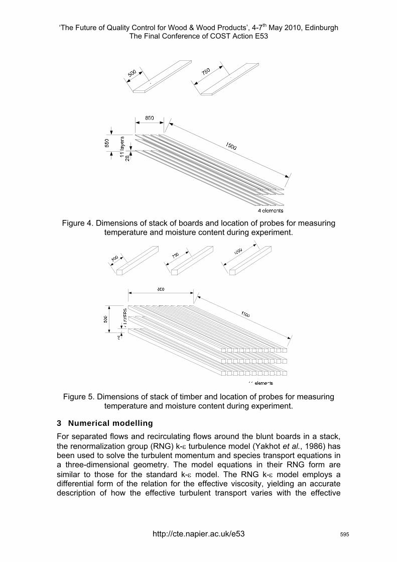
‘The Future of Quality Control for Wood & Wood Products’, 4-7th May 2010, Edinburgh The Final Conference of COST Action E53
Figure 4. Dimensions of stack of boards and location of probes for measuring temperature and moisture content during experiment.
Figure 5. Dimensions of stack of timber and location of probes for measuring
temperature and moisture content during experiment.
3 Numerical modelling For separated flows and recirculating flows around the blunt boards in a stack, the renormalization group (RNG) k-ε turbulence model (Yakhot et al., 1986) has been used to solve the turbulent momentum and species transport equations in a three-dimensional geometry. The model equations in their RNG form are similar to those for the standard k-ε model. The RNG k-ε model employs a differential form of the relation for the effective viscosity, yielding an accurate description of how the effective turbulent transport varies with the effective
http://cte.napier.ac.uk/e53 595
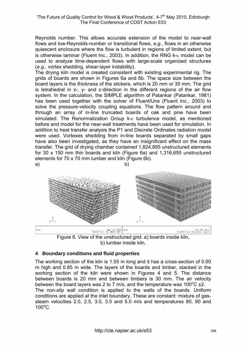
‘The Future of Quality Control for Wood & Wood Products’, 4-7th May 2010, Edinburgh The Final Conference of COST Action E53
Reynolds number. This allows accurate extension of the model to near-wall flows and low-Reynolds-number or transitional flows, e.g., flows in an otherwise quiescent enclosure where the flow is turbulent in regions of limited extent, but is otherwise laminar (Fluent Inc., 2003). In addition, the RNG k-ε model can be used to analyze time-dependent flows with large-scale organized structures (e.g., vortex shedding, shear-layer instability). The drying kiln model is created consistent with existing experimental rig. The grids of boards are shown in Figures 6a and 6b. The space size between the board layers is the thickness of the stickers, which is 20 mm or 30 mm. The grid is tetrahedral in x-, y- and z-direction in the different regions of the air flow system. In the calculation, the SIMPLE algorithm of Patankar (Patankar, 1981) has been used together with the solver of Fluent/Uns (Fluent Inc., 2003) to solve the pressure-velocity coupling equations. The flow pattern around and through an array of in-line truncated boards of oak and pine have been simulated. The Renormalization Group k-ε turbulence model, as mentioned before and model for the near-wall treatments have been used for simulation. In addition to heat transfer analysis the P1 and Discrete Ordinates radiation model were used. Vortexes shedding from in-line boards separated by small gaps have also been investigated, as they have an insignificant effect on the mass transfer. The grid of drying chamber contained 1,824,895 unstructured elements for 30 x 150 mm thin boards and kiln (Figure 6a) and 1,316,655 unstructured elements for 70 x 70 mm lumber and kiln (Figure 6b). a) b)
Figure 6. View of the unstructured grid: a) boards inside kiln,
b) lumber inside kiln.
4 Boundary conditions and fluid properties The working section of the kiln is 1.55 m long and it has a cross-section of 0.60 m high and 0.85 m wide. The layers of the boards and timber, stacked in the working section of the kiln were shown in Figures 4 and 5. The distance between boards is 20 mm and between timbers is 30 mm. The air velocity between the board layers was 2 to 7 m/s, and the temperature was 100oC ±2. The non-slip wall condition is applied to the walls of the boards. Uniform conditions are applied at the inlet boundary. These are constant: mixture of gas-steam velocities 2.0, 2.5, 3.0, 3.5 and 5.0 m/s and temperatures 80, 90 and 100oC.
http://cte.napier.ac.uk/e53 596
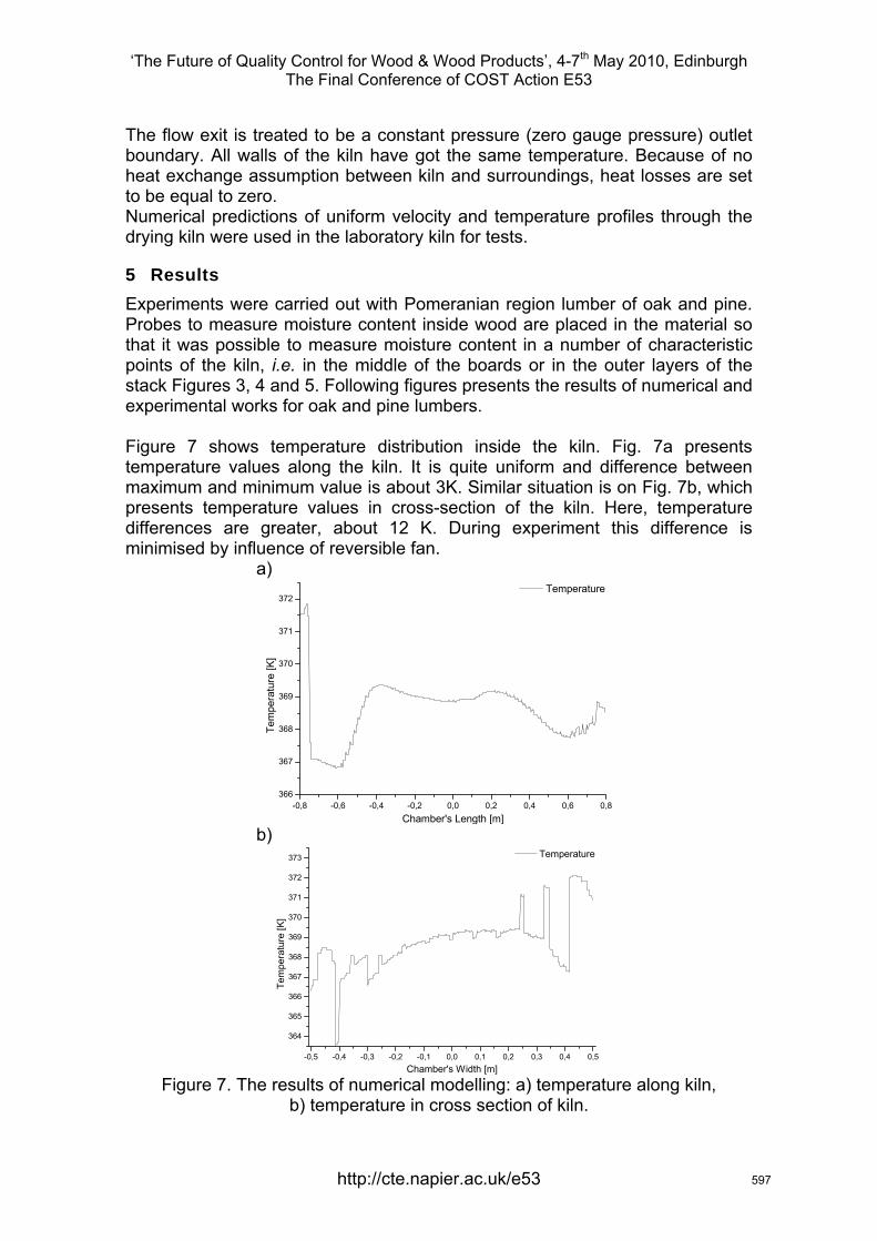
‘The Future of Quality Control for Wood & Wood Products’, 4-7th May 2010, Edinburgh The Final Conference of COST Action E53
The flow exit is treated to be a constant pressure (zero gauge pressure) outlet boundary. All walls of the kiln have got the same temperature. Because of no heat exchange assumption between kiln and surroundings, heat losses are set to be equal to zero. Numerical predictions of uniform velocity and temperature profiles through the drying kiln were used in the laboratory kiln for tests.
5 Results Experiments were carried out with Pomeranian region lumber of oak and pine. Probes to measure moisture content inside wood are placed in the material so that it was possible to measure moisture content in a number of characteristic points of the kiln, i.e. in the middle of the boards or in the outer layers of the stack Figures 3, 4 and 5. Following figures presents the results of numerical and experimental works for oak and pine lumbers. Figure 7 shows temperature distribution inside the kiln. Fig. 7a presents temperature values along the kiln. It is quite uniform and difference between maximum and minimum value is about 3K. Similar situation is on Fig. 7b, which presents temperature values in cross-section of the kiln. Here, temperature differences are greater, about 12 K. During experiment this difference is minimised by influence of reversible fan. a)
-0,8 -0,6 -0,4 -0,2 0,0 0,2 0,4 0,6 0,8366
367
368
369
370
371
372
Tem
pera
ture
[K]
Chamber's Length [m]
Temperature
b)
-0,5 -0,4 -0,3 -0,2 -0,1 0,0 0,1 0,2 0,3 0,4 0,5
364
365
366
367
368
369
370
371
372
373
Tem
pera
ture
[K]
Chamber's Width [m]
Temperature
Figure 7. The results of numerical modelling: a) temperature along kiln,
b) temperature in cross section of kiln.
http://cte.napier.ac.uk/e53 597
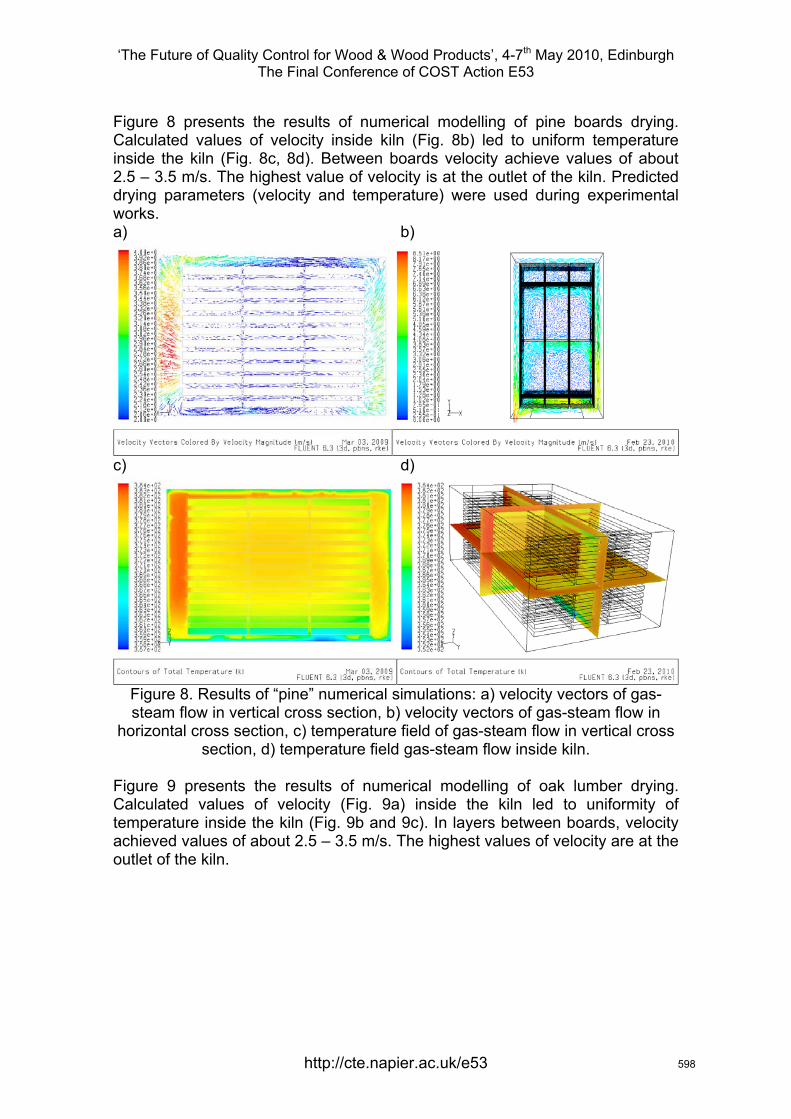
‘The Future of Quality Control for Wood & Wood Products’, 4-7th May 2010, Edinburgh The Final Conference of COST Action E53
Figure 8 presents the results of numerical modelling of pine boards drying. Calculated values of velocity inside kiln (Fig. 8b) led to uniform temperature inside the kiln (Fig. 8c, 8d). Between boards velocity achieve values of about 2.5 – 3.5 m/s. The highest value of velocity is at the outlet of the kiln. Predicted drying parameters (velocity and temperature) were used during experimental works. a) b)
c) d)
Figure 8. Results of “pine” numerical simulations: a) velocity vectors of gas-steam flow in vertical cross section, b) velocity vectors of gas-steam flow in
horizontal cross section, c) temperature field of gas-steam flow in vertical cross section, d) temperature field gas-steam flow inside kiln.
Figure 9 presents the results of numerical modelling of oak lumber drying. Calculated values of velocity (Fig. 9a) inside the kiln led to uniformity of temperature inside the kiln (Fig. 9b and 9c). In layers between boards, velocity achieved values of about 2.5 – 3.5 m/s. The highest values of velocity are at the outlet of the kiln.
http://cte.napier.ac.uk/e53 598
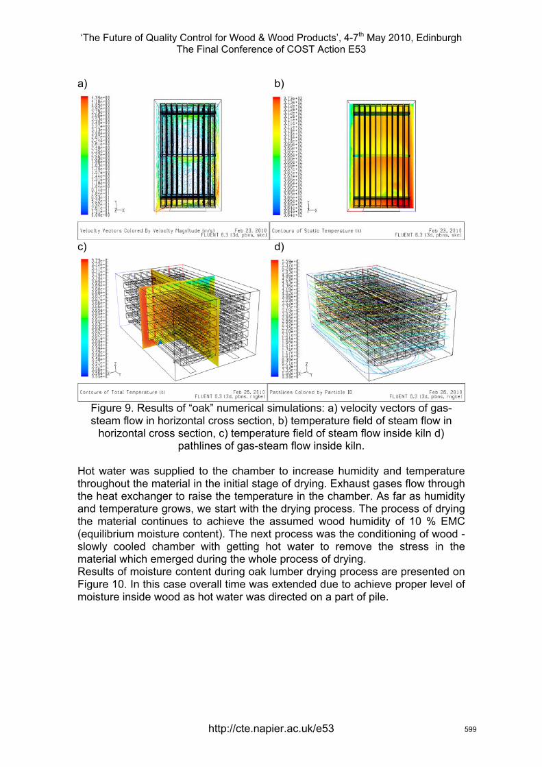
‘The Future of Quality Control for Wood & Wood Products’, 4-7th May 2010, Edinburgh The Final Conference of COST Action E53
a) b)
c) d)
Figure 9. Results of “oak” numerical simulations: a) velocity vectors of gas-steam flow in horizontal cross section, b) temperature field of steam flow in
horizontal cross section, c) temperature field of steam flow inside kiln d) pathlines of gas-steam flow inside kiln.
Hot water was supplied to the chamber to increase humidity and temperature throughout the material in the initial stage of drying. Exhaust gases flow through the heat exchanger to raise the temperature in the chamber. As far as humidity and temperature grows, we start with the drying process. The process of drying the material continues to achieve the assumed wood humidity of 10 % EMC (equilibrium moisture content). The next process was the conditioning of wood - slowly cooled chamber with getting hot water to remove the stress in the material which emerged during the whole process of drying. Results of moisture content during oak lumber drying process are presented on Figure 10. In this case overall time was extended due to achieve proper level of moisture inside wood as hot water was directed on a part of pile.
http://cte.napier.ac.uk/e53 599
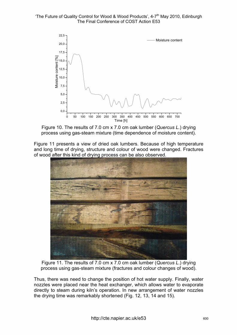
‘The Future of Quality Control for Wood & Wood Products’, 4-7th May 2010, Edinburgh The Final Conference of COST Action E53
0 50 100 150 200 250 300 350 400 450 500 550 600 650 700
0,0
2,5
5,0
7,5
10,0
12,5
15,0
17,5
20,0
22,5
Moi
stur
e co
nten
t [%
]
Time [h]
Moisture content
Figure 10. The results of 7.0 cm x 7.0 cm oak lumber (Quercus L.) drying process using gas-steam mixture (time dependence of moisture content).
Figure 11 presents a view of dried oak lumbers. Because of high temperature and long time of drying, structure and colour of wood were changed. Fractures of wood after this kind of drying process can be also observed.
Figure 11. The results of 7.0 cm x 7.0 cm oak lumber (Quercus L.) drying process using gas-steam mixture (fractures and colour changes of wood).
Thus, there was need to change the position of hot water supply. Finally, water nozzles were placed near the heat exchanger, which allows water to evaporate directly to steam during kiln’s operation. In new arrangement of water nozzles the drying time was remarkably shortened (Fig. 12, 13, 14 and 15).
http://cte.napier.ac.uk/e53 600
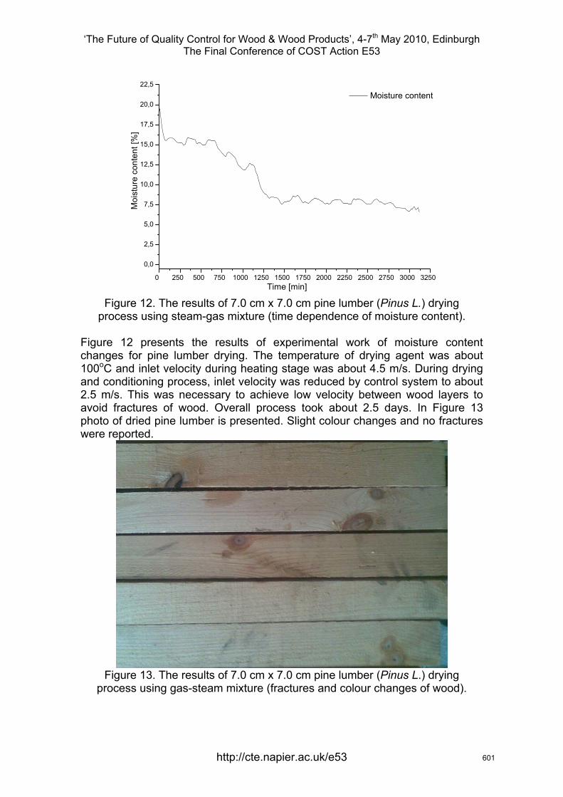
‘The Future of Quality Control for Wood & Wood Products’, 4-7th May 2010, Edinburgh The Final Conference of COST Action E53
0 250 500 750 1000 1250 1500 1750 2000 2250 2500 2750 3000 3250
0,0
2,5
5,0
7,5
10,0
12,5
15,0
17,5
20,0
22,5
Moi
stur
e co
nten
t [%
]
Time [min]
Moisture content
Figure 12. The results of 7.0 cm x 7.0 cm pine lumber (Pinus L.) drying
process using steam-gas mixture (time dependence of moisture content). Figure 12 presents the results of experimental work of moisture content changes for pine lumber drying. The temperature of drying agent was about 100oC and inlet velocity during heating stage was about 4.5 m/s. During drying and conditioning process, inlet velocity was reduced by control system to about 2.5 m/s. This was necessary to achieve low velocity between wood layers to avoid fractures of wood. Overall process took about 2.5 days. In Figure 13 photo of dried pine lumber is presented. Slight colour changes and no fractures were reported.
Figure 13. The results of 7.0 cm x 7.0 cm pine lumber (Pinus L.) drying
process using gas-steam mixture (fractures and colour changes of wood).
http://cte.napier.ac.uk/e53 601
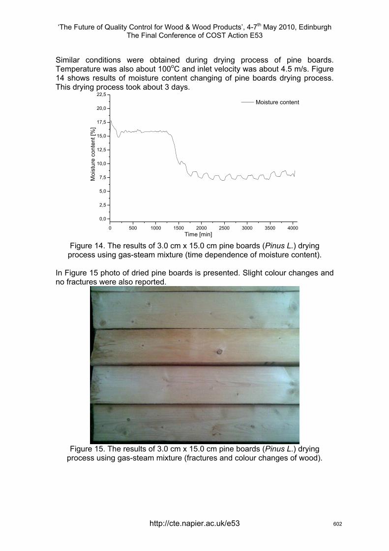
‘The Future of Quality Control for Wood & Wood Products’, 4-7th May 2010, Edinburgh The Final Conference of COST Action E53
Similar conditions were obtained during drying process of pine boards. Temperature was also about 100oC and inlet velocity was about 4.5 m/s. Figure 14 shows results of moisture content changing of pine boards drying process. This drying process took about 3 days.
0 500 1000 1500 2000 2500 3000 3500 4000
0,0
2,5
5,0
7,5
10,0
12,5
15,0
17,5
20,0
22,5M
oist
ure
cont
ent [
%]
Time [min]
Moisture content
Figure 14. The results of 3.0 cm x 15.0 cm pine boards (Pinus L.) drying process using gas-steam mixture (time dependence of moisture content).
In Figure 15 photo of dried pine boards is presented. Slight colour changes and no fractures were also reported.
Figure 15. The results of 3.0 cm x 15.0 cm pine boards (Pinus L.) drying
process using gas-steam mixture (fractures and colour changes of wood).
http://cte.napier.ac.uk/e53 602
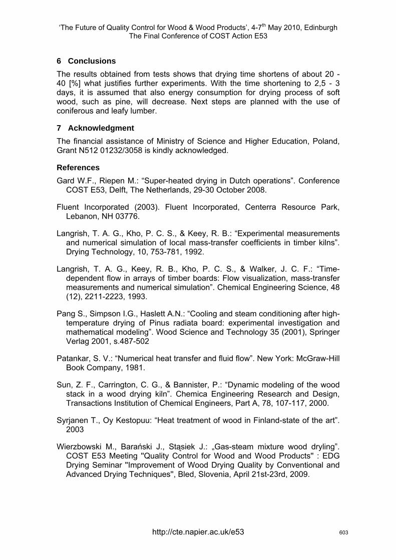
‘The Future of Quality Control for Wood & Wood Products’, 4-7th May 2010, Edinburgh The Final Conference of COST Action E53
6 Conclusions The results obtained from tests shows that drying time shortens of about 20 - 40 [%] what justifies further experiments. With the time shortening to 2,5 - 3 days, it is assumed that also energy consumption for drying process of soft wood, such as pine, will decrease. Next steps are planned with the use of coniferous and leafy lumber.
7 Acknowledgment The financial assistance of Ministry of Science and Higher Education, Poland, Grant N512 01232/3058 is kindly acknowledged.
References Gard W.F., Riepen M.: “Super-heated drying in Dutch operations”. Conference
COST E53, Delft, The Netherlands, 29-30 October 2008.
Fluent Incorporated (2003). Fluent Incorporated, Centerra Resource Park, Lebanon, NH 03776.
Langrish, T. A. G., Kho, P. C. S., & Keey, R. B.: “Experimental measurements and numerical simulation of local mass-transfer coefficients in timber kilns”. Drying Technology, 10, 753-781, 1992.
Langrish, T. A. G., Keey, R. B., Kho, P. C. S., & Walker, J. C. F.: “Time-dependent flow in arrays of timber boards: Flow visualization, mass-transfer measurements and numerical simulation”. Chemical Engineering Science, 48 (12), 2211-2223, 1993.
Pang S., Simpson I.G., Haslett A.N.: “Cooling and steam conditioning after high-temperature drying of Pinus radiata board: experimental investigation and mathematical modeling”. Wood Science and Technology 35 (2001), Springer Verlag 2001, s.487-502
Patankar, S. V.: “Numerical heat transfer and fluid flow”. New York: McGraw-Hill Book Company, 1981.
Sun, Z. F., Carrington, C. G., & Bannister, P.: “Dynamic modeling of the wood stack in a wood drying kiln”. Chemica Engineering Research and Design, Transactions Institution of Chemical Engineers, Part A, 78, 107-117, 2000.
Syrjanen T., Oy Kestopuu: “Heat treatment of wood in Finland-state of the art”. 2003
Wierzbowski M., Barański J., Stąsiek J.: „Gas-steam mixture wood dryling”. COST E53 Meeting ''Quality Control for Wood and Wood Products'' : EDG Drying Seminar ''Improvement of Wood Drying Quality by Conventional and Advanced Drying Techniques'', Bled, Slovenia, April 21st-23rd, 2009.
http://cte.napier.ac.uk/e53 603

‘The Future of Quality Control for Wood & Wood Products’, 4-7th May 2010, Edinburgh The Final Conference of COST Action E53
Wierzbowski M., Barański J., Stąsiek J.: „Suszenie drewna mieszaniną parowo-gazową”. Termodynamika w nauce i gospodarce. Wrocław, 2008 (in polish).
Yakhot, V., & Orszag, S. A.: “Renormalization group analysis of turbulence”. Basic theory. Journal of Scientific Computing, 1, 1-51, 1986.
http://cte.napier.ac.uk/e53 604
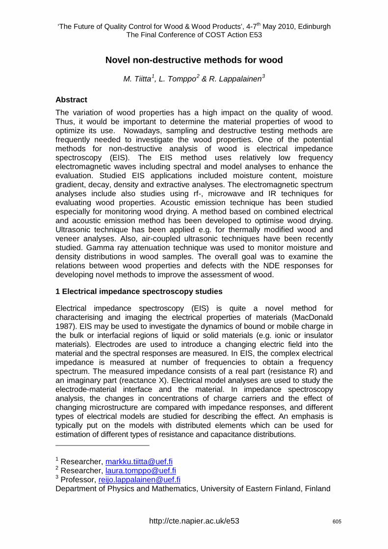
‘The Future of Quality Control for Wood & Wood Products’, 4-7th May 2010, Edinburgh The Final Conference of COST Action E53
http://cte.napier.ac.uk/e53
Novel non-destructive methods for wood
M. Tiitta1, L. Tomppo2 & R. Lappalainen3
Abstract
The variation of wood properties has a high impact on the quality of wood. Thus, it would be important to determine the material properties of wood to optimize its use. Nowadays, sampling and destructive testing methods are frequently needed to investigate the wood properties. One of the potential methods for non-destructive analysis of wood is electrical impedance spectroscopy (EIS). The EIS method uses relatively low frequency electromagnetic waves including spectral and model analyses to enhance the evaluation. Studied EIS applications included moisture content, moisture gradient, decay, density and extractive analyses. The electromagnetic spectrum analyses include also studies using rf-, microwave and IR techniques for evaluating wood properties. Acoustic emission technique has been studied especially for monitoring wood drying. A method based on combined electrical and acoustic emission method has been developed to optimise wood drying. Ultrasonic technique has been applied e.g. for thermally modified wood and veneer analyses. Also, air-coupled ultrasonic techniques have been recently studied. Gamma ray attenuation technique was used to monitor moisture and density distributions in wood samples. The overall goal was to examine the relations between wood properties and defects with the NDE responses for developing novel methods to improve the assessment of wood.
1 Electrical impedance spectroscopy studies
Electrical impedance spectroscopy (EIS) is quite a novel method for characterising and imaging the electrical properties of materials (MacDonald 1987). EIS may be used to investigate the dynamics of bound or mobile charge in the bulk or interfacial regions of liquid or solid materials (e.g. ionic or insulator materials). Electrodes are used to introduce a changing electric field into the material and the spectral responses are measured. In EIS, the complex electrical impedance is measured at number of frequencies to obtain a frequency spectrum. The measured impedance consists of a real part (resistance R) and an imaginary part (reactance X). Electrical model analyses are used to study the electrode-material interface and the material. In impedance spectroscopy analysis, the changes in concentrations of charge carriers and the effect of changing microstructure are compared with impedance responses, and different types of electrical models are studied for describing the effect. An emphasis is typically put on the models with distributed elements which can be used for estimation of different types of resistance and capacitance distributions.
1 Researcher, [email protected] 2 Researcher, [email protected] 3 Professor, [email protected] Department of Physics and Mathematics, University of Eastern Finland, Finland
605
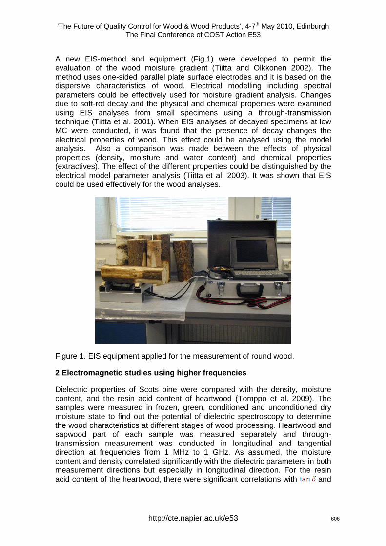
‘The Future of Quality Control for Wood & Wood Products’, 4-7th May 2010, Edinburgh The Final Conference of COST Action E53
http://cte.napier.ac.uk/e53
A new EIS-method and equipment (Fig.1) were developed to permit the evaluation of the wood moisture gradient (Tiitta and Olkkonen 2002). The method uses one-sided parallel plate surface electrodes and it is based on the dispersive characteristics of wood. Electrical modelling including spectral parameters could be effectively used for moisture gradient analysis. Changes due to soft-rot decay and the physical and chemical properties were examined using EIS analyses from small specimens using a through-transmission technique (Tiitta et al. 2001). When EIS analyses of decayed specimens at low MC were conducted, it was found that the presence of decay changes the electrical properties of wood. This effect could be analysed using the model analysis. Also a comparison was made between the effects of physical properties (density, moisture and water content) and chemical properties (extractives). The effect of the different properties could be distinguished by the electrical model parameter analysis (Tiitta et al. 2003). It was shown that EIS could be used effectively for the wood analyses.
Figure 1. EIS equipment applied for the measurement of round wood.
2 Electromagnetic studies using higher frequencies
Dielectric properties of Scots pine were compared with the density, moisture content, and the resin acid content of heartwood (Tomppo et al. 2009). The samples were measured in frozen, green, conditioned and unconditioned dry moisture state to find out the potential of dielectric spectroscopy to determine the wood characteristics at different stages of wood processing. Heartwood and sapwood part of each sample was measured separately and through-transmission measurement was conducted in longitudinal and tangential direction at frequencies from 1 MHz to 1 GHz. As assumed, the moisture content and density correlated significantly with the dielectric parameters in both measurement directions but especially in longitudinal direction. For the resin acid content of the heartwood, there were significant correlations with and
606

‘The Future of Quality Control for Wood & Wood Products’, 4-7th May 2010, Edinburgh The Final Conference of COST Action E53
http://cte.napier.ac.uk/e53
of the green samples measured in tangential direction at frequencies above 200 MHz.
3 Combined Acoustic emission and EIS technique Acoustic emission (AE) is defined as the spontaneous release of localized strain energy in a stressed material (Beall 2002). AE can be sensed with piezoelectric transducers coupled physically to the surface of the material and the method is useful especially for the investigation of local damage in materials. Wave pattern recognition analyses have been widely used in AE. With the AE method, cracking of wood can be measured quantitatively even before any visible macro-cracks appear in the wood (Beall 2002, Tiitta et al. 2007). The emissions generated by the cracks are proportional to the stresses appearing inside the wood. The combined method is based on using electrical method for moisture gradient monitoring and acoustic emission method for detection of micro-cracking. In the method, electrodes are used to create electric field in drying wood and measure the electric complex spectrum using the impedance spectroscopy method while at the same time measuring acoustic emissions from drying wood. When the electric complex spectrum and acoustic emission response are determined, it is possible to estimate both the main reason for the stresses (moisture gradient) and the outcome (micro- and macro-cracking). Thus the results may be used to control drying in order to achieve wood products of high quality. Combination of the EIS and AE techniques allowed us to develop more comprehensive solutions to monitor and control wood quality during drying (Tiitta et al. 2007). These techniques were used first in laboratory tests and then in industrial wood drying kiln (Fig.2). The first prototype included two measurement channels for both AE and impedance. Temperature and four channels for MC measurement using electrical resistance pin electrodes were also included for reference MG measurements. Cooled instrumentation box was installed inside an industrial kiln for the tests. AE sensors and impedance electrodes were attached between the lumber boards on the upper surface. Labview based program was used for the measurements. Significant correlations between moisture gradient and impedance responses were found when using resistance pin electrodes for reference technique to evaluate moisture gradient during the drying process. For individual dryings, the correlation between impedance response and moisture gradient was typically about 0.9. The overall correlation between impedance response and moisture gradient was 0.8 when all successful measurements were analyzed with the same method. The inaccuracy of the reference method affected the results. The relation between AE responses and cracking was evident: correlation between surface cracking and AE count number was 0.81 when all successful measurements were included.
607
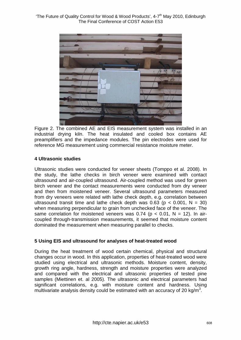
‘The Future of Quality Control for Wood & Wood Products’, 4-7th May 2010, Edinburgh The Final Conference of COST Action E53
http://cte.napier.ac.uk/e53
Figure 2. The combined AE and EIS measurement system was installed in an industrial drying kiln. The heat insulated and cooled box contains AE preamplifiers and the impedance modules. The pin electrodes were used for reference MG measurement using commercial resistance moisture meter. 4 Ultrasonic studies
Ultrasonic studies were conducted for veneer sheets (Tomppo et al. 2008). In the study, the lathe checks in birch veneer were examined with contact ultrasound and air-coupled ultrasound. Air-coupled method was used for green birch veneer and the contact measurements were conducted from dry veneer and then from moistened veneer. Several ultrasound parameters measured from dry veneers were related with lathe check depth, e.g. correlation between ultrasound transit time and lathe check depth was 0.63 (p < 0.001, N = 30) when measuring perpendicular to grain from unchecked face of the veneer. The same correlation for moistened veneers was 0.74 (p < 0.01, N = 12). In air-coupled through-transmission measurements, it seemed that moisture content dominated the measurement when measuring parallel to checks.
5 Using EIS and ultrasound for analyses of heat-treated wood
During the heat treatment of wood certain chemical, physical and structural changes occur in wood. In this application, properties of heat-treated wood were studied using electrical and ultrasonic methods. Moisture content, density, growth ring angle, hardness, strength and moisture properties were analyzed and compared with the electrical and ultrasonic properties of tested pine samples (Miettinen et. al 2005). The ultrasonic and electrical parameters had significant correlations, e.g. with moisture content and hardness. Using multivariate analysis density could be estimated with an accuracy of 20 kg/m3.
608
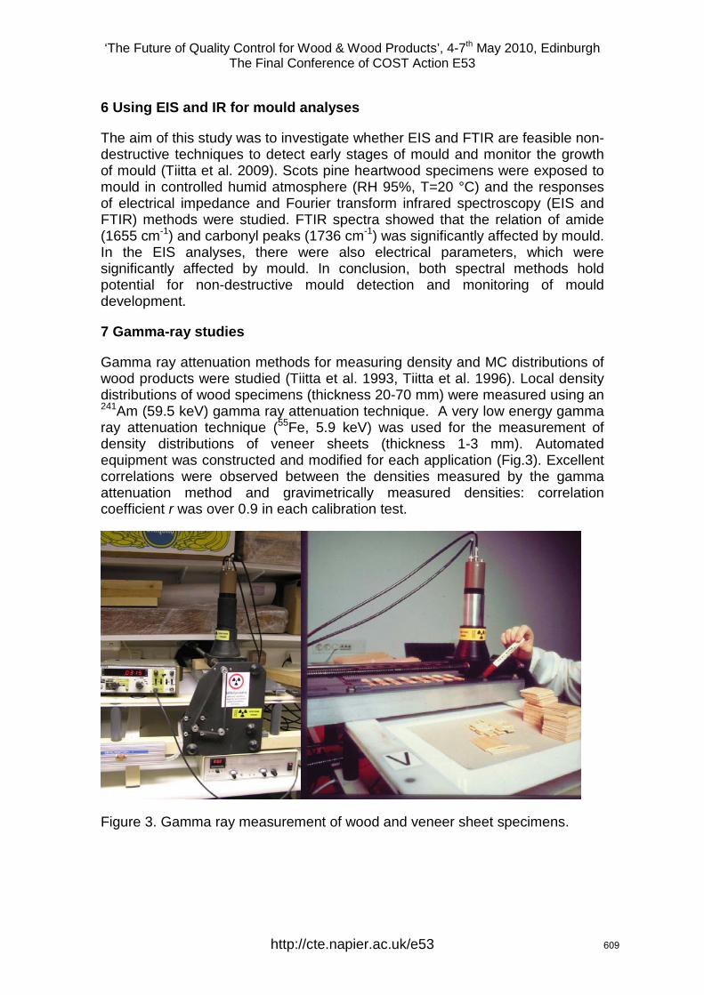
‘The Future of Quality Control for Wood & Wood Products’, 4-7th May 2010, Edinburgh The Final Conference of COST Action E53
http://cte.napier.ac.uk/e53
6 Using EIS and IR for mould analyses
The aim of this study was to investigate whether EIS and FTIR are feasible non-destructive techniques to detect early stages of mould and monitor the growth of mould (Tiitta et al. 2009). Scots pine heartwood specimens were exposed to mould in controlled humid atmosphere (RH 95%, T=20 °C) and the responses of electrical impedance and Fourier transform infrared spectroscopy (EIS and FTIR) methods were studied. FTIR spectra showed that the relation of amide (1655 cm-1) and carbonyl peaks (1736 cm-1) was significantly affected by mould. In the EIS analyses, there were also electrical parameters, which were significantly affected by mould. In conclusion, both spectral methods hold potential for non-destructive mould detection and monitoring of mould development.
7 Gamma-ray studies
Gamma ray attenuation methods for measuring density and MC distributions of wood products were studied (Tiitta et al. 1993, Tiitta et al. 1996). Local density distributions of wood specimens (thickness 20-70 mm) were measured using an 241Am (59.5 keV) gamma ray attenuation technique. A very low energy gamma ray attenuation technique (55Fe, 5.9 keV) was used for the measurement of density distributions of veneer sheets (thickness 1-3 mm). Automated equipment was constructed and modified for each application (Fig.3). Excellent correlations were observed between the densities measured by the gamma attenuation method and gravimetrically measured densities: correlation coefficient r was over 0.9 in each calibration test.
Figure 3. Gamma ray measurement of wood and veneer sheet specimens.
609
‘The Future of Quality Control for Wood & Wood Products’, 4-7th May 2010, Edinburgh The Final Conference of COST Action E53
http://cte.napier.ac.uk/e53
References
Beall, F. C. (2002). Overview of the use of ultrasonic technologies in research on wood properties. Wood Science and Technology, 36, 197-212. MacDonald, J. R. (1987). Impedance spectroscopy. New York, USA: John Wiley & Sons. Miettinen P., Tiitta M. & Lappalainen R. (2005). Electrical and ultrasonic analysis of heat-treated wood. Proc. 14th Int. Symp. on NDT of Wood, Univ. of Ebesrswalde, Germany, p. 265-274.
Tiitta, M.; Miettinen, P. & Lappalainen, R. (2007). Method for the determination of the stresses occurring in wood when drying. PCT-patent CA2633499 (A1).
Tiitta M., Tomppo L., Järnström H., Löija M., Laakso T., Harju A., Venäläinen M., Iitti H., Paajanen L., Saranpää P. & Lappalainen R., Viitanen H. (2009). Spectral and chemical analyses of mould development on Scots pine heartwood. European Journal of Wood and Wood Products 67, p.151-158. Tiitta M., Kainulainen P., Harju A-M., Venäläinen M, Manninen A-M, Vuorinen M. & Viitanen H. (2003). Comparing the effect of chemical and physical properties on complex electrical impedance of Scots pine wood. Holzforschung 57, p. 433-439.
Tiitta M. & Olkkonen H. (2002). Electrical impedance spectroscopy device for measurement of moisture gradients in wood. Rev. Sci. Instr. 73 (8), p. 3093-3100.
Tiitta M., Repo T. & Viitanen H. (2001). Effect of soft rot and bacteria on electrical properties of wood at low moisture content. Mat. Org. 33(4), p.271-288.
Tiitta M., Olkkonen H. & Kanko T. (1996). Veneer sheet density measurement by the 55Fe gamma attenuation method. Holz Roh- Werkstoff 54, p.81-84.
Tiitta M., Olkkonen H., Lappalainen T. & Kanko T. (1993). Automated low energy photon absorption equipment for measuring internal moisture and density distributions of wood samples. Holz Roh- Werkstoff 51, p.417-421.
Tomppo L. , Tiitta M., Laakso T., Harju A., Venäläinen M. & Lappalainen R. (2009). Dielectric spectroscopy of Scots pine. Wood Science and Technology 43 (7/8), p.653-667.
Tomppo L., Tiitta M. & Lappalainen R. (2008). Ultrasound evaluation of lathe check depth in birch veneer. European Journal of Wood and Wood Products 67, p.27-35.
610
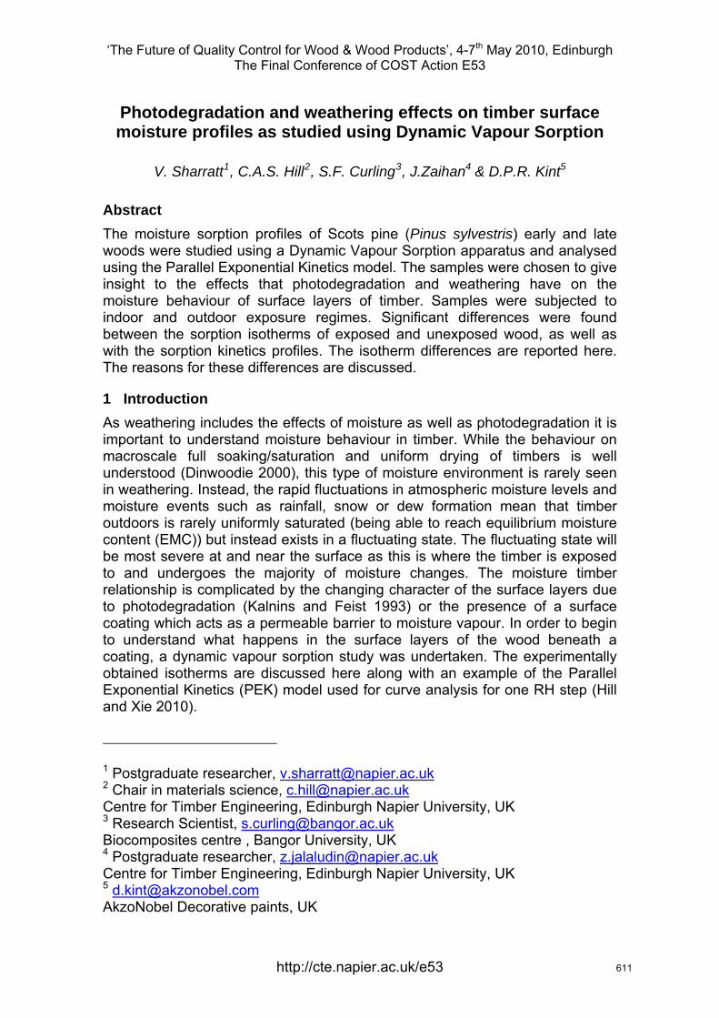
‘The Future of Quality Control for Wood & Wood Products’, 4-7th May 2010, Edinburgh The Final Conference of COST Action E53
Photodegradation and weathering effects on timber surface moisture profiles as studied using Dynamic Vapour Sorption
V. Sharratt1, C.A.S. Hill2, S.F. Curling3, J.Zaihan4 & D.P.R. Kint5
Abstract The moisture sorption profiles of Scots pine (Pinus sylvestris) early and late woods were studied using a Dynamic Vapour Sorption apparatus and analysed using the Parallel Exponential Kinetics model. The samples were chosen to give insight to the effects that photodegradation and weathering have on the moisture behaviour of surface layers of timber. Samples were subjected to indoor and outdoor exposure regimes. Significant differences were found between the sorption isotherms of exposed and unexposed wood, as well as with the sorption kinetics profiles. The isotherm differences are reported here. The reasons for these differences are discussed.
1 Introduction As weathering includes the effects of moisture as well as photodegradation it is important to understand moisture behaviour in timber. While the behaviour on macroscale full soaking/saturation and uniform drying of timbers is well understood (Dinwoodie 2000), this type of moisture environment is rarely seen in weathering. Instead, the rapid fluctuations in atmospheric moisture levels and moisture events such as rainfall, snow or dew formation mean that timber outdoors is rarely uniformly saturated (being able to reach equilibrium moisture content (EMC)) but instead exists in a fluctuating state. The fluctuating state will be most severe at and near the surface as this is where the timber is exposed to and undergoes the majority of moisture changes. The moisture timber relationship is complicated by the changing character of the surface layers due to photodegradation (Kalnins and Feist 1993) or the presence of a surface coating which acts as a permeable barrier to moisture vapour. In order to begin to understand what happens in the surface layers of the wood beneath a coating, a dynamic vapour sorption study was undertaken. The experimentally obtained isotherms are discussed here along with an example of the Parallel Exponential Kinetics (PEK) model used for curve analysis for one RH step (Hill and Xie 2010).
1 Postgraduate researcher, [email protected] Chair in materials science, [email protected] for Timber Engineering, Edinburgh Napier University, UK 3 Research Scientist, [email protected] centre , Bangor University, UK
4 Postgraduate researcher, [email protected] for Timber Engineering, Edinburgh Napier University, UK 5 [email protected] Decorative paints, UK
http://cte.napier.ac.uk/e53 611
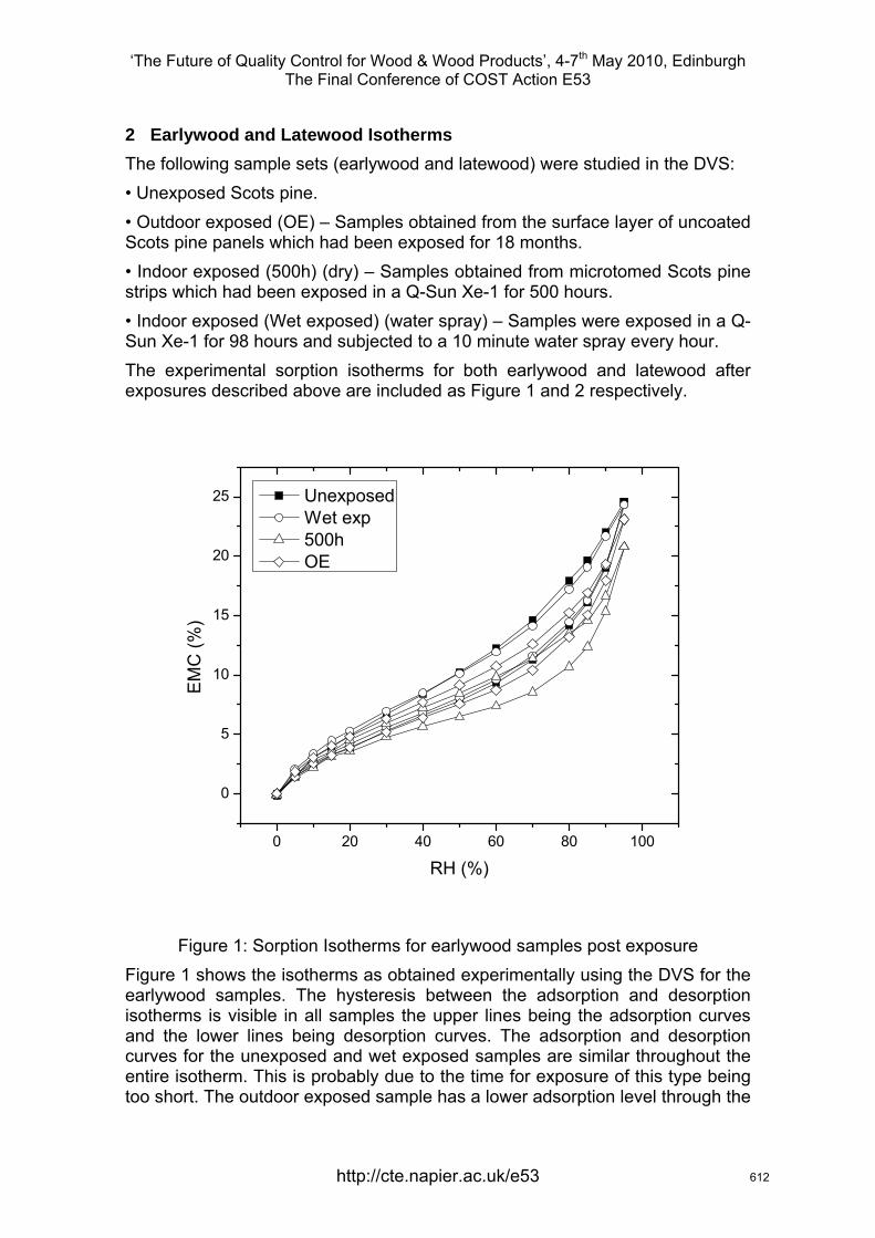
‘The Future of Quality Control for Wood & Wood Products’, 4-7th May 2010, Edinburgh The Final Conference of COST Action E53
2 Earlywood and Latewood Isotherms The following sample sets (earlywood and latewood) were studied in the DVS: • Unexposed Scots pine. • Outdoor exposed (OE) – Samples obtained from the surface layer of uncoated Scots pine panels which had been exposed for 18 months. • Indoor exposed (500h) (dry) – Samples obtained from microtomed Scots pine strips which had been exposed in a Q-Sun Xe-1 for 500 hours. • Indoor exposed (Wet exposed) (water spray) – Samples were exposed in a Q-Sun Xe-1 for 98 hours and subjected to a 10 minute water spray every hour. The experimental sorption isotherms for both earlywood and latewood after exposures described above are included as Figure 1 and 2 respectively.
0 20 40 60 80 100
0
5
10
15
20
25
EM
C (%
)
RH (%)
Unexposed Wet exp 500h OE
Figure 1: Sorption Isotherms for earlywood samples post exposure
Figure 1 shows the isotherms as obtained experimentally using the DVS for the earlywood samples. The hysteresis between the adsorption and desorption isotherms is visible in all samples the upper lines being the adsorption curves and the lower lines being desorption curves. The adsorption and desorption curves for the unexposed and wet exposed samples are similar throughout the entire isotherm. This is probably due to the time for exposure of this type being too short. The outdoor exposed sample has a lower adsorption level through the
http://cte.napier.ac.uk/e53 612
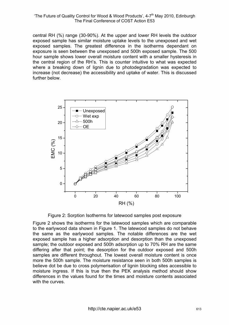
‘The Future of Quality Control for Wood & Wood Products’, 4-7th May 2010, Edinburgh The Final Conference of COST Action E53
central RH (%) range (30-90%). At the upper and lower RH levels the outdoor exposed sample has similar moisture uptake levels to the unexposed and wet exposed samples. The greatest difference in the isotherms dependant on exposure is seen between the unexposed and 500h exposed sample. The 500 hour sample shows lower overall moisture content with a smaller hysteresis in the central region of the RH’s. This is counter intuitive to what was expected where a breaking down of lignin due to photodegradation was expected to increase (not decrease) the accessibility and uptake of water. This is discussed further below.
0 20 40 60 80 100
0
5
10
15
20
25
EM
C (%
)
RH (%)
Unexposed Wet exp 500h OE
Figure 2: Sorption Isotherms for latewood samples post exposure Figure 2 shows the isotherms for the latewood samples which are comparable to the earlywood data shown in Figure 1. The latewood samples do not behave the same as the earlywood samples. The notable differences are the wet exposed sample has a higher adsorption and desorption than the unexposed sample; the outdoor exposed and 500h adsorption up to 70% RH are the same differing after that point; the desorption for the outdoor exposed and 500h samples are different throughout. The lowest overall moisture content is once more the 500h sample. The moisture resistance seen in both 500h samples is believe dot be due to cross polymerisation of lignin blocking sites accessible to moisture ingress. If this is true then the PEK analysis method should show differences in the values found for the times and moisture contents associated with the curves.
http://cte.napier.ac.uk/e53 613
‘The Future of Quality Control for Wood & Wood Products’, 4-7th May 2010, Edinburgh The Final Conference of COST Action E53
3 An example of exposure effects on step curves using the PEK analysis Below is an example of an individual step curve for earlywood Scots pine which has been exposed or unexposed as mentioned above. A definition of the PEK model is given in the proceedings (Hill and Xie 2010).
0 20 40 60 80 100
8.5
9.0
9.5
10.0
10.5
11.0
11.5
Unexposed Wet exp 500h OE
EM
C (%
)
Time (mins)
Figure 3: 70-80% RH sorption step for earlywood showing exposure differences
Table 1: Values obtained for times and moisture contents using PEK model for analysis of step curves shown in Figure 3
Exposure type
t1 (fast process)
t2
(slow process)
MC0 MC1
MC2
Unexposed 10.49569 43.62648 11.43386 8.34794 5.20833
Wet exposed
10.87989 34.45708 11.62765 8.37887 6.22136
500h 5.45717 58.20325 8.55298 5.65199 4.91891
OE 6.18846 26.19716 10.30156 8.25946 4.64608
http://cte.napier.ac.uk/e53 614
‘The Future of Quality Control for Wood & Wood Products’, 4-7th May 2010, Edinburgh The Final Conference of COST Action E53
All curves have been analysed using the PEK model prior to normalisation to the lowest initial moisture content (MC0) value for the step. The normalisation allows the curves to be compared as shown in Figure 3. The lowest initial moisture content was found in the 500h exposed sample. As can be seen on Figure 3 this sample continues to have the lowest moisture content throughout the entire RH step change. The unexposed and wet exposed samples have similar curves showing little difference between the samples. This is seen in the similar values given using the PEK model. This follows the findings on the isotherms as discussed above. The 500h curve is a dominated by a slower process (as seen in the shallower curve) than the other samples. This is shown by the smaller difference between the fast and slow moisture contents, MC1 ≈ MC2, while the characteristic times (t1 and t2) show the greatest difference out of all samples t2>10t1. This compares to the outdoor exposed sample which is a fast process curve with MC1=1.77MC2 while the characteristic times t2>4t1 show the difference in moisture content combined with the smaller differences in characteristic times are due to the outdoor exposed sample being dominated by a fast process. Two possible explanations for the fast and slow processes have been suggested; the fast process is due to fast moisture sorption at ‘external’ surfaces and amorphous regions, while the slow process is due to sorption onto ‘inner’ surfaces and ‘crystallites’ (Morton and Hearle 1997); or the fast process is connected with readily accessible sorption sites within the cell wall and the slow process with new sites made accessible by expansion due to moisture uptake (Hill, Norton et al. 2010). The outdoor exposed sample when compared to the unexposed sample gives evidence for the second definition. As the outdoor exposed sample has more exposed fast sites due to the loss of lignin (caused by weathering processes) than the unexposed the curve should be dominated more by the fast process. This is seen in the curve comparison and PEK analysis. This contrasts to what would be predicted if the 1st definition were correct whereby the curve should be dominated by the slow process. The 500h exposed sample was expected to behave the same as the outdoor exposed sample due to the lignin being photodegraded, however, as mentioned before this has not happened. Instead the overall moisture content is lower and the kinetics are dominated by the slow process as seen on the curve and the values from the PEK analysis. This indicates that instead of opening up the timber photodegradation causes a blocking of readily accessible sites. Two possible reasons for this are lignin fragments physically block accessible sites, or the lignin cross polymerised creating more slow process sites as the easily accessible fast process sites were changed. Cross linking is more likely the factor as the lignin fragments are water soluble and would be expected to dissolve and move leading to a change in the amount of hysteresis seen in the isotherms. As the size of the hysteresis remained unchanged it supports a cross linking rather than fragmentary blocking mechanism. The 500h exposed sample data therefore supports the second definition.
http://cte.napier.ac.uk/e53 615
‘The Future of Quality Control for Wood & Wood Products’, 4-7th May 2010, Edinburgh The Final Conference of COST Action E53
4 Conclusions This study has shown that differences in the moisture-timber behaviour exist depending on type of exposure. The effects seen show a lower moisture affinity for moisture on photodegraded samples when there has been no leaching due to prior changes in moisture. This is believed to be due to cross polymerisation of lignin blocking fast process sites accessible to moisture ingress. This study shows the difficulties in interpreting the data and furthering the understanding of the physical processes which underlie the moisture-timber behaviour as modelled by the PEK model.
5 Acknowledgements
This research is part of a project funded by Akzo Nobel Decorative Paints. The authors would like to thank Akzo Nobel for their assistance in this research.
References Dinwoodie, J. M. (2000). "Timber: Its nature and behaviour". London, E&FN Spon.
Hill, C. A. S., A. J. Norton, et al. (2010). "The Water Vapour Sorption Properties of Sitka Spruce Determined using a Dynamic Vapour Sorption Apparatus." Wood Science and Technology.
Hill, C. A. S. and Y.-J. Xie (2010). "The Water Vapour Sorption Kinetics of Sitka Spruce at Different Temperatures Analysed Using the Parallel Exponential Kinetics Model". COST Action E53. Edinburgh.
Kalnins, M. A. and W. C. Feist (1993). "Increase in wettability of wood with weathering." Forest Products Journal 42(2): 55-57.
Morton, W. E. and J. W. S. Hearle (1997). "Physical properties of textile fibres". UK , The Textile Institute.
http://cte.napier.ac.uk/e53 616
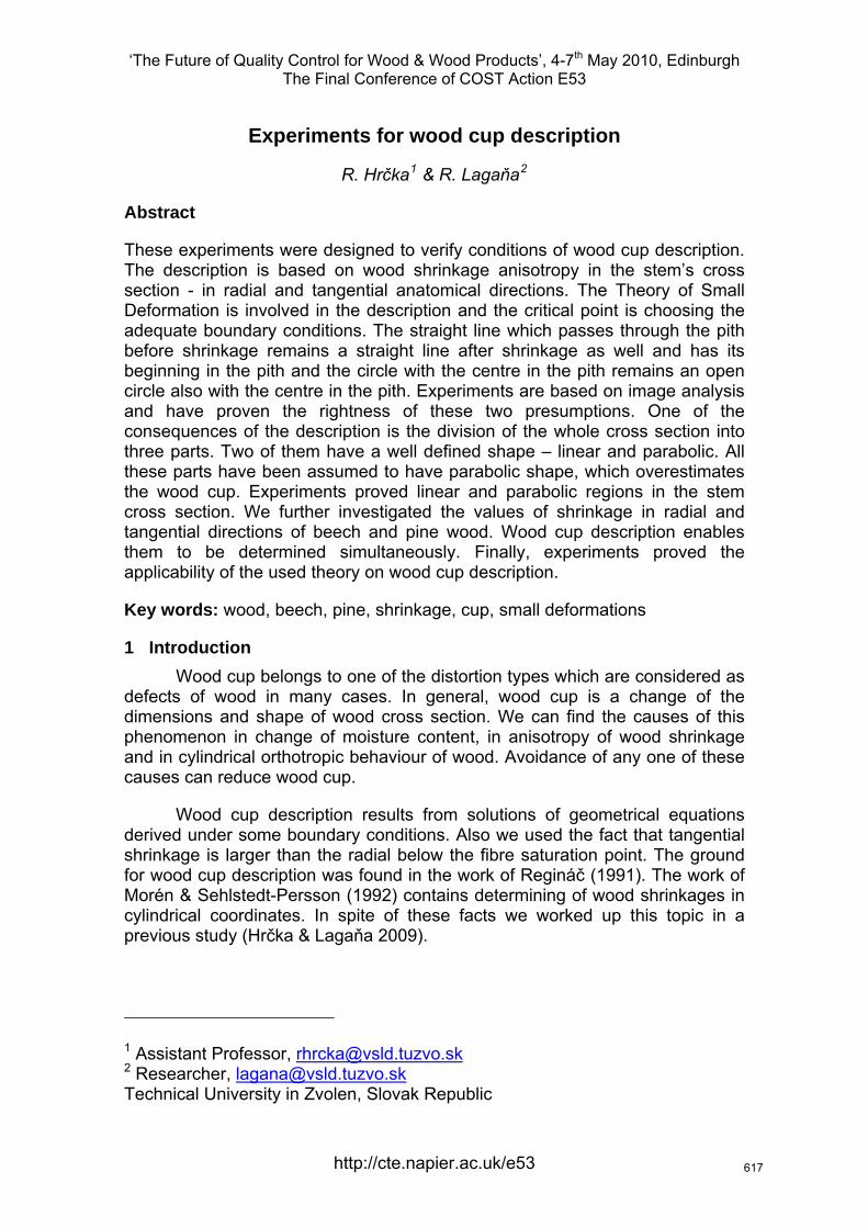
‘The Future of Quality Control for Wood & Wood Products’, 4-7th May 2010, Edinburgh The Final Conference of COST Action E53
Experiments for wood cup description
R. Hrčka1 & R. Lagaňa2
Abstract
These experiments were designed to verify conditions of wood cup description. The description is based on wood shrinkage anisotropy in the stem’s cross section - in radial and tangential anatomical directions. The Theory of Small Deformation is involved in the description and the critical point is choosing the adequate boundary conditions. The straight line which passes through the pith before shrinkage remains a straight line after shrinkage as well and has its beginning in the pith and the circle with the centre in the pith remains an open circle also with the centre in the pith. Experiments are based on image analysis and have proven the rightness of these two presumptions. One of the consequences of the description is the division of the whole cross section into three parts. Two of them have a well defined shape – linear and parabolic. All these parts have been assumed to have parabolic shape, which overestimates the wood cup. Experiments proved linear and parabolic regions in the stem cross section. We further investigated the values of shrinkage in radial and tangential directions of beech and pine wood. Wood cup description enables them to be determined simultaneously. Finally, experiments proved the applicability of the used theory on wood cup description.
Key words: wood, beech, pine, shrinkage, cup, small deformations
1 Introduction Wood cup belongs to one of the distortion types which are considered as defects of wood in many cases. In general, wood cup is a change of the dimensions and shape of wood cross section. We can find the causes of this phenomenon in change of moisture content, in anisotropy of wood shrinkage and in cylindrical orthotropic behaviour of wood. Avoidance of any one of these causes can reduce wood cup.
Wood cup description results from solutions of geometrical equations derived under some boundary conditions. Also we used the fact that tangential shrinkage is larger than the radial below the fibre saturation point. The ground for wood cup description was found in the work of Regináč (1991). The work of Morén & Sehlstedt-Persson (1992) contains determining of wood shrinkages in cylindrical coordinates. In spite of these facts we worked up this topic in a previous study (Hrčka & Lagaňa 2009).
1 Assistant Professor, [email protected] Researcher, [email protected] University in Zvolen, Slovak Republic
http://cte.napier.ac.uk/e53
617
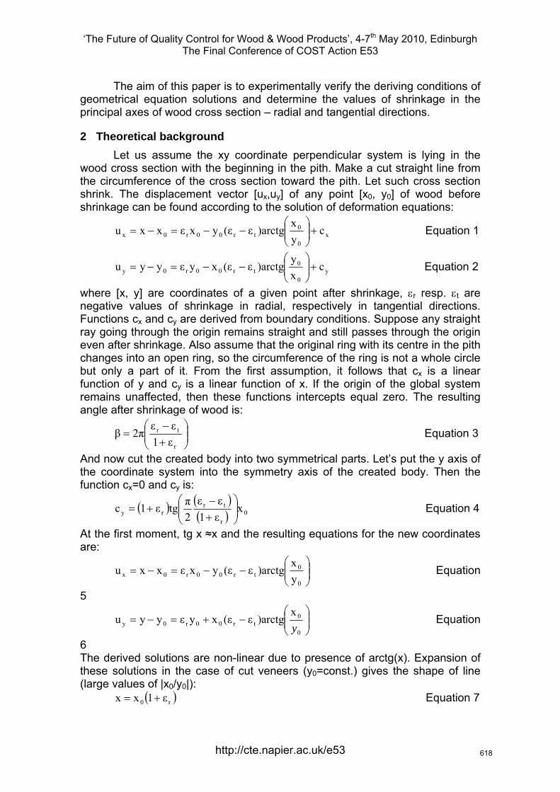
‘The Future of Quality Control for Wood & Wood Products’, 4-7th May 2010, Edinburgh The Final Conference of COST Action E53
The aim of this paper is to experimentally verify the deriving conditions of geometrical equation solutions and determine the values of shrinkage in the principal axes of wood cross section – radial and tangential directions.
2 Theoretical background Let us assume the xy coordinate perpendicular system is lying in the wood cross section with the beginning in the pith. Make a cut straight line from the circumference of the cross section toward the pith. Let such cross section shrink. The displacement vector [ux,uy] of any point [x0, y0] of wood before shrinkage can be found according to the solution of deformation equations:
x0
0tr00r0x c
yx
)arctgε(εyxεxxu +⎟⎟⎠
⎞⎜⎜⎝
⎛−−=−= Equation 1
y0
0tr00r0y c
xy
)arctgε(εxyεyyu +⎟⎟⎠
⎞⎜⎜⎝
⎛−−=−= Equation 2
where [x, y] are coordinates of a given point after shrinkage, εr resp. εt are negative values of shrinkage in radial, respectively in tangential directions. Functions cx and cy are derived from boundary conditions. Suppose any straight ray going through the origin remains straight and still passes through the origin even after shrinkage. Also assume that the original ring with its centre in the pith changes into an open ring, so the circumference of the ring is not a whole circle but only a part of it. From the first assumption, it follows that cx is a linear function of y and cy is a linear function of x. If the origin of the global system remains unaffected, then these functions intercepts equal zero. The resulting angle after shrinkage of wood is:
⎟⎟⎠
⎞⎜⎜⎝
⎛+−
=r
tr
ε1εε
2πβ Equation 3
And now cut the created body into two symmetrical parts. Let’s put the y axis of the coordinate system into the symmetry axis of the created body. Then the function cx=0 and cy is:
( ) ( )( ) 0
r
trry x
ε1εε
2πtgε1c ⎟⎟
⎠
⎞⎜⎜⎝
⎛+−
+= Equation 4
At the first moment, tg x ≈x and the resulting equations for the new coordinates are:
⎟⎟⎠
⎞⎜⎜⎝
⎛−−=−=
0
0tr00r0x y
x)arctgε(εyxεxxu Equation
5
⎟⎟⎠
⎞⎜⎜⎝
⎛−+=−=
0
0tr00r0y
x)arctgε(εxyεyyu
y Equation
6 The derived solutions are non-linear due to presence of arctg(x). Expansion of these solutions in the case of cut veneers (y0=const.) gives the shape of line (large values of |x0/y0|):
( )r0 ε1xx += Equation 7
http://cte.napier.ac.uk/e53
618
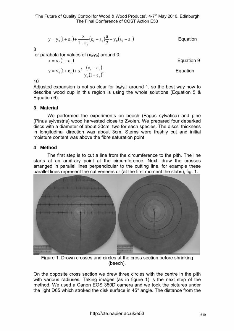
‘The Future of Quality Control for Wood & Wood Products’, 4-7th May 2010, Edinburgh The Final Conference of COST Action E53
( ) ( ) ( tr0trr
r0 εεy2πεε
ε1xε1yy −−−+
++= )
)
Equation
8 or parabola for values of (x0/y0) around 0: Equation 9 ( t0 ε1xx +=
( ) ( )( )2
t0
tr2r0 ε1y
εεxε1yy
+
−++= Equation
10 Adjusted expansion is not so clear for |x0/y0| around 1, so the best way how to describe wood cup in this region is using the whole solutions (Equation 5 & Equation 6).
3 Material We performed the experiments on beech (Fagus sylvatica) and pine (Pinus sylvestris) wood harvested close to Zvolen. We prepared four debarked discs with a diameter of about 30cm, two for each species. The discs’ thickness in longitudinal direction was about 3cm. Stems were freshly cut and initial moisture content was above the fibre saturation point.
4 Method The first step is to cut a line from the circumference to the pith. The line starts at an arbitrary point at the circumference. Next, draw the crosses arranged in parallel lines perpendicular to the cutting line, for example these parallel lines represent the cut veneers or (at the first moment the slabs), fig. 1.
Figure 1: Drown crosses and circles at the cross section before shrinking
(beech). On the opposite cross section we drew three circles with the centre in the pith with various radiuses. Taking images (as in figure 1) is the next step of the method. We used a Canon EOS 350D camera and we took the pictures under the light D65 which stroked the disk surface in 45° angle. The distance from the
http://cte.napier.ac.uk/e53
619
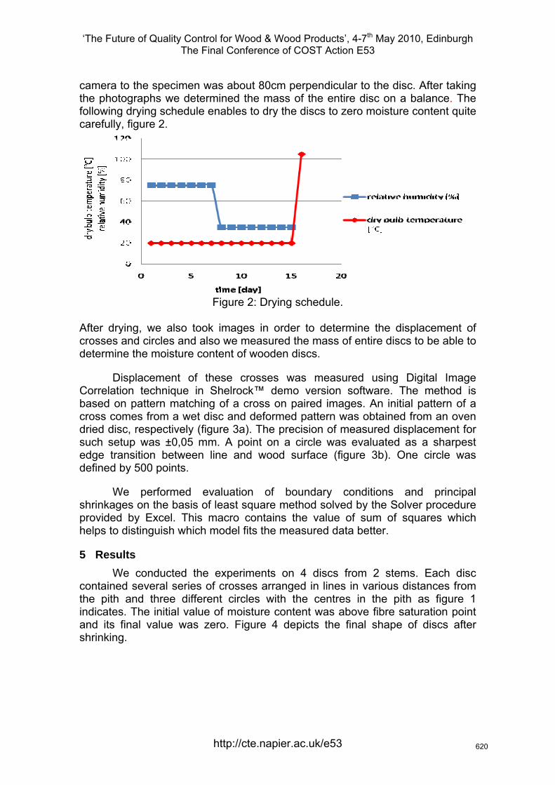
‘The Future of Quality Control for Wood & Wood Products’, 4-7th May 2010, Edinburgh The Final Conference of COST Action E53
camera to the specimen was about 80cm perpendicular to the disc. After taking the photographs we determined the mass of the entire disc on a balance. The following drying schedule enables to dry the discs to zero moisture content quite carefully, figure 2.
Figure 2: Drying schedule.
After drying, we also took images in order to determine the displacement of crosses and circles and also we measured the mass of entire discs to be able to determine the moisture content of wooden discs.
Displacement of these crosses was measured using Digital Image Correlation technique in Shelrock™ demo version software. The method is based on pattern matching of a cross on paired images. An initial pattern of a cross comes from a wet disc and deformed pattern was obtained from an oven dried disc, respectively (figure 3a). The precision of measured displacement for such setup was ±0,05 mm. A point on a circle was evaluated as a sharpest edge transition between line and wood surface (figure 3b). One circle was defined by 500 points.
We performed evaluation of boundary conditions and principal shrinkages on the basis of least square method solved by the Solver procedure provided by Excel. This macro contains the value of sum of squares which helps to distinguish which model fits the measured data better.
5 Results We conducted the experiments on 4 discs from 2 stems. Each disc contained several series of crosses arranged in lines in various distances from the pith and three different circles with the centres in the pith as figure 1 indicates. The initial value of moisture content was above fibre saturation point and its final value was zero. Figure 4 depicts the final shape of discs after shrinking.
http://cte.napier.ac.uk/e53
620
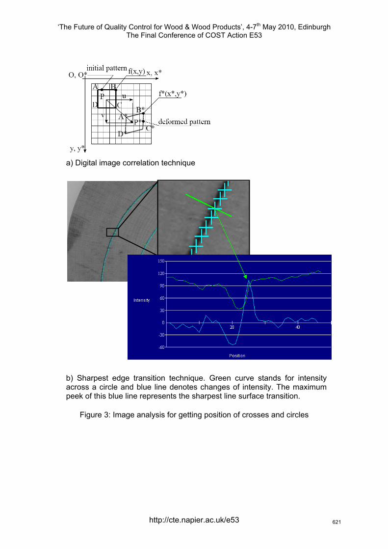
‘The Future of Quality Control for Wood & Wood Products’, 4-7th May 2010, Edinburgh The Final Conference of COST Action E53
a) Digital image correlation technique
b) Sharpest edge transition technique. Green curve stands for intensity across a circle and blue line denotes changes of intensity. The maximum peek of this blue line represents the sharpest line surface transition.
Figure 3: Image analysis for getting position of crosses and circles
http://cte.napier.ac.uk/e53
621
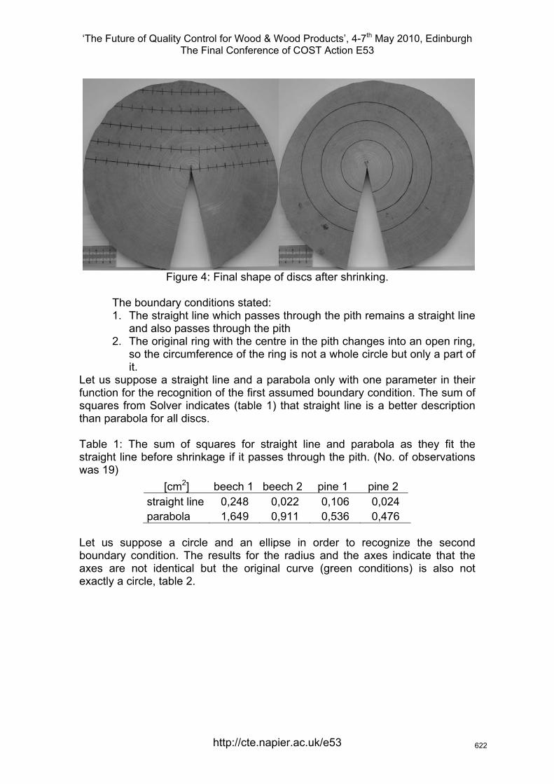
‘The Future of Quality Control for Wood & Wood Products’, 4-7th May 2010, Edinburgh The Final Conference of COST Action E53
Figure 4: Final shape of discs after shrinking.
The boundary conditions stated: 1. The straight line which passes through the pith remains a straight line
and also passes through the pith 2. The original ring with the centre in the pith changes into an open ring,
so the circumference of the ring is not a whole circle but only a part of it.
Let us suppose a straight line and a parabola only with one parameter in their function for the recognition of the first assumed boundary condition. The sum of squares from Solver indicates (table 1) that straight line is a better description than parabola for all discs. Table 1: The sum of squares for straight line and parabola as they fit the straight line before shrinkage if it passes through the pith. (No. of observations was 19)
[cm2] beech 1 beech 2 pine 1 pine 2 straight line 0,248 0,022 0,106 0,024 parabola 1,649 0,911 0,536 0,476
Let us suppose a circle and an ellipse in order to recognize the second boundary condition. The results for the radius and the axes indicate that the axes are not identical but the original curve (green conditions) is also not exactly a circle, table 2.
http://cte.napier.ac.uk/e53
622
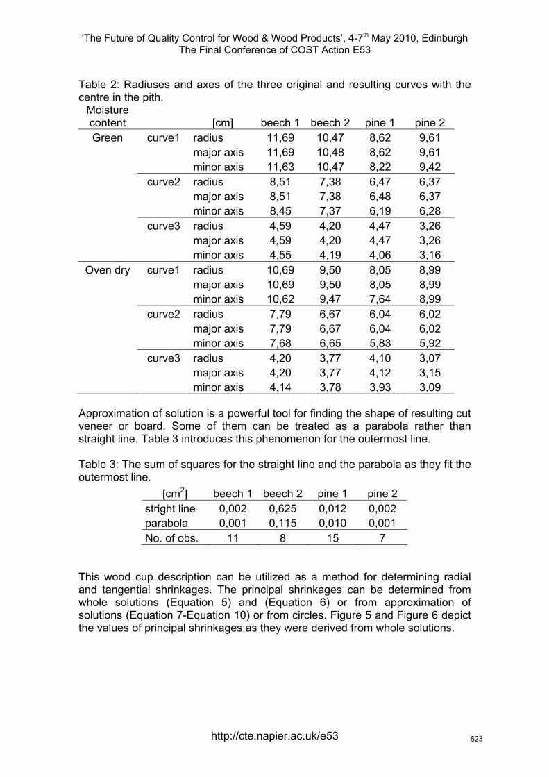
‘The Future of Quality Control for Wood & Wood Products’, 4-7th May 2010, Edinburgh The Final Conference of COST Action E53
Table 2: Radiuses and axes of the three original and resulting curves with the centre in the pith.
Moisture content [cm] beech 1 beech 2 pine 1 pine 2 Green curve1 radius 11,69 10,47 8,62 9,61
major axis 11,69 10,48 8,62 9,61 minor axis 11,63 10,47 8,22 9,42 curve2 radius 8,51 7,38 6,47 6,37 major axis 8,51 7,38 6,48 6,37 minor axis 8,45 7,37 6,19 6,28 curve3 radius 4,59 4,20 4,47 3,26 major axis 4,59 4,20 4,47 3,26 minor axis 4,55 4,19 4,06 3,16
Oven dry curve1 radius 10,69 9,50 8,05 8,99 major axis 10,69 9,50 8,05 8,99 minor axis 10,62 9,47 7,64 8,99 curve2 radius 7,79 6,67 6,04 6,02 major axis 7,79 6,67 6,04 6,02 minor axis 7,68 6,65 5,83 5,92 curve3 radius 4,20 3,77 4,10 3,07 major axis 4,20 3,77 4,12 3,15 minor axis 4,14 3,78 3,93 3,09
Approximation of solution is a powerful tool for finding the shape of resulting cut veneer or board. Some of them can be treated as a parabola rather than straight line. Table 3 introduces this phenomenon for the outermost line. Table 3: The sum of squares for the straight line and the parabola as they fit the outermost line.
[cm2] beech 1 beech 2 pine 1 pine 2 stright line 0,002 0,625 0,012 0,002 parabola 0,001 0,115 0,010 0,001 No. of obs. 11 8 15 7
This wood cup description can be utilized as a method for determining radial and tangential shrinkages. The principal shrinkages can be determined from whole solutions (Equation 5) and (Equation 6) or from approximation of solutions (Equation 7-Equation 10) or from circles. Figure 5 and Figure 6 depict the values of principal shrinkages as they were derived from whole solutions.
http://cte.napier.ac.uk/e53
623
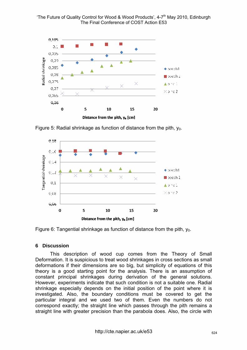
‘The Future of Quality Control for Wood & Wood Products’, 4-7th May 2010, Edinburgh The Final Conference of COST Action E53
Figure 5: Radial shrinkage as function of distance from the pith, y0.
Figure 6: Tangential shrinkage as function of distance from the pith, y0.
6 Discussion This description of wood cup comes from the Theory of Small Deformation. It is suspicious to treat wood shrinkages in cross sections as small deformations if their dimensions are so big, but simplicity of equations of this theory is a good starting point for the analysis. There is an assumption of constant principal shrinkages during derivation of the general solutions. However, experiments indicate that such condition is not a suitable one. Radial shrinkage especially depends on the initial position of the point where it is investigated. Also, the boundary conditions must be covered to get the particular integral and we used two of them. Even the numbers do not correspond exactly; the straight line which passes through the pith remains a straight line with greater precision than the parabola does. Also, the circle with
http://cte.napier.ac.uk/e53
624
‘The Future of Quality Control for Wood & Wood Products’, 4-7th May 2010, Edinburgh The Final Conference of COST Action E53
the centre in the pith remains an open circle (arch). The comparison with the ellipse indicates this conclusion. Deviations from perfection can be explained by the weaker ability of a nonlinear method to meet the correct values of points on the circle near the axes. The derived particular integrals are nonlinear functions. Their linearization also enables one to determine the shape of different wooden products, e.g. cut veneers or at the first moment wooden slabs or cross section can be divided into linear or quadratic parts (Hrčka & Lagaňa 2009). The linearization is useful for cut veneers in these parts because we need only the y0 position of veneer for determining the displacements of its other points. In other cases we need to know the whole position [x0,y0].
As we mentioned before we used this description as the method for determining the radial and tangential shrinkages of wood. Their values can be determined from whole nonlinear solutions, their linearization solutions or circles. The results are mutually comparable and there are some discrepancies as table 2 and figure 5 and figure 6 indicate. Also our results are comparable with values for Fagus sylvatica and Pinus sylvestris published in previous reachable literature. For example Požgaj et al. 1997 published the following values, table 4.
Table 4: Radial and tangential shrinkages as measured by the standard method (Požgaj et al. 1997). −εR −εT
average var.
coefficient no. of
observations average var.
coefficient no. of
observationsbeech 0,053 0,122 149 0,0125 0,105 149 pine 0,041 0,083
Our results attained higher values and this result was proved briefly by statistics.
7 Conclusions In the article we described experiments for wood cup description.
Experiments were based on displacement description of wood cross section points during shrinking. The developed theory agreed with the experiments with satisfactory precision as was indicated in the results. Also results indicate good agreement of approximated solutions to experimental results for linear and quadratic regions of any cross section. This description can serve as a basis for the method of shrinkage evaluation as we demonstrated. Non-linear analysis showed that radial shrinkage at a given moisture content changes. This phenomenon can be assumed as a non-constant parameter problem, which must be included in a more precise wood cup description. Regardless of this problem, present wood cup description is useable in developing standards, experiment planning, or in training wood industry scanning systems.
http://cte.napier.ac.uk/e53
625

‘The Future of Quality Control for Wood & Wood Products’, 4-7th May 2010, Edinburgh The Final Conference of COST Action E53
8 References Hrčka, R. & Lagaňa, R. (2009) “Wood cup description.” In: Proceedings Cost E53, Economic and Technical aspects of quality control for wood and wood products, Lisbon, Portugal, 14. ISBN: 978-989-96428-1-2. Morén, T. & Sehlstedt-Persson, M. (1992) “Cupping of center boards during drying due to anisotropic shrinkage.” In: Proceedings of the 3 IUFRO Conference on Wood Drying, Vienna, Austria, 160-164
rd
Požgaj, A. et al. (1997) “Štruktúra a vlastnosti dreva.” 1. ed., Bratislava, Príroda a.s.. 486p. ISBN 80-07-00-960-4 Regináč, L. et al. (1991) “Náuka o dreve II.” Zvolen, VŠLD Zvolen, 424p. Acknowledgement This work was supported by the Slovak Research and Development Agency under the contract No. APVV-0282-06.
http://cte.napier.ac.uk/e53
626
‘The Future of Quality Control for Wood & Wood Products’, 4-7th May 2010, Edinburgh The Final Conference of COST Action E53
Ultrasound measurements of glulam beams to assess bending stiffness and strength
R. Stöd1 & H. Heräjärvi2
Abstract The objective of this study was to determine the possibilities to assess the bending properties of 44x200x3800 mm, 44x300x5700 mm, 70x200x3800 mm, and 70x300x5700 mm dimensioned glulam beams made of Norway spruce and Scots pine with ultrasonic measurements of ready-made beams. The beams consisted of 8–13 finger jointed lamellae. Lamellae on the tensile and compressive faces of the beams were machine strength graded to represent grade C24, at minimum, whereas the inner lamellae represented poorer strength grades. Altogether 163 Norway spruce and 91 Scots pine beams were measured both using non-destructive ultrasonic measurements with portable Pundit testing device (CNS Farnell Ltd., London, UK) and destructive static bending tests according to EN 408. The ultrasonic measurements were done separately for compressive and tensile faces, and the lamella in the middle of the beam. Due to the cross-sectional dimensions of the beams, extra supports were needed during the destructive bending tests to avoid buckling. The average ultrasound velocities for spruce and pine beams were 5,302 and 4,987 m/s, respectively. The results showed that the correlation between ultrasound velocity and bending properties was higher for the spruce beams than for the pine beams. Ultrasound velocity of the lamella on tensile face appeared to somewhat correlate with beam’s modulus of elasticity. The beam dimensions did not differ from each other concerning the correlation between the ultrasound velocity and bending properties. The current material does not yet provide enough accuracy for reliable prediction models or generalisation of the results.
1 Introduction Glulam is an engineered structural material that optimises the technical properties of timber. Glulam components consist of individual laminates of structural timber. The laminates are not only strength graded but also finger jointed to give greater mechanical performance and higher lengths, and are then glued together to produce the desired size. As a result of the production method, very large structural components can be manufactured. Also smaller glulam beams typically have higher characteristic strength and stiffness than the solid structural timber with corresponding dimensions(e.g., Heikkilä & Heräjärvi 2008). In comparison with its self-weight, glulam is stronger than steel. This means that glulam beams can span large distances with a minimal need of
1 Researcher, [email protected] Researcher, [email protected] 1,2Finnish Forest Research Institute, Finland
http://cte.napier.ac.uk/e53 627
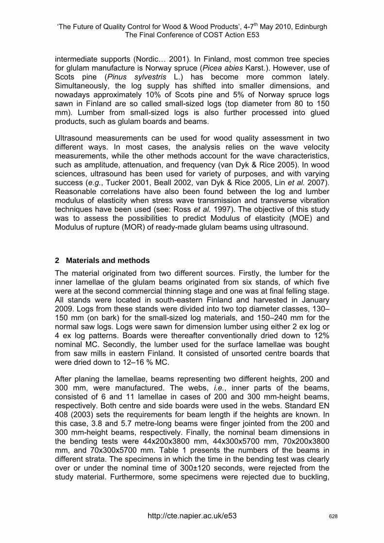
‘The Future of Quality Control for Wood & Wood Products’, 4-7th May 2010, Edinburgh The Final Conference of COST Action E53
intermediate supports (Nordic… 2001). In Finland, most common tree species for glulam manufacture is Norway spruce (Picea abies Karst.). However, use of Scots pine (Pinus sylvestris L.) has become more common lately. Simultaneously, the log supply has shifted into smaller dimensions, and nowadays approximately 10% of Scots pine and 5% of Norway spruce logs sawn in Finland are so called small-sized logs (top diameter from 80 to 150 mm). Lumber from small-sized logs is also further processed into glued products, such as glulam boards and beams.
Ultrasound measurements can be used for wood quality assessment in two different ways. In most cases, the analysis relies on the wave velocity measurements, while the other methods account for the wave characteristics, such as amplitude, attenuation, and frequency (van Dyk & Rice 2005). In wood sciences, ultrasound has been used for variety of purposes, and with varying success (e.g., Tucker 2001, Beall 2002, van Dyk & Rice 2005, Lin et al. 2007). Reasonable correlations have also been found between the log and lumber modulus of elasticity when stress wave transmission and transverse vibration techniques have been used (see: Ross et al. 1997). The objective of this study was to assess the possibilities to predict Modulus of elasticity (MOE) and Modulus of rupture (MOR) of ready-made glulam beams using ultrasound.
2 Materials and methods The material originated from two different sources. Firstly, the lumber for the inner lamellae of the glulam beams originated from six stands, of which five were at the second commercial thinning stage and one was at final felling stage. All stands were located in south-eastern Finland and harvested in January 2009. Logs from these stands were divided into two top diameter classes, 130–150 mm (on bark) for the small-sized log materials, and 150–240 mm for the normal saw logs. Logs were sawn for dimension lumber using either 2 ex log or 4 ex log patterns. Boards were thereafter conventionally dried down to 12% nominal MC. Secondly, the lumber used for the surface lamellae was bought from saw mills in eastern Finland. It consisted of unsorted centre boards that were dried down to 12–16 % MC.
After planing the lamellae, beams representing two different heights, 200 and 300 mm, were manufactured. The webs, i.e., inner parts of the beams, consisted of 6 and 11 lamellae in cases of 200 and 300 mm-height beams, respectively. Both centre and side boards were used in the webs. Standard EN 408 (2003) sets the requirements for beam length if the heights are known. In this case, 3.8 and 5.7 metre-long beams were finger jointed from the 200 and 300 mm-height beams, respectively. Finally, the nominal beam dimensions in the bending tests were 44x200x3800 mm, 44x300x5700 mm, 70x200x3800 mm, and 70x300x5700 mm. Table 1 presents the numbers of the beams in different strata. The specimens in which the time in the bending test was clearly over or under the nominal time of 300±120 seconds, were rejected from the study material. Furthermore, some specimens were rejected due to buckling,
http://cte.napier.ac.uk/e53 628
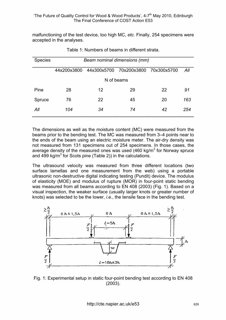
‘The Future of Quality Control for Wood & Wood Products’, 4-7th May 2010, Edinburgh The Final Conference of COST Action E53
malfunctioning of the test device, too high MC, etc. Finally, 254 specimens were accepted in the analyses.
Table 1: Numbers of beams in different strata.
Species Beam nominal dimensions (mm)
44x200x3800 44x300x5700 70x200x3800 70x300x5700 All
N of beams
Pine 28 12 29 22 91
Spruce 76 22 45 20 163
All 104 34 74 42 254
The dimensions as well as the moisture content (MC) were measured from the beams prior to the bending test. The MC was measured from 3–4 points near to the ends of the beam using an electric moisture meter. The air-dry density was not measured from 131 specimens out of 254 specimens. In those cases, the average density of the measured ones was used (460 kg/m3 for Norway spruce and 499 kg/m3 for Scots pine (Table 2)) in the calculations.
The ultrasound velocity was measured from three different locations (two surface lamellas and one measurement from the web) using a portable ultrasonic non-destructive digital indicating testing (Pundit) device. The modulus of elasticity (MOE) and modulus of rupture (MOR) in four-point static bending was measured from all beams according to EN 408 (2003) (Fig. 1). Based on a visual inspection, the weaker surface (usually larger knots or greater number of knots) was selected to be the lower, i.e., the tensile face in the bending test.
Fig. 1: Experimental setup in static four-point bending test according to EN 408 (2003).
http://cte.napier.ac.uk/e53 629

‘The Future of Quality Control for Wood & Wood Products’, 4-7th May 2010, Edinburgh The Final Conference of COST Action E53
The global MOE (Em,g, N/mm2=MPa) was calculated according to Equation 1:
( )( ) ⎥⎦
⎤⎢⎣⎡= 3
123
123
, )(-)43(
--
la
la
wwbhFFlE gm , Equation 1
where l = distance between the lower supports (mm), b = specimen width (mm), h = specimen height (mm), a = distance between the load point and the closest support point (mm), F2 = 0.4Fmax (N), F1 = 0.1Fmax, w2 = displacement at the point F2 (mm), w1 = displacement at the point F1 (mm).
In case of MOE, the MC’s of the beams were adjusted to correspond to 12% using Equation 2 (Boström 1994):
( )ω-120143.01ω
12 +=
EE , Equation 2
where E12 = MOE in 12% MC (MPa), ω = MC at the time of test (%), Eω = MOE at the MC of ω % (MPa).
MOR (fm, N/mm2=MPa) was calculated according to Equation 3:
WaF
fm 2= max , Equation 3
where a = distance between the load point and the lowest support point (mm), Fmax = maximum force (N), and W = section modulus (mm3).
In case of MOR, the MC’s of the beams were adjusted to correspond to 12% using Equation 4 (Boström 1994):
( )-ω+f
=f ωm, 120295.0112 , Equation 4
where fm,12 = MOR in 12% MC (MPa), ω = MC at the time of test (%), fω = MOR at the MC of ω % (MPa).
Dynamic MOE, based on the ultrasound velocity, was calculated using Equation 5:
122ρ= vEd , Equation 5
where Ed = dynamic MOE (GPa), v = ultrasound velocity (m/s) ja ρ12 = air-dry density (kg/m3). Both air-dry density and ultrasound velocity values are measured from specimens with 14% MC, on average.
http://cte.napier.ac.uk/e53 630
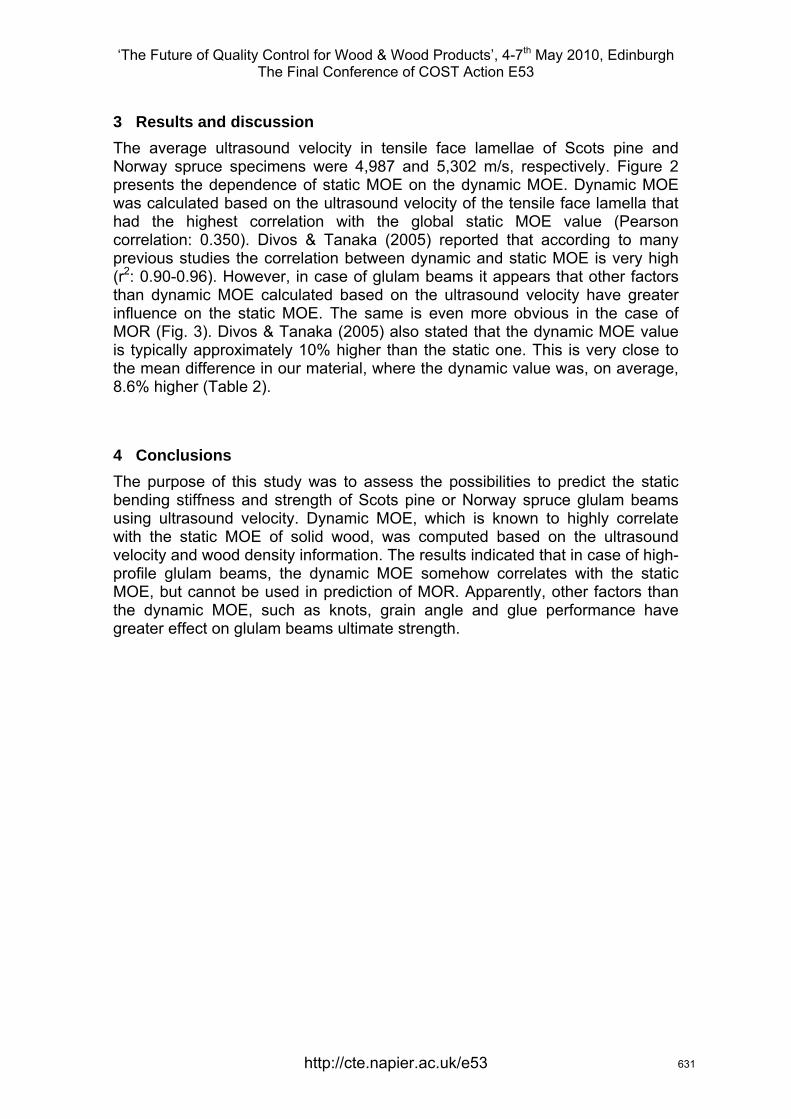
‘The Future of Quality Control for Wood & Wood Products’, 4-7th May 2010, Edinburgh The Final Conference of COST Action E53
3 Results and discussion The average ultrasound velocity in tensile face lamellae of Scots pine and Norway spruce specimens were 4,987 and 5,302 m/s, respectively. Figure 2 presents the dependence of static MOE on the dynamic MOE. Dynamic MOE was calculated based on the ultrasound velocity of the tensile face lamella that had the highest correlation with the global static MOE value (Pearson correlation: 0.350). Divos & Tanaka (2005) reported that according to many previous studies the correlation between dynamic and static MOE is very high (r2: 0.90-0.96). However, in case of glulam beams it appears that other factors than dynamic MOE calculated based on the ultrasound velocity have greater influence on the static MOE. The same is even more obvious in the case of MOR (Fig. 3). Divos & Tanaka (2005) also stated that the dynamic MOE value is typically approximately 10% higher than the static one. This is very close to the mean difference in our material, where the dynamic value was, on average, 8.6% higher (Table 2).
4 Conclusions The purpose of this study was to assess the possibilities to predict the static bending stiffness and strength of Scots pine or Norway spruce glulam beams using ultrasound velocity. Dynamic MOE, which is known to highly correlate with the static MOE of solid wood, was computed based on the ultrasound velocity and wood density information. The results indicated that in case of high-profile glulam beams, the dynamic MOE somehow correlates with the static MOE, but cannot be used in prediction of MOR. Apparently, other factors than the dynamic MOE, such as knots, grain angle and glue performance have greater effect on glulam beams ultimate strength.
http://cte.napier.ac.uk/e53 631
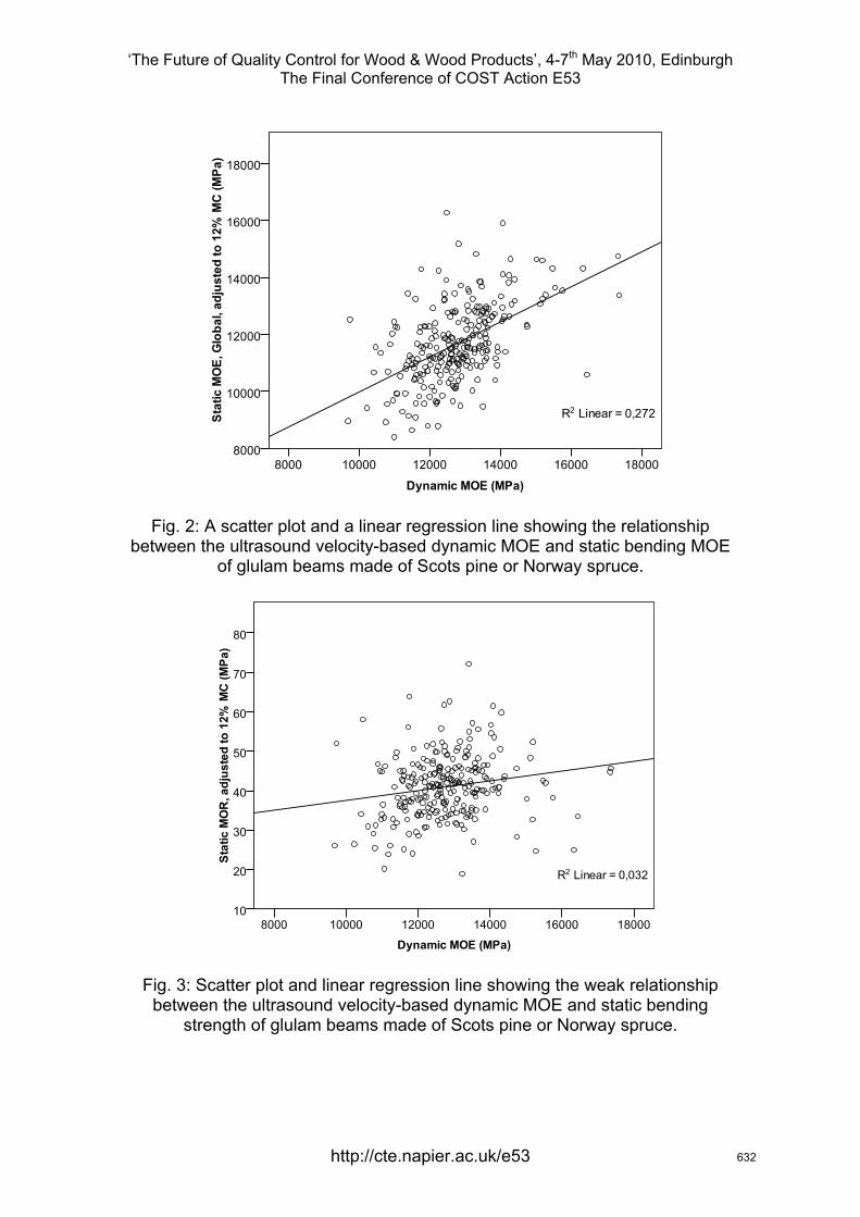
‘The Future of Quality Control for Wood & Wood Products’, 4-7th May 2010, Edinburgh The Final Conference of COST Action E53
Fig. 2: A scatter plot and a linear regression line showing the relationship between the ultrasound velocity-based dynamic MOE and static bending MOE
of glulam beams made of Scots pine or Norway spruce.
Fig. 3: Scatter plot and linear regression line showing the weak relationship between the ultrasound velocity-based dynamic MOE and static bending
strength of glulam beams made of Scots pine or Norway spruce.
http://cte.napier.ac.uk/e53 632
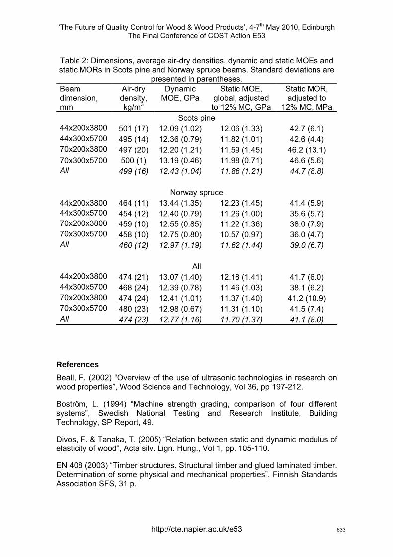
‘The Future of Quality Control for Wood & Wood Products’, 4-7th May 2010, Edinburgh The Final Conference of COST Action E53
Table 2: Dimensions, average air-dry densities, dynamic and static MOEs and static MORs in Scots pine and Norway spruce beams. Standard deviations are
presented in parentheses. Beam dimension, mm
Air-dry density, kg/m3
Dynamic MOE, GPa
Static MOE, global, adjusted to 12% MC, GPa
Static MOR, adjusted to
12% MC, MPa Scots pine
44x200x3800 501 (17) 12.09 (1.02) 12.06 (1.33) 42.7 (6.1) 44x300x5700 495 (14) 12.36 (0.79) 11.82 (1.01) 42.6 (4.4) 70x200x3800 497 (20) 12.20 (1.21) 11.59 (1.45) 46.2 (13.1) 70x300x5700 500 (1) 13.19 (0.46) 11.98 (0.71) 46.6 (5.6) All 499 (16) 12.43 (1.04) 11.86 (1.21) 44.7 (8.8)
Norway spruce
44x200x3800 464 (11) 13.44 (1.35) 12.23 (1.45) 41.4 (5.9) 44x300x5700 454 (12) 12.40 (0.79) 11.26 (1.00) 35.6 (5.7) 70x200x3800 459 (10) 12.55 (0.85) 11.22 (1.36) 38.0 (7.9) 70x300x5700 458 (10) 12.75 (0.80) 10.57 (0.97) 36.0 (4.7) All 460 (12) 12.97 (1.19) 11.62 (1.44) 39.0 (6.7)
All
44x200x3800 474 (21) 13.07 (1.40) 12.18 (1.41) 41.7 (6.0) 44x300x5700 468 (24) 12.39 (0.78) 11.46 (1.03) 38.1 (6.2) 70x200x3800 474 (24) 12.41 (1.01) 11.37 (1.40) 41.2 (10.9) 70x300x5700 480 (23) 12.98 (0.67) 11.31 (1.10) 41.5 (7.4) All 474 (23) 12.77 (1.16) 11.70 (1.37) 41.1 (8.0)
References Beall, F. (2002) “Overview of the use of ultrasonic technologies in research on wood properties”, Wood Science and Technology, Vol 36, pp 197-212.
Boström, L. (1994) “Machine strength grading, comparison of four different systems”, Swedish National Testing and Research Institute, Building Technology, SP Report, 49.
Divos, F. & Tanaka, T. (2005) “Relation between static and dynamic modulus of elasticity of wood”, Acta silv. Lign. Hung., Vol 1, pp. 105-110.
EN 408 (2003) “Timber structures. Structural timber and glued laminated timber. Determination of some physical and mechanical properties”, Finnish Standards Association SFS, 31 p.
http://cte.napier.ac.uk/e53 633
‘The Future of Quality Control for Wood & Wood Products’, 4-7th May 2010, Edinburgh The Final Conference of COST Action E53
Heikkilä, K. & Heräjärvi, H. (2008) “Stiffness and strength of 45x95 mm beams glued from Norway spruce using 8 different structural models”. In: Gard, W.F. & van de Kuilen, J.W.G. (eds.). Proceedings of COST E53 conference “End user’s needs for wood material and products”, 29th-30th October 2008, Delft, The Netherlands, pp. 271-280.
Lin, C.-J., Yang, T.-H., Zhang, D.-Z., Wang, S.-Y. & Lin, F.-C. (2007) “Changes in the dynamic modulus of elasticity and bending properties of railroad ties after 20 years of service in Taiwan”, Building and Environment, Vol 42, pp 1250-1256.
Nordic Glulam Handbook. (2001), Finnish Glulam Association, 360 p. http://www.glulam.fi/liimapuu/?__EVIA_WYSIWYG_FILE=28190&name=file
Ross, R.J., McDonald, K.A., Green, D.W. & Schad, K.C. (1997) “Relationship between log and lumber modulus of elasticity”, Forest Products Journal, Vol 47(2), pp. 89-92.
Tucker, B.J. (2001) “Ultrasonic plate waves in wood based composites”, Doctoral thesis. Washington State University, Department of Civil and Environmental Engineering, 113 p.
van Dyk, H. & Rice, R.W. (2005) “An assessment of the feasibility of ultrasound as a defect detector in lumber”, Holzforschung, Vol 59, pp 551-445.
http://cte.napier.ac.uk/e53 634

‘The Future of Quality Control for Wood & Wood Products’, 4-7th May 2010, Edinburgh The Final Conference of COST Action E53
Quality Approval System for Wood Products in Korea
S.M. Kang1, D.Y. Kang2, W.M. Koo3, K.M. Kim4 & J.Y. Park5
Abstract Korean government has started quality approval (QA) system for wood products including preservative treated wood, wood charcoal, and pyroligneous acid in July 1, 2004. The QA system has been now expanding product items to drying lumber, wood pellets and wood composite materials. The QA system is based on the two forest laws such as the Act on the Promotion and Management of Forest Resources and the Act on Promotion of Forestry and Mountain Villages. Labelling of quality is mandatory and is subject to the Act on the Promotion and Management of Forest Resources and The Act on Promotion of Forestry. The law has applied to both domestic and imported wood products including preservative treated wood, plywood and structural lumber. The QA system becomes effective under Article 12 of Act on Promotion of Forestry and Mountain Villages. The QA system, however, has led voluntary participation of companies. The national research institute, Korea Forest Research Institute (KFRI) takes charge of the QA system. We have also conducted investigations and researches for development of the QA system. The main projects include grading of kiln dried wood, treatability of wood species, fixation mechanism of preservative treated wood, leaching of biocides from treated wood on environments, and development of analytical methods for wood products. Over all objectives of the QA system are to improve quality of wood products, to enhance distribution system of wood products and to protect customers.
1. Korean Forest Resources
The Korean peninsula is located at the North Western Pacific region. Forest areas cover 65% of the land, estimated 6.39 million ha. The Korean forests are grouped into warm temperate, cool-temperate, and boreal forests. Cool temperate forests consist about 85% of them.
While coniferous forests are composed of 42.3% (2.70 million ha) of the total forest, broadleaved forest and mixed forest make up 25.9% (1.66 million ha) and 29.3% (1.87 million ha), respectively (Forest statistics, 2005). The remaining 2.5% (0.16 million ha) is classified as others such as forest-steppe.
1 Research Scientist, [email protected] Research Assistant, [email protected] Research Assistant, [email protected] Research Assistant, [email protected] Team Leader, [email protected] of Forest Products, Korea Forest Research Institute Seoul, Republic of Korea
http://cte.napier.ac.uk/e53 635
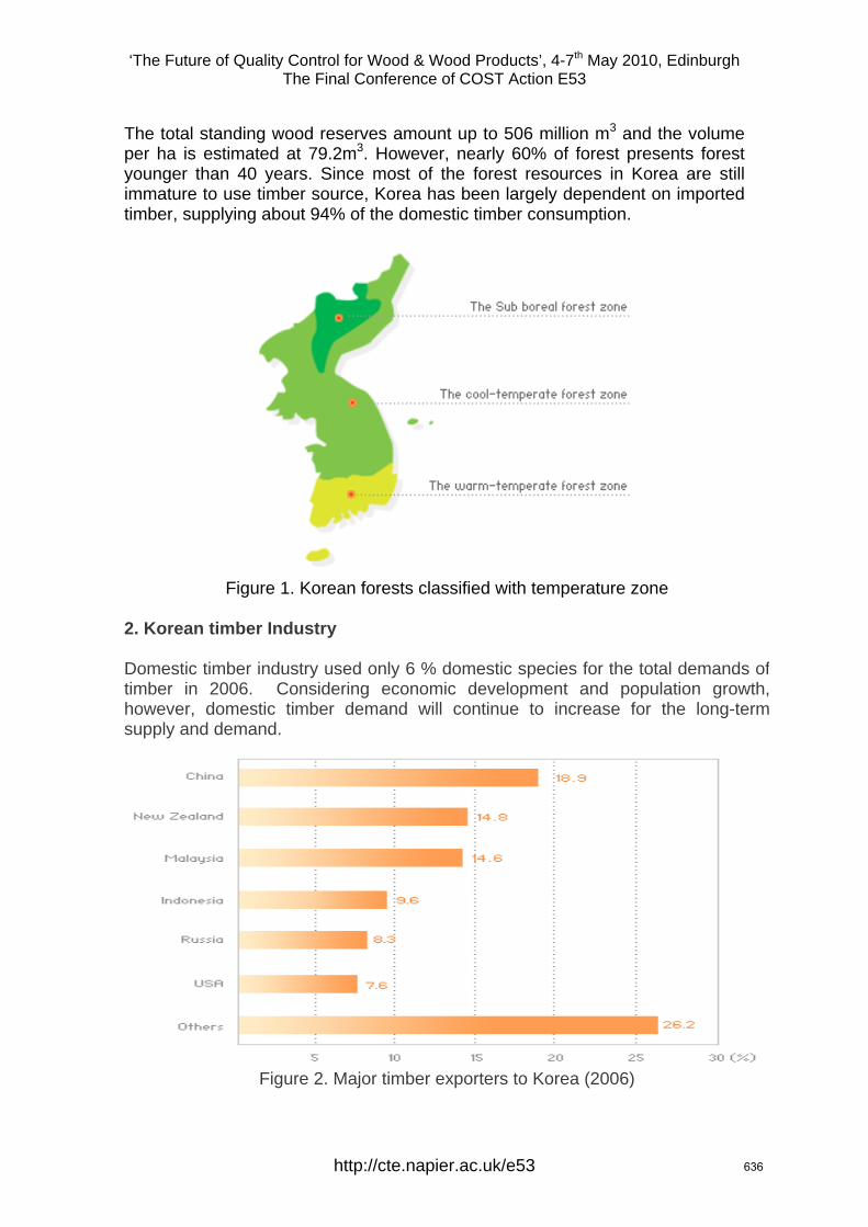
‘The Future of Quality Control for Wood & Wood Products’, 4-7th May 2010, Edinburgh The Final Conference of COST Action E53
The total standing wood reserves amount up to 506 million m3 and the volume per ha is estimated at 79.2m3. However, nearly 60% of forest presents forest younger than 40 years. Since most of the forest resources in Korea are still immature to use timber source, Korea has been largely dependent on imported timber, supplying about 94% of the domestic timber consumption.
Figure 1. Korean forests classified with temperature zone
2. Korean timber Industry Domestic timber industry used only 6 % domestic species for the total demands oftimber in 2006. Considering economic development and population growth, however, domestic timber demand will continue to increase for the long-term supply and demand.
Figure 2. Major timber exporters to Korea (2006)
http://cte.napier.ac.uk/e53 636
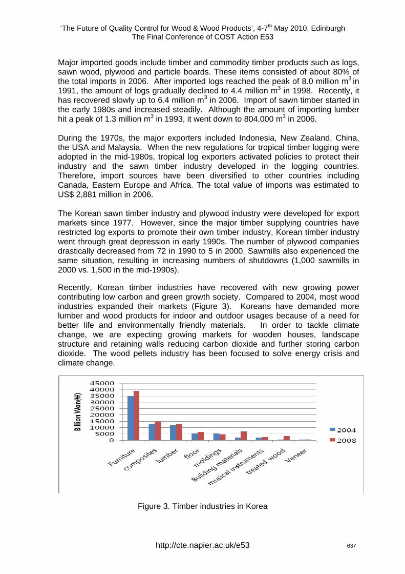
‘The Future of Quality Control for Wood & Wood Products’, 4-7th May 2010, Edinburgh The Final Conference of COST Action E53
Major imported goods include timber and commodity timber products such as logs,sawn wood, plywood and particle boards. These items consisted of about 80% of the total imports in 2006. After imported logs reached the peak of 8.0 million m3 in 1991, the amount of logs gradually declined to 4.4 million m3 in 1998. Recently, it has recovered slowly up to 6.4 million m3 in 2006. Import of sawn timber started in the early 1980s and increased steadily. Although the amount of importing lumber hit a peak of 1.3 million m3 in 1993, it went down to 804,000 m3 in 2006.
During the 1970s, the major exporters included Indonesia, New Zealand, China, the USA and Malaysia. When the new regulations for tropical timber logging wereadopted in the mid-1980s, tropical log exporters activated policies to protect their industry and the sawn timber industry developed in the logging countries. Therefore, import sources have been diversified to other countries including Canada, Eastern Europe and Africa. The total value of imports was estimated to US$ 2,881 million in 2006.
The Korean sawn timber industry and plywood industry were developed for exportmarkets since 1977. However, since the major timber supplying countries haverestricted log exports to promote their own timber industry, Korean timber industry went through great depression in early 1990s. The number of plywood companies drastically decreased from 72 in 1990 to 5 in 2000. Sawmills also experienced the same situation, resulting in increasing numbers of shutdowns (1,000 sawmills in 2000 vs. 1,500 in the mid-1990s).
Recently, Korean timber industries have recovered with new growing power contributing low carbon and green growth society. Compared to 2004, most wood industries expanded their markets (Figure 3). Koreans have demanded more lumber and wood products for indoor and outdoor usages because of a need for better life and environmentally friendly materials. In order to tackle climate change, we are expecting growing markets for wooden houses, landscapestructure and retaining walls reducing carbon dioxide and further storing carbon dioxide. The wood pellets industry has been focused to solve energy crisis and climate change.
Figure 3. Timber industries in Korea
http://cte.napier.ac.uk/e53 637

‘The Future of Quality Control for Wood & Wood Products’, 4-7th May 2010, Edinburgh The Final Conference of COST Action E53
3. The Quality Control System for Wood Products in Korea The Korean Government, especially Forest Service, has made efforts to develop timber industry. The concrete objectives are enhancing competitiveness, improving product quality, supporting automation facilities and securing a stable supply of raw materials. One of the policies was launching the QA system to improve quality of wood products, to enhance distribution system of wood products and to protect customers.
The QA system is based on the two forest laws such as the Act on the Promotion and Management of Forest Resources and the Act on Promotion of Forestry and Mountain Villages. Labelling of quality is mandatory and is subject to the Act on the Promotion and Management of Forest Resources and The Act on Promotion of Forestry. The law has applied to both domestic and imported wood products including preservative treated wood, plywood and structural lumber. The QA system becomes effective under Article 12 of Act on Promotion of Forestry and Mountain Villages. The QA system, however, has led voluntary participation of companies.
Korean government has started the QA system for wood products including preservative treated wood, wood charcoal, and pyroligneous acid in July 1, 2004. The QA system has been now expanded product items to drying lumber, wood pellets and wood composite materials.
The national research institute, Korea Forest Research Institute (KFRI) takes charge of the QA system. We have also conducted investigations and researches for development of the QA system.
4. Main projects for QA system Korea Forest Research Institute (KFRI) has developed high utilization techniques for forest products. We have also improved forest industries which are new growing power in Korea to contribute low carbon and green growth society. The utilization techniques have facilitated to add values for wood products.
We conducted investigations and researches for the development of the QA system. The main projects include kiln dried wood, treatability of wood species, fixation mechanism of preservative treated wood, leaching of biocides from treated wood on environments, and development analytical methods for wood products.
4.1. Kiln dried wood
We analyzed wood characteristic variations and investigated major domestic timbers to identify wood species with explication of variation of microscopic
http://cte.napier.ac.uk/e53 638
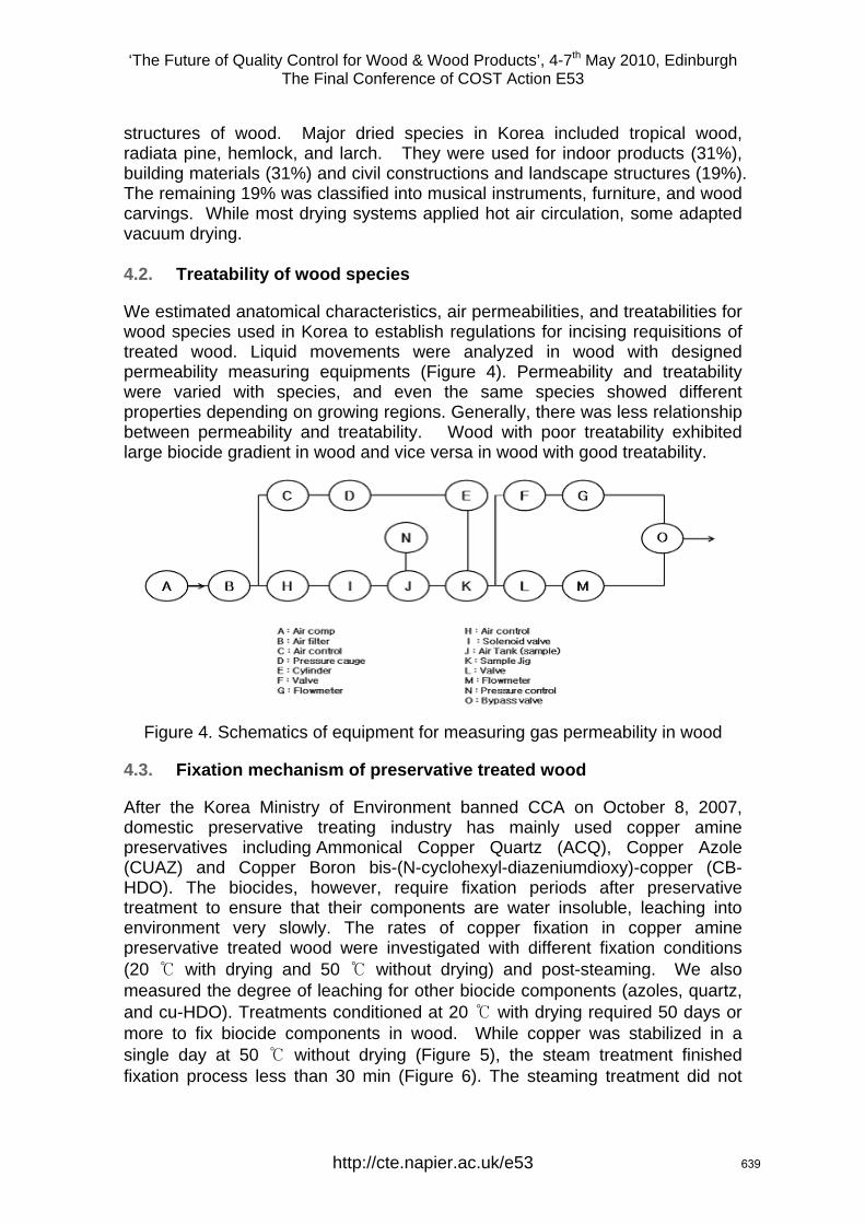
‘The Future of Quality Control for Wood & Wood Products’, 4-7th May 2010, Edinburgh The Final Conference of COST Action E53
structures of wood. Major dried species in Korea included tropical wood, radiata pine, hemlock, and larch. They were used for indoor products (31%), building materials (31%) and civil constructions and landscape structures (19%). The remaining 19% was classified into musical instruments, furniture, and wood carvings. While most drying systems applied hot air circulation, some adapted vacuum drying.
4.2. Treatability of wood species
We estimated anatomical characteristics, air permeabilities, and treatabilities for wood species used in Korea to establish regulations for incising requisitions of treated wood. Liquid movements were analyzed in wood with designed permeability measuring equipments (Figure 4). Permeability and treatability were varied with species, and even the same species showed different properties depending on growing regions. Generally, there was less relationship between permeability and treatability. Wood with poor treatability exhibited large biocide gradient in wood and vice versa in wood with good treatability.
Figure 4. Schematics of equipment for measuring gas permeability in wood
4.3. Fixation mechanism of preservative treated wood
After the Korea Ministry of Environment banned CCA on October 8, 2007, domestic preservative treating industry has mainly used copper amine preservatives including Ammonical Copper Quartz (ACQ), Copper Azole (CUAZ) and Copper Boron bis-(N-cyclohexyl-diazeniumdioxy)-copper (CB-HDO). The biocides, however, require fixation periods after preservative treatment to ensure that their components are water insoluble, leaching into environment very slowly. The rates of copper fixation in copper amine preservative treated wood were investigated with different fixation conditions (20 ℃ with drying and 50 ℃ without drying) and post-steaming. We also measured the degree of leaching for other biocide components (azoles, quartz, and cu-HDO). Treatments conditioned at 20 ℃ with drying required 50 days or more to fix biocide components in wood. While copper was stabilized in a single day at 50 ℃ without drying (Figure 5), the steam treatment finished fixation process less than 30 min (Figure 6). The steaming treatment did not
http://cte.napier.ac.uk/e53 639
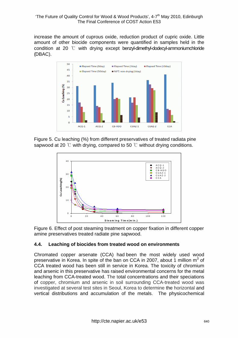
‘The Future of Quality Control for Wood & Wood Products’, 4-7th May 2010, Edinburgh The Final Conference of COST Action E53
increase the amount of cuprous oxide, reduction product of cupric oxide. Little amount of other biocide components were quantified in samples held in the condition at 20 ℃ with drying except benzyl-dimethyl-dodecyl-ammoniumchloride (DBAC).
Figure 5. Cu leaching (%) from different preservatives of treated radiata pine sapwood at 20 ℃ with drying, compared to 50 ℃ without drying conditions.
S te a m in g T im e (m in .)
0 2 0 4 0 6 0 8 0 1 0 0 1 2 0
Cu
Leac
hing
(%)
0
1 0
2 0
3 0
4 0
A C Q -1A C Q -2C B -H D OC U A Z -1C U A Z -2C C A
Figure 6. Effect of post steaming treatment on copper fixation in different copper amine preservatives treated radiate pine sapwood.
4.4. Leaching of biocides from treated wood on environments
Chromated copper arsenate (CCA) had been the most widely used wood preservative in Korea. In spite of the ban on CCA in 2007, about 1 million m3 of CCA treated wood has been still in service in Korea. The toxicity of chromium and arsenic in this preservative has raised environmental concerns for the metal leaching from CCA-treated wood. The total concentrations and their speciations of copper, chromium and arsenic in soil surrounding CCA-treated wood was investigated at several test sites in Seoul, Korea to determine the horizontal and vertical distributions and accumulation of the metals. The physicochemical
http://cte.napier.ac.uk/e53 640
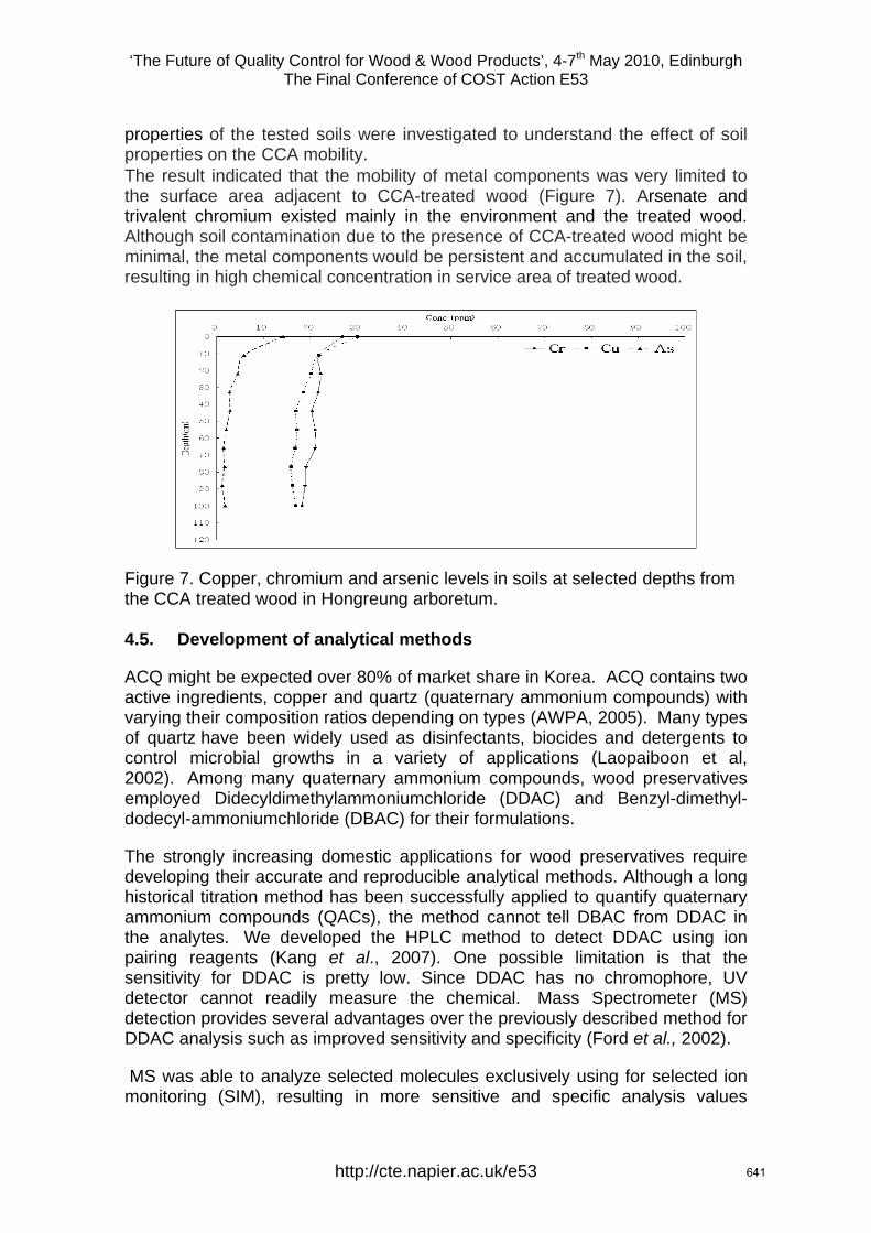
‘The Future of Quality Control for Wood & Wood Products’, 4-7th May 2010, Edinburgh The Final Conference of COST Action E53
properties of the tested soils were investigated to understand the effect of soil properties on the CCA mobility. The result indicated that the mobility of metal components was very limited to the surface area adjacent to CCA-treated wood (Figure 7). Arsenate and trivalent chromium existed mainly in the environment and the treated wood. Although soil contamination due to the presence of CCA-treated wood might be minimal, the metal components would be persistent and accumulated in the soil, resulting in high chemical concentration in service area of treated wood.
Figure 7. Copper, chromium and arsenic levels in soils at selected depths from the CCA treated wood in Hongreung arboretum. 4.5. Development of analytical methods
ACQ might be expected over 80% of market share in Korea. ACQ contains two active ingredients, copper and quartz (quaternary ammonium compounds) with varying their composition ratios depending on types (AWPA, 2005). Many types of quartz have been widely used as disinfectants, biocides and detergents to control microbial growths in a variety of applications (Laopaiboon et al, 2002). Among many quaternary ammonium compounds, wood preservatives employed Didecyldimethylammoniumchloride (DDAC) and Benzyl-dimethyl-dodecyl-ammoniumchloride (DBAC) for their formulations.
The strongly increasing domestic applications for wood preservatives require developing their accurate and reproducible analytical methods. Although a long historical titration method has been successfully applied to quantify quaternary ammonium compounds (QACs), the method cannot tell DBAC from DDAC in the analytes. We developed the HPLC method to detect DDAC using ion pairing reagents (Kang et al., 2007). One possible limitation is that the sensitivity for DDAC is pretty low. Since DDAC has no chromophore, UV detector cannot readily measure the chemical. Mass Spectrometer (MS) detection provides several advantages over the previously described method for DDAC analysis such as improved sensitivity and specificity (Ford et al., 2002).
MS was able to analyze selected molecules exclusively using for selected ion monitoring (SIM), resulting in more sensitive and specific analysis values
http://cte.napier.ac.uk/e53 641
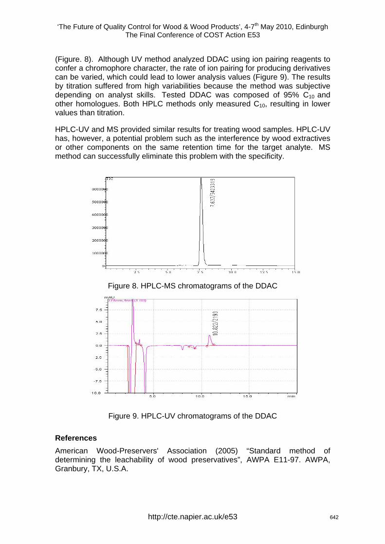
‘The Future of Quality Control for Wood & Wood Products’, 4-7th May 2010, Edinburgh The Final Conference of COST Action E53
(Figure. 8). Although UV method analyzed DDAC using ion pairing reagents to confer a chromophore character, the rate of ion pairing for producing derivatives can be varied, which could lead to lower analysis values (Figure 9). The results by titration suffered from high variabilities because the method was subjective depending on analyst skills. Tested DDAC was composed of 95% C10 and other homologues. Both HPLC methods only measured C10, resulting in lower values than titration.
HPLC-UV and MS provided similar results for treating wood samples. HPLC-UV has, however, a potential problem such as the interference by wood extractives or other components on the same retention time for the target analyte. MS method can successfully eliminate this problem with the specificity.
Figure 8. HPLC-MS chromatograms of the DDAC
Figure 9. HPLC-UV chromatograms of the DDAC
References American Wood-Preservers' Association (2005) “Standard method of determining the leachability of wood preservatives”, AWPA E11-97. AWPA, Granbury, TX, U.S.A.
http://cte.napier.ac.uk/e53 642
‘The Future of Quality Control for Wood & Wood Products’, 4-7th May 2010, Edinburgh The Final Conference of COST Action E53
Ford, M.J., L.E. Tetler, J.O. White and D.U. Rimmer (2002) “Determination of alkyl benzyl and dialkyl dimethyl quaternary ammonium biocides in occupational hygiene and environmental media by liquid chromatography with electrospray ionization mass spectrometry and tandem mass spectrometry”.
Forest Service (2005) “Forest Statistics”, Korean Forest Service.
Forest Service (2009) “Act on the Promotion and Management of Forest Resources”, Korean Forest Service.
Forest Service (2009) “Act on Promotion of Forestry and Mountain Villages”, Korean Forest Service.
Kang, S.M., M.Y. Cho, G.Y. Kim and J.A. Koo (2007) “Determination of Quaternary Ammonium Compounds (DBAC, DDAC) using HPLC”, 2007 proceedings of the Korean society of wood science and technology annual meeting.
Kang, S.M., M.Y. Cho, S.Y. Park and S.K. Kim (2008) “Developing Analytical Methods for Determination of Quaternary Ammonium Compounds (DDAC) using HPLC-MS”, 2008 proceedings of the Korean society of wood science and technology annual meeting.
KFRI (2007) “Notice 2007-09 on Quality approval”, Korea Forest Research Institute.
Laopaiboon L., S.J. Hall and R.N. Smith (2002) “The effect of a quaternary ammonium biocide on the performance and characteristics of laboratory-scale rotating biological contactors” Journal of Applied Microbiology. 93, 1051-1058.
Ministry of Environment (2007)”Notice 2007-152 on ban or limitation of chemical production, import and usage “, Korea Ministry of Environment.
http://cte.napier.ac.uk/e53 643
‘The Future of Quality Control for Wood & Wood Products’, 4-7th May 2010, Edinburgh The Final Conference of COST Action E53
Lumber value of dead and sound black spruce trees in the boreal forest of Québec
J.Barrette1, D.Pothier2, I. Duchesne3 & N. Gélinas4
.
1 Introduction The forest industry in Québec (Canada) is going through an important economic crisis. It has to deal with the economic slowdown of the U.S. market and with the reduction of its annual allowable cut coming from public land. As a result, many forest industries had to shut down temporarily or permanently. In order to help the forest industry, the government of Québec decided to allocate dead and sound wood in addition to the annual allowable cut of living trees. Dead and sound wood comes from standing trees that have died recently and that do not show signs of decay. In the North Shore region of Québec it can represent as much as 20% percent of the volume of an old-growth forest. This special allowance is seen by the government as a good way to help the industry as it brings more timber to the sawmills, which is especially important in a period of economic crisis. However, the use of dead and sound wood by the sawmillers is sometimes criticized. Indeed, many sawmillers complain about the poor quality and value of the boards produced from this type of wood. Yet, the stumpage price of dead and sound trees harvested in the public forests of the province is the same as that of living trees.
The aim of this project is to compare the wood properties and value of the dead and sound wood with those of living trees.
2 Methods Our study was conducted in the Québec North Shore region, in the northeastern part of the Canadian boreal forest. This area is mainly characterized by old-growth forests of uneven age structure. The forest stands are dominated by black spruce (Picea mariana (Mill.)) with balsam fir (Abies balsamea (L.) Mill), white birch (Betula papyrifera Marsh.) and trembling aspen (Populus tremuloides Michx.) as co-dominant species.
1 PhD student, [email protected] Université Laval, Canada, 2 Professor, [email protected] Université Laval, Canada 3 Research Scientist, [email protected] FPInnovations, Forintek Division, Canada 4 Professor, [email protected] Université Laval, Canada
http://cte.napier.ac.uk/e53 644
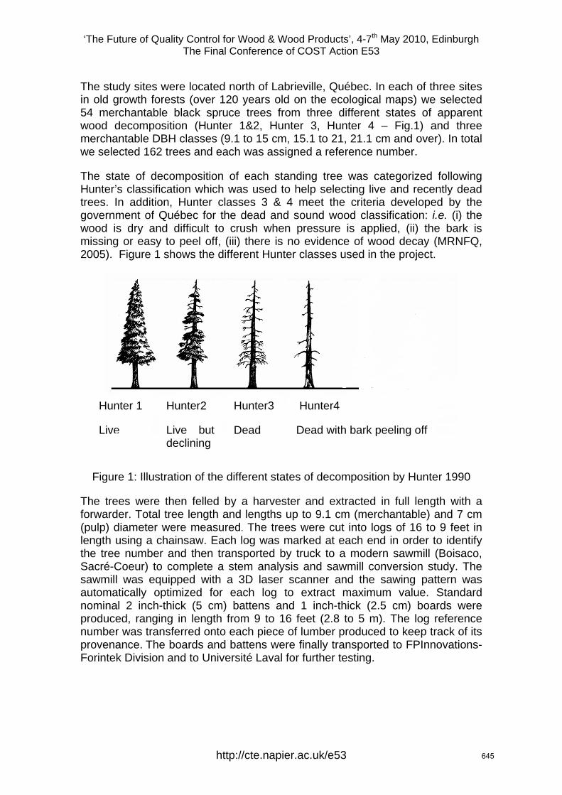
‘The Future of Quality Control for Wood & Wood Products’, 4-7th May 2010, Edinburgh The Final Conference of COST Action E53
The study sites were located north of Labrieville, Québec. In each of three sites in old growth forests (over 120 years old on the ecological maps) we selected 54 merchantable black spruce trees from three different states of apparent wood decomposition (Hunter 1&2, Hunter 3, Hunter 4 – Fig.1) and three merchantable DBH classes (9.1 to 15 cm, 15.1 to 21, 21.1 cm and over). In total we selected 162 trees and each was assigned a reference number.
The state of decomposition of each standing tree was categorized following Hunter’s classification which was used to help selecting live and recently dead trees. In addition, Hunter classes 3 & 4 meet the criteria developed by the government of Québec for the dead and sound wood classification: i.e. (i) the wood is dry and difficult to crush when pressure is applied, (ii) the bark is missing or easy to peel off, (iii) there is no evidence of wood decay (MRNFQ, 2005). Figure 1 shows the different Hunter classes used in the project.
Hunter 1
Live
Hunter2
Live but declining
Hunter3
Dead
Hunter4
Dead with bark peeling off
Figure 1: Illustration of the different states of decomposition by Hunter 1990
The trees were then felled by a harvester and extracted in full length with a forwarder. Total tree length and lengths up to 9.1 cm (merchantable) and 7 cm (pulp) diameter were measured. The trees were cut into logs of 16 to 9 feet in length using a chainsaw. Each log was marked at each end in order to identify the tree number and then transported by truck to a modern sawmill (Boisaco, Sacré-Coeur) to complete a stem analysis and sawmill conversion study. The sawmill was equipped with a 3D laser scanner and the sawing pattern was automatically optimized for each log to extract maximum value. Standard nominal 2 inch-thick (5 cm) battens and 1 inch-thick (2.5 cm) boards were produced, ranging in length from 9 to 16 feet (2.8 to 5 m). The log reference number was transferred onto each piece of lumber produced to keep track of its provenance. The boards and battens were finally transported to FPInnovations- Forintek Division and to Université Laval for further testing.
http://cte.napier.ac.uk/e53 645
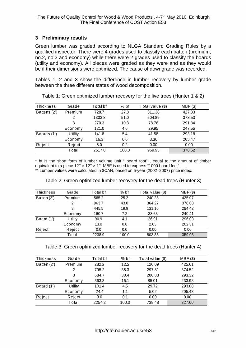
‘The Future of Quality Control for Wood & Wood Products’, 4-7th May 2010, Edinburgh The Final Conference of COST Action E53
3 Preliminary results Green lumber was graded according to NLGA Standard Grading Rules by a qualified inspector. There were 4 grades used to classify each batten (premium, no.2, no.3 and economy) while there were 2 grades used to classify the boards (utility and economy). All pieces were graded as they were and as they would be if their dimensions were optimized. The cause of downgrade was recorded.
Tables 1, 2 and 3 show the difference in lumber recovery by lumber grade between the three different states of wood decomposition.
Table 1: Green optimized lumber recovery for the live trees (Hunter 1 & 2)
Thickness Grade Total bf % bf Tota l value ($) MBF ($)Battens (2') Premium 728.7 27.8 311.38 427.33
2 1333.8 51.0 504.89 378.533 270.3 10.3 78.76 291.34
Economy 121.0 4.6 29.95 247.55Boards (1') Utility 141.8 5.4 41.58 293.18
Economy 16.3 0.6 3.36 205.47Reject Reject 5.0 0.2 0.00 0.00
Total 2617.0 100.0 969.93 370.62
* bf is the short form of lumber volume unit “ board foot” , equal to the amount of timber equivalent to a piece 12’’ × 12’’ × 1’’. MBF is used to express “1000 board feet”. ** Lumber values were calculated in $CAN, based on 5-year (2002–2007) price index.
Table 2: Green optimized lumber recovery for the dead trees (Hunter 3)
Thickness Grade Total bf % bf Total value ($) MBF ($)Batten (2') Premium 565.2 25.2 240.23 425.07
2 963.7 43.0 364.27 378.003 445.5 19.9 131.16 294.42
Economy 160.7 7.2 38.63 240.41Board (1') Utility 90.9 4.1 26.91 296.00
Economy 13.0 0.6 2.63 202.31Reject Reject 0.0 0.0 0.00 0.00
Total 2238.9 100.0 803.83 359.03
Table 3: Green optimized lumber recovery for the dead trees (Hunter 4)
Thickness Grade Total bf % bf Total value ($) MBF ($)Batten (2') Premium 282.2 12.5 120.09 425.61
2 795.2 35.3 297.81 374.523 684.7 30.4 200.83 293.32
Economy 363.3 16.1 85.01 233.98Board (1') Utility 101.4 4.5 29.72 293.08
Economy 24.4 1.1 5.02 205.43Reject Reject 3.0 0.1 0.00 0.00
Total 2254.2 100.0 738.48 327.60
http://cte.napier.ac.uk/e53 646
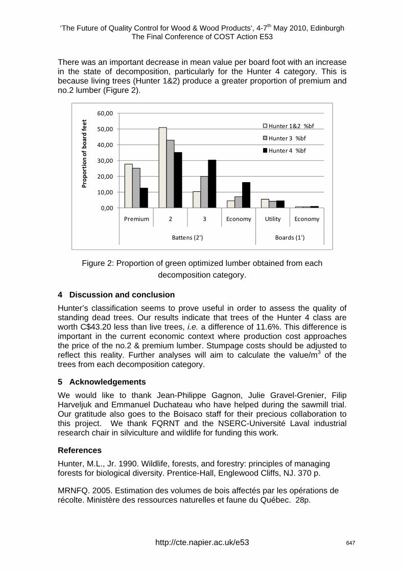
‘The Future of Quality Control for Wood & Wood Products’, 4-7th May 2010, Edinburgh The Final Conference of COST Action E53
There was an important decrease in mean value per board foot with an increase in the state of decomposition, particularly for the Hunter 4 category. This is because living trees (Hunter 1&2) produce a greater proportion of premium and no.2 lumber (Figure 2).
0,00
10,00
20,00
30,00
40,00
50,00
60,00
Premium 2 3 Economy Utility Economy
Battens (2') Boards (1')
Prop
ortion
of bo
ard feet Hunter 1&2 %bf
Hunter 3 %bf
Hunter 4 %bf
Figure 2: Proportion of green optimized lumber obtained from each decomposition category.
4 Discussion and conclusion Hunter’s classification seems to prove useful in order to assess the quality of standing dead trees. Our results indicate that trees of the Hunter 4 class are worth C$43.20 less than live trees, i.e. a difference of 11.6%. This difference is important in the current economic context where production cost approaches the price of the no.2 & premium lumber. Stumpage costs should be adjusted to reflect this reality. Further analyses will aim to calculate the value/m3 of the trees from each decomposition category.
5 Acknowledgements We would like to thank Jean-Philippe Gagnon, Julie Gravel-Grenier, Filip Harveljuk and Emmanuel Duchateau who have helped during the sawmill trial. Our gratitude also goes to the Boisaco staff for their precious collaboration to this project. We thank FQRNT and the NSERC-Université Laval industrial research chair in silviculture and wildlife for funding this work.
References Hunter, M.L., Jr. 1990. Wildlife, forests, and forestry: principles of managing forests for biological diversity. Prentice-Hall, Englewood Cliffs, NJ. 370 p.
MRNFQ. 2005. Estimation des volumes de bois affectés par les opérations de récolte. Ministère des ressources naturelles et faune du Québec. 28p.
http://cte.napier.ac.uk/e53 647

“The future of quality control for wood & wood products”, Proceedings of the final conference of COST Action E53, Editors D.J. Ridley-Ellis & J.R. Moore, Edinburgh (UK), 2010. ISBN 978-09566187-0-2 [electronic proceedings]. Published by: Forest Products Research Institute / Centre for Timber Engineering, Edinburgh Napier University, 10 Colinton Road, Edinburgh EH10 5DT, UK http://cte.napier.ac.uk