Relational Database Management System - PTU (Punjab Technical ...

Self Learning Material

Relational Database

Management System (PDCA-104)

Course: Post Graduate Diploma in

Computer Applications

Semester-I

Distance Education Programme

I.K. Gujral Punjab Technical University

Jalandhar

I.K. Gujral Punjab Technical University

Syllabus

Scheme of (PGDCA)

Batch 2012 Onwards

PDCA 104 Relational Database Management System Max. Marks: 100

External Assessment: 60

Internal Assessment: 40

Objective: The objective of this course is to help the students to get knowledge about databases its

architecture various models. Students will be able to develop databases with all the constraints which

help in storing and retrieving data easily.

Unit –I

An Overview of DBMS and DB Systems Architecture : Introduction to Database Management

systems, Data Models, Database System Architecture, Relational Database Management systems,

Candidate Key and Primary Key in a Relation, Foreign Keys, Relational Operators, Set Operations on

Relations, Attribute domains and their Implementation. The Normalization Process : Introduction,

first Normal Form, Partial Dependencies, Second Normal Form, data Anomalies in 2NF Relations,

Transitive Dependencies, Third Normal Form.

Unit- II

The Entity Relationship Model: The Entity Relationship Model, Entities and Attributes,

Relationships, One-One Relationships, Many-to-one Relationships, Normalizing the Model, Table

instance charts. Interactive SQL : SQL commands , Data Definition Language Commands, Data

Manipulation Language Commands, insertion of data into the tables, Viewing of data into the tables,

Deletion operations, updating the contents of the table, modifying the structure of the table, renaming

table, destroying tables, Data Constraints, Type of Data Constraint, Column Level Constraint, Table

Level Constraint.

Unit- III

Viewing The Data : Computations on Table Data, Arithmetic Operators, Logical Operators,

Comparison Operators, Range Searching, Pattern Searching, ORACLE FUNCTIONS, Number

Functions, Group Functions, Scalar Functions, Data Conversion Functions, Manipulating Dates in

SQl , Character Functions, Sub queries and Joins : Joins, Equi Joins, Non Equi Joins, Self Joins,

Outer Joins, Sub Queries, Correlated Queries, Using Set Operators:- Union , Intersect, Minus.

Unit- IV

Views and Indexes : Definition and Advantages Views, Creating and Altering Views, Using Views,

Indexed Views, Partitioned views, Definition and Advantages of Indexes, Composite Index and

Unique Indexes, Accessing Data With and without Indexes, Creating Indexes and Statistics.

Introduction to PL/SQL : Advantage of PL/SQL, The Generic PL/SQL Block, The Declaration

Section, The Begin Section, The End Section, The Character set, Literals, PL/SQL Data types,

Variables, Constants, Logical Comparison, Conditional Control in PL/SQL, Iterative Control.

Suggested Readings/ Books

1 .Ramez Elmasri, "Fundamentals of Database Systems”, Edition 5th, Pearson Education India, 2009 2. JD Ullman,Garcia-Molina, “Database System: The Complete Book”, Edition 4th, Pearson Education India,2009 3. S.K Singh, “Database Systems: Concepts, Design and Applications”, Edition 2 nd, Pearson Education India 2008 4. C.J Date, “An Introduction to Database System”, Edition 8th, Pearson Education India. 2009 5 Ivan Bayross,”Database Concepts & Systems for Students”, Edition 3rd, Shroff Publishers & Distributors Pvt Limited, 2009.

Table of Contents

Chapter No. Title Written By Page No.

1 Introduction to Database System Ms. Preeti Sharma

Department of Computer

Science Engineering, SBS

Technical Campus, Ferozpur

1

2 Database keys and Constraints Ms. Preeti Sharma




18

3 Normalization in DBMS Ms. Preeti Sharma




33

4 Entity Relationship Model Ms. Preeti Sharma




48

5 Interactive Structure Query

Language

(SQL)

Ms. Preeti Sharma




62

6 Data Retrieval & Transaction

Control using SQL

Ms. Preeti Sharma




77

7 Data Constraints using SQL Ms. Preeti Sharma




110

8 Data Viewing using SQL - Part 1 Dr. Gulshan Ahuja




122





134





148

11 Data Viewing using SQL - Part 4 Dr. Gulshan Ahuja Department of Computer Science Engineering, SBS


171

12 Views using SQL Dr. Gulshan Ahuja Department of Computer Science Engineering, SBS


190

13 Indexes using SQL Dr. Gulshan Ahuja Department of Computer Science Engineering, SBS


203

14 Introduction to PL/SQL Dr. Gulshan Ahuja Department of Computer Science Engineering, SBS


213

15 PL/SQL Basics Dr. Gulshan Ahuja

Department of Computer Science Engineering, SBS


223

Reviewed by: Dr. Krishan Saluja

Department of Computer Science and Engineering,

SBS Technical Campus, Ferozpur

© IK Gujral Punjab Technical University Jalandhar

All rights reserved with IK Gujral Punjab Technical University

Jalandhar

1

Unit 1

Lesson 1 - Introduction to database systems

1.1. Objective

1.2. Introduction to Database Systems

1.3. Components of Database System

1.3.1. Software

1.3.2. Hardware

1.3.3. Data

1.3.4. Procedure

1.4. Introduction to DBMS

1.5. Architecture of DBMS

1.5.1. Internal Data Level

1.5.2. Conceptual Data Level

1.5.3. External Data Level

1.6. Data independence

1.6.1. Logical data independence

1.6.2. Physical data independence

1.7. Data Models

1.7.1. Entity-Relationship Model

1.7.2. Network model

1.7.3. Hierarchical model

1.7.4. Object oriented models

1.7.5. Relational Model

1.8. Summary

1.9. Glossary

1.10. Questions/Answers

1.11. References

1.12. Suggested readings

1.1 Objective

To learn the basic concepts of database systems

To understand the components of a database system

1.2 Introduction to Database Systems:

Databases and database technology have a major impact on the growing use of Computers. It is fair

to say that databases play a critical role in almost all areas where Computers are used, including

Page 1 of 252

2

business, electronic commerce, engineering, medicine, Genetics, law, education, and library science.

The word database is so common used that we must begin by defining what a database is.

1.3 Components of Database System:

Following are the basic components of a DBMS:

1.3.1 Software:

Software is the part and parcel of DBMS. This is the programs set used to handle the database

and to manage and control the automated database.

DBMS software itself, is the most important software component in the overall

System.

An operating system in the network, for sharing the data of database among many users.

1.3.2 Hardware:

Hardware is a set of physical, electronic devices such as computers (together with associated I/O

devices like disk drives), storage devices, I/O channels, electromechanical devices that hook up

between computers and the real world systems.

1.3.3 Data:

Data is the crucial part of the DBMS. The prime purpose of DBMS is to process the data. In DBMS,

databases are constructed, defined and then the data is reposited, updating are made and retrieved

to and from the databases. The database contains both the metadata (data about data or description

about data) and actual (or operational) data.

1.3.4 Procedure:

Procedures refer to the rules and directions that will help to design the database and to use the

DBMS. These may include.

Procedure for the installation of the new DBMS.

To log on to the DBMS.

To access the DBMS.

To backing up the database.

1.4 Introduction to DBMS:

A database is a shared, integrated computer structure that stores a collection of:

End-user data, that is, raw facts of interest to the end user.

Metadata, or data about data, through which the end-user data are integrated and managed.

The metadata provides a description of the data characteristics and the set of relationships that links

the data found Within the database. For example, the metadata component stores information such

as the name of each data element, the type of values (numeric, dates, or text) stored in each data

element, whether or not the data element can be left empty, and so on. The metadata provides

information that complements and expands the value and use of the data.

In short, metadata present a more complete picture of the data in the database. Given the

characteristics of metadata, you might hear a database described as a ―collection of self-describing

data.‖

Page 2 of 252

3

A database management system (DBMS) is a collection of programs that manages the database

structure and controls access to the data stored in the database. In a sense, a database resembles a

very well-organized electronic filing cabinet in which powerful software, known as a database

management system, helps manage the cabinet‘s contents.

1.5 Architecture of DBMS:

Three of the four important characteristics of the database approach are

(1) Use of a catalog to store the database description (schema) so as to make it self-describing.

(2) Insulation of programs and data (program-data and program-operation independence)

(3) Support of multiple user views.

In this section we specify an architecture for database systems, called the three-schema

architecture that was proposed to help achieve and visualize these characteristics.

1.5.1 Internal Level:

The internal level has an internal schema, which describes the physical storage structure of the

database. The internal schema uses a physical data model and describes the complete details of data

storage and access paths in the database.

1.5.2 Conceptual Data Level:

The conceptual level has a conceptual schema, which describes the structure of the whole

database for a community of users. The conceptual schema hides the details of physical storage

structures and concentrates on describing entities, data types, relationships, user operations, and

constraints. Usually, a representational data model is used to describe the conceptual schema when

a database system is implemented. This implementation conceptual schema is often based on a

conceptual schema design in a high-level data model.

1.5.3 External Data Level:

The external or view level includes a number of external schemas or user views. Each external

schema describes the part of the database that a particular user group is interested in and hides the

rest of the database from that user group. As in the previous level, each external schema is typically

implemented using a representational data model, possibly based on an external schema design in a

high-level data model.

1.6 Data independence:

The three-schema architecture can be used to further explain the concept of data independence,

which can be defined as the capacity to change the schema at one level of a database system without

having to change the schema at the next higher level. We can define two types of data independence:

Page 3 of 252

4

1.6.1 Logical data independence:

It is the capacity to change the conceptual schema without having to change external schemas or

application programs. We may change the conceptual schema to expand the database (by adding a

record type or data item), to change constraints, or to reduce the database (by removing a record type

or data item). In the last case, external schemas that refer only to the remaining data should not be

affected. Only the view definition and the mappings need to be changed in a DBMS that supports

logical data independence. After the conceptual schema undergoes a logical reorganization,

application programs that reference the external schema constructs must work as before.

1.6.2 Physical data independence:

It is the capacity to change the internal schema without having to change the conceptual schema.

Hence, the external schemas need not be changed as well. Changes to the internal schema may be

needed because some physical files were reorganized—for example, by creating additional access

structures—to improve the performance of retrieval or update. If the same data as before remains in

the database, we should not have to change the conceptual schema.

1.7 Data Models:

One fundamental characteristic of the database approach is that it provides some level of data

abstraction.

Data abstraction generally refers to the suppression of details of data organization and storage, and

the highlighting of the essential features for an improved understanding of data. One of the main

characteristics of the database approach is to support data abstraction so that different users can

perceive data at their preferred level of detail.

A data model is a collection of concepts that can be used to describe the structure of a database. It

provides the necessary means to achieve this abstraction. By structure of a database, we mean the

data types, relationships, and constraints that apply to the data. Most data models also include a set

of basic operations for specifying retrievals and updates on the database.

Many data models have been proposed for describing the databases as explained in subsequent

paragraphs.

1.7.1 Entity-Relationship Model:

It is a semantic model that capture meaning.

Page 4 of 252

5

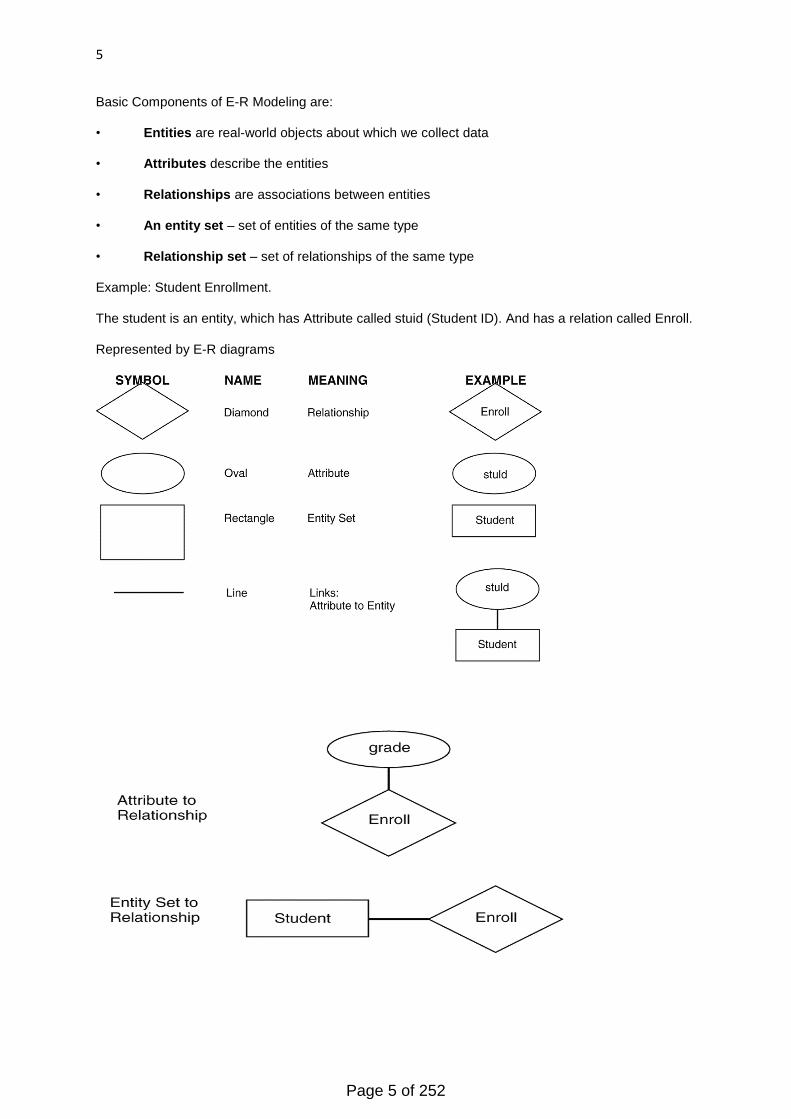
Basic Components of E-R Modeling are:

• Entities are real-world objects about which we collect data

• Attributes describe the entities

• Relationships are associations between entities

• An entity set – set of entities of the same type

• Relationship set – set of relationships of the same type

Example: Student Enrollment.

The student is an entity, which has Attribute called stuid (Student ID). And has a relation called Enroll.

Represented by E-R diagrams

Page 5 of 252

6

Example: Student Relationship: Student is enrolling for admission. The student is Related to Grades

only when its has unique Id (stuid)

1.7.2 Network model:

The network model was created to represent complex data relationships more effectively than the

hierarchical model, to improve database performance, and to impose a database standard. In the

network model, the user perceives the network database as a collection of records in 1:M

relationships. However, unlike the hierarchical model, the network model allows a record to have

more than one parent. While the network database model is generally not used today, the definitions

of standard database concepts that emerged with the network model are still used by modern data

models. Some important concepts that were defined at this time are:

The schema, which is the conceptual organization of the entire database as viewed by the

database administrator.

The subschema, which defines the portion of the database ―seen‖ by the application

programs that actually produce the desired information from the data contained within the database.

A data management language (DML), which defines the environment in which data can be

managed and to work with the data in the database.

A schema data definition language (DDL), which enables the database administrator to

define the schema components.

1.7.3 Hierarchical model:

The hierarchical model was developed to manage large amounts of data for complex manufacturing

projects such as the Apollo rocket that landed on the moon in 1969. Its basic logical structure is

represented by an upside-down tree. The hierarchical structure contains levels, or segments. A

segment is the equivalent of a file system‘s record type. Within the hierarchy, a higher layer is

perceived as the parent of the segment directly beneath it, which is called the child. The hierarchical

model depicts a set of one-to-many (1:M) relationships between a parent and its child segments.

(Each parent can have many children, but each child has only one parent.)

1.7.4 Object oriented models:

It uses the E-R modeling as a basis, but extended to include inheritance and encapsulation. Objects

have both behavior and state.

• Behavior is defined by the methods (functions or procedures)

• The state is defined by attributes

The designer defines classes with methods, attributes and relationships.

• Database objects have persistence

• Classes related by class hierarchies

• Each object has a unique object ID

1.7.5 Relational Model:

Page 6 of 252

7

It is a table and Record-based model. Relational database modeling is a logical-level model

proposed by Dr E.F. Codd. It has the following characteristics.

• Uses relations, represented as tables

• Tables represent relationships as well as entities

• Based on mathematical relations

• Columns of tables represent attributes

Successor to earlier record-based models—hierarchical and network

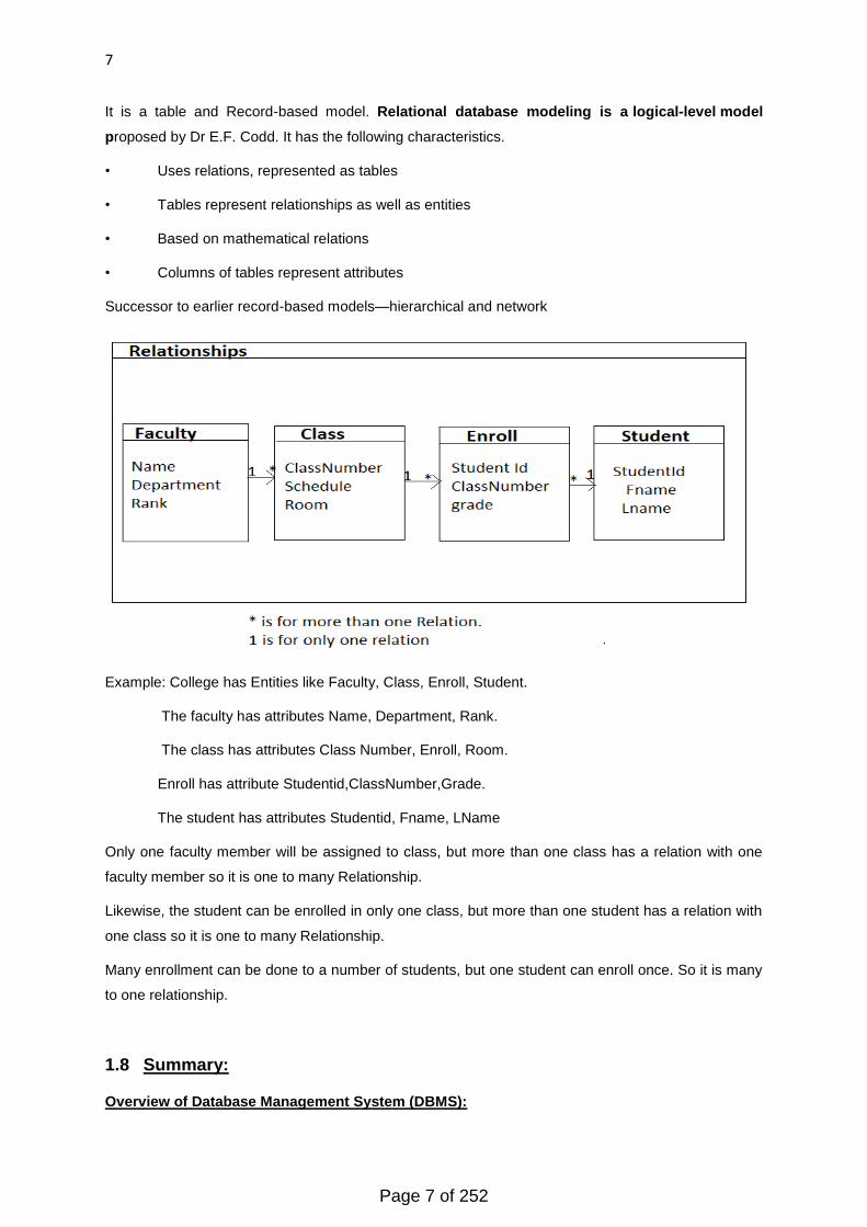
Example: College has Entities like Faculty, Class, Enroll, Student.

The faculty has attributes Name, Department, Rank.

The class has attributes Class Number, Enroll, Room.

Enroll has attribute Studentid,ClassNumber,Grade.

The student has attributes Studentid, Fname, LName

Only one faculty member will be assigned to class, but more than one class has a relation with one

faculty member so it is one to many Relationship.

Likewise, the student can be enrolled in only one class, but more than one student has a relation with

one class so it is one to many Relationship.

Many enrollment can be done to a number of students, but one student can enroll once. So it is many

to one relationship.

1.8 Summary:

Overview of Database Management System (DBMS):

Page 7 of 252

8

Related data collated to form Database, tabulated in such way that it can be managed, accessed and

updated easily.

Components of DBMS:

There are following components of a DBMS

• Software

• Hardware

• Data

• Procedures

Software

The programs and other operating information used by a computer.

Hardware

The machines, wiring, and other physical components of a computer or other electronic system.

Data

Data is a set of values of qualitative or quantitative variables; restated, data are individual pieces

of information. Data in computing (or data processing) are represented in a structure that is

often tabular (represented by rows and columns).

Procedures


DBMS.

Introduction to DBMS

DBMS: A collection of programs that enables you to store, modify, and extract information from

a database. There are many different types of DBMSs, ranging from

small systems that run on personal computers to huge systems that run on mainframes. The following

are examples of database applications:

Computerized library systems

Automated teller machines

Flight reservation systems

Computerized parts inventory systems

Database System Architecture:

It consist of Following Levels:

EXTERNAL LEVEL

How data is viewed by an individual user

CONCEPTUAL LEVEL

Page 8 of 252

http://en.wikipedia.org/wiki/Value_(computer_science)

http://en.wikipedia.org/wiki/Qualitative_data

http://en.wikipedia.org/wiki/Quantitative_data

http://en.wikipedia.org/wiki/Variable_and_attribute_(research)

http://en.wikipedia.org/wiki/Information

http://en.wikipedia.org/wiki/Computing

http://en.wikipedia.org/wiki/Data_processing

http://en.wikipedia.org/wiki/Structure

http://en.wikipedia.org/wiki/Tabular

http://en.wikipedia.org/wiki/Row_(database)

http://en.wikipedia.org/wiki/Column_(database)

http://www.webopedia.com/TERM/P/program.html

http://www.webopedia.com/TERM/S/store.html

http://www.webopedia.com/TERM/D/database.html

http://www.webopedia.com/TERM/S/system.html

http://www.webopedia.com/TERM/R/run.html

http://www.webopedia.com/TERM/P/personal_computer.html

http://www.webopedia.com/TERM/M/mainframe.html

http://www.webopedia.com/TERM/D/database_management_system_DBMS.html

9

How data is viewed by a community of users

INTERNAL LEVEL

How data is physically stored

Data Model:

A data model is an abstraction of a complex real-world data environment. Database designers use

data models to communicate with applications programmers and end users. The basic data-modeling

components are entities,attributes, relationships, and constraints. Business rules are used to identify

and define the basic modeling components within a specific real-world environment.

Hierarchical Model:The hierarchical are no longer used, but some of the concepts are found in

current data models. The hierarchical model depicts a set of one-to-many (1:M) relationships between

a parent and its children segments.

Network Model:The network model uses sets to represent 1:M relationships between record types.

Relational Model:The relational model is the current database implementation standard. In the

relational model, the end user perceives the data as being stored in tables. Tables are related to each

other by means of common values in common attributes. The entity relationship (ER) model is a

popular graphical tool for data modeling that complements the relational model. The ER model allows

database designers to visually present different views of the data—as seen by database designers,

programmers, and end users—and to integrate the data into a common

framework.

Entity Relationship Model: The ER model is based on the following components:

Entity. Earlier in this chapter, an entity was defined as anything about which data are to be

collected and stored. An entity is represented in the ERD by a rectangle, also known as an

entity box. The name of the entity, a noun, is written in the center of the rectangle. The entity

name is generally written in capital letters and is written in the singular form: PAINTER rather

than PAINTERS, and EMPLOYEE rather than EMPLOYEES.Usually, when applying the ERD

to the relational model, an entity is mapped to a relational table. Each row in the relational

table is known as an entity instance or entity occurrence in the ER model.Each entity is

described by a set of attributes that describes particular characteristics of the entity. For

example, the entity EMPLOYEE will have attributes such as a Social Security number, a last

name, and a first name.

Relationships. Relationships describe associations among data. Most relationships describe

associations between two entities. When the basic data model components were introduced,

three types of relationships among data were illustrated: one-to-many (1:M), many-to-many

(M:N), and one-to-one (1:1).

The ER model uses the term connectivity to label the relationship types. The name of the

relationship is usually an activeor passive verb. For example, a PAINTER paints many PAINTINGs;

an EMPLOYEE learns many SKILLs; an EMPLOYEE manages a STORE.

Object Oriented Model: The object-oriented data model (OODM) uses objects as the basic modeling

structure. An object resembles an entity

Page 9 of 252

10

in that it includes the facts that define it. But unlike an entity, the object also includes information

about relationships between the facts, as well as relationships with other objects, thus giving its data

more meaning.

Relational Model: The relational model has adopted many object-oriented (OO) extensions to

become the extended relational data model (ERDM). Object/relational database management

systems (O/R DBMS) were developed to implement the ERDM. At this point, the OODM is largely

used in specialized engineering and scientific applications, while the ERDM is primarily geared to

business applications. Although the most likely future scenario is an increasing merger of OODM and

ERDM technologies, both are overshadowed by the need to develop Internet access strategies for

databases. Usually OO data models are depicted using Unified Modeling Language (UML) class

diagrams.

Data-modeling requirements are a function of different data views (global vs. local) and the level of

data abstraction. The American National Standards Institute Standards Planning and Requirements

Committee (ANSI/SPARC) describes three levels of data abstraction: external, conceptual, and

internal. There is also a fourth level of data abstraction, the physical level. This lowest level of data

abstraction is concerned exclusively with physical storage methods.

1.9 Glossary:

DBMS: DATABASE MANAGEMENT SYSTEM.

Software: The programs and other operating information used by a computer.

Hardware: The machines, wiring, and other physical components of a computer or other electronic

system.

Procedure: An established or official way of doing something.

Language: A system of communication used by a particular country or community.

Transaction: A transaction comprises a unit of work performed within a database management

system

Level: A position on a scale of amount, quantity, extent, or quality.

RDBMS: RELATIONAL DATABASE MANAGEMENT SYSTEM.

Models: Description of data at different level

Interface: Interact with (another system, person, etc.).

Relation: A relation is a data structure which consists of a heading and an unordered set of tuples

which share the same type.

Table: A table is an organized set of data elements.

Attribute: An attribute is a property or characteristic.

Record: A record is a collection of data items arranged for processing by a program.

Inheritance: Inheritance allows a class to have the same behavior as another class and extend or

tailor that behavior to provide special action for specific needs.

Encapsulation: The condition of being enclosed.

State: State is defined by the attributes of the object and by the values these have.

Class: A class can be defined as a template/blue print that describes the behaviors/states that the

object of its type support.

Page 10 of 252

11

Object: Objects have states and behaviors. Example: A dog has states - color, name, breed as well

as behaviors -wagging, barking, and eating. An object is an instance of a class.

1.10 Questions/Answers:

Q1. What are the different components of Database Management System?

Ans: There are following components of a DBMS

• Software

• Hardware

• Data

• Procedures

Software

Software is the part and parcel of DBMS. This is the programs set used to handle the database and

to manage and control the automated database.

• DBMS software itself, is the most important software component in the overall system

• An operating system like network software used in the network, for sharing the data of

database among many users.

Hardware

Hardware is a set of physical, electronic devices such as computers (together with associated I/O

devices like disk drives), storage devices, I/O channels, electromechanical devices that hook up

between computers and the real world systems.

Data

Data is the crucial part of the DBMS. The prime purpose of DBMS is to process the data. In DBMS,

databases are constructed,defined and then data is reposited, updations are made and retrieved to

and from the databases. The database contains both the metadata (data about data or description

about data) and actual (or operational) data.

Procedures


DBMS. The users that maintain and operate the These may include.

• Procedure for the installation of the new DBMS.

• To logging on to the DBMS.

• To access the DBMS.

• To backing up the database.

Q2.What is the different segments of DBMS?

Page 11 of 252

12

Ans: DBMS consists of following segments:

• A modelling language, used for structural characterization, or Database schema. Common database

models are network, relational, hierarchical and object based. These Models are distinguished from

one another in a way how they connect related information.

• A database engine that shape up the storage of data, even if it is record, field, object or file, to

counterbalance between better fetching of data and businesslikeness.

• A database query language, such as SQL, that prepares the developers to write programs that

extract data from the database, represent it to the user, and save changes.

• A transaction mechanism that verifies data entered in allowed types before its storage, and make

sure that multiple users cannot simultaneously update the same information, potentially corrupting the

data.

Q3.Explain the Database System Architecture?

Ans: Data are actually stored as bits, or numbers and strings, but it is difficult to work with data at this

level.

Schema:

Description of data at some level. We will be concerned with three forms of schemas:

• Physical

• Conceptual

• External.

Physical Data Level

The physical schema describing details of how data is stored: files, indices, etc. On the random

access disk system. It also typically describes the layout of record, files and type of files.

Early applications worked at this level - explicitly dealt with details. E.g., Minimizing physical distances

between related data and organizing the data structures within the file (blocked records, linked lists of

blocks, etc.)

The problem at this level are as follows:

• Routines are hard to cope with a physical representation.

• It is difficult to make changes to the data structure.

• Difficulty in the Rapid implementation of new features.

Conceptual Data Level

Also called as the Logical level

It hides the details of the physical level.

• In the relational modelling, the conceptual schema presents data as a set of tables.

Page 12 of 252

13

The DBMS maps data access between the conceptual to physical schemas automatically.

• Physical schema can be changed without changing applications:

• DBMS must change mapping from conceptual to physical.

• Referred to as physical data independence.

External Data Level

In the relational model, the external schema also presents data as a set of relations. It specifies

a view of the data in terms of the conceptual level. It is cater to the needs of a particular category of

users. Segment of stored data should not be seen by some users

Examples:

• Students should not see salaries of faculty.

• Faculty should not see billing or payment data.

Applications are written in terms of an external schema. The external view will be computed when

accessed. It is not possible to store it. Different external schemas can be provided to different

categories of users. Translation from external level to conceptual level is done automatically by DBMS

at run time is called conceptual data independence.

Q4. Explain various data models?

Ans: Model: languages and tool for describing:

• Integrity constraints, domains described by DDL

• Conceptual/logical and external schema described by the data definition language (DDL)

• Directives that influence the physical schema (affects performance, not semantics) are described by

the storage definition language (SDL)

• Operations on the data described by the data manipulation language (DML)

Data Independence

Logical data independence

Page 13 of 252

14

• Prevention of external models to cope with the changes in the logical model

• Occurs at user interface level

Physical data independence

• Prevention of logical model to changes in internal model

• Occurs at logical interface level

Entity-Relationship Model

It is a Semantic model that capture meaning.

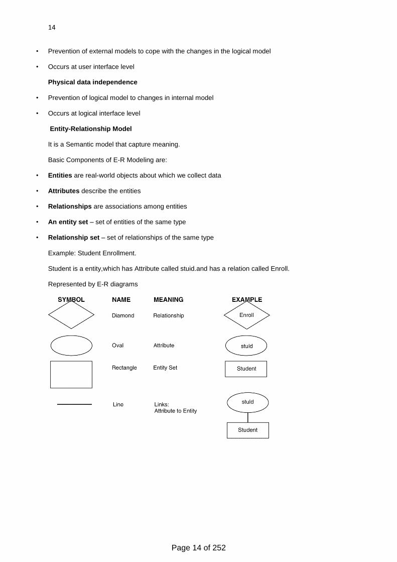
Basic Components of E-R Modeling are:

• Entities are real-world objects about which we collect data

• Attributes describe the entities

• Relationships are associations among entities

• An entity set – set of entities of the same type

• Relationship set – set of relationships of the same type

Example: Student Enrollment.

Student is a entity,which has Attribute called stuid.and has a relation called Enroll.

Represented by E-R diagrams

Page 14 of 252

15

Example: Student Relationship: Student is enrolling for admission.

Student is Related to Grades only when its has unique Id(stuid)

Relational Model

Table and Record-based model.

Relational database modeling is a logical-level model

Proposed by E.F. Codd

• Uses relations, represented as tables

• Tables represent relationships as well as entities

• Based on mathematical relations

• Columns of tables represent attributes

Successor to earlier record-based models—hierarchical and network

Page 15 of 252

16

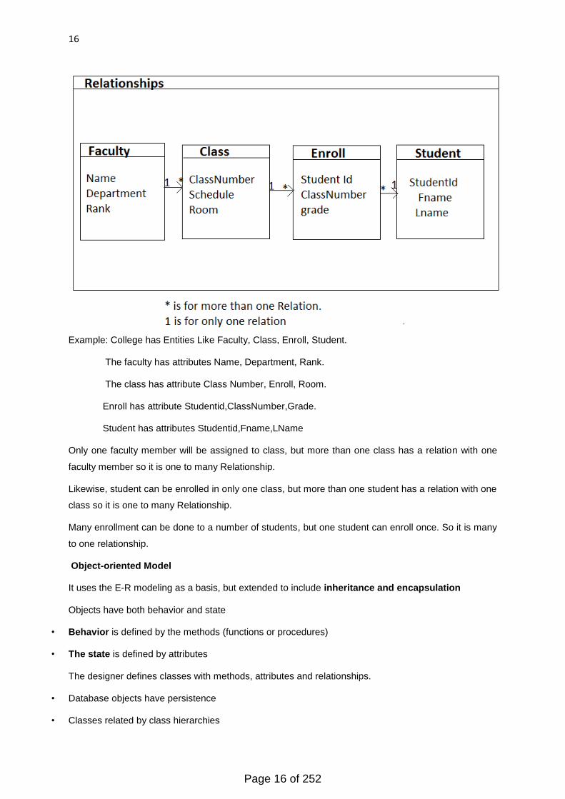
Example: College has Entities Like Faculty, Class, Enroll, Student.

The faculty has attributes Name, Department, Rank.

The class has attribute Class Number, Enroll, Room.

Enroll has attribute Studentid,ClassNumber,Grade.

Student has attributes Studentid,Fname,LName

Only one faculty member will be assigned to class, but more than one class has a relation with one

faculty member so it is one to many Relationship.

Likewise, student can be enrolled in only one class, but more than one student has a relation with one

class so it is one to many Relationship.

Many enrollment can be done to a number of students, but one student can enroll once. So it is many

to one relationship.

Object-oriented Model

It uses the E-R modeling as a basis, but extended to include inheritance and encapsulation

Objects have both behavior and state

• Behavior is defined by the methods (functions or procedures)

• The state is defined by attributes

The designer defines classes with methods, attributes and relationships.

• Database objects have persistence

• Classes related by class hierarchies

Page 16 of 252

17

• Each object has a unique object ID

1.11 References:


http://pages.cs.wisc.edu/~dbbook/

http://pages.cs.wisc.edu/~dbbook/openAccess/thirdEdition/slides/slides3ed.html

http://publib.boulder.ibm.com/infocenter/zos/basics/topic/com.ibm.zos.zmiddbmg/zmiddle_46.

htm

1.12 Suggested readings:

Database Management System (P. K Yadav (Author)

Database Management System (GBTU & MTU) Kedar S (Author)

Concept Of Database Management Systems (DBMS), 2nd Edition Author: V K Pallaw

Page 17 of 252


http://pages.cs.wisc.edu/~dbbook/

http://pages.cs.wisc.edu/~dbbook/openAccess/thirdEdition/slides/slides3ed.html

http://publib.boulder.ibm.com/infocenter/zos/basics/topic/com.ibm.zos.zmiddbmg/zmiddle_46.htm

http://publib.boulder.ibm.com/infocenter/zos/basics/topic/com.ibm.zos.zmiddbmg/zmiddle_46.htm

18

Unit 1

Lesson 2 - Database Keys & Constraints

2.1 Objective

2.2 Introduction to database keys

2.2.1 Candidate key

2.2.2 Primary key

2.2.3 Super key

2.2.4 Foreign key

2.2.5 Alternate key

2.3 Relational operators

2.4 Relational calculus

2.4.1 Tuple oriented

2.4.2 Domain oriented

2.5 Relational algebra

2.5.1 Selection

2.5.2 Projection

2.5.3 Cartesian product

2.5.4 Join

2.5.5 Difference

2.5.6 Division

2.5.7 Union

2.5.8 Intersection

2.6 Summary

2.7 Glossary

2.8 Questions/Answers

2.9 References

2.10 Suggested readings

2.1 Objective

To learn the basic data constraints

To use of data constraints in SQL

2.2 Introduction to database keys:

Database Key as its name says, a basic part of an RDBMS and a significant part of the table

structure. They make sure that each record within a table can be uniquely identified by one or a

combination of fields within the table. They help us to enforce integrity and help identify the

Page 18 of 252

19

relationship between tables. There are three main types of keys, candidate keys, primary keys

and foreign keys.

2.2.1 Candidate key:

A candidate is a subdivision of a super key. It is a single field or the combination of fields that

uniquely identifies each record in the table. The least combination of fields differentiates between

candidate key from a super key.

SID FNAME LNAME CLASS COURSEID

1001 ANUJ SHARMA BCA C1001

1002 ARYAN SHARMA MCA C1002

1003 NEHA JOSHI MCA C1003

As an example, we might have a student id (SID) that uniquely identifies the students in a student

table. This would be a candidate key. But in the same table, we might have the student‘s first

name (FNAME) and last name (LNAME) that also, when combined, uniquely identify the student

in a student table. These would both be candidate keys.

Important criteria for the eligibility of Candidate key:

It must contain unique values

It must not contain null values

Once we have chosen candidate keys we can now select Primary key from these candidate keys.

2.2.2 Primary key:

As its name suggests, it is the primary key of reference for the table and is used throughout the

database to help establish relationships with other tables.

It is a candidate key that is relevant to be the main reference key for the table. As with any candidate

key the primary key

• Must contain unique values.

• Must never be null and uniquely identify each record in the table.

As an example, a student id (SID) might be a primary key in a student table.In the table below we

have selected the candidate key student_id to be our most convenient primary key.




Page 19 of 252

20


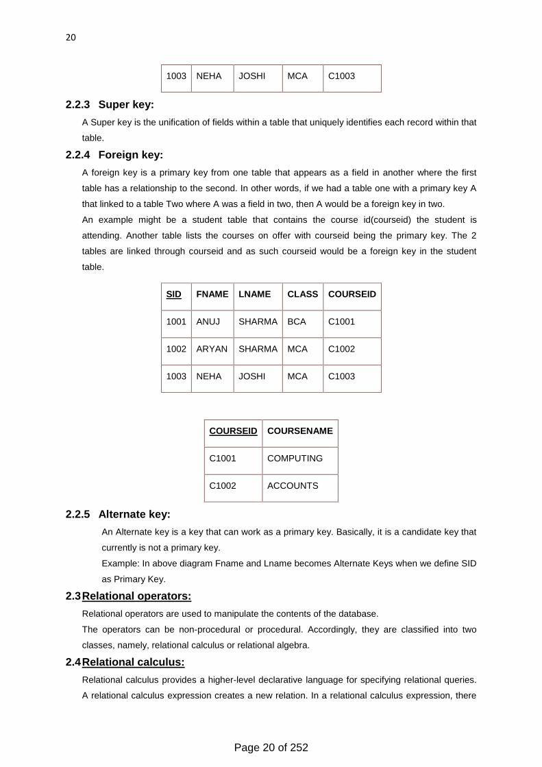
2.2.3 Super key:

A Super key is the unification of fields within a table that uniquely identifies each record within that

table.

2.2.4 Foreign key:

A foreign key is a primary key from one table that appears as a field in another where the first

table has a relationship to the second. In other words, if we had a table one with a primary key A

that linked to a table Two where A was a field in two, then A would be a foreign key in two.

An example might be a student table that contains the course id(courseid) the student is

attending. Another table lists the courses on offer with courseid being the primary key. The 2

tables are linked through courseid and as such courseid would be a foreign key in the student

table.





COURSEID COURSENAME

C1001 COMPUTING

C1002 ACCOUNTS

2.2.5 Alternate key:

An Alternate key is a key that can work as a primary key. Basically, it is a candidate key that

currently is not a primary key.

Example: In above diagram Fname and Lname becomes Alternate Keys when we define SID

as Primary Key.

2.3 Relational operators:

Relational operators are used to manipulate the contents of the database.

The operators can be non-procedural or procedural. Accordingly, they are classified into two

classes, namely, relational calculus or relational algebra.

2.4 Relational calculus:

Relational calculus provides a higher-level declarative language for specifying relational queries.

A relational calculus expression creates a new relation. In a relational calculus expression, there

Page 20 of 252

21

is no order of operations to specify how to retrieve the query result—only what information the

result should contain. This is the main distinguishing feature between relational algebra and

relational calculus. The relational calculus is important because it has a firm basis in mathematical

logic and because the standard query language (SQL) for RDBMSs. The operators in relational

calculus can be classified into two classes, namely, tuple oriented and domain oriented.

2.4.1 Tuple oriented:

It is a non procedural query language: Describes the desired information without giving a specific

procedure for obtaining that information. A query in tuple relational calculus is expressed as:

{t | P(t)}

This represents a set of all tuples t such that predicate P is true for t.

Example: Finding the branch – name, loan – number, and amount for loans of over $ 1200

{t | t € loan ٨ t[amount] > 1200}

In English this query would mean: The set of tuples t where t belongs to the loan relation and the loan

amount for each t is greater than $ 1200.

2.4.2 Domain oriented:

This is the second form of relational calculus

Uses domain variables that take on values from an attribute domain, rather than

values for an entire tuple.

Closely related to tuple relational calculus.

Example: Find the names of all customers who have an account at all branches located in Brooklyn:

{<c> | Э n(<c,n> Є customer) ٨ Џ x,y,z (<x,y,z> Є branch ٨ y = ―Brooklyn‖ => Э a,b(<a,x,b> Є

account ٨ <c,a> Є depositor))}

In English, we interpret this expression as ―The set of all(customer name) tuples c such that, for all

(branch – name, branch – city, assets) tuples, x,y,z, if the branch city is Brooklyn, then the following is

true:

1. There exists a tuple in the relation account with account number a and branch name x.

2. There exists a tuple in the relation depositor with customer c and account number a.‖

2.5 Relational algebra:

The basic set of operations for the relational model is the relational algebra. These operations

enable a user to specify basic retrieval requests as relational algebra expressions. The result of a

retrieval is a new relation, which may have been formed from one or more relations. The algebra

operations, thus produce new relations, which can be further manipulated using operations of the

same algebra. A sequence of relational algebra operations forms a relational algebra

expression, whose result will also be a relation that represents the result of a database query (or

retrieval request).The relational algebra is very important for several reasons. First, it provides a

Page 21 of 252

22

formal foundation for relational model operations. Second, and perhaps more important,it is used

as a basis for implementing and optimizing queries in the query processing and optimization

modules that are integral parts of relational database management systems (RDBMSs).

2.5.1 Selection:

The SELECT operation is used to choose a subset of the tuples from a relation that satisfies a

selection condition. One can consider the SELECT operation to be a filter that keeps only those

tuples that satisfy a qualifying condition. Alternatively,we can consider the SELECT operation to

restrict the tuples in a relation to only those tuples that satisfy the condition. The SELECT

operation can also be visualized as a horizontal partition of the relation into two sets of tuples—

those tuples that satisfy the condition and are selected, and those tuples that do not satisfy the

condition and are discarded. For example, to select the EMPLOYEE tuples whose department is

4, or those whose salary is greater than $30,000, we can individually specify each of these two

conditions with a SELECT operation as follows:

σDno=4(EMPLOYEE)

σSalary>30000(EMPLOYEE)

In general, the SELECT operation is denoted by:

σ<selection condition>(R)

where the symbol σ (sigma) is used to denote the SELECT operator and the selection condition is

a Boolean expression (condition) specified on the attributes of relation R. Notice that R is

generally a relational algebra expression whose result is a relation—the simplest such expression

is just the name of a database relation. Th relation resulting from the SELECT operation has the

same attributes as R.

2.5.2 Projection:

If we think of a relation as a table, the SELECT operation chooses some of the rows from the

table while discarding other rows. The PROJECT operation, on the other hand, selects certain

columns from the table and discards the other columns. If we are interested in only certain

attributes of a relation, we use the PROJECT operation to project the relation over these

attributes only. Therefore, the result of the PROJECT operation can be visualized as a vertical

partition of the relation into two relations:

one has the needed columns (attributes) and contains the result of the operation,

and the other contains the discarded columns. For example, to list each employee‘s

first and last name and salary, we can use the PROJECT operation as follows:

πLname, Fname, Salary(EMPLOYEE)

Page 22 of 252

23

The general form of the PROJECT operation is

π<attribute list>(R)

where π (pi) is the symbol used to represent the PROJECT operation, and <attribute list> is the

desired sublist of attributes from the attributes of relation R. Again,notice that R is, in general, a

relational algebra expression whose result is a relation,which in the simplest case is just the name of

a database relation. The result of the PROJECT operation has only the attributes specified in

<attribute list> in the same order as they appear in the list. Hence, its degree is equal to the number

of attributes in <attribute list>.

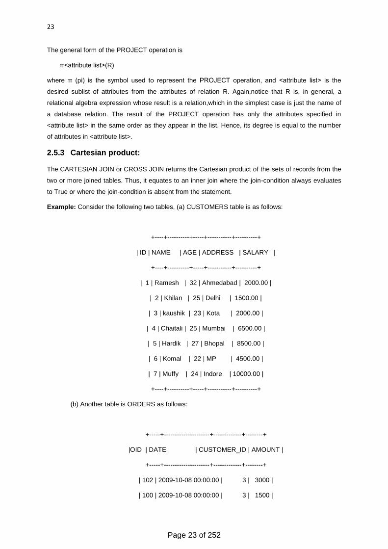
2.5.3 Cartesian product:

The CARTESIAN JOIN or CROSS JOIN returns the Cartesian product of the sets of records from the

two or more joined tables. Thus, it equates to an inner join where the join-condition always evaluates

to True or where the join-condition is absent from the statement.

Example: Consider the following two tables, (a) CUSTOMERS table is as follows:

+----+----------+-----+-----------+----------+

| ID | NAME | AGE | ADDRESS | SALARY |

+----+----------+-----+-----------+----------+

| 1 | Ramesh | 32 | Ahmedabad | 2000.00 |

| 2 | Khilan | 25 | Delhi | 1500.00 |

| 3 | kaushik | 23 | Kota | 2000.00 |

| 4 | Chaitali | 25 | Mumbai | 6500.00 |

| 5 | Hardik | 27 | Bhopal | 8500.00 |

| 6 | Komal | 22 | MP | 4500.00 |

| 7 | Muffy | 24 | Indore | 10000.00 |

+----+----------+-----+-----------+----------+

(b) Another table is ORDERS as follows:

+-----+---------------------+-------------+--------+

|OID | DATE | CUSTOMER_ID | AMOUNT |

+-----+---------------------+-------------+--------+

| 102 | 2009-10-08 00:00:00 | 3 | 3000 |

| 100 | 2009-10-08 00:00:00 | 3 | 1500 |

Page 23 of 252

24

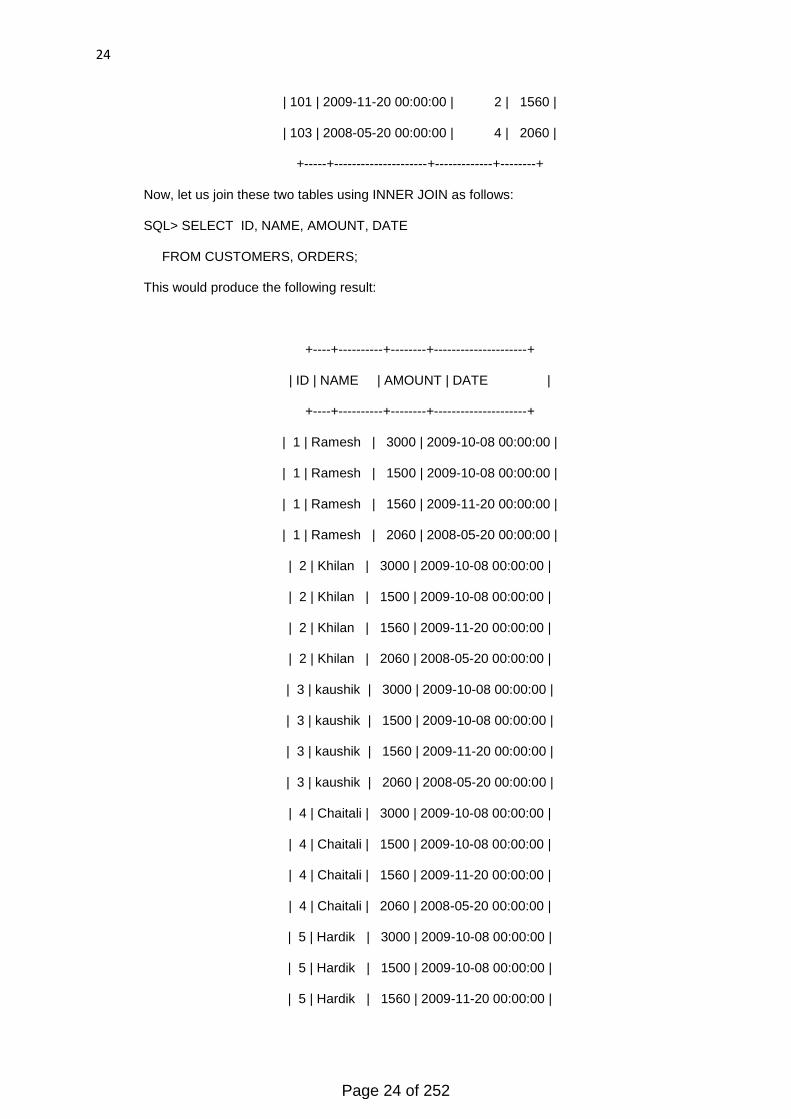
| 101 | 2009-11-20 00:00:00 | 2 | 1560 |

| 103 | 2008-05-20 00:00:00 | 4 | 2060 |

+-----+---------------------+-------------+--------+

Now, let us join these two tables using INNER JOIN as follows:

SQL> SELECT ID, NAME, AMOUNT, DATE

FROM CUSTOMERS, ORDERS;

This would produce the following result:

+----+----------+--------+---------------------+

| ID | NAME | AMOUNT | DATE |

+----+----------+--------+---------------------+

| 1 | Ramesh | 3000 | 2009-10-08 00:00:00 |

| 1 | Ramesh | 1500 | 2009-10-08 00:00:00 |

| 1 | Ramesh | 1560 | 2009-11-20 00:00:00 |

| 1 | Ramesh | 2060 | 2008-05-20 00:00:00 |

| 2 | Khilan | 3000 | 2009-10-08 00:00:00 |

| 2 | Khilan | 1500 | 2009-10-08 00:00:00 |

| 2 | Khilan | 1560 | 2009-11-20 00:00:00 |

| 2 | Khilan | 2060 | 2008-05-20 00:00:00 |

| 3 | kaushik | 3000 | 2009-10-08 00:00:00 |

| 3 | kaushik | 1500 | 2009-10-08 00:00:00 |

| 3 | kaushik | 1560 | 2009-11-20 00:00:00 |

| 3 | kaushik | 2060 | 2008-05-20 00:00:00 |

| 4 | Chaitali | 3000 | 2009-10-08 00:00:00 |

| 4 | Chaitali | 1500 | 2009-10-08 00:00:00 |

| 4 | Chaitali | 1560 | 2009-11-20 00:00:00 |

| 4 | Chaitali | 2060 | 2008-05-20 00:00:00 |

| 5 | Hardik | 3000 | 2009-10-08 00:00:00 |

| 5 | Hardik | 1500 | 2009-10-08 00:00:00 |

| 5 | Hardik | 1560 | 2009-11-20 00:00:00 |

Page 24 of 252

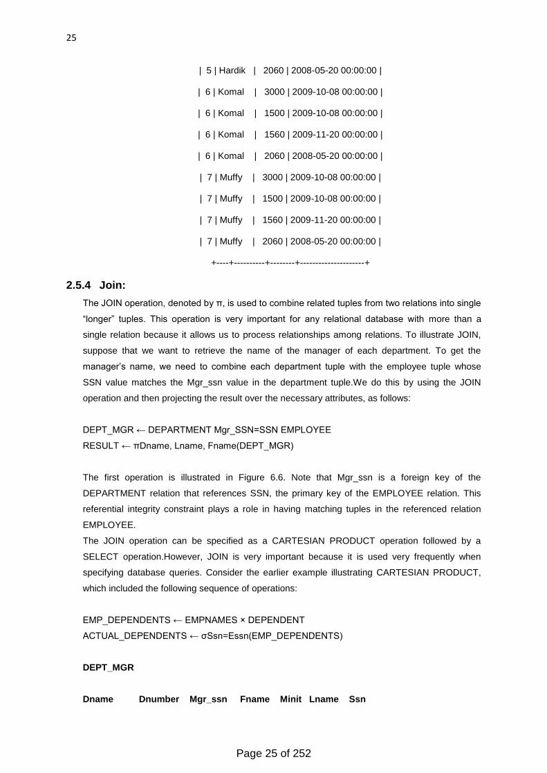
25

| 5 | Hardik | 2060 | 2008-05-20 00:00:00 |

| 6 | Komal | 3000 | 2009-10-08 00:00:00 |

| 6 | Komal | 1500 | 2009-10-08 00:00:00 |

| 6 | Komal | 1560 | 2009-11-20 00:00:00 |

| 6 | Komal | 2060 | 2008-05-20 00:00:00 |

| 7 | Muffy | 3000 | 2009-10-08 00:00:00 |

| 7 | Muffy | 1500 | 2009-10-08 00:00:00 |

| 7 | Muffy | 1560 | 2009-11-20 00:00:00 |

| 7 | Muffy | 2060 | 2008-05-20 00:00:00 |

+----+----------+--------+---------------------+

2.5.4 Join:

The JOIN operation, denoted by π, is used to combine related tuples from two relations into single

―longer‖ tuples. This operation is very important for any relational database with more than a

single relation because it allows us to process relationships among relations. To illustrate JOIN,

suppose that we want to retrieve the name of the manager of each department. To get the

manager‘s name, we need to combine each department tuple with the employee tuple whose

SSN value matches the Mgr_ssn value in the department tuple.We do this by using the JOIN

operation and then projecting the result over the necessary attributes, as follows:

DEPT_MGR ← DEPARTMENT Mgr_SSN=SSN EMPLOYEE

RESULT ← πDname, Lname, Fname(DEPT_MGR)

The first operation is illustrated in Figure 6.6. Note that Mgr_ssn is a foreign key of the

DEPARTMENT relation that references SSN, the primary key of the EMPLOYEE relation. This

referential integrity constraint plays a role in having matching tuples in the referenced relation

EMPLOYEE.

The JOIN operation can be specified as a CARTESIAN PRODUCT operation followed by a

SELECT operation.However, JOIN is very important because it is used very frequently when

specifying database queries. Consider the earlier example illustrating CARTESIAN PRODUCT,

which included the following sequence of operations:

EMP_DEPENDENTS ← EMPNAMES × DEPENDENT

ACTUAL_DEPENDENTS ← σSsn=Essn(EMP_DEPENDENTS)

DEPT_MGR

Dname Dnumber Mgr_ssn Fname Minit Lname Ssn

Page 25 of 252

26

Research 5 333445555 Franklin T Wong 333445555

Administration 4 987654321 Jennifer S Wallace 987654321

Headquarters 1 888665555 James E Borg 888665555

The result of the JOIN is a relation Q with n + m attributes Q(A1, A2, ..., An, B1, B2,... , Bm) in that

order; Q has one tuple for each combination of tuples—one from R and one from S—whenever the

combination satisfies the join condition. This is the main difference between CARTESIAN PRODUCT

and JOIN. In JOIN, only combinations of tuples satisfying the join condition appear in the result,

whereas in the CARTESIAN PRODUCT all combinations of tuples are included in the result. The

join condition is specified on attributes from the two relations R and S and is evaluated for each

combination of tuples. Each tuple combination for which the join condition evaluates to TRUE is

included in the resulting relation Q as a single combined tuple.

A general join condition is of the form

<condition> AND <condition> AND...AND <condition>

where each <condition> is of the form Ai θ Bj, Ai is an attribute of R, Bj is an attribute

of S, Ai and Bj have the same domain, and θ (theta) is one of the comparison operators {=, <, ≤, >, ≥,

≠}.

2.5.5 Difference:

DIFFERENCE on two union-compatible relations R and S as follows:

The result of this operation, denoted by R – S, is a relation that includes all tuples that are in R

but not in S.

2.5.6 Division:

The DIVISION operation, denoted by ÷, is useful for a special kind of query that sometimes

occurs in database applications. An example is to retrieve the names of employees who work on

all the projects that ‗John Smith‘ works on. To express this query using the DIVISION operation,

proceed as follows. First, retrieve the list of project numbers that ‗John Smith‘ works on in the

intermediate relation SMITH_PNOS:

SMITH ← σFname=‗John‘ AND Lname=‗Smith‘(EMPLOYEE)

SMITH_PNOS ← πPno(WORKS_ON Essn=SsnSMITH)

Next, create a relation that includes a tuple <Pno, Essn> whenever the employee whose Ssn is

Essn works on the project whose number is Pno in the intermediate relation SSN_PNOS:

SSN_PNOS ← πEssn, Pno(WORKS_ON)

Finally, apply the DIVISION operation to the two relations, which gives the desired employees‘

Social Security numbers:

SSNS(Ssn) ← SSN_PNOS ’ SMITH_PNOS

Page 26 of 252

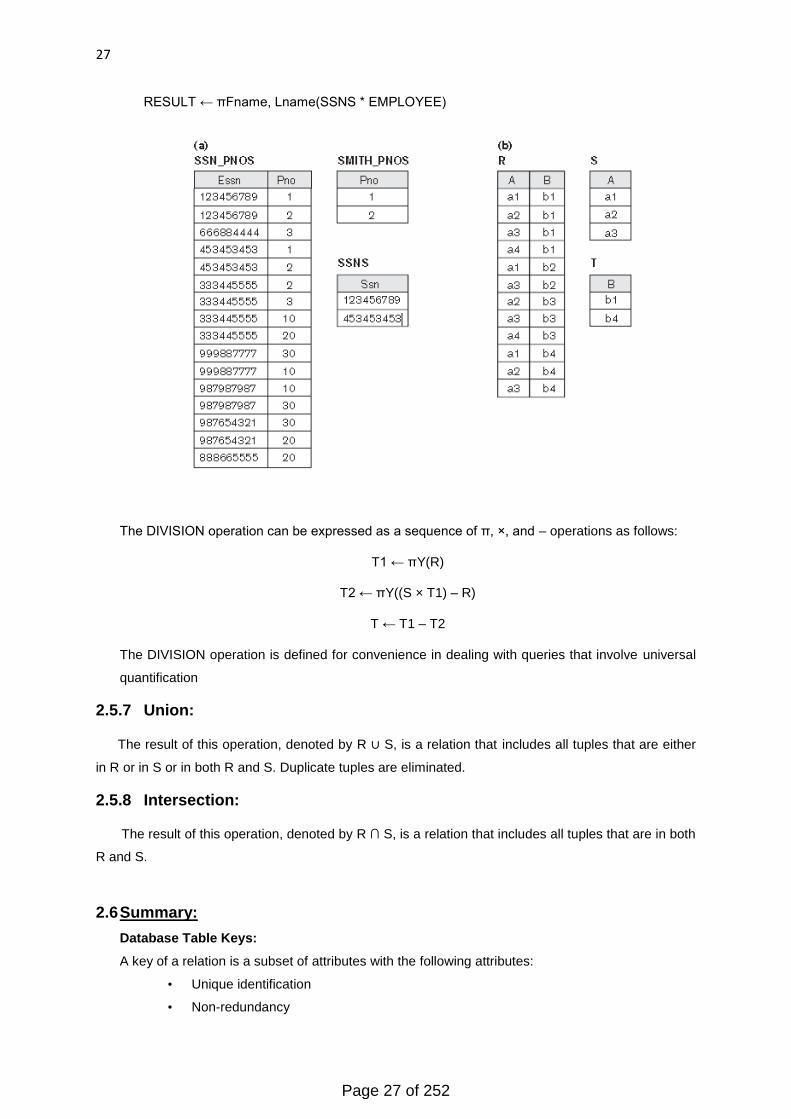
27

RESULT ← πFname, Lname(SSNS * EMPLOYEE)

The DIVISION operation can be expressed as a sequence of π, ×, and – operations as follows:

T1 ← πY(R)

T2 ← πY((S × T1) – R)

T ← T1 – T2

The DIVISION operation is defined for convenience in dealing with queries that involve universal

quantification

2.5.7 Union:

The result of this operation, denoted by R ∪ S, is a relation that includes all tuples that are either

in R or in S or in both R and S. Duplicate tuples are eliminated.

2.5.8 Intersection:

The result of this operation, denoted by R ∩ S, is a relation that includes all tuples that are in both

R and S.

2.6 Summary:

Database Table Keys:

A key of a relation is a subset of attributes with the following attributes:

• Unique identification

• Non-redundancy

Page 27 of 252

28

PRIMARY KEY

Serves as the row level addressing mechanism in the relational database model.

It can be formed through the combination of several items.

FOREIGN KEY

A column or set of columns within a table that are required to match those of a

primary key of a second table.

These keys are used to form a RELATIONAL JOIN - thereby connecting row to row across

the individual tables.

Super Key

A Super key is the unification of fields within a table that uniquely identifies each record

within that table.

Candidate Key

A candidate is a subdivision of a super key. It is a single field or the combination of fields

that uniquely identifies each record in the table. The least combination of fields

differentiates between candidate key from a super key.

Relational Operators:

Relational Operations used in relational algebra to manipulate contents in a database. There are eight

different types of operators. There are following Relational operators:

UNION: It will conjoin all of the rows in one table with all of the rows in another table except

for the duplicate rows.

INTERSECT: It takes two tables and combines only the rows that appear in both tables.

DIFFERENCE: Basically, it subtracts one table from the other table to leave only the

attributes that are not the same in both tables.

PRODUCT: This command would show all possible pairs of rows from both tables being

used.

SELECT: This command to show all rows in a table. It can be used to select only specific

data from the table that meet certain criteria.

JOIN: It takes two or more tables, combines them into one table. This can be used in

combination with other commands to get specific information.

2.7 Glossary:

Database Keys:


structure.

Null: It is temporarily blank but can be filled in the future.

Query: In general, a query is a form of questioning, in a line of inquiry.

Query language: A computer language used to make queries into databases and information

systems.

Page 28 of 252

http://en.wikipedia.org/wiki/Question

http://en.wikipedia.org/wiki/Query_language

29

Data Integrity: Data integrity refers to maintaining and assuring the accuracy and consistency

of data over its entire life-cycle.

Domain: Description of an attribute allowed values.

Data Type: A particular kind of data item, as defined by the values it can take, the programming

language used, or the operations that can be performed on it.


Q1.What do we mean by Database Keys? How many types of keys are there in DBMS?

Ans: Database Keys:


structure. They make sure that each record within a table can be uniquely identified by one or a

combination of fields within the table. They help us to enforce integrity and help identify the

relationship between tables. There are three main types of keys, candidate keys, primary keys and

foreign keys.

Different keys in DBMS:

There are following keys in a DBMS:

Super Key

A Super key is the unification of fields within a table that uniquely identifies each record within that

table.

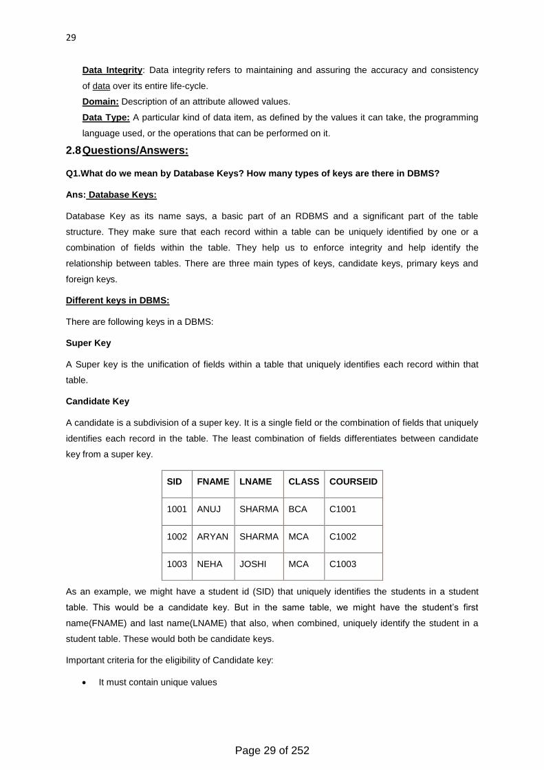
Candidate Key

A candidate is a subdivision of a super key. It is a single field or the combination of fields that uniquely

identifies each record in the table. The least combination of fields differentiates between candidate

key from a super key.





As an example, we might have a student id (SID) that uniquely identifies the students in a student

table. This would be a candidate key. But in the same table, we might have the student‘s first

name(FNAME) and last name(LNAME) that also, when combined, uniquely identify the student in a

student table. These would both be candidate keys.

Important criteria for the eligibility of Candidate key:

It must contain unique values

Page 29 of 252

http://en.wikipedia.org/wiki/Data

30

It must not contain null values

Once we have chosen candidate keys we can now select Primary key from these candidate keys.

Primary Key

As its name suggests, it is the primary key of reference for the table and is used throughout the

database to help establish relationships with other tables.

It is a candidate key that is relevant to be the main reference key for the table. As with any candidate

key the primary key

• Must contain unique values.

• Must never be null and uniquely identify each record in the table.

As an example, a student id (SID) might be a primary key in a student table.In the table below we

have selected the candidate key student_id to be our most convenient primary key.





Foreign Key

A foreign key is a primary key from one table that appears as a field in another where the first table

has a relationship to the second. In other words, if we had a table One with a primary key A that

linked to a table Two where A was a field in Two, then A would be a foreign key in Two.

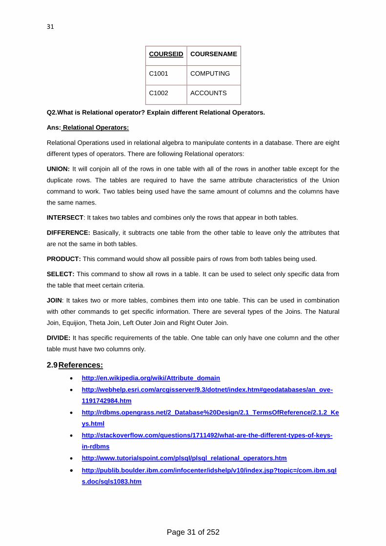
An example might be a student table that contains the course id (courseid) the student is attending.

Another table lists the courses on offer with courseid being the primary key. The two tables are linked

through courseid and as such courseid would be a foreign key in the student table.





Page 30 of 252

31

COURSEID COURSENAME

C1001 COMPUTING

C1002 ACCOUNTS

Q2.What is Relational operator? Explain different Relational Operators.

Ans: Relational Operators:

Relational Operations used in relational algebra to manipulate contents in a database. There are eight

different types of operators. There are following Relational operators:

UNION: It will conjoin all of the rows in one table with all of the rows in another table except for the

duplicate rows. The tables are required to have the same attribute characteristics of the Union

command to work. Two tables being used have the same amount of columns and the columns have

the same names.

INTERSECT: It takes two tables and combines only the rows that appear in both tables.

DIFFERENCE: Basically, it subtracts one table from the other table to leave only the attributes that

are not the same in both tables.

PRODUCT: This command would show all possible pairs of rows from both tables being used.

SELECT: This command to show all rows in a table. It can be used to select only specific data from

the table that meet certain criteria.

JOIN: It takes two or more tables, combines them into one table. This can be used in combination

with other commands to get specific information. There are several types of the Joins. The Natural

Join, Equijion, Theta Join, Left Outer Join and Right Outer Join.

DIVIDE: It has specific requirements of the table. One table can only have one column and the other

table must have two columns only.

2.9 References:

http://en.wikipedia.org/wiki/Attribute_domain

http://webhelp.esri.com/arcgisserver/9.3/dotnet/index.htm#geodatabases/an_ove-

1191742984.htm

http://rdbms.opengrass.net/2_Database%20Design/2.1_TermsOfReference/2.1.2_Ke

ys.html

http://stackoverflow.com/questions/1711492/what-are-the-different-types-of-keys-

in-rdbms

http://www.tutorialspoint.com/plsql/plsql_relational_operators.htm

http://publib.boulder.ibm.com/infocenter/idshelp/v10/index.jsp?topic=/com.ibm.sql

s.doc/sqls1083.htm

Page 31 of 252

http://en.wikipedia.org/wiki/Attribute_domain

http://webhelp.esri.com/arcgisserver/9.3/dotnet/index.htm#geodatabases/an_ove-1191742984.htm

http://webhelp.esri.com/arcgisserver/9.3/dotnet/index.htm#geodatabases/an_ove-1191742984.htm

http://rdbms.opengrass.net/2_Database%20Design/2.1_TermsOfReference/2.1.2_Keys.html

http://rdbms.opengrass.net/2_Database%20Design/2.1_TermsOfReference/2.1.2_Keys.html

http://stackoverflow.com/questions/1711492/what-are-the-different-types-of-keys-in-rdbms

http://stackoverflow.com/questions/1711492/what-are-the-different-types-of-keys-in-rdbms

http://www.tutorialspoint.com/plsql/plsql_relational_operators.htm

http://publib.boulder.ibm.com/infocenter/idshelp/v10/index.jsp?topic=/com.ibm.sqls.doc/sqls1083.htm

http://publib.boulder.ibm.com/infocenter/idshelp/v10/index.jsp?topic=/com.ibm.sqls.doc/sqls1083.htm

32


Database Management Systems, 3rd Edition

Ramakrishnan (Author), Gehrke (Author)

SQL & Pl/SQL For Oracle 11G Black Book

Author: P.S Deshpande.

Database Management Systems

Author: G K Gupta, Publisher: Tata McGraw Hill Educationa

Page 32 of 252

33

Unit 1

Lesson 3 – Normalization in DBMS

3.1 Objective

3.2 Introduction to normalization process

3.3 The Need for Normalization

3.4 Steps for normalization

3.5 Normal forms

3.5.1 First Normal Form

3.5.2 Functional dependencies in data

3.5.3 Second Normal Form

3.6 Anomalies in second normal form

3.6.1 Insertion anomaly

3.6.2 Deletion anomaly

3.6.3 Update anomaly

3.6.4 Transitive dependency

3.7 Third normal form

3.8 Summary

3.9 Glossary


3.11 References


3.1 Objective

To learn the process of normalization

To understand different normal forms

To understand data anomalies

3.2 Introduction to Normalization process:

Database normalization is the process of Arranging the fields and tables of a relational database to

minimize redundancy and dependency. It involves dividing large tables into smaller tables and

defining relationships between them. The objective is to isolate data so that modifications, deletions,

and additions of a field can be made in just one table and then proliferate through the rest of the

database using the defined relationships.

3.3 The Need for Normalization:

Normalization is the aim of well designed Relational Database. It is a step by step set of rules by

which data is put in its simplest forms. We normalize the relational database management system

because of the following reasons:

Minimize data redundancy, i.e. no unnecessary duplication of data.

Page 33 of 252

34

To make the database structure flexible i.e. it should be possible to add new data values and rows

without reorganizing the database structure.

Data should be consistent throughout the database, i.e. it should not suffer from following

anomalies.

Insert Anomaly - Due to lack of data, i.e. all the data available for insertion such that null values in

keys should be avoided. This kind of anomaly can seriously damage a database

Update Anomaly - It is due to data redundancy, i.e., multiple occurrences of the same values in a

column. This can lead to inefficiency.

Deletion Anomaly - It leads to loss of data for rows that are not stored elsewhere. It could result in

loss of vital data.

Complex queries required by the user should be easy to handle.

On decomposition of a relation into smaller relations with fewer attributes on normalization the

resulting relations whenever joined must result in the same relation without any extra rows. The join

operations can be performed in any order. This is known as Lossless Join decomposition.

The resulting relations (tables) obtained on normalization should possess the properties such as

each row must be identified by a unique key, no repeating groups, homogeneous columns, each

column is assigned a unique name etc.

3.4 Steps for normalization:

Basic steps for normalization are as follows:

Definitions of the Normal Forms

Functional Dependency and Determinants

The 1st Normal Form (1NF)

The 2nd Normal Form (2NF)

Anomalies and Normalization

The 3rd Normal Form (3NF)

And higher normal forms

3.5 Normal forms:

The database community has developed a protocol for ensuring that databases are normalized.

These are referred to as normal forms and are numbered from one (the lowest form of

normalization, referred to as first normal form or 1NF) through five (fifth normal form or 5NF).

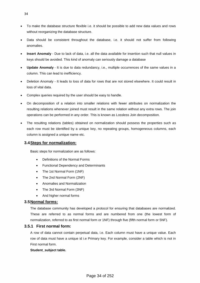
3.5.1 First normal form:

A row of data cannot contain perpetual data, i.e. Each column must have a unique value. Each

row of data must have a unique id i.e Primary key. For example, consider a table which is not in

First normal form.

Student_subject table.

Page 34 of 252

35

Stu_id Stu_name Sub_name

1001 Aryan Physics

1001 Aryan Chemistry

1003 Shaurya Mathematics

1004 Sunny Mathematics

You can clearly see here that the student name Aryan is used twice in the table and subject

mathematics is also repeated. This violates the First Normal form. To reduce the above table to

First Normal form break the table into two different tables.

New Student table

Stu_id Stu_name

1001 Aryan

1003 Shaurya

1004 Sunny

New Subject table

Sub_id Stu_id Sub_name

101 1001 Physics

102 1001 Chemistry

103 1003 Mathematics


3.5.2 Functional dependencies in data:

When a non-key attribute is determined by a part, but not the whole, of a COMPOSITE primary

key. Like here in example Attributes are identified by either by Cust_id or by O_id both.

Cust_id Cust_name O_id

101 Harshit 1001

102 Karan 1002

Page 35 of 252

36

103 Akshay 1003

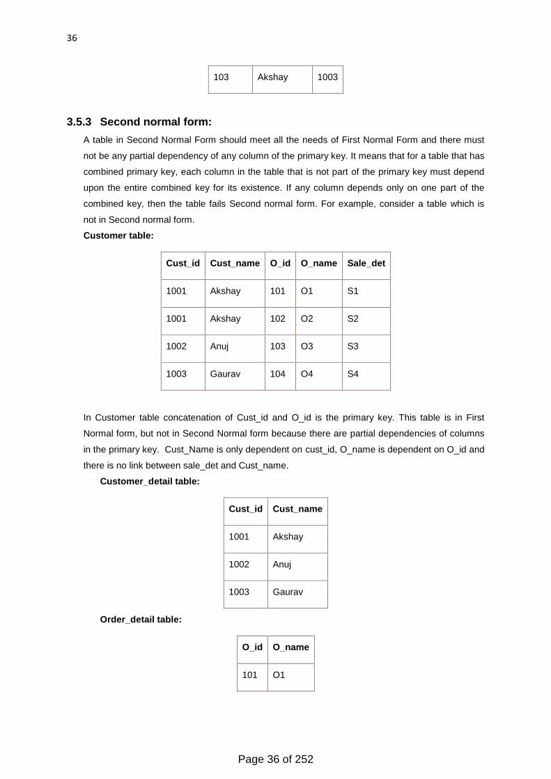
3.5.3 Second normal form:

A table in Second Normal Form should meet all the needs of First Normal Form and there must

not be any partial dependency of any column of the primary key. It means that for a table that has

combined primary key, each column in the table that is not part of the primary key must depend

upon the entire combined key for its existence. If any column depends only on one part of the

combined key, then the table fails Second normal form. For example, consider a table which is

not in Second normal form.

Customer table:

Cust_id Cust_name O_id O_name Sale_det

1001 Akshay 101 O1 S1

1001 Akshay 102 O2 S2

1002 Anuj 103 O3 S3

1003 Gaurav 104 O4 S4

In Customer table concatenation of Cust_id and O_id is the primary key. This table is in First

Normal form, but not in Second Normal form because there are partial dependencies of columns

in the primary key. Cust_Name is only dependent on cust_id, O_name is dependent on O_id and

there is no link between sale_det and Cust_name.

Customer_detail table:

Cust_id Cust_name

1001 Akshay

1002 Anuj

1003 Gaurav

Order_detail table:

O_id O_name

101 O1

Page 36 of 252

37

102 O2

103 O3

104 O4

Sales_detail table:

Cust_id O_id Sale_det

1001 101 S1

1001 102 S2

1002 103 S3

1003 104 S4

3.6 Anomalies in second normal form:

Database anomalies, are unmatched or missing information caused by flaws within a given

database. Databases are designed to collect data and sort or present it in specific ways to

the end user. Entering or deleting information, be it an update or a new record can cause

issues if the database is limited or has errors. There are following types of Data Anomalies:

3.6.1 Insertion anomaly:

When you are inserting information into the database for the first time. To insert the information

into the table, we must enter the correct details so that they are consistent with the values of the

other rows. Missing or incorrectly formatted entries are two of the more common insertion errors.

Most developers acknowledge that this will happen and build in error codes that tell you exactly

what went wrong.

An Insert Anomaly occurs when certain attributes cannot be inserted into the database without the

presence of other attributes. For example, this is the converse of deleting anomaly - we can't add

a new course unless we have at least one student enrolled on the course.

Stu_Num Cou_Num Stu_Name Address Course

S001 C001 Gaurav Ludhiana Computing


S003 C002 Anuj Moga Maths

S004 C003 Aman Ferozepur Accounts

S004 C004 Bunny Faridkot Physics

Page 37 of 252

38

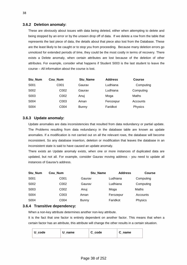
3.6.2 Deletion anomaly:

These are obviously about issues with data being deleted, either when attempting to delete and

being stopped by an error or by the unseen drop off of data. If we delete a row from the table that

represents the last piece of data, the details about that piece also lost from the Database. These

are the least likely to be caught or to stop you from proceeding. Because many deletion errors go

unnoticed for extended periods of time, they could be the most costly in terms of recovery. There

exists a Delete anomaly, when certain attributes are lost because of the deletion of other

attributes. For example, consider what happens if Student S003 is the last student to leave the

course – All information about the course is lost.







3.6.3 Update anomaly:

Update anomalies are data inconsistencies that resulted from data redundancy or partial update.

The Problems resulting from data redundancy in the database table are known as update

anomalies. If a modification is not carried out on all the relevant rows, the database will become

inconsistent. So any database insertion, deletion or modification that leaves the database in an

inconsistent state is said to have caused an update anomaly.

There exists an Update anomaly exists, when one or more instances of duplicated data are

updated, but not all. For example, consider Gaurav moving address - you need to update all

instances of Gaurav's address.







3.6.4 Transitive dependency:

When a non-key attribute determines another non-key attribute.

It is the fact that one factor is entirely dependent on another factor. This means that when a

certain factor has an attribute, this attribute will change the other results in a certain situation.

U_code U_name C_code C_name

Page 38 of 252

39

U1001 DBMS C101 Accounts

U1002 RDBMS C101 Accounts

U1003 C++ C102 Computing

U1004 JAVA C102 Computing

In our example above, we have U_code as our primary key, we also have a C_name that is

dependent on C_code and courseCode, dependent on U_code. Though C_name could be

dependent on U_code it more dependent on C_code, therefore it is transitively dependent on

U_code.

3.7 Third normal form:

Third Normal Form deals with transitive dependencies. This means if we have a primary key A and a

non-key domain B and C where C is more dependent on B than A and B is directly dependent on A,

then C can be considered transitively dependent on A.

Before we start with the steps, if we have any relations with zero or only one non-key domain we can‘t

have a transitive dependency so this move straight to 3rd Normal Form

For the rest the steps from 2NF to 3NF are:

• Take each non-key domain in turn and check it is more dependent on another non-key

domain than the primary key. If yes

• Move the dependent domain, together with a copy of the non-key attribute upon which it is

dependent, to a new relation.

• Make the non-key domain, upon which it is dependent, the key in the new relation.

• Underline the key in this new relation as the primary key.

• Leave the non-key domain, upon which it was dependent, in the original relation and mark it a

foreign key (*).

• Move down the relation to each of the domains repeating steps 1 and 2 till you have covered

the whole relation.

Once completed with all transitive dependencies removed, the table is in 3rd normal form.

So following the steps, remove course Name with a copy of course code to another relation and make

course Code the primary key of the new relation. In the original table mark course Code as our foreign

key.

U_code U_name C_code

U1001 DBMS C101

Page 39 of 252

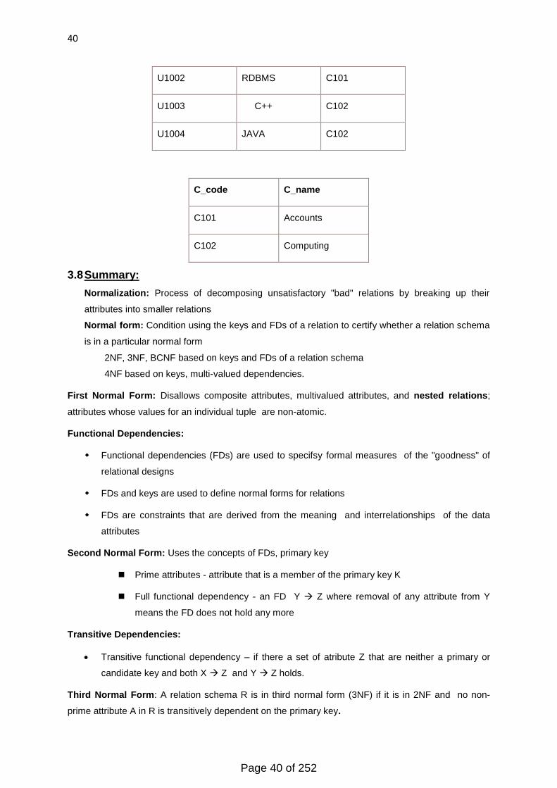
40

U1002 RDBMS C101

U1003 C++ C102

U1004 JAVA C102

C_code C_name

C101 Accounts

C102 Computing

3.8 Summary:

Normalization: Process of decomposing unsatisfactory "bad" relations by breaking up their

attributes into smaller relations

Normal form: Condition using the keys and FDs of a relation to certify whether a relation schema

is in a particular normal form

2NF, 3NF, BCNF based on keys and FDs of a relation schema

4NF based on keys, multi-valued dependencies.

First Normal Form: Disallows composite attributes, multivalued attributes, and nested relations;

attributes whose values for an individual tuple are non-atomic.

Functional Dependencies:

Functional dependencies (FDs) are used to specifsy formal measures of the "goodness" of

relational designs

FDs and keys are used to define normal forms for relations

FDs are constraints that are derived from the meaning and interrelationships of the data

attributes

Second Normal Form: Uses the concepts of FDs, primary key

Prime attributes - attribute that is a member of the primary key K

Full functional dependency - an FD Y Z where removal of any attribute from Y

means the FD does not hold any more

Transitive Dependencies:

Transitive functional dependency – if there a set of atribute Z that are neither a primary or

candidate key and both X Z and Y Z holds.

Third Normal Form: A relation schema R is in third normal form (3NF) if it is in 2NF and no non-

prime attribute A in R is transitively dependent on the primary key.

Page 40 of 252

41

Data Anomalies:

Anything we try to do with a database that leads to unexpected and/or unpredictable results.

Three types of Anomaly to guard against:

Insert Anomaly: When we want to enter a value into a data cell, but the attempt is prevented,

as another value is not known.

Delete Anomaly: When a value we want to delete also means we will delete values we wish

to keep.

Update Anomaly: When we want to change a single data item value, but must update

multiple entries.

3.9 Glossary:

Redundancy: Redundancy is the duplication of critical components or functions of a system with

the intention of increasing reliability of the system.

Dependency: Relationship between conditions, events, or tasks such that one cannot begin or

be-completed until one or more other conditions, events, or tasks have occurred, begun, or

completed.

Protocol: The official procedure or system of rules governing the affairs of state or diplomatic

occasions.

Row: A row also called a record represents a single, implicitly structured data item in a table.

Column: A column is a set of data values of a particular simple type, one for each row of the

table.


Q1. What do you mean by normalization?

Ans: Normalization: Database normalization is the process of Arranging the fields and tables of

a relational database to minimize redundancy and dependency. It involves dividing large tables

into smaller tables and defining relationships between them. The objective is to isolate data so

that modifications, deletions, and additions of a field can be made in just one table and then

proliferate through the rest of the database using the defined relationships.

Q2. What do you mean by Normal Form? How many types of normal forms are there in

DBMS?

Ans: The Normal Forms: The database community has developed a protocol for ensuring that

databases are normalized. These are referred to as normal forms and are numbered from one

(the lowest form of normalization, referred to as first normal form or 1NF) through five (fifth normal

form or 5NF).

First Normal Form

A row of data cannot contain perpetual data, i.e. each column must have a unique value. Each

row of data must have a unique id i.e Primary key. For example, consider a table which is not in

First normal form.

Page 41 of 252

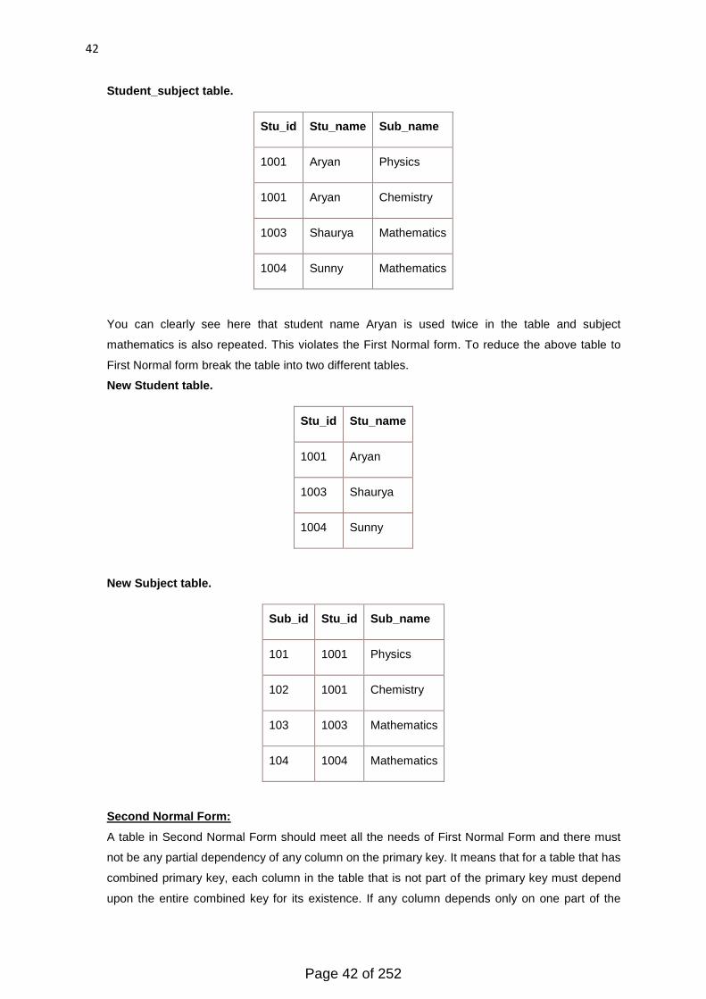
42

Student_subject table.

Stu_id Stu_name Sub_name

1001 Aryan Physics

1001 Aryan Chemistry

1003 Shaurya Mathematics

1004 Sunny Mathematics

You can clearly see here that student name Aryan is used twice in the table and subject

mathematics is also repeated. This violates the First Normal form. To reduce the above table to

First Normal form break the table into two different tables.

New Student table.

Stu_id Stu_name

1001 Aryan

1003 Shaurya

1004 Sunny

New Subject table.

Sub_id Stu_id Sub_name

101 1001 Physics

102 1001 Chemistry



Second Normal Form:

A table in Second Normal Form should meet all the needs of First Normal Form and there must

not be any partial dependency of any column on the primary key. It means that for a table that has

combined primary key, each column in the table that is not part of the primary key must depend

upon the entire combined key for its existence. If any column depends only on one part of the

Page 42 of 252

43

combined key, then the table fails Second normal form. For example, consider a table which is

not in Second normal form.

Customer table:

Cust_id Cust_name O_id O_name Sale_det

1001 Akshay 101 O1 S1

1001 Akshay 102 O2 S2

1002 Anuj 103 O3 S3

1003 Gaurav 104 O4 S4

In Customer table concatenation of Cust_id and O_id is the primary key. This table is in First

Normal form, but not in Second Normal form because there are partial dependencies of columns

on the primary key. Cust_Name is only dependent on cust_id, O_name is dependent on O_id

and there is no link between sale_det and Cust_name.

Customer_detail table:

Cust_id Cust_name

1001 Akshay

1002 Anuj

1003 Gaurav

Order_detail table:

O_id O_name

101 O1

102 O2

103 O3

104 O4

Sales_detail table:

Page 43 of 252

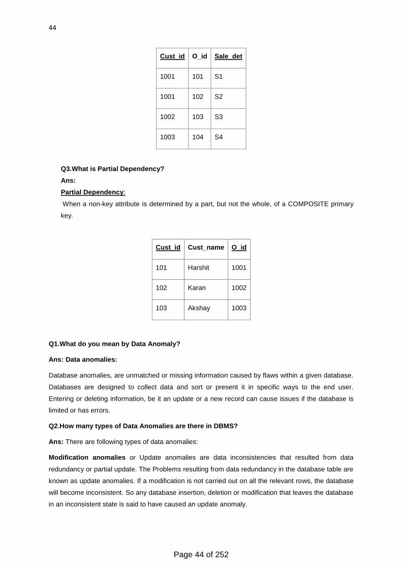
44

Cust_id O_id Sale_det

1001 101 S1

1001 102 S2

1002 103 S3

1003 104 S4

Q3.What is Partial Dependency?

Ans:

Partial Dependency:

When a non-key attribute is determined by a part, but not the whole, of a COMPOSITE primary

key.

Cust_id Cust_name O_id

101 Harshit 1001

102 Karan 1002

103 Akshay 1003

Q1.What do you mean by Data Anomaly?

Ans: Data anomalies:

Database anomalies, are unmatched or missing information caused by flaws within a given database.

Databases are designed to collect data and sort or present it in specific ways to the end user.

Entering or deleting information, be it an update or a new record can cause issues if the database is

limited or has errors.

Q2.How many types of Data Anomalies are there in DBMS?

Ans: There are following types of data anomalies:

Modification anomalies or Update anomalies are data inconsistencies that resulted from data

redundancy or partial update. The Problems resulting from data redundancy in the database table are

known as update anomalies. If a modification is not carried out on all the relevant rows, the database

will become inconsistent. So any database insertion, deletion or modification that leaves the database

in an inconsistent state is said to have caused an update anomaly.

Page 44 of 252

45

An Update Anomaly exists when one or more instances of duplicated data are updated, but not all.

For example, consider Gaurav moving address - you need to update all instances of Gaurav's

address.







Insertion anomalies. When you are inserting information into the database for the first time. To

insert the information into the table, we must enter the correct details so that they are consistent with

the values of the other rows. Missing or incorrectly formatted entries are two of the more common

insertion errors. Most developers acknowledge that this will happen and build in error codes that tell

you exactly what went wrong.

An Insert Anomaly occurs when certain attributes cannot be inserted into the database without the

presence of other attributes. For example, this is the converse of delete anomaly - we can't add a new

course unless we have at least one student enrolled on the course.







Deletion anomalies are obviously about issues with data being deleted, either when attempting to

delete and being stopped by an error or by the unseen drop off of data. If we delete a row from the

table that represents the last piece of data, the details about that piece are also lost from the

Database. These are the least likely to be caught or to stop you from proceeding. Because many

deletion errors go unnoticed for extended periods of time, they could be the most costly in terms of

recovery.

A Delete Anomaly existing when certain attributes are lost because of the deletion of other attributes.

For example, consider what happens if Student S30 is the last student to leave the course - All

information about the course is lost.



Page 45 of 252

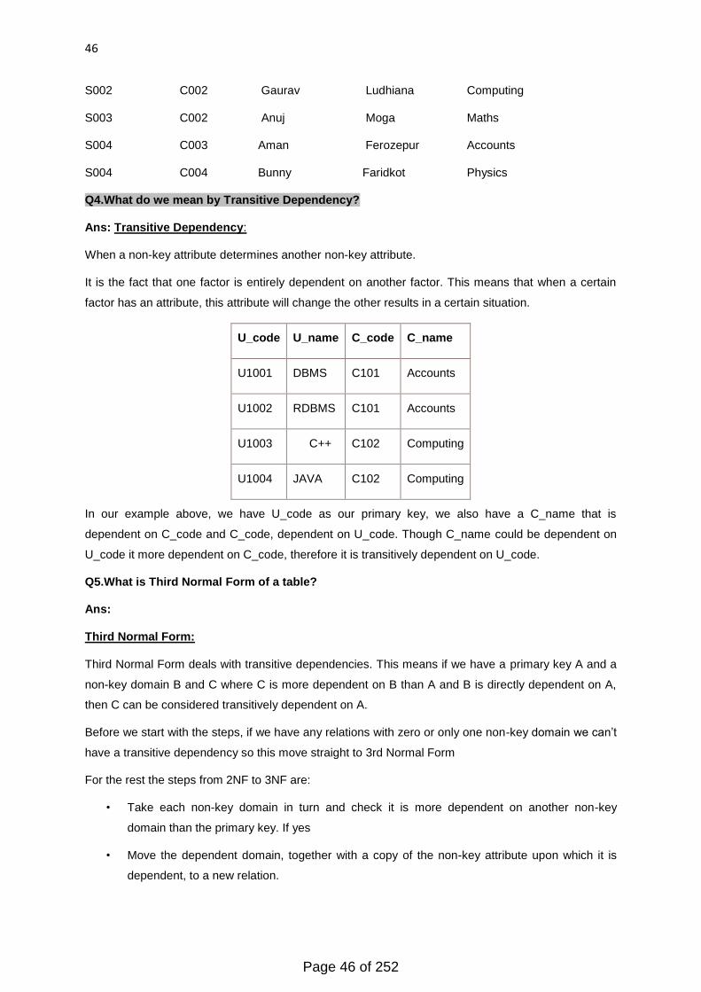
46





Q4.What do we mean by Transitive Dependency?

Ans: Transitive Dependency:

When a non-key attribute determines another non-key attribute.

It is the fact that one factor is entirely dependent on another factor. This means that when a certain

factor has an attribute, this attribute will change the other results in a certain situation.

U_code U_name C_code C_name

U1001 DBMS C101 Accounts

U1002 RDBMS C101 Accounts

U1003 C++ C102 Computing

U1004 JAVA C102 Computing

In our example above, we have U_code as our primary key, we also have a C_name that is

dependent on C_code and C_code, dependent on U_code. Though C_name could be dependent on

U_code it more dependent on C_code, therefore it is transitively dependent on U_code.

Q5.What is Third Normal Form of a table?

Ans:

Third Normal Form:

Third Normal Form deals with transitive dependencies. This means if we have a primary key A and a

non-key domain B and C where C is more dependent on B than A and B is directly dependent on A,

then C can be considered transitively dependent on A.

Before we start with the steps, if we have any relations with zero or only one non-key domain we can‘t

have a transitive dependency so this move straight to 3rd Normal Form

For the rest the steps from 2NF to 3NF are:

• Take each non-key domain in turn and check it is more dependent on another non-key

domain than the primary key. If yes

• Move the dependent domain, together with a copy of the non-key attribute upon which it is

dependent, to a new relation.

Page 46 of 252

47

• Make the non-key domain, upon which it is dependent, the key in the new relation.

• Underline the key in this new relation as the primary key.

• Leave the non-key domain, upon which it was dependent, in the original relation and mark it a

foreign key (*).

• Move down the relation to each of the domains repeating steps 1 and 2 till you have covered

the whole relation.

Once completed with all transitive dependencies removed, the table is in 3rd normal form.

So following the steps, remove course Name with a copy of course code to another relation and make

course Code the primary key of the new relation. In the original table mark course Code as our foreign

key.

U_code U_name C_code

U1001 DBMS C101

U1002 RDBMS C101

U1003 C++ C102

U1004 JAVA C102

C_code C_name

C101 Accounts

C102 Computing

3.11 References:

http://publib.boulder.ibm.com/infocenter/zos/basics/index.jsp?topic=/com.ibm.zos.zmiddbmg/z

middle_46.htm

http://www.techopedia.com/definition/24361/database-management-systems-dbms


Database Management System by Seema Kedar.

Database Management System by Patricia Ward, George Dafoulas

Six-Step Relational Database Design (TM): A step by step approach to relational

database design and development Second Edition of Fidel A Captain.

Page 47 of 252

http://publib.boulder.ibm.com/infocenter/zos/basics/index.jsp?topic=/com.ibm.zos.zmiddbmg/zmiddle_46.htm

http://publib.boulder.ibm.com/infocenter/zos/basics/index.jsp?topic=/com.ibm.zos.zmiddbmg/zmiddle_46.htm

http://www.techopedia.com/definition/24361/database-management-systems-dbms

48

Unit 2

Lesson 4 - Entity R e l a t i o n s h i p M o d e l

4.1 Objective

4.2 Introduction to Entity Relation Modelling

4.3 Entity, Entity Type

4.4 Attributes of an Entity

4.5 Relationships

4.5.1 One to One Relationship

4.5.2 Many to One Relationship

4.6 Developing E-R Model.

4.7 Normalizing a Model

4.7.1 First Normal Form: Eliminating Repeating Groups

4.7.2 Second Normal Form: Eliminating Redundant Data

4.7.3 Third Normal Form: Eliminating Columns Not Dependent on Keys

4.8 Summary

4.9 Glossary


4.11 References


4.1 Objectives:

To understand the concepts of data modelling

To understand the concepts of ER model

To illustrate the data modeling process with ER diagrams

4.2 Introduction to entity relationship model:

An Entity-Relationship model is a representation of structured data; E-R modelling is the process of

generating these models. The ultimate output of the modelling process is an entity-relationship

diagram, a type of conceptual data model or semantic data model.

The E-R Model Comprise of following:

• Entities

• Relationships among entities

Symbols used in E-R Diagram

• Entity – rectangle

• Attribute – oval

• Relationship – diamond

Page 48 of 252

49

• Link – line

4.3 Entity, entity types:

Entity: An object that is involved in the Business and that be distinguished from other objects.

• Can be a person, place, event, object, concept in the real world

• Ex: "John", "CSE305"

Entity Type: It is a collection of similar objects or a category of entities; they are well defined

• A rectangle represents an entity set

• Ex: students, courses

• Strong entity: A strong entity set has a primary key. All tuples in the set are distinguishable

by that key. A weak entity set has no primary key unless attributes of the strong entity set on

which it depends are included. Tuples in a weak entity set are partitioned according to their

relationship with tuples in a strong entity set. Tuples within each partition are distinguishable

by a discriminator, which is a set of attributes.

• Weak entity: A weak entity is existence dependent. That is the existence of a weak entity

depends on the existence of an identifying entity set.

• Composite Entity: If a Many to Many relationship exist we must create a bridge entity to

convert it into 1 to Many. Bridge entity composed of the primary keys of each of the entities

to be connected. The bridge entity is known as a composite entity. A composite entity is

represented by a diamond shape with in a rectangle in an ER Diagram

4.4 Attributes of entity: It describes a property or characteristic of an entity usually single

valued and indivisible (atomic).

4.5 Relationships: It connects two or more entities into an association/relationship.

• "Rohan" Exam in "Accounts"

Page 49 of 252

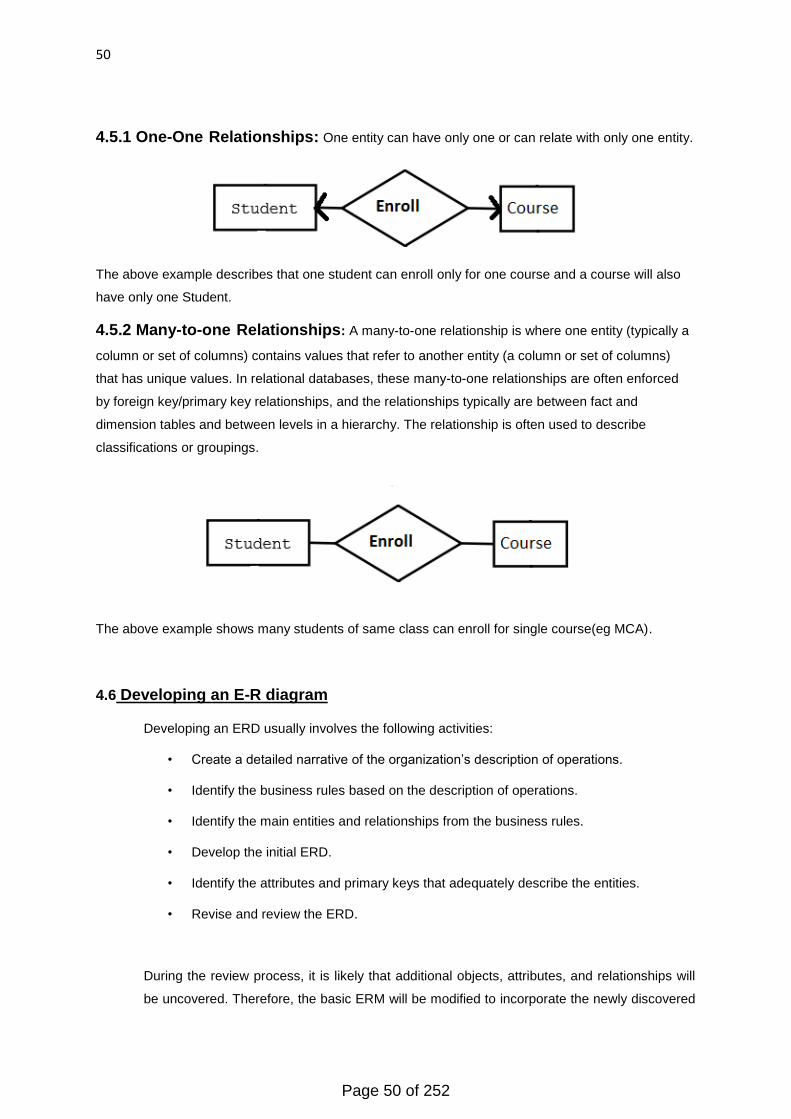
50

4.5.1 One-One Relationships: One entity can have only one or can relate with only one entity.

The above example describes that one student can enroll only for one course and a course will also

have only one Student.

4.5.2 Many-to-one Relationships: A many-to-one relationship is where one entity (typically a

column or set of columns) contains values that refer to another entity (a column or set of columns)

that has unique values. In relational databases, these many-to-one relationships are often enforced

by foreign key/primary key relationships, and the relationships typically are between fact and

dimension tables and between levels in a hierarchy. The relationship is often used to describe

classifications or groupings.

The above example shows many students of same class can enroll for single course(eg MCA).

4.6 Developing an E-R diagram

Developing an ERD usually involves the following activities:

• Create a detailed narrative of the organization‘s description of operations.

• Identify the business rules based on the description of operations.

• Identify the main entities and relationships from the business rules.

• Develop the initial ERD.

• Identify the attributes and primary keys that adequately describe the entities.

• Revise and review the ERD.

During the review process, it is likely that additional objects, attributes, and relationships will

be uncovered. Therefore, the basic ERM will be modified to incorporate the newly discovered

Page 50 of 252

51

ER components. Subsequently, another round of reviews might yield additional components

or clarification of the existing diagram. The process is repeated until the end users and

designers agree that the ERD is a fair representation of the organization‘s activities and

functions.

During the design process, the database designer does not depend simply on interviews to

help define entities, attributes, and relationships. A surprising amount of information can be

gathered by examining the business forms and reports that an organization uses in its daily

operations.

4.7 Normalizing the Model:

Normalization is a formal approach that applies a set of rules to associate attributes with entities.

When you normalize your data model, you can achieve the following goals. You can:

• Ensure that attributes are placed in the proper tables.

• Reduce data redundancy.

• Lower application maintenance costs.

• Maximize stability of the data structure.

• Produce greater flexibility in your design.

• Increase programmer effectiveness.

Normalization consists of steps to reduce the entities to more desirable physical properties. These

steps are called normalization rules, also referred to as normal forms. Each normal form constrains

the data more than the last form. Because of this, you must achieve first normal form before you can

achieve second normal form, and you must achieve second normal form before you can achieve third

normal form.

To illustrate the normalization process, consider the following list of unnormalized data items:

• Cust_ID (customer id) (primary key)

• Cust_Name (customer name)

• Cust_Type (customer type)

• Contact Name (one to many)

• Category Name (one to many)

In this example, a customer record length is variable because each customer can have a different

number of contacts and each customer can be part of multiple categories. Let's begin by taking the

previous structure and placing it into the first normal form.

Page 51 of 252

52

4.7.1 First Normal Form: Eliminating Repeating Groups

The first normal form (1NF) involves the removal of repeating groups. The question remains, "What is

a repeating group?" The previous example, has two repeating groups: contacts and category.

Remember, for a given customer, one or more contacts and one or more categories can exist.

For each repeating group you encounter, the repeating group moves to a separate table. In this case,

you end up with two new tables that store the contact and category data. The following outlines the

new structure and entities:

Customer table:

• Customer ID

• Customer Name

• Customer Type

Contact table:

• Contact ID

• Customer ID

• Contact Name

Category table:

• Category ID

• Customer ID

• Category Name

As you might guess, the Customer table is a super table to the Contact and Category tables. The two

relationships are one to many. In other words, each customer can have one or more contacts and can

be associated with one or more categories.

Before moving forward, it is important that you see the benefits derived by moving contacts and

categories to separate tables. Imagine how difficult the task of managing contacts would be if contacts

were kept in the Customer table. If a customer could have only one contact, the argument could be

made that contact data, such as name, phone number, and so on, could be stored in the Customer

table. After all, in this case, you would be dealing with a finite set of columns. But what if somebody

makes a request that involves the support of multiple contacts per customer? You have two choices:

• Add more columns to the Customer table to support multiple contacts.

• Add a child table that allows for any number of contacts.

Clearly, choice number two is the easier, more flexible, and more cost-effective alternative. With

choice one, your database design could continually be changing whenever a specific customer has

exceeded the number of contacts the Customer table can support.

Page 52 of 252

53

4.7.2 Second Normal Form: Eliminating Redundant Data

To get tables into the second normal form, you must analyze the fields in relation to the primary key.

The question of primary keys was raised in the previous section. The Contact and Category tables'

primary key are a multivalued key, so you can't look at a single field that can uniquely identify a

record. Looking at the Category table, the primary key is a combination of the Category ID and

Customer ID fields. Many customers can use the same category, and a customer can be part of many

categories. A customer, however, can't be part of the same category more than once. This makes

sense. Because of this rule, the combination of Category ID and Customer ID uniquely identifies a

record in the Category table. Let's turn our attention to the Contact table. As you will see, this scenario

presents an ambiguous situation.

Does Contact ID uniquely identify a contact record? It might uniquely identify a record; then again, it

might not. How is that for an answer? The answer depends on the context. Is the Contact table purely

about contacts? Or, is it more accurately named a Customer Contacts table? Again, the answer

depends on the context. Can a contact be associated with multiple customers? Or, can a contact be

linked with one and only one customer? It is quite possible that a contact person could be linked to

several customer records.

4.7.3 Third Normal Form: Eliminating Columns Not Dependent on Keys

You started with a single flat structure. To get to the first normal form, repeating groups were moved

to separate tables. This resulted in three new tables: Contact, Category, and Customer Type. The

next step is to get the tables in the third normal form. In order to illustrate this process, some new

fields need to be added to the Customer table. The following outlines the new structure of the

Customer table:

• Customer ID

• Customer Name

• Customer Type ID

• City

• State

• Pin Code

The Customer table is in the first normal form because no repeating groups exist, and the Customer

table is in the second normal form because a multivalue key does not exist. What about fields such as

city, state, and Pin Code—do they depend on the Customer ID Primary Key? The answer is no.

These elements are completely independent of the Customer ID Primary Key.

Let's take a few moments to examine the relationship between city, state, and PIN Code. A PIN Code

is specific to a city and a state. For example, 152202 is Ferozepur City Pin code. Remember the goal

of normalization is to remove redundant data. You only want to have to define an element of data one

time and reuse that element of data as needed. Consider a city like Mumbai that has hundreds of PIN

Page 53 of 252

54

Codes. As you examine the problem, it becomes clear that new tables will be required. In this case,

you would create a state, city, and city state Pin table. The following outlines the various table

structures:

• State table:

• State ID

• State Name

• City table:

• City ID

• City Name

• City State Pin table:

• PIN Code

• City ID

• State ID

Because you can be sure a PIN Code is unique, you could use the PIN Code itself as the primary

key.

4.8 Summary:

Entity-Relationship model to get a high-level graphical view of the essential components of enterprise

and how they are related

Then convert the E-R diagram to SQL DDL, or whatever database model you are using

E-R Model is not SQL based. It's not limited to any particular DBMS. It is a conceptual and semantic

model – captures meanings rather than an actual implementation.

Entity: an object that is involved in the enterprise and that be distinguished from other objects.

Entity Type: set of similar objects or a category of entities; they are well defined.

Attribute: describes one aspect of an entity type; usually

Relationship: It describes the connection between two entities.

This is further divided into three types:

• One to One

• One to Many

• Many to Many

Page 54 of 252

55

Normalizing the Model:


• First Normal Form: Eliminating Repeating Groups

• Second Normal Form: Eliminating Redundant Data

• Third Normal Form: Eliminating Columns Not Dependent on Keys

4.9 Glossary:

Semantic: It is related to meaning in language or logic.

Data Model: It is a description of the objects represented by a computer system together with their

properties and relationships

Object: It is a person or thing to which a specified action or feeling is directed.

Redundancy: It is the appearance of the same data factor in more than one field or table of data, or

including a data factor as a separate entity when it can be easily inferred from information in

existing data fields.

Flexibility: It is modifiability of Data.

Dependency: Relationship between conditions, events, or tasks such that one cannot begin or be-

completed until one or more other conditions, events, or tasks have occurred, begun, or completed.


Q1.What do you mean by Entity-Relationship Model? What are the basic Components of this

model?

Ans: Entity-Relationship Model:

An Entity-Relationship model is a representation of structured data; E-R modeling is the process of

generating these models. The ultimate output of the modeling process is an entity-relationship

diagram, a type of conceptual data model or semantic data model.

The E-R Model Comprise of following:

• Entities

• Relationships among entities

Symbols used in E-R Diagram

• Entity – rectangle

• Attribute – oval

Page 55 of 252

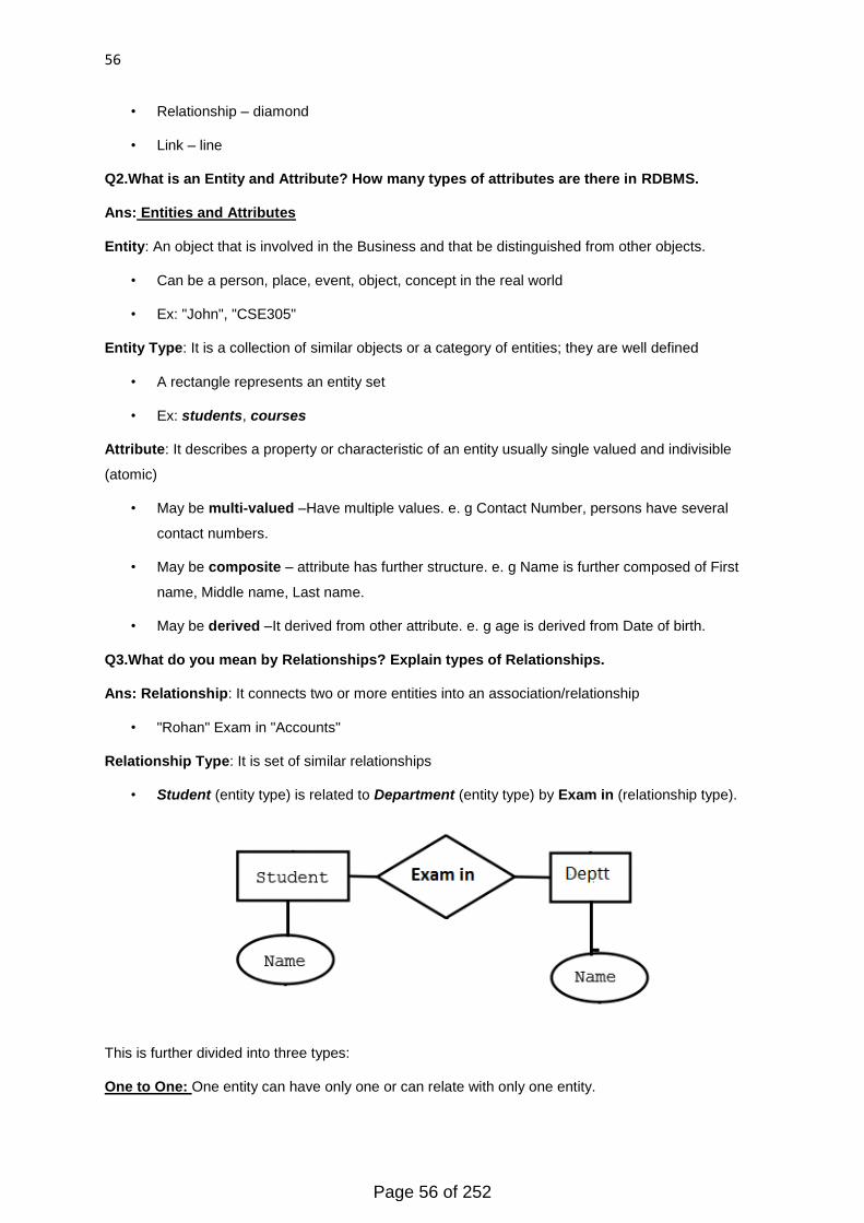
http://www.businessdictionary.com/definition/data-field.html

56

• Relationship – diamond

• Link – line

Q2.What is an Entity and Attribute? How many types of attributes are there in RDBMS.

Ans: Entities and Attributes

Entity: An object that is involved in the Business and that be distinguished from other objects.

• Can be a person, place, event, object, concept in the real world

• Ex: "John", "CSE305"

Entity Type: It is a collection of similar objects or a category of entities; they are well defined

• A rectangle represents an entity set

• Ex: students, courses

Attribute: It describes a property or characteristic of an entity usually single valued and indivisible

(atomic)

• May be multi-valued –Have multiple values. e. g Contact Number, persons have several

contact numbers.

• May be composite – attribute has further structure. e. g Name is further composed of First

name, Middle name, Last name.

• May be derived –It derived from other attribute. e. g age is derived from Date of birth.

Q3.What do you mean by Relationships? Explain types of Relationships.

Ans: Relationship: It connects two or more entities into an association/relationship

• "Rohan" Exam in "Accounts"

Relationship Type: It is set of similar relationships

• Student (entity type) is related to Department (entity type) by Exam in (relationship type).

This is further divided into three types:

One to One: One entity can have only one or can relate with only one entity.

Page 56 of 252

57

The above example describes that one student can enroll only for one course and a course will also

have only one Student.

One to Many: In this type of Relationship one entity is associated with many numbers of the same

entity. For example, Student enrolls for only one Course but a Course can have many Students.

Many to Many: Many entities can have a relationship with many entities.

The above diagram represents that many students can enroll for more than one courses.

Q4.How we can normalize a data model Explain with the help of an example?

Ans: Normalizing the Model:


When you normalize your data model, you can achieve the following goals. You can:

• Ensure that attributes are placed in the proper tables.

• Reduce data redundancy.

• Lower application maintenance costs.

• Maximize stability of the data structure.

• Produce greater flexibility in your design.

• Increase programmer effectiveness.

Page 57 of 252

58

Normalization consists of steps to reduce the entities to more desirable physical properties. These

steps are called normalization rules, also referred to as normal forms. Each normal form constrains

the data more than the last form. Because of this, you must achieve first normal form before you can

achieve second normal form, and you must achieve second normal form before you can achieve third

normal form.

To illustrate the normalization process, consider the following list of unnormalized data items:

• Cust_ID (customer id) (primary key)

• Cust_Name (customer name)

• Cust_Type (customer type)

• Contact Name (one to many)

• Category Name (one to many)

In this example, a customer record length is variable because each customer can have a different

number of contacts and each customer can be part of multiple categories. Let's begin by taking the

previous structure and placing it into the first normal form.

First Normal Form: Eliminating Repeating Groups

The first normal form (1NF) involves the removal of repeating groups. The question remains, "What is

a repeating group?" The previous example, has two repeating groups: contacts and category.

Remember, for a given customer, one or more contacts and one or more categories can exist.

For each repeating group you encounter, the repeating group moves to a separate table. In this case,

you end up with two new tables that store the contact and category data. The following outlines the

new structure and entities:

Customer table:

• Customer ID

• Customer Name

• Customer Type

Contact table:

• Contact ID

• Customer ID

• Contact Name

Category table:

• Category ID

• Customer ID

• Category Name

Page 58 of 252

59

As you might guess, the Customer table is a super table to the Contact and Category tables. The two

relationships are one to many. In other words, each customer can have one or more contacts and can

be associated with one or more categories.

Before moving forward, it is important that you see the benefits derived by moving contacts and

categories to separate tables. Imagine how difficult the task of managing contacts would be if contacts

were kept in the Customer table. If a customer could have only one contact, the argument could be

made that contact data, such as name, phone number, and so on, could be stored in the Customer

table. After all, in this case, you would be dealing with a finite set of columns. But what if somebody

makes a request that involves the support of multiple contacts per customer? You have two choices:

• Add more columns to the Customer table to support multiple contacts.

• Add a child table that allows for any number of contacts.

Clearly, choice number two is the easier, more flexible, and more cost-effective alternative. With

choice one, your database design could continually be changing whenever a specific customer has

exceeded the number of contacts the Customer table can support.

Second Normal Form: Eliminating Redundant Data

To get tables into the second normal form, you must analyze the fields in relation to the primary key.

The question of primary keys was raised in the previous section. The Contact and Category tables'

primary key are a multivalued key, so you can't look at a single field that can uniquely identify a

record. Looking at the Category table, the primary key is a combination of the Category ID and

Customer ID fields. Many customers can use the same category, and a customer can be part of many

categories. A customer, however, can't be part of the same category more than once. This makes

sense. Because of this rule, the combination of Category ID and Customer ID uniquely identifies a

record in the Category table. Let's turn our attention to the Contact table. As you will see, this scenario

presents an ambiguous situation.

Does Contact ID uniquely identify a contact record? It might uniquely identify a record; then again, it

might not. How is that for an answer? The answer depends on the context. Is the Contact table purely

about contacts? Or, is it more accurately named a Customer Contacts table? Again, the answer

depends on the context. Can a contact be associated with multiple customers? Or, can a contact be

linked with one and only one customer? It is quite possible that a contact person could be linked to

several customer records.

Third Normal Form: Eliminating Columns Not Dependent on Keys

You started with a single flat structure. To get to the first normal form, repeating groups were moved

to separate tables. This resulted in three new tables: Contact, Category, and Customer Type. The

next step is to get the tables in the third normal form. In order to illustrate this process, some new

fields need to be added to the Customer table. The following outlines the new structure of the

Customer table:

• Customer ID

Page 59 of 252

60

• Customer Name

• Customer Type ID

• City

• State

• Pin Code

The Customer table is in the first normal form because no repeating groups exist, and the Customer

table is in the second normal form because a multivalued key does not exist. What about fields such

as city, state, and Pin Code—do they depend on the Customer ID Primary Key? The answer is no.

These elements are completely independent of the Customer ID Primary Key.

Let's take a few moments to examine the relationship between city, state, and PIN Code. A PIN Code

is specific to a city and a state. For example, 152202 is Ferozepur City Pin code. Remember the goal

of normalization is to remove redundant data. You only want to have to define an element of data one

time and reuse that element of data as needed. Consider a city like Mumbai that has hundreds of PIN

Codes. As you examine the problem, it becomes clear that new tables will be required. In this case,

you would create a state, city, and city state Pin table. The following outlines the various table

structures:

• State table:

• State ID

• State Name

• City table:

• City ID

• City Name

• City State Pin table:

• PIN Code

• City ID

• State ID

Because you can be sure a PIN Code is unique, you could use the PIN Code itself as the primary

key.

4.11 References:

http://jcsites.juniata.edu/faculty/rhodes/dbms/ermodel.htm

http://www.studytonight.com/dbms/er-diagram.php

Page 60 of 252

http://jcsites.juniata.edu/faculty/rhodes/dbms/ermodel.htm

http://www.studytonight.com/dbms/er-diagram.php

61

http://www.help2engg.com/dbms/dbms-e-r-model

http://www.businessdictionary.com/definition/data-redundancy.html


• TechRadar: Enterprise DBMS, Q1 2014

By Noel Yuhanna with Boris Evelson, Brain Hopkins, Emily Jedniak

• The 2009-2014 World Outlook for Database Management Systems (DBMS)

Author: ICON Group International, Inc.

Publisher: ICON Group International, Inc.

• Starting out with Oracle

Author:John Day,Cralg Von Styke.

Page 61 of 252

http://www.help2engg.com/dbms/dbms-e-r-model

http://www.businessdictionary.com/definition/data-redundancy.html

http://www.forrester.com/Noel-Yuhanna

62

Unit 2

Lesson 5 - Interactive Structured Query Language (SQL)

5.1 Objective

5.2 Introduction to SQL

5.3 Data Types in SQL

5.4 Data Definition Language

5.4.1 Create Table

5.4.2 Alter Table

5.4.3 Drop Table

5.4.4 Rename Table

5.4.5 Truncate Table

5.5 Creation of Table With Constraints

5.5.1 Primary Key

5.5.2 Foreign Key

5.6 Summary

5.7 Glossary


5.9 References


5.1 Objective:

The basic commands and functions of SQL

Use SQL for data administration (e.g. Create tables)

Use SQL to create a database for maintaining information

5.2 Introduction to Structured Query Language (SQL):

Interactive SQL is a tool for sending SQL statements to the database server. You can use this utility:

Flick through the information in a database.

Try out SQL statements that you want to include in an application.

Load data into a database and accomplish other administrative tasks.

5.3 Data types in SQL:

Each column in a database table is required to have a name and a data type. SQL developers

have to decide what types of data will be stored inside each and every table column when

creating a SQL table. The data type is a label and a guideline for SQL to understand what type of

data is expected inside of each column, and it also identifies how SQL will interact with the stored

data.

The table 1 lists the general data types in SQL:

Page 62 of 252

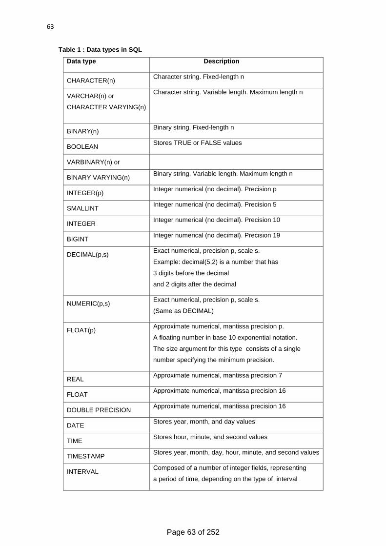
63

Table 1 : Data types in SQL

Data type Description

CHARACTER(n) Character string. Fixed-length n

VARCHAR(n) or

CHARACTER VARYING(n)

Character string. Variable length. Maximum length n

BINARY(n) Binary string. Fixed-length n

BOOLEAN Stores TRUE or FALSE values

VARBINARY(n) or

BINARY VARYING(n) Binary string. Variable length. Maximum length n

INTEGER(p) Integer numerical (no decimal). Precision p

SMALLINT Integer numerical (no decimal). Precision 5

INTEGER Integer numerical (no decimal). Precision 10

BIGINT Integer numerical (no decimal). Precision 19

DECIMAL(p,s) Exact numerical, precision p, scale s.

Example: decimal(5,2) is a number that has

3 digits before the decimal

and 2 digits after the decimal

NUMERIC(p,s) Exact numerical, precision p, scale s.

(Same as DECIMAL)

FLOAT(p) Approximate numerical, mantissa precision p.

A floating number in base 10 exponential notation.

The size argument for this type consists of a single

number specifying the minimum precision.

REAL Approximate numerical, mantissa precision 7

FLOAT Approximate numerical, mantissa precision 16

DOUBLE PRECISION Approximate numerical, mantissa precision 16

DATE Stores year, month, and day values

TIME Stores hour, minute, and second values

TIMESTAMP Stores year, month, day, hour, minute, and second values

INTERVAL Composed of a number of integer fields, representing

a period of time, depending on the type of interval

Page 63 of 252

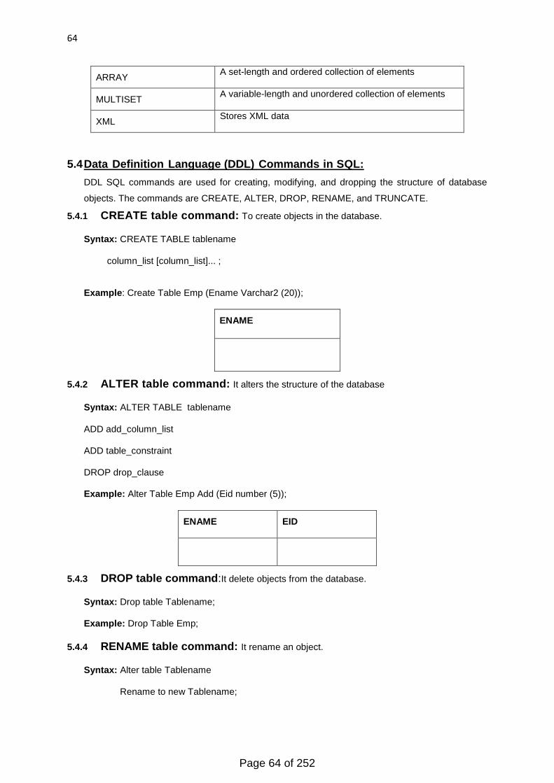
64

ARRAY A set-length and ordered collection of elements

MULTISET A variable-length and unordered collection of elements

XML Stores XML data

5.4 Data Definition Language (DDL) Commands in SQL:

DDL SQL commands are used for creating, modifying, and dropping the structure of database

objects. The commands are CREATE, ALTER, DROP, RENAME, and TRUNCATE.

5.4.1 CREATE table command: To create objects in the database.

Syntax: CREATE TABLE tablename

column_list [column_list]... ;

Example: Create Table Emp (Ename Varchar2 (20));

ENAME

5.4.2 ALTER table command: It alters the structure of the database

Syntax: ALTER TABLE tablename

ADD add_column_list

ADD table_constraint

DROP drop_clause

Example: Alter Table Emp Add (Eid number (5));

ENAME EID

5.4.3 DROP table command:It delete objects from the database.

Syntax: Drop table Tablename;

Example: Drop Table Emp;

5.4.4 RENAME table command: It rename an object.

Syntax: Alter table Tablename

Rename to new Tablename;

Page 64 of 252

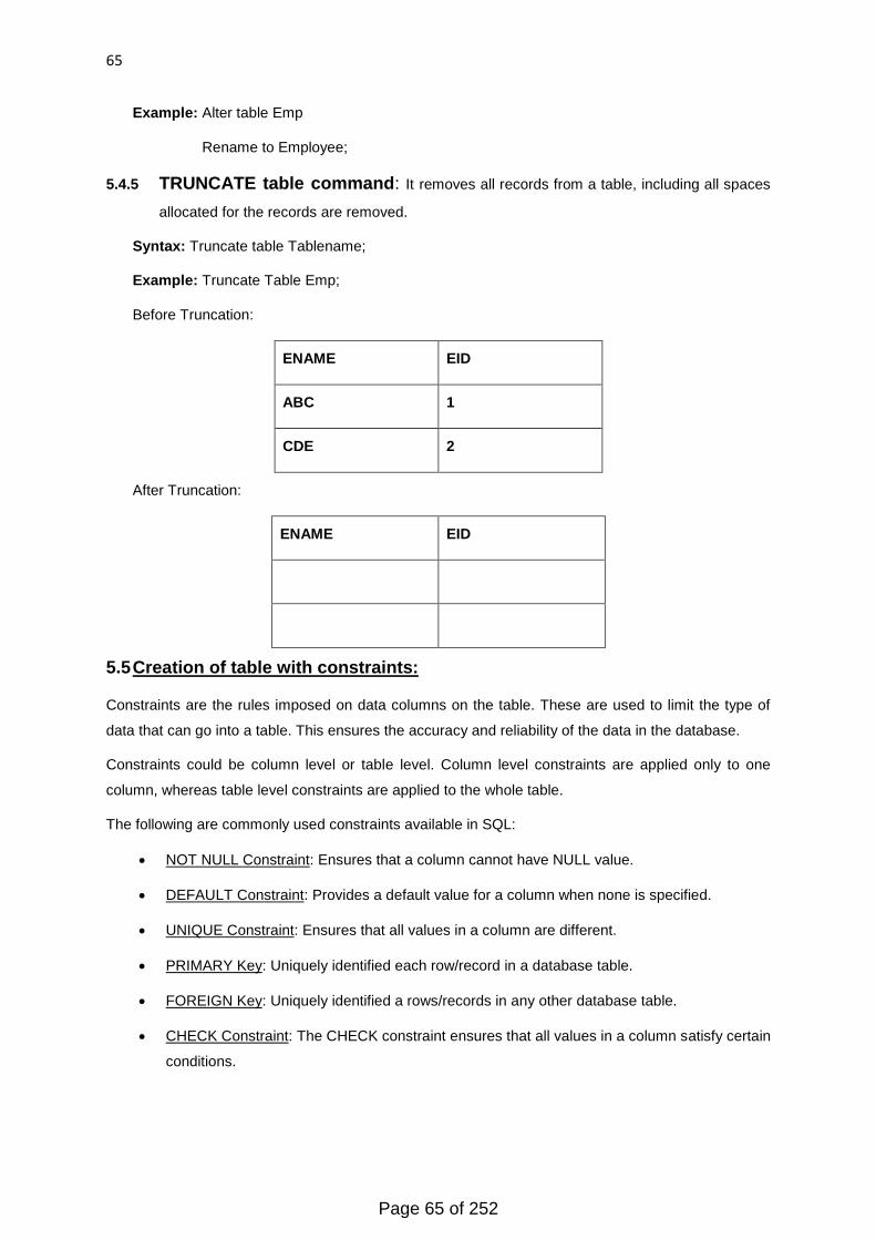
65

Example: Alter table Emp

Rename to Employee;

5.4.5 TRUNCATE table command: It removes all records from a table, including all spaces

allocated for the records are removed.

Syntax: Truncate table Tablename;

Example: Truncate Table Emp;

Before Truncation:

ENAME EID

ABC 1

CDE 2

After Truncation:

ENAME EID

5.5 Creation of table with constraints:

Constraints are the rules imposed on data columns on the table. These are used to limit the type of

data that can go into a table. This ensures the accuracy and reliability of the data in the database.

Constraints could be column level or table level. Column level constraints are applied only to one

column, whereas table level constraints are applied to the whole table.

The following are commonly used constraints available in SQL:

NOT NULL Constraint: Ensures that a column cannot have NULL value.

DEFAULT Constraint: Provides a default value for a column when none is specified.

UNIQUE Constraint: Ensures that all values in a column are different.

PRIMARY Key: Uniquely identified each row/record in a database table.

FOREIGN Key: Uniquely identified a rows/records in any other database table.

CHECK Constraint: The CHECK constraint ensures that all values in a column satisfy certain

conditions.

Page 65 of 252

http://www.tutorialspoint.com/sql/sql-not-null.htm

http://www.tutorialspoint.com/sql/sql-default.htm

http://www.tutorialspoint.com/sql/sql-unique.htm

http://www.tutorialspoint.com/sql/sql-primary-key.htm

http://www.tutorialspoint.com/sql/sql-foreign-key.htm

http://www.tutorialspoint.com/sql/sql-check.htm

66

5.5.1 Primary key constraint: This constraint defines a column or combination of columns

which uniquely identifies each row in the table.

Syntax:

[CONSTRAINT constraint_name] PRIMARY KEY (column_name1, column_name2...)

Example:

CREATE TABLE employee (id number (5), NOT, NULL, name char (20), Dept char (10),

location char (10));

ALTER TABLE employee ADD CONSTRAINT PK_EMPLOYEE_ID PRIMARY KEY (id));

5.5.2 Foreign key constraint: This constraint identifies any column referencing the PRIMARY

KEY in another table. It establishes a relationship between two columns in the same table or between

different tables. For a column to be defined as a Foreign Key, it should be a defined as a Primary Key

in the table which it is referring. One or more columns can be defined as Foreign key.

Syntax:

[CONSTRAINT constraint_name] FOREIGN KEY (column_name) REFERENCES

referenced_table_name (column_name);

Example:

CREATE TABLE order_items (order_id number (5), product_id number (5), product_name

char (20), CONSTRAINT od_id_pk PRIMARY KEY (order_id), CONSTRAINT pd_id_fk

FOREIGN KEY (product_id) REFERENCES product (product_id) );

5.6 Summary:

Interactive SQL:

Interactive SQL is a utility for sending SQL statements to the database server. You can use this utility:

Browse the information in a database.

Try out SQL statements that you plan to include in an application.

SQL Commands:

Each record has a unique identifier or primary key. SQL, which stands for Structured Query

Language, is used to communicate with a database. Through SQL one can create and delete tables.

Here are some commands:

Data Definition Language:

CREATE TABLE - creates a new database table

ALTER TABLE - alters a database table

DROP TABLE - deletes a database table

Page 66 of 252

67

CREATE INDEX - creates an index (search key)

DROP INDEX - deletes an index

SQL also has syntax to update, insert, and delete records.

Constraints:

SQL Constraints are the rules used to limit the type of data that can go into a table, to maintain the

accuracy and integrity of the data in the table. Constraints can be divided into following types:

Column level constraints: limits only column data.

Table level constraints: limits whole table data.

Table Level Constraints:

This constraint defines a column or combination of columns which uniquely identifies each row in the

table.

Primary Key:


table.

Foreign key or Referential Integrity:

This constraint identifies any column referencing the PRIMARY KEY in another table. It establishes a

relationship between two columns in the same table or between different tables. For a column to be

defined as a Foreign Key, it should be a defined as a Primary Key in the table which it is referring.

One or more columns can be defined as Foreign key.

Not Null Constraint:

This constraint ensures all rows in the table contain a definite value for the column which is specified

as not null. Which means a null value is not allowed.

Unique Key:

This constraint ensures that a column or a group of columns in each row has a distinct value. A

column(s) can have a null value, but the values cannot be duplicated.

Check Constraint:

This constraint defines a business rule on a column. All the rows must satisfy this rule. The constraint

can be applied for a single column or a group of columns.

Column Level Constraints:


table.

Primary Key:

Page 67 of 252

68


table.


This constraint identifies any column referencing the PRIMARY KEY in another table. It establishes a

relationship between two columns in the same table or between different tables. For a column to be

defined as a Foreign Key, it should be a defined as a Primary Key in the table which it is referring.

One or more columns can be defined as foreign key.


This constraint ensures all rows in the table contain a definite value for the column which is specified

as not null. Which means a null value is not allowed.

Unique Key:



5.7 Glossary:


Data Model: It is a description of the objects represented by a computer system together with

their properties and relationships

Object: It is a person or thing to which a specified action or feeling is directed.

Redundancy: It is the appearance of the same data factor in more than one field or table of data,

or including a data factor as a separate entity when it can be easily inferred from information in

existing data fields.



table.

Retrieve: To find or extract (information stored in a computer).

Data Model: It is a description of the objects represented by a computer system together with

their properties and relationships


Q1.What do you mean by interactive SQL?

Ans:

Interactive SQL:

Interactive SQL is a tool for sending SQL statements to the database server. You can use this utility:

Flick through the information in a database.

Try out SQL statements that you want to include in an application.

Load data into a database and accomplish other administrative tasks.

Page 68 of 252

http://www.businessdictionary.com/definition/appearance.html

http://www.businessdictionary.com/definition/data.html

http://www.businessdictionary.com/definition/factor.html

http://www.businessdictionary.com/definition/field.html

http://www.businessdictionary.com/definition/table.html

http://www.businessdictionary.com/definition/separate-entity.html

http://www.businessdictionary.com/definition/information.html

http://www.businessdictionary.com/definition/data-field.html

69

Q2.What is an SQL Command? How many types of SQL commands are there in DBMS?

Ans:

SQL Commands:

SQL commands are edifications used to communicate with the database to perform specific task

that work with data. SQL commands can be used not only for searching the database but also to

perform various other functions, for example, set permissions for users, you can create tables, add

data to tables, or modify data, drop the table. SQL commands are grouped into four major

categories depending on their functionality:

Data Definition Language (DDL) - These SQL commands are used for creating, modifying, and

dropping the structure of database objects. The commands are CREATE, ALTER, DROP,

RENAME, and TRUNCATE.

Data Manipulation Language (DML) - These SQL commands are used for storing, retrieving,

modifying, and deleting data. These commands are SELECT, INSERT, UPDATE, and DELETE.

Transaction Control Language (TCL) - These SQL commands are used for managing changes

affecting the data. These commands are COMMIT, ROLLBACK, and SAVEPOINT.

Data Control Language (DCL) - These SQL commands are used for providing security to

database objects. These commands are GRANT and REVOKE.

Q3.What is Data Definition Language Commands? Explain each with the help of an example.

Ans:

Data Definition Language (DDL):

Data Definition Language (DDL) statements are used to define the database structure or schema.

Some examples:

CREATE - to create objects in the database

ALTER - alters the structure of the database

DROP - delete objects from the database

TRUNCATE - remove all records from a table, including all spaces allocated for the records

are removed.

RENAME - rename an object

CREATE TABLE:

Syntax: CREATE TABLE tablename

column_list [column_list]... ;

Example: Create Table Emp (Ename Varchar2 (20));

Page 69 of 252

70

ENAME

ALTER TABLE:

Syntax: ALTER TABLE tablename

ADD add_column_list

ADD table_constraint

DROP drop_clause

Example: Alter Table Emp Add (Eid number (5));

ENAME EID

TRUNCATE TABLE:

Syntax: Truncate table Tablename;

Example: Truncate Table Emp;

Before Truncation:

ENAME EID

ABC 1

CDE 2

After Truncation:

ENAME EID

RENAME TABLE:

Syntax: Alter table Tablename

Page 70 of 252

71

Rename to new Tablename;

Example: Alter table Emp

Rename to Employee;

DROP TABLE:

Syntax: Drop table Tablename;

Example: Drop Table Emp;

Q4.What do you mean by constraint? How many types of constraints are there in DBMS?

Ans: Constraints are the rules enforced on data columns on the table. These are used to limit the

type of data that can go into a table. This ensures the accuracy and reliability of the data in the

database.

Column level: Column level constraints are applied only to one column.

Table level: Table level constraints are applied to the whole table.

Q5. What do you mean by Table Level Constraint? Explain each constraint with the help of

example.

Ans:


This constraint defines a column or combination of columns which uniquely identifies each row in

the table.

Primary Key:


table.

Syntax:

[CONSTRAINT constraint_name] PRIMARY KEY (column_name1, column_name2,..)

Example:



This constraint identifies any column referencing the PRIMARY KEY in another table. It establishes

a relationship between two columns in the same table or between different tables. For a column to

be defined as a Foreign Key, it should be a defined as a Primary Key in the table which it is

referring. One or more columns can be defined as Foreign key.

Syntax:



Page 71 of 252

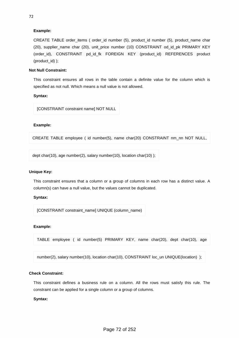
72

Example:

CREATE TABLE order_items ( order_id number (5), product_id number (5), product_name char

(20), supplier_name char (20), unit_price number (10) CONSTRAINT od_id_pk PRIMARY KEY

(order_id), CONSTRAINT pd_id_fk FOREIGN KEY (product_id) REFERENCES product

(product_id) );


This constraint ensures all rows in the table contain a definite value for the column which is

specified as not null. Which means a null value is not allowed.

Syntax:

[CONSTRAINT constraint name] NOT NULL

Example:

CREATE TABLE employee ( id number(5), name char(20) CONSTRAINT nm_nn NOT NULL,

dept char(10), age number(2), salary number(10), location char(10) );

Unique Key:



Syntax:

[CONSTRAINT constraint_name] UNIQUE (column_name)

Example:

TABLE employee ( id number(5) PRIMARY KEY, name char(20), dept char(10), age

number(2), salary number(10), location char(10), CONSTRAINT loc_un UNIQUE(location) );

Check Constraint:

This constraint defines a business rule on a column. All the rows must satisfy this rule. The

constraint can be applied for a single column or a group of columns.

Syntax:

Page 72 of 252

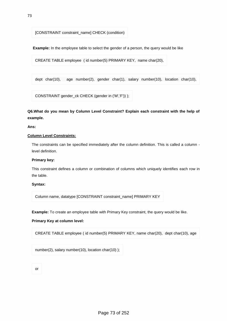
73

[CONSTRAINT constraint_name] CHECK (condition)

Example: In the employee table to select the gender of a person, the query would be like

CREATE TABLE employee ( id number(5) PRIMARY KEY, name char(20),

dept char(10), age number(2), gender char(1), salary number(10), location char(10),

CONSTRAINT gender_ck CHECK (gender in ('M','F')) );

Q6.What do you mean by Column Level Constraint? Explain each constraint with the help of

example.

Ans:


The constraints can be specified immediately after the column definition. This is called a column -

level definition.

Primary key:


the table.

Syntax:

Column name, datatype [CONSTRAINT constraint_name] PRIMARY KEY

Example: To create an employee table with Primary Key constraint, the query would be like.

Primary Key at column level:

CREATE TABLE employee ( id number(5) PRIMARY KEY, name char(20), dept char(10), age

number(2), salary number(10), location char(10) );

or

Page 73 of 252

74

CREATE TABLE employee ( id number(5) CONSTRAINT emp_id_pk PRIMARY KEY, name

char(20), dept char(10), age number(2), salary number(10), location char(10) );


CREATE TABLE employee ( id number(5), name char(20), dept char(10), age number(2),

salary number(10), location char(10), CONSTRAINT emp_id_pk PRIMARY KEY (id) );






Syntax:

[CONSTRAINT constraint_name] REFERENCES Referenced_Table_name (column_name)

Example:

CREATE TABLE product ( product_id number(5) CONSTRAINT pd_id_pk PRIMARY KEY,

product_name char(20), supplier_name char(20), unit_price number(10) );

CREATE TABLE order_items ( order_id number(5) CONSTRAINT od_id_pk PRIMARY KEY,

product_id number(5) CONSTRAINT pd_id_fk REFERENCES, product(product_id),



Page 74 of 252

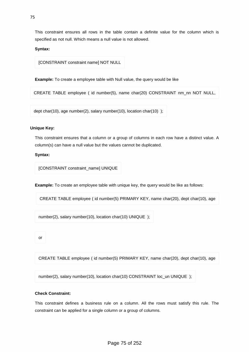
75



Syntax:


Example: To create a employee table with Null value, the query would be like



Unique Key:

This constraint ensures that a column or a group of columns in each row have a distinct value. A

column(s) can have a null value but the values cannot be duplicated.

Syntax:

[CONSTRAINT constraint_name] UNIQUE

Example: To create an employee table with unique key, the query would be like as follows:


number(2), salary number(10), location char(10) UNIQUE );

or


number(2), salary number(10), location char(10) CONSTRAINT loc_un UNIQUE );

Check Constraint:



Page 75 of 252

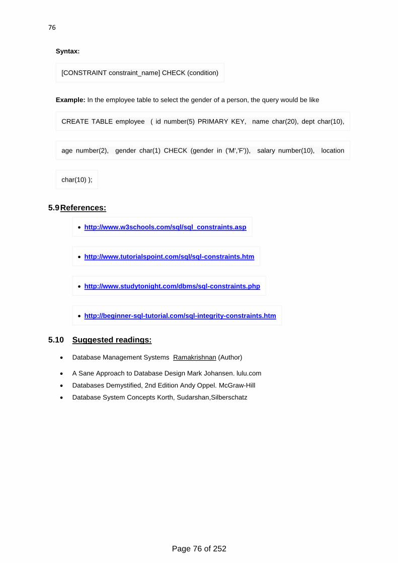
76

Syntax:



CREATE TABLE employee ( id number(5) PRIMARY KEY, name char(20), dept char(10),

age number(2), gender char(1) CHECK (gender in ('M','F')), salary number(10), location

char(10) );

5.9 References:

http://www.w3schools.com/sql/sql_constraints.asp

http://www.tutorialspoint.com/sql/sql-constraints.htm

http://www.studytonight.com/dbms/sql-constraints.php

http://beginner-sql-tutorial.com/sql-integrity-constraints.htm


Database Management Systems Ramakrishnan (Author)

A Sane Approach to Database Design Mark Johansen. lulu.com

Databases Demystified, 2nd Edition Andy Oppel. McGraw-Hill

Database System Concepts Korth, Sudarshan,Silberschatz

Page 76 of 252





http://www.amazon.in/s/277-0654621-8732668?_encoding=UTF8&field-author=Ramakrishnan&search-alias=stripbooks

77

Unit 1

Lesson 6: Data retrieval & transaction control using SQL

6.1 Objective

6.2 SELECT command

6.3 To Make Use SELECT Command With Options

6.3.1 Where clause

6.3.2 Order by clause

6.3.3 Group by clause

6.3.4 Having clause

6.3.5 Union clause

6.3.6 Intersection clause

6.3.7 Set difference clause

6.4 To use SQL functions

6.4.1 Numeric

6.4.2 Aggregate

6.4.3 Conversion

6.4.4 String function

6.5 To make views of a table

6.5.1 Creating View

6.5.2 Altering View

6.6 Types Of Views

6.6.1 Indexed View

6.6.2 Partitioned View

6.7 To make indexes of a table

6.7.1 Unique Index

6.7.2 Composite Index

6.8 To make use of transaction control statements viz. Rollback, Commit and Save point

6.8.1 Rollback

6.8.2 Commit

6.8.3 Save point

6.9 Summary

6.10 Glossary


6.12 References


6.1 Objective

Page 77 of 252

78

• To perform retrieval operations on the database

• To perform transaction control using SQL

6.2 SELECT command:

SELECT command is used to fetch the data from a database table which return data in the form

of result table. These result tables are called result-sets.

Syntax (a): SELECT column1, column2, column FROM table_name;

Syntax (b): SELECT * FROM table_name;

Example: Suppose, we have a table Employee1 with columns Eid, Ename,Esal,Eloc.


Eid Ename Esal Eloc

101 Anu 5000 Moga

102 Sonam 4000 Ferozepur

103 Shweta 4500 Sangrur

Eid Ename Esal Eloc

104 Sonu 5000 Moga


105 Sneha 4500 Sangrur

• Select Eid,Esal from Employee;

Output: Columns named Eid and Esal will be selected

Eid Esal

101 5000

Page 78 of 252

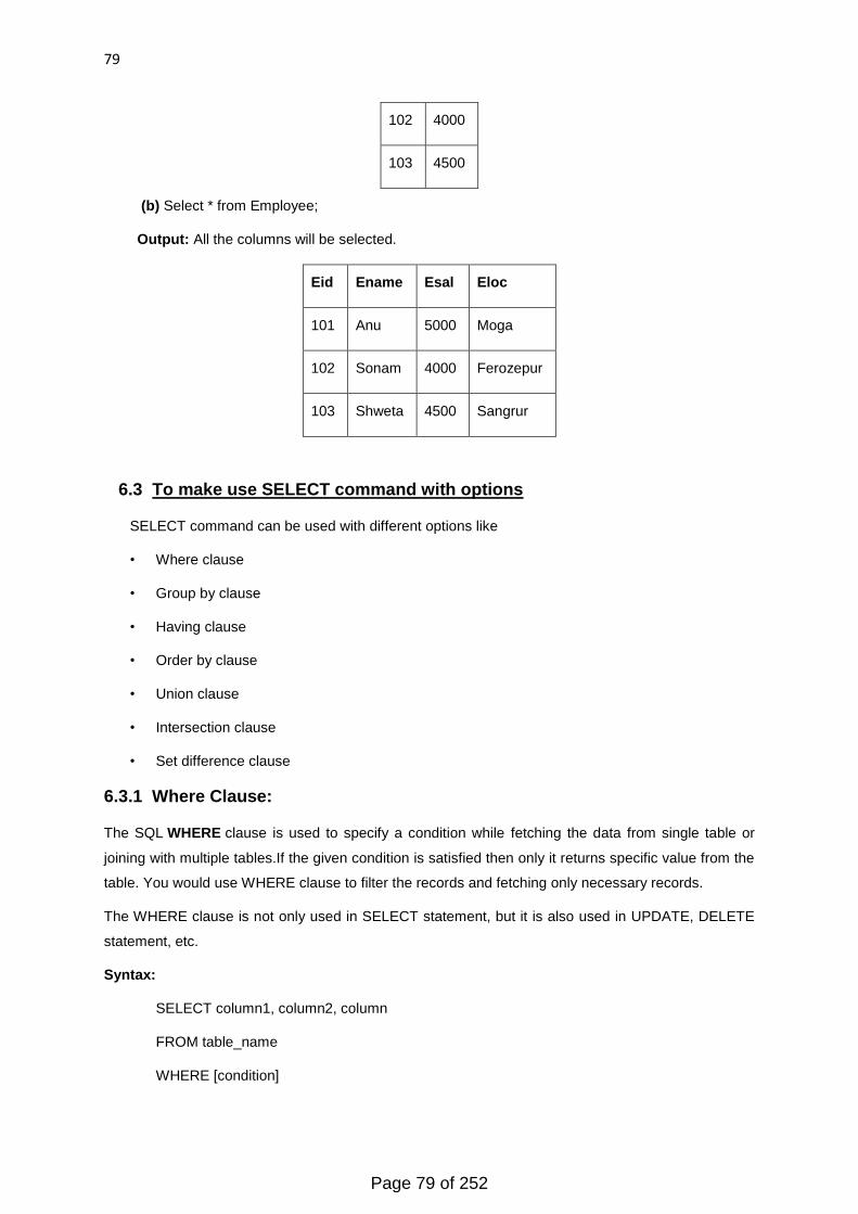
79

102 4000

103 4500

(b) Select * from Employee;

Output: All the columns will be selected.

Eid Ename Esal Eloc

101 Anu 5000 Moga



6.3 To make use SELECT command with options

SELECT command can be used with different options like

• Where clause

• Group by clause

• Having clause

• Order by clause

• Union clause

• Intersection clause

• Set difference clause

6.3.1 Where Clause:

The SQL WHERE clause is used to specify a condition while fetching the data from single table or

joining with multiple tables.If the given condition is satisfied then only it returns specific value from the

table. You would use WHERE clause to filter the records and fetching only necessary records.

The WHERE clause is not only used in SELECT statement, but it is also used in UPDATE, DELETE

statement, etc.

Syntax:

SELECT column1, column2, column

FROM table_name

WHERE [condition]

Page 79 of 252

80

Example: In the table Employee we will select the column with Where Clause.

Select * from Employee where Eid=101;

Output: All the rows with Employee id 101 will be selected.

Eid Ename Esal Eloc

101 Anu 5000 Moga

6.3.2 Order by Clause:

The SQL ORDER BY clause is used to sort the data in ascending or descending order, based on one

or more columns. Some database sorts query results in ascending order by default.

Syntax:

SELECT column-list

FROM table_name

[WHERE condition]

[ORDER BY column1, column2, .. columnN] [ASC | DESC];

Example:

Select * from Employee order by Ename;

Output: All the records will be selected and sorted in ascending order in Alphabetic order with

Employee Name.Similarly we can sort data in descending order.

Eid Ename Esal Eloc

101 Anu 5000 Moga



6.3.3 GROUP By Clause:

The SQL GROUP BY clause is used in collaboration with the SELECT statement to arrange identical

data into groups.The GROUP BY clause follows the WHERE clause in a SELECT statement and

precedes the ORDER BY clause.

Syntax:

SELECT column1, column2 FROM table_name

WHERE [ conditions ]

Page 80 of 252

81

GROUP BY column1, column2

ORDER BY column1, column2

Example:

Select * from employee sum(Esal) Group by Ename;

Output: First sum of all the salaries will be done, then grouping will be started by Emplyee Name.

Eid Ename Esal Eloc

101 Anu 5000 Moga



6.3.4 Having Clause:

The HAVING clause enables you to specify conditions that filter which group results appear in the

final results.

The WHERE clause places conditions on the selected columns, whereas the HAVING clause places

conditions on groups created by the GROUP BY clause.

Syntax:

SELECT column1, column2

FROM table1, table2

WHERE [ conditions ]

GROUP BY column1, column2

HAVING [ conditions ]

ORDER BY column1, column2

Example:

SELECT * FROM Employee

GROUP BY Ename

HAVING Min(Esal) >= 4200;

Output: The SQL HAVING clause will return only those records where the minimum salary is greater

than 4200.

Eid Ename Esal Eloc

Page 81 of 252

82

101 Anu 5000 Moga


6.3.5 Union Operator:

The UNION operator is used to combine the result-set of two or more SELECT statements.

Notice that each SELECT statement within the UNION must have the same number of columns. The

columns must also have similar data types. Also, the columns in each SELECT statement must be in

the same order.

Syntax:

SELECT column_name(s) FROM table1

UNION

SELECT column_name(s) FROM table2;

Example:

SELECT Eid,Ename,Esal,Eloc FROM Employee

UNION

SELECT Eid,Ename,Esal,Eloc FROM Employee1;

Output: All the fields from both the tables having same data type will be selected duplicate rows will

be eliminated.

Eid Ename Esal Eloc

101 Anu 5000 Moga



104 Sonu 5000 Moga


6.3.6 Intersection Operator:

This statement combines the results with the INTERSECT operator, which returns only those rows

returned by both queries.

Syntax:

SELECT column1 [, column2 ]

Page 82 of 252

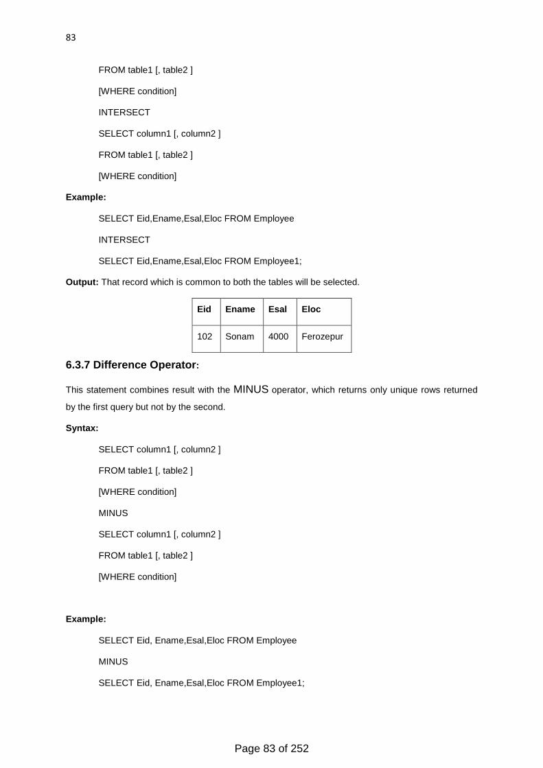
83

FROM table1 [, table2 ]

[WHERE condition]

INTERSECT



[WHERE condition]

Example:

SELECT Eid,Ename,Esal,Eloc FROM Employee

INTERSECT

SELECT Eid,Ename,Esal,Eloc FROM Employee1;

Output: That record which is common to both the tables will be selected.

Eid Ename Esal Eloc


6.3.7 Difference Operator:

This statement combines result with the MINUS operator, which returns only unique rows returned

by the first query but not by the second.

Syntax:



[WHERE condition]

MINUS



[WHERE condition]

Example:

SELECT Eid, Ename,Esal,Eloc FROM Employee

MINUS

SELECT Eid, Ename,Esal,Eloc FROM Employee1;

Page 83 of 252

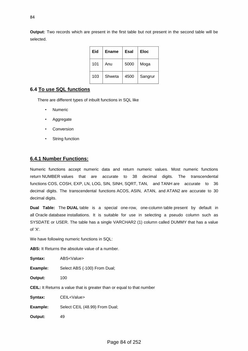
84

Output: Two records which are present in the first table but not present in the second table will be

selected.

Eid Ename Esal Eloc

101 Anu 5000 Moga


6.4 To use SQL functions

There are different types of inbuilt functions in SQL like

• Numeric

• Aggregate

• Conversion

• String function

6.4.1 Number Functions:

Numeric functions accept numeric data and return numeric values. Most numeric functions

return NUMBER values that are accurate to 38 decimal digits. The transcendental

functions COS, COSH, EXP, LN, LOG, SIN, SINH, SQRT, TAN, and TANH are accurate to 36

decimal digits. The transcendental functions ACOS, ASIN, ATAN, and ATAN2 are accurate to 30

decimal digits.

Dual Table: The DUAL table is a special one-row, one-column table present by default in

all Oracle database installations. It is suitable for use in selecting a pseudo column such as

SYSDATE or USER. The table has a single VARCHAR2 (1) column called DUMMY that has a value

of 'X'.

We have following numeric functions in SQL:

ABS: It Returns the absolute value of a number.

Syntax: ABS<Value>

Example: Select ABS (-100) From Dual;

Output: 100

CEIL: It Returns a value that is greater than or equal to that number

Syntax: CEIL<Value>

Example: Select CEIL (48.99) From Dual;

Output: 49

Page 84 of 252

http://en.wikipedia.org/wiki/Table_(database)

http://en.wikipedia.org/wiki/Oracle_database

http://en.wikipedia.org/wiki/Relational_database

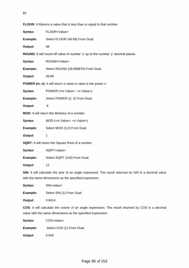
85

FLOOR: It Returns a value that is less than or equal to that number

Syntax: FLOOR<Value>

Example: Select FLOOR (48.99) From Dual;

Output: 48

ROUND: It will round off value of number ‗x‘ up to the number ‗y‘ decimal places.

Syntax: ROUND<Value>

Example: Select ROUND (48.998876) From Dual;

Output: 49.99

POWER (m, n): It will return a value m raise to the power n.

Syntax: POWER (<m Value>, <n Value>)

Example: Select POWER (2, 3) From Dual;

Output: 8

MOD: It will return the Modulus of a number.

Syntax: MOD (<m Value>, <n Value>)

Example: Select MOD (3,2) From Dual;

Output: 1

SQRT: It will return the Square Root of a number.

Syntax: SQRT<value>

Example: Select SQRT (144) From Dual;

Output: 12

SIN: It will calculate the sine of an angle expressed. The result returned by SIN is a decimal value

with the same dimensions as the specified expression.

Syntax: SIN<value>

Example: Select SIN (1) From Dual;

Output: 0.8414

COS: It will calculate the cosine of an angle expression. The result returned by COS is a decimal

value with the same dimensions as the specified expression.

Syntax: COS<value>

Example: Select COS (1) From Dual;

Output: 0.540

Page 85 of 252

86

6.4.2 Group Functions:

Aggregate functions return a single result row based on groups of rows, rather than on single rows.

Aggregate functions can appear in select lists and in ORDER BY and HAVING clauses. They are

commonly used with the GROUP BY clause in a SELECT statement, where Oracle Database divides

the rows of a queried table or view into groups. In a query containing a GROUP BY clause, the

elements of the select list can be aggregate functions, GROUP BY expressions, constants, or

expressions involving one of these. Oracle applies the aggregate functions to each group of rows and

returns a single result row for each group.

You use aggregate functions in the HAVING clause to eliminate groups from the output based on the

results of the aggregate functions, rather than on the values of the individual rows of the queried table

or view.

AVG: AVG returns the average value of expression.

Example: Select AVG (Esal) From Employee;

Output: 3000

SUM: It will return the sum of values of expression. You can use it as an aggregate or analytic

function.

Example: Select SUM (Esal) From Employee;

Output: 9000

MIN: It will return the minimum value of expression.

Example: Select MIN (Esal) From Employee;

Output: 2000

MAX: It will return the MAXIMUM of values of expression.

Example: Select MAX (Esal) From Employee;

Output: 4000

COUNT: It will return the number of rows returned by the query. You can use it as an aggregate or

analytic function.

Example: Select COUNT (*) From Employee;

Output: 3

MEDIAN: MEDIAN is an inverse distribution function that assumes a continuous distribution model. It

takes a numeric or date time value and returns the middle value or an interpolated value that would

be the middle value once the values are sorted. Nulls are ignored in the calculation.

Example: Select MEDIAN (Esal) From Employee;

Output: 3000

Page 86 of 252

87

STDDEV: STDDEV returns the sample standard deviation of expr, a set of numbers. You can use it

as both an aggregate and analytic function. It differs from STDDEV_SAMP in that STDDEV returns

zero when it has only 1 row of input data, whereas STDDEV_SAMP returns null.

Example: Select STDDEV (Esal) From Employee;

Output: 1000

6.4.3 Scalar Functions:

Scalar functions do not aggregate data or compute aggregate statistics. Instead, scalar functions

compute and substitute a new data value for each value associated with a data item

Following are the basic scalar functions:

CHAR_LENGTH: Returns an integer value representing the number of characters in an expression.

Example: Select CHAR_LENGTH (‗HELLO‘);

Output: 5

OCTET_LENGTH: Returns an integer representing the number of octets in an expression.


POSITION: The POSITION function returns an integer that indicates the starting position of a

string within the search string.

Example: SELECT LOCATE ('bar', 'foobar');

Output: 4

Example: SELECT POSITION ('bar', 'fooJKbrFG');

Output: 0

CHARINDEX: It will find the index of a given character.

Example: SELECT CHARINDEX ('bar', 'foobar');

Output: 3

CONCATENATE: Appends two or more literal expressions, column values, or variables together into

one string.

Example: SELECT CONCAT ('My ', 'dog ', 'has ', 'a ', 'first ', 'name...');

Output: 'My dog has a first name...'

6.4.4 Character Functions

Character functions that return character values return values of the following data types unless

otherwise documented:

• If the input argument is CHAR or VARCHAR2, then the value returned

is VARCHAR2.

Page 87 of 252

88

• If the input argument is NCHAR or NVARCHAR2, then the value returned

is NVARCHAR2.

The length of the value returned by the function is limited by the maximum length of the data type

returned.

• For functions that return CHAR or VARCHAR2, if the length of the return value

exceeds the limit, then Oracle Database truncates it and returns the result without an error

message.

• For functions that return CLOB values, if the length of the return values exceeds the

limit, then Oracle raises an error and returns no data.

We have following character functions in oracle:

CHR: CHR returns the character having the binary equivalent to and as a VARCHAR2, value in either

the database character set or, if you specify USING NCHAR_CS, the national character set.

Example: SELECT CHR (67) | FROM DUAL;

Output

INITCAP: INITCAP returns char, with the first letter of each word in uppercase, all other letters in

lowercase. Words are delimited by white space or characters that are not alphanumeric.

Example: SELECT INITCAP ('the soap') "Capitals" FROM DUAL;

Output: The Soap

LOWER: LOWER returns char, with all letters lowercase. Char can be any of the data

types CHAR, VARCHAR2, NCHAR, NVARCHAR2, CLOB, or NCLOB. The return value is the same

data type as char.

Example: SELECT LOWER (‗KARAN‘) FROM DUAL;

Output: karan

UPPER: UPPER returns char, with all letters uppercase. Char can be any of the data


data type as char.

Example: SELECT UPPER (‗karan‘) FROM DUAL;

Output: KARAN

LPAD: LPAD returns expr1, left-padded to length n characters with the sequence of characters

in expr2. This function is useful for formatting the output of a query.

Both expr1 and expr2 can be any of the

datatypes CHAR, VARCHAR2, NCHAR, NVARCHAR2, CLOB, or NCLOB. The string returned is

of VARCHAR2 datatype if expr1is a character datatype and a LOB if expr1 is a LOB datatype. The

Page 88 of 252

89

string returned is in the same character set as expr1. The argument n must be a NUMBER integer or

a value that can be implicitly converted to a NUMBER integer.

Example: SELECT LPAD ('Page 1', 15,'*.') "LPAD example"

FROM DUAL;

Output: *.*.*.*.*Page 1

RPAD: RPAD returns expr1, right-padded to length n characters with expr2, replicated as many times

as necessary. This function is useful for formatting the output of a query.






Example: SELECT RPAD ('Page 1', 15,'*.') "LPAD example"

FROM DUAL;

Output: Page 1*.*.*.*.*

REPLACE: REPLACE returns char with every occurrence of search string replaced with the

replacement string. If the replacement string is omitted or null, then all occurrences of the search

string are removed. If the search string is null, then char is returned.

Both search string and replacement string, as well as char, can be any of the

datatypes CHAR, VARCHAR2, NCHAR, NVARCHAR2, CLOB, or NCLOB. The string returned is in

the same character set as char. The function returns VARCHAR2 if the first argument is not a LOB

and returns CLOB if the first argument is a LOB.

Example: SELECT REPLACE ('JACK and JUE','J','BL') "Changes"

FROM DUAL;

Output: BLACK AND BLUE.

SUBSTR: The SUBSTR functions return a portion of a char, beginning at character position, substring

length characters long. SUBSTR calculates lengths using characters as defined by the input character

set. SUBSTRB uses bytes instead of characters. SUBSTRC uses Unicode complete

characters. SUBSTR2 uses UCS2 code points. SUBSTR4 uses UCS4 code points.

• If position is 0, then it is treated as 1.

• If the position is positive, then Oracle Database counts from the beginning of char to

find the first character.

Page 89 of 252

90

• If position is negative, then Oracle counts backward from the end of char.

• If substring length is omitted, then Oracle returns all characters to the end of char.

If substring length is less than 1, then Oracle returns null.

Example: SELECT SUBSTR ('ABCDEFG', 3,4) "Substring"

FROM DUAL;

Output: CDEF

6.4.5 Data Conversion Functions:

Conversion functions convert a value from one datatype to another. Generally, the form of the

function names follows the convention datatype TO datatype. The first data type is the input data

type. The second datatype is the output datatype. The SQL conversion functions are:

CONVERT: The CONVERT function converts values from one type of data to another. CONVERT is

primarily useful for changing values from a numeric or DATE data type to a text data type, or vice

versa.

Example: SHOW CONVERT ('1/3/98' DATE 'MDY')

Output: 03JAN98

TCONVERT: TCONVERT function converts time-series data from one dimension of type DAY,

WEEK, MONTH, QUARTER, or YEAR to another dimension of type DAY, WEEK, MONTH,

QUARTER, or YEAR. You can specify an aggregation method or an allocation method to use in the

conversion.

Example: SHOW TCONVERT ('1/3/98' DATE 'MDY')

TO_CHAR: The TO_CHAR function converts a date, number, or NTEXT expression to a TEXT

expression in a specified format. This function is typically used to format output data.

Example: SHOW TO_CHAR (SYSDATE, 'Month DD, YYYY HH24: MI: SS‘)

Output: November 30, 2000 10:01:29

TO_DATE: The TO_DATE function converts a formatted TEXT or NTEXT expression to a DATETIME

value. This function is typically used to convert the formatted date output of one application (which

includes information such as month, day, and year in any order and any language, and separators

such as slashes, dashes, or spaces) so that it can be used as input to another application.

Example: SHOW TO_DATE ('November 15, 2001', 'Month dd, yyyy', -

Page 90 of 252

91

NLS_DATE_LANGUAGE 'american')

Output: Jueves: November 15, 2001 12:00:00 AM

TO_NCHAR: The TO_NCHAR function converts a TEXT expression, date, or number to NTEXT in a

specified format. This function is typically used to format output data.

Example: SHOW TO_NCHAR (SYSDATE, 'Month DD, YYYY HH24: MI: SS‘)


TO_NUMBER: The TO_NUMBER function converts a formatted TEXT or NTEXT expression to a

number. This function is typically used to convert the formatted numerical output of one application

(which includes currency symbols, decimal markers, thousands group markers, and so forth) so that it

can be used as input to another application.

Example: DEFINE money VARIABLE DECIMAL

Money = TO_NUMBER ('$94,567,00', 'L999G999D00', NLS_NUMERIC_CHARACTERS ', ')

SHOW money

Output: 94,567.00

6.4.6 Manipulating Dates in Oracle:

Datetime functions operate on date (DATE), timestamp

(TIMESTAMP, TIMESTAMP WITH TIME ZONE, and TIMESTAMP WITH LOCAL TIME ZONE), and

interval (INTERVAL DAY TO SECOND, INTERVAL YEAR TO MONTH) values.

Some of the datetime functions were designed for the Oracle DATE data type

(ADD_MONTHS, CURRENT_DATE, LAST_DAY, NEW_TIME, and NEXT_DAY). If you provide a

timestamp value as their argument, then Oracle Database internally converts the input type to

a DATE value and returns a DATE value. The exceptions are the MONTHS_BETWEEN function,

which returns a number, and the ROUND and TRUNC functions, which do not accept timestamp or

interval values at all.

The remaining datetime functions were designed to accept any of the three types of data (date,

timestamp, and interval) and to return a value of one of these types.

Page 91 of 252

92

All of the datetime functions that return current system datetime information, such

as SYSDATE, SYSTIMESTAMP, CURRENT_TIMESTAMP, and so forth, is evaluated once for each

SQL statement, regardless how many times they are referenced in that statement.

The datetime functions are:

ADD_MONTHS: DD_MONTHS returns the date, date plus integer months. A month is defined by the

session parameter NLS_CALENDAR. The date argument can be a datetime value or any value that

can be implicitly converted to DATE. The integer argument can be an integer or any value that can be

implicitly converted to an integer. The return type is always DATE, regardless of the data type of date.

If date is the last day of the month or if the resulting month has fewer days than the day component

of date, then the result is the last day of the resulting month. Otherwise, the result has the same day

component as a date.

Example: SELECT TO_CHAR (ADD_MONTHS (22-mar-1990, 1), 'DD-MON-YYYY')

Output: 22-apr-1990

CURRENT_DATE: CURRENT_DATE returns the current date in the session time zone, in a value in

the Gregorian calendar of data type DATE

Example: SELECT CURRENT_DATE from dual;

Output: 15-apr-2014

CURTIME: It returns the current time.

Example: SELECT CURTIME ();

Output: 12:45:34

EXTRACT: The EXTRACT () function is used to return a single part of a date/time, such as year,

month, day, hour, minute, etc.

Example: SELECT EXTRACT (YEAR FROM 22-MAR-1990)

Output: 1990

MONTHS_BETWEEN: MONTHS_BETWEEN returns number of months between

dates date1 and date2. The month and the last day of the month are defined by the

parameterNLS_CALENDAR. If date1 is later than date2, then the result is positive. If date1 is earlier

than date2, then the result is negative. If date1 and date2 are either the same days of the month or

both last days of months, then the result is always an integer. Otherwise, Oracle Database calculates

the fractional portion of the result based on a 31-day, month and considers the difference in time

components date1 and date2.

Example: SELECT MONTHS_BETWEEN

(TO_DATE ('02-02-1995','MM-DD-YYYY'),

TO_DATE ('01-01-1995','MM-DD-YYYY')) "Months"

Page 92 of 252

93

FROM DUAL;

Output: 1.03

LAST_DAY: LAST_DAY returns the date of the last day of the month that contains a date. The last

day of the month is defined by the session parameter NLS_CALENDAR. The return type is

always DATE, regardless of the data type of date.

Example: SELECT SYSDATE,

LAST_DAY (SYSDATE) "Last",

LAST_DAY (SYSDATE) - SYSDATE "Days Left"

FROM DUAL;

Output: 30-MAY-09 31-MAY-09 1

NEXT_DAY: NEXT_DAY returns the date of the first weekday named by char that is later than the

date. The return type is always DATE, regardless of the data type of date. The argument char must

be a day of the week in the date language of your session, either the full name or the abbreviation.

The minimum number of letters required is the number of letters in the abbreviated version. Any

characters immediately following the valid abbreviation are ignored. The return value has the same

hours, minutes, and seconds component as the argument date.

Example: SELECT NEXT_DAY ('15-OCT-2009','TUESDAY') "NEXT DAY"

FROM DUAL;

Output: 20-OCT-2009 00:00:00

6.5 To make views of a table:

Views: A view is nothing more than a SQL statement that is stored in the database with an

associated name. A view is actually a composition of a table in the form of a predefined SQL query.

A view can contain all rows of a table or select rows from a table. A view can be created from one or

many tables which depends on the written SQL query to create a view.

Views, which are a kind of virtual tables, allow users to do the following:

• Structure data in a way that users or classes of users find natural or intuitive.

• Restrict access to the data such that a user can see and (sometimes) modify exactly what they

need and no more.

• Summarize data from various tables which can be used to generate reports.

6.5.1 Creating View: In SQL, a view is a virtual table based on the result-set of an SQL

statement.

Page 93 of 252

94

A view contains rows and columns, just like a real table. The fields in a view are fields from one or

more real table in the database.

You can add SQL functions, WHERE, and JOIN statements to a view and present the data as if the

data were coming from one single table.

Syntax:

CREATE VIEW view_name AS SELECT column_name (s) FROM table_name

WHERE condition;

Example:

CREATE VIEW [Emp_view] AS SELECT Eid, Ename FROM Employee

WHERE Eid=101;

6.5.2 Altering a view: We can alter an already created view with Replace statement.

Syntax:

CREATE OR REPLACE VIEW view_name AS

SELECT column_name (s)

FROM table_name

WHERE condition

Now we can Loc column to previous View.

Example: CREATE VIEW [Emp_view] AS

SELECT Eid, Ename, Loc

FROM Employee

WHERE Eid=101;

6.6 Types of views:

6.6.1 Indexed View: An indexed view has a unique clustered index. The clustered index is stored

in SQL Server and updated like any other clustered index, providing SQL Server with another place to

look to potentially optimize a query utilizing the indexed view. Queries that don‘t specifically use the

indexed view can even benefit from the existence of the clustered index from the view. In the

Page 94 of 252

95

development and enterprise editions of SQL Server, the optimizer can use the indexes of views to

optimize queries that do not specify the indexed view. In the other editions of SQL Server, however,

the query must include the indexed view and specify the hint NOEXPAND to get the benefit of the

index on the view. If your queries could benefit from having more than one index on the view, non-

clustered indexes can also be created in the view. This would supply the optimizer with more

possibilities to speed up the queries referencing the columns included in the view.

A view that is to be indexed has to be created with schema binding. This means that once the indexed

view is created, the underlying tables cannot be altered in any way that would materially affect the

indexed view unless the view is first altered or dropped. It also means that all the tables referenced in

the view must be referenced by their two-part name (schemaname. table name). Below is an example

of the CREATE statement for an indexed view, MyView, and its underlying table, MyBigTable. The

table is first created, then the view that references two of the table‘s three columns, and finally the

unique clustered index on the view making it an indexed view.

Example:

CREATE VIEW emp_view1

WITH SCHEMABINDING AS

SELECT

e. Eid,

d.depid,

FROM e. Employee AS e

JOIN d.deptt AS d

ON d.depid = e.depid;

6.6.2 Partitioned View: Partitioning SQL data sets is an ideal way to improve scale out, and

distributed partitioning is particularly valuable in this regard. Here I will explain the benefits of using

partitioned views, and offer some points to keep in mind when defining and creating them.

A partitioned view will show row data (horizontal partitioning) from one or more tables, across one or

more servers. When a single server is used, the view is referred to as a local-partitioned view. When

this type of view spans more than one server, it is a distributed-partitioned view. Distributed-partition

views were added in SQL Server 2000, and the collection of instances on different servers is

sometimes referred to as a federated database server set.

Example

Page 95 of 252

96

To get the most benefit from partition views, the parameter PARTITION_VIEW_ENABLED must be

set. This example shows how to:

• Create the Tables Underlying the Partition View

• Load Each Partition View

• Enable Check Constraints

• Add Additional Overlapping Partition Criteria

• Create Indexes for Each Partition

• Analyze the Partitions

• Create the View that Ties the Partitions Together

Create the Tables Underlying the Partition View

This example involves two tables, created with the following syntax:

create table line_item_1992 ( constraint C_send_date_1992 check(send_date < 'Jan-01-1993')

disable, order_key number , part_key number , source_key number ,

send_date date , promise_date date , receive_date date );

create table line_item_1993 ( constraint C_send_date_1993 check(send_date => 'Jan-01-1993'

and send_date < 'Jan-01-1994') disable, order_key number , part_key number ,

source_key number , send_date date , promise_date date , receive_date

date );

Load Each Partition View

You can load each partition using a SQL*Loader process. Each load process can reference the same

loader control file (in this example it is "LI. ctl"), but should use a different data file. Also, the data files

must match the partitioning criteria given in the send_date check constraints. For improved

performance, disable constraints that define the partitioning criteria until after the partitions are

loaded.

slqldr scott/tiger direct=true control=LI.ctl data=LI1992.dat


Enable Check Constraints

After loading the partitions, you define the partition view. This example does so by enabling the check

constraints. Enabling the check constraints allows the optimizer to recognize and skip irrelevant

partitions.

alter table line_item_1992 enable constraint C_send_date_1992

Page 96 of 252

97


Add Additional Overlapping Partition Criteria

It is possible to have additional partitioning criteria or partitions that overlap. The application in this

example guarantees that all line items are received within 90 days of shipment.

Attention: These constructs will not be directly available for partitioned tables in Oracle8. Using them

might introduce additional complexity in migrating partition views to partitioned tables.

alter table line_item_1992

add constraint C_receive_date_1992 check ( receive_date between 'Jan-01-1992' and 'Jan-

01-1993' + 90);


add constraint C_receive_date_1993 check ( receive_date between 'Jan-01-1993' and 'Jan-

01-1994' + 90);

Create Indexes for Each Partition

If you need an index on a partition view, you must create the index on each of the partitions. If you do

not index each partition identically, the optimizer will be unable to recognize your UNION ALL view as

a partition view.

create index part_key_source_key_1992 on line_item_1992 (part_key, source_key)

create index part_key_source_key_1993 on line_item_1993 (part_key, source_key)

Analyze the Partitions

Now analyze the partitions.

analyze table line_item_1992 compute statistics;


Note: The cost-based optimizer is always used with partition views. You must therefore perform

ANALYZE at the partition level with partitioned tables. You can submit an ANALYZE statement on

each partition in parallel, using multiple logon sessions.

Create the View that Ties the Partitions Together

Once you identify or create the tables that you wish to use, you can create the view text that ties the

partitions together.

create or replace view line_item as select * from line_item_1992 union all select * from

line_item_1993;

6.7 To make indexes of a table:

Page 97 of 252

98

Index: Indexes are optional structures associated with tables and clusters that allow SQL

statements to execute more quickly against a table. Just as the index in this manual helps you

locate information faster than if there were no index, an Oracle Database index provides a faster

access path to table data. You can use the indexes without rewriting any queries. Your results

are the same, but you see them more quickly.

Syntax:

CREATE INDEX index_name

ON table_name (column_name)

Example:

CREATE INDEX PIndex ON Employee (Ename);

6.7.1 Unique Index:

Unique indexes are used not only for performance, but also for data integrity. A unique index does not

allow any duplicate values to be inserted into the table. The basic syntax is as follows:

Syntax:

CREATE UNIQUE INDEX index_name ON table_name (column_name)

Example:

CREATE UNIQUE INDEX PIndex ON Employee (Ename);

6.7.2 Composite Index:

A composite index is an index on two or more columns of a table. The basic syntax is as

follows:

Syntax:

CREATE INDEX index_name ON table_name (column_name1, column_name2);

Example:

CREATE INDEX PIndex ON Employee (Ename, Eid);

6.8 To make use of transaction control statements viz. Rollback, Commit and

Save point:

A transaction is a unit of work that is performed against a database. Transactions are units or

sequences of work accomplished in a logical order, whether in a manual fashion by a user or

automatically by some sort of a database program.

A transaction is the propagation of one or more changes to the database. For example, if you are

creating a record or updating a record or deleting a record from the table, then you are performing

Page 98 of 252

99

transactions a on the table. It is important to control transactions to ensure data integrity and to

handle database errors.

Practically, you will club many SQL queries into a group and you will execute all of them together as a

part of a transaction.

Properties of Transactions:

Transactions have the following four standard properties, usually referred to by the acronym ACID:

• Atomicity: ensures that all operations within the work unit are completed successfully; otherwise, the

transaction is aborted at the point of failure, and previous operations are rolled back to their former

state.

• Consistency: ensures that the database properly changes states upon a successfully committed

transaction.

• Isolation: enables transactions to operate independently of and transparent to each other.

• Durability: ensures that the result or effect of a committed transaction persists in case of a system

failure.

6.8.1 Rollback:

The ROLLBACK command is the transactional command used to undo transactions that have not

already been saved to the database.

The ROLLBACK command can only be used to undo transactions since the last COMMIT or

ROLLBACK command was issued.

The syntax for ROLLBACK command is as follows:

ROLLBACK;

6.8.2 Commit:

The COMMIT command is the transactional command used to save changes invoked by a transaction

to the database.

The COMMIT command saves all transactions to the database since the last COMMIT or ROLLBACK

command.

The syntax for COMMIT command is as follows:

Page 99 of 252

100

COMMIT;

6.8.3 Save point:

A SAVEPOINT is a point in a transaction when you can roll the transaction back to a certain point

without rolling back the entire transaction.

The syntax for SAVEPOINT command is as follows:

SAVEPOINT SAVEPOINT_NAME;

This command serves only in the creation of a SAVEPOINT among transactional statements. The

ROLLBACK command is used to undo a group of transactions.

The syntax for rolling back to a SAVEPOINT is as follows:

ROLLBACK TO SAVEPOINT_NAME;

Following is an example where you plan to delete the three different records from the CUSTOMERS

table. You want to create a SAVEPOINT before each delete, so that you can ROLLBACK to any

SAVEPOINT at any time to return the appropriate data to its original state.

6.9 Summary:

Viewing of Data:

We can view data with the SELECT command. We can also perform arithmetic, logical operations

on data. We can also alter the way of representation of data.

Arithmetic Operators:

You can use an arithmetic operator with one or two arguments to negate, add, subtract, multiply,

and divide numeric values. Some of these operators are also used in date, time and interval

arithmetic.

Logical Operators:

Logical operators manipulate the results of conditions.

Comparison Operators:

Comparison operators are used in conditions that compare one expression with another. The

result of a comparison can be TRUE, FALSE, or UNKNOWN.

Page 100 of 252

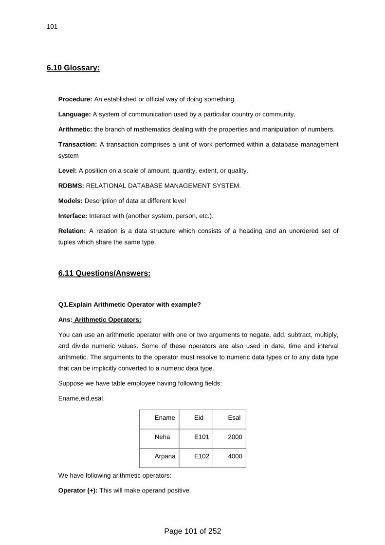
101

6.10 Glossary:



Arithmetic: the branch of mathematics dealing with the properties and manipulation of numbers.


system





Relation: A relation is a data structure which consists of a heading and an unordered set of

tuples which share the same type.


Q1.Explain Arithmetic Operator with example?

Ans: Arithmetic Operators:



arithmetic. The arguments to the operator must resolve to numeric data types or to any data type

that can be implicitly converted to a numeric data type.

Suppose we have table employee having following fields:

Ename,eid,esal.

Ename Eid Esal

Neha E101 2000

Arpana E102 4000

We have following arithmetic operators:

Operator (+): This will make operand positive.

Page 101 of 252

102

Example: SELECT * FROM employee WHERE Esal = -1;

Operator (-): This will negate the operand.


Addition (+): This will add two Operands.

Example: UPDATE employee set esal=esal+1000;

Subtraction (-): This will subtract two Operands.

Example: UPDATE employee set esal=esal-1000;

Multiplication (*): This will multiply two Operands.

Example: UPDATE employee set esal=esal*15. 5;

Division (/): This will divide two Operands.

Example: UPDATE employee set esal=esal/10;

Q2. Explain Logical Operator with example?

Ans: Logical Operators:


NOT Operator: Returns TRUE if the following condition is FALSE. Returns FALSE if it is TRUE. If

it is UNKNOWN, it remains UNKNOWN.

Example: SELECT * FROM Employee WHERE NOT (Esal IS NULL)

AND Operator: Returns TRUE if both component conditions are TRUE. Returns FALSE if either

is FALSE; otherwise returns UNKNOWN.

Example: SELECT * FROM Employee WHERE Esal=2000 AND Eid=E101;

OR Operator: Returns TRUE if either component condition is TRUE. Returns FALSE if both are

FALSE. Otherwise, returns UNKNOWN.

Example: SELECT * FROM Employee WHERE Esal=3000 OR Eid=E102;

Page 102 of 252

103

Q3. Explain Comparison Operator with example?

Ans: Comparison Operators:



Operator (=): It will Equates two operands.

Example: SELECT ENAME FROM Employee WHERE SAL = 1500;

Operator (! =): It is basically an Inequality test operator.

Example: SELECT ENAME FROM EMP WHERE SAL! = 5000;

Operator (>): This will give greater among two operators.

Example: SELECT ENAME FROM Employee WHERE SAL > 3000;

Operator (<): This will give lesser among two operators.

Example: SELECT ENAME FROM Employee WHERE SAL < 3000;

Operator (>=): This will give greater and equal operand among two operators.

Example: SELECT ENAME FROM Employee WHERE SAL >= 3000;

Operator (<=): This will give lesser than or equal operand among two operators.

Example: SELECT ENAME FROM Employee WHERE SAL <= 3000;

Q4.What is a View in the database? Explain with example?

Ans: View in A a database:

In database theory, a view is the result set of a stored query on the data, which

the database users can query just as they would in a persistent database collection object. This

pre-established query command is kept in the database dictionary. Unlike ordinary base tables in

a relational database, a view does not form part of the physical schema: as a result set, it is a

virtual table computed or collated from data in the database, dynamically when access to that

view is requested. Changes applied to the data in a relevant underlying table are reflected in the

data shown in subsequent invocations of the view.

Creating View: In SQL, a view is a virtual table based on the result-set of an SQL statement.



You can add SQL functions, WHERE, and JOIN statements to a view and present the data as if

the data were coming from one single table.

Syntax:

Page 103 of 252

http://en.wikipedia.org/wiki/Database_theory

http://en.wikipedia.org/wiki/Result_set



http://en.wikipedia.org/wiki/Database


http://en.wikipedia.org/wiki/Database_design

104

CREATE VIEW view_name AS


FROM table_name

WHERE condition

Example:

CREATE VIEW [Emp_view] AS

SELECT Eid, Ename

FROM Employee

WHERE Eid=101;

Altering a view: We can alter an already created view with Replace statement.

Syntax:



FROM table_name

WHERE condition


Example: CREATE VIEW [Emp_view] AS


FROM Employee

WHERE Eid=101;

Q5.What are the advantages of Views?

Ans: Advantages of Views:

Views can provide advantages over tables:

Views can represent a subset of the data contained in a table; consequently, a view can limit the

degree of exposure of the underlying tables to the outer world: a given user may have permission

to query the view, while denying access to the rest of the base table.

Views can join and simplify multiple tables into a single virtual table

Page 104 of 252

http://en.wikipedia.org/wiki/Join_(SQL)

105

Views can act as aggregated tables, where the database engine aggregates data

(sum, average etc.) And presents the calculated results as part of the data

Views can hide the complexity of data; for example a view could appear as Sales2000 or

Sales2001, transparently partitioning the actual underlying table

Views take very little space to store; the database contains only the definition of a view, not a

copy of all the data which it presents

Depending on the SQL engine used, views can provide extra security

Q6.What is an Index in Database?

Ans: Index: Indexes are optional structures associated with tables and clusters that allow SQL

statements to execute more quickly against a table. Just as the index in this manual helps you

locate information faster than if there were no index, an Oracle Database index provides a faster

access path to table data. You can use indexes without rewriting any queries. Your results are the

same, but you see them more quickly.

Q7.What is an Indexed View? Explain with example?

Ans: Indexed View: An indexed view has a unique clustered index. The clustered index is stored

in SQL Server and updated like any other clustered index, providing SQL Server with another

place to look to potentially optimize a query utilizing the indexed view. Queries that don‘t

specifically use the indexed view can even benefit from the existence of the clustered index from

the view. In the development and enterprise editions of SQL Server, the optimizer can use the

indexes of views to optimize queries that do not specify the indexed view. In the other editions of

SQL Server, however, the query must include the indexed view and specify the

hint NOEXPAND to get the benefit of the index on the view. If your queries could benefit from

having more than one index on the view, non-clustered indexes can also be created in the view.

This would supply the optimizer with more possibilities to speed up the queries referencing the

columns included in the view.

A view that is to be indexed has to be created with schema binding. This means that once the

indexed view is created, the underlying tables cannot be altered in any way that would materially

affect the indexed view unless the view is first altered or dropped. It also means that all the tables

referenced in the view must be referenced by their two-part name (schemaname. table name).

Below is an example of the CREATE statement for an indexed view, MyView, and its underlying

table, MyBigTable. The table is first created, then the view that references two of the table‘s three

columns, and finally the unique clustered index on the view making it an indexed view.

Example:

Page 105 of 252

http://en.wikipedia.org/wiki/Database_engine

http://en.wikipedia.org/wiki/Sum

http://en.wikipedia.org/wiki/Average

http://en.wikipedia.org/wiki/Partition_(database)

http://en.wikipedia.org/wiki/SQL

106



SELECT

e. Eid,

d.depid,

FROM e.Employee AS e

JOIN d.deptt AS d


Q8.What is a Partitioned View? Explain with example?

Ans: Partitioned View: Partitioning SQL data sets is an ideal way to improve scale out, and

distributed partitioning is particularly valuable in this regard. Here I will explain the benefits of

using partitioned views, and offer some points to keep in mind when defining and creating them.

A partitioned view will show row data (horizontal partitioning) from one or more tables, across one

or more servers. When a single server is used, the view is referred to as a local-partitioned view.

When this type of view spans more than one server, it is a distributed-partitioned view.

Distributed-partition views were added in SQL Server 2000, and the collection of instances on

different servers is sometimes referred to as a federated database server set.

Example

To get the most benefit from partition views, the parameter PARTITION_VIEW_ENABLED must

be set. This example shows how to:










Page 106 of 252

http://docs.oracle.com/cd/A57673_01/DOC/server/doc/A48506/partview.htm







107

create table line_item_1992 ( constraint C_send_date_1992 check(send_date < 'Jan-01-1993') disable, order_key number , part_key number , source_key number , send_date date , promise_date date , receive_date date );

create table line_item_1993 (constraint C_send_date_1993 check(send_date => 'Jan-01-1993'

and send_date < 'Jan-01-1994') disable, order_key number , part_key number ,

source_key number , send_date date ,promise_date date , receive_date date );


You can load each partition using a SQL*Loader process. Each load process can reference the

same loader control file (in this example it is "LI.ctl"), but should use a different data file. Also, the

data files must match the partitioning criteria given in the send_date check constraints. For

improved performance, disable constraints that define the partitioning criteria until after the

partitions are loaded.




After loading the partitions, you define the partition view. This example does so by enabling the

check constraints. Enabling the check constraints allows the optimizer to recognize and skip

irrelevant partitions.






Attention: These constructs will not be directly available for partitioned tables in Oracle8. Using

them might introduce additional complexity in migrating partition views to partitioned tables.


add constraint C_receive_date_1992 check ( receive_date between 'Jan-01-1992' and 'Jan-01-

1993' + 90);

alter table line_item_1993 add constraint C_receive_date_1993 check ( receive_date between

'Jan-01-1993' and 'Jan-01-1994' + 90);


Page 107 of 252

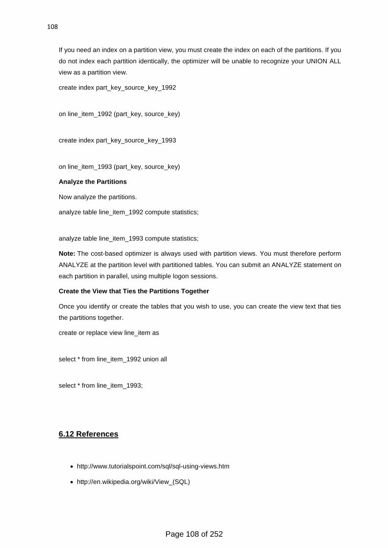
108

If you need an index on a partition view, you must create the index on each of the partitions. If you

do not index each partition identically, the optimizer will be unable to recognize your UNION ALL

view as a partition view.

create index part_key_source_key_1992

on line_item_1992 (part_key, source_key)











Once you identify or create the tables that you wish to use, you can create the view text that ties

the partitions together.

create or replace view line_item as

select * from line_item_1992 union all

select * from line_item_1993;

6.12 References

http://www.tutorialspoint.com/sql/sql-using-views.htm

http://en.wikipedia.org/wiki/View_(SQL)

Page 108 of 252


http://en.wikipedia.org/wiki/View_(SQL

109

http://www.w3schools.com/sql/sql_view.asp

http://www.dba-oracle.com/art_9i_indexing.htm

http://docs.oracle.com/cd/E11882_01/server.112/e25789/indexiot.htm#CNCPT721

http://www.sqlperformance.com/2014/01/sql-plan/indexed-views-and-statistics

http://www.codeproject.com/Articles/199058/SQL-Server-Indexed-Views-Speed-Up-Your-

Select-Quer

http://searchwindowsserver.techtarget.com/tip/Improving-partition-views-in-SQL-Server

http://sqlblog.com/blogs/piotr_rodak/archive/2010/09/11/partitioned-views.aspx

http://technet.microsoft.com/en-us/library/aa933141(v=sql.80).aspx

http://docs.oracle.com/cd/A57673_01/DOC/server/doc/A48506/partview.htm#383


Database System. A practical approach to design, implementation and management.

Author: Thomas Connoly, Corlyn Begg.

Taxonomy of database management system.

Author: Aditya Kumar Gupta.

Database management System

Author: Alex Leon, Mathew Leon.

Page 109 of 252



http://docs.oracle.com/cd/E11882_01/server.112/e25789/indexiot.htm


http://www.codeproject.com/Articles/199058/SQL-Server-Indexed-Views-Speed-Up-Your-Select-Quer






110

Unit 2

Lesson 7 - Data Constraints using SQL

7.1 Objective

7.2 Introduction to Data Constraints

7.3 Data Constraints

7.3.1 Column Level Constraints

7.3.1.1 Not Key

7.3.1.2 Primary Key

7.3.1.3 Foreign Key

7.3.1.4 Check Key

7.3.1.5 Unique Constraint

7.3.1.6 Default

7.3.2 Table Level Constraints

7.3.2.1 Primary Key

7.3.2.2 Foreign Key

7.3.2.3 Unique Key

7.4 Summary

7.5 Glossary


7.7 References


7.1 Objective:

The basic constraints in database systems

Use SQL for adding constraints

7.2 Introduction to data constraints:

Constraints are the rules imposed on data columns on the table. These are used to limit the type

of data that can go into a table. This ensures the accuracy and reliability of the data in the

database. Constraints could be at column level or table level. Column level constraints are

applied only to one or more columns, whereas table level constraints are applied to the whole

table.

7.3 Type of Data Constraints:

Page 110 of 252

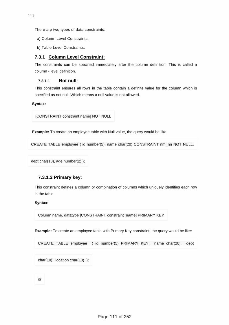
111

There are two types of data constraints:

a) Column Level Constraints.

b) Table Level Constraints.

7.3.1 Column Level Constraint:

The constraints can be specified immediately after the column definition. This is called a

column - level definition.

7.3.1.1 Not null:



Syntax:


Example: To create an employee table with Null value, the query would be like


dept char(10), age number(2) );

7.3.1.2 Primary key:

This constraint defines a column or combination of columns which uniquely identifies each row

in the table.

Syntax:


Example: To create an employee table with Primary Key constraint, the query would be like:

CREATE TABLE employee ( id number(5) PRIMARY KEY, name char(20), dept

char(10), location char(10) );

or

Page 111 of 252

112

CREATE TABLE employee ( id number(5) CONSTRAINT emp_id_pk PRIMARY KEY,

name char(20), dept char(10), location char(10) );


CREATE TABLE employee ( id number(5), name char(20), dept char(10), location

char(10), CONSTRAINT emp_id_pk PRIMARY KEY (id) );

7.3.1.3 Foreign key:

This constraint identifies any column referencing the PRIMARY KEY in another table. It

establishes a relationship between two columns in the same table or between different tables.

For a column to be defined as a Foreign Key, it should be a defined as a Primary Key in the

table which it is referring. One or more columns can be defined as Foreign key.

Syntax:

[CONSTRAINT constraint_name] REFERENCES Referenced_Table_name

(column_name)

Example:

CREATE TABLE product product_id number (5) CONSTRAINT pd_id_pk PRIMARY KEY,

product_name char (20), supplier_name char (20) );

CREATE TABLE order_items (order_id number (5) CONSTRAINT od_id_pk PRIMARY

KEY, product_id number (5) CONSTRAINT pd_id_fk REFERENCES, product (product_id),

product_name char (20) );

Page 112 of 252

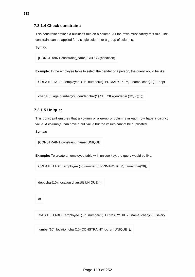
113

7.3.1.4 Check constraint:



Syntax:



CREATE TABLE employee ( id number(5) PRIMARY KEY, name char(20), dept

char(10), age number(2), gender char(1) CHECK (gender in ('M','F')) );

7.3.1.5 Unique:

This constraint ensures that a column or a group of columns in each row have a distinct

value. A column(s) can have a null value but the values cannot be duplicated.

Syntax:


Example: To create an employee table with unique key, the query would be like,

CREATE TABLE employee ( id number(5) PRIMARY KEY, name char(20),

dept char(10), location char(10) UNIQUE );

or

CREATE TABLE employee ( id number(5) PRIMARY KEY, name char(20), salary

number(10), location char(10) CONSTRAINT loc_un UNIQUE );

Page 113 of 252

114

7.3.1.6 Default:

The DEFAULT constraint is used to insert a default value into a column.The default

value will be added to all new records, if no other value is specified.

Syntax:

Column name, datatype [CONSTRAINT constraint_name] Default Value

Example:

CREATE TABLE CUSTOMERS ( ID INT NOT NULL, NAME VARCHAR (20) NOT

NULL, AGE NUMBER(3) NOT NULL, ADDRESS CHAR (25) , SALARY DECIMAL

(18, 2) DEFAULT 5000.00, PRIMARY KEY (ID) );

7.3.2 Table Level Constraint:


in the table.

7.3.2.1 Primary key:


in the table.

Syntax:

[CONSTRAINT constraint_name] PRIMARY KEY (column_name1, column_name2...)

Example:

CREATE TABLE employee (id number (5), NOT, NULL, name char (20), Dept char (10), location

char (10);


7.3.2.2 Foreign key:





Syntax:



Page 114 of 252

115

Example:

CREATE TABLE order_items (order_id number (5), product_id number (5), product_name char

(20), CONSTRAINT od_id_pk PRIMARY KEY (order_id), CONSTRAINT pd_id_fk FOREIGN KEY

(product_id) REFERENCES product(product_id) );

7.3.2.3 Unique key:



Syntax:


Example:


Location char (10), CONSTRAINT loc_un UNIQUE(location) );

7.4 Summary:

Constraints:

SQL Constraints are the rules used to limit the type of data that can go into a table, to maintain

the accuracy and integrity of the data in the table.

Constraints can be divided into following two types:

Column level constraints: limits only column data.

Table level constraints: limits whole table data.



in the table.

Primary Key:


the table.




Page 115 of 252

116



Unique Key:





in the table.

Primary Key:


the table.





table which it is referring. One or more columns can be defined as foreign key.




Unique Key:



Check Constraint:



7.5 Glossary:


Data Model: It is a description of the objects represented by a computer system together with their

properties and relationships

Reliability: It means dependability: the quality of being dependable or reliable


Column: A column is a set of data values of a particular simple type, one for each row of the table.

Page 116 of 252

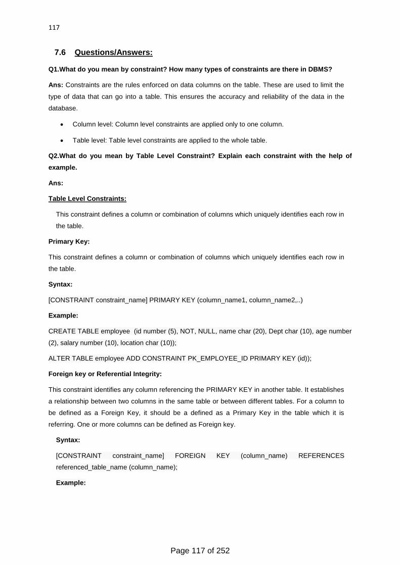
117


Q1.What do you mean by constraint? How many types of constraints are there in DBMS?

Ans: Constraints are the rules enforced on data columns on the table. These are used to limit the

type of data that can go into a table. This ensures the accuracy and reliability of the data in the

database.

Column level: Column level constraints are applied only to one column.

Table level: Table level constraints are applied to the whole table.

Q2.What do you mean by Table Level Constraint? Explain each constraint with the help of

example.

Ans:



the table.

Primary Key:


the table.

Syntax:

[CONSTRAINT constraint_name] PRIMARY KEY (column_name1, column_name2,..)

Example:

CREATE TABLE employee (id number (5), NOT, NULL, name char (20), Dept char (10), age number

(2), salary number (10), location char (10));







Syntax:



Example:

Page 117 of 252

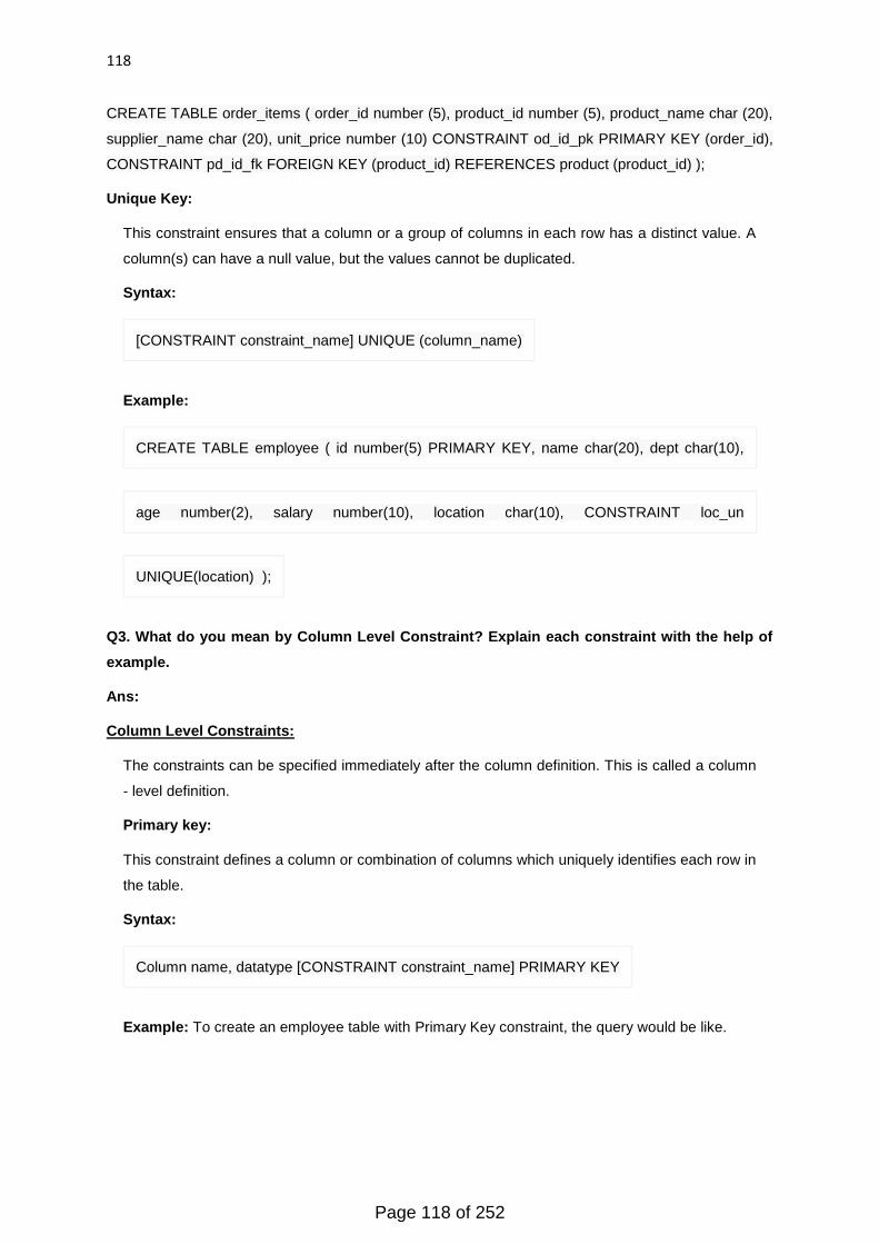
118

CREATE TABLE order_items ( order_id number (5), product_id number (5), product_name char (20),

supplier_name char (20), unit_price number (10) CONSTRAINT od_id_pk PRIMARY KEY (order_id),

CONSTRAINT pd_id_fk FOREIGN KEY (product_id) REFERENCES product (product_id) );

Unique Key:



Syntax:


Example:


age number(2), salary number(10), location char(10), CONSTRAINT loc_un

UNIQUE(location) );

Q3. What do you mean by Column Level Constraint? Explain each constraint with the help of

example.

Ans:


The constraints can be specified immediately after the column definition. This is called a column

- level definition.

Primary key:


the table.

Syntax:


Example: To create an employee table with Primary Key constraint, the query would be like.

Page 118 of 252

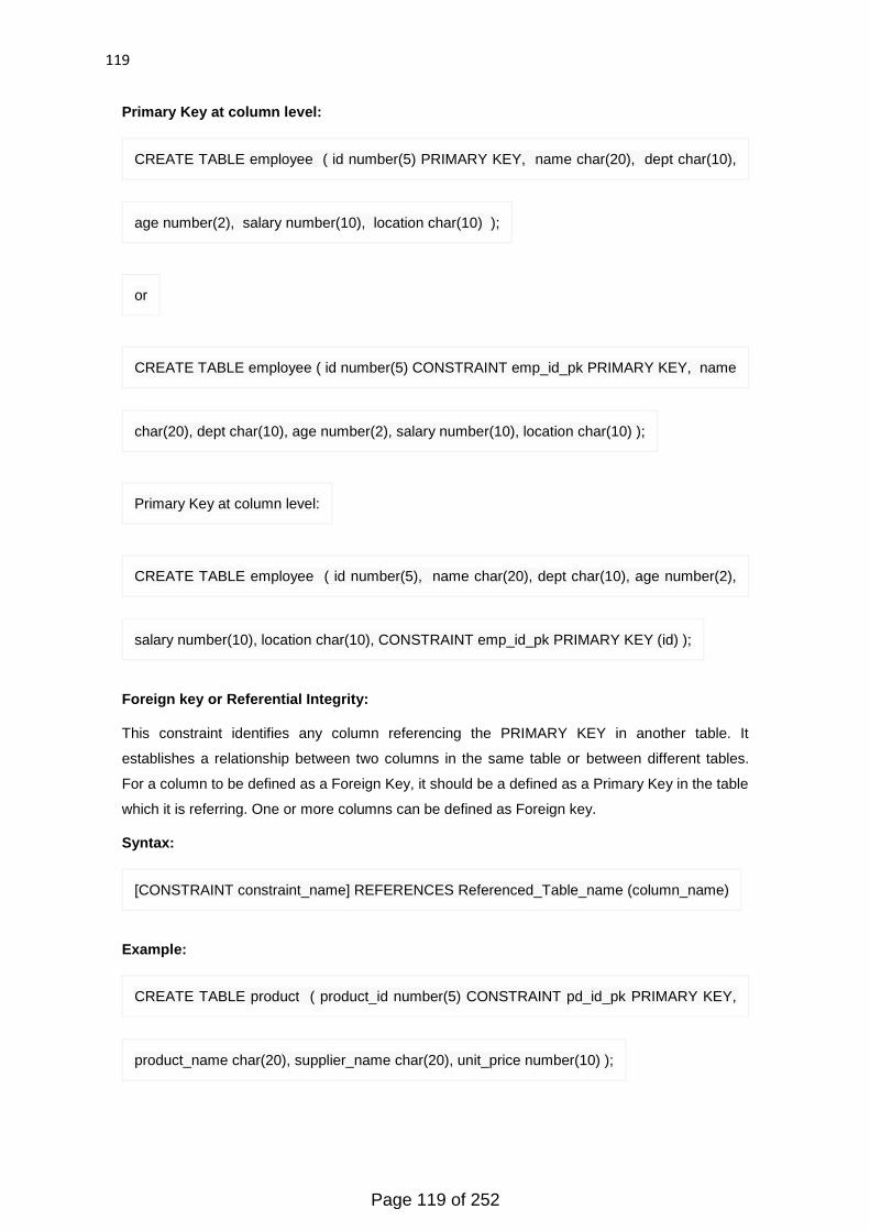
119



age number(2), salary number(10), location char(10) );

or

CREATE TABLE employee ( id number(5) CONSTRAINT emp_id_pk PRIMARY KEY, name

char(20), dept char(10), age number(2), salary number(10), location char(10) );


CREATE TABLE employee ( id number(5), name char(20), dept char(10), age number(2),

salary number(10), location char(10), CONSTRAINT emp_id_pk PRIMARY KEY (id) );




For a column to be defined as a Foreign Key, it should be a defined as a Primary Key in the table

which it is referring. One or more columns can be defined as Foreign key.

Syntax:

[CONSTRAINT constraint_name] REFERENCES Referenced_Table_name (column_name)

Example:

CREATE TABLE product ( product_id number(5) CONSTRAINT pd_id_pk PRIMARY KEY,


Page 119 of 252

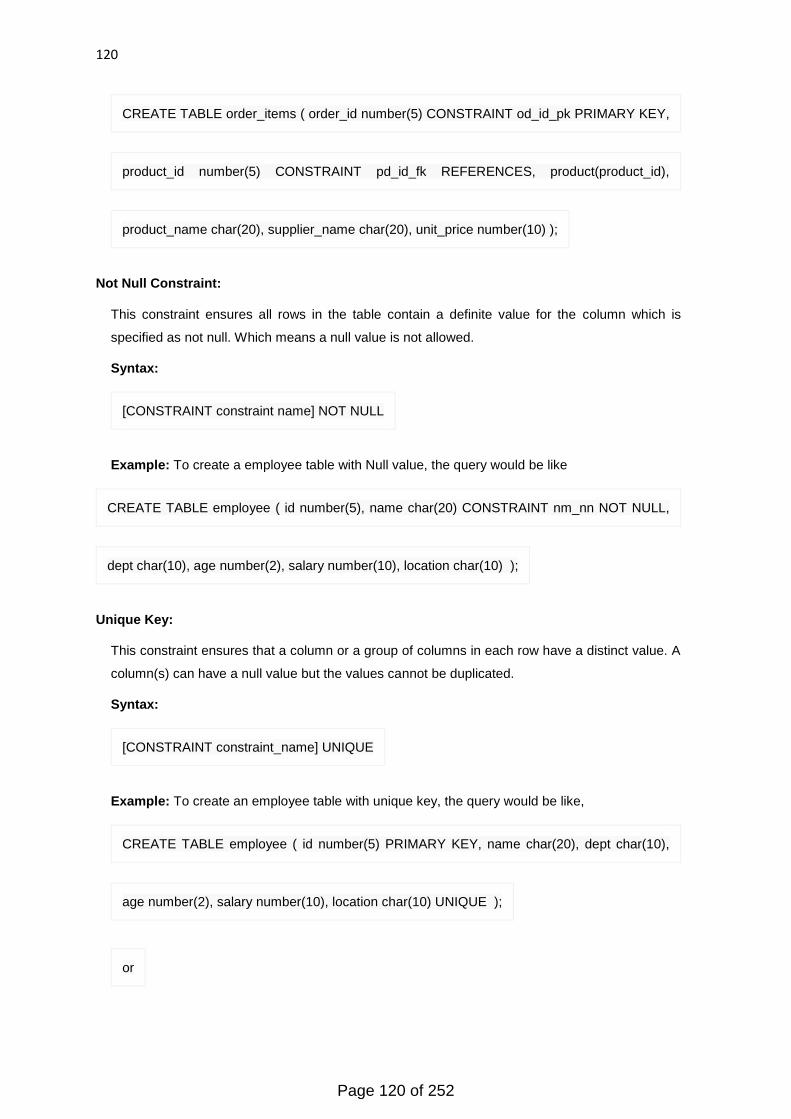
120

CREATE TABLE order_items ( order_id number(5) CONSTRAINT od_id_pk PRIMARY KEY,

product_id number(5) CONSTRAINT pd_id_fk REFERENCES, product(product_id),





Syntax:


Example: To create a employee table with Null value, the query would be like



Unique Key:

This constraint ensures that a column or a group of columns in each row have a distinct value. A

column(s) can have a null value but the values cannot be duplicated.

Syntax:


Example: To create an employee table with unique key, the query would be like,


age number(2), salary number(10), location char(10) UNIQUE );

or

Page 120 of 252

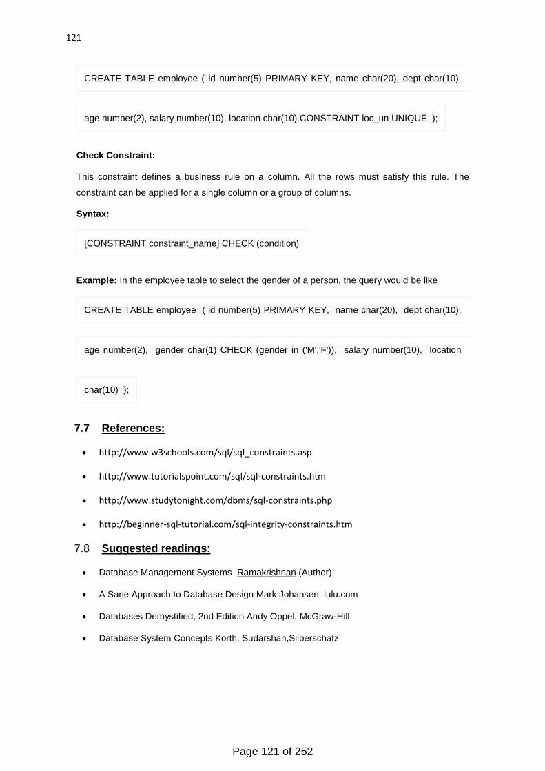
121


age number(2), salary number(10), location char(10) CONSTRAINT loc_un UNIQUE );

Check Constraint:



Syntax:




age number(2), gender char(1) CHECK (gender in ('M','F')), salary number(10), location

char(10) );

7.7 References:







A Sane Approach to Database Design Mark Johansen. lulu.com


Database System Concepts Korth, Sudarshan,Silberschatz

Page 121 of 252





http://www.amazon.in/s/277-0654621-8732668?_encoding=UTF8&field-author=Ramakrishnan&search-alias=stripbooks

122

Unit 3

Lesson 8 - Data Viewing using SQL – Part 1

8.1 Objective

8.2 Introduction to SELECT clause

8.3 Operators in SQL

8.3.1 Arithmetic operators

8.3.2 Logical operators

8.3.3 Special operators

8.3.3.1 BETWEEN

8.3.3.2 ISNULL

8.3.3.3 IN

8.3.3.4 EXISTS

8.4 Comparison operators

8.5 Summary

8.6 Glossary


8.8 References


8.1 Objective

Use of SELECT clause in SQL

Use SELECT clause with different operators

8.2 Introduction to SELECT clause:

Viewing of Data:

We can view the data with the SELECT command. We can also perform arithmetic, logical operations


The SELECT statement has many optional clauses:

WHERE specifies which rows to retrieve.

GROUP BY groups, rows sharing a property so that an aggregate function can be applied to each

group.

Page 122 of 252

http://en.wikipedia.org/wiki/Where_(SQL)

http://en.wikipedia.org/wiki/Group_by_(SQL)

http://en.wikipedia.org/wiki/Aggregate_function

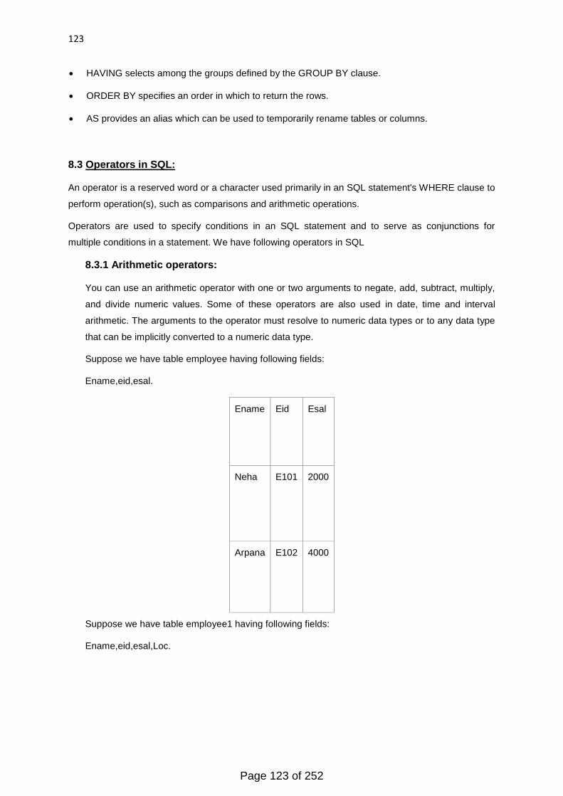
123

HAVING selects among the groups defined by the GROUP BY clause.

ORDER BY specifies an order in which to return the rows.

AS provides an alias which can be used to temporarily rename tables or columns.

8.3 Operators in SQL:

An operator is a reserved word or a character used primarily in an SQL statement's WHERE clause to

perform operation(s), such as comparisons and arithmetic operations.

Operators are used to specify conditions in an SQL statement and to serve as conjunctions for

multiple conditions in a statement. We have following operators in SQL

8.3.1 Arithmetic operators:



arithmetic. The arguments to the operator must resolve to numeric data types or to any data type

that can be implicitly converted to a numeric data type.


Ename,eid,esal.

Ename Eid Esal

Neha E101 2000

Arpana E102 4000

Suppose we have table employee1 having following fields:

Ename,eid,esal,Loc.

Page 123 of 252

http://en.wikipedia.org/wiki/Having_(SQL)

http://en.wikipedia.org/wiki/Order_by_(SQL)

http://en.wikipedia.org/wiki/Alias_(SQL)

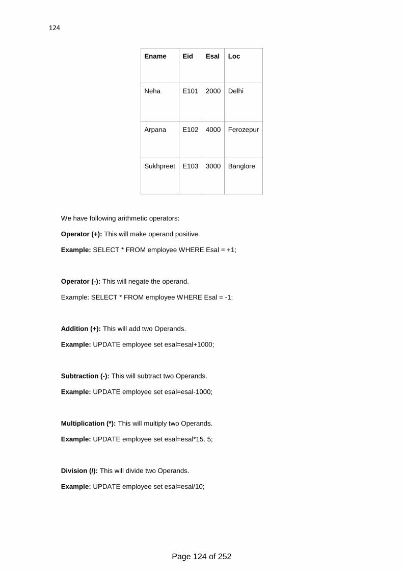
124

Ename Eid Esal Loc

Neha E101 2000 Delhi

Arpana E102 4000 Ferozepur

Sukhpreet E103 3000 Banglore



Example: SELECT * FROM employee WHERE Esal = +1;











Page 124 of 252

125

8.3.2 Logical operators:


NOT Operator: Returns TRUE if the following condition is FALSE. Returns FALSE if it is TRUE. If

it is UNKNOWN, it remains UNKNOWN.


AND Operator: Returns TRUE if both component conditions are TRUE. Returns FALSE if either

is FALSE; otherwise returns UNKNOWN.





8.3.3 Special operators:

8.3.3.1 BETWEEN:

The BETWEEN operator selects values within a range. The values can be numbers, text, or

dates.

Syntax:

SELECT column_name(s)

FROM table_name

WHERE column_name BETWEEN value1 AND value2;

Example:


WHERE Esal BETWEEN 2000 AND 4000;

NOT BETWEEN:

The BETWEEN operator selects values within a range. The value must not match with the given

values. The values can be numbers, text, or dates.

Syntax:


FROM table_name


Example:


Page 125 of 252

126

WHERE Esal NOT BETWEEN 2000 AND 4000;

8.3.3.2 ISNULL:

If a column in a table is optional, we can insert a new record or update an existing record without

adding a value to this column. This means that the field will be saved with a NULL value.

NULL values are treated differently from other values.

NULL is used as a placeholder for unknown or inapplicable values.

Syntax:


FROM table_name

WHERE column_name ISNULL (value1, value2,...);

Example:


WHERE Loc ISNULL;

8.3.3.3 IN:

The IN operator allows you to specify multiple values in a WHERE clause.

Syntax:


FROM table_name

WHERE column_name IN (value1, value2,...);

Example:


WHERE Loc IN ('Delhi','Banglore');

NOT IN Operator: The NOT IN operator allows you to specify multiple values in a WHERE

clause which should not match with the given value.

Syntax:


FROM table_name

WHERE column_name NOT IN (value1, value2,...);

Example:


Page 126 of 252

127


8.3.3.4 EXISTS:

The EXISTS checks the existence of a result of a subquery. The EXISTS subquery tests

whether a subquery fetches at least one row. When no data is returned then this operator

returns 'FALSE'.

A valid EXISTS subquery must contain an outer reference and it must be a correlated subquery.

The select list in the EXISTS subquery is not actually used in evaluating the EXISTS so it can

contain any valid select list

Syntax:


FROM table_name

WHERE EXISTS (Select Column+_name(s) From 2ndTable_name);

Example:

SELECT * FROM Employee WHERE exists (SELECT loc FROM Employee1

WHERE Eid=103 );

8.4 Comparison operators:















Page 127 of 252

128

8.5 Summary:

Viewing of Data:

We can view data with the SELECT command. We can also perform arithmetic, logical operations on

data. We can also alter the way of representation of data.

Arithmetic Operators:

You can use an arithmetic operator with one or two arguments to negate, add, subtract, multiply, and

divide numeric values. Some of these operators are also used in date, time and interval arithmetic.

Logical Operators:


Comparison Operators:

Comparison operators are used in conditions that compare one expression with another. The result of

a comparison can be TRUE, FALSE, or UNKNOWN.

8.6 Glossary:





system








Q1.Explain Arithmetic Operator with example?

Ans: Arithmetic Operators:

Page 128 of 252

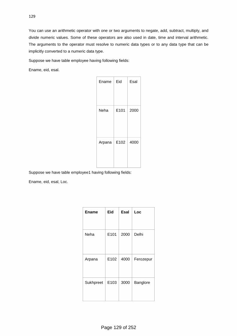
129

You can use an arithmetic operator with one or two arguments to negate, add, subtract, multiply, and

divide numeric values. Some of these operators are also used in date, time and interval arithmetic.

The arguments to the operator must resolve to numeric data types or to any data type that can be

implicitly converted to a numeric data type.


Ename, eid, esal.

Ename Eid Esal

Neha E101 2000

Arpana E102 4000

Suppose we have table employee1 having following fields:

Ename, eid, esal, Loc.

Ename Eid Esal Loc




Page 129 of 252

130














Q2. Explain Logical Operator with example?

Ans: Logical Operators:


NOT Operator: Returns TRUE if the following condition is FALSE. Returns FALSE if it is TRUE. If it is

UNKNOWN, it remains UNKNOWN.


AND Operator: Returns TRUE if both component conditions are TRUE. Returns FALSE if either is

FALSE; otherwise returns UNKNOWN.


Page 130 of 252

131




Q3. Explain Comparison Operator with example?

Ans: Comparison Operators:

Comparison operators are used in conditions that compare one expression with another. The result of

a comparison can be TRUE, FALSE, or UNKNOWN.













Q4. Explain Special Operators with example?

Ans: Special operators:

BETWEEN:

The BETWEEN operator selects values within a range. The values can be numbers, text, or

dates.

Syntax:SELECT column_name(s)

FROM table_name


Example: SELECT * FROM Employee


Page 131 of 252

132

NOT BETWEEN:

The BETWEEN operator selects values within a range. The value must not match with the

given values. The values can be numbers, text, or dates.

Syntax: SELECT column_name (s)

FROM table_name




ISNULL:

If a column in a table is optional, we can insert a new record or update an existing record

without adding a value to this column. This means that the field will be saved with a NULL

value.

NULL values are treated differently from other values.

NULL is used as a placeholder for unknown or inapplicable values.


FROM table_name

WHERE column_name ISNULL (value1, value2,...);


WHERE Loc ISNULL ;

IN:



FROM table_name




NOT IN Operator: The NOT IN operator allows you to specify multiple values in a WHERE

clause which should not match with the given value.


FROM table_name


Page 132 of 252

133



EXISTS:

The EXISTS checks the existence of a result of a subquery. The EXISTS subquery tests

whether a subquery fetches at least one row. When no data is returned then this operator

returns 'FALSE'.

A valid EXISTS subquery must contain an outer reference and it must be a correlated

subquery.

The select list in the EXISTS subquery is not actually used in evaluating the EXISTS so it can

contain any valid select list


FROM table_name

WHERE EXISTS (Select Column+_name(s) From 2ndTable_name);

Example: SELECT * FROM Employee WHERE exists (SELECT loc FROM Employee1

WHERE Eid=103 );

8.8 References:

http://docs.oracle.com/cd/E16655_01/server.121/e17209/operators002.htm#SQLRF51157

http://docs.oracle.com/cd/B28359_01/server.111/b28286/operators002.htm#SQLRF51154

http://docs.oracle.com/cd/E11882_01/appdev.112/e41502/adfns_sqltypes.htm#ADFNS0002


Six-Step Relational Database Design (TM): A step by step approach to relational database design

and development Second Edition of Fidel A Captain.


Database Management System (GBTU & MTU) Kedar S (Author)

Database Management System by Patricia Ward, George Dafoulas

Page 133 of 252

http://docs.oracle.com/cd/E16655_01/server.121/e17209/operators002.htm

http://docs.oracle.com/cd/B28359_01/server.111/b28286/operators002.htm

http://docs.oracle.com/cd/E11882_01/appdev.112/e41502/adfns_sqltypes.htm

134

Unit 3

Lesson 9 - Data viewing using SQL – Part 2

9.1 Objective

9.2 Introduction to Select Clause

9.3 Range Searching using SQL

9.3.1 Any and Not Any Operator

9.3.2 In and Not In Operator

9.3.3 Between and Not Between Operator

9.3.4 Pattern Matching Using SQL

9.3.4.1 LIKE Operator

9.3.4.1.1 % (Percentage) Operator

9.3.4.1.2 _ (Underscore) Operator

9.4 Oracle Functions

9.4.1 Single-row Functions

9.4.2 Group Functions

9.4.2.1 Numeric Functions

9.4.2.2 Character or Text Functions

9.4.2.3 Date Functions

9.4.2.4 Conversion Functions

9.5 Summary

9.6 Glossary


9.8 References


9.1 Objective


Use of SELECT clause range searching and pattern matching

9.2 Introduction to SELECT clause :

We can view the data with the SELECT command. We can also perform arithmetic, logical operations


Page 134 of 252

135

The SELECT statement has many optional clauses:

WHERE specifies which rows to retrieve.

GROUP BY groups, rows sharing a property so that an aggregate function can be applied to each

group.

HAVING selects among the groups defined by the GROUP BY clause.

ORDER BY specifies an order in which to return the rows.

AS provides an alias which can be used to temporarily rename tables or columns.

9.3 Range searching using SQL:

A range search is one that returns all values between two specified values. Inclusive ranges

return any values that match the two specified values. Exclusive ranges do not return any values

that match the two specified values.


Ename,eid,esal,Loc.

Ename Eid Esal Loc




9.3.1 ANY & NOT ANY Operator:

The ANY comparison condition is used to compare a value to a list or subquery. It must be preceded

by =, !=, >, <, <=, >= and followed by a list or subquery. Unlike When the ANY condition is followed by

a list, the optimizer expands the initial condition to all elements of the list and strings them together

with OR operators, as shown below.

NOT ANY Operator: The NOT ANY operator allows you to specify multiple values in a WHERE clause

which should not match with the given value.

Syntax:


FROM table_name

WHERE column_name NOT ANY(value1, value2,...);

Syntax:

Page 135 of 252

http://en.wikipedia.org/wiki/Where_(SQL)

http://en.wikipedia.org/wiki/Group_by_(SQL)

http://en.wikipedia.org/wiki/Aggregate_function

http://en.wikipedia.org/wiki/Having_(SQL)

http://en.wikipedia.org/wiki/Order_by_(SQL)

http://en.wikipedia.org/wiki/Alias_(SQL)

136


FROM table_name

WHERE column_name >|<|>=|<= ANY (value1, value2,...);

Example:

SELECT Eid, Esal

FROM Employee

WHERE Esal > ANY (2000, 3000, 4000);

Example:

SELECT Eid, Esal

FROM Employee

WHERE Esal > NOT ANY (2000, 3000, 4000);

9.3.2 IN & NOT IN operator:



FROM table_name


Example:



NOT IN Operator: The NOT IN operator allows you to specify multiple values in a WHERE clause


Syntax:


FROM table_name


Example:


WHERE Loc NOT IN ('Delhi','Banglore');

9.3.3 BETWEEN and NOT BETWEEN:

The BETWEEN operator selects values within a range. The values can be numbers, text, or dates.

Page 136 of 252

137

Syntax:


FROM table_name


Example:



NOT BETWEEN Operator: The BETWEEN operator selects values within a range. The value must

not match with the given values. The values can be numbers, text, or dates.


FROM table_name




9.3.4 Pattern matching using SQL:

After a range searching now suppose we have more alphabetic data and we want to search

through it so we will use Pattern Matching Operators. It will match a value with the given Pattern.

We have following Pattern Matching Operators:

9.3.4.1 LIKE Operator: The Oracle LIKE operator is used to match or test a conditional term

using a "wildcard search". Wildcard characters (operators) are used to create the search string.

The two operators are the percent sign ('%') and the underscore ('_').

9.3.4.1.1 Percent matching (%):

The percent ('%') matches any group of characters. It can 'stand in' for zero or more characters,

with no upper limit. Consider the string 'hood%' used as a search term with LIKE. Because of the

percent sign at the end of the term, the search term will match anything and everything after

'wood'. It will match on 'wood', 'hooded', 'hoodland', 'hoods', 'hoods!', 'hoods in the country' and so

on.

It would not match on 'darkhood', 'redwood', or 'parkhoods' because the string starts with 'wood'.

If the search term was '%hood' then it could (and would) attempt to match anything before 'hood'.

It would match on 'darkhood' and 'redwood', but not on 'parkhoods' (because of the‘s‘ at the end

of 'parkhoods').

Page 137 of 252

138

The term '%hood%' used as a search term would match ANY text with the word 'wood' in it. The

leading and trailing percent signs tell the LIKE operator to basically match anything before and/or

after the text 'hood', as long as it found 'hood' somewhere in the search text.

9.3.4.1.2 Underscore matching:

The underscore ('_') is more selective- it matches any single character.

Consider the string 'w__d' used as a search term with LIKE. The two underscores in the middle

tell the LIKE operator to look for a 'w', then any two characters, and then a‘d‘.

This search term will match an 'wood', wild', 'wand', 'ward', and so on. It would not match on

'weird', 'wad', 'wide', or 'wed'. (There are either too few characters or too many to satisfy the

match condition.)

Similarly, the search term 'wood_' will match an 'woods', 'wood', 'woody', 'wood!', and any other

instance of 'wood' with one and only one additional character after it. It would not match 'wooded',

'woodland', 'redwood', or 'woodsman'.


FROM table_name

WHERE column_name LIKE pattern;

Example: The following SQL statement selects all customers with a City starting with the letter

"F":


WHERE Loc LIKE 'F%';

Example: The following SQL statement selects all customers with a City ending with the letter

"F":


WHERE Loc LIKE '%F';

Example: The following SQL statement selects all customers with a Country containing the

pattern "ang":


WHERE Loc LIKE '%ang%';

Example: The SQL statement below displays any employee whose four-digit salary ends with

'200':


WHERE Esal LIKE '_200';

Page 138 of 252

139

Example: The SQL statement below displays any employee whose name has six (6) letters,

starts with letter 'A' and ends with 'a':


WHERE Ename LIKE 'A____a';

9.4 Oracle functions:

There are following Oracle Functions.

9.4.1 Single row functions:

Single row or Scalar functions return a value for every row that is processed in a query.

9.4.2 Group functions:

These functional groups the rows of data based on the values returned by the query. The group

functions are used to calculate aggregate values like total or average, which return just one

total or one average value after processing a group of rows.

There are four types of single row functions. They are:

9.4.2.1 Numeric Functions: These are functions that accept numeric input and return numeric

values.

9.4.1.2 Character or Text Functions: These are functions that accept character input and can

return both character and number values.

9.4.1.3 Date Functions: These are functions that take values that are of datatype DATE as

input and return values of datatype DATE, except for the MONTHS_BETWEEN function, which

returns a number.

9.4.1.4 Conversion Functions: These are functions that help us to convert a value in one form

to another form. For Example: a null value into an actual value, or a value from one datatype to

another datatype like NVL, TO_CHAR, TO_NUMBER, TO_DATE etc.

You can combine more than one function together in an expression. This is known as nesting

of functions.

9.5 Summary:

Introduction:

A range search is one that returns all values between two specified values. Inclusive ranges return

any values that match the two specified values. Exclusive ranges do not return any values that match

the two specified values.

IN Operator: The IN operator allows you to specify multiple values in a WHERE clause.

Page 139 of 252

140



ANY Operator: The ANY comparison condition is used to compare a value to a list or subquery. It

must be preceded by =, =, >, <, <=, >= and followed by a list or subquery. When the ANY condition is

followed by a list, the optimizer expands the initial condition to all elements of the list and strings them

together

BETWEEN Operator: The BETWEEN operator selects values within a range. The values can be

numbers, text, or dates.



Pattern matching using SQL:

After a range searching now suppose we have more alphabetic data and we want to search

through it so we will use Pattern Matching Operators. It will match a value with the given Pattern.

We have following Pattern Matching Operators:

LIKE Operator: The Oracle LIKE operator is used to match or test a conditional term using a

"wildcard search". Wildcard characters (operators) are used to create the search string. The two

operators are the percent sign ('%') and the underscore ('_').

Percent matching (%):

The percent ('%') matches any group of characters. It can 'stand in' for zero or more characters, with

no upper limit. Consider the string 'hood%' used as a search term with LIKE. Because of the percent

sign at the end of the term, the search term will match anything and everything after 'wood'. It will

match on 'wood', 'hooded', 'hoodland', 'hoods', 'hoods!', 'hoods in the country' and so on.


If the search term was '%hood' then it could (and would) attempt to match anything before 'hood'. It

would match on 'darkhood' and 'redwood', but not on 'parkhoods' (because of the‘s‘ at the end of

'parkhoods').


leading and trailing percent signs tell the LIKE operator to basically match anything before and/or after

the text 'hood', as long as it found 'hood' somewhere in the search text.

Underscore matching:


Consider the string 'w__d' used as a search term with LIKE. The two underscores in the middle tell

the LIKE operator to look for a 'w', then any two characters, and then a‘d‘.

Page 140 of 252

141

This search term will match an 'wood', wild', 'wand', 'ward', and so on. It would not match on 'weird',

'wad', 'wide', or 'wed'. (There are either too few characters or too many to satisfy the match condition.)




Oracle Functions: There are following Oracle Functions.

Single Row Functions: Single row or Scalar functions return a value for every row that is

processed in a query.

Group Functions: These functional groups the rows of data based on the values returned by the

query. This is discussed in SQL GROUP Functions. The group functions are used to calculate

aggregate values like total or average, which return just one total or one average value after

processing a group of rows.


Numeric Functions: These are functions that accept numeric input and return numeric values.

Character or Text Functions: These are functions that accept character input and can return

both character and number values.

Date Functions: These are functions that take values that are of datatype DATE as input and

return values of datatype DATE, except for the MONTHS_BETWEEN function, which returns a

number.

Conversion Functions: These are functions that help us to convert a value in one form to

another form. For Example: a null value into an actual value, or a value from one datatype to


You can combine more than one function together in an expression. This is known as nesting of

functions.

9.6 Glossary:




system

Reliability: It means dependability: the quality of being dependable or reliable


Page 141 of 252

142





Aggregate: Whole formed by combining several separate elements.


Q1.Explain Range Searching with example?

Ans Range searching using SQL:

A range search is one that returns all values between two specified values. Inclusive ranges return any

values that match the two specified values. Exclusive ranges do not return any values that match the

two specified values.


Ename,eid,esal,Loc.

Ename Eid Esal Loc




ANY & NOT ANYoperator:

The ANY comparison condition is used to compare a value to a list or subquery. It must be preceded

by =, !=, >, <, <=, >= and followed by a list or subquery. Unlike When the ANY condition is followed by

a list, the optimizer expands the initial condition to all elements of the list and strings them together

with OR operators, as shown below.

NOT ANY Operator: The NOT ANY operator allows you to specify multiple values in a WHERE clause



FROM table_name

WHERE column_name NOT ANY(value1, value2,...);


FROM table_name

Page 142 of 252

143

WHERE column_name >|<|>=|<= ANY (value1, value2,...);

Example: SELECT Eid, Esal

FROM Employee

WHERE Esal > ANY (2000, 3000, 4000);

Example: SELECT Eid, Esal

FROM Employee

WHERE Esal > NOT ANY (2000, 3000, 4000);

IN & NOT IN operator:



FROM table_name







FROM table_name



WHERE Loc NOT IN ('Delhi','Banglore');

BETWEEN and NOT BETWEEN:

The BETWEEN operator selects values within a range. The values can be numbers, text, or dates.


FROM table_name


Page 143 of 252

144






FROM table_name




Q2.Explain Pattern Matching with examples?

Ans Pattern matching using SQL:

After a range searching now suppose we have more alphabetic data and we want to search through it

so we will use Pattern Matching Operators. It will match a value with the given Pattern. We have

following Pattern Matching Operators:

LIKE Operator: The Oracle LIKE operator is used to match or test a conditional term using a

"wildcard search". Wildcard characters (operators) are used to create the search string. The two

operators are the percent sign ('%') and the underscore ('_').

Percent matching (%):

The percent ('%') matches any group of characters. It can 'stand in' for zero or more characters, with

no upper limit. Consider the string 'hood%' used as a search term with LIKE. Because of the percent

sign at the end of the term, the search term will match anything and everything after 'wood'. It will

match on 'wood', 'hooded', 'hoodland', 'hoods', 'hoods!', 'hoods in the country' and so on.


If the search term was '%hood' then it could (and would) attempt to match anything before 'hood'. It

would match on 'darkhood' and 'redwood', but not on 'parkhoods' (because of the‘s‘ at the end of

'parkhoods').


leading and trailing percent signs tell the LIKE operator to basically match anything before and/or after

the text 'hood', as long as it found 'hood' somewhere in the search text.

Page 144 of 252

145

Underscore matching:


Consider the string 'w__d' used as a search term with LIKE. The two underscores in the middle tell

the LIKE operator to look for a 'w', then any two characters, and then a‘d‘.

This search term will match an 'wood', wild', 'wand', 'ward', and so on. It would not match on 'weird',

'wad', 'wide', or 'wed'. (There are either too few characters or too many to satisfy the match condition.)





FROM table_name

WHERE column_name LIKE pattern;

Example: The following SQL statement selects all customers with a City starting with the letter "F":


WHERE Loc LIKE 'F%';

Example: The following SQL statement selects all customers with a City ending with the letter "F":


WHERE Loc LIKE '%F';

Example: The following SQL statement selects all customers with a Country containing the pattern

"ang":


WHERE Loc LIKE '%ang%';

Example: The SQL statement below displays any employee whose four-digit salary ends with '200':


WHERE Esal LIKE '_200';

Example: The SQL statement below displays any employee whose name has six (6) letters, starts

with letter 'A' and ends with 'a':


WHERE Ename LIKE 'A____a';

Page 145 of 252

146

Q3.How many Oracle Function is there in SQL?

Ans: Oracle Functions: There are following Oracle Functions.

Single Row Functions: Single row or Scalar functions return a value for every row that is

processed in a query.

Group Functions: These functional groups the rows of data based on the values returned by the

query. This is discussed in SQL GROUP Functions. The group functions are used to calculate

aggregate values like total or average, which return just one total or one average value after

processing a group of rows.


Numeric Functions: These are functions that accept numeric input and return numeric values.

Character or Text Functions: These are functions that accept character input and can return both

character and number values.

Date Functions: These are functions that take values that are of datatype DATE as input and

return values of datatype DATE, except for the MONTHS_BETWEEN function, which returns a

number.

Conversion Functions: These are functions that help us to convert a value in one form to

another form. For Example: a null value into an actual value, or a value from one datatype to


You can combine more than one function together in an expression. This is known as nesting

of functions.

9.8 References:

http://psoug.org/definition/LIKE.htm

http://docs.oracle.com/cd/B19306_01/server.102/b14200/conditions007.htm

http://docs.oracle.com/cd/E14004_01/books/PersAdm/PersAdmOperators5.html

http://beginner-sql-tutorial.com/oracle-functions.htm

http://docs.oracle.com/javadb/10.4.2.1/ref/rrefsqlj29026.html

http://docs.oracle.com/cd/B19306_01/server.102/b14200/functions001.htm


Advance Database Management System Book

Page 146 of 252

http://psoug.org/definition/LIKE.htm

http://docs.oracle.com/cd/B19306_01/server.102/b14200/conditions007.htm

http://docs.oracle.com/cd/E14004_01/books/PersAdm/PersAdmOperators5.html

http://beginner-sql-tutorial.com/oracle-functions.htm

http://docs.oracle.com/javadb/10.4.2.1/ref/rrefsqlj29026.html

http://docs.oracle.com/cd/B19306_01/server.102/b14200/functions001.htm

147

Authors: Arihant Khicha, Neeti Kapoor.

Database Management System Book

Authors: Suresh Fatehpuria, Hansraj Yadav.

Database Systems – The Complete Book : By Hector Garcia-Molina, Jeffrey D. Ullman and

Jennifer Widom, Second Edition.

Page 147 of 252

148

Unit 3


10.1 Objective


10.3 Oracle functions

10.3.1 Number Functions

10.3.2 Group Functions

10.3.3 Scalar Functions


10.3.5 Data Conversion Functions

10.3.6 Manipulating Dates in SQL

10.4 Summary

10.5 Glossary


10.7 References


10.1 Objective


Use of SELECT clause with oracle functions

10.2 Introduction to SELECT clause :

SELECT command is used to fetch the data from a database table which return data in the form

of result table. These result tables are called result-sets.





Page 148 of 252

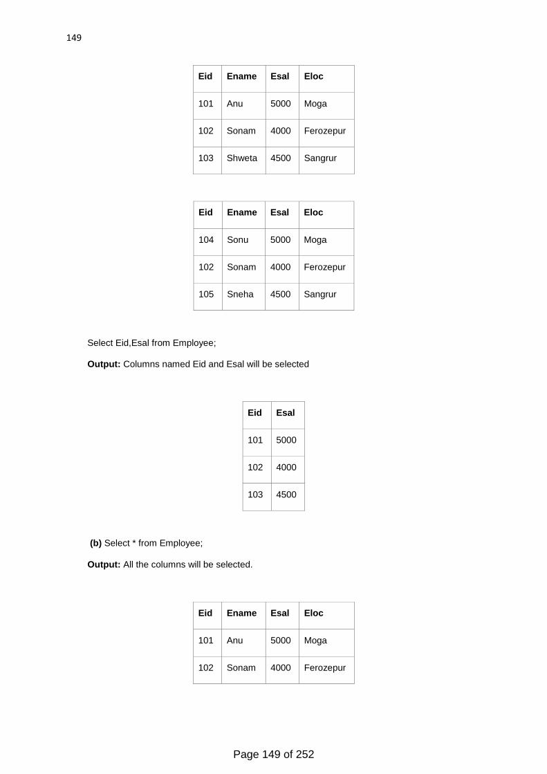
149

Eid Ename Esal Eloc

101 Anu 5000 Moga



Eid Ename Esal Eloc

104 Sonu 5000 Moga



Select Eid,Esal from Employee;


Eid Esal

101 5000

102 4000

103 4500



Eid Ename Esal Eloc

101 Anu 5000 Moga


Page 149 of 252

150


10.3 Oracle functions:

There are different types of inbuilt functions in SQL like

Numeric

Aggregate

Conversion

String function

10.3.1 Number Functions:

Numeric functions accept numeric data and return numeric values. Most numeric functions

return NUMBER values that are accurate to 38 decimal digits. The transcendental



decimal digits.




of 'X'.

We have following numeric functions in SQL:

ABS: It Returns the absolute value of a number.

Syntax: ABS<Value>


Output: 100


Syntax: CEIL<Value>


Output: 49




Output: 48

Page 150 of 252




151

ROUND: It will round off value of number ‗x‘ up to the number ‗y‘ decimal places.



Output: 49.99

POWER (m, n): It will return a value m raise to the power n.



Output: 8

MOD: It will return the Modulus of a number.

Syntax: MOD (<m Value>, <n Value>)


Output: 1


Syntax: SQRT<value>


Output: 12



Syntax: SIN<value>


Output: 0.8414

COS: It will calculates the cosine of an angle expression. The result returned by COS is a decimal


Syntax: COS<value>


Output: 0.540

10.3.2 Group Functions:

Aggregate functions return a single result row based on groups of rows, rather than on single rows.

Aggregate functions can appear in select lists and in ORDER BY and HAVING clauses. They are

commonly used with the GROUP BY clause in a SELECT statement, where Oracle Database divides

the rows of a queried table or view into groups. In a query containing a GROUP BY clause, the

Page 151 of 252

152

elements of the select list can be aggregate functions, GROUP BY expressions, constants, or

expressions involving one of these. Oracle applies the aggregate functions to each group of rows and

returns a single result row for each group.

You use aggregate functions in the HAVING clause to eliminate groups from the output based on the

results of the aggregate functions, rather than on the values of the individual rows of the queried table

or view.

AVG: It will AVG returns the average value of expression.


Output: 3000

SUM: It will return the sum of values of expression. You can use it as an aggregate or analytic

function.


Output: 9000

MIN: It will return the minimum value of expression.


Output: 2000

MAX: It will return the MAXIMUM of values of expression.

Example: Select MAX (Esal) From Employee;

Output: 4000

COUNT: It will return the number of rows returned by the query. You can use it as an aggregate or

analytic function.

Example: Select COUNT (*) From Employee;

Output: 3


takes a numeric or date time value and returns the middle value or an interpolated value that would

be the middle value once the values are sorted. Nulls are ignored in the calculation.

Example: Select MEDIAN (Esal) From Employee;

Output: 3000




Example: Select STDDEV (Esal) From Employee;

Output: 1000

Page 152 of 252

153

10.3.3 Scalar Functions:

Scalar functions do not aggregate data or compute aggregate statistics. Instead, scalar functions

compute and substitute a new data value for each value associated with a data item




Output: 5



POSITION: The POSITION function returns an integer that indicates the starting position of a

string within the search string.

Example: SELECT LOCATE ('bar', 'foobar');

Output: 4


Output: 0



Output: 3


one string.




Character functions that return character values return values of the following data types unless

otherwise documented:

If the input argument is CHAR or VARCHAR2, then the value returned is VARCHAR2.

If the input argument is NCHAR or NVARCHAR2, then the value returned is NVARCHAR2.

The length of the value returned by the function is limited by the maximum length of the data type

returned.

For functions that return CHAR or VARCHAR2, if the length of the return value exceeds the limit,

then Oracle Database truncates it and returns the result without an error message.

Page 153 of 252

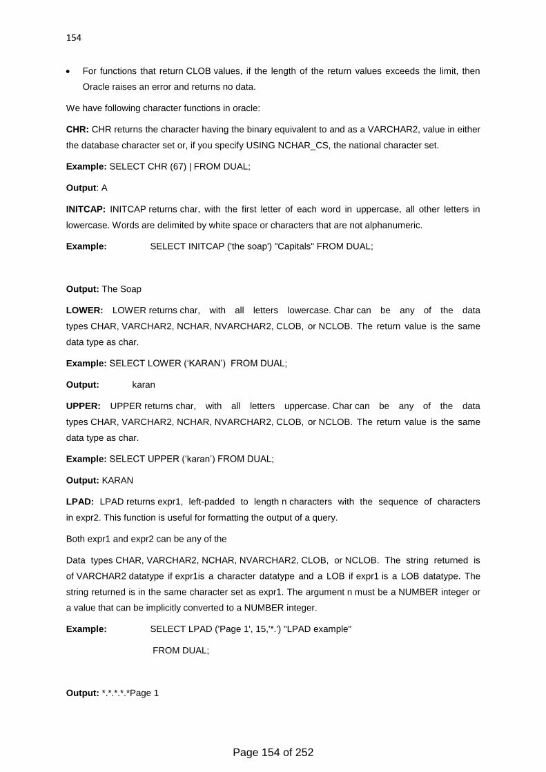
154

For functions that return CLOB values, if the length of the return values exceeds the limit, then

Oracle raises an error and returns no data.

We have following character functions in oracle:

CHR: CHR returns the character having the binary equivalent to and as a VARCHAR2, value in either


Example: SELECT CHR (67) | FROM DUAL;

Output: A



Example: SELECT INITCAP ('the soap') "Capitals" FROM DUAL;

Output: The Soap

LOWER: LOWER returns char, with all letters lowercase. Char can be any of the data


data type as char.

Example: SELECT LOWER (‗KARAN‘) FROM DUAL;

Output: karan

UPPER: UPPER returns char, with all letters uppercase. Char can be any of the data


data type as char.

Example: SELECT UPPER (‗karan‘) FROM DUAL;

Output: KARAN




Data types CHAR, VARCHAR2, NCHAR, NVARCHAR2, CLOB, or NCLOB. The string returned is




Example: SELECT LPAD ('Page 1', 15,'*.') "LPAD example"

FROM DUAL;


Page 154 of 252

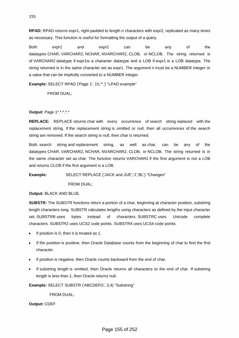
155








Example: SELECT RPAD ('Page 1', 15,'*.') "LPAD example"

FROM DUAL;


REPLACE: REPLACE returns char with every occurrence of search string replaced with the

replacement string. If the replacement string is omitted or null, then all occurrences of the search

string are removed. If the search string is null, then char is returned.

Both, search string and replacement string, as well as char, can be any of the




Example: SELECT REPLACE ('JACK and JUE','J','BL') "Changes"

FROM DUAL;


SUBSTR: The SUBSTR functions return a portion of a char, beginning at character position, substring

length characters long. SUBSTR calculates lengths using characters as defined by the input character

set. SUBSTRB uses bytes instead of characters. SUBSTRC uses Unicode complete

characters. SUBSTR2 uses UCS2 code points. SUBSTR4 uses UCS4 code points.

If position is 0, then it is treated as 1.

If the position is positive, then Oracle Database counts from the beginning of char to find the first

character.

If position is negative, then Oracle counts backward from the end of char.

If substring length is omitted, then Oracle returns all characters to the end of char. If substring

length is less than 1, then Oracle returns null.

Example: SELECT SUBSTR ('ABCDEFG', 3,4) "Substring"

FROM DUAL;

Output: CDEF

Page 155 of 252

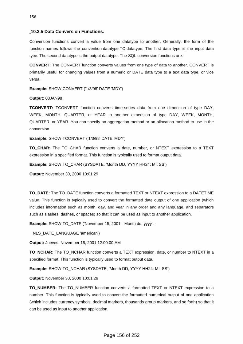
156

10.3.5 Data Conversion Functions:



type. The second datatype is the output datatype. The SQL conversion functions are:



versa.


Output: 03JAN98




conversion.




Example: SHOW TO_CHAR (SYSDATE, 'Month DD, YYYY HH24: MI: SS‘)








Output: Jueves: November 15, 2001 12:00:00 AM



Example: SHOW TO_NCHAR (SYSDATE, 'Month DD, YYYY HH24: MI: SS‘)






Page 156 of 252

157


Money = TO_NUMBER ('$94,567,00', 'L999G999D00', NLS_NUMERIC_CHARACTERS ', ')

SHOW money

Output: 94,567.00

10.3.6 Manipulating Dates in Oracle:

Datetime functions operate on date (DATE), time stamp












as SYSDATE, SYSTIMESTAMP, CURRENT_TIMESTAMP, and so forth, is evaluated once for each


The date time functions are:

ADD_MONTHS: DD_MONTHS returns the date, date plus integer months. A month is defined by the






component as a date.

Example: SELECT TO_CHAR (ADD_MONTHS (22-mar-1990, 1), 'DD-MON-YYYY')

Output: 22-apr-1990




Output: 15-apr-2014

Page 157 of 252

158

CURTIME: It returns the current time.


Output: 12:45:34




Output: 1990





both last days of months, then the result is always an integer. Otherwise, Oracle Database calculates

the fractional portion of the result based on a 31-day, month and considers the difference in time



(TO_DATE ('02-02-1995','MM-DD-YYYY'),


FROM DUAL;

Output: 1.03

LAST_DAY: LAST_DAY returns the date of the last day of the month that contains a date. The last

day of the month is defined by the session parameter NLS_CALENDAR. The return type is

always DATE, regardless of the data type of date.


LAST_DAY (SYSDATE) "Last",

LAST_DAY (SYSDATE) - SYSDATE "Days Left"

FROM DUAL;



date. The return type is always DATE, regardless of the data type of date. The argument char must

be a day of the week in the date language of your session, either the full name or the abbreviation.

The minimum number of letters required is the number of letters in the abbreviated version. Any

characters immediately following the valid abbreviation are ignored. The return value has the same

hours, minutes, and seconds component as the argument date.

Page 158 of 252

159

Example: SELECT NEXT_DAY ('15-OCT-2009','TUESDAY') "NEXT DAY"

FROM DUAL;

Output: 20-OCT-2009 00:00:00

10.4 Summary:

Number Functions: Numeric functions accept numeric input and return numeric values. Most

numeric functions return NUMBER values that are accurate to 38 decimal digits. The transcendental



decimal digits.




of 'X'.

Group Functions: Aggregate functions return a single result row based on groups of rows, rather

than on single rows. Aggregate functions can appear in select lists and in

ORDER BY and HAVING clauses. They are commonly used with the GROUP BY clause in

a SELECT statement, where Oracle Database divides the rows of a queried table or view into groups.

In a query containing a GROUP BY clause, the elements of the select list can be aggregate

functions, GROUP BY expressions, constants, or expressions involving one of these. Oracle applies

the aggregate functions to each group of rows and returns a single result row for each group.

Scalar Functions:

Scalar functions (in contrast to data functions) do not aggregate data or compute aggregate statistics.

Instead, scalar functions compute and substitute a new data value for each value associated with a

data item

Character Functions: Character functions that return character values return values of the following

datatypes unless otherwise documented:



The length of the value returned by the function is limited by the maximum length of the datatype

returned.

Data Conversion Functions:

Page 159 of 252




http://docs.oracle.com/cd/E12032_01/doc/epm.921/html_ir_studio/ir_studio-15-26.html

160



type. The second datatype is the output datatype.

Manipulating Dates in Oracle:










10,5 Glossary:





system








Q1.What are Number Functions in Oracle? Explain with example?

Ans: Number Functions: Numeric functions accept numeric input and return numeric values. Most

numeric functions return NUMBER values that are accurate to 38 decimal digits. The transcendental


Page 160 of 252

161


decimal digits.




of 'X'.

We have following numeric functions in oracle:

ABS: It returns the absolute value of a number.

Syntax: ABS<Value>


Output: 100


Syntax: CEIL<Value>


Output: 49




Output: 48

ROUND: It will round off value of number ‗x‘ upto the number ‗y‘ decimal places.



Output: 49.99

POWER (m,n):It will return a value m raise to the power n.



Output: 8

MOD:It will retun the Modulus of a number.

Syntax:MOD(<m Value>,<n Value>)


Output: 1

Page 161 of 252




162


Syntax: SQRT<value>


Output: 12



Syntax: SIN<value>


Output: 0.8414

COS: It will calculate the cosine of an angle expressed. The result returned by COS is a decimal


Syntax: COS<value>


Output: 0.540

Q2.What is Group Functions in Oracle? Explain with example?

Ans: Group Functions: Aggregate functions return a single result row based on groups of rows,

rather than on single rows. Aggregate functions can appear in select lists and in

ORDER BY and HAVING clauses. They are commonly used with the GROUP BY clause in

a SELECT statement, where Oracle Database divides the rows of a queried table or view into groups.

In a query containing a GROUP BY clause, the elements of the select list can be aggregate

functions, GROUP BY expressions, constants, or expressions involving one of these. Oracle applies

the aggregate functions to each group of rows and returns a single result row for each group.

If you omit the GROUP BY clause, then Oracle applies aggregate functions in the select list to all the

rows in the queried table or view. You use aggregate functions in the HAVING clause to eliminate

groups from the output based on the results of the aggregate functions, rather than on the values of

the individual rows of the queried table or view.

AVG: It will AVG returns the average value of expr.


Output: 3000

SUM: It will returns the sum of values of expr. You can use it as an aggregate or analytic function.


Output: 9000

Page 162 of 252

163

MIN: It will returns the minimum of values of expr.


Output: 2000

MAX: It will returns the MAXIMUM of values of expr.

Example: Select MAX(Esal )From Employee;

Output: 4000

COUNT: It will returns the number of rows returned by the query. You can use it as an aggregate or

analytic function.

Example: Select COUNT(*)From Employee;

Output: 3


takes a numeric or datetime value and returns the middle value or an interpolated value that would be

the middle value once the values are sorted. Nulls are ignored in the calculation.

Example: Select MEDIAN(Esal)From Employee;

Output: 3000




Example: Select STDDEV(Esal)From Employee;

Output: 1000

Q3.What are Scalar Functions in Oracle? Explain with example?

Ans: Scalar Functions:

Scalar functions (in contrast to data functions) do not aggregate data or compute aggregate statistics.

Instead, scalar functions compute and substitute a new data value for each value associated with a

data item



Example: Select CHAR_LENGTH(‗HELLO‘);

Output: 5


Example: Select CHAR_LENGTH(‗HELLO‘);

Page 163 of 252

http://docs.oracle.com/cd/E12032_01/doc/epm.921/html_ir_studio/ir_studio-15-26.html

164

POSITION: The POSITION function returns an integer that indicates the starting position of a string

within the search string.

Example: SELECT LOCATE('bar', 'foobar');

Output: 4


Output: 0



Output: 3


one string.



Q4.What are Character Functions in Oracle? Explain with example?

Ans: Character Functions: Character functions that return character values return values of the

following datatypes unless otherwise documented:



The length of the value returned by the function is limited by the maximum length of the datatype

returned.

For functions that return CHAR or VARCHAR2, if the length of the return value exceeds the limit,

then Oracle Database truncates it and returns the result without an error message.

For functions that return CLOB values, if the length of the return values exceeds the limit, then

Oracle raises an error and returns no data.

We have following character funtions in oracle:

CHR: CHR returns the character having the binary equivalent to n as a VARCHAR2 value in either


Example: SELECT CHR(67)| FROM DUAL;

Output



Page 164 of 252

165

Example: SELECT INITCAP('the soap') "Capitals" FROM DUAL;

Output:The Soap

LOWER: LOWER returns char, with all letters lowercase. char can be any of the

datatypes CHAR, VARCHAR2, NCHAR, NVARCHAR2, CLOB, or NCLOB. The return value is the

same datatype as char.

Example: SELECT LOWER(‗KARAN‘) FROM DUAL;

Output:karan

UPPER: UPPER returns char, with all letters uppercase. char can be any of the

datatypes CHAR, VARCHAR2, NCHAR, NVARCHAR2, CLOB, or NCLOB. The return value is the

same datatype as char.

Example: SELECT UPPER(‗karan‘) FROM DUAL;

Output:KARAN






string returned is in the same character set as expr1. The argument n must be a NUMBERinteger or a

value that can be implicitly converted to a NUMBER integer.

Example: SELECT LPAD('Page 1',15,'*.') "LPAD example"

FROM DUAL;







string returned is in the same character set as expr1. The argument n must be a NUMBERinteger or a

value that can be implicitly converted to a NUMBER integer.

Example: SELECT RPAD('Page 1',15,'*.') "LPAD example"

FROM DUAL;

Page 165 of 252

166


REPLACE: REPLACE returns char with every occurrence of search_string replaced

with replacement_string. If replacement_string is omitted or null, then all occurrences

of search_string are removed. If search_string is null, then char is returned.

Both search_string and replacement_string, as well as char, can be any of the




Example: SELECT REPLACE('JACK and JUE','J','BL') "Changes"

FROM DUAL;


SUBSTR: The SUBSTR functions return a portion of char, beginning at

character position, substring_length characters long. SUBSTR calculates lengths using characters as

defined by the input character set. SUBSTRB uses bytes instead of characters. SUBSTRC uses

Unicode complete characters. SUBSTR2 uses UCS2 code points. SUBSTR4 uses UCS4 code points.

If position is 0, then it is treated as 1.

If position is positive, then Oracle Database counts from the beginning of char to find the first

character.

If position is negative, then Oracle counts backward from the end of char.

If substring_length is omitted, then Oracle returns all characters to the end of char.

If substring_length is less than 1, then Oracle returns null.

Example: SELECT SUBSTR('ABCDEFG',3,4) "Substring"

FROM DUAL;

Output: CDEF

Q5.What are DateTime Functions in Oracle? Explain with example?

Ans: Manipulation Dates in Oracle:







Page 166 of 252

167







as SYSDATE, SYSTIMESTAMP, CURRENT_TIMESTAMP, and so forth, are evaluated once for each


The datetime functions are:

ADD_MONTHS: DD_MONTHS returns the date date plus integer months. A month is defined by the






component as date.

Example: SELECT TO_CHAR (ADD_MONTHS(22-mar-1990, 1), 'DD-MON-YYYY')

Output: 22-apr-1990




Output: 15-apr-2014

CURTIME: It return the current time.


Output: 12:45:34




Output: 1990





both last days of months, then the result is always an integer. Otherwise Oracle Database calculates

Page 167 of 252

168

the fractional portion of the result based on a 31-day month and considers the difference in time



(TO_DATE ('02-02-1995','MM-DD-YYYY'),


FROM DUAL;

Output: 1.03

LAST_DAY: LAST_DAY returns the date of the last day of the month that contains date. The last day

of the month is defined by the session parameter NLS_CALENDAR. The return type is always DATE,

regardless of the data type of date.


LAST_DAY(SYSDATE) "Last",

LAST_DAY(SYSDATE) - SYSDATE "Days Left"

FROM DUAL;



date date. The return type is always DATE, regardless of the data type ofdate. The

argument char must be a day of the week in the date language of your session, either the full name or

the abbreviation. The minimum number of letters required is the number of letters in the abbreviated

version. Any characters immediately following the valid abbreviation are ignored. The return value has

the same hours, minutes, and seconds component as the argument date.

Example: SELECT NEXT_DAY('15-OCT-2009','TUESDAY') "NEXT DAY"

FROM DUAL;

Output: 20-OCT-2009 00:00:00

Q6.What are Data Conversion Functions in Oracle? Explain with example?

Ans: Data Conversion Functions:


function names follows the convention datatype TO datatype. The first datatype is the input datatype.

The second datatype is the output datatype. The SQL conversion functions are:

Page 168 of 252

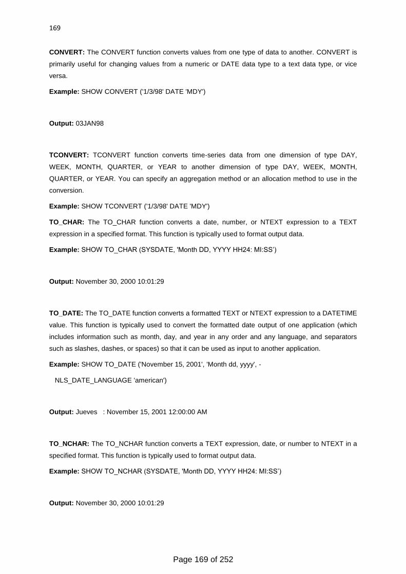
169



versa.


Output: 03JAN98




conversion.




Example: SHOW TO_CHAR (SYSDATE, 'Month DD, YYYY HH24: MI:SS‘)








Output: Jueves : November 15, 2001 12:00:00 AM



Example: SHOW TO_NCHAR (SYSDATE, 'Month DD, YYYY HH24: MI:SS‘)


Page 169 of 252

170






Money = TO_NUMBER ('$94 567,00', 'L999G999D00', NLS_NUMERIC_CHARACTERS ', ')

SHOW money

Output: 94,567.00

10.7 References:

http://en.wikipedia.org/wiki/DUAL_table

https://www.stanford.edu/dept/itss/docs/oracle/10g/olap.101/b10339/appcats007.htm

http://psoug.org/reference/number_func.html

http://dwhlaureate.blogspot.in/2012/09/numeric-functions-in-oracle-with.html

http://docs.oracle.com/cd/E11882_01/server.112/e26088/functions003.htm#SQLRF20035

http://docs.oracle.com/cd/E17952_01/refman-5.1-en/group-by-functions.html

http://musingdba.wordpress.com/2013/01/24/oracle-sql-scalar-functions-reg-exp/

http://oreilly.com/catalog/sqlnut/chapter/ch04.html


Concept Of Database Management Systems (DBMS), 2nd Edition Author: V K Pallaw

Database Management System by Seema Kedar

Starting out with Oracle Author: John Day, Cralg Von Styke.


Page 170 of 252

http://en.wikipedia.org/wiki/DUAL_table

https://www.stanford.edu/dept/itss/docs/oracle/10g/olap.101/b10339/appcats007.htm

http://psoug.org/reference/number_func.html

http://dwhlaureate.blogspot.in/2012/09/numeric-functions-in-oracle-with.html

http://docs.oracle.com/cd/E11882_01/server.112/e26088/functions003.htm

http://docs.oracle.com/cd/E17952_01/refman-5.1-en/group-by-functions.html

http://musingdba.wordpress.com/2013/01/24/oracle-sql-scalar-functions-reg-exp/

http://oreilly.com/catalog/sqlnut/chapter/ch04.html

171

Unit 3


11.1 Objective


11.3 Join and its types

11.3.1 Equi join

11.3.2 Self-join

11.3.3 Non Equi Join

11.3.4 Outer join

11.4 Sub queries using SQL

11.5 Correlated queries in SQL

11.6 Summary

11.7 Glossary


11.9 References


11.1 Objective


Use of SELECT clause for joining the table

Use of SELECT clause for sub queries

11.2 Introduction to SELECT clause:

SELECT command is used to fetch the data from a database table, which return data in the form of

result table. These result tables are called result-sets.





Page 171 of 252

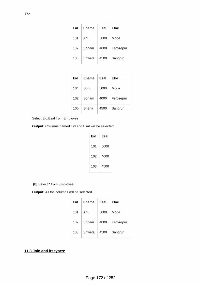
172

Eid Ename Esal Eloc

101 Anu 5000 Moga



Eid Ename Esal Eloc

104 Sonu 5000 Moga



Select Eid,Esal from Employee;


Eid Esal

101 5000

102 4000

103 4500



Eid Ename Esal Eloc

101 Anu 5000 Moga



11.3 Join and its types:

Page 172 of 252

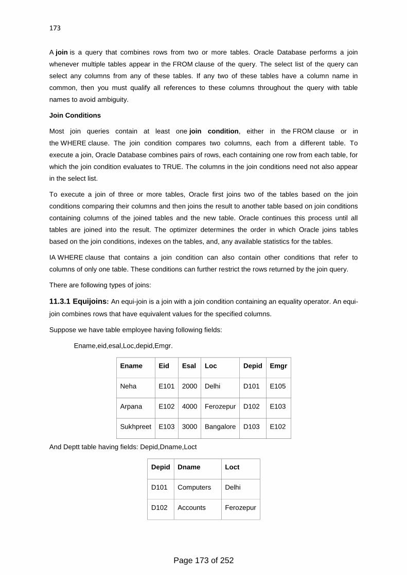
173

A join is a query that combines rows from two or more tables. Oracle Database performs a join

whenever multiple tables appear in the FROM clause of the query. The select list of the query can

select any columns from any of these tables. If any two of these tables have a column name in

common, then you must qualify all references to these columns throughout the query with table

names to avoid ambiguity.

Join Conditions

Most join queries contain at least one join condition, either in the FROM clause or in

the WHERE clause. The join condition compares two columns, each from a different table. To

execute a join, Oracle Database combines pairs of rows, each containing one row from each table, for

which the join condition evaluates to TRUE. The columns in the join conditions need not also appear

in the select list.

To execute a join of three or more tables, Oracle first joins two of the tables based on the join

conditions comparing their columns and then joins the result to another table based on join conditions

containing columns of the joined tables and the new table. Oracle continues this process until all

tables are joined into the result. The optimizer determines the order in which Oracle joins tables

based on the join conditions, indexes on the tables, and, any available statistics for the tables.

IA WHERE clause that contains a join condition can also contain other conditions that refer to

columns of only one table. These conditions can further restrict the rows returned by the join query.

There are following types of joins:

11.3.1 Equijoins: An equi-join is a join with a join condition containing an equality operator. An equi-

join combines rows that have equivalent values for the specified columns.


Ename,eid,esal,Loc,depid,Emgr.

Ename Eid Esal Loc Depid Emgr

Neha E101 2000 Delhi D101 E105

Arpana E102 4000 Ferozepur D102 E103

Sukhpreet E103 3000 Bangalore D103 E102

And Deptt table having fields: Depid,Dname,Loct

Depid Dname Loct

D101 Computers Delhi

D102 Accounts Ferozepur

Page 173 of 252

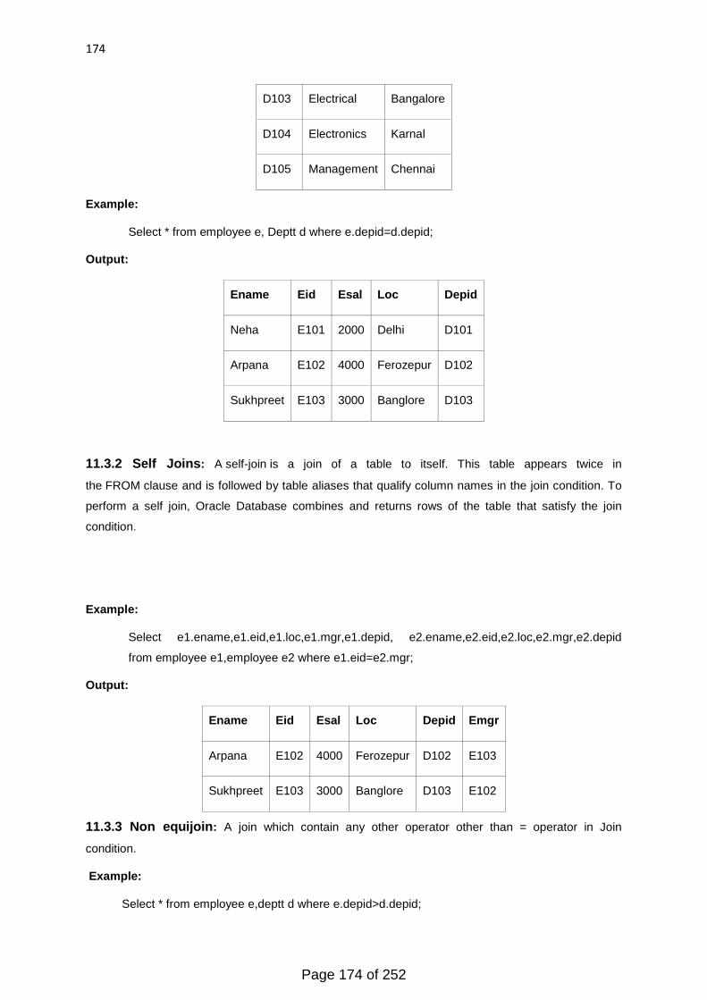
174

D103 Electrical Bangalore

D104 Electronics Karnal

D105 Management Chennai

Example:

Select * from employee e, Deptt d where e.depid=d.depid;

Output:

Ename Eid Esal Loc Depid

Neha E101 2000 Delhi D101

Arpana E102 4000 Ferozepur D102

Sukhpreet E103 3000 Banglore D103

11.3.2 Self Joins: A self-join is a join of a table to itself. This table appears twice in

the FROM clause and is followed by table aliases that qualify column names in the join condition. To

perform a self join, Oracle Database combines and returns rows of the table that satisfy the join

condition.

Example:

Select e1.ename,e1.eid,e1.loc,e1.mgr,e1.depid, e2.ename,e2.eid,e2.loc,e2.mgr,e2.depid

from employee e1,employee e2 where e1.eid=e2.mgr;

Output:



Sukhpreet E103 3000 Banglore D103 E102

11.3.3 Non equijoin: A join which contain any other operator other than = operator in Join

condition.

Example:

Select * from employee e,deptt d where e.depid>d.depid;

Page 174 of 252

175

Output: No row selected.

11.3.4 Outer join: An outer join extends the result of a simple join. An outer join returns all rows

that satisfy the join condition and also returns some or all of those rows from one table for which no

rows from the other satisfy the join condition.

To write a query that performs an outer join of tables A and B and returns all rows from A (a left

outer join), use the LEFT [OUTER] JOIN syntax in the FROM clause, or apply the outer join

operator (+) to all columns of B in the join condition in the WHERE clause. For all rows in A that

have no matching rows in B, Oracle Database returns null for any select list expressions

containing columns of B.

To write a query that performs an outer join of tables A and B and returns all rows from B (a right

outer join), use the RIGHT [OUTER] JOIN syntax in the FROM clause, or apply the outer join

operator (+) to all columns of A in the join condition in the WHERE clause. For all rows in B that

have no matching rows in A, Oracle returns null for any select list expressions containing columns

of A.

To write a query that performs an outer join and returns all rows from A and B, extended with nulls

if they do not satisfy the join condition (a full outer join), use the FULL [OUTER] JOIN syntax in

the FROM clause.

Example:







Deepak E104 5000 Jamshedpur D106 E106

Sonam E105 3500 Chandigarh D107 E101

And Deptt table having fields: Depid,Dname,Loct

Depid Dname Loct


Page 175 of 252

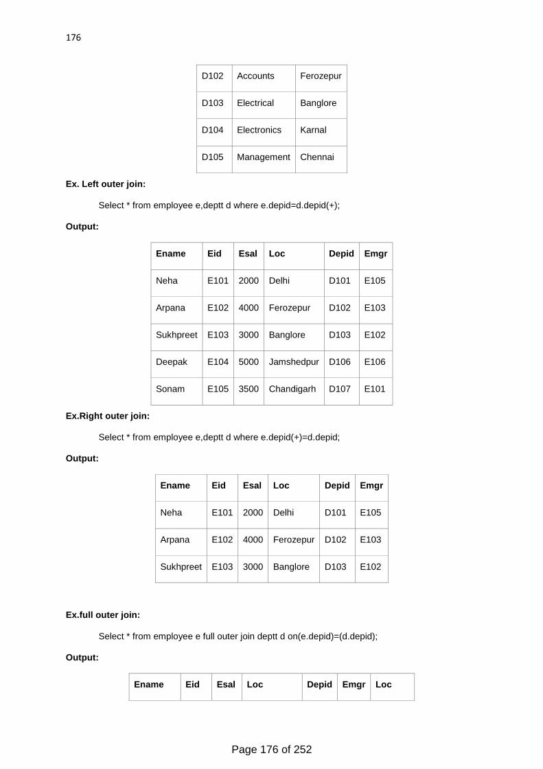
176


D103 Electrical Banglore



Ex. Left outer join:

Select * from employee e,deptt d where e.depid=d.depid(+);

Output:







Ex.Right outer join:

Select * from employee e,deptt d where e.depid(+)=d.depid;

Output:





Ex.full outer join:

Select * from employee e full outer join deptt d on(e.depid)=(d.depid);

Output:

Ename Eid Esal Loc Depid Emgr Loc

Page 176 of 252

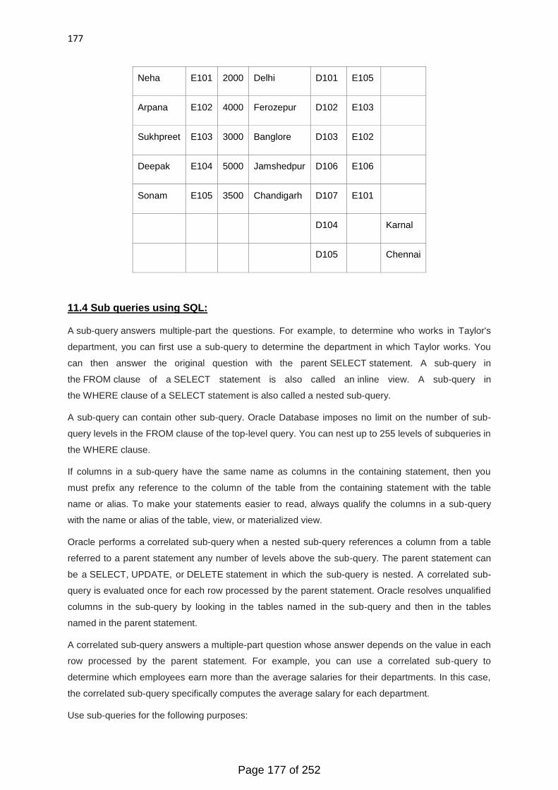
177






D104 Karnal

D105 Chennai

11.4 Sub queries using SQL:

A sub-query answers multiple-part the questions. For example, to determine who works in Taylor's

department, you can first use a sub-query to determine the department in which Taylor works. You

can then answer the original question with the parent SELECT statement. A sub-query in

the FROM clause of a SELECT statement is also called an inline view. A sub-query in

the WHERE clause of a SELECT statement is also called a nested sub-query.

A sub-query can contain other sub-query. Oracle Database imposes no limit on the number of sub-

query levels in the FROM clause of the top-level query. You can nest up to 255 levels of subqueries in

the WHERE clause.

If columns in a sub-query have the same name as columns in the containing statement, then you

must prefix any reference to the column of the table from the containing statement with the table

name or alias. To make your statements easier to read, always qualify the columns in a sub-query

with the name or alias of the table, view, or materialized view.

Oracle performs a correlated sub-query when a nested sub-query references a column from a table

referred to a parent statement any number of levels above the sub-query. The parent statement can

be a SELECT, UPDATE, or DELETE statement in which the sub-query is nested. A correlated sub-

query is evaluated once for each row processed by the parent statement. Oracle resolves unqualified

columns in the sub-query by looking in the tables named in the sub-query and then in the tables

named in the parent statement.

A correlated sub-query answers a multiple-part question whose answer depends on the value in each

row processed by the parent statement. For example, you can use a correlated sub-query to

determine which employees earn more than the average salaries for their departments. In this case,

the correlated sub-query specifically computes the average salary for each department.

Use sub-queries for the following purposes:

Page 177 of 252

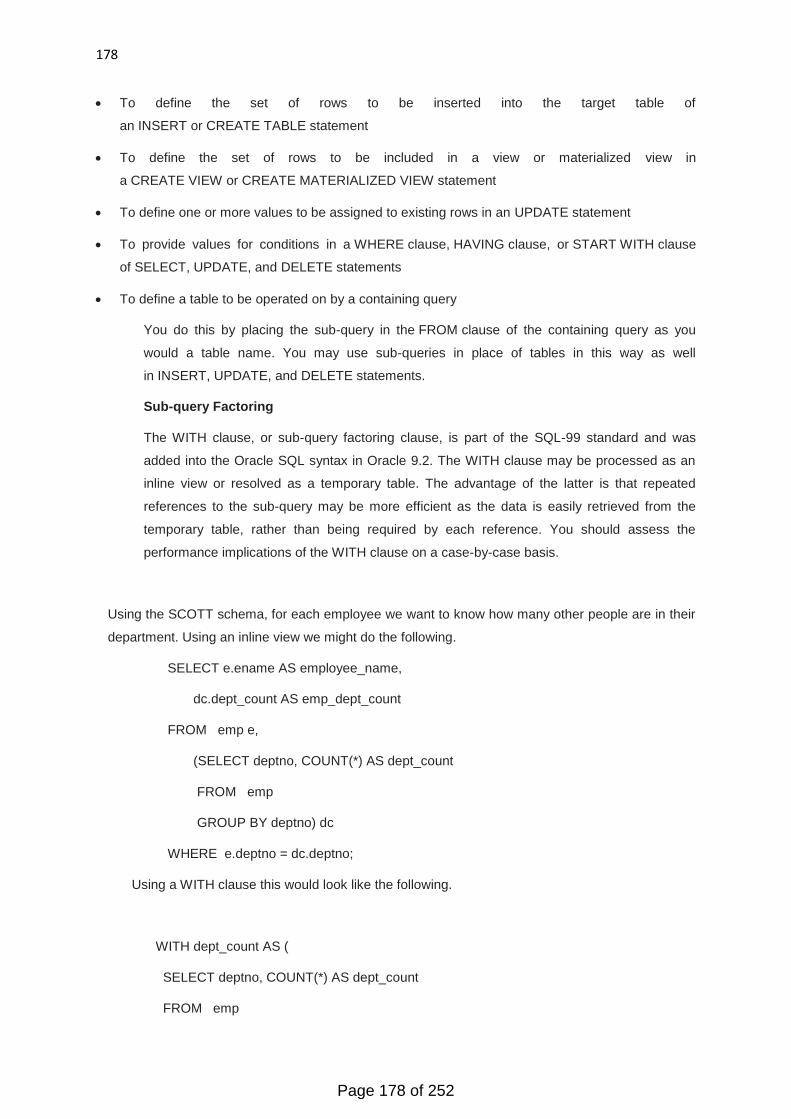
178

To define the set of rows to be inserted into the target table of

an INSERT or CREATE TABLE statement

To define the set of rows to be included in a view or materialized view in

a CREATE VIEW or CREATE MATERIALIZED VIEW statement

To define one or more values to be assigned to existing rows in an UPDATE statement

To provide values for conditions in a WHERE clause, HAVING clause, or START WITH clause

of SELECT, UPDATE, and DELETE statements

To define a table to be operated on by a containing query

You do this by placing the sub-query in the FROM clause of the containing query as you

would a table name. You may use sub-queries in place of tables in this way as well

in INSERT, UPDATE, and DELETE statements.

Sub-query Factoring

The WITH clause, or sub-query factoring clause, is part of the SQL-99 standard and was

added into the Oracle SQL syntax in Oracle 9.2. The WITH clause may be processed as an

inline view or resolved as a temporary table. The advantage of the latter is that repeated

references to the sub-query may be more efficient as the data is easily retrieved from the

temporary table, rather than being required by each reference. You should assess the

performance implications of the WITH clause on a case-by-case basis.

Using the SCOTT schema, for each employee we want to know how many other people are in their

department. Using an inline view we might do the following.

SELECT e.ename AS employee_name,

dc.dept_count AS emp_dept_count

FROM emp e,

(SELECT deptno, COUNT(*) AS dept_count

FROM emp

GROUP BY deptno) dc

WHERE e.deptno = dc.deptno;

Using a WITH clause this would look like the following.

WITH dept_count AS (

SELECT deptno, COUNT(*) AS dept_count

FROM emp

Page 178 of 252

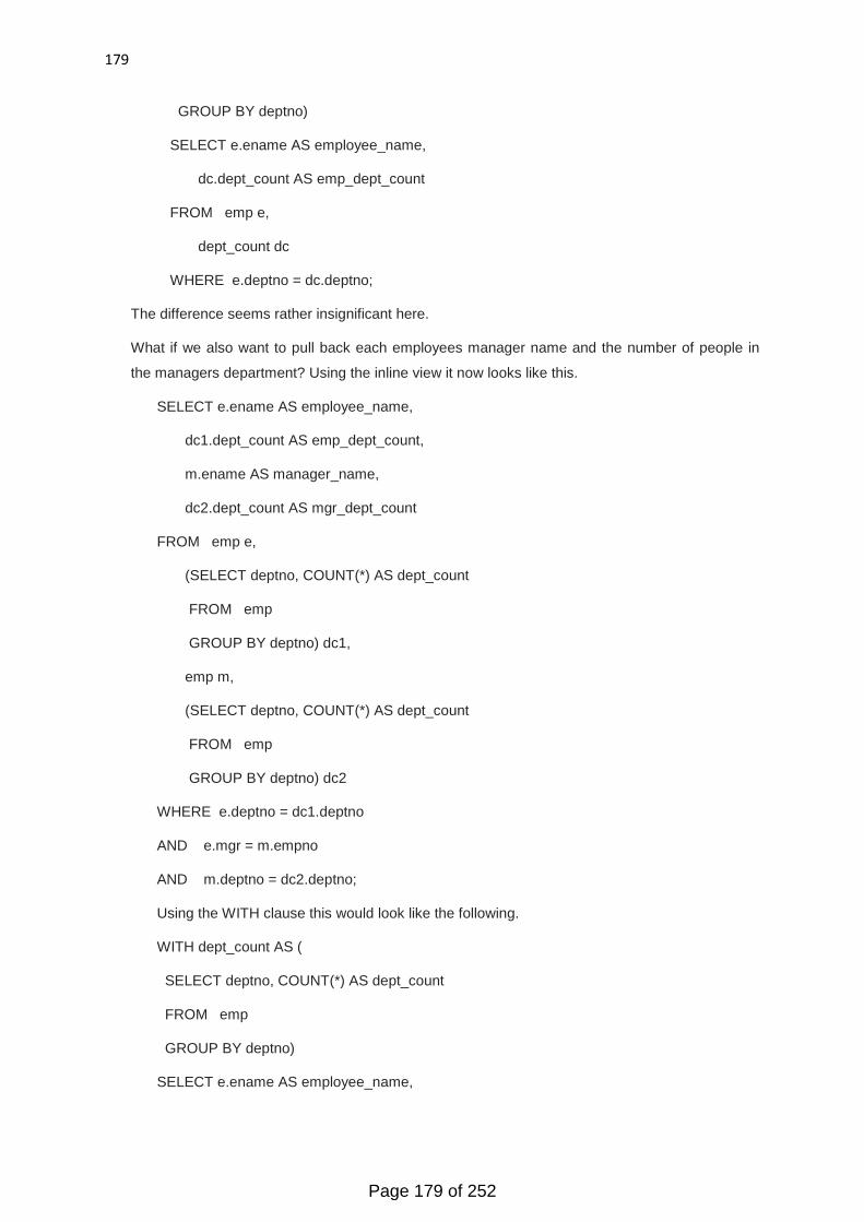
179

GROUP BY deptno)


dc.dept_count AS emp_dept_count

FROM emp e,

dept_count dc

WHERE e.deptno = dc.deptno;

The difference seems rather insignificant here.

What if we also want to pull back each employees manager name and the number of people in

the managers department? Using the inline view it now looks like this.


dc1.dept_count AS emp_dept_count,

m.ename AS manager_name,

dc2.dept_count AS mgr_dept_count

FROM emp e,


FROM emp

GROUP BY deptno) dc1,

emp m,


FROM emp

GROUP BY deptno) dc2

WHERE e.deptno = dc1.deptno

AND e.mgr = m.empno

AND m.deptno = dc2.deptno;

Using the WITH clause this would look like the following.



FROM emp

GROUP BY deptno)


Page 179 of 252

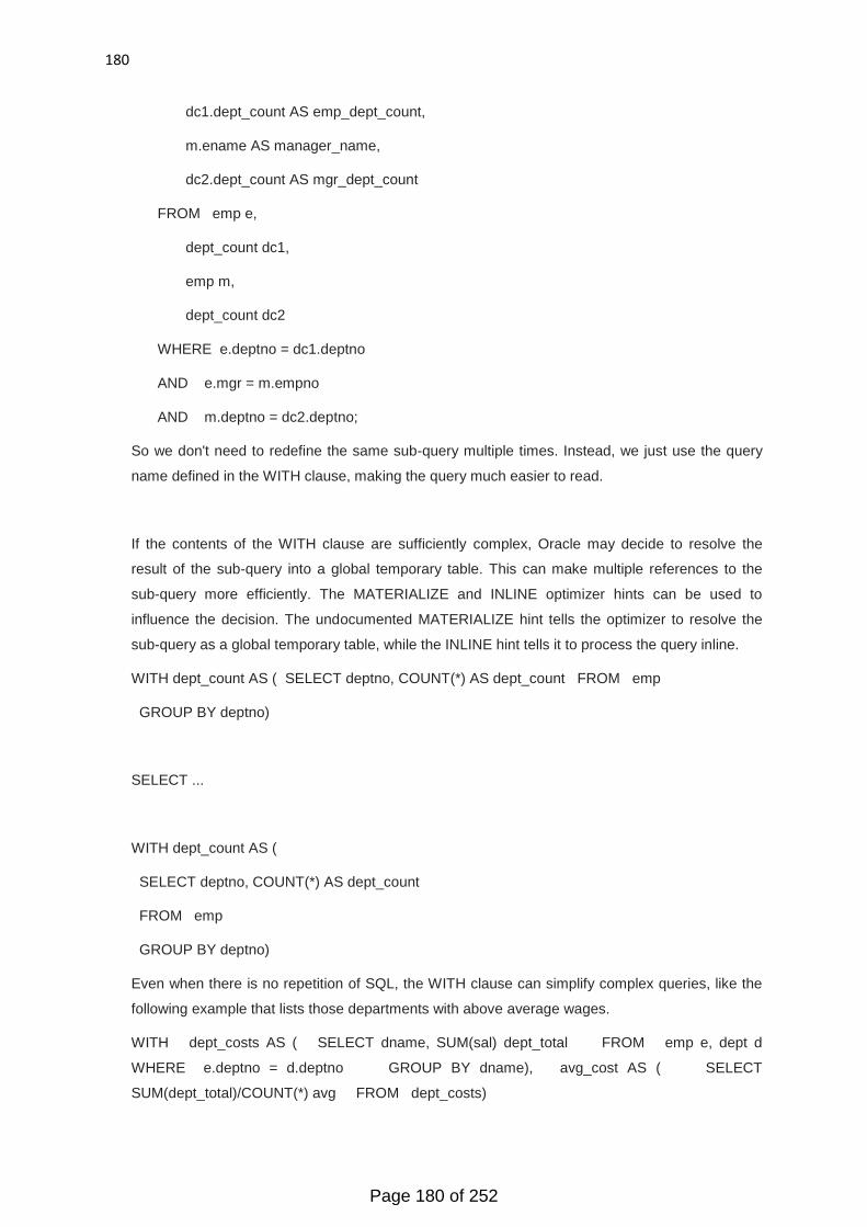
180

dc1.dept_count AS emp_dept_count,

m.ename AS manager_name,

dc2.dept_count AS mgr_dept_count

FROM emp e,

dept_count dc1,

emp m,

dept_count dc2

WHERE e.deptno = dc1.deptno

AND e.mgr = m.empno

AND m.deptno = dc2.deptno;

So we don't need to redefine the same sub-query multiple times. Instead, we just use the query

name defined in the WITH clause, making the query much easier to read.

If the contents of the WITH clause are sufficiently complex, Oracle may decide to resolve the

result of the sub-query into a global temporary table. This can make multiple references to the

sub-query more efficiently. The MATERIALIZE and INLINE optimizer hints can be used to

influence the decision. The undocumented MATERIALIZE hint tells the optimizer to resolve the

sub-query as a global temporary table, while the INLINE hint tells it to process the query inline.

WITH dept_count AS ( SELECT deptno, COUNT(*) AS dept_count FROM emp

GROUP BY deptno)

SELECT ...



FROM emp

GROUP BY deptno)

Even when there is no repetition of SQL, the WITH clause can simplify complex queries, like the

following example that lists those departments with above average wages.

WITH dept_costs AS ( SELECT dname, SUM(sal) dept_total FROM emp e, dept d

WHERE e.deptno = d.deptno GROUP BY dname), avg_cost AS ( SELECT

SUM(dept_total)/COUNT(*) avg FROM dept_costs)

Page 180 of 252

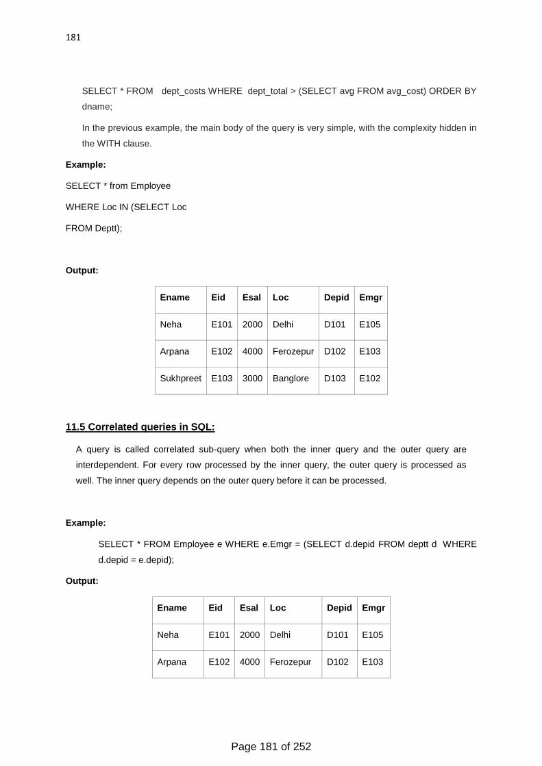
181

SELECT * FROM dept_costs WHERE dept_total > (SELECT avg FROM avg_cost) ORDER BY

dname;

In the previous example, the main body of the query is very simple, with the complexity hidden in

the WITH clause.

Example:

SELECT * from Employee

WHERE Loc IN (SELECT Loc

FROM Deptt);

Output:





11.5 Correlated queries in SQL:

A query is called correlated sub-query when both the inner query and the outer query are

interdependent. For every row processed by the inner query, the outer query is processed as

well. The inner query depends on the outer query before it can be processed.

Example:

SELECT * FROM Employee e WHERE e.Emgr = (SELECT d.depid FROM deptt d WHERE

d.depid = e.depid);

Output:




Page 181 of 252

182

Sukhpreet E103 3000 Bangalore D103 E102


11.6 Summary:

Subquery:

A subquery answers, multiple-part questions. For example, to determine who works in Taylor's

department, you can first use a subquery to determine the department in which Taylor works. You can

then answer the original question with the parent SELECT statement. A subquery in the FROM clause

of a SELECT statement is also called an inline view. A subquery in the WHERE clause of a SELECT

statement is also called a nested subquery.

Joins: A join is a query that combines rows from two or more tables, views, or materialized views.

Oracle Database performs a join whenever multiple tables appear in the FROM clause of the query.

The select list of the query can select any columns from any of these tables. If any two of these tables

have a column name in common, then you must qualify all references to these columns throughout

the query with table names to avoid ambiguity.


Equijoins: An equijoin is a join with a join condition containing an equality operator. An equijoin

combines rows that have equivalent values for the specified columns. Depending on the internal

algorithm the optimizer chooses to execute the join, the total size of the columns in the equijoin

condition in a single table may be limited to the size of a data block minus some overhead.

Self Joins: A self join is a join of a table to itself. This table appears twice in the FROM clause and is

followed by table aliases that qualify column names in the join condition. To perform a self join, Oracle

Database combines and returns rows of the table that satisfy the join condition.

Non equijoin:A join which contain any other operator other than = operator in Join condition.

Outer join: An outer join extends the result of a simple join. An outer join returns all rows that satisfy

the join condition and also returns some or all of those rows from one table for which no rows from the

other satisfy the join condition.

To write a query that performs an outer join of tables A and B and returns all rows from A (a left outer

join), use the LEFT [OUTER] JOIN syntax in the FROM clause, or apply the outer join operator (+) to

all columns of B in the join condition in the WHERE clause. For all rows in A that have no matching

rows in B, Oracle Database returns null for any select list expressions containing columns of B.



operator (+) to all columns of A in the join condition in the WHERE clause. For all rows in B that have

no matching rows in A, Oracle returns null for any select list expressions containing columns of A.

Page 182 of 252

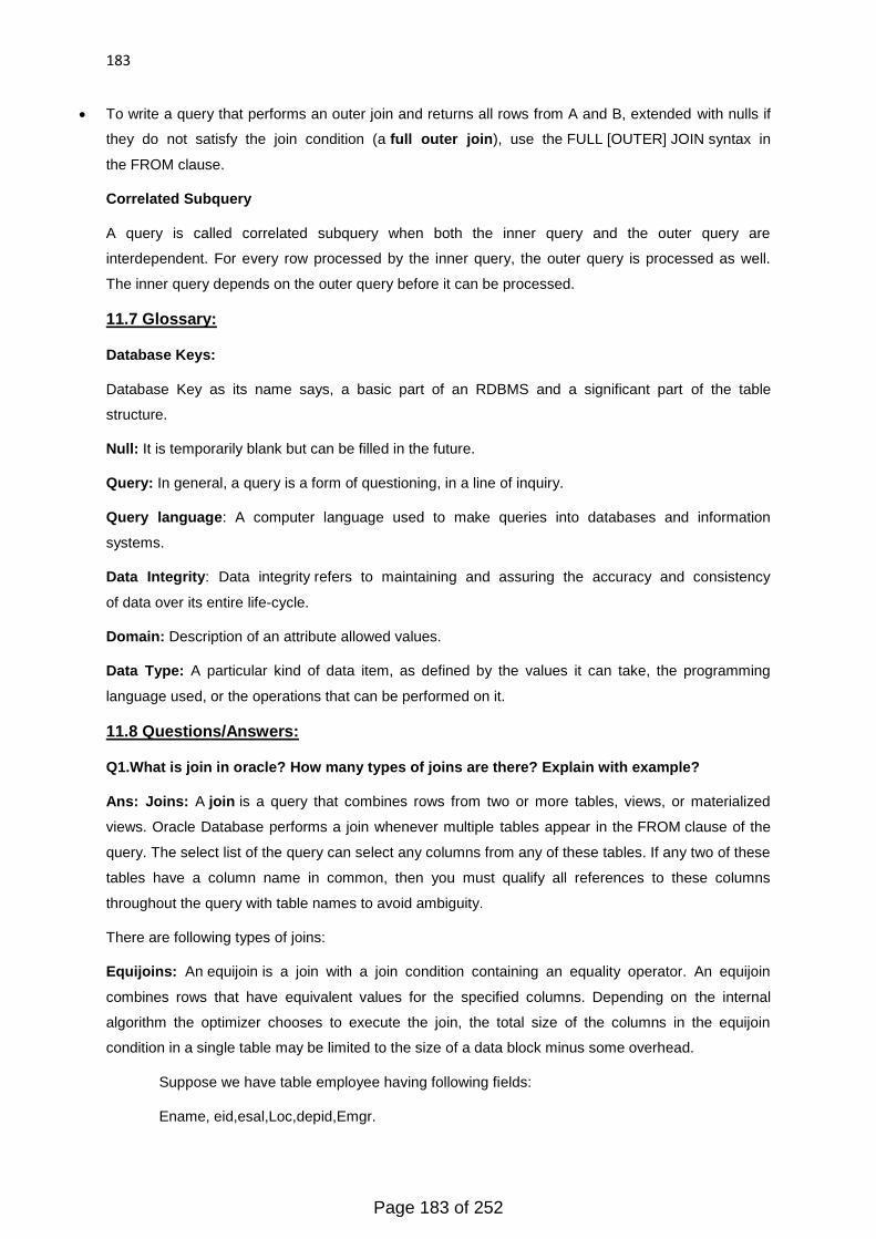
183

To write a query that performs an outer join and returns all rows from A and B, extended with nulls if

they do not satisfy the join condition (a full outer join), use the FULL [OUTER] JOIN syntax in

the FROM clause.

Correlated Subquery

A query is called correlated subquery when both the inner query and the outer query are

interdependent. For every row processed by the inner query, the outer query is processed as well.

The inner query depends on the outer query before it can be processed.

11.7 Glossary:

Database Keys:


structure.

Null: It is temporarily blank but can be filled in the future.

Query: In general, a query is a form of questioning, in a line of inquiry.

Query language: A computer language used to make queries into databases and information

systems.

Data Integrity: Data integrity refers to maintaining and assuring the accuracy and consistency

of data over its entire life-cycle.

Domain: Description of an attribute allowed values.

Data Type: A particular kind of data item, as defined by the values it can take, the programming

language used, or the operations that can be performed on it.


Q1.What is join in oracle? How many types of joins are there? Explain with example?

Ans: Joins: A join is a query that combines rows from two or more tables, views, or materialized

views. Oracle Database performs a join whenever multiple tables appear in the FROM clause of the

query. The select list of the query can select any columns from any of these tables. If any two of these

tables have a column name in common, then you must qualify all references to these columns

throughout the query with table names to avoid ambiguity.


Equijoins: An equijoin is a join with a join condition containing an equality operator. An equijoin

combines rows that have equivalent values for the specified columns. Depending on the internal

algorithm the optimizer chooses to execute the join, the total size of the columns in the equijoin

condition in a single table may be limited to the size of a data block minus some overhead.


Ename, eid,esal,Loc,depid,Emgr.

Page 183 of 252

http://en.wikipedia.org/wiki/Question



184





And Deptt table having fields:Depid,Dname,Loct

Depid Dname Loc






Example:

Select * from employee e,Deptt d where e.depid=d.depid;

Output:

Ename Eid Esal Loc Depid

Neha E101 2000 Delhi D101

Arpana E102 4000 Ferozepur D102

Sukhpreet E103 3000 Banglore D103

Self Joins: A self-join is a join of a table to itself. This table appears twice in the FROM clause

and is followed by table aliases that qualify column names in the join condition. To perform a

self-join, Oracle Database combines and returns rows of the table that satisfy the join condition.

Example:

Select e1.ename, e1.eid,e1.loc,e1.mgr,e1.depid, e2.ename,e2.eid,e2.loc,e2.mgr,e2.depid from

employee e1,employee e2 where e1.eid=e2.mgr;

Output:

Page 184 of 252

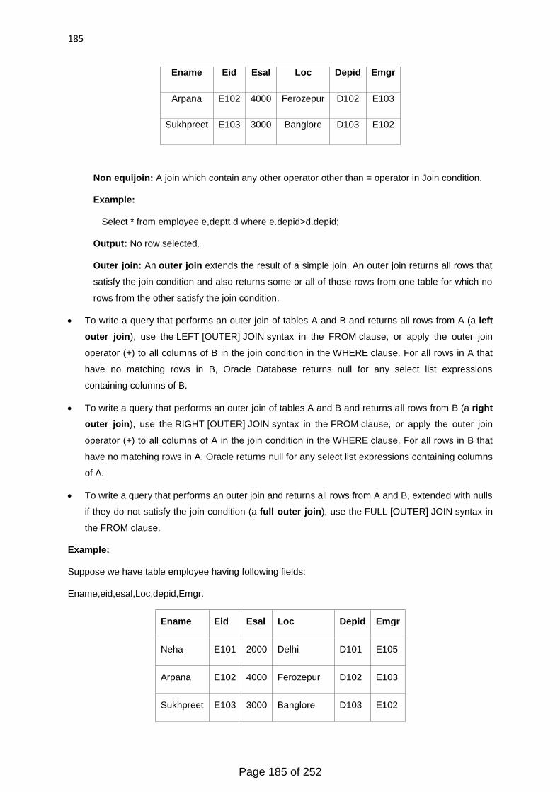
185




Non equijoin: A join which contain any other operator other than = operator in Join condition.

Example:

Select * from employee e,deptt d where e.depid>d.depid;

Output: No row selected.

Outer join: An outer join extends the result of a simple join. An outer join returns all rows that

satisfy the join condition and also returns some or all of those rows from one table for which no

rows from the other satisfy the join condition.

To write a query that performs an outer join of tables A and B and returns all rows from A (a left

outer join), use the LEFT [OUTER] JOIN syntax in the FROM clause, or apply the outer join

operator (+) to all columns of B in the join condition in the WHERE clause. For all rows in A that

have no matching rows in B, Oracle Database returns null for any select list expressions

containing columns of B.



operator (+) to all columns of A in the join condition in the WHERE clause. For all rows in B that

have no matching rows in A, Oracle returns null for any select list expressions containing columns

of A.

To write a query that performs an outer join and returns all rows from A and B, extended with nulls

if they do not satisfy the join condition (a full outer join), use the FULL [OUTER] JOIN syntax in

the FROM clause.

Example:







Page 185 of 252

186



And Deptt table having fields:Depid,Dname,Loct

Depid Dname Loc






Example:

Left outer join:

Select * from employee e,deptt d where e.depid=d.depid(+);

Output:







Example:

Right outer join:

Select * from employee e,deptt d where e.depid(+)=d.depid;

Output:


Page 186 of 252

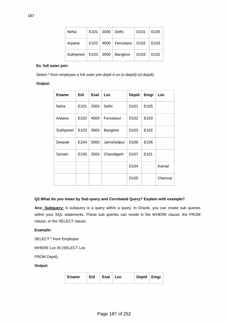
187




Ex. full outer join:

Select * from employee e full outer join deptt d on (e.depid)=(d.depid);

Output:

Ename Eid Esal Loc Depid Emgr Loc






D104 Karnal

D105 Chennai

Q2.What do you mean by Sub query and Correlated Query? Explain with example?

Ans: Subquery: A subquery is a query within a query. In Oracle, you can create sub queries

within your SQL statements. These sub queries can reside in the WHERE clause, the FROM

clause, or the SELECT clause.

Example:

SELECT * from Employee

WHERE Loc IN (SELECT Loc

FROM Deptt);

Output:


Page 187 of 252

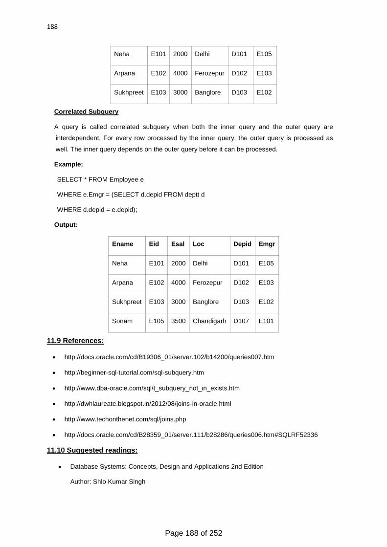
188




Correlated Subquery

A query is called correlated subquery when both the inner query and the outer query are

interdependent. For every row processed by the inner query, the outer query is processed as

well. The inner query depends on the outer query before it can be processed.

Example:

SELECT * FROM Employee e

WHERE e.Emgr = (SELECT d.depid FROM deptt d

WHERE d.depid = e.depid);

Output:






11.9 References:

http://docs.oracle.com/cd/B19306_01/server.102/b14200/queries007.htm

http://beginner-sql-tutorial.com/sql-subquery.htm

http://www.dba-oracle.com/sql/t_subquery_not_in_exists.htm

http://dwhlaureate.blogspot.in/2012/08/joins-in-oracle.html

http://www.techonthenet.com/sql/joins.php

http://docs.oracle.com/cd/B28359_01/server.111/b28286/queries006.htm#SQLRF52336


Database Systems: Concepts, Design and Applications 2nd Edition

Author: Shlo Kumar Singh

Page 188 of 252


http://beginner-sql-tutorial.com/sql-subquery.htm

http://www.dba-oracle.com/sql/t_subquery_not_in_exists.htm

http://dwhlaureate.blogspot.in/2012/08/joins-in-oracle.html

http://www.techonthenet.com/sql/joins.php


189

Database Management Systems (Special Indian Edition) (Schaums‘s Outline) 1st Edition

Author: A Mata TOLEDO

Page 189 of 252

http://www.flipkart.com/author/toledo

190

Unit 4

Lesson 12 – Views using SQL

12.1 Objective

12.2 Introduction to views

12.3 Advantages of views

12.4 Creation of views

12.5 Types of views

12.5.1 Indexed view

12.5.2 Partitioned view

12.6 Alteration of views

12.7 Summary

12.8 Glossary


12.10 References


12.1 Objective:

Introduction to Database Views

Creating and altering views.

12.2 Introduction to views:

A view is nothing more than a SQL statement that is stored in the database with a linked name. A

view is actually a composite form of a table in the form of a predefined SQL query.


many tables which depend on the SQL query to create a view.

Views, which are a kind of virtual tables, allow users to do the following:

Structure data in a way that users or classes of users find natural or intuitive.

Restrict access to the data such that a user can see and (sometimes) modify exactly what they

need and no more.

Summarize data from various tables which can be used to generate reports.

12.3 Advantages of views:

Page 190 of 252

191


Views can be used to represent a subset of the data contained in a table; consequently, a

view can limit the degree of exposure of the underlying tables to the outer world.

Views can be used to join and simplify multiple tables into a single virtual table.

Views can be used to act as aggregated tables, where the database engine aggregates data

And presents the calculated results as part of the data

The views can take very little space to store; the database contains only the definition of a

view, not a copy of all the data which it presents

12.4 Creation of views:

In SQL, a view is a virtual table based on the result-set of an SQL statement.





Syntax:



FROM table_name

WHERE condition

Example:


SELECT Eid, Ename

FROM Employee

WHERE Eid=101;

12.5 Types of views:

There are two types of views:

12.5.1 Indexed view:

Page 191 of 252

192

An indexed view has a unique clustered index. The clustered index is stored in SQL Server and

updated like any other clustered index, providing SQL Server with another place to look to potentially

optimize a query utilizing the indexed view. Queries that don‘t specifically use the indexed view can

even benefit from the existence of the clustered index from the view. In the development and

enterprise editions of SQL Server, the optimizer can use the indexes of views to optimize queries that

do not specify the indexed view. In the other editions of SQL Server, however, the query must include

the indexed view and specify the hint NOEXPAND to get the benefit of the index on the view. If your

queries could benefit from having more than one index on the view, non-clustered indexes can also

be created in the view. This would supply the optimizer with more possibilities to speed up the queries

referencing the columns included in the view.








Example:



SELECT

e. Eid,

d.depid,

FROM e. Employee AS e

JOIN d.deptt AS d


12.5.2 Partitioned view:

Partitioning SQL data sets is an ideal way to improve scale out, and distributed partitioning is

particularly valuable in this regard. Here I will explain the benefits of using partitioned views, and offer

some points to keep in mind when defining and creating them.




Page 192 of 252

193



Example












create table line_item_1992 (

constraint C_send_date_1992

check(send_date < 'Jan-01-1993')

disable,

order_key number ,

part_key number ,

source_key number ,

send_date date ,

promise_date date ,

receive_date date );



check(send_date => 'Jan-01-1993' and send_date < 'Jan-01-1994')

disable,

order_key number ,

part_key number ,

Page 193 of 252

194

source_key number ,

send_date date ,

promise_date date ,




loader control file (in this example it is "LI. ctl"), but should use a different data file. Also, the data files



loaded.






partitions.







add constraint C_receive_date_1992 check ( receive_date between

'Jan-01-1992' and 'Jan-01-1993' + 90);



'Jan-01-1993' and 'Jan-01-1994' + 90);




a partition view.


Page 194 of 252

195

















12.6 Alteration of views:

We can alter an already created view with Replace statement.

Syntax:



FROM table_name

WHERE condition


Example:



FROM Employee

WHERE Eid=101;

12.7 Summary:

Page 195 of 252

196

View: A view is nothing more than a SQL statement that is stored in the database with an associated

name. A view is actually a composition of a table in the form of a predefined SQL query.


many tables which depends on the written SQL query to create a view.

Index: Indexes are optional structures associated with tables and clusters that allow SQL statements

to execute more quickly against a table. Just as the index in this manual helps you locate information

faster than if there were no index, an Oracle Database index provides a faster access path to table

data. You can use the indexes without rewriting any queries. Your results are the same, but you see

them more quickly.

Indexed View: An indexed view has a unique clustered index. The clustered index is stored in SQL

Server and updated like any other clustered index, providing SQL Server with another place to look to

potentially optimize a query utilizing the indexed view. Queries that don‘t specifically use the indexed

view can even benefit from the existence of the clustered index from the view. In the development and

enterprise editions of SQL Server, the optimizer can use the indexes of views to optimize queries that

do not specify the indexed view. In the other editions of SQL Server, however, the query must include

the indexed view and specify the hint NOEXPAND to get the benefit of the index on the view. If your

queries could benefit from having more than one index on the view, non-clustered indexes can also

be created in the view. This would supply the optimizer with more possibilities to speed up the queries

referencing the columns included in the view.

Partitioned View: Partitioning SQL data sets is an ideal way to improve scale out, and distributed

partitioning is particularly valuable in this regard. Here I will explain the benefits of using partitioned

views, and offer some points to keep in mind when defining and creating them.






12.8 Glossary:

Redundancy: Redundancy is the duplication of critical components or functions of a system with the

intention of increasing reliability of the system.

Dependency: Relationship between conditions, events, or tasks such that one cannot begin or be-

completed until one or more other conditions, events, or tasks have occurred, begun, or completed.


occasions.


Column: A column is a set of data values of a particular simple type, one for each row of the table.

Page 196 of 252

197


Q1.What is a View in the database? Explain with example?

Ans: View in A a database:

A view is the result of a stored query on the data, which the database users can query just as they

would in a persistent database collection object. This pre-established query command is kept in the

database dictionary. It is a virtual table computed or collated from data in the database, dynamically

when access to that view is requested. Changes applied to the data in a relevant underlying table are

reflected in the data shown in subsequent invocations of the view.

Creating View: In SQL, a view is a virtual table based on the result-set of an SQL statement.





Syntax:



FROM table_name

WHERE condition

Example:


SELECT Eid, Ename

FROM Employee

WHERE Eid=101;

Altering a view: We can alter an already created view with Replace statement.

Syntax:



FROM table_name

WHERE condition

Page 197 of 252

198


Example:



FROM Employee

WHERE Eid=101;

Q2.What is the advantages of Views?

Ans: Advantages of Views:


Views can represent a subset of the data contained in a table; consequently, a view can limit the

degree of exposure of the underlying tables to the outer world: a given user may have permission

to query the view, while denying access to the rest of the base table.

Views can be used to join and simplify multiple tables into a single virtual table

Views can be used to act as aggregated tables, where the database engine aggregate data

(sum, average etc.) And presents the calculated results as part of the data

Views can be used to hide the complexity of data; for example a view could appear as

Sales2000 or Sales2001, transparently partitioning the actual underlying table

Views can take very little space to store; the database contains only the definition of a view, not a

copy of all the data which it presents

Depending on the SQL engine used, views can provide extra security

Q3.What is an Index in Database?

Ans: Index: Indexes are optional structures associated with tables and clusters that allow SQL

statements to execute more quickly against a table. Just as the index in this manual helps you locate

information faster than if there were no index, an Oracle Database index provides a faster access

path to table data. You can use the indexes without rewriting any queries. Your results are the same,

but you see them more quickly.

Q4.What is an Indexed View? Explain with example?

Ans: Indexed View: An indexed view has a unique clustered index. The clustered index is stored in

SQL Server and updated like any other clustered index, providing SQL Server with another place to

look to potentially optimize a query utilizing the indexed view. Queries that don‘t specifically use the

indexed view can even benefit from the existence of the clustered index from the view. In the

development and enterprise editions of SQL Server, the optimizer can use the indexes of views to

optimize queries that do not specify the indexed view. In the other editions of SQL Server, however,

the query must include the indexed view and specify the hint NOEXPAND to get the benefit of the

Page 198 of 252

http://en.wikipedia.org/wiki/Join_(SQL)

http://en.wikipedia.org/wiki/Database_engine

http://en.wikipedia.org/wiki/Sum

http://en.wikipedia.org/wiki/Average

http://en.wikipedia.org/wiki/Partition_(database)

http://en.wikipedia.org/wiki/SQL

199

index on the view. If your queries could benefit from having more than one index on the view, non-

clustered indexes can also be created in the view. This would supply the optimizer with more

possibilities to speed up the queries referencing the columns included in the view.








Example:



SELECT

e. Eid,

d.depid,

FROM e.Employee AS e

JOIN d.deptt AS d


Q5.What is a Partitioned View? Explain with example?

Ans: Partitioned View: Partitioning SQL datasets are an ideal way to improve scale out, and

distributed partitioning is particularly valuable in this regard. Here I will explain the benefits of using

partitioned views, and offer some points to keep in mind when defining and creating them.






Example





Page 199 of 252

200









check(send_date < 'Jan-01-1993')

disable,

order_key number ,

part_key number ,

source_key number ,

send_date date ,

promise_date date ,




check(send_date => 'Jan-01-1993' and send_date < 'Jan-01-1994')

disable,

order_key number ,

part_key number ,

source_key number ,

send_date date ,

promise_date date ,




loader control file (in this example it is "LI.ctl"), but should use a different data file. Also, the data files

Page 200 of 252

201



loaded.






partitions.






Attention: These constructs will not be directly available for partitioned tables in Oracle8. Using them

might introduce additional complexity in migrating partition views to partitioned tables.



'Jan-01-1992' and 'Jan-01-1993' + 90);



'Jan-01-1993' and 'Jan-01-1994' + 90);




a partition view.







Page 201 of 252

202












12.10 References;


http://en.wikipedia.org/wiki/View_(SQL)



http://docs.oracle.com/cd/E11882_01/server.112/e25789/indexiot.htm#CNCPT721


http://www.codeproject.com/Articles/199058/SQL-Server-Indexed-Views-Speed-Up-Your-

Select-Quer




http://docs.oracle.com/cd/A57673_01/DOC/server/doc/A48506/partview.htm#383


Database System. A practical approach to design, implementation and management. Author:

Thomas connoly, corlyn begg.

Taxonomy of database management system.

Author: Aditya Kumar gupta.

Database management System.

Author: Alex Leon, Mathew Leon.

Page 202 of 252



http://docs.oracle.com/cd/E11882_01/server.112/e25789/indexiot.htm








203

Unit 4

Lesson 13 - Indexes using SQL

13.1 Objective

13.2 Introduction to indexes

13.3 Advantages of indexes

13.4 Creation of index

13.5 Types of indexes

13.5.1 Unique index

13.5.2 Composite index

13.6 Altering Index

13.7 Use of index for accessing data

13.8 Summary

13.9 Glossary


13.11 References


13.1 Objective;

Introduction to indexes

Creating and Altering an index

13.2 Introduction to indexes:

The index is a data structure that stores the values for a specific column in a table. An index is

created on a column of a Table. So, the key points to remember are that an index consists of a

column values from one table, and that those values are stored in a data structure.

Index Characteristics:

Indexes are schema objects that are logically and physically independent of the data in the

objects with which they are associated. Thus, an index can be dropped or created without

physically affecting the table for the index.

The absence or presence of an index does not require a change in the wording of any SQL

statement. An index is a fast access path to a single row of data. It affects only the speed of

Page 203 of 252

204

execution. Given a data value that has been indexed, the index points directly to the location of

the rows containing that value.

The database automatically maintains and uses indexes after they are created. The database

also automatically reflects changes to data, such as adding, updating, and deleting rows, in all

relevant indexes with no additional actions required by users. Retrieval performance of indexed

data remains almost constant, even as rows are inserted. However, the presence of many

indexes on a table degrades DML performance because the database must also update the

indexes.

Indexes have the following properties:

Usability

Indexes are usable (default) or unusable. An unusable index is not maintained by DML operations

and is ignored by the optimizer. An unusable index can improve the performance of bulk loads.

Instead of dropping an index and later re-creating it, you can make the index unusable and then

rebuild it. Unusable indexes and index partitions do not consume space. When you make a

usable index unusable, the database drops its index segment.

Visibility

Indexes are visible (default) or invisible. An invisible index is maintained by DML operations and is

not used by default by the optimizer. Making an index invisible is an alternative to making it

unusable or dropping it. Invisible indexes are especially useful for testing the removal of an index

before dropping it or using indexes temporarily without affecting the overall application.

13.3 Advantages of indexes:

If no index exists on a table, a table scan must be performed for each table referenced in a

database query. The larger the table, the longer a table scan takes because a table scan requires

each table row to be accessed sequentially. Although a table scan might be more efficient for a

complex query that requires most of the rows in a table, for a query that returns only some table

rows an index scan can access table rows more efficiently.

The optimizer chooses an index scan if the indexed columns are referenced in the SELECT

statement and if the optimizer estimates that an index scan will be faster than a table scan. Index

files generally are smaller and require less time to read than an entire table, particularly as tables

grow larger. In addition, the entire index may not need to be scanned. The predicates that are

applied to the index reduce the number of rows to be read from the data pages.

If an ordering requirement on the output can be matched with an index column, then scanning the

index in column order will allow the rows to be retrieved in the correct order without a sort.

13.4 Creation of index:

For creating an index we have to specify index name and column on which it will be created.To

create an index in your own schema, at least one of the following conditions must be true:

Page 204 of 252

205

The table or cluster to be indexed is in your own schema.

You have INDEX privilege on the table to be indexed.

You have CREATE ANY INDEX system privilege.

To create an index in another schema, all of the following conditions must be true:

You have CREATE ANY INDEX system privilege.

The owner of the other schema has a quota for the tablespaces to contain the index or index

partitions, or UNLIMITED TABLESPACE system privilege.

Syntax:

CREATE INDEX index_name

ON table_name (column_name)

Example:


Creating an Index Associated with a Constraint

Oracle Database enforces a UNIQUE key or PRIMARY KEY integrity constraint on a table by

creating a unique index on the unique key or primary key. This index is automatically created by

the database when the constraint is enabled. No action is required by you when you issue the

CREATE TABLE or ALTER TABLE statement to create the index, but you can optionally specify a

USING INDEX clause to exercise control over its creation. This includes both when a constraint is

defined and enabled, and when a defined but disabled constraint is enabled.

To enable a UNIQUE or PRIMARY KEY constraint, thus creating an associated index, the owner

of the table must have a quota for the tablespace intended to contain the index, or the

UNLIMITED TABLESPACE system privilege. The index associated with a constraint always takes

the name of the constraint, unless you optionally specify otherwise.

Specifying Storage Options for an Index Associated with a Constraint

You can set the storage options for the indexes associated with UNIQUE and PRIMARY KEY

constraints using the USING INDEX clause. The following CREATE TABLE statement enables a

PRIMARY KEY constraint and specifies the storage options of the associated index:

CREATE TABLE emp (empno NUMBER(5) PRIMARY KEY, age INTEGER)

ENABLE PRIMARY KEY USING INDEX

TABLESPACE users;

Page 205 of 252

206

Specifying the Index Associated with a Constraint

If you require more explicit control over the indexes associated with UNIQUE and PRIMARY KEY

constraints, the database lets you:

Specify an existing index that the database is to use to enforce the constraint

Specify a CREATE INDEX statement that the database is to use to create the index and enforce

the constraint

These options are specified using the USING INDEX clause. The following statements present

some examples.

Example 1:

CREATE TABLE a (a1 INT PRIMARY KEY USING INDEX (create index ai on a (a1)));

Example 2:

CREATE TABLE b (b1 INT, b2 INT, CONSTRAINT bu1 UNIQUE (b1, b2) USING INDEX (create

unique index bi on b(b1, b2)), CONSTRAINT bu2 UNIQUE (b2, b1) USING INDEX bi);

Example 3:

CREATE TABLE c(c1 INT, c2 INT);

CREATE INDEX ci ON c (c1, c2);

ALTER TABLE c ADD CONSTRAINT cpk PRIMARY KEY (c1) USING INDEX ci;

If a single statement creates an index with one constraint and also uses that index for another

constraint, the system will attempt to rearrange the clauses to create the index before reusing it.

13.5 Types of indexes:

There are two types of index:

13.5.1 Unique index:

Unique indexes are used not only for performance, but also for data integrity. A unique index

does not allow any duplicate values to be inserted into the table. The basic syntax is as

follows:

Syntax:


Example:


13.5.2 Composite index:

Page 206 of 252

207

A composite index is an index on two or more columns of a table. The basic syntax is as

follows:

Syntax:


Example:


13.6 Altering Indexes

To alter an index, your schema must contain the index or you must have the ALTER ANY

INDEX system privilege. Among the actions allowed by the ALTER INDEX statement are:

Rebuild or coalesce an existing index

Deallocate unused space or allocate a new extent

Specify parallel execution (or not) and alter the degree of parallelism

Alter storage parameters or physical attributes

Specify LOGGING or NOLOGGING

Enable or disable key compression

Mark the index unusable

Start or stop the monitoring of index usage

Altering Storage Characteristics of an Index

Alter the storage parameters of any index, including those created by the database to enforce

primary and unique key integrity constraints, using the ALTER INDEX statement. For example, the

following statement alters the emp_ename index:

ALTER INDEX emp_ename STORAGE (PCTINCREASE 50);

The storage parameters INITIAL and MINEXTENTS cannot be altered. All new settings for the

other storage parameters affect only extents subsequently allocated for the index.

For indexes that implement integrity constraints, you can adjust storage parameters by issuing an

ALTER TABLE statement that includes the USING INDEX subclause of the ENABLE clause. For

example, the following statement changes the storage options of the index created on table emp

to enforce the primary key constraint:

ALTER TABLE emp ENABLE PRIMARY KEY USING INDEX;

13.7 Use of index for accessing data:

Page 207 of 252

208

Suppose that we have a database table called Employee with three columns – Employee_Name,

Employee_Age, and Employee_Address. Assume that the Employee table has thousands of

rows.

Now, let‘s say that we want to run a query to find all the details of any employees who are named

‗Jesus‘? So, we decide to run a simple query like this:


WHERE Employee_Name = 'Jesus'

Without Index: Once we run that query, what exactly goes on behind the scenes to find

employees who are named Jesus? Well, the database software would literally have to look at

every single row in the Employee table to see if the Employee_Name for that row is ‗Jesus‘. And,

because we want every row with the name ‗Jesus‘ inside it, we cannot just stop looking once we

find just one row with the name ‗Jesus‘, because there could be other rows with the name Jesus.

So, every row up until the last row must be searched – which means thousands of rows in this

scenario will have to be examined by the database to find the rows with the name ‗Jesus‘. This is

what is called a Full Table Scan

With Index: You might be thinking that doing a full table scan sounds inefficient for something so

simple – shouldn‘t software be smarter? It‘s almost like looking through the entire table with the

human eye – very slow and not at all sleek. But, as you probably guessed by the title of this

article, this is where indexes can help a great deal. The whole point of having an index is to speed

up search queries by essentially cutting down the number of records/rows in a table that need to

be examined.

Because an index is basically a data structure that is used to store column values, looking up

those values becomes much faster. And, if an index is using the most commonly used data

structure type – a B- tree – then the data structure is also sorted. Having the column values be

sorted can be a major performance enhancement – read on to find out why.

Let‘s say that we create a B- tree index on the Employee_Name column this means that when we

search for employees named ―Jesus‖ using the SQL we showed earlier, then the entire Employee

table does not have to be searched to find employees named ―Jesus‖. Instead, the database will

use the index to find employees named Jesus, because the index will presumably be sorted

alphabetically by the Employee‘s name. And, because it is sorted, it means searching for a name

is a lot faster because all names starting with a ―J‖ will be right next to each other in the index! It‘s

also important to note that the index also stores pointers to the table row so that other column

values can be retrieved – read on for more details on that.

13.8 Summary:

The index is a data structure (most commonly a B- tree) that stores the values for a specific

column in a table. An index is created on a column of a table. So, the key points to remember are

Page 208 of 252

209

that an index consists of a column values from one table, and that those values are stored in a

data structure.

Advantages of an index over no index











Unique Index: Unique indexes are used not only for performance, but also for data integrity. A

unique index does not allow any duplicate values to be inserted into the table.

Composite Index: A composite index is an index on two or more columns of a table.

13.9 Glossary:

Composite: It means made up of several parts or elements.


table.

Redundancy: Redundancy is the duplication of critical components or functions of a system with

the intention of increasing reliability of the system.

Dependency: Relationship between conditions, events, or tasks such that one cannot begin or

be-completed until one or more other conditions, events, or tasks have occurred, begun, or

completed.


occasions.




Inheritance: Inheritance allows a class to have the same behavior as another class and extend

or tailor that behavior to provide special action for specific needs.

Encapsulation: The condition of being enclosed.


Page 209 of 252

210

Q1.What is a Database Index? What are the advantages of Index? Explain with example?

Ans: Index is a data structure (most commonly a B- tree) that stores the values for a specific

column in a table. An index is created on a column of a table. So, the key points to remember are

that an index consists of a column values from one table, and that those values are stored in a

data structure.

Advantages of an index over no index











If an ordering requirement on the output can be matched with an index column, then scanning the

index in column order will allow the rows to be retrieved in the correct order without a sort.

Each index entry contains a search-key value and a pointer to the row containing that value. If

you specify the ALLOW REVERSE SCANS parameter in the CREATE INDEX statement, the

values can be searched in both ascending and descending order. It is therefore possible to

bracket the search, given the right predicate. An index can also be used to obtain rows in an

ordered sequence, eliminating the need for the database manager to sort the rows after they are

read from the table.

In addition to the search-key value and row pointer, an index can contain include columns, which

are non-indexed columns in the indexed row. Such columns might make it possible for the

optimizer to get required information only from the index, without accessing the table itself.

Syntax:

CREATE INDEX index_name ON table_name (column_name)

Example:


Q2.Explain Types of Index with example?

Page 210 of 252

211

Ans: Unique Index: Unique indexes are used not only for performance, but also for data

integrity. A unique index does not allow any duplicate values to be inserted into the table. The

basic syntax is as follows:

Syntax:


Example:


Composite Index: A composite index is an index on two or more columns of a table. The basic

syntax is as follows:

Syntax:


Example:


Q3.How we can access data with or without Index?

Ans: Accessing data with or without Index:

Suppose that we have a database table called Employee with three columns – Employee_Name,

Employee_Age, and Employee_Address. Assume that the Employee table has thousands of

rows.

Now, let‘s say that we want to run a query to find all the details of any employees who are named

‗Jesus‘? So, we decide to run a simple query like this:

SELECT * FROM Employee WHERE Employee_Name = 'Jesus'

Without Index: Once we run that query, what exactly goes on behind the scenes to find

employees who are named Jesus? Well, the database software would literally have to look at

every single row in the Employee table to see if the Employee_Name for that row is ‗Jesus‘. And,

because we want every row with the name ‗Jesus‘ inside it, we cannot just stop looking once we

find just one row with the name ‗Jesus‘, because there could be other rows with the name Jesus.

So, every row up until the last row must be searched – which means thousands of rows in this

scenario will have to be examined by the database to find the rows with the name ‗Jesus‘. This is

what is called a Full table Scan

With Index: You might be thinking that doing a full table scan sounds inefficient for something so

simple – shouldn‘t software be smarter? It‘s almost like looking through the entire table with the

human eye – very slow and not at all sleek. But, as you probably guessed by the title of this

article, this is where indexes can help a great deal. The whole point of having an index is to speed

up search queries by essentially cutting down the number of records/rows in a table that need to

be examined.

Page 211 of 252

212

Because an index is basically a data structure that is used to store column values, looking up

those values becomes much faster. And, if an index is using the most commonly used data

structure type – a B- tree – then the data structure is also sorted. Having the column values be

sorted can be a major performance enhancement – read on to find out why.

Let‘s say that we create a B- tree index on the Employee_Name column, this means that when

we search for employees named ―Jesus‖ using the SQL we showed earlier, then the entire

Employee table does not have to be searched to find employees named ―Jesus‖. Instead, the

database will use the index to find employees named Jesus, because the index will presumably

be sorted alphabetically by the Employee‘s name. And, because it is sorted, it means searching

for a name is a lot faster because all names starting with a ―J‖ will be right next to each other in

the index! It‘s also important to note that the index also stores pointers to the table row, so that

other column values can be retrieved – read on for more details on that.

13.11 References:

http://antognini.ch/2009/12/does-create-index-gather-global-statistics/

http://www.w3schools.com/sql/sql_create_index.asp

http://publib.boulder.ibm.com/infocenter/db2luw/v8/index.jsp?topic=/com.ibm.db2.udb.doc

/admin/c0005052.htm

http://www.programmerinterview.com/index.php/database-sql/what-is-an-index/


Relational Database Management System.

Author: Sujata P patil,Vidya H Bankar,Deepashree K MehenDale.

Database Management System

Author:Anjali Bhatnagar

Database Management System

Author: Malay K Pakhira

Page 212 of 252

213

Unit 4

Lesson 14 - Introduction to PL/SQL

14.1 Objective

14.2 Introduction

14.3 Features of PL/SQL

14.4 Need of PL/SQL

14.5 Fundamentals of PL/SQL

14.6 Advantages of PL/SQL

14.7 The Generic PL/SQL Block

14.7.1 The Declaration Section

14.7.2 The Begin Section

14.7.3 The End Section

14.8 Summary

14.9 Glossary


14.11 References


14.1 Objective:

An introduction to PL/SQL.

A generic block structure of PL/SQL.

14.2 Introduction:

The PL/SQL language is an extension of SQL language developed by Oracle Corporation and the

full name it is the Procedural Language/Structured Query Language.

The PL/SQL language is a procedural programming language which allows data manipulation and

SQL query to be included in blocks. PL/SQL can be used to group multiple instructions in a single

block and sending the entire block to the server in a single call.

The PL/SQL programming language was developed by Oracle Corporation in the late 1980s as a

procedural extension language for SQL and the Oracle relational database.PL/SQL is a

completely portable, high-performance transaction-processing language.

PL/SQL provides a built-in interpreted and OS independent programming environment.

Page 213 of 252

214

PL/SQL can also be called directly from the command-line SQL*Plus interface.

Direct call can also be made from external programming language calls to databases.

PL/SQL's general syntax is based on that of ADA and Pascal programming language.

14.3 Features of PL/SQL

PL/SQL has the following features:

PL/SQL is tightly integrated with SQL.

It offers extensive error checking.

It offers numerous data types.

It offers a variety of programming structures.

It supports structured programming through functions and procedures.

It supports object-oriented programming.

It supports developing web applications and server pages.

14.4 Need for PL/SQL

SQL statements are defined in term of constraints, we wish to fix on the result of a query. Such a

language is commonly referred to as declarative. This contrasts with the so called procedural

languages where a program specifies a list of operations to be performed sequentially to achieve the

desired result. PL/SQL adds selective (i.e. if...then...else...) and iterative constructs (i.e. loops) to

SQL.

PL/SQL is most useful to write triggers and stored procedures. Stored procedures are units of

procedural code stored in a compiled form within the database.

14.5 PL/SQL Fundamentals

PL/SQL programs are organized in functions, procedures and packages (somewhat similar to Java

packages). There is a limited support for object-oriented programming. PL/SQL is based on the Ada

programming language, and as such it shares many elements of its syntax with Pascal.

Your first example in PL/SQL will be an anonymous block —that is a short program that is ran once,

but that is neither named nor stored persistently in the database.

SQL> SET SERVEROUTPUT ON

SQL> BEGIN

2 dbms_output.put_line('Welcome to PL/SQL');

3 END;

4 /

Page 214 of 252

215

SET SERVEROUTPUT ON is the SQL*Plus command1 to activate the console output. You only need

to issue this command once in a SQL*Plus session.

The keywords BEGIN...END define a scope and are equivalent to the curly braces in Java {...} a

semi-column character (;) marks the end of a statement

The put_line function (in the built-in package dbms_output) displays a string in the SQL*Plus console.

You are referred to Table 2 for a list of operators, and to Table 3 for some useful built-in functions.

Compiling your code.

PL/SQL code is compiled by submitting it to SQL*Plus. Remember that it is advisable to type your

program in an external editor, as you have done with SQL (see Introduction to Oracle).

Debugging.

Unless your program is an anonymous block, your errors will not be reported. Instead, SQL*Plus will

display the message ``warning: procedure created with compilation errors''. You will then need to

type:

SQL> SHOW ERRORS

To see your errors listed. If you do not understand the error message and you are using

Executing PL/SQL

If you have submitted the program above to Oracle, you have probably noticed that it is executed

straight away. This is the case for anonymous blocks, but not for procedures and functions. The

simplest way to run a function (e.g. sysdate) is to call it from within an SQL statement:

SQL> SELECT sysdate FROM DUAL

2 /

Next, we will rewrite the anonymous block above as a procedure. Note that we now use the user

function to greet the user.

CREATE OR REPLACE PROCEDURE welcome

IS

user_name VARCHAR2(8) := user;

BEGIN -- `BEGIN' ex

dbms_output.put_line('Welcome to PL/SQL, '

|| user_name || '!');

Page 215 of 252

216

END;

/

Make sure you understand the changes made in the code:

A variable user_name of type VARCHAR2 is declared

user_name is initialised using the user2 built-in function

``:='' is the assignment operator (see. Table 2)

Once you have compiled the procedure, execute it using the EXEC command.

SQL> EXEC welcome

14.6 Advantages of PL/SQL:

PL/SQL has the following advantages:

SQL is the standard database language and PL/SQL is strongly integrated with SQL. PL/SQL

supports both static and dynamic SQL. Static SQL supports DML operations and transaction

control from PL/SQL block. Dynamic SQL is SQL allows embedding DDL statements in

PL/SQL blocks.

PL/SQL allows sending an entire block of statements to the database at one time. This

reduces network traffic and provides high performance for the applications.

PL/SQL gives high productivity to programmers as it can query, transform, and update data in

a database.

PL/SQL saves time on design and debugging by strong features, such as exception handling,

encapsulation, data hiding, and object-oriented data types.

Applications written in PL/SQL are fully portable.

PL/SQL provides high security level.

PL/SQL provides access to predefined SQL packages.

PL/SQL provides support for Object-Oriented Programming.

PL/SQL provides support for Developing Web Applications and Server Pages.

Block Structures: PL SQL consists of blocks of code, which can be nested within each

other. Each block forms a unit of a task or a logical module. PL/SQL Blocks can be stored in

the database and reused.

Page 216 of 252

217

Procedural Language Capability: PL SQL consists of procedural language constructs such

as conditional statements (if else statements) and loops like (FOR loops).

Better Performance: PL SQL engine processes multiple SQL statements simultaneously as

a single block, thereby reducing network traffic.

Error Handling: PL/SQL handles errors or exceptions effectively during the execution of a

PL/SQL program. Once an exception is caught, specific actions can be taken depending upon

the type of the exception or it can be displayed to the user with a message.

14.7 The Generic PL/SQL Block:

Each PL/SQL program consists of SQL and PL/SQL statements which from a PL/SQL block.

PL/SQL Block consists of three sections:

The Declaration section (optional).

The Execution section (mandatory).

The Exception (or Error) Handling section (optional).

14.7.1 The Declaration Section:

The Declaration section of a PL/SQL Block starts with the reserved keyword DECLARE. This

section is optional and is used to declare any placeholders like variables, constants, records and

cursors, which are used to manipulate data in the execution section. Placeholders may be any of

Variables, Constants, and Records, which stores data temporarily. Cursors are also declared in

this section.

14.7.2 The Begin Section:

The Execution section of a PL/SQL Block starts with the reserved keyword BEGIN and ends with

END. This is a mandatory section and is the section where the program logic is written to perform

any task. The programmatic constructs like loops, conditional statement and SQL statements

form the part of execution section.

14.7.3 The Exception Section:

The Exception section of a PL/SQL Block starts with the reserved keyword EXCEPTION. This

section is optional. Any errors in the program can be handled in this section, so that the PL/SQL

Blocks terminates gracefully. If the PL/SQL Block contains exceptions that cannot be handled, the

Block terminates abruptly with errors.

Every statement in the above three sections must end with a semicolon; PL/SQL blocks can be

nested within other PL/SQL blocks. Comments can be used to document code.

Page 217 of 252

218

Example:

DECLARE

/* Declarative section: variables, types, and local subprograms. */

BEGIN

/* Executable section: procedural and SQL statements go here. */

/* this is the only section of the block that is required. */

EXCEPTION

/* Exception handling section: error handling statements go here. */

END;

14.8 Summary:

PL/SQL is a block-structured language, meaning that PL/SQL programs are divided and written in

logical blocks of code. Each block consists of three sub-parts:

Declarations

This section starts with the keyword DECLARE. It is an optional section and defines all variables,

cursors, subprograms, and other elements to be used in the program.

Executable Commands

This section is enclosed between the keywords BEGIN and END and it is a mandatory section. It

consists of the executable PL/SQL statements of the program. It should have at least one

executable line of code, which may be just a NULL command to indicate that nothing should be

executed.

Exception Handling

This section starts with the keyword EXCEPTION. This section is again optional and contains

exception(s) that handle errors in the program.

Features of PL/SQL

PL/SQL has the following features:

PL/SQL is tightly integrated with SQL.

It offers extensive error checking.

It offers numerous data types.

It offers a variety of programming structures.

Block Structures: PL SQL consists of blocks of code, which can be nested within

each other. Each block forms a unit of a task or a logical module. PL/SQL Blocks can

be stored in the database and reused.

Page 218 of 252

219

Procedural Language Capability: PL SQL consists of procedural language

constructs such as conditional statements (if else statements) and loops like (FOR

loops).

Need for PL/SQL

SQL statements are defined in term of constraints, we wish to fix on the result of a query. Such a

language is commonly referred to as declarative. This contrasts with the so called procedural

languages where a program specifies a list of operations to be performed sequentially to achieve

the desired result. PL/SQL adds selective (i.e. if...then...else...) and iterative constructs (i.e.

loops) to SQL.

PL/SQL Fundamentals

PL/SQL programs are organized in functions, procedures and packages (somewhat similar to

Java packages). There is a limited support for object-oriented programming. PL/SQL is based on

the Ada programming language, and as such it shares many elements of its syntax with Pascal.

Your first example in PL/SQL will be an anonymous block —that is a short program that is ran

once, but that is neither named nor stored persistently in the database.

Compiling your code.

PL/SQL code is compiled by submitting it to SQL*Plus. Remember that it is advisable to type your

program in an external editor, as you have done with SQL (see Introduction to Oracle).

Debugging.

Unless your program is an anonymous block, your errors will not be reported. Instead, SQL*Plus

will display the message ``warning: procedure created with compilation errors''. You will then need

to type:

SQL> SHOW ERRORS

14.9 Glossary:


occasions.




Inheritance: Inheritance allows a class to have the same behavior as another class and extend

or tailor that behavior to provide special action for specific needs.

Page 219 of 252

220


table.

Procedure: It is an established or official way of doing something.


Q1.What is PL/SQL? What are the advantages of PL/SQL?

Ans: The PL/SQL language is an extension of SQL language developed by Oracle Corporation

and the full name it is the Procedural Language/Structured Query Language.

The PL/SQL language is a procedural programming language which allows data manipulation and

sql query to be included in blocks. PL/SQL can be used to group multiple instructions in a single

block and sending the entire block to the server in a single call.

Advantages of PL/SQL:

Block Structures: PL SQL consists of blocks of code, which can be nested within each other.

Each block forms a unit of a task or a logical module. PL/SQL Blocks can be stored in the

database and reused.

Procedural Language Capability: PL SQL consists of procedural language constructs such as

conditional statements (if else statements) and loops like (FOR loops).

Better Performance: PL SQL engine processes multiple SQL statements simultaneously as a

single block, thereby reducing network traffic.

Error Handling: PL/SQL handles errors or exceptions effectively during the execution of a

PL/SQL program. Once an exception is caught, specific actions can be taken depending upon the

type of the exception or it can be displayed to the user with a message.

Q2.Explain Generic Block of PL/SQL with example?

Ans: Generic block of PL/SQL:

Each PL/SQL program consists of SQL and PL/SQL statements which from a PL/SQL block.

PL/SQL Block consists of three sections:

The Declaration section (optional).

The Execution section (mandatory).

The Exception (or Error) Handling section (optional).

Declaration Section:

The Declaration section of a PL/SQL Block starts with the reserved keyword DECLARE. This

section is optional and is used to declare any placeholders like variables, constants, records and

cursors, which are used to manipulate data in the execution section. Placeholders may be any of

Variables, Constants and Records, which stores data temporarily. Cursors are also declared in

this section.

Page 220 of 252

221

Execution Section:

The Execution section of a PL/SQL Block starts with the reserved keyword BEGIN and ends with

END. This is a mandatory section and is the section where the program logic is written to perform

any task. The programmatic constructs like loops, conditional statement and SQL statements

form the part of execution section.

Exception Section:

The Exception section of a PL/SQL Block starts with the reserved keyword EXCEPTION. This

section is optional. Any errors in the program can be handled in this section, so that the PL/SQL

Blocks terminates gracefully. If the PL/SQL Block contains exceptions that cannot be handled, the

Block terminates abruptly with errors.

Every statement in the above three sections must end with a semicolon; PL/SQL blocks can be

nested within other PL/SQL blocks. Comments can be used to document code.

Example:

DECLARE

/* Declarative section: variables, types, and local subprograms. */

BEGIN

/* Executable section: procedural and SQL statements go here. */

/* this is the only section of the block that is required. */

EXCEPTION

/* Exception handling section: error handling statements go here. */

END;

14.11 References:

http://www.plsql.co/

http://oreilly.com/catalog/learnoracle/chapter/ch01.html

http://www.tutorialspoint.com/plsql/

http://plsql-tutorial.com/


SQL & Pl/SQL For Oracle 11G Black Book

Author: P. S. Deshpande

Database Management System, Oracle SQL and Pl/SQL

Author:Pranab Kumar Dasgupta

Page 221 of 252

222

SQL, PL/SQL: The Programming Language Of Oracle 4th Revised Edition

Author: Ivan Bayross

Page 222 of 252

223

Unit 4

Lesson 15 - PL/SQL basics

15.1 Objective

15.2 Introduction to PL/SQL

15.3 Character set in PL/SQL

15.3.1 Identifier

15.3.2 Reserve Words

15.3.3 Literals

15.3.3.1 Numeric Literal

15.3.3.2 Character Literal

15.3.3.3 String Literal

15.3.3.4 Boolean Literal

15.3.3.5 Date-time Literal

15.4 PL/SQL Data types

15.5 Logical Comparison

15.5.1 AND Operator

15.5.2 OR Operator

15.5.3 NOT Operator

15.6 Control statement in PL/SQL

15.6.1 Conditional Control

15.6.1.1 If-then

15.6.1.2 If-then-else

15.6.1.3 If-then-elseif

15.6.2 Iterative Control

15.6.2.1 Do-while

15.6.2.2 While

15.6.2.3 For loop

15.7 Procedure & function

15.7.1 Functions

15.7.2 Procedures

15.8 Cursors

15.9 Triggers

15.10 Summary

15.11 Glossary


15.13 References


Page 223 of 252

224

15.1 Objective

Introduction to PL/SQL Data types, literals.

Preface to Advantages of Loops.

15.2 Introduction to PL/SQL

This chapter focuses on the small aspects of the language. Like every other programming language,

PL/SQL has a character set, reserved words, punctuation, data types, rigid syntax, and fixed rules of

usage and statement formation. You use these basic elements of PL/SQL to represent real-world

objects and operations.

15.3 Characterset in PL/SQL

A PL/SQL program consists of a sequence of statements, each made up of one or more lines of text.

The precise characters available to you will depend on what database character set you're using.

A lexical unit in PL/SQL is any of the following:

• Identifier

• Reserve Words

•Literal

• Comment

15.3.1 Identifiers

You use identifiers to name PL/SQL program items and units, which include constants, variables,

exceptions, cursors, cursor variables, subprograms, and packages. Some examples of identifiers

follow:

X

t2

Phone#

credit_limit

LastName

oracle$number

An identifier consists of a letter optionally followed by more letters, numerals, dollar signs,

underscores, and number signs. Other characters such as hyphens, slashes, and spaces are not

allowed, as the following examples show:

mine&yours -- not allowed because of the ampersand

Debit-amount -- not allowed because of the hyphen

On/off -- not allowed because of slash

User id -- not allowed because of space

Page 224 of 252

225

The next examples show that adjoining and trailing dollar signs, underscores, and number signs are

allowed:

money$$$tree

SN##

try_again_

15.3.2 Reserved Words:

Some identifiers, called reserved words, have a special syntactic meaning to PL/SQL and so should

not be redefined. For example, the words BEGIN and END, which bracket the executable part of a

block or subprogram, are reserved. As the next example shows, if you try to redefine a reserved word,

you get a compilation error:

DECLARE

End BOOLEAN; -- not allowed; causes a compilation error

However, you can embed reserved words in an identifier, as the following example shows:

DECLARE

end_of_game BOOLEAN; -- allowed

Often, reserved words are written in upper case to promote readability.

The words listed in this appendix are reserved by PL/SQL. That is, they have a special syntactic

meaning to PL/SQL. So, you should not use them to name program objects such as constants,

variables, or cursors. Some of these words (marked by an asterisk) are also reserved by SQL. So,

you should not use them to name schema objects such as columns, tables, or indexes. Following are

the some reserve words of PL/SQL.

ALL* ALTER* AND ANY* ARRAY AS* ASC*

AT AUTHID AVG BEGIN BETWEEN* BINARY_INTEGER

BODY BOOLEAN BULK BY* CASE

15.3.3 Literals

A literal is an explicit numeric, character, string, or Boolean value not represented by an identifier. The

numeric literal 147 and the Boolean literal FALSE are examples.

15.3.3.1 Numeric Literals

Two kinds of numeric literals can be used in arithmetic expressions: integers and reals. An integer

literal is an optionally signed whole number without a decimal point. Some examples follow:

Page 225 of 252

226

030 6 -14 0 +32767

A real literal is an optionally signed whole or fractional number with a decimal point. Several examples

follow:

6.6667 0.0 -12.0 3.14159 +8300.00 .5 25.

PL/SQL considers numbers such as 12.0 and 25. To be reals, even though they have integral values.

Numeric literals cannot contain dollar signs or commas, but can be written using scientific notation.

Simply suffix the number with an E (or e) followed by an optional signed integer. A few examples

follow:

2E5 1.0E-7 3.14159e0 -1E38 -9.5e-3

E stands for "times ten to the power of." As the next example shows, the number after E is the power

of ten by which the number before E must be multiplied (the double asterisk (**) is the exponentiation

operator):

5E3 = 5 * 10**3 = 5 * 1000 = 5000

The number after E also corresponds to the number of places the decimal point shifts. In the last

example, the implicit decimal point shifted three places to the right. In this example, it shifts three

places to the left:

5E-3 = 5 * 10**-3 = 5 * 0.001 = 0.005

As the following example shows, if the value of a numeric literal falls outside the range 1E-

130.. 10E125, you get a compilation error:

DECLARE

n NUMBER;

BEGIN

n := 10E127; -- causes a 'numeric overflow or underflow' error

15.3.3.2 Character Literals

A character literal is an individual character enclosed by single quotes (apostrophes). Character

literals include all the printable characters in the PL/SQL character set: letters, numerals, spaces, and

special symbols. Some examples follow:

'Z' '%' '7' ' ' 'z' '('

PL/SQL is case sensitive within character literals. For example, PL/SQL considers the

literals 'Z' and 'z' to be different. Also, the character literals '0'..'9' are not equivalent to integer literals

but can be used in arithmetic expressions because they are implicitly convertible to integers.

Page 226 of 252

227

15.3.3.3 String Literals

A character value can be represented by an identifier or explicitly written as a string literal, which is a

sequence of zero or more characters enclosed by single quotes. Several examples follow:

'Hello, world!'

'XYZ Corporation'

'10-NOV-91'

'He said "Life is like licking honey from a thorn."'

'$1,000,000'

All string literals except the null string ('') have datatype CHAR.

Given that apostrophes (single quotes) delimit string literals, how do you represent an apostrophe

within a string? As the next example shows, you write two single quotes, which is not the same as

writing a double quote:

'Don''t leave without saving your work.'

PL/SQL is case sensitive within string literals. For example, PL/SQL considers the following literals to

be different:

'baker'

'Baker'

15.3.3.4 Boolean Literals

Boolean literals are the predefined values TRUE, FALSE, and NULL (which stand for a missing,

unknown, or inapplicable value). Remember, Boolean literals are values, not strings. For

example, TRUE is no less a value than the number 25.

15.3.3.5 Datetime Literals

Datetime literals have various formats depending on the data type. For example:

DECLARE

d1 DATE := DATE '1998-12-25';

t1 TIMESTAMP := TIMESTAMP '1997-10-22 13:01:01';

t2 TIMESTAMP WITH TIME ZONE := TIMESTAMP '1997-01-31 09:26:56.66

+02:00';

-- Three years and two months

-- (For greater precision, we would use the day-to-second interval)

i1 INTERVAL YEAR TO MONTH := INTERVAL '3-2' YEAR TO MONTH;

Page 227 of 252

228

-- Five days, four hours, three minutes, two and 1/100 seconds

i2 INTERVAL DAY TO SECOND := INTERVAL '5 04:03:02.01' DAY TO SECOND;

...

You can also specify whether a given interval value is YEAR TO MONTH or DAY TO SECOND. For

example, current_timestamp - current_timestamp produces a value of type INTERVAL DAY TO

SECOND by default. You can specify the type of the interval using the formats:

(interval_expression) DAY TO SECOND

(interval_expression) YEAR TO MONTH

15.4 Data Types

PL/SQL variables, constants and parameters must have a valid data type, which specifies a storage

format, constraints, and valid range of values. This tutorial will take you

through SCALAR and LOB data types available in PL/SQL.

Scalar: Single values with no internal components, such as a NUMBER, DATE, or BOOLEAN.

Large Object (LOB): Pointers to large objects that are stored separately from other data items, such

as text, graphic images, video clips, and sound waveforms.

Composite: Data items that have internal components that can be accessed individually. For

example, collections and records.

Reference: Pointers to other data items.

PL/SQL Scalar Data Types and Subtypes:

PL/SQL Scalar Data Types and Subtypes come under the following categories:

Numeric: Numeric values on which arithmetic operations are performed.

Character: Alphanumeric values that represent single characters or strings of

Characters.

Boolean: Logical values on which logical operations are performed.

Datetime: Dates and times.

PL/SQL provides subtypes of data types. For example, the data type NUMBER has a subtype called

INTEGER. You can use subtypes in your PL/SQL program to make the data types compatible with

data types in other programs while embedding PL/SQL code in another program, such as a Java

program.

PL/SQL Numeric Data Types and Subtypes

Following is the detail of PL/SQL pre-defined numeric data types and their sub-types:

Page 228 of 252

229

PLS_INTEGER: Signed integer in the range -2,147,483,648 through 2,147,483,647, represented in

32 bits

BINARY_INTEGER: Signed integer in the range -2,147,483,648 through 2,147,483,647, represented

in 32 bits

BINARY_FLOAT: Single-precision IEEE 754-format floating-point number

BINARY_DOUBLE: Double-precision IEEE 754-format floating-point number

NUMBER (prec, scale): Fixed-point or floating-point number with absolute value in the range 1E-130

to (but not including) 1.0E126. A NUMBER variable can also represent 0.

DEC (prec, scale): ANSI specific fixed-point type with maximum precision of 38 decimal digits.

DECIMAL (prec, scale): IBM specific fixed-point type with maximum precision of 38 decimal digits.

NUMERIC (pre, scale): Floating type with maximum precision of 38 decimal digits.

DOUBLE PRECISION: ANSI specific floating-point type with maximum precision of 126 binary digits

(approximately 38 decimal digits)

FLOAT: ANSI and IBM specific floating-point type with maximum precision of 126 binary digits


INT: ANSI specific integer type with maximum precision of 38 decimal digits

SMALLINT: ANSI and IBM specific integer type with maximum precision of 38 decimal digits

REAL: Floating-point type with maximum precision of 63 binary digits (approximately 18 decimal

digits)

PL/SQL Character Data Types and Subtypes

Following is the detail of PL/SQL pre-defined character data types and their sub-types:

CHAR: Fixed-length character string with maximum size of 32,767 bytes

VARCHAR2: Variable-length character string with maximum size of 32,767 bytes

RAW: Variable-length binary or byte string with a maximum size of 32,767 bytes, not interpreted by

PL/SQL

NCHAR: Fixed-length national character string with maximum size of 32,767 bytes

NVARCHAR2: Variable-length national character string with maximum size of 32,767 bytes

LONG: Variable-length character string with maximum size of 32,760 bytes

LONG RAW: Variable-length binary or byte string with a maximum size of 32,760 bytes, not

interpreted by PL/SQL

Page 229 of 252

230

PL/SQL Boolean Data Types

The BOOLEAN data type stores logical values that are used in logical operations. The logical values

are the Boolean values TRUE and FALSE and the value NULL.

PL/SQL Datetime and Interval Types

The DATE datatype to store fixed-length datetimes, which include the time of day in seconds since

midnight. Valid dates range from January 1, 4712 BC to December 31, 9999 AD.

The default date format is set by the Oracle initialization parameter NLS_DATE_FORMAT. For

example, the default might be 'DD-MON-YY', which includes a two-digit number for the day of the

month, an abbreviation of the month name, and the last two digits of the year, for example, 01-OCT-

12.

PL/SQL Large Object (LOB) Data Types

Large object (LOB) data types refer large to data items such as text, graphic images, video clips, and

sound waveforms. LOB data types allow efficient, random, piecewise access to this data. Following

are the predefined PL/SQL LOB data types:

BFILE: Used to store large binary objects in operating system files outside the database.

BLOB: Used to store large binary objects in the database.

CLOB: Used to store large blocks of character data in the database.

NCLOB: Used to store large blocks of NCHAR data in the database.

15.5 Logical Comparison:

All these operators work on Boolean operands and produces a Boolean results.

The following table shows the Logical operators supported by PL/SQL.

Assume variable A holds true and variable B holds false, then:

And: Called logical AND operator. If both the operands are true, then condition becomes true.

Or: Called logical OR Operator. If any of the two operands is true, then condition becomes true.

Not: Called logical NOT Operator. Used to reverse the logical state of its operand. If a condition is

true, then Logical NOT operator will make it false.

Example:

DECLARE

a boolean := true;

b boolean := false;

BEGIN

Page 230 of 252

231

IF (a AND b) THEN

dbms_output.put_line('Line 1 - Condition is true');

END IF;

IF (a OR b) THEN

dbms_output.put_line('Line 2 - Condition is true');

END IF;

IF (NOT a) THEN

dbms_output.put_line('Line 3 - a is not true');

ELSE

dbms_output.put_line('Line 3 - a is true');

END IF;

IF (NOT b) THEN

dbms_output.put_line('Line 4 - b is not true');

ELSE

dbms_output.put_line('Line 4 - b is true');

END IF;

END;

/

When the above code is executed at SQL prompt, it produces the following result:

Line 2 - Condition is true

Line 3 - a is true

Line 4 - b is not true

PL/SQL procedure successfully completed.

15.6 Control statements in SQL

As the name implies, PL/SQL supports programming language features like conditional statements, iterative

statements.

The programming constructs are similar to how you use in programming languages like Java and C++.

Page 231 of 252

232

15.6.1 Conditional Control Statement:

It will run different statements for different data values. The conditional selection statements are IF and

CASE. These are of three types:

15.6.1.1 IF –THEN STATEMENT: The IF-THEN-ELSE statement is used to execute code when a

condition is TRUE, or execute different code if the condition evaluates to FALSE.

Syntax:

IF condition THEN

{...statements to execute when condition is TRUE...}

END IF;

15.6.1.2 IF-THEN-ELSE Statement: The IF-THEN-ELSE syntax, when you want to execute one set

of statements when condition is TRUE or a different set of statements when condition is FALSE.

Syntax: IF condition THEN

{...statements to execute when condition is TRUE...}

ELSE

{...statements to execute when condition is FALSE...}

END IF;

15.6.1.3 IF-THEN-ELSE IF Statement: The IF-THEN-ELSEIF syntax, when you want to execute one

set of statements when condition1 is TRUE or a different set of statements when condition2 is TRUE.

Syntax:

IF condition1 THEN

{...statements to execute when condition1 is TRUE...}

ELSIF condition2 THEN

{...statements to execute when condition2 is TRUE...}

END IF;

15.6.2 Iterative Control:

Iterative control Statements are used when we want to repeat the execution of one or more statements for a

specified number of times.

There are three types of loops in PL/SQL:

Page 232 of 252

233

• Simple Loop

• While Loop

• For Loop

15.6.2.1 Simple Loop

A Simple Loop is used when a set of statements is to be executed at least once before the loop terminates.

An EXIT condition must be specified in the loop, otherwise the loop will get into an infinite number of

iterations. When the EXIT condition is satisfied the process exits from the loop.

General Syntax to write a Simple Loop is

:LOOP

statements;

EXIT;

{or EXIT WHEN condition;}

END LOOP;

These are the important steps to be followed while using Simple Loop.

1) Initialize a variable before the loop body.

2) Increment the variable in the loop.

3) Use a EXIT WHEN statement to exit from the Loop. If you use a EXIT statement without WHEN

condition, the statements in the loop is executed only once.

15.6.2.2 While Loop

A WHILE LOOP is used when a set of statements has to be executed as long as a condition is true.

The condition is evaluated at the beginning of each iteration. The iteration continues until the

condition becomes false.

The General Syntax to write a WHILE LOOP is:

WHILE <condition>

LOOP statements;

END LOOP;

Important steps to follow when executing a while loop:

1) Initialise a variable before the loop body.


3) EXIT WHEN statement and EXIT statements can be used in while loops but it's not done

oftenly.

Page 233 of 252

234

15.6.2.3 FOR Loop

A FOR LOOP is used to execute a set of statements for a predetermined number of times. Iteration

occurs between the start and end integer values given. The counter is always incremented by 1. The

loop exits when the counter reaches the value of the end integer.

The General Syntax to write a FOR LOOP is:

FOR counter IN val1..val2

LOOP statements;

END LOOP;

val1 - Start integer value.

val2 - End integer value.


1) The counter variable is implicitly declared in the declaration section, so it's not necessary to

declare it explicity.

2) The counter variable is incremented by 1 and does not need to be incremented explicitly.

3) EXIT WHEN statement and EXIT statements can be used in FOR loops but it's not done

often.

15.7 Procedure and Functions:

15.7.1 Functions: A function is a named PL/SQL Block which is similar to a procedure. The major

difference between a procedure and a function is, a function must always return a value, but a

procedure may or may not return a value.

Syntax: CREATE [OR REPLACE] FUNCTION function_name [parameters]

RETURN return_datatype;

IS

Declaration_section

BEGIN

Execution_section

Return return_variable;

EXCEPTION

Exception section

Return return_variable;

END;

Page 234 of 252

235

Return Type: The header section defines the return type of the function. The return datatype can be

any of the oracle datatype like varchar, number etc.

The execution and exception section both should return a value which is of the datatype defined in

the header section.

Example: CREATE OR REPLACE FUNCTION employer_details_func

RETURN VARCHAR(20);

IS

emp_name VARCHAR(20);

BEGIN

SELECT first_name INTO emp_name

FROM emp_tbl WHERE empID = '100';

RETURN emp_name;

END;

/

15.7.2 Procedure: A subprogram is a program unit/module that performs a particular task. These

subprograms are combined to form larger programs. This is basically called the 'Modular design'. A

subprogram can be invoked by another subprogram or program which is called the calling program.

A subprogram can be created:

At schema level

Inside a package

Inside a PL/SQL block

When you create a Procedure or function, you have to define these three parameters.

1.) IN - IN parameter is referenced to the procedure or function. And the value of parameter

in not overwritten.

2.) OUT - OUT parameter is referenced to the procedure or function. And the value of the

parameter is overwritten allowed.

3.) IN OUT - IN OUT parameter is referenced to the procedure or function. And the value of

the parameter is both overwritten allowed or not allowed.

Syntax: CREATE [OR REPLACE] PROCEDURE procedure_name

Page 235 of 252

236

[(parameter_name [IN | OUT | IN OUT] type [, ...])]

{IS | AS}

BEGIN

< procedure_body >

END procedure_name;

Example:

CREATE OR REPLACE PROCEDURE greetings

AS

BEGIN

dbms_output.put_line('Hello World!');

END;

/

1.8 Cursors:

A cursor is a temporary work area created in the system memory when a SQL statement is executed.

A cursor contains information on a select statement and the rows of data accessed by it.

This temporary work area is used to store the data retrieved from the database, and manipulate this

data. A cursor can hold more than one row, but can process only one row at a time. The set of rows

the cursor holds is called the active set.

There are two types of cursors in PL/SQL:

Implicit cursors

These are created by default when DML statements like, INSERT, UPDATE, and DELETE

statements are executed. They are also created when a SELECT statement that returns just one row

is executed.

Explicit cursors

They must be created when you are executing a SELECT statement that returns more than one row.

Even though the cursor stores multiple records, only one record can be processed at a time, which is

called as current row. When you fetch a row the current row position moves to next row.

Both implicit and explicit cursors have the same functionality, but they differ in the way they are

accessed.

Syntax: CURSOR cursor_name IS select statement;

Page 236 of 252

237

Cursor name – A suitable name for the cursor.

Select statement – A select query which returns multiple rows.

Example: DECLARE

CURSOR emp_cur IS

SELECT *

FROM emp_tbl

WHERE salary > 5000;

15.9 Trigger:

A trigger is a Pl/SQL block structure which is fired when a DML statements like Insert, Delete, Update

is executed on a database table. A trigger is triggered automatically when an associated DML

statement is executed.

Syntax:

CREATE [OR REPLACE ] TRIGGER trigger_name

{BEFORE | AFTER | INSTEAD OF }

{INSERT [OR] | UPDATE [OR] | DELETE}

[OF col_name]

ON table_name

[REFERENCING OLD AS o NEW AS n]

[FOR EACH ROW]

WHEN (condition)

BEGIN

--- sql statements

END;

Example: The price of a product changes constantly. It is important to maintain the history of the

prices of the products.

We can create a trigger to update the 'product_price_history' table when the price of the product is

updated in the 'product' table.

Create the 'product' table and 'product_price_history' table

CREATE TABLE product_price_history

Page 237 of 252

238

(product_id number(5),

product_name varchar2(32),

supplier_name varchar2(32),

unit_price number(7,2) );

CREATE TABLE product

(product_id number(5),

product_name varchar2(32),

supplier_name varchar2(32),

unit_price number(7,2) );

2) Create the price_history_trigger and execute it.

CREATE or REPLACE TRIGGER price_history_trigger

BEFORE UPDATE OF unit_price

ON product

FOR EACH ROW

BEGIN

INSERT INTO product_price_history

VALUES

(:old.product_id,

:old.product_name,

:old.supplier_name,

:old.unit_price);

END;

/

3) Lets update the price of a product.

UPDATE PRODUCT SET unit_price = 800 WHERE product_id = 100

Once the above update query is executed, the trigger fires and updates the 'product_price_history'

table.

4) If you ROLLBACK the transaction before committing to the database, the data inserted to the table

is also rolled back.

Page 238 of 252

239

15.10 Summary:

Character Set: A PL/SQL program consists of a sequence of statements, each made up of one or

more lines of text. The precise characters available to you will depend on what database character set

you're using.

Characters are grouped together into lexical units, also called atomics in the language because they

are the smallest individual components. A lexical unit in PL/SQL is any of the following:

• Identifier

• Reserve Words

•Literal

• Comment

Identifiers


exceptions, cursors, cursor variables, subprograms, and packages.

Reserved Words:



block or subprogram, are reserved.

Literals



Comments

The PL/SQL compiler ignores comments, but you should not. Adding comments to your program

promotes readability and aids understanding. Generally, you use comments to describe the purpose

and use of each code segment. PL/SQL supports two comment styles: single-line and multi-line.

Data Types: PL/SQL variables, constants and parameters must have a valid data type, which

specifies a storage format, constraints, and valid range of values. This tutorial will take you





Page 239 of 252

240




Logical Comparison:

All these operators work on Boolean operands and produces Boolean results.

Following table shows the Logical operators supported by PL/SQL.

Assume variable A holds true and variable B holds false, then:

And: Called logical AND operator. If both the operands are true then condition becomes true.

Or: Called logical OR Operator. If any of the two operands is true then condition becomes true.

Not: Called logical NOT Operator. Used to reverse the logical state of its operand. If a condition is

true then Logical NOT operator will make it false.

Condition Control:

As the name implies, PL/SQL supports programming language features like conditional statements,

iterative statements.

The programming constructs are similar to how you use in programming languages like Java and

C++.

Iterative control:

Iterative control Statements are used when we want to repeat the execution of one or more

statements for a specified number of times.


• Simple Loop

• While Loop

• For Loop

15.11 Glossary:


occasions.



Iterative: It is the repetition of a process or utterance.

Condition: It has a significant influence on or determine (the manner or outcome of something).

15.11 Question/Answers:

Page 240 of 252

241

Q1.What is a Character Set in PL/SQL?

Ans: Character Set: A PL/SQL program consists of a sequence of statements, each made up of one

or more lines of text. The precise characters available to you will depend on what database character

set you're using.

Characters are grouped together into lexical units, also called atomics of the language because they

are the smallest individual components. A lexical unit in PL/SQL is any of the following:

• Identifier

•Reserve Words

•Literal

•Comment

Identifiers


exceptions, cursors, cursor variables, subprograms, and packages. Some examples of identifiers

follow:

X

t2

phone#

credit_limit

LastName

oracle$number

An identifier consists of a letter optionally followed by more letters, numerals, dollar signs,

underscores, and number signs. Other characters such as hyphens, slashes, and spaces are not

allowed, as the following examples show:

mine&yours -- not allowed because of ampersand

debit-amount -- not allowed because of hyphen

on/off -- not allowed because of slash

user id -- not allowed because of space

The next examples show that adjoining and trailing dollar signs, underscores, and number signs are

allowed:

Page 241 of 252

242

money$$$tree

SN##

try_again_

Reserved Words:



block or subprogram, are reserved. As the next example shows, if you try to redefine a reserved word,

you get a compilation error:

DECLARE

end BOOLEAN; -- not allowed; causes compilation error

However, you can embed reserved words in an identifier, as the following example shows:

DECLARE

end_of_game BOOLEAN; -- allowed

Often, reserved words are written in upper case to promote readability.

The words listed in this appendix are reserved by PL/SQL. That is, they have a special syntactic

meaning to PL/SQL. So, you should not use them to name program objects such as constants,

variables, or cursors. Some of these words (marked by an asterisk) are also reserved by SQL. So,

you should not use them to name schema objects such as columns, tables, or indexes.

ALL* ALTER* AND ANY* ARRAY AS* ASC*

AT AUTHID AVG BEGIN BETWEEN* BINARY_INTEGER

BODY BOOLEAN BULK BY* CASE

Literals



Numeric Literals

Two kinds of numeric literals can be used in arithmetic expressions: integers and reals. An integer

literal is an optionally signed whole number without a decimal point. Some examples follow:

030 6 -14 0 +32767

Page 242 of 252

243

A real literal is an optionally signed whole or fractional number with a decimal point. Several examples

follow:

6.6667 0.0 -12.0 3.14159 +8300.00 .5 25.

PL/SQL considers numbers such as 12.0 and 25. to be reals even though they have integral values.

Numeric literals cannot contain dollar signs or commas, but can be written using scientific notation.

Simply suffix the number with an E (or e) followed by an optionally signed integer. A few examples

follow:

2E5 1.0E-7 3.14159e0 -1E38 -9.5e-3

E stands for "times ten to the power of." As the next example shows, the number after E is the power

of ten by which the number before E must be multiplied (the double asterisk (**) is the exponentiation

operator):

5E3 = 5 * 10**3 = 5 * 1000 = 5000

The number after E also corresponds to the number of places the decimal point shifts. In the last

example, the implicit decimal point shifted three places to the right. In this example, it shifts three

places to the left:

5E-3 = 5 * 10**-3 = 5 * 0.001 = 0.005

As the following example shows, if the value of a numeric literal falls outside the range 1E-

130 .. 10E125, you get a compilation error:

DECLARE

n NUMBER;

BEGIN

n := 10E127; -- causes a 'numeric overflow or underflow' error

Character Literals

A character literal is an individual character enclosed by single quotes (apostrophes). Character

literals include all the printable characters in the PL/SQL character set: letters, numerals, spaces, and

special symbols. Some examples follow:

'Z' '%' '7' ' ' 'z' '('

Page 243 of 252

244

PL/SQL is case sensitive within character literals. For example, PL/SQL considers the

literals 'Z' and 'z' to be different. Also, the character literals '0'..'9' are not equivalent to integer literals

but can be used in arithmetic expressions because they are implicitly convertible to integers.

String Literals

A character value can be represented by an identifier or explicitly written as a string literal, which is a

sequence of zero or more characters enclosed by single quotes. Several examples follow:

'Hello, world!'

'XYZ Corporation'

'10-NOV-91'

'He said "Life is like licking honey from a thorn."'

'$1,000,000'

All string literals except the null string ('') have datatype CHAR.

Given that apostrophes (single quotes) delimit string literals, how do you represent an apostrophe

within a string? As the next example shows, you write two single quotes, which is not the same as

writing a double quote:

'Don''t leave without saving your work.'

PL/SQL is case sensitive within string literals. For example, PL/SQL considers the following literals to

be different:

'baker'

'Baker'

Boolean Literals

Boolean literals are the predefined values TRUE, FALSE, and NULL (which stands for a missing,

unknown, or inapplicable value). Remember, Boolean literals are values, not strings. For

example, TRUE is no less a value than the number 25.

Datetime Literals

Datetime literals have various formats depending on the datatype. For example:

DECLARE

d1 DATE := DATE '1998-12-25';

t1 TIMESTAMP := TIMESTAMP '1997-10-22 13:01:01';

t2 TIMESTAMP WITH TIME ZONE := TIMESTAMP '1997-01-31 09:26:56.66

+02:00';

Page 244 of 252

245

-- Three years and two months

-- (For greater precision, we would use the day-to-second interval)

i1 INTERVAL YEAR TO MONTH := INTERVAL '3-2' YEAR TO MONTH;

-- Five days, four hours, three minutes, two and 1/100 seconds

i2 INTERVAL DAY TO SECOND := INTERVAL '5 04:03:02.01' DAY TO SECOND;

...

You can also specify whether a given interval value is YEAR TO MONTH or DAY TO SECOND. For

example, current_timestamp - current_timestamp produces a value of type INTERVAL DAY TO

SECOND by default. You can specify the type of the interval using the formats:

(interval_expression) DAY TO SECOND

(interval_expression) YEAR TO MONTH

For details on the syntax for the date and time types, see the Oracle9i SQL Reference. For examples

of performing date/time arithmetic, see Oracle9i Application Developer's Guide - Fundamentals.

Comments

The PL/SQL compiler ignores comments, but you should not. Adding comments to your program

promotes readability and aids understanding. Generally, you use comments to describe the purpose

and use of each code segment. PL/SQL supports two comment styles: single-line and multi-line.

Single-Line Comments

Single-line comments begin with a double hyphen (--) anywhere on a line and extend to the end of the

line. A few examples follow:

-- begin processing

SELECT sal INTO salary FROM emp -- get current salary

WHERE empno = emp_id;

bonus := salary * 0.15; -- compute bonus amount

Notice that comments can appear within a statement at the end of a line.

While testing or debugging a program, you might want to disable a line of code. The following

example shows how you can "comment-out" the line:

-- DELETE FROM emp WHERE comm IS NULL;

Page 245 of 252

http://docs.oracle.com/cd/A97630_01/server.920/a96540/toc.htm

http://docs.oracle.com/cd/A97630_01/appdev.920/a96590/toc.htm

246

Multi-line Comments

Multi-line comments begin with a slash-asterisk (/*), end with an asterisk-slash (*/), and can span

multiple lines. Some examples follow:

BEGIN

...

/* Compute a 15% bonus for top-rated employees. */

IF rating > 90 THEN

bonus := salary * 0.15 /* bonus is based on salary */

ELSE

bonus := 0;

END IF;

...

/* The following line computes the area of a

circle using pi, which is the ratio between

the circumference and diameter. */

area := pi * radius**2;

END;

You can use multi-line comment delimiters to comment-out whole sections of code, as the following

example shows:

/*

LOOP

FETCH c1 INTO emp_rec;

EXIT WHEN c1%NOTFOUND;

...

END LOOP;

*/

Q2.How many Data types available in Pl/SQL. Explain each with example?

Page 246 of 252

247

Ans: Data Types: PL/SQL variables, constants and parameters must have a valid data type, which

specifies a storage format, constraints, and valid range of values. This tutorial will take you








PL/SQL Scalar Data Types and Subtypes:

PL/SQL Scalar Data Types and Subtypes come under the following categories:

Numeric: Numeric values on which arithmetic operations are performed.

Character: Alphanumeric values that represent single characters or strings of

Characters.

Boolean: Logical values on which logical operations are performed.

Datetime: Dates and times.

PL/SQL provides subtypes of data types. For example, the data type NUMBER has a subtype called

INTEGER. You can use subtypes in your PL/SQL program to make the data types compatible with

data types in other programs while embedding PL/SQL code in another program, such as a Java

program.

PL/SQL Numeric Data Types and Subtypes

Following is the detail of PL/SQL pre-defined numeric data types and their sub-types:

PLS_INTEGER: Signed integer in the range -2,147,483,648 through 2,147,483,647, represented in

32 bits

BINARY_INTEGER: Signed integer in the range -2,147,483,648 through 2,147,483,647, represented

in 32 bits

BINARY_FLOAT: Single-precision IEEE 754-format floating-point number

BINARY_DOUBLE: Double-precision IEEE 754-format floating-point number

NUMBER (prec, scale): Fixed-point or floating-point number with absolute value in the range 1E-130

to (but not including) 1.0E126. A NUMBER variable can also represent 0.

DEC (prec, scale): ANSI specific fixed-point type with maximum precision of 38 decimal digits.

DECIMAL (prec, scale): IBM specific fixed-point type with maximum precision of 38 decimal digits.

NUMERIC (pre, scale): Floating type with maximum precision of 38 decimal digits.

Page 247 of 252

248

DOUBLE PRECISION: ANSI specific floating-point type with maximum precision of 126 binary digits


FLOAT: ANSI and IBM specific floating-point type with maximum precision of 126 binary digits


INT: ANSI specific integer type with maximum precision of 38 decimal digits

SMALLINT: ANSI and IBM specific integer type with maximum precision of 38 decimal digits

REAL: Floating-point type with maximum precision of 63 binary digits (approximately 18 decimal

digits)

PL/SQL Character Data Types and Subtypes

Following is the detail of PL/SQL pre-defined character data types and their sub-types:

CHAR: Fixed-length character string with maximum size of 32,767 bytes

VARCHAR2: Variable-length character string with maximum size of 32,767 bytes

RAW: Variable-length binary or byte string with a maximum size of 32,767 bytes, not interpreted by

PL/SQL

NCHAR: Fixed-length national character string with maximum size of 32,767 bytes

NVARCHAR2: Variable-length national character string with maximum size of 32,767 bytes

LONG: Variable-length character string with maximum size of 32,760 bytes

LONG RAW: Variable-length binary or byte string with a maximum size of 32,760 bytes, not

interpreted by PL/SQL

PL/SQL Boolean Data Types

The BOOLEAN data type stores logical values that are used in logical operations. The logical values

are the Boolean values TRUE and FALSE and the value NULL.

PL/SQL Datetime and Interval Types

The DATE datatype to store fixed-length datetimes, which include the time of day in seconds since

midnight. Valid dates range from January 1, 4712 BC to December 31, 9999 AD.

The default date format is set by the Oracle initialization parameter NLS_DATE_FORMAT. For

example, the default might be 'DD-MON-YY', which includes a two-digit number for the day of the

month, an abbreviation of the month name, and the last two digits of the year, for example, 01-OCT-

12.

PL/SQL Large Object (LOB) Data Types

Large object (LOB) data types refer large to data items such as text, graphic images, video clips, and

sound waveforms. LOB data types allow efficient, random, piecewise access to this data. Following

are the predefined PL/SQL LOB data types:

Page 248 of 252

249

BFILE: Used to store large binary objects in operating system files outside the database.

BLOB: Used to store large binary objects in the database.

CLOB: Used to store large blocks of character data in the database.

NCLOB: Used to store large blocks of NCHAR data in the database.

Q3.Explain Control Statements in PL/SQL?

Ans: Conditional Control:

As the name implies, PL/SQL supports programming language features like conditional statements, iterative

statements.

The programming constructs are similar to how you use in programming languages like Java and C++.

In this section I will provide you syntax of how to use conditional statements in PL/SQL programming.

Conditional Statements in PL/SQL

IF THEN ELSE STATEMENT

1)

IF condition

THEN

statement 1;

ELSE

statement 2;

END IF;

2)

IF condition 1

THEN

statement 1;

statement 2;

ELSIF condtion2 THEN

statement 3;

ELSE

Page 249 of 252

250

statement 4;

END IF

3)

IF condition 1

THEN

statement 1;

statement 2;

ELSIF condtion2 THEN

statement 3;

ELSE

statement 4;

END IF;

4)

IF condition1 THEN

ELSE

IF condition2 THEN

statement1;

END IF;

ELSIF condition3 THEN

statement2;

END IF;

Iterative Control:

Iterative control Statements are used when we want to repeat the execution of one or more statements for a

specified number of times.


•Simple Loop

• While Loop

Page 250 of 252

251

• For Loop

1) Simple Loop

A Simple Loop is used when a set of statements is to be executed at least once before the loop terminates.

An EXIT condition must be specified in the loop, otherwise the loop will get into an infinite number of

iterations. When the EXIT condition is satisfied the process exits from the loop.

General Syntax to write a Simple Loop is

:

LOOP

statements;

EXIT;

{or EXIT WHEN condition;}

END LOOP;

These are the important steps to be followed while using Simple Loop.



3) Use an EXIT WHEN statement to exit from the Loop. If you use a EXIT statement

without WHEN condition, the statements in the loop are executed only once.

2) While Loop

A WHILE LOOP is used when a set of statements has to be executed as long as a condition is true.

The condition is evaluated at the beginning of each iteration. The iteration continues until the

condition becomes false.

The General Syntax to write a WHILE LOOP is:

WHILE <condition>

LOOP statements;

END LOOP;




3) EXIT WHEN statement and EXIT statements can be used in while loops, but it's not done

oftenly.

Page 251 of 252

252

3) FOR Loop

A FOR LOOP is used to execute a set of statements for a predetermined number of times. Iteration

occurs between the start and end integer values given. The counter is always incremented by 1. The

loop exits when the counter reaches the value of the end integer.

The General Syntax to write a FOR LOOP is:

FOR counter IN val1..val2

LOOP statements;

END LOOP;

val1 - Start integer value.

val2 - End integer value.


1) The counter variable is implicitly declared in the declaration section, so it's not

necessary to declare it explicitly.

2) The counter variable is incremented by 1 and does not need to be incremented

explicitly.

3) EXIT WHEN statement and EXIT statements can be used in FOR loops. But, it's not

done often.

15.13 References:

http://docs.oracle.com/cd/A97630_01/appdev.920/a96624/02_funds.htm

http://community.dbapool.com/articlelist.php?articles=0208200801

http://docs.oracle.com/cd/E11882_01/appdev.112/e25519/fundamentals.htm#LNPLS002

http://www.tutorialspoint.com/plsql/

http://plsql-tutorial.com/plsql-variables.htm

http://docs.oracle.com/cd/A97630_01/appdev.920/a96624/03_types.htm

15.4 Suggested Readings:

Mastering Oracle SQL 2nd Edition

Author: Sanjay Mishra

Oracle PL/SQL Programming 5th Edition

Author: Steven Feuerstein

SQL Tuning 1st Edition

Author: Dan Tow

Page 252 of 252

Relational Database Management System - PTU (Punjab Technical ...

Documents

Transcript of Relational Database Management System - PTU (Punjab Technical ...