This is a preprint of an article which is available on www.springerlink.comJournal of Computational Neuroscience (2010) 29(1-2):149-169DOI 10.1007/s10827-009-0157-3.

Feature extraction from spike trains with Bayesian binning:’Latency is where the signal starts’

Dominik Endres and Mike Oram

Received: 13 November 2008 / Revised: 2 March 2009 / Accepted: 14 April 2009

Abstract The peristimulus time histogram (PSTH) and itsmore continuous cousin, the spike density function (SDF)are staples in the analytic toolkit of neurophysiologists.Theformer is usually obtained by binning spike trains, whereasthe standard method for the latter is smoothing with a Gaus-sian kernel. Selection of a bin width or a kernel size is of-ten done in an relatively arbitrary fashion, even though therehave been recent attempts to remedy this situation (DiMatteo et al2001; Shimazaki and Shinomoto 2007c,b,a; Cunningham et al2008). We develop an exact Bayesian, generative model ap-proach to estimating PSTHs. Advantages of our scheme in-clude automatic complexity control and error bars on itspredictions. We show how to perform feature extraction onspike trains in a principled way, exemplified through latencyand firing rate posterior distribution evaluations on repeatedand single trial data. We also demonstrate using both sim-ulated and real neuronal data that our approach provides amore accurate estimates of the PSTH and the latency thancurrent competing methods. We employ the posterior dis-tributions for an information theoretic analysis of the neu-ral code comprised of latency and firing rate of neurons inhigh-level visual area STSa. A software implementation ofour method is available at the machine learning open sourcesoftware repository (www.mloss.org, project ’binsdfc’).

Keywords spike train analysis· Bayesian methods·response latency· PSTH· SDF · information theory

1 Introduction

Plotting a peristimulus time histogram (PSTH), or a spikedensity function (SDF), from spiketrains evoked by and aligned

D. Endres, M. OramSchool of Psychology, University of St. Andrews, KY16 9JP, UKE-mail:{dme2,mwo}@st-andrews.ac.uk

to the onset of a stimulus is often one of the first steps inthe analysis of neurophysiological data. It is an easy wayof visualising certain characteristics of the neural response,such as instantaneous firing rates (or firing probabilities), la-tencies and response offsets. These measures also implicitlyrepresent a model of the neuron’s response as a function oftime and are important parts of their functional description.Yet PSTHs are frequently constructed in an unsystematicmanner, e.g. the choice of time bin size is driven by result ex-pectations as much as by the data. Recently, there have beenmore principled approaches to the problem of determiningthe appropriate temporal resolution (Shimazaki and Shinomoto2007c,b,a).

We recently developed an exact Bayesian, generative modelapproach to estimating PSTH/SDFs (Endres et al 2008). Ourmodel encodes a spike generator described by an inhomo-geneous Bernoulli process with piecewise constant (in time)firing probabilities. We demonstrated that relevant marginaldistributions, e.g. the posterior distribution of the numberof bins, can be evaluated from the full posterior distribu-tion over the model parameters efficiently, i.e. in polyno-mial time. Extending earlier dynamic programming schemes(Endres and Foldiak 2005), we also showed that expectedvalues, such as the predictive firing rate and its standard er-ror, are computable with at most cubic effort.

Here we extend the performance comparisons in (Endres et al2008) and illustrate the usefulness of our method. We alsodemonstrate how to use our Bayesian approach for princi-pled feature extraction from spike trains. Specifically weexamine latencies and firing rates, since previous studies(Richmond and Optican 1987b; Tovee et al 1993) indicatethat much of the stimulus-related information carried by neu-rons is contained in these measures (see (Oram et al 2002)for a review). We give a ’minimal’ definition of latency andshow how the latency posterior distribution and the firingrate posterior density can be evaluated. These posteriors are

2

then employed for an information theoretic analysis of theneural code comprised of latency and firing rate. Note thatwe do in no way claim that a PSTH is a complete generativedescription of spiking neurons. We are merely concernedwith inferring that part of the generative process which canbe described by a PSTH in a Bayes-optimal way. This papertries to appeal to computational neuroscientists and neuro-physiologists alike. While the former require sound deriva-tions to accept a method’s validity, the latter need to be con-vinced of a method’s superiority through demonstrations ifthey are to adopt it. We attempt to present a balanced mix ofboth.

2 The model

2.1 Traditional approaches

The traditional approaches to estimating firing probabilitiesor firing rates from neurophysiological data can roughly bedivided into two classes: binning and smoothing. The formeryields PSTHs, whereas the latter produces SDFs (Richmond and Optican1987a). Both are instances of regularisation procedures, whichtry to deal with the ubiquitous noise and data scarcity bymaking various implicit assumptions. From a generative modelperspective, binning basically presupposes that the firingprob-abilities are constant within each bin, whereas smoothingimposes the prior belief that high-frequency fluctuations aremostly noise. Whether these assumptions are correct can notbe decided a priori, but must be evaluated by comparing thepredictive performances of all models in question on realneurophysiological data (see section 3.4).

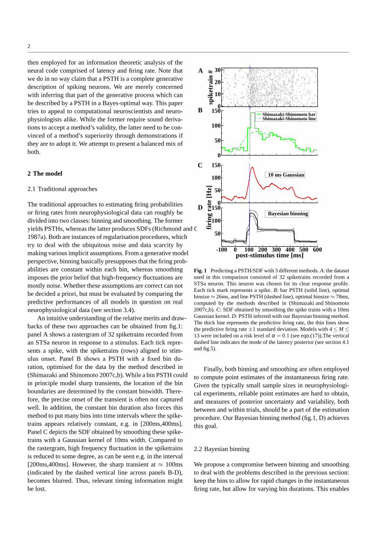
An intuitive understanding of the relative merits and draw-backs of these two approaches can be obtained from fig.1:panel A shows a rastergram of 32 spiketrains recorded froman STSa neuron in response to a stimulus. Each tick repre-sents a spike, with the spiketrains (rows) aligned to stim-ulus onset. Panel B shows a PSTH with a fixed bin du-ration, optimised for the data by the method described in(Shimazaki and Shinomoto 2007c,b). While a bin PSTH couldin principle model sharp transients, the location of the binboundaries are determined by the constant binwidth. There-fore, the precise onset of the transient is often not capturedwell. In addition, the constant bin duration also forces thismethod to put many bins into time intervals where the spike-trains appears relatively constant, e.g. in [200ms,400ms].Panel C depicts the SDF obtained by smoothing these spike-trains with a Gaussian kernel of 10ms width. Compared tothe rastergram, high frequency fluctuation in the spiketrainsis reduced to some degree, as can be seen e.g. in the interval[200ms,400ms]. However, the sharp transient at≈ 100ms(indicated by the dashed vertical line across panels B-D),becomes blurred. Thus, relevant timing information mightbe lost.

| | | || | | | | | | | | | | | | | | | | | | | | | | | | | | | | || | | | | | | | | | | | | | | | | | | | | | | | | | | |

| | | | | | | | | | | | | | | || | | | | | | | | | | | | | | | | | | | ||| || | | | | | | || | || | | | | ||| | | | | | | || | | | | | | |

| | || | | | | | | | | | | | | | || | | | | | || | | | | | | | | | | || || | | | || | || | | | | | | | || | || | | | | | | | | | | | |

| | | | | | | | || | | | | | | | | | | || | | | | | | | | | | | | | | | | | | || | || | || | | | | | | | | | | | | | | | | | | | | | | | |

| | | | || | | | | | | | | | | | | | | | | | | | | || || | || | | | | | | || | || | | | | | | | | | | | | | | | | | | | | | | |

| || | | | | | | | | || | | | | | | | | | | | | | | | | | | | | | | | | || | | | | | || | | | | | | | | | | | | | | | | | | | | | | | | | | | | || | |

|| | | | | | || | | | | | | | | | | | | | | | | | | | | | | || | | || | || | | | | | | | | | | || | | || | | | | | | |

| | || | | | | | | | | | | || | | | || | | | | | | | | | | | | | | | | || || || | || | | | || | | | | | | | | | | | | | | | || |

| | || ||| | ||| | | | | | | | || | | | | | | | | | | | | | | ||| | | | | | | | || | | | | | | | | | | | | | | | | | | | |

| || | | | || | | | | | | | | | | | | | | | | | | | | | | | || | | || | || | | | | | | | | | | | | | | | || | || | | | | | | | || |

| | | | | | | | | | | | | | | | | || | || || | | | | | | | | | | | | | | | | | | | | | | || |

| | | | | | || | | | | | | | | | | || || | | | | | | | | | || | | | | | | | | | | | | | | || | | | | | | | | | | | |

| | | | | | || | | | | | | | | | | | | | | | | | | | | | | | |||| | | | | | | | | | | | | | | | | | | | | | | | | | | | |

| | | | | | | | | | || | | | | | | | | | | || | | | || | | | | | | | | | | | | | | | |

| | | | || | | | | | | | | | | | | | | | | | | | || | | | | | || | | | | | | | | | | | | | | | | | | | | | |

| || | || | || | | | | | | | | | | | | | | | | | | | | | | | | | | || | | ||| | | | | | | | | | | | | | | | | | | | |

0

10

20

30

spik

etra

in #

0

50

100

150Shimazaki-Shinomoto barShimazaki-Shinomoto line

A

B

0

50

100

150

10 ms Gaussian

-100 0 100 200 300 400 500 600post-stimulus time [ms]

50

100

150fir

ing

rate

[Hz]

Bayesian binningD

C

Fig. 1 Predicting a PSTH/SDF with 3 different methods.A: the datasetused in this comparison consisted of 32 spiketrains recorded from aSTSa neuron. This neuron was chosen for its clear response profile.Each tick mark represents a spike.B: bar PSTH (solid line), optimalbinsize≈ 26ms, and line PSTH (dashed line), optimal binsize≈ 78ms,computed by the methods described in (Shimazaki and Shinomoto2007c,b).C: SDF obtained by smoothing the spike trains with a 10msGaussian kernel.D: PSTH inferred with our Bayesian binning method.The thick line represents the predictive firing rate, the thinlines showthe predictive firing rate±1 standard deviation. Models with 4≤ M ≤13 were included on a risk level ofα = 0.1 (see eqn.(17)).The verticaldashed line indicates the mode of the latency posterior (see section 4.1and fig.5).

Finally, both binning and smoothing are often employedto compute point estimates of the instantaneous firing rate.Given the typically small sample sizes in neurophysiologi-cal experiments, reliable point estimates are hard to obtain,and measures of posterior uncertainty and variability, bothbetween and within trials, should be a part of the estimationprocedure. Our Bayesian binning method (fig.1, D) achievesthis goal.

2.2 Bayesian binning

We propose a compromise between binning and smoothingto deal with the problems described in the previous section:keep the bins to allow for rapid changes in the instantaneousfiring rate, but allow for varying bin durations. This enables

3

0 10 20M

0,05

0,1

P(M

|{z i })

C

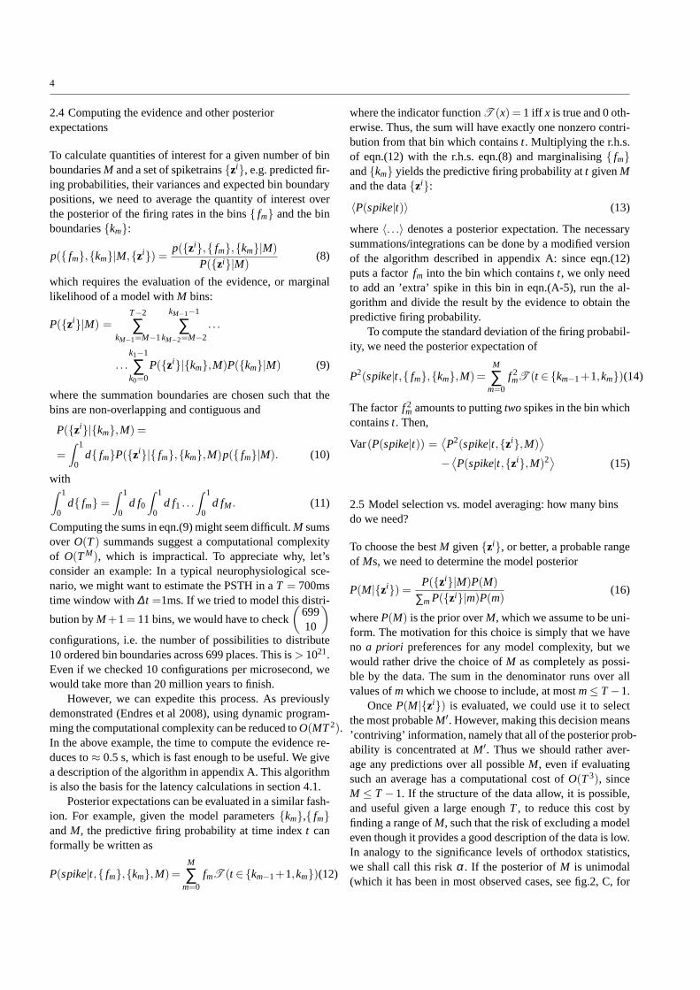
Fig. 2 A: A spike train, recorded between timestmin andtmax is rep-resented by a binary vectorzi. B: The time span betweentmin andtmax

is discretised intoT intervals of duration∆ t = (tmax − tmin)/T , suchthat intervalk lasts fromk×∆ t + tmin to (k+1)×∆ t + tmin. ∆ t is cho-sen such that at most one spike is observed per∆ t interval for anygiven spike train. Then, we model the firing probabilitiesP(spike|t)by M + 1 = 4 contiguous, non-overlapping bins (M is the number ofbin boundaries inside the time span[tmin, tmax]), having inclusive up-per boundarieskm andP(spike|t ∈ (tmin+∆ t(km−1+1), tmin+∆ t(km+1)]) = fm. C: model posteriorP(M|{zi}) (see eqn.(16)) computed fromthe data shown in fig.1. The shape is fairly typical for model posteriorscomputed from the neural data used in this paper: a sharp rise at a mod-erately lowM followed by a maximum (here atM = 6) and an approx-imately exponential decay. Even though a maximumM of 699 wouldhave been possible,P(M > 23|{zi})< 0.001. Thus, we can acceleratethe averaging process for quantities of interest (e.g. the predictive fir-ing rate) by choosing a moderately small maximumM. For details, seetext.

us to put the bin boundaries at only those time points wherethe changes in firing rate happen. As a consequence, timeintervals in which the firing rate does not change can nowbe modelled by one (or a few) bins, which reduces the riskof overfitting noise. Uncertainties and variabilities willbecomputed in an exact Bayesian fashion. The resultant ex-pected firing rates (complete with their uncertainties) willtherefore have a more continuous appearance, similar to theresults yielded by a smoothing technique.

Details of the formal model have been described in (Endres etal2008). Briefly, we model a PSTH on[tmin, tmax] discretisedinto T contiguous intervals of duration∆ t = (tmax − tmin)/T(see fig.2, A and B). We select a discretisation fine enough(here 1ms) so that we will not observe more than one spikein a ∆ t interval for any given spike train. Spike traini canthen be represented by a binary vectorzi of dimensionalityT . We model the PSTH byM+1 contiguous, non-overlappingbins having inclusive upper boundarieskm, within whichthe firing probability fm = P(spike|t ∈ (tmin + ∆ t(km−1 +

1), tmin +∆ t(km +1)]) is constant. Importantly, the bin size(distance between bin boundaries) is not fixeda priori butcan vary depending on the observed data. The relationshipbetween the firing probabilitiesfm and the instantaneous fir-ing rates is given by

firing rate=fm

∆ t. (1)

M is the number of bin boundaries inside[tmin, tmax]. Theprobability of a spike trainzi of independent spikes/gaps isthen

P(zi|{ fm},{km},M) =M

∏m=0

f s(zi,m)m (1− fm)

g(zi,m) (2)

wheres(zi,m) is the number of spikes andg(zi,m) is thenumber of non-spikes, or gaps in spiketrainzi in bin m,i.e. between intervalskm−1 + 1 andkm (both inclusive). Inother words, we model the spiketrains by an inhomogeneousBernoulli process with piecewise constant probabilities.Wealso definek−1 = −1 andkM = T −1. Note that there is nobinomial factor associated with the contribution of each bin,because we donot want to ignore the spike timing informa-tion within the bins, but rather, we try to build a simplifiedgenerative model of the spike train. Therefore, the probabil-ity of a (multi)set of spiketrains{zi}= {z1, . . . ,zN}, assum-ing independent generation, is

P({zi}|{ fm},{km},M) =N

∏i=1

M

∏m=0

f s(zi,m)m (1− fm)

g(zi,m)

=M

∏m=0

f s({zi},m)m (1− fm)

g({zi},m) (3)

wheres({zi},m)=∑Ni=1 s(zi,m) andg({zi},m)=∑N

i=1 g(zi,m).

2.3 The priors

We make a non-informative prior assumption for the jointprior of the firing probabilities{ fm} and the bin boundaries{km} given the total number of bin boundariesM, namely

p({ fm},{km}|M) = p({ fm}|M)P({km}|M). (4)

i.e. we have no a priori preferences for the firing rates basedon the bin boundary positions. Note that the prior of thefm,being continuous model parameters, is a density. Given theform of eqn.(2) and the constraintfm ∈ [0,1], it is natural tochoose a conjugate prior

p({ fm}|M) =M

∏m=0

B( fm;σm,γm). (5)

The Beta density is defined in the usual way (see e.g. (Berger1985)):

B(p;σ ,γ) =Γ (σ + γ)Γ (σ)Γ (γ)

pσ−1(1− p)γ−1. (6)

There are only finitely many configurations of thekm. As-suming we have no preferences for any of them, the priorfor the bin boundaries becomes

P({km}|M) =1

(

T −1M

) . (7)

where the denominator is just the number of possibilities inwhich M ordered bin boundaries can be distributed acrossT −1 places (bin boundaryM always occupies positionT −

1, see fig.2, B, hence there are onlyT −1 positions left).

4

2.4 Computing the evidence and other posteriorexpectations

To calculate quantities of interest for a given number of binboundariesM and a set of spiketrains{zi}, e.g. predicted fir-ing probabilities, their variances and expected bin boundarypositions, we need to average the quantity of interest overthe posterior of the firing rates in the bins{ fm} and the binboundaries{km}:

p({ fm},{km}|M,{zi}) =p({zi},{ fm},{km}|M)

P({zi}|M)(8)

which requires the evaluation of the evidence, or marginallikelihood of a model withM bins:

P({zi}|M) =T−2

∑kM−1=M−1

kM−1−1

∑kM−2=M−2

. . .

. . .k1−1

∑k0=0

P({zi}|{km},M)P({km}|M) (9)

where the summation boundaries are chosen such that thebins are non-overlapping and contiguous and

P({zi}|{km},M) =

=∫ 1

0d{ fm}P({zi}|{ fm},{km},M)p({ fm}|M). (10)

with∫ 1

0d{ fm}=

∫ 1

0d f0

∫ 1

0d f1 . . .

∫ 1

0d fM. (11)

Computing the sums in eqn.(9) might seem difficult.M sumsover O(T ) summands suggest a computational complexityof O(T M), which is impractical. To appreciate why, let’sconsider an example: In a typical neurophysiological sce-nario, we might want to estimate the PSTH in aT = 700mstime window with∆ t =1ms. If we tried to model this distri-

bution byM+1= 11 bins, we would have to check

(

69910

)

configurations, i.e. the number of possibilities to distribute10 ordered bin boundaries across 699 places. This is> 1021.Even if we checked 10 configurations per microsecond, wewould take more than 20 million years to finish.

However, we can expedite this process. As previouslydemonstrated (Endres et al 2008), using dynamic program-ming the computational complexity can be reduced toO(MT 2).In the above example, the time to compute the evidence re-duces to≈ 0.5 s, which is fast enough to be useful. We givea description of the algorithm in appendix A. This algorithmis also the basis for the latency calculations in section 4.1.

Posterior expectations can be evaluated in a similar fash-ion. For example, given the model parameters{km},{ fm}andM, the predictive firing probability at time indext canformally be written as

P(spike|t,{ fm},{km},M)=M

∑m=0

fmT (t ∈{km−1+1,km})(12)

where the indicator functionT (x) = 1 iff x is true and 0 oth-erwise. Thus, the sum will have exactly one nonzero contri-bution from that bin which containst. Multiplying the r.h.s.of eqn.(12) with the r.h.s. eqn.(8) and marginalising{ fm}

and{km} yields the predictive firing probability att givenMand the data{zi}:

〈P(spike|t)〉 (13)

where〈. . .〉 denotes a posterior expectation. The necessarysummations/integrations can be done by a modified versionof the algorithm described in appendix A: since eqn.(12)puts a factorfm into the bin which containst, we only needto add an ’extra’ spike in this bin in eqn.(A-5), run the al-gorithm and divide the result by the evidence to obtain thepredictive firing probability.

To compute the standard deviation of the firing probabil-ity, we need the posterior expectation of

P2(spike|t,{ fm},{km},M)=M

∑m=0

f 2mT (t ∈{km−1+1,km})(14)

The factorf 2m amounts to puttingtwo spikes in the bin which

containst. Then,

Var(P(spike|t)) =⟨

P2(spike|t,{zi},M)⟩

−⟨

P(spike|t,{zi},M)2⟩ (15)

2.5 Model selection vs. model averaging: how many binsdo we need?

To choose the bestM given{zi}, or better, a probable rangeof Ms, we need to determine the model posterior

P(M|{zi}) =P({zi}|M)P(M)

∑m P({zi}|m)P(m)(16)

whereP(M) is the prior overM, which we assume to be uni-form. The motivation for this choice is simply that we haveno a priori preferences for any model complexity, but wewould rather drive the choice ofM as completely as possi-ble by the data. The sum in the denominator runs over allvalues ofm which we choose to include, at mostm ≤ T −1.

OnceP(M|{zi}) is evaluated, we could use it to selectthe most probableM′. However, making this decision means’contriving’ information, namely that all of the posteriorprob-ability is concentrated atM′. Thus we should rather aver-age any predictions over all possibleM, even if evaluatingsuch an average has a computational cost ofO(T 3), sinceM ≤ T −1. If the structure of the data allow, it is possible,and useful given a large enoughT , to reduce this cost byfinding a range ofM, such that the risk of excluding a modeleven though it provides a good description of the data is low.In analogy to the significance levels of orthodox statistics,we shall call this riskα. If the posterior ofM is unimodal(which it has been in most observed cases, see fig.2, C, for

5

an example), we can then choose the smallest interval ofMsaround the maximum ofP(M|{zi}) such that

P(Mmin ≤ M ≤ Mmax|{zi})≤ 1−α (17)

and carry out the averages over this range ofM after renor-malising the model posterior. We useα = 0.1 unless statedotherwise.

3 Simulations and comparison to other methods

3.1 Predicted PSTH convergence to simulated generator

0 100 200 300 400 500post-stimulus time [ms]

0

50

100

firin

g ra

te [H

z]

50

100

1501 trial

30 trials

0 100 200 300 400 500post-stimulus time [ms]

0

50

100

firin

g ra

te [H

z]

50

100

1501 trial

30 trials

1 3 10 30 100number of trials

0,0001

0,001

0,01

0,1

tKLd

[nat

s]

Bay.Bin10ms Gaussian

1 3 10 30 100number of trials

0,0001

0,001

0,01

0,1

tKLd

[nat

s]

Bay.Bin10ms Gaussian

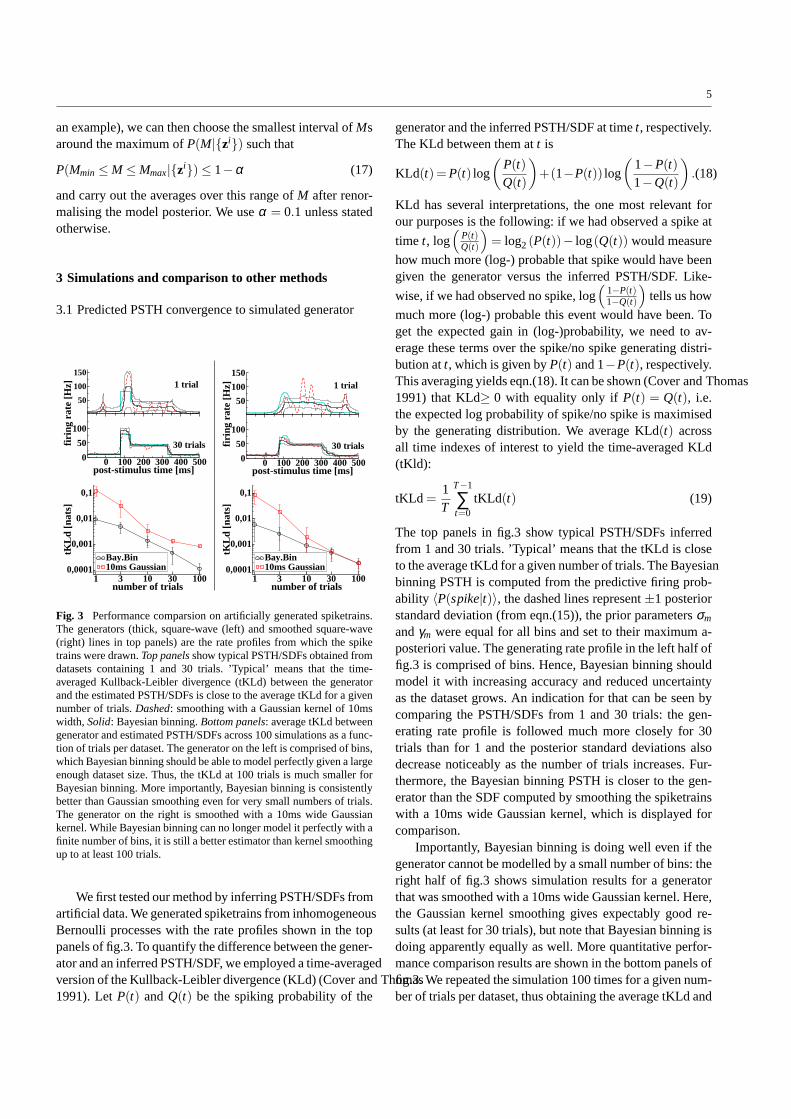
Fig. 3 Performance comparsion on artificially generated spiketrains.The generators (thick, square-wave (left) and smoothed square-wave(right) lines in top panels) are the rate profiles from which the spiketrains were drawn.Top panels show typical PSTH/SDFs obtained fromdatasets containing 1 and 30 trials. ’Typical’ means that the time-averaged Kullback-Leibler divergence (tKLd) between the generatorand the estimated PSTH/SDFs is close to the average tKLd for a givennumber of trials.Dashed: smoothing with a Gaussian kernel of 10mswidth, Solid: Bayesian binning.Bottom panels: average tKLd betweengenerator and estimated PSTH/SDFs across 100 simulations as a func-tion of trials per dataset. The generator on the left is comprised of bins,which Bayesian binning should be able to model perfectly given alargeenough dataset size. Thus, the tKLd at 100 trials is much smaller forBayesian binning. More importantly, Bayesian binning is consistentlybetter than Gaussian smoothing even for very small numbers of trials.The generator on the right is smoothed with a 10ms wide Gaussiankernel. While Bayesian binning can no longer model it perfectly with afinite number of bins, it is still a better estimator than kernel smoothingup to at least 100 trials.

We first tested our method by inferring PSTH/SDFs fromartificial data. We generated spiketrains from inhomogeneousBernoulli processes with the rate profiles shown in the toppanels of fig.3. To quantify the difference between the gener-ator and an inferred PSTH/SDF, we employed a time-averagedversion of the Kullback-Leibler divergence (KLd) (Cover and Thomas1991). LetP(t) andQ(t) be the spiking probability of the

generator and the inferred PSTH/SDF at timet, respectively.The KLd between them att is

KLd(t)=P(t) log

(

P(t)Q(t)

)

+(1−P(t)) log

(

1−P(t)1−Q(t)

)

.(18)

KLd has several interpretations, the one most relevant forour purposes is the following: if we had observed a spike at

time t, log(

P(t)Q(t)

)

= log2 (P(t))− log(Q(t)) would measure

how much more (log-) probable that spike would have beengiven the generator versus the inferred PSTH/SDF. Like-

wise, if we had observed no spike, log(

1−P(t)1−Q(t)

)

tells us how

much more (log-) probable this event would have been. Toget the expected gain in (log-)probability, we need to av-erage these terms over the spike/no spike generating distri-bution att, which is given byP(t) and 1−P(t), respectively.This averaging yields eqn.(18). It can be shown (Cover and Thomas1991) that KLd≥ 0 with equality only if P(t) = Q(t), i.e.the expected log probability of spike/no spike is maximisedby the generating distribution. We average KLd(t) acrossall time indexes of interest to yield the time-averaged KLd(tKld):

tKLd =1T

T−1

∑t=0

tKLd(t) (19)

The top panels in fig.3 show typical PSTH/SDFs inferredfrom 1 and 30 trials. ’Typical’ means that the tKLd is closeto the average tKLd for a given number of trials. The Bayesianbinning PSTH is computed from the predictive firing prob-ability 〈P(spike|t)〉, the dashed lines represent±1 posteriorstandard deviation (from eqn.(15)), the prior parametersσm

andγm were equal for all bins and set to their maximum a-posteriori value. The generating rate profile in the left half offig.3 is comprised of bins. Hence, Bayesian binning shouldmodel it with increasing accuracy and reduced uncertaintyas the dataset grows. An indication for that can be seen bycomparing the PSTH/SDFs from 1 and 30 trials: the gen-erating rate profile is followed much more closely for 30trials than for 1 and the posterior standard deviations alsodecrease noticeably as the number of trials increases. Fur-thermore, the Bayesian binning PSTH is closer to the gen-erator than the SDF computed by smoothing the spiketrainswith a 10ms wide Gaussian kernel, which is displayed forcomparison.

Importantly, Bayesian binning is doing well even if thegenerator cannot be modelled by a small number of bins: theright half of fig.3 shows simulation results for a generatorthat was smoothed with a 10ms wide Gaussian kernel. Here,the Gaussian kernel smoothing gives expectably good re-sults (at least for 30 trials), but note that Bayesian binning isdoing apparently equally as well. More quantitative perfor-mance comparison results are shown in the bottom panels offig.3. We repeated the simulation 100 times for a given num-ber of trials per dataset, thus obtaining the average tKLd and

6

its standard deviation. For the bin generator, Bayesian bin-ning outperforms Gaussian kernel smoothing for all datasetsizes. For the smoothed generator, Bayesian binning stilloutperforms Gaussian kernel smoothing, while the differ-ence between the two methods shrinks as the number of tri-als per dataset increases. But even for 100 trials, Bayesianbinning is as good as Gaussian kernel smoothing. We havethus reason to hope that Bayesian binning might outperformother PSTH/SDF estimation methods on real neural data.This will be shown in the next subsections.

3.2 Data acquisition

The experimental protocols have been described before (Oram et al2002; van Rossum et al 2008). Briefly, extra-cellular single-unit recordings were made using standard techniques fromthe upper and lower banks of the anterior part of the supe-rior temporal sulcus (STSa) of two monkeys (Macaca mu-latta) performing a visual fixation task. The subject receiveda drop of fruit juice reward every 500ms of fixation whilestatic stimuli (10o by 12.5o) were displayed. Static imageswere presented centrally on the monitor. Stimuli consistedof256 gray scale pictures of familiar and unfamiliar objects,heads, body parts and whole bodies. Visual stimuli werepresented in a random sequence for 333ms with a 333msinter-stimulus interval centrally on a black monitor screen(Sony GDM-20D11, resolution 25.7 pixels/degree, refreshrate 72Hz), 57cm from the subject. Stimulus contrast wasdetermined using foreground regions of the image. The 100%Michelson contrast =Lmax−Lmin

Lmax+Lmin, whereL is the luminance,

was formed by normalising the foreground pixel values suchthat they occupied the monitor full luminance range afteradjusting the initial greyscale image to have mid (50%) lu-minance. Other contrast versions (75%, 50%, 25%, 12.5%)were achieved by systematically varying the width of thedistribution of the foreground pixel values of the 100% con-trast version while maintaining the average foreground lu-minance. All manipulations were performed after correctingfor the measured gamma function of the display monitor.

Stimulus presentation began after 500ms of fixation cen-trally on the screen (fixation deviations outside the fixationwindow lasting≤100ms were ignored to allow for blink-ing). Fixation was rewarded with the delivery of fruit juice.Spikes were recorded during the period of fixation. If thesubject looked away for longer than 100ms, both spike record-ing and presentation of stimuli stopped until the subject re-sumed fixation for 500ms. The results from initial screen-ing (Edwards et al 2003) were used to select stimuli thatelicited large responses from the neuron (effective stimuli)and to select stimuli that elicited small or no response (inef-fective stimuli). For different neurons effective and ineffec-tive stimuli included different views of the head (Perrett et al1991), abstract patterns and familiar objects (Foldiak et al

2004). Details of the stimulus selectivity of these neuronshas been reported elsewhere (Oram et al 2002; Foldiak et al2004; Edwards et al 2003; Barraclough et al 2005; Edwards et al2003). The anterior-posterior extent of the recorded cellswas from 7mm to 10mm anterior of the interaural plane, inthe upper bank (TAa, TPO), lower bank (TEa, TEm) andfundus (PGa, IPa) of the superior temporal sulcus (STS)and in the anterior areas of TE (AIT of [Tanaka1991]), ar-eas which we collectively call the anterior STS (STSa, see(Barraclough et al 2005) for further discussion). The recordedfiring patterns were turned into distinct samples, each ofwhich contained the spikes from−300 ms to 600 ms afterthe stimulus onset with a temporal resolution of 1ms.

3.3 Inferring PSTHs

To see the method in action on real neural data, inferred aPSTH from 32 spiketrains recorded from one of the avail-able STSa neurons (see fig.1, A). We discretised the inter-val from−100ms pre-stimulus to 600ms post-stimulus into∆ t = 1ms time intervals and computed the posterior (eqn.(16))for models with varying number of binsM (see fig.2, C). Theprior parameters were equal for all bins and set toσm = 1andγm = 32. This choice corresponds to a firing probabilityof ≈ 0.03 in each 1 ms time interval (30 spikes/s), which istypical for the neurons in this study1. Models with 4≤ M ≤13 (expected bin sizes between≈ 23ms-148ms) were in-cluded on anα = 0.1 risk level (eqn.(17)) in the subsequentcalculation of the predictive firing rate (i.e. theexpected fir-ing rate, hence the continuous appearance) and standard de-viation (fig.1, D). For comparison, fig.1, B, shows a bar PSTHand a line PSTH computed with the recently developed meth-ods described in (Shimazaki and Shinomoto 2007c,b). Roughlyspeaking, these methods try to optimise a compromise be-tween minimal within-bin variance and maximal between-bin variance. In this example, the bar PSTH consists of 26bins. Panel C in fig.1 depicts a SDF obtained by smoothingthe spiketrains with a 10ms wide Gaussian kernel, a stan-dard way of calculating SDFs in the neurophysiological lit-erature.

All tested methods produce results which are, upon cur-sory visual inspection, largely consistent with the spiketrains.However, Bayesian binning is better suited than Gaussiansmoothing to model steep changes, such as the transient re-sponse starting at≈ 100ms. While the methods from (Shimazaki and Shinomoto2007c,b) share this advantage, they suffer from two draw-backs: firstly, the bin boundaries are evenly spaced, hencethe peak of the transient is later than visual examination ofthe rastergrams would suggest. Secondly, because the bin

1 Alternatively, one could search for theσm,γm which maximiseof P({zi}|σm,γm) = ∑M P({zi}|M)P(M|σm,γm), whereP({zi}|M) isgiven by eqn.(9). Using a uniformP(M|σm,γm), we foundσm ≈ 2.3andγm ≈ 37 for the data in fig.1, A

7

duration is the only parameter of the model, these methodsare forced to put many bins even in intervals that are rel-atively constant, such as the baselines before and after thestimulus-driven response. In contrast, Bayesian binning isable to put bin boundaries anywhere in the time span of in-terest and can model the data with less bins – the modelposterior has its maximum atM = 6 (7 bins), whereas thebar PSTH consists of 26 bins.

3.4 Performance comparison by cross-validation

0 0,005 0,01 0,015CV error relative to Bay. bin.0

0,30,6

Shim.-Shin. kernel

00,20,4

rela

tive

freq

uenc

y

Shim.-Shin. line PSTH

00,20,4

Shim.-Shin. bar PSTH

0 0,005 0,01 0,015CV error relative to Bay. bin.0

0,20,4

local likelihood fit

00,20,4

rela

tive

freq

uenc

y

Gaussian kernel, 10ms

00,20,4 BARS

Fig. 4 Comparison of Bayesian Binning with competing methodsby 5-fold crossvalidation. The CV error is the negative expected log-probability of the test data. The histograms show relative frequen-cies of CV error differences to our Bayesian binning approach. Left:Shimazaki’s and Shinomoto’s methods (Shimazaki and Shinomoto2007b,a).Right, top Bayesian Adaptive Regression Splines (BARS)(DiMatteo et al 2001).Right, middle: smoothing with a Gaussian ker-nel of 10ms width.Right, bottom: local likelihood adaptive fitting(Loader 1997, 1999).

For a more rigorous method comparison, we split thedata into distinct sets, each of which contained the responsesof a cell to a different stimulus. This procedure yielded 336sets from 20 cells with at least 20 spiketrains per set. We thenperformed 5-fold crossvalidation. The crossvalidation erroris given by the negative logarithm of the predicted probabil-ity (eqn.(13)) of the data (spike or no spike) in the test sets.Let sn(t) = 1 if trial n of N in the test set contains a spike attime indext ∈ {0, . . . ,T −1} andsn(t) = 0 otherwise. Then

CV error=−1N

N−1

∑n=0

1T

T−1

∑t=0

log〈(P(sn(t)|t))〉 . (20)

Thus, we measure how well the PSTHs/SDFs predict thetest data on average across time and across all test trials.Note that this CV error is similar to the tKLd (eqn.(19)): theconstant terms referring to the generator have been dropped,because the generator is not known here and the averagingis done across the data rather than the generating distribu-tion for the same reason. We average the CV error over the5 estimates to obtain a single estimate for each of the 336neuron/stimulus combinations. The prior parametersσm,γm

were equal for all bins and MAP optimised for each indi-vidual training dataset. In (Endres et al 2008) we already

Table 1 Average log prediction error differences to Bayesian binningfrom 5 fold crossvalidation on 336 datasets. A positive value meansthat our method predicts the data better than the competitor.

Method CV error diff.

Shimazaki and Shinomoto (2007b) bar (2.35±0.23)×10−3

Shimazaki and Shinomoto (2007b) line (1.22±0.10)×10−3

Gauss 10ms (1.29±0.11)×10−3

Local likelihood fit (Loader 1997) (7.34±0.48)×10−4

Shimazaki and Shinomoto (2007a) kernel(3.14±0.39)×10−4

BARS (DiMatteo et al 2001) (0.8±1.6)×10−5

Bayesian binning 0

demonstrated that Bayesian binning outperforms SDFs ob-tained by Gaussian smoothing, and the bin and line his-togram methods from (Shimazaki and Shinomoto 2007c,b).

We also tested Bayesian binning against the kernel smooth-ing method described in (Shimazaki and Shinomoto 2007a),a local likelihood adaptive fit (Loader 1999) and BayesianAdaptive Regression Splines (BARS) (DiMatteo et al 2001).To compare the performances between the different meth-ods directly, we calculated the difference in CV error foreach neuron/stimulus configuration. Here a positive valueindicates that Bayesian binning predicts the test data moreaccurately than the alternative method. Fig.4, shows the rel-ative frequencies of CV error differences between the othermethods and our approach. In the large majority of cases weare at least as good, but frequently better than the competi-tors, indicating the general utility of our approach. Amongstthe competitors, BARS is the only method with a compara-ble predictive performance on these STSa data. The averageCV error differences, summarised in table 1, support thisclaim: they are all significantly> 0, except for the BARSvalue.

4 Response latency

Besides the instantaneous firing rate, another frequently usedfeature for the description of a neuron’s response is responselatency. But unlike the former, a definition of latency seemsmuch less agreed. A wide range of methods to estimate re-sponse latency exist. Changes in phase between neuronal ac-tivity and sinusoidal drifting gratings with changing stimu-lus parameters can provide an indirect measure of responselatency (Gawne et al 1996b; Alitto and Usrey 2004). Directmeasures of response latency of neurons with low back-ground or spontaneous activity can be obtained from thetime of the first spike after stimulus onset (Heil and Irvine1997; Richmond et al 1999; Syka et al 2000; Stecker and Middlebrooks2003; Hurley and Pollak 2005; van Rossum et al 2008).

Statistical approaches compare activity levels at two timepoints. While the baseline level is usually taken from a ”pre-stimulus” period the window containing the greatest activ-

8

0 200 400 600post-stimulus time [ms]

50

100

150

firin

g ra

te [H

z]

signal level S

latency L

| | | || | | | | | | | | | | | | | | | | | | | | | | | | | | | | || | | | | | | | | | | | | | | | | | | | | | | | | | | || | | | | | | | | | | | | | | || | | | | | | | | | | | | | | | | | | | ||| || | | | | | | || | || | | | | ||| | | | | | | || | | | | | | || | || | | | | | | | | | | | | | || | | | | | || | | | | | | | | | | || || | | | || | || | | | | | | | || | || | | | | | | | | | | | || | | | | | | | || | | | | | | | | | | || | | | | | | | | | | | | | | | | | | || | || | || | | | | | | | | | | | | | | | | | | | | | | | || | | | || | | | | | | | | | | | | | | | | | | | | || || | || | | | | | | || | || | | | | | | | | | | | | | | | | | | | | | | || || | | | | | | | | || | | | | | | | | | | | | | | | | | | | | | | | | || | | | | | || | | | | | | | | | | | | | | | | | | | | | | | | | | | | || | ||| | | | | | || | | | | | | | | | | | | | | | | | | | | | | || | | || | || | | | | | | | | | | || | | || | | | | | | || | || | | | | | | | | | | || | | | || | | | | | | | | | | | | | | | | || || || | || | | | || | | | | | | | | | | | | | | | || || | || ||| | ||| | | | | | | | || | | | | | | | | | | | | | | ||| | | | | | | | || | | | | | | | | | | | | | | | | | | | || || | | | || | | | | | | | | | | | | | | | | | | | | | | | || | | || | || | | | | | | | | | | | | | | | || | || | | | | | | | || || | | | | | | | | | | | | | | | | || | || || | | | | | | | | | | | | | | | | | | | | | | || || | | | | | || | | | | | | | | | | || || | | | | | | | | | || | | | | | | | | | | | | | | || | | | | | | | | | | | || | | | | | || | | | | | | | | | | | | | | | | | | | | | | | |||| | | | | | | | | | | | | | | | | | | | | | | | | | | | || | | | | | | | | | || | | | | | | | | | | || | | | || | | | | | | | | | | | | | | | || | | | || | | | | | | | | | | | | | | | | | | | || | | | | | || | | | | | | | | | | | | | | | | | | | | | || || | || | || | | | | | | | | | | | | | | | | | | | | | | | | | | || | | ||| | | | | | | | | | | | | | | | | | | | |

102030

sp.tr

.0 200 400 600

post-stimulus time t [ms]

50100

rate

[Hz]

0,10,2

P(L

=t)

signal level S

A

B

C

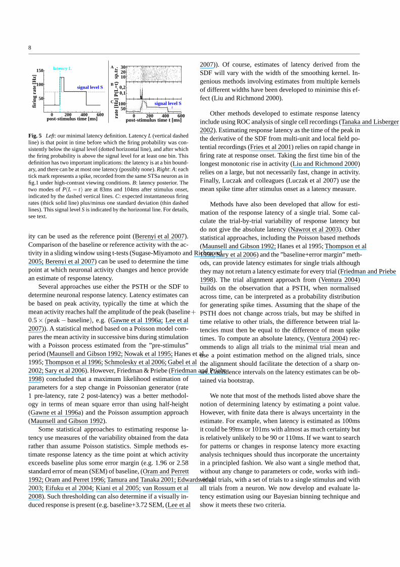
Fig. 5 Left: our minimal latency definition. LatencyL (vertical dashedline) is that point in time before which the firing probabilitywas con-sistently below the signal level (dotted horizontal line), andafter whichthe firing probability is above the signal level for at least onebin. Thisdefinition has two important implications: the latency is at a bin bound-ary, and there can be at most one latency (possibly none).Right: A: eachtick mark represents a spike, recorded from the same STSa neuron asinfig.1 under high-contrast viewing conditions.B: latency posterior. Thetwo modes ofP(L = t) are at 83ms and 104ms after stimulus onset,indicated by the dashed vertical lines.C: expected instantaneous firingrates (thick solid line) plus/minus one standard deviation (thin dashedlines). This signal levelS is indicated by the horizontal line. For details,see text.

ity can be used as the reference point (Berenyi et al 2007).Comparison of the baseline or reference activity with the ac-tivity in a sliding window using t-tests (Sugase-Miyamoto and Richmond2005; Berenyi et al 2007) can be used to determine the timepoint at which neuronal activity changes and hence providean estimate of response latency.

Several approaches use either the PSTH or the SDF todetermine neuronal response latency. Latency estimates canbe based on peak activity, typically the time at which themean activity reaches half the amplitude of the peak (baseline+0.5× (peak− baseline), e.g. (Gawne et al 1996a; Lee et al2007)). A statistical method based on a Poisson model com-pares the mean activity in successive bins during stimulationwith a Poisson process estimated from the ”pre-stimulus”period (Maunsell and Gibson 1992; Nowak et al 1995; Hanes et al1995; Thompson et al 1996; Schmolesky et al 2006; Gabel et al2002; Sary et al 2006). However, Friedman & Priebe (Friedmanand Priebe1998) concluded that a maximum likelihood estimation ofparameters for a step change in Poissonian generator (rate1 pre-latency, rate 2 post-latency) was a better methodol-ogy in terms of mean square error than using half-height(Gawne et al 1996a) and the Poisson assumption approach(Maunsell and Gibson 1992).

Some statistical approaches to estimating response la-tency use measures of the variability obtained from the datarather than assume Poisson statistics. Simple methods es-timate response latency as the time point at which activityexceeds baseline plus some error margin (e.g. 1.96 or 2.58standard error of mean (SEM) of baseline, (Oram and Perrett1992; Oram and Perret 1996; Tamura and Tanaka 2001; Edwards et al2003; Eifuku et al 2004; Kiani et al 2005; van Rossum et al2008). Such thresholding can also determine if a visually in-duced response is present (e.g. baseline+3.72 SEM, (Lee et al

2007)). Of course, estimates of latency derived from theSDF will vary with the width of the smoothing kernel. In-genious methods involving estimates from multiple kernelsof different widths have been developed to minimise this ef-fect (Liu and Richmond 2000).

Other methods developed to estimate response latencyinclude using ROC analysis of single cell recordings (Tanaka and Lisberger2002). Estimating response latency as the time of the peak inthe derivative of the SDF from multi-unit and local field po-tential recordings (Fries et al 2001) relies on rapid changeinfiring rate at response onset. Taking the first time bin of thelongest monotonic rise in activity (Liu and Richmond 2000)relies on a large, but not necessarily fast, change in activity.Finally, Luczak and colleagues (Luczak et al 2007) use themean spike time after stimulus onset as a latency measure.

Methods have also been developed that allow for esti-mation of the response latency of a single trial. Some cal-culate the trial-by-trial variability of response latencybutdo not give the absolute latency (Nawrot et al 2003). Otherstatistical approaches, including the Poisson based methods(Maunsell and Gibson 1992; Hanes et al 1995; Thompson et al1996; Sary et al 2006) and the ”baseline+error margin” meth-ods, can provide latency estimates for single trials althoughthey may not return a latency estimate for every trial (Friedman and Priebe1998). The trial alignment approach from (Ventura 2004)builds on the observation that a PSTH, when normalisedacross time, can be interpreted as a probability distributionfor generating spike times. Assuming that the shape of thePSTH does not change across trials, but may be shifted intime relative to other trials, the difference between trialla-tencies must then be equal to the difference of mean spiketimes. To compute an absolute latency, (Ventura 2004) rec-ommends to align all trials to the minimal trial mean anduse a point estimation method on the aligned trials, sincethe alignment should facilitate the detection of a sharp on-set. Confidence intervals on the latency estimates can be ob-tained via bootstrap.

We note that most of the methods listed above share thenotion of determining latency by estimating a point value.However, with finite data there is always uncertainty in theestimate. For example, when latency is estimated as 100msit could be 99ms or 101ms with almost as much certainty butis relatively unlikely to be 90 or 110ms. If we want to searchfor patterns or changes in response latency more exactinganalysis techniques should thus incorporate the uncertaintyin a principled fashion. We also want a single method that,without any change to parameters or code, works with indi-vidual trials, with a set of trials to a single stimulus and withall trials from a neuron. We now develop and evaluate la-tency estimation using our Bayesian binning technique andshow it meets these two criteria.

9

4.1 A minimal definition of response latency

Most people interested in latency would probably agree withthe notion that ’latency is where the signal starts’. Signalvs.no signal can usually be translated into firing rate above orbelow a threshold, which we will call thesignal level (seefig.5, left). In other words,latency is that point in time priorto which there was no signal, and after which there is a sig-nal for at least some duration. This is the ’minimal’ latencydefinition which we will employ in the following.

For given bin boundaries{km} and firing probabilities{ fm}, latency must be at a bin boundary, because firing prob-abilities are constant within each bin. Note that our latencydefinition implies that there can be at most one latency. If thefiring probabilities are below the signal level in every bin,orif f0, the firing rate in the first bin is already above the signallevel, then there will be no latency.

To obtain a latency posterior distribution, we formallydefine the probability that the latencyL is at time indextgiven {km},{ fm},M and the signal levelS ∈ [0,1] (S is afiring probability. Division by the discretisation stepsize ∆ tyields firing rate) as

P(L = t|{km},{ fm},M,S) =

=

1 if ∃k j−1 ∈ {km} : k j−1+1= tand f j ≥ S and∀m < j : fm < S

0 otherwise(21)

which can be exactly averaged over the posterior eqn.(8) bya dynamic programming algorithm similar to that used forthe evidence evaluation, as detailed in appendix B. We thusobtainP(L= t,{zi}|M,S) and hence, noting thatP({zi}|M)=

P({zi}|M,S):

P(L = t|{zi},M,S) =P(L = t,{zi}|M,S)

P({zi}|M). (22)

What remains to be determined is the signal levelS. Assum-ing that the data span the response range of the neuron (i.e.the data contain responses to at least one effective stimulus),one can proceed as follows: for a givenS, marginalise thelatency posterior across the time interval of interest, therebyobtaining the probabilityP(L exists) that a latency exists atthatS. Repeat this procedure for differentS until the maxi-mal P(L exists) is found. We use 10 golden section refine-ment steps (Press et al 1986) for the maximum search withan initial interval of[0Hz,100Hz], thereby achieving an ac-curacy of≤1Hz.

4.2 Properties of latency posterior distributions

Fig.6 illustrates the consequences of our latency definitionon simulated data. We generated 10 spiketrains from inho-mogeneous Bernoulli processes with a step in firing rate10Hz→80Hz or 10Hz→30Hz at 80ms after stimulus onset.

255075

rate

[Hz] 80 Hz

0 50 100 150post-stimulus time t [ms]

0,10,20,3

P(L

=t) L=81.1±2.8

L=83±11

255075

30 Hz

0 20 40 60 80 100signal separation level S [Hz]

0,2

0,4

0,6

0,8

1

P(L

exi

sts)

80 Hz30 Hz

Fig. 6 Latency posterior and signal separation levels.Left: 10 spike-trains were drawn from generators with 80Hz and 30Hz peak firingrate. Both generators had a baseline of 10Hz and a latency at 80msafter stimulus onset. The dashed lines show the generating rates, thesolid lines represent the predictive firing rate of the BayesianbinningPSTHs. The resulting latency posterior distributions are shown at thebottom, including the latency expectations± 1 posterior standard de-viation. The posterior uncertainty in the 30Hz peak rate condition issignificantly larger than in the 80Hz condition.Right: determinationof signal separation levelS. P(L exists) is the probability that the la-tency was somewhere in the latency search interval (here[0,200]msafter stimulus onset) givenS. The symbols are located at the pointswhereP(L exists) was evaluated by a golden section maximum search(Press et al 1986). TheS was chosen to be the firing rate which max-imises the probability that a latency exists. In the 30Hz condition, thereis a relatively clear maximum at≈17Hz, whereas in the 80Hz condi-tion, the maximum is much broader. This is due to the larger differencebetween baseline and peak firing rate in the latter condition:even forthis relatively small dataset (10 trials), there is a range of similarly goodsignal separation levels that allow for the distinction between baselineand peak firing. For details, see text.

The firing rate stayed at this value for 50ms, then droppedto 45Hz and 20Hz for 200ms before returning to the 10Hzbaseline. In both conditions, most of the probability mass ofthe latency posterior (fig.6, left bottom) is concentrated inthe vicinity of the generator’s latency. The best signal sep-aration levelS (fig.6, right) for each condition reflects thedifference in peak firing rates: for 30Hz,S ≈17Hz, whereas for 80 Hz,S ≈39Hz. In both cases,S is roughly in themiddle between baseline and peak firing rate. Latency wassearched in the interval[0,200]ms after stimulus onset.

In addition to the location of the latency, the latencyposterior distributions (fig.6, left bottom) also contain infor-mation about uncertainty. It is evident that a smaller stepin firing rate leads to a wider latency posterior, which canalso be captured by computing the standard deviation fromthat posterior. This observation is not particularly surprising,but nevertheless important: virtually all other latency esti-mation methods ignore uncertainty due to their point esti-mation nature. As a consequence, the latency posterior con-tains information about the change in firing rate, which is apoint that we will return to later (section 5) when we anal-yse latency and firing rate with information-theoretic meth-ods. Note also that the latency posteriors are far from Gaus-sian: a description in terms of mean and standard deviationis therefore inadequate for an information-theoretic analysisand might distort conclusions drawn from it.

10

Non-Gaussian latency posteriors are also observed in thereal data. Fig.5, right, has two distinct peaks, the lower oneat≈ 83 ms, the higher one being at≈ 104 ms after stimulusonset. The location of these peaks can be understood fromthe height of the PSTH (fig.5, right, C) relative to the signallevel: at 83 ms, one can be fairly certain that the PSTH wasbelow the signal level prior to this time index, and there isa nonzero probability (albeit not nearly certainty) that thePSTH is above the signal level directly afterwards. At 104ms, the PSTH is above the signal level with near certaintydirectly after the peak in the latency posterior, whereas onecan not be quite sure that the PSTH was below the signallevel the interval immediately before this point in time. Theexpected latency± SEM is (94± 10)ms. A conventionalinterpretation of these values would suggest that the bulk ofthe probability mass can be found close to the mean, whichis not true.

4.3 Simulation results

For a quantitative evaluation of the accuracy of our latencydetection method, we generated spiketrains from inhomo-geneous Bernoulli processes with the rate profiles shownin the insets of fig.7. Root-mean-square (RMS) errors werecomputed from 100 repetitions of the simulation for a givennumber of trials per dataset, see fig.7. We used the expectedlatency as the prediction of Bayesian binning for each dataset(similar results were found using a MAP estimate). To fur-ther illustrate the performance of out approach, we com-pared it to three other ways of latency detection: the half-height method (Gawne et al 1996a) (’HH’ in fig.7), latency= the first time where activity exceeds baseline rate plus2 SEM of baseline rate (Oram and Perrett 1992) (’2SD’ infig.7) and the trial alignment approach from (Ventura 2004).This approach yields a relative latency for each trial, abso-lute latency can be determined by a suitable change-pointmethod applied to the aligned trials. We used the half-heightmethod here, since it gives good estimates of the latencywithout alignment.

Our method is more accurate than the others in all testedconditions. This is true even if the generator has a sloping re-sponse onset (fig.7, right) and can no longer be easily mod-elled by bins. In this case, latency is not as clearly defined asfor a step response onset. We took the point of the first rateinflection at 80ms to be the ’true’ latency. Note that this is anadditional condition which is not a part of our latency defi-nition. If we had certain knowledge of the generating firingrates, anyS ∈ (10Hz,80Hz) would be suitable as a separa-tion level. A consequence of choosing the first point of in-flection as ’true’ latency is an increase in RMS of Bayesianbinning between 10 and 30 trials for the 80Hz peak, slopingonset condition. This is due to a very flat signal separationmaximum (see also fig.6, right), i.e. there are many values

1 3 10 30number of trials

1

10

RM

S e

rror

[ms]

Bay.BinHH2SDVentura

0 80130 330

post-stim. time [ms]0

20

40

60

80

rate

[Hz]

A

1 3 10 30number of trials

10

100

RM

S e

rror

[ms]

0 80 130 330

post-stim. time [ms]0

20

40

60

80

rate

[Hz]B

1 3 10 30number of trials

10

100

RM

S e

rror

[ms]

0 80 130 330

post-stim. time [ms]0

20

40

60

80

rate

[Hz]C

1 3 10 30number of trials

10

100

RM

S e

rror

[ms]

Bay.BinHH2SDVentura

0 80 130 330

post-stim. time [ms]0

20

40

60

80

rate

[Hz]D

Fig. 7 Comparison of latency estimates. RMS errors were computedfrom 100 repetitions of the simulation for a given number of trials perdataset. ’HH’ are the results from the half-height method (Gawne et al1996a), ’2SD’ determines latency to be the first time where activityexceeds baseline rate plus 2 SEM of baseline rate (Oram and Perrett1992), ’Ventura’ is the trial alignment method from (Ventura 2004)and ’Bay.Bin’ shows the RMS errors using the expected latency fromour method. Insets show generating rate profiles.Left: generators com-prised of bins with latency at 80ms. Bayesian binning latency detectionoutperforms the other methods for all dataset sizes. The high, flater-ror curve of the 2SD method in the 80Hz peak firing rate conditionis due to a consistent underestimation of latency, which is an artifactof Gaussian kernel smoothing combined with a baseline SEM that issmall in comparison with the firing rate step at the latency.Right: gen-erator with sloping response onsets. We measured the RMS against anassumed latency of 80ms, even though latency is no longer well de-fined in these conditions. Our Bayesian binning method is still betterthan the competitors, despite the fact that a slope is hard to modelwithbins. Its increase in RMS between 10 trials and 30 trials in the highpeak firing condition is due to a flat signal separation maximum (seealso fig.6, right).

of S which allow for an almost equally certain separation be-tween ’firing rate aboveS’ and ’firing rate belowS’. Sincewe search for a single maximum, this maximum’s locationwill then mostly be determined by noise, and not by differ-ences in signal quality. If we wanted to bring theL closerto the first rate inflection point, we would have to optimisea compromise between largeP(L exists) and smallS. Thiscould be accomplished by adding a weak prior overS whichprefers smallS. However, this is no longer a ’minimal’ def-inition of latency, so we will continue to use our originaldefinition.

4.4 Trial-by-trial latency and firing rate estimation

So far, we computed the model posteriors and all quanti-ties derived thereof on the assumption that there is a sin-gle ’correct’ PSTH from which the data were generated. Inother words, we presupposed that the experimentally con-trolled parameters (e.g. stimulus identity and presentation

11

50 100 150 200 250post-stimulus time t [ms]

0,005

0,01

0,015

0,02

0,025

0,03

P(L

=t)

high contrastmedium contrastlow contrast

50 100 150 200firing rate f [Hz]

0

0,01

0,02

0,03

0,04

0,05

p(f)

high contrastmedium contrastlow contrast

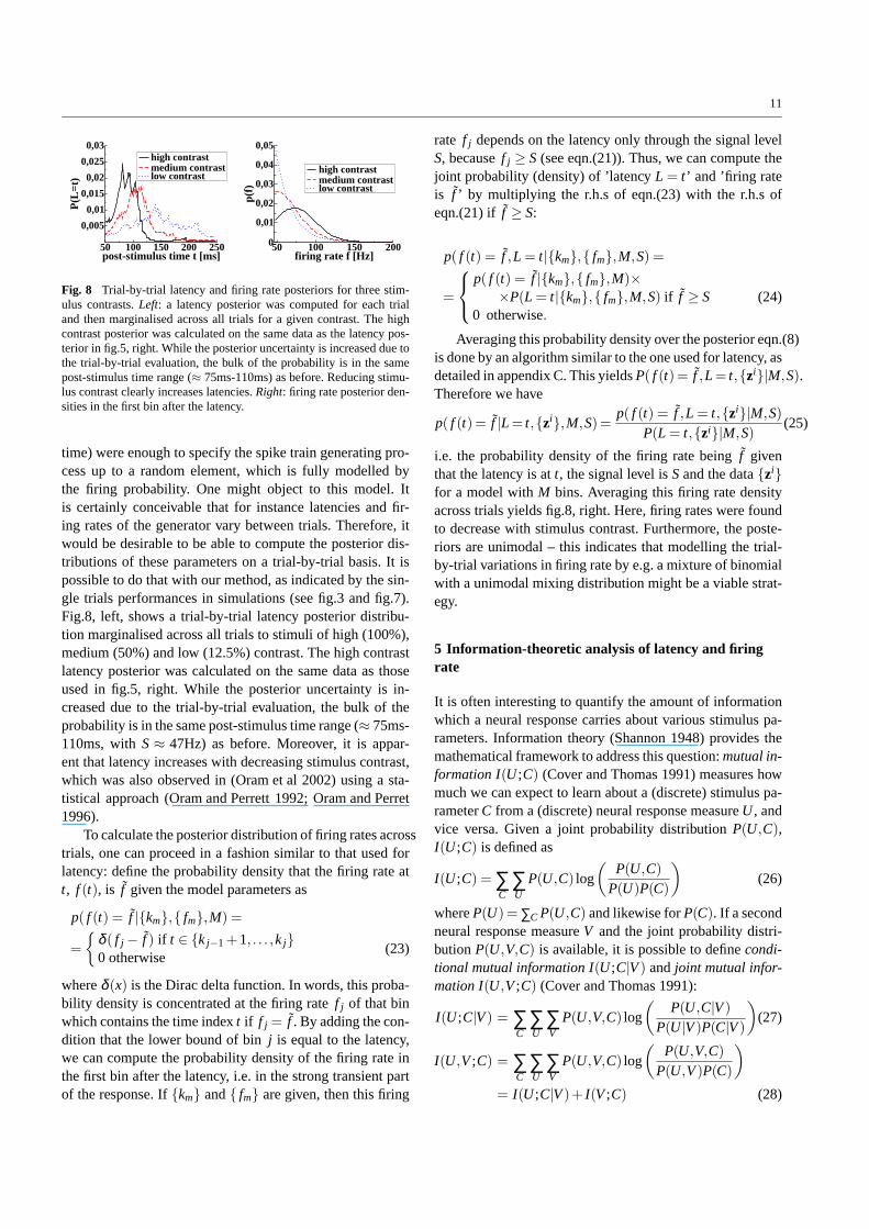
Fig. 8 Trial-by-trial latency and firing rate posteriors for three stim-ulus contrasts.Left: a latency posterior was computed for each trialand then marginalised across all trials for a given contrast. Thehighcontrast posterior was calculated on the same data as the latencypos-terior in fig.5, right. While the posterior uncertainty is increased due tothe trial-by-trial evaluation, the bulk of the probabilityis in the samepost-stimulus time range (≈ 75ms-110ms) as before. Reducing stimu-lus contrast clearly increases latencies.Right: firing rate posterior den-sities in the first bin after the latency.

time) were enough to specify the spike train generating pro-cess up to a random element, which is fully modelled bythe firing probability. One might object to this model. Itis certainly conceivable that for instance latencies and fir-ing rates of the generator vary between trials. Therefore, itwould be desirable to be able to compute the posterior dis-tributions of these parameters on a trial-by-trial basis. It ispossible to do that with our method, as indicated by the sin-gle trials performances in simulations (see fig.3 and fig.7).Fig.8, left, shows a trial-by-trial latency posterior distribu-tion marginalised across all trials to stimuli of high (100%),medium (50%) and low (12.5%) contrast. The high contrastlatency posterior was calculated on the same data as thoseused in fig.5, right. While the posterior uncertainty is in-creased due to the trial-by-trial evaluation, the bulk of theprobability is in the same post-stimulus time range (≈ 75ms-110ms, withS ≈ 47Hz) as before. Moreover, it is appar-ent that latency increases with decreasing stimulus contrast,which was also observed in (Oram et al 2002) using a sta-tistical approach (Oram and Perrett 1992; Oram and Perret1996).

To calculate the posterior distribution of firing rates acrosstrials, one can proceed in a fashion similar to that used forlatency: define the probability density that the firing rate att, f (t), is f given the model parameters as

p( f (t) = f |{km},{ fm},M) =

=

{

δ ( f j − f ) if t ∈ {k j−1+1, . . . ,k j}0 otherwise

(23)

whereδ (x) is the Dirac delta function. In words, this proba-bility density is concentrated at the firing ratef j of that binwhich contains the time indext if f j = f . By adding the con-dition that the lower bound of binj is equal to the latency,we can compute the probability density of the firing rate inthe first bin after the latency, i.e. in the strong transient partof the response. If{km} and{ fm} are given, then this firing

rate f j depends on the latency only through the signal levelS, becausef j ≥ S (see eqn.(21)). Thus, we can compute thejoint probability (density) of ’latencyL = t ’ and ’firing rateis f ’ by multiplying the r.h.s of eqn.(23) with the r.h.s ofeqn.(21) if f ≥ S:

p( f (t) = f ,L = t|{km},{ fm},M,S) =

=

p( f (t) = f |{km},{ fm},M)×

×P(L = t|{km},{ fm},M,S) if f ≥ S0 otherwise.

(24)

Averaging this probability density over the posterior eqn.(8)is done by an algorithm similar to the one used for latency, asdetailed in appendix C. This yieldsP( f (t)= f ,L= t,{zi}|M,S).Therefore we have

p( f (t)= f |L= t,{zi},M,S)=p( f (t) = f ,L = t,{zi}|M,S)

P(L = t,{zi}|M,S)(25)

i.e. the probability density of the firing rate beingf giventhat the latency is att, the signal level isS and the data{zi}

for a model withM bins. Averaging this firing rate densityacross trials yields fig.8, right. Here, firing rates were foundto decrease with stimulus contrast. Furthermore, the poste-riors are unimodal – this indicates that modelling the trial-by-trial variations in firing rate by e.g. a mixture of binomialwith a unimodal mixing distribution might be a viable strat-egy.

5 Information-theoretic analysis of latency and firingrate

It is often interesting to quantify the amount of informationwhich a neural response carries about various stimulus pa-rameters. Information theory (Shannon 1948) provides themathematical framework to address this question:mutual in-formation I(U ;C) (Cover and Thomas 1991) measures howmuch we can expect to learn about a (discrete) stimulus pa-rameterC from a (discrete) neural response measureU , andvice versa. Given a joint probability distributionP(U,C),I(U ;C) is defined as

I(U ;C) = ∑C

∑U

P(U,C) log

(

P(U,C)

P(U)P(C)

)

(26)

whereP(U) =∑C P(U,C) and likewise forP(C). If a secondneural response measureV and the joint probability distri-butionP(U,V,C) is available, it is possible to definecondi-tional mutual information I(U ;C|V ) andjoint mutual infor-mation I(U,V ;C) (Cover and Thomas 1991):

I(U ;C|V ) = ∑C

∑U

∑V

P(U,V,C) log

(

P(U,C|V )

P(U |V )P(C|V )

)

(27)

I(U,V ;C) = ∑C

∑U

∑V

P(U,V,C) log

(

P(U,V,C)

P(U,V )P(C)

)

= I(U ;C|V )+ I(V ;C) (28)

12

I(U ;C|V ) can be understood as the amount of informationwe expect to gain aboutC by observingU if we knew V ,whereasI(U,V ;C) is the expected information gain aboutCif we learned the values of bothU andV . Extending thesedefinitions to continuous variables is straightforward (Cover and Thomas1991).

In sections 4.1 and 4.4, we developed the formalism tocompute the posterior distribution of the latencyL (eqn.(22))and the posterior density of the firing ratef (t) in the first binafter latency (eqn.(25)), providing the joint density

p( f (t) = f ,L = t|{zi},M,S) =

= p( f (t) = f |L = t,{zi},M,S) P(L = t|{zi},M,S) (29)

which we need to compute joint, conditional and marginalmutual informations betweenL, f (t) and any stimulus pa-rameter. Note that these distributions/densities are condi-tioned on the signal levelS. So far, we described a procedureto determineS for a single stimulus conditionC (see end ofsection 4.1). We defineS for multi-valuedC based on twoassumptions:

1. the signal levelS is a property of the cell, not of the stim-ulus. In other words, there is a singleS per cell across allC. If S was allowed to vary withC, the choice ofS wouldinject stimulus-related information into the informationestimates which is not present in the data.

2. S is determined by maximising the marginal probabilityof latency existenceP(L exists|S) (and therefore, signalexistence)

P(L exists|S) = ∑C

P(L exists|S,C)P(C) (30)

whereP(C) is the prior probability of each stimulus con-dition, which is controlled by the experimenter.

3. We assume that there is noa-priori dependency betweenS andC.

Assumption 2 is a consequence of the experimental designwhich we are about to analyse. Cells and stimuli were se-lected such that there was at least one stimulus which evokeda strong response, and at least one that evoked a weak re-sponse (possible none). Maximising the marginal probabil-ity of latency existence thus has the effect of choosing anSsuch that as many stimulus conditions as possible have a de-tectable latency. If there is a strong and a weak (but still de-tectable) response, this procedure chooses a relatively smallS such thatP(L exists|S,C) is high for bothC. However, ifthere is a strong and a non-detectable response, the value ofS will be higher, since it will be driven only by the strongresponse. It remains to be seen if this procedure needs to beadapted for different cell/stimulus choices.

5.1 Results on simulated data

We mentioned in section 4.2 that the latency posterior in-evitably contains information about the change in firing rate

at the latency. To illustrate this point, we performed an information-theoretic analysis of a two-stimulus scenario on simulateddata. Each stimulus evoked a 50ms long transient response,followed by a sustained response (duration 250ms) with afiring rate between the transient and the 10Hz baseline. Inthe ’no difference’ condition, the two simulated responseshad the same underlying generator. We also varied just thefiring rate (transient: 100Hz vs. 30Hz), just the latency (80msvs. 90ms) or both firing rate and latency. Each dataset con-tained 10 trials per stimulus and was analysed trial-by-trial(i.e. one PSTH inferred per trial). The average results from10 repetitions of the simulations are summarised in table 2.This table shows the mutual informations between stimulusidentityC, and the variables:

– E: latency exists, i.e.L ∈ {30ms, . . . ,250ms}.– L: L = t for t ∈ {30ms, . . . ,250ms}, see eqn.(22). Addi-

tionally, L has a special value indicating that a latencydoes not exist (i.e. no transition from below the signalthresholdS to aboveS).

– f : firing probability f (t) = f in the first bin after latencyfor f ∈ [S,1], see eqn.(25).f also has a special valueindicating that a firing probability in the first bin afterlatency does not exist.

Note that bothL and f determineE: if latency is some-where in the latency search interval or if the firing rate in thefirst bin after latency is somewhere above the signal level,thenE is true, otherwiseE is false.E can also be read as’firing rate went above the signal levelS somewhere in thelatency search interval’, and might therefore be viewed as afiring rate related variable, rather than a property of latency.This ambiguity highlights the difficulty of separating firingrate and latency related information, which is due to latencybeing defined by a firing rate based criterion. We choose tointerpretE as carrying firing rate information, since latencyis concerned with thetiming of response onset, rather thanjust the presence or absence of a response. Thus, informationaboutC in L is given by the conditional mutual informationI(L;C|E).

The values in the ’no difference’ condition in table 2 rep-resent the overestimation biases of our method in this sce-nario. Overestimation of mutual information (and the closelyrelated underestimation of entropy) from small datasets isa well-known problem, and many remedies have been de-vised for it (Optican et al 1991; Panzeri and Treves 1996;Nemenman et al 2004; Paninski 2004; Endres and Foldiak2005). However, most of these methods assume a set of dat-apoints as a starting point, not a set of posterior distributions.Hence, they can not be applied to our analysis unaltered.Further work will be needed to understand how best to pro-vide, within our analysis framework, information estimateswhose overestimation is as small as possible.

If there is only a difference in firing rates, thenI( f ;C)>

I(L;C|E) but I(L;C|E) is still significantly greater than in

13

Table 2 Mutual informationI in [bit] for simulated neurons with abaseline firing rate of 10Hz, trial-by-trial analysis.C is stimulus iden-tity, there were two stimuli.L is latency,f is firing rate in the first binafter latency and latency existence isE. The latter is the truth value ofthe proposition ’Latency is somewhere between 30ms and 250ms afterstimulus onset’. Difference inf means that the peak firing rates were30Hz for one stimulus and 100Hz for the other, duration of peak re-sponse 50ms, latency 80ms after stimulus onset. In the ’difference inL’condition, both neurons had a peak firing rate of 100Hz for 50ms,witha latency of 80ms for one stimulus and 90ms for the other. ’No differ-ence’ means that both peak firing rates (100Hz) and latencies (80ms)were equal. Errors are SEM computed from 10 repetitions of thesim-ulations. For details, see text.

Difference in I(E;C) I(L;C|E) I( f ;C)

no difference 0.002±0.001 0.045±0.004 0.008±0.002f : 100/30Hz 0.255±0.023 0.079±0.014 0.314±0.023L: 80/90ms 0.007±0.002 0.084±0.010 0.016±0.004f : 100/30Hz,

0.206±0.026 0.072±0.007 0.265±0.023L: 80/90ms

the ’No difference’ condition. In other words, even thoughthe simulated cells were designed to have the same latency(80ms), the latency posterior distributions inferred froma fi-nite sample carry information about the magnitude of the fir-ing rate change – a large response allows for the determina-tion of latency with greater certainty than a small one. Com-pare this to the ’difference inL’ condition: whileI(L;C|E) isabout as large as before,I(L;C|E)> I( f ;C), i.e. our methodis able to distinguish between (un)certainty related and vari-ability related latency information via the information inf .Furthermore, in both ’difference inf ’ conditions,E containsa large fraction of the firing rate information, i.e. knowingwhether the signal threshold was crossed is the most infor-mative aspect off .

In summary, our method yields the results one would ex-pect for each condition: if the stimulus identityC is encodedin f , thenI( f ;C) is maximal, if changes inC cause changesin L, I(L;C|E) is maximal. If bothL and f are influenced byC, then both can be used together to determineC.

5.2 Results on STSa data

It is known that stimulus contrast influences latency of STSaneurons (Oram et al 2002; van Rossum et al 2008). We nowexamine responses to high-contrast presentations to ask whetherlatency changes convey stimulus identity related informa-tion in the absence of contrast change. The results of a trial-by-trial analysis of mutual informations computed from 29STSa neurons under high-contrast viewing conditions areshown in table 3. Entropy of stimulus identityC is H(C)≈1bit for all cells. SinceI( f ;C)> I(L;C|E), firing rate f in thefirst bin after latency carries slightly more information aboutC than latencyL, but the difference is not significant. Thejoint code of latency and firing rate is almost as informative

Table 3 Average trial-by-trial mutual informations and standard er-rors of the mean (SEM) computed from 29 STSa neurons under high-contrast viewing conditions. Entropy of stimulus identityC is H(C)≈1bit for all cells.E, L and f have the same meaning as in table 2. Fir-ing rate f in the first bin after latency carries slightly more informationabout stimulus identityC than latencyL. For details, see text.

Mutual information betweenC and average± SEM [bit]

signal existenceE I(E;C) 0.0594±0.0191latencyL givenE I(L;C|E) 0.0650±0.0075firing rate f I( f ;C) 0.0730±0.0205firing rate given latency I( f ;C|L) 0.0136±0.0020latency given firing rate I(L;C| f ) 0.0649±0.0077joint code I( f ,L;C) 0.1379±0.0074

as the sum of the individual codes,I( f ,L;C) ≈ I( f ;C) +

I(L;C|E). This is also indicated byI(L;C| f ) ≈ I(L;C|E):the stimulus identity information in firing rate which is re-dundant with latency is almost completely contained inE.In other words, the most informative firing rate feature iswhether the firing rate crosses the signal threshold or not. Todecode stimulus identity, we should therefore answer ques-tions about latency and firing rate in the following orderof importance:has the cell fired aboveS, when has it firedaboveS, how much has it fired aboveS? While these conclu-sions are certainly conditioned on our small stimulus set (2stimuli per cell), the values of the mutual informations aresmall compared to the theoretical maximum of 1 bit. Thismakes ceiling effects unlikely.

6 Summary

We have extended our exact Bayesian binning method (Endres et al2008) for the estimation of PSTHs. Besides treating uncer-tainty – a real problem with small neurophysiological datasets– in a principled fashion, it also outperforms several compet-ing methods on real neural data. Amongst the competitors,we found that only BARS (DiMatteo et al 2001) offers com-parable predictive performance. However, BARS requiressampling to compute posterior averages, which can poten-tially take very long or even get stuck, a problem whichwe observed on data sets containing only a small numberof spikes. Bayesian binning allows for the exact evaluationof posterior averages (within numerical roundoff errors) in-dependent of the contents of the data set. It also offers au-tomatic complexity control because the model posterior canbe evaluated. While its computational cost is significant, itis still fast enough to be useful: evaluating the predictiveprobability takes less than 1s on a modern PC2, with a smallmemory footprint (<10MB for 512 spiketrains). We showedhow our approach can be adapted to extract characteristicfeatures of neural responses in a Bayesian way, e.g. response

2 3.2 GHz Intel XeonTM , SuSE Linux 10.1

14

latencies or firing rate distributions. But we are not restrictedthese features: we can use our method to compute expecta-tions of any function of the PSTH, subject to the conditionthat the function depends on the PSTH in a bin-wise fashion.A free software implementation is available at the machinelearning open source software repository3. This implemen-tation contains a short tutorial, computes expected PSTHand posterior standard deviations, separation level and la-tency posterior. It also allows for the optimisation of theprior hyperparameters. The code for the information theo-retic calculations is available from the authors on request,but it requires a cluster computer to run efficiently: the inte-gration over the posterior distribution of the firing rate needsto be done numerically and is time consuming (≈ 1-2 daysper processor per spiketrain for a trial-by-trial analysis).

The latency alignment procedure of Ventura (2004) wasdeveloped to quantify trial-by-trial variation of the responselatencies, and as such was not intended to determine an ab-solute latency estimate. However, Ventura (2004) suggestedthat the minimal latency estimate from the individual tri-als could be used. We find this yields a poor estimate ofabsolute latency which tends to get worse with increasingnumber of trials. We therefore used the half height methodfrom (Gawne et al 1996a) on the aligned spiketrains to im-prove the absolute latency estimate. This appears to makethe estimate largely independent of the number of trials (seefig.7). In the majority of cases, this procedure still underes-timates the absolute latency, since the trials are aligned tothe minimal trial latency. To counter this systematic under-estimation, we experimented with shifting all aligned trialsby the difference between the total pre-alignment and post-alignment means, thereby restoring the original total meanspike time. However, this did not improve results notably.Aligning trials by mean spike time works well on relativelyregular spiketrains (such as the gamma order 8 ISI distri-bution simulations used in (Ventura 2004)). In our simula-tions with short transients and Bernoulli spike generation, itappears not to work. We would therefore conclude that thepoor performance of this method is due to poor estimates ofthe mean spike time of each trial.

Substituting our observation model eqn.(2) with any otherdistribution is straightforward, as long as the replacement isalso comprised of bins. One might e.g. model each spiketrain within a bin by a separate Bernoulli process and mixthese with a suitable distribution to capture the inter-trial dif-ferences. Alternatively, one could use a model similar to thatof (Shinomoto and Koyama 2007): choose a Gamma pro-cess for the inter-spike intervals and model the time-dependentrate with a bin model.

There are a number of other approaches to PSTH/SDFestimation which were not included in our comparisons. Per-haps most noteworthy (from a Bayesian perspective) are (Shinomoto and Koyama

3 http://www.mloss.org, package ’binsdfc’.

2007) and a recent Gaussian process model (Cunningham et al2008). We have not yet directly compared our method to ei-ther of them. Comparisons to (Cunningham et al 2008) and(Shinomoto and Koyama 2007) will be interesting future work,once the authors of these works release their code.

Finally, we used our approach to compute exact (up toroundoff errors) expectations of information-theoretic quan-tities, e.g. mutual informations between latency, firing rateand stimulus identity. We demonstrated that STSa neuronsconvey most of the information about stimulus identity throughchanges in firing rate. Specifically, we found that the cross-ing of a signal thresholdS is the most informative firing ratefeature. However, extra information about stimulus identitycan be gained by looking at the response latency.

Acknowledgements D. Endres was supported by a Medical ResearchCouncil (UK) special training fellowship in bioinformatics G0501319.Both authors would like to thank P. Foldiak and J. Schindelin for stim-ulating discussions and comments on the manuscript. Data collectionwas supported by EU framework grant (FP5-Mirror) to M. Oram. Wethank the unknown reviewers for their clarifying suggestionsand ref-erences.

Appendix A: Computing the evidence with dynamicprogramming

The evidence, or marginal likelihood of a model withM bins is givenby (see eqn.(9)):

P({zi}|M) =T−2

∑kM−1=M−1

kM−1−1

∑kM−2=M−2

. . .

. . .k1−1

∑k0=0

P({zi}|{km},M)P({km}|M) (A-1)

where the summation boundaries are chosen such that the bins are non-overlapping and contiguous and

P({zi}|{km},M) =∫ 1

0d{ fm}P({zi}|{ fm},{km},M)p({ fm}|M).(A-2)

Recall that the probability of a (multi)set of spiketrains{zi}= {z1, . . . ,zN},assuming independent generation, is given by eqn.(3):

P({zi}|{ fm},{km},M) =N

∏i=1

M

∏m=0

f s(zi,m)m (1− fm)

g(zi,m)

=M

∏m=0

f s({zi},m)m (1− fm)

g({zi},m) (A-3)

wheres({zi},m) = ∑Ni=1 s(zi,m) is the number of spikes in all spike-

trains in binm andg({zi},m) = ∑Ni=1 g(zi,m) is the number of all non-

spikes, or gaps. The prior of the firing rates (eqn.(5)) is

p({ fm}|M) =M

∏m=0

B( fm;σm,γm). (A-4)

The integrals in eqn.(A-2) can be evaluated by virtue of eqn.(A-3) andeqn.(A-4):

P({zi}|{km},M) =M

∏m=0

B(s({zi},m)+σm,g({zi},m)+ γm)

B(σm,γm)(A-5)

15

where B(x,y)= Γ (x)Γ (y)Γ (x+y) is Euler’s Beta function (Davis 1972). Eqn.(A-5)

is a product with one factor per bin, and each factor depends only onspike/gap counts and prior parameters in that bin. To compute eqn.(A-1),we can therefore use an approach very similar to that described in(Endres and Foldiak 2005; Endres 2006) in the context of density es-timation and in (Hutter 2006, 2007) for Bayesian function approxima-tion: define the function

getIEC(ks,ke,m) := B(s({zi},ks,ke)+σm,g({zi},ks,ke)+ γm) (A-6)

wheres({zi},ks,ke) is the number of spikes andg({zi},ks,ke) is thenumber of gaps in{zi} between the start intervalks and the end intervalke (both included). Furthermore, collect all contributions toeqn.(A-1)that do not depend on the data (i.e.{zi}) and store them in the arraypr[M]:

pr[M] :=∏M

m=01

B(σm,γm)(

T −1M

) . (A-7)

Substituting eqn.(A-5) into eqn.(A-1) and using the definitions (A-6)and (A-7), we obtain

P({zi}|M) ∝T−2

∑kM−1=M−1

. . .k1−1

∑k0=0

M

∏m=1

getIEC(km−1+1,km,m)×

×getIEC(0,k0,0) (A-8)

with kM = T −1 and the constant of proportionality being pr[M]. Sincethe factors on the r.h.s. depend only on two consecutive bin boundarieseach, it is possible to apply dynamic programming (Bertsekas 2000):rewrite the r.h.s. by ’pushing’ the sums as far to the right as possible:

P({zi}|M) ∝T−2

∑kM−1=M−1

getIEC(kM−1+1,T−1,M)×

×kM−1−1

∑kM−2=M−2

getIEC(kM−2+1,kM−1,M−1)×

× . . .k1−1

∑k0=0

getIEC(k0+1,k1,1)getIEC(0,k0,0). (A-9)

Evaluating the sum overk0 requiresO(T ) operations (assuming thatT ≫ M, which is likely to be the case in real-world applications). Asthe summands depend also onk1, we need to repeat this evaluationO(T ) times, i.e. summing outk0 for all possible values ofk1 requiresO(T 2) operations. This procedure is then repeated for the remainingM − 1 sums, yielding a total computational effort ofO(MT 2). Thus,initialise the array subE0[k] := getIEC(0,k,0), and iterate for allm =1, . . . ,M:

subEm[k] :=k−1

∑r=m−1

getIEC(r+1,k,m)subEm−1[r], (A-10)

A close look at eqn.(A-9) reveals that while we sum overkM−1, weneed subEM−1[k] for k = M −1;. . . ;T −2 to compute the evidence ofa model with its latest boundary atT −1. We can, however, computesubEM−1[T −1] with little extra effort, which is, up to a factor pr[M−1], equal toP({zi}|M − 1), i.e. the evidence for a model withM − 1bin boundaries. Moreover, having computed subEm[k], we do not needsubEm−1[k−1] anymore. Hence, the array subEm−1[k] can be reused tostore subEm[k], if overwritten in reverse order. Table A-T1 shows thisalgorithm in pseudo-code (E[m] contains the evidence of a model withm bin boundaries inside[tmin, tmax] after termination).

Table A-T1 Computing the evidences of models with up toM binboundaries

1. for k := 0. . .T −1 : subE[k] := getIEC(0,k,0)2. E[0] := subE[T −1]×pr[0]3. for m := 1. . .M :

(a) if m = M thenl := T −1 elsel := m(b) for k := T −1. . . l

subE[k] := ∑k−1r:=m−1 subE[r]×getIEC(r+1,k,m)

(c) E[m] = subE[T −1]×pr[m]4. return E[]

Appendix B: Computing the posterior distribution ofthe latency

We compute the joint probability of the latencyL = t and the observedspiketrains{zi} given the number of bins and the signal separationlevel S via

P(L = t,{zi}|M,S) =T−2

∑kM−1=M−1

kM−1−1

∑kM−2=M−2

. . .

. . .k1−1

∑k0=0

P(L = t,{zi},{km}|M,S) (B-11)

where

P(L = t,{zi},{km}|M,S) =

=∫ 1

0d{ fm}P(L = t|{km},{ fm},M,S)p({zi},{ fm},{km}|M).(B-12)

Note thatP(L= t|{km},{ fm},M,S) is the r.h.s of eqn.(21) andp({zi},{ fm},{km}|M)is the numerator of the r.h.s. of eqn.(8). As a consequence of eqn.(21),the only nonzero contributions to the average are models which havea (lower) bin boundary att. Assumet was at the lower bound of binj, i.e. att = k j−1+1 (the{km} are inclusive upper bin boundaries, asdefined above). Carrying out the integrals over the{ fm} yields:

P(L = t,{zi},{km}|M,S)

=∫ 1

0d{ fm}P(L = t|{km},{ fm},M,S)p({zi},{ fm},{km}|M)

=∫ S

0d f0 . . .

∫ S

0d f j−1

∫ 1

Sd f j

∫ 1

0d f j+1 . . .

∫ 1

0d fM p({zi},{ fm},{km}|M)

(B-13)

The integration boundaries in the last line of eqn.(B-13) area conse-quence of our latency definition: all binsm < j will contribute to theintegral only as long asfm < S, hence the upper bound of their inte-grals is atS. Bin j contributes only iff j ≥ S, thus the lower bound ofthe integral overf j is S. The binsm > j are not affected by the latencyprobability (eqn.(21)) whence their integrals still run from 0 to 1. Byvirtue of eqn.(3) and eqn.(5), we obtain

P(L = t,{zi},{km}|M,S) =j−1

∏m=0

BS(s({zi},m)+σm,g({zi},m)+ γm)

× BS(s({zi}, j)+σm,g({zi}, j)+ γm))

×M

∏m= j+1

B(s({zi},m)+σm,g({zi},m)+ γm)

×M

∏m=0

1B(σm,γm)

P({km}|M) (B-14)

whereBS(a,b) =∫ S

0 ta−1(1− t)b−1dt is the incomplete Beta function(Davis 1972) andBS(a,b) =

∫ 1S ta−1(1− t)b−1dt = B(a,b)−BS(a,b)

16

is its complement. Note that up to the factorP({km}|M), eqn.(B-14)is basically eqn.(A-5) with some of the Beta functions replacedby in-complete Beta functions. Hence, the remaining summations over the{km} can be carried out by using

getIECL(ks,ke,m) :=

=

BS(s({zi},ks,ke)+σm,g({zi},ks,ke)+ γm) if ke < tBS(s({zi},ks,ke)+σm,g({zi},ks,ke)+ γm)) if ks = tB(s({zi},ks,ke)+σm,g({zi},ks,ke)+ γm) if ks > t0 otherwise

(B-15)

instead of getIEC(ks,ke,m) (eqn.(A-6)) in the evidence computationalgorithm. This procedure yields the desiredP(L = t,{zi}|M,S). Theabove derivation is an instance of the general framework for comput-ing expectations of functions of bin boundaries and firing probabilitiesdescribed in (Endres and Foldiak 2005).

Appendix C: Computing the posterior density of thefiring rate

We compute the joint probability density of the firing ratef (t) = f ,the latencyL = t and the observed spiketrains{zi} given the numberof bins and the signal separation levelS via

P( f (t) = f ,L = t,{zi}|M,S) =

=T−2

∑kM−1=M−1

kM−1−1

∑kM−2=M−2

. . .k1−1

∑k0=0

P( f (t) = f ,L = t,{zi},{km}|M,S)

(C-16)

where

p( f (t) = f ,L = t,{zi},{km}|M,S) =

=∫ 1

0d{ fm}P( f (t) = f ,L = t|{km},{ fm},M,S)p({zi},{ fm},{km}|M)

(C-17)

Note thatP( f (t) = f ,L = t|{km},{ fm},M,S) is the r.h.s of eqn.(24)andp({zi},{ fm},{km}|M) is the numerator of the r.h.s. of eqn.(8). As aconsequence of eqn.(24), the only nonzero contributions to the averageare models which have a (lower) bin boundary att. Assumet was at thelower bound of binj, i.e. att = k j−1+1 (the{km} are inclusive upperbin boundaries, as defined above). Integrating out the{ fm} yields

p( f (t) = f ,L = t,{zi},{km}|M,S) =

=j−1

∏m=0

BS(s({zi},m)+σm,g({zi},m)+ γm)

× f s({zi}, j)+σm−1 (1− f )g({zi}, j)+γm)−1

×M

∏m= j+1

B(s({zi},m)+σm,g({zi},m)+ γm)

×M

∏m=0

1B(σm,γm)

P({km}|M) (C-18)

where the second line is a result of eqn.(3) and eqn.(5) multiplied withthe Dirac delta function in eqn.(23). Hence, the remaining summationsover the{km} can be carried out by using

getIECf ,L(ks,ke,m) :=

BS(s({zi},ks,ke)+σm,g({zi},ks,ke)+ γm) if ke < tf s({zi},ks,ke)+σm−1 (1− f )g({zi},ks,ke)+γm)−1 if ks = tB(s({zi},ks,ke)+σm,g({zi},ks,ke)+ γm) if ks > t0 otherwise

(C-19)

instead of getIEC(ks,ke,m) (eqn.(A-6)) in the evidence computationalgorithm. Thus we obtainP( f (t) = f ,L = t,{zi}|M,S).

References

Alitto HJ, Usrey WM (2004) Influence of contrast on orientation andtemporal frequency tuning in ferret primary visual cortex. Journalof Neurophysiology 91:2797–2808

Barraclough N, Xiao D, Baker C, Oram M, Perrett D (2005) Integra-tion of visual and auditory information by superior temporal sul-cus neurons responsive to the sight of actions. Journal of CognitiveNeuroscience 17

Berenyi A, Benedek G, Nagy A (2007) Double sliding-window tech-nique: A new method to calculate the neuronal response onset la-tency. Brain Research 1178:141–148

Berger J (1985) Statistical Decision Theory and Bayesian Analysis.Springer, New York

Bertsekas DP (2000) Dynamic Programming and Optimal Control.Athena Scientific

Cover T, Thomas J (1991) Elements of Information Theory. Wiley,New York

Cunningham J, Yu B, Shenoy K, Sahani M (2008) Inferring neuralfir-ing rates from spike trains using Gaussian processes. In: Platt J,Koller D, Singer Y, Roweis S (eds) Advances in Neural Informa-tion Processing Systems 20, MIT Press, Cambridge, MA

Davis P (1972) Gamma function and related functions. In: AbramowitzM, Stegun I (eds) Handbook of mathematical functions, Dover,New York

DiMatteo I, Genovese CR, E KR (2001) Bayesian curve-fitting withfree-knot splines. Biometrika 88(4):1055–1071

Edwards R, Xiao D, Keysers C, Foldiak P, Perrett DI (2003)Color Sensitivity of Cells Responsive to Complex Stim-uli in the Temporal Cortex. Journal of Neurophysiol-ogy 90(2):1245–1256, DOI 10.1152/jn.00524.2002, URLhttp://jn.physiology.org/cgi/content/abstract/90/2/1245,http://jn.physiology.org/cgi/reprint/90/2/1245.pdf

Eifuku S, De Souza WC, Tamura R, H N, T O (2004) Neuronal corre-lates of face identification in the monkey anterior temporal corticalareas. Journal of Neurophysiology 91:358–371

Endres D (2006) Bayesian and information-theoretic tools forneuro-science. PhD thesis, School of Psychology, University of St. An-drews, U.K., http://hdl.handle.net/10023/162

Endres D, Foldiak P (2005) Bayesian bin distribution inference andmutual information. IEEE Transactions on Information Theory51(11)

Endres D, Oram M, Schindelin J, Foldiak P (2008) Bayesian binningbeats approximate alternatives: estimating peri-stimulus time his-tograms. In: Platt J, Koller D, Singer Y, Roweis S (eds) Advancesin Neural Information Processing Systems 20, MIT Press, Cam-bridge, MA

Foldiak P, Xiao D, Keysers C, Edwards R, Perrett DI (2004) Rapidserial visual presentation for the determination of neural selectivityin area STSa. Progress in Brain Research 144:107–116

Friedman HS, Priebe CE (1998) Estimating stimulus response latency.Journal of Neuroscience Methods 83:185–194

Fries P, Neuenschwander S, Engel AK, Goebel R, Singer W (2001)Rapid feature selective neuronal synchronization through corre-lated latency shifting. Nature Neuroscience 4:194–200

Gabel SF, Misslisch H, Schaafsma SJ, Duysens J (2002) Temporalproperties of optic flow responses in the ventral intraparietal area.Visual Neuroscience 19:381–388

Gawne TJ, Kjaer TW, Hertz JA, Richmond BJ (1996a) Adjacent visualcortical complex cells share about 20% of their stimulus-relatedinformation. Cerebral Cortex 6(3):482–9

Gawne TJ, Kjaer TW, Richmond BJ (1996b) Latency: another potentialcode for feature binding in striate cortex. Journal of Neurophysi-ology 76:1356–1360

Hanes DP, Thompson KG, Schall JD (1995) Relationship of presac-cadic activity in frontal eye field and supplementary eye field to

17

saccade initiation in macaque - poisson spike train analysis. Ex-perimental Brain Research 103:85–96

Heil P, Irvine DRF (1997) First-spike timing of auditory-nervefibersand comparison with auditory cortex. Journal of Neurophysiology78:2438–2454

Hurley LM, Pollak GD (2005) Serotonin shifts first-spike latenciesof inferior colliculus neurons. Journal of Neuroscience 25:7876–7886

Hutter M (2006) Bayesian regression of piecewise constant functions.Tech. Rep. arXiv:math/0606315v1, IDSIA-14-05

Hutter M (2007) Exact bayesian regression of piecewise constant func-tions. Journal of Bayesian Analysis 2(4):635–664

Kiani R, Esteky H, Tanaka K (2005) Differences in Onset La-tency of Macaque Inferotemporal Neural Responses toPrimate and Non-Primate Faces. Journal of Neurophysiol-ogy 94(2):1587–1596, DOI 10.1152/jn.00540.2004, URLhttp://jn.physiology.org/cgi/content/abstract/94/2/1587,http://jn.physiology.org/cgi/reprint/94/2/1587.pdf

Lee J, Williford T, Maunsell JHR (2007) Spatial attention and the la-tency of neuronal responses in macaque area V4. Journal of Neu-roscience 27:9632–9637

Liu Z, Richmond BJ (2000) Response differences in monkey te andperirhinal cortex: Stimulus association related to reward sched-ules. Journal of Neurophysiology 83:1677–1692

Loader C (1997) LOCFIT: an introduction. Statistical Comput-ing and Graphics Newsletter 8(1):11–17, uRL: http://www.stat-computing.org/newsletter

Loader C (1999) Local Regression and Likelihood. Springer, NewYork

Luczak A, Bartho P, Marguet SL, Buzsaki G, Harris KD (2007) Se-quential structure of neocortical spontaneous activity in vivo. Pro-ceedings of the National Academy of Sciences USA 104:347–352

Maunsell JH, Gibson JR (1992) Visual response latencies in striate cor-tex of the macaque monkey. Journal of Neurophysiology 68:1332–1344

Nawrot MP, Aertsen A, Rotter S (2003) Elimination of response la-tency variability in neuronal spike trains. Biological Cybernetics88:321–334

Nemenman I, Bialek W, van Steveninck R (2004) Entropyand information in neural spike trains: Progress on thesampling problem. Physical Review E 69(5):056111, URLhttp://link.aps.org/abstract/PRE/v69/e056111

Nowak LG, Munk MHJ, Girard P, Bullier J (1995) Visual latenciesin areas v1 and v2 of the macaque monkey. Visual Neuroscience12:371–384

Optican L, Gawne T, Richmond B, Joseph P (1991) Unbiased measuresof transmitted information and channel capacity from multivariateneuronal data. Biological Cybernetics 65:305–310

Oram M, Perret D (1996) Integration of form and motion in the anteriorsuperior temporal polysensory area (stpa) of the macaque monkey.Journal of Neurophysiology 19:109–129

Oram MW, Perrett DI (1992) Time course of neural responses discrim-inating different views of the face and head. Journal of Neurophys-iology 68(1):70–84

Oram MW, Xiao D, Dritschel B, Payne K (2002) The temporal preci-sion of neural signals: A unique role for response latency? Philo-sophical Transactions of the Royal Society, Series B 357:987–1001

Paninski L (2004) Estimating entropy on m bins given fewer than msamples. IEEE Transactions on Information Theory 50(9):2200–2203

Panzeri S, Treves A (1996) Analytical estimates of limited samplingbiases in different information measures. Network: Computationin Neural Systems 7:87–107

Perrett DI, Oram MW, Harries MH, Bevan R, Hietanen JK, Benson PJ(1991) Viewer-centered and object-centered coding of heads in the

macaque temporal cortex. Experimental Brain Research 86:159–173

Press W, Flannery B, Teukolsky S, Vetterling W (1986) NumericalRecipes in C: The Art of Scientific Computing. Cambridge Uni-versity Press, New York

Richmond BJ, Optican LM (1987a) Temporal encoding of two-dimensional patterns by single units in primate inferior temporalcortex. ii. quantification of response waveform. Journal of Neuro-physiology 57(1):147–161

Richmond BJ, Optican LM (1987b) Temporal encoding of two-dimensional patterns by single units in primate inferior temporalcortex. iii. information theoretic analysis. Journal of Neurophysi-ology 57(1):162–178

Richmond BJ, Oram MW, Wiener MC (1999) Response features de-termining spike times. Neural Plasticity 6:133–145

van Rossum MCW, van der Meer MAA, Xiao D, Oram MW (2008)Adaptive Integration in the Visual Cortex by Depressing RecurrentCortical Circuits. Neural Computation 20(7):1847–1872, URLhttp://neco.mitpress.org/cgi/content/abstract/20/7/1847,http://neco.mitpress.org/cgi/reprint/20/7/1847.pdf

Sary G, Koteles K, Chadaide Z, Tompa T, Benedek G (2006) Task-related modulation in the monkey inferotemporal cortex. BrainRe-search 1121:76–82

Schmolesky MT, Wang Y, Hanes DP, Thompson KG, Leutgeb S, SchallJD, Leventhal AG (2006) Signal timing across the macaque visualsystem. Journal of Neurophysiology 79:3272–3278

Shannon CE (1948) The mathematical theory of communication. TheBell Systems Technical Journal 27:379–423, 623–656

Shimazaki H, Shinomoto S (2007a) Kernel width optimiza-tion in the spike-rate estimation. In: Budelli R, Caputi A,Gomez L (eds) Neural Coding 2007, pp 143–146, URLhttp://neuralcoding2007.edu.uy

Shimazaki H, Shinomoto S (2007b) A method for selecting the bin sizeof a time histogram. Neural Computation 19(6):1503–1527

Shimazaki H, Shinomoto S (2007c) A recipe for optimizing a time-histogram. In: Scholkopf B, Platt J, Hoffman T (eds) Advancesin Neural Information Processing Systems 19, MIT Press, Cam-bridge, MA, pp 1289–1296

Shinomoto S, Koyama S (2007) A solution to the controversy betweenrate and temporal coding. Statistics in Medicine 26:4032–4038

Stecker GC, Middlebrooks JC (2003) Distributed coding of soundlo-cations in the auditory cortex. Biological Cybernetics 89:341–349

Sugase-Miyamoto Y, Richmond BJ (2005) Neuronal signals in themonkey basolateral amygdala during reward schedules. Journal ofNeuroscience 25:11,071–11,083

Syka J, Popelar J, Kvasnak E, Astl J (2000) Response properties ofneurons in the central nucleus and external send dorsal cortices ofthe inferior colliculus in guinea pig. Experimental Brain Research133:254–266

Tamura H, Tanaka K (2001) Visual response properties of cells in theventral and dorsal parts of the macaque inferotemporal cortex.Cerebral Cortex 11:384–399

Tanaka M, Lisberger SG (2002) Role of arcuate frontal cortex of mon-keys in smooth pursuit eye movements. I. Basic response proper-ties to retinal image motion and position. Journal of Neurophysi-ology 87:2684–2699

Thompson KG, Hanes DP, Bichot NP, Schall JD (1996) Perceptualand motor processing stages identified in the activity of macaquefrontal eye field neurons during visual search. Journal of Neuro-physiology 76:4040–4055

Tovee MJ, Rolls ET, Treves A, Bellis RP (1993) Information encodingand the responses of single neurons in the primate temporalvisual cortex. Journal of Neurophysiology 70(2):640–654, URLhttp://jn.physiology.org/cgi/content/abstract/70/2/640,http://jn.physiology.org/cgi/reprint/70/2/640.pdf

18

Ventura V (2004) Testing for and estimating latency effects forpoissonand non-poisson spike trains. Neural Computation 16(11):2323–2349, DOI http://dx.doi.org/10.1162/0899766041941952