UNIVERSIDAD DE GUANAJUATO

Centro de Investigaciones en Óptica, A.C.

DEVELOPMENT OF THE PARTICLE IMAGE VELOCIMETRY (PIV) TECHNIQUE FOR THREE DIMENSIONS:

TUNNELING VELOCIMETRY

A dissertation submitted by

Ing. J. Ascención Guerrero Viramontes

In partial fulfillment of the requirements for the degree of

Doctor in Science (Optics)

León, Gto. February 2002

DEVELOPMENT OF THE PARTICLE IMAGE VELOCIMETRY (PIV) TECHNIQUE FOR THREE DIMENSIONS:

TUNNELING VELOCIMETRY.

A dissertation submitted

by

Ing. J. Ascención Guerrero Viramontes

In partial fulfillment of the requirements for the degree of Doctor in Science (Optics)

Centro de Investigaciones en Óptica A. C.

February 2002

Supervisors: Dr. Fernando Mendoza Santoyo Dr. Marcelo Funes-Gallanzi (INAOE)

Special Thanks to:

God. Thanks to let me know my position into Your Creation.

My best friend and beautiful wife Claudia Rubí. Thanks for loving me.

My Dad José and Mom Reyes, thanks for your testimony and your love.

My brother and sisters, Memo, Toña, Lety, Mella, Chabe and Ceci, my teachers.

My second family: Luis, Juanita, Cheli, Sagra, Marlene and Dany. Thanks to

let me feel at home.

Marcelo and Claudia and their beautiful daughters Gaby, Sofy and Ale, Fernando and Lucy. Thanks for your friendship, support, love and much

more…

All my family: Ramón, Cuco, Lola, Concha, Chema, Chole, lupe, Orlando, Paola, Nadia, Lulú, Euridice, Lalo, Quique y Kikin, Paquito,Mario y Mary, Rei, Karina, Ariel y Tere, Andrea, Arielito, Alfredo “Pez” y Lilian “La Diva”, Lilieired, Periquin, Hugo, Memo y Paty, Gisela, Memo, Diana, Rubichunda, Chuy y Gaby, Zaira, Valeria, Jaime and Alicia, Lichita, Alejandra, Maritza,

Rodolfo and Tere, Kuku, Renato and Aldo. Thanks to all for your trust.

Psalms 139:6-10. This knowledge is beyond me, Its lofty, I can’t attain it. Where could I go from your Spirit? Or where could I flee from your presence?. If I ascend up into heaven You are there!. If I make my bed in Shed, behold You are there!. If I take the wings of the dawn and settle in the uttermost parts of the sea, even there Your hand will lead me and

Your right hand will hold me.

Más maravillosa es la ciencia que mi capacidad; alta es, no puedo entenderla. ¿Adónde me iré de tu Espíritu? ¿Y a dónde huiré de tu presencia?. Si subiere a los cielos, allí estas

Tú y si en el abismo hiciere mi estrado, he aquí allí Tu estás. SI tomare las alas del alba y habitare en el extremo de la mar, aún allí me guiará Tu mano y me asirá Tu diestra.

iii

ACKNOWLEDGEMENTS

Main acknowledgement is credited to Dr. Fernando Mendoza Santoyo from Centro

de Investigaciones en Óptica A.C. (CIO) and Dr. Marcelo Funes-Gallanzi from the Instituto

Nacional de Astrofísica Óptica y Electrónica (INAOE) for their tireless efforts and

guidance associated with this research. The author gratefully acknowledges the scholarship

granted by Consejo Nacional de Ciencia y Tecnología (CONACYT) under projects 32709-

A and 35062-E. I would also like to thank ASCI SA de CV, Alstom Power Plc., and Centro

de Investigaciones en Óptica, A.C. for their installation facilities. Thanks also to my

teachers: Memo, Samuel, Nachito, Miramontes, Dr. Ramón Rodríguez, Dr. Cristina Solano,

Dr. Daniel Malacara, Dr. Zacarias Malacara, Dr. Bernardo Mendoza, Dr. Sergio Calixto

and Dr. Oracio Barbosa. To my revisers: Dr. Bernardino Barrientos and Dr. Jorge Rojas.

My honest thanks go to all my friendly pals from CIO: Eli, Carlos P.L., Laura, Pepillo,

David “Don Moletrompero”, Marcial, Charo, Claudia, Manuel, Apolinar, Alejandro, Gaby,

Luis, “La guera”, Guille, Miguel, Ili, Juanjo, Juan Carlos, Alma and Juan Manuel, Javier,

Chemo, Chuy Lee, Marco, Luis, Ese, The Santos Team, Reyna, Noe, Los Tolucos, Saul,

Chuy Cervantes, Angeles, Marite, Luli, Rodolfo, Pepe Puga, Paty Padilla, Doña Liz,

Carmelita, Raymundo, Carlos P.S, Lic. Martínez, Erika. And my outsiders pals: Felipe and

Angelica del Castillo, Bibiano and Nohemí Medina, José Luis and Perla Ortega, Joel and

Luli Vázquez, Miguel and Adi, Orlando and Ceci, Adan and Vero Segura, Joseph and

Azucena, Laura, Victor and Bertha H. Anteles, Gabriel, Memo and Sofy Caballero,

Marisol, Alejandro, Los Bombones, Humberto and Rober. Paty, Irma and Moises Olvera,

Nila, Petre, Daci and Aleks. I am sorry if I forgot someone.

iv

ABSTRACT

Conventional velocimetry has an intrinsic limitation because it yields 2D data,

neglecting the third velocity component. For this reason, 3D-PIV has recently evolved as

an area of research with success at the cost of increasing complexity in its methodology.

The increased complexity and the limited optical access found in most industrial

applications, meant that many of the 3D-PIV techniques, although of academic interest,

cannot be used in practical industrial applications.

For practical applications restricted viewing eliminates stereoscopic approaches.

Lack of robustness and ease to perform an experiment make of conventional holography an

unattractive option due to the fact that it involves a wet developing process, hence is very

slow to yield results. However, its large depth of field and storing capacity makes it a

technique that should, under the correct environment, be used. Scanning light-sheets are

difficult to obtain for restricted optical access and high speeds, so they have not been tried

in industrial conditions.

The required capabilities for 3D real-time measurement include the following three

aspects: illumination of a volume rather than a plane, particle positioning in 3D from 2D

camera information, and positioning calculation at low-magnification. Three-dimensional

position and velocity information can be extracted by directly analyzing the diffraction

patterns of seeding particles in imaging velocimetry using real-time CCD cameras. The

Generalised Lorenz-Mie theory is shown to yield quantitative accurate models of particle

position, such that it can be deduced with good accuracy from typical experimental particle

images.

Tunneling Velocimetry, the proposed technique to perform 3D velocity

measurements, is able to provide the means to obtain particle images in a volume of interest

rather than on a light sheet. Moreover, with this technique pressure and temperature

measurements are feasible from the system background surface. The research reported here

is concentrated in the experimental characterization of Tunneling Velocimetry and the

problems involved with it. A discussion of the preliminary results is presented.

v

DEVELOPMENT OF THE PARTICLE IMAGE

VELOCIMETRY (PIV) TECHNIQUE FOR THREE DIMENSIONS: TUNNELING VELOCIMETRY.

By J. Ascención Guerrero Viramontes.

CONTENTS ACKNOWLEDGEMENTS ……………………………………………………………….. iv

ABSTRACT …………………………………………………………………………….. v

LIST OF FIGURES …………………………………………………………………… viii

LIST OF REFEREED PUBLICATIONS AND CONFERENCES DERIVED FROM

THIS RESEARCH ………………………………………………………………….. xi

INTRODUCTION ……………………………………………………………………. 13

REFERENCES …………………………………………………..…….. 16

CHAPTER I VELOCITY MEASUREMENT TECHNIQUES …………………… 18

1.0 INTRODUCTION ……………………………………………………………………. 18

1.1 FLUID VELOCITY MEASUREMENT INTRUSIVE TECHNIQUES …………. 19

1.1.0 THERMAL ANEMOMETRY (HOT-WIRES AND HOT-FILMS) …………. 19

1.1.1 PITOT STATIC TUBES ……………………………………………….. 19

1.2 FLUID VELOCITY IN-PLANE MEASUREMENT TECHNIQUES …………. 21

1.2.0 LASER TWO FOCUS (L2F) VELOCIMETRY …………………………….. 21

1.2.1 PARTICLE IMAGE VELOCIMETRY (PIV) …………………………….. 22

1.2.2 LASER SPECKLE VELOCIMETRY (LSV) …………………………….. 26

1.2.3 LASER DOPPLER VELOCIMETRY (LDV) …………………………….. 27

1.2.4 DOPPLER GLOBAL VELOCIMETRY (DGV) …………………………….. 29

1.2.5 DIGITAL PARTICLE IMAGE VELOCIMETRY (D-PIV) …………. 30

1.2.6 THREE STATE ANEMOMETRY (3SA) …………………………….. 30

1.3 FLUID VELOCITY MEASUREMENT VOLUMETRIC TECHNIQUES ………….. 32

1.3.0 STEREOSCOPIC PARTICLE IMAGE VELOCIMETRY (STEREO PIV) … 32

1.3.1 HOLOGRAPHIC PARTICLE IMAGE VELOCIMETRY (HOLOGRAPHIC PIV) 34

1.4 CONCLUSIONS …………………………………………………………………. 34

1.5 REFERENCES ………………………………………………………………….. 35

vi

CHAPTER II PRESSURE AND TEMPERATURE MEASUREMENTS …………. 40

2.0 INTRODUCTION ………………………………………………………………….. 40

2.1 PARAMETER SENSITIVE PAINTS ……………………………………… 42

2.2 PRESSURE SENSITIVE PAINTS (PSP) ……………………………..………. 43

2.3 TEMPERATURE SENSITIVE PAINTS (TSP) …………………………………… … 44

2.4 TSP AND PSP PHYSICAL PRINCIPLES ……………………………………… 44

2.5 CALIBRATION OF PRESSURE/TEMPERATURE SENSORS …….…………….. 46

2.6 CONCLUSIONS …………………………………………………………………. 47

2.7 REFERENCES ………………………………………………………………….. 47

CHAPTER III PATTERN DIFFRACTION ANALYSIS …………………………….. 49

3.0 INTRODUCTION …………………………………………………………. 49

3.1 DIFFRACTION THEORY ……………………………………………….. 51

3.2 THEORETICAL MODEL ……………………………………………….. 54

3.2.1 THE GLMT FOR A ELECTROMAGNETIC SPHERICAL WAVE …………. 54

3.2.2 INCIDENT FIELD DESCRIPTION ……………………………………… 55

3.2.3. SCATTERED NEAR FIELD COMPONENTS ……………………………. 57

3.2.4 THE BSC COMPUTATIONS ………………………………………………. 59

3.2.5. NUMERICAL RESULTS ………………………………………………. 61

3.3 EXPERIMENTAL ARRANGEMENT ……………………………………… 67

3.4 RESULTS AND DISCUSSION ……………………………………………….. 69

3.5 CONCLUSIONS ………………………………………………………………….. 75

3.6 REFERENCES ………………………………………………………………….. 76

CHAPTER IV TUNNELLING VELOCIMETRY (TV) ……………………………. 80

4.0 INTRODUCTION ………………………………………………………… 80

4.1 REQUIRED CAPABILITIES AND TOOLS ……………………………………… 81

4.2 TUNNELING VELOCIMETRY ……………………………………………….. 82

4.3 EXPERIMENTAL TESTING ……………………………………………….. 91

4.4 CONCLUSIONS ………………………………………………………………….. 99

4.5 REFERENCES ………………………………………………………………….. 99

GENERAL CONCLUSIONS AND FUTURE WORK …………………………………. 101

vii

LIST OF FIGURES

CHAPTER I • Figure 1.1. Example of pitot tubes ………………………………… 20

• Figure 1.2. L2F system ………………………………………………... 21

• Figure 1.3. Basic PIV system configuration ………………………… 23

• Figure 1.4. Anatomy of a typical LDA signal burst generated when a

particle passes through the measurement volume …………………… 27

• Figure 1.5. A single-component dual-beam LDA system in forward

scatter mode………………………………………………………………… 28

CHAPTER II • Figure 2.1 Schlieren method for determining gas temperature ………… 42

• Figure 2.2. Interferometric technique for gas temperature measurement... 42

• Figure 2.3. Emission and excitation spectra of Temperature Sensitive

Paint TSP E40 from Optrod, Ltd. …………………………………… 45

• Figure 2.4. Emission spectra of different kinds of PSP also called

Luminescent Pressure Sensor LPS, by Optrod Ltd. …………………… 46

CHAPTER III • Figure 3.1. Simplified imaging layout ………………………………… 53

• Figure 3.2. System geometry for the GLMT calculations using a

spherical wavefront ……………………………………………….. 55

• Figure 3.3 Plane wave and spherical wave case comparison for a

220 μm glass spherical particle: a) plane wave, b) 0.1m, c) 0.5m,

d) 1.0m and e) 10.0 m (considered for practical purposes as infinity)

of distance from the particle to the illumination source. The horizontal

axes represent the radial intensity, while the vertical axes represent

normalised intensity values ……………………………………… 62-64

• Figure 3.4. Particle image scattering computed using the GLMT

with a spherical wavefront. The same conditions as those for the

experimental data were used, particles separated by 1 cm ……… 64

viii

• Figure 3.5. Plane wave and spherical wave case comparison for the

same conditions as in the experimental data. Vertical and

horizontal axes as in figure 3.3 ………………………………………… 66

• Figure 3.6. Aperture effect of the six blades commercial lens in

particle scattered images. The image was taken with a SIGMA 90

lens, f# = 8, for a polystyrene particle size of 18 μm and λ = 632.8 nm.

The slight asymmetry is due to camera misalignment ………………….. 67

• Figure 3.7. Normalised scattering pattern for a water particle 5 μm

in diameter suspended in air, using different incident wavefields.

(λ = 532nm, n = 1.3372 + 1.4991e-9i) ………………………………. 68

• Figure 3.8. Experimental set-up. Object plane is at 102 mm and

image plane is at 801 mm from the lens. In back scatter configuration,

19 mm are added to objet plane distance to compensate prism optical

path difference …………………………………………….……….. 69

• Figure 3.9. Experimental images for three viewing directions,

see figure 7: a) forward, b) side and c) back scatter, and three

illumination types for side scatter viewing: d) Gaussian beam,

e) light sheet and f) plane wave ………………………………………. 72

• Figure 3.10. Comparison between experimental and theoretical particle

images of 18 μm glass in forward scatter: a) experimental particle

image 1.5 mm after the focal plane, b) numerical prediction using

GLMT for previous image, c) experimental particle image 1.5 mm

before the focal plane, and d) numerical prediction using GLMT for

previous image ………………..……………………………………. 74

• Figure 3.11. Radial intensity comparison between experimental

and numerical predictions for a 18 μm glass particle image at 1.5 mm

after the focal plane ……………………………………………… 75

CHAPTER IV

• Figure 4.1. Experimental tunneling velocimetry (TV) system ……….. 84

• Figure 4.2. 21μm glass particle intensity as a function of

depth over the measurement volume ………………………………. 85

• Figure 4.3. Side view of particle scattering as a function of defocus .. 86

ix

• Figure 4.4. TSP Measurement using TV technique ………………. 94

• Figure 4.5. Velocimetry data using TV technique ………………. 95

• Figure 4.6. Prototype for secondary flow research on a two-stage

air turbine …………………………………………………………….. 96

• Figure 4.7. Conventional 2D PIV analysis ……………………… 97

• Figure 4.8. Full 3D flow field analysis ……………………………… 98

x

LIST OF PUBLICATIONS AND CONFERENCES DERIVED OF THIS

RESEARCH

I. REFEREED PUBLICATIONS 1. J. A. Guerrero, F. Mendoza Santoyo, D. Moreno, M. Funes-Gallanzi and S.

Fernandez Orozco, “Particle positioning from CCD images: experiments and

comparison with the generalized Lorenz-Mie theory”, Measurements Science and

Technology, 11, pp 568-575 (2000).

2. J. A. Guerrero, F. Mendoza Santoyo, D. Moreno, and M. Funes-Gallanzi, “The case

of a spherical wave-front in the Generalized Lorenz-Mie Theory including a

comparison to experimental data”, Accepted Optics Communications, January 2002.

3. D. Moreno, F. Mendoza Santoyo, J. Ascención Guerrero and M. Funes-Gallanzi,

"Particle positioning from CCD images using the Generalized Lorenz-Mie Theory

and comparison to experiment", Applied Optics, 39 (28), pp. 5117-5124 (2000).

4. P. Padilla Sosa, D. Moreno, J. A. Guerrero, M. Funes-Gallanzi,“Low- Magnification

Particle Positioning for 3D Velocimetry Applications”, Accepted Optics and laser

Technology, 2001.

5. J. A. Guerrero, F. Mendoza Santoyo, M. Funes-Gallanzi, D. Moreno and P. Padilla

Sosa, “Tunneling Velocimetry: A technique combining 3D velocimetry with

Parameter Sensitive Paint”, sent to Review of Scientific Instruments 2001.

II. NATIONAL CONFERENCES 1. J.A.Guerrero, F. Mendoza Santoyo y M.Funes-Gallanzi, “SISTEMA DE

ADQUISICIÓN DE IMÁGENES POR MEDIO DE LA TÉCNICA DE PIV”, XLI

Congreso Nacional de Física, San Luis Potosi, Octubre 1998.

2. J.A.Guerrero, F.Mendoza-Santoyo, D.Moreno y M.Funes-Gallanzi, “ANALISIS

EXPERIMENTAL DE IMÁGENES DE PIV PARA DETERMINAR LA

VELOCIDAD FUERA DE PLANO DE UN FLUIDO”, XLII Congreso Nacional de

Física, Villahermosa, Tabasco, Noviembre de 1999.

xi

3. D. Moreno, F. Mendoza Santoyo, J. Ascención Guerrero, y M. Funes-Gallanzi,

“MODELO TEÓRICO DE LA IMAGEN DE UNA PARTÍCULA ESFÉRICA

ILUMINADA CON UNA HOJA DE LUZ, PARA APLICARSE A PIV: TEORÍA

Y COMPARACIÓN CON EL EXPERIMENTO”, XLII Congreso Nacional de

Física, Villahermosa, Tabasco, Noviembre de 1999.

4. J. A. Guerrero, F. Mendoza Santoyo, D. Moreno, M. Funes-Gallanzi,

“VELOCIMETRÍA VOLUMÉTRICA: OBTENCIÓN DE LAS TRES

COMPONENTES DE VELOCIDAD DE UN FLUIDO EN FORMA

INSTANTANEA”, VI congreso nacional de la división de dinámica de fluidos de la

sociedad mexicana de física, Puebla, Puebla, Octubre 2000.

5. J. Ascención Guerrero Viramontes, Fernando Mendoza Santoyo, Marcelo Funes-

Gallanzi y David Moreno.”TUNNELING VELOCIMETRY : UNA NOVEDOSA

EXTENSIÓN DE PIV PARA TRES DIMENSIONES CON UN SOLO ACCESO Y

SU APLICACIÓN PRACTICA”. Taller de Velocimetría por Imágenes de Partículas

(PIV), 6 y 7 de septiembre de 2001, UAM-I, México DF,CIE UNAM, Temixco,

Morelos, México.

6. Funes-Gallanzi, M. & Guerrero, J.A. “The applicability of tunnelling velocimetry

to the measurement of secondary flow in a two-stage air turbine rig”, Septima

Conferencia de Ingenieria Electrica CIE-2001, Septiembre 3-7, 2001,CINVESTAV-

IPN, México DF.

III. INTERNATIONAL CONFERENCES 1. J. A. Guerrero, M. Funes-Gallanzi, D. Moreno and F. Mendoza Santoyo,

“TUNNELLING VELOCIMETRY: VOLUMETRIC VELOCIMETRY”, Simposio

XX aniversario CIO, León, Gto, junio de 2000.

2. D. Moreno, F. Mendoza Santoyo, J. Ascencion Guerrero and M. Funes-Gallanzi,

“Exact model for the image of a spherical particle using Generalized Lorenz-Mie

Theory (GLMT) for application in three-dimensional Particle Image Velocimetry

(3D PIV)” ,Simposio XX aniversario CIO, León, Gto, junio de 2000.

3. J. A. García Aragón,P. Morales, P. Padilla, J.E. Valdez, J.A.Guerrero, D. Moreno,

M. Funes-Gallanzi, ”Non-spherical particle positioning from CCD images for

velocimetry applied to two-phase flows”, Third International Symposium on

Environmental Hydraulics, Tempe, Arizona, December 5-7, 2001.

xii

INTRODUCTION

The aerospace and power generation industries are constantly seeking

improvements in efficiency, performance and reliability, while meeting increasingly

tight regulations for engine noise and pollution parameters. For instance, a prediction of

the heat transfer to blade and endwalls is particularly important for an accurate

assessment of turbomachinery component life. On the endwalls, there are complex 3D

secondary flows present that make predictions of heat transfer difficult. In order to

increase thrust-to-weight ratios and achieve maximum cycle efficiencies with gas

turbine engines it is necessary to raise the cycle temperatures to the maximum, within

constraints of structural integrity. Thus, the need to understand in detail and predict

accurately the heat transfer distributions for high-pressure turbines becomes an

important factor. The presence of complex three-dimensional secondary flows within

the turbine passage makes the turbine designer's task very difficult and requires

accompanying detailed aerodynamic information. Moreover, in turbulent flow

conditions, where free-stream turbulence is high, heat flux on the blades is largely

controlled by both free stream eddies of large size and energy reaching deep into the

blade's boundary layer [1]. Furthermore, aeroelastic interaction between fluid and

machine blades that induce blade vibrations, known as flutter, is the subject of much

research. These vibrations can cause blade failure, and hence endanger turbomachines.

Aerodynamic structures, such as aircraft and aircraft components, are commonly tested

in a wind tunnel in order to gather data to be used in the verification of their

characteristics and in design improvements. Various quantities are measured in wind

tunnel testing including, for example, the pressure distribution at the surface of the

structure under study. The pressure information is used to calculate air flows and

pressure distributions. Thus, the aerodynamic structure can be effectively

“instrumented” for wind tunnel testing by painting it with a Pressure/Temperature

Sensitive Paint (PSP/TSP), illuminating it with the required wavelength, and measuring

the luminescence and light output intensities over its surface using an optical imaging

system. These measurements are often made over the entire structure, but if

corresponding local aerodynamic information is required – such as in wakes,

shock/vortex interactions, stagnation regions, transition, etc. - simultaneous data

13

acquisition between the parameter sensitive paint and aerodynamic information is

difficult to achieve.

A variety of techniques have evolved to achieve fluid-variable measurements.

Some techniques are able to measure intrusively by point measurements, some are

basically two-dimensional, while others being three-dimensional and non-intrusive

integrate in one of the three dimensions. In recent years a lot of successful development

effort has been oriented towards measuring the fourth variable: velocity.

Existing methods for measuring flow velocity in wind tunnels are mainly based on

single point Laser Doppler Velocimetry (LDV) and Laser-2-Focus (L2F) velocimeters.

These techniques, and their sundry variants, require scanning over the region of interest

to obtain whole-field velocity measurements and are therefore time-consuming. They

are primarily effective for steady flows, though there has been a shift towards

developing the ability of LDV to deal with unsteady flows. For unsteady turbulent flows

several methods of multi-point or whole-field measurement have been proposed, such

as Doppler Global velocimetry [2,3], Laser Induced Fluorescence [4], and Particle

Image Velocimetry (PIV) [5]. The last technique has been shown to work even in

hostile industrial environments [6].

The conventional way to achieve three-component fluid velocity measurements

has been to use holography [7] or a stereoscopic camera arrangement. An image-shifted

version of stereoscopic viewing has been reported [8], as well as a version using two

parallel light sheets [9]. Brücker [10], describes a scanning light sheet approach. Grant

[11], used a beam-splitter and two cameras focussed on two different planes to achieve

3D measurements. However, these methods mainly look at a light sheet perpendicularly

and consist of essentially two modules: the light delivery module, and a stereo camera

arrangement which have to be correctly placed and calibrated in relation to each other.

A method using a dual-reference-beam to record PIV images holographically is

described by Cha [12]. It uses an off-axis holographic set-up and correlation between

"slices" of the recorded volume to calculate the out-of-plane displacement. This method,

although volumetric, does not use the particle-scattered field to achieve three-

dimensional positioning and it is not integrated in a single instrument. A single-port

access implementation of PIV using holographic recording of the particle back-scattered

light has been reported in the literature [13], where off-axis recording was employed.

However, the arrangement was not aimed at creating a single measurement instrument,

14

it used wet processing so it was intrinsically not for real-time applications, and it used a

conventional beam splitter rather than exploiting polarization to maximize the sensed

light reflected from the particles that fall on the detector. A cumbersome stereo

multiplexed holographic particle velocimeter has also been described by Adrian [14] to

estimate 3D fluid velocity fields. In this case, the system comprises a number of sub-

assemblies, with separate light-delivery and recording optics, and the physical access

required around the working volume is so large that it rules out almost all industrial

applications. There has even been an attempt at combining holography, laser sheet

illumination and stereoscopic analysis to achieve 3D measurements [15].

Another development is Forward Scattering PIV [16]. It is a microscopic

technique, which uses forward-scattering information to yield 3D information, though

this is a development of a 30-year old pioneering method [17]. However, it presents

field-of-view, alignment and optical access problems due to the magnification

employed. The system has the light source and imaging module on either side of the

measured volume, rather than having a single module to do the light delivery and

sensing.

A more recent development is that of Three-State-Anemometry (3SA) [18], a

spin-off from PIV, which uses a combination of three mono-disperse sizes of seeding

particles to yield velocity, viscosity and density, by the differential paths of each

particle seeding population. From the viscosity information, temperature can be

derived, and by using the perfect-gas thermodynamic law pressure can also be inferred.

There, for the first time, a technique was proposed which aims at having a non-

intrusive, instantaneous and simultaneous measurement of all four variables in a fluid

flow. However, this technique also suffers from the same experimental deficiencies as

PIV.

There was a need therefore, to provide a system for measuring and visualizing

an arbitrary velocity field. A system that: minimized alignment/experimental errors, for

instance by integration of all components into a single instrument; required low power

so high repetition lasers can be used; could be operated in real-time; was intrinsically

volumetric in order to measure flows more reliably; and had single optical-access

requirements.

It was also desirable to have a system capable of measuring temperature/pressure of

near-surfaces, using a single apparatus able to derive fluid flow and surface data. The

15

aim of such a system was to provide a technique to solve the disadvantages of

holography, conventional PIV, and 3SA, complementing it with parameter-sensitive

coating information.

Thus, this thesis layout is such that the reader can understand the proposed technique

and the development of the experimental work. A background introduction is given to

understand the relevance of this research.

Chapter I describes the more used techniques to measure fluid flow velocity. It gives

their characteristics and limitations like a reference to the proposed technique.

Chapter II gives a description of temperature and pressure fluid flow techniques, their

advantages and disadvantages and the limitations to their application.

Chapter III shows the application of diffraction theory to the measurement of fluid flow

three dimensional (3D) velocity from the diffraction pattern of a particle image.

Chapter IV describes the proposed technique, Tunneling Velocimetry (TV), that

measures 3D fluid flow velocity from a single CCD image, and the surface

temperature/pressure of the background from a single access. It is ideal to measure

velocity and temperature/pressure in structures with complex access.

REFERENCES

1. D. G. Holmberg and D. J. Pestian, "Wall-Jet Turbulent boundary layer heat flux,

velocity, and temperature spectra and time scales", ASME 96-GT-529, June 10-13,

1996.

2. H. Komine, U.S. Pat. No. 4,919,536, 1990.

3. K. Bütefisch, U.S. Pat. No. 5,684,572, 1997.

4. J. C. McDaniel, "Investigation of Laser-Induced Iodine Fluorescence for the

measurement of density in compressible Flows", Stanford University, SUDAAR

No. 532, 1982.

5. R. J. Adrian, "Particle-Tracking Techniques for Experimental Fluid Mechanics",

Annu. Rev. Fluid Mech., 23, 261-304, 1991.

16

6. M. Funes-Gallanzi, P. J. Bryanston-Cross and K. S. Chana, "Wake Region

Measurement of a highly three- dimensional nozzle guide vane tested at DRA

Pyestock using Particle Image Velocimetry", ASME, 94-GT-349, The Hague, June

13-16, 1994.

7. J. M. Coupland and N. A. Halliwell, "Holographic Particle Image Velocimetry:

three-dimensional Fluid Velocity Measurements Using holographic recording and

Optical Correlation", Applied Optics, Vol. 31, 1005-1007, 1992.

8. M. Raffel, J. Kompenhans and H. Hofer, U.S. Pat. No. 5,440,144, 1995.

9. M. Raffel, J. Kompenhans and H. Hofer, U.S. Pat. No. 5,610,703, 1997.

10. Ch. Brücker, "Whole-volume PIV by the concept of a scanning light sheet:

technique and application to 3D unsteady bluff body wakes", ASME FED-229,

Laser Anemometry, 115-121, 1995.

11. I. Grant, X. Pan, F. Romano and X. Wang, "Neural- network method applied to the

stereo image correspondence problem in three-component particle image

velocimetry", Applied Optics, Vol. 37, No. 17, 3656-3663, June 1998.

12. S. S. Cha, U.S. Pat. No. 5,532,814, July 1996.

13. S. D. Woodruff, D. J. Cha and G. A. Richards, "Single Port Access Holographic

Particle Image Velocimetry", ASME FED, Vol. 229, Laser Anemometry, 65-70,

1995.

14. R. J. Adrian, D. H. Barnhart and G. A. Papen, U.S. Pat. No. 5,548,419, August

1996.

15. E. P. Fabry, “3D holographic PIV with forward-scattering laser sheet and

stereoscopic analysis”, Exp. In Fluids, Vol. 24, pp. 39-46, 1998.

16. B. Ovryn, T. Wright and J. D. Khaydarov, "Measurement of three-dimensional

velocity profiles using forward scattering particle image velocimetry (FSPIV) and

neural net pattern recognition", SPIE Vol. 2546, pp. 112-123, 1995.

17. R. Menzel and F. M. Shofner, “An investigation of Fraunhofer Holography for

Velocimetry Applications”, App. Optics, Vol. 9, pp. 2073-2079, 1970.

18. M. Funes-Gallanzi, "A Numerical Investigation of Flow Past a Bluff Body Using

Three-State- Anemometry (3SA)", Int. J. for Numer. Meth. in Fluids, Vol. 26, pp.

1023-1038, 1998.

17

CHAPTER I

VELOCITY MEASUREMENT TECHNIQUES

1.0 INTRODUCTION In modern fluid mechanics, considerable attention has been paid to the study of

turbulent and highly unsteady flows. The importance of these phenomena is apparent

when considering technical processes as fuel-air mixture in combustion chambers, the

study of separated flows in high angle of attack aerodynamics or the wake generated by

rotors and wind turbines.

Aerodynamic structures such as aircraft and aircraft components are commonly

tested in a wind tunnel to gather data for use in verification of their characteristics and

in design improvements. Various quantities are measured in wind tunnel testing

including, for example, the pressure distribution at the surface of the structure. The

pressure information is used to calculate air flows and force/pressure distributions over

the structure.

A quantitative analysis of these types of flows is needed to complement the

qualitative insight provided by flow visualisation. Also, accurate data about the velocity

and vorticity fields are required in Computational Fluid Dynamics (CFD) to validate the

numerical simulations of turbulent and unsteady flows.

A variety of techniques have evolved to achieve fluid-variable measurements.

Some are able to measure intrusively point wise like hot wire anemometry and pitot

tube anemometry and non intrusively like Laser Doppler Velocimetry; some are

basically two-dimensional and non-intrusive like Particle Image Velocimetry and

Global Doppler Velocimetry, while others are three-dimensional integrating in one of

the three dimensions. In the last few years, a lot of successful development effort has

been oriented towards measuring velocity.

18

1.1 FLUID VELOCITY INTRUSIVE MEASUREMENT

TECHNIQUES

1.1.0 THERMAL ANEMOMETRY (HOT-WIRES AND HOT-FILMS)

Thermal hot-wire or hot-film anemometry, is a technique in which fluid

properties are measured via a very small heated wire or thin film [1]. The thermal

balance between the small heated element and the fluid stream is the fundamental

concept at the heart of thermal anemometry. The fluid mass flux, or Reynolds number,

can be determined via a heat transfer law (calibration curve) by equating the power

across the element to the heat transfer between the element and the fluid. Constant

temperature and constant current anemometry are the two common modes of operation.

The constant temperature method monitors the voltage required to maintain the element

at a constant temperature (or resistance), while the constant current technique fixes the

current across the element. Hot-wire or hot-film anemometry is a popular instrument

for measuring turbulence [2].

There are two primary considerations to evaluate thermal anemometer systems:

present requirements and possible future requirements. Some requirements are: velocity

range (and, therefore, frequency response), number of sensors operating simultaneously,

number of velocity components to measure (one, two, or three), temperature

fluctuations in the flow that need to be measured, the need to use an automated

traversing system to position the thermal anemometry probe during measurements, and

an adequate computer system for data processing.

A hot-wire sensor is a small-diameter, solid metallic cylinder, usually made of

tungsten, platinum, or platinum-iridium. The typical diameter is approximately 4

microns (0.00015 inch) with a length of 1 to 2 mm. The ends of the wire are copper

plated to isolate the sensing portion from the support needles. This defines the sensing

area better and reduces flow interference from the needles. Plating reduces the heat

conducted from the sensor to the support needles and results in a more uniform

temperature distribution along the sensor length.

1.1.1 PITOT-STATIC PROBES

A pitot-static probe [3] is perhaps the simplest device for measuring flow-

velocity at a point. A pitot probe measures stagnation pressure (the pressure produced to

bring the flow to a stop). It consists of a tube connected at one end to a pressure-sensing

19

device (such as a manometer or pressure transducer) and open at the other. Stagnation

pressure is measured by pointing the open end of the tube towards the oncoming flow.

A static probe measures static pressure (the actual pressure in the flow). It

consists of an opening (or 'pressure tap') parallel to the local flow direction. The

pressure tap may be located in a tube (as shown in the figure 1.1), or in the surface of a

structure.

A pitot-static probe is a combination of a pitot tube and a static tube. Given the

flow density a pitot static probe can thus be used to measure velocity. The main sources

of error in velocity measurements made with a pitot-static probe are misalignment and

turbulence.

Figure 1.1. Example of pitot tubes.

Since the local direction of the flow around a structure is not known in advance,

it is usual to make measurements with the pitot-static probe pointing in the direction of

the oncoming free stream. Some misalignment of the pitot-static probe may therefore

occur. Errors in velocity measurements as a function of angle misalignment become

substantial for angles greater than 30º.

A pitot-static probe is designed only to measure velocities in a steady flow. In a

turbulent flow, where the magnitude and direction of the velocity fluctuates with time,

the pitot-static probe measures, approximately, the time-averaged flow velocity. The

errors in this measurement depend on the scale of the turbulent eddies encountered by

the probe. If the open end of the probe is large in comparison to the turbulent eddies

then eddies stagnate at the end of the probe, artificially increasing the pressure

difference it senses. If it is small then turbulent fluctuations in the flow direction

produced by eddies passing the probe, appear as misalignment and artificially decrease

the measured pressure difference.

20

1.2 FLUID VELOCITY IN-PLANE MEASUREMENT

TECHNIQUES

1.2.0 LASER TWO FOCUS (L2F) VELOCIMETRY

The conventional Laser-Two-Focus (L2F) method also known as Laser Transit

Anemometry (LTA) measures two components of the flow vector in the plane normal to

the optical axis by measuring the time of flight of particles crossing two laser beams in

the probe volume [1].

L2F is a non-intrusive technique for the measurement of flow velocities in gases

and liquids. Here the velocity of extremely small particles, which are usually present in

all technical flows or may be added if required, is recorded. The light scattered by the

particles is used in this measurement. The required particles are in the size range of the

light wavelength (<1μm), and follow the flow even at high acceleration so that

correlation between particles and flow velocity is assured.

Figure 1.2. L2F system

In the measuring volume of the L2F device [4] (see figure 1.2), two highly

focussed parallel beams are projected and employed as a time-of-flight gate. Particles

which traverse the two beams in this volume, emit two scattering light pulses which are

detected by two photodetectors, each one assigned to a beam in the measuring volume.

6

v

Particle

Laser beam

Laser beam

α Vz

β

t

Start Stop

21

The two scattering signals have a time interval that provides a value for the

velocity component in the plane perpendicular to the beam axis. Two associated double

signals are obtained when the plane through which the two beams are spread out is

nearly parallel to the flow direction. The beam plane is routable and its angular position

is determined by the angle α. In turbulent flows the magnitude and direction of the

momentary velocity vector changes constantly. The flow values are therefore usually

given as mean values, measuring fluctuation. For this reason the beam plane for L2F

measurements is adjusted in various positions (angle α) in the range of the mean flow

direction and some thousands of time-of-flight measurements are carried out for each

position. The measured data may be represented graphically as a two-dimensional

frequency distribution. Incorrect measurements are then separated from correct

measurements by means of a statistical method. Incorrect measurements, which arise

when two different particles trigger the start and stop signals of the time measurement

process, appear in the statistical representation as a constant background and can thus be

recognized and subtracted. Further evaluation of the data results in the 2-dimensional

components of the flow vector: magnitude and direction as well as the degree of

turbulence, shearing stress and other high order moments of the fluctuation velocities.

1.2.1 PARTICLE IMAGE VELOCIMETRY (PIV) A comprehensive introduction to PIV is contained in Adrian [5]. Adrian

describes particle Image Velocimetry (PIV) as a method of measuring fluid velocity

almost instantaneously, over extended regions of a flow domain. This approach

combines the accuracy of single-point methods such as Laser Doppler Velocimetry with

the multi-point nature of flow visualisation techniques. Numerous research groups have

undertaken efforts along these lines during the past decade. PIV is one of several

approaches that has been aimed at measuring accurately whole-field velocity

information in two or three dimensions.

Typically, a double exposure of the light scattered by particles in the flow, when lit by a

pulsed light source, is recorded during a sampling period gathering images of particle

pairs, where the displacement between the particle pair images relates to their velocity

(see figure 1.3). The seeding marker used to visualise the high-speed flows using PIV is

a small particle, such as Styrene, or liquid droplet (such as water) in gaseous flows. An

analysis system is then employed which measures velocity from individual particle pairs

22

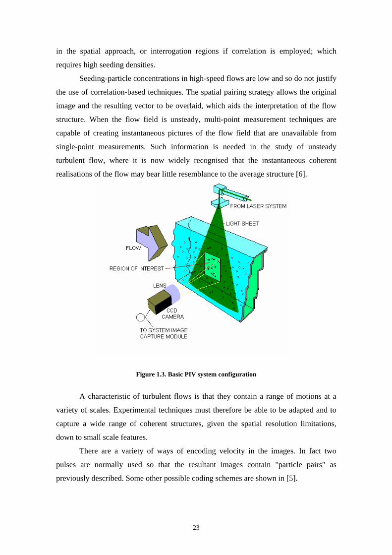
in the spatial approach, or interrogation regions if correlation is employed; which

requires high seeding densities.

Seeding-particle concentrations in high-speed flows are low and so do not justify

the use of correlation-based techniques. The spatial pairing strategy allows the original

image and the resulting vector to be overlaid, which aids the interpretation of the flow

structure. When the flow field is unsteady, multi-point measurement techniques are

capable of creating instantaneous pictures of the flow field that are unavailable from

single-point measurements. Such information is needed in the study of unsteady

turbulent flow, where it is now widely recognised that the instantaneous coherent

realisations of the flow may bear little resemblance to the average structure [6].

Figure 1.3. Basic PIV system configuration

A characteristic of turbulent flows is that they contain a range of motions at a

variety of scales. Experimental techniques must therefore be able to be adapted and to

capture a wide range of coherent structures, given the spatial resolution limitations,

down to small scale features.

There are a variety of ways of encoding velocity in the images. In fact two

pulses are normally used so that the resultant images contain "particle pairs" as

previously described. Some other possible coding schemes are shown in [5].

23

Double-pulsed Pockels or Kerr switched lasers such as Nd/YAG produce high

energies in pulses of very short duration, of the order of 10 to 25ns. Because the

particles being imaged are so small the power supplied by such lasers is a must. This is

related to the light scattering properties of small particles (the Mie light scattering

theory is described in detail in [7]). The particles have to be small to faithfully follow

the flow. Bryanston-Cross & Epstein [8] have explored the subject of visualising such

small particles in PIV.

The Mie theory shows that the size of a sub-micron particle is related

logarithmically to its ability to scatter light. Thus, halving the particle size from 500nm

to 250nm theoretically decreases an order of magnitude the scattered light which can be

collected in the side-scatter mode.

There is a limiting balance between the amount of light scattered from a particle

and the speed and resolution of the film required to image it. It is also known that this is

of particular importance when sub-micron particles are considered [9].

Grant and Smith [10] give a summary of the development of PIV. The history

below is based upon this reference. PIV was first described in papers by Grousson and

Mallick [11], Barker and Fourney [12] and Dudderar and Simpkins [13]. Grousson and

Mallick [11] employed polystyrene spheres of 0.5 µm diameter as a seeding material in

their fluid, and an electro-optic modulator in the path of their 0.8 Watt continuous wave

laser to generate light pulses. A cylindrical lens was used to create the light sheet. The

image of the fluid consisted of a speckle structure. Illumination of the fluid by two

pulses left two mutually displaced speckle patterns upon the film. The displacement is

different for different areas of the flow. The analysis technique employed was based

upon Fourier plane methods. The application of PIV in these first reports was to liquid

flows. Experimental difficulties limited the speed of flows that could be investigated to

the order of millimetres per second and over regions of the order of square centimetres.

Adrian and Yao [14] detailed the differences between the particle image and the

speckle regimes, and discussed the effects of particle scattering characteristics. They

also point out the difference between the techniques to record multiple exposures of the

speckle pattern translation during surface motion and applications involving fluids.

The light scattering characteristics of fluids containing small particles can be quite

different from those of solid surfaces. For example, a pulsed sheet of laser whose

thickness is of the order of 1mm is used to illuminate fluids. Hence scattering occurs

from a volume distribution of particle scattering sites rather than a surface distribution.

24

The particles are typically small (0.1-10 micrometers), and they act as discrete point

sources of scattered light. The density of particles per unit volume and their size can

vary over a very wide range of values, depending upon the fluid and its treatment. For

speckle patterns to exist, the number of scattering sites per unit volume must be so high

that many images overlap creating random phase in the image plane. Since the density

of scatterers in fluids can be quite low, it is possible that speckle is not present in many

fluid applications, and those discrete images of particles are photographed instead. This

then changes the mode of operation from laser speckle velocimetry to particle image

velocimetry. Finally they conclude that the source densities encountered in many air and

water flows of interest in research and practical applications are often not high enough

to produce speckle, and that seeding in large scale flows or high speed flow becomes

increasingly difficult and expensive as the concentration increases.

The intuitively simplest processing method, for resolved particles, is direct

analysis of the PIV negative to determine the distance and direction through which the

particles have translated between exposures. The problem then is to identify a particle

and its partner. In densely seeded flows the probability of mis-matching particle images

is high. One method that helps to resolve this problem is to pulse the laser several times,

to create multiple images of each particle, which provides additional criteria for

allocating particles to unique groups. Alternatively, two pulses of different wavelength

can be used in order to distinguish the first and second partner in the pair, thereby

accounting for any directional uncertainty.

An alternative processing method demonstrated by Meynart [15] uses whole

field analysis of the image by optical Fourier transformation and filtering. This provides

a pattern of fringes that represent iso-velocity contours.

The most appropriate method of analysis depends on the particle density within

the image. In the application of high speed PIV it is difficult and expensive to introduce

the seeding material, which makes images produced from high speed PIV sparse. Due to

the sparse nature of the data, methods which rely upon local statistical averaging of

many particle pairs are not appropriate.

Thus, the two general and powerful analysis methods although of great

theoretical interest, namely a) full two-dimensional correlation in the case of the image

plane, and b) full two-dimensional spectrum analysis of the Young’s fringe pattern in

the case of analysis in the Fourier transform plane, are not applicable to high speed

flows due to the sparse nature of the particle distribution.

25

So, in summary Particle Image Velocimetry was developed from Laser Speckle

Velocimetry in the early 1980s, and has now reached an advanced state. The technology

required to implement PIV is well documented in the literature e.g., Adrian [5]. The

process of velocity measurement with PIV can be divided into the following stages:

1. Seeding of the flow with small, passive tracer particles which follow the motion of

the fluid.

2. Illumination of the measurement area with a two-dimensional pulsed light sheet.

3. Image capture, using either a photographic camera, a video camera or a CCD camera,

with a resolution which allows individual particles to be distinguished.

4. Analysis of the image by dividing it up into a number of small ``interrogation areas'',

and calculating the velocity vector for each interrogation area.

5. Post-processing of the resulting vector map to remove systematic errors, noise and

erroneous vectors.

1.2.2 LASER SPECKLE VELOCIMETRY (LSV)

The system and procedures just described for PIV are similar for Laser Speckle

Velocimetry (LSV). The differences between PIV and LSV rest on the effects of the

mean concentration of scattering particles per unit volume upon the image field and in

relation to the scales of the fluid flow field [5].

In LSV the concentration of scattering particles in the fluid is so large that the

images of the particles overlap on the image plane. The random phase differences

between the images of individual randomly located particles create the random

interference patterns commonly known as laser speckle. The local speckle pattern is the

superposition of images from a local group of scattering particles. Hence, velocity can

be measured by measuring speckle displacement.

LSV has its roots in non-specular objects, where coherent light scattered from

the opaque surfaces forms speckle patterns [16]. Simple manual analysis of a double

exposed specklegram is not feasible, because the human eye cannot untangle the

superposed speckle fields. Analysis of such fields became possible with the

development of the Young's fringe method of interrogation, in which an interrogation

spot on a double-exposed specklegram is illuminated with a laser beam. The speckle

field from the first exposure diffracts the light wave from the coherent interrogation

beam, which interferes with another wave created from the second speckle field

exposure to form a Young's fringe pattern. The orientation of the fringes is

26

perpendicular to the direction of the displacement, and the spacing is inversely

proportional to the magnitude of the displacement. Some practical applications of such

technique to measure fluid velocities are given by Barker and Fourney [12], Dudderar

and Simpkins [13, 17], Grousson and Mallick [11] and Meynart [15,18,19].

1.2.3 LASER DOPPLER VELOCIMETRY (LDV)

Laser Doppler velocimetry is a well-proven technique that measures fluid

velocity accurately and non-invasively [20-24]. LDV makes velocity measurements by

identifying the Doppler frequency shift of scattered laser light from sub-micron sized

particles present and moving within a flow . The exact frequency of the scattered light is

Figure 1.4 . Anatomy of a typical LDA signal burst generated when a particle passes through the

measurement volume determined through the Doppler Effect (figure 1.4). A laser beam illuminates the flow,

and light scattered from particles in the flow is collected and processed. In practice, a

single laser beam is split into two equal-intensity beams, which are focused at a

common point in the flow field. An interference pattern is formed at the point where the

beams intersect, defining the measuring volume (figure 1.5 ).

27

Particles moving through the measuring volume scatter light of varying

intensity, some of which is collected by a photodetector. The resulting frequency shift

of the photodetector output is related directly to particle velocity. If additional laser

beam pairs with different wavelengths (colors) are directed at the same measuring

volume two and even three velocity components can be determined simultaneously.

Figure 1.5 . A single-component dual-beam LDV system in forward scatter mode

Typically, the blue and green or blue, green, and violet lines of an argon-ion

laser are used for multi-component measurements. If one of the beams in each beam

pair is frequency shifted, the LDV system can also measure flow reversals.

LDV provides velocity data at a single point. Using a traverse system to move

the laser source (the measuring volume) point-by-point makes it possible to perform an

area analysis. The technique is non-invasive since laser light is the measuring tool. With

proper experimental design, LDV can reach difficult measurement locations without

disturbing the flow, for instance in moving propeller blades and inside engine cylinders.

LDV works in air or water. It measures over a wide velocity range, micrometers

per second to Mach 8. And it works in many environments, from high temperature to

highly corrosive. LDV has been used successfully in areas as diverse as transonic and

supersonic flows, boundary layers, and flames. It has played a significant role in

designing modern aircraft and ship propellers, ship hulls, aircraft flight structures,

turbomachinery, automobile shapes, hydrofoils, and other products.

28

1.2.4 DOPPLER GLOBAL VELOCIMETRY (DGV)

Doppler Global Velocimetry makes velocity measurements by identifying the

Doppler frequency shift of scattered laser light from sub-micron sized particles present

and moving within a flow. The exact frequency shift of the scattered light is determined

through the Doppler Effect .

Since a global measurement is desired, a sheet of laser light is used to illuminate

the flow field. Frequency discrimination to measure flow velocity values rely on

identifying the scattered light frequency shift. DGV accomplishes this task by using a

unique and key component known as an Absorption Line Filter or ALF. An ALF is

essentially an optical filter assembly. The amount of light passing through the filter will

depend on the frequency of the input light. The DGV illumination laser is carefully

tuned to a frequency which intersects the ALF transfer function at approximately the 50

percent transmission or absorption location. The flow field of interest is then directly

viewed through the ALF. The unique Doppler interaction of the moving particles,

illuminating laser and viewing vectors determine the scattered light frequency. Scattered

light from the illuminated flow field will pass through an ALF with an output intensity

level proportional to the frequency, or most importantly to the particle velocity. The

ALF thus performs a linear frequency - to - intensity conversion over approximately

500 MHz. A normally difficult Doppler frequency measurement has been reduced to a

relatively simple intensity measurement task, as a result of using an ALF.

Wide area, or global, intensity measurements are typically performed using

Charge Coupled Device (CCD) based video cameras. The recorded intensity data, for a

large flow field region viewed through the ALF, can be related to the flow velocity once

the ALF transfer function has been identified through calibration.

DGV, much like other laser based methods, requires the presence of particles

within the flow to make measurements. Direct injection of particles, known as seeds,

into the flow is often necessary since a sufficient number and size of particles may not

naturally exist. The seed size, number, and distribution must be carefully considered in

order to assure good DGV measurements. Particle size and mass will affect both the

scattered light intensity and the ability of the seeds to follow the flow accurately.

Particle number and distribution throughout the flow will affect the data acquisition rate

and the completeness of the global measurements. In general, seeding guidelines

utilised for LDA flow measurements apply.

29

Unfortunately, practical factors prevent perfectly uniform flow field illumination

and seeding. These nonuniformities produce varying scattered light intensities. DGV

measurement errors would result if these intensity variations, as measured by a CCD

camera, were assumed to represent velocity information. To avoid potential problems of

this nature, a second camera is used to measure the simple intensity variations in the

flow field. These recorded intensities are then used to normalize the output from the

other CCD camera and ALF. The normalized ratio of camera outputs thus contains only

velocity information. This technique has been widely used and tested in practical

applications [25-30].

1.2.5 DIGITAL PARTICLE IMAGE VELOCIMETRY (D-PIV) Digital Particle Image Velocimetry (D-PIV) [31] is the digital counterpart of

conventional Laser Speckle Velocimetry (LSV) and Particle Image Velocimetry (PIV)

techniques. In this novel two-dimensional non-intrusive technique, digitally recorded

video images are analysed computationally, removing slow and opto-mechanical

processing steps. Depending on the procedures adopted to analyse the PIV images the

performance of the technique can vary dramatically [32]. The accessibility in terms of

cost to more powerful computers makes it possible to develop very accurate processing

techniques that are leading the technique to the top of the advanced experimental, non-

intrusive, tools for quantitative multidimensional measurements [33-35]. It is

worthwhile to remember that the more accurate the results of a measurement are the

better the basic fluid dynamics phenomena like instability, turbulence and combustion

can be understood. Nowadays, the D-PIV technique is known like conventional PIV.

1.2.6 THREE STATE ANEMOMETRY (3SA) Three-State anemometry (3SA) is a derivative of PIV [36], which uses a

combination of three monodisperse sizes of styrene seeding particles. A marker seeding

is chosen to follow the flow as closely as possible, while intermediate and large seeding

populations provide two supplementary velocity fields, which are also dependent on

fluid density and viscosity.

The compromise required regarding the size of the intermediate and large

particle sub-groups require extensive research to determine the optimum sizes and

proportion in the seeding mixture. The larger particles would provide more sensitivity to

30

viscosity and ease the particle population discrimination requirement, to be able to

separate the three velocities fields. On the other hand, the smaller the particles the more

closely they will follow the flow and therefore will provide more detailed coverage of

the field for all three state variables.

The nature of the particle trajectory, in a free-vortex swirling flow, is to a large

degree governed by the Stokes number: St=(w/v)2 dp, where w is the angular frequency

of the turbulent motion, v is the viscosity and dp is the particle diameter. When this

parameter is less than 0.1, the particle will closely follow the circular fluid streamlines.

When Stokes is larger than 1.0 the particle will be ultimately centrifuged out across the

fluid streamlines in swirling flows. For particle Stokes values higher than 0.1 in high

Reynolds number flows, two extra parameters are required to describe the nature of the

particle trajectory; one essentially dependent on viscosity and the other on density.

Thus, the ideal composition of the seeding mixture depends on the expected radius of

curvature the particles take before being centrifuged out. The Stokes number

considerations determines the upper particle size limit, while discrimination between

particle velocity fields determines the lower limits.

An aspect of the technique, which is of particular importance, is that since three

convolved randomly distributed particle populations are being sampled, the three

measurements will not refer to the same position in space. Therefore, interpolation is

necessary to be able to provide three estimates of the seeding velocities at the same

position. Therefore, a large number of velocity samples are required to provide well-

conditioned velocity field matrices.

A limitation of the 3SA technique is that the larger particle subgroups do not

follow the flow as closely as the flow marker particles by definition, and therefore some

regions of the flow would not be suitably covered by all three seeding populations. In

regions of high turning or back flow, it is very difficult to inject seeding at all, and if

velocity is very low the dynamic range constrains would have to be altered together

with the seeding rate.

31

1.3 FLUID VELOCITY VOLUMETRIC MEASUREMENT TECHNIQUES

1.3.0 STEREOSCOPIC PARTICLE IMAGE VELOCIMETRY

(STEREOPIV)

Stereo PIV is the natural advancement of PIV [37-41]. Stereo PIV is the

determination of the flow velocity in all 3 dimensions rather than two, as was the case in

traditional PIV. To obtain the 3rd component of velocity, it is necessary to use two

cameras or use cunning optical effects.

The PIV data to date has, as yet, inherently been of a two-dimensional nature. In

order to extract the out-of-plane component various authors have concentrated on the

use of geometry in a stereo set-up [42,43]. However, if only triangulation is used, the

relative error in the out-of-plane direction is of the order of three times larger than in the

x-y direction. This effectively makes the whole technique rather unreliable [44,45].

Furthermore, both the relative and absolute co-ordinate systems remain basically

unrelated as the measurements obtained by triangulation are relative between pairs of

particles and have no relation to an absolute frame of reference.

Once initial results were obtained it became clear that, given the large errors in

the out-of-plane direction, the stereoscopic approach to PIV would remain impractical

unless a way was found to increase the accuracy in the z-direction.

One way to increase the accuracy in general, is of course, to increase the angle

subtended by the two cameras. However, this is often not possible in real applications,

as facilities have to be adapted to, and often were not particularly designed for

visualisation purposes. The depth of field required increases as the angle increases

(leading to less photons falling on the imaging sensor), and is further restricted by the

need for simplicity and economy. Furthermore, as the angle increases the absolute

spatial errors also increase; thus denying some of the increase in accuracy.

As mentioned earlier, the spatial approach to PIV has as one of its advantages

the ability to apply fairly intensive processing to the PIV pairs found; thanks to the large

data reduction involved. Now, a digital image is a spatial, intensity and temporal

quantized representation of a real-world scene. The precise representation of position is

critical to the successful extraction of velocity data from a PIV image. For a reliable

PIV to approach the precision of a photographic image, accurate sub-pixel position

32

estimates are necessary. Otherwise, the large number of required digital images

represent un-surmountable problems of registration, data volume and throughput.

Note that in order to simplify the discussion, the centre of the Nd/YAG sheet and

the centre of focus are made co-incident, and the depth of view is made somewhat larger

than the width of the light sheet. Thus, the amplitude can be seen to depend on the z-

position of the particle, and varies according to the change in intensity of the laser over

the depth of the region of interest. On the other hand, the amplitude varies

approximately linearly with respect to the z-position in relation to the position of focus.

It has been found that the behaviour is not strictly linear but that a linear approximation

is sufficient for the accuracies quoted. This focal length can be accurately calculated for

a given objective in the case of the K2 diffraction limited optics.

This technique has two major advantages. Firstly, it provides three measures for

the z-component. Two from the depth ratio from each image in a stereo case, and the

third from triangulation. Just as importantly though, it provides a way in which these

relative velocity measurements can be related to an absolute frame of reference. The

depth ratio will exhibit a maximum where the particle is in line with the focal length of

the lens, and will then tail off as a particle moves in front or behind this position. Thus,

the system has symmetry about this focal length leading to an ambiguity in the

measurement of the depth ratio. In order to account for it, triangulation needs to be used

as well. Thus if a particle pair lies in a equidistant position from this axis, the ratio will

be equal but triangulation will show one to lie ahead of the other, thus enabling the data

to be unscrambled.

Stereo PIV appears to be a robust and well researched method. However various

problems and sources of inaccuracies must be looked into. These problems, which are

outlined in greater detail in Adrian [5], include:

1.The particle accurately following the fluid flow.

2.The particle reflecting enough light for it to be observed.

3.Aberrations caused by the optics within the stereo PIV system.

4.The sub-pixel accuracy of the system. There are various techniques such as;

Gaussian fitting, and centre of mass estimations, to increase the accuracy in the

measurement of the distance that the particle has travelled [46].

33

1.3.1 HOLOGRAPHIC PARTICLE IMAGE VELOCIMETRY

(HOLOGRAPHIC PIV)

Holography is best known for its ability to reproduce three-dimensional images.

However, it has many other applications. Holographic non-destructive testing is the

largest commercial application of holography. Holography can also be used to make

precise interferometric measurements, pattern recognition, image processing,

holographic optical elements (eg. complex spatial filters), and storage of data and

images.

Any propagating wave phenomenon, such as microwaves or acoustic waves, is a

candidate for application of the principles of holography. Most interest in this field has

centred on waves in the visible portion of the spectrum, and to use it in the area of flow

visualisation with PIV.

There are several well-known difficulties in forming and analysing holographic

particle data in the sub-micron range. It is suggested that these problems can be

overcome by using a combination of research techniques. First, it has been found that it

is possible to record images of sub-particles using conventional photographic materials.

Essentially, a diffraction limited optical component has been used to provide aberration

free particle images. Second, the sensitivity of the holographic material has been

increased with the use of specialised holographic processing chemicals. Third, it has

been found that it is possible to encode holographically double, slightly displaced,

particle images using a pulsed laser. Thus Young’s fringes can be obtained directly

from the stored holographic data and the particle velocity can be measured directly from

the hologram. Fourth, the holographic particle data can be automatically analysed using

a software program. Finally, since the data is stored holographically, it is possible to

obtain instantaneous 3-D particle velocity. Developments and applications can be found

in references [47-52].

1.4 CONCLUSIONS Different methods and techniques to measure fluid flow velocities are described

in this chapter. However, each one is used for different applications and conditions. No

one can measure the 3D instantaneous velocity vector in an industrial application. Some

of them are point wise techniques while others measure with in-plane sensitivity. The

volumetric techniques showed to distinctive restrictions. Holography is practical in

34

laboratory controlled environments, but not in hostile conditions. Stereo PIV requires

multiple optical access, so it is impractical for industrial applications.

1.5 REFERENCES 1. Oldfield M.L.G, “Experimental Techniques in Unsteady Flows”, Lecture Notes for

the VKI lectures on Unsteady Aerodynamics, April 18-22, 1988.

2. Hince, J. O., Turbulence, 2n ed., McGraw-Hill, New York, 1975.

3. Dare, J. A., Notes for experiments, Department Of Aerospace And Ocean

Engineering, Virginia Tech., 1996.

4. Föster W., Karpinsky G., Krain H., Röhle I., and Schodl R., “3-Component-

Doppler-Laser-Two-Focus Velocimetry Applied to a Transonic Centrifugal

Compressor”, Tenth International Symposium on Applications of Laser Techniques

to Fluid Mechanics, Instituto Superior Tecnico, LADOAN, Lisbon, July 10-13,

2000.

5. Adrian, R. J., "Particle-Imaging Techniques For Experimental Fluid Mechanics",

Annual Review of Fluids Mechanics, Vol. 23, pp. 261-304, 1991.

6. Nixon(ed.) D., "Unsteady Transonic Aerodynamics", Vol. 120, AIAA, 1989.

7. Mie, G., "Beiträge zur Optik trüber Medien, speziell kolloidaler Metallösungen",

Ann. Phys. 25, 377-445, 1908.

8. Bryanston-Cross P.J. and Epstein, A., "The application of sub- particle visualisation

for PIV (Particle Image Velocimetry) at transonic and supersonic speeds", Prog in

Aerospace Sci. 27, pp. 237-340, 1990.

9. Bryanston-Cross, P.J., Harasgama, S. P., Towers, C. E., Towers, D. P., Judge, T. R.,

and Hopwood, S. T. “The Application of Particle Image Velocimetry (PIV) in a

Short Duration Transonic Annular Turbine Cascade”, Journal of Turbomachinery,

Vol.114, No.3, pp504-510, July 1991.

10. Grant I. and Smith G. H., “Modern Developments in Particle Image Velocimetry”,

Optics and Lasers in Engineering, Vol. 9, pp. 245-264, 1988.

11. Grousson R. and Mallick S., “Study of Flow Patterns in a Fluid by Scattered Laser

Light”, Applied Optics, Vol. 16, pp. 2334, 1977.

12. Barker D. B., and Fourney M. E., “Measuring Fluid Velocities with Speckle

Patterns”, Optics Letters, Vol. 1, pp. 135, 1977.

35

13. Dudderar T. D., and Simpkins P. G., “Laser Speckle Photography in a Fluid

Medium”, Nature, Vol. 270, pp. 45, 1977.

14. Adrian R.J. and Yao C.S., “Pulsed Laser Technique Application to Liquid and

Gaseous Flows and the Scattering Power of Seed Materials”, Applied Optics, Vol.

24, pp. 44-52, 1985.

15. Meynart R., “Equal Velocity Fringes in a Raleigh-Bernard Flow by a Speckle

method”, Appl. Opt., 19, pp.1385-1386, 1980.

16. Archbold E. and Ennos A.E., “Displacement measurement from double-exposure

laser photographs”, Optica Acta, Vol. 19(4), pp. 253-271, 1972.

17. Dudderar T. D., and Simpkins P. G., ”Laser Speckle measurements of transcient

Bénard convection”, Journal of Fluid Mechanics, Vol. 89(4), pp.665-671, 1978.

18. Meynart R., “Instantaneous Velocity Field Measurement in Unsteady Gas Flow by

Speckle Velocimetry”, Applied Optics, Vol 22(4), pp. 535-540, 1983.

19. Meynart R., “Speckle Velocimetry Study of Vortex pairing in a Low-Re unexcited

jet”, Physcics of Fluids, Vol. 26(8), pp. 2074-2079, 1983.

20. Gartrell Luther R., Tabibi Bagher M., Hunter William W. Jr., Lee Ja H. and Fletcher

Mark T. , Application of Laser Doppler Velocimeter to Chemical Vapor Laser

System , NASA TM-4409, January 1993.

21. Sellers William L. III, Meyers James F. and Hepner Timothy E., “LDV Surveys

Over a Fighter Model at Moderate to High Angles of Attack”, SAE Aerospace

Technology Conference and Exposition, Anaheim, California, SAE Paper No.

881448, October 3-6, 1988.

22. Podboy Gary G., Bridges James E., Saiyed Naseem H., and Krupar Martin J. “Laser

Doppler Velocimeter System for Subsonic Jet Mixer Nozzle Testing at the NASA”,

Lewis Aeroacoustic Propulsion Lab. Prepared for the 31st Joint Propulsion

Conference and Exhibit cosponsored by AIAA, ASME, SAE, and ASEE, July 10-

12, 1995, San Diego, California.

23. Gartrell Luther R., Tabibi Bagher M., Hunter William W., Jr., Lee Ja H., and

Fletcher Mark T., “Application of Laser Doppler Velocimeter to Chemical Vapor

Laser System”, NASA Technical Memorandum 4409 JANUARY 1993.

24. Neuhart Dan H., Wing David J. and Henderson Uleses C. Jr., “Simultaneous Three-

Dimensional Velocity and Mixing Measurements by Use of Laser Doppler

Velocimetry and Fluorescence Probes in a Water Tunnel”, NASA TP-3454 ,

September 1994.

36

25. Meyers James F., “Technology and Spin-Offs From Doppler Global Velocimetry”,

12th International Symposium on the Unification of Analytical Computational and

Experimental Solution Methodologies, Worcester, Massachusetts, July 6-8, 1995.

26. Meyers James F., “Development of Doppler Global Velocimetry for Wind Tunnel

Testing”, AIAA 18th Aerospace Ground Testing Conference, Colorado Springs,

Colorado, AIAA-94-2582, June 20-23, 1994.

27. Meyers James F., Lee W., Fletcher Mark T. and South Bruce W., “Hardening

Doppler Global Velocimetry Systems for Large Wind Tunnel Applications”, 20th

AIAA Advanced Measurement and Ground Testing Technology Conference,

Albuquerque, New Mexico, AIAA 98-2606, June 15-18, 1998.

28. Meyers James F. and Komine Hiroshi, “Doppler Global Velocimetry---A New Way

to Look at Velocity”, 4th International Conference on Laser Anemometry---

Advances and Applications, Cleveland, Ohio, August 5-9, 1991.

29. Gorton S. A., Meyers J. F. and Berry J. D., “Laser Velocimetry and Doppler Global

Velocimetry Measurements of Velocity Near the Empennage of a Small-Scale

Helicopter Model”, 20th Army Science Conference, Norfolk, Virginia, June 24-27,

1996.

30. James F. Meyers, “Doppler Global Velocimetry - The Next Generation?”, AIAA

17th Aerospace Ground Testing Conference, Nashville, Tennessee, AIAA 92-3897,

July 6-8, 1992.

31. J. Westerweel, “Fundamentals of Digital Particle Image Velocimetry”, meas. Sci.

Technol. 8, pp. 1379-1392, 1997.

32. Funes-Gallanzi, M., “High Accuracy techniques Applied to the Extraction of

Absolute Position Estimation in DPIV systems”, VII International Symposyum on

Applications of Laser Techniques to Fluid Mechanics, Lisbon, July, 1994.

33. Willert, C. E. and Gharib, M. ”Digital particle image velocimetry”, Experiments in

Fluids, Vol. 10, no. 4, p. 181-193, 1991.

34. William M. Humphreys, Jr., Scott M. Bartram, Tony L. Parrott and Michael G.

Jones, “Digital PIV Measurements of Acoustic Particle Displacements in a Normal

Incidence Impedance Tube”, 20th AIAA Advanced Measurement and Ground

Testing Technology Conference, Albuquerque, New Mexico, AIAA 98-2611, June

15-18, 1998.

37

35. Bruecker, CH. ”Digital-Particle-Image-Velocimetry (DPIV) in a scanning light-

sheet: 3D starting flow around a short cylinder”, Experiments in Fluids, Vol. 19, no.

4, p. 255-263, 1995.

36. Funes-Gallanzi, M. " A novel fluids research Technique: three state anemometry",

International Gas Turbine and Aeroengine Congress & Exhibition, Birmingham,

UK, June 10-13, 1999.

37. Funes-Gallanzi M. and Bryanston-Cross P.J., “Solid State Visualization of a highly

three dimensional flow using stereoscopic Particle Image Velocimetry (3DPIV)”,

SPIE Vol. 2005, pp.360-369, 1995.

38. Westerweel J. and Nievwstadt F.T.M., “Performance test on 3-Dimensional

Velocity Measurements with a two Camera digital particle-image velocimeter”,

Laser Anemometry Vol. 1 ASME, pp.349-355, 1991.

39. Arroyo M.P. and Greated C.A., “Stereoscopic Particle Image Velocimetry”, Meas.

Sci. Technol. 2, pp. 1181-1186, 1991.

40. Prasd A.K. and Adrian R.J., “Stereoscopic Particle Image Velocimetry Applied to

Liquid Flows”, Experiments in Fluids, Vol. 15, pp.49-60, 1993.

41. Hinsch K.D., “ Three Dimensional Particle Velocimetry”, Meas. Sci. Technol. Vol.

6, pp. 742-753, 1995.

42. Willert C., “Stereoscopic Digital Particle Image Velocimetry for Application in

Wind Tunnel Flows”, Meas. Sci. Technol. Vol 8, pp. 1465-1479.

43. Lecert A., Renou B., Allano D., Boukhalfa A. and Trinité M., “Stereoscopic PIV:

Validation and Application to an Isotropic Turbulent Flow”, Experiments in Fluids,

pp. 107-115, 1999.

44. Lawson N.J. and Wu J., “ Three Dimensional Particle Image Velocimetry:

Experimental Error Analysis of a Digital Angular Stereoscopic System”, Measc.

Sci. Tech. Vol. 8, pp.1455-1464, 1997.

45. Blostein S.D. and Huang T.S., “ Error Analysis in Stereo Determination of 3D Point

Positions”, IEEE Transactions on Pattern Analysis and Machine Intelligence,

Vol.PAMI-9, No. 6, 1987.

46. Burnett, M., ‘Methods of Quantitative Flow Visualisation,’ MRes paper, University

of Warwick, 1996.

47. Bryanston-Cross P.J., Funes-Gallanzi M., Quan C. and Judge T.R., “ Holographic

Particle Image Velocimetry (HPIV)”, Optics and Laser Technology, Vol. 24(5),

pp.251-256, 1992.

38

48. Malyak P.H. and Thompson B.J., “Particle Displacement and Velocity

Measurement Using Holography”, Optical Engineering, vol 23(5), pp.567-576,1984.

49. Judge T.R., Quan C. and Bryanston-Cross P.J., “Holographic Deformation

Measurements by Fourier Transform Technique with Automatic Phase

Unwrapping”, Optical Engineering, Vol. 31(3), pp.533-543, 1992.

50. Trolinger J.D., “ Diagnostics of Turbulence by Holography”, Advances in Laser

Technology for Atmospheric Sciences, SPIE, vol 125, pp. 105-113, 1997.

51. Fabry E.P., “ 3D Holographic PIV with Forward-Scattering Laser Sheet and

Stereoscopic Analysis”, Experiments in Fluids, vol 24, pp. 39-46, 1998.

52. Royer H., “ Holography and Particle Image Velocimetry”, Meas. Sci. Technol., Vol.

8, pp. 1562-1572, 1997.

39

CHAPTER II

PRESSURE AND TEMPERATURE MEASUREMENTS

2.0 INTRODUCTION

Because temperature affects material properties, there are numerous methods for

measuring temperature [1]. The simplest methods employ thermal expansion. The most

common electrical-based sensors are thermocouples and resistance elements. Optical

methods such as liquid crystals, infrared detectors and thermographic phosphors have

the advantage of non-contact measurement. They can provide a two-dimensional

temperature field over a surface. However it is more difficult to obtain absolute

temperatures and they require more sophisticated data acquisition equipment.

Pressure is defined as the normal force per unit area acting upon some real or

imaginary boundary. The static pressure, p, in a fluid stream is the normal force per unit

area on a boundary moving with the flow. Assuming local thermodynamic equilibrium,

this definition is consistent whit the thermodynamic definition of pressure.

Many convenient and useful temperature sensing devices, based on the

phenomenon of thermal expansion of the materials, may be found for a specific

temperature range. Most common ones are the liquid-in-glass thermometers,

particularly the mercury-in-glass thermometer, which has an operating temperature

range from the freezing point to the boiling point. The latter can be increased by

pressurising the inert gas in the capillary space above the liquid.

Pressure thermometers, which are widely used in industrial applications, consist

of three basic elements: a sensitive bulb containing a liquid, gas or vapour, an

interconnecting capillary tube, and a pressure-sensing devise such as a Bourdon tube.

Temperature variations in the bulb results in a volume change of the fluid, causing a

pressure change which can be calibrated to record the temperature variation.

The phenomenon of thermal expansion in metals is employed in bimetallic

thermometers. When two strips of metals with different thermal expansion coefficients

are bonded together, a change in temperature will result in a deflection of the strip due

to differential expansion. This kind of thermometers have an operating temperature

range of about 200-810 K.

40

The most important of all temperature sensors is the thermoelastic sensor,

commonly known as the thermocouple. The operating principle is as follows: when two

wires of dissimilar metals, A and B, are joined to form a circuit with the two junctions

maintained at two different temperatures T1 y T2, an electromotive force E is obtained,

wich can be measured by a voltmeter or potentiometer.

The electrical resistance of most materials changes with temperature. Due to the

fact that electrical circuits for measuring resistance are common, this is an easy method

for measuring temperature. The resulting sensors have a variety of names. RTD's

generally refer to metal wires wrapped around an insulator to minimise the effects of

strain. An RTS usually refers to a metal thin film deposited in an insulator to give fast

time response. The resistance measurement is usually performed by passing a small

known current through the resistor and monitoring the corresponding voltage drop.

All these techniques are point wise and do not provide an area temperature map.

In compressible flows the density changes with velocity to give measurable

results in the variation of the refractive index so the temperature can be inferred from it.

For compressible flows, such as free convection where the velocity is relatively low, the

density, and hence the refractive index is directly related to temperature. Methods for

observing this density variation include Schlieren, shadowgraph and some

interferometric techniques. In these methods, light and dark patterns are formed by the

bending of light as it passes through a region of varying density.

A Schlieren arrangement is illustrated in figure 2.1. A light source such as an arc

lamp is focused onto one point at the same distance from the two lenses, and through

the gas or flame. A camera behind a knife-edge is focused onto the test object and can

record the deviation of the light due to changes in the refractive index [2,3].

Tomographic or temperature mapping utilising Schlieren methods have been reported

by Schwarz [4].

In the shadowgraph method, the linear displacement of a perturbed light beam is

observed, rather than the angular deflection as in the Schlieren method [2].

In the Mach-Zender interferometric technique (figure 2.2) a beam of light is split

in two, with one beam avoiding the test section called the reference beam, and the other

beam falling through the test section, also called the object or measuring beam. The

splitter plate near the screen is used to combine and convey the beams onto it for optical

mixing and recording. Light and dark patterns are formed as a result of phase shifts

between the reference and measuring beams.

41

Figure 2.1 Schlieren method for determining gas temperature.

figure 2..2. Mach-Zender interferometer for gas temperature measurement, [1]

2.1 PARAMETER SENSITIVE PAINTS Parameter sensitive paints are luminescent coatings engineered such that the

luminescence is a function of pressure, temperature, strain, or some other parameter of

interest. By measuring some characteristics of luminescence (intensity of lifetime) the

corresponding parameter can be determined. The concept of this method was invented

in the Central Aerohydrodynamic Institute (TsAGI) of Russia, with the idea to use this

phenomenon for pressure measurements in experimental aerodynamics, by G. Pervushin

and L. Nevsky [5].

Gas orflameLens

Background source

Camera

Monochromatic Light source

Lens

Splitter plate Mirror

Screen

Splitter plate Mirror

Gas orflame

Lens Knife edge

42

Several types of parameter sensing paints are under development, the most

mature of these are the Pressure Sensitive Paint (PSP) and the Temperature Sensitive

Paint (TSP) [6,7]. Both types of paints can be used with the same set of excitation

lamps, detectors, computer hardware, and software. The main difference is that PSP

contains a luminescent compound that is sensitive to local pressure, and TSP contains a

luminescent compound that is sensitive to local temperature.

2.2 PRESSURE SENSITIVE PAINT (PSP) The ability to determine instantaneous two-dimensional pressure distributions on

the surface of a structure in test facilities like wind tunnels or turbomachines, by

applying pressure-sensitive paint (PSP), is a major advance in the field of non-contact

measurement techniques in aerodynamics. This so-called PSP method allows one to

obtain not only qualitative pressure images, but also quantitative absolute pressure

values at the desired locations on the structure, without introducing flow-disturbing

probes or affecting the surface of the structure [8]. Such a fluorescent image arising

under the flow conditions in a wind tunnel can be recorded using a CCD camera (in the

intensity method) or a photomultiplier with an appropriate filter for the luminescent

emission (in the lifetime method). The final pressure map is obtained using complex

image processing techniques.

Impurities, such as oil, solvents or large dirt particles in the test facility can

adversely affect the achievable accuracy and can also damage the optical pressure

sensor.

Conventional pressure measurement methods, based on pressure sensors

installed at discrete points on the structure surface, may give better accuracie of

measurement, but the two-dimensional PSP method has definite advantages. Firstly, in

the case of these conventional techniques there are restrictions to creating holes on a

thin wind tunnel structure; secondly the deformation of the structure due to several

holes, and the geometry change associated with them due to the wind forces, leads to

increased measurement errors.

The determination of the hole locations at the points of measurement must also

be done prior to the preparation of the structure, that is, without exact knowledge of the

flow pattern which will be occurring later.

43

Other methods of flow visualisation on the structure surface, such as the use of

oil or phenol coatings, indeed give information on the wall streamline, but allow no

quantitative expression of the pressure distribution. On the other hand, they facilitate the

recognition of flow separation as well as the laminar–turbulent flow changeover.

2.3 TEMPERATURE SENSITIVE PAINT (TSP) Temperature Sensitive Paint is a luminescent paint good enough to determine

surface temperature distributions. TSP may be used for visualisation of heat transfer

rate, boundary layer transition, flow separation and flow reattachment on the structure

in transonic, supersonic and shock wind tunnels.

This technique is very similar to PSP except that the coating is temperature sensitive

rather than pressure sensitive. The luminescence of TSP decreases as the temperature

increases. As in PSP, a ratio of two images provides the temperature. In this case, one

image is taken at a known, constant temperature, and the other is taken at the unknown

conditions. The ratio of the two images is then converted to temperature using the

appropriate calibration (which is too, close to PSP). As in PSP testing, during the

acquisition of the images the test surface is exposed to excitation light in only a narrow

frequency band. The detector is then notch filtered to pass only the luminescence band

for the luminescent molecule.

Temperature sensitive paint (TSP) has recently been used to detect small temperature

differences on aerodynamic structure surfaces [9]. These types of applications impose

stringent performance requirements on a paint system. The TSP must operate over a

broad temperature range, must be physically robust, must be polishable to at least the

smoothness of the structure surface, must be easily applied over a large surface area,

must be removable without damaging the structure surface finish to which it is applied,

and must have sufficient sensitivity to detect small temperature differences.

2.4 TSP AND PSP PHYSICAL PRINCIPLES The PSP measurement procedure is based on the deactivation of

photochemically excited molecules, i.e. luminophores by oxygen molecules. By means

of a special technique and application of suitable optical systems, static pressure values

can be measured on the surface of the structure in the test facility (wind tunnel) and the

flow phenomena can be assessed quantitatively. However, the precise determination of

44

pressure needs a measurement system with a high local resolution capability, as

required in the transonic velocity range. Most PSP and TSP formulations use organic

luminophores [10]. A molecule absorbs a photon [11] ultraviolet or blue (see figure 2.3

for TSP and figure 2.4 for PSP excitation and emission responses) and jumps to an

excited energy level. There is a finite probability that the excited molecule will emit a

photon at a longer wavelength, generally red, and collapse to the ground state.

Figure 2.3. Emission and excitation spectra of Temperature Sensitive Paint TSP E40 from Optrod, Ltd.

There is also a finite probability that the excited molecule will interact with

nearby molecules so that the excited molecule drops to ground state without emitting a

photon. This process is commonly called "internal conversion". For some paint

mixtures, the probability of internal conversion depends on temperature. As temperature

increases, collision frequency increases, and the probability of internal conversion

increases. Conversely, the probability of emitting a photon decreases, and the intensity

of luminescent emission decreases. This phenomena is called thermal quenching and

forms the basis for temperature sensitive paints. For a typical TSP, the brighter the

surface, the lower the temperature.

Some paints have a small dependence on temperature. The probability of

internal conversion depends strongly on the types of molecules in the paint film and the

type of supporting polymer. For some luminescent molecules, if an oxygen molecule

45

collides with an excited probe molecule, the probability of deactivation is very large.

This deactivation mechanism is commonly called oxygen quenching. The presence of

oxygen reduces the probability of emission. If the paint is permeable to oxygen, then the

number density of oxygen molecules inside the paint film depends directly on the partial

pressure of oxygen at the paint surface. This quenching phenomenon forms the basis for

a pressure sensitive paint. For a typical PSP, the brighter the surface, the lower pressure.

Figure 2.4. Emission spectra of different kinds of PSP also called Luminescent Pressure Sensor

LPS, by Optrod Ltd.

2.5 CALIBRATION OF PRESSURE/TEMPERATURE SENSORS Engler et al [12], showed that calibration of the optical pressure sensor is

necessary for reconstructing a quantitative pressure image from the initial qualitative

image of the flow phenomenon on the surface of the structure. This can be done in two

different ways. In the first method, a test specimen is calibrated parallel to the structure

paint and subsequently subjected to known pressures and temperatures in an external

calibration chamber. In the second method, the entire structure can be calibrated in the

wind tunnel itself, provided pressure changes can be statically produced at constant

temperature in the test section. In the external calibration chamber the pressure and

46

temperature can be varied and consequently the temperature-dependent calibration

constants described can be determined and related to pressure reconstruction. When

large temperature distribution effects exist on the structure surface it is necessary to

correct the pressure computations using thermocouples or IR cameras. The disadvantage

of an external calibration procedure is that the test specimen can indeed be painted

simultaneously with that of the structure, but will definitely not possess identical optical

properties to the latter due to possible differences in the thicknesses of the layers.

Therefore, if possible, direct calibration of the model is always preferable, since

the peculiarities of the structure geometry and the layer thickness are automatically

taken into account. A special calibration cuvette must be mounted in direct contact with

the model surface in which the pressure and temperature can be controlled. In addition,

for every angle of attack of the structure a separate calibration data set can be

calculated. Besides, there is the advantage that a separate calibration data set is available

for each pixel of the recorded image of the wind tunnel model and therefore a higher

pressure resolution is possible.

Oglesby, et al [13] discuss the dependence of the relative error in pressure with signal

intensity, and a sensitivity analysis of the PSP technique.

2.6 CONCLUSIONS The techniques, other than optical, just described are point wise and do not

provide an area map for temperature/pressure. Optical techniques are non-contact and

give two dimensional temperature/pressure measurements requiring special conditions

to operate. Some fluid temperature measurement techniques that detect variations of the

refractive index are inadequate for practical applications due to instability conditions.

TSP and PSP are simple and non-expensive measurement techniques that gives

three-dimensional temperature and pressure data. The two techniques can be used in

conjunction with velocimetry techniques.

2.7 REFERENCES 1. Childs P. R. N., Greenwood J. R. and Long A.., "Review of temperature

measurement.", Review of Scientific Instruments, v 71, pp.2959-2978, 2000.

47

2. Goldstein R. J., "Optical Measurement of Temperature," Measurement techniques in

Heat Transfer, edited by E. R. G. Eckert and R. J. Goldstein (AGARD, Slough,

1970), pp. 177-228.

3. Gaydon A.G. and Wolfhard H.G., Flames. Their Structure, Radiation and

Temperature (Chapman and Hall, London, 1979).

4. Schwarz A., "Multi-tomographic Flame Analysis with a Schlieren Apparatus,"

Meas. Sci. Technol. Vol.7, pp. 406-413, 1996.

5. Pervushin G.E. and L. Nevsky B., " Composition for Indicating Coating.", Patent of

USSR – SU 1065452 A, 1981 (In Russian).

6. McLachlan, B.G. and Bell, J.H., "Pressure-Sensitive Paint in Aerodynamic Testing."

Exp. Thermal and Fluid Science, Vol. 10, pp. 470-485.1995

7. Tianshu Liu, Campbell, B.T., Burns, S.P. and Sullivan, J.P.,"Temperature- and

Pressure-Sensitive Luminescent Paints in Aerodynamics.", Appl. Mech. Rev., Vol.

50, no. 4. (1997)

8. Navarra K., “Development of the pressure-sensitive paint technique for advanced

turbomachinery applications”, Master of Science Thesis, Faculty of the Virginia

Polytechnic Institute and State University, Blacksburg, VA,1997

9. Donald M. Oglesby, Billy T. Upchurch, Bradley S. Sealey, Bradley D. Leighty,

Cecil G. Burkett, Jr. and Amir J. Jagharghi, "Development Of Temperature

Sensitive Paints For The Detection Of Small Temperature Differences" , Isa 43rd

International Instrumentation, Symposium, Orlando, Florida, May 4-8, 1997.

10. Lumb, M. D., "Organic Luminescence", published in Luminescence Spectroscopy,

Academic Press, 1978, pp 94-146.

11. Crites R. and Morris M., "Parameter Sensing Paints-Current Capabilities and Future

Potencial", McDonnell Douglas Aerospace, McDonnell Douglas Corporation. St.

Louis, Missouri USA.

12. Engler R H, Klein Chr and Trinks O, "Pressure sensitive paint systems for pressure

distribution measurements in wind tunnels and turbomachines",Meas. Sci. Technol.

11 (2000) 1077–1085.

13. Donald M. Oglesby, Chith K. Puram and Billy T. Upchurch, "Optimization of

Measurements With Pressure Sensitive Paints", NASA Technical Memorandum

4695, Old Dominion University Norfolk, Virginia.

48

CHAPTER III

PATTERN DIFFRACTION ANALYSIS

3.0 INTRODUCTION Conventional velocimetry has an intrinsic limitation because it yields 2D data,

neglecting the third velocity component. For this reason, 3D-PIV has recently evolved

as an area of research [1-16], with success at the cost of increasing complexity in its

methodology. The increased complexity and the limited optical access found in most

industrial applications, mean that many of the 3D-PIV techniques, although of academic

interest, cannot be used in practical industrial applications. Some of the techniques used

involve scanning light-sheets, stereoscopic views, holographic recording, parallel light-

sheets, graded intensity light-sheets, or combinations thereof.

For practical applications restricted viewing eliminates stereoscopic approaches.

Lack of robustness and ease to perform an experiment make of conventional holography

an unattractive option due to the fact that it involves a wet developing process, thus is

very slow to yield results. However, its large depth of field and storing capacity makes

it a technique that should, under the correct environment, be used. When holography is

used, the hologram is interrogated with the aid of cameras mounted on a high-precision

3D positioning system to resolve position based on particle image information.

Scanning light-sheets are difficult to obtain for restricted optical access and high speeds,

so they have not been tried in industrial conditions.

CCD cameras are nowadays being used as image recording medium, replacing

conventional storage medium. Restricted optical access to flows of interest, such as

those found in turbomachinery, means that only one camera is often what can be

accommodated. An extension to the high-accuracy techniques for 3D, exploiting the

digital representation of particle images in intensity as well as spatially, is described in

previous work [17]. The analysis of digital PIV data typically involves two quantization

steps: spatial and intensity quantization. It is of crucial importance to have reliable error

bounds and a sufficiently accurate estimate of particle position, taking into

consideration both types of quantization. The approach of using the Gaussian profile of

the particle images to yield sub-pixel accurate position estimates has resulted in robust

49

measurements being taken to an accuracy of 1/10th pixel and 1% in velocity for the in-

plane velocity, even in hostile industrial environments. The out-of-plane velocity

estimate can be derived from the change in the ratio of amplitude to variance - known as

the depth factor - of the Gaussian form, as a particle traverses the beam profile.

However, such measurements are crucially dependent not only on an accurate position

estimate but also on an equally accurate estimate of the amplitude and variance. The

accuracy of the Gaussian profile fit using a Nelder-Meade optimization method was not

capable of providing the required accuracies. Therefore, a development of the "locales"

approach to position estimation was presented to achieve the desired objective of high

accuracy PIV measurements. This approach makes use of the fact that by considering

the possible digital representations of the Gaussian particle profile, regions of

indistinguishable position can be derived. These positions are referred to as "locales".

By considering the density, distribution, and shape of these locales, the available

precision can be estimated and a high in-plane velocity accuracy can be obtained, while

at the same time providing high-accuracy estimates of the depth factor. This work

described the implementation of an efficient algorithm to provide velocity estimates,

together with a discussion of the required constraints imposed on the imaging. The

algorithm was used to map an experimental transonic flow field of the stator trailing

edge region of a full-size annular cascade with an estimated error of 0.5%. The

experimental results were found to be in good agreement with a previously reported

steady state viscous calculation and PIV mapping. This work has been extended to a

model, using simplified Fraunhoffer particle diffraction, for pattern-matching low-

magnification 3D particle positioning, where particles are illuminated by

monochromatic light [18]. Detailed theoretical models will then be useful for examining

the effect of changing the aperture size on the observed particle images, the nature of

image quality variation with the degree of particle defocus, etc. The most advanced such

model is that based on the Generalised Lorenz-Mie theory which takes into account

typical wave-fronts occurring in velocimetry applications, such as that of a light sheet

which is elliptical, rather than the simple plane wave-front assumption of classical

Lorenz-Mie theory. These models need to be validated against experimental data, so

they may be used to find out what parameters are more important and therefore require

further modelling, in order to achieve a quantitatively accurate representation of

diffraction for a given position and particle characteristics.

50

The case of a spherical absorbing particle illuminated with monochromatic

coherent light is considered. Three different illumination wavefront shapes and three

viewing positions are used, and their relative merit is studied. The data obtained has

been used to validate a model of particle scattering. An experimental 18 μm glass

sample image is quantitatively compared to the calculated image for a Gaussian

wavefront in forward scatter. This sample image in this viewing configuration has been

chosen and described by a number of authors [19-23] and therefore was chosen as the

sample case for the present research.

3.1 DIFFRACTION THEORY. Adrian & Yao [24] first proposed using a quadrature to derive a nominal particle

image diameter de according to:

)( 222spe ddMd += (1)

where M is the lateral magnification of a lens, and dp is the particle diameter.

In this equation

/#)1(44.2 fMds λ+= (2)

is the diameter of the point response function of a diffraction-limited lens measured at

the first dark ring of the intensity distribution of the Airy disk, λ is the wavelength of

the laser light used, and the focal length of the lens divided by the aperture diameter is

f/#. As defined here, ds may also be regarded as equal to the mean diameter of a laser

speckle. Equation (1) shows the combined effects of magnification and image blurring

and is an approximate quadrature determining the final diameter of the image. If the

point response function and the geometric image were both Gaussian, equation (1)

would be exact. In fact a Gaussian intensity distribution has been widely used as an

adequate approximation to the Airy intensity distribution for velocimetry applications.

Hence, equation (1) was used as an approximation, assuming the geometric image

distribution is not too different from a Gaussian distribution function.

This approach represents a compromise between geometrical optics and a simplified

approximation to the Lorentz-Mie Theory (LMT). However, the former is only valid

51

when the wavelength λ is much smaller than a length given by the standard deviation of

surface roughness (scattering size), i.e., for optically smooth surfaces, and the latter is

valid only when the particle is illuminated by a plane wave. The plane wave

assumption holds when the scattering size of the particle is small compared to the

characteristic dimensions of the incident beam, however in many cases this condition is

not satisfied. Even if the plane wave assumption holds in a velocimetry set-up, the

orientation of this wave-front relative to the viewing camera, generally changes across

the field of view in such a way that major corrections are required for each particle’s

scattered image because particles are away from the optical axis and intensity

distributions are not uniform over the whole image. This effect may not be readily

apparent in applications involving thin light sheets and small particles, viewed by

imaging lenses focussed on said light sheet, where the particle image approximates a

Gaussian function and it is only a few pixels in diameter. However, where larger

illumination depths are used the particle image diameter quickly extends substantially.

Even for thin light sheets, where the CCD camera is adjusted so it saturates at the higher

light intensities, diffraction rings become visible and these vary substantially with

particle position within the light sheet down to a movement of as little as 20 μm.

An accurate analysis of the resulting diffraction field relies, for any position in

the illuminated field, on the Generalised Lorentz-Mie Theory (GLMT). The GLMT

deals with arbitrarily shaped incident beams [25,26]. It is thoroughly covered in a

complementary article applied to velocimetry [27], where the full mathematical

approach is described.

Simplifications in formulating the physical problem to be solved were

considered, e.g., assuming a particle as a point function. However, such a treatment

does not consider the particle complex refractive index, neither the incident laser power,

nor the different intensity distributions exhibited by particles that are within an equal

distance away from focus on opposite sides of the focal plane. The latter aspect is of

crucial importance in making such an approach worthwhile, since if a particle position

behind of and in front of the focal plane cannot be distinguished, the approach would be

meaningless.

Initially, a theoretical model was signed which allows calculation of the image

produced by a spherical absorbing particle illuminated with monochromatic light,

including the amount of light energy falling onto a CCD sensor.

52

The imaging system under consideration has been described in detail in previous

work by other authors [19,20] and can be summarised in Figure 3.1. This system was

used as a starting point to validate the theoretical model and experimental results [28].

An object located on plane z0 is illuminated with a He-Ne laser. The object image is

formed by letting the scattered light go through a plano-convex lens (f = 90 mm, D =

32mm) onto a sensor (plane z3). The image captured is then sent to a frame grabber.

Assuming that the laser/droplet interaction can be modelled as a linearly

polarised plane wave incident on a spherical absorbing particle, the electromagnetic

field distribution at any point can be obtained using the classic Lorenz-Mie theory

[29,30]. These equations give the correct solution for the electromagnetic field at every

point within the aperture located at z1. The scalar diffraction theory outlined by

Goodman [31] assumes that the x-component of the electric field will be the only

significant electric field component throughout the imaging system, and makes use of

the Fresnel approximation to propagate the field to the image plane.

The actual physical problem depicted in Figure 3.1 can be further simplified

based on several experimental observations. Diffraction effects due to a given aperture

size for the imaging system may be neglected, and if the aperture decreases the effective

lens diameter the f/# is increased. As the aperture size becomes smaller, however,

diffraction effects should be taken into account and the model needs to include the

shape of the aperture.

Figure 3.1. Simplified imaging layout.

53

3.2 THEORETICAL MODEL The theory for a plane wave scattered by a spherical, isotropic, homogeneous,

non-magnetic particle can be found in the literature [29,30]. More advanced theoretical

and experimental techniques may be used, but these depend on the solution to the

general problem where the scatter centre is illuminated by a laser beam, leading to the

so-called Generalised Lorenz-Mie Theory (GLMT) [25,26]. The Gaussian beam case

has been extensively explored and applied in the analysis and improvement of practical

devices such as Phase Doppler systems. However, these techniques have not been

previously applied to velocimetry. Velocimetry requires the application of GLMT

techniques to the case of a beam with an elliptical cross-section, which is the case of

laser sheets.

If we want a high interrogation area, it is necessary to expand the illumination

source into a spherical wave. Moreover, in the case of holographic PIV the volume of

interest is often illuminated by a spherical wave front, and it is therefore of interest to be

able to estimate particle position from these holographic recordings. Thus, the need to

develop the GLMT for the case of light scattered by spherical particles illuminated with

a spherical wavefront. A spherical wave front makes particle positioning more exact

because digital image representation changes makes it approximately 30 times more

sensitive to a depth movement than the same particle illuminated by a plane wave front

[32].

3.2.1 THE GLMT FOR A ELECTROMAGNETIC SPHERICAL WAVE

The GLMT is a generalization of Lorenz-Mie Theory for arbitrary incident

shaped beams such as Gaussian, light sheet and top hat beams. GLMT describes the

angular and integral properties (amplitudes, intensities, phase angle, cross section

including radiation pressure cross-section) of the light scattered by an ideal sphere

arbitrarily located in an arbitrary shaped beam. Formalism details can be found in

reference [26].

The geometry used for the incident field and particle location is defined in

Figure 3.2. Consider two Cartesian co-ordinate systems (OPSuvw) and (Opxyz), attached

to the incident field and to the particle center respectively, with OPSu parallel to Opx and

OPSv parallel to Opy. OPS and Op are the point source localization for a spherical wave

and the particle center respectively. The incident field is linearly polarized, propagating

54

towards the positive w axis with the electric field E parallel to the u axis. The scattered

light is observed at point M'(r,θ,φ), where r, θ, φ are spherical co-ordinates attached to

the particle system (Opxyz).

Figure 3.2. System geometry for the GLMT calculations using a spherical wavefront.

3.2.2 INCIDENT FIELD DESCRIPTION

This section derives the vectorial form of the incident field, for a vectorial

spherical wave. The expressions for this wave assume its most convenient form with the

Hertz vector, which represents the radiation emitted by a linearly oscillating dipole. The

magnetic field lines are circles about the direction of oscillation, while the electric field

lines are the meridian planes of that direction.

A physical light source contains all possible directions of oscillation. Such a

source emits an average field in which no single direction is preferred. The field

intensity is therefore spherically symmetric. Furthermore, a field intensity emanating

from an ideal lens or a pinhole is spherically symmetric too. Thus, we may model the

electromagnetic spherical wave as it emanates from a point source of unit strength.

55

In the TM-mode, the electric field E is polarized parallel to the u-axis, i.e.

Ev=Ew=0 and consequently Hu=0. We consider a point source of unit strength located at

the position (u0,v0,w0). Thus, the field equation in the presence of a source satisfies the

inhomogeneous wave equation [33].

)()()( 0002

2

2

2

2

2

2

wwvvuuEkwvu u −−−=⎟⎟

⎠

⎞⎜⎜⎝

⎛+

∂∂

+∂∂

+∂∂ δδδ (3)

Where k=ω0(ε0μ0)1/2=2π/λ, λ is the point source light wavelength and ω is the angular

frequency. In the TE-mode, the magnetic field H is polarized parallel to the u-axis, i.e.

Hv=Hw = Eu= 0and Hu satisfies equation (3).

Equation (3) can be solved by using Green’s functions. The Green’s function

that satisfies the inhomogeneous wave equation is given as:

2121 4),(

21

rrerrG

rrik

−=

−

π (4)

where r1 and r2 are position vectors representing the field point and source point,

respectively. Thus, the electric field can be obtained from Green’s function expressions

given by equation (4), as:

214

21

rreE

rrik

u −=

−

π (5)

Equation (5) represents the electric field of a diverging spherical wave from a point

source. From equation (5), we obtain by simple projections the field components in the

(r,θ,φ) system:

( )

214cos

21

rresinE

rrik

r −=

−

πθφ (6)

( )

214coscos

21

rreE

rrik

−=

−

πθφθ (7)

56

( )

214

21

rresinE

rrik

−=

−

πφφ (8)

In a similar way the magnetic components can be determined:

( )

214

21

rresinsinH

rrik

r −=

−

πθφ (9)

( )

214cos

21

rresinH

rrik

−=

−

πθφθ (10)

( )

214cos

21

rreH

rrik

−−=

−

πφφ (11)

The radial components Er and Hr play a special role in the theory because we need to

know them to derive the Beam Shape Coefficients (BSC).

3.2.3. SCATTERED NEAR FIELD COMPONENTS

According to reference [26] the scattering field components in the near field are

described as:

[ ] ,)(cos)~()~(~1

)(",0

)( ∑ ∑∞

=

+

−=

+−=n

n

nm

immnnn

mTMnn

PWn

sr ePrrgaCkEE φθαξαξ (12)

∑ ∑∞

=

+

−= ⎥⎥⎦

⎤

⎢⎢⎣

⎡

Π+−=

1

)(

,

',0)( ,

)(cos)~(

)(cos)~(~

~n

n

nm

immnn

mTEnn

mnn

mTMnnPW

ns e

rgmb

rgaC

rE

E φθ

θαξ

θταξ (13)

∑ ∑∞

=

+

−= ⎥⎥⎦

⎤

⎢⎢⎣

⎡

+

Π−=

1

)(

,

',0)( .

)(cos)~(

)(cos)~(~

~n

n

nm

imm

nnm

TEnn

mnn

mTMnnPW

ns e

rgb

rgmaC

riE

E φφ

θταξ

θαξ (14)

57

[ ] ,)(cos)~()~(~1

)(",0

)( ∑ ∑∞

=

+

−=

+−=n

n

nm

immnnn

mTEnn

PWn

sr ePrrgaCkHH φθαξαξ (15)

∑ ∑∞

=

+

−= ⎥⎥⎦

⎤

⎢⎢⎣

⎡

−

Π=

1

)(

',

,0)( ,)(cos)~(

)(cos)~(~

~n

n

nm

imm

nnm

TEnn

mnn

mTMnnPW

ns e

rgb

rgmaC

rH

H φθ

θταξ

θαξ (16)

∑ ∑∞

=

+

−= ⎥⎥⎦

⎤

⎢⎢⎣

⎡

Π−=

1

)(

',

,0)( .)(cos)~(

)(cos)~(~

~n

n

nm

immnn

mTEnn

mnn

mTMnnPW

ns e

rgmb

rgaC

riH

H φφ

θαξ

θταξ (17)

Where,

)1(

12)1(1 1

++

−= −

nnni

kC nnPW

n (18)

and,

α = ka (19)

is the size parameter, k is the wave number of the incident beam, a is the particle radius,

an and bn are the partial-wave scattering amplitudes of plane-wave Mie theory, ψn, χn,

and ξn= ψn - iχn are the Riccati-Bessel functions, which are related to the Bessel

functions of half-integer order; Pn|m|(cosθ) are the associated Legendre polynomials,

depending uniquely on the observation direction. n is the complex refractive index of

the sphere, and r~ = r/a is the normalized distance from the particle to the scattered light

observation point M’. All variables having the symbol ∼ are normalized with respect to

the particle radius. Primed quantities denote differentiation with respect to the argument

of the function. The beam shape coefficients, , are specific to GLMT and

involve the characterization of the incident beam. They are described by use of

expansions into partial waves expressed in the spherical coordinate system (r,θ,φ), and

can be determined from the mathematical expressions of the radial electric field E

mTETMng ,,

r (for

) and the radial magnetic field HmTMng , r (for ), by use of the quadrature, the finite

series method or localized approximations.

mTEng ,

58

3.2.4 THE BSC COMPUTATIONS

Different methods have been developed to compute the BSC’s. A rigorous

approach is based on the surface integral [34]. The coefficients of a Gaussian beam can

also be computed by finite series for on-axis particle positions [35]. The localized

approximation of the beam shape coefficients leads to the fastest algorithm, as has been

demonstrated by Lock [36]. In this thesis we used a combination of the localized

approximation and integral quadrature given in reference [37].

To ease the procedure outlined in reference [37], the absolute value

)()()( 00021 zzyyxxrr −+−+−=− in equations (6) and (9) is approximated by

taking the first two terms of the binomial expansion,

⎥⎥⎦

⎤

⎢⎢⎣

⎡⎟⎠⎞

⎜⎝⎛ −

+⎟⎠⎞

⎜⎝⎛ −

+=−2

02

021 22

122

11yyxx

zrr (20)

which can be transformed into spherical coordinates, as:

⎥⎦

⎤⎢⎣

⎡−

+++−+−=−

)cos(2)()cos(2)(

)cos(0

20

2000

2

021 zryxsinyxrsinrsin

zrrrθ

φφθθθ (21)

Equation (21) is substituted in equations (6) and (9). For space shortness only the radial

electric field is shown:

⎟⎟⎠

⎞⎜⎜⎝

⎛⎥⎦

⎤⎢⎣

⎡−

+++−+−

×

⎥⎦

⎤⎢⎣

⎡−

+++−+−

=

)cos(2)()sincos(sin2)sin(

)cos(exp

)cos(2)()sincos(sin2)sin(

)cos(

sincos

0

20

2000

2

0

0

20

2000

2

0

zryxyxrr

zrik

zryxyxrr

zrEr

θφφθθ

θ

θφφθθ

θ

θφ

(22)

Consider the simplest case where the particle is located on axis, thus the radial electric

field is reduced to:

59

⎟⎟⎠

⎞⎜⎜⎝

⎛⎥⎦

⎤⎢⎣

⎡−

+−×

⎥⎦

⎤⎢⎣

⎡−

+−=

)cos(2)sin()cos(exp

)cos(2)sin()cos(

sincos

0

2

0

0

2

0

zrrzrik

zrrzr

Er

θθθ

θθθ

θφ

(23)

The BSC’s for a particle located on axis are given as, viz. [37]:

( )[ ] (∫ ±−=±π

φφφθπ

2

00

1, )1(exp,,ˆ

21 dirEGE

g rTMn ) (24)

( )[ ] ( )∫ ±−=±π

φφφθπ

2

00

1, )1(exp,,ˆ

21 dirHGH

g rTEn (25)

Applying the procedure outlined in reference [37] , we obtain the following expressions

for the BSC’s

0

1,

1, 2E

Agg TMnTMn == − (26)

0

1,

1, 2E

iAgg TEnTEn −=−= − (27)

Where A is given as:

( ) ⎟⎟⎠

⎞⎜⎜⎝

⎛−−

+

−=

0

2

0

0

2 2expexp

2

1z

Rikikz

zRz

A

o

(28)

where R is the rescaled coordinate expressed as:

R = kr = n + 1/2 (29)

60

3.2.5. NUMERICAL RESULTS

The GLMT for the case of an electromagnetic spherical wave will be compared

with the classical Lorenz-Mie theory that is, the plane wave case. Close to the source we

have a spherical electromagnetic wave, but as the light source moves away from the

particle the electromagnetic wave can be considered as plane. We will use this fact to

compare our proposed model.

The technique used to compute the Ricatti-Bessel functions, and the coefficients

an, bn are described elsewhere [38]. Computation of the associated Legendre function is

accomplished by using standard recursion formulas such as those presented by

Abramowitz and Stegun [39]. All electric field quantities are normalized based on an

assumed uniform incident electric field of unit amplitude.

The observation point M’ receives light from the scattered and incident waves.

The total field in the forward scatter case is composed by the incident plus scattered

fields. The intensity value at the observation point M’ is given by Poynting vector, as is

the direction of propagation, and is symmetrical to the axis Opz. Hence, the intensity

value needs only to be calculated for one axis, like Opy. Figure 3.3 shows forward

scatter plots of a 220 μm glass spherical particle illuminated with a He-Ne laser, as the

illumination source was moved away from the particle to 0.1, 0.5, 1.0, 3.0 and 10.0 m,

considered for practical purposes as infinity. The vertical axes in these plots show the

scattering calculations for the electromagnetic spherical wave case normalized to the

central value of the intensity found at the start of the Opy axis, shown as the horizontal

axes in the plots. The plots show that the particle scattering when using a spherical

wave front approximates, in the limit of a large distance, to the plane wave scattering

case.

The model is also compared to experimental Fraunhofer in-line holograms of

spherical particles [32]. The experiment used coherent light from a laser passed through

a condensing lens-pinhole system to produce a diverging beam, which illuminated

spherical particles introduced into its path, at a distance zo from the pinhole. Light

diffracted by the particles adds coherently with light that has not been diffracted, i.e.

background light. The resulting amplitude distribution forms an interference pattern

whose fringes are recorded as intensities on film, at a distance z1 from the particle. The

interference pattern is symmetrical about the z axis which is the optical axis originating

at the pinhole. Figure 3.4 shows the results from the theoretical model when using the

same conditions than those for the experimental result (two spherical particles of

61

a)

b)

62

c)

d)

63

Original experimental image GLMT calculation with a spherical wavefront

e) Figure 3.3 Plane wave and spherical wave case comparison for a 220 μm glass spherical particle: a) plane wave, b) 0.1m, c) 0.5m, d) 1.0m and e) 10.0 m (considered for practical purposes as infinity) of distance from the particle to the illumination source. The horizontal axes represent the radial intensity, while the vertical axes represent normalized intensity values.

Figure 3.4. Particle image scattering computed using the GLMT with a spherical wavefront. The same conditions as those for the experimental data were used, particles separated by 1 cm.

diameter 220 μm, separated 1 cm from each other) where some background fringes are

seen to dark some places on the experimental image. These fringes are due to

64

experimental conditions typical of a holographic experiment, and are not simulated in

the theoretical model, hence the theoretical model and experimental data show good

agreement. Figure 3.5 shows the convenience of using the GLMT with an

electromagnetic spherical wave, depicting the difference with the plane wave case for

the same experimental conditions.

Beginning with the classical treatment, the geometry for a simplified model was

used. The experimental results using the classical LMT treatment however, proved

insufficient to provide high accuracy 3D particle positioning and therefore the algorithm

was extended to use a GLMT treatment [40] for a plane wave-front, Gaussian beam and

a light sheet.

Moreover, experiments pointed towards the need to consider third-order Seidel

aberrations in a typical lens used for velocimetry, such as a 90mm SIGMA Macro, in

order to increase the accuracy of the model and thereby the accuracy of the particle

positioning algorithm. The aberrations included in the model are sphericity and coma.

Currently, aperture shapes other than circular are being considered, for instance typical

commercial lenses have 6 blades to form an aperture. It has been shown that when the

aperture size is reduced the effect produced needs to be taken into consideration and at

low apertures the particle image is degraded as shown in figure 3.6.

The GLMT code produced for this research work was verified in a number of different

ways, namely, the Legendre polynomials were derived and compared to established

algorithms [39], the numerical integration algorithm was a simple Gauss quadrature

scheme, the Ricatti-Bessel coefficients were derived from the work in [38] for

convenience, though faster more modern algorithms exist. For the case of a plane wave-

front, the calculations were compared to the experimental results and calculations of

Schaub et al [20]. Gaussian wave-fronts were also compared to

experimental/computational results and found to be in good agreement. The GLMT

algorithm itself was extensively compared to the results discussed by Gouesbet et al.

and found to coincide well, within computational limitations [25,40,41]. No

experimental data exists for comparison of the diffraction image arising out of

elliptically-shaped wave-fronts. Therefore, the GLMT predictions could only be

compared to the experimental images shown here.

65

a)

b)

Figure 3.5. Plane wave and spherical wave case comparison for the same conditions as in the

experimental data. Vertical and horizontal axes as in figure 3.3.

66

Figure 3.6. Aperture effect of the six blades commercial lens in particle scattered images. The image was taken with a SIGMA 90 lens, f# = 8, for a polystyrene particle size of 18 μm and λ = 632.8 nm.

The slight asymmetry is due to camera misalignment.

To illustrate the differences between the three illumination schemes, figure 3.7

shows the intensity distribution as a function of viewing angle for a particle of 5 μm,

using the Generalised Lorenz-Mie Theory. According to this figure, at 0º (forward

scatter) and 180º (back scatter) the distribution is symmetrical for a given ratio in three

co-ordinates, so the calculation for the particle diffraction pattern is easier to perform

than that at 90º or 270º (side scatter), where the distribution shape of the diffraction

pattern is not symmetrical and the calculation needs to be made at each point in the

aperture, and the radial symmetry simplification does not apply. Moreover, figure 3.7

shows the vast differences in intensity between viewing positions and illumination

wavefronts. Therefore, it is advantageous to carry out bespoke tuning of the CCD

camera, including switching to manual gain from automatic gain, to exploit to the full

the CCD dynamic range available. Finally, predictions using the GLMT confirmed the

observation made by other authors [19-23] that particle images are different on either

side of the focus plane.

3.3 EXPERIMENTAL ARRANGEMENT. The experimental set-up allows recording forward scattering, as in [20], The

results were compared with backward scattering, and the more conventional orthogonal

viewing with a thin light-sheet used in PIV. Figure 3.8 shows this experimental set-up

for the three configurations. Figure 3.8a shows a view of the particle in the conventional

PIV side-scatter mode. The slide used to holds the particle was antireflection coated to

optimise the signal-to-noise ratio (SNR). In order to view the same particle in back-

67

scatter, a polarising beam-splitter was used in conjunction with a ¼-wave retarder plate

like in figure 3.8b. Figure 3.8c shows the typical forward-scatter configuration.

Figure 3.7. Normalised scattering pattern for a water particle 5 μm in diameter suspended in air, using different incident wavefields. (λ = 532nm, n = 1.3372 + 1.4991e-9i).

Three types of illumination were used, a plane wave-front as in classical

Lorentz-Mie Theory , a Gaussian wave-front such as those used in particle-sizing, and a

light sheet as in PIV. The incident beam's power is taken into account by the model

used. So, although a Nd:YAG is normally used, rather than a He-Ne (at 20mW and λ =

.6328 μm.) as employed for these tests, only the difference results in a change of energy

delivered to the particle and a consequent change in the particle scattered field energy

which is expressed in Luxes in the code, in order to allow simpler calibration of CCD

camera response. It is worth mentioning that the code developed does not make any

simplifying assumptions based on size. Therefore, if the code could be validated for

larger particles, it can also be applied to micron-sized particles, as commonly employed

in PIV. Larger particle sizes were chosen for handling convenience only.

Different kinds of particles and sizes were investigated. These ranged from

water droplets [42], glass spheres to pollen. Actual particle sizes were verified by

microscopic techniques. Available sizes ranged from 4 μm to 150μm.

68

Figure 3.8. Experimental set-up. Object plane is at 102 mm and image plane is at 801 mm from the lens. In the back scatter configuration, 19 mm are added to the objet plane distance to in order to compensate prism optical path difference.

3.4 RESULTS AND DISCUSSION. The initial part of the research work reported here consisted in carrying out a

first approximation simulating particles as pin-holes and observing the variation of the

diffraction pattern as defocus was applied. For these tests the arrangement used was for

a forward scatter experiment as reported by other workers [19,20]. The laser beam was

collimated to a diameter of approximately 2 cm. Pin-hole sizes of 5, 13, 15, 25 and 50

μm were tested. For a 5 μm pin-hole the diffraction pattern was too small to study and

only the first few rings were visible, which were insufficient for code validation. As

pin-hole size increased, more rings were visible. At 50 μm, corresponding to the

experimental data of Schaub et al. [20], the first 4 rings had high visibility and an

adequate SNR. A point of interest is that when a non-collimated beam was used

defocus effects were more noticeable, with qualitative differences being visible for

movements of as little as 10 μm, while for a collimated beam qualitative changes were

only visible for a 20 μm movement. This is consistent with theoretical calculations, and

69

also with simplified calculations and experimental results dating back to 1970 using a

simplified Fraunhofer treatment [32], showing that plane wave sensitivity to defocus is

less than for spherical wavefronts, with Gaussian wavefronts having a sensitivity in

between these two.

The next step in the research was to devise a method to work with particles. The

main problem to be solved is that of working with a single particle at a given time and

at a fixed position in space, with a particle size measured with microscopic techniques.

To derive 3D information, data from the x-y position and the diffraction pattern is used

to yield the out-of-plane component. For this, it must be assumed sphericity of particles

so that seeding with pollen which is not spherical was not studied. To start with,

spherical glass and polystyrene particles were used.

Several methods were tried to isolate a single particle, a layer of monodisperse

polystyrene spheres was deposited on a slide, with a range of sizes tested from 3 μm to

13 μm. However, some problems were encountered as the solvent in which the

polystyrene spheres were held evaporated, leaving cloudy contours on the slide surface.

This noise precluded an accurate measurement of diffraction rings. Some were isolated

and could be investigated but when defocus was increased near-by particles caused

problems. This approach was abandoned.

Glass particles not suspended in a solvent were used in sizes from 4 μm to 150

μm. Particles, small enough to be of interest and large enough to be easy to handle, in

the range 10 μm to 30 μm were selected from this distribution. These particles were

deposited on a slide and stuck to the glass surface by leaving some residual humidity on

the slide. This arrangement worked well for forward scatter and for large particle sizes.

For smaller sizes, the system did not yield adequate ring definition due to noise. So,

initially the larger 18 μm particles were selected.

Tests were carried out for three scattering configurations: back, forward and side scatter,

each employing three illumination wavefronts: plane, Gaussian and a sheet of light.

Under the three configurations, the distance between particle image rings appeared

unaltered, qualitatively, when using different wave-fronts for particle illumination

because they were all at the same out of focus distance. However, an overall difference

in intensity was recorded when using the three illumination wavefronts, where this

intensity variation is given by illumination wavefronts and not by incident beam

intensity according to our numerical model.

70

In forward scatter, noise was less than expected, while both, the diffracted light

from the particle and the undiffracted background light intensity, had to be adjusted to

match it to the CCD camera gain to avoid saturation. In back scatter, noise increased

primarily due to the fact that the scattering field goes through more optical elements.

Qualitatively, the images were similar to those in forward scatter.

The interesting point to note for the side scatter case, was that the number of

rings did vary significantly compared to those in back and forward scatter. This effect

is due to the asymmetry of the particle field in side scattering, needing full aperture

calculation rather than a simplified radial calculation. Moreover, these scattering

characteristics vary over a very narrow angular movement such that the particle image

varies with even a small angular displacement, leading to an almost impossible

matching, with sufficient accuracy given experimental parameter uncertainty, of side

scattering velocimetry images with theoretical predictions.

In order to compare the results obtained here with those obtained by other

workers, particle images in forward scatter were selected for comparison to theoretical

calculations using the GLMT, to other experimental data and to image predictions using

other codes such as that of the University of Nebraska [28] as well as existing classical

Lorenz-Mie code.

With expected CCD camera noise and experimental variations, the results presented

here are encouraging, they were very close to those obtained by Schaub et al. [20], both

in terms of the experimental images and numerical calculations for a comparable image

size. Note, however, that the results reported in this thesis are the first where a

quantitative comparison of numerical predictions to experimental images are given.

Figure 3.9a, 3.9b and 3.9c shows enhanced experimental particle images for three

viewing configurations: forward, side and back scatter respectively. The particle size is

18 μm and is located 2.0 mm out of focus. Figure 3.9d, 3.9e and 3.9f shows enhanced

experimental particle images in side-scatter viewing for a Gaussian beam, a light sheet

and plane wavefront, respectively. In this case the particle is located 1.5 mm out of

focus. As previously stated, these images are similar but of varying intensity.

An important aspect of the research was a preliminary study of the most

significant sources of error, both with a view to minimize them and to estimate the

likely sensitivity and accuracy of the method. There are five main types of error

involved in this experiment:

71

Mathematical modelling of a physical problem - because of the complexity of the

physical problem, a variety of simplifying assumptions need to be made which have an

impact on the ultimate accuracy of the technique. These involve assumptions about

particle characteristics such as homogeneity and non-magnetic, symmetry assumptions,

the thin-lens approximation, Seidel aberrations, and the elastic collision between the

wavefront and the particle. A great deal of effort has been made in order to create a

model of the scattering process so that these simplifications are not significant.

Blunders - as computer programs become complex and lengthy, the existence of

a small program error may be hard to detect and correct. There are basically two

methods to deal with this kind of errors. Verification against a known answer and the

Figure 3.9. Experimental images for three viewing directions, see figure 3.7: a) forward, b) side and c) back scatter, and three illumination types for side scatter viewing: d) Gaussian beam, e) light sheet and f) plane wave. break-up of the program into modules and the testing of these separately. The GLMT

toolbox was tested by testing each of its modules separately against established

algorithms and other authors calculated results and their software, where available.

72

Moreover, the complete software was also validated against experimental results and to

predicted results produced by other authors.

Uncertainty in physical data - this is a major source of error as many physical

constants of interest are not known with sufficient accuracy, such as complex index of

refraction, beam parameters, camera CCD pixel size, object and image distance, particle

size, etc. Here, we include camera noise as it results in an uncertainty in the measured

intensity field.

Machine errors - these are errors inherent in using the floating point

representation of numbers. Here we include also the imaging rounding error produced

by CCD cameras as they record an image with a finite spatial and intensity scale. This

imaging error is several orders of magnitude larger than machine rounding error. For

these tests, CCIR CCD cameras were used, having an eight-bit intensity range and a

pixel size of approximately 10 μm with a total of 768x576 pixels. This factor

contributed significantly to the measured error.

Mathematical truncation error - numerically solving a mathematical problem

results in this kind of error, where an infinite process is approximated by a finite one. In

this instance, the use of series expansions and numerical integration contributed

significantly to this type of error.

Two further sources of error were identified but not accounted for in these first results:

camera calibration involving bespoke tuning, noise calibration, and pixel sensitivity

correction, and the inclusion of the system Modulation Transfer Function (MTF) in

producing the calculated particle image. This is a complex problem, and it will be

treated in future research.

A simple study of the above-mentioned factors was carried out involving direct

measurement where possible, numerical simulations to establish variances and

numerical partial derivatives, analytical treatment, and the use of published data. The

results were combined to yield an estimate of the expected RMS error between the

predicted and experimental images. The error was estimated as at least 6 gray levels

RMS.

Figure 3.10a and 3.10c shows experimental, not digitally processed, glass

particle images (magnification: 7.5 in a 101x101 pixels 8-bit .tif image) of a 18 μm and

1.5 mm out of focus, and 1.5mm into focus, respectively, in forward scatter, illuminated

by a 1.5 mm wide, λ = .6328 μm Gaussian beam. It may be compared to the numerical

73

prediction shown in figure 3.10b and 3.10d using the Generalised Lorenz-Mie Theory.

Figure 3.11 shows a radial intensity comparison between experimental and the

numerical prediction images given in 3.10a and 3.10b. The quantitative RMS variation

between them was measured to be 9.9 grey levels, compared to a expected minimum of

6 grey levels. It is believed that the camera calibration and MTF correction will yield a

further 2-3 grey levels. Pixel sensitivity was not calibrated, and camera noise can be

considered to be approximately 1.0 grey levels RMS. For positional purposes, it is the

relative position of diffraction rings, which predominantly determines accuracy.

Figure 3.10. Comparison between experimental and theoretical particle images of 18 μm glass in forward scatter: a) experimental particle image 1.5 mm after the focal plane, b) numerical prediction using the GLMT for previous image, c) experimental particle image 1.5 mm before the focal plane, and d) numerical prediction using the GLMT for previous image. Germane to this technique is primarily determining the accuracy of out-of-plane

position estimation, for the image above was estimated as 5 μm out-of-plane. This

accuracy can be increased at the cost of a diminished region-of-interest [23]. For many

velocimetry applications, where the magnification is in the region of 1-3, the potential

74

accuracy of this method is estimated as 20-30 μm, using an approach of comparing

predicted to experimental images and a Nelder-Mead optimisation, though this may be

increased with more sophisticated approaches to optimisation.

Figure 3.11. Radial intensity comparison between experimental and numerical predictions for a 18 μm glass particle image at 1.5 mm after the focal plane.

3.5 CONCLUSIONS For the first time, the formulation of a spherical wave front in the context of the

Generalized Lorenz-Mie theory is presented. This is important for velocimetry

applications for two reasons: a) a larger region of interest can be illuminated, and b) the

positioning of seeding particles is more accurate, as the digital representation of the

75

particle image now changes, not only due to particle and lens characteristics, but also

due to the changing incident field for varying positions.

Moreover, the importance of considering the wavefront shape for each

application has been illustrated. Much work remains to be done on refining the code,

speeding it up and extending it so that all forms of aberrations may be considered.

However, having a quantitatively accurate particle image model is a step forward,

particularly in velocimetry applications. This step forward opens the way for routine

accurate three-dimensional velocity estimation, by three-dimensional particle

positioning from two-dimensional camera images.

3.6 REFERENCES 1. Gauthier V. and Riethmuller M.L, "Application of PIDV to complex flows:

Measurements of third component," Von Karman Institute Lecture Series 6, Rhode

Saint Genese, Belgium, (1988).

2. Westerweel J. and Nieuwstadt F.T.M., "Performance tests on 3-dimensional velocity

measurements with a two-camera digital particle image velocimeter," ASME Laser

Anemometry, 1, 349-355, (1991).

3. Gray C., Greated C.A., McCluskey D.R. and Easson W.J., "An analysis of the

scanning beam PIV illumination system," Measurement Science Technology, 2,

717-724, (1991).

4. Meng H. and Hussain F.: Holographic particle velocimetry, "A 3D measurement

technique for vortex interactions, coherent structures and turbulence," Fluid

Dynamics Research, 8, 33-52, (1991).

5. Brüker, Ch. and Althaus, W., “Study of vortex breakdown by particle tracking

velocimetry (PTV). Part 1: Bubble-type vortex breakdow”, Exp. in Fluids 13, pp.

339-349, 1992.

6. Bryanston-Cross P.J., Funes-Gallanzi M., Quan T.R. and Judge T.R., "Holographic

particle image velocimetry (HPIV)," Optics and Laser Technology, 24, 251-256,

(1992).

7. Dinkelaker F., Schaffer M., Ketterle W. and Wolfrum J., "Determination of the third

velocity component with PTA using an intensity graded light sheet," Experiments

in Fluids, 13, 357-359, (1992).

76

8. Willert C.E. and Gharib M., "Three-dimensional particle imaging with a single

camera," Experiments in Fluids, 12, 353-358, (1992).

9. Ovryn B. and Hovenac E.A., "Coherent forward scattering particle image

velocimetry: application of Poisson's spot for velocity measurements in fluids,"

SPIE, 2005, 338-348, (1993).

10. Prasad A.K. and Adrian R.J., "Stereoscopic particle image velocimetry applied to

liquid flows," Experiments in Fluids, 15, 49-60, (1993).

11. Adrian R.J., Meinhart C.D., Barnhart D.H. and Papen G.C., "An HPIV system for

turbulence research", ASME Holographic Particle Image Velocimetry, 148, 17-21,

(1993).

12. Guezennec Y.G., Zhao Y. and Gieseke T.J., "High-speed 3D scanning particle

image velocimetry (3-D PIV) technique," Proceedings of The Seventh International

Symposium on Applications of Laser Techniques to Fluid Mechanics, Lisbon,

26.2.1-26.2.10, (1994).

13. Prasad A.K. and Jensen K.: Schiempflug stereocamera for particle image

velocimetry in liquid flows, Applied Optics 34, 7092- 7099, 1995

14. Hinsch K.D.: Three-dimensional particle velocimetry, Measurement Science

Technology 6, 742-753, 1995

15. Allano D., Lecerf A. And Trinite M. : High resolution PIV applied to 3D component

velocity measurements, Report 06PT18, Contract BriteEuram BR.PR-CT95-0118,

1998.

16. Raffel, M., Westerweel, J., Willert, C., Gharib, M. and Kompenhans. "Analytical

and experimental investigations of dual-plane particle image velocimetry", Optical

Engineering, vol 35(7), pp 2067-2074, 1996.

17. Funes-Gallanzi, M., "High Accuracy Measurement of Unsteady flows using digital

PIV", Laser & Optics Technology, Vol. 30, pp. 349-359, 1998.

18. Padilla Sosa, P. and Funes-Gallanzi, M., “"High Accuracy at Low Magnification 3D

PIV Measurement Using the Concept of Locales", submitted to Laser & Optics

Technology, 1999.

19. Wiles, K.J., "Development of a system for secondary liquid injection into a Mach 2

supersonic flow to study drop size and distribution by video imaging techniques",

Master's thesis, Univ. of Nebraska, Lincoln, 1985.

77

20. Schaub, S.A., Alexander,D.R. and Barton, J.P., "Theoretical model for the image

formed by a spherical particle in coherent imaging system, comparison to

experiment", Opt. Eng., Vol. 23, No. 5, pp. 565-571, 1989.

21. Seeman, M.P., "Aerosol characterization using a PDPA and laser imaging/video

processing system", Master's thesis, Univ. of Nebraska, Lincoln 1987.

22. Schaub, S.A., Alexander, D.R. and Barton, J.P., "Theoretical model of the laser

imaging of small aerosols: applications to aerosol sizing", App. Optics Vol. 30, no.

33, pp. 4777-4784, 1991.

23. Ovryn, B., Wright, T. and Khaydarov, J.D., "Measurement of three-dimensional

velocity profiles using forward scattering particle image velocimetry (FSPIV) and

neural net pattern recognition", SPIE Vol. 2546, pp. 112-123, 1995.

24. Adrian, R.J. and Yao, C.S., "Development of pulsed laser velocimetry for

measurement of fluid flow", in Proceedings, Eighth biennial Symposium of

Turbulence, G. Patterson & J.L. Zakin, eds. (University of Missouri, Rolla, 1983).

25. Gouesbet, G. and Gréhan, G., “Sur la généralisation de la théorie de Lorenz-Mie”, J.

Opt. (Paris), Vol. 13, pp. 97-103, 1982.

26. Gouesbet G., Maheu B., and Gréhan G., “Light scattering from a sphere arbitrarily

located in a Gaussian beam, using a Bromwich formulation”, J. Opt. Soc. Am. A,

Vol. 5, No. 9, 1998.

27. Moreno D., Mendoza Santoyo, Guerrero, J. A. F. and Funes-Gallanzi, M., , “Particle

positioning from a single CCD image for Application to Velocimetry: theory and

comparison to experiment”, ", Applied Optics, Vol. 39, No. 28, pp. 5117-5124,

(2000)

28. The software was kindly made available by Prof. Alexander from the Center for

Electro-Optics in the Mechanical Engineering Department at the University of

Nebraska-Lincoln.

29. Debye, P., "Der Lichtdruck auf Kugeln von beliebigem Material", Ann. Phys. 30,

57-136, 1909.

30. Mie, G., "Beiträge zur Optik trüber Medien, speziell kolloidaler Metallösungen",

Ann. Phys. 25, 377-445, 1908.

31. Goodman, J.W., "Introduction to Fourier Optics", McGraw-Hill, New York, 1968.

32. Menzel, R. and Shofner, F.M., “An investigation of Fraunhofer Holography for

Velocimetry Applications”, App. Opt., Vol. 9, pp. 2073-2079, 1970.

78

33. Jackson J. D., “Classical Electrodynamical”, John Wiley & Sons, New York, (1975)

183.

34. Gouesbet G., Letellier C., Ren K. F., and Gre´han G., “Discussion of two quadrature

methods of evaluating beam shape coefficients in generalized Lorenz–Mie theory,”

Appl. Opt. 35, 1537–1542 ~1996.

35. Gouesbet G., Gre´han G., and Maheu B., “Expressions to compute the coefficients

gn m in the generalized Lorenz–Mie theory, using finite series,” J. Opt. ~Paris! 19,

35–48 ~1998!.

36. Gre´han G., Maheu B., and Gouesbet G., “Scattering of laser beams by Mie scatters

centers: numerical results using a localized approximation,” Appl. Opt. 25, 3539–

3548, ~1986!.

37. Ren K. F., Gouesbet G., and Gre´han G., “The integral localized approximation in

generalized Lorenz–Mie theory,” Appl. Opt., Vol. 37, 4218–4225 ~1998!.

38. Dave J. V., “Scattering Of The Electromagnetic Radiation By Large Absorbing

Sphere”, IBM Journal of Research & Development, 13(3), pp. 302-313, 1969.

39. Abramowitz M. and Stegun I. A., “Handbook of Mathematical Functions”, pp 332-

334, Dover, New York, 1972.

40. Ren, K.F., Gréhan, G. and Gouesbet, G., “Electromagnetic field expression of a

laser sheet and the order of approximation”, J. Optics (Paris), Vol. 25, no. 4, pp.

165-176, 1994.

41. Gréhan, G., Gouesbet, G.,Guilloteau, F., Chevaillier, J.P., "Comparison of the

diffraction theory and the generalised Lorentz-Mie theory for sphere arbitrarily

located into a laser beam", Optics Communications, Vol. 90, pp. 1-6, 1992.

42. Hale, G.M. and Querry, M.R., "Optical constants of water in the 200nm to 200

microns wavelength region", Appl. Opt. 12 (3), 555-563, 1973.

79

CHAPTER IV

TUNNELING VELOCIMETRY

4.0 INTRODUCTION One of the problems to be solved when performing volumetric measurement is

the illumination system. In-line holographic velocimetry schemes, which use particle

back/forward scattering, have been widely used in holographic approaches because of

their simple optical configuration and low laser power and coherence requirements.

However, in some cases the inherent speckle noise proves to be a major obstacle. A

way around this problem is to use off-axis holography, which uses particle side

scattering, at the cost of increased laser power because of the low scattering efficiency

obtained in side scattering. Variations using a Fourier-transform lens have been

proposed in an in-line holographic arrangement. Holographic approaches are generally

not robust enough for industrial applications and are not real-time, a most desirable

feature.

Adrian [1] describes the PIV technique as a method of measuring fluid velocity

almost instantaneously, over extended regions of a flow domain. This approach

combines the accuracy of single-point methods such as Laser Doppler Velocimetry with

the multi-point nature of flow visualization techniques. As a measuring technique and

illumination technique, PIV suffers several major disadvantages, namely: the need for

orthogonal viewing of the light-sheet places severe restrictions on its applicability, as

many flow fields of interest do not allow the required optical access; since a thin light-

sheet is normally used, it is intrinsically a 2D technique; the separation between the

optics that produce the light-sheet and the imaging optics means that the latter need to

focus and align on to the light-sheet plane, making of this process a source of

experimental constraints and errors, as well as unsuitable where any component is likely

to suffer vibrations; side-scattering efficiency is very low compared to back-scatter and

forward-scatter, so high illuminating powers are required for small particles. Finally it

cannot cope with arbitrary magnitudes for the velocity components in all three

dimensions. For a given viewing position, the largest velocity component needs to lie

80

in-plane as otherwise the particle transit time through the light sheet severely limits the

technique's accuracy.

4.1 REQUIRED CAPABILITIES AND TOOLS

The required capabilities for 3D real-time measurement include the following

three aspects: illumination of a volume rather than a plane, particle positioning in 3D

from 2D camera information, and positioning calculation at low-magnification.

Tunneling Velocimetry [2] is able to provide the means to obtain particle images in a

volume of interest rather than on a light sheet.

The second requirement of obtaining 3D particle position information from 2D

CCD/film camera information is quite challenging. An accurate analysis of the wave

field, applicable for arbitrarily shaped incident beams, relies on the Generalized Lorenz-

Mie theory (GLMT) [3]. A computer program has been developed, capable of

calculating the image, including aberrations at the image plane of an imaging system, of

a spherical particle due to a plane/Gaussian/spherical wavefront in any illuminated 3D

position [4], with experimental results obtained in full agreement [5].

For practical whole-field applications a magnification close to unity is required.

This objective has been achieved by considering in detail the effect of image

digitization based on the concept of “locales” [6] as applied to PIV [7], and recently

extended to 3D [8]. At low magnifications, the particle image is scrambled and the

problem of inferring co-ordinates is more akin to cryptology. The GLMT acts as the

encryption algorithm, co-ordinate information is the key, and the low-magnification

image is the enciphered message. Since the GLMT is a smooth-varying function, it is

possible to iterate to a solution by pattern matching, subject to digitization constraints.

To solve the problem by applying inverse-value techniques is theoretically possible,

though there are very complex stability issues. A function-fitting approach comparing

the radial intensity field of an experimental particle to a calculation is impractical. In

order to obtain say a 25-point vector, an image of 50x50 pixels needs to be obtained,

which amounts to 2500 pixels from which only 25 would actually be used. Therefore, a

pattern-matching approach was chosen. In this way, if a 25x25 pixel image is

generated, all 625 pixels will be used, thus allowing a higher accuracy at a lower

magnification than otherwise available. This approach depends crucially on two factors:

81

an accurate digital representation of the scattered field and a robust image-matching

algorithm.

Pressure and temperature sensitive paints offer a unique and inexpensive means

of determining body surface pressure and temperature distributions [9], not easy to

obtain using conventional measurement techniques. These distributions are critical for

understanding complex flow mechanisms, and allow direct comparisons with results

from computational fluid dynamic (CFD) calculations. The cost of the PSP/TSP

technique is competitive in comparison to the cost of pressure/temperature transducers.

Not only is the cost and size of installing these conventional probes an issue, but the

aerodynamics and structural dynamics of the component can be seriously altered by

modifications when accommodating such transducers. Data rates for PSP/TSP are also

faster than those for conventional techniques.

4.2 TUNNELING VELOCIMETRY. This is a new technique which aims at improving over previous methods of the

kind described by Adrian [1]. It proposes for the first time a 3D, real-time, non-

intrusive, instantaneous and simultaneous measurement of all physical variables of a

fluid, as well as near-surface pressure/temperature. A tunneling velocimeter is shown

schematically in Figure 4.1. A flow streams along a profile. The flow is seeded with

particles, such as polystyrene spheres. A collimated laser beam - typically vertically

polarized - introduced into the optical axis of a video detector, by a polarization-

sensitive beam splitter arrangement, illuminates the flow field. A quarter-wave

retarding plate is placed between the polarizing beam splitter and the volume of interest.

It is used to circularize the polarization of the illuminating beam on its way to the

measurement volume, and to make the particle-scattered light horizontally-polarized on

the return path, and so the polarizing beam splitter arrangement transmits the light onto

the imaging lens and CCD camera. Hence the name of the technique, tunneling

velocimetry: it is as if the camera was viewing the particles, from whose motion

velocity is derived, inside a lit tunnel. With the pulsed laser the CCD camera records

multiple images of the light scattered back by the seeding particles. The light power

density falling on the particles is lower than for PIV for instance, since power is being

distributed over a volume rather than a light sheet. However, the resulting light

intensity scattered by the particles in this arrangement is actually higher than for a

82

comparable light sheet because the efficiency of back/forward scattering is much higher

for micrometer sized particles. A further advantage of this arrangement is that the drop

in power density allows the use of conventional optical components, many of which

have a power threshold of 0.1 J/cm2. A ½-wave retarding plate is placed in the beam

path before the beam splitter. This allows the adjustment of the power to be transmitted

to the measurement volume, providing power level measurement through a photodiode.

The flow field images, captured after passing through a filter which excludes all

frequencies other than that desired, are then processed in a computer to extract the

motion information from which, knowing the time separation between pulses of light,

the velocity field can be derived in 3D. If fluorescent or phosphorescent particles are

used, the filter acceptance frequency can be altered to be that of the fluorescence

frequency rather than that of the laser.

The imaging lens and CCD sensor setting characteristics give the effective depth

of field over which the camera will be able to record particle images. Thus the camera

can view a “tunnel” of varying length. With reference to figure 4.2, a mesh plot of

image intensity as a function of position for a 10 mm particle movement is shown,

where the particle is only 21 μm in diameter. Note that the intensity field is not

symmetric about the focal plane and that the particle image is not identical either side of

the focal plane. Therefore, there can be no ambiguity of particle position based on

particle image analysis.

Figure 4.3 is a plot of a side-view of the scattering field in figure 4.2, which

shows a particle illuminated by a Gaussian wavefront and viewed at a distance of 12 cm

with a 90 mm SIGMA macro lens. Several points can be illustrated using this figure.

The plot shows the on-axis intensity (Poisson Spot) with a solid line, the maximum

intensity of the scattering field with a dotted line, and the minimum intensity is shown

with a dashed line. It is clear that it is important for ease of camera calibration to carry

out this type of calculation in Luxes. Thus, knowing the minimum sensitivity of the

camera and the largest intensity to be measured, the gain can be calculated with the gain

set to “manual”, as the automatic gain control makes the whole approach impractical.

In this forward scatter arrangement it is comparatively easy to adjust the camera, as the

mean background level to which the field tends, i.e. 250 Luxes, can be set equal to mid-

range gray levels (for instance 128 gray levels in an 8-bit system) by the right amount of

defocusing. The peak intensity is then clipped at peak levels where position is estimated

taking this clipping into consideration. Now, if the black-clip is set at a suitably large

83

level such as 350 Luxes in this case, the particle will only be visible in a depth of field

of less than 0.5mm and so the measurement will be essentially a 2D measurement,

though the whole volume might be illuminated. Furthemore, it can be seen from the

dashed line that information is contained not only by

Figure 4.1 - Experimental system for Tunneling Velocimetry (TV).

the peaks but also by the minima of the scattering field. Finally, the dotted line shows

clearly how the maxima provides information about particle position over a range of

almost 25 mm, while if one considers simultaneously the maxima and minima we can

see that information extends beyond 30 mm.

84

Figure 4.2 - 21μm glass particle intensity as a function of depth over the measurement volume.

The dichroic beam splitter in front of the ¼-wave retarder plate is used to

separate the fluorescent signal coming from the object surface, redirecting it to the near-

surface parameter-sensing camera. These paints can be excited either by the tunneling

velocimeter laser, for instance when using an Argon Ion or Nd/YAG laser, or an

external source such as an ultraviolet lamp.

To evaluate TV in comparison to the more conventional use of holography, the

relative measurement density capability of both techniques needs to be considered.

Holography, albeit the wet-process, has the advantages of a larger sensing area and

higher resolution. The former advantage however, is only valid for laboratory

conditions, large particles and low speeds. As flow speeds increase, light power density

considerations to obtain enough particle scattering energy to expose the plate, limit the

usable plate area since typical Nd:YAG pulsed lasers have energy deliveries of the order

of 200 mJ/pulse. Attempts at using forward scattering where particle scattering

85

efficiency is larger has proven to be much more complicated than conventional in-line

methods and often also require multiple optical access, thus unsuitable for industrial

applications.

Figure 4.3 – Side view of particle scattering as a function of defocus.

The latter advantage is applicable for the case where noise is low compared to

high noise levels found in industrial applications. The geometric precision of a noise-

free digital image can be improved by increasing either the spatial or intensity

resolution. If a is the width of the sampling interval and b is the number of bits per

pixel, based on theory [7], precision varies as 2b/a. Setting quantization steps to be

larger than the noise level can minimize noise in digital images. Thus, this is the

limitation for increasing the number of intensity levels to achieve increased accuracy.

The noise level also depends to a large degree on the system aperture. In high speed PIV

the aperture is limited to a narrow range, in order to match the system aperture to the

sampling interval a. Assuming this condition is achieved, for spatially uncorrelated

noise, the noise power will vary as 1/a. The noise level determines the number of

useful quantization levels so that the number of levels will also vary linearly with pixel

On-axis

Maximum

Minimum

86

size. Since precision varies linearly with quantization levels and inversely with the

sampling interval, there will be no change in precision as pixel size changes, in the

presence of noise. This result has been supported by experimental evidence [10]. Once

the pixel size is small enough to ensure a noise power of 1 quantization level, allowing

for particle recognition, theory predicts that precision will not be improved by reducing

pixel size. So, for the case of holographic PIV, accuracy is not improved by the large

resolution of holographic emulsions in the presence of noise.

It is generally assumed that to extract velocity data conventional 2D correlation

methods can be extended to 3D, and used for Holographic PIV (HPIV) [11]. It is well

known that the success of correlation methods requires high-density particle recording.

However, the high densities required are difficult to achieve at an acceptable signal-to-

noise ratio. Typically, at a density of 10 particles/mm3 HPIV encounters speckle noise

[12]. Although speckle noise can be controlled to various extents at the cost of increased

complexity, densities are still rather low, leading to measurement rates of the order of

0.5 measurements/mm3 or less using correlation approaches. In order to overcome this

problem, research work has been reported on more advanced 3D velocity extraction

algorithms which can cope with the low seeding densities of HPIV using, for instance,

artificial intelligence [13]. This particular method, however, still uses a low accuracy

convoluted method to obtain the particle vectors in the first place. The particle tracking

method however, has been shown to work successfully in HPIV also achieving a

considerable reduction in data processing compared to frequency methods [14]. So,

speckle noise limits the potential measurement density of HPIV, pointing to tracking

methods as the most appropriate for 3D velocity estimation, due to the low particle

seeding density required by these methods compared to frequency approaches.

The potential measurement density of Tunneling Velocimetry can be calculated

for a typical macro lens, starting from a comparison with the planar PIV case, which is

reasonable since the technique typically uses a CCD camera to view the volume of

interest in real-time. A standard CCD sensor of 768x576 pixels, where each pixel is

roughly 8.5 μm in size, can be assumed to contain 500-700 particle pairs for a typical

PIV arrangement. This is equivalent to (at a magnification of 1) 20 measurements/mm3.

If an ideal sensor of 10x10 mm is considered, and an equal-sided volume symmetrically

about the focal plane, the volume becomes 10x10x20 mm3 and the measurement density

will then drop close to that obtained for holography, of the order of 0.5

87

measurements/mm3. Naturally, the more advanced cameras now available would

improve this number, particularly by using double-frame correlation cameras at higher

sensor sizes and higher Analogue-to-Digital Conversion resolution.

An important point to be investigated is how much detail can be glanced at by sparse

random 3D point measurements of a velocity field. In the 2D case where data refers to a

light-sheet, two or three components of velocity can be readily related to a position.

However, in three dimensions the minimum grid size must be derived based on the data

field. To this end some work has previously been performed with the aim of producing

a method which determines the optimum grid size for interpolated velocimetry data,

without making any a-priori assumptions about the velocity fields, the system or

analysis method used [15]. The method employs condition number as the main criterion

for deciding the adequate grid size for a given data set and was developed for the case

of PIV, but it is equally valid for 3D Tunneling Velocimetry. Data sets are directly

comparable, independently of differing experimental parameters or data processing

methods. This method illustrates the advantage of using velocimetry for unsteady flow

research, i.e., using a comparatively small number of measurement points a detailed

mesh of the underlying flow field can be derived. Thus, although velocimetry delivers a

limited number of measurement points compared to Doppler Global velocimetry, for

instance, which essentially yields a measurement per pixel, in general a high

measurement data rate is not required to adequately reconstruct a flow field.

Conceptually, the grid separation determined by this method can be considered

to yield an estimate of the number of mesh points required to compute an equivalent

CFD field, which is much larger than the number of velocimetry measurement points.

There are three sets of independent constraints in velocimetry measurements, which

must be related. Firstly, the physical characteristics of the sensor with which the

velocimetry image is to be recorded. Secondly, the range of scales in the velocity field

under investigation (ranging from those of the same order as the characteristic length

down to the Kolmogorov scale). Thirdly, once the data has been analyzed and the

velocity vectors calculated, the grid size for an interpolated representation of the

continuos field must be defined. The unifying concept for these three constraints is the

condition number. The latter can be regarded as the ratio of the resolution to the largest

sensor axis in the first case, the ratio of the characteristic length to the Kolmogorov

scale in the second, and the sensitivity of the approximating matrix to perturbations in

the third. By setting the resolution to be equal to the Kolmogorov scale, the required

88

sensor size and magnification are fixed, and setting the resolution to be equal to the

Kolmogorov scale makes the first and second constraints consistent. The third

constraint requires the determination of a grid size, which exhibits minimum error,

without detailed knowledge of the velocity field under investigation. This is achieved

by setting the condition number of the interpolation to twice the condition number of

the flow field. Finally, the calculated grid size requires the number of mesh points,

which need to be used to compare numerical calculations to experimental data. Much

work remains to be done. An analytical description of all the parameters involved has

started to be developed to enable the implementation of high-accuracy measurements in

all conditions. This approach opens the way for the investigation of complex flows with

high accuracy and detail at the cost of extra processing, though this is increasingly

economically feasible and widely available.

It is also an important advantage for practical applications that the Tunneling

Velocimetry method uses virtually the same equipment as conventional PIV, except for

the polarized beam-splitter arrangement and retarder plates.

It is worth mentioning that it is well known that non-spherical particles exhibit a

scattering field, which is very close to that of the equivalent spherical particle on-axis,

but differ significantly for larger angles [16]. Therefore, this method can be used for

high temperature seeding, such as stabilized alumina seeding, since high temperatures

are not uncommon in subsonic and transonic flows, which are of particular interest in

turbomachinery component testing.

The technique can be extended to measure simultaneously velocity, density, viscosity

(from which temperature can be deduced for both air and water), and pressure. A

mixture of three mono-disperse seeding particles is used to derive an estimate of density

and viscosity as well as velocity. A marker seeding is chosen to follow the flow as

closely as possible, while intermediate and large seeding populations provide two

supplementary velocity fields, which are also dependent on fluid density and viscosity.

A particle motion equation is then solved over the whole field to provide both density

and viscosity data. The three velocity fields can be separated in a number of ways. One

way is to color the different populations with fluorescent dyes. Since CCDs have a

wavelength and frequency dependent sensitivity, each population will appear to have

different size and peak intensity on the image plane. The combination of the three

measured variables and the perfect-gas law then leads to an estimate of the flow field

89

thermodynamic pressure. Thus, the instantaneous state of a flow field can be completely

described.

In summary, the major characteristics of TV can be considered to include an

intrinsically volumetric method, low to moderate power requirements, single optical

access position required, camera focal position defining the volume of interest, high

seeding scattering efficiency as back or forward scattering is used, and the ability to

cope with arbitrary 3D flow velocity fields. The technique allows the simultaneous

measurement of near-surface temperature/pressure using TSP/PSP, and finally it is

versatile as it includes variations such as off-axis and in-line holography, stereo-

viewing, and image-shifting.

Surfaces behind the measurement volume can cause the particle scattered light to

be overwhelmed by the light reflected back from those surfaces. To avoid this effect, a

number of solutions can be employed, such as: to cover the surface with a fluorescent

paint which will emit light of a lower frequency and thus will be blocked by the viewing

filter, if the latter only passes the laser frequency; use fluorescent particles and set the

filter to pass only at the fluorescence frequency, thereby also blocking harmful

background glare; direct the light beam towards a light dump; if the surface is specular

then, since this apparatus has no preferred orientation of the measurement volume

relative to the flow direction, the apparatus can be aimed at a slight angle relative to the

surface so the reflecting light does not enter the primary optical axis but is reflected

away from it, for instance towards the plenum of a wind tunnel; and if the back-surface

can be made specular, the beam can be aimed so that it reflects back along the optical

axis, hitting the particles on their return path as well, thereby generating a forward

scattering field. Since this is larger than the back scattered field, the CCD camera can

be tuned to record forward particle scattering, for cases where the particles are too small

and require the higher scattering efficiency of forward scattering to be recorded.

The first option mentioned for suppressing light reflected by a surface behind

the flow measurement volume, i.e., using a fluorescent coating, provides two benefits: it

allows particle-scattered light discrimination and achieves a means by which TSP/PSP

measurements can be accomplished. If the fluorescent/phosphorescent coating used is

parameter-sensitive, then the surface’s temperature/pressure, for instance, can be

calculated. Therefore, the remaining portion of the light beam not striking any seeding

can be used, in conjunction with parameter-sensing paints (parameters such as

temperature, pressure, or shear-stress), to derive back-surface temperature/pressure.

90

Thus, this apparatus is capable of providing simultaneously, through a single integrated

measurement means, aerodynamic together with back-surface heat transfer and/or

pressure information.

TSP/PSP are sometimes employed using a number of cameras to gather whole-

body forces and in conjunction with flash lamps for instance, rather than the very local

nature of the TV area sensing. However, the use of TV is very useful for registration

purposes so that it can be used to calculate the exact volume where aerodynamic

information was obtained when combined with the whole-body TSP/PSP data. Often

this is of crucial importance as certain small areas create a large proportion of losses

such as wakes, secondary flow, surface/vortex and shock/boundary layer interactions.

4.3 EXPERIMENTAL TESTING. For the initial tests a plate was coated with an in-house TSP, and excited with a

Nd:YAG. This forms part of current research to further develop this technique. The

ultimate aim is to produce a good PSP/TSP bi-luminophore paint in the near future.

An inclined hot jet at a temperature of 50º Celsius and a peak velocity of 10 m/s

was employed as the sample flow. Modeling and calibration have established accuracies

for this method, in laboratory conditions, as 0.5 kPa for pressure and 0.2 oC for

temperature, with a spatial resolution, for a 20 μm layer, of 0.1 mm. The temperature

accuracy is comparable to that of thermal imaging cameras, though they are nowhere

near their dynamic range which can measure object temperatures from 200 to 2,000 oC.

These results being consistent with those obtained by other authors. However, it is

worthy to note that errors in industrial applications have been reported to be of the order

of one order of magnitude larger.

The system uses three 8-bit 768x576 pixel genlocked CCD cameras together

with all the concomitant standard color image capture and triggering electronics. A

PENTAX 35mm SLR camera using TMAX 3200 ASA film is also currently being

tested, in order to yield 3200x2000 pixels and 12-bit resolution by digitizing film, as a

scientific grade camera is not available. A Nd:YAG 100mJ/pulse twin cavity frequency-

doubled laser was employed for the velocimetry and the TSP illumination. The lens was

a standard 90mm SIGMA macro for the velocimetry data and a 70mm SIGMA zoom

for the TSP measurements. The complete instrument is contained in a single assembly

with adjustments for light intensity to be projected to the measured volume, TSP lens

91

focus and velocimetry lens focus. A high-speed photodiode was also employed for

power level measurement.

Figures 4.4 and 4.5 show the initial system results of the TSP and double-pulse

velocimeter tests respectively. The TSP data extended from 20 to 50 degrees Celsius. In

the velocimetry data the seeding material was flowing in a free jet at a speed of 9.5 m/s

and an angle of 32o degrees to the image plane. A frequency-doubled Nd/YAG laser

with energy of 100 mJ per pulse and a pulse separation of 100 μs illuminated the

seeding. The resulting image was recorded at a magnification of 1.7x, and viewed

through a 90mm SIGMA lens. A conventional analysis of the data is shown in Figure

4.6, where the average velocity of the field was measured to be 8.05 m/s, which was

consistent with the incidence angle and the speed of the free jet.

Figure 4.7 shows the resulting full 3D-velocity field. There are only a few

particle pairs in this image but it does serve to illustrate the feasibility of the method.

The mean measured velocity was 9.77 m/s, some 3% higher than the actual velocity.

This discrepancy led to a further review of the velocity vectors and the corresponding

experimental image. Four of the velocity vectors were found to have a large error in

terms of peak signal-to-noise ratio, compared to the corresponding experimental image.

After further investigation it was concluded that the jet contained some water particles

that had not yet evaporated, as well as the intended polystyrene seeding. Since the

GLMT code requires knowledge of the complex refractive index and seeding particle

size, it generated erroneous positions for those seeding particles that were not made

from the same material as the seeding. Therefore, this is an effective means to isolate

contaminant particles in velocimetry images. However, there are some cases, such as

two-phase flow studies, where a number of seeding populations might be used and need

to be identified separately. For this type of application, which is actively being

developed in the laboratory where the research was done, the method herein described

needs to be extended to both position a given particle and also identify to which

population it belongs. This is currently the subject of much research and beyond the

scope of this thesis, so it will be reported in the near future.

The theoretical calculation used for positioning purposes does not make any

simplifications related to size and so is equally applicable to micrometer-sized particles.

Larger particles were used for handling convenience only.

Where the magnification is in the region of 1 to 3, using an approach of comparing

calculated to experimental images and a Nelder-Mead optimisation, the accuracy of this

92

method is estimated as 20-30 μm, though this may be increased with more sophisticated

positioning algorithms. Pixel sensitivity was not calibrated, and camera noise was

considered to be approximately 1.0 grey levels RMS. For positional purposes, it is the

relative position of the diffraction rings, which predominantly determines accuracy.

Naturally, at these low magnifications the positional accuracy is nevertheless

diminished [8]. However, since TV analyses particle images belonging to a volume,

rather than a light sheet as in conventional PIV, the probability of pair ambiguity is

much reduced and so larger pulse separations can be used. This fact results in two

advantages: increasing the distance traveled between pulses increases velocity accuracy,

and the dynamic range of the method is also larger than for PIV. In initial tests, pulse

separations about 5 times larger have been employed.

Figure 4.8 shows a simplified prototype, currently under final development, for

use on a two-stage air turbine at a free-stream velocity of 0.5 Mach, aimed at secondary

flow research in power generation. The tube and adapter at the front of the instrument

allows the velocimeter to go into the passage in place of conventional hot-wire probes

between the stator and rotor rows. The investigation region is a cylinder of 10 mm

diameter and 20 mm depth. The pulsed laser used is a two-cavity frequency-doubled

200 mJ Nd:YAG, with λ = 532 nm. The results of this research are currently being

produced and will be reported elsewhere.

93

Figure 4.4 - TSP Measurement using TV technique.

94

Figure 4.5 - Velocimetry data using TV technique.

95

Figure 4.6. Conventional 2D PIV analysis of data shown in Figure 4.5.

0 1 2 3 4 5 6 7 8 9 1 0-8

-7

-6

-5

-4

-3

-2

-1

0C o n ve n t io n a l 2 D P IV flo w fie ld m e a s u re m e n t

H o riz o n t a l D ire c t io n (m m )

Ver

tical

Dire

ctio

n (m

m)

96

0

2

46

8

1 0

0

1

2

3

4

5

6

7

8

8

1 0

1 2

V e rt ic a l D ire c t io n (m m )

F u ll 3 D flo w fie ld m e a s u re m e n t

H o riz o n ta l D ire c t io n (m m )

Dep

th C

ompo

nent

(m

m)

Figure 4.7. Full 3D flow field velocity data shown in figure 4.5

97

Figure 4.8 - Prototype for secondary flow research on two-stage air turbine

98

4.4. CONCLUSIONS Tunneling Velocimetry has the following characteristics, which make it ideal for

unsteady fluid flow studies:

• It is a volumetric method.

• It requires low to moderate illuminating powers, and so can potentially be used with

high-pulse-rate lasers.

• It requires a single optical access point.

• It can cope with arbitrary 3D velocity fields.

• It can be combined with PSP/TSP near-surface measurement.

• It is a robust method as it is contained within a single instrument.

These concepts are at an early state of application and much work remains to be

done but there are many areas of application, ranging from turbomachinery to fluid

mixing in chemical engineering, as well as fundamental questions in the field of

turbulence. These results support the feasibility of the technique to make combined

surface and fluid velocity measurements.

So far, the system has been used to obtain 3D velocimetry data in conjunction

with TSP data, in a uniquely integrated robust instrument. The TSP data had an

accuracy of 0.5% while the velocimetry data had an estimated accuracy of 1.0%.

4.5 REFERENCES 1. Adrian R. J., "Particle-Tracking Techniques for Experimental Fluid Mechanics",

Annu. Rev. Fluid Mech., 23, 261-304, 1991.

2. Funes-Gallanzi M., “Tunnelling Velocimetry: conciliation comes to the study of

fluid dynamics”, Tenth International Symposium on Applications of Laser

Techniques to Fluid Mechanics, Instituto Superior Tecnico, LADOAN, Lisbon, July

10-13, 2000. U.K., U.S. and P.C.T. patents pending.

3. Gouesbet G. and Gréhan G., “Sur la généralisation de la théorie de Lorentz-Mie”, J.

Opt. (Paris), Vol. 13, pp. 97-103, 1982.

4. Moreno D., Mendoza Santoyo F., Guerrero, J. A. and Funes-Gallanzi, M., “Particle

positioning from a single CCD image for Application to Velocimetry: theory and

comparison to experiment”, ", Applied Optics, Vol. 39, No. 28, pp. 5117-5124,

(2000)

99

5. Guerrero J. A., Mendoza Santoyo F., Moreno D., Funes-Gallanzi M. and Fernandez-

Orozco S., "Particle positioning from CCD images: experiments and comparison to

the Generalized Lorenz-Mie Theory", Meas. Sci. Technol., Vol. 11, No. 5, pp. 568-

575, 2000.

6. Havelock D. I., "High precision position estimation in digital image metrology",

Ph.D. Thesis, Carleton University, Dept. Syst. Eng. Comput. Sci., Ottawa, Canada,

July 1989.

7. Funes-Gallanzi M., “High Accuracy Measurement of Unsteady flows using digital

PIV”, Optics and Laser Technology, 30, pp. 349-359, 1998.

8. Padilla Sosa P., Moreno D., Guerrero J. A. and Funes-Gallanzi M., “Low-

Magnification Particle Positioning for 3D Velocimetry Applications”, Accepted to

Optics & Laser Technology, 2001

9. Mosharov V., Orlov A., Petunin A., Radchenko V., Rozanov N., Talykov V., Fonov

S. and Chikin I., “Luminescent Coating for Pressure Distribution Investigation on

the Models Surface in Wind Tunnels”, CIAM Proceedings, N1232, (in Russian),

1988.

10. Unruh J. E. and Mikhail E. M., "Mensuration tests using digital images",

Photogramm. Eng. Remote Sensing, Vol. 48, no. 8, pp. 1343-1349, 1982.

11. Bryanston-Cross P. J., Funes-Gallanzi M., Quan C. and Judge T. R., “Holographic

particle Image Velocimetry(HPIV)”, Optics & Laser Technology, Vol. 24, No. 5,

pp. 251-256, 1992.

12. Gray C. and Greated C. A., “Processing system for the analysis of particle

displacement hologram”, SPIE, Vol. 2005, pp. 636-647, 1993.

13. Meng H., “Development of holographic particle image velocimetry”, Ph.D.

Dissertation, University of Houston, 1994.

14. Sheng J. and Meng H., “A genetic algorithm particle pairing technique for 3D

velocity field extraction in holographic particle image velocimetry”, Exp. In Fluids,

Vol. 25, pp. 461-473, 1998.

15. Moreno D., Mendoza Santoyo F., Funes-Gallanzi M. and Fernandez Orozco S., “An

Optimum Velocimetry Data Display Method”, Optics & Laser Technology, No. 2,

Vol. 32, pp. 121-128, 2000.

16. Bohren C. F. and Huffman D. R., “Absorption and Scattering of Light by Small

Particles”, John Wiley & Sons, 1983

100

GENERAL CONCLUSIONS AND

FUTURE WORK

The first part of this thesis shows that there was a need to provide a system for

measuring and visualizing an arbitrary velocity field. A system that: minimized

alignment/experimental errors, for instance by integration of all components into a

single instrument; required low power so high repetition lasers can be used; could be

operated in real-time; was intrinsically volumetric in order to measure flows more

reliably; and had single optical-access requirements.

It was also desirable to have a system capable of measuring temperature/pressure

of near-surfaces, using a single apparatus able to derive fluid flow and surface data.

The aim of such a system was to provide a technique to solve the disadvantages of

holography, conventional PIV, and 3SA, complementing it with parameter-sensitive

coating information.

Tunneling Velocimetry was developed to enable the four-variable investigation

of fluids (velocity, viscosity, density and pressure) and their interactions with surfaces.

This technique opens the way for the investigation of complex flow phenomena with

high accuracy, using a robust and cost-effective means of measurement.

Future work will include:

• Post-processing refinements, full fluid flow variable measurements and

further particle scattering code development.

• Characterization of the velocimeter for all of its different applications such

as: holography, stereo configuration and Three State Anemometry. The latter

consists of seeding the flow with a mixture of three different size

monodisperse particles to get three different velocity fields and hence derive

an estimate of density and viscosity as well as velocity.

• The use of two or more laser beams to eliminate the ambiguity direction of

the tracer particles.

• Characterization of the velocimeter to perform velocity measurements of the

complete fluid flow. Also, temperature and pressure measurement

101

characterization in the background surface, and volume, of a structure using

Temperature and Pressure Sensitive Paints at the same wavelength.

• Design and test different systems to be coupled to the velocimeter such as

endoscopes, periscopes and optical fibers, with the purpose of achieving

remote viewing in constrained geometries such as in turbomachinery,

turbines, aircrafts and chemical industry, among others.

© Copyright 2002 by J. Ascención Guerrero Viramontes

102