ABSTRACT

Title of Document: A PARTICLE EROSION MODEL OF

MONOCRYSTALLINE SILICON FOR HIGH

HEAT FLUX MICROCHANNEL HEAT

EXCHANGERS

David William Squiller

Doctor of Philosophy

2017

Directed by: Professor Patrick McCluskey

Department of Mechanical Engineering

As package-level heat generation pushes past 1 kW/cm3 in various military,

aerospace, and commercial applications, new thermal management technologies are

needed to maximize efficiency and permit advanced power electronic devices to

operate closer to their inherent electrical limit. In an effort to align with the size,

weight and performance optimization of high temperature electronics, cooling

channels embedded directly into the backside of the chip or substrate significantly

reduce thermal resistances by minimizing the number of thermal interfaces and

distance the heat must travel. One implementation of embedded cooling considers

microfluidic jets that directly cool the backside of the substrate. However, as fluid

velocities exceed 20 m/s the potential for particle erosion becomes a significant

reliability threat. While numerous particle erosion models exist, seldom are the

velocities, particle sizes, materials and testing times in alignment with those present

in embedded cooling systems. This research fills the above-stated gaps and

culminates in a calibrated particle-based erosion model for single crystal silicon. In

this type of model the mass of material removed due to a single impacting particle of

known velocity and impact angle is calculated. Including this model in commercial

computational fluid dynamics (CFD) codes, such as ANSYS FLUENT, can enable

erosion predictions in a variety of different microfluidic geometries.

First, a CFD model was constructed of a quarter-symmetry impinging jet.

Lagrangian particle tracking was used to identify localized particle impact

characteristics such as impact velocity, impact angle and the percentage of entrained

particle that reach the surface. Next, a slurry erosion jet-impingement test apparatus

was constructed to gain insight into the primary material removal mechanisms of

silicon under slurry flow conditions. A series of 14 different experiments were

performed to identify the effect of jet velocity, particle size, particulate concentration,

fluid viscosity and time on maximum erosion depth and volume of material removed.

Combining the experimental erosion efforts with the localized particle impact

characteristics from the CFD model enabled the previously developed Huang et al.

cutting erosion model to be extended to new parameter and application ranges. The

model was validated by performing CFD erosion simulations that matched with the

experimental test cases in order to compare one-dimensional erosion rates. An impact

dampening coefficient was additionally proposed to account for slight deviations

between the CFD erosion predictions and experimental erosion rates. The product of

this research will ultimately enable high fidelity erosion predictions specifically in

mission-critical military, commercial and aerospace applications.

A PARTICLE EROSION MODEL OF MONOCRYSTALLINE SILICON FOR

HIGH HEAT FLUX MICROCHANNEL HEAT EXCHANGERS

By

David William Squiller

Dissertation submitted to the Faculty of the Graduate School of the

University of Maryland, College Park, in partial fulfillment

of the requirements for the degree of

Doctor of Philosophy

2017

Advisory Committee:

Professor Patrick McCluskey, Chair

Professor Michael Ohadi

Professor Aris Christou

Professor Bao Yang

Professor Isabel Lloyd

© Copyright by

David W. Squiller

2017

ii

Table of Contents

Table of Contents .......................................................................................................... ii

List of Figures ............................................................................................................... v List of Tables ................................................................................................................ x 1 INTRODUCTION ................................................................................................ 1

1.1 Fundamentals of Power Electronics and Thermal Management ................ 1 1.1.1 High Temperature Considerations ............................................... 3

1.1.2 GaN High Electron-Mobility Transistors .................................... 5 1.2 The Embedded Cooling Paradigm Shift ..................................................... 7

1.2.1 Manifolded Microchannel Heat Exchangers ............................... 8 1.2.2 Pin-fin Array ................................................................................ 9

1.2.3 Jet-Impingement Cooling............................................................. 9 1.3 Reliability Concerns of Embedded Cooling Systems ............................... 10

1.3.1 Particle Erosion .......................................................................... 11 1.3.2 Corrosion and Dissolution ......................................................... 12

1.3.3 Erosion-Corrosion ...................................................................... 12 1.3.4 Clogging and Fouling ................................................................ 14

1.4 Dissertation Outline .................................................................................. 15

2 LITERATURE REVIEW ................................................................................... 17 2.1 Early Erosion Studies of Sheldon and Finnie ........................................... 17 2.2 Micro-Indentation Studies of Brittle Materials ......................................... 23

2.2.1 Crack Propagation of Median/Radial and Lateral Cracks ......... 24 2.2.2 Threshold Conditions for Crack Initiation ................................. 27

2.2.3 Unifying Models of Lawn, Evans and Marshall ........................ 28 2.3 Elastic-Plastic Particle Damage Theories ................................................. 32

2.3.1 Quasi-Static Particle Impact Theory .......................................... 32 2.3.2 Dynamic Impact Theory ............................................................ 36

2.3.3 Comparison of Quasi-Static vs. Dynamic Impact Theories....... 38 2.4 Particle Erosion of Brittle Materials ......................................................... 42

2.4.1 Single Crystal Silicon ................................................................ 42

2.4.2 Sapphire and Zinc Sulphide ....................................................... 48 2.5 Slurry Erosion of Brittle Materials ........................................................... 52

2.5.1 Observations from Slurry Pot Erosion Experiments .................. 53 2.5.2 Jet Impingement Studies of Ceramics........................................ 60 2.5.3 Abrasive Slurry Jet Machining .................................................. 62 2.5.4 Nanofluid Erosion ...................................................................... 76

2.6 Brittle-to-Ductile Transition ..................................................................... 79 2.6.1 Transitional Wear Maps ............................................................. 81 2.6.2 Glass and Silicon........................................................................ 84

2.7 Concluding Remarks ................................................................................. 87 3 PROBLEM STATEMENT AND OBJECTIVES ............................................... 90 4 COMPUTATIONAL FLUID DYNAMICS ....................................................... 94

4.1 Introduction ............................................................................................... 94 4.2 Theory and Models ................................................................................... 95

iii

4.2.1 Fundamental Transport Equations ............................................. 96

4.2.2 Multiphase Volume-of-Fluid (VOF) model............................... 97 4.2.3 SST k-ω Turbulence Model ....................................................... 98 4.2.4 Discrete Phase Model (DPM) .................................................... 99

4.2.5 Solver Theory........................................................................... 101 4.3 Geometry and Meshing ........................................................................... 102

4.3.1 Dimensions of Jet and Flow Field ........................................... 102 4.3.2 Boundary Conditions ............................................................... 104 4.3.3 Meshing.................................................................................... 106

4.3.4 Convergence Criteria ............................................................... 108 4.3.5 Mesh Independency Study ....................................................... 109

4.4 Flow Field Solutions ............................................................................... 111 4.5 Implementation of Particle Tracking using Discrete Phase Modeling ... 117

4.5.1 Injection Parameters................................................................. 117 4.5.2 Particle Track Independency Study ......................................... 118

4.5.3 Development of User Defined Functions ................................ 119 4.6 Particle Impact Results ........................................................................... 122

4.6.1 Effect of Jet Velocity ............................................................... 124 4.6.2 Effect of Particle Size .............................................................. 127 4.6.3 Effect of Fluid Viscosity .......................................................... 130

4.6.4 Effect of Particulate Concentration .......................................... 133 4.7 Conclusion .............................................................................................. 134

5 DESIGN OF SLURRY EROSION TEST APPARATUS ................................ 137 5.1 Overview ................................................................................................. 137 5.2 Reservoir, Plumbing and Sealing ............................................................ 139

5.3 Stirring Mechanism ................................................................................. 141

5.4 Pump and Motor ..................................................................................... 142 5.4.1 Pump Calibration ..................................................................... 143

5.5 Nozzle and Nominal Jet Velocity ........................................................... 146

5.6 Sample Holder and Fabrication of Test Samples .................................... 147 5.7 Creation of Testing Slurry ...................................................................... 149

5.8 Cleaning Procedure ................................................................................. 149 5.9 Limitations .............................................................................................. 150

6 EXPERIMENTAL EROSION TESTING OF SILICON ................................. 153 6.1 Introduction ............................................................................................. 153 6.2 Design of Experiments ............................................................................ 154 6.3 Measurement Techniques ....................................................................... 157

6.3.1 Stylus Profilometer .................................................................. 157

6.3.2 Initial Warpage Considerations................................................ 160 6.3.3 Calculating Mass Loss in MATLAB ....................................... 161

6.4 Erosion Results ....................................................................................... 164 6.4.1 Effect of Velocity ..................................................................... 166 6.4.2 Effect of Particle Size .............................................................. 170 6.4.3 Effect of Concentration ............................................................ 175 6.4.4 Effect of Viscosity ................................................................... 180 6.4.5 Effect of Testing Time ............................................................. 184

iv

6.5 SEM Observations of Ductile Erosion Modes ........................................ 187

6.6 Conclusion .............................................................................................. 197 7 DEVELOPMENT OF A PARTICLE EROSION MODEL ............................. 200

7.1 Introduction ............................................................................................. 200

7.2 Particle Based Erosion Results ............................................................... 201 7.2.1 Experimental Results as Erosion Ratios .................................. 201 7.2.2 Calculating Total Mass of Impacting Particles ........................ 206

7.3 Introduction to Huang et. al. Cutting Erosion Model ............................. 208 7.4 Model Calibration ................................................................................... 211

7.4.1 Particle Size Exponent ............................................................. 211 7.4.2 Velocity Exponent ................................................................... 211

7.5 Model Validation .................................................................................... 214 7.5.1 Effect of Velocity ..................................................................... 216

7.5.2 Effect of Particle Size .............................................................. 218 7.5.3 Effect of Concentration ............................................................ 220

7.5.4 Effect of Viscosity ................................................................... 225 7.6 Proposed Impact Dampening Coefficient ............................................... 227

7.6.1 Model re-validation .................................................................. 230 7.7 Model Discussion.................................................................................... 234 7.8 Notion of Threshold Conditions ............................................................. 238

7.9 Limitations .............................................................................................. 241 8 CONCLUSION AND SUMMARY ................................................................. 244

8.1 Academic and Technical Contributions .................................................. 249 8.2 Future Work ............................................................................................ 253

9 Appendices ........................................................................................................ 256

Appendix A – Raw Erosion Profile Contours.................................................. 256

Appendix B – Raw Particle Size Data ............................................................. 285 Appendix C – FLUENT User Defined Function Codes .................................. 294 Appendix D – MATLAB Post-Processing Codes ........................................... 303

Bibliography ............................................................................................................. 307

v

List of Figures

Figure 1-1 Schematic of power electronic package ...................................................... 2

Figure 1-2 Field effect transistor with positive voltage applied to gate ....................... 5 Figure 1-3 AlGaN/GaN HEMT structure ..................................................................... 6 Figure 1-4 Force Fed Microchannel Heat Exchanger, as described in [22] ................. 8 Figure 1-5 Operation of manifolded microchannel cooler ........................................... 9 Figure 1-6 Diagram showing erosion-corrosion phenomenon ................................... 13

Figure 1-7 Four main mechanisms of clogging/fouling. Image taken from [37] ....... 14 Figure 2-1 Schematic of cutting action from impacting particle on ductile material . 18 Figure 2-2 Cone-cracks resulting from spherical particle impact on brittle materials 19 Figure 2-3 Crack diameter vs. angle of incidence for 0.58mm impacting steel shot on

glass (A) on left and variation of erosion vs. impact angle for ductile materials (B) on

right [38] ..................................................................................................................... 20

Figure 2-4 Erosion of glass as a function of impact angle by angular SiC particles at

152 m/s [40] ................................................................................................................ 22

Figure 2-5 Median/Radial crack system upon indenter loading ................................. 24 Figure 2-6 Lateral cracks form upon indenter removal (A). Upon reaching the surface

chipping occurs (B). Image taken from [47]. .............................................................. 25

Figure 2-7 Universal plot relating material properties to fracture and deformation

parameters in a variety of engineering materials [56] ................................................ 31 Figure 2-8 Comparison of surface damage in SiC caused by normal impingement of

150um SiC particle at 90 m/s (A) and quasi-static indentation of Vickers diamond

pyramid, 400g load (B). .............................................................................................. 34

Figure 2-9 Dependence of erosion rate on impingement angle at 25ºC and 1000ºC [

[61] .............................................................................................................................. 35

Figure 2-10 Volume of material removed a function of material properties [62] ...... 38 Figure 2-11 Comparison of erosion data with the dynamic (a) and quasi-static (b)

theories [63] ................................................................................................................ 40 Figure 2-12 Steady state erosion rate as a function of Vsinα [65] .............................. 43 Figure 2-13 Erosion Rate as a function of D - Do for different impact angles [65] ... 45

Figure 2-14 Erosion rate as a function of velocity for different particle sizes [67] .... 46 Figure 2-15 Effect of particle size and velocity on the particle erosion of Zinc

Sulphide (A) and Sapphire (B), taken from [72] ........................................................ 49 Figure 2-16 Threshold velocity vs. particle size to induce cracking - silicon target and

alumina particles ......................................................................................................... 51 Figure 2-17 Schematic of slurry pot erosion testing apparatus ................................... 54

Figure 2-18 Collision efficiency (A) and impact velocity (B) as a function of particle

size and fluid viscosity [77] ........................................................................................ 55 Figure 2-19 Erosion rate as a function of particle size [86] ........................................ 57

Figure 2-20 Microhole profile, 13um particles, 2.5% concentration [92] .................. 64 Figure 2-21 Effect of water pressure and particulate concentration on channel depth

(A), channel width (B) and wall inclination angle (C) taken from [96] ..................... 66 Figure 2-22 Centerline velocity of a 25μm Al2O3 particle decelerating near the wall

[97] .............................................................................................................................. 68

vi

Figure 2-23 Comparison of normalized profile of ASJM and AJM [97] ................... 69

Figure 2-24 Schematic of ASJM channel cross-section ............................................. 71 Figure 2-25 Predicted vs. experimental results [104] ................................................. 72 Figure 2-26 Erosion rate of borosilicate glass as a function of effective average

normal impact kinetic energy [105] ............................................................................ 76 Figure 2-27 Erosion rate vs velocity of angular and rounded particles at 30º impact

[113] ............................................................................................................................ 80 Figure 2-28 Schematic showing transitional wear map associated with Hertzian

fracture [114] .............................................................................................................. 82

Figure 2-29 Schematic showing transitional wear map associated with lateral cracking

[114] ............................................................................................................................ 83 Figure 2-30 ECV and erosion rate of silicon as a function of kinetic energy [100] ... 85 Figure 4-1 Three steps involved in erosion prediction using CFD ............................. 94

Figure 4-2 Overview of quarter-symmetry jet-impingement geometry ................... 103 Figure 4-3 Dimensions of jet-impingement simulation ............................................ 104

Figure 4-4 Boundary conditions for jet-impingement model ................................... 105 Figure 4-5 Mesh constructed using prism elements ................................................. 106

Figure 4-6 Mesh size control .................................................................................... 107 Figure 4-7 Convergence achieved by monitoring volume integrals ......................... 109 Figure 4-8 Results of mesh independency study indicating chosen mesh ................ 110

Figure 4-9 Contours of air volume fraction for different flow field solutions.......... 113 Figure 4-10 Velocity fields of 20 m/s and 40 m/s jet velocity, taken at 34ºC. ......... 114

Figure 4-11 Velocity field of Water and 50% PG at 40 m/s jet velocity, taken at 34ºC

................................................................................................................................... 114 Figure 4-12 Laminar and turbulent velocity profile in tube ..................................... 115

Figure 4-13 Region of high velocity near surface suggests location of maximum

erosion ....................................................................................................................... 116 Figure 4-14 Results of particle track independency study ........................................ 119 Figure 4-15 SEM image of 20μm particles ............................................................... 124

Figure 4-16 Particle impact velocity as a function of nominal jet velocity .............. 125 Figure 4-17 Particle impact angle as a function of nominal jet velocity .................. 126

Figure 4-18 Comparison of high and low impact angles .......................................... 126 Figure 4-19 Particle impact ratio as a function of jet velocity .................................. 127

Figure 4-20 Particle impact velocity as a function of particle size ........................... 128 Figure 4-21 Particle impact angle as a function of particle size ............................... 129 Figure 4-22 Particle impact ratio as a function of particle size ................................ 130 Figure 4-23 Particle impact velocity as a function of fluid viscosity ....................... 131 Figure 4-24 Particle impact angle as a function of fluid viscosity ........................... 132

Figure 4-25 Particle impact ratio as a function of fluid viscosity ............................. 133 Figure 5-1 Overview of slurry erosion test apparatus ............................................... 138

Figure 5-2 Schematic of test rig ................................................................................ 138 Figure 5-3 Bulkhead fitting leading to nozzle (left) and drain welded to reservoir

(right). ....................................................................................................................... 139 Figure 5-4 Schematic cross-section of reservoir, cover and O-ring. ........................ 140 Figure 5-5 Valve system with filter in parallel to main fluid line ............................ 141 Figure 5-6 Stirring mechanism - motor, shaft, propeller .......................................... 142

vii

Figure 5-7 Motor drive, pump and motor ................................................................. 143

Figure 5-8 Flowrate vs. pump speed for D10-E pump, from manufacturer [122].... 144 Figure 5-9 Pump calibration raw data ....................................................................... 145 Figure 5-10 Nozzle used in the test setup. Image taken from [123] ......................... 146

Figure 5-11 Nominal velocity of jet as a function of nozzle size and motor speed .. 147 Figure 5-12 Nozzle and Sample Holder.................................................................... 148 Figure 5-13 Metallization stack used for soldering chip to substrate ....................... 148 Figure 6-1 Explanation of Test IDs .......................................................................... 154 Figure 6-2 Tencor P-20 Long Scan Profiler ............................................................. 158

Figure 6-3 Schematic of erosion scar and stylus profilometer scans ........................ 159 Figure 6-4 Schematic of initial warpage scans ......................................................... 161 Figure 6-5 Volume-of-revolution numerical integration ......................................... 162 Figure 6-6 Accounting for initial warpage ................................................................ 163

Figure 6-7 LR-102010 Profile Scan .......................................................................... 166 Figure 6-8 LR-102510 Profile Scan .......................................................................... 166

Figure 6-9 LR-103010 Profile Scan .......................................................................... 167 Figure 6-10 LR-104010C Profile Scan ..................................................................... 167

Figure 6-11 Mass Loss Rate vs. Jet Velocity ............................................................ 169 Figure 6-12 Erosion Rate vs. Jet Velocity ................................................................ 170 Figure 6-13 LR-24010 Profile Scan .......................................................................... 171

Figure 6-14 LR-54010 Profile Scan .......................................................................... 171 Figure 6-15 LR-104010C Profile Scan ..................................................................... 172

Figure 6-16 LR-204010 Profile Scan ........................................................................ 172 Figure 6-17 Mass Loss Rate vs. Average Particle Size ............................................ 174 Figure 6-18 Erosion Rate vs. Avg. Particle Size ...................................................... 174

Figure 6-19 LR-1040025B Profile Scan ................................................................... 175

Figure 6-20 UD-104005B Profile Scan .................................................................... 176 Figure 6-21 LR-104010C Profile Scan ..................................................................... 176 Figure 6-22 LR-104020 Profile Scan ........................................................................ 177

Figure 6-23 Mass Loss Rate vs. Particle Concentration ........................................... 178 Figure 6-24 Erosion Rate vs. Particulate Concentration ........................................... 178

Figure 6-25 Particulate fouling near seals in test setup ............................................ 179 Figure 6-26 PG25 Profile Scan ................................................................................. 180

Figure 6-27 PG10 Profile Scan ................................................................................. 181 Figure 6-28 LR-104010C Profile Scan ..................................................................... 181 Figure 6-29 Mass Loss Rate vs. Fluid Viscosity ...................................................... 182 Figure 6-30 Erosion Rate vs. Fluid Viscosity ........................................................... 183 Figure 6-31 104010 Transient 1 Profile Scan ........................................................... 184

Figure 6-32 LR-104010 Transient 2 Profile Scan..................................................... 184 Figure 6-33 LR-104010 Transient 3 Profile Scan..................................................... 185

Figure 6-34 LR-104010 Transient 4 Profile Scan..................................................... 185 Figure 6-35 Cumulative Mass Loss vs. Time ........................................................... 186 Figure 6-36 Cumulative Erosion Rate vs. Time ....................................................... 187 Figure 6-37 Overview of eroded surface .................................................................. 188 Figure 6-38 Magnified overview image showing small surface scratch .................. 189

viii

Figure 6-39 Magnified overview image showing particle indentation and shallow

scratch ....................................................................................................................... 190 Figure 6-40 Flake formation as a result of shallow ploughing ................................. 192 Figure 6-41 SEM overview showing discrete sites of ductile/brittle mixed erosion

modes ........................................................................................................................ 193 Figure 6-42 Magnified image of overview showing mixed ductile/brittle wear ...... 194 Figure 6-43 Magnified image of surface showing a discrete ‘deep gouge’ .............. 195 Figure 6-44 SEM image showing long scratches and ploughing marks ................... 197 Figure 7-1 Erosion Ratio vs. Jet Velocity ................................................................. 203

Figure 7-2 Erosion Ratio vs. Average Particle Size ................................................. 203 Figure 7-3 Erosion Ratio vs. Concentration ............................................................. 204 Figure 7-4 Erosion Ratio vs. Viscosity ..................................................................... 205 Figure 7-5 Erosion Ratio vs. Time, compared with constant ratio ........................... 206

Figure 7-6 Velocity exponent calibration ................................................................. 213 Figure 7-7 CFD erosion maps of velocity test cases, 20 m/s (left) and 40 m/s (right)

................................................................................................................................... 217 Figure 7-8 Comparison of experimental and simulation-based erosion rate prediction,

nominal jet velocity................................................................................................... 218 Figure 7-9 CFD erosion maps of particle size test cases, 2.5μm (left) and 20μm (right)

................................................................................................................................... 219

Figure 7-10 Comparison of experimental and simulation-based erosion rate

prediction, average particle size ................................................................................ 220

Figure 7-11 CFD erosion maps of concentration test cases, 0.025% (left) and 0.2%

(right) ........................................................................................................................ 221 Figure 7-12 Comparison of experimental and simulation-based erosion rate

prediction, concentration........................................................................................... 222

Figure 7-13 Calculating the difference between measured and constant erosion ratio

for the 40 m/s transient test case. .............................................................................. 223 Figure 7-14 Change in concentration as a function of time for the transient test cases

................................................................................................................................... 224 Figure 7-15 Comparison of experimental and CFD predicted erosion rates with time-

adjustment ................................................................................................................. 225 Figure 7-16 CFD erosion maps of viscosity test cases, 25% PG (left) and water (right)

................................................................................................................................... 226 Figure 7-17 Comparison of experimental and simulation-based erosion rate

prediction, viscosity .................................................................................................. 227 Figure 7-18 Difference between actual and CFD-based particle impact velocities .. 229

Figure 7-19 Comparison of experimental, validation and influence of β = 0.92, effect

of nominal jet velocity .............................................................................................. 230 Figure 7-20 Comparison of experimental, validation and influence of β = 0.92, effect

of average particle size .............................................................................................. 231 Figure 7-21 Comparison of experimental, validation and influence of β = 0.92, effect

of concentration ........................................................................................................ 232

Figure 7-22 Comparison of experimental, validation and influence of β = 0.92, effect

of viscosity ................................................................................................................ 233

ix

Figure 7-23 Effect of transport medium on particle size exponent. Small particles in

air (a), large particles in air (b), small particles in fluid (c), large particles in fluid (d)

................................................................................................................................... 237 Figure 7-24 Maximum 1-D erosion rates for different jet velocities and particle sizes

................................................................................................................................... 240 Figure 9-1 Erosion Profile for Test: 24010 ............................................................... 256 Figure 9-2 Erosion Profile for Test: 24010B ............................................................ 257 Figure 9-3 Erosion Profile for Test: 54010 ............................................................... 258 Figure 9-4 Erosion Profile for Test: 54010B ............................................................ 259

Figure 9-5 Erosion Profile for Test: 54010C ............................................................ 260 Figure 9-6 Erosion Profile for Test: 104010C .......................................................... 261 Figure 9-7 Erosion Profile for Test: 104010D .......................................................... 262 Figure 9-8 Erosion Profile for Test: 204010 ............................................................. 263

Figure 9-9 Erosion Profile for Test: 204010B .......................................................... 264 Figure 9-10 Erosion Profile for Test: 102010 ........................................................... 265

Figure 9-11 Erosion Profile for Test: 102010B ........................................................ 266 Figure 9-12 Erosion Profile for Test: 102510 ........................................................... 267

Figure 9-13 Erosion Profile for Test: 103010 ........................................................... 268 Figure 9-14 Erosion Profile for Test: 103010B ........................................................ 269 Figure 9-15 Erosion Profile for Test: 1040025 ......................................................... 270

Figure 9-16 Erosion Profile for Test: 1040025B ...................................................... 271 Figure 9-17 Erosion Profile for Test: 104005 ........................................................... 272

Figure 9-18 Erosion Profile for Test: 104005B ........................................................ 273 Figure 9-19 Erosion Profile for Test: 104020 ........................................................... 274 Figure 9-20 Erosion Profile for Test: PG10 .............................................................. 275

Figure 9-21 Erosion Profile for Test: PG25 .............................................................. 276

Figure 9-22 Erosion Profile for Test: 103010T1 – 2717 min. .................................. 277 Figure 9-23 Erosion Profile for Test: 103010T2 – 5449 min. .................................. 278 Figure 9-24 Erosion Profile for Test: 103010T3 – 11175 min. ................................ 279

Figure 9-25 Erosion Profile for Test: 103010T4 – 14053 min. ................................ 280 Figure 9-26 Erosion Profile for Test: 104010T1 – 1540 min. .................................. 281

Figure 9-27 Erosion Profile for Test: 104010T2 – 2843 min. .................................. 282 Figure 9-28 Erosion Profile for Test: 104010T3 – 4348 min. .................................. 283

Figure 9-29 Erosion Profile for Test: 104010T4 – 5637 min. .................................. 284 Figure 9-30 Raw Particle Size Data - 10μm, sample 1 ............................................. 285 Figure 9-31 Raw Particle Size Data - 10μm, sample 2 ............................................. 286 Figure 9-32 Raw Particle Size Data - 10μm, sample 3 ............................................. 287 Figure 9-33 Raw Particle Size Data - 5μm, sample 1 ............................................... 288

Figure 9-34 Raw Particle Size Data - 5μm, sample 2 ............................................... 289 Figure 9-35 Raw Particle Size Data - 5μm, sample 3 ............................................... 290

Figure 9-36 Raw Particle Size Data – 2.5μm, sample 1 ........................................... 291 Figure 9-37 Raw Particle Size Data – 2.5μm, sample 2 ........................................... 292 Figure 9-38 Raw Particle Size Data – 2.5μm, sample 3 ........................................... 293

x

List of Tables

Table 1-1 Material properties for a variety of WBG Semiconductors [12] .................. 4

Table 2-1 Summary of experimental results showing radius and velocity exponents

[39] .............................................................................................................................. 21 Table 2-2 Hardness, Toughness and Brittleness [55] ................................................. 29 Table 2-3 Velocity exponents at normal incidence for 25ºC, 500ºC and 1000ºC [63] 39 Table 2-4 Velocity exponent as a function of erodent material and size [69] ............ 47

Table 2-5 Threshold particle sizes for Zinc Sulphide and Sapphire at given impact

velocities [72].............................................................................................................. 50 Table 2-6 Kinetic energy exponents for high and low energy regimes [100] ............ 86 Table 2-7 Analytical and experimental threshold impact energy [100] ..................... 87 Table 4-1 Material properties of fluids used, 34ºC ................................................... 111

Table 4-2 CFD simulations conducted ..................................................................... 112

Table 4-3 Point properties for particle injection ....................................................... 118 Table 4-4 Comparison of manufacturer specified and measured average particle sizes

................................................................................................................................... 123 Table 6-1 Design of experiment, 14 experimental test cases .................................... 156 Table 6-2 Profilometer Operating Conditions .......................................................... 158

Table 6-3 Summary of Raw Erosion Results ............................................................ 165 Table 7-1 Data used to calculate erosion ratios ........................................................ 202 Table 7-2 Parameters of the Huang et. al. cutting erosion model ............................. 209

Table 7-3 Parameters used in validation simulations ............................................... 215

1

1 INTRODUCTION

As package-level heat generation pushes past 1 kW/cm3 in various military,

aerospace and commercial applications, new thermal management technologies are

needed to maximize efficiency and to permit advanced power electronic devices to

operate closer to their inherent electrical limits [1]. In order to continue the trend of

optimizing the size, weight and performance of advanced electronic systems, new

technologies must emerge which tackle the thermal management bottleneck imposed

on current power electronic packages.

1.1 Fundamentals of Power Electronics and Thermal Management

Despite aggressive cooling strategies such as integrating state-of-the-art

materials and complex junction-to-ambient thermal paths, the limitations imposed by

conventional “remote cooling” strategies impede significant progress to be made in

the realm of high powered electronic cooling [2]. In one fashion or another,

conventional power electronic modules and components rely on thermal conduction

and heat spreading to transfer generated heat to locations away from the source. This

creates a remote cooling scheme where the cooling action takes place somewhat

removed from the source. The inherent limitation to this type of cooling method lies

in the junction-to-ambient thermal resistance which restricts heat from being

adequately removed. There exist a number of ways to reduce this thermal resistance

such as using higher conducting materials, more efficient thermal pastes, optimizing

heat sink design, and to decrease the overall distance the heat must travel before it can

2

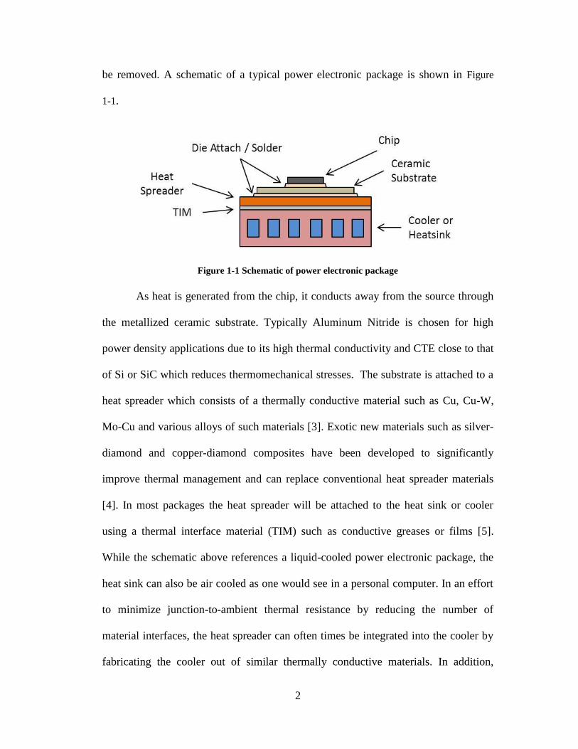
be removed. A schematic of a typical power electronic package is shown in Figure

1-1.

Figure 1-1 Schematic of power electronic package

As heat is generated from the chip, it conducts away from the source through

the metallized ceramic substrate. Typically Aluminum Nitride is chosen for high

power density applications due to its high thermal conductivity and CTE close to that

of Si or SiC which reduces thermomechanical stresses. The substrate is attached to a

heat spreader which consists of a thermally conductive material such as Cu, Cu-W,

Mo-Cu and various alloys of such materials [3]. Exotic new materials such as silver-

diamond and copper-diamond composites have been developed to significantly

improve thermal management and can replace conventional heat spreader materials

[4]. In most packages the heat spreader will be attached to the heat sink or cooler

using a thermal interface material (TIM) such as conductive greases or films [5].

While the schematic above references a liquid-cooled power electronic package, the

heat sink can also be air cooled as one would see in a personal computer. In an effort

to minimize junction-to-ambient thermal resistance by reducing the number of

material interfaces, the heat spreader can often times be integrated into the cooler by

fabricating the cooler out of similar thermally conductive materials. In addition,

3

eliminating the substrate is made possible by directly attaching the chip to the cooler

[6] [7]. This can only be done however if the CTE mismatch between the bonded

materials is small enough such that cracking and attach failure will not occur.

1.1.1 High Temperature Considerations

The primary concern arising from insufficient cooling is reliability [8].

Increased heat fluxes can adversely affect device performance and lead to a number

of degradation mechanisms at both the chip and package level including passivation

cracking, electromigration, chip or substrate cracking, wirebond lift-off and die attach

failure [9]. The temperature limit for most silicon chips is around 150-175°C [8].

Above these temperatures the increased leakage current across the p-n junction

typically renders the device inoperable resulting in permanent failure. In the past 20

years wide bandgap (WBG) semiconductor devices such as Silicon Carbide (SiC) and

Gallium Nitride (GaN) have enabled increased power densities and heat fluxes by

allowing devices to operate reliably at temperatures significantly greater than 150°C.

For example, a SiC transistor was shown to reliably operate at 500°C for 6000 hours

[10] and a SiC based electronics and ceramic package was shown to operate at 300°C

for 1000 hours for a geothermal wellbore monitoring application [11]. Aside from

being able to operate at higher temperatures than silicon, additional benefits of WBGs

are as follows [12]:

Lower on-state resistances yielding lower conduction losses. Overall this leads

to increased efficiency for systems containing WBG semiconductors.

4

Higher breakdown voltages due to their higher dielectric breakdown field. SiC

diodes are commercially available with breakdown voltages upwards of 10 kV

[13].

Increased thermal conductivity enabling heat to be more efficiently

transported away from the source.

Lower switching losses enable WBG devices to operate at frequencies much

greater than that of Si (> 20 kHz).

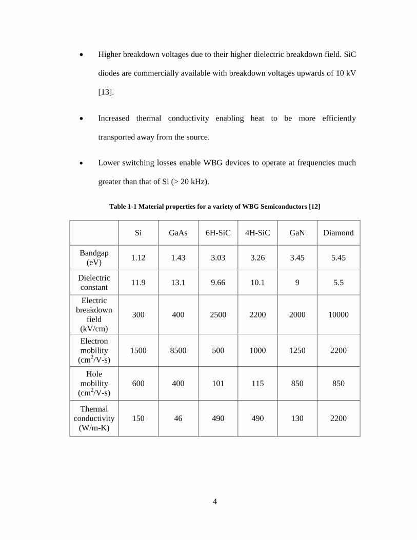
Table 1-1 Material properties for a variety of WBG Semiconductors [12]

Si GaAs 6H-SiC 4H-SiC GaN Diamond

Bandgap

(eV) 1.12 1.43 3.03 3.26 3.45 5.45

Dielectric

constant 11.9 13.1 9.66 10.1 9 5.5

Electric

breakdown

field

(kV/cm)

300 400 2500 2200 2000 10000

Electron

mobility

(cm2/V-s)

1500 8500 500 1000 1250 2200

Hole

mobility

(cm2/V-s)

600 400 101 115 850 850

Thermal

conductivity

(W/m-K)

150 46 490 490 130 2200

5

1.1.2 GaN High Electron-Mobility Transistors

While SiC devices are typically used for high voltage power conversion

applications due to their substantial electric breakdown field and low conduction

losses, GaN devices are most often used in applications involving radio frequency

(RF) transmission or very high switching speeds. High electron mobility transistors

(HEMTs) are best suited for applications requiring high gain and low noise at high

frequencies used in microwave satellite communications, radar, imaging, remote

sensing and radio astronomy. MOSFETs and other Field Effect Transistors (FETs)

operate based on the principle of doping the semiconductor to create alternating n-

type and p-type regions, shown in Figure 1-2. If a positive voltage is applied to the

gate, a positive electrical field is built up which attracts electrons in the p-type layer

and repels holes. These electrons form an n-channel which carries electrons from

source to drain. Raising the potential on the gate increases the electric field allowing a

larger current to flow throw the p-type region.

Figure 1-2 Field effect transistor with positive voltage applied to gate

6

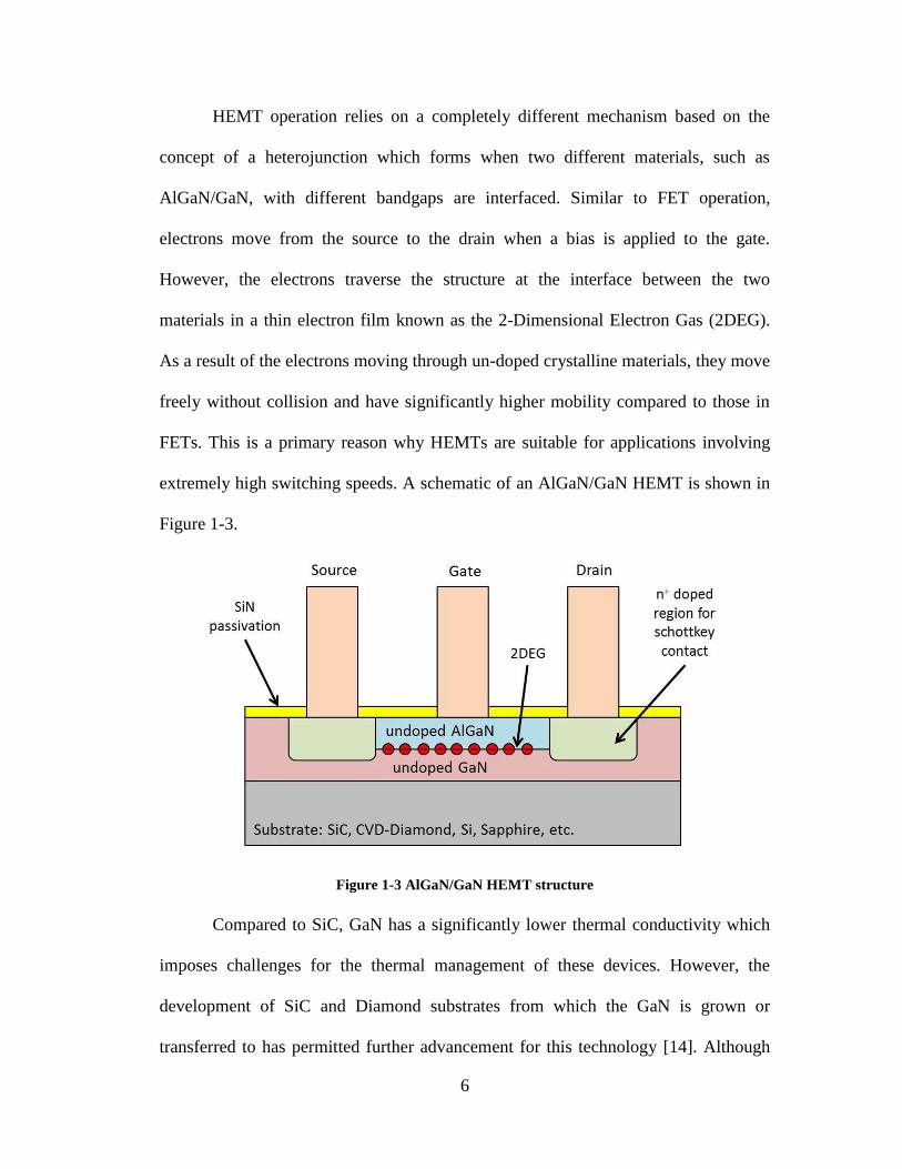
HEMT operation relies on a completely different mechanism based on the

concept of a heterojunction which forms when two different materials, such as

AlGaN/GaN, with different bandgaps are interfaced. Similar to FET operation,

electrons move from the source to the drain when a bias is applied to the gate.

However, the electrons traverse the structure at the interface between the two

materials in a thin electron film known as the 2-Dimensional Electron Gas (2DEG).

As a result of the electrons moving through un-doped crystalline materials, they move

freely without collision and have significantly higher mobility compared to those in

FETs. This is a primary reason why HEMTs are suitable for applications involving

extremely high switching speeds. A schematic of an AlGaN/GaN HEMT is shown in

Figure 1-3.

Figure 1-3 AlGaN/GaN HEMT structure

Compared to SiC, GaN has a significantly lower thermal conductivity which

imposes challenges for the thermal management of these devices. However, the

development of SiC and Diamond substrates from which the GaN is grown or

transferred to has permitted further advancement for this technology [14]. Although

7

Diamond and SiC substrates enable heat to be removed from the source efficiently,

their high-price and fabrication complexities may yield them unsuitable for large

scale commercial applications. While these substrates have very niche applications

fitting for defense and military electronics [6] [14] [15], GaN-on-Si technology has

been shown to be low-cost solution for increasing the flexibility of GaN power

devices [16].

1.2 The Embedded Cooling Paradigm Shift

In an effort to align with the size, weight and performance optimization of

high temperature and high powered electronics, cooling channels embedded directly

into the backside of the substrate significantly reduce the junction-to-ambient thermal

resistance by reducing the number of thermal interfaces and overall distance the heat

must travel. Compared to other “remote cooling” type approaches, embedded cooling

can enable chips to operate at higher power levels while maintaining the same

junction temperature. Over 30 years ago, Tuckerman and Pease [17] etched 300

micron deep channels into the backside of a silicon wafer and demonstrated a cooling

capacity of 790 W/cm2. Although this pioneering effort demonstrated a novel

technique for electronic cooling, fabrication efforts posed many challenges and

pressure drops were very high. With the development of Deep Reactive Ion Etching

(DRIE) fabrication became simplified and facilitated further research in the area of Si

microchannel design [18].

8

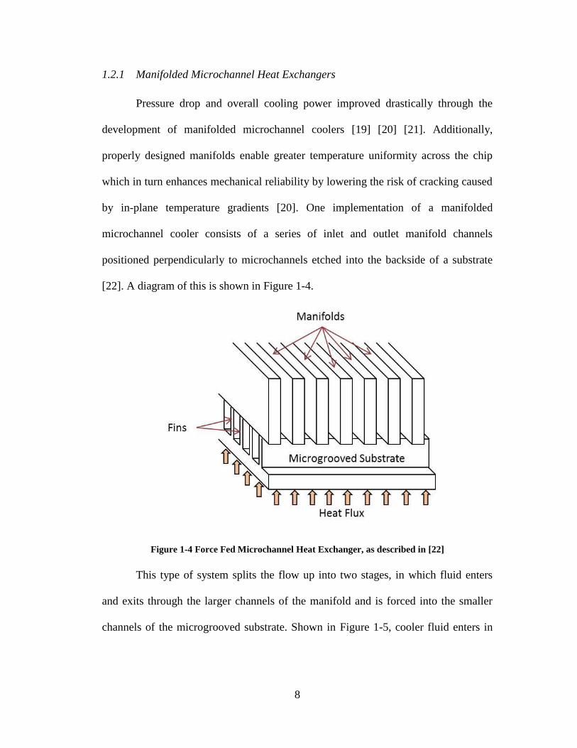
1.2.1 Manifolded Microchannel Heat Exchangers

Pressure drop and overall cooling power improved drastically through the

development of manifolded microchannel coolers [19] [20] [21]. Additionally,

properly designed manifolds enable greater temperature uniformity across the chip

which in turn enhances mechanical reliability by lowering the risk of cracking caused

by in-plane temperature gradients [20]. One implementation of a manifolded

microchannel cooler consists of a series of inlet and outlet manifold channels

positioned perpendicularly to microchannels etched into the backside of a substrate

[22]. A diagram of this is shown in Figure 1-4.

Figure 1-4 Force Fed Microchannel Heat Exchanger, as described in [22]

This type of system splits the flow up into two stages, in which fluid enters

and exits through the larger channels of the manifold and is forced into the smaller

channels of the microgrooved substrate. Shown in Figure 1-5, cooler fluid enters in

9

alternating manifold channels and subsequently exits in the same fashion at a higher

temperature.

Figure 1-5 Operation of manifolded microchannel cooler

1.2.2 Pin-fin Array

Aside from etching microchannels into the backside of a chip or substrate,

micropins or blunt fins can also be selectively etched to enhance heat transfer by

increasing surface area. This type of approach was demonstrated to successfully cool

power densities greater than 300 W/cm2 and is suggested to be able to cool chips with

power densities greater than 400 W/cm2 [23]. A variety of shapes can be used for the

fins, including circular [24] and hydrofoil [25] shapes, however the general premise

of this design is to maximize the area over which heat transfer can occur.

1.2.3 Jet-Impingement Cooling

Another implementation of embedded cooling considers microfluidic

impingement jets that directly cool the backside of a substrate [26] [27] [28]. One

advantage to this type of design over the manifold or pin-fin designs is that it requires

10

minimum modifications to the substrate, if any at all. While the manifold design

requires channels to be etched into the backside of the substrate, jet impingement

cooling would not. The primary issue with etching the backside of the substrate lies in

the fact that it must be done very carefully as to not disrupt the electrical design of the

device or introduce crystalline defects that may propagate up to the active layer.

With jet impingement cooling however, the major reliability challenge lies in

the potential for erosion. For a jet impingement configuration with velocities greater

than 5 m/s, particle erosion must be considered [29]. While there exists numerous

particle erosion studies in literature for a wide variety of materials (discussed

thoroughly in Chapter 2), seldom are the velocities, particle sizes, materials and

testing times in alignment with those that may be present in embedded cooling

systems. While jet-impingement cooling offers a feasible technique for embedded

cooling, it would be very difficult to predict with any level of certainty whether or not

a specific jet-impingement configuration would induce catastrophic erosion damage.

1.3 Reliability Concerns of Embedded Cooling Systems

Reliability can be defined as “the ability of a product or system to perform as

intended (i.e., without failure and within specified performance limits) for a specified

time in its life cycle conditions” [30] . In any system there may be specific processes

at work – mechanical, thermal, electrical or chemical in nature - which cause the

system performance to degrade or catastrophically fail in time. In an effort to design a

reliable product, it is imperative to understand the potential threats which may

compromise normal operation. This approach, wherein the designer considers the

11

physics of the specific degradation or failure mechanisms at play, is referred to as a

“physics-of-failure” methodology [31].

The primary function of an embedded cooling system is to maintain the chip

or device temperature below a certain critical temperature, above which the electrical

performance will suffer. As such, the degradation mechanisms of the cooling system

pertain to the processes that hinder or reduce the ability to dissipate heat from the

chip. Any process that occurs throughout the lifetime of the cooler that alters the

geometry or internal features, which were precisely chosen by system designers to

dissipate a definitive amount of heat, can be characterized as the fundamental

degradation mechanisms. The three most prominent and likely to occur in embedded

cooling systems are particle erosion, corrosion and clogging.

1.3.1 Particle Erosion

Particle erosion occurs when a particle entrained in the fluid stream impinges

on a surface resulting in wear and the subsequent removal of material. In the pin fin

or microchannel type implementations of embedded cooling, erosion may result in the

alteration of pin or channel geometries lending to a change in the heat dissipation

ability. Additionally, in the jet impingement scenario where the backside of the chip

is cooled by high-velocity fluid jets, the substrate material may erode away leading to

direct contact between the fluid and the active electronics on the topside of the die. As

the concentration of particles build up in the fluid stream, this mechanism may

intensify in a snowball-like effect as more and more particle impingements occur.

Although filters are typically required for these types of systems, they can be quite

12

bulky especially if a small pressure drop across the system is critical. Furthermore,

micrometer and sub-micrometer sized particles may still get through the filter.

1.3.2 Corrosion and Dissolution

The chemical process known as corrosion occurs when the working fluid

interacts unfavorably with the cooler material. Corrosion often refers to the build-up

of an oxide or thin film layer at the interface between the fluid and the surface.

Depending on the material, this can lead to poor thermal transport by increasing the

junction-to-ambient thermal resistance for two reasons: the additional thermal

interface between the oxide and the bulk material and the typically lower thermal

conductivity of the oxide compared to the bulk material (i.e. silicon has a thermal

conductivity of 156 W/m-K at room temperature [32] while silicon dioxide has a

thermal conductivity of around 1.4 W/m-K [33]).

A similar chemical interaction that may occur between fluid and surface is

dissolution. This process refers to the uniform wear across all fluid-surface interfaces

where the substrate material reacts with the fluid and dissolves. Although single

crystal silicon is relatively inert, a thorough reliability analysis should still consider

this mechanism as corrosion or dissolution rates on the order of 1 micron per year

would be drastic over the 10 or 20 year life cycle of the device.

1.3.3 Erosion-Corrosion

While particle erosion and corrosion are independent mechanisms the

combined effect, known simply as erosion-corrosion, can impose a synergistic effect

13

on the wear-rate depending on the materials [34] [35] [36]. This process is shown in

Figure 1-6.

Figure 1-6 Diagram showing erosion-corrosion phenomenon

First, an oxide is formed due to the chemical interaction between the working

fluid and the substrate material (A). Next, a particle entrained in the fluid stream

impinges on the oxide layer removing small fragments of material into the coolant

loop (B). As fresh substrate is exposed, corrosion continues by transforming this

unprotected region into another oxide layer (C). This process perpetuates as more and

more oxide particles become entrained in the fluid stream (D). It should also be noted

that the erosion-corrosion process is highly material and chemically dependent. In

some instances the oxide layer may in fact protect the substrate material from

impinging particles while in other instances the oxide layer may be more susceptible

to erosion than the pure substrate

14

1.3.4 Clogging and Fouling

The continuous deposition and subsequent build-up of particles on a clean

surface is referred to as fouling and can eventually lead to a complete blockage of the

fluid cross-section. Channels or fluid paths can be clogged entirely, where no fluid

can enter, or they can be partially clogged which results in a significant increase in

pressure. With respect to heat transfer, fouling can increase the junction-to-ambient

thermal resistance in a similar fashion as corrosion would; the fouled layer both

introduces an additional thermal boundary resistance and may be of a lower thermal

conductivity than the bulk substrate. Furthermore, fully or partially clogged channels

can decrease the cooling uniformity of the chip which may permit certain regions of

the active layer to exceed the maximum allowable chip temperature. The four basic

mechanism of particulate clogging and fouling are depicted in Figure 1-7, where each

of these processes are a result of various particle-particle, particle-particle fluid, and

particle-surface interactions [37].

Figure 1-7 Four main mechanisms of clogging/fouling. Image taken from [37]

15

1.4 Dissertation Outline

This dissertation is divided into eight essential chapters. The present chapter

introduces the reader to the concept of embedded cooling and discusses the potential

degradation mechanisms associated with failure. Chapter 2 surveys much of the

related particle erosion research and methodologies. Topics discussed pertain to

particle erosion of brittle materials, two theories surrounding brittle erosion, slurry

erosion and related modeling, and the concept of the brittle-to-ductile transition.

Based on the gaps in literature and need for further research, Chapter 3 explicitly

outlines the problem statement, scope of work and discrete objectives of this

dissertation.

Chapter 4 describes the computational fluid dynamics (CFD) simulations

performed which investigate how various slurry erosion parameters such as nominal

jet velocity, particle size and fluid viscosity affect particle impact characteristics.

Through running a series of simulations that correlate directly to the experimental

efforts discussed in Chapter 6, the impact parameters extracted will facilitate the

calibration of a particle erosion model within a new set of operating parameters.

Chapter 5 describes the design and construction of a slurry erosion test

apparatus. Aspects pertaining to pump calibration, materials, creation of the testing

slurry, cleaning procedures and sample holder fabrication will be discussed.

Additionally, limitations surrounding the test setup will also be disclosed.

The primary experimental efforts are described in Chapter 6, which outline the

14 slurry erosion experiments. A stylus profilometer was used to capture the two-

dimension erosion contours which were then processed in MATLAB to approximate

16

the total volume of material removed. To perform this task and algorithm was

developed which uses a numerical volume of revolutions type approach to

approximate the total volume of material removed. Furthermore, this chapter presents

the results of these experiments in two principle erosion metrics: a mass loss rate in

units of milligrams-per-year and a one-dimensional erosion rate in units of

micrometers-per-year.

Chapter 7 discusses the development and calibration of a particle erosion model

based on the slurry erosion experiments and CFD simulation efforts. First, the data

from the previous chapter is converted to the conventional erosion ratio metric, in

units of milligrams-per-milligram, and represents the mass of material removed per

mass of impacting particles. In the simplifying case of a single particle of known

mass, this ratio defines the amount of mass removed per single impacting particle.

Both the calibration process and the results of the validation testing are described.

Furthermore, an impact dampening factor is proposed and validated. This factor

serves as a possible explanation as to why CFD erosion simulations tend to over-

predict experimental results. While there are numerous findings of this research, one

of the major products of this dissertation is the calibrated and validation erosion

model.

A concluding section, Chapter 8, will summarize the efforts and findings

described throughout each chapter of this work. Technical and academic

contributions will be explicitly listed. Lastly, potential areas of future work will be

described based on the work performed in this study,

17

2 LITERATURE REVIEW

This chapter will introduce the fundamental concepts pertaining to particle

erosion and wear of brittle materials. A number of studies will be reviewed along

with associated models. In addition, a series of related topics will be discussed to

thoroughly describe the mechanisms associated with the degradation of such

materials.

2.1 Early Erosion Studies of Sheldon and Finnie

Materials can typically be classified as either ductile or brittle. While this is an

oversimplification as materials can exhibit both ductile and brittle behaviors under

different conditions, these terms will be used to describe the nominal behavior under

most conditions. With respect to material removal, nominally ductile materials

undergo large plastic strains which precede fracture and the subsequent ejection of

material. Nominally brittle materials undergo no plastic deformation and material is

removed by the propagation and intersection of cracks surrounding an impact or

defect site.

It should additionally be mentioned that many of the particle erosion models

presented in this chapter assume a continuum mechanics approach wherein the

crystallographic structure of the material is not inherently considered in the model.

Rather, the material is treated in a bulk fashion and the models reflect how much

mass of material is removed per particle impact. One caveat to this is with regard to

the mechanisms taking place, such as in the cases of grains or grain boundaries

influencing the type of wear. That being said, the final erosion model reflects the

18

amount of material removed and typically does not consider grains, grain boundaries,

or crystallographic structure in the analytical or empirical formulation.

One of the first efforts to study particle erosion was conducted in 1960 by

Finnie [38]. The effects of particle impact velocity and impingement angle were

studied by measuring the weight loss of 1020 steel, aluminum and copper samples. It

was found that for these materials maximum material removal occurred at impact

angles around 20°. This observation can be explained by the cutting action an

impacting particle has on the target surface, as depicted in Figure 2-1. It can be seen

that plastic deformation is a primary mechanism leading to the eventual loss of

material.

Figure 2-1 Schematic of cutting action from impacting particle on ductile material

It was also found that for ductile materials target weight loss ‘W’ was

proportional to velocity squared, W ~ V2, of the impacting particles. It was predicted

that at lower velocities (38 m/s was the minimum velocity tested) particles would

tend to produce only elastic stresses upon impact lending to a deviation in the W ~ V2

prediction.

In the same study [38], Finnie attempted to study the erosive nature of brittle

materials but found that weight loss measurements conducted in the same fashion as

the ductile materials would not suffice. Impacting spherical steel shot against glass

resulted in the formation of cone-cracks, shown in Figure 2-2, but no material loss.

19

As the number of particle impacts increased, the cone shaped cracks began to

intersect resulting in eventual material loss. Once a first layer of material was

removed it became difficult to observe the formation of individual fracture surfaces.

As such, the diameter of the crack-ring was used to assess how velocity and impact

angle would affect the propensity for erosion.

Figure 2-2 Cone-cracks resulting from spherical particle impact on brittle materials

Assuming the glass would remain perfectly elastic until fracture, Hertzian

analysis was conducted to show that the magnitude of the maximum radial stress was

a function of density, velocity, Poisson’s ratio and modulus of elasticity of the

impacting sphere as well as the Poisson’s ratio and modulus of elasticity of the target

surface. This analysis predicted that the diameter of the crack was proportional to V0.4

but if it was assumed that the shear stress due to oblique impact was neglected, the

diameter of the crack would be proportional to (Vsinα)0.4

, where α is the impact angle.

This suggested that the maximum diameter of the cone-crack is formed when a

particle is impacting the target surface at a normal incidence. Figure 2-3a shows the

relationship between the size of crack ring formed from 0.58 mm impacting steel shot

and the angle of incidence, revealing a close match between experimental results and

theory. For a comparison, Figure 2-3b shows the variation of volume removal for

20

aluminum, copper and 1020 steel (all ductile materials) showing that maximum

erosion occurs at an impact angle of around 20°.

Figure 2-3 Crack diameter vs. angle of incidence for 0.58mm impacting steel shot on glass (A) on

left and variation of erosion vs. impact angle for ductile materials (B) on right [38]

Although information surrounding the mechanisms brittle erosion was

acquired, the following conclusions were drawn from this initial study: “there is no

very simple parameter which combines the effects of velocity and angle in producing

material removal.” It was also concluded that “if a prediction of erosion is required

there appears to be no satisfactory approach except that of testing under the specific

conditions of interest.”

One of the first successful attempts quantify the erosive nature of brittle

materials was conducted in 1966 by Sheldon and Finnie [39]. For a variety of brittle

materials including glass, MgO, graphite, hardened steel and Al2O3, they showed that

the volume of material removed, W, by a normal impacting particle could be related

by the following:

𝑊 = 𝑘𝑅𝑓1(𝑚𝑤,𝑠)𝑉𝑓2(𝑚𝑤,𝑠) (2-1)

21

where k is a material constant, R is the particle radius and V is the particle impact

velocity. The exponents f1 and f2 can be considered the radius and velocity exponents

respectively and are functions of the flaw parameter of the Weibull fracture strength

distribution, mw, and the shape of the particle, s, for angular or spherical particles. The

particle diameters ranged from 22 – 335 µm for angular SiC and 282 – 940 µm for

steel shot, while the velocities ranged from 38 – 183 m/s. Table 2-1 summarizes the

experimentally derived radius and velocity exponents obtained for different materials.

Table 2-1 Summary of experimental results showing radius and velocity exponents [39]

Material

Experimental Values

Steel Shot SiC Grit

Radius

Exponent

Velocity

Exponent

Radius

Exponent

Velocity

Exponent

Glass 5.12 4.37 4.25 3.0

MgO 3.39 2.73 3.95 2.74

Graphite 3.14 2.67 3.78 2.69

Hardened Steel n/a n/a 3.58 2.53

Al2O3 n/a n/a 3.86 2.62

Overall the experimental data matched well with their derived model showing

that particle size and shape, velocity, and target material parameters could be

systematically correlated to a metric of erosion.

In a parallel study, Sheldon and Finnie [40] studied the ductile behavior that

nominally brittle materials sometimes exhibit during erosion under specific impact

conditions. Using the same testing apparatus and methodology as their previous study

[39], the effect of impact angle was investigated in the erosion of glass using 9μm,

21μm and 127μm angular SiC particles. The results can be summarized in Figure 2-4.

22

Figure 2-4 Erosion of glass as a function of impact angle by angular SiC particles at 152 m/s [40]

For the larger 127μm particles, the effect of impact angle is characteristic of

nominally brittle materials, as shown previously in Figure 2-3a. However, as the

particle size decreases to 9μm the graph shifts and reveals material behavior similar to

that of nominally ductile materials where the impact angle leading to the greatest

erosion is approximately 20°. It was also shown that even at 305 m/s, the glass still

produced this characteristic curve. Although glass exhibited this brittle-to-ductile

transition at small particle sizes, when high density Alumina was tested it behaved in

a nominally brittle fashion.

The occurrence of plastic deformation is suggested to be the primary

mechanism justifying these results as previous studies involving micro-indentation,

scratching, and abrasion also produced ductile behavior in nominally brittle materials.

For example, Klemm and Smekal [41] [42] showed that silicate glass, quartz and

23

Corundum crystals could be scratched without inducing fracture if the scratch width

was very small, on the order of 1μm. It was also shown that plastically displaced

material would pile up on the sides of the scratches without inducing any fracture

[43].

In another study Hockey [44] examined the room-temperature abrasion and

micro-indentation of single crystal and polycrystalline Al2O3. Transmission Electron

Microscopy (TEM) showed regions of high-density dislocations in the near-surface

regions after mechanical polishing with 0.25μm diamond abrasives. It was also

shown that plastic deformation by both slip and mechanical twinning mechanisms

occurred near the region of a Vickers hardness micro-indenter. It was suggested that

the occurrence of plastic deformation was a result of the local stress fields that

evolved under irregularly shaped abrasive and small tipped indenters.

2.2 Micro-Indentation Studies of Brittle Materials

The primary conclusion that can be drawn from early erosion work is that under

certain small-scale conditions nominally brittle materials can behave in a ductile

manner by exhibiting modes of plastic deformation. If the impact area between a

particle and target surface is large, for example rounded steel shot impacting a glass

plate, the interaction would be completely elastic up until the initiation of fracture at

some dominant flaw resulting from a critical loading. This results in the characteristic

Hertzian cone-crack shown previously in Figure 2-2.

24

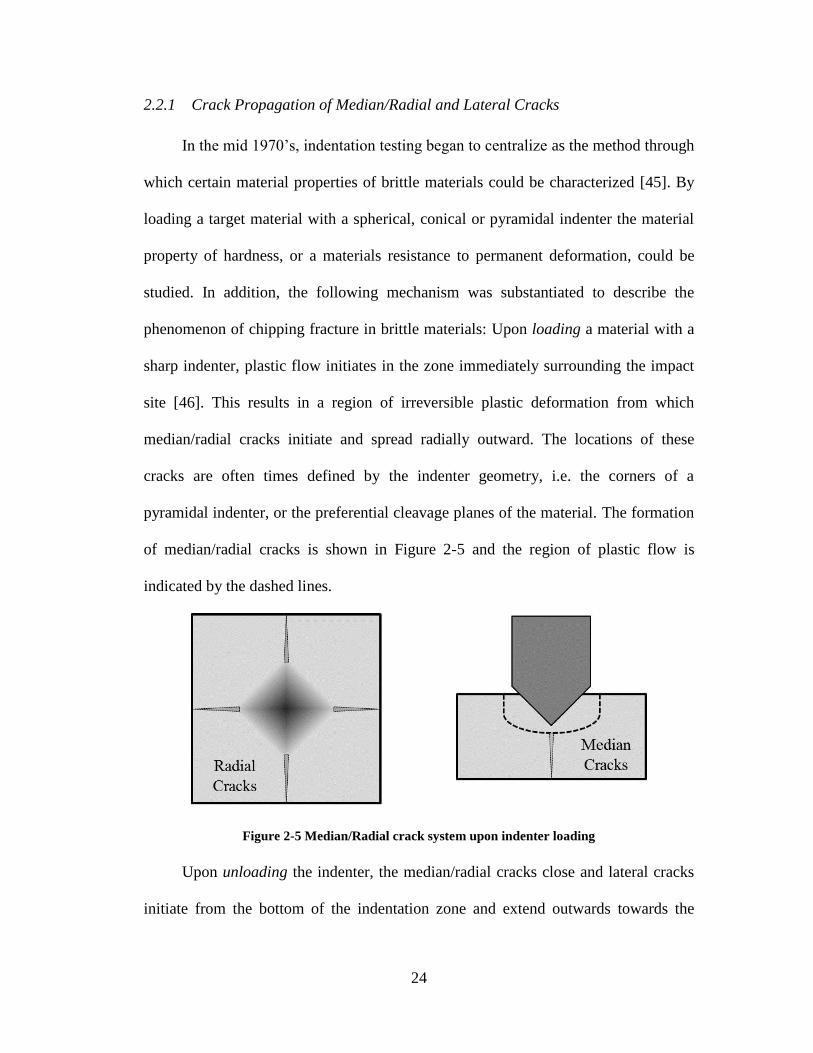
2.2.1 Crack Propagation of Median/Radial and Lateral Cracks

In the mid 1970’s, indentation testing began to centralize as the method through

which certain material properties of brittle materials could be characterized [45]. By

loading a target material with a spherical, conical or pyramidal indenter the material

property of hardness, or a materials resistance to permanent deformation, could be

studied. In addition, the following mechanism was substantiated to describe the

phenomenon of chipping fracture in brittle materials: Upon loading a material with a

sharp indenter, plastic flow initiates in the zone immediately surrounding the impact

site [46]. This results in a region of irreversible plastic deformation from which

median/radial cracks initiate and spread radially outward. The locations of these

cracks are often times defined by the indenter geometry, i.e. the corners of a

pyramidal indenter, or the preferential cleavage planes of the material. The formation

of median/radial cracks is shown in Figure 2-5 and the region of plastic flow is

indicated by the dashed lines.

Figure 2-5 Median/Radial crack system upon indenter loading

Upon unloading the indenter, the median/radial cracks close and lateral cracks

initiate from the bottom of the indentation zone and extend outwards towards the

25

surface. This phenomenon is depicted in Figure 2-6. Upon reaching the surface,

material is removed in a fashion characteristic of brittle chipping.

Figure 2-6 Lateral cracks form upon indenter removal (A). Upon reaching the surface chipping

occurs (B). Image taken from [47].

Since the lateral crack system initiates upon unloading, it becomes clear that

the conditions under which these cracks form originate from a residual stress field

associated with the irreversible deformation zone [46]. As such, it can be suggested

that material hardness, or resistance to plastic deformation, plays an important role in

determining the extent of crack propagation.

From this observation a number of studies began to examine the

characteristics of these two crack systems surrounding various loading conditions.

Hockey and Lawn [48] used TEM to exam geometrical features of the micro-crack

patterns formed upon indenting sapphire and carborundum. They found that the

crystallographic structure plays a significant role in the crack evolution - that silicon

carbide has a greater tendency to cleave along the basal plane while sapphire tends to

cleave nearly parallel to the (0001) plane. Although both materials are single crystal,

the idea of anisotropic micro-fracture suggests further investigations are necessary.

26

In studying the damage and fracture modes developed during plastic

indentation, Evans and Wilshaw [49] showed that lateral crack extension depend on

the radius of the indenter and the hardness-to-fracture toughness ratio of the target

material. Extending their observations to abrasive wear by assuming the radius of the

plastic deformation region can be related to the force on the particle, they obtained

the following relation for the volume removed by N abrasive particles:

𝑊 ∝1

𝐾𝑐

34𝐻

12

∑𝑃𝑖𝑙𝑖

𝑖=𝑁

𝑖=1

(2-2)

where Pi is the vertical force on a particle, li is sliding distance, Kc is the fracture

toughness and H is the hardness.

Assuming that the pressure induced by an impacting particle can be replaced

by a functional dependence on particle impact velocity, the volume of material

removed was derived in a similar fashion for N impacting particles:

𝑊 ∝𝑁𝑅4𝐺

45𝑉

125 𝜌𝑝

65

𝐾𝐷

32𝐻𝐷

12

(2-3)

where G is the shear modulus of the target, ρpart is the particle density, and KD and HD

are the dynamic fracture toughness and dynamic hardness of the target respectively. It

is further noted that this relation is predicted to hold true only for low velocity

impacts due to the fact that the force-velocity dependence cannot be described by a

single function over the entire velocity range [49]. At higher velocities the force-

velocity function cannot be expressed in terms of simple material and projectile

properties as these properties cannot be modeled in a static fashion. One example of

27

this is that the velocity exponent is expected to decrease as the velocity or hardness

decreases [49]. This theory would eventually become the foundation for the dynamic

particle impact theory [50] discussed in a later section.

Additionally Swain and Lawn [51] studied localized cracking of Westerly

granite and silicate glass by indentation of sharp and blunt indenters. By measuring

crack length as a function of indenter load, they produced explicit relations which

identify the role of basic material properties such as fracture surface energy and

hardness to crack propagation.

2.2.2 Threshold Conditions for Crack Initiation

While the discussion to this point has focused on how the median/radial and

lateral crack systems evolve and ultimately result in material removal under quasi-

static indentation conditions, this subsection will briefly discuss conditions of crack

initiation. Lawn and Evans [52] proposed a model which provides a relationship

between the size of a critical flaw located directly below the indenter and the load

necessary to make the flaw extend into median cracks. The model proposes three

distinct regions of stability pertaining to flaw size at a constant load: (1) small flaws

which can never fully expand into median cracks, (2) intermediate flaws which

expand spontaneously into median cracks and (3) large flaws which describe the

initiation of median cracks as a continuous event as opposed to an abrupt event – it is

in this region where Griffith-based fracture mechanics takes over. In the context of

micro-indentation, this study concluded that materials most resistant to cracking

would be those of high fracture toughness, Kc, and low hardness, H.

28

In another study, Perrott [53] proposed a similar model which assumes that

the maximum stress within the plastic zone occurs at the surface of the target material

near the indenter corners as opposed to underneath the indenter. As such, this model

proposes the initiation of radial cracks at the surface as opposed to median cracks

under the indenter.

In an effort to compare both models, Lankford and Davidson [54] used

Scanning Electron Microscopy (SEM) and acoustic emission techniques to assess the

threshold indentation loads leading to crack initiation for a variety of materials

including crystalline NaCl, Si and Ge and polycrystalline Al2O3 and SiC. In all the

materials studied it was found that the first cracks to form, thus the cracks associated

with threshold events, were the radial surface cracks. While Perrott’s model was

correct with respect to the crack system associated with threshold events, Lawn and

Evan’s model perfectly predicted the ordering of materials with respect to indenter

load and crack size, although the threshold load was more than an order of magnitude

in error. By considering the indentation and stress field analysis conducted by Perrott,

it was found that an adjustment could be made to the threshold loads in Lawn and

Evan’s model leading to more accurate predictions.

2.2.3 Unifying Models of Lawn, Evans and Marshall

By combing theories of crack initiation and propagation, Lawn and Marshall

[55] proposed the ratio H/Kc as an index of brittleness, where hardness is the

resistance to deformation and fracture toughness is the resistance to fracture.

Brittleness essentially describes the relative susceptibility to both these mechanisms

and provides a convenient explanation for the empirically discovered brittle-to-ductile

29

transition. In their analysis, a variety of materials were ranked according to their

index of brittleness, shown in Table 2-2. The term P* represents the maximum load a

material can sustain without the onset of fracture assuming a material dependent

critical flaw size.

Table 2-2 Hardness, Toughness and Brittleness [55]

Material Comments H

(GPa)

Kc

(MPa-m1/2

)

H/Kc

(μm-1/2

)

P*

(N)

Fe Medium Strength

Steel 5 50 0.1 800000

NaCl Monocrystalline 0.24 0.4 0.6 30

ZnSe Vapor Deposited 1.1 0.9 1.2 8

WC Co-bonded 19 13 1.4 70

ZnS Vapor Deposited 1.9 1.0 2 2

Si3N4 Hot Pressed 16 5 3 2

Al2O3 MgO-doped 12 4 3 2

SiC Hot Pressed 19 4 5 0.6

MgF2 Hot Pressed 5.8 0.9 6 0.05

MgO Hot Pressed 9.2 1.2 8 0.04

SiO2 Glass 6.2 0.7 9 0.02

B4C Hot Pressed 77 6 13 0.05

Si Single Crystal 10 0.6 17 0.002

According to this analysis and based upon specific loads or environments,

optimal materials can be selected for a variety of engineering applications. For

example, in abrasive environments such as those with high concentrations of small

particle where the nominal load P is less than P*, materials exhibiting high hardness

would be most appropriate as the damage mode would primarily be deformation

based. Consequently, materials with high fracture toughness would be most

appropriate in environments where the load P is greater than P*, such as those with

high energy impacts. In environments where P ≈ P*, the metric of brittleness should

be minimized in order to prevent crack initiation once deformation takes place. A

30

prime example of this is the use of ZnSe [55] to promote optical integrity in infrared

windows where preventing crack initiation if of great importance. Of course, in the

selection of engineering materials care must be taken to choose materials that are also

chemically, thermally, electrically and optically suited for the specific application.

Compiling over a decade of research in indentation mechanics, Lawn, Evans

and Marshall developed a universal theory for describing the evolution of both the

median/radial [56] and lateral crack systems [57]. Regarding the growth of

median/radial cracks, their analysis assumes the stress field below the indenter can be

resolved into elastic and residual components. The reversible elastic component is

largely responsible for the downward growth of median cracks during the loading

cycle, and the plastic residual component is largely responsible for the growth of

radial cracks during the unloading cycle. They established a model for predicting

crack propagation mechanics, specifically relating crack length and the plastically

deformed indenter contact area to known material properties such as H, Kc and the

elastic modulus E. Assuming the load is sufficient enough to induce cracking, i.e. the

radial crack length cR is larger than the plastically deformed indenter contact length a,

the following relation was made using soda-lime glass as a calibration material:

(𝐾𝑐

𝐻𝑎12

)(𝐻

𝐸)

12= 0.28(

𝑐𝑅

𝑎)

−32

(2-4)

Figure 2-7 demonstrates its capability in predicting the crack growth

characteristics for a variety of materials.

31

Figure 2-7 Universal plot relating material properties to fracture and deformation parameters in

a variety of engineering materials [56]

Concerning the lateral crack system, a similar analysis demonstrated the

relation between load and crack parameters to material properties. An interesting

consequence of lateral cracking is the role it plays in material removal if the contact

pressure is significantly larger than the threshold pressure to induce cracking. It was

shown that the volume of material removed could be predicted by [57]:

𝑊 ∝

(

(𝐸𝐻)

54

𝐾𝑐𝐻16

)

𝑈𝑘

76 (2-5)

where Uk is the incident kinetic energy of the particle. In both crack propagation

models, specific attention is drawn to the modulus-to-hardness E/H ratio which serves

as a metric to determine the effects of the elastic and residual components in the

stress field. According to the equation above, decreasing this ratio has a direct effect

in reducing the volume of material removed due to impacts causing lateral cracking.

32

Consequently, in ceramics with higher values of E/H there is the tendency for

material to pile up around the indenter similar to the behavior of ductile materials [56]

[58].

2.3 Elastic-Plastic Particle Damage Theories

In parallel with research surrounding crack evolution in brittle materials, two

elastic-plastic theories emerged and would become the basis for subsequent erosion

modeling. Termed the “Quasi-Static” and “Dynamic Impact” theories, both are based

on the concept that lateral crack growth results from residual stresses induced by

particle impact events. In short, the volume of material removed can be predicted by

the size and depth of the lateral crack formed beneath an impact site.

2.3.1 Quasi-Static Particle Impact Theory

The quasi-static theory originated from studies involving indentation

mechanics but was later defined more explicitly by Wiederhorn and Lawn [59]. This

theory stems from the idea that particle impact damage can be closely correlated to

plastic indentation physics and subsequent fracture associated with indentation

experiments. The “quasi-static” model assumes that the kinetic energy of an

impacting particle is completely dissipated into plastic flow [59]. While this would

represent a condition where no rebound occurs, this assumption serves as an upper

bound in predicting the impulse load. Additionally, the “quasi-static” condition

assumes that the contact velocity is relatively slow compared to the sonic velocities of

the particle or the target materials.

33

Ruff and Wiederhorn [60] derived an erosion model based on the quasi-static

theory by assuming that the radial and lateral crack sizes are proportional to one

another and that the maximum penetration depth of the particle is proportional to the

depth of the lateral crack. The following relation was formed which describes the

factors affecting the volume of material removed for a single impacting particle at

normal incidence.

𝑊 ∝𝑉229 𝑅

113 𝜌𝑝

119 𝐻

19

𝐾𝐶

43

(2-6)

The velocity exponent, n = 2.44, compares well with the n = 2.4 value

determined by Evans and Wilshaw [49] in Equation 2-3 and that of the n = 2.24 value

determined by Marshall, Lawn and Evans [57] in Equation 2-5. Additionally the

radius exponent, m = 3.67, compares well with the m = 4 value also determined by

Evans and Wilshaw [49]. Lastly, these values compare well with those determined by

Sheldon and Finnie [39] denoted in Table 2-1.

Hockey, Wiederhorn and Johnson [61] examined the quasi-static approach by

demonstrating the correlation between quasi-static indention and sharp particle

impact in both single particle impact tests and multiple particle erosion tests. Figure

2-8 compares the damage caused by an impacting particle and a Vickers diamond

pyramidal indenter.

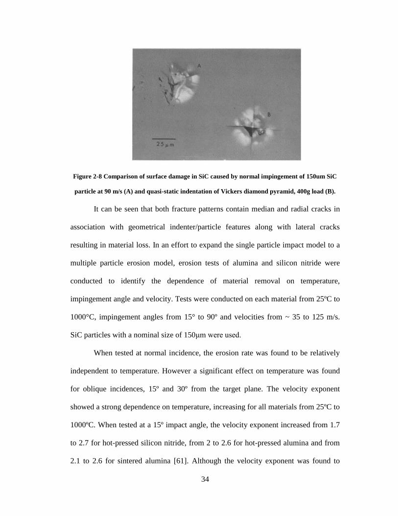
34

Figure 2-8 Comparison of surface damage in SiC caused by normal impingement of 150um SiC

particle at 90 m/s (A) and quasi-static indentation of Vickers diamond pyramid, 400g load (B).

It can be seen that both fracture patterns contain median and radial cracks in

association with geometrical indenter/particle features along with lateral cracks

resulting in material loss. In an effort to expand the single particle impact model to a

multiple particle erosion model, erosion tests of alumina and silicon nitride were

conducted to identify the dependence of material removal on temperature,

impingement angle and velocity. Tests were conducted on each material from 25ºC to

1000°C, impingement angles from 15° to 90º and velocities from ~ 35 to 125 m/s.

SiC particles with a nominal size of 150μm were used.

When tested at normal incidence, the erosion rate was found to be relatively

independent to temperature. However a significant effect on temperature was found

for oblique incidences, 15º and 30º from the target plane. The velocity exponent

showed a strong dependence on temperature, increasing for all materials from 25ºC to

1000ºC. When tested at a 15º impact angle, the velocity exponent increased from 1.7

to 2.7 for hot-pressed silicon nitride, from 2 to 2.6 for hot-pressed alumina and from

2.1 to 2.6 for sintered alumina [61]. Although the velocity exponent was found to

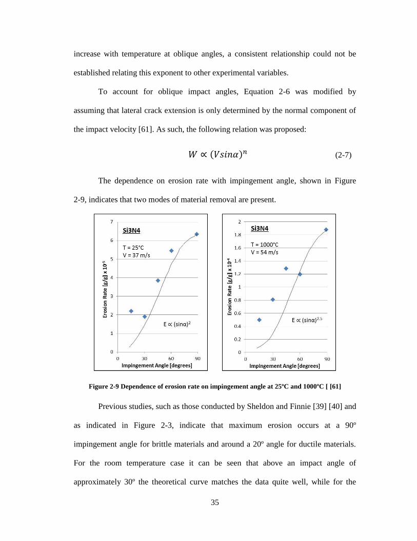
35

increase with temperature at oblique angles, a consistent relationship could not be

established relating this exponent to other experimental variables.

To account for oblique impact angles, Equation 2-6 was modified by

assuming that lateral crack extension is only determined by the normal component of

the impact velocity [61]. As such, the following relation was proposed:

𝑊 ∝ (𝑉𝑠𝑖𝑛𝛼)𝑛 (2-7)

The dependence on erosion rate with impingement angle, shown in Figure

2-9, indicates that two modes of material removal are present.

Figure 2-9 Dependence of erosion rate on impingement angle at 25ºC and 1000ºC [ [61]

Previous studies, such as those conducted by Sheldon and Finnie [39] [40] and

as indicated in Figure 2-3, indicate that maximum erosion occurs at a 90º

impingement angle for brittle materials and around a 20º angle for ductile materials.

For the room temperature case it can be seen that above an impact angle of

approximately 30º the theoretical curve matches the data quite well, while for the

36

1000ºC case the curve matches the data for impact angle above 60º. These deviations

at low impact angles suggest that ductile wear mechanisms become more pronounced

[61]. Additionally the more pronounced deviations at 1000ºC suggest that the role of

plastic flow in erosion becomes increasingly more important [61].

2.3.2 Dynamic Impact Theory

In parallel with the quasi-static theory, the dynamic impact theory was

originally developed by Evans and Wilshaw [50] but more explicitly defined by

Evans, Gulden and Rosenblatt [62]. While similar in nature, the fundamental

difference between the two theories is their assumed dependence of impact load on

the material and kinetic parameters most affecting erosion [63]. While the quasi-static

theory assumes that the kinetic energy of an impacting particle completely transforms

into work creating plastic flow, and can thus be modeled assuming static material

properties, the dynamic theory predicts that substantial changes in material response

may occur due to impact. Under impact conditions, the stress fields are expected to be

more complex due to the potential introduction of shock waves and elastic and plastic

waves that interact with rapidly moving cracks [62].

This idea is based off of earlier work by Tabor [64] who conducted static and

dynamic hardness tests on soft metals. He found that the force required to induce

plastic flow in metals via indentation is greater the faster the indentation test is

performed. Essentially the pressure required to produce plastic deformation in a

dynamic manner, such as that involved in a particle impact, would be much greater

when compared to the pressure involved in a quasi-static indentation test. The other

consideration regarding dynamic indentation as it differs from quasi-static indentation

37

is that particle rebound is assumed to occur. As such, the contact time between a

particle and target surface becomes a critical factor as well.

Based on these principles, Evans, Gulden and Rosenblatt [62] derived a model

that relates the volume of material removed by a single particle to various impact and

material properties:

𝑊 ∝𝑉196 𝑅

113 𝜌𝑝

14

𝐾𝑐

43𝐻

14

(2-8)

This model varies slightly from that derived assuming the quasi-static

condition, Equation 2-6, in the velocity exponent n = 3.17 vs. n = 2.44 and the

relationship to hardness. The quasi-static theory predicts that as the target hardness

increases, the erosion rate will increase slightly, however the dynamic impact theory

predicts a slight inverse relationship between erosion rate and hardness.

To test their theory a series of erosion experiments were conducted on four

ceramic materials by impacting 115μm quartz particles under normal incidence at

velocities between 98 – 180 m/s [62]. Figure 2-10 shows the results of the

experiments, where the volume of material removed was displayed as a function of

the quantity K4/3

H1/4

.

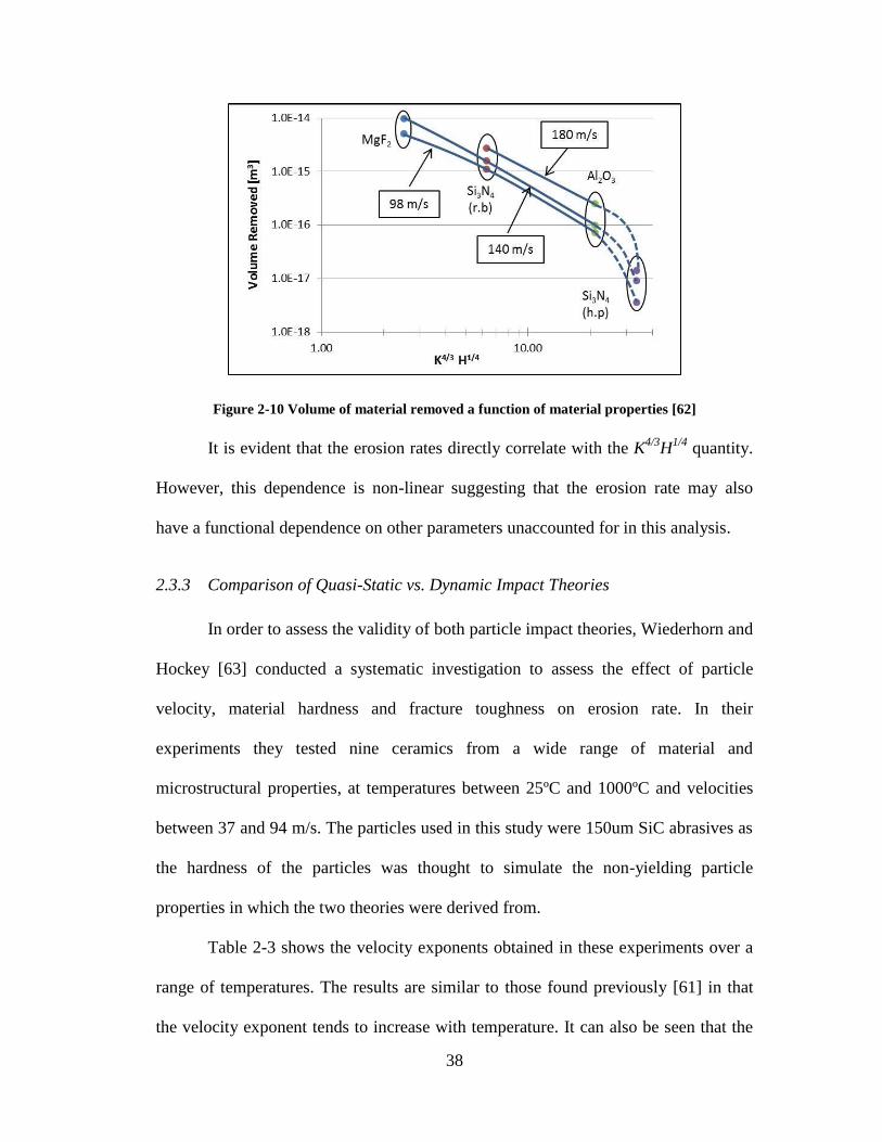
38

Figure 2-10 Volume of material removed a function of material properties [62]

It is evident that the erosion rates directly correlate with the K4/3

H1/4

quantity.

However, this dependence is non-linear suggesting that the erosion rate may also

have a functional dependence on other parameters unaccounted for in this analysis.

2.3.3 Comparison of Quasi-Static vs. Dynamic Impact Theories

In order to assess the validity of both particle impact theories, Wiederhorn and

Hockey [63] conducted a systematic investigation to assess the effect of particle

velocity, material hardness and fracture toughness on erosion rate. In their

experiments they tested nine ceramics from a wide range of material and

microstructural properties, at temperatures between 25ºC and 1000ºC and velocities

between 37 and 94 m/s. The particles used in this study were 150um SiC abrasives as

the hardness of the particles was thought to simulate the non-yielding particle

properties in which the two theories were derived from.

Table 2-3 shows the velocity exponents obtained in these experiments over a

range of temperatures. The results are similar to those found previously [61] in that

the velocity exponent tends to increase with temperature. It can also be seen that the

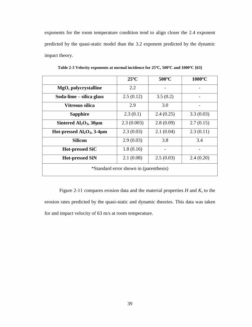
39

exponents for the room temperature condition tend to align closer the 2.4 exponent

predicted by the quasi-static model than the 3.2 exponent predicted by the dynamic

impact theory.

Table 2-3 Velocity exponents at normal incidence for 25ºC, 500ºC and 1000ºC [63]

25ºC 500ºC 1000ºC

MgO, polycrystalline 2.2 - -

Soda-lime – silica glass 2.5 (0.12) 3.5 (0.2) -

Vitreous silica 2.9 3.0 -

Sapphire 2.3 (0.1) 2.4 (0.25) 3.3 (0.03)

Sintered Al2O3, 30μm 2.3 (0.003) 2.8 (0.09) 2.7 (0.15)

Hot-pressed Al2O3, 3-4μm 2.3 (0.03) 2.1 (0.04) 2.3 (0.11)

Silicon 2.9 (0.03) 3.8 3.4

Hot-pressed SiC 1.8 (0.16) - -

Hot-pressed SiN 2.1 (0.08) 2.5 (0.03) 2.4 (0.20)

*Standard error shown in (parenthesis)

Figure 2-11 compares erosion data and the material properties H and Kc to the

erosion rates predicted by the quasi-static and dynamic theories. This data was taken

for and impact velocity of 63 m/s at room temperature.

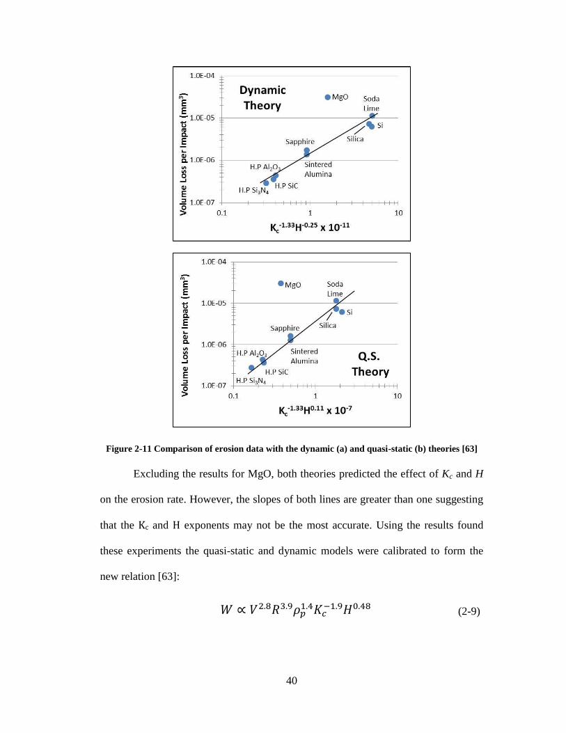
40

Figure 2-11 Comparison of erosion data with the dynamic (a) and quasi-static (b) theories [63]

Excluding the results for MgO, both theories predicted the effect of Kc and H

on the erosion rate. However, the slopes of both lines are greater than one suggesting

that the Kc and H exponents may not be the most accurate. Using the results found

these experiments the quasi-static and dynamic models were calibrated to form the

new relation [63]:

𝑊 ∝ 𝑉2.8𝑅3.9𝜌𝑝1.4𝐾𝑐

−1.9𝐻0.48 (2-9)

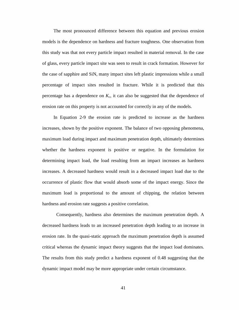
41

The most pronounced difference between this equation and previous erosion

models is the dependence on hardness and fracture toughness. One observation from

this study was that not every particle impact resulted in material removal. In the case

of glass, every particle impact site was seen to result in crack formation. However for

the case of sapphire and SiN, many impact sites left plastic impressions while a small

percentage of impact sites resulted in fracture. While it is predicted that this

percentage has a dependence on Kc, it can also be suggested that the dependence of

erosion rate on this property is not accounted for correctly in any of the models.

In Equation 2-9 the erosion rate is predicted to increase as the hardness

increases, shown by the positive exponent. The balance of two opposing phenomena,

maximum load during impact and maximum penetration depth, ultimately determines

whether the hardness exponent is positive or negative. In the formulation for

determining impact load, the load resulting from an impact increases as hardness

increases. A decreased hardness would result in a decreased impact load due to the

occurrence of plastic flow that would absorb some of the impact energy. Since the

maximum load is proportional to the amount of chipping, the relation between

hardness and erosion rate suggests a positive correlation.

Consequently, hardness also determines the maximum penetration depth. A

decreased hardness leads to an increased penetration depth leading to an increase in

erosion rate. In the quasi-static approach the maximum penetration depth is assumed

critical whereas the dynamic impact theory suggests that the impact load dominates.

The results from this study predict a hardness exponent of 0.48 suggesting that the

dynamic impact model may be more appropriate under certain circumstance.

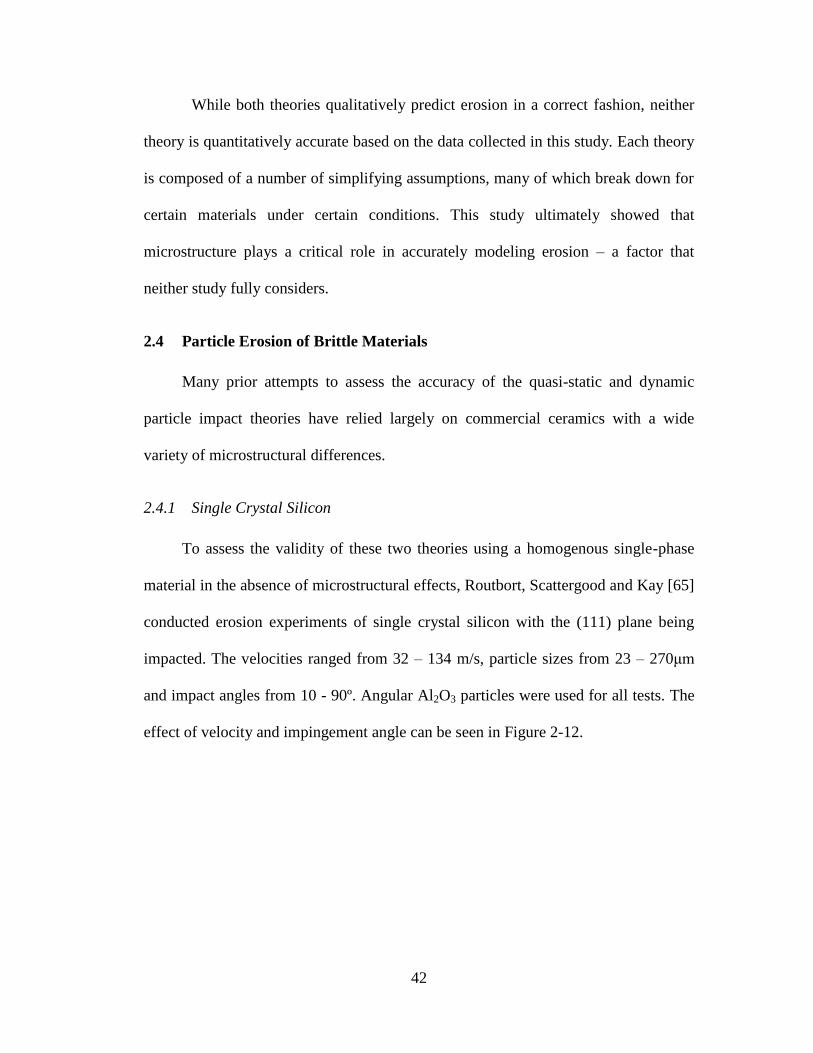
42

While both theories qualitatively predict erosion in a correct fashion, neither

theory is quantitatively accurate based on the data collected in this study. Each theory

is composed of a number of simplifying assumptions, many of which break down for

certain materials under certain conditions. This study ultimately showed that

microstructure plays a critical role in accurately modeling erosion – a factor that

neither study fully considers.

2.4 Particle Erosion of Brittle Materials

Many prior attempts to assess the accuracy of the quasi-static and dynamic

particle impact theories have relied largely on commercial ceramics with a wide

variety of microstructural differences.

2.4.1 Single Crystal Silicon

To assess the validity of these two theories using a homogenous single-phase

material in the absence of microstructural effects, Routbort, Scattergood and Kay [65]

conducted erosion experiments of single crystal silicon with the (111) plane being

impacted. The velocities ranged from 32 – 134 m/s, particle sizes from 23 – 270μm

and impact angles from 10 - 90º. Angular Al2O3 particles were used for all tests. The

effect of velocity and impingement angle can be seen in Figure 2-12.

43

Figure 2-12 Steady state erosion rate as a function of Vsinα [65]

The data is in good agreement with the quasi-static theory, assuming the

oblique angle adjustment proposed by Hockey [61], W ∝ (Vsinα)n where n = 2.6 for

impingements angle above 45º. However at low impingement angles the model under

predicts the erosion rate. This is thought to occur due to the fact that the erosion

model only accounts for the normal component of the velocity vector thus neglecting

the cutting and scribing processes that tend to occur at low impingement angles.

Additionally, the concepts of threshold particle sizes and velocities are

considered. This idea is based off previous work by Routbort, Scattergood and Turner

[66] who studied particle erosion of reaction bonded SiC. They discovered that at the

smallest particle size, 23μm, the erosion rate became anomalously low indicating

either a microstructural effect or a true threshold effect. In the case of Silicon the

44

same threshold effects were observed and are suggested to follow the following

relation DoVo = 2200x10-6

, where Do and Vo are the threshold particle diameter and

velocity respectively. Considering these effects, they formulated a new model:

𝐸𝑅 = 𝑘(𝑉𝑠𝑖𝑛𝛼 − 𝑉𝑜)2.6(𝐷 − 𝐷𝑜)

0.6 (2-10)

where ER is the erosion ratio (presented as the mass of material removed to the mass

of impacting particles) and k is a material constant. The particle size exponent m = 0.6

varies significantly from those presented in the quasi-static or dynamic theories, m =

11/3 or 3.67 due to the way the erosion metric is presented. In previously studies the

erosion metric is given as the volume of material removed, W in units of [length]3,

due to a single impacting particle. This study presents the erosion metric as a change

in weight-loss per dose of impacting particles ΔW in units of grams/gram. The erosion

formulation from previous studies:

𝑊 [𝑙𝑒𝑛𝑔𝑡ℎ]3 ∝ (𝑅 [𝑙𝑒𝑛𝑔𝑡ℎ])113 (2-11)

can be converted to the erosion metric of the present study by normalizing each side

of the above equation by the units [length]3 :

𝑊[𝑙𝑒𝑛𝑔𝑡ℎ]3

[𝑙𝑒𝑛𝑔𝑡ℎ]3∝(𝑅 [𝑙𝑒𝑛𝑔𝑡ℎ])

113

[𝑙𝑒𝑛𝑔𝑡ℎ]3 (2-12)

which gives the dimensionless erosion ratio ER:

𝐸𝑅 [𝑑𝑖𝑚𝑒𝑛𝑠𝑖𝑜𝑛𝑙𝑒𝑠𝑠] ∝ (𝑅 [𝑙𝑒𝑛𝑔𝑡ℎ])23 (2-13)

In light of this conversion, it can be seen that the particle size exponent m =

0.6 determined in this study matches well to the predicted m = 2/3 or 0.67 predicted

45

by both the quasi-static and dynamic impact theories. Figure 2-13 shows that their

experimental data matches quite well with their erosion model if threshold effects are

considered for impact angles above 45º.

Figure 2-13 Erosion Rate as a function of D - Do for different impact angles [65]

The divergence between the model and experimental data for an impact angle

of 22º lies in the fact that the model only considers the effect of the normal

component of the velocity vector. This would neglect cutting and other ductile

erosion mechanisms that may be present at smaller impact angles.

2.4.1.1 Velocity Exponent as a Function of Particle Size

One observation in previous studies is that the velocity and size exponents are

not constant values through the entire range of experiments. This suggests that there

may be some hidden dependencies of these values not captured by either the quasi-

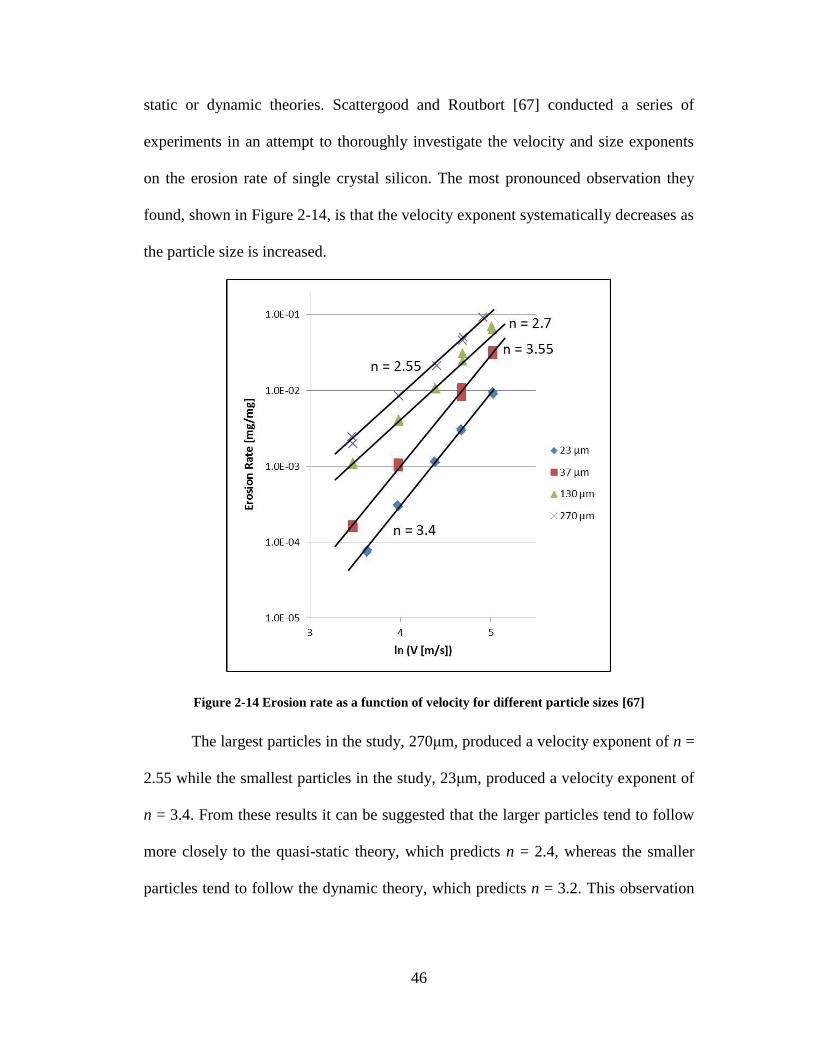
46

static or dynamic theories. Scattergood and Routbort [67] conducted a series of

experiments in an attempt to thoroughly investigate the velocity and size exponents

on the erosion rate of single crystal silicon. The most pronounced observation they

found, shown in Figure 2-14, is that the velocity exponent systematically decreases as

the particle size is increased.

Figure 2-14 Erosion rate as a function of velocity for different particle sizes [67]

The largest particles in the study, 270μm, produced a velocity exponent of n =

2.55 while the smallest particles in the study, 23μm, produced a velocity exponent of

n = 3.4. From these results it can be suggested that the larger particles tend to follow

more closely to the quasi-static theory, which predicts n = 2.4, whereas the smaller

particles tend to follow the dynamic theory, which predicts n = 3.2. This observation

47

is not just limited to silicon, but has been found previously in erosion studies of

reaction-bonded SiC [66] and hot-pressed SiC [68].

Another observation was that the particle size exponent changed as the

particle size changed. For particle sizes above 130μm, the erosion rate could be

accurately modeled assuming the typical m = 0.6 found in previous studies. However

for particles below 37μm, the erosion model would better fit the data assuming a size

exponent of approximately m ≈ 1.8. In addition to this observation, the tests

conducted at small particle sizes indicated a constant velocity exponent even at low

velocities. This invalidates the DoVo = 2200x10-6

velocity threshold prediction

previously made [65].

In a follow-up study Scattergood and Routbort [69] performed similar tests

with angular SiC and rounded SiO2 particles and compared the results to those

previously conducted with Al2O3 particles [65]. The results of these experiments,

shown in Table 2-4, aligned with those found in previous tests; that the velocity

exponent is dependent on particle size.

Table 2-4 Velocity exponent as a function of erodent material and size [69]

Erodent Material Velocity Exponent

40um Particles

Velocity Exponent

270um Particles

Al2O3 3.55 ± 0.1 2.55 ± 0.1

SiC 3.18 ± 0.1 2.65 ± 0.09

SiO2 3.44 ± 0.07 2.48 ± 0.09

While some variation exists between erodent materials, it can be suggested

that the particle size effect on the velocity exponent is material and shape

independent. One explanation that may account for this is localized heating due to

48

particle impact [69]. This anomaly was also found by Yust and Crouse [70] who

observed via SEM images localized melting in the case of 240μm SiC particles

impacting mullite ceramic at 24 m/s with an impact angle of 20º.

In an analysis by Shewmon [71] it was postulated that localized heating of the

target surface increases as particle size increases. Larger particles would thus better

facilitate the development of a plastically deformed region surrounding the impact

site. As the quasi-static theory suggests that the kinetic energy of an impacting

particle is converted into work creating plastic flow, this would explain why larger

particles tend to follow along the quasi-static theory more closely than smaller

particles. Since smaller amounts of localized heating would occur for small particles,

the dynamic model would conversely fit better. It was also calculated that the

threshold particle sizes above which localized heating becomes important in the

erosion of silicon is 46μm for Al2O3 particles and 41μm for SiC particles [69].

2.4.2 Sapphire and Zinc Sulphide

Telling and Field [72] studied the degradation of Sapphire (single crystal

Al2O3) and Zinc Sulphide by weight loss measurements and optical transmission

tests. They impinged 25 - 700μm quartz particles at velocities between 25 – 200 m/s.

The erosion rate results for zinc sulphide and sapphire are shown in Figure 2-15.

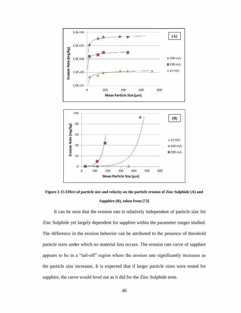
49

Figure 2-15 Effect of particle size and velocity on the particle erosion of Zinc Sulphide (A) and

Sapphire (B), taken from [72]

It can be seen that the erosion rate is relatively independent of particle size for

Zinc Sulphide yet largely dependent for sapphire within the parameter ranges studied.

The difference in the erosion behavior can be attributed to the presence of threshold

particle sizes under which no material loss occurs. The erosion rate curve of sapphire

appears to be in a “tail-off” region where the erosion rate significantly increases as

the particle size increases. It is expected that if larger particle sizes were tested for

sapphire, the curve would level out as it did for the Zinc Sulphide tests.

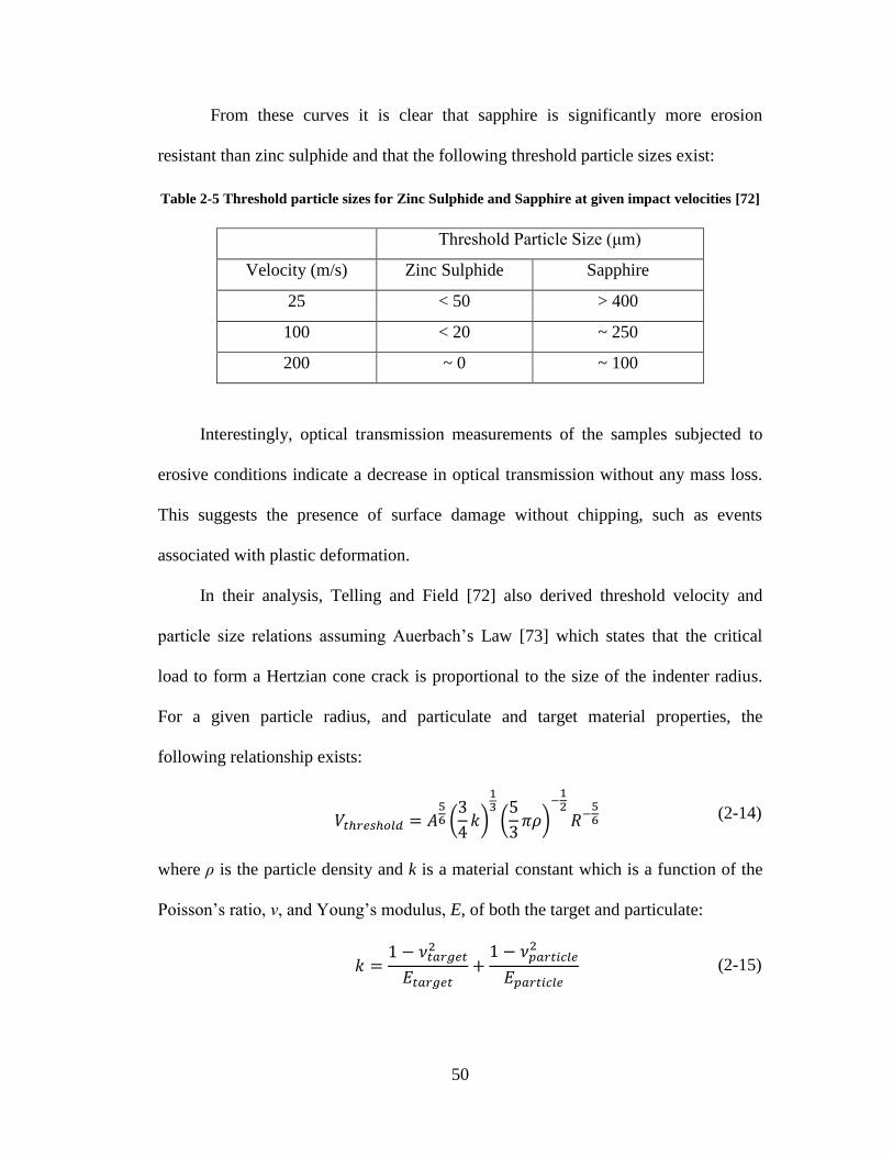
50

From these curves it is clear that sapphire is significantly more erosion

resistant than zinc sulphide and that the following threshold particle sizes exist:

Table 2-5 Threshold particle sizes for Zinc Sulphide and Sapphire at given impact velocities [72]

Threshold Particle Size (μm)

Velocity (m/s) Zinc Sulphide Sapphire

25 < 50 > 400

100 < 20 ~ 250

200 ~ 0 ~ 100

Interestingly, optical transmission measurements of the samples subjected to

erosive conditions indicate a decrease in optical transmission without any mass loss.

This suggests the presence of surface damage without chipping, such as events

associated with plastic deformation.

In their analysis, Telling and Field [72] also derived threshold velocity and

particle size relations assuming Auerbach’s Law [73] which states that the critical

load to form a Hertzian cone crack is proportional to the size of the indenter radius.

For a given particle radius, and particulate and target material properties, the

following relationship exists:

𝑉𝑡ℎ𝑟𝑒𝑠ℎ𝑜𝑙𝑑 = 𝐴56 (3

4𝑘)

13(5

3𝜋𝜌)

−12𝑅−

56 (2-14)

where ρ is the particle density and k is a material constant which is a function of the

Poisson’s ratio, ν, and Young’s modulus, E, of both the target and particulate:

𝑘 =1 − 𝜈𝑡𝑎𝑟𝑔𝑒𝑡

2

𝐸𝑡𝑎𝑟𝑔𝑒𝑡+1 − 𝜈𝑝𝑎𝑟𝑡𝑖𝑐𝑙𝑒

2

𝐸𝑝𝑎𝑟𝑡𝑖𝑐𝑙𝑒 (2-15)

51

A is Auerbach’s constant defined by Mouginot and Maugis [74]:

𝐴 = 6.7𝑥103𝑘𝑏𝛾 (2-16)

where γ is the free surface energy of the target and kb is also a material constant:

𝑘𝑏 = 1 +

(1 − 𝜈𝑡𝑎𝑟𝑔𝑒𝑡2 )𝐸𝑝𝑎𝑟𝑡𝑖𝑐𝑙𝑒

(1 − 𝜈𝑝𝑎𝑟𝑡𝑖𝑐𝑙𝑒2 )𝐸𝑡𝑎𝑟𝑔𝑒𝑡

(2-17)

This analytical relationship can be applied to the silicon-alumina target-

particulate system found in the works of Routbort and Scattergood [65]. Using the

experimentally derived threshold relation where DoVo = 2200x10-9

and assuming the

free surface energy of silicon to be 1.24 J/m2 [75] a comparison can be made between

analytical predictions and experimental findings:

Figure 2-16 Threshold velocity vs. particle size to induce cracking - silicon target and alumina

particles

It can be seen in Figure 2-16 that above a particle diameter of approximately

100μm, the experimental and analytical findings match well. However, below 100μm

52

the two results diverge. This can be primarily attributed to two reasons. First, at

particle sizes above 100μm and at the velocities used in the Routbort and Scattergood

studies, the mechanism of erosion is primarily fracture, chipping and cracking.

However below 100μm, the contribution of ductile erosion mechanisms and plastic

deformation take on more prominent roles. The analysis by Telling and Field does not

consider the effects of ductile erosion mechanisms. Secondly, the divergence between

experimental and analytical threshold conditions can also be attributed to the fact that

the analytical model assumes a perfectly uniform particle size whereas the

experimental study used alumina particles with some (unspecified) particle size

distribution. While the mean particle size may be under the analytical threshold, a

percentage of particles may be above it. As such, the experimental threshold particle

velocity at a given particle size should be lower than the analytical which assumes

uniform particle size.

2.5 Slurry Erosion of Brittle Materials

The discussion up to this point has assumed air to be the medium through

which particles travel through. Erosion experiments are typically conducted by

“sandblasting” target materials with a known quantity of particulates and measuring

the resultant weight loss that occurs. In the case where erodent particles are entrained

in a fluid, factors such as impact angle and impact velocity can be significantly

skewed due to the strong particle-fluid interactions that occur.

The Stokes number, defined in Equation 2-18, represents how strongly the

trajectory of an entrained particle is coupled to the fluid flow in the presence of an

obstacle.

53

𝑆𝑡 =𝜌𝑑2𝑈

18𝑙𝑜𝜇𝑓 (2-18)

where ρ is the particle density, d is the particle diameter, U is the velocity of the fluid

far away from the obstacle, lo is the characteristic dimension of the obstacle and μf is

the viscosity of the fluid. Particles with very high stokes numbers >> 1 are highly

inertial and respond slow to changes in fluid velocity whereas particles with very low

Stokes number << 1 are strongly coupled to the flow conditions [76]. Additionally the

presence of chemical or physical interactions between the fluid and wall may exist,

requiring a decoupling procedure to separate out which variables contribute to overall

material loss.

This section will discuss a number of factors affecting erosion specific to

slurry conditions along with implications pertaining to nanofluid erosion and abrasive

waterjet machining.

2.5.1 Observations from Slurry Pot Erosion Experiments

In a number of studies Clark, Lynn, Wong and co-workers [77] [78] [79] [80]

[81] examined the effects of particle size, velocity and fluid viscosity on the erosion

characteristics for ductile and brittle material. In all experiments they used a slurry

pot erosion tester which operates by rotating a stainless steel shaft via electric motor

through a slurry in a confined vessel. Cylindrical samples are attached to shaft such

that the rotational speed of the shaft can be correlated to the nominal velocity the

sample move through the fluid. This type of testing apparatus is shown in Figure 2-17

and more details regarding design, construction and modifications can be found

elsewhere in literature [82] [83] [84].

54

Figure 2-17 Schematic of slurry pot erosion testing apparatus

Clark [77] conducted short-term erosion tests on polished copper samples with

dilute suspensions of water/glycerin and glass beads ranging in sizes from 75 -

750μm. Two nominal speeds were used in the tests, 9.35 and 18.7 m/s. A collision

efficiency metric was determined by counting the number of impact sites per square

millimeter and dividing this by the number of particles estimated to be in the volume

of a 1 mm2 swept zone assuming a homogenous slurry. An average impact velocity

was also determined by measuring the crater diameter formed during impact and

comparing it to microhardness indentation tests. In this manner it was assumed that

all kinetic energy was transferred into work creating plastic flow in the copper

samples.

It was discovered that fluid viscosity, particle size and nominal flow velocity

directly influence the collision efficiency and actual impact velocity. Figure 2-18

shows the results of the 18.7 m/s tests.

55

Figure 2-18 Collision efficiency (A) and impact velocity (B) as a function of particle size and fluid

viscosity [77]

Referring to Equation 2-9, it can be seen that increasing the particle size and

decreasing the fluid viscosity result in a higher particle Stokes number meaning they

are less responsive to changes in the flow field. As the sample is swept through the

slurry, more particles would tend to impact the specimen as their motion is less

affected by the displaced fluid. The decrease in impact velocity with increasing fluid

viscosity and decreasing particle size is suggested to be a function of a boundary layer

56

effect. In order for a particle to impact the surface it must penetrate a boundary layer

of slow moving fluid and as the particle travels through this layer a significant

deceleration is suggested to occur.

Using the same type of slurry pot erosion testing apparatus Lathabai and

Pender [85] investigated the effects of varying the particle size distribution and

particle concentration on the erosion of a variety of ceramics. One observation they

found was that increasing the particle concentration from 5% to 20% a significant

increase in material loss was measured. However increasing the particle loading from

20% to 30% resulted in much less of an increase and even a decrease in material loss

for certain materials. This implies that at higher particle concentrations particle-

particle interactions become more prevalent and in some cases may inhibit particles

from striking the target surface.

Upon SEM inspection of the surface it was found that microstructure played a

critical role in the erosion mechanism. Inspection of fine and course grained alumina

samples both indicated that the wear mechanism was primarily grain ejection and

grain boundary microfracture. In the case of the Si3N4-SiC composite, preferential

phase erosion was observed causing the grains of the SiC phase to protrude as the

Si3N4 phase was removed. 3Y-TZP showed the least amount of erosion. Inspection of

the surface morphology indicated the presence of significant plastic deformation wear

scars but no signs of lateral fracture. The biggest conclusion from this study was that

microstructure plays a critical role in the erosion mechanisms of ceramics.

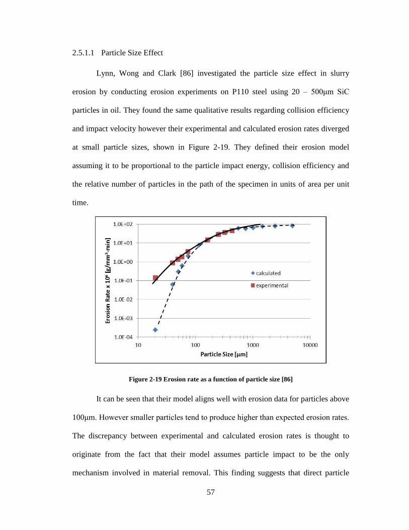
57

2.5.1.1 Particle Size Effect

Lynn, Wong and Clark [86] investigated the particle size effect in slurry

erosion by conducting erosion experiments on P110 steel using 20 – 500μm SiC

particles in oil. They found the same qualitative results regarding collision efficiency

and impact velocity however their experimental and calculated erosion rates diverged

at small particle sizes, shown in Figure 2-19. They defined their erosion model

assuming it to be proportional to the particle impact energy, collision efficiency and

the relative number of particles in the path of the specimen in units of area per unit

time.

Figure 2-19 Erosion rate as a function of particle size [86]

It can be seen that their model aligns well with erosion data for particles above

100μm. However smaller particles tend to produce higher than expected erosion rates.

The discrepancy between experimental and calculated erosion rates is thought to

originate from the fact that their model assumes particle impact to be the only

mechanism involved in material removal. This finding suggests that direct particle

58

impact may take on a smaller role and other material removal mechanisms may

become prominent.

In a later study Clark and Hartwich [81] re-examined the particle size effect

by conducting experiments on Pyrex glass and Aluminum using 14 - 780μm SiC

particles in oil. For Pyrex glass, the peak wear rate for particle sizes between 390 -

780μm was found to be proportional to D4, as was suggested by the quasi-static and

dynamic theories. No measurable damage was observed for particle sizes under

196μm however damage was observed for particle sizes between 196 - 275μm. Under

the experimental conditions used in this study, specifically a nominal velocity of 18.7

m/s, they estimated the threshold particle size under which no damage should occur

was between 300 - 425μm. The reason damage was observed in the 196 - 275μm was

thought to be a function of the particle size distribution in each batch of particles. In

each batch of erodent, there exists a spread of particle sizes with the mean particle

size presented as the nominal size. Although the mean particle size in each batch was

below the theoretically determined thresholds, the portion of particles above this

threshold is thought to cause the observed damage.

For the aluminum samples erosion was found at all particle sizes even though

direct impact was expected to cease for small particles. It is suggested the primary

wear mechanism taking place at these small particle sizes was a byproduct of the

boundary layer directly above the surface of the sample. This layer is referred to as

the “squeeze film” and is thought to inhibit direct particle impact but also prevents

particles from rebounding back into bulk fluid flow. As such, small particles are

thought to accumulate in this fluid layer and are swept away by tangential flow –

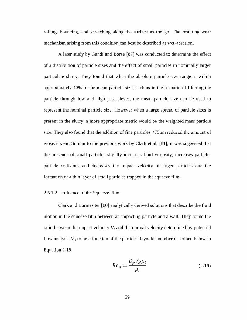
59

rolling, bouncing, and scratching along the surface as the go. The resulting wear

mechanism arising from this condition can best be described as wet-abrasion.

A later study by Gandi and Borse [87] was conducted to determine the effect

of a distribution of particle sizes and the effect of small particles in nominally larger

particulate slurry. They found that when the absolute particle size range is within

approximately 40% of the mean particle size, such as in the scenario of filtering the

particle through low and high pass sieves, the mean particle size can be used to

represent the nominal particle size. However when a large spread of particle sizes is

present in the slurry, a more appropriate metric would be the weighted mass particle

size. They also found that the addition of fine particles <75μm reduced the amount of

erosive wear. Similar to the previous work by Clark et al. [81], it was suggested that

the presence of small particles slightly increases fluid viscosity, increases particle-

particle collisions and decreases the impact velocity of larger particles due the

formation of a thin layer of small particles trapped in the squeeze film.

2.5.1.2 Influence of the Squeeze Film

Clark and Burmesiter [80] analytically derived solutions that describe the fluid

motion in the squeeze film between an impacting particle and a wall. They found the

ratio between the impact velocity Vi and the normal velocity determined by potential

flow analysis VN to be a function of the particle Reynolds number described below in

Equation 2-19.

𝑅𝑒𝑝 =𝐷𝑝𝑉𝑁𝜌𝑙𝜇𝑙

(2-19)

60

where ρl is the liquid density and μ is the liquid viscosity. Through this analysis they

determined a critical Reynolds number, Rec, below which impact would cease to

exist. The relationship describing this critical particle Reynolds number is described

in Equation 2-20.

𝑅𝑒𝑐 (𝜌𝑝𝜌𝑙+1

2) = 80 (2-20)

Another finding was that the squeeze film should also retard the particle’s

velocity on the rebound as well as the approach. For example, if the rebound is

considered elastic the particle Reynolds number upon entering the squeeze film must

be twice that of the critical Reynolds number in order escape the squeeze film [80]. In

the case of a ductile material with a coefficient of restitution of 0.1, the particle

Reynolds number upon entering the squeeze film must be 10x that of the critical

Reynolds number in order to exit the squeeze film.

This analysis suggests that particles may tend to congregate near the surface

forming an abrasive bed. Not only would this alter the experimental particle

concentration of the slurry, as the squeeze film would contain a denser particle count,

but the abrasive bed may act as a shield for incoming particles [79]. This may

introduce an additional factor reducing the collision efficiency.

2.5.2 Jet Impingement Studies of Ceramics

Fang et al. [88] studied the erosion behavior of four ceramics using a slurry jet

impingement apparatus. The particulate used was 600 - 850μm silica sand in

concentrations between 3 – 7.5% by weight. The nominal impingement velocity was

set at 7.3 m/s and the impingement angle was varied from 15 - 90º. Of all the

61

materials tested Al2O3 was found to be most susceptible to erosion, even more than

aluminum metal which was also tested. PSZ had the lowest erosion rate, about 100

times less than that of Al2O3. For all materials tested, the erosion rate was found to be

constant with time.

For Sialon and PSZ the effect on particle concentration was negligible,

however for SiC an increased particle concentration led to an increased erosion rate.

For Al2O3 the opposite was found where an increased particle concentration led to a

decreased erosion rate. Additionally the effect on impact angle was not uniform for

all materials. Al2O3 showed a typical brittle response peaking in erosion rate around

90º while SiC showed a larger than expected jump between erosion at 60º and 90º.

For Sialon and PSZ the erosion rate was relatively unaffected by impact angles

between 30º and 90º suggesting that these materials undergo different wear

mechanism. The fundamental justification for the wide range of erosion observation

originates from the microstructural differences. Similar to the results found by

Lathabai and Pender [85], the significantly high erosion rates of alumina compared to

the other tested materials was due to the mechanism of grain ejection and grain

dislodgement. While other materials showed signs of both brittle and ductile material

removal mechanisms, it was thought that grain ejection would disrupt the

development of plastic flow.

In an effort to examine more closely the effects of microstructure on erosion,

Zhang et al. [89] conducted air and slurry jet impingement experiments on three types

of alumina ceramics. Slightly rounded 200 - 600μm garnet particles were used as

abrasives. At low impact angles, material removal was characterized by ploughing

62

and subsequent spalling while at normal incidence grain ejection was the primary

mechanism of wear. In the case of airborne tests, localized melting of the target and

splashing of the garnet was observed generated by adiabatic heating caused by

impact. This localized heating phenomenon was not observed in slurry tests.

Regarding microstructure, lower velocity exponents were found for the

samples that contained a higher presence of intergranular glass phase. The glass phase

is thought to enable a higher absorption of impact energy. This belief was based on a

prior test that showed alumina with a 4% wt. intergranular phase exhibited an

increase in erosion resistance at increased temperatures [90]. It has also been

suggested that the presence of an intergranular glass phase can reduce stresses at the

grain boundaries, accommodate the non-uniform deformation behavior and reduce

residual stress at the grain boundaries [89] [91]. Comparing two samples of different

grain sizes but the same weight percentage of alumina, it was found that the samples

with larger grain sizes were more susceptible to erosion. This originates from the fact

that the main wear mechanism is grain boundary fracture resulting in grain ejection.

Lastly it was found that when the slurry and dry erosion data were

extrapolated to similar conditions, the slurry erosion was shown to be much more

severe. It is suggested that the fluid plays a critical role in crack propagation, thus

facilitating the erosion process.

2.5.3 Abrasive Slurry Jet Machining

Abrasive Slurry Jet Machining (ASJM) is used specifically to etch channels

and holes in brittle materials where other conventional machining methods may not

be appropriate. Machining occurs by impinging a high velocity slurry jet onto a

63

substrate that is either stationary, in the case of micro-hole formation, or is moving in

the case of channel formation. Typically the abrasive particles are small, on the order

to tens of micrometers or less, and the impinging jet is often less than a millimeter in

diameter. As such, the erosion modeling and characteristics involved in this process

have similar characteristics to those that would be involved in embedded cooling

systems.

2.5.3.1 Mechanisms of Microhole and Microchannel Formation

Wang et al. [92] studied the mechanisms of microhole formation in soda-lime

glass using a 200μm jet, alumina particle sizes between 10 – 17μm with concentration

of 2.5% and 5% by mass at nominal jet pressures of 1, 2 and 3 MPa. These pressures

approximately translate to nominal fluid velocities of 44, 63 and 77 m/s respectively.

Scanning the cross-sectional profiles using a stylus profilometer it was found that the

holes were characterized by a “W” shape, shown in Figure 2-20, where the outer

diameter of the etched region is nearly four times the diameter of the nozzle.

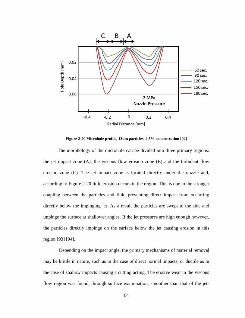
64

Figure 2-20 Microhole profile, 13um particles, 2.5% concentration [92]

The morphology of the microhole can be divided into three primary regions:

the jet impact zone (A), the viscous flow erosion zone (B) and the turbulent flow

erosion zone (C). The jet impact zone is located directly under the nozzle and,

according to Figure 2-20 little erosion occurs in the region. This is due to the stronger

coupling between the particles and fluid preventing direct impact from occurring

directly below the impinging jet. As a result the particles are swept to the side and

impinge the surface at shallower angles. If the jet pressures are high enough however,

the particles directly impinge on the surface below the jet causing erosion in this

region [93] [94].

Depending on the impact angle, the primary mechanisms of material removal

may be brittle in nature, such as in the case of direct normal impacts, or ductile as in

the case of shallow impacts causing a cutting acting. The erosive wear in the viscous

flow region was found, through surface examination, smoother than that of the jet-

65

impact or turbulent regions. It is suggested that this is a result of the squeeze film that

forms on the surface acting to lubricate and reduce friction between the particles and

surface. The surface characteristics indicate that the mode of material removal is

primarily ductile in the viscous flow region.

The turbulent zone forms as the erosion depth increases and causes a sudden

change in fluid direction. This region is suggested to be the cause of the substantially

large hole-width due to particles continuously recirculating thus increasing the

number of impacts. Interestingly, it was also found that that as the test parameters

changed, i.e. increasing particle size velocity or particle concentration, the overall

width of the hole changed.

In a similar study, Dadkhahipour et al. [95] studied the mechanisms of

microchannel formation using a high pressure slurry jet (100 – 200 MPa,

approximately 450 – 630 m/s) by traversing the nozzle across a glass substrate. They

also investigated the effects of standoff distance, traverse speed and impact angle.

Given the high pressures of the slurry jet, the cross-sectional profile appeared more

along the lines of a “U” shape rather than the “W” shaped profile found in lower

pressure systems. Increasing the nozzle traverse speed reduces substrate exposure

time to the abrasive jet, thus reducing the number of particle impacts.

Overall, they found the material removal rate to be relatively independent of

nozzle impact angle and standoff distance when compared to the effects of pressure

and traverse speed. Conversely the resulting wall inclination angle, defined as the

angle between the side of the channel and the non-eroded surface, was largely

66

affected by the standoff distance and water pressure, slightly dependent on jet impact

angle and relatively independent of nozzle traverse speed.

Using a test rig designed for lower velocities, Pang et al. [96] investigated the

effects of water pressure, nozzle traverse speed, particle concentration and stand-off

distance on channel depth, width and inclination angle in glass. Alumina particles

with a nominal size of 25μm were used, the water pressure varied between 8 – 14

MPa (approximately 126 – 167 m/s), the standoff distance was varied between 3 – 6

mm, particle concentrations varied between 15% and 30% and the nozzle traverse

speed varied between 0.15 – 0.3 mm/s. Figure 2-21 shows the effects of pressure and

particle concentration on channel width, depth and wall inclination angle where the

traverse speed is 15 mm/s and standoff height is 3 mm.

Figure 2-21 Effect of water pressure and particulate concentration on channel depth (A), channel

width (B) and wall inclination angle (C) taken from [96]

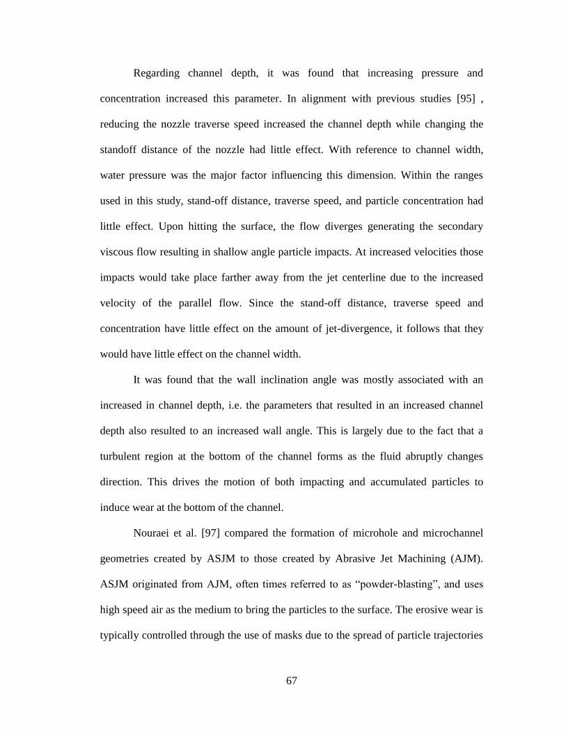
67

Regarding channel depth, it was found that increasing pressure and

concentration increased this parameter. In alignment with previous studies [95] ,

reducing the nozzle traverse speed increased the channel depth while changing the

standoff distance of the nozzle had little effect. With reference to channel width,

water pressure was the major factor influencing this dimension. Within the ranges

used in this study, stand-off distance, traverse speed, and particle concentration had

little effect. Upon hitting the surface, the flow diverges generating the secondary

viscous flow resulting in shallow angle particle impacts. At increased velocities those

impacts would take place farther away from the jet centerline due to the increased

velocity of the parallel flow. Since the stand-off distance, traverse speed and

concentration have little effect on the amount of jet-divergence, it follows that they

would have little effect on the channel width.

It was found that the wall inclination angle was mostly associated with an

increased in channel depth, i.e. the parameters that resulted in an increased channel

depth also resulted to an increased wall angle. This is largely due to the fact that a

turbulent region at the bottom of the channel forms as the fluid abruptly changes

direction. This drives the motion of both impacting and accumulated particles to

induce wear at the bottom of the channel.

Nouraei et al. [97] compared the formation of microhole and microchannel

geometries created by ASJM to those created by Abrasive Jet Machining (AJM).

ASJM originated from AJM, often times referred to as “powder-blasting”, and uses

high speed air as the medium to bring the particles to the surface. The erosive wear is

typically controlled through the use of masks due to the spread of particle trajectories

68

as they leave the nozzle. Ghobeity et al. conducted a number of studies on AJM such

as creating predictive surface evolution models [98] and an analytical model to deal

with the particle size distribution of abrasives [99].

In the work of Nouraei et al. [97] lower pressures between 1 – 4 MPa and

lower particulate concentrations between 0.25 – 1% by mass were used. As in other

experiments the effects of the nozzle traverse speed, standoff distance and jet impact

angle were also investigated. Similar to the analysis conducted by Clark [78], who

found that the impact velocity of particles entrained in the fluid was different than the

nominal fluid velocity due to the presence of a squeeze film, the difference between

the particle and fluid velocities at the centerline of the jet near the impact wall was

found. Shown in Figure 2-22, it can be seen that for a slurry jet exiting the nozzle at

approximately 62 m/s, a 25μm spherical alumina particle decelerates to

approximately 28 m/s upon impact.

Figure 2-22 Centerline velocity of a 25μm Al2O3 particle decelerating near the wall [97]

69

Examination of the glass surface showed signs of both brittle and ductile wear

mechanisms. Wensink and Elwenspoek [100] found that the brittle-to-ductile

transition for borosilicate glass was occurs at an impact kinetic energy of 17 nJ. This

translates to an impact velocity of 32 m/s for a 25μm alumina particle. Although the

nominal particle size was 25μm, Ghobeity et al. [99] found that for these same

particles approximately 27% were larger than 25μm, and would thus decrease the

brittle-to-ductile impact energy. While the majority of the particles would induce

ductile modes wear on the glass surface, a small percentage of particles would have

enough kinetic energy to cause fracture.

Figure 2-23 compares the normalized profiles of holes machined using ASJM

and AJM. For both profiles the dimensions were normalized by dividing by the

diameter of the hole formed. The ASJM profile was conducted by Nouraei [97] using

a 254μm nozzle, 25μm alumina particles, 0.25% mass concentration, 20mm standoff

while the AJM profile was created by Ghobeity [101], 760μm nozzle, 2.83 g/min of

25μm alumina particles, 200kPa and a 20mm standoff distance.

Figure 2-23 Comparison of normalized profile of ASJM and AJM [97]

70

It can clearly be seen that the ASJM shape more closely resembles a “U”

while the AJM shape appears to be a “V”. The difference in shape is largely attributed

to the non-uniform particle flux and velocity distribution across the air-jet. It was

found by Li et al. [102] and Dehnadfar et al. [103] that radial distance from the

centerline of the jet largely determines the air and particle velocities. Compared to

AJM, the velocity profile and thus inherently the particle flux in ASJM are relatively

uniform across the jet. This is due to the fact that the slurry jet has a low drag force

acting on it from the surrounding air. In summary the velocity profile across the jet is

non-uniform in AJM systems, however the trajectories of the particles are not

influenced by objects creating changes to the air streamlines. While the velocity

profile is relatively uniform across the jet in ASJM systems, changes in the fluid flow

field caused by obstacles can largely influence the trajectories of the particles given

low enough Stokes numbers.

2.5.3.2 Erosion Modeling in ASJM

Pang et al. [104] developed predictive models for the material removal rate

(MRR), channel height, width and wall inclination angle for the ASJM micro-

channeling process in amorphous glass. A schematic of the channel cross-section with

specific geometries is shown in Figure 2-24.

71

Figure 2-24 Schematic of ASJM channel cross-section

A total of 90 tests were performed over the following operating conditions:

water pressure between 8 – 14 MPa (126 – 167 m/s), nozzle traverse speed between

0.15 – 0.3 mm/s, alumina particle concentration between 15 – 30% by mass and

nozzle standoff distance between 3 – 6mm. For all tests alumina particles with a mean

particle size of 25μm were used. Additionally, due to the high velocity slurry used in

these tests, a “U” shaped channel geometry was formed as opposed to the “W” shape

found in lower velocity slurry jets [92].

The derived model that relates the MRR to various operating parameters is as

follows:

𝑀𝑅𝑅 = 𝑘 (𝑃

𝜌𝑠)1.83

𝐶𝑝1.78 (

𝑣𝑛√𝜌𝑠

√𝑃)

−0.78

(2-21)

where k is a material constant found to be 1.99x10-22

, P is jet pressure, vn is the nozzle

traverse speed, Cp is the particle concentration and ρs is the slurry density calculated

by:

𝜌𝑠 =𝜌𝑝𝜌𝑓

𝜌𝑝 + 𝐶𝑝(𝜌𝑓 − 𝜌𝑝) (2-22)

72

where ρp is the particle density and ρf is the fluid density. Overall, the model

correlated well with experimental results according to Figure 2-25.

Figure 2-25 Predicted vs. experimental results [104]

The most prominent factor affecting MRR was the jet pressure which is

intuitive due to the fact that pressure is proportional to velocity-squared according to

Bernoulli’s principle. As such, the MRR was found to be proportional to V3.66

, i.e. the

nominal jet velocity exponent is 3.66. This value is within the ballpark of previously

found velocity exponents for brittle erosion assuming the dynamic impact theory

holds true. One drawback to this model is that it assumes a non-zero value for the

nozzle traverse speed. In the case of jet-impingement cooling, the nozzle would be

73

stationary. While this model shows good correlations to experimental results, the

highly empirical nature suggests that this model may only be applicable within the

specific parameter ranges used in this study. As such, the applicability to other

scenarios is unknown.

Jafar et al. [105] used a combined CFD-experimental approach to investigate

how various operating parameters, such as pressure and jet angle, influenced the

erosion rate of channels etched into borosilicate glass. CFD was used to determine the

impact angle and impact velocity of individual alumina particles in order to calculate

the normal component of the particle’s kinetic energy upon impact. The normal

component was used for analysis because surface examination revealed that brittle

fracture was the primary mode of material removal.

The erosion model was based on the fact that particles will only cause damage

in glass if the normal component of the kinetic energy is above the threshold impact

energy, Uth, determined by Slikkerveer [106]:

𝑈𝑡ℎ = 23,225 𝐸32𝐾𝐶

6

𝐻132

(2-23)

While the threshold value for borosilicate glass was calculated to be 39 nJ

using this formulation, Wensink and Elwenspoek [100] experimentally found this

value to be 19 nJ for Pyrex glass. As such, 19 nJ was used in this study as the

threshold kinetic energy.

To predict the volume of material removed due to an impacting particle, two

different models for the erosion rates were assessed. The first model, ER1, assumes

that the lateral crack formed from a particle impact originates at the base of the plastic

74

zone, aligning with the theory developed by Marshall, Lawn and Evans [57]. The

second erosion model, ER2, is based on previous work by Jafar et al. [107] who

showed that the depth of the chip removed can be better approximated by the

indentation depth of the particle as opposed to the depth of the plastic zone. The

erosion models are defined as follows:

𝐸𝑅1 =𝜋

6

𝜌𝑡𝑏(𝑏2 + 3𝑐𝐿

2)2

𝑚𝑝 (2-24)

𝐸𝑅2 =𝜋

6

𝜌𝑡𝑎(𝑎2 + 3𝑐𝐿

2)2

𝑚𝑝 (2-25)

where mp is the mass of particle, ρt is the density of the glass and a and b are the

depths of the indentation zone and plastic zone respectively, defined as [106]:

𝑎 = (3𝑈

2𝜋𝐻)

13 (2-26)

𝑏 ≅ 0.63𝑎 (𝐸

𝐻)

12

(2-27)

The size of the lateral crack, CL, was derived by Marshal et al. [57] as:

𝑐𝐿 = (𝜁𝐿

√𝐴(cot(𝜓))

56𝐸34

𝐻𝐾𝐶)

12

(1 − (𝐹0𝐹)

14)

12

(2-28)

75

𝐹 = (18𝐻 tan2(𝜓)13𝑈

23 (2-29)

𝐹0 =𝜁0𝐴2cot(𝜓)−

23 (𝐸𝐾𝑐

4

𝐻4) (1-30)

where F and F0 are the indentation force and the threshold load for cracking

respectively, ζL is a constant found to be 0.025, A is a geometrical constant equal to

0.75, ψ is the indenter angle assumed to be 74º and ζ0 was experimentally determined

to be 1200 [57].

Particle sizes between 5 - 45μm were considered due to the fact that a known

particle size distribution exists for a batch of nominally sized 25μm alumina particles.

To deal with the particle size distribution, an effective kinetic energy was used in the

modeling efforts and defined to be the weighted average normal kinetic energy of the

particles above the threshold kinetic energy. Using this assumption, the impact kinetic

energy of the particle, U in the Equation 2-26, is essentially an effective average

impact kinetic energy of the particle size distribution.

A comparison of the predicted erosion rate, defined as the ratio of the mass of

material removed to the mass of impacting particles, is shown in Figure 2-26. The

experimental conditions were composed of 25μm alumina particles (with known

particle size distribution ranging from 5 - 45μm), jet pressures between 2.1 – 6.1 MPa

(approximately 65 – 110 m/s), 0.25% by mass particle concentration and a normal jet

impingement.

76

Figure 2-26 Erosion rate of borosilicate glass as a function of effective average normal impact

kinetic energy [105]

It can be seen that ER2 (Model II), which assumes that the depth of the chip

removed can best be approximated by the indentation depth of the particle, matches

the experimental data quite well. While Model II better predicted the erosion rate

compared to Model I, it was still found to under predict the erosion rate by an average

of 41%. It was found that increasing the crater depth a by 22% to match the

experimental results in another study [107] reduced the average error down to 12%.

2.5.4 Nanofluid Erosion

While the majority of particle erosion and slurry erosion studies assume

particle sizes on the order of tens to hundreds of micrometers, erosion studies

involving nanofluids may offer additional insight regarding the potential for erosion

in microchannel and embedded cooling loops due to the small particles used. The

primary parallelism lies in the fact that electronic cooling loops typically have filters

that prevent larger particles from entering the region where erosion protection is

critical. Nanofluids typically have high concentrations of particles that are on the

77

order of tens of nanometers in size. They are prepared in such a way to prevent

particle agglomeration, meaning they would be extremely challenging to filter out

using conventional filtering techniques. While the number of erosion studies

involving nanofluids is limited, the information presented here may provide insight

regarding the phenomenon of fine-scale erosion.

Routbort, Singh and co-workers [108] studied the effects of nanofluids on

heavy vehicle cooling systems, specifically the potential for erosion on select

materials. The erosion of Aluminum 3003 was assessed using a suspension of copper

nanoparticles in 50/50 water/ethylene glycol and trichloroethylene at 50ºC. Through

mass loss measurements, the erosion rate was determined for impingements velocities

between 1 – 10 m/s and impact angles from 30 - 90º. The only test that showed any

measureable erosion between 200 – 300 hours of testing was the test of 9.6 m/s at

normal incidence resulting in a mass loss rate of 3.5x10-6

grams/hour, or

approximately 165 μm/year. CuO/ethylene glycol and SiC/water nanofluids were also

tested [109] and yielded no measureable erosion, although surface pitting and

corrosion was observed upon closer inspection of the surface.

In conducting these experiments it was found that significant wear of the

pump occurred, specifically in the gears. In a test running > 700 hours using a 2% by

volume SiC nanofluid at 8 m/s and an impact angle of 30º, erosion of the target

material was not observed, however pump wear was [110] [108]. While these studies

may provide valuable insight regarding the potential for erosion in radiator

applications, velocities of less than 10 m/s are about half that of those present in

embedded cooling systems.

78

In a similar study Nguyen et al. [111] studied the jet impingement slurry

erosion of aluminum at 19 m/s using a SiC-water nanofluid (36nm particles, 5% by

volume concentration). After 180 hours of testing a total of 14 mg mass loss was

recorded, while the control sample showed no change in mass loss. Surface

examinations revealed rounded microstructures and pits not present on the pre-eroded

samples. While it was concluded that nanofluids can lead to significant wear over

time, the specific mechanism of material removal was not assessed.

Molina et al. [112] conducted erosion experiments on aluminum and copper

samples using an alumina-water/ethylene glycol nanofluid (2% volume concentration,

10nm particle size before agglomeration) at 10.7 m/s normal impact. Tests times

ranged from 3 to 112 hours. Mass loss and surface roughness measurements were

taken periodically throughout the experiments to monitor surface evolution.

For aluminum a slight 5mg mass gain was observed over the first 28 hours

followed by no measureable change. This was likely due to the formation of a

protective oxide layer that formed on the surface. Additionally, roughness

measurements indicated that surface modification takes place over the course of the

first 28 hours in the form scratch removal and slight removal of loose surface

fragments. After 28 hours slight pitting was observed specifically near the original

polishing lines, suggesting the presence of a mild abrasion mechanism.

No measureable weight change was measured for copper, however mild

surface modifications were observed throughout the test. Similar to aluminum, mild

pitting was observed for both the reference fluid and nanofluid, suggesting a slight

chemical component affecting material removal.

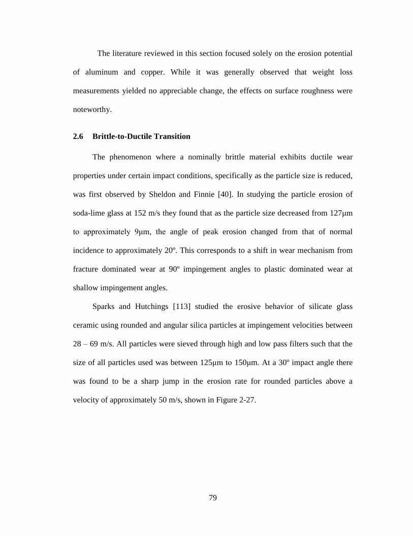
79

The literature reviewed in this section focused solely on the erosion potential

of aluminum and copper. While it was generally observed that weight loss

measurements yielded no appreciable change, the effects on surface roughness were

noteworthy.

2.6 Brittle-to-Ductile Transition

The phenomenon where a nominally brittle material exhibits ductile wear

properties under certain impact conditions, specifically as the particle size is reduced,

was first observed by Sheldon and Finnie [40]. In studying the particle erosion of

soda-lime glass at 152 m/s they found that as the particle size decreased from 127μm

to approximately 9μm, the angle of peak erosion changed from that of normal

incidence to approximately 20º. This corresponds to a shift in wear mechanism from

fracture dominated wear at 90º impingement angles to plastic dominated wear at

shallow impingement angles.

Sparks and Hutchings [113] studied the erosive behavior of silicate glass

ceramic using rounded and angular silica particles at impingement velocities between

28 – 69 m/s. All particles were sieved through high and low pass filters such that the

size of all particles used was between 125μm to 150μm. At a 30º impact angle there

was found to be a sharp jump in the erosion rate for rounded particles above a

velocity of approximately 50 m/s, shown in Figure 2-27.

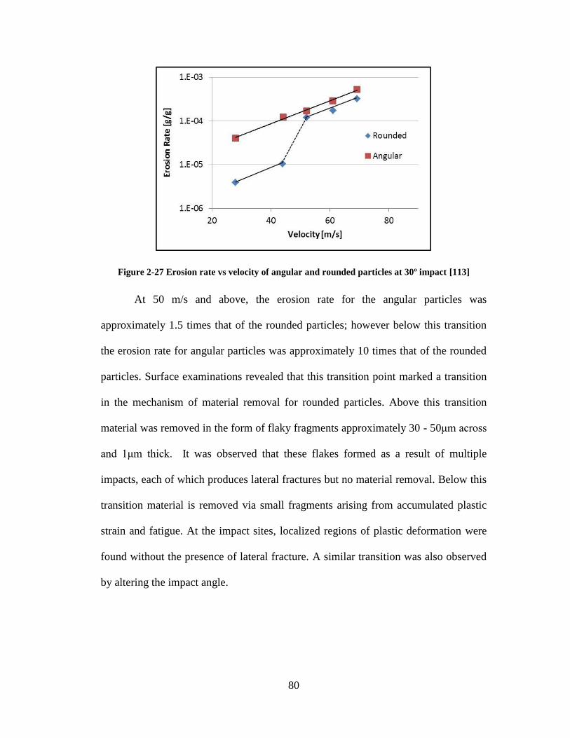
80

Figure 2-27 Erosion rate vs velocity of angular and rounded particles at 30º impact [113]

At 50 m/s and above, the erosion rate for the angular particles was

approximately 1.5 times that of the rounded particles; however below this transition

the erosion rate for angular particles was approximately 10 times that of the rounded

particles. Surface examinations revealed that this transition point marked a transition

in the mechanism of material removal for rounded particles. Above this transition

material was removed in the form of flaky fragments approximately 30 - 50μm across

and 1μm thick. It was observed that these flakes formed as a result of multiple

impacts, each of which produces lateral fractures but no material removal. Below this

transition material is removed via small fragments arising from accumulated plastic

strain and fatigue. At the impact sites, localized regions of plastic deformation were

found without the presence of lateral fracture. A similar transition was also observed

by altering the impact angle.

81

2.6.1 Transitional Wear Maps

Hutchings [114] developed wear maps to illustrate how altering the particle size

and impact velocity shift the wear mechanisms away from fracture dominated to

those dominated by plastic flow. These maps consider the effects of both rounded and

angular particles and assess whether the potential fractures takes the form of Hertzian

or lateral cracking.

The transition map depicting the onset of Hertzian cracking from either elastic

or plastic collisions was developed by plotting two equations and assessing their

intersection point. The first equation was derived by Wiederhorn and Lawn [115] and

showed that the critical impact velocity above which Hertzian fracture will occur, VH,

can be related to the diameter of the impacting sphere:

𝑉𝐻 ∝𝐾𝑐

53

𝐸76

𝜌−12𝑑−

56 (2-31)

where E is an effective elastic constant and depends on the Young’s modulus and

poisons ratio of both the impacting particle and target surface. This equation can

alternatively be written to relate the critical dimeter of the impacting sphere, dH, to the

impact velocity:

𝑑𝐻 ∝𝐾𝐶2

𝐸75

𝜌−35𝑉−

65 (2-32)

The second equation used to create the transitional wear map for Hertzian

fracture relates the critical velocity necessary to initiate plastic flow, VP, to various

material parameters. This formulation additionally assumes that the mean contact

pressure is independent of the diameter of the sphere [116].

82

𝑉𝑃 ∝𝜌−

12𝐻

52

𝐸2 (2-33)

Plotting Equations 2-32 and 2-33, as shown in Figure 2-28, a number of

regions can be discerned which indicate the primary wear mechanisms associated

with the impact conditions.

Figure 2-28 Schematic showing transitional wear map associated with Hertzian fracture [114]

In region I at low velocities and small particle sizes, the impact is purely

elastic and any wear in this region can be associated with fatigue processes, i.e. many

impacts would be required to induce cracking. Increasing the velocity at small

particle sizes transitions the system to region II, where ductile wear mechanisms

begin dominate the erosion process. At large particle sizes and low velocities, region

III, Hertzian cone cracks will form. If the system enters region IV the assumptions

presented in the previous equations will no longer be valid, however it is predicted

that both Hertzian fracture and plastic deformation mechanisms will be present.

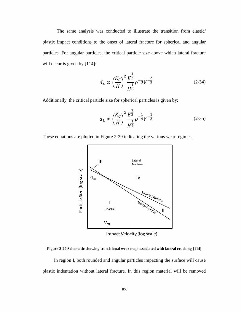
83

The same analysis was conducted to illustrate the transition from elastic/

plastic impact conditions to the onset of lateral fracture for spherical and angular

particles. For angular particles, the critical particle size above which lateral fracture

will occur is given by [114]:

𝑑𝐿 ∝ (𝐾𝐶𝐻)2 𝐸

12

𝐻16

𝜌−13𝑉−

23 (2-34)

Additionally, the critical particle size for spherical particles is given by:

𝑑𝐿 ∝ (𝐾𝐶𝐻)2 𝐸

12

𝐻14

𝜌−14𝑉−

12 (2-35)

These equations are plotted in Figure 2-29 indicating the various wear regimes.

Figure 2-29 Schematic showing transitional wear map associated with lateral cracking [114]

In region I, both rounded and angular particles impacting the surface will cause

plastic indentation without lateral fracture. In this region material will be removed

84

primarily by plastic processes, although brittle mechanisms may occur due to cyclic

fatigue arising from multiple impacts. According to the assumptions inherent in the

defining equations, all particles are expected to cause plastic flow due to the notion

that an indenter, whether perfectly sharp or with a slight radius of curvature, will

cause a stress singularity. In region IV lateral fracture will occur for all particles

regardless of shape, and the erosion mechanisms will be dominantly brittle. In region

II, angular particles will cause lateral fracture while rounded particles will just result

in plastic flow. Region III represents the region where rounded particles will cause

fracture but rounded particles will not. It is not clear if this region has physical

significance as it is suggested that key assumptions in the equations may break down

at these low velocities. Although ideal angular particles will cause plastic flow at all

velocities, in reality the velocity may not be high enough to induce plastic

deformation resulting in an elastic collision.

2.6.2 Glass and Silicon

Wensink and Elwenspoek [100] examined the transition from brittle to ductile

wear processes for Pyrex, sodalime glass and single crystal <100> silicon. In their

experiments, sharp alumina particles from 3 – 29.2μm were air-blasted onto the

various substrates at velocities up to 200 m/s. Weight loss measurements were

conducted post-erosion to determine the erosion rate in grams of material lost divided

by the grams of particulate used. An erosion classification value was defined, ECV,

which is the ratio of the erosion rate at 45º impingement to that of the erosion rate at

normal incidence. Additionally, the erosion rate at 90º was fitted to be proportional to

the kinetic energy of the impacting particle:

85

𝐸𝑅 ∝ 𝑈𝑘𝑖𝑛𝑝

(2-36)

where p is the kinetic energy exponent and is half that of the typically defined

velocity exponent. Figure 2-30 shows the results for silicon where ECV and the

erosion rate are plotted against the kinetic energy.

Figure 2-30 ECV and erosion rate of silicon as a function of kinetic energy [100]

Regarding the erosion rate plot, two regimes can be seen. One regime is

considered the low energy regime and is mostly comprised of ductile erosion

mechanisms while the other high energy regime consists mostly of the brittle wear

mechanisms. The intersection of these two lines is considered the brittle-to-ductile

86

transition point. For the three materials studied, the kinetic energy exponents for both

regimes are shown in Table 2-6.

Table 2-6 Kinetic energy exponents for high and low energy regimes [100]

High Energy

Regime

Low Energy

Regime

Pyrex 1.42 2.35

Silicon 1.53 2.35

Sodalime Glass 1.38 3.2

This transition was found to be relatively gradual due to the many variances

between individual impacts such as particle size, shape, velocity and angle. However,

at low enough kinetic energies it is expected that the velocity exponent should

converge to that of a typical ductile material, between 2.2 and 2.4 [117].

The ECV graph can be divided into three primary stages with respect to the

impact kinetic energy. Transitioning from the high energy region to low energy

region, the ECV initially rises. It is suggested that at lower kinetic energies the

contribution of tangential forces, such as those present in 45º impacts, contribute

more to lateral crack propagation. In the second stage, the ECV decreases slightly to a

minimum as the tangential impact force plays less of a role in enhancing lateral crack

propagation. In the third stage the ECV rises as the number of ductile impacts

occurring at normal incidence increases. An ECV > 1 indicates a shift in the erosion

rate vs. impact angle curve from nominally brittle to nominally ductile behavior.

Using the analysis conducted by Slikkerveer et al. [106], the theoretical

threshold energies for lateral crack propagation were calculated. These values are

compared to the experimentally determined ones in Table 2-7.

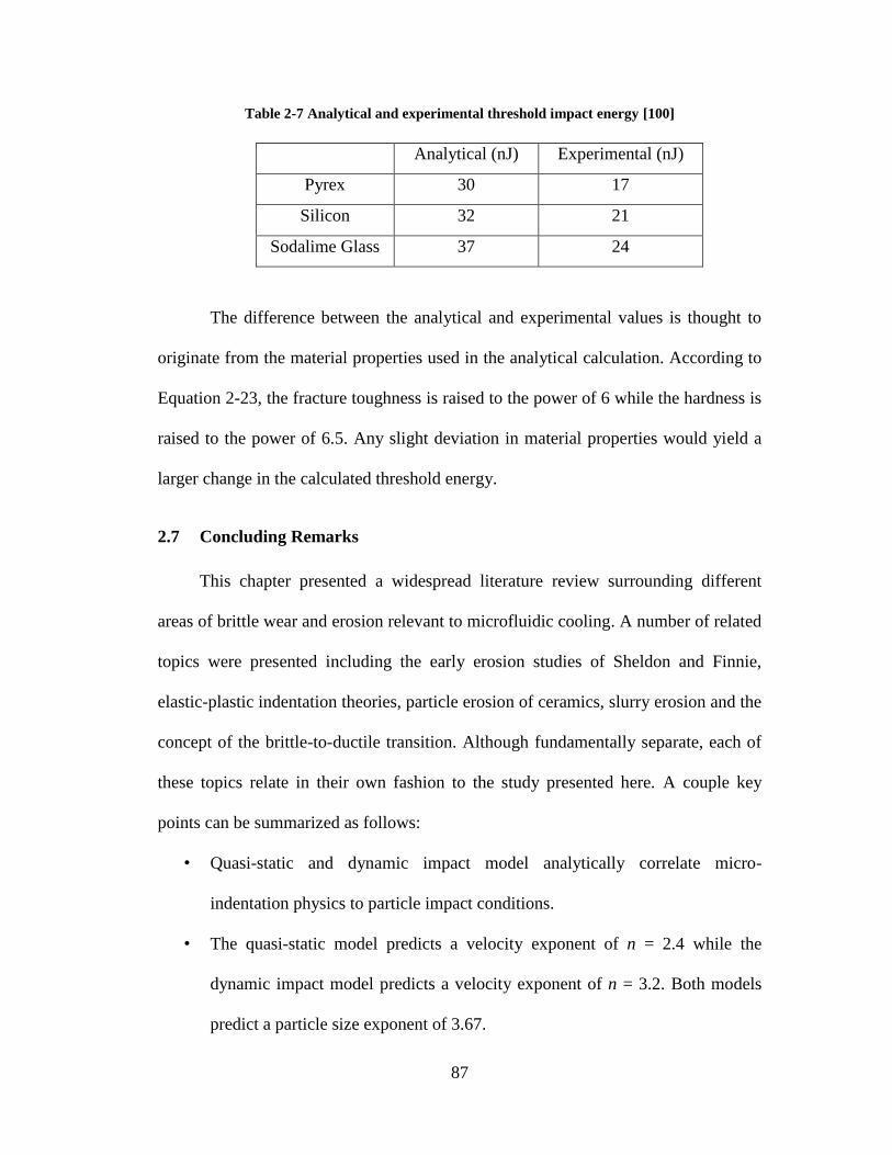
87

Table 2-7 Analytical and experimental threshold impact energy [100]

Analytical (nJ) Experimental (nJ)

Pyrex 30 17

Silicon 32 21

Sodalime Glass 37 24

The difference between the analytical and experimental values is thought to

originate from the material properties used in the analytical calculation. According to

Equation 2-23, the fracture toughness is raised to the power of 6 while the hardness is

raised to the power of 6.5. Any slight deviation in material properties would yield a

larger change in the calculated threshold energy.

2.7 Concluding Remarks

This chapter presented a widespread literature review surrounding different

areas of brittle wear and erosion relevant to microfluidic cooling. A number of related

topics were presented including the early erosion studies of Sheldon and Finnie,

elastic-plastic indentation theories, particle erosion of ceramics, slurry erosion and the

concept of the brittle-to-ductile transition. Although fundamentally separate, each of

these topics relate in their own fashion to the study presented here. A couple key

points can be summarized as follows:

• Quasi-static and dynamic impact model analytically correlate micro-

indentation physics to particle impact conditions.

• The quasi-static model predicts a velocity exponent of n = 2.4 while the

dynamic impact model predicts a velocity exponent of n = 3.2. Both models

predict a particle size exponent of 3.67.

88

• Units through which the erosion rate metrics are presented vary from author to

author. Typically, the erosion rate is described as a volume loss rate (ex:

mm3/hour), a mass loss rate (ex: mg/hour) or an erosion ratio in units of

mg/mg defined as the ratio of material removed per mass of impacting

particle. Erosion models are often formulated such that the mass of material

removed can be calculated for a single impacting particle.

• Routbort and Scattergood showed that the velocity exponent changes

depending on particle size. Small particles (40μm) tend to follow the dynamic

impact theory while large particles (270μm) tend to follow the quasi-static

model.

• Fluid plays a large role in particle impact conditions. Fluid velocity does not

equate to particle impact velocity. The Stokes number can be used to

determine how closely coupled a particle trajectory is to a fluid streamline.

• The squeeze-film may facilitate erosion by introducing an additional ‘wet-

abrasion’ mechanism. This has only been observed in ductile materials.

• Brittle-to-ductile transition occurs as the impact kinetic energy of particles is

decreased. At low velocities and particle sizes, brittle erosion transitions into

ductile wear.

• ASJM offers qualitative insight into the type of erosion resulting from jet-

impingement cooling. Characteristic ‘W’ erosion contour will likely be

observed.

As discussed in the Chapter 1, a common theme surrounding previously

conducted erosion studies is that the particle sizes, velocities and materials used are

89

vastly different than those present in microchannel or embedded cooling systems. It is

unknown if these models can be extrapolated down to the particle sizes or velocities

of interest given that they were calibrated for vastly different parameter ranges.

Additionally, the brittle-to-ductile transition suggests that a shift in wear mechanism

may occur at the conditions present in microchannel and embedded coolers. Although

unknown, it is unlikely that erosion from this alternative mechanism can be modeled

using the same predictive equations as the brittle erosion mechanism. It will be the

purpose of this study to fill this research gap and conduct erosion studies using

conditions most likely found in microchannel and embedded cooling systems.

90

3 PROBLEM STATEMENT AND OBJECTIVES

This brief chapter recounts the fundamental problem statement and explicitly

states the goals of this research. Of the various embedded cooling architectures

described in the introduction and literature review chapters, jet-impingement cooling

provides excellent cooling capabilities, however the major drawback is the potential

for particle erosion and wear of the substrate. As jet velocities reach and exceed 20

m/s, this mechanism becomes a significant reliability threat due to the fact that the

substrate separating the active electronics from the impinging jet can be on the order

of 50-100μm thick. While jet-impingement cooling may be most susceptible to

erosion, other types of liquid cooling techniques may be at risk especially over long

term operation.

In the design phase of an embedded or microchannel cooling system, an erosion

prediction is vital to ensure that catastrophic damage does not occur over the expected

lifetime of the device. Even more important is to identify safe operating regions

where, even though erosion may be present, significant damage will not occur. This

erosion prediction is typically conducted using CFD simulations and tracking particle

impingements using Lagrangian methodologies. An erosion equation determines how

much material is removed per impinging particle. Commercial CFD codes such as

ANSYS FLUENT and CFX have built in erosion equations and/or predefined

constants in their user manuals that can be used. Other times erosion equations taken

from the open literature are hooked into the CFD code using custom scripts.

While numerous particle erosion models exist, seldom are the velocities,

particle sizes, materials and testing times in alignment with those that would exist in

91

embedded cooling systems. In addition, the models from literature are typically

calibrated using air as the transportation medium which ignores potential surface-

particle interaction effects caused by fluids. Furthermore, as discussed in the Chapter

2, at very low particle sizes and velocities there exists a fundamental shift in wear

mechanism that takes place in nominally brittle materials. The accuracy of the

established brittle erosion models is unknown given this shift in wear mechanism.

This same principle applies to the erosion correlations built into the commercial CFD

codes - they were derived for ductile materials such as copper, steel and aluminum.

While many of these models may provide a sound first order approximation as to the

qualitative extent of erosion, it is unknown how well they can be applied to the

specific conditions present in microchannel coolers.

Given the need for high accuracy erosion predictions, this research aims to fill

the gap in erosion models currently available in literature. Nominal jet velocities will

be kept in the range of 20 – 40 m/s, considering both realistic and accelerated

velocities. Particle sizes will be kept below 20μm enabling the consideration of many

different filtering levels. Silicon was chosen as the material of interest due to its wide

use in power electronic substrates, specifically in the current and future

implementations of GaN-on-Si power devices.

The primary objective of this research is to develop a particle erosion model,

calibrated for silicon, within the parameter ranges relevant to those in microchannel

and embedded cooling systems. However, this objective can be broken down into six

fundamental segments:

92

1) Develop a jet-impingement CFD model in ANSYS FLUENT to obtain localized

particle impact characteristics. Along with this task comes the development of

user-defined functions to amend the abilities inherently present in the software.

Simulations will be performed that correspond directly to the slurry erosion

experiments.

2) Design and construct a slurry erosion jet-impingement test apparatus to perform

erosion experiments on single crystal silicon.

3) Formulate and execute a series of tests to investigate the effects of jet velocity,

particle size, concentration, fluid viscosity and time.

4) Gain insight into the wear mechanisms of single crystal silicon under

microchannel cooler operating conditions, namely particle sizes less than 20μm

and jet velocities less than 40 m/s.

5) Combine localized particle impact data from the CFD simulations with

experimental erosion data to extend the Huang cutting erosion model to new

parameter ranges and new materials. This involves developing the process and

calibrating new particle size and velocity exponents, along with a new

material/system constant.

6) Perform validation simulations in FLUENT to compare measured 1-D erosion

rates from experiments to the predicted 1-D erosion rates of the simulations.

While the model will be developed using the erosion ratio metric, the output of

the validation simulations will be in units of micrometers-per-year. As such, a

different erosion metric will be used to validate the model compared the one used

to calibrate the model. Lastly, an impact dampening coefficient will be proposed

93

to provide potential explanations for slight inconsistencies between experiments

and the CFD predictions.

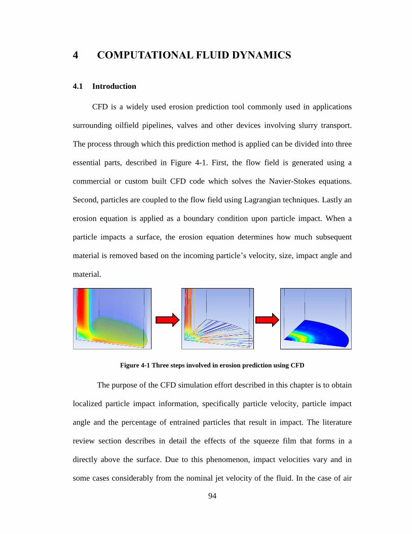
94

4 COMPUTATIONAL FLUID DYNAMICS

4.1 Introduction

CFD is a widely used erosion prediction tool commonly used in applications

surrounding oilfield pipelines, valves and other devices involving slurry transport.

The process through which this prediction method is applied can be divided into three

essential parts, described in Figure 4-1. First, the flow field is generated using a

commercial or custom built CFD code which solves the Navier-Stokes equations.

Second, particles are coupled to the flow field using Lagrangian techniques. Lastly an

erosion equation is applied as a boundary condition upon particle impact. When a

particle impacts a surface, the erosion equation determines how much subsequent

material is removed based on the incoming particle’s velocity, size, impact angle and

material.

Figure 4-1 Three steps involved in erosion prediction using CFD

The purpose of the CFD simulation effort described in this chapter is to obtain

localized particle impact information, specifically particle velocity, particle impact

angle and the percentage of entrained particles that result in impact. The literature

review section describes in detail the effects of the squeeze film that forms in a

directly above the surface. Due to this phenomenon, impact velocities vary and in

some cases considerably from the nominal jet velocity of the fluid. In the case of air

95

where the carrier medium has negligible viscosity, the particle impact velocity can be

taken as the same velocity at which the particles exit the jet. As the viscosity of the

fluid increases, particles become more strongly coupled to the fluid motion and

therefore this viscous effect becomes more pronounced. This has a significant effect

on where the particles impact the surface, the speed and angle at which they impact,

and how many entrained particles actually reach the surface. In the case of air it can

be assumed that all particles reach the surface, however as the fluid viscosity

increases a smaller percentage of particles reach the surface as many become

entrained in the bulk flow.

This chapter will be outlined as follows. First, a general description of CFD

theory will be given along with an explanation of the flow and particle-specific

models implemented in ANSYS FLUENT. Next, the quarter-symmetry jet-

impingement geometry will be introduced. Meshing strategies, convergence criteria

and mesh independence will be discussed. The flow field solutions for seven different

simulations will be presented which satisfy the first step in conducting a CFD-based

particle erosion prediction. In order to capture particle impact characteristics, a series

of user-defined functions (UDFs) were written, of which the details will be given.

Lastly, the results will be presented including the effect of jet-velocity, particle size,

particle concentration and fluid viscosity. The chapter will conclude by addressing the

relevance to high heat flux embedded cooling systems.

4.2 Theory and Models

Computational fluid dynamics is a numerical technique used to analyze and

solve problems involving fluid flow. Fundamentally, CFD operates by discretizing

96

the flow field geometry into a finite number of control volumes. The basic equations

of fluid motion are solved in an iterative fashion until a defined convergence criteria

is met. As a result, approximate values of each flow variable are solved for at each

control volume throughout the domain enabling a clear representation of the behavior

of the flow. One assumption specific to the CFD approach is that the flow is treated

as a continuum implying that molecular and atomic forces can be ignored. In

addition, the models presented in this section are described in a manner compatible

with ANSYS FLUENT. More detailed information surrounding each model can be

found in the ANSYS Documentation [118].

4.2.1 Fundamental Transport Equations

For all types of flow, the conservation equations for mass and momentum are

solved. For flows involving heat transfer or compressibility, the energy equation is

solved in conjunction. The equation describing conservation of mass is as follows:

𝜕𝜌

𝜕𝑡+ 𝛻 ∙ (𝜌�⃗⃗� ) = 𝑆𝑚 (3-1)

where ρ is the density, v is the velocity field and the source Sm represents the mass

added to the continuous phase from secondary phases or user-defined sources. For the

simulations used in this work, the flow is considered incompressible and mass is not

added to or taken away from the system. Therefore the continuity equation simplifies

to:

𝛻 ∙ �⃗⃗� = 0 (3-2)

Given the 3D nature of the simulations, the expanded form of the divergence of

the velocity field is given as:

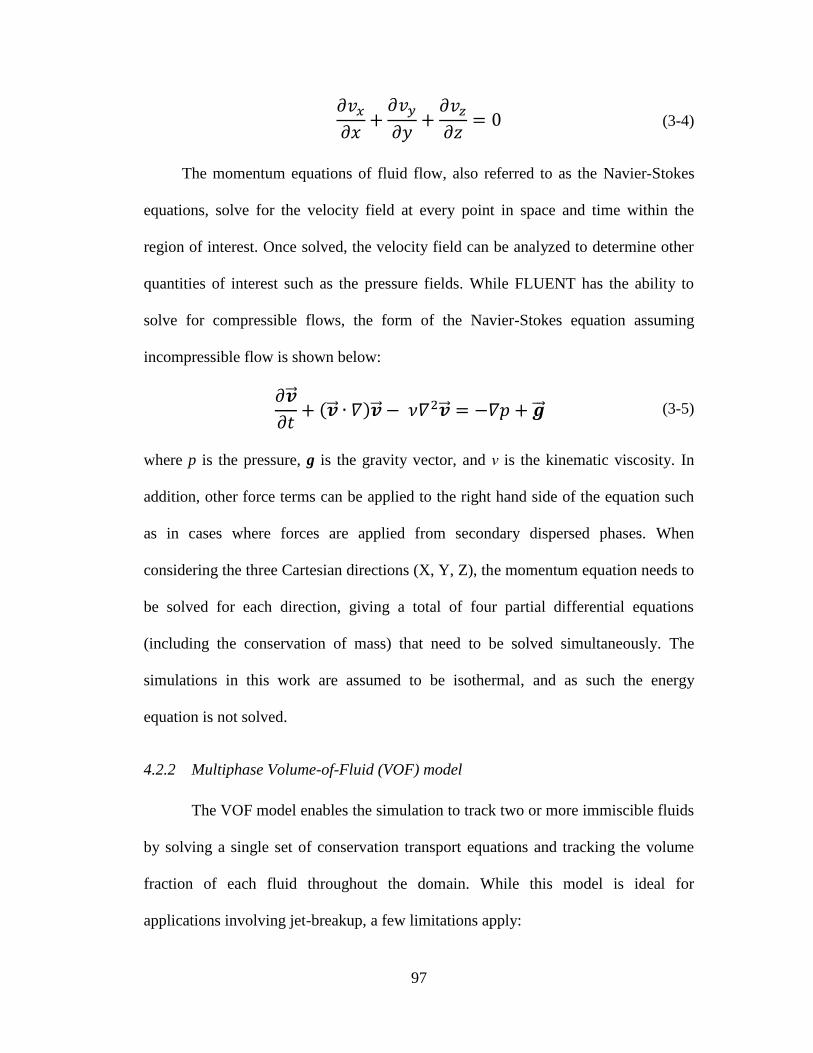
97

𝜕𝑣𝑥𝜕𝑥

+𝜕𝑣𝑦𝜕𝑦

+𝜕𝑣𝑧𝜕𝑧

= 0 (3-4)

The momentum equations of fluid flow, also referred to as the Navier-Stokes

equations, solve for the velocity field at every point in space and time within the

region of interest. Once solved, the velocity field can be analyzed to determine other

quantities of interest such as the pressure fields. While FLUENT has the ability to

solve for compressible flows, the form of the Navier-Stokes equation assuming

incompressible flow is shown below:

𝜕�⃗⃗�

𝜕𝑡+ (�⃗⃗� ∙ 𝛻)�⃗⃗� − 𝜈𝛻2�⃗⃗� = −𝛻𝑝 + �⃗⃗� (3-5)

where p is the pressure, g is the gravity vector, and ν is the kinematic viscosity. In

addition, other force terms can be applied to the right hand side of the equation such

as in cases where forces are applied from secondary dispersed phases. When

considering the three Cartesian directions (X, Y, Z), the momentum equation needs to

be solved for each direction, giving a total of four partial differential equations

(including the conservation of mass) that need to be solved simultaneously. The

simulations in this work are assumed to be isothermal, and as such the energy

equation is not solved.

4.2.2 Multiphase Volume-of-Fluid (VOF) model

The VOF model enables the simulation to track two or more immiscible fluids

by solving a single set of conservation transport equations and tracking the volume

fraction of each fluid throughout the domain. While this model is ideal for

applications involving jet-breakup, a few limitations apply:

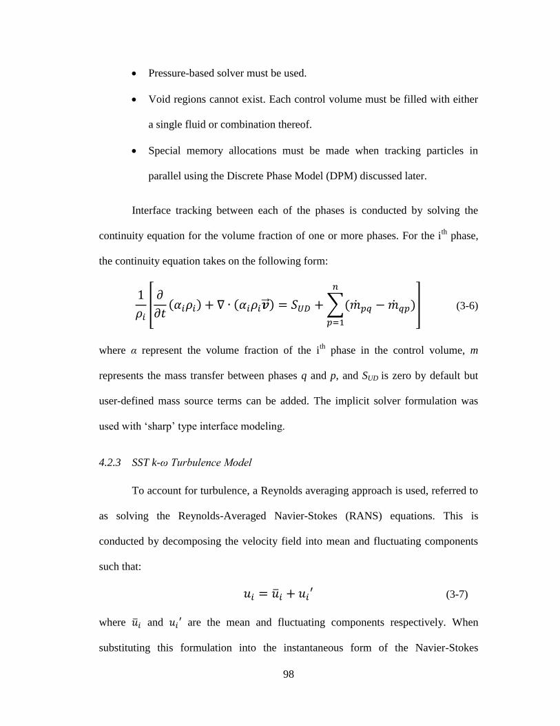
98

Pressure-based solver must be used.

Void regions cannot exist. Each control volume must be filled with either

a single fluid or combination thereof.

Special memory allocations must be made when tracking particles in

parallel using the Discrete Phase Model (DPM) discussed later.

Interface tracking between each of the phases is conducted by solving the

continuity equation for the volume fraction of one or more phases. For the ith

phase,

the continuity equation takes on the following form:

1

𝜌𝑖[𝜕

𝜕𝑡(𝛼𝑖𝜌𝑖) + ∇ ∙ (𝛼𝑖𝜌𝑖 �⃗⃗� ) = 𝑆𝑈𝐷 +∑(�̇�𝑝𝑞 − �̇�𝑞𝑝)

𝑛

𝑝=1

] (3-6)

where α represent the volume fraction of the ith

phase in the control volume, m

represents the mass transfer between phases q and p, and SUD is zero by default but

user-defined mass source terms can be added. The implicit solver formulation was

used with ‘sharp’ type interface modeling.

4.2.3 SST k-ω Turbulence Model

To account for turbulence, a Reynolds averaging approach is used, referred to

as solving the Reynolds-Averaged Navier-Stokes (RANS) equations. This is

conducted by decomposing the velocity field into mean and fluctuating components

such that:

𝑢𝑖 = �̅�𝑖 + 𝑢𝑖′ (3-7)

where �̅�𝑖 and 𝑢𝑖′ are the mean and fluctuating components respectively. When

substituting this formulation into the instantaneous form of the Navier-Stokes

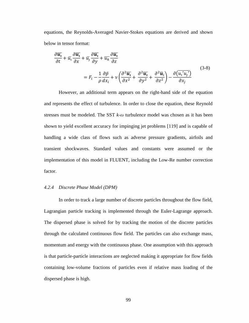
99

equations, the Reynolds-Averaged Navier-Stokes equations are derived and shown

below in tensor format:

𝜕𝒖𝒊̅̅̅

𝜕𝑡+ 𝑢�̅�

𝜕𝒖𝒊̅̅̅

𝜕𝑥+ 𝑢�̅�

𝜕𝒖𝒊̅̅̅

𝜕𝑦+ 𝑢𝑘̅̅ ̅

𝜕𝒖𝒊̅̅̅

𝜕𝑧

= 𝐹𝑖 −1

𝜌

𝜕�̅�

𝑑𝑥𝑖+ 𝜈 (

𝜕2𝒖𝒊̅̅̅

𝜕𝑥2+ 𝜕2𝒖𝒊̅̅̅

𝜕𝑦2+ 𝜕2�̅�𝑖𝜕𝑧2

) −𝜕(𝑢𝑖′𝑢𝑗′̅̅ ̅̅ ̅̅ ̅)

𝜕𝑥𝑗

(3-8)

However, an additional term appears on the right-hand side of the equation

and represents the effect of turbulence. In order to close the equation, these Reynold

stresses must be modeled. The SST k-ω turbulence model was chosen as it has been

shown to yield excellent accuracy for impinging jet problems [119] and is capable of

handling a wide class of flows such as adverse pressure gradients, airfoils and

transient shockwaves. Standard values and constants were assumed or the

implementation of this model in FLUENT, including the Low-Re number correction

factor.

4.2.4 Discrete Phase Model (DPM)

In order to track a large number of discrete particles throughout the flow field,

Lagrangian particle tracking is implemented through the Euler-Lagrange approach.

The dispersed phase is solved for by tracking the motion of the discrete particles

through the calculated continuous flow field. The particles can also exchange mass,

momentum and energy with the continuous phase. One assumption with this approach

is that particle-particle interactions are neglected making it appropriate for flow fields

containing low-volume fractions of particles even if relative mass loading of the

dispersed phase is high.

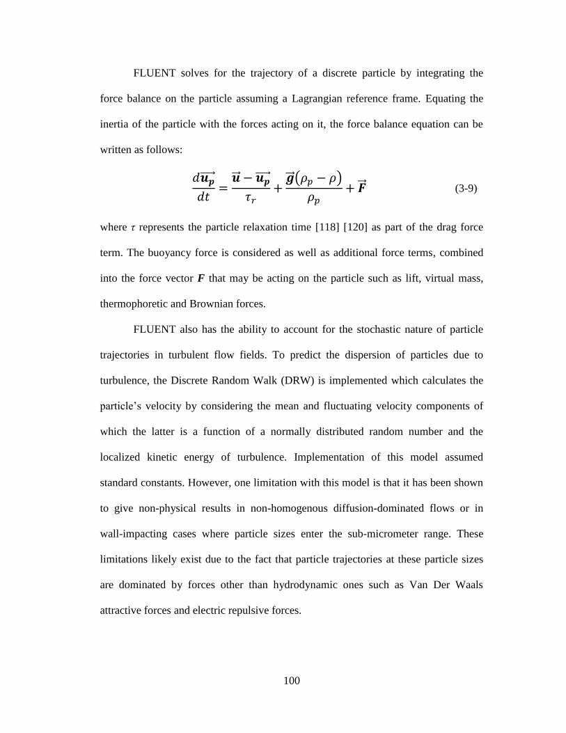
100

FLUENT solves for the trajectory of a discrete particle by integrating the

force balance on the particle assuming a Lagrangian reference frame. Equating the

inertia of the particle with the forces acting on it, the force balance equation can be

written as follows:

𝑑𝒖𝒑⃗⃗ ⃗⃗

𝑑𝑡=�⃗⃗� − 𝒖𝒑⃗⃗ ⃗⃗

𝜏𝑟+�⃗⃗� (𝜌𝑝 − 𝜌)

𝜌𝑝+ �⃗⃗� (3-9)

where τ represents the particle relaxation time [118] [120] as part of the drag force

term. The buoyancy force is considered as well as additional force terms, combined

into the force vector F that may be acting on the particle such as lift, virtual mass,

thermophoretic and Brownian forces.

FLUENT also has the ability to account for the stochastic nature of particle

trajectories in turbulent flow fields. To predict the dispersion of particles due to

turbulence, the Discrete Random Walk (DRW) is implemented which calculates the

particle’s velocity by considering the mean and fluctuating velocity components of

which the latter is a function of a normally distributed random number and the

localized kinetic energy of turbulence. Implementation of this model assumed

standard constants. However, one limitation with this model is that it has been shown

to give non-physical results in non-homogenous diffusion-dominated flows or in

wall-impacting cases where particle sizes enter the sub-micrometer range. These

limitations likely exist due to the fact that particle trajectories at these particle sizes

are dominated by forces other than hydrodynamic ones such as Van Der Waals

attractive forces and electric repulsive forces.

101

Additionally, two different types of particle-fluid coupling options are

available. One-way coupling assumes that the fluid phase can transfer energy (heat,

momentum or mass) to the discrete phase but the discrete phase cannot transfer

energy to the fluid phase. Two-way coupling assumes that both the fluid and discrete

phases can exchange energy between one-another. Although one-way coupling is

computationally less expensive than two-way coupling, erosion predictions in

FLUENT can only be conducted if two-way coupling is implemented.

4.2.5 Solver Theory

In this work the pressure-based solver was used which operates by solving a

pressure or pressure correction equation obtained through manipulating the continuity

and momentum transport equations. The solution generates the pressure field from

which other flow quantities can be derived. The other solver available is the density-

based solver which calculates the density field from the continuity equation and the

pressure field from the equation of state. The density-based solver is mainly used for

high speed compressible flow containing large density gradients. While both

approaches use the finite-volume approach, they each linearize and discretize the

fundamental transport equations in different manners.

Spatial discretization for momentum and turbulent quantities are achieved

using the Second-Order Upwind Scheme. The First-Order Upwind Schemes assumes

that the cell-face quantities are identical to the cell-center quantities; however the

Second-Order scheme uses a multidimensional linear reconstruction approach which

considers the cell-center value and the gradient in the upstream cell. While

102

computationally more expensive, the Second-Order scheme can enable higher

accuracy numerical simulations.

Gradient discretization was achieved using the Least Squares Cell-Based

approach and pressure-velocity coupling was performed using the Pressure Implicit

with Splitting Operators (PISO) algorithm. This approach, compared to the SIMPLE

or SIMPLEC algorithms can provide a higher degree of the approximate coupling

between the corrections for velocity and pressure.

In some cases, solution steering was implemented to achieve convergence

quickly. This was performed by manually adjusting the under-relaxation factors

(URFs). If the URFs are too low the solution will take a very long time to converge,

however if the URFs are too high the solution will not reach convergence as

oscillations will begin to occur. By starting the simulation with high URFs and

decreasing them as the solution proceeds, convergence can be reached in a timely

fashion.

The sections previously described should provide a reasonable introduction to

the theory and models implemented and available in FLUENT. A more thorough

description can be found in the ANSYS Workbench Documentation [118].

4.3 Geometry and Meshing

4.3.1 Dimensions of Jet and Flow Field

A quarter-symmetry 3D jet-impingement geometry, shown in Figure 4-2, was

developed using ANSYS DesignModeler.

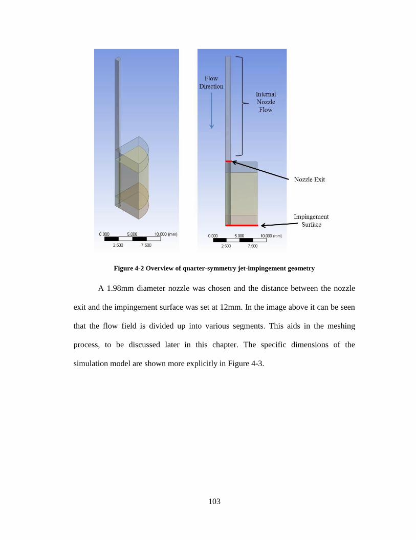
103

Figure 4-2 Overview of quarter-symmetry jet-impingement geometry

A 1.98mm diameter nozzle was chosen and the distance between the nozzle

exit and the impingement surface was set at 12mm. In the image above it can be seen

that the flow field is divided up into various segments. This aids in the meshing

process, to be discussed later in this chapter. The specific dimensions of the

simulation model are shown more explicitly in Figure 4-3.

104

Figure 4-3 Dimensions of jet-impingement simulation

The fluid will travel a length 10x the nozzle diameter before exiting in order

for the flow to fully develop. To capture all relevant information pertaining to the jet

impact, a radius of 6mm was chosen. Information greater than 6mm away from the

nozzle center was found not to affect the localized flow field near the impingement

region. As such, the far-field was truncated to reduce computational efforts.

4.3.2 Boundary Conditions

Figure 4-4 shows the boundary conditions chosen to set up this model.

105

Figure 4-4 Boundary conditions for jet-impingement model

The velocity inlet condition assumes a constant velocity across the domain

entrance. As stated previously, a length 10x the nozzle diameter was chosen in order

for the flow to reach a fully developed state before exiting the nozzle. A pressure

outlet boundary condition was chosen to represent the far-field flow boundary. At

these locations, a value of 0 Pa was chosen to represent the relative pressure

compared to the high pressure impingement region directly below the nozzle. The

impingement surface boundary condition was represented by a custom written user-

defined function, more of which will be explained later in this chapter. In short, the

UDF was written to optimize the particle impact data collection process.

106

The symmetry condition was chosen to minimize computational effort by

assuming the flow field is pseudo-axisymmetric about the nozzle center. One

alternative to the 3D flow simulation was to perform a 2D axisymmetric simulation.

Although this would significantly reduce computational effort, much of the

information pertaining to localized particle impact parameters would be lost due to

the reduction of impingement area.

4.3.3 Meshing

In order to discretize the flow domain, ANSYS’ built in meshing program was

used. As stated earlier, the flow domain was divided up into seven parts, each of

which was meshed separately using the ‘MultiZone’ method. This facilitated better

control over localized and global meshing parameters such as element sizing and bias

type. Additionally prism-type mesh elements were used, shown in Figure 4-5, which

allowed for a smoother mesh construction compared to hex-elements.

Figure 4-5 Mesh constructed using prism elements

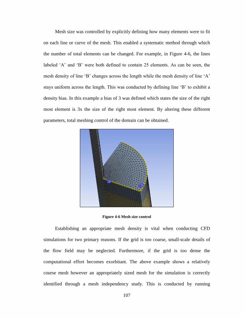
107

Mesh size was controlled by explicitly defining how many elements were to fit

on each line or curve of the mesh. This enabled a systematic method through which

the number of total elements can be changed. For example, in Figure 4-6, the lines

labeled ‘A’ and ‘B’ were both defined to contain 25 elements. As can be seen, the

mesh density of line ‘B’ changes across the length while the mesh density of line ‘A’

stays uniform across the length. This was conducted by defining line ‘B’ to exhibit a

density bias. In this example a bias of 3 was defined which states the size of the right

most element is 3x the size of the right most element. By altering these different

parameters, total meshing control of the domain can be obtained.

Figure 4-6 Mesh size control

Establishing an appropriate mesh density is vital when conducting CFD

simulations for two primary reasons. If the grid is too coarse, small-scale details of

the flow field may be neglected. Furthermore, if the grid is too dense the

computational effort becomes exorbitant. The above example shows a relatively

course mesh however an appropriately sized mesh for the simulation is correctly

identified through a mesh independency study. This is conducted by running

108

simulations using different mesh sizes and monitoring the flow solution. A solution is

said to be ‘mesh-independent’ when the monitored variables maintain their value as

the mesh is increased further.

4.3.4 Convergence Criteria

Prior to discussing the mesh independency study, convergence criteria will be

identified. As a simulation transpires, the flow field changes and values are updated

each iteration. Eventually the changes that occur between iterations become smaller

and smaller to the point when these changes become negligible. When this occurs the

simulation is said to be converged. However, explicit convergence criteria cannot be

universally defined across every type of CFD simulation although certain guidelines

can be commonly applied. As such, the criteria used to identify convergence in these

particular simulations will be stated.

During the simulations, four different monitors were used to check for

convergence: the maximum velocity, a volume integral of the velocity field, a volume

integral of the phase volume fraction and residuals. The maximum velocity monitor

tracks the absolute magnitude of the velocity anywhere in the flow field while the

volume integrals are computed by summing the product of the cell volume and the

selected variable across the entire flow field. Essentially, the volume integrals provide

a metric by considering every element in the flow field. Residuals were used as a

secondary means of identifying convergence due to the fact that certain mesh

densities yielded oscillating solutions even though the other monitoring points

suggested convergence.

109

Convergence was achieved when the three volume monitoring points reached

a steady value, shown in Figure 4-7, and when all residuals dropped below 10-3

. In

cases of high mesh density, such as the simulations containing greater than 500K

elements, the residuals dropped below 10-4

well before the other monitoring points

achieved convergence. In the coarser meshes however, solution oscillations prevented

the continuity residual from dropping to this point. While the coarser meshed

simulations were conducted as part of the mesh independency study, difficulty in

achieving convergence further justified the need for a finer mesh.

Figure 4-7 Convergence achieved by monitoring volume integrals

4.3.5 Mesh Independency Study

The process for identifying mesh independency was conducted by running the

same simulation, including all boundary conditions, at different mesh densities and

monitoring the outputs. The outputs used to track the effect of mesh density were

maximum velocity and the volume integrals of the velocity field and phase volume

fraction. A total of seven different mesh densities were used as part of this study with

110

the resulting total number of elements ranging from approximately 24,700 to

2,050,000. For all simulations, 20 m/s was assumed to be the inlet velocity.

Figure 4-8 shows the results of the mesh independency study indicating the

chosen mesh of 936,950 elements to perform further studies with.

Figure 4-8 Results of mesh independency study indicating chosen mesh

In some instances higher mesh density does not always equate to higher

accuracy simulations. For example, if simulations were performed using higher

density meshes than those performed in this independency study, there would likely

be a divergence of the monitored quantities. As such this type of study is necessary in

order to identify how coarse a mesh needs to be as opposed to simply choosing a very

dense mesh.

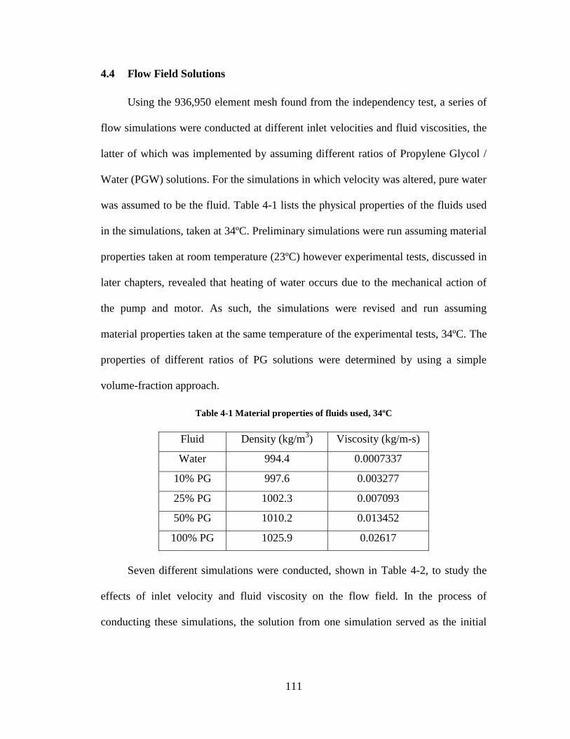
111

4.4 Flow Field Solutions

Using the 936,950 element mesh found from the independency test, a series of

flow simulations were conducted at different inlet velocities and fluid viscosities, the

latter of which was implemented by assuming different ratios of Propylene Glycol /

Water (PGW) solutions. For the simulations in which velocity was altered, pure water

was assumed to be the fluid. Table 4-1 lists the physical properties of the fluids used

in the simulations, taken at 34ºC. Preliminary simulations were run assuming material

properties taken at room temperature (23ºC) however experimental tests, discussed in

later chapters, revealed that heating of water occurs due to the mechanical action of

the pump and motor. As such, the simulations were revised and run assuming

material properties taken at the same temperature of the experimental tests, 34ºC. The

properties of different ratios of PG solutions were determined by using a simple

volume-fraction approach.

Table 4-1 Material properties of fluids used, 34ºC

Fluid Density (kg/m3) Viscosity (kg/m-s)

Water 994.4 0.0007337

10% PG 997.6 0.003277

25% PG 1002.3 0.007093

50% PG 1010.2 0.013452

100% PG 1025.9 0.02617

Seven different simulations were conducted, shown in Table 4-2, to study the

effects of inlet velocity and fluid viscosity on the flow field. In the process of

conducting these simulations, the solution from one simulation served as the initial

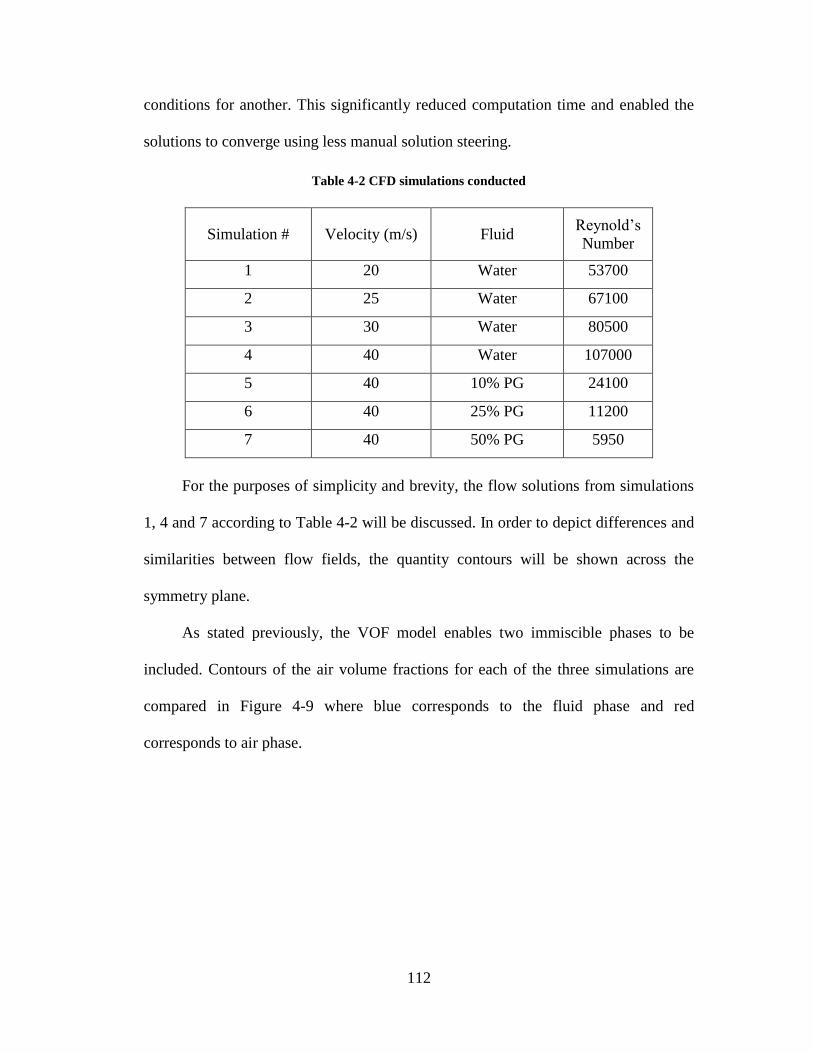
112

conditions for another. This significantly reduced computation time and enabled the

solutions to converge using less manual solution steering.

Table 4-2 CFD simulations conducted

Simulation # Velocity (m/s) Fluid Reynold’s

Number

1 20 Water 53700

2 25 Water 67100

3 30 Water 80500

4 40 Water 107000

5 40 10% PG 24100

6 40 25% PG 11200

7 40 50% PG 5950

For the purposes of simplicity and brevity, the flow solutions from simulations

1, 4 and 7 according to Table 4-2 will be discussed. In order to depict differences and

similarities between flow fields, the quantity contours will be shown across the

symmetry plane.

As stated previously, the VOF model enables two immiscible phases to be

included. Contours of the air volume fractions for each of the three simulations are

compared in Figure 4-9 where blue corresponds to the fluid phase and red

corresponds to air phase.

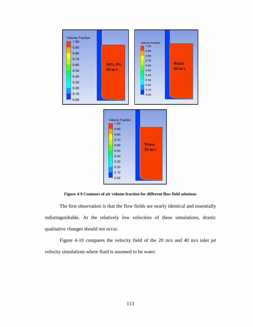
113

Figure 4-9 Contours of air volume fraction for different flow field solutions

The first observation is that the flow fields are nearly identical and essentially

indistinguishable. At the relatively low velocities of these simulations, drastic

qualitative changes should not occur.

Figure 4-10 compares the velocity field of the 20 m/s and 40 m/s inlet jet

velocity simulations where fluid is assumed to be water.

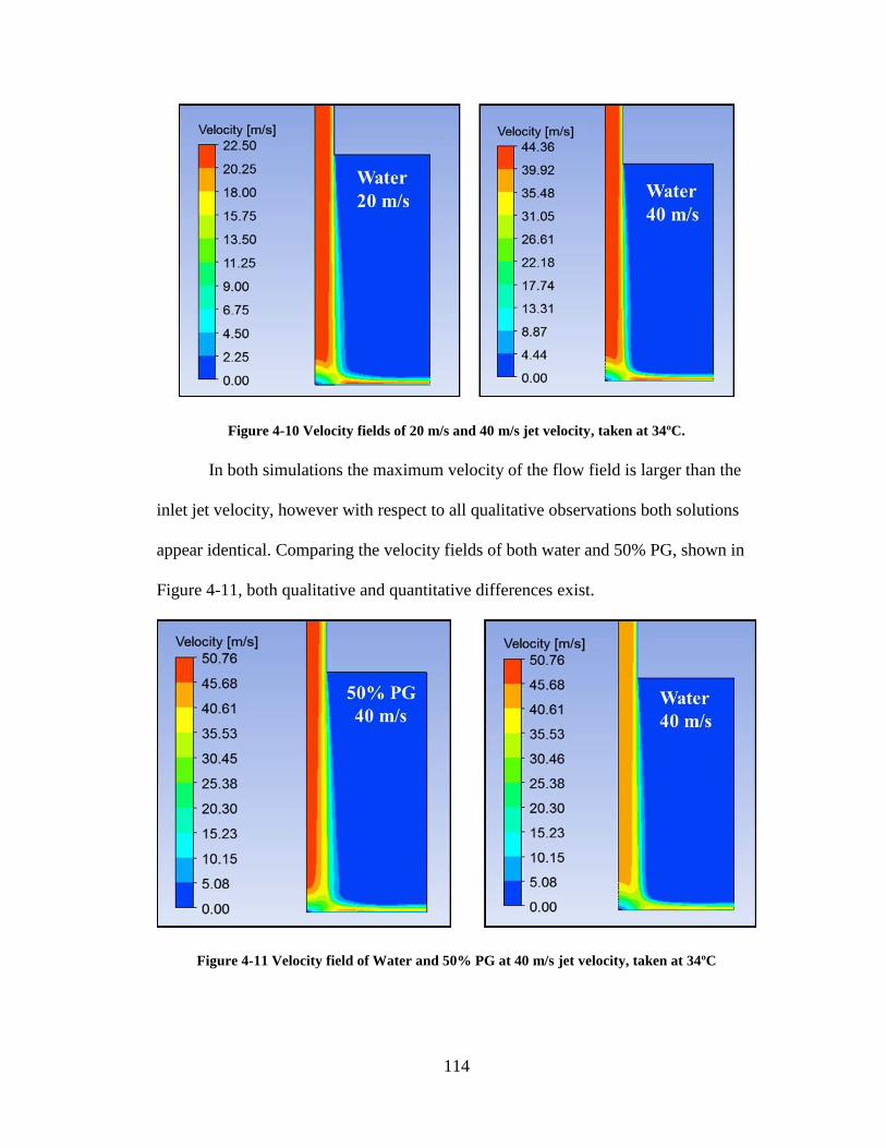
114

Figure 4-10 Velocity fields of 20 m/s and 40 m/s jet velocity, taken at 34ºC.

In both simulations the maximum velocity of the flow field is larger than the

inlet jet velocity, however with respect to all qualitative observations both solutions

appear identical. Comparing the velocity fields of both water and 50% PG, shown in

Figure 4-11, both qualitative and quantitative differences exist.

Figure 4-11 Velocity field of Water and 50% PG at 40 m/s jet velocity, taken at 34ºC

115

First, the maximum velocity is larger in the 50% PG fluid compared to pure

water. According to Figure 4-12 as the percentage of PG in the solution is increased,

the resulting Reynolds number of the jet decreases and the flow transitions from a

turbulent flow regime to a laminar flow regime. As this transition begins the velocity

profile becomes fuller, as depicted in Figure 4-12. In addition, the localized velocities

of the flow field are affected by the fluid properties which will ultimately affect the

particle impact parameters.

Figure 4-12 Laminar and turbulent velocity profile in tube

One interesting prediction concerning erosion can be made from qualitatively

analyzing the flow field solutions. For example, by assessing the 40 m/s water

solution shown in Figure 4-13, one can identify the region near the surface that

contains a local maximum velocity.

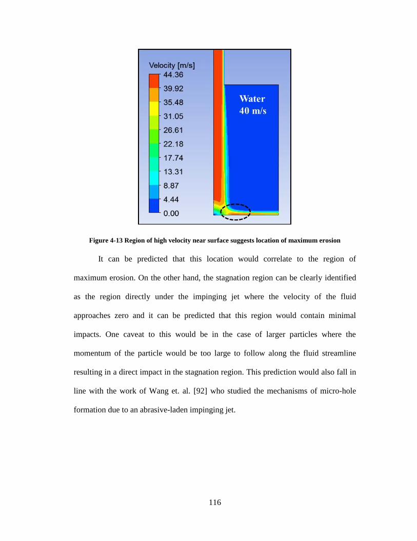
116

Figure 4-13 Region of high velocity near surface suggests location of maximum erosion

It can be predicted that this location would correlate to the region of

maximum erosion. On the other hand, the stagnation region can be clearly identified

as the region directly under the impinging jet where the velocity of the fluid

approaches zero and it can be predicted that this region would contain minimal

impacts. One caveat to this would be in the case of larger particles where the

momentum of the particle would be too large to follow along the fluid streamline

resulting in a direct impact in the stagnation region. This prediction would also fall in

line with the work of Wang et. al. [92] who studied the mechanisms of micro-hole

formation due to an abrasive-laden impinging jet.

117

4.5 Implementation of Particle Tracking using Discrete Phase Modeling

The main purpose of developing the abovementioned CFD simulations is to

enable localized particle impact information to be gathered. As discussed in the

literature review section the main parameters influencing the amount of material

removed for a single particle impact are impact velocity, impact angle and particle

size. While particle size can be experimentally controlled, impact velocity and impact

angle can be determined via simulation efforts.

While FLUENT can easily track particle motion through the flow field, there is

no built-in way to obtain, store and analyze particle impact information. As such, two

User-Defined Functions (UDFs) were written to aid in this process and an additional

UDF was written to hook in custom erosion models. This section will discuss how

FLUENT’s discrete phase model was implemented and how the UDFs operate to

gather relevant data.

4.5.1 Injection Parameters

FLUENT enables the user to explicitly define properties of the discrete phase

including start positions, velocities, size or size distribution of the particles,

concentration loading, etc. The injection parameters serve as the initial conditions for

the discrete phase and, once released, FLUENT calculates the trajectories of the

particles throughout the fluid phase. The particles were chosen to be inert, alumina

(Al2O3) particles with a uniform diameter distribution. Table 4-3 lists the following

point-properties used for this injection.

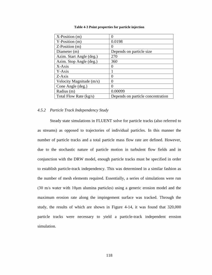
118

Table 4-3 Point properties for particle injection

X-Position (m) 0

Y-Position (m) 0.0198

Z-Position (m) 0

Diameter (m) Depends on particle size

Azim. Start Angle (deg.) 270

Azim. Stop Angle (deg.) 360

X-Axis 0

Y-Axis 1

Z-Axis 0

Velocity Magnitude (m/s) 0

Cone Angle (deg.) 0

Radius (m) 0.00099

Total Flow Rate (kg/s) Depends on particle concentration

4.5.2 Particle Track Independency Study

Steady state simulations in FLUENT solve for particle tracks (also referred to

as streams) as opposed to trajectories of individual particles. In this manner the

number of particle tracks and a total particle mass flow rate are defined. However,

due to the stochastic nature of particle motion in turbulent flow fields and in

conjunction with the DRW model, enough particle tracks must be specified in order

to establish particle-track independency. This was determined in a similar fashion as

the number of mesh elements required. Essentially, a series of simulations were run

(30 m/s water with 10μm alumina particles) using a generic erosion model and the

maximum erosion rate along the impingement surface was tracked. Through the

study, the results of which are shown in Figure 4-14, it was found that 320,000

particle tracks were necessary to yield a particle-track independent erosion

simulation.

119

Figure 4-14 Results of particle track independency study

4.5.3 Development of User Defined Functions

A user-defined function is a custom script written in C that can be loaded into

FLUENT to enhance and/or customize standard features. More information on the

capabilities, limitations and implementation strategies can be found in the ANSYS

Help Documentation [118]. In this work three UDFs were written and they all

incorporate the DEFINE_DPM macro. This section will simply describe the purpose

and function for each UDF, however the complete code will be included in Appendix

C.

4.5.3.1 DPM Erosion Model

FLUENT enables user-defined erosion models to be hooked into the software

using the DEFINE_DPM_EROSION macro. These types of UDFs calculated the

mass of material removed for a single particle or particle track impact given the

impact velocity, impact angle and particle or particle track mass flow rate.

120

Generically, the erosion rate for a given cell face on the impingement surface can be

defined as:

𝐸𝑅 =∑𝑚𝑝̇ 𝑓(𝐷)𝑓(𝛼)𝑓(𝑉)

𝐴𝑐𝑒𝑙𝑙 (3-10)

where mp is the particle mass flowrate of a given particle track and f(D), f(α) and f(V)

are all functions of the particle size, impact angle and impact velocity respectively. In

addition, the summation is taken across all particles or particle tracks that impact the

unit cell. In FLUENT the erosion rate is calculated as an erosion flux in units of

kg/m2-s. In order to convert this unit into a one-dimension erosion rate, such as m/s or

μm/year, the erosion flux should be divided by the density of the substrate material.

4.5.3.2 DPM Boundary Condition

Through the DEFINE_DPM_BC macro, user-specified boundary conditions

can be applied which execute every time a particle is found to impact the specified

surface. This UDF was written to gather and store pertinent information specifically

relating to particle impact characteristics such as impact velocity, impact angle,

impact position and the number of times a specific particle track hits the surface.

Each of these values were stored in a user-defined storage array associated with each

particle track using the P_USER_REAL(p,i) macro where ‘p’ refers to the tracked

particle and ‘i’ refers to the index of the array.

The index i = 0 was used to count the number of impacts for a specific particle

track, therefore each time the UDF was called (each time the particle track results in

an impact) the value stored at the i = 0 location would increment by 1. Indexes i = 1

through i = 10 were used to store the impact velocity for the first ten impacts.

121

Likewise, indexes i = 11 through i = 20 were used to store the impact angle for the

first ten impacts. Tracking up to ten particle impacts was deemed appropriate as the

contribution to erosion from more than ten impacts per particle was assumed to be

negligible compared to the effect of the first couple impacts.

These simulations consider all geometries with reference to the standard XYZ

Cartesian coordinate system. When storing the impact velocity, the magnitude of the

velocity must be taken because some particle velocities are negative with respect to

the positive XYZ directions. Likewise, the impact angle is determined by considering

the impact velocity vector and the cell face normal direction vector and is defined as

the angle between the impingement surface and the impacting particle track.

One concern regarding the DEFINE_DPM_BC macro is that the rebound

conditions of a particle must be explicitly defined, meaning the rebound angle and the

rebound velocity need to be calculated within the UDF. This enables the user to also

define coefficients of restitution for both the normal and tangential directions. For this

work it was assumed that these coefficients were both one, primarily due to the

assumption that the fluid flow largely dictates the particle motion. Even if a slight

amount of kinetic energy was removed from the particle this would likely be

negligible considering how closely coupled the particle motion is to the fluid motion.

In cases where the medium is gaseous or if the particles are quite large, then it may be

wise to introduce more accurate coefficients of restitution.

Preliminary CFD simulations suggest that the majority of erosion is due to the

first few impacts per particle track as the impact angle and velocity decrease once the

particles are swept away in the tangentially moving fluid. Additionally, Mansouri et

122

al. [121] showed that tracking six impacts per particle track slightly under predicted

erosion rates with 25μm particles by a factor of 0.87 while tracking up to 30 impacts

per particle over predicted erosion rates by a factor of 2.74. For this work it was

assumed that ten impacts per particle track would be sufficient to capture the

overwhelming majority of erosion-pertinent impacts.

4.5.3.3 DPM Sampling Output

While the DEFINE_DPM_BC macro gathers and stores particle impact data,

the DEFINE_DPM_OUTPUT macro outputs the stored data into a *.dpm file which

can be converted to a *.dat or a *.txt file for post-processing. In FLUENT, the

sampling can be taken at any boundary through which the particles pass through, and

for this work that boundary was taken to be the outlet of the simulation. In this UDF

once each particle passes through the outlet boundary all the velocity, impact angle

and position variables are printed to the sampling output. This file is then imported

into a MATLAB code for post-processing.

4.6 Particle Impact Results

This section shows the results of the simulations previously discussed to depict

how altering the jet velocity, particle size, fluid viscosity and particulate

concentration effect particle impact characteristics. For the purposes of data

presentation, averages of the 320,000 particle tracks will be given for each impact for

each of the impact characteristics. The impact ratio is defined as the ratio of the

number of impacts to the total number of particle tracks.

123

In order to better relate the results of these simulations to the experimental work

discussed in later chapters, the particle sizes used in these simulations were the

average particle sizes measured from a particle size distribution analysis. Samples of

nominally sized 2.5μm, 5μm, 10μm and 20μm alumina particles were acquired from

Inframat Advanced Materials and sent out for independent particle size distribution

analysis using a CILAS laser particle size analyzer. A comparison of the

manufacturer specified average particle size and the independently measured average

particle size used in the simulations are shown in Table 4-4. The raw data from these

tests are included in Appendix B.

Table 4-4 Comparison of manufacturer specified and measured average particle sizes

Manufacturer

(μm)

Measured and used in simulations

(μm)

2.5 2.59

5 5.53

10 8.95

20 16.5

The 20μm particles were not measured using the particle size analyzer, but

were rather approximated using SEM. An image of the 20μm particles are shown in

Figure 4-15.

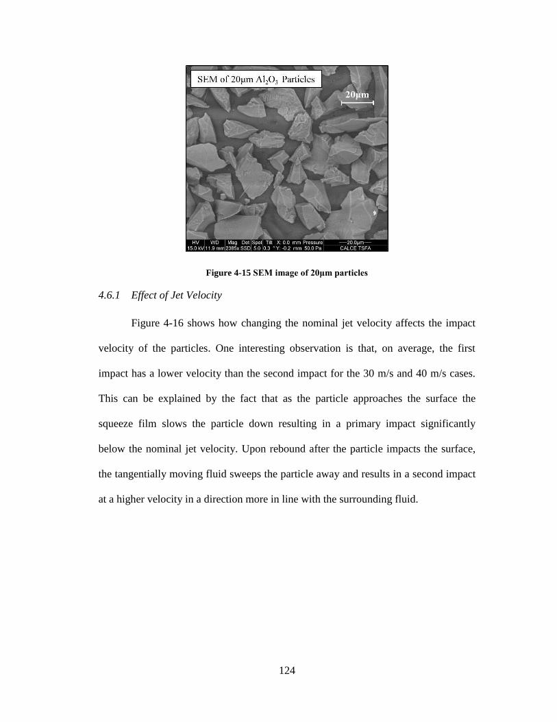
124

Figure 4-15 SEM image of 20μm particles

4.6.1 Effect of Jet Velocity

Figure 4-16 shows how changing the nominal jet velocity affects the impact

velocity of the particles. One interesting observation is that, on average, the first

impact has a lower velocity than the second impact for the 30 m/s and 40 m/s cases.

This can be explained by the fact that as the particle approaches the surface the

squeeze film slows the particle down resulting in a primary impact significantly

below the nominal jet velocity. Upon rebound after the particle impacts the surface,

the tangentially moving fluid sweeps the particle away and results in a second impact

at a higher velocity in a direction more in line with the surrounding fluid.

125

Figure 4-16 Particle impact velocity as a function of nominal jet velocity

After the first few impacts occur, the average impact velocity steadies out and

slightly decreases as the impacts continue to occur. For the 20 m/s and 25 m/s cases

the impact velocity does not increase on the secondary impact because the particles

are more closely coupled to the fluid streamlines. As such, the squeeze film plays less

of a role in slowing the particle down right before impact.

Figure 4-17 shows the particle impact angle as a function of different jet

velocities. All impacts in each simulation occur at shallow angles. The first few

impacts occur at larger angles because the fluid is changing directions from a normal

impacting jet to tangentially moving fluid. However after the first few impacts the

data suggests that the particles roll, bounce and scratch along the surface. This is

evident from the shallow angle impacts occurring at relatively constant velocities for

each jet velocity.

126

Figure 4-17 Particle impact angle as a function of nominal jet velocity

While it can be seen that the impact angle of the first impact for the 40 m/s jet

is slightly higher than the rest of the jets, the shapes of the trends are relatively

uniform. This suggests that the impact angle of the particles is not largely affected by

jet velocity assuming all other properties are the same. For impacts 4 through 10, the

impact angles within the 40 m/s case are less than that of the 20 m/s case. This can be

attributed to the fact that particles exhibiting a larger impact would be swept away in

the bulk fluid rather than being stuck in the slower moving squeeze film. This

phenomenon can be seen in Figure 4-18 which shows why particles wouldn’t likely

impact the surface at higher impact angles in the tangentially moving fluid.

Figure 4-18 Comparison of high and low impact angles

127

The effects of the particle impact ratio can be seen in Figure 4-19. The first

observation is that the general shapes of the trends are not significantly affected by jet

velocity. Higher velocity jets do slightly result in a larger percentage of entrained

particles that reach the surface, approximately 93% for the 40 m/s jet and 82% for the

20 m/s jet. High velocities result in a looser coupling between the particle trajectories

and fluid streamlines and therefore makes it easier for the particles to diverge from

the fluid streamline and impact the surface.

Figure 4-19 Particle impact ratio as a function of jet velocity

For subsequent impacts at all jet velocities, the number of particle tracks

resulting in impacts uniformly decrease. This can be explained in a similar manner

using Figure 4-18 where more and more particles are carried out of the squeeze film

and swept away in the bulk moving fluid.

4.6.2 Effect of Particle Size

As described above, Figure 4-20 reinforces the notion that secondary and

subsequent impacts play an import role in jet-impingement erosion scenarios.

128

Comparing the impact velocities for 10μm and 20μm particles, it can be seen that the

10μm particles result in a higher first impact velocity and a lower secondary impact

velocity. This can be explained by also considering the results in Figure 4-21 which

show the effect of particle size on impact angle.

Figure 4-20 Particle impact velocity as a function of particle size

The first impact in the 20μm particle size case hits the surface at a relatively

high angle compared to the other particle sizes. As such, the squeeze film has a

greater effect on slowing the larger particles down. This can be further justified with

the idea that larger particles have a greater surface area, and although FLUENT treats

the particles as a point, an effective drag force is calculated and influences the

trajectories of the particles. Additionally, at shallower impact angles the particle

trajectories are more in line with the tangentially moving fluid and thus require less

energy to change direction.

129

Figure 4-21 Particle impact angle as a function of particle size

It can also be seen that subsequent impacts still take place at shallow impact

angles regardless of particle size. From this data, it can be seen that particle size

greatly influences the impact angle of the first impact but has negligible effect on

additional impacts.

Compared to the effect of jet velocity, particle size has a greater effect on the

percentage of entrained particles that reach the surface as shown in Figure 4-22. For

the 20μm particles, the data suggests that 100% of entrained particles reach the

surface. As the particle size decreases, it can be seen that fewer particles reach the

surface. In addition, it can be seen that subsequent impacts have fewer impacts

associated with them for all particle sizes.

130

Figure 4-22 Particle impact ratio as a function of particle size

Looking at the curve for the 2.5μm particles, impacts 6 through 10 have a

larger percentage of impacts compared to the curves from other particle sizes. This

can be explained by the fact that smaller particles have a greater tendency to stay

entrained in the squeeze film compared to larger particles. As suggested by Clark and

Hartwich [81], the squeeze film not only slows down incoming particles but also acts

to prevent particles from rebounding into the free stream fluid flow.

4.6.3 Effect of Fluid Viscosity

Figure 4-23 shows that particle impact velocity decreases as fluid viscosity

increases for the same relative jet velocity and particulate loading. As previously

discussed, this is due to the stronger coupling between particle trajectories and fluid

streamlines.

131

Figure 4-23 Particle impact velocity as a function of fluid viscosity

For the 50% PG solution cases, the impact velocity is significantly below that

of the nominal fluid velocity suggesting that particles are trapped in the squeeze film

and are not easily swept away by the tangentially moving flow. This would also

suggest more of an abrasion wear mechanism as predicted by Clark et al. [81] where

particles accumulate in the slower moving viscous film directly above the surface.

The relationship between particle impact angle and fluid viscosity is shown in

Figure 4-24. The results seem somewhat counter-intuitive as a stronger coupling

between particle and fluid would suggest a lower angle of impact for impingement

scenarios. In order to justify the CFD results, the percentage of entrained particles

that reach the surface must also be considered, shown in Figure 4-25.

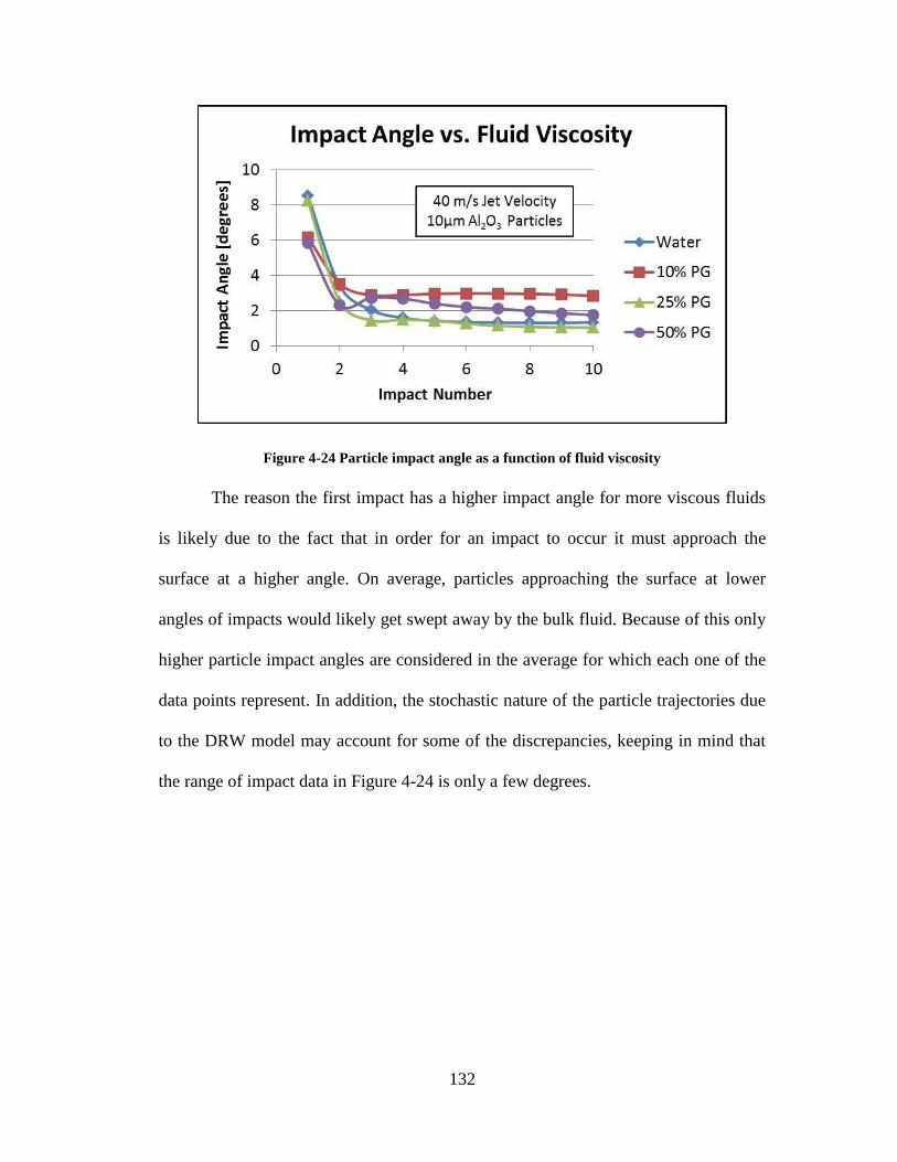
132

Figure 4-24 Particle impact angle as a function of fluid viscosity

The reason the first impact has a higher impact angle for more viscous fluids

is likely due to the fact that in order for an impact to occur it must approach the

surface at a higher angle. On average, particles approaching the surface at lower

angles of impacts would likely get swept away by the bulk fluid. Because of this only

higher particle impact angles are considered in the average for which each one of the

data points represent. In addition, the stochastic nature of the particle trajectories due

to the DRW model may account for some of the discrepancies, keeping in mind that

the range of impact data in Figure 4-24 is only a few degrees.

133

Figure 4-25 Particle impact ratio as a function of fluid viscosity

As the fluid becomes more viscous, fewer particle tracks have enough

momentum to divert from the fluid streamlines which result in a surface impact.

Reflecting on how fluid viscosity affects particle impact characteristics, it can be

predicted that more viscous fluids can significantly reduce erosion. In the case of high

heat flux cooling loops, of which 50% PG/W is a common fluid, entrained particles

would impact the surface at low velocities compared to less viscous fluids like water.

4.6.4 Effect of Particulate Concentration

In the simulations presented here the particulate concentration of the slurry is

defined as a particle mass flow rate. For example, in the case of the a 40 m/s jet

flowing through a 1.98 mm nozzle the mass flowrate is calculated:

(40𝑚

𝑠) (𝜋

4∗ 0.001982) (998.2

𝑘𝑔

𝑚3) = 0.12294

𝑘𝑔

𝑠 (3-11)

134

However, considering the quarter symmetry geometry this value must be

divided by a factor of four to give: 3.0735x10-2

kg/s. In the case where particle

concentration is assumed to be 0.1% by mass, this would yield a particle mass flow

rate of:

(3.0735𝑥10−2𝑘𝑔

𝑠) (0.001) = 3.0735𝑥10−5

𝑘𝑔

𝑠 (3-12)

This value is the total particulate mass flowrate of all particle tracks. Therefore

to calculate the mass flowrate of an individual particle track this value would be

divided by the number of particle tracks in the simulation. In theory, doubling the

particulate concentration should yield twice as much mass removed because twice as

many particles per unit time would be traversing through a given particle stream. In

addition, the major assumption when implementing Lagrangian particle tracking is

that particles are non-interacting, therefore the interaction of particle tracks should not

be considered.

4.7 Conclusion

This chapter outlines the development and results of a series of 3D quarter-

symmetry jet-impingement simulations constructed using ANSYS FLUENT 16.1.

The main purpose of these simulations was to obtain particle impact data, specifically

particle impact velocities, impact angles and the percentage of entrained particles that

reach the surface.

First, a brief overview of CFD theory was presented and the main models used

in the simulations were discussed. Multi-phase modeling is handled using the VOF

model which tracks the boundary between the fluid and surrounding air. Turbulence

135

is modeled using the SST k-ω turbulence model assuming standard values and

constants. The DRW model is included in the Lagrangian particle tracking calculation

as this enables the stochastic nature of particle trajectories in turbulent flow fields to

be considered.

Next, a thorough description of the geometry, boundary conditions, meshing

properties and convergence criteria was given. Through the mesh independency study

it was found that independency was achieved at slightly less than 1 million elements.

A series of seven different flow field simulations were conducted at different fluid

velocities and viscosities assuming different mixtures of propylene glycol / water

solutions.

A series of UDFs were written to gather and store particle impact

characteristics as FLUENT does not have this inherent capability. Through a particle-

track independency study using a generic erosion model, it was found that 320,000

particle tracks needed to be simulated in order to produce track-independent erosion

results. For each of the 320,000 particle tracks, up to ten impacts were considered.

The UDFs were written so that an output data file could be imported into MATLAB

for post-processing.

The results of these simulations were presented in a series of graphs that show

how nominal jet velocity, particle size and fluid viscosity affect localized impact

characteristics. To summarize a few points:

Particle impact velocity is less than the nominal jet velocity due to the

dampening action of the squeeze film.

136

In some cases the velocity magnitude of the second impact is larger than the

first due to the tangentially moving fluid and dampening action of the squeeze

film.

Increasing fluid viscosity magnified the effect of the squeeze film and further

reduces impact velocity.

Impact angles for particles less than 10μm are small, typically less than 6º.

Impact angles of subsequent impacts after the first suggest that particles are

rolling, bouncing and scratching along the surface

The 20μm particles yielded significantly higher impact angles on the first

impact, approximately 45º, due to the weaker coupling between particle

trajectory and fluid streamline.

In the simulations with lower jet velocities, smaller particle sizes, and higher

fluid viscosities, a smaller percentage of entrained particle tracks resulted in

impact.

Due to the assumptions inherent in steady-state particle tracking in CFD,

concentration affects the mass flow rate of individual particle tracks. As such,

the mass of material removed is expected to vary linearly with concentration.

137

5 DESIGN OF SLURRY EROSION TEST APPARATUS

This chapter will discuss the design and development of the jet-impingement

slurry erosion test apparatus.

5.1 Overview

Multiples types of erosion test setups exist, each of which enable the erosion of

different materials to be studied under a variety of conditions. Some examples of

these test setups include “sandblasting” rigs, such as those used by Sheldon and

Finnie [39] [40], Wiederhorn and Hockey [63], Telling and Field [72], as well as

many others. With these types of test setups the velocity of particles can be

determined directly from the air pressure. In addition, the impingement angle of all

the particles in the stream is assumed to be relatively constant.

In the case of particles entrained in a fluid, one method of studying erosion is

through the use of a slurry pot erosion rig, as was employed by Clark and co-workers

[77] [79] [78]. While this type of test rig allows for the effect of different fluids to be

considered, the major limitation is with regards to discerning the particle impact

velocity.

A final method used to study slurry erosion of various materials is the jet-

impingement apparatus, as will be discussed in this chapter. With regards to

electronics cooling, jet-impingement type architectures are quite prevalent [29] and

enable highly localized cooling of hot spots as well as bulk cooling of cold plates.

Due to the wide range of applicability and ease of parameter control, this type of

slurry erosion test rig was constructed to study the erosion potential of silicon and. An

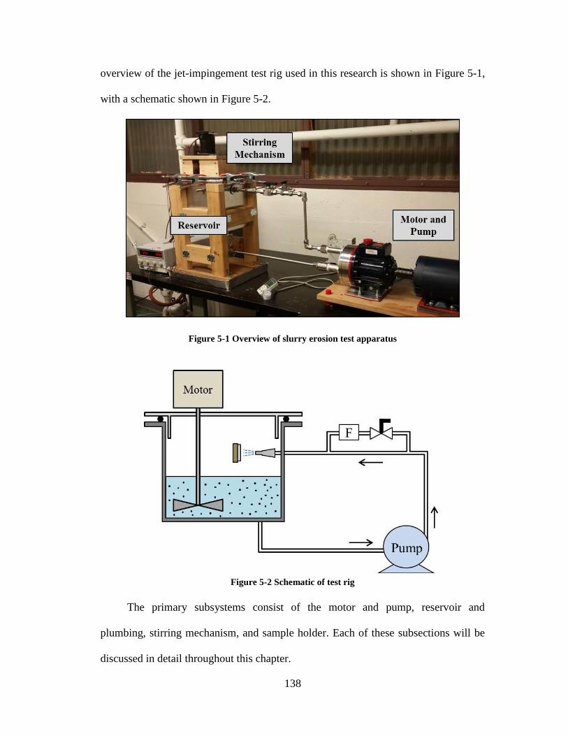
138

overview of the jet-impingement test rig used in this research is shown in Figure 5-1,

with a schematic shown in Figure 5-2.

Figure 5-1 Overview of slurry erosion test apparatus

Figure 5-2 Schematic of test rig

The primary subsystems consist of the motor and pump, reservoir and

plumbing, stirring mechanism, and sample holder. Each of these subsections will be

discussed in detail throughout this chapter.

139

5.2 Reservoir, Plumbing and Sealing

The reservoir was constructed of 316 Stainless Steel, had dimensions of

approximately 11” x 8” x 10.5” (LxWxH) and was purchased by Stainless Steel

Fabricators, Inc. A drain was fabricated in the bottom of the reservoir, shown in

Figure 5-3 by welding a half coupling in place. This facilitates the transition from

reservoir to the compression fitting based plumbing network. Additionally, the nozzle

enters the front of the reservoir through a bulkhead fitting also shown in Figure 5-3.

Figure 5-3 Bulkhead fitting leading to nozzle (left) and drain welded to reservoir (right).

The cover was made of 3/8” thick acrylic. Vertical side walls were attached to

the underside of the cover to minimize direct splashing of the slurry near the O-ring.

The O-ring was made of Viton Fluoroelastomer to ensure that the test setup

chemically compatible with a variety of glycol based fluids that may be tested.

Additionally the O-ring was looped around the flanges and was attached using

superglue and Gorilla Glue®. A schematic cross section of the reservoir, O-Ring and

cover is shown in Figure 5-4.

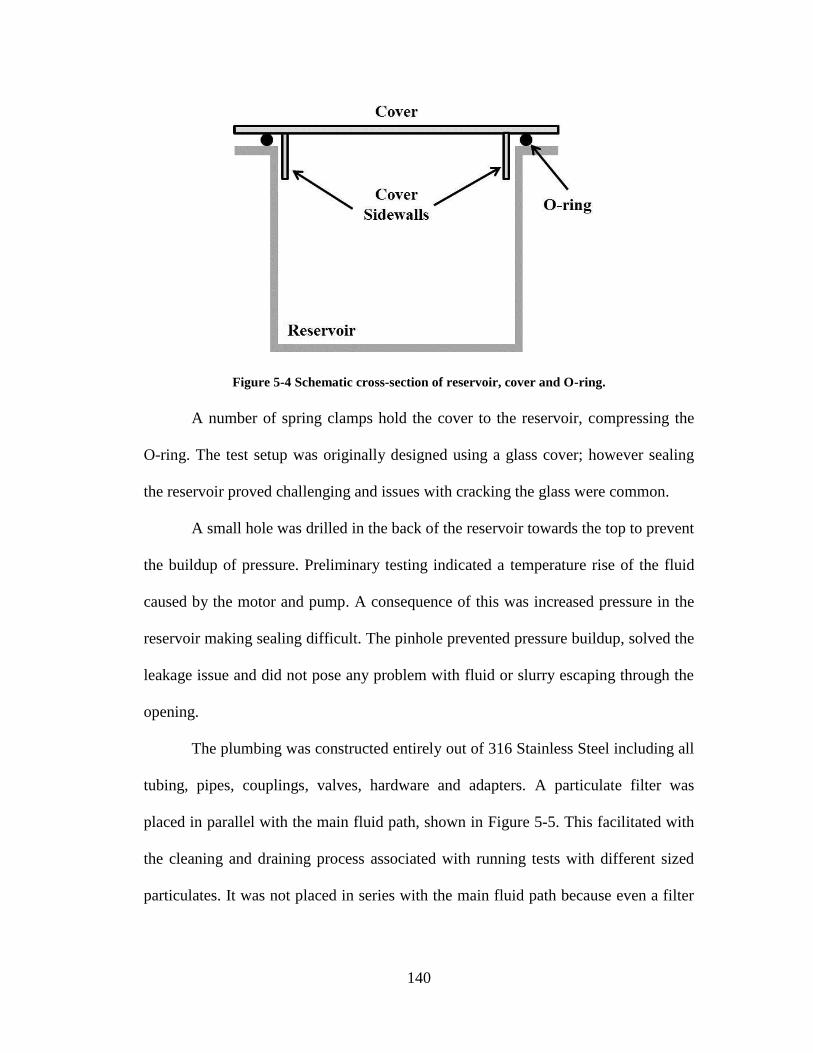
140

Figure 5-4 Schematic cross-section of reservoir, cover and O-ring.

A number of spring clamps hold the cover to the reservoir, compressing the

O-ring. The test setup was originally designed using a glass cover; however sealing

the reservoir proved challenging and issues with cracking the glass were common.

A small hole was drilled in the back of the reservoir towards the top to prevent

the buildup of pressure. Preliminary testing indicated a temperature rise of the fluid

caused by the motor and pump. A consequence of this was increased pressure in the

reservoir making sealing difficult. The pinhole prevented pressure buildup, solved the

leakage issue and did not pose any problem with fluid or slurry escaping through the

opening.

The plumbing was constructed entirely out of 316 Stainless Steel including all

tubing, pipes, couplings, valves, hardware and adapters. A particulate filter was

placed in parallel with the main fluid path, shown in Figure 5-5. This facilitated with

the cleaning and draining process associated with running tests with different sized

particulates. It was not placed in series with the main fluid path because even a filter

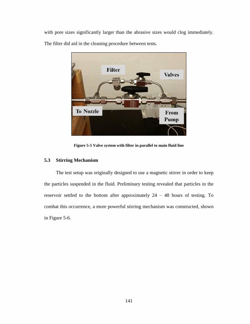
141

with pore sizes significantly larger than the abrasive sizes would clog immediately.

The filter did aid in the cleaning procedure between tests.

Figure 5-5 Valve system with filter in parallel to main fluid line

5.3 Stirring Mechanism

The test setup was originally designed to use a magnetic stirrer in order to keep

the particles suspended in the fluid. Preliminary testing revealed that particles in the

reservoir settled to the bottom after approximately 24 – 48 hours of testing. To

combat this occurrence, a more powerful stirring mechanism was constructed, shown

in Figure 5-6.

142

Figure 5-6 Stirring mechanism - motor, shaft, propeller

A motor drives the propeller, connected by a shaft and coupling. The motor is

mounted to a supportive wooden box which is also attached to the reservoir cover via

epoxy. The length of the shaft was designed such that approximately 3 inches of

space lie between the bottom of the reservoir and the propeller. Additionally, the

propeller pushes water down towards the bottom of the reservoir to induce a

significant turbulent effect throughout the entire volume of slurry. Testing of this

stirring mechanism further revealed that particle settling in the reservoir did not

occur. Vibration was found not to be an issue as well.

5.4 Pump and Motor

The pump used in this test setup was a Hydracell D10 model slurry pump,

with specific part number D10EKSTHFHHA. This pump is a positive displacement

diaphragm pump and is specifically designed to handle abrasive slurries and corrosive

and viscous fluids. The D10 model can deliver up to 8.0 GPM and has a maximum

outlet pressure of 1000 psi. The speed of the pump, thus the flowrate, is controlled by

143

a three-phase induction motor. The motor is driven by a 3HP 460V variable

frequency ABB motor drive. These instruments are all shown in Figure 5-7.

Figure 5-7 Motor drive, pump and motor

The pump and motor subsystem are mounted to a wooden board which has

rubber vibration-dampening feet. While the motor can induce significant vibration

when operated at higher speeds, the speeds at which these tests take place do not pose

issues with vibration.

5.4.1 Pump Calibration

The pump documentation outlines a flow rate vs revolutions chart at pressures

between 100 – 1000 psi, shown in Figure 5-8.

144

Figure 5-8 Flowrate vs. pump speed for D10-E pump, from manufacturer [122]

Given that the slurries will contain very fine abrasive particles, direct flowrate

measurement were not included in the test setup. Of the various techniques that can

measure flow rate, each one posed potential issues. Turbine flow meters rely on a

propeller that spins by the force imposed from the moving fluid. The rotational speed

is thus proportional to the velocity of the fluid. However, the propeller would

eventually wear due to the fine particles entrained in the flow. While slight wear is

not an issue for most of the test apparatus, slight wear of this propeller would

significantly alter the flowrate calibration. Ultrasonic flow meters were also

145

considered, however these are typically the most expensive flow measuring

techniques.

The technique ultimately chosen to calibrate the pump was to weigh the amount

of fluid displaced by the pump over a known period of time. A hose was connected to

the plumbing and led to a ~30 gallon trash can. After each test the fluid was weighed

and a mass flow rate was calculated. This test was repeated for pump speeds ranging

from 3 – 12 Hz. Approximately 12 gallons of fluid were used for each test. The

results of the pump calibration are shown in Figure 5-9.

Figure 5-9 Pump calibration raw data

The calibration data varies slightly from the manufacturer data at frequencies

below ~ 9 Hz. This is largely due to the fact that this pump is not necessarily designed

to run at the low frequencies required by this application. Therefore the flowrate for

each test will be determined by the calibration data as opposed to the manufacturer

data.

146

5.5 Nozzle and Nominal Jet Velocity

The nozzle orifice size is the prime factor determining the nominal jet velocity.

While there are a number of different types of commercially available nozzles, a

1.98mm nozzle purchased from Jetstream® and shown in Figure 5-10 was chosen. It

consists of a tungsten carbide liner which interfaces with the slurry and is enveloped

by a stainless steel shell. Additionally, the ¼ NPT fitting enabled easy installment to

the test setup.

Figure 5-10 Nozzle used in the test setup. Image taken from [123]

Due to the non-uniform pump flowrate at various motor speeds, a nominal jet

velocity – motor speed relation was constructed. Given that the controller determines

the motor speed in Hz (as opposed to RPM), a jet velocity vs. Hz graph was

constructed for easy determination of the nominal jet velocity. This relation is shown

in Figure 5-11. When describing jet velocity, the term ‘nominal’ is used due to

localized fluctuations within the jet that may occur. Additionally, this quantity is

defined as the flowrate divided by the nozzle orifice.

147

Figure 5-11 Nominal velocity of jet as a function of nozzle size and motor speed

5.6 Sample Holder and Fabrication of Test Samples

A sample holder was placed within the reservoir and was positioned such that

approximately 1cm of space lies between the surface of the sample and the nozzle

exit. The sample holder, shown in Figure 5-12, was fabricated from 316 stainless steel

and was welded to a stainless steel ‘allthread’ rod that spans the width of the

reservoir. This configuration allows the sample holder to be rotated, changing the jet

impingement angle. Additionally, four set screws hold the sample in the holder.

148

Figure 5-12 Nozzle and Sample Holder

The samples were fabricated by soldering 12x12mm Si chips to a 14x14x5mm

Kovar coupon. Originally copper was used as the sample substrate however

preliminary studies indicated relatively large global warpages due to the CTE

mismatch between copper and Si. Kovar has a significantly better matched CTE

reducing, but not completely eliminating, the initial warpages induced from soldering.

In order to solder the Si sample chips to the Kovar coupon, the backside of the

chip was metallized using the stack depicted in Figure 5-13.

Figure 5-13 Metallization stack used for soldering chip to substrate

149

The Kovar coupon was prepared for soldering by grinding down and polishing

the surface using SiC grit paper to remove any surface oxides. After the chip was

soldered to the Kovar substrate using a standard Tin-based solder, the surface was

cleaned with acetone, methanol and isopropyl alcohol with Q-tips.

5.7 Creation of Testing Slurry

The testing slurries were created by measuring out the appropriate amount of

abrasive and mixing it with a small amount of water (or whichever solution was being

used) in a 500mL glass jar. In addition a polyacrylic acid dispersant was added,

Dispex AA 4140 NS manufactured by BASF, to appropriately disperse the abrasives

within the fluid. The mass of dispersant added was equal to the mass of abrasive used.

The solution was then sonicated for 20 minutes to further ensure agglomerates were

broken up. This mixture was then added to the test setup with the remaining two

gallons of fluid for testing.

5.8 Cleaning Procedure

In order to ensure that unwanted particles from previous tests are removed from

the test loop, a robust cleaning and flushing procedure was followed. First, the dirty

fluid was drained from the system at the filter port and two gallons of water were

flushed through the loop. All parts of the reservoir, O-ring stirrer and cover were

wiped down to remove all visible remnants of particulate fouling and build-up.

Next, one gallon of water was added to reservoir and a “dummy” sample was

placed in the sample holder. The system was then run for 10-20 minutes at a high

flowrate (10 Hz). Upon examination the water usually appeared murky, signifying

150

that particles were picked up from places in the fluid loop other than the reservoir.

The water was then drained and fresh water was added. This process was repeated

approximately 4-6 times or until the water appeared visibly clear and without

contaminants. Although this process may not remove every particle, the extremely

sparse particles that may be left in the solution are assumed to affect the erosion

negligibly compared to the relatively large concentration of other sized particles. In

addition, more stringent cleaning process occurred when smaller particles would be

used in tests after large particles.

5.9 Limitations

While this setup enables the slurry erosion phenomena to be studied, a number

of limitations exist. These limitations are inherent in this type of slurry erosion test

apparatus and should be taken into account during the post-erosion analysis and in

any future studies involving jet-impingement slurry erosion.

The primary limitation of the test setup lies in the fact that a filter is not used in

the main fluid loop. Although a small filter in the secondary parallel loop exists

which aids in cleaning the test setup, a primary filter is not used during the

experiments. The reasoning behind this is that a filter, regardless of the size, would

inevitably clog. For example, in the case of a 25μm filter and 1μm abrasive particles,

the filter may do its job for a period of time, trapping unwanted particles larger than

25μm that develop during the test. However, at some point a small percentage of the

filter would get clogged from these larger particles. In a “snow-ball” like effect, the

smaller 1 micron particles would get trapped also in the filter. Not only would this

perpetuate the clogging process of the filter but it would significantly change the pre-

151

defined particulate concentration of the slurry. Although continuous cleaning of the

filter could be used, preliminary studies showed that this may not be necessary. It was

found in the first couple experiments that the vast majority of the observed wear was

in fact due to the particulate abrasives even with larger particles existing in the fluid

loop. Particles generated in the test setup most often originated from the rubber seals

and gaskets or the acrylic cover. Despite the size of these particles, their impact on

erosion was trivial due to their soft nature.

It should be mentioned however that further inspection of the surface did reveal

a few locations of discrete chipping likely caused by the impact of higher energy

particles. However, the relative number of these discrete impacts is small and

considered negligible compared to the amount of wear caused by the abrasive

particles.

Another challenge the test setup imposes is that the temperature of the slurry

heats up during the experiments. This is caused by the mechanical action of the pump.

To deal with any significant heating, a fan was setup to continuously blow air over

the motor and pump. This minimized the overall temperature change of the fluid and

kept the bulk fluid temperature at approximately 34°C.

Lastly, the final limitation with the test setup is that the pump occasionally

produces random pulsations. These most often occur at frequencies below 2 Hz, but

occur periodically throughout all testing ranges. The main effect arising from this is

that a pulsating jet will exit the nozzle as opposed to a smooth fluid stream. Pulsation

dampeners are typically installed in systems like these, however it was predicted that

the inclusion of one of these dampeners may cause more harm than good. One type of

152

pulsation dampener utilizes a rubber diaphragm to smooth out the flow rate

fluctuations. This may be a viable solution if the fluid had no abrasive particles in it

due to the fact that they may eventually wear away the rubber. Another type of

pulsation dampener operates by significantly increasing the volume of the fluid loop,

operating much like a “fluid-capacitor”. While this design may also work if the fluid

had no particles, over time the particles may settle out in the sub-reservoir and

significantly reduce the predefined particulate concentration of the slurry.

While these factors impose certain challenges and limitations regarding the

operation and test procedure, they are acknowledged and will be taken into

considering during the post-erosion analysis and model development.

153

6 EXPERIMENTAL EROSION TESTING OF

SILICON

6.1 Introduction

This section discusses the procedures involved in testing and measuring the

Silicon erosion samples. First, the Design of Experiments (DOE) is presented which

covers the range of experiments performed. The parameters investigated are

nominally jet velocity, particle size, particulate concentration, fluid viscosity and

time. Next, the method in which the stylus profilometer was used to approximate the

total amount of volume loss will be discussed including the numerical analysis

performed in MATLAB. Additionally, the procedure for factoring in initial warpage

will be described.

Two principle erosion metrics are described in this chapter, a mass loss rate in

units of milligrams per year and a one-dimensional erosion rate in units of

micrometers per year. The mass loss rates found in this chapter will be used to

formulate the erosion ratio metrics while the one-dimensional erosion rates will serve

as the metric through which the final erosion model will be validated against.

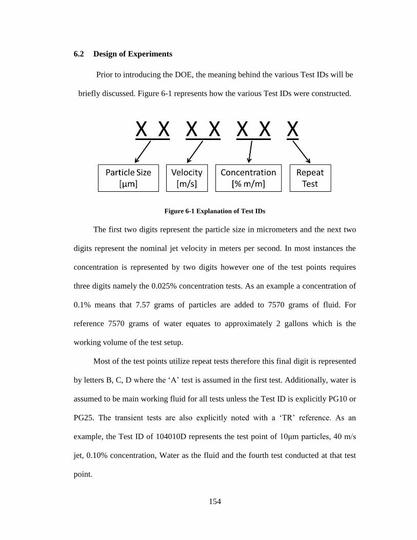
154

6.2 Design of Experiments

Prior to introducing the DOE, the meaning behind the various Test IDs will be

briefly discussed. Figure 6-1 represents how the various Test IDs were constructed.

Figure 6-1 Explanation of Test IDs

The first two digits represent the particle size in micrometers and the next two

digits represent the nominal jet velocity in meters per second. In most instances the

concentration is represented by two digits however one of the test points requires

three digits namely the 0.025% concentration tests. As an example a concentration of

0.1% means that 7.57 grams of particles are added to 7570 grams of fluid. For

reference 7570 grams of water equates to approximately 2 gallons which is the

working volume of the test setup.

Most of the test points utilize repeat tests therefore this final digit is represented

by letters B, C, D where the ‘A’ test is assumed in the first test. Additionally, water is

assumed to be main working fluid for all tests unless the Test ID is explicitly PG10 or

PG25. The transient tests are also explicitly noted with a ‘TR’ reference. As an

example, the Test ID of 104010D represents the test point of 10μm particles, 40 m/s

jet, 0.10% concentration, Water as the fluid and the fourth test conducted at that test

point.

155

Table 6-1 shows the 14 different erosion test cases performed. The ranges

chosen in this study were developed largely to correspond to specific proprietary

systems found throughout DARPA’s ICECOOL program and due to the proprietary

nature of these systems, specific references cannot be provided. Depending on the

application, certain systems may employ more modest or accelerated values

depending on the specific microchannel or jet architectures. Although specifics vary

widely from system to system, the general goal of this DOE was to conduct a series

of experiments within the ballpark parameter ranges of typical systems. Depending on

the type of microchannel or jet implementation, the model could then be applied to

specific design and filtering restraints.

156

Table 6-1 Design of experiment, 14 experimental test cases

Particles sizes between 2.5 - 20μm were studied and represent some of the

various filtering levels commonly found in electronic cooling loops. While particles

upwards of 20μm in diameter would not be commonly found in real life applications,

accelerated erosion tests are necessary in order to formulate relations among the

various parameters. Typical sizes of commercially available filters are 0.5μm, 1μm,

3μm, 5μm, and 10μm where these values represent the approximate pore size.

Nominal jet velocities between 20 – 40 m/s were tested. Again, these are within

the range of typical values found in single phase jet-impingement systems. In single

phase manifolded systems the velocities may be significantly lower than these, often

157

times less than 5 m/s, yet in two phase systems the velocities of entrained particles as

the fluid evaporates may be around the 40 m/s value.

Dilute concentrations were chosen to represent the fact that most real

applications have decent filtering systems. While the concentration test points are

considered highly accelerated based on some of the typical ISO Fluid Cleanliness

codes used in high performance servos and aerospace hydraulic systems, enough

particles had to be used in order to obtain measureable results in a reasonable amount

of time. More will be discussed on this later in the chapter.

Water is the primarily fluid used in these tests, however two other tests were

conducted using a 10% and a 25% propylene glycol – water solution. These two test

points were included to assess how well the developed model, calibrated in water,

could be applied to other working fluids.

Lastly, two transient tests were conducted at 30 m/s and 40 m/s to assess the

dependence of erosion on time.

6.3 Measurement Techniques

6.3.1 Stylus Profilometer

A stylus profilometer, also known as a line scan profilometer, generates a 2D

profile by tracking the surface height across the length of the scan. A stylus is

dragged horizontally across the surface and enables small surface features, on the

order of tens of nanometers, to be observed. A Tencor P-20 Long Scan Profiler,

shown in Figure 6-2, was used to perform these measurements.

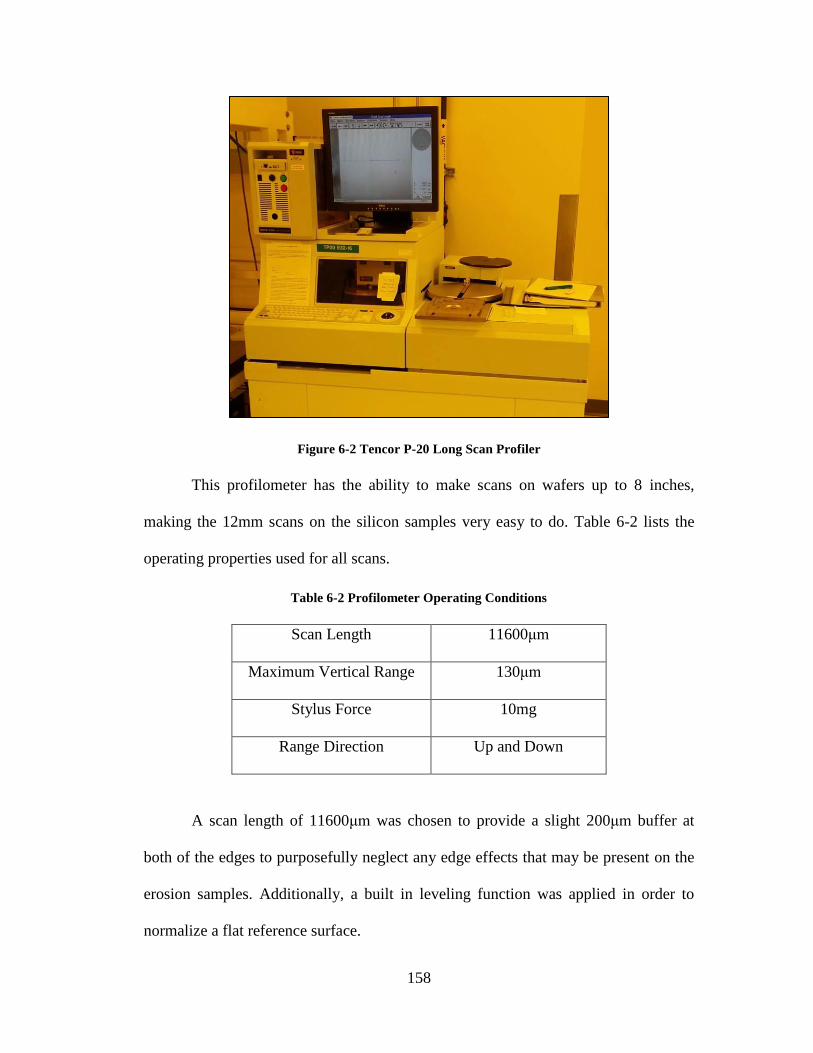
158

Figure 6-2 Tencor P-20 Long Scan Profiler

This profilometer has the ability to make scans on wafers up to 8 inches,

making the 12mm scans on the silicon samples very easy to do. Table 6-2 lists the

operating properties used for all scans.

Table 6-2 Profilometer Operating Conditions

Scan Length 11600μm

Maximum Vertical Range 130μm

Stylus Force 10mg

Range Direction Up and Down

A scan length of 11600μm was chosen to provide a slight 200μm buffer at

both of the edges to purposefully neglect any edge effects that may be present on the

erosion samples. Additionally, a built in leveling function was applied in order to

normalize a flat reference surface.

159

Assuming the jet impinges perpendicularly on the sample, the erosion scar

should ideally exhibit axisymmetric properties about the stagnation region.

Experimental error and uncontrollable inconsistencies prevented perfectly

axisymmetric contours to be achieved. To obtain well-rounded data for each test, two

profile scans were taken. One from left to right, termed the ‘LR’ scan, and the other

from the top to the bottom termed the ‘UD’ scan, short for Up-Down. A schematic of

the profile and the corresponding scans are shown in Figure 6-3.

Figure 6-3 Schematic of erosion scar and stylus profilometer scans

In agreement with the findings of Wang et al. [92] the general erosion scar

was found to exhibit the characteristic ‘W’ shape. The center, termed the stagnation

region, is a region in which minimal wear occurs due to the lack of direct impacts.

160

The results of the CFD study described in the previous chapter indicate a high

prevalence of low angle impacts which occur outside the jet-impingement region. In

addition, the CFD study also indicated that particle impacts do not occur in the center

of the jet region. Therefore the height of the stagnation region is assumed to serve as

the reference point where no wear is assumed to occur.

6.3.2 Initial Warpage Considerations

In order to more accurately measure the quantity of eroded material, the

amount of initial warpage across the Silicon sample was taken into consideration.

Preliminary erosion tests were conducted by soldering the silicon samples to copper

coupons. It was typically found that the initial maximum warpage height across that

wafer, as measured by the stylus profilometer, was on the order of 1-2μm. This

occurred due to the coefficient of thermal expansion (CTE) mismatch between the

Silicon (~ 3 ppm/°K) and copper (~ 16.6 ppm/°K). While this is relatively small, the

erosion depth from some of the tests was expected to be near this value. As such,

Kovar coupons were chosen to replace the copper coupons for all the tests which has

a CTE closer to that of Silicon, which is approximately 5.3 ppm/°K.

After soldering the silicon samples to the Kovar coupons, a profilometer

measurement was taken across the sample to assess the maximum initial warpage.

Only samples which had a maximum average initial warpage of less than 0.6μm were

used in the erosion studies. The maximum average initial warpage was taken by

averaging three measurements from the ‘LR’ direction and three measurements from

the ‘UD’ direction, shown in Figure 6-4. For these measurements it was assumed that

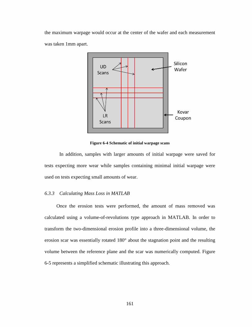
161

the maximum warpage would occur at the center of the wafer and each measurement

was taken 1mm apart.

Figure 6-4 Schematic of initial warpage scans

In addition, samples with larger amounts of initial warpage were saved for

tests expecting more wear while samples containing minimal initial warpage were

used on tests expecting small amounts of wear.

6.3.3 Calculating Mass Loss in MATLAB

Once the erosion tests were performed, the amount of mass removed was

calculated using a volume-of-revolutions type approach in MATLAB. In order to

transform the two-dimensional erosion profile into a three-dimensional volume, the

erosion scar was essentially rotated 180° about the stagnation point and the resulting

volume between the reference plane and the scar was numerically computed. Figure

6-5 represents a simplified schematic illustrating this approach.

162

Figure 6-5 Volume-of-revolution numerical integration

Rotating the erosion scar 180° about the stagnation region enables a three-

dimensional volume to be calculated. The two-dimension area was broken up into a

large number of rectangles with heights corresponding to the distance between the

eroded depth and the reference plane. This type of approach is also referred to as the

midpoint approximation rectangular method. This procedure was repeated for both

the LR and UD scans of a sample and the results were averaged together to

approximate to total volume loss of the sample.

To account for the initial warpage, a similar algorithm was devised to

approximate the volume associated with the initial warpage. According to Figure 6-6,

the measured erosion contour does not inherently capture the initial warpage

characteristics, which is shown as the grey shaded area above the erosion profile.

163

Figure 6-6 Accounting for initial warpage

The curve of the initial profile was approximated by a quadratic function

corresponding to the general shape of the ‘smile’ warpage. In a similar manner as

previously described, the shape was divided up into a large number of rectangles and

rotated 180° about the center point. A resulting volume was then calculated. Due to

the fact that the reference plane was taken at the highest point in the stagnation

region, the volume computed from the initial warpage calculation was added to the

volume loss from due to erosion. In the few instances where the initial warpage

resulted in a ‘frown’, this process was inverted and the appropriate calculations were

performed.

Due to the fact that samples with larger amounts of initial warpage were

reserved for tests expecting larger amounts of erosion, the volume associated with the

initial warpage was typically a small percentage of the measured erosion wear. In

many cases the percentage was negligible.

164

6.4 Erosion Results

This section presents the results of the erosion experiments. For the purpose of

brevity, data from select tests will be included in this section, however Appendix A

will include all the data.

Table 6-3 summarizes the results for all erosion tests. Mass loss from the LR

and the UD scans are both given separately along with the calculated initial warpage

mass approximations. Typically on samples where the initial warpage was less than

0.2μm a discernable ‘frown’ or ‘smile’ did not exist. Therefore it was assumed that

initial warpages of this magnitude played a negligible role in calculating total mass of

material removed.

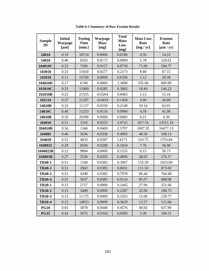
165

Table 6-3 Summary of Raw Erosion Results

Sample

ID

Initial

Warpage

[μm]

Testing

Time

[min.]

Warpage

Mass

[mg]

Total

Mass

Loss

[mg]

Mass Loss

Rate

[mg / yr]

Erosion

Rate

[μm / yr]

24010 0.19 18714 0.0000 0.0180 0.50 14.53

54010 0.40 8263 0.0173 0.0909 5.78 120.61

104010C 0.25 7200 0.0157 0.9739 71.09 594.77

103010 0.32 11650 0.0277 0.2173 9.80 87.72

102010 0.11 15749 0.0000 0.0336 1.12 20.38

104010D 0.17 6740 0.0000 1.3090 102.08 800.80

103010C 0.33 11060 0.0285 0.3892 18.49 144.22

102010B 0.23 21555 -0.0264 0.0463 1.13 15.16

102510 0.37 21297 -0.0433 0.1458 3.60 34.09

54010B 0.33 11137 0.0230 0.2149 10.14 62.91

54010C 0.40 11253 0.0116 0.0984 4.59 41.96

24010B 0.16 20390 0.0000 0.0083 0.21 4.39

204010 0.51 1316 0.0525 2.0725 827.74 13511.10

204010B 0.56 1346 0.0469 2.5797 1007.35 16477.13

104005 0.46 5636 0.0358 0.4993 46.56 338.13

104020 0.51 4033 0.0287 1.6171 210.75 1753.84

1040025 0.29 6936 0.0290 0.1024 7.76 56.90

1040025B 0.12 9894 0.0000 0.1535 8.15 56.73

104005B 0.27 5536 0.0205 0.4006 38.03 276.17

TR40-1 0.51 1540 0.0383 0.3967 135.39 1023.04

TR40-2 0.51 2843 0.0383 0.6031 111.50 873.69

TR40-3 0.51 4348 0.0383 0.7978 96.44 764.48

TR40-4 0.51 5637 0.0383 0.9124 85.07 688.08

TR30-1 0.15 2717 0.0000 0.1445 27.94 251.66

TR30-2 0.15 5449 0.0000 0.2287 22.06 188.73

TR30-3 0.15 11175 0.0000 0.3203 15.06 129.77

TR30-4 0.15 14053 0.0000 0.3629 13.57 115.94

PG10 0.65 5878 0.0448 0.4576 40.92 637.90

PG25 0.42 5675 -0.0162 0.0583 5.39 194.21

166

6.4.1 Effect of Velocity

Sample profile scans are presented here which show the effect of nominal jet

velocity on erosion. For the following tests, 10μm nominally sized Al2O3 particles

were used at a concentration of 0.1% in water.

Figure 6-7 LR-102010 Profile Scan

Figure 6-8 LR-102510 Profile Scan

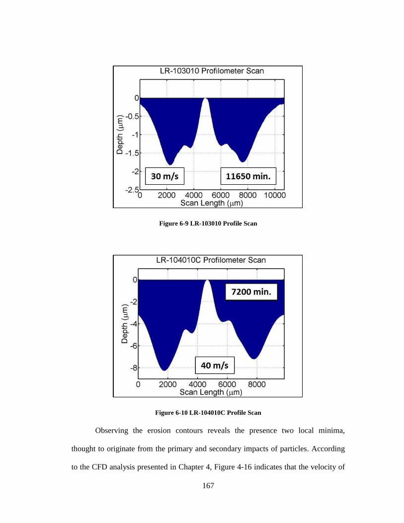
167

Figure 6-9 LR-103010 Profile Scan

Figure 6-10 LR-104010C Profile Scan

Observing the erosion contours reveals the presence two local minima,

thought to originate from the primary and secondary impacts of particles. According

to the CFD analysis presented in Chapter 4, Figure 4-16 indicates that the velocity of

168

the first impact in the 40 m/s case is smaller than the velocity of the second impact.

According to Figure 6-10 above, the depth of the local minima closest to the

stagnation region for the 40 m/s case is less eroded than the minima further away

from the stagnation region. It is thought that the minima closest to the stagnation

region corresponds to the first impact while the minima further away corresponds to

the second. Additionally as the impact number increase past two, the impact angle

and the percentage of particle streams resulting in impacts significantly decreases.

Discrete impact regions become indistinguishable from one-another due to the fact

that material is removed in a wet abrasion mechanism. This most observable in the 40

m/s case where the edges of the profile have worn down significantly below the

height of the stagnation region.

Furthermore, the relative height difference of the primary and secondary

impacts correspond closely to the impact velocities determined through CFD.

According to the profile scans, the primary impact depth of the 30 m/s and 40 m/s

case is higher than the secondary impact depths, however in the 20 m/s and 25 m/s

cases the primary impact depth surpasses that of the secondary impact depth. This is

also observed in the CFD simulations where the velocity of the second impact

decreases relative the first impact as the nominal jet velocity decreases.

It is also interesting to note that the distance between the primary impact sites

on each side of the stagnation region stays relatively constant, approximately 2mm,

throughout each of the test cases. This is most likely due to the fact that the average

impact angle of the first impact stays within a few degrees across all tests. According

to Figure 4-17 which shows how impact angle varies across different jet velocities,

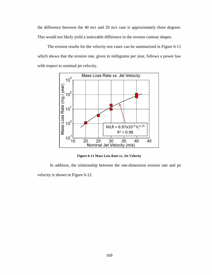
169

the difference between the 40 m/s and 20 m/s case is approximately three degrees.

This would not likely yield a noticeable difference in the erosion contour shapes.

The erosion results for the velocity test cases can be summarized in Figure 6-11

which shows that the erosion rate, given in milligrams per year, follows a power law

with respect to nominal jet velocity.

Figure 6-11 Mass Loss Rate vs. Jet Velocity

In addition, the relationship between the one-dimension erosion rate and jet

velocity is shown in Figure 6-12.

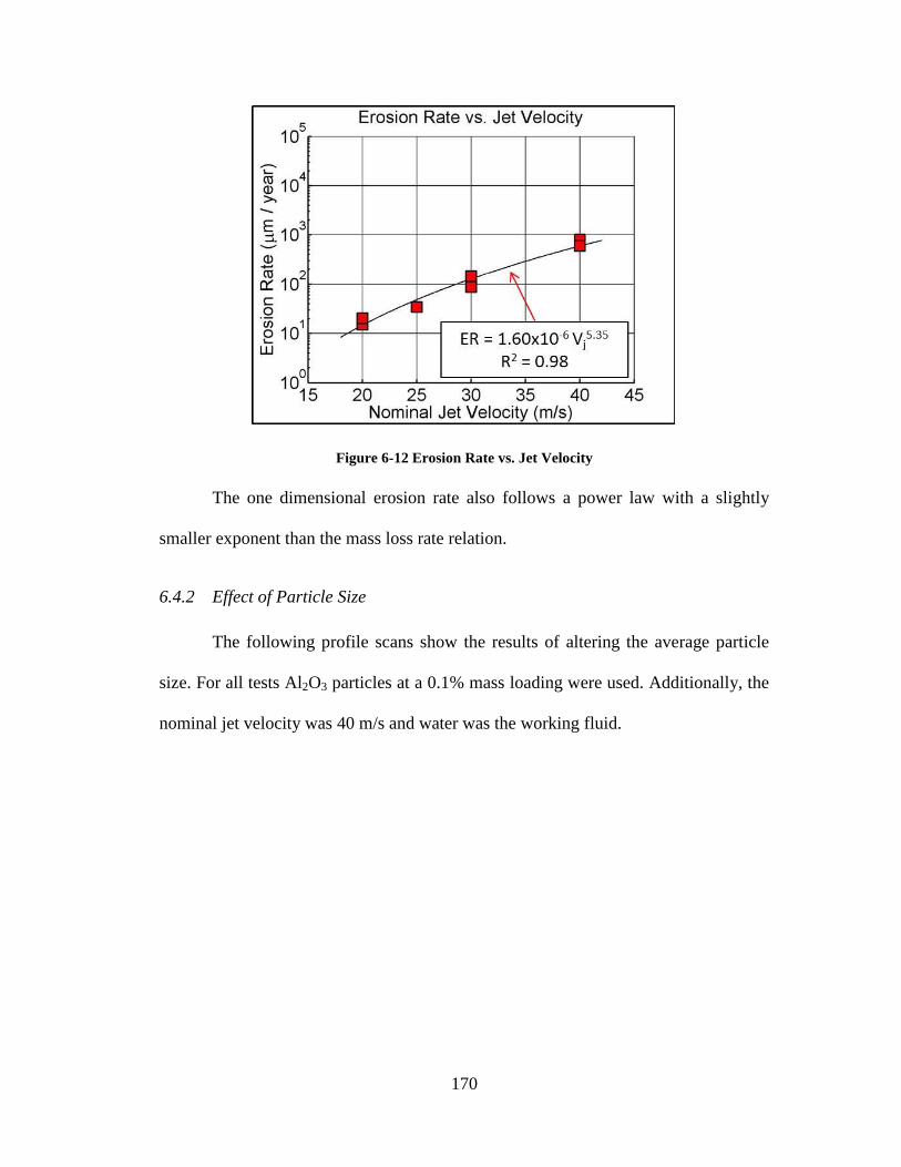
170

Figure 6-12 Erosion Rate vs. Jet Velocity

The one dimensional erosion rate also follows a power law with a slightly

smaller exponent than the mass loss rate relation.

6.4.2 Effect of Particle Size

The following profile scans show the results of altering the average particle

size. For all tests Al2O3 particles at a 0.1% mass loading were used. Additionally, the

nominal jet velocity was 40 m/s and water was the working fluid.

171

Figure 6-13 LR-24010 Profile Scan

Figure 6-14 LR-54010 Profile Scan

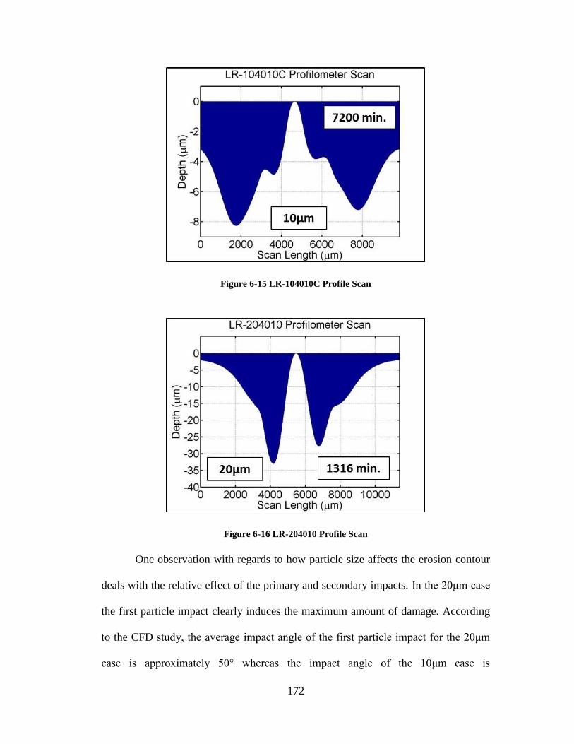
172

Figure 6-15 LR-104010C Profile Scan

Figure 6-16 LR-204010 Profile Scan

One observation with regards to how particle size affects the erosion contour

deals with the relative effect of the primary and secondary impacts. In the 20μm case

the first particle impact clearly induces the maximum amount of damage. According

to the CFD study, the average impact angle of the first particle impact for the 20μm

case is approximately 50° whereas the impact angle of the 10μm case is

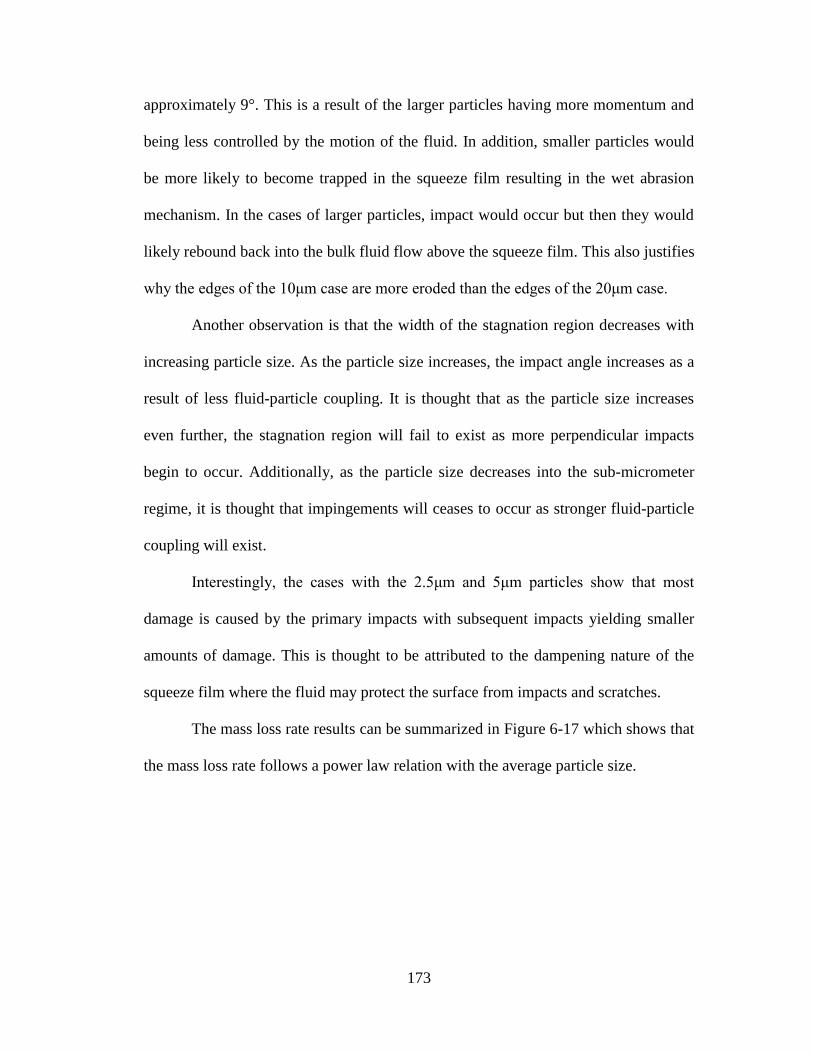
173

approximately 9°. This is a result of the larger particles having more momentum and

being less controlled by the motion of the fluid. In addition, smaller particles would

be more likely to become trapped in the squeeze film resulting in the wet abrasion

mechanism. In the cases of larger particles, impact would occur but then they would

likely rebound back into the bulk fluid flow above the squeeze film. This also justifies

why the edges of the 10μm case are more eroded than the edges of the 20μm case.

Another observation is that the width of the stagnation region decreases with

increasing particle size. As the particle size increases, the impact angle increases as a

result of less fluid-particle coupling. It is thought that as the particle size increases

even further, the stagnation region will fail to exist as more perpendicular impacts

begin to occur. Additionally, as the particle size decreases into the sub-micrometer

regime, it is thought that impingements will ceases to occur as stronger fluid-particle

coupling will exist.

Interestingly, the cases with the 2.5μm and 5μm particles show that most

damage is caused by the primary impacts with subsequent impacts yielding smaller

amounts of damage. This is thought to be attributed to the dampening nature of the

squeeze film where the fluid may protect the surface from impacts and scratches.

The mass loss rate results can be summarized in Figure 6-17 which shows that

the mass loss rate follows a power law relation with the average particle size.

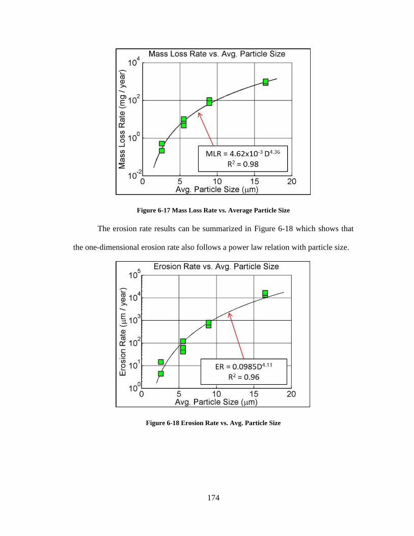
174

Figure 6-17 Mass Loss Rate vs. Average Particle Size

The erosion rate results can be summarized in Figure 6-18 which shows that

the one-dimensional erosion rate also follows a power law relation with particle size.

Figure 6-18 Erosion Rate vs. Avg. Particle Size

175

6.4.3 Effect of Concentration

The following profile scans show the result of altering the particulate loading

concentration. For all tests the nominal jet velocity was 40 m/s with water as the

working fluid. As stated earlier, the concentration is defined as the ratio of the mass

of particles to the mass of fluid.

Figure 6-19 LR-1040025B Profile Scan

176

Figure 6-20 UD-104005B Profile Scan

Figure 6-21 LR-104010C Profile Scan

177

Figure 6-22 LR-104020 Profile Scan

Comparing the erosion contours from the concentration experiments, it can be

seen that they all share similar qualitative attributes. All the contours exhibit similar

primary and secondary impact locations, with the depth of the first impact being less

than the second. Essentially the only difference between the profiles is the y-axis

scale measuring depth. As described in the CFD chapter, doubling the particulate

concentration should in theory double the mass loss rate as twice as many particle

impingements per unit time would take place. At the low concentrations used in these

experiments, particle-particle interactions can be assumed negligible, however at

much higher particulate concentrations, particle-particle interactions may occur. In

these scenarios, particles may agglomerate at the surface and act as a shield for

incoming particles resulting in a reduction in erosion rate [85] [124].

The mass loss rate results for the concentration experiments can be

summarized in Figure 6-23 which shows a linear relationship.

178

Figure 6-23 Mass Loss Rate vs. Particle Concentration

The one-dimensional erosion rates summarizing the concentration

experiments are shown in Figure 6-24.

Figure 6-24 Erosion Rate vs. Particulate Concentration

Looking at the above graphs, it can be seen that the assumption where

doubling the concentration doubles the mass loss rate and erosion rate is validated.

The slope of the graph in Figure 6-24 is close to 1000 while the slope of the graph in

179

Figure 6-24 is 10,000 meaning that doubling the concentration effectively doubles the

erosion metric. While the y-intercept should theoretically be zero, the negative y-

intercept suggests the presence of a threshold concentration. It is thought that the

negative y-intercept is a result of slight particle fouling phenomenon, where the actual

concentration of the fluid impinging the surface is less than the concentration at the

start of the test. Upon inspecting the test setup it was clear that particulate fouling

occurred, specifically around the seals and O-ring as shown in Figure 6-25.

Figure 6-25 Particulate fouling near seals in test setup

Later sections will discuss the pertinence of this phenomenon more in depth,

however from the work in this chapter it can be reasoned that of the factors

contributing to erosion, concentration is least influential. The relationships between

mass loss rate and erosion rate with particle size and jet velocity both follow power

laws with exponents greater than four. This is compared to the linear relationship that

concentration holds with these erosion metrics. As such, while a decrease in expected

concentration will affect erosion results and subsequent predictions, other factors play

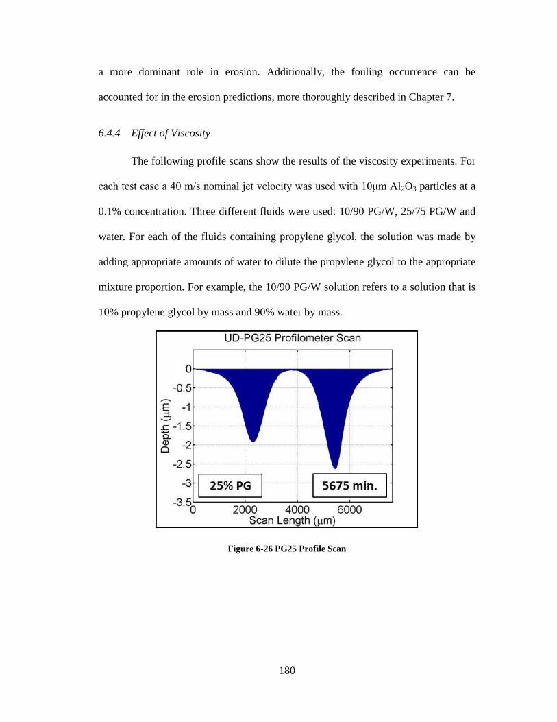
180

a more dominant role in erosion. Additionally, the fouling occurrence can be

accounted for in the erosion predictions, more thoroughly described in Chapter 7.

6.4.4 Effect of Viscosity

The following profile scans show the results of the viscosity experiments. For

each test case a 40 m/s nominal jet velocity was used with 10μm Al2O3 particles at a

0.1% concentration. Three different fluids were used: 10/90 PG/W, 25/75 PG/W and

water. For each of the fluids containing propylene glycol, the solution was made by

adding appropriate amounts of water to dilute the propylene glycol to the appropriate

mixture proportion. For example, the 10/90 PG/W solution refers to a solution that is

10% propylene glycol by mass and 90% water by mass.

Figure 6-26 PG25 Profile Scan

181

Figure 6-27 PG10 Profile Scan

Figure 6-28 LR-104010C Profile Scan

Comparing the PG10 case to the water case , the first observation regarding

the erosion contours is that distinct secondary impact sites are not observable. The

viscosity of the PG10 solution is more than four times that of the water solution (0.73

cP for Water verses 3.3 cP for PG10) suggesting that stronger coupling between fluid

182

streamlines and particle motion exists. According to Table 4-2 the Reynold’s number

for both flows suggest that both are in the turbulent regime, however the PG10

solution (Re = 24100) is much less turbulent than the Water flow (Re = 107000). This

may potentially reduce the random particle movement fluctuations and lead to a more

precise impact location outcome.

It is also observed that the edges of the samples become less eroded with

increased viscosity. As the viscosity of the fluid increases, the squeeze film may act

more to protect the surface from scratches thus reducing the effect of low angle

particle impacts. Comparing the PG10 and PG25 cases, it can be seen that subsequent

impacts play less of a role in overall wear in the more viscous fluid.

The results of the mass loss rate experiments are shown in Figure 6-29 which

suggests that the mass loss rate may follow a decreasing exponential relationship with

fluid viscosity.

Figure 6-29 Mass Loss Rate vs. Fluid Viscosity

183

The relationship between the one-dimensional erosion rate and viscosity is

shown in Figure 6-30.

Figure 6-30 Erosion Rate vs. Fluid Viscosity

Although regression analysis suggests decreasing exponential relationships

between the wear rates and viscosity, a much more thorough investigation would be

necessary to confirm the exact calibration constants.

According to the graphs above, the erosion rates of the water and PG10 cases

are very similar. This can be confirmed by looking at the CFD results, shown in

Figure 4-23, which indicate that the impact velocities of the first particle impact are

approximately 22 m/s and 23 m/s respectively for the PG10 and Water cases. This is

compared to the velocity of the first impact for the PG25 case which is approximately

12.5 m/s. However, the impact velocities of subsequent impacts in the PG10 case are

significantly less than those of water case. This is likely a result of the more viscous

fluid (PG10) moving slower close to the surface while the less viscous fluid (water)

moves quicker.

184

6.4.5 Effect of Testing Time

The following profile scans show the results of the 40 m/s transient test where

four measurements were conducted periodically throughout the test. 10μm Al2O3

particles at a concentration of 0.1% in water were used as the testing slurry.

Figure 6-31 104010 Transient 1 Profile Scan

Figure 6-32 LR-104010 Transient 2 Profile Scan

185

Figure 6-33 LR-104010 Transient 3 Profile Scan

Figure 6-34 LR-104010 Transient 4 Profile Scan

Upon observation, the only distinguishable feature between each of the above

profile scans is the y-axis scale. Each of the scans exhibit the same qualitative

features and they all exhibit proportionally similar primary and secondary impact

location depths.

186

The results of the mass loss rate experiments for the both the 30 m/s and 40

m/s test cases are shown in Figure 6-35.

Figure 6-35 Cumulative Mass Loss vs. Time

Along the same logic of the concentration experiments, a linear relationship

between mass removed and time should exist indicating a constant erosion rate. There

have been many studies in literature which confirm that the amount of material

removed has a linear relationship with the dose of impacting particles, in other words

concentration or time [65] [125]. As such, it is thought that the major contributor to

the non-linear relationship shown above is the fouling of particles on the surface of

the test setup. Another contributor could be that the eroded surface changes the way

particles interact with and impact the surface. However, given the similarities

between each of the contours it can be assumed that the eroded surface does not

change these impact properties significantly. If the erosion rates were orders of

magnitude larger or the total depth was significantly greater, then this might become a

concern.

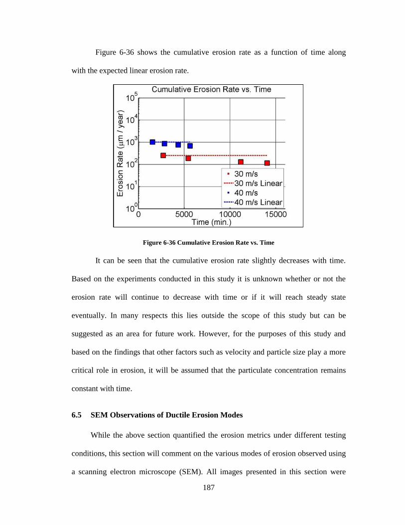
187

Figure 6-36 shows the cumulative erosion rate as a function of time along

with the expected linear erosion rate.

Figure 6-36 Cumulative Erosion Rate vs. Time

It can be seen that the cumulative erosion rate slightly decreases with time.

Based on the experiments conducted in this study it is unknown whether or not the

erosion rate will continue to decrease with time or if it will reach steady state

eventually. In many respects this lies outside the scope of this study but can be

suggested as an area for future work. However, for the purposes of this study and

based on the findings that other factors such as velocity and particle size play a more

critical role in erosion, it will be assumed that the particulate concentration remains

constant with time.

6.5 SEM Observations of Ductile Erosion Modes

While the above section quantified the erosion metrics under different testing

conditions, this section will comment on the various modes of erosion observed using

a scanning electron microscope (SEM). All images presented in this section were

188

taken with an ultra-high resolution Hitachi SU-70 FEG SEM and the sample analyzed

has the sample ID: 104010; 10μm particles, 40 m/s nominal jet velocity, 0.1%

concentration in water.

Figure 6-37 shows an overview SEM image of the eroded surface taken near

the region of maximum erosion. The first observation is that the surface features are

significantly smaller than the particles creating them. While the average particle size

is approximately 9μm, many of the features shown below have sizes on the order of

1μm. In addition, the direction of fluid flow can easily be recognized by the nearly

uniform orientation of scratches on the surface.

Figure 6-37 Overview of eroded surface

From this overview different modes of erosion can be identified, specifically

scratching, indenting and flaking. A magnified image of this overview, shown in

Figure 6-38, displays a small surface scratch on the order of 1μm in length.

189

Figure 6-38 Magnified overview image showing small surface scratch

This type of surface asperity was likely caused by a sharp particle brushing

lightly against the surface. However, it can also be seen in the above images that the

geometries of scratches vary from thin and deep to broad and shallow. This suggests

that the particulate shape plays a significant role in the type of wear observed. While

sharper particles impacting the surface would cause thin and deep scratches, impacts

by blunt or more rounded particles would yield wide and shallow abrasions taking on

more of a ploughing mechanism.

Magnifying a different region of the overview image shows a particle

indentation likely caused by a higher angle impact. Figure 6-39 shows two

overlapping modes of erosion; an indentation with trapped debris and an overlaying

shallower scratch.

190

Figure 6-39 Magnified overview image showing particle indentation and shallow scratch

Although the CFD results suggest that the majority of impact angles are small,

there may occasionally be an anomalously higher angle impact caused by local

turbulent velocity fluctuations. This type of damage would fall in line with the quasi-

static formulation of erosion which states that the particle’s kinetic energy is

transformed into plastic flow within the material. Unlike the quasi-static model

however, the formation of median/radial and lateral crack systems cannot be seen and

thus the observed indentations are thought to be primarily plastic in nature.

Although the terms ‘plastic’, ‘plastic flow’ and ‘plastic deformation’ are used

throughout this section, the more appropriate term to be used would be ‘pseudo-

plastic’. As discussed in the literature review section, the differentiation between

ductile and brittle wear can become hazy as the impact conditions largely dictate how

the material responds. Along the quasi-static and dynamic models of brittle erosion,

an impacting particle creates a region of plastic deformation followed by the creation

191

of various crack systems. With ductile erosion, impacting particles cause material

displacement in the form of plastic deformation surrounding the impact site. With the

type of wear observed in this study, it can be seen that the classical lateral and

median/radial crack systems do not form thus rendering the quasi-static and dynamic

model inapplicable. However, the mechanisms taking place at the crystallographic

level cannot be observed using the techniques available in this study. In other words,

it is unclear whether or not the ‘plastic flow’ is analogous to the movement of ‘silly-

putty’, or if there exists small-scale microfracture and intracrystalline movement

along slip bands. Most likely the observed mechanisms are a combination of both.

Flaking and platelet formation, as a result of shallow ploughing, can also be

seen throughout the images. As described by Levy [126], ploughing can be described

as the formation of a crater and the subsequent piling up of plastically deformed

material around the impact zone. In the case of ductile materials like aluminum or

copper, the displaced material may be removed due to additional particle impacts or

flattened out to form platelets. In the case of silicon however, the piling up of material

is not as pronounced but rather the formation of thin flakes originates from the

shallow ploughing of relatively blunter particles. One such flake can be seen in Figure

6-40.

192

Figure 6-40 Flake formation as a result of shallow ploughing

It can be suggested that these flakes, having thicknesses on the order of

approximately 50nm, break off from the bulk material as a unit. Levy [126] describes

the platelet formation in nominally ductile materials arising from repeated particle

impacts forging the material pile-up into flat segments. While it is unclear whether or

not the observed platelet formation arises from a single impact or multiple, it is clear

that predominately ductile material removal mechanisms are taking place.

Another potential explanation for these thin flakes is the somewhat bulk

movement of material across a slip plane. Upon the shallow angle impact from a

larger blunt particle, the induced shearing force may cause the crystallographic planes

to slide over one another in a “deck-of-cards” type movement. While this may explain

the formation of thin flakes, modeling this phenomenon at these size scales would be

outside the scope of this work.

193

Another overview image, shown in Figure 6-41, reveals similar

characteristics, such as the deeper scratches and ploughing but also indicates the

presence of relatively discrete impacts causing mixed ductile/brittle modes of erosion.

Figure 6-41 SEM overview showing discrete sites of ductile/brittle mixed erosion modes

For reference, the lighter parts of the image represent elevated regions while

the darker parts represent depressed regions. As such, scratches can be seen as black

gashes whereas the white locations represent elevated material and typically surround

indentation sites. Figure 6-42 shows a magnified view of one of the discrete impact

sites from the overview image.

194

Figure 6-42 Magnified image of overview showing mixed ductile/brittle wear

It can be reasoned that the initial indentation was caused by a larger sharp

particle with a significant amount of kinetic energy to cause the quasi-static

indentation. However, the displaced material piling up on the sites appears to have

fractured resulting in an array of micro-flakes surrounding the impact zone. Due to

the fact that material was originally displaced in a plastic manner but ultimately

removed due to the fracture and chipping away of the micro-flakes, it can be

suggested that the mode of wear in this image is that of a combined ductile/brittle

mode. The image also reveals fine-scale fracture along slip bands as indicated by the

darker near-parallel bands within the indentation. Due to the fact that the radial crack

systems cannot be observed, but material pile-up and microfracture can be, further

suggests that the type of occurrence here is along the lines of a pseudo-plastic

indentation.

195

Much like the flake formation previously discussed, the action of plastically

deformed bulk material tends to facilitate the development of fine flake features near

the surface. While the flake formation can be considered a nominally ductile

mechanism, the susceptibility to flake formation would likely be higher in nominally

brittle materials due to higher surface hardness properties. Increased surface hardness

reduces the susceptibility to localized plastic deformation resulting in the formation

of brittle flakes more easily. In this light the increased material hardness of silicon, as

compared to other metals, inhibits the continuation of plastic flow causing the

material to displace in other fashions, i.e. micro-scale chipping.

Another magnified image of a discrete impact site likely caused by a single

larger particle is shown in Figure 6-43.

Figure 6-43 Magnified image of surface showing a discrete ‘deep gouge’

In this image the material pile-up can clearly be seen surrounding, what can be

referred to as, the ‘deep gouge’. Additionally, the initiation of the micro-flaking

mechanism within the plastically deformed pile-up is shown by the arrows. While the

196

initial material pileup is attributed to plastic flow, the subsequent material removal of

the micro-flakes is likely brittle in nature. Due to the fact that the median/radial and

lateral crack systems cannot be observed, the main mechanism of material removal

here is plastic indentation coupled with the lateral motion of the particle. However,

the initiation of flake formations can be observed towards the bottom of the impact

site by the arrows. Unlike the Figure 6-42 which showed micro-fracture and small

chip formations, the mechanism here suggests that a larger mass of material could be

removed in a single flake. This indicates that the localized stresses in the plastically

deformed region surpass a threshold value initiating the subsurface crack system.

Much like the lateral crack system formed in quasi-static indentations, once the

subsurface cracks reach the surface material can be removed in the form of a chipping

mechanism.

Lastly, an image was taken near the edge region of the sample where the wet-

abrasion mechanism is thought to dominate material removal. Shown in Figure 6-44,

the presence of longer scratches and ploughing marks can be seen indicating that the

majority of particle impacts are a result of low impact angle collisions where the

particles are dragged along the surface under the influence of the squeeze film. The

regions of the surface that appear to be “smeared” indicate that a localized plastic

process is taking place.

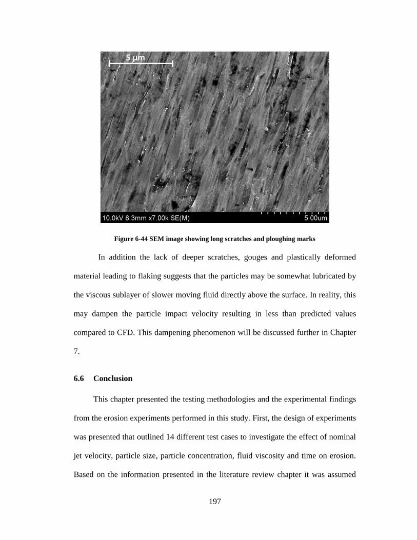
197

Figure 6-44 SEM image showing long scratches and ploughing marks

In addition the lack of deeper scratches, gouges and plastically deformed

material leading to flaking suggests that the particles may be somewhat lubricated by

the viscous sublayer of slower moving fluid directly above the surface. In reality, this

may dampen the particle impact velocity resulting in less than predicted values

compared to CFD. This dampening phenomenon will be discussed further in Chapter

7.

6.6 Conclusion

This chapter presented the testing methodologies and the experimental findings

from the erosion experiments performed in this study. First, the design of experiments

was presented that outlined 14 different test cases to investigate the effect of nominal

jet velocity, particle size, particle concentration, fluid viscosity and time on erosion.

Based on the information presented in the literature review chapter it was assumed

198

these were the most important factors contributing to erosion. Next, the measurement

techniques were described which combine stylus profilometry and MATLAB to

determine the total amount of material removed for each test sample. In addition the

algorithm to factor in the initial warpage of each test sample was presented.

While there are a variety of different erosion metrics, this chapter presented

both a mass loss rate in units of milligrams per year and a one-dimensional maximum

erosion rate in units of micrometers per year. A sampling of raw erosion profile scans

describing each of the different testing variables was included; however the complete

array of raw data is included in Appendix A. It was found that the nominal jet

velocity and average particle size each exhibit a power law relation with the mass loss

rate and erosion rates, while concentration shows a linear relationship. This aligns

well with previous erosion studies suggesting that particle size and velocity are the

critical factors contributing to erosion. Viscosity showed a slight decreasing

exponential relationship with erosion; however a more thorough investigation is

needed to determine if this holds up over a wider range of viscosities. Lastly the mass

loss rate and erosion rates were both expected to be constant with time; however

experiments showed that the wear rates slightly decreased with time. One explanation

is that the particulate concentration slightly decreases with time due to a fouling

phenomenon where particle exist the bulk flow and deposit in the test setup. This can

be shown in Figure 6-25, however quantifying this mechanism in depth lies outside

the scope of this study.

SEM images were taken of the eroded surface and revealed valuable

information regarding the types of erosion mechanisms taking place. For example, a

199

few overview images suggest the presence of deep scratches, gouges, flakes and

ploughing marks. Upon further inspection, mixed modes of erosion were found where

discrete particle impacts cause material to pile-up around the impact site under the

action of plastic flow. Closer observation suggests that the piled-up material fractures

and forms micro-flakes which are then subsequently removed by the fluid flow. From

this information is can be deduced that the majority of wear occurs in a ductile

manner due to low angle impacts. As such, a ductile erosion model would ideally be

chosen to capture this specific type of wear.

The following chapter will use the experimental results from this chapter in

order to redefine the primary erosion metric as a ratio, i.e. the mass of material

removed to the mass of impacting particles. This will enable comparisons to be made

from previous work but will also facilitate the development of a particle-based

erosion model.

200

7 DEVELOPMENT OF A PARTICLE EROSION

MODEL

7.1 Introduction

This chapter builds off the previous chapter and discusses the development,

calibration and validation of a particle based erosion model. While Chapter 6

presented the erosion results as mass loss rates and one-dimensional erosion rates,

this chapter will convert mass loss rates into non-dimension erosion ratios by utilizing

particle impact data from the CFD simulations. The erosion ratio is a commonly used

erosion metric and is defined as the mass of material removed to the mass of

impacting particles. From a particle based perspective, this ratio describes the amount

of mass removed from each individual particle impact. Given the nature of CFD

simulations where hundreds of thousands, if not millions, of particle tracks can be

simulated, implementing this type of erosion model yields an erosion flux, presented

in units of kg/m2-s. Dividing this value by the substrate’s density alters the erosion

metric to a one-dimensional erosion rate.

First, the experimental erosion results from the previous chapter will be

presented in the newly transformed erosion metric. The method in which the total

mass of impacting particles was calculated will be given followed by the erosion ratio

graphs describing the effects of jet velocity, particle size, concentration, fluid

viscosity and time. Next, the Huang et al. [127] phenomenological erosion model will

be presented which serves as the framework for the new erosion model created. The

calibration procedure will be described including the method used to determine the

201

velocity and particle size exponents and the material/system constant. This model will

then be hooked into FLUENT for validation simulations where the one-dimensional

erosion rates from the experimental efforts and the CFD simulations will be

compared.

Although the validation simulations indicate a close comparison between CFD

and experiments, the CFD results tend to over-predict the erosion rates in most test

cases. To explain this small inconsistency an impact dampening coefficient, β, is

proposed which suggests that the impact velocity from the CFD simulations is

slightly larger than the real-life impact velocities. While individual particle impact

velocities were not measured in this study, the inclusion of the proposed β factor

significantly reduces the difference between the CFD simulations and the

experiments.

7.2 Particle Based Erosion Results

This section will present the new form of the erosion data as the previously

discussed erosion ratio.

7.2.1 Experimental Results as Erosion Ratios

Using the particle impact data from the CFD simulations and given that the

erosion ratio is defined as the mass of material removed to the mass of impacting

particles, the erosion results presented in Chapter 6 can be converted to erosion ratios.

In the simplifying case of a single particle impact, the erosion ratio determines the

amount of mass removed due to a single particle impact. Table 7-1 lists the raw data

used to generate the erosion ratio graphs.

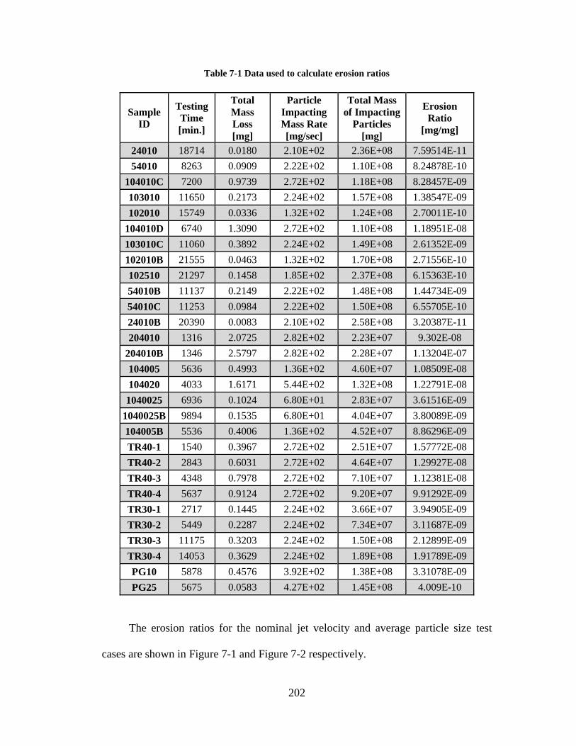
202

Table 7-1 Data used to calculate erosion ratios

Sample

ID

Testing

Time

[min.]

Total

Mass

Loss

[mg]

Particle

Impacting

Mass Rate

[mg/sec]

Total Mass

of Impacting

Particles

[mg]

Erosion

Ratio

[mg/mg]

24010 18714 0.0180 2.10E+02 2.36E+08 7.59514E-11

54010 8263 0.0909 2.22E+02 1.10E+08 8.24878E-10

104010C 7200 0.9739 2.72E+02 1.18E+08 8.28457E-09

103010 11650 0.2173 2.24E+02 1.57E+08 1.38547E-09

102010 15749 0.0336 1.32E+02 1.24E+08 2.70011E-10

104010D 6740 1.3090 2.72E+02 1.10E+08 1.18951E-08

103010C 11060 0.3892 2.24E+02 1.49E+08 2.61352E-09

102010B 21555 0.0463 1.32E+02 1.70E+08 2.71556E-10

102510 21297 0.1458 1.85E+02 2.37E+08 6.15363E-10

54010B 11137 0.2149 2.22E+02 1.48E+08 1.44734E-09

54010C 11253 0.0984 2.22E+02 1.50E+08 6.55705E-10

24010B 20390 0.0083 2.10E+02 2.58E+08 3.20387E-11

204010 1316 2.0725 2.82E+02 2.23E+07 9.302E-08

204010B 1346 2.5797 2.82E+02 2.28E+07 1.13204E-07

104005 5636 0.4993 1.36E+02 4.60E+07 1.08509E-08

104020 4033 1.6171 5.44E+02 1.32E+08 1.22791E-08

1040025 6936 0.1024 6.80E+01 2.83E+07 3.61516E-09

1040025B 9894 0.1535 6.80E+01 4.04E+07 3.80089E-09

104005B 5536 0.4006 1.36E+02 4.52E+07 8.86296E-09

TR40-1 1540 0.3967 2.72E+02 2.51E+07 1.57772E-08

TR40-2 2843 0.6031 2.72E+02 4.64E+07 1.29927E-08

TR40-3 4348 0.7978 2.72E+02 7.10E+07 1.12381E-08

TR40-4 5637 0.9124 2.72E+02 9.20E+07 9.91292E-09

TR30-1 2717 0.1445 2.24E+02 3.66E+07 3.94905E-09

TR30-2 5449 0.2287 2.24E+02 7.34E+07 3.11687E-09

TR30-3 11175 0.3203 2.24E+02 1.50E+08 2.12899E-09

TR30-4 14053 0.3629 2.24E+02 1.89E+08 1.91789E-09

PG10 5878 0.4576 3.92E+02 1.38E+08 3.31078E-09

PG25 5675 0.0583 4.27E+02 1.45E+08 4.009E-10

The erosion ratios for the nominal jet velocity and average particle size test

cases are shown in Figure 7-1 and Figure 7-2 respectively.

203

Figure 7-1 Erosion Ratio vs. Jet Velocity

Figure 7-2 Erosion Ratio vs. Average Particle Size

Much like the mass loss and 1-D erosion rates in Chapter 6, jet velocity and

particle size both exhibit power law relations with exponents of 5.24 and 4.19

respectively. The particle size results can directly be used in the development of a

particle based erosion model due to the fact that the erosion ratio is directly

204

proportional to the particle size. Regarding jet velocity however, the erosion ratios

described above need to be transformed into a form that considers individual particle

impact velocities. Due to the fact that particle impact velocities are different than the

nominal jet velocity and due to the wide ranges of impact velocities for a single jet

velocity, further data processing will be necessary. This will be described in a later

section of this chapter.

Figure 7-3 shows the relation between particulate concentration and erosion

ratio. One of the assumptions in these experiments is that the particles are non-

interacting due to the dilute nature of the slurries. As such, the concentration of

particles should not have an effect on the erosion ratio. A single particle in a slurry

with 0.1% concentration should yield the same amount of damage as a single particle

in a slurry with a concentration of 0.2%.

Figure 7-3 Erosion Ratio vs. Concentration

The graph above shows the data compared with the expected constant erosion

ratio. While the data for the 0.05%, 0.1% and 0.2% cases align with this assumption,

205

the 0.025% case exhibits a slightly lower than expected erosion ratio. As discussed

previously in Chapter 6, it is thought this inconsistency is due to a slight fouling

phenomenon where particles settle out in the test setup.

Figure 7-4 shows the effect of viscosity on the erosion ratio. Similar to the

mass loss and erosion rate results, viscosity shows an inverse relation with erosion

ratio. While quantifying this trend would require a more thorough investigation, this

information suggests that particles induce less damage as the viscosity increases for

similar nominal jet velocities.

Figure 7-4 Erosion Ratio vs. Viscosity

This highlights the importance of understanding actual particle impact

velocities rather than just fluid velocities. In the viscosity tests, the fluid acts to

dampen the velocity of an approaching velocity. In addition, as particles are swept

away in the tangential flow the more viscous fluid may act to lubricate the surface

protecting it from particles trapped in the squeeze film. As such the rolling, bouncing

206

and scratching action of the particles would yield less damage compared to similar

conditions in less viscous fluids.

Figure 7-5 shows the cumulative erosion ratio as a function of time for both the

30 m/s and 40 m/s transient tests. In addition, the assumed constant rates are shown

on the graph where the value is equivalent to the erosion ratio calculated for the first

data point.

Figure 7-5 Erosion Ratio vs. Time, compared with constant ratio

It can be seen that the erosion ratio decreases slightly for both test cases and is

thought to be caused by a decrease in particulate concentration with time. While it is

assumed that the concentration of the solution stays constant with time, but in reality

decreases, an apparent decrease in the erosion ratio would be observed.

7.2.2 Calculating Total Mass of Impacting Particles

Given that the mass of material removed was calculated in the Chapter 6 and

that the erosion ratio is defined as the mass of material removed to the mass of

impacting particles, the remaining unknown is the total mass of impacting particles.

207

While this cannot be directly measured from an experimental point of view, the CFD

simulations provide a method through which this can be calculated.

In a steady state CFD simulation Lagrangian particle tracking is conducted such

that the trajectories of particle streams, rather than individual particles, are

determined. To begin, the mass flow rate of an individual particle stream must be

calculated. First, the fluid flow rate is calculated:

𝐹𝑙𝑢𝑖𝑑 𝐹𝑙𝑜𝑤 𝑅𝑎𝑡𝑒 = 𝑁𝑜𝑚𝑖𝑛𝑎𝑙 𝐽𝑒𝑡 𝑉𝑒𝑙𝑜𝑐𝑖𝑡𝑦 ∗ 𝑁𝑜𝑧𝑧𝑙𝑒 𝐴𝑟𝑒𝑎 (7-1)

By considering the known particulate concentration defined as the ratio of the

mass of particles to the mass of fluid, the total particle flow rate can be determined:

𝑇𝑜𝑡𝑎𝑙 𝑃𝑎𝑟𝑡𝑖𝑐𝑙𝑒 𝐹𝑅 = 𝐹𝑙𝑢𝑖𝑑 𝐹𝑅 ∗ 𝐶𝑜𝑛𝑐𝑒𝑛𝑡𝑟𝑎𝑡𝑖𝑜𝑛 (7-2)

In Chapter 4, it was found that 320,000 particle streams must be simulated in

order to achieve erosion independence with respect to the number of particle tracks.

The individual particle stream flowrate is determined as:

𝐼𝑛𝑑𝑖𝑣𝑖𝑑𝑢𝑎𝑙 𝑃𝑎𝑟𝑡𝑖𝑐𝑙𝑒 𝑆𝑡𝑟𝑒𝑎𝑚 𝐹𝑅 = 𝑇𝑜𝑡𝑎𝑙 𝑃𝑎𝑟𝑡𝑖𝑐𝑙𝑒 𝐹𝑅

# 𝑃𝑎𝑟𝑡𝑖𝑐𝑙𝑒 𝑆𝑡𝑟𝑒𝑎𝑚𝑠 (7-3)

where the number of particle streams is approximately 320,000. Occasionally particle

streams are deemed incomplete thus the real number of particle streams is often

slightly less than then the defined 320,000.

To determine the total mass of impacting particles, the individual particle

stream flow rate is multiplied by the total number of impacts determined from CFD.

𝑇𝑜𝑡𝑎𝑙 𝐼𝑚𝑝𝑎𝑐𝑡𝑖𝑛𝑔 𝑀𝑎𝑠𝑠 𝑅𝑎𝑡𝑒

= 𝑃𝑎𝑟𝑡𝑖𝑐𝑙𝑒 𝑆𝑡𝑟𝑒𝑎𝑚 𝐹𝑅 ∗ 𝑇𝑜𝑡𝑎𝑙 # 𝐼𝑚𝑝𝑎𝑐𝑡𝑠 ∗ 𝑇𝑖𝑚𝑒 (7-4)

208

The total number of impacts is taken across all ~320,000 particle streams and

up to 10 impacts per stream. Given the steady state nature of the CFD simulations, a

number of inherent assumptions exist in this calculation. First, the concentration is

assumed to remain constant throughout the duration of the test. While the

concentration was found to slightly decrease with time due to fouling, this assumption

needs to be made and will be accounted for later in this Chapter. In addition, the

number of impact locations is assumed to remain constant. The particle track

independency study showed that a large number of streams are needed in order to

make this assumption hold true. Lastly, the fluid flow rate is assumed to be constant.

While direct flow measurement were not taken, as discussed in Chapter 5, continual

observation and the initial calibration of the pump suggests that this can be a valid

assumption.

7.3 Introduction to Huang et. al. Cutting Erosion Model

The Huang et al. cutting erosion model [127] is a phenomenologically

developed erosion model that considers the major factors contributing to erosion such

as particle size impingement angle, impingement velocity, particle shape and material

properties. The term phenomenological is used as its derivation stems from an

analytical formulation based on real-world phenomenon. The model captures two

principle modes of erosion, namely deformation and cutting wear. Deformation wear

originates from higher angle impacts resulting in plastic flow pile-up surrounding the

impact crater while cutting wear originates from shallow angle impacts slicing into

the surface. Analytically, the volume of material removed due to deformation wear is

analyzed by factoring in the force and volume of indentation, the surface strain

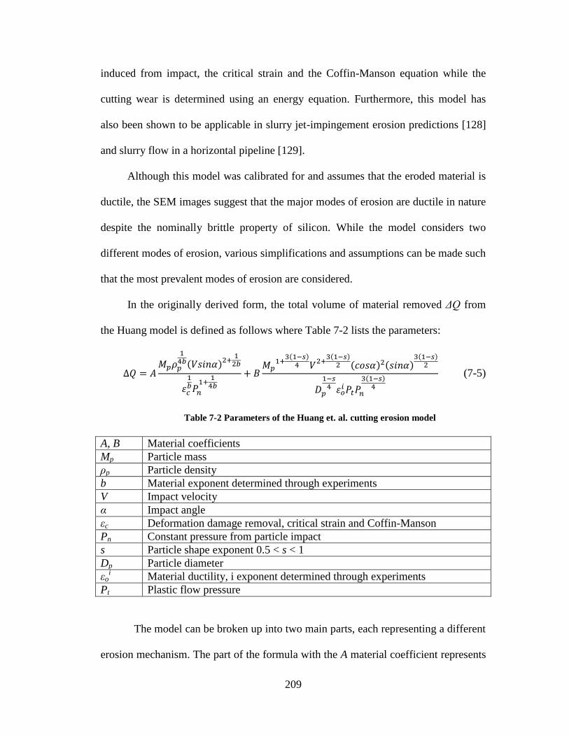
209

induced from impact, the critical strain and the Coffin-Manson equation while the

cutting wear is determined using an energy equation. Furthermore, this model has

also been shown to be applicable in slurry jet-impingement erosion predictions [128]

and slurry flow in a horizontal pipeline [129].

Although this model was calibrated for and assumes that the eroded material is

ductile, the SEM images suggest that the major modes of erosion are ductile in nature

despite the nominally brittle property of silicon. While the model considers two

different modes of erosion, various simplifications and assumptions can be made such

that the most prevalent modes of erosion are considered.

In the originally derived form, the total volume of material removed ΔQ from

the Huang model is defined as follows where Table 7-2 lists the parameters:

∆𝑄 = 𝐴𝑀𝑝𝜌𝑝

14𝑏(𝑉𝑠𝑖𝑛𝛼)2+

12𝑏

𝜀𝑐

1𝑏𝑃𝑛

1+14𝑏

+ 𝐵𝑀𝑝

1+3(1−𝑠)4 𝑉2+

3(1−𝑠)2 (𝑐𝑜𝑠𝛼)2(𝑠𝑖𝑛𝛼)

3(1−𝑠)2

𝐷𝑝

1−𝑠4 𝜀𝑜

𝑖𝑃𝑡𝑃𝑛

3(1−𝑠)4

(7-5)

Table 7-2 Parameters of the Huang et. al. cutting erosion model

A, B Material coefficients

Mp Particle mass

ρp Particle density

b Material exponent determined through experiments

V Impact velocity

α Impact angle

εc Deformation damage removal, critical strain and Coffin-Manson

Pn Constant pressure from particle impact

s Particle shape exponent 0.5 < s < 1

Dp Particle diameter

εoi Material ductility, i exponent determined through experiments

Pt Plastic flow pressure

The model can be broken up into two main parts, each representing a different

erosion mechanism. The part of the formula with the A material coefficient represents

210

the volume of material removed due to deformation damage and the other part of the

formula represents the volume of material removed due to cutting wear. Given that

the CFD results and SEM images indicate primarily low-impact angle wear resulting

in cutting and shallow ploughing, the first part of the equation can be assumed

negligible. Additionally, the particle shape exponent was chosen to be 0.75. A value

of 0.5 represents line cutting conditions while a value of 1 represent area cutting

conditions. Typically line cutting occurs for extremely sharp particles where area

cutting is a result of large impact surfaces and rounder particles. The SEM images

suggested that a variety of different particle shapes induced the cutting damage and,

in addition, the authors suggest that a value of 0.75 is a good approximation. Taking

all these assumptions into consideration, conglomerating the material parameters into

a single material/system constant, and converting the erosion units from volume loss

to an erosion ratio, the Huang cutting model simplifies down to the following form:

𝐸𝑅 =∆𝑄

𝑀𝑝𝜌𝑆𝑖= 𝐾𝐷𝑚𝑉𝑛 cos2 𝛼 sin0.375 𝛼 (7-6)

where K is the new material constant, and m and n are the particle size and velocity

exponents respectively in need of new calibration. The reason these exponents need

to be calibrated is because they were originally calibrated for ductile materials such as

aluminum, copper and steel. Additionally, the experiments used to calibrate these

values were conducted by Misra and Finnie [130] and assessed by Bitter [131] and

thus the particle sizes and impact velocities are far outside the range used in the

present experiments. Most of these experiments used 250μm particles with impact

velocities greater than 100 m/s. As such, it becomes necessary to recalibrate these

exponents within the particle size and velocity ranges of interest.

211

7.4 Model Calibration

This section describes the process through which the variables in the Huang

cutting erosion model, namely the material constant, velocity and size exponents,

were calibrated based on the erosion experiments described in Chapter 5.

7.4.1 Particle Size Exponent

The particle size exponent m is the most straightforward unknown to

determine. Through the reformulation of erosion results into erosion ratios, it was

shown that the erosion ratio is directly proportional to the average particle size raised

to the power of 4.19.

𝐸𝑅 ∝ 𝐷4.19 (7-7)

As such m can be taken as 4.19 where D represents the average particle size.

7.4.2 Velocity Exponent

In the previous section it was found that the erosion ratio is proportional to the

jet velocity raised to the power of 5.24.

𝐸𝑅 ∝ 𝑉𝑗5.24 (7-8)

However, the erosion ratio ultimately needs to be proportional to the particle

impact velocity raised to a power; however the value of this power is unknown. Thus

finding the exponent n requires a coupling between jet velocity and particle impact

velocity. The CFD results shows that a single impact velocity could not be

representative of the impacts caused at a specific jet velocity due to the wide spread

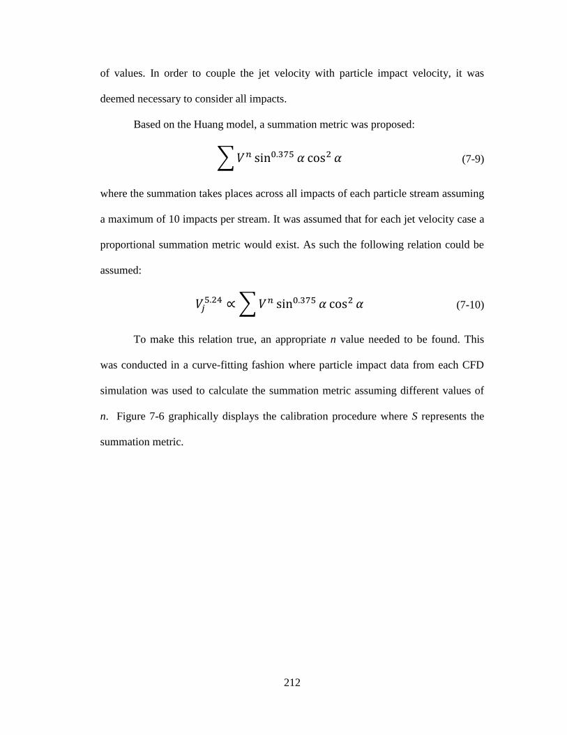
212

of values. In order to couple the jet velocity with particle impact velocity, it was

deemed necessary to consider all impacts.

Based on the Huang model, a summation metric was proposed:

∑𝑉𝑛 sin0.375 𝛼 cos2 𝛼 (7-9)

where the summation takes places across all impacts of each particle stream assuming

a maximum of 10 impacts per stream. It was assumed that for each jet velocity case a

proportional summation metric would exist. As such the following relation could be

assumed:

𝑉𝑗5.24 ∝∑𝑉𝑛 sin0.375 𝛼 cos2 𝛼 (7-10)

To make this relation true, an appropriate n value needed to be found. This

was conducted in a curve-fitting fashion where particle impact data from each CFD

simulation was used to calculate the summation metric assuming different values of

n. Figure 7-6 graphically displays the calibration procedure where S represents the

summation metric.

213

Figure 7-6 Velocity exponent calibration

For each of the jet velocity cases – 20, 25, 30 and 40 m/s – different values of

n were assumed and the summation metric was calculated. Then for each n, a power

law relation was found relating the summation metric to the jet velocity. Due to the

fact that the summation metric is proportional to the jet velocity, which is in turn

proportional to the erosion ratio, an appropriate n was found once the resulting jet

velocity exponent was equivalent to the 5.24 determined previously. It was found that

when n = 4.75, the following relation holds true:

𝐸𝑅 ∝ 𝑉𝑗5.24 ∝∑𝑉4.75 sin0.375 𝛼 cos2 𝛼 (7-11)

While the summation metric considers all particle impacts, the erosion ratio

considers a single particle impact. In the simplifying case of a single particle impact

the following relation can be made:

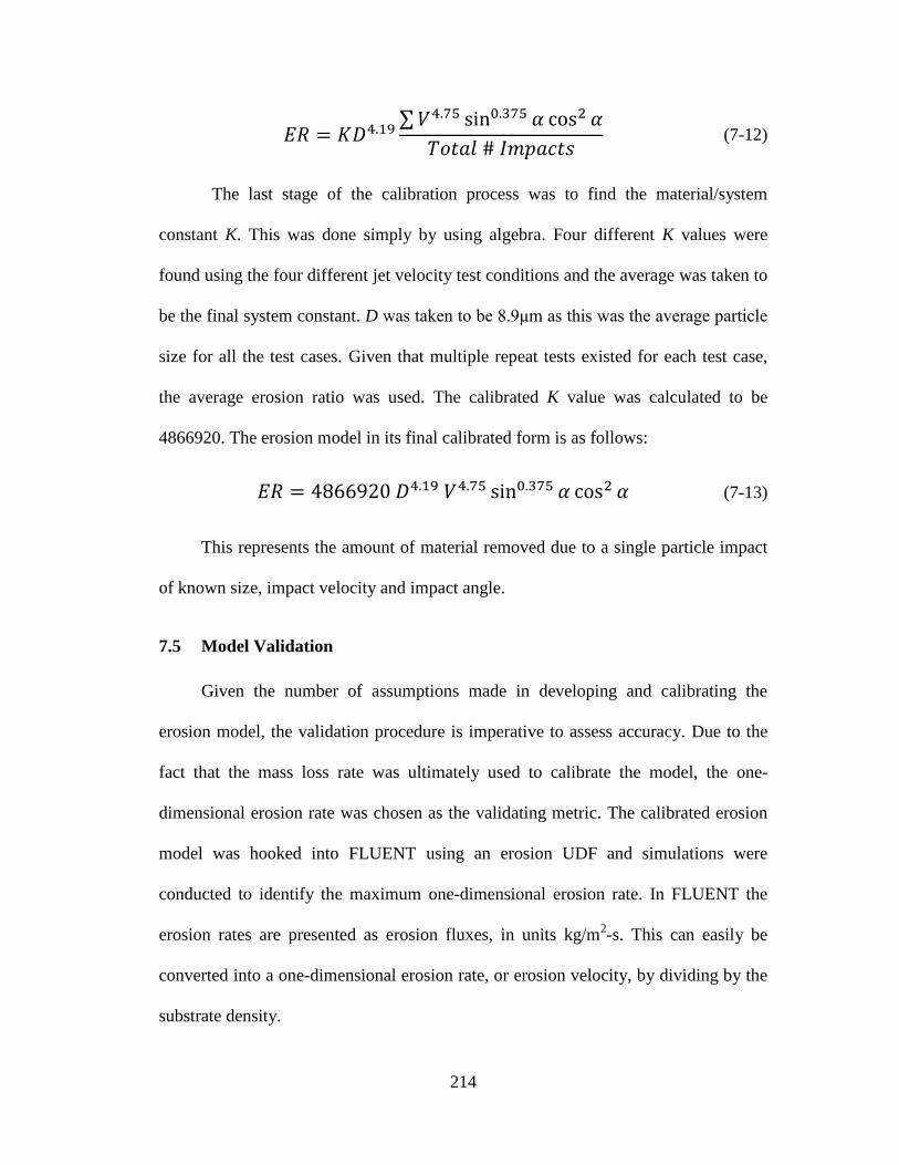
214

𝐸𝑅 = 𝐾𝐷4.19∑𝑉4.75 sin0.375 𝛼 cos2 𝛼

𝑇𝑜𝑡𝑎𝑙 # 𝐼𝑚𝑝𝑎𝑐𝑡𝑠 (7-12)

The last stage of the calibration process was to find the material/system

constant K. This was done simply by using algebra. Four different K values were

found using the four different jet velocity test conditions and the average was taken to

be the final system constant. D was taken to be 8.9μm as this was the average particle

size for all the test cases. Given that multiple repeat tests existed for each test case,

the average erosion ratio was used. The calibrated K value was calculated to be

4866920. The erosion model in its final calibrated form is as follows:

𝐸𝑅 = 4866920 𝐷4.19 𝑉4.75 sin0.375 𝛼 cos2 𝛼 (7-13)

This represents the amount of material removed due to a single particle impact

of known size, impact velocity and impact angle.

7.5 Model Validation

Given the number of assumptions made in developing and calibrating the

erosion model, the validation procedure is imperative to assess accuracy. Due to the

fact that the mass loss rate was ultimately used to calibrate the model, the one-

dimensional erosion rate was chosen as the validating metric. The calibrated erosion

model was hooked into FLUENT using an erosion UDF and simulations were

conducted to identify the maximum one-dimensional erosion rate. In FLUENT the

erosion rates are presented as erosion fluxes, in units kg/m2-s. This can easily be

converted into a one-dimensional erosion rate, or erosion velocity, by dividing by the

substrate density.

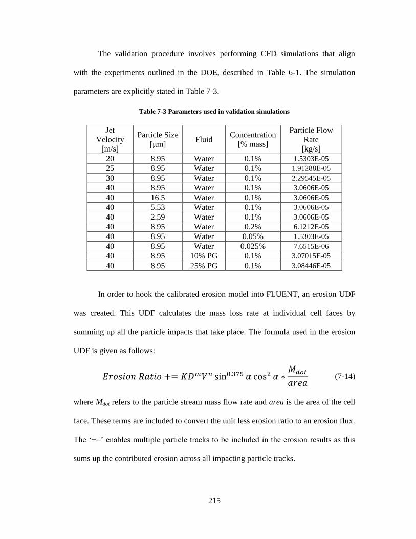
215

The validation procedure involves performing CFD simulations that align

with the experiments outlined in the DOE, described in Table 6-1. The simulation

parameters are explicitly stated in Table 7-3.

Table 7-3 Parameters used in validation simulations

Jet

Velocity

[m/s]

Particle Size

[μm] Fluid

Concentration

[% mass]

Particle Flow

Rate

[kg/s]

20 8.95 Water 0.1% 1.5303E-05

25 8.95 Water 0.1% 1.91288E-05

30 8.95 Water 0.1% 2.29545E-05

40 8.95 Water 0.1% 3.0606E-05

40 16.5 Water 0.1% 3.0606E-05

40 5.53 Water 0.1% 3.0606E-05

40 2.59 Water 0.1% 3.0606E-05

40 8.95 Water 0.2% 6.1212E-05

40 8.95 Water 0.05% 1.5303E-05

40 8.95 Water 0.025% 7.6515E-06

40 8.95 10% PG 0.1% 3.07015E-05

40 8.95 25% PG 0.1% 3.08446E-05

In order to hook the calibrated erosion model into FLUENT, an erosion UDF

was created. This UDF calculates the mass loss rate at individual cell faces by

summing up all the particle impacts that take place. The formula used in the erosion

UDF is given as follows:

𝐸𝑟𝑜𝑠𝑖𝑜𝑛 𝑅𝑎𝑡𝑖𝑜 += 𝐾𝐷𝑚𝑉𝑛 sin0.375 𝛼 cos2 𝛼 ∗𝑀𝑑𝑜𝑡𝑎𝑟𝑒𝑎

(7-14)

where Mdot refers to the particle stream mass flow rate and area is the area of the cell

face. These terms are included to convert the unit less erosion ratio to an erosion flux.

The ‘+=’ enables multiple particle tracks to be included in the erosion results as this

sums up the contributed erosion across all impacting particle tracks.

216

7.5.1 Effect of Velocity

This section presents the results of the validation simulations and compares

them to the experimental results. As described earlier, the main erosion metric in this

part of the study is the one-dimensional erosion rate in units of micrometers-per-year.

Erosion contour maps resulting from the CFD simulations will also be shown, of

which the maximum value will be compared to the maximum erosion rate from the

samples in Chapter 6.

Figure 7-7 shows the CFD erosion contours comparing the 20 m/s and 40 m/s

test cases. It can be seen that the characteristic ‘W’ shape is observed with the

stagnation region in the center of the jet. This also helps validate the assumption that

the height of the stagnation region can be taken as the reference plane due to the lack

of particle impacts shown. However, one qualitative feature between the CFD and the

experimental erosion contours is that the CFD simulations do not indicate the

presence of the discrete locations for the first and second impacts. While this was

most heavily observed in the experimental case of the 40 m/s jet, the CFD contours

suggest a smoother erosion gradient rather than discrete impact sites. Further research

will have to be conducted in this area, but one possible explanation could be due to

the manner in which the particle tracking is performed within the near wall region. As

has been stated previously, CFD treats each particle as a volume-less point and this

fact may pose certain inconsistencies between experimental and simulation-based

work. This discrepancy may also be more noticeable at smaller particle sizes

especially in turbulent flow fields due to the complexity of modelling parcels of fluid

comparably sized to the particles.

217

Figure 7-7 CFD erosion maps of velocity test cases, 20 m/s (left) and 40 m/s (right)

It can also be seen that the region of maximum erosion, shown by the red

bands, is relatively thicker in the 20 m/s case and thinner in the 40 m/s case. This is

likely due to the increased particle-fluid coupling that occurs at higher velocities

whereas particles in the slower moving fluid may be more acted upon by turbulent

fluctuations in the flow field.

Figure 7-8 shows the comparison between experimental and simulation-based

erosion rate predictions for different nominal jet velocities.

218

Figure 7-8 Comparison of experimental and simulation-based erosion rate prediction, nominal

jet velocity

The graph shows that while the experimental data lines up fairly well with the

CFD predictions, the predictions tend to overestimate the erosion rates across most

test cases. While this will be discussed in a later section, this fact has also been

observed by Chen [132], Mansouri [121], and Zhang [133] and is especially prevent

in cases involving fine particles.

7.5.2 Effect of Particle Size

Figure 7-9 shows the CFD erosion contour maps comparing the 2.5μm and

20μm test cases. While the characteristic ‘W’ shape can be seen in the 2.5μm case,

the 20μm test case indicates the presence of primary and secondary discrete impact

zones. The experimental results showed that these discrete impact zones were not

clearly visible in the 20μm test case but were more evident in the 10μm cases. While

it is unclear precisely why this discrepancy exists, it is thought that the particle

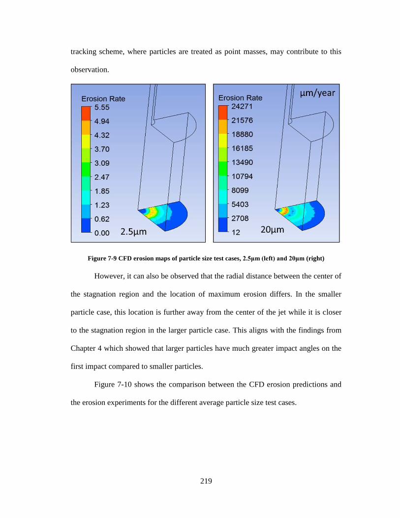
219

tracking scheme, where particles are treated as point masses, may contribute to this

observation.

Figure 7-9 CFD erosion maps of particle size test cases, 2.5μm (left) and 20μm (right)

However, it can also be observed that the radial distance between the center of

the stagnation region and the location of maximum erosion differs. In the smaller

particle case, this location is further away from the center of the jet while it is closer

to the stagnation region in the larger particle case. This aligns with the findings from

Chapter 4 which showed that larger particles have much greater impact angles on the

first impact compared to smaller particles.

Figure 7-10 shows the comparison between the CFD erosion predictions and

the erosion experiments for the different average particle size test cases.

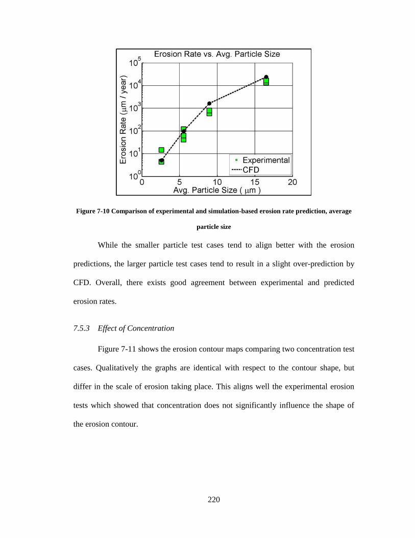
220

Figure 7-10 Comparison of experimental and simulation-based erosion rate prediction, average

particle size

While the smaller particle test cases tend to align better with the erosion

predictions, the larger particle test cases tend to result in a slight over-prediction by

CFD. Overall, there exists good agreement between experimental and predicted

erosion rates.

7.5.3 Effect of Concentration

Figure 7-11 shows the erosion contour maps comparing two concentration test

cases. Qualitatively the graphs are identical with respect to the contour shape, but

differ in the scale of erosion taking place. This aligns well the experimental erosion

tests which showed that concentration does not significantly influence the shape of

the erosion contour.

221

Figure 7-11 CFD erosion maps of concentration test cases, 0.025% (left) and 0.2% (right)

Both erosion maps exhibit similarly sized stagnation regions and the

characteristic ‘W’ shape, however neither graph shows the discrete particle impact

locations that were present in the corresponding experiments.

Figure 7-12 compares the erosion rate predictions from the CFD simulations

and the experimental work. It should first be noted that the y-axis scale is linear

compared to the previously shown graphs which have logarithmic scales.

Nonetheless, the CFD predictions over-estimate the erosion in cases.

222

Figure 7-12 Comparison of experimental and simulation-based erosion rate prediction,

concentration

According to the CFD erosion rate predictions, the curve appears to have a y-

intercept value close to zero. This indicates that a threshold concentration is not

predicted, as was suggested in the Chapter 6 analysis. It can also be seen that the

difference between the predicted erosion rate and the experimental erosion rate

increases as the concentration increases. As was described in Chapter 6, one

explanation for this is that the concentration decreases with time as particles are

deposited in the test setup due to a fouling phenomenon. It was also realized after

performing the concentration experiments that they also indirectly measure the effects

of the length of the test; the lower concentration test cases were run longer than the

higher concentration test cases. Prior to this study it was assumed that the erosion rate

would be constant with time and thus the test durations were not strictly chosen but

rather recorded and factored into the erosion rate calculation.

223

In order to investigate this further, the results from the transient experiments

(TR30 and TR40, Table 6-1) were used to approximate a fouling rate, or the rate at

which the initial concentration decreases with time. Revisiting Figure 7-5 helps with

this analysis, which compares the measured erosion ratios and the constant erosion

ratio for the transient experiments. Looking at the 40 m/s transient test, as these

operating conditions are identical to those in the concentration experiments, the

difference between the measured erosion ratio and the assumed constant erosion ratio

can be measured. This is depicted in Figure 7-13, adjusting the scale for better

portrayal.

Figure 7-13 Calculating the difference between measured and constant erosion ratio for the 40

m/s transient test case.

For this analysis, it is assumed that negligible fouling occurs between the start

of the test and the first data point. By calculating the difference between the assumed

constant erosion ratio and the measured erosion ratio, the amount of mass that should

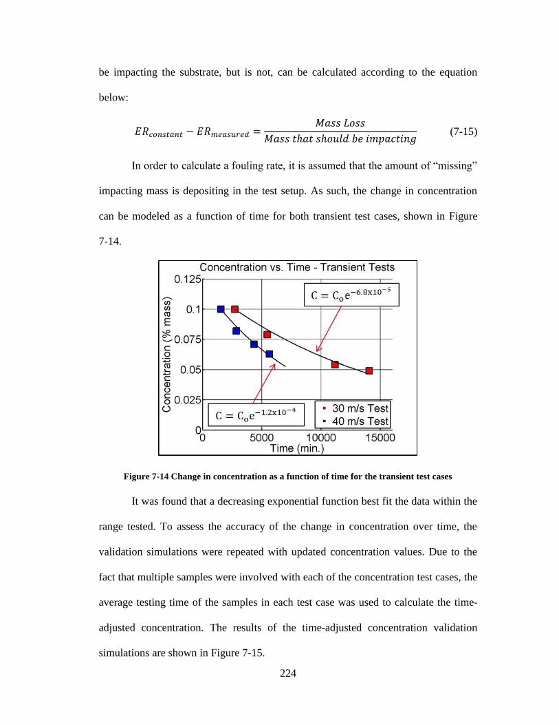
224

be impacting the substrate, but is not, can be calculated according to the equation

below:

𝐸𝑅𝑐𝑜𝑛𝑠𝑡𝑎𝑛𝑡 − 𝐸𝑅𝑚𝑒𝑎𝑠𝑢𝑟𝑒𝑑 =𝑀𝑎𝑠𝑠 𝐿𝑜𝑠𝑠

𝑀𝑎𝑠𝑠 𝑡ℎ𝑎𝑡 𝑠ℎ𝑜𝑢𝑙𝑑 𝑏𝑒 𝑖𝑚𝑝𝑎𝑐𝑡𝑖𝑛𝑔 (7-15)

In order to calculate a fouling rate, it is assumed that the amount of “missing”

impacting mass is depositing in the test setup. As such, the change in concentration

can be modeled as a function of time for both transient test cases, shown in Figure

7-14.

Figure 7-14 Change in concentration as a function of time for the transient test cases

It was found that a decreasing exponential function best fit the data within the

range tested. To assess the accuracy of the change in concentration over time, the

validation simulations were repeated with updated concentration values. Due to the

fact that multiple samples were involved with each of the concentration test cases, the

average testing time of the samples in each test case was used to calculate the time-

adjusted concentration. The results of the time-adjusted concentration validation

simulations are shown in Figure 7-15.

225

Figure 7-15 Comparison of experimental and CFD predicted erosion rates with time-adjustment

While it can clearly be seen that including the time-adjusted concentration

greatly improves the CFD erosion predictions, the predictions slightly over-estimate

the experiments. Furthermore, due to the fact that fouling is a complex process

involving many factors, such as electrochemical properties, particle size, flow

patterns, velocity and viscosity, determining a fouling rate for each experiment

performed in this study would fall outside the basic objectives of this study. However,

it can be stated that a change in concentration is significantly less influential than a

change in particle size or jet velocity. As such, the final erosion model will account

for a slight fouling rate inherently in the calibration process.

7.5.4 Effect of Viscosity

Figure 7-16 shows the CFD erosion maps comparing fluids of different

viscosities. Both simulations use the same nominal jet velocity (40 m/s), same

particulate concentration (0.1%) and same average particle size (10μm particles),

however qualitatively and quantitatively there exists differences between the two.

226

Figure 7-16 CFD erosion maps of viscosity test cases, 25% PG (left) and water (right)

In alignment with the experimental erosion profiles from Chapter 6, the more

viscous fluid produces a thinner ‘valley’, or region, of maximum erosion. One

explanation for this is that the higher particle Stokes number achieved in more

viscous fluid decreases the ability for turbulent velocity fluctuations to alter particle

trajectories. This would result in a lower spread of particle impact locations. In

addition it can also be seen that the stagnation region covers a greater area in the more

viscous fluid compared to that of water. Due to stronger particle-fluid coupling,

The comparison of the erosion rates between the CFD predictions and the

experimental efforts are shown in Figure 7-17.

227

Figure 7-17 Comparison of experimental and simulation-based erosion rate prediction, viscosity

Interestingly, there exists good agreement between CFD prediction and

experiment for the more viscous fluids. This suggests that viscosity may affect how

particles interact with the surface in ways that may not be comprehensively modeled

in FLUENT. This factor will be discussed more thoroughly in the next section.

7.6 Proposed Impact Dampening Coefficient

One characteristic prevalent throughout the validation simulations was that the

CFD predictions tend to over predict the experimental erosion rates. As described

earlier, this finding is not limited to this study but has been found throughout

literature [132] [121] [133] suggesting that limitations exist in the particle tracking

methodology employed by the CFD solver. This section proposes an impact

dampening coefficient, β, which explains some of the discrepancies found in the

original validation efforts.

228

One of the main limitations surrounding the Lagrangian particle tracking

methodology is that it treats each particle as a point-mass. Although a drag-model is

included in calculating the particle trajectory through the flow field, the empirical

constants inherent in the model are generic and may not be appropriately calibrated

for the system.

Looking at Figure 7-8, it can be seen that by shifting the CFD erosion curve

down, the two curves would align better. Shifting this observation to a particle impact

basis, this discrepancy indicates that that the CFD predicts more damage per particle

impact than is occurring in the experiments. Assuming the calibration procedure and

the impact velocity and angle capturing process were performed correctly, one

explanation is that the particle impact velocity in the experiments is slightly lower

than those in the CFD simulations.

The impact dampening coefficient β is defined as the ratio of the actual impact

velocity in the experiments to the impact velocity found in simulations.

𝛽 =𝐸𝑥𝑝𝑒𝑟𝑖𝑚𝑒𝑛𝑡𝑎𝑙 𝐼𝑚𝑝𝑎𝑐𝑡 𝑉𝑒𝑙𝑜𝑐𝑖𝑡𝑦

𝐶𝑎𝑙𝑐𝑢𝑙𝑎𝑡𝑒𝑑 𝐶𝐹𝐷 𝐼𝑚𝑝𝑎𝑐𝑡 𝑉𝑒𝑙𝑜𝑐𝑖𝑡𝑦 (7-16)

Implementation in the final erosion model would appear as follows:

𝐸𝑅 = 𝐾(𝛽𝑉)𝑛𝐷𝑚 cos2 𝛼 sin0.375 𝛼 (7-17)

Due to the fact that particles are treated as point-masses in FLUENT, certain

surface-level effects cannot accurately be captured. For example, in the proposed

impact dampening scenario adsorbed fluid surrounding the particle may act as a

cushion dampening the impact velocity, shown in Figure 7-18. CFD would not be

able to accurately predict this due to the size of the meshing elements involved in the

229

simulations. Furthermore, at these size scales the fundamental equations modeling

fluid flow may break down due to other forces taking on more prevalent of a role,

such as Van Der Waals attractive forces or electrochemical repulsion forces.

Figure 7-18 Difference between actual and CFD-based particle impact velocities

Like the effects of the squeeze film, the adsorbed fluid may alter the manner in

which particles interact with the surface. While the effects of the squeeze film can be

captured in CFD through the use of appropriate meshing techniques, the additional

dampening caused by potentially adsorbed fluid cannot. Although the dampening

coefficient is likely a complex function involving many variables such as free stream

velocity, the drag model implement in FLUENT, particle size and shape, fluid

viscosity, and particle-fluid adsorption characteristics, an empirical approach was

used to determine an appropriate value. While assigning a more physical explanation

to this dampening coefficient requires extensive further research, the final effect of

reducing the CFD-determined impact velocity is the most important aspect in this

work.

Through a trial-and-error process and using engineering judgement, it was

found that a value of 0.92 better aligns the CFD predictions with the experimental

230

results. This suggests that the actual particle impact velocity is approximately 92% of

the impact velocity found through CFD. In other words, the adsorbed fluid found in

the experimental efforts results in an 8% decrease in impact velocity.

7.6.1 Model re-validation

In order to test this theory, the validation simulations were re-run

implementing a β value of 0.92. Figure 7-19 and Figure 7-20 show comparisons of

the experimental results, the initial CFD validation simulation results and the re-

validated erosion rates for the nominal jet-velocity and particle size effects

respectively.

Figure 7-19 Comparison of experimental, validation and influence of β = 0.92, effect of nominal

jet velocity

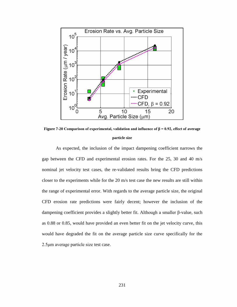
231

Figure 7-20 Comparison of experimental, validation and influence of β = 0.92, effect of average

particle size

As expected, the inclusion of the impact dampening coefficient narrows the

gap between the CFD and experimental erosion rates. For the 25, 30 and 40 m/s

nominal jet velocity test cases, the re-validated results bring the CFD predictions

closer to the experiments while for the 20 m/s test case the new results are still within

the range of experimental error. With regards to the average particle size, the original

CFD erosion rate predictions were fairly decent; however the inclusion of the

dampening coefficient provides a slightly better fit. Although a smaller β-value, such

as 0.88 or 0.85, would have provided an even better fit on the jet velocity curve, this

would have degraded the fit on the average particle size curve specifically for the

2.5μm average particle size test case.

232

Figure 7-21 compares the experimental results, the initial CFD validation

simulation results, the time-adjusted CFD results and the impact dampening

coefficient erosion results as a function of particulate concentration.

Figure 7-21 Comparison of experimental, validation and influence of β = 0.92, effect of

concentration

It can be seen that the inclusion of the impact dampening coefficient

significantly improved the fit between experimental and CFD predicted erosion rates.

While the original CFD predictions showed were sub-par, the good fit brought about

by the inclusion of the time adjusted concentration and the impact dampening

coefficient indicate that the original mismatch can be accounted for by these two

factors.

Figure 7-22 shows how the impact dampening coefficient influences the

erosion rate as a function of fluid viscosity.

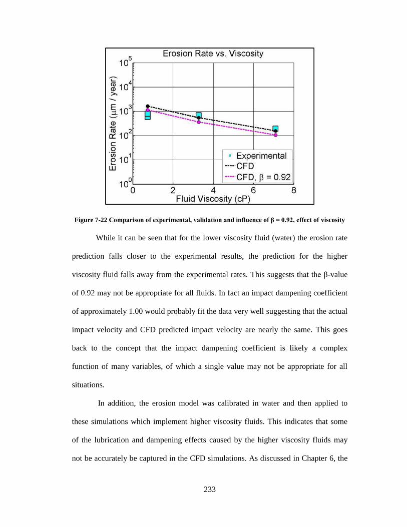
233

Figure 7-22 Comparison of experimental, validation and influence of β = 0.92, effect of viscosity

While it can be seen that for the lower viscosity fluid (water) the erosion rate

prediction falls closer to the experimental results, the prediction for the higher

viscosity fluid falls away from the experimental rates. This suggests that the β-value

of 0.92 may not be appropriate for all fluids. In fact an impact dampening coefficient

of approximately 1.00 would probably fit the data very well suggesting that the actual

impact velocity and CFD predicted impact velocity are nearly the same. This goes

back to the concept that the impact dampening coefficient is likely a complex

function of many variables, of which a single value may not be appropriate for all

situations.

In addition, the erosion model was calibrated in water and then applied to

these simulations which implement higher viscosity fluids. This indicates that some

of the lubrication and dampening effects caused by the higher viscosity fluids may

not be accurately be captured in the CFD simulations. As discussed in Chapter 6, the

234

experiments conducted using the PG fluids indicated that the wet-abrasion

mechanism was less pronounced than in water. Due to stronger fluid-particle coupling

in the higher viscosity fluids, the particles would be less likely to impose abrasive

damage onto the surface given their stronger ties to the fluid streamlines. This

signifies the importance of the fluid used in the calibration procedure especially in the

case of fine particles where surface effects become more pronounced. It would be

interesting to observe how the erosion model would change if it was calibrated in a

more viscous fluid.

7.7 Model Discussion

The final form of the erosion model developed in this research is shown below:

𝐸𝑅 = 𝐾𝐷4.19(𝛽𝑉)4.75 sin0.375 𝛼 cos2 𝛼 (7-18)

In this model the velocity exponent is 4.75, the particle size exponent is 4.19

and the impact dampening coefficient β is 0.92. The material/system constant was

found to be 4866920. Derived from the Huang model, the present model is based on

the assumption that low-angle impacts dominate the overall wear as evident from the

sine and cosine angle functions.

As discussed in the literature review section, brittle erosion is typically

modeled using derivatives of the quasi-static or dynamic impact theory which both

assume that the maximum erosive wear occurs at normal impact angles. This is

typically found in literature by the inclusion of a (Vsinα)n term first proposed by

Hockey [61]. While the quasi-static and dynamic impact models were calibrated and

validated using normal particle impact experiments, the inherent assumption in those

235

models is that the indenting or impacting element produces the greatest elastic/plastic

damage if it impacts perpendicularly to the surface. This brittle erosion assumption is

further justified from the early works of Sheldon and Finnie [39] [40] who found that

the greatest elastic crack length is formed upon normal impact from a spherical

particle.

In this research however, the shift in wear mechanisms from brittle to ductile

suggests that a change in erosion model is also necessary to capture the physics of

wear. Using fluid as the particle transfer medium also has direct influence on the type

of model chosen as the fluid flow directly affects how the particles interact with the

surface. In addition to showing that the squeeze fluid reduces the particle impact

velocity, the concept of the impact dampening coefficients suggests that surface level

forces may be acting to further dampen the impact.

To the best of the author’s knowledge, this is the first time that a nominally

ductile erosion model has been applied to predict the erosion of a nominally brittle

material behaving in a ductile fashion. This suggests that the models are not

necessarily material dependent, but rather mechanism dependent.

The exponents found through the calibration efforts may also have significant

physical meaning. However, it becomes challenging to compare the data found in this

research to the findings of others due to the great amount of differences in operating

and test conditions. For example Routbort and Scattergood [65] [67] [69] studied the

erosion of single crystal silicon, however the particle sizes and velocities used in their

experiments were significantly higher than those performed in this study. In addition,

they used sandblasting techniques. One thing they found in their research was that at

236

low particle impact angles (less than 20°) the amount of measurable erosion becomes

anomalously low and deviates from the impact angle relation found at larger impact

angles. This suggests that either a shift in mechanism or threshold effects begin to

take place. Nonetheless, the velocity exponents found in their study were between

3.18 and 3.55 for 40μm particles across a velocity range of approximately 33 – 150

m/s. The velocity exponent found in this study was 4.75, slightly larger than the ones

found by other authors.

In a study conducted by Wensink and Elwenspoek [100], they found two

different velocity exponents corresponding to two different impact energy regimes.

The high energy regime, characterized by kinetic impact energies above their

determined threshold value of 21 nJ, exhibited an equivalent velocity exponent of

3.06 whereas the velocity exponent of the low impact energy regime was found to be

4.7. It was shown that this shift in regimes occurs when the primary wear mechanism

shifts from brittle to ductile.

Validated by the SEM images, the primary wear mechanisms in the present

research were shown to be primarily ductile in nature with pseudo-plastic and mixed-

mode tendencies. Given the velocity exponent of 4.75, the findings here align quite

well with the findings of Wensink. However the primary difference is that the study

performed by Wensink utilized impact angles of 90° while the present study mainly

contained impact angles less than 10°. One conclusion that can be made is that the

velocity exponent is independent of impact angle as suggested by the similar velocity

exponent found by this study.

237

The particle size exponent found in this study, 4.19, is significantly larger than

those found in literature. The only comparable study were those conducted by

Routbort and Scattergood who found particle size exponents between 0.6 – 1.8. The

main difference between the present study and previous studies is the influence of

water. The wet abrasion mechanism observed in this study acts by dragging particles

across the surface inducing larger scratches and deep gouges. Due to the fact that air

is the primary medium bringing particles to the surface, the wet-abrasion mechanism

does not take place but rather a simple bouncing action occurs. It is thought the

significantly increased particle size exponent originates from the shift in wear

mechanism, but also from the scratching and gouging action. Given otherwise similar

impact conditions, particles in water would remove more surface material due the

added momentum induced by the fluid flow. This phenomenon can best be depicted

in Figure 7-23.

Figure 7-23 Effect of transport medium on particle size exponent. Small particles in air (a), large

particles in air (b), small particles in fluid (c), large particles in fluid (d)

238

Figure 7-23a and Figure 7-23b show that a particle traversing through air

rebounds from the surface leaving a localized region of material removal. The size of

the particle most influences the affected area while the impact kinetic energy most

influences the impact depth. However, Figure 7-23c and Figure 7-23d show how the

particle interacts with the surface under fluid flow conditions. Since the particle’s

motion is coupled to the fluid flow and the fluid directly above the surface flows

tangentially, there is a significant portion of the particle’s momentum running parallel

to the surface. This causes the particle to effectively carve out a larger volume of

material under slurry flow conditions when compared to air conditions, even at low

impact angles. As such, this may justify the significantly larger particle size exponent

found in fluid flow conditions when compared to those found in sandblasting

conditions

7.8 Notion of Threshold Conditions

An important aspect of erosion modeling efforts lies in the idea of identifying

critical threshold conditions, under which erosion does not occur. This concept was

briefly introduced in the literature review section by assuming the main mechanism of

wear was the induction of crack systems followed by coalescence and ultimately mass

loss. As such, the threshold conditions for those systems are identified as the impact

conditions necessary to induce cracks. However, the findings of this study indicate

that the primary mechanisms of wear shift away from brittle cracking and fracture to

more pseudo-plastic scribing, gouging and ploughing. This also suggests a change in

the conditions through which threshold conditions are defined.

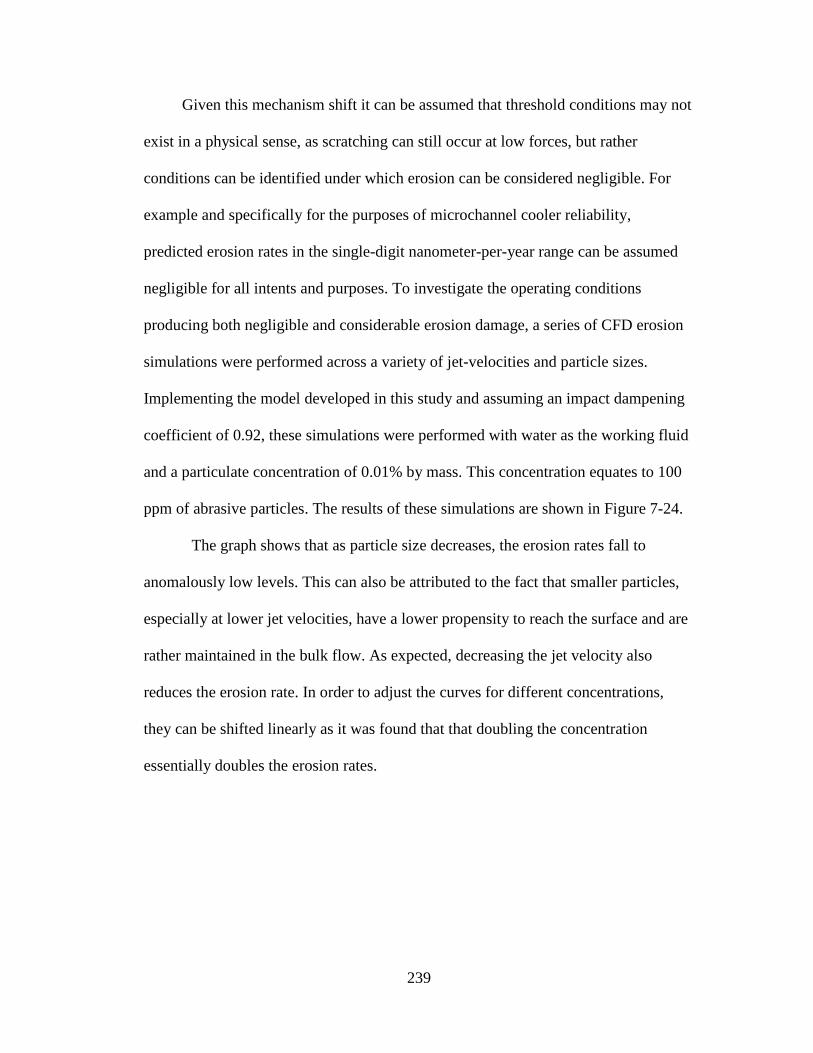
239

Given this mechanism shift it can be assumed that threshold conditions may not

exist in a physical sense, as scratching can still occur at low forces, but rather

conditions can be identified under which erosion can be considered negligible. For

example and specifically for the purposes of microchannel cooler reliability,

predicted erosion rates in the single-digit nanometer-per-year range can be assumed

negligible for all intents and purposes. To investigate the operating conditions

producing both negligible and considerable erosion damage, a series of CFD erosion

simulations were performed across a variety of jet-velocities and particle sizes.

Implementing the model developed in this study and assuming an impact dampening

coefficient of 0.92, these simulations were performed with water as the working fluid

and a particulate concentration of 0.01% by mass. This concentration equates to 100

ppm of abrasive particles. The results of these simulations are shown in Figure 7-24.

The graph shows that as particle size decreases, the erosion rates fall to

anomalously low levels. This can also be attributed to the fact that smaller particles,

especially at lower jet velocities, have a lower propensity to reach the surface and are

rather maintained in the bulk flow. As expected, decreasing the jet velocity also

reduces the erosion rate. In order to adjust the curves for different concentrations,

they can be shifted linearly as it was found that that doubling the concentration

essentially doubles the erosion rates.

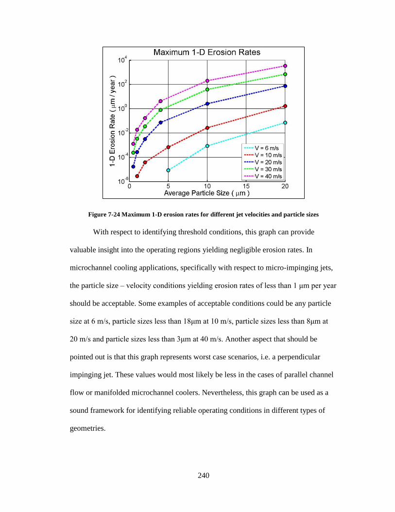
240

Figure 7-24 Maximum 1-D erosion rates for different jet velocities and particle sizes

With respect to identifying threshold conditions, this graph can provide

valuable insight into the operating regions yielding negligible erosion rates. In

microchannel cooling applications, specifically with respect to micro-impinging jets,

the particle size – velocity conditions yielding erosion rates of less than 1 μm per year

should be acceptable. Some examples of acceptable conditions could be any particle

size at 6 m/s, particle sizes less than 18μm at 10 m/s, particle sizes less than 8μm at

20 m/s and particle sizes less than 3μm at 40 m/s. Another aspect that should be

pointed out is that this graph represents worst case scenarios, i.e. a perpendicular

impinging jet. These values would most likely be less in the cases of parallel channel

flow or manifolded microchannel coolers. Nevertheless, this graph can be used as a

sound framework for identifying reliable operating conditions in different types of

geometries.

241

7.9 Limitations

This chapter describes the development of a particle erosion model that can be

used to predict maximum one-dimensional erosion rates in microfluidic geometries.

While this model has been validated and shows good agreement with experimental

results, there exist some limitations when applying this model. First, the model has

been calibrated specifically with the alumina particle and silicon substrate system. If

this model were to be applied to another substrate material, the accuracy would be

unknown without first conducting a couple validation experiments with the new

material.

Secondly, the major wear mechanism taking place is assumed to be the deep

cutting and gouging shown in Chapter 6. As described in the literature review chapter

increasing the particle size or impact velocity could shift the wear mechanisms away

from those plastic in nature to those behaving more in a brittle fashion. Since this

model has been calibrated and validated within specific particle size and velocity

ranges, it would be most accurate to apply this model in situations where the average

particle size is less than 20μm and the average impact velocity is less than

approximately 30 m/s (the CFD simulations indicated that 20μm particles in a 40 m/s

jet impact the wall at approximately 30 m/s – see Chapter 4). A caveat to the above

notion could occur in the case of smaller particles at larger velocities. While this

would shift the conditions outside of the calibration/validation realm, it can be

predicted that the fundamental wear mechanism would not change.

Another limitation is that this model was calibrated in water and, as shown by

the validation simulations, may need to be re-calibrated if the working fluid is a more

242

viscous fluid such as 100% PG. This may also be necessary in less viscous fluids such

as refrigerants or even two-phase flow. However, the validation simulations still

showed good agreement between experimental and CFD predictions suggesting that

this model could still serve as a sound prediction tool in a variety of working fluids.

As indicated by the concentration experiments, knowing the proper particulate

concentration of the fluid is critical for ensuring accurate erosion predictions.

However, this sometimes poses an issue as the concentration may change with time.

Therefore when using this model to make an erosion prediction, it would be optimal

to assume a maximum allowable concentration which would yield a worst case

scenario prediction. Typically microfluidic or hydraulic systems have acceptable

particulate contamination levels. When these levels are reached, an indicator would

suggest that the fluid needs to be changed. While this approach would yield a worst

case scenario erosion prediction, it can still be viewed as relatively accurate due to the

fact that concentration has a linear relationship with erosion while particle size and

impact velocity exhibit power law relations.

Furthermore, in developing this erosion model it was assumed that any surface

changes caused by erosion would not influence future erosion. Essentially, the surface

is always assumed to be flat while in reality the surface changes as erosion

progresses. Due to the fact that the erosion depths achieved in these experiments were

at most a few tens of micrometers and the particle sizes were of a similar order of

magnitude, this effect was assumed negligible. However, future experiments may

need to be conducted if the maximum expected erosion depth is on the order of a few

hundred micrometers.

243

Lastly, an assumption inherent in the Huang model is that the wear is

dominated by low angle particle impacts. In the section introducing this erosion

model, two separate wear mechanisms are described: deformation wear and cutting

wear. To simplify the model, deformation wear was assumed to be negligible

compared to cutting wear due to the low angle impacts found via CFD simulations

and the cutting mechanisms found in the SEM surface images. This assumption may

not hold true in all operating conditions and scenarios, but for the velocity and

particle size ranges of this study it was assumed to be true.

244

8 CONCLUSION AND SUMMARY

This chapter serves to summarize the contents of this dissertation, discuss the

technical and academic contributions made throughout this research and outline a few

pertinent areas for related future work.

Chapter 1 introduces the concept of embedded cooling by describing the

paradigm shift away from conventional remote cooling techniques. Conventional

power electronics cooling relies on conducting heat away from the source into an air

or liquid cooled heat sink. While this established technique provides thermal

management solutions for a variety of different applications, bringing cooling power

virtually to the source enables significantly higher power levels to be reached while

maintaining similar junction temperatures. Through various implementations such as

manifolded microchannel coolers, arrays of impinging micro-jets and pin fin arrays,

liquid cooling can be brought to within a few hundred micrometers of the source.

However, as this cooling technique is relatively experimental and new there exist a

number of potential reliability threats that have not thoroughly been explored, namely

particle erosion, corrosion and clogging. This dissertation serves to investigate the

particle erosion phenomenon.

Chapter 2 provides a detailed literature review focusing mainly on the subject

of brittle erosion. Two main brittle erosion theories are discussed; the quasi-static

model and the dynamic impact theory, both of which show good alignment with

many other erosion studies. Characteristics of slurry erosion are also discussed which

differs from typical particle erosion studies due to the effect that the fluid has on

particle-surface interactions. One attribute of slurry erosion is the development of a

245

“squeeze-film” which is essentially a viscous sublayer forming directly above the

surface. This slow moving fluid may act to trap smaller particles resulting in a wet

abrasion mechanism as the particles are swept away by the tangentially moving flow.

Additionally, the trapped particle bed may protect the surface from incoming

particles. Studies involving abrasive slurry jet micromachining were discussed as they

provide insight into the type of wear patterns thought to occur in the case of jet-

impingement erosion. The characteristic ‘W’ shape arises mainly due to the

stagnation region directly below the impinging jet where minimal particle impacts

occur. Lastly, the concept of the brittle-to-ductile transition is discussed where

nominally brittle materials behave in ductile fashions under specific wear conditions.

When the kinetic energy of an impacting particle is low enough, either by a decreased

particle size or low impact velocity, the elastic/plastic wear mechanism described by

the quasi-static and dynamic impact theories are replaced by ductile wear

mechanisms such as scratching and deep gouging. With regards to erosion modeling,

this tends to increase the particle size and velocity exponents compared to those

derived from strictly brittle erosion.

Chapter 3 briefly outlines the problem statement and summarizes the core

objectives of this research. Given the need for high fidelity erosion predictions in

embedded and microchannel cooling applications, a new particle erosion model needs

to be developed. The literature review section indicated that existing erosion models

would likely not suffice for the given applications due to the shift in wear

mechanisms away from brittle cracking and fracture towards those ductile in nature.

Ultimately, the main goal of this research is to develop a new particle erosion model

246

calibrated and validated within the typical operating conditions found in

microchannel and embedded cooling systems. The steps taken to accomplish this can

be broken down into six main objectives:

1) Develop a jet-impingement CFD model in ANSYS FLUENT to obtain

localized particle impact characteristics.

2) Design and construct a jet-impingement slurry erosion test apparatus to

perform slurry erosion experiments.

3) Formulate and execute a series of tests (DOE) to investigate the effects of jet

velocity, particle size, concentration, fluid viscosity and time.

4) Gain insight into the wear mechanisms of single crystal silicon under

microchannel cooler operating conditions. (Particle Sizes: < 20μm, Velocities:

< 40 m/s)

5) Combine localized particle impact characteristics from CFD simulations with

experimental erosion data to formulate a particle-based erosion model.

6) Perform validation simulations to identify how well the model predicts

maximum 1-dimension erosion rates (μm/year).

Chapter 4 discusses the CFD simulations performed using ANSYS FLUENT

in order to identify localized particle impact characteristics, specifically impact angle

and impact velocity. Adjusting various operating conditions such as nominal jet

velocity, average particle size and fluid viscosity resulted in significant changes in

particle impact angle, impact velocity and percentage of entrained particles that

actually impact the surface. The Stokes number can be used to justify the results from

these simulations which describes how closely coupled the motion of a particle is to

247

the surrounding fluid. In addition, a series of user-defined functions were written and

hooked into FLUENT in order to capture the necessary impact data.

Chapter 5 covers the design and construction of the slurry erosion jet-

impingement test apparatus. The test setup is capable of handling nominal jet

velocities of up to 60 m/s (through a 1.98 mm nozzle), a large spread of particle sizes

due to abrasive slurry pump and is chemically compatible with a variety of working

fluids including ethylene and propylene glycols solutions. A propeller-based stirring

mechanism, powered by a motor, ensures that particle settling does not occur within

the reservoir. Additionally, this chapter discusses topics such as cleaning the test

setup in between uses, creating the testing slurry and the process used to manufacture

the silicon samples for testing.

Chapter 6 outlines the experimental erosion testing performed in this study. A

design of experiments outlining the 14 different test cases is presented enabling the

most critical factors of erosion to be tested: nominal jet velocity, particle size,

particulate concentration, fluid viscosity and time. A stylus profilometer was used to

capture the erosion contour created by each of the different samples, and from this

two principle erosion metrics could be evaluated: maximum one-dimensional erosion

rate in units of micrometers per year and a mass loss rate in units of milligrams per

year. The one-dimension erosion rate could be directly extracted from the erosion

contour by factoring in the testing time. However, in order to convert the 2-D erosion

contours to 3-D volumes (then convert to mass by dividing by density) an algorithm

was developed in MATLAB. Based on a simple volume-of-revolutions type approach

and assuming the contours were axisymmetric about the stagnation region, this

248

calculation was performed. To sum up the erosion results the following statements

can be made where MLR and ER stand for the Mass Loss Rate and one-dimensional

Erosion Rate respectively, and V and D stand for the nominal jet velocity and average

particle size respectively:

MLR ∝ V6.29

ER ∝ V5.35

MLR ∝ D4.36 ER ∝ D

4.11

Lastly, high-resolution SEM images were taken of the eroded surface in order

to identify the types of wear mechanism taking place. Based on these images it was

verified that ductile wear mechanisms dominated the erosion in the form of deep

cutting, gouging, flaking.

Chapter 7 discusses the development and calibration of the particle-based

erosion model. First, the total mass of impacting particles for each test case was

determined using the CFD simulations in order to convert the mass loss rates from

Chapter 5 into the conventional erosion ratios. The Huang cutting erosion model was

also introduced which serves as the basis of the newly developed erosion model. Next

the process through which the calibration efforts took place was described and

validation simulations were performed to address how accurate the model was at

predicting the maximum one-dimensional erosion rates. While good agreement was

shown between experimental and simulation-based erosion predictions, the

simulations tended to over-predict the experiments. As such an impact dampening

coefficient was proposed, β, which is defined as the ratio of the actual impact velocity

to the velocity determined through CFD predictions. It was found that a value of

approximately 0.92 best fit the data, however future studies will have to be conducted

249

to further examine the physical nature of the dampening coefficient. The final erosion

model produced in this study is shown below

𝐸𝑅 = 𝑘𝐷𝑚(𝛽𝑉)𝑛 sin0.375 𝛼 cos2 𝛼 (7-18)

ER Erosion ratio [mg/mg]

k = 4866920 System constant

D Average particle diameter [m]

m = 4.19 Particle size exponent

β ≈ 0.92 Impact dampening coefficient

V Particle impact velocity [m/s]

n = 4.75 Particle impact velocity exponent

α Impact angle

This model has the capability to be hooked into commercial CFD codes

through user-defined functions in order to replace generic or built in erosion models.

In addition to accurately performing erosion predictions in jet-impingement scenarios,

this model can also be used to perform erosion predictions in a variety of

microchannel-based environments, so long as the limitations discussed in Chapter 7

are considered.

8.1 Academic and Technical Contributions

From the results and methodologies proposed in this study, a number of

academic and technical contributions have been made. First and foremost and to the

best of the author’s knowledge, this was the first slurry erosion study conducted on

single crystal silicon. While a number of erosion studies on silicon have been

performed using sandblasting techniques, the use of water as a transport medium has

250

contributed to the low angle impacts resulting in the ductile wear mechanisms not

observed in previous studies.

Furthermore, erosion studies of brittle materials are typically conducted with

impact velocities and particle sizes well outside the range of those tested in this

research. This is often times necessary in order to produce measurable wear in a

reasonable period of time. However, in this study the use of a slurry environment

enabled longer testing times and therefore significantly lower velocities and particle

sizes could be used. To the best of the author’s knowledge this is the first slurry

erosion study to be performed using particle sizes and velocities within the ranges

present in microchannel coolers. Due to this factor, the erosion model developed here

is optimally suited to make erosion predictions in these applications compared to

other previously published models.

In addition, SEM images of the eroded surfaces revealed that the primary

wear mechanisms were ductile in nature as was suggested by literature. These wear

mechanisms were mainly in the form of deep and shallow scratches caused by sharp

particles and shallow ploughing caused by blunter particles. Other less prevalent

mechanisms were also observed such as a mixed-mode erosion mechanism where

material was displaced in a ductile fashion to be subsequently followed by brittle

flaking. While this wet-abrasion mechanism has been previously observed in slurry

erosion studies of metals, to the best of the authors knowledge it has not been

observed and quantified in brittle materials under jet-impingement conditions.

In conjunction with this finding, a ductile erosion model was used to capture

the erosive wear of a nominally brittle material. As was shown in the literature review

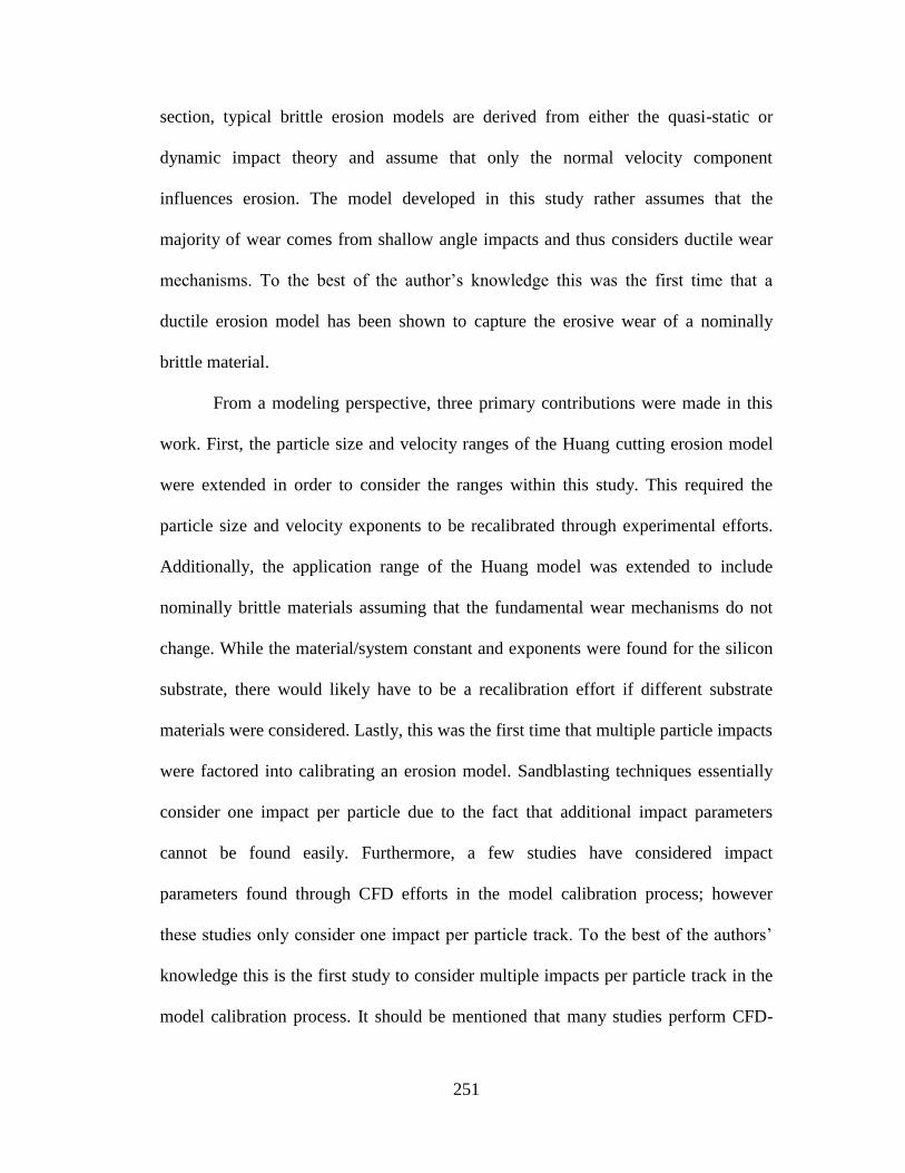
251

section, typical brittle erosion models are derived from either the quasi-static or

dynamic impact theory and assume that only the normal velocity component

influences erosion. The model developed in this study rather assumes that the

majority of wear comes from shallow angle impacts and thus considers ductile wear

mechanisms. To the best of the author’s knowledge this was the first time that a

ductile erosion model has been shown to capture the erosive wear of a nominally

brittle material.

From a modeling perspective, three primary contributions were made in this

work. First, the particle size and velocity ranges of the Huang cutting erosion model

were extended in order to consider the ranges within this study. This required the

particle size and velocity exponents to be recalibrated through experimental efforts.

Additionally, the application range of the Huang model was extended to include

nominally brittle materials assuming that the fundamental wear mechanisms do not

change. While the material/system constant and exponents were found for the silicon

substrate, there would likely have to be a recalibration effort if different substrate

materials were considered. Lastly, this was the first time that multiple particle impacts

were factored into calibrating an erosion model. Sandblasting techniques essentially

consider one impact per particle due to the fact that additional impact parameters

cannot be found easily. Furthermore, a few studies have considered impact

parameters found through CFD efforts in the model calibration process; however

these studies only consider one impact per particle track. To the best of the authors’

knowledge this is the first study to consider multiple impacts per particle track in the

model calibration process. It should be mentioned that many studies perform CFD-

252

based erosion predictions that do consider multiple impacts per particle track,

however the contribution referred to here is specifically with respect to the calibration

procedure.

A new impact dampening coefficient was also proposed which implies that

the actual impact velocity of a particle is less than the CFD predicted impact velocity.

For this set of operating conditions, a value of 0.92 was found to fit the data well

which suggests that the actual impact velocity is 92% of the CFD predicted impact

velocity. From a physical perspective, the impact dampening coefficient may be an

artifact of the method in which particle tracking is performed in CFD – that particles

are treated as point-masses rather than having a definitive volume and surface area.

This observation, where CFD-based erosion predictions tend to over predict

experimental wear is a phenomenon prevalent throughout literature and is especially

noticeable in applications involving micrometer-scale particles. While further

research needs to be conducted in this area, it is thought that the particle tracking

methodology loses accuracy at these small scales where other factors not accounted

for in the CFD code may begin to take place.

From an engineering perspective, the methodology developed here can be

extended to a variety of other materials that are likely to be found in microchannel

coolers such as sapphire, titanium, tungsten and glass. Assuming the erosion

mechanisms remain ductile and the impact angles are relatively low, a few additional

experiments could be performed to recalibrate the constants from the final model to

fit these new materials. Lastly, the final product of this research is a particle-based

erosion model which can be hooked into commercial CFD codes and used to perform

253

erosion predictions in a variety of different microchannel and embedded cooling

geometries. This enables more accurate erosion predictions to be made enabling

system designers to determine the expected lifetime of coolers and necessary filtering

requirements for different operating conditions.

8.2 Future Work

Based on the findings and results of this research, a number of areas involving

potential future work can be identified. These potential future research areas will help

enrich the findings of this study but will also provide relevant information in the

fields of particle erosion modeling and microchannel/embedded cooler reliability.

First, the tests conducted in this study were performed using a jet-impingement

style test setup mimicking one possible type of embedded cooling scheme. Although

the particle erosion model developed here is considered geometry independent, it has

not yet been validated for other types of embedded cooling styles such as pin fin

arrays or manifolded microchannel coolers. One type of study could perform similar

erosion experiments on etched silicon surfaces containing either pin fins or

microchannels. It would be ideal to perform these experiments using a variety of

different jet-impingement angles, which the test setup developed in this work is

currently capable of doing. Typically in pin-fin array coolers, fluid is flowing parallel

to the surface while in manifolded microchannel coolers fluid is flowing

perpendicular to the surface as it enters the channels followed by an abrupt change in

direction as it leaves. These different tests would enable a more real-world view of

how the erosion phenomena affects different types of geometries in conjunction with

the erosion predictions made using CFD.

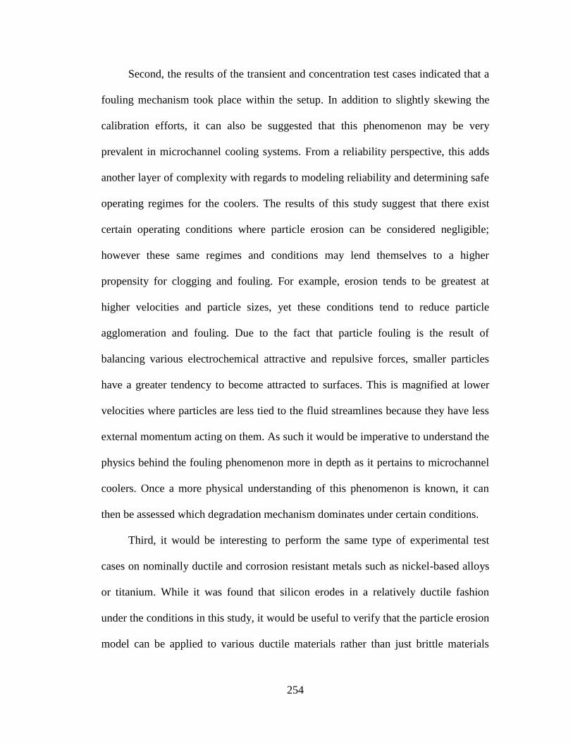
254

Second, the results of the transient and concentration test cases indicated that a

fouling mechanism took place within the setup. In addition to slightly skewing the

calibration efforts, it can also be suggested that this phenomenon may be very

prevalent in microchannel cooling systems. From a reliability perspective, this adds

another layer of complexity with regards to modeling reliability and determining safe

operating regimes for the coolers. The results of this study suggest that there exist

certain operating conditions where particle erosion can be considered negligible;

however these same regimes and conditions may lend themselves to a higher

propensity for clogging and fouling. For example, erosion tends to be greatest at

higher velocities and particle sizes, yet these conditions tend to reduce particle

agglomeration and fouling. Due to the fact that particle fouling is the result of

balancing various electrochemical attractive and repulsive forces, smaller particles

have a greater tendency to become attracted to surfaces. This is magnified at lower

velocities where particles are less tied to the fluid streamlines because they have less

external momentum acting on them. As such it would be imperative to understand the

physics behind the fouling phenomenon more in depth as it pertains to microchannel

coolers. Once a more physical understanding of this phenomenon is known, it can

then be assessed which degradation mechanism dominates under certain conditions.

Third, it would be interesting to perform the same type of experimental test

cases on nominally ductile and corrosion resistant metals such as nickel-based alloys

or titanium. While it was found that silicon erodes in a relatively ductile fashion

under the conditions in this study, it would be useful to verify that the particle erosion

model can be applied to various ductile materials rather than just brittle materials

255

behaving in a ductile manner. Corrosion resistance would be an important

characteristic such that the dominant wear mechanism could be assumed physical in

nature rather than chemical or a combination of the two.

Fourth, it should be pointed out that the final erosion model was calibrated

using water with additional experiments performed in higher viscosity fluids. The

idea behind this was to identify local particle impact characteristics in order to

formulate the model. Once calibrated, the model could then be applied to predict wear

rates in a variety of different geometries using a range of working fluids. It can be

stated that particles in higher viscosity fluids typically exhibit lower impact velocities

and the subsequent effects on erosion should inherently be accounted for in the

calibration procedure. In order to validate this, it would be advantageous to perform

the same calibration experiments using a higher viscosity fluid such as PG10 or

PG25. After recalibrating the model, the particle size and velocity exponents could be

compared in order to identify any effects that the working fluid has on the calibration

procedure.

Finally, the impact dampening coefficient was found empirically using

engineering judgement. Although a value of approximately 0.92 was shown to fit the

data, further studies should focus on determining and quantifying the parameters that

most affect this factor. It can be suggested that the variables likely influencing the

impact dampening coefficient are free stream velocity, fluid viscosity, distance from

surface, particle size, particle shape and fluid-particle adsorption properties. By

examining this more in detail, further insight can be provided as to why CFD erosion

predictions often over-estimate their experimental counterparts.

256

9 Appendices

Appendix A – Raw Erosion Profile Contours

Figure 9-1 Erosion Profile for Test: 24010

257

Figure 9-2 Erosion Profile for Test: 24010B

258

Figure 9-3 Erosion Profile for Test: 54010

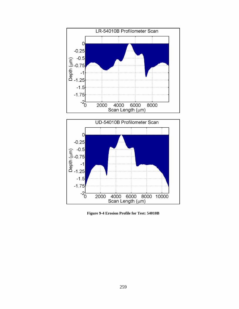
259

Figure 9-4 Erosion Profile for Test: 54010B

260

Figure 9-5 Erosion Profile for Test: 54010C

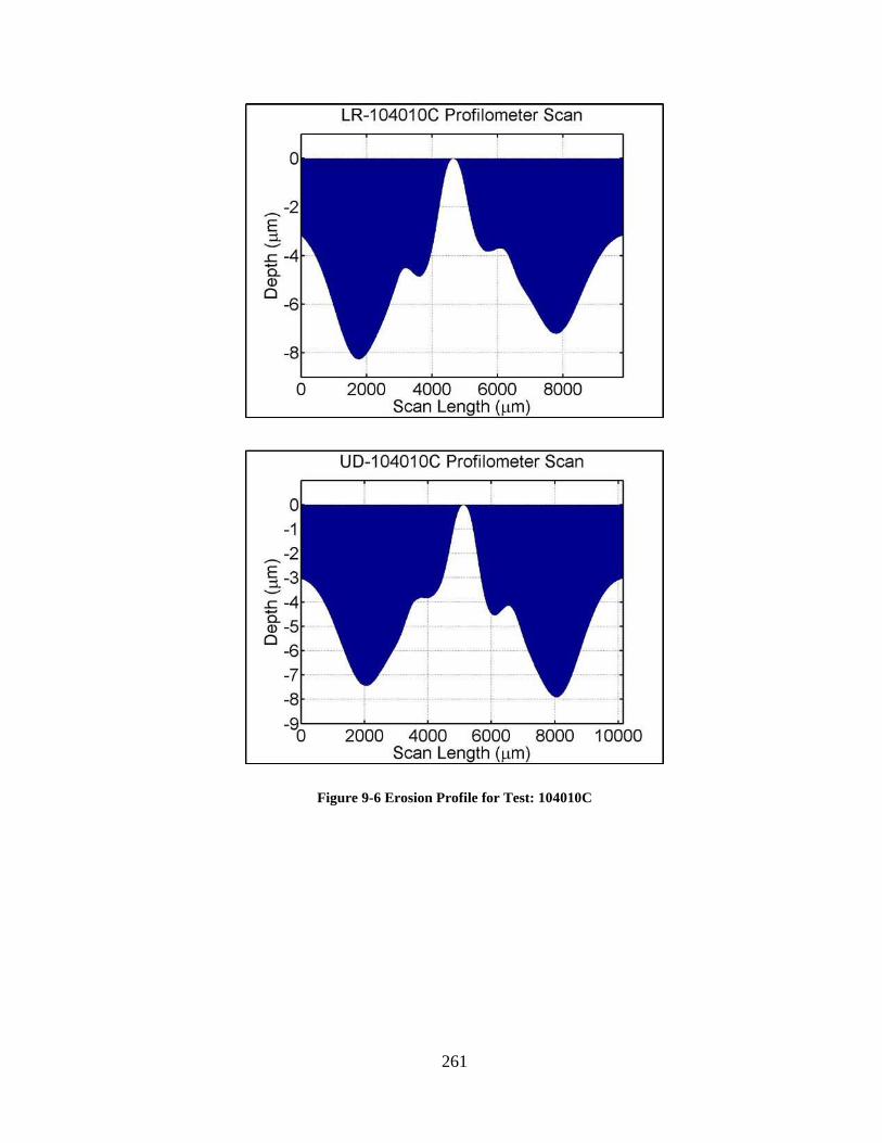
261

Figure 9-6 Erosion Profile for Test: 104010C

262

Figure 9-7 Erosion Profile for Test: 104010D

263

Figure 9-8 Erosion Profile for Test: 204010

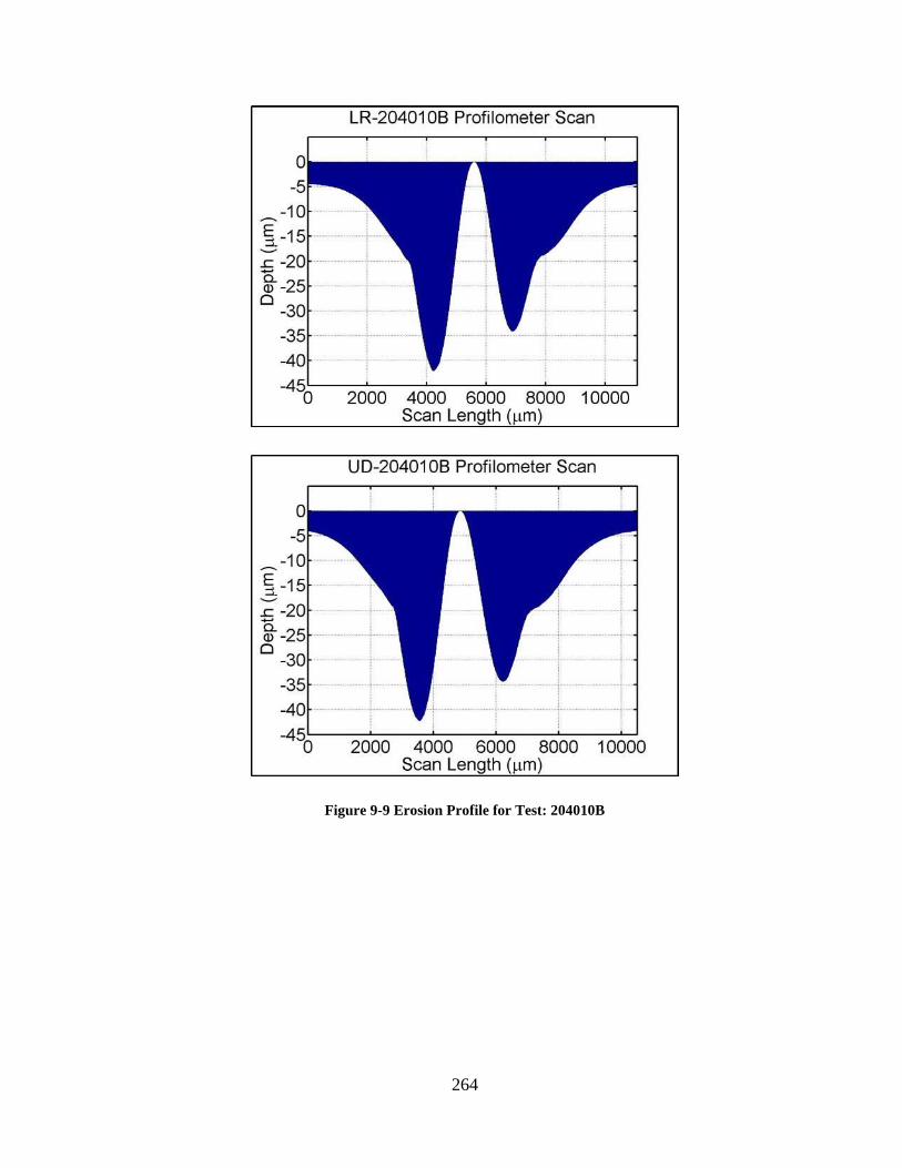
264

Figure 9-9 Erosion Profile for Test: 204010B

265

Figure 9-10 Erosion Profile for Test: 102010

266

Figure 9-11 Erosion Profile for Test: 102010B

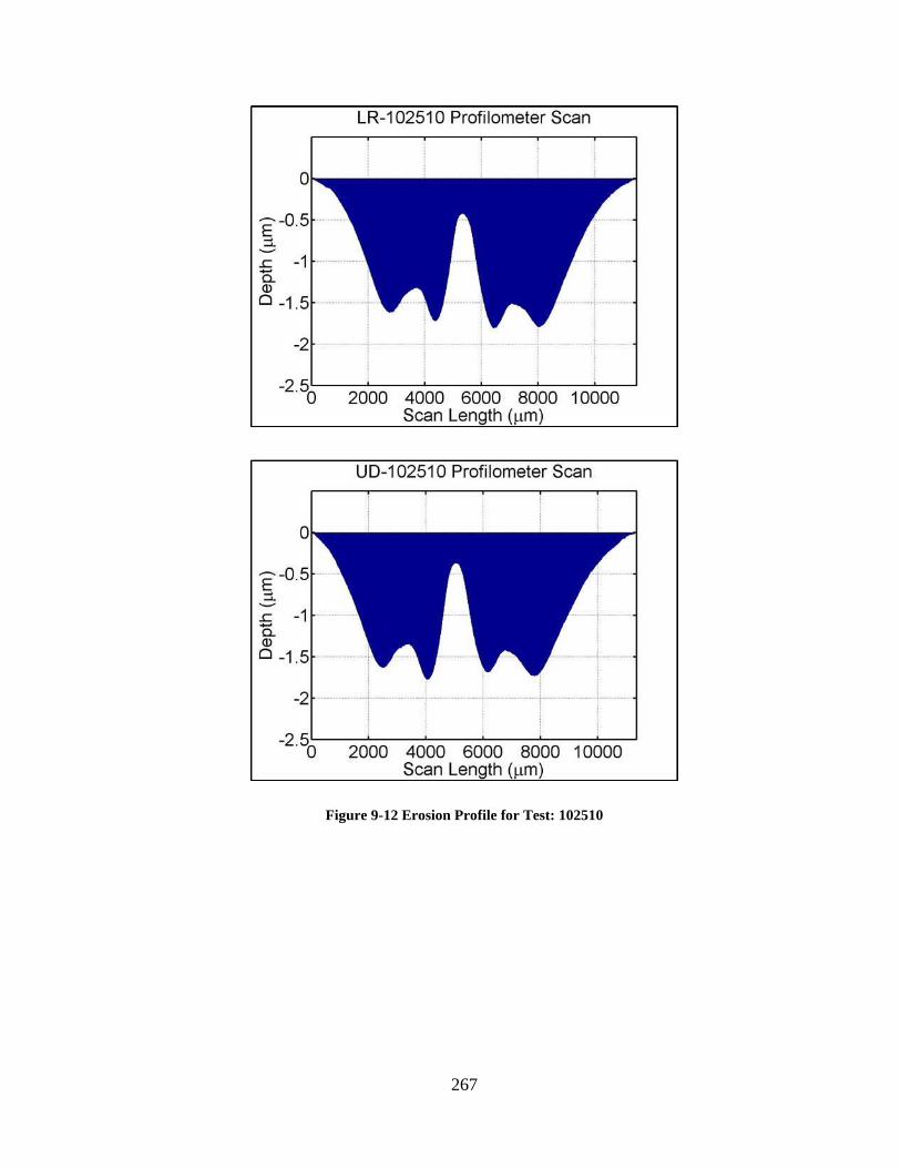
267

Figure 9-12 Erosion Profile for Test: 102510

268

Figure 9-13 Erosion Profile for Test: 103010

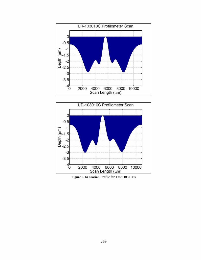
269

Figure 9-14 Erosion Profile for Test: 103010B

270

Figure 9-15 Erosion Profile for Test: 1040025

271

Figure 9-16 Erosion Profile for Test: 1040025B

272

Figure 9-17 Erosion Profile for Test: 104005

273

Figure 9-18 Erosion Profile for Test: 104005B

274

Figure 9-19 Erosion Profile for Test: 104020

275

Figure 9-20 Erosion Profile for Test: PG10

276

Figure 9-21 Erosion Profile for Test: PG25

277

Figure 9-22 Erosion Profile for Test: 103010T1 – 2717 min.

278

Figure 9-23 Erosion Profile for Test: 103010T2 – 5449 min.

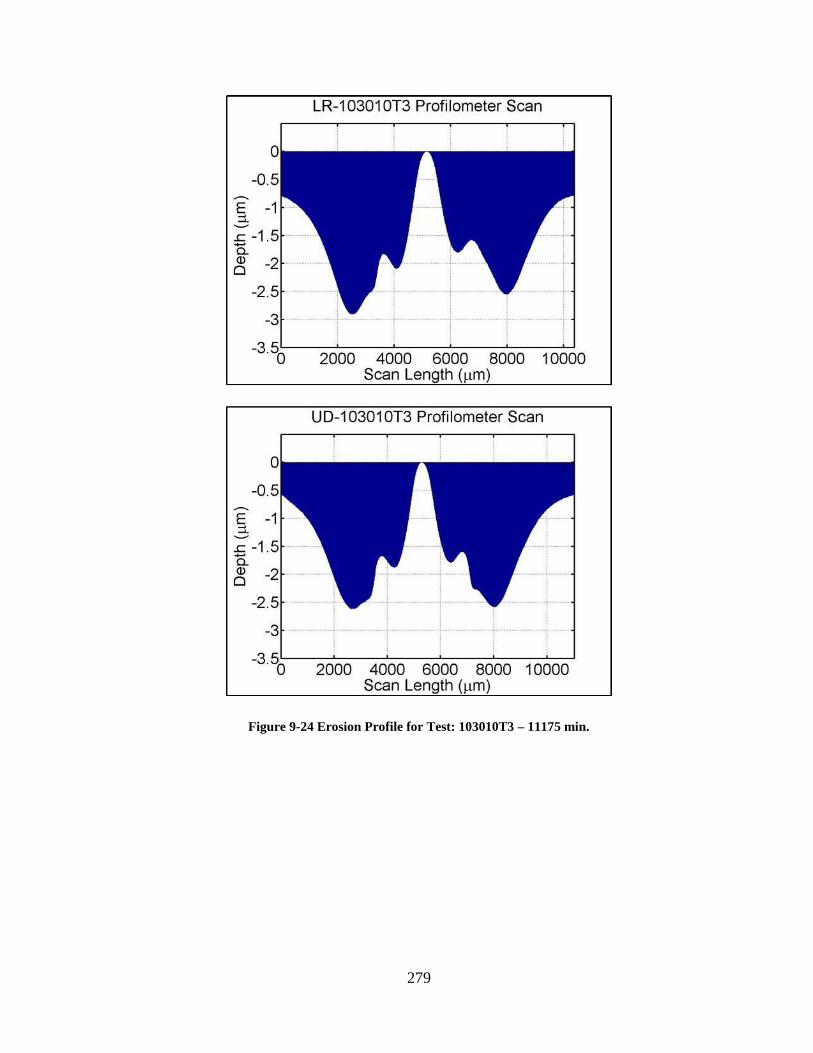
279

Figure 9-24 Erosion Profile for Test: 103010T3 – 11175 min.

280

Figure 9-25 Erosion Profile for Test: 103010T4 – 14053 min.

281

Figure 9-26 Erosion Profile for Test: 104010T1 – 1540 min.

282

Figure 9-27 Erosion Profile for Test: 104010T2 – 2843 min.

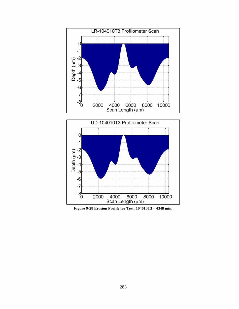
283

Figure 9-28 Erosion Profile for Test: 104010T3 – 4348 min.

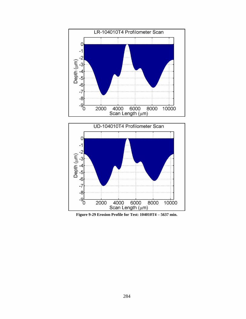
284

Figure 9-29 Erosion Profile for Test: 104010T4 – 5637 min.

285

Appendix B – Raw Particle Size Data

Figure 9-30 Raw Particle Size Data - 10μm, sample 1

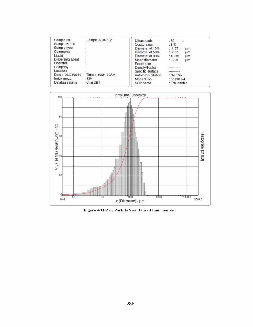
286

Figure 9-31 Raw Particle Size Data - 10μm, sample 2

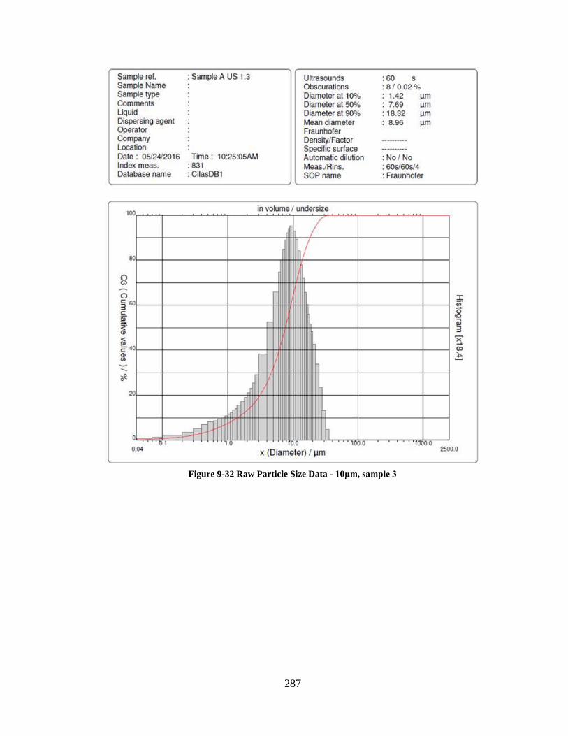
287

Figure 9-32 Raw Particle Size Data - 10μm, sample 3

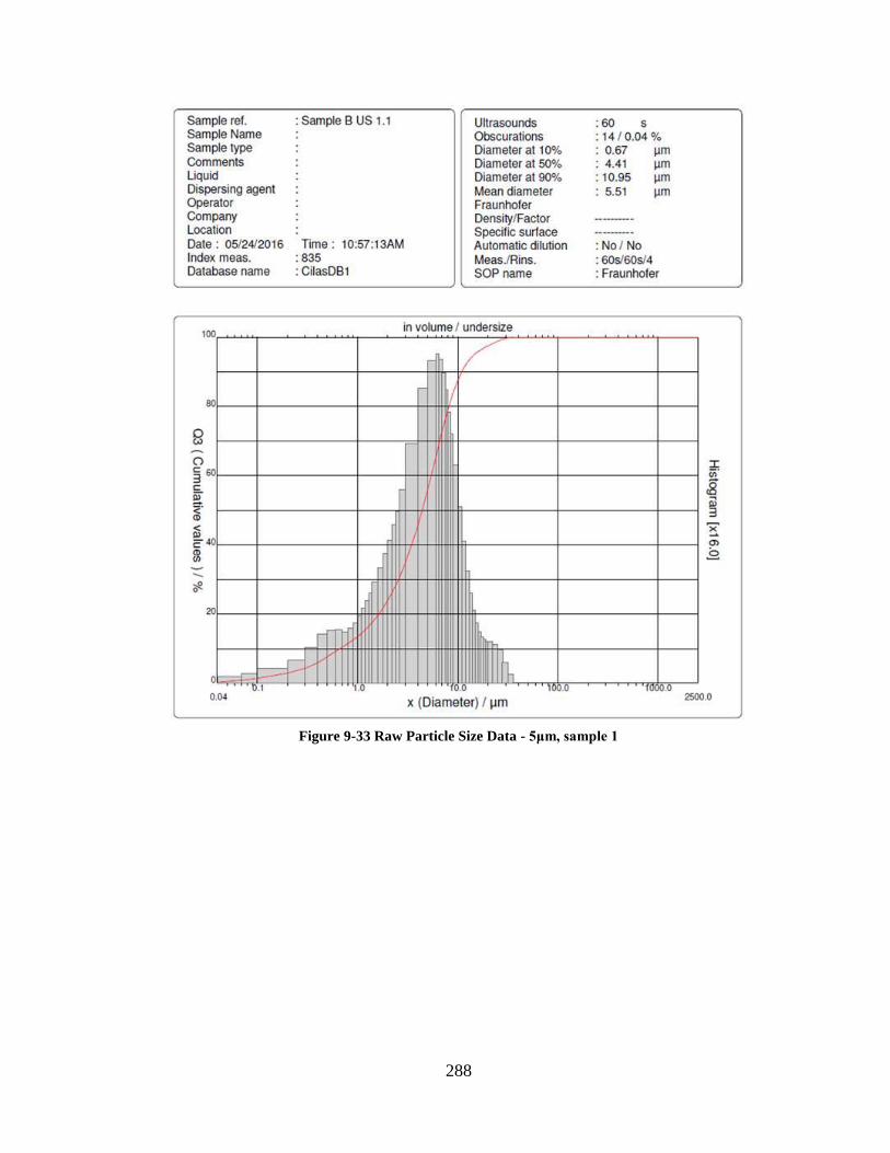
288

Figure 9-33 Raw Particle Size Data - 5μm, sample 1

289

Figure 9-34 Raw Particle Size Data - 5μm, sample 2

290

Figure 9-35 Raw Particle Size Data - 5μm, sample 3

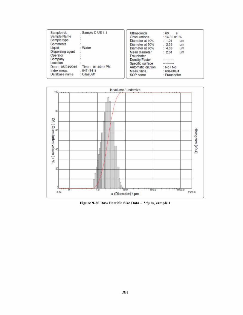
291

Figure 9-36 Raw Particle Size Data – 2.5μm, sample 1

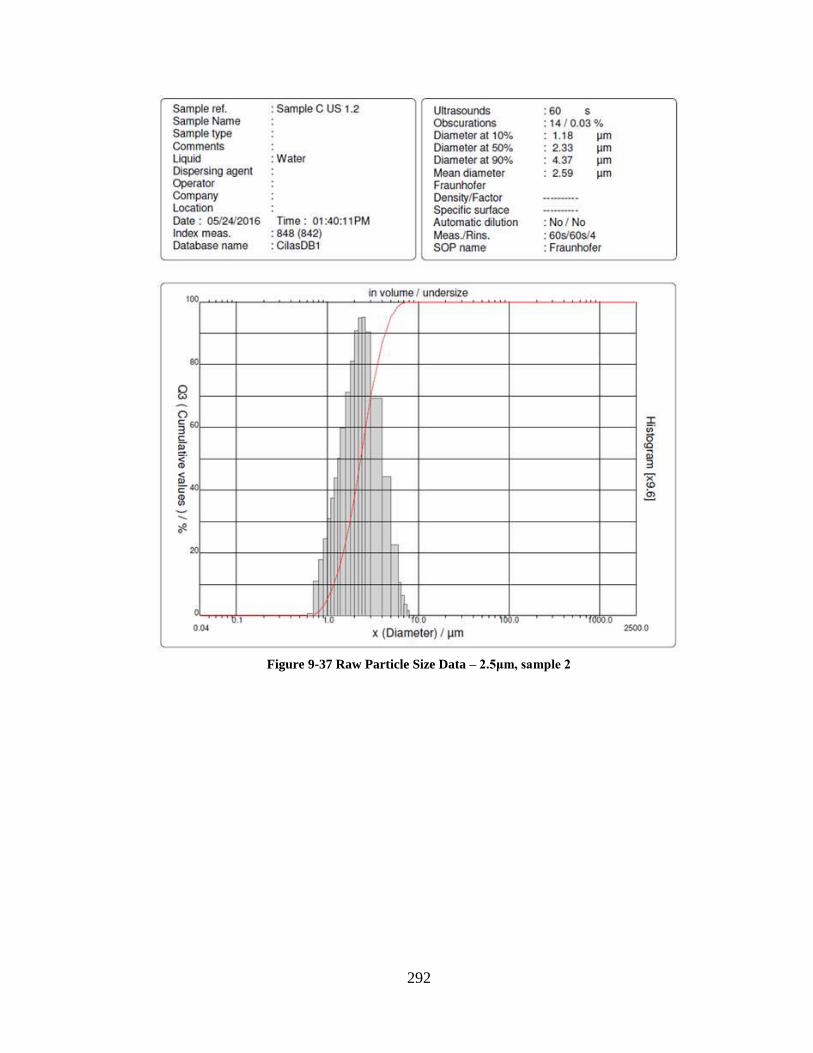
292

Figure 9-37 Raw Particle Size Data – 2.5μm, sample 2

293

Figure 9-38 Raw Particle Size Data – 2.5μm, sample 3

294

Appendix C – FLUENT User Defined Function Codes

This code captures the impact velocity and impact angle of the particle tracks

impinging on the surface. The DEFINE_DPM_BC function activates upon particle

impact and stores the relevant data in the P_USER_REAL(p,x) variable where ‘p’

indicates the current particle and ‘x’ is a variable representing the index in the particle

variable array. This UDF stores and tracks data for up to ten impacts, where the 11th

impact triggers the end of the particle and thus no more impact data is gathered for

that particle. Following the impact, a new trajectory for the particle track is computed.

#include "udf.h"

DEFINE_DPM_BC(numhits2, p, t, f, f_normal, dim)

{

/* increments particle impact counter */

P_USER_REAL(p, 0) = P_USER_REAL(p, 0) + 1.;

/* stops particle if too many hits occur */

if (P_USER_REAL(p, 0) > 9)

{

return PATH_END;

}

/* stores radial location of impact */

if (P_USER_REAL(p, 0) == 1)

{

P_USER_REAL(p, 21) = sqrt(pow(P_POS(p)[0],2) + pow(P_POS(p)[2],2));

}

if (P_USER_REAL(p, 0) == 2)

{

P_USER_REAL(p, 22) = sqrt(pow(P_POS(p)[0],2) + pow(P_POS(p)[2],2));

}

if (P_USER_REAL(p, 0) == 3)

{

P_USER_REAL(p, 23) = sqrt(pow(P_POS(p)[0],2) + pow(P_POS(p)[2],2));

}

if (P_USER_REAL(p, 0) == 4)

{

P_USER_REAL(p, 24) = sqrt(pow(P_POS(p)[0],2) + pow(P_POS(p)[2],2));

}

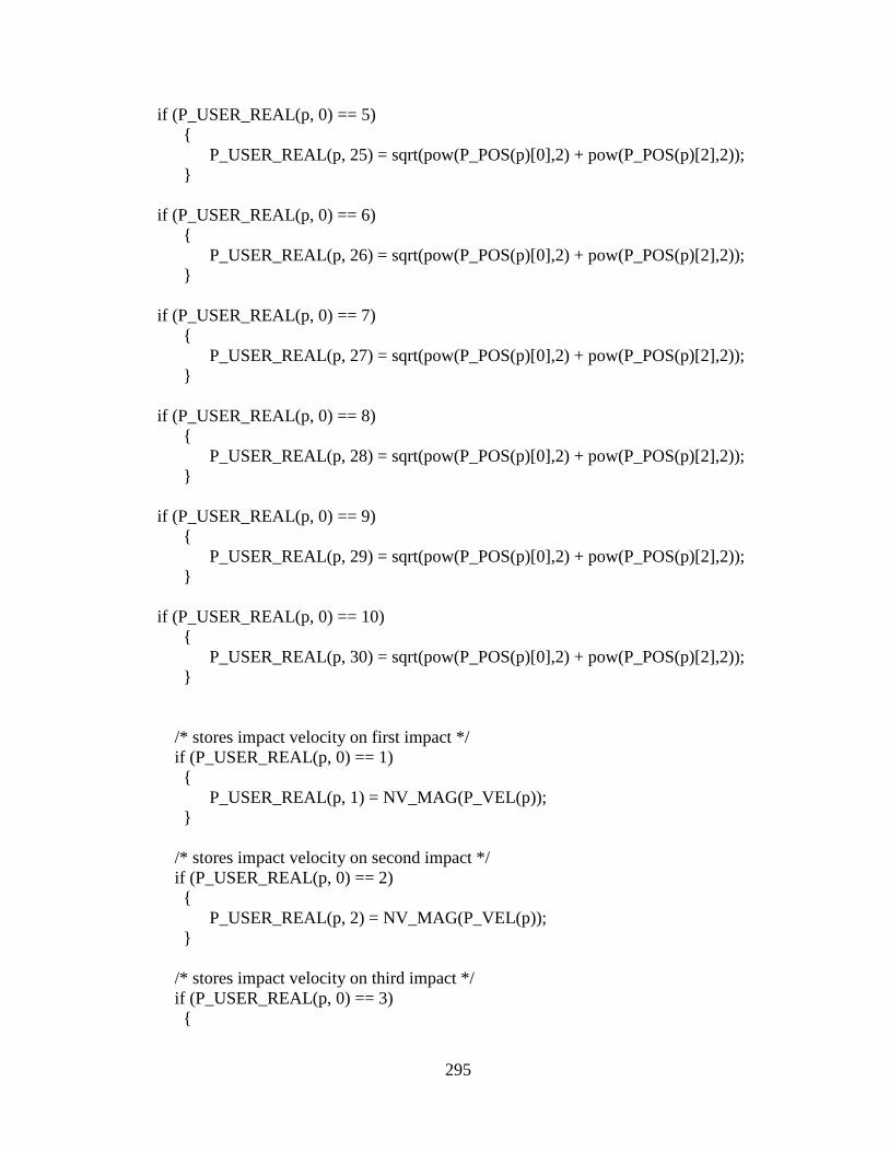
295

if (P_USER_REAL(p, 0) == 5)

{

P_USER_REAL(p, 25) = sqrt(pow(P_POS(p)[0],2) + pow(P_POS(p)[2],2));

}

if (P_USER_REAL(p, 0) == 6)

{

P_USER_REAL(p, 26) = sqrt(pow(P_POS(p)[0],2) + pow(P_POS(p)[2],2));

}

if (P_USER_REAL(p, 0) == 7)

{

P_USER_REAL(p, 27) = sqrt(pow(P_POS(p)[0],2) + pow(P_POS(p)[2],2));

}

if (P_USER_REAL(p, 0) == 8)

{

P_USER_REAL(p, 28) = sqrt(pow(P_POS(p)[0],2) + pow(P_POS(p)[2],2));

}

if (P_USER_REAL(p, 0) == 9)

{

P_USER_REAL(p, 29) = sqrt(pow(P_POS(p)[0],2) + pow(P_POS(p)[2],2));

}

if (P_USER_REAL(p, 0) == 10)

{

P_USER_REAL(p, 30) = sqrt(pow(P_POS(p)[0],2) + pow(P_POS(p)[2],2));

}

/* stores impact velocity on first impact */

if (P_USER_REAL(p, 0) == 1)

{

P_USER_REAL(p, 1) = NV_MAG(P_VEL(p));

}

/* stores impact velocity on second impact */

if (P_USER_REAL(p, 0) == 2)

{

P_USER_REAL(p, 2) = NV_MAG(P_VEL(p));

}

/* stores impact velocity on third impact */

if (P_USER_REAL(p, 0) == 3)

{

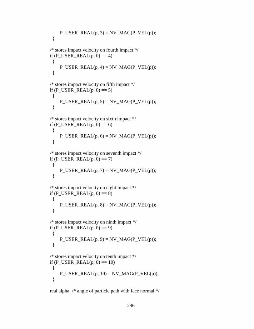
296

P_USER_REAL(p, 3) = NV_MAG(P_VEL(p));

}

/* stores impact velocity on fourth impact */

if (P_USER_REAL(p, 0) == 4)

{

P_USER_REAL(p, 4) = NV_MAG(P_VEL(p));

}

/* stores impact velocity on fifth impact */

if (P_USER_REAL(p, 0) == 5)

{

P_USER_REAL(p, 5) = NV_MAG(P_VEL(p));

}

/* stores impact velocity on sixth impact */

if (P_USER_REAL(p, 0) == 6)

{

P_USER_REAL(p, 6) = NV_MAG(P_VEL(p));

}

/* stores impact velocity on seventh impact */

if (P_USER_REAL(p, 0) == 7)

{

P_USER_REAL(p, 7) = NV_MAG(P_VEL(p));

}

/* stores impact velocity on eight impact */

if (P_USER_REAL(p, 0) == 8)

{

P_USER_REAL(p, 8) = NV_MAG(P_VEL(p));

}

/* stores impact velocity on ninth impact */

if (P_USER_REAL(p, 0) == 9)

{

P_USER_REAL(p, 9) = NV_MAG(P_VEL(p));

}

/* stores impact velocity on tenth impact */

if (P_USER_REAL(p, 0) == 10)

{

P_USER_REAL(p, 10) = NV_MAG(P_VEL(p));

}

real alpha; /* angle of particle path with face normal */

297

real vn=0.;

real nor_coeff = 1.0;

real tan_coeff = 1.0;

real normal[3];

int i, idim = dim;

real NV_VEC(x);

#if RP_2D

/* dim is always 2 in 2D compilation. Need special treatment for 2d

axisymmetric and swirl flows */

if (rp_axi_swirl)

{

real R = sqrt(P_POS(p)[1]*P_POS(p)[1] +

P_POS(p)[2]*P_POS(p)[2]);

if (R > 1.e-20)

{

idim = 3;

normal[0] = f_normal[0];

normal[1] = (f_normal[1]*P_POS(p)[1])/R;

normal[2] = (f_normal[1]*P_POS(p)[2])/R;

}

else

{

for (i=0; i<idim; i++)

normal[i] = f_normal[i];

}

}

else

#endif

for (i=0; i<idim; i++)

normal[i] = f_normal[i];

if(p->type==DPM_TYPE_INERT)

{

alpha = (180/M_PI)*((M_PI/2) -

acos(NV_DOT(f_normal,P_VEL(p))/NV_MAG(P_VEL(p))));

/* stores impact angle on first impact */

if (P_USER_REAL(p, 0) == 1)

{

P_USER_REAL(p, 11) = alpha;

}

/* stores impact angle on second impact */

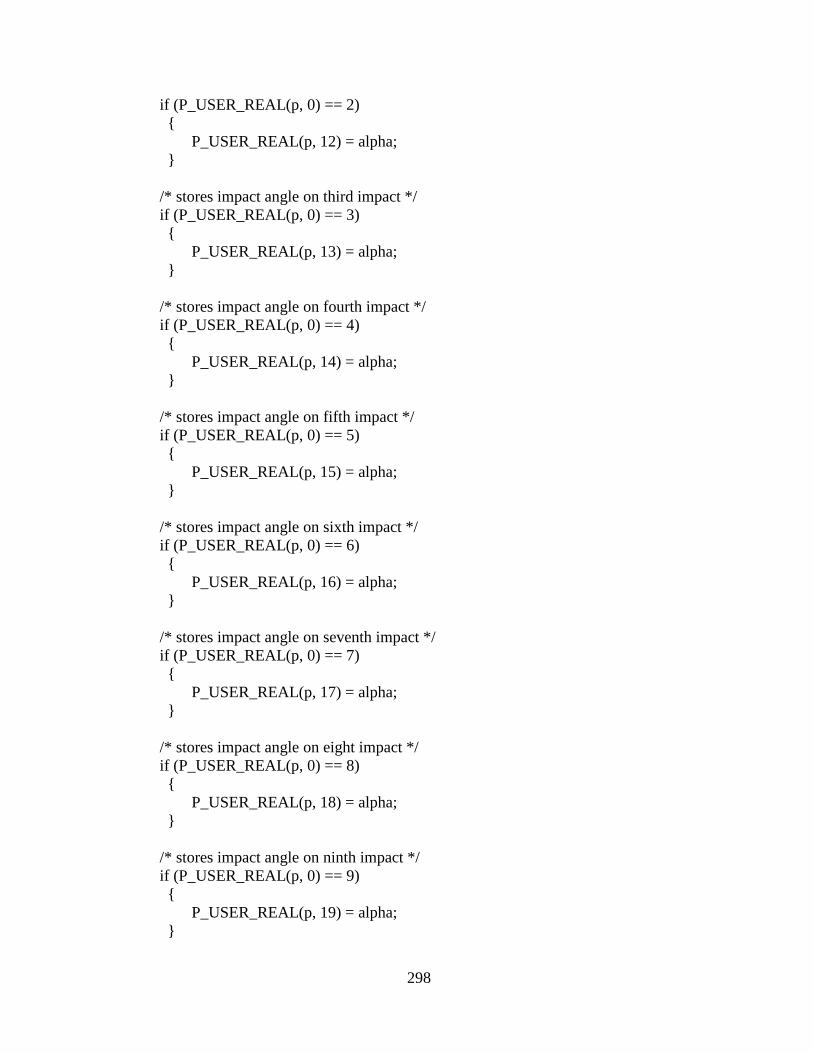
298

if (P_USER_REAL(p, 0) == 2)

{

P_USER_REAL(p, 12) = alpha;

}

/* stores impact angle on third impact */

if (P_USER_REAL(p, 0) == 3)

{

P_USER_REAL(p, 13) = alpha;

}

/* stores impact angle on fourth impact */

if (P_USER_REAL(p, 0) == 4)

{

P_USER_REAL(p, 14) = alpha;

}

/* stores impact angle on fifth impact */

if (P_USER_REAL(p, 0) == 5)

{

P_USER_REAL(p, 15) = alpha;

}

/* stores impact angle on sixth impact */

if (P_USER_REAL(p, 0) == 6)

{

P_USER_REAL(p, 16) = alpha;

}

/* stores impact angle on seventh impact */

if (P_USER_REAL(p, 0) == 7)

{

P_USER_REAL(p, 17) = alpha;

}

/* stores impact angle on eight impact */

if (P_USER_REAL(p, 0) == 8)

{

P_USER_REAL(p, 18) = alpha;

}

/* stores impact angle on ninth impact */

if (P_USER_REAL(p, 0) == 9)

{

P_USER_REAL(p, 19) = alpha;

}

299

/* stores impact angle on tenth impact */

if (P_USER_REAL(p, 0) == 10)

{

P_USER_REAL(p, 20) = alpha;

}

if ((NNULLP(t)) && (THREAD_TYPE(t) == THREAD_F_WALL))

F_CENTROID(x,f,t);

/* calculate the normal component, rescale its magnitude by

the coefficient of restitution and subtract the change */

/* Compute normal velocity. */

for(i=0; i<idim; i++)

vn += P_VEL(p)[i]*normal[i];

/* Subtract off normal velocity. */

for(i=0; i<idim; i++)

P_VEL(p)[i] -= vn*normal[i];

/* Apply tangential coefficient of restitution. */

for(i=0; i<idim; i++)

P_VEL(p)[i] *= tan_coeff;

/* Add reflected normal velocity. */

for(i=0; i<idim; i++)

P_VEL(p)[i] -= nor_coeff*vn*normal[i];

/* Store new velocity in P_VEL0 of particle */

for(i=0; i<idim; i++)

P_VEL0(p)[i] = P_VEL(p)[i];

return PATH_ACTIVE;

}

return PATH_ABORT;

}

300

This code serves as a sampling tool to extract the particle impact data from the

P_USER_REAL(p,x) variables. The code is activated using the Reports -> Discrete

Phase -> Sample task in FLUENT where the boundary chosen to sample from is the

outlet. This means that as the particles pass through the outlet boundary, all the

P_USER_REAL(p,x) variables are read and stored in a data file for easy post-

processing to take place in MATLAB.

#include "udf.h"

/******************************************************************/

/* UDF that samples discrete phase size and velocity distributions*/

/* within the domain. */

/******************************************************************/

#define REMOVE_PARTICLES FALSE

DEFINE_DPM_OUTPUT(discrete_phase_sample,header,fp,p,t,plane)

{

#if RP_2D

real y;

if(header)

{

par_fprintf_head(fp," #Time[s] R [m] X-velocity[m/s]");

par_fprintf_head(fp," W-velocity[m/s] R-velocity[m/s] ");

par_fprintf_head(fp,"Drop Diameter[m] Number of Drops ");

par_fprintf_head(fp,"Temperature [K] Initial Diam [m] ");

par_fprintf_head(fp,"Injection Time [s] \n");

}

if(NULLP(p))

return;

if (rp_axi && (sg_swirl || rp_ke))

y = MAX(sqrt(SQR(P_POS(p)[1]) + SQR(P_POS(p)[2])),DPM_SMALL);

else

y = P_POS(p)[1];

par_fprintf(fp,"%d %" int64_fmt " %e %f %f %f %f %e %e %f %e %f \n",

P_INJ_ID(P_INJECTION(p)),p->part_id, P_TIME(p),y,P_VEL(p)[0],

P_VEL(p)[1],P_VEL(p)[2],P_DIAM(p),P_N(p),

P_T(p), P_INIT_DIAM(p),p->time_of_birth);

#else

real r, x, y;

if(header)

{

par_fprintf_head(fp," v1 v2 v3 v4 v5 v6 v7 v8 v9 v10 a1

a2 a3 a4 a5 a6 a7 a8 a9 a10 P1 P2 P3 P4 P5 P6

P7 P8 P9 P10 D\n");

301

}

if(NULLP(p))

return;

x = P_POS(p)[0];

y = P_POS(p)[1];

r = sqrt(SQR(x) + SQR(y));

par_fprintf(fp,"%d %" int64_fmt " %6.3f %6.3f %6.3f %6.3f %6.3f %6.3f %6.3f

%6.3f %6.3f %6.3f %6.3f %6.3f %6.3f %6.3f %6.3f %6.3f %6.3f %6.3f %6.3f %6.3f

%6.6f %6.6f %6.6f %6.6f %6.6f %6.6f %6.6f %6.6f %6.6f %6.6f %6.8f\n",

P_INJ_ID(P_INJECTION(p)),p-

>part_id,P_USER_REAL(p,1),P_USER_REAL(p,2),P_USER_REAL(p,3),P_USER_

REAL(p,4),P_USER_REAL(p,5),P_USER_REAL(p,6),P_USER_REAL(p,7),P_USE

R_REAL(p,8),P_USER_REAL(p,9),P_USER_REAL(p,10),P_USER_REAL(p,11),P

_USER_REAL(p,12),P_USER_REAL(p,13),P_USER_REAL(p,14),P_USER_REAL

(p,15),P_USER_REAL(p,16),P_USER_REAL(p,17),P_USER_REAL(p,18),P_USER

_REAL(p,19),P_USER_REAL(p,20),P_USER_REAL(p,21),P_USER_REAL(p,22),

P_USER_REAL(p,23),P_USER_REAL(p,24),P_USER_REAL(p,25),P_USER_REA

L(p,26),P_USER_REAL(p,27),P_USER_REAL(p,28),P_USER_REAL(p,29),P_USE

R_REAL(p,30),P_DIAM(p));

#endif

#if REMOVE_PARTICLES

MARK_PARTICLE(p, P_FL_REMOVED);

#endif

}

302

This UDF contains the final code of the erosion model developed.

#include "udf.h"

#include "dpm.h"

DEFINE_DPM_EROSION(Scattergood, p, t, f, normal, alpha, Vmag, Mdot)

{

real A[ND_ND], area;

double k = 4866920;

double n = 4.75;

double m = 4.186;

//k is A in the delta w equation

F_AREA(A,f,t);

area = NV_MAG(A);

F_STORAGE_R(f,t,SV_DPMS_EROSION) +=

k*pow(P_DIAM(p),m)*pow(1.00*Vmag,n)*pow(sin(alpha),0.375)*pow(cos(alpha),2

)*Mdot/area;

}

303

Appendix D – MATLAB Post-Processing Codes

This code was used to formulate the erosion profile graphs and to calculate the total

amount of material removed. Once generated, the graphs were then used to identify

the maximum eroded depth. This code was used in the test case: 104010D.

% Obtain middle peak of Edited Data image LR_LengthPeak = 5415.4; UD_LengthPeak = 4781.1; LR_HeightPeak = 5.2226; % offset above y = 0 UD_HeightPeak = 9.8226; % offset above y = 0

% Obtain resolution from raw Data ScanLength = 11600; % microns delimiterIn = ' '; headerlinesIn = 4; LR_RawData =

importdata('LR_104010D_raw.txt',delimiterIn,headerlinesIn); UD_RawData =

importdata('UD_104010D_raw.txt',delimiterIn,headerlinesIn); LR_ptDist = ScanLength / length(LR_RawData.data(:,1)); UD_ptDist = ScanLength / length(UD_RawData.data(:,1));

% Code for edited LR Scan f1 = figure(); A = importdata('LR_104010D_edited.txt',delimiterIn,headerlinesIn); LR_HeightEdited = A.data(:,4)/10000 - LR_HeightPeak; LR_LengthEdited =

transpose([0:LR_ptDist:LR_ptDist*length(A.data(:,1))-LR_ptDist]); area(LR_LengthEdited, LR_HeightEdited, 0) xlabel('Scan Length (\mum)', 'fontsize', 24); ylabel('Depth (\mum)', 'fontsize', 24); title('LR-104010D Profilometer Scan', 'fontsize', 24') axis([0, LR_LengthEdited(length(LR_LengthEdited)), -12, 2]) set(gca,'ytick',[-12:2:0], 'fontsize', 24); set(gca, 'LineWidth', 2); grid on %grid minor

% Calculating the volume over 180 degrees of rotation LR_discrVolArray = []; for i=1:1:size(LR_LengthEdited)-1 LR_discrVolArray(i) =

0.5*abs(pi()*LR_HeightEdited(i)*abs((abs(LR_LengthPeak-

LR_LengthEdited(i)-LR_ptDist/2))^2 - (abs(LR_LengthPeak-

LR_LengthEdited(i)+LR_ptDist/2))^2)); end

% Code for edited UD Scan B = importdata('UD_104010D_edited.txt',delimiterIn,headerlinesIn); UD_HeightEdited = B.data(:,1)/10000 - UD_HeightPeak;

304

UD_LengthEdited =

transpose([0:UD_ptDist:UD_ptDist*length(B.data(:,1))-UD_ptDist]); f2 = figure(); area(UD_LengthEdited, UD_HeightEdited, 0) title('UD-104010D Profilometer Scan', 'fontsize', 24) xlabel('Scan Length (\mum)', 'fontsize', 24); ylabel('Depth (\mum)', 'fontsize', 24); axis([0, UD_LengthEdited(length(UD_LengthEdited)), -12, 2]) set(gca,'ytick',[-12:2:0], 'fontsize', 24); set(gca, 'LineWidth', 2); grid on %grid minor

% Calculating the volume over 180 degrees of rotation UD_discrVolArray = []; for i=1:1:size(UD_LengthEdited)-1 UD_discrVolArray(i) =

0.5*abs(pi()*UD_HeightEdited(i)*abs((abs(UD_LengthPeak-

UD_LengthEdited(i)-UD_ptDist/2))^2 - (abs(UD_LengthPeak-

UD_LengthEdited(i)+UD_ptDist/2))^2)); end

saveas(f1,'LR-104010D Profilometer Scan.jpg') saveas(f2,'UD-104010D Profilometer Scan.jpg') DensitySi = 2329; % kg/m^3 UD_TotalErodedVolumeMicrons3 = sum(UD_discrVolArray) UD_TotalErodedVolumeMeter3 = UD_TotalErodedVolumeMicrons3*10^-18; UD_MassLoss = UD_TotalErodedVolumeMeter3*DensitySi*10^6 LR_TotalErodedVolumeMicrons3 = sum(LR_discrVolArray) LR_TotalErodedVolumeMeter3 = LR_TotalErodedVolumeMicrons3*10^-18; LR_MassLoss = LR_TotalErodedVolumeMeter3*DensitySi*10^6

305

This code contains the post-processing script used to analyze the particle impact data.

A number of metrics and values were calculated in this code including the average

impact velocity and average impact angle for each of the ten impacts, percentage of

entrained particles that impact the surface, the total impacting mass flow rate, and the

summation metric used in the model calibration. Additionally, if the radial impact

location was larger than the experimental graph boundaries, the impact was not

included in the analysis.

%% Particle Post-Processing

% considers first 10 impacts for each particle v1-10, a1-10 fileIn = importdata('34C_320K_40ms_10mic_Water.dat',' ',1); rawData = fileIn.data; aveImpact = mean(rawData);

numImpactsConsidered = 10; % splits rawData into three matrices rawVel = abs(rawData(:,1:numImpactsConsidered)); rawAng = abs(rawData(:,11:(10+numImpactsConsidered))); rawPos = abs(rawData(:,21:(20+numImpactsConsidered)));

avgPerc = []; avgVel = []; avgAng = []; avgPos = [];

for i=1:numImpactsConsidered avgPerc(i) = nnz(rawVel(:,i))/length(rawData); avgVel(i) = sum(rawVel(:,i))/nnz(rawVel(:,i)); avgAng(i) = sum(rawAng(:,i))/nnz(rawAng(:,i)); avgPos(i) = sum(rawPos(:,i))/nnz(rawPos(:,i)); end

% moves all velocity and angle data into single columns velCol = rawVel(:); angCol = rawAng(:); posCol = rawPos(:);

%takes out impacts past a radial position maxPos = 5012.5e-6; newVelCol = []; newAngCol = [];

for i=1:length(posCol) if(posCol(i) < maxPos) newVelCol(i,1) = velCol(i); newAngCol(i,1) = angCol(i); else newVelCol(i,1) = 0; newAngCol(i,1) = 0; end end

306

masterArray = zeros(length(velCol), 3);

% Nandakumar erosion models % col-1 = combined, col-2 = line, col-3 = area masterArray(:,1) = cosd(angCol).^2;

exp = [4:0.1:6.6]; combined = zeros(length(masterArray),length(exp));

% raises each impact velocity to a fitted pwoer for i= 1:length(exp) combined(:,i) = newVelCol.^exp(i).*masterArray(:,1); %line(:,i) = velCol(:,1).^exp(i).*masterArray(:,2); %area(:,i) = velCol(:,1).^exp(i).*masterArray(:,3); end

% calculates sum metric for erosion model sumCombined = sum(combined);

QSYMpartMassFR = 3.0606e-05; % [kg/s] Particle mass flowrate, from

FLUENT injection for WATER trackFR = QSYMpartMassFR / length(rawVel); % mass FR per particle

track numImpacts = nnz(newVelCol); % total number of impacts impMassFR = 4*numImpacts*trackFR

307

Bibliography

[1] DARPA-BAA-1250. Intrachip/Interchip Enhanced Cooling Fundamentals (ICECool

Fundamentals). Microsystems Technology Office, June 7, 2012.

[2] DARPA-BAA-13-21. ICECool Applications (ICECool Apps). Microsystems

Technology Office, February 6, 2013.

[3] G. Jiang, L. Diao and K. Kuang, Properties of WCu, MoCu, and Cu/MoCu/Cu High-

performance Heat Sink Materials and Manufacturing Technologies, In Advanced

Thermal Management Materials (pp. 73-87). Springer New York., 2013.

[4] M. Faqir, T. Batten, T. Mrotzek, S. Knippscheer, M. Massiot, M. Buchta and M.

Kuball, Improved thermal management for GaN power electronics: Silver diamond

composite packages, Microelectronics Reliability, 52(12), 3022-3025, 2012.

[5] S. Narumanchi, M. Mihalic, K. Kelly and G. Eesley, Thermal interface materials for

power electronics applications, Thermal and Thermomechanical Phenomena in

Electronic Systems, ITHERM 2008. 11th Intersociety Conference, 2008.

[6] C. Creamer, K. Chu, P. Chao, B. Schmanski, T. Yurovchak, S. Sweetland and P.

McCluskey, S2-T6: Microchannel cooled, high power GaN-on-Diamond MMIC,

Lester Eastman Conference on High Performance Devices, 2014.

[7] C. J, R. Myers, F. Wood and S. Binari, Simulations of direct-die-attached

microchannel coolers for the thermal management of GaN-on-SiC microwave

amplifiers, Components and Packaging Technologies, IEEE Transactions on, 28(4),

79, 2005.

[8] P. McCluskey, T. Podlesak and R. Grzybowski, High temperature electronics, CRC

press, 1996.

[9] D. Squiller, H. Greve, E. Mengotti and P. McCluskey, Physics-of-failure assessment

methodology for power electronic systems, Microelectronics Reliability, 54(9), 1680-

1685.

[10] G. Beheim, P. Neudeck, D. Spry, M. Scardelletti, G. Ponchak, R. Meredith and G.

Hunter, High Temperature SiC Electronics: Update and Outlook, Propulsion Controls

and Diagnostics Workshop Cleveland (pp. 28-29), 2012.

[11] A. Kashyap, C. Chen, R. Ghandi, A. Patil, E. Andarawis, L. Yin and W. Johnson,

Silicon carbide integrated circuits for extreme environments, Wide Bandgap Power

Devices and Applications (WiPDA), 2013 IEEE Workshop, 2013.

308

[12] B. Ozpineci and L. Tolbert, Comparison of wide-bandgap semiconductors for power

electronics applications, United States. Department of Energy, 2004.

[13] Wolfspeed, [Online]. Available:

http://www.wolfspeed.com/Power/Products/MOSFETs/TO247/C2M1000170D.

[Accessed December 2015].

[14] J. Felbinger, M. Chandra, Y. Sun, L. Eastman, J. Wasserbauer, F. Fali and F.

Ejeckam, Comparison of GaN HEMTs on diamond and SiC substrates, Electron

Device Letters, IEEE, 28(11), 948-950, 2007.

[15] R. Pengelly, S. Wood, J. Milligan, S. Sheppard and W. Pribble, A review of GaN on

SiC high electron-mobility power transistors and MMICs, Microwave Theory and

Techniques, IEEE Transactions on, 60(6), 1764-1783.

[16] J. Chung, K. Ryu, B. Lu and T. Palacios, GaN-on-Si technology, a new approach for

advanced devices in energy and communications, Solid-State Device Research

Conference (ESSDERC) (pp. 52-56), 2010.

[17] D. Tuckerman and R. Pease, High-performance heat sinking for VLSI, Electron

Device Letters, IEEE, 2(5), 126-129, 1981.

[18] F. Laermer and A. Urban, Challenges, developments and applications of silicon deep

reactive ion etching, Microelectronic Engineering, 67, 349-355, 2003.

[19] G. Harpole and J. Eninger, Micro-channel heat exchanger optimization,

Semiconductor Thermal Measurement and Management Symposium, 1991. SEMI-

THERM VII (pp. 59-63), 1991.

[20] L. Boteler, Microfabrication and analysis of manifold microchannel coolers for

power electronics (Doctoral Dissertation), UNIVERSITY OF MARYLAND,

COLLEGE PARK, 2001.

[21] L. Boteler, N. Jankowski, P. McCluskey and B. Morgan, Numerical investigation and

sensitivity analysis of manifold microchannel coolers, International Journal of Heat

and Mass Transfer, 55(25), 7698-7708, 2012.

[22] M. Ohadi, K. Choo, S. Dessiatoun and E. Cetegen, Next Generation Microchannel

Heat Exchangers, Springer, 2013.

[23] E. Colgan, B. Furman, M. Gaynes, W. Graham, N. LaBianca, J. Magerlein and R.

Schmidt, A practical implementation of silicon microchannel coolers for high power

chips, Components and Packaging Technologies, IEEE Transactions, 2007.

309

[24] K. Moores, Y. Joshi and G. Schiroky, Thermal characterization of a liquid cooled

AlSiC base plate with integral pin fins, Components and Packaging Technologies,

IEEE Transactions on, 24(2), 213-219, 2001.

[25] A. Kosar and Y. Peles, Boiling heat transfer in a hydrofoil-based micro pin fin heat

sink, International Journal of Heat and Mass Transfer, 50(5), 1018-1034, 2007.

[26] J. Ditri, M. McNulty and S. Igoe, S3-P10: Embedded microfluidic cooling of high

heat flux electronic components, Lester Eastman Conference on High Performance

Devices (pp. 1-4)., 2014.

[27] Y. Han, B. Lau, H. Zhang and X. Zhang, Package-level Si-based micro-jet

impingement cooling solution with multiple drainage micro-trenches, Electronics

Packaging Technology Conference (pp. 330-334), 2014.

[28] A. Bhunia, A. Brackley, C. Nguyen and B. Brar, Device scale heat removal for high

power density GaN devices, Compound Semiconductor Integrated Circuit Symposium

(pp. 1-4), 2012.

[29] S. Narumanchi, V. Hassani and D. Bharathan, Modeling single-phase and boiling

liquid jet impingement cooling in power electronics, National Renewable Energy

Laboratory, 2005.

[30] K. Kapur and M. Pecht, Reliability Engineering, John Wiley & Sons, 2014.

[31] M. Pecht and D. A, Physics-of-failure: an approach to reliable product development,

Journal of the IES, 38(5), 30-34, 1995.

[32] C. Glassbrenner and G. Slack, Thermal conductivity of silicon and germanium from 3

K to the melting point, Physical Review, 134(4A), A1058, 1964.

[33] R. Powell, C. Ho and P. Liley, Thermal Conductivity of Selected Materials, National

Standard Reference Data Series - National Bureau of Standards, 1996.

[34] V. Souza and A. Neville, Corrosion and synergy in a WC Co Cr HVOF thermal spray

coating—understanding their role in erosion–corrosion degradation, Wear, 259(1),

171-180, 2005.

[35] M. Stack and G. Abdulrahman, Mapping erosion-corrosion of carbon steel in oil

exploration conditions: Some new approaches to characterizing mechanisms and

synergies, Tribology International, 43(7), 1268-1277, 2010.

[36] R. Wood, Tribo-corrosion of coatings: a review, Journal of Physics D: Applied

Physics, 40(18), 5502, 2007.

310

[37] C. Henry, J. Minier and G. Lefevre, Towards a description of particulate fouling:

From single particle deposition to clogging, Advances in colloid and interface

science, 185, 34-76, 2012.

[38] I. Finnie, Erosion of surfaces by solid particles, Wear, 3(2), 87-103., 1960.

[39] G. Sheldon and I. Finnie, The mechanism of material removal in the erosive cutting of

brittle materials, Journal of Manufacturing Science and Engineering, 88(4), 393-399,

1966.

[40] G. Sheldon and I. Finnie, On the ductile behavior of nominally brittle materials

during erosive cutting, Journal of Manufacturing Science and Engineering, 88(4),

387-392, 1966.

[41] A. Smekal and W. Klemm, Mechanische Messung chemischer Bindefestigkeiten,

Monatshefte für Chemie/Chemical Monthly, 82(3), 411-421, 1951.

[42] A. Smekal, Uber die Abmessungen ideates Kristallgittes, Acta Physica Austriaca, 7,

324., 1953.

[43] W. Klemm and A. Smekal, über den Grundvorgang des Polierens von Gläsern,

Naturwissenschaften, 29(45), 688-690., 1941.

[44] B. Hockey, Plastic deformation of aluminum oxide by indentation and abrasion,

Journal of the American Ceramic Society 54.5 (1971): 223-231.

[45] B. Lawn and R. Wilshaw, Indentation fracture: principles and applications, Journal

of Materials Science, 10(6), 1049-1081, 1975.

[46] B. Lawn, M. Swain and K. Philips, On the mode of chipping fracture in brittle solids,

Journal of Materials Science 10.7 (1975): 1236-1239, 1975.

[47] S. Srinivasan and R. Scattergood, On lateral cracks in glass, Journal of materials

science, 22(10), 3463-3469, 1987.

[48] B. Hockey and B. Lawn, Electron microscopy of microcracking about indentations in

aluminium oxide and silicon carbide, Journal of Materials Science, 10(8), 1275-1284,

1975.

[49] A. Evans and T. Wilshaw, Quasi-static solid particle damage in brittle solids—I.

Observations analysis and implications, Acta Metallurgica, 24(10), 939-956, 1976.

[50] A. Evans and T. Wilshaw, Dynamic solid particle damage in brittle materials: an

appraisal, Journal of Materials Science, 12(1), 97-116, 1977.

311

[51] M. Swain and B. Lawn, Indentation fracture in brittle rocks and glasses, International

Journal of Rock Mechanics and Mining Sciences & Geomechanics Abstracts. Vol. 13.

No. 11. Pergamon, 1976.

[52] B. Lawn and A. Evans, A model for crack initiation in elastic/plastic indentation

fields, Journal of Materials Science, 12(11), 2195-2199, 1977.

[53] C. Perrott, Elastic-plastic indentation: Hardness and fracture, Wear, 45(3), 293-309,

1977.

[54] J. Lankford and D. Davidson, The crack-initiation threshold in ceramic materials

subject to elastic/plastic indentation, Journal of Materials Science, 14(7), 1662-1668,

1979.

[55] B. Lawn and D. Marshall, Hardness, Toughmess, and Brittleness: An Indentation

Analysis, J. Am. Ceram. Soc., 62(7), 347, 1979.

[56] B. Lawn, A. Evans and D. Marshall, Elastic/plastic indentation damage in ceramics:

the median/radial crack system, Journal of the American Ceramic Society, 63(9‐10),

574-581, 1980.

[57] D. Marshall, B. Lawn and A. Evans, Elastic/plastic indentation damage in ceramics:

the lateral crack system, Journal of the American Ceramic Society, 65(11), 561-566,

1982.

[58] D. Tabor, Hardness of Metals, Clarendon Press, Oxford, 1951.

[59] S. Wiederhorn and B. Lawn, Strength degradation of glass impacted with sharp

particles: I, Annealed surfaces, Journal of the American Ceramic Society, 62(1‐2),

66-70, 1979.

[60] A. Ruff and S. Wiederhorn, Erosion by solid particle impact (No. NBSIR-78-1575),

National Bureau of Standards, National Measurement Lab. Gaithersburg, MD., 1979.

[61] B. Hockey, S. Wiederhorn and H. Johnson, Erosion of brittle materials by solid

particle impact (pp. 379-402), Springer US, 1978.

[62] A. Evans, M. Gulden and M. Rosenblatt, Impact damage in brittle materials in the

elastic-plastic response regime, Proceedings of the Royal Society of London A:

Mathematical, Physical and Engineering Sciences (Vol. 361, No. 1706, pp. 343-365),

1978.

[63] S. Wiederhorn and B. Hockey, Effect of material parameters on the erosion resistance

of brittle materials, Journal of Materials Science, 18(3), 766-780, 1983.

312

[64] D. Tabor, A simple theory of static and dynamic hardness, Proceedings of the Royal

Society of London A: Mathematical, Physical and Engineering Sciences (Vol. 192,

No. 1029, pp. 247-274), 1948.

[65] J. Routbort, R. Scattergood and E. Kay, Erosion of silicon single crystals, Journal of

the American Ceramic Society, 63(11‐12), 635-640, 1980.

[66] J. Routbort, R. Scattergood and A. Turner, The erosion of reaction-bonded SiC, Wear,

59(2), 363-375, 1980.

[67] R. Scattergood and J. Routbort, Velocity and size dependences of the erosion rate in

silicon, Wear, 67(2), 227-232, 1981.

[68] J. Routbort and R. Scattergood, Anomalous Solid‐Particle Erosion Rate of Hot‐

Pressed Silicon Carbide, Journal of the American Ceramic Society, 63(9‐10), 593-

595, 1980.

[69] R. Scattergood and J. Routbort, Velocity Exponent in Solid‐Particle Erosion of

Silicon, Journal of the American Ceramic Society, 66(10), c184-c186, 1983.

[70] C. Yust and R. Crouse, Melting at particle impact sites during erosion of ceramics,

Wear, 51(1), 193-196, 1978.

[71] P. Shewmon, Particle size threshold in the erosion of metals, Wear, 68(2), 253-258,

1981.

[72] R. Telling and J. Field, The erosion of diamond, sapphire and zinc sulphide by quartz

particles, Wear, 233, 666-673, 1999.

[73] F. Auerbach, Measurement of hardness, Ann. Phys. Chem, 43, 61, 1891.

[74] R. Mouginot and D. Maugis, Fracture indentation beneath flat and spherical punches,

Journal of Materials Science, 20(12), 4354-4376, 1985.

[75] R. Jaccodine, Surface energy of germanium and silicon, Journal of The

Electrochemical Society, 110(6), 524-527, 1963.

[76] J. Humphrey, Fundamentals of fluid motion in erosion by solid particle impact,

International Journal of Heat and Fluid Flow, 11(3), 170-195, 1990.

[77] H. Clark, On the impact rate and impact energy of particles in a slurry pot erosion

tester, Wear, 147(1), 165-183, 1991.

[78] H. Clark, The influence of the flow field in slurry erosion, Wear, 152(2), 223-240,

1992.

313

[79] H. Clark, The influence of the squeeze film in slurry erosion, Wear, 256(9), 918-926,

2004.

[80] H. Clark and L. Burmeister, The influence of the squeeze film on particle impact

velocities in erosion, International journal of impact engineering, 12(3), 415-426,

1992.

[81] H. Clark and R. Hartwich, A re-examination of the ‘particle size effect’ in slurry

erosion, Wear, 248(1), 147-161, 2001.

[82] A. Gadhikar, A. Aniruddha, A. Sharma, D. Goel and C. Sharma, Fabrication and

testing of slurry pot erosion tester, Transactions of the Indian Institute of Metals,

64(4-5), 493-500, 2011.

[83] S. Rajahram, T. Harvey and R. Wood, Electrochemical investigation of erosion–

corrosion using a slurry pot erosion tester, Tribology International, 44(3), 232-240,

2011.

[84] G. Desale, B. Gandhi and S. Jain, Improvement in the design of a pot tester to

simulate erosion wear due to solid–liquid mixture, Wear, 259(1), 196-202, 2005.

[85] S. Lathabai and D. Pender, Microstructural influence in slurry erosion of ceramics,

Wear, 189(1), 122-135, 1995.

[86] R. Lynn, K. Wong and H. Clark, On the particle size effect in slurry erosion, Wear,

149(1), 55-71, 1991.

[87] B. Ghandi and S. Borse, Nominal particle size of multi-sized particulate slurries for

evaluation of erosion wear and effect of fine particles, Wear, 257(1), 73-79, 2004.

[88] Q. Fang, H. Xu, P. Sidky and M. Hocking, Erosion of ceramic materials by a

sand/water slurry jet, Wear, 224(2), 183-193, 1999.

[89] Y. Zhang, Y. Cheng and S. Lathabai, Erosion of alumina ceramics by air-and water-

suspended garnet particles, Wear, 240(1), 40-51, 2000.

[90] J. Zhou and S. Bahadur, Erosion characteristics of alumina ceramics at high

temperatures, Wear, 181, 178-188, 1995.

[91] O. Ajayi and K. Ludema, The effect of microstructure on wear modes of ceramic

materials, Wear, 154(2), 371-385.

[92] J. Wang, T. Nguyen and K. Pang, Mechanisms of microhole formation on glasses by

an abrasive slurry jet, Journal of Applied Physics, 105(4), 044906, 2009.

314

[93] J. Wang, Abrasive Waterjet Machining of Engineering Materials, Trans Tech

Publications Ltd, Zurich, Switzerland, 2003.

[94] A. Momber and R. Kovacevic, Principles of abrasive water jet machining, Springer

Science & Business Media, 1998 and 2012.

[95] K. Dadkhahipour, T. Nguyen and J. Wang, Mechanisms of channel formation on

glasses by abrasive waterjet milling, Wear, 292, 1-10, 2012.

[96] K. Pang, T. Nguyen, J. Fan and J. Wang, A study of micro-channeling on glasses

using an abrasive slurry jet, Machining Science and Technology, 16(4), 547-563,

2012.

[97] H. Nouraei, A. Wodoslawsky, M. Papini and J. Spelt, Characteristics of abrasive

slurry jet micro-machining: a comparison with abrasive air jet micro-machining,

Journal of Materials Processing Technology, 213(10), 1711-1724, 2013.

[98] A. Ghobeity, T. Krajac, T. Burzynski, M. Papini and J. Spelt, Surface evolution

models in abrasive jet micromachining, Wear, 264(3), 185-198, 2008.

[99] A. Ghobeity, D. Ciampini and M. Papini, An analytical model of the effect of particle

size distribution on the surface profile evolution in abrasive jet micromachining,

Journal of Materials Processing Technology, 209(20), 6067-6077, 2009.

[100] H. Wensink and M. Elwenspoek, A closer look at the ductile–brittle transition in solid

particle erosion, Wear, 253(9), 1035-1043, 2002.

[101] A. Ghobeity, H. Getu, M. Papini and J. Spelt, Surface evolution models for abrasive

jet micromachining of holes in glass and polymethylmethacrylate (PMMA), Journal of

Micromechanics and Microengineering, 17(11), 2175, 2007.

[102] H. Li, Z. Wang and J. Fan, Analysis and modelling of particle velocities in micro-

abrasive air jet, International Journal of Machine Tools and Manufacture, 49(11),

850-858, 2009.

[103] D. Dehnadfar, J. Friedman and M. Papini, Laser shadowgraphy measurements of

abrasive particle spatial, size and velocity distributions through micro-masks used in

abrasive jet micro-machining, Journal of Materials Processing Technology, 212(1),

137-149, 2012.

[104] K. Pang, T. Nguyen, J. Fan and J. Wang, Modelling of the micro-channelling process

on glasses using an abrasive slurry jet, International Journal of Machine Tools and

Manufacture, 53(1), 118-126, 2011.

315

[105] R. Jafar, H. Nouraei, M. Emamifar, M. Papini and J. Spelt, Erosion modeling in

abrasive slurry jet micro-machining of brittle materials, Journal of Manufacturing

Processes, 17, 127-140, 2015.

[106] P. Slikkerveer, P. Bouten, F. In't Veld and H. Scholten , Erosion and damage by sharp

particles, Wear, 217(2), 237-250, 1998.

[107] R. Jafar, J. Spelt and M. Papini, Surface roughness and erosion rate of abrasive jet

micro-machined channels: experiments and analytical model, Wear, 303(1), 138-145,

2013.

[108] J. Routbort, D. Singh, E. Tomofeeva, E. Yu and R. Smith, Erosion of Radiator

Materials by Nanofluids, Vehicle Technologies Annual Review. Argonne National

Lab, 2001.

[109] D. Singh and J. Routbort, Effects of nanofluids on heavy vehicle systems, Argonne

National Laboratory (ANL) Report, US Department of Energy, 2008.

[110] D. Singh, J. Routbort, T. Sofu and R. Smith, Erosion of Radiator Materials by

Nanofluids, Vehicle Technologies Annual Review. Argonne National Labs, 2009.

[111] C. Nguyen, G. Laplante, M. Cury and G. Simon, Experimental investigation of

impinging jet heat transfer and erosion effect using Al2O3-water nanofluid,

Proceedings of the 6th IASME/WSEAS International Conference on Fluid Mechanics

and Aerodynamics, 2008.

[112] G. Molina, F. Aktaruzzaman, W. Stregles, V. Soloiu and M. Rahman, Jet-

impingement effects of alumina-nanofluid on aluminum and copper, Advances in

Tribology, 2014.

[113] A. Sparks and I. Hutchings, Transitions in the erosive wear behaviour of a glass

ceramic, Wear 149.1 (1991): 99-110, 1991.

[114] I. Hutchings, Ductile-brittle transitions and wear maps for the erosion and abrasion

of brittle materials, Journal of Physics D: Applied Physics 25.1A (1992): A212.

[115] S. Wiederhorn and B. Lawn, Strength degradation of glass resulting from impact with

spheres, Journal of the American Ceramic Society, 60(9), 451-58, 1977.

[116] I. Hutchings, Strain rate effects in microparticle impact, Journal of Physics D:

Applied Physics, 10(14), L179, 1977.

[117] I. Finnie, Some reflections on the past and future of erosion, Wear, 186, 1-10, 1995.

[118] ANSYS v16.0 Documentation.

316

[119] N. Chougule, G. Parishwad, P. Gore, S. Pagnis and S. Sapali, CFD analysis of Multi-

jet air Impingement on flat plate, Proceeding of the World Congress on Engineering,

London, UK (Vol. 3), 2011.

[120] A. D. Gosman and E. Ioannides, Aspects of computer simulation of liquid-fuelled

combustors, J. Energy 7(6). 482–490, 1983.

[121] A. Mansouri, H. Arabnejad, S. Karimi, S. Shirazi and B. McLaury, Improved CFD

modeling and validation of erosion damage due to fine sand particles, Wear, 338,

pp.339-350, 2015.

[122] Wanner Engineering, Hydracell D10 Series Pump Specifications Documentation,

September 2014.

[123] http://www.waterblast.com/Products/Nozzles/Nozzle_Inserts_(Tips)/HHTC_Nozzles/

HHTC0_Nozzle_Tips/.

[124] K. Anand, S. Hovis, H. Conrad and R. Scattergood, Flux Effects in Solid Particle

Erosion, Wear, 118(2), 243-257, 1987.

[125] A. Mansouri, M. Mahdavi, S. Shirazi and B. McLaury, Investigating the Effect of

Sand Concentration on Erosion Rate in Slurry Flows, CORROSION 2015. NACE

International, 2015.

[126] A. Levy, Solid particle erosion and erosion-corrosion of materials, Asm

International, 1995.

[127] C. Huang, S. Chiovello, P. Minev, Luo, J and K. Nandakumar, A comprehensive

phenomenological model for erosion of materials in jet flow, Powder Technology

187.3 (2008): 273-279, 2008.

[128] M. Wang, C. Huang, K. Nandakumar, P. Minev, J. Luo and S. Chiovelli,

Computational fluid dynamics modelling and experimental study of erosion in slurry

jet flows, International Journal of Computational Fluid Dynamics, 23(2), 155-172,

2009.

[129] C. Huang, P. Minev, J. Luo and K. Nandakumar, A phenomenological model for

erosion of material in a horizontal slurry pipeline flow, Wear, 269(3), 190-196., 2010.

[130] A. Misra and I. Finnie, On the size effect in abrasive and erosive wear, Wear, 65(3),

359-373., 1981.

[131] J. Bitter, A study of erosion phenomena: Part II, Wear, 6(3), 169-190., 1963.

[132] X. Chen, B. McLaury and S. Shirazi, Application and experimental validation of a

317

computational fluid dynamics (CFD)-based erosion prediction model in elbows and

plugged tees., Computers & Fluids, 33(10), 1251-1272, 2004.

[133] Y. Zhang, B. McLaury and S. Shirazi, Improvements of particle near-wall velocity

and erosion predictions using a commercial CFD code, Journal of Fluids

Engineering, 131(3), 031303., 2009.

[134] D. Singh and J. Routbort, Effects of nanofluids on heavy vehicle systems, Argonne

National Laboratory (ANL) Report, US Department of Energy, 2006.

[135] A. Levy, Solid particle erosion and erosion-corrosion of materials, ASM

International, 1995.