Bayesian parameter estimation in dynamic population model via particle Markov chain Monte Carlo

Computational Ecology and Software, 2012, 2(4):181-197

IAEES www.iaees.org

Article

Bayesian parameter estimation in dynamic population model via particle

Markov chain Monte Carlo

Meng Gao1, XingHua Chang2, XinXiu Wang1

1Key Laboratory of Coastal Zone Environmental Processes, Yantai Institute of Coastal Zone Research, Chinese Academy of

Sciences, Yantai, 264003, China 2School of Mathematics and Information Sciences, Yantai University, Yantai, 264005, China

E-mail: [email protected]

Received 13 September 2012; Accepted 16 October 2012; Published online 1 December 2012

IAEES

Abstract

In nature, population dynamics are subject to multiple sources of stochasticity. State-space models (SSMs)

provide an ideal framework for incorporating both environmental noises and measurement errors into dynamic

population models. In this paper, we present a recently developed method, Particle Markov Chain Monte Carlo

(Particle MCMC), for parameter estimation in nonlinear SSMs. We use one effective algorithm of Particle

MCMC, Particle Gibbs sampling algorithm, to estimate the parameters of a state-space model of population

dynamics. The posterior distributions of parameters are derived given the conjugate prior distribution.

Numerical simulations showed that the model parameters can be accurately estimated, no matter the

deterministic model is stable, periodic or chaotic. Moreover, we fit the model to 16 representative time series

from Global Population Dynamics Database (GPDD). It is verified that the results of parameter and state

estimation using Particle Gibbs sampling algorithm are satisfactory for a majority of time series. For other time

series, the quality of parameter estimation can also be improved, if prior knowledge is constrained. In

conclusion, Particle Gibbs sampling algorithm provides a new Bayesian parameter inference method for

studying population dynamics.

Keywords Ricker model; state-space model; time series; Bayesian inference; particle Gibbs sampling.

1 Introduction

In the natural world, the variations of population numbers are usually irregular in period and always irregular

in amplitude (Tilman and Wedin, 1991; Hanski et al., 1993; Costantino et al., 1997; Bjørnstad 2000; Winder

and Cloern, 2010). The complicated population dynamics is subject to both endogenous dynamic processes

and extraneous environmental disturbances (Sugihara 1996; Dixon et al., 1999; Pascual et al. 2000; Blasius et

al., 2007; Nedorezov, 2011a; Elsadany, 2012). Using time series data to infer the factors that regulate natural

populations is a common approach in population ecology (De Valpine and Hastings, 2002; Nedorezov, 2011b).

Such inference mainly depends on an accurate estimate of states and parameters of dynamic population models

(Meyer and Millar, 1998, 1999; Lindley, 2003; Viljugrein et al., 2005; Stafford and Lloyd, 2011). However,

there exist three factors affecting state and parameter estimation. First, the population dynamic process is

influenced by density- dependence, which can be reflected as some nonlinearity in the population models


IAEES www.iaees.org

(Nedorezova and Nedorezov, 2012). Second, besides environmental stochasticity, population dynamic process

is also affected by demographic stochasticity (Wang, 2007). Third, field measurements of population

abundance are usually not free of errors and ignoring these observational errors also results in misleading

inference (Calder et al., 2003). Incorporating multiple sources of uncertainty into dynamic population models

is crucial to improve the performance of statistical inference (De Valpine and Hastings, 2002; Calder et al.,

2003; Wang, 2007; Polansky et al., 2008).

State-space model (SSM), which is also known as a hidden Markov model in statistical literatures,

provides a standard framework to unify deterministic dynamic process and multiple sources of stochasticity. A

generic SSM consists of a process model and an observation model, which can be expressed as follows:

, (1)

, (2)

where is the time index, is the state vector, and is the measurement vector. and are independent

and identically distributed noises for the model process and measurement, espectively. Standard SSMs further

assume that the error terms are conditionally independent.

The utility of SSM for statistical inference in noisy dynamic population models have been widely

recognized by ecologists in the past two decades (Schnute, 1994; De Valpine and Hastings, 2002; Calder et al.,

2003; Wang, 2007; Lele et al., 2007; Lillegard et al., 2008; Zhang and Wei, 2009; Wood, 2010; Zhang, 2010).

Because SSM derived from dynamic population model are usually nonlinear and non-Gaussian, conventional

statistical methods for parameter estimation are not applicable (Wood, 2010). Then, many alternative solutions

have been proposed for parameter estimation in dynamic population models, such as “Markov chain Monte

Carlo method” (Harmon and Challenor, 1997; Meyer and Miller, 1999; Calder et al., 2003), “numerically

integrated state-space method” (De Valpine and Hastings, 2002), “Maximum likelihood via iterated filtering”

(Ionides et al., 2006), “data cloning” (Lele et al., 2007) and “likelihood via Markov chain Monte Carlo” (Wood,

2010). For general SSMs, many sophisticated algorithms have been proposed to perform parameter estimation

(Kantas et al., 2009). Most of these methods originated from computational statistics and relied on powerful

computing. Particle Markov Chain Monte Carlo (Particle MCMC) method is one recently proposed Bayesian

parameter estimation method in general SSMs (Andrieu et al., 2010). Parameter estimation using Particle

MCMC methods is a natural extension of state estimation using sequential Monte Carlo (SMC) methods. It has

been proven that Particle MCMC method is a very effective parameter estimation method (Rasmussen et al.,

2011; Golightly and Wilkinson, 2011).

In this study, we use Particle Gibbs (PG) sampling algorithm, belonging to Particle MCMC method, to

estimate parameters in a dynamic population model. The dynamic population model is the famous Ricker

model (Ricker, 1954). The rest of this paper is organized as follows. In Section 2, we show how deterministic

Ricker model is formulated within the framework of standard SSM and how to estimate parameters in SSM

using PG sampling algorithm. In Section 3, we test the performance of PG sampling algorithm for parameter

estimation using simulated data and empirical data. Finally, a short discussion is given in Section 4.

2 Model and Method

2.1 The dynamic population model

The Ricker model is one classic discrete population model, which gives the expected number (or density) of

individuals in generation 1 as a function of the number of individuals in the previous generation

(Ricker, 1954). This model is described by a difference equation,

182


IAEES www.iaees.org

exp 1 (3)

where r is the maximum per capita growth rate, is the environmental carrying capacity. When multiple

sources of stochasticity are incorporated, a log-transformed theta-Ricker model is frequently used to keep

consistence with general SSM. The log-transformed Ricker model can be written as (De Valpine and Hastings,

2002; Calder et al., 2003):

(4)

(5)

where log is the true model state and is equivalent to the observed population size.

Moreover, we have and / . In this study, the process noises an measurement errors are also

chosen as Gaussian normal distributions: ~ 0, , and ~ 0, (De Valpine and Hastings, 2002;

Calder et al., 2003).

2.2 Bayesian parameter estimation in SSM

For Bayesian inference in SSMs, the state variables are denoted as : , , , and the

measurements as : , , , , where T indicates the length of the period of interest of the SSMs.

Given the observations : , simply applying Bayes rule yields the following:

: | :: | : :

:: | : : (6)

If the parameter is unknown, we ascribe a prior density to ; then we have

: , | :: | : :

: : | : : (7)

Hereafter, we use two denotations of probability density functions (pdf), · and ,· , cor-responding to

cases when parameters are known and unknown. Applying a Markov assumption to : results in

: ∏ | (8)

where | is the evolution distribution. Another critical assumption is that the observations are

independent given that the true model states are known. Then, the likelihood function is

: | : ∏ | (9)

Combining eq.(7-9), the posterior pdf of states and parameters becomes

: , | : ∏ | ∏ | (10)

Eqs.(6-10) provide the mathematical basis for Bayesian parameter estimation in SSMs. In this study, we will

use a new Bayesian parameter estimation method, Particle MCMC method, to estimate the unknown parameter

.

183


IAEES www.iaees.org

2.3 Sequential Monte Carlo method

Prior to parameter estimation in SSM, state estimation is critical. SMC method is the standard method for state

estimation in non-linear non-Gaussian SSMs. SMC is one kind of approximation method. Since the analytical

expression of posterior pdf : | : is not available, instead, we use a discrete weighted approximation

: | : ∑ : : (11)

, where : , ω are referred to as support particles and associated weights (Arulampalam et al., 2003).

· is the Dirac delta function. In SMC method, the approximation of : | : , 1, 2, , , can be

obtained sequentially (Doucet et al., 2001). At each time step, one has samples of : | : and wants

to approximate : | : with a new set of samples. From eq.(6), it is easy to check that

: | : : | : | |

| : : | : | |

(12)

Assuming the approximate samples : of : | : are available at time t, then we can draw

samples from the proposal density · , : . The importance weight of is defined as

· , :. This sequential updating algorithm is also referred to as a particle filter in literatures

(Arulampalam et al., 2003). Then the output of the SMC algorithm are filtered particles : , ω ,

1, 2, , . With these particles and weights, sampling a particle : from : | : is trivial.

2.4 Particle Gibbs sampling algorithm

Particle MCMC originates from MCMC methods, which is a class of approaches for computational Bayesian

statistics (Andrieu et al., 2010). The basic idea of an MCMC is to generate, a Markov Chain with a stationary

distribution (target distribution) that cannot be sampled directly (Metropolis et al., 1953; Hastings, 1970; Gilks

et al., 1996). For SSMs, the target distribution of a Bayesian inference is : , | : when the model

parameters are unknown. However, : , | : cannot be sampled directly. The key feature of Particle

MCMC is using the approximations of : | : produced by an SMC to construct the Markov Chain with

the target distribution (Andrieu et al., 2010). There are two algorithms to implement Particle MCMC. The first

algorithm of Particle MCMC is the Particle Marginal Metropolis-Hastings (PMMH) sampling algorithm,

which is derived from classical Metropolis-Hastings algorithm. PMMH is the most commonly used Particle

MCMC algorithm, but the computational cost is very large (Rasmussen et al., 2011; Golightly and Wilkinson,

2011). For some simple SSMs, there is an alternative algorithm, Particle Gibbs (PG) sampling algorithm.

Compared with PMMH, PG is more efficient when the full conditional distributions of the parameters can

bederived analytically (Andrieu et al., 2010).

In PG algorithm, parameter and model state : are not updated jointly in the target distribution

: , | : . The PG sampler is more complicated than the classical Gibbs sampler, because a conditional

SMC algorithm is used to generate the sample : from : | : . A conditional SMC algorithm is

similar to standard SMC but is such that a pre-specified particle : with ancestral lineage is ensured to

survive all the resampling steps, while the other N-1 particles are generated in the usual way. Then, the

particles generated in the next step are conditional on the current particle. In this study, we merely introduce

184


IAEES www.iaees.org

the main procedures of PG sampling algorithm but omit the conditional SMC algorithm. Interested readers

may refer to Andrieu et al. (2010). The pseudocode of the PG sampling algorithm is as follows:

(a) initialize the Markov Chain ( 0) by setting , : and its ancestral lineage arbitrarily,

(b) set 1 and sample from | : 1 , : ,

(c) run a conditional SMC algorithm targeting : | : conditional on : 1 with its

ancestral lineage returning an estimate : | : ,

(d) sample : from : | : and return its ancestral lineage,

(e) iterate steps times and record the Markov Chain and : 0, 1, , .

Besides the conditional SMC algorithm, another key step in PG sampling algorithm is to derive the full

conditional distributions of parameters. In this study, there are four parameters to be estimated: , , , and

. We specify the prior distribution for the unknown parameters: a~ , , b~ , , σ ~ , ,

σ ~ , . , represents a continuous uniform istribution in interval , , and , is the

inverse Gamma distribution with shape parameter and scale parameter . Then in the PG sampling

algorithm, we first initialize 0 using the prior distribution, and run SMC to obtain a sample : 0 from

the particles ensemble : . Then, we use the full-conditional distributions to obtain samples of unknown

parameters. The derivations of all full-conditional distributions are shown in the Appendix, and we list only the

results here:

| , : , : ~ ,∑

, (13)

| , : , : ~ ,∑

∑,∑

(14)

| , : , : ~ , (15)

| , : , : ~ , (16)

where , ·,· is a truncated normal distribution within interval , and the minus before a parameter

indicates taking out this parameter from the parameter set . Other terms in eq. (11-14) are

12

12

The PG algorithm can be implemented using these full-conditional distributions, and samples of the

posterior distribution of model state and parameters can be generated. The reason we ascribe Inverse Gamma

distributions to parameters and is that Inverse Gamma distribution is the conjugate prior to the

185


IAEES www.iaees.org

likelihood in eq.(A3). If there is no prior knowledge, it is usual to choose a Uniform distribution as the prior

distribution. The more reliable prior information we have, the more accurate the parameter estimation is.

In practical applications, the convergence of the Markov Chain should be checked to ensure that the

samples drawn from the Markov Chain are truly representative of the target distribution. In general, a “burn-in”

period is required and the samples in this period are discarded. Although there are many methods that can be

used for convergence monitoring, one of the simplest to understand and implement is the autocorrelation

function (ACF). The faster the ACF drops, the better the algorithm is.

3 Results

3.1 Simulation test

To illustrate the utility of PG sampling algorithm for parameter estimation, we first simulate the SSM(4-5)

with known parameters and then examine how well the algorithm estimates parameter values. Because

parameter K has no impact on the dynamics of the deterministic Ricker model, we set K = 10 for simplicity.

For the process noises and observation errors, we use the large standard deviations 0.04 (De

Valpine and Hastings, 2002). For parameter , we consider four choices with different deterministic

dynamics: r= 0.5, 1, 2.6 and 3. The length of time series is chosen as T = 20, which approximately equals to

the length of empirical time series data. With these model parameters, we can generate the true model state and

observations with errors.

Next, we use the PG sampling algorithm to generate a Markov Chain targeting the posterior distribution

, : | : . The first guess of parameter set is , , , 2, 0.2, 0.1, 0.1 ) that is used as the

initialization of the Markov Chain. In each conditional SMC, the number of particles is chosen as N = 500,

which is large enough for a short time series. Uniform and Inverse Gamma distributions are chosen as prior

distributions. The ranges of the parameters are restricted within , 0, 3.5 , , 0, 1 ,

, 3, 0.2 and , 2, 0.2 . The length of Markov Chain is 104, and the first 5000 steps are

chosen as “Burn-in” period. Convergence diagnosis based on ACFs indicates that these two lengths are long

enough. The posterior mean and 95% credible interval for the four parameters are reported in Table 1. For the

purpose of comparison, we show the results of original parameters rather than the transformed parameters. It is

clear that the PG sampling algorithm gives a good estimation, irrespective of the deterministic Ricker model is

stable, periodic or chaotic. Replicated simulations with shorter or longer time series (T= 15, 50, 100) give

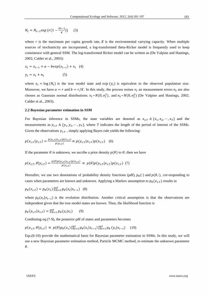
similar estimation. To explicitly illustrate Bayesian inference based on particle MCMC, we show the

trajectories of Markov Chain of parameters and their associated ACFs in Fig.1 based on one simulation

experiment when r = 3. ACFs indicate that the convergence of Markov Chains is very good. The last 5000

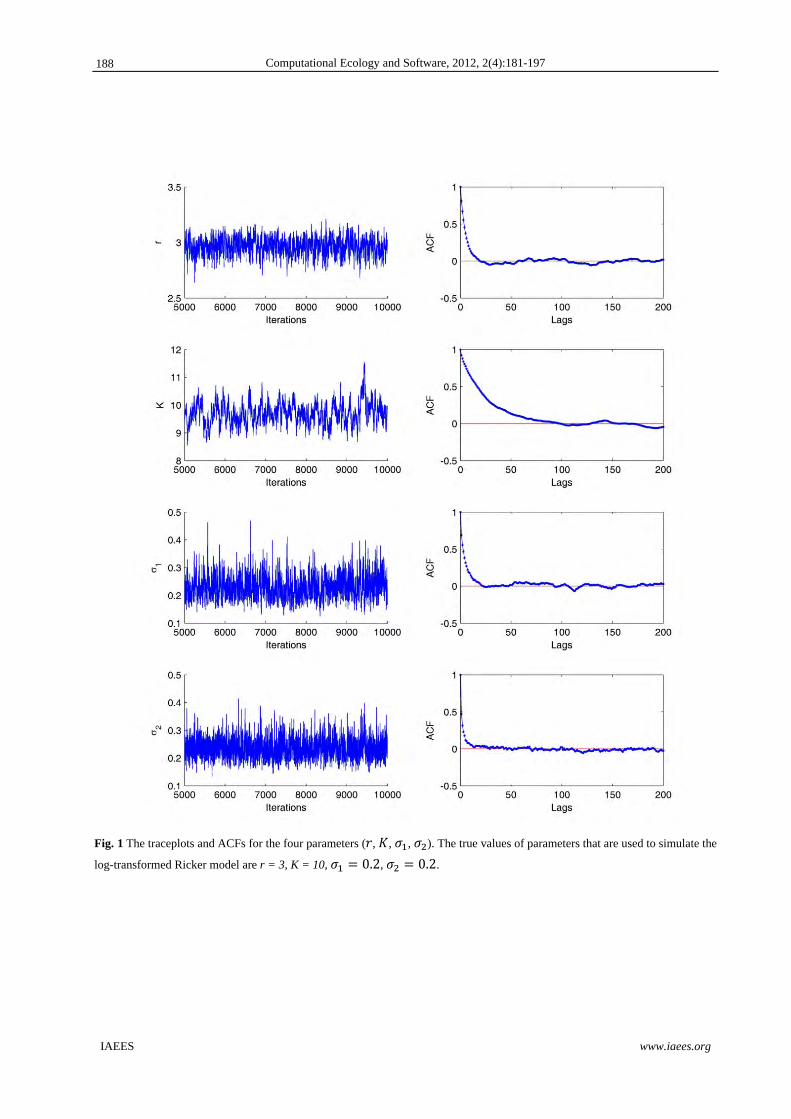
samples that are used to compute the posterior mean and posterior distributions are shown in Fig.2. In addition,

we find that the estimated state : and true model state : are almost identical, but we do not show these

results as figures here. This result again verifies the accuracy of PG sampling algorithm for state and parameter

estimation in SSMs.

Table 1 The results of parameter estimation using simulated data. The posterior means and 95% credible intervals are both reported.

10 0.2 0.2 Mean interval Mean interval Mean interval Mean interval

0.5 0.49 (0.09,0.81) 9.67 (7.26,11.75) 0.23 (0.16,0.31) 0.23 (0.17,0.31)1 1.10 (0.79,1.56) 10.06 (9.25,11.03) 0.19 (0.15,0.26) 0.21 (0.17,0.29)

a 2.6 2.55 (2.39,2.70) 9.52 (9.27,10.10) 0.21 (0.17,0.31) 0.20 (0.15,0.26)3 2.96 (2.81,3.10) 9.68 (8.97,10.46) 0.22 (0.16,0.31) 0.23 (0.17,0.31)

186


IAEES www.iaees.org

3.2 Empirical test

In this section, we fit the log-transformed Ricker model to empirical time series from Global Population

Dynamics Database (GPDD) to test the performance of PG sampling algorithm for parameter estimation. The

GPDD is a collection of time series of population counts or indices of more than 1400 species ranging from

insects to mammals (GPDD 2010). Because there are a variety of long time series in GPDD, biological and

ecological scientists have fitted many dynamic population models to these time series to infer the key

parameters; however, different choices of population model or estimation methods usually leaded to divergent

results (Polansky et al., 2009). It is nearly impossible to evaluate the PG sampling algorithm by directly

comparing parameter estimates from different parameter estimation methods. In this study, although

observation errors are incorporated in the SSM, we assume that these observational errors are not significant to

affect the basic characteristics of true time series (such as trends or periodicity). In other words, the difference

between “true” state : and observations : cannot be too large. Based on this assumption, we use state

estimates as the reference to evaluate the accuracy of parameter estimation.

Although there are thousands of time series in GPDD, we do not intend to use all of them in this paper.

According to the trends and periodicity of time series, we classify these time series into five categories: 1)

increasing time series; 2) decreasing time series; 3) quasi-periodic time series with small or moderate

variations; 4) quasi-periodic time series with large variations or strong fluctuations; 5) irregular time series

with outbreaks.

At first, we assume the four parameters are all unknown and infer them using PG sampling algorithm. The

prior distributions are the same to that in simulation test. The initial value of parameter set

, , , 2, 2/ , 0.1, 0.1 , where K0 is chosen as the average of the whole observed time series. The

length of Markov Chain is chosen as 2 10 , and the “Burn in” period is 104. To fully evaluate the

performance of parameter estimation, ACFs are firstly used to judge the convergence of Markov chains. Then,

we compare the state estimates with the observations. As the basic characteristics of different time series differ

greatly, it is not easily to define a variable to evaluate state estimation. Here, state estimation is evaluated

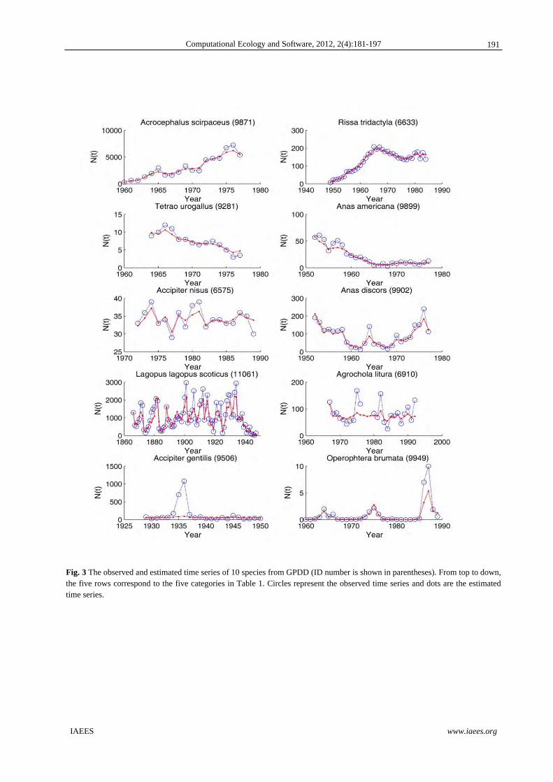
simply be inspecting the estimated and observed time series in figures. In this paper, we illustrate the results of

parameter estimation for 16 randomly selected time series. Parameter estimates for all the 16 time series are

listed in Table 2, and state estimates for 10 of them are shown in Fig.3. For time series belonging to categories

(1-3), we found that the basic characteristics of estimated and observed time series are almost equal. However,

for time series in categories (4), parameter estimation using PG sampling algorithm is not always satisfactory.

For longer time series (such as 243 and 11061), Particle Gibbs sampling algorithm performed well; while for

shorter time series (such as 6910, 6929 and 9922) PG sampling algorithm does not perform well. For time

series that belong to categories (5), parameter estimation using PG sampling algorithm is not good either.

187


IAEES www.iaees.org

Fig. 1 The traceplots and ACFs for the four parameters ( , , , ). The true values of parameters that are used to simulate the

log-transformed Ricker model are r = 3, K = 10, 0.2, 0.2.

188


IAEES www.iaees.org

Fig. 2 Histogram approximations of the posterior densities (diagonal plots) and samples (scatter plots) of model parameters. In the diagonal plots, the solid lines are the prior densities , and the dash-dotted lines indicate the true value of parameters. In the scatter plots, the red crosses indicate the true values. The parameters are the same to that in Fig.1.

Table 2 Parameter estimates of the log-transformed Ricker model fit to 16 time series from GPDD (ID number is shown in parentheses). All four parameters are assumed to be unknown, and only the posterior means are reported.

Categories Species Posterior Mean

1 Acrocephalus scirpaceus (9871) 0.3985 7482 0.2252 0.2327 Rissa tridactyla (6633) 0.3630 165.13 0.1436 0.1432 Turdus merula(1238) 1.0336 9.87 0.1630 0.1956

2 Ennomos autumnaria (6878) 0.0669 9.62 0.2527 0.4908 Tetrao urogallus (9281) 0.2659 7.04 0.1983 0.2217 Anas americana (9899) 0.0583 13.33 0.2461 0.2894

3 Accipiter nisus (6575) 1.1345 34.99 0.1381 0.1484 Spiza americana (9446) 0.9040 65.21 0.1946 0.2477 Anas discors (9902) 0.2872 92.80 0.4116 0.3398

4

Canis latrans (243) 0.1676 22966 0.3691 0.2463 Lagopus lagopus scoticus (11061) 0.3051 922.92 0.5164 0.3807 Agrochola litura (6910) 0.8588 74.10 0.2143 0.3806 Caradrina morpheus (6929) 0.9903 585.68 0.1971 0.2516 Aegolius funereus (9922) 2.4960 10.21 0.1908 0.2631

5 Accipiter gentilis (9506) 0.9008 84.14 0.3006 0.8619 Operophtera brumata (9949) 0.3929 2.066 1.1117 0.6210

189


IAEES www.iaees.org

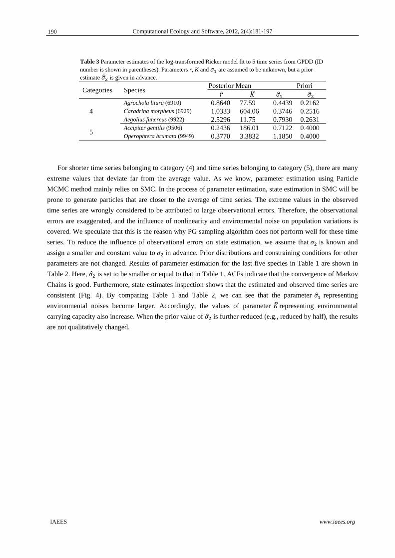
Table 3 Parameter estimates of the log-transformed Ricker model fit to 5 time series from GPDD (ID number is shown in parentheses). Parameters r, K and are assumed to be unknown, but a prior estimate is given in advance.

Categories Species Posterior Mean Priori

4 Agrochola litura (6910) 0.8640 77.59 0.4439 0.2162 Caradrina morpheus (6929) 1.0333 604.06 0.3746 0.2516 Aegolius funereus (9922) 2.5296 11.75 0.7930 0.2631

5 Accipiter gentilis (9506) 0.2436 186.01 0.7122 0.4000 Operophtera brumata (9949) 0.3770 3.3832 1.1850 0.4000

For shorter time series belonging to category (4) and time series belonging to category (5), there are many

extreme values that deviate far from the average value. As we know, parameter estimation using Particle

MCMC method mainly relies on SMC. In the process of parameter estimation, state estimation in SMC will be

prone to generate particles that are closer to the average of time series. The extreme values in the observed

time series are wrongly considered to be attributed to large observational errors. Therefore, the observational

errors are exaggerated, and the influence of nonlinearity and environmental noise on population variations is

covered. We speculate that this is the reason why PG sampling algorithm does not perform well for these time

series. To reduce the influence of observational errors on state estimation, we assume that is known and

assign a smaller and constant value to in advance. Prior distributions and constraining conditions for other

parameters are not changed. Results of parameter estimation for the last five species in Table 1 are shown in

Table 2. Here, is set to be smaller or equal to that in Table 1. ACFs indicate that the convergence of Markov

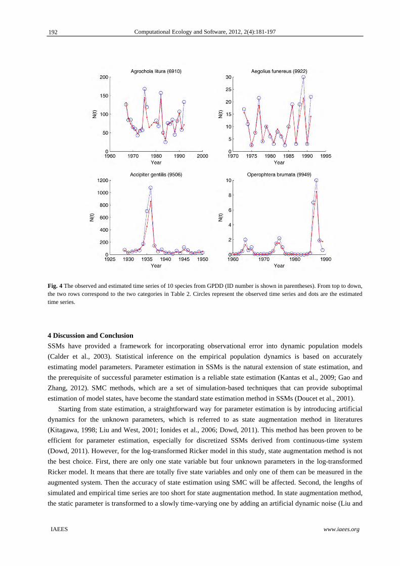
Chains is good. Furthermore, state estimates inspection shows that the estimated and observed time series are

consistent (Fig. 4). By comparing Table 1 and Table 2, we can see that the parameter representing

environmental noises become larger. Accordingly, the values of parameter representing environmental

carrying capacity also increase. When the prior value of is further reduced (e.g., reduced by half), the results

are not qualitatively changed.

190


IAEES www.iaees.org

Fig. 3 The observed and estimated time series of 10 species from GPDD (ID number is shown in parentheses). From top to down, the five rows correspond to the five categories in Table 1. Circles represent the observed time series and dots are the estimated time series.

191


IAEES www.iaees.org

Fig. 4 The observed and estimated time series of 10 species from GPDD (ID number is shown in parentheses). From top to down, the two rows correspond to the two categories in Table 2. Circles represent the observed time series and dots are the estimated time series.

4 Discussion and Conclusion

SSMs have provided a framework for incorporating observational error into dynamic population models

(Calder et al., 2003). Statistical inference on the empirical population dynamics is based on accurately

estimating model parameters. Parameter estimation in SSMs is the natural extension of state estimation, and

the prerequisite of successful parameter estimation is a reliable state estimation (Kantas et al., 2009; Gao and

Zhang, 2012). SMC methods, which are a set of simulation-based techniques that can provide suboptimal

estimation of model states, have become the standard state estimation method in SSMs (Doucet et al., 2001).

Starting from state estimation, a straightforward way for parameter estimation is by introducing artificial

dynamics for the unknown parameters, which is referred to as state augmentation method in literatures

(Kitagawa, 1998; Liu and West, 2001; Ionides et al., 2006; Dowd, 2011). This method has been proven to be

efficient for parameter estimation, especially for discretized SSMs derived from continuous-time system

(Dowd, 2011). However, for the log-transformed Ricker model in this study, state augmentation method is not

the best choice. First, there are only one state variable but four unknown parameters in the log-transformed

Ricker model. It means that there are totally five state variables and only one of them can be measured in the

augmented system. Then the accuracy of state estimation using SMC will be affected. Second, the lengths of

simulated and empirical time series are too short for state augmentation method. In state augmentation method,

the static parameter is transformed to a slowly time-varying one by adding an artificial dynamic noise (Liu and

192


IAEES www.iaees.org

West, 2001). To eliminate such artificial influence in SMC, a relative long time series in needed. State

augmentation method usually works well for these long time series.

Another choice for parameter estimation in SSMs is SMC-based Maximum likelihood (ML) estimation.

ML point estimation based on SMC used to be an open problem (Poyadjis et al., 2005). Like general ML

estimation, ML point estimate of parameters in SSM is also the maximizing argument of the marginal

likelihood of the observed data (Dowd, 2011). Then either gradient approach or Expectation-Maximization

method can be used to find the optimal estimates (Kantas et al., 2009, Gao and Zhang, 2012). However, due to

Monte Carlo variation, the computed likelihood surfaces are found to be rough, and searching the maximizing

argument might be trapped in a local maximum (Polansky et al., 2009; Dowd, 2011). De Valpine and Hastings

(2002) suggested profiling the likelihood surfaces in detail to avoid the problem of local trapping. Moreover, in

order to reduce the Monte Carlo variation in computing the marginal likelihood function, statisticians proposed

using MCMC method instead of SMC method to compute the likelihood function, such as Lele et al. (2007)

and Wood (2010). Although Bayesian techniques are used, these methods are still being recognized as

frequentist inference.

Actually, Bayesian statistics provides an appropriate framework for state and parameter estimation in

SSMs (Wikle and Berliner, 2007; Andrieu et al., 2010). In the Bayesian inference, one commonly applied

approach to approximate the joint probability density : , | : is to use MCMC methods. Calder et al.

(2003) used the Gibbs sampling algorithm to estimate the parameters in the log-transformed Ricker model.

Theoretically, using MCMC method to estimate model parameters is substantial and feasible. However, the

procedure to implement MCMC is a little troublesome. For instance, if we use Metropolis-Hastings algorithm,

it is difficult to choose a good proposal distributions to construct the Markov Chain; if we use Gibbs sampling

algorithm, it is not easily to derive the full-conditional distributions analytically that are used to generate

marginal samples. These problems were successfully solved when Particle MCMC method was proposed

(Andrieu et al., 2010). In parallel to general MCMC, there are two algorithms of Particle MCMC method:

PMMH sampling algorithm and PG sampling algorithm (Andrieu et al., 2010). The advantage of PMMH

sampling algorithm is its universality; however, slow convergence rate is its disadvantage. The convergence

rate of PG sampling algorithm is much faster, but this algorithm is only applicable for SSMs with analytical

full conditional distributions. In this study, the SSM is the log-transformed Ricker model. The full conditional

distributions can be derived analytically. So we chose the efficient PG sampling algorithm to estimate the

model parameters.

The performance of PG sampling algorithm for parameter estimation was tested using both simulated and

empirical time data. In simulation test, the posterior means of parameters were very close to the true values

that were used to generate the simulated data. Extensive simulations verified that PG sampling algorithm was

both robust and efficient. The empirical time series in this study were chosen from GPDD. We found that PG

sampling algorithm performed well for increasing, decreasing, moderately fluctuated and long time series. For

intensively fluctuated time series, PG sampling algorithm also gave a good estimation, if observational errors

were constrained. In addition, we found that PG sampling algorithm still performed well for empirical time

series with missing data. As we know, one purpose of parameter estimation in dynamic population models is to

infer the relative contributions of endogenous and extraneous factors on population dynamics. In this study, the

estimated for most time series were smaller than 2 indicting that the variations of population dynamics were

not induced by nonlinearity but by environmental noises. The only exception was time series 9922 ( 2).

The estimated of time series 9922 was still very large, then the combining effect of nonlinearity and

environmental noises resulted in a time series with regular period but irregular amplitude. Parameter

estimation using Particle MCMC methods is based on recovering the true states behind the observations

193


IAEES www.iaees.org

(Andrieu et al., 2010). The estimated parameters using Particle MCMC methods are “virtual” parameters that

are most prone to simulate the so called “true” states. In this study, we have assumed that the observational

errors were not large enough and the basic characteristics of “true” time series and observed time series were

consistent. So, state estimates were used to evaluate parameter estimates. This criterion might result in the

problem of over-fitting for empirical time series. Therefore, on the one hand, we should fit dynamic population

model to more empirical data to reveal the population regulation mechanism; on the other hand, we should use

other prior distributions or dynamic population models to obtain more reliable parameter estimates in future

work.

Acknowledgements

This work was supported by National Natural Science Foundation of China (No.31000197) to GM, as well as

Knowledge Innovation Project of Chinese Academy of Sciences (No. KZCX2-EW-QN209).

Appendix

The posterior distribution of parameter can be simply derived as

| , : , : : , : p a p | |

|1

2 / 1

∑1

(A1)

The minus before parameter a indicates taking a out off resulting in a subset , , . As the prior

distribution of a is a continuous uniform distribution , , then we have

| , : , : ~ ,∑

1,

1

where , ·,· is a truncated normal distribution. The posterior distribution of parameter b can be

analogously derived.

The prior distribution assigned to 1, 2 is inverse gamma distribution , , then we have

exp (A2)

We first show how the posterior distribution of is derived,

| , : , : | : : | | ,

1

√2 2

(A3)

194


IAEES www.iaees.org

where ∑ . From eq.(A3), we find that the posterior distribution of is an

inverse gamma distribution,

| , : , : ~ , (A4)

Similarly, we can derive the posterior distribution of ,

| , : , : ~ , (A5)

where ∑ .

References

Andrieu C, Doucet A, Holenstein R. 2010. Particle Markov chain Monte Carlo methods. Journal of the Royal

Statistical Society Series B, 72: 269-342

Arulampalam MS, Maskell S, Gordon N, et al. 2002. A tutorial on particle filters for online nonlinear/non-

Gaussian Bayesian tracking. IEEE Transactions on Signalling Process. 50: 174-188

Blasius B, Kurths J, Stone L, 2007. Complex Population Dynamics: Nonlinear Modeling in Ecology,

Epidemiology and Genetics. World Scientific, Singapore

Bjørnstad ON. 2000. Cycles and synchrony: two historical ‘experiments’ and one experience. Journal of

Animal Ecology, 69: 869-873

Calder C, Lavine M, Müller P, et al. 2003. Incorporating multiple sources of stochasticity into dynamic

population models. Ecology, 84(3): 1395-1402

Costantino R F, Desharnais RA, Cushing JM, et al. 1997. Chaotic Dynamics in an Insect Population. Science,

275: 390-391

De Valpine P, Hastings A. 2002. Fitting population models incorporating process noise and observation error.

Ecological Monographs, 72: 57-76

Dixon PA, Milicich MJ, Sugihara G. 1999. Episodic fluctuations in larval supply. Science, 283: 1528-1530

Doucet A, de Freitas N, Gordon N. 2001. Sequential Monte Carlo in Practice. Springer-Verlag, New York,

USA

Dowd M. 2011. Estimating parameters for s stochastic dynamic marine ecological system. Environmetrics,

22(4): 501-515

Elsadany AEA. 2012. Dynamical complexities in a discrete-time food chain. Computational Ecology and

Software, 2(2): 124-139

Gao M, Zhang H. 2012. Sequential Monte Carlo methods for parameter estimation in nonlinear state-space

models. Computers and Geosciences, 44: 70-77

Gilks WR, Richardson S, Spiegelhalter DJ. 1996. Markov Chain Monte Carlo in Practice. Chapman and Hall,

London, UK

Golightly A, Wilkinson DJ. 2011. Bayesian parameter inference for stochastic biochemical network models

using particle Markov chain Monte Carlo. Interface Focus, 1: 807-820

Hanski I, Turchin P, Korpimäki E, et al. 1993. Population oscillations of boreal rodents: regulation by mustelid

predators leads to chaos. Nature, 364: 232-235

Harmon R, Challenor P. 1997. A Markov chain Monte Carlo method for estimation and assimilation into

models. Ecological Modelling, 101(1): 41-59

195


IAEES www.iaees.org

Hastings WK. 1970. Monte Carlo sampling methods using Markov Chains and their applications. Biometrika,

57: 97-109

Ionides EL, Bretó C, King AA. 2006. Inference for nonlinear dynamical systems. Proceedings of the National

Academy of Sciences of USA, 103: 18438-18443

Kantas N, Doucet A, Singh S, et al. 2009. An overview of sequential Monte Carlo methodsfor parameter

estimation in general state-space models. In: Proc. IFAC Sympo-sium on System Identification (SYSID)

Kitagawa G. 1998. A self-organizing state space model. Journal of the American Statistical Association,

93(443): 1203-1215

Lele SR, Dennis B, Lutscher F. 2007. Data cloning: easy maximum likelihood estimation for complex

ecological models using Bayesian Markov chain Monte Carlo methods. Ecological Letters, 10: 551-563

Lillegard M, Engen S, Sæther BE, Grøtan V, Drever MC. 2008. Estimation of population parameters from

aerial counts of the north American Mallards: a cautionary tale. Ecological Applications, 18(1): 197-207

Lindley ST. 2003. Estimation of population growth and extinction parameters from noisy data. Ecological

Applications, 13: 806-813

Liu J, West M. 2001. Combined parameter and state estimation in simulation-based filtering. In: Sequential

Monte Carlo in Practice (Doucet A, de Freitas N, Gordon N, eds). 197-223, Springer-Verlag, New York,

USA

Metropolis N, Rosenbluth AW, Rosenbluth MN, et al. 1953. Equation of state calculations by fast computing

machines. Journal of Chemical Physics, 21: 1087-1091

Meyer R, Millar RB. 1998. Bayesian stock assessment using a state-space implementation of the delay

difference model. Canadian Journal of Fisheries and Aquatic Sciences, 56: 37-52

Meyer R, Millar RB. 1999. BUGs in Bayesian stock assessments. Canadian Journal of Fisheries and Aquatic

Sciences, 56: 1078-1086

Nedorezov LV. 2011a. About a dynamic model of interaction of insect population with food plant.

Computational Ecology and Software, 1(4): 208-217

Nedorezov LV. 2011b. Analysis of some experimental time series by Gause: application of simple

mathematical models. Computational Ecology and Software, 1(1):25-36

Nedorezova BN, Nedorezov LV. 2012. Pine looper moth population dynamics in Netherlands: Prognosis with

generalized logistic model. Proceedings of the International Academy of Ecology and Environmental

Sciences, 2(2): 70-83

Pascual M, Rodo X, Ellner SP, et al. 2000. Cholera dynamics and El Nino Southern Oscillation. Science, 289:

1766-1769

Rasmussen DA, Ratmann O, Koelle K. 2011. Inference for nonlinear empidemiological models using

genealogies and time series. Plos Computational Biology, 7(8): e1002136

Ricker WE. 1954. Stock and recruitment. Journal of Fisheries Research Board of Canada, 11: 559-623

Polansky L, De Valpine P, Lloyd-Smith JO, et al. 2008. Parameter estimation in a generalized discrete-time

model of density dependence. Theoretical Ecology, 1: 221-229

Polansky L, De Valpine P, Lloyd-Smith JO, et al. 2009. Likelihood ridges and multimodality in population

growth rate models. Ecology, 90(8): 2313-2320.

Poyadjis G, Doucet A, Singh SS. 2005. Maximum likelihood parameter estimation using particle methods. In:

Proc. Joint Statistical Meeting

Schnute JT. 1994. A general framework for developing sequential fisheries models. Canadian Journal of

Fisheries and Aquatic Sciences, 51: 1676-1688

196


IAEES www.iaees.org

Stafford R, Lloyd JR. 2011. Evaluating a Bayesian approach to improve accuracy of individual photographic

identification methods using ecological distribution data. Computational Ecology and Software, 1(1): 49-54

Sugihara G. 1996. Red/blue chaotic power spectra. Nature, 381: 198-199

Tilman D, Wedin D. 1991. Oscillations and chaos in the dynamics of a perennial grass. Nature, 353: 653-655

Viljugrein H, Stenseth NC, Smith GW, et al. 2005. Density dependence in North American ducks. Ecology, 86:

245-254

Wang GM. 2007. On the latent state estimation of nonlinear population dynamics using Bayesian and non-

Bayesian state-space model. Ecological Modelling, 200: 521-528

Winder M, Cloern JE. 2010. The annual cycles of phytoplanton biomass. Proceedings of the Royal Society B-

Biological Sciences, 365: 3215-3226

Wikle CK, Berlinder LM. 2007. A Bayesian tutorial for data assimilation. Physica D, 230: 1-16

Wood SN. 2010. Statistical inference for noisy nonlinear ecological dynamic systems. Nature, 466: 1102-1104

Zhang WJ. Computational Ecology: Artificial Neural Networks and Their Applications. World Scientific,

Singapore, 2010

Zhang WJ, Wei W. 2009. Spatial succession modeling of biological communities: a multi-model approach.

Environmental Monitoring and Assessment, 158: 213-230

197

Bayesian parameter estimation in dynamic population model via particle Markov chain Monte Carlo

Documents

Transcript of Bayesian parameter estimation in dynamic population model via particle Markov chain Monte Carlo