Detection of Deformable Objects in 3D Images Using Markov-Chain Monte Carlo and Spherical Harmonics

Life on the LatticeMarkov Chain Monte Carlo
and all that
David SchaichAdvisor: Prof. Loinaz
Preliminary Thesis TalkAmherst College
29 November 2005

David Schaich Preliminary Thesis Talk – 29 November 2005 2
Outline
Ising Model: A simple model of a magnetPhases, phase transitions, and a context for...
Numerical (lattice) simulationsThe rather large problem of very large numbers
Markov Chain Monte CarloEfficient 'importance sampling'
4 Theory (time permitting)

David Schaich Preliminary Thesis Talk – 29 November 2005 3
Ising ModelImagine a lattice of 'spins' of magnitude 1 that can only point up (+1) or down (1).
Spins correspond to magnetic dipoles at temperature T.
Energy: (only nearest neighbors interact)
E=−∑⟨i , j ⟩
si s j

David Schaich Preliminary Thesis Talk – 29 November 2005 4
Ising ModelImagine a lattice of 'spins' of magnitude 1 that can only point up (+1) or down (1).
Energy
Parallel spins have lower energy, but thermal energy causes fluctuations that randomize the lattice – if the temperature is high enough.
E=−∑⟨i , j ⟩
si s j

David Schaich Preliminary Thesis Talk – 29 November 2005 5
Ising Model PhasesThus the Ising model has two phases:
ferromagnetic unordered
Spins aligned Lower energy Higher magnetization
Equilibrium for low temperatures
Spins unordered Higher energy Lower magnetization
Equilibrium for higher temperatures

David Schaich Preliminary Thesis Talk – 29 November 2005 6
Ising Model Phase Transitionsferromagnetic unordered
:Energy :Magnetizatione= EN=−1N ∑
⟨ i , j⟩si s j m=M
N=∑
i=0
N−1
si

David Schaich Preliminary Thesis Talk – 29 November 2005 7
Ising Model Phase TransitionsPhase transition becomes sharp as lattice size L∞ (equivalent to lattice spacing a ).0
Point at which phase transition occurs is 'critical temperature'
T c=2
ln 12=2.269

David Schaich Preliminary Thesis Talk – 29 November 2005 8
Numerical Simulations How to calculate those pretty graphs on the previous slide?
#Idea 1: , Set up each possible configuration calculate the desired quantity and weigh it by its Boltzmann probability
⟨Q ⟩=∑i
Qie−E i /kT
∑i
e−E i /kT( )See Physics 30

David Schaich Preliminary Thesis Talk – 29 November 2005 9
#Idea 1: , Set up each possible configuration calculate the desired quantity and weigh it by its Boltzmann probability
# : .Problem 1 This isn't practical
: ( ) ~Example Even a very small 16x16 Ising lattice has 2256 (~1077) , ~configurations which will take at least 1060 years to
.fully calculate
- ( ) It gets even worse for moderately sized 512x512 lattices
(~10 , 78 900 ) (~years or small thermodynamic systems 101023
)years
Numerical Simulations
⟨Q ⟩=∑i
Qie−E i /kT
∑i
e−E i /kT( )See Physics 30

David Schaich Preliminary Thesis Talk – 29 November 2005 10
#Idea 1: , Set up each possible configuration calculate the desired quantity and weigh it by its Boltzmann probability
# : .Problem 1 This isn't practical
: ( ) ~Example Even a very small 16x16 Ising lattice has 2256 (~1077) , ~configurations which will take at least 1060 years to
.fully calculate
- ( ) It gets even worse for moderately sized 512x512 lattices
(~10 , 78 900 ) (~years or small thermodynamic systems 101023
)years
Numerical Simulations
⟨Q ⟩=∑i
Qie−E i /kT
∑i
e−E i /kT( )See Physics 30
DUE 12 MAY

David Schaich Preliminary Thesis Talk – 29 November 2005 11
#Idea 1: , Set up each possible configuration calculate the desired quantity and weigh it by its Boltzmann probability
# : Problem 2 This is just silly
Generally only a very small proportion of the possible states . .actually matter It's a waste of time to worry about the others
Numerical Simulations
⟨Q ⟩=∑i
Qie−E i /kT
∑i
e−E i /kT( )See Physics 30

David Schaich Preliminary Thesis Talk – 29 November 2005 12
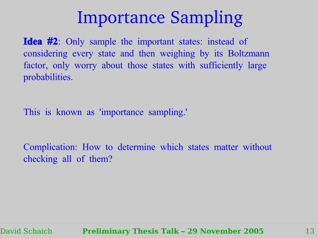
#Idea 2: : Only sample the important states instead of considering every state and then weighing by its Boltzmann
, factor only worry about those states with sufficiently large.probabilities
.This is known as 'importance sampling '
Importance Sampling
David Schaich Preliminary Thesis Talk – 29 November 2005 13
#Idea 2: : Only sample the important states instead of considering every state and then weighing by its Boltzmann
, factor only worry about those states with sufficiently large.probabilities
.This is known as 'importance sampling '
: Complication How to determine which states matter without checking all of them?
Importance Sampling

David Schaich Preliminary Thesis Talk – 29 November 2005 14
Markov processes are ways to generate a random set of states . ( )according to the Boltzmann probabilities Proof left to reader
But what are Markov processes?
Markov Processes

David Schaich Preliminary Thesis Talk – 29 November 2005 15
, Given an initial state X a Markov process randomly generates a (new state Y with 'transition probability' P X ).Y
This series of states produced by the Markov process is known .as a 'Markov chain '
, Because of its use of randomness this approach is known as the ( ) 'Markov Chain Monte Carlo MCMC method' in honor of the .famous casino center in Monaco
, To reproduce the Boltzmann distribution the Markov process .needs to satisfy three conditions
Markov Chain Monte Carlo

David Schaich Preliminary Thesis Talk – 29 November 2005 16
:Three conditions guarantee Boltzmann distribution
)1 ( ) – , P X Y can depend only on X and Y in particular none of the previous states can influence the transition probability to ( ).the next state hence 'chain'
Markov Chain Monte Carlo

David Schaich Preliminary Thesis Talk – 29 November 2005 17
:Three conditions guarantee Boltzmann distribution
)1 ( ) – , P X Y can depend only on X and Y in particular none of the previous states can influence the transition probability to ( ).the next state hence 'chain'
)2 It must be possible to reach any state from any other state( ), possibly passing through intermediate states since Boltzmann
. (“ ”)factors are always greater than zero Ergodicity
Markov Chain Monte Carlo

David Schaich Preliminary Thesis Talk – 29 November 2005 18
:Three conditions guarantee Boltzmann distribution
)1 ( ) – , P X Y can depend only on X and Y in particular none of the previous states can influence the transition probability to ( ).the next state hence 'chain'
)2 It must be possible to reach any state from any other state( ), possibly passing through intermediate states since Boltzmann
. (“ ”)factors are always greater than zero Ergodicity
)3 The probability of going from X to Y must be the same as :the probability of going from Y to X
where pX and p
Y are the probabilities of actually being in states
, . (“ ”)X and Y respectively Detailed Balance
Markov Chain Monte Carlo
pX P X Y = pY P Y X

David Schaich Preliminary Thesis Talk – 29 November 2005 19
:Three conditions guarantee Boltzmann distribution
)1 ( ) – , P X Y can depend only on X and Y in particular none of the previous states can influence the transition probability to ( ).the next state hence 'chain'
)2 It must be possible to reach any state from any other state( ), possibly passing through intermediate states since Boltzmann
. (“ ”)factors are always greater than zero Ergodicity
)3 The probability of going from X to Y must be the same as :the probability of going from Y to X
where pX and p
Y are the probabilities of actually being in states
, . (“ ”)X and Y respectively Detailed Balance
Markov Chain Monte Carlo
pX P X Y = pY P Y X ⇒ P X Y P Y X
=pYpX
=exp [−EY−E X
kT]

David Schaich Preliminary Thesis Talk – 29 November 2005 20
4 Theory (in 2D)Lagrangian (density):
(∈ℝ)ℒ=1
2∂21
222
44

David Schaich Preliminary Thesis Talk – 29 November 2005 21
Discretized 4 Theory (in 2D)Lagrangian (density):
(∈ℝ)
Discretized action (energy):
ℒ=12∂21
222
44
E=−∑⟨ i , j ⟩
i j∑n
[20L
2
2n
2 L4n
4]

David Schaich Preliminary Thesis Talk – 29 November 2005 22
Discretized 4 Theory (in 2D)Lagrangian (density):
(∈ℝ)
Discretized action (energy):
(In case you're wondering how the action became the energy, I should mention that discretizing the action involves making a Wick rotation (t it), which changes Minkowski space into Euclidean space and identifies the action and energy. It's a bit too messy for the time I have.)
ℒ=12∂21
222
44
E=−∑⟨i , j ⟩
i j∑n
[20L
2
2n
2 L4n
4]

David Schaich Preliminary Thesis Talk – 29 November 2005 23
Discretized 4 Theory ParametersLagrangian (density):
(∈ℝ)
Discretized action (energy):
(In case you're wondering how the action became the energy, I should mention that discretizing the action involves making a Wick rotation (t it), which changes Minkowski space into Euclidean space and identifies the action and energy. It's a bit too messy for the time I have.)
The discretized theory is characterized by two independent dimensionless parameters that depend on the lattice spacing a:
(both 0
2 and have dimensions of mass squared)
ℒ=12∂21
222
44
E=−∑⟨i , j ⟩
i j∑n
[20L
2
2n
2 L4n
4]
0L2 =0
2 a2
L= a2

David Schaich Preliminary Thesis Talk – 29 November 2005 24
Discretized 4 Theory Phase Transition
As with the Ising model, 4 theory also exhibits a phase transition, with a critical 2
0L for each
L > 0.
E=−∑⟨i , j ⟩
i j∑n
[20L
2
2n
2 L4n
4]
[0L2 ]crit=−0.10

David Schaich Preliminary Thesis Talk – 29 November 2005 25
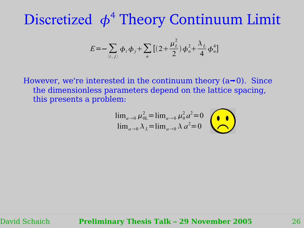
Discretized 4 Theory Continuum Limit
However, we're interested in the continuum theory (a0). Since the dimensionless parameters depend on the lattice spacing, this presents a problem:
E=−∑⟨i , j ⟩
i j∑n
[2L
2
2n
2 L4n
4]
lima0 0L2 =lima 0 0
2 a2=0
lima0 L=lima0 a2=0
David Schaich Preliminary Thesis Talk – 29 November 2005 26
Discretized 4 Theory Continuum Limit
However, we're interested in the continuum theory (a0). Since the dimensionless parameters depend on the lattice spacing, this presents a problem:
E=−∑⟨i , j ⟩
i j∑n
[2L
2
2n
2 L4n
4]
lima0 0L2 =lima 0 0
2 a2=0
lima0 L=lima0 a2=0

David Schaich Preliminary Thesis Talk – 29 November 2005 27
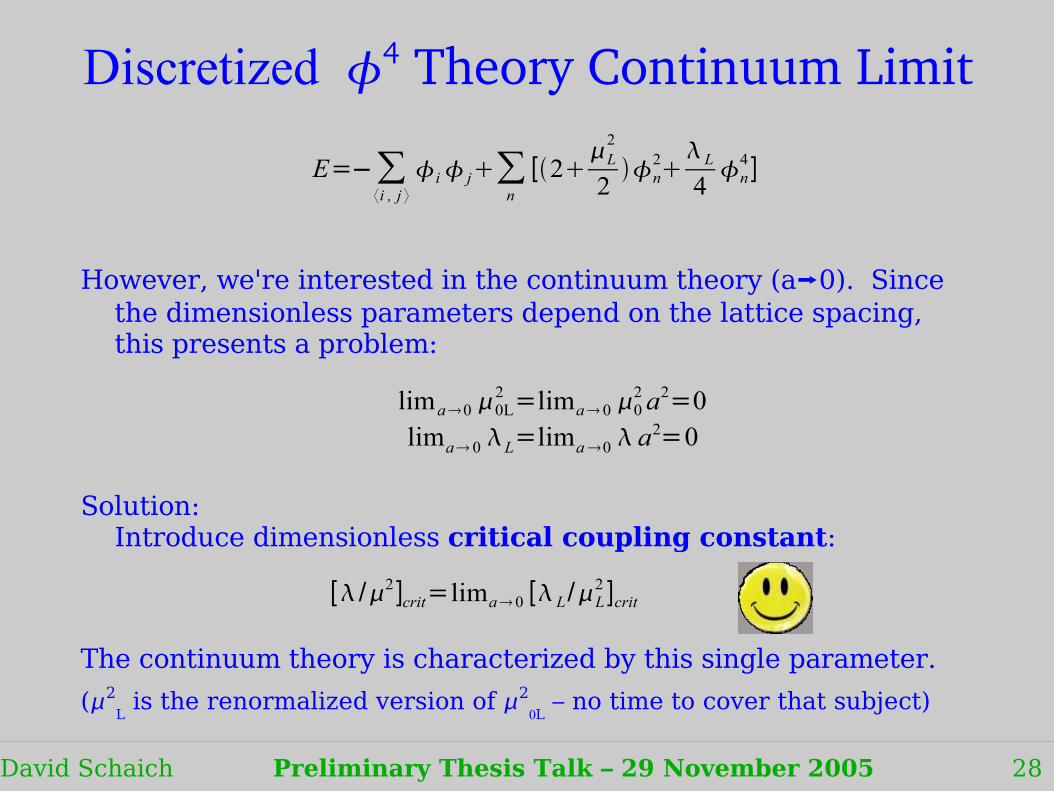
Discretized 4 Theory Continuum Limit
However, we're interested in the continuum theory (a0). Since the dimensionless parameters depend on the lattice spacing, this presents a problem:
Solution:Introduce dimensionless critical coupling constant:
The continuum theory is characterized by this single parameter.
(2L is the renormalized version of 2
0L – no time to cover that subject)
E=−∑⟨i , j ⟩
i j∑n
[2L
2
2n
2 L4n
4]
lima0 0L2 =lima 0 0
2a2=0lima 0 L=lima0 a
2=0
[ /2]crit=lima 0 [ L/L2 ]crit
David Schaich Preliminary Thesis Talk – 29 November 2005 28
Discretized 4 Theory Continuum Limit
However, we're interested in the continuum theory (a0). Since the dimensionless parameters depend on the lattice spacing, this presents a problem:
Solution:Introduce dimensionless critical coupling constant:
The continuum theory is characterized by this single parameter.
(2L is the renormalized version of 2
0L – no time to cover that subject)
E=−∑⟨i , j ⟩
i j∑n
[2L
2
2n
2 L4n
4]
lima0 0L2 =lima 0 0
2a2=0lima 0 L=lima0 a
2=0
[ /2]crit=lima 0 [ L/L2 ]crit

David Schaich Preliminary Thesis Talk – 29 November 2005 29
Preliminary ResultsCritical coupling constant is inverse of slope:

David Schaich Preliminary Thesis Talk – 29 November 2005 30
Preliminary Results
[ /2]crit=10.27−.05.06
Critical coupling constant is inverse of slope:

David Schaich Preliminary Thesis Talk – 29 November 2005 31
Preliminary Results
Published Results:
W. Loinaz & R. S. Willey, Phys. Rev. D. 58, 076003 (1998).
[ /2]crit=10.26−.04.08
[ /2]crit=10.27−.05.06

David Schaich Preliminary Thesis Talk – 29 November 2005 32
Future Plans
Polish up result on previous slide
Calculate critical coupling constant for four-dimensional 4 theory
Calculate soliton masses in two-dimensional 4 theory
Time permitting, calculate soliton masses in four-dimensional 4 theory and other simple nonperturbative field theories

David Schaich Preliminary Thesis Talk – 29 November 2005 33
Acknowledgments
National Science FoundationThis work was partially funded by NSF grant 0521169
Prof. Loinaz
Prof. Kaplan
Chris Bednarzyk '01
Copyright © 2022 FDOKUMEN