arX

iv:1

401.

1667

v1 [

stat

.CO

] 8

Jan

201

4

On general sampling schemes for Particle Markov chain Monte

Carlo methods

Eduardo F. Mendes

School of Economics

University of New South Wales

Christopher K. Carter

School of Economics

University of New South Wales

Robert Kohn

School of Economics

University of New South Wales

January 9, 2014

Abstract

Particle Markov Chain Monte Carlo methods [Andrieu et al., 2010] are used to carry out inferencein non-linear and non-Gaussian state space models, where the posterior density of the states isapproximated using particles. Current approaches have usually carried out Bayesian inference usinga particle Metropolis-Hastings algorithm or a particle Gibbs sampler. In this paper, we give ageneral approach to constructing sampling schemes that converge to the target distributions given inAndrieu et al. [2010] and Olsson and Ryden [2011]. We describe our methods as a particle Metropoliswithin Gibbs sampler (PMwG). The advantage of our general approach is that the sampling schemecan be tailored to obtain good results for different applications. We investigate the properties ofthe general sampling scheme, including conditions for uniform convergence to the posterior. Weillustrate our methods with examples of state space models where one group of parameters can begenerated in a straightforward manner in a particle Gibbs step by conditioning on the states, butwhere it is cumbersome and inefficient to generate such parameters when the states are integratedout. Conversely, it may be necessary to generate a second group of parameters without conditioningon the states because of the high dependence between such parameters and the states. Our examplesinclude state space models with diffuse initial conditions, where we introduce two methods to dealwith the initial conditions.

1 Introduction

Our article deals with statistical inference for both the unobserved states and the parameters in a classof state space models. Our main goal is to give a general approach to constructing sampling schemesthat converge to the posterior distribution of the states and the parameters. The sampling schemes alsogenerate particles as auxilary variables and we describe our methods as a particle Metropolis within Gibbssampler (PMwG). This work extends the methods proposed by Andrieu et al. [2010], Lindsten and Schon[2012] and Olsson and Ryden [2011]. Furthermore, we consider state space models with diffuse initialconditions and provide algorithms to deal with this feature in a particle MCMC framework.

If the state space model is Gaussian or Gaussian conditional on a set of latent state variables, thenthere are well established MCMC methods for carrying out Bayesian inference e.g. Carter and Kohn[1994], Fruhwirth-Schnatter [1994], Gerlach et al. [2000] and Fruhwirth-Schnatter [2006]. However, inmany cases it is not possible to use such conditionally Gaussian formulations, and it is necessary touse other methods, e.g. single site sampling of the states as proposed by Carlin et al. [1992], or blocksampling of the states conditional on the parameters as proposed by Shephard and Pitt [1997]. Even so,these methods can be very inefficient, and cannot be applied in a general way as they require a numberof tuning parameters to be specified, such as the block size.

The bootstrap (standard) particle filter was introduced by Gordon et al. [1993], and independently byKitagawa [1996], for online filtering of general state space models, with the parameters assumed known.

1

The bootstrap particle filter just requires that it is possible to generate from the state transition equationand evaluate the observation equation. Pitt and Shephard [1999] introduce the class of auxiliary particlefilters which can be much more efficient than the bootstrap filter, especially when the signal to noiseratio is high. There have been a number of approaches to use the particle filter for Bayesian inference onthe parameters. Liu and West [2001] perform online inference including the unknown parameter vectoras part of the states. Storvik [2002] and Polson et al. [2008] use a sequential updating scheme that relieson conjugacy to update the parameters.

Andrieu et al. [2010] introduce two particle MCMC methods. The first is particle marginal MetropolisHastings (PMMH), where the parameters are generated with the states integrated out. The second isparticle Gibbs (PG), which generates the parameters given the states. They show that the augmenteddensity targeted by this algorithm has the joint posterior density of the parameters and states as amarginal density. Andrieu et al. [2010] and Andrieu and Roberts [2009] show that the law of the marginalsequence of parameters and states, sampled using either PG or PMMH, converges to the true posterioras the number of iterations increase. Both particle MCMC methods have been focus of research in thelast years. Olsson and Ryden [2011] and Lindsten and Schon [2012] consider using backward simulation[Godsill et al., 2004] for sampling the state vector, instead of Kitagawa’s ancestral tracing. The authorsderive the augmented target distribution and find that, in simulation studies, their method performedbetter than the PMMH or PG counterpart using ancestral tracing. Chopin and Singh [2013] show thatusing backward simulation is more efficient than ancestral tracing in a PG setting, on the top of beingrobust to the resampling method used (e.g., multinomial, residual, stratified).

In a separate line of research, Pitt et al. [2012] and Doucet et al. [2012] investigate optimal choice ofparticles in a PMMH algorithm. They show that best tradeoff between computational cost and integratedautocorrelation time is attained when the standard deviation of the estimated log-likelihood from theparticle filter is close to one. Their results are valid for the PMMH algorithm. As for the PG, it is notclear whether the standard deviation of the likelihood from the particle filter plays any role in the choicethe number of particles used.

Using only Metropolis-Hastings or the Gibbs sampler may be undesirable. We know from the liter-ature on Gaussian and conditionally Gaussian state space models that confining MCMC for state spacemodels to Gibbs sampling or Metropolis-Hastings sampling can result in inefficient or even degeneratesampling. See, for example, Kim et al. [1998] who showed that for a stochastic volatility model thatgenerating the states conditional on the parameters and the parameters conditional on the states canresult in a highly inefficient sampler. See also Carter and Kohn [1996] and Gerlach et al. [2000] whodemonstrated using a simple signal plus noise model that allows for structural breaks using indicatorvariables, that a Gibbs sampler for the states and indicator variables produces a degenerate sampler. Anatural solution is to combine Gibbs and Metropolis-Hastings samplers.

Our work extends the particle MCMC framework introduced in Andrieu et al. [2010] and Lindsten and Schon[2012] to situations which using just PMMH or just PG is impossible or inefficient. We derive a par-ticle Metropolis within Gibbs sampler on the same augmented space as the PG and PMMH samplers,in which some parameters are sampled conditionally on the states and the remaining parameters aresampled with the states integrated out. We show that the PMwG sampler targets the same augmenteddensity as the PG or PMMH and that the Markov chain generated by the algorithm is uniformly ergodic,given regularity conditions. It implies that the marginal law of the the Markov chain generated by nth

iteration of the algorithm, converges to the posterior density function geometrically fast, uniformly onthe starting value, as n→ ∞.

The method is introduced in a simple Markov state-space setting, with possibly fully adapted proposaldensity and using ancestral tracing. The proposed method can be modified in a straightforward way toa non-Markov case (the state at time t depends on the states at times 1, . . . , t − 1), auxiliary particlefilters and backward simulation. Although these modifications are encouraged in applications, we choseto sacrifice generality in favor of a more accessible presentation. The proofs may also be modified usingarguments found in Olsson and Ryden [2011], and the same results hold. We conjecture it is possibleto show geometric ergodicity, instead of uniform ergodicity, using arguments similar to those used in[Andrieu and Vihola, 2012, Propositions 7 and 9], but both the notation and algebra are more involvedand it is not the main purpose of this paper.

We also propose using look-ahead strategies to deal with diffuse initial conditions. This is thefirst paper, as far as we are aware, that deals directly with this problem. In the discussion followingDel Moral et al. [2007], Paul Fearnhead displays concern on how informative is the prior and suggests

2

conditioning sampling the initial state on a few observations. In reply, the authors emphasize that it ispossible to use a proposal from a extended Kalman filter, but it may work badly in some nonlinear, non-Gaussian settings. We follow a distinct approach and sample the initial state from an efficient importancedensity [Richard and Zhang, 2007], constructed conditional on the parameters and a few observations.Another approach is to sample the initial state from the reduced conditional, which fits naturally in thePMwG specification. We show in simulations that using the efficient importance density may improvethe performance of particle Gibbs samplers, at the cost of an increase in the variance of the estimatedlog-likelihood.

The paper is organized as follows. In Section 2 we introduce the basic concepts and notation usedthroughout the paper. The particle Metropolis within Gibbs sampler is introduced in Section 3, togetherwith the theory showing the sampler is ergodic, under regularity conditions. In Section 4 we explainhow to construct the efficient initial density used in sampling the initial state and explain how to usethe PMwG sampler to handle diffuse initial conditions. All the simulations are grouped in Section 5.Theextension to backward simulation is discussed in Appendix A.

2 Preliminaries

In this section, we introduce the models and the main algorithms to generate Metropolis-Hasting propos-als and to generate from useful conditional distributions. These are the main components that are usedin the sampling schemes in Section 3. There are strong relationships between these components becausethe target distribution in Section 2.3 is on an augmented space that includes the particles from theSequential Monte Carlo algorithm described in Section 2.2. It is chosen to have marginal distributionsthat match the State Space Model in Section 2.1 and to include terms from the Sequential Monte Carloalgorithm. The algorithms in Section 2.4 generates from an exact conditional distribution and is usedfor the Gibbs sampling steps described in Section 3.

2.1 State Space Model

Define N as the set of positive integers and let {Xt}t∈N and {Yt}t∈N denote X -valued and Y-valuedstochastic processes, where {Xt}t∈N is a latent Markov process with initial density µθ(x) and transitiondensity fθ(x

′|x), i.e.,

X1 ∼ µθ(·) and Xt+1|(Xt = x) ∼ fθ(·|x) (t = 1, 2, . . . ).

The latent process {Xt}t∈N is observed only through {Yt}t∈N, whose value at time t depends on the valueof the hidden state at time t, and is distributed according to gθ(y|x):

Yt|(Xt = x) ∼ gθ(·|x) (t = 1, 2, . . . ).

The densities µθ, fθ and gθ are indexed by a parameter vector θ ∈ Θ where Θ is an open subset of Rdθ ,and all densities are with respect to suitable dominating measures, denoted dx and dy. The dominatingmeasure is frequently taken to be the Lebesgue measure if X ∈ B(Rdx) and Y ∈ B(Rdy), where B(A) isthe Borel σ-algebra generated by the set A.

We use the colon notation for collections of random variables, i.e., for integers r ≤ s, ar:s =(ar, . . . , as), a

r:st = {(art , . . . , a

st ) and for t ≤ u, at:ur:s = (at:ur , . . . , at:us )}. The joint probability density

function of (x1:T , y1:T )} is given by

p (x1:T , y1:T |θ) = µθ(x1)gθ(y1|x1)

T∏

t=2

fθ(xt|xt−1) gθ(yt|xt).

We denote the likelihood by

Z1:T (θ) = p(y1|θ)

T∏

t=2

p(yt|y1:t−1, θ) =

∫p(x1:T , y1:T |θ)dx1:T ,

3

and Zt(θ) = p(yt|y1:t−1, θ). The joint filtering density of X1:T is

p (x1:T |y1:T , θ) =p (x1:T , y1:T |θ)

Z1:T (θ),

and the joint filtering density at time t is given by p (x1:t, y1:t|θ) /Z1:t(θ).The filtering density of θ and X1:T can also be factorized as

p(x1:T , θ|y1:T ) =p(x1:T , y1:T |θ)p(θ)

Z1:T,

where Z1:T =∫ΘZ1:T (θ) p(θ) dθ = p(y1:T ). This factorization is used in the particle Monte Carlo

Markov chain algorithms.

2.2 Sequential Monte Carlo

This involves constructing a particulate approximation using a sequential Monte Carlo (or a particlefilter) method. The idea is to approximate the joint filtering densities {p(xt|y1:t, θ) : t = 1, 2, . . .} se-quentially, using particles, i.e., weighted samples, (x1:Nt , w1:N

t ), drawn from auxiliary distributions mθt .

It requires the specification of importance densities mθ1(x1) := m1(x1|Y1 = y1, θ) and mθ

t (xt|xt−1) :=mt(xt|Xt−1 = xt−1, Y1:t = y1:t, θ), and a resampling scheme M(a1:Nt−1|w

1:Nt−1), where each ait−1 = k

index a particle in (x1:Nt−1, w1:Nt−1), and is sampled with probability wk

t−1. We refer to Doucet et al.[2000], Van Der Merwe et al. [2001], and Guo et al. [2005] for the choice of importance densities andDouc and Cappe [2005] for a comparison between resampling schemes.

The Sequential Monte Carlo algorithm used here is the same one in Andrieu et al. [2010] and isdefined as follows.

Algorithm 1 (Sequential Monte Carlo).

1. For t = 1:

(a) Sample X i1 from mθ

1(x)dx, for i = 1, . . . , N

(b) Calculate the importance weights

wi1 =

µθ(xi1) gθ(y1|x

i1)

mθ1(x

i1)

(i = 1, . . . , N),

and normalize them to obtain w1:N1 .

2. For t = 2, 3, . . . :

(a) Sample the ancestral indices A1:Nt−1 ∼ M

(a1:N |w1:N

t−1

)da1:N

(b) Sample X it from mθ

t

(x|x

ait−1

t−1

)dx, i = 1, . . . , N

(c) Calculate the importance weights

wit =

fθ

(xit|x

ait−1

t−1

)gθ(yt|x

it

)

mθt

(xit|x

ait−1

t−1

) (i = 1, . . . , N)

and normalized them to obtain w1:Nt .

We deonte the vector of particles by U1:T :=(X1:N

1 , . . . , X1:NT , A1:N

1 , . . . , A1:NT−1

)and its sample space

by U := X TN×N(T−1)N . The algorithm automatically provides an estimate of the likelihood Z(u1:T , θ) =∏T

t=1

(N−1

∑Ni=1 w

it

). The joint distribution of the particles given the parameters is given by

ψ(u1:N1:T |θ

):=

N∏

i=1

mθ1

(xi1) T∏

t=2

{M(a1:Nt−1|w

1:Nt−1)

N∏

i=1

mθt

(xit|x

ait−1

t−1

)}. (1)

4

2.3 Target distribution

The key idea of particle MCMC methods is to construct a target distribution on an augmented space thatincludes the particles U1:T and has maginal distributions matching p(x1:T , θ|y1:T ). In this section, wewill describe the target distribution from Andrieu et al. [2010]. Subsequent sections will describe currentMCMC methods to sample from this distribution and hence sample from p(x1:T , θ|y1:T ). Appendix Adescribes other choices of target distribution and how our results can be modified in a straightforwardway to apply to these distributions.

The simplest way of sampling from the particulate approximation of p(x1:T |y1:T , θ) is denoted an-cestral tracing. It was introduced in Kitagawa [1996] and used in Andrieu et al. [2010] and consists ofsampling one particle from the final particle filter. The method is equivalent to sampling an index J = j

with probability wjT , tracing back its ancestral lineage bj1:T (bjT = j and bjt−1 = a

bjtt−1) and choosing the

particle xj1:T = (xbj1

1 , . . . , xbjT

T ).

With some abuse of notation, for a vector at, denote a(−k)t = {

(a1t , . . . , a

k−1t , ak+1

t , . . . , aNt), with

obvious changes for k ∈ {1, N}, and denote

u(−j)1:T =

{x(−bj

1)

1 , . . . , x(−bj

T−1)

T−1 , x(−j)T , a

(−b11)1 , . . . , a

(−bjT−1

)

T−1

}.

It will simplify the notation to sometimes use the following one-to-one transformation

(u1:T , j) ↔{xj1:T , b

j1:T−1, j, u

(−j)1:T

}

We will switch between the two transformations and use whichever is more convenient. Note that theright hand expression will sometimes be written as

{x1:T , b1:T−1, j, u

(−j)1:T

}without ambiguity. We will

make the following assumptions from [Andrieu et al., 2010, Section 4.1].

Assumption 1. The resampling scheme, M(a1:Nt−1|w1:Nt−1), satisfies

P (Ait−1 = k|W 1:N

t−1 = w1:Nt−1) = wk

t−1 and E[Okt−1|w

1:Nt−1 ] = N wk

t−1,

for t = 2, . . . , T , where Okt−1 is the number of offspring of particle k propagated at time t.

Assumption 2. For any θ ∈ Θ, define

Sn(θ) = {x1:n ∈ Xn : p(x1:n|y1:n, θ) > 0} for n = 1, . . . , T,

Qn(θ) = {x1:n ∈ Xn : p(x1:n−1|y1:n−1, θ)mθn(xn|xn−1) > 0} for n = 1, . . . , T,

with the convention that p(x1:0|y1:0) := 1 and mθ0(x0|x1:0) := 1, and S = {θ ∈ Θ; p(θ|y1:T ) > 0}. For

any θ ∈ S, Sn(θ) ⊆ Qn(θ) for n = 1, . . . , T .

The target distribution from Andrieu et al. [2010] is

πN(x1:T , b1:T−1, j, u

(−j)1:T , θ

):=

p(x1:T , θ|y1:T )

NT

ψ (u1:T |θ)

mθ1

(xb11

) ∏Tt=2 w

ait−1

t−1 mθt

(xbtt |x

abtt−1

t−1

) . (2)

From Andrieu et al. [2010], under Assumption 1, this has the following marginal distribution

πN (x1:T , b1:T−1, j, θ) =p(x1:T , θ|y1:T )

NT

and henceπN (x1:T , θ) = p(x1:T , θ|y1:T ).

Assumption 2 ensures that πN (u1:T |θ) is absolutely continuous with respect to ψ (u1:T |θ), as summarizedin the following Lemma.

Lemma 1.πN (·|θ) ≪ ψ (·|θ) for p(θ|y1:n) almost all θ ∈ Θ.

The proof is staightforward and is omitted.

5

2.4 Conditional Sequential Monte Carlo

The particle Gibbs algorithm in Andrieu et al. [2010] uses exact conditional distributions to give a Gibbssampler. If we use the ancestral tracing augmented distribution given in (2) then this includes theconditional distribution given by

πN(u(−j)1:T |xj1:T , b

j1:T−1, j, θ

)

which involves constructing the particulate approximation conditional on a pre-specified path. The con-ditional sequential Monte Carlo algorithm, introduced in Andrieu et al. [2010], is a sequential Monte

Carlo algorithm in which a particle XJ1:T = (XBJ

1 , . . . , XBJ

T

T ), and the associated sequence of ances-tral indices BJ

1:T−1 are kept unchanged. In other words, the conditional sequential Monte Carlo algo-rithm is a procedure that resample all the particles and indices except for UJ

1:T = (XJ1:T , A

J1:T−1) =

(XBJ

1

1 , . . . , XBJ

T

T , BJ1 , . . . , B

JT−1). The conditional sequential Monte Carlo algorithm (as in Andrieu et al.

[2010]), consistent with (xj1:T , aj1:T−1, j) is described as follows.

Algorithm 2 (Conditional Sequential Monte Carlo).

1. fix Xj1:T = xj1:T and Aj

1:T−1 = bj1:T−1.

2. For t = 1:

(a) Sample X i1 from mθ

1(x)dx, for i ∈ {1, . . . , N} \ {bj1}.

(b) Calculate the importance weights

wi1 =

µθ(xi1) gθ(y1|x

i1)

mθ1(x

i1)

(i = 1, . . . , N),

and normalize them to obtain w1:N1 .

3. For t = 2, . . . , T :

(a) Sample the ancestral indices A−(bjt)t−1 ∼ M

(a(−bjt)|w1:N

t−1

)da(−bjt).

(b) Sample X it from mθ

t

(x|x

ait−1

t−1

)dx, i ∈ {1, . . . , N} \ {bjt}.

(c) Calculate the importance weights

wit =

fθ

(xit|x

ait−1

t−1

)gθ(yt|x

it

)

mθt

(xit|x

ait−1

t−1

) (i = 1, . . . , N)

and normalized them to obtain w1:Nt .

Under assumption 1, it is straightforward show that the algorithm samples from the target density

of the random variable U(−J)1:T =

(X

(−BJ1 )

1 , . . . , X(−BJ

T )T , A

(−BJ2 )

1 , . . . , A(−BJ

T )T−1

), conditional on UJ

1:T and

index J given by

πN(u(−j)1:T |x1:T , b1:T−1, j, θ

)=

ψ (u1:T |θ)

mθ1

(xb11

) ∏Tt=2 w

ait−1

t−1 mθt

(xbtt |x

abtt−1

t−1

) ,

see Andrieu et al. [2010] for details.

6

3 General sampling schemes

In this section, we describe general sampling schemes using the distributions and algorithms from Section2. We then discuss special cases including the particle Marginal Metropolis-Hasting algorithms and theparticle Gibbs algorithms of Andrieu et al. [2010]. We also define an ideal particle Metropolis withinGibbs sampler which does not require particulate approximations and we give results on the relationshipbetween the convergence rates of the particle Metropolis within Gibbs sampler and the ideal Metropoliswithin Gibbs sampler.

3.1 Particle Metropolis within Gibbs sampler

This sampling scheme is suitable for State Space Models where some of the parameters can be generatedexactly conditional on the state vectors, but other parameters must be generated using Metropolis-Hasting proposals. Let θ = (θ1, . . . , θp) be a partition of the parameter vector into p components whereeach component may be a vector and let 0 ≤ p1 ≤ p2 ≤ p. Let Θ = Θ1 × . . .× Θp be the correspondingpartition of the parameter space. We will use the notation θ−i = (θ1, . . . , θi−1, θi+1, . . . , θp). The fol-lowing sampling scheme generates the parameters θ1, . . . , θp1

using particle Marginal Metropolis-Hastingsteps and the parameters θp1+1, . . . , θp using particle Gibbs steps. We call this a particle Metropoliswithin Gibbs sampler.

Sampling Scheme 1 (PMwG). Given initial values for U1:T , J and θ, one iteration of the MCMCinvolves the following steps

1. (PMMH sampling) For i = 1, . . . , p1

Step i:

(a) Sample θ∗i ∼ qi,1(·|U1:T , J, θ−i, θi).

(b) Sample U∗1:T ∼ qi,2(·|U1:T , J, θ−i, θ

∗i ).

(c) Sample J∗ from πN (·|U∗1:T , θ−i, θ

∗i ).

(d) Accept the proposed values θ∗i , U∗1:T and J∗ with probability

αi (U1:T , J, θi;U∗1:T , J

∗, θ∗i |θ−i) = 1 ∧πN (U∗

1:T , θ∗i |θ−i)

πN (U1:T , θi|θ−i)

qi(U1:T , θi|U∗1:T , J

∗, θ−i, θ∗i )

qi(U∗1:T , θ

∗|U1:T , J, θ−i, θi)(3)

where

qi(U∗1:T , θ

∗i |U1:T , J, θ−i, θi) = qi,1(θ

∗i |U1:T , J, θ−i, θi)qi,2(U

∗1:T |U1:T , J, θ−i, θ

∗i ).

2. (PMH sampling) For i = p1 + 1, . . . , p2

Step i:

(a) Sample θ∗i ∼ qi(·|XJ1:T , B

J1:T−1, J, θ−i, θi).

(b) Sample U(−J),∗1:T ∼ πN(·|XJ

1:T , BJ1:T−1, J, θ−i, θ

∗i ) using Algorithm 2.

(c) Accept the proposed values U(−J),∗1:T and θ∗i with probability

αi

(U

(−J)1:T , θi;U

(−J),∗1:T , θ∗i |X

J1:T , B

J1:T−1, J, θ−i

)

= 1 ∧πN(θ∗i |X

J1:T , B

J1:T−1, J, θ−i

)

πN(θi|XJ

1:T , BJ1:T−1, J, θ−i

) qi(θi|XJ1:T , B

J1:T−1, J, θ−i, θ

∗i )

qi(θ∗|XJ

1:T , BJ1:T−1, J, θ−i, θi)

. (4)

(d) Sample J ∼ πN (·|U1:T , θ).

3. (PG sampling) For i = p2 + 1, . . . , p

Step i:

7

(a) Sample{U

(−J)1:T , θi

}∼ πN (·|XJ

1:T , BJ1:T−1, J, θ−i). using Algorithm 2.

(b) Sample J ∼ πN (·|U1:T , θ).

For some applications there may be considerable flexibility to choose amongst different possiblesamplers and there may be trade-offs between computational time and the convergence rate of thesampler. We make the following remarks and discuss the PMMH steps in more detail in Section 3.2.

Remark 1. If the general Metropolis-Hastings proposals described in Tierney [1998] are used in Part1, then it is possible to obtain the Metropolis-Hastings steps in Part 2 and the Gibbs sampling stepsin Part 3 as special cases. In this paper, we separate the cases as shown above so we can discuss thecomputational efficiency and the mixing rates of different sampling schemes. We have chosen the mostcommonly used methods to simplify the discussion and more general sampling schemes may be used insome applications.

Remark 2. Part 1 of the sampling scheme is a good choice for parameters θi where a good approximationfor the distribution πN (θi|θ−i) = p (θi|y1:T , θ−i) is available as a Metropolis-Hastings proposal, whereasPart 2 of the sampling scheme is more suited for parameters θi where a good approximation for thedistribution πN (θi|X1:T , θ−i) = p (θi|X1:T , y1:T , θ−i) is available as a Metropolis-Hastings proposal. SeeLindsten and Schon [2012] for more discussion about the Metropolis-Hasting proposals in Part 2.

Remark 3. It is possible to simplify Part 2 of the sampling scheme in certain cases. For example, ifp2 < p, so there is at least one PG step, then in Part 2 it is possible to omit generating J in Step i(d)and still obtain an irreducible Markov chain. It may be the case, however, that generating J more oftenwill improve the mixing rate of the resulting Markov chain.

Remark 4. In Part 2, the generated values of U(−J)1:T in Step i(b) are not required to evaluate the

Metropolis-Hastings ratio in (4), so the values only need to be generated if the proposal is accepted andthe value is used in subsequent steps of the sampling scheme.

Remark 5. In Part 3 of the sampling scheme, it is only necessary to generate U(−J)1:T in Step i(a) and

J in Step i(b) for the final case of i = p. This is because the previous values are never used. Thismeans that it is computationally more efficient to sample from all the particle Gibbs components insequence, rather than switching between the particle Gibbs and the particle Marginal Metropolis-Hastingscomponents. It also means that is computationally more efficient to use particle Gibbs steps instead ofparticle Marginal Metropolis-Hastings steps, if possible, for a given parameter. The downside of particleGibbs steps, however, may be slower mixing of the sampler caused by parameters that have concentrateddistributions conditional on the state vectors.

Remark 6. For some applications it may be possible to choose p = p1 = 1 and use a single particleMetropolis-Hasting step, however, large parameter vectors may need to be split into multiple componentsto avoid the problem of very small acceptance probabilities in (3).

Remark 7. If p1 = p we obtain the particle Marginal Metropolis-Hasting algorithm and if p1 = p2 = 0we obtain the particle Gibbs sampler.

Remark 8. A random scan version of the particle Metropolis within Gibbs sampler Samping Scheme 1is also possible.

3.2 Particle Marginal Metropolis Hastings

The PMMH approach in Andrieu et al. [2010] corresponds to a particular choice of proposal distribution.Andrieu et al. [2010] show that

πN (U1:T , θi|θ−i)

ψ (U1:T |θ−i, θi)=Z(U1:T , θ)p(θi|θ−i)

p (y1:T |θ−i)(5)

and hence ifqi,2 (·|U1:T , J, θ) = ψ (·|θ)

8

then the Metropolis-Hasting acceptance probability in (3) simplifies to

1 ∧Z(θ∗i , θ−i, U

∗1:T )

Z(θi, θ−i, U1:T )

qi,1(θi|U∗1:T , J

∗, θ−i, θ∗i )p(θ

∗i |θ−i)

qi,1(θ∗|U1:T , J, θ−i, θi)p(θi|θ−i)

. (6)

With this choice of Metropolis-Hasting proposal, the PMMH steps can be viewed as involving partic-ulate approximation to an ideal sampler. The approximation is effectively used to estimate the likelihoodof the model. Pitt et al. [2012] show that the performance of the PMMH algorithm depends on how wellthe particle filter approximates the log-likelihood. They prove that the optimal tradeoff between com-putational cost (number of particles) and mixing of the marginal chain is attained when the standarddeviation of the estimated likelihood is close to one. This version of the PMMH algorithm can also beviewed as a Metropolis-Hastings algorithm with an unbiased estimate of the likelihood.

3.3 Updating the particles

One important application of the PMwG algorithm is to update the particles in the PMMH algorithmusing a particle Gibbs step, either every a certain numbers of operations, or with certain probability.This is designed to prevent the algorithm getting stuck because of spurious high likelihood ratios asdiscussed in Pitt et al. [2012]. This modification was first noticed in [Andrieu et al., 2010, Section 3.1] asa way of improving the performance of the PMMH algorithm and helping getting away of local modes.Let θ = (θ1, . . . , θp) be a partition of the parameter vector into p components where each componentmay be a vector. The mixture algorithm is defined as follows. Suppose 0 ≤ p∗ ≤ 1.

Sampling Scheme 2. Given initial values for U1:T , J and θ, one iteration of the MCMC involves thefollowing steps

1. Sample k from a Bernoulli distribution with parameter p∗

2. If k = 0 (PMMH sampling) For i = 1, . . . , p

Step i:

(a) Sample θ∗i ∼ qi,1(·|U1:T , J, θ−i, θi).

(b) Sample U∗1:T ∼ qi,2(·|U1:T , J, θ−i, θ

∗i ).

(c) Sample J∗ from πN (·|U∗1:T , θ−i, θ

∗i ).

(d) Accept the proposed values θ∗i , U∗1:T and J∗ with probability

1 ∧πN (U∗

1:T , θ∗i |θ−i)

πN (U1:T , θi|θ−i)

qi(U1:T , θi|U∗1:T , J

∗, θ−i, θ∗i )

qi(U∗1:T , θ

∗|U1:T , J, θ−i, θi)

where

qi(U∗1:T , θ

∗i |U1:T , J, θ−i, θi) = qi,1(θ

∗i |U1:T , J, θ−i, θi)qi,2(U

∗1:T |U1:T , J, θ−i, θ

∗i ).

2. else if k = 1 (PG sampling update)

(b) Sample U(−J)1:T ∼ πN

(·|XJ

1:T , BJ1:T−1, J, θ

)using Algorithm 2.

(c) Sample J ∼ πN (·|U1:T , θ).

The sequential algorithm is obtained by setting p1 = p− 1 and making θp empty in Samping Scheme1. This way, the Gibbs step of the algorithm only samples the particles and the trajectory. Othervariations are possible. For example, it is possible to carry out multiple PMMH steps for every Gibbssteps.

9

3.4 Ergodicity

In this section, we first discuss convergence in total variation norm before considering the strongercondition of uniform convergence.

Note that Sampling Scheme 1 has the distribution πN(x1:T , b1:T−1, j, u

(−j)1:T , θ

)defined in (2) as its

stationary distribution by construction. From Roberts and Rosenthal [2004] Theorem 4, irreducibilityand aperiodicity are sufficient conditions for the Markov chain obtained using Sampling Scheme 1 toconverge to its stationary distribution in total variation norm for πN -almost all starting values. Theseconditions must be checked for a particular sampler and it is often straightforward to do so. We willrelate Sampling Scheme 1 to the particle Metropolis within Gibbs sampling scheme defined below.

Sampling Scheme 3 (Ideal PMwG). Given initial values for U1:T , J and θ, one iteration of theMCMC involves the following steps

1. (PMMH sampling) For i = 1, . . . , p1

Step i:

(a) Sample θ∗i ∼ qi,1(·|U1:T , J, θ−i, θi).

(b) Sample (J∗, U∗1:T ) ∼ πN (·|θ−i, θ

∗i ).

(c) Accept the proposed values θ∗i , U∗1:T and J∗ with probability

αi (U1:T , J, θi;U∗1:T , J

∗, θ∗i |θ−i) = 1 ∧πN (θ∗i |θ−i)

πN (θi|θ−i)

qi,1(θi|U∗1:T , J

∗, θ−i, θ∗i )

qi,1(θ∗i |U1:T , J, θ−i, θi)

(7)

2. (PMH sampling) For i = p1 + 1, . . . , p2

Step i:

(a) Sample θ∗i ∼ qi(·|XJ1:T , B

J1:T−1, J, θ−i, θi).

(b) Sample U(−J),∗1:T ∼ πN(·|XJ

1:T , BJ1:T−1, J, θ−i, θ

∗i ) using Algorithm 2.

(c) Accept the proposed values U(−J),∗1:T and θ∗i with probability

αi

(U

(−J)1:T , θi;U

(−J),∗1:T , θ∗i |X

J1:T , B

J1:T−1, J, θ−i

)

= 1 ∧πN(θ∗i |X

J1:T , B

J1:T−1, J, θ−i

)

πN(θi|XJ

1:T , BJ1:T−1, J, θ−i

) qi(θi|XJ1:T , B

J1:T−1, J, θ−i, θ

∗i )

qi(θ∗|XJ

1:T , BJ1:T−1, J, θ−i, θi)

. (8)

(d) Sample J ∼ πN (·|U1:T , θ).

(3) (PG sampling) For i = p2 + 1, . . . , p

Step i:

(a) Sample θi ∼ πN (·|Xj1:T , B

j1:T−1, J, θ−i).

(b) Sample U(−j)1:T ∼ πN

(·|Xj

1:T , Bj1:T−1, J, θ

)using Algorithm 2.

(c) Sample J ∼ πN (·|U1:T , θ).

We call Sampling Scheme 3 an ideal particle Metropolis within Gibbs sampling scheme because inPart 1 Step i(b) it generates the particles U∗

1:T from their conditional distribution πN (·|θ−i, θ∗i ) instead of

using a Metropolis-Hasting proposal. Thus comparing Sampling Schemes 1 and 3 allows us to concentrateon the effect of the Metropolis-Hastings proposal for the particles on the convergence of the sampler.

Remark 9. Andrieu and Roberts [2009] and Andrieu and Vihola [2012] discuss the relationship be-tween PMMH sampling schemes with one block of parameters and an ideal Metropolis-Hastings samplingscheme not involving the particles. Sampling Schemes 1 and 3 are more general. Our approach, how-ever, is similar, so this paper gives a generalisation of the results in Andrieu and Roberts [2009] andAndrieu and Vihola [2012] to more complex sampling schemes.

10

To develop the theory of Sampling Schemes 1 and 3 we require the following definitions. Let{V (n), n = 1, 2, . . .

}be the iterates of a Markov chain defined on the state space V := U × N×Θ.

Let K(v; ·) be the substochastic transition kernel of Sampling Scheme 1 that define the probabilitiesfor accepted Metropolis-Hastings moves. Note that this is the product of substochastic transition kernelsfor each of the p steps of the sampling scheme, which we denote by

K = K1K2 . . .Kp.

Note that for i = 1, . . . , p1

Ki (U1:T , J, θ−i, θi;U∗1:T , J

∗i , θ−i, θ

∗i )

= πN (J∗|U∗1:T , θ−i, θ

∗i )qi(U

∗1:T , θ

∗i |U1:T , J, θ−i, θi)αi (U1:T , J, θi;U

∗1:T , J

∗, θ∗i |θ−i)

Similarly, let K(v; ·) be the substochastic transition kernel of Sampling Scheme 3 that define the prob-abilities for accepted Metropolis-Hastings moves, which is also the product of substochastic transitionkernels for each step of the sampling scheme denoted by

K = K1K2 . . . Kp.

Note that the kernels Ki and Ki only differ for i = 1, . . . , p1.A sufficient condition for Sampling Scheme 1 to be irreducible and aperiodic is given in the following

theorem.

Theorem 1. Suppose that K is irreducible and aperiodic and that for i = 1, . . . , p1 and for all (U1:T , J, θ−i, θ∗i ) ∈

VπN (·|θ−i, θ

∗i ) ≪ qi,2(·|U1:T , J, θ−i, θ

∗i ). (9)

Then K is irreducible and aperiodic.

Proof. From (9) Ki ≪ Ki for i = 1, . . . , p1 and hence K ≪ K. So K irreducible and aperiodic impliesthat K is irreducible and aperiodic.

Theorem 1 gives the following Corollary, which is similar to Theorem 1 of Andrieu and Roberts [2009].

Corollary 1. Suppose that K is irreducible and aperiodic and that for i = 1, . . . , p1

qi,2(·|U1:T , J, θ−i, θ∗i ) = ψ (·|θ−i, θ

∗i ) .

Then K is irreducible and aperiodic.

Proof. This follows from Lemma 1 and Theorem 1.

We now consider uniform ergodicity of the Sampling Schemes. We follow the approach in Andrieu and Roberts[2009] and give suficient conditions for the existence of minorization conditions for Sampling Scheme 1.From Roberts and Rosenthal [2004] Theorem 8, these minorization conditions are equivalent to uniformergodicity. The results will use the following technical lemmas.

Lemma 2. For i = 1, . . . , p1

αi (U1:T , J, θi;U∗1:T , J

∗, θ∗i |θ−i) ≥

{1 ∧

πN (U∗1:T |θ−i, θ

∗i ) qi,2(U1:T |U

∗1:T , J

∗, θ−i, θi)

πN (U1:T |θ−i, θi) qi,2(U∗1:T |U1:T , J, θ−i, θ

∗i )

}×

αi (U1:T , J, θi;U∗1:T , J

∗, θ∗i |θ−i)

11

Proof. From (3)

αi (U1:T , J, θi;U∗1:T , J

∗, θ∗i |θ−i)

= 1 ∧πN (U∗

1:T , θ∗i |θ−i)

πN (U1:T , θi|θ−i)

qi(U1:T , θi|U∗1:T , J

∗, θ−i, θ∗i )

qi(U∗1:T , θ

∗|U1:T , J, θ−i, θi)

= 1 ∧πN (U∗

1:T |θ−i, θ∗i )

πN (U1:T |θ−i, θi)

qi,2(U1:T |U∗1:T , J

∗, θ−i, θi)πN (θ∗i |θ−i) qi,1(θi|U

∗1:T , J

∗, θ−i, θ∗i )

qi,2(U∗1:T |U1:T , J, θ−i, θ

∗)πN (θi|θ−i) qi,1(θ∗i |U1:T , J, θ−i, θi)

≥

{1 ∧

πN (U∗1:T |θ−i, θ

∗i )

πN (U1:T |θ−i, θi)

qi,2(U1:T |U∗1:T , J

∗, θ−i, θi)

qi,2(U∗1:T |U1:T , J, θ−i, θ

∗)

}{1 ∧

πN (θ∗i |θ−i) qi,1(θi|U∗1:T , J

∗, θ−i, θ∗i )

πN (θi|θ−i) qi,1(θ∗i |U1:T , J, θ−i, θi)

}

=

{1 ∧

πN (U∗1:T |θ−i, θ

∗i ) qi,2(U1:T |U

∗1:T , J

∗, θ−i, θi)

πN (U1:T |θ−i, θi) qi,2(U∗1:T |U1:T , J, θ−i, θ

∗i )

}αi (U1:T , J, θi;U

∗1:T , J

∗, θ∗i |θ−i)

as required.

Lemma 3. Suppose that for i = 1, . . . , p1

πN (U∗1:T |θ)

qi,2(U∗1:T |U1:T , J, θ)

≤ γi <∞ for all U∗1:T ∈ U , (U1:T , J, θ) ∈ V (10)

Then for i = 1, . . . , p1Ki ≥ γ−1

i Ki (11)

and hence

K ≥

(p1∏

i=1

γi

)−1

K (12)

Proof. Fix i ∈ {1, . . . , p1} and let A ∈ B (U), J, J∗ ∈ {1, . . . , N} and B ∈ B (Θi). Then

Ki (U1:T , J, θ−i, θi;A, J∗, θ−i, B)

=

∫

A×B

πN (J∗|U∗1:T , θ−i, θ

∗i )qi(U

∗1:T , θ

∗i |U1:T , J, θ−i, θi)αi (U1:T , J, θi;U

∗1:T , J

∗, θ∗i |θ−i) dU∗1:Tdθ

∗i

≥

∫

A×B

πN (J∗|U∗1:T , θ−i, θ

∗i )qi(U

∗1:T , θ

∗i |U1:T , J, θ−i, θi)

{1 ∧

πN (U∗1:T |θ−i, θ

∗i ) qi,2(U1:T |U

∗1:T , J

∗, θ−i, θi)

πN (U1:T |θ−i, θi) qi,2(U∗1:T |U1:T , J, θ−i, θ

∗i )

}×

αi (U1:T , J, θi;U∗1:T , J

∗, θ∗i |θ−i) dU∗1:Tdθ

∗i

≥ γ−1i

∫

A×B

πN (U∗1:T , J

∗|θ−i, θ∗i ) qi,1(θ

∗i |U1:T , J, θ−i, θi)αi (U1:T , J, θi;U

∗1:T , J

∗, θ∗i |θ−i) dU∗1:Tdθ

∗i

= γ−1i Ki (U1:T , J, θ−i, θi;A, J

∗, θ−i, B) ,

which proves (11). Apply (11) repeatedly to get (12).

Lemma 3 can be used to find sufficient conditions for the existence of minorization conditions forSampling Scheme 1 as given in the theorem below, which is similar to Andrieu and Roberts [2009]Theorem 8. Let LN{V (n) ∈ ·} denote the sequence of distribution functions of the random variables{V (n) : n = 1, 2, . . . }, generated by the PMwG sampler, and let | · |TV be total variation norm of ·.

Theorem 2. Suppose that Sampling Scheme 3 satisfies the following minorization condition: there existsa constant ǫ > 0, a number n0 ≥ 1, and a probability measure ν on V such that Kn0(v;A) ≥ ǫ ν(A) forall v ∈ V , A ∈ B (V). Suppose also that the conditions of Lemma 3 are satisfied. Then Sampling Scheme1 satisfies the minorization condition

Kn0(v;A) ≥

(p1∏

i=1

γi

)−n0

ǫν(A)

and for all starting values for the Markov Chain∣∣∣LN{V (n) ∈ ·} − πN

{V (n) ∈ ·

}∣∣∣TV

≤ (1− δ)⌊n/n0⌋ ,

where 0 < δ < 1 and ⌊n/n0⌋ is the greatest integer not exceeding n/n0.

12

Proof. To show the first part, suppose Kn0(v;A) ≥ ǫ ν(A) for all v ∈ V , A ∈ B (V). Fix v ∈ V , A ∈ B (V).Applying Lemma 3 repeatedly gives

Kn0(v;A) ≥

(p1∏

i=1

γi

)−n0

Kn0(v;A)

≥

(p1∏

i=1

γi

)−n0

ǫν(A)

as required. The second part follows from the first part and Roberts and Rosenthal [2004] Theorem8.

An important case is when qi,2(·|U1:T , J, θ) = ψ (·|θ). Substituting into (10) and using (5) gives

πN (U∗1:T |θ)

qi,2(U∗1:T |U1:T , J, θ)

=πN (U∗

1:T |θ)

ψ (U∗1:T |θ)

=Z(U1:T , θ)

p (y1:T |θ). (13)

The following lemma gives sufficient conditions for the conditions in Lemma 3 to be satisfied in the casewhen qi,2(·|U1:T , J, θ) = ψ (·|θ). The first condition is from Andrieu et al. [2010].

Lemma 4. Suppose

(i) There is a sequence of finite, positive constants {ct : t = 1, . . . , T } such that for any x1:t ∈ St(θ) andall θ ∈ S, fθ(xt|xt−1)gθ(yt|xt) ≤ ctm

θt (xt|xt−1).

(ii) There exists ε > 0 such that for all θ ∈ S, p (y1:T |θ) > ε.

Then the conditions in Lemma 3 are satisfied.

Proof. Part (i) implies that for all θ ∈ S and all U1:T ∈ U , Z(U1:T , θ) ≤∏T

t=1ct. So Part (ii) implies

that

Z(U1:T , θ)

p (y1:T |θ)<

∏T

t=1ct

ε.

and subsituting into (13) gives the result.

Remark 10. If the state is sampled using backward simulation, similar arguments can be applied toobtain corresponding results (see Appendix A). The mathematical details of the derivation use the resultsin Olsson and Ryden [2011] and Lindsten and Schon [2012].

Remark 11. As discussed in Remark 8, it is possible to construct a mixture version of Sampling Scheme1 where each step is selected randomly with probability given by a fixed multinomial distribution. In thiscase, the mixture sampler inherits the uniform ergodicity of the deterministic scan sampler. See, forexample, Roberts and Rosenthal [1997] Proposition 3.2. This also applies to Sampling Scheme 2.

4 Diffuse initial conditions

In this section the initial state is assumed diffuse (or vague), i.e., X1 ∼ limk→∞ µθ(·; k), where k controlsthe spread of the distribution. For instance, in elliptic distributions k is proportional to the variance.

Assumption 3. There exists 1 ≤ n ≤ T such that, given y1:n, the initial state has a non-diffusedistribution, and

limk→∞

p(x1:n|y1:n; k) ∝ gθ(y1|x1)

n∏

i=2

fθ(xt|xt−1) gθ(yt|xt).

13

Diffuse initial conditions cause problems to the particle filter in two directions: the importance weightsat t = 1, w1 = µθ(x1)g(y1|x1)/m

θ1(x1), are zero; and given the weights can be calculated the importance

density mθ1 may be very far from the filtering density. In this section we propose two ways of handling

this situation, conditionally on the filtering density being non-diffuse given n ≤ T observations.The most natural way of handling this problem in a Bayesian framework is to treat the initial state

x1 as a parameter. This approach yields two possible algorithms. The first one is a Gibbs sampler, inwhich the initial state is sampled given the remaining states and the parameters. The second one isto use a PMwG algorithm and sample x1 from its posterior in the Metropolis-Hastings step. In thisparticular situation, using the Gibbs sampler may be undesirable since it generates highly correlatedsamples. The alternative approach fits nicely in the particle Metropolis within Gibbs framework inSection 3.1. Another advantage is that conditioning on the (diffuse) initial state yields particle filterswith smaller variance.

In a particle filter setting, the natural way of handling it is to have an informative importance densityand sample jointly the initial t = 1, . . . , n states. We propose a way of constructing the initial importancedensity inspired by the idea of efficient importance density in Richard and Zhang [2007]. The advantageof this approach is that we have distinct trajectories, as opposed to distinct trajectories conditional on thesame initial state. Yet, it may increase the variance of the estimated log-likelihood, which is undesirablein a PMMH algorithm.

4.1 Treating x1 as a parameter

Treating x1 as a parameter changes the particle filter. Instead of targeting p(x1:t|θ, y1:t), the particle filtertargets p(x2:t|x1, θ, y2:t) ∝

∏ti=2 fθ(xi|xi−1) gθ(yi|xi). We use the notation u2:T = (x1:N2 , . . . , x1:NT , a1:N2 , . . . , a1:NT−1)

and uj2:T = (xbj2

2 , . . . , xbjT

T , abj3

2 , . . . , abjT

T−1).The particle Metropolis within Gibbs sampling scheme with diffuse initial state is described as follows.

Denote the augmented parameter vector by θ = (X1, θ). Then we apply Sampling Scheme 1 with the

variables U2:T , J and θ.

4.2 Efficient initial importance density

The goal is to construct mθ1:n(x1:n; ν) = mθ

1(x1; ν)∏n

i=2mθi (xi|xi−1), the importance density for the

grouped initial state x1:n, where mθ1(·; ν) = c(ν) exp{φ(x; ν)} approximates p(x1|y1:n, θ) and each mθ

t

(t = 2, . . . , n) targets p(xt|xt−1, yt). The importance densities mθt (t = 2, . . . , n) are not estimated, but

chosen as in the particle filter case, whereas mθ1 is estimated within some parametric class indexed by

ν ∈ V ⊆ Rdν .

We are interested in the parameter vector ν∗ defined as the solution to

(ν∗, c∗) = arg minν∈V, c∈R

∫[log l(x1)− c− φ(x1; ν)]

2 dx1,

where

l(x1) = gθ(y1|x1)

∫ n∏

t=2

fθ(xt|xt−1) gθ(yt|xt) dx2:n.

The integral in the right hand side cannot be easily calculated and we use an approximation of l usingN2 particles sampled using sequential importance sampling with importance densities mθ

2, . . . ,mθn

lN(x1) = gθ(y1|x1)N−12

N2∑

i=1

wi2(x1)

n∏

t=3

wit,

where

wi2(x1) =

gθ(y2|xi2) fθ(x

i2|x1)

m2(xi2|x1), and wi

t =gθ(yt|x

it) fθ(x

it|x

it−1)

mθt (x

it|x

it−1)

.

Now we employ a fixed point nonlinear least squares algorithm to estimate ν∗.

Algorithm 3. Given an initial value ν(0), at step k = 1, 2, . . .

14

1. sample x1:N1

1 independently from mθ1(·; ν

(k−1))

2. for each xi1, calculate ξi = log lN(xi1)

3. solve the (non-linear) least squares problem

(ν(k), c(k)) = arg minν∈V, c∈R

N1∑

i=1

[ξi − c− φ(xi1; ν)

]2(14)

4. stop if |ν(k) − ν(k−1)| < ε, for some ε small; otherwise set k = k + 1 and go back to (1).

A particular case of interest is when mθ1 is in the exponential family of distributions. In this case, we

have mθ1(x; ν) = c(ν) exp{log b(x) + ν′τ(x)}, where τ (x) is a vector of sufficient statistics. Substituting

this formula on (14) yields

(ν(k), c(k)) = arg minν∈V, c∈R

N1∑

i=1

[ξi − c− log b(xi1)− ν′τ(xi1)

]2,

which can be solved by ordinary least squares. In any case, the optimization is only performed a few timesuntil the parameter vector converges and the parameter is only estimated once every MCMC iteration,and has a fixed computational cost, for any sample size T and number of particles N in the particlefilter.

The main limitation of this method is that n has to be reasonably small, otherwise the approximationlN will be very imprecise. In such situations, we suggest sampling the initial state in the PMMH step ofthe algorithm, which is always possible, but not always efficient.

5 Example

We illustrate the performance of the PMwG sampler. In the first example the goal is to evaluatethe performance of the PMwG and the efficient importance density in estimating a model with diffuseinitial conditions. The second example illustrates how the PMwG can improve the mixing of the chain,when compared to the PG and PMMH samplers. The third example compares PMMH and PMwG inestimating a nonlinear state space model with diffuse initial state. We use the integrated autocorrelationtime (IACT), calculated using non-overlapping batch means [Jones et al., 2006, Section 3.2], as a measureof performance of an MCMC algorithm, i.e., smaller the better.

5.1 Example 1: Diffuse initial conditions in the cubic spline model

The goal of this first example is to evaluate the two algorithms proposed to handle diffuse initial con-ditions. We use the performance of the exact Gibbs sampler to evaluate our methods. We analyse theeffect of the efficient importance density both in the standard deviation of the log likelihood and in theperformance of the particle Gibbs sampler. We conclude that using the efficient importance densityincreases the standard deviation of the likelihood, but performs better than the PMwG algorithm inthe PG sampler. The results are grouped by target running time (sec/1000 runs): group 1 targets 3.5seconds, group 2 targets 5.5 seconds and group 3 targets 20 seconds. The algorithms use distinct numberof particles within each group.

5.1.1 Cubic spline model

Consider a continuous time stochastic tend model in which the signal is estimated using a cubic splinemodel, same as in Carter and Kohn [1994]. Suppose we observe the process {yt, t = 1, 2, . . . } from thesignal plus noise model

yt = g(it) + σ εt, (15)

where εt ∼ N(0, 1), with the signal generated by the stochastic differential equation

d2g(i)

di2= τ

dW (i)

di, (16)

15

where W (i) is a Wiener process with W (0) = 0 and var[W (1)] = 1, and τ is a scale parameter.We assume the initial conditions on g(i) and dg(i)/di are diffuse, meaning that (g(i1), dg(i1)/di)

′ ∼limk→∞N(0, k I2) and I2 is the two-dimension identity matrix. It is assumed that 0 ≤ i1 < · · · < iTis the ordered sequence of evaluation points. Following Wecker and Ansley [1983], this model can bewritten in state space form as

yt = [1, 0]xt + σ εt, xt+1 = Ft+1xt + ηt,

where ηt are IID centered Gaussian random vectors with var(ηt) = τ2 Ut,

Ft ≡ F (δt) =

(1 δt0 1

)and Ut ≡ U(δt) =

(δ3t /3 δ2t/2

δ2t /2 δt

),

and δt = it − it−1 (i0 = 0). For simplicity assume δt ≡ δ = 1/T for t = 1, . . . , T . The parameters ofinterest are θ = (σ, τ ) and we impose the following priors

σ2 ∼ σ−2eβ0/σ2

and τ2 ∼ τ−2e−β0/τ2

.

The initial state x1 has a diffuse prior. The conditional posterior for σ2 is

p(σ2|x1:T , τ2, y1:T ) ∝ (σ2)−T/2−1 exp

{−

1

σ2

(β0 +

1

2

T∑

i=1

ε2t

)},

where εt = yt − x1,t. Hence, σ2 is generated from an Inverse Gamma (IG) distribution with parameters

T/2 and β0+0.5∑T

i=1 ε2t . Similarly, it follows from Ansley and Kohn [1985] that the conditional posterior

for τ2 is

limk→∞

p(τ2|x1:T , σ2, y1:T ; k) ∝ (τ2)−(T−1)−1 exp

{−

1

τ2

(β0 +

1

2

T∑

t=2

η′t U−1t ηt

)},

where ηt = xt − Ftxt−1, which also implies an inverse gamma distribution with parameters T − 1 and

β0 + 0.5∑T

t=2 η′t U

−1t ηt.

In general state space models, we cannot sample from the posteriorX1|y1:T , θ and sampling the initialstate from X1|x2:T , y1:T , θ is extremely inefficient. In linear, Gaussian state space models, the posteriordensity X1|y1:T , θ can be calculated in closed form using the Kalman filter and smoother, and it is usedin our exact Gibbs sampler.

5.1.2 Empirical analysis

We now compare empirically our approach with the exact Gibbs sampler. The data is generated by (15)with

g(i) =β10,5(i) + β7,7(i) + β5,10(i)

3,

where βa,b(i) is the beta density function with parameters a and b, evaluated at i ∈ [0, 1]. This functionwas used by Wahba [1983] and Carter and Kohn [1994] in their simulations. We choose σ = 0.2 andT = 50 observations, which means that δ = 1/50 in our example. In all algorithms we choose initialvalues σ = 1 and τ = 1.

We run both methods over 100,000 iterations and discard the initial 40,000. We calculate the posteriormean, the corresponding standard deviation, and inefficiency factors using overlapping batch means. Theparticle filter used in the examples is the bootstrap particle filter. The adaptive random walk algorithm[Roberts and Rosenthal, 2009] is used as proposal in the Metropolis-Hastings step [Pitt et al., 2010].

The first goal is to analyse how the efficient initial importance density affects the standard deviationof the log-likelihood, calculated using the particle filter. This statistic is important to measure theeffectiveness of a PMMH sampler, but may change depending on the parameter value. Table 1 givesthe 25%, 50% and 75% quantiles of the distribution of the standard deviation of the log-likelihood.Quantiles in the table are calculated in the following way: (1) sample 100 distinct parameter values from

16

Fixed x1 Using EIDN 25% 50% 75% 25% 50% 75%50 1.49 1.99 3.01 38.87 95.32 191.38100 0.91 1.10 1.36 3.52 7.57 15.41500 0.37 0.42 0.49 0.62 0.71 0.86

Table 1: Quartiles of the standard deviation of the log-likelihood with fixed initial value x1 and using the efficient

initial importance density. All statistics are calculated using 100 distinct parameter values and 100 replications

of the particle filter at each parameter value.

the posterior; (2) for each parameter value, calculate the standard deviation of the log-likelihood using100 replications of the particle filter; (3) use these 100 estimated likelihood to calculate the quantiles.

Table 1 shows that sampling the initial state within the particle filter (using the initial efficient impor-tance density) increases the standard deviation of the log-likelihood. It may also cause the distributionof the estimated log-likelihood to be highly asymmetric when the number of particles is small. This be-haviour advocate for sampling the initial state within the MH step whenever using PMMH with diffuseinitial conditions.

One drawback of fixing the initial state is that the cubic spline model may be highly sensitive toinitial values. Write the observation equation as

yt = x1,1 + (t− 1) δ x1,2 + x1,t + σ εt

where xt is the latent process centered on the initial state. Clearly, the effect of the initial value doesnot attenuate as we move along in t, and can be particularly damaging in settings with low signal. Onthe other hand, by sampling many initial state values x1, it is more likely that at least one of them willbe adequate. This reason motivates the use of the efficient initial importance density in a particle Gibbssetting, where the standard deviation of the likelihood does not play a clear role.

Table 2 shows that the PG-EID works better than the PMwG and that its performance is reasonablyclose to the exact Gibbs sampler even with 80 particles. This result is not in conflict with the extremelyhigh values found in the analysis of the standard deviation log-likelihood of the filter. In the particleGibbs sampler, we need only that a few particles are in the “right region” meaning that they are samplesfrom the smoothing distribution of the state, as opposed to the PMMH in which we need the distributionof the estimated log-likelihood to be tight to work well [Pitt et al., 2012].

In the PMwG sampler the MH step either accept or reject the full state vector, meaning that manyiterations may pass until a new state is sampled, which compromises the performance of the method.Alternatively, if a good independent proposal can be constructed, the Metropolis-Hastings step willdepend only on the quality of the filter and may work as well as the PG with EID. In this example weonly considered an adaptive random walk proposal.

5.2 Example 2: Combining samplers in the cubic spline model

In this example we illustrate the effect of using the PMwG sampler compared to both the PG andPMMH sampling schemes. We show that the PMwG sampler performs better than the other samplingschemes, even using less particles. We run four samplers: PMMH, PG with efficient importance densityand backward simulation (PG), PMwG with efficient importance density (PMwG+EID) and PMwGsampling the initial state in the MH step (PMwG+x1). The model used is the cubic spline modelin example 1, the particle filter used is the bootstrap filter and we use the adaptive random walk ofRoberts and Rosenthal [2009] in all MH steps.

The results are grouped by target running time (sec/1000 runs): group 1 targets 3.5 seconds, group2 targets 5.5 seconds and group 3 targets 20 seconds. The samplers use distinct number of particleswithin each group. Table 3 shows the actual number of particles used by each particle-based method,time to run 1,000 simulations and the acceptance rate of the Metropolis-hastings step. The particlefilter is implemented in C, while the efficient importance density estimation and parameter samplers areimplemented in Matlab. The time to run each method is given for reference only and only serve as abaseline to choose the number of particles in each method, for fair comparison. The PMwG sampler

17

Group Exact GS PG+EID PMwG1 σ 0.2367 0.2365 0.2358

s.d.(σ) 0.0001 0.0001 0.0002IACT 1.2926 1.6600 4.3518τ 9.8195 10.0487 10.2606s.d.(τ ) 0.0970 0.1096 0.1900IACT 41.7627 46.9719 154.322time/1000 3.49 3.13# of particles 80 50

2 σ 0.2367 0.2365 0.2361s.d.(σ) 0.0001 0.0001 0.0002IACT 1.2926 1.5378 3.0720τ 9.8195 9.7527 9.6230s.d.(τ ) 0.0970 0.1025 0.1642IACT 41.7627 45.5146 125.699time/1000 5.45 5.52# of particles 160 100

3 σ 0.2367 0.2366 0.2365s.d.(σ) 0.0001 0.0001 0.0002IACT 1.2926 1.2968 3.0303τ 9.8195 9.8630 9.7672s.d.(τ ) 0.0970 0.1046 0.1464IACT 41.7627 45.7754 112.904time/1000 21.01 24.6# of particles 800 500

Table 2: Comparison between the two methods for handle diffuse initial conditions. Exact GS is the exact Gibbs

sampler, PG+EID is the particle Gibbs sampler using Backward simulation and efficient importance density and

PMwG is the particle Metropolis within Gibbs sampler with the initial state sampled in the MH step. We run

100,000 simulations and discard the initial 40,000. We calculate the mean of the posterior density, the standard

deviation of the mean and IACT for the observation and state variances. The IACT is calculated using non-

overlapping batch means, with window size 245 [Jones et al., 2006, Section 3.2]. Time/1000 and # of particles

are the time to run 1000 simulations and number of particles used in the simulation, respectively

18

using the importance density is the most time consuming, while the PMMH is the least time consuming,which means that the number of particles used in the PMMH can be larger than the number of particlesin the other methods.

Group PMMH PMwG+EID PMwG+x1 PG1 Acc. Rate 15.41% 10.67% 14.50%

Time (sec) /1000 runs 3.31 3.45 3.63 3.49# of particles 170 50 80 80

2 Acc. Rate 16.65% 18.91% 17.78%Time (sec) /1000 runs 5.40 5.33 5.53 5.45# of particles 280 100 130 160

3 Acc. Rate 23.60% 33.24% 25.50%Time (sec) /1000 runs 21.90 19.96 20.98 21.01# of particles 1160 500 530 800

Table 3: Number of particles (# of particles), acceptance rates(acc. rate) and time in seconds spent in 1,000

runs of the methods, for all particle-based algorithms.

Table 4 shows the result of the simulation for both σ and τ using the four sampling schemes considered.Looking at the IACT for the distinct methods, we see that the PMwG sampler performs better than thePG sampler (using backward simulation and efficient importance density) and the PMMH every time.

In the PMMH sampler, we are sampling both variances and the initial state, four parameters in total.Comparing the PG and PMMH samplers we see a clear decrease in the IACT for parameter τ and anincrease in the IACT for σ. As the number of particles increase, the IACT for τ decreases sharply, whilethe IACT for σ remains practically unchanged. It suggests that the PMMH sampler has reached theIACT for the ideal Metropolis-Hastings algorithm, which the PMCMC methods aim to approximate.This behaviour also motivates sampling τ from the posterior and σ conditional on the state vector.

Sampling scheme PMwG-x1 samples the initial state and τ in the MH step and σ conditional on x1:T .It is clear that, even though the number of particles used in halved, the IACTs are uniformly better thanthe PMMH equivalent. As the number of particles increases the performance of the method improves,in particular for σ. When comparing PMwG+x1 with particle Gibbs, we see that there is a significantimprovement on the inefficiency of τ , while not having a meaningful decrease in the inefficiency factorfor σ.

The comparison between both PMwG specifications gives counterintuitive results. The standarddeviation of the particle filter with fixed initial state is much lower than the one using the efficientimportance density. We could expect that the Metropolis-Hastings step in PMwG+EID would be lessefficient than the one in PMwG+x1, since the variance of the estimated log-likelihood is larger [Pitt et al.,2012]. The result is the opposite. PMwG+EID is more efficient than PMwG+x1 in all simulations, evenusing less particles. We conjecture that this improvement is related to the fact that for the particleGibbs to work well, we need a particle filter that generate samples on regions where the posterior is moreconcentrated. In this case, having many candidates for initial values may generate good trajectories everytime, instead of being conditional on one specific initial value. The IACT for τ is uniformly smaller thanany other method used, while the IACT for σ is small and almost optimal (meaning equal to one) as thenumber of particles increase.

We conclude that for this example, the PMwG+EID sampler is the best candidate among the com-petitors. In particular, it is preferable to either using only PG or PMMH.

5.3 Example 3: Nonlinear state-space model

We consider the non-linear state space model

yt = |xt|2/20 + σ εt and xt = xt−1/2 + 25 xt−1/(1 + x2t−1) + 8 cos(1.2t) + τ ηt,

where εt and ηt are independent standard Gaussian innovations and x1 ∼ N(0, 5). This model is theclassical nonlinear state space model, introduced by Andrade Netto et al. [1978], and frequently used in

19

Group PMMH PMwG+EID PMwG+x1 PG1 σ 0.2366 0.2358 0.2361 0.2365

s.d.(σ) 0.0004 0.0002 0.0002 0.0001IACT 17.5502 4.4975 4.4146 1.6600τ 9.7295 9.4647 9.4846 10.0487s.d.(τ ) 0.0935 0.0771 0.0869 0.1096IACT 38.2914 26.8848 33.7206 46.9719time/1000 3.31 3.45 3.63 3.49# of particles 170 50 80 80

2 σ 0.2373 0.2364 0.2365 0.2365s.d.(σ) 0.0004 0.0002 0.0002 0.0001IACT 15.2341 2.5547 3.0152 1.5378τ 9.9402 9.4833 9.5622 9.7527s.d.(τ ) 0.1036 0.0569 0.0794 0.1025IACT 43.8568 14.6613 28.4847 45.5146time/1000 5.40 5.33 5.53 5.45# of particles 280 100 130 160

3 σ 0.2365 0.2370 0.2368 0.2366s.d.(σ) 0.0004 0.0001 0.0002 0.0001IACT 14.9505 1.8542 2.3865 1.2968τ 9.7516 9.7347 9.7230 9.8630s.d.(τ ) 0.0717 0.0434 0.0644 0.1046IACT 22.8378 8.1300 17.6712 45.7754time/1000 21.90 19.96 20.98 21.01# of particles 1160 500 530 800

Table 4: Comparison of the posterior mean, standard deviation of the mean and IACT of σ and τ for four

algorithms: PMMH, PMwG + efficient importance density (PMwG+EID), PMwG + sampling x1 in the MH

step (PMwG+x1), and Particle Gibbs with backward simulation and efficient importance density(PG). We run

100,000 simulations and discard the initial 40,000. The Standard deviation of the mean and IACT are calculated

using non-overlapping batch means, with window size 245 [Jones et al., 2006, Section 3.2]. The results are grouped

by “target time” and the actual running time (time/1000) and number of particles (# of particles) are displayed

for each algorithm.

20

the nonlinear state space models literature. Among many other papers, this the classical model has beenused in Andrieu et al. [2010], Olsson and Ryden [2011] and Lindsten and Schon [2012].

The goal is to estimate the parameter vector (σ2, τ2)′ under two distinct settings: (σ2, τ2) = (10, 1)(low signal) and (σ2, τ2) = (10, 10) (high signal). The sample size is fixed in T = 100 observations andthe filter used is the bootstrap filter with N ∈ {50, 100, 200} particles.

We split the parameter vector in Section 3.1 as θ1 = τ2 and θ2 = σ2. To complete the Bayesianspecification, we set σ2 ∼ IG(0.01, 0.01) and τ2 ∼ IG(0.01, 0.01). The parameter τ2 in the MH stepis sampled using the adaptive random walk algorithm in Roberts and Rosenthal [2009], while σ2 issampled from its conditional posterior. One interesting feature about this example is that the posteriordistribution of each state is bimodal. We compare our sampler with the PMMH equivalent, i.e., bothparameters sampled in the MH step.

Figure 1 displays the box-plot of the standard deviation of the estimated log-likelihood calculatedover 500 distinct parameter values and 500 replications each. The parameters are drawn from the poolof distinct parameters simulated using the PMwG sampler with N=200 particles. We show the plots forthe two noise settings (high/low) and all values of N ∈ {50, 100, 200}. The distribution of the estimatedlog-likelihood in the low signal setting is less dispersed than the one in the high signal setting. For N=100the estimated likelihood is well behaved in the low signal setting, but the same is not true for the highsignal setting.

0

1

2

3

4

5

6

7

8

9

10

50 100 200

Standard deviation of log−likelihood (low)

(a) Low signal setting

0

2

4

6

8

10

12

14

16

18

50 100 200

Standard deviation of log−likelihood (high)

(b) High signal setting

Figure 1: Box-plot of the standard deviation of the estimated likelihood, calculated over 500 parameter values

and 500 replications each.

Table 5 shows the simulation results for N = 100 particles. The results are summarized by theposterior mean, standard deviation of the mean and IACT. Both the standard deviation of the meanand IACT are calculated using the non-overlapping batch means algorithm with a window size of 134observations. As expected, the inefficiency factors are smaller in the low signal than the high signal case.The PMwG sampler gives smaller IACT in both low and high signal settings, when compared to thePMMH equivalent.

The results of this simulation appear contradictory as the PMMH sampler works even in a setting withhigh variance (i.e.the variance of the log-likelihood estimator is high). Figure 2 displays the histogramof the estimated log likelihood over 5000 simulations in an area of low variance (left) and high variance(right), for the high signal setting. We see that the distribution of the estimated likelihood in highvariance settings is skewed to the left, meaning that high standard deviation is caused by very lowlikelihood values, which does not affect the simulation (see figure 2). This finding does not contradictsPitt et al. [2012], as the normality assumption is clearly violated. Intuitively, the algorithm is unlikelyto generate artificially high likelihoods which would cause the PMMH sampler to get stuck.

21

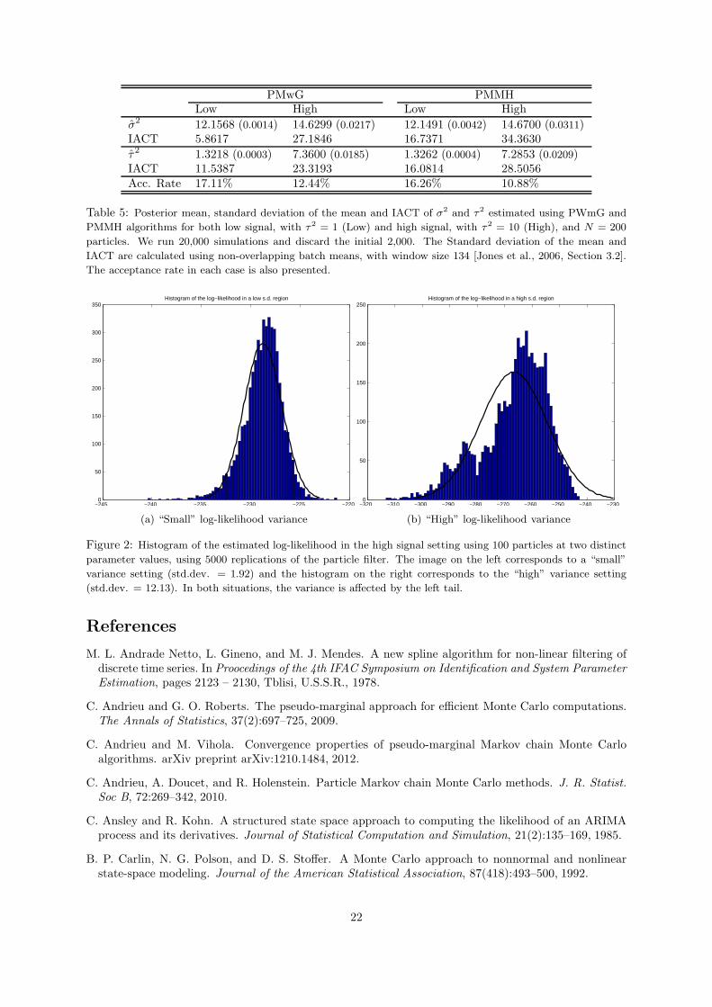
PMwG PMMHLow High Low High

σ2 12.1568 (0.0014) 14.6299 (0.0217) 12.1491 (0.0042) 14.6700 (0.0311)IACT 5.8617 27.1846 16.7371 34.3630

τ2 1.3218 (0.0003) 7.3600 (0.0185) 1.3262 (0.0004) 7.2853 (0.0209)IACT 11.5387 23.3193 16.0814 28.5056Acc. Rate 17.11% 12.44% 16.26% 10.88%

Table 5: Posterior mean, standard deviation of the mean and IACT of σ2 and τ2 estimated using PWmG and

PMMH algorithms for both low signal, with τ2 = 1 (Low) and high signal, with τ

2 = 10 (High), and N = 200

particles. We run 20,000 simulations and discard the initial 2,000. The Standard deviation of the mean and

IACT are calculated using non-overlapping batch means, with window size 134 [Jones et al., 2006, Section 3.2].

The acceptance rate in each case is also presented.

−245 −240 −235 −230 −225 −2200

50

100

150

200

250

300

350Histogram of the log−likelihood in a low s.d. region

(a) “Small” log-likelihood variance

−320 −310 −300 −290 −280 −270 −260 −250 −240 −2300

50

100

150

200

250Histogram of the log−likelihood in a high s.d. region

(b) “High” log-likelihood variance

Figure 2: Histogram of the estimated log-likelihood in the high signal setting using 100 particles at two distinct

parameter values, using 5000 replications of the particle filter. The image on the left corresponds to a “small”

variance setting (std.dev. = 1.92) and the histogram on the right corresponds to the “high” variance setting

(std.dev. = 12.13). In both situations, the variance is affected by the left tail.

References

M. L. Andrade Netto, L. Gineno, and M. J. Mendes. A new spline algorithm for non-linear filtering ofdiscrete time series. In Proocedings of the 4th IFAC Symposium on Identification and System ParameterEstimation, pages 2123 – 2130, Tblisi, U.S.S.R., 1978.

C. Andrieu and G. O. Roberts. The pseudo-marginal approach for efficient Monte Carlo computations.The Annals of Statistics, 37(2):697–725, 2009.

C. Andrieu and M. Vihola. Convergence properties of pseudo-marginal Markov chain Monte Carloalgorithms. arXiv preprint arXiv:1210.1484, 2012.

C. Andrieu, A. Doucet, and R. Holenstein. Particle Markov chain Monte Carlo methods. J. R. Statist.Soc B, 72:269–342, 2010.

C. Ansley and R. Kohn. A structured state space approach to computing the likelihood of an ARIMAprocess and its derivatives. Journal of Statistical Computation and Simulation, 21(2):135–169, 1985.

B. P. Carlin, N. G. Polson, and D. S. Stoffer. A Monte Carlo approach to nonnormal and nonlinearstate-space modeling. Journal of the American Statistical Association, 87(418):493–500, 1992.

22

C. Carter and R. Kohn. Markov chain Monte Carlo in conditionally Gaussian state space models.Biometrika, 83(3):589–601, 1996.

C. K. Carter and R. Kohn. On Gibbs sampling for state space models. Biometrika, 81(3):541–553, 1994.

N. Chopin and S. S. Singh. On the particle Gibbs sampler. arXiv preprint arXiv:1304.1887, 2013.

P. Del Moral, A. Doucet, and A. Jasra. Sequential Monte Carlo for Bayesian computation. In J. Bernardo,M. Bayarri, J. Berger, A. Dawid, D. Heckerman, A. Smith, and M. West, editors, Bayesian statistics8: proceedings of the eighth Valencia International Meeting, June 2-6, 2006, volume 8, pages 115–148.Oxford University Press, 2007.

R. Douc and O. Cappe. Comparison of resampling schemes for particle filtering. In Image and SignalProcessing and Analysis, 2005. ISPA 2005. Proceedings of the 4th International Symposium on, pages64–69. IEEE, 2005.

A. Doucet, S. Godsill, and C. Andrieu. On sequential Monte Carlo sampling methods for Bayesianfiltering. Statistics and Computing, 10(3):197–208, 2000.

A. Doucet, M. K. Pitt, and R. Kohn. Efficient implementation of Markov chain Monte Carlo when usingan unbiased likelihood estimator. arXiv:1210.1871, 2012.

S. Fruhwirth-Schnatter. Data augmentation and dynamic linear models. Journal of Time Series Analysis,15(2):183–202, 1994.

S. Fruhwirth-Schnatter. Finite Mixture and Markov Switching Models. New York, NY: Springer Science+Business Media, LLC, 2006.

R. Gerlach, C. Carter, and R. Kohn. Efficient Bayesian inference for dynamic mixture models. Journalof the American Statistical Association, 95(451):819–828, 2000.

S. Godsill, A. Doucet, and M. West. Monte Carlo smoothing for nonlinear time series. Journal of theAmerican Statistical Association, 99(465):156–168, 2004.

N. J. Gordon, D. J. Salmond, and A. F. Smith. Novel approach to nonlinear/non-Gaussian Bayesianstate estimation. In IEE Proceedings F (Radar and Signal Processing), volume 140, pages 107–113.IET, 1993.

D. Guo, X. Wang, and R. Chen. New sequential Monte Carlo methods for nonlinear dynamic systems.Statistics and computing, 15:135–147, 2005.

G. L. Jones, M. Haran, B. S. Caffo, and R. Neath. Fixed-width output analysis for Markov chain MonteCarlo. Journal of the American Statistical Association, 101(476):1537–1547, 2006.

S. Kim, N. Shephard, and S. Chib. Stochastic volatility: likelihood inference and comparison with ARCHmodels. The Review of Economic Studies, 65(3):361–393, 1998.

G. Kitagawa. Monte Carlo filter and smoother for non-Gaussian nonlinear state space models. Journalof computational and graphical statistics, 5(1):1–25, 1996.

F. Lindsten and T. C. Schon. On the use of backward simulation in particle Markov chain Monte Carlomethods. arxiv:1110.2873, 2012.

J. Liu and M. West. Combined parameter and state estimation in simulation-based filtering. In N. de Fre-itas, A. Doucet, and N. Gordon, editors, Sequential Monte Carlo Methods in Practice, pages 197 –223. Springer-verlag, New York, 2001.

J. Olsson and T. Ryden. Rao-Blackwellization of particle Markov chain Monte Carlo methods usingforward filtering backward sampling. Signal Processing, IEEE Transactions on, 59(10):4606–4619,2011.

M. K. Pitt and N. Shephard. Filtering via simulation: Auxiliary particle filters. Journal of the Americanstatistical association, 94(446):590–599, 1999.

23

M. K. Pitt, R. Silva, P. Giordani, and R. Kohn. Auxiliary particle filtering within adaptive Metropolis-Hastings sampling. arXiv preprint arXiv:1006.1914, 2010.

M. K. Pitt, R. d. S. Silva, P. Giordani, and R. Kohn. On some properties of Markov chain Monte Carlosimulation methods based on the particle filter. Journal of Econometrics, 171:134–151, 2012.

N. G. Polson, J. R. Stroud, and P. Muller. Practical filtering with sequential parameter learning. Journalof the Royal Statistical Society: Series B (Statistical Methodology), 70(2):413–428, 2008.

J.-F. Richard and W. Zhang. Efficient high-dimensional importance sampling. Journal of Econometrics,141(2):1385–1411, 2007.

G. O. Roberts and J. S. Rosenthal. Geometric ergodicity and hybrid Markov chains. Electron. Comm.Probab, 2(2):13–25, 1997.

G. O. Roberts and J. S. Rosenthal. General state space Markov chains and MCMC algorithms. ProbabilitySurveys, 1:20–71, 2004.

G. O. Roberts and J. S. Rosenthal. Examples of adaptive MCMC. Journal of Computational andGraphical Statistics, 18(2):349–367, 2009.

N. Shephard and M. K. Pitt. Likelihood analysis of non-Gaussian measurement time series. Biometrika,84(3):653–667, 1997.

G. Storvik. Particle filters for state-space models with the presence of unknown static parameters. SignalProcessing, IEEE Transactions on, 50(2):281–289, 2002.

L. Tierney. A note on Metropolis-Hastings kernels for general state spaces. The Annals of AppliedProbability, 8(1):1–9, 1998.

R. Van Der Merwe, A. Doucet, N. De Freitas, and E. Wan. The unscented particle filter. Advances inneural information processing systems, pages 584–590, 2001.

G. Wahba. Bayesian ”confidence intervals” for the cross-validated smoothing spline. Journal of the RoyalStatistical Society. Series B (Methodological), 45:133–150, 1983.

W. E. Wecker and C. F. Ansley. The signal extraction approach to nonlinear regression and splinesmoothing. Journal of the American Statistical Association, 78(381):81–89, 1983.

A Backward simulation

Godsill et al. [2004] introduce an alternative way of sampling a particle from a particle filter. Theirapproach differs from ancestral tracing in that it samples the indices JT , JT−1, . . . , J1 sequentially, in-stead of sampling one index J and tracing back its ancestral lineage. The backward simulation algo-rithm has been used in the PMCMC setting by Olsson and Ryden [2011] (in the PMMH algorithm) andLindsten and Schon [2012] (in the PG algorithm). Chopin and Singh [2013] studied the PG algorithmwith backward simulation and found that it yields a smaller autocorrelation than the correspondingalgorithm using ancestral tracing. Moreover, it is more robust to the resampling scheme (multinomialresampling, systematic resampling, residual resampling or stratified resampling) used in the resamplingstep of the algorithm.

The backward simulation algorithm is given below.

Algorithm 4 (Backward Simulation). 1. Sample JT = jt conditional on u1:T , with probability pro-portional to wjT

T , and choose xjTT ;

2. For t = T − 1, . . . , 1, sample Jt = jt conditional on (u1:t, jt+1:T , xjt+1

t+1 , . . . , xjTT ), with probability

proportional to wjtt fθ(x

jt+1

t+1 |xjtt ), and choose xjtt .

24

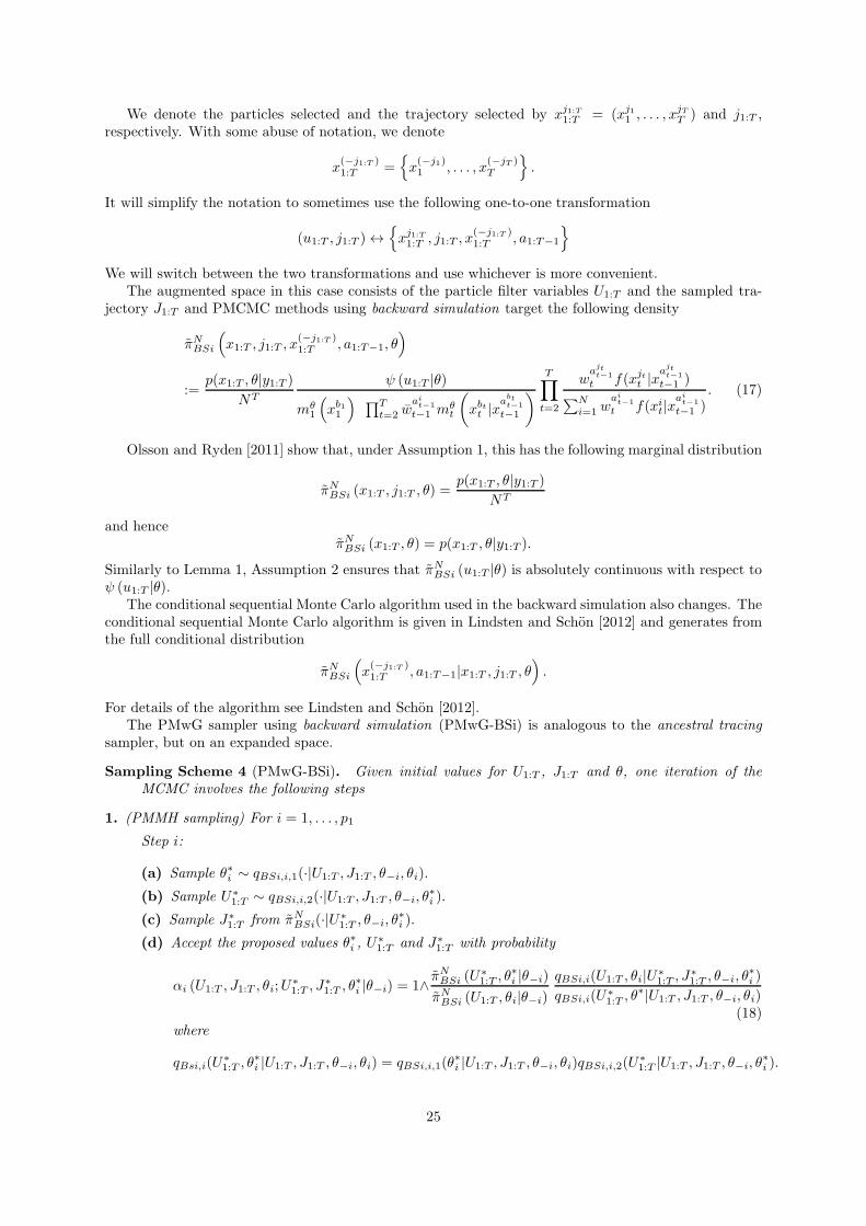
We denote the particles selected and the trajectory selected by xj1:T1:T = (xj11 , . . . , xjTT ) and j1:T ,

respectively. With some abuse of notation, we denote

x(−j1:T )1:T =

{x(−j1)1 , . . . , x

(−jT )T

}.

It will simplify the notation to sometimes use the following one-to-one transformation

(u1:T , j1:T ) ↔{xj1:T1:T , j1:T , x

(−j1:T )1:T , a1:T−1

}

We will switch between the two transformations and use whichever is more convenient.The augmented space in this case consists of the particle filter variables U1:T and the sampled tra-

jectory J1:T and PMCMC methods using backward simulation target the following density

πNBSi

(x1:T , j1:T , x

(−j1:T )1:T , a1:T−1, θ

)

:=p(x1:T , θ|y1:T )

NT

ψ (u1:T |θ)

mθ1

(xb11

) ∏Tt=2 w

ait−1

t−1 mθt

(xbtt |x

abtt−1

t−1

)T∏

t=2

wajtt−1

t f(xjtt |xajtt−1

t−1 )∑N

i=1 wait−1

t f(xit|xait−1

t−1 ). (17)

Olsson and Ryden [2011] show that, under Assumption 1, this has the following marginal distribution

πNBSi (x1:T , j1:T , θ) =

p(x1:T , θ|y1:T )

NT

and henceπNBSi (x1:T , θ) = p(x1:T , θ|y1:T ).

Similarly to Lemma 1, Assumption 2 ensures that πNBSi (u1:T |θ) is absolutely continuous with respect to

ψ (u1:T |θ).The conditional sequential Monte Carlo algorithm used in the backward simulation also changes. The

conditional sequential Monte Carlo algorithm is given in Lindsten and Schon [2012] and generates fromthe full conditional distribution

πNBSi

(x(−j1:T )1:T , a1:T−1|x1:T , j1:T , θ

).

For details of the algorithm see Lindsten and Schon [2012].The PMwG sampler using backward simulation (PMwG-BSi) is analogous to the ancestral tracing

sampler, but on an expanded space.

Sampling Scheme 4 (PMwG-BSi). Given initial values for U1:T , J1:T and θ, one iteration of theMCMC involves the following steps

1. (PMMH sampling) For i = 1, . . . , p1

Step i:

(a) Sample θ∗i ∼ qBSi,i,1(·|U1:T , J1:T , θ−i, θi).

(b) Sample U∗1:T ∼ qBSi,i,2(·|U1:T , J1:T , θ−i, θ

∗i ).

(c) Sample J∗1:T from πN

BSi(·|U∗1:T , θ−i, θ

∗i ).

(d) Accept the proposed values θ∗i , U∗1:T and J∗

1:T with probability

αi (U1:T , J1:T , θi;U∗1:T , J

∗1:T , θ

∗i |θ−i) = 1∧

πNBSi (U

∗1:T , θ

∗i |θ−i)

πNBSi (U1:T , θi|θ−i)

qBSi,i(U1:T , θi|U∗1:T , J

∗1:T , θ−i, θ

∗i )

qBSi,i(U∗1:T , θ

∗|U1:T , J1:T , θ−i, θi)(18)

where

qBsi,i(U∗1:T , θ

∗i |U1:T , J1:T , θ−i, θi) = qBSi,i,1(θ

∗i |U1:T , J1:T , θ−i, θi)qBSi,i,2(U

∗1:T |U1:T , J1:T , θ−i, θ

∗i ).

25

2. (PMH sampling) For i = p1 + 1, . . . , p2

Step i:

(a) Sample θ∗i ∼ qi(·|XJ1:T , B

J1:T−1, J, θ−i, θi).

(b) Sample U(−J),∗1:T ∼ πN(·|XJ

1:T , BJ1:T−1, J, θ−i, θ

∗i ) using Algorithm 2.

(c) Accept the proposed values U(−J),∗1:T and θ∗i with probability

αi

(U

(−J)1:T , θi;U

(−J),∗1:T , θ∗i |X

J1:T , B

J1:T−1, J, θ−i

)

= 1 ∧πN(θ∗i |X

J1:T , B

J1:T−1, J, θ−i

)

πN(θi|XJ

1:T , BJ1:T−1, J, θ−i

) qi(θi|XJ1:T , B

J1:T−1, J, θ−i, θ

∗i )

qi(θ∗|XJ

1:T , BJ1:T−1, J, θ−i, θi)

. (19)

(d) Sample J ∼ πN (·|U1:T , θ).

3. (PG sampling) For i = p2 + 1, . . . , p

Step i:

(a) Sample{X

(−j1:T )1:T , A1:T−1, θi

}∼ πN

BSi(·|XJ1:T

1:T , J1:T , θ−i). using conditional sequential Monte

Carlo algorithm from Lindsten and Schon [2012].

(b) Sample J1:T ∼ πNBSi (·|U1:T , θ).

The PMMH steps in Sampling Scheme 4 simplify in a similar way to Sampling Scheme 1. Olsson and Ryden[2011] show that

πNBSi (U1:T , θi|θ−i)

ψ (U1:T |θ−i, θi)=Z(U1:T , θ)p(θi|θ−i)

p (y1:T |θ−i),

which is the same expression as (5). Hence if

qBSi,i,2 (·|U1:T , J, θ) = ψ (·|θ)

then the Metropolis-Hasting acceptance probability in (18) simplifies to

1 ∧Z(θ∗i , θ−i, U

∗1:T )

Z(θi, θ−i, U1:T )

qBSi,i,1(θi|U∗1:T , J

∗, θ−i, θ∗i )p(θ

∗i |θ−i)

qBSi,i,1(θ∗|U1:T , J, θ−i, θi)p(θi|θ−i)

.

The results in Section 3.4 can be modified for the distribution πNBSi (·), instead of the distribution

πN (·) in a straightforward way. Details are available from the authors on request.

26