ARTICLE IN PRESS

0378-4371/$ - se

doi:10.1016/j.ph

�CorrespondE-mail addr

Physica A 363 (2006) 393–403

www.elsevier.com/locate/physa

A Markov model of financial returns

M. Servaa,b, U.L. Fulcob,c, I.M. Gleriab, M.L. Lyrab,F. Petronia, G.M. Viswanathanb,�

aDipartimento di Matematica and I.N.F.M. Universita dell’Aquila, I-67010 L’Aquila, ItalybDepartamento de Fısica, Universidade Federal de Alagoas, Maceio– AL, 57072-970, Brazil

cDepartamento de Fsica, Universidade Federal do Piau, Terezina– PI, 64049-550, Brazil

Received 2 February 2005; received in revised form 28 June 2005

Available online 17 October 2005

Abstract

We address the general problem of how to quantify the kinematics of time series with stationary first moments but

having non stationary multifractal long-range correlated second moments. We show that a Markov process is sufficient to

model important aspects of the multifractality observed in financial time series and propose a kinematic model of price

fluctuations. We test the proposed model by analyzing index closing prices of the New York Stock Exchange and the

DEM/USD tick-by-tick exchange rates obtained from Reuters EFX. We show that the model captures the characteristic

features observed in actual financial time series, including volatility clustering, time scaling and fat tails in the probability

density functions, power-law behavior of volatility correlations and, most importantly, the observed nonuniversal

multifractal singularity spectrum. Motivated by our finding of strong agreement between the model and the data, we argue

that at least two independent stochastic Gaussian variables are required to adequately model price fluctuations.

r 2005 Elsevier B.V. All rights reserved.

Keywords: Times series analysis; Volatility correlations; Multifractals

1. Introduction

The quantitative description of economic [1] phenomena has recently become a new challenge for a largecommunity of physicists [1–9], due to the many similarities with collective phenomena in physics and theincreasing availability of data records [10–23]. Prices have no stationary moments; however, price incrementshave approximately stationary mean. Let St represent the market price at a given instant t, e.g., of a stock, astock market index or the exchange rate between two currencies. We define the log-returns rt at time t as

rt ¼ log10Stþ1

St

. (1)

Such returns have nonstationary multifractal long-range power-law correlated local variances [1,4,7]. Thestudy of long-range memory is an important issue in finance. During the last several years, research in physics,

e front matter r 2005 Elsevier B.V. All rights reserved.

ysa.2005.08.070

ing author.

ess: gandhi@df.ufal.br (G.M. Viswanathan).

ARTICLE IN PRESSM. Serva et al. / Physica A 363 (2006) 393–403394

mathematical finance and econometrics has attempted to give an explanation to this long-range memory of themarkets [21–23]. The issue is appealing to physicists since it involves non linear dynamics, noise modeling,collective phenomena and fractals. Here we investigate the kinematics of financial time series (see Fig. 1) andpropose a model that, despite being Markovian, captures important features of actual financial time series,including the observed fat tails, their nonuniversal volatility multifractal singularity spectra, as well as fat tailsand time scaling in the probability density functions (PDFs).

An important contribution in modeling time series with nonstationary second moments came from thestudy of auto-regressive conditional heteroscedasticity (ARCH) models, introduced by Engle in 1982 [24].ARCH models refer to Markovian stochastic processes characterized by zero mean and nonconstant variancesdependent on the past. Such models can simultaneously have global stationarity as well as local nonstationarybehavior. The simplest ARCH model of returns has local variance defined by

s2t ¼ a0 þ a1r2t�1,

with returns defined as

rt ¼ stot.

The random Gaussian variable ot has unitary variance and zero mean, while a0 and a1 represent tunableparameters. Hence, the returns rt follow a Gaussian distribution with zero mean and a volatility given by s2t :In more general ARCH processes, the local variance can depend not only on the previous value rt�1, but onany finite number n of previous values rt�1 . . . rt�n. GARCH [25] models result from a further generalization inwhich the local variance can depend not only on previous values of the returns but also on the previous valuesof the locally measured variances (see Eq. (8)). All such stochastic kinematic models neglect the causesunderlying the price variations and only consider the equations of motion governing the fluctuating returns.Specifically, ARCH–GARCH models neglect the interacting buying and selling processes. Such models havenevertheless succeeded in capturing some features of actual financial data, e.g., volatility clustering. The threemost important (and difficult to model) features not well accounted in ARCH–GARCH models are (i) thetime scaling of the PDF of the returns, (ii) the known long-range power-law correlations in the volatility, and(iii) the multifractality of the returns, i.e., the volatility power-law correlation exponents depend on themagnitude of the events considered. Whereas ‘‘monofractals’’ have a single fractal dimension, on the other

-0.06

-0.04

-0.02

0.00

0.02

0.04

0.06

r

0 1000 2000 3000 4000 5000 6000 7000 8000 9000t

0.00

0.01

0.02

0.03

0.04

0.05

0.06

|r|

(a)

(b)

Fig. 1. (a) Daily log-returns (see Eq. (1)) and (b) absolute log-returns for the New York Stock Exchange (NYSE) data set. Such time series

have stationary means but nonstationary second moments (hence, the ‘‘volatility’’). Moreover, the absolute returns have long-range

power-law correlations. The values of the scaling exponents depend on the moment studied, i.e., the correlations have multifractal rather

than monofractal characteristics.

ARTICLE IN PRESSM. Serva et al. / Physica A 363 (2006) 393–403 395

hand a multifractal typically has a fractal dimension that depends on the moment studied. We discussmultifractality more thoroughly in Section 2.4.

As an alternative model, Levy [26] and truncated Levy distributions [27] have been proposed to fit theobserved fat tailed distributions. The recently proposed [28] BNS stochastic volatility (SV) continuous-timemodel attempts to describe returns in terms of a differential equation with the volatility s2t following a nonGaussian Ornstein–Uhlenbeck process driven by a Levy stochastic process with no correlations (i.e.,independent Levy variables). Moreover, to better characterize financial time series, a number of other modelshave been proposed, including TARCH [21] and FIGARCH [29] processes, multifractal random walks [23],and other SV and similar models [30–33]. Levy-based models can approximately (but not correctly [6,34])reproduce the time scaling of the PDF. However, such models cannot account for known multifractal long-range correlations in volatility. Some studies have suggested that such correlations may generate volatilityclustering and lead to the persistence of fat tails over long time lags [6,34].

Motivated by the need to adequately address these concerns, we investigate here a new model that does notsuffer from the drawbacks mentioned [35]. We construct the model by taking into account the following recentfindings: (i) the PDF of the local variance st is similar to a log-normal [4], (ii) long-range correlations found inthe absolute value of the returns; the multifractal behavior of the returns [7]. Based on these findings, andliberally extending a model proposed in Ref. [36], we propose the following map for the evolution of thevolatility:

stþ1 ¼ e½aþbotþ1�ðstÞd , (2)

with returns defined as

rt ¼ st ~ot, (3)

where ~ot and ot are independently distributed unitary Gaussian variables with zero mean that are alsoindependent from each other. The term st represents the average with respect to the last T times, from t� T tot. Since the average involves a number T of lags (typically in the range 2pTp10), therefore Eqs. (2), (3) forma Markov process. We find, remarkably, that the correlation time for the model far exceeds T, by more thanan order of magnitude. We note that while we have used an unweighted average for calculating st, in principlewe could have used any kind of moving average, e.g., an exponentially weighted moving average.

Since the proposed model represents a variation of a multiplicative process, it is not surprising that it shouldlead to multifractal features. The tunable constants a, b and d allow for diverse phenomena and nonuniversalmarket characteristics, and relate to the nearly log-normal form of st: The model requires do1 to guaranteeglobally stationary returns. While a relates to the mean of the daily volatility, b relates to the variance of thevolatility. Notice that this model, with two mutually independent Gaussian variables, contrasts with GARCHmodels, which only have one Gaussian variable. Below, we discuss why this feature might better correspond toactual markets. As a final remark we emphasize the fact that time is discrete in this model and takes integervalues, as in actual markets.

There are two important differences between our model and the families of ARCH–GARCH models. Thefirst is the presence of two independent Gaussian variables, one for returns and one for volatility. This choice,besides giving reasonable agreement with experimental data, has a deeper underlying motivation. InARCH–GARCH models there is an explicit dependence between the present-day volatility and the previousday’s absolute return while in our model the temporal evolution of volatility and returns is separated. In fact,it is commonly accepted that today’s sentiment about volatility does not depend on the previous day’svariation of price but rather on other quantities, such as previous day intraday volatility, implicit volatility inderivative products and public (or less public) information. Therefore, the present day volatility is notinfluenced by the previous day’s absolute return (which can be small after a fearful market day with enormousvariation of prices), and so the evolution of the first should be kept separate, exactly as we have done in themodel proposed (see also Ref. [30]). Indeed, such a separation can become necessary whenever we encounternonstationary second moments. Audio time series also have non-stationary variance [37] and also effectivelyrequire two independent variables, one to model the audio frequency signal and another to vary independentlythe sub-audio frequency loudness or intensity modulation [38] (i.e., the local variance).

ARTICLE IN PRESSM. Serva et al. / Physica A 363 (2006) 393–403396

The proposed model bears some resemblance to a latent volatility model proposed in Ref. [36] in twoaspects: (i) the volatility term contains a nonlinear power-law feedback on the previous day’s volatility, and (ii)both models use two independent Gaussian variables. Since our focus here lies in the returns PDF andmultifractality, we have extended the model to allow the present volatility to depend nonlinearly on anonuniformly weighted moving average of the previous days’ volatility.

Although volatility correlations exist, return correlations must decay rapidly for a market to beefficient. The efficient market hypothesis (EMH) holds that markets tend to reflect the available infor-mation. Specifically, to the extent that price changes appear non-random and hence forecastable, tothat extent a profit-seeking arbitrageurs can make appropriate purchases and sales of assets to exploitthis information [39–41]. An expected consequence is that correlations in the returns decay very rapidlyin time.

2. Method and results

2.1. Data

We base our study on two significantly different data sets: the New York Stock Exchange (NYSE) dailycomposite index price closes from January 1966 to September 2001 (a total of some 9000 data points) andpreprocessed [42] DEM/USD tick-by-tick exchange rates taken from Reuters EFX (provided by Olsen &Associates) during a period of 1 year from January to December 1998, corresponding to 1:620843� 106 quoteentries in the EFX system. We thus use data obtained from two entirely different markets: the DEM/USDdata set contains quotes for approximately every 20 s while the NYSE closes daily. Note the difference in thedata set sizes. By using two substantially different data sets, we can obtain a more rigorous testing of theproposed kinematic model.

2.2. Long-range power-law volatility correlations

We test the model against the NYSE time series by generating 9000 artificial returns using Eqs. (2), (3). Wehave empirically estimated the choice of constants a ¼ �0:1, b ¼ 0:1, d ¼ 0:98 and T ¼ 10 days. To measurecorrelations efficiently in non-stationary time series, we apply a variation of the well documented detrendedfluctuation analysis (DFA) [43,44]. Consider the cumulative returns ftðLÞ, defined as the mean value of L

successive returns:

ftðLÞ �1

L

XL

i¼1

rtþi.

One can define N=L nonoverlapping variables of this type, and compute the associated variance s2ðfðLÞÞ,where N denotes the number of data points in the data set. According to the central limit theorem, if rt areuncorrelated variables (i.e., white noise), then the cumulative return fluctuations will scale as a power-law,

s2ðfðLÞÞ�L�a, (4)

with exponent a ¼ 1 for large L, while a ¼ 0 for 1=f -noise and a ¼ �1 for Brown noise. Indeed, a ¼ 2� 2H,where H is the Hurst exponent. We find that the exponent a both for the NYSE index and the model proposedhere falls near 1 (see Fig. 2). In fact, daily returns have no auto-correlations for lags larger than a single day, inagreement with the EMH.

Correlations do appear, however, if we consider the absolute returns rather than the returns themselves. Inorder to perform the appropriate multifractal scaling analysis, we introduce the generalized cumulativeabsolute returns, defined as the mean value of L successive absolute return powers jrtj

q; . . . ; jrtþL�1jq,

ftðL; qÞ �1

L

XL

i¼1

jrtþijq,

ARTICLE IN PRESS

2-16

-14

-12

-10

-8

-6

-4

-12

-8

-6

-4 α =1.007±0.01

α(2)=0.734±0.013

α(4)=0.979±0.003

α=1.025±0.008

α(2)=0.386±0.008

α(4)=0.556±0.009

10

φ(L)

φ(L,2)

φ(L,4)

log10 L

log 10

σ2

log 10

σ2

-10

(b)(a)

210log10 L

Fig. 2. Double log plot of the variance s2ðfðL; qÞÞ�L�aðqÞ defined in Eq. (5) of the generalized cumulative absolute returns for (a) the

NYSE index and (b) the proposed kinematic model. Data for the absolute moments with q ¼ 2 (square) and q ¼ 4 (diamond) are

compared with the variance s2ðfðLÞÞ�L�a (see Eq. (4)) of the cumulative returns (circles). Both data and model show multifractal

behavior, since there is no unique scaling exponent. The ability of the proposed kinematic model to generate multifractal behavior

distinguishes it from the well-known families of models.

M. Serva et al. / Physica A 363 (2006) 393–403 397

where q is a real exponent. Note that we use nonoverlapping quantities. If the absolute returns have long-range power-law correlations, then

s2ðfðL; qÞÞ�L�aðqÞ. (5)

However, if the jrtjq are short-range correlated or power-law-anticorrelated with an exponent aðqÞ41, then we

would not detect anomalous scaling in the analysis of variance, because it is not possible to detect a41 usingthe method discussed here. This situation rarely or never arises for absolute returns.

We find that both the actual data and the model (Fig. 2) show apparent multifractal behavior with non-unique scaling exponents, i.e., aðqÞa constant. Note that the function aðqÞ is not universal [4,7] but depends onthe particular asset considered. Therefore, it is not surprising that the values aðqÞ we compute do not coincidefor the actual data and the model. Indeed, we expect the model and the data not to have identical aðqÞ due tothe nonuniversality inherent in finance. The important point to note is the (nonuniversal) multifractality.

In order to obtain better agreement for the multifractal exponents for a specific choice of financial timeseries one can generalize the map as follows:

xtþ1 ¼ eaþbotþ1 ðxct Þ

d , (6)

where the exponent c in the volatility average would allow for a finer control of the effects caused by extremalevents. The resulting returns could also be written as

rt ¼ ðav þ xtÞ ~ot � st ~ot, (7)

with av representing an intrinsic constant contribution to daily volatility. Using this generalized map wegenerate a data set of 1:6� 106 returns to compare our model with high frequency data from the foreignexchange market. We use the following estimated parameters: a ¼ �0:29, b ¼ 0:37, d ¼ 0:98, c ¼ 1,a ¼ 0:1� 10�4, T ¼ 10. We also consider for completeness a data set of identical size generated using aGARCH(1,1) model defined as

s2t ¼ a0 þ a1r2t�1 þ b1s2t�1, (8)

ARTICLE IN PRESSM. Serva et al. / Physica A 363 (2006) 393–403398

with returns defined as

rt ¼ stot, (9)

with parameters a0 ¼ 2:3� 10�5, a1 ¼ 0:085 and b1 ¼ 0:9 [1]. We chose the parameters for the GARCH(1,1)model on the basis of the kurtosis and variance estimated from actual data.

2.3. Autocorrelation function

Unlike the NYSE index data, which have only around 9000 data points, the relatively large numberof data points available in the DEM/USD data set permits a direct estimation of autocorrelations and aquantitative comparison of the multifractal power-law correlations with the models. We define theautocovariances CðL; qÞ as

CðL; qÞ � hjrtjqjrtþLj

qi � hjrtjqi2 (10)

for time lag L. Results for different values of q and for the two data sets are presented in Fig. 3. We find thatwhile the power-law behavior of autocovariances is preserved when data are generated using our model, aGARCH(1,1) model does not show this behavior [1], as seen in Fig. 3(c). Moreover the power-law behavior ofautocovariances shows multifractality since the exponent aðqÞ is different for each q. This behavior isqualitatively identical for the actual data and the proposed model. However, multifractal power-law behaviorappears inconsistent with the GARCH(1,1) model.

2.4. Multifractal singularity spectra

Mandelbrot pioneered research into multifractal measures [45,46]. Later, a number of studies appliedmultifractal concepts to describe quantitatively the behavior of financial processes [47,48]. More recently,multifractal models incorporating elements of Mandelbrot’s past research have been proposed [49–51] asalternatives to ARCH-type representations. Indeed, price changes in financial markets appear to share manyfeatures characterizing turbulent flows and multifractal models seem to provide a surprisingly good fit of thePDF of the data [50]. We follow a similar approach with our focus on mutifractality, fat tails and long rangecorrelations in volatility. Most previous studies have investigated the multifractality of returns, however ourinterest here lies in the multifractality of the absolute returns.

Motivated thus to quantify further the multifractal properties of the time series, we now study theirmultifractal spectra. The multifractal spectrum of a time series contains information about n-pointcorrelations [52] and thus provides more information compared to two-point correlation functions. We applythe multifractal detrended fluctuation analysis (MF-DFA) method to study the multifractal spectrum [53].Like the wavelet transform modulus maximus (WTMM) method [54], the MF-DFA method avoids thedifficulties of managing diverging negative moments. We briefly summarize the MF-DFA method as follows:

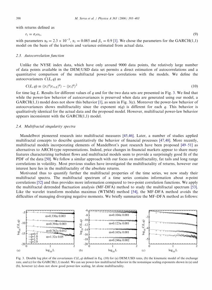
-20

-15

-10

-5

q=0.5q=1.0q=1.5q=2.0

-20

-18

-16

-14

-12

-10

-8

-6

2

-5

-4

-3α=0.330± 0.003

α=0.394± 0.003

α=0.762± 0.012

α=1.32± 0.05

α=0.104± 0.001

α=0.123± 0.001

α=0.165± 0.001

α=0.246± 0.002

102102log10 L log10 L log10 L

10

log 10

C(L

,q)

log 10

C(L

,q)

log 10

C(L

,q)

(a) (b) (c)

Fig. 3. Double log plot of the covariances CðL; qÞ defined in Eq. (10) for (a) DEM/USD rates, (b) the kinematic model of the exchange

rate, and (c) for the GARCH(1,1) model. We can see power-law multifractal behavior in the nonunique scaling exponents shown in (a) and

(b), however (c) does not show good power-law scaling, let alone multifractality.

ARTICLE IN PRESSM. Serva et al. / Physica A 363 (2006) 393–403 399

First, we integrate the time series jrtj to generate a profile yðtÞ �Pt

k¼1 jrtj, which we can visualize as a one-dimensional random walk. We then divide the series yðtÞ into Ns segments of size s. We use non overlappingsegments, so the product sNs gives the total length of the complete time series. For each segment n, we applylinear regression (generalizable to polynomial regression) to calculate a best fitting ‘‘trend’’ ynðiÞ, wherei ¼ 1; 2; . . . ; s. For each segment n we can thus define a mean square fluctuation

F2ðn; sÞ �1

s

Xs

i¼1

jyððn� 1Þsþ iÞ � ynðiÞj2,

which corresponds to a measure of the second moment for segment n. We then define a qth order fluctuationfunction

FqðsÞ �1

Ns

XNs

n¼1

F2ðn; sÞq=2.

Positive values of q weight large fluctuations while negative moments weight small fluctuations. The fact thatF2ðn; sÞ always remains positive avoids the divergence of the negative moments. The scaling of the fluctuationfor moment q follows

FqðsÞ�sqhðqÞ, (11)

where hðqÞ represents a generalized Hurst exponent, with the traditional Hurst exponent given by H ¼ hð2Þ.Monofractal time series have a unique Hurst exponent hðqÞ ¼ H, while for multifractal series the value of hðqÞ

depends on q.We can relate hðqÞ to the exponents tðqÞ conventionally used to quantify the scaling of the partition function

ZqðsÞ�stðqÞ

in the standard textbook multifractal formalism [53] via

tðqÞ ¼ qhðqÞ � 1. (12)

We can obtain this relation by noting that for any positive, normalized and stationary time series xðtÞ, we candefine a ‘‘box probability’’

psðnÞ �Xns

k¼ðn�1Þsþ1

xðtÞ

for box size s, given the normalizationPsNs

k¼1 xðkÞ ¼ 1. The partition function is defined as

ZqðsÞ �XNs

n¼1

jpsðnÞjq.

The relation given by Eq. (12) can be seen by noting that ZqðsÞ�NsF qðsÞ. The advantage of methods such asWTMM and MF-DFA arises due to not being limited to stationary, positive, and normalized time series.Fig. 4(a) shows that except for the GARCH series, tðqÞ is not linear, indicating multifractality. The GARCHseries has approximately linear behavior, indicative of monofractality. Note that uncorrelated white noise hasHurst exponent hðqÞ ¼ 1

2and tðqÞ ¼ q=2� 1, so plotting t� q=2 will give a horizontal (i.e., constant) line. We

have therefore plotted tðqÞ � q=2 instead of tðqÞ for easier visualization.The Legendre transform of Eq. (12) gives the multifractal singularity spectrum f ðasÞ:

as ¼ dtðqÞ=dq, (13)

f ðasÞ ¼ qas � tðqÞ. (14)

Here, f gives the dimension of the subset of the series characterized by the singularity strength as. Theliterature also refers to as as the Holder exponent, which represents a measure of the number of continuousderivatives that the underlying signal possesses. The singularity spectrum of monofractal time series will showa unique Holder exponent, while a multifractal series will show a range of values for as. Fig. 4(b) shows that

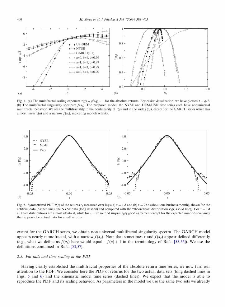
ARTICLE IN PRESS

-4 -2 0 2 4q

-8

-6

-4

-2

0

US-DEMNYSEGARCH(1,1)a=0, b=1, d=0.99

a=1, b=1, d=0.99

a=1, b=3, d=0.99

a=0, b=1, d=0.90

0.5 1.0 1.5 2.00.2

0.4

0.6

0.8

1

f(α s

)

αs

τ (q

)- q

/2

(a) (b)

Fig. 4. (a) The multifractal scaling exponent tðqÞ ¼ qhðqÞ � 1 for the absolute returns. For easier visualization, we have plotted t� q=2.(b) The multifractal singularity spectrum f ðasÞ. The proposed model, the NYSE and DEM/USD time series each have nonuniversal

multifractal behavior. We see the multifractality in the nonlinearity of tðqÞ and in the wide f ðasÞ, except for the GARCH series which has

almost linear tðqÞ and a narrow f ðasÞ, indicating monofractality.

-4.0

-2.0

0.0

2.0

4.0

ln P

(r)

NYSEModel

-0.05 0.00 0.05r

-4.0

-2.0

0.0

2.0

4.0

ln P

(r)

-0.05 0.00 0.05r

Pt(r)

(a) (b)

Fig. 5. Symmetrized PDF PðrÞ of the returns rt measured over lags (a) t ¼ 1 d and (b) t ¼ 25 d (about one business month), shown for the

artificial data (dashed line), the NYSE data (long dashed) and compared with the ‘‘theoretical’’ distribution PtðrÞ (solid line)). For t ¼ 1 d

all three distributions are almost identical, while for t ¼ 25 we find surprisingly good agreement except for the expected minor discrepancy

that appears for actual data for small returns.

M. Serva et al. / Physica A 363 (2006) 393–403400

except for the GARCH series, we obtain non universal multifractal singularity spectra. The GARCH modelappears nearly monofractal, with a narrow f ðasÞ. Note that sometimes t and f ðasÞ appear defined differently(e.g., what we define as f ðasÞ here would equal �f ðaÞ þ 1 in the terminology of Refs. [55,56]). We use thedefinitions contained in Refs. [53,57].

2.5. Fat tails and time scaling in the PDF

Having clearly established the multifractal properties of the absolute return time series, we now turn ourattention to the PDF. We consider here the PDF of returns for the two actual data sets (long dashed lines inFigs. 5 and 6) and the kinematic model time series (dashed lines). We expect that the model is able toreproduce the PDF and its scaling behavior. As parameters in the model we use the same two sets we already

ARTICLE IN PRESS

-10 -5 0 5 10-5

-4

-3

-2

-1

0

DEM-USDMODEL

log 10

P(r

)

Pt(r)

r/σ

Fig. 6. Symmetrized PDF PðrÞ of the returns rt shown for the high frequency DEM/USD series, the artificial data, and the theoretical

distribution PtðrÞ. We see that a Gaussian with log-normally distributed variance provides a good description of the absolute return

distribution up until 10 standard deviations.

M. Serva et al. / Physica A 363 (2006) 393–403 401

used for autocorrelations. We also compare the PDF of actual and artificial data with a ‘‘theoretical’’distribution (solid line), which we introduce to obtain a better understanding of the form of the actual dataand model PDF. The proposed ‘‘theoretical’’ distribution is a Gaussian Pt with log normally distributed localvariance:

PtðrÞ ¼

ZrðsÞ

exp �r2

2s2

� �ffiffiffiffiffiffi2pp

sds, (15)

rðsÞ ¼1ffiffiffiffiffiffi2pp

ssexp �

1

2

log s�m

s

� �2" #

. (16)

Indeed, the resulting PDF is the convolution of Gaussian PDF with different (lognormally distributed)volatilities. We obtain two sets of constants for the two data sets, s ¼ 0:41 and m ¼ �0:34 for the NYSE series,and s ¼ 0:78 and m ¼ �0:35 for the DEM/USD series. In order to estimate the PDF of returns from the twodata sets using the standard histogram method, we have used the equivalent smooth interpolation given by

PðrÞ ¼1

N

XN

i¼1

1ffiffiffiffiffiffi2pp

Dexp

�ðr� riÞ2

2D2

� �

with a smoothing window of D ¼ 0:001 (Fig. 5(a) for the NYSE index and D ¼ 0:4 for the DEM/USD rates(Fig. 6). The ri in this expression can be either from the actual or artificial data and N is their number. Thesolid lines in Figs. 5(a) and 6 suggest that this distribution is among the better candidates for describing thedistribution of price variations. The agreement found is unexpectedly strong.

We next study the PDF time scaling typically observed in financial times series. For both actual andartificial data we estimate (using the same smoothing window) the distribution for monthly (25 business days)returns (Fig. 5(b)) of the NYSE indexP25

i¼1 riþt

ð25Þd¼

1

ð25Þdlog

Stþ25

St

,

using the measured value d ¼ 0:53 of the scaling exponent. Note that the solid line curve is exactly the same inthe two figures, therefore both actual and artificial data exhibit almost perfect time scale invariance of thereturn distributions (see also Ref. [34]). The lack of agreement for small monthly returns is due to short-range

ARTICLE IN PRESSM. Serva et al. / Physica A 363 (2006) 393–403402

(1 d) correlations in the signs of the returns that are neglected in our model, but that could easily beincorporated [34]. Compared to other models of financial returns, this model shows remarkably goodagreement with actual data.

3. Discussion

Our results show that the proposed kinematic model can reproduce the non universal multifractality and thePDF of the absolute returns. The model is able to generate a wide range of multifractal behavior.Nevertheless, note that we are not interested in obtaining perfectly identical multifractal properties for theproposed model and the actual data. Indeed, the observed non universality would invalidate such attempts.

A second important difference relates to how the proposed model generates volatility similarly to amultiplicative process, in spite of being an additive process. The similarity with multiplicative processes arisesdue to the log-normally distributed variance (Eq. (16)), which enters the model via the exponential term inEq. (2). The additivity enters the model in the moving average of Eq. (2). This ingredient in the model isdesirable in order to account for the approximately lognormal PDF of volatilities observed in actual financialtime series.

Finally, we note that these results are obtained by means of the proposed Markov process and that themultifractal volatility correlations are not in the input, but are generated a posteriori by the model. Thiskinematic model is thus different from others (see for example Ref. [58]) where correlations are already presentin the input ingredients, i.e., it is assumed a priori that increments are long-range correlated. Furthermore, themodel presented here also seems to represent an advance due to the much improved agreement with actualdata. Indeed, we find good agreement for up to 10 standard deviations in the PDF (Fig. 6). How strong thisagreement is becomes particularly evident if one considers that the two data sets analyzed significantly differ innature. One consists of a daily stock market index and the other of high frequency currency exchange rate datasampled up to every 2 s. An interesting question for future study is how to modify the model to account for theexistence of return-volatility asymmetric correlations (i.e., the ‘‘leverage effect’’) [30,33,59]. Anotherinteresting question concerns the implications for efficiency of a Markov model of financial returns.

Acknowledgements

We thank the anonymous referees for very helpful suggestions. We thank Y. Ashkenazy and MichelePasquini for discussions and the Brazilian research agencies CAPES, CNPq and FAPEAL. One of us (F.P.)acknowledges the financial support of Cofin MIUR 2002 prot. 2002027798_005.

References

[1] R.N. Mantegna, H.E. Stanley, An Introduction to Econophysics: Correlations and Complexity in Finance, Cambridge University

Press, Cambridge, 2000.

[2] J.-P. Bouchaud, A. Matacz, M. Potters, Phys. Rev. Lett. 87 (2001) 228701.

[3] B. Podobnik, P.Ch. Ivanov, Y. Lee, A. Chessa, H.E. Stanley, Europhys. Lett. 50 (6) (2000) 711.

[4] M. Pasquini, M. Serva, Euro. Phys. J. B 16 (2000) 195.

[5] Y. Liu, P. Gopikrishnan, P. Cizeau, M. Meyer, C.-K. Peng, H.E. Stanley, Phys. Rev. E. 60 (1999) 1390.

[6] P. Gopikrishnan, V. Plerou, L.A. NunesAmaral, M. Meyer, H.E. Stanley, Phys. Rev. E 60 (1999) 5305.

[7] M. Pasquini, M. Serva, Econ. Lett. 65 (1999) 275.

[8] R.N. Mantegna, H.E. Stanley, Nature 383 (1996) 587.

[9] R.N. Mantegna, H.E. Stanley, Nature 376 (1995) 46.

[10] L. Bachelier, Ann. Sci. Ecole Norm. Sup. 17 (1900) 21.

[11] Newton Da Costa Jr., Silvia Nunes, Paulo Ceretta, Sergio Da Silva, Econ. Bull. 7 (3) (2005) 1–9.

[12] Z. Ding, C.W.J. Granger, R.F. Engle, J. Empirical Finance 1 (1993) 83.

[13] N. Crato, P. De Lima, Econ. Lett. 45 (1994) 281.

[14] J.-P. Bouchaud, D. Sornette, J. Phys. I France 4 (1994) 863.

[15] M. Mevy, S. Solomon, Int. J. Mod. Phys. C 7 (1996) 595.

[16] R.T. Baillie, J. Econometrics 73 (1996) 5.

[17] S. Gallucio, G. Caldarelli, M. Marsili, Y.-C. Zhang, Physica A 245 (1997) 423.

ARTICLE IN PRESSM. Serva et al. / Physica A 363 (2006) 393–403 403

[18] N. Vandewalle, M. Ausloos, Physica A 246 (1997) 454.

[19] Y. Liu, P. Cizeau, M. Meyer, C.-K. Peng, H.E. Stanley, Physica A 245 (1997) 437.

[20] B. Podobnik, K. Matia, A. Chessa, P.Ch. Ivanov, Y. Lee, H.E. Stanley, Physica A 300 (2001) 300.

[21] R.F. Engle, A.J. Patton, Quant. Finance 1 (2001) 237.

[22] E. Bacry, J. Delour, J.F. Muzy, Phys. Rev. E 64 (2001) 026103.

[23] A.P. Kirman, G. Teyssiere, Microeconomic models for long-memory in the volatility of financial time series, in: Studies in Nonlinear

Dynamics and Econometrics, vol. 5(4), Berkeley Electronic Press, 2002, p. 1083.

[24] R.F. Engle, Econometrica 50 (1982) 987.

[25] T. Bollerslev, J. Econometrics 31 (1986) 307–327.

[26] B.B. Mandelbrot, J. Bus. 36 (1963) 394.

[27] R.N. Mantegna, H.E. Stanley, Phys. Rev. Lett. 73 (1994) 2946.

[28] Ole E. Barndorff-Nielsen, Neil Shephard, J. Statistics 30 (2003) 277–295.

[29] R.T. Baillie, J. Econometrics 73 (1996) 5.

[30] J. Perell, J. Masoliver, Phys. Rev. E 67 (2003) 037102.

[31] J. Perell, J. Masoliver, N. Anento, Physica A 344 (2004) 134–137.

[32] G. Zumbach, Quant. Finance 4 (2004) 70.

[33] J. Perell, J. Masoliver, J.-P. Bouchaud, Appl. Math. Finance 11 (2004) 27–50.

[34] G.M. Viswanathan, U.L. Fulco, M.L. Lyra, M. Serva, Physica A 329 (2003) 273–280.

[35] U.L. Fulco, M.L. Lyra, F. Petroni, M. Serva, G.M. Viswanathan, Int. J. Mod. Phys. B 18 (2004) 681–689.

[36] R.F. Engle, A.J. Patton, Quant. Finance 1 (2001) 237–245.

[37] H.D. Jennings, P.Ch. Ivanov, A.M. Martins, P.C. Silva, G.M. Viswanathan, Physica A 336 (2004) 585–594.

[38] D. Panter, Modulation, Noise and Spectral Analysis, McGraw-Hill, New York, 1965.

[39] P.A. Samuelson, Ind. Manage. Rev. 6 (1965) 41–50.

[40] B.B. Mandelbrot, J. Bus. Univ. Chicago 39 (1966) 242.

[41] E.F. Fama, J. Finance 25 (1970) 383–417.

[42] F. Petroni, M. Serva, Euro. Phys. J. B 34 (2003) 495–500.

[43] C.-K. Peng, S.V. Buldyrev, S. Havlin, M. Simons, H.E. Stanley, A.L. Goldberger, Phys. Rev. E 49 (1994) 1685.

[44] K. Hu, Plamen Ch. Ivanov, Zhi Chen, Pedro Carpena, H.E. Stanley, Phys. Rev. E 64 (2001) 011114.

[45] B.B. Mandelbrot, in: M. Rosenblatt, C. Van Atta (Eds.), Statistical Models and Turbulence, Springer, New York, 1972.

[46] B.B. Mandelbrot, J. Fluid Mech. 62 (1974) 331–358.

[47] B.B. Mandelbrot, Fractals and Scaling in Finance: Discontinuity, Concentration, Risk, Springer, New York, 1997.

[48] B.B. Mandelbrot, Sci. Am. 280 (1999) 70–73.

[49] B.B. Mandelbrot, A.J. Fisher, L.E. Calvet, Cowles Foundation Discussion Paper No. 1164, http://ssrn.com/abstract=78588.

[50] T. Lux, Quantitative Finance 1 (2001) 632–640.

[51] T. Lux, Int. J. Mod. Phys. 15 (2004) 481–491.

[52] A.L. Barabasi, T. Vicsek, Phys. Rev. A 44 (1991) 2730.

[53] J.W. Kantelhardt, S.A. Zschiegner, E. Koscielny-Bunde, S. Havlin, A. Bunde, H.E. Stanley, Physica A 316 (2002) 87–114.

[54] J.F. Muzy, E. Bacry, A. Arneodo, Phys. Rev. Lett. 67 (1991) 3515.

[55] G. Paladin, A. Vulpiani, Phys. Rep. 156 (1987) 147–225.

[56] G. Paladin, A. Vulpiani, Phys. Rev. B 35 (1987) 2015.

[57] K. Matia, Y. Ashkenazy, H.E. Stanley, Europhys. Lett. 61 (2003) 422–428.

[58] E. Bacry, J. Delour, J.F. Muzy, Phys. Rev. E 64 (2001) 026103.

[59] J.-P. Bouchaud, A. Matacz, M. Potters, Phys. Rev. Lett. 87 (2001) 228701.