April 14, 2009

Institutional Herdingand Future Stock Returns∗

Roberto C. Gutierrez Jr.†

andEric K. Kelley‡

Abstract

When the trading of institutional investors is imbalanced between buys and sells,how are stock prices affected? The extant literature on such herding by institutions,represented by Wermers (1999) and Sias (2004), concludes that herding promotesprice discovery and helps adjust prices to their intrinsic levels. That is, they findherding to correctly predict stock returns in the coming months. In contrast, twoto three years after the herding, we find that stocks with buy herds realize negativeabnormal returns. This longer run reversal in returns is robust across subperiodsand performance metrics and impedes the interpretation of herding as solely pro-moting price discovery. In addition, we find that non-13F investors, roughly labeledindividual investors, suffer these longer run reversals in returns. The performancesof the herding and nonherding institutions are less clear. On the sell side, however,herding does not explain future abnormal returns.

∗This is a substantial revision of a prior paper on which we received helpful comments from seminarparticipants at Arizona State University, University of Oregon, the Pacific Northwest Finance Confer-ence, and the 2008 Summer Finance Conference at the University of British Columbia, and especiallyMarkus Brunnermeier, Diane Del Guercio, Jon Reuter, and Rick Sias. We thank them for their com-ments. Any errors are our own.†Corresponding author. Lundquist College of Business, University of Oregon (rcg@uoregon.edu).‡Eller College of Management, University of Arizona (ekelley@eller.arizona.edu).

Institutional Herding

and Future Stock Returns

Abstract

When the trading of institutional investors is imbalanced between buys and sells,how are stock prices affected? The extant literature on such herding by institutions,represented by Wermers (1999) and Sias (2004), concludes that herding promotesprice discovery and helps adjust prices to their intrinsic levels. That is, they findherding to correctly predict stock returns in the coming months. In contrast, twoto three years after the herding, we find that stocks with buy herds realize negativeabnormal returns. This longer run reversal in returns is robust across subperiodsand performance metrics and impedes the interpretation of herding as solely pro-moting price discovery. In addition, we find that non-13F investors, roughly labeledindividual investors, suffer these longer run reversals in returns. The performancesof the herding and nonherding institutions are less clear. On the sell side, however,herding does not explain future abnormal returns.

Institutional investors are increasingly larger players in equity markets. Their own-

ership of U.S. stocks has more than doubled in the past twenty years to over 60% of the

total market value, and their trading volume accounts for over 90% of the total dollar

volume.1 Consequently, there is much interest in the trading behaviors of institutional

investors and their effects on stock prices. Beginning at least with Kraus and Stoll

(1972a) and more recently with Lakonishok, Shleifer, and Vishny (1992), economists

have recognized the possibility that institutions relying on similar information and fac-

ing similar incentives might trade in the same direction. Hirshleifer and Teoh (2003)

and Brunnermeier (2001) provide a detailed and rich review of the large literature on

herding, providing overviews of theories as well as the evidence from financial markets.

In short, institutions might trade in the same direction for at least four reasons. One,

they observe similar information. Two, they favor stocks with certain characteristics,

such as “prudent,” liquid, or better-known stocks. Three, money managers concerned

for their reputations choose to mimic the trades of other managers. Four, managers

infer stock-valuation signals from others managers’ trades.2

These motivations for institutions to herd in their trades can result in varying effects

on stock prices. On one hand, as sophisticated and better-informed investors, institu-

tions might push prices toward their intrinsic values when they herd in their trading.

On the other hand, institutions might drive prices away from intrinsic levels if their

herding is based on characteristic preferences or managerial reputation.

Examining future stock returns offers a means of determining whether herding

pushes prices toward or away from intrinsic price levels. Wermers (1999) in his study

of mutual funds and Sias (2004) in his study of all institutions provide the most recent

analyses on this issue. Each measures herding as an imbalance of institutions that are

net buyers or net sellers over a given quarter, and each finds that the buy/sell im-

balance of institutional trades correctly anticipates the next several months of stock1Institutional ownership is estimated from 13F filings provided by Thomson Financial. The trading

volume estimates come from Kaniel, Saar, and Titman (2006) who examine all orders executed on theNYSE from 2000 to 2003 for all listed common U.S. stocks.

2Sias (2004) also provides a useful reference for studies identifying these motives to herd.

1

returns. They conclude that herds of institutional trades tend to reduce mispricings,

thereby aiding price discovery.

However, a longer run analysis is warranted. If a mispricing in fact does stem from

the herding, we learn from many studies of stock returns that presumed correctional re-

versals in prices tend to occur at horizons longer than one year. For example, Jegadeesh

and Titman (1993) and many others find a second-year reversal in returns to follow the

initial momentum in returns. Also, we should note that both Wermers (1999) and

Sias (2004) find evidence of a return reversal occurring at the end of the year following

the herd, granted this end-of-year reversal is small relative to the return continuations

earlier in the year.3

In this study, we examine the relations between longer run stock returns and insti-

tutional herding from 1980 to 2005. While we confirm earlier findings that a prepon-

derance of net buyers (or net sellers) correctly predicts shorter run returns, we find a

robust return reversal which begins in the fourth quarter after the herding and persists

throughout years two and three. Our findings suggest that institutional herding does

result in stock prices that reliably deviate from intrinsic levels, altering the extant view

of herding as solely benefiting price discovery.

Furthermore, the longer run return reversal is concentrated on the buy side, with

stocks in the top decile of herding experiencing about a negative 4% return over years

two and three, adjusted for size, book-to-market equity, and momentum effects. Herding

on the sell side has no relation to future returns across our full sample period, though

it does predict poor performance in the first half of our sample, similar to Wermers’

(1999) sample period and results. In contrast, the return reversals driven by the buy

herds are strongly evident in both halves of our sample period. We offer conjectures for

why the concentration of the return reversal is on the buy side in the conclusion of the

paper.3See Table VI of Wermers (1999) and Table 5 of Sias (2004).

2

Given that the longer run reversal finding on the buy side is the novel result of this

study, we focus our main attention on this reversal and its robustness.4 This longer run

return reversal is evident in portfolios of stocks with extreme herds, in cross-sectional

regressions identifying a sensitivity of future returns to variations in herding, in both

small and large stocks, and across a variety of performance metrics.5

After linking the return reversals to buy herds, we turn our attention to the herding

institutions and their trading acumen regarding the stocks into which they herd. Do

these institutions suffer the impending return reversals, or do they sell beforehand? To

address this, we evaluate the performances of portfolios formed by aggregating the stock

holdings of the institutions comprising a herd. These portfolios are tracked for three

years following the herd, and stock weights are updated quarterly using the holdings

data. We find mixed evidence of abnormal returns in the herding institutions’ trading of

the buy-herd stocks, and can make no clear conclusions. Similarly, the findings for the

other, non-herding institutions are also mixed. In contrast, the third type of investor

that we examine, the “individual” investors, defined as the complement of the 13F

holdings, bear robust reversals in stock returns. Furthermore, we find that individual

investors, after the herding quarter, increase their positions in stocks for which future

abnormal returns are negative. These findings for individual investors are evident in

both halves of our sample period. In short, institutional herding is ultimately hurting

at least one group of investors – individual investors.

Overall, our finding of longer run reversals in stock returns following institutional

herding transforms our understanding of herding from an aid in the process of price4Brown, Wei, and Wermers (2007) find that the herding of mutual fund trades in recent years predicts

shorter run (year one) return reversals. They highlight the differences in shorter run returns betweenthe last fifteen years and prior periods, consistent with differences we detect using 13F data. Our mainfocus however is on longer run returns, years two and three. We find that reversals in these longerhorizons have existed since 1980, as far back as we can look. Also, Coval and Stafford (2007) find returnreversals following herds of mutual fund trades driven by extreme fund flows. By examining herds offire sales and purchases, which are rare events, they cannot speak to any overall, unconditional effectsof herding, which is our focus.

5We also examine changes in the level of aggregate institutional ownership (∆IO), which is positivelycorrelated with the proportion of trading institutions that are net buyers, and find that it also predictslong run return reversal. However, the proportion of buyers dominates ∆IO as a predictor of long runreversal. That is, the imbalance across the numbers of buyers and sellers is more important than theimbalance across the sizes of the buys and sells.

3

discovery to a presumed trigger of mispricings which require the future reversal in

returns. Future research with higher frequency trade data can perhaps shed more light

on the dynamics of the trading between institutional and individual investors in these

stocks, including more examinations of whether institutions profit from their herding.

In addition, our results indicate that future researchers of institutional herding must

carefully control for returns contemporaneous and prior to the herding quarter. We find

that the failure to control for these returns significantly affects standard measures of

future abnormal returns of stocks with herds, potentially confounding a herding effect

on stock prices with a lagged-return effect.

In section 1, we present the data and methodology. Section 2 details our exami-

nations of the relations between herding and future stock returns. Section 3 discusses

motives for herding and examines the trading performances of investors in the buy-herd

stocks. We conclude in section 4.

1. Data and Methodology

The data on institutional stock holdings are obtained from Thomson Financial and are

gathered from 13F filings of institutional investors from 1980 to 2005. We gather stock

price, shares outstanding, and return data from CRSP and book value of equity from

Compustat. After merging these data sources and cleaning the holdings data, we have

a sample of 4,115 institutions. Details of our handling of the 13F data are given in the

appendix.

1.1. Herding Measure

Our measure of herding is based on Lakonishok, Shleifer, and Vishny’s (1992) and is

commonly used in the literature. For each institution and each stock in quarter t, we

first determine the change in the number of shares held from quarter t − 1 to quarter

t, adjusted for stock splits. Herding by institutions for each stock in quarter t is then

4

defined as follows.

HERDt =number of net buyers

number of net buyers + number of net sellers(1)

This variable measures the imbalance of institutional trading between buys and sells.

Note that we are not concerned with whether the herding is greater than that which

might have occurred by chance, as Lakonishok, Shleifer, and Vishny (1992) and Kraus

and Stoll (1972a) are. Our interest is simply to examine the effects of institutional

trades on stock prices when these trades cluster together.

For all of our tabulated results, we require a stock to have at least 10 institutional

traders in quarter t and institutional ownership less than or equal to 100% of the shares

outstanding. Varying the filter on the number of traders from 1 to 20 has little effect on

our overall findings. Inspection of the data reveals that imposing a maximum of 100%

institutional ownership results in the removal of extreme observations that are surely

data errors. Also, we consider a second measure of herding using the number of shares

bought and sold, instead of the number of buyers and sellers, and our main findings

remain.6

1.2. Abnormal Returns

Our tests examine the relation between herding and future abnormal returns. The

measure of abnormal returns that we employ accounts for size, book-to-market equity,

and momentum effects. As done by Daniel, Grinblatt, Titman, and Wermers (1997),

hereafter “DGTW,” and many others, we identify a benchmark portfolio for each stock6 We discuss the results using the share-based measure, as well as using the change in the percentage

of institutional ownership, in section 2.4. For several reasons we prefer to measure herding based on thenumbers of buyers and sellers instead of the numbers of shares bought and sold. First, Jones, Kaul, andLipson (1994) find that stock price movements are due more to the number of trades than to the size oftrades, and Sias, Starks, and Titman (2006) find that the number of institutions holding a stock is morestrongly related to returns than is the percentage of institutional ownership. Second, the reputationalmotive to follow the herd considers the imbalance in the number of institutions buying or selling. And,although less clear, the signal-inference motive would seem to weight the number of traders more thanthe volume traded since the sizes of managed portfolios can vary greatly. Last, the price impact of asingle trader with a given trade size should be lower than that of a number of traders with a collectivelysimilar trade size, as the single trader can strategically work his order over time to reduce price impact.

5

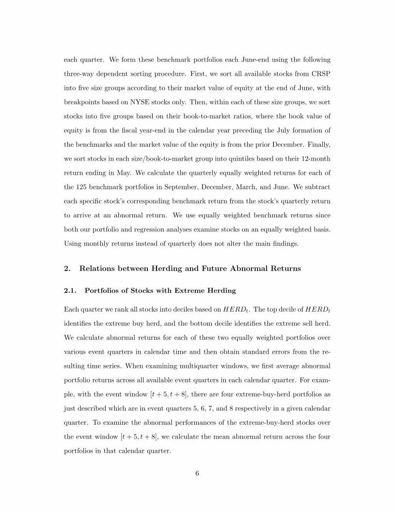
each quarter. We form these benchmark portfolios each June-end using the following

three-way dependent sorting procedure. First, we sort all available stocks from CRSP

into five size groups according to their market value of equity at the end of June, with

breakpoints based on NYSE stocks only. Then, within each of these size groups, we sort

stocks into five groups based on their book-to-market ratios, where the book value of

equity is from the fiscal year-end in the calendar year preceding the July formation of

the benchmarks and the market value of the equity is from the prior December. Finally,

we sort stocks in each size/book-to-market group into quintiles based on their 12-month

return ending in May. We calculate the quarterly equally weighted returns for each of

the 125 benchmark portfolios in September, December, March, and June. We subtract

each specific stock’s corresponding benchmark return from the stock’s quarterly return

to arrive at an abnormal return. We use equally weighted benchmark returns since

both our portfolio and regression analyses examine stocks on an equally weighted basis.

Using monthly returns instead of quarterly does not alter the main findings.

2. Relations between Herding and Future Abnormal Returns

2.1. Portfolios of Stocks with Extreme Herding

Each quarter we rank all stocks into deciles based on HERDt. The top decile of HERDt

identifies the extreme buy herd, and the bottom decile identifies the extreme sell herd.

We calculate abnormal returns for each of these two equally weighted portfolios over

various event quarters in calendar time and then obtain standard errors from the re-

sulting time series. When examining multiquarter windows, we first average abnormal

portfolio returns across all available event quarters in each calendar quarter. For exam-

ple, with the event window [t + 5, t + 8], there are four extreme-buy-herd portfolios as

just described which are in event quarters 5, 6, 7, and 8 respectively in a given calendar

quarter. To examine the abnormal performances of the extreme-buy-herd stocks over

the event window [t+ 5, t+ 8], we calculate the mean abnormal return across the four

portfolios in that calendar quarter.

6

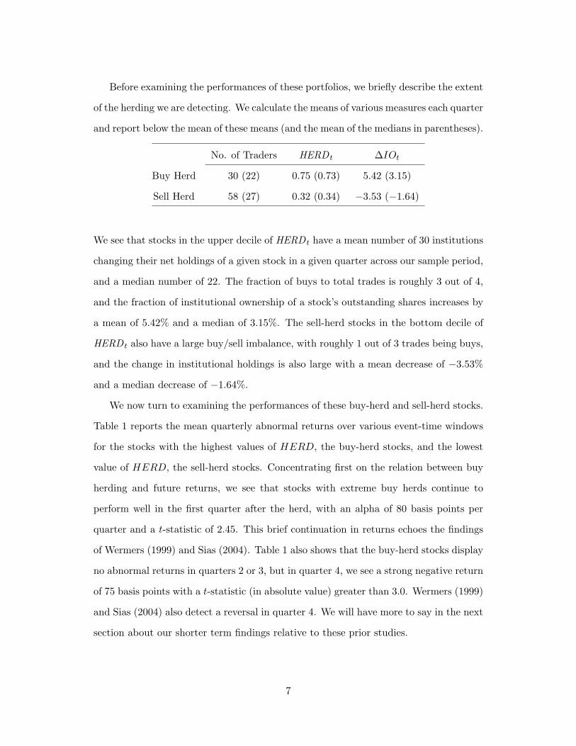
Before examining the performances of these portfolios, we briefly describe the extent

of the herding we are detecting. We calculate the means of various measures each quarter

and report below the mean of these means (and the mean of the medians in parentheses).

No. of Traders HERD t ∆IOt

Buy Herd 30 (22) 0.75 (0.73) 5.42 (3.15)

Sell Herd 58 (27) 0.32 (0.34) −3.53 (−1.64)

We see that stocks in the upper decile of HERD t have a mean number of 30 institutions

changing their net holdings of a given stock in a given quarter across our sample period,

and a median number of 22. The fraction of buys to total trades is roughly 3 out of 4,

and the fraction of institutional ownership of a stock’s outstanding shares increases by

a mean of 5.42% and a median of 3.15%. The sell-herd stocks in the bottom decile of

HERD t also have a large buy/sell imbalance, with roughly 1 out of 3 trades being buys,

and the change in institutional holdings is also large with a mean decrease of −3.53%

and a median decrease of −1.64%.

We now turn to examining the performances of these buy-herd and sell-herd stocks.

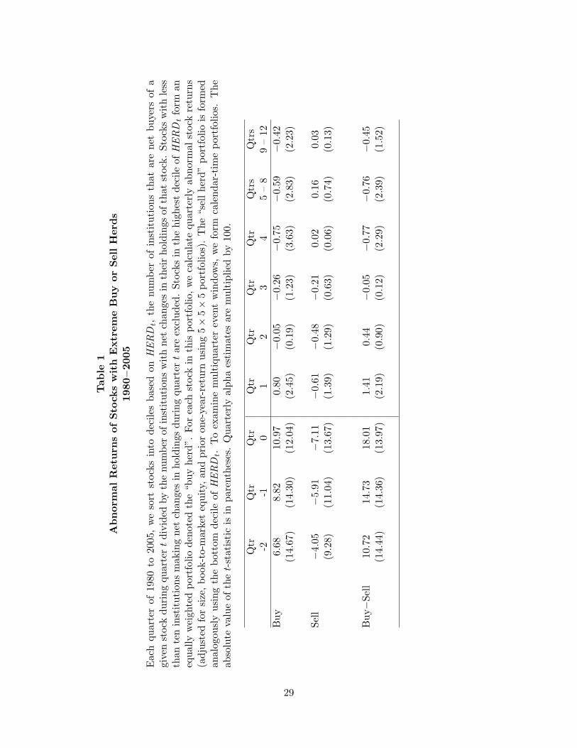
Table 1 reports the mean quarterly abnormal returns over various event-time windows

for the stocks with the highest values of HERD, the buy-herd stocks, and the lowest

value of HERD, the sell-herd stocks. Concentrating first on the relation between buy

herding and future returns, we see that stocks with extreme buy herds continue to

perform well in the first quarter after the herd, with an alpha of 80 basis points per

quarter and a t-statistic of 2.45. This brief continuation in returns echoes the findings

of Wermers (1999) and Sias (2004). Table 1 also shows that the buy-herd stocks display

no abnormal returns in quarters 2 or 3, but in quarter 4, we see a strong negative return

of 75 basis points with a t-statistic (in absolute value) greater than 3.0. Wermers (1999)

and Sias (2004) also detect a reversal in quarter 4. We will have more to say in the next

section about our shorter term findings relative to these prior studies.

7

The main – and new – finding of Table 1 is the strong longer run reversal in returns

displayed in years two and three. The buy-herd stocks have an alpha of negative 59

and negative 42 basis points per quarter, respectively, across year two and year three,

with t-statistics greater than 2.2 in each case. The longer run reversals are strong

enough to offset any brief continuation in returns following the buy herd. Specifically,

the alpha estimate across quarters 1 through 12 is negative 0.30% with a t−statistic

of 1.86. These longer run reversals following a buy herd are robust across alternative

measures of abnormal returns, across subperiods, and across large and small stocks. We

discuss each of these considerations in more detail in later sections.

Before moving to the performances of the extreme sell-herd stocks, we should high-

light the dramatically large abnormal returns occurring in the two quarters before we

measure herding as well as in the formation quarter. Table 1 reports abnormal returns

between 6% and 11% per quarter over these horizons. This is not surprising, but it does

present an important issue. Much evidence links institutional trading to prior returns.

Specifically, Bennett, Sias, and Starks (2003), Chen, Hong, and Stein (2002), and others

find that changes in institutional stock holdings are strongly positively related to both

current and lagged returns. Furthermore, Wermers (1999) and Sias (2004) find the

institutional herding measure we employ here to be positively related to current and

past returns as well. Since the DGTW measure of abnormal returns only controls for

12-month returns ending in May, we expect to see large abnormal returns in quarters

−2 to 0. Wermers (1999) and Sias (2004) find this as well. However, given that various

horizons of shorter term lagged returns are known to each display marginal effects on

future returns (see Gutierrez and Kelley (2008)), it is therefore important to control

for these lagged-return effects in our examinations of future returns. As Jegadeesh and

Titman (1993) and many subsequent studies document, returns over several quarters

are persistent for several more quarters but tend to reverse over longer run horizons.

Therefore, we need to ensure that the perceived effects of herding on future returns

8

are distinct from the known effects of lagged returns. In subsequent tests we control

explicitly for returns in quarters −2 to 0.

Finally, Table 1 also shows that stocks with extreme sell herds display no evidence

of abnormal returns in any of the future windows we examine. It is interesting to

note that our sell-side results differ from Wermers’ (1999) as he finds evidence of return

continuation on the sell side of herding. This difference is due to variation across sample

periods, as we discuss in the next section.

Note also from Table 1 that the shorter run continuation and the longer run reversal

in the returns of the buy-herd stocks makes the return spread between the buy-herd and

sell-herd stocks display both of these patterns as well. In other words, herding predicts

future reversals in returns unconditionally as well, not only when conditioning on a buy

herd.

2.2. Reconciling our Results with Prior Studies

While we examine abnormal returns over a much longer future window than prior studies

do, our shorter run results for the extreme sell herds find no relation with future returns

from 1980 to 2005. In contrast, Wermers (1999) finds that sell herds predict low future

returns from 1975 to 1994 in the four quarters following the sell herd. Since Sias (2004)

does not consider buy and sell herds separately, we focus our comparison on Wermers’

study, in particular his Table VI. At this point in our study, we have three variations

in our test design from that of Wermers. One, we have a different sample period. Two,

we use 13F data while Wermers uses mutual fund data. Three, we examine returns

adjusted for size, book-to-market equity, and prior twelve-month return effects while

Wermers adjusts for only size effects.7

7The 13F data are holdings data for all institutions (with at least $100 million under management andfor positions of least $200,000 or 10,000 shares), whereas the mutual fund data used by Wermers (1999)are only holdings of mutual funds. The 13F data might provide an advantage in a study of herding asthe data better reflect overall institutional demand. However, as the 13F data are aggregated over allmoney managers within a given institution, some information is possibly lost. Other differences between13F and mutual fund holdings are the timing and frequency of the reporting. 13F reports must be filedeach calendar quarter while mutual fund reporting is based on fiscal year ends of each fund and wasrequired only semiannually until 2004.

9

To ascertain which of the three appears to be the driver of our sell-side finding, we

begin by splitting our sample into two halves, 1980 to 1992 and 1993 to 2005, with the

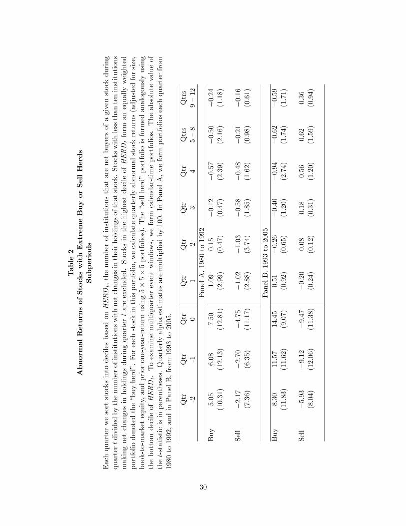
early sample including all formation periods through the end of 1992. Table 2 provides

the performances of the portfolios of stocks with extreme buy and sell herds, as in

Table 1. Panel A gives the early results and Panel B the later. We see in Panel A that

the earlier sample period produces results very similar to those of the “heavy buying”

and “heavy selling” portfolios in Table VI of Wermers (1999). Both our extreme buy-

side and extreme sell-side herding predict short-run continuations in returns. These

continuations last only for one quarter on the buy side but several quarters on the sell

side, similar to Wermers’ results. Also, our buy-side portfolio displays a return reversal

in the fourth quarter just as Wermers’ does.

The later sample period, given in Panel B, finds no evidence of continuations in re-

turns following neither buy nor sell herds. Importantly, the buy side still displays longer

run reversal starting in quarter 4 and continuing through year 3. The sell side, however,

now produces a different return pattern as there are large positive point estimates of

alphas, for example above 60 basis points per quarter in year two, but no statistical

significance. We also examine abnormal returns adjusted for size and book-to-market

equity only and for size only. These alphas are similar to those in Table 2. For the sell

herd, these alternative measures offer evidence of statistical reversal in the later period.

Brown, Wei, and Wermers (2007) find statistical evidence of reversals in returns in the

fourth quarter following both buy and sell herding of mutual funds in a similar sample

period from 1994 to 2003. The upshot of all this is that the sample period drives the

sell-side differences between our findings and those of Wermers (1999).

To see this in perhaps an easier way, the top plot of Figure 1 clearly depicts our

findings for the stocks with extreme buy herds. Here we cumulate the abnormal returns

quarter by quarter in event time. We can see that the alphas of these stocks are negative

in the longer run across the full period as well as the two subperiods. The returns of

these buy-herd stocks are persistently negative from quarter 4 to about quarter 12.8

8We examine performances out to quarter 20 but find no reliably nonzero alphas beyond quarter 12.

10

The bottom plot of Figure 1 shows our findings for the stocks with extreme sell

herds. The early period finds continuations in the returns of the sell-herd stocks, but no

longer run reversals. Moreover, the later period finds reversals in returns from quarter

4 to about quarter 11, but these are not statistically significant, as noted in Table

2. Nevertheless, the point estimates from the later period are impressive going from

roughly 0% in quarter 3 to a cumulative 4% in quarter 9.

As discussed earlier, prior returns during quarters −2,−1, and 0 can confound the

effects of herding on future returns, especially in the more recent years as the abnormal

returns from [t− 2, t] grow substantially (see Panel B of Table 1). To illustrate this, we

form portfolios that are neutral regarding raw returns over the formation quarter, rt, as

well as raw returns over the two quarters prior to formation, rt−2,t−1. Each quarter we

first sort all stocks into quintiles based on rt. We then sort each of these five portfolios

into five further portfolios based on rt−2,t−1. Lastly, we sort each of these 25 portfolios

into deciles based on HERD t. Each calendar quarter, we combine all the stocks in the

25 portfolios with the largest values of HERD t into an equally weighted portfolio to

estimate the performances of the extreme buy-herd stocks controlling for both rt and

rt−2,t−1. We do the analogous procedure for the extreme sell-herd stocks, the stocks in

the lowest deciles of HERD t.

The cumulative abnormal returns controlling for both rt and rt−2,t−1 are plotted in

Figure 2 for the extreme buy-herd and sell-herd stocks in the early and late subperiods.

First, in the top graph, we can see that controlling for lagged returns has little effect

on the buy side, another indication of the robustness of the longer run reversal in

returns. Specifically, using calendar-time tests as in Table 2, both the early and late

abnormal returns on the buy side display significant reversals across quarters 5 to 8 with

t-statistics above 1.98. Second, on the sell side of the herding, we see in the bottom

graph that lagged returns account for the disparity across subperiods shown in Figure

1. In fact, using calendar-time tests once again, we find that in the later subperiod

across quarters 5 to 8, the alpha on the sell-herd stocks controlling for rt and rt−2,t−1 is

11

65 basis points per quarter lower than the DGTW alpha in Table 2, with a t-statistic

of 2.32. This finding is a caution to current and future researchers of herding and stock

returns: Standard procedures to control for the effects of lagged returns may not be

sufficient.

In short, the findings of longer run reversal in the returns of stocks with extreme buy

herds is robust across sample periods and methods for defining abnormal returns. These

reversals strongly contrast with the messages of the shorter-run studies of Wermers

(1999) and Sias (2004).

2.3. Cross-Sectional Regressions

2.3.1. Method

We employ cross-sectional regressions to further examine the relation between herding

and future abnormal returns. Regressions allow us to succinctly examine the full cross

section of stocks, not only those in the extremes of herding, and to precisely control for

lagged returns. In the prior section, we discuss the need to control for rt and rt−2,t−1

based on the findings in Table 1. Furthermore, the additional return-neutral portfolio

testing, discussed above, offers evidence that failure to control for these return effects can

substantially alter estimates of the effect herding has on future returns. The portfolio

testing, however, is limited in its ability to account for lagged returns since quintile

sorts are used, leaving some variation within the portfolios. Employing rt and rt−2,t−1

in the regressions as controls allows us to fully account for the effects these measures

can have on future returns.9

Also in the prior section, we see the disparity between the buy herd and sell herd

effects on future returns. Specifically, the sell herd has little relation to future returns

while the buy herd predicts a strong longer run reversal in returns. We therefore ac-

commodate this asymmetry in our regressions. We define two continuous measures of9Controlling for rt−4,t−1 as well does not alter the findings.

12

herding,

BuyHERD t =

HERD t if HERD t ≥ HERD t

0 otherwise(2)

SellHERD t =

HERD t if HERD t < HERD t

0 otherwise(3)

where HERD t is the cross-sectional median of HERD in quarter t. Similar adjustments

are commonly used in the literature to define buying and selling herds. Employed as

regressors, the two above measures estimate the slopes of the relations between herding

and future returns across buy and sell herding respectively.

We estimate the following cross-sectional regression each quarter.

ARt+k = a+ b1BuyHERD t + b2SellHERD t + b3rt + b4r[t−2,t−1] + b5DUMBuyt + εt, (4)

where ARt+k is the benchmark-adjusted quarterly return for a given stock in quarter

t + k, with k varying from 1 to 12 quarters in the future, BuyHERD and SellHERD

are the measures just defined, rt is the raw return of the stock in quarter t, rt−2,t−1

is the raw return over the two prior quarters, and DUMBuyt is a dummy variable

set to one when HERD t ≥ HERD t and zero otherwise. The respective t-statistics

are calculated by dividing the mean of the quarterly time series of each coefficient by

its time-series standard error. When we examine multiple-quarter windows of future

returns, for example quarters 5 through 8, we pool the time series of coefficients from

each single-quarter analysis. That is, to explain abnormal returns in the quarter ending

October 1988, we consider four estimates of b1 corresponding to four separate and

rolling regressions, one using the BuyHERD in June of 1987 (5 quarters back), another

using BuyHERD in March 1987 (6 quarters back), and so on. We account for any

contemporaneous correlations in the coefficient estimates by clustering the standard

errors within each calendar quarter. Using the efficient-weighting procedure of Ferson

13

and Harvey (1999) to account for heteroskedasticity or using monthly abnormal returns

and monthly regressions, instead of quarterly, does not alter our main findings.

2.3.2. Regression Results

Table 3 reports the results of the regression in equation (4). Controlling more precisely

for rt and rt−2,t−1, the relations between herding and future returns are essentially the

same as those found using the portfolio analyses in the prior sections. Namely, as buy

herds increase, returns increase in the short-term but decrease in the longer term. The

reversals are again found to begin in quarter 4 and to persist through quarter 12. On

the other hand, the sell-herd stocks again display no abnormal future returns.

Analogous to Table 2, Tables 4 and 5 split our sample into early and late periods,

1980 to 1992 and 1993 to 2005, respectively. The results again mirror the prior portfolio

analyses. The early period in Table 4 shows evidence of a short-run positive relation

for both buy and sell herding, with the sell side displaying significance in quarter 2 but

not quarter 1. The longer relation between buy herding and future returns remains

negative in the early period. In the late period of Table 5, the longer run relation for

buy herding is still strongly negative.

2.4. Robustness Considerations

In the next few subsections, we further consider the robustness of the longer run relation

between institutional buy herding and future stock returns. We examine this relation

within subsamples of small and large stocks, using two alternative measures of herding,

not controlling for lagged returns, and controlling for the effects of size and book-to-

market equity on the right-hand side of the regression instead of the left-hand side.

2.4.1. Small and Large Stocks

Table 6 shows the regression results within small and large stocks respectively. We

define small stocks as those with market capitalizations less than that of the median

14

value across NYSE stocks in the most recent June, before the herding quarter. Large

stocks are the remaining stocks. We see a negative relation between buy herding and

returns over quarters 4 to 12 within both small and large subsamples.

2.4.2. Other Measures of Herding

Of the number of institutions that change their holdings of a stock in quarter t, we em-

ploy the proportion of those institutions that increase their holdings as our measure of

herding in the prior sections. Here we show that our main finding of a negative relation

between buy herding and future returns is obtained using an analogous share-based mea-

sure of herding as well as simply using the change in aggregate institutional ownership.

Specifically, the volume-based measure is the total number of shares bought on net by

all institutions that increased their positions in a given stock divided by the number of

shares in that stock traded on net by all institutions, labeled HERDShrst . Institutional

ownership is defined as the percentage of shares outstanding held by institutions, and

its change is labeled ∆IO.

Our preferred measure of herding (equation (1)) examines the number of institutions

that are buyers and sellers. The other two measures can be driven by a few large

institutions and therefore can more easily deviate from the intended goal of capturing

a preference among institutional traders to be buyers. Regardless of our inclinations,

however, the other two measures each empirically predict a longer run reversal in stock

returns. Again, we require at least 10 traders for each stock in quarter t.10

The first three columns of Table 7 examine the share-based measure and its relation

to future abnormal returns. As in earlier regressions, we split the herding measure into

separate buy and sell variables. We see a strong negative coefficient on buy herding

using the share-based measure in years one, two, and three. In the remaining three

columns, we compete the original measure, HERD t, with the share-based one. Longer

run reversal is better captured with the original measure, as the share-based measure

no longer displays any significance.10See footnote 6 for more discussion of our preferred measure of herding.

15

The first three columns of Table 8 examine changes in institutional ownership sep-

arated into buying and selling measures, positive ∆IO and negative ∆IO respectively.

This alternative measure also predicts reversals in future returns following buy herd-

ing.11 However, the ability of Positive∆IO to predict longer run reversals in returns is

also dominated by the explanatory power of the original measure, BuyHERD.

We do see some interesting differences though between these two alternative mea-

sures and HERD. In Table 8, changes in institutional ownership are negatively related

to future returns in year one even in the presence of HERD. For brevity’s sake we do

not report each quarter separately, but neither the share-based measure nor the change

in institutional ownership display any positive relation to future returns in the first few

quarters. Only BuyHERD captures a short-run continuation in returns (see Table 3).

2.4.3. Control Variables

To further document the robustness of the longer run reversals in returns that follow

buy herds, which examine two additional regression specifications. First, we remove rt

and rt−2,t−1 as regressors. We argue earlier that these controls are important to employ,

to ensure that the herding effects we find are unrelated to known lagged-return effects.

However, the first two columns of Table 9 show that removing rt and rt−2,t−1 from

the regressions does not alter the finding of longer run reversals due to buy herding,

consistent with the portfolio tests in Table 1.

The second specification that we consider in Table 9 controls for book-to-market-

equity and size effects on the right-hand side instead of on the left-hand side via the

DGTW adjusted returns. The last two columns of Table 9 show that stocks with buy

herds suffer return reversals in years two and three with this specification as well.11Dasgupta, Prat, and Verardo (2007) examine stocks with persistent changes in aggregate institu-

tional ownership over several quarters and find their returns to reverse in the future. Yan and Zhang(2009) examine short-term and long-term institutions and find that changes in holdings of only short-term institutions predict stock returns in the next year.

16

3. Do the herding institutions suffer the return reversals?

The prior sections document that buy herds of institutional investors negatively predict

future returns. Specifically, we find that the prices of stocks with extreme buy herds

fall by about 4.5% from quarter 4 to quarter 12, as shown in Table 1 and Figure 1.

This return pattern lends itself to a wide array of interpretations regarding the actions

of the herders themselves. On one extreme, the entering herd might be uninformed

about stock valuations and unaware of the impending price declines, leaving themselves

to suffer the price falls. On the other extreme, the herds of institutions might be fully

informed and sophisticated investors who through their herding seek to push stock prices

up only to exit the stocks ahead of the correctional declines in prices. We discuss each

of these views in the following sections.

3.1. Uninformed herd

Perhaps the more straightforward interpretation of the herding is that these institutions

are unaware of the impending price declines. One possible reason for their being unaware

can come from the nature of the herd itself. For example, to the extent that these herds

are formed on the basis of one manager following other managers, prior theoretical

research shows how the resulting herd can be uninformed about the intrinsic values of

the stocks they buy. The rational extraction of another trader’s signal from his actions

can lead subsequent traders to follow the earlier trader’s actions regardless of their own

valuation signals. Such an outcome impedes all information from being fully impounded

into prices. See the works of Banerjee (1992), Bikhchandani, Hirshleifer, and Welch

(1992), Welch (1992), and Avery and Zemsky (1998) for more detail. An uninformed

herd can similarly also result from the reputation-based herding noted by Scharfstein

and Stein (1990). Managers who are concerned about developing or maintaining their

reputations as good managers might rationally choose to mimic the actions of other

managers, possibly ignoring their own signals.

17

3.2. Hyperinformed herd

On the other extreme, prior literature identifies the possibility that the herders are so-

phisticated well-informed traders despite their taking positions in stocks whose prices

will soon fall. De Long, Shleifer, Summers, and Waldmann (1990) note how the pres-

ence of uninformed “noise” traders can result in sophisticated and informed investors

rationally choosing to buy an overvalued stock. The reason they buy an overvalued

stock today is the expectation that positive-feedback traders will be willing to buy the

stock tomorrow at an even higher price. Essentially, rational investors buy to stimulate

others’ demand for the stock and profit at the expense of the uninformed trend chasers.

Hence, the informed traders aggravate overpricing instead of correcting it. This no-

tion goes beyond the reasoning that limits to arbitrage inhibit informed and rational

investors from correcting mispricings that they know to exist, as advanced by Pontiff

(1996), Shleifer and Vishny (1997), and others. Limits to arbitrage predict that the

sizes of the positions taken by arbitragers are smaller than they would otherwise be,

but rational investors still trade to correct mispricings.

Abreu and Brunnermeier (2003) also note that informed and rational investors might

choose to aggravate mispricings. If more than one investor must trade against a “bubble”

to burst it, then rational investors face a coordination problem. In light of this, rational

investors who are uncertain about the actions the other rational investors will take

might decide to “ride the bubble” expecting to sell the stock at a higher price in the

future, as the bubble continues to grow.

Brunnermeier and Nagel (2004) provide empirical evidence consistent with sophisti-

cated investors choosing to ride bubbles. From 1998 to 2000, they find that hedge funds

increased their weights in technology stocks as the prices of those stocks rose, and then

decreased their weights before the prices of those stocks fell. A portfolio tracking their

trading in these stocks generates an abnormal return of 4.5% per quarter. In short,

18

hedge funds traded these stocks as if they were aware of the overvaluations, selling

before prices collapsed.12

Given these varied interpretations of the behaviors of the buy herders, we next ex-

amine whether these herders are better characterized as uninformed or informed traders,

using their trading performances in the buy-herd stocks to distinguish these two possi-

bilities. That is, we assume that a necessary condition for being informed is the ability

to generate positive abnormal returns.

3.3. How Well do the Herders Trade the Buy-Herd Stocks?

We evaluate trading performance by forming portfolios that mimic the herders’ trading

of these stocks. Since institutional ownership is only reported at quarter end, we cannot

determine precisely when their trades occur within the quarter. Therefore, we examine

the two extreme scenarios whereby trading in all quarters occurs either at the beginning

of the period or at the end.

Specifically, we identify the buy-herd stocks each calendar quarter as those in the

top decile of HERD t. We then identify every institution buying these stocks in that

quarter and track their aggregate current and future positions in these stocks. We

form a portfolio comprised of these aggregate positions, where the weights are based on

the dollar values of the positions held by the herding institutions. The performances

of these portfolios are determined in calendar time over various event windows, as in

earlier sections.

Table 10 provides the abnormal returns of these portfolios mimicking the trading of

the herding institutions. Panel A reports results for the full sample, 1980 to 2005; Panel

B for the early period, 1980 to 1992; Panel C for the late period, 1993 to 2005. Assum-

ing either beginning-of-period (BOP) trading or end-of-period (EOP) trading, Panel A

reveals no evidence of positive abnormal returns. That is, the herding institutions are

not trading these buy-herd stocks well. We can say no more than this as evidence of12The conclusion that a bubble existed in tech stocks in the late 1990s is debatable. Pastor and

Veronesi (2006) question whether NASDAQ prices ex ante were too high in the late 1990s.

19

negative abnormal returns are not robust across the BOP and EOP methods. The early

and late periods also lack robust evidence of abnormal returns.

We also consider the performances of two groups of other investors and examine

how each fares in their trading of the buy-herd stocks. The two trader groups are: 13F

institutions not buying with the herd in quarter t and non-13F traders. We label the

first group as “other” institutions, and the second as “individual” investors. The trading

of the individual investors is determined as the complement of the trading recorded in

the 13F data.13

Panel A of Table 10 indicates that the evidence on the performances of the other,

non-herding institutions’ portfolios of buy-herd stocks is also mixed. On one hand, the

BOP analysis finds positive alphas in the two years after the herding quarter. On the

other, the EOP method finds only evidence of negative abnormal returns in year 3. The

early and late periods display no robust alphas either. Hence, we can make no clear

conclusion.

Panel A of Table 10 also shows the performances of individual investors. For this

group the evidence is clear: Individual investors are strongly hurt by their trading of

these buy-herd stocks. Individual investors suffer negative alphas assuming either BOP

or EOP trading. The negative alphas for individual investors are robustly evident in each

of the subperiods as well. Moreover, in untabulated results, we identify a benchmark

no-trade portfolio which maintains the stock positions held in quarter t for the aggregate

individual-investor portfolio. Using this no-trade portfolio, we can see that individual

investors make themselves significantly worse off in their subsequent trading of the buy-

herd stocks. After quarter t, they increase their positions in stocks that will perform

poorly in the future. Specifically, over the full period, the actual portfolio for individual

investors underperforms its no-trade benchmark over quarters 1 to 12 by 0.20% per

quarter using EOP and by 0.72% per quarter using BOP, with t-statistics greater than

3.9 in each case. The finding that the post-herd trading of individual investors make13This complement is more than just trading by individual investors, as it includes small institutions

managing less than $100 million, small institutional positions of less than $200,000 and less than 10,000shares, and institutional short selling.

20

themselves worse off is also evident in each of the subperiods, with t-statistics greater

than 2.16 in each of the four cases (BOP/early, EOP/early, BOP/late, EOP/late).

Finally, we note that controlling for rt and rt−2,t−1 with the sorting procedure de-

scribed in section (2.2) also leaves no robust conclusions across BOP and EOP trading

for the herding and non-herding institutions, but once again, individual investors incur

significantly negative abnormal returns across both BOP and EOP trading.

Without higher frequency trade data, we are admittedly limited in what we can say

regarding the trading acumen of investors in the buy-herd stocks. The evidence using

quarterly data, however, does strongly suggest that individual investors make themselves

worse off by buying buy-herd stocks whose prices will subsequently fall. Why individual

investors pursue these buy-herd stocks is an interesting avenue for further research.

4. Conclusion

We find that buy herds predict negative abnormal stock returns two and three years

after the herding. This result suggests that buy herds trigger overvaluations, warranting

a correction. Our finding consequently alters the perception of institutional herding as

benefiting price discovery, as the extant literature concludes. The evidence we detect

of institutions’ having deleterious effects on stock prices (when they herd together to

buy) echoes the messages of recent studies examining institutions in other settings. For

example, Dasgupta, Prat, and Verardo (2007), Gutierrez and Pirinsky (2007), and Shu

(2007) link aggregate institutional trading to various cases of presumed stock mispric-

ings. These studies suggest, as we do, that some trading by institutions reliably drives

prices away from intrinsic values. Moreover, as discussed in these prior studies as well,

such trading can be a rational consequence of agency issues in money management or

of the presence of “noise” traders in the stock market. Further research to identify and

isolate why institutions trade as they do in these various circumstances is warranted.

On the sell side, in contrast to prior studies, we find that sell herds do not predict

future returns. While sell herds predicted return continuations in the early part of the

21

sample period, they have no explanatory power for future returns after 1992, nor for

the full period.

Our asymmetric findings for buy and sell herds seemingly contrast with the asym-

metries found in studies of daily and weekly institutional trading where return reversals

are found in the days following an institutional sell, but not following a buy. That is,

the price impact of a sell is temporary while the impact of a buy is permanent. See

the works of Kraus and Stoll (1972b), Chan and Lakonishok (1995), Kaniel, Saar, and

Titman (2006) and Campbell, Ramadorai, and Schwartz (2007). We suspect that these

high-frequency results are related to ours. On the buy side, the accumulation of the

price impacts of a herd of buys over a quarter should seemingly result in a sizable price

increase, which warrants a future correction in the stock’s price. On the sell side, the

accumulated price impacts of a herd of sells should remain small as the price impacts of

each trade typically reverse, requiring no future correction. Of course, these statements

remain conjectures at this point, and we leave their investigation to future research.

A second conjecture is that short-sale constraints might also contribute to the asym-

metries we find across buy and sell herds. These constraints diminish the market’s abil-

ity to adjust prices downward following a sell herd, which in this case might be a good

thing.

We also examine the trading acumen of the herding institutions regarding the stocks

into which they herd. We fail to find robust evidence of the herders’ profiting from their

herding. Beyond that, the evidence on the alphas of their portfolios of buy-herd stocks

is a mixed bag of inferences, as are the alphas on the other, non-herding institutions’

portfolios of buy-herd stocks. However, we find strong evidence that individual investors

bear the brunt of the poor performances of these buy-herd stocks. Future examinations

of performance with high-frequency data might shed more light on the trading dynamics

highlighted here.

22

A. Appendix

A.1. 13F data in more detail

From Thomson’s data on the 13F filings of institutions, we identify all stocks with CRSP

data, matching first on cusip and then on ticker. Thomson provides a change vari-

able which tracks split-adjusted changes in each institution’s holdings. For 24,605,585

stock/institution/quarters, SHSt − CHGt = SHSt−1, where SHSt is the number of

shares held in a given stock at the end of quarter t (with the stock subscript i and the

institutional subscript m suppressed) and CHGt is Thomson’s determined change in

the number of shares held this quarter from the last quarter, adjusted for stock splits.

When SHSt = CHGt, we label these entries by a given institution into the stock.

There are 4,070,465 entries. The remaining, discrepant observations are reexamined us-

ing split factors from CRSP. 726,774 of these discrepancies are due to splits in quarter

t, confirming that CHGt is correctly accounting for the split. For 732,574 observations

we cannot reconcile SHSt and CHGt with SHSt−1. For these records, we leave SHSt

and CHGt at their reported levels.14

For reasons we do not know, the Thomson data at times are missing filings for an

institution in quarter t but the filing for quarter t+1 and CHGt+1 is not missing. So we

have the opportunity to backfill observations. Thomson also provides the prior report

date from which their change variable is determined, though it is not well populated

until June 2000. For the cases where a hole occurs in the time-series of an institutions

filings, we proceed as follows. For June 2000 and later, if the first available data after

the hole, quarter t+ 1, states the prior report date to be quarter t, we then backfill the

holdings for quarter t using SHSt+1, CHGt+1, and split factors in quarter t + 1. This

enables us to recover CHGt if SHSt−1 is available. If SHSt−1 is missing we do not14One reason for our decision to trust the data in these discrepant cases is that we find instances

where an institution reports its holdings together with a parent or related institution. We confirm thatthe changes are correctly determined using the aggregate holdings from the two separate reports for theprior quarter. These are clearly cases where SHSt − CHGt 6= SHSt−1 for the single filer in quarter t.

23

assume that a stock entry occurred in quarter t; instead, we set CHGt to missing.15

For March 2000 and earlier, we do the same if the prior report date is given. If it is not

given, we identify the institutions with only one-quarter holes in their time series; we

assume that the prior report date is the previous quarter and backfill the holdings as

just described.16

There are 769,938 observations where the prior quarter’s filing is missing, but the

filing from two quarters ago is not. From these, 768,109 observations are recovered;

when data for the stock on CRSP is not available in quarter t − 1, we do not backfill.

Also when backfilling, we impose the filter that SHSt be nonnegative, setting the 148

observations that fail this filter to missing. Finally, 938,311 observations are missing

lagged holdings and are not backfilled because it is the first time-series quarter for the

institution or the reporting gap for the institution is longer than one quarter.

We identify 3,534,387 exits of a given stock by a given institution. These are defined

when (i) the institution held shares in the stock last quarter, (ii) there is no record of

that institution holding any shares of the stock this quarter, and (iii) that institution

filed a 13F in this quarter. Our final sample contains 36,146,143 observations of SHSt,

and 36,039,486 observations of CHGt.

15See footnote 14.16The prior report date is the previous quarter in 99.2% of the observations with nonmissing data

for the prior report date. Conditional on a one-quarter hole in an institution’s time series of filings, thefrequency is 95.6%.

24

References

Abreu, Dilip, and Markus Brunnermeier, 2003, Bubbles and crashes, Econometrica 71,

173–204.

Avery, Christopher, and Peter Zemsky, 1998, Multidimensional uncertainty and herd

behavior in financial markets, American Economic Review 88, 724–748.

Banerjee, Abhijit V., 1992, A simple model of herd behavior, Quarterly Journal of

Economics 107, 797–817.

Bennett, James A., Richard W. Sias, and Laura T. Starks, 2003, Greener pastures

and the impact of dynamic institutional preferences, Review of Financial Studies 16,

1203–1238.

Bikhchandani, Sushil, David Hirshleifer, and Ivo Welch, 1992, A theory of fads, custom,

and cultural change as informational cascades, Journal of Political Economy 100,

992–1026.

Brown, Nerissa C., Kelsey D. Wei, and Russ Wermers, 2007, Analyst recommendations,

mutual fund herding, and overreaction in stock prices, unpublished manuscript, Uni-

versity of Maryland.

Brunnermeier, Markus K., 2001, Asset Pricing under Asymmetric Information (Oxford

University Press).

Brunnermeier, Markus K., and Stefan Nagel, 2004, Hedge funds and the technology

bubble, Journal of Finance 59, 2013–2040.

Campbell, John Y., Tarun Ramadorai, and Allie Schwartz, 2007, Caught on tape: In-

stitutional trading, stock returns, and earnings announcements, Harvard University,

working paper.

Chan, Louis K. C., and Josef Lakonishok, 1995, The behavior of stock prices around

institutional trades, Journal of Finance 50, 1147–1174.

25

Chen, Joseph, Harrison Hong, and Jeremy C. Stein, 2002, Breadth of ownership and

stock returns, Journal of Financial Economics 66, 171–205.

Coval, Joshua, and Erik Stafford, 2007, Asset fire sales (and purchases) in equity mar-

kets, Journal of Financial Economics 86, 479–512.

Daniel, Kent, Mark Grinblatt, Sheridan Titman, and Russ Wermers, 1997, Measuring

mutual fund performance with characteristic-based benchmarks, Journal of Finance

52, 1035–1058.

Dasgupta, Amil, Andrea Prat, and Michela Verardo, 2007, Institutional trade per-

sistence and long-term equity returns, unpublished manuscript, London School of

Economics.

De Long, J. Bradford, Andrei Shleifer, Lawrence H. Summers, and Robert J. Waldmann,

1990, Positive feedback investment strategies and destabilizing rational speculation,

Journal of Finance 45, 379–395.

Ferson, Wayne E., and Campbell R. Harvey, 1999, Conditioning variables and the cross

section of stock returns, Journal of Finance 54, 1325–1360.

Gutierrez, Jr., Roberto C., and Eric K. Kelley, 2008, The long-lasting momentum in

weekly returns, Journal of Finance 63, 415–447.

Gutierrez, Jr., Roberto C., and Christo A. Pirinsky, 2007, Momentum, reversal, and

the trading behaviors of institutions, Journal of Financial Markets 10, 48–75.

Hirshleifer, David, and Siew Hong Teoh, 2003, Herd behaviour and cascading in capital

markets: A review and synthesis, European Financial Management 9, 25–66.

Jegadeesh, Narasimhan, and Sheridan Titman, 1993, Returns to buying winners and

selling losers: Implications for market efficiency, Journal of Finance 48, 65–92.

Jones, Charles M., Gautam Kaul, and Marc L. Lipson, 1994, Transactions, volume, and

volatility, Review of Financial Studies 7, 631–651.

26

Kaniel, Ron, Gideon Saar, and Sheridan Titman, 2006, Individual investor trading and

stock returns, Journal of Finance, forthcoming.

Kraus, Alan, and Hans R. Stoll, 1972a, Parallel trading by institutional investors, Jour-

nal of Financial and Quantitative Analysis 7, 2107–2138.

Kraus, Alan, and Hans R. Stoll, 1972b, Price impacts of block trading on the new york

stock exchange, Journal of Finance 27, 569–588.

Lakonishok, Josef, Andrei Shleifer, and Robert W. Vishny, 1992, The impact of insti-

tutional trading on stock prices, Journal of Financial Economics 32, 23–43.

Pastor, Lubos, and Pietro Veronesi, 2006, Was there a nasdaq bubble in the late 1990s?,

Journal of Financial Economics 81, 61–100.

Pontiff, Jeffrey, 1996, Costly arbitrage: Evidence from closed-end funds, Quarterly Jour-

nal of Economics 111, 1135–1151.

Scharfstein, David S., and Jeremy C. Stein, 1990, Herd behavior and investment, Amer-

ican Economic Review 80, 465–479.

Shleifer, Andrei, and Robert W. Vishny, 1997, The limits of arbitrage, Journal of Fi-

nance 52, 35–55.

Shu, Tao, 2007, Does positive-feedback trading by institutions contribute to stock return

momentum?, University of Texas, unpublished manuscript.

Sias, Richard W., 2004, Institutional herding, Review of Financial Studies 17, 165–206.

Sias, Richard W., Laura T. Starks, and Sheridan Titman, 2006, Changes in institutional

ownership and stock returns: Assessment and methodology, Journal of Business 79,

2869–2910.

Welch, Ivo, 1992, Sequential sales, learning, and cascades, Journal of Finance 47.

27

Wermers, Russ, 1999, Mutual fund trading and the impact on stock prices, Journal of

Finance 54, 581–622.

Yan, Xuemin Sterling, and Zhe Zhang, 2009, Institutional investors and equity returns:

Are short-term institutions better informed, Review of Financial Studies 22, 893–924.

28

Tab

le1

Ab

nor

mal

Ret

urn

sof

Sto

cks

wit

hE

xtr

eme

Bu

yor

Sel

lH

erd

s19

80−

2005

Eac

hqu

arte

rof

1980

to20

05,

we

sort

stoc

ksin

tode

cile

sba

sed

onH

ER

Dt,

the

num

ber

ofin

stit

utio

nsth

atar

ene

tbu

yers

ofa

give

nst

ock

duri

ngqu

arte

rt

divi

ded

byth

enu

mbe

rof

inst

itut

ions

wit

hne

tch

ange

sin

thei

rho

ldin

gsof

that

stoc

k.St

ocks

wit

hle

ssth

ante

nin

stit

utio

nsm

akin

gne

tch

ange

sin

hold

ings

duri

ngqu

arte

rt

are

excl

uded

.St

ocks

inth

ehi

ghes

tde

cile

ofH

ER

Dt

form

aneq

ually

wei

ghte

dpo

rtfo

liode

note

dth

e“b

uyhe

rd”.

For

each

stoc

kin

this

port

folio

,w

eca

lcul

ate

quar

terl

yab

norm

alst

ock

retu

rns

(adj

uste

dfo

rsi

ze,b

ook-

to-m

arke

teq

uity

,and

prio

ron

e-ye

ar-r

etur

nus

ing

5×

5×

5po

rtfo

lios)

.T

he“s

ellh

erd”

port

folio

isfo

rmed

anal

ogou

sly

usin

gth

ebo

ttom

deci

leof

HER

Dt.

To

exam

ine

mul

tiqu

arte

rev

ent

win

dow

s,w

efo

rmca

lend

ar-t

ime

port

folio

s.T

heab

solu

teva

lue

ofth

et-

stat

isti

cis

inpa

rent

hese

s.Q

uart

erly

alph

aes

tim

ates

are

mul

tipl

ied

by10

0.

Qtr

Qtr

Qtr

Qtr

Qtr

Qtr

Qtr

Qtr

sQ

trs

-2-1

01

23

45

–8

9–

12B

uy6.

688.

8210

.97

0.80

−0.

05−

0.26

−0.

75−

0.59

−0.

42(1

4.67

)(1

4.30

)(1

2.04

)(2

.45)

(0.1

9)(1.2

3)(3.6

3)(2.8

3)(2

.23)

Sell

−4.

05−

5.91

−7.

11−

0.61

−0.

48−

0.21

0.02

0.16

0.03

(9.2

8)(1

1.04

)(1

3.67

)(1.3

9)(1.2

9)(0.6

3)(0.0

6)(0.7

4)(0

.13)

Buy−

Sell

10.7

214

.73

18.0

11.

410.

44−

0.05

−0.

77−

0.76

−0.

45(1

4.44

)(1

4.36

)(1

3.97

)(2

.19)

(0.9

0)(0.1

2)(2.2

9)(2.3

9)(1

.52)

29

Tab

le2

Ab

nor

mal

Ret

urn

sof

Sto

cks

wit

hE

xtr

eme

Bu

yor

Sel

lH

erd

sS

ub

per

iod

s

Eac

hqu

arte

rw

eso

rtst

ocks

into

deci

les

base

don

HER

Dt,

the

num

ber

ofin

stit

utio

nsth

atar

ene

tbu

yers

ofa

give

nst

ock

duri

ngqu

arte

rt

divi

ded

byth

enu

mbe

rof

inst

itut

ions

wit

hne

tch

ange

sin

thei

rho

ldin

gsof

that

stoc

k.St

ocks

wit

hle

ssth

ante

nin

stit

utio

nsm

akin

gne

tch

ange

sin

hold

ings

duri

ngqu

arte

rt

are

excl

uded

.St

ocks

inth

ehi

ghes

tde

cile

ofH

ER

Dt

form

aneq

ually

wei

ghte

dpo

rtfo

liode

note

dth

e“b

uyhe

rd”.

For

each

stoc

kin

this

port

folio

,we

calc

ulat

equ

arte

rly

abno

rmal

stoc

kre

turn

s(a

djus

ted

for

size

,bo

ok-t

o-m

arke

teq

uity

,and

prio

ron

e-ye

ar-r

etur

nus

ing

5×

5×

5po

rtfo

lios)

.T

he“s

ellh

erd”

port

folio

isfo

rmed

anal

ogou

sly

usin

gth

ebo

ttom

deci

leof

HER

Dt.

To

exam

ine

mul

tiqu

arte

rev

ent

win

dow

s,w

efo

rmca

lend

ar-t

ime

port

folio

s.T

heab

solu

teva

lue

ofth

et-

stat

isti

cis

inpa

rent

hese

s.Q

uart

erly

alph

aes

tim

ates

are

mul

tipl

ied

by10

0.In

Pan

elA

,we

form

port

folio

sea

chqu

arte

rfr

om19

80to

1992

,an

din

Pan

elB

,fr

om19

93to

2005

.

Qtr

Qtr

Qtr

Qtr

Qtr

Qtr

Qtr

Qtr

sQ

trs

-2-1

01

23

45

–8

9–

12P

anel

A.

1980

to19

92B

uy5.

056.

087.

501.

090.

15−

0.12

−0.

57−

0.50

−0.

24(1

0.31

)(1

2.13

)(1

2.81

)(2

.99)

(0.4

7)(0.4

7)(2.3

9)(2.1

6)(1

.18)

Sell

−2.

17−

2.70

−4.

75−

1.02

−1.

03−

0.58

−0.

48−

0.21

−0.

16(7.3

6)(6.3

5)(1

1.17

)(2.8

8)(3.7

4)(1.8

5)(1.6

2)(0.9

8)(0

.61)

Pan

elB

.19

93to

2005

Buy

8.30

11.5

714

.45

0.51

−0.

26−

0.40

−0.

94−

0.62

−0.

59(1

1.83

)(1

1.62

)(9

.07)

(0.9

2)(0.6

5)(1.2

0)(2.7

4)(1.7

4)(1

.71)

Sell

−5.

93−

9.12

−9.

47−

0.20

0.08

0.18

0.56

0.62

0.36

(8.0

4)(1

2.06

)(1

1.38

)(0.2

4)(0.1

2)(0.3

1)(1.2

0)(1.5

9)(0

.94)

30

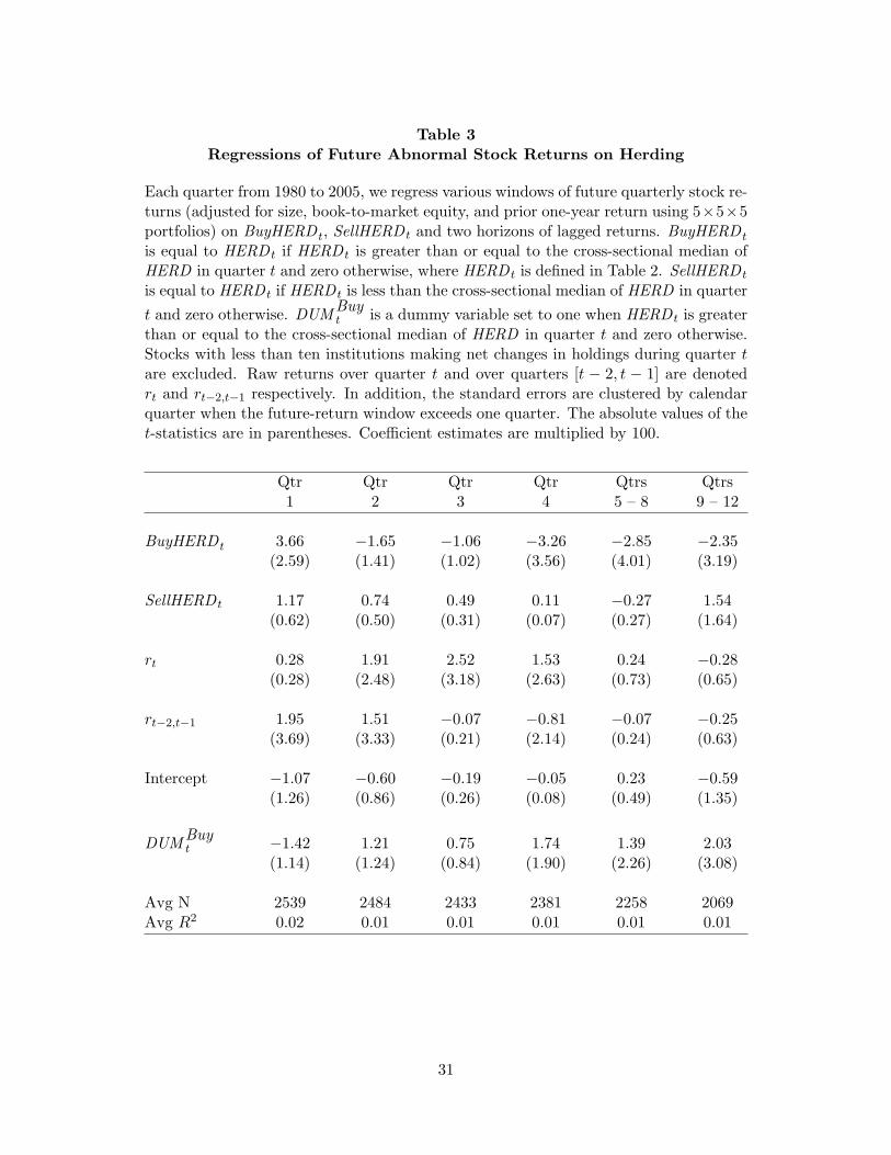
Table 3Regressions of Future Abnormal Stock Returns on Herding

Each quarter from 1980 to 2005, we regress various windows of future quarterly stock re-turns (adjusted for size, book-to-market equity, and prior one-year return using 5×5×5portfolios) on BuyHERD t, SellHERD t and two horizons of lagged returns. BuyHERD t

is equal to HERD t if HERD t is greater than or equal to the cross-sectional median ofHERD in quarter t and zero otherwise, where HERD t is defined in Table 2. SellHERD t

is equal to HERD t if HERD t is less than the cross-sectional median of HERD in quartert and zero otherwise. DUMBuy

t is a dummy variable set to one when HERD t is greaterthan or equal to the cross-sectional median of HERD in quarter t and zero otherwise.Stocks with less than ten institutions making net changes in holdings during quarter tare excluded. Raw returns over quarter t and over quarters [t − 2, t − 1] are denotedrt and rt−2,t−1 respectively. In addition, the standard errors are clustered by calendarquarter when the future-return window exceeds one quarter. The absolute values of thet-statistics are in parentheses. Coefficient estimates are multiplied by 100.

Qtr Qtr Qtr Qtr Qtrs Qtrs1 2 3 4 5 – 8 9 – 12

BuyHERD t 3.66 −1.65 −1.06 −3.26 −2.85 −2.35(2.59) (1.41) (1.02) (3.56) (4.01) (3.19)

SellHERD t 1.17 0.74 0.49 0.11 −0.27 1.54(0.62) (0.50) (0.31) (0.07) (0.27) (1.64)

rt 0.28 1.91 2.52 1.53 0.24 −0.28(0.28) (2.48) (3.18) (2.63) (0.73) (0.65)

rt−2,t−1 1.95 1.51 −0.07 −0.81 −0.07 −0.25(3.69) (3.33) (0.21) (2.14) (0.24) (0.63)

Intercept −1.07 −0.60 −0.19 −0.05 0.23 −0.59(1.26) (0.86) (0.26) (0.08) (0.49) (1.35)

DUMBuyt −1.42 1.21 0.75 1.74 1.39 2.03

(1.14) (1.24) (0.84) (1.90) (2.26) (3.08)

Avg N 2539 2484 2433 2381 2258 2069Avg R2 0.02 0.01 0.01 0.01 0.01 0.01

31

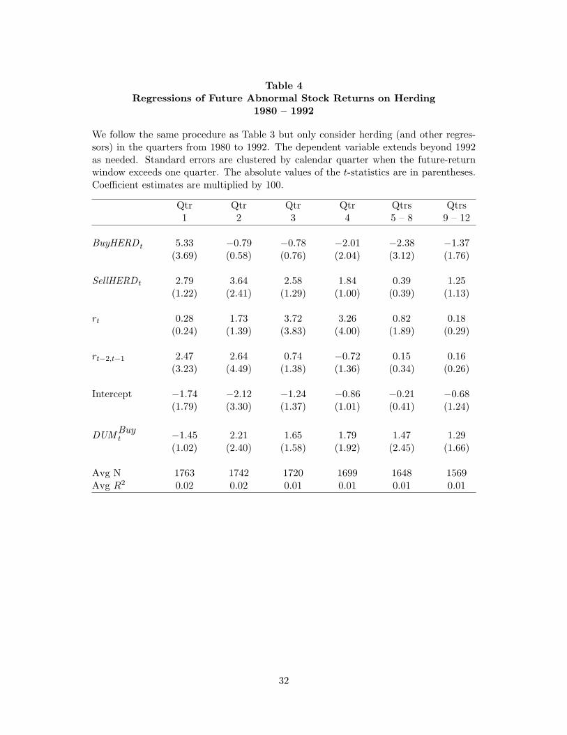
Table 4Regressions of Future Abnormal Stock Returns on Herding

1980 – 1992

We follow the same procedure as Table 3 but only consider herding (and other regres-sors) in the quarters from 1980 to 1992. The dependent variable extends beyond 1992as needed. Standard errors are clustered by calendar quarter when the future-returnwindow exceeds one quarter. The absolute values of the t-statistics are in parentheses.Coefficient estimates are multiplied by 100.

Qtr Qtr Qtr Qtr Qtrs Qtrs1 2 3 4 5 – 8 9 – 12

BuyHERD t 5.33 −0.79 −0.78 −2.01 −2.38 −1.37(3.69) (0.58) (0.76) (2.04) (3.12) (1.76)

SellHERD t 2.79 3.64 2.58 1.84 0.39 1.25(1.22) (2.41) (1.29) (1.00) (0.39) (1.13)

rt 0.28 1.73 3.72 3.26 0.82 0.18(0.24) (1.39) (3.83) (4.00) (1.89) (0.29)

rt−2,t−1 2.47 2.64 0.74 −0.72 0.15 0.16(3.23) (4.49) (1.38) (1.36) (0.34) (0.26)

Intercept −1.74 −2.12 −1.24 −0.86 −0.21 −0.68(1.79) (3.30) (1.37) (1.01) (0.41) (1.24)

DUMBuyt −1.45 2.21 1.65 1.79 1.47 1.29

(1.02) (2.40) (1.58) (1.92) (2.45) (1.66)

Avg N 1763 1742 1720 1699 1648 1569Avg R2 0.02 0.02 0.01 0.01 0.01 0.01

32

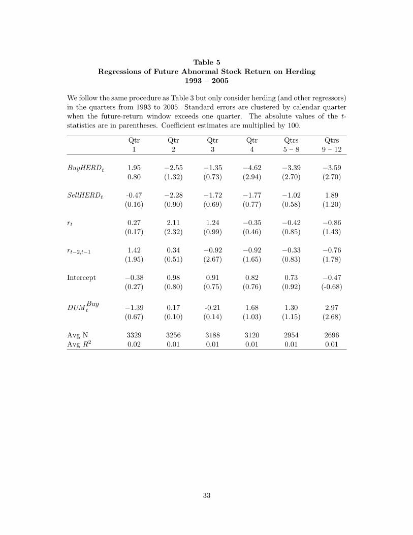
Table 5Regressions of Future Abnormal Stock Return on Herding

1993 – 2005

We follow the same procedure as Table 3 but only consider herding (and other regressors)in the quarters from 1993 to 2005. Standard errors are clustered by calendar quarterwhen the future-return window exceeds one quarter. The absolute values of the t-statistics are in parentheses. Coefficient estimates are multiplied by 100.

Qtr Qtr Qtr Qtr Qtrs Qtrs1 2 3 4 5 – 8 9 – 12

BuyHERD t 1.95 −2.55 −1.35 −4.62 −3.39 −3.590.80 (1.32) (0.73) (2.94) (2.70) (2.70)

SellHERD t -0.47 −2.28 −1.72 −1.77 −1.02 1.89(0.16) (0.90) (0.69) (0.77) (0.58) (1.20)

rt 0.27 2.11 1.24 −0.35 −0.42 −0.86(0.17) (2.32) (0.99) (0.46) (0.85) (1.43)

rt−2,t−1 1.42 0.34 −0.92 −0.92 −0.33 −0.76(1.95) (0.51) (2.67) (1.65) (0.83) (1.78)

Intercept −0.38 0.98 0.91 0.82 0.73 −0.47(0.27) (0.80) (0.75) (0.76) (0.92) (-0.68)

DUMBuyt −1.39 0.17 -0.21 1.68 1.30 2.97

(0.67) (0.10) (0.14) (1.03) (1.15) (2.68)

Avg N 3329 3256 3188 3120 2954 2696Avg R2 0.02 0.01 0.01 0.01 0.01 0.01

33

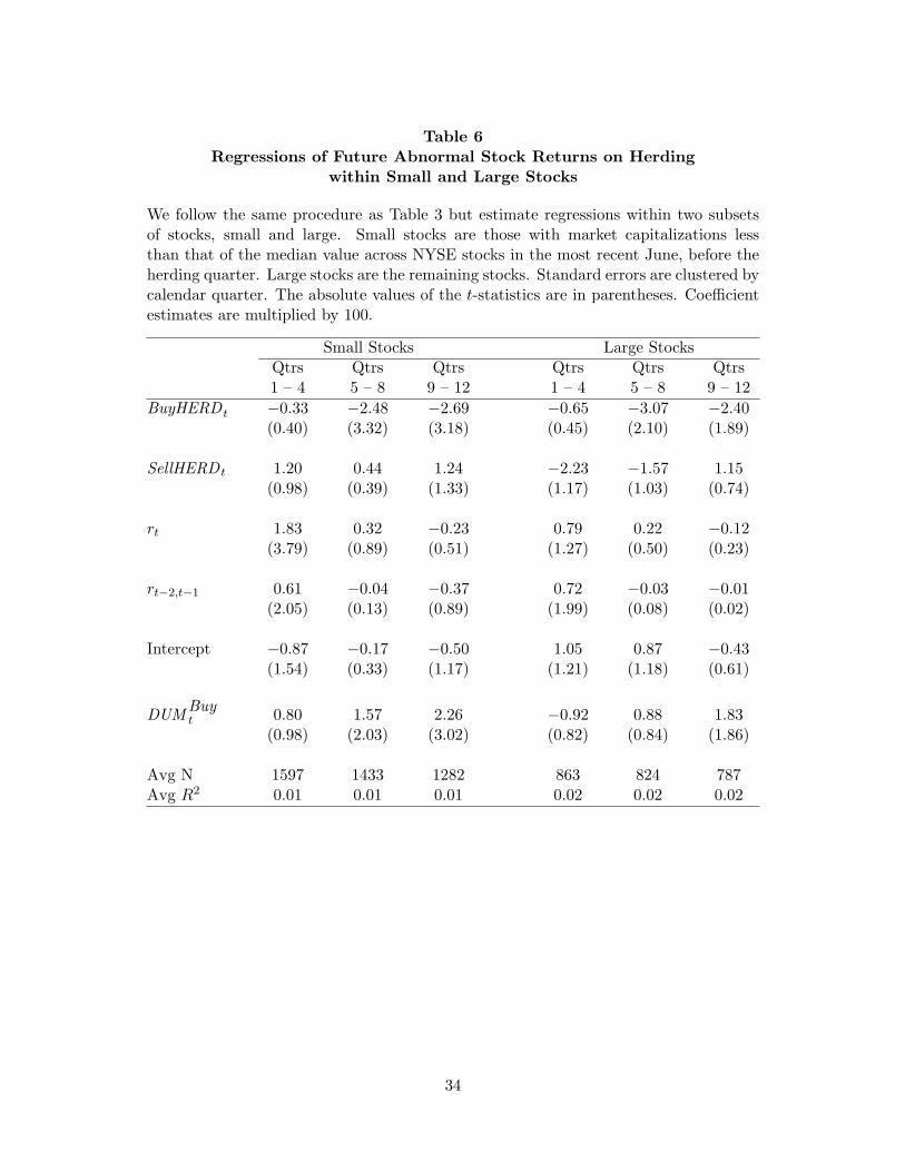
Table 6Regressions of Future Abnormal Stock Returns on Herding

within Small and Large Stocks

We follow the same procedure as Table 3 but estimate regressions within two subsetsof stocks, small and large. Small stocks are those with market capitalizations lessthan that of the median value across NYSE stocks in the most recent June, before theherding quarter. Large stocks are the remaining stocks. Standard errors are clustered bycalendar quarter. The absolute values of the t-statistics are in parentheses. Coefficientestimates are multiplied by 100.

Small Stocks Large StocksQtrs Qtrs Qtrs Qtrs Qtrs Qtrs1 – 4 5 – 8 9 – 12 1 – 4 5 – 8 9 – 12

BuyHERD t −0.33 −2.48 −2.69 −0.65 −3.07 −2.40(0.40) (3.32) (3.18) (0.45) (2.10) (1.89)

SellHERD t 1.20 0.44 1.24 −2.23 −1.57 1.15(0.98) (0.39) (1.33) (1.17) (1.03) (0.74)

rt 1.83 0.32 −0.23 0.79 0.22 −0.12(3.79) (0.89) (0.51) (1.27) (0.50) (0.23)

rt−2,t−1 0.61 −0.04 −0.37 0.72 −0.03 −0.01(2.05) (0.13) (0.89) (1.99) (0.08) (0.02)

Intercept −0.87 −0.17 −0.50 1.05 0.87 −0.43(1.54) (0.33) (1.17) (1.21) (1.18) (0.61)

DUMBuyt 0.80 1.57 2.26 −0.92 0.88 1.83

(0.98) (2.03) (3.02) (0.82) (0.84) (1.86)

Avg N 1597 1433 1282 863 824 787Avg R2 0.01 0.01 0.01 0.02 0.02 0.02

34

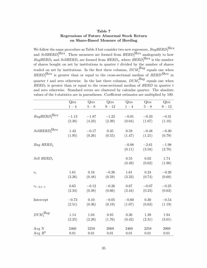
Table 7Regressions of Future Abnormal Stock Return

on Share-Based Measure of Herding

We follow the same procedure as Table 3 but consider two new regressors, BuyHERDShrst

and SellHERDShrst . These measures are formed from HERDShrs

t analogously to howBuyHERD t and SellHERD t are formed from HERD t, where HERDShrs

t is the numberof shares bought on net by institutions in quarter t divided by the number of sharestraded on net by institutions. In the first three columns, DUMBuy

t equals one whenHERDShrs

t is greater than or equal to the cross-sectional median of HERDShrs in

quarter t and zero otherwise. In the last three columns, DUMBuyt equals one when

HERD t is greater than or equal to the cross-sectional median of HERD in quarter tand zero otherwise. Standard errors are clustered by calendar quarter. The absolutevalues of the t-statistics are in parentheses. Coefficient estimates are multiplied by 100.

Qtrs Qtrs Qtrs Qtrs Qtrs Qtrs1 – 4 5 – 8 9 – 12 1 – 4 5 – 8 9 – 12

BuyHERDShrst −1.13 −1.87 −1.22 −0.01 −0.33 −0.31

(2.38) (4.23) (2.39) (0.04) (1.07) (1.10)

SellHERDShrst 1.43 −0.17 0.35 0.59 −0.48 −0.30

(1.95) (0.26) (0.55) (1.47) (1.21) (0.79)

Buy HERD t −0.08 −2.61 −1.98(0.11) (3.58) (2.70)

Sell HERD t 0.55 0.02 1.74(0.49) (0.02) (1.90)

rt 1.61 0.16 −0.26 1.61 0.24 −0.26(3.26) (0.48) (0.59) (3.33) (0.74) (0.60)

rt−2,t−1 0.65 −0.12 −0.26 0.67 −0.07 −0.25(2.34) (0.38) (0.66) (2.44) (0.23) (0.63)

Intercept −0.73 0.10 −0.05 −0.60 0.30 −0.54(2.51) (0.36) (0.19) (1.07) (0.63) (1.19)

DUMBuyt 1.14 1.04 0.85 0.30 1.39 1.94

(2.25) (2.26) (1.76) (0.42) (2.31) (3.01)

Avg N 2460 2258 2069 2460 2258 2069Avg R2 0.01 0.01 0.01 0.01 0.01 0.01

35

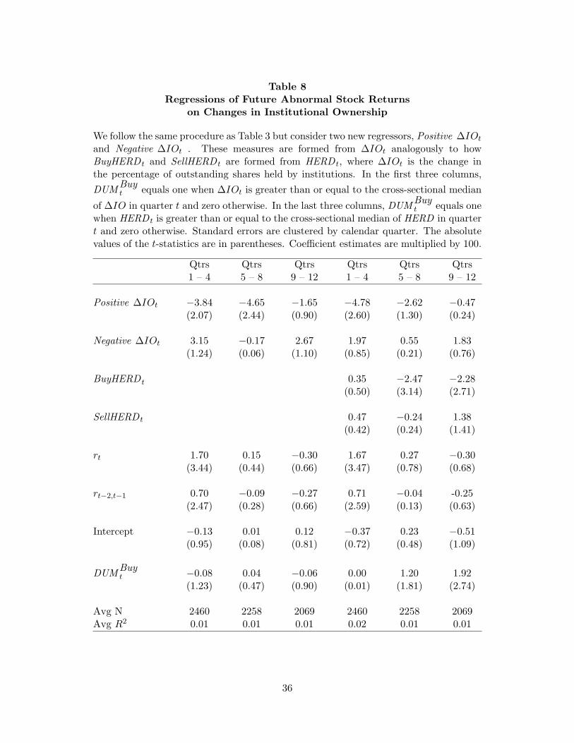
Table 8Regressions of Future Abnormal Stock Returns

on Changes in Institutional Ownership

We follow the same procedure as Table 3 but consider two new regressors, Positive ∆IOt

and Negative ∆IOt . These measures are formed from ∆IOt analogously to howBuyHERD t and SellHERD t are formed from HERD t, where ∆IOt is the change inthe percentage of outstanding shares held by institutions. In the first three columns,DUMBuy

t equals one when ∆IOt is greater than or equal to the cross-sectional median

of ∆IO in quarter t and zero otherwise. In the last three columns, DUMBuyt equals one

when HERD t is greater than or equal to the cross-sectional median of HERD in quartert and zero otherwise. Standard errors are clustered by calendar quarter. The absolutevalues of the t-statistics are in parentheses. Coefficient estimates are multiplied by 100.

Qtrs Qtrs Qtrs Qtrs Qtrs Qtrs1 – 4 5 – 8 9 – 12 1 – 4 5 – 8 9 – 12

Positive ∆IOt −3.84 −4.65 −1.65 −4.78 −2.62 −0.47(2.07) (2.44) (0.90) (2.60) (1.30) (0.24)

Negative ∆IOt 3.15 −0.17 2.67 1.97 0.55 1.83(1.24) (0.06) (1.10) (0.85) (0.21) (0.76)

BuyHERD t 0.35 −2.47 −2.28(0.50) (3.14) (2.71)

SellHERD t 0.47 −0.24 1.38(0.42) (0.24) (1.41)

rt 1.70 0.15 −0.30 1.67 0.27 −0.30(3.44) (0.44) (0.66) (3.47) (0.78) (0.68)

rt−2,t−1 0.70 −0.09 −0.27 0.71 −0.04 -0.25(2.47) (0.28) (0.66) (2.59) (0.13) (0.63)

Intercept −0.13 0.01 0.12 −0.37 0.23 −0.51(0.95) (0.08) (0.81) (0.72) (0.48) (1.09)

DUMBuyt −0.08 0.04 −0.06 0.00 1.20 1.92

(1.23) (0.47) (0.90) (0.01) (1.81) (2.74)

Avg N 2460 2258 2069 2460 2258 2069Avg R2 0.01 0.01 0.01 0.02 0.01 0.01

36

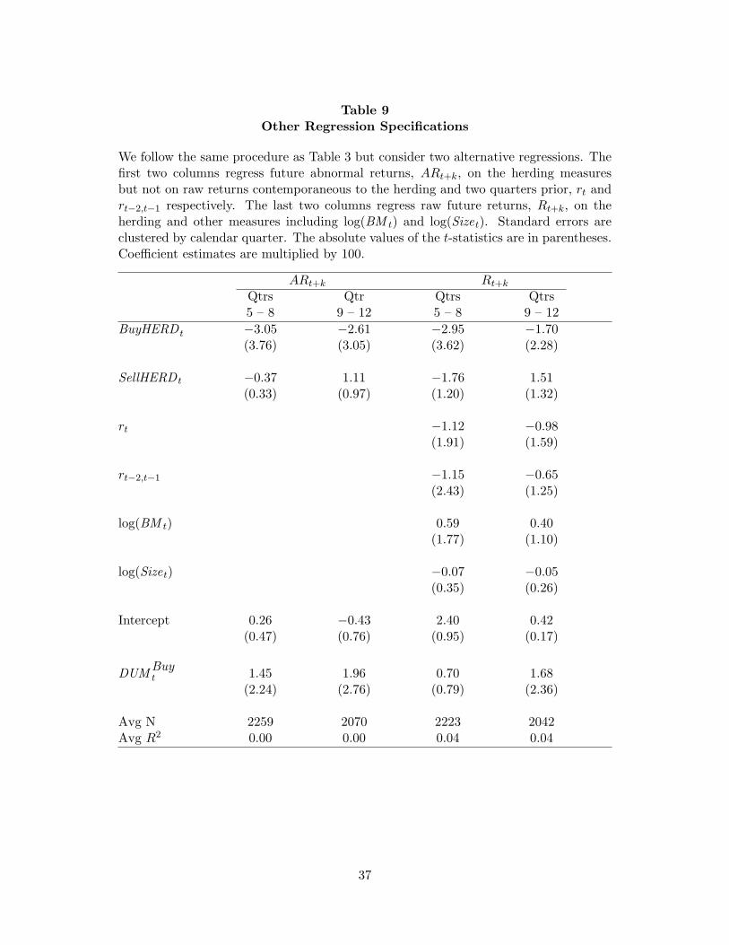
Table 9Other Regression Specifications

We follow the same procedure as Table 3 but consider two alternative regressions. Thefirst two columns regress future abnormal returns, ARt+k, on the herding measuresbut not on raw returns contemporaneous to the herding and two quarters prior, rt andrt−2,t−1 respectively. The last two columns regress raw future returns, Rt+k, on theherding and other measures including log(BM t) and log(Sizet). Standard errors areclustered by calendar quarter. The absolute values of the t-statistics are in parentheses.Coefficient estimates are multiplied by 100.

ARt+k Rt+k

Qtrs Qtr Qtrs Qtrs5 – 8 9 – 12 5 – 8 9 – 12

BuyHERD t −3.05 −2.61 −2.95 −1.70(3.76) (3.05) (3.62) (2.28)

SellHERD t −0.37 1.11 −1.76 1.51(0.33) (0.97) (1.20) (1.32)

rt −1.12 −0.98(1.91) (1.59)

rt−2,t−1 −1.15 −0.65(2.43) (1.25)

log(BM t) 0.59 0.40(1.77) (1.10)

log(Sizet) −0.07 −0.05(0.35) (0.26)

Intercept 0.26 −0.43 2.40 0.42(0.47) (0.76) (0.95) (0.17)

DUMBuyt 1.45 1.96 0.70 1.68

(2.24) (2.76) (0.79) (2.36)

Avg N 2259 2070 2223 2042Avg R2 0.00 0.00 0.04 0.04

37

Table 10How Well Do Investors Trade the Buy-Herd Stocks?

Each quarter from 1980 to 2005, we identify the stocks in the top decile of HERD t,defined in Table 1. Using the abnormal returns of these buy-herd stocks (adjustedfor size, book-to-market, and prior one-year return using 5 × 5 × 5 portfolios), weevaluate how well the herding institutions trade these stocks. An aggregate portfolioof buy-herd stocks is formed each quarter, and their performances over various holdingperiods are evaluated using a calendar-time method. The amount invested by all theherding institutions in each buy-herd stock relative to the amount invested by theseinstitutions across the set of buy-herd stocks forms the portfolio’s weights. An aggregateportfolio for the institutions not buying in quarter t, the “other institutions,” andan aggregate portfolio for the complement of the 13F holdings, the “individuals,” areformed analogously. Panel A reports results for the full period, Panel B for 1980 to 1992,and Panel C for 1993 to 2005. The absolute value of the t-statistics are in parentheses.Quarterly alpha estimates are multiplied by 100.

38

BOP EOPQtrs Qtrs Qtrs Qtrs Qtrs Qtrs1 – 4 5 – 8 9 – 12 1 – 4 5 – 8 9 – 12

Panel A. 1980 to 2005

Herding Institutions 0.28 0.00 −0.40 −0.04 −0.28 −0.72(0.94) (0.01) (1.22) (0.10) (1.10) (2.19)

Other Institutions 0.93 0.53 −0.09 0.11 −0.12 −0.68(2.79) (2.19) (0.29) (0.32) (0.47) (2.21)

Individuals −0.85 −0.95 −1.33 −0.36 −0.51 −0.81(3.16) (4.04) (4.83) (1.50) (2.31) (3.02)

Panel B. 1980 to 1992

Herding Institutions 0.32 −0.11 −0.04 0.11 −0.33 −0.27(1.09) (0.38) (0.11) (0.37) (1.19) (0.86)

Other Institutions 0.72 0.20 0.43 0.33 −0.35 −0.04(2.06) (0.77) (1.38) (0.10) (1.36) (0.13)

Individuals −0.31 −0.73 −0.50 −0.06 −0.44 −0.18(1.55) (2.89) (2.43) (0.29) (1.82) (0.89)

Panel C. 1993 to 2005

Herding Institutions 0.26 0.05 −0.63 −0.16 −0.30 −1.07(0.49) (0.13) (1.00) (0.26) (0.67) (1.72)

Other Institutions 1.11 0.84 −0.52 0.18 0.09 −1.28(1.96) (2.02) (0.91) (0.31) (0.21) (2.28)

Individuals −1.43 −1.20 −2.22 −0.70 −0.57 −1.44(2.92) (3.00) (4.17) (1.58) (1.55) (2.70)

39

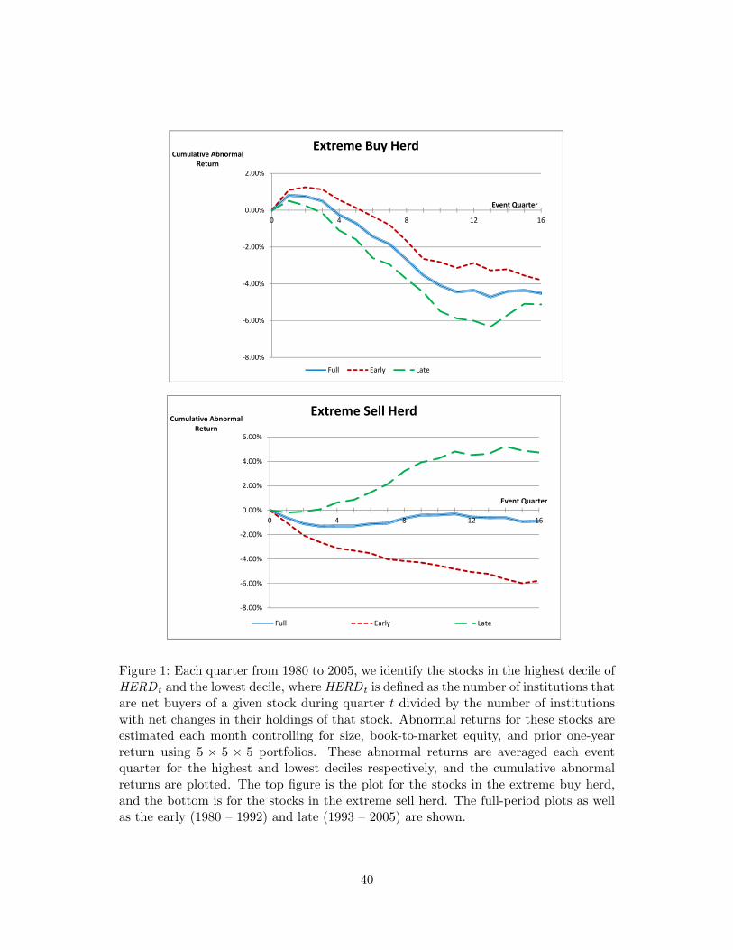
2 00%

0.00%

2.00%

0 4 8 12 16

Cumulative Abnormal Return

Event Quarter 

Extreme Buy Herd 

‐8.00%

‐6.00%

‐4.00%

‐2.00%

Full Early Late

2.00%

4.00%

6.00%

Cumulative Abnormal Return

Event Quarter 

Extreme Sell Herd

‐8.00%

‐6.00%

‐4.00%

‐2.00%

0.00%0 4 8 12 16

Full Early Late

Figure 1: Each quarter from 1980 to 2005, we identify the stocks in the highest decile ofHERD t and the lowest decile, where HERD t is defined as the number of institutions thatare net buyers of a given stock during quarter t divided by the number of institutionswith net changes in their holdings of that stock. Abnormal returns for these stocks areestimated each month controlling for size, book-to-market equity, and prior one-yearreturn using 5 × 5 × 5 portfolios. These abnormal returns are averaged each eventquarter for the highest and lowest deciles respectively, and the cumulative abnormalreturns are plotted. The top figure is the plot for the stocks in the extreme buy herd,and the bottom is for the stocks in the extreme sell herd. The full-period plots as wellas the early (1980 – 1992) and late (1993 – 2005) are shown.

40

2 00%

0.00%

2.00%

0 4 8 12 16

Cumulative Abnormal Return

Event Quarter 

Extreme Buy Herd 

‐8.00%

‐6.00%

‐4.00%

‐2.00%

Early/Lag Ret Neutral Late/Lag Ret Neutral

2.00%

4.00%

6.00%

Cumulative Abnormal Return

Event Quarter 

Extreme Sell Herd

‐8.00%

‐6.00%

‐4.00%

‐2.00%

0.00%0 4 8 12 16

Late/Lag Ret Neutral Early/Lag Ret netural

Figure 2: These plots are similar to Figure 1 except that these portfolios also control forraw returns in quarter t and raw returns over quarters [t− 2, t− 1] using the followingsorting procedure. Each quarter stocks are first sorted into quintiles based on rt. Wethen sort each of these five portfolios into five further portfolios based on rt−2,t−1. Lastly,we sort each of these 25 portfolios into deciles based on HERD t. Each calendar quarter,we form an equally weighted portfolio of all stocks in the 25 portfolios with the largestvalues of HERD t. The abnormal returns of this portfolio estimate the performancesof the extreme buy-herd stocks controlling for both rt and rt−2,t−1 in addition to size,book-to-market equity and one year prior return. We do the analogous procedure forthe extreme sell-herd stocks. Only the early period (1980 – 1992) and the late period(1993 – 2005) are shown.

41