Fundamental Analysis, Stock Returns and High B/M Companies

International Journal of Economics and Business Administration

Volume V, Issue 4, 2017

pp. 3-18

Fundamental Analysis, Stock Returns and High B/M

Companies

G.P. Kourtis1, E.P. Κourtis2, M.P. Kourtis3, P.G. Curtis4

Abstract:

Ιn this paper we initially estimate the financial performance of high BM companies based on

the analysis of profitability, liquidity-leverage and operating efficiency ratios.

The performance of the specific group as a whole, was found to be quite poor and that is why

it is reflected in a high BM ratio score for the companies involved.

The research then showed that a portfolio of the best performing high BM companies, chosen

through the F-score mechanism, exhibits a statistically significant higher mean of market-

adjusted as well as raw returns, compared to any other type of classification of the

companies of the category.

The research was conducted for the period 2010-2015 and applied to companies listed in the

North America Stock Exchange Markets.

1MSc Accounting and Control, Erasmus University, Rotterdam,

[email protected] 2School of Civil Engineering NTUA 3School of Electrical and Computer Engineering NTUA 4Ass. Professor TEI Stereas Elladas, [email protected]

mailto:[email protected]

mailto:[email protected]

Fundamental Analysis, Stock Returns and High B/M Companies

4

1. Introduction

Ball and Brown (1968) were pioneers in examining whether the accounting data and

more specifically the change of net income, matters in explaining the changes in

stock prices in the capital markets. They used the CAPM model as the mechanism to

associate the accounting numbers to stock returns. Ball and Brown investigated the

relationship between unexpected earnings and abnormal rates of return for 261

stocks of companies listed at the New York Stock Exchange, during the period 1957

to 1965. They argued that the evaluation of accounting income requires to examine

the “content and the timing” of the income and “its usefulness could be impaired by

deficiencies in either”. They showed, contrary to what up to then was the prevalent

belief, that the movements of stocks’ returns and the financial statement information

are associated. In addition, they stated that earnings contain a great deal of

information reflected in stocks returns as well as and highlighted the predictive

power of earnings in explaining future abnormal stock returns.

According to Kothari (2001), the investment strategy that relies on financial

statement analysis data, forms a discrete field of research in accounting, the so-

called capital markets research originated in the landmark work of Ball and Brown.

Dechow et al. (2014) consider that their work is based on three assumptions about

how investors use earnings to determine stock prices (Thalassinos and Politis, 2011;

Thalassinos and Thalassinos, 2006; Thalassinos et al., 2015).

These assumptions are the following: a) markets are efficient, b) higher earnings are

linked to higher firm value and c) their model reflects investors’ earnings

expectations.

Fama (1965), who previously conceived a framework of stock prices prediction

based on pertinent information, facilitated this development in capital markets

research in accounting. He argued that prices contain all available information and

follow a random walk. It is also known, that Fama (1965) is identified with the

EMH.

Beaver (1968), in the same year with the study of Ball and Brown (1968), focused

on the information relevance of net income at the moment of the announcement of

financial statements. He searched for empirical evidence based on trading volume

and the volatility of earnings that ensue an earnings announcement. Beaver

concluded that net income figures were relevant since the announcement of the

financial results, affected the volume and the price of stocks involved in the week

after the announcement. In addition Beaver (1968) argued, that the link between

earnings and stock prices is the assumption that the current earnings provide

information to predict future earnings.

To test the validity of the allegations that fundamentals and financial statement

analysis are valuable in explaining stock price changes, we explore the case of high

G.P. Kourtis , E.P. Κourtis, M.P. Kourtis, P.G. Curtis

5

BM companies. The researchers have identified the poor fundamentals of high BM

companies. The financial underperformance of these companies is reflected in their

lower market value compared to their book one. Fama and French (1992) argued that

high Book to Market (where BM>1) companies exhibit rather financially distressed

fundamentals and so their stocks can be characterized as riskier, compared to the

ones of other companies that trade in the same market. As a result, the higher returns

(compared to the growth stocks’ ones ) that these companies earn in the market, are

justified as a kind of remuneration for the additional risk they bear. They specify that

the signs of financial distress are the higher leverage, the lower return on equity, the

lower liquidity, the earnings fluctuations etc., (Fama and French, 1995). Lakonishok

et al. (1994) believe that as a result of the unsatisfactory performance of those

companies, create pessimistic expectations, don’t draw enough investors’ attention

and exhibit lower demand for their stocks. Consequently they allege, whenever their

financial performance improves it is understandably translated into higher market

value changes.

The F-score screening mechanism (introduced by Piotroski in 2000), encourages the

use of the fundamental analysis, which exploits financial statements data. The model

implicitly stresses the need for dependable data and prudent financial reporting

policies that finally compensate all stakeholders and the economy. Piotroski (2000)

recognizes problems regarding the quality of financial reporting. That is why the F-

score model, is embedding in the analysis of accruals and cash flows measures when

profitability is examined. Two of the four profitability ratios, that are included in the

F-score, refer to earnings that are based on the accruals and the rest two refer to the

cash flows and their amount in comparison to accruals. By doing so Piotroski takes

care of the problem of the quality of the data and therefore he bolsters the

effectiveness of the F-score as a tool of assessment of the real current financial

performance of companies, that can also be used to evaluate the future earnings and

the change in the returns of stocks involved. The model finally contributes to more

efficient allocation of resources in the economy, by directing resources to companies

that expose more sound fundamentals (Hanias et al., 2007; Thalassinos et al., 2012).

2. Methodology and Data

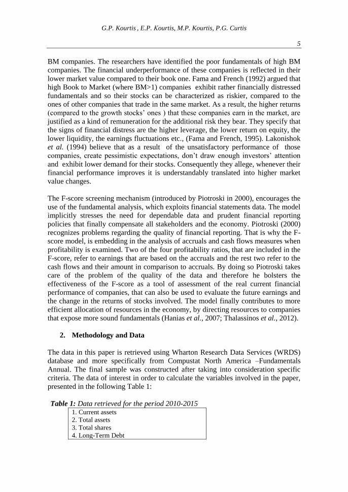
The data in this paper is retrieved using Wharton Research Data Services (WRDS)

database and more specifically from Compustat North America –Fundamentals

Annual. The final sample was constructed after taking into consideration specific

criteria. The data of interest in order to calculate the variables involved in the paper,

presented in the following Table 1:

Table 1: Data retrieved for the period 2010-2015

1. Current assets

2. Total assets

3. Total shares

4. Long-Term Debt


6

5. Gross Profit

6. Current Liabilities

7. Net Profit

8. Cash flows from operations

9. Sales

10. Equity

11. Market value of equity

12.Year-end closing stock price

13.Year-end closing market index (NASDAQ,

NYSE, S&P/TSX)

The sample consists of listed companies operating in North America during the

period 2010-2015. The initial sample consisted of 51.994 observations, in which

were involved all listed companies in North America, excluding the ones operating

in the financial services sector (Table 2).

Table 2: Sample selection stages

Sample selection

Observations

Companies

Listed companies in North America excluding

those providing financial services 51.944 12.986

Delete companies that do not have available

data in the period 2011-2014 26.940 6.735

Delete companies that do not have 12-month

year end fiscal years 14.664 3.666

Keep companies with Book-to-Market ratio

above one 2.808 702

Keep companies with revenue above zero 2.252 563

Keep companies that have available data for

all years 2010-2015 456 114

Delete companies listed in OTC markets 284 71

Source: Wharton Research Data Services (WRDS): Compustat North America –

Fundamentals Annual.

Nevertheless, during the data analysis, and especially after the calculation of the

market-adjusted stocks returns (MA_RET) and raw returns (RAW_RET) for each

company at the end of each year (during the period 2011-2014), it was observed that

some companies exhibit stock returns considerably higher than 30% of the

respective market index. According to Field (2009), the outliers can cause biased


7

models because they influence the values of the estimated regression coefficients. It

is known that, outliers’ repercussions especially in the samples that are not large

enough may cause model misspecification biased parameter estimation, and

therefore incorrect analysis results. For that reason, companies achieved one-year

ahead change of market-adjusted returns (MA_RET) 30% or more during the period

2010-2015 were excluded. Therefore, the final sample consists of 71 companies and

their observations differ from year to year.

3. Model and Variables

The variable MAR_RET is defined as the one-year ahead change of the stocks’

market-adjusted return, for company i, from year t to the next t+1. MA_RET

variable is calculated as follows:

Stock price in the year-end t and

Market index in the year-end t

Respectively, for the study’s purposes, we define the variable RAW_RET as the

one-year ahead change only in the stock return (without adjusting for the impact of

the respective Index as it is in the calculation of MA_RET) for company i, from year

t to the next t+1. RAW_RET variable is calculated as follows:

We calculate the variables MAR_RET and RAW_RET as well as all the ratios

included in the F-score of Piotroski (2000).

3.1 F_SCORE variable

According to prior researches and specifically those of Piotroski (2000), Krauss et

al. (2015), Fama and French (1995), Chen and Zhang (1998), Harris and Raviv

(1990), Myers and Majluf (1984), Miller and Rock (1985) three aspects of financial

performance fundamentals exist that can differentiate high from low performance

companies. Those are: (i) profitability, (ii) leverage-liquidity and (iii) operating

efficiency. Profitability reflects the ability of a company to use its assets in order to

generate profits measured on accruals and/or cash flows from operations (CFO). The

liquidity ratios measure the ability of a company to meet its short-term obligations

based on current assets and cash. In addition the leverage ratios measure the

proportion of debt to equity that implies the ability of a company to finance its


8

operations. Operating efficiency is comprised of two financial ratios. The first one is

the so-called assets turnover ratio and portrays of how efficiently a company

transforms the invested capital into sales. Sales value is attributed to either higher

quality-differentiation or to lower cost and/or focus, depending on the company’s

generic strategies in the market according to Porter(1980). The other ratio refers to

the improvement of the gross profit margin of the last year compared to the previous

one and it indicates better performance mainly in restraining costs. By examining,

each of the nine ratios each one individually leads to:

(i) Profitability ratios:

1. Positive ROA in the current year t gets a score 1, otherwise 0.

2. Positive operating cash flow in the current year t gets a score 1, otherwise 0.

3. Higher ROA in the current year t compared to ROA in previous year t-1 scores 1,

otherwise 0.

4. CFO greater than ROA scores 1, otherwise 0.

(ii) Leverage/liquidity ratios:

5. Lower value of long-term debt in the current year t compared to previous year t-1

scores 1, otherwise 0.

6. Higher current ratio (current assets divided by current liabilities) in the current

year t compared to previous year t-1 scores 1, otherwise 0.

7. New shares issued in the current year t scores 0, otherwise 1.

(iii) Operating efficiency ratios:

8. A higher gross margin this year t than in previous year t-1 scores 1, otherwise 0

9. A higher asset turnover ratio (total sales divided by total assets) in current year t

than the previous year t-1 scores 1, otherwise 0.

Therefore, the nine financial ratios and the respective dummies were constructed for

F_SCORE and

OFFEREQLIQUIDFLEVERF

TURNFMARGINFACCRUALFCFOFROAFROAFSCOREF

___

_______

+++

+++++=

According to Piotroski (2000) investing in companies that exhibit a greater total

sum, means that the corresponding ratios improved in the current year compared to

the previous one and therefore their financial performance is bolstered.

In the sample of companies examined, the maximum F-score reported was nine (9)

and the lowest one (1). We considered as high financial performing companies the

ones that receive F-score equals from seven to nine (7-9), the medium financial

performing companies get F-score from four to six (4-6) and the rest that exhibit F-

score from one to three (1-3) were characterized as low financial performing

companies.


9

4. Financial Statement Analysis

High BM companies, financial ratios and F-score:

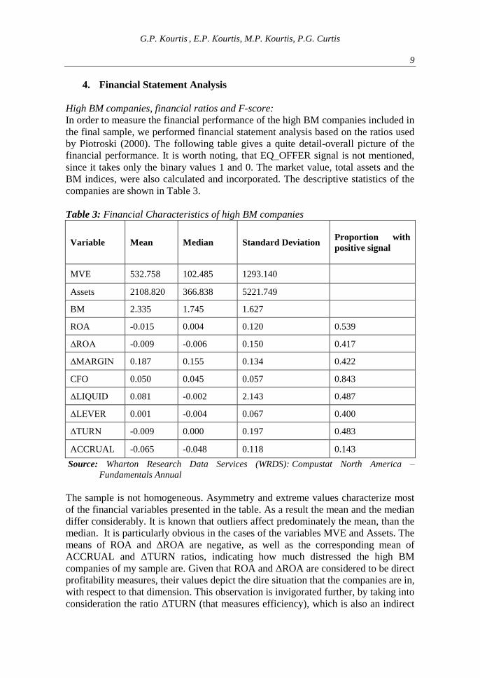
In order to measure the financial performance of the high BM companies included in

the final sample, we performed financial statement analysis based on the ratios used

by Piotroski (2000). The following table gives a quite detail-overall picture of the

financial performance. It is worth noting, that EQ_OFFER signal is not mentioned,

since it takes only the binary values 1 and 0. The market value, total assets and the

BM indices, were also calculated and incorporated. The descriptive statistics of the

companies are shown in Table 3.

Table 3: Financial Characteristics of high BM companies

Variable Mean Median Standard Deviation Proportion with

positive signal

MVE 532.758 102.485 1293.140

Assets 2108.820 366.838 5221.749

BM 2.335 1.745 1.627

ROA -0.015 0.004 0.120 0.539

ΔROA -0.009 -0.006 0.150 0.417

ΔMARGIN 0.187 0.155 0.134 0.422

CFO 0.050 0.045 0.057 0.843

ΔLIQUID 0.081 -0.002 2.143 0.487

ΔLEVER 0.001 -0.004 0.067 0.400

ΔTURN -0.009 0.000 0.197 0.483

ACCRUAL -0.065 -0.048 0.118 0.143


Fundamentals Annual

The sample is not homogeneous. Asymmetry and extreme values characterize most

of the financial variables presented in the table. As a result the mean and the median

differ considerably. It is known that outliers affect predominately the mean, than the

median. It is particularly obvious in the cases of the variables MVE and Assets. The

means of ROA and ΔROA are negative, as well as the corresponding mean of

ACCRUAL and ΔTURN ratios, indicating how much distressed the high BM

companies of my sample are. Given that ROA and ΔROA are considered to be direct

profitability measures, their values depict the dire situation that the companies are in,

with respect to that dimension. This observation is invigorated further, by taking into

consideration the ratio ΔTURN (that measures efficiency), which is also an indirect


10

measure of ROA (since ROA = Net profit margin multiplied by sales turnover).

TURN ratio is calculated dividing sales by the assets employed. Given that its mean

is also negative, it constitutes an additional factor that is aggravating further the poor

performance of the high BM stocks of my sample. These findings are in line with the

previous research of Fama and French (1992) regarding high BM companies and the

general perception regarding the financial performance of this category of

companies.

ACCRUAL (defined as ROA minus CFO scaled by total assets), it is the only

negative financial ratio (only 14.3 % of the companies’ observations involved in the

period under consideration is positive), and that does not represent a drawback. The

variable CFO is positive in 84.3 % of the sample. CFO at the same time is

considered the least amenable to manipulation item by the management, compared

to accrual accounting earnings. A positive CFO greater than accruals, is considered a

measure of quality of earnings. It was found that during the crisis “ the change in

most determinants of earnings quality, favors higher earnings quality” (Kousenidis et

al., 2013). All these observations justify the negative sign of ACCRUAL, meaning

that CFO are greater than earnings. The fact that profitability of the high BM

companies is low or even negative in the sample, indicates the poor financial

performance of the companies involved. The latter, represents a factor contributing

to a low value of the company in the market, compared to the corresponding book

one, resulting finally into high BM ratio.

Raw and market-adjusted returns:

We saw that he high BM companies exhibit poor financial performance that, is

reflected in their low market value. Those companies exhibit quite often erratic

behavior with respect to their stock returns. We then filter extreme returns in order to

purge the sample of the outliers and construct the return of investment strategy for

those companies as shown in Table 4.

Table 4: One-year ahead returns of an investment in high BM companies

Returns Mean

Percentile

Percent Positive

10th 25th Median 75th 90th

RAW_RET -0.093 -0.509 -0.275 -0.063 0.125 0.254 0.396

MA_RET -0.200 -0.577 -0.388 -0.193 0.028 0.147 0.287



To examine the hypothesis that the market adjusted returns (MA_RET) are normally

distributed with mean value -0.20 and standard deviation 0.28, the normality Shapiro

– Wilks (S-W) and Kolmogorov-Smirnov (K-S) tests are used. Since the sample size


11

is large enough the S – W test is not biased. Furthermore, since the extreme values

have been removed from the sample, the K-S test can be also used as well.

According to the results of the S-W (W=0.990, p value =0.11>0.05) and K-S tests (p

value =0.41>0.05). Thus we cannot reject the hypothesis that the distribution is

normal. Taking into account raw returns (RAW_RET) and trying to examine the

same hypothesis (normal destitution with mean -0.09 and standard deviation= 0.30),

the result of the S -W (W = 0.992, p value=0.24>0.05) and K-S (p value 0.316

>0.05) tests, lead us not to reject the hypothesis.

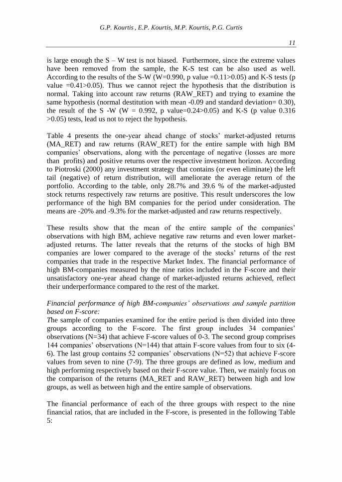
Table 4 presents the one-year ahead change of stocks’ market-adjusted returns

(MA_RET) and raw returns (RAW_RET) for the entire sample with high BM

companies’ observations, along with the percentage of negative (losses are more

than profits) and positive returns over the respective investment horizon. According

to Piotroski (2000) any investment strategy that contains (or even eliminate) the left

tail (negative) of return distribution, will ameliorate the average return of the

portfolio. According to the table, only 28.7% and 39.6 % of the market-adjusted

stock returns respectively raw returns are positive. This result underscores the low

performance of the high BM companies for the period under consideration. The

means are -20% and -9.3% for the market-adjusted and raw returns respectively.

These results show that the mean of the entire sample of the companies’

observations with high BM, achieve negative raw returns and even lower market-

adjusted returns. The latter reveals that the returns of the stocks of high BM

companies are lower compared to the average of the stocks’ returns of the rest

companies that trade in the respective Market Index. The financial performance of

high BM-companies measured by the nine ratios included in the F-score and their

unsatisfactory one-year ahead change of market-adjusted returns achieved, reflect

their underperformance compared to the rest of the market.

Financial performance of high BM-companies’ observations and sample partition

based on F-score:

The sample of companies examined for the entire period is then divided into three

groups according to the F-score. The first group includes 34 companies’

observations (N=34) that achieve F-score values of 0-3. The second group comprises

144 companies’ observations (N=144) that attain F-score values from four to six (4-

6). The last group contains 52 companies’ observations (N=52) that achieve F-score

values from seven to nine (7-9). The three groups are defined as low, medium and

high performing respectively based on their F-score value. Then, we mainly focus on

the comparison of the returns (MA_RET and RAW_RET) between high and low

groups, as well as between high and the entire sample of observations.

The financial performance of each of the three groups with respect to the nine

financial ratios, that are included in the F-score, is presented in the following Table

5:


12

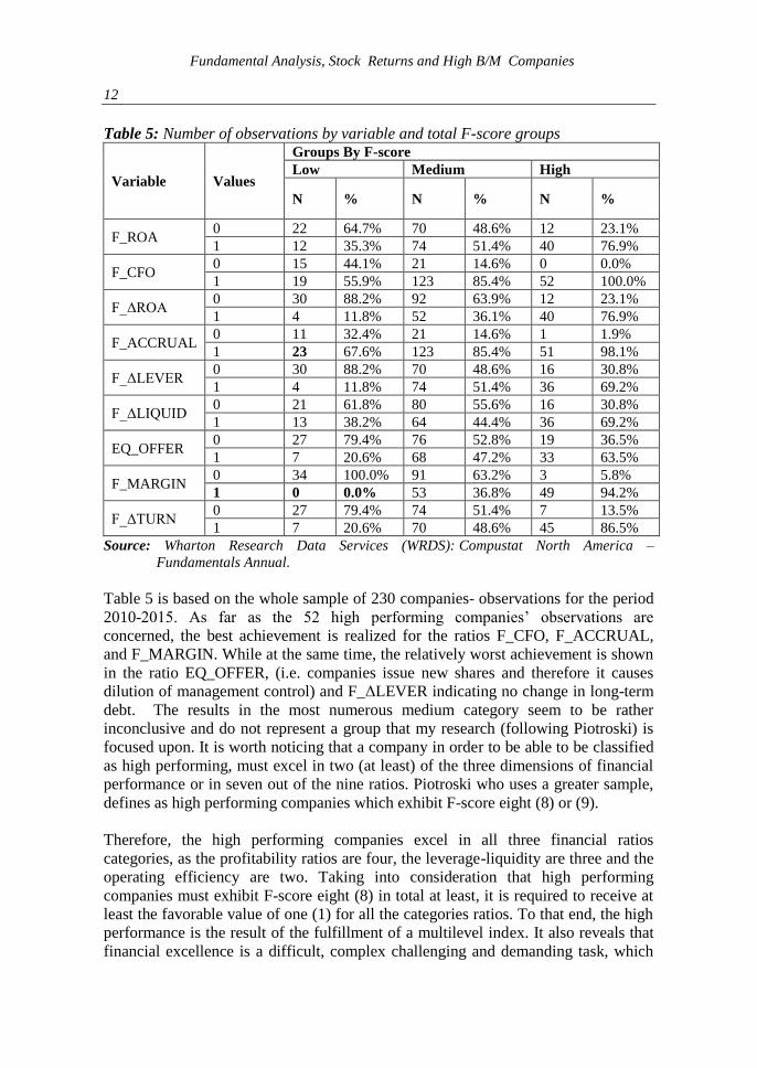
Table 5: Number of observations by variable and total F-score groups

Variable Values

Groups By F-score

Low Medium High

N % N % N %

F_ROA 0 22 64.7% 70 48.6% 12 23.1%

1 12 35.3% 74 51.4% 40 76.9%

F_CFO 0 15 44.1% 21 14.6% 0 0.0%

1 19 55.9% 123 85.4% 52 100.0%

F_ΔROA 0 30 88.2% 92 63.9% 12 23.1%

1 4 11.8% 52 36.1% 40 76.9%

F_ACCRUAL 0 11 32.4% 21 14.6% 1 1.9%

1 23 67.6% 123 85.4% 51 98.1%

F_ΔLEVER 0 30 88.2% 70 48.6% 16 30.8%

1 4 11.8% 74 51.4% 36 69.2%

F_ΔLIQUID 0 21 61.8% 80 55.6% 16 30.8%

1 13 38.2% 64 44.4% 36 69.2%

EQ_OFFER 0 27 79.4% 76 52.8% 19 36.5%

1 7 20.6% 68 47.2% 33 63.5%

F_MARGIN 0 34 100.0% 91 63.2% 3 5.8%

1 0 0.0% 53 36.8% 49 94.2%

F_ΔTURN 0 27 79.4% 74 51.4% 7 13.5%

1 7 20.6% 70 48.6% 45 86.5%



Table 5 is based on the whole sample of 230 companies- observations for the period

2010-2015. As far as the 52 high performing companies’ observations are

concerned, the best achievement is realized for the ratios F_CFO, F_ACCRUAL,

and F_MARGIN. While at the same time, the relatively worst achievement is shown

in the ratio EQ_OFFER, (i.e. companies issue new shares and therefore it causes

dilution of management control) and F_ΔLEVER indicating no change in long-term

debt. The results in the most numerous medium category seem to be rather

inconclusive and do not represent a group that my research (following Piotroski) is

focused upon. It is worth noticing that a company in order to be able to be classified

as high performing, must excel in two (at least) of the three dimensions of financial

performance or in seven out of the nine ratios. Piotroski who uses a greater sample,

defines as high performing companies which exhibit F-score eight (8) or (9).

Therefore, the high performing companies excel in all three financial ratios

categories, as the profitability ratios are four, the leverage-liquidity are three and the

operating efficiency are two. Taking into consideration that high performing

companies must exhibit F-score eight (8) in total at least, it is required to receive at

least the favorable value of one (1) for all the categories ratios. To that end, the high

performance is the result of the fulfillment of a multilevel index. It also reveals that

financial excellence is a difficult, complex challenging and demanding task, which


13

encompasses many facets of performance. To that extend it is indicative that Ou and

Penman (1989), Lev and Thiagarajan (1993), Abarbanell and Bushee (1998) before

Piotroski (2000) used a number of ratios combined into an index, in order to forecast

future company performance. In addition, the Z-score of Altman (1968) includes a

weighted average of five ratios that measure profitability, liquidity, debt/equity and

efficiency in order to assess the probability that the company will be solvent (or not)

in the near future.

Market-adjusted returns, raw returns and financial performance:

In this section, the focus is on the association of the one-year ahead change of

market-adjusted returns as well as raw returns, with each of the nine financial ratios

individually and the aggregate measure of F-score.

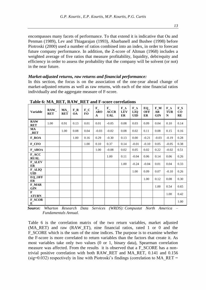
Table 6: MA_RET, RAW_RET and F-score correlations

Variable RAW_

RET

MA_

RET

F_R

OA

F_C

FO

F_

ΔRO

A

F_

ACCR

UAL

F_Δ

LEV

ER

F_Δ

LIQ

UID

EQ_

OFF

ER

F_M

AR

GIN

F_Δ

TUR

N

F_S

CO

RE

RAW

RET 1.00 0.91 0.13 0.01 0.01 -0.05 0.08 0.03 0.09 0.04 0.10 0.14

MA

_RET 1.00 0.08 0.04 -0.03 -0.02 0.08 0.02 0.11 0.08 0.15 0.16

F_ROA 1.00 0.16 0.29 -0.30 0.13 0.00 -0.21 -0.03 -0.19 0.28

F_CFO 1.00 0.10 0.37 0.14 -0.01 -0.10 0.05 -0.05 0.38

F_ΔROA 1.00 -0.08 0.02 0.05 0.02 0.22 -0.02 0.51

F_ACC

RUAL 1.00 0.11 -0.04 0.06 0.14 0.06 0.26

F_ΔLEV

ER 1.00 -0.24 -0.04 0.01 0.04 0.33

F_ΔLIQ

UID 1.00 0.09 0.07 -0.10 0.26

EQ_OFF

ER 1.00 0.12 0.08 0.30

F_MAR

GIN 1.00 0.54 0.65

F

ΔTURN 1.00 0.42

F_SCOR

E 1.00



Table 6 is the correlation matrix of the two return variables, market adjusted

(MA_RET) and raw (RAW_ET), nine financial ratios, rated 1 or 0 and the

F_SCORE which is the sum of the nine indices. The purpose is to examine whether

the F-score is more correlated to return variables than the factors that create it. As

most variables take only two values (0 or 1, binary data), Spearman correlation

measure was affected. From the results it is observed that a F_SCORE has a non-

trivial positive correlation with both RAW_RET and MA_RET, 0.141 and 0.156

(sig=0.032) respectively in line with Piotroski’s findings (correlation to MA_RET =


14

0.121 and RAW_RE=0.124) and comparable to them. At the same time, the three

strongest individual explanatory variables of MA_RET are F_ΔTURN, F_ROA and

F_MARGIN (correlation of 0.152 (sig. 0.021), 0.078 (sig.0.240) and 0.076 (sig

0.252) respectively. Furthermore, the ACCRUAL variable shows a negative

correlation -0.020 with respect to MA_RET (though not statistically significant,

sig=0.761. Finally, MA_RET shows a greater correlation (0.156, sig=0.032) than

RAW_RET (0.141, sig=0.032) with respect to the F-score and both of them are

statistically significant at the 0.05 significance level.

Market-adjusted returns (MA_RET) of an investment strategy of high performing

portfolio screened by the F-score:

We then examine the possibility to lose useful information by transforming the

financial variables-ratios in to their binary form of 0 and 1, in order to follow

Piotroski’s method. Therefore, we recalculate the results using binary signs this

time.

Table 7: Investment strategy through the screening mechanism of F-score using

binary signs

MA_RET Mean of

MA_RET 5% 25% 50% 75% 95% N

n%

positive

F_SCORE= 1 -0.192 -0.213 -0.213 -0.192 -0.170 -0.170 2 0.00%

F_SCORE= 2 -0.271 -0.674 -0.420 -0.297 -0.121 0.160 9 0.11%

F_SCORE= 3 -0.320 -0.802 -0.610 -0.264 -0.162 0.125 23 0.17%

F_SCORE= 4 -0.206 -0.614 -0.481 -0.176 0.009 0.229 55 0.25%

F_SCORE= 5 -0.194 -0.825 -0.354 -0.207 0.067 0.177 53 0.40%

F_SCORE= 6 -0.210 -0.906 -0.366 -0.213 -0.027 0.143 36 0.22%

F_SCORE= 7 -0.118 -0.528 -0.254 -0.110 0.082 0.275 36 0.36%

F_SCORE= 8 -0.163 -0.772 -0.324 -0.120 0.020 0.260 14 0.29%

F_SCORE= 9 -0.077 -0.250 -0.250 -0.077 0.096 0.096 2 0.50%

All Firms -0.200 -0.677 -0.387 -0.193 0.025 0.207 230 0.29%

Low -0.300 -0.802 -0.525 -0.252 -0.162 0.160 34 0.15%

Medium -0.203 -0.677 -0.388 -0.191 0.038 0.177 144 0.30%

High -0.129 -0.538 -0.281 -0.112 0.059 0.271 52 0.35%

High-All 0.072 0.139 0.106 0.081 0.034 0.064

t statistics -2.115 p-

value: 0.036


15

High-Low 0.171 0.264 0.244 0.140 0.221 0.111


value: 0.005



Table 7 represents the means of the MA_RET, the number of observations (N) as

well as the portion of the positive MA_RET that was found for each F_SCORE

value (1-9). Most of the observations are clustered around F_SCORES with values

equal to four to six (4-6). The mean of MA_RET of all companies’ observations

(N=230) within the period under examination (2011-2014), is negative and equal to -

0.2. This it is attributed to the poor financial performance of high BM companies

that comprise the entire sample.

For the group of high performing companies (with F-score higher than 7) the mean

of MA_RET equals to -0.129 (N=34) and for low performing companies (with F-

score lower than 4), the mean of MA_RET equals to -0.300 (N=144). The findings

show that by choosing the high performing companies to form the portfolio, the

latter minimizes the losses that exhibiting the high BM companies for the specific

period under examination. In particular, the high performing companies show the

least negative return (-0.129) among all companies that achieve collectively

considerable losses to the tune of -0.20 on the average. Therefore, the difference in

the means between high and all companies’ observations is equal to

0.071.Significantly, the mean of MA_RET earned by a high BM-portfolio can be

increased by at least 7.1% annually, through the selection of high performing

companies. The findings are in line with Piotroski’s claims that the mean returns

earned by a high BM-portfolio, is bolstered annually through the inclusion of high

performing companies, based on the F-score screening mechanism. The specific

portfolio of stocks chosen minimizes the losses of the entire high BM companies

group.

Using the t-test, we compare the mean return of high performing companies and all

others. According to the results the t-statistic = -2.115 and the p-value = 0.036 <

0.05. Therefore, we have to reject the hypothesis that the mean return of high

performing companies is the same as the mean return of all others companies. High

performing companies exhibit a greater mean of MA_RET that is equal to 0.072.

Using the t-test, we compare the mean return of high performing companies and low

performing companies. According to the results, the t-statistics = -2.918 and the p-

value = 0.005 < 0.05. Therefore, I have to reject the hypothesis that the mean return

of high performing companies is the same as the mean return of low performing

companies. High performing companies exhibit a greater mean of MA_RET that is

equal to 0.171


16

Then, we repeat the recalculation of the previous table using as dependent variable

RAW_RET, instead of MA_RET.

Table 8: Raw Returns by F-score groups

RAW_RET Mean of

Raw_RET 5% 25% 50% 75% 95% N

n%

positive

F_SCORE= 1 -0.045 -0.079 -0.079 -0.045 -0.011 -0.011 2 0.00%

F_SCORE= 2 -0.144 -0.632 -0.284 -0.111 -0.065 0.203 9 0.22%

F_SCORE= 3 -0.222 -0.668 -0.443 -0.228 0.015 0.126 23 0.26%

F_SCORE= 4 -0.110 -0.639 -0.392 -0.024 0.113 0.317 55 0.44%

F_SCORE= 5 -0.079 -0.696 -0.258 -0.026 0.184 0.344 53 0.42%

F_SCORE= 6 -0.123 -0.774 -0.220 -0.088 0.041 0.220 36 0.39%

F_SCORE= 7 0.009 -0.559 -0.153 -0.022 0.176 0.654 36 0.47%

F_SCORE= 8 -0.022 -0.613 -0.216 -0.052 0.285 0.492 14 0.43%

F_SCORE= 9 -0.095 -0.176 -0.176 -0.095 -0.014 -0.014 2 0.00%

All Firms -0.093 -0.636 -0.273 -0.063 0.125 0.361 230 0.40%

Low -0.191 -0.668 -0.348 -0.156 -0.011 0.203 34 0.24%

Medium -0.102 -0.659 -0.317 -0.055 0.128 0.273 144 0.42%

High -0.004 -0.559 -0.178 -0.025 0.176 0.492 52 0.44%

High-All 0.089 0.077 0.096 0.038 0.051 0.131

t statistics 2.456 p-

value: 0.015

High-Low 0.187 0.109 0.171 0.131 0.187 0.289


value: 0.004



According to the findings exposed in the table above not only the market-adjusted

stock returns (MA_RET), but also the raw ones (RAW_RET) exhibit similar

behavior with respect to the F_SCORE. The high performing group exhibits mean of

RAW_RET that is equal to -0.004. The latter reveals that the mean of RAW_RET

for high performing group is higher compared to the means of medium and low

performing groups, which are equal to -0,102 and -0.191 respectively. The mean


17

differences are statistically significant, since the t test values are 2.456 and -2.970

and the corresponding p-values 0.015 and 0.004 at the 5 % level.

Given the above results, it is obvious that the F-score screening apparatus that

segregates high and low performing companies’ observations, contributes to the

creation of a portfolio that improves the mean of returns. Therefore, we can accept

the main hypothesis of my research states that “the one-year ahead change of stocks’

market-adjusted returns (MA_RET) and raw returns (RAW_RET), is at high

financial performing companies higher than that of lower performing companies’’.

5. Conclusion

The F score model challenges the semi strong form of efficient market hypothesis

(EMH) according to which all publicly available relevant information is already

embedded in the stock prices and therefore investors are not able to achieve returns

that outpeform the market. The model defies the view that there is no way for

someone to “beat” the markets, since all the investors face the same information set

and financial statements’ data are already available to the public. The F-score

mechanism represents a rewarding investment strategy for the practitioners, if it is

properly applied. It also contributes to more efficient allocation of resources in the

economy, by directing resources to companies that expose more sound

fundamentals.

References:

Altman, E., 1968. Financial Ratios, Discriminant Analysis and the Prediction of Corporate

Bankruptcy. Journal of Finance, September.

Abarbanell, J. and Bushee, B. 1998. Abnormal returns to a fundamental analysis strategy.

The Accounting Review, 73, 19-45.

Ball, R. and Brown, P. 1968. An empirical evaluation of accounting income numbers.

Journal of Accounting Research, 6, 159-178.

Beaver, W. 1968. The information content of annual earnings announcements. Journal of

Accounting Research, Supplement, 67-92.

Chen, N.F. and Zhang, F. 1998. Risk and return of value stocks. The Journal of

Business, 71(4), 501-535.

Dechow, P. 1994. Accounting Earnings and Cash Flows as Measures of Firm Performance:

The Role of Accounting Accruals. Journal of Accounting and Economics, 18, 3-42.

Dechow, P. and Dichev, I. 2002. The quality of accruals and earnings: The role of accrual

estimation errors. The Accounting Review, 77, 35-39.

Dechow, P., Sloan, R. and Zha, J. 2014. Stock Prices & Earnings: A History of Research.

Fama, E.F. 1965. The behavior of stock market prices. Journal of Business, 38, 34-105.

Fama, E.F., French, K.R. 1992. The Cross-Section of Expected Returns. Journal of Finance,

47, 427-465.

Fama, E.F., French, K.R. 1995. Size and book‐to‐market factors in earnings and returns. The

Journal of Finance, 50(1), 131-155.

Fama, E.F., French, K.R. 2008. Dissecting anomalies. The Journal of Finance, 63. 1653-

1678.


18

Field, A. 2009. Discovering statistics using SPSS (3nd ed.). London: Sage.

Hanias, P.M., Curtis, G.P. and Thalassinos, E.J. 2007. Non-linear dynamics and chaos: The

case of the price indicator at the Athens Stock Exchange. International Research

Journal of Finance and Economics, 11(1), 154-163.

Harris, M., Raviv, A. 1990. Capital structure and the informational role of debt. The Journal

of Finance, 45(2), 321-349.

Kothari, S.P. 2001. Capital markets research in accounting. Journal of Accounting and

Economics, 31, 105-231.

Kousenidis, D.V., Ladas, A.C. and Negakis, C.I. 2013. The effects of the European debt

crisis on earnings quality. International Review of Financial Analysis, 30, 351-362.

Krauss, Ch., Krüger, T., Beerstecher, D. 2015. The Piotroski F-Score: A fundamental value

strategy revisited from an investor's perspective. IWQW Discussion Paper Series,

13.

Lakonishok, J., Shleifer, A. and Vishny, R. 1994. Contrarian investment, extrapolation, and

risk. Journal of Finance, 49, 1541-1578.

Miller, M.H., Rock, K. 1985. Dividend policy under asymmetric information. The Journal of

finance, 40(4), 1031-1051.

Myers, S.C., Majluf, N.S. 1984. Corporate financing and investment decisions when

companies have information that investors do not have. Journal of financial

economics, 13(2), 187-221.

Ou, J. and S. Penman, S. 1989. Financial statement analysis and the prediction of stock

returns. Journal of Accounting and Economics, 11, 295-329.

Piotroski, J. 2000. Value investing: The use of historical financial statement information to

separate winners from losers. Journal of Accounting Research 38 (Supplement), 1-

41.

Porter, M.E. 1980. Competitive Strategy. Free Press.

Thalassinos, I.E., Thalassinos, E.P. 2006. Stock Markets' Integration Analysis. European

Research Studies Journal, 9(3-4), 3-14.

Thalassinos, I.E. and Politis, D.E. 2011. International Stock Markets: A Co-integration

Analysis. European Research Studies Journal, 14(4), 113-129.

Thalassinos, I.E., Hanias, P.M. and Curtis, G.P. 2012. Time series prediction with neural

networks for the Athens Stock Exchange indicator. European Research Studies

Journal, 15(2), 23-31.

Thalassinos, I.E., Stamatopoulos, D.T. and Thalassinos, E.P. 2015. The European Sovereign

Debt Crisis and the Role of Credit Swaps. Chapter book in The WSPC Handbook

of Futures Markets (eds) W. T. Ziemba and A.G. Malliaris, in memory of Late

Milton Miller (Nobel 1990) World Scientific Handbook in Financial Economic

Series Vol. 5, Chapter 20, pp. 605-639, ISBN: 978-981-4566-91-9, (doi:

10.1142/9789814566926_0020).

https://en.wikipedia.org/wiki/Competitive_Strategy

Fundamental Analysis, Stock Returns and High B/M Companies

Documents

Transcript of Fundamental Analysis, Stock Returns and High B/M Companies