Fundamental Constants

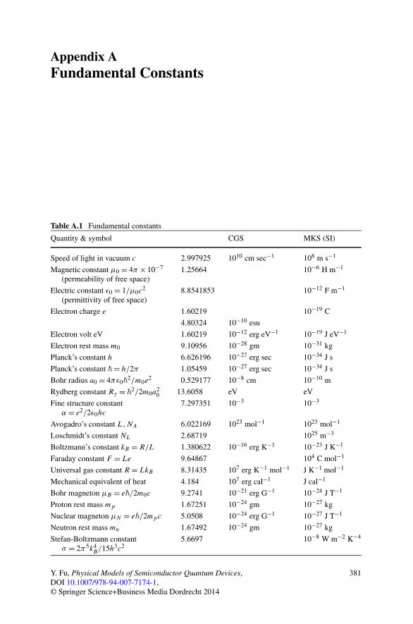
Appendix AFundamental Constants

Table A.1 Fundamental constants

Quantity & symbol CGS MKS (SI)

Speed of light in vacuum c 2.997925 1010 cm sec−1 108 m s−1

Magnetic constant μ0 = 4π × 10−7

(permeability of free space)1.25664 10−6 H m−1

Electric constant ε0 = 1/μ0c2

(permittivity of free space)8.8541853 10−12 F m−1

Electron charge e 1.60219 10−19 C

4.80324 10−10 esu

Electron volt eV 1.60219 10−12 erg eV−1 10−19 J eV−1

Electron rest mass m0 9.10956 10−28 gm 10−31 kg

Planck’s constant h 6.626196 10−27 erg sec 10−34 J s

Planck’s constant �= h/2π 1.05459 10−27 erg sec 10−34 J s

Bohr radius a0 = 4πε0�2/m0e

2 0.529177 10−8 cm 10−10 m

Rydberg constant Ry = �2/2m0a

20 13.6058 eV eV

Fine structure constantα = e2/2ε0hc

7.297351 10−3 10−3

Avogadro’s constant L,NA 6.022169 1023 mol−1 1023 mol−1

Loschmidt’s constant NL 2.68719 1025 m−3

Boltzmann’s constant kB = R/L 1.380622 10−16 erg K−1 10−23 J K−1

Faraday constant F = Le 9.64867 104 C mol−1

Universal gas constant R = LkB 8.31435 107 erg K−1 mol−1 J K−1 mol−1

Mechanical equivalent of heat 4.184 107 erg cal−1 J cal−1

Bohr magneton μB = e�/2m0c 9.2741 10−21 erg G−1 10−24 J T−1

Proton rest mass mp 1.67251 10−24 gm 10−27 kg

Nuclear magneton μN = e�/2mpc 5.0508 10−24 erg G−1 10−27 J T−1

Neutron rest mass mn 1.67492 10−24 gm 10−27 kg

Stefan-Boltzmann constantσ = 2π5k4

B/15h3c25.6697 10−8 W m−2 K−4

Y. Fu, Physical Models of Semiconductor Quantum Devices,DOI 10.1007/978-94-007-7174-1,© Springer Science+Business Media Dordrecht 2014

381

http://dx.doi.org/10.1007/978-94-007-7174-1

382 A Fundamental Constants

Table A.1 (Continued)

Quantity & symbol CGS MKS (SI)

Gravitational constant G 6.6732 10−11 N m2 kg−2

Acceleration of free fall gn 9.80665 m s−2

1.0 [eV] = 2.41796 × 1014 [Hz] = 8.0655 × 103 wavenumber [cm−1] =1.1604 × 104 [K] = 1.239855 wavelength [µm]

W: watt, G: gauss, T: tesla, N: newton, C: coulomb

Appendix BQuantum Physics

B.1 Black Body Radiation

Planck’s law for the energy density distribution for the radiation from a black bodyat temperature T is

w(f,T ) = 8πhf 3

c3

1

ehf/kBT − 1(B.1)

where h is the Planck’s constant, and f is the frequency. Note that ω = 2πf is theangular frequency, and � = h/2π . The low-frequency Rayleigh-Jens law

w(f,T ) = 8πf 2kBT

c3

is obtained when hf � kBT . Stefan-Boltzmann’s law for the total radiation energyper unit volume can be derived

W(T ) =ˆ ∞

0w(f,T )df = 8π5k4

B

15h3c3T 4 = 4σ

cT 4 (B.2)

where σ = 2π5k4B/15h3c2 is the Stefan-Boltzmann constant. Wien’s law for the

wavelength λmax at which the energy density has its maximum value can be derivedfrom Eq. (B.1)

λmax = b

T(B.3)

where b = 0.2898 cm·K is a universal constant. Note λ = c/f .

B.2 The Compton Effect

A photon with initial wavelength λ incident upon an electron at rest with a rest massm0. After the collision, the photon has a wavelength of λ′ scattered into a direction


383

http://dx.doi.org/10.1007/978-94-007-7174-1

384 B Quantum Physics

at an angle θ with respect to its initial propagation direction, which is also referredto be the photon scattering angle.

λ′ = λ + h

m0c(1 − cos θ) = λ + λC(1 − cos θ) (B.4)

where λC = h/m0c is called the Compton wavelength of the electron.

B.3 Electron Diffraction

Diffraction pattern of electron from a crystal can be explained by the dual particle-wave nature of matter. A particle having a momentum p is associated the so-calledde Broglie wavelength

λ = h

p(B.5)

B.4 Operators in Quantum Physics

In quantum mechanics, classical physical quantities are translated into quantum op-erators. The measurement of a physical quantity 〈A〉 is described quantum mechan-ically by

〈A〉 =ˆ

ψ∗1 Aψ2dr =

ˆ(Aψ1)

∗ψ2dr (B.6)

where ψ is the wave function that describes the quantum mechanical state of thesystem under measurement. The only possible values that can be obtained whenmeasuring a physical quantity 〈A〉 are the eigen values of the quantum operator A.Thus, the operator is hermitian and its eigen values are real, i.e., Aun = anun, whereun is the eigen function, an is the eigen value which is real. Subscript n denotes theindex of the eigen functions, i.e., operator A may have multiple eigen functions andeigen values.

B.5 The Schrödinger Equation

The momentum operator is given by p = −i�∇ , and the position operator is r =i�∇p . The energy operator is

E = i�∂

∂t

B.5 The Schrödinger Equation 385

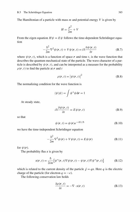
The Hamiltonian of a particle with mass m and potential energy V is given by

H = p2

2m+ V

From the eigen equation Hψ = Eψ follows the time-dependent Schrödinger equa-tion

− �2

2m∇2ψ(r, t) + V ψ(r, t) = i�

∂ψ(r, t)

∂t(B.7)

where ψ(r, t), which is a function of space r and time t , is the wave function thatdescribes the quantum mechanical state of the particle. The wave character of a par-ticle is described by ψ(r, t), and can be interpreted as a measure for the probabilityρ(r, t) to find the particle at r and t

ρ(r, t) = ∣∣ψ(r, t)

∣∣2 (B.8)

The normalizing condition for the wave function is

〈ψ |ψ〉 =ˆ

ψ∗ψdr = 1

At steady state,

i�∂ψ(r, t)

∂t= Eψ(r, t) (B.9)

so that

ψ(r, t) = ψ(r)e−iEt/� (B.10)

we have the time-independent Schrödinger equation

− �2

2m∇2ψ(r) + V ψ(r, t) = Eψ(r) (B.11)

for ψ(r).The probability flus s is given by

s(r, t) = �

2im

[

ψ∗(r, t)∇ψ(r, t) − ψ(r, t)∇ψ∗(r, t)]

(B.12)

which is related to the current density of the particle j = qs. Here q is the electriccharge of the particle (for electron q = −e).

The following conservation law holds

∂ρ(r, t)

∂t= −∇ · s(r, t) (B.13)


The time dependence of an operator A is given by (Heisenberg):

dA

dt= ∂A

∂t+ [A,H ]

i�(B.14)

where H is the Hamiltonian and [A,B] ≡ AB −BA is the commutator of A and B .For hermitian operators the commutator is always complex. If [A,B] = 0, the oper-ators A and B have a common set of eigen functions. By applying this to p and r itfollows (Ehrenfest)

md2〈r〉t

dt2= −〈∇V 〉 (B.15)

which is the classical Newton’s second law of motion.A classical product AB becomes 1

2 (AB + BA) in quantum mechanics.

B.6 The Uncertainty Principle

The uncertainty ΔA in A is defined as

(ΔA)2 = ⟨

ψ∣∣A − 〈A〉∣∣2

ψ⟩ = ⟨

A2⟩ − 〈A〉2

it follows

ΔA · ΔB ≥ 1

2

∣∣⟨

ψ∣∣[A,B]∣∣ψ ⟩∣

∣ (B.16)

from which it follows:

ΔE · Δt ≥ �

2, Δpx · Δx ≥ �

2(B.17)

B.7 Parity

The parity operator in one dimension is given by Pψ(x) = ψ(−x). If the wavefunction is split into even and odd functions, it can be expanded into eigen functionsof P :

ψ(x) = 1

2

[

ψ(x) + ψ(−x)]

︸︷︷︸

even: ψ+

+ 1

2

[

ψ(x) − ψ(−x)]

︸︷︷︸

odd: ψ−

(B.18)

with

ψ+ = 1

2(1 +P)ψ(x), ψ− = 1

2(1 −P)ψ(x)

both of which satisfy the Schrödinger equation. Hence, parity is a conserved quan-tity. Moreover, [P,H ] = 0.

B.8 The Tunneling Effect 387

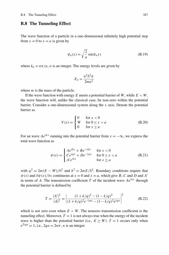
B.8 The Tunneling Effect

The wave function of a particle in a one-dimensional infinitely high potential stepfrom x = 0 to x = a is given by

ψn(x) =√

2

asin(knx) (B.19)

where kn = nπ/a, n is an integer. The energy levels are given by

En = n2�

2π

2ma2

where m is the mass of the particle.If the wave function with energy E meets a potential barrier of W , while E < W ,

the wave function will, unlike the classical case, be non-zero within the potentialbarrier. Consider a one-dimensional system along the x axis. Denote the potentialbarrier as

V (x) =⎧

⎨

⎩

0 for x < 0W for 0 ≤ x < a

0 for x ≥ a

(B.20)

For an wave Aeikx running into the potential barrier from x = −∞, we express thetotal wave function as

ψ(x) =⎧

⎨

⎩

Aeikx + Be−ikx for x < 0Ceiqx + De−iqx for 0 ≤ x < a

A′eikx for x ≥ a

(B.21)

with q2 = 2m(E − W)/�2 and k2 = 2mE/�2. Boundary conditions require thatψ(x) and ∂ψ(x)/∂x continuous at x = 0 and x = a, which give B , C and D and A′in terms of A. The transmission coefficient T of the incident wave Aeikx throughthe potential barrier is defined by

T = |A′|2|A|2 =

∣∣∣∣

(1 + k/q)2 − (1 − k/q)2

(1 + k/q)2e−iqa − (1 − k/q)2eiqa

∣∣∣∣

2

(B.22)

which is not zero even when E < W . The nonzero transmission coefficient is thetunneling effect. Moreover, T = 1 is not always true when the energy of the incidentwave is higher than the potential barrier (i.e., E ≥ W ). T = 1 occurs only whene2iqa = 1, i.e., 2qa = 2nπ , n is an integer.


B.9 Harmonic Oscillator

For the one-dimensional potential energy

V (x) = 1

2bx2 (B.23)

Let ω2 = b/m, the Hamiltonian H is then given by:

H = p2

2m+ 1

2mω2x2 = 1

2�ω + ωA†A (B.24)

with

A =√

m

2ωx + ip√

2mω, A† =

√

m

2ωx − ip√

2mω(B.25)

A = A† is non hermitian. [A,A†] = � and [A,H ] = �ωA. A is a so called cre-ation operator, and A† an annihilation operator. HAuE = (E − �ω)AuE . There isa ground-state u0 such Au0 = 0. The energy in this ground state is 1

2�ω, which isnormally known as the zero-point energy. Let n be a positive integer, normalizedeigen functions and corresponding eigen values are

un = 1√n!

(A†

√�

)n

u0, u0 = 4

√

mω

π�exp

(

−mωx2

2�

)

, En =(

1

2+ n

)

�ω

(B.26)

B.10 Angular Momentum and Spin

The orbital angular momentum operator is defined as

L = −i�r × ∇ (B.27)

[Lz,L2] = [Lz,H ] = [L2,H ] = 0, [Lx,Ly] = i�Lz, [Ly,Lz] = i�Lx , [Lz,Lx] =

i�Ly . Not all components of L can be known at the same time with arbitrary accu-racy

ΔLxΔLy ≥ �

2Lz (B.28)

Lz in spherical polar and Cartesian coordinates is

Lz = xpy − ypx − i�∂

∂ϕ= −i�

(

x∂

∂y− y

∂

∂x

)

(B.29)

The creation and annihilation operators L± are defined by: L± = Lx ± iLy . L2 =L+L− + L2

z − �Lz.

B.10 Angular Momentum and Spin 389

Eigen value relations of angular momentum L with eigen function Y�m

L2Y�m = �(� + 1)�2Y�m(B.30)

LzY�m = m�Y�m

where � ≥ 0 and 2� + 1 is an integer, −� ≤ m ≤ � and can take on the values

m = −�,−� + 1,−� + 2, . . . , � − 1, �

Y�m is the spherical harmonics

Y�m(θ,ψ) = N�mP|m|� (cos θ)eimψ (B.31)

where P|m|� (cos θ) is the associated Legendre polynomials.

For integral values of �, we discuss orbit angular momentum,

L+Y�m = √

�(� + 1) − m(m + 1)�Y�m+1(B.32)

L−Y�m = √

�(� + 1) − m(m − 1)�Y�m−1

Addition theorem for angular momentum:

L = L1 + L2 (B.33)

L has eigen functions Y�m with

� = |�1 − �2|, |�1 − �2| + 1, . . . , �1 + �2, m = −�,−� + 1, . . . , � (B.34)

When � takes on the values of half-odd integral, i.e., � = 1/2,3/2, . . ., we discussspin. Spin operators are defined by their commutation relations: [Sx,Sy] = i�Sz,they do not act in the physical space (x, y, z). Furthermore, [L,S] = 0 so that spinand angular momentum operators do not have a common set of eigen functions. Thespin operators are given by S = 1

2�σ , where

σ x =(

0 11 0

)

, σ y =(

0 −i

i 0

)

, σ z =(

1 00 −1

)

(B.35)

are Pauli spin matrices. Denote the eigen function of spin as χ ,

S2χs,ms = s(s + 1)�2χs,ms , s = 1

2(B.36)

We normally denote χ 12 , 1

2= α and χ 1

2 ,− 12

= β .

Addition of two spins S = S1 + S2,⎧

⎪⎪⎪⎪⎨

⎪⎪⎪⎪⎩

triplet, parity = 1

⎧

⎪⎨

⎪⎩

χ1,1 = α1α2

χ1,0 = 1√2(α1β2 + β1α2)

χ1,−1 = β1β2

singlet, parity = −1 χ0,0 = 1√2(α1β2 − β1α2)

(B.37)


The electron has an intrinsic magnetic dipole moment M due to its spin, M =−egsS/2m, with gs = 2(1 + α/2π + · · · ) is the gyromagnetic ratio. In the pres-ence of an external magnetic field this gives a potential energy V = −M · B . TheSchrödinger equation then becomes (because ∂χ/∂xi ≡ 0):

i�∂χ(t)

∂t= egs�

4mσ · Bχ(t) (B.38)

with σ = (σ x,σ y,σ z). If B = Bez there are two eigenvalues for this equation,±egs�B/4m = ±�ω, and the general solution is given by χ(t) = Ae−iωt + Beiωt .From these,

〈Sx〉 = 1

2� cos(2ωt), 〈Sy〉 = 1

2� sin(2ωt) (B.39)

Thus the spin precesses about the z axis with frequency 2ω. This causes the Zeemansplitting of spectral lines.

B.11 Hydrogen Atom

The hydrogen atom contains one proton and one electron. The Schrödinger equationbecomes a one-particle equation after the center-of-mass motion is separated out. Inspherical coordinate, the potential energy is

V (r) = − e2

4πεr(B.40)

[

− �2

2m∇2 + V (r)

]

ψ(r) = ψ(r) (B.41)

where m is the reduced mass which is approximately the same as the electron massm0.

The solutions of the above Schrödinger equation in spherical coordinates if thepotential energy is a function of r can be written as

ψ(r, θ,ϕ) = Rn�(r)Y�m(θ,ϕ)

Y�m is the spherical harmonics in Eq. (B.31). Let un�(r) = rRn�(r), the equationthat determines un�(r) is

d2un�(r)

dr2+ 2m

�2

[

En − V (r) − �(� + 1)�2

2mr2

]

un�(r) = 0 (B.42)

Solution of the above equation for V (r) in Eq. (B.40) when ε = ε0 and m = m0

En = −Ry

n2(B.43)

B.12 Interaction with Electromagnetic Fields 391

where Ry = �2/2m0a

20 = 13.6058 eV is Rydberg, a0 = 4πε0�

2/m0e2 = 0.529 Å is

Bohr radius. The parity of these solutions is (−1)�, and the functions are

2n−1∑

�=0

(2� + 1) = 2n2

fold degenerated.

B.12 Interaction with Electromagnetic Fields

The Hamiltonian of an electron in an electromagnetic field is given by:

H = 1

2μ(p + eA)2 − eφ = − �

2

2μ∇2 + i�e

2μ(A · ∇ + ∇ · A) + e2

2μA2 − eφ (B.44)

where μ is the reduced mass of the system, A is the vector field and φ is the scalarfield of the electromagnetic field. The term ∼ A2 can usually be neglected, exceptfor very strong fields or macroscopic motions.

B.13 Time-Independent Perturbation Theory

Consider a time-independent perturbation V ′ so that the Schrödinger equation be-comes (H0 + λV ′)Ψn = EnΨn. Let ψn be the complete set of eigen functions of thenon-perturbed Hamiltonian H0, i.e., H0ψn = E0

nψn. We write

Ψn = ψn +∑

k =n

cnk(λ)ψk (B.45)

Expanding cnk and En into λ

cnk = λc(1)nk + λ2c

(2)nk + · · ·

(B.46)En = E0

n + λE(1)n + λ2E(2)

n + · · ·inserting them into the Schrödinger equation result in the first-order correction

E(1)n = ⟨

φn

∣∣V ′∣∣φn

⟩

, c(1)nk,k =n = 〈ψk|V ′|ψn〉

E0n − E0

k(B.47)

Ψn = ψn +∑

k =n

〈ψk|V ′|ψn〉E0

n − E0k

ψk


where m = n, and the second-order correction of the energy

E(2)n =

∑

k =n

|〈ψk|V ′|ψn〉|2E0

n − E0k

(B.48)

B.14 Time-Dependent Perturbation Theory

When the perturbation is time-dependent, i.e., V ′(t), the Schrödinger equation is

i�∂Ψ (t)

∂t= [

H0 + λV ′(t)]

Ψ (t) (B.49)

and

Ψ (t) =∑

n

cn(t) exp

(−iE0nt

�

)

ψn (B.50)

with cn(t) = δnk + λc(1)n (t) + · · · . The first-order correction follows

c(1)n (t) = 1

i�

ˆ t

0

⟨

ψn

∣∣V ′(τ )

∣∣ψk

⟩

exp

[i(E0

n − E0k )τ

�

]

dτ (B.51)

B.15 N -Particle System

Identical particles are indistinguishable. For the total wave function of a system ofidentical particles,

1. Particles with a half-odd integer spin (Fermions): Ψtotal must be anti-symmetricwith respect to interchanges of the coordinates (spatial and spin) of each pair ofparticles. The Pauli principle results from this: two Fermions cannot exist in anidentical state because then Ψtotal = 0.

2. Particles with an integer spin (Bosons): Ψtotal must be symmetric with respect tointerchange of the coordinates (spatial and spin) of each pair of particles.

For a system of two electrons there are 2 possibilities for the spatial wave func-tion. When a and b are the quantum numbers of electron 1 and 2,

ψS(1,2) = ψa(1)ψb(2) + ψa(2)ψb(1)(B.52)

ψA(1,2) = ψa(1)ψb(2) − ψa(2)ψb(1)

Following spin wave functions are possible:

χA = 1√2

[

χ+(1)χ−(2) − χ+(2)χ−(1)]

(B.53)

B.16 Quantum Statistics 393

χS =⎧

⎨

⎩

χ+(1)χ+(2)1√2[χ+(1)χ−(2) + χ+(2)χ−(1)]

χ−(1)χ−(2)

Because the total wave function must be anti-symmetric, Ψtotal = ψSχA, or Ψtotal =ψAχS.

For N particles the symmetric spatial function is given by:

ψS(1, . . . ,N) =∑

ψ(all permutations of 1, . . . ,N) (B.54)

The anti-symmetric wave function is given by the Slater determinant

ψA(1, . . . ,N) = 1√N !

∣∣∣∣∣∣∣∣∣

ψE1(1) ψE1(2) · · · ψE1(N)

ψE2(1) ψE2(2) · · · ψE2(N)...

ψEN(1) ψEN

(2) · · · ψEN(N)

∣∣∣∣∣∣∣∣∣

(B.55)

B.16 Quantum Statistics

If a system exists in a state in which one has not the disposal of the maximal amountof information about the system, it can be described by a density matrix ρ. If theprobability that the system is in state Ψi is given by ci , one can write for the expec-tation value a of A

a = 〈A〉 =∑

i

ci〈Ψi |A|Ψi〉 (B.56)

If Ψ is expanded into an orthonormal basis {ψk} as ψ(i) = ∑

k c(i)k φk ,

〈A〉 =∑

k

(Aρ)kk = Tr(Aρ) (B.57)

where ρ�k = c∗kc�. ρ is hermitian, with Tr(ρ) = 1. Further holds

ρ =∑

ri |ψi〉〈ψi |

The probability to find eigenvalue an when measuring A is given by ρnn if oneuses a basis of eigen vectors of A for {φk}. For the time-dependence holds (in theSchrödinger image operators are not explicitly time-dependent):

i�dρ

dt= [H,ρ] (B.58)


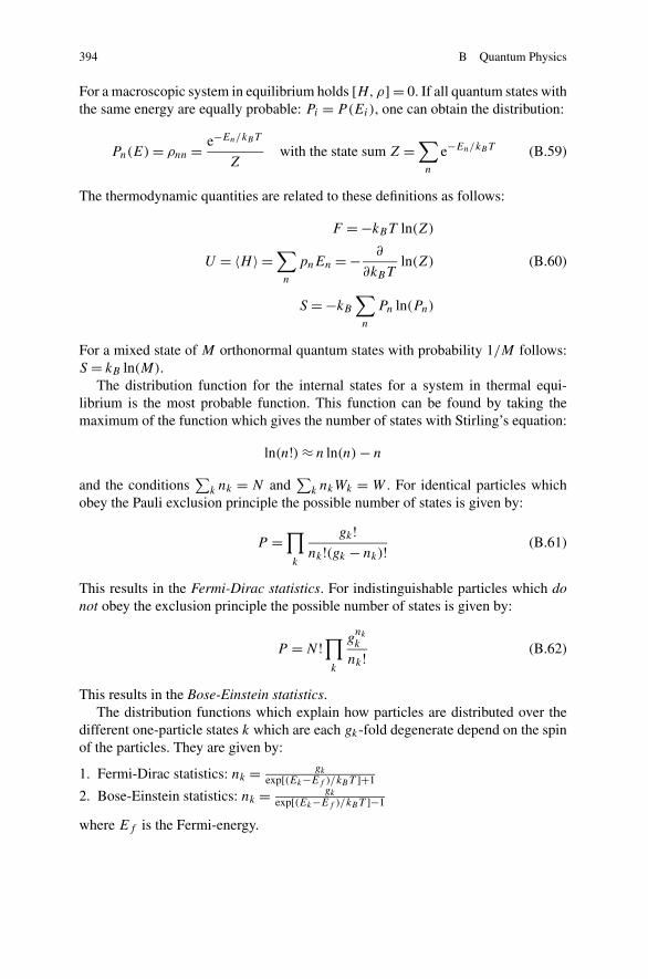
For a macroscopic system in equilibrium holds [H,ρ] = 0. If all quantum states withthe same energy are equally probable: Pi = P(Ei), one can obtain the distribution:

Pn(E) = ρnn = e−En/kBT

Zwith the state sum Z =

∑

n

e−En/kBT (B.59)

The thermodynamic quantities are related to these definitions as follows:

F = −kBT ln(Z)

U = 〈H 〉 =∑

n

pnEn = − ∂

∂kBTln(Z) (B.60)

S = −kB

∑

n

Pn ln(Pn)

For a mixed state of M orthonormal quantum states with probability 1/M follows:S = kB ln(M).

The distribution function for the internal states for a system in thermal equi-librium is the most probable function. This function can be found by taking themaximum of the function which gives the number of states with Stirling’s equation:

ln(n!) ≈ n ln(n) − n

and the conditions∑

k nk = N and∑

k nkWk = W . For identical particles whichobey the Pauli exclusion principle the possible number of states is given by:

P =∏

k

gk!nk!(gk − nk)! (B.61)

This results in the Fermi-Dirac statistics. For indistinguishable particles which donot obey the exclusion principle the possible number of states is given by:

P = N !∏

k

gnk

k

nk! (B.62)

This results in the Bose-Einstein statistics.The distribution functions which explain how particles are distributed over the

different one-particle states k which are each gk-fold degenerate depend on the spinof the particles. They are given by:

1. Fermi-Dirac statistics: nk = gk

exp[(Ek−Ef )/kBT ]+1

2. Bose-Einstein statistics: nk = gk

exp[(Ek−Ef )/kBT ]−1

where Ef is the Fermi-energy.

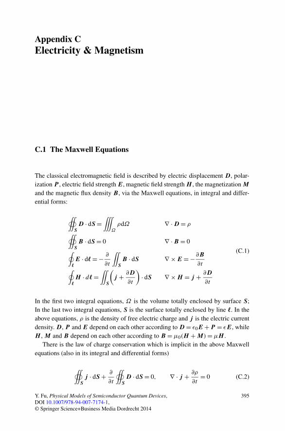
Appendix CElectricity & Magnetism

C.1 The Maxwell Equations

The classical electromagnetic field is described by electric displacement D, polar-ization P , electric field strength E, magnetic field strength H , the magnetization M

and the magnetic flux density B , via the Maxwell equations, in integral and differ-ential forms:

‹S

D · dS =˚

Ω

ρdΩ ∇ · D = ρ

‹S

B · dS = 0 ∇ · B = 0˛

�E · d� = − ∂

∂t

¨S

B · dS ∇ × E = −∂B

∂t˛�H · d� =

¨S

(

j + ∂D

∂t

)

· dS ∇ × H = j + ∂D

∂t

(C.1)

In the first two integral equations, Ω is the volume totally enclosed by surface S;In the last two integral equations, S is the surface totally enclosed by line �. In theabove equations, ρ is the density of free electric charge and j is the electric currentdensity. D, P and E depend on each other according to D = ε0E +P = εE, whileH , M and B depend on each other according to B = μ0(H + M) = μH .

There is the law of charge conservation which is implicit in the above Maxwellequations (also in its integral and differential forms)

‹S

j · dS + ∂

∂t

‹S

D · dS = 0, ∇ · j + ∂ρ

∂t= 0 (C.2)


395

http://dx.doi.org/10.1007/978-94-007-7174-1

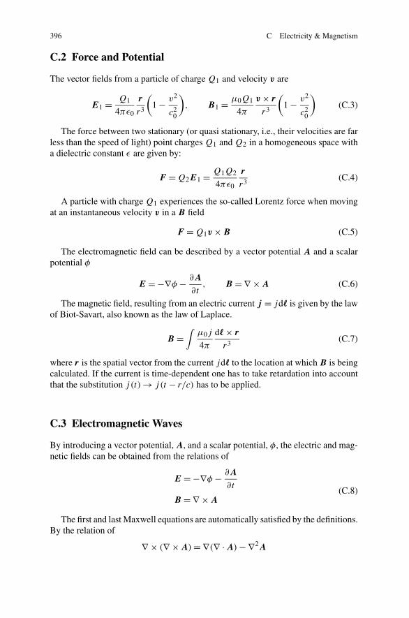
396 C Electricity & Magnetism

C.2 Force and Potential

The vector fields from a particle of charge Q1 and velocity v are

E1 = Q1

4πε0

r

r3

(

1 − v2

c20

)

, B1 = μ0Q1

4π

v × r

r3

(

1 − v2

c20

)

(C.3)

The force between two stationary (or quasi stationary, i.e., their velocities are farless than the speed of light) point charges Q1 and Q2 in a homogeneous space witha dielectric constant ε are given by:

F = Q2E1 = Q1Q2

4πε0

r

r3(C.4)

A particle with charge Q1 experiences the so-called Lorentz force when movingat an instantaneous velocity v in a B field

F = Q1v × B (C.5)

The electromagnetic field can be described by a vector potential A and a scalarpotential φ

E = −∇φ − ∂A

∂t, B = ∇ × A (C.6)

The magnetic field, resulting from an electric current j = jd� is given by the lawof Biot-Savart, also known as the law of Laplace.

B =ˆ

μ0j

4π

d� × r

r3(C.7)

where r is the spatial vector from the current jd� to the location at which B is beingcalculated. If the current is time-dependent one has to take retardation into accountthat the substitution j (t) → j (t − r/c) has to be applied.

C.3 Electromagnetic Waves

By introducing a vector potential, A, and a scalar potential, φ, the electric and mag-netic fields can be obtained from the relations of

E = −∇φ − ∂A

∂t(C.8)

B = ∇ × A

The first and last Maxwell equations are automatically satisfied by the definitions.By the relation of

∇ × (∇ × A) = ∇(∇ · A) − ∇2A

C.3 Electromagnetic Waves 397

and in the Lorentz gauge of

1

μ∇ · A + ε

∂φ

∂t= 0 (C.9)

we have the following equations for the vector and scalar potentials

∇2A − εμ∂2A

∂t2= −μJ (C.10)

∇2φ − εμ∂2φ

∂t2= −ρ

ε(C.11)

The wave equation �Ψ (r, t) = −f (r, t) has the following general solution

Ψ (r, t) =ˆ

f (r, t − |r − r ′|/c)4π |r − r ′| dr ′ (C.12)

where c = 1/√

εμ. When J (r, t) and ρ(r, t) can be expressed as J (r) exp(−iωt)

and ρ(r) exp(−iωt), respectively, A(r, t) and φ(r, t) have the similar forms ofA(r) exp(−iωt) and φ(r) exp(−iωt) with:

A(r) = μ

4π

ˆJ

(

r ′)exp[ik · (r − r ′)]|r − r ′| dr ′

(C.13)

φ(r) = 1

4πε

ˆρ(

r ′)exp[ik · (r − r ′)]|r − r ′| dr ′

An ideal dipole that oscillates in time

p(t) = p0 cos(ωt) (C.14)

The electric and magnetic fields, the Poynting flux, and angular distribution of thisoscillating dipole are

E = −θ0p0

4πε0r

ω2

c20

sin θ cos(ωt − k · r)

B = −φ0μ0p0

4πr

ω2

c0sin θ cos(ωt − k · r)

S = r0p2

0

16π2ε0r2

ω4

c3sin2 θ cos2(ωt − k · r) (C.15)

〈S〉t = r0p2

0 sin2 θ

32π2ε0r2

ω4

c3

dP

dΩ= r2r0 · 〈S〉t = p2

0 sin2 θ

32π2ε0r2

ω4

c3

398 C Electricity & Magnetism

in spherical coordinate, where r0, θ0 and φ0 are the three unit vectors. Note thatthe above expressions are valid for the following conditions: the dipole dimensionis much less than the distance to the dipole, it is also very small compared withthe wavelength of radiation. The distance to the dipole is much longer than thewavelength.

The wave equations in matter, with cmat = (εμ)−1/2 the light speed in matter,are:

(

∇2 − εμ∂2

∂t2− μ

ρ

∂

∂t

)

E = 0

(C.16)(

∇2 − εμ∂2

∂t2− μ

ρ

∂

∂t

)

B = 0

give, after substitution of monochromatic plane waves:

E = E0 exp[

i(k · r − ωt)]

and B = B0 exp[

i(k · r − ωt)]

the dispersion relation:

k2 = εμω2 + iμω

ρ(C.17)

The first term arises from the displacement current, the second from the conductancecurrent. If k is written in the form k = k′ + ik′′ it follows that:

k′ = ω

√

1

2εμ

√√√√1 +

√

1 + 1

(ρεω)2and k′′ = ω

√

1

2εμ

√√√√−1 +

√

1 + 1

(ρεω)2

(C.18)This results in a damped wave:

E = E0 exp(−k′′n · r)

exp[

i(

k′n · r − ωt)]

(C.19)

Appendix DSolid State Physics

D.1 Crystal Structure

A lattice is defined by the 3 translation vectors ai , so that the atomic compositionlooks the same from each point r and r ′ = r + R, where R is a translation vectorgiven by: R = u1a1 +u2a2 +u3a3 with ui are integers. A lattice can be constructedfrom primitive cells. As a primitive cell one can take a parallelepiped, with volume

Ωcell = a1 · (a2 × a3) (D.1)

Because a lattice has a periodical structure the physical properties n which are con-nected with the lattice have the same periodicity (neglecting boundary effects):

n(r + R) = n(r) (D.2)

This periodicity is suitable to use Fourier analysis: n(r) is expanded as:

n(r) =∑

G

nG exp(iG · r) (D.3)

with

nG = 1

Ωcell

ˆcell

n(r) exp(−iG · r)dr (D.4)

G is the reciprocal lattice vector. If G is written as G = v1b1 + v2b2 + v3b3 withvi as integers, it follows for the vectors bi , cyclically:

bi = 2πai+1 × ai+2

ai · (ai+1 × ai+2)(D.5)

The set of G-vectors determines the Röntgen diffractions: a maximum in the re-flected radiation occurs if: Δk = G with Δk = k − k′. So: 2k · G = G2. Fromthis follows for parallel lattice planes (Bragg reflection) that for the maxima holds:2d sin(θ) = nλ.

The Brillouin zone is defined as a Wigner-Seitz cell in the reciprocal lattice.


399

http://dx.doi.org/10.1007/978-94-007-7174-1

400 D Solid State Physics

D.2 Crystal Binding

A distinction can be made between 4 binding types:

1. van der Waals bond2. Ion bond3. Covalent or homopolar bond4. Metallic bond

The interaction in a covalent bond depends on the relative spin orientations ofthe electrons constituting the bond. The potential energy for two parallel spins ishigher than the potential energy for two antiparallel spins. Furthermore the potentialenergy for two parallel spins has sometimes no minimum. In that case binding is notpossible.

D.3 Crystal Vibrations

For a lattice with one type of atoms and only nearest-neighbor interactions are takeninto account, the force on atom s with mass M can then be written as:

Fs = Md2us

dt2= C(us+1 − us) + C(us−1 − us) (D.6)

Assuming that all solutions have the same time-dependence exp(−iωt) this resultsin:

−Mω2us = C(us+1 + us−1 − 2us) (D.7)

Further it is postulated that: us±1 = u exp(isKa) exp(±iKa). This gives: us =exp(iKsa). Substituting the latter two equations in the first results in a system oflinear equations, which has only one solution if their determinant is 0. This gives:

ω2 = 4C

Msin2

(1

2Ka

)

(D.8)

Only vibrations with a wavelength within the first Brillouin Zone have a physicalsignificance. This requires that −π < Ka ≤ π . The group velocity of these vibra-tions is given by:

vg = dω

dK=

√

Ca2

Mcos

(1

2Ka

)

(D.9)

and is 0 on the edge of a Brillouin Zone. Here, there is a standing wave.For a lattice with two types of atoms, the solutions are:

ω2 = C

(1

M1+ 1

M2

)

± C

√(

1

M1+ 1

M2

)2

− 4 sin2(Ka)

M1M2(D.10)

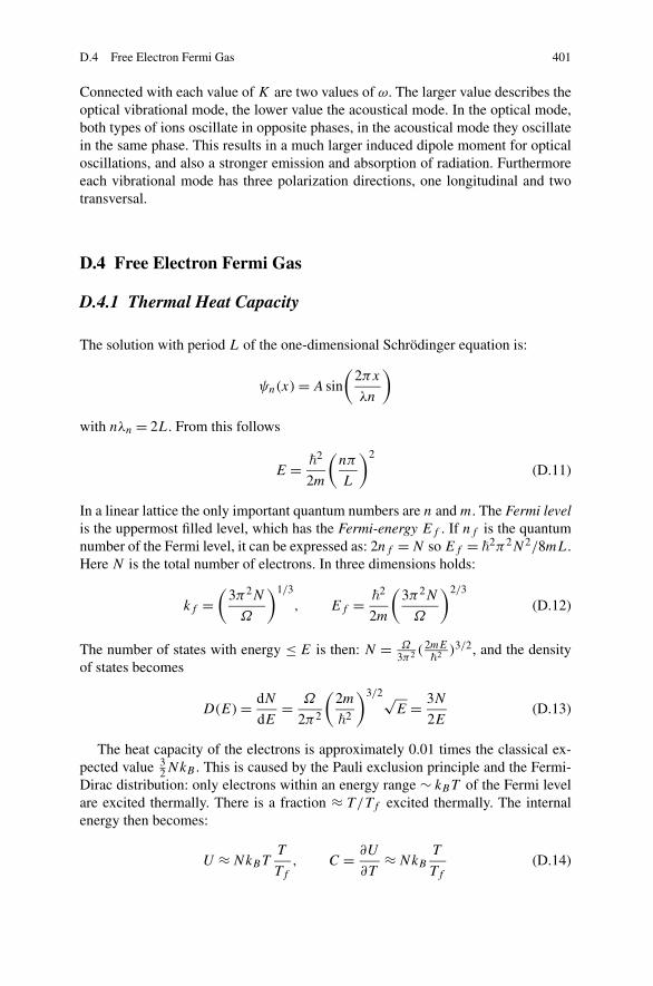
D.4 Free Electron Fermi Gas 401

Connected with each value of K are two values of ω. The larger value describes theoptical vibrational mode, the lower value the acoustical mode. In the optical mode,both types of ions oscillate in opposite phases, in the acoustical mode they oscillatein the same phase. This results in a much larger induced dipole moment for opticaloscillations, and also a stronger emission and absorption of radiation. Furthermoreeach vibrational mode has three polarization directions, one longitudinal and twotransversal.

D.4 Free Electron Fermi Gas

D.4.1 Thermal Heat Capacity

The solution with period L of the one-dimensional Schrödinger equation is:

ψn(x) = A sin

(2πx

λn

)

with nλn = 2L. From this follows

E = �2

2m

(nπ

L

)2

(D.11)

In a linear lattice the only important quantum numbers are n and m. The Fermi levelis the uppermost filled level, which has the Fermi-energy Ef . If nf is the quantumnumber of the Fermi level, it can be expressed as: 2nf = N so Ef = �

2π2N2/8mL.Here N is the total number of electrons. In three dimensions holds:

kf =(

3π2N

Ω

)1/3

, Ef = �2

2m

(3π2N

Ω

)2/3

(D.12)

The number of states with energy ≤ E is then: N = Ω

3π2 ( 2mE

�2 )3/2, and the densityof states becomes

D(E) = dN

dE= Ω

2π2

(2m

�2

)3/2√E = 3N

2E(D.13)

The heat capacity of the electrons is approximately 0.01 times the classical ex-pected value 3

2NkB . This is caused by the Pauli exclusion principle and the Fermi-Dirac distribution: only electrons within an energy range ∼ kBT of the Fermi levelare excited thermally. There is a fraction ≈ T/Tf excited thermally. The internalenergy then becomes:

U ≈ NkBTT

Tf

, C = ∂U

∂T≈ NkB

T

Tf

(D.14)

402 D Solid State Physics

A more accurate analysis gives:

Celectrons = 1

2π2NkBT/Tf ∼ T

Together with the T 3 dependence of the thermal heat capacity of the phonons thetotal thermal heat capacity of metals is described by

C = γ T + AT 3

D.4.2 Electric Conductance

The equation of motion for the charge carriers is:

F = mdv

dt= �

dk

dt(D.15)

The variation of k is given by

δk = k(t) − k(0) = −eEt

�

If τ is the characteristic collision time of the electrons, δk remains stable if t = τ .

〈v〉 = μE (D.16)

with μ = eτ/m the mobility of the electrons. The current in a conductor is given by:

J = nqv = σE = E

ρ= neμE (D.17)

D.5 Energy Bands

In the tight-bond approximation it is assumed that

ψ = eiknaφ(x − na)

from this follows for the energy:

〈E〉 = 〈ψ |H |ψ〉 = Eat − α − 2β cos(ka)

This gives a cosine superimposed on the atomic energy, which can often be approx-imated by a harmonic oscillator. If it is assumed that the electron is nearly free onecan postulate

ψ = eik·r

D.5 Energy Bands 403

i.e., a traveling wave. This wave can be decomposed into two standing waves:

ψ(+) = exp(iπx/a) + exp(−iπx/a) = 2 cos(πx/a)

ψ(−) = exp(iπx/a) − exp(−iπx/a) = 2i sin(πx/a)

The probability density |ψ(+)|2 is high near the atoms of the lattice and low inbetween. The probability density |ψ(−)|2 is low near the atoms of the lattice andhigh in between. Hence the energy of ψ(+) is also lower than the energy of ψ(−).Suppose that V (x) = V cos(2πx/a), than the bandgap is given by:

Eg =ˆ 1

0V (x)

[∣∣ψ(+)

∣∣2 − ∣

∣ψ(−)∣∣2]dx = V (D.18)

Index

AAcceleration effective mass, 31Angular momentum, 4–5, 7, 142, 149,

388–389

BBiaxially strain, 42Bloch theorem, 1, 19–21, 50, 59, 75, 84, 130,

226, 353Bloch wave function, 69, 363Body-centered cubic lattics, 11Bohr radius, 4, 6, 96–97, 141, 143–144, 160,

178, 324, 330, 348, 391Boltzmann (electron wave) transport, 97, 100,

239Bose-Einstein distribution, 394Bowing parameter, 38Bravais crystal, 10, 13, 44, 90, 137Bravais lattice, 10, 13Brillouin zone, 14, 32, 130, 135, 138, 288,

353, 399–400

CCarrier-concentration effective mass, 32,

315–316Cauchy stress tensor, 42Cauchy’s infinitesimal strain tensor, 42Cayley form, 71, 377Cladding layer, 347Complementary metal-oxide-semiconductor,

CMOS, 190–191, 233, 253, 257–258Complex conjugate, c.c., 114–116, 158, 211,

358Compound semiconductor, 103Conduction channel, 190, 237, 239–242,

244–247, 249–250, 252–254, 258Conductivity effective mass, 31, 33

Core electron, 9–10, 302, 345–346Coulomb blockade, 245, 258, 261Crystal lattice and lattice basis, 10, 14, 17, 44,

89–91, 137Crystal momentum, 118Czochralski (CZ) technique, 15

DDeformation potential, 34–35, 103, 170δ doping, 230–231, 233, 302, 345–346Density of states, 32–33, 59–62, 82, 93, 98,

170, 180, 187, 200, 216, 233–236,285–286, 338–339, 369, 373

Density-of-states effective mass, 32Depletion layer, 219Diamond crystal structure, 10Dielectric coefficient, 323Dielectric polarization, 158, 160, 162, 165,

324, 329Diffusion coefficient, 90, 100–101, 192, 346Diffusion length, 56Distributed Bragg reflector, DBR, 399Dynamic random access memory, DRAM, 2

EEdge emission, 222Effective mass, 29–33, 38, 53–54, 56–57, 93,

118, 136–137, 142–143, 147–148,249–250, 276–280, 282–286, 306–307,314–316, 353–355

Effective mass approximation, 53–54, 118,137, 142, 147–148, 177, 307

Effective medium approximation, 25–26, 48Einstein ratio, 101, 191Einstein relation, 101, 191Electron affinity, 24, 147, 188, 190Electron-beam direct-writing technique, 3,

257–258


405

http://dx.doi.org/10.1007/978-94-007-7174-1

406 Index

Electron-phonon interaction, 104–105,107–108, 207, 209–213

Electron wavelength, 2Elemental semiconductor, 103Ellipsoidal band, 31Energy band offset, 24Energy dispersion relation, 85, 114Envelope function, 1, 27–28, 52–53, 56–59,

92, 134, 140, 143–144, 160, 226, 275,277, 311, 340, 353

Evanescent states, 108, 195, 209, 211–212Exciton, x, 79, 111, 117, 134–135, 137–146,

157–163, 165–168, 172–173, 176, 298,317, 323–325, 327–335, 348–349

Exciton binding energy, 141, 144, 146Exciton Bohr radius, 141, 143, 324, 330, 348Exciton polariton, 117, 162, 298, 323, 332

FFabry-Perot microcavity, 342Face-centered cubic lattice, 11–12Fermi level, 23, 89, 95–96, 102–103, 106–107,

187–188, 190, 208, 219, 228, 230–231,315–316, 336–337, 353–355, 401

Field-effect transistor, v, 2, 185, 188, 230–231,233, 239, 245, 248–249, 253, 255, 368

First-order perturbations, 28, 74, 78–79, 83,85, 157–158, 167, 204

Fourier transform, 53, 138–139, 332Frequency multiplier, 213–214

GGate length, 2, 236, 252Gaussian wave packet, 71–72, 378Gunn effect, 213

HHarmonics, 5, 153, 179, 213, 295, 326,

389–390Heterostructure, vi, 1, 3, 17–18, 39, 50, 53–56,

104, 185, 213–216, 218, 224, 249,313–314, 343–344

Heterostructure barrier varactor, HBV, 185,213–214, 216, 249

Heterostructure barrier varactor diode, HBV,213

High-electron-mobility transistor, HEMT, 185,224–226, 229–230, 243–245, 247, 263

IImpurity state, 93–94, 96Index guiding, 343Infinitely deep quantum well, 62, 144–145,

272–274, 278, 305, 373Interface diffusion, 18, 51Inverse effective mass, 276–277, 279–280,

282–283

KKane parameter, 36Kramers’ theorem, 21

LLarge scale integration, LSI, 112, 262Localized state, 107, 223, 366Longitudinal effective mass, 31, 38, 276, 355Luttinger parameters, 36

MMaxwell equations, 113–114, 324, 395–396Metal-organic chemical vapor deposition,

MOCVD, 3, 15, 18–19, 43, 310Metal-oxide-semiconductor, MOSFET, v, 2,

188–191, 230–231, 252–255, 257, 262,368

Misfit dislocation, 24, 40Mobility, vi, 33, 67, 100–101, 185, 192,

224–226, 228–230, 233, 238, 243, 247,263, 287, 320

Mole fraction, 26–27, 36, 47–48, 55Molecular beam epitaxy, MBE, 3, 15, 17–19,

40, 200, 224, 230, 246, 310Momentum operator, 27–28, 118, 141, 159,

384, 388Monte Carlo scheme, 45, 170–172Mott phase transition, 94, 354–355

NNanofabrication technique, 3

OOptical absorption coefficient, 279, 302,

306–307Optical grating, 271, 289, 294, 298, 307–308,

310, 312Optical transition matrix, 35, 128, 131, 142,

163, 275–276, 302, 306, 322Orbital angular momentum, 7, 388Oscillator strength, 402

PPauli exclusion principle, 8, 68, 89, 93, 98,

117, 127, 193, 227, 296, 317, 394, 401

Index 407

Photocurrent, 302, 305, 307–308, 310,312–313, 316, 319–323

Photonic bandgap, 328Photonic bandgap crystal, PBC, 323Photonic crystal, 309, 323Poisson effect, 234, 315, 368Population inversion, 128, 133, 167, 336–337,

342–343, 345Poynting vector, 114, 116–117, 165–166Primitive vector, 10–13, 20

QQuantum cascade laser, 345Quantum confinement, 57–58, 61, 133, 146,

160, 178, 243, 348Quantum dot, QD, 43, 45–47, 61–62,

133–134, 146–148, 150, 160–163,167–174, 257–261, 312, 318, 322–324,328–330, 332–333, 348–350

Quantum dot cellular automata, QCA,258–259, 261

Quantum effect device, 3Quantum efficiency, 317Quantum number, 4, 7, 20, 57, 138, 142, 401Quantum well, QW, 46–48, 53–55, 59,

130–131, 133–134, 144–146, 223,229–230, 271–279, 281–291, 299–308,341, 346–347, 367–369, 373

Quantum well infrared photodetector, QWIP,290–291, 294, 299–300, 302–303,305–308

Quantum wire, QWR, 57, 59, 61–62, 71–73,108, 132–134, 154–155, 238–239, 253,255–257, 262–263, 307–308, 310–311,368–369, 375–377

RRadial Schrödinger equation, 6, 149Random walking, 45Reciprocal lattice vector, 13, 130, 399Reciprocal space, 12–14Recursion method, 234, 368Reflection high energy electron diffraction,

RHEED, 18Resonant cavity, 342Resonant tunneling diode, RTD, 106, 185,

195–196, 198, 200, 208, 218, 339–340,359

Resonant-tunneling light-emitting diode,RTLED, 339

Rydberg constant, 4, 381

SSchottky barrier, 213, 313Schottky diode, 213Schrödinger equation, 5–6, 19–20, 27–28,

68–71, 77, 92–93, 143, 168–169, 198,234, 239–240, 259–260, 368, 385–386,390–392

Second-order perturbations, 28Secular determinant, 22Secular equation, 22Selection rule, 153, 276, 282, 307–308Semiclassical picture (theory), 192Semiconductor microelectronics, 2Semiconductor optoelectronics, 2Sequential tunneling, 199, 202Shockley matrix, 35Si-on-insulator, 253, 257Silicon on insulator, SOI, 253, 257Simple cubic lattice, 11, 14Single electron transistor, SET, 257–258,

261–263Slater determinant, 135, 177, 393Soft lithography, 3Spherical band, 31, 276Spherical harmonics, 5, 153, 179, 389–390Spherical symmetry, 5Spin angular momentum, 7Spin split off, 30, 33Stark effect, 347, 367–368Stranski-Krastanov growth, 40, 42–43Superlattice, 18, 51, 195, 271, 287–289, 345,

362–363, 365Surface emission, 51

TTight-binding model, 21–23, 55, 136, 148Transfer-matrix method, 288, 363Transition matrix, 35, 76, 87, 109, 121, 128,

131, 142, 163–164, 275–276, 302, 306,321–322, 340

Transverse effective mass, 31, 38, 276, 355Tunneling probability, 200–201, 206, 209–211,

314Two-dimensional electron gas, 2DEG,

225–226, 228–230

UUniaxially strain, 43Unit cells, 20–25, 44, 50–51, 57, 70, 86–87,

89–90, 104, 129–131, 137, 211

VValence-band offset, VBO, 36, 362Valence electron, 9–10, 21–23, 91–92, 185

408 Index

Valence-force-field (VFF) approach, 43

Varactor, 185, 213–218, 221, 223–224, 249

Varshni approximation, 36

Varshni parameters, 36

Vertical cavity surface emitting laser, VCSEL,345

Virtual crystal approximation, 37, 56

WWannier function, 50–52, 92Wave vector space, 12Wavelength division multiplexing, 116, 165Work function, 188, 190

ZZincblende crystal structure, 12, 22, 44

Fundamental Constants

Documents

Transcript of Fundamental Constants