Predicting Stock and Bond Returns: The Impact of Global Variables

Predicting Stock and Bond Returns: the Impact

of Global Variables*

David Ely and Mehdi SalehizadehDepartment of Finance, College of Business Administration,

San Diego State University.

Abstract

Prior research demonstrates that returns on US stocks and bonds over time

can be predicted using models containing proxies for domestic business

conditions and the stance of monetary policy. This paper has two object-

ives. First, it examines the benefits of adding international economic and

monetary variables to US stock and bond prediction models. We specify

a base model (employing US variables only), along with two alternative

approaches that supplement or replace US measures with weighted average

measures of corresponding variables based on the economic environment

of the G-7 countries. Monthly and quarterly holding period returns are exam-

ined over the time period August 1976 to December 1997. We conclude that,

for some assets, using international information can improve forecasts of

returns. The second objective of this paper is to re-examine issues addressed

in earlier studies using the international versions of our models. Our find-

ings suggest that bond returns can be predicted with a common set of variables

and that variables characterizing the monetary sector contain information

about expected bond returns beyond that of business conditions proxies.

© Blackwell Publishers Ltd. 1999. 108 Cowley Road, Oxford OX4 1JF, UK and 350 Main Street, Malden, MA 02148, USA

International Finance 2:2, 1999: pp. 203–226

*The authors would like to thank Benn Steil, the Editor, and two anonymous referees for in-

valuable comments and suggestions. The authors remain, of course, responsible for the contents.

I. Introduction

In recent decades, the ownership base of US stocks and bonds has become

increasingly international as the US economy, along with those of other

advanced and emerging countries, has received large sums of foreign capital.

In the case of the US, the need since 1969 to finance the annual budget deficit

has led the Treasury to offer government securities to the public. Moreover,

the significant growth of the US current account deficit has resulted in a

substantial increase in holdings of US dollars by foreign private and official

investors. Indeed, data reported by the US Treasury Department and pre-

sented in Figure 1 show that the share of US Treasury securities held by

foreign investors exceeded 38% in December 1998.1 Similar information on

the ownership of stocks and corporate bonds is unavailable, but the rising

importance of the global financial markets to US securities is also evident

from the changing patterns of transactions involving purchases and sales of

long-term securities by foreign investors. Table 1 presents information by

decade on US transactions with foreigners in US federal securities, corporate

bonds and corporate stocks. Average monthly gross purchases of Treasury

bonds and notes by foreigners from US residents rose from $3.4 billion in the

late 1970s to $273.6 billion in the 1990s. Gross sales by foreigners to US

residents of Treasury bonds and notes rose from $2.7 billion to $265.7 billion

over the same period. Purchases and sales of US corporate stocks in the 1990s

are 25 times their levels in the late 1970s. Similarly dramatic increases in the

level of transactions of other securities are apparent from this table. Global

capital flows associated with stock and bond holdings are generally regarded

as being highly liquid. Concerns are periodically expressed (Melloan 1996;

Pulliam and Zuckerman 1996) over whether foreign investors, especially

Japanese institutions, will ‘dump’ their holdings of US Treasuries, causing a

sharp decline in prices. The Japanese held approximately $276 billion of the

US public debt owned by private investors in December 1998 (US Treasury

1999).

One can infer from Figure 1 and Table 1 that the magnitude of the activity

of external investors in US securities has placed them in an influential

position, suggesting that models designed to predict stock and bond returns

could be improved by incorporating factors that capture the impact of foreign

economic conditions and monetary environments on the expected returns of

US financial assets.

204 David Ely and Mehdi Salehizadeh

© Blackwell Publishers Ltd. 1999

1December 1998 figures indicate that US$3.33 trillion of federal securities were privately held

(that is by investors other than agencies of the US government). Of this amount, about US$1.28

trillion were held by overseas investors. The comparable figure for 1970 is 11% (US Treasury,

1999).

Previous studies demonstrate that the variation in returns on US stocks and

bonds over time can be predicted using models containing proxies for dom-

estic business conditions and the stance of monetary policy (see, for example,

Predicting Stock and Bond Returns 205


Table 1: Foreign Purchases and Sales of Long-term Securities: Average

Monthly Transactions by Decade ($million)

US US US corp. US corp. Foreign Foreign

Treasury govt bonds stocks bonds stocks

bonds & agency

notes bonds

Gross purchases by foreigners from US residents

1977–80 3,405 503 336 2,029 1,019 384

1981–90 74,397 2,447 3,743 10,500 11,273 4,316

1991–8 273,606 15,990 16,760 50,528 75,300 35,363

Gross sales by foreigners to US residents

1977–80 2,653 354 210 1,774 1,317 443

1981–90 72,276 2,057 2,313 10,125 11,855 4,611

1991–8 265,702 13,275 12,022 48,685 78,288 38,665

Source. Authors’ calculations based on data provided by the US Treasury (1999).

Figure 1: Foreign ownership of US Treasury securities

Keim and Stambaugh 1986; Fama and French 1989, 1993; Jensen et al. 1996).

While these findings might be attributable to inefficient markets, they are also

consistent with rational time-varying required returns on assets. That is, the

forecasting power of these variables is derived from their ability to proxy for

business conditions and/or the monetary environment. As business con-

ditions and monetary policy change, so does the required return on financial

assets. One possible explanation for this pattern is that consumption smooth-

ing by investors causes changes in required returns (Fama and French 1989).

When income is high, investors are willing to accept lower expected returns in

order to increase savings and shift consumption into the future.

If foreign investors, in their consumption and investment decisions, behave

similarly to those based in the US, then identifying and incorporating inter-

national measures of economic conditions and monetary environments into

prediction models of asset returns should enhance their performance. This

paper has two objectives. First, it examines the benefits of adding international

economic and monetary variables to US stock- and bond-prediction models.

The second objective is to re-examine issues addressed in earlier studies using

the global versions of our models. In particular, we investigate whether tests

conducted using our alternative specifications lead to the same conclusions

reported by other authors about market efficiency and the influence of mon-

etary policy on expected returns. The paper is organized as follows. Section II

provides an overview of the recent literature on predicting stock and bond

returns. Section III develops the prediction models estimated in this paper

and explains our testing procedures. Estimates of the prediction models are

presented in Section IV, along with the results of tests conducted using the

models. Section V summarizes and concludes the paper.

II. Prior Research

Prior research shows that a number of key economic and financial variables

are capable of predicting excess returns on US stocks and bonds over long

horizons. Keim and Stambaugh (1986) find that the variation in returns on

seven stock and bond portfolios over the 1928–78 time period are related to:

(a) the yield difference between longer-term risky (low-grade corporate)

bonds and one-month Treasury bills; (b) a measure based on the ratio of the

real S&P’s index to its previous historical average; and (c) minus the logarithm

of share price as averaged across New York Stock Exchange firms in the quintile

of smallest market value. Even though the first variable is generally associated

with the bond markets, it proves useful in predicting stock returns. Likewise,

even though the second and third variables are normally associated with stock

markets, they are useful in predicting bond returns.



Fama and French (1989) focus on stocks and the corporate bond sector and

also conclude that a common set of three variables – dividend yields, a default

premium measuring the yield difference between corporate bonds and Aaa

bonds, and a term premium recording the difference between the Aaa yield and

the one-month Treasury bill – forecast excess returns. Because dividend yields,

a factor usually associated with stock returns, is a predictor of bond returns

and because default and term premiums, factors usually associated with bond

returns, are predictors of stock returns, they argue that the time variation

in expected returns is largely common across securities. Their analysis leads

them to conclude that the predictive power of the variables arises from their

ability to act as proxies for business conditions. In a later study, Fama and

French (1993) argue that returns on stocks and bonds are related to five com-

mon risk factors, including three stock market variables, consisting of market,

size and book-to-equity. The spread between the returns on a portfolio of

large companies and a portfolio of small companies is used to mimic the risk

factor related to size, and the spread between returns on portfolios of high and

low book-to-market equity companies is used to mimic the risk factor asso-

ciated with book-to-market equity. The two other common risk factors are

bond factors related to term and default risk. A model containing the three

stock market factors is shown to explain excess returns on a cross-section of

portfolios with similar size and book-to-market equity characteristics. Fama

and French (1996) extend this analysis to portfolios formed on additional

firm characteristics. However, Daniel and Titman (1997) challenge Fama and

French’s interpretation that the cross-section variation in stock returns they

document is due to co-movements with pervasive risk factors proxied by size

and book-to-market equity.

Jensen et al. (1996) extend Fama and French’s (1989) model by considering

the role of the monetary environment along with business conditions vari-

ables. They conclude that the Federal Reserve’s monetary stance – indicated by

periods of expansive or restrictive monetary policy and measured in terms

of the directional change of the discount rate – affect the manner in which

the Fama and French business condition proxies track variation in expected

returns. While concluding that predictable time-varying returns are rational,

they find that only in restrictive monetary environments do the variables

explain expected bond returns and only in expansionary environments do

the variables explain expected stock returns. Booth and Booth (1997) also

find that the monetary policy indicators have explanatory power beyond

those reflecting business condition proxies. However, their results suggest that

conclusions about the impact of the monetary environment on the relations

between business condition proxies and asset returns may be sensitive to

the choices of asset portfolios or the selection of variables representing busi-

ness conditions. Patelis (1997), using a broad set of monetary and financial



variables, also concludes that both categories of variables are useful in

predicting stock returns.

Despite the increased activity of foreign investors in US stock and bond

markets, generally researchers have restricted themselves to US variables when

constructing models to predict US stock and bond returns. Exceptions include

Ferson and Harvey (1993), who use a combination of global and local

variables to investigate the predictability of equity returns in 18 countries.

They conclude that a time-varying global risk premium accounts for a greater

fraction of the predictability of returns in the national equity markets than

time-varying betas based on local information. Also focusing on international

variables is Ilmanen (1995), who examines long-term government bonds for

six members of the G-7 (excluding Italy), and finds that while country-specific

local instruments can forecast excess bond returns, common ‘world’ instru-

ments (GDP-weighted averages of local instruments) are better predictors. In

another study, Ilmanen (1996) provides additional evidence that excess long-

term bond returns can be forecast using local and global variables, such as

past stock market performance, the term spread and the real bond yield.

Our paper follows the approach of these authors by exploring the benefits

of augmenting local variables with information on conditions in foreign

economies.

III. Methodology and Data

A. Models and Data

Two models are employed to assess the impact of incorporating international

economic information in returns-forecasting models. The first model is sim-

ilar to those used by Fama and French (1989) and Jensen et al. (1996).2 The

model is:

r(t, t + T) = b0 + b1DYt + b2TERMt + b3MPt + b4REALt + et (1)

where: r(t, t + T) denotes the return on an asset held over T time periods; DY

denotes the dividend yield in the US, TERM denotes the US term premium,

MP denotes the stance of US monetary policy, and REAL denotes the US real

interest rate.



2Fama and French (1989) do not include monetary environment or real interest rate variables.

Jensen et al. (1996) include a monetary policy variable but not a real interest rate variable. Real

interest rates are found to be predictors of asset returns by Ilmanen (1995) and Patelis (1997),

and are therefore used here.

We refer to this equation throughout our paper as the ‘base model’. As in

Fama and French and Jensen et al., we also estimate the equation using a US

default premium (DEF) in place of the dividend yield as a proxy for business

conditions. We choose this model over others developed in later studies by

Fama and French (1993, 1996) because it allows us to make comparisons

not only to the results presented in Fama and French (1989), but also to the

work of Jensen et al. (1996) and Booth and Booth (1997). This is particularly

important given the latter studies’ examination of the impact of the monetary

environment on expected returns, an issue we also consider. Furthermore, a

lack of data precludes us from creating equivalent global counterparts to the

size or the book-to-market equity variables employed in Fama and French

(1993, 1996).

The second model we estimate, which we refer to as the ‘global model’,

replaces the US variables with similar global measures. That is:

r(t, t + T) = b0 + b1GDYt + b2GTERMt + b3GMPt + b4GREALt + et (2)

where: GDY denotes a dividend yield based on the MSCI world index;

GTERM denotes the GDP-weighted average of term premiums in the G-7

countries; GMP denotes the GDP-weighted average of monetary policy meas-

ures in the G-7 countries; and GREAL denotes the GDP-weighted average of

real interest rates in the G-7 countries. Here, as in the base model, we also

estimate equation (2) substituting a measure of global default risk (GDEF) for

the dividend yield.3

We indirectly estimate a third model, referred to as the ‘expanded model’,

that adds foreign or global measures of dividend yields, default premiums,

term premiums, real interest rates and monetary policy. The foreign variables

reflect the non-US G-7 economies and consist of a weighted average of term

premiums (FTERM), a weighted average of monetary policy indicators (FMP)

and a weighted average of real interest rates (FREAL). The difference between

foreign and global variables is that US data are included in the weighted

averages for the global variables but not for the foreign variables.

Four assets are considered in this study: stock returns as measured by the

CRSP value-weighted index (VW), stock returns as measured by the CRSP

equal-weighted index (EW), corporate bond returns (CB) and US govern-

ment bond returns (GB). By construction, the CRSP value-weighted index

weights high capitalization (large) stocks more heavily, while the equal-weighted



3We also tried using the change in the value of the trade-weighted US dollar as used by Ferson

and Harvey (1993). It proved to be insignificant in all equations and was therefore dropped

from the analysis.

index gives disproportionate weight to low capitalization (small) stocks.

Excess returns are derived by subtracting returns on one-month US Treasury

bills (from Ibbotson Associates) from total returns for each series. Data for

corporate bonds and government bonds are also from Ibbotson Associates

(1998).4

Dividend yields are derived from the CRSP indices using the procedure

described in Fama and French (1988). Following Fama and French, the yield

for month t is based on income returns over month t – 11 to month t. The US

term premium is defined as the spread between ten-year and one-year bonds.

The default premium is measured as the spread between the Moody’s Baa

Corporate Bond Yield and US government ten-year bond yield. The federal

funds rate is used to measure the stance of monetary policy in the US. Bernanke

and Blinder (1992) offer evidence that the federal funds rate reflects the stance

of monetary policy. Patelis (1997) and Booth and Booth (1997) also use the

federal funds rate to represent the monetary environment. The real interest

rate is derived as the ten-year government bond rate less expected inflation,

proxied by the actual growth in the Consumer Price Index (CPI) over the

previous 12 months.5 Finally, the predictions of asset returns are based on

values of independent variables in the month prior to the start of the holding

period.

The global dividend yield variable (GDY), based on the Morgan Stanley

Capital International (MSCI) world stock market index, is derived using a

similar procedure as was used to calculate the US dividend yield. As in Ferson

and Harvey (1993), global default risk (GDEF) is measured by the spread

between the three-month Eurodollar deposit rate and the three-month US

Treasury bill rate. Measures of the stance of monetary policy, term premiums

and real interest rates employed for the other G-7 countries are similar to

those identified for the US variables. Data on US bond yields are from the

St Louis Federal Reserve’s economic database. The US federal funds rate, data

on the rates of foreign government bonds and consumer prices are from the

IMF’s International Financial Statistics database. Generally, we use the time



4Corporate bond returns are based on the Salomon Brothers Long-Term High-Grade Corporate

Bond Index, which includes nearly all Aaa- and Aa-rated bonds (Ibbotson Associates 1997,

p. 54). Long-term government bond returns are based on the total return of a one-bond port-

folio with a term of approximately 20 years (Ibbotson Associates 1997, p. 56). Total returns for

US Treasury bills are based on the bill with the shortest maturity not less than one month

(Ibbotson 1997, p. 63).

5Since expected inflation cannot be observed, a model of expected inflation must be adopted to

create REAL. Inflation over the prior year as an approximation of expected inflation is also used

by Ilmanen (1995, 1996).

period from August 1976 to December 1997.6 Analyses for monthly and quar-

terly holding periods are presented; thus, we have 256 monthly observations

and 85 quarterly observations.

B. Comparison of Domestic and Foreign Monetary Environments

Figure 2 presents a comparison of the US term premium with those of Japan

and Germany.7 At several points in time, the US pattern of premiums deviates

from that of the other two countries. The US term premium began to decline

in mid-1977, while declines in Germany and Japan did not occur until mid-

1979. In mid-1990, the US term premium was rising, while those for Japan

and Germany continued to decline until early 1992 or early 1993. Figure 3

presents similar information for monetary policy indicators for the three



6For foreign countries, IFS item number 61 is used for long-term government rates; item

number 60CS (UK, France), 60BS (Germany), 60B (Italy) or 60C (Canada) is used for the short-

term rate; and item 60B is used for the monetary policy variable. The CD rate, collected from

the Federal Reserve Bulletin, is used for the Japanese short-term interest rate.

7For the US, the term premium is calculated as the spread between the ten- and the one-year

Treasury bond rates. The term premiums are calculated as the spread between the government

bond yield and the three-month interbank deposit rate for Germany and the spread between the

government bond yield and CD rate for Japan.

Figure 2: Term premium comparison, 1976–1997

1976 1979 1982 1985 1988 1991 1994 1997

countries. The US federal funds rate began to decline in May 1989, while the

call money rates did not begin to decline until April 1991 in Japan, and until

August 1992 in Germany. The central hypothesis of this paper is that incor-

porating information on business conditions being experienced by foreign

investors has the potential to improve the predictability of asset returns.

C. Preliminary Analysis

Table 2 presents descriptive statistics, based on monthly data, for the variables

used in this study. Table 3 presents estimates of the models similar to those

employed by Fama and French (1989) and Jensen et al. (1996). So that com-

parisons can be made with these earlier studies, results for monthly and

quarterly return horizons are presented for the time period 1954–92. This

is the same time period as used by Jensen et al., but a later period than that

employed by Fama and French.

Our results are similar to the findings of these other authors. The stock-

return models which have (a) DY or DEF and (b) TERM as independent

variables can be compared directly to Jensen et al. (1996, Table 4) since they

provide models estimated with the same variables using the same time period.

Our estimates closely match their results. We find that the dividend yield, the

term premium and the default premium were all related to stock returns. In



Figure 3: Monetary policy comparison, 1976–1997

Pred

icting Stock a

nd

Bon

d R

eturn

s2

13

©B

lackw

ell Pu

blish

ers Ltd

. 19

99

Table 2: Descriptive Statistics: August 1976 to December 1997

VW EW CB GB DY DEF MP TERM REAL GDY GDEF GTERM GMP GREAL

Mean 0.20 0.39 0.28 0.29 3.94 1.92 7.83 1.02 3.93 2.57 0.02 0.75 7.69 3.89 Median 0.19 0.41 0.43 0.42 4.06 1.85 7.16 1.10 4.08 2.39 0.00 1.03 7.25 4.24 Maximum 3.80 5.59 12.50 13.97 6.09 3.82 19.10 3.29 9.45 4.22 5.87 2.05 15.79 7.61 Minimum –3.94 –3.07 –9.77 –9.28 1.90 0.93 2.92 –3.07 –3.73 1.52 –1.99 –2.14 3.80 –1.66 Std dev. 0.73 0.62 2.86 3.29 1.00 0.53 3.49 1.19 2.58 0.78 0.52 0.77 2.83 1.94

Correlation coefficients

DY DEF TERM MP REAL GDY GDEF GTERM GMP GREAL

DY 1.000DEF 0.211 1.000TERM –0.474 0.269 1.000MP 0.715 0.149 –0.749 1.000REAL –0.130 0.371 0.428 –0.023 1.000GDY 0.892 0.211 –0.385 0.640 –0.116 1.000GDEF 0.018 –0.143 –0.073 0.017 –0.020 0.023 1.000GTERM –0.460 –0.042 0.689 –0.675 0.394 –0.262 –0.015 1.000GMP 0.765 0.322 –0.523 0.920 0.006 0.666 –0.010 –0.702 1.000

GREAL –0.173 0.375 0.430 –0.047 0.961 –0.193 –0.052 0.333 0.002 1.000

Notes: All statistics are based on monthly data. Excess returns of the value-weighted CRSP index (VW), equal-weighted CRSP index (EW), long-term corporatebonds (CB) and long-term government bonds (GB) are calculated as asset returns less the one-month return on US Treasury bills. The independent variablesconsist of dividend yields (DY), derived from the CRSP indices using the procedure described in Fama and French (1988); default risk (DEF), calculated as thedifference between Moody’s Baa Corporate Bond Yield and US government ten-year bond rate; US term premium (TERM), defined as the difference betweenthe ten-year and the one-year government bond rates; US monetary policy (MP) indicator, defined as the federal funds rate; real US interest rate (REAL),defined as the ten-year government bond rate less expected inflation, proxied by the actual growth in the Consumer Price Index (CPI) over the previous twelvemonths; a measure of global dividend yields based on the MSCI world index (GDY); a GDP-weighted average of term premiums (GTERM) for the G-7countries; global default risk (GDEF) defined as the difference between the Eurodollar deposit rate and the US Treasury three-month rate; a GDP-weightedaverage of monetary policy indicators for the G-7 countries (GMP); and a GDP-weighted average of real interest rates (GREAL).



Table 3: Regressions of Excess Returns on Measures of Business

Conditions and Monetary Policy Indicators: August 1954 to December

1992

DY TERM DEF MP REAL R2 F-test

A. Monthly results

VW 0.4135 0.6065 0.03 7.052

(0.0368) (0.0009) (0.0010)

0.5275 0.3195 0.02 5.556

(0.0207) (0.3437) (0.0041)

0.7760 0.3096 –0.2076 –0.0514 0.04 4.269

(0.0030) (0.1921) (0.0125) (0.6559) (0.0021)

–0.4365 1.589 –0.3171 0.0687 0.05 5.116

(0.1929) (0.0010) (0.0020) (0.5394) (0.0005)

EW 0.5362 0.6625 0.03 6.536

(0.0355) (0.0025) (0.0016)

0.4931 0.6632 0.02 5.824

(0.0677) (0.1331) (0.0032)

1.0707 0.4769 –0.2356 –0.1865 0.05 4.873

(0.0024) (0.1176) (0.0203) (0.2001) (0.0008)

–0.5130 2.1250 –0.3761 –0.0254 0.05 5.751

(0.2327) (0.0017) (0.0044) (0.8512) (0.0002)

CB –0.0191 0.3174 0.02 4.144

(0.8941) (0.0582) (0.0165)

0.2431 0.2747 0.02 5.417

(0.2040) (0.1781) (0.0047)

–0.1843 0.1775 0.0362 0.1774 0.05 5.132

(0.3226) (0.3070) (0.5031) (0.0197) (0.0005)

–0.1667 0.5084 –0.0764 0.2090 0.05 5.666

(0.5502) (0.1126) (0.2231) (0.0066) (0.0002)

GB 0.0047 0.2441 0.01 1.954

(0.9734) (0.1454) (0.1428)

0.2095 0.1289 0.01 2.177

(0.2686) (0.5221) (0.1145)

–0.2011 0.1143 0.0503 0.1831 0.03 3.735

(0.2748) (0.5361) (0.3539) (0.0119) (0.0053)

–0.0097 0.1273 –0.0057 0.1886 0.03 3.467

(0.9745) (0.7023) (0.9316) (0.0168) (0.0084)

B. Quarterly results

VW 1.2969 1.5888 0.06 5.057

(0.0620) (0.0177) (0.0075)

1.4080 0.8162 0.04 3.514

(0.0868) (0.4868) (0.0322)

2.2987 0.7105 –0.5860 –0.1448 0.08 2.907

(0.0122) (0.4200) (0.0587) (0.7382) (0.0241)

–1.1604 4.1439 –0.8382 0.1909 0.08 3.090

(0.3124) (0.0113) (0.0137) (0.6332) (0.0180)

addition, there is some support that corporate bond yields were related to the

term premium. In models that also incorporate a monetary policy indicator,

our results are consistent with Jensen et al. The indicator is related to stock

returns but not to bond returns. Fama and French (1989) and Jensen et al.

(1996) do not consider real interest rates, but we find that they too help to

explain the variation in corporate and government bond returns.



Table 3: Continued

DY TERM DEF MP REAL R2 F-test

EW 1.5695 1.6874 0.05 3.666

(0.0793) (0.0349) (0.0279)

1.2170 1.9766 0.04 3.275

(0.2247) (0.2258) (0.0405)

2.9629 1.3401 –0.5874 –0.6216 0.08 2.765

(0.0152) (0.2404) (0.1221) (0.2863) (0.0301)

–1.3237 5.7649 –0.9814 –0.1585 0.09 3.224

(0.3531) (0.0158) (0.0227) (0.7497) (0.0146)

CB –0.0375 0.7529 0.02 1.841

(0.9382) (0.2797) (0.1622)

0.6134 0.5454 0.03 2.250

(0.4253) (0.4192) (0.1089)

–0.5936 0.3436 0.1243 0.5575 0.10 3.589

(0.3054) (0.6483) (0.5175) (0.0274) (0.0082)

–0.3377 0.8866 –0.1283 0.6110 0.10 3.520

(0.7418) (0.3460) (0.5620) (0.0230) (0.0091)

GB –0.0127 0.5675 0.01 0.933

(0.9784) (0.4186) (0.3957)

0.5030 0.2525 0.01 1.010

(0.5138) (0.7039) (0.3666)

–0.7399 0.2530 0.1966 0.5682 0.09 3.198

(0.1745) (0.7425) (0.3006) (0.0171) (0.0152)

0.1606 –0.1666 0.0883 0.5438 0.08 2.810

(0.8819) (0.8643) (0.7117) (0.0427) (0.0280)

Notes. Excess returns of the value-weighted CRSP index (VW), equally-weighted CRSP index

(EW), long-term corporate bonds (CB) and long-term government bonds (GB) are calculated

as asset returns less the one-month return on US Treasury bills. The independent variables

consist of dividend yields (DY), derived from the CRSP indices using the procedure described

in Fama and French (1988); default risk (DEF), calculated as the difference between Moody’s

Baa Corporate Bond Yield and US government ten-year bond rate; US term premium

(TERM), defined as the difference between the ten-year and the one-year government bond

rates; US monetary policy (MP) indicator, defined as the federal funds rate; real US interest

rate (REAL), defined as the ten-year government bond rate less expected inflation, proxied by

the actual growth in the Consumer Price Index (CPI) over the previous 12 months. Values in

parentheses are p values. All explanatory variables are annualized.

21

6D

avid E

ly an

d M

ehd

i Sa

lehiza

deh

©B

lackw

ell Pu

blish

ers Ltd

. 19

99

Table 4: Regressions of Excess Returns on Measures of Business Conditions and Monetary Policy Indicators: August 1976 to

December 1997

DY TERM DEF MP REAL GDY GTERM GDEF GMP GREAL R2 F-test

A. Monthly results

VW 0.2499 –0.2005 –0.1959 0.0517 0.01 0.507

(0.4477) (0.6059) (0.2338) (0.7103) (0.7309)

–0.6894 1.5374 –0.3024 0.0212 0.03 2.041

(0.0777) (0.0116) (0.0209) (0.8565) (0.0892)

0.4428 –0.7468 –0.3195 0.1673 0.01 0.601

(0.3981) (0.2572) (0.1659) (0.2778) (0.6620)

–0.4418 –0.1287 –0.1805 0.0904 0.01 0.470

(0.4217) (0.7550) (0.2157) (0.5054) (0.7575)

EW 0.6105 0.2487 –0.1553 –0.1093 0.04 2.144

(0.1368) (0.5735) (0.3971) (0.4608) (0.0609)

–0.3047 2.0410 –0.2125 –0.1734 0.07 3.6745

(0.4907) (0.0042) (0.1462) (0.1470) (0.0032)

0.7770 –0.2385 –0.2460 –0.0151 0.03 1.707

(0.2406) (0.7463) (0.3516) (0.9295) (0.1336)

0.2986 –0.2831 –0.0018 –0.1509 0.03 1.454

(0.6597) (0.5056) (0.9914) (0.3432) (0.2056)

CB –0.3077 –0.0484 0.0229 0.2730 0.07 4.548

(0.2768) (0.8531) (0.8724) (0.0091) (0.0015)

–0.1388 –0.0447 –0.0651 0.2990 0.06 4.151

(0.6658) (0.9252) (0.5353) (0.0035) (0.0028)

–0.5064 0.4550 0.1555 0.2435 0.06 4.106

(0.1258) (0.3962) (0.3137) (0.0279) (0.0031)

0.1104 0.6587 –0.0017 0.3380 0.07 4.678

(0.7976) (0.1166) (0.9867) (0.0007) (0.0012)

Pred

icting Stock a

nd

Bon

d R

eturn

s2

17

©B

lackw

ell Pu

blish

ers Ltd

. 19

99

Table 4: Continued


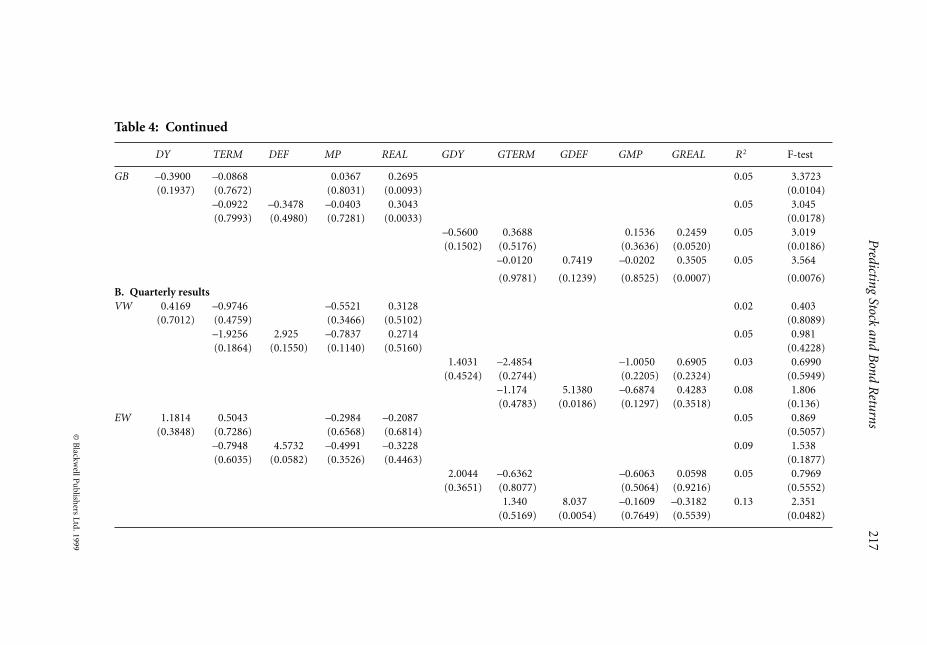
GB –0.3900 –0.0868 0.0367 0.2695 0.05 3.3723

(0.1937) (0.7672) (0.8031) (0.0093) (0.0104)

–0.0922 –0.3478 –0.0403 0.3043 0.05 3.045

(0.7993) (0.4980) (0.7281) (0.0033) (0.0178)

–0.5600 0.3688 0.1536 0.2459 0.05 3.019

(0.1502) (0.5176) (0.3636) (0.0520) (0.0186)

–0.0120 0.7419 –0.0202 0.3505 0.05 3.564

(0.9781) (0.1239) (0.8525) (0.0007) (0.0076)

B. Quarterly results

VW 0.4169 –0.9746 –0.5521 0.3128 0.02 0.403

(0.7012) (0.4759) (0.3466) (0.5102) (0.8089)

–1.9256 2.925 –0.7837 0.2714 0.05 0.981

(0.1864) (0.1550) (0.1140) (0.5160) (0.4228)

1.4031 –2.4854 –1.0050 0.6905 0.03 0.6990

(0.4524) (0.2744) (0.2205) (0.2324) (0.5949)

–1.174 5.1380 –0.6874 0.4283 0.08 1.806

(0.4783) (0.0186) (0.1297) (0.3518) (0.136)

EW 1.1814 0.5043 –0.2984 –0.2087 0.05 0.869

(0.3848) (0.7286) (0.6568) (0.6814) (0.5057)

–0.7948 4.5732 –0.4991 –0.3228 0.09 1.538

(0.6035) (0.0582) (0.3526) (0.4463) (0.1877)

2.0044 –0.6362 –0.6063 0.0598 0.05 0.7969

(0.3651) (0.8077) (0.5064) (0.9216) (0.5552)

1.340 8.037 –0.1609 –0.3182 0.13 2.351

(0.5169) (0.0054) (0.7649) (0.5539) (0.0482)

21

8D

avid E

ly an

d M

ehd

i Sa

lehiza

deh

©B

lackw

ell Pu

blish

ers Ltd

. 19

99

Table 4: Continued


CB –1.1607 –0.4726 0.0901 0.8698 0.15 3.576

(0.1417) (0.6458) (0.8584) (0.0031) (0.0098)

–0.2928 –1.566 –0.0693 0.9719 0.15 3.39

(0.8016) (0.2111) (0.8526) (0.0008) (0.0129)

–1.8270 1.2699 0.5674 0.7328 0.14 3.302

(0.1032) (0.5392) (0.3152) (0.0386) (0.0148)

0.7219 8.6033 –0.2068 1.0262 0.35 10.899

(0.4702) (0.0021) (0.5431) (0.0007) (0.0000)

GB –1.5046 –0.4058 0.1969 0.8370 0.13 3.012

(0.0648) (0.7229) (0.7086) (0.0074) (0.0228)

0.0807 –2.7054 0.0727 0.9707 0.13 3.105

(0.9498) (0.0477) (0.8594) (0.0013) (0.0198)

–2.1254 1.285 0.6376 0.7099 0.12 2.7799

(0.0944) (0.5444) (0.2807) (0.0785) (0.0323)

0.5640 8.9030 –0.2370 1.0547 0.30 8.639

(0.5986) (0.0021) (0.5220) (0.0010) (0.0000)

Notes. Excess returns of the value-weighted CRSP index (VW), equally-weighted CRSP index (EW), long-term corporate bonds (CB), and long-term

government bonds (GB) are calculated as asset returns less the one-month return on US Treasury bills. The independent variables consist of dividend yields

(DY), derived from the CRSP indices using the procedure described in Fama and French (1988); default risk (DEF), calculated as the difference between

Moody’s Baa Corporate Bond Yield and US government 10-year bond rate; US term premium (TERM), defined as the difference between the 10-year and the

1-year government bond rates; US monetary policy (MP) indicator, defined as the federal-funds rate; real US interest rate (REAL), defined as the

10-year government bond rate less expected inflation, proxied by the actual growth in the Consumer Price Index (CPI) over the previous twelve months; a

measure of global dividend yields based on the MSCI world index (GDY); a GDP-weighted average of term premiums (GTERM) for the G-7 countries; global

default risk (GDEF) defined as the difference between the Eurodollar deposit rate and the US Treasury 3-month rate; and a GDP-weighted average of

monetary policy indicators for the G-7 countries (GMP). Values in parentheses are p values. All explanatory variables are annualized.

D. Hypotheses and Testing Procedures

Our first objective is to investigate the value of supplementing US data with

foreign or global measures of economic conditions or monetary policy in-

dicators when forecasting US asset returns. By estimating variations of equa-

tions (1) and (2), we compare the three approaches to forecasting returns:

using US data only, replacing US measures with corresponding global vari-

ables and supplementing US factors with foreign and global measures of some

of the variables. Standard t-statistics, goodness-of-fit measures and out-of-

sample prediction errors are used to judge and compare the performance of

the three approaches.

Our second objective in this study is to retest several hypotheses considered

by other authors using the alternative prediction models that incorporate

information on foreign economies. Fama and French (1989) find that the same

set of variables is capable of predicting both stock and bond excess returns.

Jensen et al. (1996) and Patelis (1997) conclude that the monetary sector has

an impact on excess returns beyond that of proxies for business conditions.

Both of these issues are analysed here by contrasting the results for the base

model to those for the global model. Our interest lies in determining whether

the conclusions are sensitive to model specification.

IV. Results

A. Performance of US Asset Returns Prediction Models EmployingGlobal or Foreign Variables

Table 4 presents estimates of models of excess returns for stocks, corporate bonds

and US government bonds. For each asset, two estimates of the base model

and two estimates of the global model are presented. All models were estimated

using least squares, and the standard errors are based on the Newey and

West (1987) procedure.8 Because of the lack of available data for the foreign

and global variables, estimates are based on the time period August 1976 to

December 1997. We also include a January binary variable for the EW regres-

sions. It proved to be insignificant and thus was not used in the other equations.

Table 4 provides standard regression performance indicators that help to

judge the merits of using measures of non-US economic conditions and

monetary policy to predict asset returns.9 As in Fama and French (1989)



8The Newey–West standard error estimates are consistent in the presence of heteroskedasticity

and autocorrelation.

9See Foster et al. (1997) for a criticism of standard goodness-of-fit measures when variable

selection is based in part on variables found to be important in other studies.

and Jensen et al., the percentage of variation in returns explained by the models

estimated using quarterly equations is higher than those estimated using

monthly data. The R2 range from 1 to 7% for the models estimated with

monthly data and from 2 to 35% for the models estimated with quarterly data.

For the base model, a comparison of the estimates presented in Table 4 with

the results in Table 3 suggests that the ability of this set of US business con-

ditions proxies and monetary policy indicators to explain stock returns is

lower in the 1976–97 period than in the 1954–92 period. This group of four

US variables is jointly significant in every equation for the earlier time period.

But, the variables are insignificant in some of the equations in Table 4,

including all of the quarterly equations for VW and EW. The group is still a

significant predictor of corporate and government bond returns and of monthly

stock returns. Overall, the results are consistent with the earlier finding that

business condition proxies and measures of the stance of monetary policy are

useful in explaining the variation in both stock returns and bond returns.

The lower significance levels in the 1976–97 period could be due to changes

in the fundamental relations between the independent variables and the asset

returns or to less variation in business conditions over the time period.

In terms of the global model, the results provide some evidence that the

global equivalents of the above variables are related to US asset returns. Like

the group of US variables, the F-tests suggest that the global variables are sig-

nificant in every corporate and government bond equation, for both monthly

and quarterly horizons. For equities, though, the global variables as a group

are significant in just one case, an equation for EW. GDEF is significant in two

of the quarterly regressions for VW and EW.

There are a number of cases where the set of independent variables is

significant and the percentage of variation in returns explained by the global

model matches or exceeds that of the base model. For monthly-based tests, the

regression R2 for the global model exceeds that for the base model in one case

(for a CB equation), while the R2 for the base model exceeds that for the global

model in four cases (for one VW, two EW and one CB equation). For the

quarterly regressions, the R2 for the global model exceeds that for the base

model in three cases (for one EW, one CB and one GB equation), whereas

the R2 for the base model exceeds that for the global model in two cases (for

one CB and one GB equation). In sum, the global model tends to perform

better in predicting quarterly returns and bond returns than in predicting

monthly returns and equity returns.

Our third approach consists of applying the expanded model. To focus

more explicitly on the incremental benefit of including foreign or global

variables in prediction models, we added, one by one, each foreign and global

measure of dividends, term premiums, monetary policy and real interests

rates to the base model. A summary of this analysis is presented in Table 5.



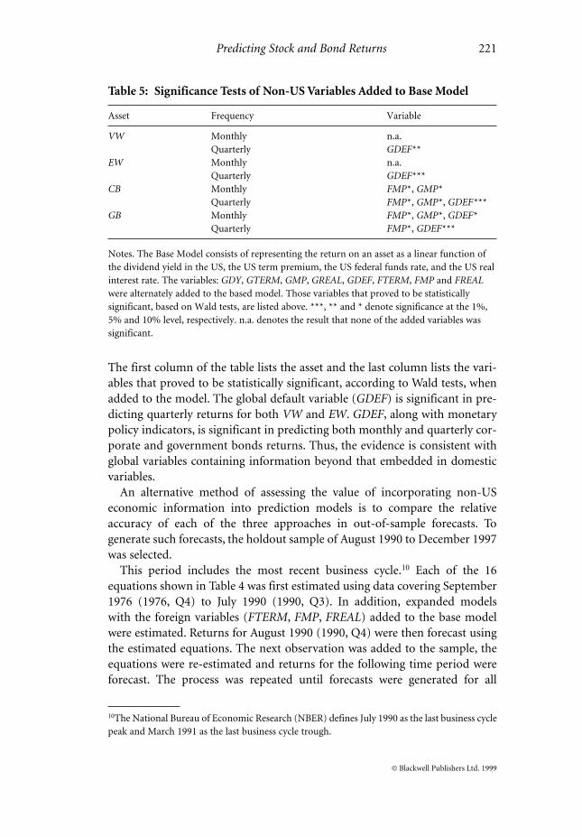
The first column of the table lists the asset and the last column lists the vari-

ables that proved to be statistically significant, according to Wald tests, when

added to the model. The global default variable (GDEF) is significant in pre-

dicting quarterly returns for both VW and EW. GDEF, along with monetary

policy indicators, is significant in predicting both monthly and quarterly cor-

porate and government bonds returns. Thus, the evidence is consistent with

global variables containing information beyond that embedded in domestic

variables.

An alternative method of assessing the value of incorporating non-US

economic information into prediction models is to compare the relative

accuracy of each of the three approaches in out-of-sample forecasts. To

generate such forecasts, the holdout sample of August 1990 to December 1997

was selected.

This period includes the most recent business cycle.10 Each of the 16

equations shown in Table 4 was first estimated using data covering September

1976 (1976, Q4) to July 1990 (1990, Q3). In addition, expanded models

with the foreign variables (FTERM, FMP, FREAL) added to the base model

were estimated. Returns for August 1990 (1990, Q4) were then forecast using

the estimated equations. The next observation was added to the sample, the

equations were re-estimated and returns for the following time period were

forecast. The process was repeated until forecasts were generated for all



10The National Bureau of Economic Research (NBER) defines July 1990 as the last business cycle

peak and March 1991 as the last business cycle trough.

Table 5: Significance Tests of Non-US Variables Added to Base Model

Asset Frequency Variable

VW Monthly n.a.

Quarterly GDEF**

EW Monthly n.a.

Quarterly GDEF***

CB Monthly FMP*, GMP*

Quarterly FMP*, GMP*, GDEF***

GB Monthly FMP*, GMP*, GDEF*

Quarterly FMP*, GDEF***

Notes. The Base Model consists of representing the return on an asset as a linear function of

the dividend yield in the US, the US term premium, the US federal funds rate, and the US real

interest rate. The variables: GDY, GTERM, GMP, GREAL, GDEF, FTERM, FMP and FREAL

were alternately added to the based model. Those variables that proved to be statistically

significant, based on Wald tests, are listed above. ***, ** and * denote significance at the 1%,

5% and 10% level, respectively. n.a. denotes the result that none of the added variables was

significant.

time periods to the end of 1997. Table 6 presents root mean squared errors

(RMSEs) for each of these out-of-sample forecasts. The results are mixed but

lend some support to augmenting asset returns prediction models with informa-

tion about foreign economies. For the equations estimated using monthly

data, the global model proved to be slightly more accurate than the others in

seven of the eight instances. Only in one case involving EW did the base model

perform best. Using quarterly data, the base model performed the best in a

corporate bond equation and a government bond equation, while the global

model performed best in all four equity equations. The expanded model per-

formed best in only one case involving government bonds. One explanation

for the stronger showing of the global models than the in-sample results is

that these out-of-sample forecasts are made over the 1990s, while the analysis

presented earlier in the paper is based on data covering a period starting in

1976. The global model may have performed better in the more recent period

because the role of foreign investors has been rising in importance. However,

several limitations of this analysis should be noted. The RMSEs across models

are generally close to one another in magnitude, which suggests that the

improvements in forecasting achieved using models based on global variables



Table 6: Comparison of Out-of-sample Forecasts: RMSEs August 1990

to December 1997

Equation Base model Expanded model Global model

Monthly results

VW 1 0.339 0.349 0.330

2 0.328 0.410 0.325

EW 3 0.372 0.376 0.362

4 0.348 0.462 0.355

CB 5 0.195 0.194 0.191

6 0.197 0.220 0.193

GB 7 0.253 0.249 0.248

8 0.254 0.269 0.250

Quarterly results

VW 1 0.949 1.047 0.942

2 0.917 1.402 0.820

EW 3 1.447 1.529 1.446

4 1.378 1.909 1.316

CB 5 0.683 0.631 0.613

6 0.684 0.980 0.709

GB 7 0.885 0.817 0.837

8 0.887 1.131 0.907

Notes. Forecasts for the base and global models are based on estimates presented in Table 4.

The Expanded model is formed by adding FTERM, FMP and FREAL to the base model.

Values in bold identify those models with the smallest RMSE.

are generally small. Furthermore, caution is appropriate, since our out-of-

sample analysis covers a short time period that was almost exclusively a strong

bull market.

B. Common Variation in Expected Returns

Tables 4 and 5 also present results that relate to the issue of market efficiency.

Do the results suggest that a common set of variables can predict both stock and

bond returns? And is the stance of monetary policy within this set of variables?

Caution is required when one is interpreting the results to assess the

importance of individual variables. The process of testing for relationships

across assets is made difficult by the high level of correlation between some

of the explanatory variables. As shown in Table 2, MP (the federal funds rate)

is correlated with dividend yields (ρ = 0.715) and the term structure

(ρ = –0.749). The real interest rate is correlated with the default premium

(ρ = 0.371) and the term structure (ρ = 0.428). Also highly correlated are US

and foreign measures of monetary policy and real interest rates. Thus, it is gen-

erally not possible to categorize cleanly variables along the lines of business con-

dition proxies or monetary policy indicators. Many variables reflect both factors.

The results for corporate and government bonds using global variables are

very similar to those based on US variables. From Table 4, the independent

variables, as a group, are statistically significant in all the equations for both

monthly and quarterly horizons. The real interest rate is significant in all

equations and therefore appears to be the most important factor in explaining

the variation in returns. However, the global dividend and default variables,

like their US equivalents, are significant in some of the quarterly regressions.

From Table 5, measures of global monetary policy help to explain the

variation in returns when added to the base models.

The results for equity returns are less consistent. From Table 4, the US

variables, as a group, are generally statistically significant in explaining monthly

returns, but not quarterly returns. The global variables, as a group, are not

significant in explaining monthly returns but are in explaining quarterly EW.

Furthermore, the default variables appear to be the most important single

factor in both the US and global versions of the equity equations. In no equity

equation is the term premium or monetary policy variable individually sig-

nificant. Nor are monthly global variables significant when added to the base

models as presented in Table 5. This lack of significance differs from the evi-

dence offered by the base-model estimates, where the group of variables is

jointly significant in most cases. Moreover, the term premium and monetary

policy variables are individually significant in the monthly base model results

for VW.



Surprisingly, the US and global dividend yields are significant only in a

quarterly government bond equation. The low explanatory power of dividend

yields might be owing to the shorter time period used here relative to other

studies. As argued by Fama and French (1989), these variables track long-term

business conditions that extend beyond a single business cycle.

In summary, our results for bonds using global variables are consistent with

those based on US variables. Both are consistent with the efficient markets

hypothesis in the sense that a common group of variables reflecting stock

market, bond market and monetary policy factors predicts returns. Our

results for stocks using global variables do not support this hypothesis. Vari-

ables associated with bond market and monetary factors do not appear to

help to explain variation in stock returns.

V. Summary and Conclusions

Prior research demonstrates that a number of proxies for economic activity

are statistically significant predictors of returns on US stocks and bonds.

However, a substantial share of US stocks and bonds are now held by inter-

national investors. If foreign investors – in their consumption and investment

decisions – behave similarly to those based in the US, then the accuracy of

asset prediction models might be raised by incorporating international meas-

ures of economic conditions and monetary environments. To explore this

possibility, we estimate and contrast the performance of models in predicting

returns of two stock portfolios, a corporate bond portfolio and a government

bond portfolio. The first, or base, model is estimated with US measures of

dividend yields or default premium, term premium, stance of monetary policy

and real interest rate variables. This model is similar to those employed by other

authors. The second, or global, model is similar to the base model except that

global variables replace the US variables. A third, or expanded, model adds

variables characterizing the states of foreign economies to the base model.

Overall, our results indicate that global measures can often improve predic-

tions of US stock and bond returns. The evidence is much stronger for bond

returns than for stock returns. Several issues addressed by other authors are

re-examined using our global model. We confirm earlier conclusions by find-

ing support for the efficient markets hypothesis, in the sense that a common

group of variables reflecting both global bond and stock market character-

istics helps to predict bond returns. Global measures of the stance of mon-

etary policy also help to predict bond returns. However, we do not find similar

support when considering equities. Variables reflecting global bond market

characteristics and monetary policy prove to be insignificant in explaining the

variation in US stock returns.



Our results do not uniformly lead to the conclusion that global models of

assets returns outperform their domestic counterparts. Nevertheless, the evid-

ence is sufficiently strong to suggest that future research aimed at identifying

additional global variables with predictive capability would be fruitful. One

approach that might be taken is to adapt the Fama and French (1993) three-

factor model to include global equivalents to their size and book-to-market

equity variables. Additionally, the measurement of the stance of monetary

policy is likely to require greater research, due to the introduction of the euro.

In this study, global measures of monetary policy are based on averages of

short-term interest rates across countries. When widely different policies are

being pursued, a numerical average cannot fully capture global monetary

conditions, since it ignores the dispersion of policies. With the full adoption

of the euro, there will be no such dispersion in policy across its members.

Therefore, an average that includes this major subset of countries should be a

more precise indicator of global policy. As a related issue, we expect that any

major policy action taken by the European Central Bank in the future will

have a greater impact on US asset prices than a similar step by a single EU

member country taken in the past. Both issues stemming from the presence of

the euro imply that prediction models should account for structural breaks

in the relation between monetary policy indicators and asset prices. Finally,

it should be recognized that a number of emerging economies are achieving

greater prominence as international investors. For example, substantial for-

eign holders of Treasury securities now include China, Hong Kong, Singapore,

Taiwan and Mexico. Holdings by each country exceed US$20 billion (US

Treasury, 1999). Thus, future research may benefit from including measures of

the economic environment of these countries in the analysis.

David Ely

5500 Campanile Drive

San Diego State University

San Diego, CA 92182-8236

USA

[email protected]

References

Bernanke, B. S., and A. S. Blinder (1992), ‘The Federal Funds Rate and the Channels

of Monetary Transmission’, American Economic Review, 82(4), 901–21.

Booth, J. R., and L. C. Booth (1997), ‘Economic Factors, Monetary Policy, and

Expected Returns on Stocks and Bonds’, Economic Review, Federal Reserve Bank of

San Francisco, 2, 32–42.



Daniel, K., and S. Titman (1997), ‘Evidence on the Characteristics of Cross Sectional

Variation in Stock Returns’, Journal of Finance, 52(1), 1–33.

Fama, E. F., and K. R. French (1988), ‘Dividend Yields and Expected Stock Returns’,

Journal of Financial Economics, 22, 3–25.

—— (1989), ‘Business Conditions and Expected Returns on Stocks and Bonds’,

Journal of Financial Economics, 25, 23–49.

—— (1993), ‘Common Risk Factors in the Returns on Stocks and Bonds’, Journal of

Financial Economics, 33, 3–56.

—— (1996), ‘Multifactor Explanations of Asset Pricing Anomalies’, Journal of

Finance, 51(1), 55–84.

Ferson, W. E., and C. R. Harvey (1993), ‘The Risk and Predictability of International

Equity Returns’, The Review of Financial Studies, 6(3), 527–66.

Foster, F. D., T. Smith and R. E. Whaley (1997), ‘Assessing Goodness-of-fit of Asset

Pricing Models: the Distribution of the Maximal R2’, Journal of Finance, 52(2),

591–607.

Ibbotson Associates (1997), Stocks, Bonds, Bills and Inflation: 1997 Yearbook. Chicago:

Ibbotson Associates.

—— (1998), Stocks, Bonds, Bills and Inflation: 1998 Yearbook. Chicago: Ibbotson

Associates.

Ilmanen, A. (1995), ‘Time-varying Expected Returns in International Bond Markets’,

The Journal of Finance, 50(2), 481–506.

—— (1996), ‘When Do Bond Markets Reward Investors for Interest Rate Risk?’,

Journal of Portfolio Management, Winter, 52–64.

Jensen, Gerald R., Jeffery M. Mercer and Robert R. Johnson (1996), ‘Business

Conditions, Monetary Policy, and Expected Security Returns’, Journal of Financial

Economics, 40, 213–37.

Keim, Donald B., and Robert F. Stambaugh (1986), ‘Predicting Returns in the Stock

and Bond Markets’, Journal of Financial Economics, 17, 357–90.

Melloan, George (1996), ‘How Japan’s Goblins Spook Wall Street’, Wall Street

Journal, 11 March, A15.

Newey, Whitney, and Kenneth West (1987), ‘A Simple Positive Semidefinite,

Heteroskedasticity and Autocorrelation Consistent Covariance Matrix’, Econometrica,

55, 703–8.

Patelis, Alex D. (1997), ‘Stock Return Predictability and the Role of Monetary Policy’,

Journal of Finance, 52, 1951–72.

Pulliam, Susan and Gregory Zuckerman (1996), ‘Japanese Role Could Hurt US

Markets’, Wall Street Journal, 12 December, C1.

US Treasury (1999), Treasury International Capital (TIC) reporting system (Online).

Available at: www.treas.gov./tic/



Predicting Stock and Bond Returns: The Impact of Global Variables

Documents

Transcript of Predicting Stock and Bond Returns: The Impact of Global Variables